ced412 report_urban flooding analysis

Title of the Project

Urban Flooding Analysis using GIS

Submitted by

Suraj Kumar

2010CE10407

A report of CED 412 - Project Part II submitted

in partial fulfilment of the requirements of the degree of

Bachelor of Technology

Department of Civil Engineering

Indian Institute of Technology Delhi

May, 2014

2

STUDENT’S CERTIFICATE

I do certify that this report explains the work carried out by me in the Course CED 412: Project –

Part II under the overall supervision of Prof. A. K. Gosain and Prof. Dhanya C.T. The contents of

the report including text, figures, tables, computer programs, etc. have not been reproduced from

other sources such as books, journals, reports, manuals, websites, etc. Wherever limited

reproduction from another source had been made the source had been duly acknowledged at that

point and also listed in the References.

Suraj Kumar

2010CE10407

3

SUPERVISOR’S CERTIFICATE

This is to certify that the report submitted by Suraj Kumar (2010CE10407) describes the work

carried out by him/her in the Course CED 412 – Project – Part II under my overall supervision.

Prof. A. K. Gosain

Prof. Dhanya C. T.

4

ACKNOWLEDGEMENT

I am very grateful to Prof. A. K. Gosain and Dr. Dhanya C. T. for the guidance, encouragement

and co-operation received throughout the project work. I owe the timely completion of this project

work to their valuable advice, support and suggestions.

I would also like to thank to bentley.com for providing with a free Bentley CivilStorm as under

IIT Delhi student license (a completion certificate of which has been attached with this report) and

Mr. Satish Kumar, from GIS Lab, for their assistance, particularly in acquiring various

measurements, support material.

Suraj Kumar

2010CE10407

May, 2014

5

ABSTRACT

This thesis deals with simulation and analysis of urban storm water drainage. The thesis review

current methods and models used in urban storm water drainage e.g. SCS-CN, Rational Method,

SWAT and SWMM. It provide a methodology for simulation of urban storm water drainage. Its

studies 10 major storm drains in Barapullah catchment of Delhi. It takes cross-section data from

Delhi Drainage Master Plan-1976. It then analyse these sections for current loadings and check

whether they are sufficient or not. The analysis is based on rational method and EPA-SWMM

model. For rational method, rainfall with 5 year return period with 5 hour rainfall duration has

been taken. For SWMM Model, rainfall of cumulative depth of 135.6 mm over 24 hours durations

has been taken to provide worst case scenario. It finds out problematic nodes and links in network.

Its estimate quantity of water being flooded from which node. It estimate which link is

overflowing, for how much time. After analyses it proposes certain recommendations in design of

drains which can be taken up to stop local level flooding problems. It then list down certain

limitation of methodology and datasets.

The objectives of this part of B.Tech Project are:

Review of current storm water modeling methods and models

Storm water modeling of a Barapulla catchment of Delhi using Bentley CivilStorm and

ArcGIS

Use of SWMM Model to calculate runoff

Use of Rational Method to calculate peak runoff

6

CONTENTS

Student’s Certificate........................................................................................................................ 2

Supervisor’s Certificate .................................................................................................................. 3

Acknowledgement .......................................................................................................................... 4

ABSTRACT .................................................................................................................................... 5

Contents .......................................................................................................................................... 6

List of figures .................................................................................................................................. 9

List of tables .................................................................................................................................. 10

Chapter 1: Introduction ............................................................................................................. 11

1.1 Urban Drainage Problem ................................................................................................ 11

1.2 Scope of Work ................................................................................................................ 11

1.3 Objectives ....................................................................................................................... 12

1.4 Report Structure ............................................................................................................. 13

Chapter 2: DEscription of the Study Area ................................................................................ 14

2.1 Geography ...................................................................................................................... 14

2.2 Drains ............................................................................................................................. 15

2.3 Cross-Section Details ..................................................................................................... 22

2.4 Subbasin Details ............................................................................................................. 22

2.5 Channel Details .............................................................................................................. 22

2.6 Storm Data Details ......................................................................................................... 23

Chapter 3: Literature review ..................................................................................................... 25

3.1 Summary ........................................................................................................................ 25

3.2 Methods and Models Used ............................................................................................. 26

7

3.2.1 SWAT Model .......................................................................................................... 26

3.2.2 SCS-CN Method of estimating runoff volume ....................................................... 26

3.2.3 Rational Method...................................................................................................... 27

3.2.4 SWMM Surface Runoff .......................................................................................... 31

3.2.5 Manning Formula.................................................................................................... 33

Chapter 4: Methodology ........................................................................................................... 34

4.1 Brief Overview ............................................................................................................... 34

4.2 Storm Data Calculation .................................................................................................. 36

4.2.1 Intensity Calculation ............................................................................................... 36

4.2.2 Rainfall Depth Calculation ..................................................................................... 38

Chapter 5: Analysis and Results ............................................................................................... 39

5.1 Verification..................................................................................................................... 39

5.1.1 Catchment Area Validation..................................................................................... 39

5.2 SWMM Model Results................................................................................................... 40

5.2.1 General Results ....................................................................................................... 40

5.3 Rational Method Results ................................................................................................ 45

5.3.1 Analysis................................................................................................................... 48

5.4 Recommendation ............................................................................................................ 49

Chapter 6: Discussion ............................................................................................................... 50

6.1 Model Application.......................................................................................................... 50

6.2 Drawbacks and limitations of the Methodology ............................................................ 50

6.3 Advantages of SWMM Method over Rational Method ................................................. 51

Chapter 7: Conclusion and Future Work .................................................................................. 52

7.1 Conclusion ...................................................................................................................... 52

7.2 Future Work ................................................................................................................... 52

8

Appenddix – A .............................................................................................................................. 53

References ..................................................................................................................................... 61

9

LIST OF FIGURES

Figure 1.1 Barapullah Catchment Boundary ................................................................................ 12

Figure 2.1: Extent of Barapullah Catchment ................................................................................ 14

Figure 2.2 Bently CivilStorm Model ............................................................................................ 15

Figure 2.3 Barapulla Catchment ................................................................................................... 16

Figure 2.4 Time Vs Depth curve of 27 July, 2009........................................................................ 23

Figure 2.5 : IDF Curve for Delhi .................................................................................................. 24

Figure 3.1 Representation of the SWMM/RUNOFF algorithm ................................................... 31

Figure 4.1: ArcSWAT Watershed Delineator Window ................................................................ 34

Figure 4.2: Hydrological Model ................................................................................................... 35

Figure 4.3 : Hydraulic Model........................................................................................................ 36

Figure 5.1: SWMM Model of Barapullah Catchment .................................................................. 40

Figure 5.2: Precipitation and Runoff in Barapullah Catchment ................................................... 40

Figure 5.3: Flow in major drains of Barapullah Catchment ......................................................... 41

Figure 5.4: Node Flooding Graph ................................................................................................. 41

Figure 5.5: Node Flooding Summary ........................................................................................... 42

Figure 5.6: Link Flow Summary ................................................................................................... 43

Figure 5.7: Flooding Nodes (shown in red) at t = 12:15 ............................................................... 44

Figure 5.8: Depth/ Rise (%) and Flow (m3/s)............................................................................... 47

10

LIST OF TABLES

Table 2.1 Drains in Barapulla Catchment ..................................................................................... 15

Table 2.2 Cross-Section Details in Drains .................................................................................... 17

Table 2.3: Subbasin Details .......................................................................................................... 18

Table 2.4: Channel Details ............................................................................................................ 20

Table 2.5: Other SWMM parameter assumed for all subbasins ................................................... 22

Table 3.1: Project Plan .................................................................................................................. 25

Table 3.2: Runoff Coefficient ....................................................................................................... 28

Table 4.1: Intensity Calculation .................................................................................................... 37

Table 4.2: Maximum Rainfall Depth in a year ............................................................................. 38

Table 5.1 Catchment Area Comparison ........................................................................................ 39

Table 5.2: Channel Flow Summary .............................................................................................. 45

Table 5.3: Catchment flow Summary ........................................................................................... 46

Table 5.4: Comparison of Discharge from Rational Method and DMP -1976 ............................. 48

11

CHAPTER 1: INTRODUCTION

1.1 Urban Drainage Problem

Urban flooding problems range from minors ones where water enters the basements of a few house

to major incidents, where large parts of cities are inundated for several days. Most modern cities

in the industrialized part of world usually experience small scale local problems mainly due to

insufficient capacity in their sewer systems during heavy rainstorms (Schmitt et al, 2004). Cities

in other regions, including those in South/South-East Asia, often have more severe problems

because of much heavier local rainfall and lower drainage standards. This situation continues to

get worse because many cities in the developing countries are growing rapidly, but without the

funds to extend and rehabilitate their existing drainage systems. Moreover New Delhi, capital of

India due to fast urbanization and rapid migration with not simultaneous progress in drainage

condition is suffering from serious waterlogging issues which result in loss to public infrastructure

and severe traffic jams. For example, population of New Delhi has grown from 4 million in 1971

to about 17 million in 2012.

1.2 Scope of Work

This project deals with analysis and simulation of storm water drainage in Barapulla catchment of

New Delhi. It studies 10 major storm drains which form the drainage network of Delhi. Delhi area

is 1484 km2 out which Barapulla catchment constitute around 140 km2 which is around one-tenth

of New Delhi. The project studies main tributaries of Kushak-Barapulla Nallah. It takes cross-

section data from 1976 Master Drainage Plan. It then analyse these sections (which were proposed

in 1976) for current loading and check whether they are sufficient or not. The analysis is based on

rational method and EPA – SWMM Model. After analyses it proposes certain recommendations

in design of drains which can be taken up to stop local level flooding problems.

12

Figure 1.1 Barapullah Catchment Boundary

1.3 Objectives

The objectives of this part of project is as follows

Review of storm water modeling methods and models

Storm water modeling of a Barapulla catchment of Delhi using Bentley CivilStorm and

ArcGIS

Use of SWMM Model to calculate runoff

Use of Rational Method to calculate peak runoff

13

1.4 Report Structure

Chapter 1: Introduction: This chapter provides the brief introduction about the problems,

objectives and scope of work for CED412- Major Project Part 2

Chapter 2: Description of study area: This chapter explains in detail about geography of

barapullah catchment and its network elements. It provides input data which is being used

for modelling.

Chapter 3: Literature Review: It begins with plan of B.tech Project Part-2 and list out

sources of literature which author has gone through. It then explain in details about methods

and model used in thesis

Chapter 4: Methodology: It provides brief overview of methodology and rainfall

calculation summary

Chapter 5: Analysis and Results: It provide results of SWMM Model and rational method.

It then verify the model using data from Drainage Master Plan for Delhi – 1976

Chapter 6: Discussion: It talks about the application of model. This chapter provides some

limitation and advantages of model.

Chapter 7: Conclusion: This chapter in brief provides the summary of thesis

14

CHAPTER 2: DESCRIPTION OF THE STUDY AREA

2.1 Geography

This project studies barapullah catchment of Delhi. Barapullah constitute around 140 km2 of area

which roughly around one-tenth of Delhi. It covers areas from Connaught place in North (Look at

Figure) to Mehrauli, Sangam Vihar in South, in east it covers till Nizamudin and in west it covers

portion of Vasant Vihar and RK Puram. It mostly consist of alluvial soil (Hydrologic Class D &

FAO Classification No. 3876).

Figure 2.1: Extent of Barapullah Catchment

15

2.2 Drains

The drains modelled in this study are presented in Table

Table 2.1 Drains in Barapulla Catchment

S.No Drain Name Length

Catchment

Area(in hectares)

1 AIIMs Drain 2289.50988 1799.17

2 Andrews Gunj Drain 3708.015119 398.5175

3 Barapullah Nallah 3681.066054 14083.945

4 Chirag Delhi Drain 9188.034697 5799.165

5 Greater Kailash Drain 1424.718489 434.64

6 Kushak Nallah 7858.408153 4879.5125

7 Lajpat Nagar Drain 4303.854535 442.8325

8 Malviya Nagar Drain 4944.39992 1112.78

9 Nauroji Nagar Drain 6859.92319 1591.65

10 Sunehri Pullah Nallah 1799 2533.3525

NOTE: Catchment Area values have been derived from watershed delineation using ArcSWAT

Figure 2.2 Bently CivilStorm Model

16

Figure 2.3 Barapulla Catchment

17

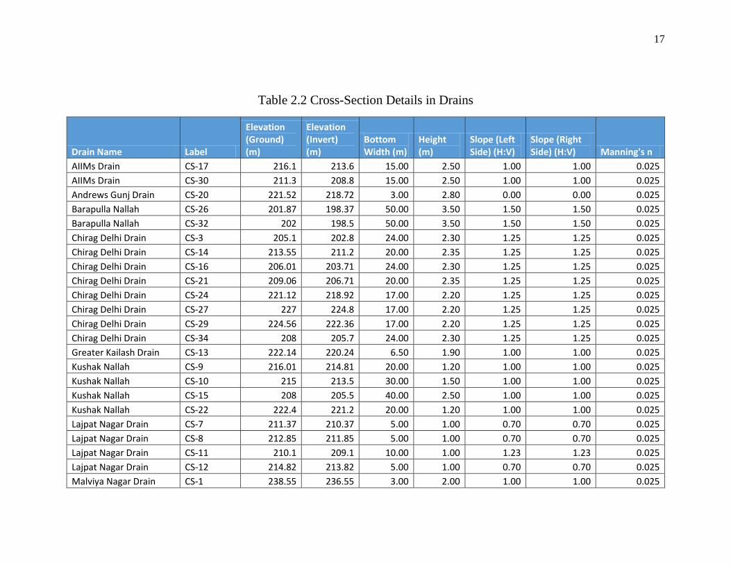
Table 2.2 Cross-Section Details in Drains

Drain Name Label

Elevation (Ground) (m)

Elevation (Invert) (m)

Bottom Width (m)

Height (m)

Slope (Left Side) (H:V)

Slope (Right Side) (H:V) Manning's n

AIIMs Drain CS-17 216.1 213.6 15.00 2.50 1.00 1.00 0.025

AIIMs Drain CS-30 211.3 208.8 15.00 2.50 1.00 1.00 0.025

Andrews Gunj Drain CS-20 221.52 218.72 3.00 2.80 0.00 0.00 0.025

Barapulla Nallah CS-26 201.87 198.37 50.00 3.50 1.50 1.50 0.025

Barapulla Nallah CS-32 202 198.5 50.00 3.50 1.50 1.50 0.025

Chirag Delhi Drain CS-3 205.1 202.8 24.00 2.30 1.25 1.25 0.025





Chirag Delhi Drain CS-27 227 224.8 17.00 2.20 1.25 1.25 0.025


Chirag Delhi Drain CS-34 208 205.7 24.00 2.30 1.25 1.25 0.025

Greater Kailash Drain CS-13 222.14 220.24 6.50 1.90 1.00 1.00 0.025

Kushak Nallah CS-9 216.01 214.81 20.00 1.20 1.00 1.00 0.025

Kushak Nallah CS-10 215 213.5 30.00 1.50 1.00 1.00 0.025

Kushak Nallah CS-15 208 205.5 40.00 2.50 1.00 1.00 0.025

Kushak Nallah CS-22 222.4 221.2 20.00 1.20 1.00 1.00 0.025

Lajpat Nagar Drain CS-7 211.37 210.37 5.00 1.00 0.70 0.70 0.025




Malviya Nagar Drain CS-1 238.55 236.55 3.00 2.00 1.00 1.00 0.025

18

Drain Name Label

Elevation (Ground) (m)

Elevation (Invert) (m)

Bottom Width (m)

Height (m)

Slope (Left Side) (H:V)

Slope (Right Side) (H:V) Manning's n

Malviya Nagar Drain CS-2 234 232 3.00 2.00 1.00 1.00 0.025

Malviya Nagar Drain CS-23 238.29 236.29 3.00 2.00 1.00 1.00 0.025

Nauroji Nagar Drain CS-5 225.15 222.95 10.00 2.20 1.25 1.25 0.025

Nauroji Nagar Drain CS-6 223 220.8 10.00 2.20 1.25 1.25 0.025

Nauroji Nagar Drain CS-19 235.15 231.95 5.00 3.20 1.25 1.25 0.025

Nauroji Nagar Drain CS-33 218.2 216 15.00 2.20 1.25 1.25 0.025

Sunehri Pullah Nallah CS-4 203 199.5 50.00 3.50 1.50 1.50 0.025


Sunehri Pullah Nallah CS-25 208.77 205.27 30.00 3.50 2.50 2.50 0.025


Table 2.3: Subbasin Details

Subbasin Area (hectares)

Slope (%)

Longest flow path length (m)

C CN Characteristic Width (m)

Time of Concentration (min)

Time of Concentration (Progressive) ( min)

Imperviousness (%)

Roughness Coefficient (n)

Depression Storage ( in mm)

1 827.77 3.56 7415.18 0.50 84.09 1116.31 67.12 146.99 54.92 0.018 2.99

2 470.95 1.28 4220.67 0.51 85.11 1115.82 64.60 144.47 57.61 0.018 2.89

3 693.63 1.84 6684.56 0.55 88.66 1037.66 79.87 79.87 66.95 0.016 2.53

4 88.21 3.99 1690.13 0.56 89.26 521.90 20.58 20.58 68.71 0.016 2.46

5 0.08 5.23 54.32 0.70 95.00 13.81 1.31 1.31 100.00 0.012 1.27

6 429.08 3.16 5399.28 0.63 93.16 794.70 55.09 55.09 83.26 0.014 1.91

7 452.72 1.80 5673.73 0.55 89.46 797.93 71.05 71.05 65.30 0.017 2.59

8 14.47 6.44 1425.27 0.47 81.56 101.54 15.01 15.01 48.82 0.019 3.22

9 442.83 2.13 5481.14 0.67 93.85 807.92 64.87 64.87 93.43 0.013 1.52

10 89.21 3.31 3371.37 0.66 93.12 264.61 37.63 37.63 89.86 0.013 1.66

19

Subbasin Area (hectares)

Slope (%)

Longest flow path length (m)

C CN Characteristic Width (m)

Time of Concentration (min)

Time of Concentration (Progressive) ( min)

Imperviousness (%)

Roughness Coefficient (n)

Depression Storage ( in mm)

11 1215.45 4.91 8889.56 0.48 83.77 1367.28 68.21 68.21 49.27 0.019 3.20

12 184.03 2.41 3184.39 0.64 92.55 577.92 40.67 40.67 84.57 0.014 1.86

13 346.21 3.07 3348.06 0.62 92.45 1034.07 38.54 38.54 79.63 0.015 2.05

14 462.51 2.19 5662.75 0.63 92.37 816.76 65.73 65.73 81.13 0.014 1.99

15 270.11 1.53 4223.66 0.65 92.63 639.52 60.29 60.29 88.83 0.013 1.70

16 398.52 1.96 5983.84 0.51 87.85 665.99 71.63 71.63 55.26 0.018 2.97

17 420.77 2.33 6409.20 0.57 89.22 656.51 70.69 70.69 70.45 0.016 2.40

18 76.45 2.20 2069.59 0.45 85.31 369.40 30.25 30.25 41.84 0.020 3.49

19 782.93 7.43 7104.23 0.52 89.23 1102.06 48.94 48.94 51.84 0.018 3.10

20 133.35 2.78 3443.97 0.60 90.85 387.19 40.92 40.92 75.87 0.015 2.19

21 434.64 2.89 4992.24 0.60 91.12 870.63 53.68 53.68 74.79 0.015 2.23

22 533.09 5.95 6465.77 0.35 78.85 824.48 49.57 79.82 20.25 0.022 4.31

23 377.52 3.94 6943.40 0.35 80.04 543.71 61.38 61.38 21.66 0.022 4.25

24 391.35 6.23 7051.34 0.36 79.24 554.99 52.07 82.32 21.43 0.022 4.26

25 529.48 2.74 7160.44 0.51 88.36 739.45 72.30 72.30 56.22 0.018 2.94

26 263.43 2.72 3297.68 0.49 86.08 798.83 39.92 39.92 48.45 0.019 3.23

27 0.51 4.89 116.75 0.57 88.17 43.68 2.43 2.43 67.16 0.016 2.52

28 315.77 5.20 7015.15 0.58 88.31 450.12 55.60 55.60 71.09 0.016 2.37

29 1112.78 4.35 9267.11 0.42 85.89 1200.78 73.79 73.79 35.92 0.020 3.71

30 865.14 4.44 7913.64 0.60 90.88 1093.23 64.87 64.87 74.31 0.015 2.25

31 556.53 3.55 6678.57 0.52 88.32 833.30 62.05 62.05 56.12 0.018 2.94

32 319.59 9.54 3708.92 0.32 74.32 861.67 26.95 88.99 10.83 0.024 4.67

33 451.52 8.09 5528.59 0.32 72.34 816.70 39.06 101.10 14.39 0.023 4.53

20

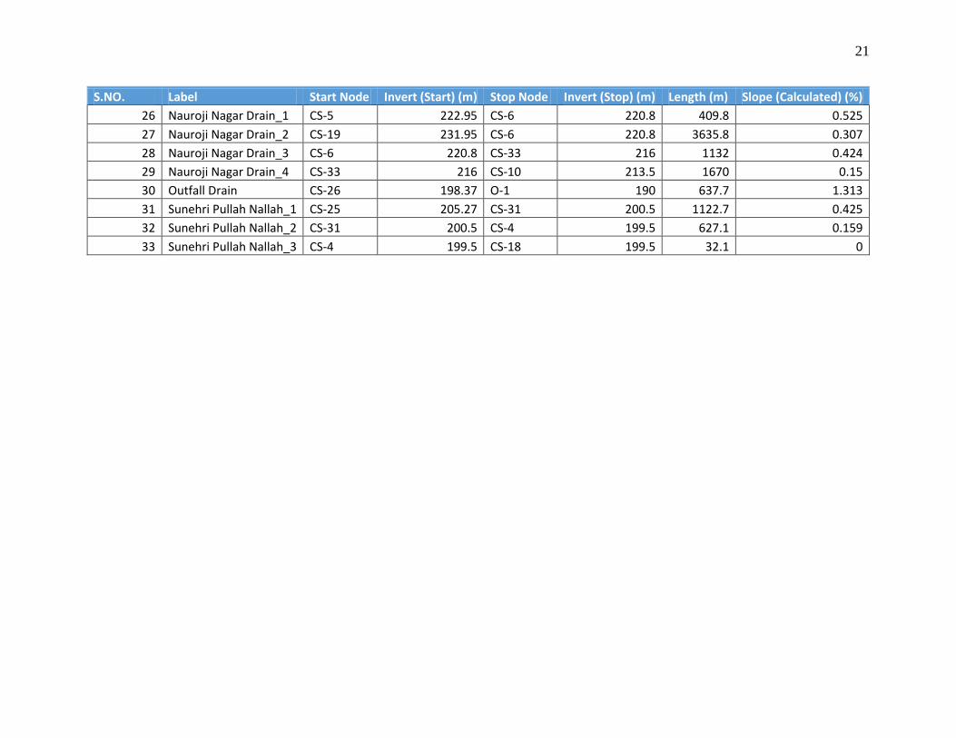
Table 2.4: Channel Details

S.NO. Label Start Node Invert (Start) (m) Stop Node Invert (Stop) (m) Length (m) Slope (Calculated) (%)

1 AIIMs Drain_1 CS-17 213.6 CS-30 208.8 519.4 0.924

2 AIIMs Drain_2 CS-30 208.8 CS-15 205.5 1756.5 0.188

3 Andrews Gunj Drain CS-20 218.72 CS-21 206.71 3707.4 0.324

4 Barapullah Nallah_1 CS-18 199.5 CS-32 198.5 1210 0.083

5 Barapullah Nallah_2 CS-32 198.5 CS-26 198.37 2335 0.006

6 Chirag Delhi Drain_1 CS-27 224.8 CS-29 222.36 724.3 0.337








14 Greater Kailash Drain CS-13 220.24 CS-14 211.2 1423.9 0.635

15 Kushak Nallah_1 CS-22 221.2 CS-9 214.81 3726.3 0.171

16 Kushak Nallah_2 CS-9 214.81 CS-10 213.5 627.5 0.209

17 Kushak Nallah_3 CS-10 213.5 CS-15 205.5 1519 0.527

18 Kushak Nallah_4 CS-15 205.5 CS-16 203.71 1977 0.091

19 Lajpat Nagar Drain_1 CS-8 211.85 CS-7 210.37 603.3 0.245


21 Lajpat Nagar Drain_3 CS-7 210.37 CS-11 209.1 211 0.602


23 Malviya Nagar Drain_1 CS-23 236.29 CS-2 232 590 0.727

24 Malviya Nagar Drain_2 CS-2 232 CS-24 218.92 3411.5 0.383

25 Malviya Nagar Drain_3 CS-1 236.55 CS-2 232 146.6 3.104

21

S.NO. Label Start Node Invert (Start) (m) Stop Node Invert (Stop) (m) Length (m) Slope (Calculated) (%)

26 Nauroji Nagar Drain_1 CS-5 222.95 CS-6 220.8 409.8 0.525

27 Nauroji Nagar Drain_2 CS-19 231.95 CS-6 220.8 3635.8 0.307

28 Nauroji Nagar Drain_3 CS-6 220.8 CS-33 216 1132 0.424

29 Nauroji Nagar Drain_4 CS-33 216 CS-10 213.5 1670 0.15

30 Outfall Drain CS-26 198.37 O-1 190 637.7 1.313

31 Sunehri Pullah Nallah_1 CS-25 205.27 CS-31 200.5 1122.7 0.425

32 Sunehri Pullah Nallah_2 CS-31 200.5 CS-4 199.5 627.1 0.159

33 Sunehri Pullah Nallah_3 CS-4 199.5 CS-18 199.5 32.1 0

22

2.3 Cross-Section Details

The cross-section used in modelling have been taken from proposed recommendation of storm

water drainage master plan 1976. Each drain or Nallah has been assumed to have trapezoidal cross-

section with varying width and height. Different cross-sections have been assumed at different

intervals along drain to simulate real-life conditions. (See Table 2.2).

2.4 Subbasin Details

Sub basin details (see table 2.3) have been derived from analysis carried in ArcSWAT and MS

Excel. Watershed parameters for example slope, longest flow path length, etc. have been derived

from watershed delineation carried out in ArcSWAT. For parameters such as C or CN, analysis

done on the basis of soil cover and land use to determine their value for each subbasin using HRU

(generated from SWAT) report in MS Excel. For Other parameter required in SWMM model

following values have been assumed for each catchment. (See table 2.5) (EPA, 2009)

Table 2.5: Other SWMM parameter assumed for all subbasins

Parameter Value

Percent of impervious area without depression

storage

25

Storage (Impervious Depression) (mm) 1.27

Storage (Pervious Depression) (mm) 5.08

Drying Time (days) 10

2.5 Channel Details

Channel details have been shown in table 2.4. It has been derived from cross-section details and

catchment detail. Note that while modelling one should look at its slope column to check whether

any link has slope close to 0 slope or negative values as it may leads to errors in modelling.

23

2.6 Storm Data Details

This thesis uses two models for simulation of storm water. One is rational method is used which

is used with rainfall of 5 hours duration with return period of 5 years. (See Figure 2.5 : IDF Curve

for Delhi). For second model i.e. SWMM, 24 hours rainfall duration with cumulative depth of

135.6 mm has been used (It occurred on 27 July, 2009). It has been chosen because it has the

highest cumulative depth in daily rainfall data available with user (for more information see 0).

Figure 2.4 Time Vs Depth curve of 27 July, 2009

0.0

2.0

4.0

6.0

8.0

10.0

12.0

14.0

16.0

18.0

20.0

0 1 2 3 4 5 6 7 8 9 10 11 12 13 14 15 16 17 18 19 20 21 22 23 24

Rai

nfa

ll D

pet

h In

crem

enta

l (in

mm

)

Time (in Hrs)

Rainfall of 24 Hours Duration (27 July, 2009)

24

Figure 2.5 : IDF Curve for Delhi

25

CHAPTER 3: LITERATURE REVIEW

3.1 Summary

For the purpose of collecting information about current practices and methodologies in storm water

simulation, author has referred to four research papers (details have been mentioned in References

section). For information on cross-section details about drains and their respective parameters,

author has referred to “Master Plan for drainage of storm water – 1976” by Flood Control Wing,

Delhi Administration. (FCW, 1976) For more information about methods used in modeling and

calculation e.g. rational method, author has repeatedly used “Engineering Hydrology” by K

Subramanya. Since this project requires to use ArcSWAT, SWMM and Bentley Civil Storm author

has referred their respective manuals (details have been mentioned in references section.).

Table 3.1: Project Plan

S. No. Steps Jan Feb March April

1 Literature Review

2

Basic Model of surface runoff and routing

via natural drains in Barapulla catchment

of Delhi

3

Building a more realistic storm water

model of a Barapulla using natural and

stormwater drains

4 Analysis (Hydrological and Hydraulic

Modeling using CivilStorm or SWMM)

5 Flood Inundation Mapping and Design

recommendations

6 Report writing

26

3.2 Methods and Models Used

From literature review, methods and models which are being used in simulation and analysis have

been described below.

3.2.1 SWAT Model

The Soil and Water Assessment Tool (SWAT) is a physically-based continuous-event hydrologic

model developed to predict the impact of land management practices on water, sediment, and

agricultural chemical yields in large, complex watersheds with varying soils, land use, and

management conditions over long periods of time.

For simulation, a watershed is subdivided into a number of homogenous subbasins (hydrologic

response units or HRUs) having unique soil, slope and land use properties. (Winchell et al. , 2013)

The input information for each subbasin is grouped into categories of weather; unique areas of

land cover, soil, and management within the subbasin; ponds/reservoirs; groundwater; and the

main channel or reach, draining the subbasin. The loading and movement of runoff, sediment,

nutrient and pesticide loadings to the main channel in each subbasin is simulated considering the

effect of several physical processes that influence the hydrology. (Chen et al. , 2009). This thesis

uses SWAT for identifying watershed boundaries, slope, longest flow path length, land use and

soil composition of each subbasin in the catchment.

3.2.2 SCS-CN Method of estimating runoff volume

1.1.1.1 Modelling equation and theory

SCS-CN method, developed by soil conservation services (SCS) of USA in 1969. It relies on only

one parameter, CN (Curve Number). The runoff curve number (also called a curve number or

simply CN) is an empirical parameter used in hydrology for predicting direct runoff or infiltration

from rainfall excess (Subramanya, 2008). The runoff curve number is based on the area's

hydrologic soil group, land use, treatment and hydrologic condition. The SCS-CN method is based

on the water balance equation of the rainfall in a known interval of time ∆t, which can be expressed

as

27

𝑃 = 𝐼𝑎 + 𝐹 + 𝑄 (water balance equation) Eq: 3.1

The runoff equation is:

𝑄 =(𝑃 − 𝐼𝑎)

2

𝑃 − 𝐼𝑎+𝑆 𝑃 > 𝐼𝑎 Eq: 3.2

𝑄 = 0 𝑃 < 𝐼𝑎 Eq: 3.3

𝑆 (𝑚𝑚) = 254(100

𝐶𝑁− 1) Eq: 3.4

Where

CN has a range from 30 to 100; lower numbers indicate low runoff potential while larger numbers

are for increasing runoff potential. The lower the curve number, the more permeable the soil is. As

can be seen in the curve number equation, runoff cannot begin until the initial abstraction has been

met.

3.2.3 Rational Method

Assumptions and Model

The most widely used method for estimating peak storm-water runoff is called the rational-formula

method. This formula assumes (a) that the rate of storm-water run-off from an area is a direct

function of the average rainfall rate during the time that it takes the runoff to travel from the most

remote point of the tributary area to the inlet or drain, (b) that the average frequency of occurrence

of the peak runoff equals the average frequency of occurrence of the rainfall rate, and (c) that the

quantity of storm water lost due to evaporation, infiltration, and surface depressions remains

constant throughout the rainfall.

P = Total precipitation

𝐼𝑎= Initial abstraction = 0.2 S or 0.05 S

F = cumulative infiltration excluding 𝐼𝑎

Q = direct surface runoff

S = Potential maximum retention

CN = Curve number

28

The coefficient of runoff is a coefficient which accounts for storm-water losses attributed to

evaporation, infiltration, and surface depressions. The peak value of the flow rate Q of storm-water

runoff is estimated using the following equations:

Q = CIA ft3/s Eq: 3.5

Q = /h Eq: 3.6

Where C = coefficient of runoff

I = rainfall rate for a specified rainfall duration and average frequency of

occurrence, in/h (cm/h)

A = tributary area to the inlet or drain, acres (m2)

Table 3.2: Runoff Coefficient

CHARACTER OF SURFACE COEFFICIENT OF RUNOFF

Pavement:

Asphaltic and concrete 0.70 – 0.95

Brick 0.70 – 0.85

Roofs 0.75 – 0.95

Lawns And Sandy Soil:

Flat, 2 percent 0.05 – 0.10

Average, 2 to 7 percent 0.10 – 0.15

Steep, 7 percent 0.15 – 0.20

Lawns, heavy soil:

Flat, 2 percent 0.13 – 0.17

Average, 2 to 7 percent 0.18 – 0.22

Steep, 7 percent 0.25 – 0.35

A given site may have areas with different coefficients of runoff all draining to a common point.

It is desirable to use a single coefficient of runoff for the entire area. Such a dimensionless

coefficient (termed a weighted coefficient of runoff) Cw, can be calculated using

29

Cw = (𝐴1 𝑥 𝐶1) + (𝐴2 𝑥 𝐶2) +⋯. + (𝐴𝑛 𝑥 𝐶𝑛) 𝐴1+𝐴2+⋯+𝐴𝑛 Eq: 3.7

Where A1, A2, and An are the area in acres (m2), and C1, C2, and Cn are the corresponding

coefficients of runoff of the individual tributary areas to a common point. A weighted coefficient

of runoff must be calculated for each segment of the stormwater drainage system.

In the design of a storm-water drainage system, runoff must be transported as fast as it is received,

unless specific provisions are made for ponding of the excess runoff which the storm-water

drainage system cannot handle. Determination of the rainfall rate to be used for design purposes

involves an evaluation of the potential damage which could occur as a result of flooding. If the

potential damage from flooding is high, the selection of an average frequency of occurrence of 50

or 100 years may be warranted. If the potential damage from flooding is rather slight, the selection

of an average frequency of occurrence of 5, 10, or 25 years may be appropriate. In many cases, the

local authority having jurisdiction will determine the average frequency of occurrence to be used

in the design of storm-water drainage systems.

IDF equation for Indian region

Ram Babu in 1979 developed an equation analysing rainfall characteristics for the 42 self-

recording rain gauge stations all over India.

𝑖 = 𝐾𝑇𝑎

(𝑡+𝑏)𝑛 Eq: 3.8

Where

i is the rainfall intensity in cm/hr

T is the return period in years

t is the storm duration in hours, and

K, a, b and n are coefficients varying with location

For New Delhi region

K = 5.208, a = 0.157, b = 0.5, n = 1.107

30

Time of concentration calculation

Time of concentration has been defined as the time taken for a drop of water from the farthest part

of catchment to reach the outlet. To calculate time of concentration, Kirpich Equation (1940) have

been used. It relates time of concentration with length of travel and slope of catchment

𝑡𝑐 = 0.01947 𝐿0.77𝑆−0.385 Eq: 3.9

Where tc = time of concentration (minutes)

L = maximum length of travel of water (m), and

S = slope of catchment = ∆H/L in which

∆H = difference in elevation between the most remote point on the catchment and the outlet

See Table 2.3 for information about time of concentration for each sub-basin. Note that table 2.3

give two time of concentration. First one i.e time of concentration is the time taken by a drop of

water to outlet of catchment. Another is time of concentration (progressive) which give actual time

taken by drop of water to reach drain inlet node.

31

3.2.4 SWMM Surface Runoff

The United States Environmental Protection Agency (EPA) Storm Water Management Model

(SWMM) is a dynamic rainfall-runoff-subsurface runoff simulation model used for single-event

to long-term (continuous) simulation of the surface/subsurface hydrology quantity and quality

from primarily urban/suburban areas. (EPA, 2009) The hydrology component of SWMM operates

on a collection of subcatchment areas divided into impervious and pervious areas with and without

depression storage to predict runoff and pollutant loads from precipitation, evaporation and

infiltration losses from each of the subcatchment. (SWMM-Runoff-Algorithm, n.d.)

Figure 3.1 Representation of the SWMM/RUNOFF algorithm

The method employs the surface water budget approach and may be visualized as shown in Figure

3-1. The incident rainfall intensity is the input to the control volume on the surface of the plane;

the output is a combination of the runoff Q and the infiltration f. Considering a unit breadth of the

catchment the continuity and dynamic equations which have to be solved are as shown in equations

below

𝑄 = 𝐵𝐶𝑚

𝑛 𝑆1/2(𝑦 − 𝑦𝑑)5/3 (Dynamic equation) Eq: 3.10

32

𝑖𝐿 = (𝑓𝐿 +𝑄

𝐵) + 𝐿

∆𝑦

∆𝑡 (Continuity equation) Eq: 3.11

Where L = overland flow length

B = catchment breadth

𝐶𝑚 = 1.0 for metric units

1.49 for Imperial or US customary units

n = Manning roughness coefficient

yd = surface depression storage depth

f = infiltration

Modelling Parameters required in simulation (EPA, 2009)

Area: This the area bounded by the subcatchment boundary.

Width: The width can be defined as the subcatchment’s area divided by the length of the

longest overland flow path that water can travel.

Slope: This is slope of the land surface over which runoff flows.

Imperviousness: This is the percentage of the subcatchment area that is covered by

impervious surfaces, such as roofs and roadways, through which rainfall cannot infiltrate.

Roughness coefficient: The roughness coefficient reflects the amount of resistance that

overland flow encounters as it runs off the subcatchment surface.

Depression storage: Depression storage corresponds to a volume that must be filled prior

to the occurrence of any rainfall.

Percent of impervious area without depression storage: This parameter accounts for

immediate runoff that occurs at the beginning of rainfall before depression storage is

satisfied.

Infiltration Model: It’s the method used for computing infiltration loss on the pervious area

of subcatchment. For this project SCS-CN method has been used

Precipitation Input: Precipitation is the principal driving variable in rainfall-runoff-quantity

simulation. For this project, Time vs Depth curve of 24 hrs duration of 27 July, 2009 has

been used.

33

Drying Time (days): Its show evaporation rate and losses during period of analysis.

3.2.5 Manning Formula

The Manning formula is an empirical formula estimating the average flow of a liquid flowing in a

conduit that does not completely enclose the liquid, i.e., open channel flow. All flow in so-called

open channels is driven by gravity.

𝑄 =1

𝑛 𝐴 𝑅2/3𝑆1/2 Eq: 3.12

Where

The Manning formula is used to estimate the average velocity of water flowing in an open channel

in locations where it is not practical to construct a weir or flume to measure flow with greater

accuracy. The hydraulic radius is a measure of a channel flow efficiency. Flow speed along the

channel depends on its cross-sectional shape (among other factors), and the hydraulic radius is a

characterisation of the channel that intends to capture such efficiency. The Manning coefficient,

often denoted as n, is an empirically derived coefficient, which is dependent on many factors,

including surface roughness and sinuosity.

A = Area of cross-section

S = Slope

P = wetted parameter (the portion of cross-section’s perimeter that is “wet”)

R = Hydraulic radius = A/P

34

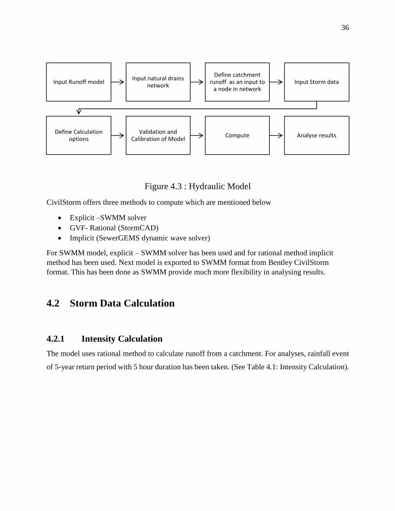
CHAPTER 4: METHODOLOGY

4.1 Brief Overview

The modelling exercise begins with importing digital elevation model of barapullah catchment and

drains network in ArcSWAT (see Figure 4.1). Then drain network is burned in DEM such that all

the water from points nearer to drains falls in it (Note that this exercise can be done without drain

network as well i.e. using only DEM but when we input drain network our accuracy of model

improves). (Mark et al. , 2004) Then model computes flow direction and accumulates flows to

generate stream network based upon threshold values given in hectares. For this thesis 300 hectares

has been used as threshold values. After stream network is generated, we need to select a point in

stream network for which we want to generate watersheds. After watershed is generated, model

calculates watershed parameters e.g. characteristic width, longest flow path, etc. Next soil data and

land use data need to be imported in model. For this project, Soil data has been taken from FAO

(Food and Agriculture Organization)

Figure 4.1: ArcSWAT Watershed Delineator Window

35

And land use data has been taken from National Remote Sensing Centre (NRSC). Soil data and

land use data are required to calculate runoff parameters e.g. curve number (SCS-CN) or runoff

coefficient (rational method) (Weng, 2001). Now after importing soil data and land use data, model

creates HRUs (Hydrologic Response Units) and generate watershed reports which give percentage

of different soil and land use types in each watershed which would then be used to input parameters

in hydraulic modelling. Refer to figure 4.2 for brief summary of hydrologic model steps.

Figure 4.2: Hydrological Model

Now after building watershed subbasin in hydrologic model, we need to import subbasin and drain

network in CivilStorm. Then we need to define runoff method as EPA-SWMM or rational method,

on the basis of which we have to input watershed parameters such as time of concentration or CN

value. This project has used Modelbuilder tool in CivilStorm to import drain network and TRex

tool to assign elevation values to nodes in network. After assigning values to network elements,

Storm events are defined. For this project two storm events such as IDF equation for Delhi and

rainfall hyetograph for 24 hours duration have been used (see 2.6 for more details). Next step is

define calculation option using solver method.

Input Digital Elevation Model

(DEM)

Input Drain Network

Flow direction and

accumulation

Stream network Definition

Outlet/Inlet definition

Watershed Delineation

Calculation of subbasin

parameters

Input Land use data

Input Soil data

Slope characterization

HRU Creation

36

Figure 4.3 : Hydraulic Model

CivilStorm offers three methods to compute which are mentioned below

Explicit –SWMM solver

GVF- Rational (StormCAD)

Implicit (SewerGEMS dynamic wave solver)

For SWMM model, explicit – SWMM solver has been used and for rational method implicit

method has been used. Next model is exported to SWMM format from Bentley CivilStorm

format. This has been done as SWMM provide much more flexibility in analysing results.

4.2 Storm Data Calculation

4.2.1 Intensity Calculation

The model uses rational method to calculate runoff from a catchment. For analyses, rainfall event

of 5-year return period with 5 hour duration has been taken. (See Table 4.1: Intensity Calculation).

Input Runoff modelInput natural drains

network

Define catchment runoff as an input to

a node in networkInput Storm data

Define Calculation options

Validation and Calibration of Model

Compute Analyse results

37

Table 4.1: Intensity Calculation

Intensity Calculation

K 5.208

n 1.107

a 0.157

b 0.5

Return Period T(Years)

Intensity(cm/hr) 1 2 5 10

Durations (Hours)

1 3.324589 3.706804 4.28032 4.772412

2 1.88865 2.10578 2.431586 2.711137

6 0.655807 0.731202 0.844334 0.941404

12 0.317974 0.35453 0.409383 0.456448

24 0.150961 0.168316 0.194358 0.216703

38

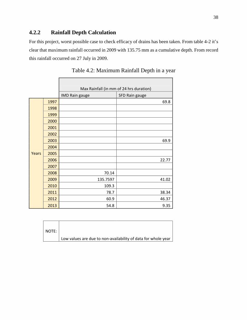
4.2.2 Rainfall Depth Calculation

For this project, worst possible case to check efficacy of drains has been taken. From table 4-2 it’s

clear that maximum rainfall occurred in 2009 with 135.75 mm as a cumulative depth. From record

this rainfall occurred on 27 July in 2009.

Table 4.2: Maximum Rainfall Depth in a year

Max Rainfall (in mm of 24 hrs duration)

IMD Rain gauge SFD Rain gauge

Years

1997 69.8

1998

1999

2000

2001

2002

2003 69.9

2004

2005

2006 22.77

2007

2008 70.14

2009 135.7597 41.02

2010 109.3

2011 78.7 38.34

2012 60.9 46.37

2013 54.8 9.35

NOTE:

Low values are due to non-availability of data for whole year

39

CHAPTER 5: ANALYSIS AND RESULTS

5.1 Verification

Verification is the process of checking the model against independent data to determine its

accuracy whilst calibration is the process of adjusting model parameters to make the model fit with

measured conditions.

5.1.1 Catchment Area Validation

To verify the watershed model built with ArcSWAT, author has used data from Master Plan for

Drainage of Storm Water, 1976. Catchment areas for each drain calculated using SWAT and

Master Plan 1976 have been presented in Table 5.1 for comparison.

Table 5.1 Catchment Area Comparison

S.No. Drain Name

Catchment Area(in hectares)

From SWAT Model

Catchment (in hectares)

From DMP 1976

1 AIIMs Drain 1799.17 2060

2 Andrews Gunj Drain 398.5175 503

3 Barapullah Nallah 14083.945 17227.5**

4 Chirag Delhi Drain 5799.165 5300


6 Kushak Nallah 4879.5125 4804

7 Lajpat Nagar Drain 442.8325 460

8 Malviya Nagar Drain 1112.78 269*

9 Nauroji Nagar Drain 1591.65 1700

10 Sunehri Pullah Nallah 2533.3525 1918*

*Note large difference in some drain is due change in drain network i.e. addition of drain which

have somewhere reduced the catchment area of other drain or in catchment area is increased due

to extension of drain.

**Barapullah Nallah catchment is basically the whole Barapullah region. Area values have been

obtained by adding catchments areas of all other drains. That is why we have such large difference

in their values.

40

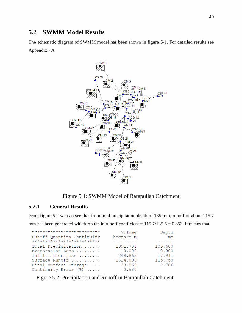
5.2 SWMM Model Results

The schematic diagram of SWMM model has been shown in figure 5-1. For detailed results see

Appendix - A

Figure 5.1: SWMM Model of Barapullah Catchment

5.2.1 General Results

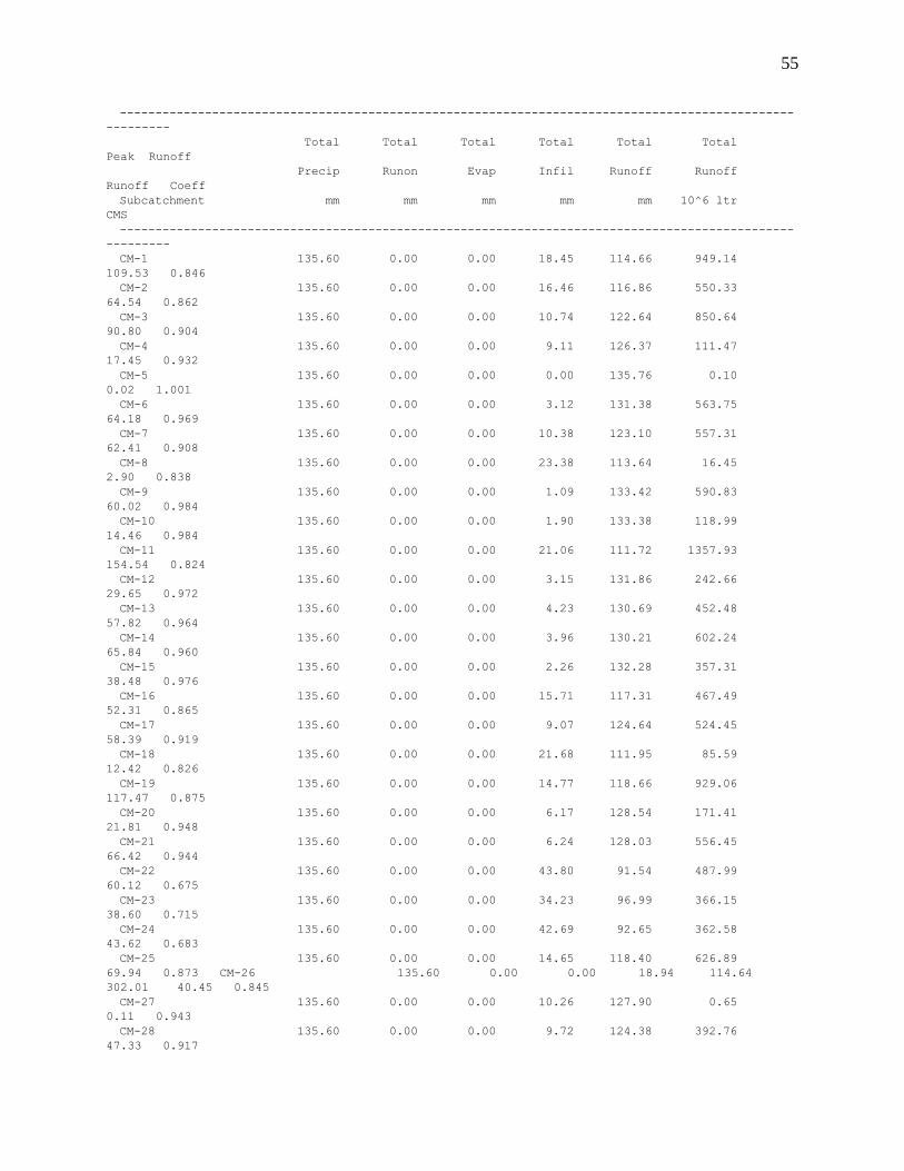
From figure 5.2 we can see that from total precipitation depth of 135 mm, runoff of about 115.7

mm has been generated which results in runoff coefficient = 115.7/135.6 = 0.853. It means that

Figure 5.2: Precipitation and Runoff in Barapullah Catchment

41

more than 85% of rainfall is converted into runoff which is intuitive also as barapullah catchment

is highly urbanized as it covers posh areas of south Delhi and central Delhi.

Figure 5.3: Flow in major drains of Barapullah Catchment

Figure 5.3 show flow (m3/s) in major tributaries of Barapullah catchment. Here we can analyse

that Chirag Delhi is the major tributary followed by Kushak Nallah which is followed by Sunehri

Pullah Nallah.

Figure 5.4: Node Flooding Graph

42

Figure 5.4 shows a profile graph of CS-2, CS-9, CS-11, CS-14 and CS-15. From this graph we

can find out how much water is being flooded a particular instant of time from a node. For more

detailed study of about how much water is being flooded from each node, let’s look at figure 5.5.

Figure 5.5: Node Flooding Summary

From figure 5.5 we can get information about how much flood volume is being generated at

node and how much ponded depth (maximum depth) it has. For detailed outlook see Figure 5.7.

Figure 5.6 display link flow summary. We can get information about maximum flow in CMS

from the figure 5.6. And also by using parameter Max/Full Depth, we can see which link has

been surcharged as Max/Full Depth ration is ratio of Maximum Depth of water in channel with

Depth of Channel. Max/Full Depth ratio >= 1 implies that channel has been surcharged. Using

this parameter it’s clear that

Chirag Delhi Drain (its subsection 2, 3 and 4) is getting surcharged, thus insufficient

needs improvement. Note that these cross-section used are being are the proposed

sections from Storm Water Drainage Master Plan – 1976 and rainfall data is of 29 July,

2009 with consideration of change in land use pattern in last 30 years taken into account.

Lajpat Nagar Drain is inadequate

Malviya Nagar is inadequate

Andrews Gunj Drain is inadequate

Kushak Nallah (subsection 2 and 4) are inadequate.

43

Note that we are using rainfall depth of 135.6 mm for 24 hours duration which is worst case

scenario or highest loading from the data available with the author. From data (See section 4.2.2)

we can see that this amount of rainfall has return period of greater than 10 years. So although it

seems they are inadequate but in day-to-day scenario it may be adequate.

Figure 5.6: Link Flow Summary

44

Figure 5.7: Flooding Nodes (shown in red) at t = 12:15

45

5.3 Rational Method Results

Rational Method analysis has been carried out using rainfall with return period of 5 years with

duration equal to 5 hours. The results are shown in Table 5-2 and Table 5-3.

Table 5.2: Channel Flow Summary

Label

Time (Maximum Flow) (hours)

Flow (Maximum) (m³/s)

Velocity (Maximum Calculated) (m/s)

Hydraulic Grade (Maximum) (m)

Greater Kailash Drain 1.85 17.88 3.26 216.17

Outfall Drain 3.15 491.66 8.94 195.67

Chirag Delhi Drain_1 1.85 12.27 2.09 223.94





Chirag Delhi Drain_6 4 190.78 3.58 206.77



Lajpat Nagar Drain_1 0 0 0 211.13

Lajpat Nagar Drain_3 1.85 0.01 0.15 209.79

Lajpat Nagar Drain_4 1.85 20.13 2.16 204.61

Lajpat Nagar Drain_2 17.95 0 0.01 212.1

Malviya Nagar Drain_1 8.5 0 0.02 234.15

Malviya Nagar Drain_2 1.25 31.46 3.72 226.27

Andrews Gunj Drain 1.2 13.69 2.51 213.2

AIIMs Drain_1 1.4 49.89 5.13 211.82

AIIMs Drain_2 2.8 49.89 2.57 207.86

Nauroji Nagar Drain_1 2.45 14.53 3.07 222.32




Kushak Nallah_1 0 0 0 218.01

Kushak Nallah_2 2.25 40.57 1.89 215.43

Kushak Nallah_3 2.5 111.13 4.37 210.25

Kushak Nallah_4 2.75 172.08 2.07 207.01

Sunehri Pullah Nallah_1 3.7 86.79 3.83 203.63



Barapullah Nallah_1 3.05 474.06 2.89 202.01

Barapullah Nallah_2 3.1 491.81 3.27 201.21

Malviya Nagar Drain_3 0 0 0 234.53

46

Table 5.3: Catchment flow Summary

Label Area (User Defined) (ha)

Volume (Total Runoff) (m³)

Flow (Maximum) (m³/s)

Time (Maximum Flow) (hours)

CM-1 827.765 5,01,823.80 27.88 2.45

CM-2 470.95 2,92,204.20 16.23 2.45

CM-3 693.633 4,66,075.80 25.89 1.35

CM-4 88.208 60,291.60 3.35 0.35

CM-5 0.075 63.8 0 0.05

CM-6 429.083 3,29,431.30 18.3 0.95

CM-7 452.723 3,02,077.00 16.78 1.2

CM-8 14.473 8,295.60 0.46 0.3

CM-9 442.833 3,62,201.00 20.12 1.1

CM-10 89.21 71,091.00 3.95 0.65

CM-11 1,215.45 7,02,474.20 39.03 1.15

CM-12 184.033 1,43,133.30 7.95 0.7

CM-13 346.213 2,61,453.70 14.53 0.65

CM-14 462.51 3,51,941.50 19.55 1.1

CM-15 270.11 2,13,923.30 11.88 1.05

CM-16 398.518 2,46,354.50 13.69 1.2

CM-17 420.77 2,93,571.20 16.31 1.2

CM-18 76.45 41,672.50 2.32 0.55

CM-19 782.928 4,95,618.00 27.53 0.85

CM-20 133.348 97,201.30 5.4 0.7

CM-21 434.64 3,15,706.60 17.54 0.9

CM-22 533.088 2,29,962.20 12.78 1.35

CM-23 377.518 1,62,145.00 9.01 1.05

CM-24 391.345 1,70,522.90 9.47 1.4

CM-25 529.478 3,28,593.90 18.26 1.25

CM-26 263.428 1,57,244.00 8.74 0.7

CM-27 0.51 352.9 0.02 0.05

CM-28 315.768 2,20,939.00 12.27 0.95

CM-29 1,112.78 5,66,302.60 31.46 1.25

CM-30 865.14 6,29,166.50 34.95 1.1

CM-31 556.525 3,54,725.80 19.71 1.05

CM-32 319.585 1,25,169.60 6.95 1.5

CM-33 451.518 1,75,677.20 9.76 1.7

47

Figure 5.8: Depth/ Rise (%) and Flow (m3/s)

48

5.3.1 Analysis

It’s clear from figure 5.8 that except Chirag Delhi Drain_7 and Kushak Nallah_2 all other drains

have sufficient capacity to carry runoff as all of them have value of Depth/Rise less than 100%.

Depth (Maximum Depth)/Rise (Height of channel) is greater than 100% only for Chirag Delhi

Drain_7 and Kushak Nallah_2.

Table 5.4: Comparison of Discharge from Rational Method and DMP -1976

S.No Drain Name

Maximum

Discharge (from

Rational Method)

Maximum

Discharge (from

DMP 1976)****

1 AIIMs Drain 49.89 66.0

2 Andrews Gunj Drain 13.69 16.41

3 Barapullah Nallah 491.81

4 Chirag Delhi Drain 190.78 NA*


6 Kushak Nallah 172.08 256.74**

7 Lajpat Nagar Drain 20.3 16.15

8 Malviya Nagar Drain 31.46 12.3***

9 Nauroji Nagar Drain 61.61 59.5

10 Sunehri Pullah Nallah 93.23 67

NA* = Not Available

** = Many changes have occurred in Kushak Nallah catchment from 1976 due to addition of new

drains near Connaught place which has reduced catchment area thus discharge from it.

*** = Malviya Nagar drain has been extended after 1976 till Lado Sarai so now it has a bigger

catchment thus more discharge.

**** = Calculation for DMP-1976 have been based on storm event with 5-year return period with

intensity = 5.17 cm/hr

49

5.4 Recommendation

Now after analysis of SWMM Model (Worst case scenario) and Rational Method (Normal

Scenario), we can say provide following design recommendations.

Chirag Delhi Drain_7 (from CS-16 to CS-3) needs to be widen up as it surcharged during

rational method simulation. It bottom width can be increased from 24 m to 30 m.

Kushak Nallah Drain_2 (from CS-9 to CS-10) needs to be widen up as it surcharged during

rational method simulation. Its bottom width should be increased from 20 m to 30 m.

50

CHAPTER 6: DISCUSSION

6.1 Model Application

The methodology described in this thesis simulate industry standard practise for storm water

drainage simulation. It uses SWMM Model (with rainfall duration of 24 hrs) and Rational Method

(with Return Period = 5 year with rainfall duration of 5 hours). It begins with watershed analysis

using ArcGIS SWAT component then import modelling parameters in Bentley CivilStorm. It uses

MS Excel to calculate CN (Curve Number) and C (Runoff Coefficient) for each catchment. Then

it refines and add modelling parameters in Civil Storm. It then uses SWMM method to calculate

runoff in worst case scenario and studies it’s routing in drains. It’s also uses rational method to

calculate runoff from normal intensity rainfall.

6.2 Drawbacks and limitations of the Methodology

Model uses longitudinal section designs which were being proposed in Master Plan for

Storm water drainage – 1976. Due to silting and illegal construction, present day cross-

section might be different.

Rainfall Data taken to simulate model in SWMM is not adequate as to get proper

understanding of capacity of drainage system, atleast past 30 year data should have been

used. This will provide proper understanding return period for which we are designing

drainage network.

This study assumes one time vs depth curve (29 July, 2009) for whole barapullah catchment

which is not correct of representation of real-life condition. In reality, thiessen polygons

method should have been used which gives weightage to each rain gauge. However due to

insufficient data, author cannot go for thiessen polygon method.

Land use data taken from NRSC has several classes not properly defined e.g. in NRSC one

class was labelled as “Double/Triple” with no explanation. So based upon author’s

understanding of land use patterns, author assumed them as agricultural area.

Soil data has been taken from FAO (Food and Agriculture Organization). Data was found

to be too coarse. If proper data set would have been available then it might would have

resulted in better results

51

This project thesis studies Barapullah catchment as a whole and routes subbasin runoff into

respective nodes. However Barapullah catchment is very big catchment and results got

from analysis can only provide us with some broad understanding of drainage network. For

e.g. thesis proposes some design recommendations in Chirag Delhi Drain 7 and Kushak

Nallah, however to actually propose what should be the width and cross-section detail,

modelling needs to be done focussing on either Chirag Delhi Catchment or Kushak Nallah

catchment.

6.3 Advantages of SWMM Method over Rational Method

The major difference between SWMM and the rational method is in SWMM's ability to

give much more than a peak runoff as a result.

SWMM uses a rainfall hyetograph(or tabular inflow data - e.g. from a flow meter) to

generate a whole runoff hydrograph and route it through a network of links and nodes -

which allows one to assess such things as volume of runoff drained, effects of detention,

etc. The rational method is a much "rougher" tool which, in turn, gives you much less in

terms of results upon which to base design decisions.

The runoff coefficient lumps in all the hydrologic characteristics (imperviousness,

infiltration, evapotranspiration, depression storage, etc...) of a watershed into one number.

Besides area, the only number in the rational method calculation with any real, observable,

physical basis is the time of concentration that you select to determine your rainfall

intensity from the IDF (rainfall intensity-duration-frequency) curve (OK, the IDF curves

are based on observed rainfall).

SWMM does allow one to explicitly select parameters to (hopefully) better match the

actual hydrology of the system (e.g. you can base your infiltration on specific known soil

characteristics, imperviousness can be scaled from aerial photographs or ground survey,

depression storage and roughness can be varied to match ground cover and topography,

catchment response to runoff can be varied using the "WIDTH" parameter, etc...) You can

also use actual rainfall data directly instead of relying on IDF curves for storm

intensity (although, in practice, we tend to still use IDF curves a great deal).

52

CHAPTER 7: CONCLUSION AND FUTURE WORK

7.1 Conclusion

In the preceding chapters, various aspects involved in the analysis and design of storm water

drainage network were looked into. This thesis provided reader with a methodology to simulate

storm drainage in urban areas. It uses present day industry tools e.g. ArcGIS SWAT, EPA-SWMM

and Bentley Civil Storm for model building and analysis. Its starts from importing digital elevation

model and drain network. It takes cross-section data from Delhi Drainage Master Plan-1976. It

then analyse these sections for current loadings and check whether they are sufficient or not. The

analysis is based on rational method and EPA-SWMM model. For rational method, rainfall with

5 year return period with 5 hour rainfall duration has been taken. For SWMM Model, rainfall of

cumulative depth of 135.6 mm over 24 hours durations has been taken to provide worst case

scenario. It finds out problematic nodes and links in network. Its estimate quantity of water being

flooded from which node. It estimate which link is overflowing, for how much time. After analyses

it proposes certain recommendations in design of drains which can be taken up to stop local level

flooding problems. It then list down certain limitation of methodology and datasets.

7.2 Future Work

Writing a research paper about this methodology

More detailed analysis of barapullah catchment using rainfall data of last 30 years

Design and analysis of Chirag Delhi Drain network and simulation for providing

recommendation

Design and analysis of Kushak Nallah network for providing recommendation.

Building a scenario to study runoff using present day cross-section with normal intensity

runoff

53

APPENDIX – A

This section consist of detailed report of SWMM Model

EPA STORM WATER MANAGEMENT MODEL - VERSION 5.0 (Build 5.0.022)

--------------------------------------------------------------

******************************************************

*** NOTE: The summary statistics displayed in this

report are based on results found at every

computational time step, not just on results from

each reporting time step.

******************************************************

***

****************

Analysis Options

****************

Flow Units ............... CMS

Process Models:

Rainfall/Runoff ........ YES

Snowmelt ............... NO

Groundwater ............ NO

Flow Routing ........... YES

Ponding Allowed ........ YES

Water Quality .......... NO

Infiltration Method ...... CURVE_NUMBER

Flow Routing Method ...... DYNWAVE

Starting Date ............ JUL-27-2009 00:00:00

Ending Date .............. JUL-28-2009 12:00:00

Antecedent Dry Days ...... 0.0

Report Time Step ......... 00:15:00

Wet Time Step ............ 00:15:00

Dry Time Step ............ 01:00:00

Routing Time Step ........

30.00 sec

WARNING 04: minimum elevation drop used for Conduit Sunehri_Pulla_Nallah_3

WARNING 02: maximum depth increased for Node CS-1






WARNING 02: maximum depth increased for Node

CS-9 WARNING 02: maximum depth increased for

Node CS-10




54










WARNING 02: maximum depth increased for Node CS-34 **************************

Volume Depth

Runoff Quantity Continuity hectare-m mm

************************** --------- -------

Total Precipitation ...... 1891.701 135.600

Evaporation Loss ......... 0.000 0.000

Infiltration Loss ........ 249.863 17.911

Surface Runoff ........... 1614.890 115.758

Final Surface Storage .... 38.869 2.786

Continuity Error (%) ..... -0.630

************************** Volume Volume

Flow Routing Continuity hectare-m 10^6 ltr

************************** --------- ---------

Dry Weather Inflow ....... 0.000 0.000

Wet Weather Inflow ....... 1614.759 16147.754

Groundwater Inflow ....... 0.000 0.000

RDII Inflow .............. 0.000 0.000

External Inflow .......... 0.000 0.000

External Outflow ......... 933.097 9331.066

Internal Outflow ......... 676.438 6764.449

Storage Losses ........... 0.000 0.000

Initial Stored Volume .... 0.002 0.024

Final Stored Volume ...... 5.564 55.640

Continuity Error (%) ..... -0.021

********************************

Highest Flow Instability Indexes

********************************

All links are stable.

*************************

Routing Time Step Summary

*************************

Minimum Time Step : 30.00 sec

Average Time Step : 30.00 sec

Maximum Time Step : 30.00 sec

Percent in Steady State : 0.00

Average Iterations per Step : 2.05

***************************

Subcatchment Runoff Summary

***************************

55

-----------------------------------------------------------------------------------------------

---------

Total Total Total Total Total Total

Peak Runoff

Precip Runon Evap Infil Runoff Runoff

Runoff Coeff

Subcatchment mm mm mm mm mm 10^6 ltr

CMS

-----------------------------------------------------------------------------------------------

---------

CM-1 135.60 0.00 0.00 18.45 114.66 949.14

109.53 0.846

CM-2 135.60 0.00 0.00 16.46 116.86 550.33

64.54 0.862

CM-3 135.60 0.00 0.00 10.74 122.64 850.64

90.80 0.904

CM-4 135.60 0.00 0.00 9.11 126.37 111.47

17.45 0.932

CM-5 135.60 0.00 0.00 0.00 135.76 0.10

0.02 1.001

CM-6 135.60 0.00 0.00 3.12 131.38 563.75

64.18 0.969

CM-7 135.60 0.00 0.00 10.38 123.10 557.31

62.41 0.908

CM-8 135.60 0.00 0.00 23.38 113.64 16.45

2.90 0.838

CM-9 135.60 0.00 0.00 1.09 133.42 590.83

60.02 0.984

CM-10 135.60 0.00 0.00 1.90 133.38 118.99

14.46 0.984

CM-11 135.60 0.00 0.00 21.06 111.72 1357.93

154.54 0.824

CM-12 135.60 0.00 0.00 3.15 131.86 242.66

29.65 0.972

CM-13 135.60 0.00 0.00 4.23 130.69 452.48

57.82 0.964

CM-14 135.60 0.00 0.00 3.96 130.21 602.24

65.84 0.960

CM-15 135.60 0.00 0.00 2.26 132.28 357.31

38.48 0.976

CM-16 135.60 0.00 0.00 15.71 117.31 467.49

52.31 0.865

CM-17 135.60 0.00 0.00 9.07 124.64 524.45

58.39 0.919

CM-18 135.60 0.00 0.00 21.68 111.95 85.59

12.42 0.826

CM-19 135.60 0.00 0.00 14.77 118.66 929.06

117.47 0.875

CM-20 135.60 0.00 0.00 6.17 128.54 171.41

21.81 0.948

CM-21 135.60 0.00 0.00 6.24 128.03 556.45

66.42 0.944

CM-22 135.60 0.00 0.00 43.80 91.54 487.99

60.12 0.675

CM-23 135.60 0.00 0.00 34.23 96.99 366.15

38.60 0.715

CM-24 135.60 0.00 0.00 42.69 92.65 362.58

43.62 0.683

CM-25 135.60 0.00 0.00 14.65 118.40 626.89

69.94 0.873 CM-26 135.60 0.00 0.00 18.94 114.64

302.01 40.45 0.845

CM-27 135.60 0.00 0.00 10.26 127.90 0.65

0.11 0.943

CM-28 135.60 0.00 0.00 9.72 124.38 392.76

47.33 0.917

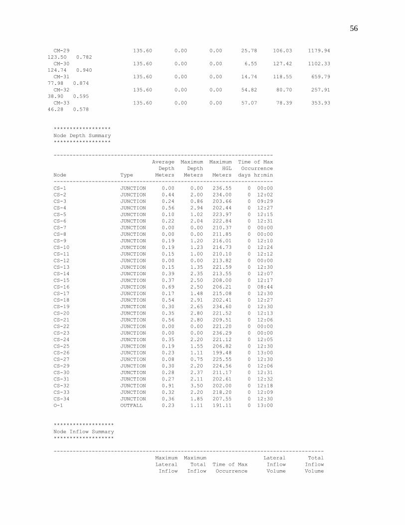
56

CM-29 135.60 0.00 0.00 25.78 106.03 1179.94

123.50 0.782

CM-30 135.60 0.00 0.00 6.55 127.42 1102.33

124.74 0.940

CM-31 135.60 0.00 0.00 14.74 118.55 659.79

77.98 0.874

CM-32 135.60 0.00 0.00 54.82 80.70 257.91

38.90 0.595

CM-33 135.60 0.00 0.00 57.07 78.39 353.93

46.28 0.578

******************

Node Depth Summary

******************

---------------------------------------------------------------------

Average Maximum Maximum Time of Max

Depth Depth HGL Occurrence

Node Type Meters Meters Meters days hr:min

---------------------------------------------------------------------

CS-1 JUNCTION 0.00 0.00 236.55 0 00:00

CS-2 JUNCTION 0.44 2.00 234.00 0 12:02

CS-3 JUNCTION 0.24 0.86 203.66 0 09:29

CS-4 JUNCTION 0.56 2.94 202.44 0 12:27

CS-5 JUNCTION 0.10 1.02 223.97 0 12:15

CS-6 JUNCTION 0.22 2.04 222.84 0 12:31

CS-7 JUNCTION 0.00 0.00 210.37 0 00:00

CS-8 JUNCTION 0.00 0.00 211.85 0 00:00

CS-9 JUNCTION 0.19 1.20 216.01 0 12:10

CS-10 JUNCTION 0.19 1.23 214.73 0 12:24

CS-11 JUNCTION 0.15 1.00 210.10 0 12:12

CS-12 JUNCTION 0.00 0.00 213.82 0 00:00

CS-13 JUNCTION 0.15 1.35 221.59 0 12:30

CS-14 JUNCTION 0.39 2.35 213.55 0 12:07

CS-15 JUNCTION 0.37 2.50 208.00 0 12:17

CS-16 JUNCTION 0.69 2.50 206.21 0 08:44

CS-17 JUNCTION 0.17 1.48 215.08 0 12:30

CS-18 JUNCTION 0.54 2.91 202.41 0 12:27

CS-19 JUNCTION 0.30 2.65 234.60 0 12:30

CS-20 JUNCTION 0.35 2.80 221.52 0 12:13

CS-21 JUNCTION 0.56 2.80 209.51 0 12:06

CS-22 JUNCTION 0.00 0.00 221.20 0 00:00

CS-23 JUNCTION 0.00 0.00 236.29 0 00:00

CS-24 JUNCTION 0.35 2.20 221.12 0 12:05

CS-25 JUNCTION 0.19 1.55 206.82 0 12:30

CS-26 JUNCTION 0.23 1.11 199.48 0 13:00

CS-27 JUNCTION 0.08 0.75 225.55 0 12:30

CS-29 JUNCTION 0.30 2.20 224.56 0 12:06

CS-30 JUNCTION 0.28 2.37 211.17 0 12:31

CS-31 JUNCTION 0.27 2.11 202.61 0 12:32

CS-32 JUNCTION 0.91 3.50 202.00 0 12:18

CS-33 JUNCTION 0.32 2.20 218.20 0 12:09

CS-34 JUNCTION 0.36 1.85 207.55 0 12:30

O-1 OUTFALL 0.23 1.11 191.11 0 13:00

*******************

Node Inflow Summary

*******************

-------------------------------------------------------------------------------------

Maximum Maximum Lateral Total

Lateral Total Time of Max Inflow Inflow

Inflow Inflow Occurrence Volume Volume

57

Node Type CMS CMS days hr:min 10^6 ltr 10^6 ltr

-------------------------------------------------------------------------------------

CS-1 JUNCTION 0.000 0.000 0 00:00 0.000 0.000

CS-2 JUNCTION 123.502 123.502 0 12:30 1179.719 1179.716

CS-3 JUNCTION 0.000 192.320 0 09:27 0.000 5405.280

CS-4 JUNCTION 0.000 530.526 0 12:32 0.000 8422.725

CS-5 JUNCTION 57.818 57.818 0 12:15 452.463 452.463

CS-6 JUNCTION 0.000 172.490 0 12:30 0.000 1381.246

CS-7 JUNCTION 0.000 0.000 0 00:00 0.000 0.000

CS-8 JUNCTION 0.000 0.000 0 00:00 0.000 0.000

CS-9 JUNCTION 154.542 154.542 0 12:30 1357.779 1357.778

CS-10 JUNCTION 0.000 236.503 0 12:14 0.000 3000.043

CS-11 JUNCTION 60.024 60.024 0 12:30 590.771 590.770

CS-12 JUNCTION 0.000 0.000 0 00:00 0.000 0.000

CS-13 JUNCTION 66.421 66.421 0 12:30 556.427 556.427

CS-14 JUNCTION 21.813 393.601 0 12:30 171.406 4865.133

CS-15 JUNCTION 44.110 488.784 0 12:31 361.638 5187.185

CS-16 JUNCTION 2.903 686.212 0 12:31 16.447 9581.123

CS-17 JUNCTION 212.786 212.786 0 12:30 1826.628 1826.626

CS-18 JUNCTION 0.016 576.391 0 12:32 0.102 8985.488

CS-19 JUNCTION 117.472 117.472 0 12:30 929.013 929.012

CS-20 JUNCTION 52.308 52.308 0 12:30 467.442 467.442

CS-21 JUNCTION 0.000 357.650 0 12:59 0.000 5034.602

CS-22 JUNCTION 0.000 0.000 0 00:00 0.000 0.000

CS-23 JUNCTION 0.000 0.000 0 00:00 0.000 0.000

CS-24 JUNCTION 69.943 379.163 0 12:30 626.825 4380.734

CS-25 JUNCTION 327.280 327.280 0 12:30 2907.154 2907.150

CS-26 JUNCTION 0.000 524.527 0 13:00 0.000 9333.276

CS-27 JUNCTION 47.326 47.326 0 12:30 392.735 392.735

CS-29 JUNCTION 328.422 375.519 0 12:30 2676.483 3069.074

CS-30 JUNCTION 0.000 212.476 0 12:30 0.000 1826.131

CS-31 JUNCTION 17.453 340.556 0 12:30 111.466 3017.808

CS-32 JUNCTION 64.183 645.909 0 12:33 563.720 9545.832

CS-33 JUNCTION 65.838 236.811 0 12:30 602.196 1982.692

CS-34 JUNCTION 38.483 262.087 0 12:30 357.283 4493.460

O-1 OUTFALL 0.000 524.527 0 13:00 0.000 9331.024

**********************

Node Surcharge Summary

**********************

Surcharging occurs when water rises above the top of the highest conduit.

---------------------------------------------------------------------

Max. Height Min. Depth

Hours Above Crown Below Rim

Node Type Surcharged Meters Meters

---------------------------------------------------------------------

CS-2 JUNCTION 2.01 0.000 0.000

CS-9 JUNCTION 1.41 0.000 0.000

CS-11 JUNCTION 0.73 0.000 0.000

CS-14 JUNCTION 1.59 0.000 0.000

CS-15 JUNCTION 0.67 0.000 0.000

CS-16 JUNCTION 4.58 0.000 0.000

CS-20 JUNCTION 0.78 0.000 0.000

CS-21 JUNCTION 2.08 0.000 0.000

CS-24 JUNCTION 1.51 0.000 0.000

CS-29 JUNCTION 0.82 0.000 0.000

CS-32 JUNCTION 0.71 0.000 0.000

CS-33 JUNCTION 0.97 0.000 0.000

*********************

Node Flooding Summary

*********************

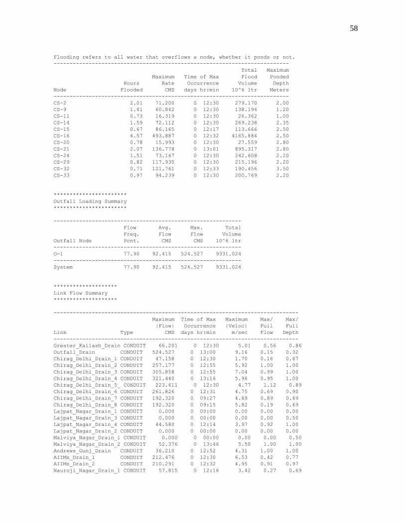
58

Flooding refers to all water that overflows a node, whether it ponds or not.

--------------------------------------------------------------------------

Total Maximum

Maximum Time of Max Flood Ponded

Hours Rate Occurrence Volume Depth

Node Flooded CMS days hr:min 10^6 ltr Meters

--------------------------------------------------------------------------

CS-2 2.01 71.200 0 12:30 279.170 2.00

CS-9 1.41 60.842 0 12:30 138.194 1.20

CS-11 0.73 16.319 0 12:30 26.362 1.00

CS-14 1.59 72.112 0 12:30 269.238 2.35

CS-15 0.67 86.165 0 12:17 113.666 2.50

CS-16 4.57 493.887 0 12:32 4165.884 2.50

CS-20 0.78 15.993 0 12:30 27.559 2.80

CS-21 2.07 136.778 0 13:01 895.317 2.80

CS-24 1.51 73.167 0 12:30 242.608 2.20

CS-29 0.82 117.935 0 12:30 215.196 2.20

CS-32 0.71 121.761 0 12:33 190.456 3.50

CS-33 0.97 94.239 0 12:30 200.769 2.20

***********************

Outfall Loading Summary

***********************

-----------------------------------------------------------

Flow Avg. Max. Total

Freq. Flow Flow Volume

Outfall Node Pcnt. CMS CMS 10^6 ltr

-----------------------------------------------------------

O-1 77.90 92.415 524.527 9331.024

-----------------------------------------------------------

System 77.90 92.415 524.527 9331.024

********************

Link Flow Summary

********************

-----------------------------------------------------------------------------

Maximum Time of Max Maximum Max/ Max/

|Flow| Occurrence |Veloc| Full Full

Link Type CMS days hr:min m/sec Flow Depth

-----------------------------------------------------------------------------

Greater_Kailash_Drain CONDUIT 66.201 0 12:30 5.01 0.56 0.86

Outfall_Drain CONDUIT 524.527 0 13:00 9.16 0.15 0.32

Chirag_Delhi_Drain_1 CONDUIT 47.158 0 12:30 1.70 0.16 0.67




Chirag_Delhi_Drain_5_ CONDUIT 223.611 0 12:30 4.77 1.12 0.89




Lajpat_Nagar_Drain_1 CONDUIT 0.000 0 00:00 0.00 0.00 0.00




Malviya_Nagar_Drain_1 CONDUIT 0.000 0 00:00 0.00 0.00 0.50


Andrews_Gunj_Drain CONDUIT 36.210 0 12:52 4.31 1.00 1.00

AIIMs_Drain_1 CONDUIT 212.476 0 12:30 6.53 0.42 0.77

AIIMs_Drain_2 CONDUIT 210.291 0 12:32 4.95 0.91 0.97

Nauroji_Nagar_Drain_1 CONDUIT 57.815 0 12:16 3.42 0.27 0.69

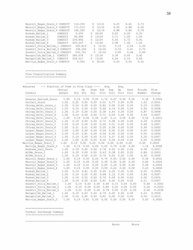
59




Kushak_Nallah_1 CONDUIT 0.000 0 00:00 0.00 0.00 0.50




Sunehri_Pulla_Nallah_1 CONDUIT 325.813 0 12:31 5.15 0.24 0.52



Barapullah_Nallah_1 CONDUIT 584.678 0 12:34 3.36 0.64 0.92

Barapullah_Nallah_2 CONDUIT 524.527 0 13:00 4.26 2.23 0.66


***************************

Flow Classification Summary

***************************

----------------------------------------------------------------------------------------

Adjusted --- Fraction of Time in Flow Class ---- Avg. Avg.

/Actual Up Down Sub Sup Up Down Froude Flow

Conduit Length Dry Dry Dry Crit Crit Crit Crit Number Change

-----------------------------------------------------------------------------------------

Greater_Kailash_Drain 1.00 0.19 0.00 0.00 0.74 0.07 0.00 0.00 0.38 0.0004

Outfall_Drain 1.00 0.22 0.00 0.00 0.01 0.77 0.00 0.00 1.63 0.0001

Chirag_Delhi_Drain_1 1.00 0.19 0.00 0.00 0.81 0.00 0.00 0.00 0.19 0.0001




Chirag_Delhi_Drain_5_ 1.00 0.19 0.02 0.00 0.67 0.11 0.00 0.00 0.56 0.0010




Lajpat_Nagar_Drain_1 1.00 1.00 0.00 0.00 0.00 0.00 0.00 0.00 0.00 0.0000




Malviya_Nagar_Drain_1 1.00 0.19 0.81 0.00 0.00 0.00 0.00 0.00 0.00 0.0000


Andrews_Gunj_Drain 1.00 0.19 0.00 0.00 0.78 0.02 0.00 0.00 0.38 0.0007

AIIMs_Drain_1 1.00 0.19 0.00 0.00 0.43 0.38 0.00 0.00 0.86 0.0003

AIIMs_Drain_2 1.00 0.19 0.00 0.00 0.76 0.05 0.00 0.00 0.46 0.0006

Nauroji_Nagar_Drain_1 1.00 0.19 0.00 0.00 0.75 0.05 0.00 0.00 0.38 0.0002




Kushak_Nallah_1 1.00 0.19 0.81 0.00 0.00 0.00 0.00 0.00 0.00 0.0000

Kushak_Nallah_2 1.00 0.19 0.00 0.00 0.68 0.12 0.00 0.00 0.64 0.0007

Kushak_Nallah_3 1.00 0.19 0.02 0.00 0.70 0.09 0.00 0.00 0.56 0.0005

Kushak_Nallah_4 1.00 0.19 0.00 0.00 0.81 0.00 0.00 0.00 0.21 0.0007

Sunehri_Pulla_Nallah_1 1.00 0.19 0.00 0.00 0.66 0.15 0.00 0.00 0.68 0.0002



Barapullah_Nallah_1 1.00 0.19 0.02 0.00 0.79 0.00 0.00 0.00 0.23 0.0004

Barapullah_Nallah_2 1.00 0.19 0.00 0.00 0.81 0.00 0.00 0.00 0.34 0.0015


*************************

Conduit Surcharge Summary

*************************

----------------------------------------------------------------------------

Hours Hours

60

--------- Hours Full -------- Above Full Capacity

Conduit Both Ends Upstream Dnstream Normal Flow Limited

----------------------------------------------------------------------------

Chirag_Delhi_Drain_5_ 0.01 0.01 0.01 2.29 0.01

Lajpat_Nagar_Drain_4 0.73 0.73 0.74 0.01 0.01

Kushak_Nallah_2 1.37 1.37 1.38 0.01 0.01

Sunehri_Pulla_Nallah_3 0.01 0.01 0.01 7.53 0.01

Barapullah_Nallah_2 0.01 0.01 0.01 5.08 0.01

Analysis begun on: Wed Apr 30 21:53:51 2014

Analysis ended on: Wed Apr 30 21:53:51 2014

Total elapsed time: < 1 sec

61

REFERENCES

Chen, J., Hill, A. A., & Urbano, L. D. (2009). A GIS-based Model for urban flood inundation.

Journal of Hydrology, 184-192.

EPA. (2009). Storm Water Managment Model: Applicatons Manual . Cincinati: United States

Environmental Protection Agency.

FCW(Flood Control Wing). (1976). Master Plan for Storm Water Drainage in Union Territory of

Delhi (MCD, DDA, NDMC & Cantonment). Delhi: Delhi Adminstration.

Mannings n Tables. (n.d.). Retrieved from

http://www.fsl.orst.edu/geowater/FX3/help/8_Hydraulic_Reference/Mannings_n_Tables.

htm

Mark, O., Weesakul, S., Apirumanekul, C., Aroonnet, S. B., & Djordjevic, S. (2004). Potential

and limitations of 1D modelling of urban flooding. Journal of Hydrology, 284-299.

Schmitt, T. G., Thomas, M., & Ettrich, N. (2004). Analysis and modeling of flooding in urban

drainage systems. Journal of Hydrology, 300-311.

Subramanya, K. (2008). Engineering Hydrology. New Delhi: Tata McGraw-Hill.

SWMM-Runoff-Algorithm. (n.d.). Retrieved from http://www.alanasmith.com/theory-Calculating-

Runoff-SWMM-RUNOFF-Algorithm.htm

Weng, Q. (2001). Modeling Urban Growth Effects on surface runoff with the integration of remote

sensing and GIS. Environmental Management Vol. 28, No. 6, 737-748.

Winchell, M., Srinivasan, R., DiLuzio, M., & Arnold, J. (2013). ArcSWAT Interface for SWAT2012

User's Guide. Texas -76502: Blackland Research and Extenstion Center.

ced412 report_urban flooding analysis

Documents