Functional ClassificationBasic Flow TheoryUninterrupted Flow FundamentalsCar Following TheoryShock Waves

JCE 4600Highway and Traffic EngineeringCE 445 Transportation Systems Analysis

FUNCTIONAL CLASSIFICATION

Roadway Classification

Provides hierarchy of purpose/use Allows focus of funds/policies on more important

facilities Assures balance between all levels of roadways

Functional Classification of Roads

Arterial – traffic movement with limited local property access

Collector – between road serving both traffic movement and local property access, bridges between local and arterial roads

Local – provides local property access with limited traffic movement

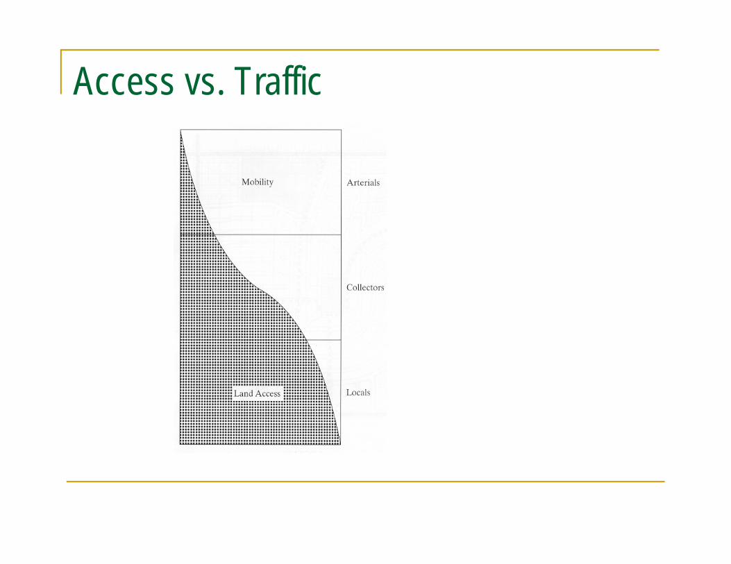
Access vs. Traffic

Rural Functional Classification

Roads and Traffic

System Traffic Volume (%) Road Mileage (%)

Principal Arterial 50 5

Minor Arterial 25 10

Collector Street 5 10

Local Street 20 75

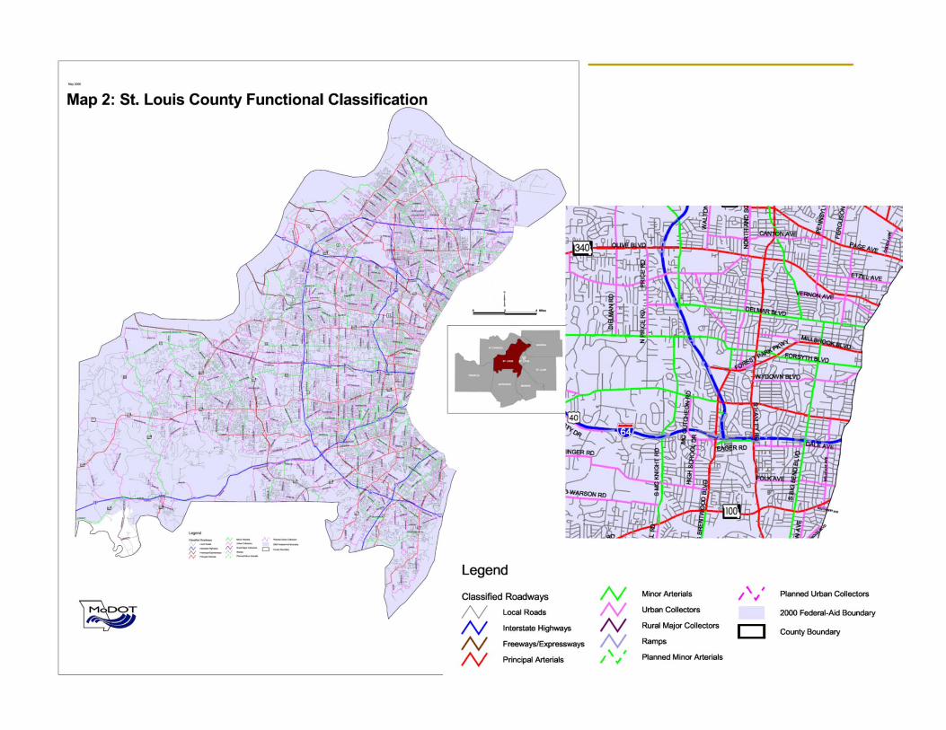
Urban/Suburban Functional Classification

Cul-de-sac Development

St. Louis Region East-West Gateway is responsible for maintaining and updating the region’s Roadway

Functional Classification System mandated under federal law. Roadways are classified according to their urban or rural setting and the type of service they provide based on considerations such as: connectivity, mobility, accessibility, vehicle miles traveled, average annual daily traffic, and abutting land use.

The purpose of roadway functional classification is to describe how travel is channelized through our roadway network and to determine project eligibility for inclusion in the Long Range Plan and short-range Transportation Improvement Program (TIP).

BREAK

Basic Flow Fundamentals

Terms and Definitions

Traffic Flow Characteristics Capacity Demand

Performance Measures Speed Density Delay Level of Service

What is Traffic Flow

Definition When do you measure? How do you measure?

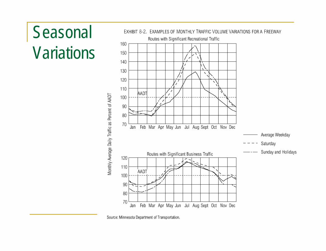
Seasonal Variations

Variations by Day of the Week

Hourly Variations

What Traffic Flows are Considered in an Operational Analysis? What season are you designing for?

Urban areas Recreational Areas

(e.g., Lake of the Ozarks and Branson) Do you design for the worst hour of the worst day?

Why or why not? How is your operational analysis tied to your design hour and

criteria? Do you just look at your design hour? Why would you want to look at anything else?

Flow Definitions

Design Hourly Volume (DHV) AADT (Average Annual Daily Traffic) K-Factor Peak Hour Factor (PHF)

Design Hourly Volume

30

Defining Design Hourly Volume

Design Hourly Volume (DHV) is defined locally by the owning agency (e.g., MoDOT)

Typically, 30th Highest Hour is used However, very rarely does an agency have hourly counts on a

facility for an entire year. In fact, many agencies count facilities for 48 hours every 2-5 years. MoDOT has factors that they apply to these counts that are assumed to

account for seasonal and daily variations. In this case, DHV is often assumed to be 12-15% of “factored”

AADT

K-Factor

Analysis Hourly Volume/AADT Normally 8-12% Typically the higher the volumes, the lower the K-factor the more urbanized the area, the lower the K-factor

Sub

-hou

rly V

aria

tions

Typically, facilities are designed for peak 15 minute flow interval

15 minute flows are accounted for through the Peak Hour Factor (PHF)

Definition:Hourly Volume

Peak 15 Minute Volume * 4

Typically range from 0.75-0.98

Peak Hour Factor (PHF)

Traffic Flow CharacteristicsWhat does it mean to You? Your operational timeframe (i.e., what volumes are you

going to use) will be one of the first, and perhaps the most important decision that you will make.

Rural characteristics are very different from Urban areas

Still, what about Rams, Cardinals, and Blues games? Do you take things into account like the VP fair?

TYPES OF VOLUME STUDIES Area-wide counting programs Generate continuing estimates of traffic volumes on extensive

highway systems Sampling procedure used to update volumes Permanent count stations: count continuously Control count stations: count one week per month or one

week per year Coverage count stations: count one day per year or one

day each 2 to 4 years

TYPES OF VOLUME STUDIES

Street counts; directional counts Turning movement counts Classification counts Occupancy counts Pedestrian counts

Sun Mon Tue Wed Thu Fri SatDay

2000

2500

3000

3500

4000

4500

AD

T

Rural State Highway Volume by Day

Volume Adjustment Factors14.1

30113419

ADTTuesday

AADTfTues

Jan Feb Mar Apr May Jun Jul Aug Sep Oct Nov Dec

Month

2000

2500

3000

3500

4000

4500

AD

T

Rural State Highway Volume by Month

Volume Adjustment Factors

11.130783419

ADTApril

AADTfApril

JCE 4600Fundamentals of Traffic Engineering

Data Needs and Collection

Manual Turning Counts

•15-Minute Intervals•12 Hour Counts

•Simple to Operate•Flexible Intersection

Configurations•Banking Movements

(Trucks, NearbyDriveways, etc)

•Pedestrian Counts

Hose Counts

3-Person Traffic Control

Procedure

Extended Count

Periods

Simple to Program

Nu-Metrics Counter

Protective Pads(Nailed to Pavement)

Tape Pads Over Counters

Hose Count Summary In Excel

IL 13 SCAT - Thurs(West of Halfway)

0200400600800

10001200140016001800

12:00

AM2:0

0 AM

4:00 A

M6:0

0 AM

8:00 A

M10

:00 AM

12:00

PM2:0

0 PM

4:00 P

M6:0

0 PM

8:00 P

M10

:00 PM

Time (Hr Begin)

Volu

me

(vph

)

EBWBBi-Dir

Econolite Autoscope Solo Pro

Typically Mounted on LuminaireOr Pole Extension

Color Camera

70 Degree Cone of Vision

Microprocessor Inside Camera

Multiple MovementsPer Camera

Counts, Classification, Speed

Autoscope Solo Pro Video

Other Count Methods

Data Collection Tradeoffs Manual Counts:

Advantages Highly Accurate Each Movement Counted Separately Ideal for Peak Period Counts (ex. 7-9am, 11-1pm, 4-6pm)

Disadvantages Manpower Intensive (Often Limits Duration and Times of Count)

Machine Counts: Advantages

Easy Setup and Summarize Can Count for Extended Periods of Time Reliable if Installed Correctly Cost Effective

Disadvantages Requires 3 Person Crew to Install and Remove Limited Ability to Gather Specific Movements

Capacity

“…the maximum hourly rate at which persons or vehicles can be expected to traverse a point or a uniform section of a lane or roadway given a time period under prevailing roadway, traffic, and control conditions.” (HCM 2000, p 2-2)

What Factors Determine Capacity

Facility Type Freeway, Rural Highway, Multimodal

Roadway Conditions Weather, Pavement Condition, Geometric Design

Traffic Conditions Vehicle Mix (e.g., Trucks, RV, SUV, Taxis) Driver Mix (e.g., Commuter versus Recreational Traffic, Geographic

location) Traffic Control

Traffic Signals, ITS, Work Zones

Demand

“…the principal measure of the amount of traffic using a given facility. Demand relates to vehicles arriving; volume relates to vehicles discharging. If there is no queue, demand is equivalent to the traffic volume at a given point on the roadway.” (HCM 2000, p 2-2)

How do you Measure Demand?

Uncongested Facilities Congested Facilities

Latent Demand and System Impacts Route 40 Improvements at Missouri River Crossing

See next slide WB bridge - 32’ wide, built 1935, 2 lanes to 3 EB bridge is 48’ wide, built 1985, 3 lanes to 4 Volumes increased by 30% almost overnight

It is difficult to measure demand in a congested network. Travel Demand Modeling (TDM) techniques have been developed to study demand in urban areas.

What about Future Demand

Governed largely by land use Interesting Trends

Population Trends

Source: http://www.theglitteringeye.com/images/usprojgrowth.jpg

Changes in population age distribution, 1960 to 2020

Largest population group in U.S. is persons 55 and older as of 2020

Emerging Megaregions in the U.S.

Source: http://www.advisorperspectives.com/dshort/updates/DOT-Miles-Traveled.php

Source: http://www.advisorperspectives.com/dshort/updates/DOT-Miles-Traveled.php

Peak-Period Congestion on High-Volume Truck Portion: 2011

PEAK-PERIOD CONGESTION ON HIGH-VOLUME TRUCK PORTION: 2040

Standard Performance Measures

Speed Density Delay Level of Service

Speed (HCM 7-3) Average running speed —A traffic stream measure based on the observation of vehicle

travel times traversing a section of highway of known length. It is the length of the segment divided by the average running time of vehicles to traverse the segment. Running time includes only time that vehicles are in motion.

Average travel speed / Space mean speed —A traffic stream measure based on travel time observed on a known length of highway. It is the length of the segment divided by the average travel time of vehicles traversing the segment, including all stopped delay times. It is also a space mean speed. It is called a space mean speed because the average travel time weights the average to the time each vehicle spends in the defined roadway segment or space.

Time mean speed —The arithmetic average of speeds of vehicles observed passing a point on a highway; also referred to as the average spot speed. The individual speeds of vehicles passing a point are recorded and averaged arithmetically.

Free-flow speed —The average speed of vehicles on a given facility, measured under low-volume conditions, when drivers tend to drive at their desired speed and are not constrained by control delay.

SpeedDistance Traveled per Unit of Time

Time Mean Speed (TMS): Time mean speed is defined as the average speed of all vehicles passing a point over a specified time period.

Space Mean Speed (SMS): Space mean speed is defined as the average speed of all vehicles occupying a given section of roadway over a specific time period

TMS

dt

ni

SMSd

td

ndti i

TMS = time mean speed (m/sec or km/h feet/sec or mph)SMS = space mean speed (m/sec or km/h feet/sec or mph)

d = distance traveled ( m or km ft or miles) n = number of vehicles observed ti = travel time for the ith vehicle (sec)

Traffic Density

Expressed as vehicles per mile

Affects freedom of movement Critical parameter in uninterrupted flow facilities Discuss in further detail

Delay

Several Types of Delay Control Geometric Total

Expressed as seconds per vehicle Critical parameter in interrupted flow facilities (e.g.,

traffic signals) Discuss in further detail

Level of Service Read “Historical Overview of the Committee on Highway

Capacity and Quality of Service” for historical context and development

Traffic Service Levels A-F A is “free flow” conditions E is capacity conditions F is breakdown conditions C, D are USUALLY design criteria

Criteria to determine is function of facility type Freeways – Density Intersections - Delay

LOS Origins

“E” - “possible capacity” (1950 Highway Capacity Manual) “D” - maximum sustainable everyday volumes (CA freeways) “C” - “practical capacity” (1950 Highway Capacity Manual) “B” - “practical capacity in a rural environment” “A” - service higher than “practical capacity” (NJ Turnpike)

Possible Capacity: The maximum number of vehicles that can pass a given point on a lane or roadway during one hour, under the prevailing roadway and traffic conditions.

Practical Capacity: The maximum number of vehicles that can pass a given point on a roadway or in a designated lane during one hour with the traffic density being so great as not to cause unreasonable delay, hazard, or restriction to the drivers’ freedom to maneuver under the prevailing roadway and traffic conditions.

Travel Time Reliability

Multi-Modal LOS (2013 Florida DOT QUALITY / LEVEL OF SERVICE HANDBOOK)

Other Measures?

BREAK

Uninterrupted Flow Fundamentals

Uninterrupted Flow Fundamentals

Basic Traffic Flow Variables Flow, Speed, Density, Headway, and Spacing

Basic car following theory Shock wave theory An application of basic traffic flow theory

Basic car following theory and shock wave theory are NOT covered in any great detail in the course reference materials

Traffic Flow

Traffic flow is a rate typically expressed in vehicles per hour (vph)

Traffic volume is a number vehicles that pass by a point in a given period of time

Traffic flow is usually expressed as vph, but is usually expressed from a 15 minute volume through the use of a PHF

Speed (HCM, p7-2) Rate of motion per unit of time A representative value is used (individual speeds vary) Time Mean Speed (average spot speeds) are usually collected in field

data collection efforts Average travel speed is used in the HCM

It is computed from observation of individual vehicles It is the most statistically relevant measure Divide the length of the segment by the average travel time of the vehicles

traversing it.

Traffic Density (HCM, p7-4)

The number of vehicles occupying a section of roadway Usually averaged over time Usually expressed as vehicles or passenger cars per mile. Direct measurement of density in the field is difficult. Density can

be computed from the average travel speed and flow rate.

Headway and Spacing (HCM, p7-4)

Spacing is the distance between successive vehicles, measured from the same point on each vehicle

Headway is the time between successive vehicles, also measured from the same point on each vehicle

Relationships

Definitions Speed (distance/time) Density (vehicles/distance) Spacing (distance/vehicle) Headway (time/vehicle) Flow (vehicles/time)

Relationships Spacing and Density are Inverse Headway and Flow are Inverse Speed * Density = Flow

Simple Car Following Theory

If you remember from physics…x = vot + ½ at2

x = distance traveled during accelerationvo= initial velocityt = timea = acceleration

x = (v2-vo2)

v= final velocity

12a

Applied to a Simple Car Following Model

vf vl

vl2/2al

xoL

sL

2 1

vf2/2afvftpr

s = (vftpr + vf2/2af + xo + L) - vl2/2al

v= 0

2 1

Resulting Speed/Flow Curve

Theoretical Speed / Flow Curve

Flow

Spe

ed

uf

0

u0

q max

Uncongested Flow

Congested Flow

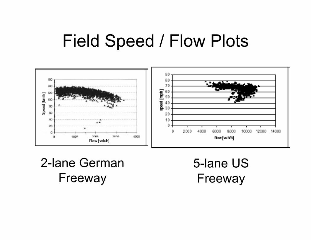
Field Speed / Flow Plots

2-lane German Freeway

5-lane US Freeway

Empirically Derived Speed Flow Curve (HCM, p13-3)

Theoretical Density / Flow Curve

Flow

Density kj0

q maxCongested

Flow

Uncongested Flow

4400

Flow

(vph

)22

00

00 440220

Density (veh/mile)110

Impact of Multiple Lanes

Shock Wave TheoryApplying Basic Traffic Flow Theory• Shock wave - a motion or propagation of change

in traffic conditions (speed, density, and flow) • A moving boundary between two different traffic

states • Forward, backward, and stationary shock waves • q = k * u• www.youtube.com/watch?v=iHzzSao6ypE&feature=youtu.be

Shock Waves

k1↑u1 k2↑u2

uw

n=(u1-uw)k1=(u2-uw)k2

s

In time “t” the number of vehicles crossing “s” is:

Shock Waves

(u1-uw)k1=(u2-uw)k2

u1k1-uwk1 = u2k2-uwk2

uwk2-uwk1= u2k2-u1k1

uw(k2-k1)= q2-q1

uw = (q2-q1) / (k2-k1)

uw = slope = ∆q/∆k

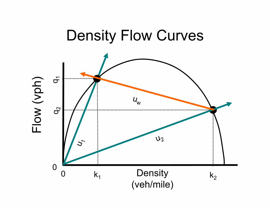
Density Flow CurvesFl

ow (v

ph) q 1

00 k2Density

(veh/mile)k1

q 2

Example Problem• Initial State

– q = 3000 vph– u = 60 mph

• Queued State (6 minutes)– q = 0 vph– u = 0 mph– Kjam = 880 vpm

• Release State– q = 8,800 vph– u = 30 mph

• Simulation

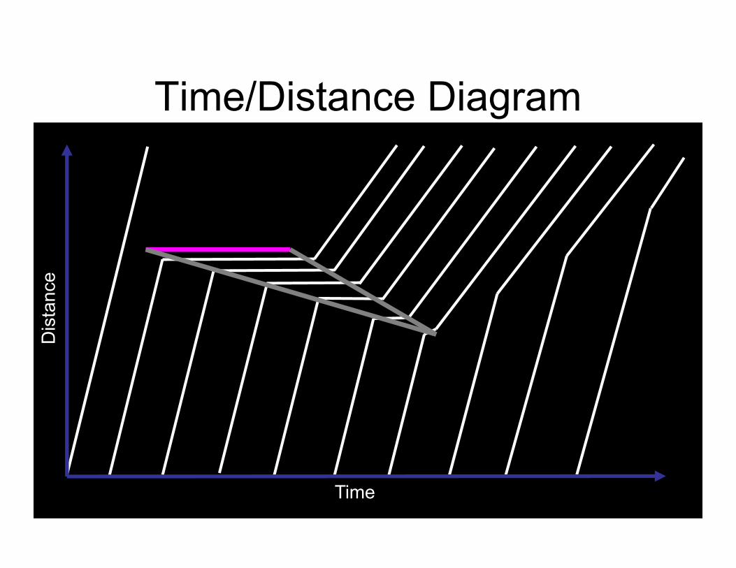
Time/Distance Diagram

Time

Dis

tanc

e

q/k CurveFl

ow (v

ph) qi =

3000

00 Density

(veh/mile)ki kjam

qmax = 8800

Calculations

• How far did the shockwave move upstream before the front of the queue started to dissipate?uback wave 1 = (qQueue-qinitial) / (kQueue-kinitial)

= (0 vph – 3000 vph) / (880 vpm – kinitial)kinitial = 3000 vph / 60 mph = 50 vpmuback wave 1 = (0 vph – 3000 vph) / (880 vpm – 50 vpm)

= 3.6 mph3.6 mph * 0.1 hour = 0.36 miles or 1900 feetThis is the Maximum Length of the Queue

Group Calculations

• What was the maximum distance that the shockwave moved upstream? How many total cars were delayed by the queue?

BREAK

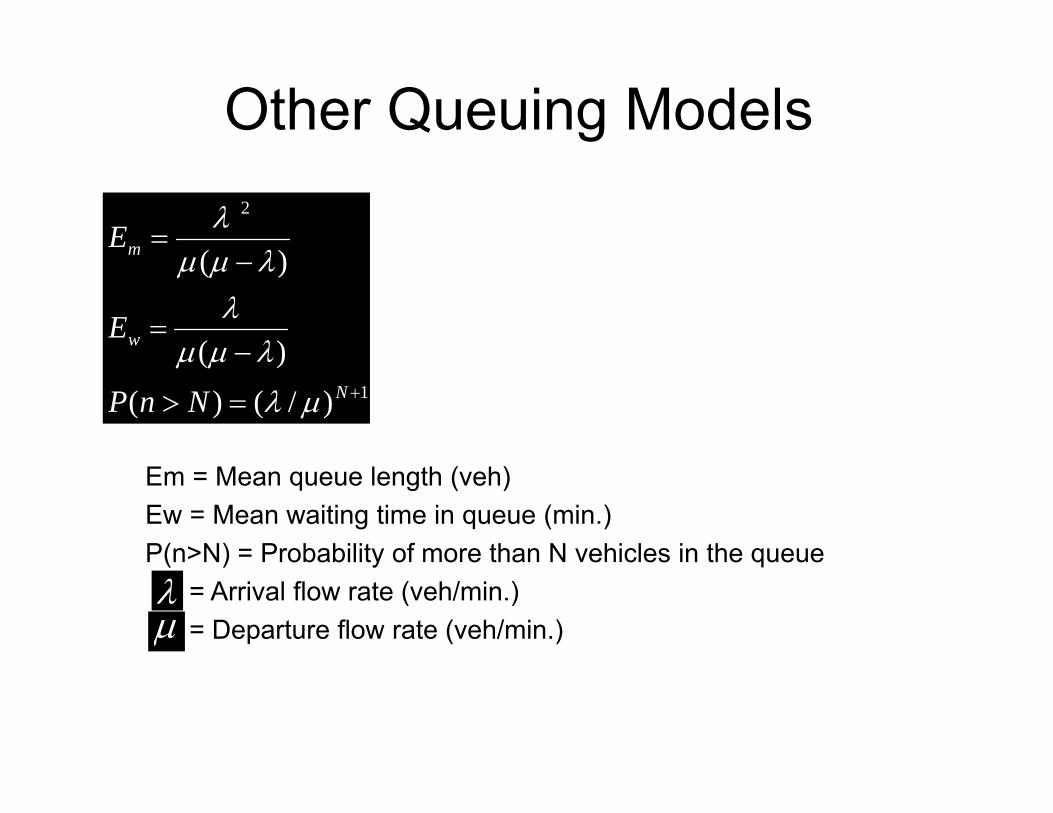
Em = Mean queue length (veh)Ew = Mean waiting time in queue (min.)P(n>N) = Probability of more than N vehicles in the queue

= Arrival flow rate (veh/min.)= Departure flow rate (veh/min.)

Other Queuing Models

1

2

)/()()(

)(

N

w

m

NnP

E

E

BREAK

JCE 4600 – Homework 1

1. A roadway carries 1000 vph in the peak flow direction at 50 mph. A farm tractor enters the highway and travels 1 mile at 15 mph. No vehicles are able to pass. Assume that the maximum flow rate that can be sustained is 1700 vph at 40 mph, and the density in the queue is 70 vpm.

a.) Sketch the q - k curve and plot the slopes of the shock waves immediately after the tractor leaves the highway.

b.) Draw a time / space diagram which illustrates the growth and dissipation of the queue. Identify and calculate the maximum number of vehicles in the queue, the total time that the queue is on the highway.

2. A school zone (speed limit = 10 mph) of 1 / 4 mile length is located on a 40 mph roadway. Up stream of the school zone the normal flow is 1000 vph at 40 mph, in the school zone the flow is 900 vph at 10 mph, and the maximum flow of the highway is 1200 vph at 30 mph.

a.) Sketch the q-k curve and identify the critical values. b.) What is the speed and direction of all shock waves? c.) If the school zone is open for 30 minutes, what is the maximum length of the

queue? d.) Plot a time versus distance curve for this situation.

3. The u - k relationship for a particular freeway lane was found to be:20u+52 = 0.02 (k - 240)2

Given that the speed is in mph and the density is in vpm find the mean free speed, jam density, maximum flow rate, and prevailing speed at the maximum flow rate. Calculate the values mathematically and plot a q - k curve.

4. Interstate 70 west of Columbia is a four lane divided freeway (2 lanes in each direction) in rolling terrain. During peak hour on Friday night, there are an average of 2500 vehicles traveling in the westbound direction at 60 mph. (STATE ALL ASSUMPTIONS WHEN REQUIRED DATA IS NOT GIVEN)

a.) Assume that capacity of the freeway is 4400 vph at 40 mph, the free flow speed is 75 mph. Assume that Kjam for the only lane cross-section is one-half of that of the two-lane section. Plot the q - k curve and label the jam density, maximum flow rate, and the speed at capacity.

b.) Assume that a 10 mile segment is being reconstructed and only 1 lane will be available for the westbound traffic. Redraw the q-k curve from above and account for the construction zone. Assume that the capacity of the construction zone is 1800 vph average speed at capacity is 30 mph in the construction zone and 15 mph upstream of the construction zone. Assume the jam density in the construction zone is 110 vpm.

c.) What is the speed and flow rate of: 10 mile segment under construction, the queue immediately upstream of the single lane segment, upstream of the queue, down stream of the construction zone (assume a speed of 65 mph)? What is the speed and direction of movement of the three shock waves?

d.) Assume that after 1 hour the incoming flow rate drops to 1000 vph at 70 mph. Show the resulting shock waves on the q-k curve. Draw a time/space diagram showing the growth and reduction of the queue upstream of the construction zone. How many total vehicles were affected?