ce154 - lecture 1-2 hydrologic study

CE154 1Fall 2009 1

Introduction & Flood Hydrologic Analysis

CE154 - Hydraulic DesignLectures 1-2

CE154 2Fall 2009 2

Green Sheet

Course Objective - Introduce design concept and procedure for a few basic types of hydraulic structures that an engineer may encounter

Hydraulic structures:- Water supply and distribution systems including spillways, reservoirs, pipeline systems - Flood protection systems including culverts, storm drains, & natural rivers

CE154 3Fall 2009 3

Green Sheet

Lecture Schedule Homework assignments Exams Grading Office hour Communication – email address, web

site Emergency evacuation route Grader selection

CE154 4

Introduction

Hydraulic Design – Design of Hydraulic Structures

Elements of Design (class discussion)- design objective- design criteria - design data and assumptions- design procedure- design calculations- design drawings- design report

Fall 2009 4

CE154 5

Hydraulic Design example

Design a channel that can safely carry the storm runoff generated from a 1% flood from a residential development that is 20 square miles in drainage area.

Design objective: Design criteria: Design data and assumptions: Design procedure:

Fall 2009 5

CE154 6Fall 2009 6

Flood Hydrology

Design flood Discharge (design flow)- peak flow rate governing the design of relevant hydraulic structures

Design flood Hydrograph- time-flow history of a design flood

Sample Flood Hydrograph

Fall 2009 CE154 7

CE154 8Fall 2009 8

Hydrology

Rainfall – Runoff Process

CE154 9Fall 2009 9

Hydrologic Parameters

Precipitation intensity & duration for design Infiltration rate (watershed soil type and

moisture condition) Watershed surface cover – overland roughness Watershed drainage network geometry Watershed slope Time of concentration

CE154 10Fall 2009 10

Rainfall – Runoff Process

Gauged Watershed-flood frequency analysis to determine peak design flow rate-Gauge data to calibrate unit hydrograph and generate design flood hydrograph

Ungauged Watershed-Hydrologic Modeling (HEC-HMS or HEC-1)-Regional regression analysis-Synthetic unit hydrograph

CE154 11Fall 2009 11

Flood Hydrology Studies

determine design rainfall duration and intensity- design rainfall ranges from probable maximum precipitation (PMP) on the high end to 100-year or 10-year return period rainfall event

develop design runoff hydrograph – includes peak flow rate and runoff volume to size reservoir and design spillway and other pertinent structures

CE154 12Fall 2009 12

Our Topics

Determine probable maximum precipitation (PMP) -”Theoretically the greatest depth of precipitation for a given duration that is physically possible over a given storm area at a particular geographical location at a certain time of the year” (HMR55A)

Bureau of Reclamation’s S-graph & dimensionless unit hydrograph methods of developing synthetic unit hydrograph

Clark unit hydrograph method

CE154 13Fall 2009 13

PMP

National Weather Service Hydrometeorological Reports (HMR)provide maximum 6, 12, 24, 48 and 72 hour PMP’s for areas of 10, 200, 1000, 5000 and 10,000 mi2.

HMR 58 – Probable Maximum Precipitation for California – Calculation Procedures, NOAA, Oct. 1998 (supersedes HMR36, Note errata for pp. 22 & 27)

http://www.weather.gov/oh/hdsc/studies/pmp.html#HR58

CE154 14Fall 2009 14

Rainfall Losses

Surface retention, evaporation and storage (usually small compared to infiltration)

Infiltration- Ranges 0.05 0.5 in/hr approximately- L = Lmin + (Lo – Lmin)e-kt

L = resulting infiltration rate Lmin = minimum rate when saturated Lo = maximum or initial infiltration rate

Rainfall – losses = Rainfall Excess

CE154 15Fall 2009 15

PMP Computation Example

Read pp. 43-48 of HMR 58 973 mi2 Auburn drainage above Folsom

Lake Step 1

Outline drainage boundary and overlay the 10-mi2, 24-hour PMP map from Plate 2, HMR 58

Step 2Determine to use all-season or seasonal PMP for design

CE154 16Fall 2009 16

Plate 2 California – Northern General Storm PMP Index Map (in inches)

CE154 17Fall 2009 17


CE154 18Fall 2009 18


Step 3Calculate average PMP value (for 10 mi2 and 24-hr) over drainage area = 24.6 inches (using a planimeter or griddled paper overlay)

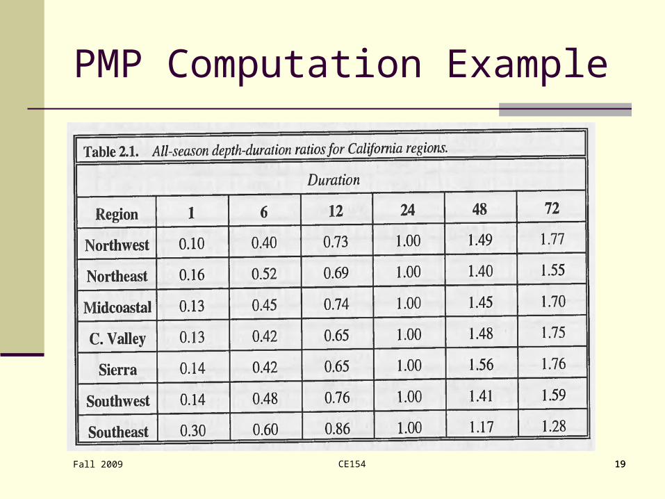
Step 4Depth-Duration Relationship- Auburn drainage is within the Sierra region. Use Table 2.1 to obtain ratios for durations from 1 to 72 hours

CE154 19Fall 2009 19


CE154 20Fall 2009 20


Step 4 Ratios for Auburn Drainage (Table 2.1 HMR58)

Duration (hours)

1 6 12 24 48 72

Ratios .14 .42 .65 1.00 1.56 1.76

CE154 21Fall 2009 21


Multiply the average value for 10-mi2, 24-hour PMP of 24.6 inches by these ratios

Step 5 Auburn drainage 10-mi2 PMP

Duration (hr)

1 6 12 24 48 72

PMP (in) 3.4 10.3 16.0 24.6 38.4 43.3

CE154 22Fall 2009 22


Step 6Determine aerial reduction factors using the Auburn drainage area of 973 mi2 & Fig. 2.15

CE154 23Fall 2009 23


Fig 2.15, HMR 58

CE154 24Fall 2009 24


Step 6 Area Reduction Factors

Duration (hr)

1 6 12 24 48 72

Factors .64 .67 .70 .72 .77 .80

CE154 25Fall 2009 25


Step 7Apply aerial reduction by multiplying PMP’s from Step 5 by factors from Step 6

Step 7 Auburn Drainage average PMP Depths

Duration (hr)

1 6 12 24 48 72

PMP (in) 2.2 6.9 11.2 17.7 29.6 34.6

CE154 26Fall 2009 26


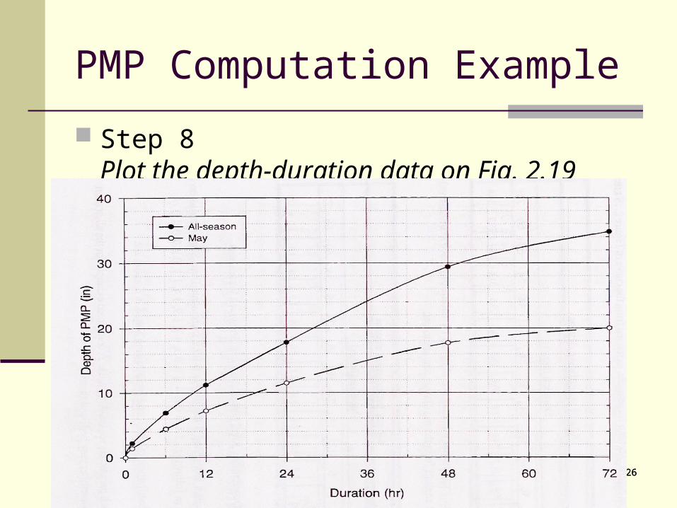
Step 8Plot the depth-duration data on Fig. 2.19

CE154 27Fall 2009 27


Extract cumulative depths from Fig. 2.19

Step 8 6-hr Cumulative Rainfall Depths

Hr. 6 12 18 24 30 36 42 48 54 60 66 72

PMP (in)

6.9 11.2 14.6 17.7 20.8 23.8 26.7 29.6 31.6 32.7 33.7 34.6

CE154 28Fall 2009 28


Compute incremental depths

Step 9

6-hr Incremental Rainfall Depths

Hr. 6 12 18 24 30 36 42 48 54 60 66 72

PMP (in)

6.9 4.3 3.4 3.1 3.1 3.0 2.9 2.9 2.0 1.1 1.0 0.9

CE154 29Fall 2009 29


Adjust temporal-distribution of these incremental rainfall based on historical data or by experiments. Keep the 4 highest increments in a series. A PMP isohyetal distribution may be

6 hr incremental rainfall depths

Hr 6 12 18 24 30 36 42 48 54 60 66 72

PMP1 6.9 4.3 3.4 3.1 3.1 3.0 2.9 2.9 2.0 1.1 1.0 0.9

PMP2 3.1 3.0 2.9 2.9 3.1 4.3 6.9 3.4 1.1 0.9 2.0 1.0

CE154 30Fall 2009 30

PMP Computation - summary

Need Hydrometeorological Report HMR 58 for northern California

Define general storms up to 72 hours in duration and 10,000 mi2 in area and local storms up to 6 hours and 500 mi2

Start with a total PMP depth for a general area and end with intensity-time distribution of rain for a specific watershed – this is the design rainfall

CE154 31Fall 2009 31

How to turn PMP (design rainfall) into PMF (design runoff)? Unit hydrograph

– a rainfall-runoff relationship characteristic of the watershed - developed in 1930’s, easy to use, less data requirements, less costly- many methods, most often seen include Soil Conservation Service (SCS) method, Snyder, Clark, and Bureau of Reclamation dimensionless unit hydrograph and S-curve methods

hydrologic modeling – used widely since PC became popular, requiring data of topo contours, surface cover, infiltration ch., etc., HEC-HMS (HEC-1)

CE154 32Fall 2009 32

Unit Hydrograph Basic unit hydrograph theory

A storm of a constant intensity over a duration (e.g, 1 hour), and of uniform distribution, produces 1 inch of excess that runs off the surface. The hydrograph that is recorded at the outlet of the watershed is a 1-hr unit hydrograph

Define several parameters to characterize the watershed response: e.g., lag time or time of concentration, time-discharge relationship, channel storage attenuation – synthetic unit hydrograph

CE154 33Fall 2009 33

Unit Hydrograph Assumptions

Rainfall excess and losses may be lumped as basin-average values (lumped)

Ordinates of runoff is linearly proportional to rainfall excess values (linearity)

Rainfall-runoff relationship does not change with time (time invariance)

CE154 34Fall 2009 34

Hydrograph Development

CE154 35Fall 2009 35

Unit Hydrograph Approaches

Conceptual models of runoff – single-linear reservoir (S=kO), Nash (multiple linear reservoirs), Clark (consider effect of basin shape on travel time)

Empirical models – Snyder, Soil Conservation Service dimensionless method

Different methods use different parameters to define the unit hydrograph

CE154 36Fall 2009 36

Unit Hydrograph Parameters

Time lag – time between center of mass of rainfall and center of mass of runoff, original definition by Horner & Flynt [1934], (SCS, Snyder). Different formulae were developed based on different watershed data (e.g., SCS & BuReC)

Time of concentration - time between end of rainfall excess and inflection point of receding runoff (Clark)

Time to peak – beginning of rise to peak (SCS) Storage coefficient – R (Clark) Temporal distribution of runoff (BuReC, SCS)

CE154 37Fall 2009 37

Unit Hydrograph & parameters

Q

time

Lag time

Rainfall excess = precipipation - loss

Rising limb

Receding limb

Point of inflection

Peak Time

Time of concentration

CE154 38Fall 2009 38

Synthetic Unit Hydrograph

Uses Lag Time and a temporal distribution (dimensionless or S-graph) to develop the unit hydrograph

CE154 39Fall 2009 39

Lag Time

Unit Hydrograph Lag Time (Tlag or Lg) per Bureau of Reclamation

Ncag

SLLL

C )( 5.0

CE154 40Fall 2009 40

Lag Time

Lg = unit hydrograph lag time in hours L = length of the longest watercourse

from the point of concentration to the drainage boundary, in miles

Lca

L

Point of concentration

CE154 41Fall 2009 41

Lag Time

Lca = length along the longest watercourse from the point of concentration to a point opposite the centroid of the drainage basin, in miles

S = average slope of the longest watercourse, in feet per mile

C, N = constant

CE154 42Fall 2009 42

Lag Time

Based on empirical data, regardless of basin location

N = 0.33 C = 26Kn where Kn is the average

Manning’s roughness coefficient for the drainage network

Note: other methods such as Snyder and SCS define lag time slightly differently

CE154 43Fall 2009 43

Lag Time

To allow estimate of lag time, the Bureau of Reclamation reconstituted 162 flood hydrographs from numerous natural basins west of Mississippi River to provide charts for lag time for 6 different regions of the US

Use Table 3-5 & Fig. 3-7 of DSD for lag time estimate for SF Bay Area

CE154 44Fall 2009 44

Lag Time

CE154 45Fall 2009 45

Lag Time

Example, Table 3-5 on p.42, DSD- San Francisquito Creek near Stanford University, drainage area 38.3 mi2, lag time 4.8 hours, Kn 0.110

- Matadero Creek at Palo Alto, drainage area 7.2 mi2, lag time 3.7 hours, Kn 0.119

CE154 46Fall 2009 46

UH Temporal Distribution

Time vs. Discharge relationship Bureau of Reclamation uses 2 methods

to develop temporal distribution based on recorded hydrographs divided into 6 regions across the US:- dimensionless unit hydrograph method, &- S-graph technique

Tables 3-15 and 3-16 (Design of Small Dams) for the SF Bay Area

CE154 47Fall 2009 47

Temporal Dist. – Table 3-16

CE154 48Fall 2009 48

Temp. Dist. - S-graph Method

CE154 49Fall 2009 49

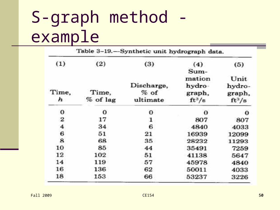
S-graph method - Example

Read pp. 37-52 of Design of Small Dams drainage area = 250 mi2

lag time = 12 hours unit duration = 12/5 2 hours (SCS

recommendation) Ultimate discharge = drainage area in

mi2 times 52802/3600/12 and divided by unit duration, in this case = 80662.5 cfs

CE154 50Fall 2009 50

S-graph method - example

CE154 51Fall 2009 51

Bureau’s Method - summary

Estimate lag time and time-flow distribution

Based on recorded hydrographs Regionalized approach – does not

consider specific local condition Works better for larger watersheds, such

as for dam construction For smaller watersheds, or smaller design

flood events, consider another method, such as the Clark unit hydrograph method

CE154 52Fall 2009 52

Clark Unit Hydrograph Method

Reading Materials:- Chapter 7 of Flood-Runoff Analysis, EM 1110-2-1417, Corps of Engineers, Aug. ’94http://www.usace.army.mil/publications/eng-manuals/em1110-2-1417/toc.htm

- if you have more time, read - Unit Hydrograph Technical Manual, National Weather Service, www.nohrsc.noaa.gov/technology/gis/uhg_manual.html

CE154 53Fall 2009 53


Uses the concept of instantaneous unit hydrograph (IUH) – hydrograph resulted from 1 unit of rainfall excess occurring over the basin in zero time

Uses IUH to compute a unit hydrograph for any unit duration equal to or greater than the time interval used in computation

Uses 2 parameters and a time-area relationship to define IUH

CE154 54Fall 2009 54


Need 2 parameters: time of concentration (Tc) and storage coefficient (R)

Tc = travel time from the most upstream point in the basin to the outflow location

or Tc = time from the end of rainfall to the inflection point on the recession limb

R = Q/(dQ/dt) at point of inflection – estimate from recorded flood hydrographs

Example – reconstitute a flood hydrograph for Thomas Creek at Paskenta, CA for Jan/1963

CE154 55Fall 2009 55

Clark Unit Hydrograph

Step 1 – Delineate watershed boundary

CE154 56Fall 2009 56


Step 2 – Identify major watercourses

CE154 57Fall 2009 57


Step 3 – Estimate time of concentration by estimating overland and river travel times through the watershed. Identify watershed slopes, surface cover types and river channel geometries, and use simplified relationships to estimate travel time.

CE154 58Fall 2009 58

Time of Concentration

Watershed flow characteristics:

• sheet flow – approximately 0.1 ft deep, less than 300 ft in length

• shallow concentrated flow

• channel flow

CE154 59Fall 2009 59

Sheet Flow Roughness Coef. [Engman 1986]

CE154 60Fall 2009 60

Sheet Flow travel time

Sheet flow travel time (Tt)Tt = travel time in hrn = Manning’s roughness coefficientL = flow length in ftP2 = 2-yr, 24-hr rainfall in inchesS = slope in ft/ft

SPT

nLt 4.05.0

2

8.0)(007.0

CE154 61Fall 2009 61

Sheet Flow travel time

NOAA Atlas – precipitation distribution maps

Northern California 2-yr, 24-hour rainfall http://hydrology.nws.noaa.gov/oh/hdsc/On-line_reports/Volume%20XI%20California/1973/North%2024%20hr%20precipitation%20charts.djvu

For San Jose area, 2.2 inches

CE154 62Fall 2009 62

Shallow Concentrated Flow velocities

CE154 63Fall 2009 63

Time of Concentration (Step 3)

Channel flow – use Manning’s equation travel time = channel length/velocity Time of concentration = summation of

travel times from sheet flow, shallow concentrated flow and channel flow

Do this for the entire watershed separated into subareas based on slope and surface cover

Sum up the travel time through the watershed and divide into equal-travel-time subareas (isochrones)

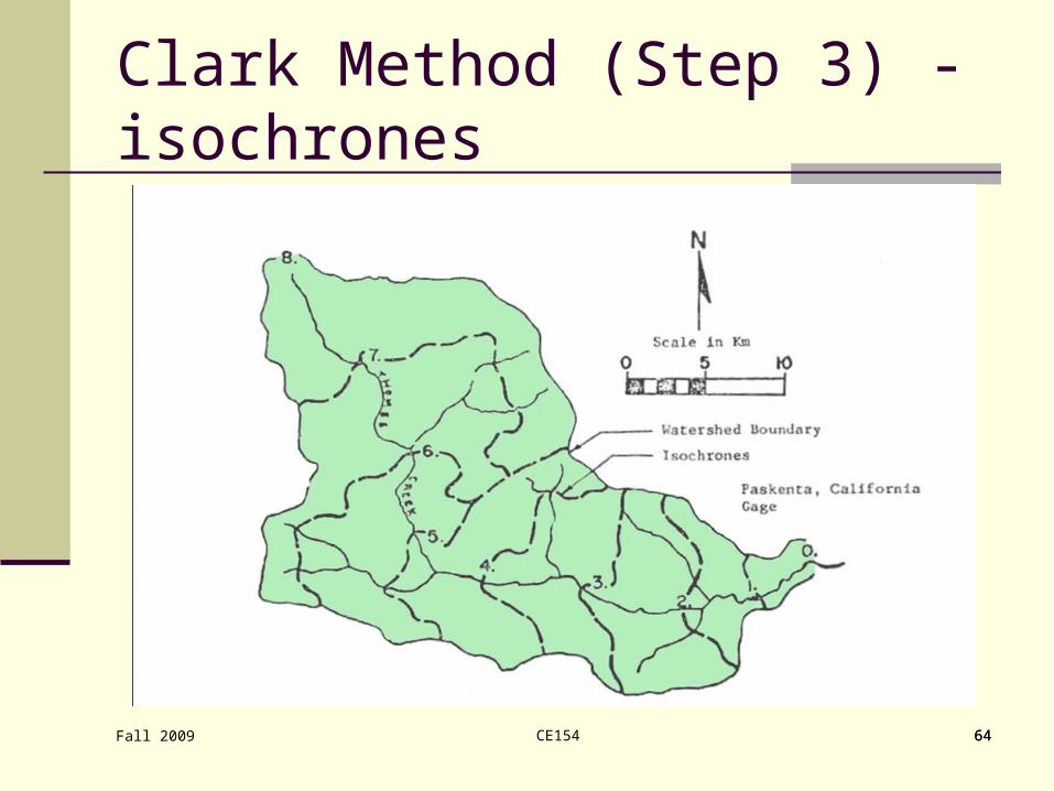
CE154 64Fall 2009 64

Clark Method (Step 3) - isochrones

CE154 65Fall 2009 65

Clark UH Procedure (Step 4)

Draw isochrones to subdivide the basin into chosen number of parts, e.g., if Tc=8 hr., choose 8 subdivisions with t=1 hr.

Measure the area (ai) between each pair of isochrones and tabulate. ai = ordinate in units of area (mi2 or km2)

Plot (% of Tc) versus (cumulative area). Tabulate increments at 1 t apart

CE154 66Fall 2009 66

Clark UH ExampleMap Area #

Planimeter Value

Accum. Value

Accum. Area (km2)

Travel time in %Tc

1 0.08 0.08 12 12.5

2 0.15 0.23 35 25.0

3 0.40 0.63 96 37.5

4 0.36 0.99 151 50.0

5 0.45 1.44 220 62.5

6 0.45 1.89 288 75.0

7 0.66 2.55 389 87.5

8 0.68 3.23 493 100.0

CE154 67Fall 2009 67

CE154 68Fall 2009 68

Clark UH Procedure

Approach

Time-Cumulative Area curve Translation hydrograph Linear reservoir routing Instantaneous Unit Hydrograph Unit Hydrograph of a duration

CE154 69Fall 2009 69

Clark UH Procedure

CE154 70Fall 2009 70

Clark UH Procedure

Convert areas into flows (area x unit rainfall / unit time) of a translation hydrograph Ii = Kai/t

where Ii = ordinate of translation hydrograph in unit of discharge (cfs or cms) at end of period i, K = conversion factor (645 to convert in-mi2 to cfs or 0.278 to convert mm-km2 to cms) 0.278 = 1000x1000/1000/3600

CE154 71Fall 2009 71

Clark UH Example

(1)

Time (hr)

(2)

Rain over ai

(mm-km2)

(3)

Inflow Ii Of translation hydrograph (cms)

(4)

IUH Oi

(cms)

(5)

2-hr UH

Qi (cms)

0 0 0

2 35 5

4 116 16

CE154 72Fall 2009 72

Storage Coefficient R (Step 5)

For linear reservoir S=RO Estimate from recorded hydrograph:

The inflection point of a recession limb, by definition, is when inflow ceases, because time of concentration is from end of rainfall to the inflection point, and is when the last rain reaches the end of the watershed.dS/dt = I-O = -O continuity equationdS/dt = R dO/dt for linear reservoir R = -O/(dO/dt) at the inflection point

CE154 73Fall 2009 73

CE154 74Fall 2009 74

Storage Coefficient R

R is used to define a dimensionless routing constant C:

C =

with R=5.5 hours and t = 2 hours,

C = 0.308

tR

t

2

2

CE154 75Fall 2009 75

Clark UH Procedure (Step 6)

Route the inflows (Col. 3) to the outflow location (Col. 4)Oi = CIi + (1-C)Oi-1

Oi = outflow from the basin at the end of period iIi = inflow from each area at the end of period i

CE154 76Fall 2009 76

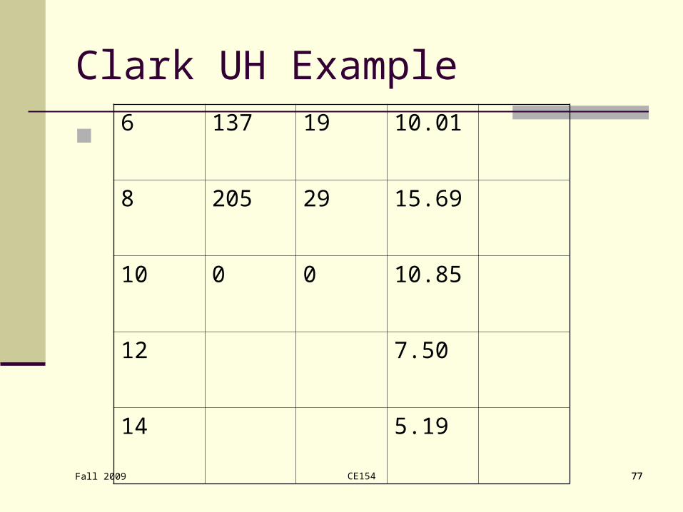
Clark UH Example

(1)

Time (hr)

(2)

Inflow ai

(mm-km2)

(3)

Inflow Ii

(cms)

(4)

IUH Oi

(cms)

(5)

2-hr UH

Qi (cms)

0 0 0 0

2 35 5 1.55

4 116 16 5.97

CE154 77Fall 2009 77

Clark UH Example

6 137 19 10.01

8 205 29 15.69

10 0 0 10.85

12 7.50

14 5.19

CE154 78Fall 2009 78

Clark UH Procedure

Average the ordinates of the IUH to create the unit hydrograph (Col. 5) Qi = 0.5 (Oi + Oi-1)

The duration of the UH may be different from t (provided that it is an exact multiple of t), and the UH follows this formulaQi = 1/n (0.5Oi-n + Oi-n+1 + … + Oi-1 + 0.5Oi)

where

CE154 79Fall 2009 79

Clark UH Procedure

Qi = ordinate at time i of unit hydrograph of duration D and tabulation interval t

n = D/ t D = unit hydrograph duration t = tabulation interval

CE154 80Fall 2009 80

Clark UH Example

(1)

Time (hr)

(2)

Inflow ai

(mm-km2)

(3)

Inflow Ii

(cms)

(4)

IUH Oi

(cms)

(5)

2-hr UH

Qi (cms)

0 0 0 0 0

2 35 5 1.55 0.78

4 116 16 5.97 3.76

CE154 81Fall 2009 81

Clark UH Example

6 137 19 10.01 7.99

8 205 29 15.69 12.85

10 0 0 10.85 13.27

12 7.50 9.17

14 5.19 6.35

CE154 82Fall 2009 82

Clark UH Example

Continue the UH calculation to Hour 46 when the discharge diminishes to 0

For each 2-hour interval of the Jan/Feb 1963 storm, compute rainfall excess, multiply by the UH ordinates and lag the time of occurrence to obtain the flood hydrograph

Compare with the measured hydrograph

CE154 83Fall 2009 83

CE154 84Fall 2009 84

The END

ce154 - lecture 1-2 hydrologic study

Documents