ccnp 1 advanced routing companion guide.pdf
TRANSCRIPT
Cis
co
Netw
ork
ing
Acad
em
y P
rog
ram
CC
NP
®1: A
dvan
ced R
ou
ting
Co
mp
an
ion
Gu
ide
Seco
nd
Ed
ition
Cisco Systems
Cisco Press
Cisco Networking Academy Program
CCNP® 1: Advanced RoutingCompanion GuideSecond Edition
The only authorized textbook for the Cisco Networking Academy Program
Cisco Networking Academy Program
CCNP® 1: Advanced RoutingCompanion GuideSecond Edition
Companion Title:
Cisco Networking Academy Program CCNP 1: Advanced Routing Lab Companion Second Edition
ISBN: 1-58713-134-X
Related Titles:
CCNP BSCI Exam Certification Guide Third Edition
ISBN: 1-58720-085-6
CCNP Certification LibraryThird Edition
ISBN: 1-58720-104-6
CCNP Flash Cards and Exam Practice Kit Second Edition
ISBN: 1-58720-091-0
This Cisco® authorized textbook is a portable desk reference designed to complement the CCNP 1: Advanced Routing course in the Cisco Networking Academy® Program.
CCNP 1: Advanced Routing is one of four courses leading to the CCNP certification. CCNP 1teaches you how to design, configure, maintain, and scale routed networks.
Cisco Networking Academy Program CCNP 1: Advanced Routing Companion Guide, SecondEdition, contains all the information from the online curriculum, with additional in-depth contentto enhance your understanding of some topics, plus pedagogical aids to help you study.
You will learn to use VLSMs, private addressing, and NAT to enable more efficient use of IPaddresses. This book also teaches you how to implement routing protocols such as RIPv2,EIGRP, OSPF, IS-IS, and BGP. In addition, this book details the important techniques used for route filtering and route redistribution. Use this Companion Guide to help prepare for theBuilding Scalable Cisco Internetworks exam (642-801 BSCI), which is one of the four requiredexams to obtain the CCNP certification.
With Cisco Networking Academy Program CCNP 1: Advanced Routing Companion Guide,Second Edition, you have access to the course information anytime, anywhere. This book provides the following reference, study, and review tools:
• Each chapter has a list of objectives referencing the key concepts for focused study.
• Key terms are highlighted in color throughout the chapter where they are used in context.The definitions are provided in a comprehensive glossary to serve as a study aid.
• Check Your Understanding review questions, presented at the end of each chapter, act as a review and study guide. They reinforce the concepts introduced in the chapter andhelp test your understanding before you move on to a new chapter. The answers to thequestions are provided in an appendix.
• Throughout this book, you see references to the lab activities found in the CiscoNetworking Academy Program CCNP 1: Advanced Routing Lab Companion, Second Edition. Completing these labs gives you hands-on experience so that you can apply theory to practice.
Cisco Press is a collaboration between Cisco Systems, Inc., and Pearson Education that is chargedwith developing high-quality, cutting-edge educational and reference products for the networkingindustry. The products in the Cisco Networking Academy Program series are designed to preparestudents for careers in the exciting networking field. These products have proven to be strongsupplements to the web-based curriculum and are the only print companions that have beenreviewed and endorsed by Cisco Systems for Cisco Networking Academy Program use.
ciscopress.com
Companion CD-ROM
The CD-ROM included withthis book provides InteractiveMedia Activities referred to
throughout the book, a test engine ofmore than 200 questions, and StudyGuides for each chapter to enhanceyour learning experience.
Cisco Systems, Inc.
Cisco Networking Academy Programciscopress.com
This book is part of the Cisco NetworkingAcademy Program Series from Cisco Press®.The products in this series support and complement the Cisco Networking Academy Program.

Cisco Networking Academy Program
CCNP 1: Advanced Routing
Companion Guide
Second Edition
Cisco Systems, Inc.
Cisco Networking Academy Program
Cisco Press
800 East 96th Street
Indianapolis, Indiana 46240 USA
1358_fmi.book Page i Thursday, May 27, 2004 2:21 PM

ii
Cisco Networking Academy Program
CCNP 1: Advanced Routing
Companion Guide
Second Edition
Cisco Systems, Inc.
Cisco Networking Academy Program
Copyright© 2004 Cisco Systems, Inc.
Published by:Cisco Press800 East 96th StreetIndianapolis, Indiana 46240 USA
All rights reserved. No part of this book may be reproduced or transmitted in any form or by any means, elec-tronic or mechanical, including photocopying, recording, or by any information storage and retrieval system, without written permission from the publisher, except for the inclusion of brief quotations in a review.
Printed in the United States of America 2 3 4 5 6 7 8 9 0
Third Printing October 2005
Library of Congress Cataloging-in-Publication Number: 2003114387
ISBN: 1-58713-135-8
Trademark Acknowledgments
All terms mentioned in this book that are known to be trademarks or service marks have been appropriately capitalized. Cisco Press or Cisco Systems, Inc. cannot attest to the accuracy of this information. Use of a term in this book should not be regarded as affecting the validity of any trademark or service mark.
Warning and Disclaimer
This book is designed to provide information about the Cisco Networking Academy Program CCNP 1: Advanced Routing course. Every effort has been made to make this book as complete and accurate as possible, but no warranty or fitness is implied.
The information is provided on an “as is” basis. The author, Cisco Press, and Cisco Systems, Inc. shall have neither liability nor responsibility to any person or entity with respect to any loss or damages arising from the information contained in this book or from the use of the discs or programs that may accompany it.
The opinions expressed in this book belong to the author and are not necessarily those of Cisco Systems, Inc.

iii
Corporate and Government Sales
Cisco Press offers excellent discounts on this book when ordered in quantity for bulk purchases or special sales. For more information, please contact:
U.S. Corporate and Government Sales
1-800-382-3419 [email protected]
For sales outside of the U.S. please contact:
International Sales
Feedback Information
At Cisco Press, our goal is to create in-depth technical books of the highest quality and value. Each book is crafted with care and precision, undergoing rigorous development that involves the unique expertise of members of the professional technical community.
Reader feedback is a natural continuation of this process. If you have any comments on how we could improve the qual-ity of this book, or otherwise alter it to better suit your needs, you can contact us through e-mail at [email protected]. Please be sure to include the book title and ISBN in your message.
We greatly appreciate your assistance.
Publisher
John Wait
Editor-in-Chief
John Kane
Executive Editor
Mary Beth Ray
Cisco Representative
Anthony Wolfenden
Cisco Press Program Manager
Nannette M. Noble
Production Manager
Patrick Kanouse
Development Editor
Andrew Cupp
Project Editor
Marc Fowler
Copy Editor
Gayle Johnson
Technical Editors
Randy Ivener, Jim Lorenz
Cover Designer
Louisa Adair
Compositor
Mark Shirar
Indexer
Larry Sweazy
1358_fmi.book Page iii Thursday, May 27, 2004 2:21 PM
iv
About the Technical Reviewers
Randy Ivener,
CCIE No. 10722, is a security specialist with Cisco Systems Advanced Ser-
vices. He is a Certified Information Systems Security Professional and ASQ Certified Soft-
ware Quality Engineer. He has spent several years as a network security consultant, helping
companies understand and secure their networks. He has worked with many security products
and technologies, including firewalls, VPNs, intrusion detection, and authentication systems.
Before becoming immersed in security, he spent time in software development and as a train-
ing instructor. He graduated from the U.S. Naval Academy and holds a master’s degree in
business administration.
Jim Lorenz
is an instructor and curriculum developer for the Cisco Networking Academy
Program. He has more than 20 years of experience in information systems and has held vari-
ous IT positions in Fortune 500 companies, including Honeywell and Motorola. He has
developed and taught computer and networking courses for both public and private institu-
tions for more than 15 years. He is coauthor of the course Cisco Networking Academy Pro-
gram Fundamentals of UNIX, he is a contributing author for the CCNA Lab Companion
manuals, and he is a technical editor for the CCNA Companion Guides. He is a Cisco Certi-
fied Academy Instructor (CCAI) for CCNA and CCNP courses. He has a bachelor’s degree in
computer information systems and is working on his master’s in information networking and
telecommunications. He and his wife, Mary, have two daughters, Jessica and Natasha.
1358_fmi.book Page iv Thursday, May 27, 2004 2:21 PM

v
Contents at a Glance
Forword. . . . . . . . . . . . . . . . . . . . . . . . . . . . . . . . . . . . . . . . . . . . .xvii
Introduction . . . . . . . . . . . . . . . . . . . . . . . . . . . . . . . . . . . . . . . . . xix
Chapter 1
Overview of Scalable Internetworks. . . . . . . . . . . . . . . . . . . . . . . .3
Chapter 2
Advanced IP Addressing Management . . . . . . . . . . . . . . . . . . . .31
Chapter 3
Routing Overview. . . . . . . . . . . . . . . . . . . . . . . . . . . . . . . . . . . . . .75
Chapter 4
Routing Information Protocol Version 2. . . . . . . . . . . . . . . . . . .103
Chapter 5
EIGRP. . . . . . . . . . . . . . . . . . . . . . . . . . . . . . . . . . . . . . . . . . . . . . .127
Chapter 6
OSPF . . . . . . . . . . . . . . . . . . . . . . . . . . . . . . . . . . . . . . . . . . . . . . .163
Chapter 7
IS-IS . . . . . . . . . . . . . . . . . . . . . . . . . . . . . . . . . . . . . . . . . . . . . . . .239
Chapter 8
Route Optimization . . . . . . . . . . . . . . . . . . . . . . . . . . . . . . . . . . .319
Chapter 9
BGP . . . . . . . . . . . . . . . . . . . . . . . . . . . . . . . . . . . . . . . . . . . . . . . .353
Appendix A
Glossary of Key Terms. . . . . . . . . . . . . . . . . . . . . . . . . . . . . . . . .423
Appendix B
Answers to the Check Your Understanding Questions. . . . . . .433
Appendix C
Case Studies . . . . . . . . . . . . . . . . . . . . . . . . . . . . . . . . . . . . . . . . .455
Index
. . . . . . . . . . . . . . . . . . . . . . . . . . . . . . . . . . . . . . . . . . . . . . . . . . . . . . . . . . .461
1358_fmi.book Page v Thursday, May 27, 2004 2:21 PM
vi
Contents
Foreword . . . . . . . . . . . . . . . . . . . . . . . . . . . . . . . . . . . . . . . . . . . .xvii
Introduction. . . . . . . . . . . . . . . . . . . . . . . . . . . . . . . . . . . . . . . . . . xix
Chapter 1
Overview of Scalable Internetworks 3
The Hierarchical Network Design Model 3
The Three-Layer Hierarchical Design Model 4
The Core Layer 5The Distribution Layer 6The Access Layer 6
Router Function in the Hierarchy 7
Core Layer Example 10
Distribution Layer Example 13
Access Layer Example 14
Key Characteristics of Scalable Internetworks 15
Five Characteristics of a Scalable Network 15
Making the Network Reliable and Available 16
Scalable Routing Protocols 17Alternative Paths 17Load Balancing 18Protocol Tunnels 18Dial Backup 18
Making the Network Responsive 19
Making the Network Efficient 20
Access Lists 20Snapshot Routing 21Compression over WANs 21
Making the Network Adaptable 22
Mixing Routable and Nonroutable Protocols 22
Making the Network Accessible but Secure 23
Basic Router Configuration Lab Exercises 24
Load Balancing Lab Exercises 25
Summary 25
Key Terms 26
Check Your Understanding 26
Chapter 2
Advanced IP Addressing Management 31
IPv4 Addressing 32
Address Architecture of the Internet 32
1358_fmi.book Page vi Thursday, May 27, 2004 2:21 PM

vii
Class A and B IP Addresses 33
Class A Addresses 34Class B Addresses 35
Classes of IP Addresses: C, D, and E 36
Class C Addresses 36Class D Addresses 36Class E Addresses 37
Subnet Masking 37
IP Addressing Crisis and Solutions 39
IP Addressing Crisis 39
Classless Interdomain Routing 40
Route Aggregation and Supernetting 41
Supernetting and Address Allocation 43
VLSM 44
Variable-Length Subnet Masks 44
Classless and Classful Routing Protocols 47
Route Summarization 49
An Overview of Route Summarization 49
Route Flapping 50
Private Addressing and NAT 51
Private IP Addresses (RFC 1918) 51
Discontiguous Subnets 52
Network Address Translation (NAT) 53
IP Unnumbered 54
Using IP Unnumbered 55
DHCP and Easy IP 56
DHCP Overview 56
DHCP Operation 58
Configuring the IOS DHCP Server 59
Easy IP 61
Helper Addresses 62
Using Helper Addresses 62
Configuring IP Helper Addresses 63
IP Helper Address Example 64
IPv6 66
IP Address Issues Solutions 66
IPv6 Address Format 67
Summary 69
1358_fmi.book Page vii Thursday, May 27, 2004 2:21 PM

viii
Key Terms 70
Check Your Understanding 72
Chapter 3
Routing Overview 75
Routing 75
Routing Fundamentals 75
Static Routing 77
Configuring Dynamic Routing 80
Routing Protocols for IPX and AppleTalk 80IP Routing Protocols and the Routing Table 81
Distance Vector Routing Protocols 83
Link-State Routing Protocols 85
Hybrid Routing Protocol: EIGRP 87
Default Routing 87
Default Routing Overview 87
Configuring Static Default Routes 88
Default Routing with IGRP 89
Default Route Caveats 91
Floating Static Routes 92
Configuring Floating Static Routes 93
Convergence 93
Convergence Issues 94
Route Calculation 94
Route Calculation Fundamentals 95
Multiple Routes to a Single Destination 95
The Initiation of Routing Updates 96
Routing Metrics 97
Summary 97
Key Terms 98
Check Your Understanding 99
Chapter 4
Routing Information Protocol Version 2 103
RIPv2 Overview 103
RIPv2 Operation 104
Issues Addressed by RIPv2 107
RIPv2 Message Format 107
Compatibility with RIPv1 109
Classless Route Lookups 110
Classless Routing Protocols 111
1358_fmi.book Page viii Thursday, May 27, 2004 2:21 PM

ix
Authentication 112
Limitations of RIPv2 114
Configuring RIPv2 116
Basic RIPv2 Configuration 116
Compatibility with RIPv1 116
Discontiguous Subnets and Classless Routing 118
Configuring Authentication 118
Verifying RIPv2 Operation 119
show Commands 120
debug Commands 122
Summary 122
Key Terms 123
Check Your Understanding 124
Chapter 5
EIGRP 127
EIGRP Fundamentals 127
EIGRP and IGRP Compatibility 128
EIGRP Design 130
EIGRP Terminology 131
EIGRP Features 131
EIGRP Technologies 132
Neighbor Discovery and Recovery 132
Reliable Transport Protocol 133
DUAL Finite-State Machine 133
Protocol-Dependent Modules 137
EIGRP Components 138
EIGRP Packet Types 138
Hello Packets 138Acknowledgment Packets 139Update Packets 139Query and Reply Packets 140
EIGRP Tables 140
The Neighbor Table 140The Topology Table 142“Stuck in Active” Routes 144
Route Tagging with EIGRP 145
EIGRP Operation 146
Convergence Using EIGRP 146
Configuring EIGRP 149
1358_fmi.book Page ix Thursday, May 27, 2004 2:21 PM

x
Configuring EIGRP for IP Networks 149
EIGRP and the bandwidth Command 151
Configuring Bandwidth over a Multipoint Network 151Configuring Bandwidth over a Hybrid Multipoint Network 152
The bandwidth-percent Command 152
Summarizing EIGRP Routes: no auto-summary 154
Summarizing EIGRP Routes: Interface Summarization 155
Monitoring EIGRP 156
Verifying EIGRP Operation 156
Summary 157
Key Terms 158
Check Your Understanding 160
Chapter 6
OSPF 163
OSPF Overview 164
Issues Addressed by OSPF 164
OSPF Terminology 165
OSPF States 169
OSPF Network Types 172
The OSPF Hello Protocol 174
OSPF Operation 177
Steps of OSPF Operation 177
Step 1: Establish Router Adjacencies 177
Step 2: Elect a DR and a BDR 178
Step 3: Discover Routes 180
Step 4: Select Appropriate Routes 181
Step 5: Maintain Routing Information 182
OSPF Configuration and Verification 184
Configuring OSPF on Routers Within a Single Area 184
Optional Configuration Commands 186
Configuring a Loopback Address 186Modifying OSPF Router Priority 187Configuring Authentication 189Configuring OSPF Timers 190
show Commands 191
clear and debug Commands 191
Configuring OSPF over NBMA 192
1358_fmi.book Page x Thursday, May 27, 2004 2:21 PM
xi
NBMA Overview 192
Full-Mesh Frame Relay 195
Configuring Subinterfaces to Create Point-to-Point Networks 196
Partial-Mesh Frame Relay 196
Point-to-Multipoint OSPF 198
Multiarea OSPF Operation 201
Creating Multiple OSPF Areas 201
OSPF Router Types 204
OSPF LSA and Area Types 205
OSPF LSA Types 205OSPF Area Type 206
Configuring OSPF Operation Across Multiple Areas 209
Flooding LSUs to Multiple Areas 211
Updating the Routing Table 213
Opaque LSAs 213
Multiarea OSPF Configuration and Verification 214
Using and Configuring OSPF Multiarea Components 214
Configuring an ABR 214Configuring an ASBR 215
Configuring OSPF Route Summarization 216
Verifying Multiarea OSPF Operation 218
Stub, Totally Stubby, and Not-So-Stubby Areas 218
Using Stub and Totally Stubby Areas 219
Stub and Totally Stubby Area Criteria 219
Configuring Stub and Totally Stubby Areas 220
OSPF Stub Area Configuration Example 221
OSPF Totally Stubby Area Configuration Example 222
NSSA Overview 223
How NSSA Operates 224
Configuring NSSA 226
Virtual Links 227
Meeting the Backbone Area Requirements 227
Configuring Virtual Links 229
Virtual Link Configuration Example 229
Summary 231
Key Terms 232
Check Your Understanding 234
1358_fmi.book Page xi Thursday, May 27, 2004 2:21 PM

xii
Chapter 7
IS-IS 239
IS-IS Fundamentals 239
OSI Protocols 240
OSI Terminology 242
ES-IS and IS-IS 243
Integrated IS-IS 244
OSPF Versus IS-IS 246
ISO Addressing 248
NSAPs 248
NETs 250
ISO Addressing with Cisco Routers 252
Identifying Systems in IS-IS 253
IS-IS Operation 255
High-Level View of IS-IS Operation 256
OSI PDUs 256
IS-IS Hello Messages 259
IS-IS Link-State PDU (LSP) Formats 262
IS-IS Routing Levels 267
IS-IS Adjacencies 271
Designated Intermediate Systems (DIS) and Pseudonodes (PSN) 274
IS-IS Data Flow 275
LSP Flooding and Synchronization 276
IS-IS Metrics 281
Default Metric 281Extended Metric 282
IS-IS Network Types 282
SPF Algorithm 283
IP Routing with Integrated IS-IS 284OSI, IP, and Dual 284
Suboptimal IS-IS Routing 285
Suboptimal Routing 286Intra-Area and Interarea Integrated IS-IS Routing Example 289
Building the IP Forwarding Table 293
Configuration of Integrated IS-IS 294Basic Configuration of Integrated IS-IS 294
Multiarea Integrated IS-IS Configuration 297
Integrated IS-IS Operation in a WAN Environment 304Point-to-Point and Point-to-Multipoint Operation with IS-IS 304
1358_fmi.book Page xii Thursday, May 27, 2004 2:21 PM
xiii
Configuring Integrated IS-IS in a WAN Environment 305
Frame Relay Point-to-Point Scenario with Integrated IS-IS 305
Frame Relay Point-to-Multipoint Scenario with Integrated IS-IS 308
Detecting Mismatched Interfaces with Integrated IS-IS 311
Summary 313
Key Terms 314
Check Your Understanding 316
Chapter 8 Route Optimization 319
Controlling Routing Update Traffic 319Controlling Routing Updates 319
Passive Interfaces 320
Filtering Routing Updates with distribute-list 323
Configuring a Passive EIGRP Interface Using the distribute-list Command 325
Policy Routing 326Policy Routing Overview 326
Policy Routing Example 327
Route Redistribution 328Redistribution Overview 328
Administrative Distance 330
Modifying Administrative Distance by Using the distance Command 332
Redistribution Guidelines 333
Configuring One-Way Redistribution 334
Configuring Two-Way Redistribution 338
Redistributing Connected and Static Routes 340
The default-metric Command 341Verifying Redistribution Operation 342
Redistribution Example 343Phase 1: Configuring a RIP Network 343
Phase 2: Adding OSPF to the Core of a RIP Network 343
Phase 3: Adding OSPF Areas 346
Summary 348
Key Terms 349
Check Your Understanding 350
1358_fmi.book Page xiii Thursday, May 27, 2004 2:21 PM
xiv
Chapter 9 BGP 353
Autonomous Systems 353Overview of Autonomous Systems 353
Single-Homed Autonomous Systems 355
Multihomed Nontransit Autonomous Systems 356
Multihomed Transit Autonomous Systems 357
When Not to Use BGP 358
Basic BGP Operation 359BGP Routing Updates 359
BGP Neighbors 360
BGP Message Types 361
BGP Neighbor Negotiation 363
The BGP FSM 363Network Layer Reachability Information 365
Withdrawn Routes 365Path Attributes 366
Configuring BGP 367Basic BGP Configuration 367
EBGP and IBGP 369
EBGP and IBGP Configuration Example 369
EBGP Multihop 371
Clearing the BGP Table 372
Peering 373
BGP Continuity Inside an AS 375
Monitoring BGP Operation 376Verifying BGP Operation 377
The BGP Routing Process 378An Overview of the BGP Routing Process 379
The BGP Routing Process Model 379
Implementing BGP Routing Policy 380
BGP Attributes 382Controlling BGP Routing with Attributes 382
The Next Hop Attribute 383
Next-Hop Behavior on Multiaccess Media 384
Next-Hop Behavior on NBMA Networks 385
The AS_Path Attribute 386
AS_Path and Private AS Numbers 387
1358_fmi.book Page xiv Thursday, May 27, 2004 2:21 PM
xv
The Atomic Aggregate Attribute 389
The Aggregator Attribute 390
The Local Preference Attribute 390
Manipulating Local Preference 391The Weight Attribute 393
The Multiple Exit Discriminator Attribute 393
MED Configuration Example 395The Origin Attribute 396
The BGP Decision Process 396
BGP Route Filtering and Policy Routing 397BGP Route Filtering 397
Using Filters to Implement Routing Policy 399
Using the distribute-list Command to Filter BGP Routes 399
The ip prefix-list Command 402
Sample ip prefix-list Configuration 403
Redundancy, Symmetry, and Load Balancing 404Issues with Redundancy, Symmetry, and Load Balancing 405
Redundancy, Symmetry, and Load Balancing 405
Default Routing in BGP Networks 407
Symmetry 409
Load Balancing 409
Multihomed Connections 410
BGP Redistribution 413BGP Redistribution Overview 413
Injecting Unwanted or Faulty Information 414
Injecting Information Statically into BGP 415
BGP Redistribution Configuration Example 415
Summary 417
Key Terms 418
Check Your Understanding 419
Appendix A Glossary of Key Terms 423
Appendix B Answers to the Check Your Understanding Questions 433
Appendix C Case Studies 455
Index 461
1358_fmi.book Page xv Thursday, May 27, 2004 2:21 PM
xvi
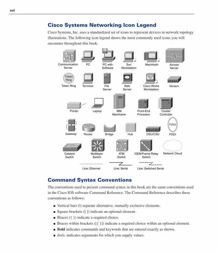
Cisco Systems Networking Icon LegendCisco Systems, Inc. uses a standardized set of icons to represent devices in network topology
illustrations. The following icon legend shows the most commonly used icons you will
encounter throughout this book.
Command Syntax ConventionsThe conventions used to present command syntax in this book are the same conventions used
in the Cisco IOS software Command Reference. The Command Reference describes these
conventions as follows:
■ Vertical bars (|) separate alternative, mutually exclusive elements.
■ Square brackets ([ ]) indicate an optional element.
■ Braces ({ }) indicate a required choice.
■ Braces within brackets ([{ }]) indicate a required choice within an optional element.
■ Bold indicates commands and keywords that are entered exactly as shown.
■ Italic indicates arguments for which you supply values.
PC PC withSoftware
SunWorkstation
Macintosh
Terminal File Server
WebServer
Cisco WorksWorkstation
Printer Laptop IBMMainframe
Front-EndProcessor
ClusterController
Modem
DSU/CSU
Router Bridge Hub DSU/CSU
CatalystSwitch
MultilayerSwitch
ATMSwitch
ISDN/Frame RelaySwitch
CommunicationServer
Gateway
AccessServer
Network Cloud
TokenRing
Token Ring
Line: Ethernet
FDDI
FDDI
Line: Serial Line: Switched Serial
1358_fmi.book Page xvi Thursday, May 27, 2004 2:21 PM

xvii
ForewordThroughout the world, the Internet has brought tremendous new opportunities for individuals
and their employers. Companies and other organizations are seeing dramatic increases in pro-
ductivity by investing in robust networking capabilities. Some studies have shown measur-
able productivity improvements in entire economies. The promise of enhanced efficiency,
profitability, and standard of living is real and growing.
Such productivity gains aren’t achieved by simply purchasing networking equipment. Skilled
professionals are needed to plan, design, install, deploy, configure, operate, maintain, and
troubleshoot today’s networks. Network managers must ensure that they have planned for
network security and continued operation. They need to design for the required performance
level in their organization. They must implement new capabilities as the demands of their
organization, and its reliance on the network, expand.
To meet the many educational needs of the internetworking community, Cisco Systems estab-
lished the Cisco Networking Academy Program. The Networking Academy is a comprehen-
sive learning program that provides students with the Internet technology skills that are
essential in a global economy. The Networking Academy integrates face-to-face teaching,
web-based content, online assessment, student performance tracking, hands-on labs, instruc-
tor training and support, and preparation for industry-standard certifications.
The Networking Academy continually raises the bar on blended learning and educational
processes. The Internet-based assessment and instructor support systems are some of the
most extensive and validated ever developed, including a 24/7 customer service system for
Networking Academy instructors. Through community feedback and electronic assessment,
the Networking Academy adapts the curriculum to improve outcomes and student achieve-
ment. The Cisco Global Learning Network infrastructure designed for the Networking Acad-
emy delivers a rich, interactive, personalized curriculum to students worldwide. The Internet
has the power to change the way people work, live, play, and learn, and the Cisco Networking
Academy Program is at the forefront of this transformation.
This Cisco Press book is one in a series of best-selling companion titles for the Cisco Net-
working Academy Program. Designed by Cisco Worldwide Education and Cisco Press, these
books provide integrated support for the online learning content that is made available to
Academies all over the world. These Cisco Press books are the only books authorized for the
Networking Academy by Cisco Systems. They provide print and CD-ROM materials that
ensure the greatest possible learning experience for Networking Academy students.
I hope you are successful as you embark on your learning path with Cisco Systems and the
Internet. I also hope that you will choose to continue your learning after you complete
the Networking Academy curriculum. In addition to its Cisco Networking Academy Program
titles, Cisco Press publishes an extensive list of networking technology and certification pub-
1358_fmi.book Page xvii Thursday, May 27, 2004 2:21 PM

xviii
lications that provide a wide range of resources. Cisco Systems has also established a net-
work of professional training companies—the Cisco Learning Partners—that provide a full
range of Cisco training courses. They offer training in many formats, including e-learning,
self-paced, and instructor-led classes. Their instructors are Cisco-certified, and Cisco creates
their materials. When you are ready, please visit the Learning & Events area at Cisco.com to
learn about all the educational support that Cisco and its partners have to offer.
Thank you for choosing this book and the Cisco Networking Academy Program.
Kevin Warner
Senior Director, Marketing
Worldwide Education
Cisco Systems, Inc.
1358_fmi.book Page xviii Thursday, May 27, 2004 2:21 PM

xix
IntroductionThis companion guide is designed as a desk reference to supplement your classroom and lab-
oratory experience with version 3 of the CCNP 1 course in the Cisco Networking Academy
Program.
CCNP 1: Advanced Routing is one of four courses leading to the Cisco Certified Network
Professional certification. CCNP 1 teaches you how to design, configure, maintain, and scale
routed networks. You will learn to use VLSMs, private addressing, and NAT to enable more
efficient use of IP addresses. This book also teaches you how to implement routing protocols
such as RIPv2, EIGRP, OSPF, IS-IS, and BGP. In addition, it details the important techniques
used for route filtering and redistribution. While taking the course, use this companion guide
to help you prepare for the Building Scalable Cisco Internetworks 642-801 BSCI exam,
which is one of the four required exams to obtain the CCNP certification.
This Book’s Goal
The goal of this book is to build on the routing concepts you learned while studying for the CCNA
exam and to teach you the foundations of advanced routing concepts. The topics are designed to
prepare you to pass the Building Scalable Cisco Internetworks exam (642-801 BSCI).
The Building Scalable Cisco Internetworks exam is a qualifying exam for the CCNP, CCDP,
and CCIP certifications. The 642-801 BSCI exam tests materials covered under the new
Building Scalable Cisco Internetworks course and exam objectives. The exam certifies that
the successful candidate has the knowledge and skills necessary to use advanced IP address-
ing and routing to implement scalability for Cisco routers connected to LANs and WANs.
The exam covers advanced IP addressing; routing principles; configuring EIGRP, OSPF, and
IS-IS; manipulating routing updates; and configuring basic BGP.
One key methodology used in this book is to help you discover the exam topics you need to
review in more depth, to help you fully understand and remember those details, and to help
you prove to yourself that you have retained your knowledge of those topics. This book does
not try to help you pass by memorization; it helps you truly learn and understand the topics.
This book focuses on introducing techniques and technology for enabling WAN solutions. To
fully benefit from this book, you should be familiar with general networking terms and con-
cepts, and you should have basic knowledge of the following:
■ Basic Cisco router operation and configuration
■ TCP/IP operation and configuration
■ Routing protocols such as RIP, OSPF, IGRP, and EIGRP
■ Routed protocols
1358_fmi.book Page xix Thursday, May 27, 2004 2:21 PM

xx
This Book’s Audience
This book has a few different audiences. First, this book is intended for students interested in
advanced routing technologies. In particular, it is targeted toward students in the Cisco Net-
working Academy Program CCNP 1: Advanced Routing course. In the classroom, this book
serves as a supplement to the online curriculum. This book is also appropriate for corporate
training faculty and staff members, as well as general users.
This book is also useful for network administrators who are responsible for implementing
and troubleshooting enterprise Cisco routers and router configuration. It is also valuable for
anyone who is interested in learning advanced routing concepts and passing the Building
Scalable Cisco Internetworks exam (BSCI 642-801).
This Book’s Features
Many of this book’s features help facilitate a full understanding of the topics covered in this book:
■ Objectives—Each chapter starts with a list of objectives that you should have mastered
by the end of the chapter. The objectives reference the key concepts covered in the
chapter.
■ Figures, examples, tables, and scenarios—This book contains figures, examples, and
tables that help explain theories, concepts, commands, and setup sequences that rein-
force concepts and help you visualize the content covered in the chapter. In addition,
the specific scenarios provide real-life situations that detail the problem and the
solution.
■ Chapter summaries—At the end of each chapter is a summary of the concepts cov-
ered in the chapter. It provides a synopsis of the chapter and serves as a study aid.
■ Key terms—Each chapter includes a list of defined key terms that are covered in the
chapter. The key terms appear in color throughout the chapter where they are used in
context. The definitions of these terms serve as a study aid. In addition, the key terms
reinforce the concepts introduced in the chapter and help you understand the chapter
material before you move on to new concepts.
■ Check Your Understanding questions and answers—Review questions, presented at
the end of each chapter, serve as a self-assessment tool. They reinforce the concepts
introduced in the chapter and help test your understanding before you move on to a new
chapter. An answer key to all the questions is provided in Appendix B, “Answers to the
Check Your Understanding Questions.”
■ Study guides and certification exam practice questions—To further assess your
understanding, you will find on the companion CD-ROM additional in-depth questions
in study guides created for each chapter. You will also find a test bank of questions
included in a test engine that simulates the exam environment for the CCNP certifica-
tion’s 642-801 BSCI exam.
1358_fmi.book Page xx Thursday, May 27, 2004 2:21 PM

xxi
■ Skill-building activities—Throughout the book are references to additional skill-
building activities to connect theory with practice. You can easily spot these activities
by the following icons:
How This Book Is Organized
Although you could read this book cover-to-cover, it is designed to be flexible and to allow
you to easily move between chapters and sections of chapters to cover just the material you
need to work with more. If you do intend to read all of the chapters, the order in which they
are presented is the ideal sequence. This book also contains three appendixes. The following
list summarizes the topics of this book’s elements:
■ Chapter 1, “Overview of Scalable Internetworks”—Good design is the key to a net-
work’s ability to scale. Poor design, not just an outdated protocol or router, prevents a
network from scaling properly. A network design should follow a hierarchical model to
be scalable. This chapter discusses the components of the hierarchical network design
model and the key characteristics of scalable internetworks.
■ Chapter 2, “Advanced IP Addressing Management”—Unfortunately, the architects
of TCP/IP could not have predicted that their protocol would eventually sustain a glo-
bal network of information, commerce, and entertainment. Twenty years ago, IP ver-
sion 4 (IPv4) offered an addressing strategy that, although scalable for a time, resulted
in an inefficient allocation of addresses. Over the past two decades, engineers have suc-
cessfully modified IPv4 so that it can survive the Internet’s exponential growth. Mean-
while, an even more extensible and scalable version of IP, IP version 6 (IPv6), has been
defined and developed. Today, IPv6 is slowly being implemented in select networks.
Eventually, IPv6 might replace IPv4 as the dominant Internet protocol. This chapter
explores the evolution and extension of IPv4, including the key scalability features that
engineers have added to it over the years, such as subnetting, classless interdomain
routing (CIDR), variable-length subnet masking (VLSM), and route summarization.
Finally, this chapter examines advanced IP implementation techniques such as IP
unnumbered, Dynamic Host Configuration Protocol (DHCP), and helper addresses.
Interactive Media Activities included on the companion CD-ROM are hands-on drag-and-drop, fill-in-the-blank, and matching exercises that help you master basic networking concepts.
The collection of lab activities developed for the course can be found in the Cisco Networking Academy Program CCNP 1: Advanced Routing Lab Companion, Second Edition.
1358_fmi.book Page xxi Thursday, May 27, 2004 2:21 PM
xxii
■ Chapter 3, “Routing Overview”—Many of the scalable design features explored in
the first two chapters, such as load balancing and route summarization, work very dif-
ferently depending on the routing protocol used. Routing protocols are the rules that
govern the exchange of routing information between routers. TCP/IP’s open architec-
ture and global popularity have encouraged the development of more than a half-dozen
prominent IP routing protocols. Each protocol has a unique combination of strengths
and weaknesses. Because routing protocols are key to network performance, you must
have a clear understanding of the attributes of each protocol, including convergence
times, overhead, and scalability features. This chapter explores various routing processes,
including default routing, floating static routes, convergence, and route calculation.
■ Chapter 4, “Routing Information Protocol Version 2”—RIPv2 is defined in RFC
1723 and is supported in Cisco IOS software Releases 11.1 and later. RIPv2 is similar
to RIPv1 but is not a new protocol. RIPv2 features extensions to bring it up-to-date
with modern routing environments. RIPv2 is the first of the classless routing protocols
discussed in this book. This chapter introduces classless routing and RIPv2.
■ Chapter 5, “EIGRP”—Enhanced Interior Gateway Routing Protocol (EIGRP) is a
Cisco-proprietary routing protocol based on IGRP. Unlike IGRP, which is a classful
routing protocol, EIGRP supports CIDR, allowing network designers to maximize
address space by using CIDR and VLSM. Compared to IGRP, EIGRP boasts faster
convergence times, improved scalability, and superior handling of routing loops.
This chapter surveys EIGRP’s key concepts, technologies, and data structures. This
conceptual overview is followed by a study of EIGRP convergence and basic operation.
Finally, this chapter shows you how to configure and verify EIGRP and the use of route
summarization.
■ Chapter 6, “OSPF”—This chapter describes how to create and configure OSPF. Spe-
cifically, it examines the different OSPF area types, including stubby, totally stubby,
and not-so-stubby areas (NSSAs). Each of these different area types uses a special
advertisement to exchange routing information with the rest of the OSPF network.
Therefore, link-state advertisements (LSAs) are covered in detail. The Area 0 backbone
rule and how virtual links can work around backbone connectivity problems are also
reviewed. Finally, this chapter surveys important show commands that can be used to
verify multiarea OSPF operation.
■ Chapter 7, “IS-IS”—In recent years, the Intermediate System-to-Intermediate System
(IS-IS) routing protocol has become increasingly popular, with widespread usage
among service providers. IS-IS enables very fast convergence and is very scalable. It is
also a very flexible protocol and has been extended to incorporate leading-edge features
such as Multiprotocol Label Switching Traffic Engineering (MPLS/TE). IS-IS features
include hierarchical routing, classless behavior, rapid flooding of new information, fast
1358_fmi.book Page xxii Thursday, May 27, 2004 2:21 PM

xxiii
convergence, good scalability, and flexible timer tuning. The Cisco IOS software
implementation of IS-IS also supports multiarea routing, route leaking, and overload
bit. All of these concepts are discussed in this chapter, beginning with an introduction
to OSI protocols.
■ Chapter 8, “Route Optimization”—Dynamic routing, even in small internetworks,
can involve much more than just enabling a routing protocol’s default behavior. A few
simple commands might be enough to get dynamic routing started. However, more
advanced configuration must be done to enable such features as routing update control
and exchanges among multiple routing protocols. You can optimize routing in a net-
work by controlling when a router exchanges routing updates and what those updates
contain. This chapter examines the key IOS route optimization features, including rout-
ing update control, policy-based routing, and route redistribution.
■ Chapter 9, “BGP”—This chapter provides an overview of the different types of auton-
omous systems and then focuses on basic BGP operation, including BGP neighbor
negotiation. It also looks at how to use the Cisco IOS software to configure BGP and
verify its operation. Finally, it examines BGP peering and the BGP routing process.
■ Appendix A, “Glossary of Key Terms”—This appendix provides a complied list of
all the key terms that appear throughout the book.
■ Appendix B, “Answers to the Check Your Understanding Questions”—This appen-
dix provides the answers to the quizzes that appear at the end of each chapter.
■ Appendix C, “Case Studies”—This appendix provides case studies that let you apply
the concepts you learn throughout this book to real-life routing scenarios. The case
studies cover EIGRP, OSPF, and BGP/OSPF.
About the CD-ROM
The CD-ROM included with this book provides Interactive Media Activities, a test engine,
and Study Guides to enhance your learning experience. You will see these referred to
throughout the book.
1358_fmi.book Page xxiii Thursday, May 27, 2004 2:21 PM

ObjectivesUpon completing this chapter, you will be able to
■ Describe the hierarchical network design model
■ State the key characteristics of scalable networks
You can reinforce your understanding of the objectives covered in this chapter by opening
the interactive media activities on the CD accompanying this book and performing the lab
activities collected in the Cisco Networking Academy Program CCNP 1: Advanced Routing
Lab Companion. Throughout this chapter, you will see references to these activities by title
and by icon. They look like this:
Interactive Media Activity
Lab Activity
1358_fmi.book Page 2 Thursday, May 27, 2004 2:21 PM
Chapter 1
Overview of Scalable Internetworks
Initially, Transmission Control Protocol/Internet Protocol (TCP/IP) networks relied on simple
distance vector routing protocols and classful 32-bit IP addressing. These technologies offered a
limited capacity for growth. Network designers must now modify, redesign, or abandon these
early technologies to build modern networks that can scale to handle fast growth and constant
change. This chapter explores networking technologies that have evolved to meet this demand
for scalability.
Scalability is a network’s capability to grow and adapt without major redesign or reinstallation.
It seems obvious to allow for growth in a network, but growth can be difficult to achieve without
redesign. This redesign might be significant and costly. For example, a network might give a
small company access to e-mail, the Internet, and shared files. If the company tripled in size and
demanded streaming video or e-commerce services, could the original networking media and
devices adequately serve these new applications? Most organizations cannot afford to recable or
redesign their networks when users are relocated, new nodes are added, or new applications are
introduced.
Good design is the key to a network’s ability to scale. Poor design, not an outdated protocol or
router, prevents a network from scaling properly. A network design should follow a hierarchical
model to be scalable. This chapter discusses the components of the hierarchical network design
model and the key characteristics of scalable internetworks.
The Hierarchical Network Design ModelIf allowed to grow helter-skelter, strictly as needs demanded, most networks would quickly
become unrecognizable and unmanageable. Worse, someday you might reach the point where
no more growth can be accommodated. Following a standardized design model allows your net-
work to grow in an established pattern that will not limit future growth.
1358_fmi.book Page 3 Thursday, May 27, 2004 2:21 PM

4 Chapter 1: Overview of Scalable Internetworks
The Three-Layer Hierarchical Design Model
A hierarchical network design model breaks the complex problem of network design into
smaller, more manageable problems. Each level or tier in the hierarchy addresses a different
set of problems. This helps the designer optimize network hardware and software to perform
specific roles. For example, devices at the lowest tier are optimized to accept traffic into a net-
work and pass that traffic to the higher layers. Cisco offers a three-tiered hierarchy as the pre-
ferred approach to network design, as illustrated in Figure 1-1.
Figure 1-1 Scalable Network Design
In the three-layer network design model, shown in Figure 1-2, network devices and links are
grouped according to the following three layers:
■ Core
■ Distribution
■ Access
Access Layer
Distribution Layer
Core Layer
Core Layer
Distribution Layer
Access Layer
To Internet
To Wide Area
1358_fmi.book Page 4 Thursday, May 27, 2004 2:21 PM

The Hierarchical Network Design Model 5
Figure 1-2 Three-Layer Network Design Model
The three-layer model is a conceptual framework. It is an abstract picture of a network simi-
lar to the concept of the Open System Interconnection (OSI) reference model.
Layered models are useful because they facilitate modularity. Devices at each layer have sim-
ilar and well-defined functions. This allows administrators to easily add, replace, and remove
individual pieces of the network. This kind of flexibility and adaptability makes a hierarchical
network design highly scalable.
At the same time, layered models can be difficult to comprehend, because the exact composi-
tion of each layer varies from network to network. Each layer of the three-tiered design
model may include the following:
■ A router
■ A switch
■ A link
■ A combination of these
Some networks might combine the function of two layers into a single device or omit a layer
entirely.
The following sections discuss each of the three layers in detail.
The Core LayerThe core layer provides an optimized and reliable transport structure by forwarding traffic at
very high speeds. In other words, the core layer switches packets as fast as possible. Devices
at the core layer should not be burdened with any processes that stand in the way of switching
Core LayerHigh-Speed Switching
Distribution LayerPolicy-Based Connectivity
Access LayerLocal and Remote Workgroup Access
1358_fmi.book Page 5 Thursday, May 27, 2004 2:21 PM

6 Chapter 1: Overview of Scalable Internetworks
packets at top speed. Examples of processes that are best performed outside the core include
the following:
■ Access list checking
■ Data encryption
■ Address translation
The Distribution LayerThe distribution layer is located between the access and core layers. It helps differentiate the
core from the rest of the network. The purpose of this layer is to provide boundary definition
using access lists and other filters to limit what gets into the core. Therefore, this layer defines
policy for the network. A policy is an approach to handling certain kinds of traffic, including
the following:
■ Routing updates
■ Route summaries
■ Virtual LAN (VLAN) traffic
■ Address aggregation
Use these policies to secure networks and to preserve resources by preventing unnecessary
traffic.
If a network has two or more routing protocols, such as Routing Information Protocol (RIP)
and Interior Gateway Routing Protocol (IGRP), information between the different routing
domains is shared, or redistributed, at the distribution layer.
The Access LayerThe access layer supplies traffic to the network and performs network entry control. End
users access network resources by way of the access layer. Acting as the front door to a net-
work, the access layer employs access lists designed to prevent unauthorized users from gaining
entry. The access layer can also give remote sites access to the network by way of a wide-area
technology, such as Frame Relay, ISDN, leased lines, DSL, cable modem, or one of several
wireless and satellite technologies.
Interactive Media Activity Point and Click: Layered Design Model
In this media activity, you learn characteristics of the layered design model. This is a
point-and-click activity where you click the correct choice.
NOTE
Although a modern Layer 3 fast switch with Policy Feature Cards can process access lists in hardware, this function normally is not activated at the core layer so that traffic can proceed as quickly as possible.
1358_fmi.book Page 6 Thursday, May 27, 2004 2:21 PM

The Hierarchical Network Design Model 7
Router Function in the Hierarchy
The core, distribution, and access layers each have clearly defined functions. For this reason,
each layer demands a different set of features than routers, switches, and links. Routers that
operate in the same layer can be configured in a consistent way, because they all must per-
form similar tasks. The router is the primary device that maintains logical and physical hier-
archy in a network. Therefore, proper and consistent configurations are imperative. Cisco
offers several router product lines. Each product line has a particular set of features for one of
the three layers:
■ Core layer—12000, 7500, 7200, and 7000 series routers, shown in Figures 1-3 and 1-4.
Figure 1-3 Cisco 12000 Series Core-Layer Router
Figure 1-4 Cisco 7000 Series Core-Layer Routers
1358_fmi.book Page 7 Thursday, May 27, 2004 2:21 PM

8 Chapter 1: Overview of Scalable Internetworks
■ Distribution layer—4500, 4000, and 3600 series routers, shown in Figures 1-5 and 1-6.
Figure 1-5 Cisco 4000 Series Distribution-Layer Router
Figure 1-6 Cisco 3600 Series Distribution-Layer Routers
■ Access layer—2600, 2500, 1700, and 1600 series routers, shown in Figures 1-7 and 1-8.
1358_fmi.book Page 8 Thursday, May 27, 2004 2:21 PM

The Hierarchical Network Design Model 9
Figure 1-7 Cisco 2600 Series Access-Layer Routers
Figure 1-8 Cisco 1700 Series Access-Layer Routers
The following sections revisit each layer and examine the specific routers and other devices
used.
Interactive Media Activity Drag and Drop: Defining the Role of the Router in the Hierarchy
In this media activity, you identify the functions of each hierarchy layer.
1358_fmi.book Page 9 Thursday, May 27, 2004 2:21 PM

10 Chapter 1: Overview of Scalable Internetworks
Core Layer Example
The core layer is the center of the network and is designed to be fast and reliable. Access lists
should be avoided in the core layer. Access lists add latency, and end users should not have
direct access to the core. In a hierarchical network, end-user traffic should reach core routers
only after those packets have passed through the distribution and access layers. Access lists
may exist in those two lower layers.
Core routing is done without access lists, address translation, or other packet manipulation.
Because of this, it might seem as though the least powerful routers would work well for so
simple a task. However, the opposite is true. The most powerful Cisco routers serve the core,
because they have the fastest switching technologies and the largest capacity for physical
interfaces.
The 7000, 7200, and 7500 series routers feature the fastest switching modes available. These
are the Cisco enterprise core routers. The 12000 series router is also a core router designed to
meet the core routing needs of Internet service providers (ISPs). Unless the company is in the
business of providing Internet access to other companies, it is unlikely that a 12000 series
router will be found in the telecommunications closet.
The 7000, 7200, and 7500 series routers are modular. This provides scalability, because
administrators can add interface modules when needed. The large chassis of this series can
accommodate dozens of interfaces on multiple modules for virtually any media type. This
makes these routers scalable and reliable core solutions.
Core routers achieve reliability through the use of redundant links, usually to all other core
routers. When possible, these redundant links should be symmetrical, having equal through-
put, so that equal-cost load balancing may be used. Core routers need a relatively large num-
ber of interfaces to enable this configuration. Core routers achieve reliability through
redundant power supplies. They usually feature two or more hot-swappable power supplies,
which may be removed and replaced individually without shutting down the router.
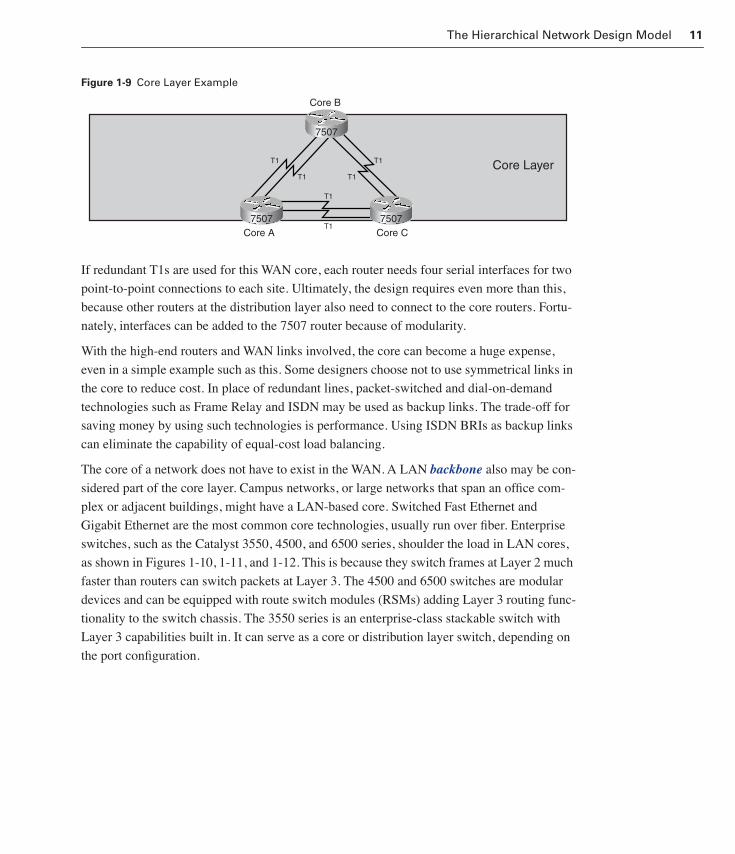
Figure 1-9 shows a simple core topology using 7507 router routers at three key sites in an
enterprise. Each Cisco 7507 router is directly connected to every other router. This type of
configuration is a full mesh. There are also two links between each router to provide redun-
dancy. Core links should be the fastest and most reliable leased lines in the WAN and can
include
■ T1
■ T3
■ OC3
■ Anything better
1358_fmi.book Page 10 Thursday, May 27, 2004 2:21 PM
The Hierarchical Network Design Model 11
Figure 1-9 Core Layer Example
If redundant T1s are used for this WAN core, each router needs four serial interfaces for two
point-to-point connections to each site. Ultimately, the design requires even more than this,
because other routers at the distribution layer also need to connect to the core routers. Fortu-
nately, interfaces can be added to the 7507 router because of modularity.
With the high-end routers and WAN links involved, the core can become a huge expense,
even in a simple example such as this. Some designers choose not to use symmetrical links in
the core to reduce cost. In place of redundant lines, packet-switched and dial-on-demand
technologies such as Frame Relay and ISDN may be used as backup links. The trade-off for
saving money by using such technologies is performance. Using ISDN BRIs as backup links
can eliminate the capability of equal-cost load balancing.
The core of a network does not have to exist in the WAN. A LAN backbone also may be con-
sidered part of the core layer. Campus networks, or large networks that span an office com-
plex or adjacent buildings, might have a LAN-based core. Switched Fast Ethernet and
Gigabit Ethernet are the most common core technologies, usually run over fiber. Enterprise
switches, such as the Catalyst 3550, 4500, and 6500 series, shoulder the load in LAN cores,
as shown in Figures 1-10, 1-11, and 1-12. This is because they switch frames at Layer 2 much
faster than routers can switch packets at Layer 3. The 4500 and 6500 switches are modular
devices and can be equipped with route switch modules (RSMs) adding Layer 3 routing func-
tionality to the switch chassis. The 3550 series is an enterprise-class stackable switch with
Layer 3 capabilities built in. It can serve as a core or distribution layer switch, depending on
the port configuration.
7507
7507 7507
T1
T1 T1
T1
T1
T1
Core Layer
Core B
Core A Core C
1358_fmi.book Page 11 Thursday, May 27, 2004 2:21 PM

12 Chapter 1: Overview of Scalable Internetworks
Figure 1-10 Catalyst 3550 Series Core Layer Switches
Figure 1-11 Catalyst 4500 Series Core Layer Switches
Figure 1-12 Catalyst 6500 Series Core Layer Switches
1358_fmi.book Page 12 Thursday, May 27, 2004 2:21 PM

The Hierarchical Network Design Model 13
Distribution Layer Example
The distribution layer, shown in Figure 1-13, enforces policies to limit traffic to and from the
core. Distribution layer routers handle less traffic than core-layer routers, so they need fewer
interfaces and less switching speed. However, a fast core is useless if a slowdown of data
transfer at the distribution layer prevents user traffic from accessing core links. For this rea-
son, Cisco offers robust, powerful distribution routers, such as the 4000, 4500, and 3600
series routers. These routers are modular, allowing interfaces to be added and removed,
depending on what is needed. However, the smaller chassis of these series are much more
limiting than those of the 7000, 7200, and 7500 series.
Figure 1-13 Distribution Layer Example
Distribution layer routers bring policy to the network by using a combination of the following:
■ Access lists
■ Route summarization
■ Distribution lists
■ Route maps
■ Other rules to define how a router should deal with traffic and routing updates
Many of these techniques are covered later in the book.
Figure 1-13 shows that two 3620 routers have been added at Core A, in the same wiring
closet as the 7507 router. In this example, high-speed LAN links connect the distribution
routers to the core router. Depending on the network’s size, these links may be part of the
campus backbone and will most likely be fiber running 100 or 1000 Mbps Ethernet. In this
example, Dist-1A and Dist-2A are part of the Core A campus backbone. Dist-1A serves
remote sites, and Dist-2A serves access routers at Site A. If Site A uses VLANs, Dist-2A may
be responsible for routing between the VLANs.
7507
7507
T1
T1 T1
T1
T1
T1
Core Layer
Core B
Core A Core C
100 Mbps
Dist-1A Dist-2A
Distribution Layer
7507
3620 3620
1358_fmi.book Page 13 Thursday, May 27, 2004 2:21 PM

14 Chapter 1: Overview of Scalable Internetworks
Both Dist-1A and Dist-2A use access lists to prevent unwanted traffic from reaching the core.
In addition, these routers summarize their routing tables in updates to Core A. This keeps the
Core A routing table small and efficient.
Access Layer Example
Routers at the access layer, as shown in Figure 1-14, give users at Site A access to the net-
work. Routers at remote sites Y and Z also give users access to the network.
Figure 1-14 Access Layer Example
Access routers generally offer fewer physical interfaces than distribution and core routers.
For this reason, Cisco access routers feature a small, streamlined chassis that might or might
not support modular interfaces. This includes the 1600, 1700, 2500, and 2600 series routers.
Two 2621s have been added to the network’s access layer at Site A. These 2621 routers have
two FastEthernet interfaces. User-end stations connect through a workgroup switch or hub to
one FastEthernet interface. The other FastEthernet interface connects to the high-speed cam-
pus backbone of Site A.
7507
7507
T1
T1 T1
T1
T1
T1
Core Layer
Core B
Core A Core C100 Mbps
Dist-1A Dist-2A
Distribution Layer
7507
Access-4 Y
Remote Site Y
Access-3 Y
Remote Site ZSite Y User Site Z User
ISDNBRI
FrameRelay
Devices at Site A
Access Layer
3620
2610 2610
3620
2621 2621
1358_fmi.book Page 14 Thursday, May 27, 2004 2:21 PM
Key Characteristics of Scalable Internetworks 15
Each remote site in the example requires only one Ethernet interface for the LAN side and
one serial interface for the WAN side. The WAN interface connects by way of Frame Relay or
ISDN to the distribution router in Site A’s wiring closet. For this application, the 2610 router
provides a single 10/100-Mbps FastEthernet port and works well at these locations. These
remote sites, Y and Z, are small branch offices that must access the core through Site A.
Therefore, Dist-1A is a WAN hub for the organization. As the network scales, more remote
sites may access the core with a connection to the distribution routers at the WAN hub.
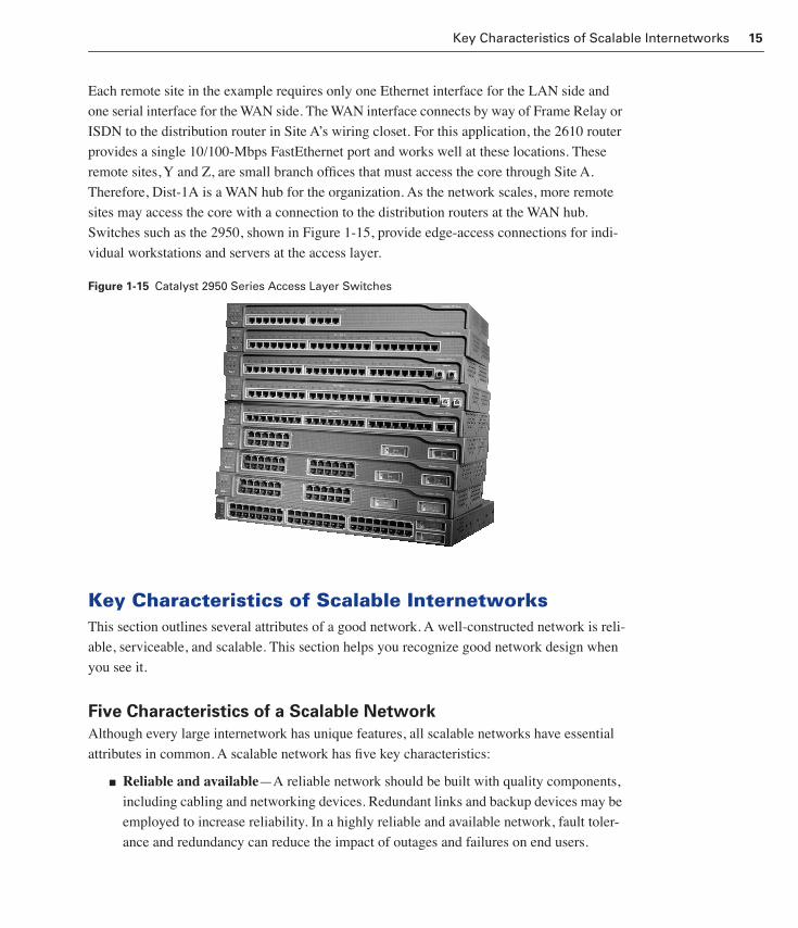
Switches such as the 2950, shown in Figure 1-15, provide edge-access connections for indi-
vidual workstations and servers at the access layer.
Figure 1-15 Catalyst 2950 Series Access Layer Switches
Key Characteristics of Scalable InternetworksThis section outlines several attributes of a good network. A well-constructed network is reli-
able, serviceable, and scalable. This section helps you recognize good network design when
you see it.
Five Characteristics of a Scalable Network
Although every large internetwork has unique features, all scalable networks have essential
attributes in common. A scalable network has five key characteristics:
■ Reliable and available—A reliable network should be built with quality components,
including cabling and networking devices. Redundant links and backup devices may be
employed to increase reliability. In a highly reliable and available network, fault toler-
ance and redundancy can reduce the impact of outages and failures on end users.
1358_fmi.book Page 15 Thursday, May 27, 2004 2:21 PM

16 Chapter 1: Overview of Scalable Internetworks
■ Responsive—A responsive network should provide quality of service (QoS) for vari-
ous applications and protocols without making responses at the desktop worse. The
internetwork must be capable of responding to latency issues common for time-sensitive
traffic, such as Systems Network Architecture (SNA) traffic and streaming video and
audio communications. However, the internetwork must still route desktop traffic with-
out compromising QoS.
■ Efficient—Large internetworks must optimize the use of resources, especially band-
width. It is possible to increase data throughput without adding hardware or buying
more WAN services. To do this, reduce unnecessary broadcasts, service location
requests, and routing updates.
■ Adaptable—An adaptable network can accommodate different protocols, applications,
and hardware technologies.
■ Accessible but secure—An accessible network allows for connections using dedi-
cated, dialup, and switched services while maintaining network integrity.
The Cisco IOS software offers a rich set of features that support network scalability. The
remainder of this chapter discusses IOS features that support these five characteristics of a
scalable network.
Making the Network Reliable and Available
A reliable and available network provides users with 24-hour-a-day, seven-day-a-week
access. In a highly reliable and available network, fault tolerance and redundancy make out-
ages and failures invisible to the end user, as shown in Figure 1-16. The high-end devices and
telecommunication links that ensure this kind of performance come with a high price tag.
Network designers constantly have to balance the needs of users with the resources at hand.
Figure 1-16 Reliable and Available Network
Broken Serial Line
1358_fmi.book Page 16 Thursday, May 27, 2004 2:21 PM
Key Characteristics of Scalable Internetworks 17
When choosing between high performance and low cost at the core layer, the network admin-
istrator should choose the best available routers and dedicated WAN links. The core must be
designed to be the most reliable and available layer. If a core router fails or a core link
becomes unstable, routing for the entire internetwork might be adversely affected.
Core routers maintain reliability and availability by rerouting traffic in the event of a failure.
Robust networks can adapt to failures quickly and effectively. To build robust networks, the
Cisco IOS software offers several features that enhance reliability and availability:
■ Support for scalable routing protocols
■ Alternative paths
■ Load balancing
■ Protocol tunnels
■ Dial backup
The following sections describe these features.
Scalable Routing ProtocolsRouters in the core of a network should converge rapidly and maintain reachability to all net-
works and subnetworks within an autonomous system (AS). Simple distance vector routing
protocols such as RIP take too long to update and adapt to topology changes to be viable core
solutions. Compatibility issues might require that some areas of a network run simple dis-
tance vector protocols such as RIP and Routing Table Maintenance Protocol (RTMP), an
Apple-proprietary routing protocol. It is best to use a scalable routing protocol in the core
layer. Good choices include Open Shortest Path First (OSPF), Intermediate System-to-
Intermediate System (IS-IS), and Enhanced Interior Gateway Routing Protocol (EIGRP).
Alternative PathsRedundant links maximize network reliability and availability, but they are expensive to
deploy throughout a large internetwork. Core links should always be redundant. Other areas
of a network also might need redundant telecommunication links. If a remote site exchanges
mission-critical information with the rest of the internetwork, that site is a candidate for
redundant links. To provide another dimension of reliability, an organization might even
invest in redundant routers to connect to these links. A network that consists of multiple links
and redundant routers contains several paths to a given destination. If a network uses a scal-
able routing protocol, each router maintains a map of the entire network topology. This map
helps routers select an alternative path quickly if a primary path fails. EIGRP actually main-
tains a database of all alternative paths if the primary route is lost.
1358_fmi.book Page 17 Thursday, May 27, 2004 2:21 PM
18 Chapter 1: Overview of Scalable Internetworks
Load BalancingRedundant links do not necessarily remain idle until a link fails. Routers can distribute the
traffic load across multiple links to the same destination. This process is called load balanc-
ing. Load balancing can be implemented using alternative paths with the same cost or metric.
This is called equal-cost load balancing. They can also be implemented over alternative paths
with different metrics. This is called unequal-cost load balancing. When routing IP, the Cisco
IOS software offers two methods of load balancing—per-packet and per-destination. If fast
switching is enabled, only one of the alternative routes is cached for the destination address.
All packets in the packet stream bound for a specific host take the same path. Packets bound
for a different host on the same network may use an alternative route. This way, traffic is
load-balanced on a per-destination basis.
Per-packet load balancing requires more CPU time than per-destination load balancing. How-
ever, per-packet load balancing allows load balancing that is proportional to the metrics of
unequal paths, which can help use bandwidth efficiently. The proportional distribution makes
per-packet load balancing better than per-destination load balancing in these cases.
Protocol TunnelsAn IP network with Novell NetWare running Internetwork Packet Exchange (IPX) at a hand-ful of remote sites may provide IPX connectivity between the remote sites by routing IPX in the core. Even if only two or three offices use NetWare IPX sparingly, this creates additional overhead associated with routing a second routed protocol, or IPX, in the core. It also requires that all routers in the data path have the appropriate IOS and hardware to support IPX. For this reason, many organizations have adopted “IP only” policies at the network core, because IP has become the dominant routed protocol and is essential for access to the Internet.
Tunneling gives an administrator a second, and more agreeable, option. The administrator can configure a point-to-point link through the core between the two routers using IP. When this link is configured, IPX packets can be encapsulated inside IP packets. IPX can then traverse the core over IP links, and the core can be spared the additional burden of routing IPX. Using tunnels, the administrator increases the availability of network services.
Dial BackupSometimes two redundant WAN links are not enough, or a single link needs to be fault-toler-ant. However, the possibility of purchasing a full-time redundant link is too expensive. In these cases, a backup link can be configured over a dialup technology, such as ISDN, or even an ordinary analog phone line. These relatively low-bandwidth links remain idle until the pri-mary link fails.
1358_fmi.book Page 18 Thursday, May 27, 2004 2:21 PM

Key Characteristics of Scalable Internetworks 19
Dial backup can be a cost-effective insurance policy, but it is not a substitute for redundant links that can effectively double throughput by using equal-cost load balancing.
Making the Network Responsive
End users notice network responsiveness as they use the network to perform routine tasks. Users expect network resources to respond quickly, as if network applications were running from a local hard drive. Networks must be configured to meet the needs of all applications, especially time-delay-sensitive applications such as voice and video. The IOS offers traffic prioritization features to tune responsiveness in a congested network. Routers may be config-ured to prioritize certain kinds of traffic based on protocol information, such as TCP port numbers. Traffic prioritization ensures that packets carrying mission-critical data take prece-dence over less-important traffic. Figure 1-17 illustrates this concept by showing how the FTP traffic waits while higher-priority voice and video traffic enters through the router interface.
If the router schedules these packets for transmission on a first-come, first-served basis, users could experience an unacceptable lack of responsiveness. For example, an end user sending delay-sensitive voice traffic might be forced to wait too long while the router empties its buffer of queued packets.
Figure 1-17 Traffic Prioritization
The IOS addresses priority and responsiveness issues through queuing. Routers that maintain
a slow WAN connection often experience congestion. These routers need a method to give
certain traffic priority. Queuing is the process that the router uses to schedule packets for
transmission during periods of congestion. By using the queuing feature, a congested router
can be configured to reorder packets so that mission-critical and delay-sensitive traffic is pro-
cessed first. These higher-priority packets are sent first even if other low-priority packets
arrive ahead of them. The IOS supports four methods of queuing:
■ First-in, first-out (FIFO) queuing
■ Priority queuing
■ Custom queuing
■ Weighted Fair Queuing (WFQ)
Only one of these queuing methods can be applied per interface, because each method han-
dles traffic in a unique way.
TP FTP
VOICE VIDEO FTP
1358_fmi.book Page 19 Thursday, May 27, 2004 2:21 PM

20 Chapter 1: Overview of Scalable Internetworks
Making the Network Efficient
An efficient network should not waste bandwidth, especially over costly WAN links. To be
efficient, routers should prevent unnecessary traffic from traversing the WAN and minimize
the size and frequency of routing updates. The IOS includes several features designed to opti-
mize a WAN connection:
■ Access lists
■ Snapshot routing
■ Compression over WANs
The following sections describe each of these features.
Access ListsAccess lists, illustrated in Figure 1-18, also called Access Control Lists (ACLs), can be used
to do all of the following:
■ Prevent traffic that the administrator defines as unnecessary, undesirable, or
unauthorized
■ Control routing updates
■ Apply route maps
■ Implement other network policies that improve efficiency by curtailing traffic
Figure 1-18 Access Lists
One access list may be applied on an interface for each protocol, per direction, in or out. Dif-
ferent filtering policies can be defined for different protocols, such as IP, IPX, and AppleTalk.
Telnet
Permit Deny
HTTP TELNET
FTP
TELNET
1358_fmi.book Page 20 Thursday, May 27, 2004 2:21 PM

Key Characteristics of Scalable Internetworks 21
Snapshot RoutingDistance vector routing protocols typically update neighbor routers with their complete rout-
ing table at regular intervals. These timed updates occur even when there have been no
changes in the network topology since the last update. If a remote site relies on a dialup tech-
nology, such as ISDN, it would be cost-prohibitive to maintain the WAN link in an active
state 24 hours a day. RIP routers expect updates every 30 seconds by default. This would
cause the ISDN link to reestablish twice a minute to maintain the routing tables. It is possible
to adjust the RIP timers, but snapshot routing provides a better solution to maximize network
efficiency.
Snapshot routing allows routers using distance vector protocols to exchange their complete
tables during an initial connection. Snapshot routing then waits until the next active period on
the line before exchanging routing information again. The router takes a snapshot of the rout-
ing table. The router then uses this picture for routing table entries while the dialup link is
down. The result is that the routing table is kept unchanged so that routes are not lost because
a routing update was not received. When the link is reestablished, usually because the router
has identified interesting traffic that needs to be routed over the WAN, the router again
updates its neighbors.
Compression over WANsThe IOS supports several compression techniques that can maximize bandwidth by reducing
the number of bits in all or part of a frame. Compression is accomplished through mathemat-
ical formulas or compression algorithms. Unfortunately, routers must dedicate a significant
amount of processor time to compress and decompress traffic, increasing latency. Therefore,
compression tends to be an efficient measure only on links with extremely limited bandwidth.
The IOS also supports the following bandwidth optimization features:
■ Dial-on-demand routing (DDR)
■ Route summarization
■ Incremental updates
Dial-on-Demand RoutingDedicated WAN circuits, even Frame Relay, might be cost-prohibitive for every remote site.
DDR offers an efficient, economic alternative for sites that require only occasional WAN con-
nectivity. A router configured for DDR listens for interesting traffic and waits to establish the
WAN link. The administrator defines what interesting traffic is. When the router receives traffic
that meets the criteria, the link is activated. DDR is most commonly used with ISDN circuits.
1358_fmi.book Page 21 Thursday, May 27, 2004 2:21 PM

22 Chapter 1: Overview of Scalable Internetworks
Route SummarizationThe number of entries in a routing table can be reduced if the router uses one network address
and mask to represent multiple networks or subnetworks. This technique is called route
aggregation or route summarization. Some routing protocols automatically summarize sub-
net routes based on the major network number. Other routing protocols, such as OSPF and
EIGRP, allow manual summarization. Route summarization is discussed in Chapter 2,
“Advanced IP Addressing Management.”
Incremental UpdatesRouting protocols such as OSPF, IS-IS, and EIGRP send routing updates that contain infor-
mation only about routes that have changed. These incremental routing updates use the band-
width more efficiently than simple distance vector protocols that transmit their complete
routing table at fixed intervals, whether or not a change has occurred.
Making the Network Adaptable
An adaptable network handles the addition and coexistence of multiple routed and routing
protocols. EIGRP is an exceptionally adaptable protocol because it supports routing informa-
tion for three routed protocols:
■ IP
■ IPX
■ AppleTalk
The IOS also supports route redistribution, which is described in Chapter 8, “Route Optimi-
zation.” Route redistribution allows routing information to be shared among two or more dif-
ferent routing protocols. For example, RIP routes can be redistributed, or injected, into an
OSPF area.
Mixing Routable and Nonroutable ProtocolsA network delivering both routable and nonroutable traffic has some unique problems.
Routable protocols, such as IP, can be forwarded from one network to another based on a net-
work-layer address. Nonroutable protocols, such as SNA, do not contain a network layer
address and cannot be forwarded by routers. Most nonroutable protocols also lack a mecha-
nism to provide flow control and are sensitive to delays in delivery. Any delays in delivery
causing packets to arrive out of order can result in the session’s being dropped. An adaptable
network must accommodate both routable and nonroutable protocols.
1358_fmi.book Page 22 Thursday, May 27, 2004 2:21 PM

Key Characteristics of Scalable Internetworks 23
Making the Network Accessible but Secure
Accessible networks let users connect easily over a variety of technologies, as shown in Fig-
ure 1-19. Campus LAN users typically connect to routers at the access layer through Ethernet
or Token Ring. Remote users and sites might have access to several types of WAN services.
Cost and geography play a significant role in determining what type of WAN services an
organization can deploy. Therefore, Cisco routers support all major WAN connection types.
As shown in Figure 1-19, these services include all of the following:
■ Dialup or circuit-switched networks
■ Dedicated or leased lines
■ Packet-switched networks
Figure 1-19 Accessible Networks
Dialup connections are circuit-switched, and leased lines are dedicated. Packet-switched net-
works, on the other hand, provide connectivity on a packet-by-packet basis:
■ Dialup and dedicated access—Cisco routers can be directly connected to basic tele-
phone service or digital services such as T1/E1. Dialup links can be used for backup or
remote sites that need occasional WAN access, and dedicated leased lines provide a
high-speed, high-capacity WAN core between key sites.
■ Packet-switched—Cisco routers support Frame Relay, X.25, Switched Multimegabit
Data Service (SMDS), and ATM. With this variety of support, the WAN service, or
combination of WAN services, to deploy can be determined based on cost, location,
and need.
Often, the easier it is for legitimate remote users to access the network, the easier it is for
unauthorized users to break in. An access strategy must be carefully planned so that
resources, such as remote-access routers and servers, are secure. If a company lets users tele-
commute through a dialup modem or via the Internet, the network administrator must secure
Dialup
Dedicated
Packet-Switched
PSTN
FrameRelay
1358_fmi.book Page 23 Thursday, May 27, 2004 2:21 PM

24 Chapter 1: Overview of Scalable Internetworks
access. The routers can be secured with access lists. Routers can also be secured with an
authentication protocol, such as Password Authentication Protocol (PAP) or Challenge Hand-
shake Authentication Protocol (CHAP). These protocols require the user to provide a valid
name and password before the router permits access to other network resources.
Basic Router Configuration Lab ExercisesYou can find the following introductory labs in the Cisco Networking Academy Program
CCNP 1: Advanced Routing Lab Companion, Second Edition.
Lab 1.4.1 Introductory Lab 1: Getting Started and Building start.txt
This lab introduces the CCNP lab equipment and some IOS features that might be
new. This introductory activity also describes how to use a simple text editor to cre-
ate all or part of a router configuration and apply that configuration to a router.
Lab 1.4.2 Introductory Lab 2: Capturing HyperTerminal and Telnet Sessions
This activity describes how to capture HyperTerminal and Telnet sessions.
Lab 1.4.3 Introductory Lab 3: Access Control List Basics and Extended Ping
This lab activity reviews the basics of standard and extended access lists, which are
used extensively in the CCNP curriculum.
Lab 1.4.4 Implementing Quality of Service with Priority Queuing
This lab activity shows you how to implement quality of service by replacing the
default queuing method with priority queuing based on protocol type.
1358_fmi.book Page 24 Thursday, May 27, 2004 2:21 PM
Summary 25
Load Balancing Lab ExercisesYou can find the following introductory labs in the Cisco Networking Academy Program
CCNP 1: Advanced Routing Lab Companion, Second Edition
SummaryThis chapter defined scalability and provided examples of Cisco IOS software features that
enable successful network expansion. It also explained the three-layer design model. This
conceptual model helps administrators configure routers to meet a layer’s specific needs.
Recall that scalable networks also have the following characteristics:
■ Reliable and available
■ Responsive
■ Efficient
■ Adaptable
■ Accessible but secure
These concepts apply throughout the entire CCNP 1 curriculum.
Lab 1.5.1 Equal-Cost Load Balancing with RIP
In this lab, you observe equal-cost load balancing on a per-packet and per-destination
basis by using advanced debug commands.
Lab 1.5.2 Unequal-Cost Load Balancing with IGRP
In this lab, you observe unequal-cost load balancing on an IGRP network by using
advanced debug commands.
1358_fmi.book Page 25 Thursday, May 27, 2004 2:21 PM

26 Chapter 1: Overview of Scalable Internetworks
Key Termsaccess layer Supplies traffic to the network and performs network-entry control.
access list A list kept by Cisco routers to control access to or from the router for a number
of services (for example, to prevent packets with a certain IP address from leaving a particu-
lar interface on the router).
backbone The part of a network that acts as the primary path for traffic that is most often
sourced from, and destined for, other networks.
core layer Provides an optimized and reliable transport structure by forwarding traffic at
very high speeds.
core router In a packet-switched star topology, a router that is part of the backbone and that
serves as the single pipe through which all traffic from peripheral networks must pass on its
way to other peripheral networks.
distribution layer Located between the access and core layers. Helps differentiate the core
from the rest of the network.
priority queuing A method of queuing that is used to guarantee bandwidth for traffic by
assigning queue space to each protocol according to the defined rules.
Check Your UnderstandingComplete all of the review questions to test your understanding of the topics and concepts in
this chapter. The answers appear in Appendix B, “Answers to the Check Your Understanding
Questions.”
For additional, more in-depth questions, refer to the chapter-specific study guides on the
companion CD-ROM.
1. The core and access layers are two of the three layers in the hierarchical design model. What is the third layer?
A. Internetwork layer
B. Distribution layer
C. Workgroup layer
D. Backbone layer
2. What is a recommended practice for the core layer?
A. Data compression for efficient link usage
B. Avoiding redundant links
C. Direct access by end users
D. Avoiding access lists because of latency
1358_fmi.book Page 26 Thursday, May 27, 2004 2:21 PM

Check Your Understanding 27
3. What is an important function of the access layer?
A. It connects the campus backbone network devices
B. It provides direct connections to the Internet
C. It provides workgroup access to corporate resources
D. It performs high-speed LAN switching
4. What method should be used to prevent regular routing updates from constantly acti-vating a dialup WAN link?
A. Dialer access list
B. Distance vector
C. Incremental updates
D. Snapshot routing
5. What feature characterizes a network that is reliable and available?
A. Load balancing
B. Securable
C. Queuing
D. Protocol integration
6. What is the primary purpose of dial backup?
A. Tunneling
B. Load balancing
C. Fault tolerance
D. Traffic prioritization
7. Which Cisco IOS software feature supports responsiveness on slow WAN links?
A. DDR
B. Tunnels
C. Queuing
D. Route summarization
1358_fmi.book Page 27 Thursday, May 27, 2004 2:21 PM

28 Chapter 1: Overview of Scalable Internetworks
8. Which three features are offered in the Cisco IOS software to optimize the efficiency of a WAN connection?
A. Access lists
B. Protocol tunnels
C. Snapshot routing
D. Compression
E. Dynamic data aggregation
9. What is a characteristic of a scalable routing protocol?
A. Fast convergence
B. Slow convergence
C. Reachability limitations
D. Simple configuration
10. What is a characteristic of nonroutable protocols?
A. No frame header
B. No network-layer addressing
C. Appropriate for WAN links
D. Best-route determination by broadcast
1358_fmi.book Page 28 Thursday, May 27, 2004 2:21 PM

1358_fmi.book Page 29 Thursday, May 27, 2004 2:21 PM
ObjectivesUpon completing this chapter, you will be able to
■ Create and configure IPv4 addresses
■ Understand and resolve IP addressing crises
■ Assign a VLSM addressing scheme
■ Configure route summarization
■ Configure private addressing and NAT
■ Use IP unnumbered
■ Understand and configure DHCP and Easy IP
■ Know when to use helper addresses
■ Understand the concepts of IPv6
You can reinforce your understanding of the objectives covered in this chapter by opening
the interactive media activities on the CD accompanying this book and performing the lab
activities collected in the Cisco Networking Academy Program CCNP 1: Advanced Routing
Lab Companion. Throughout this chapter, you will see references to these activities by title
and by icon. They look like this:
Interactive Media Activity
Lab Activity
1358_fmi.book Page 30 Thursday, May 27, 2004 2:21 PM

Chapter 2
Advanced IP Addressing Management
A scalable network requires an addressing scheme that allows for growth. However, several
unanticipated consequences can result from unmanaged network growth. As new nodes and net-
works are added to the enterprise, existing addresses might need to be reassigned. Excessively
large routing tables might slow down older routers, and the supply of available addresses might
simply run out. You can avoid these unpleasant consequences with careful planning and deploy-
ment of a scalable network addressing system.
Network designers can choose from among many different network protocols and addressing
schemes. However, with the emergence of the Internet and its nonproprietary protocol, Trans-
mission Control Protocol/Internet Protocol (TCP/IP), this has meant that virtually every enterprise
must implement an IP addressing scheme. In addition to TCP/IP, several proprietary network
protocols and addressing schemes have been used. Companies such as Apple and Novell have
recently migrated their network software to TCP/IP and away from their proprietary protocols.
Presently, many organizations choose to run TCP/IP as the only routed protocol on the network.
The bottom line is that administrators must find ways to scale their networks by using IP
addressing.
Unfortunately, the architects of TCP/IP could not have predicted that their protocol would even-
tually sustain a global network of information, commerce, and entertainment. Twenty years ago,
IP version 4 (IPv4) offered an addressing strategy that, although scalable for a time, resulted in
an inefficient allocation of addresses. Over the past two decades, engineers have successfully
modified IPv4 so that it can survive the Internet’s exponential growth. Meanwhile, an even more
extensible and scalable version of IP, IP version 6 (IPv6), has been defined and developed.
Today, IPv6 is slowly being implemented in select networks. Eventually, IPv6 might replace
IPv4 as the dominant Internet protocol.
1358_fmi.book Page 31 Thursday, May 27, 2004 2:21 PM
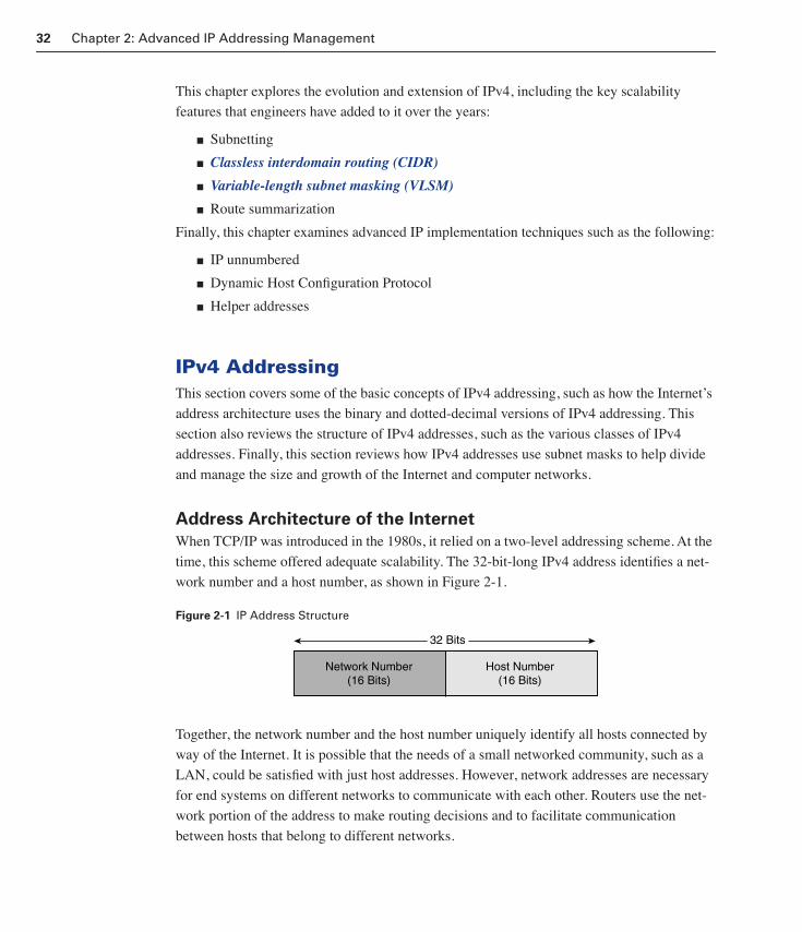
32 Chapter 2: Advanced IP Addressing Management
This chapter explores the evolution and extension of IPv4, including the key scalability
features that engineers have added to it over the years:
■ Subnetting
■ Classless interdomain routing (CIDR)
■ Variable-length subnet masking (VLSM)
■ Route summarization
Finally, this chapter examines advanced IP implementation techniques such as the following:
■ IP unnumbered
■ Dynamic Host Configuration Protocol
■ Helper addresses
IPv4 AddressingThis section covers some of the basic concepts of IPv4 addressing, such as how the Internet’s
address architecture uses the binary and dotted-decimal versions of IPv4 addressing. This
section also reviews the structure of IPv4 addresses, such as the various classes of IPv4
addresses. Finally, this section reviews how IPv4 addresses use subnet masks to help divide
and manage the size and growth of the Internet and computer networks.
Address Architecture of the Internet
When TCP/IP was introduced in the 1980s, it relied on a two-level addressing scheme. At the
time, this scheme offered adequate scalability. The 32-bit-long IPv4 address identifies a net-
work number and a host number, as shown in Figure 2-1.
Figure 2-1 IP Address Structure
Together, the network number and the host number uniquely identify all hosts connected by
way of the Internet. It is possible that the needs of a small networked community, such as a
LAN, could be satisfied with just host addresses. However, network addresses are necessary
for end systems on different networks to communicate with each other. Routers use the net-
work portion of the address to make routing decisions and to facilitate communication
between hosts that belong to different networks.
32 Bits
Network Number(16 Bits)
Host Number(16 Bits)
1358_fmi.book Page 32 Thursday, May 27, 2004 2:21 PM

IPv4 Addressing 33
Unlike routers, humans find working with strings of 32 1s and 0s tedious and clumsy. There-
fore, 32-bit IP addresses are written using dotted-decimal notation. Each 32-bit address is
divided into four groups of eight, called octets. Each octet is converted to decimal and then
separated by decimal points, or dots. This is illustrated as follows:
■ A 32-bit IP address is a binary number:
10101100000111101000000000010001
■ This binary number can be divided into four octets:
10101100 00011110 10000000 00010001
■ Each octet (or byte) can be converted to decimal:
172 30 128 17
■ Finally, the address can be written in dotted-decimal notation:
172.30.128.17
In the dotted-decimal address 172.30.128.17, which of these four numbers represents the net-
work portion of the address? Which numbers are the host numbers? Finding the answers to
these questions is complicated by the fact that IP addresses are not really four numbers. They
actually consist of 32 different numbers, or 32 bits.
In the early days of TCP/IP, a class system was used to define the network and host portions
of the address. IPv4 addresses were grouped into five distinct classes. This was done accord-
ing to the value of the first few bits in the first octet of the address. Although the class system
can still be applied to IP addresses, networks today often ignore the rules of class in favor of
a classless IP scheme.
The next few sections cover all of the following topics related to IP addressing:
■ The limitations of the IP address classes
■ The subsequent addition of the subnet mask
■ The addressing crisis that led to the adoption of a classless system
Class A and B IP Addresses
In a class system, IP addresses can be grouped into one of five different classes:
■ A
■ B
■ C
■ D
■ E
1358_fmi.book Page 33 Thursday, May 27, 2004 2:21 PM

34 Chapter 2: Advanced IP Addressing Management
Each of the four octets of an IP address represents either the network portion or the host por-
tion of the address, depending on the address class. The network and host portions of the
respective Class A, B, C, and D addresses are shown in Figure 2-2.
Figure 2-2 Address Structure
Only the first three classes—A, B, and C—are used to address actual hosts on IP networks.
Class D addresses are used for multicasting. Class E addresses are reserved for experimenta-
tion and are not shown in Figure 2-2. The following sections explore each of the five classes
of addresses.
Class A AddressesIf the first bit of the first octet of an IP address is a binary 0, the address is a Class A address.
With that first bit being a 0, the lowest number that can be represented is 00000000, decimal
0. The highest number that can be represented is 01111111, decimal 127. Any address that
starts with a value between 0 and 127 in the first octet is a Class A address. These two num-
bers, 0 and 127, are reserved and cannot be used as a network address.
Class A addresses were intended to accommodate very large networks, so only the first octet
is used to represent the network number. This leaves three octets, or 24 bits, to represent the
host portion of the address. With 24 bits total, 224 combinations are possible, yielding
16,777,216 possible addresses. Two of those possibilities, the lowest and highest values, are
reserved for special purposes. The low value is 24 0s, and the high value is 24 1s. Therefore,
each Class A address can support up to 16,777,214 unique host addresses.
Why are two host addresses reserved for special purposes? Every network requires a network
number. A network number is an ID number that is used to refer to the entire range of hosts
when building routing tables. The address that contains all 0s in the host portion is used as the
Class A Network Host
Octet 1 2 3 4
Class B Network Host
Octet 1 2 3 4
Class C Network Host
Octet 1 2 3 4
Class D Host
Octet 1 2 3 4
1358_fmi.book Page 34 Thursday, May 27, 2004 2:21 PM

IPv4 Addressing 35
network number and cannot be used to address an individual node. 46.0.0.0 is a Class A net-
work number. Similarly, every network requires a broadcast address that can be used to
address a message to every host on a network. It is created when the host portion of the
address has all 1s. For example, a broadcast address for network 46.0.0.0 would be
46.255.255.255.
With almost 17 million host addresses available, a Class A network actually provides too
many possibilities for one company or campus. Although it is easy to imagine an enormous
global network with that many nodes, the hosts in such a network could not function as mem-
bers of the same logical group. Administrators require much smaller logical groupings to
control broadcasts, apply policies, and troubleshoot problems. Fortunately, the subnet mask
allows subnetting, which breaks a large block of addresses into smaller groups called subnet-
works. All Class A networks are subnetted. If they were not, Class A networks would repre-
sent huge waste and inefficiency.
How many Class A addresses are there? Because only the first octet is used as a network
number, and it contains a value between 0 and 126, 126 Class A networks exist. Each of the
126 Class A addresses has almost 17 million possible host addresses that make up about half
of the entire IPv4 address space. Recall that the network address 127.0.0.1 is reserved for the
local loopback address, which is why Class A addresses stop at 126.0.0.0 and Class B
addresses start at 128.0.0.0. Under this system, a mere handful of organizations control half
of the available Internet addresses.
Class B AddressesClass B addresses start with a binary 10 in the first 2 bits of the first octet. Therefore, the low-
est number that can be represented with a Class B address is 10000000, decimal 128. The
highest number that can be represented is 10111111, decimal 191. Any address that starts
with a value in the range of 128 to 191 in the first octet is a Class B address.
Class B addresses were intended to accommodate medium-size networks. Therefore, the first
two octets are used to represent the network number, which leaves two octets or 16 bits to
represent the host portion of the address. With 16 bits total, 216 combinations are possible,
yielding 65,536 Class B addresses. Recall that two of those numbers, the lowest and highest
values, are reserved for special purposes. Therefore, each Class B address can support up to
65,534 hosts. Although it is significantly smaller than the networks created by Class A
addresses, a logical group of more than 65,000 hosts is still unmanageable and impractical.
Therefore, like Class A networks, Class B addresses are subnetted to improve efficiency.
Because the first 2 bits of a Class B address are always 10, 14 bits are left in the network por-
tion of the address, resulting in 214 or 16,384 Class B networks. The first octet of a Class B
address offers 64 possibilities, 128 to 191. The second octet has 256 possibilities, 0 to 255.
1358_fmi.book Page 35 Thursday, May 27, 2004 2:21 PM

36 Chapter 2: Advanced IP Addressing Management
That yields 16,384 addresses, or 25 percent of the total IP space. Nevertheless, given the pop-
ularity and importance of the Internet, these addresses have run out quickly. This essentially
leaves only Class C addresses available for new growth.
Classes of IP Addresses: C, D, and E
This section covers Class C, D, and E IP addresses.
Class C AddressesA Class C address begins with binary 110. Therefore, the lowest number that can be repre-
sented is 11000000, decimal 192. The highest number that can be represented is 11011111,
decimal 223. If an IPv4 address contains a number in the range of 192 to 223 in the first octet,
it is a Class C address.
Class C addresses were originally intended to support small networks. The first three octets of
a Class C address represent the network number. The last octet may be used for hosts. One
host octet yields 256 (28) possibilities. After the all-0s network number and the all-1s broad-
cast address are subtracted, only 254 hosts may be addressed on a Class C network. Whereas
Class A and Class B networks prove impossibly large without subnetting, Class C networks
can impose an overly restrictive limit on hosts.
Because the first 3 bits of a Class C address are always 110, 21 bits are left in the network
portion of the address, resulting in 221 or 2,097,152 Class C networks. With 2,097,152 total
network addresses containing a mere 254 hosts each, Class C addresses account for 12.5 per-
cent of the Internet address space. Because Class A and B addresses are nearly exhausted, the
remaining Class C addresses are all that is left to be assigned to new organizations that need
IP networks. Table 2-1 summarizes the ranges and availability of the three address classes
used to address Internet hosts.
Class D AddressesA Class D address begins with binary 1110 in the first octet. Therefore, the first octet range
for a Class D address is 11100000 to 11101111, or 224 to 239. Class D addresses are not used
Table 2-1 IP Addresses Available to Internet Hosts
Address
Class
First Octet
Range
Number of Possible
Networks
Number of Hosts Per
Network
Class A 0 to 126 127 (2 are reserved) 16,777,214
Class B 128 to 191 16,384 65,534
Class C 192 to 223 2,097,152 254
1358_fmi.book Page 36 Thursday, May 27, 2004 2:21 PM

IPv4 Addressing 37
to address individual hosts. Instead, each Class D address can be used to represent a group of
hosts called a host group, or multicast group.
For example, a router configured to run Enhanced Interior Gateway Routing Protocol
(EIGRP) joins a group that includes other nodes that are also running EIGRP. Members of
this group still have unique IP addresses from the Class A, B, or C range, but they also listen
for messages addressed to 224.0.0.10. The 224 octet designates the address as a Class D
address. Therefore, a single routing update message can be sent to 224.0.0.10, and all EIGRP
routers will receive it. A single message sent to several select recipients is called a multicast.
Class D addresses are also called multicast addresses.
A multicast is different from a broadcast. Every device on a logical network must process a
broadcast, whereas only devices configured to listen for a Class D address receive a multicast.
Class E AddressesIf the first octet of an IP address begins with 1111, the address is a Class E address. There-
fore, the first octet range for Class E addresses is 11110000 to 1111111, or 240 to 255. Class
E addresses are reserved for experimental purposes and should not be used to address hosts or
multicast groups.
Subnet Masking
Subnet masking, or subnetting, is used to break one large group into several smaller subnet-
works, as shown in Figure 2-3. These subnets can then be distributed throughout an enter-
prise. This results in less IP address waste and better logical organization. Formalized with
RFC 950 in 1985, subnetting introduced a third level of hierarchy to the IPv4 addressing
structure. The number of bits available to the network, subnet, and host portions of a given
address varies depending on the size of the subnet mask.
Figure 2-3 IP Address Structure After Subnetting
A subnet mask is a 32-bit number that acts as a counterpart to the IP address. Each bit in the
mask corresponds to its counterpart bit in the IP address. Logical ANDing is applied to the
address and mask. If a bit in the IP address corresponds to a 1 bit in the subnet mask, the IP
address bit represents a network number. If a bit in the IP address corresponds to a 0 bit in the
subnet mask, the IP address bit represents a host number.
32 Bits
NetworkNumber
SubnetNumber
HostNumber
1358_fmi.book Page 37 Thursday, May 27, 2004 2:21 PM

38 Chapter 2: Advanced IP Addressing Management
When the subnet mask is known, it overrides the address class to determine whether a bit is
either a network or a host. This allows routers to recognize addresses differently than the for-
mat dictated by class. The mask can be used to tell hosts that although their addresses are
Class B, the first three octets, instead of the first two, are the network number. In this case, the
additional octet acts like part of the network number, but only inside the organization where
the mask is configured.
The subnet mask applied to an address ultimately determines the network and host portions
of an IP address. The network and host portions change when the subnet mask changes. If a
16-bit mask, 255.255.0.0, is applied to an IP address, only the first 16 bits, or two octets, of
the IP address 172.24.100.45 represent the network number. Therefore, the network number
for this host address is 172.24.0.0. The colored portion of the address shown in Figure 2-4
indicates the network number.
Figure 2-4 Class B Address Without Subnetting
Because the rules of class dictate that the first two octets of a Class B address are the network
number, this 16-bit mask does not create subnets within the 172.24.0.0 network.
To create subnets with this Class B address, a mask must be used that identifies bits in the
third or fourth octet as part of the network number.
If a 24-bit mask such as 255.255.255.0 is applied, the first 24 bits of the IP address are speci-
fied as the network number. The network number for the host in this example is 172.24.100.0.
The gray portion of the address shown in Figure 2-5 indicates this.
Routers and hosts configured with this mask see all 8 bits in the third octet as part of the net-
work number. These 8 bits are considered to be the subnet field because they represent
network bits beyond the two octets prescribed by classful addressing.
Inside this network, devices configured with a 24-bit mask use the 8 bits of the third octet to
determine to what subnet a host belongs. Because 8 bits remain in the host field, 254 hosts
may populate each network. Just as hosts must have identical network addresses, they also
must match subnet fields to communicate with each other directly. Otherwise, the services of
a router must be used so that a host on one network or subnet can talk to a host on another.
IP Address 172.24.100.45
Dotted Decimal
Binary
172
10101100 00011000
24 100
01100100
45
00101101
Subnet Mask 255.255.0.0
Dotted Decimal
Binary
255 255 0 0
11111111 11111111 00000000 00000000
1358_fmi.book Page 38 Thursday, May 27, 2004 2:21 PM
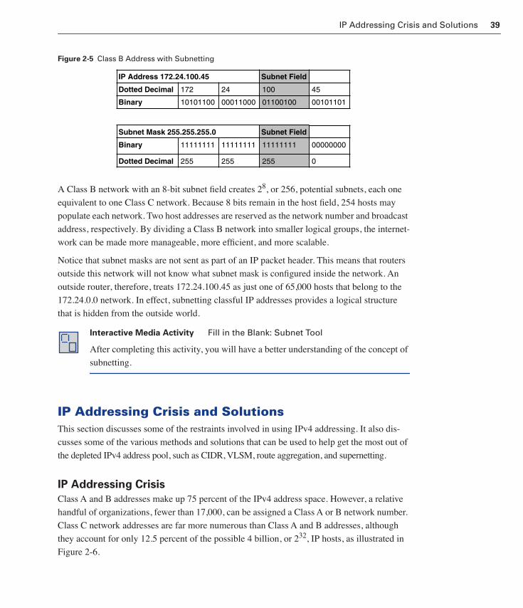
IP Addressing Crisis and Solutions 39
Figure 2-5 Class B Address with Subnetting
A Class B network with an 8-bit subnet field creates 28, or 256, potential subnets, each one
equivalent to one Class C network. Because 8 bits remain in the host field, 254 hosts may
populate each network. Two host addresses are reserved as the network number and broadcast
address, respectively. By dividing a Class B network into smaller logical groups, the internet-
work can be made more manageable, more efficient, and more scalable.
Notice that subnet masks are not sent as part of an IP packet header. This means that routers
outside this network will not know what subnet mask is configured inside the network. An
outside router, therefore, treats 172.24.100.45 as just one of 65,000 hosts that belong to the
172.24.0.0 network. In effect, subnetting classful IP addresses provides a logical structure
that is hidden from the outside world.
IP Addressing Crisis and SolutionsThis section discusses some of the restraints involved in using IPv4 addressing. It also dis-
cusses some of the various methods and solutions that can be used to help get the most out of
the depleted IPv4 address pool, such as CIDR, VLSM, route aggregation, and supernetting.
IP Addressing Crisis
Class A and B addresses make up 75 percent of the IPv4 address space. However, a relative
handful of organizations, fewer than 17,000, can be assigned a Class A or B network number.
Class C network addresses are far more numerous than Class A and B addresses, although
they account for only 12.5 percent of the possible 4 billion, or 232, IP hosts, as illustrated in
Figure 2-6.
Interactive Media Activity Fill in the Blank: Subnet Tool
After completing this activity, you will have a better understanding of the concept of
subnetting.
00101101011001000001100010101100Binary
4510024172Dotted Decimal
Subnet FieldIP Address 172.24.100.45
0255255255Dotted Decimal
00000000111111111111111111111111Binary
Subnet FieldSubnet Mask 255.255.255.0
1358_fmi.book Page 39 Thursday, May 27, 2004 2:21 PM

40 Chapter 2: Advanced IP Addressing Management
Figure 2-6 IP Address Allocation
Unfortunately, Class C addresses are limited to 254 hosts, which will not meet the needs of
larger organizations that cannot acquire a Class A or B address. Even if there were more
Class A, B, and C addresses, too many network addresses would cause Internet routers to
grind to a halt under the weight of enormous routing tables.
Ultimately, the classful system of IP addressing, even with subnetting, could not scale to
effectively handle global demand for Internet connectivity. As early as 1992, the Internet
Engineering Task Force (IETF) identified two specific concerns:
■ Exhaustion of the remaining, unassigned IPv4 network addresses. At the time, the
Class B space was on the verge of depletion.
■ The rapid and substantial increase in the size of the Internet routing tables is because of
the Internet’s growth. As more Class C addresses came online, the resulting flood of new
network information threatened the capability of Internet routers to cope effectively.
In the short term, the IETF decided that a retooled IPv4 would have to hold out long enough
for engineers to design and deploy a completely new Internet Protocol. That new protocol,
IPv6, solves the address crisis by using a 128-bit address space. After years of planning and
development, IPv6 promises to be ready for wide-scale implementation. However, IPv6 con-
tinues, for the most part, to wait for that implementation.
One reason that IPv6 has not been rushed into service is that the short-term extensions to IPv4
have been so effective. By eliminating the rules of class, IPv4 now enjoys renewed viability.
Classless Interdomain Routing
Routers use a form of IPv4 addressing called Classless Interdomain Routing (CIDR) that
ignores class.
Class D and E12.5%
Class C12.5%
Class B25%
Class A50%
NOTE
CIDR is pronounced “cider.” In a classful sys-tem, a router determines the class of an address and then identifies the network and host octets based on that class. With CIDR, a router uses a bit mask to determine the network and host portions of an address, which are no longer restricted to using an entire octet.
1358_fmi.book Page 40 Thursday, May 27, 2004 2:21 PM

IP Addressing Crisis and Solutions 41
CIDR was introduced in 1993 by RFCs 1517, 1518, 1519, and 1520. It was deployed in 1994. CIDR
dramatically improves the scalability and efficiency of IPv4 by providing the following:
■ Replacement of classful addressing with a more flexible and less wasteful classless
scheme
■ Enhanced route aggregation, also known as supernetting or summarization
■ Supernetting, which is the combination of contiguous network addresses into a new
address defined by the subnet mask
The following sections describe route aggregation, supernetting, and address allocation in
more detail.
Route Aggregation and Supernetting
CIDR allows routers to aggregate, or summarize, routing information. It does this by using a
bit mask instead of an address class to determine the network portion of an address. This
shrinks the size of the routing tables used by the router. In other words, just one address and
mask combination can represent the routes to multiple networks.
Without CIDR and route aggregation, a router must maintain many individual entries for the
routes within the same network, as opposed to one route for that particular network when
using CIDR addressing.
The shaded entries in Table 2-2 identify the 16 bits that, based on the rules of class, represent
the network number. Classful routers are forced to handle Class B networks using these 16
bits. Because the first 16 bits of each of these eight network numbers are unique, a classful
router sees eight unique networks and must create a routing table entry for each. However,
these eight networks do have common bits.Table 2-2 Route Aggregation and Supernetting
Network Number First Octet Second Octet Third Octet Fourth Octet
172.24.0.0/16 10101100 00011000 00000000 00000000
172.25.0.0/16 10101100 00011001 00000000 00000000
172.26.0.0/16 10101100 00011010 00000000 00000000
172.27.0.0/16 10101100 00011011 00000000 00000000
172.28.0.0/16 10101100 00011100 00000000 00000000
172.29.0.0/16 10101100 00011101 00000000 00000000
172.30.0.0/16 10101100 00011110 00000000 00000000
172.31.0.0/16 10101100 00011111 00000000 00000000
1358_fmi.book Page 41 Thursday, May 27, 2004 2:21 PM

42 Chapter 2: Advanced IP Addressing Management
Table 2-3 shows that the eight network addresses have the first 13 bits in common. A CIDR-
compliant router can summarize routes to these eight networks by using a 13-bit prefix. Only
these eight networks share these bits:
10101100 00011
To represent this prefix in decimal terms, the rest of the address is padded with 0s and then
paired with a 13-bit subnet mask:
10101100 00011000 00000000 00000000 = 172.24.0.0
11111111 11111000 00000000 00000000 = 255.248.0.0
Therefore, a single address and mask define a classless prefix that summarizes routes to the
eight networks, 172.24.0.0/13.
By using a prefix address to summarize routes, routing table entries can be kept more man-
ageable. The following benefits are a result of the summarized routes:
■ More efficient routing
■ Reduced number of CPU cycles when recalculating a routing table or when sorting
through the routing table entries to find a match
■ Reduced router memory requirements
Supernetting is the practice of using a bit mask to group multiple classful networks as a single
network address. Supernetting and route aggregation are different names for the same pro-
cess. However, the term supernetting is most often applied when the aggregated networks are
under common administrative control. Supernetting takes bits from the network portion of
the network mask, whereas subnetting takes bits from the host portion of the subnet mask.
Supernetting and route aggregation are essentially the inverse of subnetting.
Table 2-3 Dotted-Decimal Notation
Network Number First Octet Second Octet Third Octet Fourth Octet
172.24.0.0/16 10101100 00011000 00000000 00000000
172.25.0.0/16 10101100 00011001 00000000 00000000
172.26.0.0/16 10101100 00011010 00000000 00000000
172.27.0.0/16 10101100 00011011 00000000 00000000
172.28.0.0/16 10101100 00011100 00000000 00000000
172.29.0.0/16 10101100 00011101 00000000 00000000
172.30.0.0/16 10101100 00011110 00000000 00000000
172.31.0.0/16 10101100 00011111 00000000 00000000
1358_fmi.book Page 42 Thursday, May 27, 2004 2:21 PM
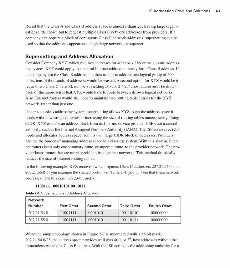
IP Addressing Crisis and Solutions 43
Recall that the Class A and Class B address space is almost exhausted, leaving large organi-
zations little choice but to request multiple Class C network addresses from providers. If a
company can acquire a block of contiguous Class C network addresses, supernetting can be
used so that the addresses appear as a single large network, or supernet.
Supernetting and Address Allocation
Consider Company XYZ, which requires addresses for 400 hosts. Under the classful address-
ing system, XYZ could apply to a central Internet address authority for a Class B address. If
the company got the Class B address and then used it to address one logical group of 400
hosts, tens of thousands of addresses would be wasted. A second option for XYZ would be to
request two Class C network numbers, yielding 508, or 2 * 254, host addresses. The draw-
back of this approach is that XYZ would have to route between its own logical networks.
Also, Internet routers would still need to maintain two routing table entries for the XYZ
network, rather than just one.
Under a classless addressing system, supernetting allows XYZ to get the address space it
needs without wasting addresses or increasing the size of routing tables unnecessarily. Using
CIDR, XYZ asks for an address block from its Internet service provider (ISP), not a central
authority, such as the Internet Assigned Numbers Authority (IANA). The ISP assesses XYZ’s
needs and allocates address space from its own large CIDR block of addresses. Providers
assume the burden of managing address space in a classless system. With this system, Inter-
net routers keep only one summary route, or supernet route, to the provider network. The pro-
vider keeps routes that are more specific to its customer networks. This method drastically
reduces the size of Internet routing tables.
In the following example, XYZ receives two contiguous Class C addresses, 207.21.54.0 and
207.21.55.0. If you examine the shaded portions of Table 2-4, you will see that these network
addresses have this common 23-bit prefix:
11001111 00010101 0011011
When the sample topology shown in Figure 2-7 is supernetted with a 23-bit mask,
207.21.54.0/23, the address space provides well over 400, or 29, host addresses without the
tremendous waste of a Class B address. With the ISP acting as the addressing authority for a
Table 2-4 Supernetting and Address Allocation
Network
Number First Octet Second Octet Third Octet Fourth Octet
207.21.54.0 11001111 00010101 00110110 00000000
207.21.55.0 11001111 00010101 00110111 00000000
1358_fmi.book Page 43 Thursday, May 27, 2004 2:21 PM

44 Chapter 2: Advanced IP Addressing Management
CIDR block of addresses, the ISP’s customer networks, which include XYZ, can be adver-
tised among Internet routers as a single supernet. The ISP manages a block of 256 Class C
network addresses and advertises them to the world using a 16-bit prefix:
207.21.0.0/16
Figure 2-7 Addressing with CIDR
When CIDR enabled ISPs to hierarchically distribute and manage blocks of contiguous
addresses, IPv4 address space enjoyed the following benefits:
■ Efficient allocation of addresses
■ Reduced number of routing table entries
VLSMThis section discusses VLSMs and how they can be used to further maximize IPv4 address-
ing efficiency.
Variable-Length Subnet Masks
VLSM allows an organization to use more than one subnet mask within the same network
address space. Implementing VLSM is often called subnetting a subnet. It can be used to
maximize addressing efficiency.
207.21.0.0/16
207.21.54.0/23
Internet
XYZ ISP
1358_fmi.book Page 44 Thursday, May 27, 2004 2:21 PM

VLSM 45
Consider Table 2-5, in which the subnets are created by borrowing 3 bits from the host por-
tion of the Class C address, 207.21.24.0.
If the ip subnet-zero command is used, this mask creates seven usable subnets of 30 hosts
each. Four of these subnets can be used to address remote offices at Sites A, B, C, and D, as
shown in Figure 2-8.
Figure 2-8 Using Subnets to Address a WAN
Unfortunately, only three subnets are left for future growth, and three point-to-point WAN
links between the four sites remain to be addressed. If the three remaining subnets were
assigned to the WAN links, the supply of IP addresses would be completely exhausted. This
addressing scheme would also waste more than a third of the available address space.
There are ways to avoid this kind of waste. Over the past 20 years, network engineers have
developed three critical strategies for efficiently addressing point-to-point WAN links:
■ Use VLSM
■ Use private addressing (RFC 1918)
■ Use IP unnumbered
Private addresses and IP unnumbered are discussed in detail later in this chapter. This section
focuses on VLSM. When VLSM is applied to an addressing problem, it breaks the address
Table 2-5 Subnetting with One Mask
Subnet Number Subnet Address
Subnet 0 207.21.24.0/27
Subnet 1 207.21.24.32/27
Subnet 2 207.21.24.64/27
Subnet 3 207.21.24.96/27
Subnet 4 207.21.24.128/27
Subnet 5 207.21.24.160/27
Subnet 6 207.21.24.192/27
Subnet 7 207.21.24.224/27
Site A Site B
Site C
Site D
207.21.24.0/27
201.21.24.32/27
207.21.24.64/27
207.21.24.96/27
1358_fmi.book Page 45 Thursday, May 27, 2004 2:21 PM

46 Chapter 2: Advanced IP Addressing Management
into groups or subnets of various sizes. Large subnets are created for addressing LANs, and
very small subnets are created for WAN links and other special cases.
A 30-bit mask is used to create subnets with two valid host addresses. This is the exact num-
ber needed for a point-to-point connection. Figure 2-9 shows what happens if one of the three
remaining subnets is subnetted again, using a 30-bit mask.
Figure 2-9 Subnetting with VLSMs
Subnetting the 207.21.24.192/27 subnet in this way supplies another eight ranges of
addresses to be used for point-to-point networks. For example, in Figure 2-10, the network
207.21.24.192/30 can be used to address the point-to-point serial link between the Site A
router and the Site B router.
Figure 2-10 Using VLSM to Address Point-to-Point Links
Example 2-1 shows the commands needed to configure the Site A router, labeled RTA, with a
27-bit mask on its Ethernet port and a 30-bit mask on its serial port.
Example 2-1 Configuring VLSM
RTA(config)#iiiinnnntttteeeerrrrffffaaaacccceeee eeee0000
RTA(config-if)#iiiipppp aaaaddddddddrrrreeeessssssss 222200007777....22221111....22224444....33333333 222255555555....222255555555....222255555555....222222224444
RTA(config-if)#iiiinnnntttteeeerrrrffffaaaacccceeee ssss0000
RTA(config-if)#iiiipppp aaaaddddddddrrrreeeessssssss 222200007777....22221111....22224444....111199993333 222255555555....222255555555....222255555555....222255552222
Subnet 0
Subnet 1
Subnet 2
Subnet 3
Subnet 4
Subnet 5
Subnet 6
Subnet 7
207.21.24.0/27
207.21.24.32/27
207.21.24.64/27
207.21.24.96/27
207.21.24.128/27
207.21.24.160/27
207.21.24.192/27
207.21.24.224/27
Sub-Subnet 0
Sub-Subnet 1
Sub-Subnet 2
Sub-Subnet 3
Sub-Subnet 4
Sub-Subnet 5
Sub-Subnet 6
Sub-Subnet 7
207.21.24.192/30
207.21.24.196/30
207.21.24.200/30
207.21.24.204/30
207.21.24.208/30
207.21.24.212/30
207.21.24.216/30
207.21.24.220/30
Site A Site B
207.21.24.32/27
207.21.24.192/30
1358_fmi.book Page 46 Thursday, May 27, 2004 2:21 PM
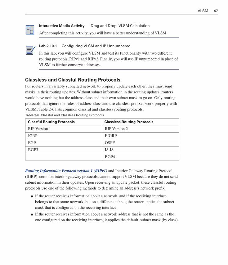
VLSM 47
Classless and Classful Routing Protocols
For routers in a variably subnetted network to properly update each other, they must send
masks in their routing updates. Without subnet information in the routing updates, routers
would have nothing but the address class and their own subnet mask to go on. Only routing
protocols that ignore the rules of address class and use classless prefixes work properly with
VLSM. Table 2-6 lists common classful and classless routing protocols.
Routing Information Protocol version 1 (RIPv1) and Interior Gateway Routing Protocol
(IGRP), common interior gateway protocols, cannot support VLSM because they do not send
subnet information in their updates. Upon receiving an update packet, these classful routing
protocols use one of the following methods to determine an address’s network prefix:
■ If the router receives information about a network, and if the receiving interface
belongs to that same network, but on a different subnet, the router applies the subnet
mask that is configured on the receiving interface.
■ If the router receives information about a network address that is not the same as the
one configured on the receiving interface, it applies the default, subnet mask (by class).
Interactive Media Activity Drag and Drop: VLSM Calculation
After completing this activity, you will have a better understanding of VLSM.
Lab 2.10.1 Configuring VLSM and IP Unnumbered
In this lab, you will configure VLSM and test its functionality with two different
routing protocols, RIPv1 and RIPv2. Finally, you will use IP unnumbered in place of
VLSM to further conserve addresses.
Table 2-6 Classful and Classless Routing Protocols
Classful Routing Protocols Classless Routing Protocols
RIP Version 1 RIP Version 2
IGRP EIGRP
EGP OSPF
BGP3 IS-IS
BGP4
1358_fmi.book Page 47 Thursday, May 27, 2004 2:21 PM
48 Chapter 2: Advanced IP Addressing Management
Despite its limitations, RIP is a very popular routing protocol and is supported by virtually all
IP routers. RIP’s popularity stems from its simplicity and universal compatibility. However,
the first version of RIP, RIPv1, suffers from several critical deficiencies:
■ RIPv1 does not send subnet mask information in its updates. Without subnet informa-
tion, VLSM and CIDR cannot be supported.
■ RIPv1 broadcasts its updates, increasing network traffic.
■ RIPv1 does not support authentication.
In 1988, RFC 1058 prescribed the new and improved Routing Information Protocol version 2 (RIPv2) to address these deficiencies. RIPv2 has the following features:
■ RIPv2 sends subnet information and, therefore, supports VLSM and CIDR.
■ RIPv2 multicasts routing updates using the Class D address 224.0.0.9, providing better
efficiency.
■ RIPv2 provides for authentication in its updates.
Because of these key features, RIPv2 should always be preferred over RIPv1, unless some
legacy device on the network does not support it.
When RIP is first enabled on a Cisco router, the router listens for version 1 and 2 updates but
sends only version 1. To take advantage of the RIPv2 features, turn off version 1 support, and
enable version 2 updates with the following commands:
Router(config)#rrrroooouuuutttteeeerrrr rrrriiiippppRouter(config-router)#vvvveeeerrrrssssiiiioooonnnn 2222
The straightforward RIP design ensures that it will continue to survive. A new version has
already been designed to support future IPv6 networks.
Lab 2.10.2a VLSM 1
In this lab, you create an addressing scheme using VLSM.
Lab 2.10.2b VLSM 2
In this lab, you create an addressing scheme using VLSM.
Lab 2.10.2c VLSM 3
In this lab, you create an addressing scheme using VLSM.
Lab 2.10.2d VLSM 4
In this lab, you create an addressing scheme using VLSM.
1358_fmi.book Page 48 Thursday, May 27, 2004 2:21 PM

Route Summarization 49
Route SummarizationThis section discusses some of the details of route summarization and how CIDR and VLSMs
use it to deal with the size of routing tables.
An Overview of Route Summarization
The use of CIDR and VLSM not only reduces address waste, but it also promotes route
aggregation, or route summarization. Without route summarization, Internet backbone rout-
ing would likely have collapsed sometime before 1997.
Figure 2-11 shows how route summarization reduces the burden on upstream routers. This
complex hierarchy of variable-sized networks and subnetworks is summarized at various
points using a prefix address until the entire network is advertised as a single aggregate route
of 192.168.48.0/20.
Figure 2-11 Route Summarization
Recall that this kind of route summarization, or supernetting, is possible only if the net-
work routers run a classless routing protocol, such as OSPF or EIGRP. Classless routing
protocols carry the prefix length and subnet mask with the 32-bit address in routing
updates. In Figure 2-11, the summary route that eventually reaches the provider contains
a 20-bit prefix common to all the addresses in the organization. This prefix is 192.168.48.0/20,
or 11000000.10101000.00110000.00000000, with a subnet mask of 11111111.11111111.
11110000.00000000. For summarization to work properly, addresses must be carefully
assigned in a hierarchical fashion so that summarized addresses share the same high-order
bits.
RTZ
192.168.48.0/24192.168.49.0/24192.168.50.0/24192.168.51.0/24
192.168.52.0/24192.168.53.0/24192.168.54.0/24192.168.55.0/24
RTA
RTB
192.168.56.0/24192.168.57.0/24…192.168.63.0/24
RTC
192.168.52.0/22 192.168.48.0/20
192.168.48.0/22
192.168.56.0/21
UpstreamProvider

50 Chapter 2: Advanced IP Addressing Management
Route Flapping
Route flapping occurs when a router interface alternates rapidly between the up and down
states. This can be caused by a number of factors, including a faulty interface or poorly termi-
nated media.
Summarization can effectively insulate upstream routers from route-flapping problems. Con-
sider RTC in Figure 2-12. If the RTC interface connected to the 200.199.56.0 network goes
down, RTC removes that route from its table. If the routers were not configured to summa-
rize, RTC would then send a triggered update to RTZ about the removal of the specific net-
work, 200.199.56.0. In turn, RTZ would update the next router upstream, and so on. Every
time these routers are updated with new information, their processors must go to work. It is
possible, especially in the case of OSPF routing, that the processors can work hard enough to
noticeably affect performance. Now, consider the impact on performance if the RTC interface
to network 200.199.56.0 comes back up after only a few seconds. The routers update each
other and recalculate. In addition, what happens when the RTC link goes back down seconds
later? And then back up? This is called route flapping, and it can cripple a router with exces-
sive updates and recalculations.
Figure 2-12 Routes Summarized to 200.199.48.0/20
However, the summarization configuration prevents the RTC route flapping from affecting
any other routers. RTC updates RTZ about a supernet, 200.199.56.0/21, which includes eight
networks, 200.199.56.0 through 200.199.63.0. The loss of one network does not invalidate
the route to the supernet. While RTC might be kept busy dealing with its own route flap, RTZ,
all upstream routers are unaware of any downstream problem. Summarization effectively
insulates the other routers from the problem of route flapping.
RTZ
200.199.48.0/24200.199.49.0/24200.199.50.0/24200.199.51.0/24
200.199.52.0/24200.199.53.0/24200.199.54.0/24200.199.55.0/24
RTA
RTB
200.199.56.0/24200.199.57.0/24…200.199.63.0/24
RTC
200.199.52.0/22 200.199.48.0/20
200.199.48.0/22
200.199.56.0/21
UpstreamProvider
1358_fmi.book Page 50 Thursday, May 27, 2004 2:21 PM

Private Addressing and NAT 51
Private Addressing and NATThis section explains Network Address Translation (NAT) and how it can limit the waste of
IP addresses by using the private addressing scheme.
Private IP Addresses (RFC 1918)
Because TCP/IP is the dominant routed protocol in the world, most network applications and
operating systems offer extensive support for it. Therefore, many designers build their net-
works around TCP/IP, even if they do not require Internet connectivity. Internet hosts require
globally unique IP addresses. However, private hosts that are not connected to the Internet
can use any valid address, as long as it is unique within the private network.
Because many private networks exist alongside public networks, just grabbing any address is
strongly discouraged. RFC 1918 sets aside three blocks of IP addresses for private or internal
use:
■ A Class A range
■ A Class B range
■ A Class C range
Addresses in one of these ranges, shown in Table 2-7, are not routed on the Internet back-
bone. Internet routers immediately discard private addresses.
If any of the following are being addressed, these private addresses can be used instead of
globally unique addresses:
■ A nonpublic intranet
■ A test lab
■ A home network
Global addresses must be obtained from a provider or a registry at some expense.
RFC 1918 addresses have found a home in production networks as well. Earlier in this chap-
ter, the advantages of using VLSM to address the point-to-point WAN links in an internet-
work were discussed. Recall that with VLSM, you can further subnet one of the subnets left
in the address space of a Class C network. Although this solution is better than wasting an
entire 30-host subnet on each two-host WAN link, it still costs one subnet that could have
Table 2-7 Private Addresses in the WAN
Class RFC 1918 Internal Address Range CIDR Prefix
A 10.0.0.0 to 10.255.255.255 10.0.0.0/8
B 172.16.0.0 to 172.31.255.255 172.16.0.0/12
C 192.168.0.0 to 192.168.255.255 192.168.0.0/16
1358_fmi.book Page 51 Thursday, May 27, 2004 2:21 PM

52 Chapter 2: Advanced IP Addressing Management
been used for future growth. A less-wasteful solution is to address the WAN links using pri-
vate network numbers. The WAN links shown in Figure 2-13 are addressed using subnets
from the private address space, 10.0.0.0/8.
Figure 2-13 Using Subnets to Address the WAN
How can these routers use private addresses if LAN users at Sites A, B, C, and D expect to
access the Internet? End users at these sites should have no problem, because they use glo-
bally unique addresses from the 207.21.24.0 network. The routers use their serial interfaces
with private addresses merely to forward traffic and exchange routing information. Upstream
providers and Internet routers see only the source and destination IP addresses in the packet.
Upstream providers do not care if the packet traveled through links with private addresses at
some point. In fact, many providers use RFC 1918 network numbers in the core of their net-
work to avoid depleting their supply of globally unique addresses.
There is one trade-off when using private numbers on WAN links. The serial interfaces can-
not be the original source of traffic bound for the Internet or the final destination of traffic
from the Internet. Routers normally do not spend time surfing the web. Therefore, this limita-
tion typically becomes an issue only when you’re troubleshooting with Internet Control Mes-
sage Protocol (ICMP), using Simple Network Management Protocol (SNMP), or connecting
remotely with Telnet over the Internet. In those cases, the router can be addressed only by its
globally unique LAN interfaces.
The following sections discuss implementing a private address scheme, including the pitfalls
of discontiguous subnets and the advantages of NAT.
Discontiguous Subnets
Mixing private addresses with globally unique addresses can create discontiguous subnets.
Discontiguous subnets are subnets from the same major network that are separated by a com-
pletely different major network or subnet.
Site A Site B
Site C
Site D
207.21.24.0/27
207.21.24.32/27
207.21.24.64/27
207.21.24.96/27
10.0.0.4/30 10.0.0.8/30 10.0.0.12/30
Internet
1358_fmi.book Page 52 Thursday, May 27, 2004 2:21 PM
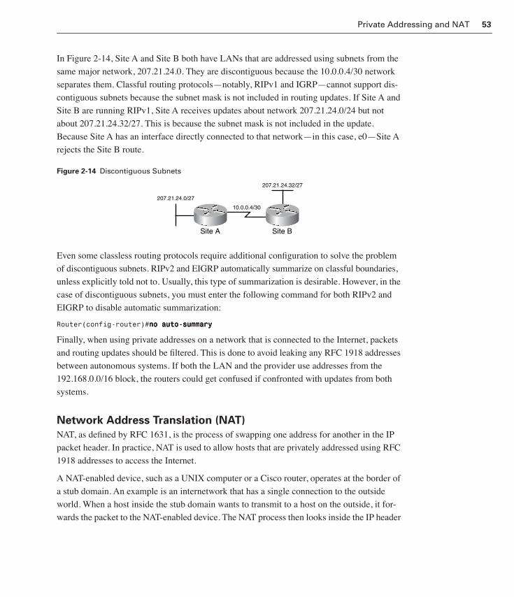
Private Addressing and NAT 53
In Figure 2-14, Site A and Site B both have LANs that are addressed using subnets from the
same major network, 207.21.24.0. They are discontiguous because the 10.0.0.4/30 network
separates them. Classful routing protocols—notably, RIPv1 and IGRP—cannot support dis-
contiguous subnets because the subnet mask is not included in routing updates. If Site A and
Site B are running RIPv1, Site A receives updates about network 207.21.24.0/24 but not
about 207.21.24.32/27. This is because the subnet mask is not included in the update.
Because Site A has an interface directly connected to that network—in this case, e0—Site A
rejects the Site B route.
Figure 2-14 Discontiguous Subnets
Even some classless routing protocols require additional configuration to solve the problem
of discontiguous subnets. RIPv2 and EIGRP automatically summarize on classful boundaries,
unless explicitly told not to. Usually, this type of summarization is desirable. However, in the
case of discontiguous subnets, you must enter the following command for both RIPv2 and
EIGRP to disable automatic summarization:
Router(config-router)#nnnnoooo aaaauuuuttttoooo----ssssuuuummmmmmmmaaaarrrryyyy
Finally, when using private addresses on a network that is connected to the Internet, packets
and routing updates should be filtered. This is done to avoid leaking any RFC 1918 addresses
between autonomous systems. If both the LAN and the provider use addresses from the
192.168.0.0/16 block, the routers could get confused if confronted with updates from both
systems.
Network Address Translation (NAT)
NAT, as defined by RFC 1631, is the process of swapping one address for another in the IP
packet header. In practice, NAT is used to allow hosts that are privately addressed using RFC
1918 addresses to access the Internet.
A NAT-enabled device, such as a UNIX computer or a Cisco router, operates at the border of
a stub domain. An example is an internetwork that has a single connection to the outside
world. When a host inside the stub domain wants to transmit to a host on the outside, it for-
wards the packet to the NAT-enabled device. The NAT process then looks inside the IP header
Site A Site B
207.21.24.0/27
207.21.24.32/27
10.0.0.4/30
1358_fmi.book Page 53 Thursday, May 27, 2004 2:21 PM
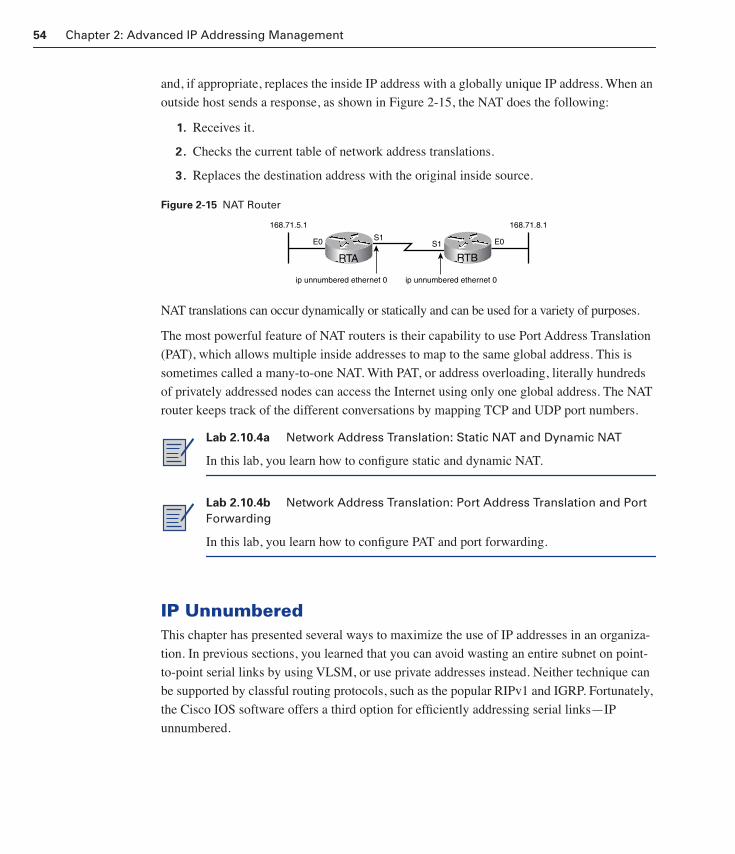
54 Chapter 2: Advanced IP Addressing Management
and, if appropriate, replaces the inside IP address with a globally unique IP address. When an
outside host sends a response, as shown in Figure 2-15, the NAT does the following:
1. Receives it.
2. Checks the current table of network address translations.
3. Replaces the destination address with the original inside source.
Figure 2-15 NAT Router
NAT translations can occur dynamically or statically and can be used for a variety of purposes.
The most powerful feature of NAT routers is their capability to use Port Address Translation
(PAT), which allows multiple inside addresses to map to the same global address. This is
sometimes called a many-to-one NAT. With PAT, or address overloading, literally hundreds
of privately addressed nodes can access the Internet using only one global address. The NAT
router keeps track of the different conversations by mapping TCP and UDP port numbers.
IP UnnumberedThis chapter has presented several ways to maximize the use of IP addresses in an organiza-
tion. In previous sections, you learned that you can avoid wasting an entire subnet on point-
to-point serial links by using VLSM, or use private addresses instead. Neither technique can
be supported by classful routing protocols, such as the popular RIPv1 and IGRP. Fortunately,
the Cisco IOS software offers a third option for efficiently addressing serial links—IP
unnumbered.
Lab 2.10.4a Network Address Translation: Static NAT and Dynamic NAT
In this lab, you learn how to configure static and dynamic NAT.
Lab 2.10.4b Network Address Translation: Port Address Translation and Port Forwarding
In this lab, you learn how to configure PAT and port forwarding.
RTA RTB
168.71.5.1
S1S1E0
168.71.8.1
E0
ip unnumbered ethernet 0 ip unnumbered ethernet 0
1358_fmi.book Page 54 Thursday, May 27, 2004 2:21 PM

IP Unnumbered 55
Using IP Unnumbered
When a serial interface is configured for IP unnumbered, it does not need its own address.
This is because it borrows the IP address of another interface, usually a LAN interface or
loopback interface. Example 2-2 shows how to configure an unnumbered interface. Not only
does IP unnumbered avoid wasting addresses on point-to-point WAN links, but it also can be
used with classful routing protocols, whereas VLSM and discontiguous subnets cannot. If the
network runs RIPv1 or IGRP, IP unnumbered might be the only solution to maximize
the addresses.
RTA e0, 168.71.5.1, and RTB e0, 168.71.8.1, can communicate using TCP/IP over this serial
link, even though they do not belong to the same IP network, as shown in Figure 2-16. This is
possible because the serial link is a point-to-point link, so there is no confusion about which
device a packet is originating from or destined for. In this case, the command ip unnum-bered e0 is entered in serial 1 interface configuration mode on both RTA and RTB. Configur-
ing IP unnumbered on an interface has two ground rules:
■ The interface is both serial and connected by way of a point-to-point link.
■ The same major network with the same mask is used to address the LAN interfaces that
lend their IP address on both sides of the WAN link.
or
Different major networks with no subnetting are used to address the LAN interfaces on both sides of the WAN link.
Example 2-2 Configuring an IP Unnumbered Interface
RTA(config)#iiiinnnntttteeeerrrrffffaaaacccceeee eeee0000
RTA(config-if)#iiiipppp aaaaddddddddrrrreeeessssssss 111166668888....77771111....5555....1111 222255555555....222255555555....222255555555....0000
RTA(config-if)#iiiinnnntttteeeerrrrffffaaaacccceeee ssss1111
RTA(config-if)#iiiipppp uuuunnnnnnnnuuuummmmbbbbeeeerrrreeeedddd eeee0000
RTB(config)#iiiinnnntttteeeerrrrffffaaaacccceeee eeee0000
RTB(config-if)#iiiipppp aaaaddddddddrrrreeeessssssss 111166668888....77771111....8888....1111 222255555555....222255555555....222255555555....0000
RTB(config-if)#iiiinnnntttteeeerrrrffffaaaacccceeee ssss1111
RTB(config-if)#iiiipppp uuuunnnnnnnnuuuummmmbbbbeeeerrrreeeedddd eeee0000
1358_fmi.book Page 55 Thursday, May 27, 2004 2:21 PM

56 Chapter 2: Advanced IP Addressing Management
Figure 2-16 IP Unnumbered Interfaces
Certain drawbacks come with using IP unnumbered:
■ The use of ping cannot determine whether the interface is up, because the interface has
no IP address.
■ A network IOS image cannot boot over an unnumbered serial interface.
■ IP security options cannot be supported on an unnumbered interface.
DHCP and Easy IPThis section discusses DHCP and its operation. It covers how to configure DHCP, and use
Easy IP as well.
DHCP Overview
After designing a scalable IP addressing scheme for the enterprise, the next step is implemen-
tation. Routers, servers, and other key nodes usually require special attention from adminis-
trators. However, desktop clients are often automatically assigned IP configurations using
Dynamic Host Configuration Protocol (DHCP). Because desktop clients typically make up
the bulk of network nodes, DHCP is good news for systems administrators. Small offices and
home offices can also take advantage of DHCP by using Easy IP, a Cisco IOS software fea-
ture set that combines DHCP with NAT functions.
DHCP works by configuring servers to give out IP configuration information to clients. Cli-
ents lease the information from the server for an administratively defined period. When the
lease is up, the host must ask for another address, although it is typically reassigned the same
one. Figures 2-17 and 2-18 illustrate this process. In Figure 2-17, Host A issues a DHCP
request for an IP address. In Figure 2-18, the DHCP server replies to the DHCP request by
leasing an IP address from the configured IP address pool.
RTA RTB
168.71.5.1
S1S1E0
168.71.8.1
E0
ip unnumbered ethernet 0 ip unnumbered ethernet 0
Internet10.4.4.5
10.4.1.1
SA = Source Address
NAT Table
SA10.4.1.1
SA2.2.2.2
Inside LocalIP Address
GlobalIP Address
10.4.4.510.4.1.1 2.2.2.2
2.2.2.3
1358_fmi.book Page 56 Thursday, May 27, 2004 2:21 PM

DHCP and Easy IP 57
Figure 2-17 Simple DHCP Operation: Client/Server
Figure 2-18 Simple DHCP Operation: Reply
Administrators typically prefer to use a Microsoft 2000 server or a UNIX computer to offer
DHCP services because these solutions are highly scalable and relatively easy to manage.
Even so, the Cisco IOS software offers an optional, fully featured DHCP server, which leases
configurations for 24 hours by default.
Administrators set up DHCP servers to assign addresses from predefined pools. DHCP serv-
ers can also provide other information:
■ Default gateway address
■ DNS server addresses
■ WINS server addresses
■ Domain names
Host A
Host B CentralDHCPServer
Host A
Host B CentralDHCPServer
“This IP AddressIs 10.0.0.1.”
1358_fmi.book Page 57 Thursday, May 27, 2004 2:21 PM

58 Chapter 2: Advanced IP Addressing Management
Most DHCP servers also let you specifically define what client MAC addresses can be ser-
viced and automatically assign the same number to a particular host each time.
DHCP Operation
The DHCP client configuration process is shown in Figure 2-19.
Figure 2-19 DHCP Operation
The DHCP client configuration process follows these steps:
1. When a client is set up for DHCP and needs an IP configuration, typically at boot time, it tries to locate a DHCP server by sending a broadcast called a DHCPDISCOVER.
2. The server sends a DHCPOFFER unicast to the client. When the server receives the broadcast, it determines whether it can service the request from its own database. If it cannot, the server might forward the request to another DHCP server or servers, depending on its configuration. If it can service the request, the DHCP server offers the client IP configuration information in the form of a unicast DHCPOFFER. The DHCPOFFER is a proposed configuration that may include IP address, DNS server address, and lease time.
3. The client sends a DHCPREQUEST broadcast to all nodes. If the client finds the offer agreeable, it sends another broadcast. This broadcast is a DHCPREQUEST, specifically requesting those particular IP parameters. Why does the client broadcast the request instead of unicasting it to the server? A broadcast is used because the very first mes-sage, the DHCPDISCOVER, might have reached more than one DHCP server. After all, it was a broadcast. If more than one server makes an offer, the broadcasted DHCPREQUEST lets the servers know which offer was accepted, which is usually the first offer received.
4. The server sends a DHCPACK unicast to the client. The server that receives the DHCPREQUEST makes the configuration official by sending a unicast acknowledg-ment, the DHCPACK. Note that it is possible but highly unlikely that the server will not send the DHCPACK, because it might have leased that information to another client in the interim. Receipt of the DHCPACK message lets the client begin using the assigned address immediately.
NOTE
BOOTP was originally defined in RFC 951 in 1985. It is the predecessor of DHCP, and it shares some operational charac-teristics. Both protocols use UDP ports 67 and 68, which are well-known as BOOTP ports, because BOOTP came before DHCP.
Host ADHCPDISCOVER (Broadcast)
DHCPOFFER (Unicast)
DHCPREQUEST (Broadcast)
DHCPACK (Unicast)
Cisco IOSDHCP Server
1358_fmi.book Page 58 Thursday, May 27, 2004 2:21 PM

DHCP and Easy IP 59
Depending on an organization’s policies, it might be possible for an end user or administrator
to statically assign a host an IP address that belongs in the DHCP server address pool. Just in
case, the Cisco IOS software DHCP server always checks to make sure that an address is not
in use before the server offers it to a client. The server issues ICMP echo requests (pings) to a
pool address before sending the DHCPOFFER to a client. Although it can be configured, the
default number of pings used to check for potential IP address conflict is two. The more
pings, the longer the configuration process takes.
Configuring the IOS DHCP Server
The DHCP server process is enabled by default on versions of the Cisco IOS software that
support it. If for some reason the DHCP server process becomes disabled, you can reenable it
by using the service dhcp global configuration command. The no service dhcp command
disables the server.
Like NAT, DHCP servers require that the administrator define a pool of addresses. In Example 2-3,
the ip dhcp pool command defines which addresses are assigned to hosts.
The first command, ip dhcp pool room12, creates a pool named room12 and puts the router
in a specialized DHCP configuration mode. In this mode, you use the network statement to
define the range of addresses to be leased. If specific addresses are to be excluded on this net-
work, return to global configuration mode and enter the ip dhcp excluded-address command.
The ip dhcp excluded-address command configures the router to exclude 172.16.1.1
through 172.16.1.10 when assigning addresses to clients. The ip dhcp excluded-address
command may be used to reserve addresses that are statically assigned to key hosts.
A DHCP server can configure much more than an IP address. Other IP configuration values
can be set from DHCP configuration mode, as shown in Example 2-4.
Example 2-3 Configuring a DHCP Address Pool
RTA(config)#iiiipppp ddddhhhhccccpppp ppppoooooooollll rrrroooooooommmm11112222
RTA(dhcp-config)#nnnneeeettttwwwwoooorrrrkkkk 111177772222....11116666....1111....0000 222255555555....222255555555....222255555555....0000
RTA(dhcp-config)#eeeexxxxiiiitttt
RTA(config-if)#iiiipppp ddddhhhhccccpppp eeeexxxxcccclllluuuuddddeeeedddd----aaaaddddddddrrrreeeessssssss 111177772222....11116666....1111....1111 111177772222....11116666....1111....11110000
Example 2-4 Assigning Key DHCP Information
RTA(config)#iiiipppp ddddhhhhccccpppp ppppoooooooollll rrrroooooooommmm11112222
RTA(dhcp-config)#ddddnnnnssss----sssseeeerrrrvvvveeeerrrr 111177772222....11116666....1111....2222
RTA(dhcp-config)#nnnneeeettttbbbbiiiioooossss----nnnnaaaammmmeeee----sssseeeerrrrvvvveeeerrrr 111177772222....11116666....1111....2222
RTA(config-if)#ddddeeeeffffaaaauuuulllltttt----rrrroooouuuutttteeeerrrr 111177772222....11116666....1111....1111
1358_fmi.book Page 59 Thursday, May 27, 2004 2:21 PM
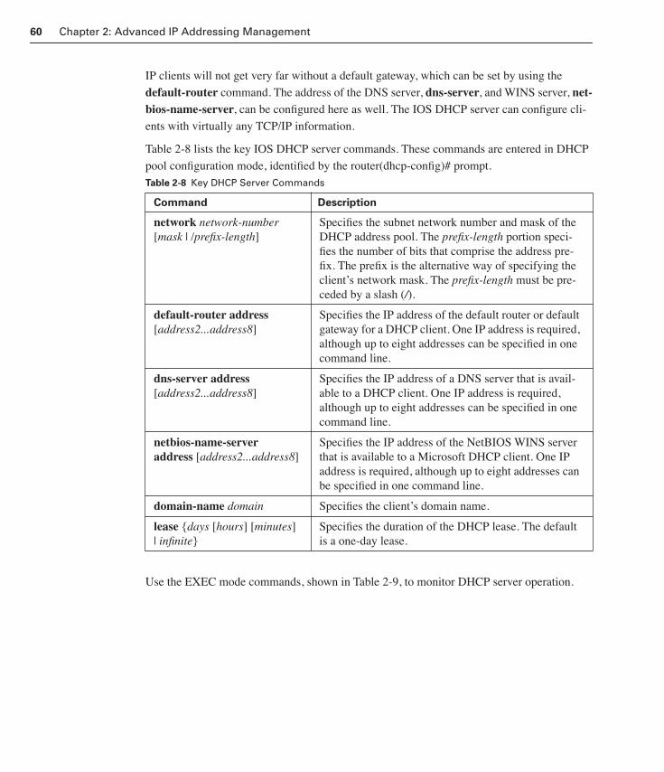
60 Chapter 2: Advanced IP Addressing Management
IP clients will not get very far without a default gateway, which can be set by using the
default-router command. The address of the DNS server, dns-server, and WINS server, net-bios-name-server, can be configured here as well. The IOS DHCP server can configure cli-
ents with virtually any TCP/IP information.
Table 2-8 lists the key IOS DHCP server commands. These commands are entered in DHCP
pool configuration mode, identified by the router(dhcp-config)# prompt.
Use the EXEC mode commands, shown in Table 2-9, to monitor DHCP server operation.
Table 2-8 Key DHCP Server Commands
Command Description
network network-number [mask | /prefix-length]
Specifies the subnet network number and mask of the DHCP address pool. The prefix-length portion speci-fies the number of bits that comprise the address pre-fix. The prefix is the alternative way of specifying the client’s network mask. The prefix-length must be pre-ceded by a slash (/).
default-router address [address2...address8]
Specifies the IP address of the default router or default gateway for a DHCP client. One IP address is required, although up to eight addresses can be specified in one command line.
dns-server address [address2...address8]
Specifies the IP address of a DNS server that is avail-able to a DHCP client. One IP address is required, although up to eight addresses can be specified in one command line.
netbios-name-server address [address2...address8]
Specifies the IP address of the NetBIOS WINS server that is available to a Microsoft DHCP client. One IP address is required, although up to eight addresses can be specified in one command line.
domain-name domain Specifies the client’s domain name.
lease {days [hours] [minutes] | infinite}
Specifies the duration of the DHCP lease. The default is a one-day lease.
1358_fmi.book Page 60 Thursday, May 27, 2004 2:21 PM

DHCP and Easy IP 61
Easy IP
Easy IP is a combination suite of Cisco IOS software features that allows a router to negotiate
its own IP address, as a DHCP client, and to do NAT through that negotiated address. Easy IP
is typically deployed on a small office, home office (SOHO) router. It is useful in cases where
a small LAN connects to the Internet by way of a provider that dynamically assigns only one
IP address for the entire remote site, as shown in Figure 2-20.
Figure 2-20 Cisco IOS Easy IP
Table 2-9 Key Commands for Monitoring DHCP Operation
Command Definition
show ip dhcp binding [address] Displays a list of all bindings (MAC to IP address) created on a specific DHCP server.
show ip dhcp conflict [address] Displays a list of all address conflicts recorded by a specific DHCP server.
show ip dhcp database [url] Displays recent activity on the DHCP database. (Use this command in privileged EXEC mode.)
show ip dhcp server statistics Displays count information about server statis-tics and messages sent and received.
TelecommuterLAN
Internet
CentralSite
Branch Office LAN Branch Office LAN
Easy IP
Easy IP Easy IP
Easy IPEasy IP
TelecommuterLAN
Branch Office LAN Telecommuter
LAN
Easy IP
1358_fmi.book Page 61 Thursday, May 27, 2004 2:21 PM

62 Chapter 2: Advanced IP Addressing Management
A SOHO router with the Easy IP feature set uses DHCP, as a server, to automatically address
local LAN clients with RFC 1918 addresses. When the router dynamically receives its WAN
interface address by way of PPP, it uses NAT overload to translate between local inside
addresses and its single global address. Therefore, both the LAN side and the WAN side are
dynamically configured with little or no administrative intervention. In effect, Easy IP offers
plug-and-play routing.
Helper AddressesThis section describes how networks and routers use helper addresses to forward broadcasts
to another server or router on another network. This section describes some of the purposes of
and scenarios in which to use helper addresses.
Using Helper Addresses
DHCP is not the only critical service that uses broadcasts. Cisco routers and other devices
might use broadcasts to locate TFTP servers. Some clients might need to broadcast to locate a
TACACS security server. In a complex hierarchical network, clients might not reside on the
same subnet as key servers. Such remote clients broadcast to locate these servers, but routers,
by default, do not forward client broadcasts beyond their subnet. Some clients are unable to
make a connection without services such as DHCP. For this reason, the administrator must
provide DHCP and DNS servers on all subnets or use the Cisco IOS software helper address
feature. Running services such as DHCP or DNS on several computers creates overhead and
administrative problems, so the first option is not very appealing. When possible, administra-
tors use the ip helper-address command to relay broadcast requests for these key User Data-
gram Protocol (UDP) services.
By using the ip helper-address command, a router can be configured to accept a broadcast
request for a UDP service and then forward it as a unicast to a specific IP address, as shown in
Figure 2-21. Alternatively, the router can forward these requests as directed broadcasts to a
specific network or subnetwork.
Figure 2-21 Helper Addresses
DisklessWorkstation
Broadcast Unicast
Looking forBoot Server.
BOOTPServer
1358_fmi.book Page 62 Thursday, May 27, 2004 2:21 PM

Helper Addresses 63
Configuring IP Helper Addresses
To configure the helper address, identify the router interface that will receive the broadcasts
for UDP services. In interface configuration mode, use the ip helper-address command to
define the address to which UDP broadcasts for services should be forwarded.
By default, the ip helper-address command forwards the eight UDP services listed in
Table 2-10.
What if Company XYZ needs to forward requests for a service not on this list? The Cisco
IOS software provides the global configuration command ip forward-protocol to allow an
administrator to forward any UDP port in addition to the default eight. To forward UDP on
port 517, use the global configuration command ip forward-protocol udp 517. This com-
mand is used not only to add a UDP port to the default eight, but also to subtract an unwanted
service from the default group. When forwarding DHCP, TFTP, and DNS without forwarding
Time, TACACS, and NetBIOS, the Cisco IOS software requires that the router be configured
according to the syntax shown in Example 2-5.
Table 2-10 Default Forward UDP Services
Service Port
Time 37
TACACS 49
DNS 53
BOOTP/DHCP Server 67
BOOTP/DHCP Client 68
TFTP 69
NetBIOS name service 137
NetBIOS datagram service 138
Example 2-5 Forwarding UDP Services
RTA(config-if)#iiiipppp hhhheeeellllppppeeeerrrr----aaaaddddddddrrrreeeessssssss 111199992222....111166668888....1111....222255554444
RTA(config-if)#eeeexxxxiiiitttt
RTA(config)#iiiipppp ffffoooorrrrwwwwaaaarrrrdddd----pppprrrroooottttooooccccoooollll uuuuddddpppp 555511117777
RTA(config)#nnnnoooo iiiipppp ffffoooorrrrwwwwaaaarrrrdddd----pppprrrroooottttooooccccoooollll uuuuddddpppp 33337777
RTA(config)#nnnnoooo iiiipppp ffffoooorrrrwwwwaaaarrrrdddd----pppprrrroooottttooooccccoooollll uuuuddddpppp 44449999
RTA(config)#nnnnoooo iiiipppp ffffoooorrrrwwwwaaaarrrrdddd----pppprrrroooottttooooccccoooollll uuuuddddpppp 111133337777
RTA(config)#nnnnoooo iiiipppp ffffoooorrrrwwwwaaaarrrrdddd----pppprrrroooottttooooccccoooollll uuuuddddpppp 111133338888
1358_fmi.book Page 63 Thursday, May 27, 2004 2:21 PM
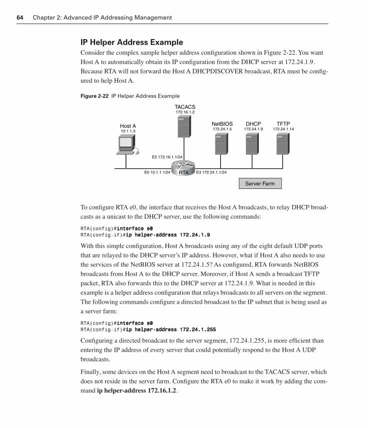
64 Chapter 2: Advanced IP Addressing Management
IP Helper Address Example
Consider the complex sample helper address configuration shown in Figure 2-22. You want
Host A to automatically obtain its IP configuration from the DHCP server at 172.24.1.9.
Because RTA will not forward the Host A DHCPDISCOVER broadcast, RTA must be config-
ured to help Host A.
Figure 2-22 IP Helper Address Example
To configure RTA e0, the interface that receives the Host A broadcasts, to relay DHCP broad-
casts as a unicast to the DHCP server, use the following commands:
RTA(config)#iiiinnnntttteeeerrrrffffaaaacccceeee eeee0000RTA(config-if)#iiiipppp hhhheeeellllppppeeeerrrr----aaaaddddddddrrrreeeessssssss 111177772222....22224444....1111....9999
With this simple configuration, Host A broadcasts using any of the eight default UDP ports
that are relayed to the DHCP server’s IP address. However, what if Host A also needs to use
the services of the NetBIOS server at 172.24.1.5? As configured, RTA forwards NetBIOS
broadcasts from Host A to the DHCP server. Moreover, if Host A sends a broadcast TFTP
packet, RTA also forwards this to the DHCP server at 172.24.1.9. What is needed in this
example is a helper address configuration that relays broadcasts to all servers on the segment.
The following commands configure a directed broadcast to the IP subnet that is being used as
a server farm:
RTA(config)#iiiinnnntttteeeerrrrffffaaaacccceeee eeee0000RTA(config-if)#iiiipppp hhhheeeellllppppeeeerrrr----aaaaddddddddrrrreeeessssssss 111177772222....22224444....1111....222255555555
Configuring a directed broadcast to the server segment, 172.24.1.255, is more efficient than
entering the IP address of every server that could potentially respond to the Host A UDP
broadcasts.
Finally, some devices on the Host A segment need to broadcast to the TACACS server, which
does not reside in the server farm. Configure the RTA e0 to make it work by adding the com-
mand ip helper-address 172.16.1.2.
Host A10.1.1.3
TACACS172.16.1.2
NetBIOS172.24.1.5
DHCP172.24.1.9
TFTP172.24.1.14
RTA
E2 172.16.1.1/24
E0 10.1.1.1/24 E3 172.24.1.1/24
Server Farm
1358_fmi.book Page 64 Thursday, May 27, 2004 2:21 PM

Helper Addresses 65
Verify the correct helper configuration with the show ip interface command, as shown in
Example 2-6.
Notice that the RTA interface e3 in Example 2-7, which connects to the server farm, is not
configured with helper addresses. However, the output shows that for this interface, directed
broadcast forwarding is disabled. This means that the router does not convert the logical broadcast
172.24.1.255 into a physical broadcast with a Layer 2 address of FF-FF-FF-FF-FF-FF.
To allow all the nodes in the server farm to receive the broadcasts at Layer 2, configure e3 to
forward directed broadcasts with the following commands:
RTA(config)#iiiinnnntttteeeerrrrffffaaaacccceeee eeee3333RTA(config-if)#iiiipppp ddddiiiirrrreeeecccctttteeeedddd----bbbbrrrrooooaaaaddddccccaaaasssstttt
Example 2-6 Verifying IP Helper Address Configuration
RTA#sssshhhhoooowwww iiiipppp iiiinnnntttteeeerrrrffffaaaacccceeee eeee0000
Ethernet0 is up, line protocol is up
Internet address is 10.1.1.1/24
Broadcast address is 255.255.255.255
Address determined by setup command
MTU is 1500 bytes
Helper addresses are 172.24.1.255
172.16.1.2
Directed broadcast forwarding is disabled
<output omitted>
Example 2-7 Verifying Directed Broadcast Forwarding
RTA#sssshhhhoooowwww iiiipppp iiiinnnntttteeeerrrrffffaaaacccceeee eeee3333
Ethernet3 is up, line protocol is up
Internet address is 172.24.1.1/24
Broadcast address is 255.255.255.255
Address determined by setup command
MTU is 1500 bytes
Helper addresses is not set
Directed broadcast forwarding is disabled
<output omitted>
NOTE
Because directed broad-casts—particularly Inter-net Control Message Protocol (ICMP) directed broadcasts—have been abused by malicious per-sons, it is recommended that security-conscious users disable the ip directed-broadcast com-mand on any interface where directed broadcasts are unneeded and that they use access lists to limit the number of exploded packets.
1358_fmi.book Page 65 Thursday, May 27, 2004 2:21 PM

66 Chapter 2: Advanced IP Addressing Management
IPv6IPv6 is an alternative and a solution to the IPv4 address crisis. This section explains
what IPv6 is and describes its address structure.
IP Address Issues Solutions
This chapter has shown that IPv4 addressing faces two major issues:
■ The depletion of addresses, particularly the key medium-sized space
■ The pervasive growth of Internet routing tables, which is illustrated in Figure 2-23
Figure 2-23 Growth of Routing Tables
In the early 1990s, CIDR ingeniously built on the concept of the address mask and stepped
forward to temporarily alleviate these overwhelming problems. CIDR’s hierarchical nature
dramatically improved IPv4’s scalability. Once again, a hierarchical design has proven to be a
scalable one.
Yet even with subnetting in 1985, variable-length subnetting in 1987, and CIDR in 1993, a
hierarchical structure could not save IPv4 from one simple problem: not enough addresses
exist to meet future needs. At roughly four billion possibilities, the IPv4 address space is
Lab 2.10.3 Using DHCP and IP Helper Addresses
In this lab, configure a Cisco router to act as a DHCP server for clients on two sepa-
rate subnets and the IP helper address feature to forward DHCP requests from a
remote subnet.
35
30
25
20
15
10
5
0
1990 1991 1992 1993 1994 1995
Rou
ting
Tabl
e E
ntrie
s(I
n T
hous
ands
)
1358_fmi.book Page 66 Thursday, May 27, 2004 2:21 PM

IPv6 67
formidable. However, it will not suffice in a future world of mobile Internet-enabled devices
and IP-addressable household appliances.
Recent short-term IPv4 solutions to the address crunch have been developed. These include
RFC 1918, which sets aside private addresses for unlimited internal use, and NAT, which
allows thousands of hosts to access the Internet with only a handful of valid addresses.
However, the ultimate solution to the address shortage is the introduction of IPv6 and its 128-
bit address. Developed to create a supply of addresses that would outlive demand, IPv6 is on
course to eventually replace IPv4. IPv6’s large address space will provide not only far more
addresses than IPv4, but additional levels of hierarchy as well.
In 1994, the IETF proposed IPv6 in RFC 1752, and a number of working groups were formed
in response. IPv6 covers issues such as the following:
■ Address depletion
■ Quality of service
■ Address autoconfiguration
■ Authentication
■ Security
It will not be easy for organizations deeply invested in the IPv4 scheme to migrate to a totally
new architecture. As long as IPv4, with its recent extensions and CIDR-enabled hierarchy,
remains viable, administrators will shy away from adopting IPv6. A new IP protocol requires
new software, new hardware, and new methods of administration. It is likely that IPv4 and
IPv6 will coexist, even within an autonomous system, for years.
IPv6 Address Format
As defined in RFC 1884 and later revised in RFC 2373, IPv6 addresses are 128-bit identifiers
for interfaces and sets of interfaces, not nodes. Three general types of addresses exist:
■ Unicast—An identifier for a single interface. A packet sent to a unicast address is deliv-
ered to the interface identified by that address.
■ Anycast—An identifier for a set of interfaces that typically belong to different nodes. A
packet sent to an anycast address is delivered to the nearest interface in the anycast
group.
■ Multicast—An identifier for a set of interfaces that typically belong to different nodes.
A packet sent to a multicast address is delivered to all interfaces in the multicast group.
To write 128-bit addresses so that they are more readable to human eyes, the IPv6 architects
abandoned dotted-decimal notation in favor of a hexadecimal format. Therefore, IPv6 is writ-
ten as 32-hex digits, with colons separating the values of the eight 16-bit pieces of the
address.
NOTE
128 bits allows for 340,282,366,920,938,463,463,374,607,431,768,211,456 possibilities.
1358_fmi.book Page 67 Thursday, May 27, 2004 2:21 PM

68 Chapter 2: Advanced IP Addressing Management
IPv6 addresses are written in hexadecimal:
1080:0000:0000:0000:0008:0800:200C:417A
Leading 0s in each 16-bit value can be omitted, so this address can be expressed as follows:
1080:0:0:0:8:800:200C:417A
Because IPv6 addresses, especially in the early implementation phase, might contain consec-
utive 16-bit values of 0, one such string of 0s per address can be omitted and replaced by a
double colon. As a result, this address can be shortened as follows:
1080::8:800:200C:417A
Under current plans, IPv6 nodes that connect to the Internet will use what is called an aggre-
gatable global unicast address. This is the familiar counterpart to the IPv4 global addresses.
Like CIDR-enhanced IPv4, aggregatable global unicast addresses rely on hierarchy to keep
Internet routing tables manageable. IPv6 global unicast addresses feature three levels of hierarchy:
■ Public topology—The collection of providers that offer Internet connectivity.
■ Site topology—The level local to an organization that does not provide connectivity to
nodes outside itself.
■ Interface identifier—The level specific to a node’s individual interface.
This three-level hierarchy is reflected by the structure of the aggregatable global unicast
address (see Figure 2-24), which includes the following fields:
■ Format Prefix (FP) field, 3 bits—The 3-bit FP is used to identify the type of address—
unicast, multicast, and so on. The bits 001 identify aggregatable global unicasts.
■ Top-Level Aggregation Identifier (TLA ID) field, 13 bits—The TLA ID field is used to
identify the authority responsible for the address at the highest level of the routing hier-
archy. Internet routers necessarily maintain routes to all TLA IDs. With 13 bits set
aside, this field can represent up to 8192 TLAs.
■ Reserved (Res) field, 8 bits—IPv6 architecture defined the Res field so that the TLA or
NLA IDs could be expanded as future growth warrants. Currently, this field must be set
to 0.
■ Next-Level Aggregation Identifier (NLA ID) field, 24 bits—The NLA ID field is used
by organizations assigned a TLA ID to create an addressing hierarchy and to identify
sites.
■ Site-Level Aggregation Identifier (SLA ID) field, 16 bits—The SLA ID is used by an
individual organization to create its own local addressing hierarchy and to identify subnets.
■ Interface ID field, 64 bits—The Interface ID field is used to identify individual inter-
faces on a link. This field is analogous to the host portion of an IPv4 address, but it is
1358_fmi.book Page 68 Thursday, May 27, 2004 2:21 PM

Summary 69
derived using the IEEE EUI-64 format. When this field is on LAN interfaces, the Inter-
face ID adds a 16-bit field to the interface MAC address.
Figure 2-24 IPv6 Address Format
In addition to the global unicast address space, IPv6 offers internal network numbers, or site
local use addresses. These are analogous to RFC 1918 addresses. If a node is not normally
addressed with a global unicast address or an internal site local use address, it can be
addressed using a link local use address, which is specific to a network segment.
SummaryThis chapter described how all of the following can enable more efficient use of IP addresses:
■ Subnet masks
■ VLSMs
■ Private addressing
■ NAT
This chapter also showed that hierarchical addressing allows for efficient allocation of
addresses and a reduced number of routing table entries. VLSMs, specifically, provide the
capability to include more than one subnet mask within a network and the capability to sub-
net an already subnetted network address. Proper IP addressing is required to ensure the most
efficient network operations. Finally, the IPv6 addressing format was presented.
Number of Bits
3 13 8 24 16 64
FP TLA ID Res NLA ID SLA ID Interface ID
Public TopologySite
TopologyInterface Identifier
1358_fmi.book Page 69 Thursday, May 27, 2004 2:21 PM

70 Chapter 2: Advanced IP Addressing Management
Key Termsanycast An identifier for a set of interfaces that typically belong to different nodes. A
packet sent to an anycast address is delivered to the nearest, or first, interface in the anycast
group.
CIDR (classless interdomain routing) An IP addressing scheme that replaces the older
system based on Classes A, B, and C. With CIDR, a single IP address can be used to desig-
nate many unique IP addresses.
Format Prefix (FP) field The 3-bit FP identifies the type of address—unicast, multicast,
and so on. The bits 001 identify aggregatable global unicasts.
interface identifier The level specific to a node’s individual interface.
Interface ID field The 64-bit Interface ID field identifies individual interfaces on a link.
This field is analogous to the host portion of an IPv4 address, but it is derived using the IEEE
EUI-64 format. When this field is on LAN interfaces, the Interface ID adds a 16-bit field to
the interface MAC address.
multicast An identifier for a set of interfaces that typically belong to different nodes. A
packet sent to a multicast address is delivered to all interfaces in the multicast group.
Next-Level Aggregation Identifier (NLA ID) field The 24-bit NLA ID field is used to iden-
tify ISPs. The field itself can be organized to reflect a hierarchy or a multitiered relationship
among providers.
public topology The collection of providers that offer Internet connectivity.
Reserved (Res) field The IPv6 architecture defines the 8-bit Res field so that the TLA or
NLA IDs can be expanded as future growth warrants. Currently, this field must be set to 0.
RIP (Routing Information Protocol) An Interior Gateway Protocol (IGP) supplied with
the FreeBSD version of UNIX. The most common IGP in the Internet. RIP uses hop count as
a routing metric.
RIPv2 (Routing Information Protocol version 2) Defined in RFC 1723 and supported in
Cisco IOS software versions 11.1 and later. RIPv2 is not a new protocol; it is just RIPv1 with
some extensions to bring it up-to-date with modern routing environments. RIPv2 has been
updated to support VLSM, authentication, and multicast updates.
route summarization The consolidation of advertised addresses in OSPF and IS-IS. In
OSPF, this causes a single summary route to be advertised to other areas by an area border
router.
Site-Level Aggregation Identifier (SLA ID) field The 16-bit SLA ID is used by an individ-
ual organization to create its own local addressing hierarchy and to identify subnets.
1358_fmi.book Page 70 Thursday, May 27, 2004 2:21 PM

Key Terms 71
site topology The level local to an organization that does not provide connectivity to nodes
outside itself.
Top-Level Aggregation Identifier (TLA ID) field The 13-bit TLA ID field is used to iden-
tify the authority responsible for the address at the highest level of the routing hierarchy.
Internet routers necessarily maintain routes to all TLA IDs. With 13 bits set aside, this field
can represent up to 8192 TLAs.
unicast An identifier for a single interface. A packet sent to a unicast address is delivered to
the interface identified by that address.
VLSM (variable-length subnet masking) The ability to specify a different subnet mask for the
same network number on different subnets. VLSM can help optimize available address space.
1358_fmi.book Page 71 Thursday, May 27, 2004 2:21 PM
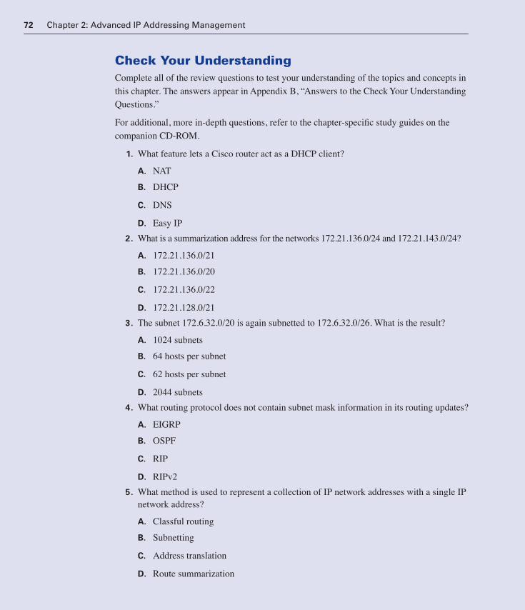
72 Chapter 2: Advanced IP Addressing Management
Check Your UnderstandingComplete all of the review questions to test your understanding of the topics and concepts in
this chapter. The answers appear in Appendix B, “Answers to the Check Your Understanding
Questions.”
For additional, more in-depth questions, refer to the chapter-specific study guides on the
companion CD-ROM.
1. What feature lets a Cisco router act as a DHCP client?
A. NAT
B. DHCP
C. DNS
D. Easy IP
2. What is a summarization address for the networks 172.21.136.0/24 and 172.21.143.0/24?
A. 172.21.136.0/21
B. 172.21.136.0/20
C. 172.21.136.0/22
D. 172.21.128.0/21
3. The subnet 172.6.32.0/20 is again subnetted to 172.6.32.0/26. What is the result?
A. 1024 subnets
B. 64 hosts per subnet
C. 62 hosts per subnet
D. 2044 subnets
4. What routing protocol does not contain subnet mask information in its routing updates?
A. EIGRP
B. OSPF
C. RIP
D. RIPv2
5. What method is used to represent a collection of IP network addresses with a single IP network address?
A. Classful routing
B. Subnetting
C. Address translation
D. Route summarization
1358_fmi.book Page 72 Thursday, May 27, 2004 2:21 PM

Check Your Understanding 73
6. According to RFC 1918, which of the following is a private Internet address?
A. 10.215.34.124
B. 192.32.146.23
C. 172.34.221.18
D. 119.12.73.215
7. Which of the following is a characteristic of IP unnumbered?
A. Avoids wasted addresses on multiaccess links
B. Efficient addressing on Ethernet links
C. Uses another router interface address
D. May be used only with classless routing protocols
8. How many bits make up an IPv6 address?
A. 32
B. 48
C. 64
D. 128
9. What is the purpose of IP helper addresses?
A. To relay key UDP broadcast requests to hosts on the same subnet
B. To relay key UDP broadcast requests to hosts on the other subnets
C. To relay key TCP broadcast requests to hosts on other subnets
D. To relay key TCP broadcast requests to hosts on the same subnet
10. What are the three general types of IPv6 addresses?
A. Class 1, Class 2, Class 3
B. Class A, Class B, Class C
C. Unicast, anycast, multicast
D. Public, site, interface

ObjectivesUpon completing this chapter, you will be able to
■ Understand the fundamentals of routing
■ Configure default routing
■ Configure floating static routes
■ Understand how convergence issues affect routing
■ Determine route calculation
You can reinforce your understanding of the objectives covered in this chapter by opening
the interactive media activities on the CD accompanying this book and performing the lab
activities collected in the Cisco Networking Academy Program CCNP 1: Advanced Routing
Lab Companion. Throughout this chapter, you will see references to these activities by title
and by icon. They look like this:
Interactive Media Activity
Lab Activity
1358_fmi.book Page 74 Thursday, May 27, 2004 2:21 PM

Chapter 3
Routing Overview
Many of the scalable design features explored in the first two chapters, such as load balancing
and route summarization, work very differently depending on the routing protocol used. Routing
protocols are the rules that govern the exchange of routing information between routers. The
Transmission Control Protocol/Internet Protocol (TCP/IP) open architecture and global popular-
ity have encouraged the development of more than a half-dozen prominent IP routing protocols.
Each protocol has a unique combination of strengths and weaknesses. Because routing protocols
are key to network performance, you need to understand the following attributes of each proto-
col:
■ Convergence times
■ Overhead
■ Scalability features
This chapter explores various routing processes, including default routing, floating static routes,
convergence, and route calculation.
RoutingOne of a router’s primary jobs is to determine the best path to a given destination. A router learns
paths, or routes, from the static configuration entered by an administrator or dynamically from
other routers, through routing protocols. Routers keep a routing table in RAM. A routing table is
a list of the best-known available routes. Routers use this table to make decisions about how to
forward a packet.
Routing Fundamentals
To view the TCP/IP routing table, issue the show ip route command. A routing table maps net-
work prefixes to an outbound interface, as shown in Example 3-1. When RTA receives a packet
destined for 192.168.4.46, it looks for the prefix 192.168.4.0/24 in the routing table. RTA then
forwards the packet out an interface, such as Ethernet0, based on the routing table entry. If RTA
receives a packet destined for 10.3.21.5/16, it sends that packet out Serial0 (S0).
1358_fmi.book Page 75 Thursday, May 27, 2004 2:21 PM
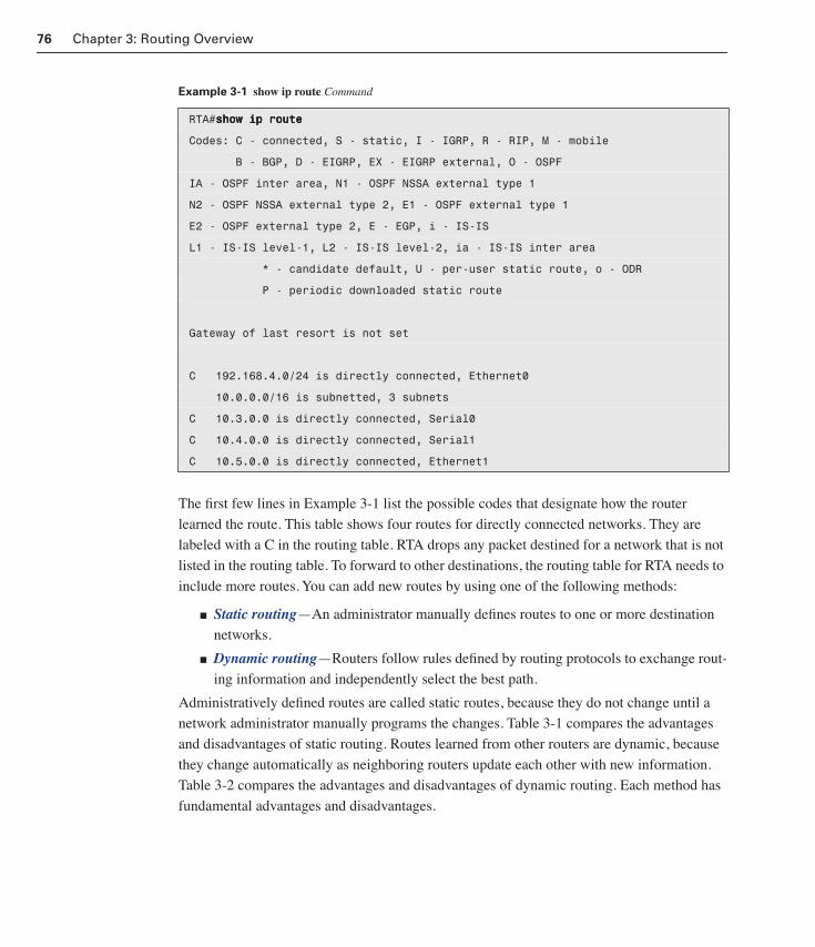
76 Chapter 3: Routing Overview
The first few lines in Example 3-1 list the possible codes that designate how the router
learned the route. This table shows four routes for directly connected networks. They are
labeled with a C in the routing table. RTA drops any packet destined for a network that is not
listed in the routing table. To forward to other destinations, the routing table for RTA needs to
include more routes. You can add new routes by using one of the following methods:
■ Static routing—An administrator manually defines routes to one or more destination
networks.
■ Dynamic routing—Routers follow rules defined by routing protocols to exchange rout-
ing information and independently select the best path.
Administratively defined routes are called static routes, because they do not change until a
network administrator manually programs the changes. Table 3-1 compares the advantages
and disadvantages of static routing. Routes learned from other routers are dynamic, because
they change automatically as neighboring routers update each other with new information.
Table 3-2 compares the advantages and disadvantages of dynamic routing. Each method has
fundamental advantages and disadvantages.
Example 3-1 show ip route Command
RTA#sssshhhhoooowwww iiiipppp rrrroooouuuutttteeee
Codes: C - connected, S - static, I - IGRP, R - RIP, M - mobile
B - BGP, D - EIGRP, EX - EIGRP external, O - OSPF
IA - OSPF inter area, N1 - OSPF NSSA external type 1
N2 - OSPF NSSA external type 2, E1 - OSPF external type 1
E2 - OSPF external type 2, E - EGP, i - IS-IS
L1 - IS-IS level-1, L2 - IS-IS level-2, ia - IS-IS inter area
* - candidate default, U - per-user static route, o - ODR
P - periodic downloaded static route
Gateway of last resort is not set
C 192.168.4.0/24 is directly connected, Ethernet0
10.0.0.0/16 is subnetted, 3 subnets
C 10.3.0.0 is directly connected, Serial0
C 10.4.0.0 is directly connected, Serial1
C 10.5.0.0 is directly connected, Ethernet1
1358_fmi.book Page 76 Thursday, May 27, 2004 2:21 PM

Routing 77
The following sections describe how to configure both static and dynamic routing on a Cisco
router.
Static Routing
Static routing is useful in networks that do not have multiple paths to any destination net-work. Static routing reduces the memory and processing burdens on a router. Even on large internetworks, administrators often configure static routes on access routers that connect stub
Table 3-1 Advantages and Disadvantages of Static Routing
Static Routing Advantages Static Routing Disadvantages
Low processor overhead. Routers do not spend valuable CPU cycles calculating the best path. This requires less memory, less processing power, and therefore a less-expensive router.
High maintenance configuration. Admin-istrators must configure all static routes manually. Complex networks might require constant reconfiguration, which is impractical.
No bandwidth utilization. Routers do not take up bandwidth updating each other about static routes.
No adaptability. Statically configured routes cannot adapt to changes in link status.
Secure operation. Routers that do not send updates do not inadvertently advertise net-work information to an untrusted source. Routers that do not accept routing updates are less vulnerable to attacks.
Predictability. Static routes let an adminis-trator precisely control the router path selection. Dynamic routing sometimes yields unexpected results, even in small networks.
Table 3-2 Advantages and Disadvantages of Dynamic Routing
Dynamic Routing Advantages Dynamic Routing Disadvantages
High degree of adaptability. Routers auto-matically learn a network’s topology and select optimum paths.
Increased processor overhead and memory utilization. Dynamic routing processes can require a significant amount of CPU time and system memory.
Low maintenance configuration. After the basic parameters for a routing protocol are set correctly, administrative intervention is not required.
High bandwidth utilization. Routers use bandwidth to send and receive routing updates, which can detrimentally affect performance on slow WAN links.
Routers can alert each other about links that have gone down or about newly dis-covered paths.
1358_fmi.book Page 77 Thursday, May 27, 2004 2:21 PM
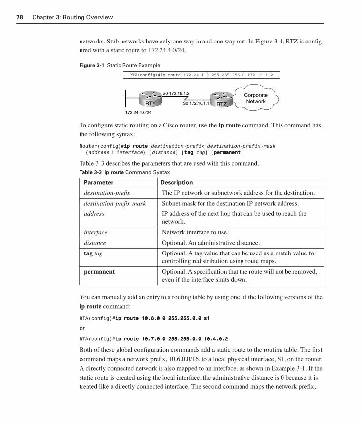
78 Chapter 3: Routing Overview
networks. Stub networks have only one way in and one way out. In Figure 3-1, RTZ is config-ured with a static route to 172.24.4.0/24.
Figure 3-1 Static Route Example
To configure static routing on a Cisco router, use the ip route command. This command has
the following syntax:
Router(config)#iiiipppp rrrroooouuuutttteeee destination-prefix destination-prefix-mask {address | interface} [distance] [ttttaaaagggg tag] [ppppeeeerrrrmmmmaaaannnneeeennnntttt]
Table 3-3 describes the parameters that are used with this command.
You can manually add an entry to a routing table by using one of the following versions of the
ip route command:
RTA(config)#iiiipppp rrrroooouuuutttteeee 11110000....6666....0000....0000 222255555555....222255555555....0000....0000 ssss1111
or
RTA(config)#iiiipppp rrrroooouuuutttteeee 11110000....7777....0000....0000 222255555555....222255555555....0000....0000 11110000....4444....0000....2222
Both of these global configuration commands add a static route to the routing table. The first
command maps a network prefix, 10.6.0.0/16, to a local physical interface, S1, on the router.
A directly connected network is also mapped to an interface, as shown in Example 3-1. If the
static route is created using the local interface, the administrative distance is 0 because it is
treated like a directly connected interface. The second command maps the network prefix,
Table 3-3 ip route Command Syntax
Parameter Description
destination-prefix The IP network or subnetwork address for the destination.
destination-prefix-mask Subnet mask for the destination IP network address.
address IP address of the next hop that can be used to reach the network.
interface Network interface to use.
distance Optional. An administrative distance.
tag tag Optional. A tag value that can be used as a match value for controlling redistribution using route maps.
permanent Optional. A specification that the route will not be removed, even if the interface shuts down.
RTZ
CorporateNetwork
RTZ(config)#ip route 172.24.4.0 255.255.255.0 172.16.1.2
S0 172.16.1.2
S0 172.16.1.1
172.24.4.0/24
RTY
1358_fmi.book Page 78 Thursday, May 27, 2004 2:21 PM

Routing 79
10.7.0.0/16, to the next-hop address, 10.4.0.2. When the next-hop address is used, the admin-
istrative distance is 1.
In Example 3-2, the route to 10.6.0.0 is identified as a static route by the S at the beginning of
the line. However, it is formatted similarly to a directly connected route. This is because the
router has been configured to forward packets for 10.6.0.0 out S1. The entry in the routing
table for the static route to 10.7.0.0 is configured with a next-hop address. This entry in the
routing table is similar to dynamic routes. The next-hop address is included in the routing
table because the packets destined for 10.7.0.0 should be forwarded to an interface at 10.4.0.2
on another router. What is the difference between these two kinds of static routes?
When a routing protocol such as RIP or Interior Gateway Routing Protocol (IGRP) is used,
static routes that are shown as directly connected are automatically advertised to other rout-
ers, if the appropriate network command has been issued. The next-hop static route is not
advertised without additional configuration. These static routes can be included in updates if
they are injected, or redistributed, into the dynamic routing protocol.
Example 3-2 Routing Table with Static Routes Configured
RTA#sssshhhhoooowwww iiiipppp rrrroooouuuutttteeee
Codes: C - connected, S - static, I - IGRP, R - RIP, M - mobile
B - BGP, D - EIGRP, EX - EIGRP external, O - OSPF
IA - OSPF inter area, N1 - OSPF NSSA external type 1
N2 - OSPF NSSA external type 2, E1 - OSPF external type 1
E2 - OSPF external type 2, E - EGP, i - IS-IS
L1 - IS-IS level-1, L2 - IS-IS level-2, ia - IS-IS inter area
* - candidate default, U - per-user static route, o - ODR
P - periodic downloaded static route
Gateway of last resort is not set
C 192.168.4.0/24 is directly connected, Ethernet0
10.0.0.0/16 is subnetted, 3 subnets
C 10.3.0.0 is directly connected, Serial0
C 10.4.0.0 is directly connected, Serial1
C 10.5.0.0 is directly connected, Ethernet1
S 10.6.0.0 is directly connected, Serial1
S 10.7.0.0 [1/0] via 10.4.0.2
1358_fmi.book Page 79 Thursday, May 27, 2004 2:21 PM

80 Chapter 3: Routing Overview
When an interface goes down, all static routes mapped to that interface are removed from the
IP routing table. If the router can no longer find a valid next hop for the address specified in a
static route, the static route is removed from the table. An alternative method is to map a static
IP address to a loopback interface, because a loopback interface is a virtual interface. There-
fore, it is always active and cannot go down like a real interface.
Static routing is unsuitable for large, complex networks that include redundant links, multiple pro-
tocols, and meshed topologies. Routers in complex networks must adapt to topology changes
quickly and select the best route from multiple candidates. Therefore, dynamic routing is the bet-
ter choice.
Configuring Dynamic Routing
Dynamic routing of TCP/IP can be implemented using one or more protocols. These proto-
cols are often grouped according to where they are used. Routing protocols designed to work
inside an autonomous system are categorized as Interior Gateway Protocols (IGPs), and pro-
tocols that work between autonomous systems are classified as Exterior Gateway Protocols
(EGPs). Table 3-4 lists widely supported EGPs and IGPs for TCP/IP routing.
This chapter focuses on IGPs. A comprehensive discussion of EGPs, particularly BGP4,
appears in Chapter 8, “Route Optimization.” These protocols can be further categorized as
either distance vector or link-state routing protocols, depending on their method of operation,
as shown in Table 3-5.
Routing Protocols for IPX and AppleTalkDespite the dominance of IP, a significant number of organizations continue to support legacy
protocols, such as Novell IPX and AppleTalk. A legacy technology is one that is supported
because of a significant past investment or deployment. Many organizations continue to
Table 3-4 Common EGPs and IGPs
EGPs IGPs
EGP3 RIPv1 and RIPv2
BGP4 IGRP
EIGRP
OSPF
IS-IS
Table 3-5 Common Distance Vector and Link-State Routing Protocols
Distance Vector Protocols Link-State Protocols
RIPv1 and RIPv2 OSPF
IGRP IS-IS
EIGRP
NOTE
As a rule, the next-hop address should always be used when defining a static route on a multiaccess net-work, such as Ethernet. A router interface on a multi-access network can have several link partners, so the next-hop address must be used to specify which neighbor should receive traffic for a given network.
1358_fmi.book Page 80 Thursday, May 27, 2004 2:21 PM

Routing 81
support IPX and AppleTalk because of a past investment in protocol-specific printers, soft-
ware, and servers. Although Cisco Enhanced Interior Gateway Routing Protocol (EIGRP)
offers comprehensive support for both IPX and AppleTalk, it is important to be familiar with
three proprietary routing protocols—IPX or Novell RIP, NetWare Link Services Protocol
(NLSP), and AppleTalk Routing Table Maintenance Protocol (RTMP), as illustrated in Table
3-6. Implementing AppleTalk and Novell proprietary routing protocols is beyond the scope of
this book.
IP Routing Protocols and the Routing TableCisco IOS software commands enable dynamic routing based on the routing protocol
used. Example 3-3 displays the routing table of a router configured to use two IP routing
protocols—RIP and EIGRP. Note that most organizations normally do not use more than one
or two routing protocols.
Table 3-6 Common Proprietary Routing Protocols for Non-IP Networks
Distance Vector Protocols Link-State Protocols
IPX or Novell RIP NetWare Link Services Protocol (NLSP)
AppleTalk Routing Maintenance Proto-col (RTMP)
Example 3-3 Sample Routing Table with Multiple Dynamic Routing Protocols
RTA#sssshhhhoooowwww iiiipppp rrrroooouuuutttteeee
Codes: C - connected, S - static, I - IGRP, R - RIP, M - mobile
B - BGP, D - EIGRP, EX - EIGRP external, O - OSPF
IA - OSPF inter area, N1 - OSPF NSSA external type 1
N2 - OSPF NSSA external type 2, E1 - OSPF external type 1
E2 - OSPF external type 2, E - EGP, i - IS-IS
L1 - IS-IS level-1, L2 - IS-IS level-2, ia - IS-IS inter area
* - candidate default, U - per-user static route, o - ODR
P - periodic downloaded static route
Gateway of last resort is not set
C 192.168.4.0/24 is directly connected, Ethernet0
R 192.168.1.0/24 [120/3] via 10.3.0.1, 00:00:06, Serial0
10.0.0.0/16 is subnetted, 6 subnets
D 10.2.0.0 [90/2681856] via 10.3.0.1, 00:26:12, Serial0
C 10.3.0.0 is directly connected, Serial1
1358_fmi.book Page 81 Thursday, May 27, 2004 2:21 PM

82 Chapter 3: Routing Overview
Figure 3-2 examines the specific table entry for 192.168.1.0/24. Routes in the routing table
that are not directly connected include two numbers in brackets—[administrative distance/
metric]. For example, [120/3] means that the administrative distance is 120 and the metric is 3.
Routers base their evaluations of routes on these two numbers. Because this is a RIP route,
the metric represents hop count.
Figure 3-2 Anatomy of a Sample Routing Table Entry
Routers use metrics to evaluate, or measure, routes. When multiple routes to the same net-
work exist and they are from the same routing protocol, the route with the lowest metric is
considered the best. Hop count is the only factor that IP RIP uses to determine the metric. In
the sample entry shown in Figure 3-2, the number 3 indicates that the destination network is
three hops away.
Each routing protocol calculates its metrics differently. EIGRP uses a complex combination
of factors that include bandwidth and reliability to calculate its metric. Using the default set-
tings, the EIGRP metric for the same route to 192.168.1.0 is 3,219,456. If RTA receives a RIP
update and an EIGRP update for this same network, it uses the administrative distance metric
to compare the two. If this administrative distance metric were used, it would be similar to
comparing three apples to more than three million oranges.
When a router receives updates from different routing protocols about the same network, it
cannot use dissimilar metrics to evaluate a route. The router uses administrative distance as
the deciding metric for route validation. The Cisco IOS software assigns a default administra-
tive distance to every routing protocol. A lower value signifies a more trustworthy routing
protocol. In the case of RTA, the EIGRP route is installed in the routing table because its
Code that identifies whatkind of route. R denotesRIP, O denotes OSPF,and so on.
Administrativedistance followedby the metric.
Time elapsedsince the lastupdate.
Network prefix and bitmaskfor the routes. Can be asubnet or supernet.
IP address of the neighborrouter interface thatsourced the update.
Local interface this routeruses when forwarding trafficto the target network.
R 192.168.1.0/24 [120/3] via 10.3.0.1, 00:00:06, Serial0
1358_fmi.book Page 82 Thursday, May 27, 2004 2:21 PM

Routing 83
administrative distance of 90 is lower than RIP, which is 120. A complete list of administra-
tive distances can be found in Chapter 8.
Distance Vector Routing Protocols
Routing protocols can be classified as either distance vector or link-state. These classifica-
tions describe the algorithm, or formula, that routers use to calculate and exchange routing
information. Distance vector routing protocols are based on the Bellman-Ford algorithm.
Routers configured to use a distance vector routing protocol typically send their complete
routing table at regular intervals to neighbor routers, as shown in Figure 3-3. Simple distance
vector protocols, such as RIP and IGRP, broadcast or multicast their routing tables on all con-
figured interfaces. Routers that use these protocols do not actually identify their neighbors for
direct communication.
Figure 3-3 Distance Vector Routing Protocols Send Routing Tables
A neighbor router receiving the broadcast update examines it and compares the information
to its current routing table. Routes to new networks, or routes to known networks with better
metrics, are inserted in the table. The neighbor then broadcasts its routing table, which
includes any updated routes.
Distance vector routing protocols are concerned with the distance and vector, or direction, of
destination networks. Before sending an update, each router adds its own distance value to
the route metric. When a router receives an update, it maps the learned network to the receiv-
ing interface, as shown in Figure 3-4. The router then uses that interface to reach those
destinations.
Interactive Media Activity Drag and Drop: Routing Table Entry
In this media activity, you identify the different fields in a routing table entry.
D C B A
RoutingTable
RoutingTable
RoutingTable
RoutingTable
1358_fmi.book Page 83 Thursday, May 27, 2004 2:21 PM
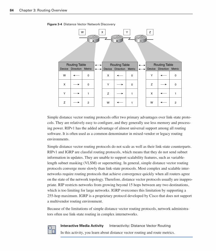
84 Chapter 3: Routing Overview
Figure 3-4 Distance Vector Network Discovery
Simple distance vector routing protocols offer two primary advantages over link-state proto-
cols. They are relatively easy to configure, and they generally use less memory and process-
ing power. RIPv1 has the added advantage of almost universal support among all routing
software. It is often used as a common denominator in mixed-vendor or legacy routing
environments.
Simple distance vector routing protocols do not scale as well as their link-state counterparts.
RIPv1 and IGRP are classful routing protocols, which means that they do not send subnet
information in updates. They are unable to support scalability features, such as variable-
length subnet masking (VLSM) or supernetting. In general, simple distance vector routing
protocols converge more slowly than link-state protocols. Most complex and scalable inter-
networks require routing protocols that achieve convergence quickly when all routers agree
on the state of the network topology. Therefore, distance vector protocols usually are inappro-
priate. RIP restricts networks from growing beyond 15 hops between any two destinations,
which is too limiting for large networks. IGRP overcomes this limitation by supporting a
255-hop maximum. IGRP is a proprietary protocol developed by Cisco that does not support
a multivendor routing environment.
Because of the limitations of simple distance vector routing protocols, network administra-
tors often use link-state routing in complex internetworks.
Interactive Media Activity Interactivity: Distance Vector Routing
In this activity, you learn about distance vector routing and route metrics.
W X Y Z
A
Routing TableDevice Direction Metric
W
X
Y
Z
0
0
1
2
Routing TableDevice Direction Metric
X
Y
Z
W
0
0
1
1
Routing TableDevice Direction Metric
Y
Z
X
W
0
0
1
2
B C
1358_fmi.book Page 84 Thursday, May 27, 2004 2:21 PM

Routing 85
Link-State Routing Protocols
Link-state routing protocols offer greater scalability and faster convergence than distance
vector protocols, such as RIP and IGRP. Link-state routing protocols require more memory
and processing power from the router and more knowledge and expertise from the adminis-
trator than distance vector routing protocols.
Link-state protocols are based on Dijkstra’s algorithm, sometimes called the shortest path
first (SPF) algorithm. The most common link-state routing protocol, Open Shortest Path First
(OSPF), is examined in Chapter 6, “OSPF.”
Routers running a link-state protocol are concerned with the state of link interfaces on other
routers in the network. A link-state router builds a complete database of all the link states of
every router in its area. In other words, a link-state router gathers enough information to cre-
ate its own map of the network. Each router then individually runs the SPF algorithm on its
own map, or link-state database, to identify the best paths to be installed in the routing table.
These paths to other networks form a tree with the local router as its root, as shown in Figure 3-5.
Figure 3-5 Link-State Algorithm Creates the SPF Tree
Instead of learning routes and then broadcasting them with incremented distances to neighbors,
link-state routers advertise the states of their own links to all other routers in the area so that
TopologicalDatabase
SPFAlgorithm
RoutingTable
Shortest-Path-First Tree
Link-State Advertisement Packets
1358_fmi.book Page 85 Thursday, May 27, 2004 2:21 PM

86 Chapter 3: Routing Overview
each router can build a complete link-state database, as shown in Figure 3-6. These advertise-
ments are called link-state advertisements (LSAs). Unlike distance vector routers, link-state
routers can form special relationships with their neighbors and other link-state routers to
ensure that the LSA information is properly and efficiently exchanged.
Figure 3-6 Link-State Advertisements Establish Neighbors
There is an initial flood of LSAs to provide routers with the information they need to build a
link-state database. Routing updates occur only when a link state changes or if no changes
have occurred after a specific interval. If a link state changes, a partial update is sent immedi-
ately. The partial update contains only link states that have changed, not a complete routing
table. An administrator concerned about WAN link utilization will find these partial and infre-
quent updates an efficient alternative to distance vector routing, which sends out a complete
routing table at each update interval. When a change occurs, link-state routers are all notified
immediately by the partial update. Distance vector routers have to wait for neighbors to note
the change, increment the change, and then pass it on to the next neighbor down the line.
The benefits of link-state routing include faster convergence and improved bandwidth utiliza-
tion over distance vector protocols. Link-state protocols support classless interdomain rout-
ing (CIDR), VLSM, and supernetting. This makes them a good choice for complex, scalable
networks. In fact, link-state protocols generally outperform distance vector protocols on any
size network. Link-state protocols do have two major disadvantages:
■ Link-state routing can overtax low-end hardware. Link-state routers require more
memory and processing power than distance vector routers, potentially making link-
state routing cost-prohibitive for organizations with tight budgets and legacy hardware.
NeighborsA and C
on Network 1
NeighborsB and C
on Network 1NeighborsC and D
on Network 2
NeighborsA and B
on Network 1NeighborsA and D
on Network 2
NeighborsA and C
on Network 2
Hello
Hello
Hello
Hello Hello
Hello
Network 1
Network 2
B
A C
D
1358_fmi.book Page 86 Thursday, May 27, 2004 2:21 PM

Default Routing 87
■ Link-state routing protocols require complex administration. Configuring link-state
routing can be a daunting task, and many administrators prefer to avoid its complexity
and implement distance vector routing. Even capable administrators might choose a
distance vector protocol on a small network.
Hybrid Routing Protocol: EIGRP
The proprietary EIGRP offered by Cisco is an advanced distance vector protocol that
employs the best features of link-state routing. For the most part, EIGRP configuration is
similar to configuring a simple distance vector protocol, such as IGRP. However, like their
link-state counterparts, EIGRP routers use partial updates, special neighbor relationships, and
topological databases to provide optimal convergence. EIGRP, which is sometimes referred
to as a hybrid protocol, is discussed in Chapter 5, “EIGRP.”
Default RoutingIt is not feasible, or even desirable, for every router to maintain routes to every possible desti-
nation. Instead, routers keep a default route or a gateway of last resort.
Default Routing Overview
Default routes are used when the router cannot match a destination network with a specific
entry in the routing table. For example, in Figure 3-7, the use of a default route is helpful if
the next hop is not explicitly listed in the routing table. In Figure 3-7, if no entry exists for the
destination network, the packet is sent to the default route (Router B) instead. The router
must use the default route, or the gateway of last resort, to send the packet to another router.
The next router has a route to that destination or its own default route to a third router. If it is
a default route to a third router, that router must have the route to the destination or another
default route, and so on. Eventually, the packet should be routed to a router that has a route to
the destination.
Lab 3.6.1 Migrating from RIP to EIGRP
In this lab, you configure RIPv2 and EIGRP to compare their metrics.
1358_fmi.book Page 87 Thursday, May 27, 2004 2:21 PM

88 Chapter 3: Routing Overview
Figure 3-7 Default Routing Example
Using default routes to keep routing tables small is a key scalability feature. They make it
possible for routers to forward packets destined for any Internet host without having to main-
tain a table entry for every destination network. Default routes can be statically entered by an
administrator or dynamically learned through a routing protocol.
Before routers can dynamically exchange default information, an administrator must config-
ure at least one router with a default route. An administrator can use two different commands
to statically configure default routes—ip route 0.0.0.0 0.0.0.0 and ip default-network.
The following sections explore these two methods in detail.
Configuring Static Default Routes
Creating an ip route to 0.0.0.0/0 is the simplest way to configure a default route. This is done
using the following syntax:
Router(config)#iiiipppp rrrroooouuuutttteeee 0000....0000....0000....0000 0000....0000....0000....0000 [next-hop-ip-address | exit-interface]
To the Cisco IOS software, network 0.0.0.0/0 has special meaning as the gateway of last
resort. All destination addresses match this route because a mask of all 0s requires none of the
32 bits in an address to be an exact match.
A route to 0.0.0.0/0 is often called a quad-zero route. Manually configuring 0.0.0.0/0 routes
on every router might suffice in a simple network. Routers might need to dynamically
exchange default routes in more complex situations. The exchange of default information
works differently, depending on the routing protocol being used. It can create severe prob-
lems when improperly configured. Default routes typically point outside the network. There-
fore, default routes are noticeable when they fail.
Company X Internet
192.34.56.0
10.0.0.0
Routing Table A
No entry for destination network.Send packet to the default route(Router B) instead.
A CB
1358_fmi.book Page 88 Thursday, May 27, 2004 2:21 PM
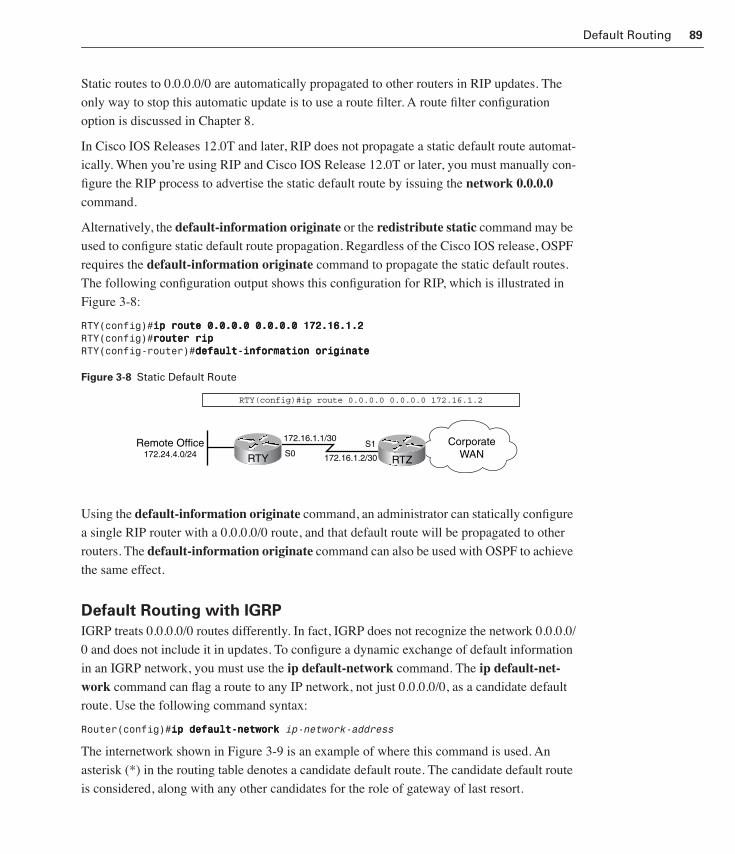
Default Routing 89
Static routes to 0.0.0.0/0 are automatically propagated to other routers in RIP updates. The
only way to stop this automatic update is to use a route filter. A route filter configuration
option is discussed in Chapter 8.
In Cisco IOS Releases 12.0T and later, RIP does not propagate a static default route automat-
ically. When you’re using RIP and Cisco IOS Release 12.0T or later, you must manually con-
figure the RIP process to advertise the static default route by issuing the network 0.0.0.0
command.
Alternatively, the default-information originate or the redistribute static command may be
used to configure static default route propagation. Regardless of the Cisco IOS release, OSPF
requires the default-information originate command to propagate the static default routes.
The following configuration output shows this configuration for RIP, which is illustrated in
Figure 3-8:
RTY(config)#iiiipppp rrrroooouuuutttteeee 0000....0000....0000....0000 0000....0000....0000....0000 111177772222....11116666....1111....2222RTY(config)#rrrroooouuuutttteeeerrrr rrrriiiippppRTY(config-router)#ddddeeeeffffaaaauuuulllltttt----iiiinnnnffffoooorrrrmmmmaaaattttiiiioooonnnn oooorrrriiiiggggiiiinnnnaaaatttteeee
Figure 3-8 Static Default Route
Using the default-information originate command, an administrator can statically configure
a single RIP router with a 0.0.0.0/0 route, and that default route will be propagated to other
routers. The default-information originate command can also be used with OSPF to achieve
the same effect.
Default Routing with IGRP
IGRP treats 0.0.0.0/0 routes differently. In fact, IGRP does not recognize the network 0.0.0.0/
0 and does not include it in updates. To configure a dynamic exchange of default information
in an IGRP network, you must use the ip default-network command. The ip default-net-work command can flag a route to any IP network, not just 0.0.0.0/0, as a candidate default
route. Use the following command syntax:
Router(config)#iiiipppp ddddeeeeffffaaaauuuulllltttt----nnnneeeettttwwwwoooorrrrkkkk ip-network-address
The internetwork shown in Figure 3-9 is an example of where this command is used. An
asterisk (*) in the routing table denotes a candidate default route. The candidate default route
is considered, along with any other candidates for the role of gateway of last resort.
RTZ
CorporateWAN
RTY(config)#ip route 0.0.0.0 0.0.0.0 172.16.1.2
172.16.1.1/30
S0S1
172.16.1.2/30
Remote Office172.24.4.0/24 RTY
1358_fmi.book Page 89 Thursday, May 27, 2004 2:21 PM
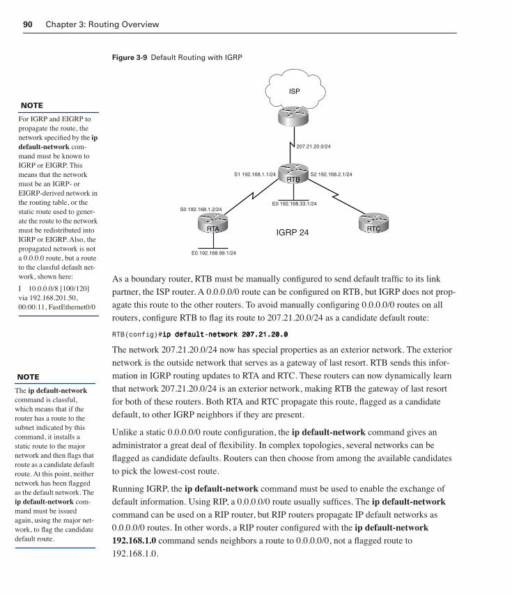
90 Chapter 3: Routing Overview
Figure 3-9 Default Routing with IGRP
As a boundary router, RTB must be manually configured to send default traffic to its link
partner, the ISP router. A 0.0.0.0/0 route can be configured on RTB, but IGRP does not prop-
agate this route to the other routers. To avoid manually configuring 0.0.0.0/0 routes on all
routers, configure RTB to flag its route to 207.21.20.0/24 as a candidate default route:
RTB(config)#iiiipppp ddddeeeeffffaaaauuuulllltttt----nnnneeeettttwwwwoooorrrrkkkk 222200007777....22221111....22220000....0000
The network 207.21.20.0/24 now has special properties as an exterior network. The exterior
network is the outside network that serves as a gateway of last resort. RTB sends this infor-
mation in IGRP routing updates to RTA and RTC. These routers can now dynamically learn
that network 207.21.20.0/24 is an exterior network, making RTB the gateway of last resort
for both of these routers. Both RTA and RTC propagate this route, flagged as a candidate
default, to other IGRP neighbors if they are present.
Unlike a static 0.0.0.0/0 route configuration, the ip default-network command gives an
administrator a great deal of flexibility. In complex topologies, several networks can be
flagged as candidate defaults. Routers can then choose from among the available candidates
to pick the lowest-cost route.
Running IGRP, the ip default-network command must be used to enable the exchange of
default information. Using RIP, a 0.0.0.0/0 route usually suffices. The ip default-network
command can be used on a RIP router, but RIP routers propagate IP default networks as
0.0.0.0/0 routes. In other words, a RIP router configured with the ip default-network 192.168.1.0 command sends neighbors a route to 0.0.0.0/0, not a flagged route to
192.168.1.0.
ISP
RTB
RTA RTC
207.21.20.0/24
S1 192.168.1.1/24 S2 192.168.2.1/24
S0 192.168.1.2/24E0 192.168.33.1/24
E0 192.168.99.1/24
IGRP 24
NOTE
The ip default-network command is classful, which means that if the router has a route to the subnet indicated by this command, it installs a static route to the major network and then flags that route as a candidate default route. At this point, neither network has been flagged as the default network. The ip default-network com-mand must be issued again, using the major net-work, to flag the candidate default route.
NOTE
For IGRP and EIGRP to propagate the route, the network specified by the ip default-network com-mand must be known to IGRP or EIGRP. This means that the network must be an IGRP- or EIGRP-derived network in the routing table, or the static route used to gener-ate the route to the network must be redistributed into IGRP or EIGRP. Also, the propagated network is not a 0.0.0.0 route, but a route to the classful default net-work, shown here:
I 10.0.0.0/8 [100/120] via 192.168.201.50, 00:00:11, FastEthernet0/0
1358_fmi.book Page 90 Thursday, May 27, 2004 2:21 PM

Default Routing 91
Default Route Caveats
A router does not use a gateway of last resort for addresses that are part of its local domain. A
local domain is a major network to which the router is connected. In Figure 3-10, RTX has
two interfaces configured with IP addresses that belong to the major network, 172.16.0.0.
Figure 3-10 RTX Has Two Interfaces Connected to the Major Network
If all three routers are running IGRP, RTX does not learn about the subnet 172.16.1.1/30
because a variable-length subnet mask is used. IGRP does not support VLSM.
A ping issued to 172.16.1.1 from RTX would be expected to use its default route to send the
ping to RTZ. RTX has interfaces connected to the major net 172.16.0.0. Therefore, RTX con-
siders 172.16.0.0 a local domain and does not use a default route to reach 172.16.1.0 or any
other local domain address. Without additional configuration, the ping will fail.
This problem may be solved in a number of ways. One approach is to configure the router
with the ip classless global configuration command. With ip classless enabled (this is the
Lab 3.6.2 Configuring IGRP
In this lab you configure IGRP for unequal-cost load balancing and tune the IGRP
timers to improve performance.
Lab 3.6.3 Configuring Default Routing with RIP and IGRP
In this lab you configure a default route and use RIP to propagate this default infor-
mation to other routers. The network must then be migrated from RIP to IGRP and
the default routing configured.
ISP
172.16.1.2/30
172.16.2.2/24
172.16.2.1/24
172.16.3.1/24
172.16.1.1/30
RTZ
RTX
RTY
172.16.3.2/24
1358_fmi.book Page 91 Thursday, May 27, 2004 2:21 PM

92 Chapter 3: Routing Overview
default in Cisco IOS Releases 11.3 and later), the router uses the best prefix match available,
including a supernet route, such as 172.0.0.0/8 or 0.0.0.0/0. By enabling ip classless, RTX
uses the 0.0.0.0/0 route to reach unknown subnets in its local domain, 172.16.0.0.
A second approach is to configure RTX with an explicit route for the major network
172.16.0.0:
RTX(config)#iiiipppp rrrroooouuuutttteeee 111177772222....11116666....0000....0000 222255555555....222255555555....0000....0000 111177772222....11116666....3333....1111
Without a more specific route available for 172.16.1.1, RTX uses the static route to the major
network number 172.16.0.0/16 and successfully routes packets destined for 172.16.1.1.
Floating Static RoutesOne of the disadvantages of static routing is that it cannot adapt to topology changes. How-
ever, you can configure static routing to have limited adaptability by creating floating static routes.
Floating static routes are static routes configured with an administrative distance value that is
greater than that of the primary route or routes. Floating static routes are fallback routes, or
backup routes, that do not appear in the routing table until another route to the same destina-
tion fails. Assume that RTB is connected to network 10.0.0.0/8 through two different links, as
shown in Figure 3-11, and that the RTB preferred route to network 10.0.0.0/8 is through RTC
because that link has a higher bandwidth. This route is learned by RIP. RTB should use the
slower link to 10.0.0.0/8 through RTA only if the primary route fails. The route to RTA is stat-
ically configured.
Figure 3-11 Sample Topology for Configuring Floating Static Routes
RTB
10.0.0.0/8
S0 1.1.1.2 S1 2.2.2.1
S0 1.1.1.1 S1 2.2.2.2
AdministrativeDistance = 130
AdministrativeDistance = 120
512 Kbps 768 Kbps
RTA RTC
1358_fmi.book Page 92 Thursday, May 27, 2004 2:21 PM

Convergence 93
Configuring Floating Static Routes
A floating static route must be used to statically configure RTB so that it will use the slower
link to reach 10.0.0.0/8 after the RIP route fails:
RTB(config)#iiiipppp rrrroooouuuutttteeee 11110000....0000....0000....0000 222255555555....0000....0000....0000 1111....1111....1111....1111 111133330000
This ip route command includes an administrative distance of 130. Recall that static routes
have a default administrative distance of 1 unless the local interface is used, in which case it
is 0. To create a floating static route, the administrative distance value must be manually con-
figured. This value must be greater than the primary route administrative distance value. In
this example, the primary route is learned by RIP and has an administrative distance of 120.
By configuring the static route with an administrative distance of 130, the static route is less
desirable than the primary route. The RIP route through RTC is preferred. However, if the
RIP route is lost, the floating static route takes its place in the routing table.
Floating static routes can be used in conjunction with other static routes to create a semi-
adaptable static routing scheme, as shown in Example 3-4.
If RTZ is configured with these commands, it installs one route to 0.0.0.0/0 using S0 and one
route to 4.0.0.0/8 using S2. If S0 becomes unavailable, RTZ installs the floating static route
to 0.0.0.0/0, using S1, into its routing table. If S2 fails, RTZ goes back to using S3 to reach
4.0.0.0/8. Finally, if both S2 and S3 go down, RTZ uses the least-desirable static route
to 4.0.0.0/8, with an administrative distance of 10.
ConvergenceThis process is both collaborative and independent. The routers share information with each
other, but they must individually recalculate their own routing tables. For individual routing
tables to be accurate, all routers must have a common view of the network topology. When all
Example 3-4 Configuring Floating Static Routes
RTZ(config)#iiiipppp rrrroooouuuutttteeee 0000....0000....0000....0000 0000....0000....0000....0000 sssseeeerrrriiiiaaaallll0000
RTZ(config)#iiiipppp rrrroooouuuutttteeee 0000....0000....0000....0000 0000....0000....0000....0000 sssseeeerrrriiiiaaaallll1111 5555
RTZ(config)#iiiipppp rrrroooouuuutttteeee 4444....0000....0000....0000 222255555555....0000....0000....0000 sssseeeerrrriiiiaaaallll2222
RTZ(config)#iiiipppp rrrroooouuuutttteeee 4444....0000....0000....0000 222255555555....0000....0000....0000 sssseeeerrrriiiiaaaallll3333 5555
RTZ(config)#iiiipppp rrrroooouuuutttteeee 4444....0000....0000....0000 222255555555....0000....0000....0000 sssseeeerrrriiiiaaaallll4444 11110000
Lab 3.6.4 Configuring Floating Static Routes
In this lab, you learn how to configure a floating static route.
1358_fmi.book Page 93 Thursday, May 27, 2004 2:21 PM

94 Chapter 3: Routing Overview
routers in a network agree on the topology, they are considered to have converged. Rapid
convergence means rapid recovery from link failure or other network changes. Routing proto-
cols and network designs are ultimately judged by how rapidly they converge.
Convergence Issues
When routers are in the process of converging, the network is susceptible to routing prob-
lems. Some routers learn that a link is down while others incorrectly believe it is still up. If
this happens, the individual tables are contradictory. This can lead to dropped packets or dev-
astating routing loops.
It is virtually impossible for all routers in a network to simultaneously detect a topology
change. Depending on the routing protocol in use, a significant amount of time might pass
before all of the routers in a network converge. Factors affecting the convergence time
include the following:
■ The routing protocol used
■ The distance of the router, or the number of hops from the point of change
■ How many routers in the network use dynamic routing protocols
■ The bandwidth and traffic load on communications links
■ The load on the router
■ The traffic patterns in relation to the topology change
The effects of some of these factors can be minimized through careful network design. A
network can be designed to minimize the load on any given router or communications link.
Other factors, such as the number of routers in the network, must be accepted as risks inher-
ent in network design. Large internetworks can reduce the number of routers that must con-
verge by using static default routes for stub networks.
Although proper network design can significantly reduce convergence time, the routing pro-
tocol’s ability to update and calculate routes efficiently also might improve convergence.
Route CalculationThis section covers the following:
■ Route calculation fundamentals
■ The initiation of routing updates
■ Routing metrics
1358_fmi.book Page 94 Thursday, May 27, 2004 2:21 PM

Route Calculation 95
Route Calculation Fundamentals
The capability of a routing protocol to update and calculate routes efficiently is based on sev-
eral factors:
■ Whether the protocol calculates and stores multiple routes to each destination
■ The manner in which routing updates are initiated
■ The metrics used to calculate distances or costs
The following sections discuss these three factors in detail.
Multiple Routes to a Single DestinationSome routing protocols allow the router to install only a single route to a destination network
in its routing table. Other routing protocols permit the router to store multiple routes to each
destination, at the cost of additional overhead, as illustrated in Figure 3-12. One advantage of
multiple routes is that equal-cost load balancing or unequal-cost load balancing may be used.
Another advantage is that maintaining multiple routes to a single destination reduces the net-
work’s vulnerability to routing loops and dropped packets when a link fails. If a router main-
tains two different routes to 10.0.0.0 and one route fails, the router can continue to route to
10.0.0.0 using the second route, without waiting for an alternative route to propagate. Main-
taining multiple routes does not reduce convergence time, but it can insulate a router from
instabilities during the convergence process.
Figure 3-12 Using Multiple Routes
10.0.0.0RTA RTC
Both RTA and RTCwill be used to get to the 10.0.0.0 network.
1358_fmi.book Page 95 Thursday, May 27, 2004 2:21 PM

96 Chapter 3: Routing Overview
The Initiation of Routing Updates
Routing protocols can instruct a router to update neighbors after a specific amount of time has
passed, after a certain event has occurred, or both. Time-driven routing protocols wait for the
update timer to expire and then send an update. RIP sends a complete update every 30 seconds
by default even if its routing table is unchanged since the last update, as shown in Figure 3-13.
In contrast, protocols that are event-driven do not require the router to update neighbors until
it detects a change in the network topology, as shown in Figure 3-14. Link-state protocols and
EIGRP send a partial update that includes only the changed information. Other protocols
might send their entire table when triggered by an event.
Figure 3-13 Timed Updates
Figure 3-14 Event-Driven Updates
Routing protocols that are exclusively time-driven react poorly to topology changes. If a
router detects a change but has to wait 30 seconds before alerting neighbors, routing in that
network could break down, and several minutes could pass before convergence. In the mean-
time, routers unaware of the change might send packets the wrong way, leading to routing
loops or loss of connectivity.
Routing protocols that are exclusively event-driven could go for extended periods of time
without sending updates. If there is no other mechanism to ensure that routers regularly
communicate, such as a Hello Timer, routers could base their routing decisions on outdated
information.
30 Seconds
Update
1358_fmi.book Page 96 Thursday, May 27, 2004 2:21 PM

Summary 97
For these reasons, most routing protocols use a combination of time-driven and event-driven
updates. RIP is time-driven, but the Cisco implementation of RIP sends triggered updates
whenever a change is detected. Topology changes also trigger immediate updates in IGRP
routers, regardless of the update timer. Without triggered updates, RIP and IGRP do not perform.
Protocols that are primarily event-driven typically use timers as well. OSPF routers assign a
MaxAge to the routing information. As soon as the information reaches its MaxAge, it can no
longer be used in the routing table, and a new update must be requested.
Routing Metrics
A routing metric is a value that measures desirability. Some routing protocols use only one
factor to calculate a metric. IP RIP uses hop count as the only factor to determine a route’s
metric. Other protocols base their metric on two or more factors, including hop count, band-
width, delay, load, and reliability.
Bandwidth and delay are static. They remain the same for each interface until the router is
reconfigured or the network is redesigned. Load and reliability are dynamic and are calcu-
lated for each interface in real time by the router.
The more factors that make up a metric, the greater the ability to adapt network operation to
meet specific needs. IGRP, by default, uses two static factors to calculate the metric—band-
width and delay. These can be configured manually, allowing precise control over what routes
a router chooses. IGRP can also be configured to include two dynamic factors in the metric
calculation—load and reliability. By using dynamic factors, IGRP routers can make decisions
based on changing conditions. Therefore, if a link becomes heavily loaded or unreliable,
IGRP increases the metric of routes using that link, and alternative routes presenting a lower
metric are used.
SummaryOne of the most important decisions in a network design is the selection of an appropriate
routing protocol or protocols. Such selection should be done carefully and with an apprecia-
tion of the decision’s long-term implications. This chapter provided an overview of the vari-
ous ways in which routing can be performed, as well as the benefits and limitations of each.
1358_fmi.book Page 97 Thursday, May 27, 2004 2:21 PM

98 Chapter 3: Routing Overview
Key Termsconvergence The speed and ability of a group of internetworking devices running a specific
routing protocol to agree on the topology of an internetwork after a change in that topology.
Dijkstra’s algorithm Also known as the shortest path first algorithm. A routing algorithm
that iterates on path length to determine a shortest-path spanning tree. Commonly used in
link-state routing algorithms.
distance vector routing A class of routing algorithms that iterate on the number of hops in
a route to find a shortest-path spanning tree. Distance vector routing algorithms call for each
router to send its entire routing table in each update, but only to its neighbors. Distance vector
routing algorithms can be prone to routing loops but are computationally simpler than link-
state routing algorithms.
dynamic routing Routers follow rules defined by routing protocols to exchange routing
information and independently select the best path.
floating static route A static route that is configured with an administrative distance value
that is greater than that of the primary route or routes. Used for fallback routes or backup
routes; they do not appear in the routing table until another route to the same destination fails.
legacy technology A technology that is supported because of a significant past investment
or deployment.
link-state routing A routing algorithm in which each router broadcasts or multicasts infor-
mation on the cost of reaching each of its neighbors to all nodes in the internetwork. Link-state
algorithms create a consistent view of the network and, therefore, are not prone to routing loops.
However, they achieve this at the cost of relatively greater computational difficulty and more
widespread traffic (compared with distance vector routing algorithms).
routing metric A method by which a routing algorithm determines that one route is better
than another. This information is stored in routing tables. Metrics include bandwidth, com-
munication cost, delay, hop count, load, path cost, and reliability. Sometimes it is simply
called a metric.
static routing An administrator manually defines routes to one or more destination networks.
1358_fmi.book Page 98 Thursday, May 27, 2004 2:21 PM

Check Your Understanding 99
Check Your UnderstandingComplete all of the review questions to test your understanding of the topics and concepts in
this chapter. The answers appear in Appendix B, “Answers to the Check Your Understanding
Questions.”
For additional, more in-depth questions, refer to the chapter-specific study guides on the
companion CD-ROM.
1. What is an advantage of static routing compared to dynamic routing?
A. Static routing sometimes yields unexpected results, even in small networks
B. Routers that don’t accept updates are less vulnerable to attack
C. The routing table contains only directly connected routes to router interfaces
D. Static routes remain in routing tables regardless of the mapped router interface status
2. What routing protocol would be used in a mixed-vender or legacy routing environment within an autonomous system?
A. RIPv1
B. RIPv2
C. IGRP
D. EIGRP
E. IS-IS
3. Which of the following commands would statically configure IGRP to use and propa-gate a default route?
A. ip route 0.0.0.0 255.255.255.255
B. ip default-network
C. ip route default-network
D. ip default network 0.0.0.0
4. What command must you use to automatically propagate a candidate default route to IGRP neighbors?
A. ip default-network ip-address
B. ip default-gateway ip-address
C. default-information originate
D. redistribute static neighbors
1358_fmi.book Page 99 Thursday, May 27, 2004 2:21 PM

100 Chapter 3: Routing Overview
5. What is a disadvantage of static routing?
A. It can cause unpredictable routing behavior
B. There is no mechanism to recover from a failed link
C. All route information is transmitted in each update
D. It produces high processor overhead
6. What is the primary purpose of configuring floating static routes?
A. To provide unlimited adaptability to network topology changes
B. To create a semiadaptable static routing scheme to activate backup routes
C. To create static routes with an administrative distance of 1
D. To create a static route that is more desirable than a dynamic route with equal
administrative distance
7. What would be a logical routing protocol configuration approach to significantly reduce the convergence time in a large internetwork?
A. Configure static default routes for stub networks
B. Increase the router processor and memory capacity
C. Configure static routes between all routers in the network
D. Decrease the number of hops between all routes in the network
8. How are stub networks defined?
A. Networks with only one router
B. Networks with multiple ways into and out of a network
C. Networks with only one ingress and egress point
D. Networks with routing policies that are controlled by a single organization
9. What mechanism ensures that a router configured with an event-driven routing protocol regularly communicates with its neighbors?
A. Hello timer
B. MaxAge timer
C. Triggered update
D. Update timer
1358_fmi.book Page 100 Thursday, May 27, 2004 2:21 PM

Check Your Understanding 101
10. What routing protocol measures route desirability based on bandwidth and delay and maintains a topological database?
A. RIPv2
B. RTMP
C. EIGRP
D. OSPF
E. IS-IS
F. NLSP
1358_fmi.book Page 101 Thursday, May 27, 2004 2:21 PM

ObjectivesUpon completing this chapter, you will be able to
■ Understand the operation of RIPv2
■ Configure RIPv2
■ Verify RIPv2 operation
You can reinforce your understanding of the objectives covered in this chapter by opening
the interactive media activities on the CD accompanying this book and performing the lab
activities collected in the Cisco Networking Academy Program CCNP 1: Advanced Routing
Lab Companion. Throughout this chapter, you will see references to these activities by title
and by icon. They look like this:
Interactive Media Activity
Lab Activity
1358_fmi.book Page 102 Thursday, May 27, 2004 2:21 PM

Chapter 4
Routing Information Protocol Version 2
Routing Information Protocol version 2 (RIPv2) is defined in RFC 1723 and is supported in
Cisco IOS Release 11.1 and later. RIPv2 is similar to RIPv1 but is not a new protocol. RIPv2
features extensions to bring it up-to-date with modern routing environments. The RIPv2 exten-
sions are as follows:
■ Subnet masks carried with each route entry
■ Authentication for routing updates
■ Next-hop addressing carried with each route entry
■ Route tags for external use
■ Queries in response to RIPv1 requests
The most important extension listed is the subnet mask field for routing-update entries. The sub-
net mask field enables the use of variable-length subnet masks (VLSMs) and qualifies RIPv2 as
a classless routing protocol.
RIPv2 is the first of the classless routing protocols discussed in this book. The following section
introduces classless routing and RIPv2.
RIPv2 OverviewAll of the operational procedures, timers, and stability functions of RIPv1 remain the same in
RIPv2, with the exception of the broadcast updates. RIPv2 sends updates to other RIPv2 inter-
network routers by multicasting. This occurs by using the reserved Class D address 224.0.0.9.
The advantage of multicasting is that devices on the local network that are not concerned with
1358_fmi.book Page 103 Thursday, May 27, 2004 2:21 PM

104 Chapter 4: Routing Information Protocol Version 2
RIP routing do not have to spend time unwrapping broadcast packets from the router. Multi-
cast updates are examined further in the section “Compatibility with RIPv1.”
After looking at how the RIP message format accommodates the version 2 extensions, this
section focuses on the operation and benefits of these additional features.
RIPv2 Operation
RIPv2 is a distance vector routing protocol. It supports VLSM, authentication, and multicast
updates. RIPv2 supports VLSM by including the subnet mask in the route information.
Neighbor routers are authenticated before the routes are exchanged. Because RIPv2 uses the
multicast address of 224.0.0.9, only devices that are part of the 224.0.0.9 multicast group
receive the RIPv2 updates.
Figures 4-1 through 4-5 illustrate how routers configured to run RIPv2 update their routing
tables. Router A in Figure 4-1 adds its directly connected network to its routing table. When
RIPv2 is enabled, it multicasts using 224.0.0.9 as the destination address to other RIP routers.
Router A uses “cisco” as the authentication password. Router A directly connected networks
have a metric of 0.
Figure 4-1 RIPv2 Network Operation
When Router B receives the routes from Router A, Router B updates its routing table, as
shown in Figure 4-2. The updates are sent through all connected interfaces at the next routing
update time interval. Notice that a metric of 1 was added to the 10.10.1.0 network. That is the
metric for the link between Router A and Router B. RIPv2 adds 1 to the metric value for
every hop the route passes.
Router A
10.10.1.0/24
Router B
10.10.3.0/24
Router C
10.10.5.0/24
Metric 1
Metric 1
Destination IP 244.0.0.9Authentication Password cisco
10.10.1.0 metric 010.10.2.0 metric 0
10.10.2.0/30 10.10.4.0/30
1358_fmi.book Page 104 Thursday, May 27, 2004 2:21 PM

RIPv2 Overview 105
Figure 4-2 RIPv2 Updates on Router B
When Router C receives the routes from Router B, Router C updates its routing table, as
shown in Figure 4-3. The updates are sent through all connected interfaces at the next routing
update time interval. The metric for network 10.10.1.0 changes to 2. This metric of 2 repre-
sents the sum of the two hops between Router A and Router C.
Figure 4-3 RIPv2 Updates on Router C
When Router B receives the routes from Router C, Router B updates its routing table, as
shown in Figure 4-4. The updates are sent through all connected interfaces at the next routing
update time interval. The metric for network 10.10.5.0 is 1. This represents the hop between
Router B and Router C.
Router A
10.10.1.0/24
Router B
10.10.3.0/24
Router C
10.10.5.0/24
Metric 1 Metric 1
Destination IP 244.0.0.9Authentication Password cisco
10.10.1.0 metric 110.10.2.0 metric 010.10.3.0 metric 010.10.4.0 metric 0
10.10.2.0/30 10.10.4.0/30
Router A
10.10.1.0/24
Router B
10.10.3.0/24
Router C
10.10.5.0/24
Metric 1 Metric 1
I Know About Networks10.10.1.0 metric 210.10.2.0 metric 110.10.3.0 metric 110.10.4.0 metric 010.10.5.0 metric 0
10.10.2.0/30
10.10.4.0/30
1358_fmi.book Page 105 Thursday, May 27, 2004 2:21 PM

106 Chapter 4: Routing Information Protocol Version 2
Figure 4-4 RIPv2 Updates on Router B
When Router A receives the routes from Router B, Router A updates its routing table, as
shown in Figure 4-5. The updates are sent through all connected interfaces at the next routing
update time interval. The metric for network 10.10.5.0 is 2. This metric of 2 represents the
sum of the two hops between Router A and Router C.
Figure 4-5 RIPv2 Operation
Now all of the routers have learned about all of the routes in the entire network and have
reached convergence.
Router A
10.10.1.0/24
Router B
10.10.3.0/24
Router C
10.10.5.0/24
Metric 1 Metric 1
Destination IP 244.0.0.9Authentication Password cisco
Networks10.10.1.0 metric 110.10.2.0 metric 010.10.3.0 metric 010.10.4.0 metric 010.10.5.0 metric 1
10.10.2.0/30 10.10.4.0/30
Router A
10.10.1.0/24
Router B
10.10.3.0/24
Router C
10.10.5.0/24
Metric 1 Metric 1
Destination IP 244.0.0.9Authentication Password cisco
Networks10.10.1.0 metric 010.10.2.0 metric 010.10.3.0 metric 110.10.4.0 metric 110.10.5.0 metric 2
10.10.2.0/30
10.10.4.0/30
1358_fmi.book Page 106 Thursday, May 27, 2004 2:21 PM

RIPv2 Overview 107
Issues Addressed by RIPv2
The following four features are the most significant new features added to RIPv2:
■ Authentication of the transmitting RIPv2 node to other RIPv2 nodes—RIPv2
added support for the authentication of the node that is transmitting response messages.
Response messages are used to propagate routing information throughout a network.
Authenticating the originator of a response message was intended to prevent routing
tables from being corrupted with illegitimate routes from a fraudulent source.
■ Subnet masks—RIPv2 allocates a four-octet field to associate a subnet mask to a des-
tination IP address. When used in tandem, the IP address and its subnet mask allow
RIPv2 to specifically identify the type of destination to which the route leads. This
allows RIPv2 to route to specific subnets, regardless of whether the subnet mask is
fixed or of variable length.
■ Next-hop IP addresses—The inclusion of a Next Hop identification field helps make
RIPv2 more efficient than RIPv1 by preventing unnecessary hops. This feature is par-
ticularly effective for network environments using multiple routing protocols simulta-
neously. Some routes go undiscovered when multiple or dissimilar routing protocols
exist.
■ Multicasting RIPv2 messages—Multicasting is a technique for simultaneously adver-
tising routing information to multiple RIPv2 devices. Multicasting is beneficial when-
ever multiple destinations must receive identical information.
RIPv2 Message Format
RIPv2 uses a special message format, or packet, to collect and share information about dis-
tances to known internetworked destinations, as shown in Figure 4-6. The basic structure is
the same as for RIPv1. All of the extensions to the original protocol are carried in the unused
fields. RIPv2 updates can contain entries for up to 25 routes, as in RIPv1. Like RIPv1, RIPv2
operates from UDP port 520, has an 8-byte header, and has a maximum datagram size of
512 bytes.
Interactive Media Activity Drag and Drop: RIPv1 and RIPv2 Comparison Table
In this activity, you identify the differences between RIPv1 and RIPv2.
1358_fmi.book Page 107 Thursday, May 27, 2004 2:21 PM

108 Chapter 4: Routing Information Protocol Version 2
Figure 4-6 RIPv2 Message Format
The Command field remains unchanged from RIPv1. It indicates whether the RIPv2 route
was generated as a request or as a response to a request.
The Version field is set to 2 for RIPv2. If it is set to 0 or 1 and the message is not a valid
RIPv1 format, the message is discarded. RIPv2 processes valid RIPv1 messages.
The Address Family Identifier (AFI) field is set to 2 for IP. The only exception is a request for
a full routing table of a router or host, in which case it is set to 0.
The Route Tag field provides a way to differentiate between internal and external routes. An
internal route is one that was learned by the RIPv2 protocols within the network or autono-
mous system. External routes are those that were learned from other routing protocols that
have been redistributed into the RIPv2 process. One suggested use of this 16-bit field is to
carry the autonomous system number of routes that have been imported from an external
routing protocol.
The IP Address field contains the destination address. It may be a major network address, a
subnet, or a host route.
The Subnet Mask field contains a 32-bit mask that identifies the network and subnet portion
of the IP address. The addition of this field is the single most important change made to the
RIPv2 message structure.
The Next Hop field contains the IP address of the next hop listed in the IP Address field.
32 Bits8 8 8 8
Command Version Unused (Set to All Zeros)
Address Family Identifier Route Tag
IP Address
Subnet Mask
Next Hop
Metric
Multiple Fields, Up to a Maximum of 25
RouteEntry
RouteEntry
Address Family Identifier Route Tag
IP Address
Subnet Mask
Next Hop
Metric
1358_fmi.book Page 108 Thursday, May 27, 2004 2:21 PM
RIPv2 Overview 109
The Metric field indicates how many internetwork hops or routers have been traversed in the
trip to the destination. This value is between 1 and 15 for a valid route or 16 for an unreach-
able route.
Compatibility with RIPv1
RIPv2 handles updates in a flexible manner. If the Version Number field in the RIPv2 Mes-
sage field indicates version 1, and if any bits in the unused field are set to 1, the update is
discarded. If the RIP version is greater than 1, the fields defined as unused are ignored,
and the message is processed. Therefore, newer versions of the RIP protocol are backward-
compatible with previous RIP versions.
RFC 1723 defines a compatibility switch with the following four settings, which allows ver-
sions 1 and 2 to interoperate:
1. RIPv1, in which only RIPv1 messages are transmitted
2. RIPv1 Compatibility, which causes RIPv2 to broadcast its messages instead of multi-casting them so that RIPv1 may receive them
3. RIPv2, in which RIPv2 messages are multicast to destination address 224.0.0.9
4. None, in which no updates are sent
RFC 1723 recommends that switches be configurable on a per-interface basis. The Cisco
commands for settings 1 through 3 are presented in the section “Configuring RIPv2.” The
Cisco command for setting 4 is accomplished by using the passive-interface command.
Additionally, RFC 1723 defines a receive control switch to regulate the reception of updates.
The four recommended settings of this switch are
1. RIPv1 only
2. RIPv2 only
3. Both
4. None
This switch should also be configurable on a per-interface basis. The Cisco commands for
settings 1 through 3 are also presented in the section “Configuring RIPv2.” Setting 4 can be
accomplished by using an access list to filter UDP source port 520, by not including a net-work statement for the interface, or by configuring a route filter.
Interactive Media Activity Drag and Drop: RIPv2 Packet
After completing this activity, you will be able to identify the different fields in a
RIPv2 packet.
1358_fmi.book Page 109 Thursday, May 27, 2004 2:21 PM

110 Chapter 4: Routing Information Protocol Version 2
Classless Route Lookups
Chapter 2, “Advanced IP Addressing Management,” explains classful route lookups, in which
a destination address is first matched to its major network address in the routing table and
then is matched to a subnet of the major network. If no match is found at either of these steps,
the packet is dropped.
This default behavior can be changed, even for classful routing protocols such as RIPv1 and
Interior Gateway Routing Protocol (IGRP). You change the default behavior by entering the
ip classless global command. When a router performs classless route lookups, it does not pay
attention to the class of the destination address. Instead, it performs a bit-by-bit best match
between the destination address and all its known routes. This capability can be very useful
when you’re working with default routes, as demonstrated in Chapter 3, “Routing Overview.”
Classless route lookups can be very powerful when coupled with the other features of class-
less routing protocols. According to rules of class, a router must keep eight separate table
entries for these Class B networks, as shown in Table 4-1. A CIDR-compliant router can sum-
marize these eight Class B networks based on their common bits of 10101100 00011, as
shown in Table 4-2.Table 4-1 Route Aggregation and Supernetting
Network Number First Octet Second Octet Third Octet Fourth Octet
172.24.0.0/16 10101100 00011000 00000000 00000000
172.25.0.0/16 10101100 00011001 00000000 00000000
172.26.0.0/16 10101100 00011010 00000000 00000000
172.27.0.0/16 10101100 00011011 00000000 00000000
172.28.0.0/16 10101100 00011100 00000000 00000000
172.29.0.0/16 10101100 00011101 00000000 00000000
172.30.0.0/16 10101100 00011110 00000000 00000000
172.31.0.0/16 10101100 00011111 00000000 00000000
Table 4-2 Classless Route Summarization
Network Number First Octet Second Octet Third Octet Fourth Octet
172.24.0.0/16 10101100 00011000 00000000 00000000
172.25.0.0/16 10101100 00011001 00000000 00000000
172.26.0.0/16 10101100 00011010 00000000 00000000
172.27.0.0/16 10101100 00011011 00000000 00000000
172.28.0.0/16 10101100 00011100 00000000 00000000
1358_fmi.book Page 110 Thursday, May 27, 2004 2:21 PM

RIPv2 Overview 111
Classless Routing Protocols
The true defining characteristic of classless routing protocols is their capability to carry sub-
net masks in their route advertisements. One benefit of having a mask associated with each
route is that the all-0s and all-1s subnets are now available for use. Classful routing protocols
cannot distinguish between an all-0s subnet, such as 172.16.0.0, and the major network num-
ber 172.16.0.0. Likewise, they cannot distinguish between a broadcast on the all-1s subnet
172.16.255.255 and an all-subnets broadcast 172.16.255.255.
If the subnet masks are included, this difficulty disappears. In this example, 172.16.0.0/16 is
the major network number, and 172.16.0.0/24 is an all-0s subnet. 172.16.255.255/16 and
172.16.255.255/24 are just as distinguishable.
By default, the Cisco IOS software rejects any attempt to configure an all-0s subnet as an
invalid address/mask combination, even if a classless routing protocol is running. To override
this default behavior, enter the global command ip subnet-zero. This command is the default
behavior in Cisco IOS Release 12.0 and later.
A much greater benefit of having a subnet mask associated with each route is being able to
use VLSM and being able to summarize a group of major network addresses with a single
aggregate address. Variable-length subnet masks and address aggregation or supernetting, are
examined in greater detail in Chapter 5, “EIGRP.”
The major classful routing protocols are
■ RIPv1
■ IGRP
■ BGP3
The major classless routing protocols are
■ RIPv2
■ EIGRP
■ OSPF
■ IS-IS
■ BGP4
Network Number First Octet Second Octet Third Octet Fourth Octet
172.29.0.0/16 10101100 00011101 00000000 00000000
172.30.0.0/16 10101100 00011110 00000000 00000000
172.31.0.0/16 10101100 00011111 00000000 00000000
Table 4-2 Classless Route Summarization (Continued)
1358_fmi.book Page 111 Thursday, May 27, 2004 2:21 PM
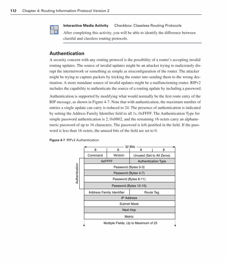
112 Chapter 4: Routing Information Protocol Version 2
Authentication
A security concern with any routing protocol is the possibility of a router’s accepting invalid
routing updates. The source of invalid updates might be an attacker trying to maliciously dis-
rupt the internetwork or something as simple as misconfiguration of the router. The attacker
might be trying to capture packets by tricking the router into sending them to the wrong des-
tination. A more mundane source of invalid updates might be a malfunctioning router. RIPv2
includes the capability to authenticate the source of a routing update by including a password.
Authentication is supported by modifying what would normally be the first route entry of the
RIP message, as shown in Figure 4-7. Note that with authentication, the maximum number of
entries a single update can carry is reduced to 24. The presence of authentication is indicated
by setting the Address Family Identifier field to all 1s, 0xFFFF. The Authentication Type for
simple password authentication is 2, 0x0002, and the remaining 16 octets carry an alphanu-
meric password of up to 16 characters. The password is left-justified in the field. If the pass-
word is less than 16 octets, the unused bits of the field are set to 0.
Figure 4-7 RIPv2 Authentication
Interactive Media Activity Checkbox: Classless Routing Protocols
After completing this activity, you will be able to identify the difference between
classful and classless routing protocols.
32 Bits8 8 8 8
Command Version Unused (Set to All Zeros)
0xFFFF Authentication Type
Password (Bytes 0-3)
Password (Bytes 4-7)
Password (Bytes 8-11)
Password (Bytes 12-15)
Aut
hent
icat
ion
Address Family Identifier Route Tag
IP Address
Subnet Mask
Next Hop
Metric
Multiple Fields, Up to Maximum of 25
1358_fmi.book Page 112 Thursday, May 27, 2004 2:21 PM

RIPv2 Overview 113
Example 4-1 shows an analyzer capture of a RIPv2 message with authentication. The output
reveals a security concern with default RIPv2 authentication. The password is transmitted in
plain text. Anyone who can capture a packet containing a RIPv2 update message can read the
authentication password.
Although RFC 1723 describes only simple password authentication, foresight is shown by
including the Authentication Type field. Cisco IOS software takes advantage of this feature
and provides the option of using Message Digest 5 (MD5) authentication instead of simple
password authentication. Cisco uses the first and last route entry spaces for MD5 authentica-
tion purposes.
Example 4-1 Message Capture
RIP (TCP/IP) - Routing Information Protocol
Decode Status: -
Command: 2 (Response)
Version: 2
Unused: 0x00
Entry 1
Address Family ID: 0xFFFFF Authentication
Authentication Type: 0x02 (Type 2)
Authentication: SunDevils
Entry 2
Address Family ID: 0x02 (IP)
Route Tag: 0x00
IP Address: 172.25.16.0
Subnet Mask: 255.255.255.0
Next Hop: 0.0.0.0
Metric: 0x1
Entry 3
Address Family ID: 0x02 (IP)
Route Tag: 0x00
IP Address: 172.25.16.0
Subnet Mask: 255.255.255.0
Next Hop: 0.0.0.0
Metric: 0x1
1358_fmi.book Page 113 Thursday, May 27, 2004 2:21 PM
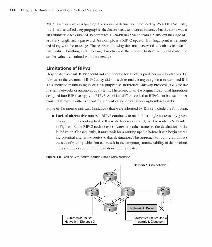
114 Chapter 4: Routing Information Protocol Version 2
MD5 is a one-way message digest or secure hash function produced by RSA Data Security,
Inc. It is also called a cryptographic checksum because it works in somewhat the same way as
an arithmetic checksum. MD5 computes a 128-bit hash value from a plain-text message of
arbitrary length and a password. An example is a RIPv2 update. This fingerprint is transmit-
ted along with the message. The receiver, knowing the same password, calculates its own
hash value. If nothing in the message has changed, the receiver hash value should match the
sender value transmitted with the message.
Limitations of RIPv2
Despite its overhaul, RIPv2 could not compensate for all of its predecessor’s limitations. In
fairness to the creators of RIPv2, they did not seek to make it anything but a modernized RIP.
This included maintaining its original purpose as an Interior Gateway Protocol (IGP) for use
in small networks or autonomous systems. Therefore, all of the original functional limitations
designed into RIP also apply to RIPv2. A critical difference is that RIPv2 can be used in net-
works that require either support for authentication or variable-length subnet masks.
Some of the more significant limitations that were inherited by RIPv2 include the following:
■ Lack of alternative routes—RIPv2 continues to maintain a single route to any given
destination in its routing tables. If a route becomes invalid, like the route to Network 1
in Figure 4-8, the RIPv2 node does not know any other routes to the destination of the
failed route. Consequently, it must wait for a routing update before it can begin assess-
ing potential alternative routes to that destination. This approach to routing minimizes
the size of routing tables but can result in the temporary unreachability of destinations
during a link or router failure, as shown in Figure 4-8.
Figure 4-8 Lack of Alternative Routes Slows Convergence
E
Network 1, Unreachable
Alternative Route:Network 1, Distance 3
Alternative Route: Use ANetwork 1, Distance 4
Network 1, Down
1
AC
B
D
1358_fmi.book Page 114 Thursday, May 27, 2004 2:21 PM

RIPv2 Overview 115
■ Counting to infinity—RIPv2 continues to rely on counting to infinity as a means of
resolving certain error conditions within the network. One such error condition is a
routing loop. RIPv2 remains dependent on timers to generate updates. Therefore, it is
also relatively slow to converge on a consensus of the network topology following any
change to that topology. The more time it takes to converge, the greater the opportunity
for obsolete information to be mistakenly propagated as current information. The result
could be a routing loop, as shown in Figure 4-9.
Figure 4-9 Routing Loop
■ 15-hop maximum—Perhaps the single greatest limitation that RIPv2 inherited from
RIP is that its interpretation of infinity remains at 16. After a route cost is incremented
to 16, that route becomes invalid, and the destination is considered unreachable, as
shown in Figure 4-10. This limits the use of RIPv2 to networks with a maximum diam-
eter of 15 or fewer hops.
Figure 4-10 Counting to Infinity
E
Network 1, Distance 6
Network 1Down
1
AC
B
D
Network 1, Distance 7
Network 1, Distance 4Network 1, Distance 5
E
Network 1, Distance 13
Network 1Down
1
AC
B
D
Network 1, Distance 14
Network 1, Distance 15Network 1, Distance 12
Routing Table
Maximum Metric is 16,Network 1 Is Unreachable
1358_fmi.book Page 115 Thursday, May 27, 2004 2:21 PM

116 Chapter 4: Routing Information Protocol Version 2
■ Static distance vector metrics—Another inherited limitation is found in the RIPv2
static cost metrics. The default value of 1 is just like RIP. However, the network admin-
istrator can manually adjust the default value. This metric remains constant; only the
administrator can change it. Therefore, RIPv2 remains unsuitable for network environ-
ments that require routes to be selected in real time based on either delay, traffic loads,
or any other dynamic network performance metric.
Configuring RIPv2RIPv2 is merely an enhancement of RIPv1; it is not a separate protocol. The commands for
manipulating timers, metrics, and updates are exactly the same in both versions. After a brief
look at configuring a RIPv2 process, the rest of this section concentrates on configuring the
new extensions.
Basic RIPv2 Configuration
When RIP is first enabled on a Cisco router, the router listens for version 1 and 2 updates but
sends only version 1. To take advantage of version 2 features, you must turn off version 1
support and enable version 2 updates with the following commands:
■ Enable RIPv2 on the router using the following commands:
Router(config)#rrrroooouuuutttteeeerrrr rrrriiiippppRouter(config-router)#vvvveeeerrrrssssiiiioooonnnn 2222Router(config-router)#nnnneeeettttwwwwoooorrrrkkkk network-number
By default, a RIP process configured on a Cisco router sends only RIPv1 messages but listens to both RIPv1 and RIPv2. This default is changed with the version command. In this mode, the router sends and receives only RIPv2 messages.
■ The router can also be configured to send and receive only RIPv1 messages:
Router(config)#rrrroooouuuutttteeeerrrr rrrriiiippppRouter(config-router)#vvvveeeerrrrssssiiiioooonnnn 1111Router(config-router)#nnnneeeettttwwwwoooorrrrkkkk network-number
You can restore the default behavior by entering the command no version in the config-router mode.
Compatibility with RIPv1
The interface-level compatibility switches recommended by RFC 1723 are implemented in
Cisco IOS software with the commands ip rip send version and ip rip receive version. The
New York router shown in Figure 4-11 is built with the configuration shown in Example 4-2.
1358_fmi.book Page 116 Thursday, May 27, 2004 2:21 PM

Configuring RIPv2 117
Figure 4-11 RIPv2 Compatibility with RIPv1
Interface FastEthernet0/0 is configured to send and receive RIPv1 updates, and
FastEthernet0/1 is configured to send both version 1 and 2 updates. FastEthernet0/2 has no
special configuration and, therefore, sends and receives version 2 by default.
Example 4-2 Configuration for the New York Router
NewYork(config)#iiiinnnntttteeeerrrrffffaaaacccceeee ffffaaaasssstttteeeetttthhhheeeerrrrnnnneeeetttt0000////0000
NewYork(config-if)#iiiipppp aaaaddddddddrrrreeeessssssss 111199992222....111166668888....55550000....111122229999 222255555555....222255555555....222255555555....111199992222
NewYork(config-if)#iiiipppp rrrriiiipppp sssseeeennnndddd vvvveeeerrrrssssiiiioooonnnn 1111
NewYork(config-if)#iiiipppp rrrriiiipppp rrrreeeecccceeeeiiiivvvveeee vvvveeeerrrrssssiiiioooonnnn 1111
NewYork(config)#iiiinnnntttteeeerrrrffffaaaacccceeee ffffaaaasssstttteeeetttthhhheeeerrrrnnnneeeetttt0000////1111
NewYork(config-if)#iiiipppp aaaaddddddddrrrreeeessssssss 111177772222....22225555....111155550000....111199993333 222255555555....222255555555....222255555555....222244440000
NewYork(config-if)#iiiipppp rrrriiiipppp sssseeeennnndddd vvvveeeerrrrssssiiiioooonnnn 1111 2222
NewYork(config)#iiiinnnntttteeeerrrrffffaaaacccceeee ffffaaaasssstttteeeetttthhhheeeerrrrnnnneeeetttt0000////2222
NewYork(config-if)#iiiipppp aaaaddddddddrrrreeeessssssss 111177772222....22225555....111155550000....222222225555 222222225555....222255555555....222255555555....222244440000
NewYork(config)#rrrroooouuuutttteeeerrrr rrrriiiipppp
NewYork(config-router)#vvvveeeerrrrssssiiiioooonnnn 2222
NewYork(config-router)#nnnneeeettttwwwwoooorrrrkkkk 111177772222....22225555....0000....0000
NewYork(config-router)#nnnneeeettttwwwwoooorrrrkkkk 111199992222....111166668888....55550000....0000
Interactive Media Activity Drag and Drop: RIPv2 Compatibility
After completing this activity, you will be able to identify the differences between
IGRP and EIGRP.
192.168.50.65/26 192.168.50.130/26
192.168.50.129/26
172.25.150.193/28
Fa 0/1
Fa 0/0
Fa 0/2172.25.150.225/28
172.25.150.226/28
172.25.150.33/28
172.25.150.194/28
172.25.150.206/28
London
Singapore
New York
San Jose
Honolulu
RIPv1
RIPv1 RIPv2
RIPv2
RIPv2
1358_fmi.book Page 117 Thursday, May 27, 2004 2:21 PM

118 Chapter 4: Routing Information Protocol Version 2
Discontiguous Subnets and Classless Routing
Route summarization reduces the amount of routing information in the routing tables. RIPv1
always uses automatic summarization. The default behavior of RIPv2 is to summarize at net-
work boundaries, the same as RIPv1. Use the no auto-summary command with the RIP pro-
cess to turn off summarization and allow subnets to be advertised across network boundaries.
This allows RIPv2 to perform routing between discontiguous subnets by advertising subnet
information, as shown in Figure 4-12. Example 4-3 shows an example of using the no auto-summary command.
Figure 4-12 Discontiguous Subnets
Configuring Authentication
The implementation of RIPv2 message authentication by Cisco includes the choice of a sim-
ple password or MD5 authentication and the option of defining multiple keys, or passwords,
on a key chain. The router then may be configured to use different keys at different times.
Plain-text authentication is the default setting in every RIPv2 packet.
The steps for setting up RIPv2 authentication are as follows:
Step 1 Define a key chain with a name.
Step 2 Define the key or keys on the key chain.
Lab 4.4.1 Routing Between RIPv1 and RIPv2
In this lab, you examine a networking scenario in which the RIPv1 and RIPv2 rout-
ing protocols are running. You also configure RIPv1 and RIPv2 routing protocols.
RIPv2 is configured to accept RIPv1 updates.
Example 4-3 no auto-summary Command
Router(config)#rrrroooouuuutttteeeerrrr rrrriiiipppp
Router(config-router)#vvvveeeerrrrssssiiiioooonnnn 2222
Router(config-router)#nnnnoooo aaaauuuuttttoooo----ssssuuuummmmmmmmaaaarrrryyyy
Site A Site B
10.0.0.4/30
207.21.24.32/27
207.21.24.0/27
1358_fmi.book Page 118 Thursday, May 27, 2004 2:21 PM
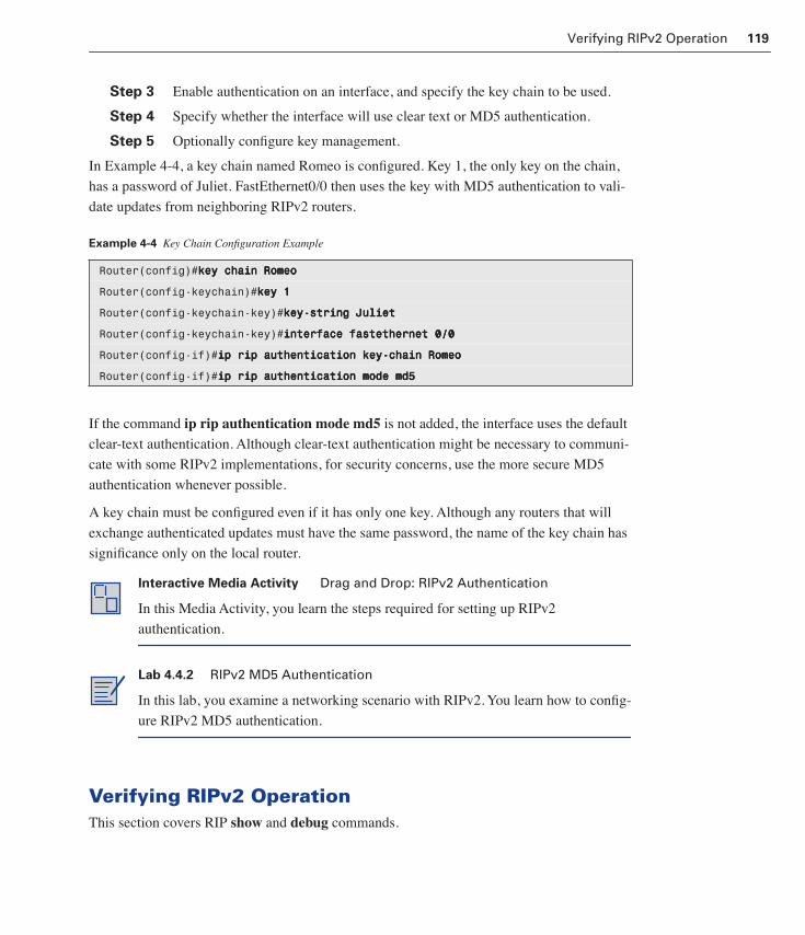
Verifying RIPv2 Operation 119
Step 3 Enable authentication on an interface, and specify the key chain to be used.
Step 4 Specify whether the interface will use clear text or MD5 authentication.
Step 5 Optionally configure key management.
In Example 4-4, a key chain named Romeo is configured. Key 1, the only key on the chain,
has a password of Juliet. FastEthernet0/0 then uses the key with MD5 authentication to vali-
date updates from neighboring RIPv2 routers.
If the command ip rip authentication mode md5 is not added, the interface uses the default
clear-text authentication. Although clear-text authentication might be necessary to communi-
cate with some RIPv2 implementations, for security concerns, use the more secure MD5
authentication whenever possible.
A key chain must be configured even if it has only one key. Although any routers that will
exchange authenticated updates must have the same password, the name of the key chain has
significance only on the local router.
Verifying RIPv2 OperationThis section covers RIP show and debug commands.
Example 4-4 Key Chain Configuration Example
Router(config)#kkkkeeeeyyyy cccchhhhaaaaiiiinnnn RRRRoooommmmeeeeoooo
Router(config-keychain)#kkkkeeeeyyyy 1111
Router(config-keychain-key)#kkkkeeeeyyyy----ssssttttrrrriiiinnnngggg JJJJuuuulllliiiieeeetttt
Router(config-keychain-key)#iiiinnnntttteeeerrrrffffaaaacccceeee ffffaaaasssstttteeeetttthhhheeeerrrrnnnneeeetttt 0000////0000
Router(config-if)#iiiipppp rrrriiiipppp aaaauuuutttthhhheeeennnnttttiiiiccccaaaattttiiiioooonnnn kkkkeeeeyyyy----cccchhhhaaaaiiiinnnn RRRRoooommmmeeeeoooo
Router(config-if)#iiiipppp rrrriiiipppp aaaauuuutttthhhheeeennnnttttiiiiccccaaaattttiiiioooonnnn mmmmooooddddeeee mmmmdddd5555
Interactive Media Activity Drag and Drop: RIPv2 Authentication
In this Media Activity, you learn the steps required for setting up RIPv2
authentication.
Lab 4.4.2 RIPv2 MD5 Authentication
In this lab, you examine a networking scenario with RIPv2. You learn how to config-
ure RIPv2 MD5 authentication.
1358_fmi.book Page 119 Thursday, May 27, 2004 2:21 PM
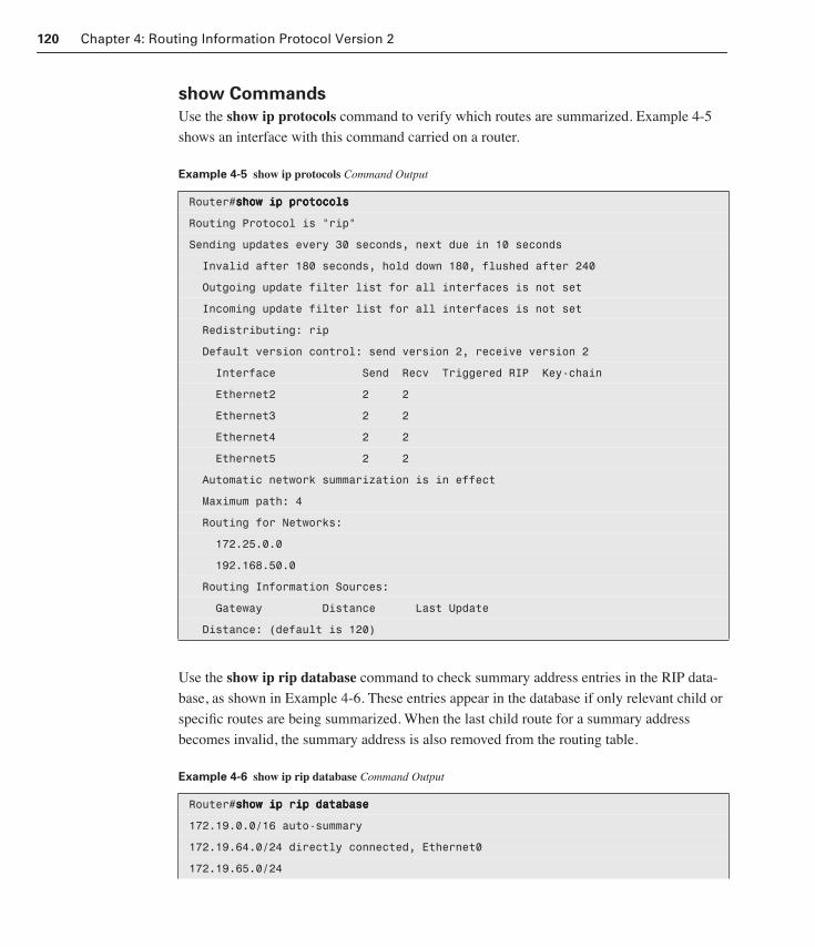
120 Chapter 4: Routing Information Protocol Version 2
show Commands
Use the show ip protocols command to verify which routes are summarized. Example 4-5
shows an interface with this command carried on a router.
Use the show ip rip database command to check summary address entries in the RIP data-
base, as shown in Example 4-6. These entries appear in the database if only relevant child or
specific routes are being summarized. When the last child route for a summary address
becomes invalid, the summary address is also removed from the routing table.
Example 4-5 show ip protocols Command Output
Router#sssshhhhoooowwww iiiipppp pppprrrroooottttooooccccoooollllssss
Routing Protocol is “rip“
Sending updates every 30 seconds, next due in 10 seconds
Invalid after 180 seconds, hold down 180, flushed after 240
Outgoing update filter list for all interfaces is not set
Incoming update filter list for all interfaces is not set
Redistributing: rip
Default version control: send version 2, receive version 2
Interface Send Recv Triggered RIP Key-chain
Ethernet2 2 2
Ethernet3 2 2
Ethernet4 2 2
Ethernet5 2 2
Automatic network summarization is in effect
Maximum path: 4
Routing for Networks:
172.25.0.0
192.168.50.0
Routing Information Sources:
Gateway Distance Last Update
Distance: (default is 120)
Example 4-6 show ip rip database Command Output
Router#sssshhhhoooowwww iiiipppp rrrriiiipppp ddddaaaattttaaaabbbbaaaasssseeee
172.19.0.0/16 auto-summary
172.19.64.0/24 directly connected, Ethernet0
172.19.65.0/24
1358_fmi.book Page 120 Thursday, May 27, 2004 2:21 PM

Verifying RIPv2 Operation 121
Use the show ip route EXEC command to display the current state of the routing table, as
shown in Example 4-7.
[1] via 172.19.70.36, 00:00:17, Serial1
[2] via 172.19.67.38, 00:00:25, Serial0
172.19.67.0/24 directly connected, Serial0
172.19.67.38/32 directly connected, Serial0
172.19.70.0/24 directly connected, Serial1
172.19.86.0/24
[1] via 172.19.67.38, 00:00:25, Serial0
[1] via 172.19.70.36, 00:00:17, Serial1
Example 4-7 show ip route Command
Router#sssshhhhoooowwww iiiipppp rrrroooouuuutttteeee
Codes: C - connected, S - static, I - IGRP, R - RIP, M - mobile, B - BGP
D - EIGRP, EX - EIGRP external, O - OSPF, IA - OSPF inter area
N1 - OSPF NSSA external type 1, N2 - OSPF NSSA external type 2
E1 - OSPF external type 1, E2 - OSPF external type 2, E - EGP
i - IS-IS, L1 - IS-IS level-1, L2 - IS-IS level-2, ia - IS-IS inter area
* - candidate default, U - per-user static route, o - ODR, P - periodic
downloaded static route
Gateway of last resort is not set
144.253.0.0/24 is subnetted, 1 subnets
C 144.253.100.0 is directly connected. FastEthernet0/1
R 133.3.0.0 [120/1] via 183.8.64.130, 00:00:17, Serial0/1
R 153.50.0.0 [120/1] via 183.8.128.12, 00:00:09, FastEthernet0/0
183.8.0.0/25 is subnetted, 4 subnets
R 183.8.0.128 [120/1] via 183.8.128.130, 00:00:17, Serial0/0
C 183.8.128.0 is directly connected, FastEthernet0/0
C 183.8.64.128 is directly connected, Serial0/1
C 183.8.128.128 is directly connected, FastEthernet0/0
Example 4-6 show ip rip database Command Output (Continued)
1358_fmi.book Page 121 Thursday, May 27, 2004 2:21 PM

122 Chapter 4: Routing Information Protocol Version 2
debug Commands
Two configuration problems common to RIPv2 are mismatched versions and misconfigured
authentication. Both difficulties are easy to discover with the following debugging com-
mands.
Use the debug ip rip EXEC command to display information on RIP routing transactions.
The no form of this command disables debugging output. Using the debug ip rip command
helps identify problems, such as a malformed packet from the sender. This is usually the case
when the following output is returned when this command is entered:
Router#ddddeeeebbbbuuuugggg iiiipppp rrrriiiippppRIP: bad version 128 from 160.89.80.43
Use the debug ip routing EXEC command to display information on RIP routing table
updates and route-cache updates. The no form of this command disables debugging output.
Using the debug ip routing command can help identify misconfiguration problems by moni-
toring the output, as shown in Example 4-8. Example 4-8 shows the “holddown” and “cache
invalidation” lines. Most of the distance vector routing protocols use “holddown” to avoid
typical problems, such as counting to infinity and routing loops. If you look at the output of
the show ip protocols command, you will see the timer values for “holddown” and “cache
invalidation.” “cache invalidation” corresponds to “came out of holddown.” “delete route” is
triggered when a better path comes along. It removes the old inferior path.
SummaryRIP is still used despite the emergence of more sophisticated routing protocols. RIP is
mature, stable, widely supported, and easy to configure. Although RIPv2 offers some decided
improvements over RIPv1, it is still limited to a maximum of 15 hops and small internet-
works. Design strategies such as VLSM have become very powerful tools for controlling pro-
tocols. One of the major improvements in and benefits of using RIPv2 compared to RIPv1 is
that RIPv2 provides authentication.
Example 4-8 debug ip routing Output
Router#ddddeeeebbbbuuuugggg iiiipppp rrrroooouuuuttttiiiinnnngggg
RT: delete route to 172.26.219.0 via 172.24.76.30, igrp metric [100/10816]
RT: no routes to 172.26.219.0, entering holddown
IP: cache invalidation from 0x115248 0x1378A, new version 5737
RT: 172.26.219.0 came out of holddown
1358_fmi.book Page 122 Thursday, May 27, 2004 2:21 PM

Key Terms 123
Key Termsconvergence The speed and ability of a group of internetworking devices running a specific
routing protocol to agree on an internetwork’s topology after a change in that topology.
metric A method by which a routing algorithm determines that one route is better than
another. This information is stored in routing tables. Metrics include bandwidth, communica-
tion cost, delay, hop count, load, path cost, and reliability.
multicasting A technique for simultaneously advertising routing information to multiple
RIPv2 devices.
RIPv2 (Routing Information Protocol version 2) Defined in RFC 1723 and supported in
Cisco IOS Release 11.1 and later. RIPv2 is not a new protocol; it is just RIPv1 with some
extensions to bring it up-to-date with modern routing environments. RIPv2 has been updated
to support VLSM, authentication, and multicast updates.
route summarization Consolidation of advertised addresses. This causes a single summary
route to be advertised to other routers.
routing update A message sent from a router to indicate network reachability and associ-
ated cost information. Routing updates are typically sent at regular intervals and after a
change in network topology.
1358_fmi.book Page 123 Thursday, May 27, 2004 2:21 PM

124 Chapter 4: Routing Information Protocol Version 2
Check Your UnderstandingComplete all of the review questions to test your understanding of the topics and concepts in this
chapter. The answers appear in Appendix B, “Answers to the Check Your Understanding Questions.”
For additional, more in-depth questions, refer to the chapter-specific study guides on the
companion CD-ROM.
1. What command disables the default network summarization in RIPv2?
A. no ip rip-summary
B. no rip auto-summarization
C. no auto-summary
D. no route-summarization
2. What command displays summary address entries in the RIP database?
A. show ip protocols
B. show ip route database
C. show ip rip database
D. show ip route
E. show ip rip
3. What command allows the use of the first subnet of any network?
A. ip subnet-zero
B. no ip subnet-zero
C. all-zero network
D. ip network-zero
4. What multicast address does RIPv2 use?
A. 224.0.0.4
B. 224.0.0.5
C. 224.0.0.8
D. 224.0.0.9
5. What is an advantage of multicasting RIPv2 updates instead of broadcasting them?
A. Ethernet interfaces ignore the multicast messages
B. It makes RIPv2 compatible with EIGRP and OSPF
C. Hosts and non-RIPv2 routers ignore the multicast messages
D. It enables faster convergence than RIPv1
1358_fmi.book Page 124 Thursday, May 27, 2004 2:21 PM

Check Your Understanding 125
6. Which statement describes the characteristics of RIPv1 and RIPv2?
A. RIPv1 imposes a maximum hop count of 16, and RIPv2 allows for a maximum of 32 hops
B. RIPv1 is classful, and RIPv2 is classless
C. RIPv1 uses only hop count, and RIPv2 uses hop count and bandwidth
D. RIPv1 sends periodical updates, and RIPv2 sends updates only as changes occur
7. Which three fields are now populated in the RIPv2 message format?
A. Route Tag
B. Subnet Mask
C. Autonomous System
D. Next Hop
E. Protocol
1358_fmi.book Page 125 Thursday, May 27, 2004 2:21 PM

ObjectivesUpon completing this chapter, you will be able to
■ Understand the fundamentals of EIGRP
■ Explain the features of EIGRP
■ Identify the components of EIGRP
■ Explain the principles of EIGRP operation
■ Configure EIGRP
■ Monitor EIGRP
You can reinforce your understanding of the objectives covered in this chapter by opening
the interactive media activities on the CD accompanying this book and performing the lab
activities collected in the Cisco Networking Academy Program CCNP 1: Advanced Routing
Lab Companion. Throughout this chapter, you will see references to these activities by title
and by icon. They look like this:
Interactive Media Activity
Lab Activity
1358_fmi.book Page 126 Thursday, May 27, 2004 2:21 PM

Chapter 5
EIGRP
Enhanced Interior Gateway Routing Protocol (EIGRP) is a Cisco-proprietary routing protocol
based on Interior Gateway Routing Protocol (IGRP). Unlike IGRP, which is a classful routing
protocol, EIGRP supports classless interdomain routing (CIDR), allowing network designers to
maximize address space by using CIDR and variable-length subnet masking (VLSM). Com-
pared to IGRP, EIGRP boasts faster convergence times, improved scalability, and superior han-
dling of routing loops.
EIGRP has been described as a hybrid routing protocol offering the best of distance vector and
link-state algorithms. Technically, EIGRP is an advanced distance vector routing protocol that
relies on features commonly associated with link-state protocols. The best traits of Open Short-
est Path First (OSPF), such as partial updates and neighbor discovery, are similarly used by
EIGRP. However, some benefits of OSPF, especially its hierarchical design, come at the price of
administrative complexity. Multiarea implementation of OSPF requires mastery of a complex
terminology and command set. Yet, EIGRP’s advanced features can be easily implemented and
maintained. Although it does not mirror the classic hierarchical design of OSPF, EIGRP is an
ideal choice for large, multiprotocol networks built primarily on Cisco routers.
This chapter surveys the key concepts, technologies, and data structures of EIGRP. This concep-
tual overview is followed by a study of EIGRP convergence and basic operation. Finally, this
chapter shows you how to configure and verify EIGRP and use route summarization.
EIGRP FundamentalsCisco released EIGRP in 1994 as a scalable, improved version of its proprietary distance vector
routing protocol, IGRP. IGRP and EIGRP are compatible with each other, although EIGRP
offers multiprotocol support and IGRP does not.
1358_fmi.book Page 127 Thursday, May 27, 2004 2:21 PM

128 Chapter 5: EIGRP
EIGRP and IGRP Compatibility
Despite being compatible with IGRP, EIGRP uses a different metric calculation and hop-
count limitation. EIGRP scales the IGRP metric by a factor of 256. This is because EIGRP
uses a metric that is 32 bits long, and IGRP uses a 24-bit metric. By multiplying or dividing
by 256, EIGRP can easily exchange information with IGRP. Both EIGRP and IGRP use the
following metric calculation:
metric = [K1 * bandwidth + (K2 * bandwidth)/(256 – load) + (K3 * delay)] *
[K5/(reliability + K4)]
The following are the default constant values:
K1 = 1, K2 = 0, K3 = 1, K4 = 0, K5 = 0
When K4 and K5 are 0, the [K5/(reliability + K4)] portion of the equation is not factored into
the metric. Constants K1 and K3 are the only ones set to 1 by default. Therefore, with the
default constant values, the metric equation is as follows:
metric = bandwidth + delay
IGRP and EIGRP, which scale the value by 256, use the following equations to determine the
values used in the metric calculation:
bandwidth for IGRP = (10000000/bandwidth)
bandwidth for EIGRP = (10000000/bandwidth) * 256
delay for IGRP = delay/10
delay for EIGRP = (delay/10) * 256
EIGRP also imposes a maximum hop limit of 224, which is slightly less than IGRP’s 255-
hop limit. However, this is more than enough to support most of the largest internetworks.
Getting dissimilar routing protocols, such as OSPF and Routing Information Protocol (RIP),
to share information requires advanced configuration. However, sharing or redistribution is
automatic between IGRP and EIGRP, as long as both processes use the same autonomous
system (AS) number. In Figure 5-1, RTB automatically redistributes routes learned by
EIGRP to the IGRP AS, and vice versa. To do this, the configuration shown in Example 5-1 is
entered on RTB.
1358_fmi.book Page 128 Thursday, May 27, 2004 2:21 PM

EIGRP Fundamentals 129
Figure 5-1 Using EIGRP with IGRP
EIGRP tags routes learned from IGRP, or any outside source, as external because they do not
originate from EIGRP routers. On the other hand, IGRP cannot differentiate between internal
and external routes. Notice that in the show ip route command output for RTA and RTC,
shown in Example 5-2, EIGRP routes are flagged with D, and external routes are denoted by
EX. RTA differentiates between the network learned via EIGRP (172.16.0.0) and the network
redistributed from IGRP (192.168.1.0). The table on RTC shows that IGRP makes no such
distinction.
Example 5-1 Using EIGRP with IGRP Configuration
RTB(config)#rrrroooouuuutttteeeerrrr iiiiggggrrrrpppp 2222444444446666
RTB(config-router)#nnnneeeettttwwwwoooorrrrkkkk 111199992222....111166668888....1111....0000
RTB(config)#rrrroooouuuutttteeeerrrr eeeeiiiiggggrrrrpppp 2222444444446666
RTB(config-router)#nnnneeeettttwwwwoooorrrrkkkk 11110000....1111....1111....0000
RTB(config-router)#nnnneeeettttwwwwoooorrrrkkkk 111177772222....11116666....1111....0000
Example 5-2 Routing Tables Using EIGRP with IGRP
RTA#sssshhhhoooowwww iiiipppp rrrroooouuuutttteeee
<output omitted>
C 10.1.1.0 is directly connected, Serial0
D 172.16.1.0 [90/2681856] via 10.1.1.1, Serial0
D EX 192.168.1.0 [170/2681859] via 10.1.1.1, 00:00:04, Serial0
RTC#sssshhhhoooowwww iiiipppp rrrroooouuuutttteeee
<output omitted>
C 192.168.1.0 is directly connected, Serial0
I 10.0.0.0 [100/10476] via 192.168.1.0, 00:00:04, Serial0
I 172.16.1.0 [100/10476] via 192.168.1.0, 00:00:04, Serial0
RTA RTCRTB
10.1.1.0/24
172.16.1.0/24
192.168.1.0/24
EIGRP 2446 IGRP 2446
1358_fmi.book Page 129 Thursday, May 27, 2004 2:21 PM

130 Chapter 5: EIGRP
RTC, which is running IGRP only, sees only IGRP routes, despite the fact that both 10.1.1.0
and 172.16.0.0 were redistributed from EIGRP.
EIGRP Design
Even though EIGRP is compatible with IGRP, it operates quite differently from its predeces-
sor. As an advanced distance vector routing protocol, EIGRP acts like a link-state protocol
when updating neighbors and maintaining routing information. The advantages of EIGRP
over simple distance vector protocols include the following:
■ Rapid convergence—EIGRP routers converge quickly because they rely on a state-of-
the-art routing algorithm called the Diffusing Update Algorithm (DUAL). DUAL guar-
antees loop-free operation at every instant during route computation and allows all
routers involved in a topology change to synchronize more quickly.
■ Efficient use of bandwidth—EIGRP makes efficient use of bandwidth by sending par-
tial, bounded updates. It also consumes minimal bandwidth when the network is stable:
— Partial, bounded updates—EIGRP routers make partial, incremental updates
rather than sending their complete tables. This is similar to OSPF operation.
However, unlike OSPF routers, EIGRP routers send these partial updates only to
the routers that need the information. They do not send to all routers in an area.
For this reason, they are called bounded updates.
— Minimal consumption of bandwidth when the network is stable—EIGRP
does not use timed routing updates. Instead, EIGRP routers keep in touch with
each other using small hello packets. Although they are exchanged regularly,
hello packets do not use a significant amount of bandwidth.
■ Support for VLSM and CIDR—Unlike IGRP, EIGRP offers full support for classless
IP addressing by exchanging subnet masks in routing updates.
■ Multiple network layer support—EIGRP supports IP, Internetwork Packet Exchange
(IPX), and AppleTalk through protocol-dependent modules (PDMs).
■ Independence from routed protocols—PDMs protect EIGRP from painstaking revi-
sion. Evolution of a routed protocol, such as IP, might require a new protocol module
but not necessarily a reworking of EIGRP itself.
Interactive Media Activity Drag and Drop: IGRP and EIGRP Comparison
After completing this activity, you will be able to identify the differences between
IGRP and EIGRP.
Interactive Media Activity Drag and Drop: EIGRP Metric Calculation
After completing this activity, you will be able to identify the equation for calculat-
ing EIGRP and IGRP metrics.
1358_fmi.book Page 130 Thursday, May 27, 2004 2:21 PM

EIGRP Features 131
EIGRP Terminology
EIGRP routers keep route and topology information readily available in Random Access
Memory so that they can react quickly to changes. Like OSPF, EIGRP keeps this information
in several tables, or databases. The following terms are related to EIGRP and its tables and
are used throughout this chapter:
■ Neighbor table—Each EIGRP router maintains a neighbor table that lists adjacent
routers. This table is comparable to the adjacency database used by OSPF. There is a
neighbor table for each protocol EIGRP supports.
■ Topology table—Every EIGRP router maintains a topology table for each configured
network protocol. This table includes route entries for all destinations that the router
has learned. All learned routes to a destination are maintained in the topology table.
■ Routing table—EIGRP chooses the best routes to a destination from the topology table
and places these routes in the routing table. Each EIGRP router maintains a routing
table for each network protocol.
■ Successor—A successor is a route selected as the primary route to use to reach a desti-
nation. Successors are the entries kept in the routing table. Multiple successors for a
destination can be retained in the routing table.
■ Feasible successor—A feasible successor is a backup route. These routes are selected
at the same time the successors are identified, but they are kept in the topology table.
Multiple feasible successors for a destination can be retained in the topology table.
EIGRP FeaturesThe following sections describe some of the main features that make up EIGRP. These tech-
nologies fall into one of the following four categories:
■ Neighbor discovery and recovery
■ Reliable Transport Protocol
■ DUAL finite-state machine
■ Protocol-specific modules
The following sections examine these technologies in detail.
Interactive Media Activity Matching: EIGRP Terminology
After completing this activity, you will be able to identify EIGRP terminology.
1358_fmi.book Page 131 Thursday, May 27, 2004 2:21 PM

132 Chapter 5: EIGRP
EIGRP Technologies
EIGRP includes many new technologies. Each of these represents an improvement in operating
efficiency, rapidity of convergence, or functionality relative to IGRP and other routing protocols.
Neighbor Discovery and Recovery
Remember that simple distance vector routers do not establish any relationship with their
neighbors. RIP and IGRP routers merely broadcast or multicast updates on configured inter-
faces. In contrast, EIGRP routers actively establish relationships with their neighbors, much
the same way OSPF routers do.
EIGRP routers establish adjacencies with neighbor routers by using small hello packets, as
shown in Figure 5-2. Hellos are sent by default every 5 seconds. An EIGRP router assumes
that as long as it is receiving hello packets from known neighbors, those neighbors (and their
routes) remain viable. By forming adjacencies, EIGRP routers do the following:
■ Dynamically learn of new routes that join their network
■ Identify routers that become either unreachable or inoperable
■ Rediscover routers that previously were unreachable
Figure 5-2 EIGRP Routers Establish Adjacencies
Topology TableA B
A B
Update
ACK
Hello
ACK
Update
This is Router A, who is on the link?
Here is the routing information.
Thanks for the information.
Here is the route information.
Thanks for the information.
Converged
1358_fmi.book Page 132 Thursday, May 27, 2004 2:21 PM

EIGRP Features 133
Reliable Transport Protocol
Reliable Transport Protocol (RTP) is a proprietary transport-layer protocol that can guarantee
ordered delivery of EIGRP packets to all neighbors. On an IP network, hosts use TCP to
sequence packets and ensure their timely delivery. However, EIGRP is protocol-independent.
Therefore, EIGRP does not rely on TCP/IP to exchange routing information the way RIP
does. To stay independent of IP, EIGRP uses its own proprietary transport-layer protocol,
RTP, to guarantee delivery of routing information.
EIGRP can call on RTP to provide reliable or unreliable service as the situation warrants. For
example, hello packets do not require the overhead of reliable delivery because they are frequent
and should be kept small. The reliable delivery of other routing information can actually speed
convergence because EIGRP routers are not waiting for a timer to expire before they retransmit.
With RTP, EIGRP can multicast and unicast to different peers simultaneously, allowing for
maximum efficiency.
DUAL Finite-State Machine
The focal point of EIGRP is DUAL. This is EIGRP’s route-calculation engine. The full name
of this technology is DUAL finite-state machine (FSM). An FSM is an abstract machine, not
a mechanical device with moving parts. It defines a set of possible states that something can
go through, what events cause those states, and what events result from those states. Design-
ers use FSMs to describe how a device, computer program, or routing algorithm will react to
a set of input events. The DUAL FSM contains all of the logic used to calculate and compare
routes in an EIGRP network.
DUAL tracks all of the routes advertised by neighbors in addition to using the composite met-
ric of each route to compare them. DUAL also guarantees that each path is loop-free. DUAL
then inserts the lowest-cost paths into the routing table.
As noted earlier, EIGRP keeps important route and topology information readily available.
This information is stored in a neighbor table and a topology table. These tables supply
DUAL with comprehensive route information in case of network disruption. DUAL quickly
selects alternative routes by using the information in these tables. If a link goes down, DUAL
looks for a feasible successor in its neighbor and topology tables.
Interactive Media Activity Drag and Drop: EIGRP Operation
After completing this activity, you will be able to identify the four key steps of
EIGRP operation.
Interactive Media Activity Checkbox: Reliable Transport Protocol
After completing this activity, you will be able to identify the operation of RTP.
1358_fmi.book Page 133 Thursday, May 27, 2004 2:21 PM

134 Chapter 5: EIGRP
A successor is a neighboring router that is currently being used for packet forwarding. A suc-
cessor also provides the least-cost route to the destination and is not part of a routing loop.
Feasible successors provide the next lowest-cost path without introducing routing loops. Fea-
sible successor routes can be used if the existing route fails. Packets to the destination net-
work are immediately forwarded to the feasible successor. The router is then promoted to the
status of successor. This process is shown in Figures 5-3 through 5-9.
Figure 5-3 D Has a Route via B and C
Figure 5-4 Successor Route for D Goes Down
(a)
(1)
(1)
(1)
(1)
(2)(2)
A
B
C
D
E
C EIGRP FD AD Topology
(a) 3 (fd)via B 3 1 (Successor)via D 4 2 (fs)via E 4 3
D EIGRP FD AD Topology
(a) 2 (fd)via B 2 1 (Successor)via C 5 3
E EIGRP FD AD Topology
(a) 3 (fd)via D 3 2 (Successor)via C 4 3
(a)
(1)
(1)
(1)
(1)
(2)(2)
A
B
C
D
E
C EIGRP FD AD Topology
(a) 3 (fd)via B 3 1 (Successor)via D 4 2 (fs)via E 4 3
D EIGRP FD AD Topology
(a) 2 (fd)via B 2 1 (Successor)via C 5 3
E EIGRP FD AD Topology
(a) 3 (fd)via D 3 2 (Successor)via C 4 3
1358_fmi.book Page 134 Thursday, May 27, 2004 2:21 PM

EIGRP Features 135
Figure 5-5 D Sends Queries to Begin Looking for a Feasible Successor
Figure 5-6 E Queries C to Find a New Route
(a)
(1)
(1)
(1)
(2)(2)
A
B
C
D
E
C EIGRP FD AD Topology
(a) 3 (fd)via B 3 1 (Successor)via D via E 4 3
D EIGRP FD AD Topology
(a)**ACTIVE**–1 (fd)via B (q)via C 5 3
E EIGRP FD AD Topology
(a) 3 (fd)via D 3 2 (Successor)via C 4 3
Q Q
(a)
(1)
(1)
(1)
(2)(2)
A
B
C
D
E
C EIGRP FD AD Topology
(a) 3 (fd)via B 3 1 (Successor)via D 4 2 (fs)via E 4 3
D EIGRP FD AD Topology
(a) **ACTIVE** –1 (fd)via B (q)via C 5 3 (q)
E EIGRP FD AD Topology
(a) **ACTIVE** –1 (fd)via Dvia C 4 3 (q)
R
Q
1358_fmi.book Page 135 Thursday, May 27, 2004 2:21 PM

136 Chapter 5: EIGRP
Figure 5-7 C Sends a Reply to E Stating That a Feasible Successor Already Exists
Figure 5-8 E Sends the Reply to D to Inform D of the Existing Feasible Successor
(a)
(1)
(1)
(1)
(2)(2)
A
B
C
D
E
C EIGRP FD AD Topology
(a) 3 (fd)via B 3 1 (Successor)via Dvia E
D EIGRP FD AD Topology
(a) **ACTIVE** –1 (fd)via E (q)via C 5 3
E EIGRP FD AD Topology
(a) 4 (fd)via C 4 3 (Successor)via D
R
(a)
(1)
(1)
(1)
(2)(2)
A
B
C
D
E
C EIGRP FD AD Topology
(a) 3 (fd)via B 3 1 (Successor)via Dvia E
D EIGRP FD AD Topology
(a) 5 (fd)via E 5 3 (Successor)via C 5 4
E EIGRP FD AD Topology
(a) 4 (fd)via C 4 3 (Successor)via D
R
1358_fmi.book Page 136 Thursday, May 27, 2004 2:21 PM

EIGRP Features 137
Figure 5-9 D Has a New Successor and Route via C and E
Notice that in Figure 5-3, Router D does not identify a feasible successor. The feasible dis-tance (FD) for Router D to Router A is 2, and the advertised distance (AD) by way of Router
C is 3. Because the AD is smaller than the best-route metric but larger than the FD, no feasi-
ble successor is placed in the topology table. Router C has a feasible successor identified as
well as Router E because the router is loop-free and because the AD for the next-hop router is
less than the FD for the successor.
Protocol-Dependent Modules
The modular design is one of the most attractive features of EIGRP. Modular designs are the
most scalable and adaptable. Support for routed protocols such as IP, IPX, and AppleTalk is
included in EIGRP through protocol-dependent modules (PDMs). In theory, EIGRP can eas-
ily adapt to new or revised routed protocols by adding PDMs.
Each PDM is responsible for all functions related to its specific routed protocol, as shown in
Figure 5-10. The IP-EIGRP module is responsible for the following:
■ Sending and receiving EIGRP packets that bear IP data
■ Notifying DUAL of new IP routing information that is received
■ Maintaining the results of DUAL routing decisions in the IP routing table
■ Redistributing routing information that was learned by other IP-capable routing protocols
(a)
(1)
(1)
(1)
(2)(2)
A
B
C
D
E
C EIGRP FD AD Topology
(a) 3 (fd)via B 3 1 (Successor)via Dvia E
D EIGRP FD AD Topology
(a) 5 (fd)via C 5 3 (Successor)via E 5 4 (Successor)
E EIGRP FD AD Topology
(a) 4 (fd)via C 4 3 (Successor)via D
1358_fmi.book Page 137 Thursday, May 27, 2004 2:21 PM

138 Chapter 5: EIGRP
Figure 5-10 EIGRP PDMs
EIGRP ComponentsAs with any routing protocol, several components contribute to the proper functionality of
EIGRP. The following sections cover these components—EIGRP packet types, EIGRP
tables, and route tagging.
EIGRP Packet Types
Like OSPF, EIGRP relies on several kinds of packets to maintain its various tables and estab-
lish complex relationships with neighbor routers:
■ Hello
■ Acknowledgment
■ Update
■ Query
■ Reply
The following sections describe these packet types in detail.
Hello PacketsEIGRP relies on hello packets to discover, verify, and rediscover neighbor routers. Rediscov-
ery occurs if EIGRP routers do not receive each other’s hellos for a hold time interval but
then reestablish communication.
Neighbor Table-Apple Talk
Neighbor Table-IPX
Neighbor Table-IPNet-HopRouter
Interface
Topology Table-Apple Talk
Topology Table-IPX
Topology-IPDestination 1Destination 1
SuccessorFeasible Successor
Routing Table-Apple Talk
Routing Table-IPX
Routing Table-IPDestination 1 Successor
1358_fmi.book Page 138 Thursday, May 27, 2004 2:21 PM

EIGRP Components 139
EIGRP routers send hellos at a fixed and configurable interval, called the hello interval. The
default hello interval depends on the interface’s bandwidth, as outlined in Table 5-1.
EIGRP hello packets are multicast. On IP networks, EIGRP routers send hellos to the multi-
cast IP address 224.0.0.10.
An EIGRP router stores information about neighbors in the neighbor table, including the last
time each neighbor responded. The information is stored only if any of its EIGRP packets,
hello or otherwise, are received. If a neighbor is not heard from for the duration of the hold
time, EIGRP considers that neighbor down, and DUAL must step in to reevaluate the routing
table. By default, the hold time is 3 times the hello interval, but an administrator can config-
ure both timers as desired.
OSPF (which is covered in Chapter 6, “OSPF”) requires neighbor routers to have the same
hello and dead intervals to communicate. EIGRP has no such restriction. Neighbor routers
learn about each other’s respective timers through the exchange of hello packets. They use
that information to forge a stable relationship, even with unlike timers.
Acknowledgment PacketsAn EIGRP router uses acknowledgment packets to indicate receipt of any EIGRP packet dur-
ing a reliable exchange. Recall that RTP can provide reliable communication between EIGRP
hosts. To be reliable, a sender’s message must be acknowledged by the recipient. Acknowl-
edgment packets, which are dataless hello packets, are used for this purpose. Unlike multicast
hellos, acknowledgment packets are unicast. Acknowledgments can also be made by piggy-
backing on other kinds of EIGRP packets, such as reply packets. Hello packets are always
sent unreliably and, therefore, do not require acknowledgment.
Update PacketsUpdate packets are used when a router discovers a new neighbor. An EIGRP router sends
unicast update packets to that new neighbor so that the new router can add to its topology
table. More than one update packet might be needed to convey all the topology information to
the newly discovered neighbor.
Table 5-1 Default Hello Intervals and Hold Times for EIGRP
Bandwidth Sample Link Default Hello Interval Default Hold Time
1.544 Mbps or less
T1, multipoint Frame Relay
60 seconds 180 seconds
Greater than 1.544 Mbps
Ethernet 5 seconds 15 seconds
1358_fmi.book Page 139 Thursday, May 27, 2004 2:21 PM

140 Chapter 5: EIGRP
Update packets are also used when a router detects a topology change. In this case, the
EIGRP router sends a multicast update packet to all neighbors, alerting them to the change.
All update packets are sent reliably.
Query and Reply PacketsAn EIGRP router uses query packets whenever it needs specific information from one or all
of its neighbors. A reply packet is used to respond to a query.
If an EIGRP router loses its successor and cannot find a feasible successor for a route, DUAL
places the route in the active state. At this point, the router multicasts a query to all neighbors,
searching for a successor to the destination network. Neighbors must send replies that either
provide information on successors or indicate that no successor information is available.
Queries can be multicast or unicast, whereas replies are always unicast. Both packet types are
sent reliably.
EIGRP Tables
DUAL can select alternative routes based on the tables kept by EIGRP. By building these
tables, every EIGRP router can track all of the routing information in an AS, not just the best
routes.
The following sections examine the EIGRP neighbor table and the EIGRP topology table in
detail and provide an example of each. In addition, the various packet types used by EIGRP
to build and maintain these tables are investigated.
The Neighbor TableThe most important table in EIGRP is the neighbor table, shown in Example 5-3. The neigh-
bor relationships tracked in the neighbor table are the basis of all the EIGRP routing update
and convergence activity.
Interactive Media Activity Drag and Drop: EIGRP Timer Basics
After completing this activity, you will be able to identify the default hello intervals
and hold times for EIGRP.
Interactive Media Activity Drag and Drop: EIGRP Packet Types
After completing this activity, you will be able to identify the different EIGRP packet
types.
1358_fmi.book Page 140 Thursday, May 27, 2004 2:21 PM

EIGRP Components 141
The neighbor table contains information about adjacent neighboring EIGRP routers. When-
ever a new neighbor is discovered, its address and the interface used to reach it are recorded
in a new neighbor table entry.
A neighbor table is used to support reliable, sequenced delivery of packets. One field in each
row of the table includes the sequence number of the last packet received from that neighbor.
EIGRP uses this field to acknowledge a neighbor’s transmission and to identify packets that
are out of sequence.
An EIGRP neighbor table includes the following key elements:
■ Neighbor address (address)—The network layer address of the neighbor router.
■ Hold time (hold uptime)—The interval to wait without receiving anything from a
neighbor before considering the link unavailable. Originally, the expected packet was
a hello packet. However, in current Cisco IOS software releases, any EIGRP packets
received after the first hello reset the timer.
■ Smooth Round-Trip Timer (SRTT)—The average amount of time it takes to send and
receive packets to and from a neighbor. This timer is used to determine the retransmit
interval.
■ Queue count (Q Cnt)—The number of packets waiting in queue to be sent. If this value
is constantly higher than 0, there might be a congestion problem at the router. A 0
means that no EIGRP packets are in the queue.
Note that an EIGRP router can maintain multiple neighbor tables, one for each PDM running,
such as IP, IPX, and AppleTalk. A router must run a unique EIGRP process for each routed
protocol, as shown in Figure 5-10.
Example 5-3 EIGRP Neighbor Tables
Router#sssshhhhoooowwww iiiipppp eeeeiiiiggggrrrrpppp nnnneeeeiiiigggghhhhbbbboooorrrrssss
IP-EIGRP neighbors for process 100
H Address Interface Hold Uptime SRTT RTO Q Seq Num
(sec) (ms) (Cnt)
2 200.10.10.10 Se1 13 00:19:09 26 200 0 10
1 200.10.10.5 Se0 12 03:31:36 50 300 0 39
0 199.55.32.10 Et0 11 03:31:40 10 400 0 40
1358_fmi.book Page 141 Thursday, May 27, 2004 2:21 PM

142 Chapter 5: EIGRP
The Topology TableEIGRP uses its topology table to store all of the information it needs to calculate a set of dis-
tances and vectors to all reachable destinations. EIGRP maintains a separate topology table
for each routed protocol, as shown in Example 5-4.
The topology table is made up of all the EIGRP routing tables in the autonomous system. By
tracking this information, EIGRP routers can find alternative routes quickly. The topology
table includes the following fields:
■ Feasible distance (FD is xxxx)—The feasible distance is the lowest calculated metric
to each destination. In Example 5-4, the feasible distance to 32.0.0.0 is 2195456, as
indicated by FD.
■ Route source (via or by way of xxx.xxx.xxx.xxx)—The route’s source is the identifi-
cation number of the router that originally advertised that route. This field is populated
only for routes learned externally from the EIGRP network. Connected routes and
learned routes appear the same in Example 5-4, except connected routers have “via
Connected” instead of “via xxx.xxx.xxx.xxx.” Route tagging can be particularly useful
with policy-based routing. In Example 5-4, the route source to 32.0.0.0 is 200.10.10.10.
■ Reported distance (RD)—The path’s reported distance is the distance reported by an
adjacent neighbor to a specific destination. In Example 5-4, the reported distance to
32.0.0.0 is 281600, as indicated by 2195456/281600.
Example 5-4 EIGRP Topology Tables
Router#sssshhhhoooowwww iiiipppp eeeeiiiiggggrrrrpppp ttttooooppppoooollllooooggggyyyy
IP-EIGRP Topology Table for process 100
Codes: P - Passive, A - Active, U - Update, Q - Query, R - Reply,
r - Reply Status
P 32.0.0.0/8, 1 successors, FD is 2195456 via 200.10.10.10 (2195456/281600),
Serial1
P 170.32.0.0/16, 1 successors, FD is 2195456 via 199.55.32.10
(2195456/2169856), Ethernet0 via 200.10.10.5 (2169856/2169856), Serial0
P 200.10.10.8/30, 1 successors, FD is 2169856 via Connected, Serial1
P 200.10.10.12/30, 1 successors, FD is 2681856 via 200.10.10.10
(2181856/2169856), Serial1
P 200.10.10.0/24, 1 successors, FD is 2169856 via summary (2199856/0), Null0
P 200.10.10.4/30, 1 successors, FD is 2169856 via Connected, Serial0
1358_fmi.book Page 142 Thursday, May 27, 2004 2:21 PM

EIGRP Components 143
In addition to these fields, each entry includes the interface through which the destination can
be reached.
EIGRP sorts the topology table so that the successor routes are at the top, followed by feasi-
ble successors. At the bottom, EIGRP lists routes that DUAL believes to be loops in the
topology table.
How does an EIGRP router determine which routers are successors and which routers are
feasible successors? Assume that the routing table for RTA includes a route to Network Z
through RTB, as shown in Figure 5-11. From RTA’s point of view, RTB is the current succes-
sor for Network Z. RTA forwards packets destined for Network Z to RTB. RTA must have at
least one successor for Network Z for DUAL to place it in the routing table.
Figure 5-11 EIGRP Successor
Can RTA have more than one successor for Network Z? If RTC claims to have a route to Net-
work Z with the exact same metric as RTB, RTA also considers RTC a successor. DUAL then
installs a second route to Network Z through RTC, as shown in Figure 5-12.
Figure 5-12 Multiple EIGRP Successors
Network Z
Here is a route toNetwork Z, witha metric of 5.
RTB is the successorto Network Z.
RTB RTA
Network Z
Here is a route toNetwork Z, witha metric of 5.
RTB is the successorto Network Z.
RTC is the successorto Network Z.
RTB RTA
RTC
This is also aroute to Network Z,with a metric of 5.
1358_fmi.book Page 143 Thursday, May 27, 2004 2:21 PM

144 Chapter 5: EIGRP
Any of the other neighbors of RTA that advertise a loop-free route to Network Z are identified
as feasible successors in the topology table, as shown in Figure 5-13. However, they must be
higher than the best-route metric and lower than the FD.
Figure 5-13 EIGRP Successors and Feasible Successors
A router views its feasible successors as neighbors that are downstream, or closer, to the des-
tination than it is. If something goes wrong with the successor, DUAL can quickly identify a
feasible successor from the topology table and install a new route to the destination. If no fea-
sible successors to the destination exist, DUAL places the route in the active state. Entries in
the topology table can be in one of two states: active or passive. These states identify the status
of the route indicated by the entry, rather than the status of the entry itself.
A passive route is one that is stable and available for use. An active route is a route in the process
of being recomputed by DUAL. Recomputation happens if a route becomes unavailable and
DUAL cannot find any feasible successors. When this occurs, the router must ask neighbors
for help in finding a new, loop-free path to the destination. Neighbor routers are compelled to
reply to this query. If a neighbor has a route, it replies with information about the successor(s).
If not, the neighbor notifies the sender that it does not have a route to the destination either.
Excess recomputation is a symptom of network instability and results in poor performance.
To prevent convergence problems, DUAL always tries to find a feasible successor before
resorting to a recomputation. If a feasible successor is available, DUAL can quickly install
the new route and avoid recomputation.
“Stuck in Active” RoutesIf one or more routers to which a query is sent do not respond with a reply within the active
time of 180 seconds or 3 minutes, the route(s) in question are placed in the “stuck in active”
Network Z
Here is a route toNetwork Z, witha metric of 5.
This is a route to Network Z,
with a metricof 6.
RTB RTA
RTC
This is also aroute to Network Z,with a metric of 5.
RTX
RTB is the successor toNetwork Z.
RTC is the successor toNetwork Z.
RTX is the feasible successorto Network Z.
1358_fmi.book Page 144 Thursday, May 27, 2004 2:21 PM

EIGRP Components 145
state. When this happens, EIGRP clears the neighbors that did not send a reply and logs a
“stuck in active” error message for the route(s) that went active.
Route Tagging with EIGRP
Not only does the topology table track information regarding route states, but it also can
record special information about each route. EIGRP classifies routes as either internal or
external. EIGRP uses a process called route tagging to add special tags to each route. These
tags identify a route as internal or external and may include other information as well.
Internal routes originate from within the EIGRP AS. External routes originate from outside
the system. Routes learned (redistributed) from other routing protocols, such as RIP, OSPF,
and IGRP, are external. Static routes originating from outside the EIGRP AS and redistrib-
uted inside are also external routes.
All external routes are included in the topology table and are tagged with the following
information:
■ The identification number (called the router ID) of the EIGRP router that redistributed
the route into the EIGRP network
■ The destination’s AS number
■ The protocol used in that external network
■ The cost or metric received from that external protocol
■ The configurable administrator tag
Example 5-5 shows a specific topology table entry for an external route.
Interactive Media Activity Point and Click: EIGRP Neighbor Table
After completing this activity, you will be able to identify the key elements of the
EIGRP neighbor table.
Example 5-5 EIGRP Route Tag Information
RTX#sssshhhhoooowwww iiiipppp eeeeiiiiggggrrrrpppp ttttoooopppp 222200004444....111100000000....55550000....0000
IP-EIGRP topology entry for 204.100.50.0/24
State is Passive, Query origin flag is 1, 1 Successor(s), FD is 2297856
Routing Descriptor Blocks:
10.1.0.1 (Serial0), from 10.1.0.1, Send flag is 0x0
Composite metric is (2297856/128256), Route is External
Vector metric:
Minimum bandwidth is 1544 Kbit
Total delay is 25000 microseconds
1358_fmi.book Page 145 Thursday, May 27, 2004 2:21 PM

146 Chapter 5: EIGRP
Using route tagging, particularly the administrator tag, gives you an advantage when developing
a precise routing policy. The administrator tag can be any number between 0 and 255. This is a
custom tag that can be used to implement a special routing policy. External routes can be
accepted, rejected, or propagated based on any of the route tags, including the administrator tag.
Configuring an administrator tag in this way affords you a high degree of control. This level of
precision and flexibility proves especially useful when EIGRP networks interact with BGP net-
works, which themselves are policy-based. BGP is covered in depth in Chapter 9, “BGP.”
EIGRP OperationThe sophisticated algorithm of DUAL results in exceptionally fast EIGRP convergence. To
better understand convergence when using DUAL, consider the scenario shown in Figure 5-14.
RTA can reach Network 24 via three different routers: RTX, RTY, or RTZ. In Figure 5-14,
RTA can reach Network 24 via three different routers, but RTY is used as the successor
because it provides the lowest-cost path.
Convergence Using EIGRP
In Figure 5-14, the composite metric of EIGRP is replaced by a link cost to simplify calcula-
tions. The RTA topology table includes a list of all routes advertised by neighbors. For each
network, RTA keeps the real, computed cost of getting to the network. RTA keeps the com-
puted cost, or feasible distance, and advertised cost, or reported distance, from its neighbor,
as shown in Table 5-2.
At first, RTY is the successor to Network 24 by virtue of its lowest computed cost. The lowest
calculated metric from RTA to Network 24 is 31. This value is the FD to Network 24. What if
the successor to Network 24, RTY, becomes unavailable, as shown in Figure 5-15? With the suc-
cessor down, RTA tries to use a feasible successor to reach Network 24.
Reliability is 255/255
Load is 1/255
Minimum MTU is 1500
Hop count is 1
External data:
Originating router is 192.168.1.1
AS number of route is 0
External protocol is Connected, external metric is 0
Administrator tag is 0 (0x00000000)
Example 5-5 EIGRP Route Tag Information (Continued)
1358_fmi.book Page 146 Thursday, May 27, 2004 2:21 PM

EIGRP Operation 147
Figure 5-14 Convergence Using EIGRP
Figure 5-15 Successor Route Goes Down
Table 5-2 Neighbor Computed Cost and Reported Distance
Neighbor Computed Cost to NETWORK 24 Reported Distance to NETWORK 24
RTY 31 21
RTZ 230 220
RTX 40 30
Network 24Cost=20
Cost=10
Cost=10Cost=10Cost=1
Cost=100 Cost=100
FDDI
RTX
RTY
RTA
RTZ
Network 24Cost=20
Cost=10
Cost=10Cost=10Cost=1
Cost=100 Cost=100
FDDI
RTX
RTY
RTA
RTZ
1358_fmi.book Page 147 Thursday, May 27, 2004 2:21 PM

148 Chapter 5: EIGRP
RTA follows a three-step process to select a feasible successor to become a successor for
NETWORK 24:
1. Determine which neighbors have a reported distance (RD) to NETWORK 24 that is less than the FD reported by RTA to NETWORK 24. The FD is 31. The RD for RTX is 30, and the RD for RTZ is 220. Therefore, the RD for RTX is less than the current FD, and the RD for RTZ is not.
2. Determine the minimum computed cost to NETWORK 24 from among the remaining routes available. The computed cost by way of RTX is 40, and the computed cost by way of RTX is 230. Therefore, RTX provides the lowest computed cost.
3. Determine whether any routers that meet the criterion in Step 1 also meet the criterion in Step 2. RTX does both, so it is the feasible successor.
With RTY down, RTA immediately uses RTX, which is the feasible successor, to forward
packets to NETWORK 24. The capability to make an immediate switchover to a backup
route gives EIGRP exceptionally fast convergence time. However, what happens if RTX also
becomes unavailable, as shown in Figure 5-16? With no routers advertising costs less than the
FD, RTA places NETWORK 24 in the active state and queries neighbors for alternative
routes.
Figure 5-16 RTX Goes Down
Can RTZ be a feasible successor? Using the same three-step process as before, RTA finds that
RTZ is advertising a cost of 220, which is greater than the FD of 31 for RTA. Therefore, RTZ
Network 24Cost=20
Cost=10
Cost=10Cost=10Cost=1
Cost=100 Cost=100
FDDI
RTX
RTY
RTA
RTZ
1358_fmi.book Page 148 Thursday, May 27, 2004 2:21 PM

Configuring EIGRP 149
cannot be a feasible successor as of yet. The FD can change only during an active-to-passive
transition, and this did not occur, so it remains at 31. At this point, because no transition to
active state for NETWORK 24 has occurred, DUAL has been performing what is called a
local computation.
RTA cannot find any feasible successors, so it finally transitions from passive to active state
for NETWORK 24 and queries its neighbors about NETWORK 24. This process is called a
diffusing computation. When NETWORK 24 is in an active state, the FD is reset. This allows
RTA to at last accept RTZ as the successor to NETWORK 24.
Configuring EIGRPThe following section covers the steps and commands to configure an EIGRP routing
scenario.
Configuring EIGRP for IP Networks
Despite DUAL’s complexity, configuring EIGRP can be relatively simple. EIGRP configuration
commands vary depending on the protocol that is to be routed, such as IP, IPX, or AppleTalk.
Perform the following steps to configure EIGRP for IP:
Step 1 Use the following command to enable EIGRP and define the autonomous system:
Router(config)#rrrroooouuuutttteeeerrrr eeeeiiiiggggrrrrpppp autonomous-system-number
The autonomous-system-number is the number that identifies the autonomous
system. It is used to indicate all routers that belong in the internetwork. This
value must match all routers in the internetwork.
Step 2 Indicate which networks belong to the EIGRP autonomous system on the local
router:
Router(config-router)#nnnneeeettttwwwwoooorrrrkkkk network-number
The network-number determines which interfaces of the router are participating
in EIGRP and which networks are advertised by the router.
The network command configures only connected networks. For example,
network 3.1.0.0, located on the far left of Figure 5-17, is not directly connected
to Router A. Consequently, that network is not part of the configuration for
Router A.
1358_fmi.book Page 149 Thursday, May 27, 2004 2:21 PM
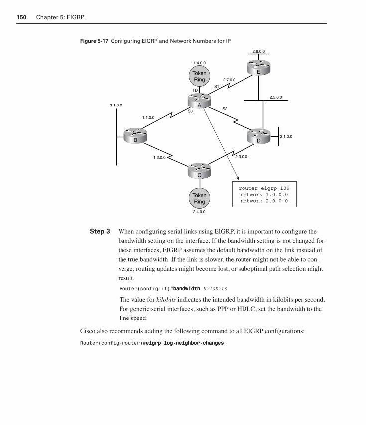
150 Chapter 5: EIGRP
Figure 5-17 Configuring EIGRP and Network Numbers for IP
Step 3 When configuring serial links using EIGRP, it is important to configure the
bandwidth setting on the interface. If the bandwidth setting is not changed for
these interfaces, EIGRP assumes the default bandwidth on the link instead of
the true bandwidth. If the link is slower, the router might not be able to con-
verge, routing updates might become lost, or suboptimal path selection might
result.
Router(config-if)#bbbbaaaannnnddddwwwwiiiiddddtttthhhh kilobits
The value for kilobits indicates the intended bandwidth in kilobits per second.
For generic serial interfaces, such as PPP or HDLC, set the bandwidth to the
line speed.
Cisco also recommends adding the following command to all EIGRP configurations:
Router(config-router)#eeeeiiiiggggrrrrpppp lllloooogggg----nnnneeeeiiiigggghhhhbbbboooorrrr----cccchhhhaaaannnnggggeeeessss
3.1.0.0
1.1.0.0
1.2.0.0
S0
S1
S2
2.6.0.0
2.5.0.0
2.1.0.0
2.3.0.0
2.4.0.0
2.7.0.0
router eigrp 109network 1.0.0.0network 2.0.0.0
E
A
C
B D
TokenRing
TokenRing
TD
1.4.0.0
1358_fmi.book Page 150 Thursday, May 27, 2004 2:21 PM

Configuring EIGRP 151
This command enables the logging of neighbor adjacency changes to monitor the routing sys-
tem’s stability and help detect problems.
EIGRP and the bandwidth Command
You should adhere to the following three rules when configuring EIGRP over an NBMA
cloud, such as Frame Relay:
■ EIGRP traffic should not exceed the virtual circuit’s (VC) CIR capacity.
■ The aggregated traffic that EIGRP has over all of the VCs should not exceed the inter-
face’s access line speed.
■ The bandwidth allocated to EIGRP on each VC must be the same in both directions.
If you understand and follow these rules, EIGRP works well over the WAN. If you aren’t
careful when configuring the WAN, EIGRP can swamp the network.
Configuring Bandwidth over a Multipoint NetworkConfiguring the bandwidth command in an NBMA cloud depends on the design of the VCs.
If the serial line has many VCs in a multipoint configuration, and all the VCs share bandwidth
evenly, set the bandwidth to the sum of all the CIRs. In Figure 5-18, the CIR for each VC is
set to 56 Kbps. Because there are four VCs, the bandwidth is set to 224 (4 * 56).
Figure 5-18 EIGRP WAN Configuration: Pure Multipoint
Lab 5.7.1 Configuring EIGRP
In this lab, EIGRP is configured on three Cisco routers within the International
Travel Agency WAN so that you can observe basic behaviors of the protocol.
FrameRelay
CIR 56 CIR 56
CIR 56 CIR 56
��������� ����� � �
����� �����������
��������� ���
C
E
F G
H
1358_fmi.book Page 151 Thursday, May 27, 2004 2:21 PM

152 Chapter 5: EIGRP
Configuring Bandwidth over a Hybrid Multipoint NetworkIf differing speeds are allocated to the VCs in the multipoint network, a more complex solu-
tion is needed. The following are the two main approaches:
■ Take the lowest CIR and multiply it by the number of VCs, as shown in Figure 5-19.
This is applied to the physical interface. The problem with this configuration is that the
higher-bandwidth links might be underutilized.
■ Use subinterfaces. The bandwidth command may be configured on each subinterface,
which allows different speeds on each VC. In this case, subinterfaces are configured for
the links with the differing CIRs. The links that have the same configured CIR are pre-
sented as a single subinterface with a bandwidth reflecting the aggregate CIR of all the
circuits. Three of the VCs have the same CIR, 256 Kbps, as shown in Figure 5-20. All
three VCs are grouped as a multipoint subinterface, serial 0/0.1. The single remaining
VC, which has a lower CIR, 56 Kbps, can be assigned a point-to-point subinterface,
serial0/0.2.
Figure 5-19 EIGRP WAN Configuration: Hybrid Multipoint
The bandwidth-percent Command
The bandwidth-percent command configures the percentage of bandwidth that EIGRP may
use on an interface. By default, EIGRP is set to use only up to 50% of an interface’s band-
width to exchange routing information. To calculate the percentage, the bandwidth-percent command relies on the value set by the bandwidth command.
FrameRelay
CIR 256BW 224
CIR 56BW 56
CIR 256BW 224
CIR 256BW 224
��������� ����� � �
����� �����������
��������� ���
C
E
F G
H
T1
S0/0
1358_fmi.book Page 152 Thursday, May 27, 2004 2:21 PM

Configuring EIGRP 153
Figure 5-20 EIGRP WAN Configuration: Hybrid Multipoint with Subinterfaces
Use the bandwidth-percent command when a link’s bandwidth setting does not reflect its
true speed. The bandwidth value might be artificially low for a variety of reasons, such as to
manipulate the routing metric or to accommodate an oversubscribed multipoint Frame Relay
configuration. Regardless of the reasons, configure EIGRP to overcome an artificially low
bandwidth setting by setting the bandwidth-percent to a higher number. In some cases, it
might even be set to a number greater than 100.
For example, assume that the actual bandwidth of a router serial link is 64 Kbps, but the
bandwidth value is set artificially low, to 32 Kbps. Figure 5-21 shows how to modify
EIGRP’s behavior so that it limits routing protocol traffic according to the serial interface’s
actual bandwidth. The sample configuration sets the bandwidth-percent on serial 0/0 to 100
percent for the EIGRP process running in AS 24. Because 100 percent of 32 Kbps is 32,
EIGRP is allowed to use half of the actual bandwidth of 64 Kbps.
Figure 5-21 Using the ip bandwidth-percent eigrp Command
FrameRelay
CIR 256BW 256
CIR 56BW 56
CIR 256BW 256
CIR 256BW 256
��������� ����� � � ����������
��������� ���
��������� �������� �
�������������� ��������� ��
C
E
F G
H
T1
S0
S0.1 S0.2
��������� ������ �
��������� ��
�� ����������������� ����� �� ���
AS Number
Percentage value=100%x32=32 kbps
NOTE
You can change the EIGRP percentage of bandwidth for IP with the following command:
Router(config-if) #iiiipppp bbbbaaaannnnddddwwwwiiiiddddtttthhhh----ppppeeeerrrrcccceeeennnntttt eeeeiiiiggggrrrrpppp
1358_fmi.book Page 153 Thursday, May 27, 2004 2:21 PM
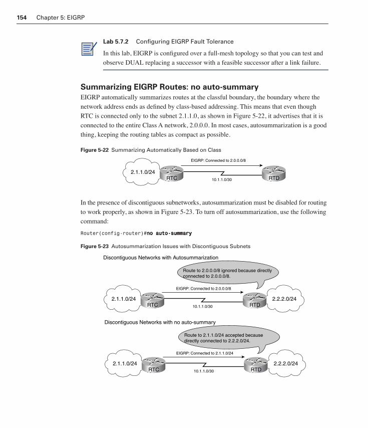
154 Chapter 5: EIGRP
Summarizing EIGRP Routes: no auto-summary
EIGRP automatically summarizes routes at the classful boundary, the boundary where the
network address ends as defined by class-based addressing. This means that even though
RTC is connected only to the subnet 2.1.1.0, as shown in Figure 5-22, it advertises that it is
connected to the entire Class A network, 2.0.0.0. In most cases, autosummarization is a good
thing, keeping the routing tables as compact as possible.
Figure 5-22 Summarizing Automatically Based on Class
In the presence of discontiguous subnetworks, autosummarization must be disabled for routing
to work properly, as shown in Figure 5-23. To turn off autosummarization, use the following
command:
Router(config-router)#nnnnoooo aaaauuuuttttoooo----ssssuuuummmmmmmmaaaarrrryyyy
Figure 5-23 Autosummarization Issues with Discontiguous Subnets
Lab 5.7.2 Configuring EIGRP Fault Tolerance
In this lab, EIGRP is configured over a full-mesh topology so that you can test and
observe DUAL replacing a successor with a feasible successor after a link failure.
2.1.1.0/24RTC RTD
EIGRP: Connected to 2.0.0.0/8
10.1.1.0/30
2.2.2.0/24
2.2.2.0/242.1.1.0/24RTC RTD
EIGRP: Connected to 2.0.0.0/8
10.1.1.0/30
Discontiguous Networks with Autosummarization
Route to 2.0.0.0/8 ignored because directlyconnected to 2.0.0.0/8.
2.1.1.0/24RTC RTD
EIGRP: Connected to 2.1.1.0/24
10.1.1.0/30
Discontiguous Networks with no auto-summary
Route to 2.1.1.0/24 accepted because directly connected to 2.2.2.0/24.
1358_fmi.book Page 154 Thursday, May 27, 2004 2:21 PM

Configuring EIGRP 155
Autosummarization prevents routers from learning about discontiguous subnets. With sum-
marization turned off, EIGRP routers advertise subnets.
Summarizing EIGRP Routes: Interface Summarization
EIGRP also lets you manually configure a prefix to use as a summary address. Manual summary
routes are configured on a per-interface basis. You select the interface that will propagate
the route summary and then define it with the ip summary-address eigrp command, which
has the following syntax:
Router(config-if)#iiiipppp ssssuuuummmmmmmmaaaarrrryyyy----aaaaddddddddrrrreeeessssssss eeeeiiiiggggrrrrpppp autonomous-system-number ip-address mask administrative-distance
EIGRP summary routes have an administrative distance of 5 by default. Optionally, they can
be configured for a value between 1 and 255.
In Figure 5-24, RTC can be configured using the commands shown in Example 5-6.
Figure 5-24 Manual Summarization with EIGRP
Therefore, RTC adds a route to its table, as follows:
D 2.1.0.0/16 is a summary, 00:00:22, Null0
Notice that the summary route is sourced from Null0, not an actual interface. This is because
this route is used for advertisement purposes and does not represent a path that RTC can take
to reach that network. On RTC, this route has an administrative distance of 5.
In Figure 5-24, RTD is oblivious to the summarization but accepts the route. It assigns the
route the administrative distance of a “normal” EIGRP route, which is 90 by default. In
the configuration for RTC, automatic summarization is turned off, with no auto-summary
Example 5-6 Configuring Manual Summarization with EIGRP
RTC(config)#rrrroooouuuutttteeeerrrr eeeeiiiiggggrrrrpppp 2222444444446666
RTC(config-router)#nnnnoooo aaaauuuuttttoooo----ssssuuuummmmmmmmaaaarrrryyyy
RTC(config-router)#eeeexxxxiiiitttt
RTC(config)#iiiinnnntttteeeerrrrffffaaaacccceeee sssseeeerrrriiiiaaaallll0000////0000
RTC(config-if)#iiiipppp ssssuuuummmmmmmmaaaarrrryyyy----aaaaddddddddrrrreeeessssssss eeeeiiiiggggrrrrpppp 2222444444446666 2222....1111....0000....0000 222255555555....222255555555....0000....0000
2.1.1.0/24RTC RTD
EIGRP: Connected to 2.1.0.0/16
10.1.1.0/30S0/0
1358_fmi.book Page 155 Thursday, May 27, 2004 2:21 PM

156 Chapter 5: EIGRP
command. Otherwise, RTD would receive two routes—the manual summary address of
2.1.0.0/16 and the automatic, classful address of 2.0.0.0/8.
In most cases, when you use manual summarization, the no auto-summary command should
be configured.
Monitoring EIGRPProper verification of EIGRP is necessary to ensure that the configuration was done correctly.
The following section explains some the commands that are used to verify EIGRP operation.
Verifying EIGRP Operation
Throughout this chapter, the EIGRP show commands have been used to verify EIGRP opera-
tion. The Cisco IOS software debug feature also provides useful EIGRP monitoring com-
mands, as shown in Table 5-3. Table 5-4 lists the key EIGRP show commands and briefly
describes their functions.
Lab 5.7.3 Configuring EIGRP Summarization
In this lab, you configure and test EIGRP over discontiguous (nonsequential) subnets
by disabling automatic route summarization. Then you manually configure EIGRP to
use specific summary routes.
Lab 5.8.1 EIGRP Challenge Lab
In this lab, you configure an EIGRP network with Network Address Translation
(NAT) and Dynamic Host Configuration Protocol (DHCP) services provided by
the routers. You also configure EIGRP interface address summarization to reduce the
number of routes in the EIGRP routing tables.
Table 5-3 EIGRP debug Commands
Command Description
debug eigrp fsm This command helps you observe EIGRP feasible successor activity and determine whether route updates are being installed and deleted by the routing process.
debug eigrp packet This command’s output shows transmission and receipt of EIGRP packets. These packet types may be hello, update, request, query, or reply packets. The sequence and acknowledg-ment numbers by the EIGRP reliable transport algorithm are shown in the output.
1358_fmi.book Page 156 Thursday, May 27, 2004 2:21 PM

Summary 157
SummaryEIGRP, a Cisco-proprietary routing protocol, is an advanced distance vector protocol that
uses the DUAL algorithm. It includes features such as rapid convergence, reduced bandwidth
usage, and multiple network layer support.
EIGRP converges rapidly, performs incremental updates, routes IP, and summarizes routes.
The labs demonstrated how to configure and verify EIGRP configuration for various protocols.
Table 5-4 EIGRP show Commands
Command Description
show ip eigrp neighbors [type number] [details]
Displays the EIGRP neighbor table. Uses the type and number options to specify an inter-face. The details keyword expands the output.
show ip eigrp interfaces [type number] [as-number] [details]
Shows EIGRP information for each inter-face. The optional keywords limit the output to a specific interface or AS. The details key-word expands the output.
show ip eigrp topology [as-number | [ip-address] mask]
Displays all feasible successors in the EIGRP topology table. The optional key-words can filter output based on AS number or specific network address.
show ip eigrp topology [active | pending | zero-successors]
Depending on which keyword is used, dis-plays all routes in the topology table that are either active, pending, or without successors.
show ip eigrp topology all-links Displays all routes, not just feasible succes-sors, in the EIGRP topology.
show ip eigrp traffic [as-number] Displays the number of EIGRP packets sent and received. You can filter the output by including an optional AS number.
1358_fmi.book Page 157 Thursday, May 27, 2004 2:21 PM

158 Chapter 5: EIGRP
Key Termsacknowledgment packet An EIGRP router uses acknowledgment packets to indicate
receipt of any EIGRP packet during a reliable exchange.
feasible distance (FD) The lowest calculated metric to each destination.
feasible successor A backup route. These routes are selected at the same time the succes-
sors are identified, but they are kept in the topology table. Multiple feasible successors for a
destination can be retained in the topology table.
hello packet EIGRP relies on hello packets to discover, verify, and rediscover neighbor
routers.
hold time (hold uptime) How long to wait without receiving anything from a neighbor
before considering the link unavailable. Originally, the expected packet was a hello packet.
However, in current Cisco IOS software releases, any EIGRP packets received after the first
hello reset the timer.
neighbor address The network layer address of the neighbor router. This is Address in the
EIGRP neighbor table.
neighbor table Each EIGRP router maintains a neighbor table that lists adjacent routers.
This table is comparable to the adjacency database used by OSPF. A neighbor table exists for
each protocol EIGRP supports.
query packet An EIGRP router uses a query packet whenever it needs specific information
from one or all of its neighbors.
queue count (Q Cnt) The number of packets waiting in queue to be sent. If this value is
constantly higher than 0, a congestion problem might exist at the router. A 0 means that no
EIGRP packets are in the queue.
reported distance (RD) A path’s RD is the distance reported by an adjacent neighbor to a
specific destination.
route source The identification number of the router that originally advertised that route.
This field is populated only for routes learned externally from the EIGRP network.
routing table EIGRP chooses the best routes to a destination from the topology table and
places them in the routing table. Each EIGRP router maintains a routing table for each net-
work protocol.
1358_fmi.book Page 158 Thursday, May 27, 2004 2:21 PM
Key Terms 159
Smooth Round-Trip Timer (SRTT) The average amount of time it takes to send and
receive packets to and from a neighbor. This timer is used to determine the retransmit interval
or retransmission timeout (RTO).
successor A route selected as the primary route to use to reach a destination. Successors are
the entries kept in the routing table. Multiple successors for a destination can be retained in
the routing table.
topology table Every EIGRP router maintains a topology table for each configured network
protocol. This table includes route entries for all destinations the router has learned. All
learned routes to a destination are maintained in the topology table.
update packet Used to update a router when the router discovers a new neighbor.
1358_fmi.book Page 159 Thursday, May 27, 2004 2:21 PM
160 Chapter 5: EIGRP
Check Your UnderstandingComplete all of the review questions to test your understanding of the topics and concepts in this
chapter. The answers appear in Appendix B, “Answers to the Check Your Understanding Questions.”
For additional, more in-depth questions, refer to the chapter-specific study guides on the
companion CD-ROM.
1. How do you configure automatic redistribution between IGRP and EIGRP?
A. Configure the two protocols with different AS numbers
B. Configure the two protocols with different DS numbers
C. Configure the two protocols with the same AS number
D. Configure the two protocols with the same DS number
2. What protocol combines the advantages of link-state and distance vector routing proto-cols?
A. RIP
B. OSPF
C. IGRP
D. EIGRP
3. What command shows the neighbors that EIGRP has discovered?
A. show eigrp neighbors
B. show ip eigrp neighbors
C. show router eigrp process-id
D. show ip eigrp networks
4. What multicast IP address does EIGRP use?
A. 224.0.0.110
B. 224.0.0.100
C. 224.0.0.11
D. 224.0.0.10
5. What table includes route entries for all destinations that the router has learned and is maintained for each configured routing protocol?
A. Topology table
B. Routing table
C. Neighbor table
D. Successor table
1358_fmi.book Page 160 Thursday, May 27, 2004 2:21 PM

Check Your Understanding 161
6. What establishes adjacencies in EIGRP?
A. DUAL finite-state machine
B. Hello packets
C. Topology table
D. Reliable Transport Protocol
7. What guarantees ordered delivery of EIGRP packets to all neighbors?
A. DUAL finite-state machine
B. Hello packets
C. Topology table
D. Reliable Transport Protocol
8. What does DUAL do after it tracks all routes, compares them, and guarantees that they are loop-free?
A. Inserts lowest-cost paths into the routing table
B. Determines the optimal path and advertises it to the neighbor routers using hello
packets
C. Supports other routed protocols through PDMs
D. Sends a unicast query to the neighboring routers
9. How does EIGRP prevent routing loops from occurring with external routes?
A. By rejecting external routes tagged with a router ID identical to their own
B. By storing the identities of neighbors that are feasible successors
C. By rejecting all neighboring routers that have an advertised composite metric that is
less than a router’s best current metric
D. By storing in a special table all neighboring routes that have loops identified
10. On higher-bandwidth connections, such as point-to point serial links or multipoint cir-cuits, how long is the hello interval used by EIGRP?
A. 5 seconds
B. 10 seconds
C. 60 seconds
D. 120 seconds
1358_fmi.book Page 161 Thursday, May 27, 2004 2:21 PM
ObjectivesUpon completing this chapter, you will be able to
■ Describe the characteristics and operation of OSPF
■ Configure and verify OSPF routing
■ Configure OSPF over NBMA
■ Describe multiarea OSPF operation
■ Configure and verify multiarea OSPF
■ Configure stubby, totally stubby, and not-so-stubby areas
■ Configure virtual links
You can reinforce your understanding of the objectives covered in this chapter by opening
the interactive media activities on the CD accompanying this book and performing the lab
activities collected in the Cisco Networking Academy Program CCNP 1: Advanced Routing
Lab Companion. Throughout this chapter, you will see references to these activities by title
and by icon. They look like this:
Interactive Media Activity
Lab Activity
1358_fmi.book Page 162 Thursday, May 27, 2004 2:21 PM

Chapter 6
OSPF
Open Shortest Path First (OSPF) is a link-state routing protocol based on open standards.
Described in several RFCs, most recently RFC 2328, the Open in Open Shortest Path First
means that OSPF is open to the public and is nonproprietary. Among nonproprietary routing pro-
tocols, such as RIPv1 and RIPv2, OSPF is preferred because of its remarkable scalability. Recall
that both versions of Routing Information Protocol (RIP) are very limited. RIP cannot scale
beyond 15 hops. It converges slowly, and it chooses suboptimal routes that ignore critical factors
such as bandwidth. OSPF addresses all of these limitations and proves to be a powerful, scalable
routing protocol.
OSPF’s considerable capability to scale is achieved through hierarchical design and the use of
areas. By defining areas in a properly designed network, an administrator can reduce routing
overhead and improve performance. To achieve scalability, OSPF relies on complex communi-
cations and relationships to maintain a comprehensive link-state database. However, as an OSPF
network scales to 100, 500, or even 1000 routers, link-state databases can balloon to include
thousands of links. To help OSPF routers route more efficiently and to preserve their CPU and
memory resources for the business of switching packets, network engineers divide OSPF net-
works into multiple areas.
This chapter describes how to create and configure OSPF. Specifically, it examines the different
OSPF area types, including stubby, totally stubby, and not-so-stubby areas (NSSAs). Each of
these different area types uses a special advertisement to exchange routing information with the
rest of the OSPF network. Therefore, link-state advertisements (LSAs) are covered in detail. The
Area 0 backbone rule and how virtual links can work around backbone connectivity problems
also are reviewed. Finally, this chapter surveys important show commands you can use to verify
multiarea OSPF operations.
1358_fmi.book Page 163 Thursday, May 27, 2004 2:21 PM

164 Chapter 6: OSPF
OSPF OverviewOSPF uses link-state technology, which uses factors such as speed or the link’s shortest path.
For example, in Figure 6-1, OSPF chooses the faster path via the T3 links between the left-
most and rightmost routers. This is opposed to distance vector technology, which uses factors
such as hop count to determine the path to the destination. Distance vector technology is used
by protocols such as RIP. For example, in Figure 6-2, RIP chooses the path via the slower
64 Kbps links because it has fewer hops.
Figure 6-1 Link-State Path Determination
Figure 6-2 Distance Vector Path Determination
Issues Addressed by OSPF
Link-state routers maintain a common picture of the network and exchange link information
upon initial discovery of network changes. Link-state routers do not broadcast their routing
tables periodically like distance vector routing protocols do. Although RIP is appropriate for
T3
T3 T3
64 Kbps 64 Kbps
OSPF
T3
T3 T3
64 Kbps64 Kbps
RIP
1358_fmi.book Page 164 Thursday, May 27, 2004 2:21 PM
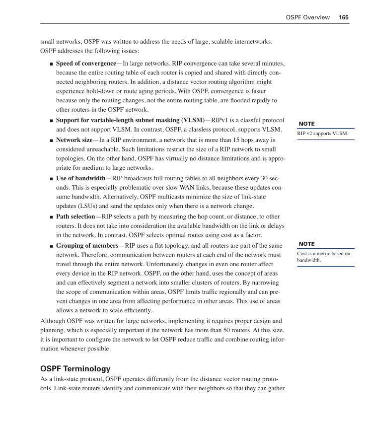
OSPF Overview 165
small networks, OSPF was written to address the needs of large, scalable internetworks.
OSPF addresses the following issues:
■ Speed of convergence—In large networks, RIP convergence can take several minutes,
because the entire routing table of each router is copied and shared with directly con-
nected neighboring routers. In addition, a distance vector routing algorithm might
experience hold-down or route aging periods. With OSPF, convergence is faster
because only the routing changes, not the entire routing table, are flooded rapidly to
other routers in the OSPF network.
■ Support for variable-length subnet masking (VLSM)—RIPv1 is a classful protocol
and does not support VLSM. In contrast, OSPF, a classless protocol, supports VLSM.
■ Network size—In a RIP environment, a network that is more than 15 hops away is
considered unreachable. Such limitations restrict the size of a RIP network to small
topologies. On the other hand, OSPF has virtually no distance limitations and is appro-
priate for medium to large networks.
■ Use of bandwidth—RIP broadcasts full routing tables to all neighbors every 30 sec-
onds. This is especially problematic over slow WAN links, because these updates con-
sume bandwidth. Alternatively, OSPF multicasts minimize the size of link-state
updates (LSUs) and send the updates only when there is a network change.
■ Path selection—RIP selects a path by measuring the hop count, or distance, to other
routers. It does not take into consideration the available bandwidth on the link or delays
in the network. In contrast, OSPF selects optimal routes using cost as a factor.
■ Grouping of members—RIP uses a flat topology, and all routers are part of the same
network. Therefore, communication between routers at each end of the network must
travel through the entire network. Unfortunately, changes in even one router affect
every device in the RIP network. OSPF, on the other hand, uses the concept of areas
and can effectively segment a network into smaller clusters of routers. By narrowing
the scope of communication within areas, OSPF limits traffic regionally and can pre-
vent changes in one area from affecting performance in other areas. This use of areas
allows a network to scale efficiently.
Although OSPF was written for large networks, implementing it requires proper design and
planning, which is especially important if the network has more than 50 routers. At this size,
it is important to configure the network to let OSPF reduce traffic and combine routing infor-
mation whenever possible.
OSPF Terminology
As a link-state protocol, OSPF operates differently from the distance vector routing proto-
cols. Link-state routers identify and communicate with their neighbors so that they can gather
NOTE
RIP v2 supports VLSM.
NOTE
Cost is a metric based on bandwidth.
1358_fmi.book Page 165 Thursday, May 27, 2004 2:21 PM

166 Chapter 6: OSPF
firsthand information from other routers in the network. The OSPF terminology is shown in
Figure 6-3. A description of each term follows.
Figure 6-3 OSPF Terminology
The information gathered from OSPF neighbors is not a complete routing table. Instead,
OSPF routers tell each other about the status of their connections or links to the internetwork,
as shown in Figure 6-4. A link, in OSPF terminology, is defined as a network communica-
tions channel that consists of a circuit or transmission path. In other words, OSPF routers
advertise their link states.
Figure 6-4 OSPF Terminology: Links
In the link between the routers shown in Figure 6-4, the routers process information
exchanged between them about the link and build link-state databases. The link state, in
OSPF terminology, is defined as the status of a link between two routers or the router’s inter-
face and its relationship to its neighboring routers.
TokenRing
Area 1
Area 0
Link-State
LinksDR
Cost=1785
Cost=10
Cost=6 BDR
TopologicalDatabase
RoutingTable
AdjacenciesDatabase
TokenRing
Links
1358_fmi.book Page 166 Thursday, May 27, 2004 2:21 PM

OSPF Overview 167
Figure 6-5 shows what is connected to what. This is called the topological or link-state data-
base, which is a list of information about all other routers in the internetwork, to show them
the internetwork topology.
Figure 6-5 OSPF Terminology: Topological Database
All routers within an area have identical topological or link-state databases. For example, all
routers in a given area should have identical link-state or topological databases, as shown in
Figure 6-6. An area, in OSPF terminology, is defined as a collection of routers that have the
same area identification. Each router within the defined area has the same link-state informa-
tion. Routers located in the defined area are called internal routers.
Figure 6-6 OSPF Terminology: Area
Independently, each router then runs the shortest path first (SPF) algorithm, also known as the
Dijkstra algorithm, on the link-state database to determine the best routes to a destination.
The SPF algorithm adds up the cost, which is a value usually based on bandwidth, of each
TokenRing
TopologicalDatabase
Area 1
Area 0
TokenRing
1358_fmi.book Page 167 Thursday, May 27, 2004 2:21 PM

168 Chapter 6: OSPF
link between the router and the destination, as shown in Figure 6-7. The cost is the value that
is assigned to the link. Rather than hops, link-state protocols assign a cost, which is based on
the medium’s speed. The router then chooses the lowest-cost path to add to its routing table,
also called a forwarding database, as shown in Figure 6-8. The routing table is generated
when the SPF algorithm is run on the topological or link-state database. Each routing table on
a router is unique.
Figure 6-7 OSPF Terminology: Cost
Figure 6-8 OSPF Terminology: Routing Table
Figure 6-9 shows how OSPF routers keep track of their neighbors in their adjacencies data-
base. The adjacencies database lists all of the neighbors to which a router has established
bidirectional communication. To simplify the exchange of routing information among several
neighbors on the same network, OSPF routers may elect a designated router (DR) and a
backup designated router (BDR), as shown in Figure 6-10, to serve as focal points for
TokenRing
Cost = 1785
Cost = 10
Cost = 6
TokenRing
RoutingTable
1358_fmi.book Page 168 Thursday, May 27, 2004 2:21 PM

OSPF Overview 169
routing updates. These are routers that are elected by all other routers on the same LAN to
represent all the routers. The DR and BDR have special responsibilities that are discussed in
later sections of this chapter.
Figure 6-9 OSPF Terminology: Adjacencies Database
Figure 6-10 OSPF Terminology: DR and BDR
OSPF States
OSPF routers establish relationships, or states, with their neighbors to efficiently share link-
state information. In contrast, distance vector routing protocols, such as RIP, blindly broad-
cast or multicast their complete routing table out every interface, hoping that a router is out
there to receive it. Every 30 seconds, by default, RIP routers send only one kind of message.
This message is their complete routing table. OSPF routers, on the other hand, rely on five
TokenRing
AdjacenciesDatabase
TokenRing
DR
BDR
1358_fmi.book Page 169 Thursday, May 27, 2004 2:21 PM

170 Chapter 6: OSPF
different kinds of packets to identify their neighbors and to update link-state routing informa-
tion, as shown in Table 6-1.
These five packet types make OSPF capable of sophisticated and complex communications.
These packet types are discussed in more detail later in this chapter. At this point, become
familiar with the different relationships, or states, possible between OSPF routers, the differ-
ent OSPF network types, and the OSPF Hello protocol.
The key to effectively designing and troubleshooting OSPF networks is to understand the
relationships, or states, that develop between OSPF routers. OSPF interfaces can be in one of
seven states. OSPF neighbor relationships progress through these states, one at a time, in the
following order:
1. Down state—In the Down state, the OSPF process has not exchanged information with any neighbor. OSPF is waiting to enter the next state—the Init state.
2. Init state—OSPF routers send Type 1 packets, or Hello packets, at regular intervals to establish a relationship with neighbor routers. These intervals are usually 10 seconds. When an interface receives its first Hello packet, the router enters the Init state. This means that the router knows a neighbor is out there and is waiting to take the relation-ship to the next step.
The two kinds of relationships are the two-way state and adjacency. A router must
receive a Hello from a neighbor before it can establish any relationship.
3. Two-way state—Using Hello packets, every OSPF router tries to establish a two-way state, or bidirectional communication, with every neighbor router on the same IP net-work. Among other things, Hello packets include a list of the sender’s known OSPF neighbors. A router enters the two-way state when it sees itself in a neighbor’s Hello. When RTB learns that RTA knows about it, it declares a two-way state to exist with RTA, as shown in Figure 6-11.
Table 6-1 OSPF Packet Types
Packet Type Name Description
Type 1 Hello Establishes and maintains adjacency information with neighbors.
Type 2 Database description (DBD) packet
Describes the contents of the link-state database on an OSPF router.
Type 3 Link-state request (LSR) Requests specific pieces of a link-state database.
Type 4 Link-state update (LSU) Transports LSAs to neighbor routers.
Type 5 Link-state acknowledg-ment (LSAck)
Acknowledgment receipt of a neighbor’s LSA.
1358_fmi.book Page 170 Thursday, May 27, 2004 2:21 PM

OSPF Overview 171
Figure 6-11 OSPF Two-Way State or Bidirectional Communication
The two-way state is the most basic relationship that OSPF neighbors can have, but
routing information is not shared between routers in this relationship. To learn about
the link states of other routers and eventually build a routing table, every OSPF router
must form at least one adjacency. An adjacency is an advanced relationship between
OSPF routers that involves a series of progressive states that rely not just on Hellos, but
also on the other four types of OSPF packets. Routers attempting to become adjacent to
one another exchange routing information even before the adjacency is fully estab-
lished. The first step toward full adjacency is the ExStart state, which is described next.
4. ExStart state—Technically, when a router and its neighbor enter the ExStart state, their conversation is characterized as an adjacency, but they have not become fully adjacent. ExStart is established using Type 2 DBD packets, also known as DDPs. The two neighbor routers use Hello packets to negotiate who is the “master” and who is the “slave” in their relationship and use DBD packets to exchange databases, as shown in Figure 6-12.
Figure 6-12 Route Discovery
Hello! RTB isa neighbor.
RTA RTB
Seen by RTA.A two-way
state now exists.
E0 E0
172.68.5.1 172.68.5.3 DR
Exstart State
Exchange State
Loading State
Full State
Starting exchange, this router has ID 172.68.5.1.
No, this router has a higher ID, this router gets to start exchange.
Here is a summary of the link-state database.
Here is a summary of the link-state database.
Thanks for the information!
The complete entry for network 172.68.6.0/24 is needed.
Here is the entry for network 172.68.6.0/24
Thanks for the information!
1358_fmi.book Page 171 Thursday, May 27, 2004 2:21 PM

172 Chapter 6: OSPF
The router with the highest OSPF router ID “wins” and becomes the master. The OSPF
router ID is discussed later in this chapter. When the neighbors establish their roles as
master and slave, they enter the Exchange state, and begin sending routing information.
5. Exchange state—In the Exchange state, neighbor routers use Type 2 DBD packets to send each other their link-state information, as shown in Figure 6-12. In other words, the routers describe their link-state databases to each other. The routers compare what they learn with their existing link-state databases and explicitly acknowledge each DBD packet. If either of the routers receives information about a link that is not already in its database, the router requests a complete update from its neighbor. Complete rout-ing information is exchanged in the Loading state.
6. Loading state—After the databases have been described to each router, they may request information that is more complete by using Type 3 packets, LSRs. When a router receives an LSR, it responds with an update by using a Type 4 LSU packet. These Type 4 LSU packets contain the actual LSAs, which are the heart of link-state routing protocols, as shown in Figure 6-12. Type 4 LSUs are acknowledged using Type 5 packets, called LSAcks.
7. Full adjacency—With the Loading state complete, the routers are fully adjacent. Each router keeps a list of adjacent neighbors, called the adjacencies database. Do not con-fuse the adjacencies database with the link-state database or the forwarding database. The forwarding database is a list of routes generated when an algorithm is run on the link-state database. The routing table on each router is unique and contains information on how and where to send packets to other routers.
OSPF Network Types
Adjacency is required to allow OSPF routers to share routing information. A router will try to
become adjacent to at least one other router on each IP network to which it is connected.
Some routers might try to become adjacent to all of their neighbor routers, and others might
try with only one or two. OSPF routers determine which routers to become adjacent to based
on what type of network connects them.
OSPF interfaces automatically recognize three types of networks: broadcast multiaccess,
nonbroadcast multiaccess (NBMA), and point-to-point networks, which are illustrated in
Figure 6-13. An administrator can configure a fourth network type, a point-to-multipoint
network.
Interactive Media Activity Drag and Drop: OSPF States
After completing this activity, you will be able to list in order the different states of
OSPF.
1358_fmi.book Page 172 Thursday, May 27, 2004 2:21 PM

OSPF Overview 173
Figure 6-13 OSPF Network Types
Table 6-2 summarizes some various types of networks that are associated with these four
OSPF network types.
The type of network dictates how OSPF routers should relate to each other. An administrator
might have to override the detected network type for OSPF to operate properly.
Some networks are defined as multiaccess because it cannot be predicted just how many routers
are connected to them. There might be one, two, or more routers. A campus that uses a
switched Ethernet core might have half a dozen routers connected to the same backbone net-
work. A school district might have 10, 12, or 25 remote-site routers connected by way of
Frame Relay PVCs to the same IP subnet.
A significant number of routers can exist on a multiaccess network. The designers of OSPF
developed a system to avoid the overhead that would be created if every router established
Table 6-2 OSPF Network Types
OSPF Network Type Network Example
Broadcast multiaccess Ethernet, Token Ring, or FDDI
Nonbroadcast multiaccess Frame Relay, X.25, SMDS
Point-to-point PPP, HDLC
Point-to-multipoint Configured by an administrator
BroadcastMultiaccess
Point-to-Point
NBMA
1358_fmi.book Page 173 Thursday, May 27, 2004 2:21 PM

174 Chapter 6: OSPF
full adjacency with every other router. This system restricts who can become adjacent to
whom by employing the services of one of the following:
■ Designated router (DR)—For every multiaccess IP network, one router is elected the
DR. The DR has two main functions—becoming adjacent to all other routers on the
network and acting as a spokesperson for the network. As spokesperson, the DR sends
network LSAs for all other IP networks to every other router. Because the DR becomes
adjacent to all other routers on the IP network, it is the focal point for collecting routing
information (LSAs).
■ Backup designated router (BDR)—The DR could represent a single point of failure,
so a second router is elected as the BDR to provide fault tolerance. Therefore, the BDR
must also become adjacent to all routers on the network and must serve as a second
focal point for LSAs, as shown in Figure 6-14. However, unlike the DR, the BDR is not
responsible for updating the other routers or sending network LSAs. Instead, the BDR
keeps a timer on the DR’s update activity to ensure that it is operational. If the BDR
does not detect activity from the DR before the timer expires, the BDR takes over the
role of DR, and a new BDR is elected.
Figure 6-14 DR and BDR Receive LSAs
On point-to-point networks, only two nodes exist. Therefore, a focal point for routing infor-
mation is not needed. No DR or BDR is elected. Both routers become fully adjacent to one
another.
The OSPF Hello Protocol
When a router starts an OSPF routing process on an interface, it sends a Hello packet and
continues to send Hellos at regular intervals. The rules that govern the exchange of OSPF
Hello packets are collectively referred to as the Hello protocol.
At Layer 3 of the OSI model, Hello packets are addressed to the multicast address 224.0.0.5.
This address in effect means all OSPF routers. OSPF routers use Hello packets to initiate new
adjacencies and to ensure that adjacent neighbors have not disappeared. Hellos are sent every
10 seconds by default on multiaccess and point-to-point networks. On interfaces that connect
to NBMA networks, such as Frame Relay, Hellos are sent every 30 seconds.
DR BDR
1358_fmi.book Page 174 Thursday, May 27, 2004 2:21 PM

OSPF Overview 175
Although the Hello packet is small, often less than 50 bytes, it contains plenty of vital infor-
mation. Like other OSPF packet types, Hello packets include an OSPF packet header, which
has the form shown in Figure 6-15.
Figure 6-15 OSPF Packet Header
All five types of OSPF packets use the OSPF packet header, which consists of eight fields.
■ Version, Type, and Packet Length—The first three fields of the OSPF packet let the
recipients know the version of OSPF that is being used by the sender, the OSPF packet
type, and the length. The OSPF version can be either 1 or 2. OSPF version 2 was intro-
duced in 1991 (RFC 1247) and is incompatible with version 1, which is obsolete. The
Cisco IOS software uses OSPF version 2 and cannot be configured to use OSPF version 1.
■ Router ID—The function of the Hello packet is to establish and maintain adjacencies.
So the sending router signs the fourth field with its router ID, which is a 32-bit number
used to identify the router to the OSPF protocol. A router uses its IP address as its ID
because both the router ID and the IP address must be unique within a network.
Because routers support multiple IP addresses, a loopback IP address is used as the
router ID. In the absence of a loopback IP address, the highest value address interface
IP is used as the router ID. This is regardless of whether that interface is involved in the
OSPF process.
If the interface associated with that IP address goes down, the router can no longer use
that IP address as its router ID. When a router’s ID changes for any reason, the router
must reintroduce itself to its neighbors on all links. To avoid the unnecessary overhead
caused by reestablishing adjacency and readvertising link states, an administrator
typically assigns an IP address to a loopback interface. Unless an administrator shuts
down a loopback interface, it always stays up, so loopback interfaces make ideal router
IDs.
■ Area ID—Multiple areas can be defined within an OSPF network to reduce and sum-
marize route information. This allows large and complex networks to continue grow-
ing. When configuring a single-area OSPF network, always use Area 0, because it is
defined as the “backbone” area. There must be a backbone area to scale or add other
OSPF areas.
Version Type Packet Length
Router ID
Area ID
Checksum Authentication Type
Authentication Data
NOTE
If a loopback interface is configured with an IP address, the Cisco IOS software uses that IP address as the router ID. This happens even if the other interfaces have higher addresses.
1358_fmi.book Page 175 Thursday, May 27, 2004 2:21 PM
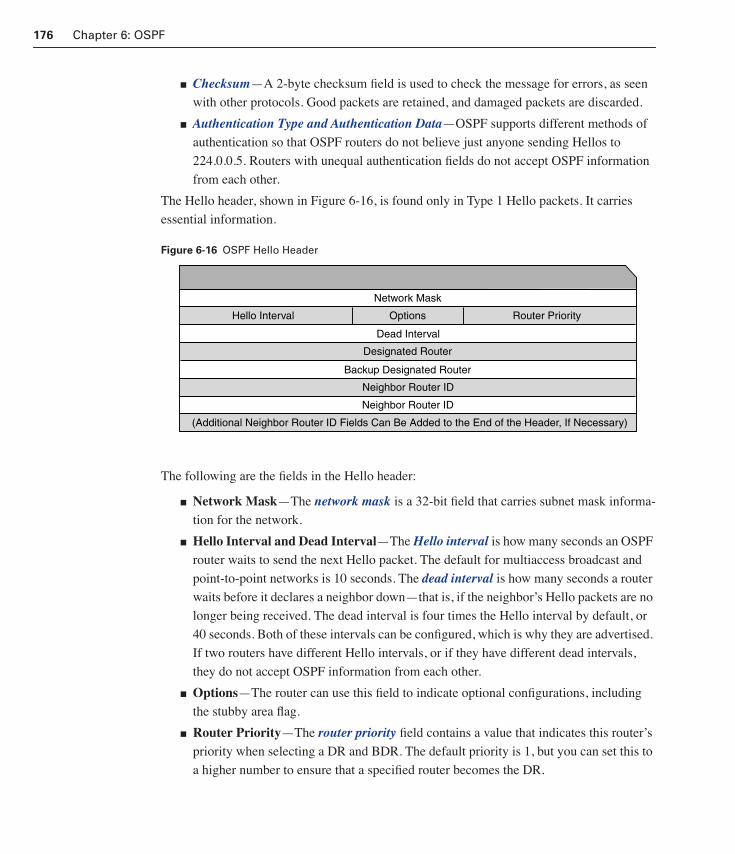
176 Chapter 6: OSPF
■ Checksum—A 2-byte checksum field is used to check the message for errors, as seen
with other protocols. Good packets are retained, and damaged packets are discarded.
■ Authentication Type and Authentication Data—OSPF supports different methods of
authentication so that OSPF routers do not believe just anyone sending Hellos to
224.0.0.5. Routers with unequal authentication fields do not accept OSPF information
from each other.
The Hello header, shown in Figure 6-16, is found only in Type 1 Hello packets. It carries
essential information.
Figure 6-16 OSPF Hello Header
The following are the fields in the Hello header:
■ Network Mask—The network mask is a 32-bit field that carries subnet mask informa-
tion for the network.
■ Hello Interval and Dead Interval—The Hello interval is how many seconds an OSPF
router waits to send the next Hello packet. The default for multiaccess broadcast and
point-to-point networks is 10 seconds. The dead interval is how many seconds a router
waits before it declares a neighbor down—that is, if the neighbor’s Hello packets are no
longer being received. The dead interval is four times the Hello interval by default, or
40 seconds. Both of these intervals can be configured, which is why they are advertised.
If two routers have different Hello intervals, or if they have different dead intervals,
they do not accept OSPF information from each other.
■ Options—The router can use this field to indicate optional configurations, including
the stubby area flag.
■ Router Priority—The router priority field contains a value that indicates this router’s
priority when selecting a DR and BDR. The default priority is 1, but you can set this to
a higher number to ensure that a specified router becomes the DR.
Network Mask
Options
(Additional Neighbor Router ID Fields Can Be Added to the End of the Header, If Necessary)
Neighbor Router ID
Backup Designated Router
Dead Interval
Hello Interval Router Priority
Designated Router
Neighbor Router ID
1358_fmi.book Page 176 Thursday, May 27, 2004 2:21 PM

OSPF Operation 177
■ Designated Router (DR) and Backup Designated Router (BDR)—The router IDs of
the DR and BDR are listed here if they are known by the source of the Hello packet.
■ Neighbor router ID—If the source of the Hello packet receives a valid Hello from any
neighbor within the dead interval, its router ID is included here.
OSPF OperationThe following sections discuss some of the details of OSPF operation:
■ Steps of OSPF operation
■ Establish router adjacencies
■ Elect a DR and a BDR
■ Discover routes
■ Select appropriate routes
■ Maintain routing information
Steps of OSPF Operation
OSPF routers progress through the following five distinct steps of operation:
1. Establish router adjacencies.
2. Elect a DR and BDR if necessary.
3. Discover routes.
4. Select the appropriate routes to use.
5. Maintain routing information.
Step 1: Establish Router Adjacencies
The first step a router takes in the OSPF operation is to establish router adjacencies. Each of
the three routers shown in Figure 6-17 attempts to become adjacent to another router on the
same IP network.
Interactive Media Activity Drag and Drop: OSPF Operation
After completing this activity, you will be able to list the steps of OSPF operation.
1358_fmi.book Page 177 Thursday, May 27, 2004 2:21 PM

178 Chapter 6: OSPF
Figure 6-17 OSPF Topology Example
To become adjacent to another router, RTB sends Hello packets, advertising its own router
ID. Because no loopback interfaces are present, RTB chooses its highest IP address, 10.6.0.1,
as its router ID.
Assuming that RTB is appropriately configured, RTB multicasts Hello packets out both S0
and E0. RTA and RTC should both receive the Hello packets. These two routers then add
RTB to the Neighbor ID field of their respective Hello packets and enter the Init state
with RTB.
RTB receives Hello packets from both its neighbors and sees its own ID number, 10.6.0.1, in
the Neighbor ID field. RTB declares a two-way state between itself and RTA and a two-way
state between itself and RTC.
At this point, RTB determines which routers to establish adjacencies with, based on the type
of network a particular interface resides on. If the network type is point-to-point, the router
becomes adjacent with its sole link partner. If the network type is multiaccess, RTB enters the
election process to become a DR or BDR. This happens unless both roles are already estab-
lished, as advertised in the Hello packet header.
If an election is necessary, OSPF routers proceed as described in the next section. However, if
an election is unnecessary, the routers enter the ExStart state, as described in the section
“Step 3: Discover Routes.”
Step 2: Elect a DR and a BDR
Because multiaccess networks can support more than two routers, OSPF elects a DR to be the
focal point of all LSUs and LSAs. The role of the DR is critical, so a BDR is elected to
“shadow” the DR. If the DR fails, the BDR can smoothly take over.
Like any election, the DR/BDR selection process can be rigged to change the outcome. The
“ballots” are Hello packets, which contain the router’s ID and priority fields. The router with
RTC
10.4.0.1 10.5.0.1 10.5.0.2 10.6.0.110.6.0.2
E0 S0
Area 0Router IDsRTA=10.5.0.1RTB=10.6.0.1RTC=10.6.0.2
RTBRTA
1358_fmi.book Page 178 Thursday, May 27, 2004 2:21 PM

OSPF Operation 179
the highest priority value among adjacent neighbors wins the election and becomes the DR.
The router with the second-highest priority is elected the BDR. When the DR and BDR have
been elected, they keep their roles until one of them fails, even if additional routers with
higher priorities show up on the network. Hello packets inform newcomers of the identity of
the existing DR and BDR.
By default, all OSPF routers have the same priority value of 1. A priority number from 0 to
255 can be assigned on any given OSPF interface. A priority of 0 prevents the router from
winning any election on that interface. A priority of 255 ensures at least a tie. The router ID
field is used to break ties. If two routers have the same priority, the router with the highest
ID is selected. You can manipulate the router ID by configuring an address on a loopback
interface, but that is not the preferred way to control the DR/BDR election process. The prior-
ity value should be used instead because each interface can have its own unique priority
value. A router can be easily configured to win an election on one interface and lose an elec-
tion on another.
How does the DR election process affect the sample network? RTB and RTC are connected
by way of PPP on a point-to-point link, as shown in Figure 6-18. Therefore, there is no need
for a DR on the network 10.6.0.0/16, because only two routers can exist on this link.
Figure 6-18 DR and BDR Election Process
Because the 10.4.0.0/16 and 10.5.0.0/16 networks are multiaccess Ethernet networks, they
may potentially connect more than two routers. Even if only one router is connected to a mul-
tiaccess segment, a DR is still elected. This is because the potential exists for more routers to be
added to the network. Therefore, a DR must be elected on both 10.4.0.0/16 and 10.5.0.0/16.
In the sample topology, RTA serves a dual role as both the DR and the BDR. Because it is the
only router on the 10.4.0.0/16 network, RTA elects itself as the DR. After all, the 10.4.0.0/16
network is a multiaccess Ethernet network. A DR is elected because multiple routers can
potentially be added to this network. RTA is also the runner-up in the election for 10.5.0.0/16
and, therefore, is the BDR for that network. Despite claiming equal priority value with RTA,
RTB is elected as the DR for 10.5.0.0/16 by virtue of the tiebreaker. The tiebreaker is having
a higher router ID of 10.5.0.2 versus 10.5.0.1.
RTC
10.4.0.1 10.5.0.1 10.5.0.2 10.6.0.1 10.6.0.2
EthernetBroadcast Multiaccess
EthernetBroadcast Multiaccess
PPP over T1Point-to-Point
DR BDR DRRTBRTA
10.4.0.0/16 10.5.0.0/16 10.6.0.0/16
NOTE
DRs and BDRs are elected on a per-network basis. An OSPF area can contain more than one IP network. Therefore, each area can, and usually does, have multiple DRs and BDRs.
1358_fmi.book Page 179 Thursday, May 27, 2004 2:21 PM

180 Chapter 6: OSPF
With elections complete and bidirectional communication established, routers are ready to
share routing information with adjacent routers and build their link-state databases. This pro-
cess is discussed in the next section.
Step 3: Discover Routes
On a multiaccess network, the exchange of routing information occurs between the DR or
BDR and every other router on the network. As the DR and BDR on the 10.5.0.0/16 network,
RTA and RTB exchange link-state information, as shown in Figure 6-18.
Link partners on a point-to-point or point-to-multipoint network also engage in the exchange
process. That means that RTA and RTB share link-state data, as shown in Figure 6-19.
Figure 6-19 Route Discovery
However, who goes first? This question is answered in the first stage of the exchange process,
the ExStart state, as shown in Figure 6-19. The purpose of ExStart is to establish a master/
slave relationship between the two routers. The router that announces the highest router ID in
Lab 6.9.2a Examining the DR/BDR Election Process
In this lab, you observe the OSPF DR and BDR election process using debug com-
mands. Then you assign each OSPF interface a priority value to force the election of
a specific router as a DR.
E0 E0
10.5.0.1 10.5.0.2 DR
Exstart State
Exchange State
Loading State
Full State
Starting exchange, this router has ID 10.5.0.1.
No, this router has a higher ID, so it will start the exchange.
Here is a summary of the link-state database.
Here is a summary of the link-state database.
Thanks for the information!
The complete entry is needed for network 10.6.0.0/16.
Here is the entry for network 10.6.0.0/16.
Thanks for the information!
RTA RTB
Hello
DBD
LSAck
LSU
Hello
DBD
LSAck
LSR
LSAck
1358_fmi.book Page 180 Thursday, May 27, 2004 2:21 PM
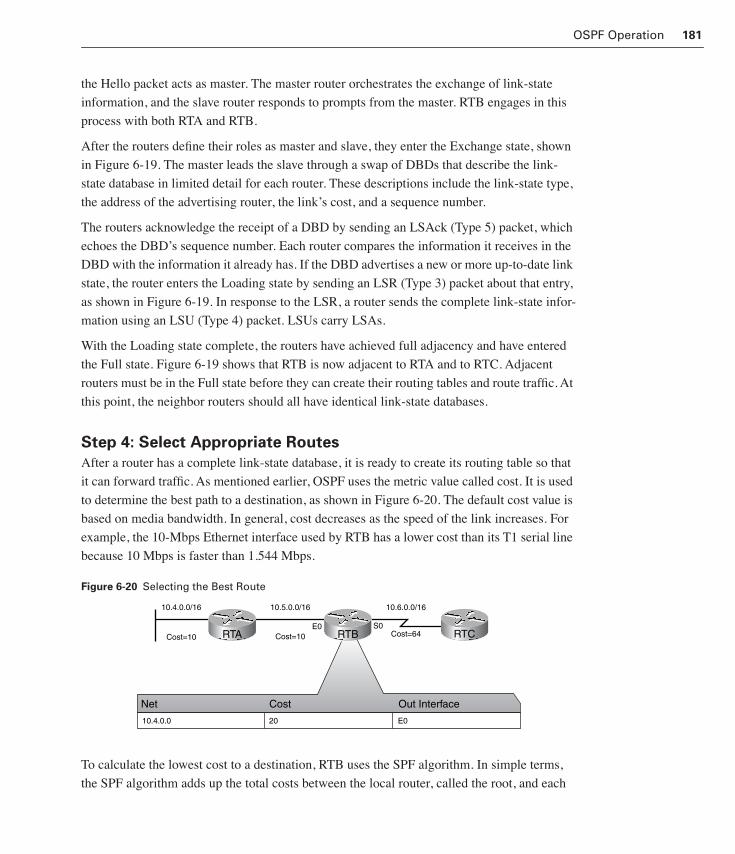
OSPF Operation 181
the Hello packet acts as master. The master router orchestrates the exchange of link-state
information, and the slave router responds to prompts from the master. RTB engages in this
process with both RTA and RTB.
After the routers define their roles as master and slave, they enter the Exchange state, shown
in Figure 6-19. The master leads the slave through a swap of DBDs that describe the link-
state database in limited detail for each router. These descriptions include the link-state type,
the address of the advertising router, the link’s cost, and a sequence number.
The routers acknowledge the receipt of a DBD by sending an LSAck (Type 5) packet, which
echoes the DBD’s sequence number. Each router compares the information it receives in the
DBD with the information it already has. If the DBD advertises a new or more up-to-date link
state, the router enters the Loading state by sending an LSR (Type 3) packet about that entry,
as shown in Figure 6-19. In response to the LSR, a router sends the complete link-state infor-
mation using an LSU (Type 4) packet. LSUs carry LSAs.
With the Loading state complete, the routers have achieved full adjacency and have entered
the Full state. Figure 6-19 shows that RTB is now adjacent to RTA and to RTC. Adjacent
routers must be in the Full state before they can create their routing tables and route traffic. At
this point, the neighbor routers should all have identical link-state databases.
Step 4: Select Appropriate Routes
After a router has a complete link-state database, it is ready to create its routing table so that
it can forward traffic. As mentioned earlier, OSPF uses the metric value called cost. It is used
to determine the best path to a destination, as shown in Figure 6-20. The default cost value is
based on media bandwidth. In general, cost decreases as the speed of the link increases. For
example, the 10-Mbps Ethernet interface used by RTB has a lower cost than its T1 serial line
because 10 Mbps is faster than 1.544 Mbps.
Figure 6-20 Selecting the Best Route
To calculate the lowest cost to a destination, RTB uses the SPF algorithm. In simple terms,
the SPF algorithm adds up the total costs between the local router, called the root, and each
RTBRTA RTC
10.6.0.0/1610.5.0.0/1610.4.0.0/16
E0 S0Cost=10 Cost=10 Cost=64
Net Cost Out Interface
10.4.0.0 20 E0
1358_fmi.book Page 181 Thursday, May 27, 2004 2:21 PM
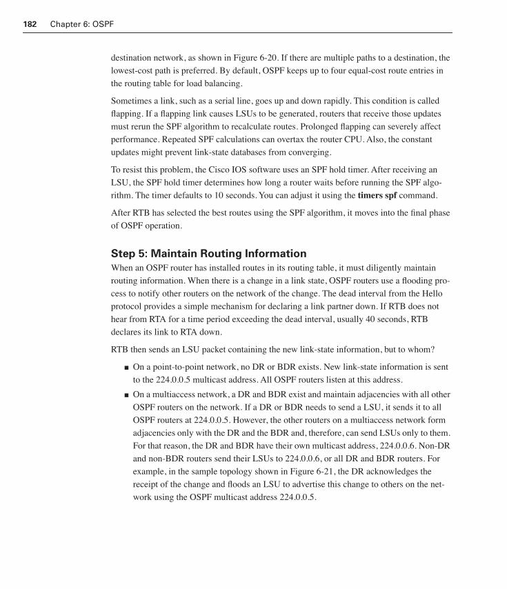
182 Chapter 6: OSPF
destination network, as shown in Figure 6-20. If there are multiple paths to a destination, the
lowest-cost path is preferred. By default, OSPF keeps up to four equal-cost route entries in
the routing table for load balancing.
Sometimes a link, such as a serial line, goes up and down rapidly. This condition is called
flapping. If a flapping link causes LSUs to be generated, routers that receive those updates
must rerun the SPF algorithm to recalculate routes. Prolonged flapping can severely affect
performance. Repeated SPF calculations can overtax the router CPU. Also, the constant
updates might prevent link-state databases from converging.
To resist this problem, the Cisco IOS software uses an SPF hold timer. After receiving an
LSU, the SPF hold timer determines how long a router waits before running the SPF algo-
rithm. The timer defaults to 10 seconds. You can adjust it using the timers spf command.
After RTB has selected the best routes using the SPF algorithm, it moves into the final phase
of OSPF operation.
Step 5: Maintain Routing Information
When an OSPF router has installed routes in its routing table, it must diligently maintain
routing information. When there is a change in a link state, OSPF routers use a flooding pro-
cess to notify other routers on the network of the change. The dead interval from the Hello
protocol provides a simple mechanism for declaring a link partner down. If RTB does not
hear from RTA for a time period exceeding the dead interval, usually 40 seconds, RTB
declares its link to RTA down.
RTB then sends an LSU packet containing the new link-state information, but to whom?
■ On a point-to-point network, no DR or BDR exists. New link-state information is sent
to the 224.0.0.5 multicast address. All OSPF routers listen at this address.
■ On a multiaccess network, a DR and BDR exist and maintain adjacencies with all other
OSPF routers on the network. If a DR or BDR needs to send a LSU, it sends it to all
OSPF routers at 224.0.0.5. However, the other routers on a multiaccess network form
adjacencies only with the DR and the BDR and, therefore, can send LSUs only to them.
For that reason, the DR and BDR have their own multicast address, 224.0.0.6. Non-DR
and non-BDR routers send their LSUs to 224.0.0.6, or all DR and BDR routers. For
example, in the sample topology shown in Figure 6-21, the DR acknowledges the
receipt of the change and floods an LSU to advertise this change to others on the net-
work using the OSPF multicast address 224.0.0.5.
1358_fmi.book Page 182 Thursday, May 27, 2004 2:21 PM
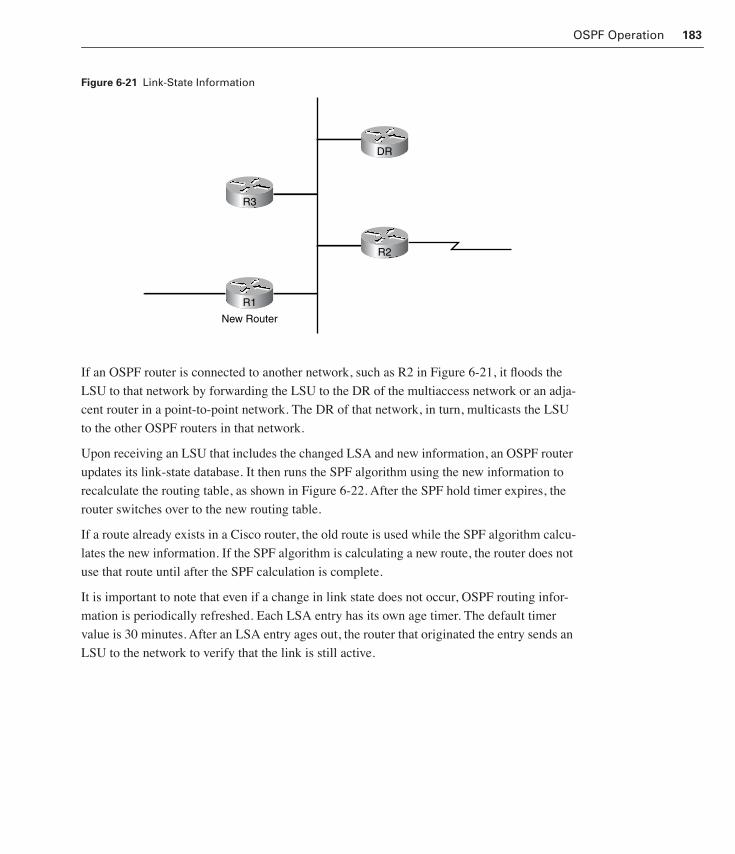
OSPF Operation 183
Figure 6-21 Link-State Information
If an OSPF router is connected to another network, such as R2 in Figure 6-21, it floods the
LSU to that network by forwarding the LSU to the DR of the multiaccess network or an adja-
cent router in a point-to-point network. The DR of that network, in turn, multicasts the LSU
to the other OSPF routers in that network.
Upon receiving an LSU that includes the changed LSA and new information, an OSPF router
updates its link-state database. It then runs the SPF algorithm using the new information to
recalculate the routing table, as shown in Figure 6-22. After the SPF hold timer expires, the
router switches over to the new routing table.
If a route already exists in a Cisco router, the old route is used while the SPF algorithm calcu-
lates the new information. If the SPF algorithm is calculating a new route, the router does not
use that route until after the SPF calculation is complete.
It is important to note that even if a change in link state does not occur, OSPF routing infor-
mation is periodically refreshed. Each LSA entry has its own age timer. The default timer
value is 30 minutes. After an LSA entry ages out, the router that originated the entry sends an
LSU to the network to verify that the link is still active.
New Router
DR
R2
R3
R1
1358_fmi.book Page 183 Thursday, May 27, 2004 2:21 PM

184 Chapter 6: OSPF
Figure 6-22 LSUs and Routing Table Updates
OSPF Configuration and VerificationIn this section, you learn how to configure OSPF on routers within a single area.
Configuring OSPF on Routers Within a Single Area
To configure OSPF, enable OSPF on Routers A and B, as shown in Figure 6-23.
Figure 6-23 Basic OSPF Topology Configuration
Configure the network addresses and area information for the router by following these steps:
Step 1 Enable OSPF on the routers using the following command:
Router(config)#rrrroooouuuutttteeeerrrr oooossssppppffff process-id
The process ID is a process number on the local router. The process ID is used
to identify multiple OSPF processes on the same router. The number can be any
value between 1 and 65,535. The OSPF processes do not need to start at 1. Most
network administrators keep the same process ID throughout the entire AS. It
is possible to run multiple OSPF processes on the same router, but this is not
recommended because it creates multiple database instances that add overhead
to the router.
New Router
DR
R2
R3
R1
This routing tableneeds to be
updated
A B C
E0
E0S0
S1
10.64.0.2
10.64.0.1 10.2.1.210.2.1.1
1358_fmi.book Page 184 Thursday, May 27, 2004 2:21 PM

OSPF Configuration and Verification 185
Enter the following OSPF process commands on the routers shown in
Figure 6-23:
RouterA(config)#rrrroooouuuutttteeeerrrr oooossssppppffff 1111
RouterB(config)#rrrroooouuuutttteeeerrrr oooossssppppffff 1111
Step 2 Identify IP networks on the router using the following command. Table 6-3
describes the parameters.
Router(config-router)#nnnneeeettttwwwwoooorrrrkkkk address wildcard-mask aaaarrrreeeeaaaa area-id
Enter the following config-router prompt commands on the routers shown in
Figure 6-23:
RouterA(config)#nnnneeeettttwwwwoooorrrrkkkk 11110000....0000....0000....0000 0000....222255555555....222255555555....222255555555 aaaarrrreeeeaaaa 0000
RouterB(config)#nnnneeeettttwwwwoooorrrrkkkk 11110000....2222....1111....2222 0000....0000....0000....0000 aaaarrrreeeeaaaa 0000
RouterB(config)#nnnneeeettttwwwwoooorrrrkkkk 11110000....66664444....0000....2222 0000....0000....0000....0000 aaaarrrreeeeaaaa 0000
For each network, identify the area to which the network belongs. The network
address value can be the network address, subnet, or interface address. The
router interprets the address by comparing it to the wildcard mask. A wildcard
mask is necessary because OSPF supports CIDR and VLSM, unlike RIPv1 and
IGRP. The area argument is needed even when you’re configuring OSPF in a
single area. Again, note that more than one IP network can belong to the same
area.
The wildcard mask is essentially an inverse subnet mask. For Router A, the entire 10.0.0.0
network is advertised by specifying the 0.255.255.255 mask. On Router B, the interface
addresses are advertised using a 0.0.0.0 mask. All interfaces are in area 0.
Table 6-4 provides other examples of addresses, subnet masks, and inverse masks. The first
example advertises the entire network address 172.16.0.0. The second advertises the entire
network address 192.168.45.0. The third advertises a small subnet with four hosts (two of
Table 6-3 network area Command Description
Parameter Description
address Can be the network address, subnet, or interface address. Instructs the router to know which links and networks to advertise and which links to listen to advertisements on.
wildcard-mask An inverse mask used to determine how to read the address. The mask has wildcard bits where 0 is a match and 1 is “do not care.” For example, 0.0.255.255 indicates a match in the first two octets. The equivalent regular subnet mask is a 16-bit mask of 255.255.0.0. If you’re specifying the interface address, use mask 0.0.0.0.
area-id Specifies the OSPF area to be associated with the address. Can be a number or can be similar to an IP address A.B.C.D. For a backbone area, the ID must equal 0.

186 Chapter 6: OSPF
which are useable) as might be found on a WAN link. The fourth advertises a subnet with 16
hosts (14 of which are useable). The fifth example advertises an interface address.
Optional Configuration Commands
Optional commands exist for doing the following:
■ Configuring a loopback address
■ Modifying OSPF router priority
■ Configuring authentication
■ Configuring OSPF timers
Configuring a Loopback AddressWhen the OSPF process starts, the Cisco IOS software uses the highest local IP address as its
OSPF router ID. If a loopback interface is configured, that address is used, regardless of its
value. You can assign an IP address to a loopback interface with the following commands:
Router(config)#iiiinnnntttteeeerrrrffffaaaacccceeee llllooooooooppppbbbbaaaacccckkkk numberRouter(config-if)#iiiipppp aaaaddddddddrrrreeeessssssss ip-address subnet-mask
A loopback-derived router ID ensures stability because that interface is immune to link fail-
ure. The loopback interface must be configured before the OSPF process starts, to override
the highest interface IP address.
It is recommended that the loopback address be used on all key routers in the OSPF-based
network. To avoid routing problems, it is good practice to use a 32-bit subnet mask when con-
figuring a loopback IP address, as shown here:
Router(config)#iiiinnnntttteeeerrrrffffaaaacccceeee llllooooooooppppbbbbaaaacccckkkk0000Router(config-if)#iiiipppp aaaaddddddddrrrreeeessssssss 111199992222....111166668888....1111....1111 222255555555....222255555555....222255555555....222255555555
Table 6-4 Network Area Command Examples
Interface Address Subnet Mask Advertised Address Wildcard Mask
172.16.0.8 255.255.0.0 172.16.0.0 0.0.255.255
192.168.45.147 255.255.255.0 192.168.45.0 0.0.0.255
192.168.45.5 255.255.255.252 192.168.45.4 0.0.0.3
192.168.45.17 255.255.255.240 192.168.45.16 0.0.0.15
192.168.45.1 255.255.255.0 192.168.45.1 0.0.0.0
Lab 6.9.1 Configuring OSPF
In this lab, you configure OSPF on three Cisco routers.
1358_fmi.book Page 186 Thursday, May 27, 2004 2:21 PM
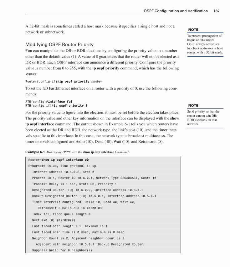
OSPF Configuration and Verification 187
A 32-bit mask is sometimes called a host mask because it specifies a single host and not a
network or subnetwork.
Modifying OSPF Router PriorityYou can manipulate the DR or BDR elections by configuring the priority value to a number
other than the default value (1). A value of 0 guarantees that the router will not be elected as a
DR or BDR. Each OSPF interface can announce a different priority. Configure the priority
value, a number from 0 to 255, with the ip ospf priority command, which has the following
syntax:
Router(config-if)#iiiipppp oooossssppppffff pppprrrriiiioooorrrriiiittttyyyy number
To set the fa0 FastEthernet interface on a router with a priority of 0, use the following com-
mands:
RTB(config)#iiiinnnntttteeeerrrrffffaaaacccceeee ffffaaaa0000RTB(config-if)#iiiipppp oooossssppppffff pppprrrriiiioooorrrriiiittttyyyy 0000
For the priority value to figure into the election, it must be set before the election takes place.
The priority value and other key information on the interface can be displayed with the show ip ospf interface command. The output shown in Example 6-1 tells you which routers have
been elected as the DR and BDR, the network type, the link’s cost (10), and the timer inter-
vals specific to this interface. In this case, the network type is broadcast multiaccess. The
timer intervals configured are Hello (10), Dead (40), Wait (40), and Retransmit (5).
Example 6-1 Monitoring OSPF with the show ip ospf interface Command
Router>sssshhhhoooowwww iiiipppp oooossssppppffff iiiinnnntttteeeerrrrffffaaaacccceeee eeee0000
Ethernet0 is up, line protocol is up
Internet Address 10.5.0.2, Area 0
Process ID 1, Router ID 10.6.0.1, Network Type BROADCAST, Cost: 10
Transmit Delay is 1 sec, State DR, Priority 1
Designated Router (ID) 10.6.0.2, Interface address 10.6.0.1
Backup Designated Router (ID) 10.5.0.1, Interface address 10.5.0.1
Timer intervals configured, Hello 10, Dead 40, Wait 40,
Retransmit 5 Hello due in 00:00:03
Index 1/1, flood queue length 0
Next 0x0 (0) (0)/0x0(0)
Last flood scan length i 1, maximum is 1
Last flood scan time is 0 msec, maximum is 0 msec
Neighbor Count is 2, Adjacent neighbor count is 2
Adjacent with neighbor 10.5.0.1 (Backup Designated Router)
Suppress hello for 0 neighbor(s)
NOTE
To prevent propagation of bogus or fake routes, OSPF always advertises loopback addresses as host routes, with a 32-bit mask.
NOTE
Set 0 priority so that the router cannot win DR/BDR elections on that network.
1358_fmi.book Page 187 Thursday, May 27, 2004 2:21 PM

188 Chapter 6: OSPF
OSPF routers use costs associated with interfaces to determine the best route. The Cisco IOS
software automatically determines cost based on an interface’s bandwidth in bits per second
using the following formula:
108 / bandwidth value
Table 6-5 shows common default path costs for a variety of media. For OSPF to calculate
routes properly, all interfaces connected to the same link must agree on that link’s cost. In a
multivendor routing environment, an interface’s default cost may be overridden to match
another vendor’s value with the ip ospf cost command, which has the following syntax:
Router(config-if)#iiiipppp oooossssppppffff ccccoooosssstttt number
The new cost can be a number between 1 and 65,535. To override the default cost on a
router’s Serial0 interface, use the following commands:
Router(config)#iiiinnnntttteeeerrrrffffaaaacccceeee ssss0000Router(config-if)#iiiipppp oooossssppppffff ccccoooosssstttt 1111000000000000
The ip ospf cost command can also be used to manipulate a route’s desirability. This is
because routers install the lowest-cost paths in their tables.
For the Cisco IOS software cost formula to be accurate, serial interfaces must be configured
with appropriate bandwidth values. Cisco routers default to T1 (1.544 Mbps) on most serial
interfaces and require manual configuration for any other bandwidth, as shown in the follow-
ing example:
Router(config)#iiiinnnntttteeeerrrrffffaaaacccceeee ssss1111Router(config-if)#bbbbaaaannnnddddwwwwiiiiddddtttthhhh 55556666
The default reference bandwidth of 100,000,000 does not account for new technologies such
as Gigabit and 10 Gigabit Ethernet. The cost of these links would still be 1, which is the same
as that of a Fast Ethernet link. Beginning with Cisco IOS Release 11.2, OSPF configuration
lets you adjust the reference bandwidth using the auto-cost reference-bandwidth command.
Table 6-5 Cisco IOS Software Default OSPF Costs
Medium Cost
56-kbps serial link 1785
T1 (1.544-Mbps serial link) 64
E1 (2.048-Mbps serial link) 48
4-Mbps Token Ring 25
Ethernet 10
16-Mbps Token Ring 6
100-Mbps Fast Ethernet, FDDI 1
1358_fmi.book Page 188 Thursday, May 27, 2004 2:21 PM
OSPF Configuration and Verification 189
The number entered is the number of Mbps. In the following, the reference bandwidth is set
to 1000 megabits, or 1 gigabit.
Router(config-router)#aaaauuuuttttoooo----ccccoooosssstttt rrrreeeeffffeeeerrrreeeennnncccceeee----bbbbaaaannnnddddwwwwiiiiddddtttthhhh 1111000000000000% OSPF: Reference bandwidth is changed.Please ensure reference bandwidth is consistent across all routers.
Configuring AuthenticationAuthentication is another interface-specific configuration. Each OSPF interface on a router
can present a different authentication key, which functions as a password among OSPF routers
in the same area. You use the following command syntax to configure OSPF authentication:
Router(config-if)#iiiipppp oooossssppppffff aaaauuuutttthhhheeeennnnttttiiiiccccaaaattttiiiioooonnnn----kkkkeeeeyyyy password
After a password is configured, you enable authentication on an area-wide basis with the fol-
lowing syntax, which must be entered on all participating routers:
Router(config-router)#aaaarrrreeeeaaaa number aaaauuuutttthhhheeeennnnttttiiiiccccaaaattttiiiioooonnnn [mmmmeeeessssssssaaaaggggeeee----ddddiiiiggggeeeesssstttt]
Although the message-digest keyword is optional, it is recommended that you always use it
with this command. By default, authentication passwords are sent in clear text over the wire.
A packet sniffer could easily capture an OSPF packet and decode the unencrypted password.
However, if the message-digest argument is used, a message digest, or hash, of the password
is sent over the wire in place of the password itself. Unless the recipient is configured with the
proper authentication key, that person cannot make sense of the message digest.
If message digest authentication is used, the authentication key is not used. Instead, configure
a message digest key on the interface of the OSPF router. The syntax for this command is as
follows:
Router(config-if)#iiiipppp oooossssppppffff mmmmeeeessssssssaaaaggggeeee----ddddiiiiggggeeeesssstttt----kkkkeeeeyyyy key-id mmmmdddd5555 [encryption-type] password
Table 6-6 describes the ip ospf message-digest-key command parameters.Table 6-6 ip ospf message-digest-key Command Parameters
Parameter Description
key-id An identifier in the range 1 to 255 that allows for multiple keys. The key’s ID configuration on each router must match to authenticate.
md5 A required value that specifies that the MD5 algorithm will be used.
[encryption-type] An optional value that specifies the type of encryption to use (0 to 7). An encryption-type value of 7 indicates Cisco-proprietary encryption. Type 0 is the default.
password An alphanumeric password to be used as the message digest key.
1358_fmi.book Page 189 Thursday, May 27, 2004 2:21 PM

190 Chapter 6: OSPF
Example 6-2 sets the message digest key to “itsasecret” and enables message digest authenti-
cation within Area 0.
Remember, the same parameters would have to be configured on the other routers in the same
area.
Configuring OSPF TimersFor OSPF routers to exchange information, they must have the same Hello intervals and the
same Dead intervals. By default, the dead interval is 4 times the value of the Hello interval.
That way, a router has four chances to send a Hello packet before being declared dead.
On broadcast OSPF networks, the default Hello interval is 10 seconds, and the default Dead
interval is 40 seconds. On nonbroadcast networks, the default Hello interval is 30 seconds,
and the default Dead interval is 120 seconds.
These default values typically result in efficient OSPF operation and, therefore, do not need
to be modified. A situation might arise in which the Hello and Dead intervals need to be
adjusted either to improve performance or to match the timers on another router. The syntax
of the commands needed to configure both the Hello and Dead intervals is as follows:
Router(config-if)#iiiipppp oooossssppppffff hhhheeeelllllllloooo----iiiinnnntttteeeerrrrvvvvaaaallll secondsRouter(config-if)#iiiipppp oooossssppppffff ddddeeeeaaaadddd----iiiinnnntttteeeerrrrvvvvaaaallll seconds
Example 6-3 sets the Hello interval to 5 seconds and the dead interval to 20 seconds.
Notice that, although it is advised, the Cisco IOS software does not require the dead interval
to be configured as 4 times the Hello interval. If the dead interval is set to less than that, the
Example 6-2 Setting the Message Digest Key
Router(config)#iiiinnnntttt ssss0000
Router(config-if)#iiiipppp oooossssppppffff mmmmeeeessssssssaaaaggggeeee----ddddiiiiggggeeeesssstttt----kkkkeeeeyyyy 1111 mmmmdddd5555 0000 iiiittttssssaaaasssseeeeccccrrrreeeetttt
Router(config-if)#iiiinnnntttt eeee0000
Router(config-if)#iiiipppp oooossssppppffff mmmmeeeessssssssaaaaggggeeee----ddddiiiiggggeeeesssstttt----kkkkeeeeyyyy 1111 mmmmdddd5555 0000 iiiittttssssaaaasssseeeeccccrrrreeeetttt
Router(config-if)#rrrroooouuuutttteeeerrrr oooossssppppffff 1111
Router(config-router)#aaaarrrreeeeaaaa 0000 aaaauuuutttthhhheeeennnnttttiiiiccccaaaattttiiiioooonnnn mmmmeeeessssssssaaaaggggeeee----ddddiiiiggggeeeesssstttt
Example 6-3 Setting the Hello Interval
Router(config)#iiiinnnntttteeeerrrrffffaaaacccceeee eeee0000
Router(config-if)#iiiipppp oooossssppppffff hhhheeeelllllllloooo----iiiinnnntttteeeerrrrvvvvaaaallll 5555
Router(config-if)#iiiipppp oooossssppppffff ddddeeeeaaaadddd----iiiinnnntttteeeerrrrvvvvaaaallll 22220000
1358_fmi.book Page 190 Thursday, May 27, 2004 2:21 PM

OSPF Configuration and Verification 191
risk is increased that a router could be declared dead. In fact, a congested or flapping link
might prevent one or two Hello packets from reaching their destination.
show Commands
Use the commands shown in Table 6-7 to verify that OSPF is working properly. Become
familiar with these commands to ensure that the routers are configured correctly and are per-
forming the way they should.
clear and debug Commands
You can use the commands described in this section and their associated options when trou-
bleshooting OSPF.
To clear all routes from the IP routing table, use this command:
Router#cccclllleeeeaaaarrrr iiiipppp rrrroooouuuutttteeee ****
To clear a specific route from the IP routing table, use this command:
Table 6-7 OSPF Operation and Statistics Commands
Command Description
show ip protocols Displays parameters about timers, filters, metrics, networks, and other information for the entire router.
show ip route Displays the routes known to the router and how they were learned. This is one of the best ways to deter-mine connectivity between the local router and the rest of the internetwork.
show ip ospf interface Verifies that interfaces have been configured in the intended areas. If no loopback address is specified, the interface with the highest address is taken as the router ID. It also gives the timer intervals, including the hello interval, and shows the neighbor adjacencies.
show ip ospf Displays the number of times the SPF algorithm has been executed. It also shows the LSU interval, assuming that no topological changes have occurred.
show ip ospf neighbor detail Displays detailed lists of neighbors, their priorities, and their state, such as Init, ExStart, or Full.
show ip ospf database Displays the contents of the topological database maintained by the router. Also shows the router ID and the OSPF process ID. A number of database types can be shown with this command using keywords.
1358_fmi.book Page 191 Thursday, May 27, 2004 2:21 PM
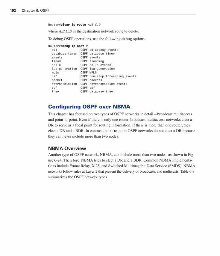
192 Chapter 6: OSPF
Router#cccclllleeeeaaaarrrr iiiipppp rrrroooouuuutttteeee A.B.C.D
where A.B.C.D is the destination network route to delete.
To debug OSPF operations, use the following debug options:
Router#ddddeeeebbbbuuuugggg iiiipppp oooossssppppffff ???? adj OSPF adjacency events database-timer OSPF database timer events OSPF events flood OSPF flooding hello OSPF hello events lsa-generation OSPF lsa generation mpls OSPF MPLS nsf OSPF non-stop forwarding events packet OSPF packets retransmission OSPF retransmission events spf OSPF spf tree OSPF database tree
Configuring OSPF over NBMAThis chapter has focused on two types of OSPF networks in detail—broadcast multiaccess
and point-to-point. Even if there is only one router, broadcast multiaccess networks elect a
DR to serve as a focal point for routing information. If there is more than one router, they
elect a DB and a BDR. In contrast, point-to-point OSPF networks do not elect a DR because
they can never include more than two nodes.
NBMA Overview
Another type of OSPF network, NBMA, can include more than two nodes, as shown in Fig-
ure 6-24. Therefore, NBMA tries to elect a DR and a BDR. Common NBMA implementa-
tions include Frame Relay, X.25, and Switched Multimegabit Data Service (SMDS). NBMA
networks follow rules at Layer 2 that prevent the delivery of broadcasts and multicasts. Table 6-8
summarizes the OSPF network types.
1358_fmi.book Page 192 Thursday, May 27, 2004 2:21 PM

Configuring OSPF over NBMA 193
Figure 6-24 Neighbor Status in Different Network Types
NBMA networks can create problems with OSPF operation—specifically, with the exchange
of multicast Hello packets. RTA, RTB, and RTC belong to the same IP subnetwork and
attempt to elect a DR and a BDR, as shown in Figure 6-25. However, these routers cannot
hold a valid election if they cannot receive multicast Hellos from every other router on the
network. Without administrative intervention, a strange election takes place. As far as RTA is
concerned, RTC is not participating. Likewise, RTC goes through the election process oblivi-
ous to RTA. This botched election can lead to problems if the central router, RTB, is not
elected the DR.
Table 6-8 Types of OSPF Networks
OSPF Network Type Characteristics DR Election?
Broadcast multiaccess Ethernet, Token Ring and FDDI Yes
Nonbroadcast multiaccess Frame Relay, X.25 and SMDS Yes
Point-to-point PPP and HDLC No
Point-to-multipoint Configured by an administrator No
BroadcastMultiaccess
Point-to-Point
NBMAX.25
Frame Relay
1358_fmi.book Page 193 Thursday, May 27, 2004 2:21 PM
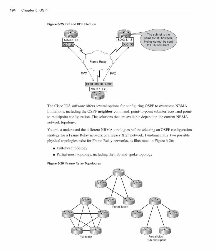
194 Chapter 6: OSPF
Figure 6-25 DR and BDR Election
The Cisco IOS software offers several options for configuring OSPF to overcome NBMA
limitations, including the OSPF neighbor command, point-to-point subinterfaces, and point-
to-multipoint configuration. The solutions that are available depend on the current NBMA
network topology.
You must understand the different NBMA topologies before selecting an OSPF configuration
strategy for a Frame Relay network or a legacy X.25 network. Fundamentally, two possible
physical topologies exist for Frame Relay networks, as illustrated in Figure 6-26:
■ Full-mesh topology
■ Partial-mesh topology, including the hub-and-spoke topology
Figure 6-26 Frame Relay Topologies
S0=3.1.1.1
DLCI 22
RTAS0=3.1.1.3
DLCI 33
RTC
DLCI 200 DLCI 300
S0=3.1.1.2
RTB
PVC PVC
Frame Relay
The subnet is thesame for all, however,Hellos cannot be sent
to RTA from here.
Partial Mesh
Full Mesh Partial MeshHub-and-Spoke
1358_fmi.book Page 194 Thursday, May 27, 2004 2:21 PM

Configuring OSPF over NBMA 195
The following sections describe how to configure OSPF in both full-mesh and partial-mesh
Frame Relay networks.
Full-Mesh Frame Relay
Organizations use Frame Relay primarily because it supports more than one logical connec-
tion over a single interface, as shown in Figure 6-27. This makes it an affordable and flexible
choice for WAN links. A full-mesh topology takes advantage of Frame Relay’s capability to
support multiple permanent virtual circuits (PVCs) on a single serial interface. In a full-mesh
topology, every router has a PVC to every other router.
Figure 6-27 Full-Mesh Frame Relay Topologies
For OSPF to work properly over a multiaccess full-mesh topology that does not support
broadcasts, you must manually enter each OSPF neighbor address on each router, one at a
time. The OSPF neighbor command tells a router about the IP addresses of its neighbors so
that it can exchange routing information without multicasts. Example 6-4 illustrates how the
neighbor command is used.
Example 6-4 neighbor Command
RTA(config)#rrrroooouuuutttteeeerrrr oooossssppppffff 1111
RTA(config-router)#nnnneeeettttwwwwoooorrrrkkkk 3333....1111....1111....0000 0000....0000....0000....222255555555 aaaarrrreeeeaaaa 0000
RTA(config-router)#nnnneeeeiiiigggghhhhbbbboooorrrr 3333....1111....1111....2222
RTA(config-router)#nnnneeeeiiiigggghhhhbbbboooorrrr 3333....1111....1111....3333
S0=3.1.1.1
DLCI 22 DLCI 44
RTAS0=3.1.1.3
DLCI 33
RTC
DLCI 200 DLCI 300
S0=3.1.1.2
RTB
PVC PVC
Frame Relay
PVC PVCDLCI 400
1358_fmi.book Page 195 Thursday, May 27, 2004 2:21 PM

196 Chapter 6: OSPF
Specifying the neighbors for each router is not the only option to make OSPF work in this
type of environment. The following section explains how configuring subinterfaces can elim-
inate the need for the neighbor command.
Configuring Subinterfaces to Create Point-to-Point NetworksThe Cisco IOS software subinterface feature can be used to break a multiaccess network into
a collection of point-to-point networks.
In Figure 6-28, a different IP subnet is assigned to each PVC. OSPF automatically recognizes
this configuration as point-to-point, not NBMA, even with Frame Relay configured on the
interfaces. Recall that OSPF point-to-point networks do not elect a DR. Instead, the Frame
Relay router uses Inverse ARP or a Frame Relay map to obtain the link partner’s address so
that routing information can be exchanged.
Figure 6-28 Neighbor Status in Different Network Types
A full-mesh topology offers numerous advantages, including maximum fault tolerance.
Unfortunately, full-mesh topologies can get expensive, because each PVC must be leased
from a provider. An organization would have to lease 45 PVCs to support just ten fully
meshed routers. If subinterfaces are used to create point-to-point networks, the 45 IP subnets
must also be allocated and managed, which is an additional expense.
Partial-Mesh Frame Relay
Because a full-mesh topology is costly, many organizations implement a partial-mesh topol-
ogy instead. A partial-mesh topology is any configuration in which at least one router
S0.1=3.1.1.1
DLCI 22
S0.1=3.2.2.2
DLCI 33
DLCI 200 DLCI 300
S0.1=3.1.1.2
PVC PVC
Frame Relay
PVC PVCDLCI 400
S0.2=3.2.2.1RTA
DLCI 44
S0.2=3.3.3.1
S0.2=3.3.3.2
RTB
RTC
Subnet PVC
3.1.1.0/24 RTA-RTB
3.2.2.0/24 RTA-RTC
3.3.3.0/24 RTB-RTC
1358_fmi.book Page 196 Thursday, May 27, 2004 2:21 PM

Configuring OSPF over NBMA 197
maintains multiple connections to other routers without being fully meshed. The most cost-
effective partial-mesh topology is a hub-and-spoke topology. This is where a single router,
the hub, connects to multiple spoke routers.
The hub-and-spoke topology is a cost-effective WAN solution that introduces a single point
of failure, the hub router. Organizations typically use Frame Relay because it is inexpensive,
not because it is fault-tolerant.
Unfortunately, the neighbor command that worked with a full-mesh topology does not work
as well with the hub-and-spoke topology. The hub router shown in Figure 6-29 sees all of the
spoke routers and can send routing information to them using the neighbor command, but the
spoke routers can send Hellos only to the hub.
Figure 6-29 Hub-and-Spoke Topology
The DR or BDR election is held, but only the hub router sees all of the candidates. Because
the hub router must act as the DR for this OSPF network to function properly, configure an
OSPF interface priority of 0 on all of the spoke routers. Recall that a priority of 0 makes it
impossible for a router to be elected as a DR or a BDR for a network.
A second approach to dealing with this topology is to avoid the DR and BDR issue altogether
by breaking the network into point-to-point connections, as shown in Figure 6-30. Point-to-
point networks do not elect a DR or BDR.
S0=3.1.1.1
DLCI 22
RTAS0=3.1.1.3
DLCI 33
RTC
DLCI 200 DLCI 300
S0=3.1.1.2
RTB
PVC PVC
Frame Relay
The subnet is thesame for all, however,Hellos cannot be sent
to RTA from here.
Spoke Router Spoke Router
Hub Router
1358_fmi.book Page 197 Thursday, May 27, 2004 2:21 PM
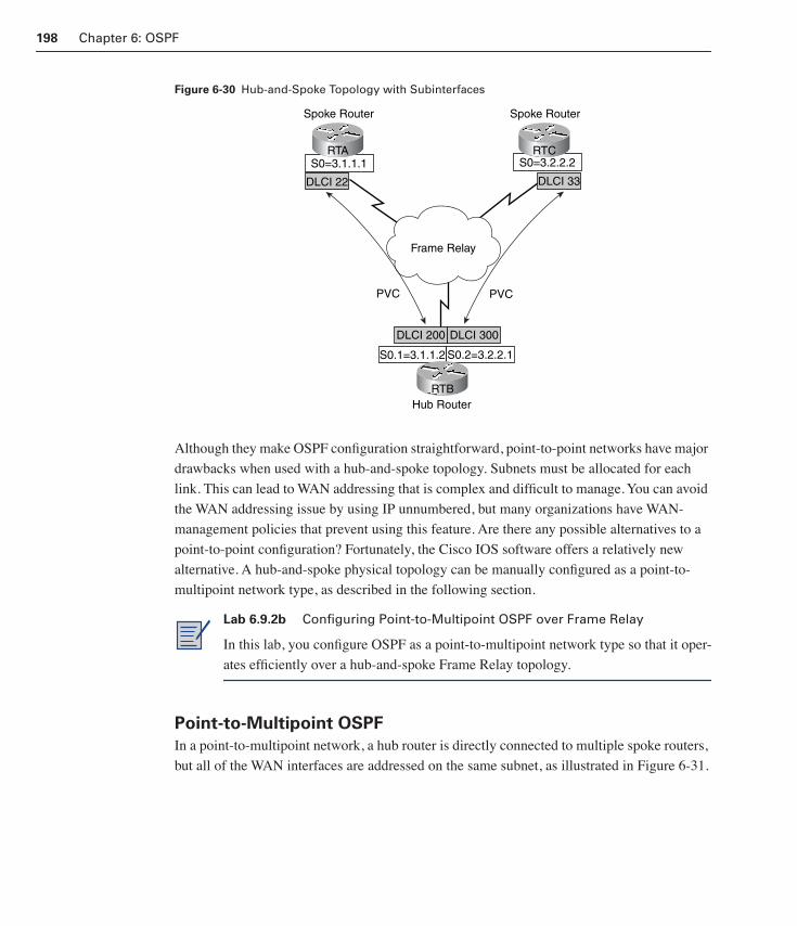
198 Chapter 6: OSPF
Figure 6-30 Hub-and-Spoke Topology with Subinterfaces
Although they make OSPF configuration straightforward, point-to-point networks have major
drawbacks when used with a hub-and-spoke topology. Subnets must be allocated for each
link. This can lead to WAN addressing that is complex and difficult to manage. You can avoid
the WAN addressing issue by using IP unnumbered, but many organizations have WAN-
management policies that prevent using this feature. Are there any possible alternatives to a
point-to-point configuration? Fortunately, the Cisco IOS software offers a relatively new
alternative. A hub-and-spoke physical topology can be manually configured as a point-to-
multipoint network type, as described in the following section.
Point-to-Multipoint OSPF
In a point-to-multipoint network, a hub router is directly connected to multiple spoke routers,
but all of the WAN interfaces are addressed on the same subnet, as illustrated in Figure 6-31.
Lab 6.9.2b Configuring Point-to-Multipoint OSPF over Frame Relay
In this lab, you configure OSPF as a point-to-multipoint network type so that it oper-
ates efficiently over a hub-and-spoke Frame Relay topology.
S0=3.1.1.1
DLCI 22
RTAS0=3.2.2.2
DLCI 33
RTC
DLCI 200 DLCI 300
S0.1=3.1.1.2
PVC PVC
Frame Relay
S0.2=3.2.2.1
RTB
Spoke Router Spoke Router
Hub Router
1358_fmi.book Page 198 Thursday, May 27, 2004 2:21 PM
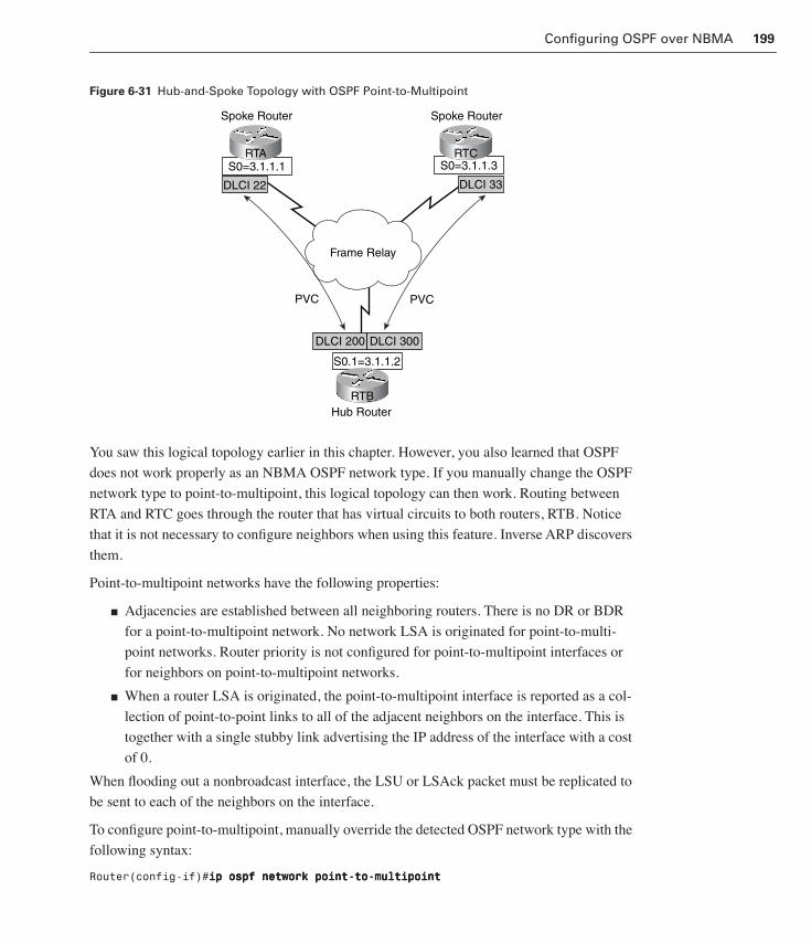
Configuring OSPF over NBMA 199
Figure 6-31 Hub-and-Spoke Topology with OSPF Point-to-Multipoint
You saw this logical topology earlier in this chapter. However, you also learned that OSPF
does not work properly as an NBMA OSPF network type. If you manually change the OSPF
network type to point-to-multipoint, this logical topology can then work. Routing between
RTA and RTC goes through the router that has virtual circuits to both routers, RTB. Notice
that it is not necessary to configure neighbors when using this feature. Inverse ARP discovers
them.
Point-to-multipoint networks have the following properties:
■ Adjacencies are established between all neighboring routers. There is no DR or BDR
for a point-to-multipoint network. No network LSA is originated for point-to-multi-
point networks. Router priority is not configured for point-to-multipoint interfaces or
for neighbors on point-to-multipoint networks.
■ When a router LSA is originated, the point-to-multipoint interface is reported as a col-
lection of point-to-point links to all of the adjacent neighbors on the interface. This is
together with a single stubby link advertising the IP address of the interface with a cost
of 0.
When flooding out a nonbroadcast interface, the LSU or LSAck packet must be replicated to
be sent to each of the neighbors on the interface.
To configure point-to-multipoint, manually override the detected OSPF network type with the
following syntax:
Router(config-if)#iiiipppp oooossssppppffff nnnneeeettttwwwwoooorrrrkkkk ppppooooiiiinnnntttt----ttttoooo----mmmmuuuullllttttiiiippppooooiiiinnnntttt
S0=3.1.1.1
DLCI 22
RTAS0=3.1.1.3
DLCI 33
RTC
DLCI 200 DLCI 300
S0.1=3.1.1.2
PVC PVC
Frame Relay
RTB
Spoke Router Spoke Router
Hub Router
1358_fmi.book Page 199 Thursday, May 27, 2004 2:21 PM

200 Chapter 6: OSPF
Also configure the interface with a frame-relay map ip command:
Router(config-if)#ffffrrrraaaammmmeeee----rrrreeeellllaaaayyyy mmmmaaaapppp iiiipppp address dlci bbbbrrrrooooaaaaddddccccaaaasssstttt
The broadcast keyword permits the router to send broadcasts by way of the specified DLCI
to the mapped neighbor or neighbors. If you’re applying the point-to-multipoint configuration
to the sample network shown in Figure 6-31, two separate frame-relay map statements
would have to be configured on the hub router, RTB, as shown in Example 6-5.
Example 6-5 Configurations for Point-to-Multipoint OSPF
RTA>sssshhhhoooowwww rrrruuuunnnnnnnniiiinnnngggg ccccoooonnnnffffiiiigggguuuurrrraaaattttiiiioooonnnn
<output omitted>
!
interface Serial0
encapsulation frame-relay
ip address 3.1.1.1 255.255.255.0
ip ospf network point-to-multipoint
frame-relay map ip 3.1.1.2 22 broadcast
!
router ospf 1
network 3.1.1.0 0.0.0.255 area 0
RTB>sssshhhhoooowwww rrrruuuunnnnnnnniiiinnnngggg ccccoooonnnnffffiiiigggguuuurrrraaaattttiiiioooonnnn
<output omitted>
!
interface Serial0
encapsulation frame-relay
ip address 3.1.1.2 255.255.255.0
ip ospf network point-to-multipoint
frame-relay map ip 3.1.1.1 200 broadcast
frame-relay map ip 3.1.1.3 300 broadcast
!
router ospf 1
network 3.1.1.0 0.0.0.255 area 0
RTC>sssshhhhoooowwww rrrruuuunnnnnnnniiiinnnngggg ccccoooonnnnffffiiiigggguuuurrrraaaattttiiiioooonnnn
<output omitted>
1358_fmi.book Page 200 Thursday, May 27, 2004 2:21 PM

Multiarea OSPF Operation 201
In a point-to-multipoint configuration, OSPF treats all router-to-router connections on the
nonbroadcast network as if they were point-to-point links. No DR is elected for the network.
Neighbors can be manually specified using the neighbor command or can be dynamically
discovered using Inverse ARP. Ultimately, point-to-multipoint OSPF offers efficient opera-
tion without administrative complexity.
Multiarea OSPF OperationThree issues can overwhelm an OSPF router in a heavily populated OSPF network:
■ High demand for router processing and memory resources
■ Large routing tables
■ Large topology tables
Creating Multiple OSPF Areas
In a very large internetwork, changes are inevitable. OSPF routers are likely to run SPF cal-
culations frequently, which deprive the router of precious CPU cycles and memory resources,
as shown in Figure 6-32.
Not only is the routing table frequently recalculated in a large OSPF network, but it also risks
being overstuffed with multiple paths and hundreds of routes. Full routing tables make rout-
ers less efficient. Finally, the link-state database, which must contain a complete topology of
the network, also threatens to consume resources and slow down the router.
Fortunately, OSPF allows large areas to be separated into smaller, more manageable areas.
These smaller areas can exchange summaries of routing information rather than exchange
every detail. By splitting the network into manageable pieces, OSPF routers can scale gracefully.
!
interface Serial0
encapsulation frame-relay
ip address 3.1.1.3 255.255.255.0
ip ospf network point-to-multipoint
frame-relay map ip 3.1.1.2 33 broadcast
!
router ospf 1
network 3.1.1.0 0.0.0.255 area 0
Example 6-5 Configurations for Point-to-Multipoint OSPF (Continued)
1358_fmi.book Page 201 Thursday, May 27, 2004 2:21 PM

202 Chapter 6: OSPF
Figure 6-32 Issues with Maintaining a Large OSPF Network
Just how many routers can an OSPF area support? Field studies have shown that a single
OSPF area should not stretch beyond 50 routers, although there is no set limit. Some areas
might do fine with more than 50 routers. Other areas, particularly those with unstable links,
might need to operate with fewer than 50 routers. Ultimately, you must determine just how
many routers a particular OSPF area can handle. Knowing the network by tracking perfor-
mance and monitoring usage is the only way to accurately gauge whether an OSPF area can
support 20, 30, or 60 routers.
OSPF’s capability to separate a large internetwork into multiple areas is called hierarchical
routing. Hierarchical routing enables the separation of large internetworks into smaller inter-
networks that are called interareas. With this technique, interarea routing still occurs. Inter-
area routing is the process of exchanging routing information between OSPF areas. However,
interarea routing allows OSPF to summarize and contain area-specific information so that
many of the smaller internal routing operations, such as recalculating the database, are
restricted within an area.
For example, if Area 1 is having problems with a link going up and down (flapping), routers
in other areas do not need to run their SPF calculation, because they are isolated from the
problems in Area 1, as shown in Figure 6-33.
OSPF
OSPF
OSPF
OSPF
OSPF
This routing table is too big.The memory is running low.
1358_fmi.book Page 202 Thursday, May 27, 2004 2:21 PM
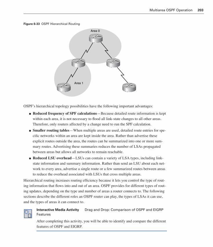
Multiarea OSPF Operation 203
Figure 6-33 OSPF Hierarchical Routing
OSPF’s hierarchical topology possibilities have the following important advantages:
■ Reduced frequency of SPF calculations—Because detailed route information is kept
within each area, it is not necessary to flood all link-state changes to all other areas.
Therefore, only routers affected by a change need to run the SPF calculation.
■ Smaller routing tables—When multiple areas are used, detailed route entries for spe-
cific networks within an area are kept inside the area. Rather than advertise these
explicit routes outside the area, the routes can be summarized into one or more sum-
mary routes. Advertising these summaries reduces the number of LSAs propagated
between areas but allows all networks to remain reachable.
■ Reduced LSU overhead—LSUs can contain a variety of LSA types, including link-
state information and summary information. Rather than send an LSU about each net-
work to every area, advertise a single route or a few summarized routes between areas
to reduce the overhead associated with LSUs that cross multiple areas.
Hierarchical routing increases routing efficiency because it lets you control the type of rout-
ing information that flows into and out of an area. OSPF provides for different types of rout-
ing updates, depending on the type and number of areas a router connects to. The following
sections describe the different roles an OSPF router can play, the types of LSAs it can use,
and the types of areas it can connect to.
Interactive Media Activity Drag and Drop: Comparison of OSPF and EIGRP Features
After completing this activity, you will be able to identify and compare the different
features of OSPF and EIGRP.
Area 0
Area 1
1358_fmi.book Page 203 Thursday, May 27, 2004 2:21 PM

204 Chapter 6: OSPF
OSPF Router Types
Four different types of OSPF routers exist, as shown in Figure 6-34:
■ Internal router—As discussed previously, routers that have all of their interfaces
within the same area are called internal routers. Internal routers in the same area have
identical link-state databases and run a single copy of the routing algorithm.
■ Backbone router—Routers that are attached to the backbone area of the OSPF net-
work are called backbone routers. They have at least one interface connected to Area 0,
the backbone area. These routers maintain OSPF routing information using the same
procedures and algorithms as internal routers.
■ Area Border Router (ABR)—ABRs are routers with interfaces attached to multiple
areas. They maintain a separate link-state database for each area to which they are con-
nected, and they route traffic destined for or arriving from other areas. ABRs are exit
points for the area, which means that routing information destined for another area can
travel there only by way of the of the local area ABR. ABRs summarize information
about the attached areas from their link-state databases and distribute the information
into the backbone. The backbone ABRs then forward the information to all other con-
nected areas. An area can have one or more ABRs.
■ Autonomous System Boundary Router (ASBR)—ASBRs are routers that have at
least one interface connected to an external internetwork—another autonomous system,
such as a non-OSPF network. These routers can import non-OSPF network information
to the OSPF network and OSPF to non-OSPF. This is called redistribution.
Figure 6-34 OSPF Multiarea Components
InternalRouters
Backbone/InternalRouters
ABR andBackbone
Router
ABR andBackbone
Router
ASBR andBackbone
Router
InternalRouters
Area 1
Area 2
Backbone Area 0
ExternalAS
1358_fmi.book Page 204 Thursday, May 27, 2004 2:21 PM

Multiarea OSPF Operation 205
A router can be more than one router type. For example, if a router interconnects to Area 0
and Area 1, as well as to a non-OSPF network, it is both an ABR and an ASBR.
OSPF LSA and Area Types
Multiarea OSPF is scalable because a router’s link-state database can include multiple types
of LSAs, as shown in Figure 6-35.
Figure 6-35 OSPF Sample OSPF Database
OSPF LSA TypesDRs and routers that reside in multiple areas or autonomous systems use special LSAs to
send or summarize routing information. The OSPF LSA types are described in Table 6-9.Table 6-9 OSPF LSA Types
LSA Type Name Description
1 Router link entry (O-OSPF)
Generated by each router for each area it belongs to. It describes the states of the link from the router to the area. These are flooded only within a particular area. The link status and cost are two of the descriptors provided. Routes learned by way of Type 1 LSAs are denoted by an O in the routing table.
2 Network link entry (O-OSPF)
Generated by the DR in multiaccess networks. A Type 2 LSA describes the set of routers attached to a particular network. Type 2 LSAs are flooded only within the area that contains the network. Routes learned by way of Type 2 LSAs are denoted by an O in the routing table.
3 Summary link entry (IA-OSPF)
Originated by ABRs. A Type 3 LSA describes the links between the ABR and the internal routers of a local area. These entries are flooded throughout the backbone area to the outer ABRs. Type 3 LSAs describe routes to networks within the local area and are sent to the backbone area. Routes learned by way of Type 3 LSAs are denoted by an O in the routing table.
Route
Network
Summary
ExternalArea 1 Area 0DR
ABR ASBRExternal
AS
continues
1358_fmi.book Page 205 Thursday, May 27, 2004 2:21 PM

206 Chapter 6: OSPF
OSPF Area TypeThe characteristics assigned to an area control the type of route information it can receive.
For example, the size of routing tables might need to be minimized in an OSPF area. In this
case, configure the routers to operate in an area that does not accept external routing informa-
tion, Type 5 LSAs.
The following are several area types that are possible, as shown in Figure 6-36:
■ Standard area—A standard area can accept link updates and route summaries.
■ Backbone area (transit area)—When interconnecting multiple areas, the backbone
area is the central entity to which all other areas connect. The backbone area is always
Area 0. All other areas must connect to this area to exchange route information. The
OSPF backbone has all of the properties of a standard OSPF area.
■ Stubby area—A stubby area is an area that does not accept information about routes
external to the autonomous system, the OSPF internetwork, such as routes from
LSA Type Name Description
4 Summary link entry (O-OSPF)
Originated by ABRs. Type 4 LSAs are flooded throughout the backbone area to the outer ABRs. Type 4 LSAs describe reachability to ASBRs. These link entries are not flooded through totally stubby areas. Routes learned by way of Type 4 LSAs are denoted by an IA in the routing table.
5 Autonomous system external link entry (E1-OSPF external Type 1 and E2-OSPF external Type 2)
Originated by ASBRs. A Type 5 LSA describes routes to destinations external to the autonomous system. These are flooded throughout an OSPF autonomous system except for stubby and totally stubby areas. Routes learned by way of Type 5 LSAs are denoted by either an E1 or E2 in the routing table.
6 Multicast OSPF (MOSPF)
Not implemented by Cisco. MOSPF enhances OSPF by letting routers use their link-state data-bases to build multicast distribution trees for the forwarding of multicast traffic.
7 Autonomous system external link entry (N1-OSPF NSSA external Type 1, N2-OSPF external Type 2)
Originated by an ASBR connected to an NSSA. Type 7 messages can be flooded throughout NSSAs and translated into LSA Type 5 messages by ABRs. Routes learned by way of Type 7 LSAs are denoted by either an N1 or an N2 in the rout-ing table.
Table 6-9 OSPF LSA Types (Continued)
1358_fmi.book Page 206 Thursday, May 27, 2004 2:21 PM
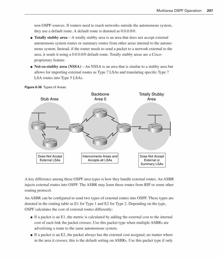
Multiarea OSPF Operation 207
non-OSPF sources. If routers need to reach networks outside the autonomous system,
they use a default route. A default route is denoted as 0.0.0.0/0.
■ Totally stubby area—A totally stubby area is an area that does not accept external
autonomous system routes or summary routes from other areas internal to the autono-
mous system. Instead, if the router needs to send a packet to a network external to the
area, it sends it using a 0.0.0.0/0 default route. Totally stubby areas are a Cisco-
proprietary feature.
■ Not-so-stubby area (NSSA)—An NSSA is an area that is similar to a stubby area but
allows for importing external routes as Type 7 LSAs and translating specific Type 7
LSA routes into Type 5 LSAs.
Figure 6-36 Types of Areas
A key difference among these OSPF area types is how they handle external routes. An ASBR
injects external routes into OSPF. The ASBR may learn these routes from RIP or some other
routing protocol.
An ASBR can be configured to send two types of external routes into OSPF. These types are
denoted in the routing table as E1 for Type 1 and E2 for Type 2. Depending on the type,
OSPF calculates the cost of external routes differently:
■ If a packet is an E1, the metric is calculated by adding the external cost to the internal
cost of each link the packet crosses. Use this packet type when multiple ASBRs are
advertising a route to the same autonomous system.
■ If a packet is an E2, the packet always has the external cost assigned, no matter where
in the area it crosses; this is the default setting on ASBRs. Use this packet type if only
Stub AreaTotally Stubby
AreaBackbone
Area 0
Does Not AcceptExternal LSAs
Interconnects Areas andAccepts all LSAs
Does Not AcceptExternal or
Summary LSAs
1358_fmi.book Page 207 Thursday, May 27, 2004 2:21 PM

208 Chapter 6: OSPF
one router is advertising a route to the autonomous system. Type 2 routes are preferred
over Type 1 routes, unless two equal-cost routes to the destination exist.
For example, consider the network shown in Figure 6-37.
Figure 6-37 OSPF LSA
In this network, RTB receives external RIP routes, including 9.0.0.0/8 from RTA. By default,
RTA sends external routing information using Type 2 metrics. Therefore, when RTB sends
this route to RTC, the metric for the external route remains the same—in this case, 20. Com-
pare the E2 routing table entries for RTB in Example 6-6 to the E2 entries for RTC in
Example 6-7.
If RTA is configured to use a Type 1 metric with external routes, OSPF increments the metric
value of the external route according to its standard cost algorithm. In the show ip route out-
put shown in Example 6-8, you can see that the same routes are now listed as E1 and have
Example 6-6 Routing Table Entries for RTB
RTB#sssshhhhoooowwww iiiipppp rrrroooouuuutttteeee
<output omitted>
O E2 9.0.0.0/8 [110/20] via 192.168.1.2, 00:00:07, Serial0/0
C 192.168.1.0/24 is directly connected, Serial0/0
C 192.168.2.0/24 is directly connected, Serial0/1
Example 6-7 Routing Table Entries for RTC
RTC#sssshhhhoooowwww iiiipppp rrrroooouuuutttteeee
<output omitted>
O E2 9.0.0.0/8 [110/20] via 192.168.2.1, 00:00:46, Serial0/0
C 192.168.1.0/24 [110/1171] via 192.168.2.1, 00:03:09, Serial0/0
C 192.168.2.0/24 is directly connected, Serial0/0
RIP9.0.0.0/8
ASBR
RTA RTB RTC
S0/0 192.168.1.2
S0/0 192.168.1.1
S0/0 192.168.2.2
S0/1 192.168.2.1
Area 0
1358_fmi.book Page 208 Thursday, May 27, 2004 2:21 PM

Multiarea OSPF Operation 209
very different metrics in each table. RTB now increments the metric for the external route, as
shown in Example 6-9.
Configuring OSPF Operation Across Multiple Areas
Internal routers, ABRs, ASBRs, and backbone routers each play a role in communicating
OSPF routing information in a multiarea network. This section summarizes how the different
types of OSPF routers flood information and how they build their routing tables when operat-
ing within a multiarea environment.
You’ve seen that a packet destined for a network within an area is merely forwarded from one
internal router to another until it reaches the destination network. However, what if a packet
must traverse multiple areas, as shown in Figures 6-38, 6-39, and 6-40?
Example 6-8 Routing Table Entries for RTB
RTB#sssshhhhoooowwww iiiipppp rrrroooouuuutttteeee
<output omitted>
O E2 9.0.0.0/8 [110/20] via 192.168.2.1, 00:00:05, Serial0/0
C 192.168.1.0/24 is directly connected, Serial0/0
C 192.168.2.0/24 is directly connected, Serial0/1
Example 6-9 Routing Table Entries for RTC
RTC#sssshhhhoooowwww iiiipppp rrrroooouuuutttteeee
<output omitted>
O E2 9.0.0.0/8 [110/1191] via 192.168.2.1, 00:00:47, Serial0/0
C 192.168.1.0/24 [110/1171] via 192.168.2.1, 00:04:50, Serial0/0
C 192.168.2.0/24 is directly connected, Serial0/0
Interactive Media Activity Drag and Drop: OSPF LSA Types
After completing this activity, you will be able to identify the different OSPF
LSA types.
1358_fmi.book Page 209 Thursday, May 27, 2004 2:21 PM

210 Chapter 6: OSPF
Figure 6-38 Packet Forwarding in a Multiarea Network to ABR1
Figure 6-39 Packet Forwarding in a Multiarea Network to the Backbone
Figure 6-40 Packet Forwarding in a Multiarea Network to the Destination Network
Area 1 Area 0 Area 50
To ABR1
Internal ABR1 ABR2 Internal
BBone
Data
Area 1 Area 0 Area 50
To Backbone
Internal ABR1 ABR2 Internal
BBone
Data
Area 1 Area 0 Area 50
To Destination Network
Internal ABR1 ABR2 Internal
BBone
Data
1358_fmi.book Page 210 Thursday, May 27, 2004 2:21 PM
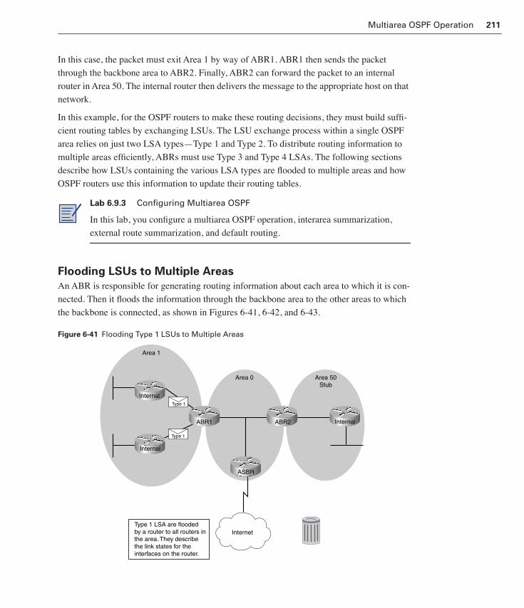
Multiarea OSPF Operation 211
In this case, the packet must exit Area 1 by way of ABR1. ABR1 then sends the packet
through the backbone area to ABR2. Finally, ABR2 can forward the packet to an internal
router in Area 50. The internal router then delivers the message to the appropriate host on that
network.
In this example, for the OSPF routers to make these routing decisions, they must build suffi-
cient routing tables by exchanging LSUs. The LSU exchange process within a single OSPF
area relies on just two LSA types—Type 1 and Type 2. To distribute routing information to
multiple areas efficiently, ABRs must use Type 3 and Type 4 LSAs. The following sections
describe how LSUs containing the various LSA types are flooded to multiple areas and how
OSPF routers use this information to update their routing tables.
Flooding LSUs to Multiple Areas
An ABR is responsible for generating routing information about each area to which it is con-
nected. Then it floods the information through the backbone area to the other areas to which
the backbone is connected, as shown in Figures 6-41, 6-42, and 6-43.
Figure 6-41 Flooding Type 1 LSUs to Multiple Areas
Lab 6.9.3 Configuring Multiarea OSPF
In this lab, you configure a multiarea OSPF operation, interarea summarization,
external route summarization, and default routing.
InternetType 1 LSA are floodedby a router to all routers inthe area. They describethe link states for theinterfaces on the router.
Type 1
Type 1
Internal
Internal
InternalABR1 ABR2
ASBR
Area 1
Area 0 Area 50Stub
1358_fmi.book Page 211 Thursday, May 27, 2004 2:21 PM
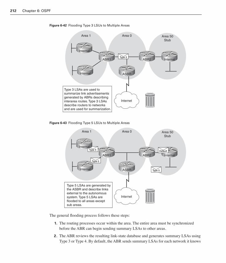
212 Chapter 6: OSPF
Figure 6-42 Flooding Type 3 LSUs to Multiple Areas
Figure 6-43 Flooding Type 5 LSUs to Multiple Areas
The general flooding process follows these steps:
1. The routing processes occur within the area. The entire area must be synchronized before the ABR can begin sending summary LSAs to other areas.
2. The ABR reviews the resulting link-state database and generates summary LSAs using Type 3 or Type 4. By default, the ABR sends summary LSAs for each network it knows
Area 1 Area 0 Area 50Stub
ABR2 InternalType 3
Internet
Internal
ABR1
Internal ASBR
Type 3 LSAs are used to summarize link advertisements generated by ABRs describing interarea routes. Type 3 LSAs describe routers to networks and are used for summarization.
Area 1 Area 0 Area 50Stub
ABR2 Internal
Internet
ABR1
ASBR
Type 5 LSAs are generated by the ASBR and describe links external to the autonomous system. Type 5 LSAs are flooded to all areas except sub areas.
Type 5Internal
Type 5
Internal Type 5
Default
1358_fmi.book Page 212 Thursday, May 27, 2004 2:21 PM

Multiarea OSPF Operation 213
about. To reduce the number of summary LSA entries, configure route summarization so that a single IP address can represent multiple networks. To use route summariza-tion, the areas need to use contiguous IP addressing, as discussed in Chapter 2, “Advanced IP Addressing Management.” The better this IP address plan is, the fewer summary LSA entries an ABR advertises.
3. The summary LSAs are placed in an LSU and are distributed through all ABR inter-faces, with the following exceptions:
— If the interface is connected to a neighboring router that is in a state below the
exchange state, the summary LSA is not forwarded.
— If the interface is connected to a totally stubby area, the summary LSA is not for-
warded.
— If the summary LSA includes a Type 5 (external) route and the interface is con-
nected to a stubby or totally stubby area, the LSA is not sent to that area.
4. After an ABR or ASBR receives summary LSAs, it adds them to its link-state databases and floods them to the local area. The internal routers then assimilate the information into their databases. Remember that OSPF lets you configure different area types so that you can reduce the number of route entries that internal routers maintain. To minimize routing information, define the area as a stubby area, a totally stubby area, or an NSSA.
Updating the Routing Table
After all routers receive the routing updates, they add them to their link-state databases and
recalculate their routing tables. Paths are calculated in this order:
1. All routers calculate the paths to destinations within their area and add these entries to the routing table. These are learned by way of Type 1 and Type 2 LSAs.
2. All routers calculate the paths to the other areas within the internetwork. These paths are learned by way of interarea route entries, or Type 3 and Type 4 LSAs. If a router has an interarea route to a destination and an intra area route to the same destination, the intra area route is kept.
3. All routers, except those that are in any of the stubby area types, calculate the paths to the AS external (Type 5) destinations.
At this point, a router can reach any network within or outside the OSPF autonomous system.
Opaque LSAs
Opaque LSAs allow for the future extensibility of OSPF. The information contained
in opaque LSAs may be used directly by OSPF or indirectly by applications that want to
distribute information throughout an OSPF domain. For example, the OSPF opaque LSA
may be used for traffic engineering with Multiprotocol Label Switching (MPLS).
1358_fmi.book Page 213 Thursday, May 27, 2004 2:21 PM

214 Chapter 6: OSPF
Opaque LSAs are Types 9, 10, and 11 LSAs. Opaque LSAs consist of a standard LSA header
followed by a 32-bit aligned application-specific information field. Like any other LSA, the
opaque LSA uses the link-state database distribution mechanism to flood this information
throughout the topology. The opaque LSA’s link-state type field identifies the LSA’s topolog-
ical distribution range. This range is called the flooding scope.
The flooding scope associated with each opaque link-state type is defined as follows:
■ Link-state Type 9 denotes a link-local scope. Type 9 opaque LSAs are not flooded
beyond the local network or subnetwork.
■ Link-state Type 10 denotes an area-local scope. Type 10 opaque LSAs are flooded only
within their associated area.
■ Link-state Type 11 denotes that the LSA is flooded throughout the entire autonomous
system. The flooding scope of Type 11 LSAs is equivalent to the flooding scope of AS-
external (Type 5) LSAs.
Multiarea OSPF Configuration and VerificationThe following sections discuss some of the details of OSPF configuration and verification:
■ Using and configuring OSPF multiarea components
■ Configuring OSPF route summarization
■ Verifying multiarea OSPF operation
Using and Configuring OSPF Multiarea Components
The following sections cover some of the multiarea OSPF capabilities and associated config-
urations in more detail. You will learn how to configure an ABR and route summarization.
Configuring an ABRNo special commands make a router an ABR or an ASBR. The router becomes an ABR as
soon as two of its interfaces are configured to operate in different areas, as shown in Figure 6-44.
Example 6-10 shows the configuration for the routers shown in Figure 6-44.
Figure 6-44 Configuring OSPF ABRs
B CA
E0
E0
S0
S110.64.0.1
10.64.0.210.2.1.1
10.2.1.2
Area 0 Area 1ABR
1358_fmi.book Page 214 Thursday, May 27, 2004 2:21 PM

Multiarea OSPF Configuration and Verification 215
Configuring an ASBRASBRs are created when OSPF is configured to import, or redistribute, external routes into
OSPF, as shown in Figure 6-45. Notice that the ASBR configuration commands include the
command redistribute rip subnets, which is shown in Example 6-11. This command tells
OSPF to import RIP routing information. A detailed discussion of route redistribution can be
found in Chapter 8, “Route Optimization.” The subnets option tells the OSPF process to
include RIP subnets in redistribution.
Figure 6-45 Configuring OSPF ASBRs
Example 6-10 Configuring OSPF ABRs
RouterA#sssshhhhoooowwww rrrruuuunnnnnnnniiiinnnngggg ccccoooonnnnffffiiiigggguuuurrrraaaattttiiiioooonnnn
<output omitted>
!
ip address 10.64.0.1 255.255.255.0
!
<output omitted>
router ospf 77
network 10.0.0.0 0.255.255.255 area 0
RouterB#sssshhhhoooowwww rrrruuuunnnnnnnniiiinnnngggg ccccoooonnnnffffiiiigggguuuurrrraaaattttiiiioooonnnn
<output omitted>
interface Ethernet0
ip address 10.64.0.2 255.255.255.0
!
interface Serial0
ip address 10.2.1.2 255.255.255.0
<output omitted>
router ospf 50
network 10.0.0.0 0.255.255.255 area 1
network 10.0.0.0 0.255.255.255 area 0
ASBR OSPF Area 0
192.168.1.0/24
RTA RTB
1358_fmi.book Page 215 Thursday, May 27, 2004 2:21 PM

216 Chapter 6: OSPF
Configuring OSPF Route Summarization
Recall that summarization is the consolidation of multiple routes into one single, supernet
advertisement. See Chapter 2, “Objectives,” for more details. Proper summarization requires
contiguous (sequential) addressing. 200.10.0.0, 200.10.1.0, 200.10.2.0, and so on are exam-
ples of contiguous addressing. OSPF routers can be manually configured to advertise a super-
net route, which is different from an LSA summary route.
Route summarization directly affects the amount of bandwidth, CPU, and memory resources
that the OSPF process consumes. With summarization, if a network link fails or flaps, the
topology change is not propagated into the backbone and other areas by way of the backbone.
As discussed in previous chapters, route summarization protects routers from needless rout-
ing table recalculations. Because the SPF calculation places a significant demand on a router
CPU, proper summarization is an important part of OSPF configuration. OSPF supports the
following two types of summarization:
■ Interarea route summarization—Interarea route summarization is done on ABRs and
applies to routes from within each area. It does not apply to external routes injected into
OSPF by way of redistribution. To take advantage of summarization, network numbers
within areas should be contiguous.
■ External route summarization—External route summarization is specific to external
routes that are injected into OSPF by way of redistribution. Here again, it is important
to ensure that external address ranges that are being summarized are contiguous.
Example 6-11 Configuring OSPF ASBR
RTA(config)#rrrroooouuuutttteeeerrrr rrrriiiipppp
RTA(config-router)#nnnneeeettttwwwwoooorrrrkkkk 11110000....0000....0000....0000
RTA(config-router)#eeeexxxxiiiitttt
RTA(config)#rrrroooouuuutttteeeerrrr oooossssppppffff 1111
RTA(config-router)#nnnneeeettttwwwwoooorrrrkkkk 111199992222....111166668888....1111....0000 0000....0000....0000....222255555555 aaaarrrreeeeaaaa 0000
RTA(config-router)#rrrreeeeddddiiiissssttttrrrriiiibbbbuuuutttteeee rrrriiiipppp ssssuuuubbbbnnnneeeettttssss
RTA(config-router)#^̂̂̂ZZZZ
RTA#sssshhhhoooowwww iiiipppp oooossssppppffff
Routing Process “ospf 1” with ID 192.168.1.2
Supports only single TOS(TOSO) routes
Supports opaque LSA
It is an autonomous system boundary router
Redistributing external routes from rip, including subnets in redistribution.
<output omitted>
1358_fmi.book Page 216 Thursday, May 27, 2004 2:21 PM

Multiarea OSPF Configuration and Verification 217
Summarization of overlapping ranges from two different routers can cause packets to
be sent to the wrong destination. Only ASBRs can summarize external routes.
To configure an ABR to summarize routes for a specific area before injecting them into a dif-
ferent area, use the following syntax:
Router(config-router)#aaaarrrreeeeaaaa area-id rrrraaaannnnggggeeee address mask
To configure an ASBR to summarize external routes before injecting them into the OSPF
domain, use the following syntax:
Router(config-router)#ssssuuuummmmmmmmaaaarrrryyyy----aaaaddddddddrrrreeeessssssss address mask
Use the following commands to configure RTA for external router summarization, as shown
in Figure 6-46.
RTA(config)#rrrroooouuuutttteeeerrrr oooossssppppffff 1111RTA(config-router)#ssssuuuummmmmmmmaaaarrrryyyy----aaaaddddddddrrrreeeessssssss 222200000000....9999....0000....0000 222255555555....222255555555....0000....0000
Figure 6-46 OSPF Route Summarization
After it is configured, RTA sends only a single summary route, 200.9.0.0/16, into the OSPF
domain.
Because RTB sits on the border between Area 0 and Area 1, it should be configured to per-
form interarea summarization, as follows:
RTB(config)#rrrroooouuuutttteeeerrrr oooossssppppffff 1111RTB(config-router)#aaaarrrreeeeaaaa 1111 rrrraaaannnnggggeeee 111199992222....111166668888....11116666....0000 222255555555....222255555555....222255552222....0000
Notice that the area 1 range command in this example specifies the area containing the range
to be summarized before being injected into Area 0. In this example, the four networks in the
area, 192.168.16.0/24 through 192.168.19.0/24, are summarized to the single summary route
192.168.16.0/22 using the common bits.
Also, depending on the network topology, you might not want to summarize Area 0 networks.
If there is more than one ABR between an area and the backbone area, for example, sending a
summary LSA with the explicit network information ensures that the shortest path is selected.
If the addresses are summarized, suboptimal path selection might occur.
200.9.1.0/24200.9.2.0/24200.9.3.0/24200.9.4.0/24…200.9.255.0/24
S1 S0
RIP
ASBRRTA
S0 S1
ABRRTB
Area 0
192.168.16.0/24192.168.17.0/24192.168.18.0/24192.168.19.0/24
Area 1
External Summary Route
200.9.0.0/16
Interarea Summary Route
192.168.16.0/22
1358_fmi.book Page 217 Thursday, May 27, 2004 2:21 PM
218 Chapter 6: OSPF
Verifying Multiarea OSPF Operation
In addition to the show commands discussed earlier, several key OSPF commands can be
used to verify multiarea operation:
■ show ip ospf border-routers—Displays the internal OSPF routing table entries to an
ABR.
■ show ip ospf virtual-links—Displays parameters about the current state of OSPF vir-
tual links.
■ show ip ospf process-id—Displays information about each area to which the router is
connected and indicates whether the router is an ABR, ASBR, or both. The process ID
is a user-defined identification parameter. It is locally assigned and can be any positive
integer. The number used here is the number assigned administratively when enabling
the OSPF routing process.
■ show ip ospf database—Displays the contents of the topological database maintained
by the router. Several keywords can be used with this command to get specific informa-
tion about the following links:
— show ip ospf [process-id area-id] database [router]—Displays individual router
link-state information.
— show ip ospf [process-id area-id] database [network]—Displays network link-
state information. The area ID is the area number associated with the OSPF
address range defined in the network router configuration command when defin-
ing a particular area.
— show ip ospf [process-id area-id] database [summary]—Displays summary
information about ABR link states.
— show ip ospf [process-id area-id] database [asbr-summary]—Displays infor-
mation about ASBR link states.
— show ip ospf [process-id area-id] database [external]—Displays information
about autonomous system external link states.
— show ip ospf [process-id area-id] database [database-summary]—Displays
database summary information and totals.
Stub, Totally Stubby, and Not-So-Stubby AreasAn OSPF router interface can be configured to operate as either a stubby area or a totally
stubby area. A stubby area does not accept information about routes external to the AS. A
totally stubby area does not accept external AS routes and summary routes from other areas
internal to the AS.
1358_fmi.book Page 218 Thursday, May 27, 2004 2:21 PM

Stub, Totally Stubby, and Not-So-Stubby Areas 219
Using Stub and Totally Stubby Areas
If you configure an area as stubby, you can greatly reduce the size of the link-state database
inside that area. As a result, this reduces the area routers’ memory requirements. Remember
that stubby areas do not accept Type 5 (external) LSAs.
Because OSPF routers internal to a stubby area do not learn about external networks, routing
to the outside world is based on a 0.0.0.0/0 default route. When configuring a stubby area, the
ABR on the stub automatically propagates a 0.0.0.0/0 default route within the area.
Stubby areas are typically created when using a hub-and-spoke topology, with the spokes
configured as stubby areas. The spokes could be the branch offices. In the case of a hub-and-
spoke topology, the branch office might not need to know about every network at the head-
quarters site. It can instead use a default route to get there.
To further reduce the number of routes in a table, create a totally stubby area, which is a
Cisco-specific feature. A totally stubby area is a stubby area that blocks external (Type 5)
LSAs and summary (Type 3 and Type 4) LSAs from entering the area. This way, intra area
routes and the default of 0.0.0.0/0 are the only routes known to the stubby area. ABRs inject
the default summary link 0.0.0.0/0 into the totally stubby area.
Therefore, totally stubby areas further minimize routing information and increase stability
and scalability of OSPF internetworks. This is typically a better solution than creating stubby
areas, unless the target area uses a mix of Cisco and non-Cisco routers. The following sec-
tions describe the criteria for determining whether an area should be configured as stubby or
totally stubby and the configuration commands necessary to implement these area types.
Stub and Totally Stubby Area Criteria
An area can be qualified as stubby or totally stubby when it meets the following criteria,
which are illustrated in Figure 6-47.
■ There is a single exit point from that area.
■ The area is not needed as a transit area for virtual links. Virtual links are discussed near
the end of this chapter.
■ No ASBR is internal to the stubby area.
■ The area is not the backbone area (Area 0).
1358_fmi.book Page 219 Thursday, May 27, 2004 2:21 PM
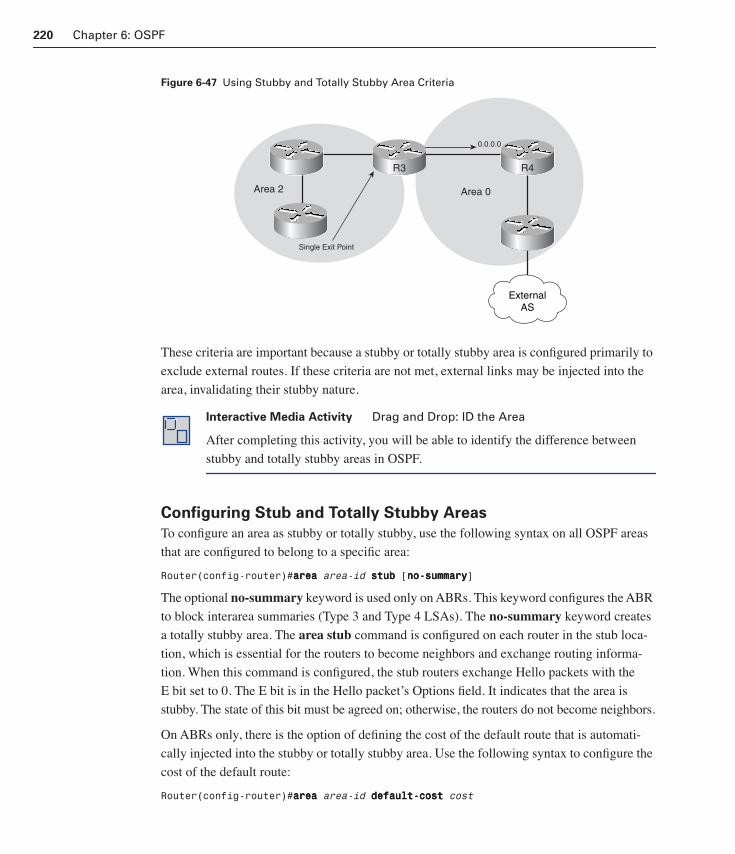
220 Chapter 6: OSPF
Figure 6-47 Using Stubby and Totally Stubby Area Criteria
These criteria are important because a stubby or totally stubby area is configured primarily to
exclude external routes. If these criteria are not met, external links may be injected into the
area, invalidating their stubby nature.
Configuring Stub and Totally Stubby Areas
To configure an area as stubby or totally stubby, use the following syntax on all OSPF areas
that are configured to belong to a specific area:
Router(config-router)#aaaarrrreeeeaaaa area-id ssssttttuuuubbbb [nnnnoooo----ssssuuuummmmmmmmaaaarrrryyyy]
The optional no-summary keyword is used only on ABRs. This keyword configures the ABR
to block interarea summaries (Type 3 and Type 4 LSAs). The no-summary keyword creates
a totally stubby area. The area stub command is configured on each router in the stub loca-
tion, which is essential for the routers to become neighbors and exchange routing informa-
tion. When this command is configured, the stub routers exchange Hello packets with the
E bit set to 0. The E bit is in the Hello packet’s Options field. It indicates that the area is
stubby. The state of this bit must be agreed on; otherwise, the routers do not become neighbors.
On ABRs only, there is the option of defining the cost of the default route that is automati-
cally injected into the stubby or totally stubby area. Use the following syntax to configure the
cost of the default route:
Router(config-router)#aaaarrrreeeeaaaa area-id ddddeeeeffffaaaauuuulllltttt----ccccoooosssstttt cost
Interactive Media Activity Drag and Drop: ID the Area
After completing this activity, you will be able to identify the difference between
stubby and totally stubby areas in OSPF.
ExternalAS
R3 R4
Area 2 Area 0
0.0.0.0
Single Exit Point
1358_fmi.book Page 220 Thursday, May 27, 2004 2:21 PM

Stub, Totally Stubby, and Not-So-Stubby Areas 221
OSPF Stub Area Configuration Example
In Figure 6-48, Area 2 is configured as stubby. No routes from the external autonomous sys-
tem are forwarded into the stub.
Figure 6-48 OSPF Stubby Area Configuration
The last line in each configuration shown in Example 6-12, area 2 stub, defines the stubby
area. The area stub default-cost has not been configured on R3, so this router advertises
0.0.0.0, the default route, with a default cost metric of 1 plus any internal costs.
Notice that the OSPF process number on each router can be different.
The only routes that appear on the routing table for R4 are intra area routes, the default route,
and interarea routes. intra area routes are designated with an O in the routing table. Both the
default and interarea routes are designated with an IA in the routing table. The default route is
denoted with an asterisk (*).
Notice that each router in the stub must be configured with the area stub command. The area stub command determines whether the routers in the stub become neighbors. This command
must be included on all routers in the stubby area if they are to exchange routing information.
Example 6-12 Stubby Area Configuration
R3(config)#rrrroooouuuutttteeeerrrr oooossssppppffff 111100000000
R3(config-router)#nnnneeeettttwwwwoooorrrrkkkk 111199992222....111166668888....11114444....0000 0000....0000....0000....222255555555 aaaarrrreeeeaaaa 0000
R3(config-router)#nnnneeeettttwwwwoooorrrrkkkk 111199992222....111166668888....11115555....0000 0000....0000....0000....222255555555 aaaarrrreeeeaaaa 2222
R3(config-router)#aaaarrrreeeeaaaa 2222 ssssttttuuuubbbb
R4(config)#rrrroooouuuutttteeeerrrr oooossssppppffff 11115555
R4(config-router)#nnnneeeettttwwwwoooorrrrkkkk 111199992222....111166668888....11115555....0000 0000....0000....0000....222255555555 aaaarrrreeeeaaaa 2222
R4(config-router)#aaaarrrreeeeaaaa 2222 ssssttttuuuubbbb
192.168.14.1
E0 S0
S0
192.168.15.1
192.168.15.2
Area 0 Stub Area 2
ExternalAS R3
R4
1358_fmi.book Page 221 Thursday, May 27, 2004 2:21 PM

222 Chapter 6: OSPF
OSPF Totally Stubby Area Configuration Example
To create a totally stubby area, the keyword no-summary is added to the area stub com-
mand configuration, as shown in Example 6-13, on R3 in Figure 6-49. This keyword causes
summary routes, delivered by both Type 3 and Type 4 LSAs, to also be blocked from the stub.
Each router in the stub picks the closest ABR as a gateway to all other networks outside
the area.
Figure 6-49 OSPF Totally Stubby Area Configuration Example
The only routes that appear on the routing table for R4 are intra area routes, designated with
an O in the routing table, and the default route. No interarea routes, designated with an IA in
the routing table, are included.
Notice that it is necessary to configure the no-summary keyword only on the totally stubby
border routers, because the area is already configured as stubby.
Example 6-13 Totally Stubby Area Configuration
R3(config)#rrrroooouuuutttteeeerrrr oooossssppppffff 111100000000
R3(config-router)#nnnneeeettttwwwwoooorrrrkkkk 111199992222....111166668888....11114444....0000 0000....0000....0000....222255555555 aaaarrrreeeeaaaa 0000
R3(config-router)#nnnneeeettttwwwwoooorrrrkkkk 111199992222....111166668888....11115555....0000 0000....0000....0000....222255555555 aaaarrrreeeeaaaa 2222
R3(config-router)#aaaarrrreeeeaaaa 2222 ssssttttuuuubbbb nnnnoooo----ssssuuuummmmmmmmaaaarrrryyyy
Lab 6.9.4 Configuring a Stubby Area and a Totally Stubby Area
In this lab, you configure an OSPF stubby area and a totally stubby area.
192.168.14.1
E0 S0
S0
192.168.15.1
192.168.15.2
Area 0 Totally StubbyArea 2
ExternalAS R3
R4
1358_fmi.book Page 222 Thursday, May 27, 2004 2:21 PM

Stub, Totally Stubby, and Not-So-Stubby Areas 223
NSSA Overview
NSSAs are a relatively new, standards-based OSPF enhancement. To understand how to
use NSSAs, consider the network shown in Figure 6-50.
Figure 6-50 Connecting OSPF to an External Autonomous System
RTA is an ASBR that connects to an external RIP domain, and RTB currently serves as an
ABR for Area 0, as shown in Figure 6-51. If the RIP domain is not under the same adminis-
trative control, what options are there to exchange routing information between these two
domains? If dynamic routing will be used, an OSPF standard area could be created.
Figure 6-51 Using an OSPF Standard Area to Connect to an External AS
However, what if the routers that are placed in Area 1 do not have the required processing
power or memory to run OSPF? You have learned that you can reduce the burden on OSPF
routers by configuring them to participate in a stubby or totally stubby area. Figure 6-52 illus-
trates what would happen in this case.
RIPRTA RTB
OSPFArea 0
RIPRTA RTB
OSPFArea 0
ASBR ABR
OSPFArea 1
1358_fmi.book Page 223 Thursday, May 27, 2004 2:21 PM

224 Chapter 6: OSPF
Figure 6-52 Using an OSPF Stubby Area to Connect to an External AS
A stubby area cannot include an ASBR because Type 5 (external) LSAs are not allowed in a
stub domain. The configuration shown in Figure 6-52 would fail miserably.
So how is external routing information dynamically exchanged without creating a standard
OSPF area? Another routing protocol could be configured, such as RIP or IGRP, in place of
creating an Area 1. This might prove to be a disadvantage. This is because an additional rout-
ing protocol must be maintained and imported into OSPF and because the RIP domain is not
under the same administrative control.
With the introduction of the NSSA, there is another, easier option, as shown in Figure 6-53.
An NSSA acts like a stub network in the sense that it does not allow Type 5 LSAs. It can also
be configured to prevent floods of Type 3 and Type 4 summary LSAs, just as a totally stubby
area would. However, an NSSA does allow Type 7 LSAs, which can carry external routing
information and be flooded throughout the NSSA.
How NSSA Operates
By configuring an area as an NSSA, you can minimize routing tables within the area but still
import external routing information into OSPF.
Figure 6-53 illustrates the sample network, including an NSSA implementation. RTA can
import external routes as Type 7 LSAs, and ABRs translate Type 7 LSAs into Type 5 LSAs as
they leave the NSSA. A benefit of Type 7 LSAs is that they can be summarized. The OSPF
specification prohibits the summarizing or filtering of Type 5 LSAs. It is an OSPF require-
ment that Type 5 LSAs always be flooded throughout a routing domain. When defining an
NSSA, specific external routes can be imported as Type 7 LSAs into the NSSA. In addition,
RIPRTA RTB
OSPFArea 0
ASBR ABR
OSPFArea 1
Stub Area(No External
Routes Allowed)
Backbone Area
Learning about external routes cannotbe done because Type 5 LSAs cannotbe sent through an OSPF stub area.
1358_fmi.book Page 224 Thursday, May 27, 2004 2:21 PM

Stub, Totally Stubby, and Not-So-Stubby Areas 225
when translating Type 7 LSAs to be imported into nonstub areas, the LSAs can be summa-
rized or filtered before importing them as Type 5 LSAs.
Figure 6-53 Using an OSPF NSSA to Connect an External AS
NSSAs are often used when a remote site that uses RIP or IGRP must be connected to a cen-
tral site using OSPF. Use NSSA to simplify the administration of this kind of topology.
Before NSSA, the connection between the corporate site ABR and the remote router used
RIP or EIGRP. This meant maintaining two routing protocols. Now, with NSSA, OSPF can
be extended to handle the remote connection by defining the area between the corporate
router and the remote router as an NSSA.
Figure 6-54 shows the central site and branch offices interconnected through a slow WAN
link. The branch office is not using OSPF, but the central site is. If a standard OSPF area
between the two networks is configured, the slow WAN link could be overwhelmed by the
ensuing flood of LSAs. This is especially true for Type 5 external LSAs. As an alternative,
you could configure a RIP domain between the two networks, but that would mean running
two routing protocols on the central site routers. A better solution is to configure an OSPF
area and define it as an NSSA, as shown in Example 6-14.
Figure 6-54 Configuring OSPF NSSA
RIPRTA RTB
OSPFArea 0
ASBR ABR
OSPFArea 1
NSSA(Type-7
LSA Allowed)
Backbone Area
Type 7 LSAs can be translated intoType 5 LSAs and optionally summarize
external routes in the process.
Type
-7 Type-7
Type
-5
Type
-5Type-7
Type
-7
Type-5
Type-5
NOTE
NSSAs are supported in Cisco IOS Release 11.2 and later.
Backbone Area 0172.19.89.0/24
RIP or EIGRP10.10.0.0/1610.11.0.0/1620.0.0.0/8 BA
200.0.0.63Router ID
200.0.0.62Router ID
19.2 kbps
NSSA1
172.19.92.0/24
1358_fmi.book Page 225 Thursday, May 27, 2004 2:21 PM

226 Chapter 6: OSPF
In this scenario, RTA is defined as an ASBR. It is configured to redistribute any routes within
the RIP or EIGRP domain to the NSSA. The following describes what happens when the area
between the connecting routers is defined as an NSSA:
■ RTA receives RIP or EIGRP routes for networks 10.10.0.0/16, 10.11.0.0/16, and
20.0.0.0/8.
■ Because RTA is also connected to an NSSA, it redistributes the RIP or EIGRP routes as
Type 7 LSAs into the NSSA.
■ RTB, an ABR between the NSSA and the backbone Area 0, receives the Type 7 LSAs.
■ After the SPF calculation on the forwarding database, RTB translates the Type 7 LSAs
into Type 5 LSAs and then floods them throughout Area 0.
At this point, RTB can summarize routes 10.10.0.0/16 and 10.11.0.0/16 as 10.0.0.0/8 or filter
one or more of the routes.
Configuring NSSA
To configure an OSPF area as an NSSA, configure all OSPF router interfaces that belong to
the area using the following command syntax:
Router(config-router)#aaaarrrreeeeaaaa area-id nnnnssssssssaaaa [nnnnoooo----ssssuuuummmmmmmmaaaarrrryyyy]
Typically, you use the optional keyword no-summary when configuring NSSA on an ABR.
This prevents Type 3 and Type 4 summary routes from flooding the NSSA area and minimizing
the routing tables within the area. In effect, the no-summary keyword makes the NSSA
totally stubby.
Optionally, you can control the summarization or filtering during the translation using the fol-
lowing syntax:
Router(config)#ssssuuuummmmmmmmaaaarrrryyyy----aaaaddddddddrrrreeeessssssss prefix mask [nnnnooootttt----aaaaddddvvvveeeerrrrttttiiiisssseeee] [ttttaaaagggg tag]
Example 6-14 NSSA Configuration
RTA(config)#rrrroooouuuutttteeeerrrr oooossssppppffff 1111
RTA(config-router)#rrrreeeeddddiiiissssttttrrrriiiibbbbuuuutttteeee rrrriiiipppp ssssuuuubbbbnnnneeeettttssss
RTA(config-router)#nnnneeeettttwwwwoooorrrrkkkk 111177772222....11119999....99992222....0000 0000....0000....0000....222255555555 aaaarrrreeeeaaaa 1111
RTA(config-router)#aaaarrrreeeeaaaa 1111 nnnnssssssssaaaa
RTB(config)#rrrroooouuuutttteeeerrrr oooossssppppffff 1111
RTB(config-router)#ssssuuuummmmmmmmaaaarrrryyyy----aaaaddddddddrrrreeeessssssss 11110000....0000....0000....0000 222255555555....0000....0000....0000 ttttaaaagggg 8888
RTB(config-router)#nnnneeeettttwwwwoooorrrrkkkk 111177772222....11119999....99992222....0000 0000....0000....0000....222255555555 aaaarrrreeeeaaaa 1111
RTB(config-router)#nnnneeeettttwwwwoooorrrrkkkk 111177772222....11119999....88889999....0000 0000....0000....0000....222255555555 aaaarrrreeeeaaaa 0000
RTB(config-router)#aaaarrrreeeeaaaa 1111 nnnnssssssssaaaa
1358_fmi.book Page 226 Thursday, May 27, 2004 2:21 PM

Virtual Links 227
The not-advertise keyword is used to suppress routes that match the prefix and mask pair.
This keyword applies to OSPF only. The tag value can also be assigned but is not required.
Route tags can be used in policy routing; they are discussed in Chapter 5, “EIGRP.”
To verify that NSSA is defined on a given router, use the show ip ospf command. This com-
mand shows the general OSPF configured parameters, including the number of NSSAs to
which the router is attached and whether the router is performing LSA translation.
Virtual LinksOSPF has certain restrictions when multiple areas are configured. One area must be defined
as Area 0, the backbone area. It is called the backbone because all interarea communication
must go through it. Therefore, all areas should be physically connected to Area 0 so that the
routing information injected into this backbone can be disseminated to other areas. The back-
bone area must always be configured as Area 0. No other area ID can function as the
backbone.
There are situations, however, when a new area is added after the OSPF internetwork has
been designed, and it is not possible to give that new area direct access to the backbone. In
these cases, a virtual link can be defined to provide the needed connectivity to the backbone
area.
Meeting the Backbone Area Requirements
The virtual link gives the disconnected area a logical path to the backbone. All areas must
connect directly to the backbone area or through a transit area, as shown in Figure 6-55.
Lab 6.9.5 Configuring an NSSA
In this lab, you configure an OSPF NSSA to import external routing information
while retaining the benefits of a stubby area.
1358_fmi.book Page 227 Thursday, May 27, 2004 2:21 PM

228 Chapter 6: OSPF
Figure 6-55 Meeting the Backbone Area Requirements
The virtual link has the following two requirements:
■ It must be established between two routers that share a common area.
■ One of these two routers must be connected to the backbone.
When virtual links are used, they require special processing during the SPF calculation. That
is, the “real” next-hop router must be determined so that the true cost to reach a destination
across the backbone can be calculated. Virtual links serve the following purposes:
■ They can link an area that does not have a physical connection to the backbone. This
linking could occur, for example, when two organizations merge.
■ They can patch the backbone if discontinuity in Area 0 occurs. Discontinuity of the
backbone might occur, for example, if two companies merge their two separate OSPF
networks into a single one with a common Area 0. The only alternative for the compa-
nies is to redesign the entire OSPF network and create a unified backbone.
Another reason for creating a virtual link is to add redundancy in cases when router failure
might cause the backbone to be split in two.
In Figure 6-56, the disconnected Area 0s are linked through a virtual link through the com-
mon area, Area 3. If a common area does not already exist, one can be created to become the
transit area. Area 0 could become partitioned, for example, if two OSPF networks were
merged.
Area 0(Backbone)
Area 1 Area 2
Area 3
Virtual LinkTransitArea
1358_fmi.book Page 228 Thursday, May 27, 2004 2:21 PM

Virtual Links 229
Figure 6-56 Meeting the Backbone Area Requirements
Configuring Virtual Links
To configure a virtual link, follow these steps:
Step 1 Configure OSPF, as described in the “Using and Configuring OSPF Multiarea
Components” section.
Step 2 On each router that will use the virtual link, create the “virtual link” configura-
tion. The routers that make the links are the ABR that connects the remote area
to the transit area and the ABR that connects the transit area to the backbone
area.
Router(config-router)#aaaarrrreeeeaaaa area-id vvvviiiirrrrttttuuuuaaaallll----lllliiiinnnnkkkk router-id
If the neighbor’s router ID is unknown, Telnet to it and enter the show ip ospf command.
Virtual Link Configuration Example
In Figure 6-57, Area 3 does not have a direct physical connection to the backbone, Area 0,
which is an OSPF requirement. This is because the backbone is a collection point for LSAs.
ABRs forward summary LSAs to the backbone, which, in turn, forward the traffic to all
areas. All interarea traffic transits the backbone. Examples 6-15 and 6-16 show the configura-
tions.
Area 0
Area 3
Area 2
Area 0
Area 1
Transit Area
1358_fmi.book Page 229 Thursday, May 27, 2004 2:21 PM

230 Chapter 6: OSPF
Figure 6-57 Virtual Link Example
To provide connectivity to the backbone, a virtual link must be configured between R2 and
R1. Area 1 is the transit area, and R1 is the entry point into Area 0. R2 has a logical connec-
tion to the backbone through the transit area.
Both sides of the virtual link must be configured as follows:
■ With the following command on R2, Area 1 is defined as the transit area, and the router
ID of the other side of the virtual link is configured:
R2(config-router)#aaaarrrreeeeaaaa 1111 vvvviiiirrrrttttuuuuaaaallll----lllliiiinnnnkkkk 11110000....3333....11110000....5555
■ With the following command on R1, Area 1 is defined as the transit area, and the router
ID of the other side of the virtual link is configured:
R1(config-router)#aaaarrrreeeeaaaa 1111 vvvviiiirrrrttttuuuuaaaallll----lllliiiinnnnkkkk 11110000....7777....22220000....111122223333
Example 6-15 Virtual Link Configuration: R1
rrrroooouuuutttteeeerrrr oooossssppppffff 111100000000
nnnneeeettttwwwwoooorrrrkkkk 11110000....2222....0000....0000 0000....0000....0000....222255555555 aaaarrrreeeeaaaa 0000
nnnneeeettttwwwwoooorrrrkkkk 11110000....3333....0000....0000 0000....0000....0000....222255555555 aaaarrrreeeeaaaa 1111
aaaarrrreeeeaaaa 1111 vvvviiiirrrrttttuuuuaaaallll----lllliiiinnnnkkkk 11110000....7777....22220000....111122223333
Example 6-16 Virtual Link Configuration: R2
rrrroooouuuutttteeeerrrr oooossssppppffff 66663333
nnnneeeettttwwwwoooorrrrkkkk 11110000....3333....0000....0000 0000....0000....0000....222255555555 aaaarrrreeeeaaaa 0000
nnnneeeettttwwwwoooorrrrkkkk 11110000....7777....0000....0000 0000....0000....0000....222255555555 aaaarrrreeeeaaaa 3333
aaaarrrreeeeaaaa 1111 vvvviiiirrrrttttuuuuaaaallll----lllliiiinnnnkkkk 11110000....3333....11110000....5555
Router ID10.7.20.123
Router ID10.3.10.5
Area 1
Area 0
Area 3
R2
R1
1358_fmi.book Page 230 Thursday, May 27, 2004 2:21 PM

Summary 231
SummaryOSPF is a scalable, standards-based link-state routing protocol. Its benefits include no hop
count limitation, the capability to multicast routing updates, faster convergence rates, and
optimal path selection. The basic steps of OSPF operation are as follows:
1. Establish router adjacencies.
2. Select a DR and a BDR.
3. Discover routes.
4. Select appropriate routes to use.
5. Maintain routing information.
The following is a summary of the topics you have learned in this chapter:
■ The advantages of multiarea OSPF configurations
■ The OSPF components used in a large multiarea OSPF internetwork
■ The benefits of multiarea configurations include reduced frequency of SPF calcula-
tions, smaller routing tables, and reduced LSU overhead.
■ The types of areas, including stubby, totally stubby, and NSSA
■ OSPF router types, including ABRs and ASBRs
■ Link-state advertisements
■ Virtual links
Lab 6.9.6 Configuring Virtual Links
In this lab, you configure an OSPF virtual link so that a disconnected area can reach
the backbone, as required by OSPF.
Lab 6.10.1 OSPF Challenge Lab
In this lab, you create a multiarea OSPF autonomous system that includes a totally
stubby area and a persistent default route toward the ISP.
1358_fmi.book Page 231 Thursday, May 27, 2004 2:21 PM

232 Chapter 6: OSPF
Key Termsarea ID Multiple areas can be defined within an OSPF network to reduce and summarize
route information.
authentication type and authentication data OSPF supports different methods of authenti-
cation so that OSPF routers do not believe just anyone sending Hellos to 224.0.0.5.
backup designated router (BDR) The DR could represent a single point of failure, so a sec-
ond router is elected as the BDR to provide fault tolerance.
checksum This 2-byte field is used to check the message for errors.
dead interval How many seconds a router waits before it declares a neighbor down. The
dead interval is 4 times the Hello interval by default, or 40 seconds.
designated router (DR) For every multiaccess IP network, one router is elected the DR.
The DR has two main functions—to become adjacent to all other routers on the network and
to act as a spokesperson for the network.
Down state In the Down state, the OSPF process has not exchanged information with any
neighbor.
Exchange state In the Exchange state, neighbor routers use Type 2 DBD packets to
send each other their link-state information. In other words, the routers describe their link-
state databases to each other. The routers compare what they learn with their existing
link-state databases.
ExStart state Technically, when a router and its neighbor enter the ExStart state, their con-
versation is characterized as an adjacency, but they have not become fully adjacent.
full adjacency With the Loading state complete, the routers are fully adjacent. Each router
keeps a list of adjacent neighbors, called the adjacencies database.
Hello interval How many seconds an OSPF router waits to send the next Hello packet.
Init state OSPF routers send Type 1 packets, or Hello packets, at regular intervals to estab-
lish a relationship with neighbor routers.
Loading state After the databases have been described to each router, they may request
information that is more complete by using Type 3 packets, link-state requests (LSRs).
network mask This 32-bit field carries subnet mask information for the network.
router ID The function of the Hello packet is to establish and maintain adjacencies. So the
sending router signs the fourth field with its router ID, which is a 32-bit number used to iden-
tify the router to the OSPF protocol.
1358_fmi.book Page 232 Thursday, May 27, 2004 2:21 PM
Key Terms 233
router priority This field contains a value that indicates this router’s priority when selecting
a designated router (DR) and backup designated router (BDR).
two-way state Using Hello packets, every OSPF router tries to establish a two-way state, or
bidirectional communication, with every neighbor router on the same IP network.
Type 1: Hello packet Establishes and maintains adjacency information with neighbors.
Type 2: database description packet (DBD) Describes the contents of the link-state data-
base on an OSPF router.
Type 3: link-state request (LSR) Requests specific pieces of a link-state database.
Type 4: link-state update (LSU) Transports link-state advertisements (LSAs) to neighbor
routers.
Type 5: link-state acknowledgment (LSAck) Acknowledgment receipt of a neighbor’s
LSA.
version, type, and packet length The first three fields of the OSPF packet let the recipients
know the version of OSPF that is being used by the sender, the OSPF packet type, and length.
1358_fmi.book Page 233 Thursday, May 27, 2004 2:21 PM

234 Chapter 6: OSPF
Check Your UnderstandingComplete all of the review questions to test your understanding of the topics and concepts in
this chapter. The answers appear in Appendix B, “Answers to the Check Your Understanding
Questions.”
For additional, more in-depth questions, refer to the chapter-specific study guides on the
companion CD-ROM.
1. Which state are the routers in an OSPF network in after the DR and BDR are elected?
A. ExStart
B. Full
C. Loading
D. Exchange
2. What is the default cost metric for OSPF based on?
A. Delay
B. Media bandwidth
C. Efficiency
D. Network traffic
3. What command can you use to change the OSPF priority on an interface?
A. ip priority number ospf
B. ip ospf priority number
C. ospf priority number
D. set priority ospf number
4. What IP address is used to send a multicast to only OSPF DRs and BDRs?
A. 224.0.0.6
B. 224.0.0.1
C. 224.0.0.4
D. 224.0.0.5
5. Which of the following is a common feature associated with NBMA networks?
A. Support for only two routers
B. Support for more than two routers
C. No election of DRs
D. Full support for broadcast and multicast packets
1358_fmi.book Page 234 Thursday, May 27, 2004 2:21 PM
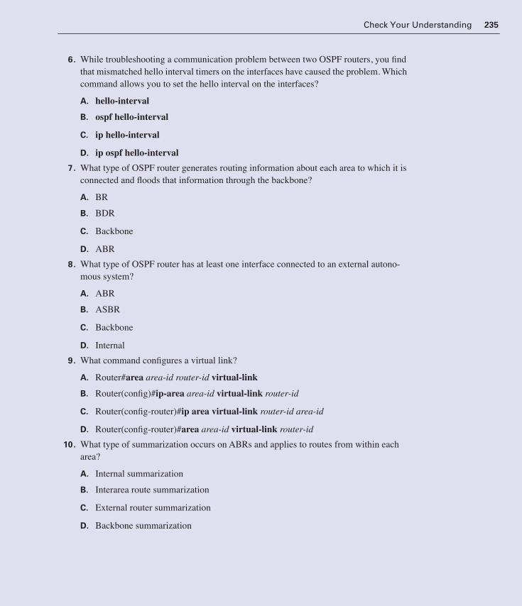
Check Your Understanding 235
6. While troubleshooting a communication problem between two OSPF routers, you find that mismatched hello interval timers on the interfaces have caused the problem. Which command allows you to set the hello interval on the interfaces?
A. hello-interval
B. ospf hello-interval
C. ip hello-interval
D. ip ospf hello-interval
7. What type of OSPF router generates routing information about each area to which it is connected and floods that information through the backbone?
A. BR
B. BDR
C. Backbone
D. ABR
8. What type of OSPF router has at least one interface connected to an external autono-mous system?
A. ABR
B. ASBR
C. Backbone
D. Internal
9. What command configures a virtual link?
A. Router#area area-id router-id virtual-link
B. Router(config)#ip-area area-id virtual-link router-id
C. Router(config-router)#ip area virtual-link router-id area-id
D. Router(config-router)#area area-id virtual-link router-id
10. What type of summarization occurs on ABRs and applies to routes from within each area?
A. Internal summarization
B. Interarea route summarization
C. External router summarization
D. Backbone summarization
1358_fmi.book Page 235 Thursday, May 27, 2004 2:21 PM

236 Chapter 6: OSPF
11. What command configures an area as an NSSA?
A. Router(config)#area area-id nssa
B. Router(config-router)#area area-id nssa
C. Router(config-router)#area-id nssa
D. Router(config)#area nssa area-id
12. What command displays information about each area to which a router is connected and indicates whether the router is an ABR, ASBR, or both?
A. show ip ospf border-routers
B. show ip ospf virtual-links
C. show ip ospf process-id
D. show ip ospf database
1358_fmi.book Page 236 Thursday, May 27, 2004 2:21 PM

1358_fmi.book Page 237 Thursday, May 27, 2004 2:21 PM

ObjectivesUpon completing this chapter, you will be able to
■ Understand IS-IS fundamentals
■ Understand ISO addressing
■ Describe IS-IS operation
■ Understand IP routing with Integrated IS-IS
■ Configure Integrated IS-IS
■ Describe Integrated IS-IS operation in a WAN environment
You can reinforce your understanding of the objectives covered in this chapter by opening
the interactive media activities on the CD accompanying this book and performing the lab
activities collected in the Cisco Networking Academy Program CCNP 1: Advanced Routing
Lab Companion. Throughout this chapter, you will see references to these activities by title
and by icon. They look like this:
Interactive Media Activity
Lab Activity
1358_fmi.book Page 238 Thursday, May 27, 2004 2:21 PM
Chapter 7
IS-IS
In recent years, the Intermediate System-to-Intermediate System (IS-IS) routing protocol has
become increasingly popular, with widespread usage among Internet service providers (ISPs).
IS-IS enables very fast convergence and is very scalable. It is also a very flexible protocol and
has been extended to incorporate leading-edge features such as Multiprotocol Label Switching/
Traffic Engineering (MPLS/TE).
The features of IS-IS include the following:
■ Hierarchical routing
■ Classless behavior
■ Rapid flooding of new information
■ Fast convergence
■ Very scalable
■ Flexible timer tuning
The Cisco IOS software implementation of IS-IS also supports the following features:
■ Multiarea routing
■ Route leaking
■ Overload bit
IS-IS FundamentalsIS-IS is an Open System Interconnection (OSI) routing protocol originally specified by Interna-
tional Organization for Standardization (ISO) 10589. IS-IS is a dynamic, link-state, intradomain
interior gateway protocol (IGP). It is designed to operate in an OSI Connectionless Network Ser-
vice (CLNS) environment. IS-IS selects routes based on a cost metric assigned to links in the IS-
IS network. The cost is an arbitrary value assigned by a network engineer as the value of the path
to a neighbor router.
1358_fmi.book Page 239 Thursday, May 27, 2004 2:21 PM

240 Chapter 7: IS-IS
A two-level hierarchy is used to support large routing domains. A large domain can be
administratively divided into areas. Each system resides in exactly one area. Routing within
an area is called Level 1 routing. Routing between areas is called Level 2 routing. A Level 2
intermediate system (IS) keeps track of the paths to destination areas. A Level 1 IS keeps
track of the routing in its own area. For a packet destined for another area, a Level 1 IS sends
the packet to the nearest Level 2 IS in its own area, regardless of the level of the destination
area. Then the packet travels by way of Level 2 routing to the destination area, where it might
travel by way of Level 1 routing to the destination. It should be noted that selecting an exit
from an area based on Level 1 routing to the closest Level 2 IS might result in suboptimal
routing.
On broadcast multiaccess media, a designated intermediate system (DIS) is elected and con-
ducts the flooding over the media. The DIS is analogous to the designated router (DR) in
OSPF, even though details such as the election process and adjacencies within a multiaccess
media differ significantly. The DIS is elected by priority. The highest priority becomes the
DIS. This can be configured on an interface basis using the isis priority command. In the
case of a tie, the router with the highest subnetwork point of attachment (SNPA) address
becomes the DIS. In the case of Ethernet, the SNPA address is just the MAC address.
OSI Protocols
The OSI protocols are the product of an international program formed to develop data net-
working protocols and other standards that facilitate multivendor equipment interoperability.
The OSI program grew out of a need for international networking standards. It is designed to
facilitate communication between hardware and software systems despite differences in
underlying architectures.
The OSI specifications were conceived and implemented by two international standards orga-
nizations—the ISO and the International Telecommunication Union Telecommunication
Standardization Sector (ITU-T). The world of OSI internetworking includes various network
services with the following characteristics:
■ Independent of underlying communications infrastructure
■ End-to-end transfer
■ Transparency
■ Quality of service (QoS) selection
■ Addressing
The OSI protocol suite supports numerous standard protocols at the physical, data link, net-
work, transport, session, presentation, and application layers, as shown in Figure 7-1.
1358_fmi.book Page 240 Thursday, May 27, 2004 2:21 PM

IS-IS Fundamentals 241
Figure 7-1 OSI Protocol Suite
OSI CLNS is a network layer service similar to bare IP service, as shown in Table 7-1.
A CLNS entity communicates over Connectionless Network Protocol (CLNP) with its peer
CLNS entity. CLNP is the OSI equivalent of IP.Table 7-1 Comparing TCP/IP to OSI
TCP/IP OSI
Basic connectionless service:IP (RFC 791)
CLNP (ISO 8473)
Neighbor greeting and error reports to source about packet delivery:ICMP (RFC 792)ARP (RFC 826)IRDP (RFC 1256)
CLNP (ISO 8473)ES-IS (ISO 9542)
Routing:Integrated IS-IS (RFC 1195)Participants are routers and hosts
IS-IS (ISO 10589)Participants are ISs and end systems (ESs)
IP autonomous system ISO routing domain
Interior Gateway Protocol (IGP) Intradomain Routing Protocol
Exterior Gateway Protocol (EGP)Border Gateway Protocol (BGP) for IP (RFC 1105)Static IP routes
Intradomain Routing ProtocolISO IDRP (proposal)Static CLNS routes
Application
Presentation
Session
Transport
Network
Data Link
Physical
CMIP DS FTAM MHS VTP
ASES ACSE ROSE RTSE CCRSE …
Presentation Service/Presentation Protocol
Session Service/Session Protocol
TP0 TP1 TP2 TP3 TP4
CONP/CMNS CLNP/CLNSIS-IS ES-IS
IEEE802.2
IEEE 802.3IEEE 802.5/Token Ring
FDDI X.25
IEEE 802.3Hardware
Token RingHardware
FDDIHardware
X.25Hardware
OSI ReferenceModel OSI Protocol Suite
1358_fmi.book Page 241 Thursday, May 27, 2004 2:21 PM

242 Chapter 7: IS-IS
CLNP is an OSI network layer protocol that carries upper-layer data and error indications
over connectionless links. CLNP provides the interface between CLNS and the upper layers.
CLNS does not perform connection setup or termination because paths are determined inde-
pendently for each packet that is transmitted through a network. In addition, CLNS provides
best-effort delivery, which means that no guarantee exists that data will not be lost, corrupted,
misordered, or duplicated. CLNS relies on transport layer protocols to perform error detec-
tion and correction.
OSI network layer addressing is implemented by using two types of hierarchical addresses—
network service access point (NSAP) and network entity title (NET).
The OSI protocol suite specifies two routing protocols at the network layer—End System-to-Intermediate System (ES-IS) and IS-IS, as shown in Table 7-1. In addition, the OSI suite
implements two types of network service—connectionless and connection-oriented.
OSI Terminology
An OSI network has four significant architectural entities—hosts, areas, a backbone, and a
domain. A domain is any portion of an OSI network that is under a common administrative
authority. Within any OSI domain, one or more areas can be defined. An area is a logical
entity. An area is formed by a set of contiguous routers and the data links that connect them.
All routers in the same area exchange information about all of the hosts they can reach. The
areas are connected to form a backbone. All routers on the backbone know how to reach all
areas. The term end system refers to any nonrouting host or node. The term intermediate sys-
tem refers to a router. These terms are the basis of the OSI ES-IS and IS-IS protocols.
An NSAP is a conceptual point on the boundary between the network and transport layers.
The NSAP is the location where OSI network services are provided to the transport layer.
Each transport layer entity is assigned a single NSAP. The NSAP address identifies any sys-
tem in an OSI network. The last byte in an NSAP identifies a process on the device, similar to
a port or socket in TCP/IP.
A NET is an NSAP in which the last byte is 0. The NET identifies a device. Therefore, each
router has a unique NET address.
An SNPA is the point at which subnetwork services are provided. This is the equivalent of the
Layer 2 address corresponding to the Layer 3 (NET or NSAP) address. This is usually a
MAC address on a LAN or virtual circuit ID in X.25, Frame Relay, or ATM.
A circuit is an interface. A link is the path between two neighbor ISs. It is defined as being up
when communication is possible between the two neighbors’ SNPAs.
1358_fmi.book Page 242 Thursday, May 27, 2004 2:21 PM

IS-IS Fundamentals 243
ES-IS and IS-IS
ISO has developed standards for two types of network protocols used in routing—ES-IS and
IS-IS. The ES-IS discovery protocols are used for routing between end systems and intermediate
systems. The IS-IS routing protocols are used for hierarchical routing between inter-
mediate systems.
ES-IS is analogous to Address Resolution Protocol (ARP) in IP. Although technically it isn’t
a routing protocol, ES-IS is included here because it is commonly used with routing protocols
to provide end-to-end data movement through an internetwork. Routing between end systems
and intermediate systems is sometimes called Level 0 routing, as shown in Figure 7-2.
Figure 7-2 ES-IS and IS-IS
With IS-IS routing, OSI distinguishes between Level 1, Level 2, and Level 3 routing to sim-
plify router design and operation. Level 1 ISs communicate with other Level 1 ISs in the
same area. Level 2 ISs route between Level 1 areas and form an intradomain routing back-
bone. Level 3 routing is done between separate domains. Hierarchical routing simplifies
backbone design, because Level 1 ISs only need to know how to get to the nearest Level 2 IS.
Each ES lives in a particular area. OSI routing begins when the ESs discover the nearest IS by
listening to Intermediate System Hello (ISH) packets. When an ES wants to send a packet to
another ES, it sends it to one of the ISs on its directly attached network, Level 0 routing. The
router then looks up the destination address and forwards the packet along the best route. If
the destination ES is on the same subnetwork, the local IS knows this from listening to End
System Hello (ESH) packets and forwards the packet appropriately. The IS also might
Level 3 Routing Between Separate Domains
Domain
Level 1 Routing Between ISsWithin the Same Area.
Level 0 Routing BetweenESs and ISs on the Same
Subnet
Area 1
IS
IS
Area 2
IS
IS
Level 2 Routing Between DifferentAreas Within the Same Domain
ES ES
1358_fmi.book Page 243 Thursday, May 27, 2004 2:21 PM

244 Chapter 7: IS-IS
provide a redirect message to the source to tell it that a more direct route is available. If the
destination address is an ES on another subnetwork in the same area, the IS knows the correct
route and forwards the packet appropriately. If the destination address is an ES in another
area, the Level 1 IS sends the packet to the nearest Level 2 IS, Level 2 routing. Forwarding
through Level 2 ISs continues until the packet reaches a Level 2 IS in the destination area.
Within the destination area, ISs forward the packet along the best path until the destination
ES is reached.
Integrated IS-IS
For routing in the ISO CLNS environment, Cisco routers support the IS-IS routing protocol.
Routers usually operate as ISs and can exchange reachability information with other ISs
using the IS-IS protocol. As an IS, a Cisco router can operate at Level 1 only, at Level 2 only,
or at both levels. In the last case, the router can advertise itself at Level 1 as an exit point from
the area. Integrated IS-IS allows the IS-IS protocol to propagate routing information for pro-
tocols other than CLNP. IS-IS can route CLNP, IP, or both when in dual mode.
IS-IS is the dynamic link-state routing protocol for the OSI protocol stack. As such, it distrib-
utes routing information for routing CLNP data for the ISO CLNS environment. When IS-IS
is used strictly for the ISO CLNS environment, it is called ISO IS-IS.
Integrated IS-IS is an implementation of the IS-IS protocol for routing multiple network pro-
tocols. Integrated IS-IS tags CLNP routes, upon which IS-IS bases its link-state database,
with information on IP networks and subnets. IS-IS provides an alternative to OSPF in the IP
world, mixing ISO CLNS and IP routing in one protocol. Again, IS-IS can be used purely for
IP routing, purely for ISO routing, or for a combination of the two, as shown in Figure 7-3.
Integrated IS-IS is deployed extensively in an IP-only environment in the top-tier ISP net-
works. The IS-IS working group of the Internet Engineering Task Force (IETF) developed the
specification for Integrated IS-IS, RFC 1195. Integrated IS-IS differs from the approach taken
by IS-IS routing, in which completely independent routing protocols are used for each of the
two protocol suites. Integrated IS-IS uses a single integrated protocol for interior routing. The
single integrated protocol is used to calculate routes within a routing domain for both proto-
col suites.
IS-IS is one of the few protocols that provides an integrated framework for concurrent pro-
cessing of more than one network layer protocol. Other routing protocols, such as OSPF, usu-
ally support routing for only one type of Layer 3 protocol. This chapter focuses mostly on the
use of IS-IS in an IP environment.
NOTE
IS-IS was originally designed for routing DEC-net Phase V and was sub-sequently adopted for ISO CLNP. DECnet is a routed protocol, like IP, IPX, and AppleTalk, used in Digital Equipment Corporation networking. IS-IS was pro-posed for use with TCP/IP in the late 1980s and early 1990s. IS-IS was ulti-mately specified for this context in RFC 1195, Use of OSI IS-IS for Routing in TCP/IP and Dual Environ-ments.
1358_fmi.book Page 244 Thursday, May 27, 2004 2:21 PM

IS-IS Fundamentals 245
Figure 7-3 Dual IS-IS
IS-IS was not designed specifically to route IP. However, its successful widespread deploy-
ment for IP routing on the Internet has led the IETF to revisit RFC 1195. The point is to
incorporate proprietary features outside the scope of RFC 1195 designed to improve usability
and to provide flexibility and scalability. MPLS traffic engineering stands out as a recent
technology that has driven advances in IS-IS feature sets, possibly vendor-specific.
The Integrated IS-IS protocol provides dynamic routing for an IP and ISO internetworking
environment. Integrated IS-IS has the following features:
■ It uses ISO IS-IS to distribute routing information.
■ It provides ISO and IP routing services.
■ It routes only within one ISO domain.
■ It provides link-state distribution of routing information.
■ It is based on the shortest path first (SPF) routing algorithm.
Integrated IS-IS provides IP routing capability by
■ Defining links with IP addresses, subnets, and metrics
■ Forwarding IP routing information within the PDUs of the ISO IS-IS packets
■ Configuring an area to support IP or both IP and CLNP
TokenRing
FDDI
Only IPOnly ISO
ISO Addresseson Interfaces
IP Area 2
Both ISO and IP
InternalRouter
ISO Area 1
ISO Area 3IP Area 3
NOTE
For routing in the ISO CLNS environment, Cisco routers, also support static CLNS routes as well as the proprietary ISO IGRP routing protocol. ISO IGRP is, as its name sug-gests, based on Cisco’s Interior Gateway Routing Protocol (IGRP). It uses distance vector technol-ogy to propagate routing information. As such, ISO IGRP shares some of the limitations of its IP coun-terpart, including long convergence times. This is because of periodic updates and long invalid times and hold times.
1358_fmi.book Page 245 Thursday, May 27, 2004 2:21 PM

246 Chapter 7: IS-IS
OSPF Versus IS-IS
The configuration of OSPF is based on a central backbone, Area 0, with all other areas being
physically attached to Area 0. Because of this, certain design constraints inevitably exist. A
good, consistent IP addressing structure is necessary when this type of hierarchical model is
used. It is used to summarize addresses into the backbone and reduce the amount of informa-
tion that is carried in the backbone and advertised across the network. In comparison, IS-IS
also has a hierarchy with Level 1 and Level 2 routers. With IS-IS, the area borders lie on the
links. However, significantly fewer link-state PDUs (LSPs) are used. Therefore, many more
routers, up to 100, can reside in a single area. This capability makes IS-IS more scalable than
OSPF. IS-IS allows a more flexible approach to extending the backbone. Adding Level 2 rout-
ers can extend the backbone. This process is less complex than with OSPF.
Here are some of the similarities between OSPF and IS-IS:
■ Classless
■ Link-state databases and Dijkstra’s Algorithm
■ Hello packets to form and maintain adjacencies
■ Use areas to form hierarchical topologies
■ Support address summarization between areas
■ Elect a designated router on multiaccess networks
■ Link-state representation, aging, and metrics
■ Update, decision, and flooding processes
■ Convergence capabilities
■ Deployed on ISP backbones
Here are some of the differences between OSPF and IS-IS:
■ IS-IS does not elect a backup designated router
■ IS-IS repeats the election process whenever a new router becomes active:
— If a new router has a higher priority or the same priority and a higher system ID,
it takes over as the DR.
— IS-IS is designed to be deterministic: The same set of routers always produces the
same DR.
■ Every time the DR changes, a new set of LSPs must be flooded.
■ IS-IS routers form adjacencies with all neighbors, not just the DR.
Interactive Media Activity Checkbox: IS-IS Terminology Quiz
After completing this activity, you will have a firm grasp on the IS-IS terminology.
1358_fmi.book Page 246 Thursday, May 27, 2004 2:21 PM

IS-IS Fundamentals 247
With regard to CPU use and the processing of routing updates, IS-IS is more efficient. Not
only are there fewer LSPs to process as compared to OSPF link-state advertisements (LSAs),
but the mechanism by which IS-IS installs and withdraws prefixes is less intensive.
Both OSPF and IS-IS are link-state protocols and therefore provide fast convergence. The
convergence time depends on a number of factors, such as timers, number of nodes, and types
of routers. Based on the default timers, IS-IS detects a failure more quickly than OSPF and
therefore should converge more rapidly. If there are many neighbors and adjacencies to con-
sider, the convergence time depends on the router’s processing power. IS-IS is typically less
CPU-intensive than OSPF. OSPF and IS-IS handle resource usage differently as well. For
example, IS-IS uses one link-state packet per router in one area, including redistributed pre-
fixes, compared to many OSPF LSAs. Here are some other differences between OSPF and
IS-IS areas:
■ OSPF is based on a central backbone with all other areas attached to it:
— In OSPF, the border lies within the area border router (ABR).
— Each link (interface) belongs to one area.
■ In IS-IS, the area border lies on the link:
— Each IS-IS router belongs to exactly one Level 2 area.
— IS-IS allows a more flexible approach to extending the backbone.
Here are some of the differences between OSPF and IS-IS scalability:
■ OSPF supports up to 50 routers per area.
■ IS-IS supports up to 100 routers per area.
■ OSPF has more features, including route tags, stubby areas/not-so-stubby areas
(NSSAs), and demand circuit.
The timers in IS-IS allow more tuning than those in OSPF. There are more timers to adjust, so
finer granularity can be achieved. By tuning the timers, you can significantly decrease con-
vergence time. However, this speed might come at the expense of stability, so you might have
to compromise. A network engineer should understand the implications of adjusting these
timers.
Interactive Media Activity Checkbox: OSPF Versus IS-IS
After completing this activity, you will be able to identify the differences between
OSPF and IS-IS.
1358_fmi.book Page 247 Thursday, May 27, 2004 2:21 PM

248 Chapter 7: IS-IS
ISO AddressingOSI network layer addressing is implemented by using two types of hierarchical addresses—
NSAP and NET.
NSAPs
The NSAP is a conceptual point on the boundary between the network and the transport lay-
ers. The NSAP is the location at which OSI network services are provided to the transport
layer. Each transport layer entity is assigned a single NSAP. The NSAP address identifies any
system in an OSI network. Various NSAP formats are used for various systems. Different
protocols might use different representations of the NSAP.
The NSAP address is the network layer address for CLNS packets. As with DECnet Phase V,
one NSAP address is used for each device, not for each interface. LSPs, Hello PDUs, and
other routing PDUs are OSI-formatted PDUs. Therefore, every IS-IS router requires an OSI
address. IS-IS uses the OSI address in the LSPs to identify the router, build the topology
table, and build the underlying IS-IS routing tree. NSAP addresses contain the device’s OSI
address and provide a link to upper-layer processes. The NSAP address can be thought of as
equivalent to the combination of an IP address and upper-layer protocol identifier in an IP
header. The Cisco implementation supports all NSAPs defined by ISO 8348/Addendum 2
and ISO 10589. The NSAP addressing structure is shown in Figure 7-4. Its fields are as fol-
lows:
■ The NSAP is formed by the Interdomain Part (IDP) and the Domain-Specific Part (DSP).
■ The IDP is composed of
— 1-byte Authority and Format Identifier (AFI)
— Variable-length initial domain identifier (IDI)
■ The DSP is composed of a
— 2-byte area
— 6-byte station ID
— 1-byte selector
Figure 7-4 NSAP Addressing Structure
IDP DSP
AFI IDI AREA STATION ID SEL
1358_fmi.book Page 248 Thursday, May 27, 2004 2:21 PM

ISO Addressing 249
A DSP address has three parts—area address, system ID, and NSAP selector (N-selector)
byte. The total length is between 8 and 20 bytes. The area address is a variable-length field
composed of high-order octets, excluding the system ID and the N-selector byte. The system
ID is the ES or IS identifier in an area, similar to the OSPF router ID. The system ID has a
fixed length of 6 bytes, as engineered in the Cisco IOS software (see Figure 7-5). The N-
selector byte is a service identifier. The role of the N-selector byte is analogous to that of a
port or socket in TCP/IP.
Figure 7-5 NSAP Addressing Structure
Cisco routers can route CLNS data that uses addressing that conforms to the ISO 10589 stan-
dard. The fields specified in this standard are as follows (see Figure 7-5):
■ Authority and Format ID (AFI)—1 byte, actually a binary value between 0 and 99,
used to specify the IDI format and DSP syntax of the address and the authority that
assigned the address.
■ Initial domain identifier (IDI)—Identifies the domain.
■ Interdomain Part (IDP)—Consists of the AFI and IDI together. This is roughly equiv-
alent to a classful IP network in decimal format.
■ High-Order Domain-Specific Part (HODSP)—Used to subdivide the domain into
areas. This is roughly equivalent to a subnet in IP.
■ System ID—Identifies an individual OSI device. In OSI, a device has an address, just
as it does in DECnet. In IP, an interface has an address.
■ NSAP selector (NSEL)—Identifies a process on the device. It is roughly equivalent to
a port or socket in TCP/IP. The NSEL is not used in routing decisions.
■ Domain-Specific Part (DSP)—Comprised of the HODSP, the system ID, and the
NSEL in binary format.
IS-IS uses a simple two-layer architecture. IS-IS joins the IDP and HODSP and treats them as
the Level 2 area ID, with the remaining system ID used for Level 1 routing. Restated, in
IS-IS, everything to the left of the system ID is used as the area ID. The minimum length of
this area ID is a single byte. The maximum is the remaining 13 bytes permitted by the ISO
standard. Therefore, an NSAP for an IS-IS network could be as little as 8 bytes in length. The
length is normally longer to permit some granularity in the allocation of areas.
IDP DSP
AFI IDI High Order DSP System ID NSEL
Used by Level 2 RoutingUsed by Level 1
Routing
Variable Length Area Address 6 Bytes 1 Byte
1358_fmi.book Page 249 Thursday, May 27, 2004 2:21 PM

250 Chapter 7: IS-IS
There are three NSAP formats, as shown in Figure 7-6. The first is a simple 8-byte area ID
and system ID format. The second is an OSI NSAP format, and the third is a Government
OSI Profile (GOSIP) NSAP format. Cisco supports all NSAP formats that are defined by ISO
8348/Ad2, as described in this section.
Figure 7-6 ISO Addressing
NETs
An NSAP address with an NSEL value of 00 is used to identify the device. This is the
device’s network address. In this case, the NSAP is called a NET. So a NET is determined by
the area ID and system ID.
All router NETs have an N-selector of 00, implying the network layer of the IS itself. The 00
indicates that no transport layer entity is associated with this address. For this reason, a
router’s NSAP is always called a NET. The NSEL is like a TCP port number.
Routers are identified with NETs of 8 to 20 bytes. ISO/IEC 10589 distinguishes only three
fields in the NSAP address format—a variable-length area address beginning with a single
octet, a system ID, and a 1-byte N-selector. Cisco implements a fixed length of 6 bytes for the
system ID, which is similar to the OSPF router ID. This is further clarified in RFC 941.
In general, the big difference between NSAP style addressing and IP style addressing is that
there will be a single NSAP address for the entire router. However, IP has one IP address per
interface. NSAP address allocation is shown in Table 7-2.Table 7-2 NSAP AFI Allocations
Address Description
00–09 Reserved—is not allocated
10–35 Reserved for future allocation by joint agreement of ISO and CCITT
36–37 X.121
38–39 ISO DCC
Area System ID SEL
Domain Area System ID SEL
Area System ID SELAFI ICD DFI AAI Reserved RDI
07.000.3090.c7df.00
47.0004.30ac.0007.0000.3090.c7df.00
47.0005.80.0000a7.0000.ffdd.0007.0000.3090.c7df.00
(a)
(b)
(c)
NOTE
Specifically, Annex A of RFC 941 states the following:
“In order to perform rout-ing functions and to dis-tribute Network Layer management information concerning routing among Network entities, it is nec-essary to be able to unam-biguously identify Network entities in end systems and intermediate systems. The Reference Model (ISO 7498) pro-vides a definition of the concept of an (N)-entity title, which might be used to permanently and unam-biguously identify a Net-work entity in an end system or intermediate system.
”Any authority responsible for allocating addresses to NSAPs may choose also to allocate Network entity titles. One of the ways in which this can be done is to use the principles and mechanisms defined in this Addendum for allocating Network addresses. When this approach is taken, a Network entity title has the same abstract syntax as an NSAP address. A value may be allocated as a Net-work entity title only if it has not been allocated as an NSAP address.”
1358_fmi.book Page 250 Thursday, May 27, 2004 2:21 PM

ISO Addressing 251
The following are some guidelines for NETs:
■ All ISs and ESs in a routing domain must have system IDs of the same length.
■ All routers in an area must have the same area address.
■ All Level 2 routers must have a unique system ID domain-wide.
■ All Level 1 routers must have a unique system ID area-wide.
■ All ESs in an area form an adjacency with a Level 1 router on a shared media segment
if they share the same area address.
■ If multiple NETs are configured on the same router, they must all have the same system ID.
Routers use the NET to identify themselves in the LSPs. The NET forms the basis of OSI
route calculation. Addresses starting with value 49 (AFI = 49) are considered private. Private
or local addresses are analogous to those specified by RFC 1918 for IP addresses. These
addresses are routed by IS-IS. However, this group of addresses should not be advertised to
other CLNS networks.
Addresses starting with AFI values of 38 or 39 represent the ISO Data Country Code. Addresses
starting with AFI values of 46 or 47 represent the ISO International Code Designator. RFC 941
allocates NSAP addresses. The division of the global network addressing domain according
to IDI format and the numbers adjacent to each line in Table 7-2 are AFI values.
It is possible to configure multiple NETs on a router, but no router is ever in more than one
area. Configuring multiple NETs causes the areas to merge into a common area, leaking the
Level 1 databases into each other. The only reasons to have multiple NETs are for splitting,
merging, or renumbering areas. This method should be used only in periods of transition.
Using multiple NETs is analogous to using secondary addresses with IP. Cisco limits the
number of configurable NETs to three per router.
40–41 F.69
42–43 E.163
44–45 E.164
46–47 ISO 6523-ICD
48–51 LOCAL
52–59 Reserved for future allocation by joint agreement of ISO and CCITT
60–69 Allocated for assignment to new IDI formats by ISO
70–79 Allocated for assignment to new IDI formats by CCITT
80–99 Reserved for future allocation by joint agreement of ISO and CCITT
Table 7-2 NSAP AFI Allocations (Continued)
1358_fmi.book Page 251 Thursday, May 27, 2004 2:21 PM

252 Chapter 7: IS-IS
ISO Addressing with Cisco Routers
NETs and NSAPs are composed entirely of hexadecimal digits and must start and end on a
byte boundary.
Cisco IOS software interprets the NSAP address starting at the right. The last byte is the
NSEL and must be specified as a single byte in length preceded by a period (.). A NET defini-
tion must set the N-selector to 00.
The preceding 6 bytes form the system ID. The IOS fixes this length at 6 bytes. It is custom-
ary to code either a Media Access Control (MAC) address from the router or an IP address,
such as a loopback address, into the system ID. With Integrated IS-IS, a loopback IP address
is commonly used for this purpose. In this case, the system ID is obtained by converting a
loopback address: 192.168.111.3 to 192.168.111.003 to 1921.6811.1003. This is further
explained as follows:
■ NET must begin with an octet:
— 47.xxxx...
— 0111.xxxx, not 111.xxxx...
■ NET must end with a single octet set to 00, identifying the network entity itself, such as
a router:
— ...xxxx.00
■ The station ID is normally 6 octets. It’s always 6 with Cisco, and it has to be the same
length everywhere.
■ The following are real examples:
— 47.0001.0000.0c12.3456.00
— 01.1921.6811.1003.00 (note the imbedded IP address)
— 1047.0001.1234.5678.9101.00
IOS treats the rest of the address as the area ID. The area ID can be as small as 1 byte and as
large as 13 bytes. It is customary to use 3 bytes for the area ID field, with an AFI of 1 byte,
such as the 47, as just shown. There are also 2 additional bytes for area IDs, shown as 0001,
and the effective area ID is 47.0001. The IOS attempts to summarize the area ID as far as pos-
sible. For example, if an IS-IS network is organized with major areas subdivided into minor
areas, and this is reflected in the area ID assignments, the IOS does the following:
■ Between minor areas, it bases the route on the whole area ID.
■ Between major areas, it summarizes into the area ID portion up to the major area
boundary.
1358_fmi.book Page 252 Thursday, May 27, 2004 2:21 PM

ISO Addressing 253
The following two examples illustrate the use of NSAP addresses with the Cisco IOS software:
■ Example 1: NSAP 47.0001.aaaa.bbbb.cccc.00
The IS-IS area ID is 47.0001.
The system ID is aaaa.bbbb.cccc.
The NSAP selector byte is 00.
■ Example 2: NSAP 39.0f01.0002.0000.0c00.1111.00
The IS-IS area ID is 39.0f01.0002.
The system ID is 0000.0c00.1111.
The NSAP selector byte is 00.
Identifying Systems in IS-IS
The router assigns a circuit ID of one octet to each interface on the router. In the case of
point-to-point interfaces, this is the sole identifier for the circuit, such as 03.
In the case of LAN interfaces, the circuit ID is tagged to the end of the system ID of the des-
ignated IS to form a 7-byte LAN ID, such as 1921.6811.1001.03. The SNPA is taken from the
following:
■ MAC address on a LAN interface
■ Virtual circuit ID for X.25 or ATM
■ Data-link connection identifier (DLCI) for Frame Relay
■ High-Level Data Link Control (HDLC) for interfaces
For convenience, the NET restrictions listed previously for devices used in IS-IS routing are
repeated here:
■ All ISs and ESs in a routing domain must have system IDs of the same length. Cisco
fixes the system ID length at 6 bytes.
■ All ISs in an area must have the same area address. This defines the area.
■ All ESs and Level 1 ISs must have a unique system ID area-wide. Level 1 routing is
based on system IDs.
■ All Level 2 ISs must have a unique system ID domain-wide. It is recommended that, in
general, all system IDs remain unique across a domain. That way, there can never be a
conflict at Level 1 or Level 2 if a device is moved into a different area.
■ All ESs in an area form an adjacency with a Level 1 IS on a shared media segment if
they share the same area address. ESs recognize only ESs and ISs on the same subnet-
work that share the same area address.
■ If multiple NETs are configured on the same IS, they must all have the same system ID.
1358_fmi.book Page 253 Thursday, May 27, 2004 2:21 PM

254 Chapter 7: IS-IS
The following are several techniques used to create unique system IDs:
■ Start numbering 1, 2, 3, 4, and so on.
■ Use MAC addresses.
■ Convert and use the loopback IP address, 192.168.11.1 to 192.168.011.001 to
1921.6801.1001. This is how most ISPs define system IDs.
The practice of using a modified loopback IP address as the system ID is becoming outdated
because of the dynamic host name feature available in Cisco IOS releases beginning with
Release 12.1.
IS-IS and ES-IS PDUs contain variable-length fields, depending on the PDU’s function. Each
field contains a type code and length, followed by the appropriate values. For that reason, the
abbreviation TLV is used for Type, Length, and Value fields. The dynamic host name feature
is specified in RFC 2763. It uses a new TLV—namely, TLV 137—to map the router’s host
name to the system ID, as shown in Table 7-3. In the LSP flooding process, a dynamic distri-
bution of host name to NET mappings takes place. This prevents having to maintain a huge
database of static mappings for system IDs on all of the IS-IS routers. Maintaining such a
database has been a very real issue faced by ISPs running Integrated IS-IS.
Finally, when routing CLNS, request an official NSAP address for use in addressing areas.
When routing only IP, just use AFI 49, which indicates local or private addressing. Then the
area numbering appears as 49.0001, 49.0002, 49.0003, and so on.
The 1-byte N-selectors are set to 00, indicating that these are NETs. The 6-byte system IDs
are unique across the network. Additionally, the 3-byte area IDs are common to each area and
are distinct between areas, as shown in Figure 7-7.
Table 7-3 New TLVs
TLV Name Type Origin
Extended IS Reachability Information
22 Used in place of TLV 2 for traffic engineering (TE).
Router-ID 134 TE extension to IS-IS.
Extended IP Reachability Information
135 TE extension to IS-IS. Used in place of TLV 128 or 130.
Dynamic Hostname Information
137 For dynamic distribution of host name-to-NET mapping through LSP flooding.
Point-to-Point Adjacency State
240 Reliable point-to-point adjacency formation.
1358_fmi.book Page 254 Thursday, May 27, 2004 2:21 PM

IS-IS Operation 255
Figure 7-7 Identifying Systems in IS-IS
IS-IS OperationThe following sections discuss some of the details of IS-IS operation. Topics that are covered
include
■ High-level view of IS-IS operation
■ OSI PDUs
■ IS-IS hello messages
■ IS-IS link-state PDU formats
■ IS-IS routing levels
■ IS-IS adjacencies
■ DIS and pseudonodes
■ IS-IS data flow
■ LSP flooding and synchronization
■ IS-IS metrics
■ IS-IS network types
■ SPF algorithm
39.0002.4444.4444.4444.00 39.0003.7777.7777.7777.00
39.0002.5555.5555.5555.00
39.0002.3333.3333.3333.00
39.0002.6666.6666.6666.00
39.0004.8888.8888.8888.0039.0001.2222.2222.2222.00
39.0001.1111.1111.1111.00 39.0004.9999.9999.9999.00
1358_fmi.book Page 255 Thursday, May 27, 2004 2:21 PM
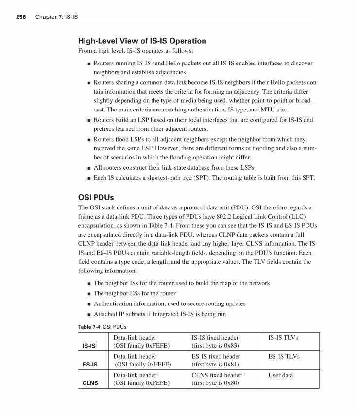
256 Chapter 7: IS-IS
High-Level View of IS-IS Operation
From a high level, IS-IS operates as follows:
■ Routers running IS-IS send Hello packets out all IS-IS enabled interfaces to discover
neighbors and establish adjacencies.
■ Routers sharing a common data link become IS-IS neighbors if their Hello packets con-
tain information that meets the criteria for forming an adjacency. The criteria differ
slightly depending on the type of media being used, whether point-to-point or broad-
cast. The main criteria are matching authentication, IS type, and MTU size.
■ Routers build an LSP based on their local interfaces that are configured for IS-IS and
prefixes learned from other adjacent routers.
■ Routers flood LSPs to all adjacent neighbors except the neighbor from which they
received the same LSP. However, there are different forms of flooding and also a num-
ber of scenarios in which the flooding operation might differ.
■ All routers construct their link-state database from these LSPs.
■ Each IS calculates a shortest-path tree (SPT). The routing table is built from this SPT.
OSI PDUs
The OSI stack defines a unit of data as a protocol data unit (PDU). OSI therefore regards a
frame as a data-link PDU. Three types of PDUs have 802.2 Logical Link Control (LLC)
encapsulation, as shown in Table 7-4. From these you can see that the IS-IS and ES-IS PDUs
are encapsulated directly in a data-link PDU, whereas CLNP data packets contain a full
CLNP header between the data-link header and any higher-layer CLNS information. The IS-
IS and ES-IS PDUs contain variable-length fields, depending on the PDU’s function. Each
field contains a type code, a length, and the appropriate values. The TLV fields contain the
following information:
■ The neighbor ISs for the router used to build the map of the network
■ The neighbor ESs for the router
■ Authentication information, used to secure routing updates
■ Attached IP subnets if Integrated IS-IS is being run
Table 7-4 OSI PDUs
IS-IS
Data-link header (OSI family 0xFEFE)
IS-IS fixed header (first byte is 0x83)
IS-IS TLVs
ES-IS
Data-link header (OSI family 0xFEFE)
ES-IS fixed header (first byte is 0x81)
ES-IS TLVs
CLNS
Data-link header (OSI family 0xFEFE)
CLNS fixed header (first byte is 0x80)
User data
1358_fmi.book Page 256 Thursday, May 27, 2004 2:21 PM

IS-IS Operation 257
IS-IS PDUs are encapsulated directly into an OSI data-link layer frame. There is no CLNP
header and no IP header. The IS-IS protocol family is OSI, and values such as 0xFE and
0xFEFE are used by the data-link protocol to identify the Layer 3 protocol as OSI. This chap-
ter focuses on the OSI PDUs specific to IS-IS.
There are four categories of IS-IS PDUs, as shown in Figure 7-8:
■ Hello PDU (ESH, ISH, IS-IS Hello [IIH])—Used to establish and maintain adjacen-
cies. ESHs are sent from ESs to ISs. ISHs are sent from ISs to ESs. IIHs are sent
between ISs. Note that ESH and ISH PDUs are ES-IS PDUs, not IS-IS PDUs.
■ LSP—Used by IS-IS to distribute link-state information. There are independent pseud-
onode (PSN) and nonpseudonode LSPs for both Level 1 and Level 2.
■ Complete Sequence Number PDU (CSNP)—Used to distribute a complete link-state
database on the router. CSNPs are used to inform other routers of LSPs that might be
outdated or missing from their own database. This ensures that all routers have the
same information and are synchronized. The packets are similar to an OSPF database
description packet.
■ Partial Sequence Number PDU (PSNP)—Used to acknowledge and request link-state
information.
Figure 7-8 Identifying Systems in IS-IS
There are nine IS-IS PDU types, as shown in Table 7-5. The value codes 1 through 10 are
defined in ISO 10589, and 128 through 133 are defined in RFC 1195. TLV Code 133, for
authentication information, is specified in RFC 1195, but Cisco technology uses the ISO
ISH
ESHSNPA ES-IS
IS-IS
IIH SNPA
ES ES ES
IS
IS
IS
1358_fmi.book Page 257 Thursday, May 27, 2004 2:21 PM

258 Chapter 7: IS-IS
Code of 10 instead. TLV Code 4 is used for partition repair and is not supported by Cisco
technology.Table 7-5 Valid Code Values for Nine Types of IS-IS PDUs
IS-IS PDUs Code Value
Level 1 LAN IS-to-IS Hello PDUType 15
Code 1 = Area addressesCode 6 = IS neighbors (hellos)Code 8 = PaddingCode 10 = Authentication informationCode 129 = Protocols supportedCode 132 = IP interface address
Level 2 LAN IS-to-IS Hello PDUType 16
Code 1 = Area addressesCode 6 = IS neighbors (hellos)Code 8 = PaddingCode 10 = Authentication informationCode 129 = Protocols supportedCode 132 = IP interface address
Point-to-Point IS-to-IS Hello PDUType 17
Code 1 = Area addressesCode 8 = PaddingCode 10 = Authentication informationCode 129 = Protocols supportedCode 132 = IP interface address
Level 1 Link-State PDUType 18
Code 1 = Area addressesCode 2 = IS neighbors (LSPs)Code 3 = ES neighborsCode 6 = IS neighborsCode 10 = Authentication informationCode 128 = IP internal reachability informationCode 129 = Protocols supportedCode 132 = IP interface address
Level 2 Link-State PDUType 20
Code 1 = Area addressesCode 2 = IS neighbors (LSPs)Code 2 = IS neighborsCode 4 = Partition designated Level 2 ISCode 5 = Prefix neighborsCode 10 = Authentication informationCode 128 = IP internal reachability informationCode 129 = Protocols supportedCode 130 = IP external reachability informationCode 131 = IDRP informationCode 132 = IP interface address
1358_fmi.book Page 258 Thursday, May 27, 2004 2:21 PM
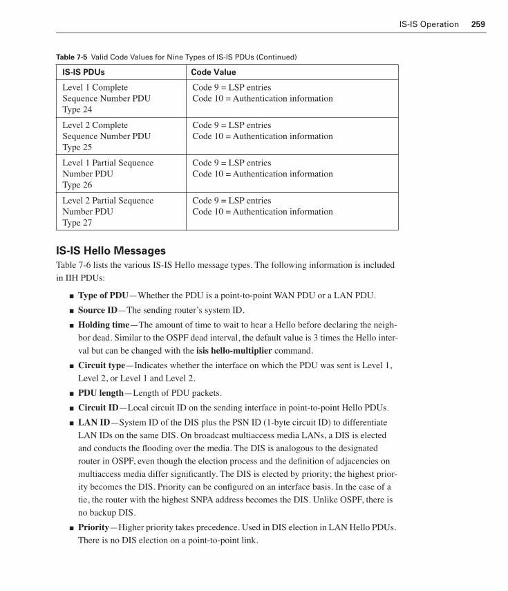
IS-IS Operation 259
IS-IS Hello Messages
Table 7-6 lists the various IS-IS Hello message types. The following information is included
in IIH PDUs:
■ Type of PDU—Whether the PDU is a point-to-point WAN PDU or a LAN PDU.
■ Source ID—The sending router’s system ID.
■ Holding time—The amount of time to wait to hear a Hello before declaring the neigh-
bor dead. Similar to the OSPF dead interval, the default value is 3 times the Hello inter-
val but can be changed with the isis hello-multiplier command.
■ Circuit type—Indicates whether the interface on which the PDU was sent is Level 1,
Level 2, or Level 1 and Level 2.
■ PDU length—Length of PDU packets.
■ Circuit ID—Local circuit ID on the sending interface in point-to-point Hello PDUs.
■ LAN ID—System ID of the DIS plus the PSN ID (1-byte circuit ID) to differentiate
LAN IDs on the same DIS. On broadcast multiaccess media LANs, a DIS is elected
and conducts the flooding over the media. The DIS is analogous to the designated
router in OSPF, even though the election process and the definition of adjacencies on
multiaccess media differ significantly. The DIS is elected by priority; the highest prior-
ity becomes the DIS. Priority can be configured on an interface basis. In the case of a
tie, the router with the highest SNPA address becomes the DIS. Unlike OSPF, there is
no backup DIS.
■ Priority—Higher priority takes precedence. Used in DIS election in LAN Hello PDUs.
There is no DIS election on a point-to-point link.
IS-IS PDUs Code Value
Level 1 Complete Sequence Number PDUType 24
Code 9 = LSP entriesCode 10 = Authentication information
Level 2 Complete Sequence Number PDUType 25
Code 9 = LSP entriesCode 10 = Authentication information
Level 1 Partial Sequence Number PDUType 26
Code 9 = LSP entriesCode 10 = Authentication information
Level 2 Partial Sequence Number PDUType 27
Code 9 = LSP entriesCode 10 = Authentication information
Table 7-5 Valid Code Values for Nine Types of IS-IS PDUs (Continued)
1358_fmi.book Page 259 Thursday, May 27, 2004 2:21 PM

260 Chapter 7: IS-IS
The IS-IS LAN Hello PDU is shown in Figure 7-9.
The IS-IS LAN Hello fields are as follows:
■ Intradomain Routing Protocol Discriminator—Network layer identifier assigned to
IS-IS in ISO 9577. The binary value is 10000011 (0x83).
■ Length Indicator—Length of the fixed header in octets.
■ Protocol ID Ext—Currently has a value of 1.
■ ID Length—Length of the System ID field. This must be the same for all nodes in the
domain. If this is set to 0, it implies six octets.
■ PDU Types—Values are 15 and 16 for Level 1 and Level 2 LSPs, respectively.
■ Version—Value is 1.
■ Maximum Area Addresses—Number of area addresses permitted for this IS area. Val-
ues are between 1 and 254 for the actual number. 0 implies a maximum of three.
■ Reserved/Circuit Type—The top 6 bits are reserved. The bottom 2 bits with a value of
0 indicates reserved. A value of 1 indicates Level 1, a value of 2 indicates Level 2, and
a value of 3 indicates Levels 1 and 2.
■ Source ID—Transmitting router’s system ID.
■ Holding Time—Holding time as configured on this router.
■ PDU Length—Length of the entire PDU, fixed header, and TLVs.
■ Reserved/Priority—Bit 8 is reserved. Bit 1 is used for priority for being the Level 1 or
Level 2 DIS. The value is copied from the IIH of the DIS.
■ LAN ID—A field composed of the system ID of the DIS, 1 to 8 bytes, plus a low-order
octet assigned by the LAN Level 1 DIS.
Table 7-6 IS-IS Hello Message Types
Number Description
1 Point-to-point IIH Part of the IS-IS spec 10589. Used by routers to form adjacencies.
2 Point-to-point IIH Part of the IS-IS spec 10589. Used by routers to form adjacencies.
3 Point-to-point IIH Part of the IS-IS spec 10589. Used by routers to form adjacencies.
4 ESH Part of the ES-IS spec. Similar to ICMP Router Discovery Protocol (IRDP) in TCP/IP. Lets routers (ISs) and ESs detect each other.
5 ISH Part of the ES-IS spec. Similar to IRDP in TCP/IP. Lets routers (ISs) and ESs detect each other.
Author Query:
both one and two are
the same. Is this OK?
1358_fmi.book Page 260 Thursday, May 27, 2004 2:21 PM

IS-IS Operation 261
Figure 7-9 IS-IS Hello PDU
Intradomain Routing ProtocolDiscriminator
1
Length Indicator 1
Vision/Protocol ID EXT 1
ID Length 1
R R R Type 1
Version 1
Reserved 1
Maximum Area Address 1
Reserved Circuit Type 1
Source ID 6
Holding Timer 2
PDU Length 2
RES Priority 1
LAN ID 7
Variable-Length Fields Variable
Number of Octets
1358_fmi.book Page 261 Thursday, May 27, 2004 2:21 PM

262 Chapter 7: IS-IS
Notice the variable-type length fields at the bottom of the packet. This is where the TLV
information is stored. Different types of PDUs have a set of currently defined codes. Any
codes that are not recognized are supposed to be ignored and passed through unchanged.
By default, IS-IS Hellos are padded to the full MTU size. The benefit of padding IIHs to the
full MTU is the early detection of errors caused by transmission problems with large frames
or MTU mismatches on adjacent interfaces. The drawbacks of IIH padding are that on high-
speed interfaces it could be a strain on huge buffers, and on low-speed interfaces, large Hello
PDUs waste bandwidth. This could affect time-sensitive applications such as voice over IP
(VoIP). The padding of IS-IS Hellos can be turned off for all interfaces on a router, beginning
with Cisco IOS Releases 12.0(5)S and 12.0(5)T, with the no hello padding command in IS-
IS router configuration mode. The padding of IS-IS Hellos can be turned off selectively for
point-to-point or multipoint interfaces with the no hello padding multipoint command or
the no hello padding point-to-point command, respectively, in IS-IS router configuration
mode. Hello padding can also be turned off on an individual interface basis using the no isis hello padding interface configuration command.
IS-IS Link-State PDU (LSP) Formats
The contents of the TLV fields, shown in Figure 7-10, include the following:
■ The neighbor ISs of the router that are used to build the map of the network
■ The neighboring router ESs for the router
■ Authentication information, used to secure routing updates
■ Attached IP subnets if Integrated IS-IS is being run
Figure 7-10 TLV Field Contents
Interactive Media Activity Drag and Drop: IS-IS Hello Messages
After completing this activity, you will be able to identify the fields in an IS-IS LAN
Hello PDU.
LSP Header
IS Neighbors
ES Neighbors
....................
1358_fmi.book Page 262 Thursday, May 27, 2004 2:21 PM
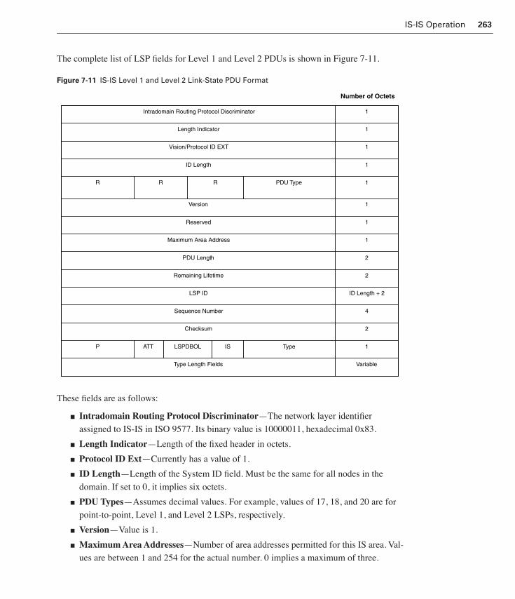
IS-IS Operation 263
The complete list of LSP fields for Level 1 and Level 2 PDUs is shown in Figure 7-11.
Figure 7-11 IS-IS Level 1 and Level 2 Link-State PDU Format
These fields are as follows:
■ Intradomain Routing Protocol Discriminator—The network layer identifier
assigned to IS-IS in ISO 9577. Its binary value is 10000011, hexadecimal 0x83.
■ Length Indicator—Length of the fixed header in octets.
■ Protocol ID Ext—Currently has a value of 1.
■ ID Length—Length of the System ID field. Must be the same for all nodes in the
domain. If set to 0, it implies six octets.
■ PDU Types—Assumes decimal values. For example, values of 17, 18, and 20 are for
point-to-point, Level 1, and Level 2 LSPs, respectively.
■ Version—Value is 1.
■ Maximum Area Addresses—Number of area addresses permitted for this IS area. Val-
ues are between 1 and 254 for the actual number. 0 implies a maximum of three.
Intradomain Routing Protocol Discriminator 1
Length Indicator 1
Vision/Protocol ID EXT 1
ID Length 1
R R R PDU Type 1
Version 1
Reserved 1
Maximum Area Address 1
PDU Length 2
Remaining Lifetime 2
LSP ID ID Length + 2
Sequence Number 4
Checksum 2
P ATT LSPDBOL IS Type 1
Type Length Fields Variable
Number of Octets
1358_fmi.book Page 263 Thursday, May 27, 2004 2:21 PM

264 Chapter 7: IS-IS
■ PDU Length—Length of the entire PDU, fixed header, and TLVs.
■ Remaining Lifetime—Time in seconds before LSP expires. Used to age out LSPs.
Outdated and invalid LSPs are removed from the topology table after a suitable period.
It is a count-to-zero operation with a default 1200-second start value, or MaxAge. If the
remaining lifetime expires, the first router that notices purges the LSP, removes the LSP
body, keeps the LSP header, and sets the age to 0. It floods this modified LSP in the
usual way throughout the network. Zero-lifetime LSPs are newer than nonzero-lifetime
LSPs. After a while, all routers remove the purged LSP from their LSP database.
■ LSP ID—Consists of the system ID, PSN ID, and LSP fragmentation number, as
shown in Figure 7-12. The PSN ID is 0 for a router LSP. Length is ID length plus 2
bytes.
Figure 7-12 LSP ID
■ Sequence Number—Used for synchronization. A higher sequence number indicates a
newer LSP. Allows receiving routers to ensure that they use only the latest LSPs in their
route calculations. Used to avoid duplicate LSPs being entered into the topology tables.
When a change occurs, the sequence number is incremented, and a new version of the
LSP is generated with the new sequence number.
When a router reloads, the sequence number is initially set to 1. The router might then
receive its own old LSPs back from its neighbors, which will have the last good sequence
number before the router reloaded. It records this number and reissues its own LSPs with
the next-highest sequence number.
■ Checksum—Computed from the source ID to the end of the PDU. Used to detect LSP
corruption during flooding. It might be that the Layer 2 CRC is insufficient for error
checking. Corruption happens in routers and switches. The checksum is computed
upon receipt of the LSP and is checked against the checksum inside the LSP. If corrupt,
the LSP is dropped, and the sender retransmits. If two LSPs have the same LSP ID, the
same sequence number, and the same remaining lifetime, the LSP with the highest
checksum is kept. This guarantees consistent LSP databases across the network. This
scenario can happen after a router reboots or is reconnected to the network.
System IDLSP Fragmentation
Number
Pseudonode ID
00c0.0040.1234.01-00
1358_fmi.book Page 264 Thursday, May 27, 2004 2:21 PM

IS-IS Operation 265
■ Partition (P)—Bit 8 of the octet. When set, this means that the originator of LSP sup-
ports partition repair.
■ Attached Bit (ATT)—Bits 4 through 7 of the octet. When any of these bits is set, the
originator is attached to another area using the referred metric. For example, as shown
in Figure 7-13, bit 4 set implies attached using the default metric. Set in the Level 1
LSP by an L1L2 router if it has connectivity to another area, it indicates to the area
routers, Level 1, that it is a potential exit point for the area. Level 1 routers select the
closest, best metric Level 2 router with the ATT bit set.
Figure 7-13 Attached Bit
■ LSPDBOL (Overload Bit)—Bit 3. When set, this indicates that the originator’s LSP
database is overloaded and should be circumvented in path calculations to other desti-
nations. Indicates that the router has an incomplete LS database and, therefore, cannot
be trusted to compute any correct routes. It is used in the LSP database, but the topol-
ogy behind it is not calculated. Therefore, other routers do not compute routes that
would require the PDU to pass through the overloaded router. An exception to this is
ES neighbors, because these paths are guaranteed to be nonlooping.
■ IS Type—Bits 1 and 2 indicate a Level 1 or Level 2 LSP type. When only Bit 1 is set, it
indicates Level 1 IS. If both bits are set, it indicates Level 2 IS.
Section 9 of RFC 1142, a rewrite of ISO 10589, gives details about the packet layouts for
each type of IS-IS PDU. It also gives the TLV information supported for each type. The first
eight octets of all IS-IS PDUs are header fields that are common to all PDU types. The Level 1
and Level 2 LAN Hello PDUs are identical, except for the PDU type, which differentiates
them as either Level 1 or Level 2, as shown in Figure 7-14. Figure 7-15 shows that the point-
to-point Hello PDU is very similar to the Level 1 and Level 2 LAN Hello PDUs.
L1-LSDB
RtrA.00-00
RtrB.00-00
RtrC.00-00
ATT-bit
L1-LSDB
RtrD.00-00
rtrE.00-00
RtrF.00-00
ATT-bitL2-LSDB
RtrA.00-00
RtrD.00-00RtrA
RtrD
Area 1 Area 2
1358_fmi.book Page 265 Thursday, May 27, 2004 2:21 PM

266 Chapter 7: IS-IS
Figure 7-14 Level 1 and Level 2 IS-IS Hello PDU
The lengths of the various ID fields in the PDUs—the LSP ID, source ID, and so on—all
assume that the length of the system ID is fixed at 6 bytes. Under the column for the number
of octets in Figure 7-11, an 8 would mean ID length + 2, a 7 would mean ID length + 1, and a
6 would mean ID length. Don’t confuse the value of the ID length variable with the size of
the ID Length field, which is fixed at 1 byte. The CLNS protocol allows the system ID, part of
the NSAP address, to vary from 3 to 8 bytes. However, in practice, a 6-byte system ID is
always used (ID length = 0). If the ID length field is 0, it means that the system ID is using
the default length of 6 bytes.
Intradomain Routing Protocol Discriminator 1
Length Indicator 1
Vision/Protocol ID EXT 1
ID Length 1
Type R R R 1
Version 1
Reserved 1
Maximum Area Address 1
Reserved/Circuit Type 1
Source ID 6
Holding Timer 2
PDU Length 2
RES Priority 1
LAN ID 7
Variable-Length Fields Variable
Number of Octets
1358_fmi.book Page 266 Thursday, May 27, 2004 2:21 PM

IS-IS Operation 267
Figure 7-15 Point-to-Point IS-IS Hello PDU
IS-IS Routing Levels
An IS-IS network is called a domain, analogous to an autonomous system in TCP/IP. The
following shows IS-IS within the domain as a two-level hierarchy:
■ Level 1 (L1) ISs, closely equivalent to OSPF internal nonbackbone routers, are responsible
for routing to ESs inside an area. L1 ISs enable communication between ESs in an area.
■ Level 2 (L2) ISs, closely equivalent to backbone routers in OSPF, route between areas
only.
Intradomain Routing ProtocolDiscriminator
1
Length Indicator 1
Vision/Protocol ID EXT 1
ID Length 1
Type R R R 1
Version 1
Reserved 1
Maximum Area Address 1
Reserved/Circuit Type 1
Source ID 6
Holding Timer 2
PDU Length 2
Local Circuit ID 1
Variable-Length Fields Variable
Number of Octets
1358_fmi.book Page 267 Thursday, May 27, 2004 2:21 PM

268 Chapter 7: IS-IS
■ Level 1 and Level 2 (L1L2) intermediate ISs, closely equivalent to ABRs in OSPF,
route between areas and the backbone. They participate in L1 intrarea routing and L2
interarea routing.
L1 routers are also called station routers because they allow stations to communicate with
each other and the rest of the network. A contiguous group of L1 routers defines an area. The
L1 routers maintain the L1 link-state PDU database (LSPD), which defines the picture of
the area itself and the exit points to neighboring areas.
L2 routers are also called area routers because they interconnect the L1 areas. L2 routers store
a separate LSPD that contains only the interarea topology information.
L1L2 routers act as if they were two IS-IS routers, as shown in Figures 7-16 and 7-17. Physi-
cally, an L1L2 router connects to L1 routers inside its area and to L2 routers in the backbone.
Notice that the boundary between areas in IS-IS exists on a link between routers and not on
an ABR, as in OSPF. Logically, the L1L2 router acts, for the purposes of IS-IS routing, as if it
were two logical routers. An L1L2 router operates an L1 routing process, with its own L1
topology table and adjacency table, to handle its association with other L1 routers and ESs.
An L1L2 router also operates an L2 routing process, with a separate L2 topology table and a
separate L2 adjacency table, to handle its association with its neighbor backbone routers.
Figure 7-16 IS-IS Routing Levels
L1L2 routers support an L1 function to communicate with the other L1 routers in their area
and maintain the L1 LSP information in an L1 LSPD. They inform other L1 routers that they
are an exit point for the area. They also support an L2 function to communicate with the rest
of the backbone and maintain an L2 topology database separately from their L1 LSPD. IS-IS
does not have the concept of an Area 0, as does OSPF. An IS-IS domain appears as a set of
distinct areas interconnected by a chain of L2 routers, weaving their way through and
between the Level 1 areas.
R3
R4
Area 2
R2
R1
Area1
L1L2 Routers
1358_fmi.book Page 268 Thursday, May 27, 2004 2:21 PM

IS-IS Operation 269
Figure 7-17 IS-IS Routing Levels
An L1 area is a collection of L1 and L1L2 routers. The backbone area is a collection of L2
and L1L2 routers and has to be contiguous. IS-IS does not have a backbone area such as
OSPF Area 0. The IS-IS backbone is a contiguous collection of L2-capable routers, each of
which can be in a different area, as shown in Figure 7-18.
Figure 7-18 IS-IS Backbone
Useful examples of the L1, L2, and L1L2 concepts are discussed in this section. As shown in
Figure 7-19, Area 1 contains two routers. One router borders Area 2 and, therefore, is an
L1L2 IS. The other router is an L1-only.
R4R1
L2
R2 R3L2
L1
L1 L1
NOTE
By default, all Cisco rout-ers behave as L1L2 rout-ers. You can override this default behavior by using the is-type router global configuration mode com-mand or the isis circuit-type interface configura-tion mode command or both.
L1
L1
L1
L1
L1/L2
L1/L2
L1/L2
L1/L2
L1/L2
L2
Area 2 Area 3
Area 1 Area 4
1358_fmi.book Page 269 Thursday, May 27, 2004 2:21 PM

270 Chapter 7: IS-IS
Figure 7-19 IS-IS Backbone
Area 2 has many routers. Some are specified as L1-only and can route internally to that area
only and to the exit points. L1L2 routers form a chain across the area linking to the neighbor
areas. Even though the middle of these three L1L2 routers does not link directly to another
area, it must support Level 2 routing so that the backbone is contiguous. If that middle router
fails, the other L1-only routers, although they provide a physical path across the area, cannot
perform the L2 function. This causes the backbone to fail.
Area 3 contains one router that borders Area 2 and Area 4 but that has no intra area neighbors,
so this router is an L2-only router. If another router were added to Area 3, the border router
would revert to L1L2.
Interactive Media Activity Matching: IS-IS Level 1 Adjacencies
After completing this activity, you will be able to identify the Level 1 adjacencies
between routers in an IS-IS network.
L1L2
L1L2
L1L2
L1-Only
L1-Only
L1-Only
IS-ISDomain
Backbone Links
L2-Only
This router must behave as an L2 as well as L1 routerin order to guarantee backbone connectivity.
L1L2
Area 1
L1-OnlyL1L2
Area 4
Area 3
Area 2
NOTE
Previously, each Cisco router could participate in only one area. The router would perform L1, intra-area routing locally. The router would perform L2, interarea routing to other areas in the network. This limitation meant that when the network was divided into a large number of L1 areas, a correspondingly large number of L1L2 routers were required to route between all areas. The need for redundancy increases the number of routers needed. With Cisco IOS Release 12.0(5)T, sup-port was added for config-uring multiple L1 areas within a single router. A single Cisco router can now participate in routing in up to 29 areas, as well as per-form L2 routing in the backbone. In other words, expanding an IS-IS net-work that consists of many small areas is simpler than before because multiple L1 areas can now be config-ured on the same Cisco router. You can do this without needing to add and configure physical units for each additional local area. This feature provides con-nectivity between L1 areas local to the router. Previ-ously, L1 areas could only be connected using the L2 backbone. However, it should be emphasized that multiarea support per IS was introduced in later implementations of IS-IS to accommodate OSI tele-communications manage-ment network needs. This functionality generally is not useful or recommended for IP network design.
1358_fmi.book Page 270 Thursday, May 27, 2004 2:21 PM

IS-IS Operation 271
IS-IS Adjacencies
IS-IS uses Hello PDUs to establish adjacencies with other routers (ISs) and ESs. Hello PDUs
carry information about the system, its parameters, and its capabilities.
ISs use IIHs to establish and maintain neighbor relationships. As soon as an adjacency is
established, the ISs exchange link-state information with LSPs.
ISs also send out ISHs. ESs listen for these ISHs and randomly pick an IS—the first one
heard—to forward all of their packets to. OSI ESs require no configuration to forward pack-
ets to the rest of the network.
ISs listen to the ESHs and learn about all of the ESs on a segment. ISs include this informa-
tion in their LSPs. For particular destinations, ISs might send redirect messages to ESs to pro-
vide them with an optimal route off the segment.
Now consider adjacencies between ISs. Separate adjacencies are established for Level 1 and
Level 2. If two neighboring routers in the same area run both Level 1 and Level 2, they estab-
lish two adjacencies, one for each level. The L1 and L2 adjacencies are stored in separate L1
and L2 adjacency tables.
On LANs, two adjacencies are established with specific L1 and L2 IIH PDUs. Routers on a
LAN establish adjacencies with all other routers on the LAN with the same area ID and level.
This is unlike OSPF, where routers establish adjacencies only with the designated router. On
LANs, IS-IS PDUs are multicast to the well-known MAC addresses, as shown in Table 7-7.
IIH PDUs announce the area ID. Separate IIH PDUs announce the Level 1 and Level 2 neigh-
bors. For example, where a LAN has routers from two areas attached, the routers from one
area accept Level 1 IIH PDUs only from their own area. Therefore, they establish adjacencies
with only their own area routers, as shown in Figure 7-20. The routers from a second area
similarly accept Level 1 IIH PDUs only from their own area. The L2 routers, or the L2 pro-
cess within any L1L2 router, accept only L2 IIH PDUs and establish only L2 adjacencies, as
shown in Figure 7-21.Table 7-7 IS-IS Layer 2 Multicast Addresses
Name Address
AllL1ISs 01-80-C2-00-00-14
AllL2ISs 01-80-C2-00-00-15
AllIntermediateSystems 09-00-2B-00-00-05
AllEndSystems 09-00-2B-00-00-04
1358_fmi.book Page 271 Thursday, May 27, 2004 2:21 PM

272 Chapter 7: IS-IS
Figure 7-20 L1 and L2 Adjacencies In Area
Figure 7-21 L1 and L2 Adjacencies In and Out of Area
Point-to-point WAN links have a common IIH format, part of which specifies whether the
Hello message relates to Level 1, Level 2, or both. The area ID is also announced in the Hello
messages.
By default, Hello PDUs are sent every 10 seconds. The timeout to declare a neighbor down is
30 seconds, which equals three missing Hello packets. These timers can be reconfigured
using the isis hello-interval and isis hello-multiplier interface configuration commands.
Various combinations are possible for links between L1, L2, and L1L2 routers. L1 routers in
the same area, which include links between L1-only and L1L2 routers, exchange IIH PDUs
specifying L1 and establish an L1 adjacency. L2 routers, when in the same area or between
Area 1 Area 1 Area 1
Area 1 Area 2
L1 AdjacencyL2 Adjacency
L1/L2
L1/L2
L1/L2L1
L1
L1/L2
L2
L2
L2
L1
L1
L1
L1
L1
L1
L1/L2
L1/L2
L1/L2 L1/L2
L1/L2
L1/L2
L2
L2
L2
L2
Area 1 Area 1
Area 1 Area 1
Area 1
Area 1
Area 1
Area 1
Area 1
Area 1
Area 1 Area 1
Area 2 Area 2
Author Query:
Figure Titles
are the same.
1358_fmi.book Page 272 Thursday, May 27, 2004 2:21 PM

IS-IS Operation 273
areas, and including links between L2-only and L1L2 routers, exchange IIH PDUs specifying
L2 and establish an L2 adjacency. Two L1L2 routers in the same area establish both L1 and L2
adjacencies. The two routers maintain these with a common IIH PDU specifying both the L1
and L2 information. Two L1 routers that might be physically connected but, that are not in the
same area, exchange L1 IIH PDUs. This includes an L1-only router to an L1L2 router in a
different L1 area. However, they ignore these because the area IDs do not match. Therefore,
they do not establish an adjacency.
L1-only routers establish L1 adjacencies. L2 routers establish L2 adjacencies between areas.
L1L2 routers establish both L1 and L2 adjacencies with their L1L2 neighbors in the same
area. L2 adjacencies exist independent of areas and must be contiguous; for example, Area 2
is not the backbone area, as shown in Figure 7-22. The backbone in IS-IS is exactly the con-
tiguous set of routers and connections between L2 and L1L2 routers. The backbone might
traverse multiple areas.
Figure 7-22 L2 Adjacencies Connect the Backbone Area
Interactive Media Activity Matching: IS-IS Level 2 Adjacencies
After completing this activity, you will be able to identify the Level 2 adjacencies
between routers in an IS-IS network.
L1L2
L1L2
L1L2
L1-Only
L1-Only
L2-Only
L1L2
Area 1
Area 3
Area 2
L1-Only
1358_fmi.book Page 273 Thursday, May 27, 2004 2:21 PM

274 Chapter 7: IS-IS
Designated Intermediate Systems (DIS) and Pseudonodes (PSN)
The idea behind the DIS is similar to the one behind the DR in OSPF. The DIS creates and
acts on behalf of a PSN, a virtual node, as shown in Figure 7-23. All the routers on the LAN,
including the DIS, form an adjacency with the PSN. Instead of flooding and database syn-
chronization taking place over n * (n – 1) adjacencies, the PSN lets the reduction in flooding
and database synchronization occur only over the adjacencies formed with the pseudonode.
On a LAN, one of the routers is elected the DIS, based on interface priority. The default prior-
ity is 64. The configurable range is 0 to 127. If all interface priorities are the same, the router
with the highest SNPA is selected. MAC addresses are the SNPAs on LANs. On Frame Relay
networks, the local DLCI is the SNPA. If the SNPA is a DLCI and is the same on both sides
of a link, the router with the higher system ID in the NSAP address becomes the DIS.
Figure 7-23 Pseudonode
A pseudonode LSP represents a LAN, including all ISs attached to that LAN. A nonpseudonode
LSP represents a router, including all ISs and LANs connected to the router.
The DIS election is preemptive, unlike DR election with OSPF. If a new router boots on the
LAN with a higher interface priority, it becomes the DIS and purges the old pseudonode LSP,
and a new set of LSPs is flooded. The DIS Hello interval, at 3.3 seconds, is 3 times faster than
the interval for other routers on the LAN. This allows for quick detection of DIS failure and
immediate replacement on the LAN. Remember that IS-IS has no concept of backup DIS.
In IS-IS, a DIS does not synchronize LSPs with its neighbors through acknowledgments.
Reliability is ensured when the DIS creates the pseudonode for the LAN. It sends L1 and L2
Hello PDUs every 10 seconds and CSNPs every 10 seconds. The Hello PDUs indicate that it
is the DIS on the LAN for that level. The CSNPs describe the summary of all the LSPs,
including the LSP ID, sequence number, checksum, and remaining lifetime. The LSPs are
always flooded to the multicast address. The CSNP mechanism only corrects for any lost
PDUs. For example, a router can ask the DIS for a missing LSP using a PSNP or, in turn, give
the DIS a new LSP. CSNPs are used to tell other routers about all the LSPs in another router’s
database. Similar to an OSPF database descriptor packet, PSNPs are used to request an LSP
and acknowledge receipt of an LSP.
DIS DIS
PSN
1358_fmi.book Page 274 Thursday, May 27, 2004 2:21 PM

IS-IS Operation 275
To restate, the DIS is responsible for conducting flooding over the LAN and also for main-
taining synchronization. A router might need an LSP because it is older than the LSP adver-
tised by the DIS in its CSNP. A router might need an LSP if it is missing an LSP that is listed
in the CSNP. If either of these is the case, the router sends a PSNP to the DIS and receives the
LSP in return. This mechanism can work both ways. If a router sees that it has a newer ver-
sion of an LSP, or if it has an LSP that the DIS does not advertise in its CSNP, the router
sends the newer or missing LSP to the DIS.
IS-IS Data Flow
In IS-IS, routers might have adjacencies with other routers on point-to-point links. In a LAN
environment, routers report their adjacencies to the DIS, which generates an additional LSP,
commonly known as the pseudonode LSP. The DIS is responsible for conducting flooding
over the LAN and also for maintaining synchronization.
The flow of information within the IS-IS routing function is shown in Figure 7-24. This con-
sists of four processes—receiver, update, decision, and forward—and a Routing Information
Base (RIB). The RIB consists of the link-state database and the forwarding database.
Figure 7-24 IS-IS Data Flow Diagram
The receive process is the entry point for all data, including user data, error reports, routing
information, and control packets. The receive process passes user data and error reports to the
forward process. It passes routing information and control packets, such as Hello messages,
LSPs, and sequence number packets, to the update process.
The update process generates local link information that is flooded to adjacent routers. In
addition, the update process receives, processes, and forwards link information received from
adjacent routers. This process manages the L1 and L2 link-state databases and floods L1 and
L2 LSPs throughout an area. Each LSP that resides in the link-state database has a remaining
lifetime, a checksum, and a sequence number. The LSP remaining lifetime counts down from
1200 seconds to 0. The MaxAge is 20 minutes. The LSP originator must periodically refresh
Update
Routing Information Base
Decision
Forward
Input Link-State Database
Forwarding Database
Output
RECEIVER
1358_fmi.book Page 275 Thursday, May 27, 2004 2:21 PM

276 Chapter 7: IS-IS
its LSPs to prevent the remaining lifetime from reaching 0. The refresh interval is 15 minutes,
with a random jitter of up to 25 percent. If the remaining lifetime reaches 0, the expired LSP
is kept in the database for an additional 60 seconds before it is purged. This additional 60 sec-
onds is called ZeroAgeLifetime. If a router receives an LSP with an incorrect checksum, the
router causes a purge of the LSP. The router does this by setting the remaining lifetime value
to 0, removing the LSP data, and reflooding it. This triggers the LSP originator to send a new
LSP. This behavior is different from that of OSPF, where only the originating router can
purge an LSP. IS-IS can be configured so that LSPs with incorrect checksums are not purged,
but the router that originated the LSP does not know that the LSP was not received.
The decision process runs the SPF algorithm on the link-state database and creates the for-
warding database. It computes next-hop information and computes sets of equal-cost paths,
creating an adjacency set that is used for load balancing. On a Cisco router, IS-IS supports
load balancing with up to six equal-cost paths.
The forward process gets its input from the receive process and uses the forwarding database to
forward data packets to their destination. It also redirects load sharing and generates error reports.
LSP Flooding and Synchronization
The following are the two types of link-state PDUs:
■ Nonpseudonode PDUs represent a router, including all ISs and LANs connected to the
router.
■ Pseudonode PDUs represent a LAN, including all ISs attached to that LAN, and are
generated by the DIS.
An L1 router creates an L1 LSP, an L2 router creates an L2 LSP, and an L1L2 router creates
both an L1 and an L2 LSP.
The DIS creates one pseudonode LSP for L1, one for L2, and one for each LAN. The use of
pseudonode LSPs reduces the number of adjacencies on a LAN and, therefore, reduces the
flooding of LSPs on the LAN, as shown in Figures 7-25 and 7-26.
The DIS creates and floods a new pseudonode LSP when the following happens:
■ A new neighbor comes up or an existing neighbor goes away
■ The refresh interval timer expires
The DIS generates the pseudonode LSP. The DIS reports all LAN neighbors, including the DIS, in
the pseudonode LSP with a metric of 0. All LAN routers, including the DIS, report connectivity to
the pseudonode in their LSPs. This is similar in concept to the network LSA in OSPF.
1358_fmi.book Page 276 Thursday, May 27, 2004 2:21 PM

IS-IS Operation 277
Figure 7-25 LSP Database Without a Pseudonode
Figure 7-26 LSP Database with a Pseudonode
Each IS creates and floods a nonpseudonode LSP when the following happens:
■ A new neighbor comes up or an existing neighbor goes away
■ New IP prefixes are inserted or removed
■ A link’s metric changes
■ The refresh interval timer expires
LSP for Router AIS: 10 B
10 C10 D
ES: 10 E
LSP for Router CIS: 10 A
10 B10 D
ES: 10 E
LSP for Router DIS: 10 A
10 B10 C
ES: 10 E
LSP for Router BIS: 10 A
10 C10 D
ES: 10 E
End System E
LSP for Router AIS: 10 P
LSP for Router CIS: 10 P
LSP for Router DIS: 10 P
LSP for Router BIS: 10 P
LSP for thePseudonode PIS: 0 A
0 B0 C0 D
ES: 0 E
End System E
1358_fmi.book Page 277 Thursday, May 27, 2004 2:21 PM
278 Chapter 7: IS-IS
For L1 LSP databases, L1 CSNPs and L1 PSNPs are used. For L2 LSP databases, L2 CSNPs
and L2 PSNPs are used.
The following are true of a CSNP:
■ It describes all LSPs in the LSP database. It contains an address range, LSP ID,
sequence number, checksum, and remaining lifetime.
■ It is used in two cases—periodic multicast by DIS every 10 seconds and on point-to-
point links when the link comes up.
■ If the LSP database is large, multiple CSNPs are sent.
Each router floods its LSPs to adjacent neighbors. The LSPs are passed along unchanged to
other adjacent routers until all of the routers in the area have received them. All of the L1
LSPs received by one router in an area describe the area’s topology.
The IS-IS link-state database consists of all of the LSPs the router has received. Each node in
the area maintains an identical link-state database. A change in the topology means a change
in one or more of the LSPs. The router that has experienced a link going up or down resends
its LSP to inform the other routers of the change. The LSP sequence number is increased by 1
to let the other routers know that the new LSP supersedes the older LSP. When a router origi-
nates an LSP, the LSP sequence number is 1. If the sequence number increases to the maxi-
mum of 0xFFFFFFFF, the IS-IS process must shut down. IS-IS must shut down for at least 21
minutes, which is MaxAge + ZeroAgeLifetime. This allows the old LSPs to age out of all the
router databases.
Flooding is the process by which these new LSPs are sent throughout the area to ensure that
the databases in all routers remain identical. If the LSP database is not synchronized, routing
loops might occur. When a router receives a new LSP, it floods this LSP to its neighbors,
except the neighbor that sent it.
On point-to-point links, the neighbors acknowledge the new LSP with a PSNP, which holds
the LSP ID, sequence number, checksum, and remaining lifetime. When the acknowledgment
PSNP is received from a neighbor, the originating router stops sending the new LSP to that
particular neighbor, although it might continue sending the new LSP to other neighbors that
have not yet acknowledged it.
On LANs, there is no explicit acknowledgment with a PSNP. Missing LSPs are detected
when a CSNP is received and the list of LSPs within the CSNP is compared to the LSPs in
that router’s database. If any LSPs are missing or outdated, the router sends a request for
these in the form of a PSNP.
If a router receives an LSP that has an older sequence number than the one in its IS-IS data-
base, it sends the newer LSP to the router that sent the old LSP. The router keeps resending it
until it receives an acknowledgment PSNP from the originator of the old LSP.
1358_fmi.book Page 278 Thursday, May 27, 2004 2:21 PM

IS-IS Operation 279
LSPs must be flooded throughout an area in order for the databases to synchronize and the
SPF tree to be consistent within an area. It is not possible to control which LSPs are flooded
by using a distribute list, although it is possible to use a route map to control which routes are
redistributed into IS-IS from another routing protocol.
New LSPs are flooded when there is a change in the topology. These changes are triggered by
the following:
■ Adjacency comes up or goes down
■ Interface comes up or goes down
■ Redistributed IP routes change
■ Interarea IP routes change
■ An interface is assigned a new metric
■ Most other configuration changes
When a new LSP is received, it is installed in the LSP database and is marked for flooding. It
is sent to all neighbors. Neighbors, in turn, flood the LSP further. Only new LSPs are flooded.
Old LSPs are simply acknowledged. This is because “state” is already maintained for this
LSP, and infinite looping of LSPs is avoided. It is also important to note that the LSP isn’t
flooded back to the router it was received from.
On a point-to-point link, as soon as an adjacency is established, both ISs send a CSNP packet.
Missing LSPs are sent by both ISs if they are not present in the received CSNP. Missing LSPs
might be requested with a PSNP, as shown in Figures 7-27 and 7-28. The ACK is communi-
cated with a PSNP.
Figure 7-27 P2P LSP Flooding
NOTE
Point-to-point is some-times abbreviated P2P.
RTA RTB RTCInterface 1
Interface 2
Interface 3
Interface 4
LSPRTA.00-00SEQ #100
LSPRTA.00-00SEQ #100
PSNPRTA.00-00SEQ#100
PSNPRTA.00-00SEQ#100
1358_fmi.book Page 279 Thursday, May 27, 2004 2:21 PM
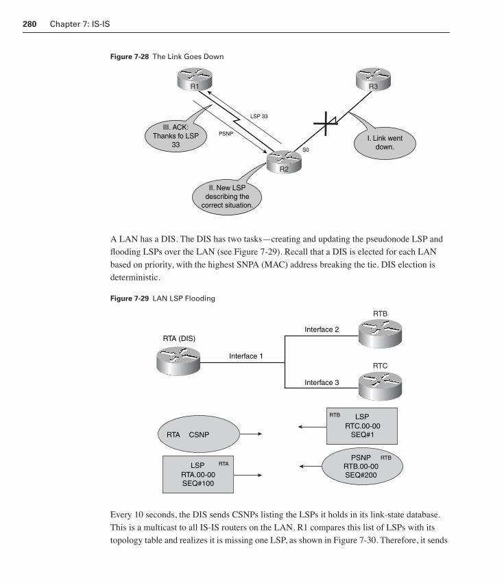
280 Chapter 7: IS-IS
Figure 7-28 The Link Goes Down
A LAN has a DIS. The DIS has two tasks—creating and updating the pseudonode LSP and
flooding LSPs over the LAN (see Figure 7-29). Recall that a DIS is elected for each LAN
based on priority, with the highest SNPA (MAC) address breaking the tie. DIS election is
deterministic.
Figure 7-29 LAN LSP Flooding
Every 10 seconds, the DIS sends CSNPs listing the LSPs it holds in its link-state database.
This is a multicast to all IS-IS routers on the LAN. R1 compares this list of LSPs with its
topology table and realizes it is missing one LSP, as shown in Figure 7-30. Therefore, it sends
LSP 33
S0
PSNPIII. ACK:
Thanks fo LSP33
II. New LSPdescribing the
correct situation.
I. Link wentdown.
R1
R2
R3
Interface 1
Interface 2
Interface 3
RTA CSNP
LSP RTA
RTA.00-00SEQ#100
LSPRTB
RTC.00-00SEQ#1
PSNPRTB.00-00SEQ#200
RTB
RTA (DIS)
RTB
RTC
1358_fmi.book Page 280 Thursday, May 27, 2004 2:21 PM

IS-IS Operation 281
a PSNP to the DIS (R2) to request the missing LSP. The DIS reissues that LSP, and R2
acknowledges it with a PSNP.
Figure 7-30 LAN LSP Flooding
IS-IS Metrics
The original IS-IS specification defines four different types of metrics. All routers support the
default metric of cost. Delay, expense, and error are optional metrics. The delay metric mea-
sures transit delay, the expense metric measures the monetary cost of link utilization, and the
error metric measures the residual error probability associated with a link.
The Cisco implementation uses cost only. If the optional metrics were implemented, there
would be a link-state database for each metric, and SPF would be run for each link-state
database.
Default MetricSome routing protocols calculate the link metric automatically based on bandwidth, OSPF,
EIGRP, or bandwidth/delay. However, IS-IS has no automatic calculation. Using old-style
metrics, an interface cost is between 1 and 63, a 6-bit metric value.
All links use a metric of 10 by default. The total cost to a destination is the sum of the costs
on all outgoing interfaces along a particular path from the source to the destination. Least-
cost paths are preferred. The total path metric is limited to 1023. This is the sum of all link
metrics along a path between the calculating router and any other node or prefix. This small
CSNP sent periodically,every ten seconds, by DIS.
PSNP
II.Request:Sorry. LSP 77was missed
I. CSNP:LSP76LSP77LSP88
CSNPPSNP
R1
R2/DIS
NOTE
Try to avoid confusing the IS-IS metric range and default with the IS-IS pri-ority range of 0 to 127 and default of 64.
1358_fmi.book Page 281 Thursday, May 27, 2004 2:21 PM

282 Chapter 7: IS-IS
metric value proved insufficient for large networks and provided too little granularity for new
features, such as traffic engineering and other applications. This is especially true with high-
bandwidth links. Wide metrics are also required if route leaking is used.
Extended MetricCisco IOS software addresses this issue by supporting a 24-bit metric field called the wide
metric. Using this new metric style, link metrics now have a maximum value of 16,777,215
(224 – 1) with a total path metric of 4,261,412,864 (232 – 225). The wide metric formulation
can be found in IETF Internet Draft document draft-ietf-isis-traffic-02.txt.
Deploying IS-IS in the IP network with wide metrics is recommended to enable finer granu-
larity and to support applications such as traffic engineering. Running different metric styles
within one network can cause a major problem. Link-state protocols calculate loop-free
routes. This is because all routers within one area calculate their routing table based on the
same link-state database. This principle is violated if some routers look at the old, narrow
style and some look at the new, wider-style TLVs. However, if the same interface cost is used
for both the old and new-style metrics, SPF computes a loop-free topology.
IS-IS Network Types
IS-IS defines point-to-point and broadcast networks.
Point-to-point networks, such as serial lines, connect a single pair of routers. A router running
IS-IS forms an adjacency with the neighbor on the other side of a point-to-point interface. A
DIS is not elected on this type of link. The basic mechanism defined in the standard is that
each side of a point-to-point link declares the other side to be reachable if a Hello packet is
received from it. When this occurs, each side then sends a CSNP to trigger database
synchronization.
Broadcast networks, such as Ethernet, Token Ring, and Fiber Distributed Data Interface
(FDDI), are multiaccess in that they can connect more than two devices. All devices con-
nected to routers receive a packet sent by one router. On broadcast networks, one IS is elected
the DIS. Hello packets on broadcast networks are sent to the AllL1ISs or AllL2ISs MAC-
layer broadcast addresses. The DIS is responsible for flooding. It creates and floods a new
pseudonode LSP for each routing level it participates in, whether L1 or L2, and for each LAN
to which it is connected. A router can be the DIS for all connected LANs or a subset of con-
nected LANS. This depends on the configured priority or, if no priority is configured, the
Layer 2 address. The DIS also creates and floods a new pseudonode LSP when a neighbor
adjacency is established or torn down or the refresh interval timer for this LSP expires. The
DIS mechanism reduces the amount of flooding on LANs.
1358_fmi.book Page 282 Thursday, May 27, 2004 2:21 PM

IS-IS Operation 283
Nonbroadcast multiaccess (NBMA) networks, such as Frame Relay, ATM, and X.25, can
connect multiple devices but have no broadcast capability. None of the other routers attached
to the network receive a packet sent by a router. Special consideration should be taken when
configuring IS-IS over NBMA networks. IS-IS has no concept of an NBMA network. IS-IS
considers these media to be just like any other broadcast media, such as Ethernet or Token
Ring. In general, it is better to configure point-to-point networks for IS-IS on WAN interfaces
and subinterfaces, such as with ATM, Frame Relay, and X.25. Unlike OSPF, no configuration
is necessary to tell IS-IS what the network type is.
SPF Algorithm
After the link-state database is updated, the router still needs to populate the routing table or
forwarding table. Just as with OSPF, IS-IS uses the Dijkstra algorithm, also called the SPF
algorithm, to compute the best path to a given destination in the link-state database. This is
the critical decision-making process that determines what routes, of those appearing in the
link-state database, will populate the routing table as IS-IS routes.
Edsger Dijkstra’s SPF algorithm is used to calculate routes with the IS-IS routing protocol,
for support of both TCP/IP and OSI. This is based on an extension to the algorithm specified
in ISO/IEC 10589.
The SPF algorithm computes the shortest paths from a single-source vertex to all other verti-
ces in a weighted, directed graph. In the Cisco IOS software implementation, the weight
assigned to the branches of a tree is a configurable metric with 224 possible values for each
link and 232 possible values for each path from the root to a leaf.
The main difference between link-state and distance vector routing protocols is that a link-
state protocol provides full visibility of the network topology, and a distance vector protocol
uses learned information to build forwarding tables. The visibility provided by a link-state
protocol is achieved through the use of a flooding mechanism. This mechanism ensures that
each router in a specified area of a network receives information that can be used to build a
network map. In IS-IS this information is flooded through the use of LSP data units. Each
intermediate system, or router, then advertises information that pertains to itself and its links.
After the information is flooded and all routers obtain the same information, the SPF algo-
rithm is applied separately to each router. This is done to determine the topology and to
extract the shortest paths for each router from the tree’s root to all its leaves. The information
derived from this process is used to create the forwarding table on the router.
1358_fmi.book Page 283 Thursday, May 27, 2004 2:21 PM

284 Chapter 7: IS-IS
IP Routing with Integrated IS-ISIntegrated IS-IS supports the following three types of networks:
■ OSI
■ IP
■ Dual, made up of both OSI and IP
The LSPs can contain many variable-length TLV fields describing OSI and IP state informa-
tion.
OSI, IP, and Dual
Integrated IS-IS LSPs describe IP information similar to how IS-IS describes ESs. There are
specific TLV types for IP information. Like all modern routing protocols, Integrated IS-IS
supports the following:
■ Variable-length subnet masks (VLSMs)—The mask is sent with the prefix in the
updates
■ Redistribution of IP routes into and out of IS-IS
■ Summarization of IP routes
Even if Integrated IS-IS is being used only for IP routing, a NET address is required for L2
forwarding and Dijkstra algorithm computation. OSI protocols are used to form the neighbor
relationship between routers. SPF calculations rely on a configured NET address to identify
the routers. The next paragraph describes IS-IS routing in a pure OSI environment. If IP rout-
ing with IS-IS is required, the same process described still takes place. TLVs are used to carry
IP routing information, enabling IP routing by way of OSI routing.
To build the OSI forwarding database, the CLNS routing table, the synchronized link-state
database is used to calculate the SPF tree to OSI destinations or NETs. The link metrics are
totaled along each path to find the shortest way to any given destination. L1 and L2 routes
have separate link-state databases. Therefore, SPF is run twice, once for each level, and sepa-
rate SPF trees are created for each level, as shown in Figure 7-31. ES reachability is calcu-
lated with a partial route calculation (PRC) based on the L1 and L2 SPF trees. There are no
OSI ESs if it is a pure IP Integrated IS-IS environment. The best paths are inserted in the
CLNS routing table, OSI forwarding database.
Routing inside an L1 area is based on the system ID of the destination ISO (NSAP) address.
OSI packets to other areas are routed to the nearest L1L2 router. L2 routing is based on the
area ID and considers only the area cost. If an L1L2 router receives a packet from an L2
neighbor destined for its own area, it routes it based on the system ID, the L1 routing.
1358_fmi.book Page 284 Thursday, May 27, 2004 2:21 PM

IP Routing with Integrated IS-IS 285
Figure 7-31 L1 and L2 SPF Tree Calculations
When routing a packet from one area to another, the L1 routers route the packet to the nearest
L1L2 router. L1 routers find the closest exit point from the area based on receipt of default
routes from the L1L2 routers in their area. The L1L2 router routes the packets into the L2
backbone based on the destination area ID. The packet travels across the L2 backbone to the
destination area. After the packet arrives at the destination area, L1 routing is again used to
route the packet to its final destination inside that area. The interface between the L1 world
and the L2 world takes place on an L1L2 router. The L1L2 router behaves as if it were both
an L1 router, by routing to L1 destinations, and an L2 router, by routing between areas.
An IS-IS domain is the equivalent of an IP AS. IS-IS can support the interconnection of mul-
tiple domains. In a pure OSI environment, ISO IGRP interprets the IDI portion of CLNS
routes and allows routing between domains. ISO-IGRP is a Cisco-proprietary routing proto-
col. A standard OSI IDRP, specified in ISO/IEC 10747, provides the same function, but it is
not supported by Cisco. IDRP is used for L3 routing in an OSI environment. This protocol
has never been deployed in a production environment. This is because by the time the ISO
formalized IDRP, IP had already become the dominant routed protocol for the Internet. The
current standard for interdomain routing in an IP environment is Border Gateway Protocol
(BGP) version 4. Chapter 9, “BGP”, discusses this further.
Suboptimal IS-IS Routing
An L1 router knows the topology of only its own area and has L1 or L1L2 neighbors within
this area. An L1 router has an L1 link-state database with all of the information for intra-area
Area 49.001
L1
L1L2
L1L2 L1L2L1 L1
Area49.002
Area49.003
1358_fmi.book Page 285 Thursday, May 27, 2004 2:21 PM

286 Chapter 7: IS-IS
routing. It uses the closest L2-capable router in its own area to send packets out of the area, a
scenario that might result in suboptimal routing.
An L1L2 router that is attached to another area sets the attached bit in its L1 LSP. All of the
L1 ISs in an area get a copy of this LSP and know where to forward packets to destinations
outside the area. If the routers are running Integrated IS-IS, a default IP route is automatically
installed in the L1 routers pointing toward the nearest L1L2 router that set the attached bit in
its L1 LSP. An L1L2 router that is not attached to another area can also detect that an L2-only
neighbor is attached to another area and can set the attached bit on behalf of this L2-only
neighbor. If there is more than one point to exit the area, the closest L1L2 router is selected
based on the cost. If there are two equal-cost paths, the traffic might load-balance over the
two paths.
Suboptimal RoutingIn Figure 7-32, assume that the cost on all links is 10. Router A, an L1, in Area X sends all
traffic destined for outside Area X to Router B, an L1L2. This is because Router B is the clos-
est L1L2 neighbor. Router B is directly connected to Area Y. Router C, also an L1L2, is in
Area X and is directly connected to Area Z. Router A sends packets destined for Area Z to
Router B. Because Router B, Router E, and Router C are backbone routers, Router B sends
this packet to Router C through Router E for delivery into Area Z. The more optimal path
would be for Router A to send the packet directly to Router C through Router D.
Figure 7-32 Suboptimal IS-IS Routing
Figure 7-33 shows a second example of suboptimal routing. Router R1 routes packets des-
tined for Router R2 to its L1L2 router. This router looks at the destination area and routes
Area Y
Router B
Router A
Router E
Area X
Area Z
Router C
Router D
L1/L2
L1/L2 L1/L2 L1/L2
L1/L2
L1 L1
1358_fmi.book Page 286 Thursday, May 27, 2004 2:21 PM
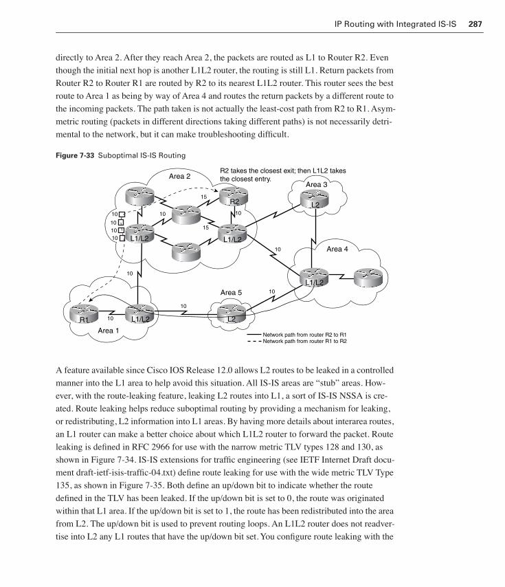
IP Routing with Integrated IS-IS 287
directly to Area 2. After they reach Area 2, the packets are routed as L1 to Router R2. Even
though the initial next hop is another L1L2 router, the routing is still L1. Return packets from
Router R2 to Router R1 are routed by R2 to its nearest L1L2 router. This router sees the best
route to Area 1 as being by way of Area 4 and routes the return packets by a different route to
the incoming packets. The path taken is not actually the least-cost path from R2 to R1. Asym-
metric routing (packets in different directions taking different paths) is not necessarily detri-
mental to the network, but it can make troubleshooting difficult.
Figure 7-33 Suboptimal IS-IS Routing
A feature available since Cisco IOS Release 12.0 allows L2 routes to be leaked in a controlled
manner into the L1 area to help avoid this situation. All IS-IS areas are “stub” areas. How-
ever, with the route-leaking feature, leaking L2 routes into L1, a sort of IS-IS NSSA is cre-
ated. Route leaking helps reduce suboptimal routing by providing a mechanism for leaking,
or redistributing, L2 information into L1 areas. By having more details about interarea routes,
an L1 router can make a better choice about which L1L2 router to forward the packet. Route
leaking is defined in RFC 2966 for use with the narrow metric TLV types 128 and 130, as
shown in Figure 7-34. IS-IS extensions for traffic engineering (see IETF Internet Draft docu-
ment draft-ietf-isis-traffic-04.txt) define route leaking for use with the wide metric TLV Type
135, as shown in Figure 7-35. Both define an up/down bit to indicate whether the route
defined in the TLV has been leaked. If the up/down bit is set to 0, the route was originated
within that L1 area. If the up/down bit is set to 1, the route has been redistributed into the area
from L2. The up/down bit is used to prevent routing loops. An L1L2 router does not readver-
tise into L2 any L1 routes that have the up/down bit set. You configure route leaking with the
10 10
10
10
101010
10
10
10
15
15
Area 2Area 3
Area 1
R2 takes the closest exit; then L1L2 takesthe closest entry.
Area 5 10
Area 4
Network path from router R2 to R1Network path from router R1 to R2
L1/L2
L1/L2 L2R1
L1/L2
R2 L2
L1/L2
1358_fmi.book Page 287 Thursday, May 27, 2004 2:21 PM

288 Chapter 7: IS-IS
IS-IS router configuration mode command redistribute isis ip level-2 into level-1 distrib-ute-list 100–199.
Figure 7-34 TLV Type 128 and Type 130
Figure 7-35 TLV Type 135
Interactive Media Activity Drag and Drop: Identifying IS-IS Routers
After completing this activity, you will be able to identify the different types of IS-IS
routers in a network.
TLV Type 128 and Type 130
1 1 6
Up/Down Int/Ext Default Metric
Supported Rsvd Delay Metric
Supported Rsvd Expense Metric
Supported Rsvd Error Metric
IPAddress
Subnet Mask
TLV Type 135
1 1 6
Metric
Up/Down Sub-TLV Prefix Length
Prefix (0-4 bytes)
Optional Sub-TLV (0-250 bytes)
1358_fmi.book Page 288 Thursday, May 27, 2004 2:21 PM
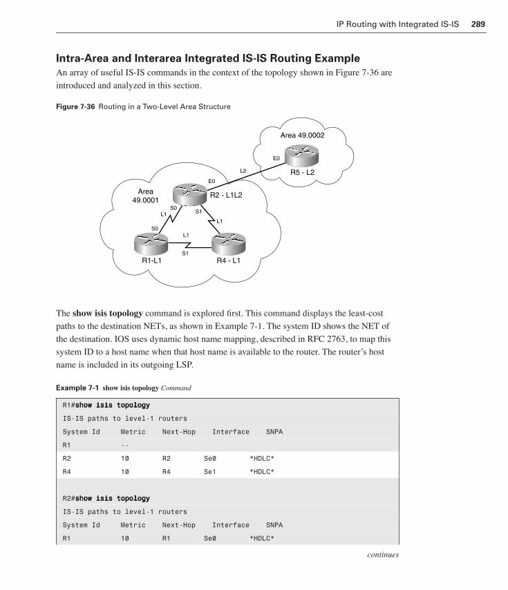
IP Routing with Integrated IS-IS 289
Intra-Area and Interarea Integrated IS-IS Routing Example
An array of useful IS-IS commands in the context of the topology shown in Figure 7-36 are
introduced and analyzed in this section.
Figure 7-36 Routing in a Two-Level Area Structure
The show isis topology command is explored first. This command displays the least-cost
paths to the destination NETs, as shown in Example 7-1. The system ID shows the NET of
the destination. IOS uses dynamic host name mapping, described in RFC 2763, to map this
system ID to a host name when that host name is available to the router. The router’s host
name is included in its outgoing LSP.
Example 7-1 show isis topology Command
R1#sssshhhhoooowwww iiiissssiiiissss ttttooooppppoooollllooooggggyyyy
IS-IS paths to level-1 routers
System Id Metric Next-Hop Interface SNPA
R1 --
R2 10 R2 Se0 *HDLC*
R4 10 R4 Se1 *HDLC*
R2#sssshhhhoooowwww iiiissssiiiissss ttttooooppppoooollllooooggggyyyy
IS-IS paths to level-1 routers
System Id Metric Next-Hop Interface SNPA
R1 10 R1 Se0 *HDLC*
E0
E0
L2
L1L1
L1
S0
S0
S1
S1
R2 - L1L2
R1-L1 R4 - L1
R5 - L2
Area49.0001
Area 49.0002
continues
1358_fmi.book Page 289 Thursday, May 27, 2004 2:21 PM

290 Chapter 7: IS-IS
The metric shows the sum of the metrics on the least-cost path to the destination. The next-
hop router, IS, is shown. Also shown is the interface through which that next hop is reached
and the SNPA of that next hop. HDLC is shown as the next hop across a serial line. The out-
put for Router R2 shows that separate topology databases exist for L1 and L2.
Recall that the SNPA is taken from the following:
■ MAC address on a LAN interface
■ Virtual circuit ID for X.25 or ATM
■ DLCI for Frame Relay
■ HDLC for interfaces
The show clns routes and show isis routes commands are the next commands to be looked
at. There is a common source of confusion for those learning about Integrated IS-IS. That
confusion comes from the frequent use of commands directly referencing CLNS but that are
used to verify and troubleshoot IP routing.
The show clns routes command displays the CLNS destinations to which this router can
route packets, as shown in Example 7-2. R1 shows only its local NET entry, because it is an
L1-only router and, therefore, has no L2 area routes to display. The show isis routes com-
mand shows the L1 routes to IS-IS neighbors. R1 has visibility of the other L1 routers in its
area. The L1L2 routers appear in the L1 routing table by virtue of their L1 connection. There
is a note at the end of their entry to show that they also act as L2. The closest L1L2 router also
appears as the default route out of area. Again, the next-hop IS, its SNPA, is the interface over
which that next hop is reached. The cumulative metric to that destination is shown for all IS
routes. The neighbors show that their state is up and that the Hello process has established an
adjacency.
R2 --
R4 10 R4 Se1 *HDLC*
IS-IS paths to level-2 routers
System Id Metric Next-Hop Interface SNPA
R2 --
R5 10 R5 Et0 0010.7bb5.9e20
Example 7-2 show clns routes and show isis routes Commands
R1#sssshhhhoooowwww ccccllllnnnnssss rrrroooouuuutttteeeessss
CLNS Prefix Routing Table
49.0001.0000.0000.0001.00, Local NET Entry
Example 7-1 show isis topology Command (Continued)
1358_fmi.book Page 290 Thursday, May 27, 2004 2:21 PM

IP Routing with Integrated IS-IS 291
The command show clns routes shows the local NET entry. This command also shows the
L2 routes to its own area and the neighbor areas. Notice in Example 7-3 that R2 regards the
route to the area of R2 as being through itself. This further emphasizes that the L1 and L2
processes operate separately. The command show isis routes shows the IS-IS neighbors.
Next, the which-route command in the context of L1 and L2 will be explored. The which-route command is an alternative method of finding the route to a destination NET or NSAP,
as shown in Example 7-4. You enter this command on the L1-only router, R1. This command
R1#sssshhhhoooowwww iiiissssiiiissss rrrroooouuuutttteeeessss
IS-IS Level-1 Routing Table - version 312
System Id Next-Hop SNPA Interface Metric State
R2 R2 *HDLC* Se0 10 Up L2-IS
R4 R4 *HDLC* Se1 10 Up
R1 --
Default Route out of Area - (via 2 L2-atached ISs)
System Id Next-Hop SNPA Interface Metric State
R2 *HDLC* Se0 10 Up
Example 7-3 show clns routes and show isis routes Commands
R2#sssshhhhoooowwww ccccllllnnnnssss rrrroooouuuutttteeeessss
Codes: C - connected, S - static, d - DecnetIV
I - ISO-IGRP, i - IS-IS, e - ES-IS
ICLNS Prefix Routing Table
49.0001.0000.0000.0002.00, Local NET Entry
C 49.0002 [110/10], via R5, IS-IS, Up, Ethernet0
C 49.0001 [110/0], via R2, IS-IS, Up
R2#sssshhhhoooowwww iiiissssiiiissss rrrroooouuuutttteeeessss
IS-IS Level-1 Routing Table - version 47
System Id Next-Hop SNPA Interface Metric State
R4 R4 *HDLC* Se1 10 Up
R1 R1 *HDLC* Se0 10 Up
Example 7-2 show clns routes and show isis routes Commands (Continued)
1358_fmi.book Page 291 Thursday, May 27, 2004 2:21 PM
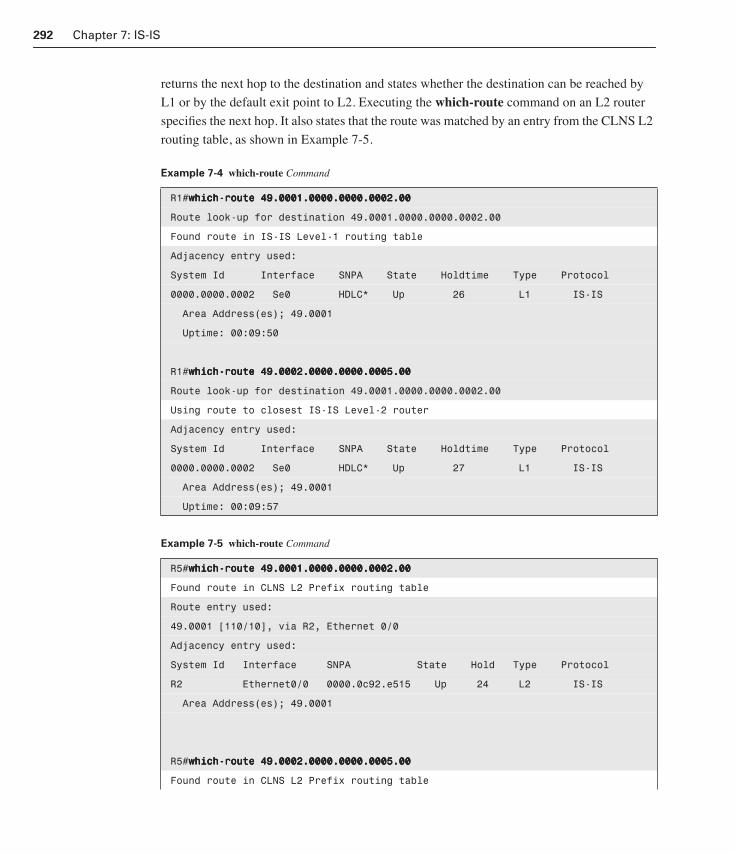
292 Chapter 7: IS-IS
returns the next hop to the destination and states whether the destination can be reached by
L1 or by the default exit point to L2. Executing the which-route command on an L2 router
specifies the next hop. It also states that the route was matched by an entry from the CLNS L2
routing table, as shown in Example 7-5.
Example 7-4 which-route Command
R1#wwwwhhhhiiiicccchhhh----rrrroooouuuutttteeee 44449999....0000000000001111....0000000000000000....0000000000000000....0000000000002222....00000000
Route look-up for destination 49.0001.0000.0000.0002.00
Found route in IS-IS Level-1 routing table
Adjacency entry used:
System Id Interface SNPA State Holdtime Type Protocol
0000.0000.0002 Se0 HDLC* Up 26 L1 IS-IS
Area Address(es); 49.0001
Uptime: 00:09:50
R1#wwwwhhhhiiiicccchhhh----rrrroooouuuutttteeee 44449999....0000000000002222....0000000000000000....0000000000000000....0000000000005555....00000000
Route look-up for destination 49.0001.0000.0000.0002.00
Using route to closest IS-IS Level-2 router
Adjacency entry used:
System Id Interface SNPA State Holdtime Type Protocol
0000.0000.0002 Se0 HDLC* Up 27 L1 IS-IS
Area Address(es); 49.0001
Uptime: 00:09:57
Example 7-5 which-route Command
R5#wwwwhhhhiiiicccchhhh----rrrroooouuuutttteeee 44449999....0000000000001111....0000000000000000....0000000000000000....0000000000002222....00000000
Found route in CLNS L2 Prefix routing table
Route entry used:
49.0001 [110/10], via R2, Ethernet 0/0
Adjacency entry used:
System Id Interface SNPA State Hold Type Protocol
R2 Ethernet0/0 0000.0c92.e515 Up 24 L2 IS-IS
Area Address(es); 49.0001
R5#wwwwhhhhiiiicccchhhh----rrrroooouuuutttteeee 44449999....0000000000002222....0000000000000000....0000000000000000....0000000000005555....00000000
Found route in CLNS L2 Prefix routing table
1358_fmi.book Page 292 Thursday, May 27, 2004 2:21 PM

IP Routing with Integrated IS-IS 293
Building the IP Forwarding TableSo far, the process and outputs have referred to the OSI part of the IS-IS process. However, in
the IP world, when running Integrated IS-IS, IP information is included in the LSPs. IP reach-
ability behaves in IS-IS as if it were ES information. IP information takes no part in the calcu-
lation of the SPF tree. It is simply information about leaf connections to the tree. Therefore,
updating the IP reachability is only a PRC. This is similar to ES reachability. IP routes are
generated by the PRC and are offered to the routing table. Here they are accepted based on
routing table rules that compare, for example, administrative distance. When entered in the
routing table, IP IS-IS routes are shown as being by way of Level 1 or Level 2, as appropriate.
The separation of IP reachability from the core IS-IS network architecture gives Integrated
IS-IS better scalability than, for example, OSPF. OSPF sends LSAs for individual IP subnets.
If an IP subnet fails, the LSA is flooded through the network. In all circumstances, all routers
must run a full SPF calculation. In Integrated IS-IS, the SPF tree is built from CLNS informa-
tion. If an IP subnet fails in Integrated IS-IS, the LSP is flooded, as it is for OSPF. However, if
this is a leaf IP subnet, meaning that the loss of the subnet has not affected the underlying
CLNS architecture, the SPF tree is unaffected. Only a PRC takes place.
The IP routing table, a pure entity, will now be looked at. The output for the show ip routes
command shows the IS-IS routes chosen by the SPF algorithm, from the IS-IS LSP database,
to populate the IP routing table, as shown in Example 7-6. The IP addresses on loopbacks of
routers are 1.0.0.1/8-R1, 2.0.0.1/8-R2, 4.0.0.1/8-R4, and 5.0.0.1/8-R5. The “i” indicates that
the route was sourced from IS-IS. L1 and L2 show whether the IS-IS path to these destination
IP networks is by way of IS-IS L1 or L2 routing. The next-hop IP addresses are matched from
the corresponding next-hop IS-IS neighbor routers. Notice that the metric is 10 for each route
because 10 is the Cisco default for the IS-IS metric over a link.
Route entry used:
49.0001 [110/10], via R2, Ethernet 0/0
Adjacency entry used:
System Id Interface SNPA State Hold Type Protocol
R2 Ethernet0/0 0000.0c92.e515 Up 21 L2 IS-IS
Area Address(es); 49.0001
Example 7-6 show ip route Command
R2#sssshhhhoooowwww iiiipppp rrrroooouuuutttteeee
i L1 1.0.0.0/8 [115/10] via 10.12.0.1, Ser0 -(R1)
i L1 4.0.0.0/8 [115/10] via 10.24.0.4, Ser1 -(R4)
i L2 5.0.0.0/8 [115/10] via 11.0.0.10, Eth0 -(R5)
Example 7-5 which-route Command (Continued)
1358_fmi.book Page 293 Thursday, May 27, 2004 2:21 PM

294 Chapter 7: IS-IS
Configuration of Integrated IS-ISAs with any routing protocol, the first step is to plan the logical topology, the addressing
scheme, and the participating interfaces. After this initial step is complete, Integrated IS-IS
can be configured on the network.
Basic Configuration of Integrated IS-IS
Enabling Integrated IS-IS on a router for IP routing is easy. Many more commands are used
to tune the IS-IS processes. However, only the following three commands are required to start
Integrated IS-IS:
■ Enable IS-IS as an IP routing protocol, using the command router isis, and assign a tag
if there are multiple IS-IS processes. If the tag is omitted, a tag of 0 is assumed.
■ Identify the router for IS-IS by assigning a NET to the router with the net command.
■ Enable IS-IS on the interfaces participating in IS-IS using the command ip router isis.
This command is configured on the interface and not on the routing process. This is
slightly different from most other IP routing protocols, in which the participating inter-
faces are specified by network statements. The IS-IS process has no network state-
ment. If multiple IS-IS processes exist, interfaces must state which process they belong
to by specifying the appropriate tag.
These commands enable Integrated IS-IS on the router. However, further commands might be
required to tune IS-IS operation.
Troubleshooting Integrated IS-IS, even in an IP-only world, requires some investigation of
CLNS data. For example, the IS-IS neighbor relationships are established over OSI, not over
IP. To view IS-IS neighbors, you use the show clns neighbors command. Two ends of a
CLNS adjacency can actually have IP addresses on different subnets, with no impact on the
operation of IS-IS. However, IP next-hop resolution could be an issue.
Figure 7-37 shows a simple topology with three routers in area 49.0001. The pertinent config-
uration for each router is shown in Examples 7-7, 7-8, and 7-9.
Figure 7-37 Basic Configuration of Integrated IS-IS
NOTE
When enabling IS-IS on a loopback interface, the loopback is usually config-ured as passive in router isis configuration mode. This is to prevent sending unnecessary Hello packets out the loopback. This is because there is no chance of finding a neighbor behind the loopback inter-face.
R1
R13
R14
Fa0/0
Fa0/0
S0/1
S0/1
1358_fmi.book Page 294 Thursday, May 27, 2004 2:21 PM
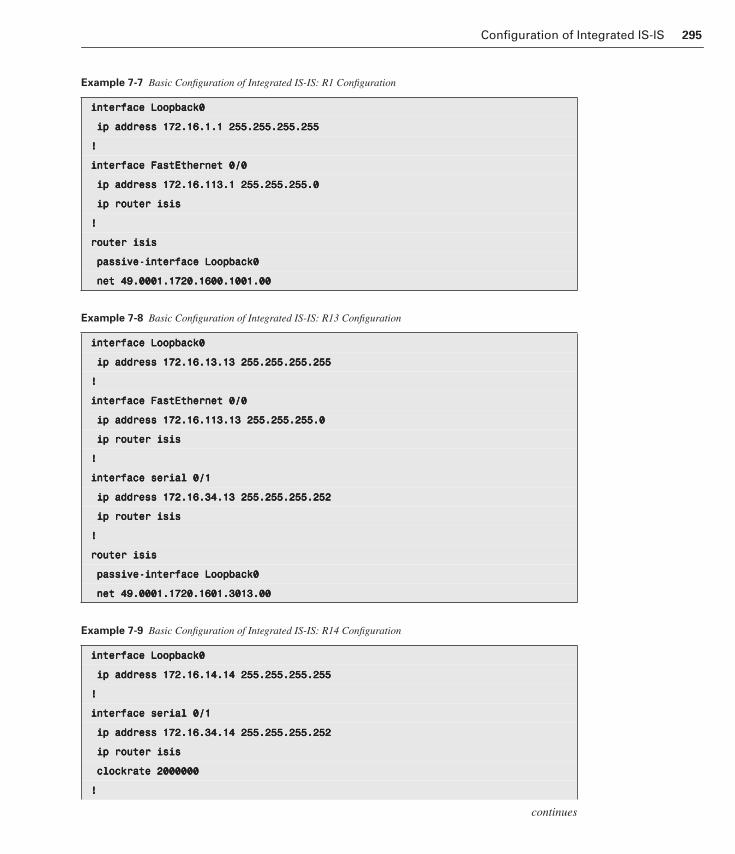
Configuration of Integrated IS-IS 295
Example 7-7 Basic Configuration of Integrated IS-IS: R1 Configuration
iiiinnnntttteeeerrrrffffaaaacccceeee LLLLooooooooppppbbbbaaaacccckkkk0000
iiiipppp aaaaddddddddrrrreeeessssssss 111177772222....11116666....1111....1111 222255555555....222255555555....222255555555....222255555555
!!!!
iiiinnnntttteeeerrrrffffaaaacccceeee FFFFaaaassssttttEEEEtttthhhheeeerrrrnnnneeeetttt 0000////0000
iiiipppp aaaaddddddddrrrreeeessssssss 111177772222....11116666....111111113333....1111 222255555555....222255555555....222255555555....0000
iiiipppp rrrroooouuuutttteeeerrrr iiiissssiiiissss
!!!!
rrrroooouuuutttteeeerrrr iiiissssiiiissss
ppppaaaassssssssiiiivvvveeee----iiiinnnntttteeeerrrrffffaaaacccceeee LLLLooooooooppppbbbbaaaacccckkkk0000
nnnneeeetttt 44449999....0000000000001111....1111777722220000....1111666600000000....1111000000001111....00000000
Example 7-8 Basic Configuration of Integrated IS-IS: R13 Configuration
iiiinnnntttteeeerrrrffffaaaacccceeee LLLLooooooooppppbbbbaaaacccckkkk0000
iiiipppp aaaaddddddddrrrreeeessssssss 111177772222....11116666....11113333....11113333 222255555555....222255555555....222255555555....222255555555
!!!!
iiiinnnntttteeeerrrrffffaaaacccceeee FFFFaaaassssttttEEEEtttthhhheeeerrrrnnnneeeetttt 0000////0000
iiiipppp aaaaddddddddrrrreeeessssssss 111177772222....11116666....111111113333....11113333 222255555555....222255555555....222255555555....0000
iiiipppp rrrroooouuuutttteeeerrrr iiiissssiiiissss
!!!!
iiiinnnntttteeeerrrrffffaaaacccceeee sssseeeerrrriiiiaaaallll 0000////1111
iiiipppp aaaaddddddddrrrreeeessssssss 111177772222....11116666....33334444....11113333 222255555555....222255555555....222255555555....222255552222
iiiipppp rrrroooouuuutttteeeerrrr iiiissssiiiissss
!!!!
rrrroooouuuutttteeeerrrr iiiissssiiiissss
ppppaaaassssssssiiiivvvveeee----iiiinnnntttteeeerrrrffffaaaacccceeee LLLLooooooooppppbbbbaaaacccckkkk0000
nnnneeeetttt 44449999....0000000000001111....1111777722220000....1111666600001111....3333000011113333....00000000
Example 7-9 Basic Configuration of Integrated IS-IS: R14 Configuration
iiiinnnntttteeeerrrrffffaaaacccceeee LLLLooooooooppppbbbbaaaacccckkkk0000
iiiipppp aaaaddddddddrrrreeeessssssss 111177772222....11116666....11114444....11114444 222255555555....222255555555....222255555555....222255555555
!!!!
iiiinnnntttteeeerrrrffffaaaacccceeee sssseeeerrrriiiiaaaallll 0000////1111
iiiipppp aaaaddddddddrrrreeeessssssss 111177772222....11116666....33334444....11114444 222255555555....222255555555....222255555555....222255552222
iiiipppp rrrroooouuuutttteeeerrrr iiiissssiiiissss
cccclllloooocccckkkkrrrraaaatttteeee 2222000000000000000000000000
!!!!
continues
1358_fmi.book Page 295 Thursday, May 27, 2004 2:21 PM

296 Chapter 7: IS-IS
Here are some informative show commands for this topology:
■ show clns neighbors—Lists the ES neighbors that the router knows about.
■ show clns interface—Lists the CLNS-specific information about each interface.
■ show isis database [detail]—Displays the database of the configuration server.
■ show ip route isis—Displays the current state of the IS-IS routing table.
■ show isis spf-log—Displays how often and why the router has run a full SPF calculation.
■ show isis lsp-log—Displays the Level 1 and Level 2 IS-IS LSP log of the interfaces
that triggered the new LSP.
For added security, configure IS-IS passwords for areas or domains. The area authentication
password is inserted in L1, which is the station router level, LSPs, CSNPs, and PSNPs. The
routing domain authentication password is inserted in L2, which is the area router level,
LSPs, CSNPs, and PSNPs. To configure area or domain authentication passwords, respec-
tively, use the following commands in router configuration mode:
aaaarrrreeeeaaaa----ppppaaaasssssssswwwwoooorrrrdddd passwordddddoooommmmaaaaiiiinnnn----ppppaaaasssssssswwwwoooorrrrdddd password
You can configure authentication for an interface using the isis password interface configura-
tion command. This command lets you prevent unauthorized routers from forming adjacen-
cies with this router. Therefore, it protects the network from intruders. The password is
exchanged as plain text and, therefore, provides only limited security. You can assign differ-
ent passwords to different routing levels using the level-1 and level-2 keyword arguments.
Specifying the level-1 or level-2 keyword enables the password only for L1 or L2 routing,
respectively.
Last, as with OSPF, aggregate addresses can be created with IS-IS. They are represented in
the routing table by a summary address. One summary address can include multiple groups
of addresses for a given level. Routes learned from other routing protocols can also be sum-
marized. The metric used to advertise the summary is the smallest metric of all the more-spe-
cific routes. To create a summary of addresses for a given level, use the command summary-address address mask {level-1 | level-1-2 | level-2} in router configuration mode.
rrrroooouuuutttteeeerrrr iiiissssiiiissss
ppppaaaassssssssiiiivvvveeee----iiiinnnntttteeeerrrrffffaaaacccceeee LLLLooooooooppppbbbbaaaacccckkkk0000
nnnneeeetttt 44449999....0000000000001111....1111777722220000....1111666600001111....4444000011114444....00000000
Interactive Media Activity Drag and Drop: Basic IS-IS Configuration
After completing this activity, you will be able to perform basic IS-IS configuration
on a Cisco router.
Example 7-9 Basic Configuration of Integrated IS-IS: R14 Configuration (Continued)
1358_fmi.book Page 296 Thursday, May 27, 2004 2:21 PM

Configuration of Integrated IS-IS 297
Multiarea Integrated IS-IS Configuration
This section explores a simple multiarea Integrated IS-IS scenario, shown in Figure 7-38. The
output in Example 7-10 shows the correct behavior for IS-IS. The IS-IS configuration com-
mands shown in Examples 7-11 through 7-14 successfully route IP by way of IS-IS. For
example, the routing tables of both Rtr-A and Rtr-D are automatically populated with a
default route.
Figure 7-38 Multiarea Integrated IS-IS Configuration
Lab 7.7.1 Configuring Basic Integrated IS-IS
In this lab, you configure basic Integrated IS-IS. You also implement IS-IS authenti-
cation for security purposes.
Example 7-10 Sample IS-IS Configuration
Rtr-A#sssshhhhoooowwww iiiipppp rrrroooouuuutttteeee
Gateway of last resort is 192.168.120.10 to network 0.0.0.0
C 192.168.120.0/24 is directly connected, FastEthernet0/0
192.168.1.0/32 is subnetted, 2 subnets
i L1 192.168.1.1 [115/10] via 192.168.120.10, FastEthernet0/0
C 192.168.1.5 is directly connected, Loopback0
i L1 192.168.222.0/24 [115/20] via 192.168.120.10, FastEthernet0/0
i*L1 0.0.0.0/0 [115/10] via 192.168.120.10, FastEthernet0/0
Rtr-D#sssshhhhoooowwww iiiipppp rrrroooouuuutttteeee
Gateway of last resort is 192.168.111.2 to network 0.0.0.0
C 192.168.111.0/24 is directly connected, FastEthernet0/0
Area49.0001
S0/1 S0/1
Fa0/0 Fa0/0 Fa0/0 Fa0/0
L1Router
L1Router
L1L2Routers
Rtr-A Rtr-B Rtr-C Rtr-D
Area49.0002
continues
1358_fmi.book Page 297 Thursday, May 27, 2004 2:21 PM

298 Chapter 7: IS-IS
192.168.2.0/32 is subnetted, 2 subnets
i L1 192.168.2.2 [115/10] via 192.168.111.2, FastEthernet0/0
C 192.168.2.4 is directly connected, Loopback0
i*L1 0.0.0.0/0 [115/10] via 192.168.111.2, FastEthernet0/0
Example 7-11 Multiarea Integrated IS-IS Configuration: Rtr-A Configuration
iiiinnnntttteeeerrrrffffaaaacccceeee LLLLooooooooppppbbbbaaaacccckkkk0000
iiiipppp aaaaddddddddrrrreeeessssssss 111199992222....111166668888....1111....5555 222255555555....222255555555....222255555555....222255555555
nnnnoooo iiiipppp ddddiiiirrrreeeecccctttteeeedddd----bbbbrrrrooooaaaaddddccccaaaasssstttt
!!!!
iiiinnnntttteeeerrrrffffaaaacccceeee FFFFaaaassssttttEEEEtttthhhheeeerrrrnnnneeeetttt 0000////0000
iiiipppp aaaaddddddddrrrreeeessssssss 111199992222....111166668888....111122220000....5555 222255555555....222255555555....222255555555....0000
iiiipppp rrrroooouuuutttteeeerrrr iiiissssiiiissss
!!!!
rrrroooouuuutttteeeerrrr iiiissssiiiissss
ppppaaaassssssssiiiivvvveeee----iiiinnnntttteeeerrrrffffaaaacccceeee LLLLooooooooppppbbbbaaaacccckkkk0000
nnnneeeetttt 44449999....0000000000001111....1111999922221111....6666888800000000....1111000000005555....00000000
iiiissss----ttttyyyyppppeeee lllleeeevvvveeeellll----1111
Example 7-12 Multiarea Integrated IS-IS Configuration: Rtr-B Configuration
iiiinnnntttteeeerrrrffffaaaacccceeee LLLLooooooooppppbbbbaaaacccckkkk0000
iiiipppp aaaaddddddddrrrreeeessssssss 111199992222....111166668888....1111....1111 222255555555....222255555555....222255555555....222255555555
!!!!
iiiinnnntttteeeerrrrffffaaaacccceeee FFFFaaaassssttttEEEEtttthhhheeeerrrrnnnneeeetttt 0000////0000
iiiipppp aaaaddddddddrrrreeeessssssss 111199992222....111166668888....111122220000....11110000 222255555555....222255555555....222255555555....0000
iiiipppp rrrroooouuuutttteeeerrrr iiiissssiiiissss
!!!!
iiiinnnntttteeeerrrrffffaaaacccceeee sssseeeerrrriiiiaaaallll 0000////1111
iiiipppp aaaaddddddddrrrreeeessssssss 111199992222....111166668888....222222222222....1111 222255555555....222255555555....222255555555....0000
iiiipppp rrrroooouuuutttteeeerrrr iiiissssiiiissss
!!!!
rrrroooouuuutttteeeerrrr iiiissssiiiissss
ppppaaaassssssssiiiivvvveeee----iiiinnnntttteeeerrrrffffaaaacccceeee LLLLooooooooppppbbbbaaaacccckkkk0000
nnnneeeetttt 44449999....0000000000001111....1111999922221111....6666888800000000....1111000000001111....00000000
Example 7-10 Sample IS-IS Configuration (Continued)
1358_fmi.book Page 298 Thursday, May 27, 2004 2:21 PM

Configuration of Integrated IS-IS 299
By default, Cisco IOS software enables both L1 and L2 operations on IS-IS routers. If a
router is to operate only as an area router or only as a backbone router, you can specify this by
entering the is-type command in IS-IS router configuration mode. To specify that the router
will act only as an area or L1 router, specify is-type level-1. To specify that the router will act
only as a backbone or L2 router, specify is-type level-2-only. Rtr-A and Rtr-D use the is-type level-1 command.
Example 7-13 Multiarea Integrated IS-IS Configuration: Rtr-C Configuration
iiiinnnntttteeeerrrrffffaaaacccceeee LLLLooooooooppppbbbbaaaacccckkkk0000
iiiipppp aaaaddddddddrrrreeeessssssss 111199992222....111166668888....2222....2222 222255555555....222255555555....222255555555....222255555555
!!!!
iiiinnnntttteeeerrrrffffaaaacccceeee FFFFaaaassssttttEEEEtttthhhheeeerrrrnnnneeeetttt 0000////0000
iiiipppp aaaaddddddddrrrreeeessssssss 111199992222....111166668888....111111111111....2222 222255555555....222255555555....222255555555....0000
iiiipppp rrrroooouuuutttteeeerrrr iiiissssiiiissss
iiiissssiiiissss cccciiiirrrrccccuuuuiiiitttt----ttttyyyyppppeeee lllleeeevvvveeeellll----1111
!!!!
iiiinnnntttteeeerrrrffffaaaacccceeee sssseeeerrrriiiiaaaallll 0000////1111
iiiipppp aaaaddddddddrrrreeeessssssss 111199992222....111166668888....222222222222....2222 222255555555....222255555555....222255555555....0000
iiiipppp rrrroooouuuutttteeeerrrr iiiissssiiiissss
cccclllloooocccckkkkrrrraaaatttteeee 2222000000000000000000000000
iiiissssiiiissss cccciiiirrrrccccuuuuiiiitttt----ttttyyyyppppeeee lllleeeevvvveeeellll----2222----oooonnnnllllyyyy
!!!!
rrrroooouuuutttteeeerrrr iiiissssiiiissss
ppppaaaassssssssiiiivvvveeee----iiiinnnntttteeeerrrrffffaaaacccceeee LLLLooooooooppppbbbbaaaacccckkkk0000
nnnneeeetttt 44449999....0000000000002222....1111999922221111....6666888800000000....2222000000002222....00000000
Example 7-14 Multiarea Integrated IS-IS Configuration: Rtr-D Configuration
iiiinnnntttteeeerrrrffffaaaacccceeee LLLLooooooooppppbbbbaaaacccckkkk0000
iiiipppp aaaaddddddddrrrreeeessssssss 111199992222....111166668888....2222....4444 222255555555....222255555555....222255555555....222255555555
!!!!
iiiinnnntttteeeerrrrffffaaaacccceeee FFFFaaaassssttttEEEEtttthhhheeeerrrrnnnneeeetttt 0000////0000
iiiipppp aaaaddddddddrrrreeeessssssss 111199992222....111166668888....111111112222....2222 222255555555....222255555555....222255555555....0000
iiiipppp rrrroooouuuutttteeeerrrr iiiissssiiiissss
!!!!
rrrroooouuuutttteeeerrrr iiiissssiiiissss
ppppaaaassssssssiiiivvvveeee----iiiinnnntttteeeerrrrffffaaaacccceeee LLLLooooooooppppbbbbaaaacccckkkk0000
nnnneeeetttt 44449999....0000000000002222....1111999922221111....6666888800000000....2222000000004444....00000000
iiiissss----ttttyyyyppppeeee lllleeeevvvveeeellll----1111
1358_fmi.book Page 299 Thursday, May 27, 2004 2:21 PM

300 Chapter 7: IS-IS
Although the router might be an L1L2 router, it might be required to establish only L1 adja-
cencies over certain interfaces and only L2 adjacencies over other interfaces. The interface
command isis circuit-type can specify level-1, level-1-2, or level-2-only. If a level is not
specified, the IOS attempts to establish both types of adjacencies over the interface. The Rtr-
C configuration uses the isis circuit-type command. Notice that L1 adjacencies cannot form
between areas. No isis circuit-type command is applied to interface Fa0/0 on Rtr-B. The
optimal configuration would include the isis circuit-type level-1 command on this interface
to avoid an attempt by Rtr-B to form an L2 adjacency with Rtr-A. This would fail, though,
because Rtr-A is configured with the IS-IS router mode command is-type level-1.
Unlike some other IP protocols, IS-IS does not consider line speed or bandwidth when setting
its link metrics. All interfaces are assigned a metric of 10. To change this value, use the inter-
face command isis metric value level-1 | level-2. The metric can have different values for
Level 1 and Level 2 over the same interface. The isis metric interface command is not used in
the scenario presented in this section.
The show clns command, shown in Example 7-15, indicates that Rtr-B is running IS-IS in IP-
only mode. This is because none of the interfaces are configured with the clns router isis
command. This would force the router to begin forwarding CLNP packets. Despite the fact
that CLNS is not being routed, the show protocol output, shown in Example 7-16, appears to
contradict this. The output says CLNS routing is enabled and says CLNS enabled on each of
the FastEthernet0/0 and Serial0/1 interfaces. However, CLNP packets are not being routed, as
verified by the show clns traffic output, shown in Example 7-17.
Example 7-15 show clns Command
Rtr-B#sssshhhhoooowwww ccccllllnnnnssss
Global CLNS Information:
2 Interfaces Enabled for CLNS
NET: 49.000101921.6800.1001.00
Configuration Timer: 60, Default Holding Timer: 300, Packet Lifetime 64
ERPDU’s requested on locally generated packets
Running IS-IS in IP-only mode with CLNS forwarding not allowed
Example 7-16 show clns protocol Command
Rtr-B#sssshhhhoooowwww pppprrrroooottttooooccccoooollll
Global values:
Internet protocol routing is enabled
CLNS routing is enabled (address 49.0001.1921.6800.1001.00)
Fastethernet0/0 is up, line protocol is up
1358_fmi.book Page 300 Thursday, May 27, 2004 2:21 PM

Configuration of Integrated IS-IS 301
Internet address is 192.168.120.10/24
CLNS enabled
Serial0/0 is administratively down, line protocol is down
Serial0/1 is up, line protocol is up
Internet address is 192.168.222.1/24
CLNS enabled
Loopback0 is up, line protocol is up
Internet address is 192.168.1.1/32
Rtr-B#sssshhhhoooowwww ccccllllnnnnssss pppprrrroooottttooooccccoooollll
IS-IS Router: <Null Tag>
System Id: 1921.6800.1001.00 IS-TypeL: level-1-2
Manual area address(es):
49.0001
Routing for area address(es):
49.0001
Interfaces supported by IS-IS:
Serial 0/1 - IP
FastEthernet 0/0 - IP
Next global update in 530 seconds
Redistributing:
static
iso-igrp (remote)
Distance: 110
Example 7-17 show clns traffic Command
Rtr-B#sssshhhhoooowwww ccccllllnnnnssss ttttrrrraaaaffffffffiiiicccc
CLNS & ESIS Output: 139885, Input: 90406
CLNS Local: 0, Forward: 0
CLNS Discards:
Hdr Syntax: 150, Checksum: 0, Lifetime: 0, Output cngstn: 0
No Route: 0, Dst Unreachable 0, Encaps. Failed: 0
NLP Unknown: 0, Not an IS: 0
CLNS Options: Packets 19, total 19, bad 0, GQOS 0, cngstn exprncd 0
CLNS Segments: Segmented: 0, Failed: 0
CLNS Broadcasts: sent: 0, rcvd: 0
Example 7-16 show clns protocol Command (Continued)
continues
1358_fmi.book Page 301 Thursday, May 27, 2004 2:21 PM

302 Chapter 7: IS-IS
The show isis database output, shown in Examples 7-18 and 7-19, demonstrates the auto-
matic setting of the ATT by the L1L2 router, Rtr-B. This tells the L1 routers that it is a poten-
tial exit point for the area.
Echos: Rcvd 0 requests, 69679 replies
Sent 69701 requests, 0 replies
ESIS(sent/rcvd): ESHs: 0/34, ISHs: 483/1839, RDs: 0/0, QCF: 0/0
ISO IGRP: Querys (sent/rcvd): 0/0 Updates (sent/rcvd): 1279/1402
ISO IGRP: Router Hellos: (sent/rcvd): 1673/1848
ISO IGRP Syntax Errors: 0
IS-IS: Level-1 Hellos (sent/rcvd): 0/0
IS-IS: Level-2 Hellos (sent/rcvd): 0/0
IS-IS: PTP Hellos (sent/rcvd): 0/0
IS-IS: Level-1 LSPs (sent/rcvd): 0/0
IS-IS: Level-2 LSPs (sent/rcvd): 0/0
IS-IS: Level-1 CSNPs (sent/rcvd): 0/0
IS-IS: Level-2 CSNPs (sent/rcvd): 0/0
IS-IS: Level-1 PSNPs (sent/rcvd): 0/0
IS-IS: Level-2 PSNPs (sent/rcvd): 0/0
IS-IS: Level-1 DR Elections: 0
IS-IS: Level-2 DR Elections: 0
IS-IS: Level-1 SPF Calculations: 0
IS-IS: Level-2 SPF Calculations: 0
Example 7-18 show isis database Command
Rtr-B#sssshhhhoooowwww iiiissssiiiissss ddddaaaattttaaaabbbbaaaasssseeee
ISIS Level-1 Link State Database:
LSPID LSP Seq Num LSP Checksum LSP Holdtime ATT/P/OL
Rtr-B.00-00 0x0000008B 0x6843 55 0/0/0
Rtr-A.00-00 0x00000083 0x276E 77 0/0/0
Rtr-B.01-00 0x00000004 0x34E1 57 0/0/0
ISIS Level-2 Link State Database:
LSPID LSP Seq Num LSP Checksum LSP Holdtime ATT/P/OL
Rtr-B.00-00 0x00000092 0x34B2 41 0/0/0
Rtr-C.00-00 0x0000008A 0x7A59 115 0/0/0
Example 7-17 show clns traffic Command (Continued)
1358_fmi.book Page 302 Thursday, May 27, 2004 2:21 PM

Configuration of Integrated IS-IS 303
The show clns traffic output lets you analyze CLNS traffic statistics. For this command out-
put, keep the following in mind:
■ LSPs sourced indicate IS stability.
■ LSP retransmissions should stay low.
■ PRCs cannot be checked elsewhere.
■ LSP checksum errors are a bad sign.
■ The update queue should not stay full.
■ The update queue should not drop much.
Example 7-19 show isis database detail Command
Rtr-B#sssshhhhoooowwww iiiissssiiiissss ddddaaaattttaaaabbbbaaaasssseeee ddddeeeettttaaaaiiiillll
ISIS Level-1 link-state database:
LSPID LSP Seq Num LSP Checksum LSP Holdtime ATT/P/OL
Rtr-B.00-00 0x00000093 0x077E 71 0/0/0
Area Address: 49.0001
NLPID: 0xCC
Hostname: R2
IP Address: 192.168.1.1
Metric: 10 IP 192.168.120.0 255.255.255.0
Metric: 10 IP 192.168.220.0 255.255.255.255
Metric: 0 IP 192.168.1.1 255.255.255.255
Metric: 10 IS Rtr-B.01
ISIS Level-2 LSP R2.00-00
LSPID LSP Seq Num LSP Checksum LSP Holdtime ATT/P/OL
Rtr-B.00-00 0x0000009A 0x5A69 103 0/0/0
Area Address: 49.0001
NLPID: 0xCC
Hostname: Rtr-B
IP Address: 192.168.1.1
Metric: 10 IS Rtr-B.01
Metric: 10 IS Rtr-C.00
Metric: 10 IP 192.168.120.0 255.255.255.0
Metric: 0 IP 192.168.1.1 255.255.255.255
Metric: 10 IP 192.168.1.5 255.255.255.255
Metric: 10 IP 192.168.220.0 255.255.255.0
1358_fmi.book Page 303 Thursday, May 27, 2004 2:21 PM

304 Chapter 7: IS-IS
The debug isis spf-triggers command is useful for determining the cause, or trigger, for an
SPF calculation.
Integrated IS-IS Operation in a WAN EnvironmentWANs are typically implemented as either point-to-point or point-to-multipoint. WAN tech-
nologies, such as Frame Relay, do not support broadcasts—thus the term nonbroadcast multi-
access (NBMA).
Point-to-Point and Point-to-Multipoint Operation with IS-IS
Point-to-point WANs can be leased circuits between two routers. A point-to-point WAN has
two devices attached, one device at each end of the circuit. Such links commonly run Cisco
HDLC or PPP. These WAN links correspond exactly to the Integrated IS-IS classification of a
point-to-point network.
Dialup networks using dial-on-demand routing (DDR) can be configured as either point-to-
point or point-to-multipoint WANs. Legacy DDR connections using dialer map statements
are NBMA networks, despite the fact that they might use PPP as their line protocol. This is
because a single dialer interface can support multiple destinations. Dialer profiles and dialer
virtual profiles are point-to-point connections, in which one dialer profile equates to one
remote profile. These connections can suffer from the same loss-of-neighbor delays as other
NBMA networks. Dialer virtual profiles are point-to-point connections in which the interface
drops immediately if the remote end disconnects, leading to faster neighbor loss detection
and faster convergence. Dial interfaces and dialer profiles are not dealt with in this book. As a
general rule, avoid using IS-IS over dialup, except to provide dial backup functionality.
IS-IS can work only over NBMA clouds, such as Frame Relay, configured with a full mesh.
Anything less than a full mesh could create serious connectivity and routing issues. However,
even if a full mesh is configured, this is no guarantee that it will exist at all times. A failure in
the underlying switched WAN network, or a misconfiguration on one or more routers, could
break the full mesh either temporarily or permanently. Avoid NBMA multipoint configura-
tions for IS-IS networks. Use point-to-point subinterfaces instead.
Point-to-point interfaces should usually be explicitly configured with an IP subnet. In this
case, a 31-bit mask (which requires Cisco IOS Release 12.2) or a 30-bit mask is applied. In
modern IP networks using private addressing and variable-length subnetting, there are usu-
ally plenty of spare IP addresses to apply to point-to-point interfaces. Alternatively, in con-
formance with RFC 1195, an unnumbered IP can be used with IS-IS on point-to-point
interfaces.
Lab 7.7.2 Configuring Multiarea Integrated IS-IS
In this lab, you configure multiarea Integrated IS-IS and level-specific routers.
NOTE
A point-to-point circuit is still regarded as an NBMA network, just as a back-to-back Ethernet connection is still a LAN. Both are examples of multiaccess networks that have only two devices attached.
1358_fmi.book Page 304 Thursday, May 27, 2004 2:21 PM

Integrated IS-IS Operation in a WAN Environment 305
Recall that, on a point-to-point link, a single IIH PDU type is used. These IIHs specify
whether the adjacency is L1, L2, or both. When the adjacency is established, each neighbor
sends a CSNP describing the contents of its link-state database. Each router then requests any
missing LSPs from the neighbor using PSNPs and acknowledges the receipt of the LSPs with
PSNPs. This activity reduces the amount of routing traffic across the point-to-point link. Each
router exchanges only the information missing from its link-state database, rather than the
entire link-state database of its neighbor router.
Configuring Integrated IS-IS in a WAN Environment
To enable IS-IS over switched WAN media, do the following:
■ Start the IS-IS process, and assign NETs as usual.
■ On each NBMA interface, do the following:
— Design a mesh between the NBMA peers, whether full or partial.
— Configure point-to-point subinterfaces for each NBMA virtual circuit (VC), and
assign IP addresses.
— Define the mapping of network protocols and addresses to the VC. If manual
mappings are used, such as x25 map or frame-relay map, the CLNS mapping
must specify broadcast. This is to support routing updates. However, the IP map-
ping does not require this. It is used only for next-hop resolution.
— Start IS-IS processing on the subinterface with the ip router isis command. This
command must not be used on the main interface, or that multipoint interface
generates a pseudonode LSP for itself.
■ Use Integrated IS-IS timer and blocking commands to control flooding of link-state
information.
To illustrate IS-IS configuration in a WAN environment, this IS-IS chapter ends with a Frame
Relay point-to-point scenario and a Frame Relay point-to-multipoint scenario.
Frame Relay Point-to-Point Scenario with Integrated IS-IS
Look at the example of a router network connected over Frame Relay using point-to-point
subinterfaces shown in Figure 7-39. Each Frame Relay PVC is treated as its own point-to-
point network, with its own IP addresses. The example is of a hub-and-spoke network topol-
ogy. It is important to note that the spoke routers are also configured with point-to-point sub-
interfaces, even though, unlike the hub router, they use only one VC. This is the best practice
in general for all routing protocols. It allows further VCs to be added without affecting the
existing VC. This practice is imperative for IS-IS. A main interface is a multipoint interface,
even if it has only one VC configured. If the single VC were configured under a main inter-
face, IS-IS would treat this as a broadcast network and attempt to elect a DIS. Also, an adja-
1358_fmi.book Page 305 Thursday, May 27, 2004 2:21 PM

306 Chapter 7: IS-IS
cency would not be established, because the multipoint end would send broadcast network-
style Hello PDUs, but the point-to-point end would send point-to-point Hello PDUs.
Figure 7-39 Frame Relay Point-to-Point Scenario with Integrated IS-IS
The hub router R4 configuration is shown in Example 7-20.
Example 7-20 R4 Configuration
iiiinnnntttteeeerrrrffffaaaacccceeee SSSSeeeerrrriiiiaaaallll0000////0000
eeeennnnccccaaaappppssssuuuullllaaaattttiiiioooonnnn ffffrrrraaaammmmeeee----rrrreeeellllaaaayyyy
!!!!
iiiinnnntttteeeerrrrffffaaaacccceeee SSSSeeeerrrriiiiaaaallll0000////0000....1111 ppppooooiiiinnnntttt----ttttoooo----ppppooooiiiinnnntttt
iiiipppp aaaaddddddddrrrreeeessssssss 11110000....1111....1111....1111 222255555555....222255555555....222255555555....222255552222
iiiipppp rrrroooouuuutttteeeerrrr iiiissssiiiissss
ffffrrrraaaammmmeeee----rrrreeeellllaaaayyyy iiiinnnntttteeeerrrrffffaaaacccceeee----ddddllllcccciiii 111100000000
!!!!
iiiinnnntttteeeerrrrffffaaaacccceeee SSSSeeeerrrriiiiaaaallll0000////0000....2222 ppppooooiiiinnnntttt----ttttoooo----ppppooooiiiinnnntttt
iiiipppp aaaaddddddddrrrreeeessssssss 11110000....1111....1111....5555 222255555555....222255555555....222255555555....222255552222
iiiipppp rrrroooouuuutttteeeerrrr iiiissssiiiissss
ffffrrrraaaammmmeeee----rrrreeeellllaaaayyyy iiiinnnntttteeeerrrrffffaaaacccceeee----ddddllllcccciiii 222200000000
!!!!
iiiinnnntttteeeerrrrffffaaaacccceeee SSSSeeeerrrriiiiaaaallll0000////0000....3333 ppppooooiiiinnnntttt----ttttoooo----ppppooooiiiinnnntttt
iiiipppp aaaaddddddddrrrreeeessssssss 11110000....1111....1111....9999 222255555555....222255555555....222255555555....222255552222
iiiipppp rrrroooouuuutttteeeerrrr iiiissssiiiissss
ffffrrrraaaammmmeeee----rrrreeeellllaaaayyyy iiiinnnntttteeeerrrrffffaaaacccceeee----ddddllllcccciiii 333300000000
R1
R2
R3
R4
Frame RelayDLCI 100DLCI 200DLCI 300
DLCI 400
DLCI 400
p2p
DLCI 400
10.1.1.2
10.1.1.6
10.2.2.10
p2p
p2pPoint-to-PointSub-Interfaces
1358_fmi.book Page 306 Thursday, May 27, 2004 2:21 PM
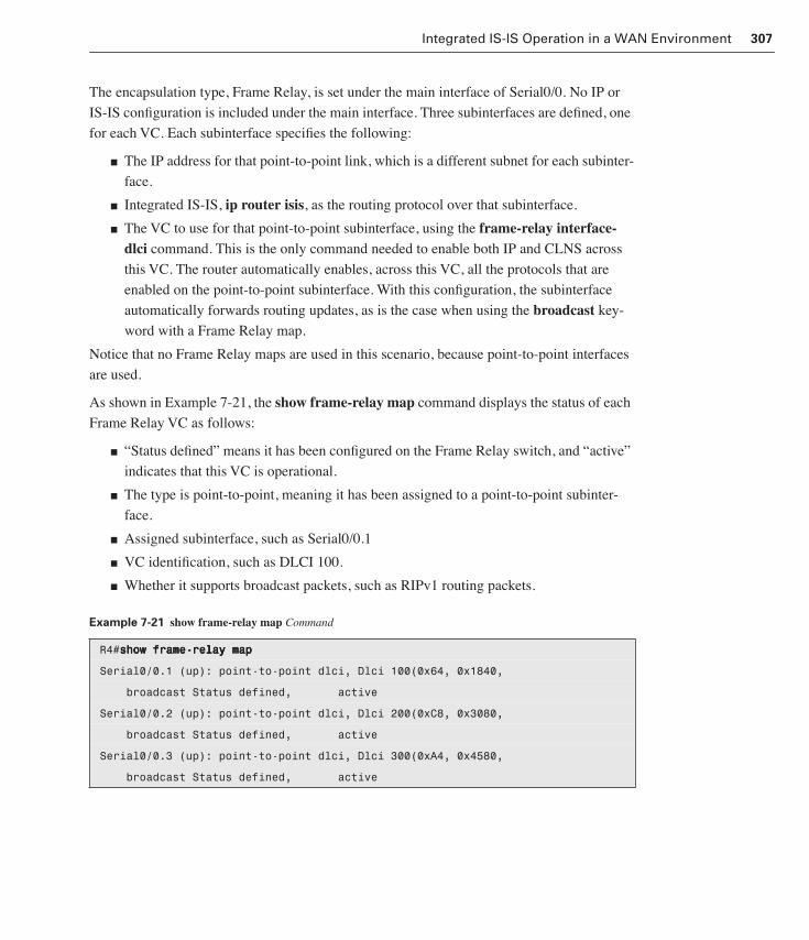
Integrated IS-IS Operation in a WAN Environment 307
The encapsulation type, Frame Relay, is set under the main interface of Serial0/0. No IP or
IS-IS configuration is included under the main interface. Three subinterfaces are defined, one
for each VC. Each subinterface specifies the following:
■ The IP address for that point-to-point link, which is a different subnet for each subinter-
face.
■ Integrated IS-IS, ip router isis, as the routing protocol over that subinterface.
■ The VC to use for that point-to-point subinterface, using the frame-relay interface-dlci command. This is the only command needed to enable both IP and CLNS across
this VC. The router automatically enables, across this VC, all the protocols that are
enabled on the point-to-point subinterface. With this configuration, the subinterface
automatically forwards routing updates, as is the case when using the broadcast key-
word with a Frame Relay map.
Notice that no Frame Relay maps are used in this scenario, because point-to-point interfaces
are used.
As shown in Example 7-21, the show frame-relay map command displays the status of each
Frame Relay VC as follows:
■ “Status defined” means it has been configured on the Frame Relay switch, and “active”
indicates that this VC is operational.
■ The type is point-to-point, meaning it has been assigned to a point-to-point subinter-
face.
■ Assigned subinterface, such as Serial0/0.1
■ VC identification, such as DLCI 100.
■ Whether it supports broadcast packets, such as RIPv1 routing packets.
Example 7-21 show frame-relay map Command
R4#sssshhhhoooowwww ffffrrrraaaammmmeeee----rrrreeeellllaaaayyyy mmmmaaaapppp
Serial0/0.1 (up): point-to-point dlci, Dlci 100(0x64, 0x1840,
broadcast Status defined, active
Serial0/0.2 (up): point-to-point dlci, Dlci 200(0xC8, 0x3080,
broadcast Status defined, active
Serial0/0.3 (up): point-to-point dlci, Dlci 300(0xA4, 0x4580,
broadcast Status defined, active
1358_fmi.book Page 307 Thursday, May 27, 2004 2:21 PM

308 Chapter 7: IS-IS
The debug isis adj-packet command in Example 7-22 shows neighbor relationship establish-
ment across one of the subinterfaces, Serial0/0.1, sending and receiving point-to-point IIH
PDUs and declaring the adjacency up. Ongoing Hello conversations for the other subinter-
faces are also shown.
Frame Relay Point-to-Multipoint Scenario with Integrated IS-IS
In this scenario, all of the Frame Relay ports are configured as multipoint interfaces. They are
configured either as a multipoint subinterface, on the hub router R4, or as a main interface on
the other routers. All interfaces share the same IP subnet in a multipoint configuration. In a
multipoint environment with IS-IS, it is important that a full mesh be implemented. There-
fore, all other routers also are interconnected by VCs, although these are not shown in Figure 7-40.
If this were a true hub-and-spoke environment, and the spoke sites had no need to communi-
cate with each other, this topology could work with only the indicated DLCIs. In this case,
the hub router must become the DIS for the NBMA network, because it is the only router vis-
ible to all others. A suitable IS-IS priority should be set on the hub router’s Frame Relay
interface using the isis priority command. Routes would be installed in each spoke router
toward the other spoke routers by way of their local IP addresses. However, packets to these
destinations would be dropped, because there are no direct VCs between the spokes, as
shown in Figure 7-40.
Example 7-22 debug isis adj-packet Command
R4#ddddeeeebbbbuuuugggg iiiissssiiiissss aaaaddddjjjj----ppppaaaacccckkkkeeeetttt
ISIS-Adj: Sending serial IIH on Serial0/0.1, length 1499
ISIS-Adj: Rec serial IIH from DLCI 100 (Serial0/0.1), cir type L1L2,
cir id 00, length 1499
ISIS-Adj: rcvd state UP, old state UP, new state UP
ISIS-Adj: Action = ACCEPT
ISIS-Adj: Sending serial IIH on Serial0/0.2, length 1499
ISIS-Adj: Rec serial IIH from DLCI 200 (Serial0/0.2), cir type L1L2,
cir id 01, length 1499
ISIS-Adj: Sending serial IIH on Serial0/0.3, length 1499
ISIS-Adj: Rec serial IIH from DLCI 300 (Serial0/0.3), cir type L1L2,
cir id 01, length 1499
1358_fmi.book Page 308 Thursday, May 27, 2004 2:21 PM

Integrated IS-IS Operation in a WAN Environment 309
Figure 7-40 Frame Relay Point-to-Multipoint Scenario with Integrated IS-IS
This point-to-multipoint scenario shows the configuration of the multipoint interface on the
R4 hub router in Example 7-23.
In a multipoint environment, IP and CLNS maps must be configured separately. The frame-relay interface-dlci command is used to enable IP across the Frame Relay PVCs. Inverse
ARP automatically resolves the remote-end IP addresses. On a point-to-point subinterface,
Example 7-23 Multipoint Interface Configuration
iiiinnnntttteeeerrrrffffaaaacccceeee SSSSeeeerrrriiiiaaaallll0000////0000....1111
eeeennnnccccaaaappppssssuuuullllaaaattttiiiioooonnnn ffffrrrraaaammmmeeee----rrrreeeellllaaaayyyy
iiiinnnntttteeeerrrrffffaaaacccceeee SSSSeeeerrrriiiiaaaallll0000////0000....2222 mmmmuuuullllttttiiiippppooooiiiinnnntttt
iiiipppp aaaaddddddddrrrreeeessssssss 11110000....0000....0000....4444 222255555555....222255555555....0000....0000
iiiipppp rrrroooouuuutttteeeerrrr iiiissssiiiissss
ffffrrrraaaammmmeeee----rrrreeeellllaaaayyyy mmmmaaaapppp ccccllllnnnnssss 111100000000 bbbbrrrrooooaaaaddddccccaaaasssstttt
ffffrrrraaaammmmeeee----rrrreeeellllaaaayyyy mmmmaaaapppp ccccllllnnnnssss 222200000000 bbbbrrrrooooaaaaddddccccaaaasssstttt
ffffrrrraaaammmmeeee----rrrreeeellllaaaayyyy mmmmaaaapppp ccccllllnnnnssss 333300000000 bbbbrrrrooooaaaaddddccccaaaasssstttt
ffffrrrraaaammmmeeee----rrrreeeellllaaaayyyy iiiinnnntttteeeerrrrffffaaaacccceeee----ddddllllcccciiii 111100000000
ffffrrrraaaammmmeeee----rrrreeeellllaaaayyyy iiiinnnntttteeeerrrrffffaaaacccceeee----ddddllllcccciiii 222200000000
ffffrrrraaaammmmeeee----rrrreeeellllaaaayyyy iiiinnnntttteeeerrrrffffaaaacccceeee----ddddllllcccciiii 333300000000
rrrroooouuuutttteeeerrrr iiiissssiiiissss
nnnneeeetttt 00000000....0000000000001111....000000000000....000000000000....0000000000004444....00000000
Frame Relay
DLCI 100DLCI 200DLCI 300
DLCI 400
DLCI 400
DLCI 400
10.0.0.1
10.0.0.2
10.0.0.3
p2mp
p2mp
p2mp
S0/0.2multiport
10.0.0.4
Point-to-PointSub-Interfaces
Outgoing, locally significant, DLCIto which remote IP Address, Inverse
ARP, and CLNS protocols are mapped.
R1
R2
R3
R4
1358_fmi.book Page 309 Thursday, May 27, 2004 2:21 PM

310 Chapter 7: IS-IS
this command enables all traffic, but in a multipoint environment it enables only IP. Alterna-
tively, the IP maps could be entered explicitly using frame-relay map ip ip address dlci. In
this case, the broadcast keyword is not necessary for IP, because only directed IP packets use
this VC. To enable CLNS, which must be done separately from IP in a multipoint environ-
ment, the frame-relay map clns command is used. CLNS is used for the IS-IS routing pack-
ets, so the broadcast keyword must be specified.
Finally, the same monitoring commands used for the point-to-point example yield slightly differ-
ent output in the point-to-multipoint environment. The show frame-relay map command, shown
in Example 7-24, displays the status of each Frame Relay VC. These time separate entries are cre-
ated as follows for the IP and CLNS mappings, even though they use the same VC:
■ The CLNS map shows that it is created as a static map and that broadcast was specified.
■ The IP map is dynamic because the IP address was resolved by inverse ARP.
The debug isis adj-packet command shown in Example 7-25 again shows the neighbor rela-
tionship establishment. However, this time the adjacency uses LAN IIH PDUs because this is
a multipoint environment. Keep in mind that the preferred configuration for Integrated IS-IS
in a WAN environment is to configure all interfaces as point-to-point subinterfaces. This
avoids the full mesh required with the point-to-multipoint option. The point-to-multipoint
option results in weak network stability. Having one PVC go down can have a domino effect
on the WAN. This points out one major difference between OSPF and IS-IS configuration.
Example 7-24 show frame-relay map Command
R4#sssshhhhoooowwww ffffrrrraaaammmmeeee----rrrreeeellllaaaayyyy mmmmaaaapppp
Serial0/0.4 (up): CLNS dlci 400(0x190, 0x6400), static, broadcast, CISCO,
status defined, active
Serial0/0.4 (up): ip 10.1.4.3 dkcu 400 (0x190, 0x6400), static, broadcast,
status defined, active
Example 7-25 debug isis adj-packet Command
R4#ddddeeeebbbbuuuugggg iiiissssiiiissss aaaaddddjjjj----ppppaaaacccckkkkeeeetttt
ISIS-Adj: Sending L2 LAN IIH on Serial0/0.2,
length 1500
ISIS-Adj: Rec L2 IIH from DLCI 400 (Serial0/0.2), cir type L1L2,
cir id 0000.0000.0004.03, length 1500
ISIS-Adj: Sending L1 LAN IIH on Serial0/0.2, length 1500
ISIS-Adj: Rec L1 IIH from DLCI 400 (Serial0/0.2), cir type L1L2,
cir id 0000.0000.0004.03, length 1500
1358_fmi.book Page 310 Thursday, May 27, 2004 2:21 PM

Integrated IS-IS Operation in a WAN Environment 311
Detecting Mismatched Interfaces with Integrated IS-IS
One important skill to develop with Integrated IS-IS configuration and troubleshooting is to
be able to identify a problem resulting from mismatched interfaces in an NBMA environment.
An example of a misconfiguration is configuring one end of a link, on router R2, to be speci-
fied as a point-to-point subinterface. The other end, router R4, is to be used as a point-to-mul-
tipoint interface. Issuing the show clns neighbor command on each router, as shown in
Example 7-26, shows a mismatch. R2, the point-to-point end router, shows the adjacency as
up. R4, the multipoint end, shows the adjacency as stuck in the init state. The misconfigura-
tion results from the fact that the two ends of the VC are set to different network types. The
point-to-point end sends serial IIH PDUs, and the multipoint end sends LAN IIH PDUs, so an
adjacency cannot form.
Lab 7.7.3 Configuring IS-IS over Frame Relay
In this lab, you configure IS-IS over a hub-and-spoke Frame Relay topology using
P2P subinterfaces. Multipoint configurations are not used with IS-IS, as they are in
OSPF.
Example 7-26 show clns neighbor Command
R2#sssshhhhoooowwww ccccllllnnnnssss nnnneeeeiiiigggghhhhbbbboooorrrr
System Id Interface SNPA State Holdtime Type Protocol
0000.0000.0004 Se0/0.2 DLCI 300 Up 8 L1 IS-IS
R5 Et0/0 0050.3ef1.5690 Up 8 L2 IS-IS
R1 Se0/0.1 DLCI 100 Up 23 L1 IS-IS
R4#sssshhhhoooowwww ccccllllnnnnssss nnnneeeeiiiigggghhhhbbbboooorrrr
System Id Interface SNPA State Holdtime Type Protocol
R6 Et0/0 0010.117e.74a8 Up 26 L2 IS-IS
R3 Se0/0.3 DLCI 400 Up 28 L1 IS-IS
0000.0000.0002 Se0/0.2 DLCI 300 Init 29 L1 IS-IS
0000.0000.0001 Se0/0.1 DLCI 200 Up 290 IS IS-IS
1358_fmi.book Page 311 Thursday, May 27, 2004 2:21 PM

312 Chapter 7: IS-IS
The ISO standard defines a three-way handshake (an agreement) for initiating LAN adjacen-
cies as follows:
■ The adjacency starts in the Down state. The IS sends out LAN IIH PDUs, identifying
itself.
■ If a LAN IIH PDU is received, the adjacency is installed in the init state. This router
then sends an IIH PDU to the neighbor, including the SNPA of the neighbor in the
Hello packet. The neighbor does the same thing with the SNPA on this router.
■ The IS receives a second IIH from the neighbor router with its own SNPA identified in
the packet. After receiving the IIH, the IS understands that the new neighbor knows of
its presence and, therefore, declares the adjacency up.
According to the ISO standard ISO 10589, this process is omitted for a point-to-point adja-
cency. However, the Cisco IOS software implements the same three-way handshake by add-
ing a point-to-point adjacency state TLV, TLV 240, in the serial Hello PDUs. In a manner
similar to the LAN adjacency, the router checks for its own SNPA in the neighbor’s Hello
PDU before declaring the adjacency up.
The result of the sample mismatch depends on the IOS release. Before Release 12.1(1)T, the
results were as follows:
■ R4, the multipoint router, receives the point-to-point Hello PDU from R2 but treats it as
a LAN Hello PDU and puts the adjacency in the init state. R4 looks for its own SNPA
in the received Hello PDUs but never finds it. In a LAN Hello PDU this would be iden-
tified in TLV 6 as IS Neighbors, but this TLV is not present in a serial Hello PDU.
Therefore, the adjacency remains in the init state.
■ R2, the point-to-point router, receives a LAN Hello PDU and treats it as a point-to-
point Hello PDU. It checks the Hello PDU for a TLV 240, point-to-point adjacency
state, and fails to find one. For backward compatibility, or perhaps to allow the link to
be made to a non-Cisco IS-IS device, the router assumes that this is an ISO-specified
point-to-point link. R2 ignores the Cisco three-way handshake and allows the adja-
cency to be established, setting it to “up.”
Since Release 12.1(1)T, the results are as follows:
■ R4, the multipoint router, receives the point-to-point Hello PDU, realizes it is the
wrong Hello type, and installs the neighbor as an ES. R4 shows R2 in the show clns neighbors with protocol ES-IS.
■ R2, the point-to-point router, receives the LAN Hello PDU, recognizes the mismatch,
and ignores the neighbor. R4 does not appear at all in the show clns neighbors output
1358_fmi.book Page 312 Thursday, May 27, 2004 2:21 PM

Summary 313
of R2, as shown in Example 7-27. The debug isis adj-packets output shows the incom-
ing LAN IIH PDU and R2 declaring the mismatch.
SummaryAfter reading this chapter, you should have a firm understanding of the following concepts:
■ CLNS addressing
■ IS-IS operation in a CLNS environment
■ Types and functions of PDUs in IS-IS routing
■ Integrated IS-IS operation in an IP and CLNS environment
■ Default behavior of Integrated IS-IS routing and the role of the attached bit, the over-
load bit, and route leaking
■ Integrated IS-IS in an NBMA environment
■ Configuration of IS-IS in single and multiple areas, L1 and L2 circuit types, authentica-
tion, and route summarization
■ Monitoring an Integrated IS-IS network with show and debug commands
IS-IS is a versatile routing protocol used by many very large ISPs. The natural scalability
of IS-IS makes it a great choice for modern large-scale IGP network deployments. IS-IS uses
the SPF algorithm, just as OSPF does, but it requires fewer SPF calculations as a result of its
ability to handle PRCs. IS-IS has established a firm foothold in many networks comprising
the Internet, and it will not be surprising if its presence expands in the years to come.
Example 7-27 show clns neighbors Command
R2#sssshhhhoooowwww ccccllllnnnnssss nnnneeeeiiiigggghhhhbbbboooorrrrssss
System Id SNPA Interface State Holdtime Type Protocol
0000.0000.0004 DLCI 300 Serial0/0.2 Up 8 L1 IS-IS
R5 0050.3ef1.5960 Ethernet0/0 Up 8 L1 IS-IS
R1 DLCI 100 Serial0/0.1 Up 23 L1 IS-IS
R2#sssshhhhoooowwww ccccllllnnnnssss nnnneeeeiiiigggghhhhbbbboooorrrrssss
System Id SNPA Interface State Holdtime Type Protocol
R6 0010.1117e.74a8 Ethernet0/0 Up 26 L2 IS-IS
R3 DLCI 400 Serial0/0.3 Up 28 L2 IS-IS
0000.0000.0002 DLCI 300 Serial0/0.2 Init 29 L1 IS-IS
0000.0000.0001 DLCI 200 Serial0/0.1 Up 230 IS ES-IS
1358_fmi.book Page 313 Thursday, May 27, 2004 2:21 PM

314 Chapter 7: IS-IS
Key Termsarea A logical set of network segments (either CLNS-, DECnet-, or OSPF-based) and their
attached devices. Areas are usually connected to other areas via routers, making up a single
autonomous system or domain.
Authority and Format ID (AFI) 1 byte, actually a binary value between 0 and 99, used to
specify the IDI format and DSP syntax of the address and the authority that assigned the
address.
Complete Sequence Number PDU (CSNP) Used to distribute a complete link-state data-
base on the router. CSNPs are used to inform other routers of LSPs that might be outdated or
missing from their own database. This ensures that all routers have the same information and
are synchronized. The packets are similar to an OSPF database description packet.
domain In IS-IS, this refers to a logical set of networks or any portion of an OSI network
that is under a common administrative authority.
Domain-Specific Part (DSP) Composed of the HODSP, the system ID, and the NSEL in
binary format.
end system (ES) Any nonrouting host or node.
End System-to-Intermediate System (ES-IS) ES-IS discovery protocols are used for rout-
ing between end systems and intermediate systems.
Hello PDU Used to establish and maintain adjacencies. ESHs are sent from ESs to ISs.
ISHs are sent from ISs to ESs. IIHs are sent between ISs. Note that ESH and ISH PDUs are
ES-IS PDUs, not IS-IS PDUs.
High-Order Domain-Specific Part (HODSP) Used for subdividing the domain into areas.
This is roughly equivalent to a subnet in IP.
Integrated IS-IS An implementation of the IS-IS protocol for routing multiple network
protocols. Integrated IS-IS tags CLNP routes, upon which IS-IS bases its link-state database,
with information about IP networks and subnets.
initial domain identifier (IDI) Identifies the domain.
Interdomain Part (IDP) Consists of the AFI and IDI together. This is roughly equivalent to
a classful IP network in decimal format.
intermediate system (IS) Another name for a router in an IS-IS system.
Intermediate System-to-Intermediate System (IS-IS) The IS-IS routing protocols are used
for hierarchical routing between intermediate systems.
1358_fmi.book Page 314 Thursday, May 27, 2004 2:21 PM

Key Terms 315
link-state PDU (LSP) Used by IS-IS to distribute link-state information. There are inde-
pendent pseudonode and nonpseudonode LSPs for both Level 1 and Level 2.
network entity title (NET) An NSAP whose last byte is 0. The NET is used to identify a
device.
network service access point (NSAP) A conceptual point on the boundary between the net-
work and transport layers. The NSAP is the location where OSI network services are pro-
vided to the transport layer. Similar to an IP address.
NSAP selector (NSEL) Identifies a process on the device. It is roughly equivalent to a port
or socket in TCP/IP. The NSEL is not used in routing decisions.
OSI protocols The product of an international program formed to develop data networking
protocols and other standards that facilitate multivendor equipment interoperability.
Partial Sequence Number PDU (PSNP) Used to acknowledge and request link-state
information.
subnetwork point of attachment (SNPA) The point at which subnetwork services are pro-
vided. This is the equivalent of the Layer 2 address corresponding to the Layer 3 (NET or
NSAP) address.
system ID Identifies an individual OSI device. In OSI, a device has an address, just as it
does in DECnet, whereas in IP an interface has an address.
1358_fmi.book Page 315 Thursday, May 27, 2004 2:21 PM
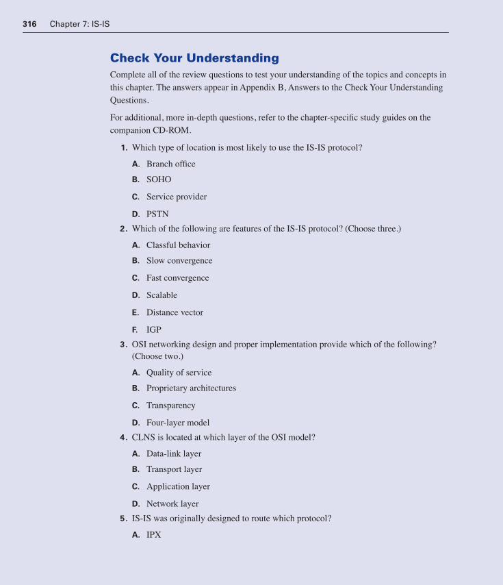
316 Chapter 7: IS-IS
Check Your UnderstandingComplete all of the review questions to test your understanding of the topics and concepts in
this chapter. The answers appear in Appendix B, Answers to the Check Your Understanding
Questions.
For additional, more in-depth questions, refer to the chapter-specific study guides on the
companion CD-ROM.
1. Which type of location is most likely to use the IS-IS protocol?
A. Branch office
B. SOHO
C. Service provider
D. PSTN
2. Which of the following are features of the IS-IS protocol? (Choose three.)
A. Classful behavior
B. Slow convergence
C. Fast convergence
D. Scalable
E. Distance vector
F. IGP
3. OSI networking design and proper implementation provide which of the following? (Choose two.)
A. Quality of service
B. Proprietary architectures
C. Transparency
D. Four-layer model
4. CLNS is located at which layer of the OSI model?
A. Data-link layer
B. Transport layer
C. Application layer
D. Network layer
5. IS-IS was originally designed to route which protocol?
A. IPX
1358_fmi.book Page 316 Thursday, May 27, 2004 2:21 PM
Check Your Understanding 317
B. AppleTalk
C. IP
D. DECnet Phase V
E. SNA
6. How many routers can exist in a single IS-IS area?
A. 15
B. 50
C. 100
D. 500
E. 1000
7. What is identified by the information contained in the CLNS system ID field?
A. A process on a device
B. The domain
C. A single OSI device
D. Port or socket information
8. How many addresses does an NSAP have?
A. A single address for the entire router
B. An address for each configured interface
C. Multiple addresses for each configured interface
D. The number of addresses depends on the routing protocol chosen
9. Which of the following is the equivalent of using more than one NET with the IS-IS protocol?
A. Using CIDR
B. Using secondary addresses with IP
C. Using VLSM
D. Implementing dynamic routing
10. What command displays the least-cost paths to a destination NET?
A. which-route
B. show isis topology
C. show clns route
D. show isis routes
1358_fmi.book Page 317 Thursday, May 27, 2004 2:21 PM

ObjectivesUpon completing this chapter, you will be able to
■ Understand methods of controlling routing update traffic
■ Describe policy-based routing
■ Understand methods and guidelines for route redistribution
■ Analyze a redistribution and summarization example
■ Apply route optimization techniques, such as routing update control, policy-based
routing, and route redistribution
You can reinforce your understanding of the objectives covered in this chapter by opening
the interactive media activities on the CD accompanying this book and performing the lab
activities collected in the Cisco Networking Academy Program CCNP 1: Advanced Routing
Lab Companion. Throughout this chapter, you will see references to these activities by title
and by icon. They look like this:
Interactive Media Activity
Lab Activity
1358_fmi.book Page 318 Thursday, May 27, 2004 2:21 PM

Chapter 8
Route Optimization
Dynamic routing, even in small internetworks, can involve much more than just enabling a routing
protocol’s default behavior. A few simple commands might be enough to get dynamic
routing started. However, more advanced configuration must be done to enable such features
as routing update control and exchanges among multiple routing protocols. You can optimize
routing in a network by controlling when a router exchanges routing updates and what those
updates contain. This chapter examines the key Cisco IOS software route optimization features,
including routing update control, policy-based routing, and route redistribution.
Controlling Routing Update TrafficThe following sections discuss some of the details of controlling routing update traffic. The top-
ics covered are
■ Controlling routing updates
■ Passive interfaces
■ Filtering routing updates with distribute-list
Controlling Routing Updates
Router RTA, as shown in Figure 8-1, is running a simple distance vector routing protocol called RIP.
The RIP configuration command network 10.0.0.0 serves two functions. First, it tells RIP where
to send and receive advertisements, and on which interfaces to send and receive updates. The
network 10.0.0.0 command enables RIP updates on all interfaces that have an IP address
belonging to the 10.0.0.0 network, such as Bri0, S1, S2, and E0. Second, this command tells the
RIP process what to advertise. All directly connected subnets belonging to the major network
10.0.0.0 are included in RIP updates in addition to any dynamically learned routes. This means
that RTA advertises the networks 10.1.1.0, 10.2.2.0, 10.3.3.0, and 10.4.4.0.
1358_fmi.book Page 319 Thursday, May 27, 2004 2:21 PM
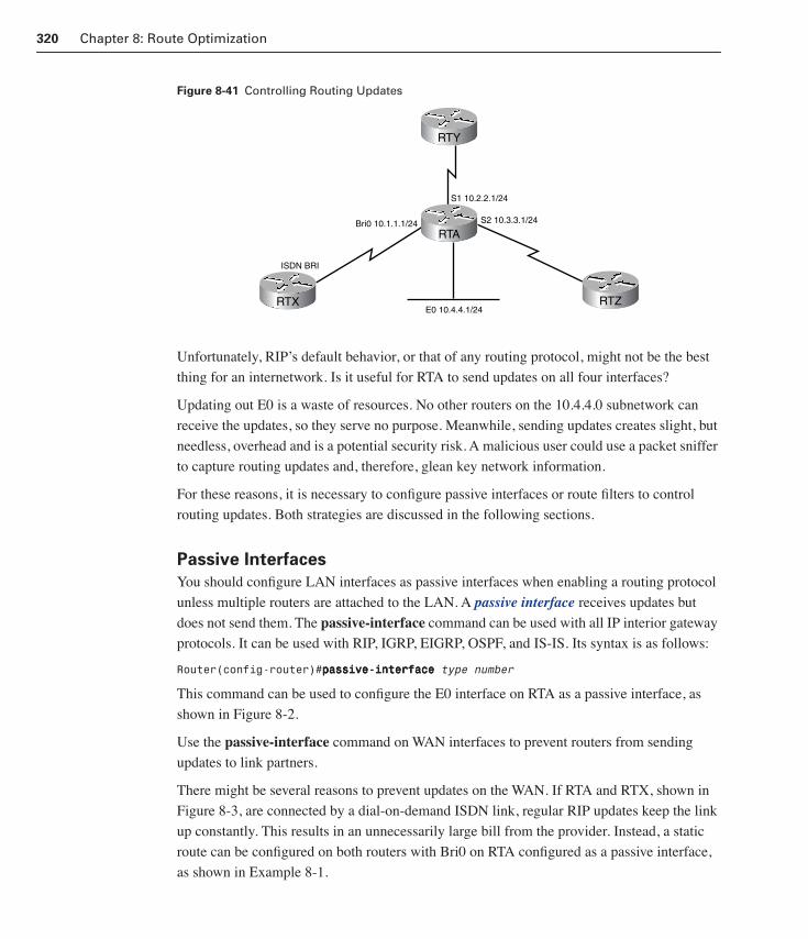
320 Chapter 8: Route Optimization
Figure 8-41 Controlling Routing Updates
Unfortunately, RIP’s default behavior, or that of any routing protocol, might not be the best
thing for an internetwork. Is it useful for RTA to send updates on all four interfaces?
Updating out E0 is a waste of resources. No other routers on the 10.4.4.0 subnetwork can
receive the updates, so they serve no purpose. Meanwhile, sending updates creates slight, but
needless, overhead and is a potential security risk. A malicious user could use a packet sniffer
to capture routing updates and, therefore, glean key network information.
For these reasons, it is necessary to configure passive interfaces or route filters to control
routing updates. Both strategies are discussed in the following sections.
Passive Interfaces
You should configure LAN interfaces as passive interfaces when enabling a routing protocol
unless multiple routers are attached to the LAN. A passive interface receives updates but
does not send them. The passive-interface command can be used with all IP interior gateway
protocols. It can be used with RIP, IGRP, EIGRP, OSPF, and IS-IS. Its syntax is as follows:
Router(config-router)#ppppaaaassssssssiiiivvvveeee----iiiinnnntttteeeerrrrffffaaaacccceeee type number
This command can be used to configure the E0 interface on RTA as a passive interface, as
shown in Figure 8-2.
Use the passive-interface command on WAN interfaces to prevent routers from sending
updates to link partners.
There might be several reasons to prevent updates on the WAN. If RTA and RTX, shown in
Figure 8-3, are connected by a dial-on-demand ISDN link, regular RIP updates keep the link
up constantly. This results in an unnecessarily large bill from the provider. Instead, a static
route can be configured on both routers with Bri0 on RTA configured as a passive interface,
as shown in Example 8-1.
S1 10.2.2.1/24
S2 10.3.3.1/24Bri0 10.1.1.1/24
ISDN BRI
E0 10.4.4.1/24
RTY
RTA
RTX RTZ
1358_fmi.book Page 320 Thursday, May 27, 2004 2:21 PM

Controlling Routing Update Traffic 321
Figure 8-42 Configuring Passive Interfaces
Figure 8-43 Configuring Passive Interfaces—Updates Prevented
Notice that for RTA to update RTY and RTZ in Figure 8-2 about the route to 172.16.1.0, it
must be configured to redistribute static routes into RIP. The redistribute static command
tells RIP to import the static routes into RIP and advertise them as part of a RIP update. Route
redistribution is covered in more detail later in this chapter.
Example 8-1 Configuring Passive Interfaces on a WAN Link
RTA(config)#rrrroooouuuutttteeeerrrr rrrriiiipppp
RTA(config-router)#nnnneeeettttwwwwoooorrrrkkkk 11110000....0000....0000....0000
RTA(config-router)#ppppaaaassssssssiiiivvvveeee----iiiinnnntttteeeerrrrffffaaaacccceeee bbbbrrrriiii0000
RTA(config-router)#rrrreeeeddddiiiissssttttrrrriiiibbbbuuuutttteeee ssssttttaaaattttiiiicccc
RTA(config-router)#eeeexxxxiiiitttt
RTA(config)#iiiipppp rrrroooouuuutttteeee 111177772222....11116666....1111....0000 222255555555....222255555555....222255555555....0000 bbbbrrrriiii0000
RTX(config)#iiiipppp rrrroooouuuutttteeee 0000....0000....0000....0000 0000....0000....0000....0000 bbbbrrrriiii0000
S1 10.2.2.1/24
S2 10.3.3.1/24Bri0 10.1.1.1/24
ISDN BRI
E0 10.4.4.1/24
RTY
RTA
RTX RTZ
Passive Interface
Bri0 10.1.1.1/24
Bri0
E0 172.16.1.0/24
RTA
RTX
ISDN BRI
1358_fmi.book Page 321 Thursday, May 27, 2004 2:21 PM

322 Chapter 8: Route Optimization
The passive-interface command works differently with the different IP routing protocols that
support it. In OSPF, the network address of the passive interface appears as a stub network.
OSPF routing information is neither sent nor received by way of a passive interface. In
EIGRP and OSPF, the router stops sending Hello packets on passive interfaces. When this
happens, the router cannot form neighbor adjacencies. Therefore, the router cannot send and
receive routing updates on the interface. You will see later in this chapter that the passive
effect can be achieved for an EIGRP interface by using the distribute-list command. This
can be done without preventing adjacency relationships. It is also important to point out that
distribute lists can be used for all routing protocols, not just EIGRP.
In some networks, there might be cases in which the user does not want the router to send
routing updates. The passive-interface command can be used to prevent routing updates
from being sent over a certain WAN or LAN interface.
For instance, the user might not want RIP updates to be sent over an ISDN (DDR) interface.
Different routing protocols behave differently with a passive interface. You can set an inter-
face to passive with the passive-interface command. When a passive interface is used with
RIP, routing updates are not sent over that interface. The RIP routing protocol continues to
receive routing updates over a passive interface, as shown in Figure 8-4.
Figure 8-44 RIP
In Figure 8-5, the network is running OSPF. The serial interface on the left router is set to passive.
OSPF does not send routing updates out of a passive interface. Unlike RIP, OSPF does not accept
any updates over a passive interface. Passive interface behavior is similar to a stub network.
Before EIGRP can send routing updates, it needs to build neighbor relationships. EIGRP uses
routing transport protocol (RTP). RTP uses keepalive messages for communication. Passive
interfaces do not allow keepalives to be sent. This prevents EIGRP from discovering its
neighbors. Because of the passive interface over the serial link, EIGRP is unable to discover
its neighbor. The router does not send router updates over the serial interface. Even though
the passive interface is set on the bottom-left router, the bottom-right router does not send any
EIGRP routing updates, as shown in Figure 8-6. EIGRP needs to discover its neighbor before
sending routing updates.
E0
E0 E0
E0
E1 E1S0
S0
Passive Interface
1358_fmi.book Page 322 Thursday, May 27, 2004 2:21 PM

Controlling Routing Update Traffic 323
Figure 8-45 OSPF
Figure 8-46 EIGRP
Filtering Routing Updates with distribute-list
Configuring an interface as passive prevents it from sending updates entirely. However,
sometimes you need to suppress only certain routes in the update from being sent or received.
In Figure 8-7, if RTA is configured with the network 10.0.0.0 command, all four directly
connected subnets are advertised in the updates from RTA, along with any dynamically
learned routes. However, RTZ might need to be prevented from learning about network
10.1.1.0 from RTA, as shown in Example 8-2.
Figure 8-47 Using Outbound Route Filters
E0
E0 E0
E0
E1 E1S0
S0
Passive Interface
E0
E0 E0
E0
E1 E1S0
S0
Passive Interface
S1
S2
Bri0
ISDN BRI
E0
RTY
RTA
RTX RTZ
S0
���������
� ������������
� ������������
� ������������
� ������������
1358_fmi.book Page 323 Thursday, May 27, 2004 2:21 PM

324 Chapter 8: Route Optimization
This might be needed to enforce a routing policy that is based on an external factor, such as
link expense, administrative jurisdiction, or security concerns. In some cases, you want to
reduce needless overhead by preventing access routers from receiving the complete, and pos-
sibly immense, core routing table. Just assume that for one of these reasons, RTZ should not
learn the route to 10.1.1.0 from RTA.
Use the distribute-list command to pick and choose which routing updates a router sends or
receives. By referencing an access list, the distribute list creates a route filter. This is a set of
rules that precisely controls what routes a router sends or receives in a routing update. This
command is available for all IP routing protocols and can be applied to either inbound or out-
bound routing updates. When applied to inbound updates, the syntax for configuring a route
filter is as follows:
Router(config-router)#ddddiiiissssttttrrrriiiibbbbuuuutttteeee----lllliiiisssstttt access-list-number iiiinnnn [interface-name]
When applied to outbound updates, the syntax can be more complicated:
Router(config-router)#ddddiiiissssttttrrrriiiibbbbuuuutttteeee----lllliiiisssstttt access-list-number oooouuuutttt [interface-name | routing-process | as-number]
The routing-process and as-number options are invoked when routes are exchanged between
different routing protocols. This is covered in the section “Route Redistribution.”
In Example 8-2, access list 24 matches the route to 10.1.1.0 and results in a deny. When refer-
enced by the distribute-list command, this match results in the removal of the route to net-
work 10.1.1.0 in the outbound update. However, there is a drawback. The distribute-list 24 out command has a global effect on RIP updates out every interface, not just out the interface
connected to RTZ. The intent is to suppress the 10.1.1.0 route from updates to RTZ only. This
level of specificity can be accomplished by using the optional interface-name argument with
the command:
RTA(config-router)#ddddiiiissssttttrrrriiiibbbbuuuutttteeee----lllliiiisssstttt 22224444 oooouuuutttt sssseeeerrrriiiiaaaallll2222
Conversely, RTZ could be told to globally filter network 10.1.1.0 from any incoming updates,
as shown in Example 8-3.
Example 8-2 Configuring Outbound Route Filters
RTA(config)#rrrroooouuuutttteeeerrrr rrrriiiipppp
RTA(config-router)#nnnneeeettttwwwwoooorrrrkkkk 11110000....0000....0000....0000
RTA(config-router)#ddddiiiissssttttrrrriiiibbbbuuuutttteeee----lllliiiisssstttt 22224444 oooouuuutttt
RTA(config-router)#eeeexxxxiiiitttt
RTA(config)#aaaacccccccceeeessssssss----lllliiiisssstttt 22224444 ddddeeeennnnyyyy 11110000....1111....1111....0000 0000....0000....0000....222222225555
RTA(config)#aaaacccccccceeeessssssss----lllliiiisssstttt 22224444 ppppeeeerrrrmmmmiiiitttt aaaannnnyyyy
1358_fmi.book Page 324 Thursday, May 27, 2004 2:21 PM

Controlling Routing Update Traffic 325
Or, 10.1.1.0 could be precisely filtered from the specific interface on RTZ:
RTZ(config-router)#ddddiiiissssttttrrrriiiibbbbuuuutttteeee----lllliiiisssstttt 11116666 iiiinnnn sssseeeerrrriiiiaaaallll0000
The distribute-list command can filter any routes in either an outbound or inbound update
globally or for a specific interface. The Cisco IOS software permits one incoming and one
outgoing global distribute list for each routing process. It also permits one incoming and one
outgoing distribute list for each interface involved in a routing process. You can keep track of
which routing filters are applied globally and which are applied on specific interfaces with the
show ip protocols command.
Configuring a Passive EIGRP Interface Using the distribute-list CommandA passive interface cannot send EIGRP Hello packets, which prevents adjacency relation-
ships with link partners. A pseudo or false passive EIGRP interface can be created by using a
route filter that suppresses routes from the EIGRP routing update, as shown in Example 8-4.
With this configuration, RTA can send EIGRP Hello packets and establish adjacencies, but no
routes appear in any updates sent out of s2. This applies to OSPF as well as EIGRP.
Example 8-3 Configuring Inbound Route Filters
RTZ(config)#rrrroooouuuutttteeeerrrr rrrriiiipppp
RTZ(config-router)#nnnneeeettttwwwwoooorrrrkkkk 11110000....0000....0000....0000
RTZ(config-router)#ddddiiiissssttttrrrriiiibbbbuuuutttteeee----lllliiiisssstttt 11116666 iiiinnnn
RTZ(config-router)#eeeexxxxiiiitttt
RTZ(config)#aaaacccccccceeeessssssss----lllliiiisssstttt 11116666 ddddeeeennnnyyyy 11110000....1111....1111....0000 0000....0000....0000....222222225555
RTZ(config)#aaaacccccccceeeessssssss----lllliiiisssstttt 11116666 ppppeeeerrrrmmmmiiiitttt aaaannnnyyyy
Example 8-4 Configuring a Passive EIGRP Interface Using the distribute-list Command
RTA(config)#rrrroooouuuutttteeeerrrr eeeeiiiiggggrrrrpppp 333366664444
RTA(config-router)#nnnneeeettttwwwwoooorrrrkkkk 11110000....0000....0000....0000
RTA(config-router)#ddddiiiissssttttrrrriiiibbbbuuuutttteeee----lllliiiisssstttt 5555 oooouuuutttt ssss2222
RTA(config-router)#eeeexxxxiiiitttt
RTA(config)#aaaacccccccceeeessssssss----lllliiiisssstttt 5555 ddddeeeennnnyyyy aaaannnnyyyy
1358_fmi.book Page 325 Thursday, May 27, 2004 2:21 PM

326 Chapter 8: Route Optimization
Policy RoutingThe following sections discuss some of the details of policy routing.
Policy Routing Overview
You use the ip route command to dictate which path to a given destination a router selects.
However, through policy routing, a router can be programmed to choose a route based not
only on destination, but on source as well.
Concerns such as monetary expense, organizational jurisdiction, or security issues can lead
administrators to establish policies or rules that routed traffic should follow. Left to their
default behavior, routing protocols might arrive at path decisions that conflict with these poli-
cies. For that reason, administrators use policy routing to override dynamic routing and to
take precise control of how their routers handle certain traffic.
Although policy routing can be used to control traffic within an autonomous system (AS), it
is typically used to control routing between autonomous systems. For that reason, policy
routing is used extensively with exterior gateway protocols (EGPs), such as Border Gateway
Protocol (BGP).
The route-map command is used to configure policy routing, which is often a complicated
task. A route map is defined using the following syntax:
Router(config)#rrrroooouuuutttteeee----mmmmaaaapppp map-tag [ppppeeeerrrrmmmmiiiitttt | ddddeeeennnnyyyy] [sequence-number]Router(config-map-router)#
The map-tag is the name, or ID, of the route map. This map tag can be set to something easily
recognizable, such as route2ISP or CHANGEROUTE. The route-map command changes
the mode on the router to route-map configuration mode. From there, you can configure con-
ditions for the route map.
Route maps operate similar to access lists, by examining one line at a time. When a match is
found, an action is taken. Route maps are different from numbered access lists because you
can modify them without changing the entire list. Each route map statement is given a num-
ber. If a sequence number is not specified, the first route map condition is automatically num-
bered as 10. The second condition is automatically numbered as 20, and so on. The optional
sequence number can be used to indicate the position that a new route map is to have in the
list of route maps already configured with the same name.
After you enter the route-map command, enter set and match commands in route-map con-
figuration mode. Each route-map command has a list of match and set commands associ-
ated with it. The match commands specify the match criteria. They are the conditions that
should be tested to determine whether to take action. The set commands specify the set actions. They are the actions to be performed if the match criteria are met.
1358_fmi.book Page 326 Thursday, May 27, 2004 2:21 PM

Policy Routing 327
Policy Routing Example
Figure 8-8 presents a policy routing scenario. A route map can be used at RTA to implement
policy routing. Assume for this example that the policy to be enforced is as follows:
■ Route Internet-bound traffic from 192.168.1.0/24 to ISP 1
■ Route Internet-bound traffic from 172.16.1.0/24 to ISP 2
Figure 8-48 Policy Routing Example
First, define the access lists that will be used in the route maps to match IP addresses. Then
configure the route map itself using the syntax shown in Example 8-5.
The commands shown in Example 8-5 have actually configured two policies. The ISP1 route
map matches access list 1 and routes traffic out S0 toward ISP1. The ISP2 route map matches
access list 2 and routes that traffic out S1 toward ISP2.
The final step is to apply each route map to the appropriate interface on RTA using the ip pol-icy route-map command, as shown in Example 8-6. The appropriate interface is the interface
Example 8-5 Configuring a Route Map
RTA(config)#aaaacccccccceeeessssssss----lllliiiisssstttt 1111 ppppeeeerrrrmmmmiiiitttt 111199992222....111166668888....1111....0000 0000....0000....0000....222255555555
RTA(config)#aaaacccccccceeeessssssss----lllliiiisssstttt 2222 ppppeeeerrrrmmmmiiiitttt 111177772222....11116666....1111....0000 0000....0000....0000....222255555555
RTA(config-router)#rrrroooouuuutttteeee----mmmmaaaapppp IIIISSSSPPPP1111 ppppeeeerrrrmmmmiiiitttt 11110000
RTA(config-route-map)#mmmmaaaattttcccchhhh iiiipppp aaaaddddddddrrrreeeessssssss 1111
RTA(config-route-map)#sssseeeetttt iiiinnnntttteeeerrrrffffaaaacccceeee sssseeeerrrriiiiaaaallll 0000
RTA(config-route-map)#eeeexxxxiiiitttt
RTA(config-router)#rrrroooouuuutttteeee----mmmmaaaapppp IIIISSSSPPPP2222 ppppeeeerrrrmmmmiiiitttt 22220000
RTA(config-route-map)#mmmmaaaattttcccchhhh iiiipppp aaaaddddddddrrrreeeessssssss 2222
RTA(config-route-map)#sssseeeetttt iiiinnnntttteeeerrrrffffaaaacccceeee sssseeeerrrriiiiaaaallll 1111
Internet
ISP 1
AS 24
192.168.1.0/24
172.16.1.0/24
E0
E1
S0
S1RTA
ISP 1
ISP 2
1358_fmi.book Page 327 Thursday, May 27, 2004 2:21 PM
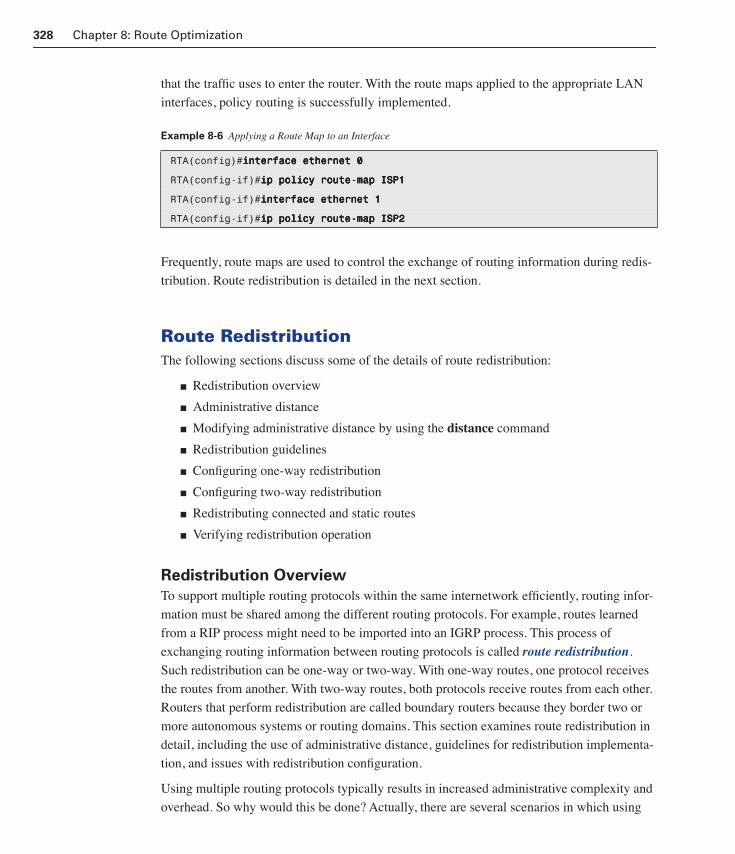
328 Chapter 8: Route Optimization
that the traffic uses to enter the router. With the route maps applied to the appropriate LAN
interfaces, policy routing is successfully implemented.
Frequently, route maps are used to control the exchange of routing information during redis-
tribution. Route redistribution is detailed in the next section.
Route RedistributionThe following sections discuss some of the details of route redistribution:
■ Redistribution overview
■ Administrative distance
■ Modifying administrative distance by using the distance command
■ Redistribution guidelines
■ Configuring one-way redistribution
■ Configuring two-way redistribution
■ Redistributing connected and static routes
■ Verifying redistribution operation
Redistribution Overview
To support multiple routing protocols within the same internetwork efficiently, routing infor-
mation must be shared among the different routing protocols. For example, routes learned
from a RIP process might need to be imported into an IGRP process. This process of
exchanging routing information between routing protocols is called route redistribution.
Such redistribution can be one-way or two-way. With one-way routes, one protocol receives
the routes from another. With two-way routes, both protocols receive routes from each other.
Routers that perform redistribution are called boundary routers because they border two or
more autonomous systems or routing domains. This section examines route redistribution in
detail, including the use of administrative distance, guidelines for redistribution implementa-
tion, and issues with redistribution configuration.
Using multiple routing protocols typically results in increased administrative complexity and
overhead. So why would this be done? Actually, there are several scenarios in which using
Example 8-6 Applying a Route Map to an Interface
RTA(config)#iiiinnnntttteeeerrrrffffaaaacccceeee eeeetttthhhheeeerrrrnnnneeeetttt 0000
RTA(config-if)#iiiipppp ppppoooolllliiiiccccyyyy rrrroooouuuutttteeee----mmmmaaaapppp IIIISSSSPPPP1111
RTA(config-if)#iiiinnnntttteeeerrrrffffaaaacccceeee eeeetttthhhheeeerrrrnnnneeeetttt 1111
RTA(config-if)#iiiipppp ppppoooolllliiiiccccyyyy rrrroooouuuutttteeee----mmmmaaaapppp IIIISSSSPPPP2222
1358_fmi.book Page 328 Thursday, May 27, 2004 2:21 PM

Route Redistribution 329
multiple routing protocols solves more problems than it creates, especially in medium- and
large-sized networks.
Consider a large, mixed-vendor routing environment in which Cisco routers work alongside
other routers, as shown in Figure 8-9. An administrator might create an all-Cisco domain,
where the advantages of proprietary protocols, such as IGRP and EIGRP, can be retained.
Meanwhile, other areas of the network run a nonproprietary protocol, such as OSPF or RIP.
Figure 8-49 Redistribution Example
Multiple routing protocols may also be effectively deployed to support legacy UNIX systems
that support RIP only. These systems might represent a significant financial investment and
might not be readily upgradeable. An administrator might elect to run RIP on subnets popu-
lated by the UNIX systems but might use a more scalable protocol elsewhere, as shown in
Figure 8-9. Also, running multiple routing protocols can be seen as a temporary fix during a
prolonged upgrade from older protocols and hardware to newer, more scalable solutions.
On some occasions, redistribution is implemented even when compatible routing platforms
are being run. For example, consider an organization with all Cisco routers running EIGRP. If
the organization is exchanging routing information with a domain outside its administrative
control, it might choose to configure route redistribution as a means of logically separating
the different routing processes, which might have different policies.
Cisco routers support up to 30 dynamic routing processes. This means that a router can run
RIP, OSPF, IGRP, IS-IS, EIGRP, IPX RIP, RTMP, AppleTalk, and other protocols simulta-
neously. Most of these routing protocols enable the configuration of multiple processes of the
EIGRP redistributes RIP routes.RIP domain uses default route.
(One-way redistribution)
UNIX Host
UNIX Host
RIP
OSPF
EIGRP
Nortel
3Com Cisco Cisco
CiscoCiscoCisco
Cisco
OSPF redistributes EIGRP routes.EIGRP redistributes OSPF routes.
(Two-way redistribution)
1358_fmi.book Page 329 Thursday, May 27, 2004 2:21 PM

330 Chapter 8: Route Optimization
same routing algorithm. RIP is a notable exception. For example, multiple IGRP processes
can be defined by using different AS numbers, or different OSPF processes can be defined by
using different process ID numbers, as shown in Example 8-7.
Notice that the OSPF processes for RTA, 24 and 46, do not share routing information unless
route redistribution is configured. Each routing process places substantial demands on the
router memory and CPU resources. Because of this, only boundary routers should run more
than one routing process for the same routed protocol and only when absolutely necessary.
Administrative Distance
If a boundary router is running multiple IP routing protocols, it might learn about the same
network from more than one routing protocol. For example, RTZ might learn about the
10.0.0.0 network from both RIP and IGRP, as shown in Figure 8-10. Which route will RTZ
install in its routing table?
Figure 8-50 Administrative Distance Example
Example 8-7 Multiple OSPF and IGRP Processes
RTA#sssshhhhoooowwww rrrruuuunnnnnnnniiiinnnngggg----ccccoooonnnnffffiiiigggg
<output omitted>
router ospf 24
network 10.2.0.0 0.0.255.255 area 0
!
router ospf 46
network 192.168.2.0 0.0.0.255 area 2
!
router igrp 53
network 172.16.0.0
network 172.17.0.0
!
router igrp 141
network 10.0.0.0
network 192.168.3.0
RTZ
I 10.0.0.0 [100/10576] R 10.0.0.0 [120/3]?
IGRP RIP
1358_fmi.book Page 330 Thursday, May 27, 2004 2:21 PM

Route Redistribution 331
A router looks at the metric value to determine the best route. However, in this case, the
router would have to compare the simple metric of RIP, its hop count, with the composite
metric of IGRP, this being derived from bandwidth and delay by default. As noted in Chapter 3,
“Routing Overview,” the metrics are not based on the same factors, so this is an unreliable
comparison. The metric of 10576 from IGRP cannot be accurately measured against the met-
ric of 3 from RIP for the same route. Instead, routers use administrative distance to choose
between routes to the same network offered by different routing protocols.
A routing protocol’s administrative distance provides a rate of trustworthiness as a source of
routing information. Administrative distance is an integer from 0 to 255. The lowest adminis-
trative distance has the highest trust rating. An administrative distance of 255 means that the
routing information source cannot be trusted and should be ignored. An administrative dis-
tance of 0 is reserved for directly connected interfaces and is always preferred.
Specifying administrative distance values allows the Cisco IOS software to discriminate
between sources of routing information. If two routes have the same network number, and
possibly the same subnet information, the Cisco IOS software always picks the route whose
routing protocol has the lowest administrative distance. Table 8-1 shows the default adminis-
trative distances for some routing information sources.Table 8-8 Administrative Distance
Route Source Default Distance
Connected interface 0
Static route 1
EIGRP summary route 5
External BGP 20
Internal EIGRP 90
IGRP 100
OSPF 110
IS-IS 115
RIP 120
EGP 140
External EIGRP 170
Internal BGP 200
Unknown 255
1358_fmi.book Page 331 Thursday, May 27, 2004 2:21 PM

332 Chapter 8: Route Optimization
The IGRP route is preferred, or trusted, over the RIP route to the same network. This is
because of IGRP’s lower administrative distance, which is 100, as opposed to RIP, which is
120. There might be a time when you need the router to believe RIP over IGRP. Fortunately,
the Cisco IOS software allows the administrative distance to be manually configured, as dis-
cussed in the next section.
Modifying Administrative Distance by Using the distance
Command
When you use multiple IP routing protocols on a router, the default administrative distance of
each is usually sufficient. However, some circumstances call for changing the administrative
distance values on a router.
For example, if a router is running both IGRP and OSPF, it might receive routes to the same
network from both protocols. The default administrative distance favors IGRP routes over
OSPF routes. However, because IGRP does not support CIDR, the router needs to use the
OSPF route instead. In this case, configure the local router to apply a custom administrative
distance to all OSPF routes.
With the distance 95 OSPF configuration command, RTZ compares the IGRP and OSPF
routes and comes up with a different result, as shown in Example 8-8. The beginning of
Example 8-8 shows route comparison with default administrative distances. The end of
Example 8-8 shows route comparison with manually configured administrative distances.
Interactive Media Activity Drag and Drop: Administrative Distance
After completing this activity, you will be able to identify the administrative dis-
tances for all entries in a routing table.
Example 8-8 Using the distance Command
I 10.0.0.0 [100/10576] via 192.168.0.1, Serial 0
O 10.0.0.0 [110/192] via 172.17.0.1, Serial 1
RTZ(config)#rrrroooouuuutttteeeerrrr oooossssppppffff 1111
RTZ(config-router)#ddddiiiissssttttaaaannnncccceeee 99995555
I 10.0.0.0 [100/10576] via 192.168.0.1, Serial 0
O 10.0.0.0 [95/192] via 172.17.0.1, Serial 1
1358_fmi.book Page 332 Thursday, May 27, 2004 2:21 PM
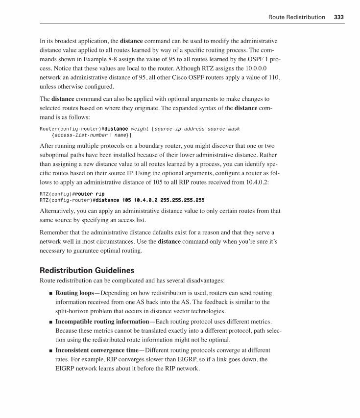
Route Redistribution 333
In its broadest application, the distance command can be used to modify the administrative
distance value applied to all routes learned by way of a specific routing process. The com-
mands shown in Example 8-8 assign the value of 95 to all routes learned by the OSPF 1 pro-
cess. Notice that these values are local to the router. Although RTZ assigns the 10.0.0.0
network an administrative distance of 95, all other Cisco OSPF routers apply a value of 110,
unless otherwise configured.
The distance command can also be applied with optional arguments to make changes to
selected routes based on where they originate. The expanded syntax of the distance com-
mand is as follows:
Router(config-router)#ddddiiiissssttttaaaannnncccceeee weight [source-ip-address source-mask {access-list-number | name}]
After running multiple protocols on a boundary router, you might discover that one or two
suboptimal paths have been installed because of their lower administrative distance. Rather
than assigning a new distance value to all routes learned by a process, you can identify spe-
cific routes based on their source IP. Using the optional arguments, configure a router as fol-
lows to apply an administrative distance of 105 to all RIP routes received from 10.4.0.2:
RTZ(config)#rrrroooouuuutttteeeerrrr rrrriiiippppRTZ(config-router)#ddddiiiissssttttaaaannnncccceeee 111100005555 11110000....4444....0000....2222 222255555555....222255555555....222255555555....222255555555
Alternatively, you can apply an administrative distance value to only certain routes from that
same source by specifying an access list.
Remember that the administrative distance defaults exist for a reason and that they serve a
network well in most circumstances. Use the distance command only when you’re sure it’s
necessary to guarantee optimal routing.
Redistribution Guidelines
Route redistribution can be complicated and has several disadvantages:
■ Routing loops—Depending on how redistribution is used, routers can send routing
information received from one AS back into the AS. The feedback is similar to the
split-horizon problem that occurs in distance vector technologies.
■ Incompatible routing information—Each routing protocol uses different metrics.
Because these metrics cannot be translated exactly into a different protocol, path selec-
tion using the redistributed route information might not be optimal.
■ Inconsistent convergence time—Different routing protocols converge at different
rates. For example, RIP converges slower than EIGRP, so if a link goes down, the
EIGRP network learns about it before the RIP network.
1358_fmi.book Page 333 Thursday, May 27, 2004 2:21 PM

334 Chapter 8: Route Optimization
You can avoid these potential trouble spots with careful planning and implementation. Follow
these important guidelines when configuring route redistribution:
■ Be familiar with the network—There are many ways to implement redistribution.
Being familiar with the network helps you make the best decisions.
■ Do not overlap routing protocols—Do not run two different protocols in the same
internetwork. Instead, have distinct boundaries between networks that use different
routing protocols.
■ Use one-way redistribution with multiple boundary routers—If more than one
router serves as a redistribution point, use one-way redistribution to avoid routing loops
and convergence problems. Consider using default routes in the domains that do not
import external routes.
■ Use two-way redistribution with a single boundary router—Two-way redistribution
works smoothly when it is configured on a single boundary router in the internetwork.
If there are multiple redistribution points, do not use two-way redistribution unless a
mechanism to reduce the chances of routing loops is enabled. You can use a combina-
tion of default routes, route filters, and distance modifications to combat routing loops.
Configuring One-Way Redistribution
Although the redistribute command is available for all IP routing protocols, it behaves dif-
ferently depending on the IP routing protocols involved. However, the underlying principles
are the same. Therefore, you can use the examples in this section as a starting point for any
redistribution scheme.
This section closely examines examples of one-way and two-way redistribution and then
focuses on specific redistribution issues, including connected, static routes and the default-metric command.
In Figure 8-11, RTB injects routes learned by way of RIP into the EIGRP domain. However,
the RIP routers do not learn about the EIGRP routes. This is one-way route distribution. In
this example, the RIP routers can use a default route to handle any traffic bound for nonlocal
destinations.
As the AS boundary router, RTB must run two routing processes, one for the RIP domain and
one for the EIGRP AS, as shown in Example 8-9. The syntax of the redistribute command is
as follows:
Router(config-router)# rrrreeeeddddiiiissssttttrrrriiiibbbbuuuutttteeee protocol [process-id] {lllleeeevvvveeeellll----1111 | lllleeeevvvveeeellll----1111----2222 | lllleeeevvvveeeellll----2222} [as-number] [mmmmeeeettttrrrriiiicccc metric-value] [mmmmeeeettttrrrriiiicccc----ttttyyyyppppeeee type-value] [mmmmaaaattttcccchhhh {iiiinnnntttteeeerrrrnnnnaaaallll | eeeexxxxtttteeeerrrrnnnnaaaallll 1111 | eeeexxxxtttteeeerrrrnnnnaaaallll 2222}] [ttttaaaagggg tag-value] [rrrroooouuuutttteeee----mmmmaaaapppp map-tag] [ssssuuuubbbbnnnneeeettttssss]
1358_fmi.book Page 334 Thursday, May 27, 2004 2:21 PM

Route Redistribution 335
Figure 8-51 One-Way Redistribution Example
The redistribute rip command enables route redistribution. RIP routes learned by RTB are
imported into the EIGRP process. The metric argument sets up the values used by EIGRP to
translate the metric from the hop count on RIP to the composite metric on EIGRP. When used
with IGRP/EIGRP, the metric keyword sets the bandwidth value, the delay, the reliability, the
load, and the maximum transmission unit (MTU). The bandwidth value is in Kbps, the delay
is in tenths of microseconds, and the reliability and load are out of 255.
These five values constitute the seed metric. The seed metric is the initial metric value of an
imported route. After it is imported into the EIGRP AS, the RIP route becomes an EIGRP
route with a composite metric derived from these seed values. Using the configuration shown
in Example 8-9, RIP routes with metrics of 2, 6, and 14 are redistributed with the same
EIGRP metric value of 2195456. However, as the imported route propagates to other EIGRP
routers, its metric values increment according to EIGRP rules.
Example 8-9 Configuring One-Way Route Redistribution
RTB(config)#rrrroooouuuutttteeeerrrr rrrriiiipppp
RTB(config-router)#nnnneeeettttwwwwoooorrrrkkkk 111177772222....11116666....0000....0000
RTB(config-router)#rrrroooouuuutttteeeerrrr eeeeiiiiggggrrrrpppp 22224444
RTB(config-router)#nnnneeeettttwwwwoooorrrrkkkk 111177772222....22224444....0000....0000
RTB(config-router)#rrrreeeeddddiiiissssttttrrrriiiibbbbuuuutttteeee rrrriiiipppp mmmmeeeettttrrrriiiicccc 11110000000000000000 111100000000 222255555555 1111 1111555500000000
S1 S0
172.24.0.0172.16.0.0
EIGRP AS 24 RIP
RIP Routes
EIGRP redistributes routes.RIP domain uses default route.
(One-way redistribution)
RTA RTB RTC
1358_fmi.book Page 335 Thursday, May 27, 2004 2:21 PM

336 Chapter 8: Route Optimization
The routing table on RTA includes not only the EIGRP routes from AS 24 but also the redis-
tributed routes from the RIP domain, as shown in Example 8-10. The internal EIGRP routes
are denoted by a D. The redistributed RIP routes that have been learned from RTB are
denoted by D EX because EIGRP considers them external. As discussed in Chapter 5,
“EIGRP,” EIGRP differentiates between internal routes and external routes. Internal routes
are learned from within the AS, and external routes are imported from outside the AS. Inter-
nal EIGRP routes have an administrative distance of 90. The Cisco IOS software assigns a
different administrative distance of 170 to the external EIGRP routes, which is much less
desirable.
The routing table from RTB, shown in Example 8-11, shows that RTB is running two routing
protocols and has learned routes by way of RIP and EIGRP. RIP is denoted by an R, and
EIGRP is denoted by a D.
Example 8-10 Routing Table for RTA
RTA#sssshhhhoooowwww iiiipppp rrrroooouuuutttteeee
<output omitted>
C 172.24.0.0/16 is directly connected, Serial 0
C 172.25.0.0/16 is directly connected, Serial 1
C 172.26.0.0/16 is directly connected, Serial 2
C 172.27.0.0/16 is directly connected, Serial 3
D 172.28.0.0/16 [90/2681856] via 172.20.0.0, 00:00:02, Serial1
D 172.29.0.0/16 [90/2681856] via 172.21.0.0, 00:00:02, Serial3
D EX 172.17.0.0/16 [170/2195456] via 172.24.0.1. 00:00:02, Serial0
D EX 172.18.0.0/16 [170/2195456] via 172.24.0.1. 00:00:02, Serial0
D EX 172.19.0.0/16 [170/2195456] via 172.24.0.1. 00:00:02, Serial0
D EX 172.20.0.0/16 [170/2195456] via 172.24.0.1. 00:00:02, Serial0
D EX 172.21.0.0/16 [170/2195456] via 172.24.0.1. 00:00:02, Serial0
Example 8-11 Routing Table for RTB
RTB#sssshhhhoooowwww iiiipppp rrrroooouuuutttteeee
<output omitted>
C 172.16.0.0/16 is directly connected, Serial 0
C 172.24.0.0/16 is directly connected, Serial 1
R 172.17.0.0/16 [120/1] via 172.16.0.2, 00:00:02, Serial0
R 172.18.0.0/16 [120/1] via 172.16.0.2, 00:00:02, Serial0
1358_fmi.book Page 336 Thursday, May 27, 2004 2:21 PM

Route Redistribution 337
In Example 8-12, RTC does not have a default route and has not learned about any routes
from the boundary router, RTB. This means that RTC cannot route to six of the 12 networks
shown in the output from RTB.
You might decide that the best solution in this scenario is to use a default route that points to
RTB. This can easily be accomplished statically:
RTC(config)#iiiipppp rrrroooouuuutttteeee 0000....0000....0000....0000 0000....0000....0000....0000 111177772222....11116666....0000....1111
Because RTC is running RIP, it can dynamically propagate its 0.0.0.0/0 route to the other
routers in the RIP domain. If you choose to implement this default route configuration, there
is no need for the boundary router, RTB, to send updates into the RIP domain. Therefore, the
RIP interface on RTB should be configured as passive:
RTB(config)#rrrroooouuuutttteeeerrrr rrrriiiippppRTB(config-router)#ppppaaaassssssssiiiivvvveeee----iiiinnnntttteeeerrrrffffaaaacccceeee ssss0000////0000
R 172.19.0.0/16 [120/1] via 172.16.0.2, 00:00:02, Serial0
R 172.20.0.0/16 [120/1] via 172.16.0.2, 00:00:02, Serial0
R 172.21.0.0/16 [120/1] via 172.16.0.2, 00:00:02, Serial0
D 172.25.0.0/16 [90/2681856] via 172.24.0.2, 00:00:02, Serial1
D 172.26.0.0/16 [90/2681856] via 172.24.0.2, 00:00:02, Serial1
D 172.37.0.0/16 [90/2681856] via 172.24.0.2, 00:00:02, Serial1
D 172.28.0.0/16 [90/3193856] via 172.24.0.2, 00:00:02, Serial1
D 172.29.0.0/16 [90/3193856] via 172.24.0.2, 00:00:02, Serial1
Example 8-12 Routing Table for RTC
RTC#sssshhhhoooowwww iiiipppp rrrroooouuuutttteeee
<output omitted>
C 172.16.0.0/16 is directly connected, Serial 0
C 172.17.0.0/16 is directly connected, Serial 1
C 172.18.0.0/16 is directly connected, Serial 2
C 172.19.0.0/16 is directly connected, Serial 3
R 172.20.0.0/16 [120/1] via 172.17.0.2, 00:00:02, Serial1
R 172.21.0.0/16 [120/1] via 172.19.0.2, 00:00:02, Serial3
*S 0.0.0.0/0 S* is directly connected, Serial0
Example 8-11 Routing Table for RTB (Continued)
1358_fmi.book Page 337 Thursday, May 27, 2004 2:21 PM

338 Chapter 8: Route Optimization
A more complex topology might require that you employ a two-way, or mutual, redistribu-
tion. You do this by importing the EIGRP routes into the RIP domain, as described in the next
section.
Configuring Two-Way Redistribution
The boundary router can be configured for two-way redistribution, as shown in Figure 8-12.
Notice that in Example 8-13, the syntax of the metric keyword varies depending on which
routing protocol it uses. For RIP, OSPF, and BGP, the metric option is followed by a single
number that represents the metric value (hop count, cost, and so on). For IGRP and EIGRP,
the metric option is followed by five values that represent bandwidth, delay, reliability, load,
and MTU.
Figure 8-52 Two-Way Redistribution Example
Lab 8.5.1 Configuring Distribute Lists and Passive Interfaces
In this lab, you configure a combination of advanced routing features to optimize
routing. These features include distribute lists, passive interfaces, default routes, and
route redistribution.
S1 S0
172.24.0.0 172.16.0.0
EIGRP AS 24 RIP
RIP Routes
EIGRP Routes
RTA RTB RTCS0
S1
S2
S3
S1
S2
S3
172.25.0.0172.28.0.0
172.26.0.0
172.29.0.0
172.27.0.0 172.19.0.0 172.21.0.0
172.18.0.0
172.17.0.0 172.20.0.0
1358_fmi.book Page 338 Thursday, May 27, 2004 2:21 PM

Route Redistribution 339
In Example 8-13, RIP is configured to import EIGRP routes and distribute them into the RIP
domain with a seed metric of two hops.
Mutual redistribution causes RTC to install 11 routes in its table, as shown in Example 8-14.
Unlike EIGRP, RIP does not differentiate between external and internal routes. Also, note
that the RTB seed metric results in a metric of two hops for all of the redistributed routes,
even though two of these networks are actually three hops away.
After configuring two-way redistribution, RTC and RTA have only 11 routes, whereas the
boundary router (RTB) has 12. What is happening? The answer lies in RTB’s directly con-
nected routes:
■ 172.16.0.0/16 (missing from the RTA table)
■ 172.24.0.0/16 (missing from the RTC table)
Example 8-13 Configuring Two-Way Route Redistribution
RTB(config)#rrrroooouuuutttteeeerrrr eeeeiiiiggggrrrrpppp 22224444
RTB(config-router)#nnnneeeettttwwwwoooorrrrkkkk 111177772222....22224444....0000....0000
RTB(config-router)#rrrreeeeddddiiiissssttttrrrriiiibbbbuuuutttteeee rrrriiiipppp mmmmeeeettttrrrriiiicccc 11110000000000000000 111100000000 222255555555 1111 1111555500000000
RTB(config-router)#rrrroooouuuutttteeeerrrr rrrriiiipppp
RTB(config-router)#nnnneeeettttwwwwoooorrrrkkkk 111177772222....11116666....0000....0000
RTB(config-router)#rrrreeeeddddiiiissssttttrrrriiiibbbbuuuutttteeee eeeeiiiiggggrrrrpppp 22224444 mmmmeeeettttrrrriiiicccc 2222
Example 8-14 Routing Table for RTC
RTC#sssshhhhoooowwww iiiipppp rrrroooouuuutttteeee
<output omitted>
C 172.16.0.0/16 is directly connected, Serial 0
C 172.17.0.0/16 is directly connected, Serial 1
C 172.18.0.0/16 is directly connected, Serial 2
R 172.19.0.0/16 is directly connected, Serial 3
R 172.20.0.0/16 [120/1] via 172.20.0.2, 00:00:02, Serial1
R 172.21.0.0/16 [120/1] via 172.21.0.2, 00:00:02, Serial3
R 172.25.0.0/16 [120/1] via 172.16.0.1, 00:00:02, Serial0
R 172.26.0.0/16 [120/1] via 172.16.0.1, 00:00:02, Serial0
R 172.27.0.0/16 [120/1] via 172.16.0.1, 00:00:02, Serial0
R 172.28.0.0/16 [120/1] via 172.16.0.1, 00:00:02, Serial0
R 172.29.0.0/16 [120/1] via 172.16.0.1, 00:00:02, Serial0
NOTE
Whenever a major network is subnetted, use the key-word subnets to redistrib-ute other routing protocols into OSPF. Without this keyword, OSPF redistrib-utes only major networks that are not subnetted. For example, to inject EIGRP routes, including subnets, into an OSPF area, use the command redistribute eigrp 24 metric 100 subnets
1358_fmi.book Page 339 Thursday, May 27, 2004 2:21 PM
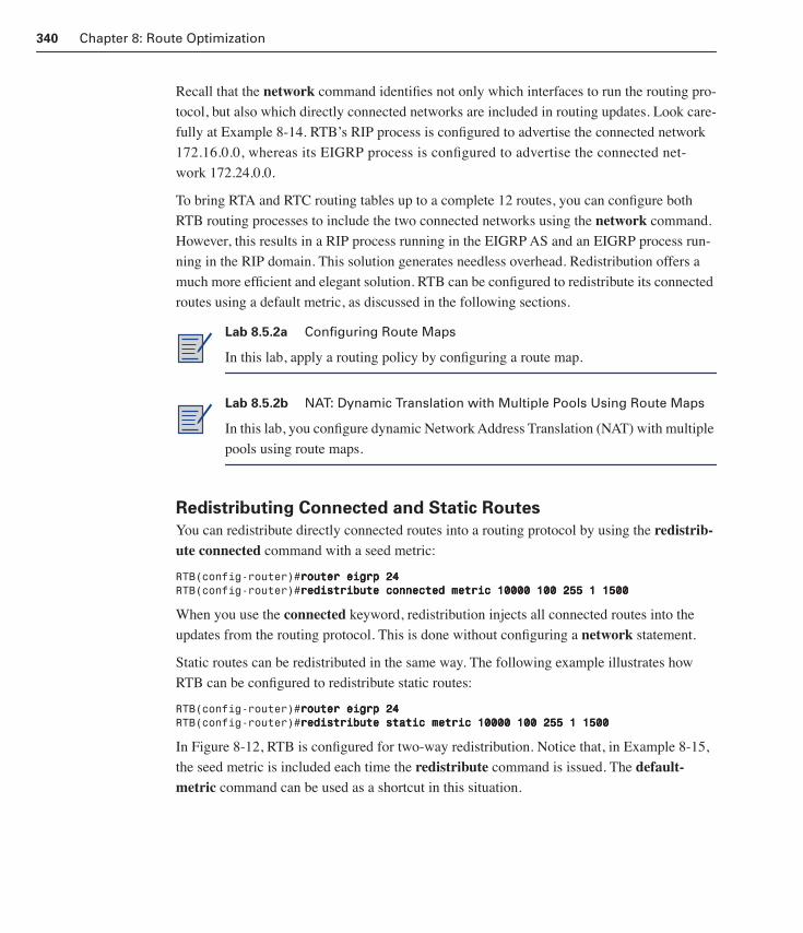
340 Chapter 8: Route Optimization
Recall that the network command identifies not only which interfaces to run the routing pro-
tocol, but also which directly connected networks are included in routing updates. Look care-
fully at Example 8-14. RTB’s RIP process is configured to advertise the connected network
172.16.0.0, whereas its EIGRP process is configured to advertise the connected net-
work 172.24.0.0.
To bring RTA and RTC routing tables up to a complete 12 routes, you can configure both
RTB routing processes to include the two connected networks using the network command.
However, this results in a RIP process running in the EIGRP AS and an EIGRP process run-
ning in the RIP domain. This solution generates needless overhead. Redistribution offers a
much more efficient and elegant solution. RTB can be configured to redistribute its connected
routes using a default metric, as discussed in the following sections.
Redistributing Connected and Static Routes
You can redistribute directly connected routes into a routing protocol by using the redistrib-ute connected command with a seed metric:
RTB(config-router)#rrrroooouuuutttteeeerrrr eeeeiiiiggggrrrrpppp 22224444RTB(config-router)#rrrreeeeddddiiiissssttttrrrriiiibbbbuuuutttteeee ccccoooonnnnnnnneeeecccctttteeeedddd mmmmeeeettttrrrriiiicccc 11110000000000000000 111100000000 222255555555 1111 1111555500000000
When you use the connected keyword, redistribution injects all connected routes into the
updates from the routing protocol. This is done without configuring a network statement.
Static routes can be redistributed in the same way. The following example illustrates how
RTB can be configured to redistribute static routes:
RTB(config-router)#rrrroooouuuutttteeeerrrr eeeeiiiiggggrrrrpppp 22224444RTB(config-router)#rrrreeeeddddiiiissssttttrrrriiiibbbbuuuutttteeee ssssttttaaaattttiiiicccc mmmmeeeettttrrrriiiicccc 11110000000000000000 111100000000 222255555555 1111 1111555500000000
In Figure 8-12, RTB is configured for two-way redistribution. Notice that, in Example 8-15,
the seed metric is included each time the redistribute command is issued. The default-metric command can be used as a shortcut in this situation.
Lab 8.5.2a Configuring Route Maps
In this lab, apply a routing policy by configuring a route map.
Lab 8.5.2b NAT: Dynamic Translation with Multiple Pools Using Route Maps
In this lab, you configure dynamic Network Address Translation (NAT) with multiple
pools using route maps.
1358_fmi.book Page 340 Thursday, May 27, 2004 2:21 PM
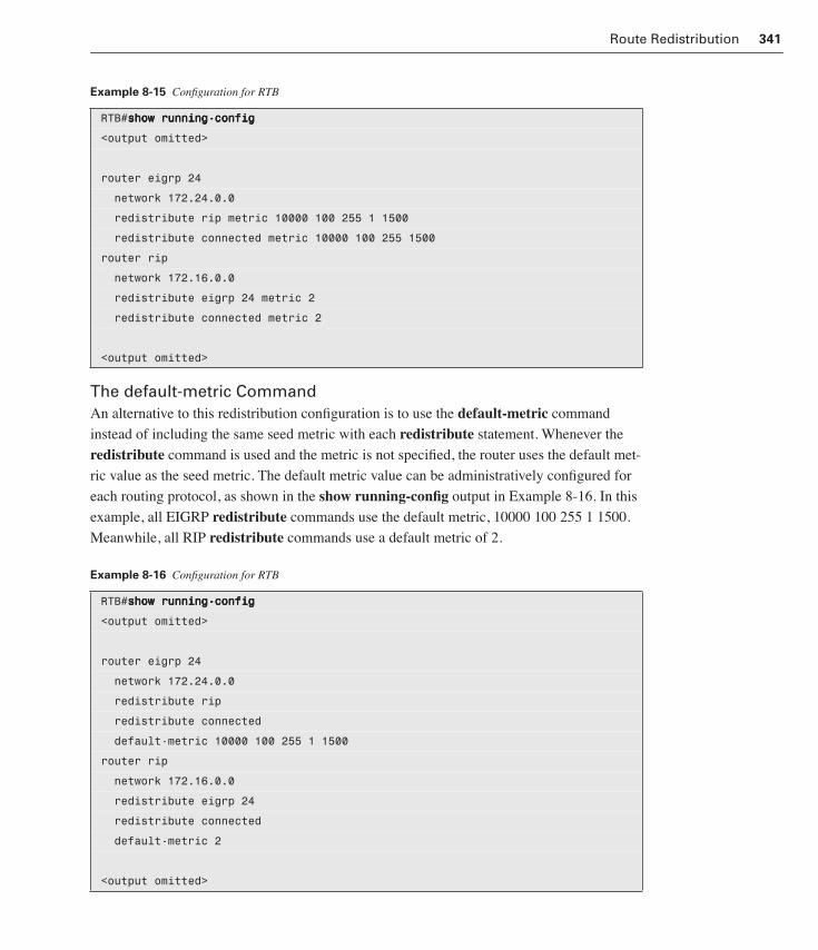
Route Redistribution 341
The default-metric CommandAn alternative to this redistribution configuration is to use the default-metric command
instead of including the same seed metric with each redistribute statement. Whenever the
redistribute command is used and the metric is not specified, the router uses the default met-
ric value as the seed metric. The default metric value can be administratively configured for
each routing protocol, as shown in the show running-config output in Example 8-16. In this
example, all EIGRP redistribute commands use the default metric, 10000 100 255 1 1500.
Meanwhile, all RIP redistribute commands use a default metric of 2.
Example 8-15 Configuration for RTB
RTB#sssshhhhoooowwww rrrruuuunnnnnnnniiiinnnngggg----ccccoooonnnnffffiiiigggg
<output omitted>
router eigrp 24
network 172.24.0.0
redistribute rip metric 10000 100 255 1 1500
redistribute connected metric 10000 100 255 1500
router rip
network 172.16.0.0
redistribute eigrp 24 metric 2
redistribute connected metric 2
<output omitted>
Example 8-16 Configuration for RTB
RTB#sssshhhhoooowwww rrrruuuunnnnnnnniiiinnnngggg----ccccoooonnnnffffiiiigggg
<output omitted>
router eigrp 24
network 172.24.0.0
redistribute rip
redistribute connected
default-metric 10000 100 255 1 1500
router rip
network 172.16.0.0
redistribute eigrp 24
redistribute connected
default-metric 2
<output omitted>
1358_fmi.book Page 341 Thursday, May 27, 2004 2:21 PM

342 Chapter 8: Route Optimization
Verifying Redistribution Operation
The commands shown in Example 8-17 are used to verify the route redistribution operation,
as shown in Figure 8-13. Example 8-17 shows the running configurations of the two routers
shown in Figure 8-13.
Figure 8-53 Redistribution Operation
Lab 8.5.3 Redistributing RIP and OSPF with Distribution Lists
In this lab, you configure mutual redistribution between RIPv1 and OSPF.
Example 8-17 Verifying Redistribution Operation
RouterC#sssshhhhoooowwww rrrruuuunnnnnnnniiiinnnngggg----ccccoooonnnnffffiiiigggg
interface Ethernet 0
ip address 203.250.14.2 255.255.255.0
interface Serial 1
ip address 203.250.15.1 255.255.255.252
router ospf 10
redistribute static metric 50 subnets
network 203.250.15.0 0.0.0.255 area 0
network 203.250.14.0 0.0.0.255
ip route 16.16.16.0 255.255.255.0 Ethernet 0
ip route 128.213.0.0 255.255.0.0 Ethernet 0
RouterE#sssshhhhoooowwww rrrruuuunnnnnnnniiiinnnngggg----ccccoooonnnnffffiiiigggg
interface Serial 0
ip address 203.250.15.2 255.255.255.252
router ospf 10
network 203.250.15.0 0.0.0.255 area 0
RTEE0
203.250.14.2
.1.2
S1S0
203.250.15.0/24
Area 0
16.16.16.0/24128.213.0.0/16
RTC
1358_fmi.book Page 342 Thursday, May 27, 2004 2:21 PM

Redistribution Example 343
The following list provides some rules to follow when verifying route redistribution operation:
■ Know the network topology, particularly where redundant routes exist.
■ Display the routing table of the appropriate routing protocol on a variety of routers in
the internetwork using the show ip route command. For example, check the routing
table on the Autonomous System Boundary Router (ASBR) as well as some of the
internal routers in each AS.
■ Perform a traceroute on some of the routes that go across the autonomous systems to
verify that the shortest path is being used for routing. Make sure that traces and
extended pings are performed on networks where redundant routes exist.
■ If you encounter routing problems, use traceroute and debug commands to observe
the routing update traffic on the ASBRs and internal routers.
Redistribution ExampleThis section presents a case study that addresses the issues associated with integrating RIP
with OSPF. Complex internetworks typically include UNIX hosts and legacy routers, neither
of which is likely to support OSPF. Because of this, most OSPF internetworks must also use
RIP in select areas. This case study provides examples of how to complete the following
phases of redistributing information between RIP and OSPF networks:
Phase 1: Configuring a RIP network
Phase 2: Adding OSPF to the core of a RIP network
Phase 3: Adding OSPF areas
Phase 1: Configuring a RIP Network
Figure 8-14 illustrates the RIP network. Three sites are connected with serial lines.
This RIP network uses a Class B address, 172.16.0.0, and a 24-bit subnet mask. All three
routers are connected to the same major network, so each is configured with the network 172.16.0.0 command.
Phase 2: Adding OSPF to the Core of a RIP Network
A common first step in migrating a RIP network to an OSPF network is to configure back-
bone routers that run both RIP and OSPF. This is while the remaining network devices run
RIP. These backbone routers act as OSPF ASBRs. Each ASBR controls the flow of routing
information between OSPF and RIP. In Figure 8-15, Router A, Router B, and Router C now
act as ASBRs.
1358_fmi.book Page 343 Thursday, May 27, 2004 2:21 PM

344 Chapter 8: Route Optimization
Figure 8-54 Typical RIP Network
Figure 8-55 RIP with an OSPF Center
Because RIP does not need to run between the backbone routers, updates can be suppressed
using the passive-interface command. Although Example 8-18 specifies RTA, the same com-
mands can be entered on the other routers.
172.16.9.1255.255.255.0
172.16.8.1255.255.255.0
To0
172.16.62.1255.255.255.0
172.16.62.2255.255.255.0
172.16.63.1255.255.255.0
172.16.64.2255.255.255.0
172.16.63.3255.255.255.0
172.16.64.3255.255.255.0
172.16.24.3255.255.255.0
172.16.17.2255.255.255.0
172.16.16.2255.255.255.0To0
RTA RTB
RTC
Site A Site B
Site C
TokenRing
TokenRing
E0S1
S0 E0S1
S0
E0
S1S0
172.16.9.1255.255.255.0
172.16.8.1255.255.255.0
To0
172.16.62.1255.255.255.0
172.16.62.2255.255.255.0
172.16.63.1255.255.255.0
172.16.64.2255.255.255.0
172.16.63.3255.255.255.0
172.16.64.3255.255.255.0
172.16.24.3255.255.255.0
172.16.17.2255.255.255.0
172.16.16.2255.255.255.0
To0RTA RTB
RTC
RIP
E0S1
S0 E0S1
S0
E0
S1S0
RIPautonomous system
OSPF
RIPautonomous system
autonomous system
TokenRing
TokenRing
1358_fmi.book Page 344 Thursday, May 27, 2004 2:21 PM
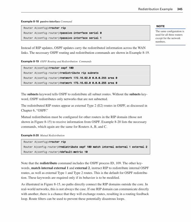
Redistribution Example 345
Instead of RIP updates, OSPF updates carry the redistributed information across the WAN
links. The necessary OSPF routing and redistribution commands are shown in Example 8-19.
The subnets keyword tells OSPF to redistribute all subnet routes. Without the subnets key-
word, OSPF redistributes only networks that are not subnetted.
The redistributed RIP routes appear as external Type 2 (E2) routes in OSPF, as discussed in
Chapter 6, “OSPF.”
Mutual redistribution must be configured for other routers in the RIP domain (those not
shown in Figure 8-15) to receive information from OSPF. Example 8-20 lists the necessary
commands, which again are the same for Routers A, B, and C.
Note that the redistribute command includes the OSPF process ID, 109. The other key-
words, match internal external 1 and external 2, instruct RIP to redistribute internal OSPF
routes, as well as external Type 1 and Type 2 routes. This is the default for OSPF redistribu-
tion. These keywords are required only if its behavior is to be modified.
As illustrated in Figure 8-15, no paths directly connect the RIP domains outside the core. In
real-world networks, this is not always the case. If one RIP domain can communicate directly
with another, there is a chance that they will exchange routes, resulting in a routing feedback
loop. Route filters can be used to prevent these potentially disastrous loops.
Example 8-18 passive-interface Command
Router A(config)#rrrroooouuuutttteeeerrrr rrrriiiipppp
Router A(config-router)#ppppaaaassssssssiiiivvvveeee----iiiinnnntttteeeerrrrffffaaaacccceeee sssseeeerrrriiiiaaaallll 0000
Router A(config-router)#ppppaaaassssssssiiiivvvveeee----iiiinnnntttteeeerrrrffffaaaacccceeee sssseeeerrrriiiiaaaallll 1111
Example 8-19 OSPF Routing and Redistribution Commands
Router A(config)#rrrroooouuuutttteeeerrrr oooossssppppffff 111100009999
Router A(config-router)#rrrreeeeddddiiiissssttttrrrriiiibbbbuuuutttteeee rrrriiiipppp ssssuuuubbbbnnnneeeettttssss
Router A(config-router)#nnnneeeettttwwwwoooorrrrkkkk 111177772222....11116666....66662222....0000 0000....0000....0000....222255555555 aaaarrrreeeeaaaa 0000
Router A(config-router)#nnnneeeettttwwwwoooorrrrkkkk 111177773333....11116666....66663333....0000 0000....0000....0000....222255555555 aaaarrrreeeeaaaa 0000
Example 8-20 Mutual Redistribution
Router A(config)#rrrroooouuuutttteeeerrrr rrrriiiipppp
Router A(config-router)#rrrreeeeddddiiiissssttttrrrriiiibbbbuuuutttteeee oooossssppppffff 111100009999 mmmmaaaattttcccchhhh iiiinnnntttteeeerrrrnnnnaaaallll eeeexxxxtttteeeerrrrnnnnaaaallll 1111 eeeexxxxtttteeeerrrrnnnnaaaallll 2222
Router A(config-router)#ddddeeeeffffaaaauuuulllltttt----mmmmeeeettttrrrriiiicccc 11110000
NOTE
The same configuration is used for all three routers except for the network numbers.
1358_fmi.book Page 345 Thursday, May 27, 2004 2:21 PM

346 Chapter 8: Route Optimization
The configuration shown in Example 8-21 allows the OSPF process on RTA to redistribute
RIP information, only for networks 172.16.8.0 through 172.16.15.0.
These commands prevent RTA from advertising networks in other RIP domains onto the
OSPF backbone. This prevents other boundary routers from using false information and
forming a loop. When an OSPF backbone area is in place, the RIP domains can easily be con-
verted into OSPF areas.
Phase 3: Adding OSPF Areas
Each RIP domain can be converted into an OSPF area independently of the other RIP
domains. This allows the migration of one section of the internetwork at a time if desired.
When all three of the RIP domains have become OSPF areas, the three core routers serve as
ABRs, as shown in Figure 8-16. Recall that ABRs control the exchange of routing informa-
tion between OSPF areas and the OSPF backbone. Each ABR keeps a detailed record of the
topology of its area and summarizes this information in its updates to other backbone routers.
Figure 8-56 Route Summarization Between OSPF Areas
Example 8-21 Redistributing RIP Information
Router A(config)#rrrroooouuuutttteeeerrrr oooossssppppffff 111100009999
Router A(config-router)#rrrreeeeddddiiiissssttttrrrriiiibbbbuuuutttteeee rrrriiiipppp ssssuuuubbbbnnnneeeettttssss
Router A(config-router)#ddddiiiissssttttrrrriiiibbbbuuuutttteeee----lllliiiisssstttt 11111111 iiiinnnn rrrriiiipppp
Router A(config)#aaaacccccccceeeessssssss----lllliiiisssstttt 11111111 ppppeeeerrrrmmmmiiiitttt 111177772222....11116666....8888....0000 0000....0000....7777....222255555555
Router A(config)#aaaacccccccceeeessssssss----lllliiiisssstttt 11111111 ddddeeeennnnyyyy 0000....0000....0000....0000 222255555555....222255555555....222255555555....222255555555
172.16.9.1255.255.255.0
172.16.8.1255.255.255.0
172.16.62.1255.255.255.248
172.16.62.2255.255.255.248
172.16.63.1255.255.255.248
172.16.64.2255.255.255.248
172.16.63.3255.255.255.248
172.16.64.3255.255.255.248
172.16.24.3255.255.255.0
172.16.17.2255.255.255.0
172.16.16.2255.255.255.0
Router A Router B
Router C
Area BorderRouter
E0S1
S0 E0S1
S0
E0
S1S0
Area 2
To00 x2 To00 x2
Area 0
Area 1 Area 3
Area BorderRouter
Area BorderRouter
1358_fmi.book Page 346 Thursday, May 27, 2004 2:21 PM

Redistribution Example 347
Notice that Figure 8-16 also presents a new addressing scheme in the core. A 29-bit mask,
255.255.255.248, is used to address WAN links and conserve address space. Meanwhile, a
24-bit mask remains on the LAN interfaces, resulting in variable-length subnet masks
(VLSM). OSPF fully supports VLSM, but RIPv1 does not. With OSPF as the sole routing
protocol, the network can now make the most of the advantages of VLSM. Example 8-22
shows the commands necessary to configure Router A for OSPF operation on all interfaces,
with the appropriate masks.
Because OSPF is classless, each ABR can be configured to use route summarization. For
example, Router A connects to eight networks, which occupy a contiguous address space.
Therefore, this ABR can be configured as follows to send a single supernet route, which
advertises all eight of the networks:
Router A(config)#rrrroooouuuutttteeeerrrr oooossssppppffff 111100009999Router A(config-router)#aaaarrrreeeeaaaa 1111 rrrraaaannnnggggeeee 111177772222....11116666....8888....0000 222255555555....222255555555....222244448888....0000
Router A advertises one route, 172.16.8.0 255.255.248.0, which covers all subnets in Area 1
into Area 0. Without the range keyword in the area command, Router A would advertise
each subnet individually, such as one route for 172.16.8.0 255.255.248.0, one route for
172.16.9.0 255.255.248.0, and so forth. The migration of the network from RIP to OSPF is
now complete, and redistribution is no longer necessary.
Example 8-22 Router A Configuration for OSPF Operation on All Interfaces
Router A(config)#rrrroooouuuutttteeeerrrr oooossssppppffff 111100009999
Router A(config-router)#nnnneeeettttwwwwoooorrrrkkkk 111177772222....11116666....66662222....0000 0000....0000....0000....7777 aaaarrrreeeeaaaa 0000
Router A(config-router)#nnnneeeettttwwwwoooorrrrkkkk 111177772222....11116666....66663333....0000 0000....0000....0000....7777 aaaarrrreeeeaaaa 0000
Router A(config-router)#nnnneeeettttwwwwoooorrrrkkkk 111177772222....11116666....8888....0000 0000....0000....0000....222255555555 aaaarrrreeeeaaaa 1111
Router A(config-router)#nnnneeeettttwwwwoooorrrrkkkk 111177772222....11116666....9999....0000 0000....0000....0000....222255555555 aaaarrrreeeeaaaa 1111
Lab 8.6.1 Route Optimization Challenge Lab
In this challenge lab, you create and optimize a network using RIPv2 and OSPF.
1358_fmi.book Page 347 Thursday, May 27, 2004 2:21 PM
348 Chapter 8: Route Optimization
SummaryThis chapter demonstrated several ways to control routing update traffic, including passive
interface, default routes, static routes, and route filtering. The chapter also clarified that route
redistribution enables the exchange of routing information between dissimilar routing proto-
cols and requires some care when configuring. Redistribution is when boundary routers con-
necting different autonomous systems exchange and advertise routing information received
from one autonomous system to the other autonomous system.
In the next chapter, you will learn how to connect an enterprise network to an Internet service
provider (ISP).
1358_fmi.book Page 348 Thursday, May 27, 2004 2:21 PM
Key Terms 349
Key Termsadministrative distance A rating of the trustworthiness of a routing information source. In
Cisco routers, administrative distance is expressed as a numeric value between 0 and 255.
The higher the value, the lower the trustworthiness rating.
autonomous system A collection of networks under a common administration sharing a
common routing strategy. Autonomous systems are subdivided by areas. An autonomous sys-
tem must be assigned a unique 16-bit number by the IANA. Sometimes abbreviated as AS.
exterior gateway protocol (EGP) Any internetwork protocol used to exchange routing
information between autonomous systems. Not to be confused with Exterior Gateway Proto-
col (EGP), which is a particular instance of an exterior gateway protocol.
keepalive message A message sent by one network device to inform another network
device that the virtual circuit between the two is still active.
passive interface A passive interface receives updates but does not send them. It is used to
control routing updates. The passive-interface command can be used with all IP interior
gateway protocols—RIP, IGRP, EIGRP, OSPF, and IS-IS.
policy routing A routing scheme that forwards packets to interfaces based on user-config-
ured policies. Such policies might specify that traffic sent from a particular network should be
forwarded out one interface, while all other traffic should be forwarded out another interface.
route redistribution Allowing routing information discovered through one routing protocol
to be distributed in the update messages of another routing protocol.
1358_fmi.book Page 349 Thursday, May 27, 2004 2:21 PM

350 Chapter 8: Route Optimization
Check Your UnderstandingComplete all of the review questions to test your understanding of the topics and concepts in
this chapter. The answers appear in Appendix B, “Answers to the Check Your Understanding
Questions.”
For additional, more in-depth questions, refer to the chapter-specific study guides on the
companion CD-ROM.
1. What method is used to prevent a routing update from being sent out of a router inter-face?
A. Redistribution
B. Summarization
C. Passive interface
D. Gateway of last resort
2. What address does a router advertise for a default route?
A. 255.255.255.255
B. 0.0.0.0
C. 255.255.0.0
D. 1.1.1.1
3. What is the default administrative distance for the OSPF routing protocol?
A. 1
B. 90
C. 110
D. 120
4. What command imports static routes into routing protocol advertisements?
A. redistribute static
B. distribute-list
C. passive-interface
D. route-map
5. What command uses match statements to create a routing policy?
A. auto summary
B. distribute-list
C. access-list
D. route-map
1358_fmi.book Page 350 Thursday, May 27, 2004 2:21 PM

Check Your Understanding 351
6. What command establishes which route a router sends or receives in updates?
A. access-list
B. network
C. passive-interface
D. distribute-list
7. What command modifies the administrative distance for all OSPF routes?
A. distance 95
B. admin distance 110
C. distance 110
D. admin distance 95
8. Which of the following is a consideration when implementing redistribution?
A. Incompatible routing tables
B. Routing feedback (loops)
C. Overlap routing protocols
D. Two-way redistribution with multiple boundary routers
9. Which administrative distance represents the most reliable protocol?
A. 5
B. 90
C. 120
D. 200
10. Which IP interior gateway protocols support passive interface?
A. RIP, IGRP, EIGRP, and BGP
B. RIP, IGRP, EIGRP, IS-IS, and IPX
C. RIP, IGRP, EIGRP, OSPF, and IPX
D. RIP, IGRP, EIGRP, OSPF, and IS-IS
11. What does the router use to make a decision when it has learned two or more routes to the same destination from multiple routing protocols?
A. Hop count
B. Administrative distance
C. Metric
D. Route summarization
1358_fmi.book Page 351 Thursday, May 27, 2004 2:21 PM

ObjectivesUpon completing this chapter, you will be able to
■ Describe autonomous systems
■ Describe basic BGP operation
■ Configure IBGP and EBGP
■ Monitor BGP operation
■ Understand the BGP routing process
■ Identify and configure BGP attributes
■ Describe the BGP decision process
■ Apply BGP route filtering and policy routing
■ Understand issues with redundancy, symmetry, and load balancing
■ Understand BGP redistribution
You can reinforce your understanding of the objectives covered in this chapter by opening
the interactive media activities on the CD accompanying this book and performing the lab
activities collected in the Cisco Networking Academy Program CCNP 1: Advanced Routing
Lab Companion. Throughout this chapter, you will see references to these activities by title
and by icon. They look like this:
Interactive Media Activity
Lab Activity
1358_fmi.book Page 352 Thursday, May 27, 2004 2:21 PM

Chapter 9
BGP
Routing protocols can be classified in many ways. It depends on where they are used in relation-
ship to the enterprise. Protocols that run inside an enterprise are called interior gateway proto-cols (IGPs). Examples of IGPs include RIP versions 1 and 2, IGRP, EIGRP, OSPF, and IS-IS.
Protocols that run outside an enterprise, or between autonomous systems, are called exterior gateway protocols (EGPs). Typically, EGPs are used to exchange routing information between
Internet service providers (ISPs) or, in some cases, between a customer’s autonomous system
and the provider’s network. Border Gateway Protocol version 4 (BGP4) is the most common
EGP and is considered the Internet standard.
This chapter provides an overview of the different types of autonomous systems and then
focuses on basic BGP operation, including BGP neighbor negotiation. This chapter also looks at
how to use the Cisco IOS software to configure BGP and verify its operation. Finally, this chap-
ter examines BGP peering and the BGP routing process.
Autonomous SystemsAn internetwork is a group of smaller, independent networks. Each of these smaller networks
may be owned and operated by a different organization. These organizations can include a com-
pany, a university, a government agency, or some other group. The Internet is one example of a
single, although immense, internetwork.
Overview of Autonomous Systems
The operators of these individual networks desire independence or self-administration over their
own systems. Because the routing and security policies of one organization might conflict with
the policies of another, internetworks are divided into domains or autonomous systems. Each AS
typically represents an independent organization and applies its own unique routing and security
1358_fmi.book Page 353 Thursday, May 27, 2004 2:21 PM
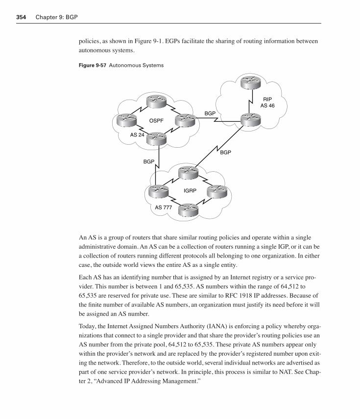
354 Chapter 9: BGP
policies, as shown in Figure 9-1. EGPs facilitate the sharing of routing information between
autonomous systems.
Figure 9-57 Autonomous Systems
An AS is a group of routers that share similar routing policies and operate within a single
administrative domain. An AS can be a collection of routers running a single IGP, or it can be
a collection of routers running different protocols all belonging to one organization. In either
case, the outside world views the entire AS as a single entity.
Each AS has an identifying number that is assigned by an Internet registry or a service pro-
vider. This number is between 1 and 65,535. AS numbers within the range of 64,512 to
65,535 are reserved for private use. These are similar to RFC 1918 IP addresses. Because of
the finite number of available AS numbers, an organization must justify its need before it will
be assigned an AS number.
Today, the Internet Assigned Numbers Authority (IANA) is enforcing a policy whereby orga-
nizations that connect to a single provider and that share the provider’s routing policies use an
AS number from the private pool, 64,512 to 65,535. These private AS numbers appear only
within the provider’s network and are replaced by the provider’s registered number upon exit-
ing the network. Therefore, to the outside world, several individual networks are advertised as
part of one service provider’s network. In principle, this process is similar to NAT. See Chap-
ter 2, “Advanced IP Addressing Management.”
IGRP
BGP
AS 777
OSPF
AS 24
BGP
BGP
RIPAS 46
1358_fmi.book Page 354 Thursday, May 27, 2004 2:21 PM
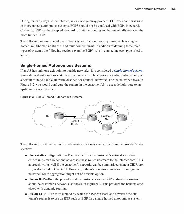
Autonomous Systems 355
During the early days of the Internet, an exterior gateway protocol, EGP version 3, was used
to interconnect autonomous systems. EGP3 should not be confused with EGPs in general.
Currently, BGP4 is the accepted standard for Internet routing and has essentially replaced the
more limited EGP3.
The following sections detail the different types of autonomous systems, such as single-
homed, multihomed nontransit, and multihomed transit. In addition to defining these three
types of systems, the following sections examine BGP’s role in connecting each type of AS to
an ISP.
Single-Homed Autonomous Systems
If an AS has only one exit point to outside networks, it is considered a single-homed system.
Single-homed autonomous systems are often called stub networks or stubs. Stubs can rely on
a default route to handle all traffic destined for nonlocal networks. For the network shown in
Figure 9-2, you would configure the routers in the customer AS to use a default route to an
upstream service provider.
Figure 9-58 Single-Homed Autonomous Systems
The following are three methods to advertise a customer’s networks from the provider’s per-
spective:
■ Use a static configuration—The provider lists the customer’s networks as static
entries in its own router and advertises these routes upstream to the Internet core. This
approach works well if the customer’s networks can be summarized using a CIDR pre-
fix, as discussed in Chapter 2. However, if the AS contains numerous discontiguous
networks, route aggregation might not be a viable option.
■ Use an IGP—Both the provider and the customers use an IGP to share information
about the customer’s networks, as shown in Figure 9-3. This provides the benefits asso-
ciated with dynamic routing.
■ Use an EGP—The third method by which the ISP can learn and advertise the cus-
tomer’s routes is to use an EGP such as BGP. In a single-homed autonomous system,
ISP CustomerNet
DefaultRoute
1358_fmi.book Page 355 Thursday, May 27, 2004 2:21 PM

356 Chapter 9: BGP
the customer’s routing policies are an extension of the provider’s policies. For this rea-
son, the Internet number registries are unlikely to assign an AS number. Instead, the
provider can give the customer an AS number from the private pool of AS numbers,
64,512 to 65,535, as shown in Figure 9-4. The provider strips these numbers when
advertising the customer’s routes toward the core of the Internet.
Figure 9-59 IGP with the ISP
Figure 9-60 BGP with the ISP
Notice that only the final solution requires the customers to enable BGP on their AS boundary
router.
Multihomed Nontransit Autonomous Systems
An AS is a multihomed system if it has more than one exit point to outside networks. An AS
connected to the Internet can be multihomed to a single provider or multiple providers. A
nontransit AS does not allow transit traffic to pass through it. Transit traffic is any traffic that
has a source and destination outside the AS. Figure 9-5 illustrates a multihomed and nontran-
sit AS, shown as AS 24, which is connected to two providers, ISP1 and ISP2.
ISP CustomerNet
OSPFRoutes
OSPF OSPF
OSPF OSPF
Advertising thesedynamically learned customer
networks to upstreamInternet routers.
ISPAS 2446
AS 65001
BGP
OSPF OSPF
OSPF OSPF
1358_fmi.book Page 356 Thursday, May 27, 2004 2:21 PM

Autonomous Systems 357
Figure 9-61 Multihomed Nontransit Autonomous Systems
A nontransit AS advertises only its own routes to both providers to which it connects. It does
not advertise routes it learned from one provider to another provider. This ensures that ISP 1
does not use AS 24 to reach destinations that belong to ISP 2 and that ISP 2 does not use AS
24 to reach destinations that belong to ISP 1. Of course, ISP 1 or ISP 2 can force traffic to be
directed to AS 24 by way of default or static routing. As a precaution against this, the router at
the border of AS 24 can filter incoming traffic to prevent transit traffic from passing through
its border router.
Multihomed nontransit autonomous systems do not really need to run BGP4 with their pro-
viders; however, ISPs usually recommend it and often require it. As you will see later in this
chapter, BGP4 offers numerous advantages, including increased control of route propagation
and filtering.
Multihomed Transit Autonomous Systems
A multihomed transit system has more than one connection to the outside world and can be
used for transit traffic by other autonomous systems. The multihomed AS views transit traffic
as any traffic originating from outside sources bound for outside destinations, as shown in
Figure 9-6.
A transit AS can route transit traffic by running BGP internally so that multiple border routers
in the same AS can share BGP information. Additional routers may be used to forward BGP
information from one border router to another. BGP can be run inside an AS to facilitate this
exchange.
AS 24
BGP
ISP 1 ISP 2
BGP
RTD
1358_fmi.book Page 357 Thursday, May 27, 2004 2:21 PM

358 Chapter 9: BGP
Figure 9-62 Multihomed Transit Autonomous Systems
When BGP is running inside an AS, it is called Internal BGP (IBGP). When BGP runs
between autonomous systems, it is called External BGP (EBGP). If the role of a BGP router
is to route IBGP traffic, it is called a transit router, as with RTA, RTB, and RTC in Figure 9-6.
Routers that sit on the boundary of an AS and that use EBGP to exchange information with
the ISP are called border or edge routers.
When Not to Use BGP
In many cases, the routing policy that is implemented in an AS is consistent with the policy
for the ISP. In these cases, it is not necessary, or even desirable, to use BGP to exchange rout-
ing information with the ISP. Instead, connectivity can be achieved through a combination of
static routes and default routes.
Do not use BGP within the AS in the following situations:
■ There is only a single connection to the Internet or the other AS.
■ The Internet routing policy and route selection are not of concern to the AS.
■ The BGP routers have insufficient RAM or processor power to handle constant updates.
■ You have a limited understanding of route filtering and the BGP path-selection process.
■ There is a low-bandwidth link between autonomous systems.
In Figure 9-7, Router A advertises a default network into the AS through a local IGP, such as
RIP. A static route affords connectivity through Router B to the AS for the ISP. The ISP is
running BGP and is recognized by other BGP routers on the Internet.
AS 24
EBGP
IBGP IBGP
ISP 1 ISP 2
EBGP
RTD
RTA
RTB
RTC Transit Routers:RTA, RTB, and RTC
RTD
NOTE
In general, when there are different policy require-ments than those of the ISP, it is necessary to use BGP to connect to an ISP.
1358_fmi.book Page 358 Thursday, May 27, 2004 2:21 PM

Basic BGP Operation 359
Figure 9-63 When Not to Use BGP
Basic BGP OperationBGP was most recently defined in RFC 1772. BGP’s function is to exchange routing infor-
mation between autonomous systems and guarantee the selection of a loop-free path. BGP4
is the first version of BGP that supports CIDR and route aggregation. Common IGPs such as
RIP, OSPF, and EIGRP use technical metrics. BGP does not use technical metrics. Instead, it
makes routing decisions based on network policies or rules.
This section offers a brief overview of how BGP works. It is followed by a more detailed
examination of the various types of BGP packets and relationship states.
BGP Routing Updates
BGP updates are carried using TCP on port 179. In contrast, RIP updates use UDP port 520,
whereas OSPF does not use a Layer 4 protocol. Because BGP requires TCP, IP connectivity
must exist between BGP peers. TCP connections must also be negotiated between them
before updates can be exchanged. Therefore, BGP inherits those reliable, connection-oriented
properties from TCP.
To guarantee loop-free path selection, BGP constructs a graph of autonomous systems based
on the information exchanged between BGP neighbors. BGP views the whole internetwork
as a graph, or tree, of autonomous systems. The connection between any two systems forms a
path. The collection of path information is expressed as a sequence of AS numbers called the
AS Path, as shown in Figure 9-8. This sequence forms a route to reach a specific destination.
Interactive Media Activity Point and Click: When to Use BGP and When Not to Use BGP
After completing this activity, you will be able to decide when to use BGP and when
not to use BGP.
Static
Default Route
Advertise DefaultNetwork by Way of IGP
NetworkNumberISP Runs
BGP CA B
1358_fmi.book Page 359 Thursday, May 27, 2004 2:21 PM

360 Chapter 9: BGP
Figure 9-64 AS Path
BGP Neighbors
When two routers establish a TCP-enabled BGP connection, they are called neighbors or
peers. Each router running BGP is called a BGP speaker. Peer routers exchange multiple
messages to open and confirm the connection parameters, such as the version of BGP to be
used. If there are any disagreements between the peers, notification errors are sent, and the
connection fails.
When BGP neighbors first establish a connection, they exchange all candidate BGP routes, as
shown in Figure 9-9. After this initial exchange, incremental updates are sent as network
information changes, as shown in Figure 9-10. As discussed in earlier chapters, incremental
updates are more efficient than complete table updates. This is especially true with BGP rout-
ers, which might contain the complete Internet routing table.
Figure 9-65 How BGP Works
Figure 9-66 How BGP Works
AS 200
AS 300 AS 100
AS 400
AS 500
AS Path500, 100, 200, 300, 400
Lo0 1.1.1.1 Lo0 2.2.2.2
Establish a NeighboringSession With 2.2.2.2
Establish a NeighboringSession With 1.1.1.1
Net 6.0.0.0/8Net 7.0.0.0/8
Net 4.0.0.0/8Net 5.0.0.0/8Net 4.0.0.0/8
Net 5.0.0.0/8Net 6.0.0.0/8Net 7.0.0.0/8
Net 6.0.0.0/8Net 7.0.0.0/8Net 4.0.0.0/8Net 5.0.0.0/8
1358_fmi.book Page 360 Thursday, May 27, 2004 2:21 PM

Basic BGP Operation 361
Peers advertise destinations that can be reached through them by using update messages.
These messages contain route prefix, AS path, path attributes (such as the degree of prefer-
ence for a particular route), and other properties.
The information for network reachability can change, such as when a route becomes unreach-
able or a better path becomes available. BGP informs its neighbors of this by withdrawing the
invalid routes and injecting the new routing information, as shown in Figure 9-11. Withdrawn
routes are part of the update message. BGP routers keep a table version number that tracks
the version of the BGP routing table received from each peer. If the table changes, BGP incre-
ments the table version number. A rapidly incrementing table version usually indicates insta-
bilities in the network or a misconfiguration.
Figure 9-67 How BGP Works
If there are no routing changes to transmit to a peer, a BGP speaker periodically sends keep-
alive messages to maintain the connection. These 19-byte keepalive packets are sent every 60
seconds by default. These packets present a negligible drain on bandwidth and the CPU time
on a router.
BGP Message Types
Different message types play an essential role in BGP operation. Each message type includes
the BGP message header.
The message header contains only three fields—a 16-byte Marker field, a 2-byte Length field,
and a 1-byte Type field.
The Marker field is used either to authenticate incoming BGP messages or to detect loss of
synchronization between two BGP peers.
The Length field indicates the total BGP message length, including the header. The smallest
BGP message is 19 bytes, 16 + 2 + 1, and the largest possible message is 4096 bytes.
The Type field can have four values, 1 to 4. Each of these values corresponds to one of the
four BGP message types:
■ Open message—Establishes connections with peers. Includes fields for the BGP ver-
sion number, the AS number, hold time, and Router ID.
Withdraw 4.0.0.0/8Net 4.0.0.0/8Net 5.0.0.0/8Net 6.0.0.0/8Net 7.0.0.0/8
Net 6.0.0.0/8Net 7.0.0.0/8Net 4.0.0.0/8Net 5.0.0.0/8
1358_fmi.book Page 361 Thursday, May 27, 2004 2:21 PM

362 Chapter 9: BGP
■ Keepalive message—This message type is sent periodically between peers to maintain
connections and verify paths held by the router sending the keepalive. If the periodic
timer is set to a value of 0, no keepalives are sent. The recommended keepalive interval
is one-third of the hold time interval. The keepalive message is a 19-byte BGP message
header with no data following it.
■ Notification message—This message type is used to inform the receiving router of
errors. This message includes a field for error codes, shown in Table 9-1, which can be
used to troubleshoot BGP connections.
■ Update message—The update message contains all of the information BGP uses to
construct a loop-free picture of the internetwork. It has three basic components: Net-
work Layer Reachability Information (NLRI), path attributes, and withdrawn routes.
These three elements are described briefly in the following sections.
Table 9-9 Notification Message Error Codes
Error Code
1 Message Header Error 1 Connection Not Synchronized2 Bad Message Length3 Bad Message Type
2 OPEN Message Error 1 Unsupported Version Number2 Bad Peer AS3 Bad BGP Identifier4 Unsupported Optional Parameter5 Authentication Failure6 Unacceptable Hold Time
3 UPDATE Message Error 1 Malformed Attribute List2 Unrecognized Well-Known Attribute3 Missing Well-Known Attribute4 Attribute Flags Error5 Attribute Length Error6 Invalid Origin Attribute7 AS Routing Loop8 Invalid NEXT_HOP Attribute9 Optional Attribute Error10 Invalid Network Field11 Malformed AS_path
4 Hold Timer Expired 0 Unspecific
5 Finite State Machine Error (for errors detected by the FSM)
0 Unspecific
6 Cease (for fatal errors besides the ones already listed)
0 Unspecific
1358_fmi.book Page 362 Thursday, May 27, 2004 2:21 PM

Basic BGP Operation 363
BGP Neighbor Negotiation
The BGP neighbor negotiation process proceeds through various states, or stages, which can
be described in terms of a finite-state machine (FSM).
The BGP FSMRecall that FSM was defined in Chapter 5, “EIGRP.” An FSM is a set of possible states that
something can go through, what events cause those states, and what events result from those
states. Figure 9-12 shows the BGP FSM, including these states and some of the message
events that cause them.
Figure 9-68 BGP FSM
The six states of the BGP FSM are as follows:
■ Idle—Idle is the first state of a BGP connection. BGP is waiting for a start event. It is
normally initiated by an administrator or a network event. At the start event, BGP ini-
tializes its resources and resets a connect retry timer. Then it starts listening for a TCP
notice that BGP can transition back to Idle from any other state in case of errors. The
Interactive Media Activity Drag and Drop: BGP Message Type
After completing this activity, you will be able to identify the properties of BGP
message types.
Active Connect
Open Sent Idle
OpenConfirm
Established
1
23
4
5
6
OpenOpen
KeepaliveNotification
KeepaliveUpdate
1358_fmi.book Page 363 Thursday, May 27, 2004 2:21 PM

364 Chapter 9: BGP
router starts its own transport connection to other BGP peers and listens for the peer’s
connection.
■ Connect—In the Connect state, BGP waits for the TCP connection to be completed. If
the TCP connection is successful, the state transitions to OpenSent. If the TCP connec-
tion fails, the state transitions to the Active state, and the router tries to connect again. If
the connect retry timer expires, the state remains in the Connect state, the timer is reset,
and a TCP connection is initiated. In case of any other event, initiated by the system or
the administrator, the state returns to Idle.
■ Active—In the Active state, BGP tries to acquire a peer by initiating a TCP connection.
If it is successful, it transitions to OpenSent. If the connect retry timer expires, BGP
restarts the connect timer and returns to the Connect state. While active, BGP still lis-
tens for a connection that may be initiated from another peer. The state might go back
to Idle in case of other events, such as a stop event initiated by the system or the opera-
tor. When the ConnectRetry time expires, the router initiates a transport connection to
the other peer.
In general, a neighbor state that switches between Connect and Active indicates that
something is wrong and that there are problems with the TCP connection. It could be
because of many TCP retransmissions or the incapability of a neighbor to reach its peer’s
IP address.
■ OpenSent—In the OpenSent state, BGP waits for an open message from its peer. The
open message is checked for correctness. In case of errors, such as an incompatible ver-
sion number or an unacceptable AS, the system sends an error notification message and
goes back to idle. If there are no errors, BGP starts sending keepalive messages and
resets the keepalive timer. At this stage, the hold time is negotiated, and the smaller
value is taken. If the negotiated hold time is 0, the hold timer and the keepalive timer
are not restarted.
At the OpenSent state, BGP recognizes whether the peer belongs to the same AS or to a
different AS. BGP does this by comparing its AS number to its peer’s AS number. A
same AS is an IBGP peer, and a different AS is an EBGP peer.
When a TCP disconnect is detected, the state falls back to Active. For any other errors,
such as an expiration of the hold timer, BGP sends a notification message with the
corresponding error code. Then it returns to the Idle state.
■ OpenConfirm—While in OpenConfirm state, BGP waits for a keepalive or notifica-
tion message. If a keepalive message is received, the state goes to the Established state,
and the neighbor negotiation is complete. If the system receives an update or keepalive
message, it restarts the hold time, assuming that the negotiated hold time is not 0. If a
notification message is received, the state falls back to Idle. The system sends periodic
1358_fmi.book Page 364 Thursday, May 27, 2004 2:21 PM

Basic BGP Operation 365
keepalive messages at the rate set by the keepalive timer. In the case of any TCP dis-
connect or in response to any stop event, initiated by the system or the administrator,
the state returns to Idle. In response to any other event, the system sends a notification
message with an FSM error code and returns to the Idle state.
■ Established—Established is the final state in the neighbor negotiation. BGP starts
exchanging update packets with its peers. If it is nonzero, the hold timer is restarted at
the receipt of an update or keepalive message.
Each update message is checked for errors, such as missing or duplicate attributes. If
errors are found, a notification is sent to the peer. Any notification received while in the
Established state causes the BGP process to drop the receiving peer back to Idle. If
the hold timer expires, a disconnect notification is received from TCP. If a stop event is
received, the system returns to Idle.
Network Layer Reachability Information
Rather than advertise reachable destinations as a network and subnet mask, BGP advertises
them using Network Layer Reachability Information (NLRI), which consists of prefixes and
prefix lengths. The prefix represents the reachable destination, and the prefix length repre-
sents the number of bits set in the subnet mask. For example, 10.1.1.0 255.255.255.0 has a
prefix of 10.1.1.0 and a prefix length of 24.
The NLRI consists of multiple instances of the two-tuple length, prefix. A tuple is a mathe-
matical term for a set of elements. In this case, two refers to the fact that the set has only two
elements. Therefore, the NLRI 19, 192.24.160.0 represents the prefix of 192.24.160.0, and
the length is a 19-bit mask. In decimal terms, this NLRI refers to the supernet 192.24.160.0
255.255.224.0.
Withdrawn RoutesWithdrawn routes provide a list of routing updates that are no longer reachable and that need
to be withdrawn or removed from the BGP routing table. Withdrawn routes have the same
format as NLRI.
An update message that has no NLRI or path attribute information is used to advertise only
routes to be withdrawn from service, as shown in Figure 9-11.
Interactive Media Activity Drag and Drop: BGP Neighbor Negotiation
After completing this activity, you will be able to understand the BGP process for
establishing neighbor relationships.
NOTE
24 bits are set in the subnet mask. Therefore, BGP would advertise it as 10.1.1.0/24.
1358_fmi.book Page 365 Thursday, May 27, 2004 2:21 PM

366 Chapter 9: BGP
Path Attributes
Much of the work in configuring BGP focuses on path attributes. Each route has its own set
of defined attributes that can include path information, route preference, next hop, and aggre-
gation information. Administrators use these values to enforce routing policy. Based on
attribute values, BGP can be configured to filter routing information, prefer certain paths, or
otherwise customize its behavior. Many of these attributes and policy configurations are
explored later in this chapter, in the section The BGP Routing Process.
Every update message has a variable-length sequence of path attributes in the form of
attribute type, attribute length, attribute value.
Because path attributes are used extensively when configuring routing policy, note that not all
vendor implementations of BGP recognize the same attributes. The following are the four dif-
ferent attribute types:
■ Well-known mandatory—An attribute that must exist in the BGP update packet. It
must be recognized by all BGP implementations. If a well-known attribute is missing, a
notification error is generated. This ensures that all BGP implementations agree on
a standard set of attributes. An example of a well-known mandatory attribute is the
AS_Path attribute.
■ Well-known discretionary—An attribute that is recognized by all BGP implementa-
tions but that might or might not be sent in the BGP update message. An example of a
well-known discretionary attribute is the LOCAL_PREF attribute.
■ Optional transitive—An attribute that might or might not be recognized by all BGP
implementations and, therefore, is optional. Because the attribute is transitive,
BGP should accept and advertise the attribute even if it is not recognized.
■ Optional nontransitive—An attribute that might or might not be recognized by all
BGP implementations. Whether or not the receiving BGP router recognizes the
attribute, it is nontransitive and is not passed along to other BGP peers.
Each attribute is identified by its type and attribute code. These codes and new attribute type
codes that are used in the Internet are registered with the IANA. Table 9-2 lists the attribute
codes that are currently defined.Table 9-10 BGP Attribute Codes and Their Respective Types
Value Attribute Code Type
1 ORIGIN Well-known mandatory
2 AS_PATH Well-known mandatory
3 NEXT_HOP Well-known mandatory
4 MULTI_EXIT_DISC Optional nontransitive
5 LOCAL_PREF Well-known discretionary
1358_fmi.book Page 366 Thursday, May 27, 2004 2:21 PM

Configuring BGP 367
Several of these attributes are discussed later in this chapter. Cisco does not implement
attributes 11, 12, and 13 because they do not add functionality. Therefore, they are not cov-
ered here.
Configuring BGPBGP configuration commands appear on the surface to mirror the syntax of familiar IGP
commands. Examples of familiar IGP commands are RIP and OSPF. Although the syntax is
similar, the function of these commands is significantly different.
Basic BGP Configuration
To begin configuring a BGP process, issue the following familiar command:
router(config)#rrrroooouuuutttteeeerrrr bbbbggggpppp AS-number
Notice that the Cisco IOS software permits only one BGP process to run at a time. Therefore,
a router cannot belong to more than one BGP AS.
The network command is used with IGPs, such as RIP, to determine the interfaces on which
to send and receive updates. This command also indicates which directly connected networks
to advertise. However, when configuring BGP, the network command does not affect what
interfaces BGP runs on. Therefore, configuring just a network statement does not establish a
Value Attribute Code Type
6 ATOMIC_AGGREGATE Well-known discretionary
7 AGGREGATOR Optional transitive (Cisco)
8 COMMUNITY Optional transitive (Cisco)
9 ORIGINATOR_ID Optional nontransitive (Cisco)
10 CLUSTER_LIST Optional nontransitive (Cisco)
11 DPA Destination preference (MCI)
12 ADVERTISER (Baynet)
13 RCID_PATH/CLUSTER_ID (Baynet)
255 Reserved for development —
Interactive Media Activity Point and Click: Classify the Attribute
After completing this activity, you will be able to identify the different BGP attribute
types.
Table 9-10 BGP Attribute Codes and Their Respective Types (Continued)
1358_fmi.book Page 367 Thursday, May 27, 2004 2:21 PM

368 Chapter 9: BGP
BGP neighbor relationship. This is a major difference between BGP and IGPs. The network
statement follows this syntax:
Router(config-router)#nnnneeeettttwwwwoooorrrrkkkk network-number [mmmmaaaasssskkkk network-mask]
In BGP, the network command tells the BGP process which locally learned networks to
advertise. The networks can be connected routes, static routes, or routes learned by way of a
dynamic routing protocol, such as RIP. These networks must also exist in the routing table of
the local router, or they will not be sent out in updates. You can use the mask keyword with
the network command to specify individual subnets. Routes learned by the BGP process are
propagated by default but are often filtered by a routing policy.
For a BGP router to establish a neighbor relationship with another BGP router, issue the fol-
lowing configuration command:
Router(config-router)#nnnneeeeiiiigggghhhhbbbboooorrrr ip-address rrrreeeemmmmooootttteeee----aaaassss AS-number
This command identifies a peer router with which the local router will establish a session.
The ip-address argument is the IP address of the neighbor interface. The AS-number argu-
ment determines whether the neighbor router is an EBGP or IBGP neighbor. Figure 9-13
shows a sample BGP configuration. The configuration commands of both routers are shown
in Example 9-1.
Figure 9-69 Sample BGP Configuration Scenario
Example 9-1 BGP Configuration
routerA(config)#rrrroooouuuutttteeeerrrr bbbbggggpppp 111100000000
routerA(config-router)#nnnneeeettttwwwwoooorrrrkkkk 11119999....0000....0000....0000
routerA(config-router)#nnnneeeeiiiigggghhhhbbbboooorrrr 11115555....1111....1111....2222 rrrreeeemmmmooootttteeee----aaaassss 222200000000
routerB(config)#rrrroooouuuutttteeeerrrr bbbbggggpppp 222200000000
routerB(config-router)#nnnneeeettttwwwwoooorrrrkkkk 11115555....0000....0000....0000
routerB(config-router)#nnnneeeeiiiigggghhhhbbbboooorrrr 11115555....1111....1111....1111 rrrreeeemmmmooootttteeee----aaaassss 111100000000
Lab 9.11.1 Configuring BGP with Default Routing
In this lab, you configure BGP to exchange routing information with two ISPs.
15.1.1.115.1.1.2
19.0.0.0 15.0.0.015.1.1.0
AS 100 AS 200RTA RTB
1358_fmi.book Page 368 Thursday, May 27, 2004 2:21 PM
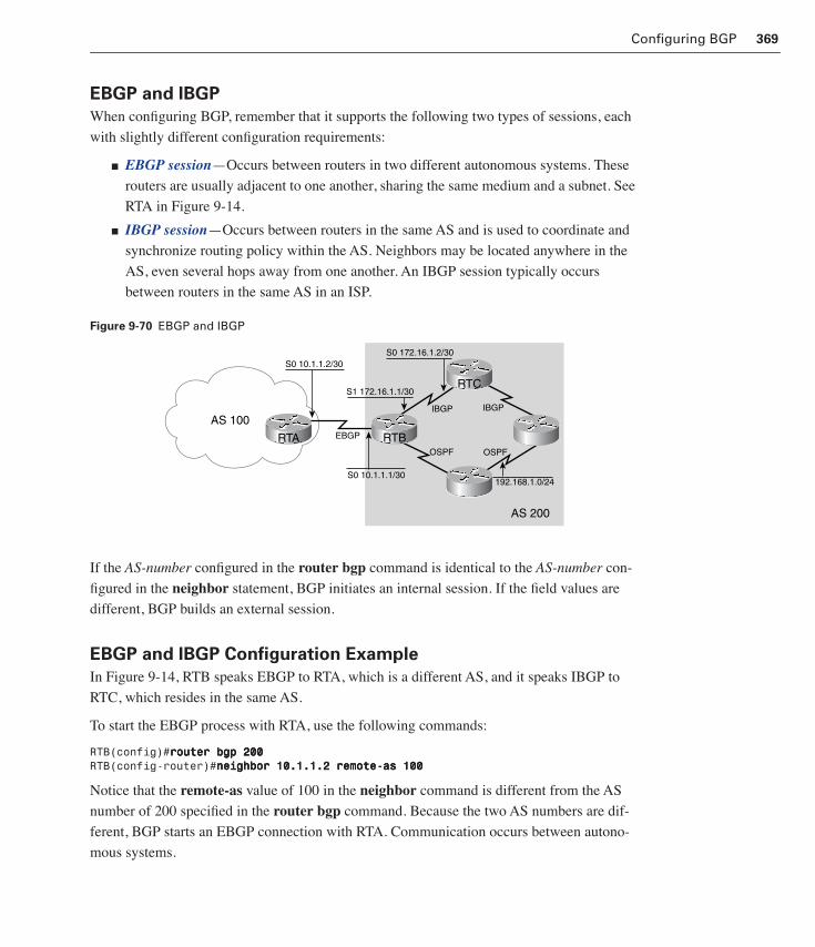
Configuring BGP 369
EBGP and IBGP
When configuring BGP, remember that it supports the following two types of sessions, each
with slightly different configuration requirements:
■ EBGP session—Occurs between routers in two different autonomous systems. These
routers are usually adjacent to one another, sharing the same medium and a subnet. See
RTA in Figure 9-14.
■ IBGP session—Occurs between routers in the same AS and is used to coordinate and
synchronize routing policy within the AS. Neighbors may be located anywhere in the
AS, even several hops away from one another. An IBGP session typically occurs
between routers in the same AS in an ISP.
Figure 9-70 EBGP and IBGP
If the AS-number configured in the router bgp command is identical to the AS-number con-
figured in the neighbor statement, BGP initiates an internal session. If the field values are
different, BGP builds an external session.
EBGP and IBGP Configuration Example
In Figure 9-14, RTB speaks EBGP to RTA, which is a different AS, and it speaks IBGP to
RTC, which resides in the same AS.
To start the EBGP process with RTA, use the following commands:
RTB(config)#rrrroooouuuutttteeeerrrr bbbbggggpppp 222200000000RTB(config-router)#nnnneeeeiiiigggghhhhbbbboooorrrr 11110000....1111....1111....2222 rrrreeeemmmmooootttteeee----aaaassss 111100000000
Notice that the remote-as value of 100 in the neighbor command is different from the AS
number of 200 specified in the router bgp command. Because the two AS numbers are dif-
ferent, BGP starts an EBGP connection with RTA. Communication occurs between autono-
mous systems.
AS 100
AS 200
EBGP
IBGP IBGP
OSPF OSPF
RTC
RTBRTA
S0 10.1.1.2/30S0 172.16.1.2/30
S1 172.16.1.1/30
S0 10.1.1.1/30192.168.1.0/24
1358_fmi.book Page 369 Thursday, May 27, 2004 2:21 PM

370 Chapter 9: BGP
The commands to configure IBGP are essentially the same as those to configure EBGP,
except for the possible addition of the update-source interface keyword:
RTB(config)#rrrroooouuuutttteeeerrrr bbbbggggpppp 222200000000RTB(config-router)#nnnneeeeiiiigggghhhhbbbboooorrrr 111177772222....11116666....1111....2222 rrrreeeemmmmooootttteeee----aaaassss 222200000000RTB(config-router)#nnnneeeeiiiigggghhhhbbbboooorrrr 111177772222....11116666....1111....2222 uuuuppppddddaaaatttteeee----ssssoooouuuurrrrcccceeee llllooooooooppppbbbbaaaacccckkkk 0000
The remote-as value, 200, is the same as the AS number for the BGP on RTB. Therefore,
BGP recognizes that this connection will occur within AS 200. It attempts to establish an
IBGP session. In reality, AS 200 is not a remote AS at all; it is the local AS with both routers
residing there. For simplicity, the keyword remote-as is used when configuring both EBGP
and IBGP sessions.
Also notice the second neighbor command. It is used to assign an optional parameter to be
used when communicating with that neighbor. It is typical to use multiple neighbor com-
mands for the same BGP neighbor, each specifying a particular BGP option.
In this example, the option specified is update-source loopback 0. If multiple pathways to
the neighbor exist, the router can use any IP interface to speak BGP with that neighbor. The
update-source loopback 0 command is used to instruct the router to use interface loopback 0
for TCP connections. This command is typically used in all IBGP configurations. Without
this command, BGP routers can use only the closest IP interface to the peer. The capability to
use any operational interface provides BGP with robustness in case the link to the closet
interface fails. Because EBGP sessions are typically point-to-point, there is no need to use
this command with EBGP.
Returning to the sample configuration, assume that the following route appears in the table
for RTB:
O 192.168.1.0/24 [110/74] via 10.2.2.1, 00:31:34, Serial2
RTB learns this route by way of an IGP by using OSPF. AS 200 uses OSPF internally to
exchange route information. RTB can advertise this network by way of BGP. Redistributing
OSPF into BGP works. However, using the following BGP network command does the same
thing:
RTB(config-router)#nnnneeeettttwwwwoooorrrrkkkk 111177772222....11116666....1111....0000 mmmmaaaasssskkkk 222255555555....222255555555....222255555555....222255552222RTB(config-router)#nnnneeeettttwwwwoooorrrrkkkk 11110000....1111....1111....0000 mmmmaaaasssskkkk 222255555555....222255555555....222255555555....222255552222RTB(config-router)#nnnneeeettttwwwwoooorrrrkkkk 111199992222....111166668888....1111....0000
The first two network commands include the mask keyword, so only a particular subnet is
specified. The third network command causes BGP to advertise the OSPF route without
1358_fmi.book Page 370 Thursday, May 27, 2004 2:21 PM

Configuring BGP 371
redistribution. Remember that the BGP network command works differently than the IGP
network command.
EBGP Multihop
These sample configurations have shown you how to configure EBGP and IBGP. However,
what is the difference between the configuration types? Figure 9-15 shows some of the
important characteristics of these BGP session types.
Figure 9-71 EBGP Multihop
RTZ and RTY have established an EBGP session. EBGP peers are normally directly con-
nected, but there are certain exceptions to this requirement. In contrast, IBGP peers merely
require TCP/IP connectivity within the same AS. As long as RTY can communicate with
RTW using TCP, both routers can establish an IBGP session. If needed, an IGP such as OSPF
can provide IBGP peers with routes to each other.
Lab 9.11.2 Configuring BGP with NAT
In this lab, you configure both IBGP and EBGP. You configure NAT with the S0/0
link to the ISP using the public IP address range of 66.122.33.96/27. The public net-
work range is then advertised via BGP.
AS 200
IBGP
EBGP EBGP
AS 100 AS 300
1.1.1.2
2.2.2.1
BGP is not spoken here.TCP/IP connectivity isprovided between RTYand RTW so that they
can speak IBGP.
BGP is not spoken here.RTW and RTU can
use Cisco’s EBGP mutlihopfeature to become
EBGP peers.
RTX
RTY RTW
RTZRTV
RTU
1358_fmi.book Page 371 Thursday, May 27, 2004 2:21 PM

372 Chapter 9: BGP
In a typical configuration, an IBGP router maintains IBGP sessions with all other IBGP rout-
ers in the AS, forming a logical full mesh. This is necessary because IBGP routers do not advertise
routes learned by way of IBGP to other IBGP peers to prevent routing loops. In other words, if the
IBGP routers are to exchange BGP routes with each other, configure a full mesh. An alternative to
this approach is to configure a route reflector. Lab 9.11.4b configures an IBGP router as a route
reflector. You can find additional information on route reflectors on the Cisco.com.
As noted, EBGP neighbors must be directly connected to establish an EBGP session. How-
ever, look again at RTW and RTU in Figure 9-15. These routers can maintain an EBGP ses-
sion even though a non-BGP router, RTV, separates them. In this situation, EBGP is running
across a non-BGP router using a configurable option called EBGP multihop. EBGP multihop
is a Cisco IOS software option that allows RTW and RTU to be logically connected in an
EBGP session. This is despite the fact that RTV does not support BGP. You configure the
EBGP multihop option on each peer with the following command:
Router(config-router)#nnnneeeeiiiigggghhhhbbbboooorrrr ip-address eeeebbbbggggpppp----mmmmuuuullllttttiiiihhhhoooopppp [hops]
This command lets you specify how many hops, up to 255, separate the EBGP peers. The
commands shown in Example 9-2 can be applied to the routers in this example.
In general, EBGP multihop is designed to allow the development of economical AS edge
router solutions. A single router with sufficient RAM and CPU power to support BGP is used
to handle the BGP routing needs. This router does not have to be an expensive modular, chas-
sis-based system. EBGP multihop allows edge routers to provide sufficient WAN interfaces
for the autonomous system’s connectivity needs.
Clearing the BGP Table
When configuring BGP, changes made to an existing configuration might not appear immediately.
To force BGP to clear its table and reset BGP sessions, use the clear ip bgp * command:
Router#cccclllleeeeaaaarrrr iiiipppp bbbbggggpppp ****
Example 9-2 EBGP Multihop Configuration
RTW(config)#rrrroooouuuutttteeeerrrr bbbbggggpppp 222200000000
RTW(config-router)#nnnneeeeiiiigggghhhhbbbboooorrrr 1111....1111....1111....2222 rrrreeeemmmmooootttteeee----aaaassss 333300000000
RTW(config-router)#nnnneeeeiiiigggghhhhbbbboooorrrr 1111....1111....1111....2222 eeeebbbbggggpppp----mmmmuuuullllttttiiiihhhhoooopppp 2222
RTU(config)#rrrroooouuuutttteeeerrrr bbbbggggpppp 333300000000
RTU(config-router)#nnnneeeeiiiigggghhhhbbbboooorrrr 2222....2222....2222....1111 rrrreeeemmmmooootttteeee----aaaassss 222200000000
RTU(config-router)#nnnneeeeiiiigggghhhhbbbboooorrrr 2222....2222....2222....1111 eeeebbbbggggpppp----mmmmuuuullllttttiiiihhhhoooopppp 2222
1358_fmi.book Page 372 Thursday, May 27, 2004 2:21 PM

Configuring BGP 373
The asterisk (*) is a wildcard that matches all table entries. Therefore, all BGP routes are lost
while the neighbor relationships are reset. This is expedient and very useful in a lab situation,
but you should be careful when issuing this command on a production router. On an Internet
backbone router, it might be more appropriate to use the following command with a specific
IP address:
Router#cccclllleeeeaaaarrrr iiiipppp bbbbggggpppp 11110000....0000....0000....0000
The specific IP address must be the address of a BGP peer, not an address in the routing table.
By specifying a particular network to clear, you prevent all BGP information from being tem-
porarily lost.
Peering
Any two routers that have formed a TCP connection to exchange BGP routing information
are called peers or neighbors.
Figure 9-16 shows the different types of BGP peering sessions you will encounter. An IBGP
peering session is formed within AS 3, between RTA’s loopback address and RTF’s physical
address. An EBGP session is also formed between AS 3 and AS 1 by using the two directly
connected IP addresses of RTA and RTC. Another EBGP session is formed between RTF in
AS 3 and RTD in AS 2, using IP addresses that are not on the same segment (multihop).
Figure 9-72 Building Peering Sessions
It is important to remember that the BGP peers never become established unless IP connec-
tivity exists between them. In this example, OSPF is used to establish the required internal
connectivity between RTD and RTE.
RTDRTC
RTF
RTE
Lo0 172.16.2.254255.255.255.255
RTA E1 172.16.1.1 172.16.1.2 E1/1
S0 172.16.20.2 192.68.5.1 S2/1
S2/1 172.16.20.1
EBGPDirectly
Connected EBGPMultihop
Internal Peer
AS 3
AS 1
AS 2This routeris not ableto run BGP.
192.68.12.1 S0/0
PhysicalLogical
1358_fmi.book Page 373 Thursday, May 27, 2004 2:21 PM

374 Chapter 9: BGP
In the RTF configuration shown in Example 9-3, the ebgp-multihop 2 command is used as
part of the neighbor configuration. This indicates that the exterior BGP peer is not directly
connected and can be reached at a maximum of two hops away. Remember that EBGP multi-
hop is applicable only with EBGP, not with IBGP.
In Example 9-4, the show ip bgp neighbor command shows you how the peer connection
looks after the neighbors are in an Established state. RTF sees neighbor 172.16.2.254 as an
internal neighbor that belongs to AS3. The neighbor connection is running BGPv4 with a
table version of 2. The table version changes every time the BGP table is updated.
The other RTF neighbor, 192.68.12.1, is also in an Established state. This is an external
neighbor that belongs to AS2. Notice that the display indicates that this neighbor is two hops
away because it was configured using the ebgp-multihop command.
Example 9-3 RTF Configuration
iiiipppp ssssuuuubbbbnnnneeeetttt----zzzzeeeerrrroooo
iiiinnnntttteeeerrrrffffaaaacccceeee EEEEtttthhhheeeerrrrnnnneeeetttt1111////1111
iiiipppp aaaaddddddddrrrreeeessssssss 111177772222....11116666....1111....2222 222255555555....222255555555....222255555555....0000
iiiinnnntttteeeerrrrffffaaaacccceeee SSSSeeeerrrriiiillllaaaa2222////1111
iiiipppp aaaaddddddddrrrreeeessssssss 111199992222....66668888....5555....1111
rrrroooouuuutttteeeerrrr oooossssppppffff 11110000
nnnneeeettttwwwwoooorrrrkkkk 111177772222....11116666....0000....0000 0000....0000....222255555555....222255555555 aaaarrrreeeeaaaa 0000
nnnneeeettttwwwwoooorrrrkkkk 111199992222....66668888....0000....0000 0000....0000....222255555555....222255555555 aaaarrrreeeeaaaa 0000
rrrroooouuuutttteeeerrrr bbbbggggpppp 3333
nnnnoooo ssssyyyynnnncccchhhhrrrroooonnnniiiizzzzaaaattttiiiioooonnnn
nnnneeeeiiiigggghhhhbbbboooorrrr 111177772222....11116666....2222....222255554444 rrrreeeemmmmooootttteeee----aaaassss 3333
nnnneeeeiiiigggghhhhbbbboooorrrr 111199992222....66668888....11112222....1111 rrrreeeemmmmooootttteeee----aaaassss 2222
nnnneeeeiiiigggghhhhbbbboooorrrr 111199992222....66668888....11112222....1111 eeeebbbbggggpppp----mmmmuuuullllttttiiiihhhhoooopppp 2222
nnnnoooo aaaauuuuttttoooo----ssssuuuummmmmmmmaaaarrrryyyy
iiiipppp ccccllllaaaasssssssslllleeeessssssss
Example 9-4 RTF show ip bgp neighbor Output
BGP neighbor is 172.16.2.254 remote AS 3, internal link
BGP version 4, remote router ID 172.16.2.254
BGP state = Established, up for 19:24:07
Last read 00:00:06, hold time is 180, keepalive interval is 60 seconds
Neighbor capabilities:
Route refresh:advertised and received(new)
1358_fmi.book Page 374 Thursday, May 27, 2004 2:21 PM

Configuring BGP 375
BGP Continuity Inside an AS
BGP does not advertise routes learned by way of IBGP peers to other IBGP peers. If it did,
BGP routing inside the AS would present a dangerous potential for routing loops. For IBGP
routers to learn about all BGP routes inside the AS, they must connect to every other IBGP
router in a full IBGP mesh. This full mesh needs to be only logical, not physical. In other
words, as long as the IBGP peers can connect to each other using TCP/IP, a logical full mesh
can be created even if the routers are not directly connected.
Figure 9-17 illustrates one of the common mistakes that administrators make when setting
BGP routing within an AS. This ISP network has three points of presence (POPs)—San Jose,
Address family IPv4 Unicast:advertised and received
Graceful Restart Capabilty:advertised and received
Remote Restart timer is 120 seconds
Address families preserved by peer:
IPv4 Unicast
Received 4231 messages, 0 notifications, 0 in queue
Sent 4167 messages, 0 notifications, 0 in queue
Default minimum time between advertisement runs is 5 seconds
For address family:IPv4 Unicast
BGP table version 159559, neighbor version 159559
Index 90, Offset 11, Mask 0x4
Route refresh request:received 0, sent 0
10031 accepted prefixes consume 441364 bytes
Prefix advertised 29403, suppressed 0, withdrawn 9801
Number of NLRIs in the update sent:max 242, min 0
Connections established 2; dropped 1
Last reset 19:26:54, due to NSF peer closed the session
Connection state is ESTAB, I/O status:1, unread input bytes:0
Local host: 192.68.5.1, Local port: 11016
Foreign host: 192.68.12.1, Foreign port: 179
Lab 9.11.4d BGP Peer Groups
In this lab, you use BGP peer groups to simplify the configuration tasks.
Example 9-4 RTF show ip bgp neighbor Output (Continued)
1358_fmi.book Page 375 Thursday, May 27, 2004 2:21 PM

376 Chapter 9: BGP
San Francisco, and Los Angeles. Each POP has multiple non-BGP routers and a BGP border
router running EBGP with other autonomous systems. The administrator has set up an IBGP
connection between the San Jose border router and the San Francisco border router. Another
IBGP connection has been set up between the San Francisco border router and the Los Ange-
les border router. In this configuration, EBGP routes learned by way of San Jose are given to
San Francisco. EBGP routes learned by way of San Francisco are given to San Jose and Los
Angeles. Last, EBGP routes learned by way of Los Angeles are given to San Francisco.
Figure 9-73 BGP Continuity Inside an AS
However, routing in this scenario is incomplete. EBGP routes learned by way of San Jose are
not given to Los Angeles, and EBGP routes learned by way of Los Angeles are not given to
San Jose. This is because the San Francisco router does not advertise IBGP routes between
San Jose and Los Angeles. What is needed is an additional IBGP connection between San
Jose and Los Angeles. This connection is shown as a dotted line in Figure 9-17.
Monitoring BGP OperationThis section covers some of the details of monitoring and verifying BGP operation.
EBGP EBGP EBGP
SJ SF LA
IBGP IBGP
IBGP
SJ POP SF POP LA POP
1358_fmi.book Page 376 Thursday, May 27, 2004 2:21 PM

Monitoring BGP Operation 377
Verifying BGP Operation
You verify BGP operation by using the key show commands listed in Table 9-3.
If the router has not installed the BGP routes you expected, use the show ip bgp command, as
shown in Example 9-5, to verify that BGP has learned these routes on RTB in Figure 9-18.
Figure 9-74 Sample Topology
Table 9-11 Key BGP show Commands
Command Description
show ip bgp Displays entries in the BGP routing table. You can specify a network to get more detailed information about a particu-lar prefix. Use the subnets keyword to get information about a particular prefix and all of its subnets.
show ip bgp summary Displays a summary of all BGP connections.
show ip bgp neighbors Displays detailed information for each BGP.
show ip bgp paths Displays all of the BGP paths in the database.
Example 9-5 show ip bgp on Router-B
BGP table version is 5, local router ID is 10.0.0.1
Status codes: s suppressed, d damped, h history, * valid, > best, i - internal
Origin codes: i - IGP, e - EGP, ? - incomplete
Network Next Hop Metric LocPrf Weight Path
*> 10.0.0.0 0.0.0.0 0 32768 i
* 11.0.0.0 3.0.0.2 0 0 200 i
* 12.0.0.0 2.0.0.2 0 0 i
AS 300
2.0.0.0/24
AS 200
3.0.0.0/2410.0.0.0/8
RTB
12.0.0.0/8
RTA
11.0.0.0/8
RTC
1358_fmi.book Page 377 Thursday, May 27, 2004 2:21 PM
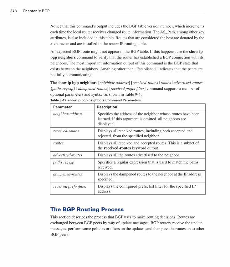
378 Chapter 9: BGP
Notice that this command’s output includes the BGP table version number, which increments
each time the local router receives changed route information. The AS_Path, among other key
attributes, is also included in this table. Routes that are considered the best are denoted by the
> character and are installed in the router IP routing table.
An expected BGP route might not appear in the BGP table. If this happens, use the show ip bgp neighbors command to verify that the router has established a BGP connection with its
neighbors. The most important information output of this command is the BGP state that
exists between the neighbors. Anything other than “Established” indicates that the peers are
not fully communicating.
The show ip bgp neighbors [neighbor-address] [received-routes | routes | advertised-routes | {paths regexp} | dampened-routes] [received prefix-filter] command supports a number of
optional parameters and syntax, as shown in Table 9-4.
The BGP Routing ProcessThis section describes the process that BGP uses to make routing decisions. Routes are
exchanged between BGP peers by way of update messages. BGP routers receive the update
messages, perform some policies or filters on the updates, and then pass the routes on to other
BGP peers.
Table 9-12 show ip bgp neighbors Command Parameters
Parameter Description
neighbor-address Specifies the address of the neighbor whose routes have been learned. If this argument is omitted, all neighbors are displayed.
received-routes Displays all received routes, including both accepted and rejected, from the specified neighbor.
routes Displays all received and accepted routes. This is a subnet of the received-routes keyword output.
advertised-routes Displays all the routes advertised to the neighbor.
paths regexp Specifies a regular expression that is used to match the paths received.
dampened-routes Displays the dampened routes to the neighbor at the IP address specified.
received prefix-filter Displays the configured prefix list filter for the specified IP address.
1358_fmi.book Page 378 Thursday, May 27, 2004 2:21 PM

The BGP Routing Process 379
An Overview of the BGP Routing Process
The Cisco implementation of BGP keeps track of all BGP updates in a BGP table separate
from the IP routing table. In case multiple routes to the same destination exist, BGP does not
flood its peers with all of those routes. Instead, BGP picks only the best route and sends it to
the peers. In addition to passing along routes from peers, a BGP router may originate routing
updates to advertise networks that belong to its own AS. Valid local routes originated in the
system and the best routes learned from BGP peers are then installed in the IP routing table.
The IP routing table is used for the final routing decision.
The following sections detail the BGP routing process, implementing BGP routing policy,
controlling BGP routing with attributes, and handling the BGP decision process.
The BGP Routing Process Model
To model the BGP process, imagine each BGP speaker having different pools of routes and
different policy engines applied to the routes. This model is shown in Figure 9-19.
Figure 9-75 Route Exchange
The model involves the following components:
■ Routes received from peers—BGP receives routes from external or internal peers.
Depending on what is configured in the input policy engines, some or all of these routes
will make it into the router BGP table.
■ Input policy engine—This engine handles route filtering and manipulation of attributes.
Filtering is done based on parameters, such as the IP prefix, the AS path, and attribute
information.
The input policy engine manipulates the path attributes and influences BGP’s decision
process. This affects what routes it uses to reach a certain destination. For example, the
policy chosen filters a certain network coming from a peer, it is an indication to BGP that
Routes ReceivedFrom Peers
FilteringAttribute
Manipulation
Choosingthe BestRoute
FilteringAttribute
Manipulation
RoutesSent
to Peers
InputPolicyEngine
DecisionProcess
RoutesUsed byRouter
OuputPolicyEngine
BGP Table
IP Routing Table
1358_fmi.book Page 379 Thursday, May 27, 2004 2:21 PM

380 Chapter 9: BGP
it should not reach that network by way of that peer. A certain route can be given a better
local preference than some other path to the same destination. This indicates that BGP
should prefer this route instead of the other available routes.
■ The decision process—BGP goes through a decision process to decide which route or
routes it wants to use to reach a certain destination. The decision process is based on
the routes that made it into the router after the input policy engine was applied. This
process is performed on the routes in the BGP routing table. The decision process looks
at all of the available routes for the same destination, compares the different attributes
associated with each route, and chooses one best route. This decision process is dis-
cussed in the section “The BGP Decision Process.”
■ Routes used by the router—The best routes, as identified by the decision process, are
candidates to be advertised to other peers. These routes are also presented to the routing
engine to be placed in the IP routing table. Not all routes presented to the routing
engine are placed in the routing table. This is because multiple protocols might present
the same prefix for installation, and the router must choose from among them based on
administrative distance. In addition to routes passed on from other peers, the router, if
configured to do so, originates updates about the networks inside its own AS. This is
how an AS injects its routes into the outside world.
■ Output policy engine—This is the same engine as the input policy engine, applied on
the output side. Routes used by the router (the best routes), in addition to routes that the
router generates locally, are given to this engine for processing. The engine might apply
filters and might change some of the attributes, such as AS_Path or metric, before send-
ing the update.
The output policy engine also differentiates between internal and external peers. For
example, routes learned from internal peers cannot be passed on to external peers.
■ Routes advertised to peers—The routes advertised to peers are routes that made it
through the output engine. They are advertised to the BGP peers, internal or external.
Implementing BGP Routing Policy
Input and output policies generally are defined using route maps. Route maps are used with
BGP to control and modify routing information. Route maps define how the routes are redis-
tributed between routing domains. Recall from Chapter 8, “Route Optimization,” that the
route-map command has the following syntax:
Router(config)#rrrroooouuuutttteeee----mmmmaaaapppp map-tag [ppppeeeerrrrmmmmiiiitttt | ddddeeeennnnyyyy] [sequence-number]
map-tag is a name that identifies the route map. sequence-number indicates the position that
an instance of the route map is to have in relation to other instances of the same route map.
Instances are ordered sequentially, starting with the number 10 by default.
1358_fmi.book Page 380 Thursday, May 27, 2004 2:21 PM
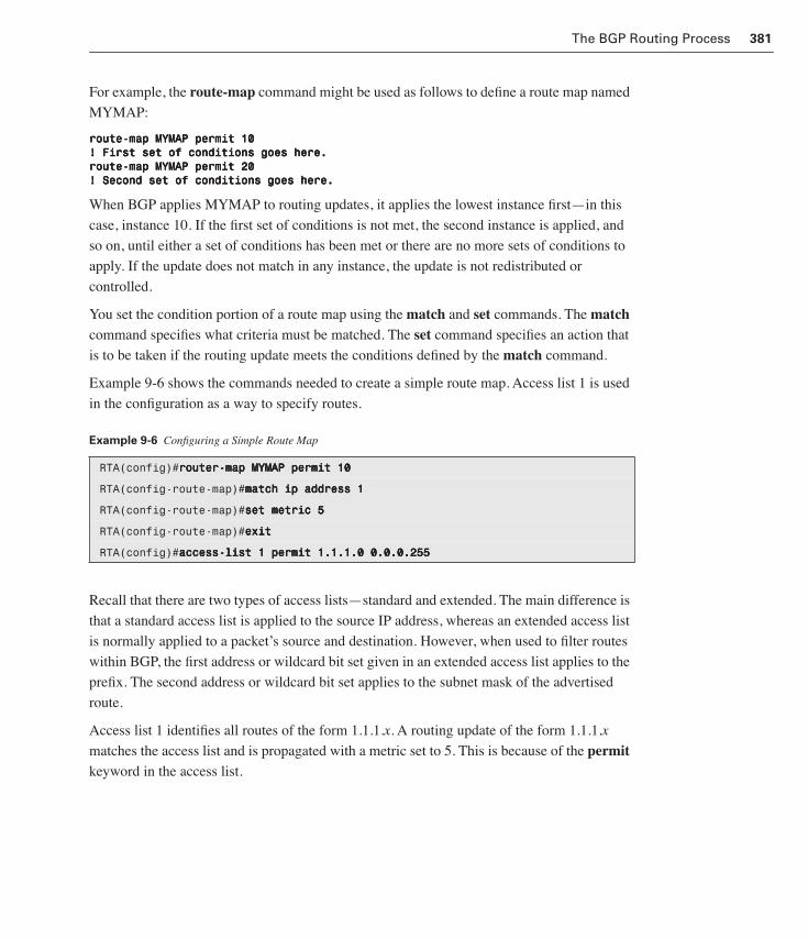
The BGP Routing Process 381
For example, the route-map command might be used as follows to define a route map named
MYMAP:
rrrroooouuuutttteeee----mmmmaaaapppp MMMMYYYYMMMMAAAAPPPP ppppeeeerrrrmmmmiiiitttt 11110000!!!! FFFFiiiirrrrsssstttt sssseeeetttt ooooffff ccccoooonnnnddddiiiittttiiiioooonnnnssss ggggooooeeeessss hhhheeeerrrreeee....rrrroooouuuutttteeee----mmmmaaaapppp MMMMYYYYMMMMAAAAPPPP ppppeeeerrrrmmmmiiiitttt 22220000!!!! SSSSeeeeccccoooonnnndddd sssseeeetttt ooooffff ccccoooonnnnddddiiiittttiiiioooonnnnssss ggggooooeeeessss hhhheeeerrrreeee....
When BGP applies MYMAP to routing updates, it applies the lowest instance first—in this
case, instance 10. If the first set of conditions is not met, the second instance is applied, and
so on, until either a set of conditions has been met or there are no more sets of conditions to
apply. If the update does not match in any instance, the update is not redistributed or
controlled.
You set the condition portion of a route map using the match and set commands. The match
command specifies what criteria must be matched. The set command specifies an action that
is to be taken if the routing update meets the conditions defined by the match command.
Example 9-6 shows the commands needed to create a simple route map. Access list 1 is used
in the configuration as a way to specify routes.
Recall that there are two types of access lists—standard and extended. The main difference is
that a standard access list is applied to the source IP address, whereas an extended access list
is normally applied to a packet’s source and destination. However, when used to filter routes
within BGP, the first address or wildcard bit set given in an extended access list applies to the
prefix. The second address or wildcard bit set applies to the subnet mask of the advertised
route.
Access list 1 identifies all routes of the form 1.1.1.x. A routing update of the form 1.1.1.x
matches the access list and is propagated with a metric set to 5. This is because of the permit keyword in the access list.
Example 9-6 Configuring a Simple Route Map
RTA(config)#rrrroooouuuutttteeeerrrr----mmmmaaaapppp MMMMYYYYMMMMAAAAPPPP ppppeeeerrrrmmmmiiiitttt 11110000
RTA(config-route-map)#mmmmaaaattttcccchhhh iiiipppp aaaaddddddddrrrreeeessssssss 1111
RTA(config-route-map)#sssseeeetttt mmmmeeeettttrrrriiiicccc 5555
RTA(config-route-map)#eeeexxxxiiiitttt
RTA(config)#aaaacccccccceeeessssssss----lllliiiisssstttt 1111 ppppeeeerrrrmmmmiiiitttt 1111....1111....1111....0000 0000....0000....0000....222255555555
1358_fmi.book Page 381 Thursday, May 27, 2004 2:21 PM

382 Chapter 9: BGP
A route map can be applied on the incoming BGP update using the keyword in or on the out-
going BGP update using the keyword out. Example 9-7 shows the commands needed to
apply the route map MYMAP on the outgoing updates toward BGP neighbor 172.16.20.2.
BGP AttributesTraffic inside and outside an AS always flows according to the road map laid out by routes. If
the routes are altered, the traffic behavior is affected. The following are some of the questions
organizations and service providers ask about controlling routes:
■ How can the private networks be prevented from being advertised?
■ How can routing updates that come from a particular neighbor be filtered?
■ How can I specify to use this link or this provider, rather than another one?
Controlling BGP Routing with Attributes
Through the use of attributes, BGP provides the answers to all of these questions and more. A
BGP speaker can receive updates from multiple autonomous systems that describe different
paths to the same destination. It must then choose the single best path for reaching that desti-
nation. After it is chosen, BGP propagates the best path to its neighbors. The decision is
based on the value of attributes, such as Next Hop or Local Preference, that the update con-
tains, as well as other configurable BGP factors. The following sections provide an overview
of these key attributes that BGP uses in the decision-making process:
■ Next Hop
■ AS_Path
■ Atomic Aggregate
■ Aggregator
■ Local Preference
■ Weight
■ Multiple Exit Discriminator (MED)
■ Origin
Example 9-7 Applying a Route Map to a BGP Neighbor
RTA(config)#rrrroooouuuutttteeee bbbbggggpppp 111100000000
RTA(config-route)#nnnneeeeiiiigggghhhhbbbboooorrrr 111177772222....11116666....22220000....2222 rrrreeeemmmmooootttteeee----aaaassss 333300000000
RTA(config-route)#nnnneeeeiiiigggghhhhbbbboooorrrr 111177772222....11116666....22220000....2222 rrrroooouuuutttteeee----mmmmaaaapppp MMMMYYYYMMMMAAAAPPPP oooouuuutttt
1358_fmi.book Page 382 Thursday, May 27, 2004 2:21 PM

BGP Attributes 383
The Next Hop Attribute
The Next Hop attribute is a well-known mandatory attribute, type code 3. In terms of an IGP,
such as RIP, the next hop to reach a route is the IP address of the router that has announced
the route. The next-hop concept with BGP is more complex and takes one of the following
forms:
■ For EBGP sessions, the next hop is the IP address of the neighbor that announced the
route.
■ For IBGP sessions, where routes originate inside the AS, the next hop is the IP address
of the neighbor that announces the route. For routes injected into the AS by way of
EBGP, the next hop learned from EBGP is carried unaltered into IBGP. The next hop is
the IP address of the EBGP neighbor from which the route was learned.
■ When the route is advertised on a multiaccess medium, such as Ethernet or Frame
Relay, the next hop is usually the IP address of the router’s interface. This is the inter-
face connected to the medium that originated the route.
Figure 9-20 illustrates the BGP Next Hop attribute. RTC is running an EBGP session with
router RTZ and an IBGP session with router RTA. RTC is learning route 128.213.1.0/24 from
RTZ. In turn, RTC is injecting the local route 128.212.1.0/24 into BGP.
Figure 9-76 Next Hop Attribute
RTA learns about route 128.212.1.0/24 by way of 2.2.2.2, the IP address of the IBGP peer
announcing the route. Therefore, according to the definition, 2.2.2.2 is the next hop for RTA
to reach 128.212.1.0/24. Similarly, RTC sees 128.213.1.0/24 coming from RTZ by way of
next hop 1.1.1.1. When it passes this route update to RTA by way of IBGP, RTC includes the
next-hop information, unaltered. Therefore, RTA receives the BGP update about 128.213.1.0/24
with next hop 1.1.1.1. This is an example of the EBGP next hop’s being carried into IBGP.
S0 3.3.3.3RTB
RTA
S0 1.1.1.1
S0 2.2.2.2
128.212.1.0/24
128.213.1.0/24
AS 1
IBGP
EBGP
Can reach 128.213.1.0 byway of 1.1.1.1 and can
reach 128.212.1.0 by way of2.2.2.2
Can reach 128.213.1.0by way of 1.1.1.1
RTZ
RTC
1358_fmi.book Page 383 Thursday, May 27, 2004 2:21 PM

384 Chapter 9: BGP
As you can see, the next hop cannot necessarily be reached by way of a direct connection.
The next hop for RTA for 128.213.1.0/24 is 1.1.1.1, but reaching it requires a pathway
through 3.3.3.3. Therefore, the next-hop behavior mandates a recursive IP routing table
lookup for a router to know where to send the packet. To reach the next hop 1.1.1.1, RTA consults
its IGP routing table to see if and how 1.1.1.1 can be reached. This recursive search continues
until the router associates destination 1.1.1.1 with an outgoing interface. The same recursive
behavior is performed to reach next hop 2.2.2.2. If a hop cannot be reached by way of an IGP,
BGP considers the route inaccessible.
Next-Hop Behavior on Multiaccess Media
Recall that a network link is considered multiaccess if more than two hosts can potentially
connect to it. Routers on a multiaccess link share the same IP subnet and can physically
access all other connected routers in one hop. Ethernet, Frame Relay, and ATM are examples
of multiaccess media.
BGP speakers should always advertise the route’s actual source if the source is on the same
multiaccess link as the speaker, as shown in Figure 9-21. In other words, RTC advertises a
route learned from RTB, and RTC and RTB share a common multiaccess medium. Then
when RTC advertises the route, it should specify RTB as the source of the route. If it doesn’t,
routers on the same medium would have to make an unnecessary hop by way of RTC to get to
a router that is sitting in the same segment.
Figure 9-77 Next Hop on Multiaccess Medium
In Figure 9-21, RTA, RTB, and RTC share a common multiaccess medium. RTA and RTC are
running EBGP, and RTC and RTB are running OSPF. RTC learns of network 11.11.11.0/24
from RTB by way of OSPF and advertises it to RTA by way of EBGP. Because RTA and RTB
.1
.2
.3
EBGP
OSPF
10.10.10.0/24
11.11.11.0/24
RTB
RTC
RTA
1358_fmi.book Page 384 Thursday, May 27, 2004 2:21 PM

BGP Attributes 385
are running different routing protocols, it would seem logical that RTA would consider RTC
(10.10.10.2) as its next hop to reach 11.11.11.0/24. However, this would not happen. The cor-
rect behavior is for RTA to consider RTB, 10.10.10.3, as the next hop because RTB shares the
medium with RTC.
When the medium is broadcast, such as Ethernet and FDDI, physical connectivity is
assumed, and the next-hop behavior is not an issue. However, when the medium is nonbroad-
cast, such as Frame Relay and ATM, special care should be taken, as described in the follow-
ing section.
Next-Hop Behavior on NBMA Networks
On a nonbroadcast multiaccess (NBMA) network, the many-to-many direct interaction
between routers is not guaranteed unless virtual circuits (VCs) are configured from each
router to all other routers. The primary reason that most organizations implement a hub-and-
spoke topology is because of cost considerations. In a hub-and-spoke topology, multiple
remote sites have VC connected to one or more routers at a central site. Figure 9-22 shows
next-hop behavior in an NBMA environment.
Figure 9-78 Next Hop Over NBMA
The only difference between the environments illustrated is that the medium in Figure 9-22 is
an NBMA Frame Relay cloud. RTC is the hub router, and RTA and RTB are the spokes.
Notice that the virtual circuits are laid out between RTC and RTA, and between RTC and
RTB, but not between RTA and RTB. This is a partial-mesh topology.
RTA gets a BGP routing update about 11.11.11.0/24 from RTC and tries to use RTB,
10.10.10.3, as the next hop. This is the same behavior as on multiaccess media, as shown in
Figure 9-21. Routing fails because no virtual circuit exists between RTA and RTB.
RTBSpoke
RTCHub
RTASpoke
10.10.10.0/24
.1
.2
.3
EBGP
OSPF
11.11.11.0/24
1358_fmi.book Page 385 Thursday, May 27, 2004 2:21 PM
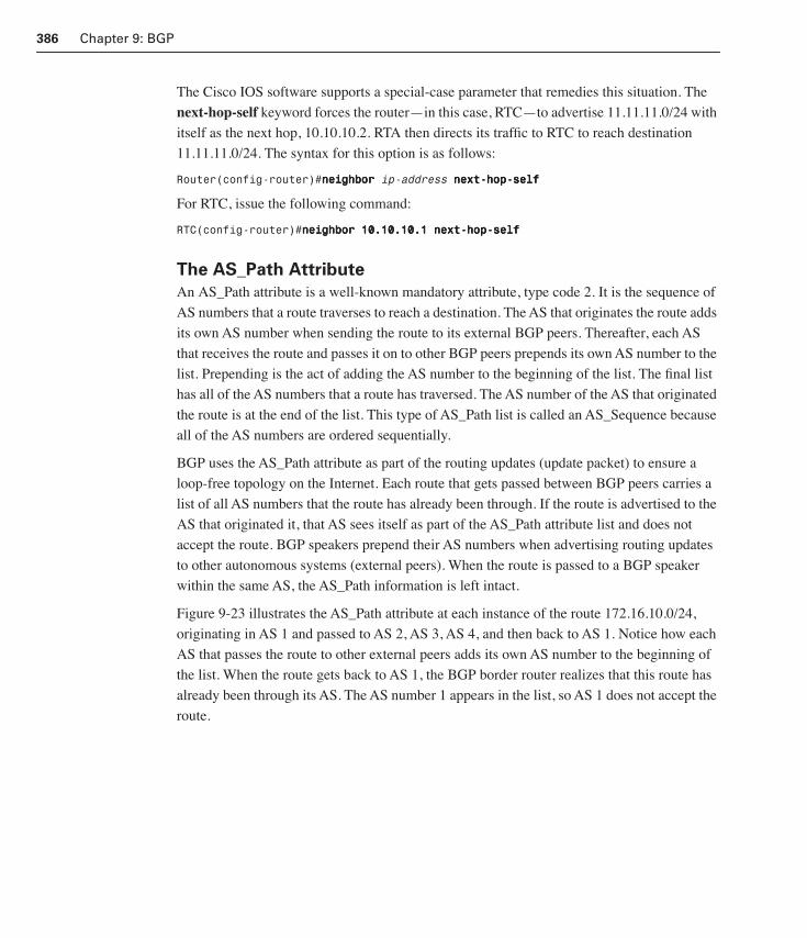
386 Chapter 9: BGP
The Cisco IOS software supports a special-case parameter that remedies this situation. The
next-hop-self keyword forces the router—in this case, RTC—to advertise 11.11.11.0/24 with
itself as the next hop, 10.10.10.2. RTA then directs its traffic to RTC to reach destination
11.11.11.0/24. The syntax for this option is as follows:
Router(config-router)#nnnneeeeiiiigggghhhhbbbboooorrrr ip-address nnnneeeexxxxtttt----hhhhoooopppp----sssseeeellllffff
For RTC, issue the following command:
RTC(config-router)#nnnneeeeiiiigggghhhhbbbboooorrrr 11110000....11110000....11110000....1111 nnnneeeexxxxtttt----hhhhoooopppp----sssseeeellllffff
The AS_Path Attribute
An AS_Path attribute is a well-known mandatory attribute, type code 2. It is the sequence of
AS numbers that a route traverses to reach a destination. The AS that originates the route adds
its own AS number when sending the route to its external BGP peers. Thereafter, each AS
that receives the route and passes it on to other BGP peers prepends its own AS number to the
list. Prepending is the act of adding the AS number to the beginning of the list. The final list
has all of the AS numbers that a route has traversed. The AS number of the AS that originated
the route is at the end of the list. This type of AS_Path list is called an AS_Sequence because
all of the AS numbers are ordered sequentially.
BGP uses the AS_Path attribute as part of the routing updates (update packet) to ensure a
loop-free topology on the Internet. Each route that gets passed between BGP peers carries a
list of all AS numbers that the route has already been through. If the route is advertised to the
AS that originated it, that AS sees itself as part of the AS_Path attribute list and does not
accept the route. BGP speakers prepend their AS numbers when advertising routing updates
to other autonomous systems (external peers). When the route is passed to a BGP speaker
within the same AS, the AS_Path information is left intact.
Figure 9-23 illustrates the AS_Path attribute at each instance of the route 172.16.10.0/24,
originating in AS 1 and passed to AS 2, AS 3, AS 4, and then back to AS 1. Notice how each
AS that passes the route to other external peers adds its own AS number to the beginning of
the list. When the route gets back to AS 1, the BGP border router realizes that this route has
already been through its AS. The AS number 1 appears in the list, so AS 1 does not accept the
route.
1358_fmi.book Page 386 Thursday, May 27, 2004 2:21 PM
BGP Attributes 387
Figure 9-79 AS_Path Attribute
AS_Path information is one of the attributes that BGP looks at to determine the best route to
reach a destination. In comparing two or more different routes, given that all other attributes
are identical, a shorter path is always preferred. In case of a tie in AS_Path length, other
attributes are used to make the decision.
AS_Path and Private AS Numbers
In an effort to conserve AS numbers, customers whose routing policies are an extension of
the policies of their provider generally are not assigned a legal or public AS number. There-
fore, if a customer is single-homed or multihomed to the same provider, the provider gener-
ally requests that the customer use an AS number taken from the private pool: 64,512 to
65,535. As such, all BGP updates that the provider receives from its customer contain private
AS numbers.
Private AS numbers cannot be advertised to the Internet because they are not unique. For this
reason, Cisco has implemented a feature to strip private AS numbers from the AS_Path list
before the routes get propagated to the Internet.
In Figure 9-24, AS1 provides Internet connectivity to its customer AS 65001. Because the
customer connects to only this provider and has no plans to connect to an additional provider
Lab 9.11.3 Using the AS_PATH Attribute
In this lab, you use BGP commands to prevent private AS numbers from being adver-
tised to the outside world. You also use the AS_PATH attribute to filter BGP routes
based on their source AS numbers.
AS1 sees its AS number inthe AS_path list and doesnot accept the update.
AS 1172.16.10.0/24
AS 3172.16.10.0/24-3,2,1
AS 2172.16.10.0/24-2,1172.16.10.0/24-1 172.16.10.0/24-1
AS 4172.16.10.0/24-4,3,2,1172.16.10.0/24-1 172.16.10.0/24-1
1358_fmi.book Page 387 Thursday, May 27, 2004 2:21 PM
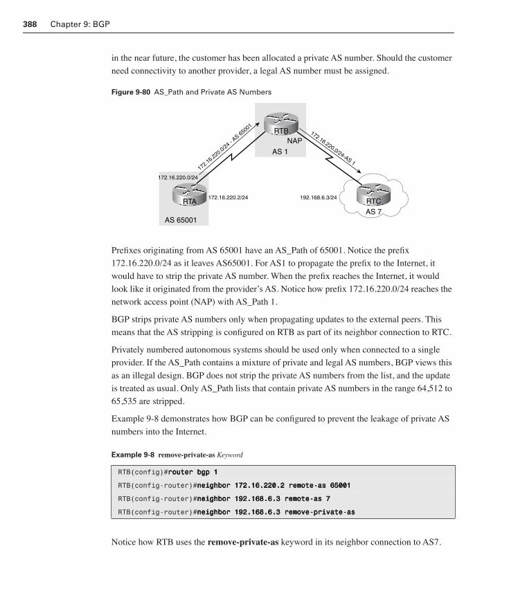
388 Chapter 9: BGP
in the near future, the customer has been allocated a private AS number. Should the customer
need connectivity to another provider, a legal AS number must be assigned.
Figure 9-80 AS_Path and Private AS Numbers
Prefixes originating from AS 65001 have an AS_Path of 65001. Notice the prefix
172.16.220.0/24 as it leaves AS65001. For AS1 to propagate the prefix to the Internet, it
would have to strip the private AS number. When the prefix reaches the Internet, it would
look like it originated from the provider’s AS. Notice how prefix 172.16.220.0/24 reaches the
network access point (NAP) with AS_Path 1.
BGP strips private AS numbers only when propagating updates to the external peers. This
means that the AS stripping is configured on RTB as part of its neighbor connection to RTC.
Privately numbered autonomous systems should be used only when connected to a single
provider. If the AS_Path contains a mixture of private and legal AS numbers, BGP views this
as an illegal design. BGP does not strip the private AS numbers from the list, and the update
is treated as usual. Only AS_Path lists that contain private AS numbers in the range 64,512 to
65,535 are stripped.
Example 9-8 demonstrates how BGP can be configured to prevent the leakage of private AS
numbers into the Internet.
Notice how RTB uses the remove-private-as keyword in its neighbor connection to AS7.
Example 9-8 remove-private-as Keyword
RTB(config)#rrrroooouuuutttteeeerrrr bbbbggggpppp 1111
RTB(config-router)#nnnneeeeiiiigggghhhhbbbboooorrrr 111177772222....11116666....222222220000....2222 rrrreeeemmmmooootttteeee----aaaassss 66665555000000001111
RTB(config-router)#nnnneeeeiiiigggghhhhbbbboooorrrr 111199992222....111166668888....6666....3333 rrrreeeemmmmooootttteeee----aaaassss 7777
RTB(config-router)#nnnneeeeiiiigggghhhhbbbboooorrrr 111199992222....111166668888....6666....3333 rrrreeeemmmmoooovvvveeee----pppprrrriiiivvvvaaaatttteeee----aaaassss
AS 7
172.16.220.0/24 - AS 65001
172.16.220.0/24
172.16.220.2/24 192.168.6.3/24
AS 65001
AS 1
NAP172.16.220.0/24-AS 1
RTA
RTB
RTC
1358_fmi.book Page 388 Thursday, May 27, 2004 2:21 PM
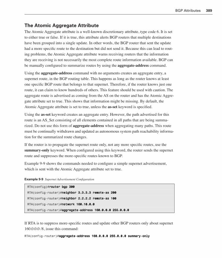
BGP Attributes 389
The Atomic Aggregate Attribute
The Atomic Aggregate attribute is a well-known discretionary attribute, type code 6. It is set
to either true or false. If it is true, this attribute alerts BGP routers that multiple destinations
have been grouped into a single update. In other words, the BGP router that sent the update
had a more specific route to the destination but did not send it. Because this can lead to rout-
ing problems, the Atomic Aggregate attribute warns receiving routers that the information
they are receiving is not necessarily the most complete route information available. BGP can
be manually configured to summarize routes by using the aggregate-address command.
Using the aggregate-address command with no arguments creates an aggregate entry, a
supernet route, in the BGP routing table. This happens as long as the router knows at least
one specific BGP route that belongs to that supernet. Therefore, if the router knows just one
route, it can claim to know hundreds of others. This feature should be used with caution. The
aggregate route is advertised as coming from the AS on the router and has the Atomic Aggre-
gate attribute set to true. This shows that information might be missing. By default, the
Atomic Aggregate attribute is set to true, unless the as-set keyword is specified.
Using the as-set keyword creates an aggregate entry. However, the path advertised for this
route is an AS_Set consisting of all elements contained in all paths that are being summa-
rized. Do not use this form of aggregate-address when aggregating many paths. This route
must be continually withdrawn and updated as autonomous system path reachability informa-
tion for the summarized route changes.
If the router is to propagate the supernet route only, not any more specific routes, use the
summary-only keyword. When configured using this keyword, the router sends the supernet
route and suppresses the more-specific routes known to BGP.
Example 9-9 shows the commands needed to configure a simple supernet advertisement,
which is sent with the Atomic Aggregate attribute set to true.
If RTA is to suppress more-specific routes and update other BGP routers only about supernet
160.0.0.0 /8, issue this command:
RTA(config-router)#aaaaggggggggrrrreeeeggggaaaatttteeee----aaaaddddddddrrrreeeessssssss 111166660000....0000....0000....0000 222255555555....0000....0000....0000 ssssuuuummmmmmmmaaaarrrryyyy----oooonnnnllllyyyy
Example 9-9 Supernet Advertisement Configuration
RTA(config)#rrrroooouuuutttteeeerrrr bbbbggggpppp 333300000000
RTA(config-router)#nnnneeeeiiiigggghhhhbbbboooorrrr 3333....3333....3333....3333 rrrreeeemmmmooootttteeee----aaaassss 222200000000
RTA(config-router)#nnnneeeeiiiigggghhhhbbbboooorrrr 2222....2222....2222....2222 rrrreeeemmmmooootttteeee----aaaassss 111100000000
RTA(config-router)#nnnneeeettttwwwwoooorrrrkkkk 111166660000....11110000....0000....0000
RTA(config-router)#aaaaggggggggrrrreeeeggggaaaatttteeee----aaaaddddddddrrrreeeessssssss 111166660000....0000....0000....0000 222255555555....0000....0000....0000
1358_fmi.book Page 389 Thursday, May 27, 2004 2:21 PM

390 Chapter 9: BGP
The Aggregator Attribute
Aggregator is a well-known discretionary attribute, type code 7. When you configure address
aggregation, the router can also be configured to include its router ID and local AS number
along with the supernet route. This attribute lets ISP administrators determine which BGP
router is responsible for a particular instance of aggregation. Tracing a supernet to its original
aggregator might be necessary for troubleshooting purposes.
The Local Preference Attribute
Local Preference is a well-known discretionary attribute, type code 5. The Local Preference
attribute is a degree of preference given to a route for comparison with other routes to the
same destination. Higher Local Preference values are preferred. Local Preference, as its name
indicates, is local to the AS and is exchanged between IBGP peers only. Local Preference is
not advertised to EBGP peers.
Routers within a multihomed AS may learn that they can reach the same destination network
by way of neighbors in two or more different autonomous systems. In effect, there could be
two or more exit points from the local AS to any given destination. Use the Local Preference
attribute to force the BGP routers to prefer one exit point over another when routing to a par-
ticular destination network. Because this attribute is communicated within all BGP routers
inside the AS, all BGP routers have a common view of how to exit the AS.
Consider the environment shown in Figure 9-25. Suppose that company ANET has purchased
Internet connections from two service providers, XNET and YNET. ANET is connected to
YNET by way of a primary T3 link and to XNET by way of a backup T1 link.
Figure 9-81 Local Preference Attribute
NOTE
Although routers always prefer the lowest route metric and administrative distance for a given desti-nation, BGP routers prefer higher Local Preference values over lower ones.
ZNET
XNET YNET
WNET
ANETT1Link
(Set localpreference to 200)
(Set local preferenceto 300 which forcestraffic to go out viathe T3 link)
T3Link
128.213.0.0/16 128.213.0.0/16 128.213.0.0/16
IBGP
> 128.213.0.0/16—300 128.213.0.0/16—200
RTA RTB
1358_fmi.book Page 390 Thursday, May 27, 2004 2:21 PM

BGP Attributes 391
It is important for ANET to decide what path its outbound traffic will take. Of course, the net-
work administrators for ANET prefer to use the T3 link by way of YNET in normal operation
because it is a high-speed link. This is where Local Preference starts. RTB can give the routes
coming from YNET a Local Preference of 300, and RTA can give the routes coming from
XNET a lower value, such as 200. Because both RTA and RTB exchange routing updates by
way of IBGP, they both agree that the autonomous system’s exit point will be by way of
YNET. This happens because of the higher local preference.
In Figure 9-25, ANET learns about route 128.213.0.0/16 by way of XNET and YNET. RTA
and RTB agree on using YNET as the exit point for destination 128.213.0.0/16 because of the
higher Local Preference value of 300. The Local Preference manipulation discussed in this
case affects the traffic going out of the AS and not traffic coming into the AS. Inbound traffic
can still come by way of the T1 link.
Manipulating Local PreferenceIn Figure 9-26, AS 256 receives route updates for network 170.10.0.0 from AS 100 and AS 300.
The following are two ways to set the Local Preference attribute on the routers in AS 256:
■ Use the bgp default local-preference command
■ Use a route map to set local preference
Figure 9-82 Local Preference
AS 100
1.1.1.1
AS 34
170.10.0.0
AS 300
3.3.3.4
AS 256
1.1.1.2 3.3.3.3
128.213.11.1 128.213.11.2
IBGP
RTC RTD
RTA RTB
AS 34
1358_fmi.book Page 391 Thursday, May 27, 2004 2:21 PM

392 Chapter 9: BGP
Using the bgp default local-preference command, set the Local Preference attribute on RTC
and RTD, as shown in Example 9-10.
The configuration from RTC causes it to set the Local Preference of all updates from AS 100
to 150. The configuration from RTD causes it to set the local preference for all updates from
AS 300 to 200. Because local preference is exchanged within the AS, both RTC and RTD
determine that updates about network 170.10.0.0 have a higher local preference when they
come from AS 300 than when they come from AS 100. As a result, all traffic in AS 256 des-
tined for network 170.10.0.0 is sent to RTD.
As an alternative configuration, use a route map. Route maps provide more flexibility than the
bgp default local-preference configuration command. When the bgp default local-prefer-ence command is used on RTD, the Local Preference attribute of all updates received by RTD
is set to 200. This includes updates from AS 34. The configuration in Example 9-11 uses a
route map to set the Local Preference attribute on RTD specifically for updates about AS 300.
Example 9-10 bgp default local-preference Command
RTC(config)#rrrroooouuuutttteeeerrrr bbbbggggpppp 222255556666
RTC(config-router)#nnnneeeeiiiigggghhhhbbbboooorrrr 1111....1111....1111....1111 rrrreeeemmmmooootttteeee----aaaassss 111100000000
RTC(config-router)#nnnneeeeiiiigggghhhhbbbboooorrrr 111122228888....222211113333....11111111....2222 rrrreeeemmmmooootttteeee----aaaassss 222255556666
RTC(config-router)#bbbbggggpppp ddddeeeeffffaaaauuuulllltttt llllooooccccaaaallll----pppprrrreeeeffffeeeerrrreeeennnncccceeee 111155550000
RTD(config)#rrrroooouuuutttteeeerrrr bbbbggggpppp 222255556666
RTD(config-router)#nnnneeeeiiiigggghhhhbbbboooorrrr 3333....3333....3333....4444 rrrreeeemmmmooootttteeee----aaaassss 333300000000
RTD(config-router)#nnnneeeeiiiigggghhhhbbbboooorrrr 111122228888....222211113333....11111111....1111 rrrreeeemmmmooootttteeee----aaaassss 222255556666
RTD(config-router)#bbbbggggpppp ddddeeeeffffaaaauuuulllltttt llllooooccccaaaallll----pppprrrreeeeffffeeeerrrreeeennnncccceeee 222200000000
Example 9-11 Using a Route Map to Control Local Preference
RTD(config)#rrrroooouuuutttteeeerrrr bbbbggggpppp 222255556666
RTD(config-router)#nnnneeeeiiiigggghhhhbbbboooorrrr 3333....3333....3333....4444 rrrreeeemmmmooootttteeee----aaaassss 333300000000
RTD(config-router)#rrrroooouuuutttteeee----mmmmaaaapppp SSSSEEEETTTTLLLLOOOOCCCCAAAALLLLIIIINNNN iiiinnnn
RTD(config-router)#nnnneeeeiiiigggghhhhbbbboooorrrr 111122228888....222211113333....11111111....1111 rrrreeeemmmmooootttteeee----aaaassss 222255556666
RTD(config-router)#eeeexxxxiiiitttt
RTD(config)#iiiipppp aaaassss----ppppaaaatttthhhh aaaacccccccceeeessssssss----lllliiiisssstttt 7777 ppppeeeerrrrmmmmiiiitttt ^̂̂̂333300000000$$$$
RTD(config)#rrrroooouuuutttteeee----mmmmaaaapppp SSSSEEEETTTTLLLLOOOOCCCCAAAALLLLIIIINNNN ppppeeeerrrrmmmmiiiitttt 11110000
RTD(config-router-map)#mmmmaaaattttcccchhhh aaaassss----ppppaaaatttthhhh 7777
RTD(config-router-map)#sssseeeetttt llllooooccccaaaallll----pppprrrreeeeffffeeeerrrreeeennnncccceeee 222200000000
1358_fmi.book Page 392 Thursday, May 27, 2004 2:21 PM
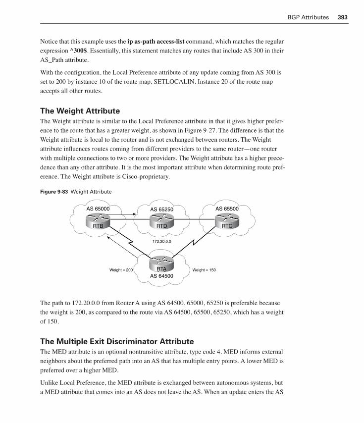
BGP Attributes 393
Notice that this example uses the ip as-path access-list command, which matches the regular
expression ^300$. Essentially, this statement matches any routes that include AS 300 in their
AS_Path attribute.
With the configuration, the Local Preference attribute of any update coming from AS 300 is
set to 200 by instance 10 of the route map, SETLOCALIN. Instance 20 of the route map
accepts all other routes.
The Weight Attribute
The Weight attribute is similar to the Local Preference attribute in that it gives higher prefer-
ence to the route that has a greater weight, as shown in Figure 9-27. The difference is that the
Weight attribute is local to the router and is not exchanged between routers. The Weight
attribute influences routes coming from different providers to the same router—one router
with multiple connections to two or more providers. The Weight attribute has a higher prece-
dence than any other attribute. It is the most important attribute when determining route pref-
erence. The Weight attribute is Cisco-proprietary.
Figure 9-83 Weight Attribute
The path to 172.20.0.0 from Router A using AS 64500, 65000, 65250 is preferable because
the weight is 200, as compared to the route via AS 64500, 65500, 65250, which has a weight
of 150.
The Multiple Exit Discriminator Attribute
The MED attribute is an optional nontransitive attribute, type code 4. MED informs external
neighbors about the preferred path into an AS that has multiple entry points. A lower MED is
preferred over a higher MED.
Unlike Local Preference, the MED attribute is exchanged between autonomous systems, but
a MED attribute that comes into an AS does not leave the AS. When an update enters the AS
AS 65000 AS 65250 AS 65500
AS 64500
172.20.0.0
Weight = 200 Weight = 150
RTB RTD RTC
RTA
1358_fmi.book Page 393 Thursday, May 27, 2004 2:21 PM

394 Chapter 9: BGP
with a certain MED value, that value is used for decision-making within the AS. When BGP
forwards the routing update to another AS, the MED is reset to 0. This is true unless the out-
going MED is set to a specific value.
When the route is originated by the AS itself, the MED value typically follows the route’s
internal IGP metric. This becomes useful when a customer has multiple connections to the
same provider. The IGP metric reflects how close to or far from a certain exit point a network
is. A network that is closer to exit point A than to exit point B has a lower IGP metric in the
border router connected to A. When the IGP metric translates to MED, traffic coming into
the AS can enter from the link that is closer to the destination. This is because a lower MED is
preferred for the same destination. Both providers and customers can use this fact to balance
the traffic over multiple links between two autonomous systems.
Unless otherwise specified, the router compares MED attributes for paths from external
neighbors that are in the same AS. MEDs from different autonomous systems are not compa-
rable because the MED associated with a route usually gives some indication of the AS inter-
nal topology. Comparing MEDs from different autonomous systems is like comparing apples
and oranges. Still, if there is a reason to do so, the Cisco IOS software offers the bgp always-compare-med router command. An AS can use the MED to influence the outbound decision
of another AS, as shown in Figure 9-28.
Figure 9-84 Multiple Exit Discriminator Attribute
XNET receives routing updates about 128.213.0.0/16 from three different sources—San Jose
as metric 120, Los Angeles as metric 200, and New York as metric 50. San Francisco com-
pares the two metric values coming from ANET and prefers the San Jose router because it
advertises a lower metric, 120. When the bgp always-compare-med command is used on the
San Francisco router, it then compares metrics. It compares metric 120 to metric 50 coming
SF
XNET
NY
YNET
MED = 50
MED = 200MED = 120
ANET
SJ LA
128.213.0.0/16
1358_fmi.book Page 394 Thursday, May 27, 2004 2:21 PM

BGP Attributes 395
from New York and prefers New York to reach 128.213.0.0/16. Notice that San Francisco can
influence its decision by using local preference inside XNET to override the metrics coming
from outside autonomous systems. Nevertheless, MED is still useful in case XNET prefers to
base its BGP decisions on outside factors to simplify router configuration on its end. Custom-
ers who connect to the same provider in multiple locations can exchange metrics with their
providers to influence the outbound traffic for each router. This leads to better load balancing.
MED Configuration ExampleIn Figure 9-29, AS 100 receives updates about network 180.10.0.0 from RTB, RTC, and
RTD. RTC and RTD are in AS 300, and RTB is in AS 400.
Figure 9-85 MED Configuration Example
Use a route map to configure the MED attribute on a router, as shown in Example 9-12.
By default, BGP compares only the MED attributes of routes coming from neighbors in the
same external AS, such as AS 300 in the example. This means that RTA compares the MED
attribute coming from RTC (120) only to the MED attribute coming from RTD (200). Even
though the update coming from RTB has the lowest MED value, RTA chooses RTC as the
Example 9-12 MED Attribute Configuration
RTB(config)#rrrroooouuuutttteeee----mmmmaaaapppp sssseeeettttmmmmeeeeddddoooouuuutttt ppppeeeerrrrmmmmiiiitttt 11110000
RTB(config-route-map)#sssseeeetttt mmmmeeeettttrrrriiiicccc 55550000
RTB(config)#rrrroooouuuutttteeeerrrr bbbbggggpppp 444400000000
RTB(config-router)#nnnneeeeiiiigggghhhhbbbboooorrrr 4444....4444....4444....4444 rrrroooouuuutttteeee----mmmmaaaapppp sssseeeettttmmmmeeeeddddoooouuuutttt oooouuuutttt
AS 100 AS 400
AS 300
170.10.0.0
2.2.2.2 3.3.3.2
4.4.4.44.4.4.3
180.10.0.0Med = 50
5.5.5.5
180.10.0.0Med = 200
2.2.2.1
1.1.1.1
180.10.0.0Med = 120
1.1.1.2
3.3.3.3
5.5.5.4
180.10.0.0
RTA RTB
RTC RTD
1358_fmi.book Page 395 Thursday, May 27, 2004 2:21 PM

396 Chapter 9: BGP
best path for reaching network 180.10.0.0. To force RTA to include updates for network
180.10.0.0 from RTB in the comparison, use the bgp always-compare-med router configu-
ration command.
RTA chooses RTB as the best next hop for reaching network 180.10.0.0, assuming that all
other attributes are the same. The MED attribute can also be set when configuring the redistri-
bution of routes into BGP. For example, on RTB the static route can be injected into BGP
with a MED of 50. The preceding configuration causes RTB to send out updates for
180.10.0.0 with a MED attribute of 50.
The Origin Attribute
The Origin attribute is a well-known mandatory attribute, type code 1, that indicates the rout-
ing update’s origin. BGP allows the following three types of origins:
■ IGP—The prefix is internal to the originating AS.
■ EGP—The prefix was learned by way of some EGP, such as BGP.
■ Incomplete—The prefix was learned by some other means—probably redistribution.
BGP considers the Origin attribute in its decision-making process to establish a preference
ranking among multiple routes. Specifically, BGP prefers the path with the lowest origin
type, where IGP is lower than EGP, and EGP is lower than Incomplete.
The BGP Decision ProcessBGP bases its decision process on the attribute values. When faced with multiple routes to the
same destination, BGP chooses the best route for routing traffic toward the destination. The
following process summarizes how BGP chooses the best route:
1. If the next hop is inaccessible, the route is ignored. This is why it is important to have an IGP route to the next hop.
2. The BGP router prefers the path with the greatest weight. Weight is a Cisco-proprietary parameter.
Lab 9.11.4a Configuring IBGP and EBGP Sessions, Local Preference, and MED
In this lab, you configure both IBGP and EBGP.
Lab 9.11.4c The BGP COMMUNITIES Attribute
In this lab, you use the COMMUNITIES attribute to enforce a routing policy.
1358_fmi.book Page 396 Thursday, May 27, 2004 2:21 PM
BGP Route Filtering and Policy Routing 397
3. If the weights are the same, the BGP router prefers the route with the largest local preference.
4. If the routes have the same local preference, the BGP router prefers the route that was locally originated by this router.
5. If the local preference is the same, the BGP router prefers the route with the shortest AS_Path.
6. If the AS_Path length is the same, the BGP router prefers the route with the lowest ori-gin type. This is when IGP is lower than EGP and EGP is lower than Incomplete.
7. If the origin type is the same, the BGP router prefers the route with the lowest MED.
8. If the routes have the same MED, the BGP router prefers the route in the following manner. Paths containing AS_CONFED_SEQUENCE are local to the confederation and, therefore, are treated as internal paths. No distinction is made between Confedera-tion External and Confederation Internal. BGP confederations are not covered in this book. For more information, consult Cisco’s website at http://www.cisco.com/univercd/home/home.htm.
9. If all of the preceding scenarios are identical, the BGP router prefers the route that can be reached by way of the closest IGP neighbor. That means taking the shortest internal path inside the AS to reach the destination by following the shortest path to the BGP next hop. When both paths are external, the path that was received first is preferred.
10. If the internal path is the same, the BGP router ID is a tiebreaker. The BGP router pre-fers the route coming from the BGP router with the lowest router ID. The router ID is usually the highest IP address on the router or the loopback address.
BGP Route Filtering and Policy RoutingThe following sections discuss some of the details of BGP route filtering and policy routing.
These topics are covered:
■ BGP route filtering
■ Using filters to implement routing policy
■ Using the distribute-list command to filter BGP routes
■ The ip prefix-list command
■ Sample ip prefix-list configuration
BGP Route Filtering
Route filtering empowers a BGP speaker to choose what routes to exchange with any of its
BGP peers. Route filtering is the cornerstone of policy routing. For example, an AS can
1358_fmi.book Page 397 Thursday, May 27, 2004 2:21 PM

398 Chapter 9: BGP
identify inbound traffic that it is willing to accept by filtering its outbound advertisements.
Conversely, an AS can control what routes its outbound traffic uses by specifying the routes
to accept from EBGP neighbors.
Policies that are even more precise can be defined by way of route filters. For example, BGP
routes passing through a filter can have their attributes manipulated to affect the best-path
decision process.
Both the inbound and outbound filtering concepts can be applied between peers and between
routing protocols running on a single router, as shown in Figure 9-30. At the peer level,
inbound filtering indicates that the BGP speaker is filtering routing updates coming from
other peers. The outbound filtering limits the routing updates advertised from this BGP
speaker toward other peers.
Figure 9-86 Inbound and Outbound Filtering
At the protocol level, inbound filtering limits the routing updates being redistributed into a
protocol. Outbound filtering limits the routing updates being injected from this protocol. With
respect to BGP, for example, inbound filtering limits the updates being redistributed from
other protocols into BGP. Outbound filtering limits the updates being redistributed from BGP
into an IGP.
The following sections examine the use of filters to implement routing policy and the use of
distribute and prefix lists to filter routing updates.
Inbound Filtering
RTABGP
BGPIGP
Inbound Filtering
Outbound Filtering Outbound Filtering
At the peer levelwith respect to RTA.
At the protocol levelwith respect to BGP.
1358_fmi.book Page 398 Thursday, May 27, 2004 2:21 PM

BGP Route Filtering and Policy Routing 399
Using Filters to Implement Routing Policy
Two distinct steps are involved in manipulating a route or a set of routes:
1. Identify the network number and subnet mask of the route to which the policies are to be applied. For BGP, this information is the NLRI. Recall that the NLRI consists of a prefix and prefix length pair. Throughout this section, the NLRI is called the prefix.
2. Implement the policies, which can be filtering out prefixes altogether or manipulating the attributes of a prefix to influence the routing decision.
The identification process typically relies on a route map. Prefixes can be selected by their
destination network number, the AS from which the prefix originated, the AS_Path, or
another specific attribute value. Prefixes are identified using the match statement from the
route map. After a route map matches a given prefix, the actions specified by the route map
are executed, and processing is considered complete. In other words, when a prefix matches,
it is not passed through any remaining clauses in the route map.
What actions can the route map take after it has identified a match? The simplest actions are
either to permit the route to pass through or to filter it out by denying it. Actions that are more
complex adjust a prefix’s attributes to influence the routing process in some way.
Notice that the route map can match a prefix based on several criteria, such as network num-
ber or AS_Path information. Also, notice that as soon as a route matches, no further compari-
sons occur. The order in which the matches are configured in the route map is important. If a
route map clause that permits all routes is put at the beginning of the list, it overrides all the
other policies configured.
Using the distribute-list Command to Filter BGP Routes
To restrict the routing information that the router learns or advertises, you filter routing
updates. You apply route filters to or from a particular neighbor by using the distribute-list command. See Chapter 8 for more details about this command’s syntax. In Figure 9-31, RTD
in AS2 originates network 192.68.10.0/24 and sends it to RTF. RTF passes the update to RTA
by way of IBGP, which in turn propagates it to AS1. By doing so, AS3 could become a transit
AS advertising that it is a path to reach network 192.68.10.0/24.
1358_fmi.book Page 399 Thursday, May 27, 2004 2:21 PM

400 Chapter 9: BGP
Figure 9-87 Distribute Lists
To prevent this situation from happening, configure RTA as shown in Example 9-13.
The distribute-list keyword, used as part of a BGP neighbor statement, prevents RTA from
advertising prefix 192.68.10.0/24 to RTC. The access list is used to identify the prefixes to be
filtered, and the distribute-list and out keywords apply the filter to outgoing updates.
Notice that access list 1 concludes with a permit 0.0.0.0 255.255.255.255 statement that is
the same as a permit any statement. Remember that, when you use access lists for filtering,
anything that does not match a permit statement is denied. Without the permit 0.0.0.0 255.255.255.255 clause, all updates to RTC would be suppressed.
Configuring BGP neighbor statements to include the distribute-list keyword is effective for
filtering specific routes, but controlling supernets can be more complicated.
Example 9-13 RTA Running Configuration Using the distribute-list Keyword
RTA#sssshhhhoooowwww rrrruuuunnnnnnnniiiinnnngggg----ccccoooonnnnffffiiiigggguuuurrrraaaattttiiiioooonnnn
router bgp 3
no synchronization
neighbor 172.16.1.2 remote-as 3
neighbor 172.16.20.1 remote-as 1
neighbor 172.16.20.1 distribute-list 1 out
no auto-summary
access-list 1 deny 192.68.10.0 0.0.0.255
access-list 1 permit 0.0.0.0 255.255.255.255
AS 3
AS 1 AS 2
172.16.10.0/24
172.16.1.2
172.16.20.2
172.16.65.0/26
172.16.20.1 192.68.10.0/24
RTA
RTC
RTF
RTD
1358_fmi.book Page 400 Thursday, May 27, 2004 2:21 PM

BGP Route Filtering and Policy Routing 401
Configuring a distribute list relies on creating an access list. If you use a standard access list,
you have only limited functionality. RTA connects to multiple subnets in the 172.16.0.0/16
address space. The purpose is to advertise an aggregate address of 172.16.0.0/16, but not the
individual subnets themselves. A standard access list would not work, because it permits more
than you want. It filters based on the network address only. The following access list would per-
mit not only the 172.16.0.0/16 summary, but also all of the components of that summary:
aaaacccccccceeeessssssss----lllliiiisssstttt 1111 ppppeeeerrrrmmmmiiiitttt 111177772222....11116666....0000....0000 0000....0000....222255555555....222255555555
To restrict the update to the 172.16.0.0/16 summary, use an extended access list. An extended
access list is usually thought of as matching both source and destination addresses. In the
case of a BGP route filter, an extended access list matches the network address first and then
the prefix’s subnet mask. Both network and mask are paired with their own wildcard bit mask
using the following syntax:
router(config)#aaaacccccccceeeessssssss----lllliiiisssstttt number {ppppeeeerrrrmmmmiiiitttt | ddddeeeennnnyyyy} nnnneeeettttwwwwoooorrrrkkkk network-wildcard mmmmaaaasssskkkk mask-wildcard
To permit the aggregate address, configure an extended access list to match the network
address and also the 16-bit prefix mask, as shown in Example 9-14. Using this configuration,
RTA does not send a subnet route, such as 172.16.0.0 /17 or 172.16.10.0 /24, in an update to
AS1.
If using an extended access list to accomplish this type of filtering seems confusing, that is
not unusual. Improved user friendliness was one of the factors that motivated Cisco to include
the ip prefix-list command in Cisco IOS Release 12.0. This command is described in the next
section.
Example 9-14 Access List Example
RTA(config)#rrrroooouuuutttteeeerrrr bbbbggggpppp 3333
RTA(config-router)#nnnneeeeiiiigggghhhhbbbboooorrrr 111177772222....11116666....1111....2222 rrrreeeemmmmooootttteeee----aaaassss 3333
RTA(config-router)#nnnneeeeiiiigggghhhhbbbboooorrrr 111177772222....11116666....22220000....1111 rrrreeeemmmmooootttteeee----aaaassss 1111
RTA(config-router)#nnnneeeeiiiigggghhhhbbbboooorrrr 111177772222....11116666....22220000....1111 ddddiiiissssttttrrrriiiibbbbuuuutttteeee----lllliiiisssstttt 111100001111 oooouuuutttt
RTA(config-router)#EEEEXXXXIIIITTTT
RTA(config)#aaaacccccccceeeessssssss----lllliiiisssstttt 111100001111 ppppeeeerrrrmmmmiiiitttt iiiipppp 111177772222....11116666....0000....0000 0000....0000....0000....0000 222255555555....222255555555....0000....0000 0000....0000....0000....0000
RTA(config)#aaaacccccccceeeessssssss----lllliiiisssstttt 111100001111 ddddeeeennnnyyyy iiiipppp 111177772222....11116666....0000....0000 0000....0000....222255555555....222255555555 222255555555....222255555555....0000....0000 0000....0000....222255555555....222255555555
RTA(config)#aaaacccccccceeeessssssss----lllliiiisssstttt 111100001111 ppppeeeerrrrmmmmiiiitttt iiiipppp aaaannnnyyyy aaaannnnyyyy
Lab 9.11.4b BGP Route Reflectors and Route Filters
In this lab, you configure IBGP routers to use a router reflector and a simple router
filter.
1358_fmi.book Page 401 Thursday, May 27, 2004 2:21 PM

402 Chapter 9: BGP
The ip prefix-list Command
You can use prefix lists as an alternative to access lists with many BGP route filtering com-
mands. Using prefix lists rather than access lists has the following advantages:
■ Significant performance improvement in loading and route lookup of large lists.
■ Support for incremental updates. Filtering by way of extended access lists does not
support incremental updates.
■ A more user-friendly command-line interface.
■ Greater flexibility.
You need to define a prefix list before applying it as a route filter. The Cisco IOS software
allows a very flexible configuration procedure in which each statement can be assigned its
own sequence numbers.
To define a prefix list, use the ip prefix-list list-name [seq seq-value] {deny network/length |
permit network/length} [ge ge-value] [le le-value] command. Table 9-5 describes the param-
eters that are used with this command.Table 9-13 ip prefix-list Command Parameters
Parameter Description
list-name Specifies the name of a prefix list.
seq (Optional) Applies the sequence number to the prefix list entry being created or deleted.
seq-value (Optional) Specifies the sequence for the prefix list entry.
deny Denies access to matching conditions.
permit Permits access for matching conditions.
network/length Gives the network number and length, in bits, of the network mask.
ge (Optional) Applies the greater-than-or-equal-to value (ge-value) to the range specified.
ge-value (Optional) Specifies the lower limit of values in an allowable range of values—the from portion of the range description.
le (Optional) Applies the lesser-than-or-equal-to value (le-value) to the range specified.
le-value (Optional) Specifies the upper limit of values in an allowable range of values—the to portion of the range description.
1358_fmi.book Page 402 Thursday, May 27, 2004 2:21 PM

BGP Route Filtering and Policy Routing 403
Sample ip prefix-list Configuration
Example 9-15 shows the commands used to create a simple prefix list and apply it during
BGP configuration. The commands define a prefix list called ELMO, which is applied to out-
going EBGP updates to 192.168.1.1 using a neighbor statement.
The real power of the ip prefix-list command is in its optional parameters. The keywords ge
and le can be used to specify the range of the prefix length to be matched for prefixes that are
more specific than the network/length value. The prefix length range is assumed to be from
ge-value to 32 if only the ge attribute is specified. The prefix length range is assumed to be
from len to le-value if only the le attribute is specified. Notice that a specified ge-value and
le-value must satisfy the following condition:
len < ge-value <= le-value <= 32
For example, to accept a mask length of up to 24 bits in routes with the prefix 192.0.0.0/8,
and to deny more-specific routes, use the following commands:
RTA(config)#iiiipppp pppprrrreeeeffffiiiixxxx----lllliiiisssstttt GGGGRRRROOOOVVVVEEEERRRR ppppeeeerrrrmmmmiiiitttt 111199992222....0000....0000....0000////8888 lllleeee 22224444RTA(config)#iiiipppp pppprrrreeeeffffiiiixxxx----lllliiiisssstttt GGGGRRRROOOOVVVVEEEERRRR ddddeeeennnnyyyy 111199992222....0000....0000....0000////8888 ggggeeee 22225555
These commands test to see if a given prefix begins with 192 in the first octet. After that, they
are concerned with only how specific the route is by checking the mask’s length. Therefore,
both 192.168.32.0/19 and 192.168.1.0/24 match the permit statement, but 192.168.1.32/27
does not because its mask length is greater than the ge value, 25. Any routes with a mask
equal to the ge value are also denied.
The le and ge keywords can be used together in the same statement:
RTA(config)#iiiipppp pppprrrreeeeffffiiiixxxx----lllliiiisssstttt OOOOSSSSCCCCAAAARRRR ppppeeeerrrrmmmmiiiitttt 11110000....0000....0000....0000////8888 ggggeeee 11116666 lllleeee 22224444
This command permits all prefixes in the 10.0.0.0/8 address space that have a mask length
from 16 to 24 bits.
Each prefix list entry is assigned a sequence number, either by default or manually by an
administrator. By numbering the prefix-list statements, new entries can be inserted at any
point in the list. This is important because routers test for prefix list matches from lowest
sequence number to highest. When a match occurs, the router does not continue through the
Example 9-15 Sample IP Prefix List Configuration
RTA(config)#iiiipppp pppprrrreeeeffffiiiixxxx----lllliiiisssstttt EEEELLLLMMMMOOOO ddddeeeennnnyyyy 0000....0000....0000....0000////0000
RTA(config)#iiiipppp pppprrrreeeeffffiiiixxxx----lllliiiisssstttt EEEELLLLMMMMOOOO ppppeeeerrrrmmmmiiiitttt 111177772222....11116666....0000....0000////11116666
RTA(config)#rrrroooouuuutttteeeerrrr bbbbggggpppp 111100000000
RTA(config-router)#nnnneeeeiiiigggghhhhbbbboooorrrr 111199992222....111166668888....1111....1111 rrrreeeemmmmooootttteeee----aaaassss 222200000000
RTA(config-router)#nnnneeeeiiiigggghhhhbbbboooorrrr 111199992222....111166668888....1111....1111 pppprrrreeeeffffiiiixxxx----lllliiiisssstttt EEEELLLLMMMMOOOO oooouuuutttt
1358_fmi.book Page 403 Thursday, May 27, 2004 2:21 PM

404 Chapter 9: BGP
rest of the prefix list. For efficiency, put the most common matches near the top of the list.
The show ip prefix-list command always includes the sequence numbers in its output, as
shown in Example 9-16.
Sequence numbers are automatically generated in increments of 5. The first sequence value
generated in a prefix list is 5, then 10, then 15, and so on. If you manually specify a value for
an entry and then don’t specify values for subsequent entries, the assigned sequence values
are incremented in units of 5. For example, the first entry in the prefix list has a specified
sequence value of 3. Then no more sequence values are specified for the other entries, so the
automatically generated numbers are 8, 13, 18, and so on. You manually specify prefix list
sequence numbers like this:
RTA(config)#iiiipppp pppprrrreeeeffffiiiixxxx----lllliiiisssstttt EEEELLLLMMMMOOOO sssseeeeqqqq 11112222 ddddeeeennnnyyyy 111199992222....111166668888....1111....0000////22224444
You can manually specify sequence values for prefix list entries in any increment you want.
However, if you unwisely specify the sequence values in increments of 1, additional entries
cannot be inserted into the prefix list.
To display information about prefix tables, prefix table entries, the policy associated with a
node, or specific information about an entry, use the show ip prefix-list command.
Finally, when using prefix lists, keep the following rules in mind:
■ An empty prefix list permits all prefixes.
■ An implicit deny is assumed if a given prefix does not match any entries of a prefix list.
■ When multiple entries of a prefix list match a given prefix, the sequence number of a
prefix list entry identifies the entry with the lowest sequence number. In this case, the
entry with the smallest sequence number is considered the “real” match.
Redundancy, Symmetry, and Load BalancingRedundancy, symmetry, and load balancing are crucial needs facing anyone in the process of
implementing a high-throughput Internet connection. ISPs and their large customers require
adequate control over how traffic enters and exits their respective autonomous systems.
Example 9-16 show ip prefix-list Command
RTA#sssshhhhoooowwww iiiipppp pppprrrreeeeffffiiiixxxx----lllliiiisssstttt
ip prefix-list ELMO: 3 entries
seq 5 deny 0.0.0.0/0
seq 10 permit 172.16.0.0/16
seq 15 permit 192.168.0.0/16 le 24
1358_fmi.book Page 404 Thursday, May 27, 2004 2:21 PM

Redundancy, Symmetry, and Load Balancing 405
Issues with Redundancy, Symmetry, and Load Balancing
Redundancy is achieved by providing multiple alternative paths for the traffic. This occurs by
having multiple connections to one or more autonomous systems, as shown in Figure 9-32.
Symmetry exists if traffic leaves the AS from a certain exit point and returns through the same
point. Load balancing, as you have seen, results in the division of traffic optimally over mul-
tiple links. Together, these three requirements can be difficult to meet in a BGP environment,
because any provider between a packet’s source and destination can affect its path.
Figure 9-88 Redundancy, Symmetry, and Load Balancing
The general design problem of how best to implement redundancy, symmetry, and load bal-
ancing is common to every network. The specific solution, however, depends on the needs
and unique configuration of an individual network. The following sections examine the gen-
eral design issues of redundancy, symmetry, and load balancing, as well as configuration
models for successful implementation.
Redundancy, Symmetry, and Load Balancing
Although corporations and ISPs prefer uninterrupted connectivity, disruptions still occur for a
variety of reasons. Connectivity is not the responsibility of one entity. A connection to the
Internet might involve a router, a CSU/DSU, premises wiring, the provider’s physical layer,
switching equipment, and numerous administrators. Each of these elements influences differ-
ent parts of the connection. At any time, end-to-end connectivity can be jeopardized by
human error, software errors, physical errors, or adverse unforeseen conditions, such as bad
weather or power outages.
AS 1 AS 2
AS 3
Internet
1358_fmi.book Page 405 Thursday, May 27, 2004 2:21 PM

406 Chapter 9: BGP
For these reasons, redundancy is generally desirable, but finding the optimal balance between
redundancy and symmetry is crucial. Redundancy and symmetry can be conflicting design
goals. The more redundant links a network has, the more unpredictable a packet’s entrance
and exit points become. For example, a customer might have multiple connections—one to a
POP in San Francisco and another to a POP in New York—as shown in Figure 9-33. There-
fore, traffic leaving San Francisco might come back through New York. Adding a third con-
nection to a POP in Dallas makes connectivity even more reliable, but it also makes traffic
symmetry more challenging. These are the trade-offs that network administrators must con-
sider when implementing routing policies.
Figure 9-89 Redundancy, Symmetry, and Load Balancing
Companies might also feel geographic pressure to implement redundancy. Many contempo-
rary companies are national, international, or multinational in nature, and their AS is a logical
entity that spans different physical locations. A corporation with an AS that spans several
geographic points can take service from a single provider or from different providers in dif-
ferent regions. In Figure 9-33, the San Francisco office of AS1 connects to the San Francisco
POP of ISP1, and the New York office connects to the New York POP of ISP2. In this envi-
ronment, traffic can take a shorter path to reach a destination by traveling by way of the geo-
graphically adjacent POP.
Because redundancy refers to the existence of alternative routes to and from a network, addi-
tional routing information needs to be kept in the routing tables. To avoid this extra routing
overhead, default routing becomes an alternative practical tool that can be used to provide
backup routes in case primary connections fail. The next section discusses the different
aspects of default routing and how it can be applied to achieve simple routing scenarios.
ISP 1SF POP ISP 2 NY POP
SanFrancisco
NewYork
AS 1
1358_fmi.book Page 406 Thursday, May 27, 2004 2:21 PM

Redundancy, Symmetry, and Load Balancing 407
Default Routing in BGP Networks
You have seen that default routes minimize the size of a routing table. They can also provide
networks with redundancy in the event of failures and connectivity interruptions. BGP, like
almost all IGPs, can distribute a default route. To provide redundancy, default information
can be received from multiple BGP sources. In a BGP system, the Local Preference attribute
can be manipulated on the various default routes. This is so that one default route is identified
as primary (the highest Local Preference), and others are kept as backups. If the primary fails,
a backup route with the next-highest preference can take its place.
In Figure 9-34, RTA is connected to RTB and is learning about two default routes—one by
way of 1.1.1.1 and a second by way of 2.2.2.2. By using the Local Preference attribute,
1.1.1.1 can be given preference and made the primary default route. RTA uses 2.2.2.2 as a
default only after 1.1.1.1 fails.
Figure 9-90 Default Routing in BGP Networks
In Figure 9-35, the same behavior can be achieved as long as IBGP is running inside the AS.
The Local Preference attribute, which is exchanged between IBGP peers, determines the pri-
mary and backup links.
RTB
AS 1 IBGP
RTA
Primary
Backup
AS 2
Set LOCAL_PREF 100
Set LOCAL_PREF 50Using 1.1.1.1 as a gateway oflast resort. 2.2.2.2 will not be
used unless 1.1.1.1 goesdown.
2.2.2.2
1.1.1.1
1358_fmi.book Page 407 Thursday, May 27, 2004 2:21 PM

408 Chapter 9: BGP
Figure 9-91 Local Preference
It is important to control default information in BGP because improper configuration can
cause serious Internet routing problems. For example, a misconfigured BGP speaker could
end up flooding a default route to all of its neighbors and quickly find itself consumed with
default routed traffic from surrounding autonomous systems. To protect against misadvertise-
ments, the Cisco IOS software provides a way to target default information at a specific
neighbor by using the default-originate option with the neighbor command, as shown in
Example 9-17.
If RTC is configured as shown in this configuration, it sends default information only to the
specified neighbor. If a BGP router is to be configured to advertise a default to all of its peers,
use the network command, as shown in Example 9-18.
Example 9-17 default-originate Option with the neighbor Command
RTC(config)#rrrroooouuuutttteeeerrrr bbbbggggpppp 3333
RTC(config-router)#nnnneeeeiiiigggghhhhbbbboooorrrr 111177772222....11116666....22220000....1111 rrrreeeemmmmooootttteeee----aaaassss 1111
RTC(config-router)#nnnneeeeiiiigggghhhhbbbboooorrrr 111177772222....11116666....22220000....1111 ddddeeeeffffaaaauuuulllltttt----oooorrrriiiiggggiiiinnnnaaaatttteeee
Example 9-18 network Command
RTC(config)#rrrroooouuuutttteeeerrrr bbbbggggpppp 3333
RTC(config-router)#nnnneeeeiiiigggghhhhbbbboooorrrr 111177772222....11116666....22220000....1111 rrrreeeemmmmooootttteeee----aaaassss 1111
RTC(config-router)#nnnneeeeiiiigggghhhhbbbboooorrrr 111177772222....11117777....1111....1111 rrrreeeemmmmooootttteeee----aaaassss 2222
RTC(config-router)#nnnneeeettttwwwwoooorrrrkkkk 0000....0000....0000....0000
Primary
AS 2
Backup
AS 1
Using 1.1.1.1 as a gateway oflast resort. 2.2.2.2 will not be
used unless 1.1.1.1 goesdown.
Set LOCAL_PREF 100
Set LOCAL_PREF 50
1.1.1.1
2.2.2.2
RTBRTA
NOTE
Both neighbors, 172.16.20.1 and 172.17.1.1, receive a default route from RTC. To propagate network 0.0.0.0, it would have to be a static route or a route learned by way of a dynamic routing protocol. It would also need to exist in the routing table.
1358_fmi.book Page 408 Thursday, May 27, 2004 2:21 PM

Redundancy, Symmetry, and Load Balancing 409
Many network administrators choose to filter dynamically learned default routes to avoid sit-
uations in which traffic ends up where it is not supposed to be. Without dynamically learned
default routes, a router must be statically configured with default information. Statically con-
figured default routes typically provide more control over routing within an AS.
Symmetry
Symmetry is achieved when traffic leaving the AS from one exit point comes back through
the same point. Symmetry always exists if an AS maintains a single connection to outside
networks. However, the need for redundancy often results in multihoming an AS. If an AS
has many different links to the outside world, traffic tends to flow asymmetrically. An asym-
metric traffic flow can result in increased delay and other routing problems. In general, cus-
tomers and providers want to see their traffic come back by way of the same point or close to
the same point where it left the AS.
To promote symmetry, choose a primary path, and configure routing policies that force traffic
to flow along this path. A default route with a low administrative distance or a high Local
Preference might control the flow of outbound traffic, but inbound traffic can be more com-
plex to manipulate. Through appropriate planning and use of BGP attributes and route filters,
an AS can control which paths the outside world finds most desirable.
Load Balancing
Load balancing is the capability to divide data traffic over multiple connections. A BGP
speaker might learn two identical EBGP paths for a prefix from a neighboring AS. If this hap-
pens, it chooses the path with the lowest route ID as the best path. This best path is installed
in the IP routing table. If BGP multipath support is enabled and the EBGP paths are learned
from the same neighboring AS, the best path might not be chosen. Instead, multiple paths are
installed in the IP routing table. To enable BGP load balancing over equal-cost paths, use the
maximum-paths command, which has the following syntax:
Router(config-router)#mmmmaaaaxxxxiiiimmmmuuuummmm----ppppaaaatttthhhhssss number
BGP supports a maximum of six paths per destination, but only if they are sourced from the
same AS. If the maximum-paths option is not enabled, BGP installs only one path to the IP
routing table.
Figure 9-36 illustrates how inbound and outbound traffic behaves. The path for outbound traf-
fic to reach Net A depends on where Net A is learned. Because Net A is received from both
San Francisco and New York, outbound traffic toward Net A can go by way of San Francisco
or New York.
1358_fmi.book Page 409 Thursday, May 27, 2004 2:21 PM

410 Chapter 9: BGP
Figure 9-92 Load Balancing
Multihomed Connections
Although running BGP when the AS is multihomed to the same ISP is not necessary, it is gener-
ally recommended. In Figure 9-37, the customer wants to configure only default routes toward the
provider. The customer does not want any part of the Internet routing table. Although it might
seem that a static configuration could work, BGP can offer a more powerful solution.
Figure 9-93 Multihomed Connections with a Single Provider
The customer wants to use one link as the primary traffic conduit and the other as a backup in
case the primary link goes down. For outbound traffic, the customer could configure two
static default routes with different administrative distances. This would create a primary route
and a floating static route to be used as a backup. The default with the lower distance would
be the primary.
Outbound DecisionNet A
Net A
SF
NY
Which way should theoutbound traffic go to
reach Net A, by way ofSF or NY?
Inbound DecisionNet B
Net B
SF
NY
Inbound traffic forNetB by way of the SF
Link is the desiredroute. Therefore, Net Bwill not be advertised
on the NY link.
SF NYProvider
AS 1
Default-2Backup
Default-1Primary
Metric 100 Metric 50
CustomerAS 3
172.16.20.1 192.168.9.2
RTA
1358_fmi.book Page 410 Thursday, May 27, 2004 2:21 PM

Redundancy, Symmetry, and Load Balancing 411
However, the customer might want to learn the default route, or a few aggregate routes,
dynamically from the provider using BGP. In this case, the ISP or the customer could filter
the advertisements so that only minimum necessary routes are sent. The Local Preference
attribute could then be used to prefer one default route over the other.
Assume that in Figure 9-37, the default route to New York is preferred over the default route
to San Francisco. In normal operations, the customer would use the New York link as the pri-
mary link and the San Francisco link as a backup.
For outbound traffic, load balancing is not an option. This is because all traffic is sent over the
primary path, and the secondary is kept as the backup. The absence of load balancing is offset
by the fact that the customer’s router requires less memory and processing power.
As for inbound traffic, the customer must carefully control updates to the provider. The cus-
tomer can advertise its networks to the provider by way of BGP. This way, the provider has
two paths to reach destinations within the customer’s network. The customer can influence
the routing decisions made by the ISP by manipulating the metrics advertised to the ISP. The
provider directs its traffic toward the customer based on the metric value. In Figure 9-37, the
customer advertises routes with a metric of 50 toward New York and a metric of 100 toward
San Francisco. Therefore, traffic toward the customer takes the New York route. Example 9-19
shows a customer’s boundary router configuration example.
Example 9-19 Configuring BGP with a Multihomed Connection
RTA(config)#rrrroooouuuutttteeeerrrr bbbbggggpppp 3333
RTA(config-router)#nnnnoooo aaaauuuuttttoooo----ssssuuuummmmmmmmaaaarrrryyyy
RTA(config-router)#nnnneeeeiiiigggghhhhbbbboooorrrr 111177772222....11116666....22220000....1111 rrrreeeemmmmooootttteeee----aaaassss 1111
RTA(config-router)#nnnneeeeiiiigggghhhhbbbboooorrrr 111177772222....11116666....22220000....1111 rrrroooouuuutttteeee----mmmmaaaapppp BBBBLLLLOOOOCCCCKKKK iiiinnnn
RTA(config-router)#nnnneeeeiiiigggghhhhbbbboooorrrr 111177772222....11116666....22220000....1111 rrrroooouuuutttteeee----mmmmaaaapppp SSSSEEEETTTTMMMMEEEETTTTRRRRIIIICCCC1111 oooouuuutttt
RTA(config-router)#nnnneeeeiiiigggghhhhbbbboooorrrr 111199992222....111166668888....9999....2222 rrrreeeemmmmooootttteeee----aaaassss 1111
RTA(config-router)#nnnneeeeiiiigggghhhhbbbboooorrrr 111199992222....111166668888....9999....2222 rrrroooouuuutttteeee----mmmmaaaapppp BBBBLLLLOOOOCCCCKKKK iiiinnnn
RTA(config-router)#nnnneeeeiiiigggghhhhbbbboooorrrr 111199992222....111166668888....9999....2222 rrrroooouuuutttteeee----mmmmaaaapppp SSSSEEEETTTTMMMMEEEETTTTRRRRIIIICCCC2222 oooouuuutttt
RTA(config-router)#eeeexxxxiiiitttt
RTA(config)#rrrroooouuuutttteeee----mmmmaaaapppp SSSSEEEETTTTMMMMEEEETTTTRRRRIIIICCCC1111 ppppeeeerrrrmmmmiiiitttt 11110000
RTA(config-route-map)#sssseeeetttt mmmmeeeettttrrrriiiicccc 111100000000
RTA(config-route-map)#rrrroooouuuutttteeee----mmmmaaaapppp SSSSEEEETTTTMMMMEEEETTTTRRRRIIIICCCC2222 ppppeeeerrrrmmmmiiiitttt 11110000
RTA(config-route-map)#sssseeeetttt mmmmeeeettttrrrriiiicccc 55550000
RTA(config-route-map)#rrrroooouuuutttteeee----mmmmaaaapppp BBBBLLLLOOOOCCCCKKKK ddddeeeennnnyyyy 11110000
RTA(config-route-map)#eeeexxxxiiiitttt
RTA(config)#iiiipppp rrrroooouuuutttteeee 0000....0000....0000....0000 0000....0000....0000....0000 111177772222....11116666....22220000....1111 55550000
RTA(config)#iiiipppp rrrroooouuuutttteeee 0000....0000....0000....0000 0000....0000....0000....0000 111199992222....111166668888....9999....2222 44440000
1358_fmi.book Page 411 Thursday, May 27, 2004 2:21 PM
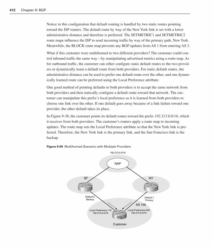
412 Chapter 9: BGP
Notice in this configuration that default routing is handled by two static routes pointing
toward the ISP routers. The default route by way of the New York link is set with a lower
administrative distance and therefore is preferred. The SETMETRIC1 and SETMETRIC2
route maps influence the ISP to send incoming traffic by way of the primary path, New York.
Meanwhile, the BLOCK route map prevents any BGP updates from AS 1 from entering AS 3.
What if this customer were multihomed to two different providers? The customer could con-
trol inbound traffic the same way—by manipulating advertised metrics using a route map. As
for outbound traffic, the customer can either configure static default routes to the two provid-
ers or dynamically learn a default route from both providers. For static default routes, the
administrative distance can be used to prefer one default route over the other, and one dynam-
ically learned route can be preferred using the Local Preference attribute.
One good method of pointing defaults to both providers is to accept the same network from
both providers and then statically configure a default route toward that network. The cus-
tomer can manipulate this prefix’s local preference as it is learned from both providers to
choose one link over the other. If one default goes away because of a link failure toward one
provider, the other default takes its place.
In Figure 9-38, the customer points its default routes toward the prefix 192.213.0.0/16, which
it receives from both providers. The customer’s routers apply a route map to incoming
updates. The route map sets the Local Preference attribute so that the New York link is pre-
ferred. Therefore, the New York link is the primary link, and the San Francisco link is the
backup.
Figure 9-94 Multihomed Scenario with Multiple Providers
RTA
192.213.0.0/16
NAP
SF NY
Default-2Backup
Default-1Primary
Local Preference-110192.213.0.0/16
Local Preference-200192.213.0.0/16
Customer
AS 100
1358_fmi.book Page 412 Thursday, May 27, 2004 2:21 PM

BGP Redistribution 413
BGP RedistributionThe following sections discuss some of the details of BGP redistribution:
■ BGP redistribution overview
■ Injecting unwanted or faulty information
■ Injecting information statically into BGP
■ BGP redistribution configuration example
BGP Redistribution Overview
When dealing with BGP, route stability is an important issue. There is a close relationship
between Internet route stability and the method used to inject routes into BGP. Information
can be injected into BGP dynamically or statically. Dynamically injected routes come and go
from the BGP routing table, depending on the status of the networks they identify. Statically
injected routes are constantly maintained by the BGP routing tables, regardless of the status
of the networks they identify. Therefore, although a dynamic advertisement ends if the net-
work being advertised no longer exists, a static advertisement does not. Each method has pros
and cons, as discussed in this section.
Dynamically injected information can be further divided into purely dynamic redistribution,
in which all of the IGP routes are redistributed into BGP using the redistribute command.
Dynamically injected information can be further divided into semidynamic redistribution, in
which only certain IGP routes are to be injected into BGP using the BGP network command.
This distinction reflects both the level of user intervention and the level of control in defining
the routes to be advertised.
Information is injected dynamically into BGP by enabling all of the IGP routes of RIP, OSPF,
EIGRP, and so on to be redistributed into BGP. Dynamic redistribution offers ease of config-
uration. All internal IGP routes dynamically flow into BGP, regardless of the protocols being
used.
The semidynamic method of injecting information into BGP is to specify a subset of IGP net-
works. This is to be advertised by individually listing them for injection into BGP by using
the network command. This method is more selective than a completely dynamic method.
You can control which IGP-learned routes BGP advertises. Unfortunately, a network com-
mand is necessary for each route prefix, so when you’re dealing with a large number of pre-
fixes, maintaining semidynamic configurations is impractical. In fact, the Cisco IOS software
sets the limit to 200 network statements. Ultimately, a semidynamic configuration provides
greater administrative control but dramatically increases administrative overhead.
BGP assumes that prefixes specified by the network command exist in an IGP domain. This
is verified by checking for them in the routing table. If an IGP has not learned about a local
1358_fmi.book Page 413 Thursday, May 27, 2004 2:21 PM

414 Chapter 9: BGP
route, BGP does not advertise it. Of course, the no synchronization command can be used to
disable this verification. However, in doing so, there is a risk that a router will advertise net-
works it cannot reach.
Injecting Unwanted or Faulty Information
Injecting routes into BGP by way of the network command might not always be practical or
even possible. Injecting routes by way of redistribution can result in polluting other autono-
mous systems with unwelcome, incorrect, or otherwise undesirable information. Redistribut-
ing the entire IGP table into BGP could result in private addresses, or illegal addresses, being
advertised outside the AS. In some cases, routes with inappropriate prefix lengths could make
it upstream to the provider, where they are not needed. For example, host routes are generally
greeted with disdain by annoyed systems administrators.
Mutual redistribution between IGP and BGP can also result in the propagation of flawed rout-
ing information. In this case, a BGP route that was injected from the outside could be sent
back into BGP by way of the IGP. This happens as if the route originated within the AS. Fig-
ure 9-39 illustrates the danger of mutual redistribution between protocols.
Figure 9-95 Practical Design Example
In Figure 9-39, AS 100 is the source of NetA and sends this information by way of BGP to
AS 200. The border router RTC injects that information into the IGP, and RTB learns about it.
RTB is configured to redistribute the IGP information into BGP. NetA ends up being adver-
tised by way of BGP back to the Internet as if it originated from AS 200. This is very mislead-
ing to autonomous systems connected to the Internet, because NetA now has two sources
rather than one source—AS 100 and AS 200.
Net A
IBGP
IGP
AS 100
AS 200
RTA
RTBRTC
RTD
RTF
1358_fmi.book Page 414 Thursday, May 27, 2004 2:21 PM

BGP Redistribution 415
To remedy these situations, special filtering should be put on the border routers to specify
what particular networks should be injected from the IGP into BGP. For protocols that differ-
entiate between internal and external routes, such as OSPF, configure the IGP to ensure that it
will redistribute only internal routes into BGP. In the Cisco implementation, external OSPF
routes are automatically blocked from being redistributed into BGP. You can override this
behavior. Certain protocols might not distinguish between internal and external routes, such
as RIP or IGRP. For these types of protocols, special route tagging should be performed to
differentiate between external routes and internal routes.
Injecting Information Statically into BGP
Injecting information statically into BGP has proven to be the most effective means of ensur-
ing route stability. Of course, this method also has drawbacks. To statically inject information
into BGP, the IGP routes, or aggregates, that need to be advertised to other peers are manually
defined as static routes. This ensures that these routes never disappear from the IP routing
table and, hence, are always advertised. Administrators are often uncomfortable advertising
routes to networks that might be down or unreachable. Whether it is appropriate to inject this
information statically depends on the particular situation.
For example, if the route is advertised to the Internet from a single point, advertising a route
that is actually down is debatable. Hosts trying to access that destination will fail, regardless
of whether the route is advertised. On the other hand, if a route is advertised to the Internet
from multiple points, advertising the route statically at all times might end up creating a black
hole for traffic. If problems inside the AS do not allow the border router to reach the network
it is advertising, traffic to that destination is dropped. This happens even though it could have
been reached from some other entry point.
BGP Redistribution Configuration Example
As with IGP routes, all known static routes can be injected into BGP using the redistribute
command. A subset of static routes can be injected using the BGP network command. The
network command provides greater control while increasing the administrative burden.
Figure 9-40 demonstrates how routing information can be injected dynamically into BGP.
Issue the commands shown in Example 9-20 to configure RTB in Figure 9-40 to redistribute
OSPF learned routes into BGP dynamically.
1358_fmi.book Page 415 Thursday, May 27, 2004 2:21 PM

416 Chapter 9: BGP
Figure 9-96 Injecting OSPF Routes Into BGP Dynamically
For insurance, configure a route map that matches any private addresses that are not to be
advertised outside the AS. This route map, appropriately called BLOCK-BAD-
ADDRESSES, is applied to outbound BGP updates. Also, BGP has been configured to redis-
tribute only internal OSPF routes and assign them a metric of 50. The redistribute static
command dynamically populates BGP with any static routes RTB happens to be configured
with. Alternatively, configure RTB to inject internal routes semidynamically by using the
BGP network command, as shown in Example 9-21.
Example 9-20 BGP Redistribution Configuration Example
RTB(config)#rrrroooouuuutttteeeerrrr bbbbggggpppp 222200000000
RTB(config-router)#nnnneeeeiiiigggghhhhbbbboooorrrr 11110000....1111....1111....2222 rrrreeeemmmmooootttteeee----aaaassss 111100000000
RTB(config-router)#nnnneeeeiiiigggghhhhbbbboooorrrr 11110000....1111....1111....2222 rrrroooouuuutttteeee----mmmmaaaapppp BBBBLLLLOOOOCCCCKKKK----BBBBAAAADDDD----AAAADDDDDDDDRRRREEEESSSSSSSSEEEESSSS oooouuuutttt
RTB(config-router)#rrrreeeeddddiiiissssttttrrrriiiibbbbuuuutttteeee oooossssppppffff 1111 mmmmaaaattttcccchhhh iiiinnnntttteeeerrrrnnnnaaaallll mmmmeeeettttrrrriiiicccc 55550000
RTB(config-router)#rrrreeeeddddiiiissssttttrrrriiiibbbbuuuutttteeee ssssttttaaaattttiiiicccc
Example 9-21 Injecting Internal Routes Semidynamically
RTB(config)#rrrroooouuuutttteeeerrrr bbbbggggpppp 222200000000
RTB(config-router)#nnnneeeeiiiigggghhhhbbbboooorrrr 11110000....1111....1111....2222 rrrreeeemmmmooootttteeee----aaaassss 111100000000
RTB(config-router)#nnnneeeeiiiigggghhhhbbbboooorrrr 11110000....1111....1111....2222 rrrroooouuuutttteeee----mmmmaaaapppp BBBBLLLLOOOOCCCCKKKK----BBBBAAAADDDD----AAAADDDDDDDDRRRREEEESSSSSSSSEEEESSSS oooouuuutttt
RTB(config-router)#nnnneeeettttwwwwoooorrrrkkkk 111199992222....111166668888....1111....0000
RTB(config-router)#nnnneeeettttwwwwoooorrrrkkkk 111199992222....111166668888....2222....0000
AS 100
S010.1.1.2/30 S0
10.1.1.1/30
EBGP
172.16.1.0/24 192.168.2.0/24
192.168.1.0/24172.16.2.0/24
OSPF OSPF
OSPF OSPF
AS 200
RTA RTB
1358_fmi.book Page 416 Thursday, May 27, 2004 2:21 PM

Summary 417
If RTB is configured accordingly, it does not inject all of the internal routes into BGP. Only
the two networks specified, 192.168.1.0 and 192.168.2.0, are injected, although all of them
could have been configured the same way. In a sense, the BGP network command redistrib-
utes the specified IGP route into BGP, allowing for precise control.
SummaryBGP defines the basis of routing architectures in the Internet. Segregating networks into
autonomous systems has logically defined the administrative and political borders between
organizations. IGPs can now run independently of each other but still interconnect by way of
BGP to provide global routing.
This chapter covered the details of the practical implementation of BGP as part of the overall
design problem in building reliable Internet connectivity. This chapter examined specific
BGP attributes and how they are applied individually and together to address this design
problem. The terminology, attributes, and details of this chapter are specific to BGP. How-
ever, the general concepts and problems raised are pertinent to routing architecture design,
regardless of the specific protocols being used.
Lab 9.12.1 BGP Challenge Lab
In this lab you configure EBGP between the company’s core routers and the two ISP
routers. You configure IBGP with peers to create a network that provides the Interna-
tional Travel Agency with a fully meshed, reliable, efficient core network.
1358_fmi.book Page 417 Thursday, May 27, 2004 2:21 PM

418 Chapter 9: BGP
Key TermsBorder Gateway Protocol (BGP) An interdomain routing protocol that replaced EGP. BGP
exchanges reachability information with other BGP systems. It is defined by RFC 1163.
EBGP session Occurs between routers in two different autonomous systems. These routers
are usually adjacent to one another, sharing the same medium and a subnet.
Exterior Gateway Protocol (EGP) An Internet protocol for exchanging routing informa-
tion between autonomous systems. Documented in RFC 904. Not to be confused with the
general term exterior gateway protocol. EGP is an obsolete protocol that has been replaced
by BGP.
IBGP session Occurs between routers in the same AS. Used to coordinate and synchronize
routing policy within the AS.
interior gateway protocol (IGP) An Internet protocol used to exchange routing information
within an autonomous system. Examples of common Internet IGPs are IGRP, OSPF, and RIP.
keepalive message Sent periodically between peers to maintain connections and verify
paths held by the router sending the keepalive.
multihomed system An autonomous system that has more than one exit point to outside
networks.
Network Layer Reachability Information (NLRI) BGP sends routing update messages
containing NLRI to describe a route and how to get there. In this context, an NLRI is a prefix.
A BGP update message carries one or more NLRI prefixes and the attributes of a route for the
NLRI prefixes. The route attributes include a BGP next-hop gateway address, community
values, and other information.
notification message Informs the receiving router of errors.
open message Establishes connections with peers. Includes fields for the BGP version
number, AS number, hold time, and Router ID.
single-homed system An autonomous system that has only one exit point to outside net-
works.
update message Contains all the information BGP uses to construct a loop-free picture of
the internetwork.
1358_fmi.book Page 418 Thursday, May 27, 2004 2:21 PM

Check Your Understanding 419
Check Your UnderstandingComplete all of the review questions to test your understanding of the topics and concepts in
this chapter. The answers appear in Appendix B, “Answers to the Check Your Understanding
Questions.”
For additional, more in-depth questions, refer to the chapter-specific study guides on the
companion CD-ROM.
1. What kind of AS features more than one exit point to outside networks but does not allow traffic to pass from one outside connection to another?
A. Stub
B. Multihomed nontransit
C. Multihomed transit
D. Totally stubby
2. In what situation is it inadvisable to run BGP?
A. Stub AS
B. Multihomed nontransit AS
C. Multihomed transit AS
D. When your AS policies differ from the ISP policies
3. What happens when a route is advertised to the AS that originated it?
A. The AS sees itself as part of the AS_Path attribute list and does not accept the route.
B. The border router prepends the AS number and advertises the router to other auton-
omous systems.
C. The route is passed to other routers within the AS as an external route.
D. The border router removes its AS number from the AS_Path list and redistributes
the route.
4. What is one way to set local preference in BGP?
A. Use the AS_Path attribute
B. Use the global prepend command
C. Use the bgp default local-preference command
D. Use the set as_path command
1358_fmi.book Page 419 Thursday, May 27, 2004 2:21 PM

420 Chapter 9: BGP
5. What command identifies the state of BGP neighbors?
A. show ip route
B. show ip bgp peer
C. show ip bgp paths
D. show ip bgp neighbors
6. In which situation is it OK to turn off BGP synchronization on a border router?
A. In a simple AS
B. In a non-fully meshed transit AS
C. When the AS is not a transit AS
D. When internal reachability is not guaranteed
7. In a BGP system, which attribute can be manipulated on the various default routes so that at least one default route is identified as primary, with other default routes being kept as backups?
A. Default-originate
B. Local Preference
C. Default Preference
D. Maximum-paths
8. What condition causes a BGP router to install multiple paths to the same destination in its IP routing table?
A. It learns two identical EBGP paths for a prefix from a neighboring AS, and both have the same route ID.
B. It learns two IBGP paths for a prefix from a neighboring AS, and both have the
same route ID.
C. BGP multipath support is enabled, and the EBGP paths are learned from the same
neighboring AS.
D. Multipath support is enabled, and the EBGP paths are learned from different neigh-
boring autonomous systems.
1358_fmi.book Page 420 Thursday, May 27, 2004 2:21 PM

Check Your Understanding 421
9. Which of the following can be used to filter routing updates based on NLRI?
A. Passive interfaces
B. Distribute list
C. Static routes
D. Default routes
10. What method injects all known static routes into BGP?
A. Configuring default routes in the BGP border router
B. Using the redistribute static command
C. Configuring an IP prefix list with the static routes
D. BGP supports only dynamically injected routes
11. How is transit traffic best defined when using BGP?
A. Any traffic that has a source and destination inside the AS
B. Any traffic that has a destination outside the AS
C. Any traffic that has a source and destination outside the AS
D. Any traffic that has a source outside a multihomed system
1358_fmi.book Page 421 Thursday, May 27, 2004 2:21 PM

1358_fmi.book Page 422 Thursday, May 27, 2004 2:21 PM

Appendix A
Glossary of Key Terms
access layer Supplies traffic to the network and performs network entry control.
access list A list kept by Cisco routers to control access to or from the router for a number of
services (for example, to prevent packets with a certain IP address from leaving a particular
interface on the router).
acknowledgment packet An EIGRP router that uses acknowledgment packets to indicate
receipt of any EIGRP packet during a reliable exchange.
administrative distance A rating of the trustworthiness of a routing information source. In
Cisco routers, administrative distance is expressed as a numeric value between 0 and 255. The
higher the value, the lower the trustworthiness rating.
anycast An identifier for a set of interfaces that typically belong to different nodes. A packet
sent to an anycast address is delivered to the nearest, or first, interface in the anycast group.
area A logical set of network segments (either CLNS-, DECnet-, or OSPF-based) and their
attached devices. Areas are usually connected to other areas via routers, making up a single
autonomous system or domain.
area ID Multiple areas can be defined within an OSPF network to reduce and summarize route
information.
authentication type and authentication data OSPF supports different methods of authentica-
tion so that OSPF routers do not believe just anyone sending Hellos to 224.0.0.5.
Authority and Format ID (AFI) 1 byte, actually a binary value between 0 and 99, used to
specify the IDI format and DSP syntax of the address and the authority that assigned the address.
autonomous system A collection of networks under a common administration sharing a com-
mon routing strategy. Autonomous systems are subdivided by areas. An autonomous system
must be assigned a unique 16-bit number by the IANA. Sometimes abbreviated as AS.
1358_fmi.book Page 423 Thursday, May 27, 2004 2:21 PM
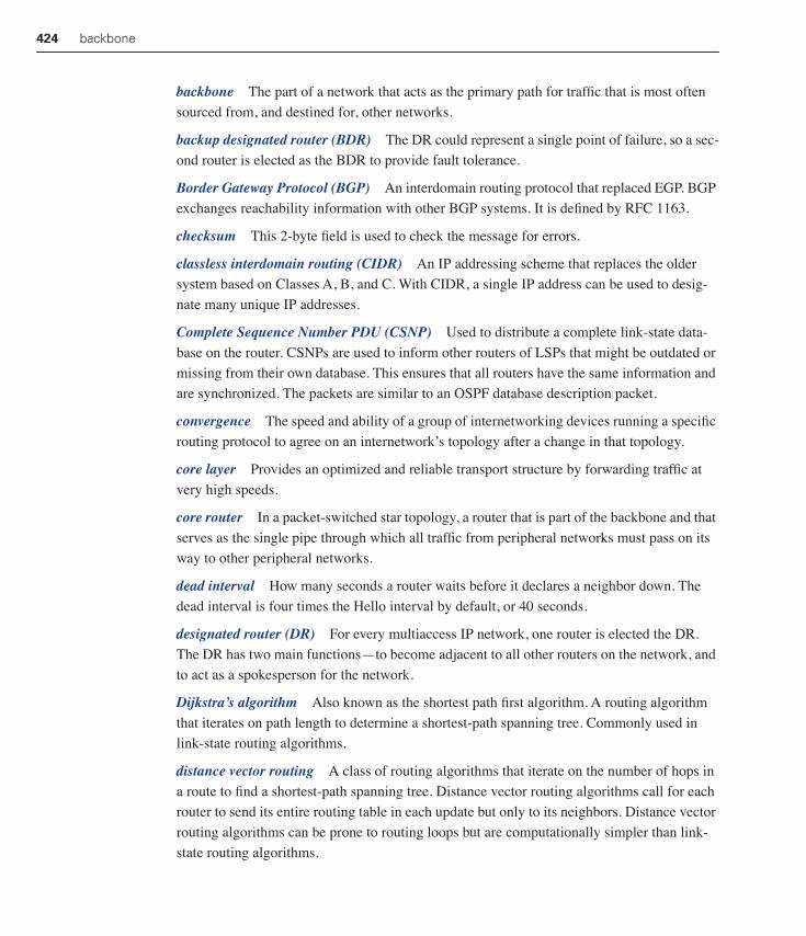
424 backbone
backbone The part of a network that acts as the primary path for traffic that is most often
sourced from, and destined for, other networks.
backup designated router (BDR) The DR could represent a single point of failure, so a sec-
ond router is elected as the BDR to provide fault tolerance.
Border Gateway Protocol (BGP) An interdomain routing protocol that replaced EGP. BGP
exchanges reachability information with other BGP systems. It is defined by RFC 1163.
checksum This 2-byte field is used to check the message for errors.
classless interdomain routing (CIDR) An IP addressing scheme that replaces the older
system based on Classes A, B, and C. With CIDR, a single IP address can be used to desig-
nate many unique IP addresses.
Complete Sequence Number PDU (CSNP) Used to distribute a complete link-state data-
base on the router. CSNPs are used to inform other routers of LSPs that might be outdated or
missing from their own database. This ensures that all routers have the same information and
are synchronized. The packets are similar to an OSPF database description packet.
convergence The speed and ability of a group of internetworking devices running a specific
routing protocol to agree on an internetwork’s topology after a change in that topology.
core layer Provides an optimized and reliable transport structure by forwarding traffic at
very high speeds.
core router In a packet-switched star topology, a router that is part of the backbone and that
serves as the single pipe through which all traffic from peripheral networks must pass on its
way to other peripheral networks.
dead interval How many seconds a router waits before it declares a neighbor down. The
dead interval is four times the Hello interval by default, or 40 seconds.
designated router (DR) For every multiaccess IP network, one router is elected the DR.
The DR has two main functions—to become adjacent to all other routers on the network, and
to act as a spokesperson for the network.
Dijkstra’s algorithm Also known as the shortest path first algorithm. A routing algorithm
that iterates on path length to determine a shortest-path spanning tree. Commonly used in
link-state routing algorithms.
distance vector routing A class of routing algorithms that iterate on the number of hops in
a route to find a shortest-path spanning tree. Distance vector routing algorithms call for each
router to send its entire routing table in each update but only to its neighbors. Distance vector
routing algorithms can be prone to routing loops but are computationally simpler than link-
state routing algorithms.
1358_fmi.book Page 424 Thursday, May 27, 2004 2:21 PM
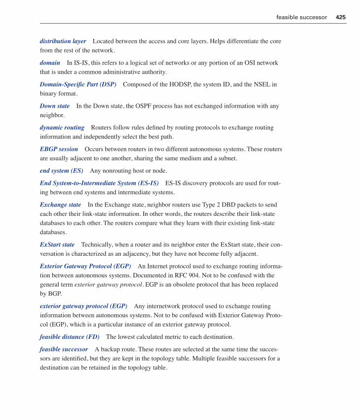
feasible successor 425
distribution layer Located between the access and core layers. Helps differentiate the core
from the rest of the network.
domain In IS-IS, this refers to a logical set of networks or any portion of an OSI network
that is under a common administrative authority.
Domain-Specific Part (DSP) Composed of the HODSP, the system ID, and the NSEL in
binary format.
Down state In the Down state, the OSPF process has not exchanged information with any
neighbor.
dynamic routing Routers follow rules defined by routing protocols to exchange routing
information and independently select the best path.
EBGP session Occurs between routers in two different autonomous systems. These routers
are usually adjacent to one another, sharing the same medium and a subnet.
end system (ES) Any nonrouting host or node.
End System-to-Intermediate System (ES-IS) ES-IS discovery protocols are used for rout-
ing between end systems and intermediate systems.
Exchange state In the Exchange state, neighbor routers use Type 2 DBD packets to send
each other their link-state information. In other words, the routers describe their link-state
databases to each other. The routers compare what they learn with their existing link-state
databases.
ExStart state Technically, when a router and its neighbor enter the ExStart state, their con-
versation is characterized as an adjacency, but they have not become fully adjacent.
Exterior Gateway Protocol (EGP) An Internet protocol used to exchange routing informa-
tion between autonomous systems. Documented in RFC 904. Not to be confused with the
general term exterior gateway protocol. EGP is an obsolete protocol that has been replaced
by BGP.
exterior gateway protocol (EGP) Any internetwork protocol used to exchange routing
information between autonomous systems. Not to be confused with Exterior Gateway Proto-
col (EGP), which is a particular instance of an exterior gateway protocol.
feasible distance (FD) The lowest calculated metric to each destination.
feasible successor A backup route. These routes are selected at the same time the succes-
sors are identified, but they are kept in the topology table. Multiple feasible successors for a
destination can be retained in the topology table.
1358_fmi.book Page 425 Thursday, May 27, 2004 2:21 PM

426 floating static route
floating static route A static route that is configured with an administrative distance value
that is greater than that of the primary route or routes. Used for fallback routes or backup
routes; they do not appear in the routing table until another route to the same destination fails.
Format Prefix (FP) field The 3-bit FP identifies the type of address—unicast, multicast,
and so on. The bits 001 identify aggregatable global unicasts.
full adjacency With the Loading state complete, the routers are fully adjacent. Each router
keeps a list of adjacent neighbors, called the adjacencies database.
Hello interval How many seconds an OSPF router waits to send the next Hello packet.
hello packet EIGRP relies on hello packets to discover, verify, and rediscover neighbor
routers.
Hello PDU Used to establish and maintain adjacencies. ESHs are sent from ESs to ISs.
ISHs are sent from ISs to ESs. IIHs are sent between ISs. Note that ESH and ISH PDUs are
ES-IS PDUs, not IS-IS PDUs.
High-Order Domain-Specific Part (HODSP) Used for subdividing the domain into areas.
This is roughly equivalent to a subnet in IP.
hold time (hold uptime) How long to wait without receiving anything from a neighbor
before considering the link unavailable. Originally, the expected packet was a hello packet.
However, in current Cisco IOS software releases, any EIGRP packets received after the first
hello reset the timer.
IBGP session Occurs between routers in the same AS. Used to coordinate and synchronize
routing policy within the AS.
Init state OSPF routers send Type 1 packets, or Hello packets, at regular intervals to estab-
lish a relationship with neighbor routers.
initial domain identifier (IDI) Identifies the domain.
Integrated IS-IS An implementation of the IS-IS protocol for routing multiple network
protocols. Integrated IS-IS tags CLNP routes, upon which IS-IS bases its link-state database,
with information about IP networks and subnets.
Interdomain Part (IDP) Consists of the AFI and IDI together. This is roughly equivalent to
a classful IP network in decimal format.
Interface ID field The 64-bit Interface ID field identifies individual interfaces on a link.
This field is analogous to the host portion of an IPv4 address, but it is derived using the IEEE
EUI-64 format. When this field is on LAN interfaces, the Interface ID adds a 16-bit field to
the interface MAC address.
interface identifier The level specific to a node’s individual interface.
1358_fmi.book Page 426 Thursday, May 27, 2004 2:21 PM
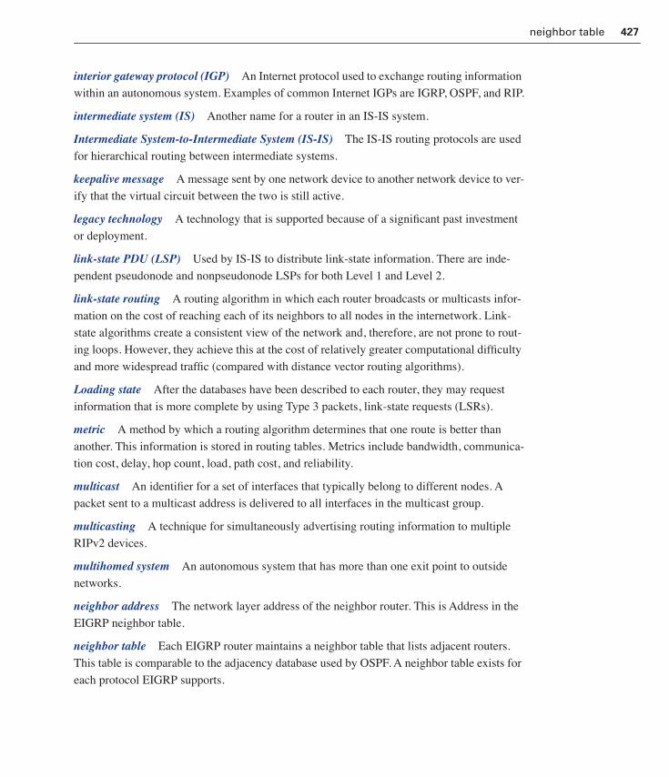
neighbor table 427
interior gateway protocol (IGP) An Internet protocol used to exchange routing information
within an autonomous system. Examples of common Internet IGPs are IGRP, OSPF, and RIP.
intermediate system (IS) Another name for a router in an IS-IS system.
Intermediate System-to-Intermediate System (IS-IS) The IS-IS routing protocols are used
for hierarchical routing between intermediate systems.
keepalive message A message sent by one network device to another network device to ver-
ify that the virtual circuit between the two is still active.
legacy technology A technology that is supported because of a significant past investment
or deployment.
link-state PDU (LSP) Used by IS-IS to distribute link-state information. There are inde-
pendent pseudonode and nonpseudonode LSPs for both Level 1 and Level 2.
link-state routing A routing algorithm in which each router broadcasts or multicasts infor-
mation on the cost of reaching each of its neighbors to all nodes in the internetwork. Link-
state algorithms create a consistent view of the network and, therefore, are not prone to rout-
ing loops. However, they achieve this at the cost of relatively greater computational difficulty
and more widespread traffic (compared with distance vector routing algorithms).
Loading state After the databases have been described to each router, they may request
information that is more complete by using Type 3 packets, link-state requests (LSRs).
metric A method by which a routing algorithm determines that one route is better than
another. This information is stored in routing tables. Metrics include bandwidth, communica-
tion cost, delay, hop count, load, path cost, and reliability.
multicast An identifier for a set of interfaces that typically belong to different nodes. A
packet sent to a multicast address is delivered to all interfaces in the multicast group.
multicasting A technique for simultaneously advertising routing information to multiple
RIPv2 devices.
multihomed system An autonomous system that has more than one exit point to outside
networks.
neighbor address The network layer address of the neighbor router. This is Address in the
EIGRP neighbor table.
neighbor table Each EIGRP router maintains a neighbor table that lists adjacent routers.
This table is comparable to the adjacency database used by OSPF. A neighbor table exists for
each protocol EIGRP supports.
1358_fmi.book Page 427 Thursday, May 27, 2004 2:21 PM

428 network entity title (NET)
network entity title (NET) An NSAP whose last byte is 0. The NET is used to identify a
device.
Network Layer Reachability Information (NLRI) BGP sends routing update messages
containing NLRI to describe a route and how to get there. In this context, an NLRI is a prefix.
A BGP update message carries one or more NLRI prefixes and the attributes of a route for the
NLRI prefixes. The route attributes include a BGP next-hop gateway address, community
values, and other information.
network mask This 32-bit field carries subnet mask information for the network.
network service access point (NSAP) A conceptual point on the boundary between the net-
work and transport layers. The NSAP is the location where OSI network services are pro-
vided to the transport layer. Similar to an IP address.
Next-Level Aggregation Identifier (NLA ID) field The 24-bit NLA ID field is used to iden-
tify ISPs. The field itself can be organized to reflect a hierarchy or a multitiered relationship
among providers.
notification message Informs the receiving router of errors.
NSAP selector (NSEL) Identifies a process on the device. It is roughly equivalent to a port
or socket in TCP/IP. The NSEL is not used in routing decisions.
open message Establishes connections with peers. Includes fields for the BGP version
number, AS number, hold time, and Router ID.
OSI protocols The product of an international program formed to develop data networking
protocols and other standards that facilitate multivendor equipment interoperability.
Partial Sequence Number PDU (PSNP) Used to acknowledge and request link-state infor-
mation.
passive interface Receives updates but does not send them. Used to control routing
updates. The passive-interface command can be used with all IP interior gateway proto-
cols—RIP, IGRP, EIGRP, OSPF, and IS-IS.
policy routing A routing scheme that forwards packets to interfaces based on user-config-
ured policies. Such policies might specify that traffic sent from a particular network should be
forwarded out one interface, while all other traffic should be forwarded out another interface.
priority queuing A method of queuing that is used to guarantee bandwidth for traffic by
assigning queue space to each protocol according to the defined rules.
public topology The collection of providers that offer Internet connectivity.
query packet An EIGRP router uses a query packet whenever it needs specific information
from one or all of its neighbors.
1358_fmi.book Page 428 Thursday, May 27, 2004 2:21 PM
routing table 429
queue count (Q Cnt) The number of packets waiting in queue to be sent. If this value is
constantly higher than 0, a congestion problem might exist at the router. A 0 means that no
EIGRP packets are in the queue.
reported distance (RD) A path’s RD is the distance reported by an adjacent neighbor to a
specific destination.
Reserved (Res) field The IPv6 architecture defines the 8-bit Res field so that the TLA or
NLA IDs can be expanded as future growth warrants. Currently, this field must be set to 0.
route redistribution Allows routing information discovered through one routing protocol to
be distributed in the update messages of another routing protocol.
route source The identification number of the router that originally advertised that route.
This field is populated only for routes learned externally from the EIGRP network.
route summarization The consolidation of advertised addresses in OSPF and IS-IS. In
OSPF, this causes a single summary route to be advertised to other areas by an area border
router.
router ID The function of the Hello packet is to establish and maintain adjacencies. So the
sending router signs the fourth field with its router ID, which is a 32-bit number used to iden-
tify the router to the OSPF protocol.
router priority This field contains a value that indicates this router’s priority when selecting
a DR and BDR.
Routing Information Protocol (RIP) An IGP supplied with the FreeBSD version of UNIX.
The most common IGP in the Internet. RIP uses hop count as a routing metric.
Routing Information Protocol version 2 (RIPv2) Defined in RFC 1723 and supported in
Cisco IOS Release 11.1 and later. RIPv2 is not a new protocol; it is just RIPv1 with some
extensions to bring it up-to-date with modern routing environments. RIPv2 has been updated
to support VLSM, authentication, and multicast updates.
routing metric A method by which a routing algorithm determines that one route is better
than another. This information is stored in routing tables. Metrics include bandwidth, com-
munication cost, delay, hop count, load, path cost, and reliability. Sometimes simply called a
metric.
routing table EIGRP chooses the best routes to a destination from the topology table and
places them in the routing table. Each EIGRP router maintains a routing table for each net-
work protocol.
1358_fmi.book Page 429 Thursday, May 27, 2004 2:21 PM

430 routing update
routing update A message sent from a router to indicate network reachability and associ-
ated cost information. Routing updates are typically sent at regular intervals and after a
change in network topology.
single-homed system An autonomous system that has only one exit point to outside net-
works.
Site-Level Aggregation Identifier (SLA ID) field The 16-bit SLA ID is used by an individ-
ual organization to create its own local addressing hierarchy and to identify subnets.
site topology The level local to an organization that does not provide connectivity to nodes
outside itself.
Smooth Round-Trip Timer (SRTT) The average amount of time it takes to send and
receive packets to and from a neighbor. This timer is used to determine the retransmit interval
or retransmission timeout (RTO).
static routing An administrator manually defines routes to one or more destination net-
works.
subnetwork point of attachment (SNPA) The point at which subnetwork services are pro-
vided. This is the equivalent of the Layer 2 address corresponding to the Layer 3 (NET or
NSAP) address.
successor A route selected as the primary route to use to reach a destination. Successors are
the entries kept in the routing table. Multiple successors for a destination can be retained in
the routing table.
system ID Identifies an individual OSI device. In OSI, a device has an address, just as it
does in DECnet, whereas in IP an interface has an address.
Top-Level Aggregation Identifier (TLA ID) field The 13-bit TLA ID field is used to iden-
tify the authority responsible for the address at the highest level of the routing hierarchy.
Internet routers necessarily maintain routes to all TLA IDs. With 13 bits set aside, this field
can represent up to 8192 TLAs.
topology table Every EIGRP router maintains a topology table for each configured network
protocol. This table includes route entries for all destinations the router has learned. All
learned routes to a destination are maintained in the topology table.
two-way state Using Hello packets, every OSPF router tries to establish a two-way state, or
bidirectional communication, with every neighbor router on the same IP network.
Type 1: Hello packet Establishes and maintains adjacency information with neighbors.
Type 2: database description packet (DBD) Describes the contents of the link-state data-
base on an OSPF router.
1358_fmi.book Page 430 Thursday, May 27, 2004 2:21 PM

version, type, and packet length 431
Type 3: link-state request (LSR) Requests specific pieces of a link-state database.
Type 4: link-state update (LSU) Transports LSAs to neighbor routers.
Type 5: link-state acknowledgment (LSAck) Acknowledgment receipt of a neighbor’s
LSA.
unicast An identifier for a single interface. A packet sent to a unicast address is delivered to
the interface identified by that address.
update message Contains all of the information BGP uses to construct a loop-free picture
of the internetwork.
update packet Used to update a router when the router discovers a new neighbor.
variable-length subnet masking (VLSM) The ability to specify a different subnet mask for
the same network number on different subnets. VLSM can help optimize available address
space.
version, type, and packet length The first three fields of the OSPF packet let the recipients
know the version of OSPF that is being used by the sender, the OSPF packet type, and length.
1358_fmi.book Page 431 Thursday, May 27, 2004 2:21 PM

1358_fmi.book Page 432 Thursday, May 27, 2004 2:21 PM
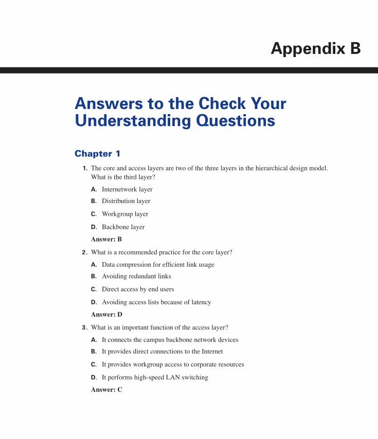
Appendix B
Answers to the Check Your Understanding Questions
Chapter 11. The core and access layers are two of the three layers in the hierarchical design model.
What is the third layer?
A. Internetwork layer
B. Distribution layer
C. Workgroup layer
D. Backbone layer
Answer: B
2. What is a recommended practice for the core layer?
A. Data compression for efficient link usage
B. Avoiding redundant links
C. Direct access by end users
D. Avoiding access lists because of latency
Answer: D
3. What is an important function of the access layer?
A. It connects the campus backbone network devices
B. It provides direct connections to the Internet
C. It provides workgroup access to corporate resources
D. It performs high-speed LAN switching
Answer: C
1358_fmi.book Page 433 Thursday, May 27, 2004 2:21 PM

434 Appendix B: Answers to the Check Your Understanding Questions
4. What method should be used to prevent regular routing updates from constantly acti-vating a dialup WAN link?
A. Dialer access list
B. Distance vector
C. Incremental updates
D. Snapshot routing
Answer: D
5. What feature characterizes a network that is reliable and available?
A. Load balancing
B. Securable
C. Queuing
D. Protocol integration
Answer: A
6. What is the primary purpose of dial backup?
A. Tunneling
B. Load balancing
C. Fault tolerance
D. Traffic prioritization
Answer: C
7. Which Cisco IOS software feature supports responsiveness on slow WAN links?
A. DDR
B. Tunnels
C. Queuing
D. Route summarization
Answer: C
1358_fmi.book Page 434 Thursday, May 27, 2004 2:21 PM

Chapter 2 435
8. Which three features are offered in the Cisco IOS software to optimize the efficiency of a WAN connection?
A. Access lists
B. Protocol tunnels
C. Snapshot routing
D. Compression
E. Dynamic data aggregation
Answer: A, C, D
9. What is a characteristic of a scalable routing protocol?
A. Fast convergence
B. Slow convergence
C. Reachability limitations
D. Simple configuration
Answer: A
10. What is a characteristic of nonroutable protocols?
A. No frame header
B. No network layer addressing
C. Appropriate for WAN links
D. Best-route determination by broadcast
Answer: B
Chapter 21. What feature lets a Cisco router act as a DHCP client?
A. NAT
B. DHCP
C. DNS
D. Easy IP
Answer: D
1358_fmi.book Page 435 Thursday, May 27, 2004 2:21 PM

436 Appendix B: Answers to the Check Your Understanding Questions
2. What is a summarization address for the networks 172.21.136.0/24 and 172.21.143.0/24?
A. 172.21.136.0/21
B. 172.21.136.0/20
C. 172.21.136.0/22
D. 172.21.128.0/21
Answer: A
3. The subnet 172.6.32.0/20 is again subnetted to 172.6.32.0/26. What is the result?
A. 1024 subnets
B. 64 hosts per subnet
C. 62 hosts per subnet
D. 2044 subnets
Answer: C
4. What routing protocol does not contain subnet mask information in its routing updates?
A. EIGRP
B. OSPF
C. RIP
D. RIPv2
Answer: C
5. What method is used to represent a collection of IP network addresses with a single IP network address?
A. Classful routing
B. Subnetting
C. Address translation
D. Route summarization
Answer: D
6. According to RFC 1918, which of the following is a private Internet address?
A. 10.215.34.124
B. 192.32.146.23
C. 172.34.221.18
D. 119.12.73.215
Answer: A
1358_fmi.book Page 436 Thursday, May 27, 2004 2:21 PM

Chapter 3 437
7. Which of the following is a characteristic of IP unnumbered?
A. Avoids wasted addresses on multiaccess links
B. Efficient addressing on Ethernet links
C. Uses another router interface address
D. May be used only with classless routing protocols
Answer: C
8. How many bits make up an IPv6 address?
A. 32
B. 48
C. 64
D. 128
Answer: D
9. What is the purpose of IP helper addresses?
A. To relay key UDP broadcast requests to hosts on the same subnet
B. To relay key UDP broadcast requests to hosts on the other subnets
C. To relay key TCP broadcast requests to hosts on other subnets
D. To relay key TCP broadcast requests to hosts on the same subnet
Answer: B
10. What are the three general types of IPv6 addresses?
A. Class 1, Class 2, Class 3
B. Class A, Class B, Class C
C. Unicast, anycast, multicast
D. Public, site, interface
Answer: C
Chapter 31. What is an advantage of static routing compared to dynamic routing?
A. Static routing sometimes yields unexpected results, even in small networks
B. Routers that don’t accept updates are less vulnerable to attack

438 Appendix B: Answers to the Check Your Understanding Questions
C. The routing table contains only directly connected routes to router interfaces
D. Static routes remain in routing tables regardless of the mapped router interface status
Answer: B
2. What routing protocol would be used in a mixed-vender or legacy routing environment within an autonomous system?
A. RIPv1
B. RIPv2
C. IGRP
D. EIGRP
E. IS-IS
Answer: A
3. Which of the following commands would statically configure IGRP to use and propa-gate a default route?
A. ip route 0.0.0.0 255.255.255.255
B. ip default-network
C. ip route default-network
D. ip default network 0.0.0.0
Answer: B
4. What command must you use to automatically propagate a candidate default route to IGRP neighbors?
A. ip default-network ip-address
B. ip default-gateway ip-address
C. default-information originate
D. redistribute static neighbors
Answer: A
5. What is a disadvantage of static routing?
A. It can cause unpredictable routing behavior
B. There is no mechanism to recover from a failed link
C. All route information is transmitted in each update
D. It produces high-processor overhead
Answer: B
1358_fmi.book Page 438 Thursday, May 27, 2004 2:21 PM

Chapter 3 439
6. What is the primary purpose of configuring floating static routes?
A. To provide unlimited adaptability to network topology changes
B. To create a semiadaptable static routing scheme to activate backup routes
C. To create static routes with an administrative distance of 1
D. To create a static route that is more desirable than a dynamic route with equal
administrative distance
Answer: B
7. What would be a logical routing protocol configuration approach to significantly reduce the convergence time in a large internetwork?
A. Configure static default routes for stub networks
B. Increase the router processor and memory capacity
C. Configure static routes between all routers in the network
D. Decrease the number of hops between all routes in the network
Answer: A
8. How are stub networks defined?
A. Networks with only one router
B. Networks with multiple ways into and out of a network
C. Networks with only one ingress and egress point
D. Networks with routing policies that are controlled by a single organization
Answer: C
9. What mechanism ensures that a router configured with an event-driven routing protocol regularly communicates with its neighbors?
A. Hello timer
B. MaxAge timer
C. Triggered update
D. Update timer
Answer: A
10. What routing protocol measures route desirability based on bandwidth and delay and maintains a topological database?
A. RIPv2
B. RTMP
1358_fmi.book Page 439 Thursday, May 27, 2004 2:21 PM

440 Appendix B: Answers to the Check Your Understanding Questions
C. EIGRP
D. OSPF
E. IS-IS
F. NLSP
Answer: C
Chapter 41. What command disables the default network summarization in RIPv2?
A. no ip rip-summary
B. no rip auto-summarization
C. no auto-summary
D. no route-summarization
Answer: C
2. What command displays summary address entries in the RIP database?
A. show ip protocols
B. show ip route database
C. show ip rip database
D. show ip route
E. show ip rip
Answer: C
3. What command allows the use of the first subnet of any network?
A. ip subnet-zero
B. no ip subnet-zero
C. all-zero network
D. ip network-zero
Answer: A
4. What multicast address does RIPv2 use?
A. 224.0.0.4
B. 224.0.0.5
1358_fmi.book Page 440 Thursday, May 27, 2004 2:21 PM

Chapter 5 441
C. 224.0.0.8
D. 224.0.0.9
Answer: D
5. What is an advantage of multicasting RIPv2 updates instead of broadcasting them?
A. Ethernet interfaces ignore the multicast messages
B. It makes RIPv2 compatible with EIGRP and OSPF
C. Hosts and non-RIPv2 routers ignore the multicast messages
D. It enables faster convergence than RIPv1
Answer: C
6. Which statement describes the characteristics of RIPv1 and RIPv2?
A. RIPv1 imposes a maximum hop count of 16, and RIPv2 allows for a maximum of 32 hops
B. RIPv1 is classful, and RIPv2 is classless
C. RIPv1 uses only hop count, and RIPv2 uses hop count and bandwidth
D. RIPv1 sends periodical updates, and RIPv2 sends updates only as changes occur
Answer: B
7. Which three fields are now populated in the RIPv2 message format?
A. Route Tag
B. Subnet Mask
C. Autonomous System
D. Next Hop
E. Protocol
Answer: A, B, D
Chapter 51. How do you configure automatic redistribution between IGRP and EIGRP?
A. Configure the two protocols with different AS numbers
B. Configure the two protocols with different DS numbers
C. Configure the two protocols with the same AS number
D. Configure the two protocols with the same DS number
Answer: C
1358_fmi.book Page 441 Thursday, May 27, 2004 2:21 PM

442 Appendix B: Answers to the Check Your Understanding Questions
2. What protocol combines the advantages of link-state and distance vector routing proto-cols?
A. RIP
B. OSPF
C. IGRP
D. EIGRP
Answer: D
3. What command shows the neighbors that EIGRP has discovered?
A. show eigrp neighbors
B. show ip eigrp neighbors
C. show router eigrp process-id
D. show ip eigrp networks
Answer: B
4. What multicast IP address does EIGRP use?
A. 224.0.0.110
B. 224.0.0.100
C. 224.0.0.11
D. 224.0.0.10
Answer: D
5. What table includes route entries for all destinations that the router has learned and is maintained for each configured routing protocol?
A. Topology table
B. Routing table
C. Neighbor table
D. Successor table
Answer: A
6. What establishes adjacencies in EIGRP?
A. DUAL finite-state machine
B. Hello packets
1358_fmi.book Page 442 Thursday, May 27, 2004 2:21 PM

Chapter 5 443
C. Topology table
D. Reliable Transport Protocol
Answer: B
7. What guarantees ordered delivery of EIGRP packets to all neighbors?
A. DUAL finite-state machine
B. Hello packets
C. Topology table
D. Reliable Transport Protocol
Answer: D
8. What does DUAL do after it tracks all routes, compares them, and guarantees that they are loop-free?
A. Inserts lowest-cost paths into the routing table
B. Determines the optimal path and advertises it to the neighbor routers using hello
packets
C. Supports other routed protocols through PDMs
D. Sends a unicast query to the neighboring routers
Answer: A
9. How does EIGRP prevent routing loops from occurring with external routes?
A. By rejecting external routes tagged with a router ID identical to their own
B. By storing the identities of neighbors that are feasible successors
C. By rejecting all neighboring routers that have an advertised composite metric that is
less than a router’s best current metric
D. By storing in a special table all neighboring routes that have loops identified
Answer: B
10. On higher-bandwidth connections such as point-to point serial links or multipoint cir-cuits, how long is the hello interval used by EIGRP?
A. 5 seconds
B. 10 seconds
C. 60 seconds
D. 120 seconds
Answer: A
1358_fmi.book Page 443 Thursday, May 27, 2004 2:21 PM

444 Appendix B: Answers to the Check Your Understanding Questions
Chapter 61. Which state are the routers in an OSPF network in after the DR and BDR are elected?
A. ExStart
B. Full
C. Loading
D. Exchange
Answer: A
2. What is the default cost metric for OSPF based on?
A. Delay
B. Media bandwidth
C. Efficiency
D. Network traffic
Answer: B
3. What command can you use to change the OSPF priority on an interface?
A. ip priority number ospf
B. ip ospf priority number
C. ospf priority number
D. set priority ospf number
Answer: B
4. What IP address is used to send a multicast to only OSPF DRs and BDRs?
A. 224.0.0.6
B. 224.0.0.1
C. 224.0.0.4
D. 224.0.0.5
Answer: A
5. Which of the following is a common feature associated with NBMA networks?
A. Support for only two routers
B. Support for more than two routers
C. No election of DRs
D. Full support for broadcast and multicast packets
Answer: B
1358_fmi.book Page 444 Thursday, May 27, 2004 2:21 PM

Chapter 6 445
6. While troubleshooting a communication problem between two OSPF routers, you find that mismatched hello interval timers on the interfaces have caused the problem. Which command allows you to set the hello interval on the interfaces?
A. hello-interval
B. ospf hello-interval
C. ip hello-interval
D. ip ospf hello-interval
Answer: D
7. What type of OSPF router generates routing information about each area to which it is connected and floods that information through the backbone?
A. BR
B. BDR
C. Backbone
D. ABR
Answer: D
8. What type of OSPF router has at least one interface connected to an external autono-mous system?
A. ABR
B. ASBR
C. Backbone
D. Internal
Answer: B
9. What command configures a virtual link?
A. Router#area area-id router-id virtual-link
B. Router(config)#ip-area area-id virtual-link router-id
C. Router(config-router)#ip area virtual-link router-id area-id
D. Router(config-router)#area area-id virtual-link router-id
Answer: D
1358_fmi.book Page 445 Thursday, May 27, 2004 2:21 PM

446 Appendix B: Answers to the Check Your Understanding Questions
10. What type of summarization occurs on ABRs and applies to routes from within each area?
A. Internal summarization
B. Interarea route summarization
C. External router summarization
D. Backbone summarization
Answer: B
11. What command configures an area as an NSSA?
A. Router(config)#area area-id nssa
B. Router(config-router)#area area-id nssa
C. Router(config-router)#area-id nssa
D. Router(config)#area nssa area-id
Answer: B
12. What command displays information about each area to which a router is connected and indicates whether the router is an ABR, ASBR, or both?
A. show ip ospf border-routers
B. show ip ospf virtual-links
C. show ip ospf process-id
D. show ip ospf database
Answer: C
Chapter 71. Which type of location is most likely to use the IS-IS protocol?
A. Branch office
B. SOHO
C. Service provider
D. PSTN
Answer: C
1358_fmi.book Page 446 Thursday, May 27, 2004 2:21 PM

Chapter 7 447
2. Which of the following are features of the IS-IS protocol? (Choose three.)
A. Classful behavior
B. Slow convergence
C. Fast convergence
D. Scalable
E. Distance vector
F. IGP
Answer: C, D, F
3. OSI networking design and proper implementation provide which of the following? (Choose two.)
A. Quality of service
B. Proprietary architectures
C. Transparency
D. Four-layer model
Answer: A, C
4. CLNS is located at which layer of the OSI model?
A. Data-link layer
B. Transport layer
C. Application layer
D. Network layer
Answer: D
5. IS-IS was originally designed to route which protocol?
A. IPX
B. AppleTalk
C. IP
D. DECnet Phase V
E. SNA
Answer: D
1358_fmi.book Page 447 Thursday, May 27, 2004 2:21 PM

448 Appendix B: Answers to the Check Your Understanding Questions
6. How many routers can exist in a single IS-IS area?
A. 15
B. 50
C. 100
D. 500
E. 1000
Answer: C
7. What is identified by the information contained in the CLNS system ID field?
A. A process on a device
B. The domain
C. A single OSI device
D. Port or socket information
Answer: C
8. How many addresses does an NSAP have?
A. A single address for the entire router
B. An address for each configured interface
C. Multiple addresses for each configured interface
D. The number of addresses depends on the routing protocol chosen
Answer: A
9. Which of the following is the equivalent of using more than one NET with the IS-IS protocol?
A. Using CIDR
B. Using secondary addresses with IP
C. Using VLSM
D. Implementing dynamic routing
Answer: B
10. What command displays the least-cost paths to a destination NET?
A. which-route
B. show isis topology
1358_fmi.book Page 448 Thursday, May 27, 2004 2:21 PM
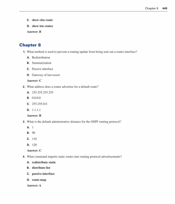
Chapter 8 449
C. show clns route
D. show isis routes
Answer: B
Chapter 81. What method is used to prevent a routing update from being sent out a router interface?
A. Redistribution
B. Summarization
C. Passive interface
D. Gateway of last resort
Answer: C
2. What address does a router advertise for a default route?
A. 255.255.255.255
B. 0.0.0.0
C. 255.255.0.0
D. 1.1.1.1
Answer: B
3. What is the default administrative distance for the OSPF routing protocol?
A. 1
B. 90
C. 110
D. 120
Answer: C
4. What command imports static routes into routing protocol advertisements?
A. redistribute static
B. distribute-list
C. passive-interface
D. route-map
Answer: A
1358_fmi.book Page 449 Thursday, May 27, 2004 2:21 PM

450 Appendix B: Answers to the Check Your Understanding Questions
5. What command uses match statements to create a routing policy?
A. auto summary
B. distribute-list
C. access-list
D. route-map
Answer: D
6. What command establishes which route a router sends or receives in updates?
A. access-list
B. network
C. passive-interface
D. distribute-list
Answer: D
7. What command modifies the administrative distance for all OSPF routes?
A. distance 95
B. admin distance 110
C. distance 110
D. admin distance 95
Answer: A
8. Which of the following is a consideration when implementing redistribution?
A. Incompatible routing tables
B. Routing feedback (loops)
C. Overlap routing protocols
D. Two-way redistribution with multiple boundary routers
Answer: B
9. Which administrative distance represents the most reliable protocol?
A. 5
B. 90
C. 120
D. 200
Answer: A
1358_fmi.book Page 450 Thursday, May 27, 2004 2:21 PM

Chapter 9 451
10. Which IP interior gateway protocols support passive interface?
A. RIP, IGRP, EIGRP, and BGP
B. RIP, IGRP, EIGRP, IS-IS, and IPX
C. RIP, IGRP, EIGRP, OSPF, and IPX
D. RIP, IGRP, EIGRP, OSPF, and IS-IS
Answer: D
11. What does the router use to make a decision when it has learned two or more routes to the same destination from multiple routing protocols?
A. Hop count
B. Administrative distance
C. Metric
D. Route summarization
Answer: B
Chapter 91. What kind of AS features more than one exit point to outside networks but does not
allow traffic to pass from one outside connection to another?
A. Stub
B. Multihomed nontransit
C. Multihomed transit
D. Totally stubby
Answer: B
2. In what situation is it inadvisable to run BGP?
A. Stub AS
B. Multihomed nontransit AS
C. Multihomed transit AS
D. When your AS policies differ from the ISP policies
Answer: A
1358_fmi.book Page 451 Thursday, May 27, 2004 2:21 PM

452 Appendix B: Answers to the Check Your Understanding Questions
3. What happens when a route is advertised to the AS that originated it?
A. The AS sees itself as part of the AS_Path attribute list and does not accept the route.
B. The border router prepends the AS number and advertises the router to other auton-
omous systems.
C. The route is passed to other routers within the AS as an external route.
D. The border router removes its AS number from the AS_Path list and redistributes
the route.
Answer: A
4. What is one way to set local preference in BGP?
A. Use the AS_Path attribute
B. Use the global prepend command
C. Use the bgp default local-preference command
D. Use the set as_path command
Answer: C
5. What command identifies the state of BGP neighbors?
A. show ip route
B. show ip bgp peer
C. show ip bgp paths
D. show ip bgp neighbors
Answer: D
6. In which situation is it OK to turn off BGP synchronization on a border router?
A. In a simple AS
B. In a nonfully meshed transit AS
C. When the AS is not a transit AS
D. When internal reachability is not guaranteed
Answer: C
7. In a BGP system, which attribute can be manipulated on the various default routes so that at least one default route is identified as primary, with other default routes being kept as backups?
A. Default-originate
B. Local Preference
1358_fmi.book Page 452 Thursday, May 27, 2004 2:21 PM

Chapter 9 453
C. Default Preference
D. Maximum-paths
Answer: B
8. What condition causes a BGP router to install multiple paths to the same destination in its IP routing table?
A. It learns two identical EBGP paths for a prefix from a neighboring AS, and both have the same route ID.
B. It learns two IBGP paths for a prefix from a neighboring AS, and both have the
same route ID.
C. BGP multipath support is enabled, and the EBGP paths are learned from the same
neighboring AS.
D. Multipath support is enabled, and the EBGP paths are learned from different neigh-
boring autonomous systems.
Answer: C
9. Which of the following can be used to filter routing updates based on NLRI?
A. Passive interfaces
B. Distribute list
C. Static routes
D. Default routes
Answer: B
10. What method injects all known static routes into BGP?
A. Configuring default routes in the BGP border router
B. Using the redistribute static command
C. Configuring an IP prefix list with the static routes
D. BGP supports only dynamically injected routes
Answer: B
11. How is transit traffic best defined when using BGP?
A. Any traffic that has a source and destination inside the AS
B. Any traffic that has a destination outside the AS
C. Any traffic that has a source and destination outside the AS
D. Any traffic that has a source outside a multihomed system
Answer: C
1358_fmi.book Page 453 Thursday, May 27, 2004 2:21 PM

1358_fmi.book Page 454 Thursday, May 27, 2004 2:21 PM
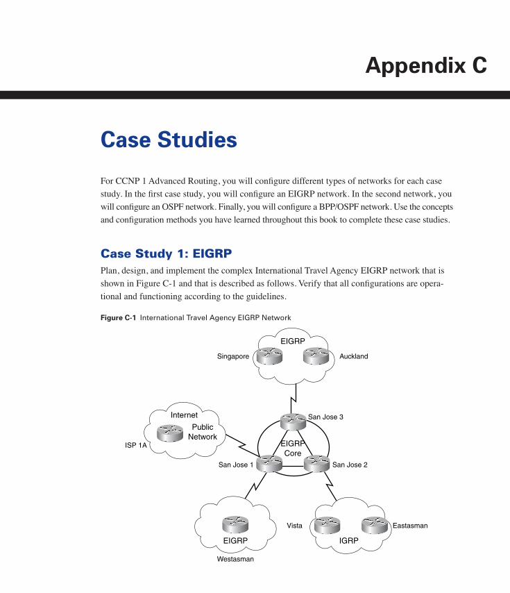
Appendix C
Case Studies
For CCNP 1 Advanced Routing, you will configure different types of networks for each case
study. In the first case study, you will configure an EIGRP network. In the second network, you
will configure an OSPF network. Finally, you will configure a BPP/OSPF network. Use the concepts
and configuration methods you have learned throughout this book to complete these case studies.
Case Study 1: EIGRPPlan, design, and implement the complex International Travel Agency EIGRP network that is
shown in Figure C-1 and that is described as follows. Verify that all configurations are opera-
tional and functioning according to the guidelines.
Figure C-1 International Travel Agency EIGRP Network
ISP 1A
EIGRP
IGRP
Internet
EIGRPCore
PublicNetwork
AucklandSingapore
EIGRP
Westasman
Vista
San Jose 3
San Jose 1 San Jose 2
Eastasman
1358_fmi.book Page 455 Thursday, May 27, 2004 2:21 PM
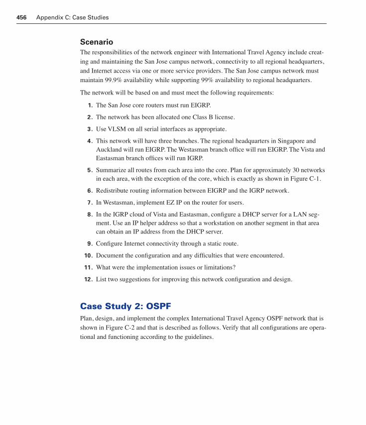
456 Appendix C: Case Studies
Scenario
The responsibilities of the network engineer with International Travel Agency include creat-
ing and maintaining the San Jose campus network, connectivity to all regional headquarters,
and Internet access via one or more service providers. The San Jose campus network must
maintain 99.9% availability while supporting 99% availability to regional headquarters.
The network will be based on and must meet the following requirements:
1. The San Jose core routers must run EIGRP.
2. The network has been allocated one Class B license.
3. Use VLSM on all serial interfaces as appropriate.
4. This network will have three branches. The regional headquarters in Singapore and Auckland will run EIGRP. The Westasman branch office will run EIGRP. The Vista and Eastasman branch offices will run IGRP.
5. Summarize all routes from each area into the core. Plan for approximately 30 networks in each area, with the exception of the core, which is exactly as shown in Figure C-1.
6. Redistribute routing information between EIGRP and the IGRP network.
7. In Westasman, implement EZ IP on the router for users.
8. In the IGRP cloud of Vista and Eastasman, configure a DHCP server for a LAN seg-ment. Use an IP helper address so that a workstation on another segment in that area can obtain an IP address from the DHCP server.
9. Configure Internet connectivity through a static route.
10. Document the configuration and any difficulties that were encountered.
11. What were the implementation issues or limitations?
12. List two suggestions for improving this network configuration and design.
Case Study 2: OSPFPlan, design, and implement the complex International Travel Agency OSPF network that is
shown in Figure C-2 and that is described as follows. Verify that all configurations are opera-
tional and functioning according to the guidelines.
1358_fmi.book Page 456 Thursday, May 27, 2004 2:21 PM

Case Study 2: OSPF 457
Figure C-2 International Travel Agency OSPF Network
Scenario
The International Travel Agency has decided to change the network routing protocol. The
responsibilities of the network engineer include creating, maintaining, and implementing
changes to the network.
The network will be based on and must meet the following requirements:
1. The San Jose core routers must run OSPF and be configured in Area 0.
2. The network has been allocated one Class A license.
3. Use VLSM on all serial interfaces as appropriate.
4. This network will have three outer areas. The regional headquarters in Singapore and Auckland in Area 1 will run OSPF normally. The Westasman branch office in Area 2 will be a totally stubby network. The Vista and Eastasman branch offices will be RIP networks.
5. Summarize all routes from each area into the core. Plan for approximately 30 networks in each area in the figure, with the exception of the core, which is exactly as shown in Area 0 in Figure C-2.
ISP 1A
Area 1
RIP
Internet
Area 0
PublicNetwork
AucklandSingapore
Area 2
Westasman
Vista
San Jose 1
San Jose 3 San Jose 2
Eastasman
Totally Stubby
Regional Headquarters
1358_fmi.book Page 457 Thursday, May 27, 2004 2:21 PM

458 Appendix C: Case Studies
6. Redistribute routing information between OSPF and the RIP network.
7. In the Westasman branch office in Area 2, implement EZ IP on the router for users.
8. In the Vista and Eastasman branch offices RIP cloud, configure a DHCP server on a LAN segment. Use an IP helper address so that a workstation on another subnet in that area can obtain an IP address from the DHCP server.
9. Configure Internet connectivity through a static route.
10. Document the configuration and any difficulties that were encountered.
11. What were the implementation issues or limitations?
12. List two suggestions for improving this network configuration and design.
Case Study 3: BGP/OSPF RoutingPlan, design, and implement the complex International Travel Agency BGP/OSPF network
that is shown in Figure C-3 and that is described as follows. Verify that all configurations are
operational and functioning according to the guidelines.
Figure C-3 International Travel Agency BGP/OSPF Network
Web Server
Internet
OSPF Area 0Area 2 NSSA
London
Easy IPRedistribution
RIP
CapetownSan Jose 1BGP
T1
T3
ISP
1A
San
Jos
e 3 Firewall
AS 200
Server
1358_fmi.book Page 458 Thursday, May 27, 2004 2:21 PM

Case Study 3: BGP/OSPF Routing 459
Scenario
The International Travel Agency relies heavily on the Internet for its advertising and sales.
Therefore, it has been decided to establish a primary and a backup route to the Internet. Addi-
tionally, other network changes have been planned, as shown in Figure C-3 and described as
follows. The responsibilities of the network engineer include creating, maintaining, and
implementing changes to the network.
The network will be based on and must meet the following requirements:
1. The San Jose core routers must run OSPF and be configured in Area 0.
2. The network has been allocated one Class B license.
3. Use VLSM on all serial interfaces as appropriate.
4. This network will have three outer areas. The London branch office in Area 1 will be a totally stubby network. The Capetown branch office in Area 2 will be an NSSA. The third area will be a RIP network.
5. Summarize all routes from each area into the core. Plan for approximately 30 networks in each area in the figure, with the exception of the core, known as Area 0.
6. Redistribute routing information from RIP into OSPF. The RIP network should use default routing to access the rest of the network and the Internet.
7. In the RIP area, implement EZ IP for users.
8. This International Travel Agency network will be multihomed to ISP1A. The primary link will be a T3 connection. A backup T1 link will also be configured. All outbound and inbound traffic are to use the T3 link. The T1 link should be used only if the T3 link goes down.
9. (Optional) A firewall must be configured on the SanJose3 ASBR. This firewall should allow all traffic originating inside AS 200 to pass freely. No traffic originating from out-side AS 200 should be permitted into the network.
10. Document the configuration and any difficulties that were encountered.
11. What were the implementation issues or limitations?
12. List two suggestions for improving this network configuration and design.
1358_fmi.book Page 459 Thursday, May 27, 2004 2:21 PM

1358_fmi.book Page 460 Thursday, May 27, 2004 2:21 PM

AABR (Area Border Router), 206, 216
access, dedicated networks, 23
access layer, three-layer hierarchical design model, 6
access lists, scalable networks, 20
accessibility, scalable networks, 16, 23
acknowledgment packets, EIGRP, 141
ACLs (Access Control Lists), 20
AD (advertised distance), 139
adaptability of scalable networks, 15, 22
addresses
IP, 33
CIDR, 42–43
Class A, 36
Class B, 37
Class C, 38
Class D, 38
discontiguous subnets, 54–55
management, 33
private, 54
route aggregation, 43–45
structure, 34
subnetting, 39–41
supernetting, 43–46
troubleshooting, 41
IPv4, 34
architecture, 34–35
classes, 35–39
subnet masks, 39–41
IS-IS, 256–263
ISO, 260
Layer 2 multicast, 279
loopback, 188
MAC, 260
next-hop, 109
NSAPs, 256, 258
adjacencies
IS-IS, 279
OSPF
databases, 171
establishing, 179
administrative distance, 84, 338–341
advertised distance (AD), 139
advertisements
loopback addresses, 189
LSAs, 88
supernets, 397
AFI (Authority and Format Identifier), 256–258
aggregate-address command, 397
aggregation, 43–45, 112
Aggregator attribute, 398
algorithms
Bellman-Ford, 85. See also distance vector routing protocols
Dijkstra’s, 87. See also link-state routing protocols
DUAL, 132
SPF, 169, 291
1358_fmi.book Page 461 Thursday, May 27, 2004 2:21 PM

462
allocation
AFI, 258
IP addresses, 42
supernetting, 45–46
alternative paths, scalable networks, 17
AppleTalk routing protocols, 82
architecture
IPv4 addressing, 34–35
IS-IS, 250–255
Area Border Router (ABR), 206, 216
area stub command, 224
areas
backbone router requirements, 229
OSPF, 169
adding, 354
configuring, 186–188
multiarea operation, 203–220
types of, 208
AS (autonomous system), 17, 334, 383
AS_Path attribute 394
ASBR (Autonomous System Boundary Router), 206, 217
assignments, IS-IS, 261
Atomic Aggregate attribute, 397
attributes
Aggregator, 398
AS_Path, 394
Atomic Attribute, 397
BGP, 390–404
Local Preference, 398
MED, 401
Next Hop, 391
Origin, 404
paths, 374–375
scalable internetwork design, 15–24
Weight, 401
authentication
OSPF, 191
RIPv2, 106, 109, 114–121
Authority and Format Identifier (AFI), 256
auto-cost reference-bandwidth command, 190
automatic route summarization, 120
autonomous system (AS), 17, 334, 383
Autonomous System Boundary Router (ASBR), 206, 217
autonomous systems (BGP), 361–363
multihomed nontransit, 364
multihomed transit, 365
single-homed, 363–364
usage selection, 366–367
autosummarization, EIGRP, 157
availability of scalable networks, 15–17
Bbackbone routers
area requirements, 229
connections, 281
IS-IS, 278
OSPF, 206, 254
backup, dial, 18
backup designated router (BDR), 170, 176, 180
bandwidth
command, 153
EIGRP, 132
OSPF, 167
bandwidth-percent command, 154, 155
BDR (backup designated router), 170, 176 180
Bellman-Ford algorithm, 85. See also distance vector routing protocols
allocation
1358_fmi.book Page 462 Thursday, May 27, 2004 2:21 PM

463
BGP (Border Gateway Protocol), 361
attributes, 390–404
autonomous systems, 361–363
multihomed nontransit, 364
multihomed transit, 365
single-homed, 363–364
usage selection, 366–367
commands
bgp always-compare-med router command, 402
bgp default local-preference command, 399
configuring, 375–376
clearing tables, 380–381
continuity inside AS, 383–384
peering, 381–383
decision process, 404
default routing, 415–417
EBGP multihop, 379–380
filtering, 405–412
FSM, 371
load balancing, 412–414, 417
multihomed connections, 418–420
operation, 367
messages, 369–371
monitoring, 384–386
neighbors, 368–369, 371–373
NLRI, 373
path attributes, 374–375
routing updates, 367
OSPF case study, 466–467
redistribution, 421–425
redundancy, 412–414
routing, 386–388
controlling, 390
policies, 388–390
routing policies, 405–412
sessions, 377–379
symmetry, 412–414, 417
bidirectional communication, 172
Border Gateway Protocol (BGP)
attributes, 390–404
autonomous systems, 361–363
multihomed nontransit, 364
multihomed transit, 365
single-homed, 363–364
usage selection, 366–367
configuring, 375–376
clearing tables, 380–381
continuity inside AS, 383–384
peering, 381–383
decision process, 404
default routing, 415–417
EBGP multihop, 379–380
filtering, 405–412
FSM, 371
load balancing, 412–414, 417
multihomed connections, 418–420
operation, 367
messages, 369–371
monitoring, 384–386
neighbors, 368–369, 371–373
NLRI, 373
path attributes, 374–375
routing updates, 367
OSPF case study, 466–467
redistribution, 421–425
redundancy, 412–414
routing, 386–388
controlling, 390
policies, 388–390
routing policies, 405–412
sessions, 377–379
symmetry, 412–414, 417
Border Gateway Protocol (BGP)
1358_fmi.book Page 463 Thursday, May 27, 2004 2:21 PM

464
bounded updates, EIGRP, 132
broadcasts, helper addresses, 64–67
building IP forwarding tables, 301
Ccalculation of routes, 96–99
case studies
BGP/OSPF routing, 466–467
EIGRP, 463–464
OSPF, 464–466
Catalyst 2950 Series access layer switches, 15
Catalyst 3550 Series core layer switches, 12
Catalyst 4500 Series core layer switches, 12
Catalyst 6500 Series core layer switches, 12
CIDR (classless interdomain routing)
IP addresses, 42–43
link-state routing protocols, 88
Cisco 4000 Series Distribution Layer Router, 8
Cisco routers. See also routers
helper addresses, 64–67
ISO addressing, 260
NETs, 258
OSPF, 166–171
adjacencies, 179
BDR/DR election, 180–182
commands, 188–194
configuring, 186–188
Hello protocol, 176–179
multiarea operation, 203–220
NBMA, 194–203
network types, 174–176
NSSA, 225–229
operation, 179
route discovery, 182–183
route selection, 183
routing information, 184–185
states, 171–174
stubby areas, 221–224
virtual links, 229–233
Class A IP addresses, 36
Class B IP addresses, 37
Class C IP addresses, 38
Class D IP addresses, 38
Class E IP addresses, 38
classes, IPv4 addressing, 35–39
classful routing protocols, VSLM, 49–50
classless interdomain routing (CIDR)
IP addresses, 42–43
link-state routing protocols, 88
classless route lookups, 112
classless routing, 113
contiguous subnets, 120
VSLM, 49–50
clear commands, OSPF, 193
clearing BGP tables, 380–381
CLNP (Connectionless Network Protocol), 249
CLNS (Connectionless Network Service), 247
code values, IS-IS PDUs, 266
commands
aggregate-address, 397
area stub, 224
auto-cost reference-bandwidth, 190
bandwidth, 153
bandwidth-percent, 154, 155
bgp
bgp always-compare-med router, 402
bgp default local-preference, 399
clear, 193
debug
EIGRP, 158
isis adj-packet, 316
bounded updates, EIGRP
1358_fmi.book Page 464 Thursday, May 27, 2004 2:21 PM

465
OSPF, 193
RIP, 121
default
default-information originate, 91
default-metric, 342, 349
DHCP servers, 62
distance, 340
distance, 95 OSPF configuration, 340
distribute-list, 331–333, 407
ebgp-multihop 2, 382
frame relay
frame-relay interface-dlci, 317
frame-relay map ip, 202
ip, 80
ip bandwidth-percent eigrp, 155
ip classless, 93
ip classless global, 112
ip default-network, 91, 92
ip helper-address, 64, 65
ip ospf cost, 190
ip ospf message-digest-key, 191
ip ospf priority, 189
ip prefix-list, 410, 411
ip rip receive version, 118
ip rip send version, 118
ip route, 80, 334
ip subnet-zero, 47, 113
ip summary-address eigrp, 157
ip unnumbered e0, 57
isis priority, 248, 316
is-type, 277
maximum-paths, 417
neighbor, 197
network, 81, 376
network 0.0.0.0, 91
network 10.0.0.0, 327
network area, 187, 188
no hello padding, 270
no-auto-summary, 120
OSPF, 188–194
passive-interface, 111, 328
redistribute
redistribute rip, 343
redistribute rip subnets, 217
redistribute static, 329
route-map, 334, 388
service dhcp, 61
show
EIGRP, 158
OSPF, 193
RIP, 121
show clns neighbor, 319
show clns routes, 299
show clns traffic, 311
show frame-relay map, 315
show ip bgp neighbor, 382
show ip bgp neighbors, 386
show ip ospf interface, 189
show ip route, 77, 131
show ip routes, 301
show isis database, 310
show isis routes, 299
show isis topology, 297
timers spf, 184
which-route, 299
compatibility
EIGRP/IGRP, 130
RIPv2, 111, 118
Complete Sequence Number PDU (CSNP), 265
components, EIGRP, 140–148
compression, WAN, 21
compression, WAN
1358_fmi.book Page 465 Thursday, May 27, 2004 2:21 PM

466
configuration
ABR, 216
ASBR, 217
authentication (OSPF), 191
BGP, 375–376
clearing tables, 380–381
continuity inside AS, 383–384
EBGP multihop, 379–380
EBGP/IBGP sessions, 377–379
peering, 381–383
DHCP, 61
distance vector routing protocols, 85–86
dynamic routing, 82–85
EIGRP, 89, 151–158
components, 140–148
design, 132–133
features, 133–139
monitoring, 158–159
operation, 148–151
IGRP, 131
inbound route filters, 332
integrated IS-IS, 302–312
IP
forwarding tables, 301
helper addresses, 65
unnumbered interfaces, 57
link-state routing protocols, 87–89
loopback addresses, 188
MED, 403
one-way route redistribution, 342–346
OSPF, 186–188
commands, 188–194
IS-IS, 254
multiarea operation, 203–220
NBMA, 194–203
NSSA, 225–229
stubby areas, 221–224
virtual links, 229–233
outbound route filters, 331–333
passive EIGRP interfaces, 333
passive interfaces, 328–330
RIP route redistribution, 351–355
RIPv2, 118–121
route summarization, 218
scalable internetworks, 3
attributes, 15–24
hierarchical, 3–15
static routing, 79, 81, 90
subinterfaces, 198
supernet advertisements, 397
timers, 192
two-way route redistribution, 346–348
connected routes, redistributing, 348–350
Connectionless Network Protocol (CLNP), 249
Connectionless Network Service (CLNS), 247
connections
backbones, 281
multihomed (BGP), 418–420
continuity inside AS, BGP, 383–384
controlling
BGP routing, 390
routing updates, 327–328
convergence, 95–96, 167
EIGRP, 132, 148, 149
IS-IS, 247
core layer, three-layer hierarchical design model,5–6
cost of OSPF, 170
CSNP (Complete Sequence NUmber PDU), 265
configuration
1358_fmi.book Page 466 Thursday, May 27, 2004 2:21 PM

467
Ddata flow, IS-IS, 283
databases, OSPF, 169
DDR (dial-on-demand routing), 21
debug commands. See also troubleshooting
EIGRP, 158
isis adj-packet command, 316
OSPF, 193
RIPv2, 121–124
decision processes, BGP, 404
DECnet Phase V, 252
dedicated access, scalable networks, 23
default metrics, IS-IS, 289
default routing, 89–94, 415–417
default-information originate command, 91
default-metric command, 342, 349
delivery, RTP, 135
design
ABR, 216
ASBR, 217
authentication (OSPF), 191
BGP, 375–376
clearing tables, 380–381
continuity inside AS, 383–384
EBGP multihop, 379–380
EBGP/IBGP sessions, 377–379
peering, 381–383
DHCP, 61
distance vector routing protocols, 85–86
dynamic routing, 82–85
EIGRP, 89, 151–158
components, 140–148
design, 132–133
features, 133–139
monitoring, 158–159
operation, 148–151
IGRP, 131
inbound route filters, 332
integrated IS-IS, 302–312
IP
forwarding tables, 301
helper addresses, 65
unnumbered interfaces, 57
link-state routing protocols, 87–89
loopback addresses, 188
MED, 403
one-way route redistribution, 342–346
OSPF, 186–188
commands, 188–194
IS-IS, 254
multiarea operation, 203–220
NBMA, 194–203
NSSA, 225–229
stubby areas, 221–224
virtual links, 229–233
outbound route filters, 331–333
passive EIGRP interfaces, 333
passive interfaces, 328–330
RIP route redistribution, 351–355
RIPv2, 118–121
route summarization, 218
scalable internetworks, 3
attributes, 15–24
hierarchical, 3–15
static routing, 79, 81, 90
subinterfaces, 198
supernet advertisements, 397
timers, 192
two-way route redistribution, 346–348
designated intermediate system (DIS), 248
designated router (DR), 170, 176, 180
detection of mismatched interfaces, 319
detection of mismatched interfaces
1358_fmi.book Page 467 Thursday, May 27, 2004 2:21 PM

468
DHCP (Dynamic Handshake Challenge Protocol), 58–64
DHCPACK unicast, 60
DHCPOFFER unicast, 60
DHCPREQUEST broadcast, 60
dial backup, 18
dial up access, scalable networks, 23
dialer map statements, 312
dial-on-demand routing (DDR), 21
Diffusing Update Algorithm (DUAL), 132
Dijkstra’s algorithm, 87. See also link-state routing protocols
DIS (designated intermediate system), 248
discontiguous subnets, 54–55, 120
discovery
distance vector networks, 86
EIGRP, 134
routes, 173, 182–183
distance commands
distance, 95 OSPF configuration command, 340
distance command, 340
distance vector paths, OSPF, 166
distance vector routing protocols, 85–86
distribute-list command, 331–333, 407
distribution layer, three-layer hierarchical design model, 6
Domain-Specific Part (DSP), 256
dotted-decimal notation, 44
Down state, OSPF, 172
DR (designated router), 170, 176, 180
DSP (Domain-Specific Part), 256
DUAL (Diffusing Update Algorithm), 132
DUAL finite-state machine (FSM), 135
dual IS-IS, 252. See also IS-IS
dynamic routing, 82–85. See also routing
EEasy IP, 58–64
EBGP (Enhanced BGP)
configuring, 377–379
multihop, 379–380
ebgp-multihop 2 command, 382
efficiency
bandwidth (EIGRP), 132
scalable networks, 15, 20
EGPs (Exterior Gateway Protocols), 82, 334
EIGRP (Enhanced Interior Gateway Routing Protocol), 89, 129–132
case study, 463–464
components, 140–148
configuring, 151–158
convergence, 148
debug commands, 158
design, 132–133
features, 133–139
IGRP compatibility, 130
monitoring, 158–159
operation, 148–151
packets, 140
passive interfaces, 333
route tagging, 147
show commands, 158
summarization, 156
tables, 142, 144
End System Hello (ESH) packets, 251
End System-to-Intermediate System (ES-IS), 250
Enhanced BGP (EBGP)
configuring, 377–379
mulithop, 379–380
Enhanced Interior Gateway Routing Protocol. See EIGRP
DHCP (Dynamic Handshake Challenge Protocol)
1358_fmi.book Page 468 Thursday, May 27, 2004 2:21 PM

469
ESH (End System Hello) packets, 251
ES-IS (End System-to-Intermediate System), 250
event-driven updates, 98
Exchange state, OSPF, 174
ExStart state, OSPF, 173
extended metrics, IS-IS, 290
Exterior Gateway Protocols (EGPs), 82, 334
external route summarization, 218
FFD (feasible distance), 139
features
EIGRP, 133–139
RIPv2, 109
fields
OSPF packet headers, 177
TLVs, 262
filtering
BGP, 405–412
routing updates, 331–333
finite-state machine (FSM), 371
flapping routes, 52
floating static routes, 94–95
flooding
LSPs, 284
LSUs, 213, 215
formatting
ABR, 216
ASBR, 217
authentication (OSPF), 191
BGP, 375–376
clearing tables, 380–381
continuity inside AS, 383–384
EBGP multihop, 379–380
EBGP/IBGP sessions, 377–379
peering, 381–383
DHCP, 61
distance vector routing protocols, 85–86
dynamic routing, 82–85
EIGRP, 89, 151–158
components, 140–148
design, 132–133
features, 133–139
monitoring, 158–159
operation, 148–151
IGRP, 131
inbound route filters, 332
integrated IS-IS, 302–312
IP
forwarding tables, 301
helper addresses, 65
unnumbered interfaces, 57
IPv6 addresses, 69
link-state routing protocols, 87–89
loopback addresses, 188
LSPs, 270
MED, 403
messages, 109
one-way route redistribution, 342–346
OSPF, 186–188
commands, 188–194
IS-IS, 254
multiarea operation, 203–220
NBMA, 194–203
NSSA, 225–229
stubby areas, 221–224
virtual links, 229–233
outbound route filters, 331–333
passive EIGRP interfaces, 333
passive interfaces, 328–330
formatting
1358_fmi.book Page 469 Thursday, May 27, 2004 2:21 PM

470
RIP route redistribution, 351–355
RIPv2, 118–121
route summarization, 218
scalable internetworks, 3
attributes, 15–24
hierarchical, 3–15
static routing, 79, 81, 90
subinterfaces, 198
supernet advertisements, 397
timers, 192
two-way route redistribution, 346–348
forwarding helper addresses, 64–67
forwarding tables, 301
Frame Relay
commands
frame-relay interface-dlci command, 317
frame-relay map ip command, 202
full-mesh, 197
integrated IS-IS, 313–321
partial-mesh, 198
FSM (finite-state machine), 371
full adjacency, 174
full-mesh Frame Relay, OSPF, 197
Ggateways
BGP, 361
attributes, 390–404
autonomous systems, 361–367
configuring, 375–384
decision process, 404
default routing, 415–417
EBGP multihop, 379–380
filtering, 405–412
FSM, 371
load balancing, 412–414, 417
monitoring, 384–386
multihomed connections, 418–420
operation, 367–375
OSPF case study, 466–467
redistribution, 421–425
redundancy, 412–414
routing, 386–390
routing policies, 405–412
sessions, 377–379
symmetry, 412–414, 417
default routing, 89–94
EIGRP, 129–132
components, 140–148
configuring, 151–158
design, 132–133
features, 133–139
monitoring, 158–159
operation, 148–151
GOSIP (Government OSI Profile), 258
groups, OSPF, 167
guidelines for route redistribution, 341–342
Hheaders, packets, 177
Hello messages, IS-IS, 267
hello packets, EIGRP, 140
Hello PDUs, 256
Hello protocol, OSPF, 176–179
helper addresses, IPv4, 64–67
hierarchical design models, 7–14
access layer, 14
core layer, 10–12
formatting
1358_fmi.book Page 470 Thursday, May 27, 2004 2:21 PM

471
distribution layer, 13–14
routers, 7–9
three-layer, 4
hierarchies, routing OSPF, 204
high level views, IS-IS operations, 264
HODSP (High-Order Domain-Specific Part), 257
hub-and-spoke topology, OSPF, 199
hybrid routing protocols, EIGRP, 89
IIANA (Internet Assigned Numbers Authority), 362
IBGP (Internal BGP), 366, 377–379
IDI (initial domain identifier), 256
IDP (Interdomain Part), 256
IDRP (Interdomain Routing Protocol), 293
IETF (Internet Engineering Task Force), 252
IGPs (Interior Gateway Protocols), 82
IGRP (Interior Gateway Routing Protocol), 129
default routing, 91
EIGRP, 130
implementation
ABR, 216
ASBR, 217
authentication (OSPF), 191
BGP, 375–376
clearing tables, 380–381
continuity inside AS, 383–384
EBGP multihop, 379–380
EBGP/IBGP sessions, 377–379
peering, 381–383
DHCP, 61
distance vector routing protocols, 85–86
dynamic routing, 82–85
EIGRP, 89, 151–158
components, 140–148
design, 132–133
features, 133–139
monitoring, 158–159
operation, 148–151
IGRP, 131
inbound route filters, 332
integrated IS-IS, 302–312
IP
forwarding tables, 301
helper addresses, 65
unnumbered interfaces, 57
link-state routing protocols, 87–89
loopback addresses, 188
MED, 403
one-way route redistribution, 342–346
OSPF, 186–188
commands, 188–194
IS-IS, 254
multiarea operation, 203–220
NBMA, 194–203
NSSA, 225–229
stubby areas, 221–224
virtual links, 229–233
outbound route filters, 331–333
passive EIGRP interfaces, 333
passive interfaces, 328–330
RIP route redistribution, 351–355
RIPv2, 118–121
route summarization, 218
routing policies, 407
scalable internetworks, 3
attributes, 15–24
hierarchical, 3–15
static routing, 79, 81, 90
subinterfaces, 198
supernet advertisements, 397
implementation
1358_fmi.book Page 471 Thursday, May 27, 2004 2:21 PM

472
timers, 192
two-way route redistribution, 346–348
inbound filtering, BGP, 406
inbound route filters, configuring, 332
incremental updates, scalable networks, 22
Init state, OSPF, 172
initial domain identifier (IDI), 256
initiation of routing updates, 98
injecting routes, 422
input policy engines, 387
Integrated IS-IS, 253. See also IS-IS
configuring, 302–312
Frame Relay, 313–321
IP routing with, 292–301
WANs, 312–313
interarea route summarization, 218
Interdomain Part (IDP), 256
Interdomain Routing Protocol (IDRP), 293
interfaces
detecting, 319
IP unnumbered, 57
IS-IS, 261
multipoint, 316
passive, 328–330
summarization, 157
Interior Gateway Protocols (IGPs), 82
Interior Gateway Routing Protocol (IGRP), 129
default routing, 91
EIGRP, 130
Intermediate System Hello (ISH) packets, 251
Intermediate System-to-Intermediate System (IS-IS), 247
addressing, 256–263
adjacencies, 279
architecture, 250–255
assigning, 261
configuring, 302–312
data flow, 283
ES-IS. See also ES-IS, 251
Frame Relay, 313–321
Hello messages, 267
IP routing with integrated, 292
LSP formats, 270
metrics, 289
networks, 290
operations, 263
OSI protocols, 248–250
overview of, 247–248
PDUs, 266
routing levels, 275
WANs, 312–313
Internal BGP (IBGP), 366, 377–379
internal routers, OSPF, 206
International Telecommunication Union Telecommunication Standardization Sector (ITU-T), 248
Internet Assigned Numbers Authority (IANA), 362
Internet Engineering Task Force (IETF), 252
Internet Protocol. See IP
Internetwork Packet Exchange (IPX), 82
internetworks
autonomous systems, 361–363
multihomed nontransit, 364
multihomed transit, 365
single-homed, 363–364
usage selection, 366–367
floating static routing, 94–95
scalable
attributes, 15–24
hierarchical design models, 3–15
overview of, 3
static routing, 79–82
implementation
1358_fmi.book Page 472 Thursday, May 27, 2004 2:21 PM

473
IOS DHCP servers, configuring, 61
IP (Internet Protocol)
addresses
CIDR, 42–43
Class A, 36
Class B, 37
Class C, 38
Class D, 38
discontiguous subnets, 54–55
management, 33
private, 54
route aggregation, 43–45
structure, 34
subnetting, 39–41
supernetting, 43–46
troubleshooting, 41
unnumbered, 56–58commands
commands
ip bandwidth-percent eigrp command, 155
ip classless command, 93
ip classless global command, 112
ip default-network command, 91, 92
ip helper-address command, 64, 65
ip ospf cost command, 190
ip ospf message-digest-key command, 191
ip ospf priority command, 189
ip prefix-list command, 410, 411
ip rip receive version command, 118
ip rip send version command, 118
ip route command, 80, 334
ip subnet-zero command, 47, 113
ip summary-address eigrp command, 157
ip unnumbered e0 command, 57
EIGRP, 151
forwarding tables, 301
routing with integrated IS-IS, 292–301
routing protocols, 83
IPv4 (Internet Protocol version, 4)
addressing, 34
architecture, 34–35
classes, 35–39
subnet masks, 39–41
DHCP, 58–64
discontiguous subnets, 54–55
Easy IP, 58–64
helper addresses, 64–67
NAT, 55–56
route summarization, 51
VSLM, 46
routing protocols, 49–50
subnet masks, 46–49
IPv6 (Internet Protocol version 6), 68–71
IPX (Internetwork Packet Exchange), 82
ISH (Intermediate System Hello) packets, 251
IS-IS (Intermediate System-to-Intermediate System), 247
addressing, 256–263
adjacencies, 279
architecture, 250–255
assigning, 261
configuring, 302–312
data flow, 283
ES-IS, 251
Frame Relay, 313–321
Hello messages, 267
IP routing with integrated, 292
LSP formats, 270
metrics, 289
networks, 290
operations, 263
IS-IS (Intermediate System-to-Intermediate System)
1358_fmi.book Page 473 Thursday, May 27, 2004 2:21 PM

474
OSI protocols, 248–250
overview of, 247–248
PDUs, 266
routing levels, 275
WANs, 312–313
isis priority command, 248, 316
is-type command, 277
ITU-T (International Telecommunication Union Telecommunication Standardization Sector), 248
Kkeywords
mask, 376
no-summary, 222
summary-only, 397
LL2 SPF tree calculations, 293
Layer 2 multicast addresses, IS-IS, 279
layers
access
hierarchical design models, 14
three-layer hierarchical design model, 6
core
hierarchical design models, 10–12
three-layer hierarchical design model, 5, 6
distribution
hierarchical design models, 13–14
three-layer hierarchical design model, 6
NLRI, 373
Level 2 routing, 248
levels, routing (IS-IS), 275
limitations of RIPv2, 117
links, 168, 229–233
link-state advertisements (LSAs), 88
opaque, 215
OSPF, 207, 255
link-state PDUs (LSPs), 254
flooding, 284
IS-IS, 270
link-state routing protocols, 87–89, 165
adjacencies, 179
BDR/DR election, 180–182
commands, 188–194
configuring, 186–188
Hello protocol, 176–179
multiarea operation, 203–220
NBMA, 194–203
network types, 174–176
NSSA, 225–229
operation, 179
overview of, 166–171
route discovery, 182–183
route selection, 183
routing information, 184–185
states, 171–174
stubby areas, 221–224
virtual links, 229–233
lists, access, 20
load balancing
BGP, 412–414, 417
scalable networks, 18
Loading state, OSPF, 174
Local Preference attribute, 398
lookups, classless route, 112
loopback addresses
configuring, 188
IP addresses (IS-IS), 260
IS-IS (Intermediate System-to-Intermediate System)
1358_fmi.book Page 474 Thursday, May 27, 2004 2:21 PM

475
loops (EIGRP), 129–132
components, 140–148
configuring, 151–158
design, 132–133
features, 133–139
monitoring, 158–159
operation, 148–151
LSAs (link-state advertisements), 88
opaque, 215
OSPF, 207, 255
LSPs (link-state PDUs), 254
flooding, 284
IS-IS, 270
MMAC (Media Access Control) addresses, 260
management of IP addresses, 33
mask keyword, 376
maximum transmission unit (MTU), 343
maximum-paths command, 417
MED (Multiple Exit Discriminator) attribute, 401
Media Access Control (MAC) addresses, 260
members, OSPF, 167
memory
floating static routing, 94–95
static routing, 79–82
messages
BGP, 369–371
Hello, 267
RIPv2
formatting, 110
multicasting, 109
metrics
IS-IS, 289
routing, 99
mismatched interfaces, detecting, 319
mixing nonroutable/routable protocols, 22
models, BGP routing process, 387. See also BGP
modification
ABR, 216
ASBR, 217
authentication (OSPF), 191
BGP, 375–376
clearing tables, 380–381
continuity inside AS, 383–384
EBGP multihop, 379–380
EBGP/IBGP sessions, 377–379
peering, 381–383
DHCP, 61
distance vector routing protocols, 85–86
dynamic routing, 82–85
EIGRP, 89, 151–158
components, 140–148
design, 132–133
features, 133–139
monitoring, 158–159
operation, 148–151
IGRP, 131
inbound route filters, 332
integrated IS-IS, 302–312
IP
forwarding tables, 301
helper addresses, 65
unnumbered interfaces, 57
link-state routing protocols, 87–89
loopback addresses, 188
MED, 403
one-way route redistribution, 342–346
OSPF, 186–188
commands, 188–194
modification
1358_fmi.book Page 475 Thursday, May 27, 2004 2:21 PM

476
IS-IS, 254
multiarea operation, 203–220
NBMA, 194–203
NSSA, 225–229
stubby areas, 221–224
virtual links, 229–233
outbound route filters, 331–333
passive EIGRP interfaces, 333
passive interfaces, 328–330
RIP route redistribution, 351–355
RIPv2, 118–121
route summarization, 218
routers, 189
routing policies, 407
scalable internetworks, 3
attributes, 15–24
hierarchical, 3–15
static routing, 79, 81, 90
subinterfaces, 198
supernet advertisements, 397
timers, 192
two-way route redistribution, 346–348
modules, PDMs, 139
monitoring BGP, 384–386
MTU (maximum transmission unit), 343
multiarea integrated IS-IS configuration, 305
multiarea OSPF operation, 203–220
multicast updates, RIPv2, 106
multicasting
Layer 2 addresses, 279
RIPv2, 109
multihomed connections, BGP, 418–420
multihomed nontransit autonomous systems, 364
multihomed transit autonomous systems, 365
multihop, EBGP, 379–380
Multiple Exit Discriminator (MED) attribute, 401
multiple routes, calculating, 97
multipoint interfaces, Frame Relay, 316
NNAT (Network Address Translation)
IPv4, 55–56
private addressing, 54
negotiation, 371–373
neighbors
BGP, 368–369, 371–373
command, 197
EIGRP, 134, 142
LSAs, 88
OSPF, 194
RTP, 135
NET (network entity title), 250, 258
network commands
network 0.0.0.0 command, 91
network 10.0.0.0 command, 327
network area command, 187, 188
network command, 81, 376
network entity title (NET), 250, 258
Network Layer Reachability Information (NLRI), 373
network service access point (NSAP), 250
networks
autonomous systems, 361–363
multihomed nonstransit, 364
multihomed transit, 365
single-homed, 363–364
usage selection, 366–367
commands. See network commands
configuring. See configuration
modification
1358_fmi.book Page 476 Thursday, May 27, 2004 2:21 PM
477
helper addresses, 64–67
IP, 151
IS-IS, 290
non-IP protocols, 83
OSPF
adjacencies, 179
BDR/DR election, 180–182
commands, 188–194
configuring, 186–188
Hello protocol, 176–179
multiarea operation, 203–220
NBMA, 194–203
NSSA, 225–229
operation, 179
overview of, 166–171
route discovery, 182–183
route selection, 183
routing information, 184–185
states, 171–174
stubby areas, 221–224
types, 174–176
virtual links, 229–233
point-to-multipoint, 200
protocols
distance vector routing protocols, 85–86
EIGRP, 89
link-state routing protocols, 87–89
RIP route redistribution, 351–355
routing
default, 89–94
dynamic, 82–85
floating static, 94–95
static, 79–82
scalable internetworks
attributes of, 15–24
hierarchical design models, 3–15
overview of, 3
WANs
compression, 21
integrated IS-IS, 312–313
passive interfaces, 329
private addresses, 53
new features, RIPv2, 109
Next Hop attribute, 391
next-hop addresses, RIPv2, 109
NLRI (Network Layer Reachability Information), 373
no auto-summary command, 120
no hello padding command, 270
non-IP network protocols, 83
nonroutable protocols, mixing, 22
no-summary keyword, 222
notation, dotted decimals, 44
not-so-stubby areas, OSPF, 221–224
NSAP (network service access point), 250, 258
NSAP selector (N-selector), 257
Oone-way route redistribution, configuring, 342–346
opaque LSAs, 215
Open Shortest Path First. See OSPF
Open System Interconnection (OSI), 247–250
operations
BGP, 367
messages, 369–371
monitoring, 384–386
neighbors, 368–373
NLRI, 373
path attributes, 374–375
routing updates, 367
DHCP, 60
operations
1358_fmi.book Page 477 Thursday, May 27, 2004 2:21 PM

478
EIGRP, 148–151
IS-IS, 263
OSPF, 179
RIPv2, 106–107
optimization
ABR, 216
ASBR, 217
authentication (OSPF), 191
BGP, 375–376
clearing tables, 380–381
continuity inside AS, 383–384
EBGP multihop, 379–380
EBGP/IBGP sessions, 377–379
peering, 381–383
DHCP, 61
distance vector routing protocols, 85–86
dynamic routing, 82–85
EIGRP, 89, 151–158
components, 140–148
design, 132–133
features, 133–139
monitoring, 158–159
operation, 148–151
IGRP, 131
inbound route filters, 332
integrated IS-IS, 302–312
IP
forwarding tables, 301
helper addresses, 65
unnumbered interfaces, 57
link-state routing protocols, 87–89
loopback addresses, 188
MED, 403
one-way route redistribution, 342–346
OSPF, 186–188
commands, 188–194
IS-IS, 254
multiarea operation, 203–220
NBMA, 194–203
NSSA, 225–229
stubby areas, 221–224
virtual links, 229–233
outbound route filters, 331–333
passive EIGRP interfaces, 333
passive interfaces, 328–330
RIP route redistribution, 351–355
RIPv2, 118–121
route summarization, 218
routing policies, 407
scalable internetworks, 3
attributes, 15–24
hierarchical, 3–15
static routing, 79, 81, 90
subinterfaces, 198
supernet advertisements, 397
timers, 192
two-way route redistribution, 346–348
Origin attribute, 404
OSI (Open System Interconnection), 247–250
OSPF (Open Shortest Path First), 165
adjacencies, 179
areas, 354
authentication, 191
BDR/DR election, 180–182
BGP case study, 466–467
case study, 464–466
clear commands, 193
commands, 188–194
configuring, 186–188
debug commands, 193
full-mesh Frame Relay, 197
Hello protocol, 176–179
operations
1358_fmi.book Page 478 Thursday, May 27, 2004 2:21 PM

479
hub-and-spoke topology, 199
IS-IS, 254
LSAs, 207, 255
multiarea operation, 203–220
NBMA, 194–203
network types, 174–176
NSSA, 225–229
operation, 179
overview of, 166–171
packet headers, 177
partial-mesh Frame Relay, 198
point-to-multipoint, 200
RIP, 351
route discovery, 182–183
route selection, 183
routers types of, 206
routing
hierarchies, 204
information, 184–185
show commands, 193
states, 171–174
stubby areas, 221–224
timers, 192
updates, 186
virtual links, 229–233
outbound filtering, BGP, 406
outbound route filters, configuring, 331–333
output policy engines, 388
Ppackets
EIGRP, 140
ESH, 251
ISH, 251
OSPF, 172, 177
routing, 77–79
RTP, 135
scalable networks, 23
Partial Sequence Number PDU (PSNP), 265
partial updates, EIGRP, 132
partial-mesh Frame Relay, OSPF, 198
passive EIGRP interfaces, configuring, 333
passive interfaces, configuring, 328–330
passive-interface command, 111, 328
passwords, IS-IS, 304
paths
attributes, 374–375
OSPF, 166
scalable networks, 17
PDMs (protocol-dependent modules), 139
PDU (protocol data unit), 264–266
peers
BGP, 381–383
routes, 387
point-to-multipoint OSPF, 200
point-to-multipoint WANs, 312
point-to-point networks, creating, 198
point-to-point serial links, VSLM, 48
point-to-point WANs, 312
policies
BGP, 405–412
routing, 334–336, 388–390
prioritization, traffic, 19
priority, OSPF routers, 189
private addressing, 54
processing
floating static routing, 94–95
static routing, 79–82
protocol data unit (PDU), 264–266
protocol-dependent modules (PDMs), 139
protocol-dependent modules (PDMs)
1358_fmi.book Page 479 Thursday, May 27, 2004 2:21 PM

480
protocols
BGP, 361
attributes, 390–404
autonomous systems, 361–367
configuring, 375–384
decision process, 404
default routing, 415–417
EBGP multihop, 379–380
filtering, 405–412
FSM, 371
load balancing, 412–414, 417
monitoring, 384–386
multihomed connections, 418–420
operation, 367–375
OSPF case study, 466–467
redistribution, 421–425
redundancy, 412–414
routing, 386–390
routing policies, 405–412
sessions, 377–379
symmetry, 412–414, 417
CLNP, 249
dynamic routing, 82–85
EGPs, 82, 334
EIGRP, 129–132
case study, 463–464
components, 140–148
configuring, 151–158
convergence, 148
debug commands, 158
design, 132–133
features, 133–139
IGRP compatibility, 130
monitoring, 158–159
operation, 148–151
packets, 140
passive interfaces, 333
route tagging, 147
show commands, 158
summarization, 156
tables, 142, 144
IGPs, 82
IP. See IP
IS-IS, 247
non-IP networks, 83
nonroutableroutable/routable, 22
OSI, 248–250
OSPF, 165
RIPv2, 105–118
configuring, 118–121
verifying, 121–124
routing
AppleTalk, 82
classless, 113
distance vector routing protocols, 85–86
EIGRP, 89
IP, 83
IPX, 82
link-state routing protocols, 87–89
route calculation, 96–99
VSLM, 49–50
RTMP, 17
RTP, 135
scalable routing, 17
tunnels, 18
PSNP (Partial Sequence Number PDU), 265
protocols
1358_fmi.book Page 480 Thursday, May 27, 2004 2:21 PM

481
Qquery packets, EIGRP, 142
Rrapid convergence, EIGRP, 132
reachability, NLRI, 373
reconfiguration of timers, 280. See also configuration
recovery, EIGRP, 134
redistribute commands
redistribute rip command, 343
redistribute rip subnets command, 217
redistribute static command, 329
redistribution
BGP, 421–425
routes, 336–338
administrative distance, 338–341
connected/static, 348–350
guidelines, 341–342
one-way configuration, 342–346
RIP configuration, 351–355
two-way configuration, 346–348
verifying, 350–351
redundancy, BGP, 412–414
relationships, OSPF, 171–174
reliability, scalable networks, 17
Reliable Transport Protocol (RTP), 135
reply packets, EIGRP, 142
requirements, backbone routers, 229
responsiveness, scalable networks, 15, 19
RFC 1918, 53
RIB (Routing Information Base), 283
RIP (Routing Information Protocol), configuring, 351–355
RIPv2 (Routing Information Protocol version 2), 105–118
configuring, 118–121
verifying, 121–124
routable protocols, mixing, 22
route switch modules (RSMs), 11
route-map command, 334, 388
routers, 7–14
helper addresses, 64–67
ISO addressing, 260
NETs, 258
OSPF, 166–171
adjacencies, 179
BDR/DR election, 180–182
commands, 188–194
configuring, 186–188
Hello protocol, 176–179
multiarea operation, 203–220
NBMA, 194–203
network types, 174–176
NSSA, 225–229
operation, 179
route discovery, 182–183
route selection, 183
routing information, 184–185
states, 171–174
stub areas, 221–224
virtual links, 229–233
routes
aggregation (IP addresses), 43–45
calculation, 96–99
classless lookups, 112
discovery, 173, 182–183
filtering, 405–412
injecting, 422
peers, 387
routes
1358_fmi.book Page 481 Thursday, May 27, 2004 2:21 PM

482
redistribution, 336–338
administrative distance, 338–341
connected/static, 348–350
guidelines, 341–342
one-way configuration, 342–346
RIP configuration, 351–355
two-way configuration, 346–348
verifying, 350–351
selection, 183
states, 146
successors, 148
summarization, 120, 218
flapping, 52
IPv4, 51
scalable networks, 22
tags, 147
withdrawn, 373
routing, 77–79
BGP, 386–388
attributes, 390–404
autonomous systems, 361–367
configuring, 375–384
decision process, 404
default routing, 415–417
EBGP multihop, 379–380
filtering, 405–412
FSM, 371
load balancing, 412–414, 417
monitoring, 384–386
multihomed connections, 418–420
operation, 367–375
OSPF case study, 466–467
redistribution, 421–425
redundancy, 412–414
routing, 386–390
routing policies, 405–412
sessions, 377–379
symmetry, 412–414, 417
CIDR, 42–43
classless, 120
convergence, 95–96
DDR, 21
default, 89–94
distance vector routing protocols, 85–86
dynamic, 82–85
EIGRP, 89, 129–132
case study, 463–464
components, 140–148
configuring, 151–158
convergence, 148
debug commands, 158
design, 132–133
features, 133–139
IGRP compatibility, 130
monitoring, 158–159
operation, 148–151
packets, 140
passive interfaces, 333
route tagging, 147
show commands, 158
summarization, 156
tables, 142, 144
information, 184–185
IP, 292–301
IS-IS, 247
Level 2, 248
levels, 275
link-state routing protocols, 87–89
metrics, 99
OSPF hierarchies, 204
passive interfaces, 328–330
policies, 334–336, 405–412
routes
1358_fmi.book Page 482 Thursday, May 27, 2004 2:21 PM

483
protocols
AppleTalk, 82
classless, 113
IP, 83
IPX, 82
route calculation, 96–99
VSLM, 49–50
scalable protocols, 17
snapshot, 21
static, 79–82
defaults, 90
floating, 94–95
tables, 83
EIGRP/IGRP, 131
OSPF, 170
updates, 186, 215
updates
BGP, 367
controlling, 327–328
filtering, 331–333
Routing Information Base (RIB), 283
Routing Information Protocol. See RIP
Routing Information Protocol version 2. See RIPv2
Routing Table Maintenance Protocol (RTMP), 17
RSMs (route switch modules), 11
RTMP (Routing Table Maintenance Protocol), 17
RTP (Reliable Transport Protocol), 135
Sscalability, IS-IS, 247
scalable internetworks
attributes of, 15–24
hierarchical design models, 3–15
overview of, 3
scalable networks, 18, 21
scalable routing protocols, 17
schemes, IPv4, 34–35
security
authentication, 191
scalable networks, 16, 23
selection of routes, 183
servers, IOS DHCP, 61
service dhcp command, 61
sessions (BGP)
configuring, 377–379
peering, 381–383
shortest path first (SPF) algorithm, 87, 169, 291. See also link-state routing protocols
show commands
EIGRP, 158
OSPF, 193
RIPv2, 121–124
show clns neighbor command, 319
show clns routes command, 299
show clns traffic command, 311
show frame-relay map command, 315
show ip bgp neighbor commands, 382
show ip bgp neighbors command, 386
show ip ospf interface command, 189
show ip route command, 77, 131
show ip routes command, 301
show isis database command, 310
show isis routes command, 299
show isis topology command, 297
single areas, OSPF, 186–188
single autonomous systems, 363–364
SMDS (Switched Multimegabit Data Service), 194
snapshot routing, 21
speed of OSPF, 167
SPF (shortest path first) algorithm, 87, 169, 291. See also link-state routing protocols
stability of networks, EIGRP, 132
stability of networks, EIGRP
1358_fmi.book Page 483 Thursday, May 27, 2004 2:21 PM

484
statements, dialer map, 312
states
EIGRP, 146
OSPF, 171–174
static routes, redistributing, 348–350
static routing, 79–82
defaults, 90
floating, 94–95
structure of IP addresses, 34, 39–41
stubby areas, OSPF, 221–224
“stuck in active” state routes, EIGRP, 146
subinterfaces. See also interfaces
hub-and-spoke topology, 200
point-to-point networks, 198
subnet masks
discontiguous, 54–55, 120
IPv4 addressing, 39–41
private addresses (with NAT), 54
RIPv2, 109
VSLM, 46–49
suboptimal IS-IS routing, 294
successors, EIGRP, 145, 148
summarization
classless route lookups, 112
EIGRP, 156
interfaces, 157
routes, 120, 218
flapping, 52
IPv4, 51
scalable networks, 22
summary-only keyword, 397
supernetting, 112
advertisements, 397
allocation, 45–46
IP addresses, 43–45
Switched Multimegabit Data Service (SMDS), 194
switches
access layer, 15
Catalyst 2950 Series access layer switches, 15
Catalyst 3550 Series core layer switches, 12
Catalyst 4500 Series core layer switches, 12
Catalyst 6500 Series core layer switches, 12
core layer, 12
switching scalable networks, 23
symmetry, BGP, 412–414, 417
synchronization, 284
Ttables
adjacencies, 279
BGP, 380–381
EIGRP, 142, 144
routing, 77–79, 83
distance vector routing protocols, 85
static, 81
tags, routes, 147
TCP/IP (Transmission Control Protocol/Internet Protocol), 249
technologies, EIGRP, 134. See also EIGRP
three-layer hierarchical design model, 4
timed updates, 98
timers
OSPF, 192
reconfiguring, 280
timers spf command, 184
TLVs (Type, Length, and Value), 262, 270
topological databases, OSPF, 169
topologies
hub-and-spoke, 199
OSPF, 180
tables, 144
statements, dialer map
1358_fmi.book Page 484 Thursday, May 27, 2004 2:21 PM
485
totally stubby areas, OSPF, 221–224
traffic, prioritization, 19
troubleshooting
BGP, 412–414
convergence, 95–96
default routing, 93
interfaces, 319
IP addresses, 41
CIDR, 42–43
route aggregation, 43–45
supernetting, 45–46
IPv6, 68
RIPv2, 116–117, 121–124
successors, 148
“stuck in active” states, 146
tunnels, protocols, 18
two-tuple length, prefixes, 373
two-way route redistribution, configuring, 346–348
two-way state, OSPF, 172
Type, Length, and Value (TLVs), 262, 270
types
of areas, 207–208
of messages, 369–371
of networks
IS-IS, 290
OSPF, 174–176
of packets
EIGRP, 140
OSPF, 172
of routers, 206
UUDP (User Datagram Protocol), 65
unnumbered IP addressing, 56–58
updates
BGP, 367
incremental, 22
OSPF, 186
packets (EIGRP), 142
passive interfaces, 328–330
RIPv2, 106
route calculation, 96–99
routing
controlling, 327–328
filtering, 331–333
tables, 186, 215
usage selection, BGP, 366–367
Vvalues
AFI, 259
IS-IS PDUs, 266
variable-length subnet masking (VLSM), 86
verification
BGP, 384–386
EIGRP, 158–159
multiarea OSPF operation, 220
RIPv2, 121–124
route redistribution, 350–351
virtual links, OSPF, 229–233
VLSM (variable-length subnet masking) supernetting, 86
IPv4, 46
routing protocols, 49–50
subnet masks, 46–49
OSPF, 167
RIPv2, 106
VLSM (variable-length subnet masking) supernetting
1358_fmi.book Page 485 Thursday, May 27, 2004 2:21 PM

486
WWAN (wide area networks)
compression, 21
integrated IS-IS, 312–313
passive interfaces, 329
private addresses, 53
Weight attribute, 401
which-route command, 299
withdrawn routes, 373
WAN (wide area networks)
1358_fmi.book Page 486 Thursday, May 27, 2004 2:21 PM

blanks.fm Page 487 Thursday, May 27, 2004 3:21 PM

blanks.fm Page 488 Thursday, May 27, 2004 3:21 PM

blanks.fm Page 489 Thursday, May 27, 2004 3:21 PM

blanks.fm Page 490 Thursday, May 27, 2004 3:21 PM