ccm-m-k4 final report 22-07-2014 - bipm - bipm final report 22 july 2014 1 / 22 key comparison of 1...

CCM.M-K4 Final Report 22 July 2014

1 / 22

Key comparison of 1 kg stainless steel mass standards

CCM.M-K4

Organized by the Working Group on Mass Standards of the Consultative Committee for Mass and Related Quantities (CCM)

Final Report

Luis Omar Becerra1, Michael Borys2, Jin Wan Chung3, Stuart Davidson4, Peter Fuchs5, Claude Jacques6, Wang Jian7, Zeina J. Kubarych8, Anil Kumar9, Andrea Malengo10, Kitty Fen11, Nieves Medina12, Paul-André Meury13, Shigeki Mizushima14, Alain Picard15, Ronél Steyn16, Zoltan Zelenka17.

Pilot Laboratory : Bureau International des Poids et Mesures, Pavillon de Breteuil, 92312 Sèvres cedex, France. Contact person: Alain Picard: mail to: [email protected]

Steering committee: The steering committee is composed of the contact persons at the NIST, NMIJ and PTB.

Its role is to assist the Pilot Laboratory in decision making to solve problems encountered during the process of the key comparison (KC) or for compiling the draft A and draft B reports. 1 Centro Nacional de Metrología, Mass and density división, km 4.5 Carretera a los Cués, municipio El Marqués Querétaro,C.P. 76246, Mexico. 2 Physikalisch-Technische Bundesanstalt 1.11, Darstellung Masse, Bundesallee 100, D-38116 Braunschweig, Germany. 3 Korea Research Institute of Standards and Science, Centre for Mass and Related Quantities, 267 Gajeong-ro, Yuseong-gu, Daejeon 305-340 Republic of Korea. 4 National Physical Laboratory, Mass group, Engineering Measurement Division, Hampton Road, Teddington, TW11 0LW, United Kingdom. 5 Federal Institute of Metrology METAS, Labor Masse, kraft und Druck, Lindenweg 50, CH-3003 Bern-Wabern, Switzerland. 6 National Research Council of Canada, Mass standards, 1200, Montréal Road, M-36 Ottawa (Ontario) K1A 0R6, Canada. 7 National Institute of Metrology, Mechanics and acoustics division No.18, Bei San Huan Dong Lu, Chaoyang Dist, Beijing,100013, China. 8 National Institute of Standards and Technology, Physical Measurement Laboratory, Quantum Measurement Division, Mass and Force group, 100 Bureau Drive, MS 8221, Maryland 20899-8221, Gaithersburg, United States of America. 9 National Physical Laboratory, Mass standards, Dr.K. S. Krishnan Road, New Delhi-110 012, India. 10 Istituto Nazionale di Ricerca Metrologica, Strada delle Cacce 91, 10135 Torino, Italy. 11 National Measurement Institute, Bradfield Road, P.O. Box 264, West Lindfield NSW 2070, Australia. 12 Centro Español de Metrología, Area de masa, Calle del Alfar n° 2, 28760, Tres Cantos-Madrid, Spain. 13 Laboratoire National de Métrologie et d’Essais, Département Masse-Volume-Masse volumique-Viscosité, DMSI, 25 avenue Albert Bartholomé, 75724 Paris Cedex 15, France. 14 National Metrology Institute of Japan, National Institute of Advanced Industrial Science and Technology Mechanical Metrology Division, AIST Tsukuba Central 3, 1-1-1 Umezono, Tsukuba, Ibaraki 305-8563, Japan. 15 Bureau International des Poids et Mesures, Pavillon de Breteuil, 92312 Sèvres Cedex, France. 16 National Metrology Institute of South Africa, Mass, density and small volume laboratory CSIR campus, Building 5n, Meiring Naudé Road, Brummeria, Pretoria 0002, South Africa. 17 Bundesamt für Eich- und Vermessungwesen, Mass and related quantities, Arltgasse 35, A 1160 Wien, Austria.


2 / 22

Abstract

This report describes a key comparison of 1 kg stainless steel mass standards, CCM.M-K4, undertaken by the Consultative Committee for Mass and Related Quantities (CCM) Working Group on the Dissemination of the kilogram (WGD-kg). The CCM.M-K4 comparison was launched during the 12th meeting of the CCM (2010). The aim of the present comparison is to verify the consistency of 1 kg stainless steel mass standards among members of the CCM.

The previous CCM 1 kg stainless steel mass standards comparison was carried out in 1995-1997 as the CCM.M-K1 comparison. The Bureau International des Poids et Mesures (BIPM) was the pilot laboratory for this key comparison. There were sixteen participants in the CCM.M-K4 comparison, all are CCM members. The comparison was structured into four petals with two stainless steel travelling mass standards per petal. The measurements and the reported results were completed between one month and five months depending on the participants. One laboratory’s results were found to be inconsistent with the other laboratories’ results and one other laboratory gave a significant deviation from the key comparison reference value (KCRV). Both laboratories were contacted before preparation of this draft A, without disclosing the details of the deviations, to allow them to check and revise their values. The fourteen other participants were in agreement with each other and degrees of equivalence have been established.

Finally, the mass values of the eight stainless steel travelling standards were determined in air by the NMIs with claimed standard uncertainties ranging from 0.007 mg to 0.021 mg. Degrees of equivalence have been established by using the Generalized Linear Least-Squares estimation (GLS) method. The result demonstrates the high quality of this comparison and that some participants are able to provide, for their mass calibration services, standard uncertainties of around ten micrograms. The good uniformity of world-wide mass dissemination since the last periodic mass verification carried out in 1992 is demonstrated by the agreement among the NMI’s results. In addition, the observed weighted mean of the NMI deviations against the BIPM is −0.0098 mg ( = 0.0036 mg). Despite the good result obtained in this particular comparison we should, in order to have a more accurate calibration system, improve the knowledge of the ageing effects of the mass references and to increase the BIPM calibration frequency of the national prototypes.


3 / 22

Table of content I. Introduction .................................................................................................................................................... 4

II. Participants ..................................................................................................................................................... 4

III. Plan the comparison ....................................................................................................................................... 5

IV. Stability of the travelling standards ................................................................................................................ 6

V. Summary of results received from participants .............................................................................................. 7

VI. Interpretation of the comparisons ................................................................................................................. 11

VII. Reference values .......................................................................................................................................... 13

VIII. Degrees of equivalence ................................................................................................................................ 16

IX. Observation: ................................................................................................................................................. 19

X. Conclusion .................................................................................................................................................... 19


4 / 22

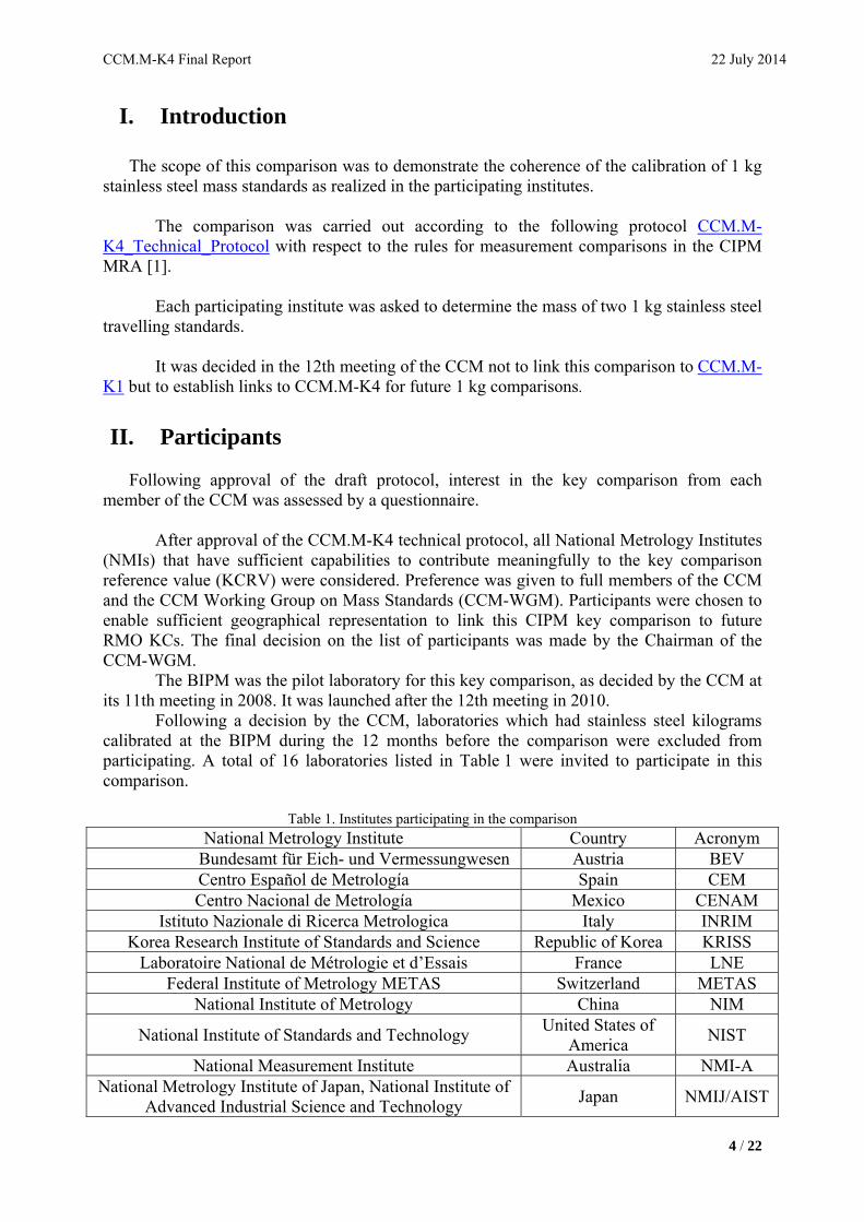
I. Introduction The scope of this comparison was to demonstrate the coherence of the calibration of 1 kg

stainless steel mass standards as realized in the participating institutes.

The comparison was carried out according to the following protocol CCM.M-K4_Technical_Protocol with respect to the rules for measurement comparisons in the CIPM MRA [1].

Each participating institute was asked to determine the mass of two 1 kg stainless steel

travelling standards. It was decided in the 12th meeting of the CCM not to link this comparison to CCM.M-

K1 but to establish links to CCM.M-K4 for future 1 kg comparisons.

II. Participants

Following approval of the draft protocol, interest in the key comparison from each

member of the CCM was assessed by a questionnaire.

After approval of the CCM.M-K4 technical protocol, all National Metrology Institutes (NMIs) that have sufficient capabilities to contribute meaningfully to the key comparison reference value (KCRV) were considered. Preference was given to full members of the CCM and the CCM Working Group on Mass Standards (CCM-WGM). Participants were chosen to enable sufficient geographical representation to link this CIPM key comparison to future RMO KCs. The final decision on the list of participants was made by the Chairman of the CCM-WGM.

The BIPM was the pilot laboratory for this key comparison, as decided by the CCM at its 11th meeting in 2008. It was launched after the 12th meeting in 2010.

Following a decision by the CCM, laboratories which had stainless steel kilograms calibrated at the BIPM during the 12 months before the comparison were excluded from participating. A total of 16 laboratories listed in Table 1 were invited to participate in this comparison.

Table 1. Institutes participating in the comparison

National Metrology Institute Country Acronym Bundesamt für Eich- und Vermessungwesen Austria BEV Centro Español de Metrología Spain CEM Centro Nacional de Metrología Mexico CENAM

Istituto Nazionale di Ricerca Metrologica Italy INRIM Korea Research Institute of Standards and Science Republic of Korea KRISS

Laboratoire National de Métrologie et d’Essais France LNE Federal Institute of Metrology METAS Switzerland METAS

National Institute of Metrology China NIM

National Institute of Standards and Technology United States of

America NIST

National Measurement Institute Australia NMI-A National Metrology Institute of Japan, National Institute of

Advanced Industrial Science and Technology Japan NMIJ/AIST


5 / 22

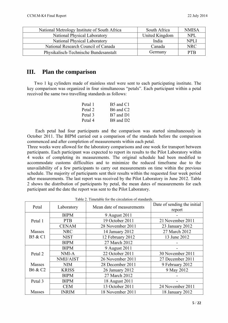
National Metrology Institute of South Africa South Africa NMISA National Physical Laboratory United Kingdom NPL National Physical Laboratory India NPLI

National Research Council of Canada Canada NRC Physikalisch-Technische Bundesanstalt Germany PTB

III. Plan the comparison

Two 1 kg cylinders made of stainless steel were sent to each participating institute. The key comparison was organized in four simultaneous “petals”. Each participant within a petal received the same two travelling standards as follows:

Petal 1 B5 and C1 Petal 2 B6 and C2 Petal 3 B7 and D1 Petal 4 B8 and D2

Each petal had four participants and the comparison was started simultaneously in

October 2011. The BIPM carried out a comparison of the standards before the comparison commenced and after completion of measurements within each petal. Three weeks were allowed for the laboratory comparisons and one week for transport between participants. Each participant was expected to report its results to the Pilot Laboratory within 4 weeks of completing its measurements. The original schedule had been modified to accommodate customs difficulties and to minimize the reduced timeframe due to the unavailability of a few participants to carry out measurements on time within the previous schedule. The majority of participants sent their results within the requested four week period after measurements. The last report was received by the Pilot Laboratory in June 2012. Table 2 shows the distribution of participants by petal, the mean dates of measurements for each participant and the date the report was sent to the Pilot Laboratory.

Table 2. Timetable for the circulation of standards.

Petal Laboratory Mean date of measurements Date of sending the initial

report

Petal 1

Masses B5 & C1

BIPM 9 August 2011 - PTB 19 October 2011 21 November 2011

CENAM 28 November 2011 23 January 2012 NRC 14 January 2012 27 March 2012 NIST 12 February 2012 13 June 2012 BIPM 27 March 2012 -

Petal 2

Masses B6 & C2

BIPM 9 August 2011 - NMI-A 22 October 2011 30 November 2011

NMIJ/AIST 26 November 2011 27 December 2011 NIM 28 December 2011 9 February 2012

KRISS 26 January 2012 9 May 2012 BIPM 27 March 2012 -

Petal 3

Masses

BIPM 18 August 2011 - CEM 13 October 2011 24 November 2011

INRIM 18 November 2011 18 January 2012


6 / 22

B7 & D1 LNE 5 December 2011 21 February 2012 NMISA 15 January 2012 1 March 2012 BIPM 6 April 2012 -

Petal 4

Masses B8 & D2

BIPM 9 August 2011 - NPL 21 October 2011 22 December 2011

METAS 13 November 2011 16 March 2012 BEV 28 December 2011 13 March 2012 NPLI 28 February 2012 2 May 2012 BIPM 10 May 2012 -

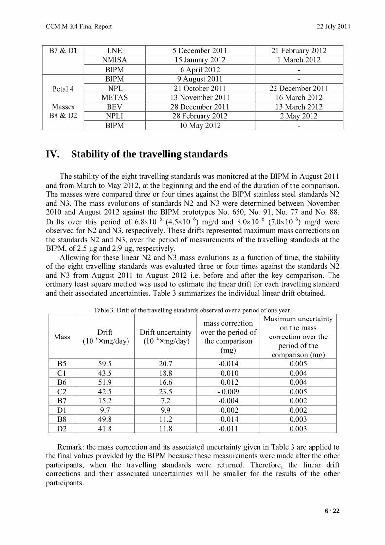
IV. Stability of the travelling standards The stability of the eight travelling standards was monitored at the BIPM in August 2011

and from March to May 2012, at the beginning and the end of the duration of the comparison. The masses were compared three or four times against the BIPM stainless steel standards N2 and N3. The mass evolutions of standards N2 and N3 were determined between November 2010 and August 2012 against the BIPM prototypes No. 650, No. 91, No. 77 and No. 88. Drifts over this period of 6.810−6 (4.510−6) mg/d and 8.010−6 (7.010−6) mg/d were observed for N2 and N3, respectively. These drifts represented maximum mass corrections on the standards N2 and N3, over the period of measurements of the travelling standards at the BIPM, of 2.5 µg and 2.9 µg, respectively.

Allowing for these linear N2 and N3 mass evolutions as a function of time, the stability of the eight travelling standards was evaluated three or four times against the standards N2 and N3 from August 2011 to August 2012 i.e. before and after the key comparison. The ordinary least square method was used to estimate the linear drift for each travelling standard and their associated uncertainties. Table 3 summarizes the individual linear drift obtained.

Table 3. Drift of the travelling standards observed over a period of one year.

Mass Drift

(10−6×mg/day) Drift uncertainty (10−6×mg/day)

mass correction over the period of the comparison

(mg)

Maximum uncertainty on the mass

correction over the period of the

comparison (mg) B5 59.5 20.7 -0.014 0.005 C1 43.5 18.8 -0.010 0.004 B6 51.9 16.6 -0.012 0.004 C2 42.5 23.5 - 0.009 0.005 B7 15.2 7.2 -0.004 0.002 D1 9.7 9.9 -0.002 0.002 B8 49.8 11.2 -0.014 0.003 D2 41.8 11.8 -0.011 0.003

Remark: the mass correction and its associated uncertainty given in Table 3 are applied to the final values provided by the BIPM because these measurements were made after the other participants, when the travelling standards were returned. Therefore, the linear drift corrections and their associated uncertainties will be smaller for the results of the other participants.


7 / 22

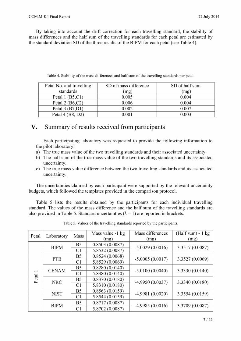
By taking into account the drift correction for each travelling standard, the stability of mass differences and the half sum of the travelling standards for each petal are estimated by the standard deviation SD of the three results of the BIPM for each petal (see Table 4).

Table 4. Stability of the mass differences and half sum of the travelling standards per petal.

Petal No. and travelling standards

SD of mass difference (mg)

SD of half sum (mg)

Petal 1 (B5,C1) 0.005 0.004 Petal 2 (B6,C2) 0.006 0.004 Petal 3 (B7,D1) 0.002 0.007 Petal 4 (B8, D2) 0.001 0.003

V. Summary of results received from participants

Each participating laboratory was requested to provide the following information to the pilot laboratory: a) The true mass value of the two travelling standards and their associated uncertainty. b) The half sum of the true mass value of the two travelling standards and its associated

uncertainty. c) The true mass value difference between the two travelling standards and its associated

uncertainty.

The uncertainties claimed by each participant were supported by the relevant uncertainty budgets, which followed the templates provided in the comparison protocol.

Table 5 lists the results obtained by the participants for each individual travelling

standard. The values of the mass difference and the half sum of the travelling standards are also provided in Table 5. Standard uncertainties (k = 1) are reported in brackets.

Table 5. Values of the travelling standards reported by the participants.

Petal Laboratory Mass Mass value -1 kg

(mg) Mass differences

(mg) (Half sum) - 1 kg

(mg)

Pet

al 1

BIPM B5 0.8503 (0.0087)

-5.0029 (0.0016) 3.3517 (0.0087) C1 5.8532 (0.0087)

PTB B5 0.8524 (0.0068)

-5.0005 (0.0017) 3.3527 (0.0069) C1 5.8529 (0.0069)

CENAM B5 0.8280 (0.0140)

-5.0100 (0.0040) 3.3330 (0.0140) C1 5.8380 (0.0140)

NRC B5 0.8370 (0.0180)

-4.9950 (0.0037) 3.3340 (0.0180) C1 5.8310 (0.0180)

NIST B5 0.8563 (0.0159)

-4.9981 (0.0020) 3.3554 (0.0159) C1 5.8544 (0.0159)

BIPM B5 0.8717 (0.0087)

-4.9985 (0.0016) 3.3709 (0.0087) C1 5.8702 (0.0087)


8 / 22

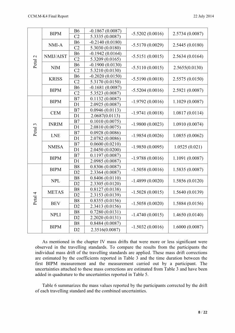
Pet

al 2

BIPM

B6 -0.1867 (0.0087) -5.5202 (0.0016) 2.5734 (0.0087)

C2 5.3335 (0.0087)

NMI-A B6 -0.2140 (0.0180)

-5.5170 (0.0029) 2.5445 (0.0180) C2 5.3030 (0.0180)

NMIJ/AIST B6 -0.1942 (0.0164)

-5.5151 (0.0015) 2.5634 (0.0164) C2 5.3209 (0.0165)

NIM B6 -0.1900 (0.0130)

-5.5110 (0.0015) 2.5655(0.0130) C2 5.3210 (0.0130)

KRISS B6 -0.2020 (0.0150)

-5.5190 (0.0018) 2.5575 (0.0150) C2 5.3170 (0.0150)

BIPM B6 -0.1681 (0.0087)

-5.5204 (0.0016) 2.5921 (0.0087) C2 5.3523 (0.0087)

Pet

al 3

BIPM B7 0.1132 (0.0087)

-1.9792 (0.0016) 1.1029 (0.0087) D1 2.0925 (0.0087)

CEM B7 0.0946 (0.0113)

-1.9741 (0.0018) 1.0817 (0.0114) D1 2.0687(0.0113)

INRIM B7 0.1010 (0.0075)

-1.9800 (0.0023) 1.0910 (0.0074) D1 2.0810 (0.0075)

LNE B7 0.0928 (0.0086)

-1.9854 (0.0026) 1.0855 (0.0062) D1 2.0782 (0.0086)

NMISA B7 0.0600 (0.0210)

-1.9850 (0.0095) 1.0525 (0.021) D1 2.0450 (0.0200)

BIPM B7 0.1197 (0.0087)

-1.9788 (0.0016) 1.1091 (0.0087) D1 2.0985 (0.0087)

Pet

al 4

BIPM B8 0.8306 (0.0087)

-1.5058 (0.0016) 1.5835 (0.0087) D2 2.3364 (0.0087)

NPL B8 0.8406 (0.0110)

-1.4899 (0.0020) 1.5856 (0.0120) D2 2.3305 (0.0120)

METAS B8 0.8127 (0.0138)

-1.5028 (0.0015) 1.5640 (0.0139) D2 2.3153 (0.0139)

BEV B8 0.8355 (0.0156)

-1.5058 (0.0020) 1.5884 (0.0156) D2 2.3413 (0.0156)

NPLI B8 0.7280 (0.0131)

-1.4740 (0.0015) 1.4650 (0.0140) D2 2.2020 (0.0131)

BIPM B8 0.8484 (0.0087)

-1.5032 (0.0016) 1.6000 (0.0087) D2 2.3516(0.0087)

As mentioned in the chapter IV mass drifts that were more or less significant were

observed in the travelling standards. To compare the results from the participants the individual mass drift of the travelling standards are applied. These mass drift corrections are estimated by the coefficients reported in Table 3 and the time duration between the first BIPM measurement and the measurement carried out by a participant. The uncertainties attached to these mass corrections are estimated from Table 3 and have been added in quadrature to the uncertainties reported in Table 5.

Table 6 summarizes the mass values reported by the participants corrected by the drift

of each travelling standard and the combined uncertainties.


9 / 22

Table 6. Values of the travelling standards reported by participants corrected for the drift and its associated uncertainties.

Petal Laboratory Mass Mass value -1 kg

(mg) Mass differences

(mg) (Half sum) - 1 kg

(mg)

Pet

al 1

BIPM B5 0.8503 (0.0087)

-5.0029 (0.0016) 3.3517 (0.0087) C1 5.8532 (0.0087)

PTB B5 0.8482 (0.0070)

-5.0020 (0.0025) 3.3492 (0.0070) C1 5.8502 (0.0070)

CENAM B5 0.8214 (0.0142)

-5.0122 (0.0050) 3.3274 (0.0142) C1 5.8335 (0.0141)

NRC B5 0.8276 (0.0183)

-4.9969 (0.0055) 3.3261 (0.0183) C1 5.8245 (0.0182)

NIST B5 0.8451 (0.0164)

-5.0015 (0.0055) 3.3459 (0.0163) C1 5.8466 (0.0162)

BIPM B5 0.8579 (0.0099)

-5.0026 (0.0065) 3.3592 (0.0103) C1 5.8605 (0.0096)

Pet

al 2

BIPM B6 -0.1867 (0.0087)

-5.5202 (0.0016) 2.5734 (0.0087) C2 5.3335 (0.0087)

NMI-A B6 -0.2179 (0.0180)

-5.5181 (0.0035) 2.5412 (0.0181) C2 5.3002 (0.0181)

NMIJ/AIST B6 -0.1999 (0.0165)

-5.5165 (0.0033) 2.5584 (0.0166) C2 5.3166 (0.0167)

NIM B6 -0.1973 (0.0132)

-5.5127 (0.0042) 2.5590 (0.0133) C2 5.3154 (0.0134)

KRISS B6 -0.2108 (0.0153)

-5.5210(0.0051) 2.5497 (0.0154) C2 5.3102 (0.0155)

BIPM B6 -0.1801 (0.0095)

-5.5230 (0.0067) 2.5814 (0.0098) C2 5.3429 (0.0101)

Pet

al 3

BIPM B7 0.1132 (0.0087)

-1.9792 (0.0016) 1.1029 (0.0087) D1 2.0925 (0.0087)

CEM B7 0.0936 (0.0113)

-1.9745 (0.0020) 1.0809 (0.0113) D1 2.0682 (0.0113)

INRIM B7 0.0995 (0.0075)

-1.9806 (0.0026) 1.0898 (0.0075) D1 2.0801 (0.0076)

LNE B7 0.0910 (0.0086)

-1.9861 (0.0029) 1.0841 (0.0087) D1 2.0771 (0.0087)

NMISA B7 0.0576 (0.0210)

-1.9860 (0.0095) 1.0506 (0.0205) D1 2.0435 (0.0201)

BIPM B7 0.1160 (0.0089)

-1.9802 (0.0033) 1.1061 (0.0089) D1 2.0962 (0.0090)

Pet

al 4

BIPM B8 0.8306 (0.0087)

-1.5058 (0.0016) 1.5835 (0.0087) D2 2.3364 (0.0087)

NPL B8 0.8369 (0.0110)

-1.4909 (0.0023) 1.5824 (0.0115) D2 2.3278(0.0120)

METAS B8 0.8079 (0.0138)

-1.5037 (0.0021) 1.5598 (0.0139) D2 2.3117 (0.0139)

BEV B8 0.8285 (0.0157)

-1.5073 (0.0030) 1.5821 (0.0157) D2 2.3358 (0.0157)


10 / 22

NPLI B8 0.7179 (0.0133)

-1.4760 (0.0036) 1.4559 (0.0133) D2 2.1939 (0.0133)

BIPM B8 0.8347 (0.0092)

-1.5058 (0.0047) 1.5876 (0.0092) D2 2.3405 (0.0093)

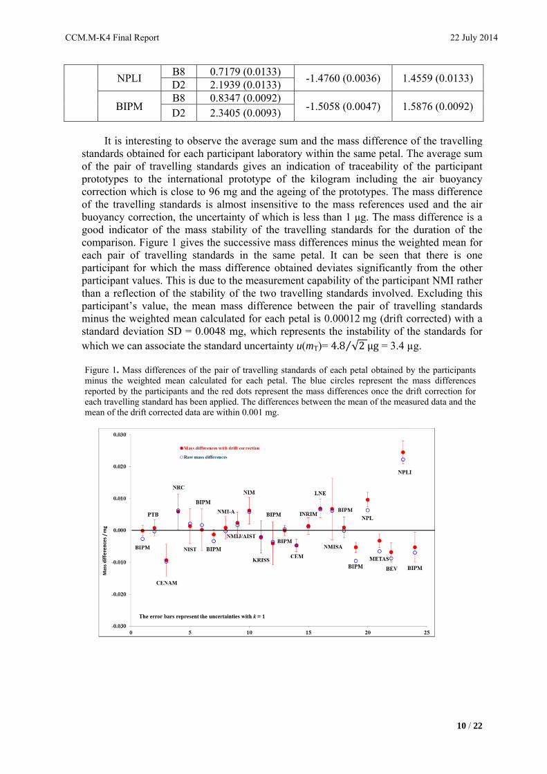
It is interesting to observe the average sum and the mass difference of the travelling

standards obtained for each participant laboratory within the same petal. The average sum of the pair of travelling standards gives an indication of traceability of the participant prototypes to the international prototype of the kilogram including the air buoyancy correction which is close to 96 mg and the ageing of the prototypes. The mass difference of the travelling standards is almost insensitive to the mass references used and the air buoyancy correction, the uncertainty of which is less than 1 μg. The mass difference is a good indicator of the mass stability of the travelling standards for the duration of the comparison. Figure 1 gives the successive mass differences minus the weighted mean for each pair of travelling standards in the same petal. It can be seen that there is one participant for which the mass difference obtained deviates significantly from the other participant values. This is due to the measurement capability of the participant NMI rather than a reflection of the stability of the two travelling standards involved. Excluding this participant’s value, the mean mass difference between the pair of travelling standards minus the weighted mean calculated for each petal is 0.00012 mg (drift corrected) with a standard deviation SD = 0.0048 mg, which represents the instability of the standards for which we can associate the standard uncertainty u(mT)= 4.8 √2μg⁄ = 3.4 µg.

Figure 1. Mass differences of the pair of travelling standards of each petal obtained by the participants minus the weighted mean calculated for each petal. The blue circles represent the mass differences reported by the participants and the red dots represent the mass differences once the drift correction for each travelling standard has been applied. The differences between the mean of the measured data and the mean of the drift corrected data are within 0.001 mg.


11 / 22

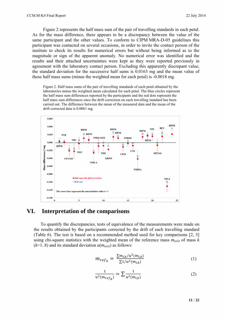
Figure 2 represents the half mass sum of the pair of travelling standards in each petal. As for the mass difference, there appears to be a discrepancy between the value of the same participant and the other values. To conform to CIPM MRA-D-05 guidelines this participant was contacted on several occasions, in order to invite the contact person of the institute to check its results for numerical errors but without being informed as to the magnitude or sign of the apparent anomaly. No numerical error was identified and the results and their attached uncertainties were kept as they were reported previously in agreement with the laboratory contact person. Excluding this apparently discrepant value, the standard deviation for the successive half sums is 0.0163 mg and the mean value of these half mass sums (minus the weighted mean for each petal) is -0.0018 mg.

Figure 2. Half mass sums of the pair of travelling standards of each petal obtained by the laboratories minus the weighted mean calculated for each petal. The blue circles represent the half mass sum differences reported by the participants and the red dots represent the half mass sum differences once the drift correction on each travelling standard has been carried out. The difference between the mean of the measured data and the mean of the drift corrected data is 0.0061 mg.

VI. Interpretation of the comparisons

To quantify the discrepancies, tests of equivalence of the measurements were made on the results obtained by the participants corrected by the drift of each travelling standard (Table 6). The test is based on a recommended method used for key comparisons [2, 3] using chi-square statistics with the weighted mean of the reference mass mref,k of mass k (k=1..8) and its standard deviation u(mref,k) as follows:

∑ , ,⁄

∑ ⁄ , (1)

∑,

(2)


12 / 22

where the summations (index i) are over the N results available and u(mi,k) are the combined standard uncertainties claimed by the participants given in brackets in the fourth column of Table 5. The chi-squared ² test is applied, to carry out an overall consistency check of the results obtained, by:

- observed chi-squared value, ∑ ,

, (3)

- degrees of freedom. = N-1

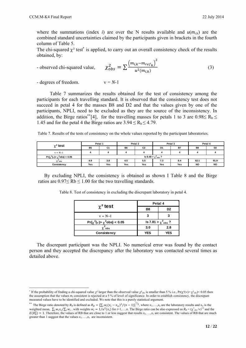
Table 7 summarizes the results obtained for the test of consistency among the participants for each travelling standard. It is observed that the consistency test does not succeed in petal 4 for the masses B8 and D2 and that the values given by one of the participants, NPLI, need to be excluded as they are the source of the inconsistency. In addition, the Birge ratios[4], for the travelling masses for petals 1 to 3 are 0.98≤ Rb ≤ 1.45 and for the petal 4 the Birge ratios are 3.94 ≤ Rb ≤ 4.79.

Table 7. Results of the tests of consistency on the whole values reported by the participant laboratories.

By excluding NPLI, the consistency is obtained as shown I Table 8 and the Birge ratios are 0.97≤ Rb ≤ 1.00 for the two travelling standards.

Table 8. Test of consistency in excluding the discrepant laboratory in petal 4.

The discrepant participant was the NPLI. No numerical error was found by the contact person and they accepted the discrepancy after the laboratory was contacted several times as detailed above.

If the probability of finding a chi-squared value ² larger than the observed value ²obs is smaller than 5 % i.e., Pr(²()> ²obs)< 0.05 then the assumption that the values mi consistent is rejected at a 5 % of level of significance. In order to establish consistency, the discrepant measured values have to be identified and excluded. We note that this is a purely statistical argument. The Birge ratio denoted by RB is defined as ∑ ² 1⁄ , where x1,….,xn are the laboratory results and xw is the weighted mean, ∑ ∑⁄ , with weights 1⁄ for i=1,….n. The Birge ratio can be also expressed as RB = (2

obs /)1/2 and the

1. Therefore, the values of RB that are close to 1 or less suggest that results x1, …,xn are consistent. The values of RB that are much greater than 1 suggest that the values x1, …,xn are inconsistent.

B5 C1 B6 C2 D1 B7 B8 D2

4 4 4 4 4 4 4 4

Pr{2()> 2obs} < 0.05

2obs 4.9 3.8 4.5 5.5 7.3 8.4 62.1 91.9

Consistency Yes Yes Yes Yes Yes Yes NO NO

Petal 4

Is 9.49 > 2obs ?

² testPetal 1 Petal 2 Petal 3

B8 D2

3 3

Pr{2()> 2obs} < 0.05

2obs 3.0 2.8

Consistency YES YES

² testPetal 4

Is 7.81 > 2obs ?


13 / 22

VII. Reference values

In the CIPM_MRA-D-05 it is stated that: "In calculating the key comparison reference value, the pilot institute will use the

method considered most appropriate for the particular comparison, subject to confirmation by the participants and, in due course, the key comparison working group and the Consultative Committee."

Therefore a vote was taken among participants to decide which KCRV estimation method is the most appropriate for this particular comparison.

The proposed methods to estimate the KCRV were the following:

A) the weighted mean (WM), B) the Ordinary Least Squares estimation (OLS), C) the Generalized Linear Least-Squares estimation (GLS), D) the Least Squares Adjustment (LSA).

The results of the vote among the seventeen participants are given in table 9 and show that 53 % of the participants prefer to use the Generalized Linear Least-Squares estimation (GLS) method to determine the KCRV.

In addition, the participants were asked to choose between two ways to determine the degree of equivalences (DoEs):

1) Estimation of DoEs by using the KCRV as an appropriate estimation of the travelling standards given by the matrix reduction.

2) Estimation of DoEs by using the KCRV as an appropriate estimation of the BIPM results given by the matrix reduction.

Of the nine participants that voted for the GLS method almost 78 % preferred to use the travelling standards as the KCRV for the estimation of the DoEs.

Table 9. Results of the vote to select the an appropriate estimation appropriate estimation method to evaluate the KCRV and the degrees of equivalence.

Therefore, from the votes obtained, the final results of the comparison are given by using the Generalized Linear Least-Squares which gives (from the table 6) an appropriate estimation of the travelling standards. Degrees of equivalence are calculated from the

KCRV Nb votes

1) Using the

travelling

standards

as KCRV.

2) Using

the BIPM

results as

KCRV.

A) the weighted mean (WM), 6 2 4

B) the Ordinary Least Squares estimation (OLS), 0 0 0

C) the Generalized Linear Least‐Squares estimation (GLS), 9 7 2

D) the Least Squares Adjustment (LSA). 2 2 0

DoE


14 / 22

differences between participant values (table 6) and the KCRV and the uncertainties estimated by the matrix reduction.

It is worth noting that, in this particular comparison, the GLS method compared to the three other methods to estimate the KCRV, provides an adjustment without bias with a minimum sum of the NMIs deviations against the KCRV. In addition, the GLS provides a minimum scattering of the DoEs and the smallest normalized deviation of the NMIs against the KCRV.

In all following calculations of the KCRV the drift correction and its associated uncertainty

is taken into account for each travelling standard. Therefore, the input values are those given in column 4 of table 6. In addition, the following KCRV is estimated without taking into account the values given by the NPLI because their results have been shown to be inconsistent with the other participants’ results (see the previous chapter). Nevertheless, their deviations from the KCRV and associated uncertainties are noted.

The generalized linear least-squares (GLS) estimation [5] is used to link the sixteen participants and the Pilot Laboratory, based on the matrix reduction. The solution is provided by the result vector as:

Φ (4)

Where the gh matrix X represents the design of the comparison as described in [5]. Each row of X (apart from the last row) represents one of the comparison measurements and the associated measurement result is in the corresponding row of vector Y. A constraint for the matrix solution is included in the last row of X and Y. The constraint is that the sum wi Di is equal to zero, where Di are the unknown deviations of laboratory from the KCRV and wi are the weights. The weights wi are determined by wi = (1/ui

2) / i(1/ui2), where ui are the mean

standard uncertainty of the drift corrected mass values for laboratories. Hence the KCRV is zero and the definition of the KCRV follows equation (1) of Cox [2]. The standard uncertainty of the constraint is assumed to be (1 / i(1/ui

2))1/2 = 0.0031 mg. In this case g = 47 and h = 24, therefore the degree of freedom is = g-h = 23.

The uncertainty matrix is given as:

TΦ (5)

Where the matrix is a symmetric gg matrix. The diagonal elements of are given by the quadratic sum of , of each laboratory, the uncertainty due to the drift and the stability of the travelling standards . The off-diagonal of represents the covariance between measurements.

In this comparison scheme we could assume there are 5 types of covariance as follows: a) Covariance among NMIs in the same petal, b) Covariance among NMIs in different petals, c) Covariance in the same petal and NMIs (between the pair of travelling

standards), d) Covariance in the same petal for the BIPM (between the pair of

travelling standards and the measurements carried out before and after the comparison),

e) Covariance in different petals for the BIPM.


15 / 22

The covariances a) and b) are evaluated by assuming that the common standard uncertainty is the average of the last calibration uncertainty reported in the BIPM certificates of the prototypes involved in this comparison. The standard uncertainty of the last calibration of the national prototype ranges from 0.0023 mg to 0.0070 mg depending on the calibration date. The arithmetic average of the calibration uncertainty is 0.0054 mg and gives in average a correlation coefficient of about 0.13. The correlation coefficients for the cases d) and e) were evaluated from the BIPM data and it was found that the covariance is 810-5 mg² which corresponds to the quadratic sum of the type B uncertainty 0.00827 mg claimed by the BIPM plus the uncertainty due to the instability of the travelling standards 0.0034 mg given in chapter V. This covariance corresponds in average among the BIPM measurements to a correlation coefficient of 0.855. It has been assumed that the correlation coefficients for the cases c) should be nearly the same as that in case d) i.e. about 0.86. The diagonal terms of the matrix are evaluated by adding in quadrature the uncertainties claimed by the laboratories (from table 6 which takes into account the uncertainty due to the linear drift of each standard) and the uncertainty due to the instabilities of the travelling standards of 0.0034 mg (see chapter V).

In total 47 variances and more than eleven hundred covariance terms were evaluated to build the matrix.

Of course, these correlation uncertainty estimations have some uncertainties

and need to be checked by the consistency between the model and the measurement results by using ² test given by:

Φ (6)

With E (²()) = or σ(²()) = √2

The correlation coefficient corresponding in the case c) was adjusted in order to keep

2 in the matrix , close to . The following results are obtained. ² = 23.0 = 23 u(² ) = 6.8 σ = 0.0093 mg

And the final values for the correlation coefficients are: Cases a) and b): = 0.13

Case c): = 0.9015 Case d): = 0.855 Case e): = 0.855

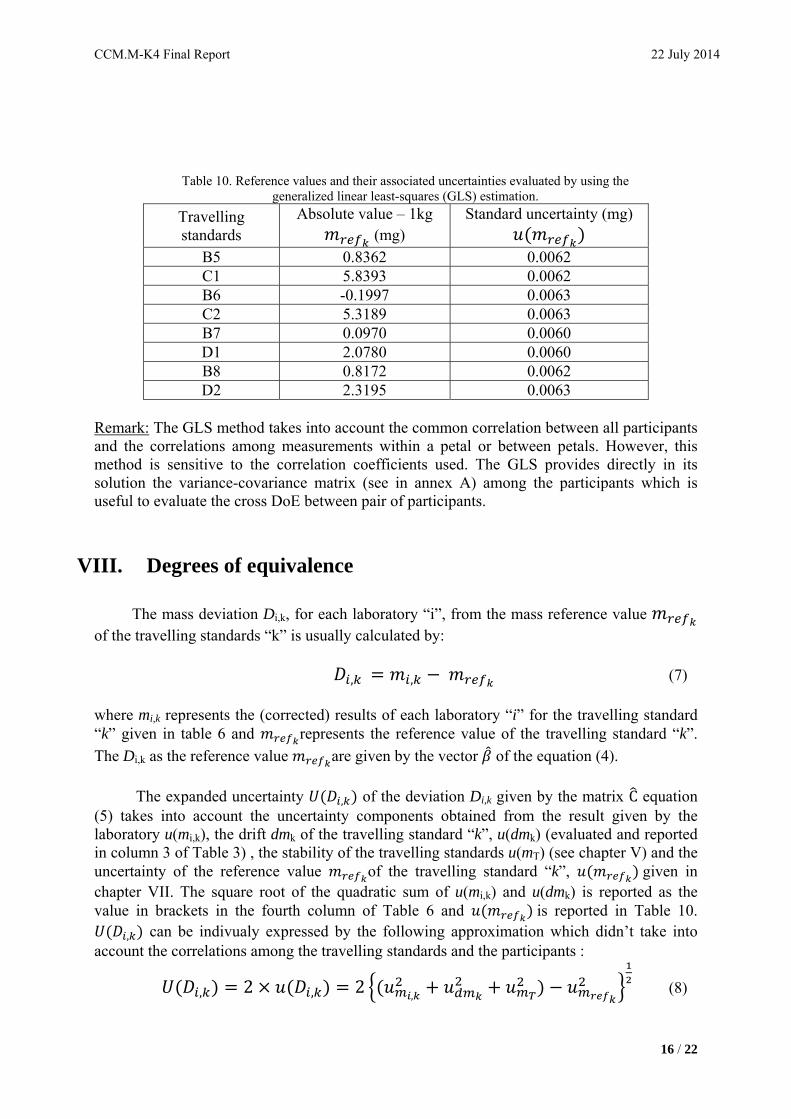
Table 10 gives the reference values for each travelling standard together with their associated uncertainty obtained by using the GLS method and the above correlation coefficients.


16 / 22

Table 10. Reference values and their associated uncertainties evaluated by using the generalized linear least-squares (GLS) estimation.

Travelling standards

Absolute value – 1kg (mg)

Standard uncertainty (mg)

B5 0.8362 0.0062 C1 5.8393 0.0062 B6 -0.1997 0.0063 C2 5.3189 0.0063 B7 0.0970 0.0060 D1 2.0780 0.0060 B8 0.8172 0.0062 D2 2.3195 0.0063

Remark: The GLS method takes into account the common correlation between all participants and the correlations among measurements within a petal or between petals. However, this method is sensitive to the correlation coefficients used. The GLS provides directly in its solution the variance-covariance matrix (see in annex A) among the participants which is useful to evaluate the cross DoE between pair of participants.

VIII. Degrees of equivalence

The mass deviation Di,k, for each laboratory “i”, from the mass reference value

of the travelling standards “k” is usually calculated by:

, , (7) where mi,k represents the (corrected) results of each laboratory “i” for the travelling standard “k” given in table 6 and represents the reference value of the travelling standard “k”.

The Di,k as the reference value are given by the vector of the equation (4).

The expanded uncertainty , of the deviation Di,k given by the matrix C equation (5) takes into account the uncertainty components obtained from the result given by the laboratory u(mi,k), the drift dmk of the travelling standard “k”, u(dmk) (evaluated and reported in column 3 of Table 3) , the stability of the travelling standards u(mT) (see chapter V) and the uncertainty of the reference value of the travelling standard “k”, given in chapter VII. The square root of the quadratic sum of u(mi,k) and u(dmk) is reported as the value in brackets in the fourth column of Table 6 and is reported in Table 10.

, can be indivualy expressed by the following approximation which didn’t take into account the correlations among the travelling standards and the participants :

, 2 , 2,

(8)


17 / 22

With the mass deviations Di,k to the reference values and their associate expanded

uncertainties Ui,k the normalized deviation di,k , which reflects the degrees of equivalence (DoE), is quantified by:

, ,

,1 (9)

The degrees of equivalence given by the GLS estimation are summarized in table 11.

As mentioned above, the KCRV estimation is calculated as described in chapter VII is carried out without taking into account the values obtained by the NPLI’s. Nevertheless, the degree of equivalence of NPLI has been calculated according to equation (8) and is included in the table.

.

Table 11. Degrees of equivalence obtained by the Generalized Linear Least-Squares (GLS) estimation and normalized deviation di against the appropriate estimation of the travelling standards .

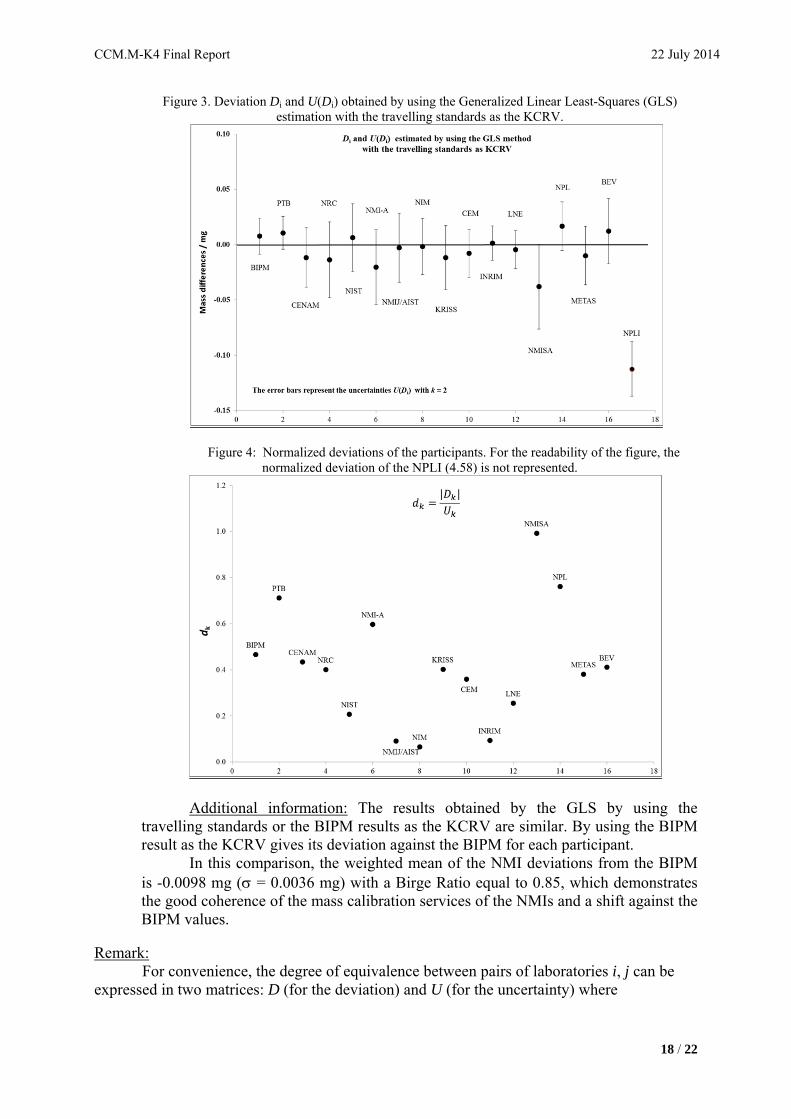
Figure 3 shows the deviations Di from the KCRV and their associated expanded uncertainties (k = 2) for each participant by using the travelling standards as the KCRV.

Laboratory Di (mg) U(Di) (mg) di BIPM 0.0076 0.0163 0.47PTB 0.0106 0.0149 0.71

CENAM -0.0116 0.0268 0.43NRC -0.0137 0.0342 0.40NIST 0.0064 0.0307 0.21

NMI-A -0.0203 0.0339 0.60NMIJ/AIST -0.0028 0.0312 0.09

NIM -0.0017 0.0253 0.07KRISS -0.0117 0.0290 0.40CEM -0.0078 0.0217 0.36

INRIM 0.0015 0.0156 0.09LNE -0.0044 0.0173 0.26

NMISA -0.0380 0.0383 0.99NPL 0.0168 0.0220 0.76

METAS -0.0100 0.0263 0.38BEV 0.0122 0.0396 0.41NPLI -0.1125 0.0246 4.58


18 / 22

Figure 3. Deviation Di and U(Di) obtained by using the Generalized Linear Least-Squares (GLS) estimation with the travelling standards as the KCRV.

Figure 4: Normalized deviations of the participants. For the readability of the figure, the normalized deviation of the NPLI (4.58) is not represented.

Additional information: The results obtained by the GLS by using the

travelling standards or the BIPM results as the KCRV are similar. By using the BIPM result as the KCRV gives its deviation against the BIPM for each participant.

In this comparison, the weighted mean of the NMI deviations from the BIPM is -0.0098 mg ( = 0.0036 mg) with a Birge Ratio equal to 0.85, which demonstrates the good coherence of the mass calibration services of the NMIs and a shift against the BIPM values.

Remark:

For convenience, the degree of equivalence between pairs of laboratories i, j can be expressed in two matrices: D (for the deviation) and U (for the uncertainty) where


19 / 22

, (12) and

, , , 2 , (13)

Where the variance and covariance terms are given in annex A.

The reader is free to carry out a link with the CCM.M-K1 comparison or other regional key comparisons by using the GLS method.

IX. Observation:

Figure 5 shows the deviations from the KCRV as well the ageing corrections applied by each laboratory. As can be observed in this comparison, about 71 % of the participants applied an ageing correction of less than 0.010 mg to their prototypes. Of note is that about 47 % of the laboratories have had their prototype calibrated by the BIPM more than five years before the comparison i.e. before 2008. For these laboratories, the weighted mean of the deviations against the BIPM value is about -0.0157 mg ( = 0.0049 mg). This weighted mean is about -0.0029 mg ( = 0.0053 mg) for the laboratories having there prototype calibrated less than five years before the comparisons i.e. from 2008. The weighted mean of the deviation against the BIPM including all of the laboratories is -0.0098 mg ( = 0.0036 mg). In addition, two participants had not had their prototypes recalibrated since the third verification and their results are fully consistent with the others. These observations suggest that we should, in order to have a more accurate calibration system, improve the knowledge of the ageing effects of the mass references and to increase the BIPM calibration frequency of the national prototypes.

Fig 5. Deviations from the KCRV and the ageing corrections applied by each laboratory excluding NPLI for the

readability of the graph. The DNPLI is -0.1125mg with an ageing correction of 0.032 mg for their prototype calibrated in December 2002.

X. Conclusion

The measurements for the CCM.M-K4 comparison were carried out by the participating laboratories over periods of one month and five months


20 / 22

depending on the participants, which demonstrates that such a complicated exercise can be achieved in a short time even with sixteen participants.

Two customs problems were encountered during the 34 shipments of the standards around the world. The packaging of the travelling standards was sufficient to avoid any risk of damage.

In this comparison, the results of one laboratory (the NPLI) were inconsistent with the results of the other laboratories by about -0.112 mg.

The NMISA result shows a significant deviation from the KCRV of about -0.038 mg although it had revised its values.

The results obtained by the other fourteen laboratories are consistent with each other and with the KCRV.

The mass values of the eight stainless steel travelling standards were determined in air by the NMIs with claimed standard uncertainties ranging from 0.007 mg to 0.021 mg. This result demonstrates the high quality of this comparison and that some participants are able to provide, for their mass calibration services, standard uncertainties of around ten micrograms.

The Generalized Linear Least Squares (GLS) method was, in this particular comparison, considered by the majority of the participants as the most appropriate method to determine the best mass estimation of the travelling standards as well as an accurate adjustment in order to determine the degrees of equivalence with the optimum accuracy.

During the comparison, the drifts have been estimated linear of the travelling standards (0.004 mg < drifttravelling standards < 0.014 mg ) and the stability of the half sums and the differences of the travelling standards were (0.003 mg < travelling standards < 0.007 mg) and (0.001 mg < travelling standards < 0.006 mg) respectively. Therefore, the travelling standards were stable enough for this comparison.

The good uniformity of world-wide mass dissemination since the last periodic mass verification carried out in 1992 is demonstrated by the agreement among the NMI’s results. In addition, the observed weighted mean of the NMI deviation against the BIPM is -0.0098 mg ( = 0.0036 mg).

In despite of the good result obtained we should, in order to have a more accurate calibration system, improve the knowledge of the ageing effects of the mass references and to increase the BIPM calibration frequency of the national prototype.

Acknowledgments The authors wish to thank Pauline Barat for her work in the preparation of this comparison, in carrying out the survey of the travelling standard stabilities and for conducting measurements before and after the comparison. We also thank Cécile Goyon for her help in collecting the data and reports from the participants and Dr Chris Sutton for his help in preliminary matrix calculation. We thank various collaborators, in particular Mr Martin Firlus, Mr Patrick Abbott, Mr Davide Torchio, Mr Stefan Russi, Mr James Berry and Mrs Yao Hong involved in this comparison. The pilot laboratory thanks the steering committee of this comparison for their involvement in drafting this report.


21 / 22 M

atr

ix C

OV

BIP

MP

TB

CE

NA

MN

RC

NIS

TN

MI-

AN

MIJ

/AIS

TN

IMK

RIS

SC

EM

INR

IML

NE

NM

ISA

NP

LM

ET

AS

BE

V

BIP

M6.

7E-0

53.

8E-0

61.

1E-0

6-4

.4E

-07

3.1E

-07

-3.2

E-0

85.

6E-0

71.

8E-0

61.

0E-0

63.

9E-0

65.

3E-0

64.

9E-0

64.

4E-0

74.

0E-0

62.

8E-0

62.

1E-0

6

PT

B3.

8E-0

65.

6E-0

52.

7E-0

67.

0E-0

71.

7E-0

6-2

.3E

-06

-1.6

E-0

67.

0E-0

8-9

.5E

-07

4.2E

-08

1.8E

-06

1.3E

-06

-4.3

E-0

61.

0E-0

6-4

.7E

-07

-1.3

E-0

6

CE

NA

M1.

1E-0

62.

7E-0

61.

8E-0

46.

6E-0

65.

9E-0

63.

4E-0

62.

9E-0

61.

7E-0

62.

5E-0

63.

5E-0

7-9

.0E

-07

-5.4

E-0

73.

6E-0

61.

2E-0

61.

9E-0

62.

5E-0

6

NR

C-4

.4E

-07

7.0E

-07

6.6E

-06

2.9E

-04

8.4E

-06

6.7E

-06

5.5E

-06

2.7E

-06

4.5E

-06

5.3E

-07

-2.5

E-0

6-1

.6E

-06

8.2E

-06

1.3E

-06

3.3E

-06

4.8E

-06

NIS

T3.

1E-0

71.

7E-0

65.

9E-0

68.

4E-0

62.

4E-0

45.

1E-0

64.

3E-0

62.

3E-0

63.

5E-0

64.

5E-0

7-1

.7E

-06

-1.1

E-0

66.

0E-0

61.

2E-0

62.

6E-0

63.

7E-0

6

NM

I-A

-3.2

E-0

8-2

.3E

-06

3.4E

-06

6.7E

-06

5.1E

-06

2.9E

-04

9.3E

-06

6.6E

-06

8.3E

-06

9.3E

-07

-2.0

E-0

6-1

.2E

-06

8.4E

-06

1.7E

-06

3.6E

-06

5.1E

-06

NM

IJ/A

IST

5.6E

-07

-1.6

E-0

62.

9E-0

65.

5E-0

64.

3E-0

69.

3E-0

62.

4E-0

46.

2E-0

67.

6E-0

68.

6E-0

7-1

.4E

-06

-7.8

E-0

76.

7E-0

61.

6E-0

63.

1E-0

64.

2E-0

6

NIM

1.8E

-06

7.0E

-08

1.7E

-06

2.7E

-06

2.3E

-06

6.6E

-06

6.2E

-06

1.6E

-04

5.9E

-06

7.1E

-07

-1.6

E-0

79.

5E-0

83.

0E-0

61.

6E-0

62.

0E-0

62.

4E-0

6

KR

ISS

1.0E

-06

-9.5

E-0

72.

5E-0

64.

5E-0

63.

5E-0

68.

3E-0

67.

6E-0

65.

9E-0

62.

1E-0

48.

1E-0

7-9

.7E

-07

-4.5

E-0

75.

3E-0

61.

6E-0

62.

7E-0

63.

6E-0

6

CE

M3.

9E-0

64.

2E-0

83.

5E-0

75.

3E-0

74.

5E-0

79.

3E-0

78.

6E-0

77.

1E-0

78.

1E-0

71.

2E-0

43.

0E-0

63.

0E-0

63.

6E-0

67.

3E-0

76.

6E-0

77.

4E-0

7

INR

IM5.

3E-0

61.

8E-0

6-9

.0E

-07

-2.5

E-0

6-1

.7E

-06

-2.0

E-0

6-1

.4E

-06

-1.6

E-0

7-9

.7E

-07

3.0E

-06

6.1E

-05

4.0E

-06

-5.0

E-0

76.

4E-0

7-5

.6E

-07

-1.3

E-0

6

LN

E4.

9E-0

61.

3E-0

6-5

.4E

-07

-1.6

E-0

6-1

.1E

-06

-1.2

E-0

6-7

.8E

-07

9.5E

-08

-4.5

E-0

73.

0E-0

64.

0E-0

67.

5E-0

56.

9E-0

76.

6E-0

7-2

.1E

-07

-6.8

E-0

7

NM

ISA

4.4E

-07

-4.3

E-0

63.

6E-0

68.

2E-0

66.

0E-0

68.

4E-0

66.

7E-0

63.

0E-0

65.

3E-0

63.

6E-0

6-5

.0E

-07

6.9E

-07

3.7E

-04

1.0E

-06

3.8E

-06

5.8E

-06

NP

L4.

0E-0

61.

0E-0

61.

2E-0

61.

3E-0

61.

2E-0

61.

7E-0

61.

6E-0

61.

6E-0

61.

6E-0

67.

3E-0

76.

4E-0

76.

6E-0

71.

0E-0

61.

2E-0

44.

9E-0

64.

8E-0

6

ME

TA

S2.

8E-0

6-4

.7E

-07

1.9E

-06

3.3E

-06

2.6E

-06

3.6E

-06

3.1E

-06

2.0E

-06

2.7E

-06

6.6E

-07

-5.6

E-0

7-2

.1E

-07

3.8E

-06

4.9E

-06

1.7E

-04

6.1E

-06

BE

V2.

1E-0

6-1

.3E

-06

2.5E

-06

4.8E

-06

3.7E

-06

5.1E

-06

4.2E

-06

2.4E

-06

3.6E

-06

7.4E

-07

-1.3

E-0

6-6

.8E

-07

5.8E

-06

4.8E

-06

6.1E

-06

2.2E

-04

An

nex

A

Var

ianc

e co

vari

ance

mat

rix

obta

ined

fro

m th

e G

ener

aliz

ed L

inea

r L

east

Squ

ares

(G

LS

).


22 / 22

References

[1] Measurement comparisons in the CIPM-MRA-D-05, CIPM-MRA-D-05 [2] Cox M.G., 2002, The evaluation of key comparison data, Metrologia, 39, 589-595. [3] Nielsen L., 2002, Identification and handling of discrepant measurements in key comparisons, DFM-02-R28, 3208 LN, 2002-11-08. [4] Kacker R., Datla R. and Parr A., 2002, Combined result and associated uncertainty from interlaboratory evaluations based on the ISO Guide, Metrologia, 39, 279-293. [5] Sutton C.M., 2004, Analysis and linking of international measurement comparisons, Metrologia 41, 272–277.

ccm-m-k4 final report 22-07-2014 - bipm - bipm final report 22 july 2014 1 / 22 key comparison of 1...

Documents