www.cbo.gov/publication/57010

Working Paper Series Congressional Budget Office

Washington, D.C.

CBO’s Simulation Model of New Drug Development

Christopher P. Adams Congressional Budget Office christopher.adams@cbo.gov

Working Paper 2021-09

August 2021

To enhance the transparency of the work of the Congressional Budget Office and to encourage external review of that work, CBO’s working paper series includes papers that provide technical descriptions of official CBO analyses as well as papers that represent independent research by CBO analysts. Papers in that series are available at http://go.usa.gov/ULE.

Thanks to David Austin, Anna Anderson-Cook, Margaret Blume-Kohout, Joseph DiMasi, Ru Ding, Pierre Dubois, Michael Falkenheim, Craig Garthwaite, Sebastien Gay, Ryan Greenfield, Tamara Hayford, Manuel Hermosilla, Evan Herrnstadt, Benedic Ippolito, Jeffrey Kling, Ellen Werble, Chapin White, and James Williamson for helpful suggestions. Thanks also to Katherine Feinerman for reviewing the code, Gabe Waggoner for editing, and Erik O’Donoghue and Jorge Salazar for help in developing the figures.

Abstract

This paper presents the Congressional Budget Office’s simulation model for analyzing leg-islative proposals that may substantially affect new drug development. The model usesestimates of changes in expected future profits or development costs to estimate the per-cent change in the number of drug candidates entering the various stages of human clinicaltrials. Given changes in decisions to enter at each stage, the model estimates when andby how much the number of new drugs entering the market will change. To illustrate theimplications of the model, the paper considers a legislative change that lowers expectedreturns for the top-earning drugs. A 15 percent to 25 percent reduction in expected returnsfor drugs in the top quintile of expected returns is associated with a 0.5 percent averageannual reduction in the number of new drugs entering the market in the first decade underthe policy, increasing to an 8 percent annual average reduction in the third decade. Theanalysis takes the estimated impact of the policy on expected returns as given. In CBO’sassessment, those estimates are in the middle of a wide distribution of potential effects. Theeffects could be smaller if expenditures in late-phase human trials are larger, for example.Alternatively, the effects could be larger if the cost of capital is larger.

Keywords: health care, prescription drugs, new drug development

JEL Classification: I11, I18

1 Introduction

Substantial interest surrounds policies that could have a major impact on the developmentof new drugs—classified here as drugs with new active ingredients, not just a new deliverymechanism or formulation. Most recently, the Congressional Budget Office released costestimates for the Elijah E. Cummings Lower Drug Costs Now Act (H.R. 3; CBO 2019a).CBO estimated that provisions in the act requiring drug price negotiations and providing asource of pressure on manufacturers to secure price concessions would have reduced federalspending by $456 billion. For new drug development, CBO estimated that H.R. 3 wouldhave reduced global revenue for new drugs by 19 percent, leading to approximately 8 fewerdrugs introduced to the U.S. market over the 2020–2029 period (a 3 percent reduction)and 30 fewer drugs over the next decade (a 10 percent reduction) (CBO 2019b).

In this paper, CBO describes an updated version of the model used to inform estimatesof the effects of H.R. 3 on the number and timing of new drugs entering the U.S. market.CBO also now expects more new drugs to be introduced over the next decade under currentlaw. To illustrate how the model works, CBO examines a policy that reduces expectedreturns of drugs in the top quintile of expected returns by 15 percent to 25 percent. Thatpolicy is estimated to lead to 2 fewer drugs in the first decade (a reduction of 0.5 percent),23 fewer over the next decade (a reduction of 5 percent), and 34 fewer drugs in the thirddecade (a reduction of 8 percent). The appendix considers a policy that both reducesexpected returns by 15 percent to 25 percent and reduces available cash to the industryby $900 billion. CBO calculates that the reduction in cash available increases the weightedaverage cost of capital (WACC) by 20 basis points (from a discount rate of 8.6 percent to8.8 percent). The combined effect is that 9 percent fewer new drugs will enter the marketin the third decade under the policy, increasing the size of the effect by 1 percentage point.

The paper discusses various forms of uncertainty affecting those estimates. In additionto the uncertainty associated with the value of the model’s parameters, inherent uncer-tainty is associated with the drug development process. Uncertainty also exists in howmanufacturers react to the major change in the government’s role in price determination.The simulations illustrate effects by using a particular set of revenue reductions (15 percentto 25 percent) as inputs. In later analyses, CBO expects to use inputs stemming from spe-cific legislation that are the agency’s best estimate of the firm’s expectations about averagerevenue reductions in the future; the firm’s own estimates may be larger or smaller thanCBO’s.

In the future, CBO could use the model to estimate whether and how various policieswould affect the development of new drugs. CBO may adjust the model to account for howpolicies influence the process of new drug development.

This paper’s simulation approach is an alternative to directly using elasticity estimatesfrom the literature. Dubois and colleagues (2015) estimate an elasticity of 0.23 for policiesthat change expected market size, where market size refers to the total quantity of thecompeting drugs sold multiplied by the prices of those drugs. For example, if a policy

1

would decrease the expected market size by 20 percent, the number of new drugs woulddecrease by about 5 percent. That work updates a similar study by Acemoglu and Linn(2004), which estimates the elasticity to be 4, corresponding to an 80 percent reduction inthe number of new drugs.1 CBO’s simulation model complements the existing literature byparameterizing a structural model of decisionmaking in drug development. Khmelnitskaya(2020) represents another recent example of an explicitly dynamic structural model ofdecisionmaking in drug development. One advantage of those models is that they canestimate how a policy’s impact may vary over periods longer than are generally seen in thedata.

In analyzing H.R. 3, CBO used elasticity estimates from the literature and adjustedthose over time on the basis of results from an earlier version of the model (CBO 2019b).That analysis used an elasticity estimate that increased to its long-run average of 0.5 after18 years. The policy example analyzed here is estimated to reduce expected returns byan average of 18 percent, and the model results indicate that it leads to 8 percent fewernew drugs after 25 years. That finding corresponds to a long-run average elasticity of 0.45,about twice the size of the estimate from Dubois and colleagues (2015) and approximatelyone-ninth the estimate from Acemoglu and Linn (2004).

Another way to interpret the results is to estimate average reduction in total net presentvalue of returns per drug lost as a result of the policy—that is, total reduction in returns asa result of the policy divided by number of drugs lost in the long run. The estimated effect ofthe illustrative policy corresponds to an average reduction in expected returns of $3.5 billionper drug lost.2 Compare that result with that of Dubois and colleagues (2015), who claimthat their elasticity estimate of 0.23 corresponds to requiring an increase in market size of$2.5 billion to yield one additional drug coming to market. The literature also contains net-present-value estimates of average costs of development and average lifetime revenues perdrug. DiMasi, Grabowski, and Hansen (2016) estimate that average development costs are$2.8 billion (including the cost of developing drugs that do not make it to market). DiMasi,Grabowski, and Vernon (2004) argue that development costs and revenue vary substantiallyacross drugs. In that study, average net present value of revenue per drug varies from$1.4 billion for analgesics to $5.5 billion for central nervous system drugs.(For consistency,dollar estimates in this paragraph are adjusted for inflation.) The average returns valuereflects the reduction in returns throughout the distribution of drugs, whereas the revenueestimates reflect average revenue for a given drug within a particular therapeutic class.

1Why such a large discrepancy exists between the two studies is unclear. Dubois and colleagues (2015)uses more recent data covering the globe rather than just U.S. entry.

2This is the “slope estimate.” Slope is rise over run. Here, rise is the reduction in expected lifetimeearnings for new drugs entering the market each year in the long term. To calculate rise, the lifetimerevenue distribution presented below (Figure 2) is adjusted to represent the total revenue for those drugsand then is used to determine the difference in total revenue with and without the policy. Run is the annualreduction in the number of drugs in the long term, from 44 to 40. Revenues and development costs arepositively correlated in CBO’s assessment, and the affected drugs would have development costs higherthan the average cost for all drugs.

2

The model is based on a stylized representation of the pharmaceutical decisionmakingprocess. A firm is projected to continue development of a drug if expected returns exceedexpected costs. The model’s parameter values are derived from both estimation and cali-bration procedures. The model uses revenue estimates calculated using nonpublic MedicarePart D data. Those data include information on the rebates paid by the manufacturingfirms, allowing those rebates to be netted out of revenue. Using data from 2010 to 2018,CBO estimates how drug revenue varies with time on market. CBO uses results from Di-Masi, Grabowski, and Hansen (2016) to estimate development costs. The agency uses a Roymodel to combine information on revenue and cost. That model accounts for selection andcorrelation in the observed revenue and cost data (Heckman and Honore 1990). Althoughan input into the Roy model is observed revenue, the output is expected returns. The as-sumption of “revealed preference” is used to elicit the firm’s expectations about the valuethe firm will receive from bringing the drug to market. Those expectations account for var-ious costs associated with producing, selling, and distributing the drug—even though thosecosts are not observed in the data. That said, CBO does have access to rebate informationin the Medicare Part D data and in the estimation procedure nets out manufacturer-paidrebates. CBO calibrated entry probabilities and other parameters on the basis of resultspresented in Blume-Kohout and Sood (2013), DiMasi (2013), and Khmelnitskaya (2020).

The analysis shows that any relationship between a policy change and the number ofnew drugs entering the market grows over time. The change would be small for the firstfew years because key decisions for drugs entering in those years would have been madebefore the policy change. However, the size of that change would increase substantially asdecisions in earlier phases of development affect later phases. The estimates of Dubois andcolleagues (2015) and Acemoglu and Linn (2004) can be thought of as the effect averagedover time.

Blume-Kohout and Sood (2013) and Dranove, Garthwaite, and Hermosilla (2020) esti-mate how increases in market size affect drug development over time. Both papers describethe impact of introducing Medicare Part D, called the Medicare Modernization Act. Bothresearch groups use pipeline data to show how increases in market size affected the num-bers and types of drugs entering each phase of development. Both reports show that theimpact of the changes increases over time. Dranove, Garthwaite, and Hermosilla (2020) usea longer panel and information on the novelty of the drug to show that the initial effectis on increasing development of the least novel drugs. That paper shows that the policychange took many years to affect the entry of the most novel drugs into various phases ofdevelopment.

Two mechanisms determine the observed change in entry into a particular phase ofdevelopment. First is an immediate change in whether a potential drug will enter one ofthe three phases of development. Second are changes to the candidates available to enter aphase of development given changes to earlier phases of development. The Blume-Kohoutand Sood (2013) estimate of a 27 percent immediate increase in phase I trials stems fromthe first mechanism, and the long-term effect of a 50 percent increase stems from both

3

mechanisms combined. Similarly, the authors find that the initial impact on phase III trialsis small but becomes much larger as decisions from earlier phases show up in changes inthe number of phase III trials. Dranove, Garthwaite, and Hermosilla (2020) show an initialimpact of non-novel drugs entering preclinical and clinical development; by definition, thoseare the drugs available to enter development. Drugs that are more novel take longer to gothrough the process, taking longer to become available for entry into the different phases.

2 Background on Drug Development

Figure 1: Evaluation and research chart of the drug development process. BLA = BiologicLicense Application; FDA = Food and Drug Administration; IND = Investigational NewDrug; NDA = New Drug Application.

Drugs go through a systematic and regulated process illustrated in Figure 1. During theinitial preclinical development period, preliminary scientific research is done to determinewhat type of drug may work on the disease. That period also includes studies of the drugworking in animals, potentially including those genetically modified, to help assess how thedisease affects humans. After determining an appropriate drug candidate, a company mayenter its drug in human clinical trials.

Human clinical trials generally begin with an Investigational New Drug applicationto the Food and Drug Administration (FDA) or equivalent international agency. Humantrials follow a regulated and standardized three-phase process. In general, a drug candidate

4

either moves to the next phase in the sequence after successfully completing the currentphase or is abandoned.

� Phase I. Small trials aimed at showing that the drug is relatively safe. Often conductedon healthy volunteers.

� Phase II. Larger trials, including approximately 200 people with the disease. Thetrials try to measure both safety and effectiveness.

� Phase III. Large trials usually necessary to gain marketing approval from FDA. Vol-unteers are generally randomized between the proposed treatment and the standardof care (or a placebo).

Once all trials are completed, the firm submits a New Drug Application or Biologic LicenseApplication for FDA approval (FDA 2019).

The development process is harmonized across the globe (the United States and Euro-pean Union, in particular, have worked to harmonize their regulations). A firm may usethe same clinical trials to get marketing approval in multiple international jurisdictions.See Department of State (2010).

3 The Firm’s Decision Problem

In general, the key elements of the firm’s problem are decisions about whether to take thedrug through each of the three phases of clinical development. The firm’s marketing team,economists, statisticians, doctors, and biologists meet to discuss the drug’s likely success,revenue, and costs. The firm then decides whether beginning the next phase of trials willbe profitable.

The three decision problems are modeled similarly. However, an important distinctionexists between the earlier decisions and the phase III decision. In the earlier problem, an“option value” is present. When making the phase II decision, the firm has an option atphase III: Once the company completes phase II, nothing forces it to begin phase III. Ifat that future point the firm expects to get negative returns, it will stop. The model takespreclinical decisionmaking as given—that is, outside the model.

In the model, no explicit link exists between decisions in each phase of development.When entering the new phase, the firm takes a new draw on the expected returns andexpected costs of the drug. That said, the phases are implicitly linked. The model allowsexpected returns and costs to be correlated, and the results indicate that they are. Infact, for decisions in phase II, the expected returns from entering phase III are positivelycorrelated with the expected costs in phase II. That is, a firm that expects high returnsfrom entering the future phase tends to have higher expected costs in the current phase.

5

3.1 Hurdle Model

Before deciding to enter the phase (phase k ∈ {1, 2, 3}), the firm observes a signal of thedrug candidate i’s “type,” denoted θik. That signal gives the firm expectations over the drugcandidate’s likelihood of success, returns once on the market, and costs of development.The firm will enter the phase of development if net expected returns are positive conditionalon the observed signal.

The firm will enter phase k with drug candidate i if and only if the following inequalityholds:

E(yikR∗ik − C∗

ik|θik) > 0 (1)

where yki ∈ {0, 1} indicates whether the drug candidate will successfully complete thephase, R∗

ki are the expected returns associated with successfully completing the phase, andC∗ki are the expected costs associated with entering the phase. Equation (1) states that

the firm will enter the phase if and only if the expected returns exceed the expected costs.The asterisk means that those values are not necessarily observed in the data set. Theidentification and estimation issues are discussed below.

3.2 Dynamic Model

Each decision is linked in that the following relationship holds:

R∗i(k−1) = E

(max{0, yikR∗

ik − C∗ik}|θi(k−1)

)(2)

Conditional on the observed signal (θi(k−1)), the decisionmaker knows both the expectedcosts and the expected return of the current phase, where the second value includes theexpected costs of the next phase. That said, the decision in the next phase is based on anew draw of the signal. A drug expected to get a low return in phase II may end up havinga high return in phase III. In the notation above, the signal at the beginning of phase k−1(θi(k−1)) is independent of the signal at the beginning of the next phase (θik). Althoughthat parameterization is less realistic, it substantially simplifies modeling and estimation.

Note also that expected net returns from the next phase may be negative. Expectedcosts of the phase may exceed expected returns from entering the phase. However, thefirm knows that it does not have to enter the phase if net expected returns are negative.Entering phase k − 1 has an option value. The firm can choose not to take the drug intophase k if information available at that time suggests the drug will be unprofitable.

3.3 Simulation Model

The simulation includes a static part and a dynamic part. The static part simulates thedecision to enter a particular phase of development. That part takes the number of availabledrug candidates as given and determines which will enter the next stage of development.The dynamic part simulates the interaction of the static decisions. That part accounts for

6

how decisions made in earlier development stages affect the number of available candidatesin later stages. The dynamic part also models the time candidates take to become availablefor the next stage.

The static decision considers three values of interest for drug candidate i enteringphase k: whether the drug will successfully complete the phase, yik; expected return fromcompleting the phase, R∗

ik; and expected costs of entering the phase, C∗ik. The simulation

proceeds by drawing those three values for many pseudo–drug candidates for each phaseof development.

In the model, yik is independent of the other two values. That independence impliesthat the parameter pik = Pr(yik = 1) can be directly estimated from drug developmentpipeline data such as those presented in DiMasi, Grabowski, and Hansen (2016).

In the model, the other two values are distributed by bivariate distribution.

{log(R∗ik), log(C∗

ik)} ∼ F (µrck, σrck, ρrck) (3)

where µrck is a vector of the mean of the expected log return and the mean expected logcosts, σrck is the equivalent vector for standard deviation of log expected returns and logexpected costs, and ρrck captures the correlation across expected returns and costs. Thebivariate distribution (F) is given by a Gaussian copula function where the expected costmarginal is a log-normal and the expected return marginal is a log-gamma distribution.The gamma distribution can capture the skewness of the data. As discussed below, theparameterization allows the distribution to be estimated with the data available.

The full simulation model is dynamic. At each period (a year), a set of candidatesis available to enter each of the three phases of development. For each candidate, thevalues described above are drawn and used to determine whether the candidate enters thedevelopment phase. That decision, and the probability that the candidate will successfullycomplete the phase, determines whether the candidate is available to enter the next phase.Drug candidate i’s time in phase k is represented by tik. As with other values, that timeis assumed to be distributed log-normal and determined by parameters µtk and σtk. Theamount of time and the expenditure (Eik) in the development phase are modeled usinga bivariate log-normal distribution, where {log(tik), log(Eik)} ∼ N (µtek,Σtek), µtek ={µtk, µek}, and

Σtek =

[σ2tk ρtekσtkσek

ρtekσtkσek σ2ek

](4)

is the variance–covariance matrix for observed time in development and expenditure indevelopment. In general, those values are observed and taken from survey data presentedin DiMasi, Grabowski, and Hansen (2016). Those two bivariate distributions are relatedthrough the interaction between expected costs of development and observed expenditurein development.

7

4 Identification

The model of the firm’s decision problem has several key inputs: estimates of successprobabilities, expected development costs, expected time in development, financing costs,and expected returns. Because CBO doesn’t observe all those values, the agency calibratessome parameters of the model and estimates others with restrictive parameterizations. Thissection discusses identifying and estimating the joint distribution of expected returns andcosts for each phase of development.

4.1 Roy Model

CBO uses information from two sources to estimate parameters of the model. For expectedreturns, the agency uses Medicare Part D data that describe what is paid to manufacturersof individual drugs over their lifetime. Those data include confidential information onrebates paid by manufacturers. For costs, CBO uses results from a survey of pharmaceuticalmanufacturers reported in DiMasi, Grabowski, and Hansen (2016).

Two concerns arise from using that information to estimate the parameters. First, ex-pected returns and expected costs are not observed as a pair for each drug candidate.Rather, CBO observes the marginal distribution of returns for one set of drug candidatesand the marginal distribution of costs for another set. Second, the data set suffers fromselection bias. CBO doesn’t observe expected returns for drug candidates under consider-ation to enter development. Instead, the agency observes returns for drugs that actuallyentered and later completed development and then entered the market. Both problemsare solved by modeling how observed distributions are related to distributions of interestthrough the decision problem presented above. In particular, this working paper uses aparametric Roy model to identify the joint distribution of expected returns and expectedcosts (Heckman and Honore 1990).3

Consider a simple version of the problem, with one data set in which expected returns fordrugs take on two values, high and low. In a second data set, expected costs for developingdrugs take on two values, high and low. Those two data sets contain only returns andcosts for drugs that enter development. (For simplicity, assume that returns and costs areobserved for all drugs that enter development.) For the firm, eventual returns and costsare known before deciding to take the drug candidate into development, which occurs onlyif expected returns exceed expected costs.

If the cost data set describes the proportion of drugs with high costs, what can belearned about returns for those drugs? They must have high expected returns. If not, thedrugs wouldn’t be observed in the data set. If the cost data describe drugs with low costs,what can be learned about expected returns for those drugs? Not much, because drugswith low costs would be developed, and appear in the data, for both high and low expected

3In the standard parametric Roy model, the econometrician observes the marginal distributions of out-comes in the two sectors, relative prices and the market share of the two employment sectors.

8

returns. Because their costs are low, those drugs are observed in the data set regardlessof expected returns. If the returns data set describes the proportion of drugs with lowreturns, what can be learned about costs? Those drugs must have low expected costs.Again, otherwise the drugs wouldn’t be observed in the data set. However, observing theproportion of drugs with high returns does not allow inferences about expected drug costs.Those drugs enter development with both high and low expected costs.

The two data sets describe the proportion of drugs with high costs and high returnsas well as the proportion of drugs with low costs and low returns. Given that and withknowledge of the proportion of drugs that enter development, the two data sets can beused to infer the proportion of drugs with high costs and low returns and the proportion ofdrugs with low costs and high returns. In that simple problem, the returns and cost datasets supply enough information to determine all the joint probabilities even though neitherdata set includes both returns and costs for any particular drug.

In the more general model, there exists an expected return R∗i and an expected cost C∗

i

and a decision problem in which the firm enters if and only if R∗i −C∗

i > 0. Let Ri and Ci

represent observed values for returns and costs. By assumption, those values are observedonly if the profitability condition holds. Moreover, those observed values are the expectedvalues known to the firm at the time of the choice.

Ri =

{R∗

i if R∗i − C∗

i > 0− otherwise

Ci =

{C∗i if R∗

i − C∗i > 0

− otherwise

(5)

In addition, CBO observes the probability of entering Pr(R∗i − C∗

i > 0) = π.Heckman and Honore (1990) show that this model is not nonparametrically identified

unless the “price” changes.4 Here, the “price” is 1 and does not change. That paper alsoshows that requiring the distribution to be a bivariate normal allows the parameters tobe identified. Given that result, CBO uses a similar distribution for {R∗

i , C∗i }.5 Following

the approach of Heckman and Honore (1990), CBO assumes that expected returns andexpected costs observed by firms are equal to observed returns and costs after the filteringprocess is accounted for.6

The model used below is more complicated. In particular, the joint distribution hasfour marginals: success rate, returns, costs, and time in development. Given that, several

4In the original example, the price is the relative wages in the two sectors.5In the actual Roy model, the econometrician observes Ci when R∗

i − C∗i < 0.

6Heckman and Vytlacil (2007) discuss identification issues with a more general model that allows dif-ferences between values observed by the firm and values observed in the data. In the policy simulationpresented below, CBO considered a robustness check wherein the firm observes an additional signal aboutthe relative profitability of the drug candidate. Though not presented, those results show that the impactof the policy is attenuated.

9

restrictions are placed on the model. The success probabilities for each phase are assumedto be independent of the other factors. Moreover, phase success rates observed by thedecisionmaker are assumed to be equal to observed success rates presented in DiMasi,Grabowski, and Hansen (2016).

In addition, the observed costs are the capitalized expenditures. Those values are deter-mined by expenditures during the phase, time in the phase, and a discount rate. Therefore,CBO needs to estimate the joint distribution of expenditures and time in development.DiMasi, Grabowski, and Hansen (2016) present the marginal distribution for expendituresand time, not the joint distribution. As a result, CBO calibrates the correlation acrossexpenditures and time, comparing results with those presented in DiMasi, Grabowski, andHansen (2016). See discussion below.

4.2 Capitalized Expenditures

DiMasi, Grabowski, and Hansen (2016) describe the actual expenditure in each phase ofdevelopment by drug. But those amounts do not account for actual costs of developmentbecause they don’t account for the opportunity cost of the money. Money invested inhuman clinical trials for a particular drug candidate could have been invested in someother project.

Capitalized expenditures are calculated in two steps. First, expenditures are assumedto be uniformly spread out over the period. That spread is approximated by rounding timein phase to the nearest year and assuming that equal fractions are spent at the beginningof each year. Those amounts are discounted to the end of the phase and summed. Second,capitalized expenditure in the phase is discounted to the expected time of entry on themarket.

All dollar amounts are discounted to the point where the drug enters the market. Thatdiscounting is done to correctly compare various expenses that occur during the drug’sdevelopment process and the returns that the drug receives while on market.

Cik =

(tik−1∑t=0

(Eik

tik

)(1 + β)tik−t

)(1 + β)Ti(k+1) (6)

where Eik is the observed expenditure of drug i in phase k, β is the discount rate (time costof money), tik denotes time in phase k, and Tik denotes time to market from the beginningof phase k.

Again, CBO doesn’t observe the joint distribution of expenditures and time in de-velopment. Therefore, the agency uses a log bivariate normal distribution and calibratesthe correlation parameter to other statistics presented in DiMasi, Grabowski, and Hansen(2016). In particular, those authors summarize the actual expenditure, time, and capital-ized expenditures in the phase. With the discount rate that study used, the correlationparameter is the one that most closely matches the summary statistics presented in the

10

paper.

5 Data

The model uses two main sources of data. Returns data come from Medicare Part Dexpenditures on brand-name drugs. Cost information comes from DiMasi, Grabowski, andHansen (2016).

5.1 Estimates of Returns

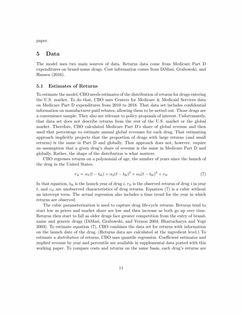
To estimate the model, CBO needs estimates of the distribution of returns for drugs enteringthe U.S. market. To do that, CBO uses Centers for Medicare & Medicaid Services dataon Medicare Part D expenditures from 2010 to 2018. That data set includes confidentialinformation on manufacturer-paid rebates, allowing them to be netted out. Those drugs area convenience sample. They also are relevant to policy proposals of interest. Unfortunately,that data set does not describe returns from the rest of the U.S. market or the globalmarket. Therefore, CBO calculated Medicare Part D’s share of global revenue and thenused that percentage to estimate annual global revenues for each drug. That estimatingapproach implicitly projects that the proportion of drugs with large returns (and smallreturns) is the same in Part D and globally. That approach does not, however, requirean assumption that a given drug’s share of revenue is the same in Medicare Part D andglobally. Rather, the shape of the distribution is what matters.

CBO regresses returns on a polynomial of age, the number of years since the launch ofthe drug in the United States.

rit = α1(t− t0i) + α2(t− t0i)2 + α3(t− t0i)3 + υit (7)

In that equation, t0i is the launch year of drug i, rit is the observed returns of drug i in yeart, and υit are unobserved characteristics of drug returns. Equation (7) is a cubic withoutan intercept term. The actual regression also includes a time trend for the year in whichreturns are observed.

The cubic parameterization is used to capture drug life-cycle returns. Returns tend tostart low as prices and market share are low and then increase as both go up over time.Returns then start to fall as older drugs face greater competition from the entry of brand-name and generic drugs (DiMasi, Grabowski, and Vernon 2004; Bhattacharya and Vogt2003). To estimate equation (7), CBO combines the data set for returns with informationon the launch date of the drug. (Returns data are calculated at the ingredient level.) Toestimate a distribution of returns, CBO uses quantile regression. Coefficient estimates andimplied revenue by year and percentile are available in supplemental data posted with thisworking paper. To compare costs and returns on the same basis, each drug’s returns are

11

discounted back to date of launch. CBO uses a discount rate of 8.6 percent (Damodaran2020).7

Figure 2: Lifetime revenue for Medicare Part D drugs is heavily skewed. Using data from2010 to 2018, CBO finds that some drugs earn less than $10,000 (4 percent), most earnmore than $1 million (81 percent), and only a few earn more than $10 billion (7 percent).

Figure 2 presents the distribution of discounted lifetime global returns associated withsuccessfully getting a drug to market. That distribution is based on the quantile regressionestimates above.

5.2 Estimates of Expenditures

CBO doesn’t have access to any similar database to estimate expenditures associated withbringing a drug through the development process. Therefore, CBO relies on informationreported in DiMasi, Grabowski, and Hansen (2016) from a survey of 10 multinationalfirms of various sizes. The authors selected a sample of about 100 drugs and requestedinformation about their associated expenditures in each stage of development. Those drugsbegan human testing somewhere in the world between 1995 and 2007. Their paper and

7The measured discount rate was substantially lower for the January 2021 release of the data, perhapsbecause of temporary factors related to the coronavirus pandemic.

12

related papers further discuss the survey design. Development expenditures used here donot include expenditures associated with marketing or postmarket studies.

Phase Mean Median SD

I 25.3 17.3 29.6II 58.6 44.8 50.8III 255.4 200.0 153.3

Table 1: Expenditure distributions in millions of dollars for each phase, from DiMasi,Grabowski, and Hansen (2016). SD = standard deviation.

Table 1 shows a skewed distribution of expenditures. In the supplement to their 2016paper, DiMasi, Grabowski, and Hansen present fitted log-normal distributions for expen-ditures and time in phase.

As mentioned, to estimate capitalized expenditures of drug development, CBO needsto know the joint distribution of expenditures and time in development. That informationis not presented in DiMasi, Grabowski, and Hansen (2016). Therefore, CBO calibrates thecorrelation parameter by using various measures of distributions of expenditure and time indevelopment presented in the paper. The calibration exercise gives a correlation coefficientof −0.5. As with other parameters, sensitivity around that value is discussed and testedbelow.

Concern exists that survey results of expenditures presented in DiMasi, Grabowski, andHansen (2016) are not representative of drugs in development. In Adams and Brantner(2006) and (2010), the authors use publicly available data and compare estimates withthose in DiMasi, Hansen, and Grabowski (2003), which used a similar analytic method tothat in DiMasi, Grabowski, and Hansen (2016). Using development times and transitionsfrom Pharmaprojects and R&D expenditure from Securities and Exchange Commissionfilings, Adams and Brantner present results broadly similar to those in DiMasi, Hansen,and Grabowski (2003). CBO doesn’t use the discount rate presented in DiMasi, Grabowski,and Hansen (2016); rather, the agency uses the WACC for pharmaceutical and biotechindustries suggested by Damodaran (2020).8

5.3 Other Observed Distributions

As inputs, the model also uses estimates for success rates of drugs through clinical trials andamount of time spent in each phase. Here CBO uses reported results in DiMasi, Grabowski,and Hansen (2016). Those numbers are from a sample of more than 1,400 drug candidatesinitially tested in humans between 1995 and 2007. Similar results are presented in Wong,

8Data used to calculate the WACC were from the January 2020 update. As with other measures, thesensitivity of the results to that parameter value is discussed more below.

13

Siah, and Lo (2019) for more than 15,000 candidates in development between 2000 and2015.

In addition, CBO sets the probability of entering each phase of development to .1, .2,and .9 for phases I, II, and III, respectively. Those numbers are chosen mostly becausethey lead to feasible results. CBO doesn’t have access to information on which drugsare available to enter a particular phase but are not doing so. Because of concern aboutthose values, this working paper presents information on how much the estimates vary ifthose values change. A survey by DiMasi (2013) asked whether the failure of the drug indevelopment was due to safety, efficacy, or commercial reasons. He found that commercialreasons were less prominent in later phases than in earlier phases, a pattern consistentwith the assumption. In recent work, Khmelnitskaya (2020) found that 8.4 percent of allattrition is strategic.

6 Estimation

The object of interest is the joint distribution of expected returns and expected costs({R∗

i , C∗i }). However, because CBO cannot observe those values, the agency observes val-

ues that have gone through the decisionmaking “filter” described above, {Ri, Ci}. To esti-mate model parameters, CBO solves a simulated generalized method of moments (GMM)problem.

GMM is a generalization of a standard least squares problem. A moment is the termused to describe the average of some set of values raised to a power. The first moment is theaverage of values to the power 1, the second moment is the average of values to the power2, and so on. Consider the problem of finding the average in a sample. In expectation,the difference between the sample value and the average is zero. Alternatively, the averagein the sample is where the first moment is zero. Similarly, the sample variance is wherethe second moment is zero (when the average is zero). Different moments characterizedifferent aspects of the distribution. The problem is that with multiple moments, potentialexists to have multiple estimates of the same parameter. The question thus arises aboutwhich estimate to use or how to average across various estimates. Hansen (1982) presentsproperties of a particular method of weighting across moments, the GMM.

Because CBO can’t observe the underlying joint distribution of expected costs andexpected returns, the agency must simulate it. Firms decide whether to enter simulateddrugs into development. Simulated expected costs and expected returns for drugs that gointo development are then compared with those that are observed.

6.1 Simulated GMM

The estimator works through a choice of the five parameters—{µrk, σrk, µck, σck, and ρrck}—that characterize the distribution of expected returns and costs ({log(R∗

ik), log(C∗ik)}).

Given that choice, the estimator simulates many expected return and expected cost pairs.

14

It then takes those that satisfy the condition that net expected returns are positive (equa-tion (5)) and compares them with the observed moments. CBO uses the first and secondmoments of the distribution of log expected returns, the first and second moments of dis-tribution of log costs, and the probability of entering the phase.

1N

∑Ni=1 log(Rik)−mrk = 0

1N

∑Ni=1(log(Rik)−mrk)2 − s2rk = 0

1N

∑Ni=1 log(Cik)−mck = 0

1N

∑Ni=1(log(Cik)−mck)2 − s2ck = 0

1N

∑Ni=1 1(R∗

ik − C∗ik > 0)− πk = 0

(8)

where mrk is the observed mean of log returns for phase k, srk is the observed standarddeviation of log returns for phase k, and πk is the observed probability of entering phase k.Although CBO observes {mrk, srk,mck, sck}, the agency does not observe πk. That valueis calibrated in the estimates below. Also note that 1() is an indicator function that is 1 ifthe expression inside the function is true and zero otherwise.

The GMM problem does not depend on the phase. However, inputs into the functionwill change with the different phases. In particular, estimates for earlier phases take resultsfrom later phases as given.

Ri(k−1) = max{0, R∗ik − C∗

ik} (9)

Equation (9) states that “observed” returns in the earlier phase are determined by netexpected returns in the latter phase. That distribution is censored at zero because the firmhas the option of not taking the drug candidate into the latter phase of development.

6.2 Parameter Estimates

Table 2 presents parameter estimates and observed moments for the simulated GMM es-timator. Results show that the distribution of expected returns and costs faced by thedecisionmaker and the observed returns and costs in the data. On average, expected coststend be lower. The heavily skewed expected returns are lower in the earlier phases buthigher in phase III. Finally, expected returns and expected costs are positively correlated.

Table 3 presents the mean and standard deviation for parameter estimates after themodel was rerun 500 times with variation in moment estimates and calibrated parameters.Given the bootstrap procedure used, the mean is not necessarily equal to the main param-eter estimates presented in Table 2. The table shows a large amount of parameter variationfor expected returns distribution in phase III. The main results of the policy illustration

15

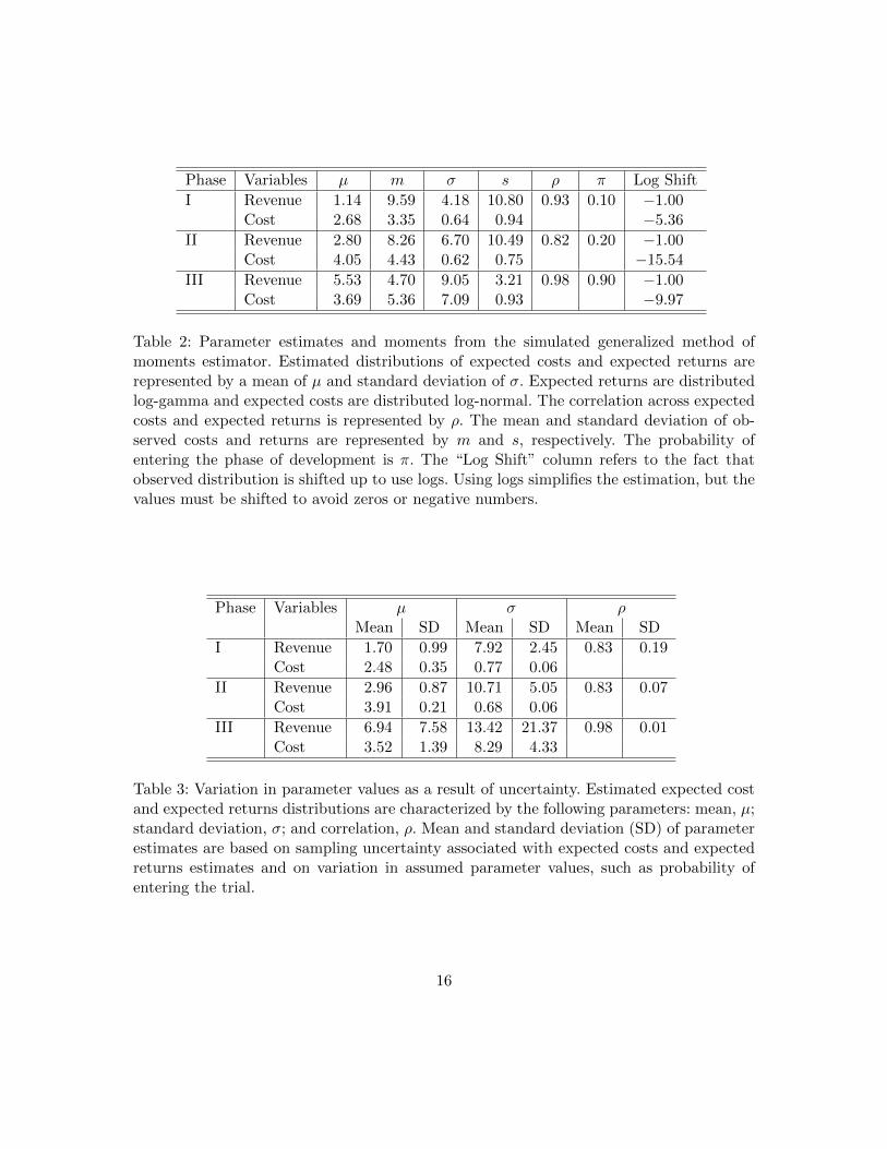
Phase Variables µ m σ s ρ π Log Shift

I Revenue 1.14 9.59 4.18 10.80 0.93 0.10 −1.00Cost 2.68 3.35 0.64 0.94 −5.36

II Revenue 2.80 8.26 6.70 10.49 0.82 0.20 −1.00Cost 4.05 4.43 0.62 0.75 −15.54

III Revenue 5.53 4.70 9.05 3.21 0.98 0.90 −1.00Cost 3.69 5.36 7.09 0.93 −9.97

Table 2: Parameter estimates and moments from the simulated generalized method ofmoments estimator. Estimated distributions of expected costs and expected returns arerepresented by a mean of µ and standard deviation of σ. Expected returns are distributedlog-gamma and expected costs are distributed log-normal. The correlation across expectedcosts and expected returns is represented by ρ. The mean and standard deviation of ob-served costs and returns are represented by m and s, respectively. The probability ofentering the phase of development is π. The “Log Shift” column refers to the fact thatobserved distribution is shifted up to use logs. Using logs simplifies the estimation, but thevalues must be shifted to avoid zeros or negative numbers.

Phase Variables µ σ ρMean SD Mean SD Mean SD

I Revenue 1.70 0.99 7.92 2.45 0.83 0.19Cost 2.48 0.35 0.77 0.06

II Revenue 2.96 0.87 10.71 5.05 0.83 0.07Cost 3.91 0.21 0.68 0.06

III Revenue 6.94 7.58 13.42 21.37 0.98 0.01Cost 3.52 1.39 8.29 4.33

Table 3: Variation in parameter values as a result of uncertainty. Estimated expected costand expected returns distributions are characterized by the following parameters: mean, µ;standard deviation, σ; and correlation, ρ. Mean and standard deviation (SD) of parameterestimates are based on sampling uncertainty associated with expected costs and expectedreturns estimates and on variation in assumed parameter values, such as probability ofentering the trial.

16

presented below are based on estimates presented in Table 2, although variation aroundentry effects is presented in section 8.

As discussed further below, uncertainty over the estimates comes from several sources.One concern is that uncertainty is associated with sampling variation in both the returnsestimates from the Centers for Medicare & Medicaid Services data and the cost and du-ration estimates from DiMasi, Grabowski, and Hansen (2016). A second concern is thatseveral parameter values were set using limited information.

7 Policy Impact: An Illustration

A range of policies could be analyzed. In particular, any policies that significantly affectexpected returns or expected costs for new drugs may lead to changes in the number ofdrugs that get to market.

To illustrate how the model works, CBO considers a policy that significantly reducesexpected returns of drugs in the top 20 percent of expected returns. That is, drugs expectingto land in the top quintile would generate expected returns 15 percent to 25 percentless than without the policy. That is a representative policy that affects expected returnssimilarly to the one proposed in H.R. 3. The policy then required the Secretary of Healthand Human Services to negotiate drug prices and prioritize drugs to areas where the impactwould be greatest. The bill also capped the price at which parties could negotiate. The pricecould not exceed 120 percent of an international price index. CBO estimated that the policywould decrease future global revenue for new drugs by 19 percent (CBO 2019a, 2019b).

In the main analysis, this working paper considers how a policy that reduces expectedreturns for the drug affects new drug development. The appendix considers an additionalimpact of a policy that reduces the cash available to invest in new drug development.

7.1 Impact on Phase III Decisions

CBO assumes that the policy’s impact is increasing over the distribution of expected re-turns. At the top end of the distribution is a 25 percent reduction in expected returns.That reduction falls to 15 percent for a drug expected to be at the 80th percentile andthen to zero reduction in expected returns below the 80th percentile.

Figure 3 illustrates the impact of the policy. Expected returns are not affected for anydrug below the 80th percentile. The figure shows that the policy has a small impact on thenumber of new drugs entering phase III. The policy affects only a few drugs on the marginbetween entering and not entering phase III. Only a few simulated drugs are near the line,and the change in expected returns is not large enough to have many drugs cross that line.CBO estimates that the policy is associated with a 0.6 percent decrease in the number ofdrugs entering phase III—that is the immediate impact. Below, this paper discusses thelonger-term impact of decisions made earlier in the R&D process.

17

Figure 3: The policy slightly reduces the number of drugs entering phase III (a 0.6 percentdecrease). The figure shows the joint distribution of expected returns and costs with (reddots) and without (X marks) the policy. Only drugs above the 40th percentile of expectedreturns are included; for those drugs, the policy leads to a shift down in expected returns(X mark → red dot). Using the log scale, the figure shows a shift in expected returnsfrom $10 billion to $7.5 billion, for example, as the difference between 23.03 and 22.74—adifference of 29 log points. The gray line represents the break-even point. Simulated drugsabove and to the left of the line have expected returns greater than expected costs andwould enter phase III. For a small proportion of drugs, the baseline expected returns placethem above and to the left of the line, but expected returns with the policy in place arebelow and to the right of the line. Those drugs would not enter phase III.

18

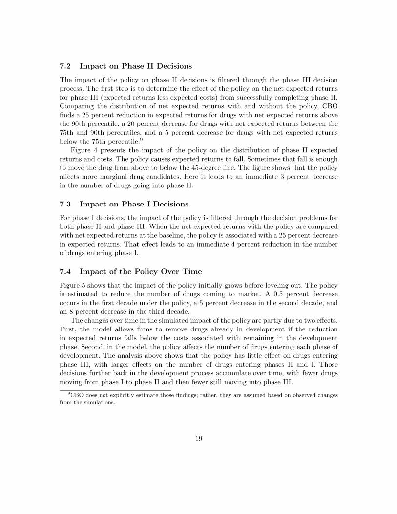
7.2 Impact on Phase II Decisions

The impact of the policy on phase II decisions is filtered through the phase III decisionprocess. The first step is to determine the effect of the policy on the net expected returnsfor phase III (expected returns less expected costs) from successfully completing phase II.Comparing the distribution of net expected returns with and without the policy, CBOfinds a 25 percent reduction in expected returns for drugs with net expected returns abovethe 90th percentile, a 20 percent decrease for drugs with net expected returns between the75th and 90th percentiles, and a 5 percent decrease for drugs with net expected returnsbelow the 75th percentile.9

Figure 4 presents the impact of the policy on the distribution of phase II expectedreturns and costs. The policy causes expected returns to fall. Sometimes that fall is enoughto move the drug from above to below the 45-degree line. The figure shows that the policyaffects more marginal drug candidates. Here it leads to an immediate 3 percent decreasein the number of drugs going into phase II.

7.3 Impact on Phase I Decisions

For phase I decisions, the impact of the policy is filtered through the decision problems forboth phase II and phase III. When the net expected returns with the policy are comparedwith net expected returns at the baseline, the policy is associated with a 25 percent decreasein expected returns. That effect leads to an immediate 4 percent reduction in the numberof drugs entering phase I.

7.4 Impact of the Policy Over Time

Figure 5 shows that the impact of the policy initially grows before leveling out. The policyis estimated to reduce the number of drugs coming to market. A 0.5 percent decreaseoccurs in the first decade under the policy, a 5 percent decrease in the second decade, andan 8 percent decrease in the third decade.

The changes over time in the simulated impact of the policy are partly due to two effects.First, the model allows firms to remove drugs already in development if the reductionin expected returns falls below the costs associated with remaining in the developmentphase. Second, in the model, the policy affects the number of drugs entering each phase ofdevelopment. The analysis above shows that the policy has little effect on drugs enteringphase III, with larger effects on the number of drugs entering phases II and I. Thosedecisions further back in the development process accumulate over time, with fewer drugsmoving from phase I to phase II and then fewer still moving into phase III.

9CBO does not explicitly estimate those findings; rather, they are assumed based on observed changesfrom the simulations.

19

Figure 4: The policy would have a greater effect on a firm’s decision to enter a drug intophase II, decreasing the number of drugs entering phase II by 3 percent. Black X marksrepresent a simulated drug’s expected costs and returns at the baseline, whereas red dotsindicate the same drug’s expected cost and returns with the policy. The figure includes onlydrugs above the 50th percentile of expected returns; for those drugs, the policy leads to ashift down in expected returns (X mark → red dot). Using the log scale, the figure showsa shift in expected returns from $10 billion to $7.5 billion, for example, as the differencebetween 23.03 and 22.74—a difference of 29 log points. A larger proportion of drugs isaffected by the policy than in phase III, causing more drugs to move from above and tothe left of the line to below and to the right of the line.

20

Figure 5: The policy would not affect the number of drugs entering the market in the shortrun but is expected to have long-run implications. The policy is implemented in year zero,but the full difference is not reached until after year 20. To illustrate, the number of newdrugs is initially set at the average for 2015–2019.

8 Uncertainty

The results presented here are uncertain. Uncertainty exists around both the values ofinputs used in the simulation model and the impact of the illustrative policy. Using theillustrative policy, the section shows how uncertainty over the model’s input values andinherent uncertainty in the simulation affect predictions of the policy’s impact on thenumber of new drugs. For example, if the WACC is higher, the policy has a larger effecton the number of new drugs. Conversely, if expenditures in phase III are higher, the policyhas a smaller effect on the number of new drugs.

The distributions shown in Figure 6 account for uncertainty over the exact value ofparameters set by CBO and uncertainty over the exact value of parameters estimatedoutside the simulation model. For input values set by CBO, a uniform distribution of

21

values is used, ranging from a “small” decrease to a “small” increase in the parametervalue. The exact size varies, but for probabilities it is generally 10 percentage points. Forestimates coming from distributions presented in DiMasi, Grabowski, and Hansen (2016), abootstrap procedure is used in which the sample size is the one equal to the survey samplesize for each phase. For estimates of returns, the quantile regressions are bootstrapped.10

Figure 6: The policy’s impact decreases as the drug moves from phase I to phase III.The uncertainty over the policy’s impact is much higher for phase I and phase II thanfor phase III. One reason is that earlier phases use estimates from later phases. That is,estimates for the impact on phase I and II entry incorporate the uncertainty for the impacton phase III entry.

In this paper, CBO estimates that the policy would lead to an immediate decrease inthe percentage of drugs entering each phase of development. Figure 6 presents distributionsfor those estimates. For phase III, the estimated impact of the policy is very small, and the

10A set of parameters estimated in DiMasi, Grabowski, and Hansen (2016) are treated as set outside theestimation procedure used here. Those are the probabilities of completing each phase and the duration fromthe end of the phase to market.

22

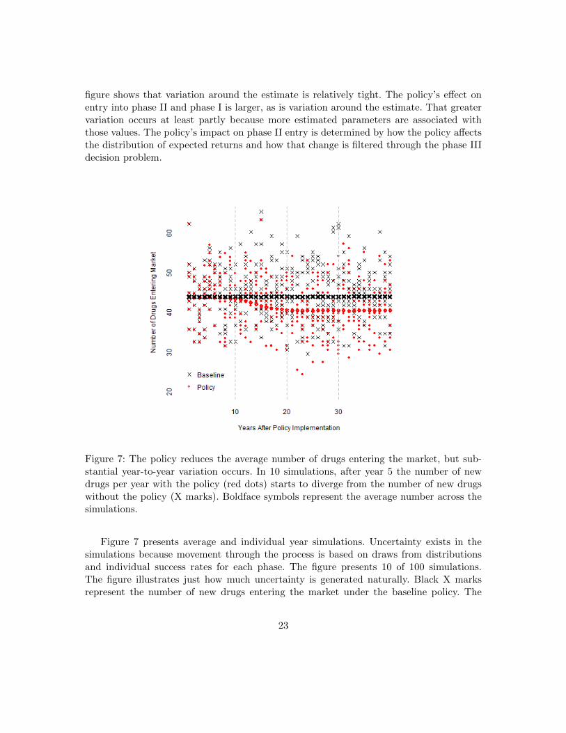
figure shows that variation around the estimate is relatively tight. The policy’s effect onentry into phase II and phase I is larger, as is variation around the estimate. That greatervariation occurs at least partly because more estimated parameters are associated withthose values. The policy’s impact on phase II entry is determined by how the policy affectsthe distribution of expected returns and how that change is filtered through the phase IIIdecision problem.

Figure 7: The policy reduces the average number of drugs entering the market, but sub-stantial year-to-year variation occurs. In 10 simulations, after year 5 the number of newdrugs per year with the policy (red dots) starts to diverge from the number of new drugswithout the policy (X marks). Boldface symbols represent the average number across thesimulations.

Figure 7 presents average and individual year simulations. Uncertainty exists in thesimulations because movement through the process is based on draws from distributionsand individual success rates for each phase. The figure presents 10 of 100 simulations.The figure illustrates just how much uncertainty is generated naturally. Black X marksrepresent the number of new drugs entering the market under the baseline policy. The

23

X marks are spread out in a large cloud, indicating that the simulation model produces alarge amount of variation in the number of drugs entering the market from year to year.Red dots represent the number of new drugs entering the market under the policy. Again,the cloud of red dots indicates a large amount of variation from the simulation. The figureshows that although on average the policy leads to fewer drugs entering the market, forany particular year the same, fewer, or more drugs could enter the market under the policyin comparison with the baseline. Whereas the policy tends to reduce the number of newdrugs entering the market, the natural variation may lead to an increase in the numberof new drugs entering the market in any particular year. In the middle two-thirds of thesimulations (that is, between the 17th and 83rd percentiles), the reduction in the number ofnew drugs entering in the third decade after implementation of the policy ranges between21 and 59. Because of uncertainty about the modeling framework itself, CBO expects thatthe range in which two-thirds of future outcomes would fall is wider than that from thosesimulations alone.

9 Conclusion

This working paper describes a model CBO uses to inform its estimates of how variouspolicies affect development of new drugs. The model considers the firm’s decision at thestart of the various phases of human clinical trials. The firm considers expected cost andexpected returns of entering the phase. The paper considers what happens when a policyis introduced that reduces the top quintile of expected returns by 15 percent to 25 percent.Using the model, CBO estimates that such a policy would reduce the number of drugsentering the market by 0.5 percent in the first decade under the policy. Owing to anaccumulated effect through the phases, CBO estimates the number of drugs entering themarket decreases by 8 percent in the third decade under the policy.

The illustrative policy’s exact implications for the health of families in the United Statesare unclear. CBO has estimated neither which types of drugs may be affected nor how thereduction in the number of new drugs will affect health outcomes. In addition, the policymay lead to lower prices and increased usage for drugs already on the market. CBO hasnot determined the overall effect of the policy on health outcomes.

10 Appendix: Accounting for Reduced Earnings

In the preceding analysis, the Congressional Budget Office assumes that a policy such asthe negotiation policy in H.R. 3 affects pharmaceutical development only through changesto the expected profitability of new investments at a fixed cost of financing. By reducingthe earnings available to pharmaceutical firms to finance new development without tappingexternal sources, the policy conceivably could raise their cost of financing, further affectingdrug development. Large drug companies are profitable enough now to finance R&D almost

24

Figure 8: A small additional reduction occurs in the number of new drugs entering themarket when higher financing costs associated with the policy are taken into account.

entirely by retaining earnings from existing sales of drugs and do not need to tap externalsources.

This section considers a policy that both reduces expected returns by 15 percent to25 percent for the top 20 percent of drugs and reduces revenue to the industry by $900 bil-lion.

One way to capture the possibility of higher financing costs is to calculate the weightedaverage cost of capital (WACC) that determines the discount rate used in this analysis.A policy that reduces revenue by $900 billion significantly affects earnings and thus theequity value of firms in the industry, raising their debt-to-equity ratio. Had the industrybeen at its optimal debt-to-equity ratio before introduction of the policy, CBO expects,firms would have taken measures to adjust the ratio back down toward the previous level.

One such measure would be to finance new projects with a greater proportion of equityrather than debt. Firms also could lower or suspend dividends to pay off some of theirmaturing debt, or issue new equity, but those approaches might be costly. To capture the

25

impact of that change on the firm’s financing strategy, CBO reweights the cost of debt andequity in determining the industry WACC for the projection period. The original valueweights the equity financing costs of 9.4 at 87 percent and the debt financing costs of 4.4at 13 percent. The new weights would be 92.5 percent and 7.5 percent, respectively, wherethose are determined by adding $900 billion to the observed equity financing levels in theindustry. That weight on equity financing may be too large, but the result can be thought ofas an upper bound on the likely effect of alternative financing. That reweighting increasesthe estimated WACC by 20 basis points, from 8.6 to 8.8 percent.

A higher WACC would have two effects. First, it would reduce expected returns fromgetting the drug to market because the initial years on the market generate less revenuethan later years. Second, it would increase the cost of spending money on drug development.Figure 8 shows that accounting for financing costs reduces the number of new drugs enteringthe market by 9 percent in the third decade under the policy, compared with 8 percent inthe main analysis.

11 References Cited

Acemoglu, Daron, and Joshua Linn. 2004. “Market Size in Innovation: Theory and Evi-dence From the Pharmaceutical Industry.” Quarterly Journal of Economics 119(3):1049–1090. https://doi.org/10.1162/0033553041502144.

Adams, Christopher P., and Van V. Brantner. 2006. “Estimating the Cost of New DrugDevelopment: Is It Really $802 Million?” Health Affairs 25(2):420–428. https://doi.org/10.1377/hlthaff.25.2.420.

Adams, Christopher P., and Van V. Brantner. 2010. “Spending on New Drug Develop-ment.” Health Economics 19(2):130–141. https://doi.org/10.1002/hec.1454.

Bhattacharya, Jayanta, and William B. Vogt. 2003. “A Simple Model of PharmaceuticalPrice Dynamics.” Journal of Law and Economics 46(2):599–626. https://doi.org/10.1086/378575.

Blume-Kohout, Margaret E., and Neeraj Sood. 2013. “Market Size and Innovation: Effectsof Medicare Part D on Pharmaceutical Research and Development.” Journal of PublicEconomics 97:327–336. https://doi.org/10.1016/j.jpubeco.2012.10.003.

Congressional Budget Office (CBO). 2019a. “Letter to the Honorable Frank Pallone Jr. Re:Effects of Drug Price Negotiation Stemming From Title 1 of H.R. 3, the Lower Drug CostsNow Act of 2019, on Spending and Revenues Related to Part D of Medicare” (October 11).www.cbo.gov/system/files/2019-10/hr3ltr.pdf (125 KB).

Congressional Budget Office (CBO). 2019b. “Letter to the Honorable Frank Pallone Jr.Re: Budgetary Effects of H.R. 3, the Elijah E. Cummings Lower Drug Costs Now Act”

26

(December 10). www.cbo.gov/system/files/2019-12/hr3_complete.pdf (230 KB).

Damodaran, Aswath. 2020. “Cost of Capital by Sector (U.S.)” (accessed December 8, 2020).http://tinyurl.com/171f0kqm.

Department of State. 2010. “Framework for Promoting Transatlantic Economic Integration,Annex I: Fostering Cooperation and Reducing Regulatory Barriers, B. Sectoral Cooperation—Medicinal Products” (January 24). https://go.usa.gov/xAMHK.

DiMasi, Joseph A., Ronald W. Hansen, and Henry G. Grabowski. 2003. “The Price ofInnovation: New Estimates of Drug Development Costs.” Journal of Heath Economics22(2):151–185. https://doi.org/10.1016/S0167-6296(02)00126-1.

DiMasi, Joseph A., Henry G. Grabowski, and John Vernon. 2004. “R&D Costs and Returnsby Therapeutic Category.” Drug Information Journal 38:211–223. https://doi.org/10.1177/009286150403800301.

DiMasi, Joseph A. 2013. “Causes of Clinical Failures Vary Widely by Therapeutic, Phaseof Study.” Impact Report 15(5). Tufts Center for the Study of Drug Development. https://csdd.tufts.edu/impact-reports.

DiMasi, Joseph A., Henry G. Grabowski, and Ronald W. Hansen. 2016. “Innovation inthe Pharmaceutical Industry: New Estimates of R&D Costs.” Journal of Heath Economics47:20–33. https://doi.org/10.1016/j.jhealeco.2016.01.012.

Dranove, David, Craig Garthwaite, and Manuel I. Hermosilla. 2020. Expected Profits andthe Scientific Novelty of Innovation. Working Paper 20-16 (Northwestern University Insti-tute for Policy Research). http://tinyurl.com/44smzy72.

Dubois, Pierre, Olivier de Mouzon, Fiona Scott-Morton, and Paul Seabright. 2015. “Mar-ket Size and Pharmaceutical Innovation.” RAND Journal of Economics 46(4):844–871.https://doi.org/10.1111/1756-2171.12113.

Food and Drug Administration (FDA). 2019. “Development & Approval Process: Drugs.”https://go.usa.gov/xAMsH.

Hansen, Lars Peter. 1982. “Large Sample Properties of Generalized Method of MomentsEstimators.” Econometrica 50(4):1029–1054. https://doi.org/10.2307/1912775.

Heckman, James, and Bo Honore. 1990. “The Empirical Content of the Roy Model.” Econo-metrica 58(5):1121–1149. https://doi.org/10.2307/2938303.

Heckman, James J., and Edward J. Vytlacil. 2007. “Econometric Evaluation of Social Pro-grams, Part I: Causal Models, Structural Models, and Econometric Policy Evaluation,” inJames J. Heckman and Edward E. Leamer, eds., Handbook of Econometrics, volume 6B(Elsevier, 2007), pp. 4779–4874. https://doi.org/10.1016/S1573-4412(07)06070-9.

27

Khmelnitskaya, Ekaterina. 2020. “Competition and Attrition in Drug Development.” Uni-versity of Virginia. https://tinyurl.com/3o6loqhf.

Wong, Chi Heem, Kien Wei Siah, and Andrew W. Lo. 2019. “Estimation of Clinical TrialSuccess Rates and Related Parameters.” Biostatistics 20(2):273–286. https://doi.org/10.1093/biostatistics/kxx069.

28