Turning Data into Insight Introduction to Data Modules and Dashboards Workshop Guide Field Edition CA11.0.7 | Version 1.4 (Revised 26Sep2017)

© Copyright IBM Corporation, 2017

This guide contains proprietary information which is protected by copyright. No part of this document may be photocopied, reproduced, or translated into another language without a legal license agreement from IBM Corporation.

Business problems are complicated.

Your Analytics Tools Shouldn’t be.

IBM Analytics Software

Author Acknowledgements Contributors: Julie Antry, Vince Babineau, Ben Foulkes, Nic Leduc, Michael Li, Kevin McFaul, Chris McPherson, Andrew Popp, Jason Tavoularis

Notices and Disclaimers

© Copyright IBM Corporation 2017.

The information contained in these materials is provided for informational purposes only, and is provided AS IS without warranty of any kind, express or implied. IBM shall not be responsible for any damages arising out of the use of, or otherwise related to, these materials. Nothing contained in these materials is intended to, nor shall have the effect of, creating any warranties or representations from IBM or its suppliers or licensors, or altering the terms and conditions of the applicable license agreement governing the use of IBM software. References in these materials to IBM products, programs, or services do not imply that they will be available in all countries in which IBM operates. This information is based on current IBM product plans and strategy, which are subject to change by IBM without notice. Product release dates and/or capabilities referenced in these materials may change at any time at IBM’s sole discretion based on market opportunities or other factors, and are not intended to be a commitment to future product or feature availability in any way.

This document is current as of the initial date of publication and may be changed by IBM at any time. Not all offerings are available in every country in which IBM operates.

IBM, the IBM logo and ibm.com are trademarks or registered trademarks of International Business Machines Corporation in the United States, other countries, or both. If these and other IBM trademarked terms are marked on their first occurrence in this information with a trademark symbol (® or ™), these symbols indicate U.S. registered or common law trademarks owned by IBM at the time this information was published. Such trademarks may also be registered or common law trademarks in other countries. A current list of IBM trademarks is available on the Web at “Copyright and trademark information” at ibm.com/legal/copytrade.shtml

Other company, product and service names may be trademarks or service marks of others.

Page 1

Table of Contents INTRODUCTION: WELCOME ................................................................................................................................................ 2 WORKSHOP 1 NAVIGATION............................................................................................................................................... 3

1.1 GETTING STARTED ....................................................................................................................... 3 1.2 NAVIGATING THE COGNOS ANALYTICS USER INTERFACE .................................................................. 5

1.2.1 USER HOME PAGE ......................................................................................................... 5 1.2.2 NAVIGATION PANEL ......................................................................................................... 7 1.2.3 APPLICATION TOOLBAR ................................................................................................... 8

1.3 USING SMART SEARCH ............................................................................................................... 11 1.4 WORKING WITH OBJECT PROPERTIES ........................................................................................... 13

WORKSHOP 2 CREATING A DATA MODULE ................................................................................................................. 17 2.1 CREATING A DATA MODULE WITH INTENT DRIVEN MODELING .......................................................... 18 2.2 ADDING AND REMOVING TABLES FROM A DATA MODULE ................................................................. 22 2.3 HIDING AND REMOVING DATA ITEMS ............................................................................................. 25 2.4 UPLOADING EXTERNAL DATA FILES TO USE IN DATA MODULES ....................................................... 27 2.5 REFINING THE DATA PROPERTIES................................................................................................. 29

2.5.1 SETTING DATA ATTRIBUTES ............................................................................................ 29 2.5.2 CHANGING DATA LABELS ............................................................................................... 30 2.5.3 SETTING DEFAULT SORT ORDER FOR DATA ...................................................................... 31 2.5.4 FILTERING DATA ........................................................................................................... 32

2.6 WORKING WITH JOINS ................................................................................................................. 35 2.7 CREATING CALCULATIONS ........................................................................................................... 45 2.8 CREATING CUSTOM DATA GROUPS .............................................................................................. 47 2.9 CREATING NAVIGATION PATHS ..................................................................................................... 51 2.10 TESTING THE DATA MODULE ........................................................................................................ 54

WORKSHOP 3 DATA DISCOVERY WITH DASHBOARDS .............................................................................................. 56 3.1 WORKING WITH TEMPLATES ......................................................................................................... 57 3.2 ASSEMBLING A DASHBOARD......................................................................................................... 59 3.3 ADDING CALCULATIONS ............................................................................................................... 62 3.4 SELF-SERVICE DATA DISCOVERY ................................................................................................. 64 3.5 USING SORTING AND TOP/BOTTOM ANALYSIS ............................................................................... 70 3.6 NESTING MULTIPLE COLUMNS IN DATA SLOTS ............................................................................... 72 3.7 ADDING TABS TO DASHBOARDS ................................................................................................... 74 3.8 WORKING WITH FILTERS .............................................................................................................. 75 3.9 WORKING WITH VISUALIZATIONS .................................................................................................. 83

IBM Software

Page 2

Introduction: Welcome

Welcome to the IBM Cognos Analytics Workshop!

Cognos Analytics is Modern Self-Service Business Intelligence Platform that provides a sleek and intuitive User Interface. Whether Users are looking for Personal Data Discovery, or to leverage their full enterprise data platform for analysis, IBM Cognos Analytics provides the capabilities to empower everyone in the organization with the insights needed to positively impact decision making.

This workshop designed to give you an opportunity to discover the ease of use of IBM Cognos Analytics V11, IBM’s Modern Business Intelligence solution that enhances the efficiency and capabilities of business users, report authors, and administrators alike.

During the workshop, you will be shown some of the newest capabilities included in IBM Cognos Analytics, and you will be able to try out some of this functionality for yourself.

After this workshop, you will have a sense of the way in which IBM Cognos Analytics empowers business users with self-service access to data blending, modeling and data discovery.

IBM, along with our network of Business Partners, offers a complete set of training courses for Cognos Analytics covering metadata modelling, professional report authoring, administration and more. Further details about the IBM Analytics Platform and Training are available from your IBM Sales and Technical Sales representatives and our network of Business Partners.

In this workshop, you will experience the following capabilities in IBM Cognos Analytics:

● Navigating the User Interface

● Intent Driven Data Modeling

● Data Blending and Refinement

● Uploading External Data Sources

● Self-Service Data Discovery

Today you will be analyzing information regarding profitability of various product lines over a period of time, followed by a more detailed review of disrupting factors in the sales cycle. Your Marketing Department has begun to compile satisfaction survey and social media data to listen to what customers are saying and would like you to add sentiment into the analysis.

Your goal at the end of the lab sessions will be to investigate why sales have declined for a particular product at a certain point in time, identify the factors that have caused the decline and create dashboards to present your findings.

Page 3

Workshop 1 Navigation

The Cognos Analytics User Interface (UI) provides Users with a fully interactive experience to view, interact with and analyze their data. The goal of the new UI and navigation panel is to provide users with a streamlined way to view content and activities pertinent to them quickly and easily. In general, Users typically are focused on accessing the reports they use most frequently (Recent), accessing additional content they have access to (My Content and Team Content), or are interested in discovering new content (Search) that will assist in their analysis.

Workshop Duration: 15-30 min

Audience: All Users

Capabilities: Cognos Analytics User Interface

Prerequisite Workshop(s) Content: None

In this Workshop, you will:

● Navigate the new IBM Cognos Analytics User Interface

● Use Smart Search to find content

1.1 Getting Started

__1. Click on FireFox and launch Cognos to bring up the login page.

IBM Software

Page 4

__2. Use the pull down arrow next to “Select Namespace” to select IBMDemo.

__3. User ID: administrator

__4. Password: IBMDem0s

__5. The NEW User Experience brings you directly into the completely redesigned Cognos Analytics User Interface (UI). All Cognos Analytics Users begin their navigation here.

IBM Cognos Analytics has a modern and sleek User Interface (UI) that provides a graduated User Experience based on the needs of the individual user. This modern purpose- built User Interface provides a highly intuitive User experience which greatly promotes User adoption.

Only IBM provides Analytics tools that provide managed self-service done in a cognitive way. Let’s take a few minutes to familiarize ourselves with the User Interface so we can take IBM

Cognos Analytics for a test drive!!

Page 5

1.2 Navigating the Cognos Analytics User Interface

The goal of the new UI, navigation panel and menu was to provide Users with a streamlined way to view content and activities pertinent to them.

1.2.1 User Home Page

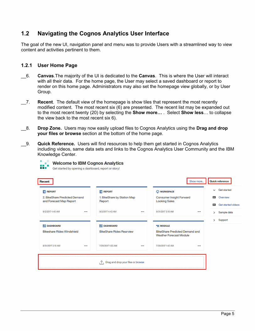
__6. Canvas.The majority of the UI is dedicated to the Canvas. This is where the User will interact with all their data. For the home page, the User may select a saved dashboard or report to render on this home page. Administrators may also set the homepage view globally, or by User Group.

__7. Recent. The default view of the homepage is show tiles that represent the most recently modified content. The most recent six (6) are presented. The recent list may be expanded out to the most recent twenty (20) by selecting the Show more… . Select Show less… to collapse the view back to the most recent six 6).

__8. Drop Zone. Users may now easily upload files to Cognos Analytics using the Drag and drop your files or browse section at the bottom of the home page.

__9. Quick Reference. Users will find resources to help them get started in Cognos Analytics including videos, same data sets and links to the Cognos Analytics User Community and the IBM Knowledge Center.

IBM Software

Page 6

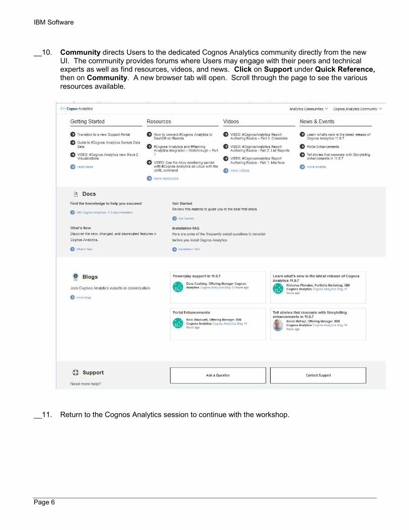
__10. Community directs Users to the dedicated Cognos Analytics community directly from the new UI. The community provides forums where Users may engage with their peers and technical experts as well as find resources, videos, and news. Click on Support under Quick Reference, then on Community. A new browser tab will open. Scroll through the page to see the various resources available.

__11. Return to the Cognos Analytics session to continue with the workshop.

Page 7

1.2.2 Navigation panel

__12. On the left side of the UI is the main Navigation bar. This navigation bar is present on the UI at all times and updates dynamically as the User works with the various capabilities within Cognos Analytics. The upper part of the bar provides Users with direct access to search for their content, and links to content to which they have access. The bottom portion of the bar provides Users with one-click access to capabilities to create and manage new activities such as creating new content, uploading personal data files, accessing notifications and managing the environment (dependent on User permissions).

__13. Home. The Home button appears in the top-left corner of the navigation panel. Users may return to this homepage at any time with the click of this button.

__14. Search. The New Smart Search in Cognos Analytics provides a modernized search engine that uses a smart, intent-driven search algorithm to assist the User. Click on Search to open the search panel. Type “Sales” in the search dialog box. As you type, an auto-fill feature will launch and render search suggestions for related terms. We will work more with this feature in an upcoming exercise. Click outside the Search panel to close it.

__15. My Content. The My Content folder provides the User with direct access to the content they have saved. This is content owned by the User and may only be viewed by the User. You will be saving your work from today’s workshop in this folder. Click on My Content to open the navigation panel to see if there is any User content in your environment. Click outside the My Content panel to close it.

__16. Team Content. The Team Content folder contains all the published enterprise and shared content the user hats permissions to view. Click on Team Content to open the navigation panel. Notice there is a list of folders. We will go deeper into these later in the exercises. Click outside the Team Content panel to close it.

__17. Recent. IBM research shows that Users typically use the same set of content on a regular basis. The Recent button shows the User the most recently used list of content, up to 20 objects (reports, dashboards, data modules, etc.). Objects appear in order based on most recently used. Once an object is viewed, it will move to the top of the list. Click on Recent to see what, if any, are the most recently used objects in your environment. Hover your mouse over the icon to the left of each object to identify the type of object. Click outside the Recent panel to close it.

IBM Software

Page 8

__18. New. The New button is used by Users to create new content. It is intent-driven, meaning that it allows Users to select what type of content they wish to create, and the Cognos Analytics UI will open the associated capabilities in the Work Area. From here, Users may create new Reports, Dashboards, Stories, Data Modules, access Other Companion Applications (legacy studios from previous versions of Cognos) and upload files.

__19. Manage. Users who have been granted departmental administration permissions can manage content and create or modify Users, schedules, data sources and customize the environment.

1.2.3 Application Toolbar

__20. Switcher Menu. The switcher menu in the center of the application toolbar provides a dropdown button that allows Users to easily move between the different objects they have worked with during their current session, without opening additional browser windows. (None will currently show as we have not opened any objects so far, but sample below shows example). The Switcher menu will display the name of the object currently active in the canvas.

__21. More (3 horizontal ellipses). The More button provides the User with options to customize their User Experience. The options presented dynamically update based the type of object open in the canvas. Click outside the More menu to close it.

Page 9

__22. Notifications. Users may subscribe to Cognos Analytics content and receive notifications when that content has been updated and is ready for review. An indicator is provided to provide Users with the number of new notifications. Clicking on the Notifications button will open a listing of all unread notifications.

__23. Personal Menu. The Personal Menu allows Users to change personal preferences for their environment and to manage their subscriptions. Click on the Personal Menu to see the capabilities available. Click outside the Personal Menu to close it.

__24. Help. The Help button allows users to access more information regarding Cognos Analytics.

__a. About provides the User with information on the software release version.

__b. Help provides a link to the IBM Knowledge Center which has technical documentation.

__c. Education portal directs users to the IBM Cognos Analytics learning portal where they will find links to videos to get started, list of new features in each release, tips, resources, training and information on upgrading.

IBM Software

Page 10

__d. Community. This is the same Community Users are directed to on the Quick Reference section. It is placed here also so that Users will still have direct access to the community even if they choose to change their default homepage thereby removing the Quick Reference section.

__25. Coach Marks. Coach Marks are available as indicated by a green button next to the action buttons on either the navigation bar or application toolbar. Coach marks provide a pop-up of User hints and are provided to enhance the User experience by providing information on how to use features.

__a. Your workshop image may not have Coach Marks turned on. To turn on Coach Marks, click on the Personal Menu button on the upper right of the Application toolbar. Select My preferences and click the box next to “Show Hints”. Click outside the pane to close it.

__b. Click the Coach Mark buttons you see on the screen to view hints. Click the “X” button to close the hints. Users may also turn off the coach marks by clicking the “Turn off hints”, or in My preferences and changing the “Show Hints” setting.

Page 11

1.3 Using Smart Search

The New Smart Search in Cognos Analytics provides a modernized search engine that uses a smart, intent-driven search algorithm to assist the User. As you type, an auto-fill feature will launch and render search suggestions for related terms. Searches may also be saved for future use.

__26. Click on “Search” to open the search menu.

__27. Begin to type “Sales” in the Search field. Notice that as the search term is typed, Cognos Analytics provides type-ahead logic and returns search suggestions. Continue typing “Sales Managers” until you see it in the suggestion window.

__28. Select “Sales Managers” to return the search results.

__29. The Smart Search engine returns all objects matching the search term it finds in the report names, descriptions, metadata as well as data saved in outputs. As the results are returned, the icons indicate the type of object. Hover your mouse over the icon to the left of each object name to identify the type of object. Notice that the Search rendered all object types such as reports, active reports, dashboards, data modules, folders, packages, as well as objects created in earlier versions of Cognos such as Workspaces.

IBM Software

Page 12

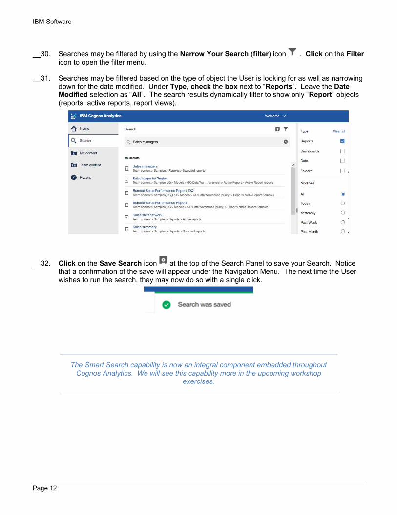
__30. Searches may be filtered by using the Narrow Your Search (filter) icon . Click on the Filter icon to open the filter menu.

__31. Searches may be filtered based on the type of object the User is looking for as well as narrowing down for the date modified. Under Type, check the box next to “Reports”. Leave the Date Modified selection as “All”. The search results dynamically filter to show only “Report” objects (reports, active reports, report views).

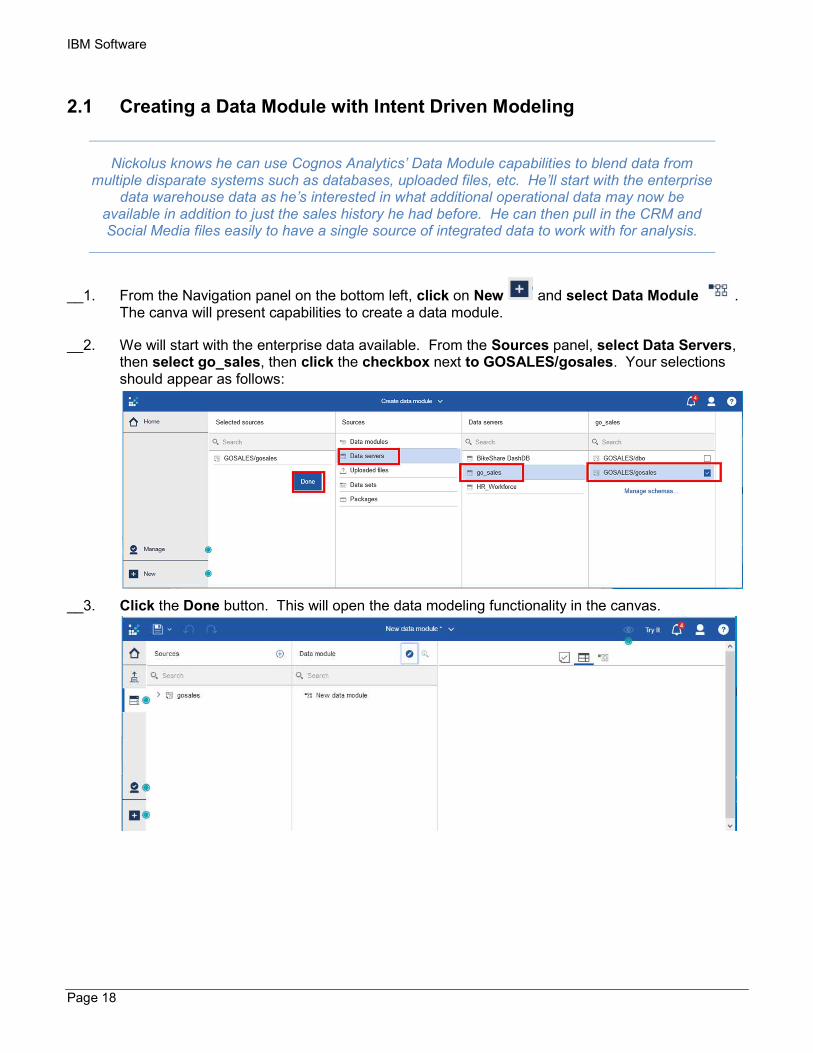
__32. Click on the Save Search icon at the top of the Search Panel to save your Search. Notice that a confirmation of the save will appear under the Navigation Menu. The next time the User wishes to run the search, they may now do so with a single click.

The Smart Search capability is now an integral component embedded throughout Cognos Analytics. We will see this capability more in the upcoming workshop

exercises.

Page 13

1.4 Working with Object Properties

__33. Returning to the Search results, we see a listing of several reports matching the search term of “Sales Managers”. Below each report listed, we also see the folder path containing the report.

__34. Click on the report file path under the report object name to open the folder containing the report. This folder may also contain potentially related content as similar content is typically organized and placed together in folders. This allows the user to easily identify existing reports which may surface additional insights related to their search and analysis.

IBM Software

Page 14

__35. Returning to the search results, we focus in on the first Sales Managers report. Click on the More button (3 horizontal ellipses) to the right of the Sales Managers report name to open Options menu.

TECH TIP: THE REPORT OPTIONS RENDERED WILL BE BASED ON THE USER PERMISSIONS

AND REPORT PROPERTIES. FOR INSTANCE, IN YOUR WORKSHOP ENVIRONMENT, YOU MAY

NOT HAVE BEEN GRANTED PERMISSIONS TO MOVE/COPY/DELETE REPORT CONTENT, THEREFORE YOU MAY NOT SEE THESE AS OPTIONS ON YOUR LIST.

__36. Click on Run As to view the Run options available. Reports may be run as all the common file format outputs Users may need. Users may also opt to have the report render prompts or to run in the background.

Page 15

__37. Click on More again and select “View Versions” . If there are Saved versions of the report, the version date will be listed. (You may not have any saved versions in your Workshop environment).

__38. Click on More once again and select Properties. Click through the properties tabs (General, Report, Schedule and Permissions) to review the various report property settings which may be applied.

IBM Software

Page 16

__39. Click on More and select Share . Cognos Analytics will provide the URL that may be used tp open the report in a web browser so that reports may be shared for use to other Users and through other applications. Using the Share feature will open the report as well as all the Cognos Analytics toolbars around the report. Click Cancel to close the window.

__40. Click on More and select Embed . Cognos Analytics reports may also be embedded into other applications. The difference with using embed is that when posted into an iFrame, the Cognos Analytics toolbars around report are removed. Users may define the size for the report by setting the Width and Height which will then update the URL accordingly. Click Cancel to close the window.

It’s great to have so many options on running reports and personalizing the properties for the User’s personal needs as well as to share and embed. But not all the

information a User needs may be available in existing reports.

Users need to have self-service access for data discovery and ad-hoc reporting. Cognos Analytics makes this access easy and intuitive as well as providing Users

access to external data that may not be available from existing reports.

Page 17

Workshop 2 Creating a data module With Cognos Analytics, Users are not restricted to only using existing enterprise data sources. The data blending and modeling capabilities in Cognos Analytics allows the business user to blend in external data sources without requiring assistance from IT. This does not replace IT, it simply augments the user experience to allow the User to work with personal data sets and analyze that data in conjunction with the enterprise data. Users can import external data from files, on premise data sources and cloud data sources into Cognos Analytics. Multiple data sources may be shaped, blended, cleansed and joined together to create a custom and reusable data module for use in dashboards and reports and may be shared with other users in the organization.

Workshop Duration: 60-90 Minutes

Audience: Line of Business

Capabilities: Data Uploads, Intent-Driven Modeling, Shaping data

In this workshop, you will:

● Create a data module using multiple data source types

● Create joins between data tables

● Shape data using filters, calculations, custom groupings, and navigation groups

● Set data properties for labels, aggregation and type Nickolus has just received the following email from Jennifer:

Nickolus, As you know, we just finalized the acquisition of CAWS, Inc. I know during conversations with our executives, there was some concern over performance of a few of their products and product lines that will become part of this new division here at Great Outdoors. IT has confirmed that CAWS sales data has been pulled into our new enterprise data warehouse alongside our Great Outdoors sales data (called GO Sales). Their CRM system will not be brought in, but they did send over a file with that information for us to review. CAWS also sent a file with some social media data they purchased from a third party. Apparently, their Marketing department was very interested in trying to determine social sentiment and I’d like to see what, if anything, this data might reveal.

Would there be a way for you work your magic on all these sources and somehow merge them together so we can begin to take a holistic look at CAWS? In a perfect world, I would love to be able to easily look at sales history, targets, product performance, social sentiment, CRM data, etc. without having to go through all this data independently. Thanks, Jennifer

IBM Software

Page 18

2.1 Creating a Data Module with Intent Driven Modeling

Nickolus knows he can use Cognos Analytics’ Data Module capabilities to blend data from multiple disparate systems such as databases, uploaded files, etc. He’ll start with the enterprise

data warehouse data as he’s interested in what additional operational data may now be available in addition to just the sales history he had before. He can then pull in the CRM and Social Media files easily to have a single source of integrated data to work with for analysis.

__1. From the Navigation panel on the bottom left, click on New and select Data Module . The canva will present capabilities to create a data module.

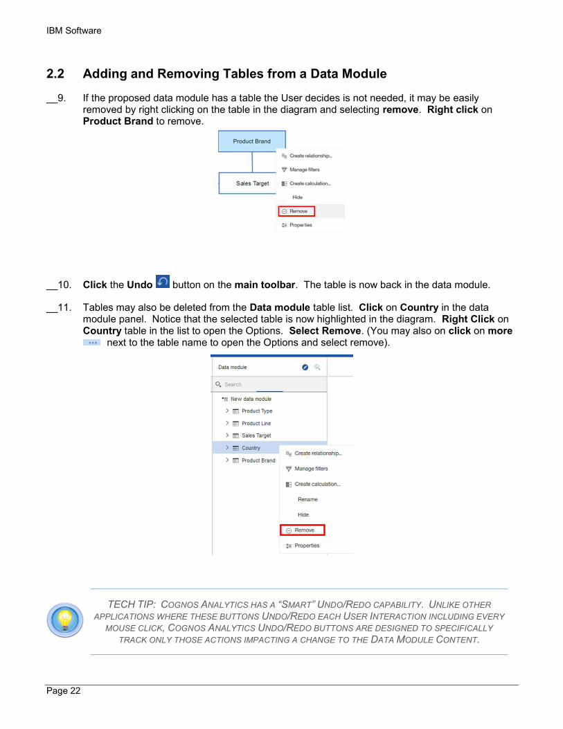
__2. We will start with the enterprise data available. From the Sources panel, select Data Servers, then select go_sales, then click the checkbox next to GOSALES/gosales. Your selections should appear as follows:

__3. Click the Done button. This will open the data modeling functionality in the canvas.

Page 19

As a User, you will be able to indicate your “intent” in creating a data module. Once a data source is selected, Users can enter their desired search terms. Cognos Analytics Intent-driven modeling proposes tables to include in the data module, based on matches between the terms

the User supplies and metadata in the underlying sources. It analyzes the data source selected and will make recommendations on which table(s) to begin with to create the User’s custom

data module. Cognos analytics will then identify a starting point for a data module by suggesting related content to be used. Since Nickolus is interested in product information for

product types and revenue targets, he can enter related terms into his search and Cognos Analytics will identify suggested data sources for his analysis.

__4. Click on the Intent button in the Data Module panel to launch the intent driven modeling panel.

__5. In the intent panel, type “product type target” and click GO. Cognos Analytics will analyze all the tables in the selected data source, and renders proposals for the data tables that contain related content.

IBM Software

Page 20

__6. Click to add the suggested tables to the data module. The canvas will open the

data Grid view. Click on the Sales Target table to open a preview of the data in the grid.

__7. Click on the diagram button. A diagram will appear of the tables selected.

TECH TIP: YOU MAY CLICK ON EACH TABLE AND MOVE IT AROUND THE SCREEN TO MODIFY

THE DISPLAY TO YOUR PREFERENCE. TO MOVE THE ENTIRE DIAGRAM AT ONCE, YOU MAY

CLICK IN THE WHITESPACE AND MOVE WHILE HOLDING DOWN THE LEFT MOUSE BUTTON. YOU MAY ALSO ZOOM IN/OUT ON THE DIAGRAM USING THE SCROLL ON YOUR MOUSE.

Page 21

__8. Relationships between tables have been determined by scanning data and column information from the data. These relationships are indicated by the lines shown connecting the tables. The relationship indicates how the files are joined to one another based on a common data item (key). Click on the relationship lines to see the detail of the join type. Click anywhere to close.

TECH TIP: COGNOS ANALYTICS WILL DETECT AND UTILIZE THE TABLE RELATIONSHIPS

WHICH ARE ALREADY DEFINED IN THE ENTERPRISE DATA WAREHOUSE (MAINTAINING

REFERENTIAL INTEGRITY). LATER IN THE WORKSHOP, WE WILL SHOW HOW USERS CAN

DEFINE AND/OR REFINE JOINS.

IBM Software

Page 22

2.2 Adding and Removing Tables from a Data Module

__9. If the proposed data module has a table the User decides is not needed, it may be easily removed by right clicking on the table in the diagram and selecting remove. Right click on Product Brand to remove.

__10. Click the Undo button on the main toolbar. The table is now back in the data module.

__11. Tables may also be deleted from the Data module table list. Click on Country in the data module panel. Notice that the selected table is now highlighted in the diagram. Right Click on Country table in the list to open the Options. Select Remove. (You may also on click on more

next to the table name to open the Options and select remove).

TECH TIP: COGNOS ANALYTICS HAS A “SMART” UNDO/REDO CAPABILITY. UNLIKE OTHER

APPLICATIONS WHERE THESE BUTTONS UNDO/REDO EACH USER INTERACTION INCLUDING EVERY

MOUSE CLICK, COGNOS ANALYTICS UNDO/REDO BUTTONS ARE DESIGNED TO SPECIFICALLY

TRACK ONLY THOSE ACTIONS IMPACTING A CHANGE TO THE DATA MODULE CONTENT.

Page 23

__12. Users can add additional tables to the proposed data modules manually. In the Sources panel, click on the arrow next to GOSALES to view all available tables. Scroll through the list to see all available data tables from the new enterprise data warehouse.

While scrolling through the data tables, Nickolus notices that there is a lot more information available. To expand out his analysis, he would like to bring more product

master tables as well as some sales order information as a starting point.

__13. To easily narrow down this list, we can search for the related tables using the Search capability. Click in the Search field in the Sources panel and Type “Product”. A list of tables and data items related to the search term are rendered.

__14. Select the Product table and drag and drop it in the Data module panel. Repeat to add in the Product Name Lookup table. Feel free to rearrange tables in your diagram.

__15. These tables are now added to the data module panel and shown in the diagram. Notice that the new tables already have join relationships to the tables. Cognos Analytics was able to analyze the tables and identify join relationships between them.

TECH TIP: EXPERT DATA MODELERS MAY HAVE NOTICED THAT THE PRODUCT BRAND TABLE IS

JOINED TO BOTH THE PRODUCT AND SALES TARGET TABLES. TO FOLLOW BEST PRACTICES, WE

WILL REFINE THE JOIN RELATIONSHIPS LATER IN THIS WORKSHOP.

IBM Software

Page 24

__16. Now let’s bring in Order Data into the module. Type “Order” in the Find field. Control + Click on Order Details and Order Header to multi-select. Drag and drop them in Data Module Panel. Arrange tables in diagram. The data module panel and diagram appear as follows:

__17. The last data we will bring into the data module is a Time Dimension so that we can have flexibility to use alternative date types in our data, such as weekday names and month names. Type “Time” in the Find field. Select the Time Dimension table and drag and drop it in the Data Module panel.

Notice for Time dimension, a join relationship was not identified by Cognos Analytics. There are multiple “Time” dimensions in the data so Cognos Analytics will err on the

side of caution and allow the User to define how the Time Dimension should be joined into the data. will work more with join relationships later in this workshop.

__18. Click on the down arrow next to the save icon on the main toolbar. Click Save As. Navigate to My Content. Save it as “[Lastname] CAWS Data Module.

Page 25

2.3 Hiding and Removing Data Items

__19. Click on the Source View button in navigation panel to collapse the Sources panel.

__20. Click on the arrow next to the Product Type table to expand and view the data items in the table. Notice that the table contains many data items, some of which may not be needed for analysis. In this case, the data items include translations of Product Type into multiple languages. For our analysis, we only need the English (En) versions and can hide the others.

__21. Right Click on “Product Type Ar” to open the options. Select “Hide”. The Product Type Ar data item is now greyed out indicating it is hidden. When using this data module, Users will not see data items hidden from view when using the data module for analysis. If the data item is needed later, it can be changed from “hide” to “show” using the same options panel.

__22. Using the shift or control key, you can multi-select data items and perform the action for all selected items simultaneously. Hide the remaining Product Type language translation data items, leaving only the first three in the list active:

IBM Software

Page 26

__23. Click the arrow next to Product Type to collapse the data item list.

__24. Click on the arrow next to the Product Brand table to expand. Hide all translations other than “Product Brand En”.

__25. Click on the arrow next to the Product Line table to expand the data item for the table. Again, we see that all language translations are available, yet we do not need them for our analysis. This time, we will remove them from the data module.

__26. Right Click on “Product Line Ar” to open the options. Select “Remove”. The data item has now been permanently removed from the list and is no longer available. Remove all remaining Product Line language translation data items, leaving only the first two in the list.

__27. Click on the arrow next to the Time dimension table to expand. Hide all data fields except “Day Date”, “Current Year”, “Day of Week”, Month En” and “Weekday En. as shown below:

__28. If you accidently hide a column, you may use the Undo Button from the toolbar or right click again and select Show

TECH TIP: IT IS A BEST PRACTICE TO HIDE DATA ITEMS RATHER THAN REMOVING AS THIS ALLOWS THE

USER TO EXPOSE THE DATA ITEM AT A LATER TIME IF NEEDED. SOME DATA ITEMS IN TABLES MAY NEVER

BE NEEDED BY THE END USER FOR ANALYSIS, SUCH AS KEYS AND IDS, AND COULD BE REMOVED

PERMANENTLY IF THEY ARE NOT NEEDED AS KEYS TO JOIN TO OTHER FILES OR FOR SORTING DATA.

__29. Save the Data Module.

Page 27

2.4 Uploading External Data Files to use in Data Modules

Nickolus has been able to easily model data from his data warehouse for use in his analysis. However, he also needs to be able to work with the two data files Jennifer sent. Cognos

Analytics allows Users to upload external data files quickly and easily on-demand while working on the data module.

The CRM file contains customer satisfaction data and sales opportunity data from the CAWS CRM system that is not available through the enterprise data warehouse. The Social Media file contains information regarding customer sentiment and includes additional information such as ages, location, etc. By bringing in these files into a single data module, Nickolus can perform analysis on this data alongside his enterprise data and build reports and dashboards all off a

single, integrated data set.

__30. We can easily upload the new CRM and Social Media files on the fly while we build our data

module. From the navigation bar on the left, select New , then Upload Files .

__31. Navigate to where you have saved the file for this workshop entitled “CAWS CRM Data.xls” and select Open.

__32. Status bars will appear as the file uploads into Cognos Analytics.

__33. Once the upload is complete, the preview will render. From here, you may select which columns will be visible by using the checkboxes on the left panel. Use the scroll bar at the bottom of the screen to navigate through the preview of the file. We will use all the columns so we will leave them all selected (the default). Click OK.

IBM Software

Page 28

__34. Repeat these steps to upload the file entitled “CAWS Social Media Data.xls”.

__35. We may now bring in these data files and add them to our data module. From the navigation

panel, click on the Sources button to open the Sources panel. Click on the Add Sources button next to Selected Sources then select Uploaded Files.

__36. To easily find the uploaded files, enter “CAWS” in the Search field and click the checkboxes next to CAWS CRM Data.xls and CAWS Social Media.xls. As each file is selected, it is added to the Sources Panel. Click DONE.

The ability for Business Users to leverage their personal/external data for discovery dramatically broadens the landscape of Users who can make new data available for analysis. Users may upload an external data file and immediately blend it with enterprise data, begin

self-service data discovery, ad hoc analysis and building dashboards.

__37. Drag each file to the Data Module panel. Notice that they have now been added to the diagram, however, they do not yet have a join relationship defined to join the other tables. We will be able to define how these tables are to be joined to the existing data module.

__38. Click on the Source View button in navigation panel to collapse the Sources panel.

Joins are based on the common information between files. Cognos Analytics has detected the relationships between the enterprise data warehouse tables and created joins for them as illustrated by the lines connecting the tables. Nickolus can now go in and refine those joins and define how to join in the two external data files to create a

single data set for his analysis.

Page 29

2.5 Refining the Data Properties

2.5.1 Setting data attributes

We’ve now had the opportunity to compile a custom data module specific to our needs. It contains our enterprise data as well as external data files from CRM and Social Media. As we uploaded our data files, Cognos Analytics analyzed the files and assigned each column a data type based on the

type of data contained in the fields. For fields that have numeric data, Cognos Analytics assigns them as a numeric data type and defaults the behavior to be summed as the data is rolled up.

However, in some cases we wish to change these properties. For instance, in columns that contain data such as “Order Number” or “Age”, we do not want these treated as numbers that will sum in a

column, rather these are attributes that just happen to be represented as numbers. Additionally, we may not want some numbers summed as the sum would be erroneous, such as summing on Unit

Price or Satisfaction score; these provide more value if they are averaged as they roll up in reporting.

__39. Expand the CAWS CRM Data.Xls. Right click on Satisfaction and select Properties. Click on the down arrow next to Aggregate. Note the various methods of aggregation available. Set Aggregate behavior to Average. Set the Usage to Measure.

__40. With the Properties window still open, expand CAWS Social Media Data.Xls. Right click on Age. Set the Usage to Attribute and set Aggregate behavior to Average.

__41. From CAWS Social Media.xlsx, click on Location. In the properties window, click on the down arrow next to Represents. Select Geographic Location. For the next pull down you can see the various Geospatial identifiers. Select Country.

__42. Data Items set to Geographic Location will be indicated by a location icon next to them.

__43. Save the Data Module.

TECH TIP: IDENTIFYING GEOSPATIAL FIELDS AS “GEOGRAPHIC LOCATION” WILL ENABLE

COGNOS TO RECOGNIZE THESE AS GEOSPATIAL DATA TO AUTO GENERATE MAPPING

VISUALIZATIONS. THESE FIELD SETTINGS ARE THE FOUNDATION USED TO LEVERAGE THE

EXTENSIVE GEOSPATIAL ANALYSIS CAPABILITIES OF MAPBOX®.

IBM Software

Page 30

2.5.2 Changing data labels

Many times, operational systems have labels that do not reflect the same nomenclature used in the business by Users. Since the “En” designator is a system identifier for language, removing it makes it easier for Users who are consuming the data to understand the data they are viewing.

It’s a best practice to expose data to the End-Users using their common business language.

__44. From Time Dimension table click on Current Year. Click in the Label field and change the name from “Current Year” to “Year”.

__45. Scroll down the properties window to Represents. Notice that Year is defined to Represent a Time/Year dimension.

__46. With this definition, these items will allow Users to be automatically presented with a calendar style picklists as prompts in dashboards. Data items set to Time will be indicated by a clock icon next to them

__47. Change the data Labels on the Time Dimension data items as follows:

__a. Select “Day Date” and change the Label to “Date”

__b. Select “Weekday En” and change the Label to Weekday”.

__c. Select “Month En” and change the Label to “Month”.

__48. Save the Data Module.

Page 31

2.5.3 Setting default sort order for data

Data may not always be stored so that when exposed, it is presented in the desired sort order. For instance, a customer table may sort records in the order that each customer record was

created. However, for Analysis, it may be more useful to expose this data to Users in alphabetical order by customer name. Cognos Analytics allows Users to easily select how data will be sorted and exposed to Users. Sort order may be selected based on any data item present in the table,

regardless of if a data item was hidden from view (as we did earlier in the workshop).

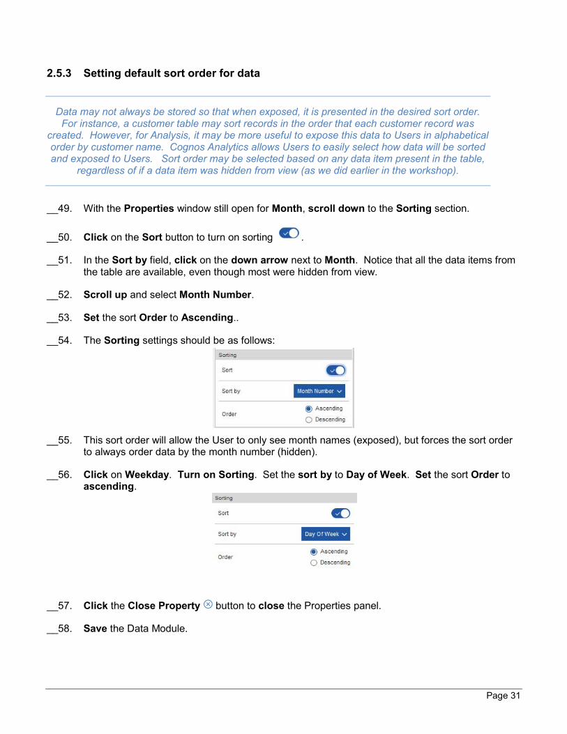
__49. With the Properties window still open for Month, scroll down to the Sorting section.

__50. Click on the Sort button to turn on sorting .

__51. In the Sort by field, click on the down arrow next to Month. Notice that all the data items from the table are available, even though most were hidden from view.

__52. Scroll up and select Month Number.

__53. Set the sort Order to Ascending..

__54. The Sorting settings should be as follows:

__55. This sort order will allow the User to only see month names (exposed), but forces the sort order to always order data by the month number (hidden).

__56. Click on Weekday. Turn on Sorting. Set the sort by to Day of Week. Set the sort Order to ascending.

__57. Click the Close Property button to close the Properties panel.

__58. Save the Data Module.

IBM Software

Page 32

2.5.4 Filtering Data

Data may exist that is not needed for End-User analysis. Cognos Analytics allows Users to place filters to specify the conditions that rows must meet to be retrieved from the table. Filters

may be placed at the table level or the column level.

__59. From Time Dimension, right click on Month to open the options. Select Filter .

__60. The filter window opens and shows a picklist for values. Notice that the in addition to the actual months, there is a data item -called “Opening Balance” (Month Number 0). If we only wanted to see the Opening Balances, we could select the checkbox. Click on the checkbox to select Opening balance.

__61. Items left unchecked will be filtered out of the data. Since we want to filter out only Opening Balance, we can easily reverse the checkboxes by clicking on Invert. Click on Invert. Scroll down to verify that all months are checked, leaving only Opening Balance unchecked.

Page 33

__62. In addition to selecting specific data items to filter, Cognos Analytics allows Users to set filter conditions. Click on Add a filter condition. A dialog box opens allowing the User to set their conditions using common conditions. Click on the down arrow next to Contains and scroll down the list to see the filter conditions available.

__63. We will not set any additional filter conditions. Click on the X to close the filter condition dialog box. Click on OK on the filter to apply it.

__64. A Filter icon has now been added next to Month to indicate a filter is currently applied.

__65. In the data diagram, we also see a Filter icon on the Time Dimension table.

__66. Expand the Product Name Lookup table and click on Product Name.

__67. Click on the Grid icon to change from the diagram view to the data grid view. Notice that this table contains language translations in rows.

IBM Software

Page 34

__68. Since we will only need the rows/records in English (where Product Language=EN), we can filter out all rows for the other languages. Right click on Product Language column header and select Filter.

__69. Click the checkbox next to “EN” and click OK. Now that the filter is applied, the data grid updates and shows that only the rows with the English names render.

__70. Click on the Diagram button to return to the data diagram. A filter icon should now appear on the Product Name Lookup table.

__71. For data items that are integers, Cognos Analytics provides the option of either selecting individual items, or setting a range of values. Expand CAWS Social Media Data.xls. Right click on Age and select Filter. Click on the radial button next to Range. The User may either type in the range values, or use the convenient slider bar to set the range. For instance, if we only wanted to look at data for the age range of working adults, we could use the slider to set the range from 18-65. This would filter out Minors, Seniors, and Baby Boomers at retirement age. Such a range would appear as follows:

__72. We do not want to set this additional filter, so click Cancel.

__73. Verify that no filter was set by looking at Age in the data module panel (no filter icon).

__74. Save the Data Module.

Page 35

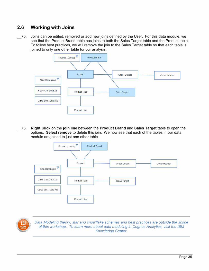
2.6 Working with Joins

__75. Joins can be edited, removed or add new joins defined by the User. For this data module, we see that the Product Brand table has joins to both the Sales Target table and the Product table. To follow best practices, we will remove the join to the Sales Target table so that each table is joined to only one other table for our analysis.

__76. Right Click on the join line between the Product Brand and Sales Target table to open the options. Select remove to delete this join. We now see that each of the tables in our data module are joined to just one other table.

Data Modeling theory, star and snowflake schemas and best practices are outside the scope of this workshop. To learn more about data modeling in Cognos Analytics, visit the IBM

Knowledge Center.

IBM Software

Page 36

__77. Let’s take a deeper look at the relationship joins. Right Click on the join line between the Product and Product Name Lookup table to open the options. Select Edit relationship. The Edit Relationship window appears showing the setup of the join relationship.

The window is neatly organized to step the User through the join definition. The window shows each table in the join and columns/fields available for the join. Below, is a preview of the data once the join has been set. The common column (join key) between the two

files is highlighted, and the preview window allows the user to now scroll through the preview to see how the data now appears as a joined table with all rows and columns.

__78. The Join settings in the lower left corner show the rules (logic) setup for the join behavior. Click on the Join settings to open the join definitions.

Page 37

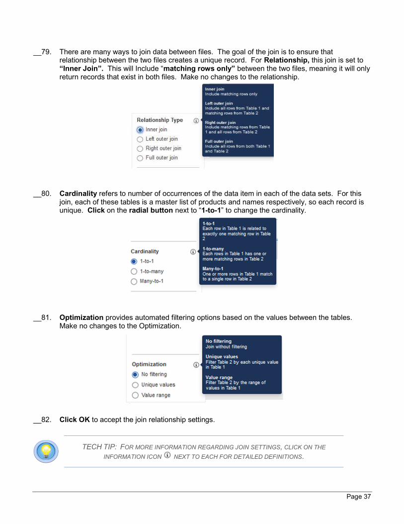
__79. There are many ways to join data between files. The goal of the join is to ensure that relationship between the two files creates a unique record. For Relationship, this join is set to “Inner Join”. This will Include “matching rows only” between the two files, meaning it will only return records that exist in both files. Make no changes to the relationship.

__80. Cardinality refers to number of occurrences of the data item in each of the data sets. For this join, each of these tables is a master list of products and names respectively, so each record is unique. Click on the radial button next to “1-to-1” to change the cardinality.

__81. Optimization provides automated filtering options based on the values between the tables. Make no changes to the Optimization.

__82. Click OK to accept the join relationship settings.

TECH TIP: FOR MORE INFORMATION REGARDING JOIN SETTINGS, CLICK ON THE

INFORMATION ICON NEXT TO EACH FOR DETAILED DEFINITIONS.

IBM Software

Page 38

__83. The CRM file contains Product Type so we would like to join that to the Product Type table. In the diagram, control click on the CAWS CRM Data.xls and then the Product Type table. Right click to open the options and select Create Relationship .

__84. The Create relationship window appears. At the top of the window, it shows the selections made for setting up the join relationship. For the instructions in this exercise, we are working with the Product Type table on the left and the CAWS CRM Data on the right. Use the toggle button to switch left and right tables to get your tables in this order.

TECH TIP: NOTICE THAT FOR THE PRODUCT TYPE TABLE, THE DATA ITEMS WE HAD HIDDEN

(SHOWN IN GREY) ARE STILL AVAILABLE TO USE FOR JOINS. HAD THEY BEEN REMOVED, WE

WOULD NOT BE ABLE TO VIEW THEM OR USE THEM AS A KEY FOR JOINS.

__85. Below, the data viewer shows the data fields from each table. You may use the scrolling tools at the bottom to view all columns available in each table.

Page 39

__86. From the data viewer, we can easily see that the common data between the files is the Product Type. In the picklists, use the down arrows to Select an Item. Select “Product Type” field on the CAWS CRM Data.xls table and select the “Product Type En” field for the Product Type table. A preview of the selected column will show next to each of the table lists so you may easily verify your selection.

__87. Click the Match button to update the viewer to show the joined tables.

__88. Click Refresh to see a preview of the joined data. We now see that the tables have been joined based on the common Product Type. The Matched columns indicator the number of relationship joins defined for these two tables.

TECH TIP: IF MULTIPLE JOINS ARE NEEDED TO CREATE A UNIQUE RECORD, THE USER MAY

ADD JOINS USING REPEATING THE PROCESS ABOVE OF SELECTING THE DATA ITEMS TO JOIN

ON AND SELECTING MATCH TO COMPLETE THE JOIN.

IBM Software

Page 40

__89. Click on the join settings next to the icon on the lower left, below the preview panel to open the join settings options.

__90. For Relationship type, select “Inner Join”. This will Include “matching rows only” between the two files, meaning it will only return records that exist in both files.

__91. In Product Type, each appears only once in the table as it is simply a table of attributes so each record is unique. This represents a “one” type of cardinality. In CAWS CRM Data Xls we have hundreds of records so there are multiple occurrences of each product type. This represents a “many” type of cardinality. So the relationship between these two tables is “one to many”. For Cardinality, select “1-to-many”.

__92. Make no changes to Optimization.

Page 41

__93. Your relationship joins and settings should look like this:

__94. Click OK to accept the relationship definition and return to the diagram.

__95. Notice there is now a line indicating the relationship join between the data module’s table Product Type and the uploaded file CAWS CRM Data Xls.

IBM Software

Page 42

__96. Now, join in the Social Media data file. In the diagram, control click on the CAWS Social Media Data.xls and then the Product table. Right click to open the options and select Create Relationship.

__97. With the Product table on the left and CAWS Social Media Data on the right, set the relationship settings as follows:

__a. Create a join relationship between Product and CAWS Social Media Data.Xls on Product number.

__b. Set Relationship type to “Inner Join”.

__c. Set Cardinality to “1-to-many”.

__d. Make no changes to Optimization.

__98. Once your join appears as below, click OK to return to the diagram.

Page 43

__99. Finally, we’ll join in the Time Dimension table. In the diagram, control click on Order Details then Time Dimension and right click to Create a Relationship.

__100. With the Time Dimension table on the left and Order Details table on the right, set the relationship settings as follows

__a. Create a join relationship using the Time Dimension “Day Date” and the Order Details “Ship Date”

__b. Set Relationship type to “Inner Join”.

__c. Set Cardinality to “1-to-many”.

__d. Make no changes to Optimization

__101. Once your join relationship appears as below, click OK to return to the diagram.

__102. Feel free to move your tables around in the diagram if needed.

IBM Software

Page 44

__103. To view the Cardinality of all the join relationships, click on the Change view button on the upper left of the main toolbar. Select the checkbox next to Cardinality.

__104. Users may use this to validate the data module created has the correct relationships established. The data module may now be visually represented as follows, where “N” represents a “many” relationship. (Feel free to move your tables around in the diagram if needed).

__105. Save the data module.

In just a few minutes, Nickolus has created a data module that has incorporated his new data from his enterprise warehouse and multiple external files into a single data set. But he’s not done yet! He knows he can make it even more robust by adding

calculated measures, custom groups and navigation groups for his analysis.

Page 45

2.7 Creating Calculations

Nickolus noticed that the Order Details table has data for both Quantity and Prices, but it would be helpful to have Revenue and Planned Revenue calculated so it is available

for analysis. By adding these calculations to the data module, they are reusable anywhere in the analysis. Users will not need to rebuild the calculations each time they need them in their dashboards, reports, etc., they simply use the calculated measures.

Create once, Use Anywhere!

__106. In the Data Module panel click on the arrow next to Order Details to expand view to data items. Control click on Quantity and Unit Sales Price. Right click and select “Create Calculation” .

__107. When the Create calculation window pops up, change the Column Name of the calculation to “Revenue”.

__108. Cognos Analytics allows us to easily create the simple calculation of Quantity multiplied by Unit Price, by using the down arrow to select the multiplication operator “X”. The calculation setup should appear as follows:

IBM Software

Page 46

__109. If we want to view the calculation detail or create a custom calculation, we can use the Calculation editor. Click on Use calculation editor to open the Calculation editor window. The current calculation is shown in the Expression window. Here, Users can build their own custom/complex calculations and validate the calculations. For this exercise, we will keep the current calculation.

We will show examples of custom/complex calculations later in this workshop. To learn more

about using the expression editor for custom calculations, click the Help icon in the upper left of the Calculation editor to open the IBM Knowledge Center.

__110. Click OK. The new calculated measure is now added to the Order Details table as a new measure. The new Revenue measure may now be used in our analysis without having to build it each time, and will automatically recalculate to show the average when summarized.

__111. Create another Calculation called “Planned Revenue” by multiplying the Quantity and Unit Price measures.

__112. You will now see your two new calculations as measures added to Order Details.

__113. Save the Data module.

Page 47

2.8 Creating Custom Data Groups

Often, Users need to organize data into groups for analysis, sometimes referred to as “binning” or “buckets”. In looking at the Social Media data items, Nickolus sees it contains some demographic information including the age of the author. This will provide him with

great insight on customers. However, analyzing sentiment on each individual age may not provide much insight. For instance, there may not be a great deal of difference between the sentiment of a 22-year-old versus a 23-year-old. Rather, he would be more interested in the

sentiment of Millennials vs. Baby Boomers. Therefore, he will create custom groupings to “bin/bucket” the individual ages into age groups.

__114. Use the arrow to the left of CAWS Social Media Data Xls to expand. Right Click on Age and

select Create data group .

__115. From the Created data group window, we will keep the default Group column name of Age group”. For Number of groups, use the arrows to set to 5. Since Age is a numeric value, an equal distribution of age ranges will be calculated. However, we would like to override the equal distribution to manually define our age groups. Using the arrows, change the Group Names and Range values as follows:

IBM Software

Page 48

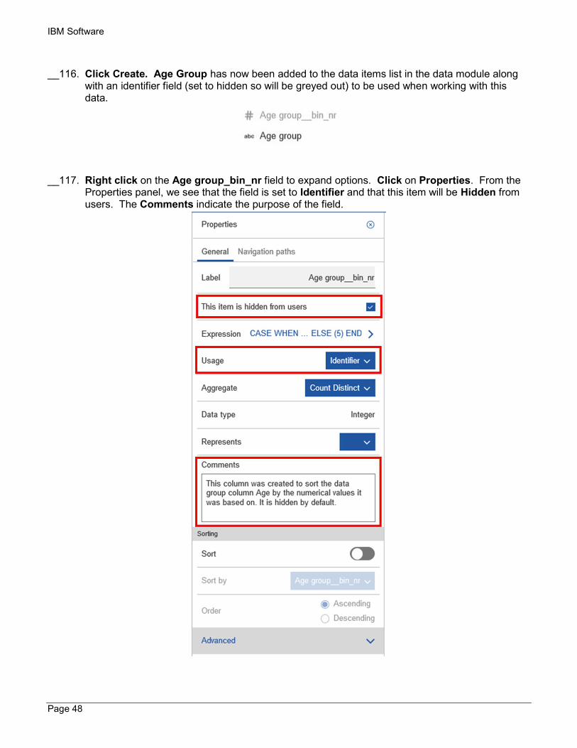
__116. Click Create. Age Group has now been added to the data items list in the data module along with an identifier field (set to hidden so will be greyed out) to be used when working with this data.

__117. Right click on the Age group_bin_nr field to expand options. Click on Properties. From the Properties panel, we see that the field is set to Identifier and that this item will be Hidden from users. The Comments indicate the purpose of the field.

Page 49

__118. Cognos Analytics created a complex calculation expression when creating the new Age Group items. To view the calculation in the calculation editor, click on the calculation next to Expression to open Calculation editor window.

__119. Cognos Analytics created a custom calculation, a CASE WHEN statement, off the range values defined in the data group setup window. Click Cancel to close the calculation editor window.

__120. With the Properties panel still open, click on the new Age Group data item. Click on the calculation next to Expression to open the Calculation editor. Again, Cognos Analytics created a custom calculation in the form of a CASE WHEN statement. For the Age Group, it shows range values and the group names we defined.

__121. Click Cancel to close the calculation editor window.

__122. Click on the close property button to close the Properties panel.

__123. Save the Data Module.

TECH TIP: THE CALCULATION EDITOR SUPPORTS ALL COGNOS FUNCTIONS AND EXPRESSIONS

FOR BUILDING CUSTOM/COMPLEX CALCULATIONS.

IBM Software

Page 50

__124. Data Groups may also be setup for non-numeric data items. Expand Product line to see the

data items. Right click on Product Line En. and select Create data group .

__125. Change the Group column name to “Product Line Group”.

__126. In the Groups pane, click on the add button. next to New group. Click in the new field and name the group “Equipment”.

__127. Control click on “Camping Equipment”, “Golf Equipment” and “Mountaineering Equipment” to multi-select. Click on the move button to add your selected product lines to the new group.

For the remaining items in “Product line En” listed, we could create another group and add them in. Then, as future product lines are added, we would define those. But Cognos Analytics is smart and

makes it easy for us to plan for the future by allowing us to group these remaining items as well as any new items that may be setup in the future. In this way, we do not run the risk of having an undefined

data item in the future.

__128. Click on the check box next to “Group remaining and future items in” and name the group “Accessories”. You should now see the setup definition for the groups as follows:

__129. Click OK. The new data item for Product Line Group has been added to the Product Line table.

__130. Save the Data Module.

Page 51

2.9 Creating Navigation Paths

A navigation group is a collection of non-measure columns that business users leverage for data exploration. Navigation groups can now be defined in a data module or dashboard to

help users easily explore and drill down to see their underlying data. These can be “natural” navigation paths that follow a defined hierarchy, or they can be defined to allow

users to navigate and drill down in any order that makes sense for their analysis.

In traditional BI and OLAP technologies, a drill down action required a pre-defined hierarchical data structure so that you could drill down from Year to Month, but was not defined to allow a User to drill from Year to Product. Navigation groups are much more flexible and can accommodate drill down that aligns with the thought process Users go

through to analyze their business.

For Nickolus, he would like to easily analyze the product line performance down to by both individual products as well as at the customer level. He will create two navigation groups

one for each line of thought for analysis.

__132. From the data module, expand the Product Line table. Right click on Product Line En to open the options.

__133. Select Create Navigation path . The Create Navigation path window opens to define the path. For each column in the navigation group, the data member selected is listed along with listing it’s source table. Since data members may exist in several tables, this provides the User with reference to the data lineage of the member used in the navigation path.

IBM Software

Page 52

__134. Columns from different tables can be added to a navigation group. Expand the Product Type Table. Add Product Type En to the Navigation Group by dragging it under Product Line En. Notice that the Name updates to reflect the Navigation path from the first level to the last. The default naming convention will be ‘[first level] – [last level]”, but may be changed at the Users discretion.

__135. Expand Product Name Lookup and add Product Name.

__136. Expand Order Details and add Order Number.

__137. Change the name to “Product to Orders”.

__138. Once your Navigation path definition appears as follows, click OK.

__139. The same column may be added to multiple navigation groups. For Nickolus, he also wanted a navigation path that would allow him to easily drill down to Retailer. Using the same steps as before, create another navigation group called “Retailer to Orders” as shown below. (HINT: Use the Find function in the data module panel to quickly find members in the data tables.)

Page 53

__140. To identify your Navigation path members in the Data Modules panel, click the Identify

navigation path members icon at the top of the Data Module panel. Each data item used in a navigation group is now underlined to identify its membership.

__141. You may also review the all the defined navigation paths on member as well as edit them. Right click on Product Line En and select Properties. Click on the Navigation paths tab. A list of the navigation paths that Product Line En is a member are listed.

__142. Click on Edit for “Product to Orders”. From the Edit navigation group panel, you may change the name or use the Remove button to delete members. You may also move members around within the navigation group by dragging it to a new position in the group. Click and hold on Order Number and drag it to the top of the list. Click Cancel so that no changes are saved to this navigation group.

__143. Click the Close Property button to close the Properties panel.

__144. Save the Data Module.

IBM Software

Page 54

2.10 Testing the Data Module

__145. Now that we have our data module, let’s test it out before creating a new dashboard for our analysis. Click on the icon on the upper left of the main toolbar. Cognos Analytics will open a new browser tab that will allow for the creation of a list report to validate the new Data Module.

__146. From the application menu bar, click on the Page Views icon and select page preview.

__147. To quickly build a report and test the model, we can select a few items from the Data Source Pane and drag them over into the Report Viewer. Click on the arrow next to CAWS Social Media Data Xls. Click and drag Age Group into the List report (Over where it says “Drop items here to create new columns”. We see our list of custom defined age groups.

__148. Drag and drop SM Count to the right of Age Group. A flashing vertical bar will appear at the drop zone.

__149. SM Counts are brought in for each of the Age Groups we defined. Notice the Overall-Summary count. We’ll use this count to verify our data module is consistent for reporting as we look at other ways to “slice and dice” our data.

__150. Click on the Age Group header. Notice that the On-Demand toolbar is available providing you with context specific formatting options. Hover over each of the icons on the toolbar to view options available. Click on the three horizontal ellipses on the far right of the On-Demand toolbar to view More options. Click on Delete. Notice that the test report updates with only the SM count and that the total remains the same.

Page 55

__151. From the data Source panel, click on the arrow to the right of Product Line. Drag and drop Product Line En to the left of SM Count (drop when the vertical bar indicates the drop zone). The SM Count should remain the same. If this is true, the module is behaving as expected.

__152. Our quick test confirms the setup is correct and the data module is behaving as expected.

TECH TIP: USERS WHO ARE INTERESTED IN SEEING THE SQL QUERY THAT COGNOS ANALYTICS

IS SENDING TO YOUR DATA WAREHOUSE TO RETRIEVE DATA CAN FOLLOW THE STEPS BELOW.

1. CLICK ON QUERIES TO OPEN THE QUERY PANEL. 2. RIGHT CLICK ON REPORT TO OPEN THE OPTIONS MENU. 3. CLICK ON “SHOW GENERATED SQL/MDX”.

THE QUERY WINDOW WILL OPEN TO SHOW THE NATIVE SQL GENERATED

.

__153. Close the Test viewer tab in the browser to return to the data module.

__154. Save the Data Module.

TECH TIP: DATA MODELING IN COGNOS ANALYTICS DOES NOT REPLACE IBM COGNOS

FRAMEWORK MANAGER, IBM COGNOS CUBE DESIGNER, OR IBM COGNOS TRANSFORMER, WHICH

REMAIN AVAILABLE FOR COMPLEX MODELING.

IBM Software

Page 56

Workshop 3 Data Discovery with Dashboards

IBM Cognos Analytics provides Users with data discovery capabilities to visually explore and interact with their data to identify the key insights for improving data driven decisions. Cognos Analytics also allows Users to perform data discovery and then quickly assemble that information which is most relevant to them into interactive, visually appealing dashboards without the need for IT assistance or formal training and without leaving a single User Interface.

Workshop Duration: 60-90 Minutes

Audience: Line of Business

Capabilities: Dashboard Assembly & Self-Service Data Discovery and Exploration

Prerequisite Workshop(s) Content: Creating a Data Module

In this workshop, you will:

● Assemble a dashboard to answer questions about business performance

● Perform data exploration to make data discoveries and find insights

Now that Nickolus has been able to build a custom data module that blended the internal enterprise data and the external marketing data, he is ready to dive into the analysis.

Using the self-service capabilities of Cognos Analytics, he can begin his ad-hoc analysis easily using dashboards. As he explores his data, he will build out dashboards to gain

insight and be able to share his findings with Jennifer.

Page 57

3.1 Working with Templates

__1. From the Navigation bar on the left, click on New and select Dashboard .

__2. The Template window appears allowing the user to select the type of dashboard and the template style. Select the tabbed dashboard style. This will allow you to have multiple pages for your dashboards. Select the template with the four (4) small panels on the upper right, and three (3) larger panels around them. Click OK.

Each panel on the template acts as a placeholder for dashboard objects, known as widgets. Templates are device aware and will auto-size to the screen of the device being used.

Cognos Analytics provides many “out of the box” templates to choose from. This library of templates is based on dashboard design best practices. The templates are simply

guidelines that allow quick and visually appealing layout of widgets onto the dashboard. However, users may still customize layouts to suit their preferences and may also choose to

start from a freeform (blank) template.

__3. As we build the dashboard, we will reference the location placement for widgets in the dashboard template using the following panel numbers:

IBM Software

Page 58

__4. The dashboard template will open in the canvas along with the data source panel. Notice that the navigation panel buttons on the upper left have now updated to show the dashboard toolbox capabilities available for assembling a dashboard. The main toolbar has also updated exposing the dashboard editing functions available.

__5. To rename the dashboard tab, click on the tab name “Tab 1” to bring up the On-Demand

Toolbar. Select the Edit icon to rename the tab. Rename it to “Historical Sales”.

__6. From the Data Source Panel, click on the Add a Source button . Navigate to My Content where the data module was saved. Select your saved data module and click Add.

__7. The Data Source panel displays the data module with each table/file used to create it listed. You may click on the Expand arrow to view the data items in each of the tables in the data module. Scrolling through you will see all the data items that were not hidden/removed from the tables and uploaded files.

Page 59

3.2 Assembling a Dashboard

To begin, Nickolus would like to understand how CAWS revenues are tracking to plan. He’ll begin with building a few key KPIs on a dashboard.

__8. Expand Order Details. Click on “Revenue” and drag it to panel 1 until you see the blue box pop up with the message “Drop here to maximize”. Release the image object when the blue box appears for the drop zone. This will automatically resize and stretch your object to fill the entire widget panel

__9. Your dashboard will now appear with revenue in the upper left small corner panel (panel 1) of the template.

__10. Click and drag “Planned Revenue” into panel 2. Both widgets have been maximized to fit the template panels. Your dashboard should appear as follows:

Cognos Analytics recognizes that a single data item was selected and automatically creates an aggregated sum. Sometimes the numbers are large and difficult to read easily on a dashboard

so we can reformat them to make them easier to consume. In the Cognos Analytics User Interface (UI), all content objects become interactive and utilize On-Demand Toolbars to

expose capabilities to the User in context with how they are currently interacting with the widget.

This Guided Analytics approach was developed to provide Users the capabilities they need when and where they need them.

IBM Software

Page 60

__11. Left click on the Revenue widget in panel 1. Clicking on a widget brings in into Focus and will present the On-Demand toolbar for the widget.

When a widget is in focus, it will have an interactive border around it and the on-demand toolbar will be exposed. From the Interactive border, Users may size the widget using the sizing buttons around the edge, move the widget around on the canvas and expand it to see the widget definitions. From

the on-demand toolbar, Users may easily select capabilities to apply to the widget. On-demand toolbars are dynamic, and will offer up the capabilities on all available options based on the widget visualization type and in regards to other widgets on the dashboard. For instance, once there are two or more widgets on the dashboard, the on-demand toolbar will provide additional options for

ordering the widgets (send to front/back)

__12. Select the Format icon to open the data format properties.

__13. Click on Abbreviate. Cognos Analytics will automatically abbreviate the number with no additional defining of the data format. Repeat on the Planned Revenue widget in panel 2.

__14. Additional formatting properties for the widget are available. Click on the Revenue widget in panel 1, then click on the Properties button on the upper right of the toolbar. The Visualization Properties panel opens to the Details tab. Here you can change your color palettes, Text color, show/hide item labels and set the widget to refresh automatically based on the frequency you set. We will keep all defaults on this tab.

Page 61

__15. Click on the General tab. Here we can change the background color and border color, choose to show/hide the widget title, and set the opacity and to show/hide title. Click on Border Color and Select a border color for your object (the example in the workshop uses dark blue).

__16. With the Properties panel still open, click on the Planned Revenue widget and add the same border. Click on the properties button again to close the panel. These data items are now much easier to read at a glance:

TECH TIP: USERS MAY SET THE PROPERTIES FOR MULTIPLE WIDGETS AT ONCE BY USING

THE CONTROL + CLICK METHOD FOR SELECTING MULTIPLE OBJECTS. THE FORMATTING WILL

APPLY TO ALL SELECTED WIDGETS SIMULTANEOUSLY.

Having both Revenue and Planned Revenue are great metrics to monitor. But even better is to have an additional measure which shows how the revenue is tracking to plan. This measure

was not calculated in the data module, but Nickolus can easily add a new calculation for “Revenue Attainment” for use in his analysis.

IBM Software

Page 62

3.3 Adding Calculations

__17. From the data source panel, control + Click on Revenue and Planned Revenue, then click on

More to open the options (or simply right click). Select Create Calculation .

__18. The Create Calculation definition box will open. Change the Column Name to “Revenue Attainment”. In the function box between the two field names, use the pulldown arrow to select “%” as show below:

TECH TIP: JUST LIKE IN DATA MODULES, USERS MAY ALSO CREATE CUSTOM CALCULATIONS

FOR USE IN THEIR DASHBOARDS BY OPENING THE USE CALCULATION EDITOR.

__19. Click OK. The calculation is now a stand-alone measure that shows at the bottom of the data sources panel and is available for use in analysis.

__20. Drag Revenue Attainment to the drop zone of Panel 3.

__21. Click on the Revenue Attainment widget to open the on-demand toolbar. Select Format and choose the format using one decimal place.

__22. Open Properties and go to the General Tab. Add the same border color as used on the widgets in panel 1 and 2. Click on the Properties button again to close the panel.

__23. The dashboard with three key KPIs should now appear as follows:

Page 63

__24. When using templates, Users can still customize their layouts. Since there are only three KPIs, but four panels, we can resize the revenue attainment measure to fill both panel 3 and panel 4 to make this KPI stand out even more. Click on the revenue attainment widget in panel 3 to bring it into focus.

__25. Use the sizing button on the right center, drag the right edge of the widget to the right to cover both panels 3 and 4.

__26. The KPIs section of the dashboard should now appear as follows:

Nickolus is off to a great start. From just these KPIs, he is immediately able to see that that the new company is tracking almost 5% below plan. This is a key insight that he wants to explore

further to determine what is driving the revenue shortfall.

__27. Click on the arrow next to the Save icon on the dashboard toolbar. Click “Save As”. Navigate to My Content. Save as “[Lastname] CAWS Dashboard.

IBM Software

Page 64

3.4 Self-Service Data Discovery

Now that Nickolus has determined sales are tracking behind plan, he wants to explore how the various product lines are performing. The data module he built has a ton of data he can choose from to bring into his analysis. Cognos Analytics will help him by visually representing his data

for him. He will start by exploring historical revenues by product line.

__28. Cognos Analytics will automatically create a visualization based on the data items selected. Using control + click to multi-select, choose the following data items:

__a. From the Order Details table, select Revenue

__b. From the Time Dimension table, select Year.

__29. Drag the data items into the drop zone of panel 5.

__30. Cognos Analytics recognizes the data as a time series and generates an appropriate visualization to illustrate the historical performance.

__31. As additional data items are added to the widget, Cognos Analytics will automatically update the visualization to optimize how the data is presented. From the Data Source panel, expand the Product Line table. Drag Product Line En and drop it on top of the widget in Panel 5. The visualization updates to show the additional data item.

Page 65

__32. Users can also change the visualization on the fly by using the on-demand toolbar. Left Click the widget to bring it into focus and expose the on-demand toolbar.

__33. Click on Change Visualization button to open the Visualization library. The visualization library renders for user to select their desired visualization.

__34. Select the Bar chart . The visualization updates but is a bit busy with the number of bars and may be difficult for some Users to read and gain insight.

__35. Let’s try another one. Change visualization to the Stacked bar chart . This one is much easier to understand as it has less bars to consume therefore making it easier and quicker for those looking at the dashboard to gain insight.

IBM Software

Page 66

__36. Properties for the visualization may also be set. Click on the Properties button to open the Properties panel. On the Details tab, we have options to set properties for palettes, colors, gridlines, scale, titles, axes, values, legends and refresh rate.

__37. Click on the checkbox next to “Display as stacked percent chart” and the checkbox next to

“Show Value Labels”. Click on the Properties button to close the panel.

__38. Our visualization updates to show a 100% stacked column chart with the value labels. We can now see both the revenue amounts as well as a visual representation of the contribution (percentage) that each product line contributes to the total revenue by year.

__39. In addition to the visualization type and properties, Users have the ability to set even more widget definitions by opening the widget in focus mode. Left click on the widget to bring it into

focus. Click on the expand button on the upper right of the widget to open it in focus mode.

__40. In Focus Mode we see the data slot panel on the left, and the visualization on the right.

Page 67

The data slots are used to set up the definitions for the widget. The Data slot options presented will vary for each type of visualization. Users have flexibility to set the definitions for the axes, colors, repeaters and local filters. The Properties panel may be used in conjunction

with Focus Mode to provide the user all capabilities needed to build their visualization.

__41. Click on Change Visualization . In the visualization types window, the recommended visualizations are at the top. Cognos Analytics recommends these visualization types based on the data you’ve selected. Scroll down the list to see all visualization types available in the Visualization library.

__42. Select the Automatic chart . Automatic visualizations will render the top recommended visualization based on Cognos Analytics’ evaluation of the types of data selected; based on both the number and type of measures and attributes. In this case, it once again returns us to the recommended line chart as it understands the data items we selected are typically best illustrated as a time series.

To learn more, check out “Using a Different Visualization type” in the IBM Knowledge Center.

IBM Software

Page 68

__43. Next, Select Heatmap . The heatmap provides us with a highly visual, and easy to interpret overview of revenues by product line. The intensity of the color represents the revenues, with the darker the color, the higher the revenue.

__44. Cognos Analytics makes it easy for us to set the data definitions and toggle the data items around to optimize the display for our dashboard. For this exercise, we will toggle the data for the rows and columns to place our years on the x-axis. From the Column data slot, click on Product line En. Drag it on top of the Year in the Columns data slot. Drop it once you see Year change to blue indicating the drop zone for replacing the data item as shown below. This will swap the two data items and update the heatmap based on the how the new row and column data slot shave been defined.

__45. Click on the Collapse button on the upper right to return the widget to the dashboard.

The heat map provides Nickolus with a tremendous amount of insight. He immediately notices that Mountaineering Equipment had no sales in 2010. He makes a note that this was a new product line introduced in 2011. He also notices that Outdoor Protection has

repeatedly been the lowest revenue generator of all product lines. But the most compelling insight he gains is that after three years of increasing revenues, Camping Equipment has

dropped in 2013 more than any of the other product lines. He needs to explore this product line further. But first, he will look to gain insight on the product types and products that are

the bottom revenue performers.

Page 69

__46. From the heatmap’s legend, click on Camping Equipment. This filters the entire dashboard and is indicated by the filter icon shown on each widget. Click on the filter icon on the

widget. A list of filters applied to the widget are listed. Click on the delete filter icon to remove the filter.

__47. Save the Dashboard.

IBM Software

Page 70

3.5 Using Sorting and Top/Bottom Analysis

In addition to the historical revenue performance for the Product Lines, Nickolus would like to identify the top and bottom performing Product Types and Products. This

information would give him a deeper understanding of the opportunities and risks for this new division.

__48. Control + Click on Revenue from the Order Details table and Product type En from Product Type table. Drag and drop into panel 6. Since we are interested in finding the top or bottom performers, lets modify the visualization to optimize the display for sorting to see the ranking order.

__49. Change visualization to a Bar chart .

__50. Right click on the X-axis title “Revenue (Sum)” to open the On Demand Toolbar for the axis.

TECH TIP: NOTICE THAT THE ON-DEMAND TOOLBAR FOR THE AXIS IS DIFFERENT THAN THE

ON DEMAND TOOLBAR FOR THE WIDGET. ON-DEMAND TOOLBARS ARE CONTEXT SENSITIVE

TO ALLOW THE USERS WITH THE EXACT CAPABILITIES AVAILABLE BASED ON WHAT OBJECTS

THEY ARE WORKING WITH AT THE TIME.

__51. Click on the Sort icon and select “Descending”. The chart is now easier to interpret, but for this analysis we want to focus on just a few of the top products.

Page 71

__52. Right click on the X-axis title “Revenue (Sum)” to again open the On Demand Toolbar for the

axis. This time, select “Top or Bottom” icon.

__53. Users may set the value for the number of results to be returned (from 1 to 100). Set the number of results to “7” and check the radial button next to bottom count. The visualization updates to show the Bottom 7 product types. Notice that there is now a filter icon on the widget indicating that there is now a filter applied. This filter is only for this widget and does not impact the other widgets on the dashboard.

__54. Change the filter to now return the Top 10. Click outside the filter dialog box to close it.

__55. We now need to add a chart title to the new widget to identify our analysis and put it in context for those who view the dashboard. Click on the widget to bring it into focus. Open the Properties panel to the General tab. Check the box next to Show title.”

__56. You will now see there is a cursor in the widget to add in the title. Type “Revenue: Top 10 Product Types”. Once complete, your dashboard will now look similar to the following:

__57. Save the Dashboard.

IBM Software

Page 72

3.6 Nesting Multiple Columns in Data Slots

Now that Nickolus has visibility into the historical performance by product lines, as well as top performing product types, he would like to explore further to understand more about the specific products. Cognos Analytics makes it easy for Users to extend out and customize their analysis while minimizing build time. Users can duplicate tabs and widgets and further personalize for their analysis, providing greater time-to-value by leveraging their work to extend it out further.

__58. Open the on demand toolbar for the widget in panel 6. select the Duplicate icon . This will create a duplicate of the widget so the User does not have to start from scratch to build a similar

chart to the one built for Top 10 Product Types. Using the Move widget button at the top center, drag the duplicate widget into panel 7, releasing when you see the drop zone.

__59. Click on new widget and then the Expand button to open in Focus Mode.

__60. Right click on the X-axis title “Revenue (Sum)” to again open the on-demand toolbar for the axis. Select Top or Bottom and update to show the Bottom 10. This provides us with a Bottom 10 perspective of the product types. Now, we can add in product information to get even more granular detail into bottom performers.

__61. Cognos Analytics allows us to use multiple data items per data slot. With product type already charted out, we can add in product names and nest it to create a more detailed visualization in the same amount of space. From the Product Name Lookup table, drag Product Name over to the categories data slot and drop below of Product Type (a horizontal blue bar will render when you’ve hit the correct location for the drop zone).

__62. Now that the visualization has been updated to the Bottom 10 and we’ve added in product data, we need to update the widget title. Double click on the widget title and change the title to “Revenue: Bottom 10 Products”.

__63. Click the Collapse button to return the widget to the dashboard.

__64. For each of the two new widgets, click on the X-axis title “Revenue (Sum)” to open the axis on-demand toolbar. Select Format, then abbreviate. This abbreviates the axis labels making them much easier to read.

__65. Since we have added titles to each of the widgets, we can remove the axis labels to maximize the space used for the chart. We can set the properties of multiple widgets simultaneously. Control + click on each of the new widgets so they are both in focus. Open the Properties panel. From the Details tab, uncheck the boxes next to “Show item axis title” and “Show value axis title”.

Page 73

__66. Close the Properties panel. Your dashboard should now look similar to the following:

__67. Save the Dashboard.

IBM Software

Page 74

3.7 Adding Tabs to Dashboards

Nickolus can preserve all work he’s done so far on the Historical Sales dashboard and continue his analysis by adding in additional tabs for more analysis. Cognos Analytics

allows Users to add new tabs, or copy an existing tab to use as a starting point.

__68. Click on the Add a new Tab button next to the Historical Sales tab. Cognos Analytics will bring up the template window. Select any Template and click Use.

__69. The new tab is added with the selected template and is ready to use. Click on the Tab 1 to expose the on-demand toolbar. The on-demand toolbar provides the User the ability to edit the tab name, duplicate and delete tabs and change the template used for the tab.

__70. Click on Change Template . Once again, Cognos Analytics presents the window to select a template. Users may select a new template to use for this tab.

__71. Click on Delete to remove the new Tab.

__72. Click on Historical Sales tab to open the on-demand toolbar.

__73. Select Duplicate . A copy of the Historical Sales tab is presented.

__74. Click the tab to open the on-demand toolbar. Select Edit. Change the name of the tab to “Historical Camping Equipment”.

__75. To change the underlying template, open the on-demand toolbar and select Change template to one of your choosing. Notice that the underlying template has changed, but the widgets on the dashboard remain in place.

If a tab already has widgets, Cognos Analytics will preserve the placement of the widgets as originally setup by the User. Only the underlying template will change. This is to ensure Users do not lose any formatting they have setup. Rather, Users can then

move widgets as desired around into the new template panels.

__76. Click Undo to restore the original template used.

Page 75

3.8 Working with Filters

Now that Nickolus has built a Historical Sales dashboard for all product lines, he would like to have a similar dashboard specifically for Camping Equipment. Cognos Analytics makes it easy for Users to leverage their completed work and extend it further, without duplicating their setup

work. Users can duplicate dashboards to maintain their desired setup and layout, then leverage the filter dock to set filters for the new variation of the dashboard.

__77. Click on the Historical Sales tab to open the on-demand toolbar. Select Duplicate . A duplicate copy of the Historical Sales dashboard is created.

__78. Click on the new tab to edit the title . Change to “Historical Camping Equipment”

__79. From the data source panel, expand the Product line table. Click on Product Line En and drag and drop it into the right section of the Filter Dock, in the “This Tab” section.

The Cognos Analytics Filter dock allows you to Focus on one area of your data or to see the impact of a specified data item. The filter doc allows Users to set filters on all tabs, or on

individual tabs. Applying a filter across all tabs will act as a global filter across all content on tabs. Applying a filter to “This tab”, will apply the filter to all content on that tab, widgets and

filter lists, without impacting other tabs in the workbook. Many times, organizations wish to have a “Corporate dashboard” as well as similarly formatted dashboards by business unit, product line, region, and so on. Users have the option of building out one dashboard and filtering for each version. However, by using multiple tabs along with filters for tabs, Users have more

flexibility to view each independently as all will open in the same session.

IBM Software

Page 76

__80. Click on the new Product Line En filter to open the filter list of values. Click the checkbox next to Camping Equipment and click OK. The new tab updates with the filter applied to all widgets.

__81. Click on the Historical Sales tab. Notice the filter does not show in the filter doc and the dashboard remains as we left it. Click back to the Historical Camping Equipment tab.

TECH TIP: FILTERS PLACED IN THE “THIS TAB” FILTER DOCK MAY ALSO BE ADDED

DIRECTLY TO THE DASHBOARD CANVAS BY USING THE MORE OPTIONS BUTTON ON THE

FILTER. WHEN USING FILTERS IN THE FILTER DOCK, THE PICK LIST WILL ALWAYS PRESENT

THE FULL LIST OF ALL DATA, REGARDLESS OF OTHER FILTERS APPLIED. LATER IN THE

WORKSHOP, WE WILL SHOW HOW USERS MAY CREATE FILTERS THAT BEHAVE AS CASCADING

PROMPTS THAT USE VALUES FROM ONE PROMPT TO FILTER VALUES IN ANOTHER PROMPT.

__82. Now that the Camping Equipment filter is applied, the KPIs update and represent performance for just this product line.

__a. What do you notice when the dashboard updates?

__b. What insight does this provide for Camping Equipment as compared to all product lines as seen on the Historical Sales tab?

TECH TIP: “REVENUE: TOP 10 PRODUCT TYPES” CHART ONLY SHOWS FIVE (5) PRODUCT LINES, WHICH IS THE TOTAL NUMBER OF CAMPING EQUIPMENT PRODUCT LINES. THE TOP OR BOTTOM

FILTER ON THIS WIDGET COULD UPDATED AND/OR TITLE RENAMED FOR CLARIFICATION.

__83. With the Camping equipment filter still applied, next, click on each of the product types in the “Revenue: Top 10 Product Types”. What insights can you derive from these results?

__a. What do you notice when the dashboard updates?

__b. What insights can you derive from these results?

__c. What should Nickolus do next to learn more?

Page 77

Beginning with the Historical Sales dashboard for the entire company, Nickolus identified Outdoor Protection as a small product line. He can immediately see that none of the Outdoor Protection Product Types are top Revenue generators. Further, he sees that all several of the

Bottom-ranking Products are from this product line. He is pleased to see that none of the bottom performing products overall are from the higher revenue generating product lines.

In addition to the declining performance of Outdoor Protection, Nickolus is very interested in the significant recent decline in the Camping Equipment product line as it is a substantially

larger contributor to revenue than Outdoor Protection. After filtering the dashboard for Camping Equipment, he found that the Revenue Attainment for this Product Line is falling

nearly 7% below plan, a larger shortfall than that of the company overall.

Within Camping Equipment, he found that Lanterns historically appear to be a significantly smaller contributor than other Product Types in this Product Line. Moreover, seven of the

Bottom 10 ranking Camping Equipment products are Lanterns.

__84. Filter the Historical Camping Equipment dashboard as Nickolus did to identify these same insights:

In just a few minutes of ad-hoc analysis, Nickolus has built a historical sales dashboard that contains the three KPI measures, and key information in regards to product line performance, and top/bottom performance. And, he could easily leverage this work to extend his analysis to focus on one product

line. With just this information, he quickly identified specific product types and products which are underperforming. Before he presents his findings to Jennifer, he wants to dive in a deeper to get

additional insights into the performance of the individual products in Camping Equipment that may be contributing to the decline. He decides to create another dashboard focusing on Camping Products.

IBM Software

Page 78

__85. Click on the to the right of the Historical Camping Equipment tab to add a new tab.

__86. The Select a Template screen will appear. Select the template that has a four (4) panels across the top, and one (1) panel below. We will reference the location placement for widgets using the following panel numbers.

__87. A new tab is created. Change the name to “Camping Products”.

__88. From the Time dimension table, click on Year, and drag it into the This tab section of the Filter dock.

__89. To add the filter on to the dashboard canvas, click on the options button next to Year. Select Add to canvas. The filter has been placed in panel 1 of the dashboard. Click on the widget and resize to show complete picklist if desired.

__90. Select 2013 on the filter and click Apply. Notice that the filter is checked in the picklist on the canvas, and is also shown in the filter dock.

__91. From the source panel, CTRL + click on Month from the Time Dimension table and Revenue from Order Details table. Drag and drop them to the drop zone of panel 5. A visualization now appears and shows the filter icon. Click on the filter icon . The new visualization detects the existing year filter as identified by the filter icon in the upper right corner of the widget. Adjust the size of the widget if desired.

Page 79

__92. For the current year, we can see that there is very little revenue data reporting for August which is due to it only being a partial month of data. Since we only want complete months, we can easily filter out August directly from our visualization. Right Click on August, and select Exclude.

__93. This data point is excluded from the visualization and now is listed on the widget filter.

__94. Click on widget to open the on demand toolbar to Change visualization. Select Line . Notice that the visualization changes, but all filters are still applied.

__95. Save the Dashboard.

In addition to using filters in the Filter dock and individual widgets, filters may be placed on the dashboard. Any data item, when added to the dashboard canvas will render as a list that may be

used as a filter.

__96. This chart shows the overall revenue trend for all products. To interact with our data more, we will add more filters to the dashboard. From the data source panel, select Product Line En and drag it to panel 2.

__97. Open the Properties panel to the General tab. Click Show Title. Type “Select Product Line”.

IBM Software

Page 80

__98. Click on any of the Product Lines. The product line selected will highlight and you will see the visualization change to reflect revenues by month for your selection.

__99. To remove the filter, click on the selected Product Line again.

__100. In panel 3, create a filter for Product Type En and add a title of “Select Product Type”.

__101. In panel 4, create a filter for Product Brand En and add a title of “Select Brand”.

__102. Using the Control key, click on the white space of each of the new filters to multi-select. Open Properties and go to the General tab to add a border. Click on the Properties button again to close the panel.

__103. Feel free to Resize the filters to the same size. Your dashboard may now look similar to the following:

Page 81

When multiple filter lists are placed on the dashboard, Cognos Analytics will recognize the relationship between them and they will behave as “Smart” or “Cascading filters”, meaning that as one value is selected from a filter, the other filters will update the list of items to respond to that filter. This makes exploration easy for the User as narrows down the pick lists to only the

valid data items

For instance, as you filter to select a specific Product Line, the Product Type and Product Brand filters dynamically update to only show the selections relevant for that Product Line. Likewise, if you select a Product Type or Product Brand, the other Product filters will update to only show the

related data items from the other pick lists. Remember, the filter from the filter doc will not update, those filter types are designed to render all available data items at all times and therefore

do not respond to other filters.

__104. Select items from Product Lines, Product Types and Product Brands to see the filter lists dynamically respond to one another. Click on the selected items again to remove the filters.

__105. From the previous dashboard, we identified that Lanterns was the bottom performing product type in Camping Equipment and had several of the Bottom SKUs. From the Product Line Filter, select Camping Equipment. From the Product Type filter, select Lanterns.

__106. Filter on each of the Product Brands individually.

__a. What Insight does this give you?

________________________________________________________________

__107. Keep the Product Brand filtered on Firefly. From the Product Name Lookup table, select Product Name and drag and drop onto the line chart. We can now see the individual products under FireFly Lanterns.

__a. What Insight does this give you?

_________________________________________________________________

Nickolus observed that after a dip in May, both EverGlow and Extreme Lanterns were trending solidly upward. However, Firefly Lanterns appeared to remain relatively flat after the May dip.

Once he brought in the individual product detail, he could immediately see that one product in particular, the Flicker Lantern, has been extremely volatile in performance this year. This is

exactly the type of insight he needed to understand which products may be contributing most to the revenue shortfall.

IBM Software

Page 82

__108. Your dashbaord may look similar to the one below:

__109. Save the Dashboard.

Page 83

3.9 Working with Visualizations

Now that Nickolus has focused in on the product line, product type, and a specific brand, he would like to understand the market’s sentiment on these products. With the additional data

Marketing provided, he can build out a social sentiment analysis.

__155. Click on the Add a New Tab icon next to the Camping Products tab. From the template menu, select the template with a single panel. We will reference the location placement for widgets using the following panel numbers.

__156. Rename the tab to “Customer Sentiment”.

__157. From the Data Source panel, you may use the Find function to help navigate; which is useful when you have a data module with many fields. At the top of the data sources panel, click on the Find icon to open the search window. In the Find field, type “count”. All data columns with “count” in name appear. Select SM Count and drag it to the upper left corner of the panel. Notice the count is the same as we verified in our testing earlier.

__158. Next, Find “Sentiment” and drag and drop it on top of the SM Count.

__159. Based on the layout we are building, we want to change the orientation of the data in this widget. Change the Visualization to a bar chart to optimize for the layout we are building.

__160. Open the Properties panel, and uncheck the Show Axis Title box to remove.

__161. Resize the widget to the upper left corner of the dashboard. Your widget will be similar proportions to the one below:

__162. Save the Dashboard.

IBM Software

Page 84

In addition to the social media data, the new data module now contains information from our CRM system on customer satisfaction by Product Type. Nickolus wants to bring in this information as part of the customer sentiment analysis. Since he’s not familiar with all the visualizations, he opens the visualizations library to review the

types of visualizations and selects the one he feels will add the most visual appeal.

__163. From the navigation panel, open Visualizations to review the visualization library.

__164. Select the Radial Bar visualization and drag it to the panel to the right of the sentiment widget.

__165. Search for “Satisfaction”. Drag and drop it into the Length field.

__166. Search for Product Line En. Notice you see Product Line En under the navigation groups we setup in the data module. Select the Product Line En from the Product Line table and drag it into the Repeat (Column) field.

__167. Use the Collapse button to restore the widget to the dashboard.

__168. Resize the widget to fit in the upper right portion of the template. Resize heights as needed. Your dashboard will appear similar to the one below:

__169. Save the Dashboard.

Page 85

__170. Click on the blue bar encircling the outside of each of the radial buttons to update the sentiment data for the Product Line. Notice that as you click each radial bar, the sentiment updates and the axis recalibrates to optimize the value display for the User. Click on the bar again to remove the filter.

The social media data contains individual product data as well as comments. Nickolus would like to bring this information in to get a better understanding of the customer

sentiment by product.

__171. From the navigation panel, open Visualizations .

__172. Select Word Cloud and drag it on to the panel below the sentiment widget.

__173. Open the Sources panel. Expand CAWS Social Media Data.xls. Select Product and drag it into the Words field. Drag SM Count into the Size field as follows:

__174. Use the Collapse button to restore the widget to the dashboard.

__175. Open Properties. On the Details tab, uncheck the box for “Display Legend”. Close the Properties panel.

IBM Software

Page 86

__176. Resize it to fill the left half of the panel. Use the layout alignment guidelines (dotted lines) to assist you in sizing your widget.

__177. From the CAWS Social Media.xlsSelect table, select Comment and drag it over to the right of the Word map. Resize to fill the right half of the panel. Close the data panel.

__178. Your dashboard will now appear as follows:

__179. Save the Dashboard.

Page 87

Nickolus is very interested in the sentiment around Camping Equipment. He filters on Camping Equipment, then on negative sentiments. In reading the comments, he

uncovers some significant insight into why the performance of Lanterns has taken a hit in revenues recently.

__180. Apply the same filters as Nickolus to update the dashboard so it appears as below:

__a. What do you notice when the dashboard updates?

__b. What do the Social Media comments reveal?

__181. Save the Dashboard.

IBM Software

Page 88

Nickolus quickly and easily took data that he was completely unfamiliar with and derived meaningful insights into the product performance of the new division. Through

his analysis, he could pinpoint down to a specific product that was underperforming. And then further, was able to identify the recent volatility. Once identified, he

leveraged the external data received from Marketing to evaluate the satisfaction and social sentiment. These insights were quite enlightening and he’s eager to share his

findings and the dashboards with Jennifer.

Nickolus sends the following email response to Jennifer:

Jennifer, Thanks for the opportunity to review the sales history for the new division. I used our NEW Cognos Analytics to build out several dashboards and found some interesting insights:

1. Camping Equipment had been growing for each of the last three years, but is down for the current year.

2. Within Camping Equipment, Lanterns are significantly smaller than the other product lines and also has several of the bottom performing products for the entire Camping Equipment Product Line.

3. One product in particular, the Flicker Lantern had some extreme seasonal volatility earlier this year. It appears there was a camping accident involving this product. Social media lit up on negative comments about it.

I’ve published my analysis in a dashboard workbook for you to review. They are fully interactive so please take them for a test drive and let me know if there are any other insights you find that you would like to investigate further. Looking forward to hearing your comments. Thanks, Nickolus

Page 89

Thank you for attending this Cognos Analytics Workshop!!

We hope you enjoyed your time with us today and are excited to continue working with Cognos Analytics.

If you are interested in additional workshops and formal training, please reach out to your IBM Sales or Tech Sales Representative or your IBM Business Partners.

IBM Analytics Software

Page 90

NOTES:

IBM Analytics Software

Page 91

NOTES:

IBM Analytics Software

Page 92

© Copyright IBM Corporation 2017.

The information contained in these materials is provided for

informational purposes only, and is provided AS IS without warranty

of any kind, express or implied. IBM shall not be responsible for any

damages arising out of the use of, or otherwise related to, these

materials. Nothing contained in these materials is intended to, nor

shall have the effect of, creating any warranties or representations

from IBM or its suppliers or licensors, or altering the terms and

conditions of the applicable license agreement governing the use of

IBM software. References in these materials to IBM products,

programs, or services do not imply that they will be available in all

countries in which IBM operates. This information is based on

current IBM product plans and strategy, which are subject to change

by IBM without notice. Product release dates and/or capabilities

referenced in these materials may change at any time at IBM’s sole

discretion based on market opportunities or other factors, and are not

intended to be a commitment to future product or feature availability

in any way.

IBM, the IBM logo and ibm.com are trademarks or registered

trademarks of International Business Machines Corporation in the

United States, other countries, or both. If these and other IBM

trademarked terms are marked on their first occurrence in this

information with a trademark symbol (® or ™), these symbols

indicate U.S. registered or common law trademarks owned by IBM at

the time this information was published. Such trademarks may also be

registered or common law trademarks in other countries. A current

list of IBM trademarks is available on the Web at “Copyright and

trademark information” at ibm.com/legal/copytrade.shtml

Other company, product and service names may be trademarks or

service marks of others.

IBM Analytics Software

Page 93