causal relationship between saving, investment and ... · pdf filecausal relationship between...

Reserve Bank of India Occasional Papers

Vol. 32, No. 1, Summer 2011

Causal Relationship between Saving, Investment

and Economic Growth for India

– What does the Relation Imply?

Ramesh Jangili*

This study investigates the relationship between saving, investment and economic growth

for India over the period 1950-51 to 2007-08. The literature on the role of saving in promoting

economic growth generally points to saving led growth. However, few studies show evidence

for growth driven saving and some suggest no relationship. In theory, saving may stimulate

economic growth, economic growth may also induce saving. This paper adds to the literature by

analysing the existence and nature of these causal relationships. The present analysis focuses on

India, where saving rate has been the most pronounced. The co-integration analysis suggests

that there is a long-run equilibrium relationship. The results of Granger causality test show that

higher saving and investment lead to higher economic growth, but the reciprocal causality is not

observed. Further, it is empirically evident that saving and investment led growth is coming

from the household sector. It may be inferred from the results that India is not too close to the

technological frontier and hence not catching up with the new technologies.

JEL Classification : F43, E21, E22, C32

Keywords : Saving, Investment, Economic growth, Granger causality

Introduction

The relationship between saving, investment and economic growth has

puzzled economists ever since economics became a scientific discipline.

Generally, a portion of income is saved and put into investment. In a closed

economy, the economy as a whole can save only as much as its income. The

economy as a whole may reduce the consumption expenditure in relation to a

given level of income and consequently increase its propensity to save. An

exogeneous increase in the desire to save leads to an unchanged level of saving

but at a lower level of income. If we define both saving and investment as the

* The author is presently working as a Research Officer in the Department of Statistics andInformation Management, Reserve Bank of India, Mumbai. The views, however, expressed inthis paper are strictly personal. Author is thankful to Shri Sanjoy Bose, Director, Department ofStatistics and Information Management, Reserve Bank of India, Mumbai for his valuablesuggestions to improve the study.

26 RESERVE BANK OF INDIA OCCASIONAL PAPERS

difference between gross domestic product and consumption, it may tend to be

interpreted in terms of cause-and-effect relationship.

The role of domestic saving and domestic investment in promoting

economic growth has received considerable attention in India and also in many

countries around the world. The central idea of Lewis’s (1955) traditional theory

was that an increase in saving would accelerate economic growth, while the

early Harrod-Domar models specified investment as the key to promoting

economic growth. On the other hand, the neoclassical Solow (1956) model

argues that the increase in the saving rate boosts steady-state output by more

than its direct impact on investment, because the induced rise in income raises

saving, leading to a further rise in investment. Jappelli and Pagano (1994)

claimed that saving contribute to higher investment and higher GDP growth in

the short-run, whereas, the Carroll-Weil hypothesis (Carroll and Weil, 1994)

states that it is economic growth that contributes to saving, not saving to growth.

The optimism about the Indian economy has been on an ascent in recent

years. This has led to a resurgence of interest in the linkages among saving,

investment and economic growth in India. Further, the recent empirical literature

on saving made the interest towards the themes of capital accumulation,

technological progress and economic growth - a shift away from the 1980s and

the 1990s when discourse on macroeconomic issues was dominated by concerns

with short term stabilisation and adjustment. Since the inception of economic

planning in India, the emphasis has been on saving and investment as the primary

instruments of economic growth and increase in national income. One of the

objectives of economic plan (for e.g., Eleventh five year plan) is to increase the

production in the economy and thus economic growth. To increase the

production, capital formation is considered as the crucial determinant; and capital

formation has to be backed by the appropriate volume of saving. Increase in

saving, use of the increased saving for increased capital formation, use of the

increased capital formation for increasing saving, and use of the increased saving

for a further increase in capital formation constituted the strategy behind

economic growth. Though, classical growth models support the hypothesis of

saving promoting economic growth, Carroll-Weil hypothesis contradicts with

the argument.

In the Indian context, though empirical studies exist on the role of saving

and investment in promoting economic growth, these provide only partial

analysis. Moreover, some empirical studies support the classical growth theory,

some studies agree with the Carroll-Weil hypothesis and some do not support

CAUSAL RELATIONSHIP BETWEEN SAVING, INVESTMENT AND 27ECONOMIC GROWTH FOR INDIA

either of these. To illustrate, Sinha (1996) looked at the causality between the

growth rates of gross domestic saving and economic growth, and found that

there was no causality running in either direction. In a study, Mühleisen (1997)

found significant causality from growth to saving but rejected causality from

saving to growth for all forms of saving. In another study, Sinha and Sinha

(2008) examined the relationships among growth rates of the GDP, household

saving, public saving and corporate saving for the period 1950 to 2001 and

found that economic growth produced higher saving in various forms and never

the other way around. Verma (2007) employed the ARDL co-integration

approach to determine the long run relationship of GDS, GDI and GDP for the

period 1950-51 to 2003-04 and supported the Carroll-Weil hypothesis that saving

does not cause growth, but growth causes saving.

It appears that there is no comprehensive study available on the analysis

of the interdependence between saving and investment of the household, private

corporate and public sectors with that of economic growth. Therefore, this

article investigates the possibility of saving investment led growth and growth

driven saving investment hypothesis, in detail, by testing for Granger causality

between the logarithms of saving, nominal investment and nominal GDP in

India. The paper is organised in four sections. Section 2 presents the behavior

of saving, investment and national income in India over the past few decades.

Section 3 discusses the data and econometric analysis along with the empirical

results. Finally, concluding observations are presented in section 4.

Section II

Saving, Investment and National Income

Trends

Saving rate has steadily increased over time, from an extremely low base

of 9.0 percent in 1950-51 to 37.7 percent in 2007-08 (Chart 1). A significant

positive and robust relationship between growth rate and saving rate was

observed during this period, as growth rate was also rising during this period.

At the same time, investment rate has steadily increased, from a low base of

10.7 percent in 1950-51 to an all time high of 39.1 percent in 2007-08. Given

that India had a closed capital account before 1991 which restricted capital

mobility through administrative controls and outright prohibition, domestic

saving and domestic investment in India were highly correlated (correlation

coefficient is 0.99 percent for the entire period). It may be observed that the

divergence between saving and investment is persistent until the liberalization


Chart 1: Saving, Investment rates and nominal growth

and was narrowed down after the 1991 balance of payments crisis and further

narrowed down after the economy shifted to a flexible exchange rate regime in

1993. The correlation between saving and investment in the post reform period

is more or less unchanged from the pre-reform period (correlation in the pre-

reform period is 0.9973 and in post reform period is 0.9972), however the gap

between them has narrowed.

As is evident from Chart 1, economic growth was largely led by investment

demand, which is captured by the gross domestic fixed capital formation in

national accounts. Though growing foreign investment, both direct and portfolio

investment play a role, the rise in investment was largely financed domestically.

From a low of 21.6 per cent in 1991-92, India’s domestic saving rate jumped to

a record high of 37.7 per cent in 2007-08. This fuelled investment, raising the

demand for all types of investment related goods. This, in turn, had a multiplier

effect on economic growth.

Composition

Domestic saving (Investment) of India is divided into two parts - Public

Saving (Investment) and Private Saving (Investment). Private Saving

(Investment) is further divided into two parts, those are Household Saving

(Investment) and Corporate Saving (Investment).

While India’s saving and investment rates have steadily increased over

time, their composition has undergone a considerable change (Chart 2). The

most noticeable trend is the growing divergence between the public and private

saving. Public saving declined from its peak level of 4.9 per cent of GDP in


Chart 2: Composition of Saving

1976-77 to –2.2 per cent in 2001-02, from where it increased to 4.5 per cent in

2007-08. During the same period, saving rates of both the household and private

corporate sectors have steadily increased, offsetting the decline in the public

sector. The share of household saving in the total saving has increased from

nearly 60 per cent in the early 1990s to a maximum of 94 per cent in 2001-02,

after which it steadily declined to nearly 65 per cent in 2007-08. The private

corporate sector, whose saving rate was stagnant till the late 1980s, has recently

emerged as the sector with the fastest rising saving rate (1.8 per cent of GDP in

1987-88 to 8.8 per cent of GDP in 2007-08). The share of private corporate

saving in total saving has increased from below 10 per cent in 1980s to more

than 23 per cent in recent years.

Similar compositional changes have occurred in investment as well. Until

late 1980s public investment rate was dominating and reached its peak of 12

per cent in 1986-87. Following the liberalisation in early 1990s, the role of

public sector has gradually reduced in number of sectors, and its place has

been taken over by the private sector. Hence, the private corporate investment

has steadily increased offsetting the decline in the public sector investment.

The share of public sector investment in total investment was stagnant at around

50 per cent till 1980s, and has declined to 23 per cent in 2007-08. On the other

hand, the share of private corporate investment, which was little more than 20

per cent in 1980s, has steadily increased to 40 per cent in 2007-08. Household

sector investment rate also increased from low base of 3.2 per cent in 1963-64

to 14.2 per cent in 2004-05 and it moderated thereafter. However, its share in

total investment broadly remained the same.


Chart 3: Composition of Investment

Section III

Econometric Analyses

Data

To understand the saving, investment led growth or growth driven saving

and investment in India, we adopt Johansen methodology as given in Annex.

The study uses the annual data to examine the causal relationships between

domestic saving, investment and income for India. Annual time series data for

gross domestic product (GDP), gross domestic saving (GDS), gross domestic

investment (GDI), saving and investment of household sector, private corporate

sector and public sector for the period 1950-51 to 2007-08 are collected from

the National Accounts Statistics, published by the Ministry of Statistics and

Programme Implementation, Government of India. All data are in terms of

domestic currency and nominal prices.

Unit Root Test

One of the most important attributes of a time series variable is its order

of integration. Hence, we first perform unit root tests in levels and first

differences in order to determine the order of integration of the series. To test

the order of integration, we employ the conventional augmented Dickey-Fuller

(ADF) test (Dickey and Fuller, 1979 and 1981). ADF test examines the null

hypothesis of a unit root against a stationary alternative. The results are presented

in Table 1.


It is evident from the table that the calculated ADF statistics for level

variables are less than the critical values in all cases, suggesting that the variables

are not level stationary. Table 1 also shows that the ADF statistics for all the

variables imply first-difference stationary, except for public sector saving (PBS).

For further analysis, series whose order of integration is same as that of the

GDP series are only retained for empirical analysis. Therefore, the series PBS

has not been considered for further analysis.

Co-integration Test

Having established that all variables, except PBS, are integrated of same

order, we proceed to test for presence of co-integration among the variables.

We employ Johansen co-integration test. It may be noted here that we are

interested to check for the presence of co-integrating relationship among the

variables, however, number of co-integrating vectors is not of our interest.

Accordingly, in Table 2, we present only the results of the null hypothesis that

there does not exist co-integration against the alternative that there exists co-

integration.

Starting with the null hypothesis that co-integration (r=0) does not exist

among the variables, the trace statistic is well above the 95 per cent critical

Table 1: Unit Root Test using Augmented Dickey Fuller Test

Variable At levelµ

At level

At first Concl-difference

µusion

Optim- ADF Optim- ADF Optim- ADFum test um test um test

Lag- statistic Lag- statistic Lag- statisticlength length length

Gross Domestic Product (GDP) 0 3.47 1 -3.46 0 -5.34* I(1)Gross Domestic Saving (GDS) 0 2.14 0 -2.86 0 -6.45* I(1)Household Saving (HHS) 0 1.29 0 -3.22 0 -7.96* I(1)Private Corporate Saving (PCS) 0 1.36 0 -1.97 0 -8.31* I(1)Public Sector Saving (PBS) 2 0.68 0 -3.81** - - I(0)Private Sector Saving (PS) 0 1.83 0 -2.87 0 -7.10* I(1)Gross Domestic Investment(GDI) 0 1.29 0 -2.64 0 -7.84* I(1)Household Investment (HHI) 1 1.22 0 -3.41 0 -9.09* I(1)Private Corporate Investment(PCI) 8 0.65 0 -3.38 7 -4.01* I(1)Public Sector Investment (PBI) 0 -0.21 0 -2.53 0 -7.42* I(1)Private Sector Investment (PI) 2 2.13 0 -3.22 0 -7.41* I(1)

Note: * and ** indicate statistical significance at 1% and 5% levels, respectively. The subscriptsµ and indicate the models that allow for a drift term and a deterministic trend, respectively.


value for all the series except private corporate sector saving (PCS). Hence, it

rejects the null hypothesis of no co-integration in favor of existence of co-

integration for all the series except PCS. Turning to the maximum eigen value

test, the null hypothesis that there does not exist co-integration is rejected at 5

per cent level of significance in favor of the specific alternative that there is at

least one co-integrating vector for all series except PCS. Thus, both the trace

and maximum eigen value test statistics suggest that there exist co-integration

relationship among all series with GDP except PCS. Hence, we use Vector

Error Correction (VEC) Model for all other series and Vector Auto Regression

(VAR) Model for PCS to test for causality.

Since GDP is co-integrated with GDS and GDI individually as well as

collectively for the Indian economy, one can infer that there is a long-run

equilibrium relationship between the two series and existence of causality in at

least one direction. Private sector’s saving and investment is also co-integrated

with the national income suggesting the existence of long-run equilibrium

relationship between national income and saving and investment of private

sector. It is evident from the empirical results that there does not exist co-

integrating relationship between national income and private corporate sector

saving. It may be noted that the existence of co-integration relationship between

national income and saving and investment of private sector is mainly because

of the households sector rather than the private corporate sector.

Table 2: Empirical Results of the Co-integration Test based on Johansen-Juselius method

H0: There does not exist co-integration

Variables in the system Trace Maximum Eigen Conclusionstatistic value statistic

GDP and GDS 24.33 * 18.03 * Co-integratedGDP and GDI 34.06 * 29.55 * Co-integratedGDP, GDS and GDI 43.46 * 30.74 * Co-integratedGDP and PS 29.94 * 22.48 * Co-integratedGDP and PI 27.19 * 21.54 * Co-integratedGDP, PS and PI 50.01 * 24.33 * Co-integratedGDP and HHS 23.95 * 17.08 * Co-integratedGDP and HHI 19.75 * 16.36 * Co-integratedGDP, HHS and HHI 39.33 * 21.71 * Co-integratedGDP and PCS 15.22 10.47 Not co-integratedGDP and PCI 39.59 * 34.93 * Co-integratedGDP, PCS and PCI 53.79 * 41.73 * Co-integratedGDP and PBI 32.69 * 32.63 * Co-integrated

Note: * indicate statistical significance at 5% levels. The critical values of Trace test and MaximumEigen value test at the 5% significance levels are 15.4947 and 14.2646, respectively.


Granger Causality

Given the results of the co-integration tests, one has to estimate the VECM/

VAR to determine the direction of causality between income, saving and

investment. If co-integration exists, the Granger-Causality test is performed

under the vector error correction methodology. Otherwise, as in the case of

saving of private corporate sector and gross domestic product, the standard

Granger-Causality test is performed under VAR framework. The results of the

causality tests under the VECM/VAR framework are shown in Table 3.

The bivariate Granger causality tests performed under VECM framework

between saving and income and between investment and income, show that

there is uni-directional causality between gross domestic saving and national

income and also between gross domestic investment and national income. In

line with the existing literature, it is evident from the empirical results that the

causality is running from saving to income rather than income to saving. It is

further evident that investment leads to higher income, whereas, income does

not lead to higher investment. Under three variable VECM framework, it is

empirically found that saving and investment collectively lead to higher income

in India. However, income does not lead to higher saving and investment.

Further, it is evident that private sector saving causes higher growth

and vice-versa, whereas, private sector investment alone may not boost the

economic growth. Moreover, private sector surplus both in the form of saving

and investment would boost economic growth. The causation of growth

from household sector and private corporate sector is further investigated

separately. It is empirically found that household saving is endogenous to

growth, but household investment is not endogenous to growth. On the other

hand, household sector saving and investment collectively are endogenous to

growth.

Bivariate granger causality test under VAR framework is employed for

private corporate sector saving and national income and it is found that national

income leads to private corporate sector saving but not the vice-versa. In the

case of private corporate sector investment and national income, the test is

performed under the VECM framework. It is found that private corporate sector

investment leads to higher growth and growth causes higher investment in the

private corporate sector. Further, it is found that saving and investment of private

corporate sector are endogenous to growth collectively. Moreover, higher

investment in the public sector improves economic growth, whereas, higher

growth does not necessarily foster higher investment in the public sector.


Table 3: Causality tests based on VECM/VAR: F statistic

Null Hypothesis F-Statistic Result

Entire economy

Gross domestic saving does not granger cause Gross domestic product 19.05 Reject

Gross domestic product does not granger cause Gross domestic saving 1.39 Do not Reject

Gross domestic investment does not granger cause Gross domestic product 18.88 Reject

Gross domestic product does not granger cause Gross domestic investment 2.53 Do not Reject

Gross domestic saving and investment does not granger cause GDP 21.33 Reject

GDP does not granger cause Gross domestic saving and investment 4.95 Do not Reject

Private sector

Private sector saving does not granger cause Gross domestic product 9.94 Reject

Gross domestic product does not granger cause Private sector saving 7.07 Reject

Private sector investment does not granger cause Gross domestic product 1.28 Do not Reject

Gross domestic product does not granger cause Private sector investment 15.49 Reject

Private sector saving and investment does not granger cause Gross

domestic product 10.29 Reject

Gross domestic product does not granger cause Private sector saving and

investment 17.97 Reject

Household sector

Household sector saving does not granger cause Gross domestic product 9.92 Reject

Gross domestic product does not granger cause Household sector saving 7.89 Reject

Household sector investment does not granger cause Gross domestic

product 3.99 Do not Reject

Gross domestic product does not granger cause Household sector


Household sector saving and investment does not granger cause Gross

domestic product 26.11 Reject

Gross domestic product does not granger cause Household sector saving

and investment 8.80 Reject

Private corporate sector

Private corporate sector saving does not granger cause GDP 1.78 Do not Reject

GDP does not granger cause Private corporate sector saving 7.50 Reject

Private corporate sector investment does not granger cause GDP 6.06 Reject

Gross domestic product does not granger cause Private corporate sector


Private corporate sector saving and investment does not granger cause GDP 8.60 Reject

GDP does not granger cause Private corporate sector saving and investment 9.00 Reject

Public sector

Public sector investment does not granger cause Gross domestic product 22.03 Reject

Gross domestic product does not granger cause Public sector investment 1.07 Do not Reject


Discussion of the empirical results

All long-run growth theories imply that an economy can grow faster by

investing more. An economy with open capital markets, viz., India, may not

need higher domestic savings to grow faster as investment can be financed by

foreign sources. However, the empirical results suggest that higher domestic

saving would boost economic growth. The positive correlation between saving

and growth appears rather puzzling from the point of view of standard growth

theory. Some researchers, for example Carroll-Weil (1994) have sought to

explain the correlation as reflecting an effect of growth on saving. But this

interpretation runs counter to mainstream economic theory in which the

representative individual’s consumption-Euler equation implies that growth

should have a negative effect on saving. India being an open economy with

domestic and foreign investors, domestic saving need not be endogenous to

growth.

Growth in emerging economy results mainly from innovations that

allow domestic sectors to catch up with the current frontier technology. But

catching up with the frontier in any sector requires the cooperation of a foreign

investor who is familiar with the frontier technology and a domestic entrepreneur

who is familiar with the local conditions to which the technology must be

adapted.

When domestic saving causes economic growth, as is empirically found

for India, the question arises as to how far the country is from the technological

frontier. Particularly, focus will be on the interaction between saving and the

country’s distance from the technological frontier. Aghion et al (2006) argues

that saving affects growth positively in those countries that are not too close to

the technological frontier, but does not affect it at all in countries that are close

to the frontier. The reason explained is that, higher saving in an emerging

economy increases the number of projects that can be co-financed by the local

entrepreneur on terms that mitigate agency problems enough to make it

worthwhile for a foreign investor to participate. However, in countries

sufficiently close to the frontier, the local firms are more likely to be familiar

themselves with the frontier technology, and therefore do not need to attract

foreign investment in order to undertake an innovation project. In such a case,

every ex ante profitable innovation project will be undertaken regardless of the

level of domestic saving because there is no need for co-financing when there

is just one agent participating in a project.


Section IV

Summary and Conclusions

The study examines the direction of the relationship between saving,

investment and economic growth in India at both aggregate level and sectoral

level for the period 1950-51 to 2007-08 by using Granger causality test. It is

empirically evident that the direction of causality is from saving and investment

to economic growth collectively as well as individually and there is no causality

from economic growth to saving and (or) investment.

The empirical results suggest that there exists reciprocal causality from

saving and investment of the private sector to economic growth. This reciprocal

causality emanates from the household sector, where saving and investment

led growth and growth driven saving and investment was observed. It is

empirically evident that private corporate sector saving does not lead to

economic growth, however, saving and investment of the sector collectively

lead to economic growth and vice-versa.

Saving led growth in emerging market economies implies that the economy

is not catching up with the technology frontier and hence growth is not driven

by the innovations that are taking place worldwide. The results indicate that

though the Indian economy is opened to foreign investments, growth is still

driven by the domestic saving. Furthermore, local firms may not be absorbing

the technology which comes through the foreign investment in order to undertake

more profitable innovation projects.

References

Aghion, Philippe., Comin, Diego and Howitt, Peter. (2006). ‘‘When DoesDomestic Saving Matter for Economic Growth?’’ NBER Working Paper No.12275 (May).

Carroll, C. and Weil, D. (1994). ‘‘Saving and Growth: A Reinterpretation’’,Carnegie-Rochester Conference Series on Public Policy, Vol. 40, June, 133-192.

Dickey, D.A. and Fuller, W.A. (1979). ‘‘Distribution of the Estimators forAutoregressive Time Series with a Unit Root’’. Journal of the AmericanStatistical Association, Vol. 74, 427-431.

Dickey, D.A. and Fuller, W.A. (1981). ‘‘Likelihood Ratio Statistics for Auto-regressive Time Series with Unit Root’’, Econometrica, Vol. 89, No. 4, 1052-1072.


Government of India (2009). ‘‘National Accounts Statistics 2009,’’ CentralStatistical Organisation, Ministry of Statistics & Programme Implementationand earlier publications on the subject.

Granger, C. (1969). ‘‘Investigating Causal Relations by Economic Models andCross-Spectral Methods’, Econometrica, Vol. 37, No. 3, 424-438.

Granger, C. (1980). ‘‘Causality, Cointegration, and Control’’, Journal ofEconomic Dynamics and Control, Vol. 12, 511-559.

Jappelli, T. and Pagano, M. (1994). ‘‘Saving, Growth and Liquidity Constraints’’,The Quarterly Journal of Economics, Vol. 109, No. 1 (Feb), 83-109.

Johansen, S. (1988). ‘‘Statistical Analysis of Cointegrating Vectors’, Journalof Economic Dynamics and Control, Vol. 12, No.2-3, 231-254.

Johansen, S. and Juselius, K. (1990), “Maximum likelihood Estimation andInference on co-integration - with Applications to the Demand for Money”,Oxford Bulletin of Economics and Statistics, Vol. 52, 169-210.

Lewis, W.A. (1955). ‘‘The Theory of Economic Growth’’, Homewood, III:Irwin.

Mühleisen, M. (1997). ‘‘Improving India’s Saving Performance’’, IMF WorkingPaper WP97/4, International Monetary Fund, Washington, D.C.

Sinha, D. (1996). ‘‘Saving and economic growth in India’’. EconomiaInternazionale, Vol. 49, No. 4, 637–647.

Sinha, D. and Sinha, T. (2008). ‘‘Relationships among Household saving, Publicsaving, Corporate saving and Economic growth’’, Journal of InternationalDevelopment, Vol. 20, No. 2, 181-186.

Solow, R. M. (1956). ‘‘A Contribution to the Theory of Economic Growth’’,Quarterly Journal of Economics, Vol. 70, No. 1 (Feb), 65-94.

Toda, H.Y. and Phillips, P.C.B. (1994). ‘‘VectorAutoregressions and Causality:A Theoretical Overview and Simulation Study’’, Econometric Reviews, Vol.13, 259-285.

Verma, R. (2007). ‘‘Savings, investment and Growth in India’’, South AsiaEconomic Journal, Vol. 8, No.1, 87-98.


Annex

Econometric methodology used

Granger (1969, 1980) is well known for his Granger causality test. The

concept of Granger causality, by which we actually understand precedence, is

based on the idea that a cause cannot come after its effect. More precisely,

variable X is said to Granger cause another variable Y, if the current value of Y

is conditional on the past values of X and thus the history of X is likely help to

predict Y.

The Granger causality method regresses variable Y on its own lagged

values (Yt-i

) and the lagged values of another variable X (Xt-i

). If the coefficients

of lagged values of X are significant, then X Granger causes Y. Similarly, to

substantiate the reverse possibility, one regresses X on its own lagged values

and lagged values of Y. Y Granger causes X if the coefficients of the lagged

values of Y are significant. In summary, Granger causality tests can be placed

in one of four categories: No causality, Y causes X only, X causes Y only, and

a bi-directional causality, i.e., Y causes X and X causes Y simultaneously.

Steps involved in implementing the Granger causality test:

1. Test for the stationarity of the data using Augumented Dickey Fuller

(ADF) test.

2. If found non-stationary, difference the data and conduct the ADF test

again on the differenced data.

3. Exclude the variables, whose order of integration is not the same as

order of integration of GDP.

4. Test for the presence of co-integration using the same order of

integrated variables.

5. Based on co-integration results, use VAR or VEC to test causality.

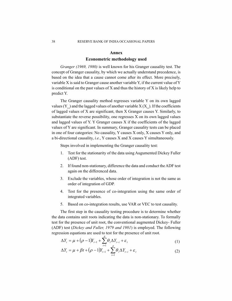
The first step in the causality testing procedure is to determine whether

the data contains unit roots indicating the data is non-stationary. To formally

test for the presence of unit root, the conventional augmented Dickey- Fuller

(ADF) test (Dickey and Fuller, 1979 and 1981) is employed. The following

regression equations are used to test for the presence of unit root.

t

p

iititt YYY

111 (1)

t

p

iititt YYtY

111 (2)


1 Trace test, tests the hypothesis that there are at most r co-integrating vectors, whereas, maximumeigenvalue test, tests the hypothesis that there are r+1 co-integrating vectors versus the hypothesisthat there are r co-integrating vectors.2 See Toda and Phillips (1994) for a detailed discussion.

where is the differencing operator

Ytis logGDP (or logorthim of GDS, HHS, PCS, PBS, GDI, HHI, PCI,

PBI) at time t

p is the maximum lag length

is the stationary random error.

Equation (1) is a test for random walk with drift term (intercept), whereas,

equation (2) tests for random walk with drift term and linear trend. Basically,

one would use the most general case and estimate a regression with both the

drift term and linear time trend, and step-by-step estimate the restricted

equations, if the test fails to reject the null hypothesis of unit root present in the

general case. The null hypothesis is that unit root present in the series (i.e., =1

or -1=0). The series is said to be stationary or do not have unit root, if 1- is

negative and statistically significant.

Once we have the results of unit roots, the next step is to determine whether

there exists co-integration, using the same order of integrated variables. To test

for co-integration, the Johansen and Juselius (1990) procedure is used, which

leads to two test statistics, trace test and maximum eigenvalue test, for co-

integration1. The two test statistics, trace and max are used to estimate the co-

integration rank r, i.e., the number of independent co-integrating vectors.

(3)

(4)

where are the estimated (n-r) smallest eigenvalues

T is the number of usable observations.

The distribution of statistics is subject to whether a constant or a driftterm is included in the co-integrating vector and the number of non-stationarycomponents under the null hypothesis.

If the rank r is zero, the variables are not co-integrated and hence thevector auto regression (VAR) method would be used to investigate causality.On the other hand, if the variables are co-integrated, the vector error correction(VEC) method is used to test for causality2.

n

riitrace Tr

1

1ln

1max 1ln1, rTrr

nr ,,1

causal relationship between saving, investment and ... · pdf filecausal relationship between...

Documents