Causal Inference in Conjoint Analysis: UnderstandingMultidimensional Choices via Stated Preference Experiments

The MIT Faculty has made this article openly available. Please share how this access benefits you. Your story matters.

Citation Hainmueller, J., D. J. Hopkins, and T. Yamamoto. “Causal Inferencein Conjoint Analysis: Understanding Multidimensional Choices viaStated Preference Experiments.” Political Analysis (December 19,2013).

As Published http://dx.doi.org/10.1093/pan/mpt024

Publisher Oxford University Press

Version Author's final manuscript

Citable link http://hdl.handle.net/1721.1/84064

Terms of Use Creative Commons Attribution-Noncommercial-Share Alike 3.0

Detailed Terms http://creativecommons.org/licenses/by-nc/3.0

Electronic copy available at: http://ssrn.com/abstract=2231687

Causal Inference in Conjoint Analysis:Understanding Multidimensional Choices via

Stated Preference Experiments∗

Jens Hainmueller† Daniel J. Hopkins‡ Teppei Yamamoto§

First Draft: July 17, 2012This Draft: November 5, 2013

Abstract

Survey experiments are a core tool for causal inference. Yet, the design of classical surveyexperiments prevents them from identifying which components of a multidimensional treat-ment are influential. Here, we show how conjoint analysis, an experimental design yet to bewidely applied in political science, enables researchers to estimate the causal effects of mul-tiple treatment components and assess several causal hypotheses simultaneously. In conjointanalysis, respondents score a set of alternatives, where each has randomly varied attributes.Here, we undertake a formal identification analysis to integrate conjoint analysis with thepotential outcomes framework for causal inference. We propose a new causal estimand andshow that it can be nonparametrically identified and easily estimated from conjoint datausing a fully randomized design. The analysis enables us to propose diagnostic checks forthe identification assumptions. We then demonstrate the value of these techniques throughempirical applications to voter decision-making and attitudes toward immigrants.

Forthcoming in Political Analysis 2013

Key Words: potential outcomes, average marginal component effects, conjoint analysis,survey experiments, public opinion, vote choice, immigration

∗We gratefully acknowledge the recommendations of Political Analysis editors Michael Alvarez and JonathanKatz as well as the anonymous reviewers. We further thank Justin Grimmer, Kosuke Imai, and seminar participantsat MIT, Harvard University, and Rochester University for their helpful comments and suggestions. We are alsograteful to Anton Strezhnev for excellent research assistance. An earlier version of this paper was presented atthe 2012 Annual Summer Meeting of the Society for Political Methodology and the 2013 Annual Meeting of theAmerican Political Science Association. Example scripts that illustrate the estimators and companion softwareto embed a conjoint analysis in Web-based survey instruments is available on the authors’ website. Replicationmaterials are available online as Hainmueller et al. (2013). Supplementary materials for this article are availableon the Political Analysis Web site.†Associate Professor, Department of Political Science, Massachusetts Institute of Technology, Cambridge, MA

02139. Email: jhainm@mit.edu, URL: http://web.mit.edu/jhainm/www‡Associate Professor, Department of Government, Georgetown University, ICC 681, Washington, DC 20057.

Email: dh335@georgetown.edu, URL: http://www.danhopkins.org§Assistant Professor, Department of Political Science, Massachusetts Institute of Technology, 77 Massachusetts

Avenue, Cambridge, MA 02139. Email: teppei@mit.edu, URL: http://web.mit.edu/teppei/www.

Electronic copy available at: http://ssrn.com/abstract=2231687

1 Introduction

The study of politics is to a significant extent the study of multidimensional choices. Voters,

interest groups, government officials and other political actors form preferences and make decisions

about alternatives which differ in multiple ways. To understand such choices, political scientists

are increasingly employing survey experiments (Schuman & Bobo 1988, Sniderman & Grob 1996,

Gaines et al. 2007, Sniderman 2011). Indeed, three leading political science journals published

72 articles with survey experiments between 2006 and 2010.1 The primary advantage of survey

experiments is their ability to produce causal conclusions. By randomly varying certain aspects

of a survey across groups of respondents, researchers can ensure that systematic differences in the

respondents’ post-treatment attitudes and behavior are attributable solely to the experimental

manipulations, making causal inference a realistic goal of empirical research.

However, the designs that are typically used in survey experiments have an important limita-

tion for analyzing multidimensional decision-making. Common experimental designs can identify

the causal effects of an experimental manipulation as a whole, but they typically do not allow

researchers to determine which components of the manipulation produce the observed effects. As

an example, consider the first experiment reported by Brader et al. (2008), a prominent study

examining respondents’ attitudes toward immigration. The researchers randomly varied two as-

pects of an otherwise identical news article: the ethnicity of the immigrant profiled in the story

and whether the story’s general tone was positive or negative. In manipulating the immigrant’s

perceived ethnicity, they only altered his face, name and country of origin to “test the impact

of the ethnic identity cue itself”(p.964). Even so, this experimental design cannot tell us which

particular aspects of the Russian- or Mexican-born immigrant influenced respondents’ attitudes.

Immigrants’ places of birth, names, and faces are correlated with many other attributes, from

their ethnic or racial background to their education, language, and religion. Put differently, the

treatments in this experiment are composites of many attributes which are “aliased,” making their

unique effects impossible to identify. This inability to decompose treatment effects is not unique

to this study; indeed, it is built into the design of most contemporary survey experiments, which

present subjects with composite treatments and vary only a few components of those treatments.

1These journals are the American Journal of Political Science, the American Political Science Review, and theJournal of Politics.

1

Electronic copy available at: http://ssrn.com/abstract=2231687

One potential solution to the issue of aliasing is to design treatments that are truly one-

dimensional. For example, Hainmueller & Hiscox (2010) report a survey experiment in which

respondents were asked whether the U.S. should admit more low- or high-skilled immigrants. In

this case, only two words differed across the arms of the experiment (“low” or “high”), so any

treatment effects can be attributed to these specific words. A drawback of this approach, however,

is that it forces researchers to examine one component of the treatment at a time. That drawback

is a significant one, especially given the high fixed costs of conducting any one survey experiment.

What is more, the conclusions based on such single-attribute designs may lack external validity if

respondents’ views when focused on a single component differ from those in more realistic scenarios

in which they consider various components at once.

In this paper, we develop an alternative approach to the problem of composite treatment ef-

fects. Specifically, we present conjoint analysis as a tool to identify the causal effects of various

components of a treatment in survey experiments. This approach enables researchers to nonpara-

metrically identify and estimate the causal effects of many treatment components simultaneously.

Because the resulting estimates represent effects on the same outcome, they can be compared on

the same scale to evaluate the relative influence of the components and to assess the plausibil-

ity of multiple theories. Moreover, the proposed estimation strategy can be easily implemented

with standard statistical software. At the same time, our estimators avoid unnecessary statistical

assumptions, affording them more internal validity than the more model-dependent procedures

typical of prior research on conjoint analysis. We also make available sample scripts that illustrate

the proposed estimators and a standalone software tool that we have developed which researchers

can use to embed a conjoint analysis in Web-based survey instruments administered through

survey tools such as Qualtrics (Strezhnev et al. 2013).

Introduced in the early 1970s (Green & Rao 1971), conjoint analysis is widely used by mar-

keting researchers to measure consumer preferences, forecast demand, and develop products (e.g.

Green et al. 2001, Raghavarao et al. 2011). These methods have been so successful that they

are now widely used in business as well (Sawtooth Software Inc. 2008). Similar tools were sep-

arately developed by sociologists in the 1970s (e.g. Jasso & Rossi 1977), and came to be known

as “vignettes” or “factorial surveys” (Wallander 2009), although their use has been infrequent in

that field to date. Irrespective of the name, these techniques ask respondents to choose from or

2

rate hypothetical profiles that combine multiple attributes, enabling researchers to estimate the

relative influence of each attribute value on the resulting choice or rating. Although the tech-

nique has many variants (Raghavarao et al. 2011), more than one such task is typically given to

each respondent, with some or all of the attribute values varied from one task to another. It is

this unique design that makes conjoint experiments well suited for analyzing component-specific

treatment effects. Here, we propose a variant of randomized conjoint analysis as an experimental

design that is particularly useful for decomposing composite treatment effects.

Although the methodological literature on conjoint analysis is old and highly sophisticated

(Luce & Tukey 1964), it has not been studied explicitly from a contemporary causal inference

perspective, making it unclear whether and how estimates based on conjoint analysis relate to well-

defined causal quantities. Moreover, conjoint analysis raises statistical challenges and modeling

choices not present in the analysis of standard experiments, as the number of possible unique

profiles typically outstrips the number of profiles observed in any empirical application. Still,

because researchers are free to manipulate profile attributes in conjoint analysis, the design lends

itself to causal investigations of respondents’ choices. In this study, we use the potential outcomes

framework of causal inference (Neyman 1923, Rubin 1974) to formally analyze the causal properties

of conjoint analysis. We define a causal quantity of interest, the average marginal component effect

(AMCE). We then show that this effect (as well as the interaction effects of the components) can

be nonparametrically identified from conjoint data under assumptions that are either guaranteed

to hold by the experimental design or else at least partially empirically testable. We also propose

a variety of diagnostic checks to probe the identification assumptions.

Our identification result implies that scholars can make inferences about key quantities of in-

terest without resorting to functional form assumptions. This stands in stark contrast to most

existing statistical approaches to conjoint data in economics and marketing research, which start

from a particular behavioral model for respondents’ decision-making processes and fit a statistical

model to observed data that is constructed based on the behavioral model. Although this model-

based approach may allow efficient estimation, a key drawback is that it is valid only when the

assumed behavioral model is true. In contrast, our approach is agnostic about how respondents

reach their observed decisions — they might be maximizing utility, they might be boundedly ra-

tional, they might use weighted adding, lexicographic, or satisficing decision strategies, or they

3

might make choices according to another model (Bettman et al. 1998). Irrespective of the un-

derlying behavioral model, our proposed method estimates the effects of causal components on

respondents’ stated preferences without bias given the identification assumptions.

The potential advantages of conjoint analysis are not limited to their desirable properties for

causal identification. Indeed, conjoint analysis has a number of features which make it an attractive

tool for applied research. First, by presenting respondents with various pieces of information and

then asking them to make choices, conjoint analysis has enhanced realism relative to the direct

elicitation of preferences on a single dimension for a variety of research questions. Second, conjoint

analysis allows researchers to test a large number of causal hypotheses in a single study, making

it a cost-effective alternative to traditional survey experiments. Third, conjoint analysis estimates

the effects of multiple treatment components in terms of a single behavioral outcome and thus

allows researchers to evaluate the relative explanatory power of different theories, moving beyond

unidimensional tests of a single hypothesis. Fourth, conjoint experiments have the potential

to limit concerns about social desirability (Wallander 2009), as they provide respondents with

multiple reasons to justify any particular choice or rating. Finally, conjoint analysis can provide

insights into practical problems such as policy design. For example, it can be used to predict the

popular combinations of components in a major policy reform.

As the foregoing discussion suggests, the applicability of conjoint analysis in political science

is broad. Many central questions in the study of politics concern multidimensional preferences

or choices. In this paper, we apply our estimators to two original conjoint experiments on topics

we consider exemplary of multidimensional political choices: voting and immigration. These are

by no means the only subjects to which conjoint analysis can be productively applied.2 As the

conclusion highlights, we suspect that many hypotheses in political behavior can be empirically

tested using conjoint experiments.

The rest of the paper is organized as follows. Section 2 presents our empirical examples. Sec-

tion 3 defines our causal quantities of interest and shows the results of our identification analysis.

2Indeed, many political scientists (including ourselves) have started to adopt conjoint analysis in their research.For example, Hainmueller & Hopkins (2012)use a conjoint experiment to study attitudes towards immigration andwe use this as a running example below. Wright et al. (2013) apply a similar approach to study attitudes towardunauthorized immigrants. Bechtel et al. (2013) examine voter attitudes in Germany toward alternative policypackages for Eurozone bailouts, and Bechtel & Scheve (2013) use a similar design to analyze attitudes about globalcooperation on climate change.

4

Section 4 presents our proposed estimation strategy. In Section 5, we apply our proposed frame-

work to the empirical examples to illustrate how our estimators work in practice. We also propose

and conduct several diagnostic analyses to investigate the plausibility of our identification assump-

tions as well as the studies’ external validity. Section 6 discusses the advantages and disadvantages

of conjoint analysis relative to traditional survey experiments. Section 7 concludes.

2 Examples

In this section, we briefly describe our empirical examples. The first is a conjoint experiment on

U.S. citizens’ preferences across presidential candidates which we conducted in July 2012. The

second is a conjoint experiment on attitudes toward immigrants whose results are reported in

more detail in Hainmueller & Hopkins (2012). Together, these two examples suggest the breadth

of possible applications of conjoint analysis within political science and illustrate some of the

common questions that emerge when implementing conjoint experiments.

2.1 The Candidate Experiment

The choice between competing candidates for elected office is central to democracy. Candidates

typically differ on a variety of dimensions, including their personal background and demographic

characteristics, issue positions, and prior experience. The centrality of partisanship to voter

decision-making is amply documented (e.g. Campbell et al. 1960, Green et al. 2002), so we focus

here on the less-examined role of candidates’ personal traits (see also Cutler 2002). Within the

U.S., there is constant speculation about the role of candidates’ personal backgrounds in generating

support or opposition; here, we harness conjoint analysis to examine those claims.

We focus on eight attributes of would-be presidential candidates, all of which have emerged in

recent campaigns. Six of these attributes can take on one of six values, including the candidates’

religion (Catholic, Evangelical Protestant, Mainline Protestant, Mormon, Jewish, or None), college

education (no college, state university, community college, Baptist college, Ivy League college, or

a small college), profession (lawyer, high school teacher, business owner, farmer, doctor, or car

dealer), annual income ($32K, $54K, $65K, $92K, $210K, and $5.1M), racial/ethnic background

(Hispanic, White, Caucasian, Black, Asian American, and Native American), and age (36, 45,

5

52, 60, 68, and 75).3 Two other attributes take on only two values: military service (served or

not) and gender (male or female). Each respondent to our online survey — administered through

Amazon’s Mechanical Turk (Berinsky et al. 2012) — saw six pairs of profiles that were generated

using the fully randomized approach described below. Figure A.1 in the Supplemental Information

(SI) illustrates one choice presented to one respondent. The profiles were presented side-by-side,

with each pair of profiles on a separate screen. To ease the cognitive burden for respondents while

also minimizing primacy and recency effects, the attributes were presented in a randomized order

that was fixed across the six pairings for each respondent.

On the same screen as each candidate pairing, respondents were asked multiple questions

which serve as dependent variables. First, they were asked to choose between the two candi-

dates, a “forced-choice” design that enables us to evaluate the role of each attribute value in the

assessment of one profile relative to another. This question closely resembles real-world voter

decision-making, in which respondents must cast a single ballot between competing candidates

who vary on multiple dimensions. In the second and third questions following the profiles, the

respondents rated each candidate on a one to seven scale, enabling evaluations of the levels of

absolute support or opposition to each profile separately.

2.2 The Immigrant Experiment

Our second example focuses on the role of immigrants’ attributes in shaping support for their

admission to the United States. A variety of prominent hypotheses lead to different expectations

about what attributes of immigrants should influence support for their admission, from their

education and skills (Scheve & Slaughter 2001, Hainmueller & Hiscox 2010) to their country of

origin (Citrin et al. 1997, Brader et al. 2008) and perceived adherence to norms about American

identity (Wong 2010, Schildkraut 2011, Wright & Citrin 2011). Yet to date, empirical tests have

commonly varied only a small subset of those attributes at one time, making it unclear whether

findings for certain attributes are masking the effects of others. For example, it is plausible that

prior findings on the importance of immigrants’ countries of origin are in fact driven by views of

immigrants’ education, authorized entry into the U.S., or other factors.

3We include “White” and “Caucasian” as separate values to identify any differential response those terms mayproduce.

6

In our experiment, Knowledge Networks respondents were asked to act as immigration officials

and to decide which of a pair of immigrants they would choose for admission. Figure 1 illustrates

one choice presented to one respondent. Respondents were asked to first choose between the

two immigrant profiles that varied across a set of attributes and then to rate each profile on a

scale from one to seven, where seven indicates that the immigrant should definitely be admitted.

Respondents evaluated a total of five pairings. The attributes include each immigrant’s gender,

education level, employment plans, job experience, profession, language skills, country of origin,

reasons for applying, and prior trips to the United States. These attributes were then randomly

chosen to form immigrant profiles.

One methodological difference in this experiment compared to the conjoint of candidate pref-

erences described above is that in randomly generating the immigrant profiles, we imposed two

restrictions on the possible combinations of immigrant attributes. First, those immigrant profiles

who were fleeing persecution were restricted to come from countries where such an application

was plausible (e.g. Iraq, Sudan). Second, those immigrants occupying high-skill occupations (e.g.

research scientists, doctors) were constrained to have at least two years of college education. As

we elaborate in Section 3, we used these restrictions to prohibit immigrant profiles that give rise

to counterfactuals that are too unrealistic to be evaluated in a meaningful way.

3 Notation and Definitions

In this section, we provide a formal analysis of conjoint experiments using the potential outcomes

framework of causal inference (Neyman 1923, Rubin 1974). We introduce the notational frame-

work, define the causal quantities of interest, and show that these quantities are nonparametrically

identified under a set of assumptions that is likely to hold in a typical conjoint experiment.

3.1 Design

As illustrated by the empirical examples in Section 2, conjoint analysis is an experimental technique

“for handling situations in which a decision maker has to deal with options that simultaneously

vary across two or more attributes”(Green et al. 2001, S57). In the literature, conjoint analysis

can refer to several distinct experimental designs. One such variation is in the outcome variable

7

with which respondents’ preferences are measured. Here, we analyze two types of outcomes which

are particularly common and straightforward. First, in so-called “choice-based conjoint analysis”

(also known as “discrete choice experimentation”; see Raghavarao et al. 2011), respondents are

presented with two or more alternatives varying in multiple attributes and are asked to choose

the one they most prefer. Choice-based conjoint is “the most widely used flavor of conjoint

analysis”(Sawtooth Software Inc. 2008, 1), as it closely approximates real-world decision-making

(e.g. Hauser 2007). We call such responses choice outcomes hereafter. Second, in “rating-based

conjoint analysis,” respondents give a numerical rating to each profile which represents their degree

of preference for the profile. This format is preferred by some analysts who contend that such

ratings provide more direct, finely grained information about respondents’ preferences. We call

this latter type of outcome a rating outcome. In practice, both choice and rating outcomes are

often measured in a single study, as is done in our running examples.4

Formally, consider a random sample of N respondents drawn from a population of interest P .

Each respondent (indexed by i ∈ {1, ..., N}) is presented with K choice (or rating) tasks, and in

each of her tasks the respondent chooses the most preferred (or rates each) of the J alternatives.

We refer to the choice alternatives as profiles. For example, in the candidate experiment, a profile

consists of one specific candidate. Each profile is characterized by a set of L discretely valued

attributes, or a treatment composed of L components. We use Dl to denote the total number

of levels for attribute l.5 For example, in the candidate experiment, N = 311 (respondents),

J = 2 (competing candidates in each choice task), K = 6 (choices made by respondents), L = 8

(candidate attributes), D1 = · · · = D6 = 6 (total number of levels for candidate’s age, education,

etc.), and D7 = D8 = 2 (for military service and gender).6

We denote the treatment given to respondent i as the jth profile in her kth choice task by

a vector Tijk, whose lth component Tijkl corresponds to the lth attribute of the profile. This

4Other common types of tasks include ordinal ranking and point allocation. The investigation of these outcomesis left to future research.

5For attributes that are inherently continuous (e.g., annual income in the candidate experiment), traditionalapproaches often assume certain functional forms between the attributes and outcome to reduce the number ofparameters required (e.g., estimate a single regression coefficient for the attribute). This approach can be justifiedwhen the functional-form assumption is reasonable. However, such an assumption is often difficult to justify, andit raises additional validity concerns such as the “range effect” and “number-of-levels effect” (Verlegh et al. 2002).

6Implicit in this notation is the assumption that the order of the attributes within a profile does not affectthe potential outcomes (defined below). This assumption might not be plausible, especially if L is so large thatrespondents must read through a long list of profile attributes. As we show in Section 5.3.4, randomizing the orderof attributes across respondents makes it possible to assess the plausibility of this assumption.

8

L-dimensional vector Tijk can take any value in set T , which can be as large as the Cartesian

product of all the possible values of the attributes but need not be. For example, if particular

combinations of the attribute values are implausible, the analyst may choose to remove them from

the set of possible profiles (or treatment values), as we do in our immigration experiment. We

then use Tik to denote the entire set of attribute values for all J profiles in respondent i’s choice

task k, and T i for the entire set of all JK profiles respondent i sees throughout the experiment.7

Using the potential outcomes framework, let Yik(t) denote the J-dimensional vector of potential

outcomes for respondent i in her kth choice task that would be observed when the respondent

received the sequence of profile attributes represented by t, with individual components Yijk(t).

As mentioned above, this variable can represent either a choice or rating outcome. In the former

case, Yijk(t) is a binary indicator variable where 1 indicates that respondent i would choose the

jth profile in her kth choice task if she got the treatment set of t and 0 implies that she would not.

In the latter case, the potential outcome represents the rating respondent i would give to the jth

profile in her kth task if she received t, and is assumed to take on a numeric value between some

known upper and lower bounds, i.e., Yijk(t) ∈ Y ≡ [y, y]. In both cases, the observed outcome in

respondent i’s kth task when the respondent receives a set of treatments T i can then be written

as Yik ≡ Yik(T i), with individual component Yijk(T i). For choice outcomes, by design respondents

must choose one preferred profile j within each choice task k, i.e,∑J

j=1 Yijk(t) = 1 for all i, k and

t, while rating outcomes do not impose such a constraint and can take on any value in Y .

3.2 Assumptions

We now make a series of simplifying assumptions. Unlike many assumptions typically made in

the literature, all of these assumptions can be either guaranteed to hold by the study design or

partially tested with observed data (see Section 5.3).

First, we assume stability and no carryover effects for the potential outcomes. This means

that the potential outcomes remain stable across the choice tasks (i.e. no period effect) and that

treatments given to a respondent in her other choice tasks do not affect her response in the current

7More precisely, Tijk is an L-dimensional column vector such that Tijk = [Tijk1 · · · TijkL]> ∈ T , where

j ∈ {1, ..., J}, the superscript > represents transposition, and T ⊆∏L

l=1 Tl where Tl = {tl1, ..., tlDl}; Tik represents

a matrix whose jth row is Tijk, i.e., Tik = [Ti1k · · · TiJk]>; and T i is a three-dimensional array of treatmentcomponents for respondent i whose (j, k, l) component equals Tijkl.

9

task. The following expression formalizes this assumption.

Assumption 1 (Stability and No Carryover Effects). For each i and all possible pairs of treatments

T i and T′i,

Yijk(T i) = Yijk′(T′i) if Tik = T ′ik′ ,

for any j, k and k′.

Assumption 1 requires that the potential outcomes always take on the same value as long

as all the profiles in the same choice task have identical sets of attributes. For example, in the

candidate conjoint experiment above, respondents would choose the same candidate as long as

the two candidates in the same choice task had identical attributes, regardless of what kinds of

candidates they had seen or would see in the rest of the experiment. This assumption may not

be plausible if, for example, respondents use the information given in earlier choice tasks as a

reference point in evaluating candidates later in the experiment.

Under Assumption 1, we can substantially simplify our analysis by writing the potential out-

comes just as Yi(t) with individual components Yij(t), where t is some realized value of Tik defined

above. Similarly, the observed outcomes become Yik = Yi(Tik).8 Practically, the assumption allows

researchers to increase efficiency of a given study by pooling information across choice tasks when

estimating the average causal effects of interest (defined in Section 3.3). Since the fixed costs of a

survey typically exceed the marginal cost of adding more choice tasks to the questionnaire, having

respondents do multiple tasks is beneficial as long as Assumption 1 holds.

We maintain Assumption 1 in the main analyses of this paper. Still, should researchers suspect

that profiles affect later responses, they can either assign a single choice task per respondent or

use data only from each respondent’s first task. Moreover, as we demonstrate in Section 5.3.1,

they can assess the plausibility of Assumption 1 by examining if the results from later tasks differ

from those obtained in the first task.

Second, we assume that there are no profile-order effects, that is, the ordering of profiles within

a choice task does not affect responses. This means that simply shuffling the order in which profiles

are presented on the questionnaire or computer screen must not alter the choice respondents would

8Note that this assumption is akin to what is known more generally as SUTVA, or the Stable Unit TreatmentValue Assumption (Rubin 1980), in the sense that it precludes some types of interference between observation unitsand specifies that the potential outcomes remain stable across treatments given in different periods.

10

make or the rating they would give, as long as all the attributes are kept the same. Again, we

formalize this assumption as follows.

Assumption 2 (No Profile-Order Effects).

Yij(Tik) = Yij′(T′ik) if Tijk = T ′ij′k and Tij′k = T ′ijk,

for any i, j, j′ and k.

Under Assumption 2, we can further simplify the analysis by writing the jth component

of the potential outcomes as Yi(tj, t[−j]), where tj is a specific value of the treatment vector

Tijk and t[−j] is a particular realization of Ti[−j]k, the unordered set of the treatment vectors

Ti1k, ..., Ti(j−1)k, Ti(j+1)k, ..., TiJk. Similarly, the jth component of the observed outcomes can now

be written as Yijk = Yi(Tijk,Ti[−j]k).

Practically, Assumption 2 makes it possible for researchers to ignore the order in which the

profiles happen to be presented and to pool information across profiles when estimating causal

quantities of interest. The assumption therefore further enhances the efficiency of the conjoint

design. Like Assumption 1, one can partially test the plausibility of Assumption 2 by investigating

whether the estimated effects of profiles vary depending on where in the conjoint table they are

presented (see Section 5.3.2). We maintain this assumption in the subsequent analyses.

Finally, we assume that the attributes of each profile are randomly generated. This randomized

design contrasts with the approach currently recommended in the conjoint literature, which uses

a systematically selected, typically small subset of the treatment profiles. Under the randomized

design, the following assumption is guaranteed to hold because of the randomization of the profile

attributes.

Assumption 3 (Randomization of the Profiles).

Yi(t) ⊥⊥ Tijkl,

for all i, j, k, l and t, where the independence is taken to be the pairwise independence between

each element of Yi(t) and Tijkl, and it is also assumed that 0 < p(t) ≡ p(Tik = t) < 1 for all t in

its support.

11

Assumption 3 states that the potential outcomes are statistically independent of the profiles.

This assumption always holds if the analyst properly employs randomization when assigning at-

tributes to profiles, for the respondents’ potential choice behavior can never be systematically

related to what profiles they will actually see in the experiment. The second part of the assump-

tion states that the randomization scheme must assign a non-zero probability to all the possible

attribute combinations for which the potential outcomes are defined. This implies that if some

attribute combinations are removed from the set of possible profiles due to theoretical concerns

(as in our immigration experiment), it will be impossible to analyze causal quantities involving

these combinations (unless we impose additional assumptions such as constant treatment effects).

Although the study design guarantees Assumption 3 at the population level, researchers might

still be concerned that the particular sample of profiles that happens to be generated in their

study may be imbalanced, especially in small samples. In Section 5.3.3, we show a simple way to

diagnose this possibility.

3.3 Causal Quantities of Interest and Identification

Researchers may be interested in various causal questions when running a conjoint experiment.

Here, we formally propose several causal quantities of particular interest. We then discuss their

properties and prove their identifiability under the assumptions introduced in Section 3.2.

3.3.1 Limits of Basic Profile Effects

The most basic causal question in conjoint analysis is whether showing one set of profiles as

opposed to another would change the respondent’s choice. For any pair of profile sets t0 and t1

and under Assumptions 1 and 2, we can define the unit treatment effect as the difference between

the two potential outcomes under those two profile sets. That is,

πi(t1, t0) ≡ Yi(t1)− Yi(t0), (1)

for all t1 and t0 in their support. For example, suppose that in a simplified version of the candidate

experiment with three binary attributes, respondent i sees a presidential candidate with military

service, high income, and a college education as Candidate 1, and a candidate with no military

12

service, low income, and a college education as Candidate 2. The respondent chooses Candidate

1. In this case, t0 =

[military service rich college

no service poor college

]and Yi(t0) =

[1

0

]. Now, suppose that in

the counterfactual scenario, Candidate 2 had military service, low income, and college education,

i.e., t1 =

[military service rich college

military service poor no college

]. If the respondent still chose Candidate 1, then the unit

treatment effect of the change from t0 to t1 for respondent i would be zero for both candidates,

i.e., πi(t1, t0) =

[1

0

]−[

1

0

]=

[0

0

].

Unit-level causal effects such as equation (1) are generally difficult to identify even with exper-

imental data, because they involve multiple potential outcomes for the same unit of observation

and all but one of them must be counterfactual in most cases. This “fundamental problem of

causal inference”(Holland 1986) also applies to conjoint analysis.9 Instead, one might focus on the

average treatment effect (ATE) defined as,

π(t1, t0) ≡ E[πi(t1, t0)] = E[Yi(t1)− Yi(t0)], (2)

where the expectation is defined over the population of interest P . When Yi(t) is a vector of binary

choice outcomes, π(t1, t0) represents the difference in the population probabilities of choosing

the J profiles that would result if a respondent were shown the profiles with attributes t1 as

opposed to t0. It is straightforward to show that π(t1, t0) is nonparametrically identified under

Assumptions 1, 2 and 3 as,

ˆπ(t1, t0) = E[Yik | Tik = t1]− E[Yik | Tik = t0], (3)

for any t1 and t0. The proof is virtually identical to the proof of the identifiability of the ATE in

a standard randomized experiment (see, e.g., Holland 1986), and therefore is omitted.

The ATE is the most basic causal quantity since it is simply the expected difference in responses

for two different sets of profiles. However, directly interpreting this quantity may not be easy. In

the above example, what does it mean in practical terms to compare t0 and t1, two different pairs of

candidates whose attributes differ on multiple dimensions at the same time? Unless there is some

substantive background (e.g., the treatments correspond to two alternative scenarios that might

9Technically, Assumptions 1 and 2 imply that unit treatment effects can be identified for the limited number ofprofile sets that are actually assigned to unit i over the course of the K choice tasks. In practice, however, theseeffects are likely to be of limited interest because they are specific to individual units and constitute only a smallfraction of the large number of unit treatment effects.

13

happen in an actual election), π(t1, t0) is typically not a useful quantity of interest. Moreover, in

a typical conjoint analysis where the profiles consist of a large number of attributes with multiple

levels, the number of observations that belong to the conditioning set in each term of equation (3)

is very small or possibly zero, rendering the estimation of ˆπ(t1, t0) difficult in practice.

3.3.2 Average Marginal Component Effect

As an alternative quantity of interest we propose to look at the effect of an individual treatment

component. Suppose that the analyst is interested in how different values of the lth attribute of

profile j influence the probability that the profile is chosen. The effect of attribute l, however,

may differ depending on the values of the other attributes. For example, the analyst might be

interested in whether respondents generally tend to choose a rich candidate over a poor candidate.

The effect of income, however, might differ depending on whether the candidate is conservative

or liberal, as the economic policy a high-income candidate is likely to pursue might vary with

her ideology. Despite such heterogeneity in effect sizes, the analyst might still wish to identify a

quantity that summarizes the overall effect of income across other attributes of the candidates,

including ideology.

The following quantity, which we call the average marginal component effect (AMCE), rep-

resents the marginal effect of attribute l averaged over the joint distribution of the remaining

attributes.

πl(t1, t0, p(t)) ≡ E[Yi(t1, Tijk[−l],Ti[−j]k)− Yi(t0, Tijk[−l],Ti[−j]k)

∣∣ (Tijk[−l],Ti[−j]k)∈ T

]=

∑(t,t)∈T

E[Yi(t1, t, t)− Yi(t0, t, t)

∣∣ (Tijk[−l],Ti[−j]k)∈ T

]× p

(Tijk[−l] = t,Ti[−j]k = t

∣∣ (Tijk[−l],Ti[−j]k)∈ T

), (4)

where Tijk[−l] denotes the vector of L− 1 treatment components for respondent i’s jth profile in

choice task k without the lth component and T is the intersection of the support of p(Tijk[−l] =

t,Ti[−j]k = t | Tijkl = t1) and p(Tijk[−l] = t,Ti[−j]k = t | Tijkl = t0).10 This quantity equals

10This definition of T is subtle but important when analyzing conjoint experiments with restrictions in thepossible attribute combinations: the unit-level effects must be averaged over the values of t and t for which bothYi(t1, t, t) and Yi(t0, t, t) are well defined. This is because the causal effects can only be meaningfully defined forthe contrasts between pairs of potential outcomes which do not involve “empty counterfactuals,” such as a researchscientist with no formal education that was a priori excluded in the immigration conjoint experiment.

14

the increase in the population probability that a profile would be chosen if the value of its lth

component were changed from t0 to t1, averaged over all the possible values of the other components

given the joint distribution of the profile attributes p(t).11

To see what this causal quantity substantively represents, consider again a simplified version

of the candidate example. The AMCE of candidate income (rich vs. poor) on the probability

of choice can be understood as the result of the following hypothetical calculation: (1) compute

the probability that a rich candidate is chosen over an opposing candidate with a specific set of

attributes, compute the probability that a poor, but otherwise identical, candidate is chosen over

the same opponent candidate, and take the difference between the probabilities for the rich and the

poor candidate; (2) compute the same difference between a rich and a poor candidate, but with a

different set of the candidate’s and opponent’s attributes (other than the candidate’s income); and

(3) take the weighted average of these differences over all possible combinations of the attributes

according to their joint distribution. Thus, the AMCE of income represents the average effect of

income on the probability that the candidate will be chosen, where the average is defined over the

distribution of the attributes (except for the candidate’s own income) and repeated samples.

Although the above hypothetical calculation is impossible in reality given the fundamental

problem of causal inference, it turns out that we can in fact identify and estimate the AMCE from

observed data from a conjoint experiment, by virtue of the random assignment of the attributes.

That is, we can show that the expectations of the potential outcomes in equation (4) are nonpara-

metrically identified as functions of the conditional expectations of the observed outcomes under

the assumptions in Section 3.2. The AMCE can be written under Assumptions 1, 2 and 3 as

ˆπl(t1, t0, p(t)) =∑

(t,t)∈T

{E[Yijk | Tijkl = t1, Tijk[−l] = t,Ti[−j]k = t]

−E[Yijk | Tijkl = t0, Tijk[−l] = t,Ti[−j]k = t]}

× p(Tijk[−l] = t,Ti[−j]k = t

∣∣ (Tijk[−l],Ti[−j]k)∈ T

). (5)

Note that the expected values of the potential outcomes in equation (4) have been replaced with

the conditional expectations of the observed outcomes in equation (5), which makes the latter

expression estimable from observed data.12 In Section 4, we propose nonparametric estimators for

11Strictly speaking, the AMCE for the choice outcome only depends on the joint distribution of Tijk[−l] andTi[−j]k after marginalizing p(t) with respect to Tijkl. We opt for the simpler notation given in the main text.

12The proof for the identifiability is straightforward: the first term in equation (4) is identical to equation (2)

15

this quantity that can be easily implemented using elementary statistical tools.

An interesting feature of the AMCE is that it is defined as a function of the distribution of

the treatment components, p(t). This can be an advantage or disadvantage. The advantage is

that the analyst can explicitly control the target of the inference by setting p(t) to be especially

plausible or interesting. In a classical survey experiment where the analyst manipulates only one

or two elements of the survey, other circumstantial aspects of the experiment that may affect

responses (such as the rest of the vignette or the broader political context) are either fixed at a

single condition or out of the analyst’s control. This implies that the causal effects identified in

such experiments are inherently conditional on those particular settings, a fact that potentially

limits external validity but is often neglected in practice. In contrast, the AMCE in conjoint

analysis incorporates some of those covariates as part of the experimental manipulation and makes

it explicit that the effect is conditional on their distribution. Moreover, note that p(t) in the

definition of the AMCE need not be identical to the distribution of the treatment components

actually used in the experiment. In fact, the analyst can choose any distribution, as long as its

support is covered by the distribution actually used. One interesting possibility, which we do

not further explore here due to space constraints, is to use the real-world distribution (e.g., the

distribution of the attributes of actual politicians) to improve external validity.

The fact that the analyst can control how the effects are averaged can also be viewed as a

potential drawback, however. In some applied settings, it is not necessarily clear what distribution

of the treatment components analysts should use to anchor inferences. In the worst case scenario,

researchers may intentionally or unintentionally misrepresent their empirical findings by using

weights that exaggerate particular attribute combinations so as to produce effects in the desired

direction. Thus, the choice of p(t) is important. It should always be made clear what weighting

distribution of the treatment components was used in calculating the AMCE, and the choice

should be convincingly justified. In practice, we suggest that the uniform distribution over all

possible attribute combinations be used as a “default,” unless there is a strong substantive reason

to prefer other distributions.

Finally, it is worth pointing out that the AMCE also arises as a natural causal estimand in

any other randomized experiment involving more than one treatment component. The simplest

(except that the expectation is defined over the truncated distribution, which does not affect identifiability underAssumption 3), and the second term can be derived from p(t), the known joint density of the profile attributes.

16

example is the often-used “2 × 2 design,” where the experimental treatment consists of two di-

mensions each taking on two levels (e.g. Brader et al. 2008, see Section 1). In such experiments,

it is commonplace to “collapse” the treatment groups into a smaller number of groups based on a

single dimension of interest and compute the difference in the mean outcome values between the

collapsed groups. By doing this calculation, the analyst is implicitly estimating the AMCE for

the dimension of interest where p(t) equals the assignment probabilities for the other treatment

dimensions. Thus, the preceding discussion applies more broadly than to the specific context of

conjoint analysis and should be kept in mind whenever treatment components are marginalized

into a single dimension in the analysis.13

3.3.3 Interaction Effects

In addition to the AMCE, researchers might also be interested in interaction effects. There are two

types of interactions that can be quantities of interest in conjoint analysis. First, an attribute may

interact with another attribute to influence responses. That is, the causal effect of one attribute

(say candidate’s income) may vary depending on what value another attribute (e.g., ideology) is

held at, and the analyst may want to quantify the size of such interactions. This quantity can be

formalized as the average component interaction effect (ACIE) defined as,

πl,m(tl1, tl0, tm1, tm0, p(t))

≡ E[ {Yi(tl1, tm1, Tijk[−(lm)],Ti[−j]k)− Yi(tl0, tm1, Tijk[−(lm)],Ti[−j]k)

}−{Yi(tl1, tm0, Tijk[−(lm)],Ti[−j]k)− Yi(tl0, tm0, Tijk[−(lm)],Ti[−j]k)

} ∣∣(Tijk[−(lm)],Ti[−j]k) ∈ ˜T], (6)

where we use Tijk[−(lm)] to denote the set of L − 2 attributes for respondent i’s jth profile in

choice task k except components l and m, and ˜T is defined analogously to T above. This quantity

represents the average difference in the AMCE of component l between the profile with Tijkm = tm1

and one with Tijkm = tm0. For example, the ACIE of candidate income and ideology on the choice

probability equals the percentage point difference in the AMCEs of income between a conservative

candidate and a liberal candidate. Like the AMCE, the ACIE in equation (6) is identifiable from

13Gerber & Green (2012) make a similar point about multi-factor experiments, though without much elaboration:“[i]f the different versions of the treatment do appear to have different effects, remember that the average effectof your treatment is a weighted average of the ATEs for each version. This point should be kept in mind whendrawing generalizations based on a multi-factor experiment”(p. 305).

17

conjoint data under Assumptions 1, 2 and 3 and can be expressed in terms of the conditional

expectations of the observed outcomes, i.e., by an expression analogous to equation (5). It should

be noted that these definitions and identification results can be generalized to the interaction

effects among more than two treatment components.

Second, the causal effect of an attribute may also interact with respondents’ background char-

acteristics. For example, in the candidate experiment, the analyst might wish to know how the

effect of the candidate’s income changes as a function of the respondent’s income. We can answer

such questions with conjoint data by studying the average of the attribute’s marginal effect condi-

tional on the respondent characteristic of interest. That is, the conditional AMCE of component

l given a set of respondent characteristics Xi can be defined as,

E[Yi(t1, Tijk[−l],Ti[−j]k)− Yi(t0, Tijk[−l],Ti[−j]k)

∣∣ (Tijk[−l],Ti[−j]k)∈ T , Xi

], (7)

where Xi ∈ X denotes the vector of respondent characteristics. Like the other causal quantities

discussed above, the conditional AMCE can also be nonparametrically identified under Assump-

tions 1, 2 and 3. One point of practical importance is that the respondent characteristics must not

be affected by the treatments. To ensure this, the analyst could measure the characteristics before

showing randomized profiles to the respondents. For example, in the immigration experiment, the

interaction between the immigrant’s education and the respondent’s eduction can be estimated

by measuring respondents’ characteristics prior to conducting the conjoint experiment.

4 Proposed Estimation Strategies

In this section, we discuss strategies for estimating the causal effects of treatment components

using conjoint analysis. We derive easy-to-implement nonparametric estimators which can be

used for both choice and rating outcomes.

4.1 Estimation under Conditionally Independent Randomization

We begin with a general case which covers attribute distributions with nonuniform assignment

and restrictions involving empty attribute combinations. Assume that the attribute of interest,

18

Tijkl, is distributed independently of a subset of the other attributes after conditioning on the

remaining attributes. That is, we make the following assumption,

Assumption 4 (Conditionally Independent Randomization). The treatment components’ distri-

bution p(t) satisfies the following relationship with respect to the treatment component of interest

Tijkl,

Tijkl ⊥⊥ {T Sijk, Ti[−j]k} | TR

ijk for all i, j, k,

where TRijk is a LR-dimensional subvector of Tijk[−l] as defined in Section 3.3 and T S

ijk is the vector

composed of the elements of Tijk[−l] not included in TRijk.

This assumption is satisfied for most attribute distributions researchers typically use in con-

joint experiments. In particular, Assumption 4 holds under the common randomization scheme

where the attribute of interest, Tijkl, is restricted to take on certain values when some of the

other attributes (TRijk) are set to some particular values, but is otherwise free to take on any of

its possible values. For example, in the immigrant experiment, immigrants who have high-skill

occupations are constrained to have at least two years of college education. In this case, the distri-

bution of immigrants’ occupations (Tijkl) is dependent on their education (TRijk), but conditionally

independent of the other attributes (T Sijk) and the other profiles in the same choice task (Ti[−j]k)

given their education.

The following proposition shows that, under Assumption 4, the AMCE for the choice outcome

can be estimated by a simple nonparametric subclassification estimator.

Proposition 1 (Nonparametric Estimation of AMCE with Conditionally Independent Random-

ization). Under Assumptions 1, 2, 3, and 4, the following subclassification estimator is unbiased

for the AMCE defined in equation (4):

ˆπl(t1, t0, p(t)) =∑

tR∈T R

{∑Ni=1

∑Jj=1

∑Kk=1 Yijk1{Tijkl = t1, T

Rijk = tR}

n1tR

−∑N

i=1

∑Jj=1

∑Kk=1 Yijk1{Tijkl = t0, T

Rijk = tR}

n0tR

}Pr(TR

ijk = tR), (8)

where ndtR represents the number of profiles for which Tijkl = td and TRijk = tR, and T R is the

intersection of the supports of p(TRijk = tR | Tijkl = t1) and p(TR

ijk = tR | Tijkl = t0).

19

A proof is provided in Appendix A. Proposition 1 states that, for any attribute of interest

Tijkl, the subclassification estimate of the AMCE can be computed simply by dividing the sample

into the strata defined by TRijk, typically the attributes on which the assignment of the attribute of

interest is restricted, calculating the difference in the average observed choice outcomes between

the treatment (Tijkl = t1) and control (Tijkl = t0) groups within each stratum, and then taking the

weighted average of these differences in means, using the known distribution of the strata as the

weights. Therefore, the estimator is fully nonparametric and does not depend on any functional

form assumption about the choice probabilities, unlike standard estimation approaches in the

conjoint literature such as conditional logit (McFadden 1974).

The next proposition shows that the above nonparametric estimator can be implemented con-

veniently by a linear regression. To simplify the presentation, we assume that the conditioning set

of treatment components TRijk consists of only one attribute. This is true in our immigration ex-

ample, as each of the four restricted attributes had a restriction involving only one other attribute

(e.g. education for occupation).

Proposition 2 (Implementation of the Nonparametric Estimator of AMCE via Linear Regres-

sion). The subclassification estimator in equation (8) can be calculated via the following procedure

when LR = 1 and TRijk = Tijkl′ ∈ {t′0, ..., t′Dl′−1}. First, regress Yijk on

1, Wijkl, Wijkl′ , and Wijkl : Wijkl′ ,

where 1 denotes an intercept, Wijkl is the vector of Dl − 1 dummy variables for the levels of Tijkl

excluding the one for t0, Wijkl′ is the similar vector of dummy variables for the levels of Tijkl′

excluding the ones for its baseline level and the levels not in T R, and Wijkl : Wijkl′ denotes the

pairwise interactions between the two sets of dummy variables. Then, set

ˆπl(t1, t0, p(t)) = β1 +

Dl′−1∑d=1

Pr(Tijkl′ = t′d)δ1l′d, (9)

where β1 is the estimated coefficient on the dummy variable for Tijkl = t1 and δ1l′d represents

the estimated coefficient for the interaction term between the t1 dummy and the dummy variable

corresponding to Tijkl′ = t′d.

20

The proposition is a direct implication of the well-known correspondence between subclassifi-

cation and linear regression, and so the proof is omitted. Note that the linear regression estimator

is simply an alternative procedure to compute the subclassification estimator, and therefore has

properties identical to those of the subclassification estimator. This implies that the linear re-

gression estimator is fully nonparametric, even though the estimation is conducted by a routine

typically used for a parametric linear regression model. We have nevertheless opted to present it

separately because we believe it to be an especially convenient procedure for applied researchers

using standard statistical software. The estimator can be implemented simply by a single call to

a linear regression routine in most statistical packages, followed by a few additional commands to

extract the estimated coefficients and calculate their linear combinations.14 In Section 5, we show

examples using data from our immigration experiment.

Even more conveniently, one can also estimate the AMCEs of all of the L attributes included

in a study from a single regression. To implement this alternative procedure, one should simply

regress the outcome variable on the L sets of dummy variables and the interaction terms for the

attributes that are involved in any of the randomization restrictions used in the study, and then

take the weighted average of the appropriate coefficients in the same manner as in equation (9)

for each AMCE. This procedure in expectation produces the identical estimates of the AMCEs

as those obtained by applying Proposition 2 for each AMCE one by one, for the regressors in the

combined regression are in expectation orthogonal to one another under Assumption 4. Since the

effects of multiple attributes are usually of interest in conjoint analysis, applied researchers may

find this procedure particularly attractive.

In addition to their avoidance of modeling assumptions, another important advantage of these

nonparametric estimators is that they can be implemented despite the high dimensionality of the

attribute space that is characteristic of conjoint analysis, as long as the number of attributes

involved in a given restriction is not too large. A typical conjoint experiment includes a large

number of attributes with multiple levels, so it is unlikely for a particular profile to appear more

14The procedure is only marginally more complicated if the conditioning set TRijk consists of more than one

attribute, as is the case where restrictions involve more than two attributes. First, the regression equation mustbe modified to include all of the LRth and lower-order interactions among the LR sets of dummy variables WR

ijk

and their main effects, as well as the pairwise interactions between the components of Wijkl and each of thoseinteraction terms. Then, the nonparametric estimator of the AMCE is the linear combination of the estimatedregression coefficients on the terms involving the Tijkl = t1 dummy, where the weights equal the corresponding cellprobabilities.

21

than a few times throughout the experiment even with a large number of respondents and choice

tasks. This makes it difficult to construct a statistical model for conjoint data without making at

least some modeling assumptions. One such assumption that is frequently made in the literature

is the absence of interaction between attributes (see Raghavarao et al. 2011). The proposed

estimators in Propositions 1 and 2, in contrast, do not rely on any direct modeling of the choice

responses and therefore can be implemented without such potentially unjustified assumptions.

The other causal quantities of interest in Section 3.3 can be estimated by the natural extensions

of the procedures in Propositions 1 and 2. For example, the ACIE can be estimated by further

subclassifying the sample into the strata defined by the attribute with which the interaction is of

interest (i.e., Ttijm in equation (6)). Mechanically, this amounts to redefining TRijk in equation (8)

to be the vector composed of the original TRijk and Tijkm and then applying the same estimator.

The linear regression estimator can also be applied in an analogous manner. Similarly, the con-

ditional AMCE and ACIE with respect to respondent characteristics (Xi) can be estimated by

subclassification into the strata defined by Xi.

4.2 Estimation under Completely Independent Randomization

Next, we consider an important special case of p(t) where the attribute of interest is distributed

independently from all other attributes. That is, we consider the following assumption,

Assumption 5 (Completely Independent Randomization). For the treatment component of in-

terest Tijkl,

Tijkl ⊥⊥ {Tijk[−l], Ti[−j]k} for all i, j, k.

This assumption is satisfied in many settings where the attribute of interest is not restricted to

take on particular levels depending on the values of the other attributes or profiles. For example,

in the immigration example, the language skills of the immigrants were not constrained and were

assigned to one of the four possible levels with equal probabilities, independent of the realized

levels of the other attributes. In the election example, each of the candidates’ attributes was

drawn from an independent uniform distribution for each profile, implying that Assumption 5 is

satisfied for all of the attributes.

The following proposition shows that the AMCE can be estimated without bias by a simple

22

difference in means when Assumption 5 holds.

Proposition 3 (Estimation of AMCE with Completely Independent Randomization). Under

Assumptions 1, 2, 3, and 5, the following estimators are unbiased for the AMCE defined in equa-

tion (4).

1. The difference-in-means estimator:

ˆπl(t1, t0, p(t)) =

∑Ni=1

∑Jj=1

∑Kk=1 Yijk1{Tijkl = t1}n1

−∑Ni=1

∑Jj=1

∑Kk=1 Yijk1{Tijkl = t0}n0

(10)

where n1 and n0 are the numbers of profiles in which Tijkl = t1 and Tijkl = t0, respectively.

2. The simple linear regression estimator: Regress Yijk on an intercept and Wijkl, as defined in

Proposition 2. Then, set ˆπl(t1, t0) = β1, the estimated coefficient on the dummy variable for

Tijkl = t1.

We omit the proof since it is a special case of Proposition 1 where T Sijk = Tijk[−l] and TR

ijk is

an empty set. Proposition 3 shows that the estimation of the AMCE is extremely simple when

Assumption 5 holds. That is, the AMCE can be estimated by the difference in the average choice

probabilities between the treatment (Tijkl = t1) and control (Tijkl = t0) groups, or equivalently by

fitting a simple regression of the observed choice outcomes on the Dl− 1 dummy variables for the

attribute of interest and looking at the estimated coefficient for the treatment level. The interaction

and conditional effects can be estimated by subclassification into the strata of interest and then by

applying either the subclassification or linear regression estimators similar to Propositions 1 and 2.

4.3 Variance Estimation

Estimation of sampling variances for the above estimators must be done with care, especially

for the choice outcomes. First, the observed choice outcomes within choice tasks are strongly

negatively correlated, because of the constraint that∑J

j=1 Yijk = 1 for all i and k. To choose

one profile is to not choose others. In particular, when J = 2 as in our immigration and election

examples, Corr(Yi1k, Yi2k) = −1—that is, if Yi1k = 1 then Yi2k must be equal to 0 and vice versa.

23

Second, both potential choice and rating outcomes within respondents are likely to be positively

correlated because of unobserved respondent characteristics influencing their preferences. For

example, a respondent who chooses a high-skilled immigrant over a low-skilled immigrant is likely

to make a similar choice when presented with another pair of high- and low-skilled immigrant

profiles. Thus, an uncertainty estimate for the estimators of the population AMCE must account

for these dependencies across profiles. In particular, the estimates based on the default standard

errors for regression coefficients or differences in means are likely to be substantially biased.

Here, we propose two simple alternative approaches. First, the point estimates of the AMCE

based on Propositions 1, 2 and 3 can be coupled with standard errors corrected for within-

respondent clustering. For example, one can obtain cluster-robust standard errors for the es-

timated regression coefficients by using the cluster option in Stata. Then, these standard errors

can be used to construct confidence intervals and conduct hypothesis tests for the AMCE based on

the expression in Proposition 2. As is well known, these standard errors are valid for population

inference when errors in potential outcomes are correlated within clusters (i.e. respondents) in an

arbitrary manner, as long as the number of clusters is sufficiently large. Since the latter condi-

tion is not problematic in typical survey experiments where the sample includes at least several

hundred respondents, we propose that this simple procedure be used in most situations.

Second, valid standard errors and confidence intervals can also be obtained for the AMCE

via the block bootstrap, where respondents are resampled with replacement and uncertainty esti-

mates are calculated based on the empirical distribution of the AMCE over the resamples. This

procedure may produce estimates with better small sample properties than the procedure based

on cluster-robust standard errors when the number of respondents is limited, although it requires

substantially more computational effort.

5 Empirical Analysis

In this section, we apply the results of our identification analysis and our estimation strategies to

the two empirical examples introduced in Section 2.

24

5.1 The Candidate Experiment

Notice that the candidate experiment used a completely independent randomization (as in As-

sumption 5). In other words, the randomization did not involve any restrictions on the possible

attribute combinations, making the attributes mutually independent. As discussed in Section 4,

this simplifies estimation and interpretation significantly. Overall, there were 3,466 rated profiles

or 1,733 pairings evaluated by 311 respondents. The design yields 186, 624 possible profiles, which

far exceeds the number of completed tasks and renders classical causal estimands impractical.

For illustrative purposes, we begin with the simple linear regression estimator of the ACMEs

for designs with completely independent randomization described in Proposition 3. Respondents

rated each candidate profile on a seven-point scale, where 1 indicates that the respondent would

“never support” the candidate and 7 indicates that she would “always support” the candidate.

We rescaled these ratings to vary from 0 to 1 and then estimated the corresponding AMCEs

by regressing this dependent variable on indicator variables for each attribute value.15 In this

application, these ratings were asked immediately after the forced choice question, and so these

responses might have been influenced by the fact that respondents just made a binary choice

between the two profiles.16 To account for the possible non-independence of ratings from the same

respondent, we cluster the standard errors by respondent.

The left side of Figure 2 shows the AMCEs and 95% confidence intervals for each attribute

value. There are a total of 32 AMCE estimates, with 8 attribute levels used as baselines (t0). The

AMCEs can be straightforwardly interpreted as the expected change in the rating of a candidate

profile when a given attribute value is compared to the researcher-chosen baseline. For instance,

we find that candidates who served in the military on average receive ratings that are 0.03 higher

15For example, to estimate the AMCEs for the candidates’ age levels we run the following regression:

ratingijk = θ0 + θ1[ageijk = 75] + θ2[ageijk = 68] + θ3[ageijk = 60] + θ4[ageijk = 52] + θ5[ageijk = 45] + εijk,

where ratingijk is the outcome variable that contains the rating and [ageijk = 68], [ageijk = 75], etc. are dummyvariables coded 1 if the age of the candidate is 68, 75, etc. and 0 otherwise. The reference category is a 36-year-oldcandidate. Accordingly, θ1, θ2, etc. are the estimators for the AMCEs for ages 68, 75, etc. compared to the ageof 36. Note that, alternatively, we can obtain the equivalent estimates of the AMCEs along with the AMCEs ofthe other attributes by running a single regression of ratingijk on the combined sets of dummies for all candidateattributes, as explained in Section 4.1.

16The value of employing ratings, forced choices, or other response options will be domain-specific, but futureresearch should certainly consider randomly assigning respondents to different formats for expressing their viewsof the profiles.

25

than those who did not on the 0 to 1 scale, with a standard error (SE) of 0.01. We also see a

bias against Mormon candidates, whose estimated level of support is 0.06 (SE = 0.03) lower when

compared to a baseline candidate with no stated religion. Support for Evangelical Protestants is

also 0.04 percentage points lower (SE= 0.02) than the baseline. Mainline Protestants, Catholics,

and Jews all receive ratings indistinguishable from those of a baseline candidate.

With respect to education, candidates who attended an Ivy League university have significantly

higher ratings (0.13, SE= 0.02) as compared to a baseline candidate without a BA, and indeed any

higher education provides a bonus. Turning to the candidates’ professions, we find that business

owners, high school teachers, lawyers, and doctors receive roughly similar support. Candidates

who are car dealers are penalized by 0.08 (SE = 0.02) compared to business owners. At the same

time, candidates’ gender does not matter.

Candidates’ income does not matter much, although candidates who make 5.1 million dollars

suffer an average penalty of 0.031 (SE= 0.015) compared to those who make 32 thousand dollars.

Candidates’ racial and ethnic backgrounds are even less influential. It is important to add that

respondents had eight pieces of information about every candidate, a fact which should reduce

social desirability biases by providing alternative justifications for sensitive choices. In contrast,

the candidates’ ages do seem to matter. Ratings of candidates who are 75 years old are -0.07

(SE= 0.01) as compared to the 36-year-old reference category. On average, older candidates are

penalized slightly more than those who identify as Mormon. The conjoint design allows us to

compare any attribute values that might be of interest, and to do so on the same scale.

We now consider a second outcome, the “forced choice” outcome in which respondents chose

one of the two profiles in each pairing to support. This outcome allows us to observe trade-offs

similar to those made in the ballot booth, as voters must choose between candidates who vary

across many dimensions. We use the same simple linear regression estimator as above and regress

the binary choice variable on dummy variables for each attribute level (excluding the baseline

levels). Here, the AMCE is interpreted as the average change in the probability that a profile will

win support when it includes the listed attribute value instead of the baseline attribute value.

The results for the choice outcome prove quite similar to those from the rating outcome, as

the right side of Figure 2 demonstrates. For example, being an Mormon as opposed to having no

religion reduces the probability that a candidate wins support by 0.14 (SE= 0.03). Substantively,

26

the only noteworthy difference between the two sets of estimates is the nearly zero penalty that

candidates making 5.1 million dollars now face. Wealthy candidates are not rated quite as highly

as others, but that does not prevent them from winning at comparable rates in head-to-head

choice tasks. The results using two different outcome measures will not always align closely, but

they do here, perhaps partly because the two outcomes were assessed jointly for all respondents.

Traditional survey experiments overwhelmingly recover the effect of one, two, or at most three

orthogonal experimental manipulations. In this conjoint analysis, we are able to obtain unbiased,

precise, and meaningful estimates of the AMCEs for eight separate attributes of presidential

candidate, a fact which allows for rich statements about the relationship between candidates’

personal attributes and reported vote choice. Taken together, these results suggest that our

Mechanical Turk respondents prefer candidates who have an Ivy League education and who are

not car dealers, Mormon, or fairly old. The conjoint design allows us to compare not only the

effects of different values within a given attribute but also the effects across attributes, allowing

us to make statements about the relative weight voters place on various criteria.

5.2 The Immigration Experiment

In our second empirical example, a population-based sample of American adults rated and chose

between hypothetical immigrants applying for admission to the U.S.. What distinguishes this ex-

ample methodologically is the randomization scheme, as it excludes some attribute combinations

from the set of possible immigrant profiles. Specifically, to maintain plausibility, the four highly

skilled occupations (doctor, research scientist, computer programmer, and financial analyst) are

only permitted for immigrants with at least some college education. Also, immigrants can be

escaping persecution when coming from Iraq, Sudan, or Somalia, but not from other countries.

Thus, for the four attributes that are involved in the restrictions we use a conditionally indepen-

dent randomization (Assumption 4), whereas for the other five attributes we have a completely

independent randomization (Assumption 5).

We focus here on the choice outcome and the linear regression estimators with standard errors

clustered by respondent. As explained in Section 4.1 we obtain the AMCEs for all attributes

simultaneously by running a single regression of the choice outcome on the sets of dummy variables

for the attribute values. The ACME for going from the reference category t0 to the comparison

27

category t1 is then given by the coefficient estimates on the respective dummy variable. For

the attributes that do not involve restrictions we simply include the set of dummy variables

for all attribute values (excluding the baseline category). For the attributes that are connected

through randomization restrictions, we use the regression estimator developed in Proposition 2 for

conditionally independent randomization, and include a set of dummy variables for the values of

both attributes (excluding baseline categories) and a full set of interaction terms for the pairwise

interactions between these dummies. To obtain the AMCE for the first attribute of going from

the reference category t0 to the comparison category t1, we then compute the weighted average

of the effects of moving from the reference to the comparison category across each of the levels

of the other linked attribute (excluding the levels that are ruled out by the restriction). The

weighted average of the level- (or stratum-) specific effects can be easily computed using the linear

combination of regression coefficients described in equation (9).

For example, to estimate the AMCEs for the immigrant’s level of education, we include indica-

tor variables for all but one value of education and occupation as well as their pairwise interactions.

To estimate the AMCE for education, we estimate its effect separately in each stratum of the linked

attribute (occupation) using the coefficients from the interacted regression. We then average across

those estimates. It is important to keep in mind that in the presence of restrictions, the AMCE

is only defined for a subset of the linked attribute values.17 In this case, the causal effects of

low levels of education are defined only for immigrant profiles which do not include high-skilled

professions. This point about interpretation is not obvious, and underscores the value of formally

analyzing the causal properties of conjoint analysis.18

17For example, imagine a simplified case with two levels of education coded with dummy variables E1 and E2,three occupations with dummy variables O1, O2 and O3, and a restriction such that the third occupation O3 (e.g.research scientist) is only allowed with the second education level E2 (e.g. college education). The regression is

chosenijk = θ0 + θ1E2ijk + θ2O2ijk + θ3O3ijk + θ4(E2ijk · O2ijk) + θ5(E2ijk · O3ijk) + εijk

and the AMCE for going from the first to the second education level is computed as

0.5× θ1 + 0.5× (θ1 + θ4) = θ1 + 0.5× θ4

Notice that the estimated education effects in the first (θ1) and second (θ1 + θ4) occupation level are weighted

equally, while the education effect in the third occupation level (θ1 + θ5) is excluded (i.e., it receives a weight ofzero) because this effect is deemed implausible by the restriction and its causal effect is undefined.

18An alternative approach to handle implausible attribute combinations is to put smaller probability weights tosuch combinations in p(t), instead of excluding them completely. This can be done either in the actual random-ization scheme or at the estimation stage, as explained in Section 3.3. In either case, it is important to use arandomization scheme in the actual experiment that covers all attribute combinations that the analyst might be

28

Overall, there are 14,018 immigrant profiles rated by respondents. In Figure 3, we summarize

the results from the binary choice outcome, although the rating-based outcome provides substan-

tively similar results (Hainmueller & Hopkins 2012). Respondents prefer immigrants with higher

levels of education, and the effect is roughly monotonic. In fact, immigrants with a B.A. are on

average 0.18 more likely to be supported for admission than immigrants with no formal education

(SE= 0.02). Differences in the immigrants’ ability to use English have similarly sized effects.

Despite the emphasis past research places on cultural differences, the effects of the immigrants’

countries of origin are typically small and statistically insignificant, with only three countries —

Sudan, Somlia, and Iraq — reducing the probability of admission as compared to a baseline Indian

immigrant. The prospective immigrant’s profession matters, with financial analysts, construction

workers, teachers, computer programmers, nurses, and doctors enjoying a pronounced bonus over

the baseline category of janitors. Job experience makes an immigrant more desirable as well. At

the same time, immigrants who have no plans to work are penalized more than immigrants with

any other single attribute value.

Conjoint analysis enables researchers to condition on specific attribute values as well as es-

timating AMCEs for theoretically relevant sub-groups, which we term the conditional AMCEs.

For example, one central question in the scholarship on immigration attitudes is about the role

of ethnocentrism, so we now present conditional AMCEs broken down by respondents’ levels of

ethnocentrism. In this example, ethnocentrism was assessed for all respondents in a prior survey

conducted at least three weeks before the conjoint experiment, and respondents were sorted into

two groups based on their relative assessments of their own group and heavily immigrant groups.

As Figure 4 makes clear, the patterns of support are generally similar for respondents irrespective

of their level of ethnocentrism. Still, there is some evidence that those with higher ethnocentrism

scores make heavier usage of immigrant’s countries of origin, as the difference between German

and Iraq immigrants grows from 0.12 to 0.17 for that group.

Additionally, scholars might also be interested in interactions among different attributes. One

of the strongest AMCEs we recover is the sizable penalty for immigrants with no plans to look

for work. Respondents might be concerned that immigrants with no plans to look for work will

require public support. To investigate that possibility, Figure 5 shows the AMCEs for eight of the

interested in, to avoid extrapolation outside of the support of the treatment distribution.

29

attributes when conditioning on two of the possible job plans that could be part of an immigrant’s

profile. As the figure illustrates, the immigrant’s profession carries more weight for immigrants

who have no plans to work, perhaps because respondents associate professions with the likelihood

of needing public benefits. Doctors are associated with a 0.22 bonus (SE= 0.06) over janitors

when they have no plans to look for work, but only an insignificant 0.07 (SE= 0.06) when the

immigrant has a contract with an employer.

5.3 Diagnostics

With any method, checking the assumptions insofar as is possible is good practice. Here, we

propose diagnostic checks for each of the assumptions we introduced in Section 3.2. We also

discuss methods for probing potential concerns about external validity by testing for row-order

effects and investigating atypical profiles.

5.3.1 Carryover Effects

The first diagnostic check involves testing Assumption 1, the stability and no carryover effects

assumption. For the immigration example, this assumption implies that respondents would choose

the same immigrant as long as the two immigrant profiles in the same choice task had identical

attributes, regardless of what immigrant profiles they had already seen or would see later. One

way of testing the plausibility of this assumption is to estimate the AMCEs separately for each of

the K rounds of choices or ratings tasks. This can be accomplished either by estimating separate

regressions for each sub-sample or by interacting the attribute indicators with indicators for the

different tasks. Assumption 1 implies that the AMCEs should be similar across tasks.

Consistent with Assumption 1, we find that the AMCEs are indeed similar across the five

tasks in the immigration study. The results are displayed in Figure A.2 in the SI. For example,

the penalty for using an interpreter compared to speaking fluent English ranges between 0.13 and

0.19, which is similar to the 0.16 estimate from the pooled analysis. We can also go further and

conduct formal tests to see if the AMCE estimates are significantly different across the tasks. For

example, to test the null hypothesis that the AMCEs for the language attribute are identical across

the tasks, we first regress the choice or rating outcome on indicators for the language attribute,

indicators for each choice task, and the interactions between the two, and then conduct an F-test

30

for the joint significance of the interaction terms. Here, we find that we cannot reject the null that

the language effects are identical (p-value ≈ 0.52).

Overall, the results of these diagnostic tests support Assumption 1 in this example, and we

obtain similar results for the candidate choice example. Nonetheless, there is no theoretical guar-

antee that the same stability applies in other cases, and so researchers are well advised to check

the validity of Assumption 1 in their own experiments. What if the assumption fails and the

AMCEs do vary across tasks? As we mentioned in Section 3.2, researchers can still use the data

from the first task only, as by design, those results cannot be contaminated by carryover effects.

Doing so, however, results in a substantial loss of data and therefore statistical precision.

5.3.2 Profile Order Effects

The second diagnostic examines Assumption 2, the assumption of no profile order effects. As

described in Section 3.2, this assumption implies that respondents ignore the order in which the

profiles are presented in a given task. One implication of this is that the estimated AMCEs should

be similar regardless of whether the attribute occurs in the first or the second profile in a given

task. Figure A.3 in the SI shows the results from this check for the immigration example. We find

that the AMCEs are similar for those who saw each attribute first or second. As one example, the

penalty for using an interpreter is 0.15 in the first profile and 0.17 in the second. Interacting the

language indicators with the profile indicator, we cannot reject the null hypothesis that the two

effects are the same (p-value ≈ 0.48). Overall, the results uphold Assumption 2 in this example,

but again, we recommend that researchers check this empirically.

5.3.3 Randomization

Although Assumption 3 is guaranteed to hold by design in randomized conjoint analysis, it is good

practice to check whether the randomization actually produces experimental groups that are well

balanced in a given sample. In the context of conjoint analysis, a sample may be poorly balanced

in terms of profile attributes or respondent characteristics. Both types of imbalances can be inves-

tigated using a variety of balance checks that are routinely used for randomized experiments. For

example, one can compare the profiles rated by different groups of respondents (e.g. male versus

female, old versus young, etc.) or conduct multivariate balance checks by regressing respondent

31

characteristics on indicator variables for all profile attributes. As an illustration, we again use

the immigration example and regress the respondents’ level of ethnocentrism on the immigrant

attributes. We find that the immigrant attributes are jointly insignificant — the p-value for the

omnibus F-test is 0.69, indicating that the attributes are jointly balanced in this test.

5.3.4 Attribute Order Effects

We now propose a diagnostic test to address concerns about the external validity of conjoint

analysis. In designing a conjoint experiment, an important question is the number of attributes

that should be used to characterize each profile. Here, researchers face a potential tradeoff. On

the one hand, including too few attributes might mean that some attributes are aliased, and

show effects because respondents use the included attribute (e.g. the immigrant’s skill) to make

inferences about omitted attributes (e.g. the immigrant’s origin). On the other hand, including

too many attributes risks reducing the findings’ external validity by overwhelming respondents

with information (Malhotra 1982). For example, when faced with a conjoint table that includes

too many attributes, respondents might disregard all but the first attribute.

In general, researchers should rely primarily on theory to guide their choice about which

and how many attributes to include. Yet there are also empirical diagnostics that can aid this

choice. One useful exercise is to examine if the AMCE of an attribute depends on the order in

which the attribute appears in the conjoint table. The logic behind this diagnostic is as follows:

when respondents suffer from information overload due to a large number of attributes, one likely

possibility is that they only pay attention to the attributes that appear near the top of the conjoint

table, exhibiting a “primacy effect.” Note that to test this possibility, the order of the attributes

must be randomly varied across respondents (as we do in the candidate and immigration examples).

To implement this diagnostic, we regress the choice or rating outcome on the dummies for

the attribute values, dummies that indicate the row positions of the attributes (1–9), and the

interactions between the two. We can then estimate the row-specific AMCEs and test whether

the estimates are significantly different from each other. For example, the top panel in Figure A.4

in the SI shows the AMCE estimates across the nine row positions for the use of an interpreter;

the top row displays the pooled estimate across all row positions for comparison.19 We find that

19Note that the pooled AMCE estimate is a weighted average of the row-specific AMCEs.

32

the penalty for using an interpreter (as opposed to being a fluent English speaker) is quite stable

regardless of which row the attribute is listed in. The point estimates range from 0.10 to 0.23,

and we cannot reject the null hypothesis that the row-specific AMCEs are identical (p-value ≈

0.14). The bottom panel shows that the same is true for the penalty of entering once without

authorization (as opposed to having never entered the U.S.).

In sum, these results suggest an absence of row order effects for these attributes in this ex-

periment, which uses nine attributes. Such stable results are consistent with experimental tests

in the literature on consumer choice, which have found that for most consumers the quality of

integrated decision-making decreases only once the choice task includes more than ten attributes

(e.g. Malhotra (1982)). Still, whether and how these results translate to typical applications in

political science is largely unknown. The effect of adding attributes is likely to be context depen-

dent (Bettman et al. 1998), and researchers should carefully determine and justify the number of

attributes for their specific applications.

5.3.5 Atypical Profiles

Another concern about external validity relates to the realism of profiles (Faia 1980). In reality,

attributes are often correlated, and randomization may result in attribute combinations that are

exceedingly rare or even nonexistent in the real world. While this is a concern, there are steps

researchers can take to reduce this problem at the design stage. First, researchers should employ

restrictions and exclude attribute combinations whenever they are deemed so unrealistic that a

counterfactual would essentially be meaningless. For instance, in our immigration example it is

highly unlikely for an immigrant with no formal education to be a research scientist, and we

therefore exclude such a combination by design.

Second, other cases involve combinations of attributes which are considered atypical, but not

impossible or illogical. Two examples are a female immigrant who works in construction and a

French immigrant with a prior unauthorized entry. While such combinations are empirically less

common, they are clearly possible given the tremendous heterogeneity in immigrant populations,

and the related counterfactuals are in principle well defined. Much can be learned by including

such combinations. Note that it is precisely by varying some attributes independently and thereby

breaking the correlations that exist in reality that we can isolate the separate effect of each attribute

33

(see also Rossi & Alves 1980, Wallander 2009). More generally, it is because of the randomization

(and the resulting orthogonality of the attributes) that we are able to generate unbiased estimates

of each AMCE; atypical combinations as such do not pose a threat to internal validity. However,

including atypical profiles might damage external validity if the atypical profiles lead respondents

to lose interest in the survey or otherwise react differently.

To check for this possibility, a simple diagnostic is to classify profiles by their typicality and

then estimate the AMCEs for groups of respondents exposed to different numbers of atypical

profiles. As an illustration, we identified immigrant profiles that might be considered atypical,20

and then divided the respondents into three groups: those exposed to a low (0-3), medium (4-5),

or high (6-9) number of atypical profiles. The estimated AMCEs for each group are displayed in

Figure A.5 in the SI. Again, the pattern of results is similar across all three groups, indicating

that in this example respondents are not distracted by less typical profiles.

6 Potential Limitations

Our analysis shows that conjoint analysis is a promising tool for causal inference in political science,

especially when researchers seek to test causal hypotheses about multidimensional preferences and

decision-making. Of course, conjoint analysis is not without limitations. Here we briefly review

common criticisms of conjoint analysis and contrast it with traditional survey experiments.

Perhaps the most common criticism of conjoint analysis is its use of stated preferences as

outcomes. Scholars have expressed concerns about the validity of conclusions based on stated

preferences, in the belief that what people say in surveys can diverge from what they would

do in actual decisions. Some skeptics go so far as to argue that social scientists should confine

themselves to studying people’s observed actions (e.g. Diamond & Hausman 1994). Yet while

external validity is an important concern in conjoint analysis (as we discussed in Section 5.3

and also below), any criticism of stated preferences in principle also applies to standard survey

experiments (Gaines et al. 2007, Barabas & Jerit 2010). The proliferation of survey experiments

in recent years is evidence of the widespread belief among scholars that stated preferences can be

20Our list of atypical profiles is somewhat arbitrary (the full list is available from the authors upon request);we however find the result of our diagnostics to be unsensitive to small changes to the list. If desired, researcherscould employ more systematic classifications that are drawn up a priori, for example, by estimating the empiricalfrequencies of the different immigrant profiles from census data.

34

useful for understanding real-world behavior. If so, the question is not whether conjoint analysis

is useful at all but whether it has advantages over traditional survey experiments.

From this viewpoint, there are several reasons to believe that conjoint analysis fares better

than traditional survey experiments in terms of external validity. First, while traditional survey

experiments often create an artificial environment in which respondents are commonly given a

single piece of information, conjoint analysis provides various pieces of information jointly and

lets respondents employ the information that they find most relevant. This suggests that conjoint

analysis may capture decision-making processes in information-rich environments more effectively

than do traditional survey experiments (Alves & Rossi 1978). Second, some point out that the

validity of stated preference experiments can be enhanced by structuring a questionnaire to mirror

real-world decision making (Alexander & Becker 1978, Rossi 1979). As we show in both the candi-

date and immigration examples, the format of conjoint analysis makes it easier to incorporate such

realistic measurement of preferences without leaving the realm of stated preference experiments.

Moreover, there may be other conjoint examples in which researchers can employ measures of

revealed preferences by, for example, asking respondents to make donations or take other costly

actions in support of their preferred option.

A related issue is social desirability bias (or “demand effects”), in which survey respondents

present themselves so as to win approval, including denying or concealing socially undesirable

prejudices (e.g. Sniderman & Carmines 1997, Mendelberg 2001). Here, too, conjoint analysis

has the potential to reduce bias as compared to traditional survey experiments (Wallander 2009),

because conjoint respondents are presented with various attributes and thus can often find multiple

justifications for a given choice. Indeed, some researchers have applied it to socially sensitive topics

precisely for this reason, including victim blame following sexual assault (Alexander & Becker

1978), and stigmas associated with HIV (Schulte 2002).

To be sure, conjoint analysis also has potential disadvantages compared to traditional survey

experiments. First, researchers may be interested in attitudes that cannot be expressed through

the ranking or rating of alternatives. Second, researchers may be concerned that the simultane-

ous provision of various pieces of information in conjoint analysis will induce forms of cognitive

processing different from those at work in more naturalistic settings. Third, more practically, con-

joint analyses can require significant computer programming, and researchers may lack sufficient

35

resources or background to implement the design. As with any decision about experimental design,

such costs must be carefully evaluated against its likely benefits, including the above-mentioned

advantages as well as its ability to produce multiple tests of causal hypotheses in a single study.

7 Concluding Remarks

Political scientists are increasingly using survey experiments to advance their knowledge about

the causes of individual political choices and preferences. Yet, traditional survey experiments

are ill-suited for analyzing political behavior that is inherently multidimensional. Because these

experiments involve a small number of treatment groups, they are limited to either identifying the

“catch-all” effects of multidimensional treatments or else the effects of a small number of treatment

components that are confounded with other, correlated components. As a result, researchers are

often left with ambiguous conclusions about whether or not the results of their experiments truly

support their theories.

We proposed conjoint analysis as a technique to address these problems. We showed how

conjoint experiments can separately identify a variety of component-specific causal effects by

randomly manipulating multiple attributes of alternatives simultaneously. Formally, we proved

that the marginal effect of each attribute averaged over a given distribution of other attributes can

be nonparametrically identified from conjoint data and estimated by simple estimators requiring

minimal assumptions. Practically, this implies that empirical researchers can apply the proposed

methods to test multiple causal hypotheses about multidimensional preferences and choices. As a

result, the proposed framework produces an unusually rich set of causal inferences, as our examples

demonstrate. Moreover, the proposed method does not require advanced statistical tools that go

beyond the statistical toolkit of typical political scientists — in fact, it only involves a few lines

of code in Stata or R once the data are appropriately organized. Sample scripts for implementing

the method are available on the authors’ website, along with a stand-alone GUI software tool for

embedding a conjoint item in Web-based survey instruments (Strezhnev et al. 2013).

Theoretically, this paper speaks to the burgeoning literature on causal mechanisms by analyzing

causal components under the potential outcomes framework. The concept of causal mechanisms

is multifaceted (Hedstrom & Ylikoski 2010), and the statistical literature on causal inference has

36

provided at least two distinct perspectives. The first defines mechanisms as causal processes by

which a treatment affects an outcome, and it primarily uses mediation analyses (e.g. Imai et al.

2011). By contrast, the second perspective equates mechanisms to the combinations of causal

components that are sufficient to produce the outcome and focuses on the analysis of interactions

(e.g. VanderWeele & Robins 2009). Our identification analysis of conjoint experiments contributes

to the latter by showing that the average marginal effects of components and their interactions

can be identified and unbiasedly estimated from a factorial experiment like conjoint analysis.

Although we focused on two specific empirical examples in this paper, the potential use of

conjoint analysis in political science is much broader. Since conjoint analysis enables the estimation

of the effects of multiple components in a single experimental design, it provides an opportunity

to link causal analysis more closely to theory. Instead of focusing on the effects of a single binary

treatment, conjoint analysis enables us to run more nuanced tests that are informative about the

relative merits of different hypotheses that map onto specific treatment components. For example,

Hainmueller & Hopkins (2012) use the immigration experiment above to distinguish between

different theories of the drivers of attitudes toward immigrants, including economic self-interest,

sociotropic concerns, prejudice and ethnocentrism, and American identity and norms. In ongoing

projects, we are using conjoint analysis to explore attitudes on welfare and health care reform.

One can easily imagine applications in still other domains that involve multidimensional attitudes

and policies. Political elites’ decision to intervene militarily, jurors’ decisions about appropriate

punishment, preferred spending levels within the U.S. federal budget, and voters decisions between

candidates — all lend themselves to conjoint analyses.

Conjoint analysis can also be used to answer research questions that are sometimes considered

outside the realm of causal inference. In the field of marketing science, where conjoint analysis has

been used and developed for the past four decades, researchers have typically used the method to

design a product with the combination of attributes that is most preferred by consumers. This

approach is directly applicable to public policy, where researchers and policy makers are often

interested in policy design. For example, conjoint analysis could be used to identify the policy

that is likely to be the most popular among voters, either nationally or in specific (e.g., geographic

or partisan) groups. In short, conjoint analysis is a promising experimental design that we believe

should be put into much greater use in political science.

37

References

Alexander, C. S. & Becker, H. J. (1978), ‘The use of vignettes in survey research’, Public opinionquarterly 42(1), 93–104.

Alves, W. M. & Rossi, P. H. (1978), ‘Who should get what? fairness judgments of the distributionof earnings’, American Journal of Sociology 84(3), 541–564.

Barabas, J. & Jerit, J. (2010), ‘Are survey experiments externally valid?’, American PoliticalScience Review 104(2), 226–242.

Bechtel, M., Hainmueller, J. & Margalit, Y. (2013), ‘Studying public opinion on multidimensionalpolicies: The case of the eurozone bailouts’, MIT Political Science Department Paper .

Bechtel, M. & Scheve, K. (2013), ‘Public support for global climate cooperation’. Mimeo, StanfordUniversity.

Berinsky, A. J., Huber, G. A. & Lenz, G. S. (2012), ‘Evaluating online labor markets for experi-mental research: Amazon.com’s mechanical turk’, Political Analysis 20, 351–368.

Bettman, J. R., Luce, M. F. & Payne, J. W. (1998), ‘Constructive consumer choice processes’,Journal of consumer research 25(3), 187–217.

Brader, T., Valentino, N. & Suhay, E. (2008), ‘Is It Immigration or the Immigrants? The Emo-tional Influence of Groups on Public Opinion and Political Action’, American Journal of PoliticalScience 52(4), 959–978.

Campbell, A., Converse, P. E., Miller, W. E. & Stokes, D. E. (1960), The American Voter, Wiley,New York.

Citrin, J., Green, D. P., Muste, C. & Wong, C. (1997), ‘Public Opinion Toward ImmigrationReform: The Role of Economic Motivations’, The Journal of Politics 59(3), 858–881.

Cutler, F. (2002), ‘The simplest shortcut of all: Sociodemographic characteristics and electoralchoice’, Journal of Politics 64(2), 466–490.

Diamond, P. A. & Hausman, J. A. (1994), ‘Contingent valuation: Is some number better than nonumber?’, The Journal of economic perspectives 8(4), 45–64.

Faia, M. A. (1980), ‘The vagaries of the vignette world: A comment on alves and rossi’.

Gaines, B. J., Kuklinski, J. H. & Quirk, P. J. (2007), ‘The logic of the survey experiment re-examined’, Political Analysis 15(1), 1–20.

Gerber, A. S. & Green, D. P. (2012), Field Experiments: Design, Analysis, and Interpretation,W. W. Norton & Company, New York, NY.

Green, D. P., Palmquist, B. & Schickler, E. (2002), Partisan Hearts and Minds, Yale UniversityPress, New Haven, CT.

38

Green, P. E., Krieger, A. M. & Wind, Y. J. (2001), ‘Thirty years of conjoint analysis: Reflectionsand prospects’, Interfaces pp. 56–73.

Green, P. E. & Rao, V. R. (1971), ‘Conjoint measurement for quantifying judgmental data’,Journal of Marketing Research VIII, 355–363.

Hainmueller, J. & Hiscox, M. J. (2010), ‘Attitudes toward Highly Skilled and Low-Skilled Immigra-tion: Evidence from a Survey Experiment’, American Political Science Review 104(01), 61–84.

Hainmueller, J. & Hopkins, D. J. (2012), ‘The hidden american immigration consensus: A conjointanalysis of attitudes toward immigrants’, SSRN Working Paper .

Hainmueller, J., Hopkins, D. J. & Yamamoto, T. (2013), ‘Replication data for: Causal inference inconjoint analysis: Understanding multidimensional choices via stated preference experiments’,hdl:1902.1/22603. The Dataverse Network.

Hauser, J. R. (2007), A note on conjoint analysis. MIT Sloan Courseware, Massachusetts Instituteof Technology.

Hedstrom, P. & Ylikoski, P. (2010), ‘Causal mechanisms in the social sciences’, Annual Review ofSociology 36, 49–67.

Holland, P. W. (1986), ‘Statistics and causal inference’, Journal of the American StatisticalAssociation 81, 945–960.

Imai, K., Keele, L., Tingley, D. & Yamamoto, T. (2011), ‘Unpacking the black box of causality:Learning about causal mechanisms from experimental and observational studies’, AmericanPolitical Science Review 105(4), 765–789.

Jasso, G. & Rossi, P. H. (1977), ‘Distributive justice and earned income’, American SociologicalReview 42(4), 639–51.

Luce, R. D. & Tukey, J. W. (1964), ‘Simultaneous conjoint measurement: A new type of funda-mental measurement’, Journal of Mathematical Psychology 1(1), 1–27.

Malhotra, N. K. (1982), ‘Information load and consumer decision making’, Journal of ConsumerResearch pp. 419–430.

McFadden, D. L. (1974), Conditional logit analysis of qualitative choice behavior, in P. Zarembka,ed., ‘Frontiers in Econometrics’, New York: Academic Press, pp. 105–142.

Mendelberg, T. (2001), The Race Card: Campaign Strategy, Implicit Messages, and the Norm ofEquality, Princeton University Press, Princeton, NJ.

Neyman, J. (1923), ‘On the application of probability theory to agricultural experiments: Essayon principles, section 9. (translated in 1990)’, Statistical Science 5, 465–480.

Raghavarao, D., Wiley, J. B. & Chitturi, P. (2011), Choice-Based Conjoint Analysis: Models andDesigns, CRC Press, Boca Raton, FL.

39

Rossi, P. H. (1979), Vignette analysis: Uncovering the normative structure of complex judgments,Free Press, p. 176.

Rossi, P. H. & Alves, W. M. (1980), ‘Rejoinder to faia’.

Rubin, D. B. (1974), ‘Estimating causal effects of treatments in randomized and nonrandomizedstudies’, Journal of Educational Psychology 66(5), 688–701.

Rubin, D. B. (1980), ‘Comments on “Randomization analysis of experimental data: The Fisherrandomization test” by D. Basu’, Journal of the American Statistical Association 75, 591–593.

Sawtooth Software Inc. (2008), ‘The CBC system for choice-based conjoint analysis’.

Scheve, K. & Slaughter, M. (2001), ‘Labor market competition and individual preferences overimmigration policy’, Review of Economics and Statistics 83(1), 133–145.

Schildkraut, D. (2011), Americanism in the Twenty-First Century: Public Opinion in the Age ofImmigration, Cambridge University Press, New York, NY.

Schulte, A. (2002), ‘Consensus versus disagreement in disease-related stigma: A comparison ofreactions to aids and cancer patients’, Sociological Perspectives 45(1), 81–104.

Schuman, H. & Bobo, L. (1988), ‘Survey-based experiments on white racial attitudes towardresidential integration’, American Journal of Sociology pp. 273–299.

Sniderman, P. & Carmines, E. (1997), Reaching Beyond Race, Harvard University Press, Cam-bridge, MA.

Sniderman, P. M. (2011), ‘The logic and design of the survey experiment’, Cambridge Handbookof Experimental Political Science p. 102.

Sniderman, P. M. & Grob, D. B. (1996), ‘Innovations in experimental design in attitude surveys’,Annual Review of Sociology 22, 377–399.

Strezhnev, A., Hainmueller, J., Hopkins, D. J. & Yamamoto, T. (2013), Conjoint SDT.URL: http://scholar.harvard.edu/astrezhnev/conjoint-survey-design-tool

VanderWeele, T. J. & Robins, J. M. (2009), ‘Minimal sufficient causation and directed acyclicgraphs’, Annals of Statistics 37(3), 1437–1465.

Verlegh, P. W., Schifferstein, H. N. & Wittink, D. R. (2002), ‘Range and number-of-levels effectsin derived and stated measures of attribute importance’, Marketing Letters 13(1), 41–52.

Wallander, L. (2009), ‘25 years of factorial surveys in sociology: A review’, Social Science Research38, 505–20.

Wong, C. J. (2010), Boundaries of Obligation in American Politics: Geographic, National, andRacial Communities, Cambridge University Press, New York, NY.

Wright, M. & Citrin, J. (2011), ‘Saved by the stars and stripes? images of protest, salience ofthreat, and immigration attitudes’, American Politics Research 39(2), 323–343.

40

Wright, M., Levy, M. & Citrin, J. (2013), Who should be allowed to stay? american public opinionon legal status for illegal immigrants. Working Paper, American University.

41

Figures and Tables

Figure 1: Experimental Design: Immigration Conjoint

Note: This figure illustrates the experimental design for the conjoint analysis that examines immigrant admission to the U.S.

42

Figure 2: Effects of Candidate Attributes

●

●

●

●

●

●

●

●

●

●

●

●

●

●

●

●

●

●

●

●

●

●

●

●

●

●

●

●

●

●

●

●

●

●

●

●

●

●

●

●

75 68 60 52 45 36Age: Asian American Caucasian Hispanic Black Native American WhiteRace/Ethnicity: 5.1M 210K 92K 65K 54K 32KIncome: Female MaleGender: Car dealer Farmer High school teacher Doctor Lawyer Business ownerProfession: Ivy League university Small college State university Community college Baptist college No BACollege: Mormon Evangelical protestant Mainline protestant Catholic Jewish NoneReligion: Served Did not serveMilitary Service:

−.2 0 .2Change: Candidate Rating (0 'never support' − 1 'always support')

●

●

●

●

●

●

●

●

●

●

●

●

●

●

●

●

●

●

●

●

●

●

●

●

●

●

●

●

●

●

●

●

●

●

●

●

●

●

●

●

75 68 60 52 45 36Age: Asian American Caucasian Hispanic Black Native American WhiteRace/Ethnicity: 5.1M 210K 92K 65K 54K 32KIncome: Female MaleGender: Car dealer Farmer High school teacher Doctor Lawyer Business ownerProfession: Ivy League university Small college State university Community college Baptist college No BACollege: Mormon Evangelical protestant Mainline protestant Catholic Jewish NoneReligion: Served Did not serveMilitary Service:

−.4 −.2 0 .2 .4Change: Pr(Prefer Candidate for President)

Note: These plot shows estimates of the effects of the randomly assigned candidate attributes on different measures of candidate support. At left, the dependent variable is therating of each candidate profile, rescaled to vary from 0 (“never support”) to 1 (“always support”). At right, the dependent variable is instead a binary “forced choice” indicatorin which respondents had to choose between the two candidates. Estimates are based on the regression estimators with clustered standard errors; bars represent 95% confidenceintervals. The points without horizontal bars denote the attribute value that is the reference category for each attribute.

43

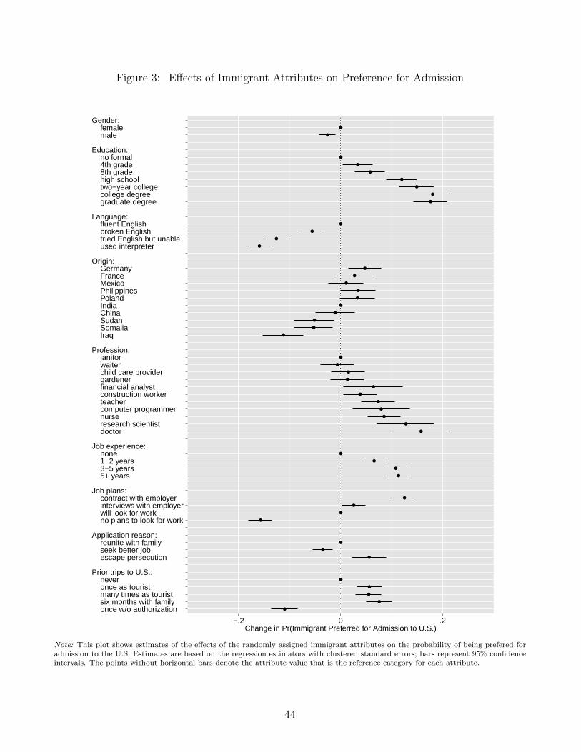
Figure 3: Effects of Immigrant Attributes on Preference for Admission

●

●

●

●

●

●

●

●

●

●

●

●

●

●

●

●

●

●

●

●

●

●

●

●

●

●

●

●

●

●

●

●

●

●

●

●

●

●

●

●

●

●

●

●

●

●

●

●

●

●

once w/o authorization six months with family many times as tourist once as tourist neverPrior trips to U.S.: escape persecution seek better job reunite with familyApplication reason: no plans to look for work will look for work interviews with employer contract with employerJob plans: 5+ years 3−5 years 1−2 years noneJob experience: doctor research scientist nurse computer programmer teacher construction worker financial analyst gardener child care provider waiter janitorProfession: Iraq Somalia Sudan China India Poland Philippines Mexico France GermanyOrigin: used interpreter tried English but unable broken English fluent EnglishLanguage: graduate degree college degree two−year college high school 8th grade 4th grade no formalEducation: male femaleGender:

−.2 0 .2Change in Pr(Immigrant Preferred for Admission to U.S.)

Note: This plot shows estimates of the effects of the randomly assigned immigrant attributes on the probability of being prefered foradmission to the U.S. Estimates are based on the regression estimators with clustered standard errors; bars represent 95% confidenceintervals. The points without horizontal bars denote the attribute value that is the reference category for each attribute.

44

Figure 4: Effects of Immigrant Attributes on Preference for Admission by Ethnocentrism

Low Ethnocentrism High Ethnocentrism

●

●

●

●

●

●

●

●

●

●

●

●

●

●

●

●

●

●

●

●

●

●

●

●

●

●

●

●

●

●

●

●

●

●

●

●

●

●

●

●

●

●

●

●

●

●

●

●

●

●

●

●

●

●

●

●

●

●

●

●

●

●

●

●

●

●

●

●

●

●

●

●

●

●

●

●

●

●

●

●

●

●

●

●

●

●

●

●

●

●

●

●

●

●

●

●

●

●

●

●

once w/o authorization six months with family many times as tourist once as tourist neverPrior trips to U.S.: escape persecution seek better job reunite with familyApplication reason: no plans to look for work will look for work interviews with employer contract with employerJob plans: 5+ years 3−5 years 1−2 years noneJob experience: doctor research scientist nurse computer programmer teacher construction worker financial analyst gardener child care provider waiter janitorProfession: Iraq Somalia Sudan China India Poland Philippines Mexico France GermanyOrigin: used interpreter tried English but unable broken English fluent EnglishLanguage: graduate degree college degree two−year college high school 8th grade 4th grade no formalEducation: male femaleGender:

−.2 0 .2 −.2 0 .2Change in Pr(Immigrant Preferred for Admission to U.S.)

Note: These plots show estimates of the effects of the randomly assigned immigrant attributes on the probability of being prefered for admission to the U.S. conditional onrespondents’ prior levels of ethnocentrism. At left, we see estimates for respondents with low levels of ethnocentrism, while at right we see estimates for respondents with highlevels of ethnocentrism. Estimates are based on the regression estimators with clustered standard errors; bars represent 95% confidence intervals. The points without horizontalbars denote the attribute value that is the reference category for each attribute.

45

Figure 5: Interaction of Immigrant’s Jobs Plans and Other Attributes on Preference for Admission

Immigrant Has Contract with an Employer Immigrant Has No Plans to Look for Work

●

●

●

●

●

●

●

●

●

●

●

●

●

●

●

●

●

●

●

●

●

●

●

●

●

●

●

●

●

●

●

●

●

●

●

●

●

●

●

●

●

●

●

●

●

●

●

●

●

●

●

●

●

●

●

●

●

●

●

●

●

●

●

●

●

●

●

●

●

●

●

●

●

●

●

●

●

●

●

●

●

●

●

●

●

●

●

●

●

●

●

●

●

●

●

●

●

●

●

●

●

●

●

●

●

●

●

once w/o authorization six months with family many times as tourist once as tourist neverPrior trips to U.S.: escape persecution seek better job reunite with familyApplication reason: 5+ years 3−5 years 1−2 years noneJob experience: doctor research scientist nurse computer programmer teacher construction worker financial analyst gardener child care provider waiter janitorProfession: Iraq Somalia Sudan China India Poland Philippines Mexico France GermanyOrigin: used interpreter tried English but unable broken English fluent EnglishLanguage: graduate degree college degree two−year college high school 8th grade 4th grade no formalEducation: male femaleGender:

−.2 0 .2 −.2 0 .2Change in Pr(Immigrant Preferred for Admission to U.S.)

Note: These plots show estimates of the effects of the randomly assigned immigrant attributes on the probability of being prefered for admission to the U.S. conditional on theimmigrant’s job plans. At left, we see estimates for profiles where the immigrant has a contract with an employer, while at right we see estimates for profiles where the immigranthas no plans to look for work. Estimates are based on the regression estimators with clustered standard errors; bars represent 95% confidence intervals. The points withouthorizontal bars denote the attribute value that is the reference category for each attribute.

46

Supplemental Information

A Proof of Proposition 1We prove that the subclassification estimator defined in equation (8) is unbiased for the AMCEdefined in equation (4). Under Assumptions 1-3, the AMCE is identified by the observed data as,

ˆπl(t1, t0, p(t)) =∑

[t[−l],t[−j]]∈T

{E[Yijk | Tijkl = t1, Tijk[−l] = t[−l],Ti[−j]k = t[−j]]

−E[Yijk | Tijkl = t0, Tijk[−l] = t[−l],Ti[−j]k = t[−j]]}

×Pr(Tijk[−l] = t[−l],Ti[−j]k = t[−j]),

which is equivalent to equation (5) except that this expression makes explicit that the componentsof Tijk[−l] and Ti[−j]k are discrete random variables. Under Assumption 4, we have

ˆπl(t1, t0, p(t))

=∑

[tS ,t[−j]]∈T S

∑tR∈T R

{E[Yijk | Tijkl = t1, T

Sijk = tS, TR

ijk = tR,Ti[−j]k = t[−j]]

−E[Yijk | Tijkl = t0, TSijk = tS, TR

ijk = tR,Ti[−j]k = t[−j]]}

×Pr(T Sijk = tS,Ti[−j]k = t[−j] | TR

ijk = tR) Pr(TRijk = tR)

=∑

[tS ,t[−j]]∈T S

∑tR∈T R

{E[Yijk | Tijkl = t1, T

Sijk = tS, TR

ijk = tR,Ti[−j]k = t[−j]]

×Pr(T Sijk = tS,Ti[−j]k = t[−j] | Tijkl = t1, T

Rijk = tR)

−E[Yijk | Tijkl = t0, TSijk = tS, TR

ijk = tR,Ti[−j]k = t[−j]]

×Pr(T Sijk = tS,Ti[−j]k = t[−j] | Tijkl = t0, T

Rijk = tR)

}Pr(TR

ijk = tR)

=∑

tR∈T R

{E[Yijk | Tijkl = t1, T

Rijk = tR]− E[Yijk | Tijkl = t0, T

Rijk = tR]

}Pr(TR

ijk = tR), (11)

where the first and third equalities follow from the law of total expectation and the second equalityfrom Assumption 4. Sample analogues provide unbiased estimators of both conditional expecta-tions in equation 11. The remaining term is a known assignment probability which we calculate bymarginalizing p(t). The resulting estimator is the subclassification estimator from equation (8).

47

Figure A.1: Experimental Design: Candidate Conjoint

Note: This figure illustrates the experimental design for the conjoint analysis that examines competing candidates for political office.

48

Figure A.2: Effects of Immigrant Attributes on Preference for Admission by Choice Task

Task Number: 1 Task Number: 2 Task Number: 3 Task Number: 4 Task Number: 5

●

●

●

●

●

●

●

●

●

●

●

●

●

●

●

●

●

●

●

●

●

●

●

●

●

●

●

●

●

●

●

●

●

●

●

●

●

●

●

●

●

●

●

●

●

●

●

●

●

●

●

●

●

●

●

●

●

●

●

●

●

●

●

●

●

●

●

●

●

●

●

●

●

●

●

●

●

●

●

●

●

●

●

●

●

●

●

●

●

●

●

●

●

●

●

●

●

●

●

●

●

●

●

●

●

●

●

●

●

●

●

●

●

●

●

●

●

●

●

●

●

●

●

●

●

●

●

●

●

●

●

●

●

●

●

●

●

●

●

●

●

●

●

●

●

●

●

●

●

●

●

●

●

●

●

●

●

●

●

●

●

●

●

●

●

●

●

●

●

●

●

●

●

●

●

●

●

●

●

●

●

●

●

●

●

●

●

●

●

●

●

●

●

●

●

●

●

●

●

●

●

●

●

●

●

●

●

●

●

●

●

●

●

●

●

●

●

●

●

●

●

●

●

●

●

●

●

●

●

●

●

●

●

●

●

●

●

●

●

●

●

●

●

●

●

●

●

●

●

●

●

●

●

●

●

●

●

●

●

●

●

●

●

●

●

●

●

once w/o authorization six months with family many times as tourist once as tourist neverPrior trips to U.S.: escape persecution seek better job reunite with familyApplication reason: no plans to look for work will look for work interviews with employer contract with employerJob plans: 5+ years 3−5 years 1−2 years noneJob experience: doctor research scientist nurse computer programmer teacher construction worker financial analyst gardener child care provider waiter janitorProfession: Iraq Somalia Sudan China India Poland Philippines Mexico France GermanyOrigin: used interpreter tried English but unable broken English fluent EnglishLanguage: graduate degree college degree two−year college high school 8th grade 4th grade no formalEducation: male femaleGender:

−.2 0 .2 −.2 0 .2 −.2 0 .2 −.2 0 .2 −.2 0 .2Change in Pr(Immigrant Preferred for Admission to U.S.)

Note: These plots show estimates of the effects of the randomly assigned immigrant attributes on the probability of being preferred for admission to the U.S. conditional onthe number of the choice task. Estimates are based on the regression estimators with clustered standard errors; bars represent 95% confidence intervals. The points withouthorizontal bars denote the attribute value that is the reference category for each attribute.

49

Figure A.3: Effects of Immigrant Attributes on Preference for Admission by Profile Number

Profile Number: 1 Profile Number: 2

●

●

●

●

●

●

●

●

●

●

●

●

●

●

●

●

●

●

●

●

●

●

●

●

●

●

●

●

●

●

●

●

●

●

●

●

●

●

●

●

●

●

●

●

●

●

●

●

●

●

●

●

●

●

●

●

●

●

●

●

●

●

●

●

●

●

●

●

●

●

●

●

●

●

●

●

●

●

●

●

●

●

●

●

●

●

●

●

●

●

●

●

●

●

●

●

●

●

●

●

●

●

●

●

●

●

●

●

●

●

●

●

●

●

●

●

●

once w/o authorization six months with family many times as tourist once as tourist neverPrior trips to U.S.: escape persecution seek better job reunite with familyApplication reason: no plans to look for work will look for work interviews with employer contract with employerJob plans: 5+ years 3−5 years 1−2 years noneJob experience: doctor research scientist nurse computer programmer teacher construction worker financial analyst gardener child care provider waiter janitorProfession: Iraq Somalia Sudan China India Poland Philippines Mexico France GermanyOrigin: used interpreter tried English but unable broken English fluent EnglishLanguage: graduate degree college degree two−year college high school 8th grade 4th grade no formalEducation: male femaleGender:

−.2 0 .2 −.2 0 .2Change in Pr(Immigrant Preferred for Admission to U.S.)

Note: These plots show estimates of the effects of the randomly assigned immigrant attributes on the probability of being preferred for admission to the U.S. conditional on theprofile number (i.e. whether the profile is listed first or second in a given task). Estimates are based on the regression estimators with clustered standard errors; bars represent95% confidence intervals. The points without horizontal bars denote the attribute value that is the reference category for each attribute.

50

Figure A.4: Effects of Immigrant Attributes on Preference for Admission by Row Position ofAttribute

●

●

●

●

●

●

●

●

●

●

−0.4 −0.3 −0.2 −0.1 0.0 0.1

Language: fluent English −> used interpreter

Change in Pr(Immigrant Preferred for Admission to U.S.)

Row

Pos

ition

of L

angu

age

Attr

ibut

e

●

98

76

54

32

1P

oole

d

●

●

●

●

●

●

●

●

●

●

−0.4 −0.3 −0.2 −0.1 0.0 0.1

Prior trips to U.S.: never −> once w/o authorization

Change in Pr(Immigrant Preferred for Admission to U.S.)

Row

Pos

ition

of P

rior

trip

s A

ttrib

ute

●

98

76

54

32

1P

oole

d

Note: These plots show estimates of the effects of the randomly assigned immigrant attributes on the probability of being preferredfor admission to the U.S. conditional on the row position of the attribute (i.e. whether the attribute is listed in the first row, secondrow, etc. in a given task). The estimate with the filled black dot in the top row in each panel refers to the pooled estimate acrossall row positions. The top panel shows the estimates for the effect of varying the Language attribute from “spoke fluent English” to“used an interpreter” during the admissions interview. The bottom panel shows the estimates for the effect of varying the “prior tripsto the U.S.” attribute from “never” to “once without authorization.” Estimates are based on the regression estimators with clusteredstandard errors; bars represent 95% confidence intervals.

51

Figure A.5: Effects of Immigrant Attributes on Preference for Admission by Number of Atypical Profiles

# of countertypical profiles: 0−3 # of countertypical profiles: 4−5 # of countertypical profiles: 6−9

●

●

●

●

●

●

●

●

●

●

●

●

●

●

●

●

●

●

●

●

●

●

●

●

●

●

●

●

●

●

●

●

●

●

●

●

●

●

●

●

●

●

●

●

●

●

●

●

●

●

●

●

●

●

●

●

●

●

●

●

●

●

●

●

●

●

●

●

●

●

●

●

●

●

●

●

●

●

●

●

●

●

●

●

●

●

●

●

●

●

●

●

●

●

●

●

●

●

●

●

●

●

●

●

●

●

●

●

●

●

●

●

●

●

●

●

●

●

●

●

●

●

●

●

●

●

●

●

●

●

●

●

●

●

●

●

●

●

●

●

●

●

●

●

●

●

●

●

●

●

●

●

●

●

●

●

●

●

●

●

●

●

●

●

●

●

●

once w/o authorization six months with family many times as tourist once as tourist neverPrior trips to U.S.: escape persecution seek better job reunite with familyApplication reason: no plans to look for work will look for work interviews with employer contract with employerJob plans: 5+ years 3−5 years 1−2 years noneJob experience: doctor research scientist nurse computer programmer teacher construction worker financial analyst gardener child care provider waiter janitorProfession: Iraq Somalia Sudan China India Poland Philippines Mexico France GermanyOrigin: used interpreter tried English but unable broken English fluent EnglishLanguage: graduate degree college degree two−year college high school 8th grade 4th grade no formalEducation: male femaleGender:

−.2 0 .2 −.2 0 .2 −.2 0 .2Change in Pr(Immigrant Preferred for Admission to U.S.)

Note: These plots show estimates of the effects of the randomly assigned immigrant attributes on the probability of being preferred for admission to the U.S. conditional on thegroup of respondents exposed to a small, medium, or high number of atypical immigrant profiles. Estimates are based on the regression estimators with clustered standard errors;bars represent 95% confidence intervals. The points without horizontal bars denote the attribute value that is the reference category for each attribute.

52