causal inference for real-world evidence: propensity score
TRANSCRIPT

Causal Inference for Real-World Evidence:Propensity Score Methods and Case Study
# 1
Hana Lee, Ph.D. [email protected]
Office of BiostatisticsCenter for Drug Evaluation and Research
U.S. Food and Drug Administration
The ASA Biopharmaceutical Section Regulatory-Industry Statistics Workshop
September 22, 2020

2
# 2
www.fda.gov
Disclaimer
This presentation reflects the view of the author and should not be construed to represent FDA’s views or policies.

3
# 3
www.fda.gov
Course Outline
• Causal Inference for Real-World Evidence (RWE) : Propensity Score Methods and Case Study
• This short course will cover:– Causal inference framework– Propensity Score (PS) and PS-based methods – Associated target population and target estimand

4
# 4
www.fda.gov
Course Outline
• At the conclusion of this short course, participants should be able to:– Distinguish causation from association– Understand why the use of standard statistical models (including machine learning)
is inadequate to estimate a causal effect – Understand causal inference framework and how to formally define a target causal
estimand– Understand necessary conditions to infer a causal effect and inherent limitation of
observational study– Understand methodologic basis of PS matching and weighting (including marginal
structural model)– Weigh pros and cons of different methods to a causal inference problem– Use best practices of matching/weighting methods to a causal inference problem – Implement different causal methods and interpret findings accordingly

5
# 5
www.fda.gov
Course Outline
• Throughout, assume that we are interested in estimating the causal effect of a binary, point drug treatment setting: • Treatment (new drug) vs. control (active or placebo) • Patients take a drug at baseline (one time)• No censoring or loss to follow-up

6
# 6
www.fda.gov
Part 1Introduction to Causal Inference
7
# 7
www.fda.gov
Introduction to Causal Inference: Association vs. Causation
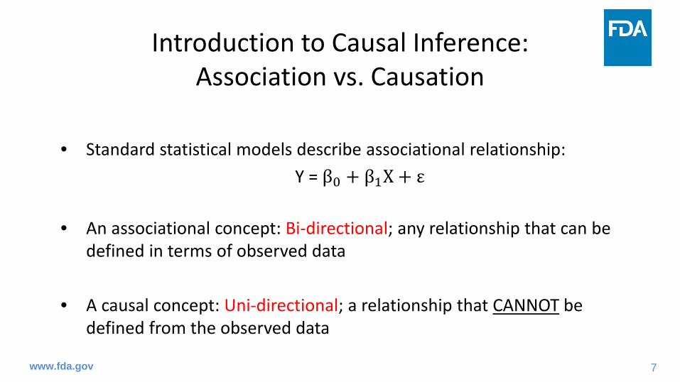
• Standard statistical models describe associational relationship:Y = β0 + β1X + ε
• An associational concept: Bi-directional; any relationship that can be defined in terms of observed data
• A causal concept: Uni-directional; a relationship that CANNOT be defined from the observed data

8
# 8
www.fda.gov
Introduction to Causal Inference: When possible?
• When data attributes allow us to infer causal effect:• Data obtained from randomized trial• When outcome and covariate have a particular direction (time, space,
etc.) in the absence of confounding Central dogma: DNA -> RNA -> protein RNA = β0 + β1DNA + ε
• Causal methods: aim to manipulate data so that it mimics (emulates) data from randomized trials

9
# 9
www.fda.gov
Introduction to Causal Inference: Randomized Trial vs. Observational Study
• Randomized clinical trial:• Treatment (intervention) assignment random• Two groups are similar on average• Difference in response treatment
• Observational study:• Treatment selection physician-patient preference• Difference in response treatment only • Confounders: related to both treatment and outcome

10
# 10
www.fda.gov
Causal Inference
• Ideal solution: Conduct a randomized trial
• Even more ideal: The best way to obtain a causal effect of a drug T=0,1 on outcome Y from your sample• Observe Y under T=0 from everybody• Observe Y under T=1 from everybody• Compare average of the two outcomes: E(Y|T=0) – E(Y|T=1)
• Requires to observe outcomes under treatment and control simultaneously from all subjects in the sample
• This problem leads to the notion of “potential outcome” • Some literature call it “counterfactual”
measured at the same time

11
# 11
www.fda.gov
Potential Outcome: Hypothetical Example
• HIV/AIDS example• Treatment: Antiretroviral therapy (ART)• Observed outcome (Y): CD4 counts after taking or not taking ART, higher the better.• Truth: ART if beneficial Taking ART increases CD4 counts (improves immune system).• Confounding by age and sex: Older male (sicker) patients are more likely to take ART.
Association= 600 – 867 = -267 <0 Treatment is detrimental.

12
# 12
www.fda.gov
How potential outcomes relate to observed data
Association and causation can be in completely opposite direction!

13
# 13
www.fda.gov
Defining Causal Estimands: Notation
• Focus on a binary point treatment setting:
• i = 1,…, N : subject ID• Ti = 1 (treatment) or 0 (control): Treatment indicator for subject i• Yi(1): potential outcome for subject i when Ti=1• Yi(0): potential outcome for subject i when Ti=0• Yi: observed outcome for subject i• Ci: baseline confounder(s) for subject i

14
# 14
www.fda.gov
Defining Causal Estimands
• Individual-level causal effect: Yi(1) - Yi(0)
• Population-level causal effect = Average treatment effect (ATE)= E{ Y(1) - Y(0) }
• Subgroup-level causal effect• Average treatment effect among treated (ATT)
= E{ Y(1) - Y(0) | T=1 }
• Can also define in terms of ratios, other sub-groups, etc.

15
# 15
www.fda.gov
Causal Estimands: ATE vs. ATT
Figure: Graphical representation of ATE and ATT
ATE: What happens if everybody had received AZT vs if everybody had received stavudine?
vs
ATT: What happens if patient received AZT would have received stavudine?
vs
AZT Stavudine
AZT Stavudine
HIV infected patients
AZTStavudine
= +

16
# 16
www.fda.gov
Causal Inference: Limitations
• The fundamental objective of causal inference is to draw conclusions about potential outcomes from observed data.
• The fundamental difficulty is that potential outcomes are never fully observed.
• Deduce the relationship between treatment and potential outcomes given covariates ({Y(1), Y(0), T, C}) using partially observed data ({(Y, T, C)}. Need to make assumptions!

17
# 17
www.fda.gov
Causal Inference: Assumptions
1. Consistency: Y = T * Y(1) + (1-T) * Y(0) • Yi = Yi(1) if subject i is treated (Ti=1)• Yi = Yi(0) if subject i is untreated (Ti=0)• May not hold under poor treatment adherence, lost-to-follow-up, and
interference
2. No unmeasured confounding: T ꓕ {Y(1), Y(0)}|C (a.k.a., strong ignorability, conditional exchangeability, exogeneity, etc.)
3. Positivity: pr(T=t | C=c) >0 for all (t,c)

18
# 18
www.fda.gov
Limitations
• Why observational studies are criticized?
• No unmeasured confounding: T ꓕ {Y(1), Y(0)}|C
• Why randomized trials are valid? T ꓕ {Y(1), Y(0)}
• When would randomized trials be invalid? When causal assumptions are not satisfied.

19
# 19
www.fda.gov
Part 2Causal Methods: Matching and IPW

20
# 20
www.fda.gov
Outline
• Propensity score (PS): Theory and implication
• PS Matching
• PS Weighting (including marginal structural model)
• Strength and limitation

21
# 21
www.fda.gov
Propensity Score

22
# 22
www.fda.gov
Propensity Score
• In a binary point treatment setting:
• Propensity score (PS) is defined by: Pr(T=1|C) = π(C)
• It refers to the probability of receiving treatment given observed covariates (patient/prescriber characteristics, etc.).

23
# 23
www.fda.gov
Key Result of PS Theory: Rosenbaum & Rubin (1983)2
• If no unmeasured confounding holds:
T ꓕ {Y(1), Y(0)}|C T ꓕ {Y(1), Y(0)}| π(C)
• If treatment is independent (= random) once conditioning on observed confounding information, treatment is also independent conditional on propensity score.
24
# 24
www.fda.gov
Key Result of PS Theory: Practical Implication
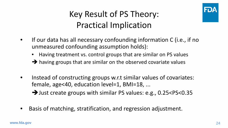
• If our data has all necessary confounding information C (i.e., if no unmeasured confounding assumption holds):• Having treatment vs. control groups that are similar on PS values having groups that are similar on the observed covariate values
• Instead of constructing groups w.r.t similar values of covariates: female, age<40, education level=1, BMI=18, ...Just create groups with similar PS values: e.g., 0.25<PS<0.35
• Basis of matching, stratification, and regression adjustment.

25
# 25
www.fda.gov
Matching

26
# 26
www.fda.gov
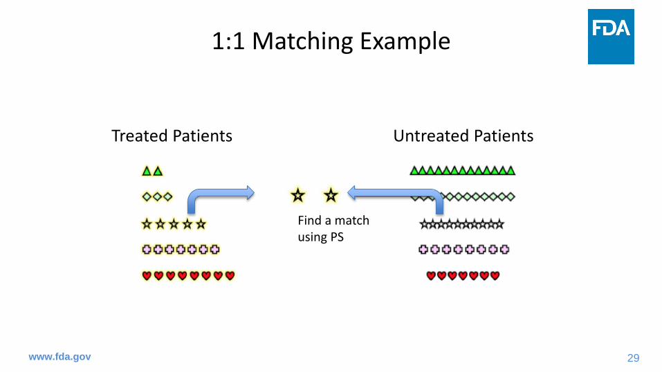
Matching: 1-to-1 Matching Example
1. Randomly select a subject from treatment group
2. Find a subject from control group who has exactly the same or similarPS: forms a matched pair
3. Iterate this process until no one left in treatment group or no match exists create final treatment and control groups
4. Examine covariate balance between treatment and control groups
5. Conduct final analysis to compare response between the two groups

27
# 27
www.fda.gov
1:1 Matching Example
Treated Patients Untreated Patients
Dr. Thomas Love, Professor of Medicine at Case Western Reserve University. Pictures taken and modified from Dr. Love’s short course material from ICHPS 2018.

28
# 28
www.fda.gov
1:1 Matching Example
Treated Patients Untreated Patients
Select a subject, perhaps at random
29
# 29
www.fda.gov
1:1 Matching Example
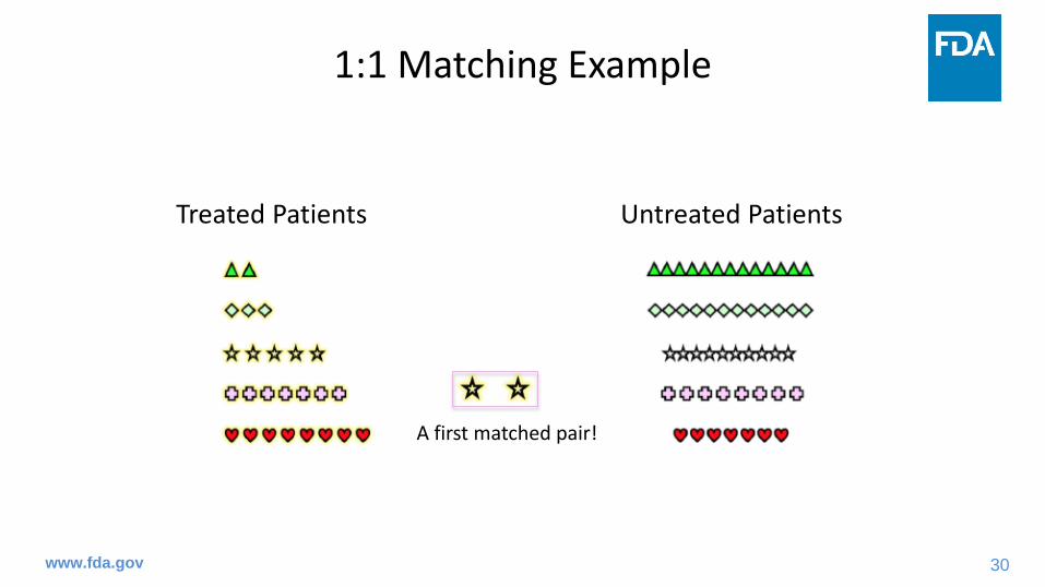
Treated Patients Untreated Patients
Find a matchusing PS
30
# 30
www.fda.gov
1:1 Matching Example
Treated Patients Untreated Patients
A first matched pair!

31
# 31
www.fda.gov
1:1 Matching Example
Treated Patients Untreated PatientsSelect another treated subject.

32
# 32
www.fda.gov
1:1 Matching Example
Treated Patients Untreated Patients
Find a good match.

33
# 33
www.fda.gov
1:1 Matching Example
Treated Patients Untreated Patients
A second matched pair!

34
# 34
www.fda.gov
1:1 Matching Example
Treated Patients Untreated Patients
Keep matching, until we find no more acceptable matches.

35
# 35
www.fda.gov
1:1 Matching Example
Treated Patients Untreated PatientsMatched Set (24 pairs)
36
# 36
www.fda.gov
Matching
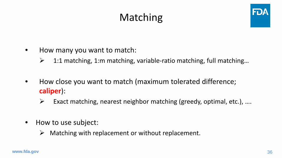
• How many you want to match: 1:1 matching, 1:m matching, variable-ratio matching, full matching…
• How close you want to match (maximum tolerated difference; caliper): Exact matching, nearest neighbor matching (greedy, optimal, etc.), ….
• How to use subject: Matching with replacement or without replacement.

37
# 37
www.fda.gov
Matching: Standard Error Estimation
• Matching without replacement: No further adjustment is needed
• Matching WITH replacement: The same subject was used multiple times• Give a weight: If a person is matched twice, give each a weight of ½• Robust standard error or bootstrap: caution when sample size is small.
• Areas of research: Should we account for variability in match? • Ignoring the matching step is asymptotically valid when matching is
done without replacement. But could be problematic when it’s done with replacement.

38
# 38
www.fda.gov
Matching: Implementation
• R package1. MatchIt: Most popular, does not do weighting (e.g., for full matching)
explicitly. Updates coming very soon. 2. twang: a very nice R package for weighting3. cobalt package and WeightIt: cobalt does some nice balance checks
• SAS: PSMATCH procedure (https://support.sas.com/documentation/onlinedoc/stat/142/psmatch.pdf)
• STATA: PSCORE for PS estimation and PSMATCH2 for PS matching
• See Dr. Joo-Yeon Lee’s presentation for more details

39
# 39
www.fda.gov
Matching: Considerations
1. How many matches to get? 1:1 vs 1:m• Some people reluctant to use small number for matched because it “throws
away data.” But sometimes it is a good thing, if that data not helpful.• If lots of controls available, may make sense to get more than one match for each
treated individual.• Unusual to be able to do more than say 1:2 unless control pool MUCH larger than
treatment group (Austin 20103).• Advice from E Stuart*: Work up from 1:1 to 1:2 to 1:3, etc.; keep increasing ratio
until balance gets worse Clearly state the process in statistical analysis plan.• Generally estimating ATT. So consider your target estimand first then choose a
method accordingly. • After that, it becomes a choice of caliper bias-variance trade-off problem.
*Dr. Elizabeth Stuart, Professor of Mental Health and Biostatistics at Johns Hopkins Bloomberg School of Public Health. Short course on PS methods at FDA, July 2017.

40
# 40
www.fda.gov
Matching: Considerations
2. Choice of caliper • Rosenbaum and Rubin (1985)4 used 0.25 standard deviations (SD) of PS
values based on the results of Cochran and Rubin (1973)5
taken as a recommendation
• Austin (2011)6 recommended reducing the caliper from 0.25 to 0.20 SD.
• The appropriate caliper depends on strength of confounding More confounding might require a tighter caliper
• Bias-variance trade-off: A tighter caliper can reduce bias but increase variance

41
# 41
www.fda.gov
Matching: Considerations
3. Greedy vs. Optimal algorithm?• Greedy: goes through treated units one at a time and picks the best match from
those available• Greedy without replacement: order matches chosen may make a difference• Optimal: allow earlier matches to be broken if overall bias will be reduced;
optimizes global distance measure• Often doesn’t make a huge difference: Gu and Rosenbaum (1993)7 “...optimal
matching picks about the same controls as greedy matching but does a better job of assigning them to treated units."
• Note: Doesn’t make a difference if matching with replacement• Advice from E Stuart: Do optimal if it’s easy but don’t worry too much about this

42
# 42
www.fda.gov
Matching: Considerations
4. Full matching• Fine stratification method: Full matching creates the subclasses
automatically• Creates lots of little subclasses, with either (1) 1 treated and multiple
controls or (2) 1 control and multiple treated in each subclass• Treated individuals with lots of good matches will get lots of matches; those
without many good matches won’t get many• Can also do constrained full matching, which limits the ratio of
treated:control in each subclass• Hansen (2004)8, Stuart and Green (2008; has sample code)9
• Optimal in terms of reducing bias on propensity score• Can estimate both ATE and ATT

43
# 43
www.fda.gov
Matching: Considerations
5. With or without replacement• Without replacement can yield bad matches higher bias• Without replacement is usually (matching) order dependent• With replacement may yield less bias but higher variance
• Keep track of how many times a control selected• Proper adjustment in standard error estimation (generally via
weighting) is required• Advice from E Stuart: Try without replacement, if not good balance
then try with replacement

44
# 44
www.fda.gov
Matching: Considerations
6. Balance check• Most common metric: Standardized mean difference (SMD)
• Difference in means between two groups, divided by standard deviation (like an effect size)
• SMD formula differ by type of variable (continuous, binary, etc.)
• Other possibilities: t-test, Wilcoxson test, Kolmogrov-Smirnov tests• Have to be careful of hypothesis tests, p-values because of differences
in power (Imai et al., 200810)

45
# 45
www.fda.gov
Matching: Considerations
7. Outcome analysis after matching (1)• Adjust or not to adjust for covariates in analysis model?
• Additional covariate adjustment is known to reduce bias and improve efficiency (Rubin and Thomas, 200011).
• Some considerations on adjusted analysis:• Non-collapsibility for non-linear models: Odds Ratio, hazard Ratio• Population-level effect (ATE): Marginal, unconditional treatment effect
additional step is needed to produce the marginal effect additional step is needed to estimate uncertainty of the effect
estimate

46
# 46
www.fda.gov
Matching: Considerations
7. Outcome analysis after matching (2)• Should we account for matched pair?
• Matches generally pooled together into just “treated” and “control” groups.
• We care only about average balance between treatment and control groups, not the balance within each pair.
• Don’t need to account for individual pairings.• See Austin (2008)12 and associated discussion and rejoinder for some
debate.

47
# 47
www.fda.gov
Inverse Probability Weighting

48
# 48
www.fda.gov
Inverse Probability Weighting: Motivation
• If we can observe potential outcomes {Yi(1), Yi(0)} from everybody:
unbiased estimator for ATE = 1N∑i=1N { Yi 1 − Yi 0 }
• However, …
• Missing data problem: Use inverse probability weighting (IPW) to account for missing potential outcome.
49
# 49
www.fda.gov
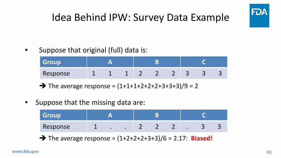
Idea Behind IPW: Survey Data Example
• Suppose that original (full) data is:
The average response = (1+1+1+2+2+2+3+3+3)/9 = 2
• Suppose that the missing data are:
The average response = (1+2+2+2+3+3)/6 = 2.17: Biased!
Group A B C
Response 1 1 1 2 2 2 3 3 3
Group A B C
Response 1 . . 2 2 2 . 3 3

50
# 50
www.fda.gov
Idea Behind IPW: Survey Data Example
Missing data:
• Group A: Probability of response = 1/3 IPW = 3• Group B: Probability of response = 1 IPW = 1• Group C: Probability of response = 2/3 IPW = 3/2
• Group A: Response 1 after weighting = 1*3 = 3 • Group B: Response 2 after weighting = 2*1 = 2• Group C: Response 3 after weighting = 3*3/2 = 9/2
Group A B C
Response 1 . . 2 2 2 . 3 3
Weighted average
= (3∗1 + 2∗3 + 9/2∗2)1∗3 + 3∗1 + 2∗3/2 = 2
Number of respondersin each group

51
# 51
www.fda.gov
Idea Behind IPW: Survey Data Example
Missing data:
• Group A: Response 1 after weighting = 1*3 3 = 1 + 1+ 1 • Group B: Response 2 after weighting = 2*1 2 + 2 + 2 = 2 + 2 + 2• Group C: Response 3 after weighting = 3*3/2 3*3/2 + 3*3/2 = 3 + 3 + (3 *1/2 + 3*1/2)
After weighting:
IPW eliminates bias by weighting “observed response” so that observed responses can represent not only themselves but also missing response from non-responders in the same group.
Group A B C
Response 1 . . 2 2 2 . 3 3
Group A B C
Response 1 1 1 2 2 2 3 3 3

52
# 52
www.fda.gov
• Analogy: • Responders vs. non-responders = Treated vs. untreated• Observed response = Observed outcome• Missing response = Unobserved part of potential outcome• Group info = confounder (patient-prescriber characteristics)• Missing at random = No unmeasured confounder
• Difference: Now each subject has two responses (potential outcomes under treatment and control) extend the idea of weighting and consider two different weighting – one for treated and the other for control.
IPW: Extend The Survey Idea

53
# 53
www.fda.gov
• Inverse probability of treatment weighting (IPTW)
• Each subject has two potential outcomes: Y(1) and Y(0)• Among untreated, Y(1) is missing.
• Recover missing Y(1) using information from treated patients: • Weight observed outcomes from treated patients (T=1) using inverse
probability of receiving treatment (= 1/PS) so that their outcomes not only represent themselves but also represent missing Y(1) from other similar individuals (in terms of C) who did NOT receive treatment.
Inverse Probability of Treatment Weighting

54
# 54
www.fda.gov
• The same principle applies to recover missing Y(0)
• Each subject has two potential outcomes: Y(1) and Y(0)• Among treated, Y(0) is missing.
• Recover missing Y(0) using information from untreated patients: • Weight observed outcomes from untreated patients (T=0) using inverse
probability of NOT receiving treatment (1/{1-PS}) so that their outcomes not only represent themselves but also represent missing Y(0) from other similar individuals (in terms of C) who DID receive treatment.
Inverse Probability of Treatment Weighting

55
# 55
www.fda.gov
IPW: Before Weighting
temp

56
# 56
www.fda.gov
IPW: After Weighting

57
# 57
www.fda.gov
IPW: After Weighting

58
# 58
www.fda.gov
• In the weighted population, these is no missing potential outcome.
• HR call it “pseudo-population” where treatment is exchangeable, i.e., there is no confounding in the pseudo-population where treatment effect can be interpreted as causal.
Inverse Probability of Treatment Weighting

59
# 59
www.fda.gov
• Common mistake: IPW artificially inflate sample size and inflate type-1 error.
• PS or 1-PS: always 0 – 1 (non-inclusive) weights are always >1 individuals will be represented multiple times in the weighted sample the IPW induces within-subject correlation
• Standard error estimation should account for the weighting (Hernan et al. 200013): Use robust (sandwich) variance estimator or bootstrap.
IPW: Standard Error Estimation

60
# 60
www.fda.gov
• Robust variance estimator is not adequate when sample size is small.• When n is small: tend to over-estimate true variance to protect model-
misspecification• When n is very small: direction unknown, either under- or over-estimate
true variance (estimation of the “meat” part is unstable)
• Rare disease: Robust variance estimator is not enough.
IPW: Standard Error Estimation

61
# 61
www.fda.gov
IPW: Implementation
• R package: A few available (eg, ipw), but no need to use a package1. Just run a regression model to estimate PS2. Add estimated PS to your data column 3. Fit final analysis model using weight option4. Don’t forget to specify a proper variance estimation option!
• SAS: same as R
• STATA: same as above. See also https://www.rand.org/content/dam/rand/pubs/presentations/PT100/PT147/RAND_PT147.binarytrts.pdf
• See Dr. Joo-Yeon Lee’s presentation for more details
62
# 62
www.fda.gov
1. Large weight• PS or 1-PS: always 0 – 1 (non-inclusive) weights are always >1 • If PS or (1-PS) is close to 0 (near positivity violation) IPW can be
very large• Strategies:
1) Stabilizing: multiply a stabilizing factor which is <1. Usually P[T=1] for treated, p[T=0] for untreated.
2) Normalize weight, standardize, etc.3) Truncation: Replace large weight(s) with smaller weight (99th, 97th, 95th
percentile…) 4) Trimming: Remove patients having large weight(s) from the sample.
IPW: Considerations

63
# 63
www.fda.gov
1. Large weight (continued)• Common misunderstanding:
• Original, unstabilized IPW artificially inflate the sample size whereas stabilized IPW does not.
• Stabilized IPW is better because treatment and control ratio is preserved.• Goal of stabilizing: downweight extreme weights. • Consequence of stabilizing: Proportion of treated and controls
remains the same as in the original (unweighted) population.
IPW: Considerations

64
# 64
www.fda.gov
IPW: Considerations
Figure: Graphical representation of ATE with and without stabilizing
ATE : What happens if everybody had received AZT vs if everybody had stavudine?= ATE with unstabilized IPW
vs
ATE with stabilized IPW: Multiply P(AZT) = 3/4 for AZT and P(stavudine)= ¼ for stavudine
vs
HIV infected patients
AZT Stavudine
AZT Stavudine
AZTStavudine
= +

65
# 65
www.fda.gov
2. Type of estimand: ATE vs ATT
• ATE weight: 1PS
for treated & 11−PS
for control• ATT weight: treated patients are reference weight is 1 for treated
equivalent to multiply ATE weight with PS
weight =1 for treated & PS1−PS
for control
• ATT weight: (somewhat) stabilized already where stabilizing factor = PS <1. In practice, extreme weights are rare with ATT unless there’s a near positivity violation.
IPW: Considerations

66
# 66
www.fda.gov
Causal Estimands: ATE vs. ATT
Figure: Graphical representation of ATE and ATT
ATE: What happens if everybody had received AZT vs if everybody had received stavudine?
vs
ATT: What happens if patient received AZT would have received stavudine?
vs
AZT Stavudine
AZT Stavudine
HIV infected patients
AZTStavudine
= +

67
# 67
www.fda.gov
Inverse Probability Weighting – Marginal Structural Model

68
# 68
www.fda.gov
• MSM: Simply, inverse-probability weighted models
• Implementation is straightforward: • Calculate PS and (1-PS) • For treated, weight their outcomes with 1/PS• For untreated, weight their outcomes with 1/(1-PS)• Fit a statistical model using treatment (T) as a sole covariate
• Idea: The weighted sample includes all Y(1) and Y(0). So you are modeling potential outcomes, not modeling observed outcomes!
Marginal Structural Model (MSM)

69
# 69
www.fda.gov
• Again, the weighting induces within-subject correlation: Use robust variance estimator or bootstrap.
MSM: Standard Error Estimation

70
# 70
www.fda.gov
• Hernan et al. (2001)13 (actually Robins et al. 199714): • IPW accounts for missing potential outcomes adjust for confounding• No confounding No need to adjust for them in the model• Model marginal mean of potential outcomes, not observed outcomes
causal model (i.e., structural model)
• We can estimate causal risk difference, causal risk ratio, causal odds ratio, causal hazard ratio, etc., using weighted sample.
MSM: Origin of Its Name

71
# 71
www.fda.gov
• Y(t): Potential outcome when treatment T=t (t=0,1)• Y: Observed outcome
Robins et al. (2000)15
• When 𝛼𝛼1 = 𝛼𝛼1∗, …? When treatment is uncounfounded (i.e., treatment is random).
Causal and Associational Models
Causal Models (MSMs) Associational Models
E{Y(t)} = 𝛼𝛼0 + 𝛼𝛼1𝑡𝑡 E(Y) = 𝛼𝛼0∗ + 𝛼𝛼1∗𝑡𝑡log [E{Y(t)}] = 𝛽𝛽0 + 𝛽𝛽1𝑡𝑡 log {E(Y)} = 𝛽𝛽0∗ + 𝛽𝛽1∗𝑡𝑡
logit [E{Y(t)}] = 𝛿𝛿0 + 𝛿𝛿1𝑡𝑡 logit {E(Y)} =𝛿𝛿0∗ + 𝛿𝛿1∗𝑡𝑡

72
# 72
www.fda.gov
Matching vs Weighting: Strength and Limitation

73
# 73
www.fda.gov
1:1 Matching Example
Treated Patients Untreated Patients
Dr. Thomas Love, Professor of Medicine at Case Western Reserve University. Pictures taken and modified from Dr. Love’s short course material from ICHPS 2018.

74
# 74
www.fda.gov
1:1 Matching Example
Treated Patients Untreated Patients
Select a subject, perhaps at random

75
# 75
www.fda.gov
1:1 Matching Example
Treated Patients Untreated Patients
Find a matchusing PS

76
# 76
www.fda.gov
1:1 Matching Example
Treated Patients Untreated Patients
A first matched pair!

77
# 77
www.fda.gov
1:1 Matching Example
Treated Patients Untreated PatientsSelect another treated subject.

78
# 78
www.fda.gov
1:1 Matching Example
Treated Patients Untreated Patients
Find a good match.

79
# 79
www.fda.gov
1:1 Matching Example
Treated Patients Untreated Patients
A second matched pair!

80
# 80
www.fda.gov
1:1 Matching Example
Treated Patients Untreated Patients
Keep matching, until we find no more acceptable matches.
81
# 81
www.fda.gov
1:1 Matching Example
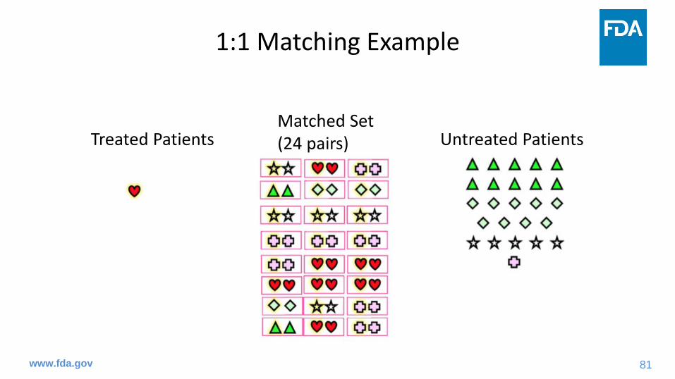
Treated Patients Untreated PatientsMatched Set (24 pairs)

82
# 82
www.fda.gov
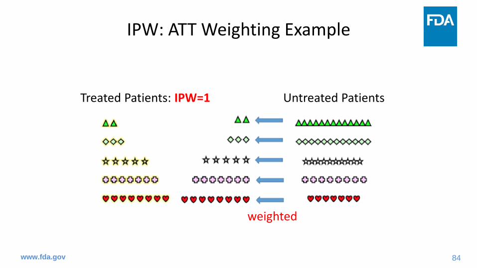
IPW: ATT Weighting Example
Treated Patients: IPW=1 Untreated Patients

83
# 83
www.fda.gov
IPW: ATT Weighting Example
Treated Patients: IPW=1 Untreated Patients
weighted
84
# 84
www.fda.gov
IPW: ATT Weighting Example
Treated Patients: IPW=1 Untreated Patients
weighted

85
# 85
www.fda.gov
IPW: ATT Weighting Example
Treated Patients: IPW=1 Untreated Patients: weighted
Weighted set: analysis sample

86
# 86
www.fda.gov
Matching• Strength: Very straightforward, easy to communicate with medical
division
• Weakness: • May discard some observations that don’t match
Distort your target population: Matched sample might not representative of your target population anymore. Less efficient, lost in power
• Some methods pre-determine your target estimand: Your estimand is ATT with 1:1 & 1:m matching.
• Extension to longitudinal setting is limited.
Strength and Limitation

87
# 87
www.fda.gov
Weighting • Strength:
• Can utilize all observations in most cases more efficient, higher power• Easy to extend to longitudinal setting: use MSM to control for time-varying
confounding
• Weakness:• Using all observations is not always a good thing. • Large weight can be problematic: distort your target population depending
on how you deal with the large weight• Some misunderstandings about the method exist.
Strength and Limitation

88
# 88
www.fda.gov
Matching & Weighting • Strength:
• Clearly separate design from analysis compared to other PS methods (eg, PS regression adjustment) or (some) outcome regression-based methods (discussed later if time permits)
• Weakness:• Compared to outcome regression-based methods
• PS methods require additional assumption: correctly specified PS model• (generally) less flexible
Strength and Limitation

89
# 89
www.fda.gov
Matching & Weighting: Statistical Analysis Plan
90
# 90
www.fda.gov
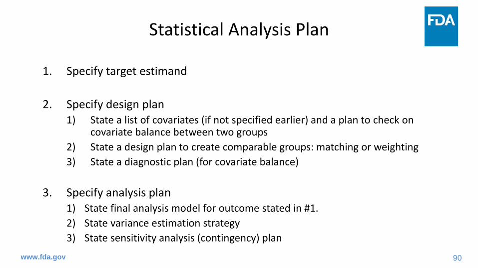
1. Specify target estimand
2. Specify design plan1) State a list of covariates (if not specified earlier) and a plan to check on
covariate balance between two groups2) State a design plan to create comparable groups: matching or weighting3) State a diagnostic plan (for covariate balance)
3. Specify analysis plan1) State final analysis model for outcome stated in #1. 2) State variance estimation strategy3) State sensitivity analysis (contingency) plan
Statistical Analysis Plan

91
# 91
www.fda.gov
1. Specify target estimand: Consider four attributes stated in ICH E9 (R1) addendum
1) Population: the patients targeted by the scientific question2) Variable (or endpoints): an measurement of some kind obtained from/for
each patient, that is required to address the scientific question3) Handling of intercurrent events: specifies how to account for intercurrent
events to reflect the scientific question of interest4) Population-level summary for the variable: provides, as required, a basis
for a comparison between treatment conditions.
Therefore, you should also provide description on population, exposure, outcome (endpoint), and a list of potential confounders in this step.
Statistical Analysis Plan: 1. Estimand

92
# 92
www.fda.gov
1. Specify target estimand
2. Specify design plan1) State a list of covariates (if not specified earlier) and a plan to check on
covariate balance between two groups2) State a design plan to create comparable groups: matching or weighting3) State a diagnostic plan (for covariate balance)
3. Specify analysis plan1) State final analysis model for outcome stated in #1. 2) State variance estimation strategy3) State sensitivity analysis (contingency) plan
Statistical Analysis Plan: 2. Design Plan
93
# 93
www.fda.gov
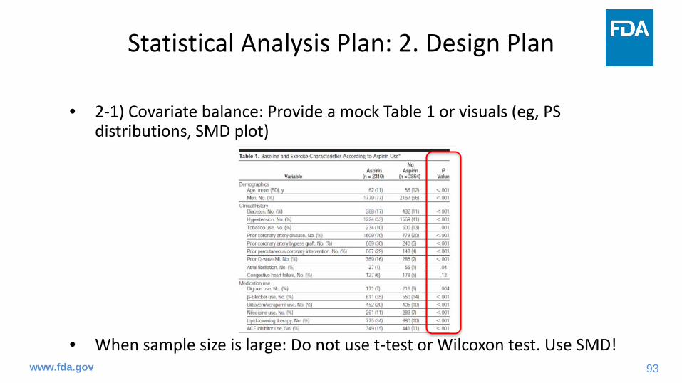
• 2-1) Covariate balance: Provide a mock Table 1 or visuals (eg, PS distributions, SMD plot)
• When sample size is large: Do not use t-test or Wilcoxon test. Use SMD!
Statistical Analysis Plan: 2. Design Plan

94
# 94
www.fda.gov
2-1) Covariate balance: PS distribution plot
Statistical Analysis Plan: 2. Design Plan
*Figures generated by an FDA reviewer for an intramural project.

95
# 95
www.fda.gov
2-1) Covariate balance: SMD plot (LOVE plot)
Statistical Analysis Plan: 2. Design Plan
*Figures generated by an FDA reviewer for an intramural project.0.2

96
# 96
www.fda.gov
2-2) State a design plan:a) State a method to create comparable groups (matching, weighting, etc.)b) State a list of potential confounders if not stated in Step 1.c) State a specific functional form of PS model:
• Main term logistic models using confounders listed in b).• Machine-learning: Specify details including information on cross-validation.• Regulatory setting emphasis is on pre-specification confounder
selection based on unblinded data is discouraged d) State details on matching/weighting:
• 1:1 matching, 1:m matching, full matching, caliper, etc. • Specific weight: ATE vs ATT? Unstabilized vs stabilized weight? Trimming?
Statistical Analysis Plan: 2. Design Plan

97
# 97
www.fda.gov
2-3) State a diagnostic plan:a) State a diagnostic plan after matching or weighting: tables or visualsb) State a contingency plan if covariate balance is unsuccessful
• Use of another PS model including interaction terms• Covariate adjustment in final analysis model using those still imbalanced
c) State a plan for poor PS overlap• Note that not including unmatched treated subjects or removing those
with large weights can distort your target population carefully think whether you can actually estimate what you stated as target estimand
Statistical Analysis Plan: 2. Design Plan

98
# 98
www.fda.gov
1. Specify target estimand
2. Specify design plan1) State a list of covariates (if not specified earlier) and a plan to check on
covariate balance between two groups2) State a design plan to create comparable groups: matching or weighting3) State a diagnostic plan (for covariate balance)
3. Specify analysis plan1) State final analysis model for outcome stated in #1. 2) State variance estimation strategy3) State sensitivity analysis (contingency) plan
Statistical Analysis Plan: 3. Analysis Plan

99
# 99
www.fda.gov
3-3) State sensitivity analysis• Data quality: Is there any important covariate that was not captured
in data? eg, smoking status in claims data • Sensitivity analysis to explore robustness of findings under the
(assumed) impact of unmeasured confounding• Sensitivity analysis using different functional forms of PS model and
outcome analysis model• Inclusion/exclusion of large weights
Statistical Analysis Plan: 3. Analysis Plan

100
# 100
www.fda.gov
Part 3Target (Causal) Estimand

101
# 101
www.fda.gov
• ICH E9 (R1) addendum: Estimands introduced with
“Central questions for drug development and licensing are to establish the existence, and to estimate the magnitude, of treatment effects: how the outcome of treatment compares to what would have happened to the same subjects under alternative treatment (i.e. had they not received the treatment, or had they received a different treatment). An estimand is a precise description of the treatment effect reflecting the clinical question posed by a given clinical trial objective. It summarises at a population level what the outcomes would be in the same patients under different treatment conditions being compared.”
Target Estimand

102
# 102
www.fda.gov
• While the main focus in the ICH E9(R1) is on randomized clinical trials (RCT), the principles are also applicable for single arm trials and observational studies as stated on page 5 of the ICH E9(R1).
• However, when it comes to non-RCT setting, defining target estimand becomes more complicated and more considerations are needed.
• This is related to causal assumptions that we HAVE TO make to be able to infer causal effect of a treatment using observational data.
Target Estimand

103
# 103
www.fda.gov
Causal Estimands: ATE vs. ATT
Figure: Graphical representation of ATE and ATT
ATE: What happens if everybody had received AZT vs if everybody had received stavudine?
vs
ATT: What happens if patient received AZT would have received stavudine?
vs
HIV infected patients
AZT Stavudine
AZT Stavudine
104
# 104
www.fda.gov
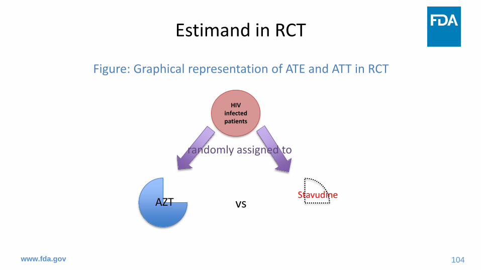
Estimand in RCT
Figure: Graphical representation of ATE and ATT in RCT
vs
HIV infected patients
AZTStavudine
randomly assigned to

105
# 105
www.fda.gov
• This choice comes in when you use non-RCT data.
• ATE: population level treatment effect
• ATT: subgroup level treatment effect
• ATE = ATT under no treatment heterogeneity (for linear outcomes)• Eg, treatment effect among female = Treatment effect among male Treatment effect among female = Treatment effect among all
• Treatment effect among treated = Treatment effect among control Treatment effect among treated/control = Treatment effect among all
ATE vs ATT

106
# 106
www.fda.gov
1. In the presence of treatment heterogeneity
2. Feasibility/Practicality
ATE vs ATT: When ATT is of interest?

107
# 107
www.fda.gov
1. In the presence of treatment heterogeneity
ATE vs ATT: When ATT is of interest?
Subject ID
(n=8)
Treatment: Low dose (0)
vs High dose (1)
Potential outcome
under low dose Y(0)
Potential outcome
under high dose Y(1)
Average Treatment Effect (ATE)
ATT for low dose
group (ATT_Low)
ATT for high dose
group (ATT_High)
1 0 1 1 0 0 NA2 0 0 1 1 1 NA3 0 0 1 1 1 NA4 0 0 0 0 0 NA5 1 0 0 0 NA 06 1 0 1 1 NA 17 1 1 1 0 NA 08 1 0 0 0 NA 0
Average 0.375 0.5 0.25
ATT_Low ≠ ATT_High ≠ ATE : Treatment heterogeneity

108
# 108
www.fda.gov
1. In the presence of treatment heterogeneity: An aggressive treatment case
(1)
(2)
• Risk detected from (1) could be much lower then risk detected from (2) • ATE may say there is no risk associated with the new treatment, but it
should not be administered to those eligible for first line therapy.
ATE vs ATT: When ATT is of interest?
Treated: Second
lineFirst line
Second line
First line
Treated: First line
Second-line

109
# 109
www.fda.gov
2. Feasibility/Practicality
• Second line chemotherapy regimen: potentially high barriers to participation and completion of the regimen• unrealistic to estimate the effect of the therapy if it were applied to all
current cancer patients
• Instead, greater interest may lie in the effect of the second line therapy on those current cancer patients who elect to receive (or eligible for) the therapy
• Limit your target population to patients who elect to receive the second line therapy
ATE vs ATT: When ATT is of interest?
110
# 110
www.fda.gov
• ATT implies that we are interested in the effect of a treatment drug (compared to a control drug) on the clinical benefit (or risk of having adverse outcome) on those who elect to take that drug (from patient perspective) or on those who are prescribed to that drug (from prescribers perspective)
ATE vs ATT: When ATT is of interest?

111
# 111
www.fda.gov
• Population with good overlap: Clinical equipoise16 or empirical equipoise17 (in treatment)
• Unlike RCT, there could be poor overlap (w.r.t PS distribution) between treatment and control groups potential bias, high variance, modeling sensitivity
• Reason for poor overlap: • Violation of positivity assumption could be a data quality issue• PS model misspecification
Estimand: Poor PS Overlap

112
# 112
www.fda.gov
• Solutions: • Matching: changing caliper, changing method (from 1:1 to full)• IPW: Weight stabilizing, truncation, trimming, normalization13
• Recent developments: overlap weights16, matching weights18, and entropy weights19
• Adjustment of covariates with remaining imbalance in analysis model• Find alternative, better quality data
• Presence of poor overlap: Reconsider your target population Reconsider if your target estimand is something you can actually estimate given your data.
Estimand: Poor Overlap


114
# 114
www.fda.gov
References1. Hernán MA, Robins JM. Estimating causal effects from epidemiological data. Journal of Epidemiology & Community Health.
2006 Jul 1;60(7):578-86.2. Rosenbaum PR, Rubin DB. The central role of the propensity score in observational studies for causal effects. Biometrika.
1983 Apr 1;70(1):41-55.3. Austin PC. Statistical criteria for selecting the optimal number of untreated subjects matched to each treated subject when
using many-to-one matching on the propensity score. American journal of epidemiology. 2010 Nov 1;172(9):1092-7.4. Rosenbaum PR, Rubin DB. Constructing a control group using multivariate matched sampling methods that incorporate the
propensity score, Am Stat, 1985, vol. 39 1(pg. 33-38)5. Cochran WG, Rubin DB. Controlling bias in observational studies: a review, Sankhyā: Indian J Stat, Ser A, 1973, vol. 35 4(pg.
417-446)6. Austin PC. Optimal caliper widths for propensity-score matching when estimating differences in means and differences in
proportions in observational studies, Pharm Stat, 2011, vol. 10 2(pg. 150-161)7. Gu XS, Rosenbaum PR. Comparison of multivariate matching methods: Structures, distances, and algorithms. Journal of
Computational and Graphical Statistics. 1993 Dec 1;2(4):405-20.8. Hansen BB. Full matching in an observational study of coaching for the SAT. Journal of the American Statistical Association.
2004 Sep 1;99(467):609-18.9. Stuart EA, Green KM. Using full matching to estimate causal effects in nonexperimental studies: examining the relationship
between adolescent marijuana use and adult outcomes. Developmental psychology. 2008 Mar;44(2):395.10. Imai K, King G, Stuart EA. Misunderstandings between experimentalists and observationalists about causal inference. Journal
of the royal statistical society: series A (statistics in society). 2008 Apr;171(2):481-502.

115
# 115
www.fda.gov
References11. Rubin DB, Thomas N. Combining propensity score matching with additional adjustments for prognostic covariates. Journal of
the American Statistical Association. 2000 Jun 1;95(450):573-85.12. Austin PC. A critical appraisal of propensity-score matching in the medical literature between 1996 and 2003. Statistics in
medicine. 2008 May 30;27(12):2037-49.13. Hernán MA, Brumback B, Robins JM. Marginal structural models to estimate the joint causal effect of nonrandomized
treatments. Journal of the American Statistical Association. 2001 Jun 1;96(454):440-8.14. Robins JM. Marginal structural models. In: 1997 Proceedings of the section on Bayesian statistical science. 15. Robins JM, Hernan MA, Brumback B. Marginal structural models and causal inference in epidemiology. 2000; 500-560.16. Li F, Thomas LE, Li F. Addressing extreme propensity scores via the overlap weights. American journal of epidemiology. 2019
Jan 1;188(1):250-7.17. Walker AM, Patrick AR, Lauer MS, Hornbrook MC, Marin MG, Platt R, Roger VL, Stang P, Schneeweiss S. A tool for assessing
the feasibility of comparative effectiveness research. Comp Eff Res. 2013 Jan 30;2013(3):11-20.18. Li L, Greene T. A weighting analogue to pair matching in propensity score analysis. The international journal of biostatistics.
2013 Jul 31;9(2):215-34.19. Hainmueller J. Entropy balancing for causal effects: A multivariate reweighting method to produce balanced samples in
observational studies. Political analysis. 2012 Jan 1:25-46.


1
Case Study
The risk of cardiovascular outcome and all cause mortality with outpatient use of
clarithromycin
Joo-Yeon Lee, Ph.D([email protected])
Division of Biometrics VIIOB/OTS/CDER/FDA
The ASA Biopharmaceutical Section Regulatory-Industry Statistics Workshop
September 22, 2020
This work has been published by American Journal of Epidemiology: https://www.ncbi.nlm.nih.gov/pubmed/29036565
2
Disclaimer• This presentation reflects the views of the
authors and should not be construed to represent FDA’s views or policies. The authors have no conflicts of interest to disclose.
3
Outline• Background• Study Overview• Statistical Methods and Results
– Two Treatment Arms Comparison (H.Pylori indication cohort)– Multiple Treatment Arms Comparison (All indication cohort)
• Software• Summary
4
Clarithromycin
• A class of macrolide antibiotics• Treatment for mild to moderate infections
caused by designated, susceptible bacteria such as acute bacterial exacerbation of chronic bronchitis, community-acquired pneumonia etc– H.Pylori bacteria eradication: triple therapy with PPI
and amoxicillin • Since approval, there were mixed findings of
risk of CV outcome or mortality

5
Drug Safety Communication
https://www.fda.gov/drugs/drug-safety-and-availability/fda-drug-safety-communication-fda-review-finds-additional-data-supports-potential-increased-long

6
Study Overview • Objective: To evaluate risks of cardiovascular events and all-
cause mortality in adult patients by use of clarithromycin • Design: A retrospective study of two new user cohorts in the
U.K. Clinical Practice Research Datalink (CPRD), from January 1, 2000 through December 31, 2013– All indication cohort (Main cohort)
• Clarithromycin (CLA) was compared to Doxycycline (DOXY) and Erythromycin (ERY)
– H. pylori indication cohort• A triple therapy with and without clarithromycin
– A proton pump inhibitor (PPI)+amoxicillin +clarithromycin(PPI+AMOX+CLA)– PPI + amoxicillin + metronidazole (PPI+AMOX+MET)
• Endpoints: – Primary endpoint: All-cause mortality– Secondary endpoints: A composite outcome defined as any first
occurrence of AMI, stroke and all-cause mortality

7
Patient Selection (All Indication)

8
Patient Selection (H.Pylori cohort)

H. pylori Indication Cohort with Two Treatment Arms

10
Confounding adjustment Method• Inverse probability of treatment weighting (IPTW) based on
propensity score (PS) – Propensity score was estimated by logistic regression by
adjusting 40 potential confounders
𝑙𝑙𝑙𝑙𝑙𝑙 𝑝𝑝(𝑇𝑇=1|𝑋𝑋)1−𝑃𝑃(𝑇𝑇=1|𝑋𝑋)
= 𝛽𝛽0 + 𝛽𝛽1X1+….+ 𝛽𝛽40X40
Where p(T=1|X) indicates the probability of treatment to PPI+AMOX+CLA group given 40 covariates
– Stabilized weight for each individual was computed by
Where PS indicates estimated PS from logistic regression and P(T=1) is the proportion of patients in PPI+AMOX+CLA group
• Targeting to estimate ATE

Why IPTW over Matching ?

12
Consideration of Sample Size• H. Pylori cohort is small cohort compared to all
indication cohort– There is less patients in comparator group
• The SS was reduced from a total of 42,502 pts to 29,726 pts by 1-1 matching – Before PS matching:
• PPI/AMOX/CLA: 27,639 (65%) • PPI/AMOX/MET: 14,863 (35%)
– After PS matching:• 14,863 for both group

13
Consideration of Consistency in Method
• All indication cohort has multiple treatment arms – CLA, DOXY and ERY
• IPTW was preferred to matching in the case of multiple treatment arms comparison – Matching is computationally intensive– Matching can lose even more sample size for
multiple arms
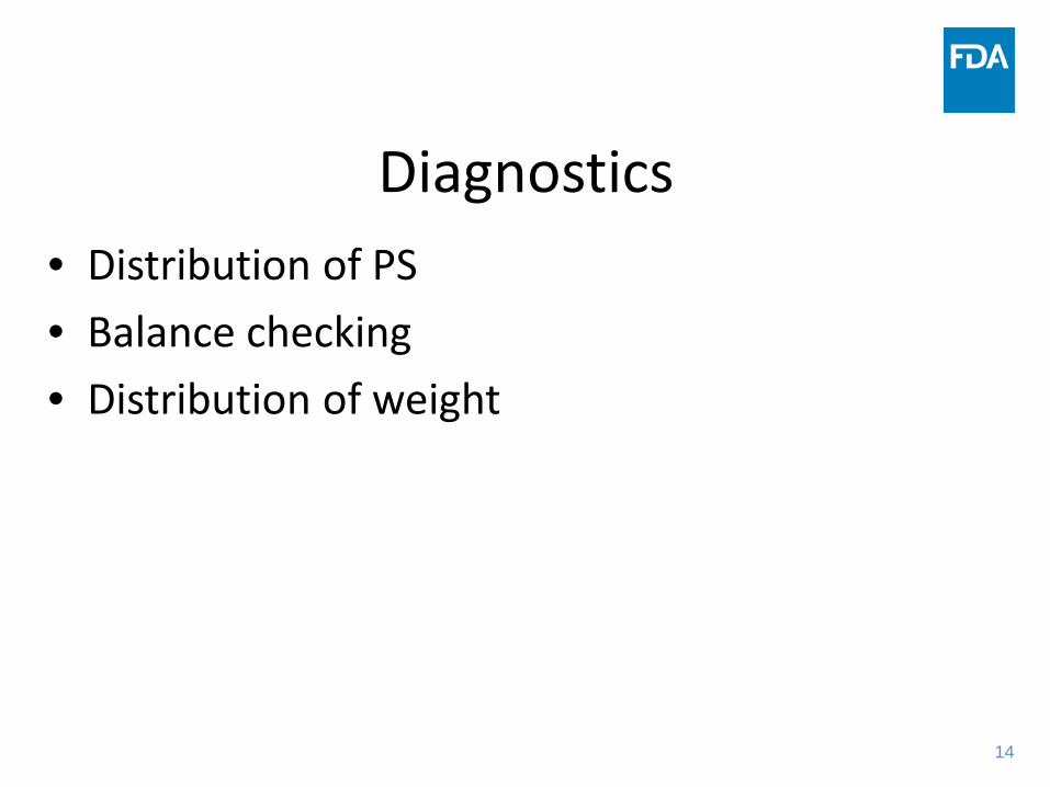
14
Diagnostics • Distribution of PS• Balance checking• Distribution of weight

15
Distribution of PS shows good overlap
Propensity Score
Test: PPI+AMOX+CLA
Comparator: PPI+AMOX+MET

16
Balance Checking
Standardized Mean Difference
● Before○ After Matching
● After IPTW
-30% -20% -10% 0 10% 20% 30%
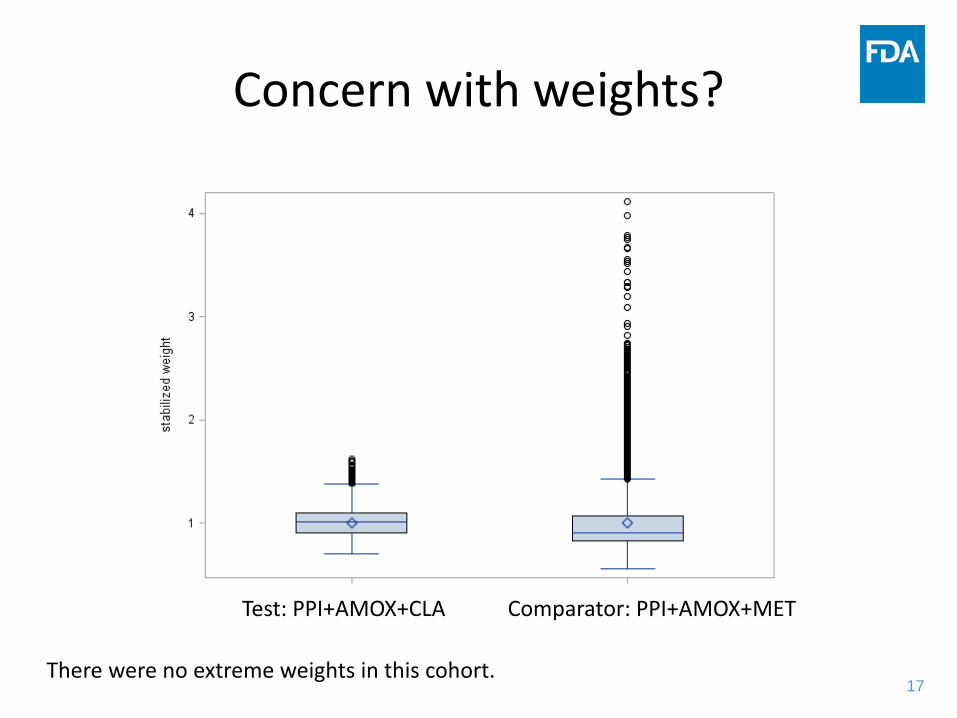
17
Concern with weights?
Test: PPI+AMOX+CLA Comparator: PPI+AMOX+MET
There were no extreme weights in this cohort.

18
Primary Outcome Model • Weighted Cox PH model
– To assess the effect of repeated exposures, the cumulative number of index drug Rx was a time-varying covariate with two levels of exposure (1 or 2+ cumulative Rx)
– Age variable (continuous) was doubly adjusted in the outcome model as well as PS model for any residual confounding.
Where Trt=1 if PPI+AMOX+CLA group, 0 otherwiseCum(t) is # of RX at time tAge is a patient age at baseline
– Robust variance estimator was used for standard error
))()(exp()()( 32100 AgetCumTrttCumTrtthth kk ββββ +•++=

19
Subgroup Analysis• Subgroup analysis was performed by statin use
– Weight was re-calculated within each subgroup
– Weighted Cox PH model was applied within subgroup

20
Primary Results:HR of All-cause Mortality

Main Cohort (All Indication Cohort) with Three Treatment Arms
(CLA vs. ERY / DOXY)

22
Propensity Score Methods for Multiple Treatment Arms
• Regression Adjustment (Imbens 2000, Spreeuwenberg 2010)• Weighting (Imbens 2000, Rao et al. 2014)• Stratification (Wang et al. 2001)• Matching (Rassen et al. 2012)• Note : Theoretical background remained same ( 2 groups vs. 3
groups) but there is practical complexity – Two groups : P(Trt=1)+P(Trt=2)=1
• So we can care about only P(Trt=1) as other probability is redundant
– Three groups : P(Trt=1)+P(Trt=2)+P(Trt=3)=1• We should care about two PSs out of Three

23
Regression Adjustment
1. Fit multinomial logistic regression 2. Predict PS1, PS2 and PS3 for each individual
using the fitted multinomial Logistic regression model
3. Include two PSs out of three PSs in the outcome model and estimate the effect of main covariate of interest– Sum of three PS should be 1 so one PS is
redundant in the model

24
Inverse Probability of Treatment Weighting (IPTW)
1. Fit a multinomial logistic regression and predict PS1, PS2 and PS3 for each individual
2. Calculate weights by taking inverse of PS or P(T=t)/PS for stabilized weight
3. Treatment effect is estimated using weighted regression model for outcome
Robust estimate of standard error should be used to account for within-subject correlation due to weighting

25
Stratification1. Fit a multinomial logistic regression and Predict PS1, PS2 and
PS3 for each individual using the fitted multinomial Logistic regression model
2. Make K strata based on percentiles of two of three PSs– Need to check the balance between groups within each stratum– If balance is not achieved, model may not be correct and need to
refine the model
3. Overall treatment effect is weighted average over each stratum by sample size in each stratum

26
PS Matching for Three groups
Three different methods (next few slides)• Pairwise matching• Common reference group matching• Three-way matching

27
Pairwise Matching
• Consider three contrast : Trt1 vs. Trt2, Trt1 vs. Trt3, Trt2 vs. Trt3
• Pairwise matching (3 cohorts)1. For each contrast estimate PS using logistic
regression2. Match on PS using proper matching method (e.g.
1:1 nearest neighbor matching) for each contrast3. Estimate treatment effect of each contrast using
matched cohort

28
Common Reference Group Matching• Consider TRT 1 (such as clarithromycin group) to be a
referent group• Using Trt 2 vs. Trt 1 and Trt 3 vs. Trt1 propensity-
matched population from pairwise matching in the previous slide1. Extract patients treated with Trt 2 or 3 who had a
common match of a patient who was treated with Trt 1.2. Form a single cohort of these patients and their Trt 1
matches.Produce generally smaller sample size

29
Three-way Matching1. Fit multinomial logistic regression to estimate three
propensity scores, PS1, PS2 and PS32. Find trio of patients – one receiving each of Trt1, 2
and 3 with the smallest within-trio distance d– One option, d= (PS1i-PS1j)2+(PS1i-PS1k)2 +(PS1j-
PS1k)2 + (PS2i-PS2j)2+(PS2i-PS2k)2 +(PS2j-PS2k)2,
where PS1, PS2 and PS3 are estimated PS score from multinomial logistic regression, i, j, k correspond to subjects who received treatment 1, 2 and 3
Computationally intensive

30
Statistical Methods• A total of 998,476 patients are in cohort
– Clarithromycin : 288,748 (28.8%)– Doxycycline : 267,729 (26.8%)– Erythromycin : 442,999 (44.4%)
• Propensity score model by multinomial logit model𝑙𝑙𝑙𝑙𝑙𝑙 𝑝𝑝(𝑇𝑇=𝑗𝑗|𝑋𝑋)
𝑃𝑃(𝑇𝑇=1|𝑋𝑋)= α𝑗𝑗 + 𝛽𝛽1X1+….+ 𝛽𝛽41X41
Where p(T=j|X) indicates the probability of treatment to CLA (j=1), DOXY(j=2) and ERY(j=3) given 41 covariates.
• Stabilized weight for each patient were calculated by
• Examined diagnostics for PS and weighting before analyzing outcome

31
Statistical Methods (cont.)• Primary outcome model: Weighted Cox PH regression
– To assess the effect of repeated exposures, the cumulative number of index drug Rx was a time-varying covariate
– Indication and age variables are doubly adjusted in the model
– Robust variance estimator was used for standard error
• Subgroup analyses by age, statin use, calcium channel blocker use, indication of COPD and pneumonia, prior ischemic heart disease status at baseline
• Sensitivity analyses by setting large weights above 90th
percentile to the ceiling of 90th percentile
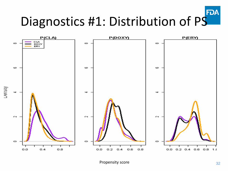
32
Diagnostics #1: Distribution of PS
Propensity score

33
Diagnostics #2: Balance CheckingBefore Weighting After Weighting
-30% -20% -10% 0 10% 20% 30% -20% -10% 0 10% 20% 30%
CLA vs. DOXY, CLA vs. ERY, DOXY vs. ERY

34
Diagnostics #3: The distribution of Weights
• It shows large weights for some patients so sensitivity analysis was performed to assessthe impact of large weights on study conclusion.
• It didn’t influence the primary study result.

35
Primary Results:HR of All-cause Mortality

SOFTWARE

37
Estimation of PS/**** SAS ***/proc logistic data = ps descending;CLASS Exp X1.. X2;MODEL exp (ref=“1”)=x1 x2… x40 /LINK=LOGIT; /** link=glogit for multinomial logit model **/ OUTPUT OUT=ps_Score PRED=ps;run;
/**** R ****//** TWO arms **/PS<-glm(exp~x1+x2+..+x40,data=, family=“binomial”)
/** THREE arms **/Library(nnet)Data$exp<-relevel(data$exp,ref=“1”)PS2<-multinom(exp~x1+x2+..x40, data=)

38
Weighted Cox PH model /*** SAS **/
proc phreg data=all covs(aggregate);ID subject;CLASS exp(ref="0") ;WEIGHT sw;model (start,stop)*out(0)=exp;run;
/*** R **/coxph(Surv(start, stop, out) ~ exp + cluster(id), weight=sw, data=)

39
Matching / *SAS macro */
%PSMatching(datatreatment=trt, datacontrol=con, method=caliper, numberofcontrols=1, caliper=0.2, replacement=no, out=psmatching_out);
/* R */library(MatchIt)psmatch <- matchit(exp ~x1+X2+..+x40,distance = "logit", method = "nearest", ratio = 1,replace = FALSE, caliper=0.2, data = data)

40
IPTW DO’S AND DON’TS
SUMMARY

41
Do # 1: Use Best Practices For Study Design
• Control for biases and confounding by design involve judicious choices ofo Data source o Inclusion/exclusion criteriao Appropriate comparatorso Outcome, exposure and
covariate codes/algorithms

42
Do # 2: Prespecify Estimand of Interest in the Protocol or SAP
• In IPTW, target estimand determines how weights are used in analysis. For example, – For target ATE all subjects are weighted– For target ATT (pairwise comparison), only control subjects are
weighted
Estimand Inference PopulationAverage Treatment Effect on the Treated (ATT) All those indicated for drug TAverage Treatment Effect (ATE) All those indicated for drugs T and C

43
Do #3 Check Diagnostics Diagnostics Checking Point
Distribution of PS To see overlap between treatment arms
Distribution of weights To examine any large weightsIf Yes → conduct sensitivity analysis
SMD before and after weighting
To ensure balance of potential confounders between treatment arms is achieved

44
Do # 4: Use Robust Estimation or Bootstrap for Standard Errors
Do #5: Include Sensitivity Analysis to Large Weights

45
Do #6: Keep yourself blinded to outcome while performing PS analysis
Lastly..

46
AcknowledgmentFDA Clarithromycin and CV Risk Study Team
Division of Biometrics VII• Joo-Yeon Lee, PhD
Office of Pharmacovigilance and Epidemiology• Andrew D Mosholder, MD, MPH (PI)• Esther H. Zhou, MD, PhD• David J. Graham, MD, MPH• Jacqueline Puigbo, PhD• Elizabeth M. Kang, MPH
Division of Anti-Infective Products• Mayurika Ghosh, MD
Children’s National Research Institute George Washington University • Rima Izem, PhD (former FDA employee)

47
References• Rao et al. “Azithromycin and Levofloxacin Use and Increased
Risk of Cardiac Arrhythmia and Death”, ANNALS OF FAMILY MEDICINE, 2014
• Imbens “The role of the propensity score in estimating dose-response functions”, Biometrika, 2000
• Spreeuwenberg et al. “The Multiple Propensity Score as Control for Bias in the Comparison of More Than Two Treatment Arms”, Medical Care, 2010
• Rassen et al. “ Matching by Propensity Score in Cohort Studies with Three Treatment Groups”, Epidemiology, 2013
• Wang et al. “The multiple propensity score for analysis of dose-response relationship in drug safety studies”, pharmacoepidemiology and drug safety, 2001
Clarithromycin CPRD Project

Thank You!