cauchy problems and best approximation by analytic functions in … · 2006-07-20 · cauchy...
TRANSCRIPT

Cauchy problems and best approximation byanalytic functions in 2 or 3 dimensions
Juliette Leblond
France
joint work with
B. Atfeh, L. Baratchart, S. Chaabane, M. Clerc, I. Fellah, M. Jaoua,M. Mahjoub, J.-P. Marmorat, T. Papadopoulo, J.R. Partington
INRIA, ENPC, EMP-CMA (France), ENIT-Lamsin (Tunisia), Univ. Leeds (U.K.)

Overview
In 2D and 3D
• Cauchy problems for ∆, examples
• Analytic functions and Hardy spaces
• Bounded extremal problems
• Numerical examples
• Conclusion

Cauchy problems for ∆
D ⊂ Rm , m = 2, 3, domain with smooth boundary T = T+ ∪ T−T± with disjoint interiors both of positive Lebesgue measure
From prescribed data φ (flux) and associated measurements ν(potential) on T+, find u, ∂nu on T−:
(IP)
∆u = 0 in Du = ν on T+
∂nu = φ on T+
ν, φ on T+ → u, ∂nu on T−?
T+T−
D
T+T
D
−

Cauchy problems for ∆
(IP)
∆u = 0 in Du = ν on T+
∂nu = φ on T+
ν, φ on T+ → u, ∂nu on T−?
(IP) admits unique solution u on T− φ ∈ L2(T+) ⇒ u ∈ W 1,2(T )
but ill-posed: strongly discontinuous w.r.t. data
∃ resolution algorithms [Kozlov, ...]
but need for numerical robustness w.r.t. errorsand stronger convergence results for non compatible data
CS for continuity / stability [Alessandrini, JuL&al, ...]

Cauchy problems for ∆ → approximation
(IP)
∆u = 0 in Du = ν on T+
∂nu = φ on T+
ν, φ on T+ → u, ∂nu on T−?
(IP) stated as best approximation issue on T+ constrained on T−
(regularization) in Hilbert classes of analytic functions in D
→ Bounded Extremal Problems (BEP) in Hardy spaces [JuL&al]
well-posed (not interpolation)
constructive resolution algorithms for m = 2, 3

Cauchy problems for ∆, example: Robin in 2D
D ⊂ R2 (conformally equivalent to) disk or annulus (plane sectionof a tube), T+ ⊂ boundary T = ∂D
(IP)
8<: ∆u = 0 in Du = ν on T+∂nu = φ on T+
ν, φ on T+ → u, ∂nu on T−?
Recover Robin coefficient q on T− = T \ T+ such that the
solution u to (IP) satisfies ∂n u + q u = 0 on T− (Rob)
T+T
D
−
Thermic exchanges, corrosiondetection, ...
Smoothness and boundedness(a priori) assumptions neededfor robust recovery (+ stability)
[Alessandrini, Jaoua&al, Vogelius, ...]

Cauchy problems for ∆, example: EEG in 3D
In R3, (IP) involved in EEG (electroencephalography) inverseproblem (medical engineering, cortical imaging)
From electric potential ν on part T+ of scalp T = ∂D ⊂ R3, findsource term δ supported in brain D1 ⊂ D
Models for the head D = ∪3i=1Di : Plane section of D:
D3
D1
T1 T2
T3
(brain D1, skull D2, skin D3)

Cauchy problems for ∆, example: EEG in 3D
• (a): ball D1, spherical layers Di , boundaries Ti
Data propagation from T+ ⊂ T3 = T to T1:solve 2 consecutive (IP) in D3 and in D2
D3
D1
T1 T2
T3 (IP)
8<: ∆u = 0 in Du = ν on T+∂nu = φ on T+
ν, φ on T+ ⊂ T3 → u, ∂nu on T− = T2 ?
u, ∂nu on T+ = T2 → u, ∂nu on T− = T1 ?
• Then, from propagated data u, ∂nu on T1, recover sources Cl
in (brain) D1:
∆u = δ =L∑
l=1
ml · ∇ δCl(pointwise, dipolar)
using best rational approximation on 2D slices (disks) [JuL&al]

Harmonic/analytic functions
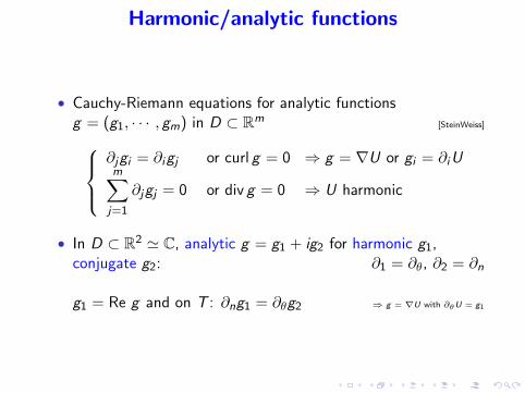
• Cauchy-Riemann equations for analytic functionsg = (g1, · · · , gm) in D ⊂ Rm
[SteinWeiss]∂jgi = ∂igj or curl g = 0 ⇒ g = ∇U or gi = ∂iUm∑
j=1
∂jgj = 0 or div g = 0 ⇒ U harmonic
• In D ⊂ R2 ' C, analytic g = g1 + ig2 for harmonic g1,conjugate g2: ∂1 = ∂θ, ∂2 = ∂n
g1 = Re g and on T : ∂ng1 = ∂θg2 ⇒ g = ∇U with ∂θU = g1
Harmonic/analytic functions
• Cauchy-Riemann equations for analytic functionsg = (g1, · · · , gm) in D ⊂ Rm
[SteinWeiss]∂jgi = ∂igj or curl g = 0 ⇒ g = ∇U or gi = ∂iUm∑
j=1
∂jgj = 0 or div g = 0 ⇒ U harmonic
• In D ⊂ R2 ' C, analytic g = g1 + ig2 for harmonic g1,conjugate g2: ∂1 = ∂θ, ∂2 = ∂n
g1 = Re g and on T : ∂ng1 = ∂θg2 ⇒ g = ∇U with ∂θU = g1

Recovery of harmonic/analytic functions
• recover analytic function g in D from its values f = g|T+on
T+ ( T −→ solution u to (IP):
2D: u = Re g
f (e iθ) = ν(e iθ) + i
∫ θ
φ(e iτ ) dτ = u + i
∫ θ
∂nu e iθ ∈ T+
3D: ∇u = g (∂1, ∂2) = ∂σ, ∂3 = ∂n
f (σ) = (∇σν, φ) = (∂σu, ∂nu) σ ∈ T+
• Ill-posed boundary interpolation issue⇒ approximation in Hilbert Hardy spaces H2
D
of functions analytic in D bounded in L2(T )

Hardy spaces, definitions
Hardy spaces H2D : functions analytic in D bounded in L2(T )
• In circular domains D ⊂ R2 ' C, Fourier coefficients
H2D = {g(z) =
∑p≥0
γp zp ,∑p≥0
|γp|2 < ∞} z = re iθ
• In spherical domains D ⊂ R3, spherical harmonics:
H2B: g = (g1, g2, g3) with gi = ∂iU, bounded in L2(T ),
U(σ, r) =∑k≥0
rkk∑
m=−k
γmk Y m
k (σ)
[Axler&al, DautrayLions]

Hardy spaces, notations, properties
• L2 = L2(T ), L2± = L2(T±),
norm/inner product ‖ ‖±, < , >±
H2 = H2D D =
{disk or annular domain (2D)ball or spherical domain (3D)
• uniqueness on subsets of T :
if g ∈ H2 and g|T+= 0, then g ≡ 0
• H2|T+
dense in L2+; however, if f ∈ L2
+ and gn → f in L2+,
then either f ∈ H2|T+
, or ‖gn‖− →∞

From (IP) to (BEP)
Back to inverse problem (IP) in (2D) and (3D) situations:
extension issue of finding g ∈ H2, g|T+= f
One can fit arbitrarily closely to noisy data f on T+ (f 6∈ H2|T+
)
But with unstable behaviour elsewhere, on T−
Related to ill-posedness of Cauchy type or interpolation issues
Add a T− norm constraint on the H2 function g :well-posed best constrained approximation issues

Bounded extremal problems in 2D and 3D
Given f ∈ L2+, M ≥ 0, find g∗ ∈ H2, ‖g∗‖− ≤ M
(BEP) ‖f − g∗‖+ = inf{‖f − g‖+ : g ∈ H2, ‖g‖− ≤ M}
admits unique solution g∗ (for R3, if f1 = f2 = 0 on ∂T±) [JuL&al]
Further, if f 6∈ {g ∈ H2, ‖g‖− < M}|T+, then ‖g∗‖− = M
Proof: best approximation projection onto closed subsets of Hilbert spaces
(BEP) also in Sobolev norm W k,2, Banach Lp, with other/mixedconstraints, criteria, ...

Bounded extremal problems in 2D and 3D
(BEP) : ming∈H2
(‖f − g‖2
+ + λ‖g‖2−)
π ⊥ projection L2 → H2, χ± characteristic function of T±Toeplitz operator T on H2 defined by Tp,q = Tp−q
< T g , γ >=< g , γ >−=
∫T−
g γ or T g = π (χ− g) ∈ H2
Construct the solution, solve variational equation:
< (I + (λ− 1) T ) g∗, γ >=< f , γ >+ , for all γ ∈ H2
for (unique) value λ > 0 (Lagrange param.): ‖g∗‖− = M

Bounded extremal problems in 2D and 3D
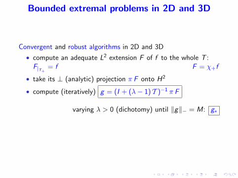
Convergent and robust algorithms in 2D and 3D
• compute an adequate L2 extension F of f to the whole T :F|T+
= f F = χ+f
• take its ⊥ (analytic) projection π F onto H2
• compute (iteratively) g = (I + (λ− 1) T )−1 π F
varying λ > 0 (dichotomy) until ‖g‖− = M: g∗
• approximation of L2+ functions: (interpolation for H2
|T+)
compromize between ‖g∗‖− = M and error ‖f − g∗‖+

Bounded extremal problems in 2D and 3D
Convergent and robust algorithms in 2D and 3D
• compute an adequate L2 extension F of f to the whole T :F|T+
= f F = χ+f
• take its ⊥ (analytic) projection π F onto H2
• compute (iteratively) g = (I + (λ− 1) T )−1 π F
varying λ > 0 (dichotomy) until ‖g‖− = M: g∗
• approximation of L2+ functions: (interpolation for H2
|T+)
compromize between ‖g∗‖− = M and error ‖f − g∗‖+

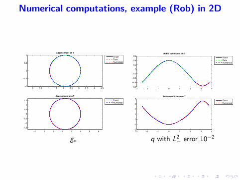
Numerical computations, example (Rob) in 2D
D = annulus, r = .6, explicit data on T+ = (e−4iπ/5, e4iπ/5)
f (z) = 2 +1
z − .1∈ H2
|T+whence ν, φ
solution g∗ to (BEP) (order 2, in W 2,2, M = ‖f ‖−)
solves for (IP) and (Rob):u ' Re g∗ , ∂nu ' ∂θ Im g∗ in D
q ' −∂θ Im g∗Re g∗
on T−
Numerical computations, example (Rob) in 2D
0 0.5 1 1.5 2 2.5 3 3.5 4 4.5−1
−0.5
0
0.5
1Approximant on T
ExactDataNumerical
−1 0 1 2 3 4 5 6−1.5
−1
−0.5
0
0.5
1
1.5
Approximant on rT
ExactNumerical
−3 −2 −1 0 1 2 3 4−0.8
−0.6
−0.4
−0.2
0
0.2
0.4
0.6Robin coefficient on T
ExactDataNumerical
−3 −2 −1 0 1 2 3 4−2
−1
0
1
2
3
4Robin coefficient on rT
ExactNumerical
g∗ q with L2− error 10−2

Numerical computations, example (EEG)
3-sphere model, radii ri = .87, .92, 1, conductivities σi = 1, 1/30, 1one dipolar source at C = (.7, .2, .1) (finite elements)
ν numerically generated on T+ = S3 from u(X ) ' < p,X − C >
‖X − C‖3
(BEP) solved with T− = S2, then with T+ = S2 and T− = S1
hence (IP), g∗ = ∇u, cortical potential u on S1:
explicit data (BEP) solution

Numerical computations, example (EEG)
True source C • localized by best L2 rational approximation •
explicit data (BEP) solution
−1−0.8−0.6−0.4−0.200.20.40.60.81
−1
−0.8
−0.6
−0.4
−0.2
0
0.2
0.4
0.6
0.8
1
X
Y
−1−0.8−0.6−0.4−0.200.20.40.60.81
−1
−0.8
−0.6
−0.4
−0.2
0
0.2
0.4
0.6
0.8
1
X
Y
−1−0.8−0.6−0.4−0.200.20.40.60.81 −101−1
−0.8
−0.6
−0.4
−0.2
0
0.2
0.4
0.6
0.8
1
YX
Z
−1−0.8−0.6−0.4−0.200.20.40.60.81 −101−1
−0.8
−0.6
−0.4
−0.2
0
0.2
0.4
0.6
0.8
1
YX
Z
error on C : 10−4 10−2

Numerical computations, example (EEG)
Several sources • localized by best L2 rational approximation •(explicit data)

Conclusion
Links between Cauchy problems (IP) for non destructive controland approximation issues in functions spaces (BEP)
(EEG) in 3D: medical data soon!
In 2D and 3D,realistic geometries (quadrature domains)
inverse problem of conductivity recovery (EIT)
In 2D, stability and error estimates for (IP)
geometrical IP for corrosion detection (unknown part of theboundary)
variable conductivity σ (plasma confinement in tokamak)

References
Atfeh, Baratchart, Leblond, Partington. ”Bounded extremal andCauchy-Laplace problems on 3D spherical domains”, inpreparation.
Baratchart, Leblond, Marmorat. “Sources identification in a 3Dball from best meromorphic approximation on 2D slices”, Elec.Trans. Num. Anal., 2006.
Baratchart, Mandrea, Saff, Wielonsky. “2D inverse problems forthe laplacian: a meromorphic approximation approach”, J. MathsPures Appl., 2006.