category structure and function of pitch accent in tokyo japanese · 2006-03-22 · overall, it was...
TRANSCRIPT

Category Structure and Function of Pitch Accent inTokyo Japanese
Mafuyu Kitahara
Submitted to the faculty of the Graduate Schoolin partial fulfillment of the requirements
for the degree ofDoctor of Philosophy
in the Department of Linguisticsand the Cognitive Science Program
Indiana University
May 26, 2001
Accepted by the Graduate Faculty, Indiana University, in partial fulfillmentof the requirements of the degree of Doctor of Philosophy.
Dr. Kenneth de Jong(Principal Adviser)
Dr. Robert F. Port
Dr. Stuart Davis
Bloomington, IndianaMarch, 2001. Dr. David B. Pisoni
ii

c© Copyright 2001Mafuyu Kitahara
All rights reserved.
iii

To my parents with gratitude and admiration.
iv
Acknowledgments
I would like to express my deepest gratitude to my committee members: Ken de Jong, BobPort, Stuart Davis, and David Pisoni. Ken, as the chair, guided me throughout the longand hilly process of thesis-writing across the ocean. I, from Japan, just had to dump afile to the very remote printer in the lab and Ken always gave me precise, practical, andinsightful comments promptly. Seminars, courses, and a teaching-assistant experience withKen have also been quite influential to me. In fact, this thesis is a development of theterm paper for the advanced phonetics class I took from him in the very first semester atIU. Thoughts about functional load and prosody came to my mind first in his seminar onfeature and contrast. I truly thank him for what he provided to me.
Bob also gave me a tremendous amount of support both intellectually and emotionally.With his assistance, I became a member of the CRANIUM lab in the Computer ScienceDepartment from which I learned most of the techniques for experiments, statistics, graph-ics, and LATEX-ing. Bob’s enthusiasm and inspirations about the dynamic and continuousnature of speech provided me a seed for an idea to take devoicing as a source of perturbation.
Stuart took care of me so much on the “Day One” at IU when I visited IU and severalother universities. His warm support and kind assistance was one of the most convincingreasons I decided to enter IU. His courses on the latest development of Optimality Theoryhave helped me to think typologically and formally.
Dave’s seminar on speech perception spoken word recognition literary opened my eyesto the vast field of cognitive psychology. By his famous thick reading packets with 4 writ-ing assignments, I was really sleep deprived in that semester! His depth and breadth ofknowledge in every corner of the history of speech sciences were quite beneficial to me.
I learned a lot about Matlab and DSP techniques from Diane Kewley-Port, statistics andscientific attitude from John Kruschke, and what cognitive science is from Rob Goldstone.Though not represented in my committee, their input formed the basis for this project. Ialso thank other faculty in various departments at IU. Steven Franks, Mike Gasser, YasukoIto-Watt, Yoshihisa Kitagawa, Paul Newman, Sam Obeng, and Natsuko Tsujimura have allgiven me helpful advice and warm support in the five years of my stay at IU.
I also would like to thank the administrative and systems staff: Ann Baker and MarilynEstep in Linguistics, Karen Loffland in Cognitive Science, and Bruce Shei in ComputerScience. They have helped me to go over bureaucratic jobs, to get financial assistance, andto solve technical problems.
All experiments and analyses which constitute the body of this thesis have been doneat the NTT Communication Science Labs in Japan. Without their financial support and
v
facilities, this thesis could not have been completed. I especially thank Shigeaki Amano forhis generous support in all aspects of research life in Japan. I also thank Tadahisa Kondo,Kenichi Sakakibara, Reiko Mazuka, and Naoko Kudo for their comments, assistance, andentertainment.
Before coming to IU, I spent my undergraduate and graduate school life at Kyoto Uni-versity in Japan. I thank Masatake Dantsuji, Haruo Kubozono, Michinao Matsui, MiyokoSugito, Yukinori Takubo, Koichi Tateishi, Masaaki Yamanashi, and Kazuhiko Yoshida fortheir helpful advice and intellectual support in the early days of my academic carrier inKyoto and their continuous support afterwards.
Special thanks to Hideki Kawahara for allowing me to use the STRAIGHT programfor F0 resynthesis. I thank Mary Beckman who first taught me the laboratory phonologyapproach in her course at the LSA institute and have given me a lot of insights about thetonal structure of Japanese. Shosuke Haraguchi, Bruce Hayes, Junko Ito, Kikuo Maekawa,and Armin Mester have provided me helpful comments and advice at various stages in thedevelopment of this thesis.
My lab-mates (or former lab members) in the CRANIUM have provided all kinds ofsupport. Keiichi Tajima, Fred Cummins, Bushra Zawaydeh, Doug Eck, Dave Wilson, Deb-bie Burleson, Dave Collins, Adam Leary have all been very stimulating and helpful. Specialthanks go to Keiichi Tajima for not only being a lab-mate but also being a room-mate, afriend, a mentor, an S-PLUS advisor, a TEX-nician, a poker-teacher, a cooking assistant, aparallel parking guide and a lot more. . .
An on-line phonology discussion group in Japan has been a source of qualified andvaluable information both in Kyoto and in Bloomington. I especially thank Takeru Honma,Hideki Zanma, Teruo Yokotani, and Masahiko Komatsu for their lively and stimulatingdiscussions. My fellow students in Bloomington, Kyoto, and other places have also beenquite supportive. Karen Baertsch, Masa Deguchi, Nicole Evans, Brian Gygi, Yasuo Iwai,Laura Knudsen, Koh Kuroda, Laura McGarrity, Kyoko Nagao, Kwang Chul Park, MarkPennington, Liz Peterson, Hisami Suzuki, Jeniffer Venditti, Kiyoko Yoneyama, HanakoYoshida, Natsuya Yoshida, and Yuko Yoshida have provided me various sorts of comments,encouragement, and friendship.
Special thanks are due to my parents, Itoko and Ryuji Kitahara, for their forbearancefrom my slippery and lengthy student-life. Back in high school days, they ignited my interestin human intelligence, which eventually lead me to study linguistics.
Finally, my wife and a research partner, Haruka Fukazawa has helped and encouragedme throughout the entire course of the writing of this thesis. She has accompanied me tomany conferences, workshops, and my defense, helping me to prepare for overheads anddrafts even when she had a heavy teaching load and deadlines for her own research. WhenI broke my leg and got hospitalized, she showed up the next morning flying over hundredsof miles. When I was stressed out writing an argument that seemed to go nowhere, shecheered me up and got my self-confidence back. It is truly difficult to imagine finishing thisthesis without her.
vi
Abstract
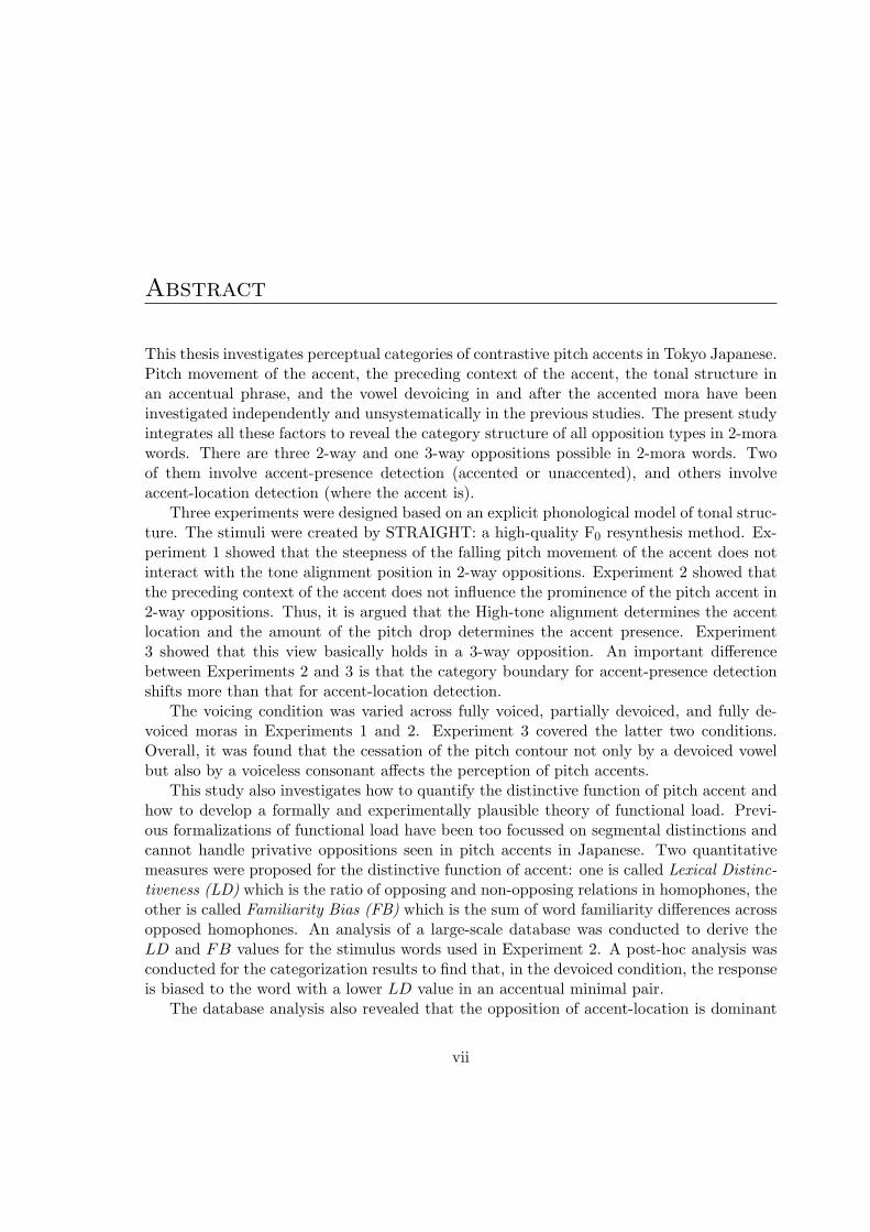
This thesis investigates perceptual categories of contrastive pitch accents in Tokyo Japanese.Pitch movement of the accent, the preceding context of the accent, the tonal structure inan accentual phrase, and the vowel devoicing in and after the accented mora have beeninvestigated independently and unsystematically in the previous studies. The present studyintegrates all these factors to reveal the category structure of all opposition types in 2-morawords. There are three 2-way and one 3-way oppositions possible in 2-mora words. Twoof them involve accent-presence detection (accented or unaccented), and others involveaccent-location detection (where the accent is).
Three experiments were designed based on an explicit phonological model of tonal struc-ture. The stimuli were created by STRAIGHT: a high-quality F0 resynthesis method. Ex-periment 1 showed that the steepness of the falling pitch movement of the accent does notinteract with the tone alignment position in 2-way oppositions. Experiment 2 showed thatthe preceding context of the accent does not influence the prominence of the pitch accent in2-way oppositions. Thus, it is argued that the High-tone alignment determines the accentlocation and the amount of the pitch drop determines the accent presence. Experiment3 showed that this view basically holds in a 3-way opposition. An important differencebetween Experiments 2 and 3 is that the category boundary for accent-presence detectionshifts more than that for accent-location detection.
The voicing condition was varied across fully voiced, partially devoiced, and fully de-voiced moras in Experiments 1 and 2. Experiment 3 covered the latter two conditions.Overall, it was found that the cessation of the pitch contour not only by a devoiced vowelbut also by a voiceless consonant affects the perception of pitch accents.
This study also investigates how to quantify the distinctive function of pitch accent andhow to develop a formally and experimentally plausible theory of functional load. Previ-ous formalizations of functional load have been too focussed on segmental distinctions andcannot handle privative oppositions seen in pitch accents in Japanese. Two quantitativemeasures were proposed for the distinctive function of accent: one is called Lexical Distinc-tiveness (LD) which is the ratio of opposing and non-opposing relations in homophones, theother is called Familiarity Bias (FB) which is the sum of word familiarity differences acrossopposed homophones. An analysis of a large-scale database was conducted to derive theLD and FB values for the stimulus words used in Experiment 2. A post-hoc analysis wasconducted for the categorization results to find that, in the devoiced condition, the responseis biased to the word with a lower LD value in an accentual minimal pair.
The database analysis also revealed that the opposition of accent-location is dominant
vii

in 2-mora words while that of accent-presence is dominant in 3- and 4-mora words. Takentogether with the observation about the shift of category boundaries, it is suggested accent-location detection is functionally more fundamental than accent-presence detection only in2-mora words.
viii
Contents
Acknowledgments v
Abstract vii
1 Introduction and background 11.1 Introduction . . . . . . . . . . . . . . . . . . . . . . . . . . . . . . . . . 11.2 Pitch accent system in Tokyo Japanese . . . . . . . . . . . . . . . . . . 2
1.2.1 Phonological/descriptive studies . . . . . . . . . . . . . . . . . 21.2.2 Statistical survey . . . . . . . . . . . . . . . . . . . . . . . . . . 31.2.3 Experimental studies . . . . . . . . . . . . . . . . . . . . . . . 41.2.4 Phonology in Pierrehumbert & Beckman’s model . . . . . . . . 61.2.5 Vowel devoicing . . . . . . . . . . . . . . . . . . . . . . . . . . 8
1.3 Functionalism in phonology . . . . . . . . . . . . . . . . . . . . . . . . 91.3.1 Classic functionalism . . . . . . . . . . . . . . . . . . . . . . . . 91.3.2 Functional load . . . . . . . . . . . . . . . . . . . . . . . . . . 101.3.3 Type/token frequency and word familiarity . . . . . . . . . . . 12
1.4 Functions of pitch accent . . . . . . . . . . . . . . . . . . . . . . . . . 131.5 Lexical access . . . . . . . . . . . . . . . . . . . . . . . . . . . . . . . 14
2 Overview of perception experiments 162.1 Introduction . . . . . . . . . . . . . . . . . . . . . . . . . . . . . . . . . 162.2 Previous experimental studies on accent perception . . . . . . . . . . . 16
2.2.1 Sugito (1982) . . . . . . . . . . . . . . . . . . . . . . . . . . . . 162.2.2 Hasegawa & Hata (1992) . . . . . . . . . . . . . . . . . . . . . 172.2.3 Matsui (1993) . . . . . . . . . . . . . . . . . . . . . . . . . . . . 19
2.3 Intonation synthesis in Pierrehumbert & Beckman’s model . . . . . . . 212.3.1 Tone sequencing . . . . . . . . . . . . . . . . . . . . . . . . . . 212.3.2 Declination . . . . . . . . . . . . . . . . . . . . . . . . . . . . . 232.3.3 Convolution and jitter . . . . . . . . . . . . . . . . . . . . . . . 25
2.4 Resynthesis procedure . . . . . . . . . . . . . . . . . . . . . . . . . . . 272.5 Stimulus preparation and presentation . . . . . . . . . . . . . . . . . . 30
3 Categorization in a 2-way distinction 313.1 Introduction . . . . . . . . . . . . . . . . . . . . . . . . . . . . . . . . . 31
ix
3.2 Experiment 1: Purpose . . . . . . . . . . . . . . . . . . . . . . . . . . 313.3 Experiment 1: Methods . . . . . . . . . . . . . . . . . . . . . . . . . . 35
3.3.1 Materials . . . . . . . . . . . . . . . . . . . . . . . . . . . . . . 353.3.2 Stimulus design . . . . . . . . . . . . . . . . . . . . . . . . . . . 353.3.3 Procedure . . . . . . . . . . . . . . . . . . . . . . . . . . . . . . 40
3.4 Experiment 1: Results . . . . . . . . . . . . . . . . . . . . . . . . . . . 403.4.1 Representations . . . . . . . . . . . . . . . . . . . . . . . . . . . 403.4.2 Effect of scaling . . . . . . . . . . . . . . . . . . . . . . . . . . . 433.4.3 Effect of slope . . . . . . . . . . . . . . . . . . . . . . . . . . . . 433.4.4 Effect of devoicing . . . . . . . . . . . . . . . . . . . . . . . . . 44
3.5 Experiment 1: Discussion . . . . . . . . . . . . . . . . . . . . . . . . . 473.6 Experiment 2: Purpose . . . . . . . . . . . . . . . . . . . . . . . . . . 503.7 Experiment 2: Methods . . . . . . . . . . . . . . . . . . . . . . . . . . 51
3.7.1 Materials . . . . . . . . . . . . . . . . . . . . . . . . . . . . . . 513.7.2 Stimulus design . . . . . . . . . . . . . . . . . . . . . . . . . . 523.7.3 Procedure . . . . . . . . . . . . . . . . . . . . . . . . . . . . . . 55
3.8 Experiment 2: Results . . . . . . . . . . . . . . . . . . . . . . . . . . . 573.8.1 Effect of devoicing . . . . . . . . . . . . . . . . . . . . . . . . . 573.8.2 Effect of phrasal H scaling . . . . . . . . . . . . . . . . . . . . 59
3.9 Experiment 2: Discussion . . . . . . . . . . . . . . . . . . . . . . . . . 60
4 Categorization in a 3-way distinction 644.1 Introduction . . . . . . . . . . . . . . . . . . . . . . . . . . . . . . . . . 644.2 Purpose and predictions . . . . . . . . . . . . . . . . . . . . . . . . . . 654.3 Methods . . . . . . . . . . . . . . . . . . . . . . . . . . . . . . . . . . . 68
4.3.1 Materials . . . . . . . . . . . . . . . . . . . . . . . . . . . . . . 684.3.2 Stimulus design . . . . . . . . . . . . . . . . . . . . . . . . . . . 694.3.3 Procedure . . . . . . . . . . . . . . . . . . . . . . . . . . . . . . 74
4.4 Results . . . . . . . . . . . . . . . . . . . . . . . . . . . . . . . . . . . . 744.4.1 Distribution of 3 accentual categories in voiced and devoiced condi-
tions . . . . . . . . . . . . . . . . . . . . . . . . . . . . . . . . . 744.4.2 Comparison with the results in a 2-way distinction . . . . . . 744.4.3 Effect of phrasal H scaling . . . . . . . . . . . . . . . . . . . . . 77
4.5 Discussion . . . . . . . . . . . . . . . . . . . . . . . . . . . . . . . . . . 80
5 Functions of pitch accent: a database analysis 825.1 Introduction . . . . . . . . . . . . . . . . . . . . . . . . . . . . . . . . 825.2 Database analysis . . . . . . . . . . . . . . . . . . . . . . . . . . . . . 82
5.2.1 Structure of the database . . . . . . . . . . . . . . . . . . . . . 825.2.2 Homophones . . . . . . . . . . . . . . . . . . . . . . . . . . . . 855.2.3 Distribution of accent locations . . . . . . . . . . . . . . . . . . 875.2.4 Distribution of oppositions . . . . . . . . . . . . . . . . . . . . 87
5.3 Formalization of oppositions . . . . . . . . . . . . . . . . . . . . . . . 90
x
5.3.1 Lexical distinctiveness . . . . . . . . . . . . . . . . . . . . . . . 915.3.2 Familiarity bias . . . . . . . . . . . . . . . . . . . . . . . . . . . 925.3.3 Examples . . . . . . . . . . . . . . . . . . . . . . . . . . . . . . 93
5.4 Summary and discussion . . . . . . . . . . . . . . . . . . . . . . . . . 94
6 Functional load of pitch accent: a post-hoc analysis 986.1 Introduction . . . . . . . . . . . . . . . . . . . . . . . . . . . . . . . . 986.2 Material . . . . . . . . . . . . . . . . . . . . . . . . . . . . . . . . . . 986.3 Analysis and discussion . . . . . . . . . . . . . . . . . . . . . . . . . . 100
7 Discussion and conclusions 1047.1 Category structure of pitch accents . . . . . . . . . . . . . . . . . . . . 104
7.1.1 Slope of the falling contour . . . . . . . . . . . . . . . . . . . . 1047.1.2 Preceding context . . . . . . . . . . . . . . . . . . . . . . . . . 1057.1.3 Tonal specifications . . . . . . . . . . . . . . . . . . . . . . . . 1057.1.4 Effect of devoicing . . . . . . . . . . . . . . . . . . . . . . . . . 106
7.2 Functions of pitch accent . . . . . . . . . . . . . . . . . . . . . . . . . 1077.3 Future directions . . . . . . . . . . . . . . . . . . . . . . . . . . . . . . 108
Bibliography 110
xi
Chapter 1
Introduction and background
1.1 Introduction
This study is an investigation of the pitch accent system in Tokyo Japanese, particularlyfocusing on its distinctive function and the realization of the function through perceptualcategories. Speech perception and phonology have been two separated fields not interact-ing very frequently until quite recently. Phonologists have long been relying on acous-tic/articulatory data to ground their theories but have rarely incorporated perceptual datain the construction of their theories. However, investigation into the role of speech percep-tion in phonological systems has recently been revived (Hume and Johnson, 2000) partlydue to the development of a flexible constraint-based framework (Prince and Smolensky,1993).
In light of this new interest to speech perception in phonology, the most frequently men-tioned terms are perhaps “contrast” and “perceptual cue” (Boersma, 1997; Flemming, 1995;Hayes, 1996a; Steriade, 1999). For example, Flemming (1995) argues that the requirementfor contrast maintenance interacts with the relative salience of perceptual cues in shapingthe vowel space.
Perceptual cues for pitch accent in Japanese is a well-cultivated area in the literature.F0 is considered the main cue for the perception of accent (Sugito, 1982) and its dynamics ismodeled in various approaches (Fujisaki and Sudo, 1971; Haraguchi, 1977; Pierrehumbertand Beckman, 1988). Among them, Pierrehumbert & Beckman’s model is grounded ona phonologically well-defined framework and mathematically explicit enough to create astimulus set in perception experiments. However, there has been no systematic attempt toapply their model in a perception experiment to describe the category structure of pitchaccents in terms of phonologically tractable parameters, such as High and Low tones.
Contrast is what the distinctive function supplies in order to distinguish lexical items.Though it has been frequently mentioned that the distinctive function is not the primaryfunction of pitch accent in Japanese (Beckman, 1986; Komatsu, 1989; Shibata and Shibata,1990; Vance, 1987), what type of contrast is still maintained and how many there are in theentire lexicon have remained unanswered.
The interaction between the perceptual cue of pitch accent and contrasts served by
1
Introduction and background 2
accent categories is thus a fruitful area to explore.The outline of the present thesis is as follows: the remainder of this chapter gives a
review of studies on Japanese pitch accent, functionalism, and speech perception. The nextchapter introduces an overview of perception experiments conducted in the present study onthe basis of criticisms of previous perception studies on pitch accent in Japanese. Chapters 3and 4 report three experiments addressing the category structure of pitch accents. Chapter5 is an extensive analysis of a large-scale database including accent, word length, and wordfamiliarity. A new proposal about the quantification of the distinctive function of pitchaccent will be introduced as well. Chapter 6 shows a post-hoc analysis of the results ofexperiments reported in Chapter 3 and 4 in order to evaluate the proposal given in Chapter5. Chapter 7 gives a general discussion and concludes the thesis.
1.2 Pitch accent system in Tokyo Japanese
1.2.1 Phonological/descriptive studies
The pitch accent system of Tokyo Japanese has been studied in a variety of frameworks.First of all, there is a long tradition of accent studies in Japanese linguistics including his-torical and dialectal comparisons (Kindaichi, 1981; Uwano, 1977; Uwano, 1989). A numberof accent dictionaries have been published as a result of cumulative efforts (Kindaichi, 1981;NHK, 1985; NHK, 1998). Akinaga (1998), included as an appendix in NHK (1998), is oneof the most comprehensive descriptions of the pitch accent system in Tokyo Japanese in thetradition of the Japanese accent literature.
Studies within generative phonology have adopted diverse theoretical models over thelast 30 years. To name a few, there are linear models (McCawley, 1968; Shibatani, 1972;McCawley, 1977), autosegmental models (Haraguchi, 1977; Clark, 1987; Ishihara, 1991),metrical models (Zubizarreta, 1982; Abe, 1987; Haraguchi, 1991), a government phonol-ogy model (Yoshida, 1995), and Optimality Theoretic models (Kubozono, 1995; Kitahara,1996a; Alderete, 1999). Some of them have a scope over not only Tokyo Japanese but alsoother dialects in Japan (Haraguchi, 1977; Haraguchi, 1991), while others focus on a specificphenomenon such as compound accent (Kubozono, 1995; Alderete, 1999), accent in loanwords (Kitahara, 1996a), or the verbal inflection paradigm (Ishihara, 1991).
At the level of general description, however, most Japanese linguists and generativephonologists agree on several basic points:
(1.1) a. One characteristic pitch pattern, namely a high-low tonal sequence, marks theword accent.
b. A word has at most one accent on any mora or can be unaccented.1
c. Thus, n-mora words have n+1 possible accentuations.1This is true for words with only light syllables. The second mora in a heavy syllable usually does not
bear an accent (McCawley, 1968).
Introduction and background 3
d. Phrase initial moras have a low tone and second moras have a high tone unless theword in that position has an initial accent.2
Conventionally, accent location is counted from the beginning of a word in the literatureof Japanese accentology. Thus, the initial-accented form is called accent-1, the final-accentedform of a 2-mora word and the penultimate-accented form of a 3-mora word are calledaccent-2, and so on. In addition, the unaccented form is called accent-0. Although someof the phonological facts are captured more elegantly by counting from the end of theword — e.g., reference to the antepenulmacy in (1.2)—, the present thesis follows theconventional counting method because the database used in this study (cf. Chapter 5)adopts the conventional method.
Accentual oppositions are labelled by a combination of the numbers for accent location.For example, the 0-1, 0-2 and 1-2 opposition are the distinction between accent-0 andaccent-1, accent-0 and accent-2, and accent-1 and accent-2, respectively.
1.2.2 Statistical survey
There are several statistical analyses of the accent pattern using a database. Sato (1993)uses about 60,000 items taken from an accent dictionary (Kindaichi, 1981) and sees thegross correlation between word length (1—10 moras) and accent pattern. In other words,the type frequency (Bybee, 1985: see Section 1.3.3 for discussion) was calculated for eachaccent pattern within a set of words of equal length. Sato’s findings are summarized asfollows:
(1.2) a. All possible accent patterns appear at about equal frequency in 1–2 mora words.
b. The unaccented form is the most frequent pattern in 3–4 mora words. When sub-analyses by vocabulary strata are performed, Sino-Japanese words contribute mostto the high frequency of unaccented forms while Native and Foreign words containa sizable number of accented forms.
c. Antepenultimate accent is dominant in 5- and 7-mora words while pre-antepenultimate accent is dominant in 8 mora words. 6 mora words have a con-siderable number of both antepenultimate and pre-antepenultimate forms.
d. Sub-analyses of 4-mora or longer words by the internal structure of words showthat the length of the second element in compound words is a good predictor ofaccent location.
These findings suggest that longer words have very few minimal pairs by accent inwhich the distinctive function of the accent is not at work. Pitch accent in longer wordshave different patterns constrained by the internal structure of compounds (McCawley, 1968;
2When the phrase initial syllable is heavy, the initial low tone appears to be higher in pitch than normal.This is represented as a weak variant of the boundary L tone (weak-L%) in Pierrehumbert & Beckman(1988). See Section 1.2.4 for an introduction to their model of tonal structure.
Introduction and background 4
McCawley, 1977; Higurashi, 1983; Abe, 1987; Sato, 1989; Kubozono, 1993; Kubozono, 1995;Yoshida, 1995; Alderete, 1999).
Sato’s study does not reveal the details of accentual minimal pairs, which is a necessarystep to investigate the distinctive function of pitch accent. There are at least two statisticalstudies concentrated on accentual minimal pairs (Miyaji, 1980; Shibata and Shibata, 1990).However, they are not extensive enough to quantify the distinctive function of accent.
Miyaji’s study was based on too coarse of a sampling (683 homophonous words in total),and he further classified the population by word classes (e.g., Sino-Japanese, Native, andForeign). His view about the set size of homophones and the number of different accentcategories within the set seems to have an impact on any measure of the distinctive functionof accent. However, his claim about different tendencies across word classes is not decisiveenough due to such a small sampling of the data.
Shibata & Shibata (1990) not only investigated Japanese but also English and Chinesein order to compare the distinctive function of prosody (as a cover term for pitch accent,stress accent, and tone) across the three languages. They adopted a binomial probabilisticmodel to estimate the maximal likelihood of a word being distinct from others in a set ofhomophones by prosody. They estimate that the probability of a word contrasting in pitchor tone in Japanese is 13.57% across the board while it is 0.47% and 71.00% in Englishand Chinese respectively. Their analysis about the differences of the distinctive functionof prosody among languages seems insightful, but they also admit that there are knownproblems in their corpus and in the data mining processes.
First, they did not count genuine homophones but relied on orthographic informationin a dictionary. They actually counted homographs but not homophones. For example,“right” and “wright” are homophones but not homographs, which were not included intheir corpus. Similar situations arose in Japanese where a long vowel can either be writtenby a sequence of two kana symbols or by a single kana followed by a hyphen-like symbol.In such cases, they did not count them as homophones.
Second, their probabilistic model did not fit well when the set size of homophones islarger than two. They just ignored the homophones with more than three members becausethe majority of homophones have only two members in their corpus.
Third, when the model is applied to words of different length, the maximal likelihoodvaries from 6% for 5-mora words to 30% for 1-mora words. They averaged out those for1- to 7-mora words for their claim, but the variation across different lengths needs furtherscrutiny.
In the present thesis, a large-scale (80,000 words) database was used to extract truehomophones irrespective of orthography. We will see that the distribution of oppositiontypes are remarkably different with respect to word length, which cast doubt on Shibata &Shibata’s across-the-board analysis of the distinctive function.
1.2.3 Experimental studies
Experimental studies on Japanese pitch accent are also numerous since the 1920’s. A re-view of early days of accent research is available in Sugito (1982). Limiting the scope
Introduction and background 5
after 1970 still leaves a number of studies. Experimental approaches classify into four cat-egories. The categories are engineering-oriented, physiology-oriented, psychology-oriented,and linguistics-oriented approaches. There is, of course, a considerable overlap betweenthese approaches which will be discussed later in this section.
Among engineering-oriented approaches, the superposition models first proposed in Fu-jisaki and Sudo (1971) and developed since then are popular in speech synthesis applications(Fujisaki, 1996; van Santen et al., 1998). The model additively superimposes a baseline F0
, a phrase component, and an accent component. The two components are controlled bycritically damped second-order systems responding to an impulse input in the case of thephrase, and to a rectangular input in the case of the accent component. The importance ofthis model to linguistic description will be discussed later in relation to Sugito (1982).
Among physiology-oriented approaches, studies about glottal mechanisms are of par-ticular interest for this thesis. It has been generally agreed that the cricothyroid muscleworks for controlling the F0 of the voice source: “the contraction of this muscle elongatesthe vocal folds, which results in an increase in the longitudinal tension and a decrease in theeffective mass of the vocal fold tissue involved in vibration during phonation (Sawashima,1980: p. 53).” A research group at the University of Tokyo further found that extrinsiclaryngeal muscles, especially the sternohyoid, are involved in F0 lowering in the lower pitchrange in the case of Japanese pitch accent (Shimada and Hirose, 1971; Sawashima et al.,1973). In later studies, they tested the relative timing of vowel articulation and activityin pitch controlling muscles (Sawashima, 1980; Sawashima and Hirose, 1980; Sugito, 1981;Sawashima et al., 1982).
What I classify as psychology-oriented approaches are those involving perception exper-iments in some form, though most of such studies are done by linguists. First of all, thereare studies that confirmed that pitch is the fundamental cue to the perception of accent inJapanese (Weitzman, 1969; Sugito, 1982; Beckman, 1986).
Impressionistic descriptions agree that pitch accent in Japanese carries a high tone.However, it was found that the pitch peak is not necessarily located in the accented morabut in the following mora in some cases (Neustupny, 1966). Sugito (1982) called thisphenomena “late fall [ososagari]” in which the high pitch of the accent-bearing mora shiftsto the following mora. This late fall tends to occur in initial accented words whose secondmora has a non-high vowel (Sugito, 1982: p. 249). Sugito conducted several perceptionexperiments to find that listeners perceive accent on a mora followed by another morawhich actually has a pitch peak. She also claimed that the downward pitch movement in amora induces a percept of accent in the preceding mora and that the exact location of thepeak is not the principal cue to the perception of accent.
Hasegawa & Hata (1992) further confirmed this by conducting a perception experimentand revealed that there is a compensatory relationship between pitch peak location andthe pitch movement after the peak. According to them, a steeper pitch fall is necessary toperceive the accent in the preceding mora when the peak location is later.
Vowel devoicing is a process where high vowels are devoiced between two voiceless con-sonants. Since there is no pitch in the devoiced vowel, it has been a matter of debate how
Introduction and background 6
listeners perceive an accent when it is on the devoiced mora. Sugito (1982) conducted an-other experiment on this phenomena and found that the pitch movement in the followingmora is the cue to the perception of accent in the devoiced mora, which is in line with herresults concerning late fall. Matsui (1993) further confirmed this with a more systematicdesign of stimuli and estimated the structure of perceptual categories for accent types bothin voiced and devoiced cases. Since the present study also involves perception of accentin a devoiced mora, Matsui’s work will be reviewed in more detail in Section 2.2.3 in thenext chapter. Phonetic and phonological studies on vowel devoicing will also be reviewedin more detail in Section 1.2.5 in this chapter.
Finally, there are numerous experimental studies done by phoneticians. I briefly sketchthose as a class of linguistics-oriented approaches, where experiments are done mainly inthe production domain. The most influential and comprehensive study of Japanese accentin this domain is Pierrehumbert & Beckman (1988). Their theoretical framework and itsdescendants (Venditti, 1995) will be used as a basic descriptive tool in this thesis and willbe reviewed in the next subsection.
Sugito (1982) which has already been mentioned several times in this section is anothermonumental piece of work which subsumes all the approaches I have mentioned so far. Incollaboration with people mentioned in engineering-oriented approaches, she simulated theproduction data by using the superposition model (Fujisaki and Sudo, 1971) and found theprototypical parameter setting for all the accent types in 2-mora words. Results of Sugito’sexperiments on accent perception are also stated in terms of these parameters, such as thetiming and the amplitude of accent component and phrase component.
She also did a collaboration with physiology-oriented approaches and investigated themuscle activities in voiced and devoiced accented moras. As expected, the cricothyroidmuscle is active for the pitch raising activity. It is noteworthy, though, that the cricothyroidmuscle is also active in the devoiced region where there is no vocal fold vibration. Sheconcluded that this activity of the cricothyroid and the following activity of the sternohyoidmuscle creates the rapid pitch fall in the mora right after the devoiced accented mora.
Studies on phrases containing more than one pitch accent are also numerous. Higurashi(1983), Poser (1984), Pierrehumbert & Beckman (1988), and Kubozono (1993) investigatedthe effect of downtrend in F0 . The effect of focus on the pitch contour has been investigatedin Pierrehumbert & Beckman (1988), Kori (1989) and Maekawa (1997).
1.2.4 Phonology in Pierrehumbert & Beckman’s model
Figure 1.1 shows an example of the tonal representation of a phrase in Pierrehumbert &Beckman’s framework. At the word level, a pitch accent (H*L) links to a lexically specifiedmora: [se] in [seetaa] in this case.3 The other word [akai] in this example is an unaccentedword but there are two tones (L% and H) associated with it. These tones come from theaccentual phrase level. One or more words constitute an accentual phrase where the phrasal
3I will use “H*L” instead of “HL” notation for the pitch accent following more recent convention inJ ToBI system (Venditti, 1995)
Introduction and background 7
Word
α
ω ω
σ σ σ σ σ
µ µ µ µ µ µµµ
L% H H*L L%
a ka i se’ e ta a -wa
AccentualPhrase
Syllable
Mora
Tone tier
Phoneme tier
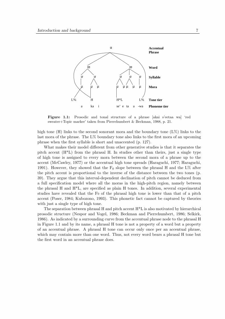
Figure 1.1: Prosodic and tonal structure of a phrase [akai s’eetaa wa] ‘redsweater+Topic marker’ taken from Pierrehumbert & Beckman, 1988, p. 21.
high tone (H) links to the second sonorant mora and the boundary tone (L%) links to thelast mora of the phrase. The L% boundary tone also links to the first mora of an upcomingphrase when the first syllable is short and unaccented (p. 127).
What makes their model different from other generative studies is that it separates thepitch accent (H*L) from the phrasal H. In studies other than theirs, just a single typeof high tone is assigned to every mora between the second mora of a phrase up to theaccent (McCawley, 1977) or the accentual high tone spreads (Haraguchi, 1977; Haraguchi,1991). However, they showed that the F0 slope between the phrasal H and the L% afterthe pitch accent is proportional to the inverse of the distance between the two tones (p.39). They argue that this interval-dependent declination of pitch cannot be deduced froma full specification model where all the moras in the high-pitch region, namely betweenthe phrasal H and H*L, are specified as plain H tones. In addition, several experimentalstudies have revealed that the F0 of the phrasal high tone is lower than that of a pitchaccent (Poser, 1984; Kubozono, 1993). This phonetic fact cannot be captured by theorieswith just a single type of high tone.
The separation between phrasal H and pitch accent H*L is also motivated by hierarchicalprosodic structure (Nespor and Vogel, 1986; Beckman and Pierrehumbert, 1986; Selkirk,1986). As indicated by a surrounding curve from the accentual phrase node to the phrasal Hin Figure 1.1 and by its name, a phrasal H tone is not a property of a word but a propertyof an accentual phrase. A phrasal H tone can occur only once per an accentual phrase,which may contain more than one word. Thus, not every word bears a phrasal H tone butthe first word in an accentual phrase does.
Introduction and background 8
1.2.5 Vowel devoicing
Vowel devoicing is one of the most well-known phenomena in Tokyo Japanese. Descriptively,high vowels (/i/ and /u/) tend to devoice between voiceless consonants under some con-straints. Constraining factors include speech rate, consecutively devoiceable context, pitchaccent, (Kondo, 1996), the type of consonants surrounding the devoiceable vowel, lexical ori-gin, such as Native, Sino-Japanese, or Foreign (Tsuchida, 1997), and morpho-phonologicalboundaries (Yokotani, 1997).
As for the mechanism of vowel devoicing, electromyography and endoscopy have revealedthat the laryngeal activity during the production of a devoiced vowel is different froma voiced vowel in that the glottis is wide open in the former by the activity of posteriorcricoarytenoid and interarytenoid muscles (Hirose, 1971; Sawashima, 1971; Yoshioka, 1981).On the perception side, it has been shown that the spectral coloring from the devoicedvowel to the preceding consonant gives listeners information about the identity of the vowel(Beckman and Shoji, 1984).
Of most concern in the present study is the relationship between vowel devoicing andthe realization of accent. Traditionally, it has been said that an accented vowel is notdevoiceable. Either the accent on the devoiced vowel is shifted to neighboring syllablesor an accented devoiceable vowel is voiced in realization (Vance, 1987). However, it hasalso been pointed out that the tendency to shift accent has become obsolete in youngergeneration (Akinaga, 1985; Kondo, 1996). A number of experimental works support thisobservation (Kitahara, 1996b; Kitahara, 1998; Kitahara, 1999; Maekawa, 1990; Nagano-Madsen, 1994; Sugito, 1982; Varden, 1998).
Then, as mentioned earlier (Section 1.2.3), it has been a matter of debate how listenersperceive an accent on the devoiced mora. In addition to Sugito (1982) and Matsui (1993),Maekawa (1990) conducted a set of production and perception experiments to find thatthe pitch right after the devoiced region is raised, which is a part of perceptual cues foraccent in the devoiced mora. However, these three studies only concerned with perceptionof an accent in a fully devoiced mora, that is, a voiceless consonant followed by a devoicedvowel. Since voiceless consonants surrounding a vowel are one of the necessary conditionsfor that vowel to be devoiced, it is impossible to set a control condition in which a voicedconsonant is followed by a devoiced vowel. But, as for the realization of pitch accent,voiceless consonants alone may erase a substantial part of accent information in a pitchcontour. Previous studies on vowel devoicing and accent seem too focused on the devoicedmora and lack a comparison with control conditions, such as a fully voiced mora and apartially voiceless mora due to voiceless consonants. The present study thus incorporatesthese conditions in order to investigate the category structure of pitch accent in more generalterms.
Introduction and background 9
1.3 Functionalism in phonology
1.3.1 Classic functionalism
Trubetzkoy (1939) proposed three major functions of phonic substances in speech.4
(1.3) The culminative function
A function which serves to indicate how many significant units (words or word-combinations) there are in an utterance.
For example, primary stress in English occurs only once per a content word, which helpsthe listener to analyze the sentence into constituents.
(1.4) The delimitative function
A function whereby a phonic element indicates the boundary between significantunits (i.e. words, word-combinations, or morphemes) in an utterance.
For example, in languages with fixed accent at word edges (Czech, in the initial position,and French, in the final position), the accent helps the listener to also analyze the sentenceinto constituents.
(1.5) The distinctive function
A function whereby significant units are distinguished from each other.
Minimal pairs in any language can serve as an example of this function in which the phone-mic difference that distinguishes the two words in the pair fulfills the distinctive function.
It is evident that the first two functions overlap with each other. That is part of thereason Martinet (1960) proposed the contrastive function which subsumes the culminativefunction and the delimitative function. It is true that the overlap is evident in cases wherethe accent is fixed, but it is still worthwhile to treat the two functions separately in the caseof free accent languages like English or Japanese. Beckman & Edwards (1994) mention thetwo functions in the general framework of prosodic phonology as follows:
(1.6) Beckman & Edwards, 1994: p. 8
4There are many other functions proposed in the literature. Akamatsu (1992) lists five other functionsproposed by Buhler (1920, 1934), Martinet (1960) and himself. They are the representative function, thecontrastive function, the appellative function, the indexical function, and the expressive function. All butthe first two functions are paralinguistic and thus are not the main focus of this thesis. The representativefunction just denotes that a linguistic sign has some referent, which is a very basic function of languagebut not particularly interesting in the context of phonetic research. The contrastive function subsumes thedelimitative and culminative functions.
Introduction and background 10
At any level of the prosodic hierarchy, the number of constituents can be in-dicated by marking the edges or by marking the heads. In the classical linearphonology of Trubetzkoy (1939), these two devices correspond to the demarca-tive and culminative functions, respectively. In metrical representations, theycan be identified roughly with tree versus grids.
1.3.2 Functional load
As for the distinctive function, the notion of functional load has been frequently discussed inthe pre-generative literature (Martinet, 1952; Martinet, 1960; Martinet, 1962; King, 1967;Hockett, 1967). A casual definition of functional load is like the following: when a contrastis more frequently used, that contrast bears a higher functional load. The chief motivationfor proposing functional load is to find a driving force for diachronic language changes.King (1967) succinctly summarizes the argument for functional load in the form of threehypotheses (p. 835):
(1.7) a. The weak point hypothesis states that, if all else is equal, soundchange is more likely to start within oppositions bearing low functionalloads than within oppositions bearing high functional loads; or, in the caseof a single phoneme, a phoneme of low frequency of occurrence is morelikely to be affected by sound change than is a high-frequency phoneme.
b. The least resistance hypothesis states that, if all else is equal, andif (for whatever reason) there is a tendency for a phoneme x to mergewith either of the two phonemes y or z, then that merger will occur forwhich the functional load of the merged opposition is smaller.
c. The frequency hypothesis states that, if an opposition x 6= y is de-stroyed by merger, then that phoneme will disappear in the merger forwhich the relative frequency of occurrence is smaller.
His formulation of functional load is not explicitly given in the paper cited here but, ashe states, it is essentially a product of two factors: the global text frequencies of the twophonemes involved and the degree to which they contrast in all possible environments.5
Hockett (1967) gives an information-theoretic approach for quantification of functionalload which is worth reviewing here since, on the one hand, his proposal is mathematicallysimple and explicit, but on the other hand, his approach makes it clear that the classic
5King (1967) however claims that functional load has very little explanatory power for language change.He investigated four cases from historical Germanic and calculated functional loads for mainly vowel con-trasts. All together, there are 19 cases supporting the three hypotheses but 24 cases rejecting them (p. 848).
Introduction and background 11
notion of functional load of phonemes has problems when applied to an analysis of thepitch accent system in Japanese.
He first introduces a simple system Lm which contains m phonemic units: for example,L4: /1/, /2/, /3/, /4/. If the first two phonemes in L4 coalesce, the system is now calledL3 which has /12/, /3/, and /4/. He states that this corresponds to a diachronic analog inthe coalescence of two phonemes of an earlier stage of a language to form a single phonemeat a later stage. Now, the notion of functional load is that a phonemic system Lm has aquantifiable job to do, and that the contrast between any two phonemes, say /a/ and /b/,carries its share. (p. 305)
Let f(L) be the load carried by a system L, and let f(/a/, /b/) be the share carried bythe contrast between /a/ and /b/. Then we have
f(Lm−11 ) = f(Lm)− f(/a/, /b/)(1.8)
Or, in a transformed form:
f(/a/, /b/) = f(Lm)− f(Lm−11 )(1.9)
Thus, if we can find a way to measure the total load of the system f(L) in differentstages, we can obtain the functional load of a particular contrast, i.e., a pair of phonemescontrasting in a given language.
He then equated the f(Lm) with entropy H (where pi is the probability of occurrenceof the i-th unit) based on mathematical properties of the system L.
H = −m∑
i=1
pi log2 pi(1.10)
So far, the formulation is simple and tractable. However, when it is extended to fea-tures as subcomponents of phonemes, a problem arises: as Hockett notes, “. . . it wouldbe awkward to have to talk about a component coalescing with nothing — that is, disap-pearing or appearing (p. 316).” This is because his system L only allows coalescence ofunits, such as /1/,/2/,/3/,/4/ → /12/,/3/,/4/, but not deletion, such as /1/,/2/,/3/,/4/→ /2/,/3/,/4/. In the case of phonemes, the units /1/, /2/, and /12/ can be anything: forexample, /1/=/p/, /2/=/b/, and /12/=/p/ where the coalescence of /p/ and /b/ results inlosing the voicing contrast in some environment. Feature-wise, however, this coalescence isthe deletion of a privative feature [voiced], which cannot happen when we take those units/1/, /2/ . . . as features in a system L.6 Hockett’s solution to this is simple: do not useprivative features, but use traditional binary features everywhere for the analysis of func-tional load. However, as we have seen in (1.1b), the pitch accent in Tokyo Japanese has aprivative contrast: unaccented vs. accented. A simple application of Hockett’s formulationof functional load would cause a problem.
6I assume privativity for the voicing feature here (Lombardi, 1995).
Introduction and background 12
Of course, it is not impossible to represent the pitch accent system with a binaryHigh/Low feature assigned to each tone-bearing unit of some sort, but such a represen-tation cannot capture the phonology of accentual contrast in Japanese. For example, tonalsequences LHL and LHH are contrastive not because the last tone is different but becausethere is a characteristic pitch pattern “HL” in the former but not in the latter. If wecompare longer sequences, such as LHLL and LHHH, it is clear that the presence/absenceof the characteristic pattern “HL” determines the contrast. The approach with a binaryHigh/Low feature specification for each unit would require the final two L tones in LHLLto somehow group together and contrast with the final two H tones in LHHH. Moreover,it would be complicated and unintuitive to apply Hockett’s formulation of functional loadto such a system in which the load can only be calculated for each High/Low feature. Toobtain the functional load of a particular accentual contrast, a second-order analysis ofsequences of High/Low features would be required.
Functional load in King (1967) and Hockett (1967) is considered as an property of eachphonemic contrast across the entire lexicon. However, the difficulty of this “across-the-board” definition becomes clear when we consider oppositions in features and privativeoppositions. In Chapter 5, I will attempt to quantify the functional load in an alternativemethod based on opposing relations in a set of homophones and word familiarity differenceswithin opposing items.
1.3.3 Type/token frequency and word familiarity
There are more recent theoretical works of phonologists who profess themselves to be func-tionalists (Bybee, 1994; Bybee, 1998; Flemming, 1995; Hayes, 1996b; Boersma, 1997; Kirch-ner, 1998). Among them, Bybee admits her model of lexicon and grammar is functional,though clearly distinguished herself from the European tradition of functionalism includingTrubetzkoy and Martinet. For her, functionalism “does not assume that grammar is createdto serve certain functions, but rather that grammar is the conventionalization of frequently-used discourse patterns” (Bybee, 1994: p. 286). Thus, her so-called usage-based phonologytakes frequency of usage as one of the main driving forces in shaping the grammar.
Though her framework has a different scope from the present study, functionalism inBybee’s sense makes us think more carefully about the notion of “frequency.” There aretwo types of frequency when we talk about the usage of language: type frequency and tokenfrequency.
Token frequency is the frequency of individual items, which corresponds to the vanillacase of the term “word frequency.” According to Bybee, this has two seemingly contra-dicting effects. One effect of high token frequency is the reductive effect, which makeswords and phrases to undergo compression and reduction. The other effect of high tokenfrequency is so-called lexical strength. Frequent items have greater strength of storage inmemory, which contributes to easier access and more resistance to change (Bybee, 1985;1998). The “easy access” part of the lexical strength is well attested in the psycholinguis-tic literature. The “word frequency effect” is that high frequency words are responded tofaster than low frequency words (Balota and Chumbley, 1984; Balota and Chumbley, 1985;
Introduction and background 13
Forster and Chambers, 1973). Token frequency in speech is, however, very cumbersometo obtain. First, it needs a tremendous amount of recording of natural speech in varioussettings, various registers, and various social-groups. Second, the recorded material has tobe segmented and labeled by trained people. Then, words (or so defined units in certainprinciples) are extracted and counted. Studies about token frequency are often based onword frequencies in large-scale text corpora as a substitute of word frequencies in speech.There are of course some problems in this substitution. Of most concern here is that writtenand spoken languages may differ substantially in their style and vocabulary. In addition,the difference in modality may cause a fundamental difference in psychological/lexical pro-cessing. Especially, ideographic Chinese characters used in written Japanese must have aspecial impact on the processing in visual modality but not in auditory modality (Amanoet al., 1995; Hino and Lupker, 1998).
Type frequency is the number of lexical items participating in a certain morphologicalpattern. In the case of accent, for example, this can be equated with the dominance ofthe pattern within a certain fixed repertoire of the accent type. Type frequency is claimedto correspond closely to the productivity of a morphological pattern (Bybee, 1998). Anoft cited example is the irregular inflection in English verbs where certain sub-regularitiesare observed within the “irregular” verbs. Type frequency describes how dominant thosesub-regularities are within the class of irregular verbs. Type frequency can be obtainedfrom a carefully structured dictionary in which relevant morpho-phonological informationhas to be well-organized.
Word familiarity is a type of psychological measure obtained from subjective ratings.Though the intricate psychological processes that account for the source of familiarity arenot clear yet (but see Whittlesea & Williams, 2000), it has been known that token frequencyand word familiarity are positively correlated. Moreover, word familiarity is claimed to bea better probe for investigating the properties of the mental lexicon than token frequency(Nusbaum et al., 1984). Recently, a large-scale word familiarity database in Japanesewas published (Amano and Kondo, 1999). They took subjective ratings of words in threemodalities: Audio, Visual, and Audio-visual. If we use the audio word familiarity, we cancircumvent the aforementioned problems in text-based token frequency for investigatingthe psychological/lexical processes. The database not only includes familiarity but alsonecessary phonological information. Thus, a type frequency analysis can also be done fromthis database. We will see a detailed introduction of the structure of the database andanalyses in Chapter 5.
1.4 Functions of pitch accent
It has been argued that the culminative function is dominant and the distinctive functionis minimal, though present, in the Japanese pitch accent system. Komatsu (1989) statesthat the balance between the two functions has been changing diachronically.
(1.11) Komatsu, 1989: p. 1662 (translation by MK)
Introduction and background 14
Pitch accent in Old Japanese played an important role both in distinctive func-tion and culminative function. However, the gradual change has reduced therole of distinctive function and has lead culminative function to flourish. Theemergence of accentual phrase crucially determines the trend that distinctivefunction is abandoned in order to make culminative function more active.
Previous statistical studies on pitch accent in Japanese have concentrated on the typefrequency of accent locations (Shibata and Shibata, 1990; Shibata et al., 1994; Sato, 1993;Akinaga, 1998). Token frequency of each item has not been taken into consideration inany of the studies I know of. However, it is quite unlikely that token frequency and typefrequency are totally independent. There might be a combined effect of both frequencies inthe comparison between a pattern to which a number of items with high token frequencybelong and the other pattern to which only items with low token frequency belong.
As pointed out in Uwano (1996), function of pitch accent is frequently mentioned butrarely approached quantitatively. Thus, the present thesis includes an extensive databaseanalysis not only to count the number of oppositions or type frequency but also to incorpo-rate word familiarity data from Amano & Kondo (1999) in order to quantify the distinctivefunction of pitch accent.
1.5 Lexical access
As reviewed in previous sections, type/token frequency and word familiarity must playa pivotal role in quantifying the distinctive function of pitch accent. Then, a questionarises: where do these properties come from and how do they affect the process of speechperception? Word frequency/familiarity are obviously the property of words and words areassumed to be stored in the lexicon. Thus, to answer the above question, it is necessaryto briefly review the role of the lexicon in current models of speech perception and spokenword recognition. In addition, as pitch accent is subsumed under a general term “prosody”,the role of prosody in lexical access is another topic to be covered in this section.
A succinct definition of the lexicon and lexical access is given in Cutler (1989) as in thefollowing:
(1.12) Cutler, 1989: p. 342
The lexicon, considered as a component of the process of recognizing speech,is a device that accepts a sound image as input and outputs meaning. Lexicalaccess is the process of formulating an appropriate input and mapping it ontoan entry in the lexicon’s store of sound images matched with their meanings.
This definition focuses, as explicitly stated in the first line, on speech perception andneglects orthography and retrieval in speech production. Models of spoken word recognitionhave been heavily influenced by those of visual word recognition, however. Early modelsof spoken word recognition, such as Logogen theory (Morton, 1979), Autonomous search
Introduction and background 15
model (Forster, 1978) and Connectionist model (McClelland and Elman, 1986) seem to beinfluenced by, or closely connected to, models in visual word recognition. As a result, thosemodels are eager to implement word (token) frequency effect in some way or another, butare reluctant to incorporate the effect of prosody in lexical access. The reason is simple:the word (token) frequency effect has been a big issue in the research history of visual wordrecognition (Broadbent, 1967; Forster & Chambers, 1973; see Balota, 1994 for a review),but prosody has been outside its scope.
Word (token) frequency is coded via the level of activation of a word-like unit in Logogenand Connectionist models where high-frequency words have higher resting level activationsthan low-frequency words. In Autonomous search model, it is implemented as the order ofthe search in which high-frequency words are searched earlier than low-frequency words.
More recently, Anne Cutler and her colleagues have been providing supporting evidencefor an active role of prosody in lexical access (Cutler and Norris, 1988; Cutler, 1989; Cut-ler, 1994). They propose the rhythmic strategy of speech segmentation in which listenershypothesize a word boundary before a metrically strong syllable (Cutler and Norris, 1988).This strategy helps listeners to access the lexicon successfully partly because the type fre-quency of words beginning with a strong syllable is quite high (about 73% in a 30,000 wordcorpus). Moreover, when the mean token frequency is taken into consideration, about 85%of open-class words in average speech contexts begin with a strong syllable (Cutler, 1989).
However, Japanese does not have the strong-weak rhythm of stress languages like En-glish. Pitch accent in Japanese is distinctive while there are very few genuine minimal pairsby stress in English since the stress often alters the vowel quality. Thus, the role of prosodyin lexical access as evidenced by Cutler and others does not directly help investigating thedistinctive function of pitch accent in speech perception. The proposed rhythmic strategyrather corresponds to the delimitative function of prosody in English.
In another study, Cutler and Otake investigated the role of pitch in speech segmentationin Japanese (Cutler and Otake, 1999). They concentrate on the difference between theinitial-accented words and the unaccented words to see if the pitch in the initial portion ofa word has a facilitating effect on lexical access. Their results are positive, which can beinterpreted as evidence for the delimitative function of accent in Japanese. If we extendtheir paradigm to the differences between accented and unaccented words in general, wewill be able to see not only how the delimitative function but also how the culminativefunction work in lexical access.
The review of the psycholinguistic literature in this section reveals that the distinc-tive function of pitch accent in speech perception is still an uncultivated area. Thoughtype/token frequency and word familiarity are assumed as a property of the lexicon, theireffects in categorization performance have not been investigated either.
Chapter 2
Overview of perception experiments
2.1 Introduction
The first part of this chapter reviews claims and methods employed in previous studieson pitch accent perception in more detail than in the previous chapter. Criticism andremaining questions in their work directly motivate the methods and procedures taken inthe present study. It will be pointed out that there has been no systematic treatment ofaccent on devoiced moras and accented words in context. Next, a review of the intonationsynthesis model in Pierrehumbert & Beckman (1988) will be given with an emphasis onthe phonetic implementation and technical details. These details also directly influence theimplementation of the stimulus resynthesis system employed in the present study. Finally,we will see the methods and techniques common to the three experiments in the presentstudy. In particular, an F0 resynthesis technique developed on the basis of STRAIGHT(Speech Transformation and Representation using Adaptive Interpolation of weiGHTedspectrogram) technology (Kawahara and Masuda, 1996) is introduced.
2.2 Previous experimental studies on accent perception
Three studies are of paramount importance to the present work: Sugito (1982), Hasegawa& Hata (1992), and Matsui (1993). Their claims and methodologies lay the groundwork fordesigning the three experiments which will be presented in the subsequent chapters. Thus,though they have been mentioned in Chapter 1, the methods and results in these previousstudies are reviewed in more detail in this section.
2.2.1 Sugito (1982)
Sugito (1982)’s claims about pitch accent perception can be summarized as follows:
(2.1) a. F0 is the fundamental cue to pitch accent perception in Japanese.
b. Intensity does not matter for accent perception even when the accented mora isdevoiced.
16
Overview of perception experiments 17
c. Accent is perceived in the mora immediately before the falling contour.
d. The start of the fall need not to be aligned with the mora boundary.
The first point here is widely acknowledged in the most studies on pitch accent per-ception in Japanese including the present work. (2.1b) is proposed against impressionisticobservations by phoneticians, such as Hattori (1954, 1960) and Kawakami (1969). Theyclaim subjectively that the accent in the devoiced mora is perceived because of the greaterintensity in that mora. Though they admit that pitch is the fundamental cue to accentperception, they take accent on a devoiced mora as a special case. Sugito, however, con-ducted a number of experiments to find that the intensity in the devoiced mora does notaffect the perception of accent in the devoiced mora. The percept of accent on a certainmora is achieved by the falling contour in the following mora, which can be generalizedfor any accent occurrences justifying (2.1c). The final claim in (2.1d) is originally foundin Neustupny (1966) where he observed that the pitch starts to fall in a mora after theaccented mora in some cases. Sugito confirmed this from the results of her experiments andcalled this phenomenon “late fall (ososagari)”.
Results of Sugito’s experiments on accent perception are stated in terms of the param-eters in the superposition model (Fujisaki and Sudo, 1971), such as the timing and theamplitude of accent component and phrase component.
However, linguistic generalizations and the parameter setting in the model do not alwaysmeet (Ladd, 1996). For example, in Sugito’s analysis unaccented forms have to have theaccent component in the same way as accented forms do (p. 292). The amplitude of theaccent component in unaccented forms is not crucially lower than that of accented forms.The difference between accented and unaccented forms is just a matter of the timing of theaccent component. This is against most phonological analyses of accent in Japanese. Theprivative nature of accent, that is, the presence/absence of accentual marking at some levelplays a crucial role in the linguistic description of accent. For this reason, the superpositionmodel is not adopted as a device for stimulus preparation in the present study.
2.2.2 Hasegawa & Hata (1992)
Hasegawa & Hata (1992) conducted an experiment focussed on this “late fall” phenomenon.1
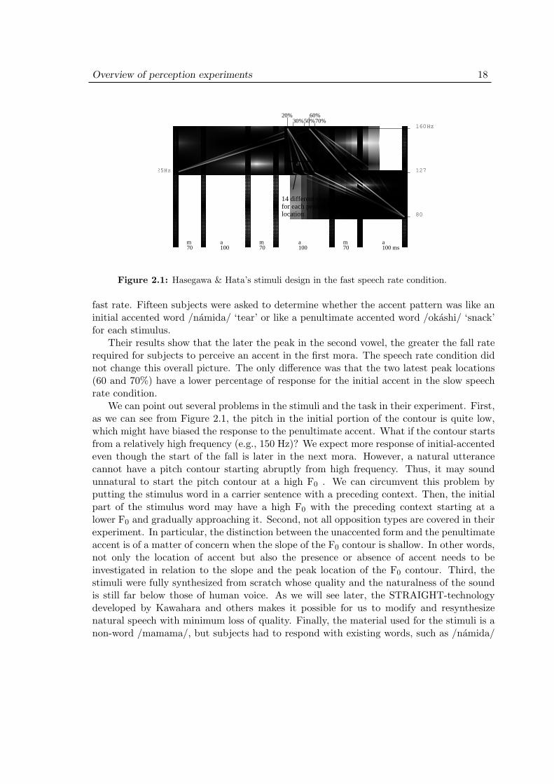
Their research question was how late the fall can be tolerated and how the slope of the fallinteracts with the starting point of the fall. They used MITalk-based full-synthesis systemto create the stimuli which are located in the space shown in Figure 2.1.
The stimulus word is a 3-mora non-word /mamama/ which was presented in isolation.The peak location is varied within the second vowel in 5 steps. The peak occurred at 20, 30,50, 60, and 70% into the second vowel. The slope was varied in 14 steps from 0.24Hz/msto 3.30Hz/ms. They also varied the speech rate of the stimuli. Two speech rates (slowand fast) were used. The vowel duration was 130ms in the slow rate and 100ms in the
1The late fall phenomenon per se is claimed to have a paralinguistic function to signal feminity in theirsubsequent study (Hasegawa and Hata, 1995).
Overview of perception experiments 18
160
127
80
Hz
70m a m a m a
100 100 70 100 ms
70%
70
60%30%50%
20%
14 different slopesfor each peak location
125Hz
Figure 2.1: Hasegawa & Hata’s stimuli design in the fast speech rate condition.
fast rate. Fifteen subjects were asked to determine whether the accent pattern was like aninitial accented word /namida/ ‘tear’ or like a penultimate accented word /okashi/ ‘snack’for each stimulus.
Their results show that the later the peak in the second vowel, the greater the fall raterequired for subjects to perceive an accent in the first mora. The speech rate condition didnot change this overall picture. The only difference was that the two latest peak locations(60 and 70%) have a lower percentage of response for the initial accent in the slow speechrate condition.
We can point out several problems in the stimuli and the task in their experiment. First,as we can see from Figure 2.1, the pitch in the initial portion of the contour is quite low,which might have biased the response to the penultimate accent. What if the contour startsfrom a relatively high frequency (e.g., 150 Hz)? We expect more response of initial-accentedeven though the start of the fall is later in the next mora. However, a natural utterancecannot have a pitch contour starting abruptly from high frequency. Thus, it may soundunnatural to start the pitch contour at a high F0 . We can circumvent this problem byputting the stimulus word in a carrier sentence with a preceding context. Then, the initialpart of the stimulus word may have a high F0 with the preceding context starting at alower F0 and gradually approaching it. Second, not all opposition types are covered in theirexperiment. In particular, the distinction between the unaccented form and the penultimateaccent is of a matter of concern when the slope of the F0 contour is shallow. In other words,not only the location of accent but also the presence or absence of accent needs to beinvestigated in relation to the slope and the peak location of the F0 contour. Third, thestimuli were fully synthesized from scratch whose quality and the naturalness of the soundis still far below those of human voice. As we will see later, the STRAIGHT-technologydeveloped by Kawahara and others makes it possible for us to modify and resynthesizenatural speech with minimum loss of quality. Finally, the material used for the stimuli is anon-word /mamama/, but subjects had to respond with existing words, such as /namida/
Overview of perception experiments 19
160Hz
212Hz
4Hz step196Hz
Devoiced
ha toshi ++ fu kuni
Figure 2.2: Schematic representation of Matsui (1993)’s stimuli design.
‘tear’ and /okashi/ ‘snack’. This is not a simple accent judgment task but some extrasteps are intervening. Subjects first had to memorize the pitch pattern of the stimuli, then,search the mental lexicon and retrieve either /namida/ ‘tear’ or /okashi/ ‘snack’, and thencompare the memory trace of the pitch pattern of the stimulus with canonical representationof accent of those words which might further be converted into a mental representation ofa pitch pattern. This task must have been introduced to circumvent the problem of askingan accent pattern of a non-word /mamama/, which does not exist in the lexicon. Subjectsthus have to go back and forth between the pitch pattern of a non-word and presumablymore abstract accent information of real words in the lexicon. However, if we ask subjectsto judge an accentual minimal pair, such as [ame] ‘candy’ and [ame] ‘rain’, there is no needfor subjects to go over those extra steps. They can just directly compare two real words inthe lexicon, which is a more naturalistic situation in assessing the process of lexical access.
2.2.3 Matsui (1993)
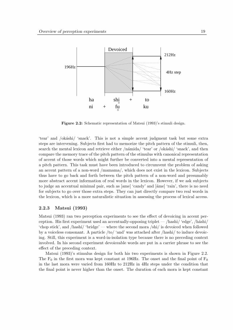
Matsui (1993) ran two perception experiments to see the effect of devoicing in accent per-ception. His first experiment used an accentually-opposing triplet — /hashi/ ‘edge’, /hashi/‘chop stick’, and /hashı/ ‘bridge’ — where the second mora /shi/ is devoiced when followedby a voiceless consonant. A particle /to/ ‘and’ was attached after /hashi/ to induce devoic-ing. Still, this experiment is a word-in-isolation type because there is no preceding contextinvolved. In his second experiment devoiceable words are put in a carrier phrase to see theeffect of the preceding context.
Matsui (1993)’s stimulus design for both his two experiments is shown in Figure 2.2.The F0 in the first mora was kept constant at 196Hz. The onset and the final point of F0
in the last mora were varied from 160Hz to 212Hz in 4Hz steps under the condition thatthe final point is never higher than the onset. The duration of each mora is kept constant
Overview of perception experiments 20
at 200msec.The results from experiment 1 basically confirm Sugito (1982)’s claim in (2.1c) suggest-
ing that the falling contour immediately after the devoiced mora induced the percept of anaccent in the devoiced mora. The results also suggest that the interpolated F0 contour inthe devoiced mora has to be falling in order to perceive an accent in the mora before thedevoiced mora.
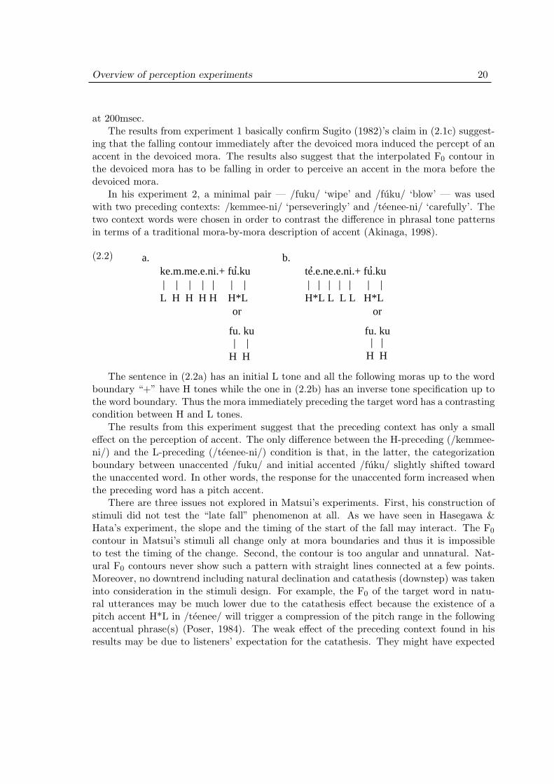
In his experiment 2, a minimal pair — /fuku/ ‘wipe’ and /fuku/ ‘blow’ — was usedwith two preceding contexts: /kemmee-ni/ ‘perseveringly’ and /teenee-ni/ ‘carefully’. Thetwo context words were chosen in order to contrast the difference in phrasal tone patternsin terms of a traditional mora-by-mora description of accent (Akinaga, 1998).
(2.2)
H H| |
H H| |
ke.m.me.e.ni.+ fu.ku
L H H H H H*L
a. b.te.e.ne.e.ni.+ fu.ku
or or
| | | | | | |’
fu. ku fu. ku
H*L L L L H*L | | | | | | |
’ ’
The sentence in (2.2a) has an initial L tone and all the following moras up to the wordboundary “+” have H tones while the one in (2.2b) has an inverse tone specification up tothe word boundary. Thus the mora immediately preceding the target word has a contrastingcondition between H and L tones.
The results from this experiment suggest that the preceding context has only a smalleffect on the perception of accent. The only difference between the H-preceding (/kemmee-ni/) and the L-preceding (/teenee-ni/) condition is that, in the latter, the categorizationboundary between unaccented /fuku/ and initial accented /fuku/ slightly shifted towardthe unaccented word. In other words, the response for the unaccented form increased whenthe preceding word has a pitch accent.
There are three issues not explored in Matsui’s experiments. First, his construction ofstimuli did not test the “late fall” phenomenon at all. As we have seen in Hasegawa &Hata’s experiment, the slope and the timing of the start of the fall may interact. The F0
contour in Matsui’s stimuli all change only at mora boundaries and thus it is impossibleto test the timing of the change. Second, the contour is too angular and unnatural. Nat-ural F0 contours never show such a pattern with straight lines connected at a few points.Moreover, no downtrend including natural declination and catathesis (downstep) was takeninto consideration in the stimuli design. For example, the F0 of the target word in natu-ral utterances may be much lower due to the catathesis effect because the existence of apitch accent H*L in /teenee/ will trigger a compression of the pitch range in the followingaccentual phrase(s) (Poser, 1984). The weak effect of the preceding context found in hisresults may be due to listeners’ expectation for the catathesis. They might have expected
Overview of perception experiments 21
a lower pitch range at the end of the phrase with an accent in the preceding context andthus responded to the accented tokens as unaccented. Third, he did not include a controlcondition where the to-be-devoiced mora is partially voiced, namely, /shi/ in /hashi/ or/fu/ in /fuku/. Although he showed the results from a pilot experiment using fully voicedpair /ame/–/ame/ ‘rain’–‘candy’, the question remains whether the accent perception isaffected only by vowel devoicing or by the combination of voiceless consonant and voweldevoicing.
2.3 Intonation synthesis in Pierrehumbert & Beckman’smodel
This section reviews the intonation synthesis model in Pierrehumbert & Beckman (1988)on which the design of the stimuli in the present study is based. As I have criticized in theprevious sections, perception experiments by Hasegawa & Hata (1992) and Matsui (1993)used angular and unnatural F0 contours as their stimuli. Moreover, their stimulus design isnot phonologically well-grounded. In other words, there is no explicit model of phonologythat produces the F0 contours used in their experiments. Thus, there is a possibility thattheir stimuli are out of the range in which a human speaker can naturally produce. Thechief motivation for adopting Pierrehumbert & Beckman’s model in this study is to pursuea phonologically tractable model of the perception of pitch accents.
Their model essentially consists of 4 major steps to produce the output intonationpattern for Tokyo Japanese, which are summarized in (2.3) and plotted graphically inFigure 2.4.
(2.3) a. Set a sequence of boundary tones (L%), phrasal H tones, and accent H*L’s.
b. Add constant declination.
c. Convolution with a mora-sized window for smoothing.
d. Add random noise for natural jitter.
The following subsections review each of these steps in order.
2.3.1 Tone sequencing
The first step in (2.3) is a linguistic specification of tonal units whose alignment (horizontaldimension in msec) and scales (vertical dimension in Hz) are fine-tuned by various phono-logical and speaker-specific requirements. As reviewed in Section 1.2.4, the output of thephonological system contains only a sparse representation of tones and thus not all morasare bound to a tone. At most one pitch accent (H*L) and some boundary or phrasal tonesin the vicinity of edges are allowed in each accentual phrase even when the number of tonebearing units (i.e., moras) by far exceeds the number of tones. The phonetic implementationof the timing and the duration of those tones are specified by a rule in the following:
Overview of perception experiments 22
(2.4) Pierrehumbert & Beckman (1988: p. 178)
Whenever a tone is associated to a mora, it has a duration. Any other toneis a single point in time, located at the relevant edge of the interval of morasgoverned by the node to which it is attached.
Thus, a phrasal H tone linked to the second mora of the phrase has a mora-lengthduration while the L% tone at the edge of the phrase has only a point specification. Thepitch accent H*L has a combined representation of time: the H* part is associated to theaccented mora and thus has a mora-length duration while the L part only has a point rightafter the H*.
As for the tone scaling, the pitch range is a speaker-specific property which is set by theupper and the lower limit. The upper limit is called a high-tone line (h) which is defined asthe value for a hypothetical H tone of maximal prominence in the phrase (Pierrehumbert& Beckman, 1988: p. 182). The lower limit is called a reference line (r) which is tentativelydefined as a speaker-specific constant but they also offer several alternative models whichrelate r to h in a linear fashion.2 In their implementation of the intonation synthesizer,only one speaker whose r value is derived from production data is modeled.
The prominence level of tones, denoted as “T(X)” where “X” represents either H or Ltones, is defined as a value of F0 expressed as a proportion of the range between h and r. Htones are scaled upward from the reference line while L tones are scaled downward from thehigh-tone line. Thus, the prominence value for H tone and L tone are defined in equation(2.5) and (2.6) respectively.
T(H) =H− r
h− r(2.5)
T(L) = 1− L− r
h− r(2.6)
For example, if h = 180Hz, r = 90Hz, H = 165Hz, and L = 120Hz, the T(H)= (165 −90)/(180 − 90) = 0.83, and T(L)= 1 − (120 − 90)/(180 − 90) = 0.67. When synthesizingan intonation contour for an utterance, we can specify the F0 of each tone by setting theprominence level as T(X). When T(H) is larger, the H tone is more prominent and thusscaled higher in Hz. On the contrary, the prominence level for L tone is scaled downward:when T(L) is larger, the L tone is lower in Hz.
By transforming the tone scale from Hz to a 0-1 ratio in the pitch range defined byh and r, all the prominence relations including boundary strength, catathesis effects, andH*-to-phrasal H relation are handled in a uniform way. On the other hand, the effect offocus and the final lowering process are captured not by the prominence of each tone but
2They propose that the relationship between r and h are captured by a simple linear equation r = ah+ band discuss possible interpretations for cases where a or b is zero. Taking r as a constant is one instanceof this model when a is set to zero. Their discussion is based on the shift of pitch range in emphasizedutterances which is out of the scope of this study, however.
Overview of perception experiments 23
by the expansion/compression of the pitch range. Though the purpose of the present studyis not to study the issue of focus and pitch contour, the final lowering process is still ofconcern since the pitch accents in our material are always placed in the domain of the finallowering. Let us review the basic facts of final lowering and its implementation in theirmodel next.
The final lowering process in Pierrehumbert & Beckman (1988) is a direct inheritancefrom Liberman & Pierrehumbert (1984)’s model on English intonation. They found thatin English final accent is always lower than what would have been predicted from a simpledownstep process. They proposed that the final lowering is an effect from the end of anutterance and is independent from both declination (a function of time from the beginning)and downstep (a function of the number of accents from the beginning). Their proposalwas exemplified across different conditions which made it possible to show the underlyinggeneralization in pitch scaling. In fact, this is claimed as an advantage to a superpositionmodel where a manipulation on a specific accent as Liberman and Pierrehumbert did seemsto be rather difficult to achieve with the same simplicity (Ladd, 1996).
The two synthesis parameters, “f rate” and “f ms”, are introduced for the final lower-ing process in Pierrehumbert & Beckman (1988, p. 207). However, their meaning is notexplained and the algorithm for the final lowering is not explicitly stated. According toBeckman (personal communication), the role of “f rate” (final lowering rate) is to specifythe rate of declination of the high tone line and the role of “f ms” (final lowering domain) isthe starting point from the end of the utterance of the final lowering in seconds. The “f rate”parameter works in the following fashion to specify the ending point of the high-tone linein Hz.
h = r + (f rate× (h− r))(2.7)
To summarize, the tone sequencing part of the intonation synthesis gives target valuesboth in horizontal and vertical dimensions. The horizontal dimension is basically determinedby the alignment of tones with moras while the vertical dimension is determined by anintricate set of rules for prominence levels and pitch range. An example of a sequenceof tones for a short phrase similar to the one used in the present study is described inFigure 2.3 with hypothetical parameter settings in Table 2.1. Sample values are not basedon measurements but arbitrary for purely expository purposes.
2.3.2 Declination
The next step in (2.3) is to tilt the whole sequence, which imitates the overall declinationof pitch seen in natural speech. The ratio of declination is a speaker specific constant inPierrehumbert & Beckman (1988) because their data show that the variability of declinationis quite huge across speakers. They give −10Hz/sec as an example in their demonstrationtaken from one speaker’s data. See Figure 2.4 for the effect of declination from panel (a) to(b).
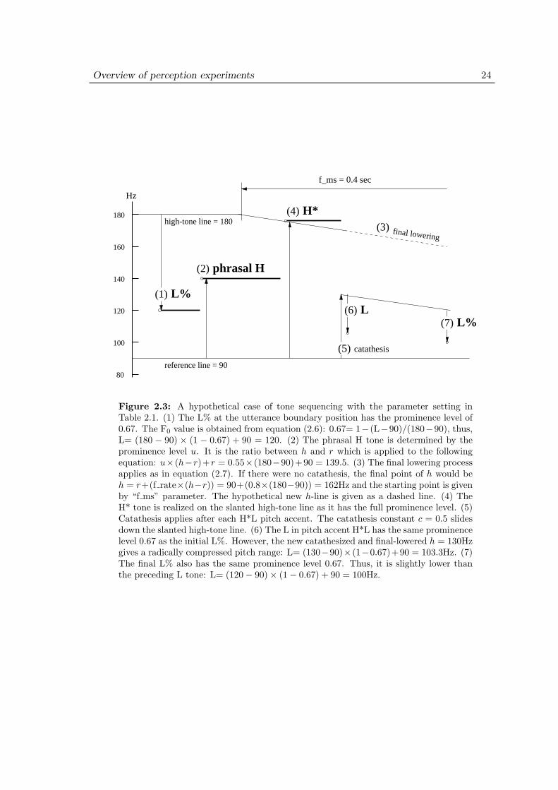
Overview of perception experiments 24
phrasal H
catathesis
80
100
120
140
160
180
Hz
f_ms = 0.4 sec
high-tone line = 180final lowering
L%
L%
H*
L
reference line = 90
(5)
(3)
(1)
(2)
(4)
(7)(6)
Figure 2.3: A hypothetical case of tone sequencing with the parameter setting inTable 2.1. (1) The L% at the utterance boundary position has the prominence level of0.67. The F0 value is obtained from equation (2.6): 0.67= 1− (L−90)/(180−90), thus,L= (180 − 90) × (1 − 0.67) + 90 = 120. (2) The phrasal H tone is determined by theprominence level u. It is the ratio between h and r which is applied to the followingequation: u× (h−r)+r = 0.55× (180−90)+90 = 139.5. (3) The final lowering processapplies as in equation (2.7). If there were no catathesis, the final point of h would beh = r+(f rate×(h−r)) = 90+(0.8×(180−90)) = 162Hz and the starting point is givenby “f ms” parameter. The hypothetical new h-line is given as a dashed line. (4) TheH* tone is realized on the slanted high-tone line as it has the full prominence level. (5)Catathesis applies after each H*L pitch accent. The catathesis constant c = 0.5 slidesdown the slanted high-tone line. (6) The L in pitch accent H*L has the same prominencelevel 0.67 as the initial L%. However, the new catathesized and final-lowered h = 130Hzgives a radically compressed pitch range: L= (130−90)× (1−0.67)+90 = 103.3Hz. (7)The final L% also has the same prominence level 0.67. Thus, it is slightly lower thanthe preceding L tone: L= (120− 90)× (1− 0.67) + 90 = 100Hz.
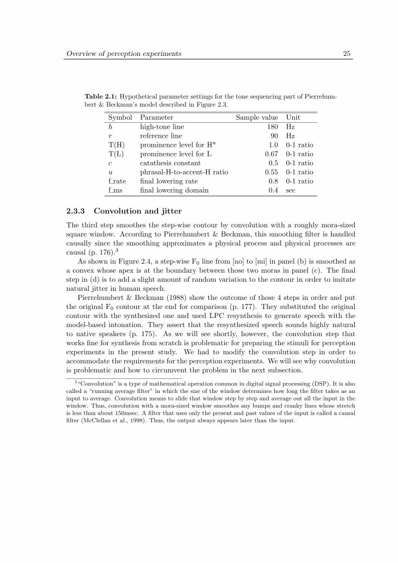
Overview of perception experiments 25
Table 2.1: Hypothetical parameter settings for the tone sequencing part of Pierrehum-bert & Beckman’s model described in Figure 2.3.
Symbol Parameter Sample value Unith high-tone line 180 Hzr reference line 90 HzT(H) prominence level for H* 1.0 0-1 ratioT(L) prominence level for L 0.67 0-1 ratioc catathesis constant 0.5 0-1 ratiou phrasal-H-to-accent-H ratio 0.55 0-1 ratiof rate final lowering rate 0.8 0-1 ratiof ms final lowering domain 0.4 sec
2.3.3 Convolution and jitter
The third step smoothes the step-wise contour by convolution with a roughly mora-sizedsquare window. According to Pierrehumbert & Beckman, this smoothing filter is handledcausally since the smoothing approximates a physical process and physical processes arecausal (p. 176).3
As shown in Figure 2.4, a step-wise F0 line from [no] to [mi] in panel (b) is smoothed asa convex whose apex is at the boundary between those two moras in panel (c). The finalstep in (d) is to add a slight amount of random variation to the contour in order to imitatenatural jitter in human speech.
Pierrehumbert & Beckman (1988) show the outcome of those 4 steps in order and putthe original F0 contour at the end for comparison (p. 177). They substituted the originalcontour with the synthesized one and used LPC resynthesis to generate speech with themodel-based intonation. They assert that the resynthesized speech sounds highly naturalto native speakers (p. 175). As we will see shortly, however, the convolution step thatworks fine for synthesis from scratch is problematic for preparing the stimuli for perceptionexperiments in the present study. We had to modify the convolution step in order toaccommodate the requirements for the perception experiments. We will see why convolutionis problematic and how to circumvent the problem in the next subsection.
3“Convolution” is a type of mathematical operation common in digital signal processing (DSP). It is alsocalled a “running average filter” in which the size of the window determines how long the filter takes as aninput to average. Convolution means to slide that window step by step and average out all the input in thewindow. Thus, convolution with a mora-sized window smoothes any bumps and cranky lines whose stretchis less than about 150msec. A filter that uses only the present and past values of the input is called a causalfilter (McClellan et al., 1998). Thus, the output always appears later than the input.
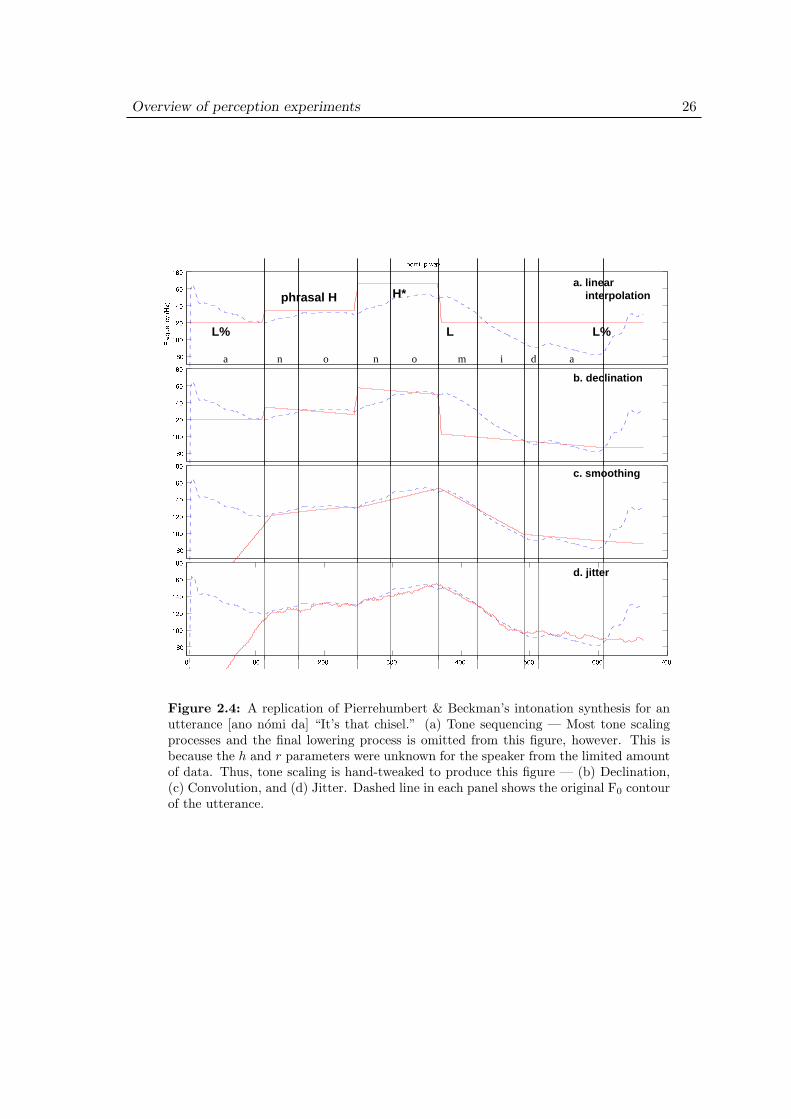
Overview of perception experiments 26
���
�����
�����
�����
����
���������� ����� �����
� ��� ��������
���
�����
�����
�����
����
�����
���
�����
�����
�����
����
�����
� ����� ����� !���� �"��� #���� ���� $�������
�����
�����
�����
����
�����
a
c. smoothing
b. declination
a. linear interpolation
L L%
H*
L%
o n o m i adn
d. jitter
phrasal H
Figure 2.4: A replication of Pierrehumbert & Beckman’s intonation synthesis for anutterance [ano nomi da] “It’s that chisel.” (a) Tone sequencing — Most tone scalingprocesses and the final lowering process is omitted from this figure, however. This isbecause the h and r parameters were unknown for the speaker from the limited amountof data. Thus, tone scaling is hand-tweaked to produce this figure — (b) Declination,(c) Convolution, and (d) Jitter. Dashed line in each panel shows the original F0 contourof the utterance.
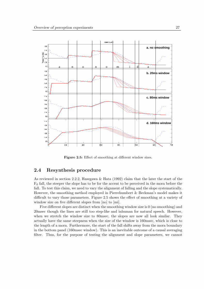
Overview of perception experiments 27
���
�����
�����
�����
�����
������ ��� ����� �����
� ���������� !
���
�����
�����
�����
�����
�����
���
�����
�����
�����
�����
�����
� ����� ����� "���� ����� #���� ����� $�������
�����
�����
�����
�����
�����
a. no smoothing
b. 20ms window
c. 80ms window
d. 160ms window
aa n do n o m i
Figure 2.5: Effect of smoothing at different window sizes.
2.4 Resynthesis procedure
As reviewed in section 2.2.2, Hasegawa & Hata (1992) claim that the later the start of theF0 fall, the steeper the slope has to be for the accent to be perceived in the mora before thefall. To test this claim, we need to vary the alignment of falling and the slope systematically.However, the smoothing method employed in Pierrehumbert & Beckman’s model makes itdifficult to vary those parameters. Figure 2.5 shows the effect of smoothing at a variety ofwindow size on five different slopes from [no] to [mi].
Five different slopes are distinct when the smoothing window size is 0 (no smoothing) and20msec though the lines are still too step-like and inhuman for natural speech. However,when we stretch the window size to 80msec, the slopes are now all look similar. Theyactually have the same steepness when the size of the window is 160msec, which is close tothe length of a mora. Furthermore, the start of the fall shifts away from the mora boundaryin the bottom panel (160msec window). This is an inevitable outcome of a causal averagingfilter. Thus, for the purpose of testing the alignment and slope parameters, we cannot
Overview of perception experiments 28
directly adopt the smoothing method in Pierrehumbert & Beckman (1988).To avoid too much smoothing while keeping the naturalness of the F0 contour, a different
approach was taken in the present study. Remember random variation was added in thelast step of Pierrehumbert & Beckman’s model for intonation synthesis summarized in (2.3)and in Figure 2.4. The idea is to use this last step also for the smoothing. The stimuli inthe present study are not fully synthesized from scratch but resynthesized from a naturalspeech with modified F0 contour. Thus, the stimuli always have the original utterance incontrast to full-synthesis models. We can always go back to the original utterance andfetch whatever properties we want in order to make the outcome of the resynthesis processnatural. Thus, the source of smoothed but somewhat jittered contour is taken from theoriginal utterance in the present study. This is a rather desirable step for a perceptionexperiment where no other parameters than the one under the scrutiny are changed fromthe original.4
The four common steps in resynthesizing the stimuli in all experiments in the presentstudy are depicted in Figure 2.6. In the top panel, the F0 contour of the original utteranceof [ano kami da] “It’s that God.” is shown in a solid line. Dashed line indicates its slightlysmoothed contour obtained by a convolution with a 50msec window.5 The purpose of thissmoothing is to obtain the difference between the smoothed contour and the original one.As for the input to the filter, the devoiced part of [k] is filled with the median of the F0
value in order to avoid a sudden drop of F0 in the smoothed contour.The second panel in Figure 2.6 shows this difference which extracts the perturbation
of F0 contour by consonants and some jitter from the original contour. This differenceterm is added to the interpolated tone sequences in the next panel. The diagonal line inthis panel shows the amount of declination which is also added to the interpolated tonesequence. The third panel shows interpolated tone sequences whose alignment and slopesare systematically varied in order to create a stimulus continuum between an initial-accentedword [kami] “God” and a final-accented word [kamı] “paper.” The bottom panel shows thefinal outcome of the resynthesis procedure in which all the elements in the second and thethird panel are summed up. As we can see, the alignment and slope structure in the stimuli
4Another technique introduced for creating a naturalistic contour was to specify level tones not for theentire duration of a mora as in Pierrehumbert & Beckman (1988) but only for the vowel part of the mora.They admit that the specification of the duration of tonal targets in their implementation is tentative andspeaker specific (p. 178). There seems to be no strong argument for stretching the duration of tones for theentire mora in terms of phonetic evidence. Phonologically, we can interpret the association from a tone toa mora to be equivalent to the association to the nucleus vowel following standard assumptions in moraicphonology (Hayes, 1989) where the onset consonant does not pertain to the syllable weight because it isnot linked to the mora node but directly to the syllable node. As a consequence, only vowels can bear leveltones for its entire duration and onset consonants cannot.
5This averaging filter is non-causal. In other words, the output of the filter was re-aligned with the originalutterance. Pierrehumbert & Beckman (1988) used a causal filter based on the fact that physical processesare causal in a real-time speech production system of humans. We are not aiming at a real-time speechproduction system but rather at a system of stimulus-preparation whose outcome is reasonably natural andat the same time manipulable for the purpose of our experiment. Thus, we do not adhere to the use of acausal filter.
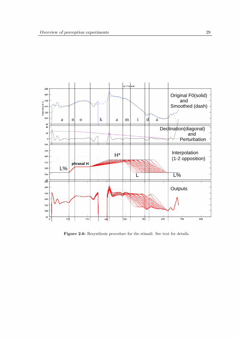
Overview of perception experiments 29
���
�����
�����
�����
�����
�����
��������� ������� � ��
� �����������
�
���
���
���
�����
�����
�����
�����
�����
�����
� ����� ����� !���� ����� "���� ����� #���� ��������
�����
�����
�����
�����
�����
�����
a n o k a i d am
Original F0(solid)
Smoothed (dash)and
Declination(diagonal)and
Perturbation
Interpolation(1-2 opposition)
Outputs
L%
H*
L L%
phrasal H
Figure 2.6: Resynthesis procedure for the stimuli. See text for details.

Overview of perception experiments 30
are modified from those in the third panel but kept distinct at least visually. Still, eachcontour seems reasonably natural and more importantly, consonantal perturbations in theoriginal utterance are maintained and well-aligned with the timing of segments.
2.5 Stimulus preparation and presentation
Procedures for stimuli preparation and presentation were basically common in all the ex-periments in the present study. This section summarizes these common steps. First of all,the original utterances for resynthesis were recorded in a sound-proof room by the author(33 years, male, Eastern dialect of Japanese) on a DAT at 44.1 kHz sampling frequency in16 bit accuracy. Then, the digitized sound files were transferred to a workstation keepingthe original sound quality and processed by the STRAIGHT package (version 30 release16) developed by Kawahara and others (Kawahara and Masuda, 1996; Kawahara et al.,1997a). The sound quality and the naturalness of the output of the STRAIGHT packageis extremely good as evidenced by a number of evaluation experiments (Kawahara et al.,1997b; Zolfaghari and Kawahara, 1999; Atake et al., 1999). The version I used was the lat-est development of the STRAIGHT package at that time which includes an algorithm forprocessing aperiodic characteristics of the input signal, which has an advantage in treatingthe voiceless part (Kawahara et al., 1999).
The input signal to STRAIGHT was normalized in amplitude since the analysis-resynthesis processes are sensitive to amplitude differences. The utterance was visuallysegmented using the STRAIGHT as an analysis tool. The duration of each mora was notmanipulated so that each stimulus had slightly different duration. A Matlab-based scriptwas used to create a set of F0 contours for resynthesis. The output contours and the seg-mented speech signal were then fed to the STRAIGHT package to create resynthesizedspeech. The output of the resynthesis processes kept a 44.1 kHz sampling frequency and 16bit accuracy for the best sound quality possible. The amplitude of the resynthesized speechwas again normalized for the perception experiment.
All experiment sessions were controlled by a Matlab script designed and programmedby the author and colleagues. Subjects were asked to click a mouse button to select anappropriate word displayed on a CRT upon hearing the audio stimuli. The audio stimuliwere presented to subjects through a STAX SR-ΛPRO headset at 69dB in a sound-proofroom. Subjects listened to each stimulus as many times as they wanted and then proceededto the next stimulus at their own pace.
Post-trials were added after all the experimental trials were done. At least 50 proto-typical stimuli in each experiment were selected for post trials from the stimuli set. Thus,the stimuli selected for post-trials were presented twice to subjects. Subjects were not toldwhether they were doing the post trials or not, however. Correlation of answers betweenthe post trials and main trials were taken to check the consistency of subjects’ performance.
Chapter 3
Categorization in a 2-way distinction
3.1 Introduction
Two experiments were carried out to investigate the category structure of pitch accents ina 2-way distinction. The first experiment was designed to check the compensatory relationbetween the H* alignment and the slope after the H* tone as claimed by Hasegawa & Hata(1992). The design also has an exploratory aspect in which the tone scaling and voicingcondition are introduced to study the category structure in 2-mora words in more generalterms.
The second experiment was a direct development from the first one with some modifi-cations in the stimulus design. Most notably, the preceding context of the pitch accent wasintroduced as another variable while the slope variable was dropped. The second experi-ment had another independent purpose, that is to investigate the role of functional load ofpitch accent in performance. This aspect of the experiment will be dealt with separately inChapter 6.
3.2 Experiment 1: Purpose
The main purpose of Experiment 1 is, as stated earlier, to check the compensatory relationbetween the H* alignment and the slope after the H* tone as claimed by Hasegawa &Hata (1992). A simple replication of their experiment only involves the accent-locationdistinction, such as initial vs. final. However, as reviewed in Chapter 2, the manipulationof slopes in accent-presence distinction, such as the 0-1 and the 0-2 oppositions, is a relatedbut unexplored area. Thus, it is necessary to probe the stimulus space for the more generalcategory structure in accent perception. Another extension from the Hasegawa & Hata’sparadigm is the issue of the effect of devoicing in accent perception. Sugito (1982) andMatsui (1993) both claim that the following falling contour induces the percept of accentin a devoiced mora. Sugito (1982) further claims that the “late falling” phenomena, whichmotivated Hasegawa & Hata’s experiment, and the percept of accent in a devoiced moraare common in the sense that the falling contour after the devoiced mora is just anothertype of “late” realization of the fall because of the intervening devoiced region between the
31
Categorization in a 2-way distinction 32
peak and the fall. Therefore, it is natural to extend the scope of the present experiment tothe question of devoicing.
At first glance, the cessation of pitch contour by any voiceless segment would seemharmful to the recovery of the accent information. However, since vowel devoicing is sucha peculiar topic in the history of Japanese phonetics (see review in Section 1.2.5), mostattention has been paid only to the effect of a devoiced vowel on pitch accent. As far asI am aware, no study has compared the effect of cessation of pitch contour by a voicelessconsonant and by a devoiced vowel (cf. House, 1990 for the effect of a brief cessation bya voiced consonant in Swedish). By incorporating a voiceless consonant, there are threedifferent voicing conditions for a certain mora: fully voiced (C V), voiceless consonant (C◦V), and devoiced (C◦ V◦).
The location of the accent with respect to the target mora of the voicing variation isanother crucial factor. Fixing the location of the mora with voicing variation to the secondmora, the falling contour will be in that mora for accent-1, or after that mora for accent-2.As for accent-0, the cessation of the pitch contour may cause an ambiguity between theunaccentedness and the accentedness.
As stated in Section 1.2.1, three types of two-way distinctions are possible in 2-morawords. They are labelled by a combination of the numbers for accent location. Thus, the0-1, 0-2 and 1-2 opposition are the distinction between accent-0 and accent-1, accent-0 andaccent-2, and accent-1 and accent-2, respectively.
Several hypotheses can be formulated by crossing these three opposition types and thethree voicing conditions. As a null hypothesis, there is a possibility that the cessation ofthe pitch contour does not matter. If it does matter, then more specific hypotheses aboutthe role of tonal specification are in order. Let us see a schematic illustration of voicingconditions and their effect on stylized pitch contours in Figure 3.1. Note that the consonantsaround a vowel have to be voiceless for that vowel to be devoiced. Therefore, the durationof the voiceless region changes with a leap from the voiceless consonant condition to thedevoiced condition.1
In the 0-1 opposition, the falling part of the contour is erased partially in the voicelessconsonant condition, or completely in the devoiced condition. Still, the remaining pitchcontour keeps the whole length of the H* and the L% level tones. Assuming that thefalling contour and level tones have independent contributions to the perception of accent,it is expected that the the erasure of the falling contour will shift the principal source ofinformation to the two level tones. Since the two level tones are kept anyway in the devoicedcondition, the effect of this shift will be more visible in the comparison between the fullyvoiced condition and the voiceless consonant condition than in the comparison between the
1As reviewed in Section 1.2.5, vowel devoicing is not a mandatory process which applies to all devoiceablecontexts. Kondo (1996) mentions some constraining conditions under which the devoiceable vowel is fully orpartially voiced. Thus, the voiceless consonant condition can be further divided into two cases: (a) followedby a voiced consonant (C◦ V C), and (b) followed by another voiceless consonant (C◦ V C◦). The vowel incase (a) is intrinsically undevoiceable while that in case (b) is a voiced realization in a devoiceable context.Experiment 3 in Chapter 4 deals with the comparison between these two cases. The discussion in the presentchapter only concerns the case (a) of the voiceless consonant condition.
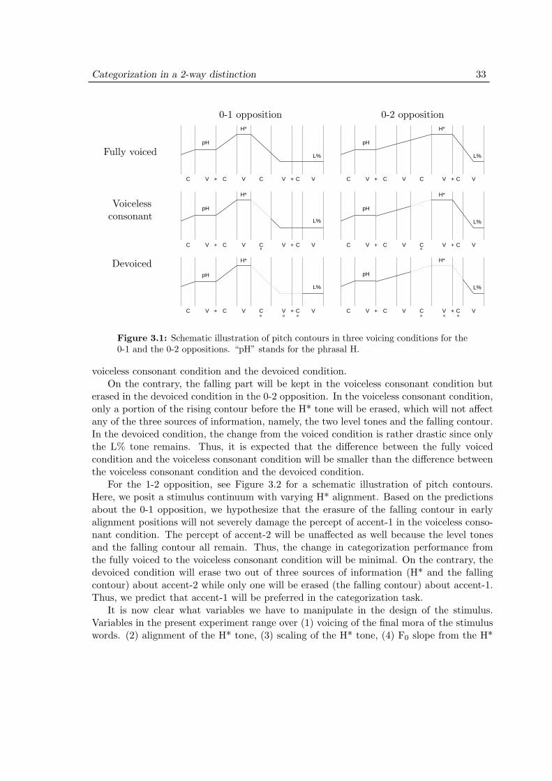
Categorization in a 2-way distinction 33
Fully voiced
Voicelessconsonant
Devoiced
0-1 opposition
C V C VV C ++ C V
C V C VV C ++ C V
C V C VV C ++ C V
pH
L%
H*
pH
pH
H*
H*
L%
L%
0-2 opposition
C V C VV C ++ C V
C V C VV C ++ C V
pH
L%
H*
pH
L%
H*
C V C VV C ++ C V
pH
L%
H*
Figure 3.1: Schematic illustration of pitch contours in three voicing conditions for the0-1 and the 0-2 oppositions. “pH” stands for the phrasal H.
voiceless consonant condition and the devoiced condition.On the contrary, the falling part will be kept in the voiceless consonant condition but
erased in the devoiced condition in the 0-2 opposition. In the voiceless consonant condition,only a portion of the rising contour before the H* tone will be erased, which will not affectany of the three sources of information, namely, the two level tones and the falling contour.In the devoiced condition, the change from the voiced condition is rather drastic since onlythe L% tone remains. Thus, it is expected that the difference between the fully voicedcondition and the voiceless consonant condition will be smaller than the difference betweenthe voiceless consonant condition and the devoiced condition.
For the 1-2 opposition, see Figure 3.2 for a schematic illustration of pitch contours.Here, we posit a stimulus continuum with varying H* alignment. Based on the predictionsabout the 0-1 opposition, we hypothesize that the erasure of the falling contour in earlyalignment positions will not severely damage the percept of accent-1 in the voiceless conso-nant condition. The percept of accent-2 will be unaffected as well because the level tonesand the falling contour all remain. Thus, the change in categorization performance fromthe fully voiced to the voiceless consonant condition will be minimal. On the contrary, thedevoiced condition will erase two out of three sources of information (H* and the fallingcontour) about accent-2 while only one will be erased (the falling contour) about accent-1.Thus, we predict that accent-1 will be preferred in the categorization task.
It is now clear what variables we have to manipulate in the design of the stimulus.Variables in the present experiment range over (1) voicing of the final mora of the stimuluswords. (2) alignment of the H* tone, (3) scaling of the H* tone, (4) F0 slope from the H*
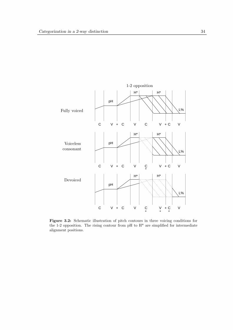
Categorization in a 2-way distinction 34
Fully voiced
Voicelessconsonant
Devoiced
1-2 opposition
C V C VV C ++ C V
C V C VV C ++ C V
pH
L%
H*
C V C VV C ++ C V
pH
L%
H*
H*
H*
H*
pH
L%
H*
Figure 3.2: Schematic illustration of pitch contours in three voicing conditions forthe 1-2 opposition. The rising contour from pH to H* are simplified for intermediatealignment positions.
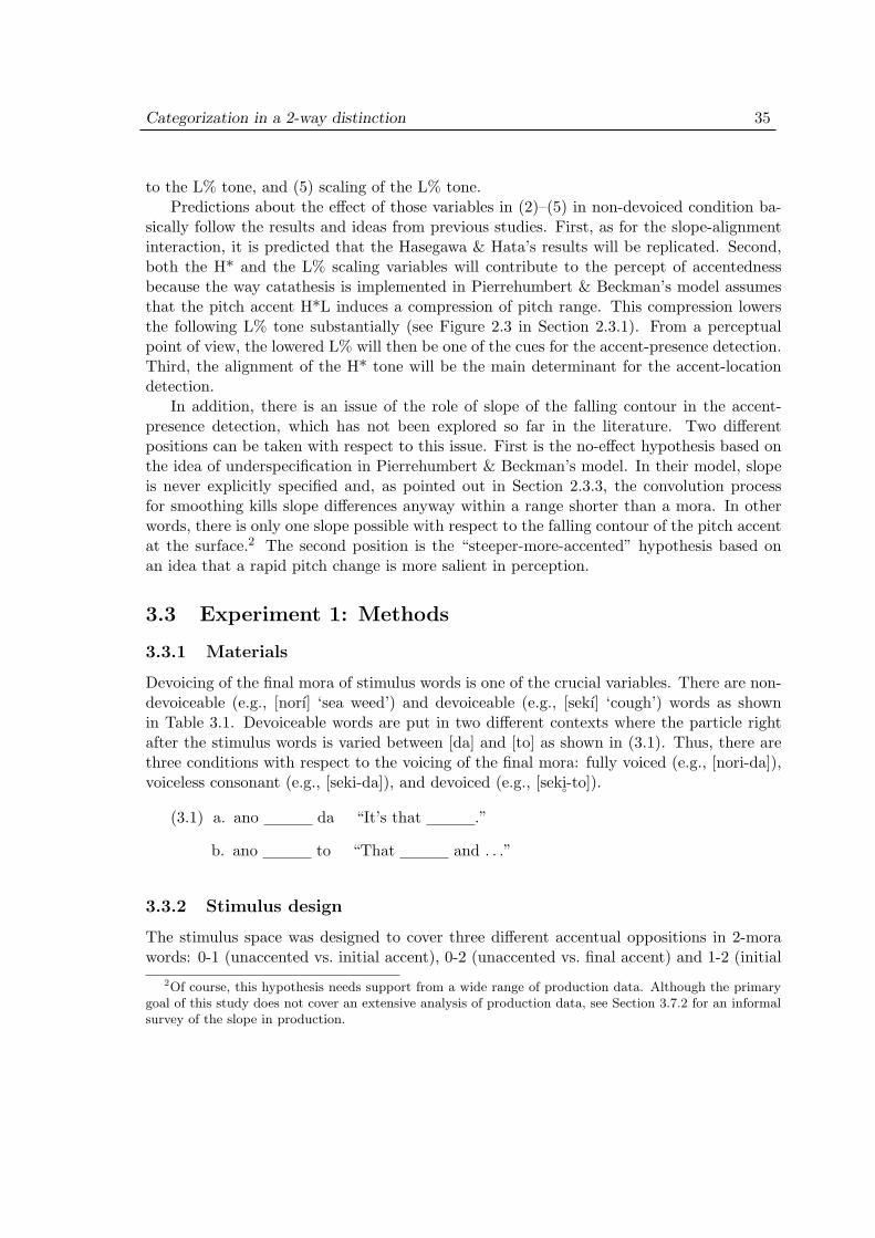
Categorization in a 2-way distinction 35
to the L% tone, and (5) scaling of the L% tone.Predictions about the effect of those variables in (2)–(5) in non-devoiced condition ba-
sically follow the results and ideas from previous studies. First, as for the slope-alignmentinteraction, it is predicted that the Hasegawa & Hata’s results will be replicated. Second,both the H* and the L% scaling variables will contribute to the percept of accentednessbecause the way catathesis is implemented in Pierrehumbert & Beckman’s model assumesthat the pitch accent H*L induces a compression of pitch range. This compression lowersthe following L% tone substantially (see Figure 2.3 in Section 2.3.1). From a perceptualpoint of view, the lowered L% will then be one of the cues for the accent-presence detection.Third, the alignment of the H* tone will be the main determinant for the accent-locationdetection.
In addition, there is an issue of the role of slope of the falling contour in the accent-presence detection, which has not been explored so far in the literature. Two differentpositions can be taken with respect to this issue. First is the no-effect hypothesis based onthe idea of underspecification in Pierrehumbert & Beckman’s model. In their model, slopeis never explicitly specified and, as pointed out in Section 2.3.3, the convolution processfor smoothing kills slope differences anyway within a range shorter than a mora. In otherwords, there is only one slope possible with respect to the falling contour of the pitch accentat the surface.2 The second position is the “steeper-more-accented” hypothesis based onan idea that a rapid pitch change is more salient in perception.
3.3 Experiment 1: Methods
3.3.1 Materials
Devoicing of the final mora of stimulus words is one of the crucial variables. There are non-devoiceable (e.g., [norı] ‘sea weed’) and devoiceable (e.g., [sekı] ‘cough’) words as shownin Table 3.1. Devoiceable words are put in two different contexts where the particle rightafter the stimulus words is varied between [da] and [to] as shown in (3.1). Thus, there arethree conditions with respect to the voicing of the final mora: fully voiced (e.g., [nori-da]),voiceless consonant (e.g., [seki-da]), and devoiced (e.g., [seki◦-to]).
(3.1) a. ano da “It’s that .”
b. ano to “That and . . .”
3.3.2 Stimulus design
The stimulus space was designed to cover three different accentual oppositions in 2-morawords: 0-1 (unaccented vs. initial accent), 0-2 (unaccented vs. final accent) and 1-2 (initial
2Of course, this hypothesis needs support from a wide range of production data. Although the primarygoal of this study does not cover an extensive analysis of production data, see Section 3.7.2 for an informalsurvey of the slope in production.
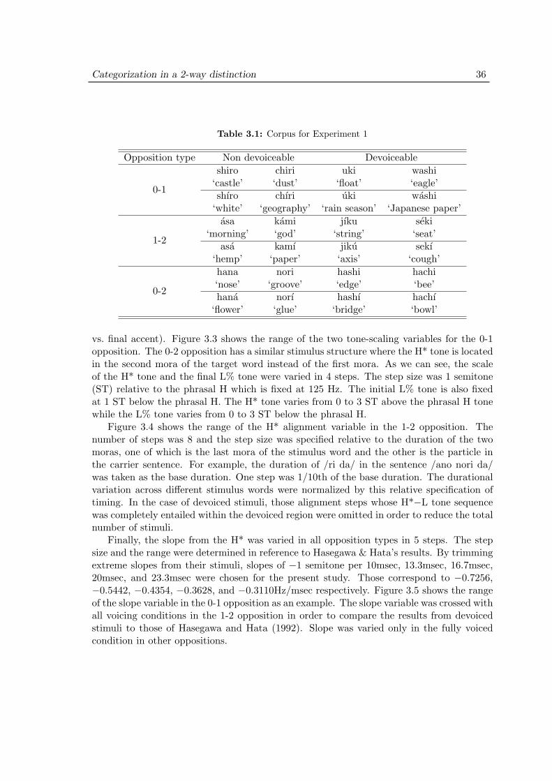
Categorization in a 2-way distinction 36
Table 3.1: Corpus for Experiment 1
Opposition type Non devoiceable Devoiceableshiro chiri uki washi
0-1‘castle’ ‘dust’ ‘float’ ‘eagle’shıro chıri uki washi
‘white’ ‘geography’ ‘rain season’ ‘Japanese paper’asa kami jıku seki
1-2‘morning’ ‘god’ ‘string’ ‘seat’
asa kamı jiku sekı‘hemp’ ‘paper’ ‘axis’ ‘cough’hana nori hashi hachi
0-2‘nose’ ‘groove’ ‘edge’ ‘bee’hana norı hashı hachı
‘flower’ ‘glue’ ‘bridge’ ‘bowl’
vs. final accent). Figure 3.3 shows the range of the two tone-scaling variables for the 0-1opposition. The 0-2 opposition has a similar stimulus structure where the H* tone is locatedin the second mora of the target word instead of the first mora. As we can see, the scaleof the H* tone and the final L% tone were varied in 4 steps. The step size was 1 semitone(ST) relative to the phrasal H which is fixed at 125 Hz. The initial L% tone is also fixedat 1 ST below the phrasal H. The H* tone varies from 0 to 3 ST above the phrasal H tonewhile the L% tone varies from 0 to 3 ST below the phrasal H.
Figure 3.4 shows the range of the H* alignment variable in the 1-2 opposition. Thenumber of steps was 8 and the step size was specified relative to the duration of the twomoras, one of which is the last mora of the stimulus word and the other is the particle inthe carrier sentence. For example, the duration of /ri da/ in the sentence /ano nori da/was taken as the base duration. One step was 1/10th of the base duration. The durationalvariation across different stimulus words were normalized by this relative specification oftiming. In the case of devoiced stimuli, those alignment steps whose H*−L tone sequencewas completely entailed within the devoiced region were omitted in order to reduce the totalnumber of stimuli.
Finally, the slope from the H* was varied in all opposition types in 5 steps. The stepsize and the range were determined in reference to Hasegawa & Hata’s results. By trimmingextreme slopes from their stimuli, slopes of −1 semitone per 10msec, 13.3msec, 16.7msec,20msec, and 23.3msec were chosen for the present study. Those correspond to −0.7256,−0.5442, −0.4354, −0.3628, and −0.3110Hz/msec respectively. Figure 3.5 shows the rangeof the slope variable in the 0-1 opposition as an example. The slope variable was crossed withall voicing conditions in the 1-2 opposition in order to compare the results from devoicedstimuli to those of Hasegawa and Hata (1992). Slope was varied only in the fully voicedcondition in other oppositions.
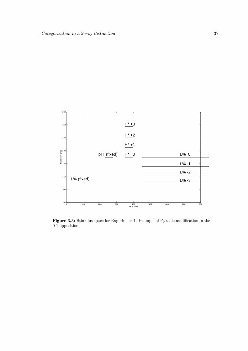
Categorization in a 2-way distinction 37
0 100 200 300 400 500 600 700 80090
100
110
120
130
140
150
160
time (ms)
Fre
quen
cy (
Hz)
L% 0
L% -1
L% -2
L% -3
H* +3
H* +1
H* 0
L% (fixed)
pH (fixed)
H* +2
Figure 3.3: Stimulus space for Experiment 1. Example of F0 scale modification in the0-1 opposition.
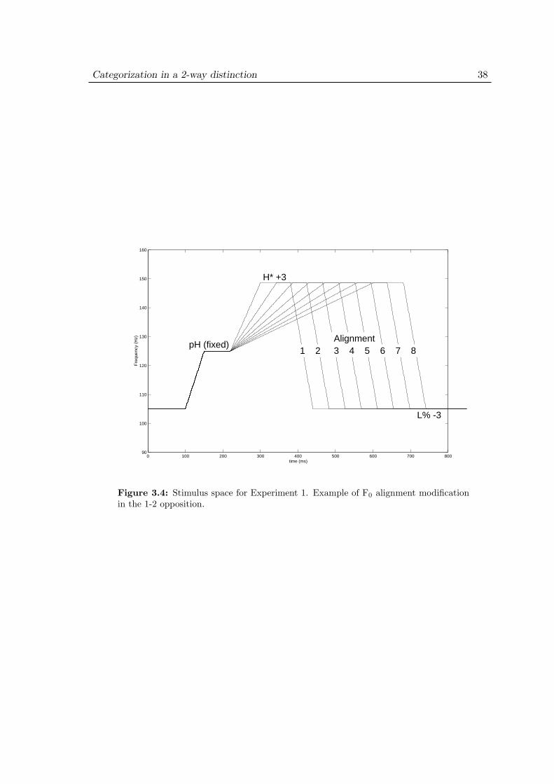
Categorization in a 2-way distinction 38
0 100 200 300 400 500 600 700 80090
100
110
120
130
140
150
160
time (ms)
Fre
quen
cy (
Hz)
H* +3
pH (fixed)
L% -3
1Alignment
2 3 4 5 6 7 8
Figure 3.4: Stimulus space for Experiment 1. Example of F0 alignment modificationin the 1-2 opposition.
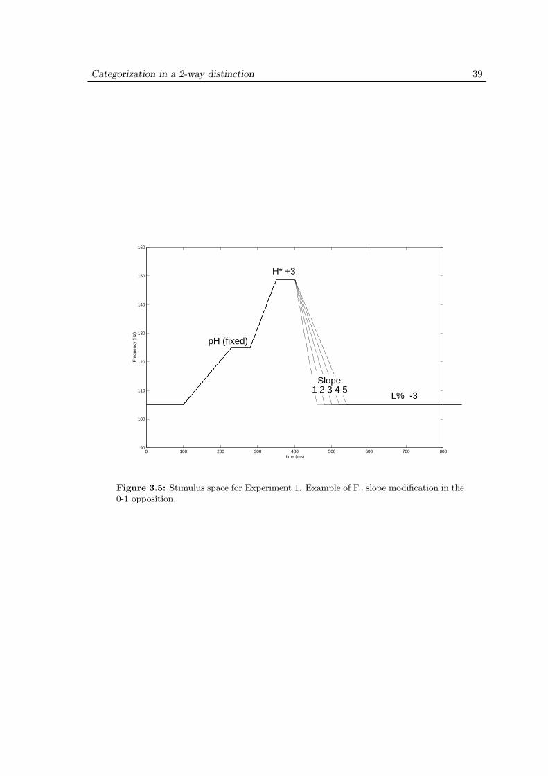
Categorization in a 2-way distinction 39
0 100 200 300 400 500 600 700 80090
100
110
120
130
140
150
160
time (ms)
Fre
quen
cy (
Hz)
pH (fixed)
L% -3
H* +3
1 2 3 4 5 Slope
Figure 3.5: Stimulus space for Experiment 1. Example of F0 slope modification in the0-1 opposition.
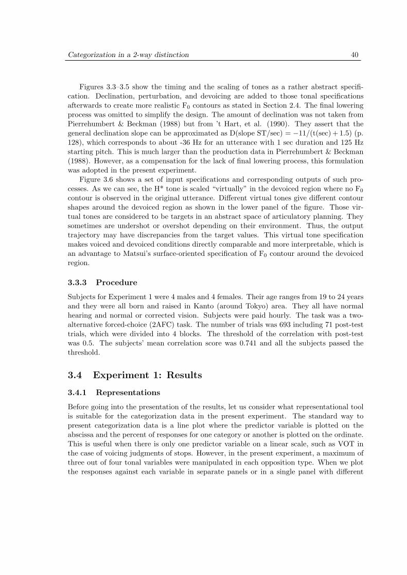
Categorization in a 2-way distinction 40
Figures 3.3–3.5 show the timing and the scaling of tones as a rather abstract specifi-cation. Declination, perturbation, and devoicing are added to those tonal specificationsafterwards to create more realistic F0 contours as stated in Section 2.4. The final loweringprocess was omitted to simplify the design. The amount of declination was not taken fromPierrehumbert & Beckman (1988) but from ’t Hart, et al. (1990). They assert that thegeneral declination slope can be approximated as D(slope ST/sec) = −11/(t(sec) + 1.5) (p.128), which corresponds to about -36 Hz for an utterance with 1 sec duration and 125 Hzstarting pitch. This is much larger than the production data in Pierrehumbert & Beckman(1988). However, as a compensation for the lack of final lowering process, this formulationwas adopted in the present experiment.
Figure 3.6 shows a set of input specifications and corresponding outputs of such pro-cesses. As we can see, the H* tone is scaled “virtually” in the devoiced region where no F0
contour is observed in the original utterance. Different virtual tones give different contourshapes around the devoiced region as shown in the lower panel of the figure. Those vir-tual tones are considered to be targets in an abstract space of articulatory planning. Theysometimes are undershot or overshot depending on their environment. Thus, the outputtrajectory may have discrepancies from the target values. This virtual tone specificationmakes voiced and devoiced conditions directly comparable and more interpretable, which isan advantage to Matsui’s surface-oriented specification of F0 contour around the devoicedregion.
3.3.3 Procedure
Subjects for Experiment 1 were 4 males and 4 females. Their age ranges from 19 to 24 yearsand they were all born and raised in Kanto (around Tokyo) area. They all have normalhearing and normal or corrected vision. Subjects were paid hourly. The task was a two-alternative forced-choice (2AFC) task. The number of trials was 693 including 71 post-testtrials, which were divided into 4 blocks. The threshold of the correlation with post-testwas 0.5. The subjects’ mean correlation score was 0.741 and all the subjects passed thethreshold.
3.4 Experiment 1: Results
3.4.1 Representations
Before going into the presentation of the results, let us consider what representational toolis suitable for the categorization data in the present experiment. The standard way topresent categorization data is a line plot where the predictor variable is plotted on theabscissa and the percent of responses for one category or another is plotted on the ordinate.This is useful when there is only one predictor variable on a linear scale, such as VOT inthe case of voicing judgments of stops. However, in the present experiment, a maximum ofthree out of four tonal variables were manipulated in each opposition type. When we plotthe responses against each variable in separate panels or in a single panel with different

Categorization in a 2-way distinction 41
���
�����
�����
�����
�����
�����
�����
� ����� ����� ����� ����� ���� ����� ���� �����
���
�����
�����
�����
�����
�����
�����
n o h a ch t oia
L%
phrasal H L%
H*
Figure 3.6: Input specifications to the resynthesis processes and the final outcome.Sample contours from [ano hachito] (0-2 opposition).
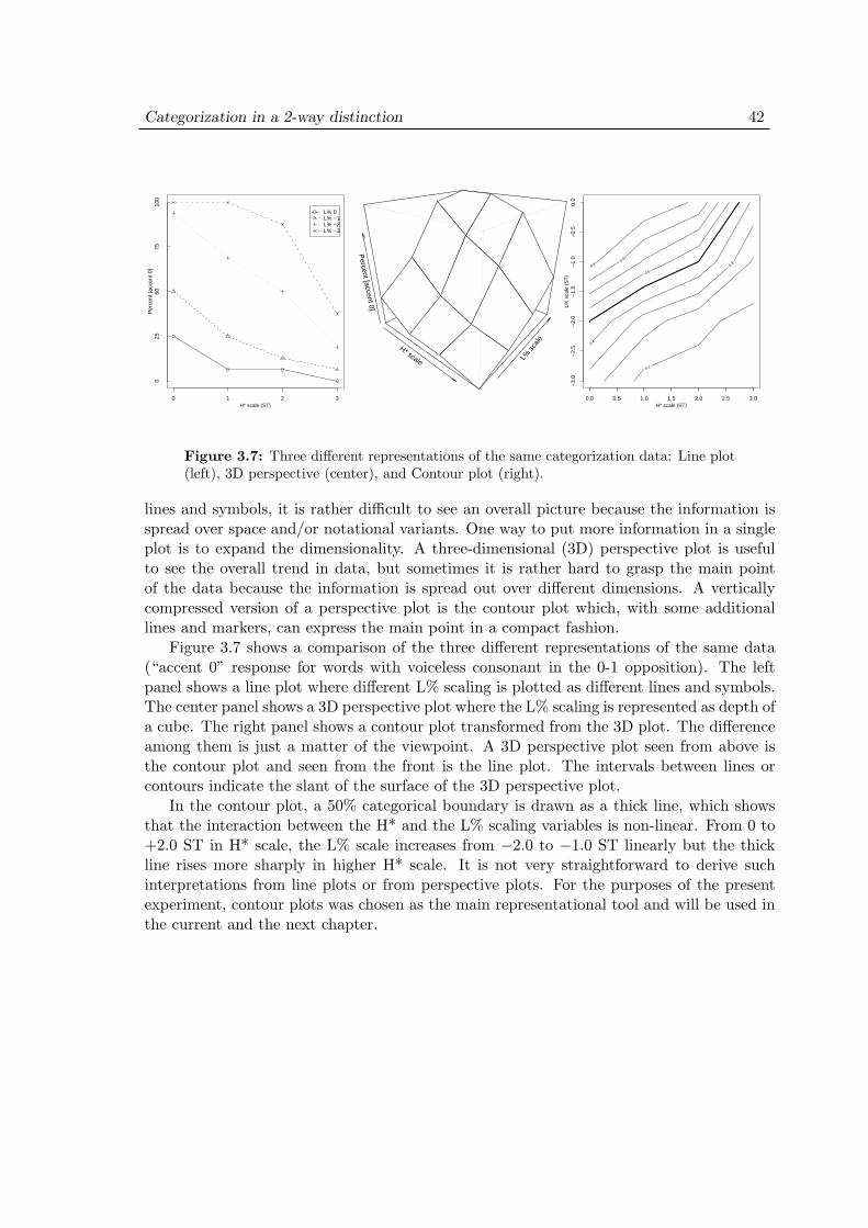
Categorization in a 2-way distinction 42
025
5075
100
0 1 2 3H* scale (ST)
Per
cent
[acc
ent 0
]
L% 0L% −1L% −2L% −3
H* scale L% s
cale
Percent [accent 0]
0.1
0.3
0.4
0.6
0.8
0.9
0.0 0.5 1.0 1.5 2.0 2.5 3.0
−3.
0−
2.5
−2.
0−
1.5
−1.
0−
0.5
0.0
H* scale (ST)
L% s
cale
(S
T)
Figure 3.7: Three different representations of the same categorization data: Line plot(left), 3D perspective (center), and Contour plot (right).
lines and symbols, it is rather difficult to see an overall picture because the information isspread over space and/or notational variants. One way to put more information in a singleplot is to expand the dimensionality. A three-dimensional (3D) perspective plot is usefulto see the overall trend in data, but sometimes it is rather hard to grasp the main pointof the data because the information is spread out over different dimensions. A verticallycompressed version of a perspective plot is the contour plot which, with some additionallines and markers, can express the main point in a compact fashion.
Figure 3.7 shows a comparison of the three different representations of the same data(“accent 0” response for words with voiceless consonant in the 0-1 opposition). The leftpanel shows a line plot where different L% scaling is plotted as different lines and symbols.The center panel shows a 3D perspective plot where the L% scaling is represented as depth ofa cube. The right panel shows a contour plot transformed from the 3D plot. The differenceamong them is just a matter of the viewpoint. A 3D perspective plot seen from above isthe contour plot and seen from the front is the line plot. The intervals between lines orcontours indicate the slant of the surface of the 3D perspective plot.
In the contour plot, a 50% categorical boundary is drawn as a thick line, which showsthat the interaction between the H* and the L% scaling variables is non-linear. From 0 to+2.0 ST in H* scale, the L% scale increases from −2.0 to −1.0 ST linearly but the thickline rises more sharply in higher H* scale. It is not very straightforward to derive suchinterpretations from line plots or from perspective plots. For the purposes of the presentexperiment, contour plots was chosen as the main representational tool and will be used inthe current and the next chapter.
Categorization in a 2-way distinction 43
L% s
cale
H* scale
more L% effect
mor
e H
* ef
fect
H*-L
% d
iffere
nce
= m
id
H*-L%
diffe
renc
e =
small
H*-L%
diffe
renc
e =
large
H* scale
L% s
cale
Figure 3.8: Schematic representation of the interaction of the scaling of H* and L%.Left: slant of the contour indicates the effect of one variable stronger than the other,Right: intercept of the contour indicates the amount of H*−L% difference necessary fora percept of accent.
3.4.2 Effect of scaling
As we have seen in the previous section, the interaction of the two scaling variables issometimes non-linear. But, what if they are linearly related? As schematically shown inthe left panel in Figure 3.8, if the contour runs more horizontally than the diagonal, theeffect of the L% scaling is stronger and if it runs more vertically, the effect of the H* scaling isstronger in categorization. In extreme cases where the contour runs completely horizontallyor vertically, the effect of only one scaling variable is visible and the other has no effect onperformance. The intercept of the contour as in the right panel of the figure indicates theamount of H*−L% difference necessary for a percept of accent. When the contour runs inthe upper left triangle, the difference is smaller and when the contour runs in the lowerright triangle, the difference is larger.
Having these in mind, we can see the results for the 0-1 and the 0-2 opposition with fullyvoiced words in Figure 3.9 as the linear pattern with a slight propensity that the effect ofL% scaling is more than that of the H* scaling. The 50% contour (thick line) runs almostlinearly in both panels though the intercept is much lower in the case of the 0-1 opposition.This indicates that more H*−L% difference is necessary in the 0-1 opposition for pitchaccents to be perceived. Other contours run almost parallel to the 50% contour with someexceptions in the 0-2 opposition where the contours for the two highest ratios (0.8 and 0.9)deviate slightly from the slope of the thick line.
3.4.3 Effect of slope
Figure 3.10 shows the ratio of responses for accent 1 or 2 as contour plots. For oppositionsinvolving unaccented forms, such as 0-1 and 0-2, responses for accented forms are plottedwhile for the accent-location contrast, the 1-2 opposition, responses for accent 1 are plotted.
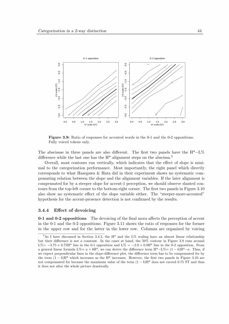
Categorization in a 2-way distinction 44
0.1
0.2
0.5
0.6
0.0 0.5 1.0 1.5 2.0 2.5 3.0
−3.0
−2.5
−2.0
−1.5
−1.0
−0.5
0.0
H* scale (ST)
L% s
cale
(S
T)
0−1 opposition
0.2
0.3
0.5
0.7
0.8
0.9
0.0 0.5 1.0 1.5 2.0 2.5 3.0
−3.0
−2.5
−2.0
−1.5
−1.0
−0.5
0.0
H* scale (ST)L%
sca
le (
ST
)
0−2 opposition
Figure 3.9: Ratio of responses for accented words in the 0-1 and the 0-2 oppositions.Fully voiced tokens only.
The abscissae in three panels are also different. The first two panels have the H*−L%difference while the last one has the H* alignment steps on the abscissa.3
Overall, most contours run vertically, which indicates that the effect of slope is mini-mal to the categorization performance. Most importantly, the right panel which directlycorresponds to what Hasegawa & Hata did in their experiment shows no systematic com-pensating relation between the slope and the alignment variables. If the later alignment iscompensated for by a steeper slope for accent-1 perception, we should observe slanted con-tours from the top-left corner to the bottom-right corner. The first two panels in Figure 3.10also show no systematic effect of the slope variable either. The “steeper-more-accented”hypothesis for the accent-presence detection is not confirmed by the results.
3.4.4 Effect of devoicing
0-1 and 0-2 oppositions The devoicing of the final mora affects the perception of accentin the 0-1 and the 0-2 oppositions. Figure 3.11 shows the ratio of responses for the formerin the upper row and for the latter in the lower row. Columns are organized by voicing
3As I have discussed in Section 3.4.2, the H* and the L% scaling have an almost linear relationshipbut their difference is not a constant. In the cases at hand, the 50% contour in Figure 3.9 runs aroundL%= −3.75 + 0.75H* line in the 0-1 opposition and L% = −2.0 + 0.8H* line in the 0-2 opposition. Froma general linear formula L%= a + bH*, we can derive the difference term H*−L%= (1 − b)H*−a. Thus, ifwe expect perpendicular lines in the slope-difference plot, the difference term has to be compensated for bythe term (1 − b)H* which increases as the H* increases. However, the first two panels in Figure 3.10 arenot compensated for because the maximum value of the term (1 − b)H* does not exceed 0.75 ST and thusit does not alter the whole picture drastically.
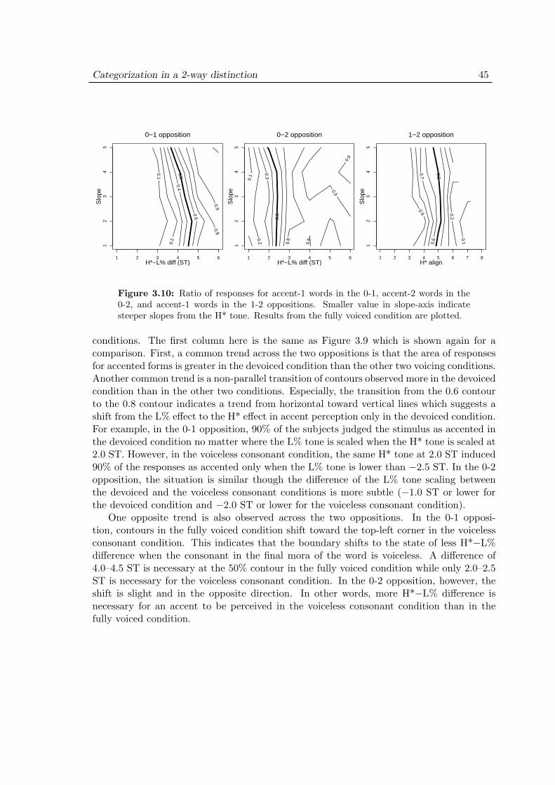
Categorization in a 2-way distinction 45
0.1
0.2
0.4 0.5
0.6
0.8 0.9
1 2 3 4 5 6
12
34
5
H*−L% diff (ST)
Slo
pe
0−1 opposition
0.1
0.2 0.3
0.5
0.8
0.8
0.9
0.9
1 2 3 4 5 6
12
34
5
H*−L% diff (ST)
Slo
pe
0−2 opposition
0.1
0.2
0.5
0.6
0.7 0.9
1 2 3 4 5 6 7 8
12
34
5
H* align
Slo
pe
1−2 opposition
Figure 3.10: Ratio of responses for accent-1 words in the 0-1, accent-2 words in the0-2, and accent-1 words in the 1-2 oppositions. Smaller value in slope-axis indicatesteeper slopes from the H* tone. Results from the fully voiced condition are plotted.
conditions. The first column here is the same as Figure 3.9 which is shown again for acomparison. First, a common trend across the two oppositions is that the area of responsesfor accented forms is greater in the devoiced condition than the other two voicing conditions.Another common trend is a non-parallel transition of contours observed more in the devoicedcondition than in the other two conditions. Especially, the transition from the 0.6 contourto the 0.8 contour indicates a trend from horizontal toward vertical lines which suggests ashift from the L% effect to the H* effect in accent perception only in the devoiced condition.For example, in the 0-1 opposition, 90% of the subjects judged the stimulus as accented inthe devoiced condition no matter where the L% tone is scaled when the H* tone is scaled at2.0 ST. However, in the voiceless consonant condition, the same H* tone at 2.0 ST induced90% of the responses as accented only when the L% tone is lower than −2.5 ST. In the 0-2opposition, the situation is similar though the difference of the L% tone scaling betweenthe devoiced and the voiceless consonant conditions is more subtle (−1.0 ST or lower forthe devoiced condition and −2.0 ST or lower for the voiceless consonant condition).
One opposite trend is also observed across the two oppositions. In the 0-1 opposi-tion, contours in the fully voiced condition shift toward the top-left corner in the voicelessconsonant condition. This indicates that the boundary shifts to the state of less H*−L%difference when the consonant in the final mora of the word is voiceless. A difference of4.0–4.5 ST is necessary at the 50% contour in the fully voiced condition while only 2.0–2.5ST is necessary for the voiceless consonant condition. In the 0-2 opposition, however, theshift is slight and in the opposite direction. In other words, more H*−L% difference isnecessary for an accent to be perceived in the voiceless consonant condition than in thefully voiced condition.
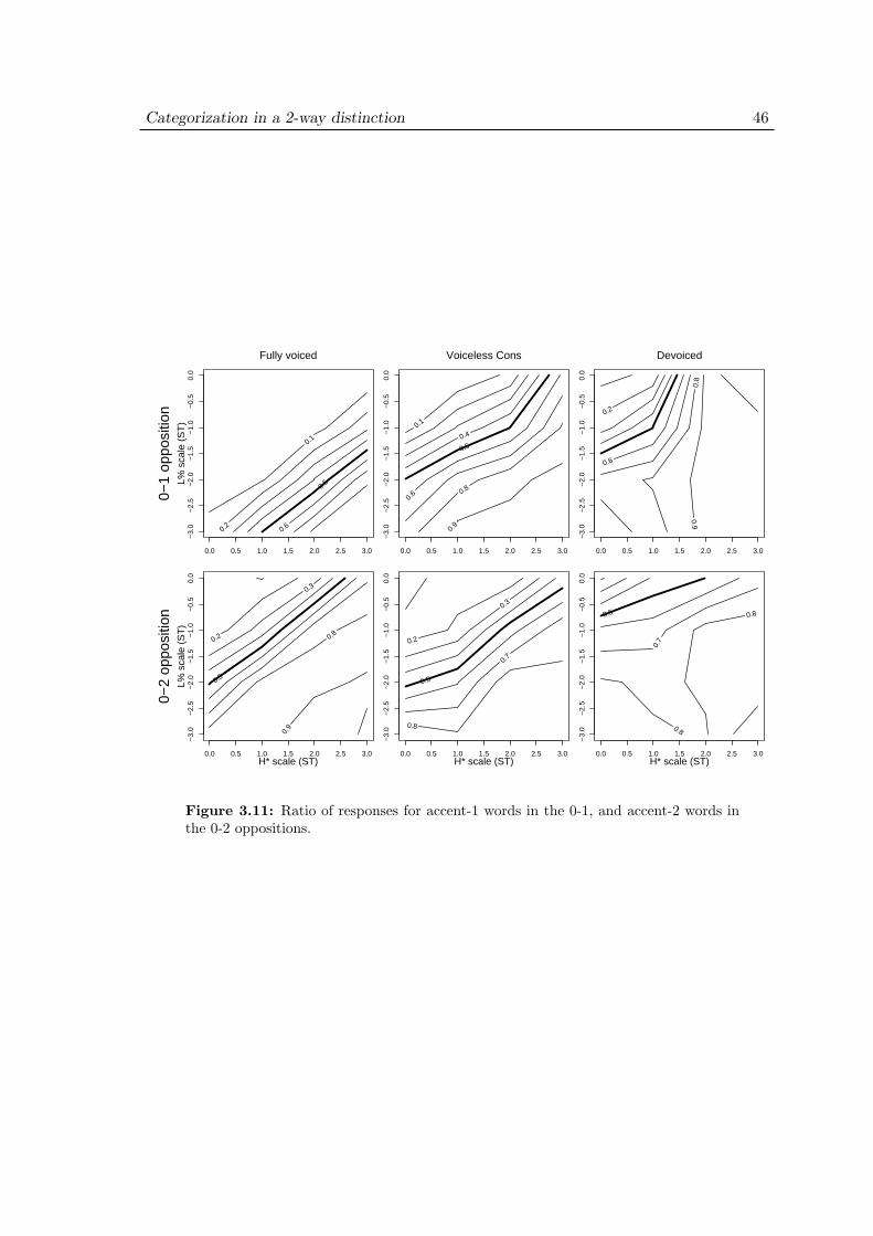
Categorization in a 2-way distinction 46
0.1
0.2
0.5
0.6
0.0 0.5 1.0 1.5 2.0 2.5 3.0
−3.
0−
2.5
−2.
0−
1.5
−1.
0−
0.5
0.0
L% s
cale
(S
T)
0−1
oppo
sitio
n
Fully voiced
0.1
0.4
0.5
0.6
0.8
0.9
0.0 0.5 1.0 1.5 2.0 2.5 3.0
−3.
0−
2.5
−2.
0−
1.5
−1.
0−
0.5
0.0
Voiceless Cons
0.2
0.6
0.8
0.9
0.0 0.5 1.0 1.5 2.0 2.5 3.0
−3.
0−
2.5
−2.
0−
1.5
−1.
0−
0.5
0.0
Devoiced
0.2
0.3
0.5
0.8
0.9
0.0 0.5 1.0 1.5 2.0 2.5 3.0
−3.
0−
2.5
−2.
0−
1.5
−1.
0−
0.5
0.0
H* scale (ST)
L% s
cale
(S
T)
0−2
oppo
sitio
n
0.2
0.3
0.5
0.7
0.8
0.0 0.5 1.0 1.5 2.0 2.5 3.0
−3.
0−
2.5
−2.
0−
1.5
−1.
0−
0.5
0.0
H* scale (ST)
0.5
0.7
0.8
0.8
0.0 0.5 1.0 1.5 2.0 2.5 3.0
−3.
0−
2.5
−2.
0−
1.5
−1.
0−
0.5
0.0
H* scale (ST)
Figure 3.11: Ratio of responses for accent-1 words in the 0-1, and accent-2 words inthe 0-2 oppositions.
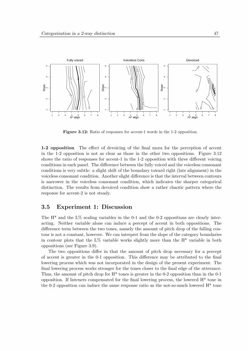
Categorization in a 2-way distinction 47
0.1
0.2
0.5
0.6
0.7 0.9
1 2 3 4 5 6 7 8
12
34
5
H* align
Slo
pe
Fully voiced
0.1 0.2
0.3 0.6
0.8
1 2 3 4 5 6 7 8
12
34
5
H* align
Slo
pe
Voiceless Cons
0.4 0.5 0.6
0.8
0.8
0.9
0
.9
0.9
1 2 3 4 5 6 7 8
12
34
5
H* align
Slo
pe
Devoiced
Figure 3.12: Ratio of responses for accent-1 words in the 1-2 opposition.
1-2 opposition The effect of devoicing of the final mora for the perception of accentin the 1-2 opposition is not as clear as those in the other two oppositions. Figure 3.12shows the ratio of responses for accent-1 in the 1-2 opposition with three different voicingconditions in each panel. The difference between the fully voiced and the voiceless consonantconditions is very subtle: a slight shift of the boundary toward right (late alignment) in thevoiceless consonant condition. Another slight difference is that the interval between contoursis narrower in the voiceless consonant condition, which indicates the sharper categoricaldistinction. The results from devoiced condition show a rather chaotic pattern where theresponse for accent-2 is not steady.
3.5 Experiment 1: Discussion
The H* and the L% scaling variables in the 0-1 and the 0-2 oppositions are clearly inter-acting. Neither variable alone can induce a percept of accent in both oppositions. Thedifference term between the two tones, namely the amount of pitch drop of the falling con-tour is not a constant, however. We can interpret from the slope of the category boundariesin contour plots that the L% variable works slightly more than the H* variable in bothoppositions (see Figure 3.9).
The two oppositions differ in that the amount of pitch drop necessary for a perceptof accent is greater in the 0-1 opposition. This difference may be attributed to the finallowering process which was not incorporated in the design of the present experiment. Thefinal lowering process works stronger for the tones closer to the final edge of the utterance.Thus, the amount of pitch drop for H* tones is greater in the 0-2 opposition than in the 0-1opposition. If listeners compensated for the final lowering process, the lowered H* tone inthe 0-2 opposition can induce the same response ratio as the not-so-much lowered H* tone
Categorization in a 2-way distinction 48
in the 0-1 opposition. We, thus, have to reconsider the design of the stimulus space andincorporate the final lowering process in the next experiment.
Observations about the effect of slope (section 3.4.3) suggest that the F0 informationabout the slope does not correlate with the H* alignment variable nor other variables. Thisis in contrast to the view in Hasegawa & Hata (1992) where they claim that there is acompensatory relation between the timing of the fall and the slope.
A possible reinterpretation of Hasegawa & Hata’s results is that there may be otherunintended parameters manipulated in their paradigm. Back in Figure 2.1, what they callslope is the rate of fall within the 160 Hz to 127 Hz range right after the peak. To changethe local slope of this region, they had to manipulate the connecting line from 127 Hz pointto 80 Hz point at the end of the utterance. For the slope to be steep until 127 Hz, theline from 127 Hz to the end must be relatively flat. In other words, if the first part of thefall is steep, the second part of the fall is gradual and vice versa. Thus, not only the localslope for the pitch accent but also the global shape of the pitch contour is modified in theirstimulus design. We could speculate that the shape, such as concave, convex, or linear, ofthe contour after the peak may influence the accent location detection. For example, thefalling part as a whole has a convex shape when the peak is quite late and the slope of thefirst part is gradual. This convex shape may decrease the percent of response for initialaccent because it is unusual for that accent.
In the present design of the stimulus space, the pitch at the end of the utterance wasindependently specified by the final L% tone. The line from the end of the fall (L in H*L)to the L% was set to flat at the level of tonal specification (i.e., before declination andsmoothing applied). Thus the global shape of the contour after the H* was always concave.The slope variable modifies the depth of the concavity.
As we have seen in Figure 3.10, the effect of the slope variable is not quite visible inaccent-presence detection either. If the steeper-more-accented hypothesis is true, we shouldexpect that the H*−L% difference is smaller when the slope of the fall is steeper. In otherwords, we predict that the salience induced by a steeper slope requires less pitch drop fromthe H* to the L% tone. However, the contours in the figure are running rather inverselyfrom this prediction. The steepest slope (1 at the bottom of the figure) requires no less pitchdrop than gradual slopes. Considering the effect of the adjustment for the linear relationshipbetween the H* and the L% (see Footnote 3), the evidence is not strong enough to claimthat the slope has a negative effect on accent perception, however. Thus, I conclude thatthe slope in the 0-1 and the 0-2 oppositions is not effective for accent-presence detection.
As for the effect of devoicing (section 3.4.4), our results give an interesting insightfrom a full comparison among the fully voiced, the voiceless consonant, and the devoicedcondition in all opposition types in 2-mora words. This is achieved by setting an abstractstimulus space based on the tone-sequence model in Pierrehumbert & Beckman (1988).The difference between a partially devoiced mora (the voiceless consonant condition) and avoiced mora for accent perception has not received much attention in previous studies. Mostproduction and perception experiments on pitch accent have used fully voiced token (e.g., allconsonants involved are nasals or liquids) in order to obtain a clear and uninterupted pitch
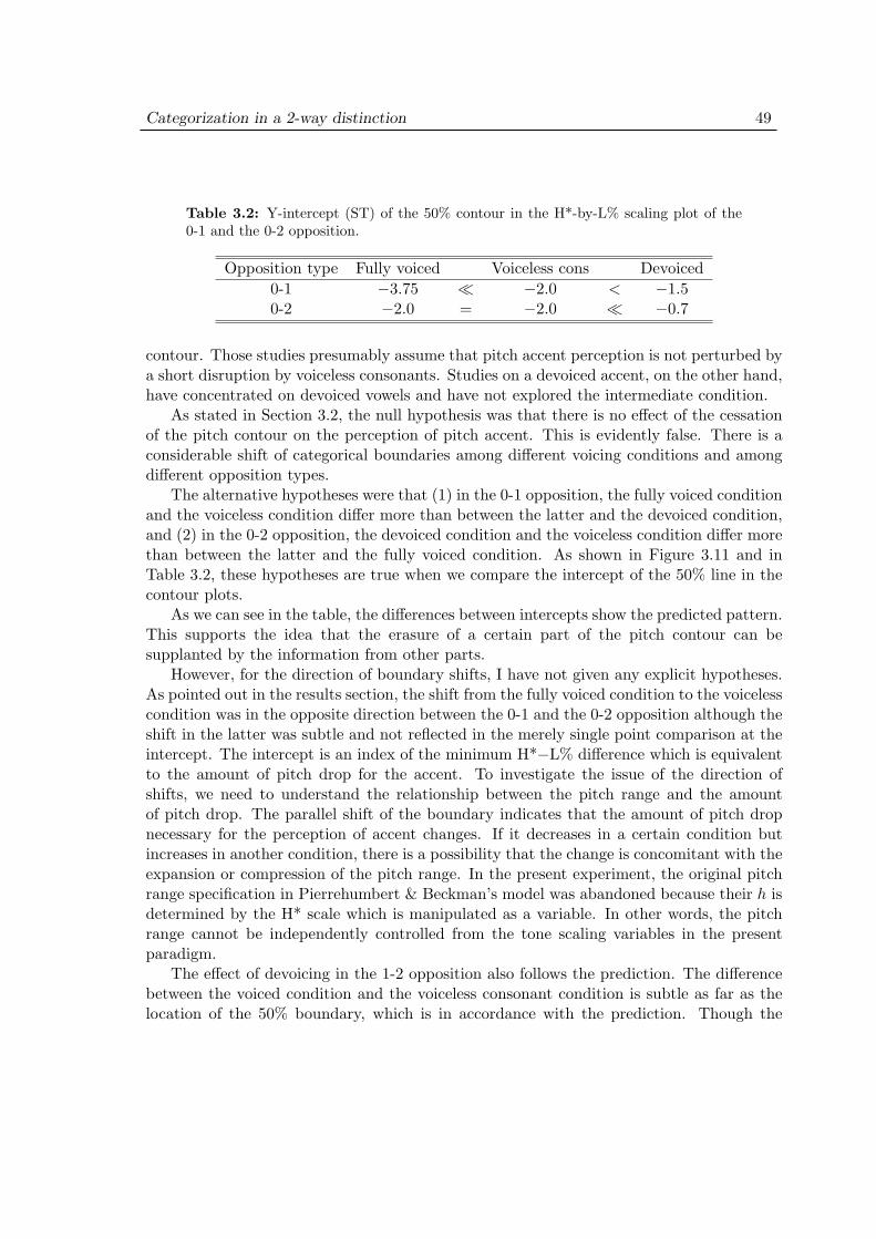
Categorization in a 2-way distinction 49
Table 3.2: Y-intercept (ST) of the 50% contour in the H*-by-L% scaling plot of the0-1 and the 0-2 opposition.
Opposition type Fully voiced Voiceless cons Devoiced0-1 −3.75 ¿ −2.0 < −1.50-2 −2.0 = −2.0 ¿ −0.7
contour. Those studies presumably assume that pitch accent perception is not perturbed bya short disruption by voiceless consonants. Studies on a devoiced accent, on the other hand,have concentrated on devoiced vowels and have not explored the intermediate condition.
As stated in Section 3.2, the null hypothesis was that there is no effect of the cessationof the pitch contour on the perception of pitch accent. This is evidently false. There is aconsiderable shift of categorical boundaries among different voicing conditions and amongdifferent opposition types.
The alternative hypotheses were that (1) in the 0-1 opposition, the fully voiced conditionand the voiceless condition differ more than between the latter and the devoiced condition,and (2) in the 0-2 opposition, the devoiced condition and the voiceless condition differ morethan between the latter and the fully voiced condition. As shown in Figure 3.11 and inTable 3.2, these hypotheses are true when we compare the intercept of the 50% line in thecontour plots.
As we can see in the table, the differences between intercepts show the predicted pattern.This supports the idea that the erasure of a certain part of the pitch contour can besupplanted by the information from other parts.
However, for the direction of boundary shifts, I have not given any explicit hypotheses.As pointed out in the results section, the shift from the fully voiced condition to the voicelesscondition was in the opposite direction between the 0-1 and the 0-2 opposition although theshift in the latter was subtle and not reflected in the merely single point comparison at theintercept. The intercept is an index of the minimum H*−L% difference which is equivalentto the amount of pitch drop for the accent. To investigate the issue of the direction ofshifts, we need to understand the relationship between the pitch range and the amountof pitch drop. The parallel shift of the boundary indicates that the amount of pitch dropnecessary for the perception of accent changes. If it decreases in a certain condition butincreases in another condition, there is a possibility that the change is concomitant with theexpansion or compression of the pitch range. In the present experiment, the original pitchrange specification in Pierrehumbert & Beckman’s model was abandoned because their h isdetermined by the H* scale which is manipulated as a variable. In other words, the pitchrange cannot be independently controlled from the tone scaling variables in the presentparadigm.
The effect of devoicing in the 1-2 opposition also follows the prediction. The differencebetween the voiced condition and the voiceless consonant condition is subtle as far as thelocation of the 50% boundary, which is in accordance with the prediction. Though the
Categorization in a 2-way distinction 50
contours for the devoiced condition (Figure 3.12, right panel) is rather chaotic, it is truethat the accent-1 response prevails.
Overall, Experiment 1 gave us a substantial amount of data and insights. The mostinteresting finding is that the local slope of the falling contour does not affect the perceptionas expected. As stated in the methods section (3.3.2), the number of steps was kept smalland the step size was rather large to probe an appropriate stimulus space. These factorswill be revised in the next experiment.
3.6 Experiment 2: Purpose
The main purpose of Experiment 2 is to see the effect of the preceding context in accentperception. The role of the preceding context was not explored in Experiment 1 though itseffect was pointed out in Matsui (1993). As I mentioned in section 2.2.3, he claimed thatthe relative height of the F0 offset and the F0 onset around the devoiced region is one of thecrucial cues for determining the accent location. F0 offset has to be lower than F0 onset foran accent on the devoiced mora to be perceived (e.g., [hashı◦]). For an accent on the morabefore devoiced region (e.g., [hashi◦]), the F0 offset has to be higher than the onset.
Put in the framework adapted in the present study, however, the F0 offset and onsetvalues cannot be directly set by the tonal specification. When an accent is on the devoicedmora, F0 offset is somewhere on the interpolated line from the phrasal H to the “virtual”H* tone on the devoiced mora. When the accent is on the mora before the devoiced region,the F0 onset is somewhere on the interpolated line from the H* tone to the following L tone.Moreover, perturbations on the F0 contour by consonants are added to the interpolationlines in the present framework to keep the naturalness of the contour. This makes theactual F0 value of the onset/offset point somewhat unpredictable and quite variable acrossthe stimulus words.
As stated in Section 2.3, the motivation for using an abstract tonal specification is,however, to pursue a phonologically tractable model of the perception of pitch accents.Artificial F0 contours in Hasegawa & Hata (1992) and Matsui (1993) are designed onlyfor perception experiments and thus are not suitable for this purpose. Put differently, theexact F0 value of the onset/offset of the devoiced region should not be directly specifiedwhen we consider a model of tonal phonology in Japanese. It is quite unlikely that the F0
onset/offset of the devoiced region is an independently controlled phonological parameterin the system of tone structure.
The preceding context of the pitch accent can be specified as the scale of the phrasal Htone in terms of Pirrehumbert-Beckman model. When both the phrasal H and the final L%tones are set low, the whole contour resembles a “hat” pattern. Under a constraint thatthe final L% is equal or lower than the phrasal H tone, setting the phrasal H tone lowermakes the height of the hat higher.4 Given that, it is expected that the salience of the H*tone will be enhanced when the phrasal H tone is lower. In other words, the role of phrasal
4This constraint is necessary to keep the declarative intonation as opposed to the question intonationwith the final H%.
Categorization in a 2-way distinction 51
H tone can be stated as the following hypothesis:
(3.2) The lower the phrasal H tone is, accent-presence detection is facilitated.
Moreover, the height of the phrasal H affects the slope of the rising contour from thephrasal H to the H* tone. Although the effect of the “falling” slope from the H* tone isdenied in Experiment 1, we have not confirmed whether the effect of the rising slope isnegligible. As in Experiment 1, a rapid change is expected to be more salient in perception.When the phrasal H tone is varied in the same amount, the change of the slope is greater asthe H* tone is closer to the phrasal H tone. Thus, the earlier the H* is aligned, the steeperthe rising slope is from the phrasal H to the H*.
(3.3) The effect of the phrasal H tone is more salient when the H* is aligned earlier.
Following this hypothesis, it is predicted that accent-1 will be more prominent thanaccent-2 when the phrasal H is scaled lower. Thus, in the 1-2 opposition, the categoryboundary is expected to be biased toward accent-1. It is also expected that the effect ofthe phrasal H is more salient in the 0-1 opposition than in the 0-2 opposition.
In addition to the main purpose, there are a number of questions and problems carriedover from Experiment 1. First of all, the density of the stimulus set is sparse in the verticaldimension in Experiment 1. There are only 4 steps in the scaling of the H* and the L%tones. What if we overlook some crucial perceptual differences between those steps? Next,the effect of the H* alignment variable in the devoiced condition is not clear from the results.
Also, the results in Experiment 1 suggest that not the slope of the falling contour butthe global shape of the whole contour affects the detection of the presence and the locationof pitch accent. Thus, we can drop the slope variable and add another variable for changingthe global shape of the contour. This is another motivation for adding the phrasal H asa variable in the present experiment. In relation to the global shape of the contour, thefinal lowering process skipped in Experiment 1 is another factor which might influence theresults. The hypotheses in Experiment 1 about the voicing conditions and opposition typesstill hold with these modifications.
3.7 Experiment 2: Methods
3.7.1 Materials
The material for Experiment 2 was slightly modified from that for Experiment 1. Only 2pairs of words were substituted for reasons related to the functional load measurement (seeChapter 6 for details). Again, devoicing of the final mora of stimulus words is one of thecrucial variables. Non-devoiceable words are put in one context while devoiceable words areput in two different contexts. Table 3.3 shows the entire corpus for Experiment 2.
Carrier sentences were lengthened by 1 mora at the end from those used in Experiment1. In Experiment 1, only one mora was put after the stimulus words which was sometimesnot long enough to have F0 contours ending at the specified L% tone.
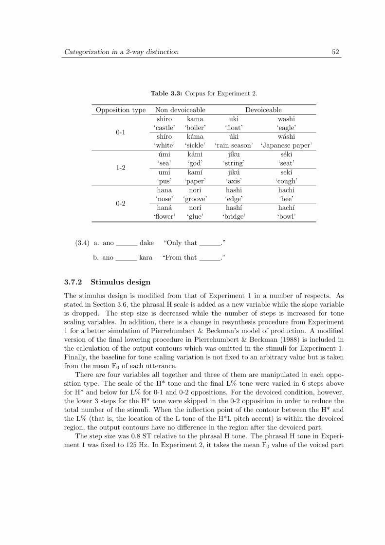
Categorization in a 2-way distinction 52
Table 3.3: Corpus for Experiment 2.
Opposition type Non devoiceable Devoiceableshiro kama uki washi
0-1‘castle’ ‘boiler’ ‘float’ ‘eagle’shıro kama uki washi
‘white’ ‘sickle’ ‘rain season’ ‘Japanese paper’umi kami jıku seki
1-2‘sea’ ‘god’ ‘string’ ‘seat’umi kamı jiku sekı‘pus’ ‘paper’ ‘axis’ ‘cough’hana nori hashi hachi
0-2‘nose’ ‘groove’ ‘edge’ ‘bee’hana norı hashı hachı
‘flower’ ‘glue’ ‘bridge’ ‘bowl’
(3.4) a. ano dake “Only that .”
b. ano kara “From that .”
3.7.2 Stimulus design
The stimulus design is modified from that of Experiment 1 in a number of respects. Asstated in Section 3.6, the phrasal H scale is added as a new variable while the slope variableis dropped. The step size is decreased while the number of steps is increased for tonescaling variables. In addition, there is a change in resynthesis procedure from Experiment1 for a better simulation of Pierrehumbert & Beckman’s model of production. A modifiedversion of the final lowering procedure in Pierrehumbert & Beckman (1988) is included inthe calculation of the output contours which was omitted in the stimuli for Experiment 1.Finally, the baseline for tone scaling variation is not fixed to an arbitrary value but is takenfrom the mean F0 of each utterance.
There are four variables all together and three of them are manipulated in each oppo-sition type. The scale of the H* tone and the final L% tone were varied in 6 steps abovefor H* and below for L% for 0-1 and 0-2 oppositions. For the devoiced condition, however,the lower 3 steps for the H* tone were skipped in the 0-2 opposition in order to reduce thetotal number of the stimuli. When the inflection point of the contour between the H* andthe L% (that is, the location of the L tone of the H*L pitch accent) is within the devoicedregion, the output contours have no difference in the region after the devoiced part.
The step size was 0.8 ST relative to the phrasal H tone. The phrasal H tone in Experi-ment 1 was fixed to 125 Hz. In Experiment 2, it takes the mean F0 value of the voiced part
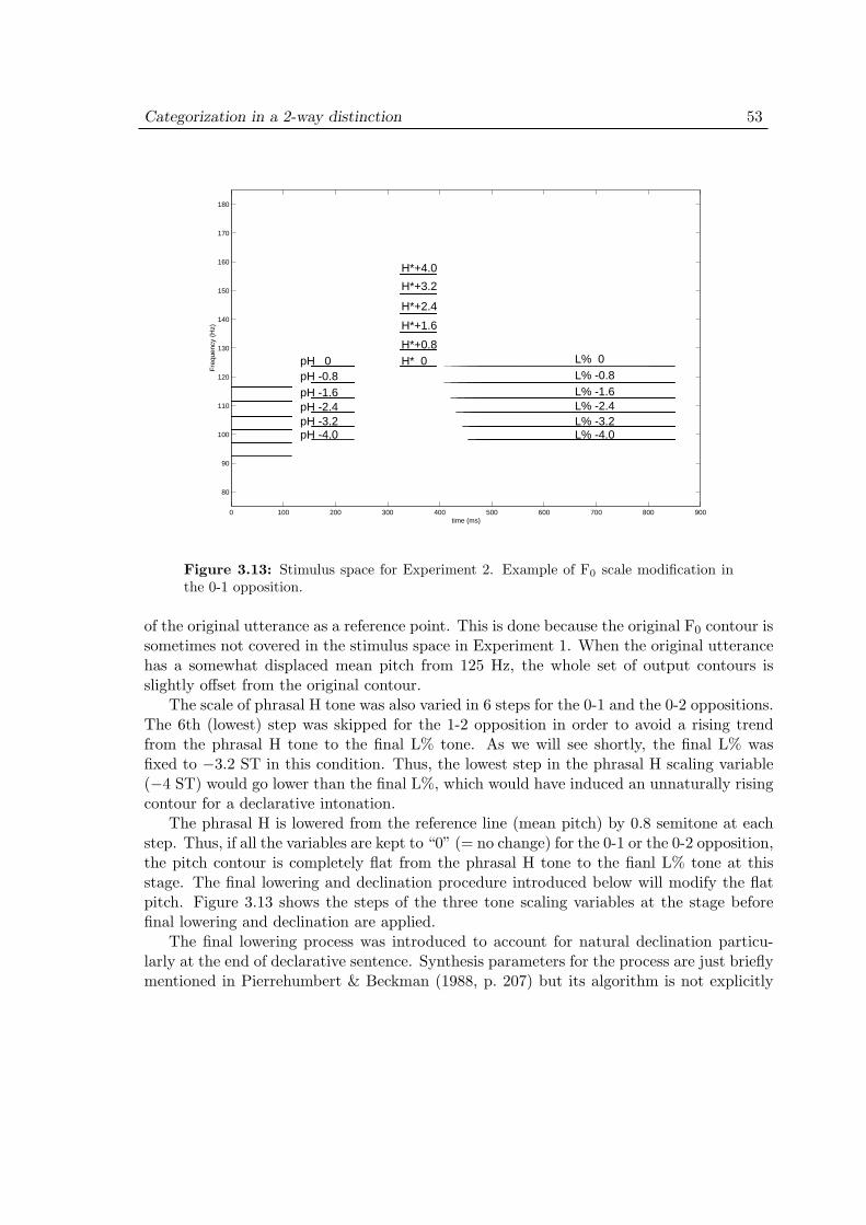
Categorization in a 2-way distinction 53
0 100 200 300 400 500 600 700 800 900
80
90
100
110
120
130
140
150
160
170
180
time (ms)
Fre
quen
cy (
Hz)
pH 0
pH -4.0pH -3.2pH -2.4pH -1.6pH -0.8
H* 0
H*+1.6
H*+2.4
H*+3.2
H*+4.0
L% 0L% -0.8L% -1.6L% -2.4L% -3.2L% -4.0
H*+0.8
Figure 3.13: Stimulus space for Experiment 2. Example of F0 scale modification inthe 0-1 opposition.
of the original utterance as a reference point. This is done because the original F0 contour issometimes not covered in the stimulus space in Experiment 1. When the original utterancehas a somewhat displaced mean pitch from 125 Hz, the whole set of output contours isslightly offset from the original contour.
The scale of phrasal H tone was also varied in 6 steps for the 0-1 and the 0-2 oppositions.The 6th (lowest) step was skipped for the 1-2 opposition in order to avoid a rising trendfrom the phrasal H tone to the final L% tone. As we will see shortly, the final L% wasfixed to −3.2 ST in this condition. Thus, the lowest step in the phrasal H scaling variable(−4 ST) would go lower than the final L%, which would have induced an unnaturally risingcontour for a declarative intonation.
The phrasal H is lowered from the reference line (mean pitch) by 0.8 semitone at eachstep. Thus, if all the variables are kept to “0” (= no change) for the 0-1 or the 0-2 opposition,the pitch contour is completely flat from the phrasal H tone to the fianl L% tone at thisstage. The final lowering and declination procedure introduced below will modify the flatpitch. Figure 3.13 shows the steps of the three tone scaling variables at the stage beforefinal lowering and declination are applied.
The final lowering process was introduced to account for natural declination particu-larly at the end of declarative sentence. Synthesis parameters for the process are just brieflymentioned in Pierrehumbert & Beckman (1988, p. 207) but its algorithm is not explicitly
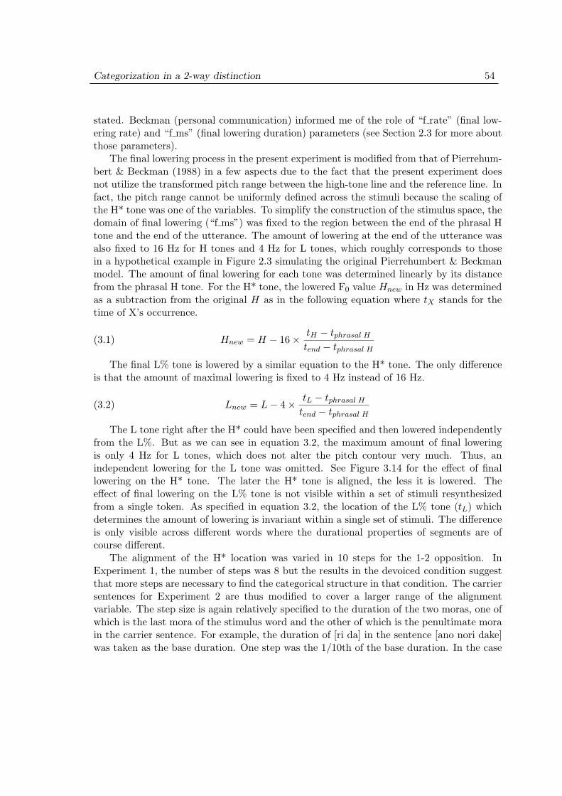
Categorization in a 2-way distinction 54
stated. Beckman (personal communication) informed me of the role of “f rate” (final low-ering rate) and “f ms” (final lowering duration) parameters (see Section 2.3 for more aboutthose parameters).
The final lowering process in the present experiment is modified from that of Pierrehum-bert & Beckman (1988) in a few aspects due to the fact that the present experiment doesnot utilize the transformed pitch range between the high-tone line and the reference line. Infact, the pitch range cannot be uniformly defined across the stimuli because the scaling ofthe H* tone was one of the variables. To simplify the construction of the stimulus space, thedomain of final lowering (“f ms”) was fixed to the region between the end of the phrasal Htone and the end of the utterance. The amount of lowering at the end of the utterance wasalso fixed to 16 Hz for H tones and 4 Hz for L tones, which roughly corresponds to thosein a hypothetical example in Figure 2.3 simulating the original Pierrehumbert & Beckmanmodel. The amount of final lowering for each tone was determined linearly by its distancefrom the phrasal H tone. For the H* tone, the lowered F0 value Hnew in Hz was determinedas a subtraction from the original H as in the following equation where tX stands for thetime of X’s occurrence.
Hnew = H − 16× tH − tphrasal H
tend − tphrasal H(3.1)
The final L% tone is lowered by a similar equation to the H* tone. The only differenceis that the amount of maximal lowering is fixed to 4 Hz instead of 16 Hz.
Lnew = L− 4× tL − tphrasal H
tend − tphrasal H(3.2)
The L tone right after the H* could have been specified and then lowered independentlyfrom the L%. But as we can see in equation 3.2, the maximum amount of final loweringis only 4 Hz for L tones, which does not alter the pitch contour very much. Thus, anindependent lowering for the L tone was omitted. See Figure 3.14 for the effect of finallowering on the H* tone. The later the H* tone is aligned, the less it is lowered. Theeffect of final lowering on the L% tone is not visible within a set of stimuli resynthesizedfrom a single token. As specified in equation 3.2, the location of the L% tone (tL) whichdetermines the amount of lowering is invariant within a single set of stimuli. The differenceis only visible across different words where the durational properties of segments are ofcourse different.
The alignment of the H* location was varied in 10 steps for the 1-2 opposition. InExperiment 1, the number of steps was 8 but the results in the devoiced condition suggestthat more steps are necessary to find the categorical structure in that condition. The carriersentences for Experiment 2 are thus modified to cover a larger range of the alignmentvariable. The step size is again relatively specified to the duration of the two moras, one ofwhich is the last mora of the stimulus word and the other of which is the penultimate morain the carrier sentence. For example, the duration of [ri da] in the sentence [ano nori dake]was taken as the base duration. One step was the 1/10th of the base duration. In the case
Categorization in a 2-way distinction 55
0 100 200 300 400 500 600 700 800 900
80
90
100
110
120
130
140
150
160
170
180
time (ms)
Fre
quen
cy (
Hz)
H* +4 (fixed)
L% -3.2(fixed)
pH 0
3 5
Alignment
1 2 4 76 1098
Figure 3.14: Stimulus space for Experiment 2. Example of F0 alignment modificationin the 1-2 opposition.
of devoiced stimuli, those alignment steps whose H*−L tone sequence is completely withinthe devoiced region were omitted in order to reduce the total number of stimuli. The H*tone is fixed for the 1-2 opposition at 5 steps (= 4 semitones) above the phrasal H tone.The L% tone is also fixed at 4 steps (3.2 semitones) below the phrasal H. Those fixed valueswere determined from informal listening sessions by the author. Figure 3.14 also shows therange of alignment variable.
Finally, the local slope from H* to L% is now fixed to −0.423 Hz/msec. This is basedon an average of 24 tokens recorded by the author in preparation for the stimuli in thecurrent experiment. The slope was calculated from the first-order derivative of the slightlysmoothed F0 contour in the accented mora.
See Figure 3.15 as an example of the stimulus space for 0-2 opposition where all thescaling variables and the final lowering process described above are put together in theupper panel and the outcome of the resynthesis is shown in the lower panel.
3.7.3 Procedure
Sixteen subjects (8 male and 8 female) naive to phonetics and phonology participated inExperiment 2. None of them participated in Experiment 1. Age, dialect, physical conditionsand terms are the same as those in the previous experiment. The task was a self-paced 2-alternative forced choice task. The number of trials was 1758 including 100 post-test trials
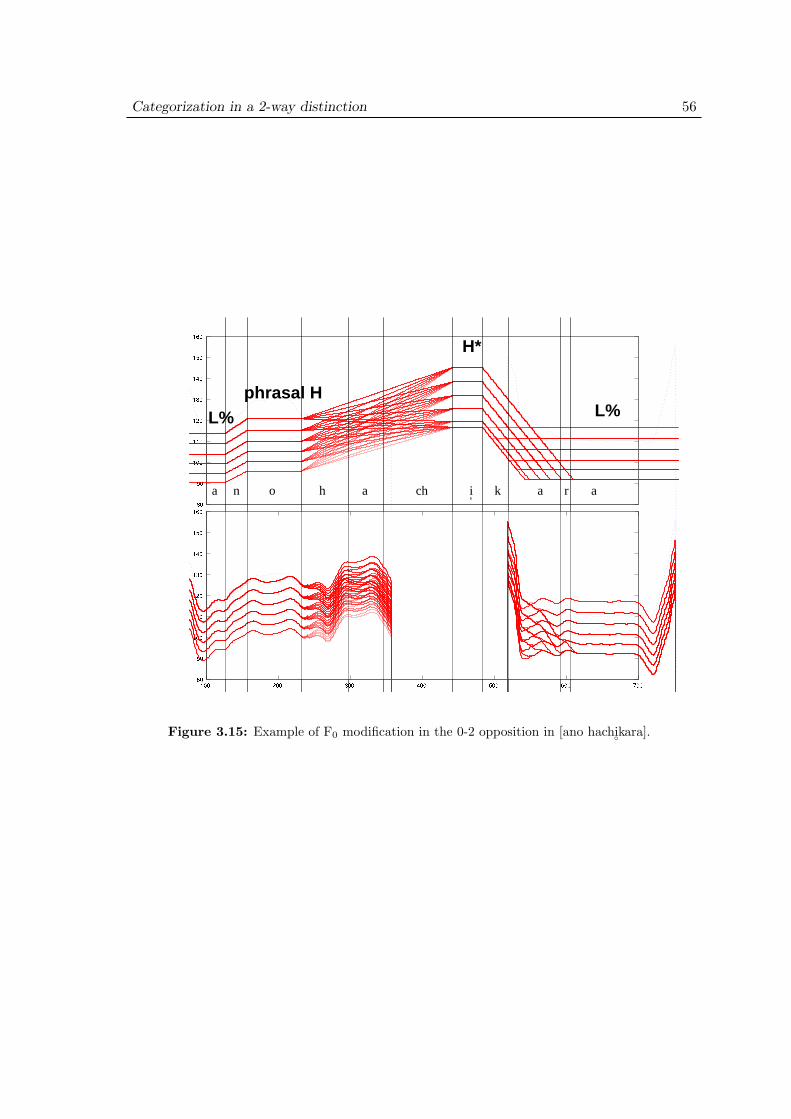
Categorization in a 2-way distinction 56
���
���
�����
�����
�����
�����
����
����
�����
����� ����� ����� ���� ���� ����� �����
���
���
�����
�����
�����
�����
����
����
�����
phrasal H
H*
L% L%
a n o h a ch i k a ar
Figure 3.15: Example of F0 modification in the 0-2 opposition in [ano hachi◦kara].
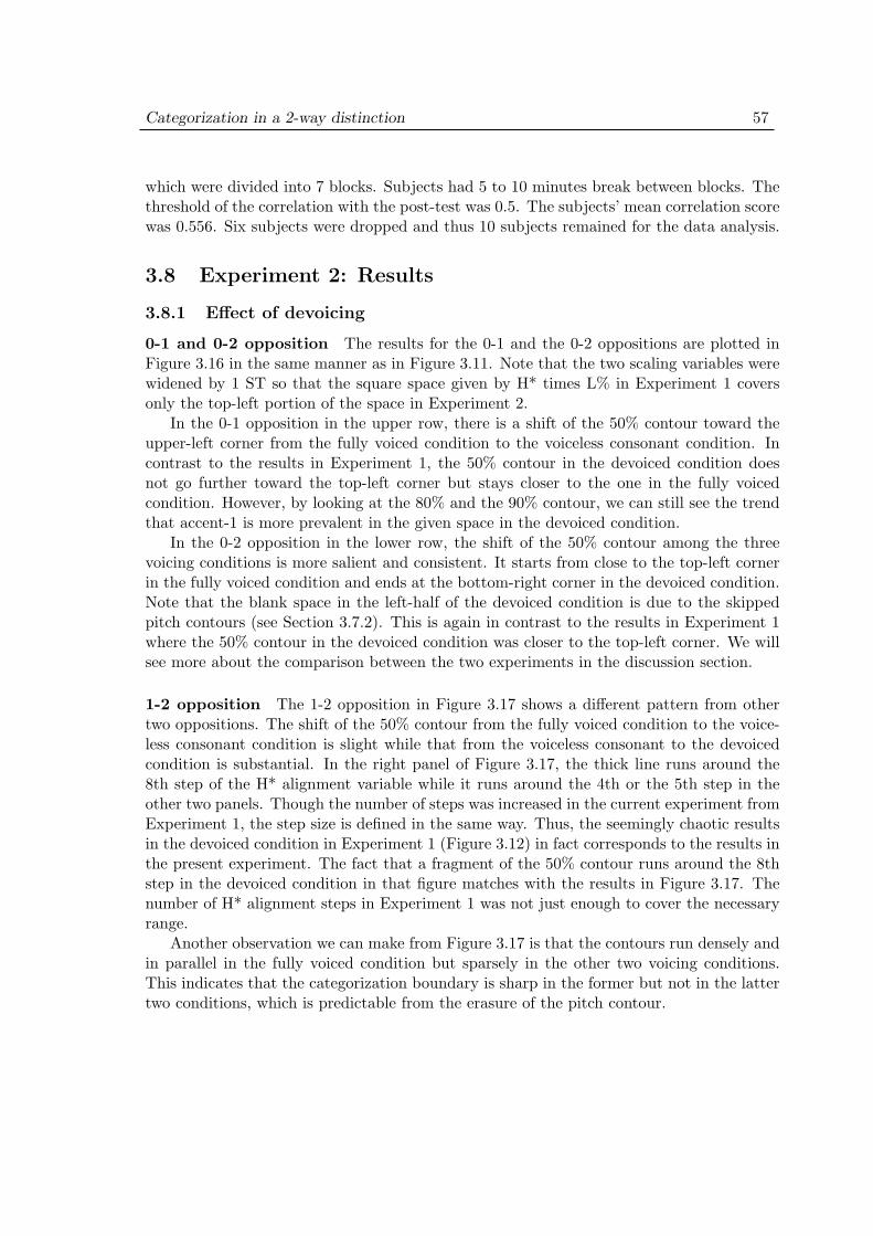
Categorization in a 2-way distinction 57
which were divided into 7 blocks. Subjects had 5 to 10 minutes break between blocks. Thethreshold of the correlation with the post-test was 0.5. The subjects’ mean correlation scorewas 0.556. Six subjects were dropped and thus 10 subjects remained for the data analysis.
3.8 Experiment 2: Results
3.8.1 Effect of devoicing
0-1 and 0-2 opposition The results for the 0-1 and the 0-2 oppositions are plotted inFigure 3.16 in the same manner as in Figure 3.11. Note that the two scaling variables werewidened by 1 ST so that the square space given by H* times L% in Experiment 1 coversonly the top-left portion of the space in Experiment 2.
In the 0-1 opposition in the upper row, there is a shift of the 50% contour toward theupper-left corner from the fully voiced condition to the voiceless consonant condition. Incontrast to the results in Experiment 1, the 50% contour in the devoiced condition doesnot go further toward the top-left corner but stays closer to the one in the fully voicedcondition. However, by looking at the 80% and the 90% contour, we can still see the trendthat accent-1 is more prevalent in the given space in the devoiced condition.
In the 0-2 opposition in the lower row, the shift of the 50% contour among the threevoicing conditions is more salient and consistent. It starts from close to the top-left cornerin the fully voiced condition and ends at the bottom-right corner in the devoiced condition.Note that the blank space in the left-half of the devoiced condition is due to the skippedpitch contours (see Section 3.7.2). This is again in contrast to the results in Experiment 1where the 50% contour in the devoiced condition was closer to the top-left corner. We willsee more about the comparison between the two experiments in the discussion section.
1-2 opposition The 1-2 opposition in Figure 3.17 shows a different pattern from othertwo oppositions. The shift of the 50% contour from the fully voiced condition to the voice-less consonant condition is slight while that from the voiceless consonant to the devoicedcondition is substantial. In the right panel of Figure 3.17, the thick line runs around the8th step of the H* alignment variable while it runs around the 4th or the 5th step in theother two panels. Though the number of steps was increased in the current experiment fromExperiment 1, the step size is defined in the same way. Thus, the seemingly chaotic resultsin the devoiced condition in Experiment 1 (Figure 3.12) in fact corresponds to the results inthe present experiment. The fact that a fragment of the 50% contour runs around the 8thstep in the devoiced condition in that figure matches with the results in Figure 3.17. Thenumber of H* alignment steps in Experiment 1 was not just enough to cover the necessaryrange.
Another observation we can make from Figure 3.17 is that the contours run densely andin parallel in the fully voiced condition but sparsely in the other two voicing conditions.This indicates that the categorization boundary is sharp in the former but not in the lattertwo conditions, which is predictable from the erasure of the pitch contour.
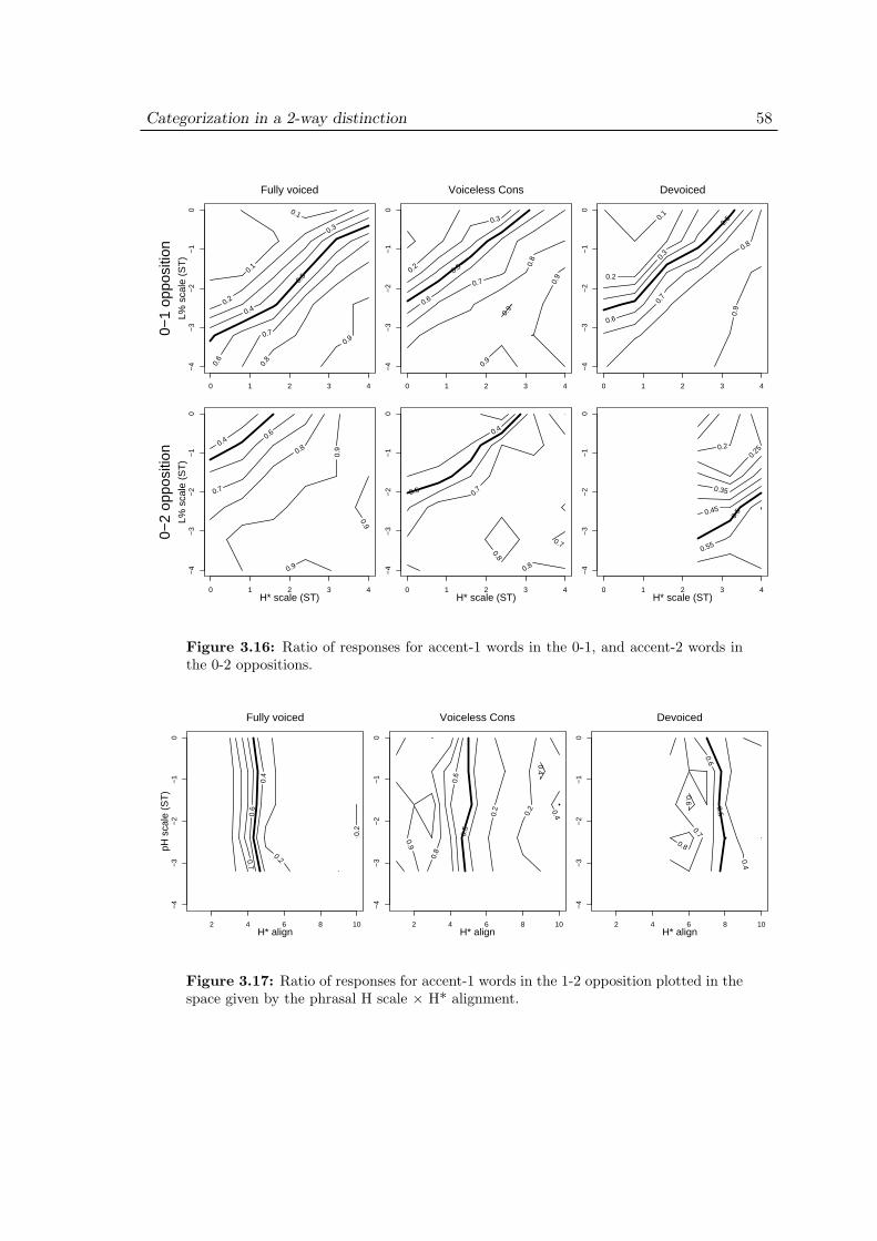
Categorization in a 2-way distinction 58
0.1
0.1
0.2
0.3
0.4
0.5
0.6
0.7
0.8
0.9
0 1 2 3 4
−4
−3
−2
−1
0L%
sca
le (
ST
)
0−1
oppo
sitio
n
Fully voiced
0.2
0.3
0.5
0.6
0.7
0.8
0.9
0.9
0.9
0 1 2 3 4−
4−
3−
2−
10
Voiceless Cons
0.1
0.2
0.3
0.5
0.6
0.7
0.8
0.9
0 1 2 3 4
−4
−3
−2
−1
0
Devoiced
0.4 0.6
0.7
0.8
0.9
0.9
0.9
0 1 2 3 4
−4
−3
−2
−1
0
H* scale (ST)
L% s
cale
(S
T)
0−2
oppo
sitio
n
0.4
0.5 0
.7
0.7 0.8
0.8
0 1 2 3 4
−4
−3
−2
−1
0
H* scale (ST)
0.2
0.2
5
0.35
0.45
0.5
0.55
0 1 2 3 4−
4−
3−
2−
10
H* scale (ST)
Figure 3.16: Ratio of responses for accent-1 words in the 0-1, and accent-2 words inthe 0-2 oppositions.
0.2
0.2
0.4
0.6
0.7
2 4 6 8 10
−4−3
−2−1
0
H* align
pH s
cale
(S
T)
Fully voiced
0.2
0.2
0.4
0.4
0.5
0.6
0.8
0.9
2 4 6 8 10
−4−3
−2−1
0
H* align
Voiceless Cons
0.4
0.5
0.6
0.6
0.7
0.8
2 4 6 8 10
−4−3
−2−1
0
H* align
Devoiced
Figure 3.17: Ratio of responses for accent-1 words in the 1-2 opposition plotted in thespace given by the phrasal H scale × H* alignment.
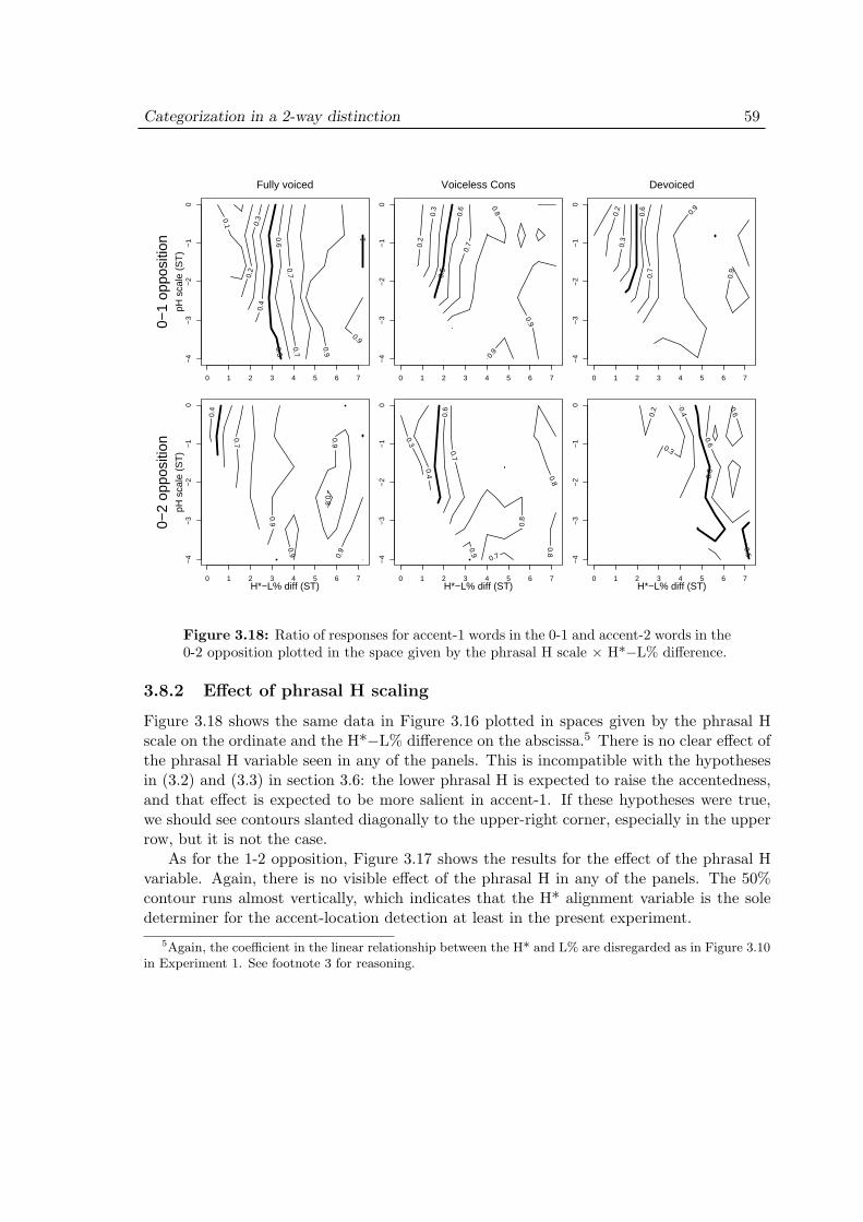
Categorization in a 2-way distinction 59
0.1
0.2
0
.3
0.4
0.5 0.6
0.7 0.7
0.9
0.9
1
0 1 2 3 4 5 6 7
−4
−3
−2
−1
0pH
sca
le (
ST
)
0−1
oppo
sitio
n
Fully voiced
0.2
0.3
0
.5
0.6
0
.7
0.8
0.9
0.9
0 1 2 3 4 5 6 7−
4−
3−
2−
10
Voiceless Cons
0.2
0
.3
0.6
0
.7
0.9
0.9
0 1 2 3 4 5 6 7
−4
−3
−2
−1
0
Devoiced
0.4
0.7
0.8
0.9
0.9
0.9
0.9
0 1 2 3 4 5 6 7
−4
−3
−2
−1
0
H*−L% diff (ST)
pH s
cale
(S
T)
0−2
oppo
sitio
n 0.3
0.4
0.6
0.7
0.7
0.8
0.8 0.8
0.9
0 1 2 3 4 5 6 7
−4
−3
−2
−1
0
H*−L% diff (ST)
0.2
0.3
0.4
0.5
0.5
0.6
0.6
0 1 2 3 4 5 6 7−
4−
3−
2−
10
H*−L% diff (ST)
Figure 3.18: Ratio of responses for accent-1 words in the 0-1 and accent-2 words in the0-2 opposition plotted in the space given by the phrasal H scale × H*−L% difference.
3.8.2 Effect of phrasal H scaling
Figure 3.18 shows the same data in Figure 3.16 plotted in spaces given by the phrasal Hscale on the ordinate and the H*−L% difference on the abscissa.5 There is no clear effect ofthe phrasal H variable seen in any of the panels. This is incompatible with the hypothesesin (3.2) and (3.3) in section 3.6: the lower phrasal H is expected to raise the accentedness,and that effect is expected to be more salient in accent-1. If these hypotheses were true,we should see contours slanted diagonally to the upper-right corner, especially in the upperrow, but it is not the case.
As for the 1-2 opposition, Figure 3.17 shows the results for the effect of the phrasal Hvariable. Again, there is no visible effect of the phrasal H in any of the panels. The 50%contour runs almost vertically, which indicates that the H* alignment variable is the soledeterminer for the accent-location detection at least in the present experiment.
5Again, the coefficient in the linear relationship between the H* and L% are disregarded as in Figure 3.10in Experiment 1. See footnote 3 for reasoning.
Categorization in a 2-way distinction 60
3.9 Experiment 2: Discussion
The effect of the preceding context was not confirmed either in the devoiced nor in thevoiced conditions. We have just seen in the previous section that the results were negativefor all of the opposition types tested in the experiment. Several reasons can be thoughtof. First, the range of the phrasal H variable might be wrong. The phrasal H in thepresent experiment varied in the range lower than the mean pitch. The range setting wasmotivated by the hypothesis that the lower phrasal H triggers more accented responses.Compared to Matsui (1993)’s design in which the preceding context is fixed at 196 Hz, therange covered in the present experiment was from about 100 Hz up to 145 Hz in the actualstimuli. Though the F0 peak in Matsui’s design is 212 Hz while it was about 180 Hz in thepresent experiment, the relative height of the phrasal H was still quite low. Second, whatMatsui compared in his experiment is the linguistic assignment of the H or the L tone tothe preceding context but not the actual pitch (see (2.2) in section 2.2.3). Thus his claimabout the effect of the preceding context is not directly applicable to the variable phrasalH in the present experiment.
However, other results resolve most of the questions carried-over from Experiment 1.First, the widened and more fine-grained stimulus space confirms that the overall trendsobserved in Experiment 1 are on the right track. Especially, the results from the devoicedcondition in the 1-2 opposition reveal that the categorical boundary lay at the edge of theH* alignment range in Experiment 1. The widened range confirms that the boundary shiftslater in the devoiced condition compared to the voiced conditions. However, we cannotexpect to have more responses to accent-2 if the range of the alignment variable is extendedfurther. Beyond the 10th step, the H* tone will be placed on the vowel of the first moraof the following context. This is not desirable for testing the accentual contrast withinthe target word. Put differently, the area in which accent-2 is perceived is compressed inthe given range in the devoiced condition both in Experiments 1 and 2. This is a naturaloutcome from the predicted schema in Figure 3.2 where the erased part contains the crucialinformation for accent-2.
Second, the fixed slope did not alter the overall picture. The rate of the fall in thepresent experiment was −0.423 Hz/msec which roughly corresponds to the 3rd step (−0.435Hz/msec) in Experiment 1. As expected, the percept of accent was achieved without anyproblem.
Third, the hypotheses about the effect of devoicing tested in Experiment 1 hold for theresults in Experiment 2. In a nutshell, the hypotheses were based on a view that thereare three sources of information for the identification of an accent: a high pitch at the H*tone, a low pitch at the L% tone, and the falling contour. Cessation of a pitch contourby a voiceless segment causes a loss of the information sources (see Figures 3.1 and 3.2 inSection 3.2 for a more detailed explanation). Predictions among different voicing conditionsare derived from the number of the losses of information sources as in Table 3.4.
The number of asterisks in each cell in Table 3.4 predicts that there is a difference in theperformance of a categorization task between the fully voiced and the voiceless consonant
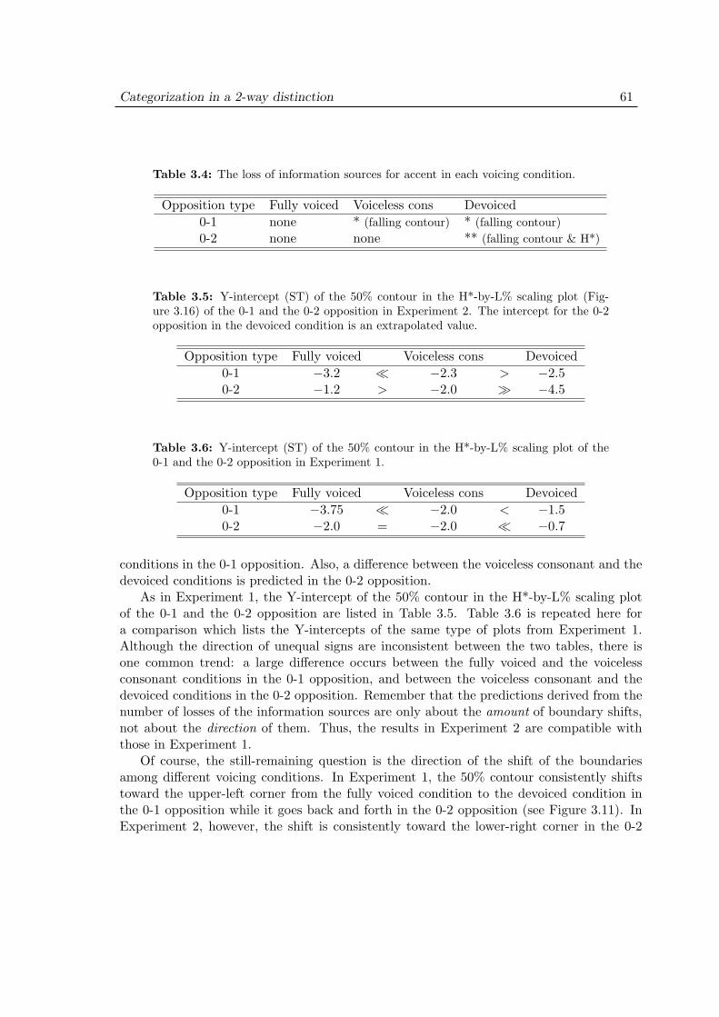
Categorization in a 2-way distinction 61
Table 3.4: The loss of information sources for accent in each voicing condition.
Opposition type Fully voiced Voiceless cons Devoiced0-1 none * (falling contour) * (falling contour)0-2 none none ** (falling contour & H*)
Table 3.5: Y-intercept (ST) of the 50% contour in the H*-by-L% scaling plot (Fig-ure 3.16) of the 0-1 and the 0-2 opposition in Experiment 2. The intercept for the 0-2opposition in the devoiced condition is an extrapolated value.
Opposition type Fully voiced Voiceless cons Devoiced0-1 −3.2 ¿ −2.3 > −2.50-2 −1.2 > −2.0 À −4.5
Table 3.6: Y-intercept (ST) of the 50% contour in the H*-by-L% scaling plot of the0-1 and the 0-2 opposition in Experiment 1.
Opposition type Fully voiced Voiceless cons Devoiced0-1 −3.75 ¿ −2.0 < −1.50-2 −2.0 = −2.0 ¿ −0.7
conditions in the 0-1 opposition. Also, a difference between the voiceless consonant and thedevoiced conditions is predicted in the 0-2 opposition.
As in Experiment 1, the Y-intercept of the 50% contour in the H*-by-L% scaling plotof the 0-1 and the 0-2 opposition are listed in Table 3.5. Table 3.6 is repeated here fora comparison which lists the Y-intercepts of the same type of plots from Experiment 1.Although the direction of unequal signs are inconsistent between the two tables, there isone common trend: a large difference occurs between the fully voiced and the voicelessconsonant conditions in the 0-1 opposition, and between the voiceless consonant and thedevoiced conditions in the 0-2 opposition. Remember that the predictions derived from thenumber of losses of the information sources are only about the amount of boundary shifts,not about the direction of them. Thus, the results in Experiment 2 are compatible withthose in Experiment 1.
Of course, the still-remaining question is the direction of the shift of the boundariesamong different voicing conditions. In Experiment 1, the 50% contour consistently shiftstoward the upper-left corner from the fully voiced condition to the devoiced condition inthe 0-1 opposition while it goes back and forth in the 0-2 opposition (see Figure 3.11). InExperiment 2, however, the shift is consistently toward the lower-right corner in the 0-2
Categorization in a 2-way distinction 62
opposition but it is not consistent in the 0-1 opposition. Thus, it is rather difficult to finda general pattern for the direction of the shift at this point.
Another remaining question is the effect of the final lowering process added to the presentexperiment. In Section 3.5, it was argued that the difference in the amount of pitch droprequired for the 0-1 and the 0-2 opposition might be attributed to listeners’ compensationfor the final lowering in the 0-2 opposition. Since the final lowering process was skippedin Experiment 1, the apparent difference between the two oppositions was expected todisappear if it is incorporated. However, the results in the present experiment show thatthe difference persists even when final lowering was incorporated in the stimulus design. Infact, the difference becomes larger in the present experiment. In the fully voiced condition,the 50% contour lies around the H*−L% difference at 3 ST in the 0-1 opposition but at 0.5ST in the 0-2 opposition (Figure 3.18).
The two remaining questions can be subsumed under a single heading: why do bound-aries (unpredictably) move around in the accent-presence detection? In fact, boundaries doshift in the accent-location detection across different voicing conditions but the directionof the shift was predictable and consistent between the two experiments. The reason forthis is simple. The accent-location detection only involves the time-axis (i.e., the H* align-ment). Different voicing conditions also involve only the time-axis. The cessation of thepitch contour by a voiceless consonant or a devoiced mora occurs at different durations butit is just a matter of a single dimension on which the accent is located. As we have seen inFigures 3.12 and 3.17, the H* has to be aligned later than the other voicing conditions forthe accent to be perceived when the second mora of the word is devoiced. However, in theaccent-presence detection, the cessation of the pitch contour on the time-axis is orthogonalto the two scaling variables, namely, H* and L%.
What is more complicating is the variability of durational properties in each token.In Experiments 1 and 2, the stimulus words were not controlled in terms of segmentalduration. The speech rate of the carrier sentences was not controlled either. Since theduration of each level tone was based on a visual segmentation process, tones within a wordnor across different words have different durations. Thus, the global shape of the pitchcontour can be different across words even with the same setting in the scaling variables.In addition, the voiced token and the devoiced token of the same word are somewhatdifferent in durational properties because of the mere fact that they are different tokens. Thecomparison across different voicing conditions might have been affected by those unintendeddurational differences. In the next chapter, this variability problem in durational propertieswill be resolved by introducing a splicing technique to created devoiced tokens from thevoiced ones.
So far in this section, we have discussed that some unintended or not-tightly-controlledphysical properties, such as pitch and duration, in the stimulus design might have obscuredthe true picture of the categorical structure. However, there might be something other thanphysical properties which differentiates one of the words in minimal pairs used in the twoexperiments. For example, if the familiarity of the words in a minimal pair greatly differ,the responses for one word might exceed those for the other word ceteris paribus. When
Categorization in a 2-way distinction 63
there is a known bias from familiarity, the results in a categorization experiment has tobe calibrated. However, studies on word familiarity and pitch accent in Japanese have notappeared at all, as far as I know. We have to first establish the basic strategy for dealingwith word familiarity in terms of the category structure of pitch accents. Chapter 5 willexplore this issue using the word familiarity data in Amano & Kondo (1999).
Chapter 4
Categorization in a 3-way distinction
4.1 Introduction
In 2-mora homophones with a 2-way accentual distinction, there is always the third accentcategory which does not correspond to an existing word. Accent-2 in the 0-1 opposition,accent-1 in the 0-2 opposition, and accent-0 in the 1-2 opposition are never involved in thecategorization task. When subjects hear a word with the F0 contour corresponding to thethird category, it may sound somewhat odd for the two alternatives at hand. Subjects,however, have no choice but the given two alternatives because the stimulus with the thirdaccent category is not a word.
Meanwhile, each accent category has a realization in a 3-way distinction. A categoriza-tion task in a 3-way distinction is expected to be harder than a 2-way distinction in tworespects. First, subjects will have to choose from a wider range of categories. Second, twofunctionally different tasks that are segregated in a 2-way distinction will be involved atthe same time. The two tasks are the accent-presence detection and the accent-locationdetection. Both the 0-1 and the 0-2 oppositions are in the realm of the accent-presencedetection task while the accent-location detection task is involved in the 1-2 opposition.Thus, only either one of the two tasks is involved in a 2-way opposition. However, whenthe third category exists as a word, not only are the available choices for subjects wider,but the two tasks will be involved.
As we have seen in the results of Experiments 1 and 2, the H* and the L% tones are thetwo interacting variables in the accent-presence detection task while the H* alignment is thesole cue for the accent-location detection task. This is achieved because the two tasks aresegregated. In a 3-way distinction, the role of each variable and their interaction might bedifferent from those in a 2-way distinction, which is the primary motivation for conductinganother experiment.
Another motivation for conducting the third experiment is that the results in Experiment1 and 2 are to some extent conflicting in the direction of the shift of category boundaries.One potentially relevant factor is the durational variation across the stimuli. In Experiment1 and 2, stimulus words were not controlled in terms of segmental duration. The speech rateof the carrier sentences was not rigorously controlled either. It is worth trying to control
64
Categorization in a 3-way distinction 65
the durational variation across the voiced and the devoiced conditions.1 By splicing outthe voiced vowel of the second mora of a devoiceable word and filling that region with thenoise of an aspiration, voiced and devoiced stimuli can be created from a single token inwhich the duration of each segment is to be the same.2 Since we are dealing with a 3-waydistinction, the three opposition types, 0-1, 0-2 and 1-2, in the previous experiments are allcovered in a single triplet, which eliminates durational variation across different minimalpairs set up for each opposition type.
Finally, the effect of the phrasal H was not observed in Experiment 2. As pointed outin Section 3.9, this may be due to the fact that the range of the variable was too low toproduce visible effects. In real speech, the phrasal H tone can be as high as the H* tone.Therefore, it is worth trying a wider range for the phrasal H tone variable.
The present experiment thus introduces several modifications in the design from that ofExperiment 2. They are: (1) use of a triplet with a 3-way accentual distinction, (2) splicingtechnique to control the duration across voiced and devoiced conditions, and (3) the rangeof the phrasal H tone variable. Two of these modifications imply a large increase in thenumber of stimuli, however. Testing a 3-way distinction requires the three variables, namelythe H* scale, the L% scale and the H* alignment, fully crossed for each token. Adding awider range of the phrasal H as another variable; the total number of the stimuli will beimpractically large. Thus, a trade-off will be made in the number of words, the number ofsteps, and the step sizes, which are further modifications from Experiment 2.
4.2 Purpose and predictions
The main purpose of Experiment 3 is to investigate the perception of pitch accent in ho-mophones with a 3-way accentual distinction. From what we have seen about a 2-waydistinction in the previous chapter, we can make several predictions about the role of eachvariable and their interaction. First, the H* and the L% scaling variables are expectedto work together in the accent-presence detection. If we take the difference between thetwo variables, the difference term will roughly correspond to the boundary in the accent-presence detection. Second, the H* alignment will be the main cue for the accent-locationdetection. Accent-1 will be perceived when the H* is aligned early while accent-2 will beperceived when the H* is aligned late. Third, in the devoiced condition, the boundary inthe accent-presence detection will be shifted to the direction in which the H*−L% differ-ence is larger and the boundary in the accent-location detection will be shifted to the right.Fourth, the “gray area” in categorization is predicted to increase in the devoiced condition.Since the present experiment is not a two-alternative forced choice but a three-alternativeone, there may be an area in which none of the choices reach the 50% response rate. As
1In the present experiment, “voiced” condition corresponds to the “voiceless consonant” condition inExperiment 1 and 2 in which the consonant is voiceless but the vowel in that mora is “voiced”.
2One might ask whether the intrinsic duration of a voiced mora and a devoiced mora differ or not. In aproduction study, the total duration of the devoiced mora and a corresponding voiced mora are about thesame (Kitahara, 1999).
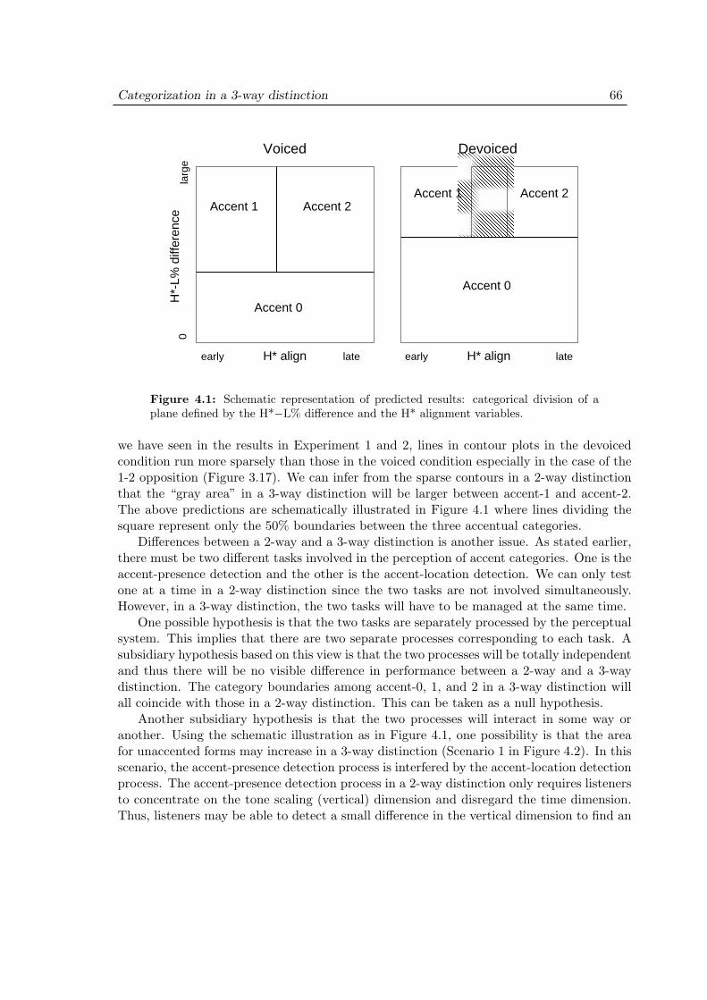
Categorization in a 3-way distinction 66
������������������������������������������
������������������������������������������
Accent 1
Accent 0
H* align
Accent 2
Voiced
early late
0
larg
eH
*-L%
diff
eren
ce
early lateH* align
Accent 0
Accent 2Accent 1
Devoiced
Figure 4.1: Schematic representation of predicted results: categorical division of aplane defined by the H*−L% difference and the H* alignment variables.
we have seen in the results in Experiment 1 and 2, lines in contour plots in the devoicedcondition run more sparsely than those in the voiced condition especially in the case of the1-2 opposition (Figure 3.17). We can infer from the sparse contours in a 2-way distinctionthat the “gray area” in a 3-way distinction will be larger between accent-1 and accent-2.The above predictions are schematically illustrated in Figure 4.1 where lines dividing thesquare represent only the 50% boundaries between the three accentual categories.
Differences between a 2-way and a 3-way distinction is another issue. As stated earlier,there must be two different tasks involved in the perception of accent categories. One is theaccent-presence detection and the other is the accent-location detection. We can only testone at a time in a 2-way distinction since the two tasks are not involved simultaneously.However, in a 3-way distinction, the two tasks will have to be managed at the same time.
One possible hypothesis is that the two tasks are separately processed by the perceptualsystem. This implies that there are two separate processes corresponding to each task. Asubsidiary hypothesis based on this view is that the two processes will be totally independentand thus there will be no visible difference in performance between a 2-way and a 3-waydistinction. The category boundaries among accent-0, 1, and 2 in a 3-way distinction willall coincide with those in a 2-way distinction. This can be taken as a null hypothesis.
Another subsidiary hypothesis is that the two processes will interact in some way oranother. Using the schematic illustration as in Figure 4.1, one possibility is that the areafor unaccented forms may increase in a 3-way distinction (Scenario 1 in Figure 4.2). In thisscenario, the accent-presence detection process is interfered by the accent-location detectionprocess. The accent-presence detection process in a 2-way distinction only requires listenersto concentrate on the tone scaling (vertical) dimension and disregard the time dimension.Thus, listeners may be able to detect a small difference in the vertical dimension to find an
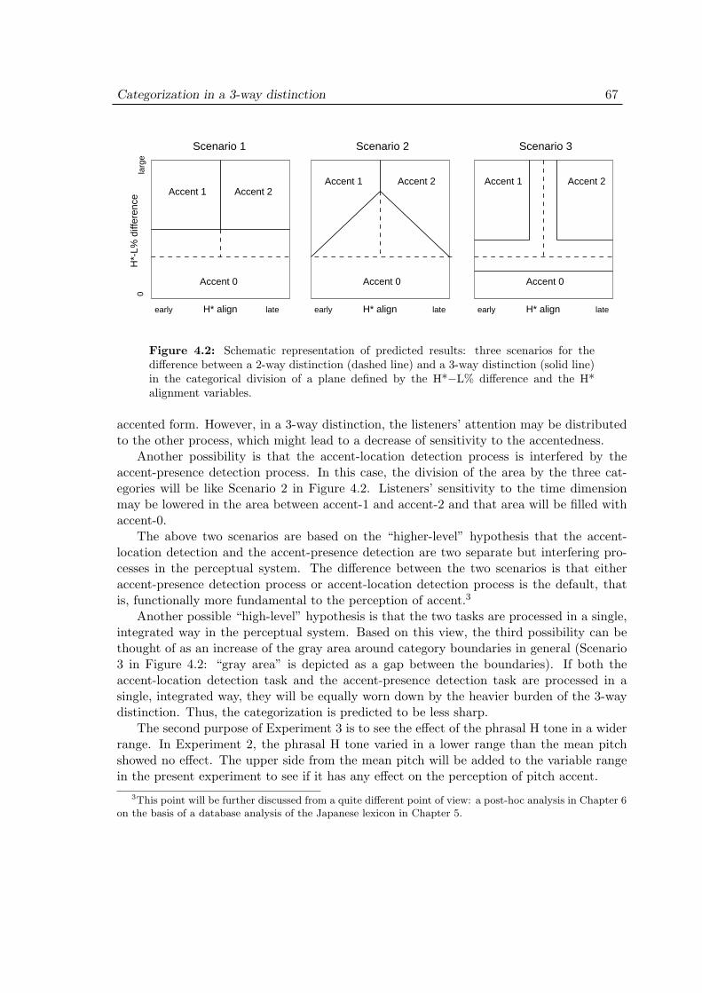
Categorization in a 3-way distinction 67
H* align
Accent 2
early late
0
larg
eH
*-L%
diff
eren
ce
Accent 0
Scenario 1
early lateH* align
Accent 2Accent 1
Accent 0
Scenario 3
early lateH* align
Scenario 2
Accent 0
Accent 1Accent 1 Accent 2
Figure 4.2: Schematic representation of predicted results: three scenarios for thedifference between a 2-way distinction (dashed line) and a 3-way distinction (solid line)in the categorical division of a plane defined by the H*−L% difference and the H*alignment variables.
accented form. However, in a 3-way distinction, the listeners’ attention may be distributedto the other process, which might lead to a decrease of sensitivity to the accentedness.
Another possibility is that the accent-location detection process is interfered by theaccent-presence detection process. In this case, the division of the area by the three cat-egories will be like Scenario 2 in Figure 4.2. Listeners’ sensitivity to the time dimensionmay be lowered in the area between accent-1 and accent-2 and that area will be filled withaccent-0.
The above two scenarios are based on the “higher-level” hypothesis that the accent-location detection and the accent-presence detection are two separate but interfering pro-cesses in the perceptual system. The difference between the two scenarios is that eitheraccent-presence detection process or accent-location detection process is the default, thatis, functionally more fundamental to the perception of accent.3
Another possible “high-level” hypothesis is that the two tasks are processed in a single,integrated way in the perceptual system. Based on this view, the third possibility can bethought of as an increase of the gray area around category boundaries in general (Scenario3 in Figure 4.2: “gray area” is depicted as a gap between the boundaries). If both theaccent-location detection task and the accent-presence detection task are processed in asingle, integrated way, they will be equally worn down by the heavier burden of the 3-waydistinction. Thus, the categorization is predicted to be less sharp.
The second purpose of Experiment 3 is to see the effect of the phrasal H tone in a widerrange. In Experiment 2, the phrasal H tone varied in a lower range than the mean pitchshowed no effect. The upper side from the mean pitch will be added to the variable rangein the present experiment to see if it has any effect on the perception of pitch accent.
3This point will be further discussed from a quite different point of view: a post-hoc analysis in Chapter 6on the basis of a database analysis of the Japanese lexicon in Chapter 5.

Categorization in a 3-way distinction 68
Table 4.1: Corpus for Experiment 3
Unaccented Initial accent Final accent
set 1hashi hashi hashı‘edge’ ‘chopstick’ ‘bridge’
set 2kaki kaki kakı
‘persimmon’ ‘summertime’ ‘fence’
The phrasal H tone set to the mean pitch creates a big bump of the H* tone in the pitchcontour. When the phrasal H is raised closer to the H* tone in the upper range, the pitchcontour will become more like a plateau between the two H tones and thus the bump of theH* tone will become less popped-out. A prediction derived from this is that the location ofthe H* tone will become more obscured by losing the left edge of the bump. That is, theaccent-location detection may become less sensitive when the phrasal H is raised. On thecontrary, the accent-presence detection may not be affected as much because the H*−L%difference is independent from the preceding context. Therefore, if we plot the results in a“phrasal H by H* align” space, we will see curved contours in the responses for accentedforms and if we plot in a “phrasal H by H*−L% difference” space, we will see straightcontours.
4.3 Methods
4.3.1 Materials
The corpus for the present experiment consists of two sets of homophones which constitutea 3-way accentual distinction within each set. Words are all 2 moras in length whose secondmora is devoiceable. Members of the two sets of homophones are listed in Table 4.1.
The carrier sentence is one of those used in Experiment 2. As in the previous exper-iments, it was intended that the preceding part “[ano]” bears the phrasal H tone, whichmakes it possible to observe the effect of pitch accent independent from the phrasal H tone.The following part “[kara]” was chosen as a devoiceable context for the final mora of theword.
(4.1) ano kara “From that .”
As opposed to Experiment 1 and 2, Experiment 3 was not designed to induce devoicingforcefully by the difference in carrier sentences. Voiced tokens were recorded first and thedevoiced variant was created by splicing the voiced tokens. Since devoicing is an optionalrule in Tokyo Japanese, a voiced utterance in a devoiceable context does not sound veryunnatural.
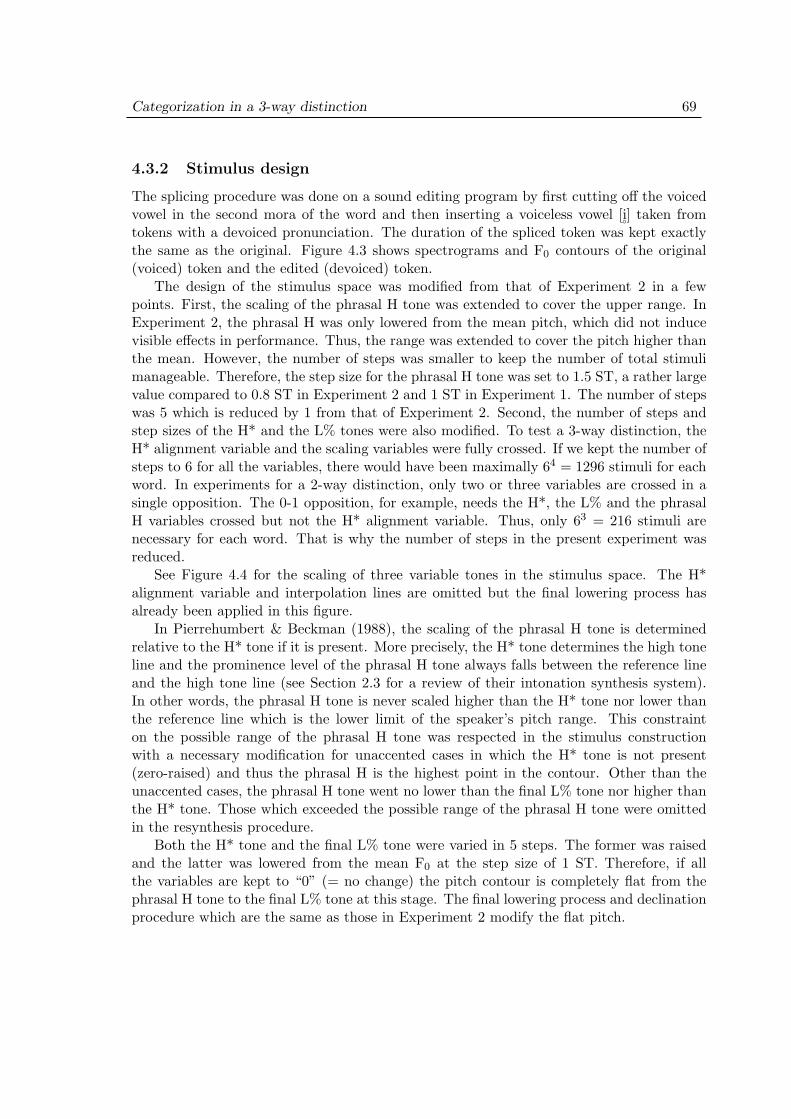
Categorization in a 3-way distinction 69
4.3.2 Stimulus design
The splicing procedure was done on a sound editing program by first cutting off the voicedvowel in the second mora of the word and then inserting a voiceless vowel [i◦] taken fromtokens with a devoiced pronunciation. The duration of the spliced token was kept exactlythe same as the original. Figure 4.3 shows spectrograms and F0 contours of the original(voiced) token and the edited (devoiced) token.
The design of the stimulus space was modified from that of Experiment 2 in a fewpoints. First, the scaling of the phrasal H tone was extended to cover the upper range. InExperiment 2, the phrasal H was only lowered from the mean pitch, which did not inducevisible effects in performance. Thus, the range was extended to cover the pitch higher thanthe mean. However, the number of steps was smaller to keep the number of total stimulimanageable. Therefore, the step size for the phrasal H tone was set to 1.5 ST, a rather largevalue compared to 0.8 ST in Experiment 2 and 1 ST in Experiment 1. The number of stepswas 5 which is reduced by 1 from that of Experiment 2. Second, the number of steps andstep sizes of the H* and the L% tones were also modified. To test a 3-way distinction, theH* alignment variable and the scaling variables were fully crossed. If we kept the number ofsteps to 6 for all the variables, there would have been maximally 64 = 1296 stimuli for eachword. In experiments for a 2-way distinction, only two or three variables are crossed in asingle opposition. The 0-1 opposition, for example, needs the H*, the L% and the phrasalH variables crossed but not the H* alignment variable. Thus, only 63 = 216 stimuli arenecessary for each word. That is why the number of steps in the present experiment wasreduced.
See Figure 4.4 for the scaling of three variable tones in the stimulus space. The H*alignment variable and interpolation lines are omitted but the final lowering process hasalready been applied in this figure.
In Pierrehumbert & Beckman (1988), the scaling of the phrasal H tone is determinedrelative to the H* tone if it is present. More precisely, the H* tone determines the high toneline and the prominence level of the phrasal H tone always falls between the reference lineand the high tone line (see Section 2.3 for a review of their intonation synthesis system).In other words, the phrasal H tone is never scaled higher than the H* tone nor lower thanthe reference line which is the lower limit of the speaker’s pitch range. This constrainton the possible range of the phrasal H tone was respected in the stimulus constructionwith a necessary modification for unaccented cases in which the H* tone is not present(zero-raised) and thus the phrasal H is the highest point in the contour. Other than theunaccented cases, the phrasal H tone went no lower than the final L% tone nor higher thanthe H* tone. Those which exceeded the possible range of the phrasal H tone were omittedin the resynthesis procedure.
Both the H* tone and the final L% tone were varied in 5 steps. The former was raisedand the latter was lowered from the mean F0 at the step size of 1 ST. Therefore, if allthe variables are kept to “0” (= no change) the pitch contour is completely flat from thephrasal H tone to the final L% tone at this stage. The final lowering process and declinationprocedure which are the same as those in Experiment 2 modify the flat pitch.

Categorization in a 3-way distinction 70
� � � � � � � � � � � � � � � � � � � � � � � �
�
� � �
� � �
� � �
� � �
� � �
� � �
� � �
� � �
� � �
��� ������
��� ��� ��� �
�� �"!"#"�"$"%�&' ������
�
� � �
� � � �
� � � �
� � � �
� � � �
� � � �
� � � �
� � � �
� � � �
� � � �
� � � � � � � � � � � � � � � � � � � � � � � �
�
� � �
� � �
� � �
� � �
� � �
� � �
� � �
� � �
��� ������
��� ��� � ��� ��
�� �"!"#"�"$"%�&' ������
�
� � �
� � � �
� � � �
� � � �
� � � �
� � � �
� � � �
� � � �
� � � �
� � � �
Figure 4.3: Spectrogram and F0 contour of the unedited voiced token of [ano kakikara] (upper two panels) and those of edited devoiced token [ano kaki◦ kara] (lower twopanels).

Categorization in a 3-way distinction 71
0 100 200 300 400 500 600 700 800 900
80
90
100
110
120
130
140
150
160
170
180
time (ms)
Fre
quen
cy (
Hz)
pH +3
pH 0
pH -1.5
pH -3
H* +3
H* +2
H* +1
H* 0
L% -1L% -2L% -3L% -4
H* +4
L% 0
pH +1.5
Figure 4.4: Stimulus design for Experiment 3: variable tone scales in semitones mea-sured from the reference pitch (mean F0 ). Interpolation and H* alignment is omitted.
Though the initial portion of the utterance is considered to be the location of anotherL% tone, it is not relevant for the pitch accent in Pierrehumbert & Beckman’s model andthus not manipulated in the present experiment. It is just stipulated as 1 ST lower than thephrasal H tone in order to implement the rising contour at the utterance-initial position.
Next, let us see the dimension of the tone alignment variable and the effect of finallowering process in Figure 4.5. The scaling of tones in this figure is specified as the following:phrasal H = 0, H* = 4, and L% = 0. The H* alignment was varied in 5 steps whose stepsize was again relatively specified to the summed duration of the two moras. One wasthe last mora of the stimulus word and the other was the penultimate mora in the carriersentence. One step was 1/5th of the base duration which is twice the step size in Experiment2. In Experiments 1 and 2, some of those alignment steps whose H*-L tone sequence arecompletely within the devoiced region were omitted. There was no omission of steps inExperiment 3 to keep complete matching between the voiced and devoiced stimuli.
Figure 4.5 also shows that the local slope from H* to L is fixed as in Experiment 2. Theslope value was again 0.423Hz/msec which was obtained from an average of 24 tokens inExperiment 2. All the major steps in resynthesis and the final outcome of the stimuli fordevoiced [hashi◦] token are given in Figure 4.6.
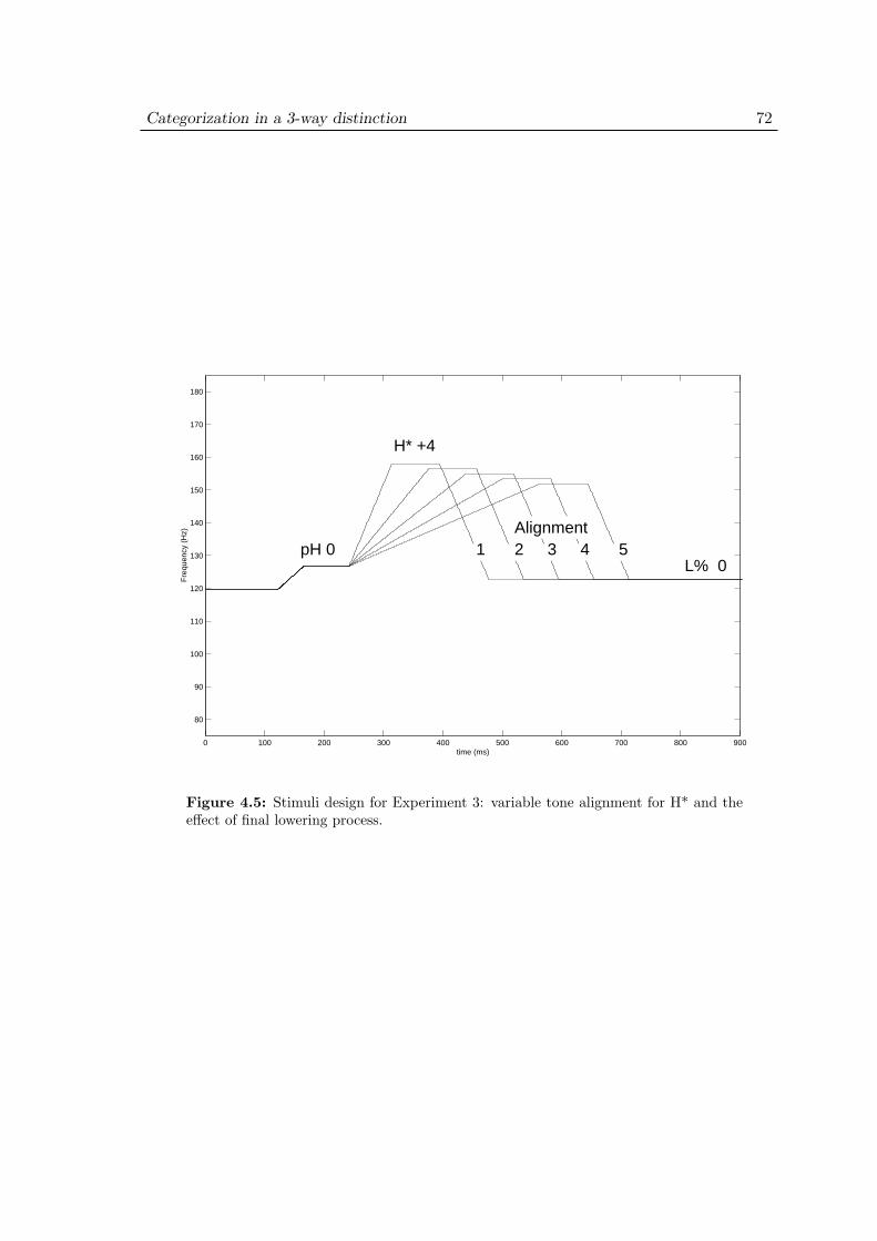
Categorization in a 3-way distinction 72
0 100 200 300 400 500 600 700 800 900
80
90
100
110
120
130
140
150
160
170
180
time (ms)
Fre
quen
cy (
Hz)
pH 0
H* +4
L% 021 3 4 5Alignment
Figure 4.5: Stimuli design for Experiment 3: variable tone alignment for H* and theeffect of final lowering process.
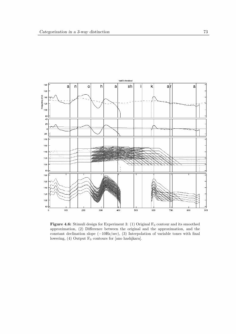
Categorization in a 3-way distinction 73
Figure 4.6: Stimuli design for Experiment 3: (1) Original F0 contour and its smoothedapproximation, (2) Difference between the original and the approximation, and theconstant declination slope (−10Hz/sec), (3) Interpolation of variable tones with finallowering, (4) Output F0 contours for [ano hashi◦kara].
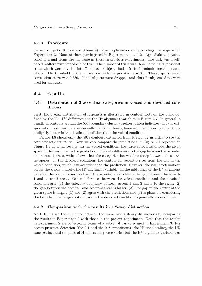
Categorization in a 3-way distinction 74
4.3.3 Procedure
Sixteen subjects (8 male and 8 female) naive to phonetics and phonology participated inExperiment 3. None of them participated in Experiment 1 and 2. Age, dialect, physicalcondition, and terms are the same as those in previous experiments. The task was a self-paced 3-alternative forced choice task. The number of trials was 1634 including 66 post-testtrials which were divided into 7 blocks. Subjects had a 5- to 10-minute break betweenblocks. The threshold of the correlation with the post-test was 0.4. The subjects’ meancorrelation score was 0.330. Nine subjects were dropped and thus 7 subjects’ data wereused for analyses.
4.4 Results
4.4.1 Distribution of 3 accentual categories in voiced and devoiced con-ditions
First, the overall distribution of responses is illustrated in contour plots on the plane de-fined by the H*−L% difference and the H* alignment variables in Figure 4.7. In general, abundle of contours around the 50% boundary cluster together, which indicates that the cat-egorization task was done successfully. Looking closely, however, the clustering of contoursis slightly looser in the devoiced condition than the voiced condition.
Figure 4.8 shows only the 50% contours extracted from Figure 4.7 in order to see thecore category structure. Now we can compare the predictions in Figure 4.1 repeated inFigure 4.9 with the results. In the voiced condition, the three categories divide the givenspace in the way close to the prediction. The only difference is the gap between the accent-0and accent-1 areas, which shows that the categorization was less sharp between those twocategories. In the devoiced condition, the contour for accent-0 rises from the one in thevoiced condition, which is in accordance to the prediction. However, the rise is not uniformacross the x-axis, namely, the H* alignment variable. In the mid-range of the H* alignmentvariable, the contour rises most as if the accent-0 area is filling the gap between the accent-1 and accent-2 areas. Other differences between the voiced condition and the devoicedcondition are: (1) the category boundary between accent-1 and 2 shifts to the right; (2)the gap between the accent-1 and accent-2 areas is larger; (3) The gap in the center of thegiven space is larger. (1) and (2) agree with the predictions and (3) is plausible consideringthe fact that the categorization task in the devoiced condition is generally more difficult.
4.4.2 Comparison with the results in a 2-way distinction
Next, let us see the difference between the 2-way and a 3-way distinctions by comparingthe results in Experiment 2 with those in the present experiment. Note that the resultsin Experiment 2 are collected in terms of a subset of variables used in Experiment 3. Foraccent-presence detection (the 0-1 and the 0-2 oppositions), the H* tone scaling, the L%tone scaling, and the phrasal H tone scaling were varied but the H* alignment variable was
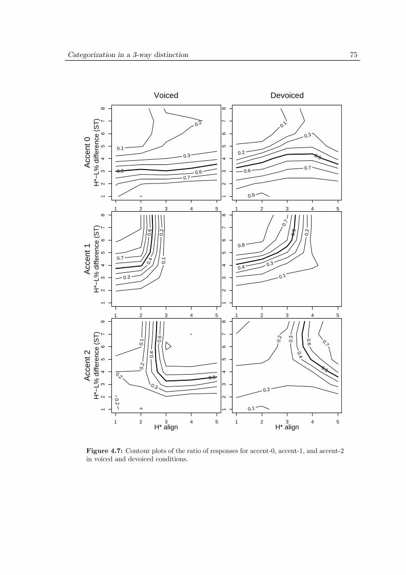
Categorization in a 3-way distinction 75
0.1
0.2
0.3
0.5 0.6 0.7
1 2 3 4 5
12
34
56
78
H*−
L% d
iffer
ence
(S
T)
VoicedA
ccen
t 0
0.1
0
.2
0.3
0.4
0
.6
0.7
1 2 3 4 5
12
34
56
78
H*−
L% d
iffer
ence
(S
T)
Acc
ent 1
0.1
0.2
0.2
0.2
0.3
0.4
0.5
0.6
1 2 3 4 5
12
34
56
78
H* align
H*−
L% d
iffer
ence
(S
T)
Acc
ent 2
0.1
0.2
0.3
0.5
0.6 0.7
0.9
1 2 3 4 5
12
34
56
78
Devoiced
0.1
0.2
0.3 0.4
0.5
0.7
0.8
1 2 3 4 5
12
34
56
78
0.1
0.2
0.2
0.3
0.4
0.5
0.6
0.7
1 2 3 4 5
12
34
56
78
H* align
Figure 4.7: Contour plots of the ratio of responses for accent-0, accent-1, and accent-2in voiced and devoiced conditions.
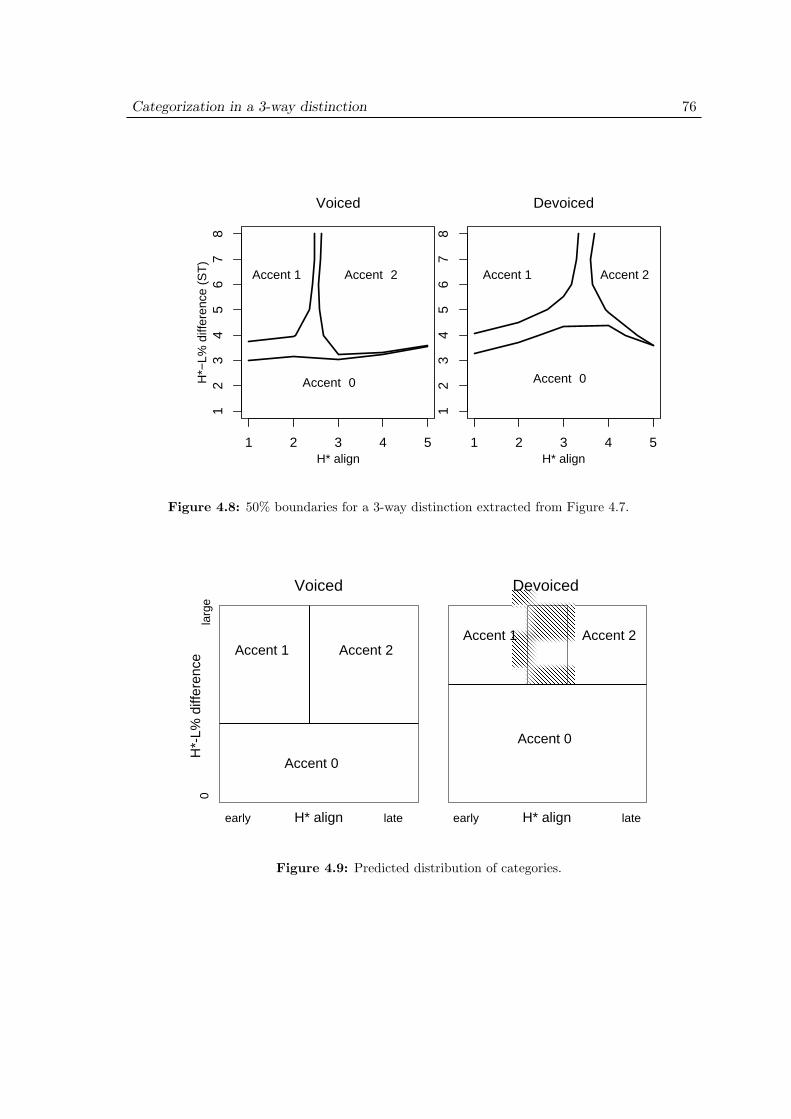
Categorization in a 3-way distinction 76
1 2 3 4 5
12
34
56
78
H* align
H*−
L% d
iffer
ence
(S
T)
Voiced
1 2 3 4 51
23
45
67
8H* align
Devoiced
Accent 1 2
0
Accent
Accent Accent
Accent Accent 21
0
Figure 4.8: 50% boundaries for a 3-way distinction extracted from Figure 4.7.
������������������������������������������
������������������������������������������
Accent 1
Accent 0
H* align
Accent 2
Voiced
early late
0
larg
eH
*-L%
diff
eren
ce
early lateH* align
Accent 0
Accent 2Accent 1
Devoiced
Figure 4.9: Predicted distribution of categories.
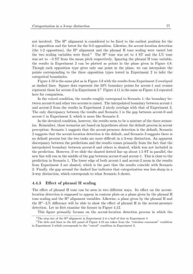
Categorization in a 3-way distinction 77
not involved. The H* alignment is considered to be fixed to the earliest position for the0-1 opposition and the latest for the 0-2 opposition. Likewise, for accent-location detection(the 1-2 opposition), the H* alignment and the phrasal H tone scaling were varied butthe two scaling variables were fixed.4 The H* tone was set to 4 ST and the L% tonewas set to −3 ST from the mean pitch respectively. Ignoring the phrasal H tone variable,the results in Experiment 2 can be plotted as points in the plane given in Figure 4.8.Though each opposition type gives only one point in the plane, we can interpolate thepoints corresponding to the three opposition types tested in Experiment 2 to infer thecategorical boundaries.
Figure 4.10 is the same plot as in Figure 4.8 with the results from Experiment 2 overlayedas dashed lines. Square dots represent the 50% boundary points for accent-1 and crossesrepresent those for accent-2 in Experiment 2.5 Figure 4.11 is the same as Figure 4.2 repeatedhere for comparison.
In the voiced condition, the results roughly correspond to Scenario 1; the boundary be-tween accent-0 and other two accents is raised. The interpolated boundary between accent-1and accent-2 from the results in Experiment 2 nicely overlaps with that of Experiment 3.The only discrepancy between the results and Scenario 1 is the gap between accent-0 andaccent-1 in Experiment 3, which is more like Scenario 3.
In the devoiced condition, however, the results seem to be a mixture of the three scenar-ios. Remember, these scenarios are based on hypotheses about the default process in accentperception: Scenario 1 suggests that the accent-presence detection is the default, Scenario2 suggests that the accent-location detection is the default, and Scenario 3 suggests there isno default process but the two tasks are more difficult in a 3-way distinction. An apparentdiscrepancy between the predictions and the results comes primarily from the fact that theinterpolated boundary between accent-0 and others is slanted, which was not included inthe prediction. However, if we slide the slanted dotted line up about 1.5 ST in parallel, thenew line will run in the middle of the gap between accent-0 and accent-1. This is close to theprediction in Scenario 1. The lower edge of both accent-1 and accent-2 areas in the resultsfrom Experiment 3 are slanted, which is the part that the results coincide with Scenario2. Finally, the gap around the dashed line indicates that categorization was less sharp in a3-way distinction, which corresponds to what Scenario 3 shows.
4.4.3 Effect of phrasal H scaling
The effect of phrasal H tone can be seen in two different ways. Its effect on the accent-location detection is supposed to appear in contour plots on a plane given by the phrasal Htone scaling and the H* alignment variables. Likewise, a plane given by the phrasal H andthe H*−L% difference will be able to show the effect of phrasal H in the accent-presencedetection. Let us first examine the former in Figure 4.12.
This figure primarily focuses on the accent-location detection process in which the4The step size of the H* alignment in Experiment 2 is a half of that in Experiment 35The dots and lines in the left panel of Figure 4.10 are taken from the “voiceless consonant” condition
in Experiment 2 which corresponds to the “voiced” condition in Experiment 3.

Categorization in a 3-way distinction 78
1 2 3 4 5
12
34
56
78
H* align
H*−
L% d
iffer
ence
(S
T)
Voiced
1 2 3 4 51
23
45
67
8
H* align
Devoiced
Accent 1 2Accent Accent 1
Accent 0
Accent 2
Accent 0
Figure 4.10: 50% boundaries for a 3-way distinction (solid) and for a 2-way distinction(dashed line interpolated from results in Experiment 2).
H* align
Accent 2
early late
0
larg
eH
*-L%
diff
eren
ce
Accent 0
Scenario 1
early lateH* align
Accent 2Accent 1
Accent 0
Scenario 3
early lateH* align
Scenario 2
Accent 0
Accent 1Accent 1 Accent 2
Figure 4.11: Three scenarios for the difference between a 2-way distinction (dashedline) and a 3-way distinction (solid line).

Categorization in a 3-way distinction 79
0.2
0.2
0.3
0.3
0.4
1 2 3 4 5
−3
−2
−1
01
23
Voiced
pH s
cale
(S
T)
Acc
ent 0
0.1 0.2
0.5
0.6
1 2 3 4 5
−3
−2
−1
01
23
pH s
cale
(S
T)
Acc
ent 1
0.2
0.3
0.6
0.6
0.7
1 2 3 4 5
−3
−2
−1
01
23
H* align
pH s
cale
(S
T)
Acc
ent 2
0.2
0.3
0.4
0.5
1 2 3 4 5
−3
−2
−1
01
23
Devoiced 0.1
0.2
0.3
0.4
0.5
0.7
1 2 3 4 5
−3
−2
−1
01
23
0.2
0
.3
0.4
0.5
0.6
1 2 3 4 5
−3
−2
−1
01
23
H* align
Figure 4.12: Contour plots of the ratio of responses for each accent category in voicedand devoiced conditions. Phrasal H (pH) in semitone on the ordinate and H* alignmenton the abscissa.
Categorization in a 3-way distinction 80
0.2
0.3
0.5
0.6
0.8
1 2 3 4 5 6 7 8
−3
−2
−1
01
23
H*−L% difference (ST)
pH s
cale
(S
T)
Voiced
0.2
0.3
0.5
0.6
0.7
0.8
1 2 3 4 5 6 7 8
−3
−2
−1
01
23
Devoiced
H*−L% difference (ST)
Figure 4.13: Contour plots of the ratio of responses for accent-0 in voiced and devoicedconditions.
phrasal H tone in the upper range is predicted to lower the categorization performance(see Section 4.2). In the voiced condition in the left column, the 50% contour runs almostperpendicular and straight in accent-1 and 2, which is against the prediction. Moreover, the60% and higher contours in those two panels make a right-angled turn consisting a shallowvalley around the phrasal H at 0 ST. This indicates that the phrasal H tone does affect theaccent-location detection process only in the mid range. The contours in the top-left panelfor accent-0 responses confirm this fact in that they form a gradually-sloping hill in the midphrasal H range.
In the devoiced condition in the right column, valleys in accent-1 and 2 and the hill inaccent-0 are more prominent. The panels for accent 1 and 2 show almost all contours arecurved which indicates the presence of the valley in the middle. Even the phrasal H in thelower range has a strong effect on the accent-location detection, which is contradictory tothe results in Experiment 2.
Meanwhile, in Figure 4.13, the effect of the phrasal H tone is not quite visible on theplane given by the phrasal H and the H*−L% difference. This agrees with the predictionthat the phrasal H has no effect on the accent-presence detection process.
4.5 Discussion
The results so far show that the perception of pitch accent in a 3-way distinction has theproperties more or less predictable from the general pattern in a 2-way distinction. TheH*−L% difference captures the accent-presence detection process and the H* alignmentcaptures the accent-location detection process as in the way in a 2-way distinction. Thediscrepancy from the prediction in the case of the voiced condition is the gap betweenaccent-0 and accent-1 (Figure 4.8). This is due to the spread of responses for accent-2 over
Categorization in a 3-way distinction 81
the whole area in the given space. The left-bottom panel in Figure 4.7 shows that the20% contour spreads in the low H*−L% difference area. In other words, listeners showeda slight amount of uncertainty between accent-0 and accent-2 even when the H* is alignedearly. We can speculate from this result that accent-0 and accent-2 are perceptually moreapproximate than between accent-0 and accent-1. The effect of devoicing was also in thepredicted fashion. The boundary for accent-0 shifted upward and the gap between accent-1and 2 widened.
The comparison with a 2-way distinction reveals that Scenario 1 provided in Section 4.2is close to the results at least in the voiced condition. Scenario 1 is based on a high-levelhypothesis that the accent-location detection and the accent-presence detection are twoseparate processes and the former is functionally more fundamental in the perception ofaccent. That is, the overall increase of the accent-0 area from a 2-way distinction to a3-way distinction indicates that the accent-presence detection is interfered with the accent-location detection process. The coincidence of the boundaries between accent-1 and 2 in a2-way distinction and a 3-way distinction also suggests that accent-location detection is notperturbed by accent-presence detection since the accuracy of the accent-location detectionhas not changed.
As for the effect of the phrasal H tone, the prediction is right in that the accent-presencedetection process is not affected at all (Figure 4.13), but it was wrong in that the accent-location detection process is affected most in the mid range of the phrasal H (Figure 4.12).More specifically, the response rates for both accent-1 and accent-2 are lowered when thephrasal H tone was around 0 ST from the mean pitch of the original token.
A possible interpretation of this result comes from the fact that the original token isunaccented. The 0 ST specification for the phrasal H tone means that it is on the originalunaccented pitch contour. Though other scaling and alignment variables are modified fromthe original, “unaccentedness” is somehow kept best in the stimuli with the phrasal H toneat 0 ST. This may lead to the lowered response rate for accented forms only around themid range of the phrasal H tone variable.
Chapter 5
Functions of pitch accent: a databaseanalysis
5.1 Introduction
Previous chapters have dealt with behavioral data in experiments in order to investigate thecategory structure of pitch accent in Japanese. This chapter, in turn, deals with a databaseof Japanese words in order to investigate the function of pitch accent. The database usedin this study is a recently published work by Amano & Kondo (1999) including word-familiarity, accent, and usage frequency among others. The next section first summarizes thestructure of the database and then gives a detailed analysis of the distribution of accentuallyopposed homophones extracted from the database. Section 5.3 proposes an attempt toformalize the opposing relations within homophones and the difference in familiarity scoresbetween the competing homophones in order to quantify the distinctive functional load ofpitch accent. Section 5.4 summarizes the database analyses and discusses predictions for apost-hoc analysis of categorization results based on the summary.
5.2 Database analysis
5.2.1 Structure of the database
The database (Amano & Kondo, 1999) has seven volumes, each of which focuses on differentaspects of Japanese lexicon shown in Table 5.1. Entries in all volumes are cross-referenced bycommon ID numbers. Words in Volume 1-4 are taken from a standard Japanese dictionary(Kindaichi et al., 1989). For the purposes of the present study, only the data in Volume 1and 3 were used. Fields in these two volumes are shown in Table 5.2 and 5.3.
The familiarity score in Volume 1 is based on subjective rating in multi-modal (Audio-Visual) and uni-modal (Audio or Visual) stimulus presentation. At least 32 subjects perword rated the familiarity of each word in a 7-step scale starting from 1 (not familiar) to 7(most familiar). Scores for three modes of presentation for a single entry differ substantiallyin their magnitude in some cases. For instance, a visually very familiar Chinese character
82
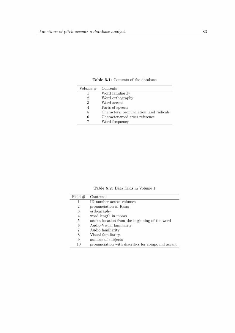
Functions of pitch accent: a database analysis 83
Table 5.1: Contents of the database
Volume # Contents1 Word familiarity2 Word orthography3 Word accent4 Parts of speech5 Characters, pronunciation, and radicals6 Character-word cross reference7 Word frequency
Table 5.2: Data fields in Volume 1
Field # Contents1 ID number across volumes2 pronunciation in Kana3 orthography4 word length in moras5 accent location from the beginning of the word6 Audio-Visual familiarity7 Audio familiarity8 Visual familiarity9 number of subjects10 pronunciation with diacritics for compound accent
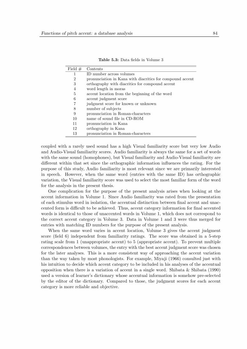
Functions of pitch accent: a database analysis 84
Table 5.3: Data fields in Volume 3
Field # Contents1 ID number across volumes2 pronunciation in Kana with diacritics for compound accent3 orthography with diacritics for compound accent4 word length in moras5 accent location from the beginning of the word6 accent judgment score7 judgment score for known or unknown8 number of subjects9 pronunciation in Roman-characters10 name of sound file in CD-ROM11 pronunciation in Kana12 orthography in Kana13 pronunciation in Roman-characters
coupled with a rarely used sound has a high Visual familiarity score but very low Audioand Audio-Visual familiarity scores. Audio familiarity is always the same for a set of wordswith the same sound (homophones), but Visual familiarity and Audio-Visual familiarity aredifferent within that set since the orthographic information influences the rating. For thepurpose of this study, Audio familiarity is most relevant since we are primarily interestedin speech. However, when the same word (entries with the same ID) has orthographicvariation, the Visual familiarity score was used to select the most familiar form of the wordfor the analysis in the present thesis.
One complication for the purpose of the present analysis arises when looking at theaccent information in Volume 1. Since Audio familiarity was rated from the presentationof each stimulus word in isolation, the accentual distinction between final accent and unac-cented form is difficult to be achieved. Thus, accent category information for final accentedwords is identical to those of unaccented words in Volume 1, which does not correspond tothe correct accent category in Volume 3. Data in Volume 1 and 3 were thus merged forentries with matching ID numbers for the purpose of the present analysis.
When the same word varies in accent location, Volume 3 gives the accent judgmentscore (field 6) independent from familiarity ratings. The score was obtained in a 5-steprating scale from 1 (unappropriate accent) to 5 (appropriate accent). To prevent multiplecorrespondences between volumes, the entry with the best accent judgment score was chosenfor the later analyses. This is a more consistent way of approaching the accent variationthan the way taken by most phonologists. For example, Miyaji (1966) consulted just withhis intuition to decide which accent category to be included in his analyses of the accentualopposition when there is a variation of accent in a single word. Shibata & Shibata (1990)used a version of learner’s dictionary whose accentual information is somehow pre-selectedby the editor of the dictionary. Compared to those, the judgment scores for each accentcategory is more reliable and objective.
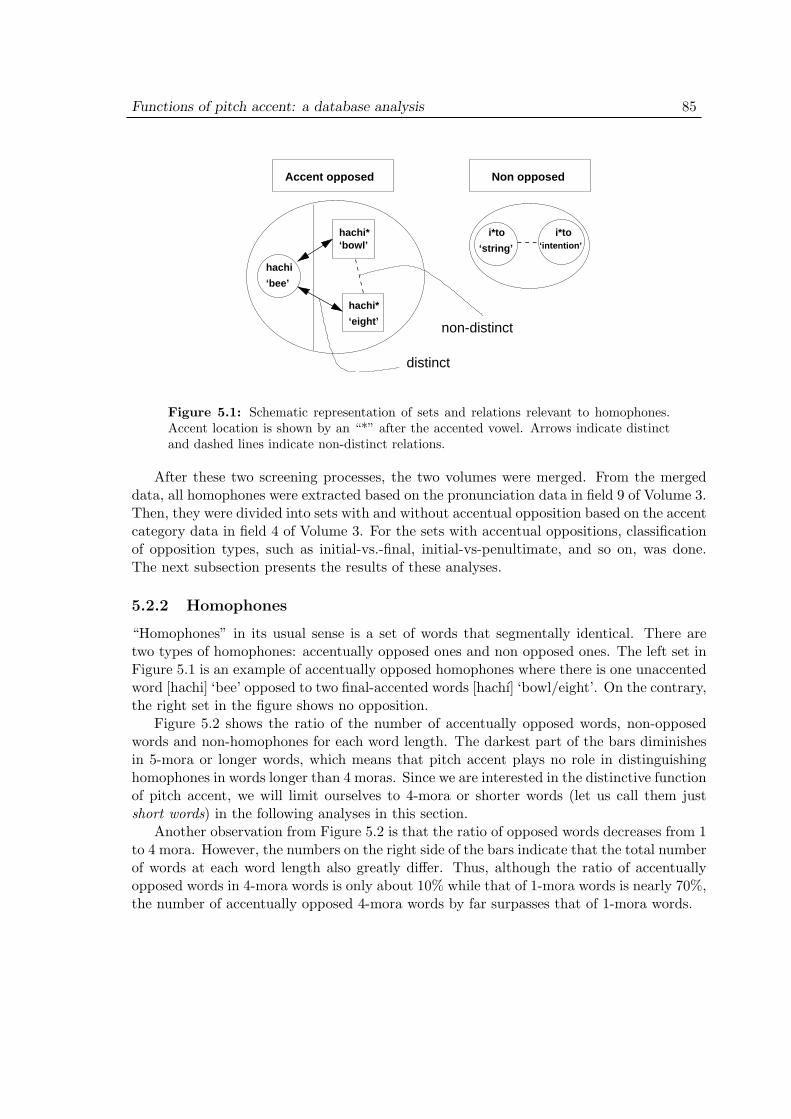
Functions of pitch accent: a database analysis 85
i*to
‘string’
i*to ‘intention’
hachi
‘bee’
hachi* ‘bowl’
hachi*
‘eight’
distinct
non-distinct
Accent opposed Non opposed
Figure 5.1: Schematic representation of sets and relations relevant to homophones.Accent location is shown by an “*” after the accented vowel. Arrows indicate distinctand dashed lines indicate non-distinct relations.
After these two screening processes, the two volumes were merged. From the mergeddata, all homophones were extracted based on the pronunciation data in field 9 of Volume 3.Then, they were divided into sets with and without accentual opposition based on the accentcategory data in field 4 of Volume 3. For the sets with accentual oppositions, classificationof opposition types, such as initial-vs.-final, initial-vs-penultimate, and so on, was done.The next subsection presents the results of these analyses.
5.2.2 Homophones
“Homophones” in its usual sense is a set of words that segmentally identical. There aretwo types of homophones: accentually opposed ones and non opposed ones. The left set inFigure 5.1 is an example of accentually opposed homophones where there is one unaccentedword [hachi] ‘bee’ opposed to two final-accented words [hachı] ‘bowl/eight’. On the contrary,the right set in the figure shows no opposition.
Figure 5.2 shows the ratio of the number of accentually opposed words, non-opposedwords and non-homophones for each word length. The darkest part of the bars diminishesin 5-mora or longer words, which means that pitch accent plays no role in distinguishinghomophones in words longer than 4 moras. Since we are interested in the distinctive functionof pitch accent, we will limit ourselves to 4-mora or shorter words (let us call them justshort words) in the following analyses in this section.
Another observation from Figure 5.2 is that the ratio of opposed words decreases from 1to 4 mora. However, the numbers on the right side of the bars indicate that the total numberof words at each word length also greatly differ. Thus, although the ratio of accentuallyopposed words in 4-mora words is only about 10% while that of 1-mora words is nearly 70%,the number of accentually opposed 4-mora words by far surpasses that of 1-mora words.
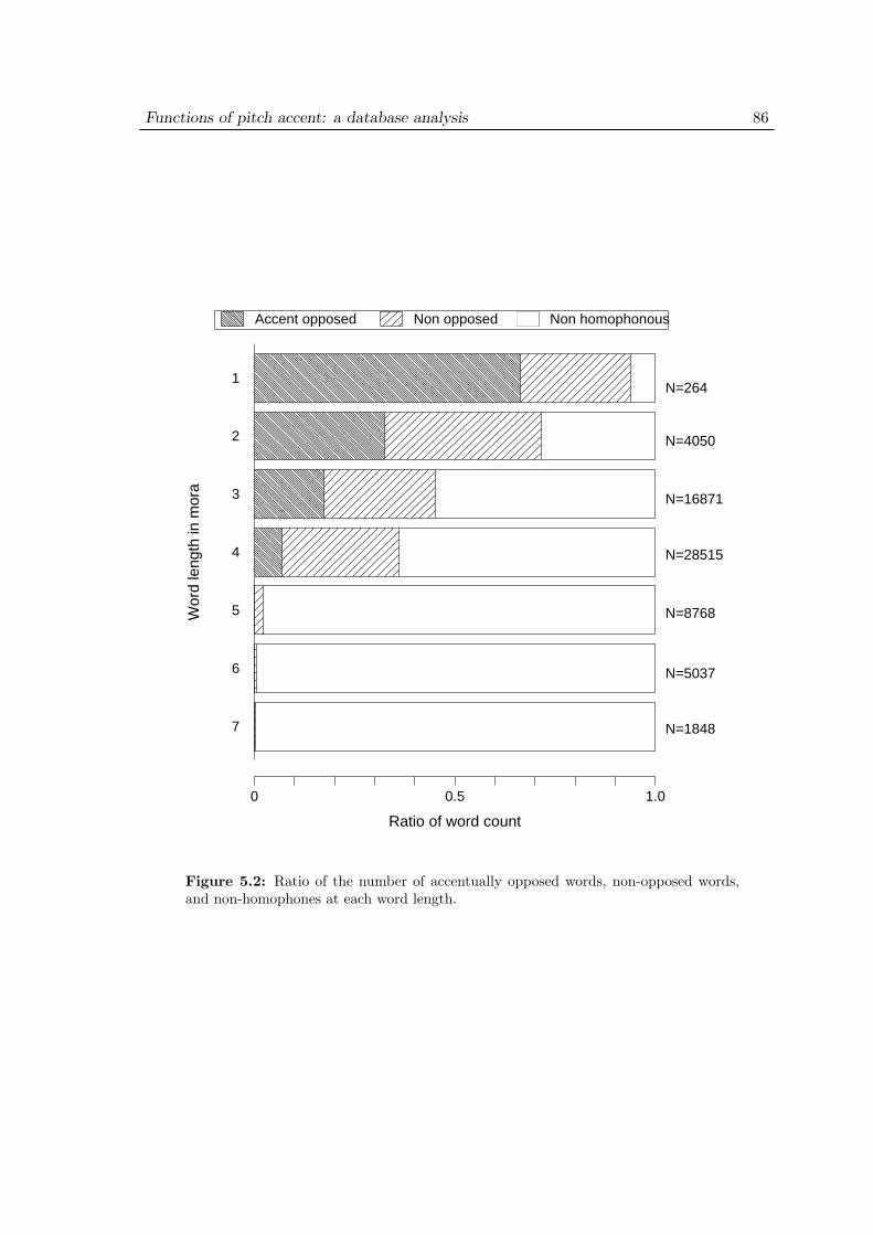
Functions of pitch accent: a database analysis 86
7
6
5
4
3
2
1
0 0.5 1.0
Ratio of word count
Wor
d le
ngth
in m
ora
N=264
N=4050
N=16871
N=28515
N=8768
N=5037
N=1848
Accent opposed Non opposed Non homophonous
Figure 5.2: Ratio of the number of accentually opposed words, non-opposed words,and non-homophones at each word length.
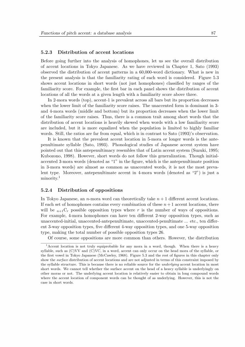
Functions of pitch accent: a database analysis 87
5.2.3 Distribution of accent locations
Before going further into the analysis of homophones, let us see the overall distributionof accent locations in Tokyo Japanese. As we have reviewed in Chapter 1, Sato (1993)observed the distribution of accent patterns in a 60,000-word dictionary. What is new inthe present analysis is that the familiarity rating of each word is considered. Figure 5.3shows accent locations in short words (not just homophones) classified by ranges of thefamiliarity score. For example, the first bar in each panel shows the distribution of accentlocations of all the words at a given length with a familiarity score above three.
In 2-mora words (top), accent-1 is prevalent across all bars but its proportion decreaseswhen the lower limit of the familiarity score raises. The unaccented form is dominant in 3-and 4-mora words (middle and bottom) but its proportion decreases when the lower limitof the familiarity score raises. Thus, there is a common trait among short words that thedistribution of accent locations is heavily skewed when words with a low familiarity scoreare included, but it is more equalized when the population is limited to highly familiarwords. Still, the ratios are far from equal, which is in contrast to Sato (1993)’s observation.
It is known that the prevalent accent location in 5-mora or longer words is the ante-penultimate syllable (Sato, 1993). Phonological studies of Japanese accent system havepointed out that this antepenultimacy resembles that of Latin accent system (Suzuki, 1995;Kubozono, 1998). However, short words do not follow this generalization. Though initial-accented 3-mora words (denoted as “1” in the figure, which is the antepenultimate positionin 3-mora words) are almost as common as unaccented words, it is not the most preva-lent type. Moreover, antepenultimate accent in 4-mora words (denoted as “2”) is just aminority.1
5.2.4 Distribution of oppositions
In Tokyo Japanese, an n-mora word can theoretically take n + 1 different accent locations.If each set of homophones contains every combination of these n+1 accent locations, therewill be n+1Cr possible opposition types where r is the number of ways of oppositions.For example, 4-mora homophones can have ten different 2-way opposition types, such asunaccented-initial, unaccented-antepenultimate, unaccented-penultimate ... etc., ten differ-ent 3-way opposition types, five different 4-way opposition types, and one 5-way oppositiontype, making the total number of possible opposition types 26.
Of course, some oppositions are more common than others. However, the distribution1Accent location is not truly equiprobable for any mora in a word, though. When there is a heavy
syllable, such as (C)VV and (C)VC, in a word, accent can only occur on the head mora of the syllable, orthe first vowel in Tokyo Japanese (McCawley, 1968). Figure 5.3 and the rest of figures in this chapter onlyshow the surface distribution of accent locations and are not adjusted in terms of this constraint imposed bythe syllable structure. This is because there is no reliable source for the underlying accent location in mostshort words. We cannot tell whether the surface accent on the head of a heavy syllable is underlyingly onother moras or not. The underlying accent location is relatively easier to obtain in long compound wordswhere the accent location of component words can be thought of as underlying. However, this is not thecase in short words.
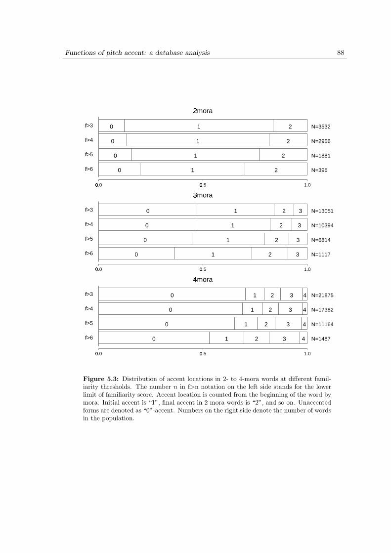
Functions of pitch accent: a database analysis 88
f>6�
f>5�
f>4�
f>3�
0.0�
0.5�
1.0
N=3532
N=2956
N=1881
N=395
0 1 2
0 1 2
0 1 2
0 1 2
2mora�
f>6�
f>5�
f>4�
f>3�
0.0�
0.5�
1.0
N=13051
N=10394
N=6814
N=1117
0 1 2 3
0 1 2 3
0 1 2 3
0 1 2 3
3mora�
f>6�
f>5�
f>4�
f>3�
0.0�
0.5�
1.0
N=21875
N=17382
N=11164
N=1487
0 1 2 3 4
0 1 2 3 4
0 1 2 3 4
0 1 2 3 4
4mora�
Figure 5.3: Distribution of accent locations in 2- to 4-mora words at different famil-iarity thresholds. The number n in f>n notation on the left side stands for the lowerlimit of familiarity score. Accent location is counted from the beginning of the word bymora. Initial accent is “1”, final accent in 2-mora words is “2”, and so on. Unaccentedforms are denoted as “0”-accent. Numbers on the right side denote the number of wordsin the population.
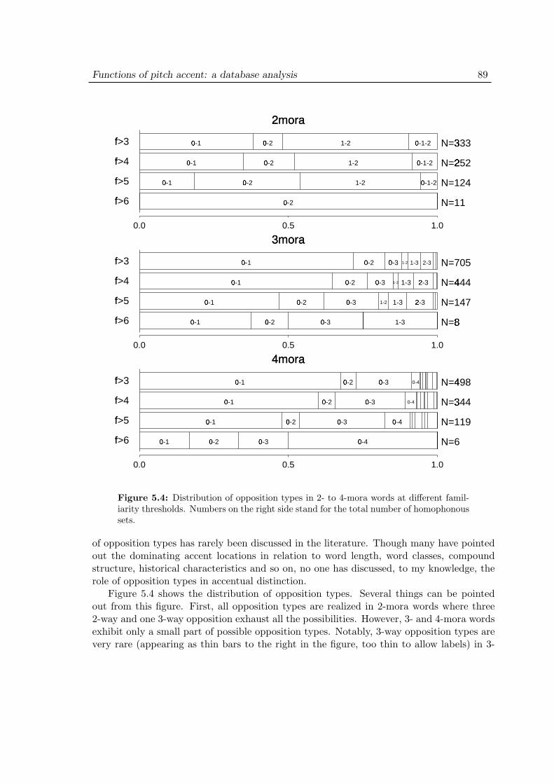
Functions of pitch accent: a database analysis 89
f>6�
f>5�
f>4�
f>3�
0.0 0.5 1.0
N=333�
N=252�
N=124
N=11
0-1�
0-2�
1-2 0-1-2�
0-1�
0-2�
1-2 0-1-2�
0-1�
0-2�
1-2 0-1-2�
0-2�
2mora
f>6�
f>5�
f>4�
f>3�
0.0 0.5 1.0
N=705
N=444�
N=147
N=8�
0-1�
0-2�
0-3�
1-2 1-3 2-3
0-1�
0-2�
0-3�
1-2 1-3 2-3�
0-1�
0-2�
0-3�
1-2 1-3 2-3�
0-1�
0-2�
0-3�
1-3
3mora
f>6�
f>5�
f>4�
f>3�
0.0 0.5 1.0
N=498�
N=344�
N=119
N=6
0-1�
0-2�
0-3�
0-4
0-1�
0-2�
0-3�
0-4
0-1�
0-2�
0-3�
0-4�
0-1�
0-2�
0-3�
0-4�
4mora
Figure 5.4: Distribution of opposition types in 2- to 4-mora words at different famil-iarity thresholds. Numbers on the right side stand for the total number of homophonoussets.
of opposition types has rarely been discussed in the literature. Though many have pointedout the dominating accent locations in relation to word length, word classes, compoundstructure, historical characteristics and so on, no one has discussed, to my knowledge, therole of opposition types in accentual distinction.
Figure 5.4 shows the distribution of opposition types. Several things can be pointedout from this figure. First, all opposition types are realized in 2-mora words where three2-way and one 3-way opposition exhaust all the possibilities. However, 3- and 4-mora wordsexhibit only a small part of possible opposition types. Notably, 3-way opposition types arevery rare (appearing as thin bars to the right in the figure, too thin to allow labels) in 3-
Functions of pitch accent: a database analysis 90
and 4-mora words.Second, realized opposition types mostly involve unaccented forms. This is particularly
striking in 3- and 4-mora words. At least 75% in 3-mora words and 90% in 4-mora wordsinvolve unaccented forms. On the contrary, the sum of the ratios of the 1-2 opposition andthe 0-1-2 opposition (3-way) are around 50% in 2-mora words except for the “f>6” bar atthe bottom.
Third, there is a common trend in all panels that the ratio of the 0-1 opposition con-stantly decreases from “f>3” to “f>6”. When the familiarity score of a word in an accentu-ally opposed pair is below the lower limit, that pair no longer constitutes an opposed pair.This decrease in the ratio of the initial-unaccented opposition may indicate a decrease in thenumber of words in unaccented forms, or of the initial-accented words, or both. However,the distribution of accent locations (including non-homophones) in Figure 5.3 by differentlower limit of familiarity scores tells us that the change of the ratio of words with eachaccent locations differs for each word length. In 2-mora words, the ratio of initial-accentedwords slightly decreases while that of unaccented words increases as with the raising of thelower limit. In 3-mora words, the ratio of initial-accented words almost stays the same whilethat of unaccented words decreases. In 4-mora words, the situation is similar to the onein 3-mora words, but there is a slight increase of the ratio of the initial-accented words inthe “f>6” range. Therefore, the common decreasing trend of initial-unaccented oppositionobserved in Figure 5.4 cannot be attributed to a single reason, such as there would be adecreasing trend of unaccented words at any word length. This third point supports theidea that the distribution analysis of opposition types is worthwhile since it is independentfrom the distribution of accent locations.
5.3 Formalization of oppositions
In this section, the size of subsets within accentually opposed homophones and familiarityscores of each word are taken into consideration in order to quantify the functional load ofpitch accent. In the previous section, we have seen the actual distribution of various wordsand sets in the database in terms of accent and familiarity. However, ratios and distributionscan only reveal general tendencies. When we want to investigate the functional load of aparticular item or a class of items, we need a more powerful and rigorous tool to scrutinizethe nature of distinctive function of accent.
Lexical access to homophones has rarely been discussed in the literature. Current spokenword recognition models such as Cohort theory (Marslen-Wilson, 1989), TRACE (McClel-land and Elman, 1986), and NAM (Luce, 1986) are segment-based and do not go beyondidentifying a segmentally unique string. Accentually opposed homophones are still segmen-tally identical. Thus, those models have nothing to say about identifying a particular targetword based on accent. As reviewed in Section 1.5, there are some studies on the role ofprosody in lexical access (Cutler, 1989; Cutler, 1994; Cutler and Chen, 1997; Cutler andOtake, 1999; Slowiaczek, 1986). However, they do not focus on accentual homophones ei-ther. For our purpose, to quantify the distinctive functional load of accent, we must assess
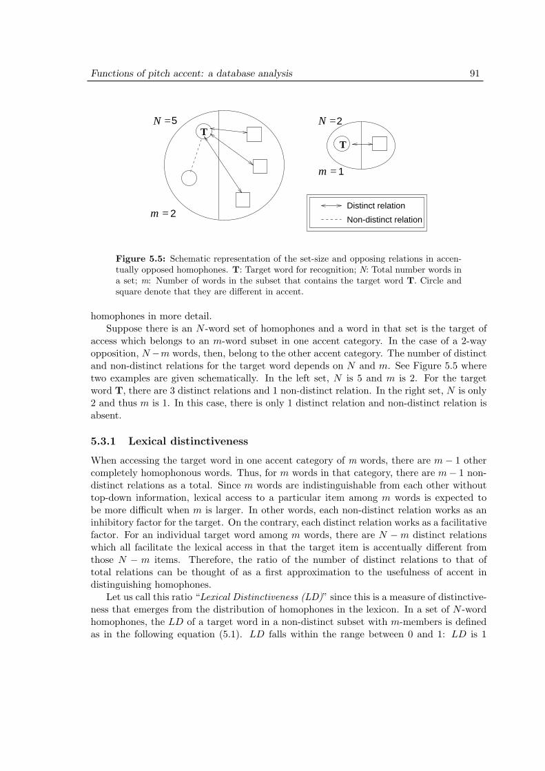
Functions of pitch accent: a database analysis 91
N =
m =2
T5
T
N =
1m =
2
Non-distinct relation
Distinct relation
Figure 5.5: Schematic representation of the set-size and opposing relations in accen-tually opposed homophones. T: Target word for recognition; N: Total number words ina set; m: Number of words in the subset that contains the target word T. Circle andsquare denote that they are different in accent.
homophones in more detail.Suppose there is an N -word set of homophones and a word in that set is the target of
access which belongs to an m-word subset in one accent category. In the case of a 2-wayopposition, N−m words, then, belong to the other accent category. The number of distinctand non-distinct relations for the target word depends on N and m. See Figure 5.5 wheretwo examples are given schematically. In the left set, N is 5 and m is 2. For the targetword T, there are 3 distinct relations and 1 non-distinct relation. In the right set, N is only2 and thus m is 1. In this case, there is only 1 distinct relation and non-distinct relation isabsent.
5.3.1 Lexical distinctiveness
When accessing the target word in one accent category of m words, there are m− 1 othercompletely homophonous words. Thus, for m words in that category, there are m− 1 non-distinct relations as a total. Since m words are indistinguishable from each other withouttop-down information, lexical access to a particular item among m words is expected tobe more difficult when m is larger. In other words, each non-distinct relation works as aninhibitory factor for the target. On the contrary, each distinct relation works as a facilitativefactor. For an individual target word among m words, there are N −m distinct relationswhich all facilitate the lexical access in that the target item is accentually different fromthose N − m items. Therefore, the ratio of the number of distinct relations to that oftotal relations can be thought of as a first approximation to the usefulness of accent indistinguishing homophones.
Let us call this ratio “Lexical Distinctiveness (LD)” since this is a measure of distinctive-ness that emerges from the distribution of homophones in the lexicon. In a set of N -wordhomophones, the LD of a target word in a non-distinct subset with m-members is definedas in the following equation (5.1). LD falls within the range between 0 and 1: LD is 1
Functions of pitch accent: a database analysis 92
when m = 1; LD approaches 0 when both N and m become large.
LD =Number of distinct relations
Number of total relations(5.1)
=N −m
(N −m) + (m− 1)
=N −m
N − 1
where m ≥ 1 and N > m
Let us examine more concrete cases to check the validity of the definition of LD. Supposea set of 2-way opposed homophones where the set-size N is very large and the size of thesubset m to which the target word belongs is very small: for example, N = 20 and m = 2.Then, there are N − m = 18 words which belong to the other accent category than thetarget word and there is only one word which is indistinguishable from the target bothsegmentally and accentually. In other words, there are 18 accentually opposed homophonesbut only one non-opposed homophone with respect to the target word. This means thataccent helps distinguishing the target word from 18 words while it does not from only oneword. Therefore, accent is quite useful for lexical access to the target word in this case.Given N = 20 and m = 2, the value of LD is 0.947 following the equation (5.1), whichmeans that the usefulness of accent is very close to the upper limit in this case.
5.3.2 Familiarity bias
When all words in the lexicon are equally familiar, the number of distinct and non-distinctrelations defined as LD in the previous section quantifies the function of accent. However,words differ in familiarity. Suppose the target word is highly familiar and all the non-opposing homophones of the target are unfamiliar. In such a case, the target word will besuccessfully accessed without much help from accentual information. On the contrary, if thetarget word is very low in familiarity and all the accentually competing words are highlyfamiliar, it is only the accent information that we can rely on to identify the target word.
To formalize these intuitions, we need to consider familiarity differences between theitems in accentual opposition. The database used in the present study has a 7-step subjectiverating of word familiarity: 7 for the most familiar items and 1 for the least familiar items.Therefore, the difference in familiarity scores between any two items can fall within the rangeof −6 to +6. Foreseeing the possibility of combining this difference with the calculation ofLD, it is better to normalize the difference into a 0-to-1 range.
The use of word familiarity data for the calculation of the functional load is novel to thepresent study. In the process of lexical access, word familiarity is considered to be a part oftop-down information that works as a bias on the perceiver’s side. The role of bottom-upinformation such as pitch contour should be maximized if it were not for such top-down
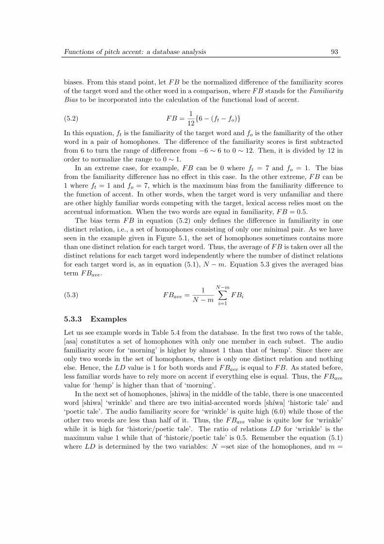
Functions of pitch accent: a database analysis 93
biases. From this stand point, let FB be the normalized difference of the familiarity scoresof the target word and the other word in a comparison, where FB stands for the FamiliarityBias to be incorporated into the calculation of the functional load of accent.
FB =112{6− (ft − fo)}(5.2)
In this equation, ft is the familiarity of the target word and fo is the familiarity of the otherword in a pair of homophones. The difference of the familiarity scores is first subtractedfrom 6 to turn the range of difference from −6 ∼ 6 to 0 ∼ 12. Then, it is divided by 12 inorder to normalize the range to 0 ∼ 1.
In an extreme case, for example, FB can be 0 where ft = 7 and fo = 1. The biasfrom the familiarity difference has no effect in this case. In the other extreme, FB can be1 where ft = 1 and fo = 7, which is the maximum bias from the familiarity difference tothe function of accent. In other words, when the target word is very unfamiliar and thereare other highly familiar words competing with the target, lexical access relies most on theaccentual information. When the two words are equal in familiarity, FB = 0.5.
The bias term FB in equation (5.2) only defines the difference in familiarity in onedistinct relation, i.e., a set of homophones consisting of only one minimal pair. As we haveseen in the example given in Figure 5.1, the set of homophones sometimes contains morethan one distinct relation for each target word. Thus, the average of FB is taken over all thedistinct relations for each target word independently where the number of distinct relationsfor each target word is, as in equation (5.1), N −m. Equation 5.3 gives the averaged biasterm FBave.
FBave =1
N −m
N−m∑
i=1
FBi(5.3)
5.3.3 Examples
Let us see example words in Table 5.4 from the database. In the first two rows of the table,[asa] constitutes a set of homophones with only one member in each subset. The audiofamiliarity score for ‘morning’ is higher by almost 1 than that of ‘hemp’. Since there areonly two words in the set of homophones, there is only one distinct relation and nothingelse. Hence, the LD value is 1 for both words and FBave is equal to FB. As stated before,less familiar words have to rely more on accent if everything else is equal. Thus, the FBave
value for ‘hemp’ is higher than that of ‘morning’.In the next set of homophones, [shiwa] in the middle of the table, there is one unaccented
word [shiwa] ‘wrinkle’ and there are two initial-accented words [shıwa] ‘historic tale’ and‘poetic tale’. The audio familiarity score for ‘wrinkle’ is quite high (6.0) while those of theother two words are less than half of it. Thus, the FBave value is quite low for ‘wrinkle’while it is high for ‘historic/poetic tale’. The ratio of relations LD for ‘wrinkle’ is themaximum value 1 while that of ‘historic/poetic tale’ is 0.5. Remember the equation (5.1)where LD is determined by the two variables: N =set size of the homophones, and m =
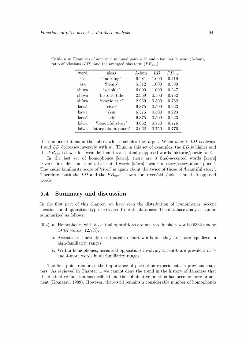
Functions of pitch accent: a database analysis 94
Table 5.4: Examples of accentual minimal pairs with audio familiarity score (A-fam),ratio of relations (LD), and the averaged bias term (FBave).
word gloss A-fam LD FBave
asa ‘morning’ 6.281 1.000 0.419asa ‘hemp’ 5.312 1.000 0.580
shiwa ‘wrinkle’ 6.000 1.000 0.247shıwa ‘historic tale’ 2.969 0.500 0.752shıwa ‘poetic tale’ 2.969 0.500 0.752kawa ‘river’ 6.375 0.500 0.223kawa ‘skin’ 6.375 0.500 0.223kawa ‘side’ 6.375 0.500 0.223kawa ‘beautiful story’ 3.062 0.750 0.776kawa ‘story about poem’ 3.062 0.750 0.776
the number of items in the subset which includes the target. When m = 1, LD is always1 and LD decreases inversely with m. Thus, in this set of examples, the LD is higher andthe FBave is lower for ‘wrinkle’ than its accentually opposed words ‘historic/poetic tale’.
In the last set of homophones [kawa], there are 3 final-accented words [kawa]‘river/skin/side’, and 2 initial-accented words [kawa] ‘beautiful story/story about poem’.The audio familiarity score of ‘river’ is again about the twice of those of ‘beautiful story’.Therefore, both the LD and the FBave is lower for ‘river/skin/side’ than their opposedwords.
5.4 Summary and discussion
In the first part of this chapter, we have seen the distribution of homophones, accentlocations, and opposition types extracted from the database. The database analyses can besummarized as follows:
(5.4) a. Homophones with accentual oppositions are not rare in short words (6332 among49702 words: 12.7%).
b. Accents are unevenly distributed in short words but they are more equalized inhigh-familiarity ranges.
c. Within homophones, accentual oppositions involving accent-0 are prevalent in 3-and 4-mora words in all familiarity ranges.
The first point reinforces the importance of perception experiments in previous chap-ters. As reviewed in Chapter 1, we cannot deny the trend in the history of Japanese thatthe distinctive function has declined and the culminative function has become more promi-nent (Komatsu, 1989). However, there still remains a considerable number of homophones
Functions of pitch accent: a database analysis 95
distinguished only by pitch accent.There are some predictions and conjectures we can make from the the summary in
(5.4b) and (5.4c). First, (5.4b) suggests that the dominant accent in each mora-lengthcan be taken as the default accent assigned by a productive morphological/phonologicalprocess. The dominance of a certain accent is what is referred to as the type frequency.Type frequency is related to morphological productivity as reviewed in Section 1.3.3. Theincreasing trend of the dominance of a certain accent in lower-familiarity ranges suggeststhat the dominant accent is assigned to low-familiarity words by some phonological rules.
Second, in relation to the more equalized distribution of accents in high-familiarityranges, the delimitative function served by accent-1 words seems to be relatively small.As reviewed in Section 1.5, Cutler & Norris (1988) and Cutler (1989) show that metricalprosody in English has a delimitative function which is enhanced by the high type andtoken frequency of words beginning with a strong syllable. Cutler & Otake (1999) foundan analogous situation where accent-1 words have a delimitative function in Japanese.However, the database analysis in this chapter suggests that the situation in Japaneseis not quite comparable to English because accent-1 words are not increasingly dominantin high-familiarity ranges.
Third, (5.4c) indicates that accent-presence detection is more important than accent-location detection in the perception of 3- and 4-mora words. From a word-recognitionperspective, only the presence or the absence of an accent is of importance in oppositionsinvolving accent-0 words. When one of the alternatives in a 2-way opposition is unaccented,accent location does not really matter to identify the other accent pattern. Just knowingthat the target word is accented is enough for narrowing down the search space within agiven set of homophones and no further information about accent location is necessary.
However, this conjecture does not apply to 2-mora words which were the focus of Exper-iments 1 through 3 in the previous chapters. As we have seen in Figure 5.4, the distributionof opposition types in 2-mora words are quite different from those in 3- and 4-mora words.First, oppositions by accent-location (1-2 and 0-1-2) are about 50% in all familiarity rangesexcept the highest one (f>6). Since the total number of homophonous sets in the “f>6”range is only 11, this exception does not seem to affect the general tendency that theaccent-location detection process is functionally most important in 2-mora words. Second,the ratio of the 0-2 opposition increases from the f>3 range to the f>6 range and that ofthe 0-1 opposition decreases inversely. This suggests that the 0-2 opposition is functionallymore important than the 0-1 oppositions within 2-mora words. These conjectures can berestated as a hypothesis in the following:
(5.5) The rank order of functional importance among opposition types is:the 1-2 opposition > the 0-2 opposition, > the 0-1 opposition.
As stated in Section 4.2, a comparison between the results of the 2-way distinction andthe 3-way distinction leads to an intriguing question about the primacy of the two processes:accent-location detection and accent-presence detection. The analysis in Section 4.4.2 sug-gests that accent-location detection wins over accent-presence detection due to the fact
Functions of pitch accent: a database analysis 96
that the boundary between accent-1 and accent-2 does not move around across the data inExperiments 2 and 3.
The analysis of type frequencies of oppositions and word familiarity ranges in this chap-ter suggests that the 1-2 opposition is consistently dominant in 2-mora words, which alsoleads to the same conclusion that accent-location detection is functionally most importantin 2-mora words.
We can also infer from the results in the 3-way distinction that the 0-2 opposition isfunctionally more important than the 0-1 opposition. Remember the unexpected gap onlybetween accent-0 and accent-1 in Figure 4.8 in Chapter 4. This can be taken as a pieceof evidence that the 0-2 opposition is more stable than the 0-1 opposition, at least in thevoiced condition. Vowel devoicing is a confounding factor in analyzing the effect of typefrequency in this respect.
In the second part of this chapter (Section 5.3), we have seen that each word in a setof accentually opposed homophones has different properties depending on the familiaritybalance in that set and the number of opposed and non-opposed members in that set.Namely, a pair of LD and FBave values are specific to each word, or more precisely, toeach accentually homogeneous subset of homophones. These two values are considered toconstitute the functional load of pitch accent. This view is in contrast to the more traditional“across-the-board” view about functional load (Hockett, 1967). In the traditional view,functional load is the property of each phonemic contrast across the entire lexicon, not eachword. However, as we have seen in Section 1.3.2, it is difficult to apply the traditional viewto elements with a privative opposition. Pitch accent in Japanese has a privative oppositionwhich is the dominant opposition type in short words.
Thus, another objective of the post-hoc analysis is to find if there is any effect of LDand FBave values in the data obtained in the categorization experiment. Before examiningany data, let us investigate what are the prerequisites for finding the correlates of LD andFBave. In contour plots, the correlates of the two values are expected to be found, if any,in the shift of the categorical boundary. For example, when a pair of words with a highLD value and a low LD value are compared, there may be a shift of the boundary towardeither a high or a low LD value word compared to the pair with an equal LD values. Thatis, the shift can only be detected in a comparison between a test pair and a control pair.The necessity for a pairwise comparison also applies to testing correlates of FBave.
Predictions about the direction of the shift can be made based on the definition of LDand FBave: indices of the usefulness of pitch accent in distinguishing homophones. Moreprecisely, they indicate how crucial pitch accent is in identifying the target word. Losingthe crucial information cuts off the only path to the target word. Thus, it is predicted thatwords with higher LD or FBave values will be more damaged than those with lower valueswhen the speech signal is degraded or ambiguous. In a minimal pair with an unbalancedLD or FBave values, the item with the lower LD or FBave value will be preferred for anambiguous/noisy speech input.
As for the degraded stimuli, Slowiaczek (1986) used noise patterns shaped in a speech-like envelope in her attempt to measure the function of stress in English. But the results

Functions of pitch accent: a database analysis 97
suggest that semantic cues override the pure effect of prosody mimicked by the noise en-velope. All the experiments in the previous chapters involve the devoicing condition. Incontrast to a noise envelope, devoicing is a naturally occurring degraded input with whichlisteners must deal in an everyday situation. Thus, devoiced stimuli are expected to give usa better probe for the nature of the function of accent.
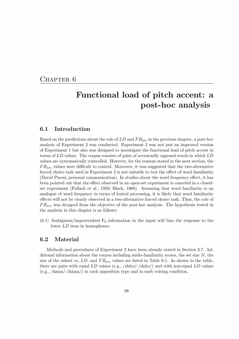
Chapter 6
Functional load of pitch accent: apost-hoc analysis
6.1 Introduction
Based on the predictions about the role of LD and FBave in the previous chapter, a post-hocanalysis of Experiment 2 was conducted. Experiment 2 was not just an improved versionof Experiment 1 but also was designed to investigate the functional load of pitch accent interms of LD values. The corpus consists of pairs of accentually opposed words in which LDvalues are systematically controlled. However, for the reasons stated in the next section, theFBave values were difficult to control. Moreover, it was suggested that the two-alternativeforced choice task used in Experiment 2 is not suitable to test the effect of word familiarity(David Pisoni, personal communication). In studies about the word frequency effect, it hasbeen pointed out that the effect observed in an open-set experiment is canceled in a closed-set experiment (Pollack et al., 1959; Black, 1968). Assuming that word familiarity is ananalogue of word frequency in terms of lexical processing, it is likely that word familiarityeffects will not be clearly observed in a two-alternative forced choice task. Thus, the role ofFBave was dropped from the objective of the post-hoc analysis. The hypothesis tested inthe analysis in this chapter is as follows:
(6.1) Ambiguous/impoverished F0 information in the input will bias the response to thelower LD item in homophones.
6.2 Material
Methods and procedures of Experiment 2 have been already stated in Section 3.7. Ad-ditional information about the corpus including audio-familiarity scores, the set size N , thesize of the subset m, LD, and FBave values are listed in Table 6.1. As shown in the table,there are pairs with equal LD values (e.g., /shiro/-/shıro/) and with non-equal LD values(e.g., /kama/-/kama/) in each opposition type and in each voicing condition.
98
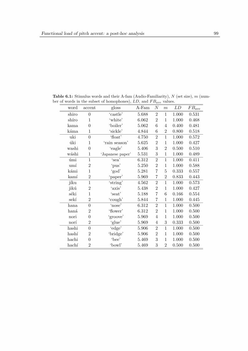
Functional load of pitch accent: a post-hoc analysis 99
Table 6.1: Stimulus words and their A-fam (Audio-Familiarity), N (set size), m (num-ber of words in the subset of homophones), LD, and FBave values.
word accent gloss A-Fam N m LD FBave
shiro 0 ‘castle’ 5.688 2 1 1.000 0.531shıro 1 ‘white’ 6.062 2 1 1.000 0.468kama 0 ‘boiler’ 5.062 6 4 0.400 0.481kama 1 ‘sickle’ 4.844 6 2 0.800 0.518uki 0 ‘float’ 4.750 2 1 1.000 0.572uki 1 ‘rain season’ 5.625 2 1 1.000 0.427
washi 0 ‘eagle’ 5.406 3 2 0.500 0.510washi 1 ‘Japanese paper’ 5.531 3 1 1.000 0.489umi 1 ‘sea’ 6.312 2 1 1.000 0.411umı 2 ‘pus’ 5.250 2 1 1.000 0.588kami 1 ‘god’ 5.281 7 5 0.333 0.557kamı 2 ‘paper’ 5.969 7 2 0.833 0.443jıku 1 ‘string’ 4.562 2 1 1.000 0.573jiku 2 ‘axis’ 5.438 2 1 1.000 0.427seki 1 ‘seat’ 5.188 7 6 0.166 0.554sekı 2 ‘cough’ 5.844 7 1 1.000 0.445hana 0 ‘nose’ 6.312 2 1 1.000 0.500hana 2 ‘flower’ 6.312 2 1 1.000 0.500nori 0 ‘groove’ 5.969 4 1 1.000 0.500norı 2 ‘glue’ 5.969 4 3 0.333 0.500hashi 0 ‘edge’ 5.906 2 1 1.000 0.500hashı 2 ‘bridge’ 5.906 2 1 1.000 0.500hachi 0 ‘bee’ 5.469 3 1 1.000 0.500hachı 2 ‘bowl’ 5.469 3 2 0.500 0.500
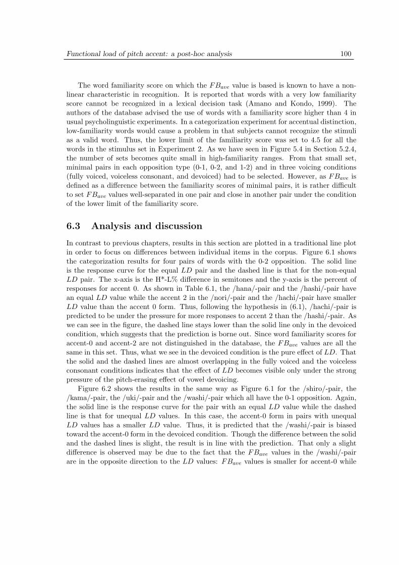
Functional load of pitch accent: a post-hoc analysis 100
The word familiarity score on which the FBave value is based is known to have a non-linear characteristic in recognition. It is reported that words with a very low familiarityscore cannot be recognized in a lexical decision task (Amano and Kondo, 1999). Theauthors of the database advised the use of words with a familiarity score higher than 4 inusual psycholinguistic experiments. In a categorization experiment for accentual distinction,low-familiarity words would cause a problem in that subjects cannot recognize the stimulias a valid word. Thus, the lower limit of the familiarity score was set to 4.5 for all thewords in the stimulus set in Experiment 2. As we have seen in Figure 5.4 in Section 5.2.4,the number of sets becomes quite small in high-familiarity ranges. From that small set,minimal pairs in each opposition type (0-1, 0-2, and 1-2) and in three voicing conditions(fully voiced, voiceless consonant, and devoiced) had to be selected. However, as FBave isdefined as a difference between the familiarity scores of minimal pairs, it is rather difficultto set FBave values well-separated in one pair and close in another pair under the conditionof the lower limit of the familiarity score.
6.3 Analysis and discussion
In contrast to previous chapters, results in this section are plotted in a traditional line plotin order to focus on differences between individual items in the corpus. Figure 6.1 showsthe categorization results for four pairs of words with the 0-2 opposition. The solid lineis the response curve for the equal LD pair and the dashed line is that for the non-equalLD pair. The x-axis is the H*-L% difference in semitones and the y-axis is the percent ofresponses for accent 0. As shown in Table 6.1, the /hana/-pair and the /hashi/-pair havean equal LD value while the accent 2 in the /nori/-pair and the /hachi/-pair have smallerLD value than the accent 0 form. Thus, following the hypothesis in (6.1), /hachi/-pair ispredicted to be under the pressure for more responses to accent 2 than the /hashi/-pair. Aswe can see in the figure, the dashed line stays lower than the solid line only in the devoicedcondition, which suggests that the prediction is borne out. Since word familiarity scores foraccent-0 and accent-2 are not distinguished in the database, the FBave values are all thesame in this set. Thus, what we see in the devoiced condition is the pure effect of LD. Thatthe solid and the dashed lines are almost overlapping in the fully voiced and the voicelessconsonant conditions indicates that the effect of LD becomes visible only under the strongpressure of the pitch-erasing effect of vowel devoicing.
Figure 6.2 shows the results in the same way as Figure 6.1 for the /shiro/-pair, the/kama/-pair, the /uki/-pair and the /washi/-pair which all have the 0-1 opposition. Again,the solid line is the response curve for the pair with an equal LD value while the dashedline is that for unequal LD values. In this case, the accent-0 form in pairs with unequalLD values has a smaller LD value. Thus, it is predicted that the /washi/-pair is biasedtoward the accent-0 form in the devoiced condition. Though the difference between the solidand the dashed lines is slight, the result is in line with the prediction. That only a slightdifference is observed may be due to the fact that the FBave values in the /washi/-pairare in the opposite direction to the LD values: FBave values is smaller for accent-0 while
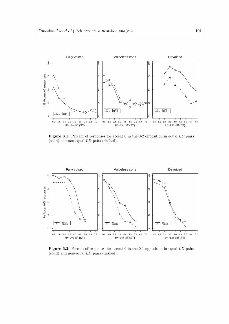
Functional load of pitch accent: a post-hoc analysis 101
025
5075
100
0.8 1.6 2.4 3.2 4.0 4.8 5.6 6.4 7.2
hananori
H*−L% diff (ST)
% A
ccen
t−0
resp
onse
s
Fully voiced
025
5075
100
0.8 1.6 2.4 3.2 4.0 4.8 5.6 6.4 7.2
hashihachi
H*−L% diff (ST)
Voiceless cons
025
5075
100
0.8 1.6 2.4 3.2 4.0 4.8 5.6 6.4 7.2
hashihachi
H*−L% diff (ST)
Devoiced
Figure 6.1: Percent of responses for accent 0 in the 0-2 opposition in equal LD pairs(solid) and non-equal LD pairs (dashed).
025
5075
100
0.8 1.6 2.4 3.2 4.0 4.8 5.6 6.4 7.2
shirokama
H*−L% diff (ST)
% A
ccen
t−0
resp
onse
s
Fully voiced
025
5075
100
0.8 1.6 2.4 3.2 4.0 4.8 5.6 6.4 7.2
ukiwashi
H*−L% diff (ST)
Voiceless cons
025
5075
100
0.8 1.6 2.4 3.2 4.0 4.8 5.6 6.4 7.2
ukiwashi
H*−L% diff (ST)
Devoiced
Figure 6.2: Percent of responses for accent 0 in the 0-1 opposition in equal LD pairs(solid) and non-equal LD pairs (dashed).
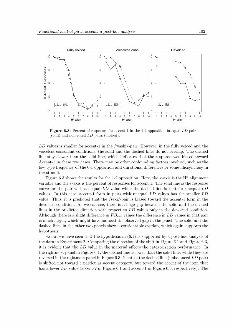
Functional load of pitch accent: a post-hoc analysis 102
025
5075
100
1 2 3 4 5 6 7 8 9 10
umikami
H* align
% A
ccen
t−1
resp
onse
s
Fully voiced
025
5075
100
1 2 3 4 5 6 7 8 9 10
jikuseki
H* align
Voiceless cons
025
5075
100
1 2 3 4 5 6 7 8 9 10
jikuseki
H* align
Devoiced
Figure 6.3: Percent of responses for accent 1 in the 1-2 opposition in equal LD pairs(solid) and non-equal LD pairs (dashed).
LD values is smaller for accent-1 in the /washi/-pair. However, in the fully voiced and thevoiceless consonant conditions, the solid and the dashed lines do not overlap. The dashedline stays lower than the solid line, which indicates that the response was biased towardAccent-1 in these two cases. There may be other confounding factors involved, such as thelow type frequency of the 0-1 opposition and durational differences or some idiosyncrasy inthe stimuli.
Figure 6.3 shows the results for the 1-2 opposition. Here, the x-axis is the H* alignmentvariable and the y-axis is the percent of responses for accent 1. The solid line is the responsecurve for the pair with an equal LD value while the dashed line is that for unequal LDvalues. In this case, accent-1 form in pairs with unequal LD values has the smaller LDvalue. Thus, it is predicted that the /seki/-pair is biased toward the accent-1 form in thedevoiced condition. As we can see, there is a huge gap between the solid and the dashedlines in the predicted direction with respect to LD values only in the devoiced condition.Although there is a slight difference in FBave values the difference in LD values in that pairis much larger, which might have induced the observed gap in the panel. The solid and thedashed lines in the other two panels show a considerable overlap, which again supports thehypothesis.
So far, we have seen that the hypothesis in (6.1) is supported by a post-hoc analysis ofthe data in Experiment 2. Comparing the direction of the shift in Figure 6.1 and Figure 6.3,it is evident that the LD value in the material affects the categorization performance. Inthe rightmost panel in Figure 6.1, the dashed line is lower than the solid line, while they arereversed in the rightmost panel in Figure 6.3. That is, the dashed line (unbalanced LD pair)is shifted not toward a particular accent category, but toward the accent of the item thathas a lower LD value (accent-2 in Figure 6.1 and accent-1 in Figure 6.3, respectively). The
Functional load of pitch accent: a post-hoc analysis 103
shift of dashed lines thus cannot be attributed to a preference or avoidance of a particularaccent category in the devoiced condition.
Also, the lack of the shift in the voiceless consonant condition confirms that the observedgap between the dashed and the solid line is not due to some idiosyncratic properties of aparticular word pair but due to the effect of LD values. The voiceless consonant conditionand the devoiced condition compares the same word pairs. That the gap is observed onlyin the devoiced condition is another support for the hypothesis in (6.1).
Chapter 7
Discussion and conclusions
In the present study, I investigated the categories in perception of contrastive pitch accentsin Tokyo Japanese. The primary goal of the study has been to fill the gaps in previousstudies in which the slope of the falling contour, the preceding tonal context of the pitchaccent, the scaling and the alignment of tonal units, and various voicing conditions areclaimed to affect the perception of pitch accent, but the interaction and the overall pictureof those components have not been made clear systematically. It has been attempted toapply a linguistically plausible model of intonation in a broader context of speech perceptionto fill those gaps in a principled and structured manner. The secondary goal of the studyhas been to quantify the distinctive function of pitch accent and to develop a formally andexperimentally tractable theory of functional load which can handle privative oppositions.The following sections discuss how much the two goals are achieved and how they contributeto the understanding of the issues around pitch accents in Japanese.
7.1 Category structure of pitch accents
7.1.1 Slope of the falling contour
As reviewed in Chapters 1 and 2, it has been claimed that the slope of the falling contourand the timing of the pitch fall have a compensatory relationship (Hasegawa and Hata,1992). However, results in Experiment 1 failed to find such a relationship in any voicingconditions. This, in turn, supports the assumption in Pierrehumbert & Beckman’s modelin which no linguistically significant role is assigned to the slope of the falling contour. TheL tone in the accent H*L is not linked to any mora but aligned right next to the H* tone.Thus the slope from the H* to the L tone is very steep and fixed at the tonal specificationlevel. The gradual slope in the output contour is determined by the amount of smoothingwhich is posited as a very low-level physical process beyond speakers’ control.
In this respect, Fujisaki model (Fujisaki and Sudo, 1971) reviewed in Chapter 1 does notutilize the slope as a variable that determines the shape of the contour either. The accentand the phrase component in the model are both a simple decaying function respondingto a vector or a rectangular input. Thus, two major models for intonation synthesis in
104
Discussion and conclusions 105
Japanese do not consider the slope of the falling as a necessary input to the system. Resultsin Experiment 1 confirmed this point from the perceptual side.
7.1.2 Preceding context
The effects of the preceding context to the perception of pitch accent were investigated inMatsui (1993), which only covered a limited subset of the possible opposition types in thedevoiced condition. His results showed a weak effect of the preceding context: the responsefor the unaccented form increased when the preceding word had a pitch accent. However,as pointed out in the review (Section 2.2.3), this may be due to the compensation for thecatathesis effect.
Experiments in the present study do not involve the catathesis effect, however. Thepreceding context of the target word never contains a pitch accent but only the initial L%and a phrasal H tones. The two tones constitute a rising contour of the beginning of anaccentual phrase. If the target word has an accent, the contour from the phrasal H tone tothe H* tone is also rising. Manipulations on the scaling of the phrasal H tone thus modifiesthe slope of the rising contour toward the target word. This has been an unexplored areain the literature of Japanese accent. As a working hypothesis, the steeper rising contourwas expected to give more salience to the pitch accent. The results in Experiment 2 and 3,however, refute any major effects of the rising contour. The scaling of the phrasal H tonedo not alter the categorization performance in all cases in a 2-way opposition (Experiment2) nor in the voiced condition in a 3-way opposition (Experiment 3). The effect is onlyseen in the devoiced condition in a 3-way opposition as an unexpected island centeredat the neutral phrasal H scaling in the response pattern for the unaccented form in acontour plot (Figure 4.12). This might be due to the fact that the base material for theresynthesis procedure was recorded in an unaccented form. Thus, an ambiguous stimulusbetween accent-1 and accent-2 with unmodified phrasal H might have been attracted to anunaccented form.
To counterbalance a possible bias from the base material, I should have included thestimuli resynthesized from both accent-1 and accent-2 forms. This would triple the totalnumber of stimulus which was already large in Experiment 3. We need some smart tricksto solve this situation, which is left for future investigation.
7.1.3 Tonal specifications
Since the slope and the preceding context are basically irrelevant, the core category structureof pitch accents in Japanese is quite simple: H* alignment determines the accent locationand the difference between the H* and L% tones determines the accent presence. This istrue both in a 2-way and a 3-way oppositions. An insight is derived from the differencebetween the two opposition types: accent-presence detection and accent-location detectionare functionally separate processes in the perceptual system. Moreover, it was shown thatthe accent-location detection is functionally more fundamental in 2-mora words, which wasevidenced both by behavioral experiments and by a large-scale database analysis (Amano

Discussion and conclusions 106
& Kondo, 1999).Not much attention has been paid to the dichotomy between the accent-presence detec-
tion and the accent-location detection in the generative literature mentioned in Chapter 1.Most analyses treat the unaccented form as just another type of accent pattern. It has anequal status with other accent patterns which are contrasted by the location. Engineering-oriented approaches are in the same vein. As pointed out in Section 2.2.1 in relation toSugito (1982), Fujisaki model (Fujisaki and Sudo, 1971) even sets an accent command forunaccented forms to generate an appropriate intonation pattern. In perception studies, atleast Sugito (1982) and Matsui (1993) reviewed in Chapter 2 do not separate the accent-presence detection from the accent-location detection.
However, in traditional accent description studies, the dichotomy has been a commonview. The primary grouping of accent patterns is to separate accented forms (Kifuku-shiki,literary “undulated style”) from unaccented forms (Heiban-shiki, literary “flat style”). Thesecondary grouping is done by the location of the accent within the undulated style: they areAtamadaka-gata “initial-high type”, Nakadaka-gata “mid-high type”, and Odaka-gata “final-high type”. If there is a need to distinguish, for example, 5-mora words with the penultimateaccent from those with the antepenultimate accent (they are both “mid-high type”), theaccent location is counted from the beginning by the number of moras (Kindaichi, 1981;Kindaichi et al., 1989; NHK, 1985; NHK, 1998).
Note that there is a clear correspondence between the primary groups and the gram-matical structure of Japanese: verbs and adjectives have only the primary level distinctionwhile nouns need the secondary grouping. That is, there is no accent-location distinction inverbs and adjectives. They are either unaccented or penultimate-accented. Thus, listenersmay have to care only about accent-presence detection in verbs and adjectives.
That the accent-location detection is functionally more fundamental in 2-mora wordsmay thus be limited to nouns since the target words used in experiments in the presentthesis are all nouns. To confirm this point, we need to design another experiment for verbsand adjectives with appropriate carrier phrases which should be different from those usedfor nouns. This is again left for future investigation.
7.1.4 Effect of devoicing
The effect of devoicing has been clearly demonstrated in the results of the three experi-ments. As it has been criticized in Sections 2.2.3 and 3.2, previous studies were concernedmainly with the vowel devoicing and paid less attention to a comparison among fully voiced,partially voiced, and fully devoiced moras. Experiments 1 and 2 investigated all three typesof voicing conditions: the fully voiced condition (C V), the voiceless consonant condition(C◦ V), and the devoiced condition (C◦ V◦). Target words for F0 manipulation or carrier sen-tences were different among the three voicing conditions, however, to cover the full range ofconditions. Thus, durational properties and spectral transitions could not be strictly con-trolled. In contrast, Experiment 3 investigated the voiceless consonant condition and thedevoiced condition. The latter was an edited version of the former in order to completelymatch the factors other than voicing.
Discussion and conclusions 107
Hypotheses tested in Experiments 1 and 2 are based on a view that there are threesources of information for the identification of an accent: a high pitch at the H* tone, a lowpitch at the L% tone, and the falling contour. Cessation of a pitch contour by a voicelesssegment causes a loss of the information sources. Fixing the location of the voicing variationto the second mora of the word, accent-1 forms lose the falling contour while accent-2 formslose none of the three sources in the voiceless consonant condition. In the devoiced condition,accent-1 forms lose the falling contour while accent-2 forms lose both the H* tone and thefalling contour.
Predictions about the categorization task were: (i) in the 0-1 opposition, it is harderin the voiceless consonant than in the fully voiced condition, while the devoiced conditionis as hard as the voiceless consonant condition; (ii) in the 0-2 opposition, the devoicedcondition is harder than the other two conditions, (iii) accent-1 forms are preferred in the1-2 opposition.
The results in Experiment 1 support these predictions in terms of the amount of shiftof the category boundaries among the three voicing conditions. The results in Experiment2 are consistent with those in Experiment 1 in terms of the amount of the shift but notin terms of the direction of the shift. When devoiced, the area for accent-2 forms on acontour plot enlarges in Experiment 1 but shrinks in Experiment 2. This inconsistency ofthe direction of the shift between the two experiments can be attributed to the durationalvariations and presumably some other unintended variations among stimulus tokens.
Experiment 3 used a splicing technique to remove any unintended variations among thestimulus sets. Since the main purpose of Experiment 3 is to see the category structure ofa 3-way distinction, the results are not directory comparable to those in Experiments 1and 2. However, the area for accent-2 forms on a contour plot also shrinks in the devoicedcondition, which is in accordance with the results in Experiment 2.
7.2 Functions of pitch accent
As for the secondary goal of the present thesis, a novel approach to the functional load ofpitch accent was proposed based on an extensive analysis of the database. The proposed twoindices, LD obtained from opposing and non-opposing relations, and FBave obtained fromword familiarity differences within accentually opposed homophones provide a quantitativemeasure for the distinctive function of pitch accent. As reviewed in Section 1.3.2, Hockett(1967)’s formulation for a quantification of the functional load is unsuitable for pitch accentsin Japanese due to the fact that they include a privative opposition. Both LD and FB aredesigned to represent the usefulness of the accent in any type of oppositions including aprivative one.
The effect of LD was confirmed in a post-hoc analysis of experimental data for thecategory structure. Within a pair of accentually opposed homophones, the response wasbiased toward the item with a lower LD value. This effect was observed only in the de-voiced condition, which suggests that the listeners rely on the relational properties betweenhomophones in the lexicon when the source of the crucial identifying cue in the auditory
Discussion and conclusions 108
signal is degraded or lost.The support for FBave in experimental data could not be obtained partly due to limita-
tions in the closed-set task and partly due to the non-linear nature of the word familiarity.Words with a low familiarity score in average are simply unknown to many people. It isvery unlikely that categorization or identification to unknown items fairly compares withthat to known items.
7.3 Future directions
Finally, I suggest several directions for future research. Two points have already beenmentioned as a direct extension of the experiments in the present study: (1) the base formfor the resynthesis should be counter balanced, and (2) verbs and adjectives should beincluded in the materials. Other than these, more ambitious extensions are listed in thefollowing.
First, the category structure of pitch accents in 3-mora or longer words has to be clar-ified. As we have seen in the discussion about the distribution of oppositions, oppositionsinvolving accent-0 is by far dominant in 3- and 4-mora words. Thus, the accent-presencedetection process is predicted to be more fundamental in those words. Future researchneeds to consider the effect of lexical strata (McCawley, 1968; Vance, 1987; Ito and Mester,1995; Fukazawa et al., 1998), such as Yamato, Sino-Japanese, Mimetics and Foreign in thedistribution of accent patterns. As reviewed in Section 1.2.2, Sino-Japanese words con-tribute most to the dominance of unaccented forms in 3- and 4-mora words. However, therehas been no reliable resource for determining the psychological status of lexical strata. Anetymological survey for each word can go as far as historical data are available, but suchknowledge does not necessarily correspond to what an average person has. Though thereis a recent psychological study of lexical strata (Moreton and Amano, 1999), much morecollective effort is awaited on this topic.
Second, the delimitative and the culminative functions of pitch accent have to be morequantitatively approached to pursue the functional approach to pitch accents. An investi-gation of the perception of compound accent may be especially helpful to clarify the roleof those two functions. As reviewed in Chapter 1, there have been a number of studiesabout the description and formalization of compound accent phenomena. For example, ithas been known that there is a class of morphemes which deaccents the whole compound(McCawley, 1968; Kubozono, 1993; Kubozono, 1995). When the compound is deaccented,the culminative function of the pitch accent is lost and the rising contour made of a combi-nation of the initial L% tone and the phrasal H tone only fulfills the delimitative function.A database analysis of those compounds will reveal how the two functions interact with themorphological processes of the language.
Third, the two indices proposed for the distinctive function of pitch accent can the-oretically be extended to other contrasts not only in prosody but in segmental/featuraldomains. As for the familiarity bias (FB), future research first needs to establish an ap-propriate paradigm to probe the familiarity differences within contrasted and uncontrasted

Discussion and conclusions 109
items. For languages other than Japanese, a word familiarity database of a comparable sizeto the one used in the present study is necessary. As for the lexical distinctiveness (LD),featural level distinctions, such as voicing, nasality, labiality and so on in various languagesare immediate candidates for future research. The proposed definition of LD circumventsthe problem for privativity in Hockett (1967)’s method for the quantification of the func-tional load. Thus, LD can handle oppositions including privativity at the featural level aswell as those at the prosodic level.
It seems that the classic functional load has been forgotten in the generative era. How-ever, as mentioned in the beginning of Chapter 1, the new interest brought up amongphonologists to the perceptual studies will flourish if we can explicitly handle the functionalload of both prosodic and segmental contrasts.
Bibliography
Abe, Y. (1987). Metrical structure and compounds in Japanese. In Imai, T. and Saito, M.,editors, Issues in Japanese Linguistics, pages 5–52. Foris, Dordrecht.
Akinaga, K. (1985). Kyootsuugo no akusento [Accent of common Japanese]. In NHK, editor,Nihongo Hatsuon Akusento Jiten [Pronunciation and Accent Dictionary of Japanese],chapter Appendix, pages 70–116. Nihon Hoosoo Syuppan Kyookai, Tokyo.
Akinaga, K. (1998). Kyootsuugo no akusento [Accent of common Japanese]. In NHK, editor,Nihongo Hatsuon Akusento Jiten [Pronunciation and Accent Dictionary of Japanese],pages 174–221. Nihon Hoosoo Syuppan Kyookai, Tokyo.
Alderete, J. (1999). Morphologically Governed Accent in Optimality Theory. Doctoraldissertation, University of Massachusetts, Amherst.
Amano, S. and Kondo, T. (1999). Nihongo-no goitokusei [Lexical properties of Japanese].Sanseido, Tokyo.
Amano, S., Kondo, T., and Kakehi, K. (1995). Modality dependency of familiarity ratingsof Japanese words. Perception and Psychophisics, 57:598–603.
Atake, Y., Riku, K., Nakamura, S., Shikano, K., and Kawahara, H. (1999). Straight nobunseki goosee hooshiki parameta no shukan hyooka ni yoru kentoo [An examinationof parameters in the analysis-synthesis method of STRAIGHT in terms of subjectiveevaluation]. In Proceedings of the 1999 Autumn meeting of the Acoustical Society ofJapan, volume 1, pages 205–206.
Balota, D. A. (1994). Visual word recognition. In Gernsbacher, M., editor, Handbook ofPsycholinguistics, pages 303–358. Academic Press, New York, NY.
Balota, D. A. and Chumbley, J. I. (1984). Are lexical decisions a good measure of lexicalaccess? Journal of Experimental Psychology: Human Perception and Performance,10:340–357.
Balota, D. A. and Chumbley, J. I. (1985). The locus of word-frequency effects in the pro-nunciation task: Lexical access and/or production? Journal of Memory and Language,24:89–106.
110
bibliography 111
Beckman, M. and Shoji, A. (1984). Spectral and perceptual evidence for CV coarticulationin devoiced /si/ and /syu/ in Japanese. Phonetica, 41:61–71.
Beckman, M. E. (1986). Stress and Non-Stress accent. Foris, Dordrecht.
Beckman, M. E. and Edwards, J. (1994). Articulatory evidence for differentiating stresscategories. In Keating, P. A., editor, Papers in Laboratory Phonology 3: PhonologicalStructure and Phonetic Form, pages 7–33. Cambridge University Press, Cambridge,UK.
Beckman, M. E. and Pierrehumbert, J. B. (1986). Intonational structure in Japanese andEnglish. Phonology Yearbook, 3:255–309.
Black, J. (1968). Responses to multiple-choice intelligibility tests. Journal of Speech andHearing Reaearch, 11:453–456.
Boersma, P. (1997). The elements of functional phonology. manuscript, University ofAmsterdam (published as part of the book Functional Phonology later).
Broadbent, D. E. (1967). Word-frequency effects and response bias. Psychological Review,74:1–15.
Buhler, K. (1920). Kritische Musterung der neuern Theorie des Satzes. Indo-GermanischesJahrbuch, 6:1–20.
Buhler, K. (1934). Sprachethorie: Die Darstellungsfunktion der Sprache. Gustav FischerVerlag, Jena.
Bybee, J. L. (1985). Morphology: A Study of the Relation between Meaning and Form.Benjamins, Philadelphia.
Bybee, J. L. (1994). A view of phonology from a cognitive and functional perspective.Cognitive Linguisitcs, 5-4:285–305.
Bybee, J. L. (1998). The emergent lexicon. In CLS34, The Panels, volume 2, pages 421–436,Chicago Linguistic Society, Chicago, IL.
Clark, M. M. (1987). Japanese as a tone language. In Imai, T. and Saito, M., editors, Issuesin Japanese Linguistics, pages 53–105. Foris, Dordrecht.
Cutler, A. (1989). Auditory lexical access: Where do we start? In Marslen-Wilson, W.,editor, Lexical Representation and Process, pages 342–356. MIT Press, Cambridge,MA.
Cutler, A. (1994). Segmentation problems, rhythmic solutions. In Gleitman, L. and Landau,B., editors, The Acquisition of the Lexicon, pages 81–104. MIT Press, Cambridge, MA.
bibliography 112
Cutler, A. and Chen, H.-C. (1997). Lexical tone in Cantonese spoken-word processing.Perception & Psychophysics, 59:165–179.
Cutler, A. and Norris, D. (1988). The role of strong syllables in segmentation for lexicalaccess. Journal of Experimental Psychology: Human Perception and Performance,14:113–121.
Cutler, A. and Otake, T. (1999). Pitch accent in spoken-word recognition in Japanese.Journal of the Acoustical Society of America, 105:1877–1888.
Flemming, E. S. (1995). Auditory Representations in Phonology. Doctoral dissertation,UCLA.
Forster, K. I. (1978). Accessing the mental lexicon. In Walker, E., editor, Explorations inthe Biology of Language, pages 139–174. Bradford, Mongomery, VT.
Forster, K. I. and Chambers, S. M. (1973). Lexical access and naming time. Journal ofVerbal Learning and Verbal Behavior, 12:627–635.
Fujisaki, H. (1996). Recent Research towards Advanced Man-machine Interface throughSpoken Language. Elsevier, New York, NY.
Fujisaki, H. and Sudo, H. (1971). Nihongo tango akusento no kihon shuuhasuu patan tosono seeseekikoo no moderu [A model for the generation of fundamental frequencycontours of Japanese word accent]. Nihon Onkyoo Gakkaishi [Journal of AcousticalSociety of Japan], 27:445–444.
Fukazawa, H., Kitahara, M., and Ota, M. (1998). Lexical stratification and ranking invari-ance in constraint-based grammars. In CLS34, The Panels, volume 2, pages 47–62,Chicago Linguistic Society, Chicago, IL.
Haraguchi, S. (1977). The Tone Pattern of Japanese: An Autosegmental Theory of Tonol-ogy. Kaitakusya, Tokyo.
Haraguchi, S. (1991). A Theory of Stress and Accent. Foris, Dordrecht.
Hasegawa, Y. and Hata, K. (1992). Fundamental frequency as an acoustic cue to accentperception. Language and Speech, 35:87–98.
Hasegawa, Y. and Hata, K. (1995). The function of f0-peak delay in Japanese. BLS,21:141–151.
Hattori, S. (1954). Oninron kara mita kokugo no akusento [Accent in Japanese in phono-logical perspective]. Kokugo Kenkyuu, 2.
Hattori, S. (1960). Gengogaku no hoohoo [Methods in Linguistics]. Iwanami, Tokyo.

bibliography 113
Hayes, B. (1989). Compensatory lengthening in moraic phonology. Linguistic Inquiry,20:253–306.
Hayes, B. (1996a). Can optimality theory serve as the medium for a functionally-guidedphonology? handout, presented at 1996 Milwaukee Conference on Formalism andFunctionalism in Linguistics, Apr, 1996.
Hayes, B. (1996b). Phonetically driven phonology: The role of optimality theory andinductive grounding 1. manuscript, UCLA.
Higurashi, Y. (1983). The Accent of Extended Word Structures in Tokyo Standard Japanese.EDUCA Inc, Tokyo, Japan.
Hino, Y. and Lupker, S. J. (1998). The effects of word frequency for Japanese kana andkanji words in naming and lexical decision: Can the dual-route model save the lexical-selection account? Journal of Experimental Psychology: Human Perception and Per-formance, 24:1431–1453.
Hirose, H. (1971). The activity of the adductor laryngeal muscles in respect to voweldevoicing in Japanese. Phonetica, 23:156–170.
Hockett, C. F. (1967). The quantification of functional load. Word, 23:301–320.
House, D. (1990). Tonal Perception in Speech. Lund University Press, Lund, Sweden.
Hume, E. and Johnson, K. (2000). A model of the interplay of speech perception andphonology. manuscript, the Ohio State University.
Ishihara, M. (1991). The Lexical Prosodic Phonology of Japanese Verbs. Doctoral disserta-tion, University of Arizona, Tucson.
Ito, J. and Mester, A. (1995). The core-periphery structure of the lexicon and constraintson reranking. In J. Beckman, L. W. D. and Urbanczyk, S., editors, University of Mas-sachusetts Occasional Papers in Linguistics 18 : PAPERS IN OPTIMALITY THE-ORY, pages 181–210. Graduate Linguisic Students Association, Amherst, MA.
Kawahara, H., Katayose, H., de Cheveigne, A., and Patterson, R. D. (1999). Fixed pointanalysis of frequency to instantaneous frequency mapping for accurate estimation of f0and periodicity. In Proceedings of EUROSPEECH’99, volume 6, pages 2781–2784.
Kawahara, H. and Masuda, I. (1996). Jikansyuuhasuu ryooiki deno hokan o mochiita onseeno henkan ni tsuite [Speech representation and transformation based on adaptive time-frequency interpolation]. Technical report, IEICE EA96-28.
Kawahara, H., Masuda-Katsuse, I., and de Cheveigne, A. (1997a). Restructuring speechrepresenttions using straight-tempo: Possible role of a repetitive structure in sounds.Technical report, ATR Human Information Processing Research Laboratories.
bibliography 114
Kawahara, H., Yamada, R., and Kubo, R. (1997b). STRAIGHT o mochiita onsee parametano soosa ni yoru inshoo no henka ni tsuite [On the change of sound impression whenmodifying phonetic parameters by STRAIGHT. Technical report, IEICE, H-97-63.
Kawakami, S. (1969). Musee haku no tsuyosa to akusento kaku [The intensity of devoicedmora and the accent nucleus]. Kokugakuindai Kokugo Kenkyu, 27.
Kindaichi, H. (1981). Meikai Nihongo Akusento Jiten. Sanseido, Tokyo, 2nd edition.
Kindaichi, K., Shibata, T., Yamada, A., and Yamada, T. (1989). Shinmeikai Kokugo Jiten.Sanseidoo, Tokyo, 4th edition.
King, R. D. (1967). Functional load and sound change. Language, 43:831–852.
Kirchner, R. (1998). An Effort-Based Approach to Consonant Lenition. Doctoral disserta-tion, UCLA.
Kitahara, M. (1996a). Consonant gemination and accent in Japanese loanwords. In Koizumi,M., Oishi, M., and Sauerland, U., editors, Formal Approaches to Japanese Linguistics2, pages 61–80. MITWPL, Cambridge, MA.
Kitahara, M. (1996b). The realization of accent in devoiced syllables in Tokyo Japanese.Paper presented at the 5th Conference on Laboratory Phonology, Northwestern Uni-versity, July, 1996.
Kitahara, M. (1998). The interaction of pitch accent and vowel devoicing in Tokyo Japanese.In Silva, D., editor, Japanese–Korean Linguistics 8, pages 303–315. CSLI, Stanford,CA.
Kitahara, M. (1999). Accentual contrast maintenance and vowel devoicing in TokyoJapanese. In Proceedings of the XIVth International Congress of Phonetic Sciences,pages 2363–2366, San Francisco, CA.
Komatsu, H. (1989). Nihongo no rekishi: akusento [History of Japanese: Accent]. In Kamei,T., Kono, R., and Chino, E., editors, Gengogaku Daijiten, pages 1651–1653. Sanseido,Tokyo.
Kondo, M. (1996). Mechanisms of Vowel Devoicing in Japanese. Doctoral dissertation,University of Edinburgh.
Kori, S. (1989). Kyoochoo to intoneeshon [Emphasis and intonation]. In Sugito, M., editor,Kouza Nihongo to Nihongo Kyouiku [Lectures on Japanese and Japanese LanguageEducation] 2, pages 316–342. Meiji shoin, Tokyo.
Kubozono, H. (1993). The Organization of Japanese Prosody. Kuroshio, Tokyo.
bibliography 115
Kubozono, H. (1995). Constraint interaction in Japanese phonology: Evidence from com-pound accent. In Walker, R., Lorentz, O., and Kubozono, H., editors, Phonology atSanta Cruz Volume 4: Papers on Stress, Accent, and Alignment, pages 21–38. Linguis-tics Research Center, University of California, Santa Cruz, Santa Cruz, CA.
Kubozono, H. (1998). Onin koozoo no fuhensee to kobetsusee [Universality and individ-uality of phonological structure]. In Minoru, N., editor, Onin Koozoo to akusento[Phonological Structure and Accent], pages 2–108. Kuroshio, Tokyo.
Ladd, D. R. (1996). Intonational Phonology. Cambridge University Press, Cambridge, UK.
Liberman, M. Y. and Pierrehumbert, J. B. (1984). Intonational invariance under changesin pitch range and length. In Aronoff and Oerle, editors, Language Sound Structure:Studies in Phonology Presented to Morris Halle, pages 157–233. MIT press, Cambridge,MA.
Lombardi, L. (1995). Laryngeal features and privativity. The Linguistic Review, 12:35–59.
Luce, P. (1986). Neighborhoods of words in the mental lexicon. Technical report, SpeechResearch Laboratory, Department of Psychology, Indiana University.
Maekawa, K. (1990). Production and perception of the accent in the consecutively devoicedsyllables in Tokyo Japanese. In Proceeedings of ICSLP 90, pages 61–64.
Maekawa, K. (1997). Effects of focus on duration and vowel formant frequency in Japanese.In Sagisaka, Y., Campbell, N., and Higuchi, N., editors, Computing Prosody: Com-putational Models for Processing Spontaneous Speech, pages 129–154. Springer-Verlag,New York, NY.
Marslen-Wilson, W. (1989). Access and integration: Projecting sound onto meaning. InMarslen-Wilson, W., editor, Lexical Representation and Process, pages 3–24. MITPress, Cambridge, MA.
Martinet, A. (1952). Function, structure, and sound change. Word, 8-1:1–32.
Martinet, A. (1960). Elements de linguistique generale. Armand Colin, Paris.
Martinet, A. (1962). A Functional View of Language. Clarendon Press, Oxford.
Matsui, M. (1993). Museihaku joo no akusento kaku no chikaku ni tsuite [Perceptual studyof the accent in the devoiced mora]. paper presented at Kinki Onsei Gengo Kenkyuukai,Osaka, Japan.
McCawley, J. D. (1968). The Phonological Component of a Grammar of Japanese. Mouton,The Hague.
bibliography 116
McCawley, J. D. (1977). Accent in Japanese. In Hyman, L. M., editor, Studies in Stressand Accent. Southern California Occasional Papers in Linguistics 4, pages 261–302.Department of Linguistics, University of Southern California, Los Angeles, CA.
McClellan, J. H., Shafer, R. W., and Yoder, M. A. (1998). DSP First: A MultimediaApproach. Prentice-Hall, Upper Saddle River, NJ.
McClelland, J. L. and Elman, J. L. (1986). Interactive processes in speech perception: TheTRACE model. In J. L. McClelland, D. E. R. and the PDP Research Group, edi-tors, Parallel Distributed Processing: Explorations in the Microstructures of Cognition,Volume 2: Psychological and Biological Models, pages 58–121. MIT Press, Cambridge,MA.
Miyaji, Y. (1980). Doo’ongo no akusento [accent in homophones]. In Tokugawa, S., editor,Ronshuu Nihongo Kenkyuu 2: Akusento [The Collection of Studies on Japanese], pages122–130. Yuuseedoo, Tokyo. originally appeared in Kokugo Kokubun 35 (1966).
Moreton, E. and Amano, S. (1999). Phonotactics in the perception of Japanese vowellength: Evidence for long-distance dependencies. In Proceedings of the Eurospeech 99Conference, volume unknown, page unknown, Budapest.
Morton, J. (1979). Word recognition. In Morton, J. and Marshall, J. C., editors, Structuresand Processes, pages 109–156. MIT Press, Cambridge, MA.
Nagano-Madsen, Y. (1994). Vowel devoicing rates in Japanese from a sentence corpus. LundUniversity Dept of Linguistics Working Papers, 42:117–127.
Nespor, M. and Vogel, I. (1986). Prosodic Phonology. Foris, Dordrecht.
Neustupny, J. V. (1966). Is the Japanese accent a pitch accent? Onsei Gakkai Kaihoo, 121.
NHK (1985). Nihongo Hatsuon Akusento Jiten [Pronunciation and Accent Dictionary ofJapanese]. Nihon Hoosoo Syuppan Kyookai, Tokyo.
NHK (1998). Nihongo Hatsuon Akusento Jiten [Pronunciation and Accent Dictionary ofJapanese]. Nihon Hoosoo Syuppan Kyookai, Tokyo.
Nusbaum, H. C., Pisoni, D. B., and Davis, C. K. (1984). Sizing up the Hoosier mentallexicon: Measuring the familiarity of 20,000 words. Research on Speech PerceptionProgress Report No, 10:427–444.
Pierrehumbert, J. and Beckman, M. (1988). Japanese Tone Structure. MIT Press, Cam-bridge, MA.
Pollack, I., Rubenstein, H., and Decker, L. (1959). Intelligibility of known and unknownmessage sets. Journal of the Acoustical Society of America, 31:273–279.

bibliography 117
Poser, W. J. (1984). The Phonetics and Phonology of Tone and Intonation in Japanese.Doctoral dissertation, MIT.
Prince, A. and Smolensky, P. (1993). Optimality theory: Constraint interaction in gener-ative grammar. Technical report, Technical Report 2, Rutgers Center for CongnitiveScience.
Sato, H. (1989). Fukugoogo ni okeru akusento kisoku to rendaku kisoku [Accent rulesand sequential voicing rules in compounds]. In Sugito, M., editor, Kooza Nihongo toNihongo Kyooiku [Lectures on Japanese and Japanese Education] 2, pages 233–265.Meiji Shoin, Tokyo.
Sato, H. (1993). Kyootsuugo akusento no seiin bunseki [Accent analysis of common Japanesewords]. Nihon Onkyoo Gakkai Shi [Journal of the Acoustic Society of Japan], 49:775–784.
Sawashima, M. (1971). Devoicing of vowels. Annual Bulletin, Research Institute of Logo-pedics and Phoniatrics, University of Tokyo, 5:7–13.
Sawashima, M. (1980). Vocal pitch control in word accent and sentence intonation inJapanese. Annual Bulletin, Research Institute of Logopedics and Phoniatrics, Univer-sity of Tokyo, 14:53–63.
Sawashima, M. and Hirose, H. (1980). Laryngeal gestures in speech production. AnnualBulletin, Research Institute of Logopedics and Phoniatrics, University of Tokyo, 14:29–51.
Sawashima, M., Hirose, H., Yoshioka, H., and Kiritani, S. (1982). Interaction betweenarticulatory movements and vocal pitch control in Japanese word accent. Phonetica,39:188–198.
Sawashima, M., Kakita, Y., and Hiki, S. (1973). Activity of the extrinsic laryngeal musclesin relation to Japanese word accent. Annual Bulletin, Research Institute of Logopedicsand Phoniatrics, University of Tokyo, 7:19–25.
Selkirk, E. (1986). On derived domains in sentence phonology. Phonology Yearbook, 3:371–405.
Shibata, T. and Shibata, R. (1990). Akusento wa doo’ongo o dono teido bembetsu shi-uru ka: Nihongo, eigo chugokugo no ba’ai [Is word-accent significant in differentiatinghomonyms in Japanese, English and Chinese?]. Keiryoo Kokugogaku [MathematicalLinguistics], 17:317–327.
Shibata, T., Sugito, M., Shibata, R., and Takagiwa, M. (1994). Akusento no doo’ongobenbetsu ryoku: Tokyo akusento to osaka akusento [Word accent for differentiatinghomonyms in Tokyo and Osaka dialects]. Keiryoo Kokugogaku [Mathematical Linguis-tics], 19:277–292.
bibliography 118
Shibatani, M. (1972). The non-cyclic nature of Japanese accentuation. Language, 48:584–595.
Shimada, Z. and Hirose, H. (1971). Physiological correlates of Japanese accent patterns.Annual Bulletin, Research Institute of Logopedics and Phoniatrics, University of Tokyo,5:41–49.
Slowiaczek, L. N. (1986). On the Role of Lexical Stress in Auditory Word Recognition. PhDthesis, Indiana University.
Steriade, D. (1999). Perceptual factors in place assimilation. Paper presented at “The Roleof Speech Perception Phenomena in Phonology,” a setellite meeting of ICPhS99, SanFrancisco, CA.
Sugito, M. (1981). The relation between voice lowering for accent and articulation of vowels.Gengo Kenkyuu, 79:1–32.
Sugito, M. (1982). Nihongo Akusento no Kenkyuu [Studies on Japanese Accent]. Sanseido,Tokyo, Japan.
Suzuki, H. (1995). Minimal words in Japanese. In Audra, D., Rachel, H., Barbara, L.,Barbara, N., and Sheri, P., editors, CLS 31, The Main Session, volume 1, pages 448–463, Chicago Linguistic Society, Chicago, IL.
’t Hart, J., Collier, R., and Cohen, A. (1990). A Perceptual Study of Intonation. CambridgeUniversity Press, Cambridge, UK.
Tsuchida, A. (1997). Phonetics and Phonology of Japanese Vowel Devoicing. Doctoraldissertation, Cornell University.
Uwano, Z. (1977). Nihongo no akusento [Japanese accent]. In Ono, S. and Shibata, T.,editors, Iwanami Kooza Nihongo 5: On’in [Iwanami Japanese Course 5: Phonology],pages 281–321. Iwanami, Tokyo.
Uwano, Z. (1989). Nihongo no akusento [Japanese accent]. In Sugito, M., editor, KouzaNihongo to Nihongo Kyouiku [Lectures on Japanese and Japanese Language Education]2, pages 178–205. Meiji shoin, Tokyo.
Uwano, Z. (1996). Akusento kenkyuu no temboo [Trends in studies on accent]. OnseigakkaiKaihoo [The Bulletin of the Phonetic Society of Japan], 211:27–34.
van Santen, J., Shih, C., and Mobius, B. (1998). Intonation. In Sproat, R., editor, Mul-tilingual Text-to-speech Synthesis: The Bell Labs Approach, pages 141–190. Kluwer,Dordrecht.
Vance, T. J. (1987). An Introduction to Japanese Phonology. State University of New YorkPress, Albany, NY.
bibliography 119
Varden, J. K. (1998). On High Vowel Devoicing in Standard Modern Japanese: Implicationsfor Current Phonological Theory. Doctoral dissertation, University of Washington.
Venditti, J. J. (1995). Japanese ToBI labeling guidelines. unpublished manuscript, the OhioState University.
Weitzman, R. (1969). Japanese accent: an analysis based on acoustic-phonetic data. Doc-toral dissertation, University of Southern California.
Whittlesea, B. W. A. and Williams, L. D. (2000). The source of feelings of familiarity: Thediscrepancy-attribution hypothesis. Journal of Experimental Psychology: Learning,Memory, and Cognition, 26:547–565.
Yokotani, T. (1997). Futto o koeru akusento idoo: Tokyo hoogen fukugoo meishi karano shooko [Accent shift beyond the foot boundary: Evidence from Tokyo Japanesecompound nouns]. Onsee Kenkyuu (Journal of the Phonetic Society of Japan), 1:54–62.
Yoshida, Y. (1995). On Pitch Accent Phenomena in Standard Japanese. Doctoral disserta-tion, University of London.
Yoshioka, H. (1981). Laryngeal adjustments in the production of the fricative consonantsand devoiced vowels in Japanese. Phonetica, 38:236–251.
Zolfaghari, P. and Kawahara, H. (1999). Subjective evaluation of STRAIGHT. In Proceed-ings of the 1999 Autumn meeting of the Acoustical Society of Japan, volume 1, pages193–194.
Zubizarreta, M. (1982). The formal interaction of harmony and accent: The tone pat-tern of Japanese. In van der Hulst et al., H., editor, The Structure of PhonologicalRepresentation (Part 2), pages 159–212. Foris, Dordrecht.