catds smos l3 soil moisture retrieval processor
TRANSCRIPT

CATDS SMOS L3 Soil moisture retrieval processor
ATBD
Ref.: SO-TN-CBSA-GS-0029
Issue: 2.0
Date:14/7/2013
Page: 1 / 73
CATDS SMOS L3 soil moisture retrieval processor
Algorithm Theoretical Baseline Document (ATBD)
Reference: SO-TN-CBSA-GS-0029
Issue: 2.0
Date: 14/07/2013
Yann Kerr PI point of contact Prepared by:
Elsa Jacquette (CNES1),
Ahmad Al Bitar, François Cabot, Arnaud Mialon, Philippe Richaume (CESBIO), Arnaud Quesney (GeoSyS), Lucie Berthon (CERFACS)
with contributions from
CESBIO and CNES CATDS teams
1 Current affiliations

CATDS SMOS L3 Soil moisture retrieval processor
ATBD
Ref.: SO-TN-CBSA-GS-0029
Issue: 2.0
Date:14/7/2013
Page: 2 / 73

CATDS SMOS L3 Soil moisture retrieval processor
ATBD
Ref.: SO-TN-CBSA-GS-0029
Issue: 2.0
Date:14/7/2013
Page: 3 / 73
Modification table
Issue Rev. Date Description Draft 0 11/01/2008 First draft Draft 1 04/02/2008 Draft issue 1
1 0 15/02/2008 Final report Major updates
1 1 25/02/2008 Final report §3.4.3.2 and 5.3.6: Clarification about decade convention §3.3: Clarification about diurnal effect considerations Footprint: Add copyright information
2 0 04/07/2013 Major updates Reworking of the document, updates aligned with the industrial development phase of CATDS processors.

CATDS SMOS L3 Soil moisture retrieval processor
ATBD
Ref.: SO-TN-CBSA-GS-0029
Issue: 2.0
Date:14/7/2013
Page: 4 / 73
Table of content
INTRODUCTION ................................................................................................................. 6
1. REFERENCES, ABBREVIATIONS AND DEFINITIONS ............................................ 6 1.1. Reference documents .................................................................................. 6 1.2. Literature reference ...................................................................................... 7 1.3. List of acronyms ........................................................................................... 9 1.4. Definitions ................................................................................................... 10
2. SMOS AND CATDS OVERVIEW ............................................................................. 13 2.1. SMOS context ............................................................................................. 13 2.2. Overview of SMOS L0 to L2 processing and products ........................... 13
3. CENTRECENTRECENTRECENTRECENTREOVERVIEW OF CATDS SOIL MOISTURE PROCESSING ............................................................................................... 14
3.1. Level 3 soil moisture objectives ................................................................ 14 3.2. Level 3 soil moisture strategy ................................................................... 15
4. L3 SM INPUTS .......................................................................................................... 18 4.1. The Discrete Global grid: EASE ................................................................ 18 4.2. L1C processing ........................................................................................... 21 4.3. Daily Brightness TEMPERATURE - L1C Filtering .................................... 22
5. L3 SM OPTIMAL PROCESSING .............................................................................. 24 5.1. Motivations and Concept ........................................................................... 24 5.2. Detailed description of the algorithms ..................................................... 26
5.2.1. Revisit selection ....................................................................................................... 28
5.2.2. Dwell lines reconstruction ........................................................................................ 28
5.2.3. Pre-processing ......................................................................................................... 29
5.2.4. Decision tree ............................................................................................................ 30 5.2.4.1. Selection of the decision tree branch and the associated model .......................................... 30 5.2.4.2. Selection of the retrieval conditions ...................................................................................... 30 5.2.4.3. Computation of prior and reference values of parameters ................................................... 31
5.2.5. Retrieval of the free parameters .............................................................................. 35 5.2.5.1. Organizing the multi-orbit information .................................................................................. 35 5.2.5.2. Simulation of the modelled brightness temperatures ........................................................... 36 5.2.5.3. Computation of the cost function .......................................................................................... 36 5.2.5.4. The minimization scheme..................................................................................................... 38
5.2.6. The post-retrieval ..................................................................................................... 39

CATDS SMOS L3 Soil moisture retrieval processor
ATBD
Ref.: SO-TN-CBSA-GS-0029
Issue: 2.0
Date:14/7/2013
Page: 5 / 73
5.2.7. Output data generation ............................................................................................ 40
5.3. Products ................................................................. Erreur ! Signet non défini. 5.3.1. User Data Product .......................................................... Erreur ! Signet non défini.
5.3.2. Data Analysis Product .................................................... Erreur ! Signet non défini.
6. SM POST-PROCESSING ......................................................................................... 41 6.1. Objective ..................................................................................................... 41 6.1. Detailed description of the algorithms ..................................................... 41
6.1.1. Vegetation optical thickness current maps for low vegetation ................................ 42
6.1.2. Vegetation optical thickness current maps for forest ............................................... 43
6.1.3. RFI current maps ..................................................................................................... 44
6.1.4. Roughness current maps ........................................................................................ 45
6.1.5. Flood current maps .................................................................................................. 46
7. L3 SM FILTERING .................................................................................................... 46 7.1. Objective ..................................................................................................... 46 7.2. Detailed description of the algorithms ..................................................... 47
7.2.1. Daily aggregation ..................................................................................................... 48
7.2.2. Event detection ........................................................................................................ 49 7.2.2.1. Time series generation ......................................................................................................... 50 7.2.2.2. Time series analysis ............................................................................................................. 51
7.3. DAILY Products .......................................................................................... 60
8. L3 SM AGGREGATION ............................................................................................ 63 8.1. Objective ..................................................................................................... 63 8.2. Detailed description of the algorithms ..................................................... 63
8.2.1. Three Day aggregation ............................................................................................ 64
8.2.2. 10-day aggregation ................................................................................................ 65
8.2.3. Monthly aggregation ................................................................................................ 66
8.3. Products ...................................................................................................... 69
8.3.1. L3 SM 3-day product ............................................................................................... 69
8.3.2. L3 SM 10-day product ............................................................................................. 70
8.3.3. L3 SM monthly product ............................................................................................ 71
8.3.4. L3 SM 3-day product ............................................................................................... 72
9. CONCLUSION AND FURTHER DEVELOPMENTS ................................................. 72

CATDS SMOS L3 Soil moisture retrieval processor
ATBD
Ref.: SO-TN-CBSA-GS-0029
Issue: 2.0
Date:14/7/2013
Page: 6 / 73
INTRODUCTION
The purpose of this ATBD is to describe the algorithms of the daily and time synthesis (Level 3) processors for SMOS (Soil Moisture and Ocean Salinity) satellite produced at CATDS : CNES’s level 3 and level 4 production centre for SMOS. The CATDS Soil Moisture Level 3 products include daily ascending and descending multi-orbit soil moisture retrieval products and time synthesis products (3-day, 10-day, monthly products). The document focuses on the scientific motivations behind the selected algorithms, the underlying assumptions and limitations, and the outline of the proposed approach. The purpose of this ATBD is to describe the algorithms behind the daily and time synthesis (Level 3) global products from SMOS (Soil Moisture and Ocean Salinity) satellite produced at CNES’s SMOS higher level products centre for SMOS at CATDS. The CATDS Soil Moisture Level 3 products include daily ascending and descending multi-orbit soil moisture retrieval products and time synthesis products (3-day, 10-day, monthly products). The document focuses on the scientific motivations behind the selected algorithms, the underlying assumptions and limitations, and the outline of the proposed approach. This document provides a short theoretical description for SMOS measurements over land surfaces useful for L3 processing, Detailed scientific explanations on radiative transfer in L-band and retrieval of soil moisture from L-band brightness temperatures for SMOS mission can be found in the L2 SM ATBD [RD 1] and (Kerr et al, 2012). A detailed description of the retrieval modules specific to the L3 is also given. The algorithms for time synthesis products are also described. L3 processing uses a different gridding system than the L1 and L2 processing, so the inputs of the L3 SM processing are also described in this document, to be able to fully understand the CATDS processing chain for soil moisture.
1. REFERENCES, ABBREVIATIONS AND DEFINITIONS
1.1. REFERENCE DOCUMENTS
[RD 1] SMOS L2 Processor for Soil Moisture. Algorithm Theoretical Based Document, ESA, 09/12/2010 ref: SO-TN-ESL-SM-GS-0001 Issue 3.e
[RD 2]
Table Generation Requirement Document (TGRD) for the SMOS Level 2 Soil Moisture Prototype Processor Development ESA/ARRAY, 31/08/06 ref: SO-TN-ARR-L2PP-0005 Issue 1.0
[RD 3]
Input/Output Data Definition (IODD) Document for the SMOS Level 2 Soil Moisture Prototype Processor Development ESA/ARRAY, 3/11/06 ref: SO-ICD-ARR-L2PP-0007 Issue 1.1
[RD 4]
SMOS L1 Processor Algorithm Theoretical Baseline Definition, ESA/DEIMOS, 07/06/06 ref: SODS-DME-L1PP-0011
[RD 5] SMOS L1 System Concept, ESA/DEIMOS, 31/08/05 ref: SO-DS-DME-L1PP-0006 Issue 2.8.
[RD 6]
Earth Explorer Mission CFI Software, Explorer_data_handling software user manual, ESA/DEIMOS, 18/11/05 ref: CS-MA-DMS-GS-0009 Issue 3.4.

CATDS SMOS L3 Soil moisture retrieval processor
ATBD
Ref.: SO-TN-CBSA-GS-0029
Issue: 2.0
Date:14/7/2013
Page: 7 / 73
[RD 7] Data Processing Model (DPM) Traitement Soil Moisture, CAPGémini/ACRI, ref: CAT-
DPM-CTSM-00013-CG_13_00, 10/09/2012 [RD 8] CATDS Level 3, Data Product Description, CESBIO/ESL, ref: SO-TN-CB-CA-0001,
Issue 1.b, 24/10/2012
1.2. LITERATURE REFERENCE
[1] Kerr Y. H., Waldteufel P., Richaume P., Wigneron J. P., Ferrazzoli P., Mahmoodi A., Al Bitar A., Cabot F., Gruhier C., Juglea S. E., Leroux D., Mialon A., Delwart S., 2012. The SMOS Soil Moisture Retrieval Algorithm, Geoscience and Remote Sensing, IEEE Transactions on, vol. 50, n°5, p1384-1403, DOI=10.1109/TGRS.2012.2184548.
[2] Jacquette E., Al Bitar A., Mialon A., Kerr Y.H., Quesney A., Cabot F., Richaume, Ph., 2010. SMOS CATDS level 3 global products over land, in Proc. SPIE 7824, DOI=10.1117/12.865093.
[2bis ] Al Bitar, A., Jacquette, E., Kerr, Y., Mialon, A., Cabot, F., Quesney, A., ... & Richaume, P. (2010, October). Event detection of hydrological processes with passive L-band data from SMOS. In Remote Sensing (pp. 78240J-78240J). International Society for Optics and Photonics.
[3] Y. H. Kerr, "The SMOS Mission: MIRAS on RAMSES. a proposal to the call for Earth Explorer Opportunity Mission," CESBIO, Toulouse (F), proposal 30/11/1998 1998.
[4] Y. H. Kerr and P. Thibaut, "MIRAS WP 1110 Scientific Requirements," 1994.
[5] Y. H. Kerr, P. Waldteufel, J.-P. Wigneron, J.-M. Martinuzzi, J. Font, and M. Berger, "Soil Moisture Retrieval from Space: The Soil Moisture and Ocean Salinity (SMOS) Mission," IEEE Trans.Geosci.and Remote Sens., vol. 39, pp. 1729-1735, 2001.
[6] Y. H. Kerr, K. Fukami, N. Skou, M. A. Srokosz, G. S. E. Lagerloef, J. M. Goutoule, D. M. L. Vine, M. Martín-Neira, W. Marczewski, B. Laursen, J. Gazdewich, J. Barà, and A. Camps, "Proceedings of the Consultative Meeting on Soil Moisture and Ocean Salinity Measurement Requirements and Radiometer Techniques (SMOS)," presented at Consultative Meeting on Soil Moisture and Ocean Salinity Measurement Requirements and Radiometer Techniques (SMOS), Noordwijk, 1995.
[7] Y. H. Kerr, A. Chanzy, J. P. Wigneron, T. J. Schmugge, and L. Laguerre, "Requirements for assessing soil moisture from space in arid and semi arid areas," in Soil Moisture and Ocean Salinity (SMOS) Measurement Requirements and Radiometer Techniques, vol. ESA WPP-87, N. ESA, Pays-Bas, Ed., 1995, pp. 15-33.
[8] Y. H. Kerr and P. Waldteufel, "Selection of a baseline configuration for SMOS.," CESBIO, Toulouse France, NOTE 9/5/2001 2001.
[9] L. Simmonds, J.-C. Calvet, J.-P. Wigneron, P. Waldteufel, and Y. Kerr, "Study on soil moisture retrieval by a future space-borne earth observation mission," University of Reading, Reading, UK, final report ESA-ITT 3552, December 2004 2004.
[10] P. Waldteufel, C. Cot, and F. Petitcolin, "Soil moisture retrieval for the SMOS mission, Retrieval Concept Document," ACRI-ST, Sophia antipolis, France, Technical note SMOS-TN-ACR-SA-001, 25/11/2002 2002.
[11] P. Waldteufel and J.-L. Vergely, "Soil moisture retrieval for the SMOS mission, Retrieval Algorithm Document," ACRI-ST, Sophia antipolis, Technical note SMOS-TN-ACR-SA-002, 25/03/2003 2003.

CATDS SMOS L3 Soil moisture retrieval processor
ATBD
Ref.: SO-TN-CBSA-GS-0029
Issue: 2.0
Date:14/7/2013
Page: 8 / 73
[12] B. Berthelot, "annexe 1 statistiques sur les jeux de données ISBA " NOVELTIS,
Toulouse, Final Report NOV-3050-NT-1966, 21/01/2004 2004.
[13] B. Berthelot, "Inversion de l_humidité de surface en utilisant une approche neuronale," Noveltis, Toulouse, Final report NOV-3050-NT-1965, 31/01/2004 2004.
[14] P. Richaume, Y. H. Kerr , P. Waldteufel, S. Dai, and A. Mahmoodi, "SMOS L2 Processor Discrete Flexible Fine Grid defintion," CBSA, Toulouse, Technical note SO-TN-CBSA-GS-0011-1.a, 23/01/2006 2006.
[15] Deimos, "SMOS L1 Processor Discrete Global Grids Document," DEIMOS / ESA, Lisboa, Portugal, Technical note SMOS-DMS-TN-5200, 2004 2004.
[16] V. Masson, J.-L. Champeau, F. Chauvin, C. Meriguet, and R. Lacaze, "A global data base of land surface parameters at 1 km resolution in meteorological and climate models," Journal of Climate, vol. 16, pp. 1261-1282, 2003.
[17] R. L. Armstrong and M. J. Brodzik, "Recent Northern Hemisphere snow extent: a comparison of data derived from visible and microwave sensors," Geophysical Research Letters vol. 28, pp. 3673-3676, 2001.
[18] A. T. C. Chang, J. L. Foster, and D. K. Hall, "Nimbus-7 derived global snow cover parameters," Annals of Glaciology, vol. 9, pp. 39-44, 1987.
[19] R. L. Armstrong and M. J. Brodzik, "A twenty year record of global snow cover fluctuations derived from passive microwave remote sensing data," presented at 5th Conference on Polar Meteorology and Oceanography, Dallas, TX, 1999.
[20] J. Pellenq, J. Kalma, G. Boulet, G.-M. Saulnier, S. Wooldridge, Y. Kerr, and A. Chehbouni, "A disaggregation scheme for soil moisture based on topography and soil depth.," Journal of Hydrology, vol. 276, pp. 112 - 127, 2003.
[21] O. Merlin, A. G. Chehbouni, Y. H. Kerr, E. G. Njoku, and D. Entekhabi, "A Combined Modelling and Multi-Spectral/Multi-Resolution Remote Sensing Approach for Disaggregation of Surface Soil Moisture: Application to SMOS Configuration " IEEE Trans. Geosc. Remote Sens., vol. 43, pp. 2036-2050, 2005.
[22] O. Merlin, A. G. Chehbouni, Y. H. Kerr, and D. Goodrich, "A downscaling method for distributing surface soil moisture within a microwave pixel: application to Monsoon '90 data.," Rem. Sens. Environ., vol. 101, pp. 379-389, 2006.
[23] Mätzler C., "Thermal microwave radiation: applications for remote sensing”, IET Electromagnetic Waves Series, 2006.
[24] Schwank M., M. Stähli, H. Wydler, J. Leuenberger, C. Mätzler and F. Hannes, "Microwave L-Band Emission of Freezing Soil", IEEE Transactions on Geoscience and Remote Sensing, 42(6): 1252-1261, 2004.
[25] Mätzler C., "Passive microwave signatures of landscapes in winter", Meteorology and atmospheric physics, vd 54, pp 241-260, 1994.

CATDS SMOS L3 Soil moisture retrieval processor
ATBD
Ref.: SO-TN-CBSA-GS-0029
Issue: 2.0
Date:14/7/2013
Page: 9 / 73
1.3. LIST OF ACRONYMS
Table 1 presents acronyms and abbreviations used in this document. Table 1: List of acronyms
Acronyms Meaning ADF Auxiliary Data File AMSR-E Advanced Microwave Scanning Radiometer - Earth Observing System ASL Above Surface Layer ATBD Algorithm Theoretical Baseline Document BREF Branch of the decision tree for the day of reference C-EC CATDS Expert Centre C-PDC CATDS Production and Distribution Centre CATDS Centre Aval de Traitement des Données SMOS CESBIO Centre d’Etudes Spatiales de la Biosphère CDTI Spanish bureau for space activities CFI Customer Furnished Items. Collection of multiplatform precompiled C
libraries for geolocation computation CNES Centre National d’Etudes Spatiales DAP Data Analysis Product (L2 product) DFFG Discrete Flexible Fine Grid DFG Discrete Fine Grid DGG Discrete Global Grid used for SMOS products.
For ESA processors, it is the ISEA grid; for CATDS processors, it is the EASE 25 km gridding system.
DPGS Data Processing Ground Segment DQX Data Quality Index (posterior theoretical uncertainty) EASE Equal-Area Scalable Earth Grid ECMWF European Centre for Medium-range Weather Forecasting ESA European Space Agency ESL Expert Support Laboratory FFO Forest fraction FM Mean fractions to compute the reference values for the free
parameters of the retrieval model(s) FM0 Mean fractions to drive the decision tree FNO Nominal soil fraction FOV Field Of View GQX Global Quality Index HR Roughness parameter ISEA Icosahedral Snyder EqualArea Earth fixed grid L0, L1, L2, L3, L4
Level 0, 1, 2, 3 and 4 respectively
LAI Leaf Area Index LAI_max Maximum value of the LAI over one year for a forest stand Lat, lon Latitude, longitude LM Levenberg-Marquardt

CATDS SMOS L3 Soil moisture retrieval processor
ATBD
Ref.: SO-TN-CBSA-GS-0029
Issue: 2.0
Date:14/7/2013
Page: 10 / 73
LUT Look-Up Table MIRAS Microwave Imaging Radiometer by Apertue Synthesis MD2, MD3, MD4 Dielectric index model retrieval options
MN2, MN3, MN4 Vegetated soil radiative model retrieval options
MW2, MW3, MW4
Open water radiative model retrieval options
NPE Non-Permanent (meteorological conditions) NSIDC National Snow and Ice Data Center OS Ocean Salinity PROTEUS Plate-forme Reconfigurable pour l’Observation, les
Télécommunications et les Usages Scientifiques RFI Radio Frequency Interference RSTD Theoretical retrieval standard deviation SM Soil volumetric Moisture content SMOS Soil Moisture and Ocean Salinity Tau Vegetation optical thickness (nadir) TB Brightness Temperature TB(ξ,η) Brightness Temperature in the antenna frame (cosdir coordinates,
spatial domain) V)(U,B~T Discrete Fourier Transform of Brightness Temperature in the antenna
frame ((U, V) frequency domain). TBF Modelled TB (from geophysical parameters). TBH Brightness Temperature for Horizontal polarization at the surface of
the earth TBM TB measurement TBV Brightness Temperature for Vertical polarization at the surface of the
earth TEC Total Electron Content (tecu unit) TOA Top Of Atmosphere UDP User Data Product (L2 product) WEF SMOS pixel Weighting Function
1.4. DEFINITIONS
Main term definition used in this document is presented Table 2.
Table 2: Definitions
Term Definition Apodization function (APF)
Function applied to TB in Fourier space in order to attenuate the effects of the sharp cut-off at the boundaries of the baseline domain
Auxiliary data Those data required by the L2 processor which are not part of SMOS data products. We differentiate two categories: fixed and evolving (or time varying).

CATDS SMOS L3 Soil moisture retrieval processor
ATBD
Ref.: SO-TN-CBSA-GS-0029
Issue: 2.0
Date:14/7/2013
Page: 11 / 73
Baseline Physical distance between any 2 elements of the interferometer Baseline domain Star shaped domain covered by every baseline provided by the instrument Bore sight Antenna axis: angular direction perpendicular to the antenna best fit plane Default contribution Contribution to the radiometric signal computed with physical parameters
obtained from auxiliary data only. DFFG working area Subset of a map on the DFFG grid, which surrounds a given DGG grid node Director cosines Natural reference frame at antenna level. Director cosines are ξ = sin(θ)
cos(φ) and η = sin(θ) sin(φ), where θ and φ are here respectively the angle to antenna bore-sight and the azimuth in the antenna plane, reference being X polarization direction.
DQX Retrieval error estimate associated to each parameter product with the same unit.
Dwell line The (not quite straight) line along the FOV on which are located views of the same area when compounding successive snapshots, for various incidence angles
Fine grid, DFG Highest resolution grid where auxiliary surface data must be provided Fixed Parameter reference value
Geophysical quantity obtained through pre-processing auxiliary data files in order to obtain a view dependant values or initial guesses for a parameter
Flexible Fine grid, DFFG
Aggregated DFG to a variable coarser resolution where computation must be done
Forward (fwd) model Radiative model to compute TB from physical medium properties Fraction Weight to be applied to a surface area when computing the radiometric
signal as a sum of contributions Free Parameter reference value
Geophysical quantity obtained through pre-processing auxiliary data files in order to apply decision tree and obtain initial guesses for a parameter
Homogeneous pixel SMOS pixel which consist of a single fraction when considering the surface characteristics (including evolving features such as snow)
L1C node ; L1C pixel
A given TB data record in the L1C data product. Such a record is defined for an earth location (L1 Auxiliary Earth Grid file DGG) and contains, among others, a collection of SMOS pixels TB and their attached incidences angles and elliptical footprint characteristics.
L1C view Subset of the L1C pixel for identical or quasi identical incidence angles Local DFG grid Subset of a map on the DFG grid, which surrounds a given DGG grid node Mean fraction Aggregated fraction where the weight is computed using a mean weighting
function which does not depend on the incidence angle Measurement Brightness temperature measured in one MIRAS polarization mode, along
with relevant information (radiometric noise, observation conditions, contributions as computed by the model, flags, polarization direction). A measurement is associated with one Grid point, one Snapshot, one WEF and one Footprint.
MEAN_WEF Weighting function used for carrying out weighted sums over the DFFG independently of incidence angle

CATDS SMOS L3 Soil moisture retrieval processor
ATBD
Ref.: SO-TN-CBSA-GS-0029
Issue: 2.0
Date:14/7/2013
Page: 12 / 73
MIRAS Polarization mode
MIRAS measures brightness temperatures in four polarization modes: -XX along polarization direction X. -YY along polarization direction Y. -XY: one arm set to X, the two others set to Y. -YX: one arm set to Y, the two others set to X. XY and YX mode produce complex brightness temperatures that are complex conjugates. In L1C product, both XY and YX modes feed the XY brightness temperature data field with real and imaginary.
MIRAS operating mode
MIRAS has two operating modes: Dual polarization mode: measurement sequence is - XX – YY – XX – YY –XX – YY -… Full polarization mode: Measurement cycle is - XX – XY – YY – YX – XX – XY – YY – YX – XX - …
Normal soil Soil which has an upper layer which is able to store liquid water Prior values Values of the geophysical parameters, obtained from external sources, that
are introduced, with their uncertainties, in the cost function, as reference information of the variability range during the iterative retrieval
Product Confidence Descriptor
Subset of processor outputs that includes indications about the quality of the product. It contains both confidence value and flags.
Product Process Descriptor
Subset of processor outputs that includes information about process options and status. A small subset is given in User Data Product, and the main part is stored in DAP for ESL analysis after launch.
Product Science Flags
Subset of processor outputs that includes information about geophysical external features
Reconstruction Computation by the L1 processor of brightness temperatures fields from visibilities
Reference value Value of a physical parameter used in a radiative model, obtained through averaging physical parameters provided as auxiliary parameters for an elementary area, over an aggregated fraction which aggregates the concerned elementary areas.
SMOS Field of view (FOV)
The extent of the snapshot, bounded by both aliased earth images and spatial resolution. The FOV may be defined in the antenna frame of reference or in a geographical system at Earth’s surface level.
SMOS fixed grid, DGG
Equi-surface grid, defined once and for all, on the nodes of which the soil moisture will be retrieved. The average inter-node distance is close to 15 km in the case of ISEA grid and 25 km in the case of EASE grid. For land surfaces only (including large ice covered areas), the grid should include about 6.5×10⁵ nodes for ISEA grid.
SMOS pixel This expression refers loosely (through its 3dB contours) to the weighting function which characterizes the spatial resolution of the interferometer.
Snapshot Ensemble of measurements acquired at the same time. The image reconstructed from SMOS interferometric data averaged over the elementary time period.
Uniform pixel Homogeneous SMOS pixel within which every physical parameter is identical. This is a convenient concept but probably does not exist over land surfaces.
Weighting function (WEF)
Function derived from the apodization function, to be applied to every elementary area inside the SMOS pixel in order to give the proper weight to the corresponding contribution to up-welling radiation.
X_Swath Distance of the grid node from the satellite track.

CATDS SMOS L3 Soil moisture retrieval processor
ATBD
Ref.: SO-TN-CBSA-GS-0029
Issue: 2.0
Date:14/7/2013
Page: 13 / 73
2. SMOS AND CATDS OVERVIEW
2.1. SMOS CONTEXT
Issues related to the state and evolution of the Earth system are currently considered as a significant problem to be addressed. Global change issues, forecasting of extreme events such as major floods and droughts, improvement of weather forecasts and better management of water resources are consequently under scrutiny. For this purpose it is necessary to achieve a better understanding of the climate system, the water cycle so as to be able to monitor it at a global scale and achieve realistic projection of trends and potential future evolutions, including anthropic effects. To achieve these ambitious goals it is necessary to improve existing models and to have access to observed global data sets of surface variables. Satellite remote sensing is a key element as it enables to gather repetitively and globally relevant surface variables. However, to be useful, such data must be acquired and processed over relatively long periods of time in a consistent manner. It is also important that data is made available to the science community and leads to innovative approaches as to their use. SMOS (Soil Moisture and Ocean Salinity), a scientific exploratory mission, has been developed by ESA, CNES and CDTI. The goal of the mission is to estimate soil moisture and sea surface salinity in order to enhance climatologic and meteorological models and forecasts, extreme event prediction (drought, flood) and water resource management. The SMOS mission is a small satellite (300-500 kg) that uses the generic PROTEUS platform developed by CNES and Thalès Alenia Space. SMOS was successfully launched on the 2nd of November 2009. The mission duration is at least three years including six months for the commissioning. Two additional years of operation have been decided.
2.2. OVERVIEW OF SMOS L0 TO L2 PROCESSING AND PRODUCTS
L0 to L2 processors are developed by the European Space Agency (ESA). The products are divided in half orbits, from pole to pole, ascending or descending, spanning about 50 minutes of acquisition. The processing chain is processed by the Data Processing Ground Segment (DPGS) and is designed with five levels of processing:
- The L0 processor aggregates Source Packets by half orbits after every data dump to the operational ground station. Level 0 (L0) products are raw data. They are consolidated (i.e. sorted and grouped by half orbit) with Science Data Packets and Ancillary Data Packets.
- The L1A processor converts all data coming from the spacecraft into engineering units. It produces calibration data and Fringe Wash Function from calibration sequences (noise injection, deep sky observations). Calibrated visibilities are then computed.

CATDS SMOS L3 Soil moisture retrieval processor
ATBD
Ref.: SO-TN-CBSA-GS-0029
Issue: 2.0
Date:14/7/2013
Page: 14 / 73
Level 1A (L1A) products are calibration data, ancillary data (e.g. telemetry), calibrated visibilities and fringe washing function data.
- The L1B processor converts calibrated visibilities into brightness temperature Fourier components. This is the so-called reconstruction process, which is based on the best approximation of the system response function and its inversion. A foreign source module applies corrections for Sun (direct, reflected and aliases). Aliases of the sky are subtracted to extend the available field of view. Data in the L1B product are sorted by snapshots according to the acquisition sequence. Level 1B (L1B) products provide the Fourier Components of the snapshots acquired by SMOS.
- The L1C processor provides brightness temperatures in the antenna polarization reference frame, along with geometry of observations, polarization rotation angles to the target polarization frame and footprint size. On a snapshot basis, apodization and inverse Fourier transformation are applied at any DGG (Discrete Global Grid) grid point in the field of view. The DGG is the ISEA grid for ESA processor. Brightness temperatures and associated data are then sorted by ISEA grid points for the land or sea L1C product. Level 1C (L1C) products provide series of brightness temperatures over a list of known points on Earth defined by the ISEA grid. Two L1C products are generated: one over land with data about 100km out to sea and one over ocean with data about 100km in land.
For more details on the L1 processors, see [RD 5].
- Both L2 processors (land and sea) derive geophysical quantities using an iterative scheme and multi-angular observations of the ISEA grid points. Models that fully simulate SMOS measurements in the antenna reference frame are implemented and certain geophysical parameters are adjusted until the cost function reaches a minimum. Over land, heterogeneity of the surface is accounted for. Quality indices such as theoretical uncertainties of adjusted parameters and flags are also computed by L2 processors. Level 2 (L2) products, one over land (L2SM), one over sea (L2OS), provide respectively soil moisture or sea surface salinity, along with quality indicators.
For more details on the L2 SM processor, see [RD 1] and Kerr et al 2012.
3. CENTRECENTRECENTRECENTRECENTREOVERVIEW OF CATDS SOIL MOISTURE PROCESSING
3.1. LEVEL 3 SOIL MOISTURE OBJECTIVES
Over land, water and energy fluxes at the surface/atmosphere interface are strongly dependent upon soil moisture. We use here the term Soil moisture (SM) to refer to the volumetric soil moisture in the first few centimetres (0-5 cm) of the soil. This is a key variable in numerical weather predictions as well as in surface hydrology and in vegetation monitoring. The level 3 products are geophysical variables with improved characteristics through temporal and/or spatial resampling or processing. The objectives of the level 3 soil moisture processing are to:

CATDS SMOS L3 Soil moisture retrieval processor
ATBD
Ref.: SO-TN-CBSA-GS-0029
Issue: 2.0
Date:14/7/2013
Page: 15 / 73
- retrieve enhanced soil moisture from SMOS brightness temperatures by taking advantage
of temporal information, - provide global temporal synthesis maps of soil moisture
Level 3 products must be compliant with the SMOS requirements for soil moisture monitoring, i.e. the theoretical uncertainties on the retrieved soil moisture is less than 0.04 m3.m-3, a global coverage of 3 days using morning or afternoon orbits independently only and a spatial resolution better than 55 km. Soil moisture is strongly dependent on the characteristics of the observed surface. In order to prevent any inconsistency resulting from interpolation over highly heterogeneous surfaces no spatial averaging is operated in the algorithms. Soil moisture can show fast temporal dynamics so climatic conditions are taken into consideration to produce temporal averages from daily to monthly basis. It must also be noted that ascending and descending overpasses are bound to show different values of the retrieved parameters that may not be always comparable. They are thus retrieved separately. Other parameters like surface temperature, dielectric constant, soil roughness, albedo, etc can be processed with soil moisture.
3.2. LEVEL 3 SOIL MOISTURE STRATEGY
1- The level 3 is implemented in a rather unusual way: usually, the level 3 is made from level 2 in a hierarchical logic. However, it has been decided at CATDS to use brightness temperature products in the Fourier domain (L1B) as input for the Level 3 processor and this for the following reasons: At CATDS the Equal-Area Scalable Earth Grid (EASE grid) has been chosen as the product gridding system. It is a more user-friendly, map based, regular global grid. As the brightness temperature products in the spatial domain from DPGS (L1C products) are over the ISEA grid, it was optimal to make the inverse Fourier transform on the EASE grid directly from L1B products. In the process of enhancing the usability of the product the NetCDF format has been selected instead of the BinX used at DPGS. The choice for EASE is based upon the following reasons: (i) L3 products are global products, they are to be used by a large scientific community, and they will be compared with other sensors products. (ii) Moreover, the EASE grid makes easier the processing of spatial neighbourhoods involved in the L3SM algorithms, and has consequences in the required CPU time. (iii) the sampling rate at ~25km is sufficient to comply with the Nyquist-Shannon sampling theorem.
2- The multi-orbit algorithm: Going back to brightness temperatures enabled the
implementation of an enhanced soil moisture retrieval algorithm that uses retrievals from several revisits at a time.
3- Producing global maps: At high latitudes SMOS has revisit rates (28.6 daily revisits at the poles) see Figure 9. By using a filtering algorithm, the acquisitions at high latitudes have been reduced to the most accurate ones for each day enabling to produce a map based product.
Figure 1 shows an overview of the soil moisture processing chain at CATDS. The first processor implemented is the L1C processor that allows computing brightness temperatures in the spatial domain L1C from the Fourier components L1B. This is the processor as the operational L1B ->

CATDS SMOS L3 Soil moisture retrieval processor
ATBD
Ref.: SO-TN-CBSA-GS-0029
Issue: 2.0
Date:14/7/2013
Page: 16 / 73
L1C processor but applied to the L3 grid (EASE grid instead ISEA grid). L1B products are processed by half-orbits. These L1C products are CATDS internal products; they are not disseminated by CATDS, but are inputs for the next processing steps. The L1C products are then aggregated over one day in a daily L1C separated for ascending and descending orbits (named Super L1C) which are used by the OS and SM processing chains. The Super L1C are then used by the L3 SM retrieval processor to obtain daily products of geophysical parameters. The L3 SM retrieval processor is based on the Level 2 SM processor adding the ability to make multi-orbit retrieval, which means process several orbits in the same retrieval loop. The L3 SM retrieval processor can also be run in mono-orbit mode; in this case the level 3 SM processor is equivalent to the level 2 SM with only minor differences mainly related to the gridding system. This allows a full coherence between the ESA Level 2 and the CATDS level 3 processors, in order to take advantage of the progress of the 2 developments. The filtering processor is then used over the level 3 retrievals, to select the best estimation of soil moisture if several retrievals are available for a given day. It also implements an event detection algorithm to flag data for particular events as freezing, dew or snow.. Only the case of freezing is currently implemented in the CATDS. The filtered daily global maps are finally aggregated over different time periods. The SMOS revisit period is 3 days at the equator, so the Earth's surface is covered by SMOS field of view in 3 days. For this reason a 3-day global product with a 3 day moving window is provided by CATDS by aggregating the daily global maps. The CATDS also provides a 10-day product that contains median, minimum and maximum values of soil moisture over 10 days. This product is useful for agronomy and water resource management. Finally, monthly products provide the mean soil moisture over a month, without taking into account the detected events. This product is useful for climate monitoring. The next chapters describe each processor in details.

CATDS SMOS L3 Soil moisture retrieval processor
ATBD
Ref.: SO-TN-CBSA-GS-0029
Issue: 2.0
Date:14/7/2013
Page: 17 / 73
Figure 1: CATDS soil moisture processing chain
L1B DPGS
L1C processor
L1C CATDS
ADF (DPGS + CATDS grid dependant)
Super L1C processor
L3 SM Optimal processor
Daily L1C
1 day
L3 SM UDP / DAP CATDS
ADF (DPGS + CATDS grid dependant)
L3 SM filtering processor
Daily L3 SM
7 days
L3 SM aggregation processor
Aggregated L3 SM 3-day ; 10-day ; 1 month
SM post-processor
CATDS Currents files
ECMWF Pre-processor
CATDS ECMWF
L3 TB processor
Daily L3 TB

CATDS SMOS L3 Soil moisture retrieval processor
ATBD
Ref.: SO-TN-CBSA-GS-0029
Issue: 2.0
Date:14/7/2013
Page: 18 / 73
4. L3 SM INPUTS
4.1. THE DISCRETE GLOBAL GRID: EASE
At CATDS, it was preferred a grid format widely used by the community of the potential users of L3 SM products. The Discrete Global Grid (DGG) that is used for all CATDS processing is the Equal-Area Scalable Earth Grid (EASE-Grid). The EASE-Grid is intended to be a versatile tool for users of global-scale gridded data, specifically remotely sensed data, although it is gaining popularity as a common gridding scheme for data from other sources as well. It is based on a philosophy of digital mapping and gridding definitions that was developed at the National Snow and Ice Data Center (NSIDC), in Boulder, Colorado (USA). EASE grid documentation can be accessed on the NSIDC website: http://nsidc.org/data/ease/ This grid is used for several remote sensing data sets like SSM/I, AVHRR, SMMR, TOVS Path-P Polar Pathfinder data sets, or AMSR-E (AQUA) and has been adapted for the SMAP mission. Therefore, EASE-Grid meets the needs to geo-localise SMOS data with other remote sensing data like AMSR-E that also provides soil moisture maps. The EASE-Grid consists of a set of three equal-area projections, combined with an infinite number of possible grid definitions. The three EASE-Grid projections comprise two azimuthal Lambert’s equal-area projections, for the Northern or Southern hemisphere, respectively, and a global cylindrical equal-area projection which is the one chosen for the CATDs products, as illustrated in Figure 2. All projections are based on a spherical model of the Earth with radius R = 6371.228 km. This radius defines a sphere with the same surface area as the 1924 International Ellipsoid (also known as the International 1924 Authalic Sphere). EASE-Grid users can specify any grid resolution.
Figure 2: The EASE-Grid global cylindrical projection (NSIDC,
http://nsidc.org/data/ease/ease_grid.html)
As stated before to reduce the unnecessary oversampling of the signal the 25km EASE-Grid is selected for operational products. This approximately doubles the sensor resolution and respects the Nyquist theorem. At the moment, the original version of the EASE Grid is used, but it is foreseen to switch to the version 2 of this grid in a near future. The cylindrical equal-area map is defined as equal-area and equidistant at 30° N/S and by the

CATDS SMOS L3 Soil moisture retrieval processor
ATBD
Ref.: SO-TN-CBSA-GS-0029
Issue: 2.0
Date:14/7/2013
Page: 19 / 73
following equations (http://nsidc.org/data/ease/ease_grid.html ) : Table 3 defines the variables used in the previous equations.
Table 3: Definitions of Variables in Projection Equations
Variable Definition R Column coordinate
S Row coordinate
H Particular scale along meridians
K Particular scale along parallels
lambda Longitude in radians
phi Latitude in radians
R Radius of the Earth = 6371.228 km
C Nominal cell size
r0 Map origin column
s0 Map origin row The values of C, r0, and s0 are determined by the grid that is chosen to overlay the projection. For the global 25km grid, C = 25.067525 km and the grid extents are presented in . Table 4: Grid extent for the global 25km EASE-Grid
Grid Dimensions Map origin Map origin Grid extent Name Width Height Column
(r0) Row (s0) Latitude Longitude Minimum
Latitude Maximum Latitude
Minimum Longitude
Maximum Longitude
ML 1383 586 691.0 292.5 0.0 0.0 86.72S 86.72N 180.00W 180.00E Each DGG node is characterised by an identification number, a longitude, latitude and an altitude. This matrix representation is equal-area: each pixel (defined by 4 grid points) has the same surface (~628.38 km2). The distance between the nodes is thus latitude-dependant. Figure 3 shows the distance between 2 grid nodes as a function of latitude, in the direction of the longitude (dx) and the latitude (dy).
r = r0 + R/C * lambda * cos(30) s = s0 - R/C * sin(phi) / cos(30) h = cos(phi) / cos(30) k = cos(30) / cos(phi)

CATDS SMOS L3 Soil moisture retrieval processor
ATBD
Ref.: SO-TN-CBSA-GS-0029
Issue: 2.0
Date:14/7/2013
Page: 20 / 73
Figure 3: Distance between 2 grid nodes as a function of latitude, in the longitude direction (dx) and latitude direction (dy).
The distance between the nodes is illustrated below for 3 different latitudes: At 30° N/S latitudes At the equator near the poles
For the CATDS processing, the following static auxiliary data files are generated off-line by ESLs with the DGG processor:
- AUX_CDGG__, which describes the EASE grid, - AUX_CDGGXYZ, which provides the geocentric coordinates of grid points
The fields contained in AUX_CDGG file are described in Table 5.
Table 5: Fields in AUX_CDGG file
Field Description NBNDS Number of nodes in the grid
IDENTIFIANT Unique identification number of a node
LATITUDE Latitude of the node [-90°,90°]
LONGITUDE Longitude of the node [-180°,180°]
ALTITUDE Altitude of the node
nlongitude Number of longitude in the grid
Latitude (degres)
Dis
tanc
e (k
m)

CATDS SMOS L3 Soil moisture retrieval processor
ATBD
Ref.: SO-TN-CBSA-GS-0029
Issue: 2.0
Date:14/7/2013
Page: 21 / 73
nlatitude Number of latitude in the grid
resolution Nominal resolution of the grid (in km)
projection Projection of the grid (cylindrical)
type Type of the grid (Ease)
globale Indication to know if the grid is global or not (yes/no)
ndselig Number of eligible nodes for a ‘list of points’ processing
flg_idelig Flag for the node eligibility (0 not eligible, 1 eligible) Customized CATDS processing can be done using a user defined EASE-grid resolution with shifted coordinates if desired. This enables to re-centre the grid on a given location, which is useful to process a calibration/validation area, for example. In this case the user needs to define the new grid and regenerate the following CATDS specific auxiliary data files:
- AUX_CDGG_ and AUX_CDGGXYZ: with the DGG processor - AUX_CLSMAS, AUX_CMASK and AUX_CRFI
When a grid is chosen as input of the processing chain, it must be kept all through the processing.
4.2. L1C PROCESSING
The L1C processor is in charge of computing SMOS brightness temperature (TB) at antenna reference frame on a given grid from L1B products. The processing is schematized in Figure 4.
Figure 4: CATDS L1B to L1C processing
The functionalities of the CATDS L1C processor should be exactly the same than those implemented in the ESA operational processing. This processing step will thus not be detailed here (for a detailed description, see L1 ATBD [RD 4]). This processing allows producing L1C CATDS products on the CATDS DGG (a 25 km EASE grid), starting from operational L1B product. Level 1B are Fourier components of the acquired snapshots and are provided by ESA’s ground segment (DPGS) by half-orbits.
Geo-location Ionospheric correction
L1B DPGS (half orbit) ),(B~T ηξ
L1C CATDS
EASE grid
Apodization coefficients
ADF TEC: geomagnetic
model
L1C processor

CATDS SMOS L3 Soil moisture retrieval processor
ATBD
Ref.: SO-TN-CBSA-GS-0029
Issue: 2.0
Date:14/7/2013
Page: 22 / 73
Several computations are also carried out to complete the L1c product:
• Computation of the footprint axes approximated by ellipses • Computation of the geometry (incidence, geometrical angle, coordinates in antenna
frame…) • Computation of geophysical parameters (Total Electron Content (TEC) from model IRI2001
or IGS combined TEC map, magnetic field, Faraday, …) • Computation of the radiometric noise
The computation of geo-location and geometric data are mainly carried out by Earth Explorer mission CFI functions ([RD 6]).
4.3. DAILY BRIGHTNESS TEMPERATURE - L1C FILTERING
The CATDS works with time aggregated daily brightness temperatures global maps. These are used by the L3 processing (OS and SM). The Super L1C processor produces two daily products (one for ascending and one for descending orbits) of brightness temperatures, which are daily aggregation of L1C products. Each product contains 14.3 half-orbits per day. The number of revisits increases with the latitude, as illustrated inFigure 5 . For any given day, there is no swath overlap below 66° latitude -or even 74° latitude if we consider the narrow swath- which leaves only the north of Greenland, Ellesmere Island and Komsomolets Island. This leaves little grid nodes where soil moisture retrieval is relevant. So, for each DGG located in high latitudes where there is a swath overlap, we select the half-orbit where measured brightness temperatures are nearest to the centre of the swath (parameter X_Swath minimized). The radiometric accuracy of brightness temperatures is generally higher at the centre of the swath than on the edges. As mentioned above the distinction between ascending and descending orbits is preserved. For one day, two daily global super L1C (SL1C) products are generated: one for ascending, one for descending orbits. SL1C product contains the same scientific fields than the L1C product, but the file is organised in a different way. L1C is organised snapshot by snapshot, and SL1C is organised by latitude bands with several snapshots, illustrated in Figure 6. The bands are still stored by temporal layers. Time being not considered here as an absolute datation of each snapshot but with respect to acquisition sequence within each orbit.

CATDS SMOS L3 Soil moisture retrieval processor
ATBD
Ref.: SO-TN-CBSA-GS-0029
Issue: 2.0
Date:14/7/2013
Page: 23 / 73
Figure 5 : Spacecraft revisits over one day for ascending orbits: : revisits per day according to the latitude (left) swath earth projection over North Pole (right).
Figure 6: Daily SL1C CATDS format organisation: bands of latitudes
Latit
ude
Time Longitude

CATDS SMOS L3 Soil moisture retrieval processor
ATBD
Ref.: SO-TN-CBSA-GS-0029
Issue: 2.0
Date:14/7/2013
Page: 24 / 73
5. L3 SM OPTIMAL PROCESSING
5.1. MOTIVATIONS AND CONCEPT
The main goal of L3 SM Optimal processor is to retrieve soil moisture from observed SMOS multi-angular brightness temperatures that come from one or several daily SL1C products. The algorithm is based on the level 2 soil moisture retrieval which is done by iteratively minimizing a cost function in a bayesian context. The cost function is constructed from quadratic difference between the observed TB and the modelled ones, and the quadratic difference between the retrieved parameter and their a-priori value, all scaled by their uncertainty. The main difference with the L2 processing is to take into account several revisits simultaneously (dwell line aggregation) in a multi-orbit retrieval. For each daily product and each grid node, three multi-angular acquisitions at maximum are considered during the synthesis period. One for the product date (reference day or “JREF”), one before and one after selected from a search period of 7 days centred around the reference day (JREF ± 3 days). These acquisitions are used to derive soil moisture and vegetation optical thickness and other geophysical parameters. Several reasons have motivated the multi-orbit retrieval choice:
• Increase the number of acquisitions over a given node: taking into account several revisits (multi-orbit) increases the number of views available for a node, improving the soil moisture retrieval. As the number of views increases, more nodes are considered for the retrieval resulting in a larger coverage. This is mostly significant at the edge of the swath for which a single overpass does not provide enough brightness temperatures for a complete retrieval. Moreover, having more views increases the number of geophysical parameters that can be derived.
• Take advantage of the temporal correlation of vegetation optical thickness: the vegetation optical thickness is mainly related to vegetation water content which can be considered as highly correlated over a period of 3 days. So considering that the vegetation optical thickness is correlated over a given period of time the number of degrees of freedom in the multi-revisits cost function optimization is decreased. The system is thus more constrained and the robustness of the retrieval is improved. As it will be detailed later the soil moisture values are considered as uncorrelated.
• Enhance the approximation behind the mean antenna weighting function: A mean theoretical antenna weighting function is used for the retrieval of geophysical parameters. This function has been computed taking into consideration all possible acquisition configurations (incidence angle, azimuth angles). But in many cases in the mono-orbit retrievals a small set of incidence angles is used, rendering the real and theoretical mean antenna weighting functions quite different. By using multi-orbit retrievals the acquisition configurations are increased and the real and theoretical mean antenna weighting functions are closer.
The L3,physical model to retrieve the soil moisture is the same as the L2 processor. Therefore, the ESA Level 2 SM processor is used and adapted in the L3 SM retrieval processor, to allow multi-orbit retrieval, i.e. processing several orbits in the same retrieval loop. The L3 SM retrieval processor can also be run in mono-orbit mode, to process only one day, in this case the level 3 SM core processor is exactly the ESA level 2 SM algorithmic core but running on

CATDS SMOS L3 Soil moisture retrieval processor
ATBD
Ref.: SO-TN-CBSA-GS-0029
Issue: 2.0
Date:14/7/2013
Page: 25 / 73
an EASE based gridding system. The L3 SM Optimal processor produces daily global maps of soil moisture and other geophysical parameters (albedo, dielectric constant, surface temperature for example). There are 3 multi-orbit products: one for the reference day, and 2 others: one for the revisits before the reference day and one for the revisits after the reference day. Ascending and descending orbits are processed separately. The reasons for this separation is that for ascending orbits (early morning, local time around 06:00 am), ionospheric effects is expected to be minimal. Surface conditions are also close to thermal equilibrium. The retrievals will then be more accurate, but dew and morning frost can sometimes affect the measurements. Furthermore, surface temperature changes affect the retrievals. During the descending orbits (local solar time around 06:00 pm) the temperature gradients are high. Also the radio frequency interference probability is different between ascending and descending orbits. The inputs and outputs of L3 SM processor are schematized in Figure 7. The L3 SM multi-orbit processor uses 7 SL1C and 7 SMOS-ECMWF products as inputs (dynamic inputs). For the static inputs, only one file is used for each type. Prior values of free parameters come from auxiliary data such as ECMWF, or from previous retrievals using “current files”. The L3 SM optimal processor selects the more recent current files from those available (one for each type). The nominal processing works only with current RFI maps; Tau, flood and HR current maps are deactivated. The user can choose to add other current maps. Only one auxiliary Leaf Area Index file (AUX_DFFLAI) is used for the processing period in the multi-orbit retrieval. It is the one which contains the reference day and whose start time is the closer to the reference day.
Figure 7: CATDS L3 SM optimal processor inputs and outputs
L3 SM optimal processor
CATDS Configuration
files
SL1C CATDS
SMOS ECMWF
L3 SM multi-orbit UDP/DAP
L2 SM ADF

CATDS SMOS L3 Soil moisture retrieval processor
ATBD
Ref.: SO-TN-CBSA-GS-0029
Issue: 2.0
Date:14/7/2013
Page: 26 / 73
5.2. DETAILED DESCRIPTION OF THE ALGORITHMS
The L3 SM processor works on a daily SL1C product, considered as the reference day. For each node, it selects two other SLC1C, picked from a time period of 7 days centred on the reference day: 1 revisit before (in the 3 days before the reference day) and 1 revisit after (in the 3 days after the reference day). The mono-orbit mode (L2 SM case) processes only the reference day. L3 SM Optimal processor is divided in 7 processing steps, as presented in Figure 8 and listed below. Several are similar to L2 SM processing steps and 2 more steps are specific to the multi-orbit processing (number 1 and 2). They are listed as follow:
1) Revisit selection 2) Dwell lines reconstruction 3) Pre-processing 4) Decision tree 5) Retrieval of free parameters 6) Post-retrieval 7) Output generation
The next paragraphs are dedicated to each step. In order to understand every step, it is strongly recommended to read the L2 SM ATBD [RD 1] before. Note that the algorithmic core that works DGG by DGG is kept from the L2 SM processor, and is not affected by the different gridding system.

CATDS SMOS L3 Soil moisture retrieval processor
ATBD
Ref.: SO-TN-CBSA-GS-0029
Issue: 2.0
Date:14/7/2013
Page: 27 / 73
Figure 8: L3 SM Optimal processing steps
DGG node data iterator
Pre-processing
Decision tree
Iterative parameters retrieval
Post-retrieval
Output data generation
CATDS SL1C products
Ref. day
Ref. day –
1, 2, 3 Ref. day
+ 1, 2, 3
SMOS Auxiliary
data
Revisit selection
Dwell lines reconstruction
L3 SM multi-orbit UDP/DAP
L3 SM Optimal processor

CATDS SMOS L3 Soil moisture retrieval processor
ATBD
Ref.: SO-TN-CBSA-GS-0029
Issue: 2.0
Date:14/7/2013
Page: 28 / 73
5.2.1. REVISIT SELECTION
For each DGG node of the reference day, we need to identify the revisit products that will be processed at the same time as the reference day (JREF). The number of available views differs from one day to another for a given DGG. Thus selecting revisits increases the angular sampling of brightness temperatures available for the retrieval. The processing works on a 7 days period centred on the reference day (JREF +/- 3 days, see Figure 9). This can be changed in the configuration file (multi-orbit mode only), that sets:
- The number of days taken into account in this time interval: TEMP_SYNTH, which is set to 7 days as default value
- The maximum number of dwell lines: N_ORB_VOIS, which is set to 3 as default value (reference product + 2 revisits products). The 2 revisit products are selected from both sides of the reference day: one before and one after the reference day.
Figure 9: Example of a revisit selection around the reference day
Seven super L1c (SL1C) products are given as input of the revisit selection processing. Only DGG nodes seen on the reference day are processed. For each DGG node, the SL1C containing measurements for the node are identified. Among them, 2 revisit products at a maximum are selected for each DGG node: one (and only one) before and one (and only one) after the reference day. If several revisits are available on a 3 days period (before or after JREF), the orbit for which the node is closer to the centre of the swath is selected. It maximizes the number of TB views and enhances the retrieval reliability. If no revisits are available on the 3 days before and after the reference day, only the reference day is processed.
5.2.2. DWELL LINES RECONSTRUCTION
The SL1C products are organised snapshot by snapshot (c.f. §4.3). For the L3 SM retrieval, the TBs for different incidence angles need to be gathered by DGG node, as dwell lines. First, dwell lines are reconstructed for the DGG nodes of the reference day, for all the products selected in the previous step. They are stored in the L3 SM int temporary file. The dwell lines reconstruction follows these processing steps, node by node:
7 days
3 days 3 days JREF
1 revisit selected: min X_Swath
1 revisit selected: min X_Swath
L3 SM-int

CATDS SMOS L3 Soil moisture retrieval processor
ATBD
Ref.: SO-TN-CBSA-GS-0029
Issue: 2.0
Date:14/7/2013
Page: 29 / 73
- Available TB at different incidence angles are selected in the temporal layers in SL1C
product (a TB in a snapshot tally with one incidence angle) - The selected TB are extracted and stored in the L3 SM int temporary file
For full polarization, the brightness temperature sequence in the snapshots is as follow:
Cross-pol TB (Real and imaginary part) - XY - XY
Pure TB XX XX YY YY Snapshot Id 1 2 3 4
SMOS is acquiring full polarization brightness temperatures as operational nominal mode. During commission phase the dual polarisation mode was tested an a 2 weekly basis from January 2010 to April 2010. The brightness temperature sequence for those aquisitions was XX, YY. Only available TB fill up the dwell line, the polarization flag is used to determine the polarization of each TB. At the end of this step, all DGG nodes “seen” by the reference day have been processed; the L3 SM int temporary file is produced and is ready for the next steps.
5.2.3. PRE-PROCESSING
The pre-processing steps are kept as there are implemented in the L2 SM operational processor, see [RD 1], section 3.2.2 for the complete explanations. It is performed on each dwell line, separately, for the reference day (the day at the middle of the seven day period) and for the revisits, if they are available. The objective of the pre-processing is to filter brightness temperatures for identified RFI pollutions and aliasing effects, to quantify radiometric uncertainties and to prepare the retrieval by determining observation conditions. The first pre-processing step consists in checking the SL1C TB for the seven days, with the following operations:
1. Spatial resolution filtering 2. RFI detection 3. Rejection of grid nodes where sun specular reflection occurs (from L1c flag) 4. Computation of CRFI (radiometric noise correction factor) 5. Computation of the initial validation index MVAL0
At the end of this process, some TBs or some grid nodes are discarded. The second pre-processing step consists in the following operations from auxiliary data:
1. Definition of the working area on the DFFG grid. The working area is a 123 x 123 km box centred on the DGG node that is being processed. It ensures that all the contributions to the signal are considered in the retrieval. The DFFG grid is a higher resolution grid (4 km in current configuration) on which parameters will be defined and surface contributions will be computed.
2. Generate DFFG LUTs: projection and resampling of auxiliary data on the DFFG grid (ECMWF data, soil properties, snow cover, sea ice). Note that seven SMOS-ECMWF products are given as input of the processing for the multi-orbit mode.
3. Compute atmospheric and sky contribution 4. Compute weighting functions: angular dependent synthetic antenna weighting function
(WEF) and mean synthetic antenna weighting function (MEAN_WEF) over the working area

CATDS SMOS L3 Soil moisture retrieval processor
ATBD
Ref.: SO-TN-CBSA-GS-0029
Issue: 2.0
Date:14/7/2013
Page: 30 / 73
on the DFFG grid.
5. Compute the geometric surface fractions and the radiometric surface fractions for the seven days
In order to optimise the pre-processing, only products in the temporary file L3 SM int are processed for L1C pre-processing, computation of atmospheric and galactic contributions, weighting functions, and fractions FM and FM0. For the generation of the LUT over the DFFG fine grid, all the products over the 7 days period are used because the reference values from climate data (AUX_ECMWF) need to be interpolated over a 123 x 123 km area and thus needs information from neighbouring nodes. The pre-processing differs from the L2 operational processor in the number of calls and in the processing conditions on DGG nodes.
5.2.4. DECISION TREE
Optimization of geophysical parameters is done over a given fraction of the surface. All other fractions are considered as default contributions to the signal following the same philosophy as in the Level 2 processor. The decision tree procedure determines the models associated to the retrieved parameters and default models according to the type of observed surface. It also determines the free and fixed parameters according to observation conditions. The decision tree is the same than the one described in the ATBD of the L2 SM processor [RD 1]. This one includes these main steps:
1. Update of the static fractions according to the ECMWF dynamic data (characterization of the possible presence of frozen soil, ice, snow, flood)
2. Selection of a tree branch according to the radiometric fractions 3. Selection of the retrieval model and the fraction(s) on which the parameters are retrieved 4. Selection of the subset of parameter to be retrieved 5. Selection of prior values for each parameter (or default values), with their associated
standard deviations. The decision tree is applied independently on each revisit of each reference day grid node.
5.2.4.1. Selection of the decision tree branch and the associated model After step 2), a decision tree branch is selected for the reference day and for each revisit. For each grid node, only revisits that have the same decision tree branch of the reference day, named BREF, are identified and selected to be retrieved at the same time as the reference day. The BREF determines the model and the fraction(s) on which the parameters are retrieved in step 3. This approach allows us to select 3-days that have consistent conditions of observations.
5.2.4.2. Selection of the retrieval conditions Step 4 defines the retrieval conditions applied to the TB: number and nature of the free parameters, their initial values and their uncertainties. The retrieval conditions are defined by testing the MVAL parameters, proportional to the number and the quality of available TBs on a grid node. The retrieval conditions are “none”, “minimum”, “full” or “maximum”, according to the MVAL value compared to thresholds. This step is adapted to the multi-orbit case. A unique MVAL parameter is taken into account in the multi-orbit case, it is the maximum of the MVAL computed for each selected revisits (with BREF parameter). Thus, the same set of parameters is retrieved on each revisit.

CATDS SMOS L3 Soil moisture retrieval processor
ATBD
Ref.: SO-TN-CBSA-GS-0029
Issue: 2.0
Date:14/7/2013
Page: 31 / 73
The maximum of MVAL has been privileged because it allows to increase the number of free parameters for some DGG nodes, especially those at the edges of the swath, for which one overpass does not provide enough TB angular samples to retrieve soil moisture.
5.2.4.3. Computation of prior and reference values of parameters In step 5, initial values of the free (retrieved) parameters and reference (default contributions) values are computed, from auxiliary data. The parameters are initialized using static and dynamic files. Only one AUX_DFFLAI is used throughout the seven days period and seven AUX_ECMWF files. The user can choose to initialise some parameters (Tau or HR) with the current files (but they are not activated by default in the actual operational mode). In this case, the same current file value is allocated to the initial values of all the revisits. For example, for 3 overpasses, tau1, tau2 and tau3 are initialised with the same current tau.
5.2.4.3.1. Prior values for free parameters
Prior values (i.e initial values) are computed for the selected free parameters Pi ,cf Table 23 of the L2 ATBD (RD1) Free parameters prior values are computed in the same way as in the L2 SM processor, their computation is reminded here. This computation is done on the working area, defined on the DFFG grid, centred on each DGG node. The prior values of the free parameters are computed from the parameter values in the DFFG LUT, at DFFG cells within the retrieval fractions. The selected free parameters are shared by all the retrieval fractions. Therefore, the prior values for the free parameters are also shared by all the retrieval fractions, i.e. the prior values are independent of fractions and incidence angles. They are thus computed by averaging the prior values over the DFFG cells in the retrieval fractions using the mean weighting function. The prior value Pi0 of a parameter on a DGG node is expressed as follow:
( ) ( ) ( )
( ) ( )∑ ∑
∑ ∑
⋅
⋅⋅
=
),(
),(0
,,
,,,
ji s
ji si
jiFjiMeanWef
jiFjiMeanWefjiPP
Where: • i,j: the indexes of a cell in the working area on the DFFG grid • P(i,): the prior value on a DFFG cell • MeanWef: mean value of the WEF on a DFFG cell • F: percentage of the free fraction Fs on a DFFG cell • S: set of the free fractions on which the free parameters are retrieved
In the L3 SM processing, the prior vegetation optical thickness spatial variability is also computed for every reference grid node. It is a vegetation optical thickness standard deviation for every reference grid node, derived from ADF LAI_MAX and LAI, on the working area and weighted by the MEAN_WEF function. It is computed as follow:
( )( ) ( )( )( )∑
∑ ⋅−
=
ji
ji
jiMeanWef
jiMeanWefTauMjiTauCStdTau
,
,
2
,
,,

CATDS SMOS L3 Soil moisture retrieval processor
ATBD
Ref.: SO-TN-CBSA-GS-0029
Issue: 2.0
Date:14/7/2013
Page: 32 / 73
Where:
• TauC(i,j) the Tau for a DFFG cell (i,j) in the working area • TauM the mean Tau computed on a grid point, weighted by the mean wef
It is computed separately for nominal and forest fractions. It is why that ( )∑
jijiMeanWef
,, is not
always equal to 1.
5.2.4.3.2. Reference values for fixed parameters
Reference values for fixed parameters are computed in the same way as the prior values of the free parameters. The only difference is that their values are computed using the actual position dependent antenna weighting function, while the prior values for free parameters are computed using the mean antenna weighting function. The idea is that depending on acquisition configuration (view angle and azimuth angle) the surface fractions might vary in a non-negligible way, due to presence of water for instance. For each parameter whose values are available on the DFFG scale, its reference values are computed by averaging the DFFG values using the incidence-angle-dependent weighting function. Thus, each fixed parameter has an array of reference values corresponding to all incidence angles. The reference value Pir of a parameter on a DGG node is expressed as follow:
( ) ( ) ( )
( ) ( )∑ ∑
∑ ∑
⋅
⋅⋅
=
),(
),(
,,
,,,
ji s
ji sir
jiFjiWef
jiFjiWefjiPP
Where: • i,j: the indexes of a cell in the working area on the DFFG grid • P(i,): the prior value on a DFFG cell • Wef: position -dependent weighting function on a DFFG cell • F: percentage of the free fraction Fs on a DFFG cell • S: set of the free fractions on which the free parameters are retrieved
5.2.4.3.3. Temporal correlation function for vegetation optical thickness
Two types of vegetation surfaces are considered in the processor: optically thin vegetation (crops, fields, savannah, etc.) which can undergo strong seasonal variations and optically thick vegetation (forest) whose signal is more linked to branch water content and more stable in time Note that specific phenomena can skew the estimator of the vegetation opacity:
• Freezing event: in the case of persistent freezing, water of the vegetation can freeze and the vegetation can thus become almost transparent in L band.
• Important rain falls: in the case of a rain interception, the vegetation can become very opaque in L-band.
• Snow cover on the vegetation: a snow cover not taken into account during the retrieval will produce a bias on the estimator of the vegetation opacity. This bias depends on the parameters of snow (thickness, snow density, snow moisture, etc…).
In the L3 SM multi-orbit processing, the vegetation optical thickness is correlated in time on a 7-days period. It is assumed that the vegetation varies slowly during this short period.

CATDS SMOS L3 Soil moisture retrieval processor
ATBD
Ref.: SO-TN-CBSA-GS-0029
Issue: 2.0
Date:14/7/2013
Page: 33 / 73
A new step in the processing is thus added to define and parameterize a temporal correlation function for the vegetation optical thickness that takes into account the impact of climatic events to avoid the specific events listed above. This step is activated only if vegetation optical thickness Tau is a free parameter, for the products selected in the previous steps. The vegetation optical thickness correlation is modelled with a Gaussian auto-correlation function:
( ) ( ) ( )
−−⋅= 2
221
21max21 exp,,Tc
ttttCorrttCorrelTau
Where: • t1 et t2 are the time (expressed in days) of the Tau(t1) and Tau(t2) retrievals • Corrmax(t1,t2) is the maximum amplitude of the correlation function between t1 et t2. • Tc is the characteristic correlation time for the vegetation optical thickness Tau..
TC depends on the selected tree branch (BREF):
• For forest surface (BREF=11): Tc = TCMAX2, with TCMAX2 = 30 days • For low vegetation (BREF=12):Tc = TCMAX1, with TCMAX1=10 days
Figure 10 illustrates the values of the correlation function Correl for different values of TC.
Figure 10: Evolution of the correlation function Correl for different values of TC.
This correlation function is convenient. For example, in order to have a constant optical thickness a high value of Tc should be considered in combination of Corrmax(t1,t2) = 1 For uncorrelated optical thickness Corrmax(t1,t2) = 0 should be chosen. These 2 parameters can be set in the configuration file.
0 0.5 1 1.5 2 2.5 3 3.5 4 4.5 50
0.1
0.2
0.3
0.4
0.5
0.6
0.7
0.8
0.9
1
Cor
rela
tion
time (days)
Correlation function
TCMAX = 30TCMAX = 10TCMAX = 1.2

CATDS SMOS L3 Soil moisture retrieval processor
ATBD
Ref.: SO-TN-CBSA-GS-0029
Issue: 2.0
Date:14/7/2013
Page: 34 / 73
The fractions on which the parameters are retrieved can vary from one revisit to the other due to climatic events, without changing the decision tree branch chosen for the retrieval. The vegetation optical thickness temporal correlation is modified in order to take into account such variations, particularly if the vegetation optical thickness is spatially variable. Corrmax(t1,t2) is thus dependent of the prior vegetation optical thickness spatial variability over the working area, and also dependent on the retrieval surface fraction change . It is computed as follow: The working area is considered as homogenous if the mean standard deviation of prior vegetation optical thickness is strictly lower than a threshold. The vegetation optical thickness taken into account depends on the decision tree branch:
- If the retrieval is performed over the forest fraction FFO (tree branch = 11), it is the vegetation optical thickness of the forest, derived from LAI_MAX.
- If the retrieval is performed on a non-forest fraction, it is the vegetation optical thickness of low vegetation, derived from LAI.
TH_STD_TAU1 and TH_STD_TAU2 are customizable and are equal to 0.05 by default in the L3 SM operational processor. If the mean standard deviation is higher than the threshold then the surface is considered as heterogeneous
1) for homogenous surfaces: 0),( 21max CttCorr =
Where C0 is a processing parameter and is equal to 0.999 by default.
2) For heterogeneous surfaces, the correlation amplitude is linearly scaled with the main surface fraction variation:.
( )
⋅
−−⋅= 0,
_1
))(),(max()()(
10max),(Pr2Pr1Pr
2Pr1Pr21max
iii
ii
DFMOTHtFMOtFMOtFMOtFMO
CttCorr
Where:
• FM0Pri(t) is the main fraction that has activated the decision tree branch BREF for the date t
• TH_DFM0Pri is a processing parameter that fixes for each FM0 the maximum of the relative variation of FM0Pri, DFM0Pri/FM0Pri. Beyond this threshold, the temporal correlation is supposed to be null.
The value of Corrmax as a function of the relative variation of FM0Pri is illustrated on Figure 11.
C0
TH_DFM0Pri DFM0Pri / FM0Pri
Corrmax
0

CATDS SMOS L3 Soil moisture retrieval processor
ATBD
Ref.: SO-TN-CBSA-GS-0029
Issue: 2.0
Date:14/7/2013
Page: 35 / 73
Figure 11: Value of Corrmax deduced from the relative variation of FM0Pri
For the heterogeneous decision tree branch (17), there is no main fraction, Corrmax is null:
0),( 21max =ttCorr if BREF = 17 The parameters of the correlation function can be modified in the processor configuration file.
5.2.5. RETRIEVAL OF THE FREE PARAMETERS
This step retrieves the identified free parameters, from SMOS brightness temperatures acquired on a DGG node. In the multi-orbit retrieval scheme, the objectives are to enhance the retrieval reliability and to extend the soil moisture retrieval areas, by taking into account a period of 7 days for the retrieval and by correlating the vegetation optical thickness over the 7 days period. This approach reduces the number of degrees of freedom in the cost function minimization, the system is more constrained and the robustness of the retrieval is improved. For each free parameter, there are as many estimated values as there are SL1C products to retrieve on each DGG node. The main modifications of L2 SM processor concern the data format and the computation of the vegetation optical thickness covariance matrix.
5.2.5.1. Organizing the multi-orbit information First, the multi-orbit information is organized. Let TBMn corresponds to the measured brightness temperatures at the antenna reference frame for a DGG node at a time tn, given in a SL1c CATDS product. It depends on the geometry geomn,k of acquisition which can be expressed as the combination of the incidence angle, the azimuthal angle and the shape of the antenna pattern. For each date tn, a set of TBMn(geomn,k, tn) is available in order to retrieve geophysical parameters. The index k spans from 1 to NTn, NTn being the total number of measurements obtained on the overpass n. The index n gives the moment of visit of the satellite and varies from 1 to NV, NV being the number of overpasses above the considered grid node. Here, it is considered that the geophysical parameters do not vary over the duration of the revisit which is a reasonable approximation as the acquisition lasts several minutes. TBMn of the NV overpasses are gathered in TBM, to be retrieved in the same cost function. For example, for a DGG node that has NV = 3 overpasses: the reference product and 2 revisits to be retrieved, the measured brightness temperatures vector TBM is expressed as follow:
( )
321321 tMtMtMM TBTBTBTB =
Where: t1: reference product (overpass n = 1)
t2: revisit product before reference day (overpass n = 2) t3: revisit product after reference day (overpass n = 3)
11
),()...,( 1,111,11 tNTMMM tgeomTBtgeomTBTB =
22
),()...,( 2,221,22 tNTMMM tgeomTBtgeomTBTB =
33
),()...,( 3,331,33 tNTMMM tgeomTBtgeomTBTB =

CATDS SMOS L3 Soil moisture retrieval processor
ATBD
Ref.: SO-TN-CBSA-GS-0029
Issue: 2.0
Date:14/7/2013
Page: 36 / 73
The size of TBM depends on the number of selected revisit products and on the number of views for each overpass. It is thus variable for one DGG node to another.
5.2.5.2. Simulation of the modelled brightness temperatures The same direct models used in the L2 processor are used during this retrieval phase. They simulate SMOS measurements in the antenna reference frame (see RD 1). TBFn correspond to the brightness temperatures computed from the parameters and the forward models, for a DGG node and at a time tn. It depends on the set of geophysical parameters P1, P2… PNP and the geometry geomn,k. TBFn = TBFn (geomn,k, P1(tn), P2(tn), …, PNP(tn)) To simplify notation, equation above is written as follow: TBFn = TBFn (geomn,k, Pi(tn)) The contribution of each fraction in the working area is simulated from fixed and free parameters that are being optimised. The global modelling of SMOS brightness temperatures on each DGG node includes:
- A variable part computed by the models where free parameters are optimized on the main fractions,
- A fixed part simulated with the default models on the other fractions. The simulated brightness temperatures for a node are modelled for each incidence angle and each polarization (X and Y polarizations). In the same way as above, let TBF corresponds to the modelled brightness temperatures from the different overpasses selected for the retrieval. It is also gathered, in the same order than TBM:
( )321
321 tFtFtFF TBTBTBTB =
Where: t1: reference product (overpass n = 1)
t2: revisit product before reference day (overpass n = 2) t3: revisit product after reference day (overpass n = 3)
5.2.5.3. Computation of the cost function In the retrieval loop, some geophysical parameters are optimised: they are adjusted in the models until a cost function reaches a minimum. This cost function is proportional to:
- The quadratic difference between the measured brightness temperatures and the modelled ones for every incidence angles selected in the previous steps. This quadratic difference is weighted by the inverse of TB covariance matrix (i.e. uncertainties if there is no covariance between TBs),
- The quadratic difference between the free parameters and their initial values, weighted by the inverse of parameter covariance matrix (i.e. uncertainties if there is no covariance between parameters).
The following cost function is iteratively minimized:

CATDS SMOS L3 Soil moisture retrieval processor
ATBD
Ref.: SO-TN-CBSA-GS-0029
Issue: 2.0
Date:14/7/2013
Page: 37 / 73
( ) [ ] ( ) ( ) [ ] ( )( ) [ ] ( ) ( ) [ ] ( )[ ]∑ −⋅⋅−+−⋅⋅−=
−⋅⋅−+−⋅⋅−=−−
−−
iiiiP
tiiFMTB
tFM
Pt
FMTBt
FM
PPCovPPTBTBCovTBTB
PPCovPPTBTBCovTBTBCost
01
01
01
01
Compare to the L2 cost function ([RD 1]), an auto-covariance function of the retrieved parameters is introduced as in the level 2 the cross-covariance terms are neglected. As only one date is considered in the level 2 the covariance function is restricted to the standard deviation for all parameters. The level 3 introduces the auto-covariance function but only for optical thickness, as the soil moisture is not considered correlated. This is an important aspect of the retrieval algorithm. The choice has been done to neglect the correlation in soil moisture over a period of 3 days even though it can be high. This has been done in order to leave the retrieval of soil moisture totally free, in order to not smooth big variations coming from rainfall, flooding, and severe evaporation. The terms of the cost function are explained as follow:
• CovTB is the covariance matrix of the measured brightness temperature. This is a diagonal matrix, which diagonal terms are the square of radiometric accuracy available for each selected brightness temperatures M_AVA . Here the auto-correlation term between 2 acquisitions is neglected.
• the superscript t stands for transposition
• Pi is a type of free parameter (SM, Tau, HR, etc. for example). The index i describe the set of the retrieved parameters and span the interval [1 NP].
Pi0 is the initial value of the free parameter Pi.
The retrieval estimates the parameters as many times as there are products to process (depends on the time dimension NV). The size of these vectors is variable for one DGG node to another.
For example, for 2 revisit products available on a DGG node, these vectors are expressed as follows:
( )( )
=
=
321
321
0000 tititii
tititii
PPPP
PPPP
Where: t1: reference product (overpass n = 1) t2: revisit product before reference day (overpass n = 2) t3: revisit product after reference day (overpass n = 3)
The various Pi and Pi0 are aggregated in the vectors P and P0.
( )( )
==
+
+
00)1(00
1
......
NPii
NPii
PPPPPPPP
• CovP is the free geophysical parameters prior covariance matrix.

CATDS SMOS L3 Soil moisture retrieval processor
ATBD
Ref.: SO-TN-CBSA-GS-0029
Issue: 2.0
Date:14/7/2013
Page: 38 / 73
[ ]
[ ]
[ ]
=
NPP
P
P
P
Cov
CovCov
Cov
0...0............0...00...0
2
1
The diagonal terms are CovPi, the free parameters covariance matrix associated to each free parameter Pi. CovPi gives the possibility of introducing temporal correlations of the same parameter Pi.
Its size is fixed by the number of selected revisit products NV; it is thus variable for one DGG node to another (between 1 and 3). The CovPi matrix dimension is NV x NV. It is written:
( ) ( ) ( ) ( ) ( ) ( ) ( )( ) ( ) ( ) ( )
( )( ) ( ) ( ) ( )
⋅⋅
⋅⋅⋅⋅⋅⋅
=
NViNViiNVi
ni
iiii
NViNViiiiii
P
tttttt
tttttttttttttt
Covi
201100
20
220121020
1010212010120
......,...............,
,...,
σρσσσ
σρσσρσσρσσσ
Where: Its diagonal terms are prior standard deviation (ASTD):
( )ni t0σ is the ASTD of the parameter Pi at the time tn
They are supposed constant on the period of 7 days, for all the products and for one parameter: ( ) ( ) ( )niii ttt 02010 σσσ ==
The non-diagonal terms are the covariance of the parameter Pi between the products at 2 different times.
( )21 , ttiρ is the auto-correlation of the parameter Pi between the times t1 and t2, it is the correlation function Correl seen in §5.2.4.3.3 . As mentioned above all cross-correlation terms are neglected.
Taking into account the hypothesis bellow, the expression of CovPi can be simplified:
( )
( ) ( )( )
( )
⋅=
1......,...1............1,,...,1
1
21
121
120
NVi
i
NVii
iP
tt
tttttt
tCovi
ρ
ρρρ
σ
And for a parameter Pi ≠ Tau: ( ) 22
0 ii PniP ASTDItCov =⋅= σ
5.2.5.4. The minimization scheme The minimization algorithm of the cost function is the same as the one used in L2 operational processor: the Levenberg-Marquardt iterative scheme. The Levenberg-Marquardt (LM) algorithm is an iterative technique that locates the minimum of a

CATDS SMOS L3 Soil moisture retrieval processor
ATBD
Ref.: SO-TN-CBSA-GS-0029
Issue: 2.0
Date:14/7/2013
Page: 39 / 73
function that is expressed as the sum of squares of nonlinear functions. It has become a standard technique for nonlinear least-squares problems and can be thought of as a combination of steepest descent and the Gauss-Newton method. When the current solution is far from the correct one, the algorithm behaves like a steepest descent method: slow, but guaranteed to converge. When the current solution is close to the correct solution, it becomes a Gauss-Newton method. For each iteration loop, some convergence criterions are evaluated to decide if the retrieval is successful or not. If the convergence criterions are not adequate, the loop continues with a new iteration, with updated estimations for free parameters. If the maximum number of iterations is reached without a successful retrieval, or if the loop didn’t converge for other reasons, the appropriated flags are raised. If the convergence criterions are adequate, the retrieval loop ends and the current values are considered optimal values of the free parameters.
5.2.6. THE POST-RETRIEVAL
The objective of the post-retrieval is to analyse the results after convergence in order to validate the retrieval or to try a new one by simplifying the initial conditions (i.e. with less free parameters). It also does a retrieval using the cardioid model if it has not been done yet. The same tests as those presented in the post-processing section of the ATBD L2 SM ([RD 1]) are applied. The post-retrieval is integrated in the previous retrieval loop; it is applied on every reference DGG with a retrieval. The distinction is kept between the parameters of each day taken into account in the retrieval. The main processing steps are:
1) Control of the retrieved parameters reliability using the parameter errors computed from pseudo-Hessian matrix at the end of the iterative scheme: they are called “theoretical uncertainties” or RSTD,
2) Outliers detection by comparing measured and modelled brightness temperatures 3) Retrieval analysis to decide if a new retrieval is necessary, 4) Computation of Chi2 and Chi2 probability (CHI2_P) retrieval performances parameters
(quality indexes) 5) Update of the flags and counters 6) Computation of TB TOA DQX and TB ASL DQX 7) Computation of the polarization ratio 8) Start additional cardioid retrieval
Some steps are adapted for the multi-orbit retrieval. For step 3), the parameter of the validation are derived from RSTD computed with the parameters of the reference day. This avoids filtering the retrievals of the reference day because of a lower reliability of the parameters retrieved on the days of revisits. If the multi-orbit retrieval is not validated in R2, the retrieval is tried again only on the reference day (i.e. a mono-orbit case) in R2. For step 4), the Chi2 and Chi2P parameters are computed on the TB vector used by the cost function that comes from the aggregation of several TB vector from several overpasses. Chi2 and Chi2P are computed one time per DGG node and are thus common to every retrieved day. These parameters are duplicated when the products are written.

CATDS SMOS L3 Soil moisture retrieval processor
ATBD
Ref.: SO-TN-CBSA-GS-0029
Issue: 2.0
Date:14/7/2013
Page: 40 / 73
5.2.7. OUTPUT DATA GENERATION
The information is formatted in order to be stored in the output products of the L3 SM optimal processor. There are 2 types of output products: User Data Product (UDP) and Data Analysis Product (DAP). Each type of product is split in 3 categories, depending on the days processed in the retrieval, as illustrated on
Figure 12: - 1 UDP and 1 DAP for the “3 days before” the reference day - 1 UDP and 1 DAP for the reference day - 1 UDP and 1 DAP for the “3 days after” the reference day
Figure 12: Products outputs for the processing of one reference day
During the retrieval loop, the variables are vectored and the information on the day they belong to is kept. The retrieved parameters on the NV products and their uncertainties are stored, and the global quality index GQX is computed independently for the NV retrievals. These variables are redistributed in the 3 categories of output products after the processing, depending on their date (before reference day, reference day, after reference day). About the GQX: The GQX is a Global Quality Index that takes into account all the sources of error, unlike the DQX that characterizes uncertainties related to radiometric uncertainty and those on the constrained parameters. The GQX is a number from 1 to 20 indicating to the user the overall quality of a given SMOS data, the lower the number the better the quality. The index is a weighted coefficient from 20 terms (see ATBD L2 SM [RD 1]), which qualitatively should be considered in an overall quality index. It is normalized so that its value can be understood as a % of soil moisture. For example if it is 4, this is the specification of SMOS. If it is 10 or more, we can consider that the information provided by SMOS is very low (= not accurate ?, low quality ?).
7 days
3 days 3 days JREF
1 UDP and 1 DAP for the days before
JREF
1 UDP and 1 DAP for the days after
JREF 1 UDP and 1 DAP for
JREF

CATDS SMOS L3 Soil moisture retrieval processor
ATBD
Ref.: SO-TN-CBSA-GS-0029
Issue: 2.0
Date:14/7/2013
Page: 41 / 73
The meaning of this index is to give an overall quality index of a SMOS data, but its numerical value will be only reliable for the current version of the products the GQX is not fully validated so the user is recommended to neglect its value and base his analysis and filtering on the DQX.
6. SM POST-PROCESSING
6.1. OBJECTIVE
For each DGG node, a parameter value is updated regularly from the retrievals of a day in a global map called current maps. The current maps are internal products of the CATDS. When activated, the current maps are used as initial value of some parameters in the next L3 SM optimal processing. The SM post-processor reads UDP products, checks quality and eventually resets or updates the maps according to a procedure described in the next paragraph. The inputs and outputs of the SM processor are schematized in Figure 13. The following parameters current maps are available:
- Radio frequencies interferences RFI: implemented / activated - Low vegetation optical thickness Tau_Nad_LV: implemented / not activated - Forest optical thickness Tau_Nad_FO: implemented / not activated - Optical thickness current - Roughness ROU: implemented / not activated can be used by a choice of the user - Flood FLOOD: not implemented / not activated
Figure 13: CATDS SM post-processor inputs and outputs
6.1. DETAILED DESCRIPTION OF THE ALGORITHMS
The post-processor first selects the most recent current map available (one for each type).
SM post-processor
CATDS current maps (RFI, TAU LV, TAU FO, ROU, FLOOD)
L3 SM multi-orbit
UDP
Updated CATDS current maps (RFI, TAU LV, TAU FO, ROU, FLOOD)

CATDS SMOS L3 Soil moisture retrieval processor
ATBD
Ref.: SO-TN-CBSA-GS-0029
Issue: 2.0
Date:14/7/2013
Page: 42 / 73
Only UDP products from the reference day are used by the post-processor to process the reference day and update the current maps. The post-processor gives to the L3 SM optimal processor some a priori values. A-priori values are in fact always computed from default parameters. For a DGG node, when an a-priori value is available in the current map, this value replaces the default one in order to be used as input of the retrieval.
6.1.1. VEGETATION OPTICAL THICKNESS CURRENT MAPS FOR LOW VEGETATION
The basic concept is when the retrieval of optical thickness is possible and successful, this optical thickness updates the current map. The idea is that the new optical thickness at nadir will be more accurate and/or up to date than the LAI derived one and remains valid for at least 3 days (DGG in swath maximum revisit time at the equator). However, it might also be affected by spurious events such as a heavy rainfall. The new optical thickness at nadir is for a whole node but actually only for the class for which the retrieval process was carried out (e.g. low vegetation or forest). Therefore, when the retrieval of optical thickness is possible and successful, the TAU map class to be updated is the fraction for which Optical_Thickness_Nad is retrieved (low vegetation or forest). The vegetation optical thickness current map for low vegetation, named AUX_CFTLV*, and stored in the NetCDF format, contains the following fields:
Parameter Description Units 1 lat Latitude degree 2 lon Longitude degree 3 Optical_Thickness_Nad_Lv Nadir optical thickness value of low vegetation neper 4 Optical_Thickness_Nad_Lv_Dqx Special DQX of nadir optical thickness value of low
vegetation neper
5 Date_Stamp Date of the parameters, expressed as a number of days since 1st January 2000, 00:00:00.
6 Dt_Branch Decision tree branch fraction code of DGG cell A period of validity is introduced: each update has a shelf life limited of some days; a parameter and its uncertainty are reinitialized beyond this period of validity. The temporal validity of the current maps is also tested in the L3 SM optimal processing. For the vegetation optical thickness current map for low vegetation, the period of validity is Temp_Tau_Lv = 3 days. This parameter is configurable in the configuration file of the post-processor. When the post-processor updates the current map, the date of the last acquisition is checked. If the lag is larger than the allowed Temps_Tau_Lv, a missing value is put. A quality check is performed on the retrieved parameters before updating a current map: the retrieved parameters must be in physical intervals to be considered valid for the update, and the flag FL_Current_Tau_Nadir_LV in UDP must be activated. The ranges of the retrieved parameters for the quality check (minimum, maximum values) are in the post-processor configuration file, and can be changed if needed. The vegetation optical thickness current map for low vegetation is only updated following LV class retrievals: Current Optical_Thickness_Nad_Lv is updated with the retrieved Optical_Thickness_Nad value (UDP).

CATDS SMOS L3 Soil moisture retrieval processor
ATBD
Ref.: SO-TN-CBSA-GS-0029
Issue: 2.0
Date:14/7/2013
Page: 43 / 73
Current Optical_Thickness_Nad_Lv_Dqx is updated with a specific RSTD, the Optical_Thickness_Cur_Dqx (in UDP), obtained like a classical RSTD, but with a matrix COVZ_CURRENT computed assuming that Optical_Thickness_Nad is completely free (that is, practically, a very high ASTD). This RSTD is lower than the DQX, which leads to constrain more the next retrieval of tau to be closer to this initial value, because the confidence in this value is better. Current date is updated with swath acquisition date. If there is a valid value in the current map, the value is updated only if the DQX of the new estimation is better and if the decision tree branch number is the same. This algorithm is activated or deactivated by the parameter Maj_Tau_Lv in the post-processor configuration file. It is performed at the end of each day (period of the processing = Periode_Tau_Lv = 1 day), with all the UDP of the day. The current maps can be also reset before use (all the file set to missing value) by activating the parameter Init_Cur_Tau_Lv in the post-processor configuration file. The use of the vegetation optical thickness current map for low vegetation in the retrieval is activated or deactivated by the parameter USE_CURRENT_TAU_NAD_LV in the L3 SM optimal processor configuration file. By default in the CATDS operational chain, it is not activated (=0).
6.1.2. VEGETATION OPTICAL THICKNESS CURRENT MAPS FOR FOREST
The principle is the same that for vegetation optical thickness current map for low vegetation. It is also considered that for forests we will only update for fine tuning as the relevant variable is linked to the branch volume and thus should remain fairly constant. Any variation should be linked to changes in other variables (interception, litter water content…) The vegetation optical thickness current map for forest, named AUX_CFTFO*, and stored in the NetCDF format, contains the following fields:
Parameter Description Units 1 lat Latitude degree 2 lon Longitude degree 3 Optical_Thickness_Nad_Fo Nadir Optical thickness value of forest neper 4 Optical_Thickness_Nad_Fo_Dqx Special DQX of Optical thickness value of forest neper 5 Date_Stamp Date of the parameters, expressed as a number of
days since 1st January 2000, 00:00:00.
6 Dt_Branch Decision tree branch fraction code of DGG cell The temporal validity of the vegetation optical thickness current map for forest is very long, it is set to one year: Temp_Tau_Fo = 365 days. A quality check is performed on the retrieved parameters before updating a current map: the retrieved parameters must be in physical intervals to be considered valid for the update, and the flag FL_Current_Tau_Nadir_FO in UDP must be activated. The ranges of the retrieved parameters for the quality check (minimum, maximum values) are in the post-processor configuration file, and can be changed if needed. The vegetation optical thickness current map for forest is only updated following FO class

CATDS SMOS L3 Soil moisture retrieval processor
ATBD
Ref.: SO-TN-CBSA-GS-0029
Issue: 2.0
Date:14/7/2013
Page: 44 / 73
retrievals: Current Optical_Thickness_Nad_Fo is updated with the retrieved Optical_Thickness_Nad value (UDP). Current Optical_Thickness_Nad_Fo_Dqx is updated with a specific RSTD, the Optical_Thickness_Cur_Dqx (in UDP). Current date is updated with swath acquisition date. If there is a valid value in the current map, the value is updated only if the DQX of the new estimation is better and if the decision tree branch number is the same. This algorithm is activated or deactivated by the parameter Maj_Tau_Fo in the post-processor configuration file. It is performed at the end of each day (period of the processing = Periode_Tau_Fo = 1 day), with all the UDP of the day. The current maps can be also reset before use (all the file set to missing value) by activating the parameter Init_Cur_Tau_Fo in the post-processor configuration file. The use of the vegetation optical thickness current map for forest in the retrieval is activated or deactivated by the parameter USE_CURRENT_TAU_NAD_FO in the L3 SM optimal processor configuration file. By default in the CATDS operational chain, it is not activated (=0).
6.1.3. RFI CURRENT MAPS
The RFI current map includes both the total number of times views have observed the DGG node: NSnap, and the total number of cases NRFIp where an anomalously high TB has been unambiguously detected for polarization p (X and Y) in the L3 SM Optimal processor. Over any node, if the RFI current map indicates potential RFI, the brightness temperatures radiometric sensitivity is degraded by a factor depending upon the ratio RRFI = NRFI / NSNAP. The polarization information may be more relevant at the Earth surface as RFI signal may be polarized and thus affect only one polarization while, at antenna level, RFI may be distributed on both X and Y component. However, though the information is used as if they were one (NRFI=NRFI-X+NRFI-Y), the statistics are established for each through individual tracking. The RFI current map, named AUX_CFRFI*, and stored in the NetCDF format, contains the following fields:
Parameter Description Units 1 lat Latitude degree 2 lon Longitude degree 3 NSnap Accumulated valid snapshots from the UDPs (sum of M_AVA0) 4 N_RFI_X
Number of FOVs considered significantly affected by RFI in X polarization on specified DGG cell
5 N_RFI_Y
Number of FOVs considered significantly affected by RFI in Y polarization on specified DGG cell
There is no temporal validity for this current file. A DGG node is updated when the flag FL_Current_RFI in the UDP is activated. For each DGG node, the RFI current map is updated as followed: the counter NSNAP is incremented by M_AVA0, while the NRFI-X, NRFI-Y counters are updated as well when RFI are detected for the X and/or Y polarized views among the M_AVA0 checked.

CATDS SMOS L3 Soil moisture retrieval processor
ATBD
Ref.: SO-TN-CBSA-GS-0029
Issue: 2.0
Date:14/7/2013
Page: 45 / 73
This algorithm is activated or deactivated by the parameter Maj_Rfi in the post-processor configuration file. It is performed at the end of each day (period of the processing = Periode_Rfi_Defaut = 1 day), with all the UDP of the day. The current maps can be also reset before use (all the file set to missing value) by activating the parameter Init_Cur_Rfi in the post-processor configuration file. The use of the RFI current map by L3 SM Optimal processor to flag the input TB is activated or deactivated by the parameter USE_CURRENT_RFI in the L3 SM optimal processor configuration file. By default in the CATDS operational chain, it is activated (=1).
6.1.4. ROUGHNESS CURRENT MAPS
The basic concept is when the retrieval of HR parameter is possible and successful the retrieved HR is used to update the evolving HR map or helps improving the current value used for HR. The current HR map will then be used in the next swath processes rather than the HR parameter derived from the surface auxiliary file. The roughness current map, named AUX_CFROU*, and stored in the NetCDF format, and contains the following fields:
Parameter Description Units 1 lat Latitude degree 2 lon Longitude degree 3 Hr Maximal roughness 4 Hr_Dqx Special DQX of Maximal roughness 5 Date_Stamp Number of days since reference day 6 Dt_Branch Decision tree branch fraction code of DGG cell The temporal validity of the roughness current map is around one month: Temp_Rou = 30 days. A quality check is performed on the retrieved parameters before updating a current map: the retrieved parameters must be within an interval of realistic values to be considered valid for the update, and the flag FL_Current_HR in UDP must be activated. The ranges of the retrieved parameters for the quality check (minimum, maximum values) are in the post-processor configuration file, and can be changed if needed. The roughness current map is only updated following LV class retrievals: Current Hr is updated with the retrieved Hr value (UDP). Current Hr_Dqx is updated with a specific RSTD, the Hr_Cur_Dqx (in UDP). Current date is updated with swath acquisition date. If there is a valid value in the current map, the value is updated only if the DQX of the new estimation is better and if the decision tree branch number is the same. This algorithm is activated or deactivated by the parameter Maj_Rfi in the post-processor configuration file. It is performed at the end of each day (period of the processing = Periode_Rou = 1 day), with all the UDP of the day. The current maps can be also reset before use (all the file set to missing value) by activating the parameter Init_Cur_Rou in the post-processor configuration file.
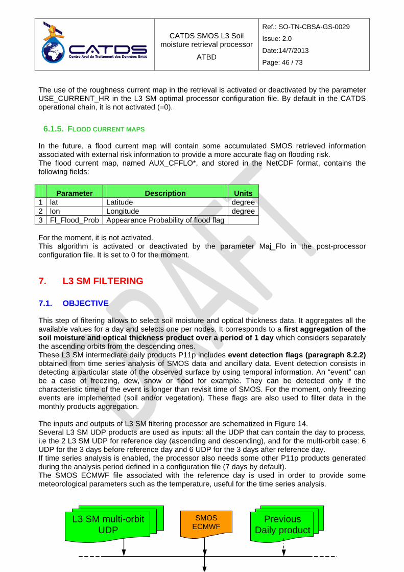
CATDS SMOS L3 Soil moisture retrieval processor
ATBD
Ref.: SO-TN-CBSA-GS-0029
Issue: 2.0
Date:14/7/2013
Page: 46 / 73
The use of the roughness current map in the retrieval is activated or deactivated by the parameter USE_CURRENT_HR in the L3 SM optimal processor configuration file. By default in the CATDS operational chain, it is not activated (=0).
6.1.5. FLOOD CURRENT MAPS
In the future, a flood current map will contain some accumulated SMOS retrieved information associated with external risk information to provide a more accurate flag on flooding risk. The flood current map, named AUX_CFFLO*, and stored in the NetCDF format, contains the following fields:
Parameter Description Units 1 lat Latitude degree 2 lon Longitude degree 3 Fl_Flood_Prob Appearance Probability of flood flag For the moment, it is not activated. This algorithm is activated or deactivated by the parameter Maj_Flo in the post-processor configuration file. It is set to 0 for the moment.
7. L3 SM FILTERING
7.1. OBJECTIVE
This step of filtering allows to select soil moisture and optical thickness data. It aggregates all the available values for a day and selects one per nodes. It corresponds to a first aggregation of the soil moisture and optical thickness product over a period of 1 day which considers separately the ascending orbits from the descending ones. These L3 SM intermediate daily products P11p includes event detection flags (paragraph 8.2.2) obtained from time series analysis of SMOS data and ancillary data. Event detection consists in detecting a particular state of the observed surface by using temporal information. An “event” can be a case of freezing, dew, snow or flood for example. They can be detected only if the characteristic time of the event is longer than revisit time of SMOS. For the moment, only freezing events are implemented (soil and/or vegetation). These flags are also used to filter data in the monthly products aggregation. The inputs and outputs of L3 SM filtering processor are schematized in Figure 14. Several L3 SM UDP products are used as inputs: all the UDP that can contain the day to process, i.e the 2 L3 SM UDP for reference day (ascending and descending), and for the multi-orbit case: 6 UDP for the 3 days before reference day and 6 UDP for the 3 days after reference day. If time series analysis is enabled, the processor also needs some other P11p products generated during the analysis period defined in a configuration file (7 days by default). The SMOS ECMWF file associated with the reference day is used in order to provide some meteorological parameters such as the temperature, useful for the time series analysis.
Previous Daily product
SMOS ECMWF
L3 SM multi-orbit UDP

CATDS SMOS L3 Soil moisture retrieval processor
ATBD
Ref.: SO-TN-CBSA-GS-0029
Issue: 2.0
Date:14/7/2013
Page: 47 / 73
Figure 14: CATDS L3 SM filtering processor inputs and outputs
7.2. DETAILED DESCRIPTION OF THE ALGORITHMS
The processing steps are the following ones: 1) A daily data aggregation, if several daily revisits are available (see Figure 18). Ascending
and descending orbits are processed separately. 2) Event detection (see paragraph 8.2.2): development in time series (ascending and
descending orbits together) and analysis of the time series to diagnose a particular behavior of the parameter evolution.
The processing chain is presented in Figure 15. The first step is always processed, while event detection should be activated or deactivated by the parameter ANALYSE_SERIE in the L3 SM filtering processor configuration file. By default in the CATDS operational chain, it is activated (=1).

CATDS SMOS L3 Soil moisture retrieval processor
ATBD
Ref.: SO-TN-CBSA-GS-0029
Issue: 2.0
Date:14/7/2013
Page: 48 / 73
Figure 15: L3 SM Filtering processing steps
7.2.1. DAILY AGGREGATION
This step is a reorganization of the data for obtaining a daily composite. The inputs of this step are the L3 SM UDP products that can contain an estimation of some parameters for the reference day. Ascending and descending orbits are processed separately. The algorithm consists in selecting a particular SM value for a day among all the SM values available the same day in L3 SM UDP products. It works around a reference day JREF, on a period of 7 days (JREF +/- 3 days), as presented on Figure 16. Note that this algorithm is
Event detection
Time series generation
L3 SM multi-orbit UDP
Ref. day –
1, 2, 3 Ref. day
+ 1, 2, 3
Daily aggregation
L3 SM Filtering processor
Ref. day
L3 SM daily product
Previous Daily prod.
Time series analysis
L3 SM daily product (with event flags)
Event flags
SMOS ECMWF
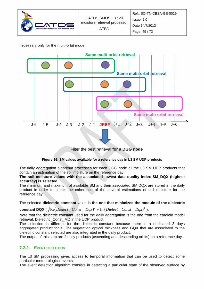
CATDS SMOS L3 Soil moisture retrieval processor
ATBD
Ref.: SO-TN-CBSA-GS-0029
Issue: 2.0
Date:14/7/2013
Page: 49 / 73
necessary only for the multi-orbit mode.
Figure 16: SM values available for a reference day in L3 SM UDP products
The daily aggregation algorithm processes for each DGG node all the L3 SM UDP products that contain an estimation of the soil moisture on the reference day. The soil moisture values with the associated lowest data quality index SM_DQX (highest accuracy) is selected. The minimum and maximum of available SM and their associated SM DQX are stored in the daily product in order to check the coherence of the several estimations of soil moisture for the reference day. The selected dielectric constant value is the one that minimizes the module of the dielectric
constant DQX ( ( ) ( )22 __Im__Re DqxConstDielectDqxConstDielect + ). Note that the dielectric constant used for the daily aggregation is the one from the cardioid model retrieval, Dielectric_Const_MD in the UDP product. The selection is different for the dielectric constant because there is a dedicated 3 days aggregated product for it. The vegetation optical thickness and GQX that are associated to the dielectric constant selected are also integrated in the daily product. The output of this step are 2 daily products (ascending and descending orbits) on a reference day.
7.2.2. EVENT DETECTION
The L3 SM processing gives access to temporal information that can be used to detect some particular meteorological events. The event detection algorithm consists in detecting a particular state of the observed surface by
JREF
J-1 J-3 J-2 J-4 J+1 J+2 J+3 J+4
Filter the best retrieval for a DGG node
J-5 J-6 J+5 J+6
Same multi-orbit retrieval
Same multi-orbit retrieval
Same multi-orbit retrieval

CATDS SMOS L3 Soil moisture retrieval processor
ATBD
Ref.: SO-TN-CBSA-GS-0029
Issue: 2.0
Date:14/7/2013
Page: 50 / 73
using temporal information [2bis]. This is a change detection algorithm. Event flags are updated in the daily products from a time series analysis. Time series of 7 days (configurable with the parameter TEMP_SERIE) are thus generated and analyzed. In the L2 processing, climate date from auxiliary ECMWF product yield the Non Permanent Event (like snow) fractions. However, it is possible that, on a grid node, this information is partially erroneous so that contributions to the simulated brightness temperatures will be inaccurate and/or biased. In this case, one could possibly detect such inaccuracies by analyzing the evolution of the geophysical parameters which will be over or underestimated. Also the information given by weather prediction model can be partially erroneous with a given uncertainty in this case the observation from SMOS can be useful to enhance the event flagging. The signature of these events on the estimation of soil moisture and other retrieved parameters is analysed which can allow us to detect them. This kind of diagnostic should be done from time series analysis when geophysical parameters estimators behave in an unexpected way. To help the diagnostic, additional information (temperature of surface, precipitations… etc) coming from external data, such as ECMWF data, are taken into consideration. The following events are potentially detectable by SMOS:
- freezing of soil and/or vegetation - dew or morning freezing - snow - ice - flood - interception of rain by vegetation (canopy, litter)
For the time being, the event detection algorithm in the CATDS chain is configured to detect the following the soil freezing and thawing
Differentiation of the vegetation freezing from soil freezing is implemented but not activated because the optical thickness change is not accurate enough to get to this level of detail. From our actual knowledge of the SMOS signal it seems that the use of angular signature and polarization signature essential to differentiate the event. This is being inspected.
7.2.2.1. Time series generation For a reference day, a time series is made to be analyzed for event detection. This time series is a chronological data reorganization of daily products, ascending and descending, over a period of 7 days. This number of days is configurable with the parameter TEMP_SERIE in the L3 SM filtering processor configuration file, the default value being 7 days. It includes the products of the reference day and the complementary products from the 6 days before the reference day. The reference day is then the last day of the time series (Figure 17).
Figure 17: time series of daily products, J0 being the reference day. Jc is a complementary day. Red dots are the reference day, blue are previous ascending retrievals and green are previous
Jc-3,a Jc-3,d Jc-2,a Jc-2,d Jc-1,a Jc-1,d Jc-5,d Jc-5,a Jc-6,d Jc-6,a Jc-7,d
desc Jc-7,a
asc J00,a J00,d

CATDS SMOS L3 Soil moisture retrieval processor
ATBD
Ref.: SO-TN-CBSA-GS-0029
Issue: 2.0
Date:14/7/2013
Page: 51 / 73
descending retrievals used for the event detection
In the time series, ascending products are always placed before descending products in the same day, because the solar local time for ascending orbits is about 6 a.m. (in the morning) and for descending orbits the solar local time is about 6 p.m. (in the afternoon). Ascending and descending products are thus distinguished by even and odd subscripts. Daily products contain event detection flags updated at the end of the analysis of each reference day. The time series contain these updated daily products with the information of event detection of the previous days.
7.2.2.2. Time series analysis The time series analysis aims at determining the value of the reference day events flags. The inputs of this step are the time series and the ECMWF files associated with the reference day. For a reference day, 2 measurements can be available in ascending and descending products. If both measurements are available, the analysis should be done on the afternoon orbit first (descending orbit type) and then on the morning orbit (ascending orbit type) because the frost risk is higher in the morning, so the knowledge of the state of the event flag in the afternoon will help to detect the frost in the morning. The event detection is based on a 3 stages detection algorithm. For each event, the following processing is applied:
1) Verification of spatio-temporal constraints: First, the probability of occurrence of the event on a DGG is assessed. This probability depends on spatio-temporal constraints, or climatic constraints from ancillary data. For example, freezing conditions occur only in some regions of the Earth.
2) “State tests”: Then, the values of geophysical retrieved parameters on the reference day are an indication on the state of the surface, and are also tested. If we keep the example above, freezing conditions need low temperature near 0°C or less.
A list of thresholds is defined for each constraint taking into account their uncertainties. An event is declared as probable if all the tests are positive.
3) Temporal evolution: The last stage consists in testing the temporal evolution of a list of selected geophysical parameters for each event over a 7 days period. This period ensures a minimum of 2 revisits per grid node. The evolution (∆X = XJc-XJ0) is computed between complementary maps that are probable and the reference day map. X is the analyzed parameter in the temporal evolution step. The event is confirmed if the parameters evolutions coincide with the expected evolution for the tested event and that for all parameters. The changes of state or, on the contrary, the stagnation are indicators of the actual state of the surface. For example, during a freezing event the soil dielectric constant decreases drastically and can be detected.
It is the combination of all the indicators that can bring to light some events. The stages of the event detection algorithm are presented on Figure 18. In this example, a chronicle of soil moisture is presented with a temporal sampling representative of this period. The values are given for information purposes only. At the end of the analysis, event flags are updated in the P11p product that corresponds to the reference day processed (J0,a or J0,d). The different values of an event flag (named FL_EV_xxx, xxx

CATDS SMOS L3 Soil moisture retrieval processor
ATBD
Ref.: SO-TN-CBSA-GS-0029
Issue: 2.0
Date:14/7/2013
Page: 52 / 73
depending on the name of the event) is presented in Table 14. Bit
code Value of the flag
FL_EV_XXX Meaning
00 -1 Missing value 01 0 The event is not verified 10 1 The event is plausible but not validated by the temporal analysis 11 2 The plausible event is verified by the time series analysis
Table 6: Meaning of the event flag
Figure 18: Time series analysis for the reference day J0
Time
FL_EV_xxx=2
True
False True
FL_EV_xxx=1
False
FL_EV_xxx=0
Spatio-temporal constraints
State tests
Temporal evolution
FL_EV_xxx=1
Jc-3,a Jc-3,d Jc-2,a Jc-2,d Jc-1,a Jc-1,d Jc-5,d Jc-5,a Jc-6,d Jc-6,a Jc-7,d
desc Jc-7,a
asc J00,a J00,d
Test FL EV ≠ 1
Test FL EV ≠ 1
Test FL EV ≠ 1
Test FL EV ≠ 1
SM
True
True
True True True False

CATDS SMOS L3 Soil moisture retrieval processor
ATBD
Ref.: SO-TN-CBSA-GS-0029
Issue: 2.0
Date:14/7/2013
Page: 53 / 73
7.2.2.2.1. Event characterization
The event detection algorithm is parameterized according to the event to identify. Each event has its own temporal signature on the retrieved parameters. The parameterization of the algorithm is defined for freezing soil and freezing vegetation. The frost can affect soil and/or vegetation. Some experiences has shown that soil dielectric properties of frozen soil are very close to a dry soil, whereas water frost on the vegetation or vegetation freezing make the vegetation almost transparent in L-band [23]. The freezing/thawing is characterized by an important variation of the emitted L-band brightness temperature, which can be detected, if a non-negligible proportion of the surface contributing to the signal is affected by the frost. Freezing soil and freezing vegetation have not the same effect on the signal; the 2 events are thus processed separately. For the forests, branches and trunks contribute strongly to the signal because their dimensions are comparable to the wavelength in L-band (λ = 21 cm). However, during freezing period, the water contained in these elements does not often freeze. So, it will be difficult to observe a case of freezing forest. if the freezing of the soil is superficial (low penetration depth), the measured brightness temperatures are affected by contributions from deeper layers. It is thus possible not to be able to measure a significant effect of the frost on the signal, and so to not detect the event. The next tables present the characteristics and the parameters that are used in the CATDS algorithms to detect a case of freezing soil (Table 15) and freezing vegetation (Table 16).
Freezing soil
Flag name FL_EV_FRS
Description
When the surface temperature is negative, the soil freezes: the water in the soil becomes solid to a certain depth and the resulting dielectric constant is greatly reduced. The soil emissivity increases. The L-band signal becomes closer to the signal of a dry soil.
Spatio-temporal constraints
Geographic constraints:
Select the latitudes from where the event is probable.
TH_FRS_LATMIN < abs(LAT) < TH_FRS_LATMAX
LAT: Latitude
Temporal constraints:
Select the seasons where the event is probable.
TH_FRS_DMIN < DOY < TH_FRS_DMAX
DOY: Day Of Year
State tests
Nominal fraction of the retrieval:
Work only on nominal soil FNO or frozen soil FRZ
FMO = TH_FRS_FM0
FM0: Nominal fraction of the retrieval

CATDS SMOS L3 Soil moisture retrieval processor
ATBD
Ref.: SO-TN-CBSA-GS-0029
Issue: 2.0
Date:14/7/2013
Page: 54 / 73
Test on the decision tree branch (FNO or FRZ)
Surface temperature is low STL1 < TH_FRS_TS
STL1: temperature of the first soil layer (K), from the ECMWF data
Retrieved soil moisture is low
SM + σ _SM < TH_FRS_SM
SM: soil moisture
σ _SM: SM uncertainty = Soil_Moisture_Dqx
The module of the retrieved dielectric constant (MOD_EPS ) is low
MOD_EPS + σ_MOD_EPS < TH_FRS_MOD_EPS
MOD_EPS = 22 ''' εε +
MOD_EPS: dielectric constant module
ε’: real part of the dielectric constant
ε’’: imaginary part of the dielectric constant
σ _MOD_EPS: MOD_EPS uncertainty
22
22
'''
''_'_21__
εε
εσεσσ
+
+=EPSMOD
σ _ ε’ : ε’ uncertainty = Re(Dielect_Const_Dqx)
σ _ ε’’ : ε’’ uncertainty = Im(Dielect_Const_Dqx)
Temporal evolution
Strong decrease in the soil moisture compared to unfrozen ground
DSM - σ _DSM > TH_FRS_DSM
DSM: SM variation between a complementary day JCi and the refrence day J0
DSM = SMJCi – SMJ0
σ_DSM: DSM uncertainty
σ_DSM = 2J0
2JC _SM_SM σσ +
Decrease in the polarization ratio compared to unfrozen soil
DPR - σ _DPR > TH_FRS_DPR
PR: polarization ratio at 42.5°
5.425.42
5.425.42
TBhTBvTBhTBv
PR+−
=

CATDS SMOS L3 Soil moisture retrieval processor
ATBD
Ref.: SO-TN-CBSA-GS-0029
Issue: 2.0
Date:14/7/2013
Page: 55 / 73
The TBh42.5 and TBv42.5 used in the computation of PR are the modelled TBs at surface level (Tb_Asl_Theta_B_H and Tb_Asl_Theta_B_H in P11p product).
( )( )2
5.425.42
5.425.425.425.42 __2_
TBhTBvTBvTBhTBhTBv
PR+
⋅−⋅⋅=
σσσ
DPR = PRJCi – PRJ0
DPR: polarization ratio variation between a complementary day JCi and the reference day J0
σ _DPR: polarization ratio uncertainty
σ _DPR = 2J0
2JC _PR_PR σσ +
Threshold values
Decision tree branch number TH_FRS_FMO = [9, 10, 12]
Threshold on soil moisture value TH_FRS_SM = 0.10 m3/m3
Threshold on surface temperature value TH_FRS_TS = 273.15 K
Variation of soil moisture TH_FRS_DSM = 0.15 m3/m3
Variation polarization ratio TH_FRS_DPR = 0.02
Threshold on the dielectric constant module value TH_FRS_MOD_EPS = 15
Latitudes of interest TH_FRS_LATMIN = 0.0 ° TH_FRS_LATMAX = 87.0 °
Day Of Year start and stop TH_FRS_DMIN = 1 TH_FRS_DMAX = 365
Table 7: Characteristics of the event “freezing soil” The spatio-temporal constraints are undifferentiated between the two terrestrial hemispheres. Although the risk of freezing is generally not identical between the two hemispheres at a given date, this solution gives the possibility to detect punctual freezing events.
Freezing vegetation
Flag name FL_EV_FRV
Description

CATDS SMOS L3 Soil moisture retrieval processor
ATBD
Ref.: SO-TN-CBSA-GS-0029
Issue: 2.0
Date:14/7/2013
Page: 56 / 73
When the air temperature is negative, the vegetation can freeze. A frozen vegetation becomes transparent at L-band, so only the soil contributes significantly to the signal. The result is a strong decrease in the vegetation optical thickness.
Spatio-temporal constraints
Geographic constraints:
Select the latitudes from where the event is probable.
TH_FRS_LATMIN < abs(LAT) < TH_FRS_LATMAX
LAT: Latitude
Temporal constraints:
Select the seasons where the event is probable.
TH_FRS_DMIN < DOY < TH_FRS_DMAX
DOY: Day Of Year
State tests
Nominal fraction of the retrieval:
Work only on nominal soil FNO or frozen soil FRZ
FMO = TH_FRS_FM0
FM0: Nominal fraction of the retrieval
Test of the decision tree branch (FNO or FRZ)
Low vegetation temperature is low
SKT < TH_FRV_TC
SKT: Soil skin temperature (K) from ECMWF data
Retrieved vegetation optical thickness is low
TAU + σ _TAU < TH_FRV_TAU
Tau: vegetation optical thickness
σ_TAU: TAU uncertainty = Optical_Thickness_NadDqx
Temporal evolution
Strong decrease in the vegetation optical thickness compared to unfrozen vegetation
DTAU - σ _DTAU > TH_FRV_DTAU
DTAU: Tau variation between a complementary day JCi and the refrence day J0
DTAU = TAUJCi – TAUJ0
σ _DTAU: DTAU uncertainty
σ_DTAU = 2J0
2JC _TAU_TAU σσ +
Threshold values
Decision tree branch number TH_FRS_FMO = [9, 10, 12]
Threshold on canopy temperature TH_FRV_TC = 273.15 K

CATDS SMOS L3 Soil moisture retrieval processor
ATBD
Ref.: SO-TN-CBSA-GS-0029
Issue: 2.0
Date:14/7/2013
Page: 57 / 73
value
Threshold on vegetation optical thickness value TH_FRV_TAU = 0.1
Variation of vegetation optical thickness TH_FRV_DTAU = 0.2
Latitudes of interest TH_FRS_LATMIN = 0.0 ° TH_FRS_LATMAX = 87.0 °
Day Of Year start and stop TH_FRS_DMIN = 1 TH_FRS_DMAX = 365
Table 8: Characteristics of the event “freezing vegetation” All the threshold values in Table 15 and Table 16 are given in the L3 SM filtering processor configuration file and can be modified if needed. Other events can be detected by SMOS and may be considered in the future evolutions of the CATDS algorithm. It includes:
- The relative variations of the equivalent dielectric constant should allow us to detect rapid changes of the surface state.
- Flood could be detected by a strong increase in SM and dielectric constant and a high value of ECMWF total precipitation.
- Rain interception could be detected by a strong increase in Tau and a high value of ECMWF total precipitation.
- Some diurnal effects like dew and frost show different values of Tau in the morning and in the afternoon.
Nevertheless, the algorithms are not so simple and have to be tested before being implemented in the CATDS chain.
7.2.2.2.2. Verification of spatio-temporal constraints
This first analysis is to identify DGG nodes that can be a priori affected by the event being detected. The geographical location of the node DGG is tested. It can also be defined by an occurrence map of the tested event. Several maps of occurrence may exist for the same event depending on the season. This approach needs climatic information from ancillary data, and is not implemented. For the time being, the test for freezing is reduced to check the latitude and the day of the year. The Table 15 and Table 16 show the settings to use depending on the event. If the result of a test is "FALSE", the event detection on the DGG node stops and the flag is set FL_EV_xxx = 0. If it is “TRUE”, it continues with the additional tests presented in the next paragraph.
7.2.2.2.3. Test of the state of the reference day map
This second step determines whether or not an event is plausible, depending on the values of some parameters. The analysis is conducted on the reference day products. The Table 15 and Table 16 show the settings to use depending on the event. Table 17 shows the list of parameters to be tested for each event Ei.

CATDS SMOS L3 Soil moisture retrieval processor
ATBD
Ref.: SO-TN-CBSA-GS-0029
Issue: 2.0
Date:14/7/2013
Page: 58 / 73
FM0 SM Tau MOD_EPS PR STL1 SKT
E1: Freezing soil X X X X
E2: Freezing vegetation X X X
Table 9: “State tests” to apply for event detection For an event Ei, a set of parameters {Xi} is tested, the test status of each parameter is noted RXi, it is given by the following rules:
- If a parameter Xi is not available (missing value), it is not included in the tests: RXi = -1 - If the test result is "True": RXi = 1 - If the test result is "False": RXi = 0
The final result of “state tests” on a DGG node and for an event Ei is given by the following rules:
- If one test is "FALSE" (RXi = 0) or if no test is performed: FL_EV_xxx = 0 - If at least one test is performed and all results are "TRUE" (RXi = 1): FL_EV_xxx = 1
It can be summarized by this formula: ∏ −≠=Xi
RXiRXixxxEVFL )1/(__
An event is declared as probable if all the tests are positive (FL_EV_xxx = 1).
7.2.2.2.4. Temporal evolution
The last step tests the temporal dynamics and identifies unexpected evolutions linked with an event. The idea is that for a DGG node some changes can be observed between the reference day and the complementary days. The temporal evolution of a list of selected geophysical parameters is tested for each event over a 7 days period.. The state of the complementary days is known throughout the event flags (updated when the previous reference days were analyzed), except for initialization (see §7.2.2.2.5). If two days have a different state, it must be sufficiently strong to be attributed to an event (this variation is small for similar states). As shown in Figure 18, only probable events are tested, i.e.FL_EV_xxx = 1 for the reference day J0. For the event Ei, the evolution of several parameters {DXi} is computed between complementary maps that are probable and the reference day map. It is tested with DXi = DXJi - DXJ0. X is the analyzed parameter in the temporal evolution step. Table 18 shows the list of parameters tested for each event Ei. DSM DPR DTAU E1: Freezing soil X X
E2: Freezing vegetation X
Table 10: Evolution tests to apply for event detection For a given parameter, the set of pair of days (Jc, J0) are tested. The example in Figure 18 has the following pairs: {DXJ-7a,J0, DXJ-6d,J0, DXJ-3a,J0, DXJ-2d,J0}. The test result of each DXi is RDXJci,J0 , which is given by the following rules:
- If a parameter Xi is not available (missing value), it is not included in the tests: RXi = -1

CATDS SMOS L3 Soil moisture retrieval processor
ATBD
Ref.: SO-TN-CBSA-GS-0029
Issue: 2.0
Date:14/7/2013
Page: 59 / 73
- If the test result is "True": RXi = 1 - If the test result is "False": RXi = 0
- If a parameter Xi is not available (missing value), the test is not applied on this parameter:
RDX = -1
- The additional day Jc with a flag FL_EV_xxx = 1 are not included in the tests, because the event is not confirmed, so we are not sure of its state: RDX = -1
- If the additional day Jc has no event detected, i.e. with a flag FL_EV_xxx = 0:
If DX - σ_DX > TH_FRX_DX, the result is "True": RDX = 1, there was no event before the reference day, the parameters have evolved significantly at the reference day, so it is confirmed that a change of state happened between the 2 days Jc and J0. else the result is "False": RDX = 0, there was no event before the reference day, the parameters haven’t evolved significantly at the reference day, so it is confirmed that there is no change of state between the 2 days Jc and J0.
- If the additional day Jc has a detected event, i.e. with a flag FL_EV_xxx = 2:
If abs(DX - σ_DX) < TH_FRX_DX, the test is "True": RDX = 1, an event was detected before the reference day, the parameters haven’t evolved at the reference day. It is confirmed that no change of state happened between the 2 days Jc and J0. The event is still present. Else the test is "False": RDX = 0, an event was detected before the reference day, the parameters have evolved significantly at the reference day. A change of state happened between the 2 days Jc and J0.and so the event is confirmed.
Every complementary day is tested, and finally a result of the evolution test is available for each day: RDX = 0 or RDX = 1. Then, every day in the time series is weighted by its distance from the reference day. The idea is to give more importance to the days closest to the reference day, in order to enhance the sudden appearance of the event (like freezing). The result of each day is thus weighted, to compute a weighted mean of the results, MRDX:
∑⋅+⋅+⋅+⋅+⋅+⋅+⋅
=
ii
JcJcJcJcJcJcJc
cRDXcRDXcRDXcRDXcRDXcRDXcRDXc
MRDX 00665544332211
The values RDXJci = -1 are not taken into account in the sum. The coefficients ci, that are the weight of each day in the temporal evolution analysis, are given by an exponential law:
)exp(TCW
TTWMAXc refi
i
−−⋅=
With: WMAX is the maximum weight at Tref, by default WMAX = 1 Ti is the time of the day i, expressed in seconds Tref is the time of the reference day, expressed in seconds
( ))ln(
86400*1_
WMINWMAX
SERIETEMPTCW −=

CATDS SMOS L3 Soil moisture retrieval processor
ATBD
Ref.: SO-TN-CBSA-GS-0029
Issue: 2.0
Date:14/7/2013
Page: 60 / 73
WMIN is the minimum weight at the beginning of the time series, by default WMIN = 0.5.
For a given test on the parameter X, the weighted mean of the results (MRDX) is compared to a threshold (TH_FL_EVENT, default value = 0.5): If MRDX > TH_FL_EVENT, then the result is “True”, else it is “False”. If all the tests on the several parameters X give a result "True" with at least one test applied, then the evolution test is positive, the event is confirmed: FL_EV_xxx = 2. The parameters evolutions coincide with the expected evolution for the tested event and that for all parameters. Else, if at least one test is negative (false), FL_EV_xxx = 1, the event is not confirmed by the temporal analysis, it is just “probable”. The event flags FL_EV_xxx are updated in the daily product. The parameters WMIN (Minimal temporal weighting), WMAX (Maximal temporal weighting), and TH_FL_EVENT (Threshold of evolution test flags consistency) are defined in the L3 SM filtering processor configuration file. If we want to give the same weight to every days in the time series, the default values of WMIN can be changed by a number very close to 1. Note that a value of 1 will lead to an indecision in the computing of TCW (see equation above).
7.2.2.2.5. Initialization
Initialization is required only the first time a time series is analyzed during the processing. The complementary days don’t have yet a valid flag for FL_EV_xxx (FL_EV_xxx = -1). It consists in applying the “state tests” to the complementary days, and then all the events considered probable will be confirmed. Then, all flag FL_EV_xxx = 1 will be replaced by FL_EV_xxx = 2.
7.3. DAILY PRODUCTS
This subsection provides the list of data present in the L3 SM daily products, at the end of the L3 SM filtering processing. The format of the product is NetCDF. Only retrieved parameters are in the product, i.e. no default value is reported. Table 19 L3 SM daily product contains the following fields: Table 11: L3 SM daily products description
Parameter Description Units 1 lat Latitude of each point in the product degree
2 lon Longitude of each point in the product degree
3 Mean_Acq_Time_Days Day of mean time of acquisition associated with the selected soil moisture value of DGG point
day
4 Mean_Acq_Time_Seconds Seconds of mean time of acquisition associated with the selected soil moisture value of DGG point
s
5 Mean_Acq_Time_Days2 Day of mean time of acquisition associated with the selected dielectric constant value of DGG point
day
6 Mean_Acq_Time_Seconds2 Seconds of mean time of acquisition associated with the selected dielectric constant value of DGG point
s

CATDS SMOS L3 Soil moisture retrieval processor
ATBD
Ref.: SO-TN-CBSA-GS-0029
Issue: 2.0
Date:14/7/2013
Page: 61 / 73
7 Soil_Moisture Retrieved soil moisture value m3.m-3
8 Soil_Moisture_Dqx DQX for Soil_Moisture m3.m-3
9 Optical_Thickness_Nad Nadir optical thickness estimate for vegetation layer associated to the Soil_Moisture, DGG per DGG
neper
10 Optical_Thickness_NadDqx DQX for Optical_Thickness_Nad neper
11 Optical_Thickness_Nad2 Nadir optical thickness estimate associated to the Dielectric Constant, DGG per DGG
neper
12 Optical_Thickness_NadDqx2 DQX of Optical_Thickness_Nad2 neper
13 Dielect_Const Dielectric constant (complex value) F.m-1
14 Dielect_Const_Dqx DQX of Dielectric constant (complex value) F.m-1
15 Hr Maximal roughness
16 Hr_Dqx DQX of Maximal roughness
17 Scattering_Albedo_H Albedo on H polarization
18 Scattering_Albedo_H_Dqx DQX of Albedo on H polarization
19 Diff_Albedos Albedo difference on H and V polarization
20 Diff_Albedos_Dqx DQX of Albedo difference on H and V polarization
21 Surface_Temperature Surface temperature associated to the Soil_Moisture, DGG per DGG
K
22 Surface_Temperature_Dqx DQX of surface temperature K
23 Temp_STL1 ECMWF temperature of the first soil layer associated with the selected SM
K
24 Temp_SKT ECMWF soil skin temperature associated with the selected SM K
25 S_Tree_1 Decision tree branch associated with the selected SM
26 Tb_Toa_Theta_B_X Top of the atmophere TB computed from forward model at specific incidence angle theta_B (42.5°), and for X polarization, at the antenna frame
K
27 Tb_Toa_Theta_B_X_Dqx DQX of Tb_Toa_Theta_B_X K
28 Tb_Toa_Theta_B_Y Top of the atmophere TB computed from forward model at specific incidence angle theta_B (42.5°), and for Y polarization, at the antenna frame
K
29 Tb_Toa_Theta_B_Y_Dqx DQX of Tb_Toa_Theta_B_Y K
30 Tb_Asl_Theta_B_H Surface level TB (corrected from sky/atmosphere contribution) computed from forward model with a specific incidence angle theta_B (42.5°), and for H polarization, at the Earth frame
K
31 Tb_Asl_Theta_B_H_Dqx DQX of Tb_Asl_Theta_B_H K
32 Tb_Asl_Theta_B_V Surface level TB (corrected from sky/atmosphere contribution) computed from forward model with a specific incidence angle theta_B (42.5°), and for V polarization, at the Earth frame.
K
33 Tb_Asl_Theta_B_V_Dqx DQX of Tb_Asl_Theta_B_V K
34 Scientific_Flags They are the Science_Flags associated with the selected SM, See Table 8

CATDS SMOS L3 Soil moisture retrieval processor
ATBD
Ref.: SO-TN-CBSA-GS-0029
Issue: 2.0
Date:14/7/2013
Page: 62 / 73
35 Fno Mean fraction in FM0 class for FNO
36 Ffo Mean fraction in FM0 class for FFO
37 M_Ava0 number of TB measurements available in L1C
38 M_Ava Pre-processing number of TB measurements available in L1C
39 N_Rfi_X Count of deleted TBs due to suspected RFI
40 N_Rfi_Y Count of deleted TBs due to suspected RFI
41 Min_Soil_Moisture Minimum value of available SM m3.m-3
42 Max_Soil_Moisture Maximum value of available SM m3.m-3
43 Min_Soil_Moisture_Dqx Dqx associated with the minimum value of SM m3.m-3
44 Max_Soil_Moisture_Dqx Dqx associated with the maximum value of SM m3.m-3
45 Soil_Moisture_Init_Val Initial value for free parameter SM m3.m-3
46 Soil_Moisture_Init_Std Initial standard deviation for free parameter SM
47 Gqx Global Quality Index associated to the Soil_Moisture, DGG per DGG
48 Gqx2 Global Quality Index associated to the Dielectric Constant, DGG per DGG
49 Event_Flags See Table 20
50 Rfi_Prob RFI Probability The parameter Event_Flags contains flags from temporal series analysis. Each flag is composed of 2 bits with the following meaning: 00 | 0 Not verified 01 | 1 Possible 10 | 2 Sure 11 | 3 Not processed, stands for -1 (missing value) At the moment, only the freezing of the soil can be detected by the processor. The freezing of the vegetation, even though implemented, is not activated and is under validation: the event flags are organised like that: [00 00 00 00 00 00 XX XX] where X = 0 or 1 VEG SOIL With this convention, the fill value of this parameter is [00 00 00 00 00 00 11 11], which corresponds to a numerical value of 15. The Table 20 presents the event flags organization: Table 12: Event flags description
Parameter Description Size (bits) FL_EV_Frost_soil Event flag on the detection of soil freezing, result of the time series
analysis 2
FL_EV_Frost_veg Event flag on the detection of vegetation freezing, result of the time series analysis
2

CATDS SMOS L3 Soil moisture retrieval processor
ATBD
Ref.: SO-TN-CBSA-GS-0029
Issue: 2.0
Date:14/7/2013
Page: 63 / 73
Spare Padded with 0 12
8. L3 SM AGGREGATION
8.1. OBJECTIVE
The objective of this last processing is to generate the CATDS L3 SM temporal syntheses over different time steps with global coverage. Daily maps are aggregated over several time periods. The need for temporal syntheses is not the same depending on the application, so 3 aggregation types have been defined:
- Over a 3-day period (P1 and P4 products) - Over a10-day period (P2 products) - Over one month (P3 products)
The inputs and outputs of L3 SM aggregation processor are schematized in Figure 19.
Figure 19: CATDS L3 SM aggregation processor inputs and outputs
8.2. DETAILED DESCRIPTION OF THE ALGORITHMS
The algorithm deals with time aggregation only, i.e.no space averaging is considered. The aggregation of ascending orbits and descending orbits are processed separately The 3 aggregation types lead to 3 separate processing. The L3 SM aggregation processor has 3 modules that work separately but with common daily products as input, as schematized in Figure 20.
L3 aggregation processor
L3 SM daily product Over several time periods
3-day global products
10-day global product
1 month global product

CATDS SMOS L3 Soil moisture retrieval processor
ATBD
Ref.: SO-TN-CBSA-GS-0029
Issue: 2.0
Date:14/7/2013
Page: 64 / 73
The next paragraphs present the algorithms used on these 3 kinds of aggregation methods.
Figure 20: L3 SM Aggregation modules
8.2.1. THREE DAY AGGREGATION
The 3-day aggregation generates, on a daily basis, global L3 SM and products on a 3-day sliding window. The main advantage is that the whole Earth's surface is covered in this 3-day product. The first step to compute the 3-day product for a given day “n” is to select the daily products at days “n-2”, “n-1” and “n”. Ascending and descending orbits are processed separately. The aggregation consists in selecting the best retrieval available on the period of 3 days if there are several values available. For the soil moisture product, the best estimation is chosen from the set of retrievals of soil
L3 SM daily product Over several time periods
3 day global products
10 day global product
1 month global product
3-day aggregation
L3 SM Aggregation processor
10-day aggregation
Monthly aggregation

CATDS SMOS L3 Soil moisture retrieval processor
ATBD
Ref.: SO-TN-CBSA-GS-0029
Issue: 2.0
Date:14/7/2013
Page: 65 / 73
moisture available on the period of 3 days by selecting the lowest soil moisture DQX. The other parameters are those retrieved at the same time as the selected SM, in order to be consistent in the same product daily L3 product (P1). All the geophysical parameter estimations are relative to the same date. For the dielectric constant product (P4), the best estimation is chosen from the set of retrievals of dielectric constant available on the period of 3 days by selecting the lowest dielectric constant DQX. As for the daily product (P1), the other parameters retrieved at the same time as the selected dielectric constant are selected, in order to have a consistent product, i.e. having all the geophysical parameter estimations relative to the same date. These 2 products, 3days soil moisture (P1) and dielectric constant (P4) are generated on a daily basis, with a 3-day sliding window (Figure 21).
Figure 21: 3-day products The 3 day aggregation is activated by the parameter FlagAgreger3j that must be “true” in the L3 SM Aggregation processor configuration file. In addition, a minimal number of days from which computations can be performed is defined: NbJoursMinAgr3j. This parameter is in the L3 SM Aggregation processor configuration file, its default value is 1.
8.2.2. 10-DAY AGGREGATION
The 10-day aggregation generates global L3 SM products on a 10-day period (no sliding window), from 10 intermediate daily products P11p, see Figure 22. Ascending and descending orbits are processed separately. This product is composed of three soil moisture values per grid node: the median, minimum and maximum values of soil moisture that are extracted out of 10 daily products. The corresponding other parameters, retrieved at the same time as the selected SM, (nominal retrieval fraction, tau, DQX, etc.) are also extracted and included in this product. Three products per month are delivered, meaning that the last one of each month can cover from 8 to 11 days according to the month. Figure 22 shows aggregation strategy for 10-day period.
d_3 d_4 d_5 d_6 …
...
Days 1 2 3 4 5 6 7 8 9 10 11 12 ...

CATDS SMOS L3 Soil moisture retrieval processor
ATBD
Ref.: SO-TN-CBSA-GS-0029
Issue: 2.0
Date:14/7/2013
Page: 66 / 73
Figure 22: 10 day product (P2) obtained at the dates d_5, d_15, The mean GQX (quality indicator) on the 10-day product is computed as follow:
n
iGQXdecadeGQX
n
i∑== 1
__
Where: i corresponds to the day i The sum is computed considering n days of the 10 days when data are available and not contaminated by an event.
The 10-day aggregation is activated by the parameter FlagAgreger10j that must be “true” in the L3 SM Aggregation processor configuration file. In addition, a minimal number of days from which computations can be performed is defined: NbJoursMinAgr10j. This parameter is in the L3 SM Aggregation processor configuration file and its default value is 3. It means that the processor needs at least 3 days in the 10-day period to process this product, otherwise there won’t be a median, a minimum and a maximum value. In order to have a full coverage of the world, the missing soil moisture is replaced by the mean value of the initial soil moisture values over the period of 10 days, computed from the ECMWF data. In that case, their GQX are set to missing value.
8.2.3. MONTHLY AGGREGATION
The monthly aggregation generates global L3 SM products per month, referred to as P3, from daily products. Ascending and descending orbits are still processed separately. This kind of product is useful for climate monitoring. For each DGG node, it provides a weighted mean of soil moisture, vegetation optical thickness, and RFI statistics over a month, without taking into account the detected events reported in the daily product. There is no sliding window, an estimation is done month by month, as presented on Figure 23. The number of days to be considered depends on the number of days in the month (28 to 31 days).
P2 10-day product 10-day product …
Days 1 2 3 4 5 6 7 8 9 10 11 12 13 14 15 16 17 18 19 …

CATDS SMOS L3 Soil moisture retrieval processor
ATBD
Ref.: SO-TN-CBSA-GS-0029
Issue: 2.0
Date:14/7/2013
Page: 67 / 73
Figure 23: monthly products
The values taken into account in the computation of the weighted mean of a parameter must not be affected by an event. So, only values from P11p with all the event flags FL_EV_xxx set to 0 are taken into account. The decision tree branch in the majority over the month is considered. Only soil moisture values associated with this decision tree branch are taken into account in the computation of the weighted mean. For the computation of the weighted mean of low vegetation optical thickness, only retrievals over a nominal fraction are taken into account (decision tree branch = 12). For the computation of the weighted mean of forest optical thickness, only retrievals over a forest fraction are taken into account (decision tree branch = 11). • The average parameter over a month, P_month, to be estimated (soil moisture SM, tau, etc) is
obtained with a weighted error (DQX). This temporal mean (no spatial average) is computed for each grid node. The weighted average for a parameter P, is computed as:
( )
( )∑
∑
=
== n
i
n
i
iPDQX
iPDQXiP
monthP
12
12
__1
___
_
Where: i corresponds to the day i
The sum is computed considering n days of the month when data are available and not contaminated by an event. DQX_P_i corresponds to the theoretical uncertainty for parameter P, at the day i
• The variance in the monthly product, VAR_P is computed as follow: The total variance (VAR_total) observed on the parameter P over one month is due to the combined effect of the real geophysical variance coming from climatic events (VAR_P) and the variance of the retrieval coming from the uncertainty of instrument and the errors of the retrieval algorithm. The latest one can be assimilated to a “noise” it may not be stationary if the instrument is presenting a drift or if special events occurs like RFI burst.. So if the user is interested in the geophysical variance we have, VAR_P = VAR_total – VAR_P_month and
P3 Monthly product Monthly product ...
Days 1 2 30 31 1 2 29 30 …

CATDS SMOS L3 Soil moisture retrieval processor
ATBD
Ref.: SO-TN-CBSA-GS-0029
Issue: 2.0
Date:14/7/2013
Page: 68 / 73
( ) ( )
n
iPDQX
n
monthPiPPVAR
n
i
n
i∑∑== −
−= 1
2
1
2 _____
The associated standard deviation is then:
( ) ( )
n
iPDQX
n
monthPiPPVARPSTD
n
i
n
i∑∑== −
−== 1
2
1
2 ______
The idea of taking into account the DQX in the formula allows us to check if the variation is due to a geophysical phenomenon and not due to significant noise measurements. When the number of retrieved values n increases, the monthly DQX decreases and the impact of instrument noise is less important. • The mean DQX_P_month is the mean error of P_i over one month (and not the error
associated to P_month). It has to be taken at the quadratic point of view:
( )
n
iPDQXmonthPDQX
n
i∑== 1
2____
• The mean GQX (quality indicator) is computed as follows (without DQX weighting):
n
iGQXmonthGQX
n
i∑== 1
__
• Concerning the RFI field, the percentage of the contaminated views will be aggregated for each
EASE grid node. RFI_month is the number of RFI-contaminated SMOS TB for a given grid node in the considered month:
∑=
=n
iiRFImonthRFI
1__
TOTview_month is the number of SMOS TB for a given grid node in the considered month:
∑∑==
==n
i
n
iiMAVAiVIEWmonthTOTview
11___
fracRFI_month presents the fraction of contaminated SMOS TB in the considered month:
monthTOTviewmonthRFImonthfracRFI_
__ =
In the P3 product, the fraction of RFI in the month is polarization dependent:
∑
∑
=
== n
i
n
i
iMAVA
iXNRFIFracXRFI
1
1
_
____

CATDS SMOS L3 Soil moisture retrieval processor
ATBD
Ref.: SO-TN-CBSA-GS-0029
Issue: 2.0
Date:14/7/2013
Page: 69 / 73
∑
∑
=
== n
i
n
i
iMAVA
iYNRFIFracYRFI
1
1
_
____
So, we have: FracYRFIFracXRFImonthfracRFI _____ +=
The monthly aggregation is activated by the parameter FlagAgreger1m that must be “true” in the L3 SM Aggregation processor configuration file. In addition, a minimal number of days from which computations can be performed is defined: NbJoursMinAgr1m. This parameter is in the L3 SM Aggregation processor configuration file, its default value is 3. It means that the processor need at least 3 days in the month to process the P3 product. In the monthly products, to cover the entire the world, missing soil moisture values are replaced by the mean value of initial soil moisture over the month, computed from the ECMWF data. In that case, their associated GQX are set to missing value.
8.3. PRODUCTS
This subsection provides the list of data present in the L3 SM temporal syntheses (3-day, 10-day, monthly) at the end of the L3 SM aggregation processing. All the products are in the NetCDF format.
8.3.1. L3 SM 3-DAY PRODUCT
The L3 SM 3-day product, dedicated to soil moisture, contains the following fields:
Table 13: L3 SM 3 day product description
Parameter Description Units 1 Lat Latitude of each point in the product degree
2 Lon Longitude of each point in the product degree
3 Nb_Sm Number of soil moisture estimates available on the period
4 Soil_Moisture Retrieved soil moisture value m3m-3
5 Soil_Moisture_Dqx DQX of retrieved soil moisture value m3m-3
6 Nominal_Fraction Nominal fraction associated to soil moisture value (Mean fraction in FM0 class for FNO)
7 Optical_Thickness_Nad Nadir optical thickness value associated to soil moisture value neper
8 Optical_Thickness_Nad_Dqx DQX of Nadir optical thickness value neper
9 Scientific_Flags They are the Science_Flags associated with the selected SM, See Table 8
10 Event_Flags See Table 20

CATDS SMOS L3 Soil moisture retrieval processor
ATBD
Ref.: SO-TN-CBSA-GS-0029
Issue: 2.0
Date:14/7/2013
Page: 70 / 73
11 Gqx Global Quality index
12 Mean_Acq_Time_Days Day of mean time of acquisition associated with the selected soil moisture value of DGG point.
d
13 Mean_Acq_Time_Seconds Seconds of mean time of acquisition associated with the selected soil moisture value of DGG point.
s
14 Dielect_Const Dielectric constant from MD retrieval (complex value), associated to soil moisture value.
F.m-1
15 Dielect_Const_Dqx DQX of Dielectric constant from MD retrieval (complex value), associated to soil moisture value.
F.m-1
16 list_of_data_set Extract of the product header. It is an XML structure containing the number of Data_Set structures, compacted as array of string.
8.3.2. L3 SM 10-DAY PRODUCT
The L3 SM 10-day product contains the following fields:
Table 14: L3 SM 10-day product description
Parameter Description Units 1 Lat Latitude of each point in the product degree
2 Lon Longitude of each point in the product degree
3 Mean_Acq_Time_Days Day of mean time of acquisition associated with the soil moisture values (with the order: median, minimum, maximum) of DGG point.
day
4 Mean_Acq_Time_Seconds Seconds of mean time of acquisition associated with the soil moisture values (with the order: median, minimum, maximum) of DGG point.
s
3 Nb_Sm Number of soil moisture estimates available on the period
4 Soil_Moisture Retrieved soil moisture values (with the order: median, minimum, maximum)
m3m-3
5 Soil_Moisture_Dqx DQX of retrieved soil moisture value (with the order: median, minimum, maximum)
m3m-3
6 Optical_Thickness_Nad Nadir optical thickness value associated with the soil moisture values (with the order: median, minimum, maximum)
neper
7 Optical_Thickness_Nad_Dqx DQX of Nadir optical thickness value associated with the soil moisture values (with the order: median, minimum, maximum)
neper
8 Hr Maximal roughness associated with the soil moisture values (with the order: median, minimum, maximum)
9 Hr_Dqx DQX of Maximal roughness associated with the soil moisture values (with the order: median, minimum, maximum)
10 Scattering_Albedo_H Scattering albedo for horizontal polarization associated with the soil moisture values (with the order: median, minimum, maximum)
11 Scattering_Albedo_H_Dqx DQX of scattering albedo for horizontal polarization associated

CATDS SMOS L3 Soil moisture retrieval processor
ATBD
Ref.: SO-TN-CBSA-GS-0029
Issue: 2.0
Date:14/7/2013
Page: 71 / 73
with the soil moisture values (with the order: median, minimum, maximum)
12 Diff_Albedos Difference of albedos wh-wv associated with the soil moisture values (with the order: median, minimum, maximum)
13 Diff_Albedos_DQX DQX of difference of albedos wh-wv associated with the soil moisture values (with the order: median, minimum, maximum)
14 Nominal_Fraction Nominal fraction (Mean fraction in FM0 class for FNO) associated with the soil moisture values (with the order: median, minimum, maximum)
15 Science_Flags They are the Science_Flags associated with the soil moisture values (with the order: median, minimum, maximum). See Table 8
16 Gqx Global Quality index on the 10-day period
17 list_of_data_set Extract of the product header. It is an XML structure containing the number of Data_Set structures, compacted as array of string.
8.3.3. L3 SM MONTHLY PRODUCT
The L3 SM monthly product contains the following fields:
Parameter Description Units 1 Lat Latitude of each point in the product degree
2 Lon Longitude of each point in the product degree
3 Nb_Sm Number of soil moisture estimates available on the period
4 Soil_Moisture Retrieved soil moisture mean value m3m-3
5 Soil_Moisture_Dqx DQX of Retrieved soil moisture value over the month (mean error) m3m-3
6 Var_Soil_Moisture Variance of Retrieved soil moisture value
7 Optical_Thickness_Lv Nadir optical thickness mean value for lower vegetation neper
8 Optical_Thickness_Lv_Dqx DQX of Nadir optical thickness value for lower vegetation over the month (mean error)
neper
9 Var_Optical_Thickness_Lv Variance of Nadir optical thickness value for lower vegetation
10 Optical_Thickness_Fo Nadir optical thickness mean value for forest neper
11 Optical_Thickness_Fo_Dqx DQX of Nadir optical thickness value for forest over the month (mean error)
neper
12 Var_Optical_Thickness_Fo Variance of Nadir optical thickness value for forest neper
13 Nominal_Fraction Nominal fraction (Mean fraction in FM0 class for FNO) mean value, associated to soil moisture
14 Forest_Fraction Forest fraction (Mean fraction in FM0 class for FFO) mean value, associated to soil moisture
15 Gqx Global Quality index on the month
16 Rfi_X_Frac Fraction of contaminated SMOS TB by RFI in the considered month, on the X polarization
17 Rfi_Y_Frac Fraction of contaminated SMOS TB by RFI in the considered

CATDS SMOS L3 Soil moisture retrieval processor
ATBD
Ref.: SO-TN-CBSA-GS-0029
Issue: 2.0
Date:14/7/2013
Page: 72 / 73
month, on the Y polarization
18 list_of_data_set Extract of the product header. It is an XML structure containing the number of Data_Set structures, compacted as array of string.
Table 15: L3 SM monthly product description
8.3.4. L3 SM 3-DAY PRODUCT
The L3 SM 3-day product dedicated to the dielectric constant contains the following fields: Table 16: L3 SM 3-day product description
Parameter Description Units 1 Lat Latitude of each point in the product degree
2 Lon Longitude of each point in the product degree
3 Dielect_Const Dielectric constant (complex value) F.m-1
4 Dielect_Const_Dqx DQX of dielectric constant (complex value) F.m-1
5 Dielect_Const_Module Module of Dielectric constant F.m-1
6 Dielect_Const_Module_Dqx Module of DQX of Dielectric constant F.m-1
7 Optical_Thickness_Nad Nadir optical thickness value associated to dielectric constant value
neper
8 Optical_Thickness_Nad_Dqx DQX of Nadir optical thickness value neper
9 Mean_Acq_Time_Days Day of mean time of acquisition associated with the selected dielectric constant value of DGG point.
day
10 Mean_Acq_Time_Seconds Seconds of mean time of acquisition associated with the selected dielectric constant value of DGG point.
s
11 Event_Flags See Table 20
12 Gqx Global Quality index
13 list_of_data_set Extract of the product header. It is an XML structure containing the number of Data_Set structures, compacted as array of string.
9. CONCLUSION AND FURTHER DEVELOPMENTS
The CATDS L3 soil moisture and brightness temperature chains have been described in this ATBD. The CATDS operational products are delivered at the CATDS production centre (C-PDC) (www.catds.fr). The main enhancements of this chain are: the use of a new map based gridding system (EASE 25 km), a user-friendly format for the products (NetCDF) and most important the use of multi-orbit information for the retrieval of soil moisture. Time synthesis products are delivered by the chain: daily, 3 day, 10-days, monthly products. The chain uses as input the L1B brightness temperature Fourier components and not the level 2 soil moisture products in order to deliver optimal brightness temperature products on the new grid that are then used in a multi-orbit retrieval schemes.

CATDS SMOS L3 Soil moisture retrieval processor
ATBD
Ref.: SO-TN-CBSA-GS-0029
Issue: 2.0
Date:14/7/2013
Page: 73 / 73
Many algorithmic improvements will be undertaken in the coming years, the retrieval algorithms for soil moisture remain at an early stage, because SMOS is the first satellite dedicated to the observation of soil moisture in L-Band. Improvements at the ESA Level 2 processor will continue to be implemented in the CATDS L3 SM optimal processor. Currently, extensive validation, evaluation and sensitivity analysis studies of the L3 multi-orbit retrieval products are underway. These studies will enable to understand the specificities of the L3 multi-orbit retrievals compared to the ESA Level 2 processor and to find optimal parameter configuration for the retrieval. The event detection has to be fine tuned and improved, by adjusting the configuration parameters, and the thresholds. Many improvements can be undertaken, by the use of occurrence maps for example. The algorithms for the event detection may then be extended to other events. A coast processing, that uses simultaneously land and sea CATDS processor, on a dedicated EASE grid, may be studied. Level 3 products are used to produce Level 4 products. As defined by EOS committee level 4 are products obtained from the combined use of different sensors or models to produce a higher level product. The opportunities for Level 4 are quite large but this is out of the scope of this ATBD. Here is a list of the main applications and products form CATDS L4:
- Assimilation of soil moisture or TBs in hydrological modelling for flood monitoring. - Soil moisture in the root zone, drought index and Fire risk. - Disaggregation of soil moisture at 1 km resolution using visible infrared remote sensing
data - Merging with other satellite datasets for a soil moisture historical dataset - Enhanced rainfall products - Advanced freezing and thawing products complementary to the event detection in the L3
daily product