catalytic three-phase reactors - Åbo akademi...
TRANSCRIPT

Catalytic three-phase reactors
Gas, liquid and solid catalyst

Function principle
Some reactants and products in gas phase
Diffusion to gas-liquid surface
Gas dissolves in liquid
Gas diffuses through the liquid film to the liquid bulk
Gas diffuses through the liquid film around the catalyst particle to the catalyst, where the reaction takes place
Simultaneous reaction and diffusion in porous particle


Three-phase reactors – catalyst
Small particles (micrometer scale < 100
micrometer)
Large particles (< 1cm)
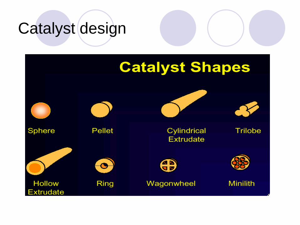
Catalyst design

Reactors
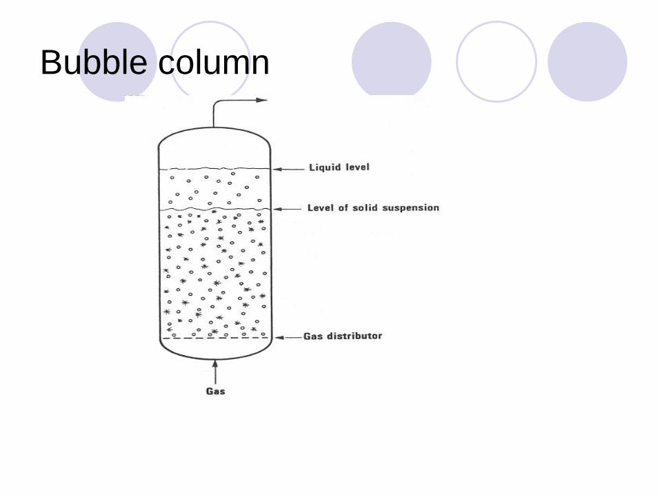
Bubble column
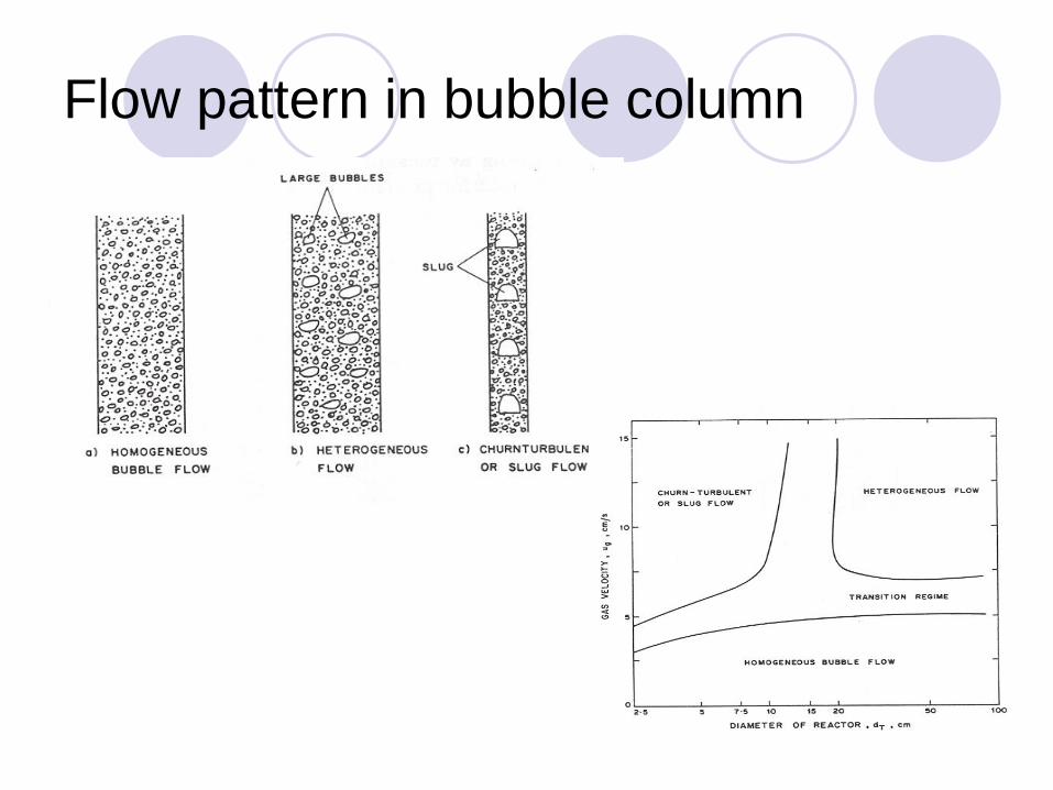
Flow pattern in bubble column

Tank reactor
Often called slurry reactor
Packed bed – trickle bed
Trickle bed
Liquid downflow – trickling flow
Packed bed, if liquid upflow

Packed bed- fixed bed – trickle bed
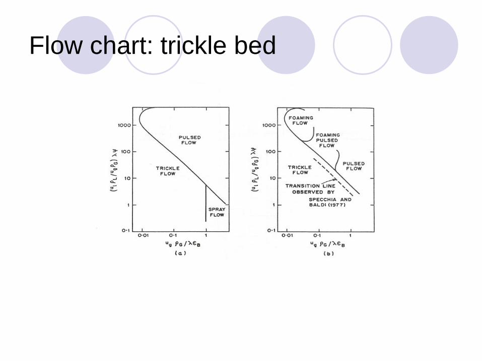
Flow chart: trickle bed

Trickle flow
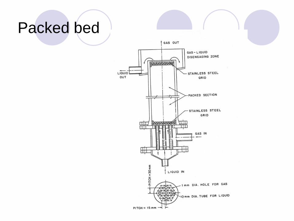
Packed bed

Three-phase fluidized bed
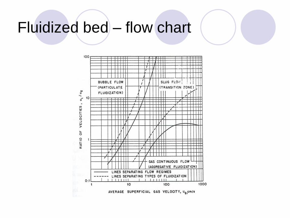
Fluidized bed – flow chart
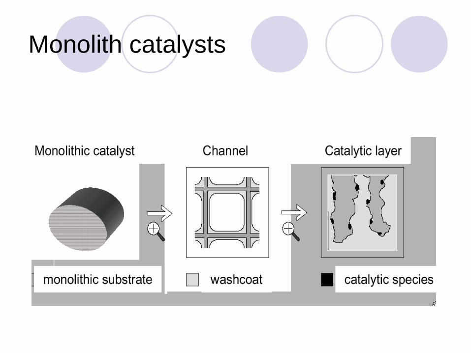
Monolith catalysts

Flow in monoliths

Monolith channel
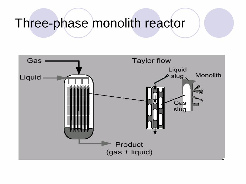
Three-phase monolith reactor
Three-phase reactors
Mass balances
Plug flow and axial dispersion
Columnr eactor
Tube reactor
Trickle bed
Monolith reactor
Backmixing
Bubble column
Tank reactor
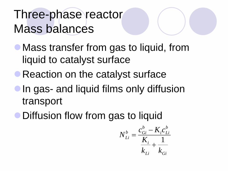
Three-phase reactor
Mass balances
Mass transfer from gas to liquid, from
liquid to catalyst surface
Reaction on the catalyst surface
In gas- and liquid films only diffusion
transport
Diffusion flow from gas to liquid
GiLi
i
b
Lii
b
Gib
Li
kk
K
cKcN
1

Three-phase reactor
Mass transfer

Three-phase reactor
Mass balances
For physical absorption the fluxes through
the gas- and liquid films are equal
Flux from liquid to catalyst particle =
component generation rate at steady state
b
Gi
s
Gi
s
Li
b
Li NNNN
0 pip
s
Li mrAN

Three-phase reactor
Mass balances
Flux through the liquid film defined with
concentration difference and liquid-film
coefficient
Catalyst bulk density defined by
s
Li
b
Li
s
Li
s
Li cckN
RL
cat
L
catB
V
m
V
m

Three-phase reactor
Mass balances
ap = total particle surface/reactor volume
iBLp
s
Li
b
Li
s
Li
s
Li racckN

Three-phase reactor
Mass balances
If diffusion inside the particle affects the
rate, the concept of effectiviness factor is
used as for two-phase reactor (only liquid
in the pores of the particles)
The same equations as for two-phase
systems can be used for porous particles
)('
Bjejj cRR

Three-phase reactor – plug flow

Three-phase reactor
- plug flow, liquid phase
For volume element in liquid phase
Liquid phase
p
s
LiutLib
LiinLi ANnANn
,,
p
s
Liv
b
Li
R
LiaNaN
dV
nd

Three-phase reactor
Plug flow - gas phase
For volume element in gas phase
Gas phase
- concurrent
+ countercurrent
ANnn b
GiutGiinGi
,,
v
b
Li
R
GiaN
dV
nd

Three-phase reactor
Plug flow
Initial conditions
Liquid phase
Gas phase, concurrent
Gas phase, countercurrent
0,0
RLiLi Vnn
0,0
RGiGi Vnn
RGiGi VVnn
,0
Three-phase reactor
- plug flow model
Good for trickle bed
Rather good for a packed bed , in which liguid
flows upwards
For bubble column plug flow is good for gas
phase but not for liquid phase which has a
higher degree of backmixing

Three-phase reactor
- complete backmixing
Liquid phase
Gas phase
p
s
Lv
b
L
R
LiLiaNaN
V
nn
0
v
b
L
R
GiGiaN
V
nn
0

Three-phase reactor
- semibatch operation
Liquid phase in batch
Gas phase continuous
Initial condition
Rp
s
Lv
b
LLi VaNaN
dt
dn
GiGinVaNn
dt
dnRv
b
LiGi
0
0
0
0
0
tnn
tnn
GiGi
LiLi

Parameters in three-phase reactors
Gas-liquid equilibrium ratio (Ki) from
Thermodynamic theories
Gas solubility in liquids (Henry’s constant)
Mass transfer coefficients kLi, kGi
Correlation equations
G
GiGi
L
LiLi
Dk
Dk

Numerical aspects
CSTR – non-linear equations
Newton-Raphson method
Reactors with plug flow (concurrent)
Runge-Kutta-, Backward difference -methods
Reactors with plug flow (countercurrent)
and reactors with axial dispersion (BVP)
orthogonal collocation

Examples
Production of Sitostanol A cholesterol suppressing agent
Carried out through hydrogenation of Sitosterol on Pd catalysts (Pd/C, Pd/Zeolite)
Production of Xylitol An anti-caries and anti-inflamatory component
Carried out through hydrogenation of Xylose on Ni- and Ru-catalysts (Raney Ni, Ru/C)

Exemple: from cholesterol tol sitostanol
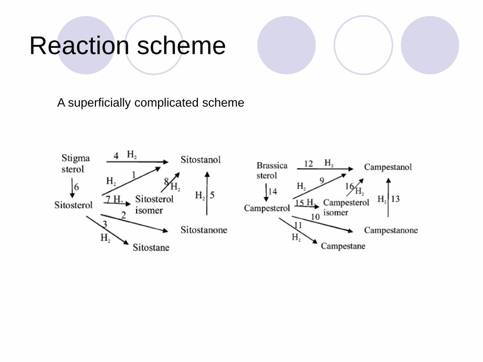
Reaction scheme
A superficially complicated scheme
From laboratory scale
to industrial scale
Slurry, three-phase reactor
Lab reactor, 1 liter, liquid amount 0.5 kg
Large scale reactor, liquid amount 8080 kg
Simulation of large-scalle reactor based on
laboratory reactor

Catalytic reactor
Semi-batch stirred tank reactor
Well agitated, no concentration differences appear in
the bulk of the liquid
Gas-liquid and liquid-solid mass transfer resistances
can prevail
The liquid phase is in batch, while gas is continuously
fed into the reactor.
The gas pressure is maintained constant.
The liquid and gas volumes inside the reactor vessel
can be regarded as constant
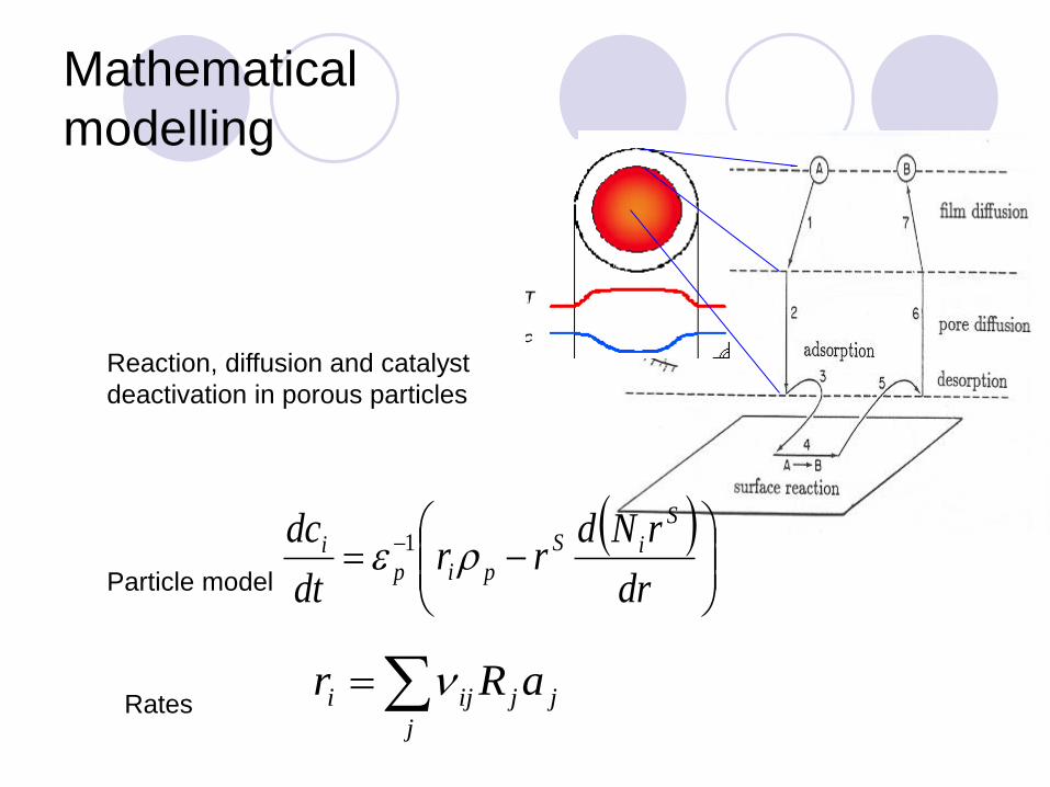
Mathematical
modelling
dr
rNdrr
dt
dc S
iS
pipi 1
j
jjiji aRr
Reaction, diffusion and catalyst
deactivation in porous particles
Particle model
Rates
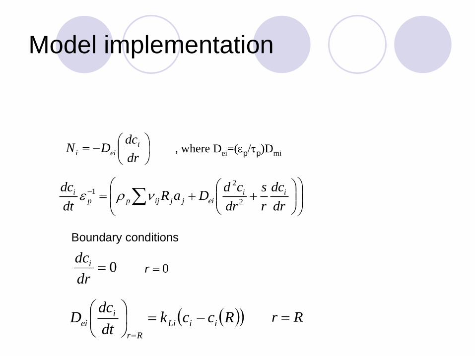
Model implementation
dr
dcDN i
eii
dr
dc
r
s
dr
cdDaR
dt
dc iieijjijpp
i
2
21
, where Dei=(p/p)Dmi
0dr
dci0r
Rcckdt
dcD iiLi
Rr
iei
Rr
Boundary conditions
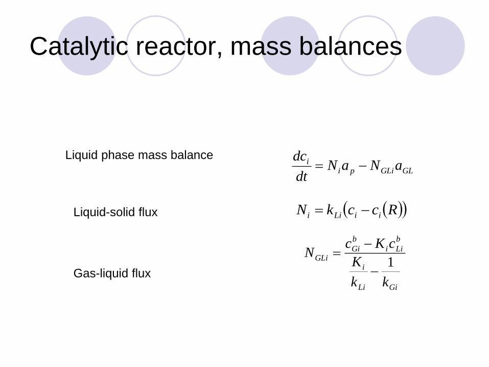
Catalytic reactor, mass balances
GLGLipii aNaN
dt
dc
RcckN iiLii
GiLi
i
b
Lii
b
GiGLi
kk
K
cKcN
1
Liquid phase mass balance
Liquid-solid flux
Gas-liquid flux

Numerical approach
PDEs discretizied with finite difference
formulae
The ODEs created solved with a stiff
algorithm (BD, Hindmarsh)
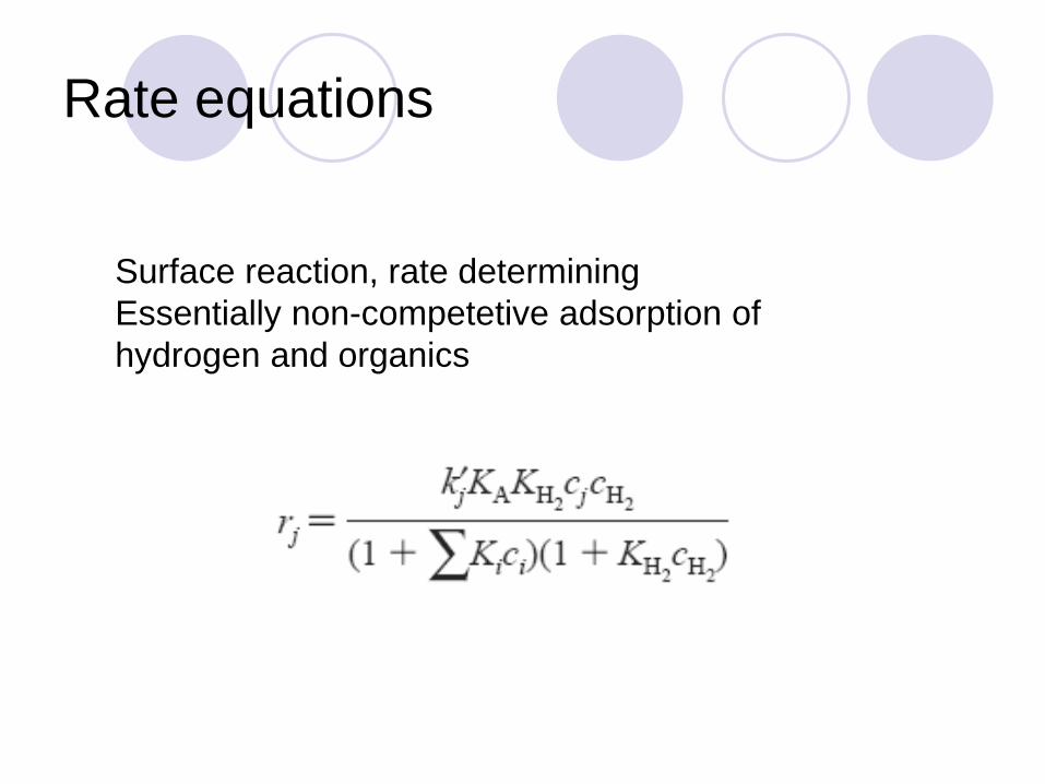
Rate equations
Surface reaction, rate determining
Essentially non-competetive adsorption of
hydrogen and organics
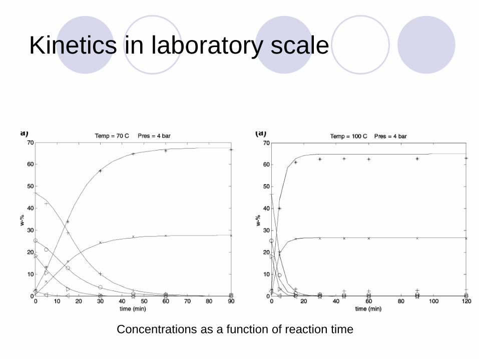
Kinetics in laboratory scale
Concentrations as a function of reaction time
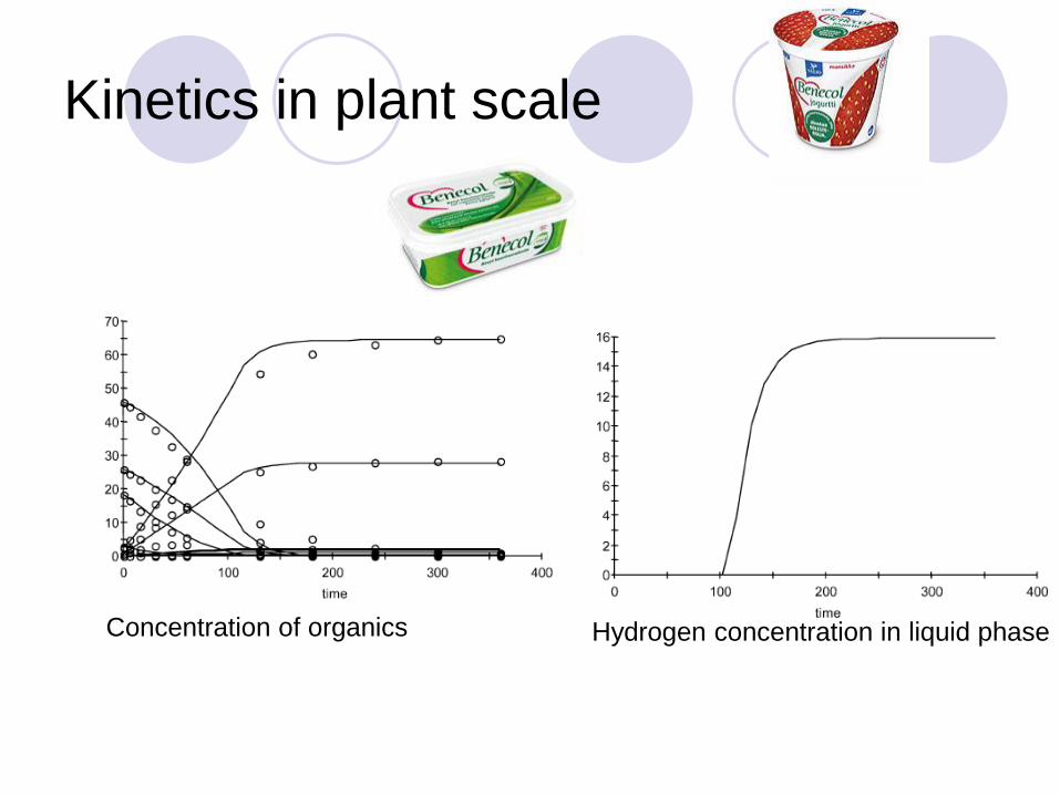
Kinetics in plant scale
Hydrogen concentration in liquid phase Concentration of organics

Comparison of lab and plant scale
Laboratory Factory
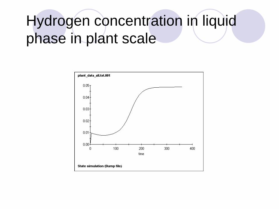
Hydrogen concentration in liquid
phase in plant scale
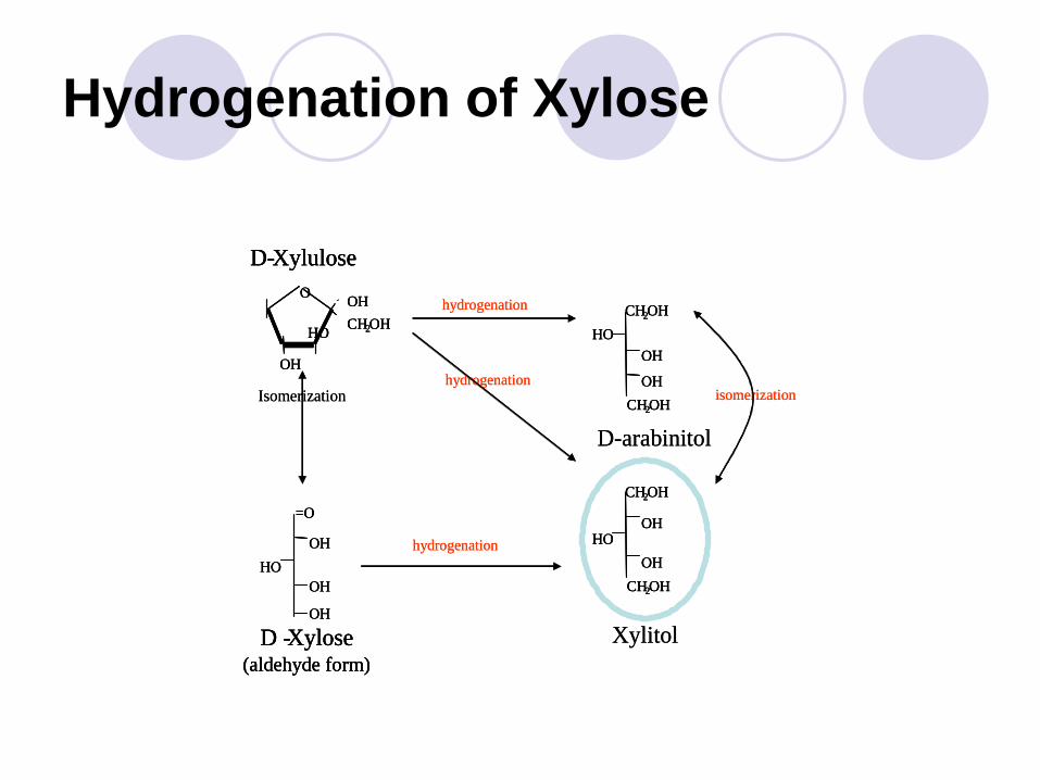
Hydrogenation of Xylose
=O
OH
HO
OH
OH
D -Xylose(aldehyde form)
Xylitol
OHHO
OH
CH2OH
CH2OH
CH2OH
OH
HO
O
OH
D-Xylulose
OH
HO
OH
CH2OH
CH2OH
D-arabinitol
isomerization
hydrogenation
hydrogenationIsomerization
hydrogenation
=O
OH
HO
OH
OH
=O
OH
HO
OH
OH
D -Xylose(aldehyde form)
D -Xylose(aldehyde form)
Xylitol
OHHO
OH
CH2OH
CH2OH
OHHO
OH
CH2OH
CH2OH
CH2OH
OH
HO
O
OH
CH2OH
OH
HO
O
OH
D-XyluloseD-Xylulose
OH
HO
OH
CH2OH
CH2OH
OH
HO
OH
CH2OH
CH2OH
D-arabinitol
isomerization
hydrogenation
hydrogenationIsomerization
hydrogenation
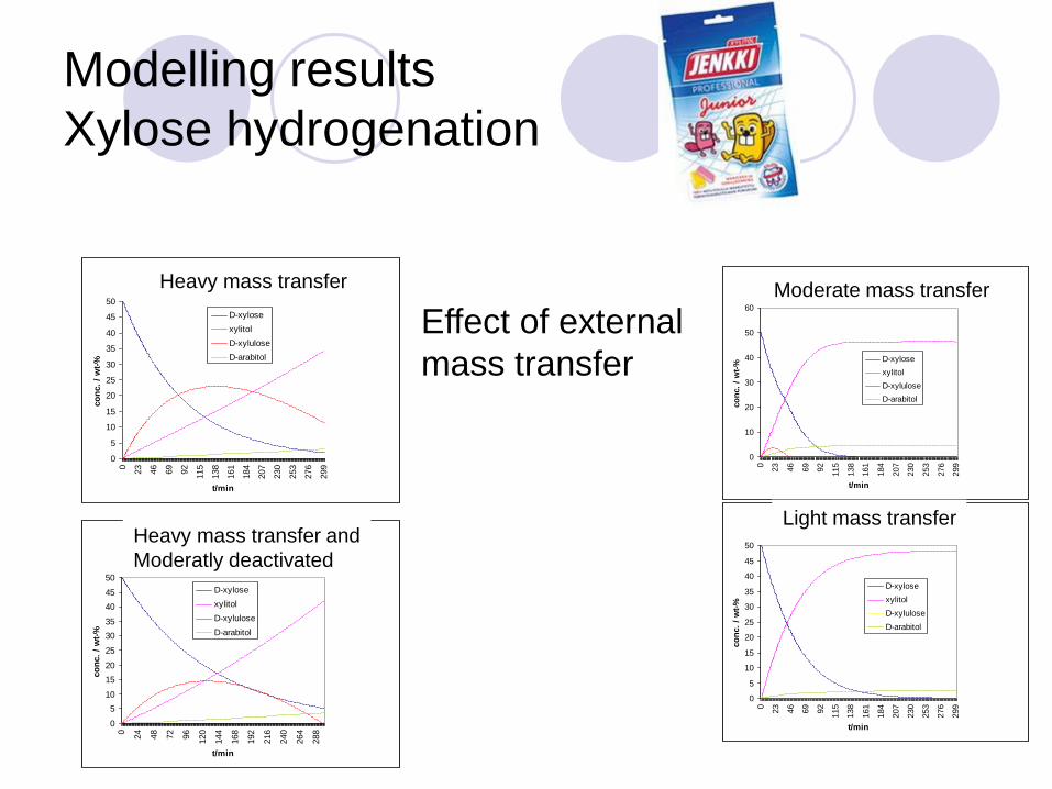
Modelling results
Xylose hydrogenation
Heavy mass-transfer limitations
0
5
10
15
20
25
30
35
40
45
50
0
23
46
69
92
115
138
161
184
207
230
253
276
299
t/min
co
nc.
/ w
t-%
D-xylose
xylitol
D-xylulose
D-arabitol
Moderate mass-transfer limitations
0
10
20
30
40
50
60
0
23
46
69
92
115
138
161
184
207
230
253
276
299
t/min
co
nc.
/ w
t-%
D-xylose
xylitol
D-xylulose
D-arabitol
Heavy mass-transfer limitations and moderately
deactivated catalyst
0
5
10
15
20
25
30
35
40
45
50
0
24
48
72
96
120
144
168
192
216
240
264
288
t/min
co
nc.
/ w
t-%
D-xylose
xylitol
D-xylulose
D-arabitol
Light mass-transfer limitations
0
5
10
15
20
25
30
35
40
45
50
0
23
46
69
92
115
138
161
184
207
230
253
276
299
t/minco
nc.
/ w
t-%
D-xylose
xylitol
D-xylulose
D-arabitol
Heavy mass transfer
Heavy mass transfer and
Moderatly deactivated
Moderate mass transfer
Light mass transfer
Effect of external
mass transfer
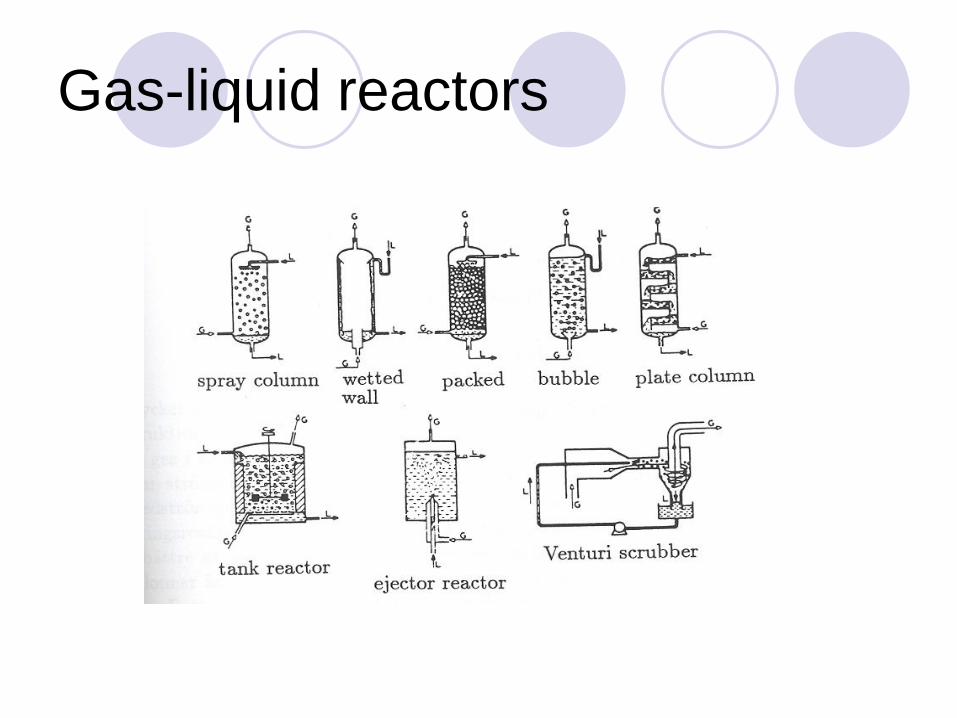
Gas-liquid reactors
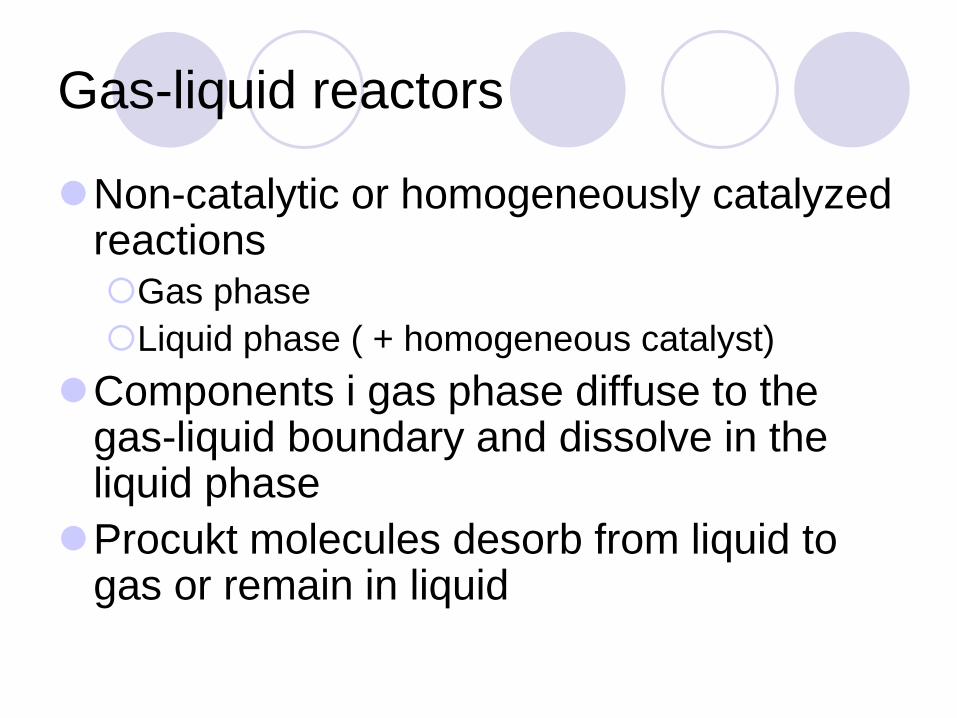
Gas-liquid reactors
Non-catalytic or homogeneously catalyzed reactions Gas phase
Liquid phase ( + homogeneous catalyst)
Components i gas phase diffuse to the gas-liquid boundary and dissolve in the liquid phase
Procukt molecules desorb from liquid to gas or remain in liquid
Gas-liquid reactions
Synthesis of chemicals
Gas absorption, gas cleaning
Very many reactor constructions used,
depending on the application

Gas-liquid reaction: basic principle
Gas-liquid reactor constructions
Spray column
Wetted wall column
Packed column
Plate column
Bubble columns
Continuous, semibatch and batch tank reactors
Gas lift reactors
Venturi scrubbers

Gas-liquid reactors - overview
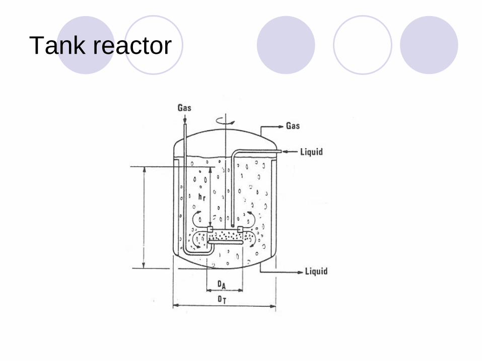
Tank reactor
Gas-liquid reactors
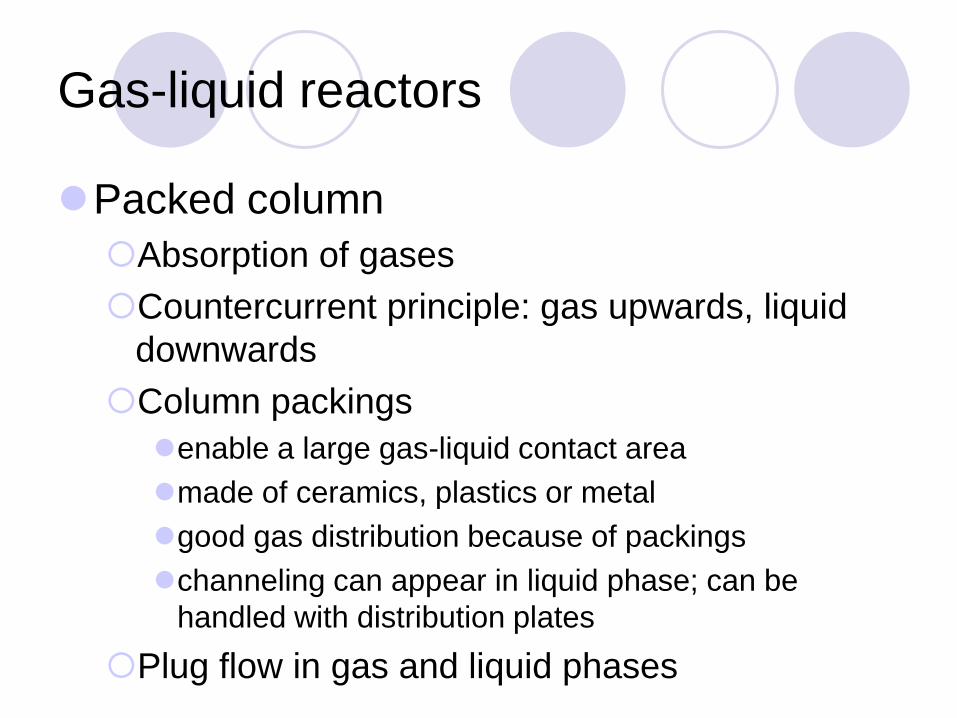
Packed column
Absorption of gases
Countercurrent principle: gas upwards, liquid
downwards
Column packings
enable a large gas-liquid contact area
made of ceramics, plastics or metal
good gas distribution because of packings
channeling can appear in liquid phase; can be
handled with distribution plates
Plug flow in gas and liquid phases

Gas-liquid reactors
Plate column Absorption of gases
Countercurrent
Various plates used as in distillation, e.g.
Bubble cap
Plate column
Packed column Absorption of gases
Countercurrent
A lot of column packings available; continuous development

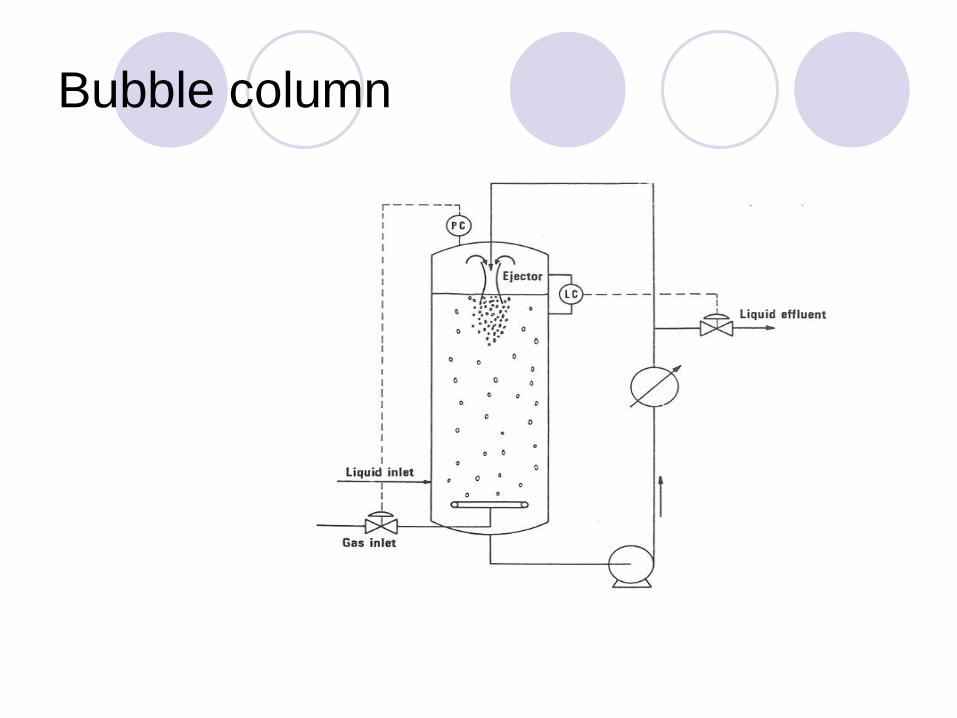
Bubble column
Gas-lift -reactor

Bubble column – design examples
Bubble column

Packed column
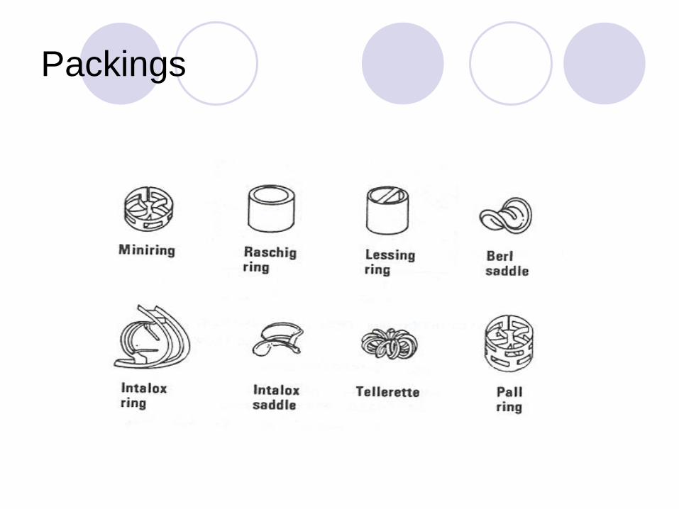
Packings

Plate column

Gas-liquid reactors
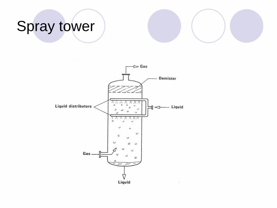
Gas scrubbers
Spray tower
Gas is the continuous phase
In shower !
Venturi scrubber
Liquid dispergation via a venturi neck
For very rapid reactions
Spray tower

Venturi scrubber
Gas-liquid reactors
Selection criteria
Bubble columns for slow reactions
Sckrubbers or spray towers for rapid reactions
Packed column or plate column if high reatant
conversion is desired
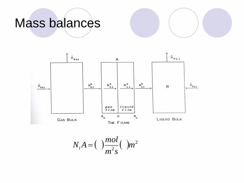
Mass balances
2
2m
sm
molANi

Gas-liquid reactors
Mass balances
Plug flow
Liquid phase
Gas phase
av =gas-liquid surface area/reactor volume
L = liquid hold-up
utLiLi
b
LiinLi nVrANn ,,
iLv
b
Li
R
Li raNdV
nd
v
b
Gi
R
Gi aNdV
nd

Gas-liquid reactions
Mass balances
Complete backmixing
Liquid phase
Gas phase
av =gas-liquid surface area/reactor volume
L = liquid hold-up
utLiLi
b
LiinLi nVrANn ,,
iLv
b
Li
R
LiLiraN
V
nn
0
v
b
Gi
R
GiGiaN
V
nn
0

Gas-liquid reactors
Mass balances
Batch reactor
Liquid phase
Gas phase
av =interfacial area/reactor volume
L = liquid hold-up
RiLv
b
LiLi VraN
dt
dn
Rv
b
GiGi VaN
dt
dn
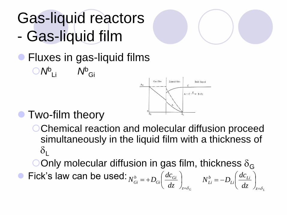
Gas-liquid reactors
- Gas-liquid film
Fluxes in gas-liquid films
NbLi Nb
Gi
Two-film theory
Chemical reaction and molecular diffusion proceed simultaneously in the liquid film with a thickness of L
Only molecular diffusion in gas film, thickness G
Fick’s law can be used:
Gz
GiGi
b
Gidz
dcDN
Lz
LiLi
b
Lidz
dcDN

Gas-liquid reactors
Gas film
Gas film, no reaction
Analytical solution possible
The flux depends on the mass transfer coefficient and concentration difference
Adz
dcDA
dz
dcD
ut
GiGi
in
GiGi
02
2
dz
cdD Gi
Gi s
Gi
b
GiGi
b
Gi cckN
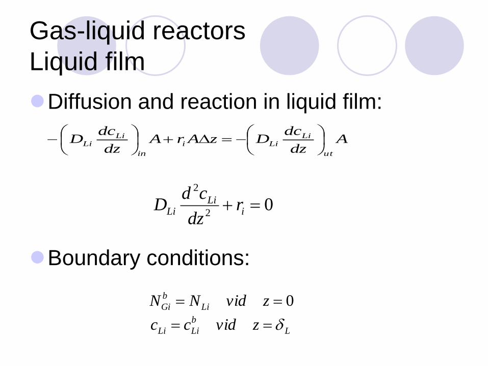
Gas-liquid reactors
Liquid film
Diffusion and reaction in liquid film:
Boundary conditions:
Adz
dcDzArA
dz
dcD
ut
LiLii
in
LiLi
02
2
iLi
Li rdz
cdD
L
b
LiLi
Li
b
Gi
zvidcc
zvidNN
0

Gas-liquid reactors
Liquid film
Liquid film
Equation can be solved analytically for
isothermas cases for few cases of linear
kinetics; in other case numerical solution should
be used

Reaction categories
Physical absorption
No reaction in liquid film, no reaction in liquid bulk
Very slow reaction
The same reaction rate in liquid film and liquid bulk – no concentration gradients in the liquid film, a pseudo-homogeneous system
Slow reaction
Reaction in the liquid film negligible, reactions in the liquid bulk; linear concentration profiles in the liquid film

Reaction categories
Moderate rates
Reaction in liquid film and liquid bulk
Rapid reaction
Chemical reactions in liquid film, no reactions in bulk
Instantaneous reaction
Reaction in liquid film; totally diffusion-controlled
process

Concentration profiles in liquid film
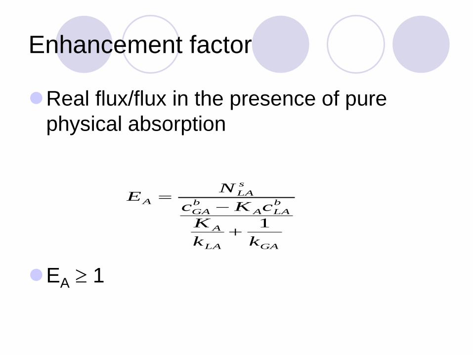
Enhancement factor
Real flux/flux in the presence of pure
physical absorption
EA 1
GALA
A
b
LAA
b
GA
s
LAA
kk
K
cKc
NE
1

Gas-liquid reactors
- very slow reaction
No concentration gradients in the liquid
film
Depends on the role of diffusion resistance
in the gas film
b
LA
b
GAAb
LA
s
GAA
c
cK
c
cK
b
LAA
b
GAGA
b
LA
b
GA cKckNN
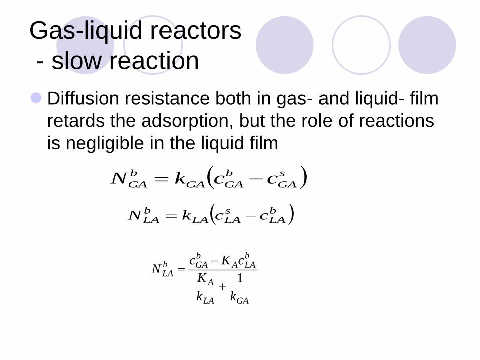
Gas-liquid reactors
- slow reaction
Diffusion resistance both in gas- and liquid- film
retards the adsorption, but the role of reactions
is negligible in the liquid film
s
GA
b
GAGA
b
GA cckN
bLA
sLALA
bLA cckN
GALA
A
bLAA
bGAb
LA
kk
K
cKcN
1
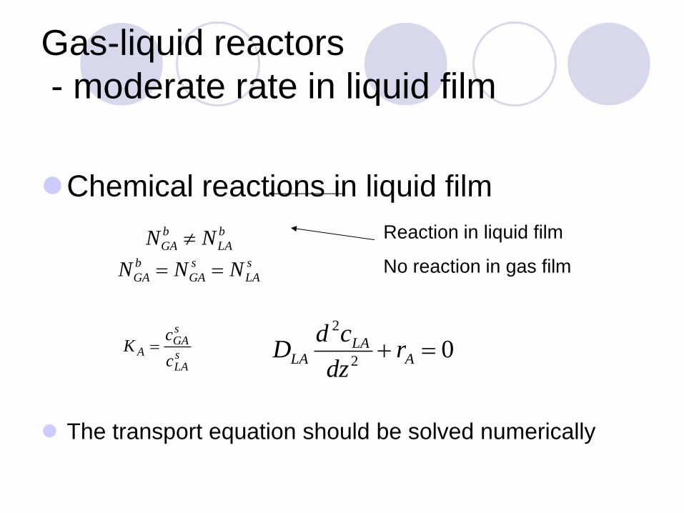
Gas-liquid reactors
- moderate rate in liquid film
Chemical reactions in liquid film
The transport equation should be solved numerically
s
LA
s
GA
b
GA
b
LA
b
GA
NNN
NN
sLA
sGA
Ac
cK 0
2
2
ALA
LA rdz
cdD
Reaction in liquid film
No reaction in gas film
Moderate rate in the liquid film
Transport equation can be solved
analytically only for some special cases:
isothermal liquid film – zero or first order
kinetics
Approximative solutions exist for rapid second
order kinetics

Moderate rate…
Zero order kinetics
LA
ALA
D
k
dz
cd
2
2
GALA
A
bLAA
bGAs
LA
kk
K
McKcN
1
1
b
LALA
LAA
ck
kDM
22

Moderate rate…
First order kinetics
Hatta number Ha=(compare with Thiele modulus)
LA
LAALA
D
kc
dz
cd
2
2
GALA
A
bLAAb
GA
sLA
kk
K
M
M
M
cKc
N1tanh
)cosh(
2
2 L
LA
A
LA
LAA
D
k
k
kDM

Rapid reactions
Special case of reactions with finite rate
All gas components totally consumed in
the film; bulk concentration is zero, cbLA=0

Instantaneous reactions
Components react completely in the liquid
film
A reaction plane exists
Reaction plane coordinate
02
2
dz
cdD LA
LA
s
LBLB
B
s
LALA
A
LBLB
LB
cDcD
cDz
'
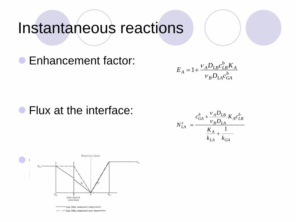
Instantaneous reactions
Enhancement factor:
Flux at the interface:
Coordinate of the
interface:
02
2
dz
cdD LA
LA
GALA
A
bLBA
LAB
LBAbGA
sLA
kk
K
cKD
Dc
N1
bGALAB
AbLBLBA
AcD
KcDE
1

Instantaneous reactions
Flux
Only diffusion coeffcients affect !
For simultaneous reactions can several reaction planes appear in the film
GALA
A
b
LBA
LAB
LBAb
GA
s
LA
kk
K
cKD
Dc
N1

Fluxes in reactor mass balances
Fluxes are inserted in
mass balances
For reactants:
For slow and very
slow reactions: (no
reaction in liquid film)
sLi
sGi
bGi NNN
sLi
bLi ΝΝ
sLi
bLi ΝΝ
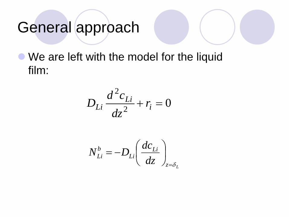
General approach
We are left with the model for the liquid
film:
Lz
LiLi
b
Lidz
dcDN
02
2
iLi
Li rdz
cdD
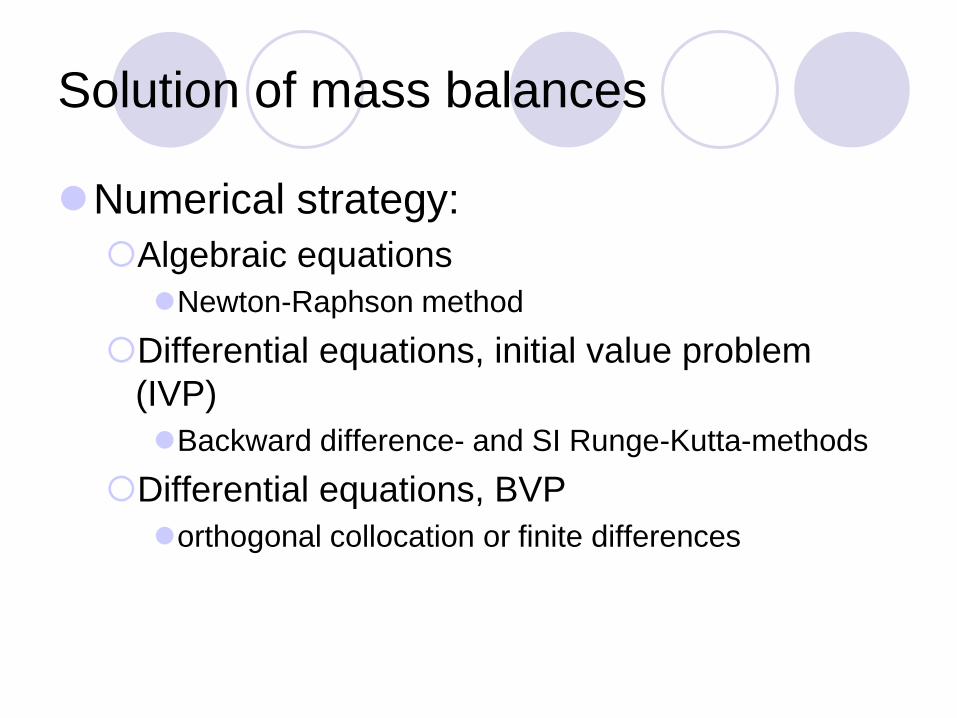
Solution of mass balances
Numerical strategy:
Algebraic equations
Newton-Raphson method
Differential equations, initial value problem
(IVP)
Backward difference- and SI Runge-Kutta-methods
Differential equations, BVP
orthogonal collocation or finite differences
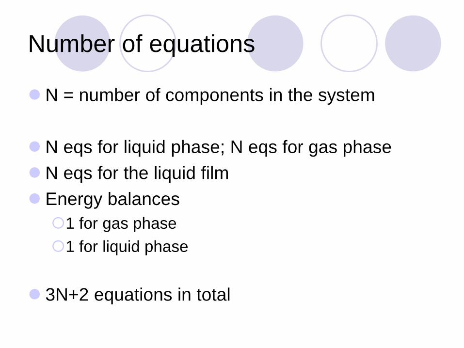
Number of equations
N = number of components in the system
N eqs for liquid phase; N eqs for gas phase
N eqs for the liquid film
Energy balances
1 for gas phase
1 for liquid phase
3N+2 equations in total
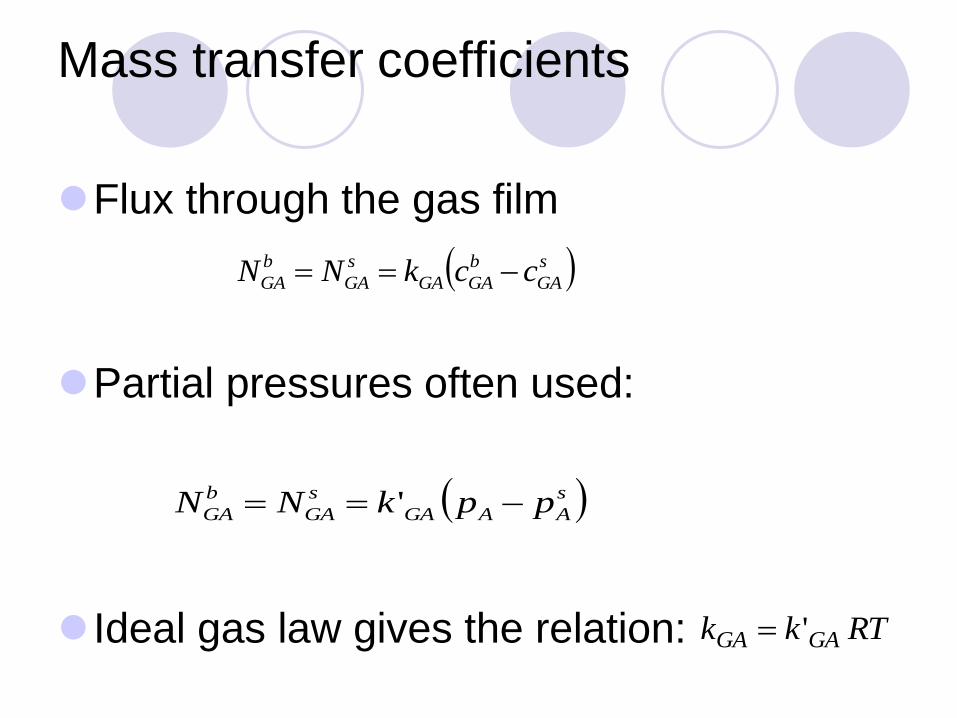
Mass transfer coefficients
Flux through the gas film
Partial pressures often used:
Ideal gas law gives the relation:
s
GA
b
GAGA
s
GA
b
GA cckNN
s
AAGA
s
GA
b
GA ppkNN '
RTkk GAGA '
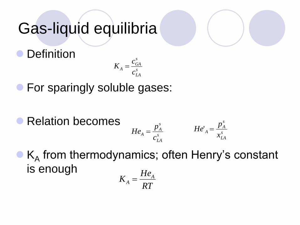
Gas-liquid equilibria
Definition
For sparingly soluble gases:
Relation becomes
KA from thermodynamics; often Henry’s constant
is enough
s
LA
s
GAA
c
cK
s
LA
s
AA
c
pHe
RT
HeK A
A
s
LA
s
AA
x
pHe '
Simulation example
Chlorination of p-kresol
p-cresol + Cl2 -> monocloro p-kresol + HCl
monocloro p-kresol + Cl2 -> dichloro p-kresol +
HCl
CSTR
Newton-Raphson-iteration
Liquid film
Orthogonal collocation
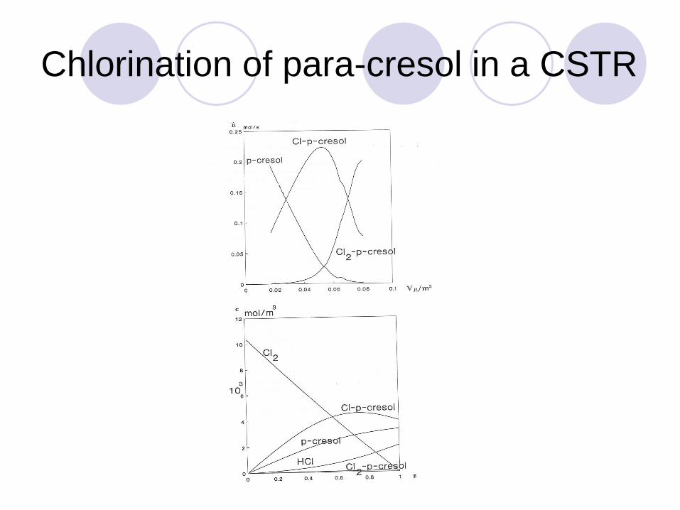
Chlorination of para-cresol in a CSTR

Fluid-solid reactions
Three main types of
reactions:
Reactions between gas
and solid
Reactions between
liquid and solid
Gas-liquid-solid
reactions

Fluid-solid reactions
The size of the solid phase
Changes:
Burning oc charcoal or wood
Does not change:
oxidation av sulfides, e.g. zinc sulphide --> zinc oxide

Reactors for fluid-solid reactions
Reactor configurations
Fluidized bed
Moving bed
Batch, semibatch and continuous tank reactors
(liquid and solid, e.g. CMC production, leaching
of minerals)
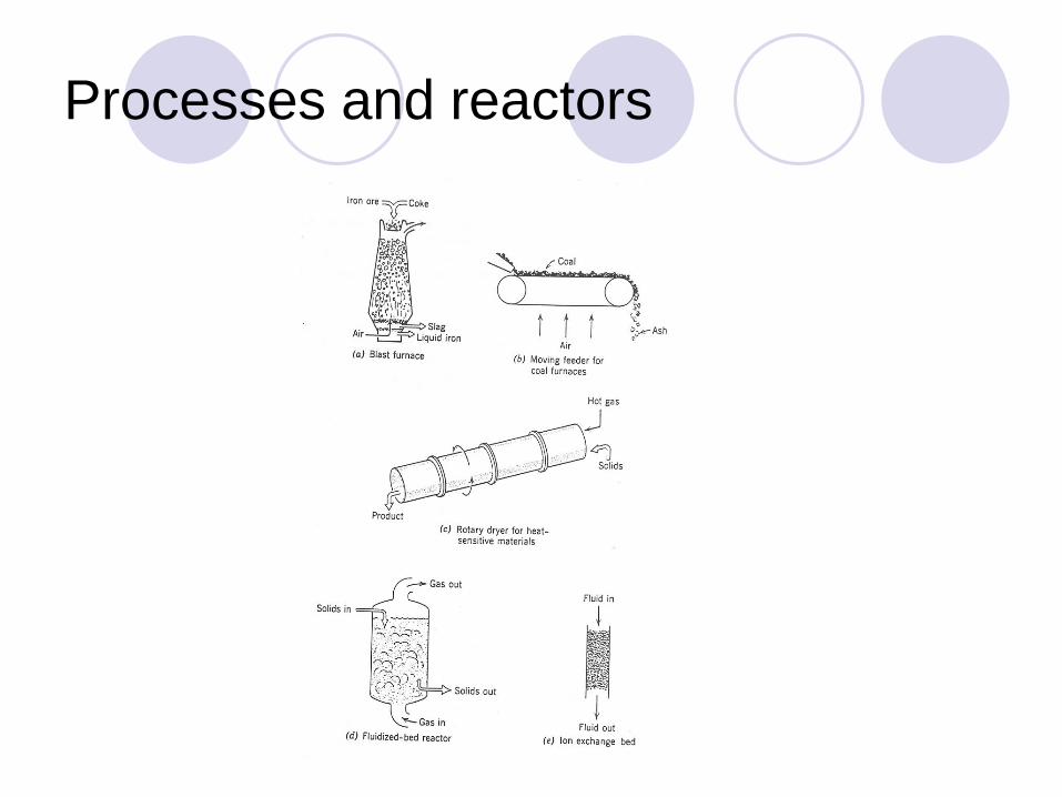
Processes and reactors
Fluid-solid reaction modelling
Mathematical models used Porous particle model
Simultaneous chemical reaction and diffusion throughout the particle
Shrinking particle model
Reaction product continuously removed from the surface
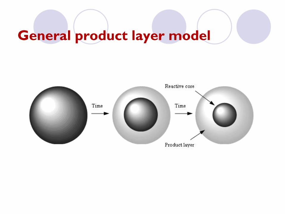
Product layer model (shrinking core model)
A porous product layer is formed around the non-reacted core of the solid particle
Grain model
The solid phase consists of smaller non-porous particles (rasberry structure)
Fluid-solid reactions
Solid particles react with gases in such a
way that a narrow reaction zone is formed
Shrinking particle model can thus often be
used even for porous particles
Grain model most rrealistic but
mathematically complicated

Product layer

Product layer
Concentration profiles in the
product layer
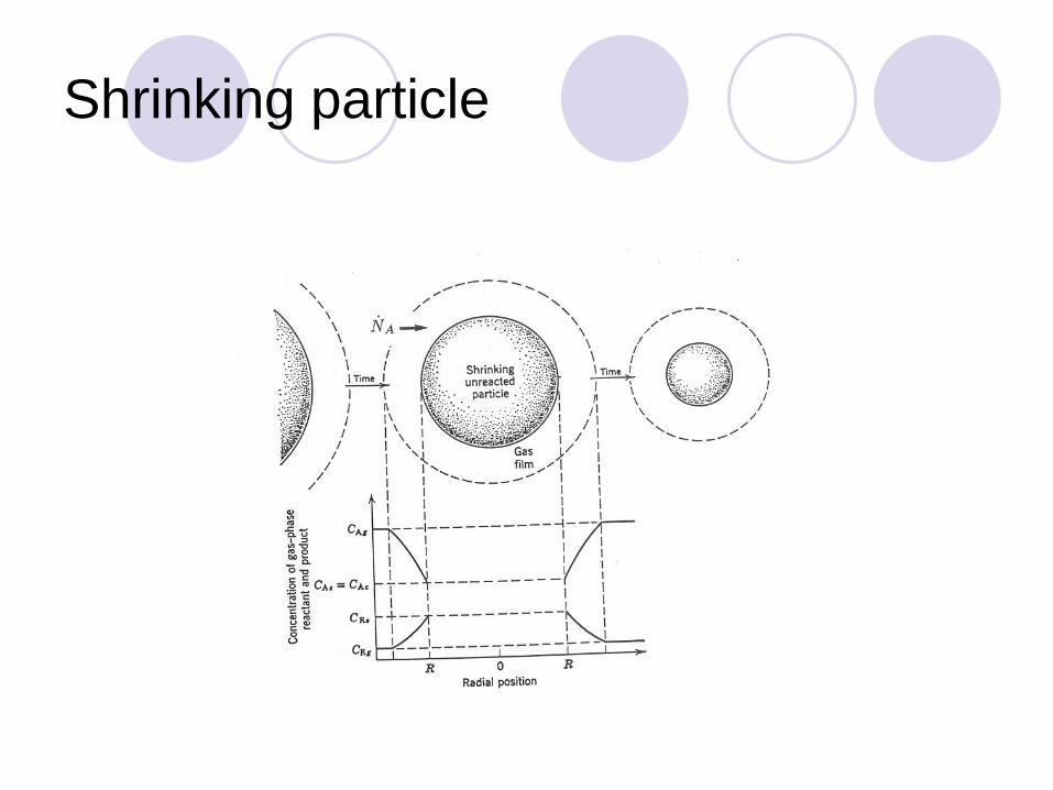
Shrinking particle

Grain model

Fluid-solid reactions
Particle with a porous product layer
Gas or liquid film around the product layer
Porous product layer
The reaction proceeds on the surface of non-
reacted solid material
Gas molecules diffuse through the gas film and
through the porous product layer to the surface of
fresh, non-reacted material

Fluid-solid reactions
Reaction between A in fluid phase and B
in solid phase
R=reaction rate, A=particle surface area
Generated B= Accumulated B
2
2()() m
sm
molRA
s
B
PB
cRx
M
dt
dr
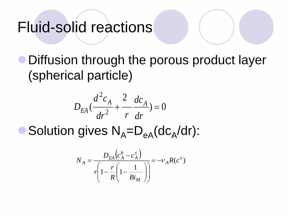
Fluid-solid reactions
Diffusion through the porous product layer
(spherical particle)
Solution gives NA=DeA(dcA/dr):
0)2
(2
2
dr
dc
rdr
cdD AA
EA
)(
111
sA
M
sA
bAEA
A cR
BiR
rr
ccDN
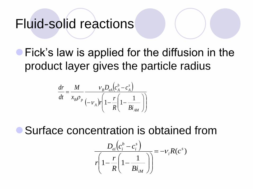
Fluid-solid reactions
Fick’s law is applied for the diffusion in the
product layer gives the particle radius
Surface concentration is obtained from
AM
A
s
A
b
AeAB
pB
BiR
rr
ccD
x
M
dt
dr
111
)(
111
s
i
iM
s
i
b
iei cR
BiR
rr
ccD
For first-order kinetics an analytical
solution is possible
Four cases – rate limiting steps
Chemical reaction
Diffusion through product layer and fluid film
Diffusion through the product layer
Diffusion through the fluid film
Fluid-solid reactions
Fluid-solid reactions
Reaction time (t) and total reaction time
(t0 ) related to the particle radius (r)
Limit cases
Chemical reaction controls the process –
Thiele modulus is small -> Thiele modulus
small
Diffusion through product layer and fluid film
rate limiting -> Thiele modulus large
Reaktorer med reaktiv fast fas
Diffusion through the product layer much slower
than diffusion through the fluid -> BiAM=
Diffusion through fluid film rate limiting ->
BiAM=0
Fluid-solid reactions
Shrinking particle
Phase boundary
Fluid film around particles
Product molecules (gas or liquid) disappear
directly from the particle surface
Mass balance
In via diffusion through the fluid film + generated = 0
Fluid-solid reactions
First order kinetics
Surface reaction rate limiting
Diffusion through fluid film rate limiting
Arbitrary kinetics
A general solution possible, if diffusion through
the fluid film is rate limiting

Semibatch reactor
An interesting special case
Semibatch reactor
High throughflow of gas so that the concentrations in
the gas phase can be regarded as constant; used
e.g. in the investigation of gas-solid kinetics
(thermogravimetric equipment)
Complete backmixing locally
simple realtions between the reaction time and the
particle radius obtained
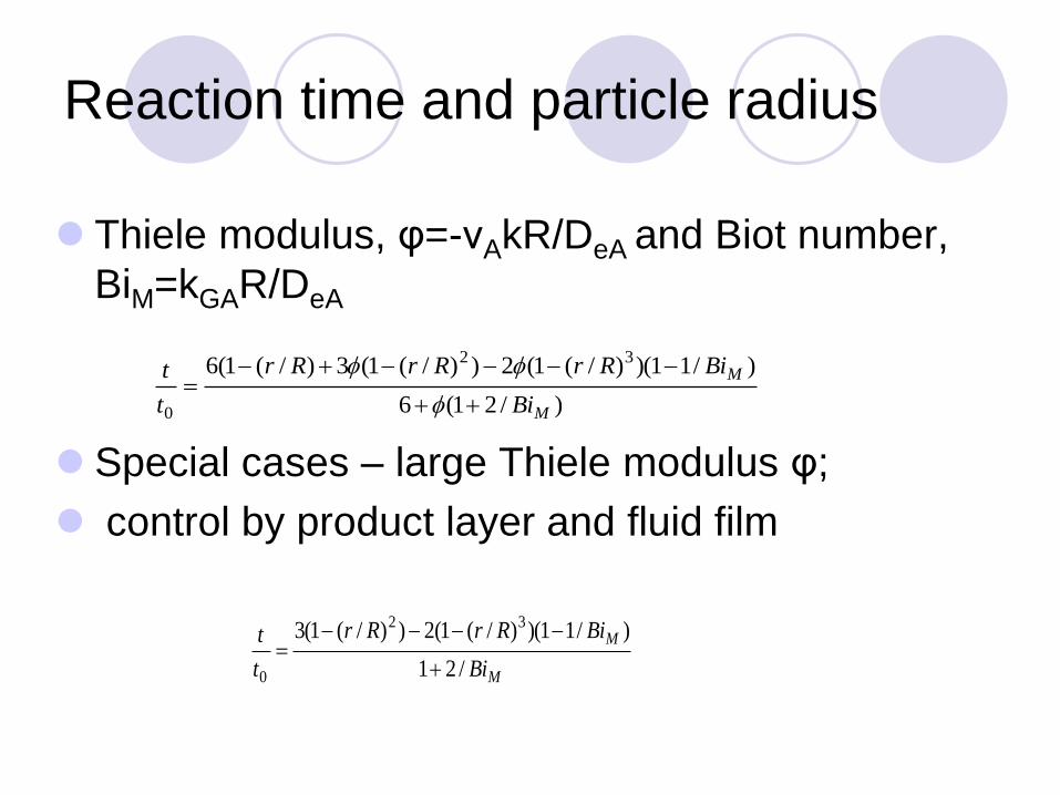
Reaction time and particle radius
Thiele modulus, φ=-νAkR/DeA and Biot number,
BiM=kGAR/DeA
Special cases – large Thiele modulus φ;
control by product layer and fluid film
M
M
Bi
BiRrRr
t
t
/21
)/11)()/(1(2))/(1(3 32
0
)/21(6
)/11)()/(1(2))/(1(3)/(1(6 32
0 M
M
Bi
BiRrRrRr
t
t

Fluid-solid reactions
Product layer model
Large Thiele modulus, φ=-νAkR/DeA and
large Bi - control by product layer
Large Thiele modulus, φ=-νAkR/DeA and
small Bi - control by film
3
0
)/(1 Rrt
t
32
0
)/(2))/(31 RrRrt
t
Fluid-solid reactions
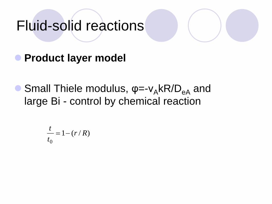
Product layer model
Small Thiele modulus, φ=-νAkR/DeA and
large Bi - control by chemical reaction
)/(10
Rrt
t
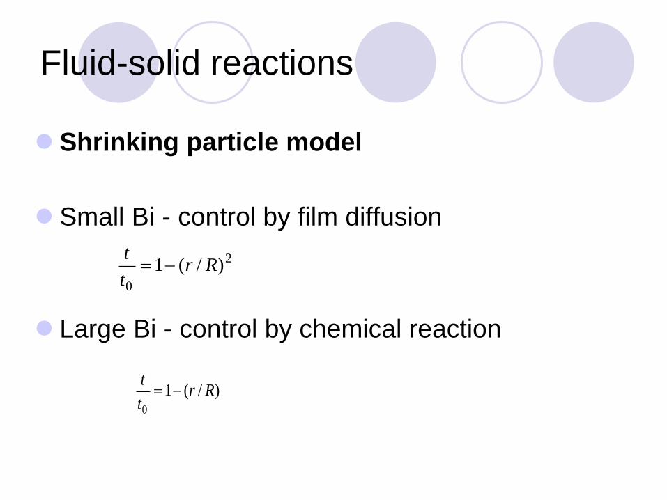
Fluid-solid reactions
Shrinking particle model
Small Bi - control by film diffusion
Large Bi - control by chemical reaction
)/(1
0
Rrt
t
2
0
)/(1 Rrt
t


Packed bed
Packed bed – operation principle
Gas or liquid flows through a stagnant bed of
particles, e.g. combustion processes or ion
exchangers
Plug flow often a sufficient description for the flow
pattern
Radial and axial dispersion effects neglected

Simulation of a packed bed

Fluid-solid reactions: the roughness of even
surfaces
Tapio Salmi and Henrik Grénman
Outline
Background of solid-liquid reactions
New methodology for solid-liquid kinetic
modeling
Description of rough particles
General product layer model
Particle size distribution
Conclusions

Solid-liquid reaction kinetics
• The aim is to develop a mathematical model for the
dissolution kinetics

Why modeling is useful?
Modeling helps in effective process and equipment design
as well as control
Empirical process development is slow in the long run
The optimum is often not achieved through empirical
development, at least in a reasonable time frame

What influences the kinetics
A
A + B → AB → C (l)
C AB
• Reaction rate depends on
– Mass transfer
• External
• Internal (often neglected)
– Intrinsic kinetics (the “real”
chemical rates
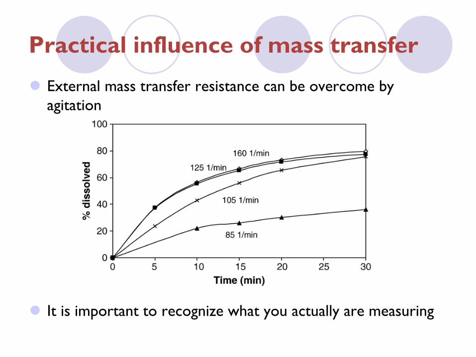
Practical influence of mass transfer
External mass transfer resistance can be overcome by
agitation
It is important to recognize what you actually are measuring
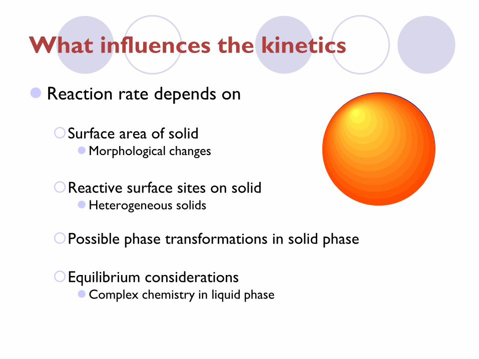
What influences the kinetics
Reaction rate depends on
Surface area of solid Morphological changes
Reactive surface sites on solid Heterogeneous solids
Possible phase transformations in solid phase
Equilibrium considerations Complex chemistry in liquid phase

Traditional methodology
The conversion is followed by measuring the solid or liquid
phase
0
2
4
6
8
10
12
0 2 4 6 8 10
Tid (min)
Ko
nc
en
tra
tio
n (
gra
m/lit
er)
50°C
80°C
Time
Concentr
atio
n

Sphere Cylinder Slab
Shrinking particle
Shrinking core
Traditional hypothesis in modeling
solid-liquid reactions

nr g() f(cS) Type of model
1 -ln(1-) cS/c0S First-order kinetics
2 (1-)-1/2
- 1 (cS/c0S)3/2
Three-halves-order kinetics
3 (1-)-1
(cS/c0S)2 Second-order kinetics
4 1 - (1-)1/2
(cS/c0S)1/2
One-half-order kinetics; two-dimensional
advance of the reaction interface
5 1 - (1-)1/3
(cS/c0S)2/3
Two-thirds-order kinetics; three-
dimensional advance of the reaction
interface
6 1 - (1-)2/3
(cS/c0S)1/3
One-thirds-order kinetics; film diffusion
7 [1 - (1-)1/3
]2 (cS/c0S)
2/3/(1 - (cS/c0S)
1/3) Jander; three-dimensional
8 1 - 2/3 - (1-)2/3
(cS/c0S)1/3
/(1 - (cS/c0S)1/3
) Crank-Ginstling-Brounshtein, mass transfer
across a nonporous product layer
9 [1/(1-)1/3
– 1]2 (cS/c0S)
5/3/(1 - (cS/c0S)
1/3)
Zhuravlev-Lesokhin-Tempelman, diffusion,
concentration of penetrating species varies
with
10 [1 - (1-)1/2
]2 (cS/c0S)
1/2/(1 - (cS/c0S)
1/2) Jander; cylindrical diffusion
11 1/(1-)1/3
- 1 (cS/c0S)4/3
Dickinson, Heal, transfer across the
contacting area
12 1-3(1-)2/3
+2(1-) (cS/c0S)1/3
/(1 - (cS/c0S)1/3
) Shrinking core, product layer (different
form of Crank-Ginstling-Brounshtein)
liquidparticles
solid ckAdt
dc
Traditional kinetic modeling –
screening models from literature
• The kinetics depends on the
surface area (A) of the
particles
• Because of the difficulties
associated with measuring the
surface area on-line, the change is
often expressed with the help of
the conversion
• Experimental test plots are used to
determine the reaction mechanism
3/1)1(1 kt

Surface area of solid phase
Mineral 1
Sphere
Cylinder
Mineral 2
Cracking
Steadily
increasing
porosity
0
5
10
15
20
25
0 20 40 60 80 100
Conversion (%)
To
tal
su
rfa
ce
are
a (
m2/L
)
• The change in the total
surface area of the solid
depends strongly on the
morphology of the particles
• Models based on ideal
geometries can be inadequate
for modeling non-ideal cases
• The particle morphology can
be implemented into the
model with the help of a
shape factor
0RV
Aa
P
P
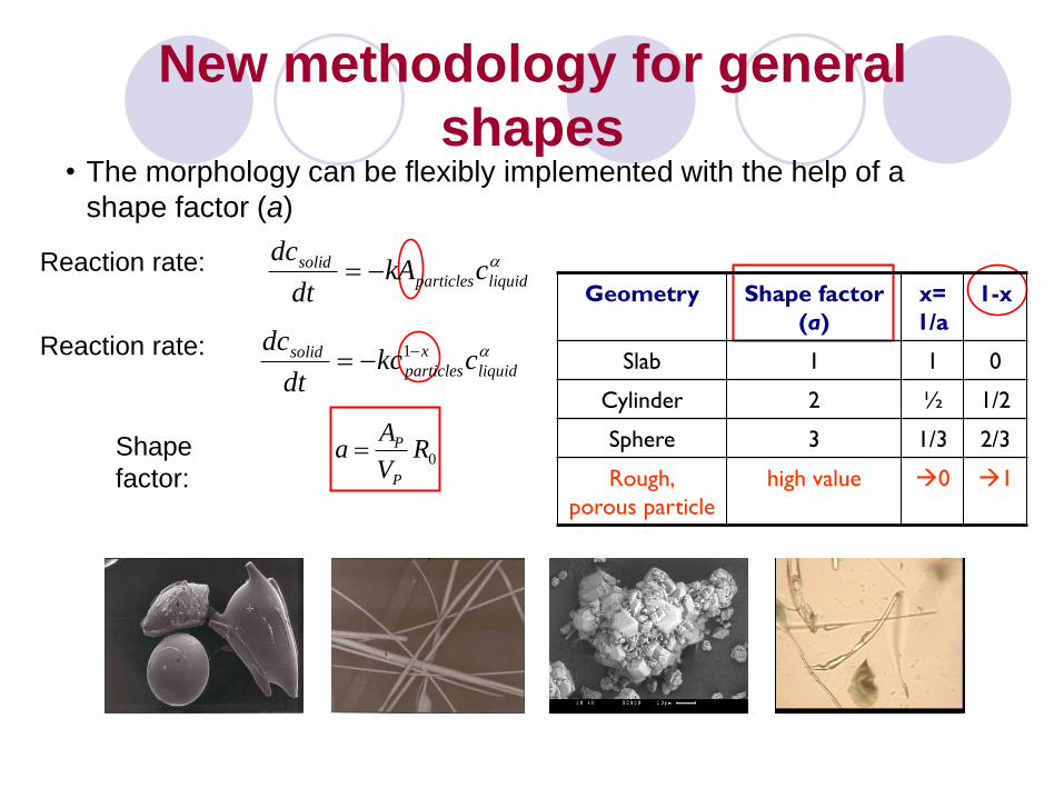
Reaction rate:
Shape
factor:
Reaction rate:
• The morphology can be flexibly implemented with the help of a
shape factor (a)
New methodology for general
shapes
Geometry Shape factor
(a)
x=
1/a
1-x
Slab 1 1 0
Cylinder 2 ½ 1/2
Sphere 3 1/3 2/3
Rough,
porous particle
high value 0 1
liquidparticles
solid ckAdt
dc
liquid
x
particles
solid ckcdt
dc 1

Detailed considerations give a relation
between area (A),
specific surface area (σ),
amount of solid (n),
initial amount of solid(n0),
and molar mass (M);
a=shape factor
aanMnA /11/1
0
Geometry Shape factor
(a)
x=
1/a
1-x
Slab 1 1 0
Cylinder 2 ½ 1/2
Sphere 3 1/3 2/3
Rough,
porous particle
high value 0 1
Often kinetics is
closer to first order!
The roughness is
always there, σ=1
m2/g is not a
perfect sphere!
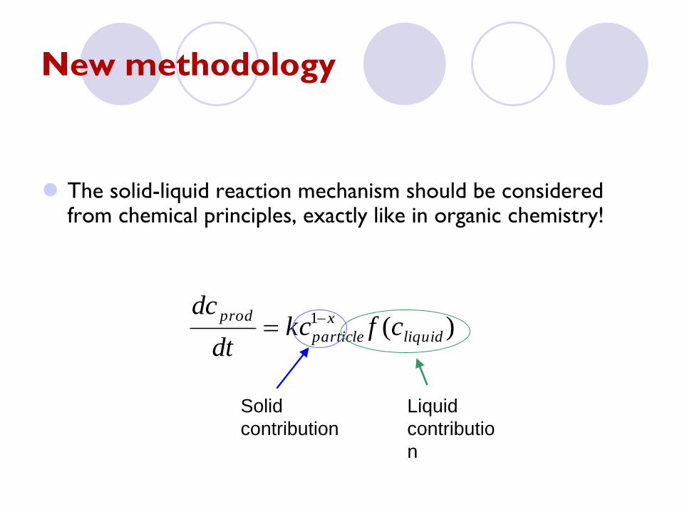
New methodology
The solid-liquid reaction mechanism should be considered from chemical principles, exactly like in organic chemistry!
)(1
liquid
x
particle
prodcfkc
dt
dc
Solid
contribution
Liquid
contributio
n

The dissolution of zink with ferric iron
ZnS(s) + Fe3+ ↔ I1 (I)
I1+ Fe3+ ↔ I2 (II)
I2 ↔ S(s) + 2 Fe2+ + Zn2+ (III)
________________________________________________
ZnS(s) + 2Fe3+ ↔ S(s) + 2 Fe2+ + Zn2+
The mechanism gave the following rate expression
D
Kccckr ZnIIFeIIFeIII )/(
22
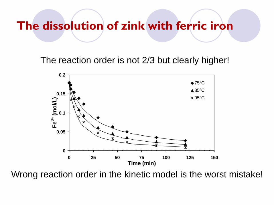
The dissolution of zink with ferric iron
0
0.05
0.1
0.15
0.2
0 25 50 75 100 125 150
Time (min)
Fe
3+ (
mo
l/L
)
75°C
85°C
95°C
The reaction order is not 2/3 but clearly higher!
Wrong reaction order in the kinetic model is the worst mistake!
General product layer model
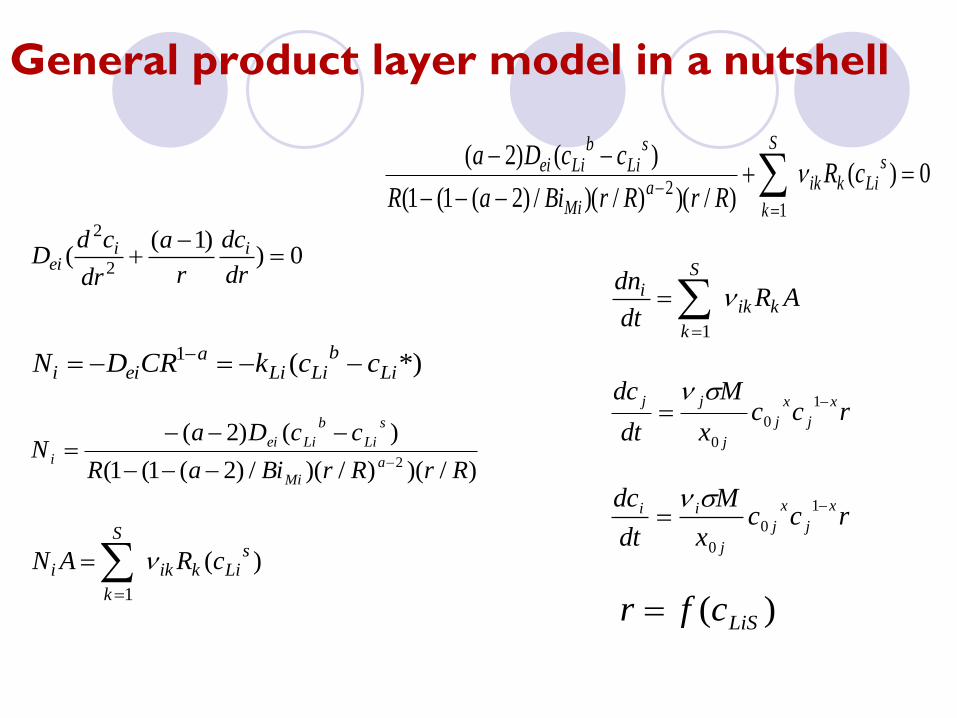
General product layer model in a nutshell
0))1(
(2
2
dr
dc
r
a
dr
cdD ii
ei
*)(1Li
bLiLi
aeii cckCRDN
)/)()/)(/)2(1(1(
)()2(2 RrRrBiaR
ccDaN
a
Mi
s
Li
b
Liei
i
)(
1
sLikik
S
k
i cRAN
0)()/)()/)(/)2(1(1(
)()2(
12
sLikik
S
ka
Mi
sLi
bLiei cR
RrRrBiaR
ccDa
ARdt
dnkik
S
k
i
1
rccx
M
dt
dc x
j
x
j
j
jj
1
0
0
rccx
M
dt
dc x
j
x
j
j
ii
1
0
0
)( LiScfr

Comparison of shrinking particle and
product layer model

Effect of shape factor

Particle size distribution
VC = standard deviation / mean particle
size
• If the particle size distribution deviates significantly from the Gaussian
distribution, erroneous conclusions can be drawn about the reaction
mechanism
VC=0
VC=1.
2
VC=1.
5
VC=0
Shrinking sphere
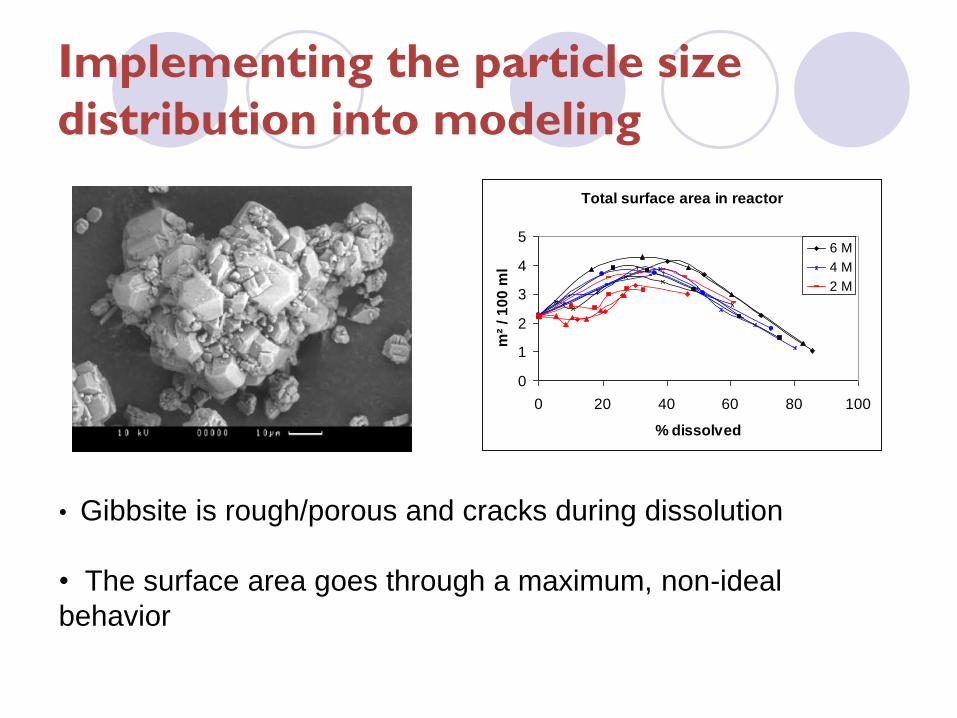
Implementing the particle size
distribution into modeling
Total surface area in reactor
0
1
2
3
4
5
0 20 40 60 80 100
% dissolved
m²
/ 1
00
ml
6 M
4 M
2 M
• Gibbsite is rough/porous and cracks during dissolution
• The surface area goes through a maximum, non-ideal
behavior

Implementing the particle size
distribution into modeling
SPkxE )(2)( SPkxVar
)()(
1
SP
k
x
k
k
exxf SP
0
1)( dtetk tk
SPSP
• The Gamma distribution is fitted to the fresh particle size distribution
and
the distribution is divided into fractions
• The shape parameter (k) and the scale parameter (θ) are kept
constant

Implementing the particle size
distribution into modeling
0 20 40 60 80 100 120 140 160 180 0
0.01
0.02
0.03
0.04
0.05
0.06
0.07
0.08
0.09
Diameter (μm)
Fre
qu
en
cy (
cou
nts
/min
)
time a
iti Xrr 0,,
tPi
tPr
tPrr
aVA i
i
,
,
, 0RV
Aa
P
P
• A new radius is calculated for each fraction and each fraction is
summed to
obtain the new surface area in the reactor
• The new surface area is implemented into to rate equation
1000
XV
V
m
m
c
c ttt
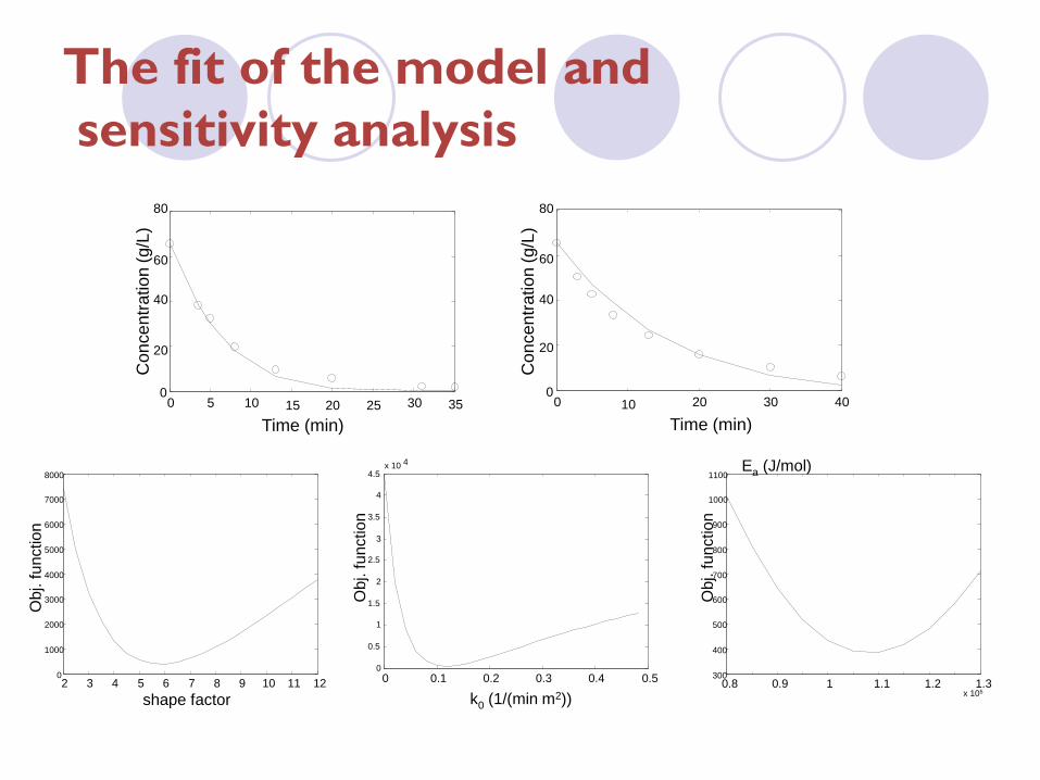
The fit of the model and
sensitivity analysis
2 3 4 5 6 7 8 9 10 11 12 0
1000
2000
3000
4000
5000
6000
7000
8000
shape factor
Ob
j. fu
nctio
n
0.8 0.9 1 1.1 1.2 1.3 x 10⁵
300
400
500
600
700
800
900
1000
1100
Ob
j. fu
nctio
n
0 0.1 0.2 0.3 0.4 0.5 0
0.5
1
1.5
2
2.5
3
3.5
4
4.5 x 10 4
k0 (1/(min m2))
Ob
j. fu
nctio
n
Ea (J/mol)
0 5 10 15 20 25 30 35 0
20
40
60
80
Time (min)
Con
ce
ntr
atio
n (
g/L
)
0 10 20 30 40 0
20
40
60
80
Time (min)
Con
ce
ntr
atio
n (
g/L
)

Selection of the experimental system and equipment
Kinetic investigations Structural investigations
Mass- and heat transfer studies
Ideas on the reaction mechanism including structural changes of the solid
Derivations (and simplification) of rate equations
Model verification by numerical simulations and additional experiments
Estimation of kinetic and mass transfer parameters

Conclusions
Modeling is an important tool in developing new processes as well as optimizing existing ones
Solid-liquid reactions are in general more difficult to model than homogeneous reactions
Traditional modeling procedures have potholes, which can severely influence the outcome
Care should be taken in drawing the right conclusions about the reaction mechanisms

Things to consider in modeling Some important factors:
1. Be sure about what you actually are measuring
2. Evaluate if the particle size distribution needs to be taken into
account (VC<0.3)
3. If the morphology is not ideal use a shape factor to describe
the change in surface area (surface area, density and
conversion measurements needed)
4. Use sensitivity analysis to see if your parameter values are well
defined
Some relevant publications Salmi, Tapio; Grénman, Henrik; Waerna, Johan; Murzin, Dmitry Yu. Revisiting shrinking
particle and product layer models for fluid-solid reactions - From ideal surfaces to real surfaces.Chemical Engineering and Processing 2011, 50(10), 1076-1084.
Salmi, Tapio; Grénman, Henrik; Bernas, Heidi; Wärnå, Johan; Murzin, Dmitry Yu. Mechanistic Modelling of Kinetics and Mass Transfer for a Solid-liquid System: Leaching of Zinc with Ferric Iron. Chemical Engineering Science 2010, 65(15), 4460-4471.
Grénman, Henrik; Salmi, Tapio; Murzin, Dmitry Yu.; Addai-Mensah, Jonas. The Dissolution Kinetics of Gibbsite in Sodium Hydroxide at Ambient Pressure. Industrial & Engineering Chemistry Research 2010, 49(6), 2600-2607.
Grénman, Henrik; Salmi, Tapio; Murzin, Dmitry Yu.; Addai-Mensah, Jonas. Dissolution of Boehmite in Sodium Hydroxide at Ambient Pressure: Kinetics and Modelling. Hydrometallurgy 2010, 102(1-4), 22-30.
Grénman, Henrik; Ingves, Malin; Wärnå, Johan; Corander, Jukka; Murzin, Dmitry Yu.; Salmi, Tapio. Common potholes in modeling solid-liquid reactions – methods for avoiding them. Chemical Engineering Science (2011), 66(20), 4459-4467.
Grénman, Henrik; Salmi, Tapio; Murzin, Dmitry Yu.. Solid-liquid reaction kinetics – experimental aspects and model development. Rev Chem Eng 27 (2011): 53–77

Mechanistic modelling of kinetics and
mass transfer
for a solid-liquid system:
Leaching of zinc with ferric iron
Tapio Salmi, Henrik Grénman, Heidi Bernas,
Johan Wärnå, Dmitry Yu. Murzin
Laboratory of Industrial Chemistry and Reaction Engineering,
Process Chemistry Centre,
Åbo Akademi, FI-20500 Turku/Åbo, Finland
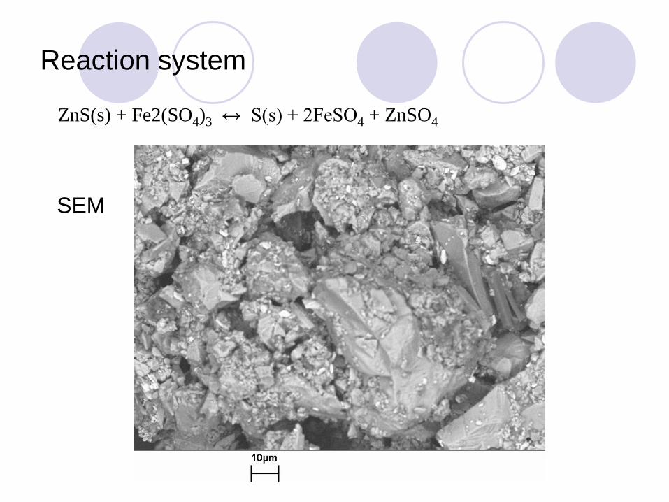
Reaction system
ZnS(s) + Fe2(SO4)3 ↔ S(s) + 2FeSO4 + ZnSO4
SEM
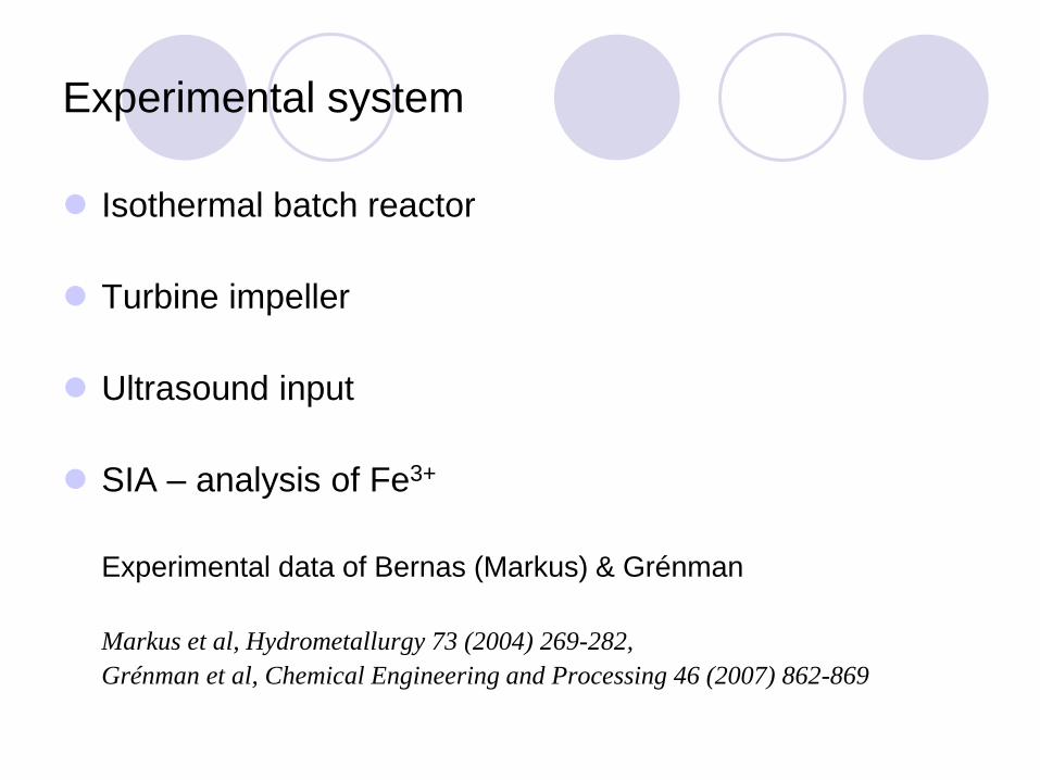
Experimental system
Isothermal batch reactor
Turbine impeller
Ultrasound input
SIA – analysis of Fe3+
Experimental data of Bernas (Markus) & Grénman
Markus et al, Hydrometallurgy 73 (2004) 269-282,
Grénman et al, Chemical Engineering and Processing 46 (2007) 862-869

Multi-transducer ultradound reactor
Generator (0-600W)
20 kHz
Reactor pot inserted
6 transducers
A time-variable
power input

Experimental results - Stirring speed
0
0.05
0.1
0.15
0.2
0 25 50 75 100 125 150
Time (min)
Fe
3+ (
mo
l/L
)
200 rpm
350 rpm500 rpm
700 rpm
T = 85°C , Sphalerite : Fe3+ = 1.1:1
The effect of the stirring speed on the leaching kinetics.

Experimental results
T = 85°C, C0Fe(III) = 0.2 mol/L
0
0.05
0.1
0.15
0.2
0 50 100 150 200
Time (min)
Fe
3+ (
mo
l/L
)
Stoic. 0.5:1Stoic. 0.9:1Stoic. 1.1:1Stoic. 1.6:1Stoic. 2.1:1
The effect of the zinc sulphide concentration on the leaching kinetics.

Experimental results
T = 95°C, Sphalerite : Fe3+ = 1.1:1
0
0.1
0.2
0.3
0 25 50 75 100 125 150
Time (min)
Fe
3+ (
mo
l/L
)
The effect of the ferric ion concentration on the leaching kinetics.

Experimental results
T = 95°C, Sphalerite : Fe3+ = 1.1:1
0
0.05
0.1
0.15
0.2
0 50 100 150 200
Time (min)
Fe
3+ (
mo
l/L
)
0.2 mol/L0.4 mol/L0.6 mol/L0.8 mol/L1.0 mol/L
The effect of sulphuric acid on the leaching kinetics.
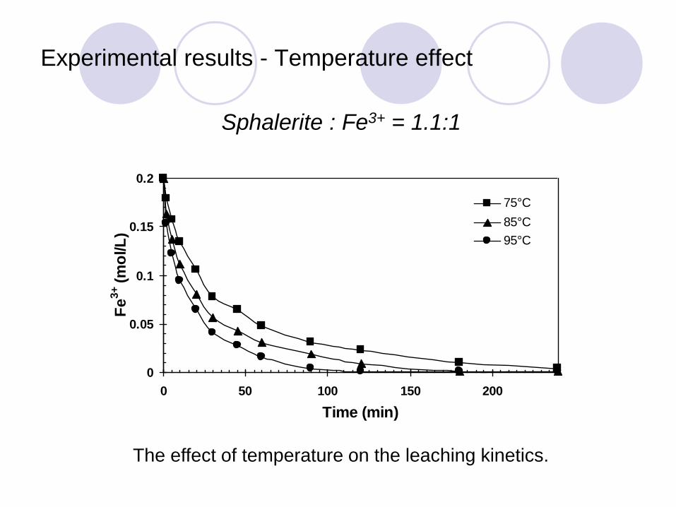
Experimental results - Temperature effect
Sphalerite : Fe3+ = 1.1:1
0
0.05
0.1
0.15
0.2
0 50 100 150 200
Time (min)
Fe
3+ (
mo
l/L
)
75°C
85°C
95°C
The effect of temperature on the leaching kinetics.

Experimental results - Ultrasound effect
T = 85°C Stirring rate 350 rpm
0
0.05
0.1
0.15
0.2
0 25 50 75 100 125 150
Time (min)
Fe
3+ (
mo
l/L
)
0 W
60 W
120 W
180 W
The effect of ultrasound on the leaching kinetics.

Reaction mechanism and rate equations
Surface reaction
Stepwise process
( first reacts one Fe3+, then the second one! )
Rough particles

Three-step surface reaction mechanism
ZnS(s) + Fe3+ ↔ I1 (I)
I1+ Fe3+ ↔ I2 (II)
I2 ↔ S(s) + 2 Fe2+ + Zn2+ (III)
ZnS(s) + 2Fe3+ ↔ S(s) + 2 Fe2+ + Zn2+
rates of steps (I-III)
cI1, cI2 and cI3 = surface concentrations of the intermediates.
1111 Icaar
22122 II cacar
3233 acar IZnIIFeIII
FeIII
FeIII
ccka
ka
ka
cka
ka
cka
2
33
33
22
22
11
11

Development of rate equations
Pseudo-steady state hypothesis
rrrr 321
Rate equation
323121
321321
aaaaaa
aaaaaar
Back-substitution of a1….a-3 gives
D
cckkkckkkr ZnIIFeIIFeIII
2321
2321
D
Kccckr ZnIIFeIIFeIII )/(
22
D = k-1k-2+k-1k+3+k+2k+3cFeIII
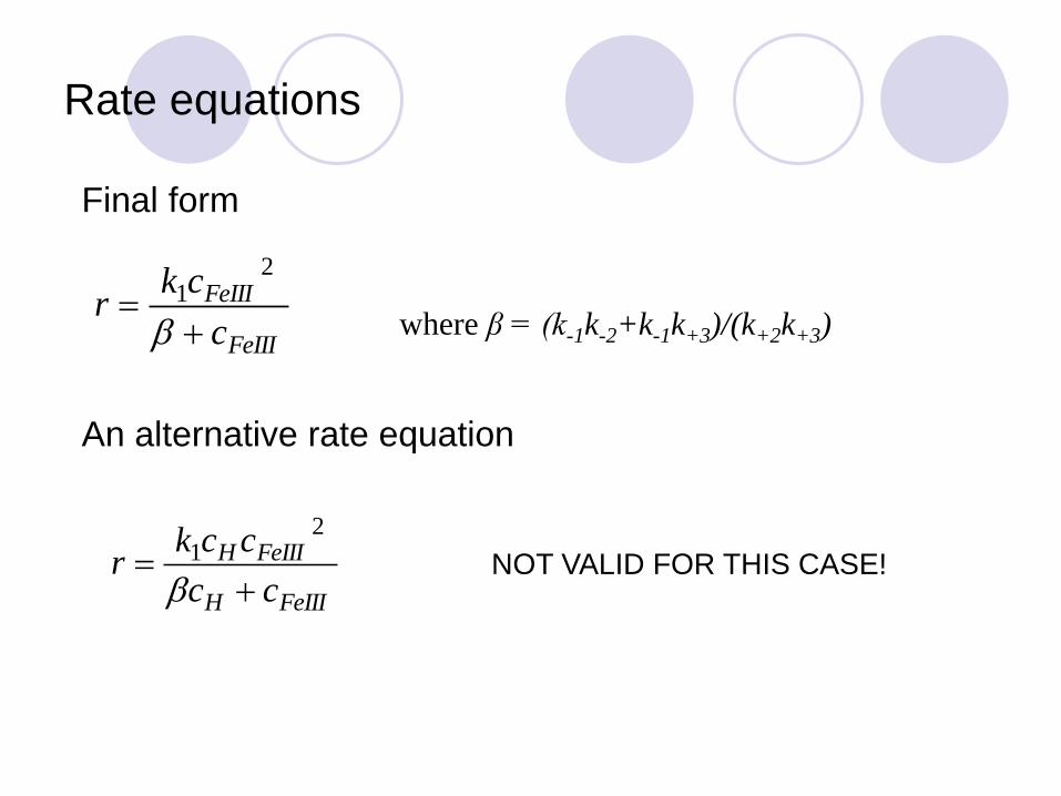
Rate equations
Final form
FeIII
FeIII
c
ckr
21
where β = (k-1k-2+k-1k+3)/(k+2k+3)
An alternative rate equation
FeIIIH
FeIIIH
cc
cckr
21 NOT VALID FOR THIS CASE!
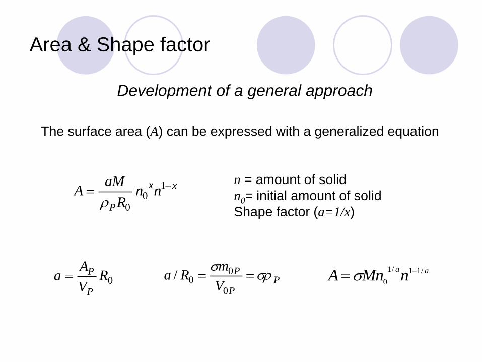
Area & Shape factor
Development of a general approach
The surface area (A) can be expressed with a generalized equation
n = amount of solid
n0= initial amount of solid
Shape factor (a=1/x)
xx
P
nnR
aMA 1
00
0RV
Aa
P
P PP
P
V
mRa
0
00/ aa
nMnA /11/1
0
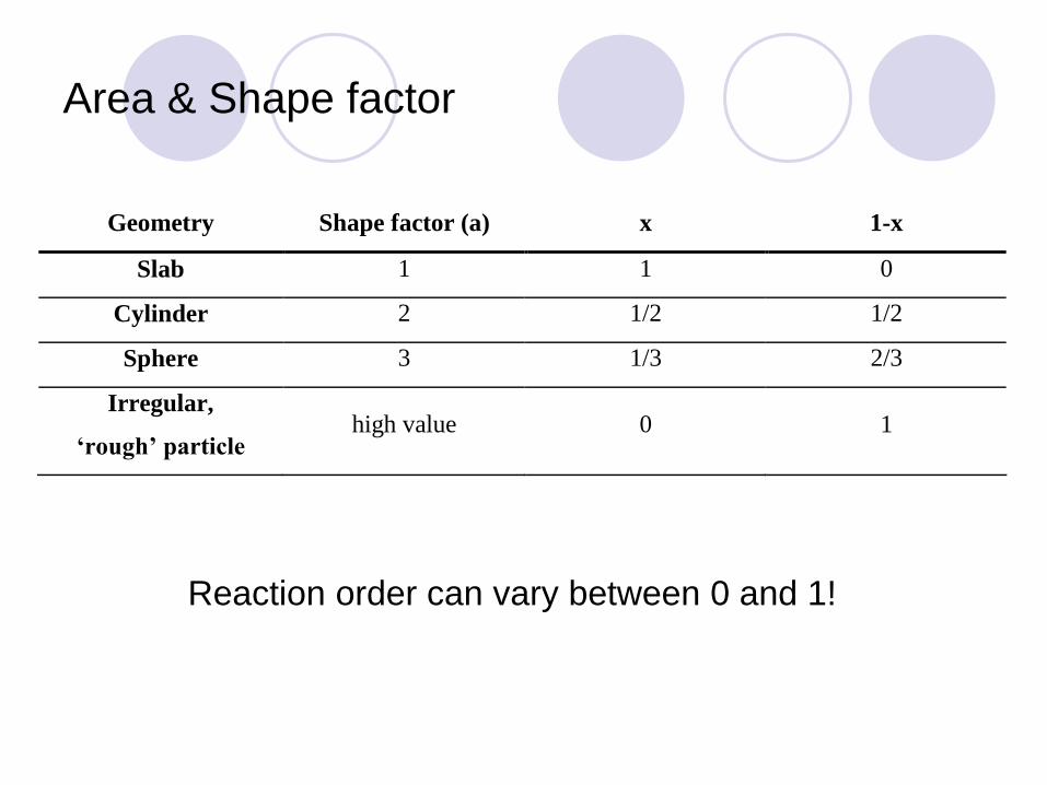
Area & Shape factor
Geometry Shape factor (a) x 1-x
Slab 1 1 0
Cylinder 2 1/2 1/2
Sphere 3 1/3 2/3
Irregular,
‘rough’ particle high value 0 1
Reaction order can vary between 0 and 1!
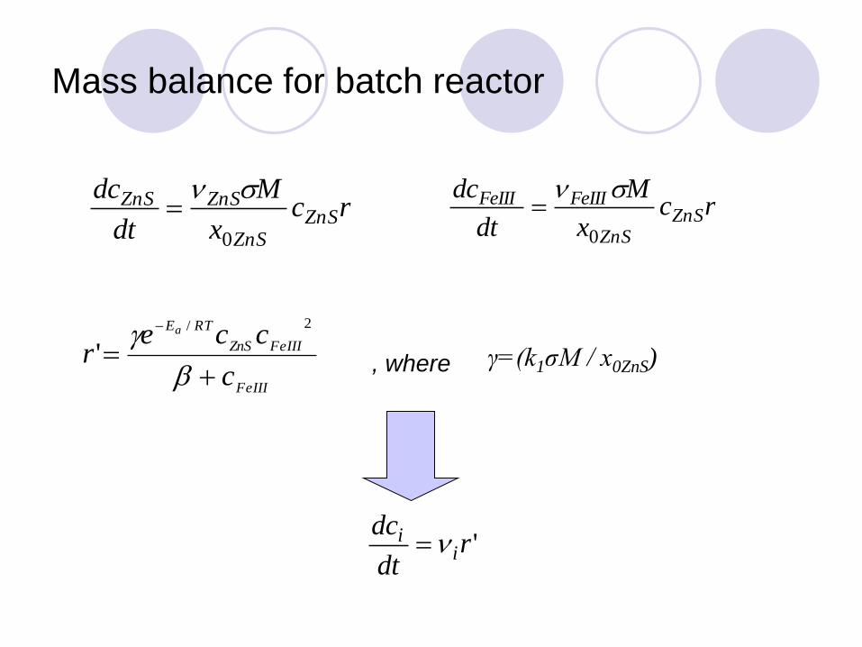
Mass balance for batch reactor
rcx
M
dt
dcZnS
ZnS
ZnSZnS
0
rc
x
M
dt
dcZnS
ZnS
FeIIIFeIII
0
FeIII
FeIIIZnS
RTE
c
ccer
a
2/
' γ=(k1σM / x0ZnS)
'rdt
dci
i
, where

Parameter estimation
Nonlinear regression applied on intrinsic kinetic data
Estimated Parameter Parameter value Est. Std. Error %
γ (L / mol min) 0.331 4.5
Ea (J / mol) 53200 4.8
β (mol / L) 0.2 24.9
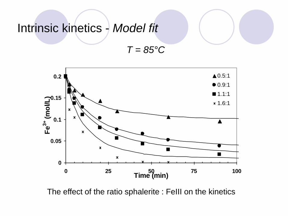
Intrinsic kinetics - Model fit
0
0.05
0.1
0.15
0.2
0 25 50 75 100Time (min)
Fe
3+ (
mo
l/L
)
0.5:1
0.9:1
1.1:1
1.6:1
T = 85°C
The effect of the ratio sphalerite : FeIII on the kinetics
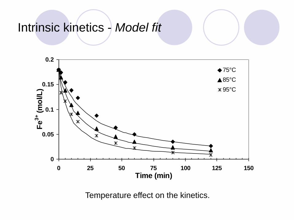
Intrinsic kinetics - Model fit
0
0.05
0.1
0.15
0.2
0 25 50 75 100 125 150
Time (min)
Fe
3+ (
mo
l/L
)
75°C
85°C
95°C
Temperature effect on the kinetics.

Mass transfer limitations in Batch reactor
0 rAAN is
Li
where ri=νir The mass transfer term (NLis) is described by Fick’s law
*
**)(
21
i
iiiiLi
c
ckcck
The solution becomes
1'')1'(4)1'(
'2/*
2
ii cc
*
*21
FeIII
FeIII
c
ckr
β’=β/ci, γ’=(-νik1ci/kLi), y=ci*/ci

Liquid-solid mass transfer coefficient
General correlation
3/12/1Re ScbaSh
iLi DdkSh /
3/1
3
4
Re
diDSc /
3/16/1
3
4
i
iLi
D
dba
d
Dk
3/16/1
3
3/440
3/10 i
iLi
D
zdba
zd
Dk
where z=cZnS/c0ZnS. The index (i) refers to Fe(III) and Fe(II)
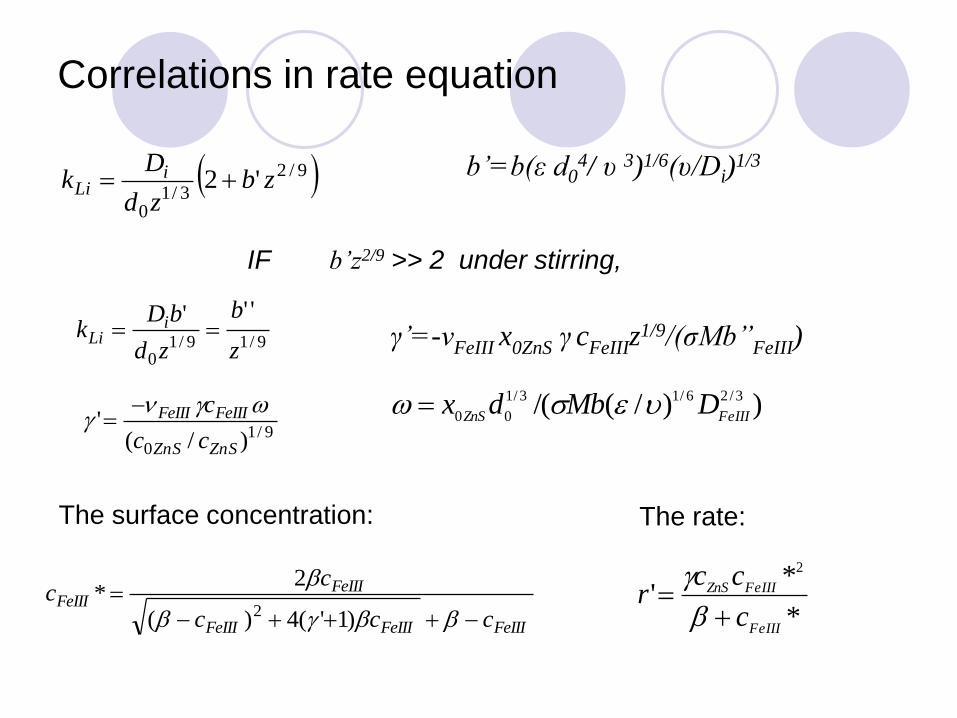
Correlations in rate equation
9/2
3/10
'2 zbzd
Dk i
Li b’=b(ε d0
4/ υ 3)1/6(υ/Di)1/3
IF b’z2/9 >> 2 under stirring,
9/19/10
'''
z
b
zd
bDk i
Li γ’=-νFeIII x0ZnS γ cFeIIIz1/9/(σMb’’FeIII)
))/(/( 3/26/13/1
00 FeIIIZnSDMbdx
9/10 )/(
'ZnSZnS
FeIIIFeIII
cc
c
The surface concentration:
FeIIIFeIIIFeIII
FeIIIFeIII
ccc
cc
)1'(4)(
2*
2
The rate:
*
*'
2
FeIII
FeIIIZnS
c
ccr
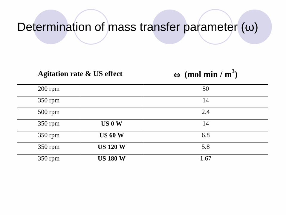
Determination of mass transfer parameter (ω)
Agitation rate & US effect ω (mol min / m3)
200 rpm 50
350 rpm 14
500 rpm 2.4
350 rpm US 0 W 14
350 rpm US 60 W 6.8
350 rpm US 120 W 5.8
350 rpm US 180 W 1.67
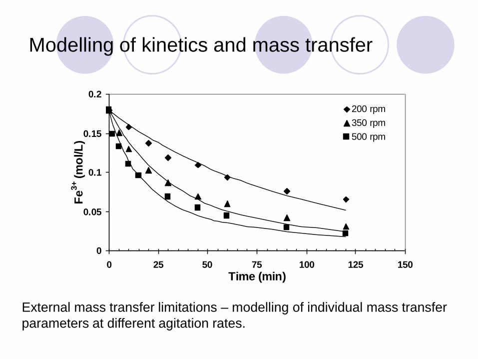
Modelling of kinetics and mass transfer
0
0.05
0.1
0.15
0.2
0 25 50 75 100 125 150
Time (min)
Fe
3+ (
mo
l/L
)
200 rpm
350 rpm
500 rpm
External mass transfer limitations – modelling of individual mass transfer
parameters at different agitation rates.
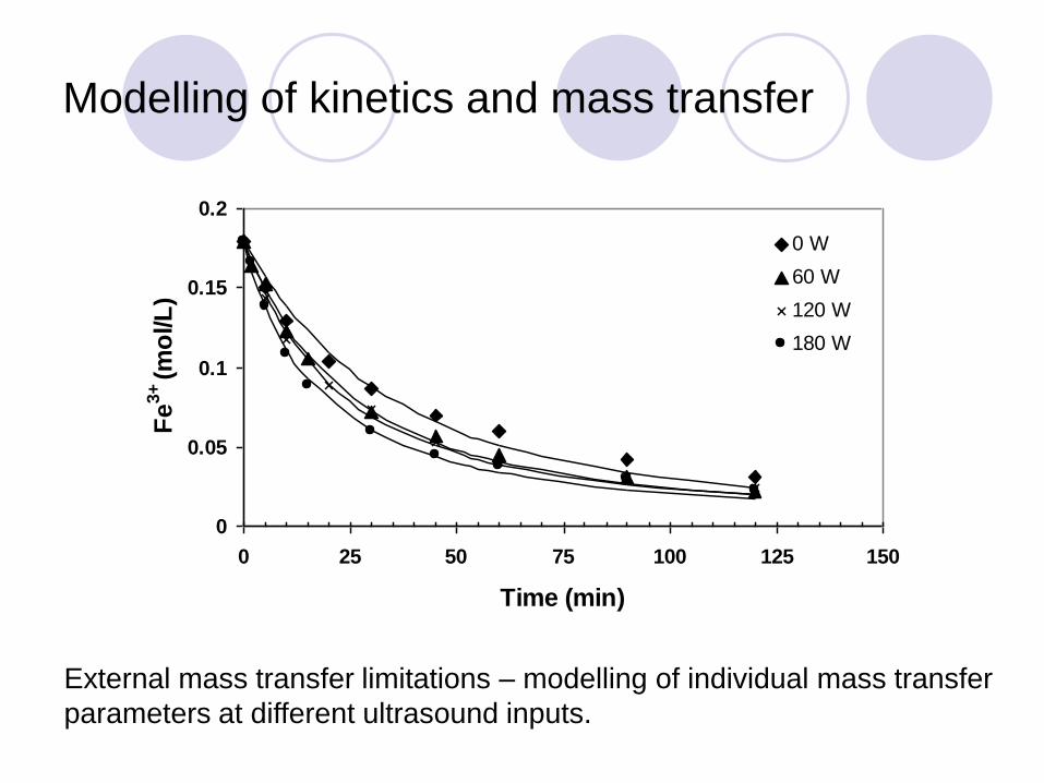
Modelling of kinetics and mass transfer
0
0.05
0.1
0.15
0.2
0 25 50 75 100 125 150
Time (min)
Fe
3+ (m
ol/L
)
0 W
60 W
120 W
180 W
External mass transfer limitations – modelling of individual mass transfer
parameters at different ultrasound inputs.

Mass transfer
parameter
0
10
20
30
40
50
60
150 200 250 300 350 400 450 500 550
rpm (1/min)
ω
0
2
4
6
8
10
12
14
16
0 50 100 150 200
US (W)
ω
Normal agitation
Ultrasound

The real impact of mass transfer limitations
0
20
40
60
80
100
120
0 25 50 75 100 125 150
Time (min)
(Fe
3+su
rface
/ F
e3+b
ulk
)*1
00
500 rpm
350 rpm
200 rpm
The difference in the model based surface concentrations and measured
bulk concentrations of Fe3+ at different stirring rates.

The real impact of mass transfer limitations
0
20
40
60
80
100
120
0 25 50 75 100 125 150
Time (min)
(Fe
3+su
rface
/ F
e3+b
ulk
)*1
00
180 W
60 W
0 W
The difference in the model based surface concentrations and measured bulk
concentrations of Fe3+ at different ultrasound inputs.

Conclusions
A new kinetic model was proposed
A general treatment of smooth, rough and porous
surfaces was developed
The theory of mass transfer was implemented in the
model
Model parameters were estimated
The model works
Modelling and simulation of
porous, reactive particles in
liquids: delignification of wood
Tapio Salmi, Johan Wärnå, J.-P. Mikkola, Mats Rönnholm
Åbo Akademi Process Chemistry Centre,
Laboratory of Industrial Chemistry
FIN-20500 Turku / Åbo Finland, [email protected]
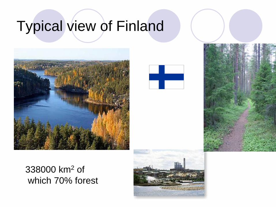
Typical view of Finland
338000 km2 of
which 70% forest

Papermaking
Wood chips
This is where paper
making begins.
A typical wood chip
measures 40 x 25 x
10 mm.

Wood
Each chip comprises
water, cellulose wood
fibres and the binding
agent lignin.
.

Pulp
To make paper, we need to first make pulp, which is the process of breaking the wood structure down into individual fibers
Digester Chips

Reactions
The reactions in chemical pulping are
numerous. Typical pulping chemicals
are NaOH and NaHS
cellulose
Overall process:
Lignin+Cellulose+Carbohydrates+Xylanes+OH+HS ->
Dissolved components
Part of Lignin
molecule
Kinetic modelling of wood delignification
Purdue model (Smith et.al. (1974) Christensen
et al. 1983), 5 pseudocomponents
Gustafson et al. 1983, 2 wood components
Lignin and Carbohydrate, 3 stages
Andersson 2003, 15 pseudocomponents
Very few models available!

Wood chip structure
Wood material is built
up of fibres
We can expect
different diffusion
rates in the fibre
direction and in the
opposite direction to
the fibres.

Existing models
The existing models for delignification of
wood consider a 1 dimensional case with
equal diffusion rates in all directions
Is a 2- or 3-dimensional model needed ?

Characteristics of our model
Time dependent dynamic model
Complex reaction network included
Mass transfer via diffusion in different
directions
Structural changes of the wood chip
included
All wood chips of equal size
Perfectly mixed batch reactor assumed

Mathematical model,volume element
3D –model for a wood
chip
x
yz
x
yz
dt
dn+AN+AN+AN
ΔVr+AN+AN+AN
i
outxyizoutxziyoutyzix
'
ixyizxziyyzix =ininin
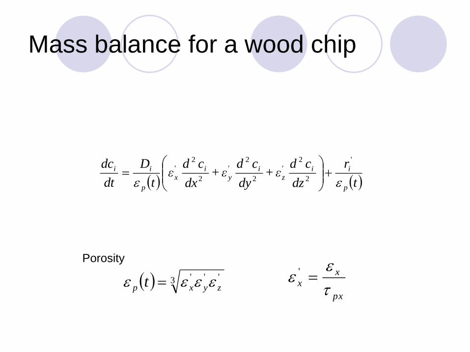
Mass balance for a wood chip
tr
dz
cdε+
dy
cdε+
dx
cdε
t
D
dt
dc
p
ii'
z
i'
y
i'
x
p
ii
'
2
2
2
2
2
2
3 '''
zyxp t px
xx
'
Porosity

Boundary conditions
The concentrations outside the wood chip are locally known
ci=cLi
at the centre of the chip (symmetry)
dci/dx=dci/dy=dci/dz=0
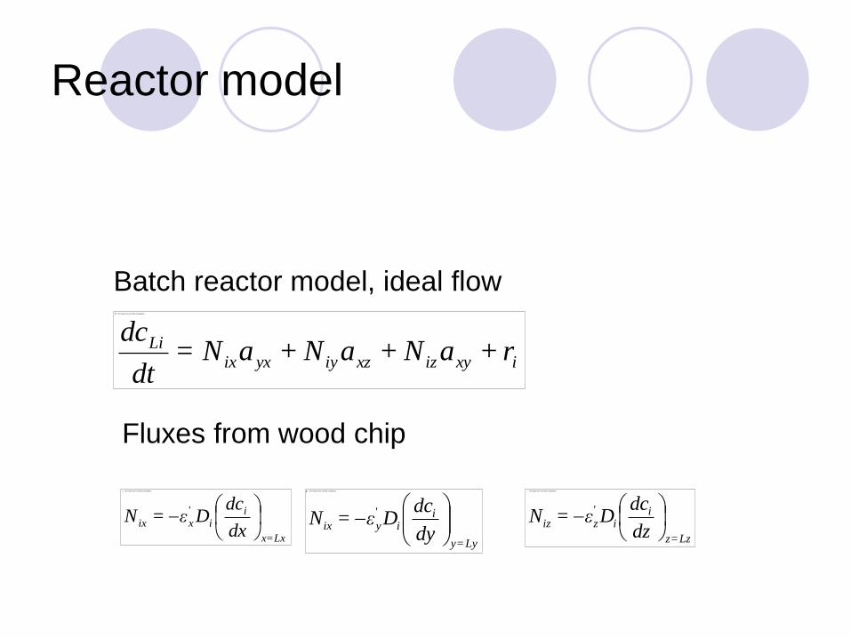
Reactor model
Lx=x
ii
'
xixdx
dcDε=N
ixyizxziyyxixLi r+aN+aN+aN=
dt
dc
Ly=y
ii
'
yixdy
dcDε=N
Lz=z
ii
'
zizdz
dcDε=N
Fluxes from wood chip
Batch reactor model, ideal flow
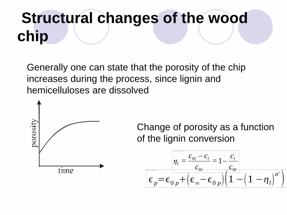
Structural changes of the wood
chip
Generally one can state that the porosity of the chip
increases during the process, since lignin and
hemicelluloses are dissolved
p 0 p 0 p 1 1 l
'l
l
l
lll
c
c=
c
cc=η
00
0 1
Change of porosity as a function
of the lignin conversion
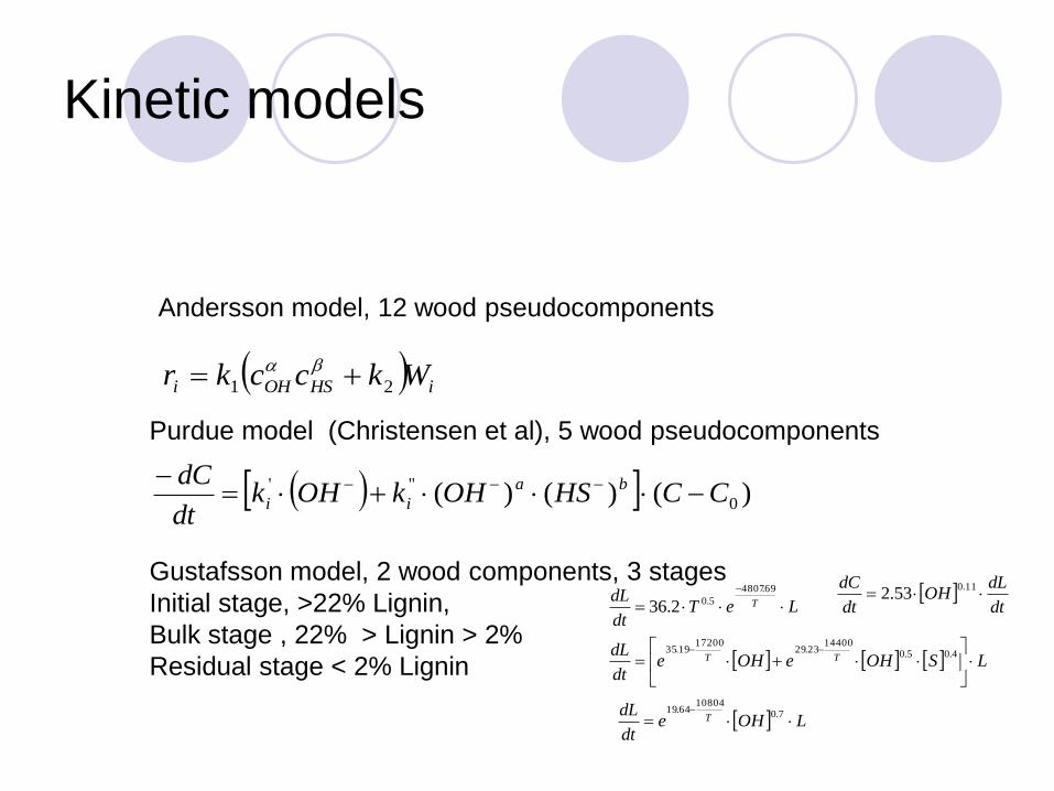
Kinetic models
)()()( 0
"' CCHSOHkOHkdt
dC ba
ii
Purdue model (Christensen et al), 5 wood pseudocomponents
iHSOHi Wkcckr 21
Andersson model, 12 wood pseudocomponents
Gustafsson model, 2 wood components, 3 stages
Initial stage, >22% Lignin,
Bulk stage , 22% > Lignin > 2%
Residual stage < 2% Lignin
LeTdt
dLT
69.4807
5.02.36
dt
dLOH
dt
dC
11.053.2
LSOHeOHedt
dLTT
4.05.014400
23.2917200
19.35
LOHedt
dLT
7.010804
64.19

Diffusion models
Del 373.15( ) 2.13 109
m
2
s
380 400 420 440 4600
1 108
2 108
3 108
McKibbins
Wilke-Chang
Nernst-Haskell
Temperature [K]
Dif
fusi
vit
y [m
^2/s
]
6.0
12104.7
AB
B
ABV
TMD
zz
zzTDo
00
001410931.8
TOHNaOH eTD
9872.1
4870
8
, 10667.52
McKibbins
Wilke-Chang
Nernst-Haskel (infinite dillution)

Kappa number
5500
CHL
L
The progress of delignification is by pulp
professionals described by the Kappa number
L = Lignin on wood, CH = Carbohydrates on wood

Numerical approach
Discretizing the partial differential equations (PDEs) with respect to the spatial coordinates (x, y, z).
Central finite difference formulae were used to approximate the spatial derivatives
Thus the PDEs were transformed to ordinary differential equations (ODEs) with respect to the reaction time with the use of the powerful finite difference method.
The created ODEs were solved with the backward difference method with the software LSODES

Simulation results,
profiles inside wood chip
0
5
10
15 0
5
10
15
0.5
0.51
0.52
0.53
0.54
0.55
y
Porosity y
x
centre
0
5
10
15
0
5
10
1517
17.5
18
18.5
19
x
L1
y
centre
0
5
10
15
0
5
10
1576
78
80
82
84
86
x
Kappa
y
centre
Lignin content
Porosity
Kappa value
T=170 ºC
C0,NaOH=0.5 mol/l
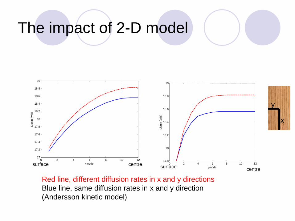
The impact of 2-D model
Red line, different diffusion rates in x and y directions
Blue line, same diffusion rates in x and y direction
(Andersson kinetic model)
0 2 4 6 8 10 12 17
17.2
17.4
17.6
17.8
18
18.2
18.4
18.6
18.8
19
x-node
Lig
nin
(w
%)
0 2 4 6 8 10 12 17.8
18
18.2
18.4
18.6
18.8
19
y-node
Lig
nin
(w
%)
surface centre surface
centre
y
x

Content of lignin on wood as a function of
reaction time
Lignin concentration (w-%) in wood chip as a function of
reaction time (min) with Andersson kinetic model (left) and
Purdue kinetic model (right).
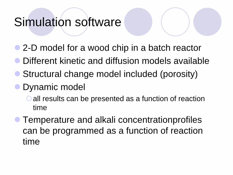
Simulation software
2-D model for a wood chip in a batch reactor
Different kinetic and diffusion models available
Structural change model included (porosity)
Dynamic model
all results can be presented as a function of reaction
time
Temperature and alkali concentrationprofiles
can be programmed as a function of reaction
time
Conclusions
A general dynamic model and software for the description of wood delignification
Solved numerically for example cases, which concerned delignification of wood chips in perfectly backmixed batch reactors.
Structural changes and anisotropies of wood chips are included in the model.
The software utilizes standard stiff ODE solvers combined with a discretization algorithm for parabolic partial differential equations.
Example simulations indicated that the selected approach is fruitful, and the software can be extended to continuous delignification processes with more complicated flow patterns.
Thank you!