Cartesian Programming

Habilitation ThesisUniversity of Grenoble, France

John Plaiceplaice@cse.unsw.edu.au

Technical ReportUNSW-CSE-TR-1101

January 2011

THE UNIVERSITY OF

NEW SOUTH WALES

School of Computer Science and EngineeringThe University of New South Wales

Sydney 2052, Australia

La programmation cartesienne

John Plaice

These presentee pour l’obtention d’uneHabilitation a Diriger des Recherches

Universite de Grenoble, France

soutenue le 20 decembre 2010 devant la commission d’examen

MM. Joseph Sifakis President

Albert Benveniste ExaminateursPaul CaspiNicolas Halbwachs

Satnam Singh RapporteursJean-Pierre TalpinWilliam W. Wadge

Abstract

We present a new form of declarative programming inspired by the Cartesian coordinate sys-tem. This Cartesian programming, illustrated by the TransLucid language, assumes that allprogrammed entities vary with respect to all possible dimensions, or degrees of freedom. Thismodel is immediately applicable to areas of science, engineering and business in which workingwith multiple dimensions is common. It is also well suited to specification and programming insituations where a problem is not fully understood, and, with refinement, more parameters willneed to be taken into consideration as time progresses.

In the Cartesian model, these dimensions include, for all entities, all possible parameters, bethese explicit or implicit, visible or hidden. As a result, defining the aggregate semantics of anentire system is simplified, much as the use of the universal relation simplifies the semantics of arelational database system. Evolution through time is handled through the use of a special timedimension that does not allow access to the future.

In TransLucid, any atomic value may be used as a dimension. A context maps each dimensionto its corresponding ordinate. A context delta is the partial equivalent. An expression is evaluatedin a given context, and this context may be queried, dimension by dimension, or perturbed by acontext delta.

A variable in TransLucid may have several definitions and, given a current context, the bestfit(most specific) definitions with respect to that context are chosen and evaluated separately, andthe results are combined together. The set of definitions for a variable define a hyperdaton, whichcan be understood as an arbitrary-dimensional array of arbitrary extent.

Functional abstraction in TransLucid requires two kinds of parameters: value parameters, withcall-by-value semantics, are used to pass dimensions and constants; named parameters, with call-by-name semantics, are used to pass hyperdatons. Where clauses, used for local definitions, defineboth new variables and new dimensions of variance.

This thesis presents the full development of Cartesian programming and of TransLucid, com-plete with a historical overview leading to their conception. Both the denotational and operationalsemantics are presented, as is the implementation, designed as a library. One important result isthat the operational semantics requires only the evaluation and caching of relevant dimensions,thereby ensuring that space usage is kept to a minimum. Two applications using the TransLucidlibrary are presented, one a standalone interpreter, the other an interactive code browser andhyperdaton visualizer.

The set of equations defining a TransLucid system can vary over time, a special dimension. Ateach instant, the set of equations may be modified, but in so doing can only affect the present andfuture of the system. Timing semantics is always synchronous. There are several possible waysfor multiple TransLucid systems to interact.

The caching mechanism provided in the operational semantics allows for the efficient imple-mentation of systems whose calling structure is highly irregular. For more regular structures, itis possible to create even more efficient bottom-up solutions, in which recursive instantiations offunctions are eliminated, with clear bounds on memory usage and computation.

Cartesian programming is not just designed as a standalone paradigm, but as a means of betterunderstanding other paradigms. We examine imperative programming and side-effects, and showthat these, under certain conditions, can be translated into TransLucid, thereby allowing thedesign of new imperative constructs in the original language.

ii

Resume

Nous presentons une nouvelle forme de programmation declarative inspiree par le systeme de coor-donnees cartesien. Cette programmation cartesienne, illustree par le langage TransLucid, supposeque toute entite programmee varie par rapport a toutes les dimensions, ou degres de liberte. Cemodele est immediatement utilisable dans les domaines de la science, du genie ou des affaires danslesquels travailler avec de multiples dimensions est courant. Le modele est aussi bien applique ala specification et la programmation dans des situations ou un probleme n’est pas entierementcompris et ou de nouveaux parametres seront pris en compte avec le fil du temps.

Dans le modele cartesien, ces dimensions incluent, pour toute entite, tous les parametres pos-sibles, que ces derniers soient explicites ou implicites, visibles ou caches. Il en suit que definirla semantique collective d’un systeme complet est simplifie, de la meme maniere que l’utilisationde la relation universelle simplifie la semantique d’un systeme de bases de donnees relationnel.L’evolution dans le temps se fait par moyen d’une dimension speciale temporelle qui ne permetpas d’acces au futur.

En TransLucid, toute valeur atomique peut etre utilisee comme dimension. Un contexte est unefonction totale portant chaque dimension a son ordonnee correspondante. Un delta de contextesest l’equivalent partiel. Une expression est evaluee dans un contexte donne, et ce contexte peutetre interroge, dimension par dimension, ou perturbe par un delta de contextes.

Une variable en TransLucid peut avoir plusieurs definitions et, etant donne un contexte courant,les definitions !bestfit" (les plus specifiques) par rapport au contexte sont choisies et evalueesseparement, et les resultats sont rassembles. L’ensemble des definitions d’une variable definit unhyperdaton, qui peut etre percu comme un tableau de taille et de dimensionalite arbitraires.

L’abstraction fonctionnelle en TransLucid necessite deux types de parametres : les parametresde valeur, avec semantique !call-by-value", sont utilises pour transmettre des dimensions et desconstantes ; les parametres nommes, avec semantique !call-by-name", sont utilises pour trans-mettre des hyperdatons. Les clauses where, utilisees pour les definitions locales, definissent a lafois de nouvelles variables et de nouvelles dimensions de variance.

La these presente le developpement de la programmation cartesienne et de TransLucid, avec unsurvol historique menant a leur conception. Les semantiques denotationnelle et operationnelle sontpresentees, ainsi que l’est la realisation, concue comme une bibliotheque. Un resultat important estque la semantique operationnelle ne necessite que l’evaluation et la memorisation de dimensionspertinentes, minimisant ainsi l’utilisation d’espace. Deux logiciels utilisant la bibliotheque Trans-Lucid sont presentes, un interprete a boucle textuelle, et un navigateur de code et d’hyperdatons.

Un ensemble d’equations definissant un systeme TransLucid peut varier dans le temps, unedimension speciale. A chaque instant, l’ensemble d’equations peut etre modifie, mais en ce faisantne peut influencer que le present et le futur du systeme. La semantique temporelle est toujourssynchrone. L’interaction de multiples systemes TransLucid peut se faire de plusieurs manieres.

Le mecanisme de memorisation fourni dans la semantique operationnelle permet la realisationefficace de systemes dont l’arborescence des appels est tres irreguliere. Pour des cas plus reguliers,il est possible de creer des solutions plus efficaces par le bas, dans lesquelles des appels recursifsde fonctions sont elimines, avec des bornes claires sur l’utilisation de la memoire et du calcul.

La programmation cartesienne n’est pas seulement concue comme un paradigme a part, maisaussi comme une methode pour mieux comprendre d’autres paradigmes. Nous examinons la pro-grammation imperative et les effets de bord et demontrons que, sous certaines conditions, ceux-cipeuvent etre traduits en TransLucid, permettant ainsi la conception de nouvelles constructionsimperatives dans le langage originel.

iii

Acknowledgements

I wish to thank the three rapporteurs of my work, Satnam Singh, Jean-Pierre Talpin and WilliamWadge, for having accepted to evaluate this thesis with a very short turnaround time. I wish tothank the other examiners of the jury, Albert Benveniste, Paul Caspi, Nicolas Halbwachs, andJoseph Sifakis for having taken the time from their Christmas holidays so that they could attendmy defense. For me, it is a great honor to be able to present my work to such a distinguished jury.

The present work is the result of many years of reflection, of individual steps forward followedby multiple steps backwards, of attempted semantics, of software development, of experiments,with successes and failures. The advances presented here would never have taken place withoutthe support of a number of people and organizations.

First, I would like to thank the School of Computer Science and Engineering at The Universityof South Wales in Sydney, Australia for providing me with a base where I was allowed to do thingsmy unorthodox way, without ever being told that I had to do things differently. My thanks go tomy Head of School for a number of years, Paul Compton.

Second, I wrote this thesis while on sabbatical from UNSW, for 9 months at the Universityof Neuchatel in Switzerland and 3 months at the Tata Institute of Fundamental Research inMumbai, India. I received support from the Swiss National Foundation and from TIFR. For thisI am grateful. My thanks go to Peter Kropf, Pascal Felber and Jacques Savoy in Neuchatel andto R. K. Shyamasundar, Paritosh K. Pandya and N. Raja in Mumbai for interesting discussions.

The intuitions behind the ideas in this work go back to a series of conversations that took placebetween 1999 and 2004: with Peter Kropf, telling me that it was time for me to start working onsomething significant; with William Wadge, with whom I discovered the pervasive nature of theintensional context; with Paul Swoboda, who did his PhD under my supervision, for helping meinvent the æther as a shared context acting as a publish-and-subscribe system; and with DavidParnas, who claimed that I was simply reinventing distributed, global variables.

The experiments took place while working with my students, both PhD and undergraduate.Paul Swoboda wrote an impressive suite of software used to experiment with intensional systems,while Gabriel Ditu wrote the initial presentation for TransLucid. Several TransLucid interpreterswere written by undergraduates, including Myatt Khine Oo, Toby Rahilly and Jarryd Beck.

Finally, I wish to thank my wife, Blanca Lucıa Mancilla, our two daughters Carolina LucianaPlaice and Alejandra Lucıa Plaice, and my son, Cyril Lucien Bouland, for encouraging me thispast year to finish this work. Blanca and I have been married 15 years and she has been workingwith me for the last eight, which includes listening to my crazy ideas in the middle of the night.

iv

Contents

Sommaire 1

Introduction 9

I Preparing the Cartesian Space 13

1 From Lucid to TransLucid: Iteration, Dataflow,Intensional and Cartesian Programming 141.1 Introduction . . . . . . . . . . . . . . . . . . . . . . . . . . . . . . . . . . . . . . . . 141.2 Iteration: Original Lucid . . . . . . . . . . . . . . . . . . . . . . . . . . . . . . . . . 151.3 Lucid, the Dataflow Programming Language . . . . . . . . . . . . . . . . . . . . . . 181.4 Implementing Lucid: Eduction . . . . . . . . . . . . . . . . . . . . . . . . . . . . . 201.5 Synchronous programming: LUSTRE . . . . . . . . . . . . . . . . . . . . . . . . . 211.6 Explicit multidimensionality: Ferd Lucid and ILucid . . . . . . . . . . . . . . . . . 211.7 Intensional programming: Field Lucid . . . . . . . . . . . . . . . . . . . . . . . . . 231.8 Dimensional abstraction: Indexical Lucid . . . . . . . . . . . . . . . . . . . . . . . 251.9 Going parallel: Granular Lucid . . . . . . . . . . . . . . . . . . . . . . . . . . . . . 261.10 Possible-worlds versioning: The context comes to the fore . . . . . . . . . . . . . . 271.11 Versioned definitions: Plane Lucid . . . . . . . . . . . . . . . . . . . . . . . . . . . 271.12 List dimensions: Attributes and functions . . . . . . . . . . . . . . . . . . . . . . . 281.13 First-class dimensions: Multidimensional Lucid . . . . . . . . . . . . . . . . . . . . 281.14 First-class contexts . . . . . . . . . . . . . . . . . . . . . . . . . . . . . . . . . . . . 291.15 Cartesian programming: TransLucid . . . . . . . . . . . . . . . . . . . . . . . . . . 291.16 Conclusions . . . . . . . . . . . . . . . . . . . . . . . . . . . . . . . . . . . . . . . . 30

2 Possible-Worlds Versioning 312.1 Introduction . . . . . . . . . . . . . . . . . . . . . . . . . . . . . . . . . . . . . . . . 312.2 Background: Possible worlds and intensional logic . . . . . . . . . . . . . . . . . . 322.3 Possible-worlds versioning . . . . . . . . . . . . . . . . . . . . . . . . . . . . . . . . 34

2.3.1 Introduction . . . . . . . . . . . . . . . . . . . . . . . . . . . . . . . . . . . 352.3.2 Basic definitions (1) . . . . . . . . . . . . . . . . . . . . . . . . . . . . . . . 352.3.3 Experiment: Software configuration . . . . . . . . . . . . . . . . . . . . . . 362.3.4 Discussion . . . . . . . . . . . . . . . . . . . . . . . . . . . . . . . . . . . . . 37

2.4 Navigation through possible worlds . . . . . . . . . . . . . . . . . . . . . . . . . . . 372.4.1 Introduction . . . . . . . . . . . . . . . . . . . . . . . . . . . . . . . . . . . 372.4.2 Basic definitions (2) . . . . . . . . . . . . . . . . . . . . . . . . . . . . . . . 372.4.3 Experiment: Intensional HTML . . . . . . . . . . . . . . . . . . . . . . . . . 382.4.4 Discussion . . . . . . . . . . . . . . . . . . . . . . . . . . . . . . . . . . . . . 39

2.5 Remote navigation across possible worlds . . . . . . . . . . . . . . . . . . . . . . . 402.5.1 Introduction . . . . . . . . . . . . . . . . . . . . . . . . . . . . . . . . . . . 402.5.2 Experiment: Intensional Sequential Evaluator . . . . . . . . . . . . . . . . . 40

v

2.5.3 Experiment: More programming languages . . . . . . . . . . . . . . . . . . 412.6 The evolution of the possible worlds . . . . . . . . . . . . . . . . . . . . . . . . . . 42

2.6.1 Introduction . . . . . . . . . . . . . . . . . . . . . . . . . . . . . . . . . . . 422.6.2 Experiment: ISE Æthers . . . . . . . . . . . . . . . . . . . . . . . . . . . . . 422.6.3 Experiment: libintense . . . . . . . . . . . . . . . . . . . . . . . . . . . . . . 422.6.4 Experiment: Anita Conti Mapping Server . . . . . . . . . . . . . . . . . . . 43

2.7 Future research: Synchronized possible worlds . . . . . . . . . . . . . . . . . . . . . 432.8 Conclusions . . . . . . . . . . . . . . . . . . . . . . . . . . . . . . . . . . . . . . . . 44

II Building the Cartesian Space 45

3 Introduction to Core TransLucid 463.1 Cartesian coordinates (two dimensions) . . . . . . . . . . . . . . . . . . . . . . . . 463.2 Cartesian coordinates (n dimensions) . . . . . . . . . . . . . . . . . . . . . . . . . . 473.3 The TransLucid constant . . . . . . . . . . . . . . . . . . . . . . . . . . . . . . . . 493.4 The TransLucid dimension query . . . . . . . . . . . . . . . . . . . . . . . . . . . . 503.5 TransLucid pointwise operators . . . . . . . . . . . . . . . . . . . . . . . . . . . . . 513.6 Change of context . . . . . . . . . . . . . . . . . . . . . . . . . . . . . . . . . . . . 513.7 Factorial function in TransLucid . . . . . . . . . . . . . . . . . . . . . . . . . . . . 523.8 Bestfitting of definitions . . . . . . . . . . . . . . . . . . . . . . . . . . . . . . . . . 523.9 Fibonacci function in TransLucid . . . . . . . . . . . . . . . . . . . . . . . . . . . . 523.10 Ackermann function in TransLucid . . . . . . . . . . . . . . . . . . . . . . . . . . . 533.11 Unlimited register machines . . . . . . . . . . . . . . . . . . . . . . . . . . . . . . . 543.12 Boolean guards . . . . . . . . . . . . . . . . . . . . . . . . . . . . . . . . . . . . . . 553.13 Functional abstraction . . . . . . . . . . . . . . . . . . . . . . . . . . . . . . . . . . 563.14 Simple recursive functions . . . . . . . . . . . . . . . . . . . . . . . . . . . . . . . . 563.15 Matrix operations . . . . . . . . . . . . . . . . . . . . . . . . . . . . . . . . . . . . 573.16 Dataflow filters . . . . . . . . . . . . . . . . . . . . . . . . . . . . . . . . . . . . . . 583.17 Higher-order functions . . . . . . . . . . . . . . . . . . . . . . . . . . . . . . . . . . 593.18 Values as dimensions . . . . . . . . . . . . . . . . . . . . . . . . . . . . . . . . . . . 603.19 Conclusions . . . . . . . . . . . . . . . . . . . . . . . . . . . . . . . . . . . . . . . . 61

4 The Syntax and Semantics of Core TransLucid 634.1 Syntax . . . . . . . . . . . . . . . . . . . . . . . . . . . . . . . . . . . . . . . . . . . 634.2 Semantics . . . . . . . . . . . . . . . . . . . . . . . . . . . . . . . . . . . . . . . . . 65

4.2.1 Functions . . . . . . . . . . . . . . . . . . . . . . . . . . . . . . . . . . . . . 654.2.2 Definitions . . . . . . . . . . . . . . . . . . . . . . . . . . . . . . . . . . . . 65

4.3 Labeling abstractions and where clauses . . . . . . . . . . . . . . . . . . . . . . . . 664.3.1 Identifiers and substitutions . . . . . . . . . . . . . . . . . . . . . . . . . . . 664.3.2 Labeling . . . . . . . . . . . . . . . . . . . . . . . . . . . . . . . . . . . . . . 66

4.4 Denotational semantics . . . . . . . . . . . . . . . . . . . . . . . . . . . . . . . . . . 674.4.1 Semantics of expressions . . . . . . . . . . . . . . . . . . . . . . . . . . . . . 67

4.5 Operational semantics . . . . . . . . . . . . . . . . . . . . . . . . . . . . . . . . . . 704.5.1 Semantics of expressions . . . . . . . . . . . . . . . . . . . . . . . . . . . . . 704.5.2 Results . . . . . . . . . . . . . . . . . . . . . . . . . . . . . . . . . . . . . . 74

4.6 Caching . . . . . . . . . . . . . . . . . . . . . . . . . . . . . . . . . . . . . . . . . . 744.6.1 Typed values . . . . . . . . . . . . . . . . . . . . . . . . . . . . . . . . . . . 744.6.2 The cache . . . . . . . . . . . . . . . . . . . . . . . . . . . . . . . . . . . . . 754.6.3 Rules . . . . . . . . . . . . . . . . . . . . . . . . . . . . . . . . . . . . . . . 764.6.4 Results . . . . . . . . . . . . . . . . . . . . . . . . . . . . . . . . . . . . . . 79

4.7 Conclusions . . . . . . . . . . . . . . . . . . . . . . . . . . . . . . . . . . . . . . . . 79

vi

5 Building an Interpreter 815.1 Types . . . . . . . . . . . . . . . . . . . . . . . . . . . . . . . . . . . . . . . . . . . 825.2 Typed values . . . . . . . . . . . . . . . . . . . . . . . . . . . . . . . . . . . . . . . 825.3 Constants . . . . . . . . . . . . . . . . . . . . . . . . . . . . . . . . . . . . . . . . . 835.4 Dimensions . . . . . . . . . . . . . . . . . . . . . . . . . . . . . . . . . . . . . . . . 845.5 Tuples . . . . . . . . . . . . . . . . . . . . . . . . . . . . . . . . . . . . . . . . . . . 845.6 Tagged constants . . . . . . . . . . . . . . . . . . . . . . . . . . . . . . . . . . . . . 855.7 Parsing expressions . . . . . . . . . . . . . . . . . . . . . . . . . . . . . . . . . . . . 855.8 Hyperdatons . . . . . . . . . . . . . . . . . . . . . . . . . . . . . . . . . . . . . . . 865.9 Expression hyperdatons . . . . . . . . . . . . . . . . . . . . . . . . . . . . . . . . . 86

5.9.1 Constant hyperdaton . . . . . . . . . . . . . . . . . . . . . . . . . . . . . . . 875.9.2 Typed-value hyperdaton . . . . . . . . . . . . . . . . . . . . . . . . . . . . . 875.9.3 Dimension hyperdaton . . . . . . . . . . . . . . . . . . . . . . . . . . . . . . 875.9.4 Identifier hyperdaton . . . . . . . . . . . . . . . . . . . . . . . . . . . . . . . 875.9.5 Operator hyperdaton . . . . . . . . . . . . . . . . . . . . . . . . . . . . . . . 875.9.6 Conditional hyperdaton . . . . . . . . . . . . . . . . . . . . . . . . . . . . . 88

5.10 Equation hyperdatons . . . . . . . . . . . . . . . . . . . . . . . . . . . . . . . . . . 885.11 Variable hyperdatons . . . . . . . . . . . . . . . . . . . . . . . . . . . . . . . . . . . 885.12 System hyperdatons . . . . . . . . . . . . . . . . . . . . . . . . . . . . . . . . . . . 895.13 Current work . . . . . . . . . . . . . . . . . . . . . . . . . . . . . . . . . . . . . . . 895.14 Conclusions . . . . . . . . . . . . . . . . . . . . . . . . . . . . . . . . . . . . . . . . 90

III Exploring the Cartesian Space 91

6 Time for Applications 926.1 The tlcore application . . . . . . . . . . . . . . . . . . . . . . . . . . . . . . . . . 92

6.1.1 Basic behavior . . . . . . . . . . . . . . . . . . . . . . . . . . . . . . . . . . 926.1.2 Equation UUIDs . . . . . . . . . . . . . . . . . . . . . . . . . . . . . . . . . 936.1.3 Reactive tlcore . . . . . . . . . . . . . . . . . . . . . . . . . . . . . . . . . 946.1.4 Adding demands . . . . . . . . . . . . . . . . . . . . . . . . . . . . . . . . . 95

6.2 Time in tlcore . . . . . . . . . . . . . . . . . . . . . . . . . . . . . . . . . . . . . . 966.3 The S3 application . . . . . . . . . . . . . . . . . . . . . . . . . . . . . . . . . . . . 97

6.3.1 Overview . . . . . . . . . . . . . . . . . . . . . . . . . . . . . . . . . . . . . 976.3.2 Example . . . . . . . . . . . . . . . . . . . . . . . . . . . . . . . . . . . . . . 976.3.3 Code browsing . . . . . . . . . . . . . . . . . . . . . . . . . . . . . . . . . . 996.3.4 Evolution . . . . . . . . . . . . . . . . . . . . . . . . . . . . . . . . . . . . . 101

6.4 Time in S3 . . . . . . . . . . . . . . . . . . . . . . . . . . . . . . . . . . . . . . . . . 1016.5 Adding context . . . . . . . . . . . . . . . . . . . . . . . . . . . . . . . . . . . . . . 1026.6 Systems within systems . . . . . . . . . . . . . . . . . . . . . . . . . . . . . . . . . 1026.7 Time in multiple TransLucid systems . . . . . . . . . . . . . . . . . . . . . . . . . . 103

7 Bottom-up Recursion 1047.1 Simple recursive functions . . . . . . . . . . . . . . . . . . . . . . . . . . . . . . . . 104

7.1.1 Factorial . . . . . . . . . . . . . . . . . . . . . . . . . . . . . . . . . . . . . . 1047.1.2 Fibonacci . . . . . . . . . . . . . . . . . . . . . . . . . . . . . . . . . . . . . 1057.1.3 Ackermann . . . . . . . . . . . . . . . . . . . . . . . . . . . . . . . . . . . . 1067.1.4 The general case . . . . . . . . . . . . . . . . . . . . . . . . . . . . . . . . . 109

7.2 Dataflow filters . . . . . . . . . . . . . . . . . . . . . . . . . . . . . . . . . . . . . . 1107.2.1 Indexical definitions . . . . . . . . . . . . . . . . . . . . . . . . . . . . . . . 1107.2.2 Iterative implementations . . . . . . . . . . . . . . . . . . . . . . . . . . . . 1107.2.3 The general case . . . . . . . . . . . . . . . . . . . . . . . . . . . . . . . . . 113

7.3 Divide-and-conquer algorithms . . . . . . . . . . . . . . . . . . . . . . . . . . . . . 1157.3.1 Factorial, version 2 . . . . . . . . . . . . . . . . . . . . . . . . . . . . . . . . 115

vii

7.3.2 Matrix multiplication, part 1 . . . . . . . . . . . . . . . . . . . . . . . . . . 1167.3.3 Matrix multiplication, part 2 . . . . . . . . . . . . . . . . . . . . . . . . . . 1187.3.4 Merge sort . . . . . . . . . . . . . . . . . . . . . . . . . . . . . . . . . . . . 1197.3.5 Fast Fourier transform . . . . . . . . . . . . . . . . . . . . . . . . . . . . . . 120

7.4 Dynamic programming algorithms . . . . . . . . . . . . . . . . . . . . . . . . . . . 1207.4.1 Edit distance . . . . . . . . . . . . . . . . . . . . . . . . . . . . . . . . . . . 120

7.5 Conclusions . . . . . . . . . . . . . . . . . . . . . . . . . . . . . . . . . . . . . . . . 121

8 Putting Control on the Index 1228.1 Side-effects in functions . . . . . . . . . . . . . . . . . . . . . . . . . . . . . . . . . 1228.2 Side-effects in objects . . . . . . . . . . . . . . . . . . . . . . . . . . . . . . . . . . 1238.3 Imperative programming . . . . . . . . . . . . . . . . . . . . . . . . . . . . . . . . . 123

8.3.1 Grammar . . . . . . . . . . . . . . . . . . . . . . . . . . . . . . . . . . . . . 1248.3.2 Tagging blocks and statements . . . . . . . . . . . . . . . . . . . . . . . . . 1258.3.3 Interpreting expressions . . . . . . . . . . . . . . . . . . . . . . . . . . . . . 1278.3.4 Interpreting expression context changes . . . . . . . . . . . . . . . . . . . . 1298.3.5 Interpreting side-effects . . . . . . . . . . . . . . . . . . . . . . . . . . . . . 1298.3.6 Interpreting labels . . . . . . . . . . . . . . . . . . . . . . . . . . . . . . . . 1308.3.7 Interpreting blocks . . . . . . . . . . . . . . . . . . . . . . . . . . . . . . . . 1308.3.8 Interpreting conditional statements . . . . . . . . . . . . . . . . . . . . . . . 1318.3.9 Interpreting loops . . . . . . . . . . . . . . . . . . . . . . . . . . . . . . . . 1318.3.10 Bringing it all together . . . . . . . . . . . . . . . . . . . . . . . . . . . . . . 132

8.4 Conclusions . . . . . . . . . . . . . . . . . . . . . . . . . . . . . . . . . . . . . . . . 132

Conclusions 133

viii

Sommaire

1

Introduction

Cette these examine plusieurs aspects de l’informatique a partir d’une perspective cartesienne,essayant ainsi de fournir un cadre unifie base sur le systeme de coordonnees cartesien. Au cœur dece travail est l’introduction de la Programmation Cartesienne, dans laquelle toute entite est senseevarier par rapport a un contexte multidimensionnel, et le langage de programmation declarativeTransLucid, realisant les idees de la programmation cartesienne.

L’intuition cle est que meme les problemes les plus simples sont multidimensionnels, et contien-nent beaucoup de parametres que l’on pourrait supposer initialement. Par exemple, si nousconsiderons le temps que devrait prendre un corps en chute libre pour atteindre le sol, nousdebuterons avec la loi de Newton, en supposant que G soit constant. Mais ce probleme est en realitetres complexe, puisqu’il y a plein de parametres : la valeur exacte de G dans le lieu specifique,l’humidite dans l’air, les vents actuels, la densite de l’object, la forme de l’objet, les proprietesmagnetiques a la fois de l’objet et du lieu, et ainsi de suite. Et, bien sur, si c’est un oiseau ou unavion, tout change.

Pour ce genre de probleme, il est typique de programmer en supposant un ensemble limite deparametres, puis d’ajouter au fur et a mesure des parametres supplementaires afin de prendre encompte un ensemble de plus en plus grand de situations ou d’atteindre un niveau de precisionou de controle sur le probleme. Pendant la programmation, il s’averera que dans un ensembledonne de situations, un ensemble de parametres sera preponderant, tandis que dans un autreensemble donne de situations, d’autres parametres seront importants. Dans certaines situationsexceptionnelles, toute la programmation precedente devra etre mise de cote et un code tout a faitnouveau devra etre ecrit.

Si nous considerons une autre branche de l’informatique, telle que la visualisation d’infor-mations geographiques, il y aura aussi de nombreux parametres : la projection geographique, lesparametres de la projection specifique choisie, la portion du globe qui est representee, la resolutionde l’ecran, la resolution des bases de donnees choisies, et ainsi de suite. Meme le texte lui-memea de nombreux parametres : codage de caracteres, ecriture, langue, utilisation de transliteration,fonte, style, etc.

Dans la programmation cartesienne, il est suppose que toutes les entites programmees varient,des le debut, dans toutes les dimensions possibles. Initialement, la programmation de ces entitespar moyen d’equations se fait par rapport a un nombre restreint de dimensions ; avec le progres dutemps, de plus en plus d’equations sont ajoutees, de plus en plus specifiques pour des situationsdonnees. L’idee est que quand une valeur est requise dans un contexte donne, les definitions les pluspertinentes de cette variable, par rapport a ce contexte, sont choisies. Puis, si certaines conditionssont exceptionnelles, ces conditions peuvent etre specifiees dans un nouvel ensemble d’equations,et ces equations seront choisies quand elles seront necessaires. Tout cela sans changer les equationsprecedentes, a moins que celles-ci se sont averees etre erronees, necessitant ainsi d’etre remplacees.

La programmation cartesienne n’est pas venue au monde par un grand !Fiat Lux !" Donc cedocument a comme objectif de presenter les developpements cle qui ont mene a la conception-meme de la programmation cartesienne : la conception, la semantique et la realisation du langageTransLucid, et les applications actuelles developpees a l’aide de TransLucid.

Le corps principal de la these est divise en trois parties. La partie I situe la recherche enprogrammation cartesienne dans son contexte historique, soulignant les developpements cle qui ontprecede l’introduction du terme !Programmation cartesienne". La partie II presente le languageTransLucid, sa semantique, a la fois denotationnelle et operationnelle, et la realisation actuelle.La partie III est utilisee pour l’exploration de plusieurs sujets en informatique a partir de laperspective cartesienne : un interprete TransLucid independant, un navigateur de code TransLucidet d’hyperdatons, la realisation efficace de fonctions recursives, le flux de controle et les effets debord, et les paradigmes de programmation et les formes de conception.

La partie I, l’histoire, comprend deux chapitres physiques, mais il existe trois fils entrelaces :la programmation intensionnelle, la programmation synchrone et le versionnement par mondespossibles.

2

En 1984, quand l’auteur etait toujours etudiant de premier cycle a l’Universite de Waterloo, ila suivi un cours sur la logique intensionnelle de Richard Montague, qui a utilise la semantique desmondes possibles et les structures de Kripke afin de donner une semantique a des fragments del’anglais. Trois ans plus tard, en ecrivant sa these de doctorat a l’Institut National Polytechniquede Grenoble, l’auteur a ete surpris de tomber sur un article ecrit par Anthony Faustini et WilliamWadge, intitule !Intensional Programming", qui demontrait comment le langage Lucid de l’epoquepouvait etre compris en utilisant la semantique des mondes possibles.

Le chapitre 1 presente une histoire du developpement des versions successives du langage Lucid,a partir du Lucid originel de 1975 jusqu’aux propositions initiales de TransLucid. L’evolution dulangage a ete accompagnee par une evolution des mots utilises : programmation flux de donnees,programmation intensionnelle, programmation indexicale et programmation cartesienne. On peutresumer ce developpement comme un processus de !liberation des dimensions". Le premier articlesur Lucid a utilise la multidimensionnalite, mais seulement une dimension pouvait etre manipulee ala fois, les dimensions devaient apparaıtre dans un ordre predetermine, et les dimensions n’etaientpas accessibles au programmeur. Le TransLucid presente dans cette these considere toutes lesdimensions comme etant egales et permet a toutes les dimensions d’etre manipulees directementet simultanement.

Dans la programmation synchrone, l’hypothese cle est que les entrees ne changent pas pendantque les sorties sont calculees ; si ceci s’avere etre vrai, on peut supposer que les entrees et les sortiessont simultanees. Le language LUSTRE developpe par Nicolas Halbwachs et Paul Caspi a fourniune semantique synchrone a un Lucid unidimensionnel, avec l’intuition que les i-emes entrees dedeux flux partageant la meme horloge soient generees dans le meme instant.

L’histoire de la programmation synchrone a deja ete ecrite [9]. L’auteur a joue un role importantau debut, en ecrivant dans le contexte de son doctorat les premieres semantiques denotationnelleet operationnelle et le premier compilateur pour LUSTRE. Ce language est le noyau du logicielde programmation Scade, vendu actuellement par Esterel Technologies et utilise pour la program-mation de l’avionique Airbus, parmi tant d’autres choses.

Le chapitre 2 presente une histoire du developpement du versionnement par les mondes pos-sibles. (Appele au debut le versionnement intensionnel, il a ete renomme puisqu’il existait dejaune autre utilisation de cette expression.) Ici, la semantique des mondes possibles de la logique in-tensionelle a ete appliquee a la structure des programmes, plutot qu’a leur comportement. Proposea l’origine pour des fins de controle de versions de logiciels, le versionnement par mondes possiblesa ete utilise pour developper des formes versionnees de plusieurs types differents de logiciel : sitessur la Toile, langages de programmation orientes-objet, processus Linux, etc.

Avec le developpement de ces experiences, de nouvelles intuitions sont arrivees. Premierement,on peut donner au contexte multidimensionnel fournissant l’index aux entites versionnees uneinterpretation physique : une entite est plongee dans un contexte penetrant, donc si le contexteest change alors chaque aspect de l’entite est informee par ce changement de contexte et peuts’adapter en consequence. La deuxieme intuition est, etant donne ce contexte physique, que plusd’une entite peut partager ce meme contexte, et que ces entites peuvent se communiquer entreelles par la diffusion, simplement en changeant ce contexte partage, appele maintenant ether.

La programmation cartesienne incorpore a la fois la programmation intensionnelle et le ver-sionnement par mondes possibles. La structure et le comportement d’une entite, representes pardes equations, varient selon le contexte. Cependant, une dimension joue le role primordial : letemps. Avec le temps, tout dans un systeme peut evoluer, meme l’ensemble des dimensions dis-ponibles pour la specification de variance. Etant donne l’experience de l’auteur a Grenoble avecla programmation synchrone, retourner a Grenoble pour presenter sa these d’habilitation semblenaturel.

La partie II presente le langage TransLucid a partir de ses fondements. Les trois chapitrescontiennent les details techniques cle necessaires pour le developpement correct du langage.

Le chapitre 3 introduit le language avec une presentation intuitive d’un grand nombre d’exem-ples. Le chapitre peut etre compris par quelqu’un avec des connaissances de base en mathematiques

3

d’ecole secondaire. Il debute avec un recapitulatif du systeme de coordonnees cartesien, et peutetre lu sans examiner les details semantiques.

Quand une expression dans un programme cartesien est execute, il y a toujours un contextecourant, c-a-d une fonction a partir d’un ensemble arbitraire (potentiellement infini) de dimensionsvers des valeurs. Durant l’evaluation d’une expression, le contexte peut etre perturbe en changeantles valeurs de certaines des dimensions ou peut etre questionne, dimension par dimension. Quandune variable est rencontree, il pourrait y avoir plusieurs definitions applicables au contexte actuel.Les definitions les plus pertinentes sont choisies, necessairement par rapport a un nombre fini dedimensions, et l’evaluation continue.

Les fonctions peuvent prendre deux genres de parametres : les parametres par valeur, utilisespour les dimensions et les constantes, sont evalues avant l’entree dans le corps de la fonction ; lesparametres par nom, utilises pour les hyperdatons, sont evalues sur demande dans le corps de lafonction.

Le chapitre 4 presente la semantique de TransLucid en trois parties. La premiere est lasemantique denotationnelle, qui est donnee par la semantique du plus petit point fixe sur desstructures de dimensionnalite arbitraire definies a partir d’ensembles d’equations recursives, c-a-davec une evaluation par le bas. La seconde est une semantique operationnelle dirigee par la de-mande, qui n’evalue que les expressions qui doivent etre evaluees. La troisieme est une semantiqueoperationnelle multi-fils dirigee par la demande, utilisant une cache dependant du contexte. L’eva-luateur et la cache jouent un jeu, s’assurant que les informations dans la cache ne font referencequ’aux dimensions actuellement rencontrees pendant l’evaluation des expressions.

Le chapitre 5 transforme le langage Core TransLucid en un vrai environnement de programma-tion, utilisable comme un langage de coordination sur C++. Un systeme TransLucid est un systemereactif qui, a chaque instant, a un ensemble courant d’equations, d’entrees, de sorties et de de-mandes. Quand l’evaluation d’un instant debute, toutes les demandes pertinentes sont evaluees,avec leurs resultats places dans les sorties appropriees.

La structure de donnees cle est l’hyperdaton, un foncteur C++ qui retourne une valeur quandelle est fournie un contexte en entree. Toutes les entites parsees, constantes, variables, expressionset equations, sont des sousclasses de la classe hyperdaton. Cette classe peut aussi etre sousclasseeafin de permettre la creation d’objects utilisables a la fois en C++ et en TransLucid.

Des moyens sont aussi fournis pour l’utilisation de types de donnees et d’operations definispar l’utilisateur, a la fois au niveau semantique qu’au niveau syntaxique, et le parseur tres flexiblepermet l’introduction de nouveaux operateurs prefixes, postfixes et infixes.

La partie III est intitulee !Exploration de l’espace cartesien".Le chapitre 6, intitule !Le temps pour les applications", presente deux applications qui utilisent

la realisation de la bibliotheque TransLucid. Le premiere est une boucle interactive textuelle, danslaquelle le systeme des equations est un systeme reactif synchrone : a chaque instant, des equationspeuvent etre ajoutees, supprimees ou remplacees, affectant seulement le comportement futur dusysteme. La seconde est un systeme graphique permettant la navigation et l’edition de systemesd’equations, et la mise en page multidimensionnelle de l’evaluation des expressions est faite. Lemodele du temps pour ces applications est completement synchrone. Pour les systemes synchronesdistribues, trois modeles d’interaction sont proposes : pair-a-pair, travailleurs hierarchiques etparent-eter.

Le chapitre 7, intitule !La recursion d’en bas", explore l’utilisation et la realisation de fonctionsrecursives, pour des fonctions simples, des filtres de flux de donnees, des algorithmes diviser-pour-regner et des algorithmes de programmation dynamique. Des techniques pour la generation del’evaluation efficace de ces fonctions sont presentees.

Le chapitre 8, intitule !Mettre le controle a l’index", considere l’inclusion d’effets de borddans le langage TransLucid. L’idee cle est qu’un effet de bord est considere comme une action quine peut avoir qu’une seule fois dans un contexte multidimensionnel donne, et que d’autres effetsde bord, dans d’autres contextes, peuvent etre obliges d’avoir lieu precedemment. La semantiquedes programmes imperatifs est presentee en TransLucid basee sur cette comprehension d’effets de

4

bord. Le chapitre termine avec une discussion des paradigmes de programmation majeurs et desformes de conception orientee-object.

La conclusion continue l’exploration de l’espace cartesien, en focalisant sur des sujets pascouverts dans le reste dans le texte. Ceux-ci incluent les structures de donnees, les types dedonnees et les algorithmes.

Partie I : Preparer l’espace cartesien

Chapitre 1 : De Lucid a TransLucid : L’iteration, les programmations deflux de donnees, intensionnelle et cartesienne

Nous presentons le developpement du langage Lucid a partir du Lucid originel des annees 1970au TransLucid d’aujourd’hui. Chaque version successive du langage a ete une generalisation delangages precedents, mais permettant une comprehension accrue des problemes etudies.

Le Lucid originel (1976), concu originellement pour des fins de verification formelle, a ete uti-lise pour formaliser l’iteration des programmes while. Le language pLucid (1982) a ete utilisepour decrire des reseaux de flux de donnees. Indexical Lucid (1987) a ete introduit pour la pro-grammation intensionnelle, dans laquelle la semantique d’une variable fut comprise comme unefonction a partir d’un univers de mondes possibles vers les valeurs ordinaires. Avec TransLucid,et l’utilisation de contextes comme valeurs de premiere classe, la programmation peut etre percuedans un cadre cartesien.

Chapitre 2 : Le versionnement par mondes possibles

Nous presentons une histoire de l’application de la semantique des mondes possibles de la logiqueintensionnelle au developpement de structures versionnees, variant de la simple configuration delogiciels a la mise en reseau d’applications distribuees sensibles au contexte penetrees par demultiples contextes partages.

Dans cette approche, toutes les composantes d’un systeme varient par rapport a un espaceuniforme multidimensionnel de versions, ou de contextes, et l’etiquette d’une version construite estla plus petite borne superieure des etiquettes de version des composantes choisies comme etant lesplus pertinentes. Les deltas de contexte permettent la description de changements de contextes,de changements successifs des composantes et des systemes d’un contexte vers un autre. Avecles ethers, des contextes actifs avec participants multiples, plusieurs programmes mis en reseaupeuvent communiquer en diffusant des deltas a travers un contexte partage auquel ils s’adaptentcontinuellement.

Partie II : Construire l’espace cartesien

Chapitre 3 : Une introduction a Core TransLucid

Nous introduisons ici le language Core TransLucid a travers une series d’exemples simples. Dans laprogrammation cartesienne, comme pour le systeme des coordonnees cartesien, la cle est la multi-dimensionnalite. Pour les coordonnees, un point dans un espace unidimensionnel devient un lignedans un espace bidimensionnel, un plan dans un espace tridimensionnel, un espace tridimension-nel dans un espace quadridimensionnel, et ainsi de suite. Similairement, dans la programmationcartesienne, toute entite est consideree comme !variante" dans toutes les dimensions, malgre lefait que cette !variance" peut etre constante dans la plupart des dimensions.

La presentation dans ce chapitre debute avec une discussion du systeme de coordonneescartesien, en focalisant sur la multidimensionnalite. Nous introduison le tuple multidimension-nel, qui est utilise pour indexer des points, des lignes et d’autres structures dans cet espace. Nous

5

continuons alors vers TransLucid et demontrons comment utiliser ce tuple et modifier des partiesde ce tuple peuvent etre utilises pour naviguer a travers cet espace et provoquer le calcul.

Les primitives TransLucid sont presentees informellement a travers les exemples suivants : fac-toriel, Fibonacci, Ackermann ; coder des programmes de machines a registres illimites ; et matricestriangulaires. Ces exemples bien connus suffisent pour presenter le langage de base. Le reste de lapresentation focalise sur deux types d’abstraction fonctionnelle—par valeur ou par nom—et surl’utilisation de valeurs calculees comme dimensions.

Chapitre 4 : La syntaxe et semantique de Core TransLucid

Dans ce chapitre, nous presentons formellement Core TransLucid. Nous debutons avec la syn-taxe abstraite et la semantique denotationnelle, utilisant un environnement portant les identifi-cateurs vers les intensions, qui portent les contextes vers les valeurs. Puis, nous introduisons unesemantique operationnelle qui correspond structurellement a la semantique denotationnelle, en fai-sant des demandes pour des couples pidentificateur , contexteq, qui peuvent a leur tour provoquerdes demandes pour d’autres couples similaires, et demontrons l’equivalence des deux semantiquespour produire des valeurs correctes.

Les appels de fonction sont transformes en changements de contexte, par l’utilisation d’unedimension pour suivre les differentes occurrences d’application. Pour l’application par valeur, ladimension prend la valeur comme argument, tandis que pour l’application par nom, cette dimensiona comme valeur une liste retenant l’ensemble des arguments (expressions) qui ont ete passes dansdes instantiations precedentes.

Nous demontrons des lors comment la semantique operationnelle peut etre adaptee afin dememoriser des valeurs calculees precedemment, ou la cache resemble l’environnement de la seman-tique denotationnelle, mais s’assure que seulement les dimensions pertinentes aux calculs sontmemorisees dans la cache.

Chapitre 5 : Construire un interprete

Dans ce chapitre, nous presentons l’interprete qui realise le langage TransLucid [8]. La differenceessentielle entre le langage Core TransLucid presente dans les chapitres precedents et le langagedont la realisation est decrite ici est la richessse et la diversite de types de donnees et operations.En particulier, le TransLucid presente ici est concu comme un langage de coordination, ce quisignifie qu’il fournit une interface a d’autres structures ecrites dans un langage hote.

L’environnement de programmation TransLucid, disponible a translucid.sourceforge.net,est ecrit en C++0x, la nouvelle norme pour C++. Pour la compilation, il necessite actuellementGNU g++ 4.5.0 (gcc.gnu.org) et les bibliotheques C++ Boost 1.43.0 (www.boost.org).

En plus des trois types de donnees atomiques decrits dans le chapitre precedent, l’environ-nement soutient naturellement les types de donnees intmp (entier multi-precision GNU), uchar(caractere Unicode 32-bit) et ustring (chaıne Unicode 32-bit). De plus, les utilisateurs peuventajouter d’autres types de donnees et operations en utilisant des bibliotheques, and ceux-ci peuventetre manipules par TransLucid. De plus, le parseur tres flexible peut etre parametrise afin que denouveaux operateurs puissent etre ajoutes, en forme prefixe, postfixe ou infixe, et les litteraux(constantes) de nouveaux types puissent etre ecrits aussi simplement que s’ils etaient des litterauxde types natifs.

L’interprete est concu pour permettre l’interaction du langage hote, ici C++, avec TransLucid :TransLucid peut appeler TransLucid ou C++, et C++ peut appeler C++ ou TransLucid. Le moyenpar lequel cette communication a lieu est l’hyperdaton, un object qui repond au contexte (un tuple)et retourne une valeur etiquetee, un couple pconstante, tupleq, ou le tuple encode le souscontexteutilise pour calculer la constante.

L’hyperdaton est la structure de donnees cle. Un hyperdaton peut etre genere a la main enC++ ou bien peut etre produit de maniere automatique a partir d’equations TransLucid. Toutesles formes d’expression sont des sousclasses de la classe hyperdaton ; ceci est aussi le cas pour lesvariables, les equations et le systeme lui-meme.

6

La variable est une specialisation de l’hyperdaton, utilisee pour stocker toutes les informations apropos d’une variable, incluant ses equations definissantes, et eventuellement ses variables locales.

Le systeme est une specialisation de variable, utilisee pour stocker un ensemble de variables,tout aussi avec un ensemble d’hyperdatons en entree, utilises par les equations definissant lesvariables, et un ensemble d’hyperdatons en sortie, remplis par l’utilisation de demandes, essentiel-lement des reservations pour des calculs qui doivent avoir lieu dans des contextes specifiques.

La semantique d’un systeme est synchrone. A chaque instant, les hyperdatons en entree, lesequations et les demandes doivent etre mis a jour. Les demandes pertinentes sont alors calculees,en se faisant remplissant les hyperdatons en sortie. Le processus est repete a chaque instant.

Puisque le systeme cartesien doit etre utilise comme un systeme reel, nous devons etre capablesde gerer les types definis par les utilisateurs, les bibliotheques, les identificateurs de dimensions, etainsi de suite. Ainsi, les parties internes d’un systeme sont concues afin qu’elles puissent etre com-prises du point de vue TransLucid : ceci est fait en utilisant des dimensions et variables predefinies,afin que, par exemple, ajouter une nouvel operateur dans un systeme revient effectivement a ajou-ter une nouvelle equation dans le systeme.

Partie III : Explorer l’espace cartesien

Chapitre 6 : Le temps pour les applications

Dans ce chapitre, nous presentons deux applications basees surTransLucid, tlcore et S3, et exami-nons comme le temps est utilise dans ces applications et dans des systemes synchrones distribues.

L’application tlcore est un interprete textuel, avec une semantique reactive synchrone. Achaque instant, on peut ajouter, remplacer ou supprimer des equations definissantes et des ex-pressions a evaluer, et la dimension speciale time peut etre interrogee afin de prendre en comptel’evolution du systeme d’equations.

L’application S3 est un navigateur graphique de code TransLucid et d’expressions, avec lequelon peut editer un ensemble d’equations definissantes et d’expressions a evaluer, et on peut visualiserl’evaluation de ces expressions dans un espace multidimensionnel. A cause de la nature exploratoirede cet outil, le temps peut advancer par des micro-pas, chaque fois que les equations ou lesexpressions sont modifiees, ou par des macro-pas, quand les changements sont valides.

Ces applications ont permis le developpement d’une semantique temporisee du systeme Trans-Lucid presentee dans le chapitre precedent. En utilisant cette semantique, nous pouvons deslors explorer differentes manieres d’avoir de multiples systemes TransLucid interagissantes. Nouspresentons trois modeles : le modele pair-a-pair, le modele travailleur-hierarchiques, et le modeleparent-ether.

Chapitre 7 : La recursion d’en bas

Dans ce chapitre, nous focalisons sur les realisations efficaces de structures de donnees ou defonctions definies recursivement. Nous considerons les fonctions recursives simples, les filtres de fluxde donnees definis de maniere recursive, et les algorithmes diviser pour regner et de programmationdynamique.

Chapitre 8 : Mettre le controle a l’index

Le language TransLucid est declaratif. Une question est donc pertinente : La programmationcartesienne peut-elle etre utilisee pour comprendre la complexite de la !programmation reelle",c-a-d avec des effets de bord et la programmation imperative ? Nous examinons ces themes dansce chapitre, et demontrons que l’approche cartesienne aide a la clarification de certains problemes.

7

Conclusions

La multidimensionnalite implicite dans la programmation cartesienne a ete demontree commeetant remarquablement versatile. Etant donne un probleme, il existe un petit ensemble fixe dedimensions qui definissent le probleme, avec un ensemble arbitrairement large de dimensions quiparametrisent le dit probleme.

L’ensemble des sujets qui suivent du document actuel est tres grand. Au lieu de couvrir tousles sujets possibles, nous examinons en detail deux themes qui n’ont pas ete discutes de manieresubstantive dans cette these : les structures de donnees et les types, et les algorithmes et lacomplexite.

Bien sur, il existe d’autres sujets qui doivent aussi etre examines. Par exemple, il y a tres peude discussion d’analyse statique. Ce sujet tres important peut etre applique en plusieurs manieresau developpement de TransLucid, incluant la verification de types, l’optimisation dans le tempset l’espace, et la verification formelle. Etant donne que TransLucid est un langage completementdeclaratif, et que les variables ont deja des declarations multiples, nous pouvons ajouter encore desdeclarations. Dans ce cas, pendant le processus de !bestfitting", si plusieurs declarations s’averentetre meilleures, alors toutes doivent etre appliquees, et toute evaluation ou verification devraits’assurer que toutes les declarations meilleures generent des resultats coherents dans un contextedonne.

Similairement, il n’y pas de discussion de ce nous appelons la !programmation orientee-recherche" (malheureusement le terme est deja consacre ailleurs), qui inclue toute forme de pro-grammation dans laquelle une part considerable du travail consiste en chercher dans de grandesbases de donnees, telle la programmation logique, la programmation de bases de donnees et le!data mining". Actuellement, nous n’avons pas de semantique pour ce genre de programmation,malgre le fait que l’utilisation de dimensions multiples est hautement pertinente.

En general, la realisation d’un probleme donne peut etre compris comme necessitant la pa-rametrisation de l’espace des solutions, basee sur les composantes disponibles pour le calcul, dansl’hierarchie de la memoire et pour la communication. La recherche selon ce theme devrait porterfruit, etant donne la grande variete de multiprocesseurs qui sortent actuellement sur le marche.

Quand Descartes a introduit son systeme de coordonnees, la presentation et la resolution d’ungrand nombre de problemes existants en geometrie a ete simplifiee, et a permis la definition deproblemes beaucoup plus difficiles qui ne pouvaient pas etre exprimes auparavant. Jusqu’a present,chaque part de l’informatique que nous avons examine sous la loupe cartesienne nous a permis denouvelles decouvertes. La programmation cartesienne nous permettra-t-elle aussi la specificationde problemes jusqu’a present inexprimables ?

8

Introduction

9

This thesis examines different aspects of computer science from a Cartesian perspective, at-tempting to provide a unified framework based on the Cartesian coordinate system. At the coreof this work is the introduction of Cartesian Programming, in which all entities are assumed tovary with respect to a multidimensional context, and the TransLucid declarative programminglanguage, implementing the ideas of Cartesian programming.

The key intuition is that even the simplest problems are multidimensional, and contain farmore parameters than might initially be assumed. For example, if we consider the time that afalling body might take to reach the ground, we would likely begin with Newton’s law, assumingthat G is constant. But this problem is actually quite complicated, as there are myriads of relevantparameters: the exact value for G in the relevant location, the humidity of the air, current winds,the density of the object, the cross-section of the object, the magnetic properties both of the objectand the location, and so on. And if the object flies, i.e., it is a bird or plane, everything changes.

For such problems, it is common to program assuming a limited set of parameters, then to addfurther parameters over time to take into account a wider set of situations or to achieve higheraccuracy or control over the problem at hand. As this programming takes place, it will turn outthat in a set of situations, one set of parameters will be preponderant, while in another set ofsituations, other parameters will be more important. In certain exceptional situations, all of theprevious programming is placed aside, and completely new code needs to be written.

If we consider another branch of computing, such as rendering geographical information ona screen, then there are also numerous parameters: the geographical projection, the parametersfor the specific projection chosen, the portion of the globe that is being presented, the screenresolution, the geographical resolution of the databases being selected, and so on. And even thetext itself has numerous parameters: character encoding, script, language, use of transliteration,font, style, etc.

In Cartesian programming, all programmed entities are assumed to vary, right from the start,in all possible dimensions. Initially, one programs these entities through equations referring to alimited set of dimensions, and as time progresses, one adds further equations that are more specificin certain situations. The idea is that when a value is needed from a variable given a runningcontext, the bestfit definitions for that variable, with respect to that context, are chosen. Then, ifcertain conditions are exceptional, these conditions can be specified in a new set of equations, andthese equations will be chosen when needed. All this without changing the previous equations,unless these have been demonstrated to be erroneous, in which case they should be replaced.

Cartesian programming did not come to life through a great Fiat Lux! Therefore, the presentwork has as objective to present the key developments that led to the very conception of Cartesianprogramming; the design, semantics and implementation of the TransLucid language; and currentapplications that have been developed using TransLucid.

The main body of the thesis is divided into three parts. Part I situates the research on Cartesianprogramming in its historical context, outlining the key developments that preceded the coining ofthe term “Cartesian Programming”. Part II presents the TransLucid language, its semantics, bothdenotational and operational, and the current implementation. Part III is used for explorationof several topics in computer science from the Cartesian perspective: a standalone TransLucidinterpreter, a TransLucid code browser and hyperdation visualizer, the efficient implementation ofrecursive functions, control flow and side-effects, and programming paradigms and design patterns.

Part I, the history, consists of two physical chapters, but there are three interwoven threads:intensional programming, synchronous programming and possible-worlds versioning.

In 1984, when the author was still an undergraduate student at the University of Waterloo,he followed a course on the intensional logic of Richard Montague, which used possible-worldssemantics and Kripke structures to give the semantics for fragments of natural language. Threeyears later, while writing his PhD thesis at the Institut National Polytechnique de Grenoble, theauthor was surprised to come across a paper written by Anthony Faustini and William Wadge,entitled “Intensional Programming”, which outlined how the Lucid language of the time could beunderstood using possible-worlds semantics.

10

Chapter 1 presents a history of the development of successive versions of the Lucid languagefrom the original Lucid of 1975 through to the initial proposals of TransLucid. As the languageevolved, so did the terms used to describe the forms of programming: dataflow programming, in-tensional programming, indexical programming and Cartesian programming. One can summarizethe development as a process of “freeing the dimensions”. The very first Lucid paper used multidi-mensionality, but only one dimension could be manipulated at a time, the dimensions had a fixedorder of appearance, and the dimensions were not directly accessible to the programmer. TheTransLucid presented in this thesis considers all dimensions to be equal and allows all dimensionsto be manipulated directly and simultaneously.

In synchronous programming, the key assumption is that inputs do not change while one is stillcalculating outputs; as a result, one may assume that the inputs and outputs are simultaneous.The LUSTRE language developed by Nicolas Halbwachs and Paul Caspi provided a synchronoussemantics to a single-dimensional Lucid, with the intuition that the i-th entries of two streams onthe same clock are generated within the same instant.

The history of synchronous programming has been written elsewhere [9]. The author didplay a key role at the beginning, by writing for his PhD the first denotational and operationalsemantics and the first compiler for LUSTRE. This language is at the core of the successful Scadeprogramming suite, currently marketed by Esterel Technologies, and used for programming theAirbus flight-control software, among other things.

Chapter 2 presents a history of the development of possible-worlds versioning. (Originallycalled intensional versioning, it was renamed to not clash with an existing use of that term.)Here, the possible-worlds semantics of intensional logic was applied to the structure of programs,as opposed to their behavior. Originally proposed for the purposes of version control of software,possible-worlds versioning was used to develop versioned forms of many different kinds of software:Web sites, object-oriented programming languages, Linux processes, etc.

As these different experiments were undertaken, new intuitions arose. The first was thatthe multidimensional context providing the indexing for the versioned entities could be given aphysical interpretation: an entity is immersed in a pervasive context, so if the context is changed,then every aspect of the entity is informed of this change of context, and may adapt accordingly.The second intuition was that, given this physical context, more than one entity could share thesame context, and these could communicate through broadcasting, simply by changing this sharedcontext, which is now called an æther.

Cartesian programming incorporates both intensional programming and possible-worlds ver-sioning. Both an entity’s structure and behavior, represented by the equations, will vary as thecontext varies. However, one dimension plays a primordial role: time. With time, everything ina system may evolve, even the set of dimensions available for the specification of variance. Giventhe author’s experience with synchronous programming, returning to Grenoble to present thishabilitation thesis seems natural.

Part II presents the TransLucid language from the ground up. The three chapters contain thekey technical details necessary for the proper development of the language.

Chapter 3 introduces the language with an intuitive presentation of a number of examples. Thechapter is standalone, and can be understood with a basic knowledge of high-school mathematics.It begins with a recapitulation of the Cartesian coordinate system and can be read without havingto delve into semantic details.

When an expression in a Cartesian program is executed, there is always a running context, amapping from a (possibly infinite) arbitrary set of dimensions to values. During the evaluationof an expression, the context can be perturbed by changing the values of some of the dimensionsor can be queried, dimension by dimension. When a variable is encountered, there may be anumber of definitions that are applicable in the current context. The bestfit definitions are chosen,necessarily according to a finite set of the available dimensions, and evaluation proceeds.

Functions can take two different kinds of parameters: call-by-value parameters, used to pass di-mensions and constants, are evaluated prior to entry in a function body; call-by-name parameters,used to pass hyperdatons, are evaluated on demand within the function body.

11

Chapter 4 presents the semantics for TransLucid, in three parts. First is the denotationalsemantics, which is given through fixed-point semantics over arbitrary dimensional structuresdefined through sets of recursive equations, i.e., with bottom-up evaluation. Second is a demand-driven operational semantics, which only evaluates those expressions that need to be evaluated.Third is a multi-threaded demand-driven operational semantics for TransLucid, using a context-dependent cache. The evaluator and the cache play a game, ensuring that entries in the cacheonly refer to dimensions actually encountered while evaluating expressions.

Chapter 5 transforms the Core TransLucid language into a real programming environment,usable as a coordination language on top of C++. A TransLucid system is a reactive system, whichat each instant, has a current set of equations, a current set of inputs, outputs and demands.When the evaluation for an instant begins, all demands that are applicable are evaluated, withtheir results placed in the appropriate outputs.

The key data structure is the hyperdaton, a C++ functor which returns a value when passed acontext as input. All parsed constants, variables, expressions and equations are subclasses of thehyperdaton class. This class can also be subclassed to provide an interface permitting the creationof objects usable both in C++ and in TransLucid.

Facilities are also provided for the use of user-defined data types and operations, both at thesemantic and the syntactic level, and the highly flexible parser allows the introduction of newprefix, postfix and infix operators.

Part III is entitled “Explorations in Cartesian Space”.Chapter 6, entitled “Time for Applications”, presents two applications that use the TransLucid

library implementation. The first is a standalone interactive loop, in which the system of equationsis actually a synchronous reactive system: at each instant, equations may be added, deleted orreplaced, only affecting the future behavior of the system. The second is a graphical systemallowing the browsing and editing of systems of equations, and the multidimensional display ofexpressions being evaluated. The model of time for these standalone applications is completelysynchronous. For distributed synchronous systems, three models of interaction are suggested:peer-to-peer, hierarchical-worker and parent-æther.

Chapter 7, entitled “Bottom-up Recursion”, explores the use and implementation of recursivefunctions, for simple functions, dataflow filters, divide-and-conquer algorithms and dynamic pro-gramming algorithms. Techniques for the generation of efficient evaluation of these functions arepresented.

Chapter 8, entitled “Putting Control on the Index”, considers the inclusion of side-effects inthe TransLucid language. The key idea is that a side-effect is considered to be an action thatmay only be undertaken once in a given multidimensional context, and that other side-effects, inother contexts, may be forced to be undertaken previously. The semantics of imperative programsis presented in TransLucid based on this understanding of side-effects. The chapter finishes withdiscussion of the major programming paradigms and object-oriented design patterns.

The conclusion continues the exploration of Cartesian space, by focusing on topics not coveredwithin the rest of the text. These include data structures, data types and algorithms.

12

Part I

Preparing the Cartesian Space

13

Chapter 1

From Lucid to TransLucid:Iteration, Dataflow, Intensionaland Cartesian Programming

(with Blanca Mancilla and Gabriel Ditu)Mathematics in Computer Science 2(1):37–61, 2008http://dx.doi.org/10.1007/s11786-008-0043-9

We present the development of the Lucid language from the Original Lucid of the mid-1970sto the TransLucid of today. Each successive version of the language has been a generalization ofprevious languages, but with a further understanding of the problems at hand.

The Original Lucid (1976), originally designed for purposes of formal verification, was used toformalize the iteration in while-loop programs. The pLucid language (1982) was used to describedataflow networks. Indexical Lucid (1987) was introduced for intensional programming, in whichthe semantics of a variable was understood as a function from a universe of possible worlds toordinary values. With TransLucid, and the use of contexts as first-class values, programming canbe understood in a Cartesian framework.

1.1 Introduction

This paper presents the development of the Lucid programming language, from 1974 to the present,with a particular focus on the seminal ideas of William (Bill) Wadge. These include the use ofinfinite data structures, the importance of iteration, the use of multidimensionality, the rise ofintensional programming, the importance of demand-driven computation, eduction as a compu-tational model, and the necessity of replacing the von Neumann architecture with more evolvedcomputational machines.

Many of these ideas were explicit right from the beginning, others implicit, while still otherswere developed through a series of implementations and expansions of Lucid. Finally, some hadto wait until the design and implementation of the most recent version, TransLucid, the result ofmany years of research.

The relevance of Wadge’s ideas is increasingly timely. Let us consider the very last topic,with respect to computer architecture. Since 2003, single processor speedup has not kept pacewith Moore’s Law. The law remains valid, with chip transistor density doubling approximatelyevery 24 months [63, 62]. However, a corresponding annual 52% single processor speedup, startingin 1986, ceased to be true in 2003, dropping to 20% [1]. To compensate, vendors have movedtowards multicore processors, and researchers are talking about manycore processors, each capableof managing very large numbers of threads.

14

The problem with these hardware developments is that the mainstream programming languagesare not well suited to these new architectures. It is difficult to transform a program written in C orsome other imperative language to take advantage of parallelism available in a new architecture,let alone to take advantage of varying amounts and forms of parallelism, as successive architecturesare brought onto the market every few months.

This kind of scenario was predicted by Wadge and Ed Ashcroft, in the introduction to their1985 book, Lucid, the Dataflow Programming Language [95]. In the introduction, they spoofedthe different researchers working in programming language design, semantics and implementa-tion, categorizing them into Cowboys, Boffins, Wizards, Preachers and Handymen, according totheir various preferences. The point of this tongue-in-cheek description was not meant to insultanyone — although a few feathers did get rustled — but, rather, to point out that most of theseapproaches implicitly assumed that the von Neumann architecture was going to remain with usforever, and that “Researchers who try to avoid the fundamental controversies in their subjectrisk seeing their lifetime’s work prove in the end to be irrelevant.”

The key insight of Bill Wadge is that significant advances in programming language design andsemantics cannot be made independently of the underlying computational models. Efficiency isnot a mere implementation detail, allowing a programmer to simply provide some unexecutablespecification. As a result, existing programming practices, although possibly limited, cannot beignored. Crucially, the most important practice is that computers iterate, i.e., they are good atdoing things over and over again, and do not recurse.

Focusing on efficiency, one must be careful to analyze the underlying assumptions that are beingmade in any given computational model. For example, one of the criticisms made towards Lucidand its implementations is that the demand-driven implementations are inefficient. Although itis true that demand-driven mechanisms do carry an overhead, it is rarely acknowledged that anycomputational model using memory is itself demand-driven. The infamous Von Neumann memorybottleneck is a bottleneck precisely because the memory is accessed in a demand-driven manner:one gives the index of a cell and makes a demand for the value therein; depending on the structureof the memory hierarchy, this demand will be treated in different ways.

The point, therefore, is not whether one should use demand-driven or data-driven mechanismsbut, rather, exactly what kind of demand-driven mechanisms are most suitable? Or, given appro-priate architectures, to what extent can demand-driven mechanisms be translated into data-drivensystems? The first question is completely compatible with the current trends in computer archi-tecture, with multiple cores each running multiple threads; if a demand in one thread blocks, itmay well be the case that a previously blocked demand in another thread has been resolved. Thesecond question deals with the development of innovative architectures.

In all of the variants of Lucid, infinite data structures are defined using mutually recursivesystems of equations. The recursion is uniquely for definitional purposes, it is not a computationalphenomenon. One iterates towards a result.

In this article, we examine the successive versions of Lucid and examine, through the useof common examples, the different interpretations and ideas associated with these different ver-sions. The general tendency is to move from sequential forms of computing to indexical forms ofcomputing, leading ultimately to Cartesian programming with TransLucid.

1.2 Iteration: Original Lucid

The Lucid language was first conceived in 1974 by Bill Wadge and Ed Ashcroft when the twowere academics at the University of Waterloo. Two major papers were published, one in 1976in SIAM Journal of Computing [2], the other in 1977 in Communications of the ACM [3]. Aswe shall see below, in the (Original) Lucid they presented in these papers, Wadge and Ashcroftintroduced infinite data structures, iteration and multidimensionality as means to formally describecomputation.

At the time, discussions around structured programming were standard. In 1968, EdsgerDijkstra had penned his famous “Go to Statement Considered Harmful” article [26], making the

15

computer science community realize that programming was not simply something that had to bedone but, rather, something that could be done with elegance and grace. One of the main ideas,associated with Tony Hoare, was that a block should have a single entry point and a single exitpoint. These ideas were well presented in the books Structured Programming by Dahl, Dijkstraand Hoare [23], and A Discipline of Programming by Dijkstra [27]. In the latter, Dijkstra’spresentation led naturally to the vision that computer programs could be formally verified if theyhad a proper mathematical description.

It is in this context that Wadge and Ashcroft began the work leading to Lucid [92]. Wadge’sPhD work at Berkeley was in descriptive set theory, leading to the development of Wadge games,described in [84]. Given this experience, he was habituated in thinking in terms of infinite sets.

Wadge was examining programs such as the following one:

I 0J 0while (...)

J J 2 I 1I I 1PRINT J

end while

which gives the output:

1 4 9 16

In this program, it is easy to understand and to prove that after the assignment:

J J 2 I 1

that J pI 1q2 and that after the assignment:

I I 1

that J I2. However, in programs of the form:

while (...)

J P J P

end while

it is much more difficult to understand the meaning of a program, because of the reassignmentsof J and P . This study led to Wadge’s insight of “(Re)Assignment Considered Harmful”. Byletting variables define infinite sequences, he could rewrite the above program as:

first I 0;

next I I 1;

first J 0;

next J J 2 I 1;

Hence:

I x0, 1, 2, 3, . . .y

next I x1, 2, 3, 4, . . .y

J x0, 1, 4, 9, . . .y

next J x1, 4, 9, 16, . . .y

16

By introducing the operators first and next, one could define the entire history of a variableusing just two lines. Formally, if the variables X and Y are defined by:

X xx0, x1, x2, . . . , xi, . . .y (1.1)

Y xy0, y1, y2, . . . , yi, . . .y (1.2)

then:

first X xx0, x0, . . . , x0, . . .y (1.3)

next X xx1, x2, . . . , xi1, . . .y (1.4)

When a constant c appears in a program, it corresponds to the infinite sequence:

c xc, c, c, . . . , c, . . .y (1.5)

Finally, when a data operator op appears in a program, it is applied pointwise to its arguments:

X op Y xx0 op y0, x1 op y1, . . . , xi op yi, . . .y (1.6)

Finally, to end an iteration, the asa operator is used:

X asa Y xxj , xj , xj , . . . , xj , . . .y, yj ^ @pi jq yi (1.7)

Here, it is assumed that the values of sequence Y must be convertible to Boolean values.As can be seen from the above discussion, Wadge and Ashcroft privileged iteration. They did

not redefine what a computer was doing but, rather, presented a formal framework in which onecould state exactly what a computer was doing. The language they had introduced had a perfectlyclear mathematical semantics, yet represented programming as it really existed.

To handle nested loops, the “time” index was extended to include “multidimensional time”.A variable F of n dimensions, instead of being a mapping from N to values, becomes a mappingfrom Nn to values. The notation

F t1 t2 tn

denotes the element where the outermost time dimension has value tn, and the innermost timedimension has value t1.

The latest operator was used to freeze the value of the current stream representing the outerloop, while reaching into the inner loop to manipulate the relevant stream, so that one could comeback to the outer loop with the result. Here are the definitions.

pfirst F q t1 t2 tn F 0 t2 tn (1.8)

pnext F q t1 t2 tn F pt11q t2 tn (1.9)

pF asa Gq t1 t2 tn F j t2 tn , G j t2 tn^@pi jq G i t2 tn (1.10)

platest F q t0 t1 t2 tn Ft1t2 tn (1.11)

Below is an example of the use of two time dimensions, with the latest operator being usedto access the values from within the nested loop. The program determines if n, the first entry inthe input , is prime:

n first input ;first i 2;

first j latest i latest i;next j j latest i;latest idivn pj latest nq asa pj ¥ latest nq;

next i i 1;output idivn asa pidivn _ i i ¥ nq;

17

So we have that:

i x2, 3, 4, 5, . . .y

j @x4, 6, 8, 10, . . .y, x9, 12, 15, 18, . . .y, . . . , xi2k, i

2k ik, i

2k 2ik, . . .y, . . .

Dand so on.

When Bill Wadge moved to the University of Warwick in the UK, he met David May, whosuggested that the Lucid streams could be understood using dataflow networks, and that thefirst and next operators could be combined using a binary operator called fby (“followed by”):

pF fby Gq t0 t1 t2

#F 0 t1 t2 , t0 0

G pt01q t1 t2 , t0 ¡ 0(1.12)

The above example then becomes:

n first input ;i 2 fby i 1;

j platest i latest iq fby pj latest iq;latest idivn pj latest nq asa pj ¥ latest nq;

next i i 1;output idivn asa pidivn _ i i ¥ nq;

With the repeated use of latest, Original Lucid variables could in theory become infiniteentities of arbitrary dimensionality. Although much of the discussion around the early versions ofLucid, both here and elsewhere, has focused on Lucid variables as sequences, effectively privilegingan implicit dimension called “time”, Lucid variables have always been multidimensional. However,with the initial set of primitives, only one dimension could be manipulated at a time, and theelements of a sequence were seen to be evaluated in order.

The “Extensions” section of [6] included a clear research agenda on user-defined functions,recursive functions, non-pointwise functions, the whenever operator, and so on. It also drew ananalogy between Lucid’s assumed dataflow execution model and the dataflow networks of Kahnand MacQueen [48, 49], both at the semantic and the operational levels. As we can see, the initialLucid papers contained far more than was apparent on the surface.

1.3 Lucid, the Dataflow Programming Language

The pLucid language is the version of Lucid presented in Lucid, the Dataflow Programming Lan-guage, by Wadge and Ashcroft [95]. In pLucid, the implicit nesting of iteration by indentation isreplaced by the use of where clauses, corresponding to the whererec of ISWIM [53]. In addition,new operators and extra syntax for structuring programs are added.

Unlike in the original ISWIM, pLucid is a first-order language, disallowing higher-order func-tions. pLucid became the “Dataflow Programming Language” because it operates on infinitestreams, and dataflow streams could now be naturally expressed. For the authors, these sequenceswere meant to be “histories of dynamic activity”.

With pLucid’s focus on dataflow, it became possible to recursively define filters over streams,using the primitive operators first, next and fby. We give below the definitions for the predefinedoperators wvr, upon and asa.

The wvr operator accepts two streams and outputs the value of the first stream whenever thesecond one is true. In other words, certain values of the first stream are suppressed, depending onthe values of the second stream:

X wvr Y if first Ythen X fby next X wvr next Yelse next X wvr next Yfi;

18

Hence if:

Y xfalse, false, true, true, false, true, . . .y (1.13)

then:

X wvr Y xx2, x3, x5, . . .y (1.14)

The upon operator accepts two streams and continually outputs the first value of the firststream until the second stream is next true. The next value of the first stream is then acceptedand the process begins all over again. In other words, the first stream is advanced upon the secondstream taking true values:

X upon Y X fby if first Ythen next X upon next Yelse X upon next Yfi;

Hence, if Y is as defined in Equation (1.13) then:

X upon Y xx0, x0, x0, x1, x2, x2, x3, . . .y (1.15)

The asa operator, described in §1.2, returns the value of the first stream that corresponds tothe first true value in the second stream. In other words, asa is capable of selecting a single valuefrom a stream. It can be used for simulating the halting clause of a loop or for terminating aprogram once it has computed the desired result.

X asa Y first pX wvr Y q

Hence, if Y is as defined in Equation (1.13) then:

X asa Y xx2, x2, x2, . . .y (1.16)

Like in the Original Lucid, programs in pLucid work with a sort of multidimensional time, butthe dimensions are not explicit. However, the latest operator is replaced with the is current

operator to freeze values for iteration in the next dimension. The example from the previoussection becomes:

idivn asa idivn _ i i ¥ Nwhere

N is current n;i 2 fby i 1;idivn j N asa j ¥ Nwhere

I is current i;j I I fby j I;

end

end

Wadge and Ashcroft do note that a similar effect to using is current could be achieved by addingextra dimensions [95, p. 106].

With the recursive definitions, it becomes possible to use next so that the order of calculationsdoes not correspond to the stream order. For example, given the definition:

howfarwhere

howfar if X 0 then 0 else 1 next howfar ;end

19

and variable X:

X x1, 6, 4, 0, 9, 2, 1, 4, 3, 0, 6, . . .y

then here is howfar :

howfar x3, 2, 1, 0, 5, 4, 3, 2, 1, 0, . . .y

We will see in the next section how the implementation moves from simple iteration to eduction.

1.4 Implementing Lucid: Eduction

Interpreters were written for the Original Lucid by Tom Cargill and David May. Despite theintuition that they were dealing with dataflow streams, they in fact implemented a demand-drivenapproach. A request is made for a pvariable, tagq pair. Should the evaluation of this variable atthat tag require the evaluation of other pvariable, tagq pairs, then requests are made for these too.This technique, known as eduction,1 has become standard in interpreters of all versions of Lucid.

The use of eduction is crucial to deal with two major problems. First, out-of-order computationmay be needed, to access streams at any point. Second, some of the operators acting like filtersneed to discard some of their input. With eduction, there are no wasted calculations.

The original interpreters were replaced by a more refined version developed by Calvin Os-trum [65]. However one problem still remained, and this was that the interpreter suffered frompoor performance, since certain values continually needed to be recalculated. The solution wasthe implementation of a warehouse to cache calculated values and accelerate future computations.

The housekeeping of the warehouse posed its own problems, as each tagged value had tobe unique. And because of tagging, the size of the warehouse could increase quite rapidly. TonyFaustini extended Ostrum’s interpreter and implemented a warehouse with a garbage collector [95]as follows: values in the warehouse have a retirement age; they grow older after successive garbagecollections and they are deleted if not accessed by the time they reach their retirement age. Theretirement threshold is determined dynamically as the warehouse is used. Although efficiency is notguaranteed, the scheme has been proven in practice. It is important to note that the performanceof the warehouse affects the runtime performance of the program but not its correctness.

From this implementation it was clear that there was a tension between the denotationalsemantics of infinite sequences and the operational semantics of iteration: the objects being im-plemented were not pipeline data, as described in the semantics. Rather, they were objects beingaccessed randomly. Data could be added to an object for any given tag, and any given tag couldbe reached at any time. The language could also handle several of these objects at the sametime. Basically the semantics and the implementation did not coincide. And they did not do so,because they could not talk of multidimensionality, even though many of the tools had alreadybeen developed.

Two choices were possible. First was to restrict Lucid so that it could become a pure dataflowlanguage; this choice was taken with the design of LUSTRE, described in §1.5. Second was to finda better model for understanding Lucid; this choice was taken with the introduction of intensionalprogramming, described in §1.7.

In fact, the two choices can be distinguished from a denotational point of view. In Lucid, fora one-dimensional stream, the order on streams is the Scott order, in which, for example:

xK, 1,K, 3,K,K,K, . . .y S xK, 1,K, 3,K, 5,K, . . .y

Ordinary dataflow, on the other hand, uses the prefix order, for example:

x0, 1, 2, 3y x0, 1, 2, 3, 4, 5y

1To educe means to draw out.

20

1.5 Synchronous programming: LUSTRE

LUSTRE (Synchronous Real-Time Lucid) [15, 42] is a simplification of the Lucid language specifi-cally designed for the programming of reactive systems in automatic control. LUSTRE was designedby Paul Caspi and Nicolas Halbwachs, and the first compiler and semantics were written by authorPlaice.

LUSTRE uses the synchronous approach to programming such systems, in which it is assumedthat the reaction to an input event always takes less time than the minimum delay between twosuccessive input events. As a result, it can be assumed that the output generated from an inputevent is simultaneous to that input event.

A LUSTRE stream is a pipeline dataflow, using the prefix order over streams. It is assumedthat all elements of a stream will be generated, in the same order as their indices. Different streamsmay have different clocks, either a global base clock or a Boolean LUSTRE dataflow.

The two main operators of LUSTRE are -> and pre. The equation:

X 0 -> pre X 1

is in some sense equivalent to the Lucid equation:

X 0 fby X 1

However, the Lucid equation has no sense of timing, while the LUSTRE equation is timed. Fur-thermore, the pre corresponds to a delay in automatic control. With the LUSTRE primitives, itis impossible to refer to the future, nor to more than a finite amount of the past.

When several dataflows share the same clock, then the i-th element of each stream sharingthat clock must be calculated within the i-th instant of that clock. This approach, a radicalsimplification of Lucid, is very powerful for representing timed systems.

Today, LUSTRE is the core language in the Scade Toolkit, distributed by Esterel Technologies,and used for programming control systems in nuclear reactors, avionics and aerospace systems [34].At the time of writing, Scade is used for programming part of the flight control or the engine controlof the following aircraft:

• Airbus A380, A340-500, A340-600 (EU).

• Sukhoi SuperJet 100 (Russia).

• Eurocopter Ecureuil/Astar AS 350 B3 (EU).

• Embraer Phenom 100 (Brazil), with Pratt-Whitney PW617F.

• Cessna Citation Encore+ (USA), with Pratt-Whitney PW535B.

• Dassault Aviation Falcon 7X (France).

1.6 Explicit multidimensionality: Ferd Lucid and ILucid

The “Beyond Lucid” chapter in [95] presents a discussion of explicitly making Lucid multidimen-sional, in order to not have to use operators such as is current. Two approaches are studied.

Ferd Lucid Ferd Lucid [95, pp. 217–22] was defined so that one could manipulate infinite arraysvarying in one time dimension and an arbitrary number of space dimensions. These arrays werecalled ferds (an obsolete word in the Oxford English Dictionary meaning “warlike arrays”). Thenotation

F s0 s1 t

21

denotes the element where the time dimension has value t, the first space dimension has value s0,the second space dimension has value s1, etc. Here are the operators:

pfirst F q s0 s1 s2 t F s0 s1 s2 0 (1.17)

pnext F q s0 s1 s2 t F s0 s1 s2 t1 (1.18)

pF fby Gq s0 s1 s2 t

#F s0 s1 s2

0 , t 0

G s0 s1 s2 t1 , t ¡ 0

(1.19)

pinitial F q s0 s1 s2 t F 0 s0 s1 s2 t (1.20)

prest F q s0 s1 s2 t Fps01q s1 s2 t (1.21)

pF cby Gq s0 s1 s2 t

#F s1 s2 s3 t , s0 0

Gps01q s1 s2 t , s0 ¡ 0

(1.22)

The operators initial, rest and cby are counterparts to the Lucid operators first, next

and fby. However, they do not have identical semantics. As can be seen above, the rank —or dimensionality — of X cby Y is one more than the rank of Y , while the rank of rest X is oneless than the rank of X. This approach is cumbersome, as the programmer needs to keep track ofthe rank of each of the objects being manipulated.

There are also operators to transform a space dimension into a time dimension, and vice versa:

pall F q s0 s1 s2 t

F s1 s2 s0 (1.23)

pelt F q s0 s1 s2 t

F t s0 s1 s2 t (1.24)

We give an example to compute the prime numbers using the sieve of Erasthones:

all pwhere

i 2 fby i 1;m all i fby m wvr m mod p 0;p initial m;

end

The behavior of this program is as follows.

i x2, 3, 4, 5, 6, . . .y

m s0zt 0 1 2 3 4 0 2 3 5 7 11 1 3 5 7 11 13 2 4 7 11 13 17 3 5 9 13 17 19 4 6 11 15 19 23 ...

......

......

.... . .

p x2, 3, 5, 7, 11, . . .y

The result is that of p, but varying in space dimension s0.The main drawback of Ferd Lucid is that the extensional treatment of arrays (i.e., a 3D object

is a sequence of 2D objects and a 2D object is a sequence of 1D objects) makes the language toodifficult to use in solving multidimensional problems, where the dimensions are not only orthogonalbut transposable.

ILucid ILucid [95, pp. 223–7] was defined to manipulate “multidimensional time.” The active

operator decreases the rank of its argument, while contemp increases its rank. The notation

F t0 t1 t2

22

denotes the element where the first time dimension has value t0, the second time dimension hasvalue t1, the third time dimension has value t2, etc. Here are the operators:

pfirst F q t0 t1 t2 F 0 t1 t2 (1.25)

pnext F q t0 t1 t2 F pt01q t1 t2 (1.26)

pF fby Gq t0 t1 t2

#F 0 t1 t2 , t0 0

G pt01q t1 t2 , t0 ¡ 0(1.27)

pactive F q t0 t1 t2 F t0 t2 t3 (1.28)

pcontemp F q t0 t1 t2 F t0 t0 t1 t2 (1.29)

A number of “interesting” operators could be defined. For example:

pcurrent F q t0 t1 t2 F t1 t1 t2 (1.30)

premaining F q t0 t1 t2 F pt1t0q t1 t2 (1.31)

Suppose that:

X @xa0, a1, a2, . . .y, xb0, b1, b2, . . .y, xc0, c1, c2, . . .y, . . .

Dthen:

current X @xa0, a0, a0, . . .y, xb1, b1, b1, . . .y, xc2, c2, c2, . . .y, . . .

Dremaining X

@xa0, a1, a2, . . .y, xb1, b2, b3, . . .y, xc2, c3, c4, . . .y, . . .

DFor example, the following program:

contemp py asa y ¡ nqwhere

n current active m;y remaining active x;

end

finds the first-encountered present or future value of x which is greater than the present (current)value of m.

However, the set of “interesting” operators is unbounded, so more general mechanisms wereneeded.

1.7 Intensional programming: Field Lucid

The aforementioned chasm between denotational and operational issues was recognized by theauthors of Lucid. Ashcroft wrote [4]:

There was no unifying concept that made sense of it all, apart from the mathematicalsemantics. It was difficult to explain the language operationally. We used statementslike “the values of variables are infinite sequences, but don’t think of them as infinitesequences — think of them as changing.”

This conundrum was solved in a 1986 paper by Faustini and Wadge entitled “IntensionalProgramming” [35]. In this paper, they made an explicit analogy between Lucid programs andthe intensional logic of Richard Montague [91, 30].

The objective of Montague’s work was to give a formal semantics to a significant subset ofnatural language, basing himself on prior work by Rudolph Carnap [14] and Saul Kripke [50].Carnap had already made the distinction between the extension of an utterance — the specific

23

meaning in the exact context of utterance (point in time and space, speaker, listener, etc.) —and its intension — the overall meaning for all of the possible contexts of utterance. Kripke haddeveloped a means for using possible worlds as indices for giving the semantics of modal logic.Montague’s work was to create a new logic, with a rich set of modal operators, using Kripkestructures.

While developing a semantics for the warehouse, Faustini and Wadge discovered Montague’swork, and understood that it is directly applicable to the variables of Lucid. Expressions becomeintensions mapping possible worlds (multidimensional tags) to extensions (ordinary values). Lu-cid’s operators can be understood as intensional context-switching operators that manipulate thetime dimension: next moves forward one timepoint and fby moves back one timepoint. Simpleoperations, such as addition, previously treated as pointwise operations on infinite sequences, weresimply applied to single values under particular contexts.

The possible worlds semantics of intensional logic significantly clarifies the use of dimensionsin Lucid. The dimensions define a coordinate system and each point in multidimensional space isa separate possible world. Lucid’s “time” dimension is no longer a conceptual prop. In the wordsof Ashcroft, “Intensionality clears up the confusion.”

Consider Lucid programs using just next and fby. Then there exists a set of possible worlds,indexed by the natural numbers, N. When the i-th value of stream X is being requested, theunderstanding should be that we are in world i and we are simply asking for the value of X(in that world). The current possible world can be determined using the # primitive, and the@ primitive can be used to access values in other possible worlds. Both # and @ are intensionaloperators, as are derived operators such as fby and next. A variable X of type D defines anintension, a mapping NÑ D. The value of X in a single possible world is an extension.

Once Lucid was understood as an intensional language, further developments consisted ofcreating more complex, multidimensional, universes of possible worlds, along with the appropriatesyntactic adjustments. The first version of Lucid taking this approach was Field Lucid. Itsmultidimensional data structures can vary independently in multiple orthogonal dimensions. TheLucid operators are expanded to an arbitrary number of dimensions: for every i ¥ 0, the operatorsinitiali, succi, sbyi, are equivalent to first, next, and fby respectively, but applied to thespecific dimension as specified by the suffix. Multidimensional objects can be manipulated, butthe dimensions cannot be manipulated, exchanged, transposed or even less created on the fly orpassed as dimensional arguments to functions. Here are the operators:

pfirst F q s0 s1 s2 si t F s0 s1 s2 si 0 (1.32)

pnext F q s0 s1 s2 t F s0 s1 s2 si t1 (1.33)

pF fby Gq s0 s1 s2 t

#F s0 s1 s2 si

0 , t 0

G s0 s1 s2 si t1 , t ¡ 0

(1.34)

pinitiali F qs0 s1 s2 si t F s0 s1 s2 0

t (1.35)

psucci F qs0 s1 s2 si t F

s0 s1 s2 psi1q t (1.36)

pF sbyi Gqs0 s1 s2 si t

#F s0 s1 s2 0 t , si 0

Gs0 s1 s2 psi1q t , si ¡ 0

(1.37)

The main drawback of Field Lucid is that it adopts an “absolute” view of the multidimensionality;the names of the multiple (orthogonal) dimensions are preordained. Thus, it is not possible toapply a function that expects its arguments to be defined over space dimension 0 to argumentsdefined over space dimension 1.

24

1.8 Dimensional abstraction: Indexical Lucid

In 1991, Faustini and Jagannathan introduced the language Indexical Lucid [36, 37], which isLucid with dimensional abstraction. In so doing, all of the multidimensional ideas being workedon were radically simplified.

In Indexical Lucid, new indices can be explicitly created using the index declaration withinan indexical where clause:

where

index a, b;

end

The new indices are a and b and variables may be defined to vary in those indices in addition tothe time dimension, the latter always implicit. As predicted in [95], the is current declarationis no longer required. The implicit, temporary dimension created by this operation can now beexplicitly declared by the programmer.

The standard Lucid operators are available, together with a dimension name suffixing scheme.For example, to access some dimension a, one can use any of first.a, next.a, fby.a, wvr.a,upon.a, asa.a and @.a. The time dimension can be accessed via the standard Lucid operators,or by suffixing .time to them. It should be noted that Indexical Lucid dimensions vary overthe integers, just as does the time dimension. Also, the terms dimension and index are usedinterchangeably here, but at the time only the word index applied. Later, with the explicitreferences to multidimensional programming, the indices were renamed dimensions.

This new feature allows functions, and even variables, to be defined with formal dimensionparameters. One or more dimensions can be added to a definition, using a suffixing schemesimilar to that used for the operators. The dimension names used are not actual dimensions,but placeholders for dimensions supplied when the function is called. Today, we might call themdimensional templates.

An additional ternary indexical operator, to, copies one dimension to another for a specificexpression: a to b x. The expression x varies now in both dimension b and dimension a. Thesame result could be achieved by writing x @.b #.a.

As mentioned before, the # and @ operators become #.d and @.d, where #.d allows one to queryabout part of the set of dimensions rather than the entire set. Similarly, @.d allows one to changesome of the dimensions at a time without having to access any of the others, or the whole set atthe same time.

The basic operators thus become:

first.d X X @.d 0;next.d X X @.d p#.d 1q;prev.d X X @.d p#.d 1q;X fby.d Y if #.d ¤ 0 then Xelse Y @.d p#.d 1q;X wvr.d Y X @.d T

where

T U fby.d U @.d pT 1q;U if Y then #.d else next.d U ;

end

X asa.d Y first.d pX wvr.d Y q;X upon.d Y X @.d W

where

W 0 fby.d if Y then pW 1q elseW ;end

25

The prime number tester becomes in Indexical Lucid:

idivn asa.a idivn_ i i ¥ nwhere

index a, b;i 2 fby.a i 1;j i i fby.b j ¥ n;idivn j n asa.b j i;

end

The eductive model of computation is still used successfully to run Indexical Lucid. Thedemand-driven interpreter coupled with the warehouse needs little modification in order to handlethe multiple dimensions. From the point of view of the eductor, the dimensional tags just becomemore complex.

To summarize, dimensions can now be manipulated, exchanged, transposed, etc., but therank of an object — the set of dimensions in which it varies — cannot be accessed. For this, it isnecessary to have dimensions as first-class values (see §1.13).

1.9 Going parallel: Granular Lucid

The first attempt at a production version of the full Lucid language took place with the creationof Granular Lucid (GLU) in the early 1990’s by Jagannathan and Faustini. GLU was a hybridparallel-programming system that used Indexical Lucid as coordination language to ensure theparallel execution of coarse-grain tasks written in C [47].

In GLU programs, an intensional core (Indexical Lucid) specifies the parallel structure of theapplication and imperative functions—written in C—perform the calculations. This high-levelapproach was designed to take advantage of coarse-grain data parallelism present in many appli-cations, for example, matrix multiplication, ray-tracing, video encoding, CT-scan reconstruction,etc.

The eduction algorithm was adapted to distribute these tasks across a shared-memory mul-tiprocessor or a network of distributed workstations. Because of the coarse-grain nature of theproblems addressed, Indexical Lucid became an efficient programming environment, since the over-head of the eductive algorithm became inconsequential. Furthermore, the runtime system couldbe compiled for a variety of system configurations.

To deal with C operations that might involve side-effects, three binary operators were added toIndexical Lucid [46]: “,”, “!” and “?”. Expression px,yq returns the value of y but only after xhas been evaluated. Expression px!yq returns the value of y, after having launched the calculationof x. The difference between these two operators is that “,” is total while “!” is partial, i.e., itwill produce a result even if x is undefined. Expression px?yq evaluates both x and y and returnsthe first value computed, corresponding to a parallel merge.

The development of GLU showed that intensional programming can be naturally applied to real-world problems. Intensional programming, coupled with eduction, provided an elegant, straight-forward solution for transforming existing imperative programs with latent parallelism into parallelprograms, simply by breaking up the imperative tasks into manageable chunks whose recombina-tion could be described in Lucid and whose distribution could be managed by the runtime system.The GLU language and runtime system were used for the second Lucid book, entitled Multidimen-sional Programming [5], published in 1995 by Ashcroft, Faustini, Jagannathan and Wadge.

The GLU system, although interesting from an academic point of view, was not widely used,for one very important reason; the reworking of existing imperative applications required diggingthrough existing C code to determine how best to distribute tasks, and this was a non-trivialactivity.

26

1.10 Possible-worlds versioning:The context comes to the fore

At the same time as the work on Indexical Lucid and GLU was taking place, author Plaice and BillWadge began to work on the problem of possible-worlds versioning, in which the very structure ofa computer program varies with a multidimensional context. Although it was not understood atthe time, this work would have tremendous influence on the future developments of Lucid.

The concept of possible-worlds versioning was first presented in [77]. A universe of possibleworlds was defined in an algebraic manner, with a partial order defined over that universe. Thestructure of a program, or of any other hierarchically defined entity, was an intension. Building aspecific extension in a specific possible world simply meant using the most relevant versions of eachcomponent, including of build files used to define how components are to be assembled together.The version tag for the resulting built component was the least upper bound of the version tagsof all the chosen source components.

In each possible world, a computer program’s structure can be different, and each componentof the program can be different. When a component is requested, then the most relevant versionof that component is chosen, and building of the system continues with lower level components.

A detailed discussion of possible-worlds versioning, complete with a presentation of a number ofexperiments in versioned electronic documents, file systems, Web pages and other electronic media,is given in “Possible Worlds Versioning”, by the first two authors, also found in this volume [59].

For the purposes of the presentation below, it became clear, as discussions took place betweenthe various researchers involved, that the context is an active entity that permeates both a pro-gram’s structure and its behavior. It would also become clear that the values held by all of thedimensions in a Lucid program formed such a context, and that it should become a first-classentity (see §1.14).

1.11 Versioned definitions: Plane Lucid

While the general problem of possible-worlds versioning was being studied, so was the more spe-cific problem of adding versioned definitions to Lucid. In particular, Du and Wadge developedPlane Lucid [32, 31], in which multiple definitions can be given for the same variable. When apidentifier, contextq is requested, then the most relevant definition for the identifier, with respectto the current context, must be chosen before that definition may be evaluated.

Du and Wadge used Plane Lucid to define a three-dimensional intensional spreadsheet. Justas in a regular spreadsheet, the intensional spreadsheet uses two spatial dimensions, but adds athird, temporal dimension. Each cell is indexed by a triple ph, v, tq. The spreadsheet is viewed asa single entity whose value varies according to the context. The value in a specific context maybe defined in terms of values in other contexts.

Plane Lucid is a language similar to Field Lucid, with additional intensional operators fornavigating the space and time dimensions. Each of the three dimensions receives five context-switching operators. These have simple Indexical Lucid equivalents. For example, Table 1.1 liststhe operators for the horizontal dimension together with their Indexical Lucid counterparts.

Table 1.1: Indexical Lucid equivalents to horizontal Plane Lucid operators

Plane Lucid operators Indexical Lucid equivalents

side A A @.h 0right A A @.h p#.h 1qleft A A @.h p#.h 1qA hsby B if #.h ¡ 0 then B @.h p#.h 1q else A fi

A hbf B if #.h 0 then A @.h p#.h 1q else B fi

27

Since not every cell has the same definition, Du and Wadge specified four definition levels forvalues of cells. They are, in decreasing order of priority: local, dimensional, planar and global. Asmight be expected, they represent progressive generalizations. For example, in spreadsheet S:

SrhÐ 3, v Ð 4, tÐ 5s 3;

Srv Ð 4, tÐ 5s 2;

SrtÐ 5s 1;

S 0;

cell p3, 4, 5q is locally defined to take the value 3; cells p?, 4, 5q are dimensionally defined to takethe value 2; cells p?, ?, 5q are planarly defined to take the value 1; and all other cells are given adefault value of 0.

1.12 List dimensions: Attributes and functions

In Indexical Lucid, a dimension can only take integers for values. This is natural, as the objectsbeing manipulated by Indexical Lucid are assumed to be multidimensional arrays, and the integertuples can be used to index into these arrays. However, there are other kinds of data structurethat require different kinds of index. In particular, a finite tree can naturally be understood as amapping from tuples — finite lists — to values.

This intuition was taken up by Senhua Tao [90], under Wadge’s supervision, to treat attributegrammars — used for defining the syntax and semantics of programming languages — intensionally,in an effort to properly support circular attribute definitions.

Tao created TLucid, an extension of Lucid with a list-valued dimension, encoding the positioninside a syntax tree, in addition to the standard time dimension. The length of the finite listcorresponds to the length of the path to the corresponding node in the tree. Context-switchingoperators are added to TLucid for traversing this new dimension. These operators are given inTable 1.2, along with equivalents in an “Indexical Lucid” that would allow non-integer dimensions.

Table 1.2: “Indexical Lucid” equivalents to TLucid operators

TLucid operators “Indexical Lucid” equivalents

index #.iroot N N @.i nilparent N N @.i ptl #.iqnextsib N N @.i ppphd #.iq 1q : ptl #.iqqchildpN, kq N @.i pk : #.iq

The same technique, this time in a multidimensional framework, was used by Panagiotis Ron-dogiannis and Wadge [81, 82, 16] to implement higher-order functions in Lucid itself. In thesearticles, they simulate the calling structure of a higher-order program by using list-valued dimen-sions indicating which of each of the functions has been called and from where. The advantage ofthis approach is that no closure operations are required. However, the technique is not generallyapplicable to partially applied functions.

1.13 First-class dimensions: Multidimensional Lucid

The natural next step was to introduce dimensions as first-class values, work undertaken by JoeyPaquet and author Plaice in Tensor Lucid [66, 68], developed to write tensor equations naturally.By allowing declared dimensions to be used as ordinary values, the total dimensionality of anobject becomes directly accessible. However, all dimensions must still be created lexically, and

28

cannot be created on demand, during execution, and defining values as dimensions was the nextstep.

Paquet’s work was simplified by author Plaice in Multidimensional Lucid [71], in which anyground value may be used as a dimension. Multidimensional Lucid is simply ISWIM with twonew primitives, indexical query (#E) and context change (E @E1 E2). In #E, expression E isevaluated to a value v and the context is then queried, using v as the dimension. In E @E1 E2,expression E1 is evaluated to v1 and E2 is evaluated to v2; then E is evaluated in the currentcontext, modified so that dimension v1 yields the value v2. The difference with Indexical Lucidis that the dimensions need not always be identifiers; therefore they can be created on the fly,opening up many new possibilities.

The example program is here shown in Multidimensional Lucid:

n input ;i 2 fby.0 i 1;j i i fby.1 j 1;idivn j n asa.1 j ¥ n;output idvin asa.0 idivn _ i i ¥ n;

The semantics of Multidimensional Lucid was much simpler than that of Indexical Lucid.However, since dimensions could be created on the fly, the eductive algorithm used since thefirst implementation of Original Lucid was no longer applicable, because the potential wastageof memory while caching partial results was essentially unbounded. Until this problem could beresolved, developing an interpreter for Multidimensional Lucid would have been of limited utility.

1.14 First-class contexts

The idea of contexts as first-class values in Lucid came from two separate directions. As mentionedin §1.10, one was the work in possible-worlds versioning, leading to an understanding of a contextas an entity permeating the behavior and structure of a program or of a set of programs. Thesecond came from Joey Paquet, in the development of the GIPSY project that he is leading indeveloping a generic infrastructure for the interpretation and compilation of Lucid variants [67].

In 2001, Paquet sent an email to his Concordia University colleague Peter Grogono and toauthor Plaice, with a proposal for generalizing the work on dimensions as values. He suggestedthat first-class contexts be added to Lucid. The proposal was that the @ operator should becomebinary: E1 @ E should mean that E should evaluate to a context, and that E1 would then beevaluated, using E as its new context. In that letter, he also proposed that perhaps the E couldeven evaluate to a set of contexts, which would mean that E1 would be evaluated in each contextwithin that set, yielding a set of values.

Notwithstanding the possible advantages of adding contexts and sets of contexts to Lucid, theimplementation issues of such an addition are daunting, because the problems outlined in theprevious section would simply be amplified.

1.15 Cartesian programming: TransLucid

The TransLucid project started in late 2005, with a visit to UNSW by Bill Wadge. During hisstay, he explained an earlier idea that he and Tony Faustini had had about lazy eduction, in whichrequests to the warehouse caching the partial results would be incremental. When requesting anpidentifier, tagq pair, the execution engine would begin with an empty tag, and the warehousewould either return a result or a request for information about additional dimensions, in whichcase a new request would need to be made with a more refined tag. Once sufficient informationwas provided, then the warehouse could provide the answer or provoke a calculation, if necessary.

With this idea, an initial set of rules for a language with contexts as values was developed, asoutlined in the previous section. This language, presented in author Ditu’s PhD thesis [28], had

29

as goal to be usable as a real programming language, either directly or as the target language forcompiling languages in a variety of paradigms. An example problem is the Ackermann function:

ack if #0 0 then #1 1elsif #1 1 then ack @ r0 Ð #0 1, 1 Ð 1selse ack @

0 Ð #0 1, 1 Ð ack @ r1 Ð #1 1s

; ;

The use of r s allows the specification of a new context relative to the current context, replacingthe values for an arbitrary set of dimensions. As in GLU, new types and operators can be addedto the language.

With TransLucid, there are two kinds of data structure: the explicit tuple, and the implicitinfinite multidimensional array, which we call a hyperdaton. When used as a context, the explicittuple corresponds exactly to a multidimensional coordinate into the hyperdaton. For this reason,we have coined a new term for programming in TransLucid: Cartesian programming, with theclear allusion to the Cartesian referential system. In some sense, everything has become simpler.We have reached, in the words of Jean Dhombres [25], La banalidad del referencial cartesiano (“The trivialitity of the Cartesian referencial system”).

Since one can always use more parameters—dimensions—as needed to describe a problem,it is possible to translate other programming paradigms into TransLucid, in order to have asingle intermediate language. It is also possible to go the other way, and to add some of themultidimensional features of TransLucid to other languages.

The development of TransLucid is continuing, with many experiments in implementation,which are highly relevant to the original discussion in the introduction, which related the im-portance of architecture design to the development of programming languages. In his honoursthesis [79], Toby Rahilly presented a multithreaded eduction engine, and in so doing, derived theidea of lazy tuples, in which the values associated with the dimensions in a context are only cal-culated if necessary. The implementation led, not simply to faster running programs, but also toa more powerful programming model. With lazy tuples, it will be possible to extend TransLucidto manipulate infinite contexts.

At the semantic level, work needs to be done so that TransLucid can be integrated withother aspects of a computer system, in order for it to be usable with files, networks, databases,stream I/O, memory-mapped I/O, and so on. To do this will require adding sets of contexts,types and expressions as values, along with means to refer to time and concurrency. In time, aTransLucid system, with an evolving set of declarations, definitions and demands, will correspondto an object in an object-oriented environment.

1.16 Conclusions

The initial Lucid publications go back to some 30 years ago, with the attempts by Bill Wadge toformalize existing computation for the purposes of formal program verification. Since then, theLucid programming language has undergone many changes, leading to the TransLucid languageof today. These changes were not mere technical sleights of hand: most of them required a radicalreinterpretation of the very concept of computation, leading each time to a deeper, yet simpler,understanding. At each of these stages, Bill Wadge has been present, with ideas for his studentsand his colleagues. We are all richer for it, as is the discipline.

The current development of a wide variety of manycore and multicore architectures makes thecurrent research in TransLucid of wide relevance. Successful deployment of declarative program-ming is of greater importance today, where high-performance computing becomes mainstream,than it ever has been.

30

Chapter 2

Possible-Worlds Versioning

(with Blanca Mancilla)Mathematics in Computer Science 2(1):63–83, 2008http://dx.doi.org/10.1007/s11786-008-0044-8

We present a history of the application of the possible-world semantics of intensional logicto the development of versioned structures, ranging from simple software configuration to thenetworking of distributed context-aware applications permeated by multiple shared contexts.

In this approach, all of the components of a system vary over a uniform multidimensional ver-sion, or context, space, and the version tag of a built version is the least upper bound of the versiontags of the selected bestfit components. Context deltas allow the description of changes to con-texts, and the subsequent changes to components and systems from one context to another. Withæthers, active contexts with multiple participants, several networked programs may communicateby broadcasting deltas through a shared context to which they are continually adapting.

2.1 Introduction

This paper presents the development of possible-worlds versioning, from 1993 to the present, andits application in the areas of software configuration, hypertext, programming language design anddistributed computing. This research has followed naturally from the seminal article by authorPlaice and William (Bill) Wadge, “A New Approach to Version Control” [77], which demonstratedthat software configuration could be understood, and greatly simplified, using the possible-worldssemantics of Richard Montague’s intensional logic, and which presented the vision of a flexibleUnix-like system called Montagunix.

The application of possible-worlds versioning has been used successfully — as will be seen in thisarticle — to add versions to C programs, electronic documents, file systems, Linux processes andprogramming languages, among others, and to create collaborative software for shared browsingof Web sites. In the 2004 ACM Hypertext conference, Doug Engelbart told the authors that thiscollaborative work [73] was “exactly what we were trying to do in the 1960s” [33].

The intuition driving the above research has changed over time, even though the technicalsolutions have been remarkably stable. Initially, when possible-worlds versioning was simply beingapplied to the problem of software configuration, the science fiction-like intuition of possible worldssufficed: in each world, there is a completely new copy of every entity. This copy may be similarto corresponding copies in other worlds, but it is a complete copy. The technical details andimplementations then followed from this vision.

Subsequently, as the problems being addressed became more dynamic in nature—as, for exam-ple, in shared browsing of a Web site—the possible world was more easily understood as a physicalmedium permeating a system and every component therein, as water does to cells in a living body.Any change to the medium can affect instantaneously any part of the system; conversely, any part

31

of the system may change the medium, indirectly affecting other components of the system. InMarshall McLuhan’s words, “Environments are not simply containers, but are processes whichchange their content entirely” [61, p.275].

The problems needing to be resolved today will require a more refined understanding of thispermeating medium. If one looks at the Web today, one can see the rise of many different kinds ofcommunities, for sharing ideas, software, entertainment, etc. This Web is neither a sea of atomizedindividuals nor one giant shared space: there are many shared spaces, and each individual mightbe participating in a number of different, overlapping spaces.

This complex arrangements of spaces is also reminiscent of science fiction, but on a higherplane, where one can pass from one virtual space to another, while still retaining some part of theoriginal space: the potentialities are mindboggling, especially when there are many overlappinguniverses of possible worlds, so that one may be simultaneously in different worlds in differentuniverses. This vision, of course, corresponds exactly to present-day needs for the interactionsbetween mobile and ubiquitous computing.

Bill Wadge has been a key player in developing these intuitions. Of course, many of the projectsdescribed below have been undertaken by students under his supervision. More importantly,however, he has always been present for the discussions about the future of the research. It washe who discovered the relevance of the ideas of visionaries such as Marshall McLuhan and TedNelson — as well as the ancient philosophical debate between atomism and plenism — to our work.

The article is arranged as follows. We begin (§2.2) with an exposition of intensional logic,possible-worlds semantics and the interplay between intension and extension. We then show (§2.3)that possible-world semantics is applicable to the structure of programs. We continue with experi-ments in electronic documents (§2.4) and in versioned programming (§2.5). The idea of intensionalcommunities leads naturally to the æther and its applications (§2.6). The concluding remarks pro-pose extending these solutions, using synchrony, to wide-scale distributed computing.

2.2 Background: Possible worlds and intensional logic

In 1987, Bill Wadge and Tony Faustini published the article “Intensional Programming” [35],which showed that the possible-worlds semantics of intensional logic was directly applicable tothe semantics of Lucid, especially its multidimensional variants. The semantics of a variable isan intension, a mapping from possible worlds to specific values. In each possible world, when onerefers to the values of other variables, one is referring to the values within the current world, unlesssome other world is explicitly mentioned.

In this section, we present a brief history — inspired directly from Bill Wadge’s article, “Inten-sional Logic in Context” [93] — of the ideas of possible-world semantics and of intensional logic.

Ever since the beginnings of logic, it has been understood that there is a difference betweensentences that are necessarily true because of the nature of logic and sentences that just happento be true because of contigent factors. For example, the sentence:

Nine is a perfect square. (2.1)

and the sentence:The number of planets is nine. (2.2)

were once both true, but the nature of the truth in the two sentences is different, and they cannotbe substituted equivalently into other sentences, as in:

Kepler believed that nine is a perfect square. (2.3)

and:Kepler believed that the number of planets is nine. (2.4)

Given that Johannes Kepler (1571–1630) was a gifted mathematician and remarkable astronomer,and that only six planets were known during his lifetime, likely (2.3) is true and (2.4) false.

32

Furthermore, in August 2006 the International Astronomical Union (IAU) re-classified Plutoas a “dwarf planet,” reducing the number of classic planets to eight. In the light of this statement,the sentence deduced from sentences (2.1) and (2.2):

The number of planets is a perfect square. (2.5)

is no longer true either.The existence of this general problem was recognized by Aristotle (384–322 B.C.E.), The Logi-

cian, “the first to state formal laws and rules” for logic [10, p.19]. In his writings on formal logic,collectively known as the Organon, Aristotle introduced modal logic and distinguished betweentwo modes of truth: necessity and contigency [10, pp.55-6].

Because of the comprehensive nature of Aristotle’s work, his writings dominated all studyof logic in the Western world until the development of mathematical logic, beginning in the lateseventeenth century. Nevertheless, developments did take place in the understanding of modalities,often with respect to theological arguments as to the nature or existence of God and the world.

In particular, John Duns Scotus (1265/6–1308), a Franciscan scholar, introduced the conceptof possible worlds. In opposition to Thomas Aquinas, Scotus asserted the primacy of Divine Willover Divine Intellect : the existing world does not exist because of some moral necessity, but,rather, because of a divine choice. The world we live in could be different and it is just one ofnumerous logically consistent possible worlds. Gottfried Wilhelm von Leibniz (1646–1716), thefounder of mathematical logic [11, p.258], put forward that “a necessary truth must hold in allpossible worlds” [14, p.10].1

As mathematical logic post-Leibniz developed, with a strong anti-Aristotelian bias, the modal-ities were pushed aside, at least temporarily, and sentences were designated as being either true orfalse. The focus of attention was placed entirely on mathematical rigor. In so doing, the distinctionbetween intension and extension surfaced.

Bertrand Russell wrote (1903) [11, p.361]: “Class may be defined either extensionally or inten-sionally. That is to say, we may define the kind of object which is a class, or the kind of conceptwhich denotes a class: this is the precise meaning of the opposition of extension and intension inthis connection.” But, he believed “this distinction to be purely psychological.” For Russell, thedifference between extension and intension is quantitative, not qualitative: the intension is onlyneeded because one cannot write down infinite classes.

However, the distinction between the two is qualitative as well. Already in the 3rd century,Porphyry of Tyre noted the difference between genus and species in his Isagoge [11, pp.135,258].2

More recently, the Logique de Port-Royal (Antoine Arnault et Pierre Nicole, 1662), distinguishedcomprehension and etendue, and Leibniz retained these terms. Leibniz called the “comprehensionof an idea the attributes which it contains and which cannot be taken from it without destroying it.”He called “the extension of an idea the subjects to which it applies” [11, p.259].

Rudolf Carnap (1891–1970), in Meaning and Necessity, made explicit the connection betweenLeibniz’s possible worlds and the intension-extension duality. He began with a first-order system SIwith standard connectives and quantifiers. A state description is a class of sentences in SI “whichcontains for every atomic sentence either this sentence or its negation, but not both, and noother sentences.” The description “obviously gives a complete description of a possible state ofthe universe of individuals with respect to all properties and relations expressed by predicates ofthe system. Thus the state-descriptions represent Leibniz’ possible worlds” [14, p.9].

Carnap then distinguished between truth and L-truth. Truth simply means truth with respectto a specific state description, and L-truth means truth in all state descriptions, using the conven-tions that two predicators (predicate symbols) have the same extension if, and only if, they areequivalent and the same intension if, and only if, they are L-equivalent.

1Nevertheless, he too used logic to participate in theological arguments. In his Essais de Theodicee sur la bontede Dieu, la liberte de l’homme et l’origine du mal (1710) he stated that notwithstanding the many evils of thisworld, “We live in the best of all possible worlds.” Francois Marie Arouet de Voltaire (1694–1778) replied in hisCandide ou l’optimisme that “If this is the best of all possible worlds, what then are the others?”

2These terms are kept in today’s classification of life: genus being a taxonomic grouping of organisms andcontaining several species, the latter designating a group of organisms capable of interbreeding.

33

To give an overall semantics to this process, Carnap stated that “an assignment is a func-tion which assigns to a variable and a state-description as arguments an individual constant asvalue” [14, p.170]. As a result, an intension becomes a mapping from the state-descriptions toits extensions. According to Dowty [30, p.145], Carnap’s “intension is nothing more than all thevarying extensions (denotations) the expression can have, put together and organized, as it were, asa function with all possible states of affairs as arguments and the appropriate extensions arrangedas values.”

Saul Kripke (1940–) went further and developed possible world semantics for modal logic, inwhich the possible worlds are indices. “The main and the original motivation for the possible worldanalysis — and the way it clarified modal logic — was that it enabled modal logic to be treatedby the same set theoretic techniques of modal theory that proved so successful when applied toextensional logic. It is also useful in making certain concepts clear” [50, p.19].

For Kripke, a possible world is “a little more than the miniworld of school probability blownlarge” [50, p.18]. Kripke does not attempt to define a “complete counterfactual course of events”arguing further that there is no need to do so: “A practical description of the extent to which the‘counterfactual situation’ differs in the relevant way from the actual facts is sufficient.” This willprove particularly useful later on when describing and formalizing only the changes to the context(and not the entire context) in a running system, changes that need “broadcasting.”

According to Dowty [30, p.145] “with the advent of Kripke’s semantics for modal logic (takingpossible worlds as indices), it became possible for the first time to give an unproblematic formaldefinition of intension for formalized languages.” Soon after, Richard Montague (1930–1971) cre-ated his intensional logic, culminating in his paper “The Proper Treatment of Quantification inOrdinary English” [91].

All this was generalized by Dana Scott in his 1969 paper “Advice on Modal Logic” [83]. Heassumed a nonempty set I of reference points that do not require any accessibility relation, justlike in possible worlds semantics. The truth value of a sentence φ at a particular point is theextension of φ at that point. The intension of φ is an element of 2I , a function that maps eachpoint i to the extension of φ at i. A (unary) intensional operator is a function mapping intensionsto intensions, i.e., an element of 2I Ñ 2I . Bill Wadge quoted the following prescient passage:

This situation is clearly situated where I is the context of time-dependent statements;that is the case where I represents the instants of time. For more general situations onemust not think of the i P I as anything as simple as instants of time or even possibleworlds. In general we will have

i pw, t, p, aq (2.6)

where the index i has coordinates; for example w is a world, t is a time, p px, y, zqis a (3-dimensional) position in the world, a is an agent [this is 1969! ], etc. Allthese coordinates can be varied, possibly independently, and thus affect the truth ofstatements which have indirect references to these coordinates.

The simplicity of Scott’s approach is directly applicable to computing. It has been used, andcontinues to be used, with success for the development of the Lucid language [74]. In this article,we take the idea and apply it to systems whose structure and behavior change as the context inwhich they are placed changes.

2.3 Possible-worlds versioning

In 1993, Bill Wadge and author Plaice published an article entitled “A New Approach to VersionControl” [77], which applied the use of possible-world semantics3 to the creation of softwarefamilies. We summarize the results here.

3Originally, the term used for this work was called intensional versioning. However, in the software configurationcommunity [18], intensional versioning has become a consecrated term for any form of automatic variant selection,but without any reference to possible-worlds semantics. For this reason, we now refer to possible-worlds versioning.

34

2.3.1 Introduction

In his 1974 seminal paper on software configuration [69], David Parnas described a need forsoftware families. In his vision, a family should contain many different pieces of software, allslightly different. These are now called variants.

Wadge and Plaice simply took the intuition of possible world, in which there is a complete stateof affairs, and assumed that in each such world, there was a version of every component and everysystem. From this intuition, it follows naturally that a software family is an intension and theindividual variants are extensions.

However, a basic software engineering principle is to have a single canonical copy of every entityand to avoid duplicate entities (i.e., their variants) in order to prevent unnecessary branching, avery error-prone process. The question remained: How could possible-world semantics be used toprovide maximum sharing of code across the variants?

The solution provided was to define a uniform version space, shared by all components ofa system, and to define thereon a partial order defined over that space. All components areunderstood to vary conceptually across the entire version space. Physically, on the other hand,any given component may only come in a very limited number of versions, thereby avoiding theunrealistic supposition that the latest version has been developed for each and every component.

When a specific version of the system is to be built, then the most relevant, or bestfit version,with respect to the partial order, of each component is selected for the build process. This approachis called the variant substructure principle. By default, the refined versions inherit from coarserversions; this is called version inheritance.

Components here mean not only pieces of codes, but also any other software (or hardware) com-ponent, such as splash screens, drop-down menus, build files, configuration files, documentation,i.e., whatever might constitute part of the final deliverable.

2.3.2 Basic definitions (1)

The definitions in this section and in section 2.4.2 do not correspond exactly to the actual defi-nitions used in the articles being summarized. Rather, the key ideas of context, versioned objectand bestfit version are being defined so that the discussion below can be understood.

Definition 1. A context κ P K is a mapping

κ :: pd : vq

where d is a dimension and v is a value.

To access the value associated with a dimension d, we write κpdq v. If κpdq is undefined, wewrite κpdq K. The empty context is written ε. The domain of κ, written dom κ, consists of theset of dimensions for which κpdq K.

Definition 2. Context κ is less refined than context κ1, written κ κ1, when @d P dom κ, κpdq κ1pdq.

Definition 3. Contexts κ and κ1 are consistent if @d P dom κX dom κ1, κpdq κ1pdq.

Definition 4. The join of two consistent contexts κ and κ1, written κ κ1, is the union of κ andκ1.

Definition 5. Let A be a set of objects. A versioned object A of type A is a set of pairs A pκ1, α1q, . . . , pκn, αnq

( K A.

The domain of A, written dom A, is the set tκ1, . . . , κnu. If pκ, αq P A, we write Apκq α.

Definition 6. Let A be a versioned object and let κreq be a context. Then the bestfit version of Awith respect to the requested context κreq is

κbest,Apκbestq

, where:

κbest maxtκ P dom A | κ κrequ

The version tag is kept alongside the component in order to be able to compute the version tagof higher-level components, as seen below.

35

2.3.3 Experiment: Software configuration

Plaice and Wadge validated this approach by taking a C programming environment, Sloth [78],and adding versions transparently to create Lemur. With Lemur, creating new variants of a pieceof software was radically simplified, in comparison to the standard methodology at the time.

The Sloth system is used to build C modules and each is held in a directory. A number ofcomponent files within the directory are used to automatically generate a C file named prog.c

for that module. Any component file can come in several versions, each encoded as a tag at thefilename level in the filename. When a version of the module is requested, the most relevantversion of each component file is chosen. In the end, the actual built version of prog.c is the leastupper bound of the chosen versions of the component files.

A Sloth C module can import other modules using an import list. This import list can itselfbe versioned, using the mechanisms described above. But it is possible to go further: for eachnamed component in the import list, a new requested version may be attached. For each of thesecomponents, Sloth proceeds with the new requested version, and returns the best possible versionof the built subsystem. The versions of these subsystems then contribute to the version tag of thewhole system.

We present a cleaned-up version of Lemur. A system contains a number of directories at thesame level, and each directory contains one module, whose name is that of the directory. In eachdirectory, there are three kinds of file:

• import κ are tagged import list files;

• header κ.i are tagged header files;

• body κ.i are tagged body files.

Each import file contains a sequence of names of other directories. When version κreq of mod-ule m0 is requested, files prog κmi

.c and dep κmiare created in each of a set of directories

tm0,m1, . . . ,mnu, as follows.Let m be a requested module and κreq. Then there will be:

• a bestfit import list file import κim

• a bestfit header file header κhm.i

• a bestfit body file body κbm.i

If file import κim is empty, then κm κim κhm κbm , and file dep κm contains:

#include header κhm.i

and file prog κm.c contains:#include dep κm#include body κbm.i

The file dep κm will be used by modules importing module m.If file import κim is non-empty, then there will be a list of modules p1, . . . , pr in that file. For

each pj , files dep κpj and prog κpj.c are created. Then κm κim κhmκbm

°j1..r κpj . File

dep κm merges the r dependency files dep κpj and adds at the end:

#include header κhm.i

File prog κm.c contains:#include dep κm#include body κbm.i

Once all of the files prog κm.c are created, then they must be compiled and linked together.The Lemur system worked remarkably well, with the caveat that a system could only includea single version of each module that was included. This was not so much a restriction of theversioning process but, rather, of the fact that the C code would have had to be created dynamicallyto ensure that there would be no name clashes for different versions of the same module.

36

2.3.4 Discussion

Possible worlds versioning tremendously simplifies configuration of any system (or of parts of it)in which the components have high variability. Configuration of the system at any requestedinstant (i.e., at any specific version) is automatic, since version κ of a compound entity is theresult of combining version κ of each of its parts. A system can be an application with manycomponents, whose version at any time can be assembled without human interaction. And sincethe configuration is demand-driven, along with version inheritance, it is possible to have very largeversion spaces without tying up resources by creating and storing unwanted versions. Versioninheritance makes the uniform version space practical, since it allows different versions of thesystem components to share code and data transparently.

This section emphasized software families, where the components and subcomponents aremainly software objects, whose version space is limited. As should already be clear from thediscussion, the components are not limited to software objects and the final system can be any-thing, even Web pages. Assuming appropriate syntax and run-time support, any entity can beversioned and adapt itself to any context, changing its internal structure as the context it residesin changes.

2.4 Navigation through possible worlds

In the mid-1990s, Bill Wadge and his students Taner Yıldırım, Gordon Brown and (Monica)m.c.schraefel applied the ideas of possible worlds versioning to the navigation of the Web and tothe creation of families of interlinked Web pages [96, 98, 12, 54]. We summarize the results here.

2.4.1 Introduction

The original article on possible worlds versioning, as discussed in the previous section, was pub-lished in March 1993, when the World Wide Web was becoming widely known. At that time,most Web sites consisted of purely static pages, all produced manually. However, there were a fewinnovative sites that did things differently: By using clickable images and other dynamic forms oflinking, pages could be generated on the fly with new or modified information. These generatedpages were really “families of pages,” equivalent to the families of software just described.

These pages were reproducing a phenomenon little known outside specialized circles at thetime: an electronic document is recreated every time it is viewed. Just as the philologist claimsthat a text is different every time it is read because each reader’s approach creates a new readingcontext, the electronic document is different every time it is viewed because it will be renderedfor a specific viewing context. It is therefore natural to consider an electronic document to be anintension, and that the extensions are the particular renderings.

What is new with the Web and other hypertext environments is that one is continually changingthe context. Every click on a button, a clickable region or a hyperlink creates a new context, andthe page must be changed accordingly. Furthermore, hyperlinks to neighbouring pages must beregenerated, because the neighbours are all slightly different, to take into account the new context.

This new situation is more dynamic than that in the previous section. One is no longer buildingisolated entities for a specific possible world but, rather, building entities for a new requested world,given an existing current world, where the new world can be accessed by changing the values ofsome of the parameters, or dimensions, defining the current world.

2.4.2 Basic definitions (2)

The key new concept defined here is the context delta, used to manipulate contexts, and thedelta-versioned object.

37

Definition 7. A context delta δ P D, or delta for short, is an operator for changing contexts:

δ :: κ | κ (2.7)

κ :: pd : vq (2.8)

v :: clear | setpvq (2.9)

When δ κ, it is absolute, and when δ κ, it is relative. The application of δ to κ0, written κ0δ,is given by:

δ κ : pκ0δqpdq κpdq

δ κ : pκ0δqpdq

$&%

v, κpdq setpvqK, κpdq clear

κ0pdq, otherwise

Definition 8. Let A be a set of objects. A delta-versioned object A of type A is a set of pairsA

pδ1, α1q, . . . , pδn, αnq

( D A.

Delta-versioned objects are a generalization of versioned objects. The domain of A, writtendom A, is the set tδ1, . . . , δnu. If pδ, αq P A, we write Apδq α. Best-fitting with delta-versionedobjects takes place with respect to a current context, by creating a versioned object first.

Definition 9. Let A pδ1, α1q, . . . , pδn, αnq

(be a delta-versioned object and let κcur be a

context. The versioned object A generated from A in the current context κcur is given by:A

pκcurδ1, α1q, . . . , pκcurδn, αnq

(.

2.4.3 Experiment: Intensional HTML

Taner Yıldırım designed the original IHTML as part of his MSc work [98] by adding versioned linksto HTML. These links are analogous to the versioned imported components in Sloth modules: theyspecify a version to use on the file specified by the URL. The versioned links of an IHTML1 pageare of the form:

<a href=URL ? s1 v1 & . . . & sn vn> (2.10)

where si are string-valued dimensions and the associated values vi are scalars, either strings orintegers.

The IHTML1 implementation was done entirely using CGI, passing the context encoded in theURL to a Perl script. The context becomes an associative array mapping dimensions to values.When the Web page is requested for a particular context, the server converts the IHTML pageinto an ordinary HTML page, rendered on the fly and adapted to the current context (specified inthe URL). If one of the versioned links in the rendered page is followed, then the new context willbe the current context modified by replacing the values of dimensions that are designated in theversioned link. Unlike in Sloth import lists, links are relative to the current context.

As an example, Yıldırım produced a family of Web pages in which one can vary background andforeground color as well as presentation language (English or Turkish). The implementation wasquite simple and the family of Web pages was reachable through a fixed main page. Nevertheless,the ideas proved fruitful.

Gordon Brown took this work and for his own MSc redesigned and reimplemented IHTML

as a plug-in for the Apache server under Linux, and created IHTML2 [12]. This version allowedfor far more complex manipulation of the context in a page because he changed the server-sideprocessing, implementing a module called httpd for the Apache Web server.

Brown’s robust implementation made possible some ambitious sites, the most complex (at4 million pages) being the French sentence builder designed by Bill Wadge and his wife, ChristineWadge, who teaches in the French Department of the University of Victoria, Canada.

At the markup level, IHTML2 includes versioned forms of the HTML tags referring to otherdocuments or files: a, img, form and frame, each allowing attributes version (absolute delta) orvmod (relative delta). These links are called versioned hyperlinks.

38

For anchor tags, the href attribute becomes optional, and can be used to link to a differentversion of the same page. For example:

<a vmod="language=French">

is a link to the current page, where the current context has been modified so that the language

dimension is set to French. On the other hand

<a version="language=French">

links to the same page, with a completely new context. In both cases, when this anchor is clickedupon, the requested delta δreq is applied to the current context κcur to create a new requestedcontext κreq κcur δreq.

Unlike in the Lemur software configuration case, IHTML2 also provides the opportunity tochange the structure of a Web page according to the context. There are two additional tags. Thefirst is iselect:

<iselect>

<icase vmod="κ1"> text1 </icase>

...

<icase vmod="κn"> textn </icase>

</iselect>

(Of course, versions’s could also be present.) If the requested context is κreq and an iselect

construct is encountered, a corresponding versioned object is created from this delta-versionedobject, and then only the code of the bestfit icase is chosen. The second construct, icollect, issimilar:

<icollect>

<icase vmod="κ1"> text1 </icase>

...

<icase vmod="κn"> textn </icase>

</icollect>

(Of course, version’s could also be present.) If the requested context is κreq and an icollect

construct is encountered, a corresponding versioned object is created from this delta-versionedobject, and the code of all of the acceptable icase’s is chosen, maintaining a stable order.

A single IHTML source file can specify a whole multiversion family of Web pages. This wasdifferent from HTML, in which a link could point just to a unique page. Nowadays, most Webprogramming is done through scripts, but these are still not intensional programs: they do managesome variance, but not arbitrary dimensionality.

In IHTML, the link points to a family of pages, all held in a single source, and the HTML pageproduced is calculated based on the current context on the fly. The resulting page is a versionof the Web page, giving hypertext a new dimension. This way of constructing the rendered Webpage can be understood as having all the components of the page (images, sections of text, locallinks, plug-ins, scripts) react simultaneously to the change of the context.

For her PhD work, m.c.schraefel [54] used the IHTML infrastructure so that the dimensions didnot correspond to technical attributes but, rather, to more subjective parameters that a reader ofa novel might be interested in. She created a multidimensional document discussing WutheringHeights, where the dimensions corresponded to level of detail, perspective, bibliography format,which characters were to be examined, and so on.

2.4.4 Discussion

These developments led Bill Wadge, author Plaice and their colleagues to study more carefullythe seminal works on hypertext by Vannevar Bush and Ted Nelson. Bush wrote in 1945 [13] aboutthe Memex, a machine in which one can read documents at different speeds or with different levelsof detail. Nelson, who coined the term hypertext in 1965, also invented the terms stretchtext,

39

plytext and poptext, where, depending of the actions of the user, text looks different. By usingthe standard intensional programming technique that any problem can be solved by adding a newdimension,4 Nelson’s stretchtext, plytext and poptext are all easily implemented.

Nevertheless, further examination of Nelson’s writings [60] showed a significant difference be-tween his view of hypertext and the intensional view. Nelson envisages that any reader can takebits and pieces of other documents to produce a hypertext system with two-way links (to ensurestrict copyright control). For him, a hypertext family of documents consists solely of juxtaposingextensions. His family of documents is not an intension, but a collection of extensions. So asconcluded in [60], “Hypertext, if it is to be meaningful, can only mean intensional hypertext.”

At the same time, Yannis Stavrakas, Manolis Gergatsoulis and Panos Rondogiannis con-tinued with the approach of intensionalizing markup languages. They developed Multidimen-sional XML [87], along with an intensionalized version of XSLT. In the long run, their workshould be highly relevant, but currently there is no distribution of any software based on theirideas.

2.5 Remote navigation across possible worlds

In the late 1990s, under the direction of Bill Wadge, Paul Swoboda developed a full context-aware sequential programming language, in which every aspect, including data structures, controlstructures and functions, was context-aware [88]. We summarize the results here.

2.5.1 Introduction

Possible-worlds versioning allowed the creation of structures that were context-dependent, possible-worlds navigation allowed the creation of context-dependent structures and their automatic recre-ation as one moved from one context to another. The next step was to integrate these ideasdirectly into a programming language and to add therein context-dependent mechanisms:

• Context-dependent variables, functions and blocks of code.

• Context deltas upon entry of blocks of code.

• Context deltas upon calling functions.

The mechanisms required for adding these features are similar to those described in the previoussection. The additional difficulty is that when a bestfit block of code or a function body is to beexecuted, the system must determine what should be the new running context. It turns out thatthere are several choices.

2.5.2 Experiment: Intensional Sequential Evaluator

The Intensional Sequential Evaluator (ISE) language developed by Paul Swoboda is a fully ver-sioned scripting imperative language whose syntax was inspired by Perl4, along with the references(pointers) of Perl5. When an ISE program is called, an execution context is initialized either froman environment variable called VERSION or from a command line argument --version=version.Every aspect of the program execution is based on the context: interpretation of variables, func-tions, control flow, system calls, etc. During execution, the current context can be modified byapplying a delta to it.

In ISE, assignments are versioned, as in:

$<lgIn:en>createMapValue = "Create Map";

$<lgIn:fr>createMapValue = "Creez la carte";

$<lgIn:es>createMapValue = "Crear el mapa";

$<>createMapValue = $<lgIn:en>createMapValue;

4A variation on Butler Lampson’s well known dictum that any problem in computer science can be solved withan extra level of indirection.

40

createMapValue is defined in four versions: the English, French and Spanish of the languageinterface dimension, and the default version, defined to be the same as the English version.

Deltas follow the scoping rules of the program structure, and can be restricted to individualblocks. Hence, in:

do δ B (2.11)

the delta δ is applied to the current context before entering block B to create a new currentcontext; upon exit, the previous context is restored. Similarly, in:

while (C) δ B (2.12)

so long as the conditional expression C is true, block B is executed with delta δ. Slightly morecomplicated is:

if (C0) δ0 B0

elif (C1) δ1 B1

. . .else δn Bn

(2.13)

If Ci is the first true expression, block Bi is executed with delta δi.The most complicated structure in ISE is the function call. Like variables, functions — but

not their types — can be defined in several versions. This means that there are several functiondefinitions, each tagged with a version, and that the function calls are themselves versioned. Theform of a function call is:

f modifier δreq δexec pargsq (2.14)

where the modifier is empty, ?, or !. If we suppose that the current context is κcur, then in allthree cases, the bestfit version of the function is chosen: pκbest, fbestq. The three different modifiersallow one to determine whether the bestfit body of the function, fbest, should be evaluated byapplying δexec to:

• the current context κcur (empty),

• the requested context κreq κcur δreq (?), or

• the bestfit context κbest (!).

As a scripting language, ISE was well suited for CGI programming. ISE was used in the firstattempts to building a mapping server with a Web interface in an intensional environment ISE [55,56, 57]. ISE introduced, for the first time, contexts as first-class values. Contexts can be assigned,stored, passed as arguments to functions or even to other processes, and so on. Swoboda [88] usedthe same runtime system to build VMake and iRCS, versioned variants of make and rcs, as well asto reimplement IHTML, so that they all use the same version space.

2.5.3 Experiment: More programming languages

Wadge developed a markup language with troff syntax called Intensional Markup Language [94].IML macros are used to generate ISE programs, which, given a multidimensional context, willproduce the appropriate HTML page. Using IML notation, the source for multidimensional Webpages becomes substantially more compact than using IHTML or raw ISE.

The idea of versioning commonly used programming languages was studied by two undergradu-ate student groups at UNSW (Australia) under author Plaice’s supervision. Ho, Su and Leung [44]developed an approach to versioning C. The Linux Process Control Block was adapted so thateach process had a version tag, and system calls were created for manipulating this tag. VersionedC functions were implemented using function pointers. Balasingham, Ditu and Hudson [7] exper-imented with versioning of C++, Eiffel and Java. With these developments, it became clear thatversioning could be applied to all sorts of different programming tools.

41

2.6 The evolution of the possible worlds

In 2003, in his PhD thesis [89], supervised under Plaice and Wadge, Swoboda created the æther.The æther is an active context which, upon being changed, broadcasts the relevant changes toregistered participants. We summarize the results here.

2.6.1 Introduction

The previous three sections showed progressively more sophisticated ways in which a single entitycould adapt itself to a single context. But what about the context itself? What is its nature?

Originally, the context was viewed simply as a useful mechanism to hold on to user prefer-ences. But there is another, very fruitful view: the context is immersive, or, in other words, thepossible world is a medium permeating the program. When the context is changed, then like thewater passing through our cells, every last subcomponent is affected by the change. As MarshallMcLuhan said, “The medium is the message.”

This plenist viewpoint — as opposed to the atomist viewpoint implicit in object-oriented pro-gramming — becomes most useful when we consider that several objects might share the samecontext, and that all of these objects are themselves capable of adapting to and modifying thecontext. In this intensional community, a term coined by author Plaice and Kropf [52, 72], thecontext can be used as a means for broadcasting to all of the other objects sharing this context.

With the æther, the active, explicit context, the intensional community can be distinguishedfrom a multi-agent system, which assumes that the agents are simply communicating betweenthemselves through a vacuum, in a point-to-point manner. In an intensional community, programscan communicate either directly, through some communication channel, or indirectly, via thecontext. Changing the context or some part thereof is equivalent to a radio broadcast: all thoselistening hear; those not listening hear nothing.

An æther contains a context and a set of active participants, each registered at some point inthe æther’s context. When the æther is modified, deltas are set to all the participants.

2.6.2 Experiment: ISE Æthers

The original æther was developed by Swoboda as a networked server to which ISE programs couldconnect in order to manipulate named contexts. The server being multithreaded, one ISE processcould wait for one of these named contexts to be changed. Should another process change thatcontext, then the waiting process was immediately notified of the new value for the context.

This infrastructure was illustrated with a Web page supporting collaborative browsing [76].An ISE script was written to present some of the best known paintings of the Louvre, the famousFrench museum. The result was an intensional Web page with five dimensions: text detail level,text language, image size, painting school and painting reference number. This simple interfacewas much more intuitive to use than the original Louvre Web page upon which it was based. Anadditional dimension (to follow, with possible values yes or no) was added to allow collaborativebrowsing. By adding a single line to the page-generation script, and writing a 20-line wrapper ISE

script, people browsing this site could choose to follow what someone else was viewing, while main-taining their own personal preferences, forming in practice an intensional community. However,the ISE æther was more a container for contexts, rather than an active entity.

2.6.3 Experiment: libintense

For his PhD thesis, Swoboda developed a complete suite of programming tools to support æthersas active contexts. These tools include: libintense, an industrial-quality body of code in C++ andJava; and libaep, which supports a new AEPD using active æthers and that allows processes totransparently access æthers over a TCP/IP network. In addition, he extended this basic infras-tructure in a number of different directions, including a Perl interface and ijsp, an extension to theJava libintense for the building of intensionalized JSP pages served by an Apache Tomcat server.

42

The æther is a reactive machine containing a context, and the interface is set up as a subclassof context. Therefore, deltas are applied to æthers in the same manner that they are appliedto contexts, with the added side effects of notifying the participants of the appropriate deltas.Any process can register a participant at a specific node. A participant is a piece of code that isexecuted when the æther’s context is modified at that node or below. Upon context change, theparticipant is executed, being passed a single argument, namely its relevant delta.

At each instant t, an æther contains:

• κt, the current context of the æther;

• Pt, the current set of active participants;

• Dp,t (for each participant p P Pt), the set of dimensions being listened to by participant p.

At instant t 1, one, and only one, of the participants may undertake an action:

• p.connectpDq:

– κt1 κt;

– if D H, then Pt1 Pt tpu;

– if D H, then Pt1 Pt Y tpu and Dp,t1 D.

• p.applypδq:

– κt1 κt δ;

– for each p P Pt, a delta δp,t1 δ|Dp,t is generated, where δ|Dp,t is the restriction of δto Dp,t.

2.6.4 Experiment: Anita Conti Mapping Server

As part of her PhD thesis [58], author Mancilla developed the Anita Conti Mapping Server (ACMS),which provides an intensional Web page, itself containing a intensional map, the two varying withseparate context. Each context can be manipulated separately, and can be sensitive to an æther,thereby allowing both the Web page and the map being shown to be changed through the actionsof another user, or, conversely, local changes can be broadcast to others. As a result, both theinterface and the content of the Web page can be shared with other users.

The ACMS software is interesting because of the nature of its content. A map is intrinsically andnaturally a multidimensional entity because it depends on a large set of parameters or dimensionsof many kinds. We consider an electronic map to be an intension, and that the specific mapsgenerated on demand are the extensions. However, we believe that intensional maps are in somesense more complex than the intensional documents described before, simply because a map is avisual presentation of a context — part of the globe’s surface — along with certain features linkedto that space. Unlike text or software, maps are not representing a sequence of discrete entitieslike words, characters or glyphs, but, rather, a continuous physical area: a map is not a graph.Magnification of the image should bring in new data from new sources, as appropriate, and in sodoing, influence the production of the map, its coloring, contents, frame, titles and labels.

The ACMS was the first full-fledged piece of software that included the libintense libraries.Demonstrations given in many different settings were very well received. Nevertheless, the servercould not scale, not because of lack of resources but, rather, because there was no means fordefining the aggregate semantics of an æther and a set of registered participants.

2.7 Future research: Synchronized possible worlds

The problem outlined in the previous section essentially comes down to unclear timing issues.When there are multiple components sharing the same permeating context, and the components

43

can—in addition to communicating indirectly through the context—communicate directly amongthemselves, the possibilities for livelocks, deadlocks and other such undesirable phenomena isenormous.

One possibility is to give a completely synchronous semantics to the interaction between ætherand participants. Each “instant” would be broken into two:

1. The æther would receive a delta, possibly empty, from each participant, and would thenmerge these deltas into a single delta, which would then be applied to its context. Shouldthere be inconsistent delta for certain dimensions, then some resolution mechanism wouldhave to be applied, possibly an error, a no-op, or a combination of the different deltas. Theæther would then send the relevant deltas to all of the participants.

2. The participants would receive their respective deltas, adapt accordingly, and then proceedto undertake their activity, possibly communicating directly among themselves. Once thisactivity is finished, then each would send its delta to the æther.

This idea could be extended so that several communities could be hooked up together, all usingthe same rhythm of alternating æthers/components in action. The intuition is simple, but thedetails are not: certain dimensions might be controlling critical resources, and would require anappropriate protocol. Similarly, clash resolution needs to be addressed.

2.8 Conclusions

This special issue [of Mathematics in Computer Science] focuses on the work undertaken by BillWadge or by people he has influenced in topics as diverse as descriptive set theory, logic program-ming, programming language semantics, hybrid logics, game theory, and other formal work. ButBill’s work has always been guided by real, practical problems. In this paper, we have focused onhis interest for providing a possible-world semantics for software configuration management, andthe surprisingly rich and unexpected consequences of this — on the surface — mundane researchtopic.

When the original possible-worlds versioning article was submitted to the IEEE Transactionson Software Engineering, two of the reviewers made sarcastic comments that Plaice and Wadgewished to do science fiction, in order to have spaceships move between possible worlds! In hind-sight, we can see that the science-fiction vision of possible worlds has been key in the creation ofvery useful software.

It is precisely with visions of future possible systems that the ideas described in this paperhave been developed. For example, the original article on possible-worlds semantics put forwardthe idea of a Montagunix, a fully versioned Unix-like system; although this idea is now partiallyavailable with the development of various flexible Linux distributions, the building process of thelatter is clearly not as flexible as the vision of Montagunix.

Similarly, the idea of the intensional communities was created by Plaice and Kropf when theywere working on the idea of the Web Operating System (WOS), a distributed operating systemwhere the behavior of every component, and their interaction, was fully versioned.

We believe that with the rise of context-aware computing, mobile computing, pervasive comput-ing and ubiquitous computing, that the relevance of possible-worlds versioning will be increasinglyfelt. We need simple but powerful techniques for adaptation of both the structure and behaviorof software.

44

Part II

Building the Cartesian Space

45

Chapter 3

Introduction to Core TransLucid

We introduce here the Core TransLucid language through a series of simple examples. In Carte-sian programming, as with the Cartesian coordinate system, the key is multidimensionality. Forcoordinates, a point in one-dimensional space becomes a line in two-dimensional space, a planein three-dimensional space, a three-dimensional space in four-dimensional space, and so on. Sim-ilarly, in Cartesian programming, any entity is considered to “vary” in all dimensions, althoughthis “variance” may well be constant in most dimensions.

The presentation in this chapter begins with a discussion of the Cartesian coordinate system,by focusing on multidimensionality. We introduce the multidimensional tuple, which is used toindex points, lines, and other structures in this space. We then move on to TransLucid and showhow using this tuple and modifying parts thereof can be used to navigate through the space andprovoke computation.

The TransLucid primitives are presented informally through the following examples: the fac-torial, Fibonacci and Ackermann functions; encoding unlimited register machine programs; andtriangular matrices. These well-understood examples suffice for presenting the basic language.The rest of the presentation focuses on the two kinds of functional abstraction—value-parameter,using call-by-value, and named-parameter, using call-by-name—and on the use of calculated valuesas dimensions.

3.1 Cartesian coordinates (two dimensions)

When Rene Descartes introduced his coordinate system in his Geometrie, he used two dimensions,and this is still the way that most people are introduced to this concept in school. For example,in Figure 3.1 we see a discrete two-dimensional grid with x as the abcissa and y as the ordinate.

6

-x

y

juuA

uB uC sssssssssrrr rrr rrr

Figure 3.1: A two-dimensional grid in x and y.

Any given point p ppx, pyq in this two-dimensional grid will be written in the TransLucidtuple notation as rx : px, y : pys. Any given horizontal line y cy will be written as ry : cys

46

while any given vertical line x cx will be written as rx : cxs. These tuples can be consideredto be indexing a subspace; should two dimensions be defined, a point is designated; should onedimension be defined, a line is designated; the empty tuple r s designates the whole space.

The coordinates of the points illustrated in this grid are given below.

• The origin O ( uj) has coordinates rx : 0, y : 0s.

• Isolated point A ( u) has coordinates rx : 3, y : 2s.

• Isolated point B ( u) has coordinates rx : 2, y : 1s.

• Isolated point C ( u) has coordinates rx : 1, y : 3s.

• The nine points ( s) in a vertical line are together designated by coordinate rx : 3s.

In addition to points, we can define intervals (in one dimension) and regions (in two di-mensions). The nine points ( r) enclosed in a square could be described by the coordinatesrx : 1..1, y : 4..2s, where the notation a..b, with a, b P Z and a ¤ b, means ta, a1, . . . , b1, bu.However, this new coordinate notation has two possible meanings: Does it mean that x P 1..1and y P 4.. 2, i.e., that px, yq is one of those points, or does it mean that x 1..1 andy 4.. 2, i.e., that px, yq is the entire set of nine points?

In TransLucid, we favor the first interpretation. Equations can be guarded by tuples likerx : 1..1, y : 4.. 2s; the guard is considered to be validated if the current context defines apoint within this region.

The second interpretation could be valid, if we allowed set values. Then, inside an expression,rx : 1..1, y : 4.. 2s would create a tuple where both x and y would take on sets as values.Currently, TransLucid does not support this kind of expression.

3.2 Cartesian coordinates (n dimensions)

Figure 3.2 presents a discrete four-dimensional grid, with dimensions w, z, x and y.The grid is arranged as a two-dimensional grid with w as the abcissa and z as the ordinate,

where every pw, zq point is in fact a two-dimensional grid with x as the abcissa and y as theordinate. This approach is commonly used to play 4-dimensional tic-tac-toe on a piece of paper.It should be understood that the choice of px, yq pairs inside pw, zq pairs is completely arbitraryand is simply for visualization purposes on a 2-dimensional visual substrate. In fact, all dimensionsare equal, and the order in which they are referred to is irrelevant.

The coordinates of the points illustrated in this grid are given below.

• The origin O ( uj) has coordinates rw : 0, z : 0, x : 0, y : 0s.

• Isolated point A ( u) has coordinates rw : 2, z : 2, x : 2, y : 2s.

• Isolated point B ( u) has coordinates rw : 1, z : 1, x : 2, y : 1s.

• Isolated point C ( u) has coordinates rw : 0, z : 2, x : 0, y : 2s. The isolated points are allzero-dimensional objects in four-dimensional space because each dimension has been fixedand there is no more variance.

• The five points ( t) in a vertical line correspond to rw : 1, x : 1, y : 1s. This is a one-dimensionalobject in four-dimensional space, varying in dimension z.

• The five points ( s) in a horizontal line correspond to rw : 2, z : 0, y : 1s. This is also aone-dimensional object in four-dimensional space, varying in dimension x.

• The 25 points ( r) forming a square correspond to rw : 1, z : 1s. This is a two-dimensionalobject in four-dimensional space, varying in dimensions x and y.

47

6

6

- -w

z

6

-x

y 6

-x

y 6

-x

y 6

-x

y 6

-x

y

6

-x

y 6

-x

y 6

-x

y 6

-x

y 6

-x

y

6

-x

y 6

-x

y 6

-x

y 6

-x

y 6

-x

y

6

-x

y 6

-x

y 6

-x

y 6

-x

y 6

-x

y

6

-x

y 6

-x

y 6

-x

y 6

-x

y 6

-x

y

ju

uA

uB

uC t

t

t

t

t

s s s s s

r r r r rr r r r rr r r r rr r r r rr r r r r

q q q q qq q q q qq q q q qq q q q qq q q q qq q q q qq q q q qq q q q qq q q q qq q q q qq q q q qq q q q qq q q q qq q q q qq q q q qq q q q qq q q q qq q q q qq q q q qq q q q qq q q q qq q q q qq q q q qq q q q qq q q q q

r r rr r rr r r

r r rr r rr r r

Figure 3.2: A four-dimensional grid in w, z, x and y.

• The 125 points ( q) forming a rectangle correspond to rw : 2s. This is a three-dimensional ob-ject in four-dimensional space (only one dimension has been specified), varying in dimensionsx, y and z.

• The index r s corresponds to the whole space, in this case four-dimensional.

In addition to the points, there is a region consisting of eighteen points ( r) enclosed in a rectangle.The coordinates for the region are rw : 0, z : 2.. 1, x : 1..1, y : 1..1s.

If we were to introduce a fifth dimension, say u, then the dimensionality of all of the aboveobjects would increase by 1, since none of the tuples refer to dimension u.

This approach can be easily extended to a countably infinite set of dimensions. The use ofa tuple then no longer designates a point in a finite-dimensional space but, rather, should beunderstood as restricting variance in an infinite-dimensional space.

48

The tuple notation can be used to fix a finite set of dimensions with their own values andthen all other dimensions to be a specific value call. For example, rx : 3, y : 4, all : calls definesdimension x to be value 3, dimension y to be value 4, and all other dimensions to be value call.

In what follows, for the purposes of our discussion, we will only need variance in the naturalnumbers, as opposed to the integers, and dimensions will be numbers rather than letters. Thisuse of values as dimensions is part of the core TransLucid language; the full language allows theuse of identifiers as dimensions.

3.3 The TransLucid constant

In TransLucid, expressions are manipulated in an arbitrary dimensional context, which correspondsto an index in the Cartesian coordinate framework. As an expression is evaluated, the context maybe queried, dimension by dimension, in order to produce an answer. In so doing, other expressionsmay need to be evaluated in other contexts.

The simplest expression in TransLucid is the constant. If we consider the value 42, its valueis 42, whatever the context. Below, we show the variance of 42 if we allow dimension 0 to vary:

dim 0 Ñ42 0 1 2 3 4 5

42 42 42 42 42 42

What this table means is that in context r0 : 0s, i.e., where dimension 0 takes on the value of 0,the value of expression ‘42’ is 42. The same holds true for all contexts r0 : is, where i P N.

Here, we show the variance of 42 if we allow dimension 1 to vary:

42dim 1 Ó 0 42

1 422 423 424 425 42...

...

So, in context r1 : 0s, i.e., where dimension 1 takes on the value of 0, the value of expression ‘42’is 42. The same holds true for all contexts r1 : js, where j P N.

The next example uses two dimensions. In context r0 : 0, 1 : 0s, i.e., where both dimensions 0and 1 take on the value 0, the value of expression ‘42’ is still 42. The same holds true for allcontexts r0 : i, 1 : js, where i, j P N.

dim 0 Ñ42 0 1 2 3 4 5

dim 1 Ó 0 42 42 42 42 42 42 1 42 42 42 42 42 42 2 42 42 42 42 42 42 3 42 42 42 42 42 42 4 42 42 42 42 42 42 5 42 42 42 42 42 42 ...

......

......

......

. . .

The ‘variance’ of ‘42’ in further dimensions would still yield, of course, the same result.

49

3.4 The TransLucid dimension query

For it to be possible for the context to affect the result of the evaluation of an expression, thecontext must be queried, using the # operator. Below we show how the value of ‘#0’ varies whenwe let dimension 0 vary:

dim 0 Ñ#0 0 1 2 3 4 5

0 1 2 3 4 5

In, say, context r0 : 4s, the value of expression ‘#0’ is 4. In fact, for all contexts r0 : is, where i P N,the value of #0 is i.

Below, we see the variance of ‘#0’ in two dimensions. There we can see that no matter whatthe value of dimension 1, only the value of dimension 0 in the current context is of relevance forevaluating expression ‘#0’. For all contexts r0 : i, 1 : js, where i, j P N, the value of #0 is i.

dim 0 Ñ#0 0 1 2 3 4 5

dim 1 Ó 0 0 1 2 3 4 5 1 0 1 2 3 4 5 2 0 1 2 3 4 5 3 0 1 2 3 4 5 4 0 1 2 3 4 5 5 0 1 2 3 4 5 ...

......

......

......

. . .

Below we show how the value of ‘#1’ varies when we let dimension 1 vary:

#1dim 1 Ó 0 0

1 12 23 34 45 5...

...

In, say, context r1 : 3s, the value of expression ‘#1’ is 3. In fact, for all contexts r1 : js, where j P N,the value of #1 is j.

Below, we see the variance of ‘#1’ in two dimensions. There we can see that no matter whatthe value of dimension 0, only the value of dimension 1 in the current context is of relevance forevaluating expression ‘#1’. For all contexts r0 : i, 1 : js, where i, j P N, the value of #1 is j.

dim 0 Ñ#1 0 1 2 3 4 5

dim 1 Ó 0 0 0 0 0 0 0 1 1 1 1 1 1 1 2 2 2 2 2 2 2 3 3 3 3 3 3 3 4 4 4 4 4 4 4 5 5 5 5 5 5 5 ...

......

......

......

. . .

50

3.5 TransLucid pointwise operators

As in all languages, TransLucid expressions allow the use of operators such as for addition, for multiplication, and so on. In TransLucid, these operators are applied pointwise to theirarguments. In other words, in a given context κ, the expression E1E2 yields the sum of E1 in κand of E2 in κ. Below is the variance of #0 #1 in two dimensions:

dim 0 Ñ#0 #1 0 1 2 3 4 5

dim 1 Ó 0 0 1 2 3 4 5 1 1 2 3 4 5 6 2 2 3 4 5 6 7 3 3 4 5 6 7 8 4 4 5 6 7 8 9 5 5 6 7 8 9 10 ...

......

......

......

. . .

In context r0 : i, 1 : js, for all i, j P N, #0 #1 has the value i j.There is also in TransLucid a conditional expression, if–then–else, whose meaning is also

given pointwise. The difference between the conditional and, say, , is that the conditional is notstrict in its last two arguments: only one of them will be evaluated, depending on the value of thecondition.

dim 0 Ñif #0 % 2 0 then #1 else #1 0 1 2 3 4 5

dim 1 Ó 0 0 0 0 0 0 0 1 1 1 1 1 1 1 2 2 2 2 2 2 2 3 3 3 3 3 3 3 4 4 4 4 4 4 4 5 5 5 5 5 5 5 ...

......

......

......

. . .

3.6 Change of context

If the context can be queried in TransLucid, then it also needs to be changeable. This is doneusing the @ operator, which takes a tuple as parameter and uses it to change the current contextbefore continuing with the evaluation of the expression. Below, the expression #0#1 is evaluatedin a new context, which is created by incrementing the 0 dimension’s ordinate by 1.

dim 0 Ñp#0 #1q @ r0 : #0 1s 0 1 2 3 4 5

dim 1 Ó 0 1 2 3 4 5 6 1 2 3 4 5 6 7 2 3 4 5 6 7 8 3 4 5 6 7 8 9 4 5 6 7 8 9 10 5 6 7 8 9 10 11 ...

......

......

......

. . .

As a result, in context r0 : i, 1 : js, expression p#0 #1q @ r0 : #0 1s evaluates to i j 1.

51

3.7 Factorial function in TransLucid

TransLucid of course needs variables and equations to define these. We introduce these with thefactorial function, whose first few entries can be found below:

dim 0 Ñfact 0 1 2 3 4 5 6 7 8 9 10

1 1 2 6 24 120 720 5040 40320 362880 3628800

The definition in TransLucid is recursive, with a base case and an inductive case.

fact if #0 0 then 1 else fact @ r0 : #0 1s #0

To evaluate 5!, we must ask for it. Equations do not run, they simply are. The demand for 5!yields the following linear expansion:

fact @ r0 : 5s

Ñ fact @ r0 : 4s 5

Ñ fact @ r0 : 3s 4 5

Ñ fact @ r0 : 2s 3 4 5

Ñ fact @ r0 : 1s 2 3 4 5

Ñ fact @ r0 : 0s 1 2 3 4 5

Ñ 1 1 2 3 4 5

Ñ 120

3.8 Bestfitting of definitions

The factorial function can be rewritten with a pair of definitions, where the current context isused to choose which is most appropriate. This choice is called bestfitting. The way that it worksis that each definition q is valid for a certain region Kq, called the context guard. Given a currentcontext κ, the applicable definitions are the ones for which κ P Kq. The bestfit definition qbest isthe one for which Kqbest

Kq for all applicable q.For factorial, there are two definitions, the r0 : 0s case and the default case.

fact | r0 : 0s 1

fact fact @ r0 : #0 1s #0

3.9 Fibonacci function in TransLucid

The Fibonacci series is probably the best-known series. Its first few entries are:

dim 0 Ñfib 0 1 2 3 4 5 6 7 8 9 10

0 1 1 2 3 5 8 13 21 34 55

The TransLucid version uses three definitions, two base cases and the iterative case.

fib | r0 : 0s 0

fib | r0 : 1s 1

fib fib @ r0 : #0 1s fib @ r0 : #0 2s

52

The naıve evaluation provokes a branching-style recursion with much repetition.

fib @ r0 : 4s

Ñ fib @ r0 : 3s fib @ r0 : 2s

Ñ fib @ r0 : 2s fib @ r0 : 1s fib @ r0 : 1s fib @ r0 : 0s

Ñ fib @ r0 : 1s fib @ r0 : 0s 1 1 0

Ñ 1 0 1 1 0

Ñ 3

3.10 Ackermann function in TransLucid

The Ackermann function is one of the first recursive functions discovered that is not primitiverecursive. It grows so fast that in general it cannot be computed once its first argument is greaterthan 3.

dim 0 Ñack 0 1 2 3 4 5 6 7 8

dim 1 Ó 0 1 2 3 4 5 6 7 8 9 1 2 3 4 5 6 7 8 9 10 2 3 5 7 9 11 13 15 17 19 3 5 13 29 61 125 253 509 1021 2045 4 13 65533 5 65533 ...

. . .

Ackermann in TransLucid uses four definitions, to ensure that there is no ambiguity with thebestfitting process.

ack | r1 : 0, 0 : 0s 1

ack | r1 : 0s #0 1

ack | r0 : 0s ack @ r1 : #1 1, 0 : 1s

ack ack @1 : #1 1, 0 : ack @ r0 : #0 1s

In the iterative case, note that the nested context change is only changing the value for dimension 0,since the value for dimension 1 need not be changed. This is similar to what happens withdifferential equations, in which only the definitions of relevance are written down.

53

The naıve evaluation of Ackermann takes place with a lot of nested recursive calls.

ack @ r1 : 3, 0 : 0s

Ñ ack @ r1 : 2, 0 : 1s

Ñ ack @1 : 1, 0 : ack @ r1 : 2, 0 : 0s

Ñ ack @

1 : 1, 0 : ack @ r1 : 1, 0 : 1s

Ñ ack @

1 : 1, 0 : ack @

1 : 0, 0 : ack @ r1 : 1, 0 : 0s

Ñ ack @

1 : 1, 0 : ack @

1 : 0, 0 : ack @ r1 : 0, 0 : 1s

Ñ ack @

1 : 1, 0 : ack @ r1 : 0, 0 : 2s

Ñ ack @ r1 : 1, 0 : 3s

Ñ ack @1 : 0, 0 : ack @ r1 : 1, 0 : 2s

Ñ ack @

1 : 0, 0 : ack @

1 : 0, 0 : ack @ r1 : 1, 0 : 1s

Ñ ack @

1 : 0, 0 : ack @

1 : 0, 0 : ack @

1 : 0, 0 : ack @ r1 : 1, 0 : 0s

Ñ ack @

1 : 0, 0 : ack @

1 : 0, 0 : ack @

1 : 0, 0 : ack @ r1 : 0, 0 : 1s

Ñ ack @1 : 0, 0 : ack @

1 : 0, 0 : ack @ r1 : 0, 0 : 2s

Ñ ack @

1 : 0, 0 : ack @ r1 : 0, 0 : 3s

Ñ ack @ r1 : 0, 0 : 4s

Ñ 5

3.11 Unlimited register machines

One of the best known models for computation is the unlimited register machine [21]. In this ma-chine, there is an infinite set of registers Ri, i ¡ 0, most of which are initialized to the value 0. Then arguments to a program are placed in registers R1, . . . , Rn. A program is made of instructionsnumbered from 1 to m. The program is started on instruction 1 and terminates with the resultin R1 when the program counter is greater than m. The possible instructions are:

Zpiq Zero Ri, go to next instruction.

Spiq Increment Ri by 1, go to next instruction.

Tpi, jq Copy the contents of Ri into Rj ,

go to next instruction.

Jpi, j, kq If the contents of Ri and Rj are equal,

go to instruction k, otherwise the next instruction.

For example, the five instructions below compute R1 R2, assuming that R1 ¥ R2.

1 : Jp1, 2, 5q

2 : Sp2q

3 : Sp3q

4 : Jp1, 1, 1q

5 : Tp3, 1q

Programs written for an unlimited register machine of length m can be encoded directly inTransLucid using m 1 definitions. The translation of a program I1, . . . , Im is as follows, where

54

T is the transformer of an instruction.

X | r0 : 1s T pI1q. . .

X | r0 : ms T pImqX #1

Here is the definition of T . Dimension 0 encodes the program counter.

TZpiq

X @ r0 : #0 1, i : 0s

TSpiq

X @ r0 : #0 1, i : #i 1s

TTpi, jq

X @ r0 : #0 1, j : #is

TJpi, j, kq

if #i #j then X @ r0 : ks else X @ r0 : #0 1s

Here is the translation of the subtraction program.

sub | r0 : 1s if #1 #2 then sub @ r0 : 5s else sub @ r0 : #0 1s

sub | r0 : 2s sub @ r0 : #0 1, 2 : #2 1s

sub | r0 : 3s sub @ r0 : #0 1, 3 : #3 1s

sub | r0 : 4s if #1 #1 then sub @ r0 : 1s else sub @ r0 : #0 1s

sub | r0 : 5s sub @ r0 : #0 1, 1 : #3s

sub #1

The demand for the computation of 4 2 requires the use of the all notation for tuples, toindicate that the default initial value for all of the registers is 0.

sub @ r0 : 1, 1 : 4, 2 : 2, all : 0s

Ñ sub @ r0 : 2, 1 : 4, 2 : 2, all : 0s

Ñ sub @ r0 : 3, 1 : 4, 2 : 3, all : 0s

Ñ sub @ r0 : 4, 1 : 4, 2 : 3, 3 : 1, all : 0s

Ñ sub @ r0 : 1, 1 : 4, 2 : 3, 3 : 1, all : 0s

Ñ sub @ r0 : 2, 1 : 4, 2 : 3, 3 : 1, all : 0s

Ñ sub @ r0 : 3, 1 : 4, 2 : 4, 3 : 1, all : 0s

Ñ sub @ r0 : 4, 1 : 4, 2 : 4, 3 : 2, all : 0s

Ñ sub @ r0 : 1, 1 : 4, 2 : 4, 3 : 2, all : 0s

Ñ sub @ r0 : 5, 1 : 4, 2 : 4, 3 : 2, all : 0s

Ñ sub @ r0 : 6, 1 : 2, 2 : 4, 3 : 2, all : 0s

Ñ 2

3.12 Boolean guards

It is sometimes the case that the context guard is not sufficient to restrict the applicability of adefinition. To do this, we introduce as well the Boolean guard. For example, the first definitiongiven below is only valid if the current context is included in r0 : 0..7, 1 : 0..7s, and if #0 ¥ #1.

triangle | r0 : 0..7, 1 : 0..7s & #0 ¥ #1 #0 #1

triangle 0

55

The result is to define an upper-triangular matrix.

dim 0 Ñtriangle 0 1 2 3 4 5 6 7

dim 1 Ó 0 0 1 2 3 4 5 6 7 1 0 2 3 4 5 6 7 8 2 0 0 4 5 6 7 8 9 3 0 0 0 6 7 8 9 10 4 0 0 0 0 8 9 10 11 5 0 0 0 0 0 10 11 12 6 0 0 0 0 0 0 12 13 7 0 0 0 0 0 0 0 14 ...

......

......

......

......

. . .

3.13 Functional abstraction

Adding functions and where clauses to TransLucid is based on the ideas used in Indexical Lu-cid [37]. A function can carry both value parameters and named parameters. Standard examplesare:

index.d #d 1 ; ;

first.d X X @ rd : 0s ; ;

prev.d X X @ rd : #d 1s ; ;

next.d X X @ rd : #d 1s ; ;

X fby.d Y if #d ¤ 0 then X else prev.d Y fi ; ;

X before.d Y if #d ¥ 0 then Y else next.d X fi ; ;

In each of these examples, each of the declared functions has a single dimensional parameter d.index takes no named parameters, first, prev, and next take one named parameter each, whilefby and before take two named parameters each.

The idea of the value parameters is that they are used to specify either constant values or thedimensions of relevance in the hyperdatons being passed. For this to work, the value parametersneed to be evaluated prior to the function being evaluated, so they are passed call-by-value. Asfor the named parameters, since they are typically infinite data structures, they are passed call-by-name.

The where clause allows the declaration of both local dimensions and local variables.

Ewhere

dimension d1, . . . , dm ; ;x1=E1 ; ;. . .xn=En ; ;

end

Dimensions d1 through dm are only visible in expressions E,E1, . . . , En, and are all initialized toan initial value, typically 0.

3.14 Simple recursive functions

The basic recursive functions presented earlier in the chapter can now be defined, not as singlehyperdatons, but as functions.

56

fact .n fwhere

f 1 fby.n f index.n ; ;end

fib.n fwhere

f 0 fby.n 1 fby.n f next.n f ; ;end

ack .m.n fwhere

f index.n fby.m pnext.n f fby.n next.m fq ; ;end

The m and n value parameters allow the creation of a number of instances of these functions,each varying in a different parameter. For example, fact .3 corresponds to:

dim 3 Ñfact .3 0 1 2 3 4 5 6 7 8 9 10

1 1 2 6 24 120 720 5040 40320 362880 3628800

while fact .42 corresponds to:

dim 42 Ñfact .42 0 1 2 3 4 5 6 7 8 9 10

1 1 2 6 24 120 720 5040 40320 362880 3628800

3.15 Matrix operations

Matrices naturally vary in two dimensions, but several operations require an additional dimension.For example, to do multiplication, two matrices, A and B, vary in dimensions x and y. To multiplythem together, one rotates the y part of A into temporary direction z, and the same for the x partof B, then these two rotated matrices are multiplied pointwise, then summed in the z direction.Here is the multiplication operation, where the n parameter corresponds to the number of elementsin the y direction for A and the x direction for B.

rotate.x.y A A @ rx : #ys ; ;

sum.d.n X Y @ rd : n 1swhere

Y X fby.d Y next.d X ; ;end

multiply .x.y.n A B Dwhere

dimension z ; ;C rotate.z.y A rotate.z.x B ; ;D sum.z.n C ; ;

end

57

3.16 Dataflow filters

In Lucid, the Dataflow Programming Language [95], Wadge and Ashcroft describe a number ofdataflow filters, defined as recursively defined functions, with every recursive application advancingon one or more of the arguments. The most important of these filters are wvr (“whenever”), upon(“advance upon”) and merge (“merge sort”). We give their definitions assuming that the streamsare infinite.

X wvr.d Y if first.d Ythen X fby.d pnext.d X wvr.d next.d Y qelse next.d X wvr.d next.d Y fi ; ;

X upon.d Y X fby.d if first.d Y

then next.d X upon.d next.d Yelse X upon.d next.d Y fi ; ;

X merge.d Y if first.d X first.d Ythen X fby.d pnext.d X merge.d Y q

elsif first.d X ¡ first.d Ythen Y fby.d pX merge.d next.d Y q

else X fby.d pnext.d X merge.d next.d Y q fi ; ;

A simple example of the use of wvr is the Sieve of Erastosthenes for computing the primes:

sieve.d fwhere

dimension z ; ;f p#z 2q fby.d

f wvr.z pf mod first.z f 0q

; ;

end

The sequence of primes is formed by the first element in each row:

dim z Ñsieve.d 0 1 2 3 4 5 6 7 8 9 10 11 12

dim d Ó 0 2 3 4 5 6 7 8 9 10 11 12 13 14 1 3 5 7 9 11 13 15 17 19 21 23 25 27 2 5 7 11 13 17 19 23 25 29 31 35 37 41 3 7 11 13 17 19 23 29 31 37 41 43 47 49 4 11 13 17 19 23 29 31 37 41 43 47 53 59 ...

......

......

......

......

......

......

.... . .

Each row corresponds to the removal of the multiples of the first element in the previous row.A simple example of the use of merge is the Hamming problem for computing, in order, with

no repetition, all numbers of the form 2i3j5k:

hamming .d hwhere

h 1 fby.d p2 hq merge.d p3 hq merge.d p5 hq ; ;end

58

Here are the first few values of Hamming:

dim d Ñhamming .d 0 1 2 3 4 5 6 7 8 9 10 11 12

1 2 3 4 5 6 8 9 10 12 15 16 18

The merge filter can be written using upon:

X merge.d Y if X 1 ¤ Y 1 then X 1 else Y 1 fi

where

X 1 X upon.d X 1 ¤ Y 1 ; ;Y 1 Y upon.d X 1 ¥ Y 1 ; ;

end

3.17 Higher-order functions

The syntax used for the functions presented in the previous sections shows that these functionsare Curryfied, i.e., they take their arguments one at a time. Hence when we write

multiply .x.y.n A B D ,

multiply is understood to take five arguments, one at a time, and that four intermediate functionsare created. In functional programming, this is done by using λ-abstraction. The same is donehere, but a distinction must be made between value and named parameters. Therefore we useλ-abstraction for value parameters and φ-abstraction for named parameters. So we can write

multiply λx. λy. λn. φA. φB. D .

If there are two different kinds of abstraction, then two different kinds of application are alsoneeded. λ-application requires a period between function and argument, while φ-application simplyrequires the juxtaposition of function and argument.

In the final section of Lucid, the Dataflow Programming Language [95], Wadge and Ashcroftexplained that the addition of functions to Lucid was problematic, because Lucid objects areinfinite. One would like to apply higher-order functions to infinite objects, to build infinite ob-jects containing higher-order functions, and even to build infinite objects containing higher-orderfunctions that can be applied to infinite objects.

The very last example of the Lucid book posited that one could build streams of functions,using λ-expressions. We go further, by allowing entire hyperdatons of functions, i.e., infinitemultidimensional families of functions. We simply index all of the occurrences of λ or φ. Here issuch a family:

powers.x.y fwhere

f pλs.1q fby.xpλs.s f sq fby.y pλs.s f sq

end

It defines the following table of functions:

dim x Ñpowers.x.y 0 1 2 3 4 5 dim y Ó 0 λs.s0 λs.s1 λs.s2 λs.s3 λs.s4 λs.s5

1 λs.s1 λs.s2 λs.s3 λs.s4 λs.s5 λs.s6 2 λs.s2 λs.s3 λs.s4 λs.s5 λs.s6 λs.s7 3 λs.s3 λs.s4 λs.s5 λs.s6 λs.s7 λs.s8 ...

......

......

......

. . .

59

3.18 Values as dimensions

The most notable feature of TransLucid with respect to previous languages derived from Lucid isthe fact that dimensions are first-class values. Below we present an example from 3D particle-in-cellsimulation in which having dimensions as values simplifies the writing of the code. The discussionbelow is inspired by Tristan, a FORTRAN program for the simulation of plasmas developed bythe late Oscar Buneman [70]. and a discussion in Joey Paquet’s PhD thesis [66].

If the units are chosen appropriately, the first two equations of Maxwell’s equations become [70]:

BBBt

cp∇Eq (3.1)

BEBt

cp∇Bq j (3.2)

where B is the magnetic field, E is the electric field, j is the electric charge, and the curl is:

∇ F x

BFzBy

BFyBz

y

BFxBz

BFzBx

z

BFyBx

BFxBy

To simulate these equations, space is partitioned into 3-dimensional cells and each cell mem-orizes the value for each of the components of the local magnetic and electric field : Bx, By,Bz, Ex, Ey and Ez, where Fx means component x of vector F. However, to ensure reasonableaccuracy in the use of difference equations, a leapfrogging technique is used: the values of thecomponents given above do not all correspond to the values at the origin of the cell, but, rather,to the following values. Note that we use bold for continuous and typewriter for discrete fields.

xyztEx px.5qyzpt.5qEx

xyztEy xpy.5qzpt.5qEy

xyztEz xypz.5qpt.5qEz

xyztBx xpy.5qpz.5qtBx

xyztBy px.5qypz.5qtBy

xyztBz px.5qpy.5qztBz

To simplify the presentation, we can summarize the above six lines by:

E pm.5qpt.5qE

B pl.5qpr.5qB

where index m corresponds to the component that is of interest, l to the component to the leftand r to the component to the right. With the same notation, the curl becomes:

∇ F prδqFl prδqFl

plδqFr plδqFr

where δ is an infinitely small value. But this same expression can also be used to define finitedifference equations, by allowing the δ to become a standard real value.

Consider Equation 3.1.

BBBt cp∇Eq

This equation can be rewritten, using an infinitesimal δ, as:

ptδqB ptδqB

2δ

c

prδqEl prδqEl

plδqEr plδqEr

60

If we shift by pt δqpl δqpr δq, we get:

pt2δqplδqprδqB plδqprδqB

2δ

c

ptδqplδqpr2δqEl ptδqplδqEl

ptδqpl2δqprδqEr ptδqprδqEr

Now if we let δ .5, we get:

pt1qB B c

pr1qEl Elpl1qEr Er

(3.3)

which can now be encoded using TransLucid. Similar reasoning gives:

pt1qE E c

pt1qBl pt1qpr1qBlpt1qBr pt1qpl1qBr

pt1qpm.5q q (3.4)

The implementation in TransLucid uses five dimensions:

• dimensions 0, 1 and 2, respectively, for x, y and z;

• dimension dim, which takes on values 0, 1 and 2;

• dimension t, for time.

In other words, at each px, y, z, tq point, there is an x-value, a y-value and a z-value.To compute the curl, we need the following three functions.

dprev .d X X prev.d X;

dnext .d X next.d X X;

curl .diff F diff .r

F @ rdim : `s

diff .`

F @ rdim : rs

where

r p#dim 1q mod 3 ; ;` p#dim 2q mod 3 ; ;

end

Now, the curl in Equation 3.3, for the magnetic field, becomes:

curl .dnext E

while the curl in Equation 3.4, for the electric field, becomes:

curl .dprev pnext.t Bq

By allowing the space dimensions to be defined by the values 0, 1 and 2, the definition of the curlbecomes very simple.

3.19 Conclusions

To understand Core TransLucid does not require any sophisticated mathematics, simply high-school mathematics, specifically the multidimensional coordinate system.

A Core TransLucid program consists of a set of guarded equations and a set of expressions to beevaluated. “Running” the program consists in evaluating the expressions. Initially, an expressionis evaluated with respect to an empty current context; as it gets evaluated, the @ operator is usedto change the current context, and the # operator is used to query the current context. When anidentifier x is encountered in an expression, the bestfit definition for x must be sought out.

61

The guard in an equation has two components, the context guard and the Boolean guard.Either of these may be empty. For the equation to be applicable, the current context must becontained in the context region defined by the context guard, and, if this is the case, the Booleanguard must evaluate to true in the current context. Once the applicable equations have beenselected, then the bestfit equation is chosen by selecting the one whose context guard defines aregion that is wholy contained in all of the others.

In the rest of the thesis, we will be examining many different aspects of computer science.Nevertheless, the key concepts of the thesis have all been presented here: everything will ultimatelybe understood in terms of context change, context query and bestfitting.

62

Chapter 4

The Syntax and Semanticsof Core TransLucid

In this chapter, we formally present the Core TransLucid. We begin with the abstract syntax andthe denotational semantics, using an environment that maps identifiers to intensions, which mapcontexts to values. We then introduce an operational semantics that corresponds structurally tothe denotational semantics, by making demands for pidentifier , contextq pairs, which in turn mayprovoke demands for other such pairs, and demonstrate the equivalence of the two semantics forproducing correct values. Function calls are transformed into changes of context, through theuse of an index, used as a dimension, to keep track of the different occurrences of λ and φ; forvalue-parameter application, this dimension takes on the value of the argument, while for named-value application, this dimension takes on a list keeping track of all of the arguments (expressions)that have been called in previous instantiations. We then show how the operational semanticscan be adapted to include caching of previously computed values, where the cache resembles theenvironment of the denotational semantics, but ensures that only dimensions of relevance to thecomputation are stored in the cache.

4.1 Syntax

A Core TransLucid program consists of a set of equations followed by an expression to be evaluated.

E :: x

| c

| oppE1, . . . , Enq

| if E1 then E2 else E3 fi

| #E

| rE11 : E12, . . . , En1 : En2s

| rE11 : E12, . . . , En1 : En2, all : Ealls

| E2 @ E1

| pλx.Eq

| E1.E2

| pφx.Eq

| E1 E2

| E where di1..m qj1..n

63

q :: xq gi1..n

g :: Bg Ñ Eg

where

• E is an expression;

• x is an identifier;

• c is a constant;

• op is a pointwise strict operator;

• d is an identifier;

• q is an equation;

• g is a guarded definition;

• B is a expression.

We summarize each of the entries in the grammar below, and will explain each of them indetail when presenting their semantics.

• x corresponds to an identifier.

• c corresponds to a constant.

• oppE1, . . . , Enq is used for applying data operators.

• if E1 then E2 else E3 fi is the conditional operator.

• #E is the dimensional query operator, used to probe the current context.

• rE11 : E12, . . . , En1 : En2s is used for creating finite context deltas.

• rE11 : E12, . . . , En1 : En2, all : Ealls is used for creating infinite context deltas, all but afinite part being constant-valued.

• E2 @ E1 is used for context perturbation.

• pλx.Eq is used for functional abstraction over value parameters.

• E1.E2 is used for application of functions taking value parameters.

• pφx.Eq is used for functional abstraction over named parameters.

• E1 E2 is used for application of functions taking named parameters.

• E where di1..m qj1..n is used for local declarations of dimensions and variables.

• q :: xq gi1..n: An equation contains a number of guarded definitions gi. xq is thevariable being defined.

• g :: Bg Ñ Eg: Bg is a Boolean guard defining the context region for which this definitionis valid, and Eg is the defining expression.

The reason that the abstract syntax for the equations is quite different from the concretesyntax presented in the previous chapter is that we can imagine adding several differentkinds of concrete syntax to allow the expression of context-dependent definitions of variables,however only one abstract syntax suffices.

64

4.2 Semantics

The first objective is to give the denotational semantics for an expression E with respect to aninterpretation ζ, an environment ξ and a current context κ, written rrEssζξκ. Before presentingthis semantics, we must first introduce some notation and present the domains.

4.2.1 Functions

Suppose f is a function with finite domain given by fpa1q b1, . . . , fpanq bn. We will write:

f tai ÞÑ bi | i 1..nu.

Suppose f is a constant-valued function with domain S. We will write:

f ta ÞÑ c | a P Su.

The perturbation f : g of a function f by a function g is given by:

pf : gqpaq

#gpaq, a P dompgq

fpaq, otherwise.

4.2.2 Definitions

In the semantic rules defined in the following sections, we will be manipulating values v in adomain D, which must include three distinguished values: true, false and init (the latter usedto initialize local dimensions). For error conditions, we will use the undefined value K R D. Thedomain including the undefined value is DK D Y tKu. We assume that equality can be testedon all values in D, which we note . We define the flat order over DK as v v and K v forall v P DK.

The domain D is the union of three sets D DconstYDfuncY I, where Dconst contains simplevalues, such as integers, strings and characters, and Dfunc, defined below, contains functions.As for I, it is a countable set of hidden dimensions, which are written γ` or γ`,i. The hiddendimensions are substituted for where clause local dimensions and used for implementing functionsin the operational semantics.

A context is a total function κ P K, where K pDconst Y Iq Ñ DK. The elements of thedomain of κ are called dimensions. If d is a dimension, then κpdq is called the d-ordinate in κ. Acontext κ is called function-free iff @d.κpdq R Dfunc.

A context delta is a partial function δ P ∆, where ∆ pDconst Y Iq Ñ DK. Contexts will bechanged by perturbing them with deltas.

The context defined nowhere κK is defined by κK td ÞÑ K | d P pDconst Y Iqu.An intension η P Intens, where Intens K Ñ D is a mapping from contexts to values.

If v P D, the constant intension ιv is defined by ιv tκ ÞÑ v | κ P Ku.An environment is a function ξ P Env, where Env Id Ñ K Ñ D. We abuse notation

and extend the order to environments: ξ ξ1 iff for all x and all κ, ξpxqpκq ξ1pxqpκq. Anenvironment ξ is called function-free iff @x.@κ.@v, if K v ξpxqpκq, then κ is function-free andv R Dfunc.

An interpretation is a function ζ P Interp, which maps syntactic constants c to elementsof Dconst and syntactic arity-n operators op to elements of Dn

const Ñ Dconst.A set of equations σ belongs to the set Eqn. An expression E belongs to the set Expr. The

set Dfunc is defined by:

Dfunc Expr Ñ Interp Ñ Env Ñ K Ñ D

65

4.3 Labeling abstractions and where clauses

The semantics given below assume that all functional parameters and local variables are unique,and that local dimension identifiers are replaced by hidden dimensions. To ensure this, a labelingprocess, using substitution, is defined, to produce a slightly different abstract syntax.

4.3.1 Identifiers and substitutions

Let X be the set of identifiers that may appear in a program. We will write X for a subset of X.In addition to these, we add a countable set of hidden identifiers Y, which are written χ0, χ1, . . ..The hidden identifiers are substituted for local variables when where clauses are encountered uponevaluation, or for input parameters in function applications.

The semantics requires the ability to substitute a set of identifiers by expressions. A substi-tution ϕ of a finite set of identifiers x1 to E1, . . . , xn to En is written rxiEi | i 1..ns. In thesemantic rules below, all substitutions are for constant values or for hidden variables.

To define the application of a substitution ϕ to an expression E or an equation q, written Eϕor qϕ, respectively, we must first define some notation:

ϕzX xE | xE P ϕ^ x R X

Here is the rule for substitution in an equation:

pxq gi1..nqϕ xqϕ gi1..nϕ

Here is the rule for substitution in a guard:

pBg Ñ Egqϕ BgϕÑ Egϕ

Here are the rules for substitution in an expression:

xϕ

#E xE P ϕ

x otherwise

cϕ coppE1, . . . , Enq

ϕ oppE1ϕ, . . . , Enϕq

pif E1 then E2 else E3 fiqϕ if E1ϕ then E2ϕ else E3ϕ fi

p#Eqϕ #pEϕqrE11 : E12, . . . , En1 : En2s

ϕ rE11ϕ : E12ϕ, . . . , En1ϕ : En2ϕs

rE11 : E12, . . . , En1 : En2, all : Eallsϕ rE11ϕ : E12ϕ, . . . , En1ϕ : En2ϕ, all : Eallϕs

pE2 @ E1qϕ pE2ϕq @ pE1ϕq

pλx.Eqϕ let ϕ1 ϕztxu in pλx.Eϕ1q

pE1.E2qϕ pE1ϕq.pE2ϕq

pφx.Eqϕ let ϕ1 ϕztxu in pφx.Eϕ1q

pE1 E2qϕ pE1ϕq pE2ϕq

pE where di1..m qj1..nqϕ let ϕ1 ϕztdi | i 1..nu Y txqj | i 1..nu

in

Eϕ1 where di1..nϕ1 qj1..nϕ

1

4.3.2 Labeling

A unique label ` is given to each λ-abstraction, φ-abstraction and where clause. The choice oflabeling is not important. Then, statically, from the top down, each of these is replaced by analternative expression, given below. The semantics given below are for the rewritten expressions.

66

• pλx.Eq is replaced by pλ` Eϕq, where ϕ rxχ`s.

• pφx.Eq is replaced by pφ` Eϕq, where ϕ rxχ`s.

• E where di1..m qj1..n is replaced by Eϕ where` γ`,i1..m qj1..nϕ, where

ϕ diγ`,i, xqkχ`,k | i 1..m, k 1..n

Since local definitions allow the use of local, named dimensions. we need to have newdimensions for each of these names. The hidden dimensions and variables are all numbered.

4.4 Denotational semantics

4.4.1 Semantics of expressions

We need to give the semantics for an expression E with respect to an interpretation ζ, an envi-ronment ξ and a current running context κ in order to produce a value v. We write this

v rrEssζξκ

i.e., rrss P Dfunc. The semantic rules for an expression E are built up through the structure of E.These rules are parameterized by the predicates moreSpecific and accessible, by the constant initand by the operator `; each of these is explained as it is encountered below.

The presentation of the semantics will require the labeling of all of the functions and localdefinitions. Therefore, we will be giving semantics to pλ`Eq instead of pλx.Eq, to pφ`Eq insteadof pφx.Eq, and to E where` γ`,i1..m qj1..n instead of E where di1..m qj1..n.

Identifiers

x: When an identifier x is encountered, we look it up in the environment ξ and then apply theresult to κ:

rrxssζξκ ξpxqpκq

Constants

c: A constant c is constant in all contexts.

rrcssζξκ ζpcq

Operations

oppE1, . . . , Enq: When an operation is to be evaluated, the operands are all evaluated in the samecontext; then the operator is applied to these, also in that context.

oppE1, . . . , Enqζξκ ζpopq

rrE1ssζξκ, . . . , rrEnssζξκ

Conditionals

if E1 then E2 else E3 fi: When a conditional expression is to be evaluated, the condition E1 isevaluated in the same context κ; then, depending on the returned value v1, one of the choices E2

or E3 is to be evaluated, also in κ.

rrif E1 then E2 else E3 fissζξκ

let v1 rrE1ssζξκ in#rrE2ssζξκ, v1 true

rrE3ssζξκ, v1 false

67

Context query

#E: The context query requires evaluating the expression E to get a value v. The context κ isthen applied to v, giving the v-ordinate of κ.

rr#Essζξκ κrrEssζξκ

Finite deltas

rE11 : E12, . . . , En1 : En2s: The finite delta requires evaluating the 2n subexpressions Eij , thenreturning a finite function built up from the results of these.

rE11 : E12, . . . , En1 : En2sζξκ

let vij rrEijssζξκ, i 1..n, j 1..2 in

tvi1 ÞÑ vi2 | i 1..nu

Infinite deltas

rE11 : E12, . . . , En1 : En2, all : Ealls: The infinite delta contains two components, a constantcontext and a finite delta used to perturb that constant context. Should an infinite delta be usedto perturb a context, then that delta will completely replace the current context.

rE11 : E12, . . . , En1 : En2, all : Eallsζξκ

let vij rrEijssζξκ, i 1..n, j 1..2 in

let vall rrEallssζξκ in v ÞÑ vall | v P pDconst Y Iq

(: tvi1 ÞÑ vi2 | i 1..nu

Context perturbation

E2 @ E1: Context perturbation requires evaluating E1 to produce a delta, which is then used asnew running context for the evaluation of E2.

rrE2 @ E1ssζξκ

let δ rrE1ssζξκ in

rrE2ssζξpκ : δq, accessiblepκ, κ : δq

The default accessible function yields true in all circumstances. Once time is introduced,accessible prevents accessing the future. In physically constrained systems, accessible could bedefined to take into account other dimensions.

Value-parameter application

The value-parameter functions are evaluated using call-by-value. The actual parameter is fullyevaluated to produce a value v, from which is created the constant intension ιv. The body of thefunction is evaluated with the meaning of χ` defined to be ιv. Note that the context κ is bounddynamically while the environment ξ is bound statically. The meaning of the function is a memberof Dfunc.

pλ`Eqζξκ λE1.λζ 1.λξ1.λκ1.

let v rrE1ssζ 1ξ1κ1 in

rrEssζξrχ`ιvs

κ1

The application of a function simply consists of applying the meaning of the function to theargument.

rrE1.E2ssζξκ rrE1ssζξκ

pE2q

ζξκ

68

Named-parameter application

The named-parameter functions are evaluated using call-by-name. Since the entities being passedas actual parameters are typically infinite, multidimensional entities, they could never be fully eval-uated anyway. The meaning of χ` is defined to be the intension η, which is defined to be rrEssζ 1ξ1,not rrEssζ 1ξ1κ1. The meaning of the function is a member of Dfunc.

pφ`Eqζξκ λE1.λζ 1.λξ1.λκ1.

let η rrE1ssζ 1ξ1 in

rrEssζξrχ`ηs

κ1

The application of a function simply consists of applying the meaning of the function to theargument.

rrE1 E2ssζξκ rrE1ssζξκ

pE2q

ζξκ

Local definitions

The meaning of the where clause is given using fixed points. A sequence of environments ξi,i P N, is defined by initializing ξ0 ξ, then applying the meaning of the individual equations toproduce ξi1 from ξi. The expression E is then evaluated in the least fixpoint environment ξ1

resulting from the sequence of the ξi.A new dimension must be set to the init value as soon as it is created.

rrE where` γ`,i1..m qj1..nssζξκ

let κ1 κ : tγ`,i ÞÑ init | i 1..mu in

let ξ0 ξ in

let ξi1 ξiχ`,jrrqjssζξi | j 1..n

in

let ξ1 lfp ξi in

rrEssζξ1κ1

The fixpoint exists because the rrEss is continuous for all E, hence monotonic.

Equations and bestfitting

An equation q will define a variable xq through a set of guarded definitions. We must look forthe bestfit definitions with respect to the current context κ, evaluate them all, then combine themwith some associative, commutative operator `.

rrqssζξκ let tg1, . . . , gnu g P q | rrBgssζξκ true^pEg1 P qq moreSpecificpBg1 , Bgq

(in

let vi rrEgissζξκ in

v1 ` ` vn

where moreSpecificpBg1 , Bgq means that the region tκ | rrBg1ssζξκ trueu is provably (computa-tionally) strictly smaller than the region tκ | rrBgssζξκ trueu.

Typical examples of ` are uniqueness (K if n ¡ 1), determinacy (K if pDi jq vi vj),median, mean, mode, average, sum, product, and set union. In the implementation, ` can bespecified separately for each variable.

We consider both the predicate moreSpecific and the ` operator to be parameters of thesemantic rules.

69

4.5 Operational semantics

4.5.1 Semantics of expressions

We need to give the semantics for an expression E with respect to an interpretation ζ, an envi-ronment ξ, set of equations σ and a current running context κ in order to produce a value v. Wewrite this

v xxEyyζξσκ

However, there are subtleties that are not shown by the syntax. In particular, the meaning of Dfunc

(not Dconst) is slighly different. Instead of

Dfunc Expr Ñ Interp Ñ Env Ñ K Ñ D,

the meaning is

Dxxyyfunc Expr Ñ Interp Ñ Env Ñ Eqn Ñ K Ñ D,

and all of the domains should then be superscripted by xxyy.

Dxxyy Dconst YDxxyyfunc

Kxxyy pDconst Y Iq Ñ DxxyyK

∆xxyy pDconst Y Iq Ñ DxxyyK

Intensxxyy Kxxyy Ñ Dxxyy

Envxxyy Id Ñ Kxxyy Ñ Dxxyy

We therefore have xxyy P Dxxyyfunc. We will avoid this superscripting when it is not necessary.

The environment ξ is not updated by the rules; it is used to provide meaning to free variablesin E. The rules for an expression E are built up through the structure of E. These rules areparameterized, like for the denotational semantics, by the predicates moreSpecific and accessible,by the constant init and by the operator `; each of these is explained as it is encountered below.

Identifiers

x: When an identifier x is encountered, we lookup its equation in σ, then evaluate that equation:

xxxyyζξσκ

#ξpxqpκq, if x P dompξq@@σpxq

DDζξσκ, otherwise

Constants

c: A constant c is constant in all contexts.

xxcyyζξσκ ζpcq

Operations

oppE1, . . . , Enq: When an operation is to be evaluated, the operands are all evaluated in the samecontext; then the operator is applied to these, also in that context.@@

oppE1, . . . , EnqDDζξσκ ζpopq

xxE1yyζξσκ, . . . , xxEnyyζξσκ

70

Conditionals

if E1 then E2 else E3 fi: When a conditional expression is to be evaluated, the condition E1 isevaluated in the same context κ; then, depending on the returned value v1, one of the choices E2

or E3 is to be evaluated, also in κ.

xxif E1 then E2 else E3 fiyyζξσκ

let v1 xxE1yyζξσκ in#xxE2yyζξσκ, v1 true

xxE3yyζξσκ, v1 false

Context query

#E: The context query requires evaluating the expression E to get a value v. The context κ isthen applied to v, giving the v-ordinate of κ.

xx#Eyyζξσκ κxxEyyζξσκ

Finite deltas

rE11 : E12, . . . , En1 : En2s: The finite delta requires evaluating the 2n subexpressions Eij , thenreturning a finite function built up from the results of these.@@

rE11 : E12, . . . , En1 : En2sDDζξσκ

let vij xxEijyyζξσκ, i 1..n, j 1..2 in

tvi1 ÞÑ vi2 | i 1..nu

Infinite deltas

rE11 : E12, . . . , En1 : En2, all : Ealls: The infinite delta contains two components, a constantcontext and a finite delta used to perturb that constant context. Should an infinite delta be usedto perturb a context, then that delta will completely replace the current context.@@

rE11 : E12, . . . , En1 : En2, all : EallsDDζξσκ

let vij xxEijyyζξσκ, i 1..n, j 1..2 in

let vall xxEallyyζξσκ in

tv ÞÑ vall | v P pDconst Y Iqu : tvi1 ÞÑ vi2 | i 1..nu

Context perturbation

E2 @ E1: Context perturbation requires evaluating E1 to produce a delta, which is then used asnew running context for the evaluation of E2.

xxE2 @ E1yyζξσκ

let δ xxE1yyζξσκ in

xxE2yyζξσpκ : δq, accessiblepκ, κ : δq

Value-parameter application

The definitions for function applications in the denotational semantics given in §4.4 explicitly ma-nipulate the environment ξ, which makes them difficult to translate into operational semantics.By introducing, for each function, a new hidden dimension, we can transform function applica-tions into context changes. This work is inspired by work by Panos Rondogiannis and William

71

Wadge [81, 82]. What is different here is that each function will get its own dimension instead ofusing one dimension for all functions or for all functions of the same order.

The denotational semantics gives:pλ`Eq

ζξκ λE1.λζ 1.λξ1.λκ1.

let v rrE1ssζ 1ξ1κ1 in

rrEssζξrχ`ιvs

κ1

rrE1.E2ssζξκ rrE1ssζξκ

pE2q

ζξκ

We handle a value-parameter application as follows:

• We use γ` as a new dimension, for all occurrences of this, and only this, function.

• We add a single new equation χ` | true Ñ #γ` to the environment σ in which the abstractionis evaluated.

• We add a single entry tγ` ÞÑ xxE1yyζ 1ξ1σ1κ1u to the context κ1 in which the argument isevaluated.

• We then evaluate the body E.

Here are the rules for value-parameter application:@@pλ`Eq

DDζξσκ λE1.λζ 1.λξ1.λσ1.λκ1.

let σ2 σ Y tχ` | true Ñ #γ`u in

let κ2 κ1 : γ` ÞÑ xxE1yyζ 1ξ1σ1κ1

(in

xxEyyζξσ2κ2

xxE1.E2yyζξσκ @@xxE1yyζξσκ

pE2q

DDζξσκ

To see that this transformation is valid, consider the evaluation of χ` inside E, with a currentcontext κin. Then

κinpγ`q xxE1yyζ 1ξ1σ1κ1

since dimension γ` can only be changed, by definition, by an invocation of λ`. Then the valueof χ` inside the evaluation of E will yield:

xxχ`yyζξσ2κin xx#γ`yyζξσ2κin v

which is exactly the value that χ` would have in ξrχ`ιvs. Hence the transformation is valid.

Named-parameter application

The denotational semantics gives:pφ`Eq

ζξκ λE1.λζ 1.λξ1.λκ1.

let η rrE1ssζ 1ξ1 in

rrEssζξrχ`ηs

κ1

rrE1 E2ssζξκ rrE1ssζξκ

pE2q

ζξκ

We handle a named-parameter application as follows:

72

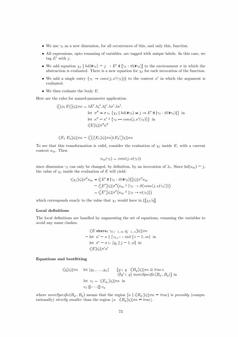
• We use γ` as a new dimension, for all occurrences of this, and only this, function.

• All expressions, upto renaming of variables, are tagged with unique labels. In this case, wetag E1 with j.

• We add equation χ` | hdp#γ`q j Ñ E1 @ rγ` : tlp#γ`qs to the environment σ in which theabstraction is evaluated. There is a new equation for χ` for each invocation of the function.

• We add a single entry tγ` ÞÑ conspj, κ1pγ`qqu to the context κ1 in which the argument isevaluated.

• We then evaluate the body E.

Here are the rules for named-parameter application:@@pφ`Eq

DDζξσκ λE1.λζ 1.λξ1.λσ1.λκ1.

let σ2 σ Y χ` | hdp#γ`q j Ñ E1 @ rγ` : tlp#γ`qs

(in

let κ2 κ1 : γ` ÞÑ conspj, κ1pγ`qq

(in

xxEyyζξσ2κ2

xxE1 E2yyζξσκ @@xxE1yyζξσκ

pE2q

DDζξσκ

To see that this transformation is valid, consider the evaluation of χ` inside E, with a currentcontext κin. Then

κinpγ`q conspj, κpγ`qq

since dimension γ` can only be changed, by definition, by an invocation of λ`. Since hdpκinq j,the value of χ` inside the evaluation of E will yield:

xxχ`yyζξσ2κin @@E1 @ rγ` : tlp#γ`qs

DDζξσ2κin

@@E1

DDζξσ2

κin : tγ` ÞÑ tlpconspj, κpγ`qqu

@@E1

DDζξσ2

κin : tγ` ÞÑ κpγ`qu

which corresponds exacly to the value that χ` would have in ξrχ`ηs.

Local definitions

The local definitions are handled by augmenting the set of equations, renaming the variables toavoid any name clashes.

xxE where` γ`,i1..m qj1..nyyζξσκ

let κ1 κ : tγ`,i ÞÑ init | i 1..mu in

let σ1 σ Y tqj | j 1..ns in

xxEyyζξσ1κ1

Equations and bestfitting

xxqyyζξσκ let tg1, . . . , gnu g P q | xxBgyyζξσκ true^pEg1 P qq moreSpecificpBg1 , Bgq

(in

let vi xxEgiyyζξσκ in

v1 ` ` vn

where moreSpecificpBg1 , Bgq means that the region tκ | xxBg1yyζξσκ trueu is provably (compu-tationally) strictly smaller than the region tκ | xxBgyyζξσκ trueu.

73

4.5.2 Results

Proposition 10. Let ξ be a function-free environment and κ be a function-free context. ThenrrEssζξκ v iff xxEyyζξHκ v, where v P Dconst.

The restriction on ξ is to ensure that it can be considered to be an element both of Envand Envxxyy. Similarly for κ, K and Kxxyy. The proof is a straightforward double-induction, firston the depth of where clause-nesting, second on the number of iterations within a where clause.The denotational semantics computes bottom-up while the operational semantics computes top-down. Nevertheless, if the denotational semantics yields a value v K, there will be a naturalnumber i for which i iterations are sufficient to compute v. The depth of the tree of the operationalsemantics will also be i. The reverse argument holds as well.

4.6 Caching

The operational semantics presented in the previous section would lead naturally to an inefficientsolution. To improve the result, we can use caching of the intermediate results, i.e., store px, κ, vqtriples in a cache to avoid recomputation. However, given that κ is very large, potentially infinite,and that most of the dimensions in κ will never even be examined, it is necessary to take anapproach in which the caching is with respect to the portion of κ that has actually been examinedduring computation.

Doing this, however, makes it more difficult to probe the cache. The solution is to begin theevaluation of an identifier with an empty context, and to evaluate the expression; should the resultbe that dimensions are missing, this information is stored in the cache, these are added to thecontext, and the expression is reevaluated. This process is repeated until the expression can beevaluated completely and the returned value can be cached.

This “game” approach to caching was first discussed by Anthony Faustini and William Wadgewhen they were writing the pLucid interpreter in the mid-1980s [38]; however they did not im-plement this caching mechanism. A sequential implementation of this caching mechanism wasdeveloped by myself in 2007, after discussion with William Wadge [75].

The semantics presented here is to support a multi-threaded implementation, with the intu-ition derived from the TransLucid implementation written by Toby Rahilly in 2009 [80]. For theevaluation of tuples and of operations, multiple threads can be spawned, and each of these mayinteract with the cache. To properly interleave the actions of each thread upon the cache, a notionof time must be introduced into the behavior of the threads.

A number of different kinds of value are manipulated by this semantics, so it is easier to typethe values being manipulated. This also gives us an opportunity to distinguish the different kindsof error situation.

4.6.1 Typed values

A value v is defined to be a pair pτpvq, ψpvqq, where τpvq is the type of v and ψpvq is the concretevalue of v. When writing down explicitly v, we can write τpvqxψpvqy.

The semantics presented here explicitly manipulates the following types:

• bool: Booleans. The concrete values are true and false.

• sp: Special values to deal with exceptional or erroneous situations. The concrete values are:

– undef: undefined variable;

– type: type error; and

– tuple: inconsistent tuple construction;

– loop: infinite loop detected.

74

To ensure that specials are used in a deterministic manner, they are ordered, with undef ¤type ¤ tuple ¤ loop. The operation minsp selects the minimum concrete special valuefrom a set.

• tuple: Tuple values used to hold deltas. The concrete values are functions from dimensionsto ordinates.

• calc: Worker threads. The concrete values are lists of natural numbers, written w. Athread w may generate several worker threads wi conspi, wq, i 1..n. Should this be thecase, we write wi ¥ w.

• dem: Demands. The concrete values are of the form demxv1, . . . , vny, which corresponds to ademand for the dimensions v1 through to vn.

4.6.2 The cache

The field β continues to provide the environment, this time in the form of a cache. There are twodata structures and two operations:

• β.time P N is a timestamp. Timestamps can be incremented (1), they can be compared (¤)and their maximum max can be computed.

• β.cache P XKNÑ V, which maps pidentifier, delta, timestampq triples to atomic values,such that none of the timestamps may be greater than the current β.time.

• β.findpx, δ, t, wq, with t ¤ β.time, yields pv, t1q, with t1 ¥ t, and is defined as follows:

Case Dt1 ¥ t.px, δ, t1q P dompβ.cacheq:let tv max

ti | px, δ, tiq P dompβ.cacheq

(;

let v β.cachepx, δ, tvq;return

v,maxpt, tvq

.

Case Et1 ¥ t.px, δ, t1q P dompβ.cacheq:β.time : β.time 1;β.cache : β.cache Y

px, δ, β.timeq ÞÑ calcxwy

(;

returncalcxwy, β.time

.

In the second case, should several threads w1, . . . , wn all attempt to access the same locationsimultaneously, then one thread w1 would be nondeterministically chosen to be calculating,and all of these threads, including w1, would receive the value calcxw1y.

• β.addpx, κ, t, vq, with t ¤ β.time, yields t1, with t1 ¥ t, and defined as follows:β.time : β.time 1;β.cache : β.cache Y

px, κ, β.timeq ÞÑ v

(;

return β.time.

The contents of the cache β are designed to work as follows, should all of the calculations fora request have been made.

β.findpx,H, t, wq demxV1y, t

β.findpx, κ | V1, t, wq

demxV2y, t

β.find

x, κ | pV1 Y V2q, t, w

demxV3y, t

. . .

β.findx, κ | pV1 Y Y Vn1q, t, w

demxVny, t

β.find

x, κ | pV1 Y Y Vnq, t, w

pv, tq

where demxViy means a demand for the dimensions in Vi. We will write βpx, κ, t, wq v iff thereis a chain of Vi as above. Furthermore, the initial environment has to be set up so that the inputsare inserted in this manner.

75

4.6.3 Rules

These rules do not work with full contexts κ, but with deltas δ. The rules are of the formpv, t1q rrEssζβσδwt, which means that expression E is evaluated using interpretation ζ andcache β in a context delta δ by a worker thread w at time t, yielding value v at time t1 ¥ t.

The meaning of Dfunc for these rules is:

Drrss

func Expr Ñ Interp Ñ Cache Ñ Eqn Ñ ∆ Ñ ListpNq Ñ NÑ pD Nq

Drrss Dconst YDrrss

func

Krrss pDconst Y Iq Ñ Drrss

K

∆rrss pDconst Y Iq Ñ Drrss

K

Intensrrss

Krrss Ñ Drrss

Envrrss Id Ñ Krrss Ñ Drrss

We have that rrss P Drrss

func . We will avoid this superscripting when it is not necessary.

Identifiers

x: For the evaluation of x, we need three different kinds of rules.

• The rrxssζβσδwt rule calls xxxyyζβσδwtH, which calculates x with an empty delta.

• xxxyy iterates through increasing subsets of δ, initially H, until a non-dem value is reached.xxxyyζβσδwtδ1 calls ttxuuζβσδ1wt. Should a demand for other dimensions be returned, andthese are in the domain of δ, then this part of δ is added to δ1.

• The ttxuuζβσδwt defines the interaction with the cache.

rrxssζβσδwt

xxxyyζβσδwtH

xxxyyζβσδwtδ1

let pv, t1q ttxuuζβσδ1wt in$''&''%pv, t1q, τpvq dem

xxxyyζβσδwt1δ1:

δ | ψpvq

, ψpvq dom δ

pv, t1q, otherwise

ttxuuζβσδwt

let pv, t1q β.findpx, δ, t, wq in$''''''''&''''''''%

pv, t1q, τpvq calcspxloopy, t1

, v calcxw1y, w1 ¥ w

ttxuuζβσδwpt1 1q, v calcxw1y

let pv1, t2q σpxq

ζβσδwt1 in

let t3 β.addpx, δ, t2, w, v1q in

pv1, t3q, otherwise

76

Constants

c: Constants are always constant, and take no time.

rrcssζβσδwt ζpcq, t

Operations

oppE1, . . . , Enq: If one or more operands returns a special, the least special value is returned. Ifsome of the operands return demands, then their union is returned. Let wi conspi, wq.

rroppE1, . . . , Enqssζβσδwt

let pvi, tiq rrEissζβσδwit in$''&''%

minsptviu,maxttiu

, Di. τpviq sp

dem@

i

ψpviq | τpviq dem

(D,maxttiu

, Di. τpviq dem

ζpopqpv1, . . . , vnq,maxttiu, otherwise

Conditionals

if E1 then E2 else E3 fi: Specials and demands from the condition are passed on directly.Otherwise, the correct branch is computed.

rrif E1 then E2 else E3 fissζβσδwt

let pv1, t1q rrE1ssζβσδwt in$'''&'''%pv1, t1q τpv1q sp or demspxtypey, t1

, τpv1q bool

rrE2ssζβσδwt1, ψpv1q true

rrE3ssζβσδwt1, ψpv1q false

Context query

#E: Specials and demands from the contained expression are passed on directly. Should the valuenot be in the domain of the active delta, then a demand is created for this value. This is the onlyplace where demands are initiated.

rr#Essζβσδwt

let pv, t1q rrEssζβσδwt in$''&''%pv, t1q τpvq sp or demdemxvy, t1

, v R dom δ

δpvq, t1, otherwise

77

Finite deltas

rE11 : E12, . . . , En1 : En2s: As for data operators, if some of the operands of the tuple operatorreturn demands, then their union is returned. Let wij conspi 2 j, wq.

rE11 : E12, . . . , En1 : En2sζβσδwt

let pvij , tijq rrEijssζβσδwijt in$'''''&'''''%

minsptviju,maxttiju

, Di. τpvijq sp

dem@

i

ψpvijq | τpvijq dem

(D,maxttiju

, Di. τpvijq dem

spxtupley,maxttiju, Di, k. i k ^ vi1 vk1

tuplextvi1 ÞÑ vi2uy,maxttij | i 1..Nu, otherwise

Infinite deltas

rE11 : E12, . . . , En1 : En2, all : Ealls: As for data operators, if some of the operands of thetuple operator return demands, then their union is returned. Let wij conspi 2 j, wq andwall consp0, wq. We use the subscript α instead of ij or all.

rE11 : E12, . . . , En1 : En2, all : Eallsζβσδwt

let pvα, tαq rrEαssζβσδwαt in$'''''''&'''''''%

minsptvαu,maxttαu

, Di. τpvαq sp

dem@

i

ψpvαq | τpvαq dem

(D,maxttαu

, Di. τpvαq dem

spxtupley,maxttαu, Di, k. i k ^ vi1 vk1

tuplextv ÞÑ vall | v P pDconst Y Iqu :

tvi1 ÞÑ vi2 | i 1..Nuy,,maxttαu

, otherwise

Context perturbation

E2 @ E1: The rule for context-change operators does not change.

rrE2 @ E1ssζβσδwt

let pv1, t1q rrE1ssζβσδwt in$'&'%pv1, t1q τpv1q sp or demspxtypey, t1

, τpv1q tuple

rrE2ssζβσδ : ψpv1q

wt1, otherwise

Value-parameter application

pλ`Eq: We must take into account the time parameter.pλ`Eq

ζβσδwt λE1.λζ 1.λβ1.λσ1.λδ1.λw1.λt1

let σ2 σ Y tχ` | true Ñ #γ`u in

let pv1, t2q rrE1ssζ 1β1σ1δ1w1t1 in

let δ2 δ1 : tγ` ÞÑ v1u in

rrEssζβσ2δ2wt2

rrE1.E2ssζβσδwt let pv, t1q rrE1ssζβσδwt invpE2q

ζβσδwt1

78

Named-parameter application

pφ`Eq: We must take into account the time parameter. We assume that E1 has been tagged withvalue j.

pφ`Eqζβσδwt λE1.λζ 1.λβ1.λσ1.λδ1.λw1.λt1

let σ2 σ Y χ` | hdp#γ`q j Ñ E1 @ rγ` : tlp#γ`qs

(in

let δ2 δ1 : γ` ÞÑ conspj, δ1pγ`qq

(in

rrEssζβσ2δ2wt1

rrE1 E2ssζβσδwt let pv, t1q rrE1ssζβσδwt invpE2q

ζβσδwt1

Local definitions

The local definitions are handled by augmenting the set of equations, renaming the variables toavoid any name clashes.

rrE where` γ`,i1..m qj1..nssζβσδwt

let δ1 δ : tγ`,i ÞÑ init | i 1..mu in

let σ1 σ Y tqj | j 1..ns in

rrEssζβσ1δ1wt

Equations and bestfitting

rrqssζβσδwt let tg1, . . . , gnu g P q | rrBgssζβσδwt ptrue, tgq^pEg1 P qq moreSpecificpBg1 , Bgq

(in

let t1 maxttgugPq in

let pvi, tiq rrEgissζβσδwt1 in

v1 ` ` vn,maxttiui1..n

, n ¡ 0

pspxundefy, t1q, otherwise

where moreSpecificpBg1 , Bgq means that the region tκ | rrBg1ssζβσδwt ptrue, tg1qu is provably(computationally) strictly smaller than the region tκ | rrBgssζβσδwt ptrue, tgqu.

4.6.4 Results

Proposition 11. Let ξ be a function-free environment and κ be a function-free context. Supposefurthermore that @x.@κ.ξpxqpκq βpx, κ, 0,nilq, and that v P Dconst. Then xxEyyξσκ v iffrrEssβσδpnilq0 pv, tq, for some δ κ, and t ¥ 0.

The restriction on ξ is to ensure that it can be considered to be an element both of Env

and Envrrss . Similarly for κ, K and Krrss . The proof is a straightforward double induction,first on the structure of the expressions, second on the interaction between the evaluator and thecache.

4.7 Conclusions

The key to the development of the semantics in this chapter is the proper definition of contextand of context delta. Once these were defined, the rules for expressions not involving identifiers,nor functions, wrote themselves.

79

The identifiers were trickier. The choice of an abstract syntax sufficiently simple, yet generalenough to cover many possible concrete syntaxes, required some thought. As for bestfitting, initialwork, as described in the chapter on possible-worlds versioning, assumed that there would alwaysbe a single bestfit equation. The solution given here allows for multiple bestfits, all of which arethen evaluated and combined post facto. This solution, much more general, is also much simpler.

Initially, all functions were perceived as having two different kinds of arguments. However, bytrying to make Curry-ed functions, it became clear that there were really two kinds of abstraction,hence the use of λ and φ. The naming of the two different kinds of application came from theircalling mechanism.

Alternative semantics have also been examined, but are not presented here. First, by using anclosure type, it is possible to make the delta evaluation lazy. In this approach, the dimensions ofa delta must be computed eagerly upon creation, while the ordinates are wrapped up in closuresincluding the current context. An ordinate closure is only opened and evaluated if the ordinate isrequested through the use of a #. For computations that yield a non-K value using the rules givenin this chapter, the result is the same. However, there could be situations where the evaluationof unused components of deltas might be nonterminating, in which case the two solutions wouldyield different results.

In this thesis, we will consider lazy tuples to be an implementation—not semantic—feature,useful for optimization. This was the approach taken by Toby Rahilly, when he developed the firstmulti-threaded implementation of the language [80].

Another alternative semantics that has been written is to consider all values to be sets. Theintuition came from a 1977 paper by Adi Shamir and William Wadge [85]. In this paper, theyproposed a theory of types, in which types and values are the same, and a type is understoodas the set of all values approximating it. In this view, no object has a canonical type. We arecurrently experimenting with this idea in the current implementation, for the bestfit selection ofoperators based on the types of arguments.

The key to the successful semantics was the recognition that there are two kinds of parameterpassing and two kinds of binding. Value-parameter abstraction uses call-by-value while named-parameter abstraction uses call-by-name. Binding of identifiers in the environment is done stati-cally, while binding of dimensions in the context is done dynamically. All are useful and necessary.

80

Chapter 5

Building an Interpreter

In this chapter, we present the interpreter that implements the TransLucid language [8]. Themain difference between the Core TransLucid language presented in the previous chapters and thelanguage whose implementation is described here is the richness and diversity of data types andoperations. In particular, the TransLucid presented here is designed as a coordination language,which means that it provides an interface to other structures written in a host language.

The TransLucid programming environment, available at translucid.sourceforge.net, iswritten in C++0x, the new standard for C++. For compilation, it currently requires GNU g++ 4.5.0

(gcc.gnu.org), and the Boost 1.43.0 C++ libraries (www.boost.org).In addition to the three atomic data types described in the previous chapter, the environment

natively supports the intmp (GNU multi-precision integer), uchar (32-bit Unicode character)and ustring (32-bit Unicode string) data types. In addition, users may add other data typesand operations through the use of libraries, and these may be manipulated from TransLucid.Furthermore, the highly flexible parser can be parameterized so that new operators can be added,in prefix, postfix or infix form, and literals (constants) of new types can be written as simply as ifthey were literals of the builtin types.

The interpreter is designed to allow the interaction of the host language, here C++, withTransLucid: TransLucid can call TransLucid or C++, and C++ can call C++ or TransLucid. Themeans by which this communication takes place is the hyperdaton, an object which responds to acontext (a tuple) and returns a tagged value, a pconstant , tupleq pair, where the tuple encodes thesubcontext used to compute the constant.

The hyperdaton is the key data structure. A hyperdaton can be generated by hand in C++

or else can be produced automatically from TransLucid equations. All forms of expression aresubclasses of the hyperdaton class, as are variables, equations, and the system itself.

The variable is a specialization of hyperdaton, used to store all of the information pertainingto a variable, including its defining equations, and possibly variables local to it.

The system is a specialization of variable, used to store a number of variables, along with a setof input hyperdatons used by the equations defining the variables, and a set of output hyperdatons,which are filled in through the use of demands, essentially reservations for computations to takeplace at specific contexts.

The semantics of a system is synchronous. Upon each instant, the input hyperdatons, equationsand demands may be updated. The applicable demands are then executed, in so doing updatingthe output hyperdatons. This process is repeated upon each instant.

Since the Cartesian system is to be used as a real system, we must be able to deal with all of thedifficulties of user-defined types, of libraries, of identifier dimensions, and so on. As a result, theinternals of a system are designed so that they can be understood from a TransLucid perspective:this is done through the use of predefined dimensions and variables, so that, for example, addinga new operator into the system effectively means adding a new equation into the system.

The presentation style of this chapter is ground up. As the internals of the C++ system areexplained, the corresponding TransLucid structures will be presented.

81

5.1 Types

Inside the interpreter, each type is given a unique type index, an unsigned integer (type_index).The following types are predefined and necessary for the behavior of the system:

• type: types (TYPE_INDEX_TYPE). The values are indices corresponding to registered types.

• dim: dimensions (TYPE_INDEX_DIMENSION). The values are indices corresponding to dimen-sions.

• sp: specials (exceptional values, TYPE_INDEX_SPECIAL). The values are indices correspond-ing to registered special values.

• tuple is used to hold tuples (TYPE_INDEX_TUPLE).

• guard is used to hold guards (TYPE_INDEX_GUARD).

• range is used to hold ranges of integers (TYPE_INDEX_RANGE).

The following types will soon be added to the interpreter.

• calc is used to hold a reference to a worker thread undertaking an unfinished computation.

• expr is used to hold expressions.

• eqn is used to hold equations.

These are the four basic types that are found in most programming languages and which are alsonecessary for the proper behavior of the system:

• bool: Booleans (TYPE_INDEX_BOOL).

• intmp: GNU MP arbitrary-precision integers (http://gmplib.org, TYPE_INDEX_INTMP).

• uchar: 32-bit Unicode character (http://www.unicode.org, TYPE_INDEX_UCHAR). Therange is 0–D7FF, E000–10FFFF hex.

• ustring: 32-bit Unicode character string (TYPE_INDEX_USTRING).

In addition to these predefined types, it is possible to add new user types through the use oflibraries.

5.2 Typed values

When evaluating expressions, the TransLucid interpreter can manipulate values of both builtintypes as well as user-defined types. In order for the interpreter to work properly, it must holdon to typed values, which are values whose type is known. All of these values are instances ofsubclasses of class TypedValue.

class TypedValue

virtual ~TypedValue()

virtual TypedValue* clone() const = 0;

virtual size_t hash() const = 0;

virtual void print(ostream& os) const = 0;

;

Depending on the type, these subclasses might simply store the values directly, as appropriate forsmall fixed-size types; or using a pointer to a possibly shared data structure, as needed for largervariable-size types.

82

5.3 Constants

Inside the interpreter, constants are pairs consisting of a typed value and the type index for theconstant’s type. The type is called Constant, and its main constructor is as follows:

Constant(const TypedValue& value, type_index index);

In expressions, constants in general appear in expressions as typename<valuetext>, wheretypename is a known type and valuetext is the text that is to be interpreted by that type’sown parser.

The four basic types can appear directly in expressions.

• The values for the sp type are:

– sperror: General-purpose error.

– spaccess: Change to unreachable context.

– sptype: Type error.

– sptuple: Dimensions for tuple formation are not disjoint.

– spdim: Undefined dimension in the current context.

– spundef: Undefined variable.

– spmultidef: Multiply defined variable.

– spconst: Error when parsing a constant.

– sploop: A value is determined in terms of itself.

– spmultival: A single value is expected.

• The two possible Boolean values are true and false.

• Integers beginning with a non-zero digit are understood to be decimal numbers. Their syntaxis [1-9][0-9]*.

• Zero is expressed simply as a standalone zero digit.

• Other integers beginning with a zero digit are expressed in a base between 2 and 61. Theirsyntax is 0[2-9a-zA-Z][0-9a-zA-Z]*. The digit or letter following the initial digit givesthe base, and what follows is the number. The digits and letters are interpreted as follows:

0 1 2 3 4 5 6 7 8 9 a b c d e f

0 1 2 3 4 5 6 7 8 9 10 11 12 13 14 15g h i j k l m n o p q r s t u v

16 17 18 19 20 21 22 23 24 25 26 27 28 29 30 31w x y z A B C D E F G H I J K L

32 33 34 35 36 37 38 39 40 41 42 43 44 45 46 47M N O P Q R S T U V W X Y Z

48 49 50 51 52 53 54 55 56 57 58 59 60 61

For a number in base n, only ‘digits’ from 0 to n 1 may be used. In computer science, themost commonly used bases are 2 (binary), 8 (octal) and 16 (hexadecimal); in everyday life,we use base 10 (decimal). Consider the number 39912. It becomes

– 021001101111101000 in binary (base 2).

– 08115750 in octal (base 8).

– 0a39912 in decimal (base 10).

– 0g9be8 in hexadecimal (base 16).

83

– 0k4jfc in vigesimal (base 20), used by the Mayans.„‹¸

– 0Yb5c in sexagesimal (base 60), used by the Babylonians.

• A single Unicode character in UTF-8 format enclosed in single quotes is understood as auchar.

• A sequence of Unicode characters in UTF-8 format enclosed in double quotes is understoodas a ustring.

When a new type is introduced, a parser and a pretty-printer for that type must be providedas well.

5.4 Dimensions

Inside the interpreter, each dimension is given a unique dimension index, an unsigned integer(dim_index). Dimensions can either be typed values or identifiers declared to be dimensions.

The following dimensions are predefined and necessary for the behavior of the system:

• id (DIM_ID): variable inside a hyperdaton.

• name (DIM_NAME): name of operation.

• text (DIM_TEXT): value text for a constant.

• type (DIM_TYPE): type string for a constant.

• _validguard (DIM_VALIDGUARD): guard of an equation.

• value (DIM_VALUE): value of a value dimension.

• time (DIM_TIME): current time.

• argi, i ¥ 0 (DIM_ARGi): i-th argument of an operation.

• all (DIM_ALL): the default value for missing dimensions.

5.5 Tuples

Tuples are used to encode the current context. For the moment, only eager tuples are implemented.Physical tuples are mappings from dimension indexes to constants. The Tuple class holds a sharedpointer to a physical tuple: many Tuple instances can share the same physical tuple, and garbagecollection is easier.

typedef map<dim_index, Constant> tuple_t;

class Tuple : public TypedValue

explicit Tuple(const tuple_t& tuple);

Tuple();

private:

boost::shared_ptr<tuple_t> m_value;

;

84

5.6 Tagged constants

The caching mechanisms described in Chapter 4 need to know exactly what part of the contextwas used to calculate the current value. As a result, calculations result in a TaggedConstant, apair including a constant and a tuple.

typedef pair<Constant, Tuple> TaggedConstant;

5.7 Parsing expressions

The Core TransLucid language simply assumes that there is a set of constants and operators.However, the real language is to be a coordination language, allowing the use of constants andoperators defined in the host language, here C++. Furthermore, we would like to allow a flexible,extensible concrete syntax, with the use of user-defined operators.

To do this, a header is used to initialize the expression parser, in order to interpret tokensappearing in expressions. This allows data operators, identifiers and constants to be properlyinterpreted.

There are no predefined data operators in TransLucid. These must all be declared in theheader. They may be unary (prefix or postfix) or infix. The infix operators may be binary orvariadic (2 or more arguments). Each operator, once recognized during the parsing process, isconverted to a function name for internal processing. The fixity declarations are as follows:

• postfix s1 s2: declares s1 to be a postfix operator, which translates to internal function s2upon being parsed. Postfix operators have highest priority. (All s occurrences are strings.)

• prefix s1 s2: declares s1 to be a prefix operator, which translates to internal function s2upon being parsed. Prefix operators have next highest priority.

• The following all declare s1 to be an infix operator, which translates to internal function s2upon being parsed, and is of precedence level n (higher precedence means higher n). Unaryoperators have higher precedence than infix operators.

– infixl s1 s2 n: declares s1 to be a left-associative binary operator.

– infixr s1 s2 n: declares s1 to be a right-associative binary operator.

– infixn s1 s2 n: declares s1 to be a non-associative binary operator.

– infixm s1 s2 n: declares s1 to be a variadic ordinary operator. For example, 2 3 4can be considered to be p2, 3, 4q.

– infixp s1 s2 n: declares s1 to be a variadic comparison operator. For example, 2 3 4 can be considered to be 2 3^ 3 4.

Identifiers in TransLucid can either be variables or dimensions. To distinguish the two, dimen-sion identifiers must be declared.

• dimension s: declares s to be a dimension when it appears in expressions.

Constants of user-defined types can be placed in expressions of the form typename<valuetext>.However, if typename is used often, then it is possible to define a shorthand, using user-defineddelimiters.

• delimiters s c1 c2: declares that a string s appearing between characters c1 and c2 in anexpression will be considered to be equivalent to typename<s>.

Types and functions implementing data operators can be defined in the host language andplaced in libraries, which can then be loaded by TransLucid.

• library s: declares s to be a dynamic library which must be loaded.

Libraries are set up to resemble sets of equations, using predefined dimensions.

85

5.8 Hyperdatons

At the core of the implementation is the hyperdaton, an arbitrary-dimensional unbounded array.The C++ class HD is given below:

class HD

virtual ~HD()

virtual TaggedConstant operator()(const Tuple& k) = 0;

virtual uuid addExpr(const Tuple& k, HD* h)

return nil_uuid();

In C++, an object x instantiating a class C with the method operator() method defined is calleda functor, or function object : when one writes xpactualsq, if operator()pformalsq is defined for Cand of the right type, then it is called; should there be more than one operator()pformalsq definedfor C, i.e., operator() is overloaded, then the one with the most specific type for the actuals iscalled.

The operator() method is used to do a lookup in the current context, which is encoded usingthe data structure Tuple. This lookup might simply require, internally, the return of a constantor a table lookup. Or, it might require some massive computation. The returned result, of typeTaggedConstant, contains the constant, and the pertinent subcontext (of the original contextpassed in as input) that was actually needed to compute the result.

The interpreter consists therefore of a number of classes defining different kinds of hyperdaton,one for each of the different kinds of expression, along with a parser that converts expressionsand equations into hyperdatons and a pretty-printer that allows printing of tagged values andhyperdatons. As a result, it is possible to do Cartesian programming either in C++ or in TransLucid,or through a judicious mix of the two.

The addExpr method is used to add equations used by a hyperdaton to change its behavior.The uuid type is a universally unique identifier generated by the Boost.Uuid library; it is a 128-bit identifier that is guaranteed—or at least extremely likely—to be unique, even in a distributedenvironment. Using this identifier, it becomes possible to replace or delete an expression that hasbeen added to a hyperdaton.

5.9 Expression hyperdatons

For the expression hyperdatons presented below, some of them will require having access to thecurrent system in which they are defined. This is because, internally, many parts of a system areencoded using bestfitting, through the use of special dimensions and variables.

When ones write x as an identifier, the TransLucid interpreter understands this as

ID @ [name: x]

Therefore, all variables are understood to be members of the same hyperdaton, namely ID.Similarly, when one writes 3 5, the TransLucid interpreter will look up the function name,

in this case operator+, and encode the whole thing as

OP @ [name:"operator+", arg0:3, arg1:5]

Therefore, all operators are understood to be members of the same hyperdaton, namely OP. Thisapproach is used for loading of libraries: when a library is loaded, it is passed the current system;the library then adds to that system equations of the following form:

OP @ [name:"operator+", arg0:type<intmp>, arg1:type<intmp>]

= <Boost.Function object>

86

where a Boost.Function is a class which can encapsulate either a function or a function object,thereby providing a unified interface. As a result, when operator+ is to be evaluated, the best-fitting process can be used to determine which instance of operator+ is to be used. A similarprocess is used to keep track of types, dimensions and demands. In time, even the parser and thepretty-printer will be defined this way.

5.9.1 Constant hyperdaton

The constant hyperdatons hold a single constant, and no matter what the context, will alwaysreturn the same value. There is one for all the builtin data types that are writable in TransLucid.

TypeConstHD (type_index);

BoolConstHD (bool);

SpecialConstHD (Special::Value);

IntmpConstHD (const mpz_class&);

UCharConstHD (char32_t);

UStringConstHD (const u32string&);

5.9.2 Typed-value hyperdaton

Expressions of the form typename<valuetext> are “constants”, yet they are not. The TransLucidinterpreter will call the parser for typename on the string valuetext , and this parser is context-dependent. The hyperdaton storing such expressions is the TypedValueHD.

TypedValueHD (HD* system, const u32string& type, const u32string& text);

5.9.3 Dimension hyperdaton

In expressions, DimensionHD is used for identifiers that have been declared to be dimensions.

DimensionHD (HD* system, const u32string& name);

5.9.4 Identifier hyperdaton

In expressions, IdentHD is used for identifiers defined by systems of equations.

IdentHD (HD* system, const u32string& name);

5.9.5 Operator hyperdaton

The abstract syntax referred to “operators”. Internally, there are hyperdatons for unary operators,binary operators, and isspecial and istype.

UnaryOpHD (HD* system, const u32string& name, HD* e);

BinaryOpHD (HD* system, const u32string& name, const vector<HD*>& operands);

VariableOpHD (HD* system, const u32string& name, const vector<HD*>& operands);

IsSpecialHD (HD* system, const u32string& special, HD* e);

IsTypeHD (HD* system, const u32string& type, HD* e);

In TransLucid, isspecialxnamey E always returns a Boolean value; it will evaluate E and de-termine if it is spxnamey. Similarly, istypexnamey E always returns a Boolean value; it willevaluate E and determine if it is of type name. Therefore, isspecial and istype are not strictwith respect to specials.

87

5.9.6 Conditional hyperdaton

Conditional, context query, tuple creation and context perturbation expressions are all handled ina straightforward manner:

IfHD (HD* cond, HD* then, const vector<pair<HD*, HD*>>& elsifs, HD* else_);

HashHD (HD* system, HD* e);

TupleHD (HD* system, const list<pair<HD*, HD*>>& elements);

AtHD (HD* e2, HD* e1);

5.10 Equation hyperdatons

Equations are also hyperdatons. The variable name is being defined. The guard valid defines thevalidity conditions of equations. The hyperdaton h is the defining expression.

EquationHD(const u32string& name, const GuardHD& valid, HD* h);

5.11 Variable hyperdatons

The VariableHD hyperdaton is given below:

typedef std::map<uuid, VariableHD*> UUIDVarMap;

typedef std::map<uuid, EquationHD> UUIDEquationMap;

typedef std::map<u32string, VariableHD*> VariableMap;

class VariableHD: public HD

uuid addExpr (const Tuple& k, HD* h);

void delExpr (const uuid);

void replExpr(const uuid, const Tuple& k, HD* h);

...

private:

UUIDVarMap m_uuidVars;

UUIDEquationMap m_equations;

VariableMap m_variables;

;

The addExpr method is used to add a new definition, itself encoded as a hyperdaton, to thevariable hyperdaton. A single variable may have multiple definitions, and when a lookup takesplace, the most specific, with respect to the current context, will be used. The uuid returned asresult from addExpr corresponds to a unique identifier generated internally so that the definitionmay be referred to explicitly. The delExpr and replExpr are used to, respectively, delete andreplace an existing equation. The m_equations field holds on to the current equations for thisvariable.

The VariableHD hyperdaton can also hold a number of variables lower down, so that one canwrite dot-separated expressions. For example, x.y.z means the z variable in the y variable in thex variable.

The m_uuidVars field maps uuid’s to children variables. The m_equations field holds on tothe equations for the current variable. The m_variables field holds on to the children variables.

The following variables are predefined and necessary for the behavior of the system:

• CONST: constants.

88

– type: type name of the constant (a string).

– text: text of constant, to be parsed in a context-dependent way.

• OP: operators.

– name: name of the operator.

– argi, i ¥ 0: arguments of the operator.

• TYPE_INDEX: type indices.

– type: type name (a string).

• DIMENSION_NAMED_INDEX: dimension indices.

– name: name of the dimension.

• DIMENSION_VALUE_INDEX: dimension indices.

– value: value designating the dimension.

5.12 System hyperdatons

The SystemHD hyperdaton is derived from VariableHD:

class SystemHD: public VariableHD

void addInput (const map<u32string, HD*>);

void addOutput(const map<u32string, HD*>);

void addDemand(const u32string& id, const EquationGuard& guard);

void tick();

;

It includes equations and is passed physical hyperdatons as input and output. In this way, it ispossible to have hyperdatons that have their own C++-specific interface for use outside of TransLu-cid, as well as the hyperdaton interface for use within TransLucid. The demands are requests foroutput hyperdatons to be calculated under certain contexts.

Once all of the equations and demands are added, then the tick() method can be called,producing all of the results, and the demands are executed, with the results being placed in theoutput hyperdatons.

In some sense, everything is a hyperdaton. This approach has simplified the programming ofthe interpreter. In particular, identifiers and operators are encoded using hyperdatons, throughthe use of special identifiers.

5.13 Current work

At the time of writing, the current implementation does not correspond directly to the CoreTransLucid presented in Chapter 4. There are currently no functions, nor local where clauses.However, the infrastructure to implement these is already included in the implementation.

To implement value-parameter functions simply requires manipulation of the parser. To im-plement named-parameter functions, however, requires the ability to manipulate finite lists. Thiswill be implemented in TransLucid by allowing the creation of inductively defined data structures,as are available in most functional languages. In TransLucid, these data structures will be im-plemented as tuples (already implemented), with two predefined dimensions: type will determinethe type and constructor will determine which kind of object of that type will be created. Oncethese types will be available, then implementing functions in TransLucid will be doable.

89

As for the local definitions, the current implementation already allows local definitions, sinceevery variable allows the use of local variables. These structures can be used to implement thewhere clauses of Core TransLucid.

Efficiency considerations are currently under study. Several implementations of earlier versionsof TransLucid have been built with caches, including for the minimal cache described in Chapter 4.With this knowledge, we will develop a cache for the current implementation, with programmersupport for garbage-collection strategies.

We are also examining means for highly efficient implementations of regularly occurring struc-tures. See Chapter 7 for a discussion about the implementation of recursive functions.

5.14 Conclusions

The interpreter presented here does much more than simply implement the Core TransLucidlanguage. It is, in fact, designed as the bootstrapping step towards an interpreter for TransLucidthat will be entirely written in TransLucid.

The key concept in the interpreter is the hyperdaton, which provides a result given a context.By subclassing the hyperdaton, and by using a restricted set of predefined dimensions, much ofthe behavior of the interpreter comes for free through the bestfitting process.

The development of Cartesian programs combining the full power of TransLucid and of thehost language will inevitably lead to new programming patterns. We look forward to this experi-mentation.

90

Part III

Exploring the Cartesian Space

91

Chapter 6

Time for Applications

In this chapter, we present two TransLucid-based applications, tlcore and S3, and examine howtime is used in these applications and in distributed synchronous systems.

The tlcore application is a standalone text-based TransLucid interpreter, with a synchronousreactive semantics. At each instant, one may add, replace or delete defining equations and expres-sions to be evaluated, and the special time dimension may be referred to in order to keep trackof the evolution of the system of equations.

The S3 application is a standalone graphical TransLucid code and expression browser, in whichone can edit the set of defining equations and expressions to be evaluated, and in which canvisualize the evaluation of these expressions in multidimensional space. Because of the exploratorynature of the tool, time may advance in micro-steps, whenever the equations or expressions aremodified, or in macro-steps, when a commit to the changes is made.

These standalone tools have allowed the development of the timed semantics of the TransLucidsystem in the library presented in the previous chapter. Using this semantics, we can then exploredifferent ways of having multiple TransLucid systems interacting. We present three models: thepeer-to-peer model, the hierarchical-worker model and the parent-æther model.

One of the longer-term goals of TransLucid is that it can be used for the writing of timedsystems. In the presentation in this chapter, we focus on allowing a system of TransLucid equationsto be reactive, i.e., that the set of equations available may differ from instant to instant.

6.1 The tlcore application

The tlcore application is a simple standalone application with an interactive loop to interpretand evaluate TransLucid programs. It is used both to test developments within the TransLucidlibrary as well as to allow users to directly write and run TransLucid programs. tlcore formspart of the TransLucid distribution.

6.1.1 Basic behavior

In its simplest form, tlcore reads either from a file or from the standard input: a TransLucidheader, a set of equations and a set of expressions. The expressions are then evaluated one byone, and the results are placed on the standard output or in a file. The interface is as follows:

tlcore --input=infile --output=outfile

along with the standard --verbose and --version options.If the --input option is not provided, input is read from the standard input. If the --output

option is not provided, output is written to the standard output. All errors or log messages,including version information, are written to the standard error.

92

The syntax of the files is simple. It consists of three parts:

header%%

equations%%

expressions

where

• header consists of declarations for libraries, dimensions, delimiters and operators (see §5.7).

• equations consists of equations, all terminated by double colons, using the information de-clared in the header.

• expressions consists of expressions, all terminated by double colons, using variables definedin the equations.

The expressions are to be read, one by one, and then evaluated. Suppose that there are n expres-sions. Their answers will be returned as follows:

answer1 ; ;. . .answern ; ;

Should the --verbose option be used, then the output will be

expr1 Ñ answer1 ; ;. . . ; ;exprn Ñ answern ; ;

6.1.2 Equation UUIDs

When an equation is added to the TransLucid system, it is automatically given a unique identifier,generated by the Boost.UUID library. When tlcore is passed the --uuid option, then both theequations and the expressions will return results. The results will be of the form

// Equationseqnuuid1 ; ;. . .eqnuuidm ; ;

// Expressionsanswer1 ; ;. . .answern ; ;

Should the --verbose option also be set, then the results will be of the form

// Equationseqn1 Ñ eqnuuid1 ; ;. . .eqnm Ñ eqnuuidm ; ;

// Expressionsexpr1 Ñ answer1 ; ;. . .exprn Ñ answern ; ;

93

Here is a sample run from tlcore --uuid:

%%

x 5; ;%%

x ; ;

// Equationsuuid<4557f67592cb498fa684d50f5511a65> ; ;

// Expressionsintmp<5> ; ;

6.1.3 Reactive tlcore

When the --reactive option is set for tlcore, then the application becomes reactive, and theset of equations is allowed to vary over time, and the expressions being evaluated can refer to thetime dimension. The idea is that at each instant,

• the header may be added to;

• the set of equations may be modified;

• the set of expressions to be evaluated may be modified; and

• then the expressions for that instant are evaluated.

When tlcore is reading from the standard input, then the input will be of the form

header0

%%

equations0%%

expressions0$$

header1

%%

equations1%%

expressions1$$

. . .

Each instant corresponds to the lines appearing between successive occurrences of $$. Theoutput is of the same form as the input, with occurrences of $$ to separate the different instants.

When the input is given in the form of option --input=infile, then the entire input, for allinstants, is read from infile. When the input is given in the form of option --inputiter=inprefix ,then the input for instant n comes from file inprefixn. In other words, the input for each instantis placed in a different file. Similarly for --output and --outputiter.

If the --uuid option is set, then the universal identifiers for the equations are presented to theprogrammer, who can then manipulate them explicitly, with lines of the form:

delete eqnuuid1 ; ;replace eqnuuid2 eqn ; ;

94

For the first line, if the current value of #time is t, then from t on, eqnuuid1 is no longer usable.For the second line, the equation corresponding to eqnuuid2 is replaced, from t on, with eqn. Ifthe value of #time is changed to t1 t, then all of the equations available at time t1 continue tobe accessible.

Changes to the set of equations are done synchronously. All additions, deletions and replace-ments for a given instant are done as a single transaction, and must be consistent.

An empty instant stops the tlcore program.

6.1.4 Adding demands

When the --demands option is set in tlcore, then it can handle demands, which are requests forpidentifier , contextq pairs to be evaluated, should this be possible. Demands are necessary for thedevelopment of large-scale Cartesian programs using the C++ interface, to force C++ data structuresto be updated through the TransLucid interpreter.

When demands are used, the TransLucid instants have four parts, not three. The fourth partis introduced with another %% pair, as follows:

header0

%%

equations0%%

expressions0%%

demands0$$

header1

%%

equations1%%

expressions1%%

demands1$$

. . .

A demand requests that a variable be computed in a specific context. It is written as a pair

px, tupleq ; ;

and it is registered internally by the system with a UUID. At each instant, should the tuple be validin that instant, then this pair is evaluated, producing the result, along with the other expressions.The response for an instant therefore looks like this:

// Expressionsanswer1 ; ;. . .answern ; ;

// Demandsdem1 Ñ demanswer1 ; ;. . .demm Ñ demanswerm ; ;

95

Note that the answers for a demand is only printed iff the demand is valid for that instant.If the --uuid option is set, then the UUID of the demands is printed out, as it is for equations:

// Equationseqnuuid1 ; ;. . .eqnuuid l ; ;

// Expressionsanswer1 ; ;. . .answern ; ;

// Demandsdem1 Ñ demuuid1 Ñ demanswer1 ; ;. . .demm Ñ demuuidm Ñ demanswerm ; ;

Should the --verbose option also be set, then the results will be of the form

// Equationseqn1 Ñ eqnuuid1 ; ;. . .eqn` Ñ eqnuuid ` ; ;

// Expressionsexpr1 Ñ answer1 ; ;. . .exprn Ñ answern ; ;

// Demandsdem1 Ñ demuuid1 Ñ demanswer1 ; ;. . .demm Ñ demuuidm Ñ demanswerm ; ;

6.2 Time in tlcore

Formalizing the behavior of the tlcore is quite simple. In tlcore, at each instant n, there is acurrent set of equations σn, and then a number of expressions Enk that need to be evaluated. Wecan therefore consider that at each instant, for each expression, we have a simplified version of aCore TransLucid program, with no local where clauses.

To be able to define these σn, we will build sets of identified equations Ω, where Ω P UNN Q, where U (Q u) is the set of possible UUIDs and Q (Q q) is the set of possible equations.The elements of Ω are of the form r pur, ir, jr, qrq, meaning that for UUID ur, for all t suchthat ir ¤ t ¤ jr, the current equation is qr.

Given a current set of identified equations Ω, one can create a new set Ω1 through one of thefollowing operations: addpqq, delpuq or replpu, qq. Suppose the current instant is n. Then:

• addpqq: Pick a u P U such that u R dompΩq.

Ω1 ΩY pu, n,8, qq

(

96

• delpuq:

Ω1 tr | r P Ω^ ur uu Y pur, ir, j, qrq | r P Ω^ j minpjr, n 1q

(• replpu, qq:

Ω1 tr | r P Ω^ ur uu Y pur, ir, j, qrq | r P Ω^ j minpjr, n 1q

(Y pu, n,8, qq

(A set of these changes is written ς. We define two sequences Ω0,Ω1, . . . and Ω1

0,Ω11, . . . of

identified equations, where:

• Ω0 H;

• Ωn1 Ω1n;

• Ω1n ςnΩn;

• σn q | pu, i, j, qq P Ω1

n ^ i ¤ t ¤ j(.

Now, for each instant n, expression Enk is evaluated with respect to the set of equations σn.

6.3 The S3 application

The S3 application provides the means for exploring a multidimensional hyperdaton defined usingthe TransLucid runtime system. The idea is that there is a collection of equations Q and anexpression E using the variables defined in Q, and that the user should be able to explore themultidimensional space and see what the values of E are as the user changes the settings of themultiple definitions in play.

6.3.1 Overview

In addition to defining a current header H, a current set of equations Q and a current expression E,the user must define a relevant set of dimensions d1, . . . , dn (some of these may be defined in theheader). To simplify the presentation, it will be assumed that all dimensions are identifiers, thatthe values of all dimensions are integer-valued, and that the user is always viewing a contiguousrange of these integer-valued dimensions.

Visualization of the results of E is done through a two-dimensional table. Given that n ismost likely greater than two, two of the n dimensions must be designated to vary, while the otherswill be fixed. The manner in which this is done is to define a current pivot point p, about whichexploration takes place. This pivot point is in fact simply an n-dimensional tuple, fixing the valuesfor all dimensions.

Let dh be the horizontal dimension and dv the vertical dimension. The user must define howmuch variance around ppdhq and around ppdvq must take place, by defining the horizontal radius shand the vertical radius sv. Then the values of dimension dh are allowed to vary between ppdhqshand ppdhq sh, while those of dimension dv are allowed to vary between ppdvq sv and ppdvq sv.

6.3.2 Example

We now consider an example.

1. Suppose the user has provided the following information:

Dimension Verticalp2q Horizontalp4q Pivotx p2–6q 4y p3–11q 7w 11z 42

97

Here x is defined to be the vertical dimension, with pivot value 4 and vertical radius 2,while y is defined to be the horizontal dimension, with pivot value 7 and horizontal radius 4.Dimensions w and z are respectively with pivot values 11 and 42.

Suppose that Q is empty and that E is #w #z #y #x. Then the table will look this:

xzy 3 4 5 6 7 8 9 10 112 54 55 56 57 58 59 60 61 623 53 54 55 56 57 58 59 60 614 52 53 54 55 56 57 58 59 605 51 52 53 54 55 56 57 58 596 50 51 52 53 54 55 56 57 58

The top left-hand corner corresponds to

p#w #z #y #xq @ rw : 11, z : 42, y : 3, x : 2s 54

while the bottom right-hand corner corresponds to

p#w #z #y #xq @ rw : 11, z : 42, y : 11, x : 6s 58

2. Suppose now the user changes the values for w and z:

Dimension Verticalp2q Horizontalp4q Pivotx p2–6q 4y p3–11q 7w 12z 38

The recalculation gives:

xzy 3 4 5 6 7 8 9 10 112 51 52 53 54 55 56 57 58 593 50 51 52 53 54 55 56 57 584 49 50 51 52 53 54 55 56 575 48 49 50 51 52 53 54 55 566 47 48 49 50 51 52 53 54 55

3. Suppose now the user makes w the horizontal dimension:

Dimension Verticalp2q Horizontalp4q Pivotx p2–6q 4y 7w p8–16q 12z 38

The recalculation gives:

xzw 8 9 10 11 12 13 14 15 162 51 52 53 54 55 56 57 58 593 50 51 52 53 54 55 56 57 584 49 50 51 52 53 54 55 56 575 48 49 50 51 52 53 54 55 566 47 48 49 50 51 52 53 54 55

98

4. Suppose now the user makes z the vertical dimension:

Dimension Verticalp2q Horizontalp4q Pivotx 4y 7w p8–16q 12z p36–40q 38

The recalculation gives:

zzw 8 9 10 11 12 13 14 15 1636 47 48 49 50 51 52 53 54 5537 48 49 50 51 52 53 54 55 5638 49 50 51 52 53 54 55 56 5739 50 51 52 53 54 55 56 57 5840 51 52 53 54 55 56 57 58 59

5. Suppose now the user shrinks the horizontal spread to 3:

Dimension Verticalp2q Horizontalp3q Pivotx 4y 7w p9–15q 12z p36–40q 38

The recalculation gives:

zzw 9 10 11 12 13 14 1536 48 49 50 51 51 52 5337 49 50 51 52 53 54 5538 50 51 52 53 54 55 5639 51 52 53 54 55 56 5740 52 53 54 55 56 57 58

6. Finally, the user changes E to #z #x #w #y.

zzw 9 10 11 12 13 14 1536 81 74 67 60 53 46 3937 85 78 71 64 57 50 4338 89 82 75 68 61 54 4739 93 86 79 72 65 58 5140 97 90 83 76 69 62 55

6.3.3 Code browsing

The S3 application does much more than exploring single hyperdatons. It is in fact a full-fledgedTransLucid code browser, allowing for the interactive editing of systems of TransLucid equations,with complete control through the use of UUIDs.

Figure 6.1 gives an example of the use of S3. It shows the current state of the system aftera header file has been loaded, along with two files containing equations, one for factorial, one forFibonacci. The UUIDs for the equations and the printout of the equations have been providedby the TransLucid runtime library, as have the evaluations provided in the table in the lowerright-hand side.

The system is ready to show three different expressions, fact , fact #m, and #n #m. Thepivot is set to ra : 22, b : 33,m : 11, n : 6, z : 42s, with vertical and horizontal radii of 6.

99

Figure 6.1: Example of use of S3.

100

The browser is designed to allow the user to experiment with the whole system. Therefore,the approach to time taken in tlcore is too rigid. In S3, the instants used by tlcore are onlyadvanced once the user has decided that the set of equations has reached a sufficiently stablecondition, i.e., once the user has pressed the Commit: Tick Time button. This button commitsthe changes and advances time.

6.3.4 Evolution

The S3 tool is very experimental, and many additions are being considered, to cover the codebrowsing experience, but more importantly, the multidimensional exploration. We envisage thatthe tables of values will only be one form of output. Graphs, maps and other visual presentationsare possible, as is navigation with dimensions that are not integer-valued. In time, multiple S3

tools will be able to interact, collectively programming large TransLucid projects.

6.4 Time in S3

To support applications like S3, the TransLucid runtime library cannot behave in the same wayas for tlcore. In tlcore, each instant is programmed in batch mode, then executed. In S3,each (macro-)instant consists of a number of micro-instants, but once the Commit button has beenpressed, then the macro-instant is finalized, as in tlcore.

The idea is that the changes made since the beginning of the current instant are all tentative,and are only finalized once the Commit button has been pressed. Any changes that are no longerseen at the end of that instant are no longer accessible.

When the system is fully built, S3 will allow navigation through previous instants as well, withReset instant and Goto previous instant buttons.

Formally, within each macro-instant n, there is a sequence of changes ςnm, 1 ¤ m ¤ kn. Wewill write ςn8 for ςnkn . Then we define

• Ω0 H;

• Ωn1 Ω1n;

• Ω1n Ωn8;

• Ωn0 Ωn;

• Ωnm ςnm Ωnpm1q;

• σn q | pu, i, j, qq P Ω1

n ^ i ¤ t ¤ j(.

Hence, once the macro-instant n is finalized, expression Enk is evaluated with respect to the setof equations σn. Furthermore, all of the changes that took place within the macro-instant becomeinvisible to future instants.

This is not the first time that we see micro-instants. The advance of time in the cachedoperational semantics (§4.6) also corresponds to micro-instants. This means that the TransLucidruntime system can advance micro-instants either through its own behavior or because of S3 tellingit to do so. To maintain determinism, therefore, TransLucid cannot provide any information aboutthe advance of its micro-instants to callers of the library.

The cached semantics uses multiple clocked threads, each of which advances automatically ifit discovers that another thread or the cache has a clock that is ahead of it. These two notionsof micro-instant can be combined, should no outside entity be aware of the internal advance ofmicro-instants. It suffices to ensure that the updates to the set of equations are fully interleavedwith the computations. In other words, either an equation update is being made, or computation istaking place. In the second case, then the equation update is simply assumed to be the empty set.

101

6.5 Adding context

Chapter 2 presented the idea of the æther. Inspired by the luminiferous æther that was the basisfor nineteenth century research in electromagnetism, the idea of an æther for computation was thatit creates an immersive context in which all calculations ‘bathe’, like the water flowing throughbiological cells. The question is, what is the relevance to TransLucid?

Up to now, all of the writing about TransLucid, whether informal presentation, formal se-mantics, or informal presentation of the implementation, has supposed that the evaluation ofexpressions is context-dependent. But is it possible to make an entire system context-dependent?The answer is yes, by introducing an inner æther, special variable ÆTHER, which is programmedas a variable, but accessed like a dimension.

The idea is that at time t, #ÆTHER will simply evaluate the variable ÆTHER with no contextinformation apart from the current value of time. Since, ÆTHER is a variable, it can have subvari-ables, and these can have subvariables, so that this runtime context can have as much substructureas is necessary.

During instant t, during the evaluation of expressions, some new equations for ÆTHER can begenerated. These do not contribute to the bestfitting for ÆTHER at macro-instant t; they onlybecome relevant at macro-instant t 1.

Using this approach, the æther can be programmed jointly by all components of a system aswell as from the outside. The bestfitting inherent in the way that TransLucid works ensures thatif multiple definitions are made, there will be some meaningful outcome.

6.6 Systems within systems

Furthermore, if we look at the current implementation, we can see that class SystemHD is a subclassof class VariableHD, and VariableHD can hold several other variables below it. What this impliesis that a system can contain other systems. But, given that these systems run with a synchronoustimed semantics, how would this work and how would it be compatible with the idea of instantsand micro-instants of the above discussion?

The solution lies in providing a system with a clock level ` P Z. Clocks of level ` advancewith ticks of size ε`, where ε is an infinitesimal level. All clocks of the same clock level would beunderstood as running “fairly close” to each other, in other words, at most finitely faster or slowerone from each other. However, a system B contained within a system A would run with a clocklevel of one plus the clock level of A. If the clock level of A is `, that of B would be ` 1, i.e.,B would run infinitely faster than A. C contained within B would run at level ` 2, and so on.

Each system has its own physical inputs and outputs, defined externally. As a result, we nowhave a model where multiple levels of system can be defined, with the inner levels running withfaster clock rates. The relation between macro-instants and micro-instants is simple: a systemrunning at clock level ` has level-` macro-instants and level-p` 1q micro-instants.

Choosing infinitely faster clocks has the same simplicity as does the original synchronous model.Were one to choose a finite amount, the immediate next question would be, “How much?”, andthe answer would change from one physical implementation to the next. By stating that the clockis infinitely faster, we need not worry about such problems.

However, in a given level-` macro-instant, we cannot allow an infinite number of level-p` 1qmicro-instants to take place, as this would mean an infinite amount of work would have to takeplace in a finite amount of physical time; this clearly is not possible. Therefore, some upper boundwould have to be placed on the number of micro-instants for each level. Demands not completedwithin this number of micro-instants would, depending on the requests, either timeout or else becontinued in subsequent macro-instants.

102

6.7 Time in multiple TransLucid systems

The fact that we can understand the timing of systems embedded at different levels does notin any way mean that we know how to program them. We have come up with three differentmodels for multiple TransLucid systems interacting. We call them the peer-to-peer model, thehierarchical-worker model and the parent-æther model.

In the peer-to-peer model, two or more systems, at the same clock level, interact by writingequations and demands for each other. Each system reacts perfectly synchronously, so will onlysee the “inputs” from the other systems at the beginning of an instant. Therefore, there can beno instantaneous chatter between two systems. It works by the following principles:

• If p1 and p2 are two peers, then the clock level of p1 is the same as the clock level of p2.

• Each instant for p1 (or p2) is synchronous in behavior, i.e., while processing an instant, theset of equations may not change.

• The real time between the end of instant i and the beginning of instant i 1 of p1 (or p2)is non-null. This is a fairnesss assumption.

• There is a maximum real delay between the request for a tick of p1 (or p2) before an instantactually begins. This is a lack-of-starvation assumption.

In the hierarchical-worker model, two or more systems lie within another system, and theinner systems respond to equations and demands provided to them by the outer system. Sincethe micro-instants of the outer system are on the same level as the macro-instants of the innersystems, this communication is possible. It works by the following principles:

• If p1 contains p2, then the clock level of p2 is one more than the clock level of p1.

• The inner system p2 will be invoked by a thread w of p1. For w, executing p2 is instantaneous,i.e., if the invocation of p2 takes place at time t of w, the result from p2 will be provided attime t as well.

• If instant i of p2 takes place at time t, instant i 1 takes place at the earliest at time t 1.

In the parent-æther model, two or more systems lie within another system, and the innersystems program the outer system. For this to work, the inner systems must “agree” on theequations and demands provided to the outer system. In this sense, the actions of the innersystems are tentative, and resemble the modifications made by the user of the S3 system. In thissituation, the “commit” can only take place when all of the inner systems concur on the changesto be made to the parent system. An example of such a system would be a central code base formultiple S3 systems. It works by the following principles:

• If p1 contains p2 and p3, then the clock level of p2 and p3 is one more than the clock levelof p1.

• If p1 contains p2 and p3, then p2 and p3 act as peers with respect to each other.

• The changes to p1 made by p2 and p3 take place through an equation registry, whose timedbehavior is as for the cache in the cached operational semantics.

• The macro-instants of p1 advance when one or both of p2 or p3 commits its changes andthere are no conflicts.

It must be made clear that the ideas developed up to now about multiple timed systems couldonly have come about through the development of physical applications. We expect these tobecome clearer as we polish the current applications and develop new ones. The same is evenmore true for developing timed primitives for TransLucid in order to manipulate the differentkinds of distributed synchronous systems described above.

103

Chapter 7

Bottom-up Recursion

In this chapter, we focus on efficient implementations of recursively defined data structures or func-tions, by their transformation into bottom-up iterative structures. We consider simple recursivefunctions, recursively defined dataflow filters, and divide-and-conquer and dynamic programmingalgorithms.

7.1 Simple recursive functions

We begin by considering the three standard recursive functions presented in Chapter 3.

7.1.1 Factorial

Consider the factorial function from Chapter 3:

fact .n fwhere

f 1 fby.n f index.n ; ;end

The recursive implementation takes Opnq time and Opnq stack. If we memoize when calculat-ing, then calculation still takes Opnq time and Opnq stack, and Opnq cache.

If we wish to generate efficient code from this function, we need to replace the recursive, stack-based, top-down evaluation by an iterative, stackless, bottom-up evaluation. We can do this byusing one counter to keep track of n and one memory to keep track of the previous element implicitin the fby.n.

template <Dimension d>

unsigned

fact (Context kappa)

unsigned mem0 = 1;

unsigned d_count = 0;

unsigned d_ord = kappa(d);

while (d_count != d_ord)

++d_count;

mem0 = d_count * mem0;

return mem0;

104

If we are going to call this function a lot, for example to produce a table, then we can cache thememory with the assumption that later calls will be for larger values of n.

template <Dimension d>

unsigned

fact (Context kappa)

static unsigned mem0 = 1;

static unsigned d_count = 0;

unsigned d_ord = kappa(d);

if (d_count > d_ord)

mem0 = 1;

d_count = 0;

while (d_count != d_ord)

++d_count;

mem0 = d_count * mem0;

return mem0;

This solution now gives sublinear amortized performance time and runs in constant space.

7.1.2 Fibonacci

Consider the Fibonacci function from Chapter 3:

fib.n fwhere

f 0 fby.n 1 fby.n f next.n f ; ;end

The recursive implementation takes Opfibpnqq time and Opnq stack. If we memoize whencalculating, then calculation takes Opnq time and Opnq stack, and Opnq cache.

The bottom-up solution matching that of factorial requires one counter (n), two memoriesimplicit in the fby.n and a temporary variable for f next.n f .

template <Dimension d>

unsigned

fib (Context kappa)

unsigned mem0 = 0;

unsigned mem1 = 1;

unsigned d_count = 1;

unsigned d_ord = kappa(d);

if (d_ord==0)

return mem0;

105

while (d_count != d_ord)

++d_count;

unsigned temp = mem0 + mem1;

mem0 = mem1;

mem1 = temp;

return mem1;

As with factorial, we can cache previously computed results. If successive calls to Fibonacci arewith larger inputs, amortized performance is sublinear.

template <Dimension d>

unsigned

fib (Context kappa)

static unsigned mem0 = 0;

static unsigned mem1 = 1;

static unsigned d_count = 1;

unsigned d_ord = kappa(d);

if (d_count > d_ord)

unsigned mem0 = 0;

unsigned mem1 = 1;

unsigned d_count = 1;

if (d_ord==0)

return mem0;

while (d_count != d_ord)

++d_count;

unsigned temp = mem0 + mem1;

mem0 = mem1;

mem1 = temp;

return mem1;

7.1.3 Ackermann

Consider the Ackermann function from Chapter 3:

ack .m.n fwhere

f index.n fby.m pnext.n f fby.n next.m fq ; ;end

The Ackermann function is one of the simplest recursive functions that is not primitive re-cursive, i.e., cannot be transformed into a single while loop. The default implementation takesOpackpm,nqq time, Opackpm,nqq cache.

Notice that for every m, there is a need for a counter (n) and a memory (fby.n). Hence, tocompute ackm, we need m counters and m memories. Here is a hand-coded solution for ack3:

106

ack3 (unsigned n)

register unsigned i1, i2, i3;

register unsigned a1 = 1, a2, a3;

// ack 2 0 = ack 1 1 = 3

for (i1 = 0; i1 <= 1; ++i1,++a1);

a2 = a1;

// ack 3 0 = ack 2 1 = 5

for (; i1 <= a2; ++i1,++a1);

a3 = a2 = a1;

i2 = 2;

// ack 3 1 ... ack 3 n

for (i3 = 1; i3 <= n; ++i3)

for (; i2 <= a3; ++i2)

for (; i1 <= a2; ++i1,++a1);

a2 = a1;

a3 = a2;

return a3;

There are two problems with this solution. The first is that it is very hard to write and debug. Thesecond is that it is not a general solution: we need to write such a program for each m. However, itis blazingly fast. The question is, “Is it possible to generate a solution that has similar efficiency?”The answer is yes, if we use C++ templates. The m argument is passed as a template parameter,while the n argument is passed as an argument to the operator() method. This solution relieson the memoize-and-reset approach introduced with the factorial and Fibonacci functions.

template <Dimension m, n, unsigned m_ord>

class ack

private:

unsigned n_count;

unsigned mem;

ack<m,n,m_ord-1> ack_mminus;

public:

ack<m,n,m_ord>()

reset();

void

reset()

n_count = 0;

mem = ack_mminus(kappa.delta(n,1));

107

unsigned

operator()(Context kappa)

unsigned n_ord = kappa(n);

if (n_count > n_ord)

reset();

return calc(n_ord);

unsigned

calc(unsigned n_ord)

while (n_count != n_ord)

n_count++;

mem = ack_mminus.calc(mem);

return mem;

;

template<>

class ack<m,n,0>

public:

ack<0>()

unsigned

operator()(Context kappa)

unsigned n_ord = kappa(n);

return calc(n_ord);

unsigned

calc(unsigned n_ord)

return n_ord+1;

;

This solution is slower than the hand-coded C program, but it is of the same order of magnitude(9% slower on ack 3 29). If one attempts to run this function on most languages and compilers,one gets perhaps to ack 3 13!

This solution still suffers from the fact that one needs to know what the value of n is atcompile time. If this is not known, then another version, using a dynamic n and a pointer to theack_mminus can be written. The continual indirection through the pointer, and the fact that thecompiler cannot optimize completely, slow down the result substantially; nevertheless, it is still alot faster and compact than a recursive implementation.

Most importantly, we have moved down to constant-size memory and cache, and sublinearamortized time in the second argument.

108

7.1.4 The general case

We are now ready to consider the general case.

general .d fwhere

f G0p0q fby.d ... fby.d Gk1pk 1, f0, . . . , fk2q fby.d Gk#d, frd:#dks, . . . , frd:#d1s

end

where G0, . . . , Gk are strict functions. The translation is as follows:

template <Dimension d>

class general

tprivate:

unsigned d count;

T mem0, ..., memk1;

public:

general<d>()

treset();

uvoid

reset()

tT mem0 = G0(0);. . .T memk1 Gk1(k 1,mem0,...,memk2);

unsigned d count = k 1;uT operator() (Context kappa)

tunsigned d ord = kappa(d);

if (d count > d ord && d count >= k)

reset();

switch (d ord)

tcase 0: return mem0;

. . .case k 1: return memk1;

default:

uwhile (d count != d ord)

t++d count;

unsigned temp = Gk(d count,mem0,...,memk1);

mem0 = mem1;

. . .memk1 = temp;

ureturn memk1;

uu;

109

7.2 Dataflow filters

Consider the dataflow filters from Chapter 3:

X wvr.d Y if first.d Ythen X fby.d pnext.d X wvr.d next.d Y qelse next.d X wvr.d next.d Y fi ; ;

X upon.d Y X fby.d if first.d Y

then next.d X upon.d next.d Yelse X upon.d next.d Y fi ; ;

X merge.d Y if first.d X first.d Ythen X fby.d pnext.d X merge.d Y q

elsif first.d X ¡ first.d Ythen Y fby.d pX merge.d next.d Y q

else Y fby.d pnext.d X merge.d next.d Y q fi ; ;

7.2.1 Indexical definitions

In the papers presenting Indexical Lucid [37, 5], it is shown that these filters can be convertedinto a set of recursive Lucid flows, without any recursive instantiation of the filters:

X wvr.d Y X @ rd : T swhere

T U fby.d U @ rd : T 1s ; ;U if Y then #d else next.d U fi ; ;

end

X upon.d Y X @ rd : W swhere

W 0 fby.d if Y thenW 1 elseW fi ; ;end

X merge.d Y if xx ¤ yy then xx else yy fi

where

xx x upon.d xx ¤ yy ; ;yy y upon.d yy ¤ xx ; ;

end

7.2.2 Iterative implementations

We apply the memoize-with-reset technique to the dataflow filters, using templated classes: thedimension is a template argument and the two hyperdatons are constructor arguments.

In order to simplify the presentation, we suppose that X and Y are infinite. In a productionsystem, they would need to be modified to take into account finite streams, but so would theoriginal recursive definitions. We also do not consider situations where part of the past mighthave been erased, thereby making resetting impossible.

110

template <Dimension d>

class wvr

private:

HD* X; HD* Y;

unsigned d_count;

unsigned d_rank;

public:

wvr(HD* X_in, HD* Y_in)

: X(X_in), Y(Y_in), d_count(0)

void reset()

d_rank = 0;

while ((*Y)(kappa.delta(d,d_rank)) == false)

++d_rank;

TypedValue operator()(Context kappa)

unsigned d_ord = kappa(d);

if (d_count > d_ord)

d_count = 0;

if (d_count == 0)

reset();

while (d_count != d_ord)

++d_count;

while ((*Y)(kappa.delta(d,d_rank)) == false)

++d_rank;

return (*X)(kappa.delta(d,d_rank));

;

template <Dimension d>

class upon

private:

HD* X; HD* Y;

unsigned d_count;

unsigned d_rank;

public:

upon(HD* X_in, HD* Y_in)

: X(X_in), Y(Y_in), d_count(0)

void reset()

d_rank = 0;

111

TypedValue operator()(Context kappa)

unsigned d_ord = kappa(d);

if (d_count > d_ord)

d_count = 0;

if (d_count == 0)

reset();

while (d_count != d_ord)

++d_count;

if ((*Y)(kappa.delta(d,d_rank)) == true)

++d_rank;

return (*X)(kappa.delta(d,d_rank));

;

template <Dimension d>

class merge

private:

HD* X; HD* Y;

unsigned d_count;

unsigned d_rankX, d_rankY;

public:

merge(HD* X_in, HD* Y_in)

: X(X_in), Y(Y_in), d_count(0)

TypedValue operator()(Context kappa)

unsigned d_ord = kappa(d);

if (d_count > d_ord)

d_count = 0;

if (d_count == 0)

reset();

while (d_count != d_ord)

++d_count;

if ((*X)(kappa.delta(d,d_rankX)) < (*Y)(kappa.delta(d,d_rankY)))

++d_rankX;

else if((*X)(kappa.delta(d,d_rankX)) > (*Y)(kappa.delta(d,d_rankY)))

++d_rankY;

else

++d_rankX;

++d_rankY;

return min((*X)(kappa.delta(d,d_rankX)),(*Y)(kappa.delta(d,d_rankY)));

112

void reset()

d_rankX = 0;

d_rankY = 0;

;

7.2.3 The general case

Here is the general case for dataflow filters:

general .d pX1, . . . , Xnq

G1pX1, . . . , Xnq fby.d fby.d GkpX1, . . . , Xnq

fby.d if cond0pfirst.d X1, . . . , first.d Xnq

then G0,1pX1, . . . , Xnq fby.d fby.d G0,k0pX1, . . . , Xnq

fby.d general .d pnexta0,1 X1, . . . , nexta0,n Xnq

. . .

elsif condm1pfirst.d X1, . . . , first.d Xnq

then Gm1,1pX1, . . . , Xnq fby.d fby.d Gm1,km1pX1, . . . , Xnq

fby.d general .d pnextam1,1 X1, . . . , nextam1,n Xnq

else Gm,1pX1, . . . , Xnq fby.d fby.d Gm,kmpX1, . . . , Xnq

fby.d general .d pnextam,1 X1, . . . , nextam,n Xnq

and here is the translation:

template <Dimension d>

class general

tprivate:

HD* X1; ...; HD* Xn;

unsigned d count;

unsigned d rankX1, ..., d rankXn;

public:

general(HD* X1 in, ..., HD* Xn in)

: X1(X1 in), ..., Xn(Xn in), d count(0)

t u

void reset()

td rankX1 = 0;

. . .d rankXn = 0;

u

113

operator()(Context kappa)

tunsigned d ord = kappa(d);

if (d count > d ord)

d count = 0;

if (d count == 0)

reset();

while (d count <= d ord)

tif (d count+k >= d ord)

return Gd ord-d count((*Xi)(kappa.delta(d,d rank Xi)))

if (cond0((*Xi)(kappa.delta(d,d rank Xi))))

tif (d count+k+k0 >= d ord)

return G0,d ord-d count-k((*Xi)(kappa.delta(d,d rank Xi)))

else

td rankX1 += a0,1;. . .d rankXn += a0,n;d count += k+k0;

uu. . .else if (condm1((*Xi)(kappa.delta(d,d rank Xi))))

tif (d count+k+km1 >= d ord)

return Gm1,d ord-d count-k((*Xi)(kappa.delta(d,d rank Xi)))

else

td rankX1 += am1,1;

. . .d rankXn += am1,n;

d count += k+km1;

uuelse

tif (d count+k+km >= d ord)

return Gm,d ord-d count-k((*Xi)(kappa.delta(d,d rank Xi)))

else

td rankX1 += am,1;. . .d rankXn += am,n;d count += k+km;

uu

u// Should never get here.

uu;

114

7.3 Divide-and-conquer algorithms

The previous sections showed that for recursive functions with a linear structure, these can beefficiently implemented by not following a naıve solution. In this section, we look at divide-and-conquer algorithms,1 where a problem is broken up into subproblems of size significantly smallerthan the original problem, typically with the same algorithm then being called on the smallerpieces. The recursion is then branching, and the arguments can be transformed into variance inspace or time dimensions, thereby allowing bottom-up computations, often in parallel. We do notgo into all of the details.

7.3.1 Factorial, version 2

Factorial of n can be writtenn¹i0

i.

To compute this number, we can divide-and-conquer, knowing that:

n¹im

i n1¹im

i n¹

in11

i,

where n1 tmn2 u.

fact2 .d if p#dq 0 then 1 else f.d.1.p#dqwhere

f.d.m.n if m n then m else f.d.m.n1 f.d.pn1 1q.nwhere

n1 pm nq2 ; ;end

end

This program can be transformed into a bottom-up solution, using a temporary dimension t. Thesolutions are not identical, as the solution below branches on powers of 2.

fact3 .d if p#dq 0 then 1 else f.d.p#dqwhere

f.d.n B @ rd : 0, t : kswhere

dimension t ; ;k rlog2 ns ; ;A if index.d ¡ n then 1 else index.d ; ;B A fby.t leftchild.d B rightchild.d B ; ;

end

end

Experiments with a hand-coded C++ multi-threaded program mimicking this structure have shownthat we can compute 106! using this method, while the iterative approach completely breaks down.

1For an introduction to algorithmic styles, see Algorithms, by Dasgupta, Papadimitriou and Vazirani [24].

115

7.3.2 Matrix multiplication, part 1

Assume that n 2k for some k ¥ 0. Given two matrices, we can multiply them in Opn3q time,counting recursive calls. Each non-trivial call branches into eight other calls.

XY

A BC D

E FG H

AE BG AF BHCE DG CF DH

This problem can be readily transformed into a two-dimensional bottom-up calculation, whichcan then be parallelized for a variety of computer architectures. The key is that the blockingstructure for a matrix must be arranged hierarchically, as is shown here for two levels:

AA AB BA BBAC AD BC BDCA CB DA DB

CC CD DC DD

EE EF FE FFEG EH FG FHGE GF HE HF

GG GH HG HH

Below, we show the blocking structure for the elements in a 23 23 array:

0 1 4 5 16 17 20 212 3 6 7 18 19 22 238 9 12 13 24 25 28 29

10 11 14 15 26 27 30 31

32 33 36 37 48 49 52 5334 35 38 39 50 51 54 5540 41 44 45 56 57 60 6142 43 46 47 58 59 62 63

To create the TransLucid solution, we first define some needed routines.

knext .d.k X X @ rd : d 2k1s ; ;kprev .d.k X X @ rd : d 2k1s ; ;combine1 .d1.k A B Zwhere

Z | rd1 : 0..2k1 1s A ; ;Z | rd1 : 2k1..2k 1s kprev .d1.k B ; ;

end

combine2 .d1.d2.k A B C D Zwhere

Z | rd1 : 0..2k1 1, d2 : 0..2k1 1s A ; ;Z | rd1 : 2k1..2k 1, d2 : 0..2k1 1s kprev .d1.k B ; ;Z | rd1 : 0..2k1 1, d2 : 2k1..2k 1s kprev .d2.k C ; ;Z | rd1 : 2k1..2k 1, d2 : 2k1..2k 1s kprev .d1.k pkprev .d2.k Dq ; ;

end

116

The TransLucid solution reflects exactly the structure of the diagram.

mult .d1.d2.k X Y if k 0 then X Yelse combine2 .d1.d2.k pAE BGqpAF BH qpCE DGqpCF DH qwhere

mm mult .d1.d2.pk 1q ; ;AE mm A E ; ;BG mm B G ; ;AF mm A F ; ;BH mm B H ; ;CE mm C E ; ;DG mm D G ; ;CF mm C F ; ;DH mm D H ; ;A X ; ;B knext .d1.k X ; ;C knext .d2.k X ; ;D knext .d2.k

knext .d1.k X

; ;

E Y ; ;F knext .d1.k Y ; ;G knext .d2.k Y ; ;H knext .d2.k

knext .d1.k Y

; ;

end

A bottom-up solution can be derived by looking at the problem from an indexical point of view:C11 C12

C21 C22

A11 A12

A21 A22

B11 B12

B21 B22

where

C11 A11B11 A12B21

C12 A11B12 A12B22

C21 A21B11 A22B21

C22 A21B12 A22B22

The bottom-up solution uses four local dimensions, i, j, ` and t. First a 3-dimensional cubevarying in dimensions i, j and ` is constructed. Then, at each t-step, this cube is collapsed by afactor of 2 2 2 8, while the square varying in dimensions d1 and d2 grows by a factor of2 2 4.

mult2 .d1.d2.k X Y W @ rt : kswhere

dimension i, j, `, t ; ;Z X @ ri : #d1, ` : #d2s Y @ r` : #d1, j : #d2s ; ;W Z fby.t reduce @ ri : 2 #i, j : 2 #j, ` : 2 #`s ; ;reduce combine2 .d1, d2.pindex.tq U pnext.i Uq pnext.j Uq pnext.i next.j Uq ; ;U W next.` W ; ;

end

117

7.3.3 Matrix multiplication, part 2

Assume that n 2k for some k ¥ 0. Given two matrices, we can multiply them using Strassen’salgorithm in Opnlog2 7q Opn2.81q time, counting recursive calls. Each non-trivial call branchesinto seven—as opposed to eight—other calls.

XY

A BC D

E FG H

P5 P4 P2 P6 P1 P2

P3 P4 P1 P5 P3 P7

where

P1 ApF Hq

P2 pABqH

P3 pC DqE

P4 DpG Eq

P5 pADqpE Hq

P6 pB DqpGHq

P7 pA CqpE F q

The TransLucid recursive solution follows exactly the definition.

mult3 .d1.d2.k X Y if k 0 then X Yelse combine2 .d1.d2.k pP5 P4 P2 P6qpP1 P2qpP3 P4qpP1 P5 P3 P7qwhere

mm mult3 .d1.d2.pk 1q ; ;P1 mm A pF Hq ; ;P2 mm pABq H ; ;P3 mm pC Dq E ; ;P4 mm D pG Eq ; ;P5 mm pADq pE Hq ; ;P6 mm pB Dq pGHq ; ;P7 mm pA Cq pE F q ; ;A X ; ;B knext .d1.k X ; ;C knext .d2.k X ; ;D knext .d2.k

knext .d1.k X

; ;

E Y ; ;F knext .d1.k Y ; ;G knext .d2.k Y ; ;H knext .d2.k

knext .d1.k Y

; ;

end

Like for the Opn3q solution, a bottom-up solution could be generated, but at the cost of additionalmemory. To go down a level, we would need to keep A, D, E and H, and to create F H, AB,CD, GE, AD, EH, BD, GH, AC and EF . There are therefore 14 submatricesgenerated from 8. As a result, the bottom-up solution would require 7

2 1.75 times the space forevery level.

Possibly, a hybrid solution using Strassen for the first 2 or 3 layers, then the Opn3q solution forthe lower layers, would be best. For example, if we wish to multiply two 1024 1024 210 210

matrices, we could apply Strassen’s algorithm for three levels, then the ordinary algorithm for the343 73 smaller (128 128 27 27) matrices.

118

7.3.4 Merge sort

Assume that n 2k for some k ¥ 0. Suppose we wish to sort an array of n elements. Usingmerge sort, we divide the array into two subarrays of 2k1 elements, sort these, then merge thetwo resulting arrays. Here is the TransLucid program:

msort .d.k X if k 0 then Xelse mer .d.pk 1q A Bwhere

A X ; ;B knext .d.k X ; ;mer .d.k X Y next.d z1

where

dimension x, y, z ; ;T rx : 0, y : 0, z : 0s fby.d

if x1 2k

thenx : x1, y : y1 1, z : Y @ rd : y1s

elsif y1 2k

thenx : x1 1, y : y1, z : X @ rd : x1s

elsif X @ rd : x1s ¤ Y @ rd : y1sthen

x : x1 1, y : y1, z : X @ rd : x1s

else

x : x1, y : y1 1, z : Y @ rd : y1s

; ;

x1 #x @ T ; ;y1 #y @ T ; ;z1 #z @ T ; ;

end

end

The bottom-up solution is derived directly:

msort2 .d.k X Z @ rt : kswhere

dimension t ; ;Z X fby mer .d.p#tq Z

knext .d.pindex.tq Z

; ;

mer .d.k X Y next.d z1

where

dimension x, y, z ; ;T rx : 0, y : 0, z : 0s fby.d

if x1 2k

thenx : x1, y : y1 1, z : Y @ rd : y1s

elsif y1 2k

thenx : x1 1, y : y1, z : X @ rd : x1s

elsif X @ rd : x1s ¤ Y @ rd : y1sthen

x : x1 1, y : y1, z : X @ rd : x1s

else

x : x1, y : y1 1, z : Y @ rd : y1s

; ;

x1 #x @ T ; ;y1 #y @ T ; ;z1 #z @ T ; ;

end

end

119

7.3.5 Fast Fourier transform

The fast Fourier transform (FFT) is one of the most important algorithms, and forms the basisfor much signal processing. Here is a recursive definition in TransLucid.

fft .d.kX if k 0 then X else combine1 .d.k A1 B1

where

A1 A ω.k B ; ;B1 A pknext .d.k ω.kq B ; ;A fft .d.pk 1q X ; ;B fft .d.pk 1q

knext .d.k X

; ;

ω.k the complex 2k-th roots of unityend

The bottom-up version has a similar structure.

fft2 .d.kX Y @ rt : kswhere

dimension t ; ;Y X fby.t combine1 .d.pindex.tq A1 B1

A1 Y ω.pindex.tq knext .d.pindex.tq Y

; ;

B1 Y knext .d.pindex.tqω.pindex.tq Y

; ;

ω.k the complex 2k-th roots of unityend

This last solution would lead naturally to the butterfly network, which is a standard hardwareimplementation of FFT.

7.4 Dynamic programming algorithms

Like divide-and-conquer, dynamic programming is a method for solving problems that consist ingenerating subproblems and solving them in turn. However, each subproblem may well be a sizecomparable to that of the original problem, and the generation of subproblems often leads tosignificant repetition. As a result, it is common to use memoization to ensure that subproblemsare only computed once. Once again, bottom-up calculation can be very effective.

We look at one example.

7.4.1 Edit distance

The edit distance between two words is computed by counting the minimum number of deletions,insertions or substitutions required to go from one word to the other. By looking at the i-th prefixof the first word and the j-th prefix of the second word, there are three possible subproblems,whose results must be brought together, giving the following code:

for i 0..m 1

Epi, 0q i

for j 0..n 1

Ep0, jq j

for i 1..m 1

for j 1..n 1

Epi, jq min Epi 1, jq 1, Epi, j 1q 1, Epi 1, j 1q diffpi, jq

(return Epm,nq

120

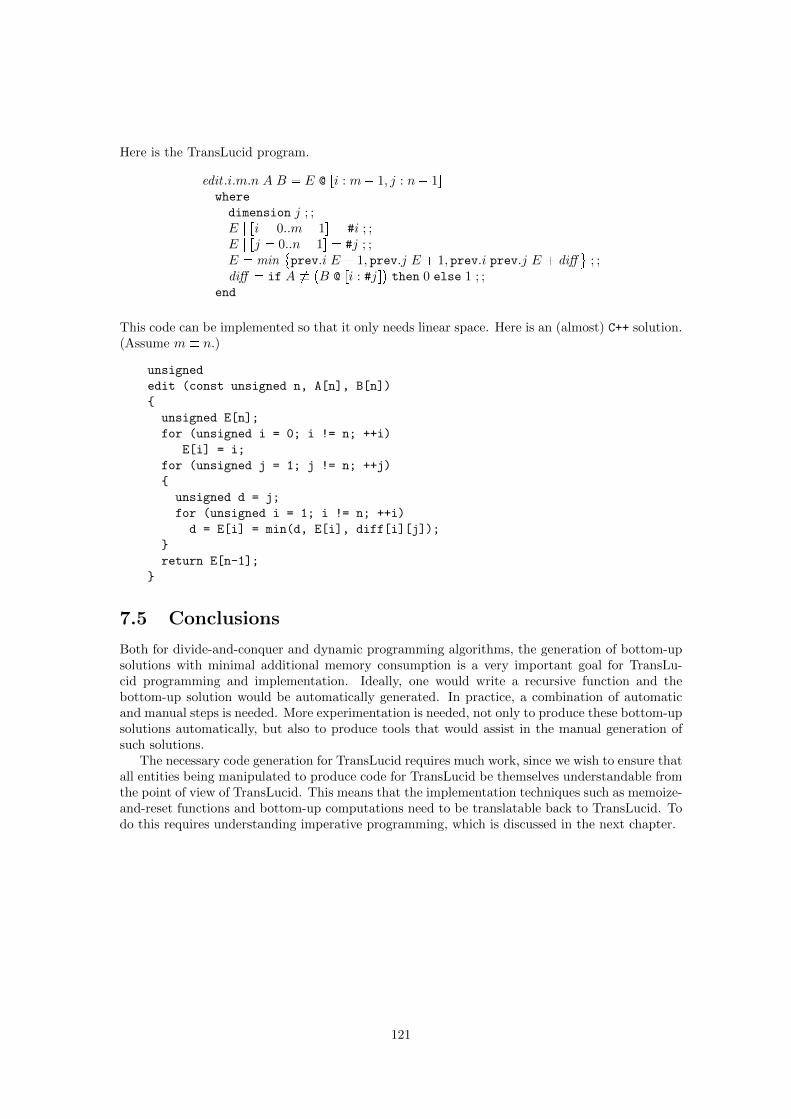
Here is the TransLucid program.

edit .i.m.n A B E @ ri : m 1, j : n 1swhere

dimension j ; ;E | ri 0..m 1s #i ; ;E | rj 0..n 1s #j ; ;E min

prev.i E 1, prev.j E 1, prev.i prev.j E diff

(; ;

diff if A B @ ri : #js

then 0 else 1 ; ;

end

This code can be implemented so that it only needs linear space. Here is an (almost) C++ solution.(Assume m n.)

unsigned

edit (const unsigned n, A[n], B[n])

unsigned E[n];

for (unsigned i = 0; i != n; ++i)

E[i] = i;

for (unsigned j = 1; j != n; ++j)

unsigned d = j;

for (unsigned i = 1; i != n; ++i)

d = E[i] = min(d, E[i], diff[i][j]);

return E[n-1];

7.5 Conclusions

Both for divide-and-conquer and dynamic programming algorithms, the generation of bottom-upsolutions with minimal additional memory consumption is a very important goal for TransLu-cid programming and implementation. Ideally, one would write a recursive function and thebottom-up solution would be automatically generated. In practice, a combination of automaticand manual steps is needed. More experimentation is needed, not only to produce these bottom-upsolutions automatically, but also to produce tools that would assist in the manual generation ofsuch solutions.

The necessary code generation for TransLucid requires much work, since we wish to ensure thatall entities being manipulated to produce code for TransLucid be themselves understandable fromthe point of view of TransLucid. This means that the implementation techniques such as memoize-and-reset functions and bottom-up computations need to be translatable back to TransLucid. Todo this requires understanding imperative programming, which is discussed in the next chapter.

121

Chapter 8

Putting Control on the Index

The TransLucid language is declarative. A question thus arises: Can Cartesian programming dealwith the complexities of “real programming”, namely with side-effects and imperative program-ming? We examine these issues in this chapter, and demonstrate that the Cartesian approachhelps clarify some issues.

8.1 Side-effects in functions

TransLucid is designed to be used as a coordination language, in which constants and data func-tions are defined in the host language. We have been supposing up to now that these constantsand data functions are stateless, and that the only semantics of interest is in the behavior ofTransLucid. However, it is quite possible, maybe even desirable, for these constants and functionsto have state. This raises the question, Is it possible for this to make sense in a declarative man-ner? The answers we will provide in this chapter will rely on the Cartesian framework. Ratherthan focusing on the semantics of the side-effect itself, we consider the very concept of side-effect,and come up with some basic conclusions.

First, we should note that side-effects are unavoidable in computing. In fact, if there were noside-effects, computing would be useless: should one put a computer in a locked chamber with noconnection to the outside world but the electrical supply, then that computer would be completelyuseless! Sooner or later, something needs to be printed, displayed on a screen, written to disk orsent over a network, or some actuator needs to be activated.

One possible answer is to state that since a TransLucid system is a reactive system, it can beleft to the calling environment to determine if these kinds of action need to be performed, and to doso should this be the case. Clearly, this kind of choice is perfectly reasonable for some applications,but is not satisfactory in general, as the power of the host language and the underlying computersystem would not be available.

So what is a side-effect? It is a change of some external state, not accessible to the TransLucidsystem. Let us consider as example that it is page 232 of a book being printed. Then if page 232is to be printed, it must be printed exactly once. Furthermore, all of the pages preceding page 232have to printed before printing it.

What we can retain from this example is that a side-effect can only take place once and that itmay depend on other side-effects having taken place prior to it taking place. How can we ensurethis sort of thing in TransLucid?

The answer is surprisingly simple. An external function f which might provoke a side-effect isdeclared in the header as such, and a set of dimensions d1, . . . , dn is declared to be variant withrespect to the execution of f . For example:

stateful f dimensions d1, . . . , dn ; ;

122

Then, for any point in d1 dn space, f may be evaluated exactly once. Should f be evaluatedat point κ rd1 : c1, . . . , dn : cns, its arguments and return value must be cached (see Chapter 4).If f is called a second time at κ, then the cache must check to ensure that the same argumentsare passed; if they are, the cached value is returned, otherwise spxstatey.

In addition to being simple, this answer has the advantage that it is fully under the control ofthe programmer. Should the programmer decide that no control over side-effects is necessary, thenthe declaration of f refers to no dimensions of variance. Furthermore, it allows different kinds ofside-effect to be subject to different sets of dimensions.

For the dependencies, two techniques are appropriate. The first introduces the “;” operator:E1;E2 returns the result of evaluating E2, but only initiates E2 once the evaluation of E1 isfinished. Should E1 and E2 both include side-effects, then the side-effects of E1 take place beforethose of E2.

The second method is to introduce a new kind of declaration, this time added to the equationset, implying a dependency between different points in the Cartesian space. Dependencies wouldbe defined by bestfitting, like for equations. A guard g for a dependency for variable x would looklike this:

Bg Ð Eg

where Eg would have to evaluate to a tuple. The idea is that if the current context were containedinside the region defined by Bg, then x would first have to be evaluated at the context definedby Eg.

8.2 Side-effects in objects

In a language such as C++, side-effects do not just take place through function calls, but alsothrough the use of class methods. Can these too be added to TransLucid? Conceptually, theanswer is yes, using the same techniques as above, with an additional dimension for the object inquestion.

In practice, this would be more difficult, as one would need to add class declarations to Trans-Lucid, complete with the typing of the methods. Should this work have been done and theinterpreter adjusted accordingly, then we could refine the above techniques by distinguishing be-tween set and get methods. Since get methods are equivalent to side-effect-free functions, if anobject is clonable, then uses of get methods would not need to be cached: caching the objectwould suffice, since one could recall get methods at will.

It would probably be safer to only work with objects that respected some clear interface, whichmight wrap around other more general objects, in such a way as to guarantee that the objects actas TransLucid hyperdatons, with synchronous semantics (see §6.7).

8.3 Imperative programming

To understand side-effects declaratively required the use of a set of dimensions in which wereregistered these effects. For an imperative program P , the same process takes place, but witha fixed set of dimensions, corresponding to the different accessible points in P , along with theiteration counts of loops belonging to P . The approach corresponds closely to those used formodern compilers [22], which use static single-assignment form to register all of the differentassignments to a specific variable, and which attempt to treat as a single sequence all thoseinstructions executed between two I/O operations.

We present a simple imperative language with blocks, conditionals, loops, function calls, dy-namic exceptions and side-effects. We then label the different positions in a program in order forit to be translated into TransLucid. We assume that the semantics of an imperative program isthe execution, in the correct order, of the chain of side-effects within the program, followed by theevaluation of the return result.

123

8.3.1 Grammar

The grammar for the language is given below. All statements can be labeled, and the label canbe used as a context, as in x @ r`s, meaning the value of x at label `. Loops must be exited with alabeled exit, and the next iteration started with a labeled continue. For blocks that are not loops,labeled exits and continues are equivalent.

In the grammar, enumerations with . . . may have no (0) occurrences.

P :: F

F :: main ( x , . . . , x ) B

B :: t LS . . . LS u

LS :: ` : S

| S

S :: E ;

| exit ` ;

| continue ` ;

| B

| loop B

| if ( E ) B B

E :: c

| x

| x @ C

| x := E

| op pE, . . . , Eq

| opS pE, . . . , Eq

C :: [ L, . . . , L]

L :: ` | `-n

where

B is a block ;

C is a context ;

E is a expression;

F is a function;

P is a program;

S is a statement ;

LS is a labelled statement ;

c is a constant ;

` is a label ;

x is a variable;

op is an operator ;

opS is an operator with side-effect.

124

The @ operator is used to refer to the value of an operator in a previous position. Normally onewill only use a single label, but should this position be within a loop, then one can write ` n todesignate the value n iterations previous from the current one in the loop labelled by `.

The labels are needed to exit or continue blocks, and are mostly used in loops. For example:

main ()

x := 0;

L1: loop

x := x+1 ;

if (x>5) exit L1;

if (x>4) continue L1;

x := x+1 ;

The exit L1; means to exit the loop labelled L1. The continue L1; means to start the nextiteration of the loop labelled L1.

8.3.2 Tagging blocks and statements

Each block and statement in a program has a unique tag. This section describes the taggingprocess. The basic idea is that the statements in a block are numbered, and the positions betweenthe statements are numbered as well. Suppose we have a block with n statements:

B t LS0 . . . LSn1 u

Then there are n 1 positions, corresponding to the beginning (1 position), and the semicolonsand block close braces (n positions, including the end):

B t p0 LS0 p1 . . . pn1 LSn1 pn u

If there were only one block in a system, then the positions could simply be tagged with0, 1, . . . , n. However, the blocks appear in a hierarchical arrangement, so we need to keep track ofthis hierarchy. For example, in program:

main ()

x := 1 ;

y:=3 ;

print (x) ;

print (y) ;

the tagging would be like this:

main ()

[main:0]

x := 1;

[main:1]

y := 3;

[main:2]

print (x);

[main:3]

print (y);

[main:4]

125

while in program

main ()

x := 1 ;

if (x>1)

y:=3 ;

y:=4 ;

print (y) ;

the tagging would give:

main ()

[main:0]

x := 1;

[main:1]

if (x > 1)

[main:1,iftrue:0]

y := 3;

[main:1,iftrue:1]

[main:1,iffalse:0]

y := 4;

[main:1,iffalse:1]

[main:2]

print (y);

[main:3]

The tagging takes place by traversing the parse tree, and is defined structurally. There are fivefunctions.

• T0pfunctionq is the top-level function called to start the process.

• T1pstatement, tagq is the function called to tag a statement. The tag is a list.

• T2pblock, tag, prefixq is the function called to tag a block. The tag is a list and the prefix isa key used to identify the current block.

• T3pexpression, tag, prefixq is the function called to tag an expression.

• T4pexpression, tag, prefixq is a subsidiary function of T3.

126

T0pF0 . . . Fn1q T0F0q . . . T0pFn1q

T0x ( x0 , . . . , xn1 ) B

x ( x0 , . . . , xn1 ) T2pB, rs, xq

T1p` : S,Lq ` : T1pS,LqT1pE,Lq T3

E,L, rs

T1pexit `,Lq exit `

T1pcontinue `,Lq continue `

T1pB,Lq T2pB,L, blockqT1ploop B,Lq T2pB,L, loopq

T1pif ( E ) B1 B2,Lq if ( E )

T2pB1,L, iftrueqT2pB2,L, iffalseq

T2LS0 . . . LSn1,L,X

[L, X:0]T1LS0, rL X : 0s

[L, X:1]. . .[L, X:n 1]T1LSn 1, rL X : n 1s

[L, X:n]

T3pE,L,X q rL X bs T4pE,L, X q rL X esT4pc,L,X q c

T4px,L,X q x

T4px @ C,L,X q x @ C

T4px : E,L,X q x : T3pE,L,X0q

T4oppE0, . . . , En1q,L,X

op

T3pE0,L,X0q, . . . T3pEn1,L,X pn 1qq

8.3.3 Interpreting expressions

The objective of the translation of an imperative program into TransLucid is to generate a set ofTransLucid equations that track the data flow of all variables. Like in C, each statement is assumedto have a value, which is the value of the last evaluated expression. Because the expressions canmodify the values of variables, we need to keep track of state during the evaluation of expressions.

For the expressions, we explain the process using an example, namely:

p px 3q py : zq; p1

which is found at current position is p and whose next position is p1. Then the tagged expressioncorresponds to the following figure:

127

p b p e

p 0b p 0e p 1b y : p 1e

p 00b x p 00e p 01b 3 p 01e p 10b z p 10e

HHHH

@@

Therefore, within the expression, there are 12 control positions: p b, p 0b, p 00b, p 00e,p 01b, p 01e, p 0e, p 1b, p 10b, p 10e, p 1e, p e.

The current value of the expression is kept track of in the variable called cur, for current. Allevaluation of expressions is assumed to be leftmost, depthfirst, to simplify the generation of therules. The generated equations for the above expression are:

S | rP : p1s S @ rP : p es; ;

S | rP : p bs S @ rP : ps; ;

S | rP : p es S @ rP : p 1es; ;

S | rvar : cur, P : p es S @ rP : p 0es S @ rP : p 1es; ;

S | rP : p 0bs S @ rP : p bs; ;

S | rP : p 0es S @ rP : p 01es; ;

S | rvar : cur, P : p 0es S @ rP : p 00es S @ rP : p 01es; ;

S | rP : p 00bs S @ rP : p 0bs; ;

S | rP : p 00es S @ rP : p 00bs; ;

S | rvar : cur, P : p 00es S @ rvar : x, P : p 00bs; ;

S | rP : p 01bs S @ rP : p 00es; ;

S | rP : p 01es S @ rP : p 01bs; ;

S | rvar : cur, P : p 01es 3; ;

S | rP : p 1bs S @ rP : p 0es; ;

S | rP : p 1es S @ rP : p 10es; ;

S | rvar : y, P : p 1es S @ rvar : cur, P : p 10es; ;

S | rP : p 10bs S @ rP : p 1bs; ;

S | rP : p 10es S @ rP : p 10bs; ;

S | rvar : cur, P : p 10es S @ rvar : z, P : p 10bs; ;

Of course, the above equations do not express how S @ rP : p bs is defined, nor how S @ rP : p eswill be used. Hence, for every node, three equations are generated:

1. The equation defining the state of the system prior to commencing this part of the compu-tation. This is the state of the system at the end of the left sibling if it exists, otherwise thestate of the system at the beginning of the parent node.

128

2. The equation defining the current node. This defines variable cur, if the current node is notan assignment, otherwise it defines the variable named in the assignment.

3. The equation defining the rest of the system. This is the state of the system at the beginningof the current node, if it is for a variable or a constant, otherwise it is the state of the systemat the end of the rightmost child node.

8.3.4 Interpreting expression context changes

The syntax for expressions includes a line for context changes.

E :: . . .

| x @ C

C :: [ L, . . . , L]

L :: ` | `-n

The change of context allows one to refer to the value of a variable, including cur, at a previousinstant. Exactly one of the labels must be an ordinary label `p for an ordinary position p, andmust be for a position which is definitely reached before reaching the current position; this labelmust be placed first. For the other labels, the labels must be for loops which include the currentposition. The translation into TransLucid for the expression:

x @ r`p, `1 2, `2 3, `3 4s

simply becomes:

S @ rvar : x, P : `p, `1 : #`1 2, `2 : #`2 3, `3 : #`3 4s

8.3.5 Interpreting side-effects

The syntax for expressions includes a line for operators with side-effects.

E :: . . .

| opS pE, . . . , Eq

To properly implement a program means to ensure that the side-effects to be created shouldbe created in the right order, then that the final return value be evaluated. To do this, we mustintroduce variable, called last, to keep track of the position in which the last side-effect waseffected.

Suppose that there is a unary operator print, which will print a value to standard output,and that it then returns a status value. Suppose that we are encoding the statement

p print pp b E p eq p1

Then the translation will be:

S | rP : p1s S @ rP : p es; ;

S | rP : p bs S @ rP : ps; ;

S | rvar : cur, P : p1s S @ rvar : last, P : p1s; ;

S | rvar : last, P : p1s S @ rvar : last, P : p es; printS @ rvar : cur, P : p es

; ;

129

8.3.6 Interpreting labels

A label is used to exit from a block or a loop or to continue on with the next iteration of a loop.A label can also be referred to in the evaluation of an expression in order to refer to the value avariable held in a previous location in the program, thereby alleviating the need for temporaryvariables.

In our approach, the way we handle exit’s and continue’s is to consider them to be specialkinds of value. Taking this approach radically simplifies their tracking through conditional blocks.

Consider the following exit statement at position p.

p exit `; p1

Its translation is simply:

S | rP : p1s S @ rP : ps; ;

S | rvar : cur, P : p1s exit`, S @ rvar : cur, P : ps

; ;

Similarly, consider the following continue statement at position P:

p continue `; p1

Its translation is simply:

S | rP : p1s S @ rP : ps; ;

S | rvar : cur, P : p1s continue`, S @ rvar : cur, P : ps

; ;

In other words, these are handled as if they are expressions.

8.3.7 Interpreting blocks

A block is interpreted by chaining all of the statements therein together. However, because ofthe possibility of exit and continue values generated from within these statements, checks mustbe made for these values, so that they can be passed from statement to statement without anyfurther calculations or changes of state taking place. To do this means generating an equationthat allows the bypassing of a statement if the current value is already an exit or continue. Forexample, suppose there were an expression statement of the form:

p E; p1

Equations of the following form should be generated:

S | rP : p bs S @ rP : ps; ;

S | rP : p1s S @ rP : p es; ;

We need to add another equation to the last one.

S | rpriority : 1, P : p1s

& istypexexityS @ rvar : cur, P : ps

_ istypexcontinuey

S @ rvar : cur, P : ps

S @ rP : ps; ;

In other words, if there is an exit or continue value, then the statement is effectively skipped.

130

8.3.8 Interpreting conditional statements

Consider the conditional statement, where we have indicated the key positions:

p

if pp b E p eq

tp iftrue : 0 BT p iftrue : nT u

tp iffalse : 0 BF p iffalse : nF u

p1

Here is the translation.

S | rP : p bs S @ rP : ps; ;

S | rP : p es

S | rP : p iftrue : 0s S @ rP : p es; ;

S | rP : p iffalse : nT s

S | rP : p iffalse : 0s S @ rP : p es; ;

S | rP : p iffalse : nF s

S | rP : p1s if S @ rvar : cur, P : p es

then S @ rP : p iftrue : nT s

else S @ rP : p iffalse : nF s

fi; ;

8.3.9 Interpreting loops

Consider the loop construct starting at position P:

p L : loop tp loop : 0 B p loop : nu p1

The translation requires the generation of three new variables and of a new dimension for eachloop, all of which are derived from the label itself.

L p; ;

S | rP : p1s S @P : p loop : n,L : itL @ rL : 0s

; ;

S | rvar : cur, P : p1s if finalL exit pT, iq then i else finalL fi; ;

itL if istypexexity pendLq ||

endL continuepL1, iq, L1 L

then #L else itL @ rL : #L 1s fi; ;

endL S @ rvar : cur, P : p loop : ns; ;

prevL endL @ rL : #L 1s; ;

finalL endL @L : itL @ rL : 0s

; ;

S | rP : p loop : 0s S @ rP : p loop : n,L : #L 1s; ;

S | rvar : cur, P : p loop : 0s if prevL continue pL, iq then i else prevL fi; ;

S | rpriority : 1, P : p loop : 0, L : 0s S @ rP : ps; ;

131

8.3.10 Bringing it all together

The semantics of the main function, starting at point p and finishing at point p1, consists of thefollowing demand:

S @ rvar : last, P : p1s;S @ rvar : cur, P : p1s

In other words, first make sure that all of the side-effects take place, then create the return result.For this process to work, then the definition for last must be given for the starting point p:

S | rP : ps 0; ;

It is straightforward to add checks to block exits to see if there is an exit or a continue, as wellas to add dynamic exceptions, as are found in languages such as C++.

More difficult, but still straightforward, is the function call, because a stack of contexts isrequired. Upon entry in a called function, the last entry must keep track of the previous side-effect, wherever it might have occurred in the calling stack.

A translator for this language to TransLucid has already been written. Note that using thisapproach, a completely declarative semantics for imperative programs can be generated, and thatthe generated set of equations can then be examined using dataflow analysis.

8.4 Conclusions

In addition to allowing us to explore imperative programming from an indexical point of view forcode generation purposes, the main aim of this chapter is to show that TransLucid can serve asintermediate language for a wide variety of languages, including procedural ones, and that thistranslation process can encourage new developments in the original languge. In fact, a number ofparadigms can easily be understood from the multidimensional perspective.

• In languages with functions and no objects, only one dimension is used to distinguish meth-ods: the function name.

• In object-oriented programming, there are two dimensions: the name of the method and thereceiver object of the message.

• In subjective programming [86], there are three dimensions: the name of the method, thereceiver and the sender.

• In context-oriented programming [43], it is as for subjective programming, but also takinginto account one ore more context dimensions.

The same approach can be taken to study the design patterns often referred to in object-oriented programming [40]. For example, the Prototype Object Creational Pattern createsa new object by cloning an existing object. There are two fixed dimensions: subclass andprototype, but one can add as many context dimensions as one wishes to get a slightly differentclone of the prototype.

Similarly, the Structural and Behavioral Patterns described in [40] essentially define how amessage can be translated by a receiving object of one class into another message to be passed onto another object of another class. For each pattern, there is a restricted set of fixed dimensions,and possibly an additional unspecified set of further dimensions for refinement purposes.

As for concurrency, studying it from an indexical perspective will require experimenting withmultiple timed systems, which was discussed in Chapter 6.

132

Conclusions

133

At electric speeds of data processing, we become aware of environments for the firsttime. We call them “parameters”. It all began in electronic research when it wasdiscovered that the instruments of observation distorted the data. Now we know thatany environment acts like the instrument of observation.

Marshall McLuhan, 1964 [61].

The multidimensionality implicit in Cartesian programming has been shown to be remarkablyversatile. Given any problem, there is a small, fixed set of dimensions that define the problem,with an arbitrarily large additional set of dimensions that parameterize that problem.

The set of topics that follows on from the current document is very large. Instead of tryingto cover all possible issues, we examine in some detail two issues that have not been discussedsubstantially in the thesis: 1) data structures and types, and 2) algorithms and complexity.

Data structures and types

The current TransLucid manipulates three kinds of objects: atomic objects, i.e., ptype, valueqpairs; tuples, i.e., mappings from values to values; and hyperdatons. The first two are completelyconstructed as expressions are evaluated, while the hyperdatons, typically being infinite, are onlysampled as needed. Type checking is done dynamically, to ensure that operators are applied toobjects of the right type, and there is no static type inference.

With respect to type inference, we could, of course, have added strong static typing to thelanguage, both for variables and for dimensions, and previous interpreters have had this. However,given that hyperdatons are infinite, multidimensional entities, it is not always clear that everycell in a hyperdaton should have the same type. This is clearly not the case for commercialspreadsheets, for example. The proper solution requires the declaration of types of variables tobe context-dependent, as is the declaration of definitions for variables; this has already been doneexperimentally in one interpreter. Type inference would in general then not be decidable, and sotyping would require some interesting mix of static and dynamic typing. Problems requiring verystringent running constraints would have to be typed fully statically, while more experimentalprograms could run with dynamic typing.

An interesting aspect of the bestfitting process within the current interpreter is that it is alsoresponsible for choosing which specific host language function should be called when an operatorappears in the source program. This process considers a type to be not a name but, rather,a set of values, and that a value may actually belong to multiple different sets. Furthermore,the bestfitting process implicitly assumes that a single object can be understood as belongingto multiple “classes”. The theory that is most promising is that introduced by Adi Shamir andWilliam Wadge [85], but details of adapting our current implementation to follow this path arenot fully worked out.

Inductively defined abstract data types, as used in languages such as Haskell and OCaml, canbe implemented in TransLucid using tuples. Different types would be distinguished using, forexample, the type dimension, while the different constructors for a given type would be distin-guished by, say, the constructor dimension. Syntactic sugar would allow these to be parsed andprinted in ways familiar to most functional programmers.

Content as index

The interaction between “atomic values” and tuples can be very interesting, even for subjectsthat are considered to be completely solved. We examine here the question of “characters” indocuments. Consider, for example, character ‘O’, typically encoded in a document as a Unicodecharacter. It will appear in a byte stream as the UTF-8 byte 4F, corresponding to the tuple:

[

Type: UnicodeChar

CodePoint: U+004F

]

134

This information can then be used to lookup this character in the Unicode Data database [19],where we will find the following entry:

004F;LATIN CAPITAL LETTER O;Lu;0;L;;;;;N;;;;006F;

If we ignore the default values, and use the explanations given in [20], the above line correspondsto the tuple:

[

CodePoint : U+004F

Name : "LATIN CAPITAL LETTER O"

GeneralCategory : "Lu"

CanonicalCombiningClass : 0

BidiClass : "L"

BidiMirrored : "N"

SimpleLowecaseMapping : U+006F

]

i.e., the official Unicode Standard name of ‘O’ is ‘latin capital letter o’; it is an uppercaseletter; it is not reordered for combining purposes; it is a strong left-to-right character and notmirrored for bidirectional text; and its lowercase mapping is code point U+006F (the letter ‘o’).

With this approach, the set of characters can grow as needed, and is not limited to Unicodeor some other established character set. After all, Unicode places restrictions not only on the setof possible dimensions, but also on the values to be taken by these dimensions.

For example, it is not possible to encode all of the Chinese characters, for one can always createnew ones, and there are many cases of hapax legomena, i.e., characters only appearing once in thehistorical corpus which are not yet encoded. Our model allows the use of a character descriptionlanguage to register unencoded characters [97].

For example, suppose that the character for ‘mıng ’, meaning bright or clear, were not encoded.Then we could break it down into its two radicals, ‘rı’ (sun) and ‘yue’ (moon), as is shown below:

135

The full set of strokes needed for ‘mıng ’ is given below (Note: just one possible representation):

[

Type: ChineseGlyph

RadicalOrder: LeftRight

Left: [

0: "shu"

1: "heng zhe"

2: "heng"

3: "heng"

]

Right: [

0: "pie"

1: "heng zhe gou"

2: "heng"

3: "heng"

]

]

Sometimes, the abstraction of ‘character’ is not sufficient, nor even an abstract visual descrip-tion. This is the case, for example, when studying steles in archæology: exact images are requiredfor presentation, discussion and analysis, yet these still need to be treated as ‘characters’. Thephotograph below presents one such example, a cartouche at the bottom of the obelisk in thecenter of Paris’s Place de la Concorde [17], originally from Luxor Temple in Egypt.

The following description suffices:

[

Type: EgyptianCartouche

CurrentLocation: "Place de la Concorde, Paris"

CurrentDate: 1833

OriginalLocation: "Temple, Luxor"

OriginalDate: "3300BP"

PNGfile: "EgyptianCartouche.png"

]

The previous examples should demonstrate that this approach is extensible as needed, inevery direction. Should further dimensions be needed, they can be added at any time. What isconsidered to be an atomic value is simply a convention, and a ‘magnifying glass’ can be used forfurther detail.

The context is the link

When we think of a programming environment, we do not just think about the language, butalso the libraries that come with that language. For example, the success of Smalltalk came in no

136

small part from the containers that were provided in the distribution. Similarly, the success of C++cannot be disassociated from the Standard Template Library (STL) and its generic algorithms.

For TransLucid, we are currently developing the indexed container, in which every cell in thecontainer has a unique index allowing direct access to it and which is robust to editing, in thesense that future modifications to the container will not affect existing indexes.

The STL provides a number of containers, including vectors, lists, deques, and so on. Weconsider all of these to be linear containers, in the sense that we can order all of the elements ina straight line, and that there is a beginning and an end to this order. However, the insertionproperties of the different containers are very different: some only allow insertion at the end orthe beginning, others anywhere.

In our vision, all of these are special cases of the one-dimensional indexed container, describedas follows:

• A container uses the set Q of rationals as the set of possible dimensions. In fact, only thoserationals with powers of 2 as denominator are needed.

• Every container responds to the dimensions 1 and 1, which respectively represent beforethe container and after the container, neither ever pointing to an actual value.

• The first element is added at dimension 0.

• If the minimum element is at dimension q, then an insertion before q is placed at pq 1q2.

• If the maximum element is at dimension q, then an insertion after q is placed at pq 1q2.

• If an element is to be placed between adjacent elements p and q, it is placed at pp qq2.

• If we keep track of the evolution of time as this structure is created, every element withinthe container has a unique address which is robust.

This approach can be extended to higher dimensions. For example, using a second-dimensionwould allow the creation of trees and dags in which one could insert nodes along a path betweenexisting nodes. In this case, the initial seed would be placed at position p0, 0q. Normal computer-science trees would continue to grow down, but we could also extend these to allow growing up,much as do real trees, but also back down again, as with the banyans found in tropical regions ofthe world.

The robustness requirement is crucial for the development of Web-enabled applications. Thereis an increasing trend towards the use of permanent URLs for documents, as in the use of DigitalObject Identifiers (DOIs) in the publishing industry. Using the mechanism above would allow theconcept of permanent URL to become even more precise, as it could accurately point to individualcharacters within documents; Ted Nelson would be proud.

137

Algorithms and complexity

In traditional complexity theory, a problem is defined in terms of its “size” n, and its complexityis defined in terms of a function in n: for example, quicksort is Opn2q worst-case and Opn log nqaverage-case time complexity. In parametric complexity theory, introduced by Michael Fellows andRodney Downey [29], a problem is defined in terms of its size n and a parameter k. A parameterizedproblem L ΣΣ is fixed-parameter tractable if it can be determined in fpkqnOp1q time whetheror not px, kq P L, where f is a computable function only depending on k. A good introduction tothe theory is the book Invitation to Fixed-Parameter Algorithms, by Rolf Niedermeier [64].

There are many problems that are known to be NP-complete which turn out to be fixed-parameter tractable, and for which realistic applications of the problem ensure that the parame-ter k is sufficiently small that the problem becomes effectively tractable on real data.

The intuition is that the hard part of these problems is in the parameter k part, not in theoverall size n of the problem. As a result, a common practice in fixed-parameter algorithm design isa process called kernelization, in which the problem is concentrated by cutting out the easier bits,leaving the separated hard parts, in which exhaustive search is not uncommon. This kernelizationis a form of preprocessing, in which the problem is “massaged” so that it is more amenable to themain algorithm.

In Part II of his book (the main part), Niedermeier goes to great lengths to show how differentapproaches can be taken to creating fixed-parameter algorithms for a wide range of problems. Oneof the important points that he makes is that preprocessing is typically not something that is runjust once, but rather the main algorithm and preprocessing must be interleaved. At each step, toreduce the search space of what remains to be solved, one should clear out the easy parts, leavingwhat is still known to be hard.

In recent discussions, Fellows proposes to develop a catalog of Total Victory Maps, in whichthe parameterized complexity approach succeeds in developing the best worst-case time bounds,for all inputs [39]. In the discussion, he raises the question, “How many dimensions are relevantto such mappings?”

This is where Cartesian programming may be relevant, using a process that we call iterativebestfitting, which we now describe. Suppose that there is a problem to solve, the input is thedata D0 and that there is a family of algorithms A pQ Aq. Then the resolution of this problem isundertaken iteratively. At each step i:

• Apply to Di a preprocessing step BipDiq, and in so doing, calculate a set of relevant param-eters pi1, . . . , pini

.

• Use bestfitting over the pi1, . . . , pini to find algorithm Ai. Run AipDiq, returning Di1.

• If there are several possible best algorithms Ai1, . . . , Aimi, then they can all be run in parallel,

and then Di1 would be the either the first or the best answer returned by AijpDiq.

• If Di1 is a solution, or it is clear that there is no solution, halt. Otherwise, start step i 1.

The iterative bestfitting approach is well-suited to developing algorithms in which it is difficultto determine statically which approach will be best in which conditions. The approach is well-suited both for theoretical complexity work as well as for the development of real algorithms forreal problems, since at each iteration, the bestfitting may take into account not just the availablealgorithms, but the knowledge of the parameters computed by the preprocessing step, as well asthe results from previous iterations.

From the analysis point of view, the fact that bestfitting of the algorithm takes place ateach iteration does not facilitate anything, as it makes any recurrence equation harder to solve.Nevertheless, we consider that the iterated bestfit approach would facilitate the development ofTotal Victory Maps. Moreover, we can envisage developing this idea even further by taking intoaccount variants of problems in the mapping process: this just means adding more dimensions.

138

Whither from here?

Apart from the topics of data and complexity, there are many other topics which we have notconsidered in this thesis.

For example, there is little discussion of static analysis. This very important topic can beapplied in numerous manners to the development of TransLucid, including type checking, spaceand time optimization and formal verification. Given that TransLucid is a completely declarativelanguage, and that variables already have multiple declarations, we can add further declarations.In this case, during the bestfitting process, should multiple declarations be “best”, then all ofthem would be applied, and any evaluation or verification would have to ensure that all of the“best” declarations yield consistent results in a given context.

Similarly, there is no discussion of what we call “search-based programming” (unfortunately theterm is consecrated elsewhere), which includes any form of programming in which a considerablepart consists of searching through large amounts of data, as in logic programming, databaseprogramming and data mining. Currently, we have no semantics for such forms of programming,although the use of multiple dimensions is clearly relevant to all of them.

In general, the implementation of a given problem can itself be understood as requiring theparameterization of the solution space, based on the available components for processing, in thememory hierarchy and for communication. Research in this area should yield fruitful results,considering the wide variety of multiprocessors being developed for the current market place.

When Descartes introduced his coordinate sytem, it greatly simplified the presentation andresolution of a number of existing problems in geometry, and allowed the definition of much moredifficult problems that previously could not be expressed. So far, each part of computer sciencethat we have examined through the Cartesian lens has allowed us new insights. Will Cartesianprogramming also lead to the future specification of problems hitherto unexpressible?

139

Bibliography

[1] Krste Asanovic, Ras Bodik, Bryan Christopher Catanzaro, Joseph James Gebis, Parry Hus-bands, Kurt Keutzer, David A. Patterson, William Lester Plishker, John Shalf, Samuel WebbWilliams, and Katherine A. Yelick. The Landscape of Parallel Computing Research: A Viewfrom Berkeley. Technical Report UCB/EECS-2006-183, Electrical Engineering and ComputerSciences, University of California at Berkeley, Berkeley, CA, 2006.

[2] E. A. Ashcroft and W. W. Wadge. Lucid—A formal system for writing and proving programs.SIAM Journal on Computing, 5(3):336–354, September 1976.

[3] E. A. Ashcroft and W. W. Wadge. Lucid, A Nonprocedural Language with Iteration. Com-munications of the ACM, 20(7):519–526, July 1977.

[4] Edward A. Ashcroft. The Lucid Language: Past, Present, and Future. In Proceedings of the5th ISLIP, pages 1–15, San Francisco, USA, Apr 1992. IEEE Computer Society. islip.web.cse.unsw.edu.au/1992.

[5] Edward A. Ashcroft, Anthony A. Faustini, Rangaswamy Jagannathan, and William W.Wadge. Multidimensional Programming. Oxford University Press, New York, 1995.

[6] Edward A. Ashcroft and William W. Wadge. Lucid, a Nonprocedural Language with Iteration.Communications of the ACM, 20(7):519–526, July 1977.

[7] Varunan Balasingham, Gabriel Ditu, and Simon Hudson. Intensionality and the object-oriented paradigm. Honours Thesis, Computer Science, UNSW, 2001.

[8] Jarryd Beck. Cartesian programming: From theory to implementation. Honours Thesis,Computer Science, UNSW, 2010.

[9] Albert Benveniste, Paul Caspi, Stephen A. Edwards, Nicolas Halbwachs, Paul Le Guernic,and Robert de Simone. The synchronous languages 12 years later. Proceedings of the IEEE,91(1):64–83, 2003.

[10] I. M. Bochenski. Ancient Formal Logic. North-Holland, Amsterdam, 1951.

[11] I. M. Bochenski. A History of Formal Logic. University of Notre Dame Press, Notre Dame,Indiana, 1961. Translated from the German Formale Logik.

[12] Gordon D. Brown. Intensional HTML 2: A practical approach. Master’s thesis, Departmentof Computer Science, University of Victoria, Canada, 1998.

[13] Vannevar Bush. As we may think. Atlantic Monthly, July 1945.

[14] Rudolph Carnap. Meaning and Necessity. University of Chicago Press, 1956. Seventh Im-pression 1975.

[15] Paul Caspi, Daniel Pilaud, Nicolas Halbwachs, and John Plaice. A declarative language forprogramming synchronous systems. In Fourteenth Annual ACM Symposium on Principles ofProgramming Languages, POPL 1987, pages 178–188, Munich, January 1987.

140

[16] Aggelos Charalambidis, Athanasios Grivas, Nikolaos Papaspyrou, and Panos Rondogiannis.Efficient intensional implementation for lazy functional languages. Mathematics in ComputerScience, 2(1):123–141, 2008.

[17] Wikipedia Commons. Image of Obelisk in Paris, 2006. upload.wikimedia.org/wikipedia/commons/3/31/Obeliskparis.jpg.

[18] Reidar Conradi and Bernhard Westfechtel. Version models for software configuration man-agement. ACM Computing Surveys, 30(2):232–282, 1998.

[19] Unicode Consortium. www.unicode.org/Public/UNIDATA/UnicodeData.txt, 2009.

[20] Unicode Consortium. www.unicode.org/reports/tr44/#UnicodeData.txt, 2009.

[21] N. J. Cutland. Computability: An Introduction to Recursive Function Theory. CambridgeUniversity Press, 1980.

[22] R. Cytron, J. Ferrante, B. Rosen, M. Wegman, and K. Zadeck. Efficiently computing staticsingle assignment form and the control dependence graph. ACM TOPLAS, 13(4):451–490,1991.

[23] Ole-Johan Dahl, Edsger Wybe Dijkstra, and C. A. R. Hoare. Structured Programming. Aca-demic Press, London, 1972. ISBN 0122005503.

[24] Sanjoy Dasgupta, Christos Papadimitriou, and Umesh Vazirani. Algorithms. McGraw Hill,2007.

[25] Jean Dhombres. La banalidad del referencial cartesiano. In Carlos Alvarez J. andJ. Rafael Martinez Enrıquez, editors, Descartes y la ciencia del siglo XVII. siglo veintiunoeditores, Mexico, 2000.

[26] Edsger Dijkstra. Go to statement considered harmful. Communications of the ACM,11(3):147–148, March 1968.

[27] Edsger Wybe Dijkstra. A Discipline of Programming. Prentice-Hall, Englewood Cliffs, NJ,1976. ISBN 013215871X.

[28] Gabriel Ditu. The Programming Language TransLucid. PhD thesis, School of ComputerScience and Engineering, The University of New South Wales, Sydney, Australia, March2007.

[29] Rodney G. Downey and Michael R. Fellows. Parameterized Complexity. Springer, 1999.

[30] David R. Dowty, Robert E. Wall, and Stanley Peters. Introduction to Montague Semantics.D. Reidel, Dordrecht, Holland, 1981.

[31] W. Du and W. W. Wadge. A 3D spreadsheet based on intensional logic. IEEE Software,7(3):78–89, 1990.

[32] W. Du and W. W. Wadge. The eductive implementation of a three-dimensional spreadsheet.Software–Practice and Experience, 20(11):1097–1114, 1990.

[33] Doug Engelbart. Personal communication, 2004.

[34] Esterel Technologies. Home page. www.esterel-technologies.com. Last visited 8 December2007.

[35] A. A. Faustini and W. W. Wadge. Intensional programming. In J. C. Boudreaux, B. W.Hamil, and R. Jenigan, editors, The Role of Languages in Problem Solving 2. Elsevier North-Holland, 1987.

141

[36] Anthony A. Faustini and Rangaswamy Jagannathan. Indexical Lucid. In Proceedings of the4th ISLIP, pages 19–34, Menlo Park, USA, Apr 1991. SRI International. islip.web.cse.

unsw.edu.au/1991.

[37] Anthony A. Faustini and Rangaswamy Jagannathan. Multidimensional Problem Solving inLucid. Technical Report SRI-CSL-93-03, Computer Science, SRI International, Menlo Park,USA, 1993.

[38] Antony A. Faustini and William W. Wadge. An eductive interpreter for lucid. In PLDI,pages 86–91. ACM, 1987.

[39] Michael Fellows. New ideas column. Parameterized Complexity News, pages 6–7, September2009. mrfellows.net/Newsletters/09_Sept_News.pdf.

[40] Erich Gamma, Richard Helm, Ralph Johnson, and John Vlissides. Design Patterns: Elementsof Reusable Object-Oriented Software. Addison-Wesley, 1995.

[41] Manolis Gergatsoulis and Panos Rondogiannis, editors. Intensional Programming II, vol-ume II. World Scientific, Singapore, 2000. Based on the papers at ISLIP’99.

[42] N. Halbwachs, P. Caspi, P. Raymond, and D. Pilaud. The synchronous data-flow programminglanguage LUSTRE. Proceedings of the IEEE, 79(9):1305–1320, September 1991.

[43] Robert Hirschfeld, Pascal Costanza, and Oscar Nierstrasz. Context-oriented programming.Journal of Object Technology, 7(3):125–151, 2008.

[44] Lapyu Kenneth Ho, Ian Su, and Patrick Leung. Multidimensional Linux library system.Honours Thesis, Computer Science, UNSW, 2001.

[45] Proceedings of the 32nd Annual IEEE International Computer Software and ApplicationsConference, COMPSAC 2008, 28 July - 1 August 2008, Turku, Finland. IEEE ComputerSociety, 2008.

[46] Rangaswamy Jagannathan and Chris Dodd. GLU Programmer’s Guide. Technical report,Computer Science, SRI International, Menlo Park, USA, 1996. Version 1.0.

[47] Rangaswamy Jagannathan, Chris Dodd, and Iskender Agi. GLU: A High-Level System forGranular Data-Parallel Programming. Concurrency: Practice and Experience, 9(1):63–83,Jan 1997.

[48] Gilles Kahn. The semantics of simple languages for parallel programming. In InformationProcessing 74, pages 471–475. North-Holland, 1974.

[49] Gilles Kahn and David B. MacQueen. Coroutines and networks of parallel processes. InInformation Processing 77, pages 993–998. North-Holland, 1977.

[50] Saul A. Kripke. Naming and Necessity. Harvard University Press, Cambridge, Mass., 1980.

[51] Peter Kropf, Gilbert Babin, John Plaice, and Herwig Unger, editors. Distributed Communitieson the Web, volume 1830 of Lecture Notes in Computer Science. Springer, Berlin, 2000. ThirdInternational Workshop, DCW 2000, Quebec, Canada, June 2000, Proceedings.

[52] P.G. Kropf and J. Plaice. WOS communities—Interactions and relations between entities indistributed systems. In Distributed Computing on the Web, DCW’99, pages 163–167, Rostock,Germany, June 1999.

[53] Peter J. Landin. The next 700 programming languages. Communications of the ACM,9(3):157–166, 1966.

142

[54] m. c. schraefel. Talking to Antigone. PhD thesis, University of Victoria, Victoria, Canada,1997.

[55] Blanca Mancilla. A new approach to on-line mapping. In Proceeding of IWHIT’00, SeventhInternational Workshop on Human Interface Technology 2000, pages 19–23. University ofAizu, Aizu-Wakamatsu, Japan, November 2000.

[56] Blanca Mancilla. A new approach to interactive mapping. In Michitake Hirose, editor,Human-Computer Interaction — INTERACT’01, pages 644–647. IOS press for IFIP, 2001.

[57] Blanca Mancilla. Omega for multilingual mapping. In Bolek and Przechlewski, editors,Proceedings of XIII European TEX Conference April 29–May 3, 2002, Bachotek, Poland,pages 60–63. GUST, 2002.

[58] Blanca Mancilla. Intensional Infrastructure for Collaborative Mapping. PhD thesis, School ofComputer Science and Engineering, University of New South Wales, Sydney, Australia, 2004.

[59] Blanca Mancilla and John Plaice. Possible worlds versioning. Mathematics in ComputerScience, 2(1):63–83, 2008.

[60] m.c. schraefel, Blanca Mancilla, and John Plaice. Intensional hypertext. In Gergatsoulis andRondogiannis [41], pages 40–54. Based on the papers at ISLIP’99.

[61] Eric McLuhan and Frank Zingrone, editors. Essential McLuhan. House of Anansi Press,Toronto, 1995.

[62] Gordon E. Moore. Excerpts from A Conversation with Gordon Moore: Moore’s Law. VideoTranscript, Intel, 2005.

[63] Gordon E. Moore. Cramming more components onto integrated circuits. Electronics Maga-zine, 38(8), April 1965.

[64] Rolf Niedermeier. Invitation to Fixed-Parameter Algorithms. Oxford University Press, 2006.

[65] Calvin B. Ostrum. The Luthid 1.0 Manual. Department of Computer Science, University ofWaterloo, Ontario, Canada, 1981.

[66] Joey Paquet. Intensional Scientific Programming. PhD thesis, Department of ComputerScience, Laval University, Quebec, Canada, April 1999.

[67] Joey Paquet and Peter G. Kropf. The GIPSY architecture. In Kropf et al. [51], pages 144–153.Third International Workshop, DCW 2000, Quebec, Canada, June 2000, Proceedings.

[68] Joey Paquet and John Plaice. The semantics of dimensions as values, pages 259–273. Vol-ume II of Gergatsoulis and Rondogiannis [41], 2000. Based on the papers at ISLIP’99.

[69] D. L. Parnas. On the design and development of program families. IEEE Transactions onSoftware Engineering, 2(1):1–9, March 1976.

[70] Anthony L. Peratt. Physics of the Plasma Universe. Springer, New York, 1992.

[71] John Plaice. Multidimensional Lucid. In Kropf et al. [51], pages 154–160. Third InternationalWorkshop, DCW 2000, Quebec, Canada, June 2000, Proceedings.

[72] John Plaice and Peter Kropf. Intensional communities, pages 292–295. Volume II of Gergat-soulis and Rondogiannis [41], 2000. Based on the papers at ISLIP’99.

[73] John Plaice and Blanca Mancilla. Collaborative intensional hypertext. In Hypertext, pages91–92. ACM, 2004.

143

[74] John Plaice, Blanca Mancilla, and Gabriel Ditu. From Lucid to TransLucid: Iteration,dataflow, intensional and Cartesian programming. Mathematics in Computer Science,2(1):37–61, 2008.

[75] John Plaice, Blanca Mancilla, Gabriel Ditu, and William W. Wadge. Sequential demand-driven evaluation of Eager TransLucid. In IEEE Computer Society [45], pages 1266–1271.

[76] John Plaice, Paul Swoboda, and Ammar Alammar. Building intensional communities usingshared context. In Kropf et al. [51], pages 55–64. Third International Workshop, DCW 2000,Quebec, Canada, June 2000, Proceedings.

[77] John Plaice and William W. Wadge. A new approach to version control. IEEE Transactionson Software Engineering, 19(3):268–276, March 1993.

[78] John Plaice and William W. Wadge. A UNIX tool for managing reusable software components.Software—Practice and Experience, 23(9):933–948, September 1993.

[79] Toby Rahilly. Experiments in concurrent implementations of TransLucid. Honours Thesis,Computer Science, UNSW, 2007.

[80] Toby Rahilly and John Plaice. A multithreaded implementation for TransLucid. In IEEEComputer Society [45], pages 1272–1277.

[81] Panos Rondogiannis and William W. Wadge. First-order functional languages and intensionallogic. Journal of Functional Programming, 7(1):73–101, January 1997.

[82] Panos Rondogiannis and William W. Wadge. Higher-order functional languages and inten-sional logic. Journal of Functional Programming, 9(5):527–564, May 1999.

[83] Dana Scott. Advice on modal logic. In Karel Lambert, editor, Philosophical Problems inLogic, pages 143–173. D. Reidel Publishing Company, Dordrecht, Holland, 1970.

[84] Victor Selivanov. Wadge reducibility and infinite computations. Mathematics in ComputerScience, 2(1):5–36, 2008.

[85] Adi Shamir and William W. Wadge. Data types as objects. In Arto Salomaa and MagnusSteinby, editors, ICALP, volume 52 of Lecture Notes in Computer Science, pages 465–479.Springer, 1977.

[86] Randall B. Smith and David Ungar. A simple and unifying approach to subjective objects.TAPOS, 2(3):161–178, 1996.

[87] Yannis Stavrakas, Manolis Gergatsoulis, and Panos Rondogiannis. Multidimensional XML. InKropf et al. [51], pages 100–109. Third International Workshop, DCW 2000, Quebec, Canada,June 2000, Proceedings.

[88] Paul Swoboda. Practical languages for intensional programming. Master’s thesis, Departmentof Computer Science, University of Victoria, Canada, 1999.

[89] Paul Swoboda. A formalization and implementation of distributed Intensional Programming.PhD thesis, School of Computer Science and Engineering, University of New South Wales,Sydney, Australia, 2003.

[90] Senhua Tao. TLucid and Intensional Attribute Grammars. In Proceedings of the 6th ISLIP,pages 94–106, Laval University, Quebec, Canada, Apr 1993. islip.web.cse.unsw.edu.au/

1993/.

[91] Richmond H. Thomason, editor. Formal Philosophy: Selected Papers of Richard Montague.Yale University Press, 1974.

144

[92] William W. Wadge. The Origins of Lucid. Presentation to the Institut fur Informatik,Christian-Albrechts-Universitat zu Kiel, Germany, 8 February 2007.

[93] William W. Wadge. Intensional logic in context, pages 1–13. Volume II of Gergatsoulis andRondogiannis [41], 2000. Based on the papers at ISLIP’99.

[94] William W. Wadge. Intensional Markup Language. In Kropf et al. [51], pages 82–89. ThirdInternational Workshop, DCW 2000, Quebec, Canada, June 2000, Proceedings.

[95] William W. Wadge and Edward A. Ashcroft. Lucid, the Dataflow Programming Language.Academic Press, London, 1985.

[96] William W. Wadge, Gordon D. Brown, m.c. schraefel, and Taner Yıldırım. Intensional HTML.In E.V. Munson, C. Nicholas, and D. Wood, editors, Principles of Digital Document Process-ing, volume 1481 of Lecture Notes in Computer Science. Springer-Verlag, 1998.

[97] Wai Wong, Candy L. K. Yiu, and Kelvin C. F. Ng. Typesetting rare Chinese characters inLATEX. TUGboat, 24(3):582–587, 2003. www.tug.org/TUGboat/Articles/tb24-3/wong.pdf.

[98] Taner Yıldırım. Intensional HTML. Master’s thesis, Department of Computer Science, Uni-versity of Victoria, Canada, 1997.

145