carrier synchronization of offset quadrature phase...
TRANSCRIPT

TMO Progress Report 42-133 May 15, 1998
Carrier Synchronization of Offset QuadraturePhase-Shift Keying
M. K. Simon1
This article contains analyses of the performance of various carrier synchro-nization loops for offset quadrature phase-shift-keying (OQPSK) modulation, allmotivated in one form or another by the maximum a posteriori (MAP) estimationof carrier phase. When they are implemented as either high or low signal-to-noiseratio (SNR) approximations to the generic implementation suggested by the MAPestimation of carrier phase for an OQPSK signal, it is shown that the loops behavemore like biphase than quadriphase loops in that they only exhibit a 180-deg phaseambiguity rather than the 90-deg phase ambiguity typical of the latter. This phaseambiguity advantage coupled with the mean-square tracking-error performance ad-vantage that results and its ultimate effect on average error probability performanceoffer a potentially significant justification for using OQPSK rather than QPSK evenon a linear transmission channel, where it often is reasoned (based on the assump-tion of an ideal environment) that the two modulation schemes perform identically.
I. Introduction
The problem of suppressed-carrier synchronization in digital coherent communication systems hasreceived widespread attention over the years from a theoretical as well as a practical point of view. Inreality, these two points of view are not separate from each other in that the carrier synchronizationstructures that commonly are employed in the design of coherent receivers are those that are motivatedby the application of the maximum a posteriori (MAP) estimation theory [1]. A common example of thisis the Costas or in-phase–quadrature (I-Q) loop [2,3] for binary phase-shift-keying (BPSK) systems thatis derived by suitably using the derivative of the open-loop MAP estimate of carrier phase as the errorsignal in a closed-loop configuration. Closed loops derived in such a fashion often are referred to as MAPestimation loops [1,4], and this terminology likewise shall be used here in this article. Extension of theabove relationship between open-loop (MAP) carrier estimation and closed-loop synchronization schemesto M -ary modulation schemes such as multiple phase-shift keying (MPSK) and quadrature amplitude-shift keying (QASK) also has been considered in the past [2,4,5].
Common to all of the above closed-loop schemes is the fact that the equivalent additive noise thatperturbs the loop error signal can be modeled as a piecewise constant (over the duration of a data sym-bol, Ts) random process that is independent from symbol to symbol. Hence, the loop update likewise isindependent from symbol to symbol, and the analysis of its performance can be determined by assuming
1 Communications Systems and Research Section.
1

a triangular correlation function of width 2Ts for the equivalent additive noise. Also, the signal com-ponent of the loop error signal, i.e., the so-called S-curve, is a nonlinear (e.g., sinusoidal for low-SNRimplementations) function of Mφc, with φc denoting the loop phase error, and as such the loop exhibitsan M -fold phase ambiguity,
When the modulation is offset, such as for offset quadrature-phase-shift keying (OQPSK), both of theabove observations become modified. First, the noise components in the I and Q channels correspondingto adjacent symbols overlap each other. Hence, the equivalent additive noise that perturbs the looperror signal, although still able to be modeled as a piecewise constant process, is no longer independentfrom symbol to symbol, i.e., adjacent symbol correlation exists. Second, the loop S-curve now need haveonly an 180-deg phase ambiguity (rather than the 90-deg phase ambiguity characteristic of QPSK carriersynchronization schemes) and as such resembles a BPSK carrier synchronization loop that tracks the2φ process. This phenomenon was identified previously by Mengali [6, p. 232] for a decision-directedimplementation of the OQPSK loop derived from MAP estimation considerations. Associated with thisobservation is the fact that, for OQPSK, the nonlinear loss that degrades the loop SNR will now be asquaring loss as opposed to the fourth-power loss typical of QPSK carrier synchronization loops.
In this article, we study the carrier synchronization problem for OQPSK in a more general frameworkthan that considered in [6] in that we do not restrict ourselves to high-SNR (decision-directed) implemen-tations of the MAP estimation loop. In particular, we explore in detail the noise and S-curve propertiesof the MAP estimation loop for OQPSK and their effect on its mean-square phase-error performance.We also present the behavior and performance of another OQPSK that has been implemented for futureuse in the Deep Space Network tracking stations [7]. This loop is an ad hoc but simple modificationof that used for nonoffset QPSK and as such tracks the 4φ process with an accompanying 90-deg phaseambiguity. The performance of this suboptimal loop is compared with that of the true MAP estimationloop for OQPSK referred to above and found to be considerably inferior. In all cases, comparisons willbe made on the basis of mean-squared phase jitter for equal loop bandwidths and signal-power-to-noise-power spectral density ratios. An equivalent comparison is in terms of the squaring loss2 (the reductionin loop SNR relative to that of a phase-locked loop (PLL) of the same loop bandwidth).
II. Received Signal Model
For OQPSK, the I–Q carrier-modulated signal seen at the input to the receiver can be written in theform
s(t, θ) =√P [mI(t) cos (ωct+ θ) +mQ(t) sin (ωct+ θ)] (1)
where P is the signal power in watts and
mI(t) =∞∑
n=−∞akp(t− kTs)
mQ(t) =∞∑
n=−∞bkp
(t−(k +
12
)Ts
)
(2)
2 Despite the fact that squaring loss is a term most appropriate to binary Costas loops, it nevertheless is used genericallyfor loops corresponding to higher-order modulations such as QPSK even though in that instance fourth-power loss wouldbe the more appropriate term.
2

with {ak} and {bk} respectively denoting the streams of independent, identically distributed (i.i.d.) binary(±1) I and Q data symbols, Ts the symbol time, p(t) a unit power rectangular pulse shape of durationTs seconds and symmetric around t = 0, and θ the unknown carrier phase to be estimated. In addition tothe signal in Eq. (1), the additive noise n(t) present at the receiver input is characterized as a band-limitedwhite Gaussian noise process with single-sided power spectral density N0 W/Hz.
III. The MAP Estimation of Carrier Phase
Based on an observation of the received signal plus noise x(t) = s(t, θ)+n(t) over a time interval KTs,we wish to estimate the random parameter θ (assumed to be time invariant over the observation interval)so as to maximize the a posteriori probability p (θ |x(t) ).3 Since the unknown phase θ can be assumed tobe uniformly distributed in the interval (−π, π), equivalently, we can maximize the conditional probabilityp (x(t) |θ ). For the assumed additive white Gaussian noise channel model, the solution to this problemis well-known and can be obtained from the solution to the same problem corresponding to unbalancedQPSK (UQPSK) modulation [5]. In particular, since OQPSK is a special case of UQPSK correspondingto equal powers and equal data rates on both the I and Q channels as well as synchronous (but offset)I and Q data streams, then from [5, Eq. (14)], we immediately obtain an expression for the error signale (φ) of the MAP estimation loop for OQPSK, namely,
e(φ) =K∑k=1
[Ic (k, φ) tanh {Is (k, φ)} − Is
(k − 1
2, φ
)tanh
{Ic
(k − 1
2, φ
)}](3)
where
Is (k, φ) 4=2√P
N0
∫ kTs
(k−1)Ts
x(t) sin(ωct+ θ
)dt
Ic (k, φ) 4=2√P
N0
∫ kTs
(k−1)Ts
x(t) cos(ωct+ θ
)dt
(4)
with θ denoting the loop’s estimate of the received carrier phase θ and φ4= θ − θ the associated loop
phase error. For conventional (nonoffset) QPSK, the corresponding error signal to Eq. (3) would be
e(φ) =K∑k=1
[Ic (k, φ) tanh {Is (k, φ)} − Is (k, φ) tanh {Ic (k, φ)}] (5)
An implementation of a closed loop4 based on Eq. (3) is illustrated in Fig. 1, where the K-symbolaccumulator associated with the open-loop MAP estimate is replaced by a digital loop filter whose designis governed by the desired dynamic behavior of the loop.
3 For convenience, we shall assume that K is integer, i.e., the observation interval corresponds to an integer number of baudintervals. This is typical of MAP estimation problems of this type.
4 The illustration in Fig. 1 is slightly more generic in that it includes the possibility of a nonrectangular unit power Ts-secondpulse shape, p(t).
3

+
( )dtTs /2
−Ts /2
( )dtTs /2
−Ts /2( )dt
Ts
0
DELAYTs /2
tanh
tanh
p (t ) DELAYTs /2
p (t − Ts /2)
( )dtTs
0
z 1DIGITALLOOP
FILTERNCO
εc (t )
y (t )
90deg
DELAYTs /2 p (t − Ts /2)
εs (t )
2 sin (ωc t + θ )
2 cos (ωc t + θ )
Fig. 1. Block diagram of the MAP carrier synchronization loop for offset pulse-shaped QPSK.
IV. Implementations for Low and High SNRs
As is customary in problems of this type, the hyperbolic tangent nonlinearity is replaced by its smalland large argument approximations corresponding to small and large SNR applications. In the caseof the latter, the appropriate approximation is tanhx ∼= sgn x, which results in a decision-directedimplementation, e.g., [6, Fig. 5.23]. A tracking-performance analysis of this scheme for Nyquist channelsand the assumption of perfect decisions [6, Eq. (5.25)] is given in [6, Section 5.4.2]. In the case of theformer, the hyperbolic tangent function is approximated by the first or first two terms of its power series.For QPSK, if we use simply the approximation tanhx ∼= x in Eq. (5), then the error signal e (φ) willdegenerate to zero value for all φ and, hence, be of no use. Thus, for QPSK, we must use the firsttwo terms of the power series, i.e., tanhx ∼= x − x3/3, in which case the linear term still results in zerocontribution to the error signal, but the cubic term gives [4]
e(φ) =K∑k=1
Ic (k, φ) Is (k, φ)[(Ic (k, φ))2 − (Is (k, φ))2
](6)
which is of the form IQ(Q2 − I2
)and involves fourth-order product terms. Thus, as previously alluded
to, in this instance the loop S-curve would be proportional to sin 4φ, and the squaring loss involvesfourth-order noise product terms.
For OQPSK, using only the linear term of the hyperbolic tangent power series does not result in adegenerate error signal since applying the approximation tanhx ∼= x to Eq. (3) results in
4

e(φ) =K∑k=1
[Ic (k, φ) Is (k, φ)− Is
(k − 1
2, φ
)Ic
(k − 1
2, φ
)](7)
which has the form of the difference of two binary PSK error signals with a half symbol separation and,in general, is nonzero for arbitrary φ. Thus, since only second-order products are involved in Eq. (7),one would anticipate that the loop S-curve might be proportional to sin 2φ, and the squaring loss wouldinvolve only second-order noise product terms, as is the case for I–Q Costas loop tracking of BPSK. Thatsuch is the case is the subject of the tracking performance analysis to be presented in the next section.
A. Tracking-Performance Analysis of the Low SNR Implementation
In this section, we first derive the S-curve and equivalent noise of the I–Q loop of Fig. 1 (with a linearapproximation to the hyperbolic tangent function) and then compute the loop’s mean-square phase jitter.As previously mentioned, the signal x(t) at the input to the receiver is composed of the sum of the signals (t, θ) and a band-limited white Gaussian noise process that can be expressed in the form
n(t) =√
2 [Nc(t) cos (ωct+ θ)−Ns(t) sin (ωct+ θ)] (8)
where Nc(t) and Ns(t) are independent low-pass white Gaussian noise processes with single-sidedpower spectral density N0 W/Hz. Demodulating x(t) with the quadrature reference signals rc(t) =√
2 cos(ωct+ θ
)and rs(t) =
√2 sin
(ωct+ θ
)produces (ignoring second-order harmonics of the carrier)
the quadrature phase detector outputs
εc(t) =
[√P
2mQ(t)−Ns(t)
]sinφ+
[√P
2mI(t) +Nc(t)
]cosφ
εs(t) =
[√P
2mQ(t)−Ns(t)
]cosφ−
[√P
2mI(t) +Nc(t)
]sinφ
(9)
where φ 4= θ − θ denotes the phase error in the loop. Integrating over the appropriate time intervalscorresponding to the transmitted I and Q symbols5 gives the pairs of signals zc(t), zs(t) and z′c(t), z
′s(t),
which are used to form the loop-error signal. Assuming a modulation m(t) as in Eq. (1), these signalstake the form6
zc(t) =∫ Ts/2
−Ts/2εc(t)dt =
[√P
2Tsb0 + b−1
2−N1
]sinφ+
[√P
2Tsa0 +N2
]cosφ
zs(t) =∫ Ts/2
−Ts/2εs(t)dt =
[√P
2Tsb0 + b−1
2−N1
]cosφ−
[√P
2Tsa0 +N2
]sinφ,
Ts2≤ t ≤ 3Ts
2
(10a)
and
5 For convenience, we assume the first (k = 1) baud interval for the I and Q integrate-and-dump (I&D) filters correspondingto the transmitted symbols a0 and b0.
6 We can ignore the weighting of the integrators by the factor 2√P/N0 since, for this implementation, this gain eventually will
be absorbed in the total loop gain. As such, zc(t), zs(t), z′c(t), and z′s(t) are normalized versions of Ic(k, θ), Is(k, θ), I′c(k, θ),and I′s(k, θ) corresponding to k = 1.
5

z′c(t) =∫ Ts
0
εc(t)dt =
[√P
2Tsb0 −N ′1
]sinφ+
[√P
2Tsa0 + a1
2+N ′2
]cosφ
z′s(t) =∫ Ts
0
εs(t)dt =
[√P
2Tsb0 −N ′1
]cosφ−
[√P
2Tsa0 + a1
2+N ′2
]sinφ, Ts ≤ t ≤ 2Ts
(10b)
where N1, N2, N′1, and N ′2 are zero-mean Gaussian random variables defined by
N14=∫ Ts/2
−Ts/2Ns(t)dt
N24=∫ Ts/2
−Ts/2Nc(t)dt
N ′14=∫ Ts
0
Ns(t)dt
N ′24=∫ Ts
0
Nc(t)dt
(11)
all with variance σ2N = N0Ts/2. Although N1 and N2 are uncorrelated, and likewise for N ′1 and N ′2,
because of the offset between the I and Q channels, the pairs N1, N′1, and N2, N
′2 are indeed correlated
with
E {N1N′1} = E {N2N
′2} =
N0Ts4
(12)
However, the pairs N1N′2 and N ′1N2 are still uncorrelated.
Multiplying z′c(t) and z′s(t) and subtracting the product of zc(t− Ts/2) and zs(t− Ts/2) produces theerror signal corresponding to the first baud interval in accordance with Eq. (7), namely,
z1(t) = z′c(t)z′s(t)− zc
(t− Ts
2
)zs
(t− Ts
2
)
=14PT 2
s
[b20 + a2
0 −(a0 + a1
2
)2
−(b0 + b−1
2
)2]
sin 2φ
+12PT 2
s
[b0
(a0 + a1
2
)− a0
(b0 + b−1
2
)]cos 2φ− Ne (t, 2φ)
2
=14PT 2
s
{[1− a0a1
2− b0b1
2
]sin 2φ+ [b0 (a0 + a1)− a0 (b0 + b1)] cos 2φ
}− Ne (t, 2φ)
2,
Ts ≤ t ≤ 2Ts (13)
6

where the first two (signal) terms account for the signal × signal products and Ne (t, 2φ) is an equivalentnoise (as if it appeared at the loop input) that accounts for the remaining signal × noise and noise × noiseproducts that, after some simplification, becomes
Ne (t, 2φ) = sin 2φ
×{− (N ′1)2 + (N ′2)2 −N2
2 +N21 −
√P
2Ts [(b0 + b−1)N1 − 2b0N ′1 − (a0 + a1)N ′2 + 2a0N2]
}
+ cos 2φ
{2N ′1N
′2 − 2N1N2 −
√P
2Ts [2b0N ′2 + 2a0N1 − (b0 + b−1)N2 − (a0 + a1)N ′1]
},
Ts ≤ t ≤ 2Ts (14)
and is a piecewise constant (over intervals of Ts seconds) random process.
The statistical mean (over the data symbols) of the signal term represents the loop S-curve. Thus,averaging the signal terms of Eq. (13) over the data gives
z1(t) 4=12S (φ) =
12
(12PT 2
s sin 2φ)4=
12Kg sin 2φ (15)
as previously anticipated, where Kg = PT 2s /2 denotes the slope (with respect to the 2φ process) of
the S-curve S (φ) at the origin. The difference between the signal components of z1(t) and their meanrepresents self-modulation noise that, at very large symbol SNR Es/N0 = PTs/N0 produces an errorfloor in the loop mean-square phase-error performance [6]. For the purpose of the analysis here, we shallignore this self-noise since, in the typical region of symbol SNRs of interest (below about 15 dB), it hasnegligible influence on the performance. If necessary, evaluation of the self-noise can be carried out in ananalogous fashion to that considered in [2,6].
Linearizing the loop (i.e., replacing sin 2φ by 2φ), as is appropriate in the typical operating regionof large loop SNRs, then following the approach in [2], the mean-square error of the 2φ process can becomputed from
σ22φ =
NEBLK2g
(16)
where BL denotes the loop bandwidth and NE is the flat single-sided power spectral density of the equiv-alent noise process7 Ne (t, 0), which can be modeled as a delta-correlated process [2] with autocorrelationfunction RNe(τ) = E {Ne (t, 0)Ne (t+ τ, 0)}. Thus,
NE = 2∫ ∞−∞
RNe(τ)dτ (17)
7 In the linear region of loop operation, we can, without loss of generality, assume φ = 0 in so far as the noise powerevaluation is concerned.
7
The mean-square phase error of Eq. (16) can be rewritten in the form
σ22φ =
4ρSL
ρ4=
P
N0BL
SL4= 4
(K2g/P
NE/N0
)
(18)
where ρ is the loop SNR of an equivalent linear loop (e.g., the PLL) and SL is the so-called squaring loss,as previously mentioned. We now proceed to evaluate the equivalent power spectral density NE definedin Eq. (17).
From Eq. (14), we have that
Ne (t, 0) = 2N ′1 (1)N ′2 (1)− 2N1 (1)N2 (1)
−√P
2Ts [2b0N ′2 (1) + 2a0N1 (1)− (b0 + b−1)N2 (1)− (a0 + a1)N ′1 (1)] ,
Ts ≤ t ≤ 2Ts (19)
where we have introduced the parenthetical notation “(1)” to the integrated noise variables to relate tothe fact that, as per their definition in Eq. (11), they correspond to the first (k = 1) baud interval. Forthe following baud interval, the analogous expression to Eq. (19) would be
Ne (t, 0) = 2N ′1 (2)N ′2 (2)− 2N1 (2)N2 (2)
−√P
2Ts [2b1N ′2 (2) + 2a1N1 (2)− (b1 + b0)N2 (2)− (a1 + a2)N ′1 (2)] ,
2Ts ≤ t ≤ 3Ts (20)
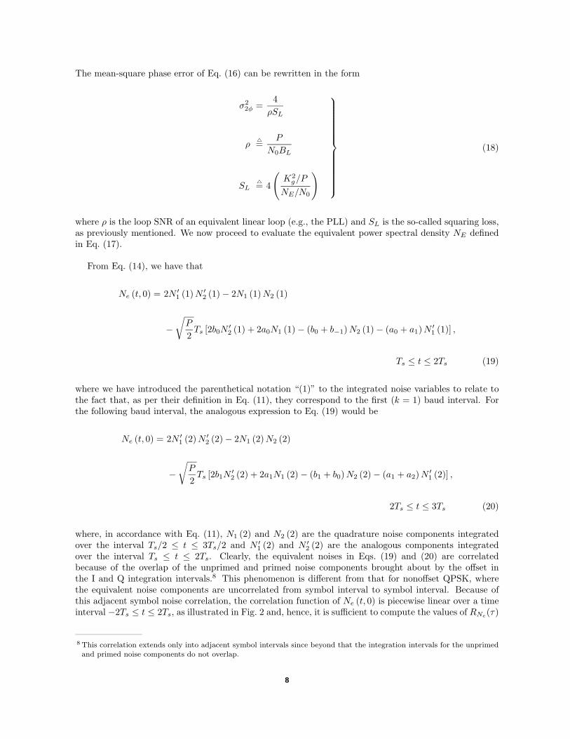
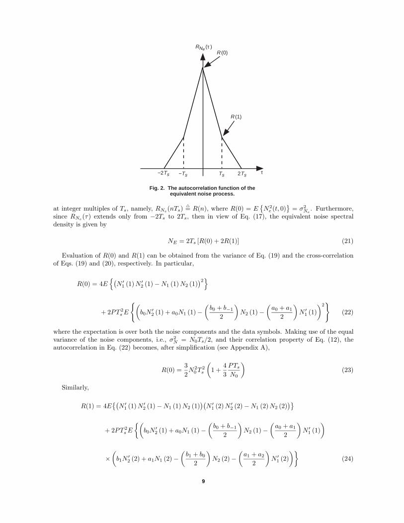
where, in accordance with Eq. (11), N1 (2) and N2 (2) are the quadrature noise components integratedover the interval Ts/2 ≤ t ≤ 3Ts/2 and N ′1 (2) and N ′2 (2) are the analogous components integratedover the interval Ts ≤ t ≤ 2Ts. Clearly, the equivalent noises in Eqs. (19) and (20) are correlatedbecause of the overlap of the unprimed and primed noise components brought about by the offset inthe I and Q integration intervals.8 This phenomenon is different from that for nonoffset QPSK, wherethe equivalent noise components are uncorrelated from symbol interval to symbol interval. Because ofthis adjacent symbol noise correlation, the correlation function of Ne (t, 0) is piecewise linear over a timeinterval −2Ts ≤ t ≤ 2Ts, as illustrated in Fig. 2 and, hence, it is sufficient to compute the values of RNe(τ)
8 This correlation extends only into adjacent symbol intervals since beyond that the integration intervals for the unprimedand primed noise components do not overlap.
8
−2Ts τ
R (1)
RNe (τ )R (0)
Ts−Ts 2Ts
Fig. 2. The autocorrelation function of theequivalent noise process.
at integer multiples of Ts, namely, RNe(nTs)4= R(n), where R(0) = E
{N2e (t, 0)
}= σ2
Ne. Furthermore,
since RNe(τ) extends only from −2Ts to 2Ts, then in view of Eq. (17), the equivalent noise spectraldensity is given by
NE = 2Ts [R(0) + 2R(1)] (21)
Evaluation of R(0) and R(1) can be obtained from the variance of Eq. (19) and the cross-correlationof Eqs. (19) and (20), respectively. In particular,
R(0) = 4E{(N ′1 (1)N ′2 (1)−N1 (1)N2 (1)
)2}
+ 2PT 2sE
{(b0N
′2 (1) + a0N1 (1)−
(b0 + b−1
2
)N2 (1)−
(a0 + a1
2
)N ′1 (1)
)2}
(22)
where the expectation is over both the noise components and the data symbols. Making use of the equalvariance of the noise components, i.e., σ2
N = N0Ts/2, and their correlation property of Eq. (12), theautocorrelation in Eq. (22) becomes, after simplification (see Appendix A),
R(0) =32N2
0T2s
(1 +
43PTsN0
)(23)
Similarly,
R(1) = 4E{(N ′1 (1)N ′2 (1)−N1 (1)N2 (1)
)(N ′1 (2)N ′2 (2)−N1 (2)N2 (2)
)}+ 2PT 2
sE
{(b0N
′2 (1) + a0N1 (1)−
(b0 + b−1
2
)N2 (1)−
(a0 + a1
2
)N ′1 (1)
)
×(b1N
′2 (2) + a1N1 (2)−
(b1 + b0
2
)N2 (2)−
(a1 + a2
2
)N ′1 (2)
)}(24)
9

which after simplification becomes
R(1) = −14N2
0T2s
(1 + 2
PTsN0
)(25)
Substituting Eqs. (23) and (25) in Eq. (21) gives
NEN0
= 2N0T3s
(1 +
PTsN0
)(26)
Finally, using Eq. (26) and the S-curve slope from Eq. (15) in Eq. (18), we obtain the desired result forthe squaring loss, namely,
SL =12
(Es/N0
1 + Es/N0
)(27a)
or, in terms of the bit-energy-to-noise ratio, Eb/N0 = Es/2N0,
SL =12
(2Eb/N0
1 + 2Eb/N0
)(27b)
which interestingly enough is one-half the result for a Costas I–Q loop-tracking BPSK modulation of thesame bit rate [2, Eq. (73)]. The analogous result to Eq. (27b) for the low-SNR implementation of theMAP carrier-synchronization loop for nonoffset QPSK is given by [8, Eq. (3.3-58)]:
SL =1
1 +9
4Eb/N0+
32 (Eb/N0)2 +
316 (Eb/N0)3
(28)
B. Tracking Performance Analysis of the High-SNR Implementation
In this section, we first derive the S-curve and equivalent noise of the I–Q loop of Fig. 1 (with a hardlimiter approximation to the hyperbolic tangent function) and then compute the loop’s mean-squarephase jitter. Analogous to Eq. (13), the loop-error signal is now
z1(t) = z′c(t) sgn z′s(t)− zs(t− Ts
2
)sgn zc
(t− Ts
2
), Ts ≤ t ≤ 2Ts (29)
where zs(t)zc(t) and z′c(t), z′s(t) are as defined in Eqs. (10a) and (10b), respectively. Substituting Eq. (10)
in Eq. (29) and averaging over the noise and data symbols, we obtain after considerable evaluation (seeAppendix B)
10

z1(t) 4=12S (φ) =
12
√P
2Ts
[(sinφ− cosφ) erf
(√Es
2N0(cosφ+ sinφ)
)
+ (sinφ+ cosφ) erf
(√Es
2N0(cosφ− sinφ)
)+ 2 sinφ erf
(√Es
2N0cosφ
)](30)
where erf (x) 4= 2/√π∫ x
0exp
(−y2/2
)dy is the error function. Note that S (φ) = S (φ± π) and, thus, once
again the S-curve is periodic with period π, i.e., the loop tracks a 2φ (rather than 4φ) process. Figure 3is a plot of the normalized S-curve [the quantity in brackets in Eq. (30)] with bit SNR Eb/N0 = Es/2N0
as a parameter. In the limit of infinite SNR, the S-curve behaves as
S (φ) =
√P
2Ts [(sinφ− cosφ) sgn (cosφ+ sinφ)+ (sinφ+ cosφ) sgn (cosφ− sinφ) + 2 sinφ sgn (cosφ)]
(31a)
or equivalently
NO
RM
ALI
ZE
D S
-CU
RV
E
−3.0
−2.0
−1.0
0.0
1.0
2.0
3.0
−3.5 −3.0 −2.5 −2.0 −1.5 −1.0 −0.5 0.0 0.5 1.0 1.5 2.0 2.5 3.0 3.5
Fig. 3. Normalized S-curves for the high SNR implementation of theMAP carrier synchronization loop for OQPSK.
φ, rad
20 dB
10 dB
6 dB
Eb /N 0 = 2 dB
11

S (φ) =
√P
2Ts
4 sinφ, 0 ≤ φ ≤ π
4
2 (sinφ− cosφ) ,π
4≤ φ ≤ π
2
2 (− sinφ− cosφ) ,π
2≤ φ ≤ 3π
4
−4 sinφ,3π4≤ φ ≤ π
(31b)
Comparing Fig. 3 with the qualitative version of the S-curve as given in [6, Fig. 5.24], we see that thelatter, which is reasoned on the basis that S (φ) ≈ sinφ in the neighborhood of small φ and S (π/2) = 0(both of which are true), is indicative of the true behavior only at a small SNR. At a large SNR, whichis the assumption made in [6] (i.e., the data decisions are assumed to be perfect), the S-curve has asomewhat different behavior, as can be seen in Fig. 3. The slope of the S-curve in Eq. (30) at the originis obtained as
Kg4=dS (φ)d (2φ)
=12dS (φ)dφ
= 2
√P
2Ts
[erf
(√Es
2N0
)−√
Es2N0π
exp(− Es
2N0
)](32)
and will be used shortly in determining the squaring loss.
The equivalent additive noise component at the loop input, which is related to the noise component ofthe error signal by Ne (t, 2φ) /2 = −
(z1(t)− z1(t)
), is obtained by subtracting Eq. (30) from Eq. (29).
When evaluated at φ = 0, this equivalent noise becomes
Ne (t, 0) =− 2
[√P
2Tsa0 + a1
2+N ′2 (1)
]sgn
[√P
2Tsb0 −N ′1 (1)
]
+ 2
[√P
2Tsb0 + b−1
2−N1 (1)
]sgn
[√P
2Tsa0 +N2 (1)
],
Ts ≤ t ≤ 2Ts (33a)
and
Ne (t, 0) =− 2
[√P
2Tsa1 + a2
2+N ′2 (2)
]sgn
[√P
2Tsb1 −N ′1 (2)
]
+ 2
[√P
2Tsb1 + b0
2−N1 (2)
]sgn
[√P
2Tsa1 +N2 (2)
],
2Ts ≤ t ≤ 3Ts (33b)
where again we have introduced the parenthetical notation “(k)” to correspond to the kth (k = 1, 2) baudintegration interval of the quadrature noise components. Once again we must determine the variance and
12

correlation coefficients of Ne (t, 0) in order to determine its equivalent noise power spectral density. Thedetails of these evaluations are quite lengthy and are presented in Appendix C. The final results are
R(0) = E{N2e (t, 0)
}= 4N0Ts
1 +Es
2N0−[√
Es4N0
erf√
Es2N0
+1√2π
exp(− Es
2N0
)]2
R(1) = E {Ne(t, 0)Ne(t+ Ts, 0)} = −2N0Ts
[√Es
4N0erf√
Es2N0
+1√2π
exp(− Es
2N0
)]2
(34)
Substituting Eq. (34) into Eq. (21), we obtain the single-sided power spectral density of the equivalentnoise as
NE = 8N0T2s
1 +Es
2N0−[√
Es2N0
erf√
Es2N0
+1√π
exp(− Es
2N0
)]2 (35)
Finally, substituting Eqs. (32) and (35) in Eq. (18) and substituting Eb/N0 for Es/2N0, the squaring lossof the high SNR implementation of the MAP carrier synchronization loop for OQPSK becomes
SL =
[erf(√
EbN0
)−√
EbN0π
exp(−EbN0
)]2
1 +EbN0−[√
EbN0
erf√EbN0
+1√π
exp(−EbN0
)]2 (36)
The analogous result to Eq. (36) for the high SNR implementation of the MAP carrier synchronizationloop for nonoffset QPSK is given by [9, Eq. (3.3-57)]:
SL =
[erf(√
EbN0
)− 2√
EbN0π
exp(−EbN0
)]2
1 +2EbN0− 2
[√EbN0
erf√EbN0
+1√π
exp(−EbN0
)]2 (37)
Figure 4 is a plot of the squaring loss versus Eb/N0 in dB for the various loop implementations consideredabove. We observe that at a low bit SNR (where the squaring loss is significant), the OQPSK implemen-tations have a decided advantage over their QPSK counterparts. Also, the crossover point below whichthe low SNR approximation of the OQPSK loop outperforms the high SNR approximation is −2.5 dB.
V. A Suboptimum Implementation Derived From the MAP Implementation forQPSK
Another (albeit ad hoc) implementation of a carrier synchronization loop for OQPSK was initiallyproposed for the design of the Advanced Receiver II (ARX II) [7] and is now included in the Block Vreceiver in NASA’s Deep Space Network (DSN) [8]. This scheme, which is illustrated in Fig. 5(a), merelydelays the quadrature arm so as to align it with the in-phase arm and then proceeds to process the
13

HIGH SNR APPROXIMATION − OQPSK
LOW SNR APPROXIMATION − OQPSK
LOW SNR APPROXIMATION − QPSK
HIGH SNR APPROXIMATION − QPSK
SQ
UA
RIN
G L
OS
S, d
B
−30.0
−25.0
−20.0
−15.0
−10.0
−5.0
0.0
−10.0 −7.5 −5.0 −2.5 0.0 2.5 5.0 7.5 10.0
Fig. 4. Squaring loss performance comparison of variousMAP carrier synchronization loop implementations.
Eb /N 0, dB
I and Q signals as one would do in the MAP implementation of nonoffset QPSK.9 Ignoring the MAPestimation approach, such a scheme could be argued to be intuitively logical in view of the manner inwhich the data symbols of OQPSK traditionally are detected. Note that this implementation forms itsI tanhQ and Q tanh I from the same pair of I and Q signals and, thus, a low SNR implementation wouldrequire the first two terms in the power series expansion of the hyperbolic tangent function, i.e., a fourth-order loop that tracks the 4φ process with an error signal akin to Eq. (5). An illustration of such a lowSNR implementation is shown in Fig. 5(b). It is interesting to investigate how suboptimal (from thestandpoint of squaring loss) this implementation is relative to that obtained by linearizing the hyperbolictangent function in Fig. 1 as analyzed in Section IV.
Analogous to Eq. (10a), the I and Q integrate-and-dump outputs in Fig. 5(b) are given by
zc(t) =∫ Ts/2
−Ts/2εc(t)dt =
[√P
2Tsb0 + b−1
2−N1
]sinφ+
[√P
2Tsa0 +N2
]cosφ
zs(t) =∫ Ts/2
−Ts/2εs
(t− Ts
2
)dt =
[√P
2Tsb−1 −N ′1
]cosφ−
[√P
2Tsa0 + a−1
2+N ′2
]sinφ,
Ts2≤ t ≤ 3Ts
2
(38)
where N1, N2, N′1, and N ′2 are zero-mean Gaussian random variables that now are defined by
9 In the actual receiver design, the delay and I&D filter in the I arm are actually reversed and, likewise, the range of theI&D filter in the Q arm extends from 0 to Ts. However, this is of no consequence to the performance analysis that follows.
14

90deg
+
DIGITALLOOP
FILTERNCO
( )dtTs /2
−Ts /2
DELAYTs /2
( )dtTs /2
−Ts /2
tanh
tanh
p (t )
z 1
εs (t )
y (t )
εc (t )
(a)
90deg
+
DIGITALLOOP
FILTERNCO
( )dtTs /2
−Ts /2
DELAYTs /2
( )dtTs /2
−Ts /2
p (t )
z 1
εs (t )
y (t )
εc (t )
(b)
( )2
( )2
Fig. 5. Offset pulse-shaped QPSK with QPSK post-detection processing: (a) the suboptimumcarrier synchronization loop and (b) the low SNR implementation of the suboptimum carriersynchronization loop.
2 sin (ωc t + θ )
2 cos (ωc t + θ )
2 cos (ωc t + θ )
2 sin (ωc t + θ )
15

N14=∫ Ts/2
−Ts/2Ns(t)dt
N24=∫ Ts/2
−Ts/2Nc(t)dt
N ′14=∫ Ts/2
−Ts/2Ns
(t− Ts
2
)dt =
∫ 0
−TsNs(t)dt
N ′24=∫ Ts/2
−Ts/2Nc
(t− Ts
2
)dt =
∫ 0
−TsNc(t)dt
(39)
all with variance σ2N = N0Ts/2. Once again N1 and N2 are uncorrelated, and likewise for N ′1 and N ′2, but
because of the offset between the I and Q channels, the pairs N1, N′1 and N2, N
′2 are indeed correlated,
with the correlation given by Eq. (12). The pairs N1N′2 and N ′1N2 are, however, still uncorrelated.
The error signal analogous to Eq. (13) is obtained from Fig. 5(b) as
z1(t) = zc(t)zs(t)[z2c (t)− z2
s(t)]
(40)
Substituting Eq. (38) into Eq. (40) and simplifying the algebra and trigonometry, the signal componentof Eq. (40), i.e., the statistical mean with respect to the noise components, is given by
EN {z1(t)} =14P 2T 4
s
{12
[b−1
(b−1 + b0
2
)− a0
(a−1 + a0
2
)]sin 2φ+ a0b−1 cos2 φ
+(a−1 + a0
2
)(b−1 + b0
2
)sin2 φ
}
×{[a0
(b−1 + b0
2
)− b−1
(a−1 + a0
2
)]sin 2φ+
(a2
0 − b2−1
)cos2 φ
+
[(b−1 + b0
2
)2
−(a−1 + a0
2
)2]
sin2 φ
}(41)
Statistically averaging Eq. (41) over the data symbols results, after much simplification, in
z1(t) 4=14S (φ) =
14P 2T 4
s sin 2φ(
cos2 φ− 14
sin2 φ
)
=14P 2T 4
s
(38
sin 2φ+516
sin 4φ)
(42)
16

As predicted, the S-curve S (φ) in Eq. (42) is periodic with period π/2 and, hence, the loop tracks the4φ process. The slope of the S-curve at the origin, Kg, is obtained by evaluating the derivative of S (φ)with respect to 4φ at φ = 0, with the result
Kg =12P 2T 4
s (43)
The noise component of the error signal evaluated at φ = 0 is obtained from Eqs. (38) and (40) as
−Ne (t, 0)4
= z1(t) |φ=0
=
(√P
2Tsb−1 −N ′1
)(√P
2Tsa0 +N2
)(√P
2Tsa0 +N2
)2
−(√
P
2Tsb−1 −N ′1
)2(44)
Evaluation of the correlation function of Ne (t, 0) for values of τ corresponding to integer multiples of Tsproceeds as in Appendix A but now involves fourth-order signal × noise and noise × noise moments. Thedetails are presented in Appendix D, where the following results are obtained:
R(0) = E{
(Ne (t, 0))2}
= 8[P 3N0T
7s +
92P 2N2
0T6s + 6PN3
0T5s +
32N4
0T4s
]
= 8P 3N0T7s
[1 +
92Es/N0
+6
(Es/N0)2 +3
2 (Es/N0)3
]
R(1) = 0
(45)
and, thus, from Eq. (21) the equivalent noise power spectral density normalized by N0 is
NEN0
= 16P 3T 8s
[1 +
92Es/N0
+6
(Es/N0)2 +3
2 (Es/N0)3
](46)
Since the loop now tracks a 4φ process, the mean-square error of this process can be written, analogousto Eq. (18), as
σ24φ =
16ρSL
ρ4=
P
N0BL
SL4= 16
(K2g/P
NE/N0
)
(47)
17

Finally, substituting Eqs. (43) and (46) in Eq. (47) gives the desired result for the squaring loss, namely,
SL =14
1
1 +9
2Es/N0+
6(Es/N0)2 +
32 (Es/N0)3
(48)
or, in terms of bit SNR,
SL =14
1
1 +9
4Eb/N0+
32 (Eb/N0)2 +
316 (Eb/N0)3
(49)
Comparing Eq. (49) with Eq. (28), we observe that the suboptimum OQPSK loop based on the MAP im-plementation for QPSK has a squaring loss that is 6-dB worse than the MAP carrier synchronization loopfor QPSK, which itself is significantly inferior at low SNRs to the MAP (optimum) carrier synchronizationloop for OQPSK illustrated in Fig. 1. While the suboptimum OQPSK loop has the advantage that itsimplementation relative to that for QPSK requires only the addition of a Ts/2 delay in the quadraturearm, its largely inferior performance coupled with the additional complication of resolving a 90-deg phaseambiguity will no doubt far outweigh the implementation advantage.
VI. Impact on Average Error Probability Performance
The conditional (on a given phase error φ) bit-error probability (BEP) of OQPSK is given as the arith-metic average of the conditional bit-error probabilities for BPSK and QPSK, namely (see Appendix E),
Pb (E;φ) |OQPSK =12Pb (E;φ) |BPSK +
12Pb (E;φ) |QPSK (50)
where [10]
Pb (E;φ) |BPSK =12
erfc
(√EbN0
cosφ
)
Pb (E;φ) |QPSK =14
erfc
(√EbN0
(cosφ+ sinφ)
)+
14
erfc
(√EbN0
(cosφ− sinφ)
)
(51)
As such, for a given phase error (greater than zero), the BEP of OQPSK would be worse than that ofBPSK but better than that of QPSK.
When a carrier synchronization loop is used to provide the carrier demodulation reference at thereceiver, as considered in this article, then the average bit-error probability (assuming perfect phaseambiguity resolution) would be obtained by averaging Eq. (50) over the probability density function(PDF) of the phase-error process, pφ (φ). For the purpose of comparison, pφ (φ) typically is modeled bya Tikhonov distribution [10,11] with an effective loop SNR, ρeq, equal to the reciprocal of the variance of
18

the phase process (2φ or 4φ as appropriate), the latter being determined from Eq. (18) or Eq. (47). Foreach of the three modulations, the appropriate relations would be
pφ (φ) |PSK =2 exp (ρeq cos 2φ)
2πI0 (ρeq), ρeq =
ρSL |PSK4
, −π2≤ φ ≤ π
2
pφ (φ) |QPSK =4 exp (ρeq cos 4φ)
2πI0 (ρeq), ρeq =
ρSL |QPSK16
, −π4≤ φ ≤ π
4
pφ (φ) |OQPSK =2 exp (ρeq cos 2φ)
2πI0 (ρeq), ρeq =
ρSL |OQPSK4
, −π2≤ φ ≤ π
2
(52)
and, thus, the average error probabilities are given by
Pb (E) |BPSK =∫ π/2
−π/2Pb (E;φ) |BPSK pφ (φ) |BPSK dφ
Pb (E) |QPSK =∫ π/4
−π/4Pb (E;φ) |QPSK pφ (φ) |QPSK dφ
Pb (E) |OQPSK =∫ π/2
−π/2Pb (E;φ) |OQPSK pφ (φ) |OQPSK dφ
(53)
Note that in the presence of a perfect carrier reference, i.e., pφ (φ) = δ (φ), all three modulations wouldhave the identical average bit-error probability.
On the basis of the above relations, we observe that OQPSK offers a two-fold average BEP advantageover QPSK, namely, the conditional BEP is itself smaller and the variance of the phase error thatcharacterizes the PDF of the phase process is considerably smaller for the former relative to the latter.In addition, as previously mentioned, OQPSK needs only to resolve a 180-deg phase ambiguity (e.g.,with binary differential encoding/decoding), whereas QPSK needs to resolve a 90-deg phase ambiguity(e.g., with four-phase differential encoding/decoding). This phase ambiguity advantage is particularlysignificant in error-correction coded communications (e.g., convolutionally coded communications) in thatif the code is transparent10 (reversal of the input bits produces a reversal of the encoder output symbols),one can resolve the phase ambiguity by including a binary differential encoder before the convolutionalencoder and a binary differential decoder after the convolutional decoder. As such, the overall BEP ofthe coded system is approximately increased by merely a factor of two. When a 90-deg phase ambiguityis present, this simple solution based on the 180-deg transparency of the code is not possible. Instead,either a redesign of the code to achieve, if possible, 90-, 180-, and 270-deg rotational invariance, which,in general, will yield a somewhat poorer performing code, or some other method for resolving the phaseambiguity at the receiver based on the rate of buildup of the convolutional decoder metrics would berequired.
10 In most cases, transparent convolutional codes can be found that have a performance either equal to or nearly equal tothat of the optimum code.
19

VII. Conclusion
OQPSK modulation, which limits the phase variation per transition to 90 deg rather than 180 deg asin QPSK, most often is used on a nonlinear channel to prevent regeneration of the spectral side lobes thathave been reduced by bandpass filtering at the transmitter. On a linear channel, OQPSK is employedless often since, in an ideal environment, it is well-known to offer no advantage to QPSK. When thechannel is linear but nonideal, i.e., in the presence of a practical carrier synchronizer, we have shownthat OQPSK offers both average bit-error probability and phase ambiguity advantages over QPSK withlittle additional implementation complexity. Although not specifically addressed, the conclusions drawnhere also apply to pulse-shaped QPSK and OQPSK since, with matched filters used in the receivers, theperformance is invariant to the specific pulse shape. As an example, precoded minimum shift keying(MSK) [10, Chapter 10], which has an equivalent representation in the form of OQPSK with a half-sinusoidal pulse shape, can be carrier synchronized as described in this article.
References
[1] H. Tsou, S. M. Hinedi, and M. K. Simon, “Closed-Loop Carrier Phase Synchro-nization Techniques Motivated by Likelihood Functions,” The Telecommunica-tions and Data Acquisition Progress Report 42-119, July–September 1994, JetPropulsion Laboratory, Pasadena, California, pp. 83–104, November 15, 1994.http://tmo.jpl.nasa.gov/tmo/progress report/42-119/119S.pdf
[2] W. C. Lindsey and M. K. Simon, “Optimum Performance of Suppressed CarrierReceivers With Costas Loop Tracking,” IEEE Trans. on Comm., vol. COM-25,no. 2, pp. 215–227, February 1977.
[3] W. C. Lindsey and M. K. Simon, Telecommunication Systems Engineering, En-glewood Cliffs, New Jersey: Prentice-Hall, Inc., 1973. Reprinted by Dover Press,New York, 1991.
[4] M. K. Simon, “Optimum Receiver Structures for Phase-Multiplexed Modula-tions,” IEEE Trans. on Comm., vol. COM-26, no. 6, pp. 865–872, June 1978.
[5] M. K. Simon and J. G. Smith, “Carrier Synchronization and Detection of QASKSignal Sets,” IEEE Trans. on Comm., vol. COM-22, no. 10, pp. 1576–1584,October 1974.
[6] U. Mengali and A. N. D’Andrea, Synchronization Techniques for Digital Re-ceivers, New York: Plenum Press, 1997.
[7] S. Hinedi, “A Functional Description of the Advanced Receiver,” The Telecom-munications and Data Acquisition Progress Report 42-100, October–December1989, Jet Propulsion Laboratory, Pasadena, California, pp. 131–149, February15, 1990.
[8] J. B. Berner and K. M. Ware, “An Extremely Sensitive Digital Receiver For DeepSpace Communications,” Eleventh Annual International Phoenix Conference onComputers and Communications, Phoenix, Arizona, April 1–3, 1992.
[9] J. H. Yuen, ed., Deep Space Telecommunications Systems Engineering, New York:Plenum Press, 1983.
[10] M. K. Simon, S. Hinedi, and W. C. Lindsey, Digital Communication Techniques:Signal Design and Detection, Englewood Cliffs, New Jersey: Prentice-Hall, Inc.,1994.
20

[11] V. I. Tikhonov, “The Effect of Noise on Phase-Locked Oscillator Operation,”Automation and Remote Control, vol. 20, pp. 1160–1168, September 1959. Trans-lated from Automatika i Telemekhaniki, Akademya Nauk SSSR, vol. 20, Septem-ber 1959.
Appendix A
Evaluation of the Correlation Function of the EquivalentNoise Process for the Low SNR Implementation of the
MAP Carrier Synchronization Loop for OQPSK
To allow evaluation of the power spectral density of the equivalent additive noise Ne (t, 0), we computehere the autocorrelation function RNe(τ) = E {Ne (t, 0)Ne (t+ τ, 0)} for values of τ corresponding tointeger multiples of the baud (symbol) interval Ts. When τ = 0, the variance of Ne (t, 0), namely,RNe(0) 4= R (0) = E
{(Ne (t, 0))2
}is given by Eq. (22) and is evaluated as follows:
R(0) =
4[E{
(N ′1 (1))2}E{
(N ′2 (1))2}
+ E{
(N1 (1))2}E{
(N2 (1))2}− 2E {N ′1 (1)N1 (1)}E {N ′2 (1)N2 (1)}
]
+ 2PT 2s
[E{
(N ′2 (1))2}
+ E{
(N1 (1))2}
+ E
{(a0 + a1
2
)2}E{
(N ′1 (1))2}
+ E
{(b0 + b−1
2
)2}E{
(N2 (1))2}− 2E
{b0
(b0 + b−1
2
)}E {N ′2 (1)N2 (1)}
− 2E{a0
(a0 + a1
2
)}E {N ′1 (1)N1 (1)}
](A-1)
Recalling the correlation properties of the primed and unprimed noise components,
21

N1 (m) 4=∫ (m−1/2)Ts
(m−3/2)Ts
Ns(t)dt
N2 (m) 4=∫ (m−1/2)Ts
(m−3/2)Ts
Nc(t)dt
N ′1 (m) 4=∫ mTs
(m−1)Ts
Ns(t)dt
N ′2 (m) 4=∫ mTs
(m−1)Ts
Nc(t)dt
(A-2)
namely,
E{
(N ′i(m))2}
= E{
(Ni(m))2}
=N0Ts
2, i = 1, 2
E {N ′i(m)Ni(m)} =N0Ts
4, i = 1, 2
(A-3)
where m is any integer; then substituting Eq. (A-3) into Eq. (A-1) and averaging over the i.i.d. datasymbols results in
R(0) = 4(
38N2
0T2s
)+ 2PT 2
s (N0Ts)
=32N2
0T2s
(1 +
43PTsN0
)(A-4)
which is given as Eq. (23) of the main text.
When τ = Ts, the cross-correlation RNe(Ts)4= R (1) = E {Ne (t, 0)Ne (t+ Ts, 0)} is given by Eq. (24)
and is evaluated as follows:
R(1) = 4 [−E {N ′1 (1)N1 (2)}E {N ′2 (1)N2 (2)}]
+ 2PT 2s
[−E
{b0
(b1 + b0
2
)}E {N ′2 (1)N2 (2)} − E
{a1
(a0 + a1
2
)}E {N ′1 (1)N1 (2)}
](A-5)
Making use of the cross-correlation property of the noise components in different baud intervals given by
E {N ′i (m)Ni (m+ 1)} =N0Ts
4, i = 1, 2 (A-6)
then the equivalent noise correlation in Eq. (A-4) evaluates to
22

R(1) = 4(− 1
16N2
0T2s
)+ 2PT 2
s
(−1
4N0Ts
)
= − 14N2
0T2s
(1 + 2
PTsN0
)(A-7)
which is given as Eq. (25) of the main text.
Appendix B
Evaluation of the S-Curve of the High SNR Implementationof the MAP Carrier Synchronization Loop for OQPSK
The error signal of the high SNR implementation of the MAP carrier synchronization loop for OQPSKis obtained by substituting Eqs. (10a) and (10b) in Eq. (29), resulting in
z1(t) =
{[√P
2Tsb0 −N ′1
]sinφ+
[√P
2Tsa0 + a1
2+N ′2
]cosφ
}
× sgn
{[√P
2Tsb0 −N ′1
]cosφ−
[√P
2Tsa0 + a1
2+N ′2
]sinφ
}
−{[√
P
2Tsb0 + b−1
2−N1
]cosφ−
[√P
2Tsa0 +N2
]sinφ
}
× sgn
{[√P
2Tsb0 + b−1
2−N1
]sinφ+
[√P
2Tsa0 +N2
]cosφ
},
Ts ≤ t ≤ 2Ts (B-1)
which is of the form
z1(t) = [X sinφ+ Y cosφ] sgn [X cosφ− Y sinφ]− [X ′ cosφ− Y ′ sinφ] sgn {X ′ sinφ+ Y ′ cosφ}
4= F1 (φ;X,Y )− F2 (φ;X ′, Y ′) (B-2)
23

with X,Y,X ′, and Y ′ functions of the data symbols and the noise components. We begin by evaluatingthe statistical average over the data and noise of F1 (φ;X,Y ). Similar evaluations then will yield thesame average of F2 (φ;X ′, Y ′).
Since for a Gaussian zero-mean random variable z with variance σ2z ,
Ez { sgn (C + z)} = erf
(C√2σ2
z
)(B-3)
with C an arbitrary constant, then performing the first average over the noise, we obtain
F1 (φ;X,Y )N
=
√P
2Ts
(b0 sinφ+
a0 + a1
2cosφ
)erf
(√Es
2N0
[b0 cosφ− a0 + a1
2sinφ
])
− sinφ EN ′1
{N ′1 erf
(√Es
2N0 sin2 φ
[b0 cosφ− a0 + a1
2sinφ−N ′1 cosφ
])}
+ cosφ EN ′2
{N ′2 erf
(√Es
2N0 cos2 φ
[b0 cosφ− a0 + a1
2sinφ−N ′2 sinφ
])}(B-4)
The remaining averages of the noise can be performed using the relation
Ez {z erf (A+Bz)} =2√π
σ2zB√
1 + 2B2σ2z
exp(− A2
1 + 2B2σ2z
)(B-5)
where again A and B are arbitrary constants. Identifying the Gaussian random variable z as either N ′1or N ′2, and then averaging over the data symbols, the first term in Eq. (B-4) finally evaluates to
Ea0,a1,b0
{√P
2Ts
(b0 sinφ+
a0 + a1
2cosφ
)erf
(√Es
2N0
[b0 cosφ− a0 + a1
2sinφ
])}=
14
√P
2Ts (sinφ− cosφ) erf
(√Es
2N0(cosφ+ sinφ)
)
+14
√P
2Ts (sinφ+ cosφ) erf
(√Es
2N0(cosφ− sinφ)
)
+12
√P
2Ts sinφ erf
(√Es
2N0cosφ
)(B-6)
whereas the second and third terms cancel. Thus, F1 (φ;X,Y ) is equal to the expression in Eq. (B-6).
24

Following a similar approach, it is straightforward to show that the first term in F2 (φ;X,Y ) is thenegative of the first term in F1 (φ;X,Y ), whereas the second and third terms of F2 (φ;X,Y ) again cancel.Hence, F2 (φ;X,Y ) is evaluated as the negative of the expression in Eq. (B-6). Finally then, fromEq. (B-1), z1(t) = 2F1 (φ;X,Y ), which is twice the result in Eq. (B-6) and thereby agrees with Eq. (30)of the main text.
Appendix C
Evaluation of the Correlation Function of the Equivalent NoiseProcess for the High SNR Implementation of the MAP
Carrier Synchronization Loop for OQPSK
As in Appendix A, to allow evaluation of the power spectral density of the equivalent additive noiseNe (t, 0), we compute here the autocorrelation function RNe(τ) = E {Ne (t, 0)Ne (t+ τ, 0)} for values ofτ corresponding to integer multiples of the baud (symbol) interval Ts. When τ = 0, the variance ofNe (t, 0), namely, RNe(0) 4= R (0) = E
{(Ne (t, 0))2
}is obtained from Eq. (33a) as follows:
R (0) = 4E
(√
P
2Tsa0 + a1
2+N ′2 (1)
)2+ 4E
(√
P
2Tsb0 + b−1
2−N1 (1)
)2
− 8E
{(√P
2Tsa0 + a1
2+N ′2 (1)
)(√P
2Tsb0 + b−1
2−N1 (1)
)
× sgn
[√P
2Tsb0 −N ′1 (1)
]sgn
[√P
2Tsa0 +N2 (1)
]}(C-1)
Expanding the squared terms and averaging over the data symbols and some of the noise componentsgives
25

R (0) = 2PT 2s + 4N0Ts − PT 2
s erf2
(√Es
2N0
)
+ 4
√P
2Ts erf
(√Es
2N0
)E
{N1 (1) sgn
[√P
2Tsb0 −N ′1 (1)
]}
− 4
√P
2T erf
(√Es
2N0
)E
{N ′2 (1) sgn
[√P
2Tsa0 +N2 (1)
]}
+ 8E
{N1 (1) sgn
[√P
2Tsb0 −N ′1 (1)
]}E
{N ′2 (1) sgn
[√P
2Tsa0 +N2 (1)
]}(C-2)
To evaluate the noise expectations in Eq. (C-2), we partition the noise components into two parts, eachcovering half the integration interval as appropriate. Specifically, let
N1(1) 4=∫ Ts/2−Ts/2Ns(t)dt = N1A(1) +N1B(1), N1A(1) 4=
∫ 0
−Ts/2Ns(t)dt, N1B(1) 4=∫ Ts/2
0Ns(t)dt
N2(1) 4=∫ Ts/2−Ts/2Nc(t)dt = N2A(1) +N2B(1), N2A(1) 4=
∫ 0
−Ts/2Nc(t)dt, N2B(1) 4=∫ Ts/2
0Nc(t)dt
N ′1(1) 4=∫ Ts
0Ns(t)dt = N1B(1) +N1C(1), N1C(1) 4=
∫ TsTs/2
Ns(t)dt
N ′2(1) 4=∫ Ts
0Nc(t)dt = N2B(1) +N2C(1), N2C(1) 4=
∫ TsTs/2
Nc(t)dt (C-3)
where all the new noise components are independent Gaussian and have variance N0Ts/4. Then, forexample, the expectation in the second term of Eq. (C-2) can be written as
E
{(N1A(1) +N1B(1)) sgn
[√P
2Tsb0 − (N1B(1) +N1C(1))
]}
= E
{N1B(1) sgn
[√P
2Tsb0 − (N1B(1) +N1C(1))
]}
= E
N1B(1) erf
√P
2Tsb0 −N1B(1)√N0Ts/2
(C-4)
which, using Eq. (B-5) of Appendix B, evaluates to
E
{N1 (1) sgn
[√P
2Tsb0 −N ′1 (1)
]}= −
√N0Ts
4πexp
(− Es
2N0
)(C-5)
26

Similarly, the expectation in the third term of Eq. (C-2) evaluates to
E
{N ′2 (1) sgn
[√P
2Tsa0 +N2 (1)
]}=
√N0Ts
4πexp
(− Es
2N0
)(C-6)
Finally, using Eqs. (C-5) and (C-6) in Eq. (C-2), we get the desired result, namely,
R (0) = 2PT 2s + 4N0Ts − PT 2
s erf2
(√Es
2N0
)
− 8
√P
2Tserf
(√Es
2N0
)√N0Ts
4πexp
(− Es
2N0
)− 8
(N0Ts
4π
)exp2
(− Es
2N0
)(C-7)
which, upon simplification, results in the first equation in Eq. (34).
Analogous to Eq. (C-1) for τ = Ts, the correlation RNe(Ts)4= R (1) = E {Ne (t, 0)Ne (t+ Ts, 0)} is
obtained from Eq. (33b) as
R (1) = 4E
{(√P
2Tsa0 + a1
2+N ′2 (1)
)
×(√
P
2Tsa1 + a2
2+N ′2 (2)
)sgn
[√P
2Tsb0 −N ′1 (1)
]sgn
[√P
2Tsb1 −N ′1 (2)
]}
− 4E
{(√P
2Tsa0 + a1
2+N ′2 (1)
)
×(√
P
2Tsb1 + b0
2−N1 (2)
)sgn
[√P
2Tsb0 −N ′1 (1)
]sgn
[√P
2Tsa1 +N2 (2)
]}
− 4E
{(√P
2Tsb0 + b−1
2−N1 (1)
)
×(√
P
2Tsa1 + a2
2+N ′2 (2)
)sgn
[√P
2Tsa0 +N2 (1)
]sgn
[√P
2Tsb1 −N ′1 (2)
]}
+ 4E
{(√P
2Tsb0 + b−1
2−N1 (1)
)
×(√
P
2Tsb1 + b0
2−N1 (2)
)sgn
[√P
2Tsa0 +N2 (1)
]sgn
[√P
2Tsa1 +N2 (2)
]}(C-8)
27

When performing the required averages over the data symbols and noise components, the first term inEq. (C-8) evaluates as
4E
{(√P
2Tsa0 + a1
2+N ′2(1)
)
×(√
P
2Tsa1 + a2
2+N ′2 (2)
)sgn
[√P
2Tsb0 −N ′1 (1)
]sgn
[√P
2Tsb1 −N ′1 (2)
]}
= 2PT 2sE
{b0
(a0 + a1
2
)b1
(a1 + a2
2
)}erf2
(√Es
2N0
)= 0 (C-9)
To evaluate the second term in Eq. (C-8), we again must partition each of the noise components into twoparts, as in Eq. (C-3), and then perform the necessary averages. When this is done, we obtain
−4E
{(√P
2Tsa0 + a1
2+N ′2(1)
)
×(√
P
2Tsb1 + b0
2−N1(2)
)sgn
[√P
2Tsb0 −N ′1(1)
]sgn
[√P
2Tsa1 +N2(2)
]}
= − 2N0Ts
[√Es
4N0erf
(√Es
2N0
)+
√1
2πexp
(− Es
2N0
)]2
(C-10)
Because of the independence of the noise components in each factor of the third and fourth terms inEq. (C-8), each expectation partitions into a four-fold product of expectations, e.g.,
−4E
{(√P
2Tsb0 + b−1
2−N1 (1)
)
×(√
P
2Tsa1 + a2
2+N ′2 (2)
)sgn
[√P
2Tsa0 +N2 (1)
]sgn
[√P
2Tsb1 −N ′1 (2)
]}
= − 4E
{(√P
2Tsb0 + b−1
2−N1 (1)
)}E
{√P
2Tsa1 + a2
2+N ′2 (2)
}
× E{
sgn
[√P
2Tsa0 +N2 (1)
]}E
{sgn
[√P
2Tsb1 −N ′1 (2)
]}= 0 (C-11)
Similarly,
28

4E
{(√P
2Tsb0 + b−1
2−N1 (1)
)
×(√
P
2Tsb1 + b0
2−N1 (2)
)sgn
[√P
2Tsa0 +N2 (1)
]sgn
[√P
2Tsa1 +N2 (2)
]}
= 4E
{(√P
2Tsb0 + b−1
2−N1 (1)
)}E
{√P
2Tsb1 + b0
2−N1 (2)
}
× E{
sgn
[√P
2Tsa0 +N2 (1)
]}E
{sgn
[√P
2Tsa1 +N2 (2)
]}= 0 (C-12)
Finally, combining Eqs. (C-9) through (C-12), we obtain the desired result for the cross-correlation R(1),namely,
R(1) = −2N0Ts
[√Es
4N0erf
(√Es
2N0
)+
√1
2πexp
(− Es
2N0
)]2
(C-13)
which agrees with the second equation of Eq. (34).
29

Appendix D
Evaluation of the Correlation Function of the Equivalent NoiseProcess for the Low SNR Implementation of the
Suboptimum Carrier Synchronization Loopfor OQPSK
Expanding the terms in Eq. (44) of the main text and combining like terms, we arrive at the followingexpressions for the equivalent additive noise, Ne (t, 0), where we again have introduced the parentheticalnotation to distinguish the noise components in two successive baud intervals:
Ne (t, 0) = 4
[−2(P
2
)3/2
T 3s [b−1N2 (1) + a0N
′1 (1)]− 3
P
2a0b−1T
2s
[(N2 (1))2 − (N ′1 (1))2
]
+(P
2
)1/2
Ts
[3b−1N2 (1) (N ′1 (1))2 + 3a0N
′1 (1) (N2 (1))2 − a0 (N ′1 (1))3 − b−1 (N2 (1))3
]
+N ′1 (1) (N2 (1))3 −N2 (1) (N ′1 (1))3],
Ts2≤ t ≤ 3Ts
2(D-1a)
Ne (t, 0) = 4
[−2(P
2
)3/2
T 3s [b0N2 (2) + a1N
′1 (2)]− 3
P
2T 2s a1b0
[(N2 (2))2 − (N ′1 (2))2
]
+(P
2
)1/2
Ts
[3b0N2 (2) (N ′1 (2))2 + 3a1N
′1 (2) (N2 (2))2 − a1 (N ′1 (2))3 − b0 (N2 (2))3
]
+N ′1 (2) (N2 (2))3 −N2 (2) (N ′1 (2))3],
3Ts2≤ t ≤ 5Ts
2(D-1b)
The variance of Ne (t, 0), namely, RNe(0) 4= R (0) = E{
(Ne (t, 0))2}
is evaluated after some simplificationand combining of terms as
30

R (0) =
16
[4(P
2
)3
T 6s
[E{
(N2 (1))2}
+ E{
(N ′1 (1))2}]
+(P
2
)2
T 4s
[13E
{(N2 (1))4
}+ 13E
{(N ′1 (1))4
}− 42E
{(N2 (1))2
}E{
(N ′1 (1))2}]
+P
2T 2s
×[3E{
(N ′1 (1))2}E{
(N2 (1))4}
+ 3E{
(N2 (1))2}E{
(N ′1 (1))4}
+ E{
(N2 (1))6}
+ E{
(N ′1 (1))6}]
+ E{
(N ′1 (1))2}E{
(N2 (1))6}
+ E{
(N2 (1))2}E{
(N ′1 (1))6}−2E
{(N2 (1))4
}E{
(N ′1 (1))4}]
(D-2)
Using the well-known relation for the even-ordered moments of a zero-mean Gaussian random variable,z, namely,
E {zn} = (n− 1)!!σnz (D-3)
where (n− 1)!! denotes the factorial made up of only odd integers, then Eq. (D-2) finally evaluates to
R (0) = 64
[(P
2
)3
N0T7s +
94
(P
2
)2
N20T
6s +
32
(P
2
)N3
0T5s +
316N4
0T4s
]
= 8[P 3N0T
7s +
92P 2N2
0T6s + 6PN3
0T5s +
32N4
0T4s
](D-4)
Next, multiplying Eqs. (D-1a) and (D-1b) and first averaging over the signal (i.i.d. data symbols) gives
Es {Ne (t, 0)Ne (t+ Ts, 0)}
= 16E{[N ′1 (1) (N2 (1))3 −N2 (1) (N ′1 (1))3
] [N ′1 (2) (N2 (2))3 −N2 (2) (N ′1 (2))3
]}
= 16[E {N ′1 (1)N ′1 (2)}E
{(N2 (1))3 (N2 (2))3
}+ E {N2 (1)N2 (2)}E
{(N ′1 (1))3 (N ′1 (2))3
}
−E{N2 (1) (N2 (2))3
}E{
(N ′1 (1))3N ′1 (2)
}− E
{(N2 (1))3
N2 (2)}E{N ′1 (1) (N ′1 (2))3
}](D-5)
Finally, because of the independence of the noise components in adjacent baud intervals, each term inEq. (D-5), when averaged over these components, equals zero. Thus, R (1) = 0.
31

Appendix E
Evaluation of the Conditional Bit-Error Probability for OQPSK
Consider the optimum (matched -filter) receiver for OQPSK, which makes independent hard decisionson the I and Q data symbol streams. The output of the I matched filter corresponding to the transmittedbit a0 [see Eq. (2)] is given by
XI4=∫ Ts/2
−Ts/2(s (t, θ) + n(t)) rI (t) dt
=∫ Ts/2
−Ts/2
√P
(a0 cos (ωct+ θ) +
(b−1 + b0
2
)sin (ωct+ θ)
)√2 cos
(ωct+ θ
)dt
+∫ Ts/2
−Ts/2
√2 [Nc(t) cos (ωct+ θ)−Ns(t) sin (ωct+ θ)]
√2 cos
(ωct+ θ
)dt
=
√P
2Ts
(a0 cosφ+
(b−1 + b0
2
)sinφ
)+NI cosφ−NQ sinφ (E-1)
where
NI4=∫ Ts/2
−Ts/2Nc(t)dt
NQ4=∫ Ts/2
−Ts/2Ns(t)dt
(E-2)
which are independent zero-mean Gaussian random variables each with variance σ2N = N0Ts/2. Making
a binary hard decision on XI results in the decision on a0. Hence, the probability of error associatedwith a0 is computed as follows. Assuming a +1 transmitted symbol for a0, the conditional (on the phaseerror φ) probability of error is
Pr {a0 = −1 |a0 = 1;φ} = Pr {XI < 0 |a0 = 1} =12
erfc{XI |a0 = 1√
2σXI
}b−1,b0
=12
erfc
{√PTs2N0
[cosφ+
(b−1 + b0
2
)sinφ
]}b−1,b0
(E-3)
where the overbar denotes statistical averaging over the equiprobable quadrature binary symbols thatinterfere with the in-phase bit a0. Since
32

b−1 + b02
=
0, b−1 = −b0 with probability =12
−1, b−1 = b0 = −1 with probability =14
1, b−1 = b0 = 1 with probability =14
(E-4)
then further noting that PTs/2N0 = PTb/N04= Eb/N0, the average probability of error in Eq. (E-3)
becomes
Pr {a0 = −1 |a0 = 1;φ} =14
erfc
[√PTs2N0
cosφ
]+
18
erfc
[√PTs2N0
(cosφ+ sinφ)
]
+18
erfc
[√PTs2N0
(cosφ− sinφ)
](E-5)
Because of the symmetry of the problem, the result for Pr {a0 = 1 |a0 = −1;φ} would be identical to thatin Eq. (E-5). Thus, the average probability of error, PI (E), for detecting the I-channel symbols is givenby the right-hand side of Eq. (E-5). Again by the symmetry of the problem, the identical expression toEq. (E-5) would be obtained for the average probability of error associated with the Q-channel symbols.Finally, the average bit-error probability (still conditioned on φ), Pb (E;φ), corresponding to the sequenceobtained by interleaving the I- and Q-channel symbol decisions, also is given by Eq. (E-5), namely,
Pb (E;φ) =14
erfc
[√PTs2N0
cosφ
]+
18
erfc
[√PTs2N0
(cosφ+ sinφ)
]
+18
erfc
[√PTs2N0
(cosφ− sinφ)
](E-6)
which can be put in the form of Eq. (50) combined with Eq. (51).
33