carnegie mellon university model selection and …herbie/thesis.pdf · carnegie mellon university...
TRANSCRIPT
CARNEGIEMELLON UNIVERSITY
MODEL SELECTIONAND MODEL AVERAGING
FORNEURAL NETWORKS
A DISSERTATION
SUBMITTED TO THE GRADUATE SCHOOL
IN PARTIAL FULFILLMENT OF THE REQUIREMENTS
for thedegree
DOCTOR OF PHILOSOPHY
in
STATISTICS
By
HERBERT KUI HAN LEE III
Departmentof Statistics
Carnegie Mellon University
Pittsburgh,Pennsylvania15213
January, 1999
Abstract
Neuralnetworksarea usefulstatisticaltool for nonparametricregression.In this thesis,I develop
a methodologyfor doing nonparametricregressionwithin the Bayesianframework. I addressthe
problemof modelselectionandmodelaveraging,includingestimationof normalizingconstantsand
searchingof themodelspacein termsof both theoptimalnumberof hiddennodesin thenetwork
aswell asthebestsubsetof explanatoryvariables.I demonstratehow to useanoninformative prior
for a neuralnetwork, which is usefulbecauseof thedifficulty in interpretingtheparameters.I also
prove theasymptoticconsistency of theposteriorfor neuralnetworks.
Keywords: Nonparametricregression,Bayesianstatistics,Noninformative prior, Asymptoticcon-
sistency, Normalizingconstants,Bayesianrandomsearching,BARS
ii

Acknowledgements
First, I needto thankmy advisor, Larry Wasserman,without whomnoneof this would have been
accomplished.Larry hasbeenanidealadvisor. Hewasalwayswilling to stopandhelpmewith any
problem.He alwayshadanabundanceof suggestions,andhehelpedmenot losesightof thebig
picture.His wisdomandpatiencearegreatlyappreciated.
I mustalsothankmy parents,for they have alwaystried to pushmeto my potential,andhave
alwaysbeentherewhenI neededthem.
I wouldliketo thankthemembersof mycommittee:RobKass,ChrisGenovese,MarkSchervish,
ValerieVentura,andAndrew Moore. They have givenmehelpful suggestionsandencouragement.
Thefacultyasawholehavemadethisdepartmentafriendly andnurturingone.And I needto thank
David Banksfor helpingconvincemeto returnto graduateschool.
I have discoveredthesecretto theoperationsof thedepartment.It is thestaff. I greatlyappre-
ciateall thehelpandmoralsupportI have received from them,particularlyRoseKrakovsky, Mari
Alice McShane,NoreneMears,Heidi Sestrich,andMargie Smykla.
Lastbut notleast,therehavebeenmy fellow students.DanCorkhasbeenanunendingsourceof
knowledgeandsupport.Hiscompanionship,aswell ashisproofreading,isgreatlyappreciated.Kert
Viele,Mark Fitzgerald,andKevin Lynchhave providedbothstatisticalwisdomandnon-statistical
diversionsto help keepme sane. Alix Gitelmanhasbeena valuablecompatriotandhashelped
me keepthingsin perspective, particularlyduring the crunchtimes. David “Soda” Algranati has
providedmuchentertainment.And I would like to thankthemany otherstudentswhohave helped
advancemy educationandhelpedmake my timehereenjoyable.
iii
Contents
Abstract ii
Acknowledgements iii
1 Intr oduction 1
1.1 Overview . . . . . . . . . . . . . . . . . . . . . . . . . . . . . . . . . . . . . . . 1
1.2 NonparametricRegression . . . . . . . . . . . . . . . . . . . . . . . . . . . . . . 3
1.3 NeuralNetworks . . . . . . . . . . . . . . . . . . . . . . . . . . . . . . . . . . . 6
1.3.1 Background. . . . . . . . . . . . . . . . . . . . . . . . . . . . . . . . . . 6
1.3.2 Fitting Algorithms . . . . . . . . . . . . . . . . . . . . . . . . . . . . . . 7
1.3.3 Fitting Algorithmsin BayesianInference . . . . . . . . . . . . . . . . . . 8
1.4 ModelSelectionandModelAveraging. . . . . . . . . . . . . . . . . . . . . . . . 10
1.4.1 Overview of ModelSelection . . . . . . . . . . . . . . . . . . . . . . . . 10
1.4.2 SelectingtheExplanatoryVariables . . . . . . . . . . . . . . . . . . . . . 11
1.4.3 SelectingtheNetwork Architecture . . . . . . . . . . . . . . . . . . . . . 14
1.4.4 SimultaneousVariableandSizeSelection . . . . . . . . . . . . . . . . . . 14
1.4.5 ModelAveraging . . . . . . . . . . . . . . . . . . . . . . . . . . . . . . . 15
1.5 Directionof theRestof theThesis . . . . . . . . . . . . . . . . . . . . . . . . . . 15
2 Priors for Neural Networks 16
2.1 Introduction . . . . . . . . . . . . . . . . . . . . . . . . . . . . . . . . . . . . . . 16
2.2 SomeProperPriors . . . . . . . . . . . . . . . . . . . . . . . . . . . . . . . . . . 18
2.2.1 TheMuller andRiosInsuaModel . . . . . . . . . . . . . . . . . . . . . . 19
2.2.2 NealModel . . . . . . . . . . . . . . . . . . . . . . . . . . . . . . . . . . 21
2.2.3 MacKayModel . . . . . . . . . . . . . . . . . . . . . . . . . . . . . . . . 22
iv
2.3 An ImproperPrior . . . . . . . . . . . . . . . . . . . . . . . . . . . . . . . . . . . 23
2.3.1 SpecifyingtheModel . . . . . . . . . . . . . . . . . . . . . . . . . . . . . 23
2.3.2 Fitting theModel . . . . . . . . . . . . . . . . . . . . . . . . . . . . . . . 24
2.4 TheoreticalJustificationfor thePriorRestrictions . . . . . . . . . . . . . . . . . . 25
2.4.1 HeuristicExplanation. . . . . . . . . . . . . . . . . . . . . . . . . . . . . 25
2.4.2 MathematicalDetails . . . . . . . . . . . . . . . . . . . . . . . . . . . . . 27
2.5 Extensionsof themodel. . . . . . . . . . . . . . . . . . . . . . . . . . . . . . . . 30
2.5.1 MultivariateResponseVariable . . . . . . . . . . . . . . . . . . . . . . . 30
2.5.2 CategoricalResponseVariable(Classification) . . . . . . . . . . . . . . . 30
2.5.3 OrdinalResponseVariable . . . . . . . . . . . . . . . . . . . . . . . . . . 32
2.6 Examples . . . . . . . . . . . . . . . . . . . . . . . . . . . . . . . . . . . . . . . 34
2.6.1 Motorcycle AccidentData . . . . . . . . . . . . . . . . . . . . . . . . . . 34
2.6.2 Iris Data. . . . . . . . . . . . . . . . . . . . . . . . . . . . . . . . . . . . 34
2.6.3 SocialAttitudesData . . . . . . . . . . . . . . . . . . . . . . . . . . . . . 35
2.7 Discussion. . . . . . . . . . . . . . . . . . . . . . . . . . . . . . . . . . . . . . . 38
3 Asymptotic Consistency 39
3.1 Introduction . . . . . . . . . . . . . . . . . . . . . . . . . . . . . . . . . . . . . . 39
3.2 Consistency . . . . . . . . . . . . . . . . . . . . . . . . . . . . . . . . . . . . . . 39
3.3 AsymptoticConsistency for NeuralNetworks . . . . . . . . . . . . . . . . . . . . 41
3.3.1 SieveAsymptotics . . . . . . . . . . . . . . . . . . . . . . . . . . . . . . 41
3.3.2 TheNumberof HiddenNodesasaParameter. . . . . . . . . . . . . . . . 59
3.4 Discussion. . . . . . . . . . . . . . . . . . . . . . . . . . . . . . . . . . . . . . . 61
4 Estimating the Normalizing Constant 63
4.1 Overview . . . . . . . . . . . . . . . . . . . . . . . . . . . . . . . . . . . . . . . 63
4.2 Methods. . . . . . . . . . . . . . . . . . . . . . . . . . . . . . . . . . . . . . . . 65
4.2.1 NumericalMethods. . . . . . . . . . . . . . . . . . . . . . . . . . . . . . 65
4.2.2 LaplaceApproximation . . . . . . . . . . . . . . . . . . . . . . . . . . . 67
4.2.3 ImportanceSampling. . . . . . . . . . . . . . . . . . . . . . . . . . . . . 68
4.2.4 ReciprocalImportanceSampling. . . . . . . . . . . . . . . . . . . . . . . 68
4.2.5 BridgeSampling . . . . . . . . . . . . . . . . . . . . . . . . . . . . . . . 69
4.2.6 PathSampling . . . . . . . . . . . . . . . . . . . . . . . . . . . . . . . . 69
4.2.7 Density-BasedApproximation . . . . . . . . . . . . . . . . . . . . . . . . 70
v

4.2.8 PartialAnalytic Integration. . . . . . . . . . . . . . . . . . . . . . . . . . 70
4.2.9 BIC . . . . . . . . . . . . . . . . . . . . . . . . . . . . . . . . . . . . . . 71
4.3 NumericalComparisonsof theMethods . . . . . . . . . . . . . . . . . . . . . . . 71
4.3.1 EthanolData . . . . . . . . . . . . . . . . . . . . . . . . . . . . . . . . . 71
4.3.2 SimulatedData . . . . . . . . . . . . . . . . . . . . . . . . . . . . . . . . 76
4.4 Discussion. . . . . . . . . . . . . . . . . . . . . . . . . . . . . . . . . . . . . . . 81
5 Model Selectionand Model Averaging 82
5.1 Overview . . . . . . . . . . . . . . . . . . . . . . . . . . . . . . . . . . . . . . . 82
5.1.1 ModelSelection . . . . . . . . . . . . . . . . . . . . . . . . . . . . . . . 82
5.1.2 ModelAveraging . . . . . . . . . . . . . . . . . . . . . . . . . . . . . . . 85
5.1.3 SearchingtheModelSpace. . . . . . . . . . . . . . . . . . . . . . . . . . 86
5.1.4 Fitting theModels . . . . . . . . . . . . . . . . . . . . . . . . . . . . . . 87
5.2 StepwiseAlgorithm . . . . . . . . . . . . . . . . . . . . . . . . . . . . . . . . . . 88
5.3 Occam’s Window . . . . . . . . . . . . . . . . . . . . . . . . . . . . . . . . . . . 90
5.4 Markov ChainMonteCarloModelComposition. . . . . . . . . . . . . . . . . . . 91
5.5 BayesianRandomSearching . . . . . . . . . . . . . . . . . . . . . . . . . . . . . 92
5.6 Alternative Approaches. . . . . . . . . . . . . . . . . . . . . . . . . . . . . . . . 93
5.7 Examples . . . . . . . . . . . . . . . . . . . . . . . . . . . . . . . . . . . . . . . 94
5.7.1 EthanolData . . . . . . . . . . . . . . . . . . . . . . . . . . . . . . . . . 94
5.7.2 SimulatedData . . . . . . . . . . . . . . . . . . . . . . . . . . . . . . . . 96
5.7.3 RobotArm Data . . . . . . . . . . . . . . . . . . . . . . . . . . . . . . . 97
5.7.4 Ozone. . . . . . . . . . . . . . . . . . . . . . . . . . . . . . . . . . . . . 101
5.8 Discussion. . . . . . . . . . . . . . . . . . . . . . . . . . . . . . . . . . . . . . . 103
6 Conclusions 104
References 106
vi

List of Tables
2.1 SocialAttitudesData . . . . . . . . . . . . . . . . . . . . . . . . . . . . . . . . . 37
4.1 NormalizingConstantEstimatesBasedon theFull Posterior . . . . . . . . . . . . 74
4.2 NormalizingConstantEstimatesBasedon theReducedPosterior. . . . . . . . . . 75
4.3 NumericalEstimatesfrom BAYESPACK . . . . . . . . . . . . . . . . . . . . . . 76
4.4 BICs for SimulatedData . . . . . . . . . . . . . . . . . . . . . . . . . . . . . . . 78
4.5 NormalizingConstantApproximationsfor SimulatedData . . . . . . . . . . . . . 79
4.6 NormalizingConstantApproximationsfor SimulatedData . . . . . . . . . . . . . 80
5.1 BICs for EthanolDatafrom BARS . . . . . . . . . . . . . . . . . . . . . . . . . . 94
5.2 Comparisonof CompetingMethodson theRobotArm Data . . . . . . . . . . . . 100
5.3 Comparisonof CompetingMethodson theOzoneData . . . . . . . . . . . . . . . 101
5.4 Comparisonof VariableSelectionon theOzoneData . . . . . . . . . . . . . . . . 102
vii

List of Figures
1.1 PairwiseScatterplotsfor theOzoneData . . . . . . . . . . . . . . . . . . . . . . . 2
1.2 EstimatedSmoothsfor theOzoneData. . . . . . . . . . . . . . . . . . . . . . . . 3
1.3 NeuralNetwork ModelDiagram . . . . . . . . . . . . . . . . . . . . . . . . . . . 7
2.1 A One-NodeFunction. . . . . . . . . . . . . . . . . . . . . . . . . . . . . . . . . 17
2.2 LogisticBasisFunctions . . . . . . . . . . . . . . . . . . . . . . . . . . . . . . . 18
2.3 FittedFunctionfor Motorcycle AccidentData . . . . . . . . . . . . . . . . . . . . 35
2.4 Iris Data . . . . . . . . . . . . . . . . . . . . . . . . . . . . . . . . . . . . . . . . 36
4.1 (Log) PosteriorContours . . . . . . . . . . . . . . . . . . . . . . . . . . . . . . . 66
4.2 AverageFittedFunctions . . . . . . . . . . . . . . . . . . . . . . . . . . . . . . . 72
4.3 SimulatedData . . . . . . . . . . . . . . . . . . . . . . . . . . . . . . . . . . . . 77
5.1 FittedFunctionandConfidenceBandsfrom ModelAveragingfor theEthanolData 95
5.2 A Six-NodeModel for theRobotArm Data . . . . . . . . . . . . . . . . . . . . . 98
5.3 TestDatafor theRobotArm Problem . . . . . . . . . . . . . . . . . . . . . . . . 99
viii

Chapter 1
Intr oduction
1.1 Overview
Thegoalof this thesisis to provide a framework for modelselectionin therealmof nonparametric
regressionandto studytheasymptoticbehavior of Bayesianmethodsfor neuralnetworks. Many
standardtechniquesfor nonparametricregressionrely on adhocmethodsto determinetheamount
of smoothingandthe subsetof explanatoryvariablesto includein the model. The Bayesianap-
proachis a framework in which modelselectionis theoreticallystraightforward. It alsoprovides
a naturalway to quantify the uncertaintyof a fitted model. Neuralnetworks have beenshown to
beableto approximatefunctionswith arbitrarily goodaccuracy andhencearea goodmethodfor
doingnonparametricregression.This thesiscombinesthesetwo ideas,showing how to useneural
networks to do a completenonparametricregression,includingtheselectionof thesizeof thenet-
work andthesubsetof explanatoryvariables.It establishesamethodologyfor doingnonparametric
regressionthat includesall aspectsof modelselectionandmodeluncertainty. Furthermore,it con-
tainsasymptoticresultswhichshow thatthemethodsin this thesishavegoodfrequentistproperties,
suchasasymptoticconsistency.
Thekey resultsof this thesisarethefollowing: First, I demonstratehow to useanoninformative
prior for neuralnetworks which is simplerthanothercurrentlyusedpriors. Second,I show that
thisnoninformative prior, aswell asmany othermorecommonpriors,combineswith thelikelihood
1

CHAPTER1. INTRODUCTION 2
OZONE
5300 5800
.. .. ... .... ....
......
. .......
... . .. . ........
.......
.
.
.... . . .... .
.....
.
.........
. .... ... ..
.
....... .. ..
..
.
. .
...
..
. .
.
..
.
....
..
..
..
....
..
.
.
... .
..........
.
..
. .
..
.....
..
...
..
.......
.
.............
..
..
.....
...
.. ..... ..
..
.....
.
...
.
.
..
.
.
.
.
.
.
..
.
.
.
.
.....
... ..
.
..
.
.
.
...
....
.
..
.... ..
..... .
..
...
.. ..
. ..
........
.. ... .... .... ............ ..
..... ... .... .. .... .
.......
. .
.. ...
. .. .. ... .......
.. ....
.
.
.
... ... .... .
....
.
.
.
.....
.. .. ..........
...... .
. ...
.
..
..
...
..
..
.
..
.
..
. ..
.
..
..
...
.
..
.
.
. .
... ....
.... .
.
..
. .
. .
...
... .
...
..
.. ...
.
..
..
.
. .......
...
..
..
....
.
.
..
.. ... ....
. .. ...
.
.
.. ..
.
..
.
.
.
.
.
.
..
.
.
.
..
..... .. ..
.
..
...
. ..
.
..
.
.
.......
.
. .....
. .
...
. .....
...
.... .
.
. .. ..... ..... .... .. ... . ........
20 60
. . . .. . ... ......
... . . ......
..
... ..... . ...
.. .
... ..
.
..
...... .. . ..
.. .
..
.
.... . .
.. .
. .... .
....
.
... ... .
....
..
.
. .
.....
..
.
..
.
......
..
..
...
.
. .
.
.
... .. ....
. ... .
.
..
..
..
. ...
...
...
..
.....
...
..
.
. ..
.....
...
. .
..
... ..
...
....
. ...
...... ..
.
.. ..
.
..
.
.
.
.
.
.
.
.
.
.
.
..
. ...
.. ....
..
...
...
..
..
.
..
. ... ..
... ..
...
.. .
... ...
.. .
.....
.
.. . .... . ......... ..... .... .
. .. .. . ... ........
.... ... .......
... . ... ......
. ... ...
..
.
.
.... .. .....
.....
.
.. . . ...
... .... .
...
.
...... .
.. ..
.
..
..
.....
. .
.
..
.
... ...
..
..
....
..
.
.
.............
.
.
.
. .
..
....
...
...
..
....
..
..
..
.
...
......
..
..
..
....
.
.
..
.. ....
.... ..
....
.
.
...
.
..
.
.
.
.
.
.
..
.
.
.
..
........
..
..
.
..
...
..
..
.
..
. ....
.
........
.
..
.. ... .
.........
... . ........ ........... ..........
0 3000
.. .. .. . . .. . .. .... ... .. . ..... .
... .. ...
.. ...
......
.
.
..
....... ...
.....
.
..... .
.......
.....
.
.
.. ....
..
..
...
..
...
..
..
.
..
.
..
...
.
..
..
...
.
. .
.
.
....
. . .... .. ..
.
..
..
..
.......
...
..
. . ....
..
.... ..
..... ...
..
.
.
.....
.. .
...
...
...
..
....
.
.
...
.
.
..
.
.
.
.
.
.
..
.
.
.
..
... .
.....
.
..
...
. .
.
..
..
.
... .
...
..
..... .
.. .
....
..
...
.... ..
.... ... .. ... .. ..... ... .....
. ... .. .... ... ..... .
.... . ..
.. ..... .
..... ... . . ...
. .... . .
..
..
.
..... .. . .... .
..
.
... . . .
.. .
... .
.. .. .
..
.. ..... ....
..
.
..
. ..
..
..
.
..
.
.....
.
..
..
....
..
.
.
....
. . ...... ..
.
..
. .
..
....
...
..
.
..
......
..
.........
...
..
..
..
....
.
.. .
....
.....
. ...
...
.
...
.
.
..
.
.
.
.
.
.
..
.
.
.
..
........
..
.
.
.
..
. ..
...
.
.
... .
.. ..
. .. ...
..
.. .
... ..... .
.....
.
...... . . .... . ........ ...... .... .
.
0 200
. .... .... ... .........
. ... ....
.. .. ... .. .. ....
.. ....
.
.
.... . ......
.....
.
.. . ....
.. ... ......
..
.. .... .
...
...
.
. .
...
..
. .
.
..
.
.....
.
..
..
....
. .
.
.
... .
..........
.
..
. .
..
.....
..
...
..
... .....
..
.
..
.........
..
..
....
.
.
..
....
. ....
..... .
.
.
....
.
..
.
.
.
.
.
.
..
.
.
.
..
....
.....
.
..
...
...
..
..
.
....
.. ..
... ..
...
...
..... ..
.......
.
... . .. . .. ..... ..... ........ ..
.... .... . .... .. . ....
. . ...... .
.. ...
. .. .. ...... .
.
......
.
.
..
.. ...... . ..
.
...
.
.
... .. .
.. .
. .. ... ..
.
.
... ... .
. ...
..
.
..
...
..
..
.
..
.
..
..
..
.
.
..
.. ..
. .
.
.
. ........... ..
.
.
.
..
. .
. ...
...
.
..
.
.
...
... .
....... .....
. .
..
.
.
. ....
...
....
. .. .
... ..
...
.
...
.
.
..
.
.
.
.
.
.
..
.
.
.
......
. . ...
.
..
..
.
...
....
.
.......
.
. .....
. .
...
.. .
.. .
...
......
. .. .. ... .. ... . ... .. ... . ...
....
0 200
010
30
................................................
.
.
.
...
...........
.
.
...................
.
............
..
..
.
..
..
.
.
.
.
.
.
..
.
.
.
.
.
.
.
..
.
..
.
.
..
..
..........
.
.
.
..
..
...
.
.
..
.
.
.
.
.
...
.
.
.
..
.
.
.
..
.
...
..
.
..
..
.
.
..
...
.
..
.
..
.
..
...
..
..
..
.
.
.
.
.
.
.
.
.
.
.
.
.
.
.
.
.
.
.
.
.
..
..
....
.
.
.
.
.
.
.
..
.
.
.
.
.
.
.
.
....
.
..
...
.
..
.
..
....
..
.
..
.
.
...
.
...........................
5300
5600
5900
...............
..
.... .
.. ... ..
.
.
.
....
...... ........ . ..
...
.
......
.... .. ....... ..... ....
.
.
. ..
.....
. .
.
.
. .. ..
. ....
. ... .... .
. ... .. .. .
... ......
. ........
.....
.. .... . ... .
. . ... .... . . . ..... .. . ... . ... ... ..... ..
....... .. .
...... ... ..... .. . ..
.. ... . .. ..... ..
.... .
. . .... ... .... .. .. ...
.... ....
.. ....
.
..
....
. . .... ................... ......... ..... VH
� ....
...
.. .... ....
.....
.... . ...
..
..
..
. .......
.. ......
..
.
.
..
.
...
... ..................
....
.....
. .
.
.
............
... .. . ... ... .. ..
. ... ... .....
. ........ ..
. .... ...
.... .. .. .... ... ....... .. ... ....... . .....
...... ... ..
... .. .... . .. .......
.... .. ..... ..... ....
.. ..... . ... ...
.. ....
... ....
..
.. ...
.
..... .
.. ... ....
. ....
.
....
.
. .... ..... . ........
. .. .
. ...
. ......
.... . . ..
.. ... ...
..
..
.
.
. . ..... .
.... .... ..
..
.
..
... .
.
.. ... .
.... . .....
....
..
...
.
... ..
. .
.
.
. .. .
.. .
.....
... .. ..
...
..... .
.... . ....
.... .....
... ..
. ...... .
. .... ... . ..... .. .. .... . .....
. .... ...... ... ..
. .... ... .
..... .... . ... .. ..
.. ........ .. ...
.. ........ ... ... ..
... ........ .
..
.. .. .
.
.
. .... .
. . ........... .
..
.. ..
........ ..... ..
.. ..
....
. ...
...
.....
.... ...
.......
.
.
.
..
..
....... .
.. ......
..
.
.
.......... .. ... . . ... .
.....
..
.
.
. ..
.....
. .
.
.
.....
.....
...
..... ... .. ..............
... .............. ... ....... ....... . ............. .................
.. .... .... ... ........... ...
. ... . .........
.....
..... ........... ...
.. .....
......
.
.
... ...
.......... . ..
...
... .
.......... .
........
.
....
... .
.. .
.. .... .... ..
. .... ..
.
..
..
.
.
... ... ..
.........
...
.
.
.
..
..
....... ..... . . .
... ...
..
.
...
.
.. ..
..
.
.
.....
.....
...
.. .. ... ..... . ... ... . ... .. ... . ....
.. ...
.... ............... . ...... . ... ....... ....... .. ..... .
. ... .....
......... .... . ... .
.. . ... .... ... .....
.... .. ... . ...... . ..
.. .....
..
... .
.
.
..
..
... .... . . .
.
... ...
..
....
. ..... ... ..... .
. ...
....
....
. ..... .
.... . ...
. .... ...
..
..
..
. . . .... .
... . .....
.
..
.
..
... .
... ... .
... . . .....
.. ...
.
...
.
.. .....
.
.
.... .
... ....
... . . ........ ...
....... . .
.... . ... ... ...
. .. . .......
.. ... . ......... ......................
.
. . ........
... ....... .... ....
..
... ....... .........
..... . .. . . ...... ...... .. .
..
... . .
.
.
. .... .
...... . ....... .
..
.. ..
............. .... .
.
. .... ...
. ... ...
....... .
... ....
.
..
..
.
.
.. .. ...... .... ...
..
.
....
...
.... ..
.. . ...... ... ...
.
.. .
.
.. ...
. .
.
.
. ....
. ....
...
..... .. ..
. .......... . ...
... ..........
...
. ... .... .
.......... . .. ........................
....
... .. . ........ . ......... ...
. .... ....... .....
. .... ... .. ......
. .......... ..
..
. ....
.
... .. .
.......... . ..
. ......
...... ..
...... ..
....
..... ... .. . ....
. . .....
. ... ...
.
..
..
..
.... ....
.........
..
.
.
.
.
... ..
.
... ... .. .. .. .
.... .
..
.
.
. ..
... ..
. .
.
.
.......
.....
.
.. .......
......
.. ... ... ............ .....
... .. .. ....... ........ ........ ..... ..... . . ...
.... ... . ..
..
.. ..... .. ..... ... .... . ..... ...... . .
...... . ...............
... ...
.
..
.....
.
... .. .
. ..... . ..
. .. ...
..
.. ... . ... ..
.... ....
....
..
..
..
..
...
..
..
.
..
.....
........
.
.
.
.
.
.
.....
.............
.
.
.
.
.
..
.
.
.....................
.
..
.
.
....
..
.
.
..
...
..
...
..
.
.....................................................................................................................................................................
.
..
..
..
.......................................
.......
.
.... .. ........
...
..
........
..... . .
.
.
.
.
.. .
. ...
...
......
.
....
. ....... ...
.. ..
..... . .
.
......
.
.
. .. ... ...
... .. .
..
...
.. .
..
.. ..
...
..
..
.
... .
.......
.
..
.. .
..
.. ... ..
..
...
......
. ..... .
..
...
. ... ...
..
... .
....
....
..
... .... .
...
....
.. . ..
.. ..
..
.. .....
...... .
. .....
..
...
.. .. .
. .... ... ..
..
..
...
.
.
..
.
. .
..
....
. ...
.
.
....... ..
..........
... ..... .. .....
.
...........
...
.....
.
.....
.. .
..... ..
.
.
.
..
. ..
..
..
. ..
....
......
............
. .... . .
.
.....
..
.
...... ...
... . ..
....
.
.. .
..
...
....
....
... ...
.....
..
............
. .........
..........
..............
........
....... .. .
........
...
... .
..
..........
.....
... .
......
.....
.... .
.... . .
....
..
..
...
.
.
...
..
.........
.
... ..
...... .
......
..... ... ....
WIND�
. . . ... ..
.
...
..
. . ... . . ..
...
..
. .....
..
.. .....
.
.
.
.
...
.. ..
...
...
. . ..
.. .
.. . .... . .....
.... ..
... .
.
.. ...
..
.
. .. . .. .
..... ...
...
.......
.. .
...
..
..
..
.. ..
..... .
..
..
....... .. ...
..
...
......
. .. ....
..
.....
.... ..
...
. ... ... ...
.... . .
......
..
...
. .. .
..
. ..
.
.
.... .. ... .
..
........
...
..... ..
. ..
. .....
.
..
..
.. .
.
.
. ..
..
..
....
....
.
.
.. ...
... ..
.
.
.
.
.
..
.
... .... . . .. ..
....
.
.
............
.......
......
..
.... ...
.
.
... ...
..
..
......
.
..... ... . . ... .
..
...
. .... . .
.
......
.
.
.....
....
... . ..
..
........
...
....
..
..
.
... ......
..
.
.... .
...
..... .
.....
...
.........
..
........
..
....
....
..
....... .
..
. ......
....
. ..
.. ..
..
.............
.......
....
.....
. .............
.
...
.
...
..
.
.
.......
.
..
......
.....
....
..
..
........ .. ..
.. . .
.
.. .
. .... ...
. ... ...
..
. ....
...
.
.. ... ..
.
.
.
.
.....
....
.
.. .
.
......
..... . . ..
.
. ..
.. .....
.
.. .
...
.
.
.....
....
......
..
..
..
.....
...
...
..
..
..
....
.....
..
.
....
.......
......... .
..
.... . .
..
..
...
......
.
...
..... . .
.
..
.
.....
.
.......
...
. . ...
... .
..
. ......
. . .....
.... ..
..
.. .
... ... .
.
...
.
...
...
.
.. .
.
.
.
.
.
....... . .
.
... .......
. ..
.
.
..
.
..
.
.
... .. .. . .. .... ..
.
..... .... . ..
.. .
...
.
....
..
..
.. . ....
.
.
.
....
.....
..
.... . .
.
.. .
.. . ... . . ...
.
...
... .....
.
. ....
..
.
.... . ..
. ..
........
.....
..
.........
...
.
....
... ..
..
..
...
...
......
.........
..... ....
.
....
............
.
. . ...
...
.....
....
...
..
.......
....
.........
...
....
.....
..
... .
.....
. ... ...
....
...
.. .
.
.
. ..
..
...
.... . .
.
.
... . .
....
. ..
....
.
....
... .... .. . ...
....
.
...
........
...
... .
..
... ...
..
.
. .. . ...
.
.
.
.. .
...
...
. .....
.
......
.. . .........
...... . .
.
. ....
..
.
. ..... ...
... . ..
..
..... .
.
..
..
....
..
..
..
. . ..
....
..
..
.. .
........ .
.....
.....
.. ......
..............
....
....
... ..
.... .
.
.... ..
..
..... ..
.. ..
..
......
....
.
. .... ....
....
.... ...
.
. . ....
..
..
.
...
.
.
...
..
.
........
.
..
.. . .. ..... .
.
...
........ .. .... ....
...
.
.. .
..... . ....
.. .
..
..
. ...
..
..
.
... ...
.
.
.
.
.....
..
..
.
.. . ..
.
...
... .. .. .. .
.
...
... ... .
.
.. ...
..
.
..... ....
.......
.
...
...
....... ...
..
......
....
.
..
.
.
.
....
.. .. .
............
... .....
.
....
.... ....
. ...
....
...
..
. .. ..
.
....
..
.....
....
....
.
.... .......
.
...
.. . ..
....
... ........
.....
..
...
.
.
...
..
.....
. . ..
..
. .....
..
...
....
....
..
. ... ... .
05
1020
....
.
..
.
.
..
..
..............
.
..
.
.
..
.
......
.
.
.
.
..
..
.
.
.
.
..
.
..
.
.
..
.
..
....................
.
...
..
.
.
.
..
...
..
.
.
.
....
.
.
.
.
.
.
..
.
.
.
..
.
..
.
.
.
.
.
.
.
..
.
...
.
.
.
.
.
.
..
.
.
.
...
..
.
.
..
.
..
.
.
.
......
.
.
.
..
..
.....
.
.
..
..............................................................................
.
..
.
.
.
.
..
.
.
.
..
...
.
.
.
...
.
..
.
.
.
.
.
.
.
.
.
.
......
2060
...
.
..
..
.
... ..
..
...
.. .
...
.
..
.......
.
.
.
.. . ..
...
. ..
...
.
...
.
.
..
.. .
.
..
.
.
.
.
...
. .
.
..
.
...
.... .
.. ..
..
..
.
. .
..
..
..
..
.. ... .
..... .. . .
..
...
...
.. .
... ..
.
.
....
...
.
. .. .... .
.
.. .
. .
...
.
.... .
. ..
.... .
..
... . .
....
. .......
..
..... .. .
.. .... ... ..
... ...
..
.
. ... . .. ...
.. .
.
.
... .
. . ..
..
....
..
. ...
.
.... .
.. .
..
.
..
..
....
..
. .
..
. ....
..
.
.
.
.
...
.
.
.... ...
...
..
...
.
.
.
...
.
..
.
.
.
... ...
..
..
.
...
.....
..
.... .. .
.
.
.
.. ...
....
. .....
.
.. .
.
..
.. . .
.
...
.
.
.
..
.
..
.
..
.
...
.... .
.. ..
..
..
.
. .
...
.....
.... ..
....... . .
.....
...
.. .......
.
....
...
.
. ... .....
.
..
..
....
........
.....
.......
.......
.... .
..
........
.. .....
........
..
..
.
.........
....
.
.
.. . .
....
.
........
..
.
...
. .
...
..
.
..
..
... .
..
..
..
......
.
. ... ..
..
...
.
........
...
. .
.. .
.
.
.
...
.
..
.
.
.
..... .
..
..
.
.
..
....
...
.... ..
.
.
.
...
..
.. ..
..... .
.
. ..
.
.... ..
.
..
.
.
.
.
...
..
.
..
.
.. .
...
... ...
..
..
.
..
........
. ..
...
.. .
... ....
......
..
.... ..
.
.
.
.
......
.
..
.. .. ...
...
. .
....
... ..
. ..
.....
..... ..
..... . ....
. ...
........
... .. .... . .. .....
..
.
... .. .....
...
.
.
.. ......
..
. . ....
..
..
.
.....
...
..
.
. .
. .
. ...
..
..
..
. ... ...
.. ....
.
.
...
.
.... .. .
.. .
..
.
..
.
.
.
HUM..
.
.
. .
..
.
.
.....
..
..
...
.....
..
.... ...
.
.
.
.. ...
.. ..
. .....
.
.. .
.
..... .
.
...
.
.
.
. ..
..
.
..
.
...
.... .
.. ..
..
..
.
. .
....
....
.... ..
...
... .. .
...
.....
.. .
......
.
.......
.
. .. . ... .
.
.
..
..
....
.... .
..
.
.....
..
... ..
.......
.... .
.
.
...
.... .
.. . ... .....
.....
.
.
.
.
. ... . .....
....
.
....
...
.
..
.....
...
..
.
.....
...
..
.
..
..
... .
..
..
.
.
.......
.. . ....
..
...
.
......
...
..
...
.
.
.
..
.
.
..
..
.
..
.. .
..
.
.
...
. ...
.
..
.
..
.. .
.
.
.
... ..
..
...
.. .
.
...
.
..
.
..
.
...
.
.
.
..
.
. .
.
..
.
.. .
. ....
. ...
.
.
..
.
.
....
..
..
. .....
.. .
.. ......
...
...
...
. .. ..
.
.
...
... .
.
..... ....
...
..
....
.
. . ....
.
.. ...
..
.....
..
.....
.. ...
..
. ...
. ...
.......
....
......
..
.
... ... ....
.
...
.
.
......
.
.
. ...
..
...
.
.
. ..
..
.
..
..
.
. .
..
. ...
.
.
..
..
.....
..
... ...
..
...
.
... .
...
.
...
.
.
.
.
..
.
..
..
.
..... .
..
...
...
. ...
.
...
.... ..
.
.
.
....
.
... .
..... .
.
...
.
......
.
...
.
.
.
. ..
..
.
..
.
. ..
. ....
. .. .
..
..
.
..
...
..
.. .
. .....
.. ..
......
........... ...
..
.
... ... .
.
.... . ....
...
..
....
.....
...
............
............
..
..
....
..
... ....... .
... ..
.
.
.
.
... ......
...
.
.
....
...
.
..
. ..
...
...
.
.
..
...
...
..
.
..
. .
....
..
..
..
.....
..
..... ..
..
...
.
....... .
...
..
...
.
.
.
...
.
. .
..
.
..
. ...
..
...
.. .
... .
.
..
.. .. ...
.
.
.
. . ...
.. .
. .....
.
.. .
.
..
... .
.
...
.
.
.
. ..
..
.
. .
.
. ..
.... .
.. . .
..
..
.
. .
...
...
..
.... ..
...
.. .. . .
..
...
..
..
. .....
..
.
.......
.
. .. . ... .
.
.
. .
..
....
.... ....
.....
.......
.......
.... .
.
.
....... .
.. .....
....
.....
.
..
.
. .... .....
.. .
.
.
... .
....
..
.. ..
....
..
.
.... .
...
..
.
..
..
....
..
..
.
.
.....
..
.. . .. ..
..
...
.
..... ...
...
..
.. .
.
.
.
..
.
.
. .
.
.
.
..
. ..
..
. ..
...
. ....
..
...
.. ..
.
.
.
. ....
..
...
....
...
.
...
.. .
.
..
.
.
.
.
. ..
..
.
..
.
. ..
. ... .
....
..
..
.
..
...
..
.
..
. .....
.........
.
..... ...
... . ..
..
.
...... .
.
..
.... ...
...
..
.
...
.....
...
.
....... ....
.
......
. . ...
..
. .... .
..
.. .. .... ..
....
..
..
.
... . ....
.....
.
....
....
. .
.........
.
.
.....
...
..
.
. .
..
. .. .
..
..
..
.......
.. .. ..
..
..
.
.
.. .. .. .
...
. .
.. .
.
.
.
.
.
.
.
..
.
.
.
.
.
..
.
.
.
.
.
..
..
..
.
.
.
.
..
...
.
.
.
...
.
.
...
..
.
.
..
.
...
.
.
.
.
..
.
.
.
.
.
.
.
..
.
..
.
..
.
...
...
..
...
.
.
.
.
.
.
.
.
.
.
.
.
..
...
...
.
...
....
.
.
.
..
..
.
.
..
....
.
.
.
.
...
...
.
..
.......
.
..
..
.
..
.
.
....
..
.
.
....
.
.
.....
.
.
..
...
...
....
..
.
.
..
..
.
...............
.
.
.
..
............
.
.
...
..
.
.
..
...
.
.
.
..
.
.
.
..
.
..
.
..
..
.
..
..
..
..
.
.
..
.
.
...
.
.
.
.
.....
.
.
.
.
.
.
....
.
..
.
.
..
.
.
.
...
.......... .. .
...
..
. .
.. ... ..
...
.......... .
......
.. ..
....
............
..
.
....
..
..
. ....
....
.
.
.....
..
. .
. ... .
.
... ... .
..
.
.. .. .
.... ..
.. ...
... ..
........
...
......
. ....
. . ... ..
..... . ..... .. . .... ... ... ..
... .
. ...
.... ..
.......
... ....
. .. ...
..
..
..
.. ..... ...... .
. . .... ... .... .. ...
....
........ ..
....... ... . .... ..
..
.
...
. .....
............... ....
. ...
...
..........
.....
.........
....
.. . ...
.....
........
....
. ..... .......
.
.
.
.
..
..
..
.....
.. ..
.
.
...
...
..
..
.... .
.
....
.....
.
.... .
................ .........
.... ........
.
...
....
............................... ...
..
..... ..
..........
.....
..
....
.............. . ............... .
.... .
...... .
.....
..
......
........
. .... .... ..
.
. ........
.... ... .... ..
.
..
.
.... ..
....
.....
..
.... . ..
. ...
. ... .....
...
....
... .. .
...... .
.....
..
.
.
...
..
..
.....
...
.
.
.
...
...
..
..
......
.. ..... ..
.
... ..
. .. ...
.....
. .
. .... ........ ..
. .... .
.....
. .... ..
. ..
. ....... .. ......
.. . .........
..
... ....
....... . .........
....
...... ..... .. .... ..... . ... .....
..
....
. ...... .. ...
....
.. ... ... ...
...
...
... ...
..... .. .
.. . ....... . .
.
...
... ....
...
.. ..
.... ... .
.
.......
. . .....
..... .
... .. .
..
.... . ...
. ....
.
.
..
..
..
..
....
.
....
.
.
.. ...
..
.
. .
. . .. . .
.. ...
.. ..
.
...... ... ..
...
. .. .... .
. .......
. ..
. ...... .. .
.
.. ... . .
...... .. .... . ....
.. .... ...
... .. . ..
. .... ... ...... .... ..
.. ....
....
.
.
...... ... .. ...
......
... ... .. ...
.
.. ..
... ..... ..
..
.. ..
.. . . . ......
..
.
.... .....
....... ..... .... .
.
TEMP�
...
..
.. .
.. . .. ...
. ...
... .... .
.
...
.. ..
...
... .
......
.
.... .
..
..
.. .........
.
.
....
..
..
. ...
.
..
..
.
.. .
...
.
.
..
.....
.
....
... ..
.
.. ..... . ...
.... .
.... ..
. . ......
..
..... ......
.
.......
. . ..
.... . ... ....... ......
.. ..... .
. ... ..
............ ..
.. . ...
... .
..
. ...
. ... . ......... ..
. ... . ... ...
....
.......
. ....
.
.
..
.
.... .... . . .
.... ... .. ..
.
.. ... ... ..... .. ..
. ...
...
... ...
... .
....
.
... .... .
.
....
. ... . ...
..
...
. . ..
.....
..
.... . ..
.. .
...
.
.
...
.
..
..
.. ...
.. ..
.
.
.....
..
.
..
.. ....
.. ...
.. . .
.
.....
.. .........
. .....
. . ... .....
.. .
.. ..
.....
.. ... . .
........ .....................
.. . .
.........
....
.... ..
.. .....
....
....... .........
...... .. . . .....
.... ..
. .. ...
... ..... .
... . ...... . .
..... . . ....
.
........ .
..... .... .. . .
.
.
..
... ... ...
.
.....
. .... ...
.
.. .
......
.. .
...
.....
...
....
. ......
.... ..
.
.
...
.
..
. .
.. .
..
....
.
.
...
...
..
. .
.... .
.
.....
....
.
.. .. .
.......... .
..... .
.........
...
....
.....
.......
....
.. ....................
........
... .. .
........ . .........
..
..
..
..
....
... ...... .... ..... ....... .
..
.. ..
... .. .
.. ...
.
...
... .........
...
.. ... ...
.
. ............. .. ...
. ...
..
.... .. . ....
. . ...
... ... ..
.
. ...
. .....
. ...
......
.
.... .
..
..
.. . .....
. ..
.
.
..
..
..
..
.. ..
.
....
.
.. ...
..
.
..
.....
.
....
.
.. ..
.
.....
....... ... .
... ...
.............
... .. .. .
.
..... ..
....
... ........ ..
.... ..... . ..
....
. ... . .
. ...
. ..
... .. ..
... ...
....
......
...... . ....... . ......... .......
.
. ...... ...
..
...
... .. ..... . .
...
. ..... ..
.
... .. .. .... . ... .... 40
6080
..
.
.
.
.
..
...
..
..
..
.
.
..
.......
...
.
...
..
.
..
..
.
..
...
.
...
..
..
..
............
.
.
.
.
.
.
.
..
...
.
.
...
.
.
.
.
..
..
.
.
.
..
...
..
.
..
..
.
....
.
.
..
..
.......................................
...
...
..
.
..............................
..
....
...
.
..
.
...
.
.
....
..
.
.
..
.
.
...........................................................
..
.
...
......
..
...
..............
020
0050
00�.
.
..
.
.
..
.
..
.
.
..
..
..
..
..
.... .
.
..
.
.
.
....
.
..
.
.
.
....
. ..
.
.
.....
.
...
. .. .. .
.......
..
..
.
...
.. .
.
. .
.
...
.
.. .
.. ..
. .
...
. .
.. .
.
.
.
.
.
.. ... .
. ..
...
..
..
.
.
..
..
..
..
..
.. .
.. .... . ... .. . ... ...
.
. .
. ...
.
.. .
..
....
.
.. ... ..
..
..
. ...
.
...
..
....... ... ....
. .
..
..
.
. ..
..
.. .
..
..
.
.
....
.
. . ..
..
..
. ..
.. .
.
..
.
.
..
.. .
..
..
.
..
.
.... .. .
.
. . ....
.
..
..
.
.
.
.
.
..
.
.
.
....
.
..
.
...
.
.
.
.
.
.
.
...
.
.
.
.
.
..
.
.
..
..
...
..
..
.....
.
..
.
.
.
. . ..
.
..
.
.
.
.....
....
.
... . . .
.
.. .
. .....
.......
..
. .
.
...
.. . .
.
. .
.
...
.
.. .
....
. .
...
..
. ..
.
.
.
.
.
.. .......
...
..
..
.
.
..
..
..
..
..
.. .
. .. ........ ........
.
..
.....
...
......
.
.......
..
..
. ...
.
. ....
... .........
....
..
..
.
...
..
.....
..
.
.
.. .
.
....
.
.....
...
.
..
.
..
..
...
..
. .
.
..
.
.. .. . ..
.
..
.....
.. .
..
.
.
.
.
.
..
.
.
.
....
.
..
.
... .
.
.
.
.
.
.
.
.
..
.
.
.
.
.
. .
.
.
. .
..
...
.
.
..
... . .
.
. .
.
.
.
... .
.
.
.
.
.
.
.. ...
....
.
.. .. .
.
. .
. .. ...
.
......
. .
. .
.
...
....
.
..
.
...
.
. ..
....
..
...
..
...
.
.
.
.
.
. ..
. .....
...
..
. .
.
.
..
..
..
..
..
. ..
. .. .
. ....... .. .. ...
...
. ....
...
......
.
.... . .
..
..
....
.
. ..
. .
.... .. .... . ..
...
..
..
.
...
..
.
....
..
.
.
. .. .
.
.. .
.
..
..
...
...
.
. .
.
..
..
. ..
..
. .
.
. .
.
. .. ..
.
.. ... .
.
. ..
..
.
.
.
.
.
..
.
.
.
...
.
. .
.
. . ..
.
.
.
.
.
.
.
.. .
.
.
..
.
..
.
.
.
. .
. .
..
..
.... .
.
..
.
.
.
.. .
.
..
.
.
.
.. .
...
.
.
..... .
.
. .
.. ... .
.... .
..
. .
. .
.
..
.
....
.
..
.
...
.
..
.. . .
. .
...
..
...
.
.
.
.
.
.... ..
. ..
...
..
. .
.
.
..
..
..
..
..
. ..
. ...... .. .... ... . ..
...
.. ...
...
..
....
.
.... ...
..
..
. . ..
.
.... .
.. .
..... ......
..
..
..
.
. ..
.
.
.....
. .
.
.
.. ..
.
....
.
... ..
...
.
..
.
..
..
...
.
.
..
.
..
.
... ....
.
. . .....
..
..
.
.
.
.
.
..
.
.
.
.
.
.
.
...
.
.
.
.
.
.
.
...
.
.
..
.
..
.
.
..
..
..
..
..
.
....
.
..
.
.
.
.. ..
.
.
.
.
.
.
.. ...
....
.
... .. .
.
...
. .. .. .
.. . . .
..
..
. .
.
..
.
.. .
.
. .
.
...
.
.. .
....
..
...
..
. ..
.
.
.
.
.
. ........
...
..
..
.
.
..
.
.
..
..
..
.. .
.. . ... ..... ... ...
..
.. .
.....
...
..
....
.
......
..
..
....
.
. ....
.
.. . ... ......
...
..
..
.
. ..
..
.
...
.
..
.
.
....
.
....
..
.....
...
.
..
.
..
..
...
..
. .
.
..
.
.. .. . ..
.
.......
...
. .
.
.
.
.
.
..
.
.
.
..
.
..
.
....
.
.
.
.
.
.
IBH .
...
.
.
..
.
..
.
.
. .
..
.. .
..
..
.
... .
.
..
.
.
.
... .
.
..
.
.
.
... . .
....
.
..... .
.
. ..
. . ... .
... . .
..
. .
..
.
...
.. ..
.
..
.
...
.
...
... .
..
. ..
..
...
.
.
.
.
.
.....
....
...
..
. .
.
.
..
..
..
. .
..
...
. .. .......... ... . ..
...
....
.
...
.
....
.
.
......
..
.
.
.. ..
.
.....
.
... ....... ..
.. .
..
..
.
...
..
....
.
..
.
.
....
.
....
..
..
. ..
...
.
..
.
..
..
. ..
..
..
.
. .
.
... ....
.
....
...
...
..
.
.
.
.
.
..
.
.
.
....
.
. .
.
....
.
.
.
.
.
.
.
...
.
.
..
.
..
.
.
..
..
..
..
..
.. ...
.
..
.
.
.
.. .
.
..
.
.
.
.. ..
. ...
.
... . ..
.
...
.... ..
.. . ...
.
..
..
.
...
... .
.
. .
.
...
.
.. .
....
. .
...
..
. ..
.
.
.
.
.
.. ...
....
..
.
..
..
.
.
..
..
..
..
..
.. .
.. . ... .... . ......
..
.. .
.. ..
.
...
......
.
.......
..
..
....
.
...
. .
... ..... . ...
....
..
..
.
. ..
..
.....
..
.
.
....
.
... .
..
..
...
...
.
..
.
..
..
...
..
. .
.
..
.
... . ..
.
......
.
...
. .
.
.
.
.
.
..
.
.
.
....
.
..
.
....
.
.
.
.
.
.
.
...
.
.
.
.
.
..
.
.
.
..
. ..
..
..
... ..
.
. .
.
.
.
..
.
..
.
.
.
.
...
.
.
. ...
.
. ..
.... ..
... ..
..
. .
. .
.
..
.
. .
.
..
.
...
.
. ..
....
..
...
..
...
.
.
.
.
.
.....
....
. ..
..
..
.
.
..
..
..
..
..
..
..... .. .. ....... ...
.
..
...
.
.
...
.
.. ...
.
.
. ....
. .
..
....
.
.
.. .
..... ..... ..
..
..
..
..
.
...
..
...
..
.
.
.
. . .
.
....
. .
.....
...
.
..
.
..
..
. ..
..
. .
.
..
.
.. ... ..
.
. ......
. ..
..
.
.
.
.
.
..
.
.
.
. ..
.
. .
.
.. . .
.
.
.
.
.
.
.
.
..
.
.
.
.
.
..
.
.
.
..
.
.
.
.
.
.
....
.
..
.
.
.
..
.
.
.
.
.
.
...
..
.
.
.
...
.
..
......
.
....
.
.
..
..
.
.
.
.
..
.
..
.
..
.
..
.
...
..
...
..
...
.
.
.
.
.
...
..
.
...
..
.
.
.
..
.
.
.
.
.
.
..
..
..
..
....
...............
.
..
...
.
.
...
.
.
...
.
.
.
......
..
.
.
...
.
.
..
.
.
.
...............
.
.
..
.
..
.
.
.
.
..
.
.
..
.
.
..
.
....
..
.
.
..
.
.
..
.
..
.
.
.
.
..
.
.
..
.
..
.
....
.
..
..
..
.
..
..
.
.
.
.
.
..
.
.
.
..
.
..
.
..
.
.
.
.
.
.
..
..
..
..
..
... .
.
.
...
.
...
.
. ....
..
....
..........
...
.. .
. ..
....
.....
..
.....
.
.
.
...
.
..
..
. .
...
...
. ..
.
.... .
.
. . .. ..
.. .
.
.
. . .. .
...
. . .. ...
.. .... ....
... .
......
....
. ...
..
... ...
.
. .
....
.... . . . ..... .. . ... . ... ... ..... .
. .....
.. .. ...
.... ... ....
...
. ..
.. ..
.. .. ..
... ...... . . . .
....
.
..
... ........ .
.. .
.....
......
.
.. ... . ....
.
.
...
.
.
.
.
.
.....
..... ........
. ..
.
....
..
..
.
..
.
.. ...
.
....
...
.
.....
..
...
.
..
...
.....
.
..
.. .
...
....
. ....
. .
......
.
.
.
.
.
.
..
..
..
.. .
..
.. .
.....
..
.
. ....
... ..
.
.. ...
...
. ......
.........
.
.......
.....
..
. .. .
..
......
.
..
...
...........................
...... .....
..... ..
...........
.... ..
....
.............. .. ...
.....
.......
..... . .
..... .
....
... ..
. ...
......
.
.
. .....
.
.
....
.
.......
..... ... ..
....
..
..
.
..
.
....
.
....
...
.
... .
.
..
...
.
..
.......
.
.. .
...
...
. .
. .
.....
. .
.....
.
.
.
.
..
.
..
..
..
. ..
..
...
...... .
.
........ ..
.
.....
...
... ..
. .
. ... ... ...
.. ....
.......
...
. .
..
. ......
. .
. ...
... ... ...
.... .. ... ....... . .......
...
........
... ...
. ... ..
.....
....
.. .....
..... .. .... .
.....
... ..... .
.....
......
. .... . ...
...
... ... ..
.
.. .....
.
...
.
.
. .......... ......
... .
. .
. .
..
..
.....
.
....
. ..
.
. ...
.
. .
....
.
..
..
....
.
...
...
.. .
. ...
.... ...
..
....
.
.
..
.
.
..
..
..
.. .
..
.. .
... ..
. .
.
.. .. .
... ..
.
.. ...
..
.
. ..... .
.. ..... . ..
.....
..
.... ..
...
. .
..
... .. .
.
..
...
...... .. ...... . ...... .... ...... .
. .... .
...... .
..... ...
. . ... .. ..
.. ..
.
.... .. ... .. ..
. ........
..
.... ...... ..
...
.....
..
.....
....
. . .....
.
...
.
.
..
.
...
..
........ ..
......
.
. ...
..
. .
..
..
.....
.
....
...
.
..
..
.
..
....
.....
...
..
.. .
.. ....
....
.....
..
...
...
.
.
...
.
..
..
..
.. .
.
.
.. .
..
.... .
.
. .....
...
.
.
.. ...
...
. ......
.........
.
............
..
. ...
..
.....
..
..
. ...
.... . ....
......... .............
......
.... ...
...........
.... ..
.. ..
.. .............. ...
....
.
.......
.......
......
....
... ..
. .........
.
.
.. . ....
.
...
..
......... ....
....
....
..
..
..
..
. .. ..
.
. ...
. ..
.
.....
. .
..
..
.
.
.
..
...
..
.
..
.
.....
. ...
..
.. .
..
......
.
.
...
.
..
..
. .
. ..
.
.
.
..
.
.. ..
..
.
......
...
.
.
.....
...
.. .....
. ... ... . ..
... .
..
....
. ..
.
....
..
.......
..
...
... . ....... ... ....... ....... .. ..... . . .
.. .
....
......... .... .
...
... .
... ...
.... . ........
. ....
..
. ... ...
. ....
.
.....
. ...
. ....
....
. .... ..
.
....
..
.
.
...
..
. ....
. ... ....
. ...
. . DPG. .
..
. .
...
.
.. ...
.
....
...
.
....
.
..
. ...
.
...
.. .
...
.. .
.. .
...
....
. ....
..
.... ..
.
.
...
.
..
. .
..
...
...
. ..
....
. .
.
. . ....
.. .
.
.
.. ...
...
. . ...
..
........ .
.
.......
.....
... .
..
..
.....
..
..
....
.... . .. ........................
......
. ... ...
..... .
......
... ..
.. ..
.. ....... ...... . ...
....
.
..
.......
... . .
...
.. ... .
.....
.
. .........
.
.
.. . ...
.
.
....
.
.....
....
....
.. ..
....
..
. .
.
.
..
. . ...
.
. . ..
...
.
... .
.
. .
...
.
....
.. .
.
..
.
..
.
.....
. ...
..
.. ...
.
..
. ..
.
.
..
.
.
..
..
..
...
.
.
...
... ..
. .
.
.....
..
...
.
.....
...
.......
..... ... ..
.. ....
....
..
......
..
. .. ..
..
..
............ .
....... ...... ..... . . ....
.. . ... .
.. ..
.. ..... .. ..... ...
....
......
...... . ..
..... . .
..
...... ........
...
...
. ...
. .. ..
. ...
. ......
.
.. .....
.
....
.
. . .....
.... . ... .
.
. .
-50
050
..
..
..
.
.
.
.
....
.
.
...
.
..
.
.
.
..
.
..
..
.
.
.
.
.
.
.
..
.
.
.
.
..
.
..
...
..
..
..
...
..
.
.
.
..
.
.
.
.
.
.
.
.
.
..
..
...
.
.
.
..
.
.
...
..
.
...
..
.
.
..
.
.
...
..
..
.
...
.
.
..
..........
.
...
.
.
.
...
..
.
.
..
..
.
.
..
...
.
.
..
...
.
............................................
.
...............
.
...
.
.......................
.
.
.....
..
.....
.
..
...
..
.
.
....
.
...
.
.......
.
...
.
.
.
.
.
.
..
.
.
..
...............
..
010
030
0�.........
...
... ..
.....
.
. ....
...
........
... ..
....
.. ..
...........
. .. .. ...
...
. ...
.. ..
..
.....
...
...
.
...
.
. ..
..
...
. .
.
. ...
.
.. ..
....
. .... .
..
.... .
.........
...
....
... ... .
. . ... ..
..... . ....
. .. . ... . ... ... ..... .. ...
....
..
....... .
.. ..... .
..
..
..
..
. ... ...
..
..
.....
. . ..
....
. ..
.. .
.
...
... ... ....
.
...
.
....
.. ... . ....
.
...
.
.
..
.
.....
.
.
....
.
.......
..
.
...
.. .. .
... .
...
.....
......
.
.....
..
.
..
.. .
..
.
.....
....
.
...
..
... . .... .
. .....
.....
..
... ..
.. .
.. ..
.
...
...
.
...
.
.......
.
..
.
....
.
.... .
......
.....
..............
.... .. ...............
..........
................
..... ...
.. ..... ..
.............
....
....
.......
..
..
... ..
....
..........
.
...... .......
.
...
.
.. .............
.. .
... ..
.. ...
.
.
....
.
...... ..
.
.
...
.... .... .
. ..
.. ..
.
.........
. ..
.
..
..
...
. ..
..
...
.. ...
...
..
. ...
.... .
. .. ........
... .. ...
..
...
.
.
...
...
.
. ..
.
.......
.
..
.
....
.
... ..
. .........
.
. .
. .... .......
. ..
. .. .. ....... .. ..
....
..
. ....... .. ... ....... . ..........
. ..
..
.... .. .... . .. ...
....
....
......
..
... .. ..
....
... .
......
.
. ..
..... ..
...
.
.. ..
. ....
..... ... ..
. ..
.....
.. ...
.
.
....
.
. ... . ....
.
...
.. . ..
....
...
.
.. . .
.. . . ..
.
. ...
.
..
.
...
... .
.
....
.
...
.
... .
..
.... ... ..
.. ... .
.... .
... .
. .... .
....
.
...
...
.
...
.
. ..
..
...
..
.
....
.
...... ..
. ..
...
..
. .....
. ..... ..
. ..
. ...
... .. ..
.. .... .......
....
.. . ...... .... ...
... .. . ...
....
... .......
... . ....
...
....
..
.... .. .
..
.. .......
..... ..
. ..
.
..
.
..
.......
..
...
.
... ..
... . . ....
.
...
.
.
...
.... .
.
.
....
.
.. ......
.
.
. ..
.. .. .
... .
...
....
.
... ..
.......
..
.
...
....
.
.....
.....
...
..
....
.....
. .. .. .
.... .
....
. ...
. .
....
.
..
.
...
.
...
.
.......
.
..
.
....
.
...........
.....
.............
...... ........... ..
.....
.......
....... .........
........
.. .
....... ... .
........
....
..
..
. ......
..
......
.....
....
..
....
.
...
....
.......
...
.
.. .............
...
.....
.... .
.
.
....
.
... ......
.
...
.. .. ..
. . .
. ..
.....
... ...
.....
...
..
.....
.
... ..
..
.
.
.
...
...........
....
....
...
. ...
.. ..
..
...
..
.
..
...
.
..
.
.
.....
...
..
.
....
.
.. ...
...
......
..
.... .
.. . .... ..
..
............
.....
... .
..
..... .
.. ....... .......
.. ..... .
...
...
.........
... ......
..
... .
... ....
..
..
.....
....
... ...
....
.
...
....
.....
..
...
.
...
.
.... .... .
.
...
..
...
.. ...
.
.
....
.
... .....
.
.
..
... ....
...
...
.. . ..
.. . ...
...
...
..
.
..
...
. ..
.... .
... ..
....
.
...
..... ..
. . ... .
...
. .
... .
......
.. ..
.
..
.
...
.
...
.
.. ..
.. .
.
..
.
... .
.
.....
...........
. ....
.. . ... ...
...
. .. .
.......
.. .... .
..
....
.. ..........
............
.. . ....
..
....
. .....
.. .... ..
...
....
.........
......
...
..
... .
. .....
.
........ ..
...
.
.. .
.
... ..
... ...... .
...
..
. ..
.... .
.
.
....
.
. ........
.
. ..
IBT.
... ..
...
...
.....
. ......
... .
.
..
.
..
...
...
. ...
.
..
.
.
.
...
..
....... ..
......
. ..
..
... .
. ...
..
.....
...
...
.
. ..
.
....
.
...
..
.
....
.
....
...
..... ..
..
... ...........
.....
... .
. .. ....... ....
..
...
.
....... ...... .....
. . ......
....
..
. .... ...
.. .. ....
..
..
....
. ..... ...
..
. . ...
....
. ...
.....
.
.
.....
... ....
..
....
.. ...
.... ..... .
. ..
..
..
.
.. .. .
.
.
. ...
.
. .... . ..
.
.
...
.
....
.
...
..
.
.
...
.
....
.
.
..
..
.
.
.
.
.
.
.
..
..
.
..
..
.
..
.
.
.
...
.
.
..
..
..
...
....
..
..
.
..
..
..
...
.
..
...
.
.
.
.
.
...
.
..
.
.
...
.
.
..
.
..
.
..
..
.
.
..
..
..
.
...
.....
..
...
.
........
..
.
..
..
..
........................................................................
.
.
..
..
.......
.
.
....
.
..
..
..
..
..
.
..
.
.
..
.
..
.....
..
.
.
.
..
.
...
.
..
........
...
.
.
..
.
...
..
.
.
....
.
.........
.
..
.
.
.
...
.
...
.
.
.
....
.
.
.
...
..
..
.
.
...
.
.
.
.
....
.
.
.. .
.
....
. ..
...
.
......
.
.
. .
.
.. ..
..
.
..
.....
.
.
..
..
. ..
.....
.
.
.
.
. . ..
. . .
..
. ... .
... . .
.. ... .. ...
. ..
.
.
... .. .
.......
.. . ..
...
. ...
... . ..
....
. . .. .
.... .. . ... .
...... ..
..
... ...
....
..
.
.
.
.
...
....
.... ..
...
.
. ..
.. ..
..
... ...
... .
.. .
..
..
.. .....
... ..
.. ..
.
....
.
.
...
.
.
.
.
.. ..
.. .....
.
.
.
.
.
.
..
.
.
.
...
..
.
.
..
..
.
.
..
.
..
.
.
....
.
. ..
.
....
.
.
.
....
. .
..
.
.
...
.
.
.
.
.. ..
.
.
...
.
.....
.....
.
.
.. . ..
..
.
. .
.
.
...
..
.
..
..
...
.
.
. .
.. .
. ..
....
.
.
.
.
.
. ...
. . .
..
... ...
... ... .
.......
...
.
.
..
.. ....
....... . . .
...
....
.. ....
.
.............
.............
..... ...
.. ....
.
.
.
.
...
.....
.....
...
.
..............
.
.. . .
.....
..
.......
....
.. . ..
.
..
. ..
.
...
.
.
.
.
....
.
.....
..
..
.
.
. ..
..
.
.
.
. ..
..
.
.
...
..
.
.
..
.
..
.
.
.
...
.
. .
.
.
... ..
.
.
....
. .
..
.
.
...
.
.
.
.
... .
.
.
.
.
.
.. ...
.... .
.
.
.. ....
.
. .
.
....
..
.
..
..
...
.
.
..
...
..
..
...
.
.
.
.
...... .
..
.....
.. . ... ... .. ... .
.. .
.
.
..
..........
. ... .
.....
..... .. ...... ..
........
.. ... ....
.. . ...
..
....
.. ...
.
.
.
.
.. .
....
.. ........
....
. ..... .....
.. .
.. ...
..
. .....
... ......
.
..
...
.
. ..
.
.
.
.
...
.
.. .. .
..
..
.
.
...
..
.
.
.
...
..
.
.
...
. .
.
.
.
.
.
.
..
.
.. .
.
.
....
.
.
.
..
.
.
..
. .
..
..
.
.
..
.
.
.
.
.
.
.. .
.
.
...
.
.. .
...
...
.
... ...
.
.
..
.
.. .
.
..
.
..
..
...
.
.
. .
...
. ..
...
..
.
.
.
.
.. ..
. . .
..
.....
.. .. ..... ... ..
.
.. .
.
.
..
.. ....... ..
. ... .
.....
...
... ...
. ..... .. .
. ..... ...... .... ...
...
.
. . ..
....
..
.
.
.
.
..
. ....
. ....
....
. ..
.
...... ...
.
....
....
.
..
.. ... ..
... ... ...
.
....
.
.
.. .
.
.
.
.
...
.
.. ....
..
.
.
.
.
. .
..
.
.
.
...
.
.
.
.
. .
..
.
.
..
.
..
.
.
...
.
.
.. ..
.
.....
.
.
..
..
. .
.
.
.
.
...
.
.
.
.
.. ..
.
.
...
.
.. ...
.....
.
.
... ....
.
. .
.
.. .
.
. .
.
..
..
...
.
.
. .
..
. ..
...
..
.
.
.
.
. ...
...
..
... ..... . .. ..
......
.
...
.
.
..... ........
.. . ..
...
. ....
. ... .....
.. ......
........ ....
......
..
....
.. ....
.
.
.
.
...
.........
....
.
. ..
.. .
...
......
....
.....
..
.......
... ..
... .
.
.....
.
...
.
.
.
.
....
.
.......
..
.
....
..
.
.
.
...
.
.
.
...
..
.
.
..
.
..
.
.
...
.
.
. . ..
.
..
..
.
.
.
.. .
. .
..
.
.
. ..
.
.
.
.
.
.
.
.
.. .
.
.
...
. ..
.
.
..
.
.
.
..
.
.
...
..
.
..
....
.
.
.
..
.
..
.
..
.
.
.
.
.
.
.
....
...
..
.....
.. ...
..... . ..
. ... .
.
.
..
. .... .... ..
....
.. ............... . ...
... .
......
.... ..
......
..
... .
.....
.
.
.
.
.
..
.....
......
...
.. ..
....
.. .. .
.
.
..
....
.
..
... . ...
... . .
... .
.
..
...
.
.. .
.
.
.
.
.
...
..... .
..
.
.
.
....
..
.
.
.
..
.
.
.
.
.
..
..
.
.
..
.
..
.
.
...
.
.
....
.
..
. ..
.
.
..
..
..
.
.
.
.
. ..
.
.
.
.
... .
.
.
...
.
... . .
.... .
.
.
... .
...
.
. .
.
.. .
.
..
.
..
..
...
.
.
..
.. .
...
. ...
.
.
.
.
.
....
...
..
....... ...
..... ..
..
....
.
.
..
..... .......... .
.. .
.....
... .... ......... .
.........
...........
.. . .
....
..
.
.
.
.
...
....
.... ..
...
.
....
.....
. .....
....
....
.
..
.. . .
....
.. ... ...
.
....
.
.
. ..
.
.
.
.
....
.
......
.
..
.
.. . .
..
.
.
.
...
..
.
.
...
..
.
.
..
.
..
.
.
....
.
....
.
..
..
.
.
.
.
...
. .
..
.
.
...
.
.
.
.
.
. .
.
.
...
.
.. ..
. ....
.
.
.. ...
..
.
..
.
...
.
. .
.
..
... ..
.
.
..
...
. ..
. ....
.
.
.
.
. ...
. . .
..
... ...
.. . ... .
.......
...
.
.
.... . .
......
.. . ..
...
. ...
.. ....
....
.. ... ...
.........
...
.........
....
... ..
.
.
.
.
.
.
..
. . ..
.....
..
...
. ..
.. .
...... ..
.
... .
... .
.
..
. ......
.....
. . ..
.
... .
.
.
...
.
.
.
.
....
......
..
..
.
.. . .
. .
.
.
.
. ..
..
.
.
...
..
.
.
..
.
..
.VIS�
010
030
0
.
.
.
.
.
..
.
.
.
.
.
.
.
.
.
.
..
..
.
.
.
.
..
.
.
.
.
.
.
..
.
.
.
..
.
...
..
.
.
.
.
.
..
.
.
.
.
.
.
.
..
.
.
.
.
.
.
.
.
.
.
.
..
..
..
.
..
.
.
.
.
.
.
.
...
.
...
..
..
..
.
.................
.
.
.
.
....
..
...
....
.
..
..
..
.
....
.
...............................
.
..
.
.
.
.
.
.
.
.
...
.
.
....
.
.
..
.
...
.
..
.
.
.
...
..
.
.
..
.
...
.
.
.
....
..
.
.
..
.
....
.
.
.
..
.
.
...
.
.
.
.
.
..
.
.
......
.
.
.
.
..
..
.
.
.
..
.
..
.
.
.
.
..
.
.
.
.
.
.
.
.
0 20
020
0
............ .. ....... ... ... ............ . ....... . . ............ . . .. ....... ..... ....... . .. ..... ... . . . ... . .... . .. .... . . .. . .. .. .... ... .... .. .......... . .. .... . ... .. . ... ..... . . . ..... .. . ... . ... ... ..... .. ....... .. ... .... ... .... .. . ... . ... . .. ..... ...... . . . .... ... .... .. .. .... ... ...... ....... .. ... . .... ....... ..... ...... ......... .....
.. .. .... .... ........... .......... . .. . ..... ....... ....... . . .... . . ............... .... ... . . .. ...... .. .. .... . ..... . ...... ... . ........... ..... ........... . . .. ........ ................................... . ..... ..... .. ............... ... ................ . . .............. ..... . ...... . ....... .. . ............ ... .... .... ............ ... ....
0 10 20
.... ... .. .... ........ .... . ... .. .. ... ...... .. ...... . .. ... .... .. .. ........... .. ... ...... ...... .. ....... ... ..... .. . ... ... .. ... ... ... .. .... ....... ... .. .. ...... .. .. .... ... ..... .. ... ...... . ..... ..... ... ..... .. .... . .. ....... .... .. ..... ..... .. ... ..... . ... ..... ....... ..... . .. .. . ... ... ... .. .. .. ...... .... .... .. ... . .......
. . . .. . ... ..... . .. . . .... ... .. ... ..... . ..... ..... .... .. ..... .. . ... ... . .... . ... .. .... ..... .... ... . .. .. . .. . ... .. ... .. .. ..... ... ..... . .. .... .. ..... ... ... ..... .. .... ... . ..... .. .. .... . ...... .... ...... .. . ... ... ... . ..... .... . ... .. .. .. ....... .. ... .. ... ..... ... ... .. ... ... ..... ..... .. .... .... . . . .......... . ... . ....... .... .... . .
40 80
.. .. . ... ........... ... ......... . ... .... .. ... ... ........ .. ..... . .. .. ... . . ... ... .... .... . .. ..... ... .. .......... . ..... . .. . ........... ...... ......... . .. . ... ..... ... ...... . ............. ............ ...... .... .. . ... .......... ... . ... . .............. ...... ........... ..... ...... ....... .. . ............. . ........ .......... ..........
.. .. .. . . .. . .. .... ... .. . .... . . ... .. .... ... .. ....... . ....... ........ ..... . . ... .. .. .... ... .... ...... ..... ..... .. ... ..... . ... ... . ... .. ... . .... .. ...... .............. . ...... . ... ....... ....... .. ..... . . ... .............. .... . ... ... . ... .... ... . ........ .. ... . ... ... . .... ...... ... . ....... .... . . .... ... .. ... .. .... ... .... .. .. .
-50 50
.. .... ... ..... . .... . .... .... . ...... ... . . .... .... . ..... ..... .. . ... . ... . ... . . ... .... ... .. ... .. ..... ...... . ... .. ..... . . ........ .......... . ..... . ... ... .... .. . ......... ... . ......... ........................ . ........... ....... .... ..... .... ....... ............... . .. . . ...... ... ... .. ...... . .... .... . ...... . ...... . . .... . ........ ...... .... ..
. .... .... ... .......... . ... ...... .. ... . .. . ..... ... . ....... . ...... .... .... . ...... ... ...... . .. . .... ... . . .... . ..... . ..... . . .. . .......... . ..... . ......... . .. . ... .... . .......... . .. ........................ ....... .. . ... .... . ......... ... . .... ....... ...... . ... ... .. ....... ..... . .... .. . .. ...... . .. ........... . .. . .. ..... ..... ........ .. ....
0 200� ... . .... .. . ..... . ...... ... ... . .. .. ..... .... ........ . ...... . .. .... ... . .. .. . .. .. ... .. .... ... .. ...... ..... ..... ............... ... ... . ......... ....... .. .. ...... ......... ........ ..... .... . . ...... . ... . .. .. .. ..... .. ..... ... .... . .... ...... . ...... . ......... ......... .... . .... .. ... .. .. .... . . .. .. ..... .. ... . .. .. .... . ... ... .
DAY
Figure1.1: PairwiseScatterplotsfor theOzoneData
to producean asymptoticallyconsistentposterior. Third, I review many methodsfor estimating
normalizingconstants,an importantissuein model selection,and draw conclusionsabouttheir
reliability. Finally, I describea methodologyfor modelselectionandmodelaveragingusingneural
networksfor nonparametricregression.
As an exampleof the type of problemto which this thesisapplies,considerthe Los Angeles
ozoneconcentrationdataof BreimanandFriedman(1985).Thedataconsistof thedaily maximum
ozonelevels andeight othermeteorologicalvariablesfor 330 daysof 1976. Pairwisescatterplots
(Figure1.1)show thatmostvariableshaveastrongnon-linearassociationwith theozonelevel, and
that many variablesarehighly relatedto eachother. BreimanandFriedmanusethesedataasan

CHAPTER1. INTRODUCTION 3
vh�s(vh
)�0.0 0.2 0.4 0.6 0.8 1.0
-0.1
5-0
.10
-0.0
50.
00.
050.
10
wind�s(w
ind)�
0.0 0.2 0.4 0.6 0.8 1.0
-0.1
0-0
.05
0.0 0.050.10
humidity
s(hu
mid
ity)�
0.2 0.4 0.6 0.8 1.0
-0.1
0-0
.05
0.0
0.05
0.10
temps(
tem
p)�0.4 0.6 0.8 1.0
-0.0
50.
00.
050.
100.
15
ibh
s(ib
h)�0.0 0.2 0.4 0.6 0.8 1.0
-0.1
0-0
.05
0.0
0.05
0.10
dpg
s(dp
g)
-0.5 0.0 0.5 1.0
-0.2
0-0
.15
-0.1
0-0
.05
0.0 0.05
ibt
s(ib
t)�0.0 0.2 0.4 0.6 0.8 1.0
-0.0
50.
00.
050.
100.
15
vis�s(vi
s)
0.0 0.2 0.4 0.6 0.8 1.0
-0.1
0-0
.05
0.0
0.05
0.10
doys(
doy)�
0.0 0.2 0.4 0.6 0.8 1.0
-0.1
0-0
.05
0.0
0.05
0.10
Figure1.2: EstimatedSmoothsfor theOzoneData
examplefor their ACE algorithm,reportingthat the bestmodelsseemto useonly four or five of
theexplanatoryvariables.HastieandTibshirani(1990)usethesedatafor comparingtheir additive
modelalgorithmsto severalotherregressionalgorithms.Theestimatedsmoothingfunctionsfor all
of thevariablesareshown in Figure1.2. I fit thesedatawith aneuralnetwork regressionof theform� ��� ��������� ������� ��"! �$#&%(')�+* (1.1)
where, is thenumberof hiddennodes,the � � ’saretheweightsof thebasisfunctions,the -+. ’sare
locationandscaleparameters(with / indexing subsetsof covariates),'0� �1�32465 �87 *:9�;0# is theerror
term,and � is thelogistic function: ���8< # � == %?>A@+B �DCE< # (1.2)
Somequestionsof interestare:F Whichexplanatoryvariables( G ) shouldbein themodel?F How many nodes( , ) shouldbein themodel?
1.2 Nonparametric Regression
Linear regressionis a methodof modelingdatawhich usesa straightline in the one-dimensional
caseor a linearcombinationof theexplanatoryvariables(a hyperplane)in thehigher-dimensional
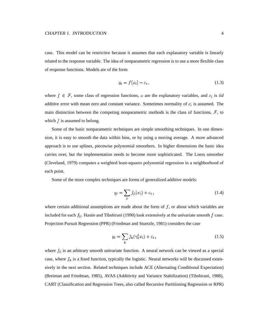
CHAPTER1. INTRODUCTION 4
case. This modelcanbe restrictive becauseit assumesthat eachexplanatoryvariableis linearly
relatedto theresponsevariable.Theideaof nonparametricregressionis to useamoreflexible class
of responsefunctions.Modelsareof theform� ���IH � G �$#&%(')�+* (1.3)
where HKJML , someclassof regressionfunctions, G are the explanatoryvariables,and ')� is iid
additive errorwith meanzeroandconstantvariance.Sometimesnormalityof ')� is assumed.The
main distinctionbetweenthe competingnonparametricmethodsis the classof functions, L , to
which H is assumedto belong.
Someof thebasicnonparametrictechniquesaresimplesmoothingtechniques.In onedimen-
sion, it is easyto smooththe datawithin bins, or by usinga moving average.A moreadvanced
approachis to usesplines,piecewise polynomialsmoothers.In higherdimensionsthe basicidea
carriesover, but the implementationneedsto becomemore sophisticated.The Loesssmoother
(Cleveland,1979)computesa weightedleast-squarespolynomialregressionin a neighborhoodof
eachpoint.
Someof themorecomplex techniquesareformsof generalizedadditive models:� �&� �ON H N � G �P#�%(')�Q* (1.4)
wherecertainadditionalassumptionsaremadeaboutthe form of H , or aboutwhich variablesare
includedfor eachH N . HastieandTibshirani(1990)look extensively at theunivariatesmoothH case.
ProjectionPursuitRegression(PPR)(FriedmanandStuetzle,1981)considersthecase� � � �ON H N � -�RN G � #�%(' � * (1.5)
where H N is anarbitrarysmoothunivariatefunction. A neuralnetwork canbeviewedasa special
case,where H N is a fixedfunction,typically the logistic. Neuralnetworkswill bediscussedexten-
sively in thenext section.RelatedtechniquesincludeACE (AlternatingConditionalExpectation)
(BreimanandFriedman,1985),AVAS (Additivity andVarianceStabilization)(Tibshirani,1988),
CART (ClassificationandRegressionTrees,alsocalledRecursive PartitioningRegressionor RPR)
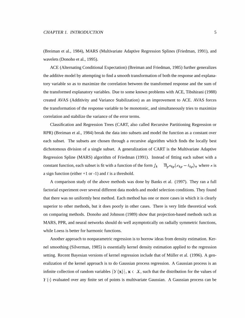
CHAPTER1. INTRODUCTION 5
(Breimanet al., 1984),MARS (MultivariateAdaptive RegressionSplines(Friedman,1991),and
wavelets(Donohoetal., 1995).
ACE (AlternatingConditionalExpectation)(BreimanandFriedman,1985)furthergeneralizes
theadditive modelby attemptingto find asmoothtransformationof boththeresponseandexplana-
tory variablesoasto maximizethe correlationbetweenthe transformedresponseandthe sumof
thetransformedexplanatoryvariables.Dueto someknown problemswith ACE,Tibshirani(1988)
createdAVAS (Additivity and VarianceStabilization)as an improvementto ACE. AVAS forces
thetransformationof theresponsevariableto bemonotonic,andsimultaneouslytriesto maximize
correlationandstabilizethevarianceof theerrorterms.
ClassificationandRegressionTrees(CART, alsocalledRecursive Partitioning Regressionor
RPR)(Breimanet al., 1984)breakthedatainto subsetsandmodelthefunctionasa constantover
eachsubset. The subsetsare chosenthrougha recursive algorithm which finds the locally best
dichotomousdivision of a singlesubset.A generalizationof CART is the MultivariateAdaptive
RegressionSpline (MARS) algorithmof Friedman(1991). Insteadof fitting eachsubsetwith a
constantfunction,eachsubsetis fit with a functionof theform H N �TSVUXW N U � G N U CZY N U #\[ whereW is
asignfunction(either+1 or -1) and Y is a threshold.
A comparisonstudyof the above methodswasdoneby Bankset al. (1997). They ran a full
factorialexperimentoverseveraldifferentdatamodelsandmodelselectionconditions.They found
thattherewasno uniformly bestmethod.Eachmethodhasoneor morecasesin which it is clearly
superiorto othermethods,but it doespoorly in othercases.Thereis very little theoreticalwork
on comparingmethods.DonohoandJohnson(1989)show thatprojection-basedmethodssuchas
MARS, PPR,andneuralnetworksshoulddo well asymptoticallyon radially symmetricfunctions,
while Loessis betterfor harmonicfunctions.
Anotherapproachto nonparametricregressionis to borrow ideasfrom densityestimation.Ker-
nel smoothing(Silverman,1985)is essentiallykerneldensityestimationappliedto the regression
setting.RecentBayesianversionsof kernelregressionincludethatof Muller et al. (1996).A gen-
eralizationof thekernelapproachis to do Gaussianprocessregression.A Gaussianprocessis an
infinite collectionof randomvariables]0^ � ! #`_ , ! Jba , suchthat thedistribution for thevaluesof^ �Dc # evaluatedover any finite setof points is multivariateGaussian.A Gaussianprocesscanbe

CHAPTER1. INTRODUCTION 6
specifieduniquelyby its meanfunction dfe ^ � ! #Pg andits covariancefunctionCov � ^ � !ih #�* ^ � ! ; #j# .Neal (1996)shows that undercertainconditionsthe limiting caseof a neuralnetwork regression
with arbitrarilymany nodesis aGaussianprocessregression.
1.3 Neural Networks
1.3.1 Background
Neuralnetworks wereoriginally createdasan attemptto model the act of thinking by modeling
neuronsin a brain. Much of the early work in this areatracesback to a paperby McCulloch
andPitts (1943)which introducedthe ideaof an activation function,althoughthe authorsuseda
threshold(indicator) function ratherthanthe sigmoidalfunctionscommontoday(as in Equation
1.2). Thresholdactivationswerefound to have severe limitations andthussigmoidalactivations
becamewidely usedinstead(Anderson,1982).
Much of therecentwork on neuralnetworksstemsfrom a numberof papers,includingFuna-
hashi(1989)andHornik et al. (1989)thatshowedthatneuralnetworksarea way to approximate
a functionarbitrarilycloselyasthenumberof hiddennodesgetslarge. Neuralnetworkswork well
with both smoothfunctionsand thosethat have breakpointsin them, sincea breakpointcan be
modeledeffectively with a singleextra hiddennode.Suchdiscontinuitiescanbedifficult for other
nonparametricmethodsto handle.
I shall only considerfeed-forward neuralnetworks with onehiddenlayer of units with logis-
tic activationsandwith onelinear outputunit, asthesearesufficient for full approximation.The
underlyingideaof theseneuralnetworks is thatthey usea particularchoiceof functionsto form a
basisover thespaceof continuousfunctions.Sigmoidfunctionsareusedto form this basis.I shall
beusingthelogistic function(Equation1.2). Thefull modelwasgivenin Equation1.1. A diagram
of themodelis shown in Figure1.3. Eachnodein thelayerof hiddenunitscorrespondsto a basis
function(a �k� in Equation1.1). In practiceonly a finite numberof hiddenunitsareused,forming
anapproximationto thebestregressionfunction.

CHAPTER1. INTRODUCTION 7
l
mnio
p q r
sItvu�wVtxu
y{z3|}|k~��
��� w}tvu
���E|}~&�� o
�x��V����Figure1.3: NeuralNetwork ModelDiagram
1.3.2 Fitting Algorithms
Thestandardmethodfor fitting aneuralnetwork is backpropagation, whichis essentiallyagradient-
descentalgorithm.Eachiterationinvolvesonly two calculationsat eachnode,makingit computa-
tionally efficient comparedto mostcompetingalgorithms.It hasapparentlybeendiscoveredinde-
pendentlymultiple times;it wasmadepopularby Rumelhartetal. (1986).
To usethebackpropagationalgorithm,samplesaretakenfrom thedata,andtheweightsof the
network areadjustedin thedirectionof maximumgradientof thelikelihood.Theadjustmentsstart
from thefinal outputnodeandare“propagated”backwardsthroughthehiddennodesto the input
nodes.
In practice,thebackpropagationalgorithmhasseveralproblems.First, it is only guaranteedto
find alocalmaximumin thelikelihood.While in many casesit will find theglobalmaximum,it can
easilyget stuckin a local maximumwhich producesdrasticover-smoothingof thedata. Second,
it canget stuckin “flat spots”wherethe gradientis computationallyindistinguishablefrom zero
(typically this occurswhenthe weightsmove the datato the tails of the activation function for a
node).Finally, it cantake a long time to converge. A goodchoiceof step-sizecanhelp,although

CHAPTER1. INTRODUCTION 8
theoptimalchoicecanvary greatlybetweendatasetsandthereis no goodmethodof determining
theright choice.Thenetwork fitting problemis still anopenresearcharea.
Therehave beenmany attemptsto improve thebackpropagationalgorithm. Onetypical fix is
to useweightdecay, which is essentiallya shrinkagemethodthat includesa momentumtermthat
is a multiple of theprevious changein weights. It canimprove both the speedandaccuracy of a
network. A further modificationis Quickprop, developedby Fahlmann(1989). It usesa combi-
nationof ordinarybackpropagationgradientdescentanda localquadraticapproximationinvolving
both the currentandprevious error derivatives. In practiceit is significantlyfasterthanstandard
backpropagationwhile not significantlylessaccurate.FahlmannandLebiere(1989)have created
anotheralgorithm,Cascade-Correlation, which bothselectsa suitablenumberof nodesandfinds
thefitted valuesfor theweights. While this methodis extremelyfast,it usesa very differentnet-
work structurethanI amconsidering(it only placesonenodein eachhiddenlayer, andconnectsall
previouslayersto thecurrentlayer).
1.3.3 Fitting Algorithms in BayesianInference
Therehasbeenmuchlesswork doneon fitting a neuralnetwork within the Bayesianframework.
TheBayesianapproachrequiresspecifyinga setof prior distributionsfor all of theweightsin the
network (andthevarianceof theerror), thencomputingtheposteriordistributionsfor theweights
usingBayes’Theorem.Therearetwo mainissuesthatneedto bedealtwith here.First, how does
onespecifya prior over parametersthathave little or no interpretablemeaning?Second,how does
oneefficiently approximatetheposteriordistribution whennoanalyticsolutionis known?
Often the choiceof a prior is basedon representingthe user’s prior beliefs. In the caseof a
neuralnetwork, it is difficult to provideany meaningfuldistribution for aparticularweightsincethe
correspondencebetweena weightanda featureof thedatais not usuallyeasilyidentifiable.Also,
thereis a certainnon-identifiabilityinherentin the model in that the nodescanbe substitutedfor
eachother;if all theinputsandoutputsfor ahiddennodewereswitchedwith thoseof anothernode
in thesamelayer, themodelwouldbefunctionallyequivalent,yet theindividual parameterswould
bedifferent. Becauseof this non-identifiability, all suggestedpriorsaresymmetricwith respectto
theorderingof theweights.

CHAPTER1. INTRODUCTION 9
In Chapter2 I shallreview severalpriorswhichhavebeenproposed.All of thesearehierarchical
in nature.My approachis to useanoninformative prior, andthenenforcecertainrestrictionsduring
thefitting processto ensuretheproprietyof theposterior.
Thesecondissueraisedin this sectionis how to find theposteriordistribution. In someprob-
lems, a good choiceof a conjugateprior can make it possibleto analytically find the posterior
distribution of theparameters.Neuralnetworks,however, have no known conjugatepriors. Some
of theearlierwork onBayesianneuralnetworksreliedonfitting thenetwork with backpropagation
andthenusinga Gaussianapproximationto get the posteriordistribution (BuntineandWeigend,
1991). ModernBayesianstatisticshasbeenaidedby the introductionof Markov Chain Monte
Carlo(MCMC) methods,which allow oneto getanapproximationof theposteriordistribution by
simulatingrandomdraws from thedistribution. To getthesedraws,onesimulatesa Markov Chain
with stationarydistribution equalto the posteriordistribution. This is relatively easyto do with
Gibbssamplingby samplingfrom the conditionaldistribution for a parameterwhenall otherpa-
rametersareknown. At eachstep,a single(possiblymultivariate)parameteris updatedfrom its
completeconditionalwherethecurrentvaluesof theotherparametersaretemporarilytakenasthe
true valuesfor the conditionaldistribution. Eachof the otherparametersis thenupdatedin turn.
In the casewherea conditionaldistribution doesnot have a recognizableform and thus cannot
beusedfor simulation,theMetropolis-Hastingsalgorithmcanbeusedfor thatstep. Let � be the
conditionaldistribution of interest,let thecurrentvaluefor a parameterbe � andgeneratea candi-
datevalue ��� from someconvenientdistribution. Thenacceptthecandidatevaluewith probability�����f� = *X�����&�j���������� andotherwisekeeptheold value.Thisalgorithmis dueto Metropoliset al. (1953)
andcontainsGibbssamplingasa specialcase,which was introducedin a paperby Gemanand
Geman(1984).Theunderlyingstatisticaltheoryof MCMC wassolidifiedby Tierney (1994).
Nearly all modernmethodsfor fitting Bayesianneuralnetworks rely on MCMC. Muller and
RiosInsua(1998b)usea multivariateversionof MCMC andmarginalizeover someparametersto
increaseperformance.Neal(1996)usesahybridMonteCarloalgorithm(Duaneetal.,1987)which
combinesthe Metropolis-Hastingsalgorithmwith methodsfrom dynamicalsimulationsampling
techniques.MacKay (1992)combinesMCMC with a local Gaussianapproximation.I shall also
useMCMC, with an additionalrestrictionduring a Metropolisstepto prevent the posteriorfrom

CHAPTER1. INTRODUCTION 10
beingimproper.
1.4 Model Selectionand Model Averaging
Model selectionfor a neuralnetwork entailsboth a selectionof the structureof the network (in
particular, how many hiddennodesto use)anda selectionof which explanatoryvariablesto use.
Thenext subsectiongivesanintroductionto theproblemandaddressessomephilosophicalaspects.
Theremainingsubsectionsdiscussvariableselectionmethods,methodsfor selectingthesizeof the
neuralnetwork, methodsfor attackingthecombinedproblem,andmodelaveraging.
1.4.1 Overview of Model Selection
Themorehiddenunitsthatareused,thebetterthefit. With enoughunits,onecangetaperfectfit of
thedata.Thusthereis theneedto balancetwo competingdesires:to increasethenumberof units
to improve thefit andto limit thenumberof units to decreaseover-fitting andimprove predictive
performance.At thesametime,we arealsointerestedin choosingamongstcompetingexplanatory
variables.Justasin a multiple linear regressionover a wide rangeof candidateexplanatoryvari-
ables,wewould like to beableto useonly theimportantvariablesandto leave theothersoutof the
model. The additionalchallengehereis that we needto simultaneouslychooseour variablesand
choosethesizeof thenetwork.
Therearemany competingideason how to choosethebestmodel. Somearebasedon maxi-
mizing the likelihoodsubjectto somepenalty, suchasthe Akaike InformationCriterion(Akaike,
1974)andtheBayesianInformationCriterion(Schwarz,1978).Anothermethodis cross-validation
(Stone,1974).Thesearediscussedin moredetailin thenext subsection.
In Bayesianinference,onecansimply pick the modelwith highestposteriorprobability. The
Bayesianapproachalsolendsitself very nicely to prediction,in theguiseof modelaveraging. In
somecases,the analystwill find morethanonemodelwith high posteriorprobability, andthese
modelswill give differentpredictions(see,for example,the heartattackdatain Raftery(1996)).
Pickingonly a singlemodelwill grosslyunderestimatethe variability of theestimate,sinceit ig-
noresthefact thatanothermodelwith significantposteriorprobabilitymadea differentprediction.
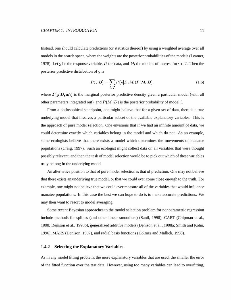
CHAPTER1. INTRODUCTION 11
Instead,oneshouldcalculatepredictions(or statisticsthereof)by usingaweightedaverageoverall
modelsin thesearchspace,wheretheweightsaretheposteriorprobabilitiesof themodels(Leamer,
1978).Let � betheresponsevariable,� thedata,and � themodelsof interestfor ¡ J�¢ . Thenthe
posteriorpredictive distribution of � is£ � �&¤ � # � � �¦¥"§ £ � �&¤ � * � # £ � � ¤ � #¨* (1.6)
where£ � ��¤ � * �P# is the marginal posteriorpredictive densitygiven a particularmodel(with all
otherparametersintegratedout),and£ � �`¤ � # is theposteriorprobabilityof model ¡ .
Froma philosophicalstandpoint,onemight believe that for a givensetof data,thereis a true
underlyingmodel that involvesa particularsubsetof the availableexplanatoryvariables.This is
theapproachof puremodelselection.Oneenvisionsthat if we hadaninfinite amountof data,we
could determineexactly which variablesbelongin the modelandwhich do not. As an example,
someecologistsbelieve that thereexists a model which determinesthe movementsof manatee
populations(Craig,1997). Suchanecologistmight collectdataon all variablesthatwerethought
possiblyrelevant,andthenthetaskof modelselectionwouldbeto pick outwhichof thesevariables
truly belongin theunderlyingmodel.
An alternativepositionto thatof puremodelselectionis thatof prediction.Onemaynotbelieve
thatthereexistsanunderlyingtruemodel,or thatwecouldevercomecloseenoughto thetruth. For
example,onemightnotbelieve thatwecouldevermeasureall of thevariablesthatwould influence
manateepopulations.In this casethebestwe canhopeto do is to make accuratepredictions.We
maythenwantto resortto modelaveraging.
SomerecentBayesianapproachesto themodelselectionproblemfor nonparametricregression
include methodsfor splines(and other linear smoothers)(Sanil, 1998), CART (Chipmanet al.,
1998;Denisonet al., 1998b),generalizedadditive models(Denisonet al., 1998a;SmithandKohn,
1996),MARS (Denison,1997),andradialbasisfunctions(HolmesandMallick, 1998).
1.4.2 Selectingthe Explanatory Variables
As in any modelfitting problem,themoreexplanatoryvariablesthatareused,thesmallertheerror
of thefitted functionover thetestdata.However, usingtoo many variablescanleadto overfitting,
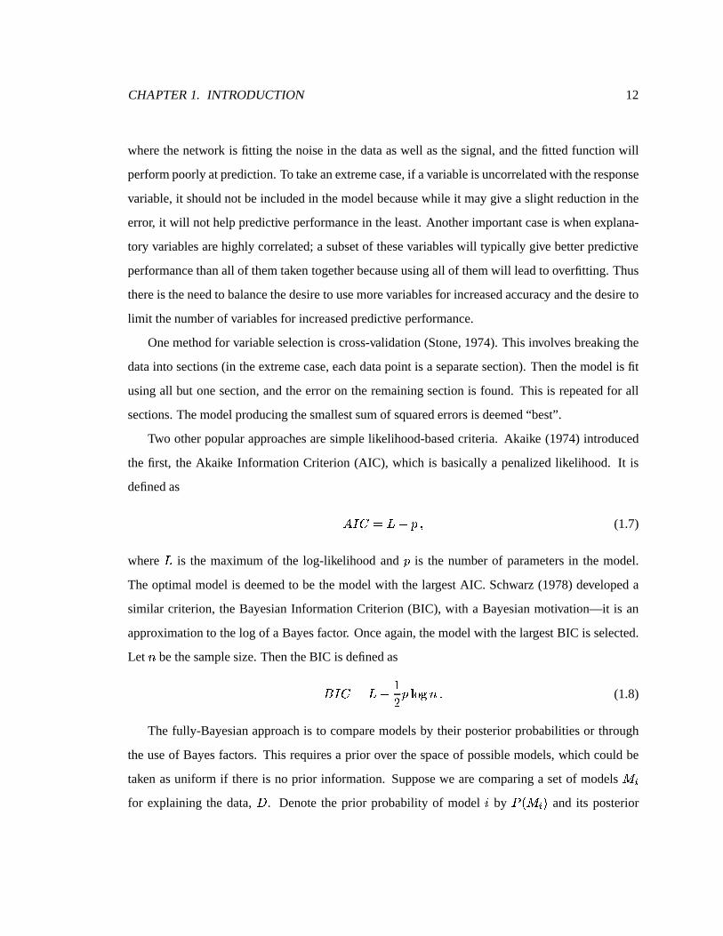
CHAPTER1. INTRODUCTION 12
wherethenetwork is fitting thenoisein thedataaswell asthesignal,andthefitted functionwill
performpoorlyatprediction.To takeanextremecase,if avariableis uncorrelatedwith theresponse
variable,it shouldnot beincludedin themodelbecausewhile it maygive a slight reductionin the
error, it will not helppredictive performancein theleast.Anotherimportantcaseis whenexplana-
tory variablesarehighly correlated;a subsetof thesevariableswill typically give betterpredictive
performancethanall of themtakentogetherbecauseusingall of themwill leadto overfitting. Thus
thereis theneedto balancethedesireto usemorevariablesfor increasedaccuracy andthedesireto
limit thenumberof variablesfor increasedpredictive performance.
Onemethodfor variableselectionis cross-validation(Stone,1974).This involvesbreakingthe
datainto sections(in theextremecase,eachdatapoint is a separatesection).Thenthemodelis fit
usingall but onesection,andtheerroron the remainingsectionis found. This is repeatedfor all
sections.Themodelproducingthesmallestsumof squarederrorsis deemed“best”.
Two otherpopularapproachesaresimplelikelihood-basedcriteria. Akaike (1974)introduced
the first, the Akaike InformationCriterion (AIC), which is basicallya penalizedlikelihood. It is
definedas ©�ª+« �T¬ C® * (1.7)
where ¬ is the maximumof the log-likelihood and is the numberof parametersin the model.
The optimalmodelis deemedto be themodelwith the largestAIC. Schwarz (1978)developeda
similar criterion, the BayesianInformationCriterion (BIC), with a Bayesianmotivation—it is an
approximationto thelog of a Bayesfactor. Onceagain,themodelwith thelargestBIC is selected.
Let ¯ bethesamplesize.ThentheBIC is definedas° ª+« �±¬ C =² �³3´ µ ¯�¶ (1.8)
The fully-Bayesianapproachis to comparemodelsby their posteriorprobabilitiesor through
theuseof Bayesfactors.This requiresa prior over thespaceof possiblemodels,which couldbe
taken asuniform if thereis no prior information. Supposewe arecomparinga setof models �for explaining the data, � . Denotethe prior probability of model ¡ by
£ � �P# and its posterior

CHAPTER1. INTRODUCTION 13
probabilityby£ � �`¤ � # . Bayes’Theoremstatesthat:£ � � ¤ � #·� £ � � ¤ �$# £ � �P#¸ � £ � � ¤ � # £ � � # ¶ (1.9)
Notethat£ � � ¤ �$# involvesmarginalizingover theparametersin themodel,which is ananalyti-
cally intractableintegral in thecaseof a neuralnetwork. Methodsfor approximatingthis integral
will bediscussedin Chapter4.
TheBayesfactorfor comparingtwo modelsis theratioof theposterioroddsin favor of thefirst
modelto theprior oddsin favor of thefirst model.Theposterioroddsin favor of model ¡ are£ � �:¤ � #£ � � ¤ � # � £ � � ¤ �$#£ � � ¤ � # £ � �$#£ � � # * (1.10)
andthustheBayesfactoris definedas ° � � � £ � � ¤ �$#£ � � ¤ � # ¶ (1.11)
KassandRaftery(1995)summarizethemodernapplicationsof Bayesfactorsin modelselection.
All of theabove techniquesrely onanexhaustive searchto find theoptimalsetof variables.For
a largesetof candidatevariables,this canbeprohibitively computationallyexpensive for nonpara-
metrictechniques.Furthermore,modelsmaybefit with iterative algorithms,andthusit is notonly
time-consuming,but for any given fitted model,the useris not guaranteedto have found the best
fit. For example,a neuralnetwork fitting algorithmmayconvergeto a localminimumratherthana
globalminimum.Thiscomplicationdoesn’t arisein thestandardmodelselectionsettingwhereit is
assumedthatthemodelcanbereliablyfit.
Two frequentistautomatedmodelselectiontechniquesareStepwiseRegressionandLeapsand
Bounds(Furnival andWilson, 1974). Two Bayesianapproaches,Occam’s Window andMarkov
ChainMonteCarloModelComposition,aregivenin Rafteryetal. (1997).They bothusetheBayes
factor(or anapproximationto it) asaguidewhenmoving throughthespaceof models.
FosterandGeorge(1997)takeanentirelydifferentapproach.They includethechoiceof model
asanotherparameterandaddanotherlevel of hierarchyto the modelandfind the joint posterior.
They useanEmpiricalBayesapproachto selecthyperparametersandthena maximumlikelihood
approximationto getamodelscorefunctionthey call theEmpiricalBayesCriterion (EBC).
CHAPTER1. INTRODUCTION 14
1.4.3 Selectingthe Network Ar chitecture
Justasin thecaseof variableselection,a delicatebalanceexists in theselectionof thesizeof the
network. Toomany hiddennodesleadsto amodelthatoverfitsandpredictspoorly. Too few nodes
producesa modelthatover-smoothsandfits poorly. Many of themethodsfor selectingthesizeof
anetwork areborroweddirectly from theproblemof variableselection.Cross-validation,AIC, and
BIC areall acceptedmethodsfor choosingthenumberof hiddennodes(Bishop,1995).
Therehave beensomemodificationsof the standardmodel selectioncriteria to specifically
addressthe size selectionproblem. Moody (1992)proposesa revisedway to count the number
of parametersin a neuralnetwork basedon the effectivenumberof parameters,which is smaller
thanthe actualnumberof parametersusedin the modelbecauseof the high correlationbetween
certainparameterswithin a neuralnetwork. Theeffective numberof parameterscanthenbeused
in a generalizationof theAIC. Murataet al. (1994)have developedanothercriterion,theNetwork
InformationCriterion(NIC) which is alsoanextensionof theAIC basedon a modifiedpenaltyfor
thenumberof parametersin themodel.
Anotherapproachto thenodeselectionproblemis a shrinkage-basedone.Oftenreferredto as
weightdecay, a penaltydependingon the magnitudeof the weightsis addedto the least-squares
error term and this sum is minimized. The hopeis that unimportantweightswill be shrunkto
zero,andthussomenodescanbe eliminated.Weightdecayis alsosometimesusedin the fitting
algorithmsto improve thespeedandaccuracy of convergence.
1.4.4 SimultaneousVariable and SizeSelection
Thereis not much in the literaturespecificallyon the problemof choosingboth the size of the
network and which inputs to use. Many of the previous methodscan be usedfor both, or one
coulduseacombinationof two methods.Onecombinedapproachis aprocedurecalledAutomatic
RelevanceDetermination(ARD) (MacKay, 1994;Neal,1996).Themainideais thateachinputhas
its own hyperparameterwhichresemblesascalefactorfor theweightsfrom thatinput to thehidden
nodes.If that input is importantfor any of thehiddennodes,thathyperparameterwill be large. If
thatinput is of nouseto thenetwork, thenthathyperparameterwill besmall.

CHAPTER1. INTRODUCTION 15
My approachto this problemis to usethe full Bayesianframework. By putting a prior over
the spaceof all possiblemodels,both in termsof variablesand numberof hiddennodes,I can
estimatetheposteriorprobabilitiesof all of themodels(or asubsetof themif thespaceis too large)
andchoosethemodelwith highestposteriorprobability. In practice,I useanapproximationto the
posteriorprobabilitiesbasedon theBIC, whichmakesit mucheasierto compute.
1.4.5 Model Averaging
Model averagingwasfirst advocatedby Leamer(1978). By using the weightedaverageof the
predictionsgiven by eachmodelunderconsideration,weightedby the posteriorprobabilitiesof
themodels,onecanboth improve predictive performanceaswell asmoreaccuratelyestimatethe
error of the prediction. This is primarily useful in the casewhen thereis no singlemodelwith
highposteriorprobability. Rafteryetal. (1997)giveexamplesof significantdecreasesin prediction
errorsthroughtheuseof modelaveraging.
Other relatedideasinclude bagging(Breiman,1994) and bumping (Tibshirani and Knight,
1995). Both of theseusebootstrapsamplesof the original data. Baggingcalculatesestimates
onthebootstrapsamplesandthenaveragestheseestimatesto obtainthebaggedestimate.Bumping
involvesa minimizationfor eachbootstrapsample,thenanotherminimizationover the estimates
from eachsample.Bothmethodsareattemptsto improvepredictionanderrorestimationin thecase
wherethereis nouniquedominantbestmodel.
1.5 Dir ectionof the Restof the Thesis
In Chapter2, I will discussthedetailsof fitting a neuralnetwork undertheBayesianapproach.In
particular, I show how to useasimplenoninformativeprior. In Chapter3, I presentsomeasymptotic
consistency resultsfor neuralnetworks in the Bayesiancontext, with the modelsof Chapter2 as
a specialcase.In Chapter4, I describetheproblemof estimatingnormalizingconstants,which is
necessaryfor Bayesianmodelselectionandmodelaveraging.Finally in Chapter5, I will discussthe
implementationof modelselectionandmodelaveragingin thenonparametricregressionproblem,
andgive severalexamplesof themethodsfrom this thesis.
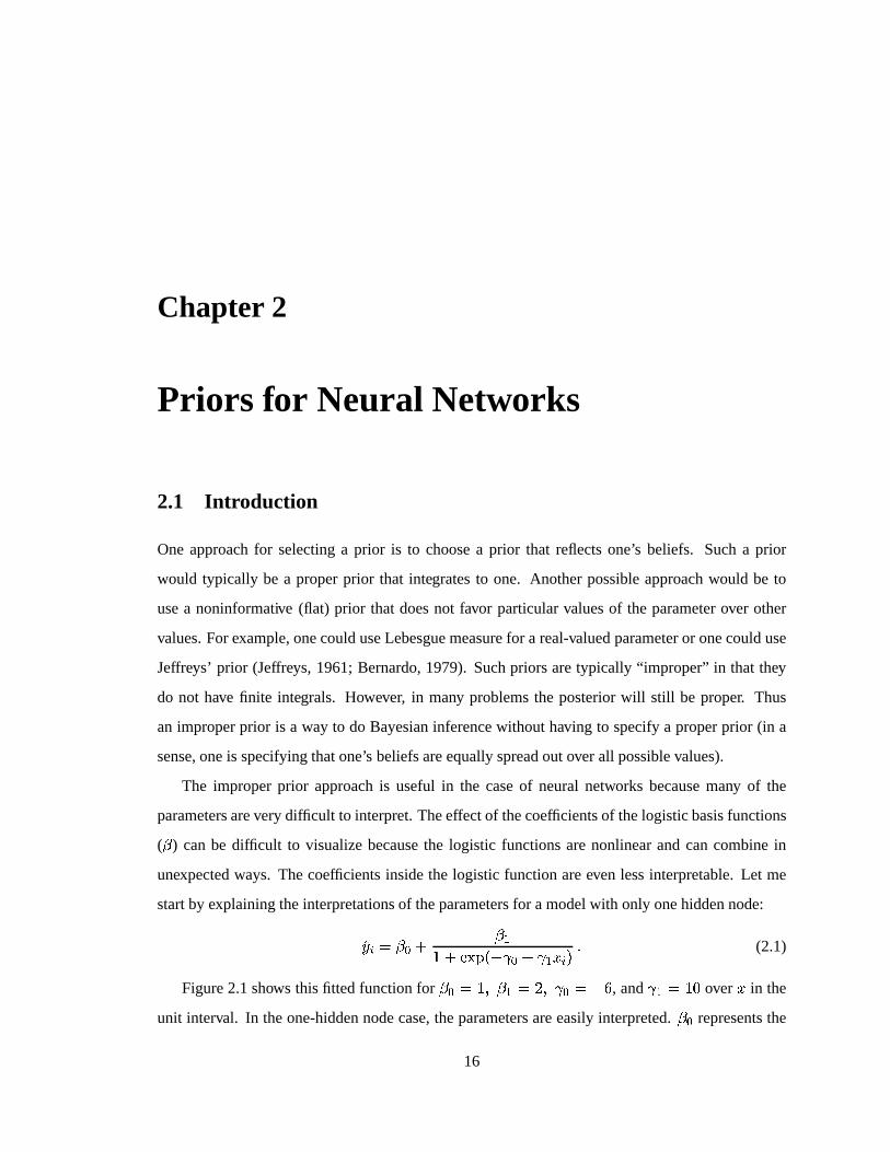
Chapter 2
Priors for Neural Networks
2.1 Intr oduction
One approachfor selectinga prior is to choosea prior that reflectsone’s beliefs. Sucha prior
would typically be a properprior that integratesto one. Anotherpossibleapproachwould be to
usea noninformative (flat) prior that doesnot favor particularvaluesof the parameterover other
values.For example,onecoulduseLebesguemeasurefor a real-valuedparameteror onecoulduse
Jeffreys’ prior (Jeffreys, 1961;Bernardo,1979). Suchpriorsaretypically “improper” in that they
do not have finite integrals. However, in many problemsthe posteriorwill still be proper. Thus
animproperprior is a way to do Bayesianinferencewithout having to specifya properprior (in a
sense,oneis specifyingthatone’s beliefsareequallyspreadoutover all possiblevalues).
The improperprior approachis useful in the caseof neuralnetworks becausemany of the
parametersareverydifficult to interpret.Theeffectof thecoefficientsof thelogisticbasisfunctions
( � ) canbe difficult to visualizebecausethe logistic functionsarenonlinearand cancombinein
unexpectedways. Thecoefficientsinsidethe logistic functionareeven lessinterpretable.Let me
startby explainingtheinterpretationsof theparametersfor amodelwith only onehiddennode:¹� �&� � � % � h= %º>A@+B �DC - �VC - h G �$# ¶ (2.1)
Figure2.1shows this fitted functionfor � � � = * � h � ² * - � � C¼» , and - h � = 7 over G in the
unit interval. In theone-hiddennodecase,theparametersareeasilyinterpreted.� � representsthe
16

CHAPTER2. PRIORSFORNEURAL NETWORKS 17
X
Y½
0.0 0.2 0.4 0.6 0.8 1.0
1.0
1.5
2.0
2.5
3.0
Figure2.1: A One-NodeFunction
overall locationof � , a sortof intercept,in thatwhenthelogistic functionis closeto zero(which it
is herefor valuesof G nearor below zero), �¾� � � . � h is theoverall scalefactorfor � , in that the
logistic function rangesfrom 0 to 1, so � h is like the rangeof � , which is this caseis ¿ C = � ².
The - parameterscontrol the locationandscaleof the logistic function. Thecenterof the logistic
functionoccursat C�À`ÁÀ) , whichin thiscaseis 0.6.Thelargerthevalueof - h , thesteepertheincrease
in � asonemovesaway from thecenter. If - h is positive, thenthelogistic risesfrom left to right. If- h is negative, thenthelogisticwill decreaseas G increases.
This interpretationworksfine for a singlehiddennode.For well-separatednodes(in termsof
theircentersandslopes,sothatfor any particularvalueof G , atmostonenodeis nearits centerand
the restarefar enoughfrom their centersthat a small changein G doesnot producea noticeable
changein thelogistic function),onecancontinueto usethis interpretation.Two nodeswith centers
neareachother, but with oppositesignson - h , cancombineto producea peak,similar in spirit to
a kernelor a radialbasisfunction.However, whenthenodeseffectively overlap,which is typically
thecasein a realproblem,theparameterscanno longerbeinterpretedasabove.
For example,the left plot of Figure2.2 resultsfrom maximumlikelihoodfitting of a two-node
network to themotorcycleaccidentdataof Silverman(1985).The G -axisis thetimein milliseconds
after thecrash,andthe � -axistheaccelerationforceon theheadof therider. Thetwo-nodemodel
doesa goodjob of capturingthe main featuresof the data,althoughperhapsit over-smoothsfor
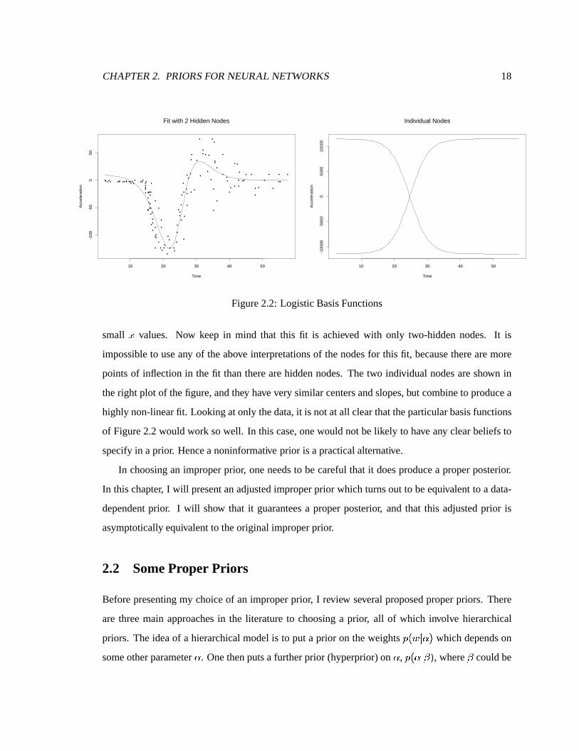
CHAPTER2. PRIORSFORNEURAL NETWORKS 18
•• ••• ••• •• •• •••••• •••
•••••
•
••
••
•
••
••
••
••
•
•
•
•
•
•
•
•
•
••••
•
•
•
•
• ••
•
••
• ••
•
•
•
•••
•
•
•
•
•
•
•
•
•
•
•••
•
••
•
•
•
•
•• •
•
•
•
•
•
•
•
••
•
•
•
•••
••
•
•
•
••
•
••• •
•
• •
••
•
•
•
•
•
Fit with 2 Hidden Nodes
Time
Acc
eler
atio
n
10 20 30 40 50
-100
-50
050
Individual Nodes
Time
Acc
eler
atio
n
10 20 30 40 50
-100
00-5
000
050
0010
000
Figure2.2: LogisticBasisFunctions
small G values. Now keep in mind that this fit is achieved with only two-hiddennodes. It is
impossibleto useany of theabove interpretationsof thenodesfor this fit, becausetherearemore
pointsof inflection in the fit thantherearehiddennodes.The two individual nodesareshown in
theright plot of thefigure,andthey have verysimilar centersandslopes,but combineto producea
highly non-linearfit. Lookingatonly thedata,it is notatall clearthattheparticularbasisfunctions
of Figure2.2wouldwork sowell. In this case,onewouldnot belikely to have any clearbeliefsto
specifyin aprior. Henceanoninformative prior is apracticalalternative.
In choosingan improperprior, oneneedsto becarefulthat it doesproducea properposterior.
In this chapter, I will presentanadjustedimproperprior which turnsout to beequivalentto a data-
dependentprior. I will show that it guaranteesa properposterior, andthat this adjustedprior is
asymptoticallyequivalentto theoriginal improperprior.
2.2 SomeProper Priors
Beforepresentingmy choiceof an improperprior, I review severalproposedproperpriors. There
are threemain approachesin the literatureto choosinga prior, all of which involve hierarchical
priors. Theideaof a hierarchicalmodelis to put a prior on theweightsÃ� � ¤ Äi# which dependson
someotherparameterÄ . Onethenputsa furtherprior (hyperprior)on Ä , Ã� Äk¤ � # , where� couldbe

CHAPTER2. PRIORSFORNEURAL NETWORKS 19
eitheranotherunknown parameterwith its own hyperprior, or could just bea fixedparameterthat
needsto bechosenaspartof theprior selectionprocess.
All approachesstartwith thesamebasicmodelfor theresponse� :� � � �ÆÅ %N���� h � � == %º>A@+BfÇ C - �`�VC ¸ U . � h - � .�G � .XÈ %(' � * (2.2)'0� �É�324 5 �87 *:9 ; # ¶ (2.3)
I will giveabrief descriptionof eachapproachhere,andthenmoredetaileddescriptionswill follow
in thesubsequentsubsections.
Thefirst approachis to useanarbitraryprior of conveniencewith a largehierarchicalstructure
to try to let thedatadetermineasmuchaspossible.Sincetheerror in themodelis assumedto be
Gaussian,usinga Gaussianprior over theweightsprovidessomeamountof conjugacy (at leastfor
theoutputweights)andhelpsto simplify thecomputations.Muller andRiosInsua(1998b)suggest
a three-stagehierarchicalmodelthatchoosestheparametersat thetop of thehierarchyto beof the
sameorderof magnitudeas the target data. The hierarchicalstructureis fairly simple,although
many parametersaremultivariate.
Neal(1996)suggestsafour-stagemodelwith arbitraryvaluesfor theparametersatthetopof the
hierarchy. Thestructureof thehierarchyis rathercomplex althoughall parametersareunivariate.
MacKay(1992)startsby trying to usean improperprior in a simpletwo-stagemodel. To get
aroundtheimproprietyof theposterior, heusesthedatato choosefixedvaluesfor thehyperparam-
eters.This is essentiallyadata-dependentprior for aone-stagemodel.
2.2.1 The Muller and Rios Insua Model
A directedacyclic graph(DAG) diagramof this model(Muller andRiosInsua,1998b)is:
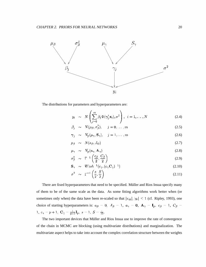
CHAPTER2. PRIORSFORNEURAL NETWORKS 20
ÊÌËÍ
ÎxÏ
Ð Í ÑÓÒÐ ÒÔiÕÖ Õ ÊÌË
Thedistributionsfor parametersandhyperparametersare:� � 4 5Ø×ÙÛÚ��Ü����� �Ý����� �� ! �Þ#�*:9 ;)ßà * ¡ � = * ¶"¶"¶ * 5 (2.4)
� � 4 5 �¦á�â *:9 ;â #�* ãä� 7 * ¶"¶"¶ *jå (2.5)� � 4 5 U �¦á À *Aæ À #�* ãä� = * ¶"¶"¶ *jå (2.6)á�â 4 5 �8ç�â * © â # (2.7)á À 4 5 U �8ç À *`è À # (2.8)9 ;â 4 é·ê hEë ì â² *« Ⲻí (2.9)æ À 4 î ¡ W / ê h � ì À * � ì ÀðïÌÀ # ê h # (2.10)9 ; 4 é ê h ë W² *Qñ ² í (2.11)
Therearefixedhyperparametersthatneedto bespecified.Muller andRiosInsuaspecifymany
of them to be of the samescaleas the data. As somefitting algorithmswork betterwhen (or
sometimesonly when)thedatahave beenre-scaledso that ¤ G � . ¤�*ݤ � �`¤xò = (cf. Ripley, 1993),one
choiceof startinghyperparametersis: çóâ � 7 * © â � = * ç À �õô�*öè À �ø÷jUQ* ì â � = *« â �= * ì À � % = * ï À � hU0[ h ÷ U *ùWÓ� = * ñ � hh � .
The two importantdevicesthatMuller andRios Insuauseto improve therateof convergence
of the chain in MCMC areblocking (usingmultivariatedistributions) andmarginalization. The
multivariateaspecthelpsto take into accountthecomplex correlationstructurebetweentheweights

CHAPTER2. PRIORSFORNEURAL NETWORKS 21
within thenetwork, whichcanotherwisecauseachainto convergeextremelyslowly. Thealgorithm
startsataninitial setof arbitraryvaluesandtheniteratesthroughthefollowing steps:
1. Giventhecurrentvaluesfor therestof theparameters,replaceú with a draw from a multi-
variatenormal. Conditionalon the otherparameters,this stepis equivalentto updatingthe
coefficientsin amultiple linearregression.
2. Given the currentvaluesfor the hyperparametersbut marginalizing over ú , replace� � via
a Metropolisstep. A possiblecandidatedistribution would be 5 ��� � * 7 ¶ 7 = ÷jU�# . Do this forãä� = * ¶"¶"¶ *jå .
3. Given the above parameters,updatethe hyperparametersfrom their completeconditional
posteriordistributions.All of thesecanbesampleddirectly, withoutMetropolissteps.
I initially worked with this model,but I discoveredthat it wasmorecomplex thannecessary.
Thelargernumberof parametersmadeit difficult to evaluateBayesfactors.ThemodelI useinstead
is in Section2.3.
2.2.2 NealModel
Neal’s four-stagemodel(1996)containsmoreparametersthanthepreviousmodel.A DAG diagram
of themodelis
ûÓüý�þ
ÿÿ�� ÿ þ���� ü ÿ���� � ü
ÿ��ÿ þ ���ÿ��
û�� �Vü � � �Vü
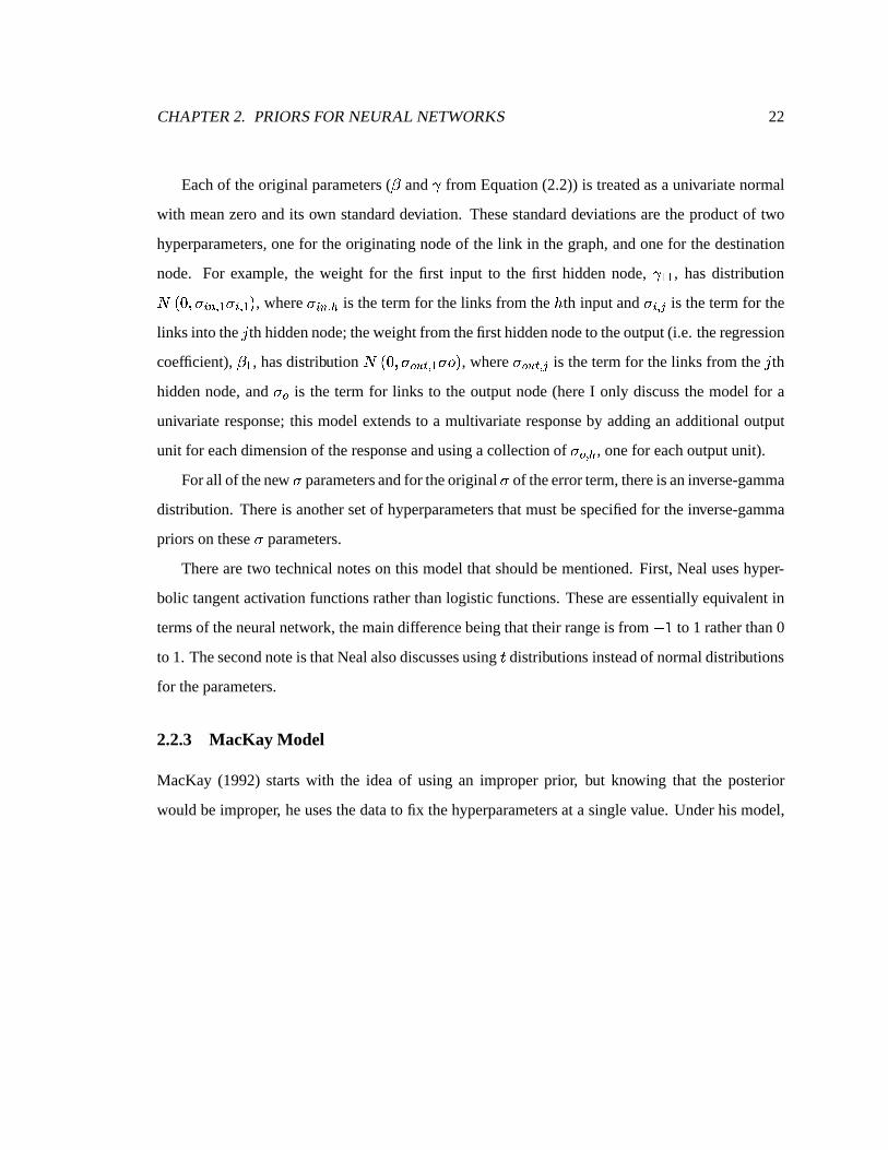
CHAPTER2. PRIORSFORNEURAL NETWORKS 22
Eachof theoriginal parameters( � and - from Equation(2.2)) is treatedasa univariatenormal
with meanzeroandits own standarddeviation. Thesestandarddeviationsarethe productof two
hyperparameters,onefor theoriginatingnodeof the link in thegraph,andonefor thedestination
node. For example,the weight for the first input to the first hiddennode, - hjh , hasdistribution5 �87 *:9 ����� h 9 ��� h # , where9 ����� . is thetermfor thelinks from the / th inputand 9 ��� � is thetermfor the
links into the ã th hiddennode;theweightfrom thefirst hiddennodeto theoutput(i.e. theregression
coefficient), � h , hasdistribution 5 �Þ7 *:9 Å�� R � h 9��X# , where9 Å�� R � � is thetermfor thelinks from the ã thhiddennode,and 9 Å is the term for links to the outputnode(hereI only discussthe modelfor a
univariateresponse;this modelextendsto a multivariateresponseby addingan additionaloutput
unit for eachdimensionof theresponseandusingacollectionof 9 Å � . , onefor eachoutputunit).
Forall of thenew 9 parametersandfor theoriginal 9 of theerrorterm,thereisaninverse-gamma
distribution. Thereis anothersetof hyperparametersthatmustbespecifiedfor theinverse-gamma
priorson these9 parameters.
Therearetwo technicalnoteson this modelthatshouldbementioned.First, Nealuseshyper-
bolic tangentactivationfunctionsratherthanlogistic functions.Theseareessentiallyequivalentin
termsof theneuralnetwork, themaindifferencebeingthattheir rangeis from C = to 1 ratherthan0
to 1. Thesecondnoteis thatNealalsodiscussesusing Y distributionsinsteadof normaldistributions
for theparameters.
2.2.3 MacKay Model
MacKay (1992) startswith the idea of using an improperprior, but knowing that the posterior
would beimproper, heusesthedatato fix thehyperparametersat a singlevalue.Underhis model,
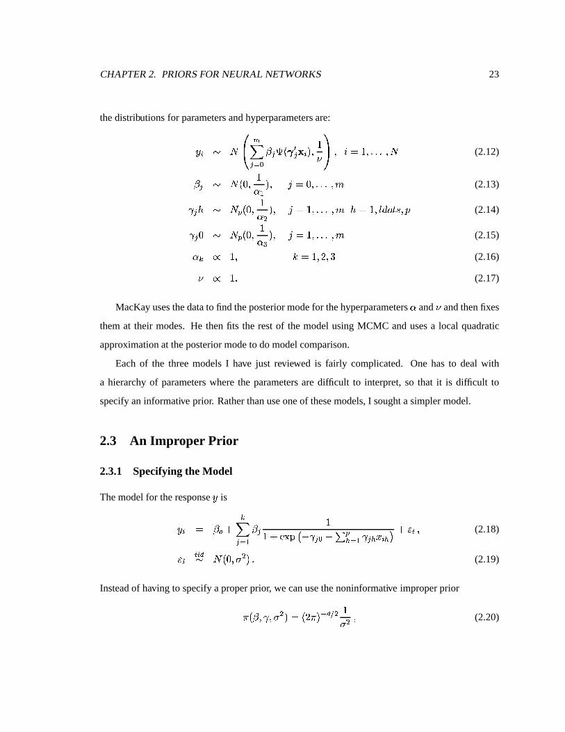
CHAPTER2. PRIORSFORNEURAL NETWORKS 23
thedistributionsfor parametersandhyperparametersare:� � 4 5 ×ÙÛÚ��Ü���¨� �Ý��������A! �P#�*�=� ßà * ¡ � = * ¶"¶"¶ * 5 (2.12)
� � 4 5 �87 *f=Ä h #�* ãä� 7 * ¶"¶"¶ *jå (2.13)- � / 4 5 U �87 * =Ä ; #�* ãä� = * ¶"¶"¶ *jå / � = * �! �� Y Wó* (2.14)- �)7 4 5 U �87 * =Ä�" #�* ãä� = * ¶"¶"¶ *jå (2.15)Ä N # = * $�� = * ² * ¿ (2.16)� # = ¶ (2.17)
MacKayusesthedatato find theposteriormodefor thehyperparametersÄ and � andthenfixes
themat their modes. He thenfits the restof the modelusingMCMC andusesa local quadratic
approximationat theposteriormodeto domodelcomparison.
Eachof the threemodelsI have just reviewed is fairly complicated. One hasto deal with
a hierarchyof parameterswherethe parametersaredifficult to interpret,so that it is difficult to
specifyaninformative prior. Ratherthanuseoneof thesemodels,I soughtasimplermodel.
2.3 An Impr oper Prior
2.3.1 Specifyingthe Model
Themodelfor theresponse� is� � � � Å %N���� h � � == %º>A@+B Ç C - �`�VC ¸ U . � h - � .�G � . È %(')�+* (2.18)'0� �É�324 5 �87 *:9 ; # ¶ (2.19)
Insteadof having to specifyaproperprior, wecanusethenoninformative improperprior� � � * - *:9 ; #·� � ² � # ê 2&% ; =9 ; * (2.20)

CHAPTER2. PRIORSFORNEURAL NETWORKS 24
where is the dimensionof the model (numberof parameters).The coefficient of � ² � # ê 2&% ; is
chosenfor reasonsexplainedlater. This prior is proportionalto thestandardnoninformative prior
for linearregression.
Toensurethattheposteriorisproper, weneedtoputcertainrestrictionsontheparametersduring
theMCMC fitting process.This ideahasappearedin theliteraturefor mixturemodels(Dieboltand
Robert,1994;Wasserman,1998a).Thekey is to ensurethatthelogisticbasisfunctionsarelinearly
independent.To make this moreformal,define< � � � ' = %(>A@+B)( C - ���VC U�. � h - � .�G � .+*-, ê h (2.21)
andlet . bethematrixwith elements�8< � � # . Thefitting of thevector� ismerelyamultipleregression
onthedesignmatrix . . Weneedarestrictionon . to ensurethelinearindependenceof thecolumns
of Z. A sufficient conditionfor linear independenceis that the determinantof . R . is larger than
somepositive value
« � . We canlet
« �0/ 7 as ¯ / 1 aslong as
« �32 7 for all ¯ . To ensure
proprietyof theposterior, wealsoneedto boundtheindividual - ’ssuchthat ¤ - � . ¤�4 � � for all ãX* / ,
aswill beexplainedlater. This turnsout to beequivalentto adata-dependentprior.
It is computationallyusefulto alsoboundtheotherparameters(namely ¤ � � ¤�4 � � ; 9 doesnot
needto bebounded).Thiscanhelpwith numericalstability in theMCMC fitting. It is alsotheoret-
ically usefulin thatwe canshow that this prior satisfiestheconditionsfor asymptoticconsistency
of theposteriorof Theorem3.3.1.For this theorem,werequire� ���5� � >A@QB � ¯�6 #j# for all 7 2 7 .In many cases,using the coefficient of � ² � # ê 28% ; on Jeffreys’ prior leadsto the BIC beinga
order 9 U � h: � � approximationto the log of the Bayesfactor, insteadof the usual 9 U � = # order
approximation.In this case,I amnot usingJeffreys’ prior, but thecoefficient is still a convenient
andreasonablechoice.
2.3.2 Fitting the Model
WeuseMCMC to fit themodel.Thefull posterioris proportionalto thelikelihoodtimestheprior:H � � * - *:9 ; ¤ �ð#;# � ² � # ê 28% ; =9 ; � ² � 9 ; # ê �<% ; >A@QB>=? C =² 9 ; �� � � h ×Ù � � C � �}CN���� h � �0< � � ßà ;&@A ¶
(2.22)

CHAPTER2. PRIORSFORNEURAL NETWORKS 25
Thecompleteconditionaldistributionsfor � and 9 ; giventheotherparametersandthedataare
9 ; ¤ - *j� 4 ª ¯�B C-C ; ×Ù ¯ C $ C = * =¯ C $ C = �� � � h ×Ù � � C ¹� � CN��Ü� h ¹� � < � � ßà ; ßà (2.23)
� ¤ - *:9 ; *j� 4 5 Ç � .ERD. # ê h .ER ��* � .ERE. # ê h 9 ; È * (2.24)
where¹� arethefittedcoefficientsfrom alinearregressionof � on . . ThustheMCMC is asfollows:
1. Startwith arbitraryinitial valuesfor - .
2. Compute. .
3. Draw 9 ; via Equation(2.23).
4. Draw � via Equation(2.24).
5. For eachã from = * ¶"¶"¶ *&$ , do thefollowing Metropolisstep:
(a) GenerateacandidateF- � 4T5 � - � * 7 ¶ 7HG ;Ý# .(b) Re-compute. with F- � andcomputeII . R .JII .(c) If II . R . II 2 « � and ¤ - � . ¤�4 � � for all ã * / , acceptF- � with probabilitymin � = *�KO� â �MLÀ � NPORQ S �KO� â � À � N O Q S � � ;
otherwise,rejectthecandidateandkeepthecurrentvalueof - � .6. Repeatsteps2 though5 for therequirednumberof iterations.
The resultingdraws will be a samplefrom the joint posteriordistribution of the parameters.An
explanationof why thedeterminantrestrictionkeepstheposteriorfrom beingimproperfollows in
thenext section.
2.4 Theoretical Justification for the Prior Restrictions
2.4.1 Heuristic Explanation
Tounderstandwhy therestrictionsforceproprietyontheposterior, first lookatasimplifiedscenario.
Considera univariate G of ¯ observations. Insteadof usinglogistic functions,supposethe basis

CHAPTER2. PRIORSFORNEURAL NETWORKS 26
functionsareindicatorfunctionsof theform�k�ó� G #·� ªTDU<VXWDYRZor �k�ó� G # � ªTDU<[XW�Y\Z ¶ (2.25)
Supposefor now thatwe arefitting only two hiddennodesandthatwe arenot fitting anintercept.
Then <�� � �8< h � * ¶"¶"¶ * < � � #·� � = * ¶"¶"¶ * = * 7 * ¶"¶"¶ * 7 # or �87 * ¶"¶"¶ * 7 * = * ¶"¶"¶ * = # . Let7 � � � � < � � for ¡ � = * ² (2.26)7 h ; � � � < � h < ; � ¶ (2.27)
Thenthematrixof interestis.ERD. �]=? ¸ < ;� h ¸ < � h < � ;¸ < � h < � ; ¸ < ;� ;@A �]=? 7 h 7 h ;7 h ; 7 ; @A ¶ (2.28)
Thedeterminantof thismatrix is II . R .JII � 7 h 7 ; C 7 ; h ; ¶ (2.29)
Then II . R .JII 2 7 aslong asneither 7 h � 7 , 7 ; � 7 , nor 7 h � 7 ; � 7 h ; —that is, if oneof the
indicatorfunctionshasnopositive values,or if thetwo indicatorfunctionsproduceidenticaloutput
for thedata G . Thedeterminantwill bepositive if eachindicatorfunctionhasat leastonepositive
valueandif thereis at leastonedatapointwherethevaluesof thetwo indicatorfunctionsdiffer (i.e.,
thereis a datapoint G � that is betweenthethresholdsof thetwo indicators).Theseareexactly the
conditionsthatpreventlineardependence.If wechooseasmallenough
« � (for indicatorfunctions,
all weneedis 7 4 « �J4 = ), thenthesameconditionsguaranteethat II . R .JII 2 « � .Now supposeweaddaninterceptto themodel.Thisaddsacolumnof 1’s to the . matrix. The
determinantnow becomes
II .�RE.JII � IIIIIIIII7 h 7 h ; 7 h7 h ; 7 ; 7 ;7 h 7 ; ¯
IIIIIIIII � 7 h 7 ; ¯ % ² 7 h 7 ; 7 h ; C 7 ; h 7 ; C 7 h 7 ;; C 7 ; h ; ¯·¶ (2.30)
This determinantwill bezeroif any of the following happen:7 �}� 7 , 7 �k� ¯ , 7 h � 7 ; � 7 h ; , or]^7 h � ¯ C 7 ; and 7 h ; � 7 _ . Essentiallyweneedto ensurethatthethresholdsfor theindicatorsare
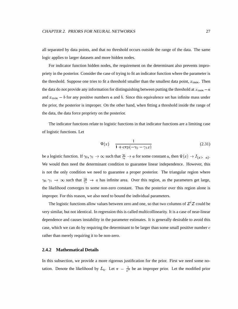
CHAPTER2. PRIORSFORNEURAL NETWORKS 27
all separatedby datapoints,andthatno thresholdoccursoutsidetherangeof thedata. Thesame
logic appliesto largerdatasetsandmorehiddennodes.
For indicatorfunctionhiddennodes,the requirementon the determinantalsopreventsimpro-
priety in theposterior. Considerthecaseof trying to fit anindicatorfunctionwheretheparameteris
thethreshold.Supposeonetriesto fit a thresholdsmallerthanthesmallestdatapoint, G Ú ��� . Then
thedatadonotprovideany informationfor distinguishingbetweenputtingthethresholdat G Ú ��� C�çand G Ú ��� C`_ for any positive numbersç and _ . Sincethis equivalencesethasinfinite massunder
theprior, theposterioris improper. On theotherhand,whenfitting a thresholdinsidetherangeof
thedata,thedataforceproprietyon theposterior.
Theindicatorfunctionsrelateto logistic functionsin thatindicatorfunctionsarea limiting case
of logistic functions.Let ��� G # � == %º>A@QB �DC - � C - h G # (2.31)
bea logisticfunction.If - � * - h /a1 suchthat À8bÀ) / ç for someconstantç , then ��� G #c/ ª TDU<[êWRZ
.
We would thenneedthe determinantconditionto guaranteelinear independence.However, this
is not the only conditionwe needto guaranteea properposterior. The triangularregion where- � * - h / 1 suchthat À bÀ0Â / ç hasinfinite area. Over this region, as the parametersget large,
the likelihoodconvergesto somenon-zeroconstant.Thusthe posteriorover this region aloneis
improper. For this reason,wealsoneedto boundtheindividualparameters.
Thelogistic functionsallow valuesbetweenzeroandone,sothattwo columnsof . R . couldbe
verysimilar, but not identical.In regressionthis is calledmulticollinearity. It is acaseof near-linear
dependenceandcausesinstability in theparameterestimates.It is generallydesirableto avoid this
case,which wecandoby requiringthedeterminantto belargerthansomesmallpositive numberìratherthanmerelyrequiringit to benon-zero.
2.4.2 Mathematical Details
In this subsection,we provide a morerigorousjustificationfor theprior. First we needsomeno-
tation. Denotethe likelihoodby ¬;� . Let � � hN O be an improperprior. Let the modifiedprior

CHAPTER2. PRIORSFORNEURAL NETWORKS 28
be � �b� � ªedgf where h � is thesetof parametervaluessuchthat II . R .JII 2 « � , ¤ - � . ¤�4 � � , and¤ � � ¤i4 � � for all ãX* / . Let
« � decreaseto 7 (for example,
« � � =j ¯ ) andlet � � increasewith ¯(for example,� ��� = 7 * 7 7 7 % ¯ ). Hereonecanclearlyseehow � � is adata-dependentprior, as h �dependsupon G through. .
Weneedto show thattheposterioris proper. Firstwewill re-writethelikelihoodsothatwecan
integrateout � . Writing thelikelihoodin vectornotationgivesus
¬ � � H � � * - *:9�¤ �ð# (2.32)� � ² � 9 ; # ê �+% ; >A@+B =? C =² 9 ; �� � � h ×ÙN�������� �0<���C � � ßà ; @A (2.33)� � ² � 9 ; # ê �+% ; >A@+Blk C =² 9 ; � . � C ^ # R � . � C ^ #Em ¶ (2.34)
Now completingthesquare:
¬n� � � ² � 9 ; # êf O >A@QB k C =² 9 ; Ç � RE.ERD. � C ² ^ RD. � .ERE. # ê h � .�RE. # � % ^ÌRE. � .ER�. # ê h .ERÞ^ %% ^ R$^ C ^ÌRD. � .ERE. # ê h .ERÞ^äÈeo (2.35)� � ² � 9 ; # êqpsr ÂO II . R . II ê ÂO >A@QBut C =² 9 ;wv � C � . R . # ê h . R ^ o R Ç . R . È v � C � . R . # ê h . R ^ o�xzy� ² � 9 ; # ê
f{}| psr Â�~O II .ERE. II ÂO >A@+B t C =² 9 ;�� ^ R$^ C ¹^ R ¹^-�ix (2.36)� H � � ¤ - *:9�*j�ð#\H � - *:9�¤ �ð#¨* (2.37)
where¹^ is thevectorof fitted values,
¹^ � d e ^ ¤ a g . Notethat H � � ¤ - *:9�*j� # is a properdensity
as long as II . R . II 2 7 , which is true over h � . Denoteby é � the subspaceof h � that relatesto
all of the - parameters,andlet � � be the subspaceof h � that relatesto all of the � parameters.
(Recallthat this boundon the � parametersis for computationalconvenienceandis necessaryfor
theconsistency of theposteriorasshown in Theorem3.3.1,but is notnecessaryfor proprietyof the
posterior.)
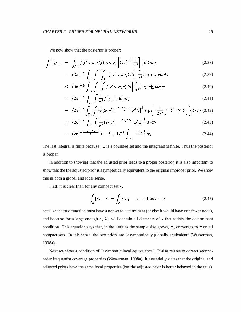
CHAPTER2. PRIORSFORNEURAL NETWORKS 29
Wenow show thattheposterioris proper:� ¬n� � � � � d f H � � ¤ - *:9�*j� #\H � - *:9�¤ � #�k � ² � # ê;� O =9 ; m� � ó9� - (2.38)� � ² � # ê � O �}� f � k ��� f H � � ¤ - *:9�*j�ð#� � m =9 ; H � - *:9�¤ �ð#� ó9� - (2.39)ò � ² � # ê;�O � � f � k � H � � ¤ - *:9�*j� #� � m =9 ; H � - *:9�¤ �ð#� ó9� - (2.40)� � ² � # ê;�O � � f � =9 ; H � - *:9�¤ � #� �9� - (2.41)� � ² � # ê;�O �}� f � =9 ; � ² � 9 ; # êf{�| psr Â�~O II . R . II ÂO >A@+Bct C =² 9 ; � ^ R ^ C ¹^ R ¹^�� x �9� - (2.42)ò � ² � # ê � O �}� f � =9 ; � ² � 9 ; # êf{}| psr Â�~O II . R . II ÂO ó9� - (2.43)� � ² � # ê
f{}| psr Â�~ rH�O � ¯ C $ % = # ê h ��� f II . R .�II ÂO - (2.44)
Thelastintegral is finite becauseé � is a boundedsetandtheintegrandis finite. Thustheposterior
is proper.
In additionto showing thattheadjustedprior leadsto a properposterior, it is alsoimportantto
show thatthetheadjustedprior is asymptoticallyequivalentto theoriginalimproperprior. Weshow
this in bothaglobalandlocalsense.
First, it is clearthat,for any compactset � ,��� ¤ � � C � ¤X� �}� ¤ � ªed f C � ¤H/ 7 as ¯ / 7 (2.45)
becausethetruefunctionmusthave anon-zerodeterminant(or elseit wouldhave onefewernode),
andbecausefor a large enough , h � will containall elementsof � that satisfythe determinant
condition. This equationsaysthat, in the limit asthesamplesizegrows, � � convergesto � on all
compactsets. In this sense,the two priors are“asymptoticallyglobally equivalent” (Wasserman,
1998a).
Next we show a conditionof “asymptoticlocal equivalence”. It alsorelatesto correctsecond-
orderfrequentistcoverageproperties(Wasserman,1998a).It essentiallystatesthattheoriginaland
adjustedpriorshave thesamelocal properties(but theadjustedprior is betterbehavedin thetails).
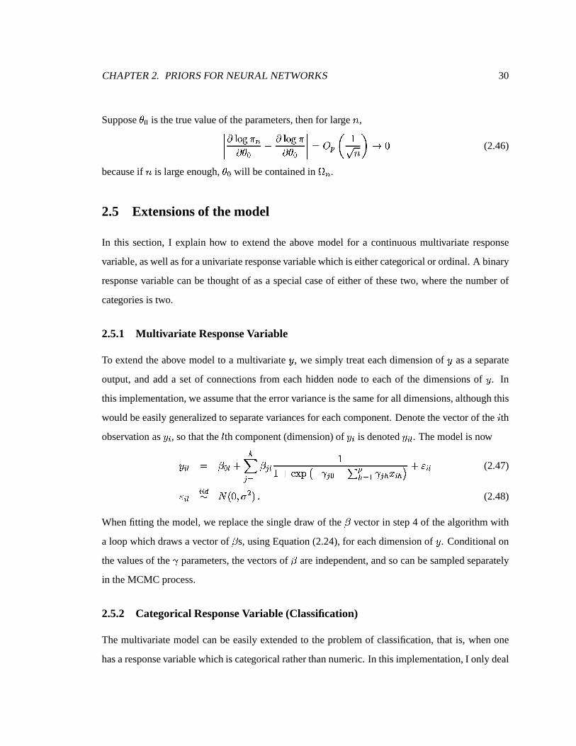
CHAPTER2. PRIORSFORNEURAL NETWORKS 30
Suppose� � is thetruevalueof theparameters,thenfor large ¯ ,IIII�� ³3´ µ � �� � � C � ³3´ µ �� � � IIII � 9 U ë =� ¯ í / 7 (2.46)
becauseif ¯ is largeenough,� � will becontainedin h � .2.5 Extensionsof the model
In this section,I explain how to extend the above model for a continuousmultivariateresponse
variable,aswell asfor aunivariateresponsevariablewhichis eithercategoricalor ordinal.A binary
responsevariablecanbe thoughtof asa specialcaseof eitherof thesetwo, wherethenumberof
categoriesis two.
2.5.1 Multi variate ResponseVariable
To extendtheabove modelto a multivariate � , we simply treateachdimensionof � asa separate
output,andadda setof connectionsfrom eachhiddennodeto eachof the dimensionsof � . In
this implementation,weassumethattheerrorvarianceis thesamefor all dimensions,althoughthis
wouldbeeasilygeneralizedto separatevariancesfor eachcomponent.Denotethevectorof the ¡ thobservationas � � , sothatthe � th component(dimension)of � � is denoted� ��� . Themodelis now� ��� � � � � %
N��Ü� h � � � == %?>A@+B Ç C - �`�VC ¸ U . � h - � .�G � . È %(' ��� (2.47)' ��� �É�324 5 �87 *:9 ; # ¶ (2.48)
Whenfitting themodel,we replacethesingledraw of the � vectorin step4 of thealgorithmwith
a loop which draws a vectorof � s,usingEquation(2.24),for eachdimensionof � . Conditionalon
thevaluesof the - parameters,thevectorsof � areindependent,andsocanbesampledseparately
in theMCMC process.
2.5.2 CategoricalResponseVariable (Classification)
The multivariatemodelcanbe easilyextendedto the problemof classification,that is, whenone
hasaresponsevariablewhichis categoricalratherthannumeric.In this implementation,I only deal

CHAPTER2. PRIORSFORNEURAL NETWORKS 31
with a univariatecategorical response.The trick is to usean alternateexpressionof the response
variable,whereinsteadof just letting the responsevariablebe thecategory number, we let it bea
vectorof indicatorvariables,whereeachcomponentcorrespondsto oneof thepossiblecategories.
Thusif wearetrying to classifyanobservationinto oneof � categories,wecanthink of theresponse
asbeingavectorof length � with aonein thepositioncorrespondingto its truecategoryandzeroes
in all of theotherpositions.
First, somenotation: let G � be the vector of explanatoryvariablesfor case¡ . Let Y � be the
responsevariablefor case¡ , wherethevalueof Y � is thecategory numberto which case¡ belongs,Y �fJ ] = * ¶"¶"¶ * � _ . Let Y �� be a vector in the alternaterepresentationof the response(a vectorof
indicatorvariables),wherethe Y ���� � = when � � Y � andzerootherwise. Now let � ��� be latent
variablescorrespondingto the Y ���� , wherethe � ��� are the resultsof fitting the multivariateneural
network modelon the G � .Someneuralnetwork classificationmodelsattemptto modeltheprobabilitythattheobservation
falls into aparticularcategory. In thatcase,onecouldhave themodel£ �¦Y �&� � Å ¤ � �Þ#·� >A@QB � � ��� Á #¸ � >A@+B � � ���Ý# ¶ (2.49)
This is thecommonmodelin thecomputerscienceliterature.However, this modelhasanentirely
differenterrorstructurethanthemodelsof this thesis.Instead,I retaintheGaussianerrorstructure
on the � � anddeterministicallyset Y �&���<� µ ����@�"¥ T h �������E� � Z � ��� (2.50)
i.e., thefitted responseis thecategory with the largest � ��� . This allows meto apply the resultsof
this thesisto thisproblemdirectly.
To fit this modelwith MCMC, we sample� � from a normaltruncatedsuchthat � � R�� 2 � ��� for�¡ � Y � . We alsoset � ��� � 7 for all ¡ , in orderto ensurethemodelis well-specified(otherwisethe
locationof all of the � ��� ’scouldbeshiftedby aconstantwithoutchangingthemodel.Thealgorithm
now becomes:
1. Startwith arbitraryinitial valuesfor - .
2. Compute. .

CHAPTER2. PRIORSFORNEURAL NETWORKS 32
3. Draw 9 ; via Equation(2.23).
4. For each� J ] = * ¶"¶"¶ * � _ , draw � � via Equation(2.24).
5. For eachã�J ] = * ¶"¶"¶ *&$¨_ , do thefollowing Metropolisstep:
(a) GenerateacandidateF- � 4T5 � - � * 7 ¶ 7HG ;Ý# .(b) Re-compute. with F- � andcomputeII . R .JII .(c) If II . R . II 2 « � and ¤ - � . ¤�4 � � for all ã * / , acceptF- � with probabilitymin � = * KO� â �MLÀ � N O Q S �KO� â � À � N O Q S � � ;
otherwiserejectthecandidateandkeepthecurrentvalueof - � .6. For each¡ andfor each� J ] = * ¶"¶"¶ * � _ , draw � ��� from anormaltruncatedsuchthat � � R�� 2 � ��� ¢
for � � � Y � .7. Repeatsteps2 though6 for therequirednumberof iterations.
2.5.3 Ordinal ResponseVariable
Sometimesonewill want to relateanordinalvariableto a setof covariates.Examplesof suchan
ordinal variableincluderankings,datawhich wereoriginally continuousbut have beencollapsed
into bins,andratingsfrom a survey wherethechoicesare“excellent”, “good”, “f air”, and“poor”.
In all of thesecases,thereis aclearorderingof thevaluesof theresponsevariable,but it is notclear
thevaluesshouldbemappedto integers.By treatingthevariableasordinal,we do not imposeany
sortof distancemetricbetweenlevelsof thevariable.
To usetheneuralnetwork modelin thischapterfor regressiononanordinalvariable,weneeda
few moreparameters.As in theclassificationsetting,let � bethenumberof levelsof theresponse
variable(the numberof bins). Let G � be the vectorof explanatoryvariablesfor case¡ . Let Y � be
the responsevariablefor case¡ , wherethe valueof Y � is the bin numberof which case¡ belongs,Y � J ] = * ¶"¶"¶ * � _ . Now let � � belatentvariablescorrespondingto the Y � , wherethe � � aretheresults
of fitting theneuralnetwork modelof thischapteronthe G � . Wealsoneedparametersfor thecut-off
valuesfor � , which we call ì h * ¶"¶"¶ * ì � ê h . If ì . ê h 4±� � ò ì . , thenwe saythat G � belongsto bin / ,
i.e., thefitted valueis¹Y �i� / . For example,if ì h 4T� � ò ì ; , thenthe ¡ th observation is assignedto
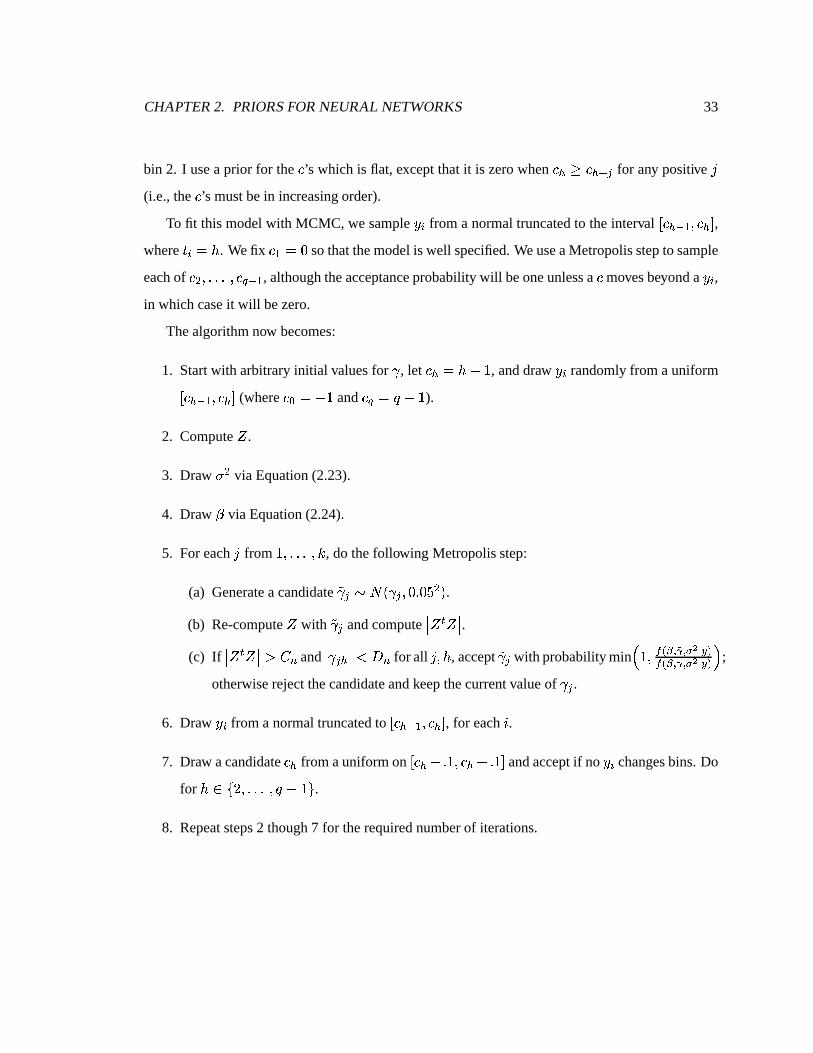
CHAPTER2. PRIORSFORNEURAL NETWORKS 33
bin 2. I usea prior for the ì ’s which is flat, exceptthatit is zerowhen ì .�£ ì . [ � for any positive ã(i.e., the ì ’smustbein increasingorder).
To fit this modelwith MCMC, we sample� � from a normaltruncatedto theinterval e ì . ê h * ì . g ,whereY �&� / . Wefix ì h � 7 sothatthemodelis well specified.WeuseaMetropolisstepto sample
eachof ì ; * ¶"¶"¶ * ì � ê h , althoughtheacceptanceprobabilitywill beoneunlessa ì movesbeyonda � � ,in whichcaseit will bezero.
Thealgorithmnow becomes:
1. Startwith arbitraryinitial valuesfor - , let ì . � / C = , anddraw � � randomlyfrom auniforme ì . ê h * ì . g (whereì � � C = and ì ��� � C = ).2. Compute. .
3. Draw 9�; via Equation(2.23).
4. Draw � via Equation(2.24).
5. For eachã from = * ¶"¶"¶ *&$ , do thefollowing Metropolisstep:
(a) GenerateacandidateF- � 4T5 � - � * 7 ¶ 7HG ; # .(b) Re-compute. with F- � andcomputeII . R . II .(c) If II . R .JII 2 « � and ¤ - � . ¤�4 � � for all ã * / , acceptF- � with probabilitymin � = *�KO� â �MLÀ � N O Q S �KO� â � À � N O Q S � � ;
otherwiserejectthecandidateandkeepthecurrentvalueof - � .6. Draw � � from a normaltruncatedto e ì . ê h * ì . g , for each¡ .7. Draw acandidateì . from auniformon e ì . C ¶ = * ì . % ¶ = g andacceptif no � � changesbins.Do
for / J ] ² * ¶"¶"¶ * � C = _ .8. Repeatsteps2 though7 for therequirednumberof iterations.

CHAPTER2. PRIORSFORNEURAL NETWORKS 34
2.6 Examples
2.6.1 MotorcycleAccident Data
Themotorcycle accidentdataof Silverman(1985)providesa niceexampleof thesmoothingabili-
tiesof a neuralnetwork nonparametricregression.Figure2.3shows theaverageof thefitted func-
tions for 10,000runs (after allowing 10,000runs for burn-in). The dark line is the meanfitted
function,andthedashedlinesarebandsof 95%posteriorpredictive probability(for thefittedvalue
of � ataparticularvalueof G ). Fourhiddennodeswereused.The G -axisis thetimein milliseconds
after thecrash,andthe � -axis theaccelerationforceon theheadof the rider. Theneuralnetwork
fitted functiondoesagoodjob of smoothingthedata,evenwith only four hiddennodes.
2.6.2 Iris Data
As anexampleof a classificationproblem,I presentananalysisof thecanonicaliris dataof Fisher
(1936).I usedonly thesubsetof thedatawhichissuppliedasabuilt-in datasetin S-Plus.Thedataset
consistsof 150observations,50 from eachof threedifferentspeciesof iris: Setosa,Versicolor, and
Virginica. For eachobservation therearefour explanatoryvariables:sepallengthandwidth, and
petallengthandwidth, all measuredin centimeters.Thegoal is to usethesefour measurementsto
classifythe flowers. Figure2.4 shows both the true andfitted values. In the top row arethe true
classificationsgiven by sepalmeasurements(on the left) andpetalmeasurements(on the right).
Usingall four variablesand3 hiddennodes,theresultsof classificationfrom a neuralnetwork are
shown in thebottomrow, with thefittedcategoriesplottedby sepalmeasurementsontheleft andby
petalmeasurementson theright. Therewerefour misclassifiedcases,all of which wereVersicolor
(denotedby % ) whichweremistakenlyclassifiedasVirginica(denotedby ¤ ). Thesefour casesare
markedwith asquarearoundthe ¤ . Noticethatthesefour casesoccurin regionsof overlapbetween
the two speciesin bothsetsof measurements,so they aredifficult casesto classifycorrectlyfrom
thisdataalone.Theneuralnetwork modelhasdoneagoodjob of classification.

CHAPTER2. PRIORSFORNEURAL NETWORKS 35
•• ••• ••• •• •• •••••• •••
•••••
•
••
••
•
••
••
••
••
•
•
•
•
•
•
•
•
•
••••
•
•
•
•
• ••
•
••
• ••
•
•
•
•••
•
•
•
•
•
•
•
•
•
•
•••
•
••
•
•
•
•
•• •
•
•
•
•
•
•
•
••
•
•
•
•••
••
•
•
•
••
•
••• •
•
• •
••
•
•
•
•
•
Time (msec)
Acc
el (
g)
10 20¥
30 40¦
50§
-100
-50
050
Figure2.3: FittedFunctionfor Motorcycle AccidentData
2.6.3 SocialAttitudes Data
Most datasetswith ordinal responsevariablestendto have relatively few continuousexplanatory
variablesand insteadhave mostly binary, ordinal, andcategorical explanatoryvariables. Neural
networks are designedfor continuousexplanatoryvariables,and may only operateto their full
potentialin that case. While they canhandleindicatorvariablesas inputs, thereis no gain to a
nonlineartransformationof anindicatorvariable,sotheretheneuralnetwork modelmaynot work
any betterthanmuchsimplermodels.Thusweshouldnotexpectbeautifulfits fromaneuralnetwork
modelif wegive it mostlynon-continuousexplanatoryvariables.

CHAPTER2. PRIORSFORNEURAL NETWORKS 36
True Values¨
Sepal Length©
Sep
al W
idth
5ª
6«
7¬
82.
02.
53.
03.
54.
0
True Values¨
Petal Length
Pet
al W
idth
1 2®
3¯
4°
5ª
6«
7¬0.
51.
01.
52.
02.
5
Fitted Values
Sepal Length©
Sep
al W
idth
5ª
6«
7¬
82.
02.
53.
03.
54.
0
Fitted Values
Petal Length
Pet
al W
idth
1 2®
3¯
4°
5ª
6«
7¬0.
51.
01.
52.
02.
5
Figure2.4: Iris Data

CHAPTER2. PRIORSFORNEURAL NETWORKS 37
FittedCategory
TrueCategory
1 2 3 4 51 29 2 23 5 72 6 4 19 4 33 7 4 25 4 24 4 3 12 4 105 5 3 18 10 51
Table2.1: SocialAttitudesData
For an exampleof an ordinal responsevariable,I fit the British SocialAttitudesSurvey data
(Witherspoon,1983). This datacomesfrom a survey of householdsin Britain in 1983of adults
18 or over living in private households.Therewasa seriesof yes/noquestionsaskingwhether
the respondentsupportedor opposeda woman’s right to have anabortionunderdifferentcircum-
stances.Therespondentswerethengroupsinto five orderedcategoriesbasedon how many of the
questionsthey answered“yes” to, with group1 answering“yes” to thefewestquestions,andgroup
5 answering“yes” to the mostquestions.The explanatoryvariablesarepolitical party affiliation
(categorical), self-assessedsocialclass(ordinal), gender(binary), age(continuous),andreligion
(categorical).
Table2.1 shows the resultsof fitting a network with 9 hiddennodesto thedata. As all of the
explanatoryvariablesbesidesagearenot continuous,thereis a high errorratefor thefitted model.
However, it is interestingto note that the modelcorrectlyfits mostof the respondentsin groups
1, 3, and5, while incorrectlyclassifyingmostof the peoplein groups2 and4 into group3. It
appearsthat peoplewho have moreextremeviews (thosein groups1 and5, i.e., peoplestrongly
opposedtheright to have anabortionor stronglyin favor of it) areeasierto classifythanthosewith
moreintermediateviews. Thosepeoplewho supportthe right to anabortionin some,but not all,
circumstancesaredifficult to distinguishby degreeto which supportthis right. It appearsthat the
modelthinksthat thedatashouldreally beclassifiedinto only threegroups,thosewho areclearly
opposedto theright to anabortionin nearlyall circumstances,thosewho favor theright in nearly
all circumstances,andthosewhofavor theright in somecircumstancesbut not in others.If thedata
werere-classifiedthisway, themodelwouldfit quitewell.

CHAPTER2. PRIORSFORNEURAL NETWORKS 38
2.7 Discussion
In this chapter, I have shown how to usean improperprior to do Bayesianinferencefor neural
networks. This is usefulbecausetheparametersin a neuralnetwork arecomplex, so it is difficult
to specifya properprior that incorporatesknowledgein a usefulway. The standardmethodsof
usinghierarchicalmodelsproducea morecomplicatedmodelthatis moredifficult to fit. Theprior
thatI have proposedis muchsimplerto work with andallows theuseof a modelwith many fewer
parametersthanahierarchicalmodel.ThismakestheMCMC processeasierandfaster.
Using restrictionsduring the Metropolis stepsof the fitting processis equivalent to the use
of a data-dependentprior. This adjustedprior producesa properposterior, andis asymptotically
equivalentto theoriginal improperprior in bothaglobalanda local sense.
The modelworkswell in practice,andhasmany usefulextensions.It canbeadaptedfor use
with multivariateresponses,aswell asbinary, categorical,andordinalresponsevariables.

Chapter 3
Asymptotic Consistency
3.1 Intr oduction
Thischapterdiscussesthelargesamplepropertiesof neuralnetwork regressionin theBayesianset-
ting. In thischapterwebuild upontheresultsof Funahashi(1989),Hornik etal. (1989),andothers.
Theseauthorshaveshown thatneuralnetworkscanapproximatea functionwith arbitraryaccuracy.
However, they all usefrequentistmethods.Herewe will show that the posterioris consistentfor
neuralnetworksin theBayesiansetting.Weshow thisconsistency in two differentparadigms.First,
we take thesieve approach,wherethenumberof hiddennodesgrows with thesamplesizesothat,
asymptotically, weuseanarbitrarily largenumberof hiddennodes.Second,wetreatthenumberof
hiddennodesasaparameterandshow thatthejoint posterioris alsoconsistent.Thus,weextendthe
theoreticaljustificationof neuralnetworksasuniversalapproximatorsto theBayesianapproach.
3.2 Consistency
Givendata ±�²´³^µ ¶·³\¸8µe¹e¹e¹ºµ±�²u»¼µ ¶¼»�¸ where²u½ maybemultivariate,let ¾<¿À±�Á�¸ betheunderlyingden-
sity of ² . Let dà¶´Ä ²ÆÅÇÁgÈcÅÇÉ+¿À±�Á�¸ bethetrueregressionfunctionof ¶ on ² , andlet ÊÉ<»i±�Á˸ be
theestimatedregressionfunction.
39

CHAPTER3. ASYMPTOTIC CONSISTENCY 40
Definition 1 ÊÉÀ» is asymptoticallyconsistentfor É+¿ ifÌ ±eÊÉ » ±�Á�¸�Í)É ¿ ±�Á�¸Î¸sÏ·¾ ¿ ±�Á�¸�ÐHÁÒÑÓÕÔ ¹ (3.1)
Anotherapproachto consistency is to take it to meanthat the posteriorprobability of every
neighborhoodof thetruefunctiontendsto oneasthesamplesizegrows large.Doob(1949)showed
thatBayesianmethodsareconsistentalmostsurelywith respectto theprior. However a prior that
putsnomassnearthetruefunctionwill givenoposteriormassnearthetruefunction.For example,
supposethat ²×Ö5ØÙ±!Ú�µ^Û¸ . If theprior is apointmassatany point, thentheposteriorwill alsobea
pointmassat thesamepoint,whichwill bethecorrectanswerwith probability1 with respectto the
prior. However, thetrueanswercouldbeany point,or any otherdistribution for Ú , sothisprior will
give anincorrectposterioranswer. Theproblemis thatall otherpossibilitieshave probabilityzero
underthis particularprior. In general,onewantsto avoid this possibleproblemandensurethatthe
choiceof prior andestimatorwill beconsistentover a largeclassof distributions.
In whatfollows, we will considertheconsistency of densityfunctions,andwill latershow that
this translatesinto theabove definitionof consistency on theassociatedregressionfunctions.Some
of theideashereandin theproof of Theorem3.3.1(in thenext section)canbefoundin Barronet
al. (1998)andWasserman(1998b).
Onepossiblechoiceof neighborhoodsfor densityfunctionsis thesetof weakneighborhoods.
Let ¾<¿P±�ÁܵÎÝg¸ by the trueunderlyingjoint densityfunctionfor Á and Ý , andlet ¾À»¼±�ÁºµÎÝ�¸ betheesti-
mateddensityfunction.Let Þ�ß beany distancethatinducestheweaktopology, i.e. Þ�ß)±à¾À»Xµ&¾<¿e¸ ÓÔ if andonly if á�Éi±�Á�¸s¾À»i±�Á�¸�ÐHÁ Ó á�Éi±�Á�¸s¾<¿+±�Á˸�ÐHÁ for every bounded,continuousfunction É . Then
defineasize â weakneighborhoodof ¾<¿ to be ãP¾;Ä Þ�ßl±à¾iµ&¾<¿\¸�ä>âRå . It hasbeenshown (Diaconisand
Freedman,1986)thathaving a prior which putspositive masson weakneighborhoodsof ¾ ¿ does
notguaranteethattheposteriormassof everyweakneighborhoodof ¾ ¿ will tendto 1.
Insteadof weakneighborhoods,we useHellinger neighborhoodswhendealingwith density
functions. This topologyis equivalentto that using æç³ neighborhoods.The Hellingerdistanceis
definedas Þ�è�±à¾iµ&¾<¿R¸cÅ Ì�ÌÆé�ê ¾c±�ÁܵÎÝg¸ºÍ ê ¾<¿<±�ÁܵÎÝg¸së Ï ÐHÁiÐHÝù (3.2)

CHAPTER3. ASYMPTOTIC CONSISTENCY 41
Definition 2 Suppose±�²u½�µ ¶¼½�¸;Ö5¾<¿ . Theposteriorisasymptoticallyconsistentfor ¾<¿ overHellinger
neighborhoodsif
for every âíì Ô µ î>±DãP¾�ï Þ�è�±à¾iµ&¾<¿e¸qð>âRå}Ä�±�²´³Pµ ¶·³\¸8µe¹e¹e¹ºµ±�²u»¼µ ¶¼»�¸Î¸JÑÓ Ûñ¹ (3.3)
In thenext section,Theorem3.3.1will show thatthedensitiesassociatedwith neuralnetworksare
asymptoticallyconsistentover Hellingerneighborhoodsundercertainconditions.
3.3 Asymptotic Consistencyfor Neural Networks
3.3.1 SieveAsymptotics
A neuralnetwork is simplyalinearcombinationof non-linearfunctionsof thecovariates.A popular
choiceof thisnon-linearfunction,alsocalledanactivationfunction,is thelogisticfunction, òu±!ó}¸;ų³Dôiõàö\÷<øúùXû&ü . The network containsý inputs (explanatoryvariables)and þ hiddennodes. At each
hiddennode,a weightedcombinationof theinputs(input weightsÿ���� ) is usedastheargumentfor
thelogistic function.Finally aweightedsumof theoutputsof thelogisticsis computedwith output
weights� � . Theresultingregressionfunctionis
dà¶X½ Ä ²u½ÜÅ ÁX½�ÈËÅ��¼¿�� ��� ³ � � ÛÛ��� ������sÍíÿ ��� Í������ ³ ÿ����ÀÁ ½ ��� ¹ (3.4)
Herewe will show theasymptoticconsistency of theposteriorfor neuralnetworks. We do this
by estimatingthejoint densityfunction ¾c±�ÁºµÎÝ�¸ , andrelatingit backto theconditionalexpectation.
We take ² to be uniformly distributed in Â Ô µ^Û\È � (sincethe explanatoryvariablesare thoughtof
asfixed, we canuseany convenientdistribution). Conditionalon ² , ¶ is normally distributed
with meandeterminedby the neuralnetwork. We shall fix its standarddeviation to be 1 for this
calculation.Thus¶´Ä ² Å ÁwÖ�Ø �� �X¿ � ��� ³ � �Û!�� ��"�#�ÎÍíÿ ��� Í � � �$ ³ ÿ����PÁ%��� µ^Û'&( ¹ (3.5)
Thenumberof inputvariables,ý , will alwaysbetakenasfixed.Thenumberof hiddennodes,þ , will
generallybeallowedto grow with thesamplesize.Now a bit of notationneedsto beintroduced.
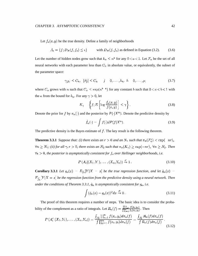
CHAPTER3. ASYMPTOTIC CONSISTENCY 42
Let ¾<¿<±�ÁܵÎÝg¸ bethetruedensity. Definea family of neighborhoods)+* Å ãP¾�ï Þ�è�±à¾iµ&¾<¿\¸ ð>âeå with Þ�è�±à¾iµ&¾<¿e¸ asdefinedin Equation(3.2). (3.6)
Let thenumberof hiddennodesgrow suchthat þ » ð�,.- for any Ô ä0/�äzÛ . Let 1 » bethesetof all
neuralnetworkswith eachparameterlessthan 2q» in absolutevalue,or equivalently, thesubsetof
theparameterspace:Ä ÿ����XÄ�ð32 » µ Ä � � Ä}ð�2 » 4 Å Ô µe¹e¹e¹Üµ&þ » µ65ÃÅ Ô µe¹e¹e¹Üµ!ýܵ (3.7)
where 2q» grows with , suchthat 2q»�ð7 ��"�º±8,.9 ù -À¸ for any constant: suchthat Ô ä;/ ä<:·älÛ with
the / from theboundfor þ » . For any ÿzì Ô , let=?> ÅA@c¾�ï:dCBEDGF�H ¾ ¿ ±�ÁܵÎÝg¸¾c±�ÁܵÎÝg¸JI ð ÿ!K´¹ (3.8)
Denotetheprior for ¾ by Lg»i±NM�¸ andtheposteriorby î�±NM�Ä ² » ¸ . Denotethepredictive densitybyʾÀ»¼±NM�¸qÅ Ì ¾c±NM�¸�Ð�î�±à¾;Ä ² » ¸8¹ (3.9)
Thepredictive densityis theBayesestimateof ¾ . Thekey resultis thefollowing theorem.
Theorem 3.3.1 Supposethat: (i) there existsan O ì Ô andan Ø�³ such that LX»i±P1?Q» ¸ äR ��"�º±�ÍS,TO�¸8µU ,WV Ø�³ ; (ii) for all ÿºµXOuì Ô , there existsan Ø Ï such that Lg»Ë± =Y> ¸ZV[ �����±�ÍS,TO�¸8µ U ,WV Ø Ï . ThenU âçì Ô , theposterioris asymptoticallyconsistentfor ¾<¿ over Hellinger neighborhoods,i.e.î ± )\* Ä�±�²´³^µ ¶·³\¸8µe¹e¹e¹ºµ±�²u»¼µ ¶¼»�¸Î¸ ÑÓ Ûñ¹ (3.10)
Corollary 3.3.1 Let É+¿+±�Á˸ Å d+]_^+ ¶ Ä ² Å ÁgÈ be the true regressionfunction, and let ÊÉ<»i±�Á˸ Åda`]Nb  ¶´Ä ² Å�ÁXÈ betheregressionfunctionfromthepredictivedensityusinga neural network.Then
undertheconditionsof Theorem3.3.1, ÊÉÀ» is asymptoticallyconsistentfor É<¿ , i.e.Ì ±\ÊÉÀ»�±�Á˸ºÍ)É+¿+±�Á˸θ Ï Ð�Á ÑÓÕÔ ¹ (3.11)
Theproof of this theoremrequiresa numberof steps.Thebasicideais to considertheproba-
bility of thecomplementasa ratioof integrals.Let c »i±à¾·¸cÅed bfhg"i ] øhj fEk lmf üd bfhgni ]_^ øhj fEk lmf ü . Thenî>± ) Q* Ä�±�²´³^µ ¶·³\¸8µe¹e¹e¹ºµ±�²u»¼µ ¶¼»�¸Î¸nÅ áporqsrt »½ ³ ¾c±�ÁX½�µÎÝ+½�¸�ÐuLg»�±à¾·¸áYt »½ ³ ¾c±�Á ½ µÎÝ ½ ¸�ÐuL » ±à¾·¸ Å á�ovqs c�»Ë±à¾·¸�ÐuLX»i±à¾·¸áwc » ±à¾·¸�ÐuL » ±à¾·¸ ¹(3.12)
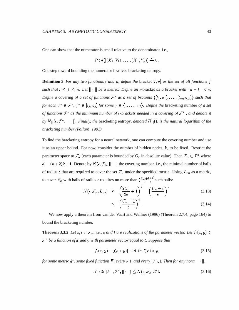
CHAPTER3. ASYMPTOTIC CONSISTENCY 43
Onecanshow thatthenumeratoris smallrelative to thedenominator, i.e.,î>± ) Q* Ä�±�² ³ µ ¶ ³ ¸8µe¹e¹e¹Üµ±�² » µ ¶ » ¸Î¸ ÑÓÕÔ ¹Onesteptowardboundingthenumeratorinvolvesbracketingentropy.
Definition 3 For any two functions x and y , definethe bracket  x�µXygÈ as the setof all functions ¾such that x ð ¾ ðzy . Let Ä�Ä{M¼Ä�Ä bea metric. Definean â -bracket as a bracket with Ä�Ä y ÍRx Ä�Ä�ä â .Definea covering of a setof functions1?| as a setof brackets ã� x ³ µXy ³ È�µe¹e¹e¹ÜµÂ x~}�µXyr}çÈàå such that
for each ¾ |�� 1 | , ¾ |��  x � µXy � È for some4 � ã�Û<µe¹e¹e¹ÜµX�0å . Definethebracketingnumberof a set
of functions1 | as theminimumnumberof â -bracketsneededin a coveringof 1 | , anddenoteit
by Ø#�G�E±àâeµ�1 | µPÄ�Ä�M�Ä�Ä�¸ . Finally, thebracketingentropy, denoted���G�E±�¸ , is thenatural logarithmof the
bracketingnumber(Pollard, 1991)
To find thebracketingentropy for a neuralnetwork, onecancomputethecoveringnumberanduse
it asan upperbound. For now, considerthenumberof hiddennodes,þ , to be fixed. Restrictthe
parameterspaceto 1ç» (eachparameteris boundedby 2q» in absolutevalue).Then 1ç»#��c�� whereÐuÅDZ�ý����H¸sþ��¡Û . Denoteby ØÙ±àâ^µ�1 » µPÄ�Ä�MPÄ�Ä�¸ thecoveringnumber, i.e., theminimalnumberof balls
of radius â thatarerequiredto cover theset 1 » underthespecifiedmetric. Using æ6� asa metric,
to cover 1ç» with ballsof radius â requiresnomorethan ��� b ôº³* � � suchballs:Ø¡±àâeµ�1ç»iµ æ � ¸ ð � ��2q»�+â � Û'� � Å�� 2q»��¡ââ � � (3.13)ð � 2q»���Ûâ � � ¹ (3.14)
We now applya theoremfrom vanderVaartandWellner(1996)(Theorem2.7.4,page164)to
boundthebracketingnumber.
Theorem 3.3.2 Let �HµX� � 1ç» , i.e., � and � are realizationsof theparametervector. Let ¾�� ±�ÁܵÎÝg¸ �1�| bea functionof Á and Ý with parametervectorequalto � . SupposethatÄ ¾��&±�ÁºµÎÝ�¸ñÍ ¾��^±�ÁܵÎÝg¸eÄ}ð Ð | ±��HµX� ¸N��±�ÁºµÎÝ�¸ (3.15)
for somemetric Ð | , somefixedfunction � , every ��µX� , andevery ±�ÁܵÎÝg¸ . Thenfor anynorm Ä�Ä�M�Ä�Ä ,Ø �~� ±��+âÀÄ�Ä �JÄ�Ä�µ�1 | µPÄ�Ä�M�Ä�Ä�¸ ð Ø¡±àâeµ�1ç»iµ Ð | ¸8¹ (3.16)

CHAPTER3. ASYMPTOTIC CONSISTENCY 44
Sincewe areinterestedin computingtheHellingerbracketingentropy for neuralnetworks,we
needto usethe æ Ï normon thesquarerootsof thedensityfunctions,¾ . The æ � coveringnumber
wascomputedabove,sohereÐ�|çÅ�æ � . Theversionof thetheoremweareinterestedin is:
If Ä ê ¾��α�ÁºµÎÝ�¸ñÍ ê ¾��±�ÁºµÎÝ�¸eÄ�ð Ð{|+±���µX�θN�J±�ÁܵÎÝg¸ for some�íµ (3.17)
then Ø��G�E±��+âÀÄ�Ä �JÄ�Ä Ï µ�1�|<µPÄ�Ä�M�Ä�Ä Ï ¸ ð>ØÙ±àâ^µ�1综µ Ð�|^¸8¹ (3.18)
To show thattheconditionholdstrue,applytheFundamentalTheoremof IntegralCalculus.For
particularvectors� and � , let Éi±8y˸qÅz� ¾ ø�øú³Îù��PüP�Dô%�p�úü ±�ÁܵÎÝg¸ . Let ¢¡·ÅDZsÛ;Í;y�¸��p¡u��yv�N¡ anddenotethe
spaceof ¢¡ by £Z¡ . Then,ê ¾�� ±�ÁºµÎÝ�¸�Í ê ¾��±�ÁºµÎÝ�¸ Å Ì ³� ÐHÉÐ�y Ð�y (3.19)Å Ì ³� � ¡ ³W¤ ɤ ¢¡ ¤ ¡¤ y Ðuy (3.20)Å Ì ³� � ¡ ³ ¤ ɤ ¢¡ ±8�_¡ËÍ¥��¡!¸}Ðuy (3.21)Å � ¡ ³ ±8�_¡ËÍ¥��¡�¸ Ì ³� ¤ ɤ ¦¡ Ðuy (3.22)ð � ¡ ³.§m¨ �¡ Ä �N¡iÍ¥�p¡ Ä Ì ³� §m¨ �© fEª�«�f�¬¬¬¬ ¤ ɤ ¢¡ ¬¬¬¬ Ð�y (3.23)Å §m¨ �¡ Ä �N¡iÍ��p¡ÎÄ � ¡ ³�§m¨ �© fEª�«vfv¬¬¬¬ ¤ ɤ ¢¡ ¬¬¬¬ Ì ³� Ð�y (3.24)ð §m¨ �¡ Ä �N¡iÍ��p¡ÎÄ � ¡ ³.§m¨ �¡ B §m¨ �© fEª�«vf ¬¬¬¬ ¤ ɤ ¡ ¬¬¬¬ I (3.25)Å Ð §m¨ �¡ Ä � ¡ Í¥� ¡ Ä §m¨ �¡ B §m¨ �© f�ª�«�f�¬¬¬¬ ¤ ɤ ¢¡ ¬¬¬¬ I (3.26)Å Ä�Ä ��Í��}Ä�Ä �w��±�ÁºµÎÝ�¸8µ (3.27)
where �J±�ÁܵÎÝg¸íÅ Ð §m¨ � ¡� §m¨ � © fEª�«�f ¬¬¬u®p¯® © f ¬¬¬ ° . Here ®'¯® © f is thepartialderivative of ± ¾ with respectto
the ² th parameter. Recallthat ¾c±�ÁºµÎÝ�¸nÅ5¾c±�Ý�Ä Á�¸s¾c±�Á˸ where¾c±�Á˸cÅ Û since² Ö´³ Â Ô µ^Û\È and ¾c±�Ý·Ä Á˸

CHAPTER3. ASYMPTOTIC CONSISTENCY 45
is normalwith meandeterminedby theneuralnetwork andvariance1. Thuswehaveê ¾c±�ÁºµÎÝ�¸ Å ±���Lܸ ù�³_µN¶ �����·¸RÍ Û¹ �� Ý�ÍW� ¿ Í ��� ³ � �Û!�� ��"�#� Ííÿ ��� Í � � �� ³ ÿ����ÀÁr��� &( Ï�º» µ¤ ± ¾¤ �X¿ Å Û� �� Ý�ÍW�¼¿qÍ ��� ³ � �Û6�� ��"� � Ííÿ ��� Í�� � �� ³ ÿ����PÁ%� � &( ê ¾c±�ÁºµÎÝ�¸\µ¤ ± ¾¤ � Q Å Û� M ÛÛu�w ���� � Ííÿ Q ¿HÍ�� � �� ³ ÿ Q �ÀÁ%� � �� ݺͼ�X¿}Í ��� ³ � �Ûu�w ��"� � Íçÿ � ¿HÍw� � �$ ³ ÿ����ÀÁ%� � &( ê ¾c±�ÁܵÎÝg¸Å ÛÛ!�� ���� � Ííÿ Q ¿ Í � � �� ³ ÿ Q �ÀÁ%� � ¤ ± ¾¤ � ¿ ½ Å Û<µe¹e¹e¹Üµ&þiµ¬¬¬¬ ¤ ± ¾¤ � Q ¬¬¬¬ 𠬬¬¬ ¤ ± ¾¤ � ¿ ¬¬¬¬ ½ Å Û<µe¹e¹e¹ºµ&þiµ¤ ± ¾¤ ÿ Q ¿ Å Í � Q ��"� � Ííÿ Q ¿qÍ¥� � �� ³ ÿ Q �PÁ%� ��ÎÛ6�� ��"�<¾�Ííÿ Q ¿ Í � � �$ ³ ÿ Q �<Ár��¿'� Ï ¤ ± ¾¤ �X¿ ½ Å Û<µe¹e¹e¹ºµ&þiµ
¬¬¬¬ ¤ ± ¾¤ ÿ Q ¿ ¬¬¬¬ 𠬬¬¬ 2q» ¤ ± ¾¤ � ¿ ¬¬¬¬ ½ Å Û<µe¹e¹e¹�µ&þiµ¤ ± ¾¤ ÿ Q � Å Í Á � � Q ��"� � Íçÿ Q ¿ Í � � �� ³ ÿ Q �ÀÁr� �� Û6�� ��"� ¾ Ííÿ Q ¿;Í � � �$ ³ ÿ Q �<Ár� ¿'� Ï ¤ ± ¾¤ �X¿ ½ Å Û<µe¹e¹e¹ºµ&þiµÜÐ�Å Û<µe¹e¹e¹Àµ!ýܵ
¬¬¬¬ ¤ ± ¾¤ ÿ Q � ¬¬¬¬ 𠬬¬¬ Á � 2q» ¤ ± ¾¤ � ¿ ¬¬¬¬ ½ ÅÇÛ<µe¹e¹e¹Üµ&þiµÜÐuÅ Û<µe¹e¹e¹µ!ýº¹Now notice that �� û é ó� ��"� é Í û�À¶ ë�ë×Å é ÛíÍ û�ÀÏ ë\ ���� é Í û�À¶ ë . So ó ��"� é Í û�À¶ ë ° has a mini-
mum of Í ± � Á ù�³_µ Ï at Í ± � anda maximumof ± � Á ù�³_µ Ï at � ± � . Thus ¬¬¬ ®� ]®'à ^ ¬¬¬ ð �ÅÄ L.Á Ï � ù�³_µN¶ ,¬¬¬ ®  ]® > q ^ ¬¬¬ ðe2q»w� Ä L.Á Ï � ù�³_µN¶ , and ¬¬¬ ®  ]® > q8Æ ¬¬¬ ð Á � 2q»�� Ä L.Á Ï � ù�³_µN¶ . Recalling that ² Ödz Â Ô µ^Û\È , it is
apparentthat ¬¬¬ ®  ]® > q8Æ ¬¬¬ ðÈ2q» �ÅÄ L.Á Ï � ù�³_µN¶ . Thus ¬¬¬ ®'¯® © f ¬¬¬ ðÈ2q» �ÅÄ L.Á Ï � ù�³_µN¶ for all ² which gives us��±�ÁºµÎÝ�¸;Å5Ð�2q» �ÉÄ L.Á Ï � ù�³_µN¶ for Equations(3.16)and(3.27).For furthermathematicalconvenience,
wewill use�J±�ÁܵÎÝg¸;Å � � bÏ ì Ð�2 » � Ä L.Á Ï � ù�³_µN¶ .Now applyTheorem3.3.2with � Å � � bÏ and æ Ï for anormonthesquarerootsof thedensities
(i.e. Hellingerdistance)to getthatØ �Ê� ±��+âPÄ�Ä �ÃÄ�Ä Ï µ�1 | µPÄ�Ä�M�Ä�Ä Ï ¸ ð Ø¡±àâeµ�1 » µ Ð | ¸ andhence (3.28)Ø��~�à±àâ^µ�1 | µPÄ�Ä�M�Ä�Ä Ï ¸ ð � Ð�2q»Ë±É2q»���Û¸â � � ð � м±É2 |» ¸ Ïâ � � where2 |» ÅË2 » �´Û<¹ (3.29)

CHAPTER3. ASYMPTOTIC CONSISTENCY 46
For notationalconvenience,thestarwill bedroppedin futurecalculations.Having establishedthis
boundfor a fixed þ , we cannow let þH» grow suchthat þ+»wð�,.- for any constantÔ ä�/íä)Û . Denote
by ���G��±�¸;Å3DGF�H Ø��Ê��±�¸ theHellingerbracketingentropy.
Lemma 3.3.1 Suppose� �G� ±8y˸�ð�DGF�H B é � Àb � b� ë � b I , ÐH» Å ±�ý<�Ì�H¸sþH»�� Û , þ+»ÒðÍ,.- and 2q»5ð ��"�º±8,.9 ù -À¸ for Ô ä´/ ä´:�ä Û . Thenfor anyfixedconstants½ , â ì Ô , andfor all sufficiently large, ,Ì *� � � �G� ±8y˸�ð ½ ± ,Üâ Ï .
Proof.Ì *� � ���G�E±8y˸�Ð�y ð Ì *� ÎÏÏÐ DGF�HÒÑ�� 2 Ï» ÐH»y � � b�Ó Ð�y by Equation(3.29) (3.30)Å ê ÐH» Ì *�7Ô DGF�H 2 Ï» ÐH»y Ð�y (3.31)Å Ô ÐH»� Ì3Õ ÏuÖØ×XÙÛÚ Àb Æ bs� Í\2 Ï» ÐH»uÜ Ï Á ù�Ý�ÀXµ Ï ÐuÜ with ÜuÅ � �ÛDGF�H � Àb � b� (3.32)Å 2 Ï» Ð » Ô Ð�»� Ì �Õ Ï{ÖØ×XÙ¦Ú Àb Æ bs Ü Ï Á ù�Ý�Àmµ Ï ÐuÜ now integrateby parts (3.33)Å 2 Ï» Ð�» Ô Ð�»� Ñ�ÍSÜ�Á ù�Ý�Àmµ Ï ¬¬¬ � Õ ÏuÖØ×XÙ¦Ú Àb Æ bs � Ì �Õ Ï�ÖØ×XÙ�Ú Àb Æ bs Á ù�Ý�Àmµ Ï ÐuÜ Ó (3.34)Å 2 Ï» Ð�» Ô Ð�»� Ñ â2 Ï» ÐH» Ô �ÛDGF�H 2 Ï» Ð�»â � ± ��L Ì �Õ ÏuÖØ×XÙÛÚ Àb Æ bs Û± ��L Á ù�Ý�ÀXµ Ï Ð�Ü Ó (3.35)
ð 2 Ï» Ð�» Ô Ð�»� ·ÞÞ¸ â2 Ï» ÐH» Ô �ÛDGF�H 2 Ï» ÐH»â � ± ��LSß � � �ÛDGF�H � Àb � b* �� �ÛDGF�H � Àb � b* ºáàà» by Mill’ sRatio (3.36)
Å 2 Ï» Ð�» Ô Ð�»� ·¸ â2 Ï» ÐH» Ô �ÛDGF�H 2 Ï» ÐH»â � ± ��L� �ÛDGF�H � Àb � b* Û± ��L â2 Ï» Ð�» º» (3.37)Å â Ô Ð�»� Ô �ÛDÊF�H 2 Ï» Ð�»â Ñ8Û6� Û�ÛDGF�H � Àb � b* Ó(3.38)ð â ê Ð�» Ô DÊF�H 2 Ï» Ð�»â Â�Û6�5Û\È (3.39)Å �+â ê Ð�» ê DÊF�HZ2 Ï» �âDGF�HqÐ�»�ÍaDGF�H�â�¹ (3.40)

CHAPTER3. ASYMPTOTIC CONSISTENCY 47
Now substitutein ÐH»Jð ±�ýÛ�Y�H¸_, - �´Û<µ�2q»JðR �����±8, 9 ù - ¸ to getthatÌ *� � � �ã� ±8y˸�Ð�yzð[�+â ê ±�ý��Y�H¸_, - �´Û � ��, 9 ù - ��DGF�Hi±Î±�ýÛ�Y�H¸_, - �´Û¸PͼDGF�H�â�¹ (3.41)
Since Ô ä7/ äÌ:�äÇÛ , thereexistsa ÿ suchthat / ä ÿ3äÌ: and :�Í¥/�ä ÛçÍ3ÿ . This follows from
thefactthatsinceÔ ä�/Jä[: äÒÛ , theremustexist a ä�ì Ô suchthat /+��ä�ä�: and :¢��ä�äÒÛ . Now
let ÿwÅ3/��âä to seethat :qÍa/ ÅË: �âä�Í>±E/��RäÀ¸ ä ÛíÍ>±E/��âä<¸;Å ÛíÍ)ÿ .
Hence,Û± , Ì *� � ���Ê��±8y�¸�Ð�y ð (3.42)�+â ± , ù > ê ±�ýY���H¸_, - ��Û ê , ù�ø�³Îù > ü � ��, 9 ù - ��DGF�H¼±Î±�ý?�â�H¸_, - �5Û¸�ÍaDGF�Hqâ¡Å (3.43)�+â � ±�ýÛ�Y�H¸_, ù�ø > ù - ü �w, ù > � ��, ù�ø�ø�³Îù > ü ùPø 9 ù - ü�ü �w, ù�øú³Îù > ü DGF�H¼±Î±�ýÛ�Y�H¸_, - �´Û¸PÍ�, ù�ø�³Îù > ü DGF�H�â (3.44)ÓÕÔ as , Óæå ¹ (3.45)
Thusfor ½ µ&â ì Ô andsufficiently large , ,Û± , Ì *� � � �G� ±8y�¸�Ð�yzð ½ â Ï ¹ (3.46)
And soÌ *� � � �G� ±8y˸�Ðuy ð ½ ± ,·â Ï ¹ ç
WongandShen(1995)showedthefollowing result:
Theorem 3.3.3 Let c »i±à¾·¸cÅÌt »¡ ³ ] øáj f�k lmf ü] ^ øáj fEk lmf ü . There exist ½ ³^µ ½ Ï µ ½�è µ ½ ¶�ì Ô such that for any âíì Ô ,if
Ì Â Ï ** À µ ÏXé � �;�G�E±8yëê ½�è ¸�Ð�y ð ½ ¶ ± ,·â Ï µ (3.47)
then î |¼ì §m¨ �] ª ovqsNí�î b c »i±à¾·¸6VR ��"�º±�Í ½ ³X,Üâ Ï ¸Nï ð ¹ �����±�Í ½ Ï ,Üâ Ï ¸8¹ (3.48)
Corollary 3.3.2 Under the conditionsof Theorem 3.3.3, §m¨ �] ª orqs í�î b c »i±à¾·¸qð ¹ ����ñ±�Í ½ Ï ,Üâ Ï ¸ a.s.
for sufficientlylarge n.
Proof. FromLemma3.3.1wehave thatÌ ** À µ Ï é � ���G��±8y˸�Ðuy ð Ì *� � �;�ã��±8y�¸�Ð�yzð ½ ¶ ± ,Üâ Ï .
Absorbthe constant½�è into the constant2q» of Lemma3.3.1andsubstitute± ��â for â to get thatÌ Â Ï ** À µ Ï é � ���G�E±8yëê ½ è ¸�Ðuy�ð[� ½ ¶ ± ,Üâ Ï . Absorbingthe � into ½ ¶ givestheconditionsfor Theorem3.3.3,
which impliesthat î | ì §�¨ �] ª orqs í�î b c »Ë±à¾·¸6VR �����±�Í ½ ³m,Üâ Ï ¸ ï ð ¹ ��"��±�Í ½ Ï ,Üâ Ï ¸ . Now apply thefirst
Borel-CantelliLemma. ç

CHAPTER3. ASYMPTOTIC CONSISTENCY 48
Wecannow boundthenumeratorof Equation(3.12).
Lemma 3.3.2 Let c »i±à¾·¸íÅzt »¡ ³ ] øáj f�k lmf ü] ^ øhj fÉk lmf ü betheratio of likelihoodsunderneural network ¾ and
thetrueneural network¾<¿ . Let 1ç» beasin Equation(3.7).SupposethatÌ *� � � �G� ±8y�¸}Ð�yzð ½ ± ,Üâ Ï
for all âçì Ô . If there existsa constantOuì Ô such that 1 » satisfiesL » ±P1 Q» ¸íä� ��"�º±�ÍS,TO�¸ U ,WV Ø ,
thenthere existsa constant½ Ï such that áporqs c »i±à¾·¸�Ð{Lg»�±à¾·¸ ä[ ��"�º±�Í »�ðÏ ¸.�� ��"�º±�ÍS, ½ Ï â Ï ¸ excepton
a setof probability tendingto zero.
Proof. Decomposetheintegral into two parts:Ì orqs c »i±à¾·¸�Ð{Lg»Ë±à¾·¸ÆÅ Ì orqs í�î¦qb c »i±à¾·¸�ÐuLX»i±à¾·¸T� Ì ovqs í�î b c »Ë±à¾·¸�ÐuLg»Ë±à¾·¸ (3.49)ð Ì î¢qb c »Ë±à¾·¸�ÐuLg»Ë±à¾·¸.� Ì orqs í�î b c »i±à¾·¸�Ð{Lg»i±à¾·¸¼¹ (3.50)
Thesecondintegral is boundedasfollows:Ì ovqs í�î b c�»Ë±à¾·¸�ÐuLX»i±à¾·¸ ð §m¨ �o q s í�î b c »Ë±à¾·¸NLg»i± ) Q*Jñ 1ç»�¸ (3.51)ð §m¨ �o q s í�î b c »Ë±à¾·¸ (3.52)ð ��"�º±�ÍS, ½ Ï â Ï ¸ a.s. by Corollary3.3.2¹ (3.53)
Now let ½ ì Ô . Denotethe samplespaceby ò » with observed data Á » , and denotethe true
distribution functionfor thedataby î »¿ . Let ó beLebesguemeasure.î ì Ì î¦qb c » ±à¾·¸�ÐuL » ±à¾·¸ ì ½ ï ð Û½vô Ñ Ì î¦qb c » ±à¾·¸�ÐuL » ±à¾·¸ Ó by Markov’s Inequality(3.54)Å Û½ Ìnõ b Ì î¢qb c » ±à¾·¸�Ð{L » ±à¾·¸}Ð�î »¿ (3.55)Å Û½ Ì õ b Ì î¢qb c »i±à¾·¸�Ð{Lg»Ë±à¾·¸ Ð�î »¿Ð"ó Ð�óº±�Á˸ (3.56)Å Û½ Ì õ b Ì î¢qb ¾c±�Á » ¸¾<¿<±�Á » ¸ ÐuLg»Ë±à¾·¸�¾<¿À±�Á » ¸}Ð"óܱ�Á » ¸ (3.57)Å Û½ Ì õ b Ì î¢qb ¾c±�Á » ¸�ÐuL » ±à¾·¸}Ð"óܱ�Á » ¸ (3.58)

CHAPTER3. ASYMPTOTIC CONSISTENCY 49
Å Û½ Ì î¢qb B Ì"õ b ¾c±�Á » ¸�Ð�óº±�Á » ¸ I ÐuLX»i±à¾·¸ by Fubini’s Theorem (3.59)Å Û½ Ì î¢qb Ð{Lg»Ë±à¾·¸ (3.60)Å Û½ Lg»Ë±P1 Q» ¸ (3.61)ä Û½ �����±�ÍS,TO�¸ for ,�V Ø�¹ (3.62)
Now let ½ Å� ��"�º±�Í »�ðÏ ¸ . Thenî ì Ì î¢qb c »i±à¾·¸�Ð{Lg»Ë±à¾·¸qìR �����±�Í ,TO� ¸ ï äö ��"�º±�Í ,TO� ¸8¹ (3.63)
Thus î é á'î¢qb c »Ë±à¾·¸�ÐuLg»Ë±à¾·¸ ìR ��"�º±�Í »�ðÏ ¸�ë ÑÓ Ô andso á�î¦qb c »i±à¾·¸�ÐuLX»Ë±à¾·¸ ä7 ��"�º±�Í »�ðÏ ¸ excepton
asetwith probabilitytendingto zero.Combiningthetwo partsof theintegral givesÌ o q s c »i±à¾·¸�ÐuLX»i±à¾·¸ ð Ì î qb c »i±à¾·¸�Ð{Lg»Ë±à¾·¸T� Ì o q sNí�î b c�»Ë±à¾·¸�ÐuLX»i±à¾·¸ (3.64)ä ����º±�Í ,TO� ¸T�� ��"�º±�ÍS, ½ Ï â Ï ¸8¹ (3.65)
Wherethelastinequalityholdsexceptonasetwith probabilitytendingto zero. çNext a lower boundis foundfor thedenominatorof Equation(3.12).
Lemma 3.3.3 Let ý and ÷ be any two densityfunctions. Denotethe Kullback-Leibler distance
betweený and ÷ by Þ?ø�±�ýºµm÷+¸ . Then
ô � ¬¬¬¬ DGF�H ý ÷ ¬¬¬¬ ð Þ?ø ±�ýܵm÷H¸.� � Á ¹ (3.66)
Proof. Let) ÅúùiÁÜïmDGF�H � û ì Ôvü . Then
ô � ¬¬¬¬ DGF�H ý ÷ ¬¬¬¬ Å Ì o ý+DGF�H ý ÷ Í Ì ovq ý+DGF�H ý ÷ � Ì ovq ý+DGF�H ý ÷ Í Ì ovq ý+DGF�H ý ÷ (3.67)Å Ì ý\DGF�H ý ÷ Í¥� Ì ovq ý\DGF�H ý ÷ (3.68)Å Þ?ø�±�ýܵm÷H¸.�â� Ì orq ÷ DGF�H û�û� ¹ (3.69)
Now notethatfor óuì Û (or indeedfor óuì Ô ), ÖØ×XÙ ûû is maximizedat ó�Å7Á . Sofor óuìÒÛ , ÖØ×XÙ ûû ð ³ý .Sowhen DGF�H � û ä Ô , then
û� ìÒÛ andthus ÖØ×XÙÛþÿþÿ ð ³ý .ô � ¬¬¬¬ DÊF�H ý ÷ ¬¬¬¬ ð Þ?ø�±�ýܵm÷H¸.� �Á Ì ovq ÷ ð Þ?ø�±�ýºµm÷+¸J� �Á ¹ (3.70)ç
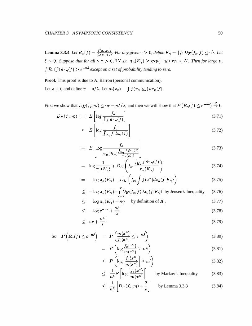
CHAPTER3. ASYMPTOTIC CONSISTENCY 50
Lemma 3.3.4 Let c »i±à¾·¸cÅ ] øáj b k l b ü]_^ øáj b k l b ü . For anygiven ÿ ì Ô , define=Y> Å ãP¾�ï Þ?ø�±à¾<¿Àµ&¾·¸qð`ÿºå . Letä�ì Ô . Supposethat for all ÿºµXO0ì Ô µ���Ø s.t. LX»¼± =Y> ¸ Vz ��"�º±�ÍS,TO�¸ U ,�V Ø . Thenfor large , ,á�c » ±à¾·¸}Ð{L » ±à¾·¸qì[Á ùg»�� exceptona setof probability tendingto zero.
Proof. Thisproof is dueto A. Barron(personalcommunication).
Let ówì Ô anddefineÿ�Å7ä�ê�ó . Let �3±�Á¼»�¸cÅ á ¾c±�Á¼»XµÎÝ+»�¸}ÐuLg»Ë±à¾·¸ .Firstweshow that Þ?ø�±à¾<¿µX� ¸ ð�,TO���,Jä�ê�ó , andthenwewill show that î � c »i±à¾·¸qð[Á ùg»�� � ÑÓ Ô .Þ?ø�±à¾<¿µX� ¸ Å ô B DGF�H ¾<¿á ¾ Ð{Lg»Ë±à¾·¸ I (3.71)ð ô Ñ_DGF�H ¾<¿á ø�� ¾ ÐuLg»Ë±à¾·¸ Ó (3.72)
Å ô ·Þ¸ DÊF�H ¾<¿Lg»Ë± =Y> ¸ �� � ] �� b ø ] ü b øãø��ü ºáà»(3.73)
Å DGF�H ÛLX»i± =Y> ¸ �`Þ?ø ì ¾<¿µ á ø � ¾ ÐuLg»Ë±à¾·¸Lg»¼± =?> ¸ ï (3.74)Å Í<DGF�H!LX»i± =?> ¸T�¡Þ?ø � ¾<¿Pµ Ì ¾c±�Á » ¸�ÐuLg»Ë±à¾;Ä =Y> ¸ � (3.75)ð Í<DGF�H!L » ± = > ¸'� Ì ø��Þ ø ±à¾ ¿ µ&¾·¸�ÐuL » ±à¾;Ä = > ¸ by Jensen’s Inequality (3.76)ð Í<DGF�H!L » ± = > ¸T��,Ëÿ by definitionof= >
(3.77)ð Í<DGF�H6Á ùg»$ð � ,Jäó (3.78)ð ,TO�� ,Jäó ¹ (3.79)
So î é c » ±à¾·¸ ð[Á ùg»�� ë Å î � �3±�Á » ¸¾<¿À±�Á » ¸ ð[Á ùg»�� � (3.80)Å î � DGF�H ¾ ¿ ±�Á » ¸�3±�Á » ¸ VR,Jä � (3.81)ð îA�vDGF�H ¬¬¬¬ ¾<¿<±�Á » ¸�3±�Á » ¸ ¬¬¬¬ VR,Jä$� (3.82)ð Û,Jä ô B DGF�H ¬¬¬¬ ¾<¿<±�Á » ¸�3±�Á » ¸ ¬¬¬¬ I by Markov’s Inequality (3.83)ð Û,Jä B�Þ?ø ±à¾<¿PµX� ¸T� �ÁvI by Lemma3.3.3 (3.84)

CHAPTER3. ASYMPTOTIC CONSISTENCY 51
ð Û,Jä B ,TO�� ,Jäó � � Á I by Equation(3.79) (3.85)Å O ä � Ûó � �,Jä�Á µ (3.86)
andhence D � �» î é c »i±à¾·¸ ð�Á ùg»�� ë ð O ä � Ûó ¹ (3.87)
Sincethelastequationholdstruefor all O�ì Ô ,D � �» î é c » ±à¾·¸�ð[Á ùg»�� ë ð Ûó ¹ (3.88)
And thisholdstruefor all ó ì Ô , so î é c »i±à¾·¸ ð[Á ùg»�� ë ÑÓÕÔ ¹ (3.89)
Thus,we canconcludethat for all ä¡ì Ô and for sufficiently large , , á�c »i±à¾·¸}Ð{Lg»i±à¾·¸wì Á ùg»��exceptonasetof probabilitytendingto 0. ç
Now wehave donethehardwork for theproofof Theorem3.3.1.
Proof of Theorem3.3.1:
By Lemma3.3.2, á orqs c » ±à¾·¸�Ð{L » ±à¾·¸qä� ����º±�Í »$ðÏ ¸T�� ��"�º±�ÍS, ½ Ï â Ï ¸ for sufficiently large , .
By Lemma3.3.4, á c »Ë±à¾·¸}ÐuLg»�±à¾·¸6V[Á ùg»�� exceptonasetof probabilitytendingto 0.î>± ) Q* Ä�±�Áܳ^µÎÝ�³\¸8µe¹e¹e¹Üµ±�ÁX»iµÎÝ+»}¸Î¸ Å á orqs c » ±à¾·¸�Ð{L » ±à¾·¸áwc »i±à¾·¸�Ð{Lg»i±à¾·¸ (3.90)ä ������ÎÍ »�ðÏ ���� ��"�#�sÍS, ½ Ï â Ï �Á ùg»�� (3.91)Å ���� é Í , O � Í¥ä ° ë?�� ���� � ÍS,Üâ Ï Â ½ Ï Í¥ä^È � ¹ (3.92)
Now chooseä suchthatboth ð Ï Í�ä�ì�� and ½ Ï Í¥ä�ì�� where� ì Ô . Thenî ± ) Q* Ä�±�Á·³^µÎÝ�³8¸8µe¹e¹e¹Üµ±�Á¼»¼µÎÝ+»�¸Î¸ ð[Á ùg»�� �âÁ ùg» * À�� ¹ (3.93)
Thusfor sufficiently large , , î ± ) Q* Ä�±�Áܳ^µÎÝ�³&¸8µe¹e¹e¹ºµ±�ÁX»iµÎÝ+»�¸Î¸ ÑÓ Ô ¹ (3.94)ç

CHAPTER3. ASYMPTOTIC CONSISTENCY 52
Theorem3.3.1impliesthat theHellingerdistanceÞ�è�±à¾<¿Àµ&¾·¸zÑÓ]Ô , where ¾ is a randomdraw
from theposterior. Whatis left to show is thatthisalsoholdstruefor thepredictive density, ʾÀ» , and
that the predictive regressionfunction, ÊÉ<»i±�Á˸�Å ô `]_b  ¶´Ä ²�È , convergesin meansquareto the true
regressionfunction,É+¿+±�Á˸;Å ô ] ^  ¶wÄ ² È�Å��X¿ � � b�� ³ � �Û6�� ����#� Ííÿ ��� Í������ ³ ÿ����<Ár��� ¹ (3.95)
Proof of Corollary 3.3.1:Firstweshow that Þ è ±à¾ ¿ µ ʾ » ¸JÑÓÕÔ . For any âçì Ô :Þ�è�±à¾<¿Àµ ʾÀ»}¸ ð Ì Þ�è�±à¾<¿Pµ&¾·¸�ÐuLg»Ë±à¾;Ä ² » ¸ by Jensen’s inequality (3.96)Å Ì o s Þ�è�±à¾<¿Pµ&¾·¸�ÐuLX»i±à¾;Ä ² » ¸T� Ì orqs Þ�è�±à¾<¿µ&¾·¸�Ð{Lg»Ë±à¾;Ä ² » ¸ (3.97)ð Ì o s âgÐ{L » ±à¾;Ä ² » ¸T� Ì ovqs Þ è ±à¾ ¿ µ&¾·¸�ÐuL » ±à¾;Ä ² » ¸ (3.98)ð â¦� Ì orqs Þ�è�±à¾<¿Pµ&¾·¸�ÐuLX»i±à¾;Ä ² » ¸8¹ (3.99)
Thesecondtermgoestozeroin probabilitybyTheorem3.3.1,andâ isarbitrary, so Þ�è�±à¾<¿µ ʾÀ»�¸�ÑÓ Ô .TheHellingerdistancebetween¾<¿ and ʾÀ» is:Þ�è�±à¾<¿µ ʾÀ»�¸�Å ì Ì�Ì B � ʾÀ»i±�ÁܵÎÝg¸�Í ê ¾<¿<±�ÁܵÎÝg¸ I Ï Ð�Ý}Ð�Árï ³_µ Ï (3.100)Å ì Ì�Ì Û± ��L BP ��"� � Í Û¹ ±�Ý�ÍÒÊÉÀ»Ë±�Á˸θ Ï � ÍW ���� � Í Û¹ ±�Ý�Í)É+¿<±�Á�¸Î¸ Ï � I Ï ÐHÝ�ÐHÁ ï ³_µ Ï(3.101)Å � Ì�Ì Û± ��L B ��"�Ò�^Í Û� ±�Ý�ÍÒÊÉÀ»Ë±�Á˸θ Ï ���� ���� �eÍ Û� ±�Ý�Í)É+¿<±�Á�¸Î¸ Ï �Í+�¦ ��"�Ò��Í Û¹W¾ ±�Ý ÍÒÊÉÀ»�±�Á˸θ Ï � ±�Ý�ÍlÉ<¿<±�Á˸θ Ï ¿ � I ÐHÝ�ÐHÁ%� ³_µ Ï (3.102)
Å � �iÍw� Ì;Ì Û± ��L ��"� � Í Û¹�¾ �ÀÝ Ï Í �ÀÝ˱RÊÉ<»�±�Á˸'��É+¿+±�Á˸θ'�0ÊÉ<»Ë±�Á�¸ Ï ��É+¿<±�Á�¸ Ï ¿ � ÐHÝ�ÐHÁ � ³_µ Ï (3.103)Å ì �iÍw� Ì;Ì Û± ��L ��"� Ñ Í Û� �sÝ�Í ÊÉÀ»Ë±�Á˸'��É+¿+±�Á˸� � Ï Ó ��"� B Í ÛÄ ±eÊÉÀ»�±�Á˸PÍ-É<¿+±�Á˸θ Ï I ÐHÝ�ÐHÁ ï ³_µ Ï (3.104)Å � � Í�� Ì ��"�WBDÍ ÛÄ ±RÊÉÀ»Ë±�Á˸�ÍlÉ<¿<±�Á˸θsÏ I ÐHÁ � ³_µ Ï ¹ (3.105)
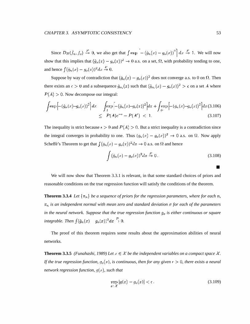
CHAPTER3. ASYMPTOTIC CONSISTENCY 53
Since Þ�è�± ʾÀ»Xµ&¾<¿e¸`ÑÓ Ô , we alsoget that á ��"� Í ±eÊÉ<»i±�Á�¸�Í)É+¿À±�Á�¸Î¸ Ï ° Ð�Á×ÑÓ Û . We will now
show thatthis impliesthat ±RÊÉ<»i±�Á˸;ÍlÉ+¿+±�Á˸θ Ï Ó Ô a.s.on a set, £ , with probabilitytendingto one,
andhenceá�±\ÊÉÀ»�±�Á˸ñÍ)É<¿<±�Á˸θ Ï ÐHÁ ÑÓaÔ .Supposeby wayof contradictionthat ±\ÊÉÀ»�±�Á˸�Í3É<¿<±�Á˸θ Ï doesnot convergea.s.to 0 on £ . Then
thereexistsan â�ì Ô anda subsequenceÊÉ » f ±�Á�¸ suchthat ±\ÊÉ » f ±�Á�¸cÍ É ¿ ±�Á˸θ Ï ì â on a set)
whereî�± ) ¸ ì Ô . Now decomposeour integral:Ì ���� Í�±RÊÉ<»i±�Á�¸�Í�É<¿+±�Á�¸Î¸ Ï ° Ð�Á>Å Ì o ���� Í�±RÊÉ<»i±�Á�¸�Í�É<¿+±�Á�¸Î¸ Ï ° Ð�ÁY� Ì orq ��"� Í�±\ÊÉÀ»�±�Á˸�Í�É+¿<±�Á˸θ Ï ° ÐHÁ (3.106)ð îJ± ) ¸�Á ù * �`î�± ) Q ¸¡ä Û<¹ (3.107)
Theinequalityis strictbecauseâíì Ô and î�± ) ¸ ì Ô . But a strict inequalityis acontradictionsince
the integral convergesin probability to one. Thus ±\ÊÉÀ»�±�Á˸�Í¡É<¿+±�Á˸θ Ï Ó Ô a.s. on £ . Now apply
Scheffe’s Theoremto getthat á ±RÊÉ<»i±�Á�¸�Í)É+¿+±�Á˸θ Ï ÐHÁ ÓÕÔ a.s.on £ andhenceÌ ±\ÊÉÀ»�±�Á˸ºÍ)É+¿+±�Á˸θ Ï Ð�Á ÑÓÕÔ ¹ (3.108)çWe will now show thatTheorem3.3.1is relevant, in thatsomestandardchoicesof priorsand
reasonableconditionson thetrueregressionfunctionwill satisfytheconditionsof thetheorem.
Theorem 3.3.4 Let ã�LX»gå bea sequenceof priors for theregressionparameters, where for each , ,Lg» is an independentnormalwith meanzero andstandard deviation � for each of theparameters
in theneural network.Supposethat the true regressionfunction É<¿ is eithercontinuousor square
integrable. Then á�±\ÊÉÀ»�±�Á˸�ÍlÉ<¿<±�Á˸θ Ï Ð�ÁÒÑÓaÔ .The proof of this theoremrequiressomeresultsaboutthe approximationabilities of neural
networks.
Theorem 3.3.5 (Funahashi,1989)Let Á � ò betheindependentvariablesona compactspaceò .
If thetrue regressionfunction, É+¿<±�Á�¸ , is continuous,thenfor anygiven â ì Ô , there existsa neural
networkregressionfunction,Éi±�Á�¸ , such that
§�¨ �j ª õ Ä Éi±�Á˸cÍ)É ¿ ±�Á�¸eÄ�ä â�¹ (3.109)
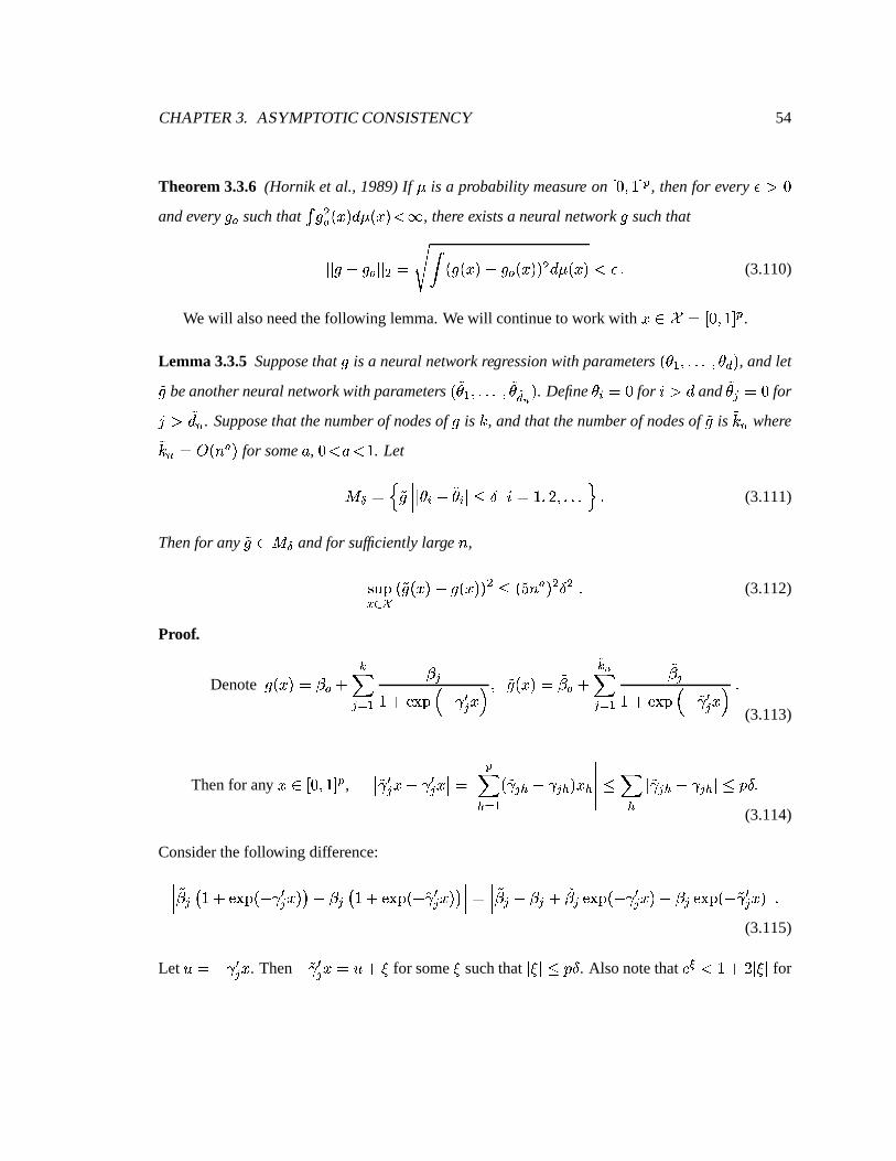
CHAPTER3. ASYMPTOTIC CONSISTENCY 54
Theorem 3.3.6 (Hornik et al., 1989)If � is a probability measure on Â Ô µ^Û\È � , thenfor every â�ì Ôandevery É+¿ such that áÜÉ Ï¿ ±�Á˸�Ð��n±�Á˸�ä å , there existsa neural networkÉ such thatÄ�Ä É�ÍlÉ<¿+Ä�Ä Ï Å Ì ±�É˱�Á˸ñÍlÉ<¿+±�Á˸θ Ï Ð��n±�Á˸ ä â�¹ (3.110)
Wewill alsoneedthefollowing lemma.Wewill continueto work with Á � ò ÅÇÂ Ô µ^Û\È � .Lemma 3.3.5 Supposethat É is a neural networkregressionwith parameters ±!Ú�³Rµe¹e¹e¹ºµ Ú � ¸ , andlet�É beanotherneural networkwith parameters ± �ÚH³^µe¹e¹e¹ºµ �Ú��� b ¸ . DefineÚ�¡ÜÅ Ô for ²nì Ð and
�Ú � Å Ô for4 ì �Ð » . Supposethat thenumberof nodesof É is þ , andthat thenumberof nodesof�É is
�þ » where�þ+»�Å���±8, - ¸ for some/ , Ô ä�/qä�Û . Let� � Å ù �É ¬¬¬ Ä Ú ¡ Í �Ú ¡ Ä}ð[ä[²cÅ Û<µ��}µe¹e¹e¹ ü ¹ (3.111)
Thenfor any�É � � � andfor sufficientlylarge , ,
§m¨ �j ª õ ± �É˱�Á˸ºÍlÉi±�Á˸θ Ï ð ±���, - ¸ Ï ä Ï ¹ (3.112)
Proof.
Denote Éi±�Á�¸nÅ��¼¿�� ��� ³ � �Û6�� ��"� é Ííÿ �� Á¼ë µ �Éi±�Á�¸;Å ��X¿ � �� b�� ³ �� �Û6�� ��"� é Í �ÿ �� Áië ¹(3.113)
Thenfor any Á � Â Ô µ^Û\È � , ¬¬ �ÿ �� Á�Ílÿ �� Á ¬¬ Å ¬¬¬¬¬ ��� ³ ± �ÿ���� Í)ÿ����H¸DÁ%� ¬¬¬¬¬ ð � Ä �ÿ���� Í)ÿ����gÄ}ðlý%ä^¹(3.114)
Considerthefollowing difference:
¬¬¬ �� �+� Û!�� ��"�º±�Ííÿ �� Á�¸ � ÍW� �+� Û!�� ��"�º±�Í �ÿ �� Á�¸ � ¬¬¬ Å ¬¬¬ �� � ÍW� � � �� � ����º±�Íçÿ �� Á�¸�ÍW� � ����º±�Í �ÿ �� Á�¸ ¬¬¬ ¹(3.115)
Let ywÅ Íçÿ �� Á . Then Í �ÿ �� ÁwÅ�y �!� for some� suchthat Ä �XÄ}ð)ýëä . Also notethat Á � äÒÛ �¥�gÄ �XÄ for
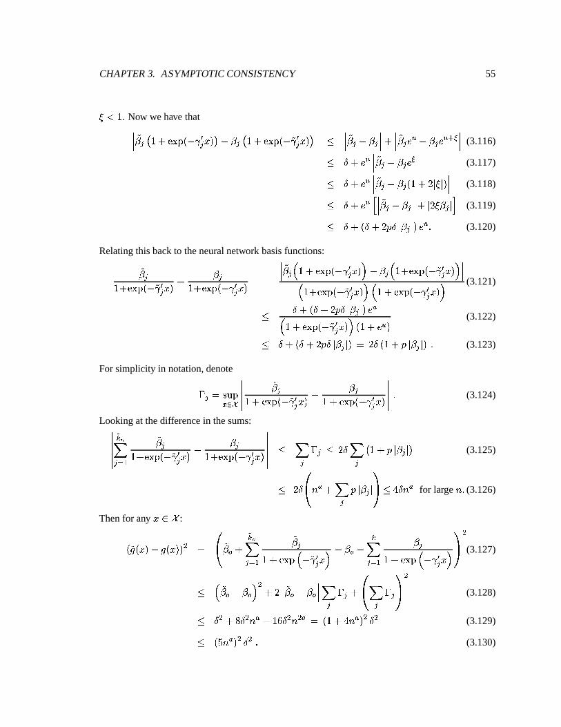
CHAPTER3. ASYMPTOTIC CONSISTENCY 55
� äÒÛ . Now wehave that¬¬¬ �� �+� Û!�� ��"�º±�Ííÿ �� Á˸ � ÍW� �+� Û!�� ��"�º±�Í �ÿ �� Á˸ � ¬¬¬ 𠬬¬ �� � ÍW� � ¬¬¬ � ¬¬¬ �� � Á � ÍW� � Á �Pô"� ¬¬¬ (3.116)ð ä��âÁ � ¬¬¬ �� � Ía� � Á � ¬¬¬ (3.117)ð ä��âÁ � ¬¬¬ �� � Ía� � ±sÛ6�â�gÄ �XÄ�¸ ¬¬¬ (3.118)ð ä��âÁ � ¬¬¬ �� � Í�� � ¬¬¬ � Ä ����� � Ä ° (3.119)ð ä��5±�ä��â�8ý%äíÄ � � Ä ¸"Á � ¹ (3.120)
Relatingthisbackto theneuralnetwork basisfunctions:¬¬¬¬¬�� �Ûu�w ��"��±�Í �ÿ �� Á˸ Í � �Ûu�w �����±�Ííÿ �� Á�¸ ¬¬¬¬¬ Å ¬¬¬ �� � é Û6�� ��"�º±�Ííÿ �� Á˸ ë ÍW� � é Ûu�w ��"�º±�Í �ÿ �� Á˸ ë ¬¬¬é Ûu�� ����º±�Í �ÿ �� Á�¸�ë é Û6�� ��"�ܱ�Ííÿ �� Á˸�ë (3.121)ð ä��5±�ä��â�8ý%äçÄ � � Ä�¸nÁ �é Û6�¥ ��"�º±�Í �ÿ"�� Á�¸�ë�±sÛ6�âÁ � ¸ (3.122)ð ä��5±�ä��â�8ýëä�Ä � � Ä ¸uÅ���äí±sÛ�� ý Ä � � Ä�¸ ¹ (3.123)
For simplicity in notation,denote# � Å §m¨ �j ª õ ¬¬¬¬¬�� �Û!�� �����±�Í �ÿ �� Á˸ Í � �Û6�� ����ܱ�Ííÿ"�� Á�¸ ¬¬¬¬¬ ¹ (3.124)
Lookingat thedifferencein thesums:¬¬¬¬¬¬�� b�� ³ �� �Ûu�� ����º±�Í �ÿ �� Á�¸ Í � �Ûu�w ��"��±�Ííÿ"�� Á˸ ¬¬¬¬¬¬ ð � # � ðC��ä � ±sÛ�� ý Ä � � Ä�¸ (3.125)
ð ��ä �� , - � � ýuÄ � � Ä &(�ð ¹ ä�, - for large ,c¹ (3.126)
Thenfor any Á � ò :± �É�±�Á˸�Í0É˱�Á˸θ Ï Å �� ��X¿ � �� b�� ³ �� �Û6�� ��"� é Í �ÿ �� Á¼ë ÍW�¼¿nÍ ��� ³ � �Û!�� ��"� é Ííÿ �� Á¼ë &( Ï (3.127)
ð é ��X¿nÍa�X¿Rë Ï �R� ¬¬¬ ��X¿ ÍW�X¿ ¬¬¬ � # � � �� � # � &( Ï (3.128)ð ä Ï � Ä ä Ï , - ��Û%$�ä Ï , Ï - Å ±sÛ6� ¹ , - ¸ Ï ä Ï (3.129)ð ±&��, - ¸ Ï ä Ï ¹ (3.130)
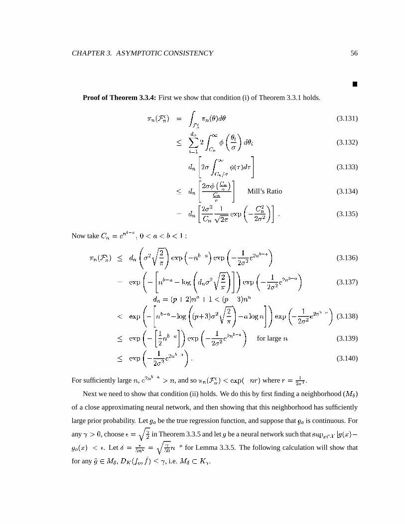
CHAPTER3. ASYMPTOTIC CONSISTENCY 56
çProof of Theorem3.3.4: Firstweshow thatcondition(i) of Theorem3.3.1holds.LX»i±P1 Q» ¸ Å Ì î qb LX»i±!Ú�¸�Ð�Ú (3.131)ð � b ¡ ³ � Ì �� b ß � Ú�¡� ��Ð�Ú�¡ (3.132)Å Ð » Ñ ��� Ì �� b µ' ß ±)(X¸�Ð*( Ó (3.133)ð ÐH» Ñ ��� ß �$� b' �� b' Ó
Mill’ s Ratio (3.134)Å Ð » B ��� Ï2q» Û± ��L ���� � Í 2 Ï»��� Ï � I ¹ (3.135)
Now take 2q»�Å7Á »�+�,�- µ Ô ä[/�ä[: ä Û :Lg»Ë±P1 Q» ¸ ð Ð�» ì � Ï Ô �L ïW ��"� é ÍS, 9 ù - ë\ ��"�Ò��Í Û��� Ï Á Ï » +�,�- � (3.136)Å ��"� ì ÍAÑÉ, 9 ù - ÍaDGF�H ì ÐH».� Ï Ô �L ï Ó ïW ��"�Ò��Í Û��� Ï Á Ï » +�,�- � (3.137)Ð�»uÅ ±�ý��â�H¸_, - �5Û�ä ±�ý��0/H¸_, -ä ��"� ì Í¥ÑÉ, 9 ù - ͼDGF�H ì ±�ýÛ�1/H¸2� Ï Ô �L ï�ͼ/�DGF�H , Ó ïW ��"�Ò�eÍ Û��� Ï Á Ï » +&,�- � (3.138)ð ��"�Ò�·Í B Û� , 9 ù - I �< ���� ��Í Û��� Ï Á Ï »�+�,�- � for large , (3.139)ð ��"�Ò�·Í Û��� Ï Á Ï » +�,�- �3¹ (3.140)
For sufficiently large , , Á Ï » +�,�- ìR, , andso LX»i±P1 Q» ¸qäR �����±�ÍS,TO�¸ whereO�Å ³Ï ' À .Next weneedto show thatcondition(ii) holds.Wedothisby first findinganeighborhood(
� � )of a closeapproximatingneuralnetwork, andthenshowing that this neighborhoodhassufficiently
largeprior probability. Let É+¿ bethetrueregressionfunction,andsupposethat É<¿ is continuous.For
any ÿ ì Ô , chooseâ Å � > Ï in Theorem3.3.5andlet É beaneuralnetwork suchthat §m¨ � j ª õ Ä Éi±�Á�¸ÍÉ+¿<±�Á�¸eÄ�ä â . Let ä�Å *3 » - Å � >3 � , ù - for Lemma3.3.5. Thefollowing calculationwill show that
for any�É � � � , Þ?ø�±à¾<¿µ �¾·¸�ð`ÿ , i.e.
� � � =Y>.
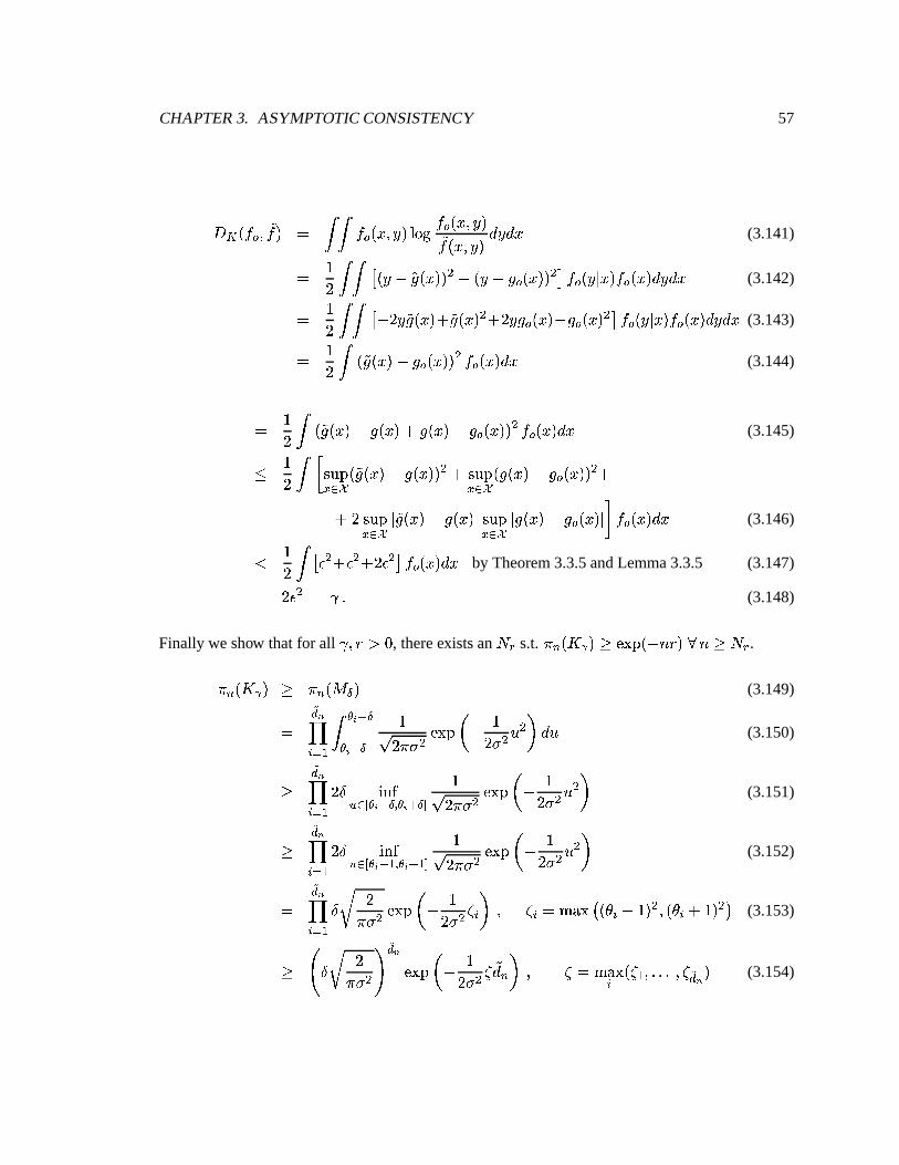
CHAPTER3. ASYMPTOTIC CONSISTENCY 57
Þ?ø ±à¾<¿Pµ �¾�¸ Å ÌuÌ ¾<¿<±�ÁܵÎÝg¸�DGF�H ¾<¿À±�ÁºµÎÝ�¸�¾�±�ÁºµÎÝ�¸ Ð�Ý}Ð�Á (3.141)Å Û� Ì�Ì ¾ ±�Ý�Í �É˱�Á�¸Î¸ Ï Í>±�Ý Í)É+¿À±�Á�¸Î¸ Ï ¿ ¾<¿À±�Ý�Ä Á�¸s¾<¿+±�Á˸�ÐHÝ�ÐHÁ (3.142)Å Û� Ì�Ì ¾ Í+�ÀÝ �Éi±�Á�¸'� �É�±�Á�¸ Ï �Y�ÀÝ�É<¿<±�Á˸PÍ�É+¿+±�Á˸ Ï ¿ ¾<¿P±�Ý·Ä Á˸s¾<¿+±�Á�¸�ÐHÝ�ÐHÁ (3.143)Å Û� Ì ± �Éi±�Á˸�ÍlÉ<¿+±�Á˸θ Ï ¾<¿<±�Á˸�Ð�Á (3.144)
Å Û� Ì ± �É˱�Á˸ñÍ)Éi±�Á˸J� Éi±�Á˸ñÍ)É<¿+±�Á�¸Î¸ Ï ¾<¿P±�Á�¸�ÐHÁ (3.145)ð Û� Ì B §m¨ �j ª õ ± �É˱�Á˸ºÍlÉi±�Á˸θ Ï � §m¨ �j ª õ ±�Éi±�Á�¸ñÍ)É ¿ ±�Á˸θ Ï ��7� §m¨ �j ª õ Ä �Éi±�Á�¸�Í)Éi±�Á�¸eÄ §m¨ �j ª õ Ä É˱�Á˸ñÍ0É+¿+±�Á˸eÄ I ¾<¿<±�Á˸�ÐHÁ (3.146)ä Û� Ì ¾ â Ï ��â Ï �Y�+â Ï ¿ ¾ ¿ ±�Á�¸�ÐHÁ by Theorem3.3.5andLemma3.3.5 (3.147)Å �+â Ï Å ÿ�¹ (3.148)
Finally weshow thatfor all ÿºµXO ì Ô , thereexistsan Ø ð s.t. L » ± = > ¸�V� ����º±�Í ,TOH¸ U , V>Ø ð .L » ± = > ¸ V L » ± � � ¸ (3.149)Å �� b4¡ ³ Ì05 f ô6�5 f ù7� Û± ��L8� Ï ��"� � Í Û��� Ï y Ï � Ðuy (3.150)
V �� b4¡ ³ ��ä � 9;:� ª � 5 f ù7� k 5 f ô6� � Û± ��L8� Ï ��"� � Í Û��� Ï y Ï � (3.151)
V �� b4¡ ³ ��ä � 9;:� ª � 5 f ù�³ k 5 f ôº³ � Û± ��L8� Ï ����Ò�·Í Û��� Ï y Ï � (3.152)Å �� b4¡ ³ ä Ô �L8� Ï ��"�Ò��Í Û��� Ï=< ¡8� µ < ¡·Å>�@?�� � ±!Ú$¡¼Í Û¸ Ï µ±!Ú�¡���Û¸ Ï � (3.153)
V ì ä Ô �L8� Ï ï �� b ��"� � Í Û��� Ï < �Ð�» � µ < Å>�@?��¡ ± < ³eµe¹e¹e¹Üµ < �� b ¸ (3.154)

CHAPTER3. ASYMPTOTIC CONSISTENCY 58
Å ì Ô ÿ� Ô , ù - Ô �L8� Ï ï �� b ���� � Í Û��� Ï=< �ÐH» � (3.155)Å ���� ��Í �Ð�» B /6DGF�H6,´ÍaDGF�H Ô ÿ�A��L8� Ï I Í Û��� Ï=< �ÐH»�� (3.156)V ���� � ÍzB���/6DÊF�H!,#� Û��� Ï < I �Ð »�� µ for large , (3.157)V ���� � Í B ��/6DGF�H6,6� <��� Ï I ±�ý��1/H¸_, - � µ �ÐH»cÅ)±�ýÛ�Y�H¸ �þH»'�´ÛËðz±�ýÛ�Y�H¸_, - �wÛËð ±�ýÛ�1/H¸_, - (3.158)V �����±�ÍS,TO�¸¼µ for any O andfor all ,�V Ø ð for someØ ð�¹ (3.159)
Onecanuseasimilarargumentto show thataneuralnetwork canapproximateany æ Ï function
arbitrarilyclosely. Notethatfor any æ Ï function 5 , Ä�Ä 5�Ä�Ä Ï V Ä�Ä 5ºÄ�ÄM³ , so
if � Ì ±�Éi±�Á˸cÍ)É<¿+±�Á�¸Î¸ Ï ÐB�n±�Á˸ � ³_µ Ï ä>â^µ thenÌ Ä Éi±�Á�¸�Í)É+¿<±�Á�¸eÄ ÐB�n±�Á�¸�ä>â·¹
(3.160)
Equations(3.144)through(3.148)now become:Þ?ø ±à¾<¿µ �¾·¸ Å Û� Ì ± �É˱�Á�¸ºÍ)É+¿<±�Á�¸Î¸ Ï ¾<¿P±�Á�¸�ÐHÁ (3.161)Å Û� Ì ± �É˱�Á�¸ºÍ)Éi±�Á�¸J� Éi±�Á�¸�Í)É+¿+±�Á˸θ Ï ¾<¿<±�Á˸�ÐHÁ (3.162)ð Û� B Ì §m¨ �j ª õ ± �É˱�Á�¸�Í)Éi±�Á�¸Î¸ Ï ¾<¿À±�Á�¸�ÐHÁ?� Ì ±�Éi±�Á�¸ñÍ)É+¿<±�Á˸θ Ï ¾<¿À±�Á˸�ÐHÁ�7� §m¨ �j ª õ Ä �É�±�Á˸�Í)É˱�Á˸eÄ Ì Ä Éi±�Á˸�ÍlÉ<¿+±�Á˸eÄ ¾<¿+±�Á�¸�ÐHÁ I (3.163)ä Û� ¾ â Ï �`â Ï �â�+â Ï ¿ by Theorem3.3.6andLemma3.3.5 (3.164)Å �+â Ï Å ÿ ¹ (3.165)çTheorem 3.3.7 Let theprior for theregressionparameters bethenoninformativeprior of Chapter
2, i.e., Lg»ÙÅ ³' À over the region where ¬¬ C � C ¬¬ ì 2q» , Ä ÿ�����Änä Þ » and Ä � � Ä;ä Þ » , for all 4 and5 . Let 2q» Ó Ô , with 2q» ì Ô for all , , and let Þ » Ó å such that Þ »`ÅED�±8 ����º±8, ð ¸Î¸ for allOuì Ô . Supposethat thetrue regressionfunction É<¿ is eithercontinuousor square integrable. Thená ±RÊÉ<»i±�Á�¸�Í)É+¿<±�Á�¸Î¸ Ï ÐHÁÒÑÓÕÔ .

CHAPTER3. ASYMPTOTIC CONSISTENCY 59
Proof. Clearlytheconditionsof Theorem3.3.1hold. Therestof thelogic from thepreviousproof
(of Theorem3.3.4)now givestheresult. ç3.3.2 The Number of Hidden Nodesasa Parameter
In theprevioussection,welet thenumberof hiddennodes,þ » , increaseto infinity asafunctionof , .
A differentapproachis to treatthenumberof hiddennodesasanotherparameterin themodeland
to specifyaprior distribution for it. Wewill show thatthisapproachalsoleadsto anasymptotically
consistentposterior.
Let ó�¡�Å�îJ±àþ�Å�²�¸ betheprior probabilitythatthenumberof hiddennodesis ² , �öó�¡·ÅÇÛ . LetL�¡ betheprior for theparametersof theregressionequation,giventhat þ�Å�² . Thejoint prior for all
of theparametersis � ¡ ó�¡�L�¡ . Wenow extendtheresultof Theorem3.3.1.
Theorem 3.3.8 Supposethat: (i) there existsa sequenceOp¡�ì Ô anda sequenceؼ¡ such that for
each ² , L ¡ ±P1 Q» ¸çä[ ��"�º±�ÍS,TO ¡ ¸ for all ,¥V�Ø ¡ ; (ii) for all ÿºµXO�ì Ô , there existsan F anda sequence� ¡ such that for any ²ZV>F , L�¡Î± =Y> ¸SV[ ��"�º±�ÍS,TO�¸ for all ,aV � ¡ ; (iii) G » is a boundwhich grows
with , such that for all Ouì Ô , there existsa ÷uì Û andan Ø such that � �¡ 8H b ôº³ ó�¡;ä� ����ܱ�Í , û O�¸for ,�V Ø ; (iv) for all ² , ón¡�ì Ô . Thenfor all âíì Ô ,î>± )+* Ä�±�Á·³^µÎÝ�³8¸8µe¹e¹e¹ºµ±�ÁX»iµÎÝ+»�¸Î¸JÑÓ Ûñ¹ (3.166)
Proof. Wewill now show thatit is still thecasethat î ± ) Q* Ä�±�Á·³^µÎÝ�³\¸8µe¹e¹e¹ºµ±�ÁX»XµÎÝ+»�¸Î¸ ÑÓÕÔ , by showing
thattheconditionsof Theorem3.3.1hold for thecombinedprior L .
For thefirst conditionof Theorem3.3.1let1 Q» Å �I¡ ë�=J Q¡ (3.167)
where J ¡ is the setof all neuralnetworks with ² nodesandwith eachparameterlessthan 2q» in

CHAPTER3. ASYMPTOTIC CONSISTENCY 60
absolutevalue, 2q»JðR �����±8, 9 ¸ , Ô ä[:�äÒÛ . Now wehave thatL;±P1 Q» ¸ Å � ¡ ë� ó�¡8Lv¡s± J Q¡ ¸ (3.168)ð Hrb ¡ ë� ó�¡8Lv¡s± J Q¡ ¸.� �¡ 8Hrb ôº³ ón¡ (3.169)ð Hrb ¡ ë� ó�¡$ ��"�º±�ÍS,TO�¡à¸T� �¡ 8H b ôº³ ó�¡ by assumption(i) (3.170)
Letting O�|çÅ>�@� 9¼ãpO � µXOH³^µe¹e¹e¹ÜµXO H b å givesL;±P1 Q» ¸]ð ��"�º±�ÍS,TO | ¸ Hrb ¡ ë� ó�¡�� �¡ 8Hrb ôº³ ón¡ (3.171)ð ��"�º±�ÍS,TO | ¸.� �¡ 8H b ôº³ ó ¡ ¹ (3.172)
By assumption(iii), � �¡ 8H b ôº³ ó�¡�ä7 ����º±�Í , û O | ¸ for sufficiently large , , where ÷Ãì Û . If we now
let O�Å3O�|'ê�� , then L;±P1 Q» ¸qäR ��"�º±�ÍS,TO�¸ for sufficiently large , .
Now wecheckthesecondconditionof Theorem3.3.1.For any ÿzì Ô ,L;± =?> ¸ÆÅ � ¡ ë� ó�¡EL�¡Î± =Y> ¸ (3.173)V ó7K'L7KH± =Y> ¸8µ whereF is from assumption(ii) (3.174)V ó7KpÁ ùg»�ðML µ (3.175)
for any O�| for sufficiently large , by assumption(ii). Since F is a constant,ó7K doesnot dependon, andis positive by assumption(iv). SinceO�| is arbitrary, L;± =?> ¸�V7Á ùg»�ð for any O for sufficiently
large , . Thustheconditionsof Theorem3.3.1hold,andsodo its conclusions. çWecanalsoextendtherestof theresultsfrom theprecedingsectionin thefollowing theorem.
Theorem 3.3.9 Let L�¡ beanindependentnormalwith meanzero andstandard deviation � for each
of the ² parameters. Let theprior for þ bea geometricwith parameterý . Let G »JÅN��±8, û ¸ for any÷ ì Û . Supposethat thetrue regressionfunction É<¿ is eithercontinuousor square integrable. Thenáí±RÊÉ<»i±�Á�¸�Í)É+¿<±�Á�¸Î¸ Ï ÐHÁÒÑÓÕÔ .

CHAPTER3. ASYMPTOTIC CONSISTENCY 61
Proof. We merelyneedto show the four conditionsof Theorem3.3.8,andthentheresultfollows
directly from that theoremandtheproof of Corollary3.3.1.Following the ideasfrom theproof of
Theorem3.3.4,wewill show thattheconditionsof Theorem3.3.8dohold true.
Condition(i) follows from theproof of Theorem3.3.4,Equations(3.131)through(3.140),be-
causefor any given ² , ²;äR,.- for /�ì Ô for sufficiently large , .
For condition(ii), first we adaptlemma3.3.5to thecaseof a fixednumberof hiddennodes² :Let
�É � � � where�É has² hiddennodes,andlet É have ² | hiddennodes.Thenfor sufficiently large, , §m¨ � j ª õ ± �Éi±�Á˸ñÍ)Éi±�Á˸θ Ï ðÍ2 Ï ä Ï , where 2 ÅO�íÂ�±�ýY�â�H¸.�@?��Ëãp² µX² | å���Û\È . Now if we let F be
thenumberof hiddennodesrequiredby Theorems3.3.5or 3.3.6,it is still truethat� � � =Y>
(c.f.
Equations(3.141)through(3.148)). Clearly Lv¡s± � � ¸�V ��"�º±�ÍS,TO�¸ , andthuscondition(ii) holds
true.
Clearlycondition(iv) is truefor ageometricprior. For condition3:î�± = ì�G »�¸ÆÅ �¡ 8Hvb ôº³ ý�±sÛíÍ´ý�¸ ¡ (3.176)Å ý�±sÛíÍ´ý�¸ Hvb ôº³ý Å ±sÛíÍwý�¸ H b ôº³ (3.177)Å ��"�ºÂ�±)G »���Û¸�DGF�H�±sÛíÍwý�¸EÈ now let G » Å�, û (3.178)Å ��"�ºÂ�ÍS, û ±�ÍÒDGF�Hi±sÛíÍ ý˸θEÈ�¹ (3.179)
Since÷�ì Û , thereexistsa ÷ | suchthat Û�ä�÷ | ä�÷ . Thenfor any O�ì Ô , î�±àþÃì�G »�¸ ð� ����ºÂ�Í , û L OÀÈfor sufficiently large , . çNotethatTheorem3.3.9alsoholdstruefor aPoissonprior for þ with G »uÅP��±8 ��"�º±8, û ¸Î¸ for ÷�ìÒÛ .Let the parameterfor the Poissondistribution be � . We canshow condition(iii) easilyby using
Markov’s inequality:îJ± = V�G�»���Û¸ ð ô  = ÈG�»���Û Å �G »��5Û ð �G » ÅQ�Û ��"�º±�ÍS, û ¸qäR ��"�º±�ÍS, û L O�¸8¹(3.180)
3.4 Discussion
Wehaveshown thatusinganeuralnetwork to estimateany continuousor squareintegrablefunction
will bearbitrarilyaccuratewith probabilitytendingto one,givenenoughdata.This is animportant

CHAPTER3. ASYMPTOTIC CONSISTENCY 62
resultin thatneuralnetworksarein widespreadusefor dataanalysistoday.
Oneshouldnotethat thetheoremsof theprevioussectionshow that theposterioris consistent
bothin thecasethatthenumberof hiddennodesgrows to infinity, andin thecasethatthenumber
of hiddennodesis a parameterwhich is estimatedfrom thedata.Thusonecouldeitherusea large
numberof hiddennodesto moresimply get a goodapproximation,or one let the datadrive the
numberof hiddennodesin the model. In the latter case,model selectionand modelaveraging
becomeimportantissues,andthesewill bediscussedin a laterchapter.
Theresultsof thischapterarealsofurthergeneralizable.Theparticularchoiceof anindependent
normalprior is sufficient, but not necessary. Clearly onecould usemany otherpriors, including
hierarchicalpriors.Oneneedonly to ensurethatthey satisfythetwo conditionsof themaintheorem.
In thecasewherethenumberof nodesis alsoaparameter, onecoulduseotherpriorsfor thenumber
of nodes.
One could also adaptthe resultsto a larger classof true regressionfunctions. The choices
of continuousandsquareintegrablefunctionsweremadebecausethey area rich enoughclassto
containnearlyall thefunctionsin which we might beinterested.Therewerealsoreadilyavailable
resultsfrom the computerscienceliteratureon the asymptoticapproximationabilities of neural
networksfor theseclassesof functions.
Finally, one neednot take the regressionerror to have varianceone, but could insteadtake¾c±!¶wÄ ²×Å5Á˸;Ö�Ø¡±�Éi±�Á�¸8µM� Ï ¸ . Thisaddsanuisanceparameterto theproblem,but shouldnotaffect
themainstructureof theproof.
Chapter 4
Estimating the Normalizing Constant
4.1 Overview
To computetheBayesfactorfor comparingtwo models,oneneedsthenormalizingconstantof the
posterior. Thusthis chapteris relevant to this thesisprimarily becauseof thefollowing chapteron
modelselectionandmodelaveraging.However, theproblemof estimatingthenormalizingconstant
for aposterioris adifficult problemin its own right.
Denotethemarginalposteriordensityof thedatafor agivenmodelas � :� Å Ì æ ±!Ú¼Ä Ýg¸NL;±!Ú�¸�Ð�Ú�Å Ì 5ܱ!Ú�¸�Ð�Úíµ (4.1)
where æ is thelikelihoodunderthemodel, L is theprior, Ú is thevectorof parameters,and 5º±NM�¸íÅæ�±NM�¸NL;±NM�¸ , theproductof thelikelihoodandtheprior. Recallthattheposteriorprobabilityof model� ¡ canbewrittenas: î�± � ¡&Ä Þw¸;Å � ¡ î�± � ¡ ¸� � � � î�± � � ¸ µ (4.2)
where Þ is the dataand ��¡ is the normalizingconstantof Equation(4.1). Thus one needsto
estimatethe ��¡ in orderto compareposteriorprobabilities.In thischapter, I will review anumberof
differentapproximationmethods,andI will try themonneuralnetwork regressionsontwo datasets.
Themethodshave difficultiesevenon thesesimpledatasets,andI will give somepossiblereasons
for theirproblems.
63

CHAPTER4. ESTIMATING THE NORMALIZING CONSTANT 64
Therehave beenmany proposalson how to estimatetheseanalytically intractableintegrals.
The methodsfall primarily into two categories: numericalmethodsand sample-basedmethods.
Numericalmethodsattemptto estimatetheintegraldirectlyfrom theunnormalizeddensityfunction
andincludesuchmethodsasquadratureandMonteCarlo integration. Sample-basedmethodsrely
onthefactthatwecanuseMarkov ChainMonteCarlo(MCMC) to getasamplefrom theposterior,
andthenusethis sampleto estimatetheintegral of Equation(4.1). ThesemethodsincludeLaplace
approximationsandimportancesampling. Finally, the BayesianInformationCriterion (BIC) can
beusedto directly approximateratiosof normalizingconstants(suchasBayesfactors),andhence
posteriorprobabilities.
This integrationproblemis difficult for several reasons.First, the integral is typically of mod-
eratelyhigh dimension,suchthatevaluatingthefunctionover a grid is infeasible.In thecaseof a
neuralnetwork, therearetwo additionalproblems.First,symmetriesin themodel(bothin thelike-
lihood andtheprior) inducemultimodality in theposterior. Second,thenonlinearityof themodel
resultsin irregularly shapedcontours,which arefar from theGaussiancontoursthatareassumed
by many standardintegrationtechniques.
As a simpleexampleof a symmetryproducingmultiple equivalentpeaksin theposterior, con-
sidera neuralnetwork with two nodes.Now considerswappingthe valuesof the parametersfor
thetwo nodes(essentiallyjust switchingtheorderof thenodes).Thelikelihoodremainsthesame
(asdoestheposteriorfor all priorswhich treatthenodessymmetrically, which minedo). Thusthe
posteriorwill have two symmetricpeakswhich correspondto thetwo ordersof thetwo nodes.Forþ nodes,thereare þ"R suchpermutations.
Thereareseveral possiblesolutionsto this problem. Onecould force the MCMC sampleto
visit all modeswith equalprobability, jumpingbetweenmodes(Nobile, 1994). Alternatively, one
could breakthe symmetryby usinga prior which is not symmetricwith respectto the ordering
of themodes.Instead,my approachis to let theMCMC samplewanderunrestricted(in practice,
primarily arounda single modeor two) and then “fold” the sampleonto a single modeby re-
orderingthe parametersof the sample. In particular, I requirethat ÿX³Î³´ä ÿ Ï ³Ãä ¹e¹e¹�ä ÿ � ³ , i.e.,
the slopeparameterinsidethe logistic functionof the first input variablemustbe increasingwith
respectto thenodenumber. For theproblemof estimatingtheareaunderthefunction,theproblem

CHAPTER4. ESTIMATING THE NORMALIZING CONSTANT 65
is equivalentto thatof estimatingtheareaunderoneof thesemodesandmultiplying by þ"R because
of thesymmetry. ThusI reflecttheMCMC samplesothatall samplesappearto befrom thesame
mode.This reflectiontechniqueeliminatesthis sourceof multimodalityandalsodoesnot put any
restrictionson theMCMC sample.An alternative approachwouldbeto restricttheMCMC sample
to a singlemode,but this would hamperthemixing of thechain. My approachallows thenormal
mixing, but still removestheproblemof multimodalityby takingadvantageof thesymmetryin the
posterior.
The secondareaof difficulty that is particularlyrelevant for neuralnetworks is the irregular
shapeof thecontoursof theposterior. As anexampleof how irregular thesecontourscanbe,even
in a simple problem,Figure 4.1 shows someof the contoursof the log of the posteriorfrom a
two-nodeneuralnetwork, after integratingout all but the four ÿ parametersinsideof the logistic
functionsof thetwo nodes.Thefour plotsaredifferentviews of thecontoursfor thelog-posterior
asa function of ÿ ³ � and ÿ Ï ³ , i.e., the locationparameterof onenodevs. the slopeparameterof
theothernode.Notethatthefirst threeplotsarelocal views in theneighborhoodof themode,and
the lastplot is a globalview. In theupperleft plot aresimply thecontoursof theposterior, where
the levelsarechosento be themaximumminusthe .5, .95, and.99 quantilesof a chi-squarewith
four degreesof freedom(e.g.87.4,81.2,and77.4,wherethemaximumis at 90.7).Noticehow the
distribution is bimodal,with eachpeakbeinga differentnon-ellipticalshape.Theupperright plot
is an imageplot, wherethehighestlevels aredarkest,andthe lower levelsarelighter. The lower
left plot is a perspective plot, alsoshowing only thosepartsof thelog-posteriorwhich areno more
thanthe.5 quantileof a S ϶ away from themaximum.Thelower right plot shows a globalview of
thelog-posterior.
4.2 Methods
4.2.1 Numerical Methods
A large numberof numericalmethodsexist for approximatingintegrals. They fall into two main
groups:quadraturemethodsandMonteCarlomethods.An attemptto usethequadraturemethods
in theIMSL softwareroutinespackage(Fortrancode)failed,asthey consistentlyreporteda failure

CHAPTER4. ESTIMATING THE NORMALIZING CONSTANT 66
Gamma-10
Gam
ma-
21
-10 -9 -8 -7 -6
-24
-22
-20
-18
-16
Gamma-10
Gam
ma-
21
-10 -9 -8 -7 -6
-24
-22
-20
-18
-16
-10T -9T -8T -7T -6TGamma-10U-24
-22
-20
-18
-16
Gamma-21
V7075
8085
9095
Log
Pos
terio
r
-14W -12W -10W -8W -6W -4W -2W 0
Gamma-10X-30
-25
-20
-15
-10-5
Gamma-21
Y-20
020
4060
8010
0Lo
g P
oste
rior
Figure4.1: (Log) PosteriorContours
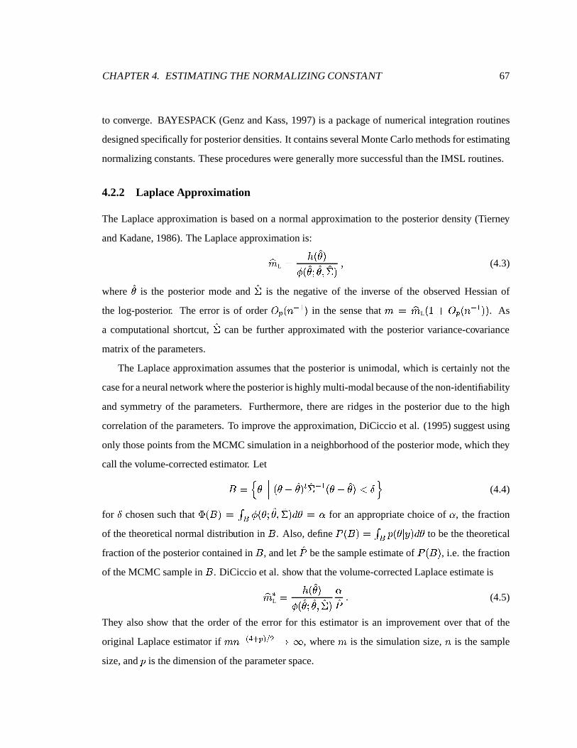
CHAPTER4. ESTIMATING THE NORMALIZING CONSTANT 67
to converge. BAYESPACK (GenzandKass,1997)is a packageof numericalintegrationroutines
designedspecificallyfor posteriordensities.It containsseveralMonteCarlomethodsfor estimating
normalizingconstants.TheseproceduresweregenerallymoresuccessfulthantheIMSL routines.
4.2.2 LaplaceApproximation
The Laplaceapproximationis basedon a normalapproximationto the posteriordensity(Tierney
andKadane,1986).TheLaplaceapproximationis:Z� L Å 5º± ÊÚ�¸ß ± ÊÚ�ï ÊÚ�µ Ê[ ¸ µ (4.3)
where ÊÚ is the posteriormodeand Ê[ is the negative of the inverseof the observed Hessianof
the log-posterior. The error is of order � � ±8, ù�³ ¸ in the sensethat � Å Z� L ±sÛ��P� � ±8, ù�³ ¸Î¸ . As
a computationalshortcut, Ê[ can be further approximatedwith the posteriorvariance-covariance
matrixof theparameters.
The Laplaceapproximationassumesthat theposterioris unimodal,which is certainlynot the
casefor aneuralnetwork wheretheposteriorishighlymulti-modalbecauseof thenon-identifiability
andsymmetryof the parameters.Furthermore,thereare ridgesin the posteriordue to the high
correlationof theparameters.To improve theapproximation,DiCiccio et al. (1995)suggestusing
only thosepointsfrom theMCMC simulationin aneighborhoodof theposteriormode,which they
call thevolume-correctedestimator. LetG ÅzùiÚ ¬¬¬ ±!Ú�Í ÊÚ�¸ � Ê[ ù�³ ±!Ú�Í ÊÚ�¸�ä[ä ü (4.4)
for ä chosensuchthat \�±)G�¸-Å á H ß ±!Ú�ï ÊÚ�µ Ê[ ¸�Ð�ÚzÅ^] for anappropriatechoiceof ] , the fraction
of thetheoreticalnormaldistribution in G . Also, define î�±)G�¸�Å á H ý�±!Ú¼Ä Ýg¸�Ð�Ú to bethetheoretical
fractionof theposteriorcontainedin G , andlet Êî bethesampleestimateof î�±)G�¸ , i.e. thefraction
of theMCMC samplein G . DiCiccio etal. show thatthevolume-correctedLaplaceestimateisZ� |L Å 5º± ÊÚ�¸ß ± ÊÚ�ï ÊÚ�µ Ê[ ¸ ] Êî ¹ (4.5)
They alsoshow that the orderof the error for this estimatoris an improvementover that of the
original Laplaceestimatorif ��, ù�øh¶&ô � ü~µ Ï Ó å , where � is the simulationsize, , is the sample
size,andý is thedimensionof theparameterspace.
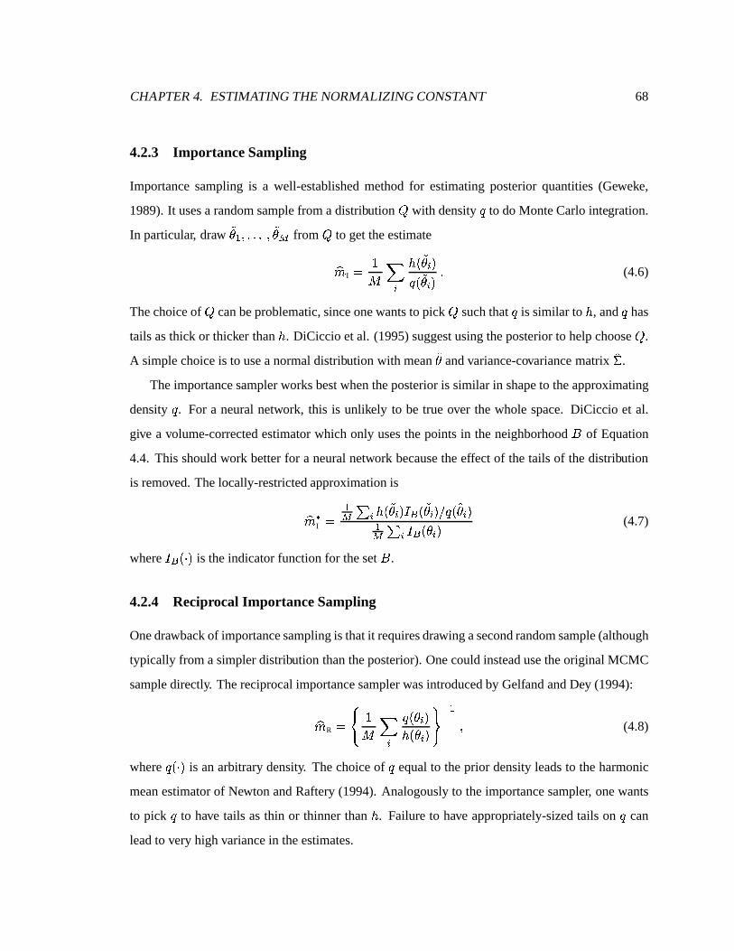
CHAPTER4. ESTIMATING THE NORMALIZING CONSTANT 68
4.2.3 Importance Sampling
Importancesamplingis a well-establishedmethodfor estimatingposteriorquantities(Geweke,
1989).It usesa randomsamplefrom adistribution _ with density÷ to doMonteCarlointegration.
In particular, draw�Ú�³eµe¹e¹e¹Üµ �Ú�` from _ to gettheestimateZ� I Å Û� ¡ 5º± �Ú�¡�¸÷�± �Ú�¡�¸ ¹ (4.6)
Thechoiceof _ canbeproblematic,sinceonewantsto pick _ suchthat ÷ is similar to 5 , and ÷ has
tails asthick or thicker than 5 . DiCiccio etal. (1995)suggestusingtheposteriorto helpchoose_ .
A simplechoiceis to useanormaldistribution with mean ÊÚ andvariance-covariancematrix Ê[ .
Theimportancesamplerworksbestwhentheposterioris similar in shapeto theapproximating
density ÷ . For a neuralnetwork, this is unlikely to be true over the whole space.DiCiccio et al.
give a volume-correctedestimatorwhich only usesthepointsin theneighborhoodG of Equation
4.4. This shouldwork betterfor a neuralnetwork becausetheeffect of thetails of thedistribution
is removed.Thelocally-restrictedapproximationisZ� |I Å ³` � ¡ 5º± �Ú�¡E¸2F H ± �Ú$¡à¸Xê�÷�± �Ú$¡E¸³` � ¡ F H ±!Ú�¡E¸ (4.7)
whereF H ±NM�¸ is theindicatorfunctionfor theset G .
4.2.4 Reciprocal Importance Sampling
Onedrawbackof importancesamplingis thatit requiresdrawing asecondrandomsample(although
typically from asimplerdistribution thantheposterior).OnecouldinsteadusetheoriginalMCMC
sampledirectly. Thereciprocalimportancesamplerwasintroducedby GelfandandDey (1994):Z� R Å a Û� ¡ ÷�±!Ú ¡ ¸5ܱ!Ú$¡�¸6b ù�³ µ (4.8)
where ÷�±NM�¸ is anarbitrarydensity. Thechoiceof ÷ equalto theprior densityleadsto theharmonic
meanestimatorof Newton andRaftery(1994).Analogouslyto theimportancesampler, onewants
to pick ÷ to have tails asthin or thinnerthan 5 . Failure to have appropriately-sizedtails on ÷ can
leadto veryhighvariancein theestimates.
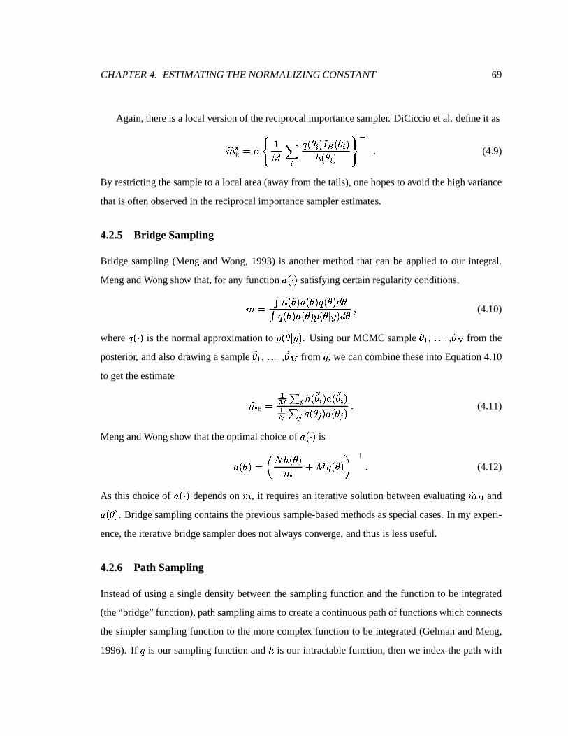
CHAPTER4. ESTIMATING THE NORMALIZING CONSTANT 69
Again,thereis a local versionof thereciprocalimportancesampler. DiCiccio etal. defineit asZ� |R Åc] a Û� ¡ ÷�±!Ú�¡�¸2F H ±!Ú$¡à¸5º±!Ú�¡�¸ b ù�³ ¹ (4.9)
By restrictingthesampleto a localarea(away from thetails),onehopesto avoid thehighvariance
thatis oftenobservedin thereciprocalimportancesamplerestimates.
4.2.5 Bridge Sampling
Bridge sampling(Meng andWong, 1993) is anothermethodthat canbe appliedto our integral.
MengandWongshow that,for any function /i±NM�¸ satisfyingcertainregularityconditions,� Å á 5º±!Ú�¸N/i±!Ú}¸N÷�±!Ú}¸�Ð�ÚáY÷�±!Ú}¸N/i±!Ú�¸úýñ±!Ú¼Ä Ý�¸�Ð�Ú µ (4.10)
where ÷�±NM�¸ is thenormalapproximationto ýñ±!Ú¼Ä Ý�¸ . Usingour MCMC sampleÚH³ , ¹e¹e¹ , Ú�d from the
posterior, andalsodrawing a sample�ÚH³ , ¹e¹e¹ ,
�Ú�` from ÷ , we cancombinetheseinto Equation4.10
to gettheestimate Z� B Å ³` � ¡ 5ܱ �Ú ¡ ¸N/i± �Ú ¡ ¸³d � � ÷�±!Ú � ¸N/˱!Ú � ¸ ¹ (4.11)
MengandWongshow thattheoptimalchoiceof /˱NM�¸ is/˱!Ú�¸;Å � Ø 5º±!Ú�¸� � � ÷�±!Ú}¸ � ù�³ ¹ (4.12)
As this choiceof /i±NM�¸ dependson � , it requiresan iterative solutionbetweenevaluating Ê� H and/˱!Ú�¸ . Bridgesamplingcontainstheprevioussample-basedmethodsasspecialcases.In my experi-
ence,theiterative bridgesamplerdoesnotalwaysconverge,andthusis lessuseful.
4.2.6 Path Sampling
Insteadof usinga singledensitybetweenthe samplingfunctionandthe function to be integrated
(the“bridge” function),pathsamplingaimsto createacontinuouspathof functionswhichconnects
thesimplersamplingfunction to the morecomplex function to be integrated(GelmanandMeng,
1996). If ÷ is our samplingfunctionand 5 is our intractablefunction,thenwe index thepathwith

CHAPTER4. ESTIMATING THE NORMALIZING CONSTANT 70
ä to getthepath ÷ | ±!Ú¼Ä ä<¸�Å7÷ ³Îù7� ±!Ú}¸�5 � ±!Ú�¸ . An estimateof theintegral canbefoundusingthis path.
However, this requiressamplesfrom the functionsalong the path, which are significantlymore
difficult to samplefrom in thecaseof neuralnetworks.Onewouldneedto useMetropolisstepson
all parameters,which would not becomputationallyfeasiblesinceoneneedsto generatea single
samplefrom many differentdensitiesalongthepath.HenceI did notpursuethismethod.
4.2.7 Density-BasedApproximation
Anotherapproachis basedonestimatingtheposteriordensityfrom theresultsof theMCMC simu-
lation. Sincetheposteriordensityisý�±!Ú¼Ä Ýg¸cÅ æ�±!Ú�¸NL;±!Ú}¸� Å 5ܱ!Ú�¸� µ (4.13)
wecanrewrite this to get � Å 5ܱ!Ú}¸ýñ±!Ú¼Ä Ý�¸ Å 5º±!Ú � ¸ý�±!Ú � Ä Ýg¸ (4.14)
for any point Ú � . If onecould do a densityestimationat Ú � , then the above equationis simple.
However, theposteriorfor a neuralnetwork is not unimodalandcontainsridgesof high posterior
probability makingdensityestimationa difficult task. The densityestimationsteprequiresuser
adjustmentof tuning parameters,which is difficult to do in higherdimensions.Becauseof this
addeduserdifficulty, it wouldnot bepracticalto usethis methodfor many differentmodelsduring
amodelselectionprocess,sothismethodwasnotpursuedfurther.
4.2.8 Partial Analytic Integration
As themodelis a hierarchicalmodel,thereis someconditionalindependenceamongsttheparam-
eters. It is indeedpossibleto analytically integrateout someof the parameters,in particularthe
outputcoefficientsandthevariance(the � ’s and � Ï ), leaving a “reduced”model. In theory, exact
integrationshouldbemoreaccuratethanusingany of theabove approximationsfor our integral.
For theimportancesampler, thereducedmodelgreatlysimplifiesthecalculationsasit removes
theneedto generaterandomdraws for thevarianceparameter� Ï . ThusI only usethe importance
CHAPTER4. ESTIMATING THE NORMALIZING CONSTANT 71
samplerandthebridgesamplerfor thereducedmodel,not for thefull model.For theotherapprox-
imations,I calculateestimatesusingboththefull andreducedmodels.
4.2.9 BIC
TheBayesianInformationCriterion(BIC) (Schwarz,1978):GeF�2 Å5ælÍ Û� ý\DGF�H ,uµ (4.15)
where æ is themaximumof the log-likelihood, ý is thenumberof parametersin themodel,and ,is thesamplesize. TheBIC is anapproximationof the log of theBayesfactorfor comparingthe
modelto thenull model(thatwith only aninterceptterm). In many casesit canbeshown that the
BIC minusthelog of theBayesfactoris � � ±sÛ¸ . Thuswecanapproximatetheposteriorprobability
of model ² with ýñ± � ¡ Ä Þ´¸gf Á H K � f� � Á H K �Ah µ (4.16)
where GiF"26¡ is theBIC for themodel� ¡ . This approximationis simplerthantheothersin that it
only requiresthe maximumlikelihoodestimatesof the parametersratherthana samplefrom the
posteriordistribution.
4.3 Numerical Comparisonsof the Methods
In this sectionI will describethe resultsof comparingthesemethodson two differentdatasets.
Thefirst is a one-variabledatasetthatlooksapproximatelyquadratic,implying two or maybethree
nodesarenecessary. Theseconddatasetis asimulatedexamplecontainingtwo variablesof interest
andtwo noisevariables,andrequiringthreenodes.
4.3.1 Ethanol Data
Thefirst datasetis theethanoldataof Brinkman(1981).Thedatacomefrom anautomobileengine
experimentwhereethanolwas burnedas a fuel. This datasetcontains88 observations for one
explanatoryand one responsevariable,so it is a simple test of the approximationmethodsfor

CHAPTER4. ESTIMATING THE NORMALIZING CONSTANT 72
comparingdifferentnumbersof hiddennodesin the model. The explanatoryvariableof interest
is theequivalenceratio at which theenginewasrun, a measureof the level of ethanolin the fuel
(which is composedof ethanolandair). Theresponsevariableis thenormalizedconcentrationof
nitrogenoxide emissions( jlk and jmk Ï ). The datahave beenscaledto the unit square(which
improvescomputationalstability).
The network wasfit usingthe MCMC algorithmdescribedin Chapter2 with 25,000burn-in
runsand100,000runsfor two, three,andfour-nodenetworks,with fiverepetitionsfor eachnumber
of nodes.Figure4.2shows thedataandtypicalmeanfitted functionsfor themodels(i.e., thefitted
valuesaveragedover all of theMCMC samples).Thetwo andthree-nodefitted functionsarevery
similar, and both appearto fit quite well. The four-nodefitted function displayssomepossible
overfitting for thesmallervaluesof theequivalenceratio, indicatingvisually thatwe would prefer
a two or three-nodemodel.Sincethefits appearsosimilar, I expectthatthevariousapproximation
methodswill produceresultseitherpreferringthetwo-nodemodel(for parsimony), or treatingthe
two andthree-nodemodelsapproximatelyequally. Onemightexpectthatthefour-nodemodelwill
notbepreferredto thesmallermodelsbecauseof theoverfitting.
•••
•
•
•
• • •
••
••
••
•
•
• •
•
•
•
•••
•
•
•
•
•
•
•
••
•
••
•
•••
•
••
••
••
••
•
•••
••
•
•
•
•
••••
•
••
••
••• ••
••••
• •• •
•
•
•
•••
Ethanol Data
Equivalence Ration
NO
x
0.5o
0.6o
0.7o
0.8o
0.9o
1.0p0.
20.
40.
60.
81.
0 2 nodesq3 nodesr4 nodess
Figure4.2: AverageFittedFunctions
Despitethefactthatthefittedcurvesappearto fit verywell in all cases,andthatthis is oneof the

CHAPTER4. ESTIMATING THE NORMALIZING CONSTANT 73
simplestpossiblecasesin that thereis only oneinput variableandonly two to four hiddennodes,
theapproximationmethodsgive vastlydifferentanswers.Sincethecorrectansweris unknown, we
can’t comparetheseresultsto the“true” value.However, wecanat leastcomparethemto thevisual
resultsof Figure4.2.
Table4.1showstheestimatesof thenormalizingconstantsusingLaplaceapproximationandRe-
ciprocalImportanceSampling(RIS)onthefull posterior(all parameters),andthevolume-corrected
versionsof thesetwo methods.Networkswith two, three,andfour hiddennodesareshown, and
therearefive repetitionsfor eachcombinationof numberof nodesandmethod.Also includedin
the last columnis the exponentiatedBIC, which shoulddiffer from the othermethodsonly by a
constant(i.e. the ratiosof modelsshouldbe equalfor the BIC and for othermethods).As one
canclearlyseefrom the table,thevariousmethodsdo not agreeat all. TheLaplaceestimatesare
larger, especiallyfor the larger models.TheBIC clearlypicksout the two-nodemodel,while the
Laplacemethodsprefersthe four-nodemodel, and the RIS gives roughly equalcredenceto the
threeandfour-nodemodels. Sincethe four-nodemodelseemsto be over-fitting, this is evidence
thatwe shouldeitherstick to theBIC, or thatall of thesemethodsarefailing. Onepossiblething
thatmaybegoingwronghereis thatoneof theparametersin themodelis thevarianceof theerror,
whichhasaconditionalposteriordistribution which is inverse-gamma,notnormal.Thismaycause
problemswith thesamplingmethodsthatexpectnormalposteriors.Anotherlikely sourceof error
is the irregularly shapedcontours.As theparametersarehighly correlated,theposteriorsbecome
harderto approximatewith a normaldensity. This problemis aggravatedasthenumberof nodes
increases,hencethe deterioratingperformanceof the Laplaceapproximation.Also notethat the
non-BIC methodsarenot very consistentacrossdifferent repetitions,meaningthat they arevery
sensitive to theMCMC sample,especiallyfor thelargermodels.Thesamplesizemayalsobetoo
smallfor goodperformanceof thesemethods.
Table4.2showsestimatesof thenormalizingconstantsbasedona reducedposterior, wherethe
outputcoefficientsandthe final varianceparameterhave beenanalytically integratedout. These
estimatesshouldbebetterthanthosein theprevioustablebecausetherearefewerdimensionsbeing
estimated.ThemethodsincludedaretheLaplaceapproximation,thereciprocalimportancesampler
(RIS), theimportancesample(Imp Samp),andthebridgesampler, aswell asthevolume-corrected

CHAPTER4. ESTIMATING THE NORMALIZING CONSTANT 74
Laplace Laplace-VC RIS RIS-VC BIC2.38e+36 2.60e+37 1.81e+36 9.03e+34 1.24e+351.39e+35 2.49e+35 1.75e+35 8.77e+33 1.14e+35
2 Nodes 3.83e+35 9.13e+35 4.74e+35 2.37e+34 1.35e+352.42e+35 6.53e+35 2.88e+35 1.44e+34 1.37e+355.04e+36 6.56e+36 9.49e+35 4.75e+34 1.33e+356.19e+44 2.77e+44 2.82e+42 1.41e+41 1.72e+322.08e+46 2.76e+46 8.13e+43 4.06e+42 4.29e+32
3 Nodes 1.09e+47 4.91e+46 3.36e+42 1.68e+41 1.55e+326.96e+45 4.98e+45 4.20e+43 2.10e+42 6.86e+324.43e+45 4.12e+45 5.79e+43 2.90e+42 3.83e+329.42e+47 5.22e+47 3.23e+42 1.62e+41 7.05e+293.36e+48 1.38e+49 4.23e+43 2.11e+42 2.08e+30
4 Nodes 2.15e+55 2.40e+55 4.99e+47 2.50e+46 3.18e+301.17e+44 5.40e+44 1.49e+41 7.44e+39 5.29e+302.60e+47 9.08e+48 7.16e+44 3.58e+43 1.04e+32
Table4.1: NormalizingConstantEstimatesBasedon theFull Posterior
versionsof thefirst three.Again,therearethreepossiblenumbersof hiddennodesfor thenetwork,
andfive repetitionsof eachcombinationof nodesandmethod.Thefive runsarethesameasin the
previoustable,sotheresultsaredirectlycomparableacrossthetwo tables.
In this table,themethodsproducemuchmoresimilar results,andthey arealsomoreconsistent
for different MCMC runs (repetitions). The volume correctionplays a larger role in the larger
models,whereit appearsto shrinktheestimatesa little. TheLaplaceapproximationsstill seemto
favor thefour-nodemodel,althoughnot by asmuchasbefore,andthetwo-nodemodelis favored
over thethree-nodemodel. Thereciprocalimportancesamplerestimatesgenerallypreferthetwo-
nodemodel. The importancesamplerfavors the four-nodemodel. The bridgesamplesupports
eitherthetwo-nodemodel,or boththetwo andfour-nodemodels,althoughit is not clearwhy this
mightbeso.
Sincethis is arealdatasetandthetrueansweris notknown, it washopedthattheBAYESPACK
software(GenzandKass,1997)would provide a “gold standard”.However this package’s numer-
ical integrationroutinesdid not seemto beany morereliablethantheabove methods.In fact,be-
causetheroutinessampletheheightof thefunctionin aneighborhoodof themode,but donothave

CHAPTER4. ESTIMATING THE NORMALIZING CONSTANT 75
Laplace Laplace-VC RIS RIS-VC Imp Samp Imp Samp-VC Bridge1.33e+38 1.24e+39 8.01e+38 4.28e+37 4.43e+38 1.23e+39 9.32e+371.41e+38 3.37e+38 3.80e+38 2.33e+37 7.05e+38 3.60e+38 1.83e+38
2 Nodes 1.26e+38 1.61e+38 1.99e+38 1.17e+37 4.84e+38 1.69e+38 1.82e+381.32e+38 3.19e+38 3.31e+38 1.91e+37 4.64e+38 3.40e+38 1.96e+382.91e+38 6.97e+38 5.70e+38 3.18e+37 4.77e+38 6.40e+38 2.05e+381.47e+38 1.67e+39 8.40e+37 4.22e+36 1.14e+39 3.65e+38 1.39e+351.49e+37 6.59e+38 1.26e+38 6.31e+36 1.51e+38 8.73e+37 1.55e+35
3 Nodes 1.31e+40 4.35e+40 1.02e+39 5.11e+37 6.89e+39 1.92e+39 8.19e+361.75e+38 2.29e+39 1.25e+38 6.26e+36 7.01e+38 2.26e+38 1.92e+351.94e+37 1.69e+38 4.94e+36 2.47e+35 2.46e+38 2.80e+37 3.85e+359.44e+37 1.06e+39 5.36e+36 2.68e+35 3.08e+40 3.70e+38 3.30e+361.02e+39 4.34e+39 9.57e+37 4.79e+36 1.61e+41 2.08e+39 1.31e+37
4 Nodes 3.43e+40 3.40e+40 5.22e+37 2.61e+36 4.82e+41 3.68e+39 1.28e+381.79e+38 2.37e+39 3.48e+37 1.74e+36 2.08e+41 4.50e+39 3.59e+362.77e+41 6.77e+41 2.01e+40 1.00e+39 1.94e+42 1.60e+41 3.92e+38
Table4.2: NormalizingConstantEstimatesBasedon theReducedPosterior
the additionalinformationaboutthe contoursfrom an MCMC sample(e.g.,a posteriorvariance-
covariancematrixfor theparameters),they endupsamplingpointsthatfall off of thepeaksbecause
theshapeof thecontoursis soirregular. Table4.3showstheresultsof six differentnumericalmeth-
odsin estimatingthenormalizingconstant,usingthereducedposterior. Of noteis thattheroutines
did not work at all for the four-nodemodel,becausethey alwaystried to evaluatetheposteriorat
pointstoo far off thepeaks(becausethey didn’t samplealongthecontours,astheMCMC methods
did). The posteriorthenbecomesnumericallyunstableandcausesthe methodsto fail. This also
appearsto bethecasefor thestochasticradial-sphericalmethodon thetwo-nodemodel. Evenfor
the caseswhereBAYESPACK did find a numericalanswer, therewasconsiderabledisagreement
betweenthe methods,especiallyfor the three-nodemodel. Thus,this packagewasnot useful in
establishinga standard.It hadasmuchtroubleasthe MCMC-basedmethodsin determiningthe
answer. SinceI encounteredthismuchtroublein thissimplecase(onevariable,two to four nodes),
I did notattemptto usethispackagein thenext example.

CHAPTER4. ESTIMATING THE NORMALIZING CONSTANT 76
2 Nodes 3 NodesMonteCarloIntegration 2.9e+40 3.6e+45Subregion Adaptive Integration 3.5e+39 5.9e+43MixedSpherical-Radial 1.9e+40 2.5e+43Gauss-HermiteIntegration 8.1e+39 9.5e+41ModifiedGauss-Hermite 8.1e+39 4.3e+46StochasticRadial-Spherical NA 5.4e+43
Table4.3: NumericalEstimatesfrom BAYESPACK
4.3.2 SimulatedData
The simpleethanoldataexampleof the previous sectionproducedfairly muddyresultsfrom the
variousapproximationmethods.To further comparethe methods,I useda simulateddatasetso
that the true answeris known. The dataconsistof 120 observations. Therearefour explanatory
variables,uniformly distributedover the four-dimensionalhyper-cube,andoneresponsevariable,
which is a functionof only thefirst two explanatoryvariablesplussomesmallrandomnoise:¶ÇÅ ÛÛ6�� ��"��±�$ Í Û Ä ²´³\¸ Í ÛÛ!�� ��"��±ÎÛp� Í Û Ä ²´³\¸ � ÛÛ!�� ��"��±ÎÛ%� Í Û%�À²´³qÍ Û%�À² Ï ¸ Í Ô ¹ut Ô �\�wvHµ(4.17)
where vuÖ ØÙ± Ô µ Ô ¹ Ô Û Ï ¸ . A graphof thesurfacefor thefirst two explanatoryvariablesis shown in
Figure4.3. Thegraphshows thattherearetwo thingsgoingon in thedata.First, thereis a “bump”
alongthe ²´³ axis, so that ¶ is higherfor ²´³ valuesin the middle thanon the ends. Also in the
datais a “wave” thatstartsout with low ¶ valuesin thefront corner, andrisesto high ¶ valuesin
therearcorner, sothat ¶ increaseswith thesumof ² ³ and ² Ï . Thusthemodelcanbefit perfectly
(without thenoise)with threehiddennodesandonly thefirst two explanatoryvariables.Notethat
interactionof ²´³ and ² Ï makesit difficult to fit thismodelwith asimpleadditive model.
To testoutthenormalizingconstantapproximationmethods,I ranafull factorialdesign.Models
werefit with two, three,andfour hiddennodes(wherethreeis thecorrectnumber).Eachpossible
combinationof explanatoryvariables(from oneto four atatime)wasused,andeachapproximation
methodwasattemptedoneachcombinationof explanatoryvariablesandnodes.In many cases,nu-
mericalproblemspreventedtheactualimplementationof theapproximations.For example,whenI
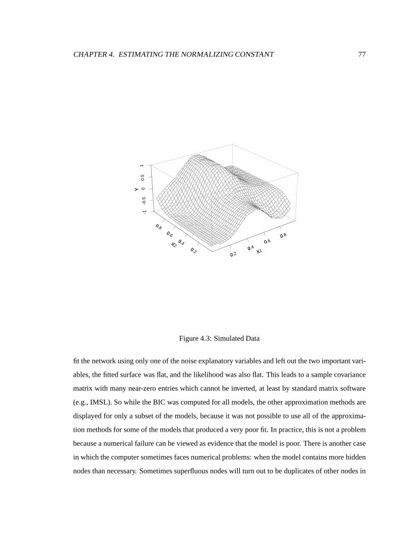
CHAPTER4. ESTIMATING THE NORMALIZING CONSTANT 77
0.2x 0.4x 0.6x 0.8
xX1y0.2z0.4z0.6z0.8z
X2{
-1-0
.5 0
0.5
1Y
|
Figure4.3: SimulatedData
fit thenetwork usingonly oneof thenoiseexplanatoryvariablesandleft out thetwo importantvari-
ables,thefittedsurfacewasflat, andthelikelihoodwasalsoflat. This leadsto a samplecovariance
matrix with many near-zeroentrieswhich cannotbe inverted,at leastby standardmatrix software
(e.g.,IMSL). Sowhile theBIC wascomputedfor all models,theotherapproximationmethodsare
displayedfor only a subsetof themodels,becauseit wasnot possibleto useall of theapproxima-
tion methodsfor someof themodelsthatproducedaverypoorfit. In practice,this is notaproblem
becauseanumericalfailurecanbeviewedasevidencethatthemodelis poor. Thereis anothercase
in whichthecomputersometimesfacesnumericalproblems:whenthemodelcontainsmorehidden
nodesthannecessary. Sometimessuperfluousnodeswill turnout to beduplicatesof othernodesin

CHAPTER4. ESTIMATING THE NORMALIZING CONSTANT 78
Variables 2 Nodes 3 Nodes 4 Nodes1 3.38e-25 1.63e-27 3.27e-30
2 4.61e-38 4.31e-41 6.13e-443 1.38e-46 1.49e-49 1.70e-52
4 1.05e-45 3.22e-49 4.03e-511 2 2.74e+23 2.77e+155 3.14e+1511 3 1.71e-26 3.37e-30 5.68e-331 4 5.29e-27 8.92e-31 1.10e-34
2 3 6.23e-39 1.01e-42 5.47e-462 4 9.60e-39 1.91e-41 5.57e-46
3 4 1.06e-47 6.52e-52 4.21e-561 2 3 5.24e+21 2.68e+152 2.31e+1471 2 4 3.36e+22 3.17e+152 4.94e+1471 3 4 7.65e-29 6.45e-34 4.69e-38
2 3 4 1.36e-40 2.16e-45 4.46e-501 2 3 4 6.09e+20 2.75e+149 1.81e+143
Table4.4: BICs for SimulatedData
thesensethatthey arelinearlydependentonothernodes;if wethink of thenodesasbasisfunctions,
thenasuperfluousnodeis in thesubspaceof thepreviousnodes.Becauseof this lineardependence,
we againfacenumericalproblemsin inverting matrices.Again, this is not a practicalproblem,in
thatthis modelwould beinferior to theonewithout thesuperfluousnode,sowe arenot losingany
modelsof highposteriorprobability.
As long aswe canfit the model,we cancomputethe BIC. Table4.4 shows theBIC for each
of the modelsin this simulation. The columnsarethe numberof hiddennodes,andthe rows are
thecombinationsof explanatoryvariables,with thenumbersindicatingthatthatvariableis present
(e.g. 124meansthat }�~���}@�A� and }Y¶ wereincludedin themodel,andthat } è wasnot). TheBIC
for the true model is shown in boldfacetype. The resultsin this tablearequite remarkable.The
BIC very clearly picks out the importantmodels—thosethat includeboth }�~ and }@� , andthose
with threeor four nodes.Two hiddennodesareclearlynotenough.And for agivensetof variables,
thethree-nodemodelsdominatethefour-nodemodels,showing thatonly threenodesarenecessary.
For the modelswhich do not includeboth }�~ and }@� , the BIC is extremelysmall anddecreases
asthenumberof hiddennodesincreases(whichmakessensebecauseweareaddingnodeswithout

CHAPTER4. ESTIMATING THE NORMALIZING CONSTANT 79
Two HiddenNodesLaplace Laplace-VC RIS RIS-VC
1 2 1.53e+25 3.34e+25 0 2.27e+231 2 3 1.05e+29 2.07e+28 1.64e+16 2.06e+151 2 4 1.47e+24 1.35e+24 9.27e+22 4.63e+211 2 3 4 3.62e+24 1.43e+24 1.75e+22 8.74e+20
ThreeHiddenNodesLaplace Laplace-VC RIS RIS-VC
1 2 5.70e+149 4.69e+149 1.24e+147 6.02e+1451 2 3 4.62e+145 5.33e+145 6.69e+141 3.35e+1401 2 4 1.48e+146 3.90e+146 1.97e+142 9.86e+1401 2 3 4 1.51e+138 3.41e+138 7.50e+132 3.75e+131
FourHiddenNodesLaplace Laplace-VC RIS RIS-VC
1 2 1.10e+159 6.56e+158 9.67e+154 4.84e+1531 2 3 1.07e+146 7.97e+146 5.36e+139 2.68e+1381 2 4 4.32e+146 3.56e+147 2.16e+140 1.08e+1391 2 3 4 6.73e+135 6.10e+136 2.98e+127 1.49e+126
Table4.5: NormalizingConstantApproximationsfor SimulatedData
any benefitin fit). TheBIC hasdoneits job.
Table4.5shows thenormalizingconstantestimatesusingthemethodsbasedon thefull poste-
rior. Again,theestimatesfor thetruemodelareshown in boldfacetype.Themethodsonlyproduced
estimatesfor modelsincluding both }�~ and }@� , asthe covariancematrix for the parameterswas
typically not invertible in the othercases.The threeand four-nodemodelsareclearly preferred
to the two-nodemodels,andthe modelwith only two variablesis clearly preferredto the larger
models.Of noteis thatboththeLaplaceapproximationandthereciprocalimportancesamplegive
significantlyhigherposteriorprobabilityto thefour-node,two-variablemodelthanthethree-node,
two-variablemodel (which is the correctmodel). Onepossibleexplanationfor the confusionof
thesemethodsis theirregularcontoursof theposterior. Usingthefull setof parametersmeansa lot
of highly correlatedparametersandnon-normallyshapedcontours.An upcomingtablewill present
approximationsbasedon the reducedposterior, andthis simplerestimationproblemprovesmore
tractablefor theapproximationmethods.
Oneotheritemof noteis thezeroentryfor thereciprocalimportancesamplerfor thetwo-node,

CHAPTER4. ESTIMATING THE NORMALIZING CONSTANT 80
Two HiddenNodesLaplace Lapl-VC RIS RIS-VC Imp Samp I. S.-VC Bridge
12 1.21e+28 1.37e+28 0.0157 1.91e+26 1.55e+27 2.26e+27 5.10e+08123 1.89e+30 3.21e+29 6.16e+16 5.44e+16 1.26e+26 2.12e+26 8.57e+10124 1.10e+27 8.88e+26 5.85e+26 2.93e+25 6.10e+26 6.14e+26 5.77e+261234 1.88e+27 6.14e+26 7.05e+25 3.53e+24 5.11e+25 4.03e+25 1.68e+25
ThreeHiddenNodesLaplace Lapl-VC RIS RIS-VC Imp Samp I. S.-VC Bridge
12 1.14e+152 1.17e+152 1.24e+151 6.18e+149 7.31e+149 1.08e+150 3.72e+149123 7.78e+147 2.61e+148 3.03e+146 1.51e+145 5.37e+145 1.42e+146 4.95e+145124 2.83e+148 3.70e+148 2.75e+146 1.38e+145 2.62e+146 1.09e+146 1.12e+1461234 8.45e+141 2.46e+142 3.88e+138 1.94e+137 1.52e+142 2.51e+142 3.64e+141
FourHiddenNodesLaplace Lapl-VC RIS RIS-VC Imp Samp I. S.-VC Bridge
12 6.03e+149 1.46e+151 7.29e+147 3.65e+146 1.25e+150 7.27e+149 1.41e+146123 5.80e+141 1.02e+143 2.90e+138 1.45e+137 5.98e+145 5.88e+143 6.69e+141124 7.46e+141 5.19e+142 4.86e+137 2.43e+136 3.88e+145 3.52e+143 1.09e+1421234 5.97e+137 1.17e+139 1.49e+132 7.45e+130 3.60e+139 2.23e+139 8.76e+128
Table4.6: NormalizingConstantApproximationsfor SimulatedData
two-variablemodel.This is anexampleof theinstabilityof thismethod,asaproblemin thetailsof
thedistribution cancausecatastrophicfailureof themethod.Thelocal (volume-corrected)version,
however, eliminatesthis tail problemandproducesanestimatecloserto theLaplaceestimates.
Table4.6 shows the normalizingconstantestimatesusing the methodsbasedon the reduced
(partially analytically integrated)posterior. Again, the smallesttwo-nodemodel presentssome
challengesto themethods,andthereciprocalimportancesamplerdemonstratesits instability. Also
noteworthyis thediscrepancy betweenthebridgesamplerestimateandtheotherestimates.Overall,
the methodsshow a significantdisagreementabout the value of the normalizingconstantfor a
particularmodel. However, they do generallyagreethat, for a given numberof nodes,the only
two importantvariablesare }�~ and }@� . And they agreethat threeis theright numberof nodesin
thattwo nodesareclearlyinsufficient,while four nodesdo not significantlyimprove thefit. In this
sense,all of themethodsdofind thecorrectanswer.

CHAPTER4. ESTIMATING THE NORMALIZING CONSTANT 81
4.4 Discussion
While all of themethodsperformedwell in therelatively straightforwardconditionsof thesimulated
data(Section4.3.2), thereis a breakdown in the consensuson the simplereal dataexample(the
ethanoldataof Section4.3.1).It is notclearwhy thevariousMCMC-basedapproximationsperform
sodifferentlyfrom theBIC in thisverysimpleexample.I hadexpectedthatusingalarge(100,000)
MCMC samplefrom the posterioralongwith oneof the above methodswould producea better
estimateof the normalizingconstantthan the BIC. While mostmethodshave theoreticalresults
showing that they areasymptoticallybetterapproximationsthanthe BIC, this is asymptoticwith
respectto thesamplesize,soit maybethatthesamplesin thischapterarenot largeenoughfor the
asymptoticsto hold. In thiscase,theBIC maybeamoreusefulapproximationfor standardsample
sizes.Furthermore,theBIC only requirescomputationof themaximumlikelihood,ratherthanan
MCMC samplefrom theposterior. In thissense,theBIC is botheasierto computeandmorestable,
in thatwe areeliminatingtheadditionalvariability inducedby theMCMC sample.Henceforth,I
will usetheBIC for all modelselectionandmodelaveragingpurposes.
It is not clearthat any of the methodsaregettingthe correctanswer. The multimodalityand
the irregularity of the posteriorcontoursappearto causeproblemsfor all of the methods.Of the
availablemethods,theBIC seemsbestableto dealwith theseproblems.
Note that even if an approximationmethodestimatesthe normalizingconstantpoorly, it may
still be useful for modelselection,as long as the rank orderof the estimatesof the normalizing
constantarecorrect.In thecasewheretheorderof two modelsis incorrect,it is still acceptableto
usethe methodif the two incorrectlyorderedmodelsgive very similar predictions.Thuswe can
still domodelselectionevenif wehave difficultiesestimatingthenormalizingconstant.
Chapter 5
Model Selectionand Model Averaging
5.1 Overview
5.1.1 Model Selection
Whenusingneuralnetworksfor nonparametricregression,wearefacedwith two relatedproblems
of model selection:we needto choosethe subsetof the explanatoryvariablesto include in the
model,andwe needto choosethenumberof hiddennodesto usein themodel.Thesechoicesare
importantbecauseaswe includemorevariablesand/ormorehiddennodes,the fit will improve.
However, at somepoint, addingmorevariablesor nodeswill result in over-fitting: the fit will be
betterfor the observed data,but will result in worsepredictive performanceon otherdata. The
variancefor predictionis a sumof two components:thesquareof thebias(errorbetweenthefitted
regressionfunctionandthetrueregressionfunction)andthevarianceof themodel.As weaddmore
variablesor nodes,the biasdecreases,but the varianceincreases.Thuswe needto find the right
trade-off betweenreducingvarianceandreducingbias.
The approachof modelselectioninvolves picking a singlebestmodel. Philosophically, this
might arisebecauseonefeelsthat thereis a singletrueunderlyingmodel,andthegoalof thedata
analysisis to identify thatmodel. In someareasof applications,this approachmaybejustified. In
otherareas,onemaydoubtthatananalystcouldever find theexact truemodel;for example,one
couldnevermeasureeveryrelevantvariableandincludeall of themin thedataset.However, westill
82

CHAPTER5. MODEL SELECTIONAND MODEL AVERAGING 83
mightdomodelselectionin orderto find theclosestapproximationto thetruemodel.For practical
purposes,we maynot needtheexact true model,but we canfind a modelusingour datathat we
feel is sufficiently closeto this truemodel.
In theBayesianframework, theproblemof modelselectionis straightforward.Oneneedmerely
put a prior over thespaceof models,thencomputetheposteriorprobabilitiesof all of themodels
andchoosethemodelwith highestposteriorprobability. Supposewearecomparingasetof models���for explainingthedata,� . Denotetheprior probabilityof model � by ��� ���&�
andits posterior
probabilityby ��� ����� � � . Bayes’Theoremstatesthat:��� �!�M� � ��� ���)� � � � � ��� � � ��0� ���)� � � � � ��� � � � � (5.1)
wherethesumis over all models.Conceptually, this processis very simple. In practice,the term���)� � � � �involvesmarginalizingover theparametersin themodel.For aneuralnetwork, this is an
analyticallyintractableintegral. Methodsfor estimatingthis integral werereviewed in Chapter4.
In thatchapter, I concludedthattheBIC (BayesianInformationCriterion)(Schwarz,1978)maybe
themostreliablewayof estimatingthisquantity. RecallthattheBIC for model���
is definedas�e�.�����Q���6����*� �� ¢¡A£g¤ � (5.2)
where� �
is the maximumof the log-likelihood,¤
is the samplesize, and � � is the numberof
parametersin model�!�
. For theprior over thespaceof models,I usethenoninformative prior that
putsequalmassoneachmodel,i.e. ��� �����¥� ��� � � �for all � and ¦ . TheBIC approximationthen
becomes ��� ����� � ��§ ���)� � � � ���� ���)� � � � � § ¨ª©8«�¬®�0� ¨ ©8«�¬A¯±° (5.3)
NotethattheBayesianapproachautomaticallytakescareof thebalancebetweenimproving fit and
not overfitting,becauseaddingadditionalvariablesor nodesthatdo not sufficiently improve thefit
will dilutetheposterior, causingalowerposteriorprobabilityfor themodel.Thisapproach,in addi-
tion to beingconceptuallystraightforward,alsohastheadvantagethatit canbeusedsimultaneously
onboththeproblemof choosinga subsetof explanatoryvariables,andon theproblemof choosing
thenumberof hiddennodesfor thenetwork. Furthermore,in many cases,theBIC hasbeenshown

CHAPTER5. MODEL SELECTIONAND MODEL AVERAGING 84
to beasymptoticallyconsistentfor choosingthetruemodel.While this hasnot yet beenshown for
neuralnetworks, Keribin (1997)hasrecentlyshown it to be true for mixture models,which have
somesimilaritiesto neuralnetworks.Soit seemsplausiblethatit wouldbetruefor neuralnetworks
aswell. Becauseof all of theadvantageslistedabove, I usethis approachin therestof thethesis.
For completeness,I shallnow review somealternative approaches.
An alternativeBayesian-motivatedapproachisAutomaticRelevanceDetection(ARD) (MacKay,
1994;Neal,1996). ARD utilizesanadditionallayerof hyperparametersin themodel,whereeach
explanatoryvariablehasanassociatedhyperparameterthatrelatesto themagnitudeof theparame-
tersassociatedwith thatexplanatoryvariable.A prior is placedover thehyperparameters,andthe
full posteriorfor the model is computed. If any of the variablehyperparametersturnsout to be
small, it indicatesthat that variablehaslittle effect on the model,andcould be dropped.A vari-
ablewith a largereffect would necessarilyhave a largerassociatedhyperparameter. Therearetwo
major drawbacksto this approach.First, oneneedsto decidehow large is large, andhow small
a hyperparameterwould have to be in orderto causethe variableto be droppedfrom the model.
Second,oneneedsto specifyaprior for thehyperparameters,andthechoiceof prior is linkedto the
determinationof “large” for a hyperparameter.
Therearemany methodsfor modelselection,althoughthey tendto treattheproblemof selecting
explanatoryvariablesandtheproblemof choosingthesizeof thenetwork astwo separateproblems,
ratherthandealingwith themsimultaneously. Thetwo maintypesof methodsfor variableselection
arecross-validation methodsand likelihood-basedcriteria. A major drawbackof many of these
methodsis that they werelargely developedasadhocmethods,anddo not give a soundtheoreti-
cal justificationfor why they would work. Sometheoreticalresultshave beenprovenaboutthese
methods,althoughthey generallydo tendto overfit themodel.
Cross-validation(Stone,1974)dividesthedatainto equally-sizedbins(sometimesassmallas
oneobservationperbin). Themodelsunderconsiderationarethenfit usingall but onebin of data,
andtheerrorontheexcludedbin undereachof themodelsis computed.Thisprocessis repeatedfor
all of thebins,andthemodelwith thesmallestsumof squarederrorsis chosenasthebestmodel.
It is hopedthatby leaving out a partof thedata,onecangetsomemeasureof thepredictive power
of themodel,thusreducingthetendency to overfit. Extensionsto theideaof cross-validationhave

CHAPTER5. MODEL SELECTIONAND MODEL AVERAGING 85
producedalargefamily of relatedmethods.In somespecificcases,cross-validationhasbeenshown
to beasymptoticallyoptimal(Stone,1982),althoughit tendsto overfit in practice.
TheBIC, discussedearlier(Equation(5.2)), is a likelihood-basedmethod.Anotherlikelihood-
basedmethodis the AIC (Akaike InformationCriterion). The AIC (Akaike, 1974)is simply the
maximumof thelog-likelihoodminusthenumberof parametersin themodel.Themodelwith the
largestAIC is deemedbest.Thus,it attemptsto balanceanimprovementin fit (measuredwith the
log-likelihood)with the sizeof the model. Comparedto the BIC, the AIC hasa smallerpenalty
for modelsize.TheBIC hasa Bayesianmotivation,in that it is anapproximationto thelog of the
Bayesfactorfor comparingthatmodelto thenull model. In many classesof models,theBIC has
beenshown to beasymptoticallyconsistentfor choosingthetruemodel(if oneassumesthatsucha
thingexists),andthis impliesthattheAIC mustbeoverfitting,sinceit usesasmallerpenalty.
Frequentistapproachesfor selectingthe numberof hiddennodesinclude the methodslisted
above for modelselectionaswell asashrinkage-basedapproachcalledweightdecay. Weightdecay
involvesanadditionalparameter, whichtranslatesinto apenaltytermassociatedwith thesizeof the
weights.This penaltyis addedinto the least-squareserror termandthis sumis thenminimizedto
find thebestmodel.Theideais for theunnecessaryweightsto beshrunktowardszero,sothatthese
extrahiddennodescanberemoved.
5.1.2 Model Averaging
An alternative to selectingasinglemodelis modelaveraging(Leamer, 1978;RafteryandMadigan,
1994). Onemight bemoreinterestedin optimizingpredictionthanin finding a singlebestmodel.
Or onemightnotsubscribeto any of thephilosophicalargumentsfor usingasinglemodel,andmay
justwantto try to useasfull amodelaspossible.Usingasinglemodelmayunderstatetheprediction
error, in thattheuncertaintyassociatedwith choosingthatmodelis not includedin thefinal model.
Modelaveragingusesaweightedaverageof all of themodelsto find predictedvalues.Thetermsin
theaverageareweightedby theirposteriorprobabilities.Let ² betheresponsevariable,� thedata,
and�!�
themodelsof interestfor ��³@´ . Thentheposteriorpredictive distribution of ² is���µ² � � ���P¶ �µ·�¸ ���µ² � �¹� ���º� ��� ���M� � � � (5.4)
CHAPTER5. MODEL SELECTIONAND MODEL AVERAGING 86
where ���µ² � �»� �!�º�is the marginal posteriorpredictive densitygiven a particularmodel(with all
otherparametersintegratedout),and ��� �!��� � �is theposteriorprobabilityof model � .
Whenmore thanone modelhasa relatively high posteriorprobability, it is advantageousto
usemodelaveragingfor predictionratherthansimply usingthe singlebestmodelfor prediction.
Someexamplesof modelaveragingresultingin dramaticdecreasesin predictionerrorsaregivenin
Rafteryet al. (1997). Model averagingcanalsohelpwhenmodelswith high posteriorprobability
give conflicting advice,warningthe userthat the uncertaintyassociatedwith thosepredictionsis
muchlargerthanonemightexpectif only asinglemodelwereused.Raftery(1996)givesamedical
examplewherethe predictionsvary greatlybetweentwo modelswhich both have similarly high
posteriorprobability.
While modelaveragingfits naturallyinto theBayesianframework, it is harderto developaFre-
quentistanalog.Someattemptsto accountfor modeluncertaintywithout theBayesianframework
includebagging(Breiman,1994)andbumping(TibshiraniandKnight, 1995).Bothof thesemeth-
odsusebootstrapsamplesof theoriginal datato try to dealwith theuncertaintyin theselectionof
thefinal modelusedfor prediction.
Onedrawbackof themodelaveragingapproachis thatthefinal “model” is anaverageof multi-
plemodels.Theresultof modelaveragingcanbedifficult to interpret,sinceit is notasinglemodel.
In thecasewheretheability to interpretthefinal modelis important,modelaveragingshouldnot
beused.In practice,neuralnetworksarenormallydifficult to interpreton their own, sothis is not
muchof aconcernin thecontext of this thesis.
5.1.3 Searching the Model Space
The above methodsfor model selectionand modelaveragingassumethat one can computethe
posteriorprobabilitiesfor all of the modelsof interest. In practice,the spaceof possiblemodels
maybetoo largeto doacompleteenumerationof all of themodels.For example,for � explanatory
variables,thereare�½¼
possiblesubsetsof variablesthatcouldbeusedfor regression;now multiply
by the numberof hiddennodesthat onemight want to considerto get an even larger numberof
modelsover which onewould needto find all of thefitted modelsandposteriorprobabilities.This
is typically not feasiblefor a complicatedmodellike a neuralnetwork wherefitting a singlemodel

CHAPTER5. MODEL SELECTIONAND MODEL AVERAGING 87
maytake sometime. Thusthereis a needfor anautomatedtechniqueto searchthroughthemodel
space.
Two traditionalsearchmethodsarestepwiseregressionandLeapsandBounds(Furnival and
Wilson,1974).In thenext section,I will describeanimplementationof astepwisealgorithm.Some
BayesianmethodsareOccam’sWindow (RafteryandMadigan,1994),Markov ChainMonteCarlo
Model Composition(Rafteryet al., 1997),anda relatedtechnique,BayesianRandomSearching
(Lee,1996),all of which I will describein latersections.TheseBayesianmethodsall useapproxi-
mationsto Bayesfactorsfor moving betweenmodelsin thesearchspace.
A final noteaboutsearchingthemodelspaceneedsto bemadein thecontext of neuralnetworks.
In many statisticalapplications,onecanfit themodelwith reasonableconfidence(e.g.linearregres-
sion).However, fitting aneuralnetwork, in eithera frequentistor Bayesianframework, involvesthe
useof aniterativealgorithmwhichcouldfind alocalmaximumratherthanaglobalmaximum.One
maywantto keepin mind thata modelvisitedduringa searchalgorithmmaynot necessarilybefit
correctly.
5.1.4 Fitting the Models
In the implementationsof all of the searchstrategies, I usethe BIC as the criterion for moving
betweenmodels. Thus I do not needto take a fully Bayesianapproachat this stepand do not
needto useMCMC to find the posteriorsfor eachof the modelsunderconsideration.Instead,I
canusestandardnumericalmaximizationmethodsto find the maximumlikelihood estimatesof
the parametersandusethoseto find the BIC. This savesmuchtime in computation,andgiven a
goodalgorithmfor finding theMLEs, couldbemorereliablethandependingon convergenceof an
MCMC run.
I have implementedin SAS,usingthe macrolanguagefacilities,all of the searchstrategies I
describebelow. Thecoreof theprogramsis codefrom Sarle(1994),of theSASInstitute,thatuses
procNLP to find themaximumlikelihoodestimatesof theparametersin a neuralnetwork. These
estimatesareall thatis necessaryto computetheBIC.
Oncea subsetof model with high posteriorprobability is found and thoseprobabilitiesare
calculated(or estimated),a morefully Bayesianapproachwould thencall for eachmodelof high
CHAPTER5. MODEL SELECTIONAND MODEL AVERAGING 88
probabilityto befit usingMCMC sothatonecanfind theposteriordistribution of theparameters,
conditionalonthatmodel.Thesefull posteriorsthencanbeusedfor prediction,eitherfrom asingle
modelor from anaverageof models.
5.2 StepwiseAlgorithm
Stepwisealgorithmsfor finding a bestmodelhave existedin the linear modelliteraturefor some
time. The basicideais to move throughthe modelspaceby taking stepsconsistingof addingor
deletinga singlevariable. At eachstep,theprocesscanbemoving forward (addingvariables)or
backward(removing variables).A greedyalgorithmpicksthesinglebestvariableto add(remove)
at eachstepby maximizingsomecriterionover thepossiblemodelsthatwould resultfrom adding
(removing) a variable. The algorithmcontinuesmoving in the samedirectionuntil no morevari-
ablescanbeadded(removed). Thealgorithmthenreversesdirectionandattemptsto remove (add)
variables.Thiscontinuesuntil thealgorithmswitchesdirectionsin two consecutivesteps,indicating
thatnobettermodelsareonestepawayfrom thecurrentmodel,or from any previousmodelvisited,
andsothealgorithmends.
I have implementeda stepwisealgorithmin SAS. I usethe BIC as the criterion for moving
betweenmodels,only moving to modelswith a larger BIC. I alsoconsideradding(removing) a
hiddennodeinsteadof addinganotherexplanatoryvariable.Thebasicalgorithmis asfollows:
1. Find thefit andBIC for thestartingmodel(typically thenull modelwith noparameters,or a
modelwith all of theparameters).
2. Generatecandidatemodels:
(a) If moving forward,fit all of themodelswith onemoreparameterthanthecurrentmodel,
aswell asthemodelwith onemorehiddennodethanthecurrentmodel.
(b) If moving backward, fit all of the modelswith one fewer parameterthan the current
model,aswell asthemodelwith onefewer hiddennodethanthecurrentmodel.
3. ComputetheBICsfor eachof thesecandidatemodels.If any of thecandidateshasaBIC that

CHAPTER5. MODEL SELECTIONAND MODEL AVERAGING 89
is largerthantheBIC of thecurrentmodel,thenchoosethecandidatemodelwith thelargest
BIC andmake thatthenew currentmodel.
4. If abettercandidatemodelwasfound,thenreturnto step2 andcontinuemoving in thesame
direction.
5. If a bettercandidatemodelwasnot found (all candidatemodelshadsmallerBICs thanthe
currentmodel),thenreturnto step2, but switchdirections.
6. If thedirectionis switchedin two consecutive passes,thenno bettermodelsexist with either
onemoreor onefewer variableor node,soterminatethealgorithm.
Stepwisealgorithmsareadmittedlyadhocandmaynot find themodelwith highestposterior
probability. However, they oftenwork well in practice,andarerelatively simpleto implement,so
they areworth trying. They tendto run into troublewhentheeffectsof variablesarecorrelated,so
thatan importantinteractionbetweentwo variablesmaynot be foundwhenthealgorithmis only
allowedto move in stepsof onevariableat a time.
Oncethestepwisealgorithmhasbeenrun, theusernow hasa subsetof modelsthathopefully
includesall of themodelswith thehighestposteriorprobabilities.If oneis doingmodelselection,
thenthefinal modelof thestepwisesearchwill beconsideredthebestmodel.If oneis doingmodel
averaging,thentheposteriorprobabilitiesof themodelsin thesubsetarecalculatedusingtheBICs.
In eithercase,a morefully Bayesiananalysiswould thenuseMCMC to find theposteriorfor the
parametersof eachof themodelsof highposteriorprobability.
In practice,I have found that a particularrun of the stepwisealgorithmwill find only a local
maximumfor oneof themodels,andsoit maygetstuckin a sub-optimalmodel.Sincethis results
from thefitting algorithmbeingstuckin a local maximum,ratherthanin a truelocal maximumof
theBIC, I usuallyfit eachcandidatemodelfive times,andusethefit with thehighestBIC asthe
candidatein thestepwisealgorithm.

CHAPTER5. MODEL SELECTIONAND MODEL AVERAGING 90
5.3 Occam’sWindow
Occam’s Window (RafteryandMadigan,1994)narrows themodelspaceby only keepingmodels
with high posteriorprobabilityin thesetof modelsunderconsideration.In addition,thealgorithm
employs theprincipleof Occam’sRazor, in thatif two modelshaveequalposteriorprobability, then
the simplermodel is to be preferredto the larger model. Thesetwo ideasform the basisof the
algorithm.
Thedetailsof which modelsarekeptunderconsiderationandwhichmodelsareexcludedfrom
thefinal setof modelsare:
1. Excludefrom considerationany modelwith posteriorprobability lessthan �ª¾�¿ timesthatof
the modelwith highestposteriorprobability. ¿ � ��Àis suggestedasa guideline,which is
comparedto thestandard0.05cutoff for a � -value.
2. Whencomparingsubmodelsof thecurrentmodel,excludeall submodelsof any submodels
whichhave beenexcludedby thefirst rule.
3. Whencomparingsupermodelsof the currentmodel,excludeall supermodelsof any super-
modelswhichdonothave higherposteriorprobabilitythanthecurrentmodel.
Note that the log of the ratio of posteriorprobabilitiescan be approximatedby a differenceof
BICs. Second,notethatstrongerevidenceis requiredto excludeasmallermodelthanis requiredto
excludea largermodel.Thisasymmetryis dueto theapplicationof Occam’s Razor.
Thealgorithmis run asa pair of algorithms,oncein anupwarddirection,oncein a downward
direction. Thesedirectionscanbedonein eitherorder, so thatonecanstartwith a small (or null)
model,grow thatmodelwith theup algorithmto geta setof modelsunderconsideration,thenrun
thedown algorithmoneachof themodelsfoundfrom theupalgorithmto getafinal setof models.
Or thealgorithmcouldstartwith a largemodelon which thedown algorithmis run. Thesubsetof
modelsfoundby thedown algorithmwould thenbefed into theupalgorithmto find thefinal setof
modelswith highposteriorprobability.
Thisalgorithmhasasimilarproblemto thestepwisealgorithm,in thatwhenacandidatemodel
is considered,onedoesnot know if the MLE hasbeenaccuratelyfound, or if the maximization

CHAPTER5. MODEL SELECTIONAND MODEL AVERAGING 91
algorithmhasmerelyfounda local maximum.SoI alsorecommendfitting eachcandidatemodel
multiple times(I usefive) andusingthefit with thebestBIC whendecidedif themodelshouldbe
keptor excluded.
5.4 Mark ov Chain Monte Carlo Model Composition
TheideabehindMarkov ChainMonteCarloModelComposition( ÁÃÂÅÄ ) (Rafteryetal.,1997)is to
createa Markov Chainwith statespaceequalto thesetof modelsunderconsiderationandequilib-
rium distribution equalto theposteriorprobabilitiesof themodels.Thusif we simulatethis chain,
theproportionof time thatthechainspendsvisiting eachmodelis a simulation-consistentestimate
of the posteriorprobability of that model. To createsucha chain, let the transitionprobabilities
betweentwo modelsbeasfollows:
1. Theprobabilityof moving from thecurrentmodelto a modelwhich differsby two or more
parameters(differing by inclusionor exclusion)is zero.
2. Theprobabilityof moving from thecurrentmodelto onewhich differsby exactly onevari-
ableor node(eitheronemoreor oneless)is ~Æ�Ç@È É Ê � ��Ë ÆÍÌÏÎiÐµÑ Ò�ÓË ÆÍÌ¢Î�Ñ Ò�Ó®Ô , where Õ is thenumberof
parametersbeingconsidered(i.e., thedimensionof thesearchspace),�mÕ=� �×Ö�� � �is thepos-
teriorprobabilityof themodelbeingmovedto, and �ØÕ;� �^� � �is theposteriordistribution of
themodelbeingmovedfrom.
3. Otherwise,thechainstaysin its currentstate.
In my implementationin SAS,I usetheBIC to approximatethemodelposteriorprobabilities.When
fitting thecandidatemodel,I first fit is asif I have not donesobefore.I thencomparetheBIC for
thisfit to all previoustimesthismodelhasbeenfit, andusethelargestBIC overall timesthismodel
hasbeenfit.
Thisalgorithmhasa featurewhich is potentiallybothadrawbackandabenefit:it mayvisit the
samemodelrepeatedly, andit will fit themodelasif it hadnot beenvisitedbefore.On onehand,
this is a drawback,becauseit maybea wasteof computingpower to re-computethemodelafterit
hasalreadybeenfit before. On theotherhand,whendealingwith iterative fitting algorithmsthat
CHAPTER5. MODEL SELECTIONAND MODEL AVERAGING 92
might not find theoptimalfit every time, ÁÃÂÅÄ hasa chanceto find a betterfit on a secondvisit, so
it is moretolerantof fitting difficulties. In thisway, it partlyavoidstheoptimalfit problemfacedby
thestepwiseandOccam’sWindow algorithms.
5.5 BayesianRandomSearching
While ÁÙÂ Ä maybe simulation-consistent,therehave not beenany studiesdoneon how long the
simulationneedsto run in orderto reachits equilibriumstate.Furthermore,theBICsof themodels
visitedarecomputed,but notuseddirectly in thefinal estimationof posteriorprobabilities.At some
level, it seemswastefulto throw this informationawayandrely solelyonthesteadystateproperties
of thechain. Instead,onecouldusethesameMarkov Chainsimulation,but keepa recordof all of
theBICs for themodelsvisited. To gettheposteriorprobabilityof eachmodel,onewould just use
theBIC if themodelwasvisited,andexcludethemodelif it wasnotvisited.In practice,thismaybe
moreaccuratethan ÁÙÂÅÄ becauseit doesnot rely on any of thesteadystatepropertiesof thechain.
Thechainis merelyusedasa mechanismfor effectively searchingthroughthelargemodelspace,
hopefullyfindingall of themodelswith high posteriorprobability. I usedthis methodsuccessfully
in anearlierwork (Lee,1996),andshall refer to it asBayesianRandomSearching(BARS). This
approachis similar to thatof Chipman,George,andMcCulloch(1998)in their implementationof
BayesianCART.
In practice,BARS seemsto work well becauseit retainstheadvantagesof the MCMC-based
searchingwithout relying on asymptoticapproximationsto theposteriorprobabilities.We get the
BIC directly, andwehave multiplechancesto fit themodels.Thesemultiplevisitshelpensurethat
wecanfind theoptimalfits of theindividual modelsandarefairly comparingthemodels.
Note that BARS is applicableto a wide variety of problems,andis not just limited to neural
network problems.The ideaof searchingthe modelspaceusinga Markov Chainwith transition
probabilitiesbasedon the BICs of the modelscould be appliedto many other model selection
problems.

CHAPTER5. MODEL SELECTIONAND MODEL AVERAGING 93
5.6 AlternativeApproaches
I amnotcurrentlyawareof any alternativemethodsthatsearchthemodelspaceoverbothsubsetsof
explanatoryvariablesandovernetworkswith differentnumbersof hiddennodes.I should,however,
mentiontwo approachesthataddressat leastpartsof theproblem.
MacKay(1994)andNeal(1996)useAutomaticRelevanceDetectionasa substitutefor model
averagingover thespaceof subsetsof explanatoryvariables.However, they do not fully integrate
this with an attemptto computethe posteriorprobabilitiesof modelswith different numbersof
hiddennodes. While MacKay doesusea Gaussianapproximationfor the normalizingconstants
(which he calls the “evidence”), he also setsasidepart of the dataas a test set, and trains the
network on the remainingdata. He thenfinds theerror on the testset,andcanchoosethe model
with the numberof nodesthat minimizesthe error on the testset. Neal advocatesusinga large
numberof hiddennodesandnot doingany modelselectionover thenumberof nodes.He asserts
that whenusingMCMC to fit the model,the chainwill mix muchbetterif therearemorenodes
thantheminimumnecessaryfor a decentfit. He proposeschoosinga prior thatwill ensureenough
shrinkageto a smootherfunction,so that themodeldoesnot overfit the data. This approachalso
avoidsany attemptto estimateposteriorprobabilitiesof models.
Muller andRiosInsua(1998a)usea reversible-jumpmechanismin their MCMC to move over
the spaceof modelswith differentnumbersof hiddennodes.The reversible-jumpchaindoesdi-
rectly give estimatesof the probabilitiesof the models,and it hasthe advantageof beingan au-
tomatedmethodof searchingthespace.However, they do not addressthe issueof selectingover
subsetsof explanatoryvariables.I have donesomeexperimentationwith reversible-jumpmethods,
but I have foundit very difficult to get thechainto mix betweenmodels.Sincetheparametersare
all highly correlatedwith eachother, addingor removing a hiddennodecandrasticallyaffect all
of theotherparameters.This canmake it difficult to generatea candidatemodelwith any realistic
chanceof beingacceptedin theMetropolisstep.This problembecomesevenmoredifficult for the
caseof moving betweenexplanatoryvariables.
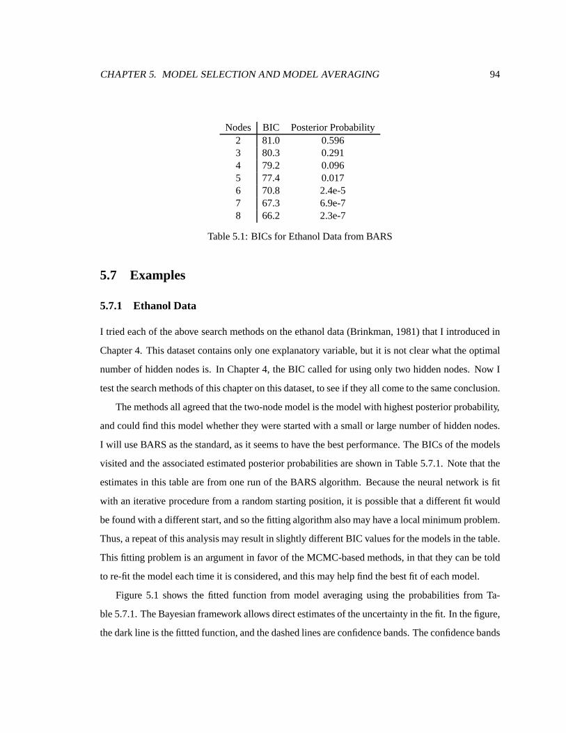
CHAPTER5. MODEL SELECTIONAND MODEL AVERAGING 94
Nodes BIC PosteriorProbability2 81.0 0.5963 80.3 0.2914 79.2 0.0965 77.4 0.0176 70.8 2.4e-57 67.3 6.9e-78 66.2 2.3e-7
Table5.1: BICs for EthanolDatafrom BARS
5.7 Examples
5.7.1 Ethanol Data
I tried eachof theabove searchmethodson theethanoldata(Brinkman,1981)thatI introducedin
Chapter4. This datasetcontainsonly oneexplanatoryvariable,but it is not clearwhattheoptimal
numberof hiddennodesis. In Chapter4, theBIC calledfor usingonly two hiddennodes.Now I
testthesearchmethodsof thischapteronthisdataset,to seeif they all cometo thesameconclusion.
Themethodsall agreedthatthetwo-nodemodelis themodelwith highestposteriorprobability,
andcouldfind this modelwhetherthey werestartedwith a smallor largenumberof hiddennodes.
I will useBARSasthestandard,asit seemsto have thebestperformance.TheBICsof themodels
visitedandtheassociatedestimatedposteriorprobabilitiesareshown in Table5.7.1. Notethat the
estimatesin this tablearefrom onerun of theBARS algorithm. Becausetheneuralnetwork is fit
with an iterative procedurefrom a randomstartingposition,it is possiblethata differentfit would
befoundwith adifferentstart,andsothefitting algorithmalsomayhavealocalminimumproblem.
Thus,arepeatof thisanalysismayresultin slightly differentBIC valuesfor themodelsin thetable.
This fitting problemis anargumentin favor of theMCMC-basedmethods,in thatthey canbetold
to re-fit themodeleachtime it is considered,andthismayhelpfind thebestfit of eachmodel.
Figure 5.1 shows the fitted function from model averagingusing the probabilitiesfrom Ta-
ble5.7.1.TheBayesianframework allowsdirectestimatesof theuncertaintyin thefit. In thefigure,
thedarkline is thefitttedfunction,andthedashedlinesareconfidencebands.Theconfidencebands

CHAPTER5. MODEL SELECTIONAND MODEL AVERAGING 95
•••
•
•
•
• • •
••••
••
•
•
• •
•
•
•
•••
•
•
•
•
•
•
•
••
•
••
•
•••
•
••
• •
••
••
•
•••
••
•
•
•
•
••••
•
••
••
••• ••
••••
• •• •
•
•
•
•••
Equivalence Ratio
NO
x
0.5 0.6 0.7 0.8 0.9 1.0
0.2
0.4
0.6
0.8
1.0
Figure5.1: FittedFunctionandConfidenceBandsfrom ModelAveragingfor theEthanolData
werecreatedby finding, for eachobserveddatapoint, an interval (with respectto the ² -axis)with
95%posteriorpredictive probability, andconnectingtheendpointsof theseintervalswith acurve.
BARS found that the two-nodemodelhasover half of theposteriorprobability. It alsofound
that the three-nodemodelhasaboutthree-tenthsof theposteriorprobability, which is higherthan
wasfoundin thepreviouschapteronnormalizingconstants.It now appearsthatthefittedvaluesin
Chapter4 wereonly from a localmaximumin thelikelihood.However, thetwo-nodemodelis still
thedominantmodel.Theposteriorprobabilitiesof themodelsdecreasewith thesizeof themodel.ÁÙÂ Ä (usingthesameMarkov ChainasBARS) foundthatthetwo-nodemodelwasthehighest
posteriorprobability model,spending53% of its time on that model. It estimatedthe posterior
probability of the three-nodemodelas 29.1%and that of the four-nodemodelas13.6%. So it
appearsthat ÁÃÂÚÄ andBARSgivesimilar resultsfor thisdataset.
Thestepwisealgorithmwouldtypically find themaximumBIC for thetwo-nodemodel.In most
cases,it wouldfind thatthethree-nodemodelwasthesecond-bestmodel,but it wouldnotfind aBIC
ashighasthe80.3foundby BARS.It typically foundaBIC of 78.8,whichis directlycomparableto
thevaluesin Chapter4. Thusit appearsthatit is difficult to find theslightly higherBIC modelthat
BARS did manageto find. As a result,stepwisewould normallyestimatetheposteriorprobability
of thetwo-nodemodelto bemuchcloserto one.
Occam’s Window excludesthe three-nodemodel from consideration,becausethe two-node

CHAPTER5. MODEL SELECTIONAND MODEL AVERAGING 96
modelis bothmoreparsimoniousandhasahigherBIC. Thusit doesnotmatterto Occam’sWindow
whetherit finds theoptimalor theclose-to-optimalthree-nodemodel,becausebothareexcluded.
Theresultof runningOccam’s Window is thatthetwo-nodemodelis theonly onereturned.
I shouldpoint out that, in running the algorithmsa numberof timeson this samedataset,I
sometimesfoundthatboththestepwiseandOccam’s Window procedureswould getstuckin local
maxima.In particular, fitting thefour-nodemodelcausedsomedifficulties,sothatif I startedthese
algorithmsona largermodel,sometimesthey wouldfind thatthefive-nodemodelwassignificantly
betterthanthefour-nodemodel,only becauseit hasmoretroublefitting thefour-nodemodel.As a
result,they would returnthefive-nodemodelasthemodelwith highestposteriorprobability.
Thisinnocent-lookingexamplehasonlyoneexplanatoryvariableandapparentlyonlyneedstwo
hiddennodes.However, it hasmanagedto causequitea numberof problems,in both thecurrent
chapter(local maximain theBIC) andin thepreviouschapter(estimatingnormalizingconstants).
It doesunderscorethe importanceof choosinga goodstartingmodelfor thesearchalgorithms,of
fitting modelsmultiple timesto betterensureoptimal fitting, andof runningthemmultiple times
from differentstartingpositionsto ensureadequateexplorationof themodelspace.
5.7.2 SimulatedData
The simulateddatathat I introducedin Chapter4 provides a handytest set, becausewe know
the right answer. The datasetcontainsfour explanatoryvariables,of which only the first two are
relevant.Thetrueregressionfunctionusesthreehiddennodes.Thetestis to seeif searchstrategies
canall find thetruefunctionasthemodelof highestposteriorprobability.
The resultsweresimilar to that of the ethanoldata. For startingpointsnot too far from the
truemodel,all of thesearchmethodsfound the truemodelto be theonly onewith high posterior
probability. TheBIC of thethree-nodemodelwith thefirst two explanatoryvariablesis 359,while
thatof eitherthefour-nodemodelwith thefirst two variablesis 357,andthatof eitherthree-node
modelwith thefirst two variablesandoneof thesecondtwo is 352.All otherBICsareevensmaller.
Theseresultsarefairly consistentacrossall of thesearchalgorithmsfor any reasonablechoiceof
startingmodel. Occam’s Window returnsthe two-variable,three-nodemodelas the only model
worthconsideringbecauseit is asubmodelof all of theotherreasonablegoodmodels.
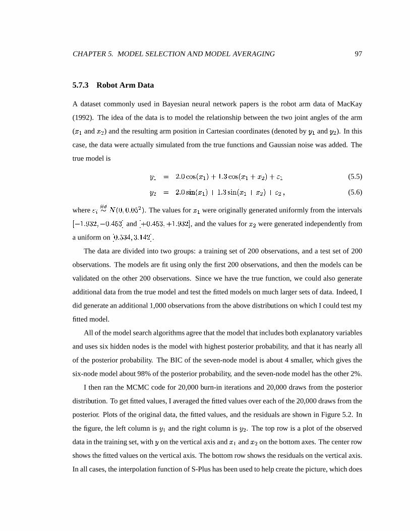
CHAPTER5. MODEL SELECTIONAND MODEL AVERAGING 97
5.7.3 Robot Arm Data
A datasetcommonlyusedin Bayesianneuralnetwork papersis the robot arm dataof MacKay
(1992). The ideaof the datais to modelthe relationshipbetweenthe two joint anglesof the arm
( Û�~ and Û"� ) andtheresultingarmpositionin Cartesiancoordinates(denotedby ²®~ and ²B� ). In this
case,thedatawereactuallysimulatedfrom thetruefunctionsandGaussiannoisewasadded.The
truemodelis ² ~ � � ° À�Ü ¡BÝ �µÛ ~ �8Þ � °uß Ü ¡BÝ �µÛ ~ Þ Û � ��Þwà ~ (5.5)² � � � ° À Ý È É �µÛ ~ �8Þ � °uß Ý È É �µÛ ~ Þ Û � ��Þwà � � (5.6)
whereàª� �á�¢âãåä � À � À ° ÀBæ � � . Thevaluesfor Ûç~ wereoriginally generateduniformly from theintervalsè � � °uéAß � � � À °ëê æ ß�ì and
è Þ À °ëê æ ß � Þ � °uéAß � ì , andthevaluesfor Û"� weregeneratedindependentlyfrom
auniformonè À ° æ ß�ê � ß.° � ê � ì .
Thedataaredivided into two groups:a trainingsetof 200observations,anda testsetof 200
observations.Themodelsarefit usingonly thefirst 200observations,andthenthemodelscanbe
validatedon the other200 observations. Sincewe have the true function,we couldalsogenerate
additionaldatafrom thetruemodelandtestthefittedmodelsonmuchlargersetsof data.Indeed,I
did generateanadditional1,000observationsfrom theabovedistributionsonwhichI couldtestmy
fittedmodel.
All of themodelsearchalgorithmsagreethatthemodelthatincludesbothexplanatoryvariables
andusessix hiddennodesis themodelwith highestposteriorprobability, andthat it hasnearlyall
of theposteriorprobability. TheBIC of theseven-nodemodelis about4 smaller, which givesthe
six-nodemodelabout98%of theposteriorprobability, andtheseven-nodemodelhastheother2%.
I thenran the MCMC codefor 20,000burn-in iterationsand20,000draws from theposterior
distribution. To getfittedvalues,I averagedthefittedvaluesovereachof the20,000draws from the
posterior. Plotsof theoriginal data,thefitted values,andtheresidualsareshown in Figure5.2. In
thefigure, the left columnis ²®~ andthe right columnis ²B� . The top row is a plot of theobserved
datain thetrainingset,with ² ontheverticalaxisand Û�~ and Û"� onthebottomaxes.Thecenterrow
showsthefittedvaluesontheverticalaxis.Thebottomrow showstheresidualsontheverticalaxis.
In all cases,theinterpolationfunctionof S-Plushasbeenusedto helpcreatethepicture,whichdoes
CHAPTER5. MODEL SELECTIONAND MODEL AVERAGING 98
-1í 0
1î
X1ï
1
1.5ð2ñ2.5ñ3ò
X2ó-2
-1 0
12
34
Y1ô
Training Data
-1õ 0
1ö
X1÷
1
1.5ø2ù2.5ù3ú
X2û-4
-2 0
24
Y2
Training Data
-1í 0
1î
X1ï
1
1.5ð2ñ2.5ñ3ò
X2ó-2
-1 0
12
34ü
Y1ô
Fitted Values
-1õ 0
1ö
X1÷
1
1.5ý2þ2.5þ3ÿ
X2�
-4-2
02
4Y
2�
Fitted Values
-1õ 0
1ö
X1÷
1
1.5�2�2.5�3�
X2�
-0.1
5-0.1-
0.05
00.
050.
10.
15Y
1
Residuals
-1� 0
1�
X1�
1
1.522.53�
X2�
-0.2
-0.1
00.
10.
20.
3Y
2�
Residuals
Figure5.2: A Six-NodeModel for theRobotArm Data
involve somesmall amountof additionalsmoothing,but is thebestway to geta viewableimage.
Noticethattheresidualsarereasonablyscattered.
I thenusedtheMCMC outputtofit themodelonthe200casesin thetestdataset.Thetheoretical
optimumvaluefor themeansquarederror(MSE) is 0.005,andmy modelactuallymanagedto have
anMSE of 0.005007.This is certainlyanexcellentfit! Plotsof thetestdata,thefitted values,and
theresidualsareshown in Figure5.3.Theredoesseemto besomesmallproblemwith theresiduals
for largevaluesof Û�~ , in that for ²®~ theresidualsareunusuallynegative for largevaluesof Ûç~ and
smallvaluesof Û � , andthat for ² � the residualsareunusuallylarge for large valuesof Û ~ and Û � .However, thesmallmeansquareerrorshows thatthis modeldoesindeedfit quitewell. In orderto

CHAPTER5. MODEL SELECTIONAND MODEL AVERAGING 99
-1 0
1�
X1�
1
1.5ø2ù2.5ù3ú
X2û-2
-1 0
12
3Y
1�
Test Data
-1 0
1�
X1�1
1.5ø2ù2.5ù3ú
X2û-4
-2 0
24
Y2�
Test Data
-1õ 0
1ö
X1÷1
1.5ø2ù2.5ù3ú
X2û-2
-1 0
12
3Y
1�
Fitted Values
-1í 0
1î
X1ï
1
1.5ð2ñ2.5ñ3ò
X2ó-3
-2-1
01
23
4Y
2ôFitted Values
-1� 0
1�
X1�
1
1.522.53�
X2�
-0.2
-0.1
00.
1Y
1
Residuals
-1� 0
1�
X1�1
1.5ø2ù2.5ù3ú
X2û-0
.2-0
.1 0
0.1
0.2
0.3
0.4
Y2�
Residuals
Figure5.3: TestDatafor theRobotArm Problem
seeif thefit on this particularsetof testdatais just a lucky break,I alsogenerateda new testsetof
1,000observationsfrom theoriginal distribution andfit themodelto thesedata. Indeed,theMSE
roseto 0.00565.This is still averygoodfit, andit will turnout to becomparableto thefits achieved
by competingmethodson thetestdata.
Thisdatasethasalsobeenanalyzedby severalothersin theBayesianneuralnetwork literature,
in particularMacKay(1992),Neal (1996),andMuller andRiosInsua(1998b).Table5.7.3shows
theMSEachievedonthetestdataby themethodsof eachof theabovecompetingmodels.MacKay
(1992)useswhat he calls the “evidence” for selectingthe numberof nodes. This evidenceis a
Gaussianapproximationof a Bayesfactor. Neitherhis modelwith highestevidence(whichhasten

CHAPTER5. MODEL SELECTIONAND MODEL AVERAGING 100
Method MeanSquareErroronTestDataMacKay, GaussianApproximationSolutionwith highestevidence 0.00573Solutionwith lowesttesterror 0.00557Neal,Hybrid MonteCarlo16-NodeModel 0.0055716Nodeswith ARD 0.00549Muller andInsuaPosteriorPredictions 0.00620My modelfrom this thesisPosteriorPredictions 0.00501
Table5.2: Comparisonof CompetingMethodson theRobotArm Data
nodes),or evenhis modelwith lowestMSE on the testdata(which hasninenodes),fit aswell as
the modelfrom this thesis.Neal (1996)achievessimilar resultsto the bestmodelof MacKayby
usinghishybridMonteCarlomethodsandaveragingoverhis runsafterremoving aburn-inperiod.
Nealusesanetwork with sixteenhiddennodes,undertheparadigmthatchoosingagoodprior will
balancethe overfitting, and so one shouldusemorenodesthannecessaryso the MCMC mixes
well. Nealalsotriesapplyinghismodelselectiontechniqueof AutomaticRelevanceDetermination
(ARD), which is meantprimarily to selectexplanatoryvariablesby addinga hyperparameterto
control themagnitudeof theparametersfor theexplanatoryvariablesinsidethe logistic functions
(seeSection1.4.4). Neal demonstratesthe viability of ARD by addingextra “noise” explanatory
variablesandthenfitting a sixteen-nodenetwork to thedata. In doingso,hemanagesto improve
his fit a little in the sensethat his MSE is smaller(seeTable5.7.3). In all cases,Neal is not that
concernedwith finding an optimal numberof hiddennodesto usein his model. Finally, Muller
andRiosInsua(1998b)appliedtheir reversible-jumpMCMC modelto thesedata.They foundthe
posteriordistribution on thenumberof nodesto be theprobabilities0.30,0.53,0.15,and0.02for
six, seven, eight, andnine nodesrespectively. Using the full posterior(averagedover all model
sizes)gavea setof predictionson thetestdatathathadMSE0.0062.
Comparedto theabovemethods,my methodshave foundamodelwhich is bothmoreparsimo-
nious(having fewer nodes)aswell asbetterfitting (in thatits MSEonthetestdatais smaller).

CHAPTER5. MODEL SELECTIONAND MODEL AVERAGING 101
5.7.4 Ozone
The modelsearchmethodswereappliedto thegroundlevel ozonedataof BreimanandFriedman
(1985) that was introducedin Chapter1. Thereare 330 observationsof the responsevariable,
groundlevel ozone(asa pollutant),andnine explanatoryvariables:VH, the altitudeat which the
pressureis 500millibars;WIND, thewind speed(mph)atLosAngelesInternationalAirport (LAX)
; HUM, thehumidity (%) atLAX; TEMP, thetemperature(degreesF) atSandburg Air ForceBase;
IBH, thetemperatureinversionbaseheight(feet);DPG,thepressuregradient(mm Hg) from LAX
to Daggert;IBT, the inversionbasetemperature(degreesF) at LAX; VIS, thevisibility (miles)at
LAX; andDAY, thedayof theyear.
All of thealgorithmsgenerallyfoundthatthemodelwith nearlyall of theposteriorprobability
wasonewith threenodesandfive variables(VH, HUM, DPG, IBT, DAY) having BIC 264. The
next bestmodelswereonewith six nodesandfive variables(HUM, DPG,IBT, VIS, DAY) having
BIC 260,andonewith threenodesandthreevariables(HUM, IBT, DAY) having BIC 259. It did
happenthatsometimesthestepwisealgorithmandtheOccam’sWindow algorithmwouldgetstuck
in a local maximumof the BIC andnot find the global maximum,underscoringthe importance
of runningthosealgorithmswith several differentstartingmodels.The MCMC-basedalgorithms
(BARSand ÁÙÂÅÄ ) did nothave thisproblemandcouldtypically find theglobalmaximum.
Method� �
ACE,9 variables 0.82ACE,4 variables 0.78GAM 0.80TURBO 0.80Box-Tidwell 0.82NeuralNetwork 0.79
Table5.3: Comparisonof CompetingMethodson theOzoneData
Thisdatasethasbeenanalyzedby severalothersin thenonparametricregressionliterature,and
soit is usefulfor comparingthemethodsof thisthesisto othernonparametricregressiontechniques.

CHAPTER5. MODEL SELECTIONAND MODEL AVERAGING 102
BreimanandFriedman(1985)usedthis datasetin their paperon AlternatingConditionalExpecta-
tion (ACE).As a goodness-of-fitmeasure,they usedtheestimatedmultiple correlationcoefficient,� � . They fit themodelbothusingall nineexplanatoryvariables,aswell asasubsetof only four that
werechosenvia a stepwisealgorithm(the four areTEMP, IBH, DPG,andVIS). Thecomparison
of the� � ’s is shown in Table5.7.4.HastieandTibshirani(1984)fit a GeneralizedAdditive Model
(GAM) to the data. FriedmanandSilverman(1989)fit thedatausingTURBO. In thediscussion
of the previous paper, Hawkins (1989)fit the datawith linear regressionafter usingBox-Tidwell
styletransformationson thevariables.For comparison,I includetheresultof my modelwith three
nodesandfive explanatoryvariables.Table5.7.4shows thatall of theabove methodshave similar
goodness-of-fitto thedata.All of themethodsdomanageto find areasonablefit, but noneis clearly
betterthantheothers.
Method VH WIND HUM TEMP IBH DPG IBT VIS DAYStepwiseACE X X X XStepwiseGAM X X X X X X X XTURBO X X X X X XBRUTO X X X X XOptimalNeuralNet (3 Nodes) X X X X XSecond-bestNN (6 Nodes) X X X X XThird-bestNN (3 Nodes) X X X
Table5.4: Comparisonof VariableSelectionon theOzoneData
AsidefromtheACEmodelwith only four variables,theothermodelsin Table5.7.4all usemore
explanatoryvariablesthandoestheneuralnetwork, andarethuslessparsimoniousandsubjectto
increasedpredictionerror. HastieandTibshirani(1990)do a comparisonof several methodson
thesedatain termsof variableselection. In addition to someof the above methods,they also
includea stepwisealgorithmfor their GAM models,aswell asa responseto TURBO which they
call BRUTO,which is meantto doautomaticvariableselectionandsmoothingparameterselection.
Table5.7.4shows thevariableschosenby themodelsin eachof thesemethods.It is interestingto
notethatthemethodsseriouslydisagreeonwhichvariablesto select.Partly, thismaybebecausethe
variablesarehighlycorrelatedwith eachother, sothatdifferentsubsetsmaygivesimilarpredictions.

CHAPTER5. MODEL SELECTIONAND MODEL AVERAGING 103
However, TURBO andBRUTO are largely in agreementwith eachother. And the threeneural
network modelshave similar choicesof variables,althoughthesearevery differentfrom thoseof
TURBOandBRUTO.At thevery least,it doesseemclearthatsomevariableselectionis necessary
becauseof thehigh level of correlationbetweentheexplanatoryvariables,even if thereis dissent
aboutwhichsubsetis optimal.
5.8 Discussion
Computingposteriorprobabilitiesfor a collectionof neuralnetwork modelsis a very difficult task.
In this chapter, I have presenteda methodfor searchingthemodelspaceandfinding modelswith
high posteriorprobability. My approachallows oneto simultaneouslysearchacrosssubsetsof ex-
planatoryvariablesandacrossnetworks of differentsizes,which the competingmethodsdo not
fully do. TheBIC providesa reasonableapproximationfor theposteriorprobabilities.TheBARS
approachprovidesausefulmethodfor finding themodelsof highestposteriorprobabilityin theex-
pansive modelspace,althoughonecanusuallyachieve similar resultsby runningseveralstepwise
algorithmsfrom differentstartingmodels.Testson several canonicalexamplesshow that my ap-
proachperformswell whencomparedto othermethods.I canoftenachieveasimilargoodness-of-fit
while usinga smaller, moreparsimoniousmodel.
The methodsof this chapterallow oneto morefully accountfor uncertainty. Model averag-
ing canhelpaccountfor theuncertaintyassociatedwith choosinga model. Sincethemodelspace
searchingtechniquesdo not actuallyvisit all possiblemodels,thereis still someuncertaintystill
unaccountedfor dueto theunvisitedmodels,althoughthis is typically unavoidabledueto thevast
sizeof themodelspace;onehopesthatthesearchdoesfind all importantmodels,sothattheaddi-
tionaluncertaintyis negligible. Finally, it is usefulto notethattheBayesianframework allowseasy
computationof furthermeasuresof uncertainty. For example,it is straightforwardto getconfidence
bandsfor thefitted regressionfunction,asshown in Figure5.1.
Chapter 6
Conclusions
This thesisprovidesa completemethodologyfor Bayesiannonparametricregressionusingneural
networks. It describeshow to usea noninformative prior, andshows thatthis prior andmany other
reasonablepriors are asymptoticallyconsistentfor the posterior. It describeshow to searchthe
modelspacefor modelsof highposteriorprobabilityusingBayesianRandomSearching(BARS)as
well asseveralothermethods.Thenonecaneitherusethesinglemodelof highestposteriorproba-
bility, or averageover theposteriordistribution of models.Theexamplesin Chapter5 show thatthe
modelsthatresultfrom themethodsin this thesisfit thedatawell andperformwell whencompared
to competingmethods.Thesemethodsalsoallow oneto morefully accountfor uncertainty, andthe
Bayesianframework allows straightforwarduncertaintycalculations.
This thesiscontributesto the bodyof statisticalresearchin several ways. It providesthe first
implementationof a fully noninformative prior for neuralnetworks. It is thefirst detailedproof of
theasymptoticconsistency of neuralnetworks for theposterior. It surveys many methodsfor esti-
matingintegrals(normalizingconstants),andfindsthat theBIC is oneof themostrobust. Finally,
it contributesto the field of modelselectionandmodelaveraging. BARS may exist by another
namein theliterature,but I amnot familiarwith publishedapplicationsof it. Little modelselection
work hasbeendonefor modelsthatarefit iteratively, whereoneis not guaranteedto have fit the
modelcorrectly, andso onemay have further troublesearchingthe modelspacebecauseof this
uncertainty. Model selectionfor Bayesianneuralnetworkshasbeenincompletein thatno oneelse
104

CHAPTER6. CONCLUSIONS 105
usesthefull posteriorfor selectingboththenumberof hiddennodesandthesubsetof explanatory
variables.This thesisfills in thatgap.
While the work in this thesisfeels largely complete,therearesomedirectionsfor future re-
search.Oneobvious extensionto this work is to apply the modelselectionresultsto modelsfor
binary, categorical,or ordinalexplanatoryvariables.Thismayinvolve eitherthemodelsof Chapter
2 or modelswith alternative probabilitydistributions(e.g.,multinomial insteadof Gaussianerror).
A majortheoreticresultthatwouldbolsterthis thesiswouldbetheproof thattheBIC minusthelog
of theBayesfactorfor comparingthatmodelto thenull modelis � ¼ � � � andthattheBIC is asymp-
totically consistentfor selectingthetruemodel.This hasbeenshown truein many othercases,but
not yet for neuralnetworks. A proof of theapproximationabilitiesof theBIC would beusefulin
furtherjustifying its usefor themodelsearchprocess.Finally, therearesomecomputationalloose
ends.Chapter4 seemssomewhatincompletein thatI couldnotfind amethodfor approximatingthe
normalizingconstantsthatwasmoreaccuratethantheBIC, which is not a high-orderapproxima-
tion. Perhapsmorework in thisareacouldproducebetternumericalintegrationandapproximation
techniques.Also, thecurrentimplementationsof themodelsearchingalgorithmsarefar from maxi-
mally efficient. Thereis muchroomfor improvementin termsof computationalspeed.In particular,
theremaybewaysto allocatehow muchtime oneshouldspendtrying to fit eachparticularmodel
in thatmodelswith potentiallyhighposteriorprobabilityshouldbegivenmoreattentionthanthose
thathave exceedinglysmallposteriorprobability(becausethey don’t fit well, perhapsbecausethey
have left out a necessaryexplanatoryvariable).Becauseof theuncertaintyin fitting an individual
model,it is sometimeshardto tell if themodelis badbecauseof a poorfitting job or becausethe
modelis actuallybad. Knowing which modelsoneshouldpay moreattentionto fitting carefully
(andthusconsumingmorecomputingtime)wouldhelptheefficiency of thealgorithms.
References
Akaike, H. (1974). “A New Look at StatisticalModel Identification.” IEEE Transactionson Auto-
maticControl, AU–19,716–722.
Anderson,J. A. (1982). “Logistic Discrimination.” In Classification,Pattern Recognition and
Reductionof Dimensionality, eds.P. R. KrishnaiahandL. N. Kanal, vol. 2 of Handbookof
Statistics, 169–191.Amsterdam:NorthHolland.
Banks,D. L., Maxion, R. A., andOlszewski, R. T. (1997). “ComparingMethodsfor Multivariate
NonparametricRegression.” Submittedto Journalof ComputationalandGraphicalStatistics.
Barron,A., Schervish,M. J., andWasserman,L. (1998). “The Consistency of PosteriorDistribu-
tionsin NonparametricProblems.” TheAnnalsof Statistics. To appear.
Bernardo,J. M. (1979). “ReferencePosteriorDistributions for BayesianInference(with discus-
sion).” Journalof theRoyalStatisticalSocietyB, 41,113–147.
Bishop,C. M. (1995).Neural Networksfor PatternRecognition. Oxford: ClarendonPress.
Breiman,L. (1994). “Bagging Predictors.” Tech.Rep.421, University of California, Berkeley,
Departmentof Statistics.
Breiman,L. andFriedman,J. H. (1985). “EstimatingOptimal Transformationsfor Multiple Re-
gressionandCorrelation.” Journalof theAmericanStatisticalAssociation, 80,580–619.
Breiman,L., Friedman,J.H., Olshen,R.,andStone,C. (1984).ClassificationandRegressionTrees.
Belmont,CA: Wadsworth.
106
REFERENCES 107
Brinkman,N. D. (1981). “EthanolFuel—A Single-CylinderEngineStudyof Efficiency andEx-
haustEmissions.” SAETransactions, 90,810345,1410–1424.
Buntine,W. L. andWeigend,A. S. (1991). “BayesianBack-Propagation.” Complex Systems, 5,
603–643.
Chipman,H., George,E.,andMcCulloch,R. (1998).“BayesianCART ModelSearch(with discus-
sion).” Journalof theAmericanStatisticalAssociation, 93,935–960.
Cleveland,W. S.(1979).“RobustLocally-WeightedRegressionandSmoothingScatterplots.” Jour-
nal of theAmericanStatisticalAssociation, 74,829–836.
Craig, B. (1997). “Manatee: SelectingFrom Among Several Models.” Presentedat 1997Joint
StatisticalMeetings,Anaheim,CA.
Denison,D., Mallick, B., andSmith,A. (1998a).“AutomaticBayesianCurve Fitting.” Journal of
theRoyalStatisticalSocietyB, 60,333–350.
— (1998b).“A BayesianCART Algorithm.” Biometrika, 85,363–377.
Denison,D. G. (1997). “SimulationBasedBayesianNonparametricRegressionMethods.” Ph.D.
thesis,ImperialCollege,London.
Diaconis,P. andFreedman,D. A. (1986). “On the Consistency of BayesEstimates.” Annalsof
Statistics, 14,1–26.
DiCiccio, T. J.,Kass,R. E., Raftery, A., andWasserman,L. (1995). “ComputingBayesFactors.”
Tech.Rep.630,Carnegie Mellon University, Departmentof Statistics.
Diebolt, J. andRobert,C. (1994). “Estimationof Finite Mixture DistributionsThroughBayesian
Sampling.” Journalof theRoyalStatisticalSocietyB, 56,363–375.
Donoho,D. L. andJohnstone,I. (1989). “ProjectionBasedApproximationsanda Duality with
KernelMethods.” Annalsof Statistics, 17,58–106.
REFERENCES 108
Donoho,D. L., Johnstone,I. M., Kerkyacharian,G., andPicard,D. (1995). “Wavelet Shrinkage:
Asymptopia?”Journalof theRoyalStatisticalSocietyB, 57,301–369.
Doob,J.L. (1949).“Applicationof theTheoryof Martingales.” In LeCalculdesProbabilitesetses
Applications, 23–27.ColloqueInternationauxduCentreNationaldela RechercheScientifique,
Paris.
Duane,S.,Kennedy, A. D., Pendleton,B. J.,andRoweth,D. (1987).“Hybrid MonteCarlo.” Physics
Letters B, 195,216–222.
Fahlmann,S.E. (1989).“FasterLearningVariationsonBack-Propagation:An EmpiricalStudy.” In
Proceedingsof the1988ConnectionistModelsSummerSchool,Pittsburgh, eds.D. Touretzky,
G. Hinton,andT. Sejnowski, 38–51.Denver: MorganKaufmann.
Fahlmann,S. E. and Lebiere,C. (1989). “The Cascade-CorrelationLearningArchitecture.” In
Advancesin Neural InformationProcessingSystems2, ed. D. Touretzky, 524–532.Denver:
MorganKaufmann.
Fisher, R. A. (1936). “The Useof Multiple Measurementsin TaxonomicProblems.” Annalsof
Eugenics, 7, 179–188.
Foster, D. P. andGeorge, E. I. (1997). “Empirical BayesVariableSelection.” The University of
PennsylvaniaandTheUniversityof TexasatAustin,unpublished.
Friedman,J. H. (1991). “Multi variateAdaptive RegressionSplines.” TheAnnalsof Statistics, 19,
1–141.
Friedman,J. H. andSilverman,B. W. (1989). “Flexible ParsimoniousSmoothingandAdditive
Modelling(with discussion).” Technometrics, 31,3–39.
Friedman,J.H. andStuetzle,W. (1981). “ProjectionPursuitRegression.” Journalof theAmerican
StatisticalAssociation, 76,817–823.
Funahashi,K. (1989). “On theApproximateRealizationof ContinuousMappingsby NeuralNet-
works.” Neural Networks, 2, 3, 183–192.

REFERENCES 109
Furnival, G. M. andWilson, R. W. J. (1974). “Regressionby LeapsandBounds.” Technometrics,
16,499–511.
Gelfand,A. E. andDey, D. K. (1994). “BayesianModel Choice:AsymptoticsandExactCalcula-
tions.” Journalof theRoyalStatisticalSocietyB, 56,501–514.
Gelman,A. andMeng,X.-L. (1996). “SimulatingNormalizingConstants:FromImportanceSam-
pling to BridgeSamplingto PathSampling.” ColumbiaUniversityandUniversityof Chicago,
unpublished.
Geman,S. andGeman,D. (1984). “StochasticRelaxation,GibbsDistributionsandthe Bayesian
Restorationof Images.” IEEE Transactionson PatternAnalysisandMachineIntelligence, 6,
721–741.
Genz,A. andKass,R. E. (1997).“Subregion-adaptive Integrationof FunctionsHaving aDominant
Peak.” Journalof ComputationalandGraphicalStatistics, 6, 92–111.
Geweke, J. (1989). “BayesianInferencein EconometricModelsUsingMonteCarlo Integration.”
Econometrica, 57,1317–1340.
Hastie,T. and Tibshirani,R. (1984). “GeneralizedAdditive Models.” Tech.Rep.98, Stanford
University, Departmentof Statistics.
— (1990).GeneralizedAdditiveModels. London:ChapmanandHall.
Hawkins, D. (1989). “Discussionof ’Flexible ParsimoniousSmoothingandAdditive Modelling’
by J.FriedmanandB. Silverman.” Technometrics, 31,3–39.
Holmes,C. andMallick, B. (1998). “BayesianRadialBasisFunctionsof VariableDimension.”
Neural Computation, 10,1217–1233.
Hornik, K., Stinchcombe,M., andWhite, H. (1989). “Multilayer FeedforwardNetworksareUni-
versalApproximators.” Neural Networks, 2, 5, 359–366.
Jeffreys,H. (1961).Theoryof Probability. Third editioned.New York: OxfordUniversityPress.
REFERENCES 110
Kass,R. E. andRaftery, A. E. (1995).“BayesFactors.” Journalof theAmericanStatisticalAssoci-
ation, 90,430,773–795.
Keribin,C. (1997).“ConsistentEstimationof theOrderof Mixture Models.” Tech.rep.,Universite
d’Evry-Val d’Essonne,LaboratoireAnalyseetProbabilite.
Leamer, E. E. (1978).SpecificationSearches:Ad Hoc Inferencewith NonexperimentalData. New
York: Wiley.
Lee,H. K. H. (1996). “Model Selectionfor ConsumerLoanApplicationData.” Tech.Rep.650,
CarnegieMellon University, Departmentof Statistics.
MacKay, D. J. C. (1992). “BayesianMethodsfor Adaptive Methods.” Ph.D. thesis,California
Instituteof Technology.
— (1994). “BayesianNon-LinearModeling for the Energy PredictionCompetition.” ASHRAE
Transactions, 100,pt. 2, 1053–1062.
McCulloch, W. S. andPitts, W. (1943). “A Logical Calculusof the IdeasImmanentin Nervous
Activity.” Bulletinof MathematicalBiophysics, 5, 115–133.
Meng,X. L. andWong,W. H. (1993). “SimulatingRatiosof NormalizingConstantsVia a Simple
Identity: a TheoreticalExploration.” Tech.Rep.365,University of Chicago,Departmentof
Statistics.
Metropolis,N., Rosenbluth,A. W., Rosenbluth,M. N., Teller, A. H., andTeller, E. (1953). “Equa-
tions of StateCalculationsby FastComputingMachine.” Journal of ChemicalPhysics, 21,
1087–1091.
Moody, J. E. (1992). “The Effective Numberof Parameters:An Analysisof Generalizationand
Regularizationin NonlinearLearningSystems.” In Advancesin Neural InformationProcessing
Systems4, eds.J. E. Moody, S. J. Hanson,and R. P. Lippmann.SanMateo, CA: Morgan
Kaufmann.
REFERENCES 111
Muller, P., Erkanli, A., andWest,M. (1996). “BayesianCurve Fitting UsingMultivariateNormal
Mixtures.” Biometrika, 83,1, 67–79.
Muller, P. and Rios Insua,D. (1998a). “Feedforward Neural Networks for NonparametricRe-
gression.” In Practical NonparametricandSemiparametricBayesianStatistics, eds.D. Dey,
P. Muller, andD. Sinha.New York: Springer-Verlag.
— (1998b). “Issuesin BayesianAnalysisof NeuralNetwork Models.” Neural Computation, 10,
571–592.
Murata,N., Yoshizawa, S., andAmari, S. (1994). “Network InformationCriterion—Determining
theNumberof HiddenUnits for anArtificial NeuralNetwork Model.” IEEE Transactionson
Neural Networks, 5, 6, 865–871.
Neal,R. M. (1996).BayesianLearningfor Neural Networks. New York: Springer.
Newton,M. andRaftery, A. (1994).“ApproximateBayesianInferenceby theWeightedLikelihood
Bootstrap(with discussion).” Journalof theRoyalStatisticalSocietyB, 56,3–48.
Nobile, A. (1994). “BayesianAnalysisof Finite Mixture Distributions.” Ph.D. thesis,Carnegie
Mellon University, Departmentof Statistics.
Pollard,D. (1991). “Bracketing Methodsin StatisticsandEconometrics.” In Nonparametricand
Semiparametric Methodsin Econometricsand Statistics: Proceedingsof the Fifth Interna-
tional Symposiumin EconometricTheoryand Econometrics, eds.W. A. Barnett,J. Powell,
andG. E. Tauchen,337–355.Cambridge,UK: CambridgeUniversityPress.
Raftery, A. (1996). “ApproximateBayesFactorsandAccountingfor Model Uncertaintyin Gener-
alizedLinearModels.” Biometrika, 83,251–266.
Raftery, A. E. andMadigan,D. (1994).“Model SelectionandAccountingfor ModelUncertaintyin
GraphicalModelsUsingOccam’s Window.” Journal of theAmericanStatisticalAssociation,
89,1535–1546.
REFERENCES 112
Raftery, A. E., Madigan,D., andHoeting,J. A. (1997). “BayesianModel Averagingfor Linear
RegressionModels.” Journalof theAmericanStatisticalAssociation, 437,179–191.
Rumelhart,D. E., Hinton, G. E., andWilliams, R. J. (1986). “Learning InternalRepresentations
by ErrorPropagation.” In Parallel DistributedProcessing:Explorationsin theMicrostructure
of Cognition, eds.D. E. Rumelhart,J. L. McClelland,andthe PDPResearchGroup,vol. 1,
318–362.Cambridge,MA: MIT Press.
Sanil,A. (1998).“An Approachfor Selectionof NonparametricRegressionMethods.” Ph.D.thesis,
CarnegieMellon University, Departmentof Statistics.
Sarle,W. S. (1994). “Neural Network Implementationin SAS Software.” In Proceedingsof the
NineteenthAnnualSASUsers Group InternationalConference, 38–51.SAS Institute,Cary,
NC.
Schwarz,G. (1978). “EstimatingtheDimensionof a Model.” TheAnnalsof Statistics, 6, 2, 461–
464.
Silverman,B. W. (1985). “SomeAspectsof the SplineSmoothingApproachto Non-Parametric
CurveFitting.” Journalof theRoyalStatisticalSocietyB, 47,1–52.
Smith,M. andKohn,R. (1996). “NonparametricRegressionusingBayesianVariableSelection.”
Journalof Econometrics, 75,317–343.
Stone,C. J. (1982). “Optimal Ratesof Convergencefor NonparametricRegression.” Annalsof
Statistics, 10,1040–1053.
Stone,M. (1974). “Cross-validatoryChoiceandAssessmentof StatisticalPredictions.” Journalof
theRoyalStatisticalSocietyB, 36,111–147.
Tibshirani,R. (1988). “EstimatingTransformationsfor RegressionVia Additivity and Variance
Stabilization.” Journalof theAmericanStatisticalAssociation, 83,394–405.
Tibshirani,R.andKnight,K. (1995).“Model SearchandInferenceby Bootstrap’Bumping’.” Tech.
rep.,Universityof Toronto,Departmentof Statistics.

REFERENCES 113
Tierney, L. (1994).“Markov Chainsfor ExploringPosteriorDistributions.” Annalsof Statistics, 22,
1701–1762.
Tierney, L. andKadane,J.(1986).“AccurateApproximationsfor PosteriorMomentsandMarginal
Densities.” Journalof theAmericanStatisticalAssociation, 81,82–86.
vanderVaart,A. W. andWellner, J.A. (1996). WeakConvergenceandEmpiricalProcesses. New
York: Springer.
Wasserman,L. (1998a).“AsymptoticInferencefor Mixture ModelsUsingDataDependentPriors.”
Tech.Rep.677,Carnegie Mellon University, Departmentof Statistics.
— (1998b). “AsymptoticPropertiesof NonparametricBayesianProcedures.” In Practical Non-
parametricand Semiparametric BayesianStatistics, eds.D. Dey, P. Mueller, andD. Sinha.
SpringerLectureNotes.To appear.
Witherspoon,S. (1983). “British SocialAttitudes.” Tech.rep.,SocialandCommunityPlanning
Research,London.
Wong,W. H. andShen,X. (1995).“ProbabilityInequalitiesfor LikelihoodRatiosandConvergence
Ratesof SieveMLEs.” Annalsof Statistics, 23,339–362.