carbon tetrachloride flow and transport in the subsurface ...pnnl-16198 carbon tetrachloride flow...

PNNL‐16198

Carbon Tetrachloride Flow and Transport in the Subsurface of the 216-Z-18 Crib and 216-Z-1A Tile Field at the Hanford Site: Multifluid Flow Simulations and Conceptual Model Update M. Oostrom M. L. Rockhold P. D. Thorne G. V. Last M. J. Truex October 2006 Prepared for the U.S. Department of Energy under Contract DE‐AC05‐76RL01830

DISCLAIMER This report was prepared as an account of work sponsored by an agency of the United States Government. Neither the United States Government nor any agency thereof, nor Battelle Memorial Institute, nor any of their employees, makes any warranty, express or implied, or assumes any legal liability or responsibility for the accuracy, completeness, or usefulness of any information, apparatus, product, or process disclosed, or represents that its use would not infringe privately owned rights. Reference herein to any specific commercial product, process, or service by trade name, trademark, manufacturer, or otherwise does not necessarily constitute or imply its endorsement, recommendation, or favoring by the United States Government or any agency thereof, or Battelle Memorial Institute. The views and opinions of authors expressed herein do not necessarily state or reflect those of the United States Government or any agency thereof.

PACIFIC NORTHWEST NATIONAL LABORATORY operated by BATTELLE

for the UNITED STATES DEPARTMENT OF ENERGY

under Contract DE-AC05-76RL01830

Printed in the United States of America

Available to DOE and DOE contractors from the Office of Scientific and Technical Information,

P.O. Box 62, Oak Ridge, TN 37831-0062; ph: (865) 576-8401 fax: (865) 576-5728

email: [email protected]

Available to the public from the National Technical Information Service, U.S. Department of Commerce, 5285 Port Royal Rd., Springfield, VA 22161

ph: (800) 553-6847 fax: (703) 605-6900

email: [email protected] online ordering: http://www.ntis.gov/ordering.htm

This document was printed on recycled paper. (8/00)

PNNL-16198

Carbon Tetrachloride Flow and Transport in the Subsurface of the 216-Z-18 Crib and 216-Z-1A Tile Field at the Hanford Site: Multifluid Flow Simulations and Conceptual Model Update M. Oostrom M. L. Rockhold P. D. Thorne G. V. Last M. J. Truex

October 2006 Prepared for the U.S. Department of Energy under Contract DE-AC05-76RL01830 Pacific Northwest National Laboratory Richland, Washington 99352

iii

Abstract

Past practices resulted in the discharge of carbon tetrachloride (CT, tetrachloromethane) to the 216-Z-9, 216-Z-1A, and 216-Z-18 waste sites in the 200-PW-1 Operable Unit in the 200 West Area of the U.S. Department of Energy’s (DOE’s) Hanford Site in Washington State. Fluor Hanford, Inc. is conducting a Comprehensive Environmental Response, Compensation, and Liability Act (CERCLA) remedial investigation/feasibility study (RI/FS) for the 200-PW-1 Operable Unit. As part of this overall effort, Pacific Northwest National Laboratory was contracted to improve the conceptual model of how CT is distributed in the Hanford 200 West Area subsurface through use of numerical flow and transport modeling. This work supports the DOE’s efforts to characterize the nature and distribution of CT in the 200 West Area and to subsequently select an appropriate final remedy.

Three-dimensional modeling was conducted with layered models to further develop the conceptual model of CT distribution in the vertical and lateral direction beneath the 216-Z-1A tile field and 216-Z-18 cribs and to investigate the effects of soil vapor extraction (SVE). Base case and sensitivity analysis simulations considered migration of dense, nonaqueous phase liquid (DNAPL) consisting of CT and co-disposed organics in the subsurface beneath the two disposal sites as a function of the properties and distribution of subsurface sediments and of the properties and disposal history of the waste. Simulations of CT migration were conducted using the Subsurface Transport Over Multiple Phases (STOMP) simulator.

Simulation results support a conceptual model for CT distribution where CT in the DNAPL phase is expected to have migrated primarily in a vertical direction below the disposal trench. None of the simu-lations predicted that CT in the DNAPL phase would move across the water table below the 216-Z-18 site. Movement of CT in the DNAPL phase across the water table below the 216-Z-1A site was only predicted in simulations with smaller disposal areas and larger volumes, compared to the base case simulation, and in isotropic porous media. Because uncertainties in disposal area and volume exist, movement of CT in the DNAPL phase across the water table in the subsurface below the 216-Z-1A site should be considered as a possibility. However, even if DNAPL moved across the water table in the past, there may not currently be a DNAPL phase in the groundwater beneath the 216-Z-1A site because of dissolution. Results also show that the Hanford 1a geologic unit, located just beneath the 216-Z-1A and 216-Z18 disposal areas, retains more CT DNAPL within the vadose zone during infiltration and redistribution than other hydrologic units. During simulated SVE operations, CT in this unit remained in the subsurface while DNAPL in other layers was effectively removed. Additional characterization of the Hanford 1a unit below the two disposal sites would provide valuable information about the quantity of DNAPL phase CT remaining in the vadose zone. A significant amount of the disposed CT DNAPL may have partitioned to the vapor phase and subsequently into water and sorbed phases. As for the 216-Z-9 site, it is predicted that any continued migration of CT from the vadose zone to the groundwater is likely to occur through interaction of vapor phase CT with the groundwater and not through continued DNAPL migration. The results indicated that SVE appears to be an effective technology for vadose zone remediation, but additional effort is needed to improve simulation of the SVE process through an enhanced understanding of rate-limited volatilization.

v

Executive Summary

Carbon tetrachloride (CT) was discharged to waste sites that are part of the 200-PW-1 Operable Unit in the 200 West Area of the U.S. Department of Energy’s (DOE’s) Hanford Site in Washington State. Fluor Hanford, Inc. is conducting a Comprehensive Environmental Response, Compensation, and Liability Act (CERCLA) remedial investigation/feasibility study (RI/FS) for the 200-PW-1 Operable Unit. The RI/FS process and remedial investigations for the 200-PW-1, 200-PW-3, and 200-PW-6 Operable Units are described in the Plutonium/Organic-Rich Process Condensate/Process Waste Groups Operable Unit RI/FS Work Plan. As part of this overall effort, Pacific Northwest National Laboratory (PNNL) was contracted to improve the conceptual model of how CT is distributed in the Hanford 200 West Area subsurface through use of numerical flow and transport modeling. This work supports the DOE’s efforts to characterize the nature and distribution of CT in the 200 West Area and to subsequently select an appropriate final remedy.

Three-dimensional modeling was conducted with layered models to refine and update the conceptual model of CT distribution in the vertical and lateral direction beneath the 216-Z-1A tile field and 216-Z18 crib and to investigate the effects of Soil Vapor Extraction (SVE) as a CT remediation option. Simu-lations targeted migration of dense, nonaqueous phase liquid (DNAPL) consisting of CT and co-disposed organics in the subsurface beneath the two disposal sites as a function of the properties and distribution of subsurface sediments and of the properties and disposal history of the waste. The geological repre-sentation of the computational domain was extracted from a larger EarthVision™ geologic model of the 200 West Area subsurface. Simulations of CT migration were conducted using the Water-Oil-Air mode of the Subsurface Transport Over Multiple Phases (STOMP) simulator (White and Oostrom 2006). The simulations considered disposal of liquid waste at the 216-Z-1, Z-2, and Z-3 sites, prior to disposal at the 216-Z-1A and 216-Z18 sites.

A total of 34 three-dimensional simulations have been conducted based on a layered EarthVision™ geologic model, which is an interpretation of available geologic data. These simulations consist of one base case simulation and 33 sensitivity analysis simulations. These simulations examined the infiltration and redistribution of CT from 1954 through 1993, just before the SVE treatment began. A second series of simulations examined the impact of SVE on the carbon tetrachloride distribution in the subsurface over the time period of 1993 to 2005. The simulations were completed on the Environmental Molecular Sciences Laboratory (EMSL) MPP2 supercomputer.

Results of the simulations, summarized below, refer to movement of CT through the different geological layers in the subsurface beneath the disposal sites. The first geologic unit encountered is the H1a unit, a near surface unit of the Hanford Formation that is present in some locations in the 200 West Area. The next units encountered are the H1 and H2 units of the Hanford formation, respectively. The Cold Creek unit (CCU) underlies the H2 unit and is significant in that it contains a fine-grained silt layer and a caliche layer. These layers have significantly different hydraulic properties and can retain more CT than other units in the vadose zone. The Ringold E unit is below the CCU. The water table is located in the Ringold E unit about 20 m below the CCU.

vi

Results of Base Case Simulation

Simulated DNAPL movement at the 216-Z-1A site for the base case simulation parameter values shows DNAPL movement only as deep as the CCU and DNAPL does not move across the water table. CT disposal at the 216-Z-1A site impacts the groundwater only through vapor and aqueous phase migration. Similarly, simulated DNAPL movement is limited at the 216-Z-18 site with DNAPL not penetrating any deeper than the H2 unit. CT disposal at the 216-Z-18 site has a limited impact on the groundwater through vapor and aqueous phase migration. The limited movement of DNAPL at these two disposal sites is partially due to the presence of the H1a unit just below the disposal site. The properties of this unit are such that DNAPL is retained to a greater extent than in the H1 and H2 units below. The H1a unit is not present at the 216-Z-9 site where previous simulations (Oostrom et al. 2004 and 2006) showed much more significant vertical movement of DNAPL.

Results of Sensitivity Simulations

The categories of sensitivity simulations conducted in this modeling effort included 1) Disposal Site Area (footprint), 2) DNAPL Volume, 3) DNAPL Properties and Porous Media Properties Related to CT, 4) Porous Media Properties of the H1a Unit, 5) Porous Media Properties of the Cold Creek Unit, and 6) Porous Media Properties of all Units. Key results of these sensitivity simulations are summarized in the following paragraphs.

Sensitivity simulations with decreased disposal site area (infiltration area) showed significantly different results than for the base case. In all three sensitivity cases, DNAPL was predicted to move across the water table beneath the 216-Z-1A site, and the DNAPL moved deeper into the H2 unit beneath the 216-Z-18 site. Increasing the DNAPL volume (category 2) also increased DNAPL penetration in the subsurface. When DNAPL volume was doubled, DNAPL was predicted to move across the water table beneath the 216-Z-1A site. Sensitivity simulations where the DNAPL properties or properties related the CT (e.g., solubility, partitioning coefficient) did not result in any DNAPL movement across the water table. Some of these sensitivity cases did change the distribution of CT within the subsurface by changing the distribution of CT between the DNAPL, vapor, aqueous, and sorbed phases. Porous media properties of the H1a unit or the CCU also impact the distribution of CT in the subsurface, but none of the sensitivity simulations for these units resulted in DNAPL moving across the water table. However, the sensitivity case where the anisotropy ratio was globally lowered to a value of 1:1 for all units and the case where the horizontal and vertical permeability of all units was increased by a factor of 10 showed significant changes in the simulated DNAPL migration and overall distribution of CT compared to the base case. The lower anisotropy ratio resulted in simulation of a large quantity of DNAPL crossing the water table beneath the 216-Z-1A site.

Of importance, some of the sensitivity simulations that showed DNAPL moving across the water table are the results of changes in parameters for which there is a large uncertainty in the actual value. For instance, the actual infiltration area is not well known and if this area were smaller than what was selected for the base case, DNAPL may have moved across the water table beneath the 216-Z-1A site. Similarly, there is some uncertainty in the volume of DNAPL disposed and the porous media property values. Thus, interpretation of the results reported herein should consider both the base case and the sensitivity simulations.

vii

Results of Soil Vapor Extraction Simulations

The simulations of SVE showed similar results to what has been previously reported in Oostrom et al. (2004 and 2006) in that the model appears to predict extraction of more CT by SVE than has been observed in the field. There are several possible reasons for the discrepancy between observed and simulated results, including uncertainties in flow rates, fluid-media properties, and disposal history (e.g., volumes, rates, and timing). The differences may also result from the current simulations being based on equilibrium phase partitioning, meaning simulations do not account for any rate-limited (kinetic) interfacial mass transfer effects. However, the SVE simulation results suggest that SVE will be effective for removing CT from the permeable units of the Hanford and Ringold Formation and that residual CT will be predominantly located in the CCU, H1a unit or in other silt lenses. Thus, SVE can be effective at removing the driving force for future CT migration to the groundwater because this migration must occur through these permeable units.

Conceptual Model Implications

The simulations results reported herein generally support the conclusions reported by Oostrom et al. (2004; 2006).

• Where is CT expected to accumulate? CT DNAPL accumulates in the finer-grain sediments of the vadose zone but does not appear to pool on top of these layers. From the 216-Z-1A and 216-Z-18 modeling effort, CT DNAPL accumulates in the finer-grained sediments of the vadose zone such as the CCU and the H1a unit.

• Where would continuing liquid CT sources to groundwater be suspected? Migration of DNAPL CT tends to be preferentially vertically downward below the disposal area. Considerable lateral move-ment of DNAPL CT is not likely. However, significant lateral migration of vapor CT occurs. From the 216-Z-1A and 216-Z-18 modeling effort, DNAPL movement to the groundwater is not likely below the 216-Z-18 site. None of the simulations reported here show any movement of DNAPL across the water table below the 216-Z-18 site. DNAPL movement to the groundwater is possible below the 216-Z-1A site, although only 5 of the 35 simulation show such DNAPL movement to below the water table.

• What is the estimated distribution and state of CT in the vadose zone? The majority of the CT was typically a DNAPL or in the sorbed phase in 1993. Heterogeneities, however, as shown in the results reported herein, tend to increase the amount of CT present in the vapor and related water and sorbed phases compared to the DNAPL phase. The center of mass for CT in the vadose zone was typically directly beneath the disposal area and within the CCU. From the 216-Z-1A and 216-Z-18 modeling effort, similar to the CT below the 216-Z-9 site, the majority of the CT was typically a DNAPL or sorbed to the solid phase in 1993 for both the 216-Z-1A and 216-Z-18 sites. The center of mass for CT in the vadose zone was typically directly beneath the disposal area and within the CCU.

• How does SVE affect the distribution of CT in the vadose zone? The 216-Z-1A and 216-Z-18 modeling effort directly supports the conclusions of the 216-Z-9 modeling results. The simulations predict that SVE effectively removes CT from the permeable layers of the vadose zone. Finer-grain porous media with larger moisture contents, such as the CCU sediments, are less affected by SVE.

viii

• Where would DNAPL contamination in groundwater be suspected? The 216-Z-1A and 216-Z-18 modeling effort directly supports the conclusions of the 216-Z-9 modeling results, although DNAPL is only predicted to move across the water table under certain sensitivity conditions for the 216-Z-1A site. Simulations indicate that migration of DNAPL is primarily in the vertical direction such that DNAPL, if present in the groundwater, would be most likely expected in a zone distributed around the centerline of the disposal area.

Updates to the previous conceptual model depicted in the RI/FS Work Plan (DOE 2004) are listed below and are consistent with conceptual model shown in the recent RI report (DOE 2006).

1. No lateral movement of DNAPL to under Plutonium Finishing Plant (PFP) is likely. 2. The zones of persistent CT mass in the vadose zone are primarily the CCU and H1a geologic

units. 3. Large vertical and lateral density-driven movement of vapor occurred in the past. 4. DNAPL penetration to groundwater is likely to have occurred at the 216-Z-9 site, possible at the

216-Z-1A site, and unlikely at the 216-Z-18 site. 5. DNAPL penetration to the groundwater from undocumented releases is unlikely. 6. The phase distribution of CT changes over time due to volatilization, interaction of gas-phase CT

with pore water and aqueous-phase CT with sorbed phase, DNAPL dissolution in groundwater, and the impact of soil vapor extraction.

Simulation results from the 216-Z-1A and 216-Z-18 modeling effort herein and from Oostrom et al. (2004 and 2006) were also compared to available field data. Key conclusions from this comparison are listed below.

• High soil concentrations and predicted areas with high DNAPL saturations are spread vertically within a relatively small lateral area within about 30 m of the disposal area footprint.

• Measured groundwater concentrations are higher and the high groundwater concentrations are spread deeper in the aquifer beneath the 216-Z-9 site compared to the 216-Z-1A and 216-Z-18 sites. This observation correlates to modeling results where the CT flux to the groundwater at the 216-Z-9 site was significantly higher than the flux at the 216-Z-1A and 216-Z-18 sites. Modeling results showing a larger number of sensitivity simulations with DNAPL flux to groundwater and deeper penetration of DNAPL within the aquifer beneath the 216-Z-9 site compared to the other two disposal areas are also consistent with these observations.

Model results can also be compared to this field data to evaluate reasonable scenarios for how CT entered the groundwater. For instance, with 100,000 kg of CT that entered the aquifer (based on the estimate in Murray et al. 2006), only by combining the estimates of CT mass flux to the groundwater from simulation sensitivities (not the base cases) that show DNAPL crossing the water table predict a combined mass of CT (216-Z-9, Z-18, and Z-1A) in the aquifer similar to the estimated CT mass. The average CT mass of dissolved CT that has been transported across the water table (a measure of the impact of vapor phase transport to the groundwater table and pore water from the vadose zone entering the groundwater) for all three sites through 1993 is approximately 5,000 – 10,000 kg. The accumulated CT mass in the aquifer would be significantly lower than the mass of CT in the groundwater estimated by Murray et al. (2006) if only aqueous and vapor phase CT and no DNAPL phase entered the groundwater. This assessment indicates that it is likely that DNAPL CT has entered the groundwater. The simulation

ix

results herein and in Oostrom et al. (2004; 2006) show that the most likely location of significant DNAPL movement across the water table is below the 216-Z-9 site.

Research Recommendations

• For the simulations described for the 216-Z-9 disposal site (Oostrom et al. 2004; 2006), the CCU silt and carbonate units accumulated and retained relatively large amounts of DNAPL CT. The simu-lation results presented in this report show that considerable accumulation is predicted in the H1a unit, located directly below the two disposal sites. Sensitivity simulations show that DNAPL flow behavior in this unit is largely affected by permeability and porosity. Additional characterization of the H1a unit hydraulic properties would yield an enhanced estimate for that unit’s ability to retain CT DNAPL.

• Similar to the results shown in Oostrom et al. (2006), the simulated SVE yields are strongly affected by the assumption of equilibrium phase partitioning. None of the simulations in this report account for any rate-limited (kinetic) interfacial mass transfer effects. Laboratory and theoretical investi-gations into the kinetic behavior of CT mass transfer between DNAPL and the aqueous, gas, and sorbed phases are necessary to develop a science-based model for CT mass transfer.

xi

Acknowledgments

The parallel processing simulations on the MPP2 supercomputer were performed under a Computational Grand Challenge Application project, “Multifluid Flow and Multicomponent Reactive Transport in Heterogeneous Subsurface Systems,” at the Molecular Science Computing Facility (MSCF) in the William R. Wiley Environmental Molecular Sciences Laboratory (EMSL), a national scientific user facility sponsored by the U.S. Department of Energy’s Office of Biological and Environmental Research and located at the Pacific Northwest National Laboratory, in Richland, Washington.

The residual DNAPL saturations were obtained in the Subsurface Flow and Transport Experimental Laboratory at the W. R. Wiley Environmental Molecular Sciences Laboratory. Development of the experimental procedures to determine residual DNAPL saturations was funded by the Remediation and Closure Science Project, through the U.S. Department of Energy’s Richland Operations Office.

xiii

Contents

Abstract ............................................................................................................................................... iii Executive Summary ............................................................................................................................ v Acknowledgments............................................................................................................................... xi 1.0 Introduction ................................................................................................................................ 1.1 2.0 STOMP Simulator and Constitutive Relations........................................................................... 2.1 3.0 Geologic Model .......................................................................................................................... 3.1 3.1 Site-Specific Geologic Model Development...................................................................... 3.1 3.2 Geologic Framework Beneath the 216-Z-1A and 216-Z-18 Facilities .............................. 3.11 3.3 EarthVision™ Geologic Model .......................................................................................... 3.14 4.0 Overview of Simulations ............................................................................................................ 4.1 4.1 Infiltration/Redistribution Simulations .............................................................................. 4.1 4.1.1 Base Case Simulation.............................................................................................. 4.1 4.1.2 Sensitivity Analysis Simulations............................................................................. 4.5 4.2 SVE Simulations ................................................................................................................ 4.7 4.3 Undocumented Discharge Simulations .............................................................................. 4.7 5.0 Results and Discussion ............................................................................................................... 5.1 5.1 Base Case Results............................................................................................................... 5.1 5.2 Sensitivity Analysis Results ............................................................................................... 5.17 5.2.1 Disposal Site Area................................................................................................... 5.19 5.2.2 DNAPL Volume...................................................................................................... 5.22 5.2.3 DNAPL Properties and Porous Media Properties Related to CT............................ 5.25 5.2.4 Porous Medium Properties of H1a Unit .................................................................. 5.34 5.2.5 Porous Medium Properties of Cold Creek Unit ...................................................... 5.37 5.2.6 Porous Medium Properties of all Units ................................................................... 5.40 5.3 Comparison of Simulation Results..................................................................................... 5.48 5.4 SVE Simulation Results ..................................................................................................... 5.54 5.4.1 Base Case with SVE................................................................................................ 5.54 5.4.2 SVE Sensitivity Simulations ................................................................................... 5.67 5.5 Undocumented Discharge Simulations .............................................................................. 5.75 6.0 Summary and Conceptual Model Update................................................................................... 6.1 7.0 References .................................................................................................................................. 7.1 Appendix – HEIS Data Used in Model............................................................................................... A.1

xiv

Figures

3.1 Outline of Regional and Site-Specific Geologic Model Domains .......................................... 3.2 3.2 Borehole/Well Locations in the Vicinity of the 216-Z-1A Tile Field..................................... 3.3 3.3 Borehole/Well Locations in the Vicinity of the 216-Z-18 Crib .............................................. 3.4 3.4 Cross Section Through 216-Z-1A Tile Field .......................................................................... 3.7 3.5 Cross Section Through 216-Z-18 Crib.................................................................................... 3.8 3.6 Three-Dimensional Geologic Model with a Cut-Out Beneath the 216-Z-18

and 216-Z-1A Sites ................................................................................................................. 3.15 3.7 STOMP Computational Domain and Location of Cross Sections Through the

Disposal Sites .......................................................................................................................... 3.15 3.8 West-East Cross Section Through 216-Z-1A Tile Field ......................................................... 3.16 3.9 South-North Cross Section Through 216-Z-1A Tile Field ..................................................... 3.16 3.10 West-East Cross Section Through 216-Z-18 Tile Field.......................................................... 3.17 3.11 South-North Cross Section Through 216-Z-18 Tile Field ...................................................... 3.17 3.12 Extent of Backfill Unit in Computational Domain ................................................................. 3.18 3.13 Extent of H1a Unit in Computational Domain........................................................................ 3.18 3.14 Extent of H1 Unit in the Computational Domain.................................................................... 3.19 3.15 Extent of H2 Unit in the Computational Domain.................................................................... 3.19 3.16 Extent of Lower Gravel Unit in the Computational Domain .................................................. 3.20 3.17 Extent of Lower Sand Unit in the Computational Domain ..................................................... 3.20 3.18 Extent of Cold Creek Silt Unit in the Computational Domain................................................ 3.21 3.19 Extent of Lower Cold Creek Caliche Unit in the Computational Domain.............................. 3.21 3.20 Extent of Upper Ringold Unit in the Computational Domain................................................. 3.22 3.21 Extent of Ringold E Unit in the Computational Domain ........................................................ 3.22 3.22 Extent of Lower Ringold in the Computational Domain ........................................................ 3.23 5.1 Differences in Water Saturations Between 1953 and 1948 (Base Case)................................. 5.4 5.2 Differences in Water Saturations Between 1960 and 1948 (Base Case)................................. 5.4 5.3 Differences in Water Saturations Between 1964 and 1948 (Base Case)................................. 5.5 5.4 Differences in Water Saturations Between 1970 and 1948 (Base Case)................................. 5.5 5.5 Differences in Water Saturations Between 1974 and 1948 (Base Case)................................. 5.6 5.6 Differences in Water Saturations Between 1993 and 1948 (Base Case)................................. 5.6 5.7 DNAPL Saturations at 1966 (Base Case)................................................................................ 5.7 5.8 DNAPL Saturations at 1968 (Base Case)................................................................................ 5.7 5.9 DNAPL Saturations at 1970 (Base Case)................................................................................ 5.8 5.10 DNAPL Saturations at 1974 (Base Case)................................................................................ 5.8 5.11 DNAPL Saturations at 1984 (Base Case)................................................................................ 5.9 5.12 DNAPL Saturations at 1993 (Base Case)................................................................................ 5.9

xv

5.13 CT Gas Concentrations at 1970 (Base Case) .......................................................................... 5.10 5.14 CT Gas Concentrations at 1974 (Base Case) .......................................................................... 5.10 5.15 CT Gas Concentrations at 1984 (Base Case) .......................................................................... 5.11 5.16 CT Gas Concentrations at 1993 (Base Case) .......................................................................... 5.11 5.17 Top View of CT Gas Concentrations in Cold Creek Unit at 1974 (Base Case)...................... 5.12 5.18 Top View of CT Gas Concentrations in Cold Creek Unit at 1993 (Base Case)...................... 5.12 5.19 Top View of CT Gas Concentrations Above Water Table at 1984 (Base Case)..................... 5.13 5.20 Top View of CT Gas Concentrations Above Water Table at 1993 (Base Case)..................... 5.13 5.21 CT Mass Distribution Over the DNAPL, Sorbed, Aqueous, and Gas Phases for

1960 – 1993 (Base Case)......................................................................................................... 5.14 5.22 DNAPL CT Mass Distribution Over the Hydrostratigraphic Units for 1960 – 1993

(Base Case).............................................................................................................................. 5.14 5.23 CT Mass Distribution Over the DNAPL, Sorbed, Aqueous, and Gas Phases for

1960 – 1993 (Base Case, 216-Z-1A Site) ............................................................................... 5.15 5.24 CT Mass Distribution Over the DNAPL, Sorbed, Aqueous, and Gas Phases for

1960 – 1993 (Base Case, 216-Z-18 Site) ................................................................................ 5.15 5.25 DNAPL CT Mass Distribution Over the Hydrostratigraphic Units for 1960 – 1993

(Base Case, 216-Z-1A Site) .................................................................................................... 5.16 5.26 DNAPL CT Mass Distribution Over the Hydrostratigraphic Units for 1960 – 1993

(Base Case, 216-Z-18 Site) ..................................................................................................... 5.16 5.27 DNAPL Saturation at 1993 for Sensitivity Case I-c ............................................................... 5.20 5.28 CT Gas Concentrations at 1993 for Sensitivity Case I-c......................................................... 5.20 5.29 CT Mass Distribution Over the DNAPL, Sorbed, Aqueous, and Gas Phases for

1960 – 1993 (Case I-c) ............................................................................................................ 5.21 5.30 DNAPL CT Mass Distribution Over the Hydrostratigraphic Units for 1960 – 1993

(Case I-c) ................................................................................................................................. 5.21 5.31 DNAPL Saturation at 1993 for Sensitivity Case II-c .............................................................. 5.23 5.32 CT Gas Concentrations at 1993 for Sensitivity Case II-c ....................................................... 5.23 5.33 CT Mass Distribution Over the DNAPL, Sorbed, Aqueous, and Gas Phases for

1960 – 1993 (Case II-c)........................................................................................................... 5.24 5.34 DNAPL CT Mass Distribution Over the Hydrostratigraphic Units for 1960 – 1993

(Case II-c)................................................................................................................................ 5.24 5.35 DNAPL Saturations at 1993 for Sensitivity Case III-d........................................................... 5.27 5.36 CT Gas Concentrations at 1993 for Sensitivity Case III-d...................................................... 5.27 5.37 CT Mass Distribution Over the DNAPL, Sorbed, Aqueous, and Gas Phases for

1960 – 1993 (Case III-d) ......................................................................................................... 5.28 5.38 DNAPL CT Mass Distribution Over the Hydrostratigraphic Units for 1960 – 1993

(Case III-d) .............................................................................................................................. 5.28 5.39 DNAPL Saturations at 1993 for Sensitivity Case III-f............................................................ 5.29 5.40 CT Aqueous Concentrations at 1993 for Sensitivity Case III-f .............................................. 5.29 5.41 CT Mass Distribution Over the DNAPL, Sorbed, Aqueous, and Gas Phases for

1960 – 1993 (Case III-f).......................................................................................................... 5.30

xvi

5.42 DNAPL CT Mass Distribution Over the Hydrostratigraphic Units for 1960 – 1993 (Case III-f)............................................................................................................................... 5.30

5.43 DNAPL Saturations at 1993 for Sensitivity Case III-g........................................................... 5.31 5.44 CT Gas Concentrations at 1993 for Sensitivity Case III-g...................................................... 5.31 5.45 CT Mass Distribution Over the DNAPL, Sorbed, Aqueous, and Gas Phases for

1960 – 1993 (Case III-g) ......................................................................................................... 5.32 5.46 DNAPL CT Mass Distribution Over the Hydrostratigraphic Units for 1960 – 1993

(Case III-g) .............................................................................................................................. 5.32 5.47 CT Mass Distribution Over the DNAPL, Sorbed, Aqueous, and Gas Phases for

1960 – 1993 (Case III-i) .......................................................................................................... 5.33 5.48 DNAPL CT Mass Distribution Over the Hydrostratigraphic Units for 1960 – 1993

(Case III-i) ............................................................................................................................... 5.33 5.49 DNAPL Saturation at 1993 for Sensitivity Case IV-d ............................................................ 5.35 5.50 CT Gas Concentrations at 1993 for Sensitivity Case IV-d ..................................................... 5.35 5.51 CT Mass Distribution Over the DNAPL, Sorbed, Aqueous, and Gas Phases for

1960 – 1993 (Case IV-d)......................................................................................................... 5.36 5.52 DNAPL CT Mass Distribution Over the Hydrostratigraphic Units for 1960 – 1993

(Case IV-d).............................................................................................................................. 5.36 5.53 DNAPL Saturations at 1993 for Sensitivity Case V-b ............................................................ 5.38 5.54 CT Gas Concentrations at 1993 for Sensitivity Case V-b....................................................... 5.38 5.55 CT Mass Distribution Over the DNAPL, Sorbed, Aqueous, and Gas Phases for

1960 – 1993 (Case V-b) .......................................................................................................... 5.39 5.56 DNAPL CT Mass Distribution Over the Hydrostratigraphic Units for 1960 – 1993

(Case V-b) ............................................................................................................................... 5.39 5.57 DNAPL Saturation at 1993 for Sensitivity Case VI-a ............................................................ 5.41 5.58 CT Gas Concentrations at 1993 for Sensitivity Case VI-a...................................................... 5.41 5.59 CT Aqueous Concentrations at 1993 for Sensitivity Case VI-a.............................................. 5.42 5.60 CT Mass Distribution Over the DNAPL, Sorbed, Aqueous, and Gas Phases for

1960 – 1993 (Case VI-a) ......................................................................................................... 5.42 5.61 DNAPL CT Mass Distribution Over the Hydrostratigraphic Units for 1960 – 1993

(Case VI-a) .............................................................................................................................. 5.43 5.62 DNAPL Saturation at 1993 for Sensitivity Case VI-g ............................................................ 5.44 5.63 CT Gas Concentrations at 1993 for Sensitivity Case VI-g ..................................................... 5.44 5.64 CT Mass Distribution Over the DNAPL, Sorbed, Aqueous, and Gas Phases for

1960 – 1993 (Case VI-g)......................................................................................................... 5.45 5.65 DNAPL CT Mass Distribution Over the Hydrostratigraphic Units for 1960 – 1993

(Case VI-g).............................................................................................................................. 5.45 5.66 DNAPL Saturation at 1993 for Sensitivity Case VI-h ............................................................ 5.46 5.67 CT Gas Concentrations at 1993 for Sensitivity Case VI-h ..................................................... 5.46 5.68 CT Mass Distribution Over the DNAPL, Sorbed, Aqueous, and Gas Phases for

1960 – 1993 (Case VI-h)......................................................................................................... 5.47

xvii

5.69 DNAPL CT Mass Distribution Over the Hydrostratigraphic Units for 1960 – 1993 (Case VI-h).............................................................................................................................. 5.47

5.70 DNAPL Saturations at 1995 (Base Case)................................................................................ 5.56 5.71 DNAPL Saturations at 1995 (Base Case with SVE)............................................................... 5.56 5.72 DNAPL Saturations at 2000 (Base Case)................................................................................ 5.57 5.73 DNAPL Saturations at 2000 (Base Case with SVE)............................................................... 5.57 5.74 CT Gas Concentrations at 1995 (Base Case) .......................................................................... 5.58 5.75 CT Gas Concentrations at 1995 (Base Case with SVE).......................................................... 5.58 5.76 CT Gas Concentrations at 2000 (Base Case) .......................................................................... 5.59 5.77 CT Gas Concentrations at 2000 (Base Case with SVE).......................................................... 5.59 5.78 Top View of CT Gas Concentrations in Cold Creek Unit at 1995 (Base Case)...................... 5.60 5.79 Top View of CT Gas Concentrations in Cold Creek Unit at 1995 (Base Case with

SVE)........................................................................................................................................ 5.60 5.80 Top View of CT Gas Concentrations in Cold Creek Unit at 2000 (Base Case)...................... 5.61 5.81 Top View of CT Gas Concentrations in Cold Creek Unit at 2000 (Base Case with

SVE)........................................................................................................................................ 5.61 5.82 Top View of CT Gas Concentrations Above Water Table at 2000 (Base Case)..................... 5.62 5.83 Top View of CT Gas Concentrations Above Water Table at 2000 (Base Case with

SVE)........................................................................................................................................ 5.62 5.84 CT Mass Distribution Over the DNAPL, Sorbed, Aqueous, and Gas Phases for

1960 – 2007 (Base Case)......................................................................................................... 5.63 5.85 CT Mass Distribution Over the DNAPL, Sorbed, Aqueous, and Gas Phases for

1960 – 2007 (Base Case with SVE) ........................................................................................ 5.63 5.86 CT Mass Distribution Over the DNAPL, Sorbed, Aqueous, and Gas Phases for

1993 – 2007 (Base Case)......................................................................................................... 5.64 5.87 CT Mass Distribution Over the DNAPL, Sorbed, Aqueous, and Gas Phases for

1993 – 2007 (Base Case with SVE) ........................................................................................ 5.64 5.88 DNAPL CT Mass Distribution Over the Hydrostratigraphic Units for 1960 – 2007

(Base Case).............................................................................................................................. 5.65 5.89 DNAPL CT Mass Distribution Over the Hydrostratigraphic Units for 1960 – 2007

(Base Case with SVE) ............................................................................................................. 5.65 5.90 DNAPL CT Mass Distribution Over the Hydrostratigraphic Units for 1993 – 2007

(Base Case).............................................................................................................................. 5.66 5.91 DNAPL CT Mass Distribution Over the Hydrostratigraphic Units for 1993 – 2007

(Base Case with SVE) ............................................................................................................. 5.66 5.92 CT Mass Distribution Over the DNAPL, Sorbed, Aqueous, and Gas Phases for

1993 – 2007 (SVE Case 2)...................................................................................................... 5.68 5.93 DNAPL CT Mass Distribution Over the Hydrostratigraphic Units for 1993 – 2007

(SVE Case 2)........................................................................................................................... 5.68 5.94 CT Mass Distribution Over the DNAPL, Sorbed, Aqueous, and Gas Phases for

1993 – 2007 (SVE Case 3)...................................................................................................... 5.69

xviii

5.95 DNAPL CT Mass Distribution Over the Hydrostratigraphic Units for 1993 – 2007 (SVE Case 3)........................................................................................................................... 5.69

5.96 CT Mass Distribution Over the DNAPL, Sorbed, Aqueous, and Gas Phases for 1993 – 2007 (SVE Case 4)...................................................................................................... 5.70










6.1 Conceptual Model Presented in the RI/FS Work Plan ............................................................ 6.5 6.2 Revised Overall Conceptual Model for CT Migration within the Subsurface........................ 6.6 6.3 Conceptual Distribution of Carbon Tetrachloride from Waste Disposed at the

216-Z-9 Site in the Years 1966 (a), 1974 (b), 1993 (c), and 2000 (d) .................................... 6.7 6.4 Conceptual Distribution of Carbon Tetrachloride from Waste Disposed at the

216-Z-1A Site in the Years 1966 (a), 1974 (b), 1993 (c), and 2000 (d) ................................. 6.11 6.5 Conceptual Distribution of Carbon Tetrachloride from Waste Disposed at the

216-Z-18 Site in the Years 1974 (a), 1993 (b), and 2000 (c) .................................................. 6.15 6.6 Areal Extent of the Zone with Greater than 1% DNAPL Saturation from Base-Case

Simulations Compared to Measured Soil Concentrations of CT in Vadose Zone at Nearby Boreholes.................................................................................................................... 6.18

6.7 Vertical Profile of CT Concentrations in Groundwater Beneath the Disposal Sites from Depth-Discrete Sampling and from Geostatistical Modeling of Field Data................... 6.19

xix

Tables 3.1 Borehole Geologic Data Sources ............................................................................................ 3.5 3.2 Borehole/Well Information and Elevation of Geologic Contacts Beneath the 216-Z-1A

and 216-Z18 sites .................................................................................................................... 3.9 3.3 Typical Particle-Size, Calcium Carbonate, and Gamma Log Activity for the Principal

Stratigraphic Units Beneath the 216-Z-1A and 216-Z-18 Disposal Facilities ........................ 3.12 4.1 Discharged Aqueous Waste Volumes for the 216-Z-1, 216-Z-2, and 216-Z-3 Sites.............. 4.2 4.2 Discharged Aqueous Waste and DNAPL Volumes for the 216-Z-18 Site ............................. 4.2 4.3 Discharged Aqueous Waste and DNAPL Volumes for the 216-Z-1A Site ............................ 4.3 4.4 Horizontal Saturated Hydraulic Conductivity, Porosity, and Retention Parameter

Values of Stratigraphic Units .................................................................................................. 4.4 4.5 Horizontal Saturated Hydraulic Conductivity, Porosity, and Retention Parameter

Values of Stratigraphic Units for Simulations ........................................................................ 4.5 5.1 Total DNAPL Mass Inventory and DNAPL Mass in Vadose Zone at 1993, as a

Percentage of Total Inventory ................................................................................................. 5.17 5.2 Time for DNAPL to Reach the Water Table, CT DNAPL Mass and Dissolved CT

Mass Transported Across the Water Table at 1993 ................................................................ 5.18 5.3 Zero and First Order Moments of CT DNAPL Mass at 1993 for DNAPL Disposed

at the 216-Z-1A Site................................................................................................................ 5.50 5.4 Zero and First Order Moments of CT DNAPL Mass at 1993 for DNAPL Disposed

at the 216-Z-18 Site................................................................................................................. 5.51 5.5 Standard Deviations of Second Order Moments of CT DNAPL Mass at 1993 for the

216-Z-1A Site.......................................................................................................................... 5.52 5.6 Standard Deviations of Second Order Moments of CT DNAPL Mass at 1993 for the

216-Z-18 Site .......................................................................................................................... 5.53 5.7 Disposed DNAPL Volume at the 216-Z-9, 216-Z-1A, and 216-Z-18 Sites and the

Volume Needed for Transport of a Minimum of 1 Kg CT Across the Water Table by 1993.................................................................................................................................... 5.75

5.8 Maximum Penetration Depth for Several Spill Scenarios and Two Geologic Domains......... 5.76

1.1

1.0 Introduction

Plutonium recovery operations within the Z-Plant aggregate area (Plutonium Finishing Plant [PFP]) at the Hanford Site resulted in organic and aqueous wastes that were disposed at several cribs, tile fields and French drains. The organic waste consisted of carbon tetrachloride (CT) mixed with lard oil, tributyl phosphate (TBP), and dibutyl butyl phosphonate (DBBP). The main disposal areas were the 216-Z-9 trench, 216-Z-1A tile field, and 216-Z-18 crib. The location of the disposal sites can be found in Figure 3.1. The three major disposal facilities received a total of about 13,400,000 L of liquid waste containing 363,000 to 580,000 L of CT. Assuming a maximum CT aqueous solubility of 800 mg/L and a fluid density of 1.59 g/cm3, the 13,400,000 L of liquid waste would be able to contain approximately 6,700 L of CT in dissolved form. This indicates the majority of the CT entered the subsurface as an organic liquid. Although a considerable amount of the disposed CT is assumed to remain in the vadose zone as a residual liquid, the physical processes describing the formation of residual dense, nonaqueous phase liquid (DNAPL) in the vadose zone are not well understood and have not previously been incorporated into multi-fluid flow simulators.

Two remediation technologies have been applied near the PFP facility. Between 1992 and 2000, about 76,500 kg (48,100 L) of CT was removed using a soil-vapor extraction (SVE) system in the vadose zone. In addition, a pump-and-treat system for the unconfined aquifer removed 4,570 kg (2,870 L) of CT from groundwater between 1996 and 2000.

Between 1996 and 2000, dissolved CT concentrations increased at several groundwater extraction wells located in the northern part of the PFP complex. The persistence of the contamination suggests that a continuing DNAPL source may be present in the vadose zone or groundwater. Further remedial action decisions require the identification of any continuing sources of CT beneath the PFP (DOE 2001).

Several conceptual models have been proposed to explain the behavior of CT mixtures in the subsurface. The conceptual models were summarized as follows (DOE 2004):

1. Downward migration of CT through disposal facilities and underlying soil column to groundwater, with lateral migration of groundwater to the PFP.

2. Downward migration of CT at the disposal site through underlying soil column to the Cold Creek unit (CCU; see Chapter 3 for a discussion of the geology), with lateral migration along the top of the unit toward the PFP. In addition, CT also moves vertically to the groundwater and laterally to the PFP.

3. Downward migration from an unknown source.

4. Vapor migration from major disposal sites to groundwater, followed by lateral movement to the PFP.

5. A combination of options 1 through 4.

A series of three-dimensional multifluid flow simulations was conducted by Oostrom et al. (2004; 2006) with the STOMP simulator (White and Oostrom 2006) to examine the impact of parameter varia-

1.2

tion on the migration of CT in the subsurface beneath the 216-Z-9 disposal area over the period from 1954 to 1993, when SVE was initiated in the area. The numerical models were configured using avail-able information regarding the hydrogeology, measured fluid properties for the likely mixtures of disposed organic liquid (e.g., mixtures of CT, lard oil, TBP, and DBBP), and estimates of hydrologic boundary conditions. The hydrogeologic setting was configured by assembling a geologic model based on interpretations of borehole geologic information at the regional and local scale. The geologic model was constructed using the EarthVision™ (Dynamic Graphics, Inc., Alameda, CA) software to provide a means for three-dimensional interpolation of borehole geologic information and to establish an electronic format for the geologic model that enabled porous media properties to be readily mapped to the numerical model grid. Fluid properties for relevant organic liquid mixtures were determined in the laboratory as part of the DOE’s Remediation and Closure Science Project (Oostrom et al. 2004). Simulation results of water flow from a regional scale model were used to establish the boundary conditions for the local model that was used to simulate DNAPL movement. Appropriate ranges for organic liquid and water disposal conditions for the local model were established based on a thorough review of historical information. The multifluid flow and transport simulations lead to the following adjustments of the conceptual model:

• Where is CT expected to accumulate? CT DNAPL accumulates in the finer-grain sediments of the vadose zone but does not appear to pool on top of these layers.

• Where would continuing liquid CT sources to groundwater be suspected? Migration of DNAPL CT tends to be preferentially vertically downward below the disposal area. Considerable lateral movement of DNAPL CT is not likely. However, significant lateral migration of vapor phase CT occurs.

• What is the estimated distribution and state of CT in the vadose zone? The majority of the CT was typically a DNAPL or in the sorbed phase in 1993. Heterogeneities, however, as shown in the results reported by Oostrom et al. (2006) tends to increase the amount of CT present in the vapor, water, and sorbed phases compared to the DNAPL phase. The center of mass for CT in the vadose zone was typically directly beneath the disposal area and within the CCU.

• How does SVE affect the distribution of CT in the vadose zone? SVE effectively removes CT from the permeable layers of the vadose zone. SVE previously applied in the 216-Z-9 trench area has likely removed a large portion of CT initially present in the permeable layers within the large radius of influence of the extraction wells. Finer-grain porous media with larger moisture contents, such as the CCU sediments, are less affected by SVE.

• Where would DNAPL contamination in groundwater be suspected? Simulations indicate that migration of DNAPL is primarily in the vertical direction such that DNAPL, if present in the groundwater, would be most likely expected in a zone distributed around the centerline of the disposal area.

This report describes three-dimensional subsurface modeling of CT in the vicinity of the 216-Z-1A and 216-Z-18 disposal sites. The modeling includes a base case simulation using the best available data and a sensitivity analysis in which disposal infiltration area, disposal volume, DNAPL properties, and porous media hydraulic properties were varied. The SVE remediation process was included for the base case simulation and several sensitivity analysis simulations. In this report the fundamentals of the

1.3

numerical model STOMP (White and Oostrom 2006) is described in Chapter 2 followed by a discussion of the geological model in Chapter 3. Chapter 4 outlines the choice of boundary and initial conditions, as well as porous medium and fluid properties for all simulations. The results are reported in Chapter 5 and an updated conceptual model is presented in Chapter 6.

2.1

2.0 STOMP Simulator and Constitutive Relations

The water-oil-air operational mode of the STOMP simulator (White and Oostrom 2006) was used to simulate multi-fluid flow and transport beneath the 216-Z-1A and 216-Z-18 disposal sites. The fully implicit integrated finite difference code has been used to simulate a variety of multi-fluid systems (e.g., Hofstee et al. 1998, Oostrom et al. 1997, 1999, 2003; Oostrom and Lenhard 1998; Schroth et al. 1998; White et al. 2004). In this section, a brief overview is presented of the governing equations and solution methods. Details of the simulation can be found in White and Oostrom (2006).

The applicable governing equations are the component mass-conservation equations for water, organic compounds, and air, expressed as, respectively:

[ ] wwlll

wlD mFsn

t&+−∇=ρω

∂∂

(2.1a)

( ) ( )( ) { } o

nl

oo

nls

osT

oD mJFnsn

t&+∑ ∇+∇−=⎥⎦

⎤⎢⎣⎡ ∑ −+

== ,,1

γγγ

γγγγ ρωρω

∂∂

(2.1b)

( ) { } a

gl

aa

gl

aD mJFsn

t&+∑ ∇+∇−=⎥⎦

⎤⎢⎣⎡ ∑

== ,, γγγ

γγγγ ρω

∂∂

(2.1c)

where

( )zrl

ww gP

kkF γγ

γ

γγγ ρ

μρω

+∇−= for γ = l,g, (2-1d)

( )zrl

oo gP

kkF γγ

γ

γγγ ρ

μρω

+∇−= for γ = l,n,g (2.1e)

( )zr

aa gP

kkF γγ

γ

γγγγ ρ

μρω

+∇−= for γ = l,g (2.1f)

www

Dw D

MMsnJ γγ

γγγγγ χρτ ∇−= for γ = l,g (2.1g)

ooo

Do D

MMsnJ γγ

γγγγγ χρτ ∇−= for γ = l,n,g (2.1h)

aaa

Da D

MMsnJ γγ

γγγγγ χρτ ∇−= for γ = l,g (2.1i)

2.2

The subscripts l, n, g, and s denote aqueous, NAPL, gas and solid phase, respectively; the superscripts w, o, and a denote water, organic compound, and air components, respectively; t is time (s), nD is the diffusive porosity, nT is the total porosity, ω is the component mass fraction, ρ is the density (kg/m3), s is the actual liquid saturation, V is the volumetric flux (m/s), J is the diffusive-dispersive mass flux vector (kg/m2s), m is the component mass source rate (kg/m3s), k is the intrinsic permeability (m2), krγ is the relative permeability of phase γ, µ is the viscosity (Pa s), P is the pressure (Pa), gz is the gravitational vector (m/s2), τ is the tortuosity, M is the molecular weight (kg/mole), D is the diffusive-dispersive tensor (m2/s), and χ is the component mole fraction. The partitioning between the aqueous and solid phases is described by a linear exchange isotherm through a constant distribution coefficient.

The governing partial differential equations (Equations 2.1a, 2.1b, and 2.1c), are discretized following the integrated-volume finite difference method by integrating over a control volume. Using Euler backward-in-time differencing, yielding a fully implicit scheme, a series of nonlinear algebraic expressions is derived. The algebraic forms of the nonlinear governing equations are solved with a multi-variable, residual-based Newton-Raphson iterative technique where the Jacobian coefficient matrix is composed of the partial derivatives of the governing equations with respect to the primary variables.

Assuming that the aqueous phase never disappears, the primary variable for the water equation is always the aqueous pressure. For the oil equation, the primary variable is Pn when free NAPL is present, sn when only entrapped NAPL is present, and the component mole fraction when no NAPL is present. For the air equation, the primary variable is Pa. The algebraic expressions are evaluated using upwind interfacial averaging to fluid density, mass fractions, and relative permeability. User specified weights (i.e., arithmetic, harmonic, geometric, upwind) are applied to the remaining flux components. For the simulations described in this report, harmonic averages were used for all other flux components, while the maximum number of Newton-Raphson iterations was sixteen, with a convergence factor of 10-6.

Secondary variables, those parameters not directly computed from the solution of the governing equations, are computed from the primary variable set through the constitutive relations. A complete overview of these relations can be found in White and Oostrom (2000). In this section, only the relations between relative permeability, fluid saturation, and capillary pressure (k-S-P) pertinent to the reported simulations are described. The used k-S-P relations consist of the Brooks and Corey (1964) S-P relations in combination with the k-S relations derived from the Burdine (1953) or Mualem (1976) model, modified with adjustments for the gas phase permeability using the theory presented by Klinkenberg (1941). A discussion of these relations and a new theory for residual saturation formation has been provided by Lenhard et al. (2004). In these relations, the effects of fluid entrapment and residual saturation formation have been included.

The k-S-P relations distinguish between actual, effective, and apparent saturations. Actual saturations are defined as the ratio of fluid volume to diffusive pore volume. Effective saturations represent normalized actual saturations based on the pore volumes above the irreducible or minimum saturation of the wetting fluid (i.e., aqueous phase liquid). Effective saturations for the aqueous phase, NAPL, and gas phase and total liquid, are defined according to Equation (2.2):

rl

rlll s

sss−−

=1

(2.2a)

2.3

rl

nn s

ss−

=1

(2.2b)

rl

gg s

ss

−=

1 (2.2c)

rl

rlnlt s

ssss−

−+=

1 (2.2d)

where srl is the irreducible aqueous phase saturation. Apparent saturations are defined in terms of effec-tive saturations. Apparent saturations represent the effective saturation of the fluid plus the effective saturations of fluids of lesser wettability entrapped within the wetting fluid. In the simulator, it is assumed that fluid wettability follows the sequence: water > NAPL > air (Leverett 1941). Fluids of lesser wettability can potentially be trapped by NAPL or aqueous phase and NAPL can be entrapped by the aqueous phase.

In a three-phase system, the apparent total-liquid saturation is considered to be a function of the air-NAPL capillary pressure, and the apparent aqueous phase saturation a function of the NAPL-water capillary pressure, as follows:

λ

β ⎥⎥⎦

⎤

⎢⎢⎣

⎡=

gngn

dt P

Ps for dgngn PP >β (2.3a)

1=ts for dgngn PP ≤β (2.3b)

λ

β ⎥⎦

⎤⎢⎣

⎡=

nlnl

dl P

Ps for dnlnl PP >β (2.3c)

1=ls for dnlnl PP ≤β (2.3d)

where Pd is the air-entry pressure, Pgn the gas phase – NAPL capillary pressure, Pnl the NAPL – aqueous phase capillary pressure, γ is a pore-size distribution factor, and βgn and βnl are interfacial tension depend-ent scaling factors, defined as ( ) gnnlgngn σσσβ /−= and ( ) nlnlgnnl σσσβ /−= , respectively. The

nature of these relations is discussed by Lenhard (1994). For aqueous-gas phase systems, Equations (2.3) are replaced by

λ

⎥⎥⎦

⎤

⎢⎢⎣

⎡=

gl

dl P

Ps for dgl PP > (2.4a)

1=ls for dgl PP ≤ (2.4b)

3.1

3.0 Geologic Model

Development of a geologic model for the 216-Z-18 and 216-Z-1A disposal sites was completed in two stages. First, a regional-scale geologic model was developed to support groundwater flow modeling and set the boundary conditions for the more detailed local model. Then a detailed site-specific scale geologic model was developed to support detailed flow and transport simulations for the two disposal sites.

3.1 Site-Specific Geologic Model Development

The boundaries of the regional geologic model domain were selected such that primary recharge or discharge areas were included within the domain. The regional model domain included important liquid disposal areas: the 216-U-14 ditch to the east, the 216-U-pond to the south, the 200-ZP-1 injection wells to the west, and the old 216-T-4 pond to the north. The extent of the regional and the site-specific models are shown in Figure 3.1. The site-specific model extent is 597 m in the East-West and 612 m in the South-North direction. To support the development of a site-specific geologic model for high-resolution groundwater modeling of the 216-Z-1A and 216-Z-18 disposal facilities, a detailed analysis was conducted of borehole data in and immediately adjacent to these sites (Figures 3.2 and 3.3). This detailed data analysis was supplemented by previous site-specific interpretations of the geologic framework beneath the 216-Z-1A site.

The Hanford Well Information System (HWIS) indicates that 109 boreholes are in the immediate vicinity of the 216-Z-1A site while 26 boreholes are in the immediate vicinity of the 216-Z-18 site. There are a number of cone penetrometer testing (CPT) and Geoprobe® boreholes in the area. These boreholes, however, tend to be very shallow and generally lack samples and direct observation/data on the sediments penetrated. Thus, our analyses focused mostly on 57 traditionally drilled and sampled boreholes where physical descriptions (i.e., geologist’s logs), laboratory data from drill cuttings and samples, and geophysical logs are available. These boreholes had the highest quality and most comprehensive data sets.

The analysis of borehole data was initiated with the assembly and entry of raw data sets for each selected borehole. These data were entered in to the Hanford Borehole Geologic Information System (HBGIS), a web-based relational database system with configuration control that provides systematic entry, management, and dissemination tools for borehole geologic data with configuration control (Last et al. 2002). The data entered for a particular borehole is dependent on the types of data available for that borehole. However, the raw data generally consists of general borehole information (location, elevation, etc.), driller’s logs, geologist’s logs, geophysical logs, and laboratory data from physical and geochemical analyses of borehole samples. The primary sources for these data are shown in Table 3.1. These data were assembled and systematically translated into electronic form and entered into HBGIS using internal PNNL procedures, DO-06, -07, and -09 as found in manual PNL-MA-567 (PNNL, 1995). The HBGIS website(http://hbgis.emsl.pnl.gov/HBGIS/login.jsp) provides a graphical user interface to browse and download the raw data for use in generating log plots and to support preparation of geologic cross sections.

3.2

Figure 3.1. Outline of Regional and Site-Specific Geologic Model Domains

Regional Geologic Model Domain

Site-Specific Geologic Model

Domain

3.3

C3532

CPT-32

Soil Gas Monitoring Well

Groundwater Monitoring WellVadose Zone Monitoring Well

Decommissioned

216-Z-1A

299-W18-87

0 13.2 m

299-W18-171299-W18-85

299-W18-86

299-W18-246

299-W18-164

299-W18-66

299-W18-150

299-W18-166

299-W18-175299-W18-168

299-W18-59299-W18-170

299-W18--58

299-W18-165299-W18-248

299-W18-7299-W18-6

299-W18-159299-W18-167

299-W18-158 299-W18-80299-W18-79

299-W18-77299-W18-81

299-W18-174

299-W18-57299-W18-78

299-W18-149 299-W18-68

299-W18-67299-W18-65299-W18-64

299-W18-62 299-W18-63

299-W18-89

299-W18-88

299-W18-60 299-W18-61

299-W18-172

299-W18-16

299-W18-56

C3966

C3967

C3968

CPT-13A

C3969

C3970

C3972

C3845

C3871

C3971

C4045 C4046 C4037 C4036 C3844 C3989 C3988

C3987

C3986

C3985

CPT-20

C3847

299-W18-76

299-W18-163

299-W18-173

A

A’

Included in Geologic Model

299-W18-169

Figure 3.2. Borehole/Well Locations in the Vicinity of the 216-Z-1A Tile Field

3.4

Included in Geologic Model

Soil Gas Monitoring Well

299-W18-24

299-W18-12

299-W18-96

299-W18-11

299-W18-95

299-W18-98 299-W18-249 299-W18-99

299-W18-9299-W18-10

299-W18-93

299-W18-97

299-W18-94

299-W18-247

299-W18-82

0 13.3mGroundwater Monitoring WellVadose Zone Monitoring Well

Decommissioned

CPT-33

CPT-34

C3595

C3841

P33B

P33C

C3968

C3967 P43A

C3966 299-W18-85

299-W18-86

C3840

C3965

216-Z-18

A

A’

Figure 3.3. Borehole/Well Locations in the Vicinity of the 216-Z-18 Crib

3.5

Table 3.1. Borehole Geologic Data Sources

Raw Data Type Primary Data Source Secondary Data Source Other Supplementary Data

Sources

Location Coordinates HWIS Interface-Survey Information-Horizontal

Casing Elevation HWIS Interface-Survey Information-Vertical

Ground Surface Elevation HWIS Interface-Survey Information-Vertical-DISC_Z

Calculated using stickup taken from HWIS Interface-Document Types-As-built, Well Summaries

Calculated using stickup taken from HWIS Interface-Well History Information-Inspection Logs; or using a default stickup of 0.91 m

Driller’s Logs HWIS Interface-Document Types-Other Well Records

PNNL’s Well Log Library

Geologist’s Borehole Logs HWIS Interface-Document Types-Other Well Records

PNNL’s Well Log Library Published and unpublished reports, field and laboratory notebooks.

Borehole Geophysics (earliest digital data available)

− New boreholes: Hanford Geophysical Logging Project Website (http://gj.em.doe.gov/hanf/)

− Older boreholes: PNNL Log Database (http://boreholelogs.pnl.gov/)

Digital data in project files (e.g., digitized from analog strip charts)

Analog strip charts from PNNL Well Log Library, published and unpublished reports

Laboratory Particle-Size and CaCO3 Data

Virtual Library – ROCSAN Data Module

Published and unpublished reports, laboratory notebooks.

Laboratory Moisture Content Data

Published and unpublished reports, laboratory notebooks.

Once the raw data sets for each selected borehole were assembled and translated into electronic form, some manipulation of the data sets was conducted to derive additional data sets (e.g., the sand:mud ratio), adjust for differences in reference elevations (e.g., account for stickup), and/or graphically portray the data. Selected data sets were then plotted side-by-side in graphical log plots to aid synergistic interpre-tation of all data sets for a given borehole. Correlation lines were added to correlate changes across multiple data sets. The choice of where to draw the correlation lines and the interpretation of these changes relative to key stratigraphic contacts and/or changes in lithologic/facies was based on the professional judgment of a qualified/licensed geologist, or their assistant, using all available data. Log plots and data from individual boreholes were often compared with the log plots and data from surrounding boreholes to improve consistency and confidence in the interpretations.

3.6

Detailed cross sections were constructed by hand using interpreted and raw data for selected bore-holes in and adjacent to each facility. Figures 3.4 and 3.5 illustrate the cross-sections for the 216-Z-1A and 216-Z-18 sites, respectively. Interpretations were made of the fine-scale facies variations (based in part on sediment size classifications and sedimentary structures). The larger-scale stratigraphic contacts were then adjusted to honor the major lithologic changes that were correlated between multiple boreholes. Once the cross sections were prepared, the correlation lines and lithofacies/stratigraphic contacts for each borehole were revisited and adjusted where appropriate. The depth of the principal stratigraphic contacts for each borehole was assembled in to an Excel spreadsheet and combined with corresponding information (e.g., top of casing elevation and the stickup of the top of casing above ground surface) to calculate contact elevations. All raw borehole geologic data are in feet, thus, all analysis was done in feet and then converted to meters. A summary of the pertinent borehole/well information and geologic contacts for those wells included in the geologic model for the 216-Z-1A and 216-Z-18 sites is provided in Table 3.2.

Borehole geologic data are of variable quality and there are many sources of uncertainty associated with these data and interpretation of the geologic units, their lateral continuity, and their thicknesses. The principal source of uncertainty for identification of geologic units and their contacts is the quality of the drilling, sampling, and descriptive logging techniques used during installation of the borehole, as well as the availability of borehole geophysical logs and laboratory data from borehole samples. Many boreholes installed prior to the 1980s were drilled without a geologist present to describe the drilling cuttings and samples. For these boreholes, only driller’s logs are available and their quality varies significantly. Furthermore, subtle differences and gradational changes between geologic facies and across stratigraphic units make delineation and correlation of individual facies and sediment packages difficult. Potentially significant sources of uncertainty come from poor survey and depth control. Of particular concern is the ground surface elevation at the time of drilling and sampling, the reference point elevation at the time of borehole geophysical logging or other measurements, and the accuracy of depth measurements. Multiple survey estimates for some wells suggest that the uncertainty in ground surface elevation could be as much as 2.4 m. This can impart a significant error in the slopes of the geologic contacts. The ground surface elevations used in this report were calculated using the following set of logic rules (see Table 3.1).

3.7

Figure 3.4. Cross Section Through 216-Z-1A Tile Field (see Figure 3.2 for Cross-Section Location)

3.8

Figure 3.5. Cross Section Through 216-Z-18 Crib (see Figure 3.3 for Cross-Section Location)

3.9

Table 3.2. Borehole/Well Information and Elevation of Geologic Contacts Beneath the 216-Z-1A and 216-Z18 Sites

Casing StickupHorizontal Coordinates

(NAD83(91))Vertical Elevation (NAVD88) Holocene Hanford Formation Cold Creek Unit Ringold Formation

Saddle Mountains Formation

Stickup from

Inspection Logs(m)

Stickup from As

Built(m)

Northing(m)

Easting(m)

Top Of Casing

(m)

DISC_Z (Brass Cap)

(m)

Best Estimate Ground Surface

Elevation(m)

Backfill Eolian SandUpper Sand

Unit

Upper Gravelly

Unit

Middle Fine Sand Unit

Lower Gravelly

Unit

Lower Sandy Unit

Lower Fine Sandy Unit Silt Unit

Carbonate Unit

Member of Taylor Flats

Member of Wooded

Island, Unit E

Member of Wooded Island,

Lower Mud

Member of Wooded

Island, Unit A

Elephant Mountain Member

216-Z-1AA7523 299-W18-6 01/15/64 91.4 0.8 0.8 135412.825 566513.075 208.123 No value 207.3 NP 207.4 - 203.1 192.4 180.2 172.3 NP 166.8 163.2 NP 160.1 ETD - -A7524 299-W18-7 01/13/64 91.4 0.8 ND 135409.803 566580.971 207.816 207.057 207.1 NP 207.1 NP 202.8 190.0 179.9 NP - 169.3 167.7 NP 161.7 ETD - -C4303 299-W18-16 10/20/04 106.1 ND ND 135425.690 566605.050 208.580 207.887 207.9 207.9 207.3 - 202.4 191.4 182.6 179.9 - 170.1 165.5 NP 162.5 ETD - -A7539 299-W18-56 03/31/49 45.7 ND ND 135439.422 566543.288 205.468 No value 204.6 204.6 - - 201.5 191.2 175.9 171.3 - 168.3 164.9 - 160.4 ETD - -A7540 299-W18-57 03/31/49 45.7 ND ND 135441.881 135441.881 205.569 No value 204.7 204.7 - - 201.9 191.3 177.5 171.4 - 168.4 163.8 160.8 159.2 ETD - -A7541 299-W18-58 03/31/49 45.7 ND ND 135396.732 566532.425 204.874 No value 204.0 204.0 - - 201.2 189.0 173.2 169.2 - 166.2 163.1 - 158.6 ETD - -A7542 299-W18-59 03/25/49 45.7 ND ND 135396.808 566562.593 205.242 No value 204.3 - 204.3 - 203.1 191.2 175.1 172.3 - 169.3 163.2 NP 160.4 ETD - -A7543 299-W18-60 04/30/49 45.7 ND ND 135476.905 566543.498 207.373 No value 206.5 206.5 - - 200.4 193.1 182.4 171.7 - 169.3 167.1 163.2 ETD - - -A7544 299-W18-61 04/30/49 45.7 ND ND 135476.924 566551.116 207.318 No value 206.4 206.4 - - 200.6 192.1 181.4 173.2 - 169.2 165.6 - 164.0 ETD - -A7545 299-W18-62 04/30/49 46.0 ND ND 135468.982 566543.518 207.214 No value 206.3 206.3 - - 200.5 192.0 182.8 172.2 - 169.1 165.5 163.0 ETD - - -A7546 299-W18-63 04/30/49 45.7 ND ND 135469.001 566551.136 207.221 No value 206.3 206.3 - - 201.1 190.5 181.3 170.7 - 169.1 165.8 - 161.5 ETD - -A7547 299-W18-64 04/30/49 45.7 ND ND 135461.363 566543.537 207.211 No value 206.3 206.3 - 201.1 197.5 191.1 179.8 171.6 - 168.5 165.5 163.9 ETD - - -A7548 299-W18-65 04/30/49 45.7 ND ND 135461.157 566550.687 207.720 No value 206.8 206.8 - - 201.6 192.5 181.8 172.7 - 169.6 168.1 - 165.1 ETD - -A7549 299-W18-66 04/30/49 45.7 ND ND 135366.906 566547.736 205.011 No value 204.1 204.1 - 0.0 202.3 190.7 175.5 170.6 - 166.0 166.0 - 162.0 ETD - -A7559 299-W18-76 03/28/67 5.9 0.3 ND 135441.910 566544.323 205.655 No value 205.4 205.4 - 202.1 ETD - - - - - - - - - - -A7560 299-W18-77 03/30/67 7.6 0.1 ND 135431.162 566544.972 205.369 No value 205.3 205.3 - - 202.5 ETD - - - - - - - - - -A7561 299-W18-78 03/30/67 5.2 0.2 ND 135441.801 566548.713 205.605 No value 205.4 205.5 - 201.8 ETD - - - - - - - - - - -A7562 299-W18-79 03/30/67 7.0 0.1 ND 135431.644 566549.436 205.370 No value 205.3 205.3 - 202.3 ETD - - - - - - - - - - -A7563 299-W18-80 03/31/67 6.6 0.1 ND 135425.927 566548.767 205.265 No value 205.1 205.2 - 202.1 ETD - - - - - - - - - - -A7564 299-W18-81 04/03/67 12.5 1.0 ND 135434.168 566546.238 206.199 No value 205.2 205.2 - 202.2 196.1 ETD - - - - - - - - - -A7568 299-W18-85 08/05/69 45.7 0.9 ND 135343.986 566512.133 208.284 No value 207.4 NP 207.4 - 205.9 191.9 176.2 - - 167.8 164.0 ETD - - - -A7569 299-W18-86 08/21/69 45.7 0.7 0.9 135379.643 566504.409 209.420 No value 208.5 208.5 - 207.0 204.2 190.2 176.8 NP - 167.4 164.6 ETD - - - -A7570 299-W18-87 09/05/69 45.7 0.7 0.7 135341.157 566546.827 207.520 No value 206.8 NP 206.8 - 205.3 188.8 178.1 - - 169.0 161.4 ETD - - - -A7571 299-W18-88 09/19/69 45.7 0.8 0.9 135438.239 566598.682 208.289 No value 207.4 NP 207.5 - 203.5 192.5 182.5 180.0 - 169.1 165.4 ETD - - - -A7572 299-W18-89 10/21/69 45.7 0.9 0.9 135456.982 566501.077 208.762 No value 207.8 - - 207.9 203.6 191.1 178.0 NP - 169.1 165.5 - 163.7 ETD - -A7632 299-W18-149 04/12/74 28.0 0.6 0.3 135447.523 566547.007 206.099 No value 205.8 205.5 - 201.8 199.4 191.5 181.1 ETD - - - - - - - -A7633 299-W18-150 06/30/73 39.0 0.9 0.9 135370.302 566547.472 205.275 204.979 205.0 205.0 NP 201.0 196.8 190.7 175.7 171.5 NP 168.1 ETD - - - - -A7641 299-W18-158 09/08/77 39.9 0.8 0.6 135428.187 566532.337 206.113 No value 205.5 205.5 - - 201.7 191.2 176.5 171.7 - 169.8 ETD - - - - -A7642 299-W18-159 01/31/78 39.6 0.3 0.3 135416.930 566547.038 205.574 No value 205.2 205.2 NP - 202.2 192.8 178.7 173.2 NP 169.0 ETD - - - - -A7645 299-W18-163 02/28/77 49.7 0.8 0.8 135433.972 566562.210 206.097 No value 205.3 205.3 NP 200.8 195.6 191.6 179.0 173.6 - 169.4 166.3 ETD - - - -A7646 299-W18-164 02/01/77 46.6 0.9 ND 135359.471 566547.207 207.826 No value 206.9 206.9 - 201.7 195.6 192.3 176.7 171.5 - 168.2 163.6 161.5 ETD - - -A7647 299-W18-165 03/31/77 41.1 0.9 0.9 135402.403 566532.425 205.970 No value 205.0 205.0 - 201.4 195.6 191.0 175.8 171.5 - 168.2 164.2 ETD - - - -A7648 299-W18-166 04/30/77 41.8 0.8 0.8 135380.206 566532.323 205.673 No value 204.8 204.8 NP 201.2 195.1 192.0 172.8 170.1 - 167.7 163.7 ETD - - - -A7649 299-W18-167 05/31/77 40.8 1.0 1.0 135412.556 566562.190 206.197 No value 205.2 205.2 NP - 202.2 192.1 178.1 174.1 0.0 169.8 164.7 ETD - - - -A7650 299-W18-168 06/30/77 39.9 1.0 1.0 135391.142 566562.572 205.840 No value 204.8 204.8 NP 201.5 194.3 191.9 174.4 173.8 - 168.3 ETD - - - - -A7651 299-W18-169 09/30/77 40.2 0.9 0.9 135369.787 566562.410 205.830 No value 204.9 204.9 NP 199.4 194.1 189.4 177.5 174.3 - 169.7 ETD - - - - -A7652 299-W18-170 09/21/77 9.1 1.1 ND 135394.261 566547.122 206.028 No value 204.9 204.9 - 201.9 195.8 ETD - - - - - - - - - -A7653 299-W18-171 08/09/77 41.5 0.8 0.8 135350.503 566546.525 207.644 No value 206.9 206.9 - 199.6 195.6 191.6 177.3 - - 169.1 ETD - - - - -A7655 299-W18-173 10/24/77 15.5 1.0 ND 135440.700 566554.641 206.327 No value 205.3 205.3 - 201.4 194.1 191.0 ETD - - - - - - - - -A7656 299-W18-174 04/27/93 40.1 ND ND 135437.384 566558.208 205.946 No value 205.0 204.9 NP 200.7 194.6 190.6 179.2 172.5 - 168.5 165.3 ETD - - - -A7657 299-W18-175 12/07/77 39.6 0.9 0.9 135392.144 566547.078 205.774 No value 204.9 204.9 NP NP 201.9 190.6 - - - 168.6 ETD - - - - -A7726 299-W18-246 03/23/92 70.1 0.3 ND 135392.613 566492.988 209.327 208.774 208.8 208.8 208.2 NP 205.0 192.3 176.9 NP NP 168.1 164.4 NP 162.8 ETD - -A7728 299-W18-248 05/26/92 43.0 ND ND 135408.957 566583.704 207.970 207.189 207.2 207.2 206.9 NP 203.7 193.9 180.8 176.4 - 168.9 165.0 ETD - - - -216-Z-18A7526 299-W18-9 12/13/68 67.1 0.9 0.9 135302.121 566472.961 209.111 No value 208.2 NP NP 208.2 198.5 190.6 175.6 NP 169.8 167.8 163.7 160.1 156.4 ETD - -A4931 216-W18-10 12/11/68 67.1 0.9 ND 135300.687 566485.910 208.870 No value 208.0 NP 208.0 205.5 197.3 189.7 177.5 NP 169.0 166.8 163.8 NP 159.2 ETD - -A7527 299-W18-11 01/04/69 67.1 1.0 1.0 135265.616 566439.603 209.468 No value 208.5 208.5 NP 203.9 197.8 190.2 175.2 ND 169.8 168.2 163.3 161.2 159.7 ETD - -A4936 299-W18-24 08/10/87 73.1 0.7 0.7 135346.316 566370.843 209.697 209.038 209.0 NP 209.0 203.9 197.5 187.7 174.9 NP NA 168.8 163.6 - 160.6 ETD - -A7565 299-W18-82 ND 44.5 73.1 ND 135216.029 566395.551 209.579 No value 136.4 136.4 - 134.9 129.6 122.1 102.9 - 97.4 95.9 NR NR ETD - - -A7576 299-W18-93 02/08/72 42.7 1.0 ND 135269.393 566454.950 209.349 No value 208.3 - 208.4 204.5 198.4 193.1 174.2 - 170.3 167.5 ETD - - - - -A7577 299-W18-94 02/10/72 24.4 1.0 ND 135244.013 566462.690 209.088 No value 208.1 - 208.1 206.3 197.1 190.1 ETD - - - - - - - - -A7578 299-W18-95 02/15/72 24.4 1.0 ~3 135244.988 566435.266 209.429 No value 208.4 NP 208.4 206.0 197.7 191.3 ETD - - - - - - - - -A7579 299-W18-96 02/18/72 45.7 0.9 0.9 135293.826 566435.228 209.060 No value 208.2 NP 208.2 206.1 197.5 192.1 176.5 - 169.2 166.5 163.5 ETD - - - -A7580 299-W18-97 02/24/72 25.9 0.8 ~3 135269.490 566490.243 208.857 No value 208.1 - 208.1 205.4 197.7 191.3 ETD - - - - - - - - -A7581 299-W18-98 02/29/72 24.4 0.9 ~3 135328.927 566462.509 209.118 No value 208.3 - 208.3 206.4 199.1 190.6 ETD - - - - - - - - -A7582 299-W18-99 03/08/72 41.1 0.9 ~3 135331.723 566496.307 208.908 No value 208.0 NP 208.0 205.2 198.8 192.4 176.0 NP - 167.7 ETD - - - - -A7581 299-W18-247 05/06/92 69.2 ND ND 135231.658 566503.137 208.679 207.789 207.8 207.8 206.6 204.8 198.7 191.2 173.5 NP 170.2 167.9 163.0 NP 160.3 ETD - -A7729 299-W18-249 07/31/92 44.7 ND ND 135329.008 566474.500 208.843 208.292 208.3 NP 208.3 206.5 197.3 190.6 177.1 NP 169.6 168.4 164.7 ETD - - - -

NA = Not ApplicableND = Not DocumentedNP = Not Present-' = Not DeterminedEDT = Exceeds Total Depth

Well ID Well Name Drill DateDrill Depth

(m)

3.10

1. If HWIS contained a DISC_Z value,1 then that value was used as a proxy for the ground surface elevation.

2. Otherwise, the ground surface elevation was calculated from the HWIS vertical survey value (assumed to be top of casing) minus the stickup value taken from as-built documents found in HWIS. If multiple stickup values were found, then professional judgment was used to select the most representative stickup value.

3. If a stickup value was not available from the “as built” documents found in HWIS, the stickup value found in Inspection Log documents in HWIS was used to calculate the ground surface elevation. If multiple stickup values were found, then professional judgment was used to select the best stickup value.

4. If a stickup value could not be found in either the “as built” document or Inspection Log documents, then a default stickup value 0.91 m was used to calculate the ground surface elevation.

The spacing and accuracy of depth-discrete observations/samples can also have a significant effect on the interpretation of the depth and thickness of geologic units. Drill cuttings and samples have routinely been collected at 1.5 m intervals. However the accuracy of depth measurements for these samples and observations is rather uncertain due to the variability in measurement techniques used by various drillers. The resulting uncertainty associated with interpretation of the depth and thickness of geologic units is estimated to be within the range of 0.7 to 3 m. Borehole geophysical logging data can help to significantly reduce depth uncertainties for geologic units with a distinct geophysical signature. A minor source of uncertainty contributing to the accuracy of depth measurements is the straightness and plumbness of the borehole. This source of uncertainty is deemed to be rather minor because most boreholes have been shown to have only minor deviations when casing liners and/or groundwater pumps have been installed.

There is also uncertainty in interpreting the geometric shape of the various geologic units (particularly within the cataclysmic flood deposits of the Hanford formation). While depth-discrete observations and samples are vertically spaced 1.5 m or less apart, the horizontal spacing between adjacent observations and samples is generally 10 to 100 times that distance. Even at the 216-Z-1A site, where borehole coverage is about the best available for any site at Hanford, the uncertainty in correlating geologic contacts between boreholes and interpreting where changes in facies and pinchouts occur, is expected to be in the range of 10s of meters. Further contributing to this uncertainty, is the potential for some wells/boreholes to be miss-labeled, and thus, the geologic information for those boreholes could be assigned to the incorrect location. For instance, it is believed that wells 299-W18-6 and 299-W18-7 were mislabeled in the field shortly after they were drilled and completed. A comparison of the scintillation and total gamma geophysical logs with geologic descriptions in the driller’s logs and borehole sample data (i.e., granulometric and calcium carbonate data), suggests that the geophysical logs labeled as being for well 299-W18-6 correlate better with the geologic materials labeled as being from 299-W18-7 and visa versa. Thus, for this analysis, we have used the driller’s log, granulometric data, and calcium carbonate data labeled as being from well 299-W18-6 for the location of well 299-W18-7 as labeled in the field and as documented in HWIS. Likewise, we used the driller’s log, granulometric data, and calcium

1 The DISC_Z field in HWIS is generally understood to contain surveyed elevations of the brass cap located on the concrete pad at or just above the ground surface.

3.11

carbonate data labeled as being from well 299-W18-7 for the location of well 299-W18-6 as labeled in the field and as documented in HWIS. Note that the geophysical logs were kept with the wells as they were labeled and located in the field and in HWIS.

3.2 Geologic Framework Beneath the 216-Z-1A and 216-Z-18 Facilities

The geologic framework beneath the 216-Z-1A and 216-Z-18 facilities can be represented by a sequence of 5 major stratigraphic units. From oldest to youngest, these are the Saddle Mountains Formation (of Miocene age), the Ringold Formation (of Miocene/Pliocene age), the CCU (Pliocene-Pleistocene), the Hanford formation (Pleistocene), and undifferentiated Holocene deposits. Each of the sedimentary sequences overlying the Saddle Mountains Formation can be further subdivided into a number of lithofacies or subunits. Table 3.3 (modified from Oostrom et al. 2004 and Last and Rohay 1993) illustrates the dominant grain size, calcium carbonate content, and gross gamma activity for the principal sedimentary sequences and lithofacies overlying the basalt bedrock.

1. Saddle Mountains Formation. The Saddle Mountains Formation forms the bedrock beneath the site. Its uppermost member, the Elephant Mountain Member lies at a depth of approximately 161 m, and slopes to southwest at a rate of about 0.015 (or 15 m/100 m). This medium- to fine-grained tholeiitic basalt essentially acts as a no-flow boundary at the floor of the unconfined aquifer

2. Ringold Formation. The basalt bedrock is overlain by the Ringold Formation, a sedimentary sequence of fluvial-lacustrine clay, silt, sand, and granule to cobble gravel deposited by the ancestral Columbia River. Beneath the 216-Z-9 site, the Ringold Formation has been subdivided into three subordinate units. From oldest to youngest, these are: 1) Unit A – fluvial sandy gravel; 2) the Lower Mud Unit – a sequence of paleosols and lake deposits, consisting of muddy medium to fine sand; and 3) Unit E – semi-indurated fluvial muddy sand gravel.

3. Cold Creek Unit. Overlying the Ringold Formation is the CCU. Locally, this unit is differentiated into the Cold Creek carbonate layer and the Cold Creek silt layer. The Cold Creek carbonate layer, formerly described as the caliche (or calcrete), is a fine- to coarse-grained, calcium-carbonate cemented paleosol that developed on top of the Ringold Formation. Overlying the Cold Creek carbonate layer is the Cold Creek silt layer formally referred to as the “Early Palouse Soil.” This unit consists of cohesive, compact, massive to laminated and stratified fine-grained sand and silt (e.g., Sandy Mud).

4. Hanford Formation. Rohay et al. (1994) locally subdivided the Hanford formation into five mapable units (from oldest to youngest): 1) a lower fine-grained unit, 2) a lower coarse-grained unit, 3) a middle fine-grained unit, 4) an upper coarse-grained unit, and 5) an upper fine-grained unit. These units vary in thickness and distribution, with the lower coarse-grained unit thinning and pinching out towards the northwest as the lower fine-grained unit thickens. The upper fine-grained unit is rather difficult to differentiate from Holocene surface deposits and appears to be fairly spotty in its distribution. The five units are:

(a) Lower Fine Unit. The lower fine-grained unit is believed to be equivalent to the H4 unit described by Lindsey et al. (1994 a, b). This unit appears to be a sequence of coarse to medium sand to silty fine to very fine sand, with some silt to silty-clayey sand lenses. It is moderate to well sorted and described as brown, olive brown, and/or light brownish gray with weak to strong

3.12

reaction to HCl. This unit varies in thickness from about 4.3 to 9.7 meters thinning and eventually pinching out beneath the western side of the 216-Z-1A tile field. Locally, a sequence of interbedded fine sand and silt that can be differentiated at the base of this unit, can be identified beneath portions of the 216-Z-18 crib.

Table 3.3. Typical Particle-Size, Calcium Carbonate, and Gamma Log Activity for the Principal Stratigraphic Units Beneath the 216-Z-1A and 216-Z-18 Disposal Facilities (after Oostrom et al. 2004)

Formation / Unit

Lithofacies or Facies

AssociationBorehole

/Depth (m)

Folk Classification /

Description

Gravel>2 mmWt. %

Very Coarse Sand

1-2 mmWt. %

Coarse Sand

0.5-1 mmWt. %

Medium Sand

0.25-0.5 mm

Wt. %

Fine Sand0.125-0.25

mmWt. %

Very Fine Sand

0.063-0.125Wt. %

Mud (Silt + Clay)

<0.063Wt. %

CaCO3 ContentWt. %

Relative Gross

Gamma Activity

Backfill 299-W15-953.0 m

gravelly medium SAND

11.9 0.6 16.8 52.5 11.9 3.3 3.1 0.5 Low - Moderate

Sand(Fine-Grained, Massive, Well

Sorted)

299-W15-53.0 m

slightly muddy, fine to very fine

SAND

0.0 0.7 4.9 13.1 30.9 33.9 16.5 0.5 Moderate

Upper Fine, H1a

(Sand Dominated)

299-W18-854.6 m

gravelly, very coarse to coarse

SAND

20.5 39.0 20.0 7.1 4.5 3.0 5.9 0.5 Low

Upper Coarse, H1

(Gravel Dominated)

299-W18-8512.2 m

sandy GRAVEL 50.1 24.6 15.9 4.3 1.8 1.1 2.1 0.6 Low

Fine, H2(Sand

Dominated)

299-W15-9519.8 m

coarse to medium SAND

3.5 14.0 30.5 29.1 10.4 4.8 7.7 1.5 Low - Moderate

Lower Coarse, H3

(Gravel Dominated)

299-W18-8536.6 m

muddy, sandy, GRAVEL

46.7 17.8 9.0 6.9 5.1 3.7 10.8 1.1 Low

299-W15-9526.8 m

slightly muddy, medium to fine

SAND

1.9 4.8 9.8 21.2 35.6 14.0 12.6 1.2

299-W15-9527.1 m

sandy MUD 0.0 0.1 0.4 2.4 11.8 46.9 38.4 1.3

Silt(Fine-Grained, Laminated, to

Massive)

299-W15-8542.7 m

sandy MUD 0.5 1.4 6.0 10.1 6.3 13.3 62.3 2.5 High

Carbonate(Coarse to Fine-

Grained, Carbonate Cemented)

299-W15-538.1 m

calcareous, gravelly,

muddy, SAND

21.6 10.6 7.6 8.8 9.2 9.9 32.4 12.8 Moderate to High

Member of Taylor Flats

(Upper)

299-W15-545.7 m

slightly muddy, slightly

gravelly, coarse to medium

SAND

7.3 8.3 22.5 30.5 10.3 6.7 14.5 4.0 Low


Unit E

299-W15-556.4 m

muddy, sandy, GRAVEL

58.7 12.4 4.0 7.9 7.3 3.8 5.9 0.3 Low-Moderate


Lower Mud

299-W15-5137.2 m

muddy, medium to fine SAND

0.9 2.4 5.5 21.4 21.6 14.0 34.3 1.6 Moderate to High


Unit A

299-W15-5147.8 m

sandy GRAVEL 40.1 33.4 17.1 4.5 1.2 1.2 2.6 0.3 Low-Moderate

* After DOE 2002

Holocene Deposits (HD)

Low-Moderate

Ringold

Hanford formation (HF)

Lower Sand, H4

(HF-SD)

InterbeddedCold Creek Unit (CCU)

3.13

(b) Lower Coarse Unit. The lower coarse-grained unit is described in geologists’ borehole logs as being an unconsolidated gravel, sandy gravel, and/or silty sandy gravel with up to 95% gravel. These materials are described as poorly sorted and bedded, with some openwork and clast supported gravels. Some silt and CaCO3 coatings were noted on some of the clasts giving rise to moderate reaction to HCl. Two thin 1.5 cm thick sandy silt to silt sand lenses were noted in well 299-W-18-246. This unit is equivalent to the H3 unit described by Lindsey et al. (1994a, b). The general thickness of this unit is highly variable ranging from about 3.4 to 10.7 m and generally thins to the east.

(c) Middle Fine Unit. The middle fine-grained unit appears to be a sequence of interbedded sand and slightly silty/clayey sand. This sequence is believed to be equivalent to the Hanford H2 unit of Lindsey et al. (1994a, b). Bedding, where noted, is described as <1 cm to 2.4 cm thick. The slightly silty/clayey sand beds are describes as moderate to poorly sorted with up to 25% silt and mostly fine to very fine sand and with similar mineralogy to that of the sand beds. Rohay et al. (1994) indicated that clastic dikes have been encountered in this unit. The general thickness of this unit varies over the study area and ranges from about 8.8 to 15.2 m.

(d) Upper Coarse Unit. The upper coarse-grained unit is a sequence of open framework gravel to coarse to medium sand. It is believed to be equivalent to the Hanford H1 unit of Lindsey et al. (1994a, b). Beneath the eastern portion of the 216-Z-1A site, the unit appears to consist of two distinct sediment packages, the lower most sediment package fines upward from poorly sorted open framework gravel to well sorted medium sand. Above this fining upward sequence lies another gravel dominated sediment package. This sediment package grades upward to a gravelly coarse sand, and finally to a moderate to well sorted medium sand. Two thin silty fine sand beds were encountered near the top of this sequence in well 299-W18-246. To the east beneath the 216-Z-1A site the two sediment packages seem to loose their definition and transition into a sequence of gravelly coarse to medium sand. The overall thickness of this upper coarse unit is fairly uniform at about 9.1 to 12.8 m.

(e) Upper Fine Unit. The upper fine-grained unit is discontinuous across the study area and is not recognized in the immediate vicinity of the 216-Z-1A site. However, it is present beneath the 216-Z-18 Crib. This unit generally consists of very coarse to medium sand to slightly pebbly very coarse sand, with some silty stringers. The general thickness of this unit beneath the 216-Z-18 ranges from about 6 to 9 m.

5. Holocene Deposits. The surface of the study area, where undisturbed, is blanketed by a sequence of slightly silty to silty fine to very fine Holecene Eolian sand. This material is described as brown to dark gray brown, well sorted, and with moderate to no reaction to HCl. This unit appears to range from about 3 m to perhaps as much as 5.5 m. The 216-Z-1A and 216-Z-18 sites were excavated in to the underlying Holocene Sand and upper Hanford units. Stockpiles of sediment created during excavation were used as backfill in and around these facilities. These backfill materials are described as poorly sorted gravelly medium sand to sandy gravel. The backfill materials are discontinuous and are highly localized in areas around the waste disposal facilities, underground pipelines, and well/storage pads. Backfill thickness ranges from less than 0.6 m beneath well/storage pads, to 3.6 m beneath the 216-Z-1A site.

3.14

To create a consistent database of geologic contacts, all pertinent data sets were mapped to a single set of hydrostratigraphic units. These hydrostratigraphic units have also been mapped to the new Standardized Stratigraphic Nomenclature (DOE 2002). To enhance the level of detail, the 5 main hydrostratigraphic units were subsequently divided into 14 units: Backfill, Holocene Sand, Hanford Upper Fine, Hanford 1, Hanford 2, Hanford Lower Gravel, Hanford Lower Sand, Cold Creek silt, Cold Creek carbonate, Upper Ringold, Ringold E, Ringold Lower Mud, Ringold A, and Elephant Mtn. Basalt.

3.3 EarthVision™ Geologic Model

EarthVision™ software was used to create a three-dimensional model of the geologic units. The EarthVsion™ model consists of a “faces” file that represents each unit as a zone within a solid three-dimensional block. The surface of each unit is defined by an XYZ grid with XY spacing of 5 m. The model domain is 597 m wide and 612 m long. Figure 3.1 shows the model domain and also shows the location of the PFP, the three major CT disposal sites, U Pond, and the 216-U-14 ditch. The faces file can be sampled using utilities provided in the EarthVision™ software to create input files for numerical flow models. Fourteen units were originally defined for the EarthVision™ model. However, based on revised geological interpretations, the Hanford lower-fines were combined with the Hanford lower-sand unit. The uppermost unit is “backfill,” which only occurs in a few locations. The unit below this, which is the first extensive unit, includes both the Holocene Sand and the Hanford Upper Fine units. These units were lumped together into the H1a unit because they are texturally similar.

The following procedure was used to build and revise the geologic model:

1. Grids representing the tops of extensive units (present over most of the model domain) were created based on the elevation picks from wells. Control points were added in areas where data were sparse, particularly on the edges of the model domain to control extrapolation.

2. Thickness (isopach) grids were calculated for less extensive geologic units based on the thickness measured at wells and zero thickness for the not present (NP) flags in the well data. For these less extensive units, it was assumed that the unit was not present in areas where there were no data for the unit.

3. Starting from the base of the model, grids for the top elevation of each less extensive geologic unit were calculated by adding the thickness grid to the elevation grid for whichever unit exists below it.

4. The model was examined to determine if any units had incorrectly “pinched-out” because the top of a deeper unit was being extrapolated above the elevation of the well pick. If this occurred, control points were added to control top of the deeper unit.

The geologic modeling procedure was an iterative process because examination of the model identified wells where elevation picks were inconsistent. The geologic data were then reevaluated by reviewing/evaluating the raw borehole data to determine whether the picks were valid.

The EarthVision™ model is displayed in series of figures. A cutout through both the 216-Z-1A and 216-Z-18 sites is show in Figure 3.6. Locations of West-East and South-North cross sections within the STOMP computational domain through the two sites are given in Figure 3.7. Figure 3.8 and 3.9 show

3.15

cross-section through the 216-Z-1A site, while Figures 3.10 and 3.11 depict cross sections through the 216-Z-18 site. Figure 3.12 through 3.22 show top views of the main hydrostratigraphic units.

Figure 3.6. Three-Dimensional Geologic Model with a Cut-Out Beneath the 216-Z-18 and 216-Z-1A Sites

Figure 3.7. STOMP Computational Domain and Location of Cross Sections Through the Disposal Sites

3.16

Figure 3.8. West-East Cross Section Through 216-Z-1A Tile Field

Figure 3.9. South-North Cross Section Through 216-Z-1A Tile Field

3.17

Figure 3.10. West-East Cross Section Through 216-Z-18 Tile Field

Figure 3.11. South-North Cross Section Through 216-Z-18 Tile Field

3.18

Figure 3.12. Extent of Backfill Unit in Computational Domain

Figure 3.13. Extent of H1a Unit in Computational Domain

3.19

Figure 3.14. Extent of H1 Unit in the Computational Domain

Figure 3.15. Extent of H2 Unit in the Computational Domain

3.20

Figure 3.16. Extent of Lower Gravel Unit in the Computational Domain

Figure 3.17. Extent of Lower Sand Unit in the Computational Domain

3.21

Figure 3.18. Extent of Cold Creek Silt Unit in the Computational Domain

Figure 3.19. Extent of Lower Cold Creek Caliche Unit in the Computational Domain

3.22

Figure 3.20. Extent of Upper Ringold Unit in the Computational Domain

Figure 3.21. Extent of Ringold E Unit in the Computational Domain

3.23

Figure 3.22. Extent of Lower Ringold in the Computational Domain

4.1

4.0 Overview of Simulations

Simulations were conducted in two phases. The first set of simulations examined the infiltration and redistribution of CT from the time of disposal through 1993, just prior to the initiation of the SVE treatment. The second phase of simulations examined the impact of SVE on the CT distribution in the subsurface over the time period of 1993 to 2007.

4.1 Infiltration/Redistribution Simulations

A total of 34 three-dimensional simulations were conducted for the infiltration/redistribution assessment. The simulations consist of one base case simulation and a sensitivity analysis consisting of 33 simulations. The computational domain was discretized into 49 x 50 x 85 = 208,250 nodes. Since the water-air-oil mode was used, this number of nodes translates into 3 x 208,250 = 624,750 unknowns. The simulation time period was from 1948 – 1993.

4.1.1 Base Case Simulation

The simulations include fluid infiltration from the 216-Z-1, 216-Z-2, 216-Z-3, 216-Z-1A, and 216-Z-18 disposal facilities. The first three sites, located in the northern part of the 219-Z-1A site footprint (Figure 3.2) received aqueous waste only. The 216-Z-1A and 216-Z-18 sites received both aqueous waste and DNAPL. The aqueous phase and DNAPL volumes reported in this section are obtained from Anderson (1976) and Rohay et al. (1994). The fluid distribution information is listed in Table 4.1 for the aqueous phase disposal sites, Table 4.2 for 216-Z-1A, and Table 4.3 for 216-Z-18. Although the majority of the aqueous waste from 216-Z-1, 216-Z-2, and 216-Z-3 were disposed well before DNAPL was released at the 216-Z-1A and 216-Z-18 sites, the releases are included in the model because the magnitude of the combined volume discharged at the three aqueous waste sites was approx-imately 2.1 x 108 L, which is almost 25 times the volume disposed of at the 216-Z-1A and 216-Z-18 sites combined. It is expected that this volume, released between 1949 and 1960, would have resulted in elevated water saturations during CT infiltration and redistribution in later years.

The modeled area of the 216-Z-1 and 216-Z-2 sites combination was 40 m2, while the modeled area of the 216-Z-3 site was assumed to be 160 m2. The modeled areas for the 216-Z-18 and 216-Z-1A sites were estimated from drawings presented in Rohay et al. (1994). For the 216-Z-18 site, it was estimated that each of the four disposal trenches was 60-m long with a disposal area of 1 m2 per m trench length, for a total area of 240 m2. The modeled area of the 216-Z-1A tile field was estimated by adding the length of the vitrified clay distributor pipes from Figure A-2 in Rohay et al. (1994) and allowing a disposal area of 1 m2 per m pipe length, yielding an area of approximately 480 m2. The base case simulation takes into account that during the disposal period for DNAPL at this site (1964 - 1969), a 5-cm-diameter stainless steel pipe was used to divide the tile field into three operational sections (216-Z-1AA, 216-Z-1AB, and 216-Z-1AC). The disposal periods for each operation section, each with an area of 160 m2, were obtained from Anderson (1976) and are listed in Table 4.3.

4.2

Table 4.1. Discharged Aqueous Waste Volumes for the 216-Z-1, 216-Z-2, and 216-Z-3 Sites. Following Anderson (1976), the discharges for the 216-Z-1 and 216-Z-2 sites are combined into one area.

216-Z-1 and 216-Z-2 216-Z-3

Year Volume (L) Year Volume (L)

1949 5.55E6 1952 9.90E6

1950 1.12E7 1953 1.41E7

1951 1.12E7 1954 1.44E7

1952 5.55E6 1955 3.32E7

1966 1.00E5 1956 2.91E7

1967 4.00E3 1957 3.40E7

1968 3.80E4 1958 3.50E7

1969 6.00E4 1959 8.70E6

Total 3.37E7 Total 1.78E8

Table 4.2. Discharged Aqueous Waste and DNAPL Volumes for the 216-Z-18 Site

Year Aqueous Phase Volume

(L) DNAPL Volume (L)

From 4/1969 5.50E5 2.20E4

1970 7.69E5 3.00E4

1971 8.84E5 3.40E4

1972 1.24E6 5.00E4

Through 4/1973 3.66E5 1.40E4

Total 3.72E6 1.47E5

The following fluid and porous media properties were used for the base case simulation.

DNAPL properties: Fluid properties were measured in the EMSL Subsurface Flow and Transport Experimental Laboratory based on average fluid composition of 8.8% TBP, 14.7% DBBP, 2.9% lard oil, and 73.6% CT.

Density: 1,426 kg/m3 Viscosity: 1.11 x 10-3 Pa s Vapor pressure: 10,830 Pa Surface tension (air-DNAPL): 25.1 dynes/cm Interfacial tension (water-DNAPL): 15.2 dynes/cm CT aqueous phase solubility: 720 mg/L CT gas phase concentration: 108,300 ppmv

4.3

Table 4.3. Discharged Aqueous Waste and DNAPL Volumes for the 216-Z-1A Site

Year Aqueous Phase Volume

(L) DNAPL Volume (L)

1949 6.00E4 -

1950 1.00E5 -

1951 1.00E5 -

1952 1.00E5 -

1953 1.00E5 -

1954 1.00E5 -

1955 1.00E5 -

1956 1.00E5 -

1957 1.00E5 -

1958 1.00E5 -

1959 4.00E4 -

1960 - 4/1963 - -

Z-1AA

5/1964 - 12/1964 4.20E5 2.00E4

1965 9.20E5 4.10E4

1/1966 – 5/1966 5.40E5 2.52E4

Z-1AB

6/1966 – 12/1966 9.60E5 4.48E4

1/1967 – 9/1967 9.40E5 3.94E4

Z-1AC

10/1967 – 12/1967 2.53E5 1.06E4

1968 1.00E6 4.50E4

1/1969 – 4/1969 1.55E5 7.00E3

Total 6.21E6 2.42E5

Porous media present in domain (bottom to top): Ringold A Lower Mud Ringold E Upper Ringold Cold Creek C Cold Creek Z Lower Sand Lower Gravel Hanford 2 Hanford 1 Hanford 1a Backfill

4.4

Sorption: A linear equilibrium Kd of 0.2 mL/g was applied to all porous media.

Hydraulic properties: Retention parameters, porosities, and hydraulic conductivities were obtained from Khaleel et al. 2001 and Khaleel and Freeman (1995). The published van Genuchten (1980) saturation-pressure parameters were converted to equivalent Brooks-Corey (1964) parameters using the algorithms presented by Lenhard et al. (1989). The Brooks-Corey (1964) and van Genuchten (1980) parameter values are listed in Table 4.4 and 4.5, respectively.

Permeability anisotropy ratio: 10:1

Boundary and initial conditions: On the top boundary, atmospheric gas pressure was assumed in conjunction with a 0.5 cm/yr water flux (recharge). For the South, North, West, and East boundary, fluctuating water table boundary conditions were imposed for the water mass balance equation below the water table and zero-flux boundary conditions were applied above the water table. The time variant boundary conditions for the water mass balance equation at the South and North boundary (water table information) were similar to the conditions imposed on the domain for the 216-Z-9 studies (Oostrom et al. 2004; 2006).

The resulting boundary conditions yielded a ground water flow direction from south to north. Neumann boundary conditions were imposed for water and DNAPL discharges for the 216-Z-9 trench area during the years that these liquids were disposed. The flow rates are listed in the section associated with the specific input parameters for each simulation case. DNAPL was allowed to move freely across all boundaries. The initial gas and aqueous phase pressure distributions in the domain at 1948 were obtained by conducting a 10,000-yr simulation using the interpolated 1948 water levels at the South and North boundary and a recharge rate of 0.5 cm/yr. It was assumed that in 1948 no DNAPL was present in the domain.

Table 4.4. Horizontal Saturated Hydraulic Conductivity (Ks), Porosity, and Retention Parameter Values (Brooks-Corey λ, hd, and irreducible water saturation, srl) of Stratigraphic Units

Stratigraphic Units Ks (cm/s) Porosity Brooks and

Corey hd (cm) Brooks and

Corey λ srl Ringold A 5.73E-3 0.0770 71.3 0.52 0.1299 Lower Mud 1.16E-8 0.0770 71.3 0.52 0.1299 Ringold E 5.73E-3 0.0770 71.3 0.52 0.1299 Upper Ringold 5.73E-3 0.0770 71.3 0.52 0.1299 Cold Creek C 6.72E-3 0.3203 36.3 0.61 0.2451 Cold Creek Z 1.48E-4 0.4238 120.0 0.79 0.0967 Lower Sand 1.87E-2 0.3359 4.7 0.78 0.0747 Lower Gravel 3.00E-2 0.2720 23.0 0.75 0.1471 Hanford 2 5.85E-3 0.3653 14.1 0.95 0.0846 Hanford 1 5.00E-2 0.1660 7.7 0.54 0.1386 Hanford 1A 5.98E-4 0.4478 58.1 0.71 0.1740 Backfill 1.5E-2 0.2620 22.0 0.36 0.3646

4.5

Table 4.5. Horizontal Saturated Hydraulic Conductivity (Ks), Porosity, and Retention Parameter Values (van Genuchten α, n, and irreducible water saturation, srl) of Stratigraphic Units for Simulations

Stratigraphic Units Ks (cm/s) Porosity

Van Genuchten α

(1/cm) Van

Genuchten n srl

Ringold A 5.73E-3 0.0770 0.0090 1.6210 0.1299

Lower Mud 1.16E-8 0.0770 0.0090 1.6210 0.1299

Ringold E 5.73E-3 0.0770 0.0090 1.6210 0.1299

Upper Ringold 5.73E-3 0.0770 0.0090 1.6210 0.1299

Cold Creek C 6.72E-3 0.3203 0.0173 1.7705 0.2451

Cold Creek Z 1.48E-4 0.4238 0.0052 2.0671 0.0967

Lower Sand 1.87E-2 0.3359 0.1338 2.0475 0.0747

Lower Gravel 3.00E-2 0.2720 0.0270 1.9940 0.1471

Hanford 2 5.85E-3 0.3653 0.0448 2.3553 0.0846

Hanford 1 5.00E-2 0.1660 0.0830 1.6600 0.1386

Hanford 1A 5.98E-4 0.4478 0.0107 1.9229 0.1740

Backfill 1.5E-2 0.2620 0.0320 1.4000 0.3646

4.1.2 Sensitivity Analysis Simulations

A total of 33 sensitivity analysis simulations were conducted for the infiltration/redistribution assessment. The simulations are categorized in six groups, depending on the imposed change.

I. Disposal Site Area

a. Infiltration area 20% of base case area for both aqueous phase and DNAPL. b. Infiltration area 10% of base case area for both aqueous phase and DNAPL. c. Infiltration area 100% of base case area for aqueous phase and 10% for DNAPL.

II. DNAPL Volume

a. 1.25 x DNAPL volume base case for both sites. b. 1.5 x DNAPL volume base case for both sites. c. 2 x DNAPL volume base case for both sites.

III. DNAPL Properties and Porous Media Properties Related to CT

a. Fluid properties of disposed DNAPL equal to properties of pure CT.

Density: 1594 kg/m3 Viscosity: 0.97x10-3 Pa s Vapor pressure: 11,950 Pa Surface tension (air-DNAPL): 26.2 dynes/cm

4.6

Interfacial tension (water-DNAPL): 40.8 dynes/cm CT aqueous phase solubility: 800 mg/L CT gas phase concentration: 120,000 ppmv

b. Properties of DNAPL reflecting DNAPL composition of 50% CT, 10% lard oil, 20% DBBP, and 20% TBP. This DNAPL composition reflects the lowest CT percentage of the disposed DNAPL.

Density: 1260 kg/m3 Viscosity: 1.357x10-3 Pa s Vapor pressure: 8,250 Pa Surface tension (air-DNAPL): 24.2 dynes/cm Interfacial tension (water-DNAPL): 11.8 dynes/cm CT aqueous phase solubility: 550 mg/L CT gas phase concentration: 82,300 ppmv

c. A DNAPL vapor pressure of 5,415 Pa.

d. A DNAPL vapor pressure of 2,708 Pa.

e. A CT solubility of 360 mg/L

f. A CT solubility of 180 mg/L

g. A Kd partitioning coefficient of 0.0 mL/g.

h. A Kd partitioning coefficient of 0.1 mL/g.

i. A Kd partitioning coefficient of 0.4 mL/g.

j. Laboratory measured maximum residual NAPL saturation for Cold Creek silt (0.13), Hanford Sand (0.10), Lower Gravel (0.05), and Ringold E material (0.11). For the other materials, a maximum residual of 0.1 was assumed.

k. Measured and assumed maximum residual DNAPL saturation times 1.25. IV. Porous Medium Properties of H1a Unit

a. Permeability of H1 unit (5.0E-2 cm/s) b. Porosity of H1 unit (0.166) c. Air-entry pressure head of H1 unit (7.7 cm) d. All porous media properties of H1 unit

V. Porous Medium Properties of Cold Creek Unit

a. 0.1 x base case permeability b. 0.1 x base case permeability and 10 x the air-entry pressure head. c. 10 x base case permeability. d. 10 x base case permeability and 1/ 10 x the base case air-entry pressure.

4.7

VI. Porous Medium Properties of all Units

a. Anisotropy ratio of 1:1. b. Anisotropy ration of 20:1 c. 1.25 x base case porosity d. 0.75 x base case porosity e. 2 x base case air-entry pressure head f. 0.5 x base case air-entry pressure head g. 10 x base case permeability h. 0.1 x base case permeability

4.2 SVE Simulations

Rohay (2002) describes the details of the field SVE campaigns for the 200-PW-1 Operable Unit, which includes the 216-Z-9 trench, 216-Z-1A tile field, and 216-Z-18 crib. There are 46 wells available for SVE in this operable unit, with well diameters ranging from 5 to 20 cm. During the active SVE campaigns, each system extracted soil vapor simultaneously from multiple wells open either above and/or below the CCU. Details on the operation of the well field can be found in Rohay (2002) and Oostrom et al. (2004; 2006).

A total of seven simulations for the period 1993 – 2007 were conducted to investigate the effect of well location, extraction rate, and vapor pressure on CT removal during SVE operations. The base case fluid and porous medium property values are used for all simulations in this section. The initial conditions of these simulations are the base case 1993 conditions. The SVE simulations are:

1. Extraction from all wells.

2. Extraction from wells with screens located in 216-Z-1A Cold Creek Silt: W18-159, -165, -166, -167, -178, and -174.

3. Extraction from wells located near water table near the 216-Z-18 trench: W18-10, -11, and -12.

4. Extraction from well W18-96 only, located below the 216-Z-18 trench.

5. Extraction from well W18-165 only, located below the 216-Z-1A tile field.

6. Extraction from well W18-246 (located west of 216-Z-1A and north of 216-Z-18)

7. Extraction with 25% of the rate.

8. Extraction from all wells and hydraulic properties of H1a the same as for H1.

4.3 Undocumented Discharge Simulations

4.8

The conceptual model for CT behavior in the subsurface of the 200 West Area includes downward migration of CT as a DNAPL or dissolved in the aqueous phase to groundwater from an undocumented source (DOE 2004). To address this issue, two types of simulations were conducted. 1. A series of simulations was conducted to estimate the volume of DNAPL needed to reach the

groundwater for each of the three DNAPL waste sites. For each site, the infiltration rate of the base case simulation was modified in an iterative manner, while keeping the disposal area and duration unchanged, to find the minimum volume of discharged DNAPL that would yield DNAPL movement across the water table by 1993. The computed volumes are assumed to be indicative of the size of undocumented discharge volumes needed at a typical disposal facility to reach the saturated zone.

2. Assuming that an undocumented discharge might result from an accidental spill, various spills were

simulated for two generalized three-dimensional geologic domains. For the first representation, the H1a, H1, H2, and Lower Sand units are assumed to be each 8 m thick. Located below the Lower Sand unit, the Cold Creek silt and caliche units are both 3-m thick. The Ringold E unit is the lowest unit of the simplified computational domain. The water table is located at 65 m below the surface. The first domain represents the subsurface of the 216-Z-1A and 216-Z-18 sites. The second domain is similar to the first with the exception that the H1a unit is not present. Instead, the H1 unit is 16-m thick. The second domain is assumed to represent the subsurface of the 216-Z-9 site (Oostrom et al. 2004, 2006). For each geologic representation, a total of nine simulations were conducted. All spills are assumed to have occurred on a 1 m2 area, with volumes of 0.2, 2, and 10 m3, and a spill duration of 1 hour, 1 day, and 10 days. A spill size of 0.2 m3 is equivalent to approximately a one 208.2-L drum. For each simulation, the maximum DNAPL penetration depth was recorded.

5.1

5.0 Results and Discussion

5.1 Base Case Results

Before DNAPL was disposed at the 216-Z-1A and 216-Z-18 sites, large volumes of aqueous phase were released at the 216-Z-1 and 216-Z-2 sites between 1949 and 1953 and the 216-Z-3 site between 1952 and 1960 (Table 4.1). These three sites, located on the footprint of the 216-Z-1A site, have received a combined volume of 212,000 m3 of aqueous phase through 1960. The combined liquid waste to the 216-Z-1A site from 1964 through 1969 and to the 216-Z-18 site from 1969 through 1973 was 9,120 m3. Because of the considerable size of the initial aqueous phase waste releases and the location of the disposal sites, liquid waste emanating from the 216-Z-1, 216-Z-2, and 216-Z-3 sites have been included. The effect of the initial water disposal are shown in Figures 5.1 through 5.3, where the differences in water saturations between 1953, 1960, and 1964, respectively, with the 1948 steady-state water saturations are shown. Figure 5.1 depicts the water saturation differences after the 33,500 m3 liquid waste disposal at the 216-Z-1 and 216-Z-2 sites was completed in 1953. The figure shows increased saturations by up to 70% below the northern part of the 216-Z-1A. The 1960 plot (Figure 5.2) shows water saturation differences directly after the 178,000 m3 distribution to the 216-Z-3 has ended. The contribution from this site, located about 40 m to the east of the shown cross-section, was able to increase saturation over a 150 x 150 m area, all the way to the water table. The plot showing the differences at 1964 (Figure 5.3) shows that the saturation differences had decreased considerable after four years of inactivity. As expected, the CCU sediments were able to retain the disposed water longer than the other units. The 216-Z-1A tile field received approximately 5,260 m3 liquid waste between 1964 and 1970, while the waste stream to the 216-Z-18 crib totaled 3,860 m3 between 1969 and 1974. Plots showing the differences in water saturation between 1948 for 1970 and 1974 are presented in Figures 5.4 and 5.5, respectively. The figures show that the effects from earlier water disposal have dissipated and that most of that water has drained from the CCU and the elevated water saturations are primarily the result of the aqueous phase disposal at the two DNAPL waste sites. Over time, the disposed water continues to flow downward and laterally through capillary forces. In 1993, at the beginning of SVE operations, elevated water saturations are only predicted to occur in the CCU (Figure 5.6).

DNAPL infiltration at the 216-Z-1A site occurred between 1964 and 1970, while the 216-Z-18 site received waste from 1969 through 1974. Disposal at the 216-Z-1A site occurred at three sub-sites: 216-Z-1AA, 216-Z-1AB, and 216-Z-1AC. Each of the three sites received waste for approximately 2 years out of the total of six years that DNAPL waste was disposed at the 216-Z-1A site. Details of the disposal history can be found in Chapter 4. Simulated DNAPL saturations at the end of 1966, 1968, 1970, 1974, 1984, and 1993 are shown in Figures 5.7, 5.8, 5.9, 5.10, 5.11, and 5.12, respectively. Figures 5.7, 5.8, and 5.9 reflect the change in disposal location within the 216-Z-1A site as the DNAPL body is getting larger in a southerly direction with time. In 1970, DNAPL has moved into the Lower Sand unit but not yet into the CCU. Figure 5.9 also shows DNAPL saturations after the first year of disposal at the 216-Z-18 site indicating DNAPL infiltrating from the four individual cribs that comprise the 216-Z-18 site. At the end of the 216-Z-18 site disposal period (1974), the infiltrated DNAPL from this site has just started to move into the H2 unit (Figure 5.10). This figure also shows that below the 216-Z-1A site, DNAPL has entered the CCU silt. After 1974 no aqueous phase or DNAPL were disposed at either site. Figures 5.11 and 5.12 show the DNAPL redistribution at 1984 and 1993 respectively. The plots for this base case simulation show that the DNAPL under the 216-Z-1A site primarily remains in the

5.2

H1a unit, H2 unit, and CCU. No DNAPL has moved across the water table by 1993. Below the 216-Z-18 site, the DNAPL has not moved below the H2 unit by 1993. The sequence of plots presented in Figures 5.7 through 5.12 clearly indicates that the disposed DNAPL remained below the footprints of both sites.

The CT gas concentrations in 1970, 1974, 1984, and 1993 are shown in Figures 5.13, 5.14, 5.15, and 5.16, respectively. The figures show that the gas plume grows rapidly and spreads out over the lower-permeability CCU and later in time over the water table. The CT component of the DNAPL is causing the density of the gas phase to increase because the gas density of air saturated with CT in the DNAPL used in the simulations was approximately 1.8 g/L at 20o C, compared with an ambient gas density of 1.2 g/L. The difference in gas density causes density-driven advection to move considerable amounts of CT downward in the vapor phase. Top views of the gas concentrations in the middle of the CCU are shown in Figure 5.17 and 5.18 for 1974 and 1993, respectively. The plots show that CT vapors appear in the CCU below the 216-Z-1A site before arriving below the 216-Z-18 site. By 1993, the plume has become rather extensive in the horizontal directions and its size clearly exceeds the footprints of both disposal sites. CT in the gas phase arrives at the water table approximately 10 years after arriving at the CCU. CT gas concentrations at the first unsaturated node above the water table are shown in Figures 5.19 and 5.20, for 1984 and 1993, respectively. Since the CT gas arrived later at this level, the horizontal extension is less pronounced than in the CCU.

The CT mass distribution over the DNAPL, sorbed, aqueous phase, liquid phase phases are shown in Figure 5.21. The plot shows that after the infiltration periods for the disposal sites (1964-1974), the total CT mass in the computational domain remained practically unchanged through 1993, meaning that only a small amount of CT mass has left the domain in the various phases. After DNAPL infiltration ceased, the CT mass in the DNAPL phase slowly decreased, while the CT mass in the other phases increased. Note that the sorbed CT mass is larger than the CT mass in the gas and aqueous phases. The relative contribution of the sorbed CT mass and the dissolved, and gas phases can be illustrated by a simple distribution calculation. The calculation assumes that an excess of CT DNAPL phase is in equilibrium with the other phases under unsaturated conditions. In this case, the sum of the sorbed and CT mass in the gas and aqueous phases per unit volume is given by

( ) llggsD CCSn θθρ ++−1 (5.1)

where the subscripts g and l denote the gas and aqueous phase, respectively, Dn is the porosity, sρ is the

particle density (M/L3), S is the sorbed CT mass per unit mass of porous medium (M/M), θ is the volumetric content, and C the concentration (M/L3). Assuming a linear sorption isotherm with

ldCKS = , where dK (L3/M) is an equilibrium partitioning coefficient, Eq. (5.1) can be rewritten to

( ) llggldsD CCCKn θθρ ++−1 (5.2)

With the following data, appropriate for the subsurface and DNAPL properties used in the STOMP simulation: Dn = 0.25, sρ = 2650 kg/m3, dK = 2 x 10-4 m3/kg, gθ = 0.2, gC = 0.73 kg/m3 lθ = 0.05, and

lC = 0.72 kg/m3. These values result in a computed sorbed CT mass of 0.3975 kg/m3, gas phase CT mass of 0.146 kg/m3, and aqueous phase CT mass of 0.036 kg/m3. The total CT mass per cubic meter is 0.5795

5.3

kg for which 3.64 x 10-4 m3 (364 mL) liquid CT is needed. In this particular example, the sorbed CT mass > gas CT mass > aqueous phase CT mass, which is consistent with Figure 5.21.

The CT DNAPL phase mass distribution of the hydrostratigraphic units for 1960-1993 is shown in Figure 5.22 for the combined sites. The plot shows that the H1a unit contains the most CT in the DNAPL phase throughout the simulation period. Note that the influence of the H1a unit was not observed in the 216-Z-9 simulations (Oostrom et al. 2004; 2006) because this unit is not present below that disposal facility based on the available geologic data. Since the CT DNAPL in the H1a unit is so large, several sensitivity cases were executed to investigate the influence of several hydraulic parameters on CT DNAPL flow in that unit. The results of these simulations are shown in Section 5.2.4. Figure 5.22 also shows that the H2 unit retains considerable volumes of CT DNAPL, while all CT DNAPL has been removed from the H1 unit before 1985. Other units above the CCU containing DNAPL are the Lower Sand and Lower Gravel units. The lowest layer with CT DNAPL is the CCU silt. No CT DNAPL was transported to the CCU caliche.

CT mass distributions over the phases for each of the two individual sites are shown in Figure 5.23 for the 216-Z-1A site and in Figure 5.24 for the 216-Z-18 site. The plots, reflecting the disposed DNAPL volumes, show similar trends as found for the figure combining the phase distributions for both sites (Figure 5.21). CT mass distributions over the hydrostratigraphic units for each individual site are shown in Figure 5.25 and Figure 5.26 for the 216-Z-1A and 216-Z-18 sites, respectively. These two figures show distributions quite different from the plot combining the two sites (Figure 5.22). For the 216-Z-1A site, the H2 unit contains the most DNAPL, followed by the H1a unit. Below the 216-Z-18 site, DNAPL is not able to penetrate lower than the H2 and the vast majority of the DNAPL is located in the H1a. This plot quantitatively describes what can be visually observed in Figures 5.7 through 5.12.

5.4

Figure 5.1. Differences in Water Saturations Between 1953 and 1948 (Base Case)


5.5



5.6



5.7

Figure 5.7. DNAPL Saturations at 1966 (Base Case)


5.8



5.9



5.10

Figure 5.13. CT Gas Concentrations (g/L) at 1970 (Base Case) (0.1 g/L is equivalent to 12,000 ppmv at standard temperature and pressure)


5.11



5.12

Figure 5.17. Top View of CT Gas Concentrations (g/L) in Cold Creek Unit at 1974 (Base Case) (0.1 g/L is equivalent to 12,000 ppmv at standard temperature and pressure)


5.13

Figure 5.19. Top View of CT Gas Concentrations (g/L) Above Water Table at 1984 (Base Case) (0.1 g/L is equivalent to 12,000 ppmv at standard temperature and pressure)


5.14

Figure 5.21. CT Mass Distribution Over the DNAPL, Sorbed, Aqueous, and Gas Phases for 1960 – 1993 (Base Case)

Figure 5.22. DNAPL CT Mass Distribution Over the Hydrostratigraphic Units for 1960 – 1993 (Base Case)

5.15

Figure 5.23. CT Mass Distribution Over the DNAPL, Sorbed, Aqueous, and Gas Phases for 1960 – 1993 (Base Case, 216-Z-1A Site)

Figure 5.24. CT Mass Distribution Over the DNAPL, Sorbed, Aqueous, and Gas Phases for 1960 – 1993 (Base Case, 216-Z-18 Site)

5.16

Figure 5.25. DNAPL CT Mass Distribution Over the Hydrostratigraphic Units for 1960 – 1993 (Base Case, 216-Z-1A Site)

Figure 5.26. DNAPL CT Mass Distribution Over the Hydrostratigraphic Units for 1960 – 1993 (Base Case, 216-Z-18 Site)

5.17

5.2 Sensitivity Analysis Results

A total of 33 sensitivity simulations were conducted in six categories, depending on the imposed variation. The categories are 1) Disposal Site Infiltration Area, 2) DNAPL Volume, 3) DNAPL Properties and Porous Media Properties Related to CT, 4) Porous Media Properties of the H1a Unit, 5) Porous Media Properties of the Cold Creek Unit, and 6) Porous Media Properties of all Units. Moment-method statistics of these simulations and a comparison with the base case results are presented in Section 5.3. In this section, the results of the sensitivity simulations are discussed in general terms, with special emphasis on simulations which yielded markedly different results than the base case simulation. Included in the discussion are data on DNAPL vadose zone retention (Table 5.1) and DNAPL movement across the water table (Table 5.2).

Table 5.1. Total DNAPL Mass Inventory and DNAPL Mass in Vadose Zone at 1993, as a Percentage of Total Inventory

Simulation

Total DNAPL Mass Inventory

(kg) DNAPL Mass (kg) in Vadose Zone at 1993

DNAPL Mass (kg) in Vadose Zone at 1993 as a Percentage of Inventory

Base Case 5.37e5 2.81e5 52 I-a 5.37e5 3.16e5 59 I-b 5.37e5 3.29e5 61 I-c 5.37e5 3.31e5 62 II-a 6.71e5 3.83e5 57 II-b 8.06e5 4.89e5 61 II-c 1.74e6 7.10e5 69 III-a 6.00e5 2.97e5 50 III-b 4.47e5 2.99e5 67 III-c 5.37e5 4.21e5 78 III-d 5.37e5 4.81e5 90 III-e 5.37e5 2.86e5 53 III-f 5.37e5 2.89e5 54 III-g 5.37e5 2.85e5 53 III-h 5.37e5 2.83e5 53 III-i 5.37e5 2.76e5 51 III-j 5.37e5 2.92e5 54 III-k 5.37e5 3.02e5 56 IV-a 5.37e5 1.66e5 31 IV-b 5.37e5 2.49e5 46 IV-c 5.37e5 2.67e5 50 IV-d 5.37e5 1.99e5 37 V-a 5.37e5 2.85e5 53 V-b 5.37e5 2.85e5 53 V-c 5.37e5 2.66e5 50 V-d 5.37e5 2.67e5 50

5.18

Table 5.1. (contd)

Simulation

Total DNAPL Mass Inventory

(kg) DNAPL Mass (kg) in Vadose Zone at 1993

DNAPL Mass (kg) in Vadose Zone at 1993 as a Percentage of Inventory

VI-a 5.37e5 1.97e5 37 VI-b 5.37e5 4.33e5 81 VI-c 5.37e5 2.91e5 54 VI-d 5.37e5 2.66e5 50 VI-e 5.37e5 2.74e5 51 VI-f 5.37e5 2.83e5 53 VI-g 5.37e5 1.71e4 3 VI-h 5.37e5 4.81e5 90

Table 5.2. Time for DNAPL to Reach the Water Table, CT DNAPL Mass and Dissolved CT Mass Transported Across the Water Table at 1993. CT DNAPL that moved across water table originated from the 216-Z-1A site.

Simulation

Time (yr) for DNAPL to Reach

Water Table

CT DNAPL Mass (kg) Moved Across Water

Table at 1993

Dissolved CT Mass Moved Across Water

Table at 1993 Base Case - 0 317

I-a 24 14 416 I-b 19 87 418 I-c 14 948 729 II-a - 0 445 II-b - 0 539 II-c 13 1,040 622 III-a - 0 453 III-b - 0 112 III-c - 0 0 III-d - 0 0 III-e - 0 788 III-f - 0 1,143 III-g - 0 5,345 III-h - 0 1,054 III-i - 0 40 III-j - 0 51 III-k - 0 47 IV-a - 0 766 IV-b - 0 513 IV-c - 0 489 IV-d - 0 617 V-a - 0 0 V-b - 0 0

5.19

Table 5.2. (contd)

Simulation

Time (yr) for DNAPL to Reach

Water Table

CT DNAPL Mass (kg) Moved Across Water

Table at 1993

Dissolved CT Mass Moved Across Water

Table at 1993 V-c - 0 2,237 V-d - 0 2.254 VI-a 6 45,570 2.076 VI-b - 0 2,310 VI-c - 0 0 VI-d - 0 234 VI-e - 0 336 VI-f - 0 543 VI-g - 0 4,387 VI-h - 0 0

5.2.1 Disposal Site Area

Three alternative disposal site area simulations were conducted. For case I-a, the infiltration area was 20% of the base case for both fluids while for case I-b, the area was only 10% of the base case. In case I-c, the base case infiltration area was used for the aqueous phase while a 10% area was assumed for the DNAPL. In all three cases, DNAPL was predicted to move across the water table beneath the 216-Z-1A site, although the volume was considerable higher in Case I-c than for the other two cases. As can be seen in Figure 5.27 the DNAPL body under the 216-Z-1A site for case I-c showed less spreading than for the base case (Figure 5.12), while the DNAPL body under the 216-Z-18 site has penetrated much deeper into the H2 unit. As a result, the CT vapor plume for this case is slightly smaller (Figure 5.28) than the base case vapor plume (Figure 5.13). The CT mass distribution curves over the phases of all three disposal area cases have similar shapes as the base case, which is illustrated in Figure 5.29 for case I-c. However, since less DNAPL spreading occurred due to more concentrated releases, more CT remained as a DNAPL in the subsurface (Table 5.1). The CT mass distribution over the hydrostratigrahic units for these cases is different than for the base case (Figure 5.22). The results of case I-c (Figure 5.30) show that, compared to the base case, less CT DNAPL remains in the H1a, but considerably more in the H2 unit and both the CCU silt and CCU caliche. The reduced infiltration area yielded larger DNAPL relative permeabilities and more rapid downward movement.

5.20

Figure 5.27. DNAPL Saturation at 1993 for Sensitivity Case I-c

Figure 5.28. CT Gas Concentrations (in g/L) at 1993 for Sensitivity Case I-c (0.1 g/L is equivalent to 12,000 ppmv at standard temperature and pressure)

5.21

Figure 5.29. CT Mass Distribution Over the DNAPL, Sorbed, Aqueous, and Gas Phases for 1960 – 1993 (Case I-c)

Figure 5.30. DNAPL CT Mass Distribution Over the Hydrostratigraphic Units for 1960 – 1993 (Case I-c)

5.22

5.2.2 DNAPL Volume

The implications of varying DNAPL volumes was investigated through three simulations with 1.25 (case II-a), 1.5 (case II-b), and 2 (case II-c) times the base case volume. Although the CT DNAPL mass retained in the vadose zone increased as a percentage of the inventory with volume size (Table 5.1), only case II-c shows CT DNAPL movement across the water table (Table 5.2). DNAPL phase saturations and CT gas phase concentrations for case II-c are shown in Figure 5.31 and 5.32, respectively. Compared to Figure 5.12 for the base case, Figure 5.31 shows DNAPL penetration into the CCU and the Ringold E unit by 1993. The resulting CT gas phase plume from case II-c is not considerably larger than the base case (Figure 5.16), although the plume contains larger areas with relatively higher CT concentrations.

The CT mass distributions over the phases (Figure 5.33) indicated the larger amount of disposed DNAPL compared to the base case (Figure 5.21). As a percentage of the inventory, less sorbed CT and CT in the aqueous and gas phases but more DNAPL are in the domain by 1993 compared to the base case. The CT DNAPL distribution over the hydrostratigraphic units (Figure 5.34) shows a considerable presence in the CCU and Ringold E unit, as is also obvious from Figure 5.31. In fact, the distribution shown in Figure 5.34 is closer to the situation depicted by Figure 5.30 for case I-c.

5.23

Figure 5.31. DNAPL Saturation at 1993 for Sensitivity Case II-c

Figure 5.32. CT Gas Concentrations (in g/L) at 1993 for Sensitivity Case II-c (0.1 g/L is equivalent to 12,000 ppmv at standard temperature and pressure)

5.24

Figure 5.33. CT Mass Distribution Over the DNAPL, Sorbed, Aqueous, and Gas Phases for 1960 – 1993 (Case II-c)

Figure 5.34. DNAPL CT Mass Distribution Over the Hydrostratigraphic Units for 1960 – 1993 (Case II-c)

5.25

5.2.3 DNAPL Properties and Porous Media Properties Related to CT

Multiple simulations were conducted to study the impact of DNAPL properties (density, viscosity, vapor pressure, and aqueous solubility), sorption, and residual DNAPL saturation on subsurface flow and transport below the two disposal sites. The simulations in this section are:

a. Fluid properties of disposed DNAPL equal to properties of pure CT.

b. Properties of DNAPL reflecting DNAPL composition of 50% CT, 10% lard oil, 20% DBBP, and 20% TBP.

c. A DNAPL vapor pressure of 5,415 Pa.

d. A DNAPL vapor pressure of 2,708 Pa.

e. A CT solubility of 360 mg/L.

f. A CT solubility of 180 mg/L.

g. A Kd partitioning coefficient of 0.0 mL/g.

h. A Kd partitioning coefficient of 0.1 mL/g.

i. A Kd partitioning coefficient of 0.4 mL/g.

j. Laboratory measured maximum residual DNAPL saturation for CCU silt (0.13), Hanford Sand (0.10), Lower Gravel (0.05), and Ringold E material (0.11). For the other materials, a maximum residual of 0.1 was assumed.

k. Measured and assumed maximum residual DNAPL saturation times 1.25.

The data in Table 5.1 show that except for cases III-b, III-d, and III-d, the CT DNAPL remaining in the vadose zone at 1993 is comparable with the base case. The reason these three cases report higher values of the remaining CT DNAPL is directly related to the lower vapor pressure in these cases. None of the cases in this category showed movement of CT in the DNAPL phase across the water table (Table 5.2).

The simulation results for cases III-a, III-b, III-j, and III-k show that DNAPL movement for these cases do not significantly differ from the base case. Although the DNAPL composition changes the CT phase distribution and CT DNAPL distribution over the hydrostratigraphic units somewhat, the changes are relatively minor. The simulations including a residual DNAPL saturation also produce results that are fairly close to the base case results as the maximum DNAPL saturations during the infiltration and redistribution stages are relatively small so that the residual mass in the units is typically less than a few percent.

The effect of a lower vapor pressure was investigated in case III-c and III-d. The DNAPL saturations and CT gas phase plume at 1993 are shown in Figure 3.35 and 3.36 for case III-d. Figure 3.35 depicts a larger DNAPL body than for the base case (Figure 5.12). In contrast, the CT gas phase plume for case

5.26

III-d is smaller than the CT gas phase plume for the base case and the concentrations are lower (Figure 5.16). Figure 5.37 shows a strong reduction in the CT gas phase mass and an increase in the CT DNAPL phase mass. Because less DNAPL volatilizes, more CT moves downwards and laterally as a DNAPL. As a result, the DNAPL body at 1993 is rather extensive with similar penetration into the CCU silt as the base case.

The simulations with lower solubility (cases III-e and III-f) result in relative minor differences in DNAPL body positioning in 1993 (Figure 5.39) but a more limited aqueous phase CT plume (Figure 5.40). The phase distributions (Figure 5.41) show a decrease in the CT mass in the aqueous phase and in the sorbed mass. The latter is explained by realizing that the sorbed mass is directly related to the aqueous phase concentration (see Equations 5.1 and 5.2). CT DNAPL phase mass distributions over the hydrostratic units (Figure 5.42) do not show major differences with the base base.

The effects of sorption were evaluated with case III-g, -h, and –I (see Figures 5.43 through 5.48). The simulation with zero sorption (case III-g) caused a large increase in the CT gas phase plume (Figure 5.44) but not in the DNAPL configuration (Figures 5.43 and 5.46). As a result, the CT phase distribution (Figure 5.45) shows relatively more CT partitioning into the gas and aqueous phases. For simulation III-i, with a portioning coefficient twice as large as for the base case, the sorbed mass at 1993 is approximately 175,000 kg (Figure 5.47), while the CT DNAPL distribution is not significantly affected (Figure 5.48).

5.27

Figure 5.35. DNAPL Saturations at 1993 for Sensitivity Case III-d

Figure 5.36. CT Gas Concentrations (in g/L) at 1993 for Sensitivity Case III-d (0.1 g/L is equivalent to 12,000 ppmv at standard temperature and pressure)

5.28

Figure 5.37. CT Mass Distribution Over the DNAPL, Sorbed, Aqueous, and Gas Phases for 1960 – 1993 (Case III-d)

Figure 5.38. DNAPL CT Mass Distribution Over the Hydrostratigraphic Units for 1960 – 1993 (Case III-d)

5.29

Figure 5.39. DNAPL Saturations at 1993 for Sensitivity Case III-f

Figure 5.40. CT Aqueous Concentrations (in g/L) at 1993 for Sensitivity Case III-f

5.30

Figure 5.41. CT Mass Distribution Over the DNAPL, Sorbed, Aqueous, and Gas Phases for 1960 – 1993 (Case III-f)

Figure 5.42. DNAPL CT Mass Distribution Over the Hydrostratigraphic Units for 1960 – 1993 (Case III-f)

5.31

Figure 5.43. DNAPL Saturations at 1993 for Sensitivity Case III-g

Figure 5.44. CT Gas Concentrations (in g/L) at 1993 for Sensitivity Case III-g (0.1 g/L is equivalent to 12,000 ppmv at standard temperature and pressure)

5.32

Figure 5.45. CT Mass Distribution Over the DNAPL, Sorbed, Aqueous, and Gas Phases for 1960 – 1993 (Case III-g)

Figure 5.46. DNAPL CT Mass Distribution Over the Hydrostratigraphic Units for 1960 – 1993 (Case III-g)

5.33

Figure 5.47. CT Mass Distribution Over the DNAPL, Sorbed, Aqueous, and Gas Phases for 1960 – 1993 (Case III-i)

Figure 5.48. DNAPL CT Mass Distribution Over the Hydrostratigraphic Units for 1960 – 1993 (Case III-i)

5.34

5.2.4 Porous Medium Properties of H1a Unit

The base case simulation indicated the importance of the H1a unit on DNAPL flow and transport. The H1a unit, located directly below the two disposal sites, has been assigned the properties of Hanford Fine Sand (see Table 3.1 in Oostrom et al. 2004) and has a considerably lower permeability than the underlying H1 sediments, but a larger porosity and entry pressure (Table 4.4 and 4.5). Note that the H1a was not observed below the 216-Z-9 site for the simulations described in Oostrom et al. 2004; 2006. Because there is considerable uncertainty about the properties of the H1a in this model, hydraulic properties of the H1a unit are varied in the four simulations in this category. In case IV-a, IV-b, and IV-c, the permeability, porosity, and air-entry pressure of the underlying H1 unit was assigned to the H1a unit, respectively. For case IV-d, all hydraulic properties of the H1a are equal to those of the H1 unit.

The simulations in this category all show a reduced amount of CT DNAPL in the vadose zone compared to the base case at 1993 (Table 5.1). No DNAPL was transported to the water table, although the dissolved CT mass transported into the saturated zone were larger than for the base case (Table 5.2). Of the three parameters varied in the simulations, the increase in permeability had the largest effect on CT DNAPL flow and CT transport in the gas phase. The decrease in air-entry pressure head for case IV-c only resulted in relatively small changes. The latter result is not unexpected because the domain above the water table remained at a total-liquid saturation less than 0.6 through the DNAPL infiltration and redistribution process. The results for case IV-d are shown in Figures 5.49 through 5.52. The plot with DNAPL saturations (Figure 5.49) show that most of the DNAPL has drained from the H1a underneath both disposal sites, which is in contrast with the findings for the base case (Figure 5.12). The CT gas phase plume of this sensitivity case (Figure 5.50) reaches a similar extension as the base case (Figure 5.16) although no vapors are present in the H1a unit. Differences between this case and the base case are minor in terms of CT phase distributions over time (Figure 5.51). However, the main differences between case IV-d and the base case become obvious in Figure 5.52 where the H2 layer is the unit containing the majority of the DNAPL throughout the infiltration and redistribution periods until 1993. In this case, some DNAPL actually shows up in the CCU caliche.

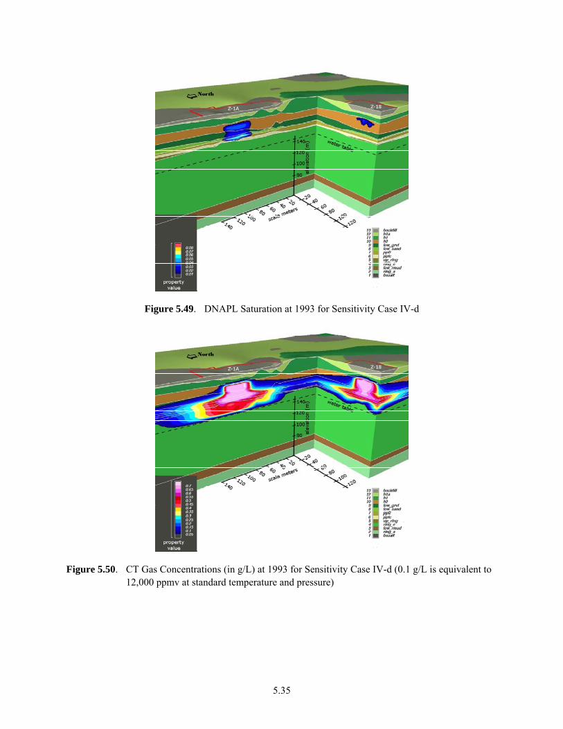
5.35

Figure 5.49. DNAPL Saturation at 1993 for Sensitivity Case IV-d

Figure 5.50. CT Gas Concentrations (in g/L) at 1993 for Sensitivity Case IV-d (0.1 g/L is equivalent to 12,000 ppmv at standard temperature and pressure)

5.36

Figure 5.51. CT Mass Distribution Over the DNAPL, Sorbed, Aqueous, and Gas Phases for 1960 – 1993 (Case IV-d)

Figure 5.52. DNAPL CT Mass Distribution Over the Hydrostratigraphic Units for 1960 – 1993 (Case IV-d)

5.37

5.2.5 Porous Medium Properties of Cold Creek Unit

The permeability and air-entry pressure of the CCU were determined to be important for DNAPL movement into the subsurface of the 216-Z-9 disposal site (Oostrom et al. 2004; 2006). Four simulations were conducted in this category of which two used a lower permeability (case V-a and V-b) and two a higher permeability (case V-c and V-d). In addition, for case V-b and V-d, the permeability was increased and decreased by 10 to be consisted with the Miller and Miller (1956) scaling theory. The simulations for the category only show minor differences with the base case. As an example, the plots shown in Figures 5.53 through 5.56 are quite similar to the equivalent figures for the base case. The main differences are observed for aqueous phase transport and the associated dissolved CT transport across the water table. In case V-a and –b, no dissolved CT is transport into the saturated zone due to a lower permeability of the CCU. For cases V-c and V-d, the dissolved phase CT mass transported across the water table in the aqueous phase is approximately six times the mass transported in the base case.

5.38

Figure 5.53. DNAPL Saturations at 1993 for Sensitivity Case V-b

Figure 5.54. CT Gas Concentrations (in g/L) at 1993 for Sensitivity Case V-b (0.1 g/L is equivalent to 12,000 ppmv at standard temperature and pressure)

5.39

Figure 5.55. CT Mass Distribution Over the DNAPL, Sorbed, Aqueous, and Gas Phases for 1960 – 1993 (Case V-b)

Figure 5.56. DNAPL CT Mass Distribution Over the Hydrostratigraphic Units for 1960 – 1993 (Case V-b)

5.40

5.2.6 Porous Medium Properties of all Units

A total of eight simulations were used to vary hydraulic properties of all units. The parameter value changes for the simulations compared to the based case are:

a. Anisotropy ratio of 1:1 b. Anisotropy ratio of 20:1 c. 1.25 x base case porosity d. 0.75 x base case porosity e. 2 x base case air-entry pressure head f. 0.5 x base case air-entry pressure head g. 10 x base case permeability h. 0.1 x base case permeability

The results of case VI-a (Figures 5.57 through 5.61) are unique as it is the only simulation that predicts DNAPL disposed at the 216-Z-1A to move down all the way to the Lower Mud unit (Figure 5.57). The isotropic conditions cause more than 45,000 kg DNAPL to move across the water table by 1993 (Table 5.2). The associated gas concentration plume is shown in Figure 5.58 while aqueous phase concentrations are depicted in Figure 5.59. The latter figure shows a dissolved CT plume ranging from the water table to the top of the lower mud. The mass distribution over the phases shows that over time, the sorbed mass becomes larger than the CT DNAPL mass. The CT distribution over the hydrostratigraphic units shown in Figure 5.61 reflects the findings shown in Figure 5.57. By 1993, the CT mass in the Ringold E is more than in the H1a unit.

All other cases in this category provide expected results (Table 5.1 and 5.2), with relative minor deviations from the base case except for case VI-g and VI-h where the permeability was increased and decreased with a factor 10, respectively. Figure 5.62 shows that for case VI-g, virtually no DNAPL phase CT was left in the subsurface by 1993. This result is supported by the estimated 3% of the inventory left in the domain according to Table 5.1 and the phase distribution plot shown in Figure 5.64. The associated gas plume (Figure 5.63) is therefore also smaller than for the base case. The CT DNAPL hydrostratigraphic distribution (Figure 5.65) shows that DNAPL only appeared in the upper part of the domain, with the vast majority in the H1a. Overall, the increase in permeability by a factor 10 in all directions caused rapid lateral DNAPL spreading and gas transport. The overall reduction in permeability imposed in case VI-h resulted in a more compact DNAPL body (Figure 5.66) and CT gas plume (Figure 5.67). The reduction caused CT to primarily remain as a DNAPL (Figure 5.68) in the upper parts of the domain (Figure 5.69).

5.41

Figure 5.57. DNAPL Saturation at 1993 for Sensitivity Case VI-a

Figure 5.58. CT Gas Concentrations (in g/L) at 1993 for Sensitivity Case VI-a (0.1 g/L is equivalent to 12,000 ppmv at standard temperature and pressure)

5.42

Figure 5.59. CT Aqueous Concentrations (in g/L) at 1993 for Sensitivity Case VI-a

Figure 5.60. CT Mass Distribution Over the DNAPL, Sorbed, Aqueous, and Gas Phases for 1960 – 1993 (Case VI-a)

5.43

Figure 5.61. DNAPL CT Mass Distribution Over the Hydrostratigraphic Units for 1960 – 1993 (Case VI-a)

5.44

Figure 5.62. DNAPL Saturation at 1993 for Sensitivity Case VI-g

Figure 5.63. CT Gas Concentrations (in g/L) at 1993 for Sensitivity Case VI-g (0.1 g/L is equivalent to 12,000 ppmv at standard temperature and pressure)

5.45

Figure 5.64. CT Mass Distribution Over the DNAPL, Sorbed, Aqueous, and Gas Phases for 1960 – 1993 (Case VI-g)

Figure 5.65. DNAPL CT Mass Distribution Over the Hydrostratigraphic Units for 1960 – 1993 (Case VI-g)

5.46

Figure 5.66. DNAPL Saturation at 1993 for Sensitivity Case VI-h

Figure 5.67. CT Gas Concentrations (in g/L) at 1993 for Sensitivity Case VI-h (0.1 g/L is equivalent to 12,000 ppmv at standard temperature and pressure)

5.47

Figure 5.68. CT Mass Distribution Over the DNAPL, Sorbed, Aqueous, and Gas Phases for 1960 – 1993 (Case VI-h)

Figure 5.69. DNAPL CT Mass Distribution Over the Hydrostratigraphic Units for 1960 – 1993 (Case VI-h)

5.48

5.3 Comparison of Simulation Results

Using similar procedures used in Oostrom et al. (2004; 2006) for the 216-Z-9 simulations, normalized spatial moments of the DNAPL distribution were calculated to provide a quantitative basis for comparing the results of the different simulation cases (Freyberg 1986). The ijkth moment of the mass distribution in space was defined as

( ) ( ) dxdydzzyxt,z,y,xStM kjinnijk ∫∫∫

∞

∞−

∞

∞−

∞

∞−

= φρ (5.1)

where ρn is the mass density of the DNAPL, φ is the porosity, Sn is the DNAPL saturation, and x, y, and z are the spatial coordinates. The integrals in Equation (5.1) were evaluated over the extent the DNAPL or dissolved component was transported from either the 216-Z-1A or 216-Z-18 sites.

The zeroth, first, and second (i + j + k = 0, 1, or 2, respectively) spatial moments of the DNAPL distribution were computed. These moments provide measures of the total DNAPL mass, the location of the center of mass, and spread about the center of mass. The zeroth moment, M000, is equal to the total mass in the domain. The first moment, normalized by the zeroth moment, defines the location of the center of mass (xc, yc, zc):

000

001

000

010

000

100

MMy

MMy

MMx ccc === (5.2)

The second moment about the center of mass defines a spatial covariance tensor (Freyberg 1986):

cczyyzcczxxzccyxxy

czzcyycxx

zzzyzx

yzyyyx

xzxyxx

zyMM

zxMM

yxMM

zMM

yMM

xMM

−==−==−==

−=−=−=

⎥⎥⎥

⎦

⎤

⎢⎢⎢

⎣

⎡

=

000

01122

000

10122

000

11022

2

000

00222

000

02022

000

2002

222

222

222

2

σσσσσσ

σσσ

σσσσσσσσσ

σ

(5-3)

The components of the covariance tensor are directly related to the spread of the DNAPL body about its center of mass. In Table 5.3 and 5.4, the zeroth and first order moments are shown for the 216-Z-18 and 216-Z-1A, respectively. Table 5.5 and 5.6 provide an overview of the second order diagonal moments for the two sites. The listed moments are computed for 1993.

The first order moments (Table 5.3 and 5.4) show that for both disposal sites, the horizontal center of mass is located below the disposal site footprint for all simulations. The vertical center of mass for the sites is located in the H2 unit for most simulations. A vertical center of mass closer to the CCU is

5.49

predicted by the cases where the hydraulic properties of the H1a unit were altered to resemble properties of the H1 unit. The standard deviations of the second order moments, shown in Table 5.5 and 5.6, provide an indication of the DNAPL spreading. According to the moment analysis, approximately 95% of the DNAPL mass is predicted to be located between the center of mass and plus or minus the computed standard deviations. For most cases, the standard deviations in the horizontal direction are less than 50 m, limiting the mass distribution to areas with roughly the same order of magnitude as the footprints. In the vertical direction, the standard deviation for the 216-Z-1A site is typically in the order of about 10 m, while the standard deviation for the 216-Z-18 site is often less than 5 m.

5.50

Table 5.3. Zero and First Order Moments of CT DNAPL Mass at 1993 for DNAPL Disposed at the 216-Z-1A Site. (The center of 216-Z-1A Trench is set at x = 0 m, y = 0 m, and z = 199 m. The CCU below the trench is approximately located between z = 162 m and z = 170 m.)

Simulation M000 xc (m) yc (m) zc (m)

Base Case 1.93e5 -2.1 -2.3 181 I-a 1.99e5 -1.4 -1.6 177 I-b 2.03e5 -2.1 -3.1 175 I-c 1.16e5 -2.4 -0.6 171 II-a 1.80e5 -0.4 -2.4 180 II-b 1.85e5 -0.9 1.4 176 II-c 1.41e5 -0.7 1.2 172 III-a 1.95e5 -1.1 -3.1 180 III-b 1.97e5 -3.1 -0.3 182 III-c 2.01e5 -2.1 0.4 182 III-d 2.02e5 -3.2 -3.1 180 III-e 1.43e5 -0.9 0.8 178 III-f 3.12e5 -1.2 -0.7 180 III-g 1.97e5 -1.3 0.3 180 III-h 1.89e5 -1.5 -0.2 179 III-i 1.91e5 -3.0 -1.1 181 III-j 2.01e5 -1.3 -1.0 184 III-k 2.05e5 -2.2 -3.3 183 IV-a 1.02e5 -1.2 -3.4 172 IV-b 1.81e5 -0.9 -4.5 171 IV-c 1.85e5 -1.5 -3.2 171 IV-d 1.45e5 -2.3 -6.1 167 V-a 2.01e5 -0.1 3.1 181 V-b 2.02e5 -0.4 2.6 180 V-c 1.90e5 -0.5 1.4 179 V-d 1.92e5 -0.6 4.2 180 VI-a 1.32e5 -0.8 -2.5 162 VI-b 3.31e5 -1.2 4.2 182 VI-c 2.02e5 -1.4 -1.3 181 VI-d 1.82e5 -2.5 -2.8 180 VI-e 1.85e5 -2.3 -3.7 182 VI-f 1.95e5 -2.7 -2.3 177 VI-g 5.04e3 4.2 0.4 184 VI-h 4.02e5 3.4 1.3 185

5.51

Table 5.4. Zero and First Order Moments of CT DNAPL Mass at 1993 for DNAPL Disposed at the 216-Z-18 Site. (The center of 216-Z-18 Trench is set at x = 0 m, y = 0 m, and z = 199 m. The CCU below the trench is approximately located between z = 162 m and z = 170 m.)

Simulation M000 xc (m) yc (m) zc (m)

Base Case 0.88e5 -6.7 7.2 184 I-a 0.93e5 -5.6 7.4 180 I-b 0.9e5 -7.2 6.5 177 I-c 0.50e5 -4.6 8.2 174 II-a 0.69e5 -6.2 5.4 182 II-b 0.82e5 -5.4 4.4 179 II-c 0.58e5 -4.1 6.5 176 III-a 0.90e5 -4.9 6.4 183 III-b 0.91e5 -6.2 8.3 185 III-c 0.65e5 -5.3 5.4 184 III-d 0.64e5 -3.6 3.6 183 III-e 0.54e5 -3.7 6.3 172 III-f 1.21e5 -5.7 7.5 181 III-g 0.94e5 -6.2 8.3 182 III-h 0.77e5 -7.8 6.9 183 III-i 0.83e5 -4.3 3.9 185 III-j 0.91e5 -5.2 5.4 186 III-k 0.97e5 -5.7 7.5 187 IV-a 0.64e5 -4.3 3.5 174 IV-b 0.68e5 -6.7 6.2 172 IV-c 0.82e5 -6.7 5.4 172 IV-d 0.54e5 -5.6 6.4 168 V-a 0.84e5 -4.6 6.7 183 V-b 0.83e5 -5.9 4.3 183 V-c 0.76e5 -2.0 6.1 182 V-d 0.74e5 -6.2 5.7 182 VI-a 0.65e5 -5.8 7.4 164 VI-b 1.02e5 -7.8 6.5 185 VI-c 0.89e5 -6.4 4.5 185 VI-d 0.84e5 -6.5 4.3 182 VI-e 0.89e5 -4.2 6.5 185 VI-f 0.88e5 -5.7 6.3 181 VI-g 1.20e4 -7.6 7.4 185 VI-h 0.79e5 -5.4 7.5 186

5.52

Table 5.5. Standard Deviations of Second Order Moments (Rounded to Nearest Meter) of CT DNAPL Mass at 1993 for the 216-Z-1A Site. (The center is at x = 0 m, y = 0 m, and z = 201 m. The CCU below the trench is approximately located between z = 162 m and z = 170 m.)

Simulation xxσ (m) yyσ (m) zzσ (m)

Base Case 54 34 12 I-a 53 32 11 I-b 53 30 10 I-c 56 23 10 II-a 52 27 9 II-b 48 29 9 II-c 49 28 10 III-a 52 36 12 III-b 50 34 10 III-c 39 29 13 III-d 41 30 11 III-e 47 34 12 III-f 49 34 11 III-g 48 32 12 III-h 52 28 11 III-i 48 27 10 III-j 32 19 8 III-k 34 17 8 IV-a 38 19 7 IV-b 36 19 8 IV-c 31 15 7 IV-d 22 16 6 V-a 46 29 10 V-b 54 27 10 V-c 51 32 11 V-d 48 29 11 VI-a 9 8 41 VI-b 12 8 8 VI-c 47 29 10 VI-d 44 28 13 VI-e 43 26 12 VI-f 43 35 12 VI-g 47 31 18 VI-h 29 18 6

5.53

Table 5.6. Standard Deviations of Second Order Moments of CT DNAPL Mass at 1993 for the 216-Z-18 Site. (The center is at x = 0 m, y = 0 m, and z = 199 m. The CCU below the trench is approximately located between z = 162 m and z = 170 m.)

Simulation xxσ (m) yyσ (m) zzσ (m)

Base Case 42 22 3 I-a 42 20 3 I-b 43 21 4 I-c 44 21 4 II-a 35 18 3 II-b 36 18 3 II-c 40 21 3 III-a 43 24 4 III-b 40 21 3 III-c 31 17 5 III-d 29 18 4 III-e 37 22 4 III-f 41 24 5 III-g 42 22 5 III-h 41 22 3 III-i 38 20 4 III-j 20 14 2 III-k 21 13 2 IV-a 31 16 3 IV-b 30 15 3 IV-c 22 13 2 IV-d 16 12 3 V-a 36 24 4 V-b 40 22 4 V-c 41 23 4 V-d 42 22 4 VI-a 8 6 14 VI-b 9 5 3 VI-c 37 21 4 VI-d 38 25 4 VI-e 32 22 5 VI-f 33 24 5 VI-g 40 21 7 VI-h 19 14 2

5.54

5.4 SVE Simulation Results

In this section the results of eight SVE simulations for the period 1993 – 2007 were conducted to investigate the effect of well location, extraction rate, and vapor pressure on CT removal. The base case fluid and porous medium property values are used for all SVE simulations except for case 8. The SVE simulations are:

1. Extraction from all wells. This case is referred to as the “base case with SVE” simulation.

2. Extraction from wells with screens located in 216-Z-1A CCU silt: W18-159, -165, -166, -167, -178, and -174.

3. Extraction from wells located near water table near the 216-Z-18 trench: W18-10, -11, and -12.

4. Extraction from well W18-96 only, located below the 216-Z-18 trench.

5. Extraction from well W18-165 only, located below the 216-Z-1A tile field.

6. Extraction from well W18-246 (located west of 216-Z-1A and north of 216-Z-18)

7. Extraction with 25% of the rate.

8. Extraction from all wells and hydraulic properties of H1a the same as for H1.

The results of SVE case 1 are discussed in Section 5.4.1., while the other simulations are described in Section 5.4.2.

5.4.1 Base Case with SVE

The results of the simulation with SVE operations in the subsurface of the two disposal sites are compared with an extension of the base case from 1993 – 2007 without the inclusion of SVE. Figure 5.70 and 5.71 show the DNAPL saturation at 1995 for the base case without, and with SVE, respectively. The figures show that after two years of extraction, most of the DNAPL in the Lower Gravel unit below the 216-Z-1A site has been removed. The remediation seems to have less impact on the DNAPL in the CCU and the H1a unit, while some removal is visible in the H2 unit, especially below the 216-Z-18. Five years later, in 2000, the situation for the base case without SVE (Figure 5.72) has not changed much while the SVE operations seem to have removed most DNAPL in the H2 unit and CCU (Figure 5.73. The SVE does not seem to have a large affect the DNAPL in the H1a unit below both sites. The relative low permeability of the unit and the larger distance to the SVE well screens are important factors limiting mass removal from this unit.

The CT gas plumes at 1995 (Figures 5.74 and 5.75) and 2000 (Figure 5.76 and 5.77) show the large impact of SVE. For the base case without SVE the plumes look fairly similar for both times. However, the figures for the base case with SVE demonstrate a rapid reduction of the plume extension, even in the lower permeability units. By the year 2000, the plume extension is reduced to a size smaller than the respective footprints of the disposal facility. Top views of the CT gas plume at 1995 (Figures 5.78 and 5.79) and at 2000 (Figures 5.80 and 5.81) in the CCU show an apparent stable gas plume for simulation

5.55

without SVE, but a rapidly decreasing extension for the case where SVE is considered. In the latter case, no gaseous CT gas is predicted to be present in the CCU below the 216-Z-18 site by 2000, while the extension below the 216-Z-1A site is less than the width of the footprint (Figure 5.81). A comparison for the CT gas concentration near the water table is shown in Figures 5.82 and 5.83. For the simulation without SVE, CT in the gas phase is still being transported to the water table (Figure 5.82) while not gaseous CT is being observed near the water table for the simulation with SVE (Figure 5.83).

Figures 5.84 and 5.85 show the CT mass distribution over the phases for the cases without and with SVE, respectively, for the period 1960 – 2007. Figure 5.84 show gradual changes in phase distribution while Figure 5.85 show abrupt changes induces by the SVE operations. Figures 5.86 and 5.87 provide the same information for the period from 1993 – 2007 when SVE was employed. Again, the figures show gradual compositional changes for the simulation without SVE (Figure 5.86) and more pronounced decreases over all phases for the simulation with SVE (Figure 5.87). Figure 5.87 demonstrates a rapid decrease in gaseous, sorbed, and aqueous phase CT, and a more gradual decrease in CT DNAPL. The rapid decrease in gaseous CT and the slower reduction in CT DNAPL shown in this plot are consistent with the CT gas plumes shown in Figures 5.75 and 5.77 and DNAPL saturations shown in Figures 5.71 and 5.73. The total mass that is predicted to be removed by SVE through 2007 is almost 400,000 kg.

The CT mass distribution over the hydrostratigraphic units for the base case without and with SVE are depicted in Figures 5.88 and 5.89, respectively. The simulation without SVE shows gradual changes in composition, while the simulation with SVE indicates rapid CT DNAPL decreases in the H2, Lower Sand, and Lower Gravel units. The CT DNAPL mass reduction in the CCU appears to be a slower process, while a reduction in the H1a unit seems to be unrelated to SVE since its CT DNAPL mass behavior looks the same as for the simulation without SVE (Figure 5.88). This information becomes more pronounced in Figures 5.90 and 5.91, where the CT mass distribution is shown for the 1990 – 2007 period. Figure 5.91 shows that by 1995, all CT DNAPL mass in the Lower Gravel has disappeared and that by 1998, the SVE has removed the CT DNAPL from the Lower Sand. Complete depletion of the H2 unit is predicted to have occurred by 2004. Again, the resilience of the CT DNAPL in the H1a unit is remarkable and is associated with its low permeability, high porosity, and considerable distance to most SVE wells.

5.56


Figure 5.71. DNAPL Saturations at 1995 (Base Case with SVE)

5.57


Figure 5.73. DNAPL Saturations at 2000 (Base Case with SVE)

5.58


Figure 5.75. CT Gas Concentrations (g/L) at 1995 (Base Case with SVE) (0.1 g/L is equivalent to 12,000 ppmv at standard temperature and pressure)

5.59


Figure 5.77. CT Gas Concentrations (g/L) at 2000 (Base Case with SVE) (0.1 g/L is equivalent to 12,000 ppmv at standard temperature and pressure)

5.60


Figure 5.79. Top View of CT Gas Concentrations (g/L) in Cold Creek Unit at 1995 (Base Case with SVE) (0.1 g/L is equivalent to 12,000 ppmv at standard temperature and pressure)

5.61


Figure 5.81. Top View of CT Gas Concentrations (g/L) in Cold Creek Unit at 2000 (Base Case with SVE) (0.1 g/L is equivalent to 12,000 ppmv at standard temperature and pressure)

5.62


Figure 5.83. Top View of CT Gas Concentrations (g/L) Above Water Table at 2000 (Base Case with SVE) (0.1 g/L is equivalent to 12,000 ppmv at standard temperature and pressure)

5.63


Figure 5.85. CT Mass Distribution Over the DNAPL, Sorbed, Aqueous, and Gas Phases for 1960 – 2007 (Base Case with SVE)

5.64


Figure 5.87. CT Mass Distribution Over the DNAPL, Sorbed, Aqueous, and Gas Phases for 1993 – 2007 (Base Case with SVE)

5.65


Figure 5.89. DNAPL CT Mass Distribution Over the Hydrostratigraphic Units for 1960 – 2007 (Base Case with SVE)

5.66


Figure 5.91. DNAPL CT Mass Distribution Over the Hydrostratigraphic Units for 1993 – 2007 (Base Case with SVE)

5.67

5.4.2 SVE Sensitivity Simulations

SVE sensitivity case 2 shows the effect of extraction from well with screen in the CCU silt below the 216-Z-1A. The CT mass distribution shows rapid changes corresponding with activation of the wells (Figure 5.92) and considerable recovery from these wells was not started until 1997. Total mass recovery was approximately 275,000 kg, which is 125,000 kg less than the base case with SVE. Removal was again the fastest from the Lower Sand, Lower Gravel, and H2 units. It is also of interest to observe that although the well screens were placed in the CCU silt, CT DNAPL removal from the unit was relatively low.

The case 3 simulations show the effect of the SVE wells located close to the water table (Figure 5.93). The predicted total mass removal is limited to approximately 50,000 kg (Figure 5.94), and most of that CT mass was removed from the Lower Sand and Lower Gravel (Figure 5.95). The distribution predicted by case 4, i.e., extraction from well W18-96 only, is shown in Figures 5.96 and 5.97. This well was only active in during the initial stages and has recovered approximately 100,000 kg from below the 216-Z-18 site. The fifth SVE case (Figures 5.98 and 5.99) looks at the recovery from a single well located below the 216-Z-1A site. This particular well was active during several periods of the campaign, yielding about 150,000 for the subsurface of this site. Most of the removed CT came from the Lower Gravel and H2 units. To investigate the effect of a well that is not located below either disposal site, a simulation was conducted (case 6) where only well W18-246 was used. This well is located west of the 216-Z-1A and north of the 216-Z-18. Although this well was located a considerable distance from both sites, the predicted removal was over 250,000 kg (Figure 5.100 and 5.101). For case 7, the effect of a 75% vapor pressure lowering on recovery was simulated (Figures 5.102 and 5.103). This simulation predicts a much slower recovery than the base case with SVE and a gradual reduction of the CT in all phases. Removal occurs primarily from the more permeable porous media, while leaving the CT mass in the H1a unit and CCU in place. The figures for SVE case 8 (Figures 5.104 and 5.105) indicate the importance of the properties of the H1a unit on CT DNAPL behavior and subsequent removal with SVE. The CT distribution over the phases (Figure 5.104) shows a larger reduction in the total VOC mass over time. The reason for the more pronounced removal is the location of the CT DNAPL at 1993. Contrary to the base case, at this point in time no CT DNAPL is located in the H1a unit because the properties of this unit are the same as for the underlying H1 unit. Most of the CT DNAPL has moved to more permeable units, allowed for a rapid removal. For this simulation, the CT DNAPL in the Cold Creek units is the most resilient (Figure 5.105).

5.68

Figure 5.92. CT Mass Distribution Over the DNAPL, Sorbed, Aqueous, and Gas Phases for 1993 – 2007 (SVE Case 2)

Figure 5.93. DNAPL CT Mass Distribution Over the Hydrostratigraphic Units for 1993 – 2007 (SVE Case 2)

5.69



5.70



5.71



5.72



5.73



5.74



5.75

5.5 Undocumented Discharge Simulations

A series of simulations was conducted for each of the major DNAPL sites to identify the minimum volume needed to result in DNAPL movement across the water table by 1993. The results of the iterative simulation are presented in Table 5.7. The results indicate that the minimum volume is 245 m3, occurring at the 216-Z-9 site. The required volumes at the other two sites are approximately twice as high. The reasons for the differences are related to size of the disposal area, disposal rate, and subsurface geology. However, if the assumption is made that an undocumented discharge should have occurred at either a crib, french tile, or trench, similar to the 216-Z-9, 216-Z-1A, or 216-Z-18, volumes in the order of 250 m3 are needed to result in DNAPL movement across the water table. Based on the available Hanford site information, additional disposal volumes of this magnitude, beyond what has been reported for the three major DNAPL sites, are not likely.

Table 5.7. Disposed DNAPL Volume at the 216-Z-9, 216-Z-1A, and 216-Z-18 Sites and the Volume Needed for Transport of a Minimum of 1 Kg CT Across the Water Table by 1993

DNAPL Site Disposed Volume

(m3)

Disposed Volume Needed for Movement Across

Water Table (m3) 216-Z-9 316 245

216-Z-1A 242 475 216-Z-18 147 535

The results of the accidental spill simulation are listed in Table 5.8. The maximum penetration depth is 28 m, which is still above the CCU silt. The geologic domain without the H1a unit resulted in smaller penetration depths than the simulations where the H1a was included. The higher permeability of the H1 unit caused more lateral movement of the DNAPL and of the CT in the gas phase, resulting in less DNAPL available for vertical movement. The important information that may be derived from Table 5.8 regarding undocumented releases is that even fairly large spills of up to 10 m3 do not result in DNAPL movement across the water table.

5.76

Table 5.8. Maximum Penetration Depth (m) for Several Spill Scenarios and Two Geologic Domains (The spill area is 1 m2 for all cases.)

Spill Size (m3)

Spill Duration

Penetration Depth Geologic Domain 1

(m)

Penetration Depth Geologic Domain

2 (m) 0.2 1 hour 6 5 0.2 1 day 5 4 0.2 10 days 3 2 1 1 hour 12 9 1 1 day 10 8 1 10 days 8 7

10 1 hour n.d. 21 10 1 day 28 19 10 10 days 22 17

n.d.= Not determined due to excessive infiltration rate.

6.1

6.0 Summary and Conceptual Model Update

A conceptual model of CT in the vadose zone and groundwater underlying the disposal sites defines the current understanding and the areas of uncertainty that need to be considered in characterization and modeling activities and to support remediation decisions. The conceptual model discussion for this report is focused on the subsurface near the disposal areas to provide a framework for describing the distribution of CT within the vadose zone, the source of CT for the existing groundwater plume, and the nature of any continuing source of CT to the groundwater plume from within the subsurface near the disposal areas. This discussion uses results of multi-phase modeling and assessment of published data near the disposal areas to refine the conceptual model that has been developed over time and summarized in the RI/FS Work Plan (DOE 2004). The conceptual model presented in the RI/FS Work Plan was the most recent conceptual model during the modeling effort described in this report. The conceptual model was updated for the RI report (DOE 2006). The discussion herein describes how the model results revise the conceptual model presented in the RI/FS Work Plan and how this update is consistent with and in addition to the conceptual model presented in the RI report. Figure 6.1 illustrates the conceptual distribution of CT in the subsurface near the disposal areas as depicted in the RI/FS Work Plan (DOE 2004) and discusses the key overall components of this conceptual model. Based on the modeling results presented herein and in Oostrom et al. (2004; 2006), Figure 6.1 has been updated as a revised overall conceptual model shown in Figure 6.2. Both Figures 6.1 and 6.2 describe how CT in the DNAPL and other phases are distributed through the subsurface, but do not necessarily represent a “picture” of the CT distribution at any given time. In addition to a static picture of the conceptual model for CT, modeling provides information about the variation in CT distri-bution over time. Thus, the revisions to the previous conceptual model include a temporal component to interpreting CT distribution in the subsurface. A conceptual depiction of temporal variation in the CT distribution over time for the 216-Z-9 and216-Z-1A are shown in Figures 6.3 and 6.4, respectively, for the years 1966, 1974, 1993, and 2000, and for the 216-Z-18 in Figure 6.5 for the years 1974, 1993, and 2000. The key revisions to the updated overall conceptual model of the RI/FS Work Plan (DOE 2004) are listed below. These items are consistent with the conceptual model update shown in the RI report (DOE 2006). However, as discussed below, the simulation results provide additional information to further refine the conceptual model presented in the RI report (DOE 2006).

1. No lateral movement of DNAPL to under the Plutonium Finishing Plant is likely.

2. The zones of persistent CT mass in the vadose zone are primarily the CCU and H1a unit.

3. Large vertical and lateral density-driven vapor movement of occurred in the past.

4. DNAPL penetration to groundwater is likely to have occurred at the 216-Z-9 site, is possible at the 216-Z-1A site, and unlikely at the 216-Z-18 site.

5. The phase distribution of CT changes over time due to volatilization, interaction of gas-phase CT with pore water and aqueous-phase CT with sorbed phase, DNAPL dissolution in groundwater, and the impact of soil vapor extraction.

The overall revisions to the conceptual model are supported by both modeling results and existing published data. Figure 6.6 shows comparison of the simulated CT DNAPL distribution and the existing

6.2

published soil data (tabulated in Appendix A, Table A.1). The vertical distribution of CT in groundwater beneath the disposal sites from field data and a three-dimensional model of the CT distribution in groundwater developed through geostatistical modeling of the CT data (Murray et al. 2006) are shown in Figure 6.7 (data tabulated in Appendix A, Table A.2). Key conclusions from this information are listed below.

• High soil concentrations and predicted areas with high DNAPL saturations are spread vertically within a relatively small lateral area within about 30 m of the disposal area footprint.

• Measured groundwater concentrations are higher and the high groundwater concentrations are spread deeper in the aquifer beneath the 216-Z-9 site compared to the 216-Z-1A and 216-Z-18 sites. This observation correlates to modeling results where the CT flux to the groundwater at the 216-Z-9 site was significantly higher than the flux at the 216-Z-1A and 216-Z-18 sites. Modeling results showing a larger number of sensitivity simulations with DNAPL flux into groundwater and deeper penetration of DNAPL within the aquifer beneath the 216-Z-9 site, as compared to the other two disposal areas are also consistent with these observations.

While these overall changes to the conceptual model are important, it is equally important to assess the behavior of CT at key locations and interfaces in the subsurface to better understand the distribution of CT within the vadose zone, the source of CT for the existing groundwater plume, and the nature of any continuing source of CT to the groundwater plume from within the subsurface near the disposal areas.

Modeling results show accumulation within the CCU. Measured CT concentrations in vadose zone soil samples from wells within 30 m of the disposal areas are consistent with these modeling results, where the CT concentration averages 2424 µg/kg within the CCU and 444 µg/kg in other units within the vadose zone, based on samples with data above the detection limit. After initial infiltration and redistri-bution of the CT in the vadose zone, CT is retained in the CCU and the flux in or out of the unit is expected to be very small and only primarily via the vapor phase. While the flux in the vapor phase can be impacted by SVE above or below the CCU, the CCU is likely a location where CT will be present over the long term. Other portions of the vadose zone with a large percentage of small particle size sediments (e.g., silt lenses) would also be expected to accumulate CT based on the modeling results. Consistent with these results, for wells within 30 m of the disposal areas, the measured CT concentrations in vadose zone soil samples with an M, sM, (g)M, (g)sM, gM, gsM, or mS sediment classification average 2099 µg/kg (not including one sample that was 380,000 µg/kg) compared to an average of 528 µg/kg for all other sediment classifications (based on samples with data above the detection limit).

Modeling results also show that CT DNAPL is distributed vertically below the disposal areas with minimal lateral spreading (see Tables 5.3 – 5.6 and Oostrom et al. 2004; 2006). With this pattern of DNAPL migration, the most likely location for any DNAPL remaining in the subsurface would be vertically below the disposal areas. Measured vadose zone soil data (see Appendix A, Table A.1) also show low CT concentrations at distances greater than 30 m from the disposal areas, where CT concen-trations average 79 µg/kg and within the CCU at these locations the CT averages only 81 µg/kg (based on samples with data above the detection limit) compared to the much higher CT concentrations vertically beneath the disposal areas (laterally within 30 m of the disposal area) shown above. Additionally, of 408 vadose zone soil samples from wells within 30 m of the disposal areas, only 70 were below detection limit (~17%) compared to 215 out of 258 samples below detection limit (83%) for soil samples greater than 30 m from the disposal areas.

6.3

Assessing mass flux at key interfaces provides another means to refine the conceptual model for CT. While mass flux measurements in the subsurface are difficult, modeling readily provides mass flux estimates. The mass flux estimates are related to the conceptual model and to measured data because the flux estimates can be used describe the amount of mass that has moved past an interface as a function of time. For instance, Murray et al. (2006) estimated the mass of CT within the groundwater based on recent data and how much CT would need to have been added to the groundwater to result in this mass estimate if hydrolysis were continually degrading CT at a specified rate. Using these estimates, the flux of CT across the groundwater since initial disposal that would be needed to accumulate the estimated mass of CT in the groundwater can be calculated. Model results can then be compared to this flux estimate to evaluate reasonable scenarios for how CT entered the groundwater. For instance, with 100,000 kg of CT that entered the aquifer (based on the estimate in Murray et al. 2006), only by combining the estimates of CT mass flux to the groundwater from simulation sensitivities (not the base cases) that show DNAPL crossing the water table, can a combined mass of CT (216-Z-9, 216-Z-18, and 216-Z-1A) in the aquifer near the estimated CT mass be predicted. The average CT mass of dissolved CT that has been transported across the water table (a measure of the impact of vapor phase transport to the groundwater table and pore water from the vadose zone entering the groundwater) for all three sites through 1993 is approximately 5,000-10,000 kg. The accumulated mass in the aquifer would be significantly lower than the mass of CT in the groundwater estimated by Murray et al. (2006) if only aqueous and vapor phase CT and no DNAPL phase entered the groundwater. This assessment indicates that it is likely that DNAPL CT has entered the groundwater. The simulation results herein and in Oostrom et al. (2004; 2006) show that the most likely location of significant DNAPL movement across the water table is below the 216-Z-9 site. In the base case simulation and other simulation sensitivities where DNAPL enters the groundwater, the DNAPL flux below the 216-Z-9 site ceases by 1995, when SVE was employed. Without the inclusion of SVE in the simulations, DNAPL movement across the water table is predicted to continue, though at a low flux through the present day.

The estimated amount of CT in the groundwater by Murray et al. (2006) does not include any DNAPL mass that may be in the aquifer now. For simulations where the mass of CT entering the groundwater is just equal to the mass of CT in the groundwater estimated by Murray et al. (2006), all of the DNAPL would need to be dissolved and distributed within the plume at the present time. For simu-lations where the mass of CT entering the groundwater is greater that the mass of CT in the groundwater estimated by Murray et al. (2006), DNAPL may still be present in the aquifer. In these cases, modeling results suggest that the DNAPL would be localized to the portion of the aquifer beneath the disposal areas (in particular at the 216-Z-9 disposal area) and laterally only within a relatively localized areal extent.

In the previous conceptual model (RI/FS Work Plan, DOE 2004), there are multiple components of the conceptual model that are included as potential mechanisms for how CT distributes through the vadose zone and groundwater near the disposal areas. The following analysis provided additional evaluation of how CT is distributed within the subsurface to help assess the importance of processes other than the CT movement simulated in the modeling effort.

Undocumented Sources – The conceptual model in the RI/FS Work Plan (DOE 2004) notes that undocumented sources may contribute to the CT plume in the groundwater. The following assessment provides information that can be used to describe the magnitude of disposal at an undocumented source that would be needed for CT for this source to have a significant impact on groundwater. A series of simulations was conducted to estimate the volume of DNAPL that is required to result in DNAPL

6.4

movement across the water table for all three sites. The simulations revealed that at least 250 m3 of DNAPL are necessary for this movement to occur if the DNAPL would have been disposed at typical waste site in the 200 West Area. Additional DNAPL volumes of that magnitude beyond what has been commonly reported for the three major DNAPL sites, are not likely. Undocumented CT sources might have also been the result of accidental spills. The simulations outlined in Chapter 4.3 considered accidental releases ranging from 0.2 m3 to 10.0 m3 (approximately 1 - 50 drums) of CT DNAPL, disposed on an area of 1 m2 for infiltration time ranging from 1 hour to 10 days. The maximum simulated infiltration depth of CT DNAPL was 28 m for the case where 50 barrels were allowed to infiltrate in 1 day. This distance is not even enough for the CT DNAPL to reach the CCU. The limited infiltration depth is directly related to sorption and mass transfer into the aqueous and gas phases as well as gaseous transport away from the infiltration zone due to advection and diffusion. Considering the size of the simulated CT DNAPL spill volumes (up to 10 m3), it is also unlikely that an undocumented spill of CT DNAPL would have been able to reach the water table.

Effect of Water Infiltration at Other Locations – Water was disposed of at sites other than the CT disposal areas. Future modeling with a larger model that encompasses all three CT disposal areas and nearby water infiltration sites (e.g., U Pond) can be conducted to support an assessment of how these water sources can impact CT distribution. The localized models used herein and by Oostrom et al. (2004 and 2006) do not directly address this issue.

Impact of Vapor Phase CT on Distribution of CT in the Groundwater – The simulation results show that CT in the gas phase is likely to have moved considerable distances in the lateral direction due to diffusion and advection. In particular, extensive CT gas plumes are predicted to develop on top of the water table. Part of the CT from the gas phase transfers into the aqueous phase but, since the diffusion transport process in the saturated zone is much smaller than in the gas phase, the amount of CT that is able to move below the water table through this process is relatively small.

6.5

Figure 6.1. Conceptual Model Presented in the RI/FS Work Plan (DOE 2004)

6.6

Figure 6.2. Revised Overall Conceptual Model for CT Migration within the Subsurface

6.7

Figure 6.3a. Conceptual Distribution of Carbon Tetrachloride from Waste Disposed at the 216-Z-9 Site in the Years 1966 (a), 1974 (b), 1993 (c), and 2000 (d). (These figures are based on the results of the base case simulations. Note that some sensitivity simulations show significantly different results. The figure for the year 2000 shows the conceptual impact of soil vapor extraction remediation operations.)

6.8

Figure 6.3b. Conceptual Distribution of Carbon Tetrachloride from Waste Disposed at the 216-Z-9 Site in the Years 1966 (a), 1974 (b), 1993 (c), and 2000 (d). (These figures are based on the results of the base case simulations. Note that some sensitivity simulations show significantly different results. The figure for the year 2000 shows the conceptual impact of soil vapor extraction remediation operations.)

6.9

Figure 6.3c. Conceptual Distribution of Carbon Tetrachloride from Waste Disposed at the 216-Z-9 Site in the Years 1966 (a), 1974 (b), 1993 (c), and 2000 (d). (These figures are based on the results of the base case simulations. Note that some sensitivity simulations show significantly different results. The figure for the year 2000 shows the conceptual impact of soil vapor extraction remediation operations.)

6.10

Figure 6.3d. Conceptual Distribution of Carbon Tetrachloride from Waste Disposed at the 216-Z-9 Site in the Years 1966 (a), 1974 (b), 1993 (c), and 2000 (d). (These figures are based on the results of the base case simulations. Note that some sensitivity simulations show significantly different results. The figure for the year 2000 shows the conceptual impact of soil vapor extraction remediation operations.)

6.11

Figure 6.4a. Conceptual Distribution of Carbon Tetrachloride from Waste Disposed at the 216-Z-1A Site in the Years 1966 (a), 1974 (b), 1993 (c), and 2000 (d). (These figures are based on the results of the base case simulations. Note that some sensitivity simulations show significantly different results. The figure for the year 2000 shows the conceptual impact of soil vapor extraction remediation operations.)

6.12

Figure 6.4b. Conceptual Distribution of Carbon Tetrachloride from Waste Disposed at the 216-Z-1A Site in the Years 1966 (a), 1974 (b), 1993 (c), and 2000 (d). (These figures are based on the results of the base case simulations. Note that some sensitivity simulations show significantly different results. The figure for the year 2000 shows the conceptual impact of soil vapor extraction remediation operations.)

6.13

Figure 6.4c. Conceptual Distribution of Carbon Tetrachloride from Waste Disposed at the 216-Z-1A Site in the Years 1966 (a), 1974 (b), 1993 (c), and 2000 (d). (These figures are based on the results of the base case simulations. Note that some sensitivity simulations show significantly different results. The figure for the year 2000 shows the conceptual impact of soil vapor extraction remediation operations.)

6.14

Figure 6.4d. Conceptual Distribution of Carbon Tetrachloride from Waste Disposed at the 216-Z-1A Site in the Years 1966 (a), 1974 (b), 1993 (c), and 2000 (d). (These figures are based on the results of the base case simulations. Note that some sensitivity simulations show significantly different results. The figure for the year 2000 shows the conceptual impact of soil vapor extraction remediation operations.)

6.15

Figure 6.5a. Conceptual Distribution of Carbon Tetrachloride from Waste Disposed at the 216-Z-18 Site in the Years 1974 (a), 1993 (b), and 2000 (c). (These figures are based on the results of the base case simulations. Note that some sensitivity simulations show significantly different results. The figure for the year 2000 shows the conceptual impact of soil vapor extraction remediation operations.)

6.16

Figure 6.5b. Conceptual Distribution of Carbon Tetrachloride from Waste Disposed at the 216-Z-18 Site in the Years 1974 (a), 1993 (b), and 2000 (c). (These figures are based on the results of the base case simulations. Note that some sensitivity simulations show significantly different results. The figure for the year 2000 shows the conceptual impact of soil vapor extraction remediation operations.)

6.17

Figure 6.5c. Conceptual Distribution of Carbon Tetrachloride from Waste Disposed at the 216-Z-18 Site in the Years 1974 (a), 1993 (b), and 2000 (c). (These figures are based on the results of the base case simulations. Note that some sensitivity simulations show significantly different results. The figure for the year 2000 shows the conceptual impact of soil vapor extraction remediation operations.)

6.18

Figure 6.6. Areal Extent of the Zone with Greater than 1% DNAPL Saturation from Base-Case Simulations Compared to Measured Soil Concentrations of CT in Vadose Zone at Nearby Boreholes (The maximum concentration measured in each well is shown in the figure.)

6.19

0

10

20

30

40

50

60

0 100 200 300 400 500 600 700 800 900 1000

Modeled CT concentration (ppb)

Dep

th b

elow

wat

er ta

ble

(m)

0 400 800 1200 1600 2000 2400 2800 3200 3600 4000

Measured CT concentration (ppb)

modeled CT near the 216-Z-9 site

modeled CT near the 216-Z-1A site

modeled CT near the 216-Z-18 site

measured CT near 216-Z-9 the site

Figure 6.7. Vertical Profile of CT Concentrations in Groundwater Beneath the Disposal Sites from Depth-Discrete Sampling and from Geostatistical Modeling of Field Data (by Murray et al. [2006])

7.1

7.0 References

Anderson JD. 1976. Input and Decayed Values of Radioactive Liquid Wastes Discharged to the Ground in the 200 Areas Through 1975. ARH-CD-745, Atlantic Richfield Hanford Company, Richland, Washington.

Brooks RH and AT Corey. 1964. “Hydraulic Properties of Porous Media.” Hydrol. Pap. 3, Civil Engineering Department, Colorado State University, Fort Collins, Colorado.

Burdine NT. 1953. “Relative Permeability Calculations from Pore-Size Distribution Data.” Petr. Trans., Am. Inst. Mining Metall. Eng. 198:71-77.

CERCLA – Comprehensive Environmental Response, Compensation, and Liability Act. 1980. Public Law 96-150, as amended, 94 Stat. 2767, 42 USC 9601 et seq.

DOE. 2001. Drilling, Sampling, and Analysis Plan for Installation of a Well Within the Vicinity of the Plutonium Finishing Plant. U.S. Department of Energy, Richland Operations Office, Richland, Washington.

DOE. 2002. Standardized Stratigraphic Nomenclature for Post-Ringold Formation Sediments Within the Central Pasco Basin. DOE/RL-2002-39. U.S. Department of Energy, Richland, Washington.

DOE. 2004. Plutonium/Organic-Rich Process Condensate/Process Waste Group Operable Unit RI/FS Work Plan, Includes: 200-PW-1, 200-PW-3, and 200-PW-6 Operable Units. DOE/RL-2001-01, Rev. 0, Reissue, U.S. Department of Energy, Richland Operations Office, Richland, Washington.

DOE. 2006. Remedial Investigation Report for the Plutonium/Organic-Rich Process Condensate/Process Waste Group Operable Unit: Includes the 200-PW-1, 200-PW-3, and 200-PW-6 Operable Units. DOE/RL-2006-51, Draft A, U.S. Department of Energy, Richland Operations Office, Richland, Washington.

Freyberg DL. 1986. “A Natural Gradient Experiment on Solute Transport in a Sand Aquifer, 2. Spatial Moments and the Advection and Dispersion of Nonreactive Tracers. Water Resour. Res. 22:2031-2046.

Hofstee C, RC Walker, and JH Dane. 1998. “Infiltration and Redistribution of Perchloroethylene in Partially Saturated, Stratified Porous Media.” J. Contam. Hydrol. 34:293-313.

Khaleel R and EJ Freeman. 1995. Variability and Scaling of Hydraulic Properties for 200 Area Soils, Hanford Site. WHC-EP-0883, Westinghouse Hanford Company, Richland, Washington.

Khaleel R, TE Jones, AJ Knepp, FM Mann, DA Myers, PM Rogers, RJ Serne, and MI Wood. 2001. Modeling Data Package for S-SX Field Investigation Report (FIR). RPP-6296 Rev. 0, CH2M HILL Hanford Group, Inc., Richland, Washington.

Klinkenberg LJ. 1941. “The Permeability of Porous Media to Liquids and Gases.” Drilling and Production Practice, 200-213, American Petroleum Institute, New York.

7.2

Last GV, DG Horton, BN Bjornstad, TJ Gilmore, R Mackley, and C Strickland. 2002. Prototype Geologic Database and User’s Guide, FY02 Status Report. CP-17090, Fluor Hanford, Richland, Washington.

Last GV and VJ Rohay. 1993. Refined Conceptual Model for the Volatile Organic Compounds-Arid Integrated Demonstration and 200 West Area Carbon Tetrachloride Expedited Response Action. PNL-8597, Pacific Northwest Laboratory, Richland, Washington.

Lenhard RJ. 1994. “Scaling Fluid Content-Pressure Relations of Different Fluid Systems in Porous Media.” In Proc. 14th Annual American Geophysical Union Hydrology Days, HJ Morel-Seytoux (ed.), Hydrology Days Publ., Atherton, California.

Lenhard RJ, M Oostrom, and JH Dane. 2004. “A Constitutive Model for Air-NAPL-Water Flow in the Vadose Zone Accounting for Immobile Non-Occluded (Residual) NAPL in Strongly Water-Wet Porous Media.” J. of Contaminant Hydrology 73:283-304

Lenhard RJ, JC Parker, and S Mishra. 1989. “On the Correspondence between Brooks-Corey and van Genuchten Models” J. of Irrigation and Drainage Engineering 115:744-751

Leverett MC. 1941. “Capillary Behavior in Porous Solids.” Trans. Soc. Pet. Eng. AIME 142:152-169.

Lindsey, K.A., SP Reidel, KR. Fecht, JL Slate, AG Law, and AM Tallman 1994a. “Geohydrologic Setting of the Hanford Site, South-Central Washington” in Geological Field Trips in the Pacific Northwest: 1994 Geologic Society of America Meeting, Chapter 1C, D. A. Swanson and R. A. Haugerud (eds.), pp. 1C-1 to 1C-16, Geological Society of America, Boulder, Colorado. Lindsey, KA, JL Slate, GK Jaeger, KJ Swett, and RB Mercer. 1994b. Geologic Setting of the Low-Level Burial Grounds. WHC-SD-EN-TI-290, Rev. 0. Westinghouse Hanford Company, Richland, Washington.

Miller EE and RD Miller. 1956. “Physical Theory for Capillary Flow Phenomena.” J. Appl. Phys. 27:324-332.

Mualem Y. 1976. “A New Model for Predicting the Hydraulic Conductivity of Unsaturated Porous Media.” Water Resour. Res. 12:513-522.

Murray, C., Y, Chien, and M. Truex. 2006. “Geostatistical Analysis of the Inventory of Carbon Tetrachloride in the Unconfined Aquifer in the 200 West Area of the Hanford Site”. Letter report submitted to Fluor Hanford, Inc., January 4, 2006.

Oostrom M and RJ Lenhard. 1998. “Comparison of Relative Permeability-Saturation-Pressure Parametric Models for Infiltration and Redistribution of a Light Nonaqueous Phase Liquid in Sandy Porous Media.” Adv. in Water Resour. 21:145-157.

Oostrom M and RJ Lenhard. 2003. “Carbon Tetrachloride Flow Behavior in Unsaturated Hanford Caliche Material: An Investigation of Residual NAPL.” Vadose Zone J. 2:25-33.

Oostrom M, C Hofstee, and JH Dane. 1997. “Light Nonaqueous-Phase Liquid Movement in a Variably Saturated Sand.” Soil Science Society of America J. 61:1547-1554.

7.3

Oostrom M, C Hofstee, RC Walker, and JH Dane. 1999. “Movement and Remediation of Trichloro-ethylene in a Saturated, Heterogeneous Porous Medium. 1. Spill Behavior and Initial Dissolution.” J. of Contaminant Hydrol. 37:159-178.

Oostrom M, C Hofstee, RJ Lenhard, and TW Wietsma. 2003. “Flow Behavior and Residual Saturation Formation of Injected Carbon Tetrachloride in Unsaturated Heterogeneous Porous Media. J. of Contaminant Hydrology 64:93-112.

Oostrom, M, ML Rockhold, PD Thorne, GV Last, and MJ Truex. 2004. Three-Dimensional Modeling of DNAPL in the Subsurface of the 216-Z-9 Trench at the Hanford Site. PNNL-14895, Pacific Northwest National Laboratory, Richland, Washington.

Oostrom, M, ML Rockhold, PD Thorne, GV Last, and MJ Truex. 2006. Carbon Tetrachloride Flow and Transport in the Subsurface of the 216-Z-9 Trench at the Hanford Site: Heterogeneous Model Develop-ment and Soil Vapor Extraction Modeling. PNNL-15914, Pacific Northwest National Laboratory, Richland, Washington.

Rohay VJ. 2002. Performance Evaluation Report for Soil Vapor Extraction Operations at the Carbon Tetrachloride Site, February 1992 – September 2001. BHI-00720, Rev. 6, Bechtel Hanford, Inc., Richland, Washington.

Rohay, VJ, KJ Swett, and GV Last. 1994. Conceptual Model of the Carbon Tetrachloride Contamination in the 200 West Area at the Hanford Site. WHC-SD-EN-TI-248, Rev. 0, Westinghouse Hanford Company, Richland, Washington.

Schroth MH, JD Istok, JS Selker, M Oostrom, and MD White. 1998. “Multifluid Flow in Bedded Porous Media: Laboratory Experiments and Numerical Simulations.” Adv. in Water Resour. 22:169-183. van Genuchten M. 1980. “A Closed-Form Equation for Predicting the Hydraulic Conductivity of Unsaturated Soils.” Soil Sci. Am. J. 44:892-898.

White MD and M Oostrom. 2000. STOMP, Subsurface Transport Over Multiple Phases. Version 2.0. Theory Guide. PNNL-12030, Pacific Northwest National Laboratory, Richland, Washington.

White MD and M Oostrom. 2003. STOMP, Subsurface Transport Over Multiple Phases. Version 3.0. User’s Guide. PNNL-14286, Pacific Northwest National Laboratory, Richland, Washington.

White MD, M Oostrom, and RJ Lenhard. 2004. “A Practical Model for Mobile, Residual, and Entrapped NAPL in Porous Media.” Ground Water 42:734-746.

White MD and M Oostrom. 2006. STOMP Subsurface Transport Over Multiple Phases, Version 4.0, User’s Guide. PNNL-15782, Pacific Northwest National Laboratory, Richland, Washington.

Appendix

HEIS Data Used in Model

A.1

Appendix

Field Data For Comparison to Model Results

Table A.1. Compilation of Vadose Zone Soil Data Compiled from HEIS and Augmented with Geologic

Unit and Sediment Classification. Geologic unit and sediment classification use the terminology presented in Section 3.

Well Name

Sample Bottom

(ft)

Sample Top (ft) Location Geologic Unit

Sediment Classification Sample Date Result Units

DataQualifier

299-W15-216 49.6 49.1 216-Z-9 H2 5/20/1992 67 µg/kg299-W15-216 110.7 110.2 216-Z-9 CCUz M 6/2/1992 54 µg/kg299-W15-216 110.7 110.2 216-Z-9 CCUz M 6/2/1992 40 µg/kg299-W15-216 110.7 110.2 216-Z-9 CCUz M 6/2/1992 U299-W15-216 116.8 116.3 216-Z-9 CCUc gS 6/3/1992 27 µg/kg299-W15-216 121 120.5 216-Z-9 Re gsM 6/8/1992 U299-W15-216 129 128.5 216-Z-9 Re gS 6/10/1992 U299-W15-217 5 5 216-Z-9 Hol mS 6/8/1992 U299-W15-217 10 10 216-Z-9 Hol mS 6/8/1992 20 µg/kg299-W15-217 15 15 216-Z-9 H1 mS 6/9/1992 16 µg/kg299-W15-217 20 20 216-Z-9 H1 S 6/9/1992 38 µg/kg299-W15-217 21 20.5 216-Z-9 H1 S 6/9/1992 4 µg/kg299-W15-217 24.5 24.5 216-Z-9 H1 sG 6/10/1992 6 µg/kg299-W15-217 26 25.5 216-Z-9 H1 msG 6/10/1992 41 µg/kg299-W15-217 30 30 216-Z-9 H1 msG 6/11/1992 17 µg/kg299-W15-217 35 35 216-Z-9 H1 mgS 6/11/1992 47 µg/kg299-W15-217 41 40.5 216-Z-9 H1 msG 6/15/1992 60 µg/kg299-W15-217 45 45 216-Z-9 H1 msG 6/16/1992 61 µg/kg299-W15-217 50 50 216-Z-9 H1 msG 6/16/1992 239 µg/kg299-W15-217 54.3 53.8 216-Z-9 H2 (g)mS 6/17/1992 330 µg/kg299-W15-217 54.3 53.8 216-Z-9 H2 (g)mS 6/17/1992 212 µg/kg299-W15-217 54.3 53.8 216-Z-9 H2 (g)mS 6/17/1992 U299-W15-217 55 55 216-Z-9 H2 (g)mS 6/17/1992 2928 µg/kg D299-W15-217 60 60 216-Z-9 H2 mgS 6/17/1992 705 µg/kg299-W15-217 65 65 216-Z-9 H2 mS 6/18/1992 5698 µg/kg299-W15-217 70 70 216-Z-9 H2 (g)S 6/18/1992 3068 µg/kg D299-W15-217 75 75 216-Z-9 H2 (g)S 6/18/1992 2333 µg/kg D299-W15-217 81 80.5 216-Z-9 H4 S 6/19/1992 1770 µg/kg299-W15-217 85 85 216-Z-9 H4 S 6/23/1992 2336 µg/kg D299-W15-217 90 90 216-Z-9 H4 mS 6/26/1992 9445 µg/kg D299-W15-217 95 95 216-Z-9 H4 S 6/26/1992 4876 µg/kg D299-W15-217 100 100 216-Z-9 H4 mS 6/26/1992 1280 µg/kg299-W15-217 101.5 101 216-Z-9 H4 mS 6/29/1992 5369 µg/kg D299-W15-217 105 105 216-Z-9 H4 mS 6/29/1992 906 µg/kg299-W15-217 110 110 216-Z-9 H4 mS 6/29/1992 1879 µg/kg299-W15-217 114 114 216-Z-9 CCUz M 6/29/1992 37817 µg/kg D299-W15-217 115.6 115.1 216-Z-9 CCUz M 6/30/1992 551 µg/kg

A.2

Table A.1. (contd)

Well Name

Sample Bottom

(ft)



DataQualifier

299-W15-217 122.1 121.6 216-Z-9 CCUc mgS 6/30/1992 4377 µg/kg D299-W15-218 7 7 216-Z-9 Bf S 2/4/1993 82 µg/kg299-W15-218 10 10 216-Z-9 Bf S 2/4/1993 84 µg/kg J299-W15-218 15 15 216-Z-9 Bf gS 2/5/1993 23 µg/kg J299-W15-218 15 15 216-Z-9 Bf gS 2/5/1993 15 µg/kg J299-W15-218 20 20 216-Z-9 H1 (g)S 2/5/1993 17 µg/kg J299-W15-218 25 25 216-Z-9 H1 sG 2/8/1993 36 µg/kg299-W15-218 27 27 216-Z-9 H1 sG 2/8/1993 106 µg/kg299-W15-218 30 30 216-Z-9 H1 gS 2/8/1993 96 µg/kg299-W15-218 30 30 216-Z-9 H1 gS 2/8/1993 112 µg/kg299-W15-218 35 35 216-Z-9 H1 (g)S 2/9/1993 16 µg/kg J299-W15-218 35 35 216-Z-9 H1 (g)S 2/9/1993 11 µg/kg J299-W15-218 35 35 216-Z-9 H1 (g)S 2/9/1993 7 µg/kg J299-W15-218 35 35 216-Z-9 H1 (g)S 2/9/1993 9 µg/kg J299-W15-218 42 42 216-Z-9 H1 G 2/10/1993 U299-W15-218 51 51 216-Z-9 H1 sG 2/10/1993 40 µg/kg299-W15-218 52.5 52.5 216-Z-9 H2 sM (clastic dike) 2/11/1993 1876 µg/kg299-W15-218 55 55 216-Z-9 H2 S 2/11/1993 198 µg/kg299-W15-218 60 60 216-Z-9 H2 S 2/11/1993 354 µg/kg299-W15-218 65 65 216-Z-9 H2 S 2/12/1993 75 µg/kg299-W15-218 70 70 216-Z-9 H2 S 2/12/1993 175 µg/kg299-W15-218 75 75 216-Z-9 H2 S 2/12/1993 389 µg/kg299-W15-218 80 80 216-Z-9 H2 S 2/12/1993 1334 µg/kg299-W15-218 85 85 216-Z-9 H4 S 2/16/1993 206 µg/kg299-W15-218 90 90 216-Z-9 H4 S 2/16/1993 810 µg/kg299-W15-218 95 95 216-Z-9 H4 gS 2/17/1993 11804 µg/kg D299-W15-218 100 100 216-Z-9 H4 gS 2/17/1993 1182 µg/kg299-W15-218 104.5 104.5 216-Z-9 H4 S 2/17/1993 2600 µg/kg299-W15-218 110 110 216-Z-9 CCUz mS 2/17/1993 15794 µg/kg D299-W15-218 116.5 116.5 216-Z-9 CCUc gS 2/24/1993 6816 µg/kg D299-W15-218 116.5 116.5 216-Z-9 CCUc gS 2/24/1993 9932 µg/kg D299-W15-218 120 120 216-Z-9 Re sG 2/25/1993 31 µg/kg299-W15-218 125 125 216-Z-9 Re msG 3/8/1993 U299-W15-218 130 130 216-Z-9 Re msG 3/8/1993 19 µg/kg299-W15-218 140 140 216-Z-9 Re sG 3/9/1993 244 µg/kg299-W15-218 145 145 216-Z-9 Re S 3/10/1993 3915 µg/kg D299-W15-218 150 150 216-Z-9 Re sG 3/10/1993 81 µg/kg299-W15-218 155 155 216-Z-9 Re sG 3/10/1993 54 µg/kg299-W15-218 160 160 216-Z-9 Re sG 3/11/1993 37 µg/kg J299-W15-218 165 165 216-Z-9 Re sG 3/11/1993 175 µg/kg299-W15-218 170 170 216-Z-9 Re sG 3/12/1993 11 µg/kg J299-W15-218 175 175 216-Z-9 Re sG 3/12/1993 25 µg/kg J299-W15-218 180 180 216-Z-9 Re sG 3/15/1993 45 µg/kg J299-W15-218 185 185 216-Z-9 Re sG 3/16/1993 3 µg/kg J299-W15-218 190 190 216-Z-9 Re sG 3/16/1993 9 µg/kg J299-W15-218 195 195 216-Z-9 Re sG 3/18/1993 38 µg/kg

A.3

Table A.1. (contd)

Well Name

Sample Bottom

(ft)



DataQualifier

299-W15-218 200 200 216-Z-9 Re sG 3/18/1993 323 µg/kg299-W15-218 205 205 216-Z-9 Re sG 3/18/1993 308 µg/kg299-W15-219 25.9 25.9 216-Z-9 H1 sG 4/22/1993 U299-W15-219 29.5 29.5 216-Z-9 H1 sG 4/23/1993 8 µg/kg299-W15-219 35.5 35.5 216-Z-9 H1 sG 4/23/1993 12 µg/kg J299-W15-219 39.75 39.75 216-Z-9 H1 gS 4/27/1993 U299-W15-219 44.75 44.75 216-Z-9 H2 S 4/27/1993 117 µg/kg299-W15-219 49.5 49.5 216-Z-9 H2 S 4/27/1993 407 µg/kg299-W15-219 53.5 53.5 216-Z-9 H2 S 4/28/1993 182 µg/kg299-W15-219 54.3 54.3 216-Z-9 H2 S 4/28/1993 288 µg/kg299-W15-219 56.55 56.55 216-Z-9 H2 S 4/28/1993 213 µg/kg299-W15-219 57.9 57.9 216-Z-9 H2 S 4/29/1993 495 µg/kg299-W15-219 65 65 216-Z-9 H2 gS 4/29/1993 283 µg/kg299-W15-219 70 70 216-Z-9 H2 (m)gS 4/29/1993 679 µg/kg D299-W15-219 75.5 75.5 216-Z-9 H2 gS 4/29/1993 867 µg/kg299-W15-219 79.5 79.5 216-Z-9 H4 S 4/30/1993 9558 µg/kg D299-W15-219 84.5 84.5 216-Z-9 H4 S 4/30/1993 2039 µg/kg D299-W15-219 87 87 216-Z-9 H4 S 5/3/1993 577 µg/kg299-W15-219 89.5 89.5 216-Z-9 H4 S 5/3/1993 1557 µg/kg299-W15-219 91 91 216-Z-9 H4 S 5/3/1993 3095 µg/kg D299-W15-219 95.5 95.5 216-Z-9 H4 S 5/4/1993 106 µg/kg299-W15-219 96.5 96.5 216-Z-9 H4 S 5/4/1993 80 µg/kg299-W15-219 100 100 216-Z-9 H4 S 5/4/1993 198 µg/kg299-W15-219 105.5 105.5 216-Z-9 H4 S 5/4/1993 376 µg/kg299-W15-219 109.5 109.5 216-Z-9 H4 S 5/4/1993 606 µg/kg299-W15-219 111.1 111.1 216-Z-9 CCUz S 5/5/1993 288 µg/kg299-W15-219 120 120 216-Z-9 CCUc msG 5/5/1993 1349 µg/kg299-W15-219 114.5 114.5 216-Z-9 CCUz sM 5/5/1993 10488 µg/kg D299-W15-219 114.5 114.5 216-Z-9 CCUz sM 5/5/1993 11688 µg/kg D299-W15-219 114.9 114.9 216-Z-9 CCUz sM 5/5/1993 9866 µg/kg D299-W15-219 124.5 124.5 216-Z-9 Re sG 5/11/1993 2345 µg/kg D299-W15-219 129.5 129.5 216-Z-9 Re gS 5/11/1993 4905 µg/kg D299-W15-219 131.5 131.5 216-Z-9 Re gS 5/11/1993 574 µg/kg299-W15-219 140 140 216-Z-9 Re sG 5/13/1993 3752 µg/kg D299-W15-219 145 145 216-Z-9 Re S 5/13/1993 55 µg/kg299-W15-219 149 149 216-Z-9 Re S 5/14/1993 3798 µg/kg D299-W15-219 150.25 150.25 216-Z-9 Re S 5/14/1993 172 µg/kg299-W15-219 153.4 153.4 216-Z-9 Re S 5/17/1993 23 µg/kg299-W15-219 155 155 216-Z-9 Re sG 5/17/1993 U299-W15-219 160 160 216-Z-9 Re sG 5/17/1993 1305 µg/kg D299-W15-219 165 165 216-Z-9 Re sG 5/18/1993 242 µg/kg299-W15-219 170 170 216-Z-9 Re sG 5/18/1993 1311 µg/kg D299-W15-219 175 175 216-Z-9 Re sG 5/18/1993 1620 µg/kg D299-W15-219 180 180 216-Z-9 Re sG 5/19/1993 1418 µg/kg D299-W15-219 185 185 216-Z-9 Re sG 5/19/1993 876 µg/kg D299-W15-219 187 187 216-Z-9 Re S 5/19/1993 705 µg/kg299-W15-219 190.3 190.3 216-Z-9 Re msG 5/20/1993 5 µg/kg J

A.4

Table A.1. (contd)

299-W15-219 195 195 216-Z-9 Re msG 5/20/1993 120 µg/kg299-W15-219 200 200 216-Z-9 Re msG 5/21/1993 13 µg/kg J299-W15-219 205 205 216-Z-9 Re msG 5/24/1993 382 µg/kg299-W15-219 210.5 210.5 216-Z-9 Re msG 5/25/1993 107 µg/kg299-W15-220 24.8 24.8 216-Z-9 H1 sG 6/3/1993 U299-W15-220 29.7 29.7 216-Z-9 H1 sG 6/5/1993 29 µg/kg299-W15-220 34.7 34.7 216-Z-9 H1 msG 6/7/1993 8 µg/kg J299-W15-220 40 40 216-Z-9 H1 msG 6/8/1993 U299-W15-220 45 45 216-Z-9 H2 S 6/9/1993 133 µg/kg J299-W15-220 50 50 216-Z-9 H2 mS 6/9/1993 1052 µg/kg299-W15-220 55 55 216-Z-9 H2 S 6/9/1993 772 µg/kg299-W15-220 60 60 216-Z-9 H2 (g)S 6/10/1993 296 µg/kg299-W15-220 64.8 64.8 216-Z-9 H2 (g)S 6/10/1993 544 µg/kg299-W15-220 69.6 69.6 216-Z-9 H2 (g)S 6/11/1993 544 µg/kg299-W15-220 75 75 216-Z-9 H4 mS 6/14/1993 261 µg/kg299-W15-220 79.8 79.8 216-Z-9 H4 mS 6/14/1993 174 µg/kg299-W15-220 84.6 84.6 216-Z-9 H4 S 6/15/1993 107 µg/kg299-W15-220 90.5 90.5 216-Z-9 H4 S 6/15/1993 1132 µg/kg299-W15-220 94.6 94.6 216-Z-9 H4 sM 6/16/1993 699 µg/kg299-W15-220 100.5 100.5 216-Z-9 H4 S 6/16/1993 545 µg/kg299-W15-220 104.5 104.5 216-Z-9 CCUz sM 6/16/1993 56 µg/kg299-W15-220 109.6 109.6 216-Z-9 CCUc sG 6/17/1993 109 µg/kg299-W15-220 114.8 114.8 216-Z-9 Re msG 6/24/1993 U299-W15-220 120 120 216-Z-9 Re msG 6/25/1993 U299-W15-220 123 123 216-Z-9 Re sG 6/25/1993 18 µg/kg J299-W15-220 127 127 216-Z-9 Re sG 6/28/1993 6 µg/kg J299-W15-220 133 133 216-Z-9 Re sG 6/28/1993 4 µg/kg J299-W15-220 138.5 138.5 216-Z-9 Re sG 6/29/1993 U299-W15-220 146 146 216-Z-9 Re msG 7/9/1993 5 µg/kg J299-W15-220 150 150 216-Z-9 Re msG 7/12/1993 8 µg/kg J299-W15-220 155 155 216-Z-9 Re msG 7/12/1993 U299-W15-220 160 160 216-Z-9 Re msG 7/12/1993 5 µg/kg J299-W15-220 164.5 164.5 216-Z-9 Re gS 7/14/1993 U299-W15-220 170 170 216-Z-9 Re sG 7/14/1993 U299-W15-220 175 175 216-Z-9 Re msG 7/15/1993 U299-W15-220 180.5 180.5 216-Z-9 Re msG 7/15/1993 U299-W15-220 185 185 216-Z-9 Re msG 7/19/1993 U299-W15-220 190 190 216-Z-9 Re msG 7/20/1993 5 µg/kg J299-W15-220 195 195 216-Z-9 Re msG 7/21/1993 5 µg/kg J299-W15-220 200 200 216-Z-9 Re msG 7/21/1993 101 µg/kg299-W15-42 2 0 Far Field Bf S 11/26/2001 6 µg/kg U299-W15-42 30.5 28 Far Field H1 gS 11/28/2001 5 µg/kg U299-W15-42 62.5 60 Far Field H2 S 11/30/2001 5 µg/kg U299-W15-42 62.5 60 Far Field H2 S 11/30/2001 6 µg/kg U299-W15-42 119.8 117.3 Far Field CCUz M 12/19/2001 6 µg/kg U299-W15-42 125.5 123 Far Field CCUc mG 12/19/2001 6 µg/kg U299-W15-42 132 Far Field Re gS 1/2/2002 6 µg/kg U299-W15-42 138.7 136.2 Far Field Re msG 1/3/2002 6 µg/kg U299-W15-42 182.1 179.6 Far Field Re sG 1/8/2002 5 µg/kg U

A.5

Table A.1. (contd)

Well Name

Sample Bottom

(ft)



DataQualifier

299-W15-42 222.5 219 Far Field Re sG 1/17/2002 5 µg/kg U299-W15-42 233 231 Far Field Re sG 1/18/2002 5 µg/kg U299-W15-42 283 281 Far Field Re msG 1/23/2002 4 µg/kg J299-W15-43 30 0 Far Field H1 mS/gmS 11/11/2002 5 µg/kg U299-W15-43 237 230 Far Field Re sG 11/11/2002 6 µg/kg U299-W15-44 30 0 Far Field H1 gS 10/14/2002 6 µg/kg U299-W15-44 30 0 Far Field H1 gS 10/14/2002 6 µg/kg U299-W15-44 240 225 Far Field Re sG 10/17/2002 5 µg/kg U299-W15-46 50 47.5 216-Z-9 H1 S/sG 10/20/2003 14 µg/kg299-W15-46 66 63.5 216-Z-9 H2 S/M 10/29/2003 µg/kg299-W15-46 92.5 90 216-Z-9 H4 S 3/23/2004 19 µg/kg299-W15-46 92.5 90 216-Z-9 H4 S 3/23/2004 5 µg/kg U299-W15-46 112 109.5 216-Z-9 CCUz M 4/8/2004 240 µg/kg U299-W15-46 112 109.5 216-Z-9 CCUz M 4/8/2004 260 µg/kg299-W15-46 117.5 115 216-Z-9 CCUz/CCUc M/Caliche 4/19/2004 290 µg/kg J299-W15-46 117.5 115 216-Z-9 CCUz/CCUc M/Caliche 4/19/2004 130 µg/kg U299-W15-46 119.5 117 216-Z-9 CCUc Caliche 4/21/2004 2.1 µg/kg U299-W15-46 119.5 117 216-Z-9 CCUc Caliche 4/21/2004 240 µg/kg299-W15-46 119.5 117 216-Z-9 CCUc Caliche 4/21/2004 140 µg/kg U299-W15-46 119.5 117 216-Z-9 CCUc Caliche 4/21/2004 92 µg/kg299-W15-46 122 119.5 216-Z-9 CCUc msG 5/3/2004 2.1 µg/kg U299-W15-46 122 119.5 216-Z-9 CCUc msG 5/3/2004 11 µg/kg U299-W15-46 176.5 174 216-Z-9 Re sG 8/23/2004 2.1 µg/kg U299-W15-46 186.5 184 216-Z-9 Re sG 8/25/2004 2.1 µg/kg U299-W15-46 186.5 184 216-Z-9 Re sG 8/25/2004 2.1 µg/kg U299-W15-46 226.5 224 216-Z-9 Re S 9/9/2004 2.1 µg/kg U299-W15-46 229 226.5 216-Z-9 Re mS 9/9/2004 1.9 µg/kg U299-W15-46 230.5 228 216-Z-9 Re mG 9/15/2004 1.8 µg/kg U299-W15-46 230.5 228 216-Z-9 Re mG 9/15/2004 1.8 µg/kg U299-W15-46 232 230.5 216-Z-9 Re mG 9/27/2004 2.3 µg/kg U299-W15-46 239.5 237 216-Z-9 Re msG 9/29/2004 2 µg/kg U299-W15-46 249.5 247 216-Z-9 Re sG 10/4/2004 2 µg/kg U299-W15-46 259.5 257 216-Z-9 Re sG 10/7/2004 2.2 µg/kg U299-W15-46 259.5 257 216-Z-9 Re sG 10/7/2004 2.2 µg/kg U299-W15-46 279.5 277 216-Z-9 Re sG 10/13/2004 73 µg/kg299-W15-46 297 294.5 216-Z-9 Re S 10/21/2004 250 µg/kg299-W15-46 297 294.5 216-Z-9 Re S 10/21/2004 180 µg/kg299-W15-46 299.5 297 216-Z-9 Re S 10/21/2004 22 µg/kg299-W15-46 319.5 317 216-Z-9 Re S 10/28/2004 2.3 µg/kg U299-W15-46 340 338 216-Z-9 Re sG 11/2/2004 1.5 µg/kg U299-W15-46 369.5 367 216-Z-9 Re S 11/10/2004 8.8 µg/kg J299-W15-46 369.5 367 216-Z-9 Re S 11/10/2004 13 µg/kg299-W15-46 379.5 377 216-Z-9 Re sG 11/11/2004 4.5 µg/kg J299-W15-46 400.5 398 216-Z-9 Re mS 11/22/2004 2.4 µg/kg U299-W15-46 419.5 417 216-Z-9 Rlm M 11/30/2004 2.3 µg/kg U299-W15-46 421 419.5 216-Z-9 Rlm M 11/30/2004 2.3 µg/kg U

A.6

Table A.1. (contd)

Well Name

Sample Bottom

(ft)



DataQualifier

299-W15-46 484.5 482 216-Z-9 Ra gmS 1/10/2005 2.5 µg/kg U299-W15-46 521.5 520 216-Z-9 Ra msG 1/21/2005 2.3 µg/kg U299-W15-48 54.5 52.5 216-Z-9 H2 S 3/13/2006 0.26 µg/kg U299-W15-48 69 67 216-Z-9 H2 S 3/20/2006 2600 µg/kg299-W15-48 69 67 216-Z-9 H2 S 3/20/2006 52 µg/kg U299-W15-48 69 67 216-Z-9 H2 S 3/20/2006 270 µg/kg E299-W15-48 72 70 216-Z-9 H2 S 3/22/2006 35 µg/kg299-W15-48 72 70 216-Z-9 H2 S 3/22/2006 520 µg/kg299-W15-48 75 73 216-Z-9 H2 S/M 3/27/2006 750 µg/kg E299-W15-48 75 73 216-Z-9 H2 S/M 3/27/2006 1500 µg/kg299-W15-48 75 73 216-Z-9 H2 S/M 3/27/2006 52 µg/kg U299-W15-48 102 100 216-Z-9 H4 M 4/4/2006 0.19 µg/kg U299-W15-48 102 100 216-Z-9 H4 M 4/4/2006 58 µg/kg U299-W15-48 102 100 216-Z-9 H4 M 4/4/2006 52 µg/kg U299-W15-48 105 103 216-Z-9 H4 mS 4/6/2006 0.17 µg/kg U299-W15-48 105 103 216-Z-9 H4 mS 4/6/2006 52 µg/kg U299-W15-48 105 103 216-Z-9 H4 mS 4/6/2006 57 µg/kg U299-W15-48 105 103 216-Z-9 H4 mS 4/6/2006 59 µg/kg U299-W15-48 105 103 216-Z-9 H4 mS 4/6/2006 0.16 µg/kg U299-W15-48 120.5 118.5 216-Z-9 H4 sM 4/13/2006 0.83 µg/kg J299-W15-48 124.5 122.5 216-Z-9 CCUz M 4/18/2006 250 µg/kg U299-W15-48 124.5 122.5 216-Z-9 CCUz M 4/18/2006 150 µg/kg E299-W15-48 124.5 122.5 216-Z-9 CCUz M 4/18/2006 470 µg/kg299-W15-48 130.5 128.5 216-Z-9 CCUz M 4/24/2006 6300 µg/kg299-W15-48 130.5 128.5 216-Z-9 CCUz M 4/24/2006 150 µg/kg E299-W15-48 130.5 128.5 216-Z-9 CCUz M 4/24/2006 250 µg/kg U299-W15-48 133 131.5 216-Z-9 CCUc Caliche 4/27/2006 1300 µg/kg299-W15-48 133 131.5 216-Z-9 CCUc Caliche 4/27/2006 130 µg/kg U299-W15-48 133 131.5 216-Z-9 CCUc Caliche 4/27/2006 4100 µg/kg299-W15-48 140 135 216-Z-9 Re msG 5/3/2006 0.16 µg/kg U299-W15-48 140 135 216-Z-9 Re msG 5/3/2006 3 µg/kg U299-W15-48 140 135 216-Z-9 Re msG 5/3/2006 320 µg/kg U299-W15-48 140 135 216-Z-9 Re msG 5/3/2006 190 µg/kg U299-W15-49 262 260 Far Field Re sG 12/2/2004 2.3 µg/kg U299-W15-49 262 260 Far Field Re sG 12/9/2004 2.3 µg/kg U299-W15-49 335 330 Far Field Re msG 12/10/2004 2.2 µg/kg U299-W15-49 406 401 Far Field Re msG 12/14/2004 2.2 µg/kg U299-W15-49 440 435 Far Field Re msG 12/15/2004 2.7 µg/kg U299-W15-49 440 435 Far Field Rlm gsM 12/15/2004 2.7 µg/kg U299-W15-762 Far Field 11/14/2000 1.3 µg/kg U299-W15-762 Far Field 12/5/2000 6 µg/kg U299-W15-763 Far Field 12/5/2000 6 µg/kg U299-W15-764 2 0 Far Field Bf backfill 10/4/2001 5 µg/kg U299-W15-764 28 Far Field H1 sG 10/10/2001 5 µg/kg U299-W15-764 60 Far Field H2 S 10/12/2001 5 µg/kg U299-W15-764 123.5 121 Far Field CCUz M 10/17/2001 4 µg/kg J

A.7

Table A.1. (contd)

Well Name

Sample Bottom

(ft)



DataQualifier

299-W15-764 125.5 125.5 Far Field CCUz M 10/18/2001 6 µg/kg U299-W15-765 Far Field 10/10/2001 5 µg/kg U299-W15-765 Far Field 10/10/2001 5 µg/kg U299-W15-765 228 220 Far Field Re msG 4/16/2002 1 µg/kg U299-W15-84 111.8 110 Far Field H4 sM 6/8/2001 6 µg/kg U299-W15-84 114.5 112.5 Far Field H4/CCUz sM 6/8/2001 5 µg/kg U299-W15-84 116.5 114.5 Far Field CCUz M 6/11/2001 5 µg/kg U299-W15-84 119 117 Far Field CCUz M 6/11/2001 2 µg/kg J299-W15-84 121 119.5 Far Field CCUz M 6/11/2001 9 µg/kg299-W15-84 123.5 121.5 Far Field CCUc Caliche 6/11/2001 6 µg/kg U299-W15-84 125.4 123.5 Far Field CCUc Caliche 6/11/2001 5 µg/kg U299-W15-84 127 125.5 Far Field CCUc Caliche 6/11/2001 5 µg/kg U299-W15-84 129 127 Far Field Re msG 6/11/2001 5 µg/kg U299-W15-84 132.3 130 Far Field Re sG 6/12/2001 6 µg/kg U299-W15-84 134.3 132 Far Field Re sG 6/12/2001 5 µg/kg U299-W15-84 143.5 141.5 Far Field Re S 6/12/2001 5 µg/kg U299-W15-84 153 151 Far Field Re S 6/12/2001 6 µg/kg U299-W15-84 173 171 Far Field Re sG 6/13/2001 5 µg/kg U299-W15-84 162.5 161 Far Field Re sG 6/13/2001 5 µg/kg U299-W15-84 195 193.5 Far Field Re msG 6/15/2001 6 µg/kg U299-W15-95 104.5 102.5 Far Field H4 (m)S 5/21/2001 5 µg/kg299-W15-95 107 Far Field CCUz mS 5/21/2001 6 µg/kg U299-W15-95 109.5 Far Field CCUz sM 5/21/2001 6 µg/kg U299-W15-95 112 109.5 Far Field CCUz sM 5/22/2001 6 µg/kg U299-W15-95 114.5 112 Far Field CCUc Caliche 5/22/2001 6 µg/kg U299-W15-95 116 114.5 Far Field CCUz Caliche 5/22/2001 6 µg/kg U299-W15-95 118 116 Far Field Re msG 5/22/2001 5 µg/kg U299-W15-95 118.5 118 Far Field Re msG 5/22/2001 5 µg/kg U299-W15-95 122 120 Far Field Re sG 5/22/2001 5 µg/kg U299-W15-95 125 122.5 Far Field Re sG 5/23/2001 6 µg/kg U299-W15-95 132.5 130 Far Field Re S 5/25/2001 6 µg/kg U299-W15-95 146.5 145 Far Field Re mS 5/25/2001 6 µg/kg U299-W15-95 157.5 155 Far Field Re msG 5/29/2001 5 µg/kg U299-W15-95 187.5 185 Far Field Re S 5/31/2001 5 µg/kg U299-W18-174 53 53 216-Z-1A H2 S 3/19/1993 28 µg/kg J299-W18-174 53 53 216-Z-1A H2 S 3/22/1993 31 µg/kg299-W18-174 56 56 216-Z-1A H2 S 3/22/1993 95 µg/kg299-W18-174 56 56 216-Z-1A H2 S 3/22/1993 41 µg/kg299-W18-174 57.5 57.5 216-Z-1A H2 S 3/24/1993 143 µg/kg299-W18-174 57.5 57.5 216-Z-1A H2 S 3/24/1993 75 µg/kg299-W18-174 61 61 216-Z-1A H2 S 3/24/1993 83 µg/kg299-W18-174 61 61 216-Z-1A H2 S 3/24/1993 126 µg/kg299-W18-174 66 66 216-Z-1A H2 S 3/25/1993 150 µg/kg299-W18-174 65.75 65.75 216-Z-1A H2 S 3/25/1993 69 µg/kg299-W18-174 71.5 71.5 216-Z-1A H2 S 3/25/1993 349 µg/kg299-W18-174 71.25 71.25 216-Z-1A H2 S 3/25/1993 52 µg/kg

A.8

Table A.1. (contd)

Well Name

Sample Bottom

(ft)



DataQualifier

299-W18-174 74.5 74.5 216-Z-1A H2 S 3/25/1993 337 µg/kg299-W18-174 74.5 74.5 216-Z-1A H2 S 3/25/1993 151 µg/kg299-W18-174 76 76 216-Z-1A H2 S 3/26/1993 67 µg/kg299-W18-174 75.8 75.8 216-Z-1A H2 S 3/26/1993 67 µg/kg299-W18-174 80.6 80.6 216-Z-1A H2 S 3/29/1993 51 µg/kg299-W18-174 80.5 80.5 216-Z-1A H2 S 3/29/1993 56 µg/kg299-W18-174 86.6 86.6 216-Z-1A H3 sG 3/29/1993 60 µg/kg299-W18-174 86.1 86.1 216-Z-1A H3 sG 3/29/1993 35 µg/kg299-W18-174 90.45 90.45 216-Z-1A H3 sG 3/29/1993 6 µg/kg J299-W18-174 90.45 90.45 216-Z-1A H3 sG 3/29/1993 18 µg/kg J299-W18-174 93.5 93.5 216-Z-1A H3 sG 3/30/1993 15 µg/kg J299-W18-174 93.5 93.5 216-Z-1A H3 sG 3/30/1993 13 µg/kg J299-W18-174 95.95 95.95 216-Z-1A H3 sG 3/30/1993 19 µg/kg J299-W18-174 95.95 95.95 216-Z-1A H3 sG 3/30/1993 13 µg/kg J299-W18-174 101.1 101.1 216-Z-1A H3 sG 4/1/1993 2 µg/kg J299-W18-174 101.1 101.1 216-Z-1A H3 sG 4/1/1993 3 µg/kg J299-W18-174 105 105 216-Z-1A H3 sG 4/2/1993 U299-W18-174 105 105 216-Z-1A H3 sG 4/2/1993 3 µg/kg J299-W18-174 111.5 111.5 216-Z-1A H4 S 4/2/1993 103 µg/kg299-W18-174 111.5 111.5 216-Z-1A H4 S 4/2/1993 24 µg/kg J299-W18-174 114.2 114.2 216-Z-1A H4 mS 4/5/1993 498 µg/kg299-W18-174 114.2 114.2 216-Z-1A H4 mS 4/5/1993 246 µg/kg299-W18-174 116.1 116.1 216-Z-1A H4 sM 4/5/1993 230 µg/kg299-W18-174 115.8 115.8 216-Z-1A H4 sM 4/5/1993 34 µg/kg299-W18-174 118.5 118.5 216-Z-1A H4 mS 4/5/1993 68 µg/kg299-W18-174 118.5 118.5 216-Z-1A H4 mS 4/5/1993 37 µg/kg299-W18-174 122.1 122.1 216-Z-1A CCUz M 4/6/1993 26 µg/kg299-W18-174 122.1 122.1 216-Z-1A CCUz M 4/6/1993 20 µg/kg299-W18-174 122.2 122.2 216-Z-1A CCUz M 4/6/1993 357 µg/kg299-W18-174 122.2 122.2 216-Z-1A CCUz M 4/6/1993 427 µg/kg299-W18-174 124.9 124.9 216-Z-1A CCUz M 4/6/1993 1247 µg/kg299-W18-174 124.9 124.9 216-Z-1A CCUz M 4/6/1993 796 µg/kg299-W18-174 124.9 124.9 216-Z-1A CCUz M 4/6/1993 890 µg/kg299-W18-174 124.9 124.9 216-Z-1A CCUz M 4/6/1993 789 µg/kg299-W18-174 127.1 127.1 216-Z-1A CCUz M 4/7/1993 6561 µg/kg D299-W18-174 126.8 126.8 216-Z-1A CCUz M 4/7/1993 749 µg/kg299-W18-174 128.9 128.9 216-Z-1A CCUz M 4/7/1993 4124 µg/kg D299-W18-174 128.9 128.9 216-Z-1A CCUz M 4/7/1993 3088 µg/kg D299-W18-174 131 131 216-Z-1A CCUc Caliche 4/8/1993 317 µg/kg299-W18-174 130.4 130.4 216-Z-1A CCUc Caliche 4/8/1993 374 µg/kg299-W18-246 56.8 56.3 216-Z-1A H1 S 3/27/1992 133 µg/kg299-W18-246 107 106.5 216-Z-1A H3 sG 4/13/1992 10 µg/kg299-W18-246 142.3 141.8 216-Z-1A CCUz M 4/16/1992 261 µg/kg299-W18-246 146.5 146 216-Z-1A CCUc mS 4/20/1992 772 µg/kg299-W18-246 194.9 194.4 216-Z-1A Re S 4/30/1992 U299-W18-247 56.1 55.6 216-Z-18 H2 S 3/4/1992 13 µg/kg

A.9

Table A.1. (contd)

Well Name

Sample Bottom

(ft)



DataQualifier

299-W18-247 111 110.5 216-Z-18 H2 S 3/18/1992 17 µg/kg299-W18-247 135.4 134.9 216-Z-18 CCUz M 3/19/1992 717 µg/kg299-W18-247 148.5 148 216-Z-18 CCUc gsM 3/20/1992 47 µg/kg299-W18-247 154.7 154.2 216-Z-18 CCUc S 3/25/1992 0.3 µg/kg J299-W18-248 20 19.5 216-Z-1A H1 gS 5/4/1992 3 µg/kg J299-W18-248 40 39.5 216-Z-1A H1 gS 5/6/1992 26 µg/kg299-W18-248 60.1 59.6 216-Z-1A H2 mS 5/11/1992 126 µg/kg299-W18-248 65 65 216-Z-1A H2 (m)S 5/12/1992 360 µg/kg299-W18-248 70 70 216-Z-1A H2 S 5/12/1992 147 µg/kg299-W18-248 75 75 216-Z-1A H2 S 5/12/1992 115 µg/kg299-W18-248 79.9 79.9 216-Z-1A H2 S 5/12/1992 137 µg/kg299-W18-248 81.5 81 216-Z-1A H2 (g)S 5/15/1992 95 µg/kg299-W18-248 85 85 216-Z-1A H2 (g)S 5/18/1992 99 µg/kg299-W18-248 90 90 216-Z-1A H3 msG 5/19/1992 74 µg/kg299-W18-248 95 95 216-Z-1A H3 msG 5/19/1992 44 µg/kg299-W18-248 100 100 216-Z-1A H3 msG 5/20/1992 16 µg/kg299-W18-248 102.5 102 216-Z-1A H4 gS 5/21/1992 61 µg/kg299-W18-248 105 105 216-Z-1A H4 S 5/21/1992 35 µg/kg299-W18-248 110 110 216-Z-1A H4 S 5/21/1992 116 µg/kg299-W18-248 115 115 216-Z-1A H4 S 5/21/1992 50 µg/kg299-W18-248 120 120 216-Z-1A H4 S 5/21/1992 63 µg/kg299-W18-248 121.5 121 216-Z-1A H4 S 5/22/1992 32 µg/kg299-W18-248 125 125 216-Z-1A H4 S 5/22/1992 72 µg/kg299-W18-248 127 126.5 216-Z-1A CCUz M 5/22/1992 45 µg/kg299-W18-248 130 130 216-Z-1A CCUz M 5/26/1992 24 µg/kg299-W18-248 135 135 216-Z-1A CCUz M 5/26/1992 1093 µg/kg299-W18-248 140.5 140 216-Z-1A CCUc (g)mS 5/26/1992 644 µg/kg299-W18-248 140 140 216-Z-1A CCUc (g)mS 5/26/1992 51 µg/kg299-W18-249 22.9 22.4 216-Z-18 H1 sG 7/7/1992 U299-W18-249 26 26 216-Z-18 H1 sG 7/7/1992 3 µg/kg299-W18-249 30 30 216-Z-18 H1 S 7/7/1992 4 µg/kg299-W18-249 31.3 30.8 216-Z-18 H1 S 7/8/1992 U299-W18-249 33.5 33 216-Z-18 H1 S 7/8/1992 3 µg/kg299-W18-249 35.5 35 216-Z-18 H1 G 7/8/1992 6 µg/kg299-W18-249 37.5 37 216-Z-18 H1 G 7/8/1992 6 µg/kg299-W18-249 39.3 38.9 216-Z-18 H1 G 7/9/1992 7 µg/kg299-W18-249 45 45 216-Z-18 H1 msG 7/10/1992 9 µg/kg299-W18-249 50 50 216-Z-18 H1 msG 7/10/1992 15 µg/kg299-W18-249 55 55 216-Z-18 H1 msG 7/13/1992 24 µg/kg299-W18-249 59 59 216-Z-18 H2 (m)S 7/13/1992 122 µg/kg299-W18-249 59.6 59.1 216-Z-18 H2 (m)S 7/13/1992 39 µg/kg299-W18-249 65 65 216-Z-18 H2 (m)S 7/13/1992 31 µg/kg299-W18-249 70 70 216-Z-18 H2 (m)S 7/13/1992 74 µg/kg299-W18-249 75 75 216-Z-18 H2 S 7/13/1992 216 µg/kg299-W18-249 80 80 216-Z-18 H2 mS 7/13/1992 184 µg/kg299-W18-249 81.4 80.9 216-Z-18 H2 mS 7/14/1992 139 µg/kg

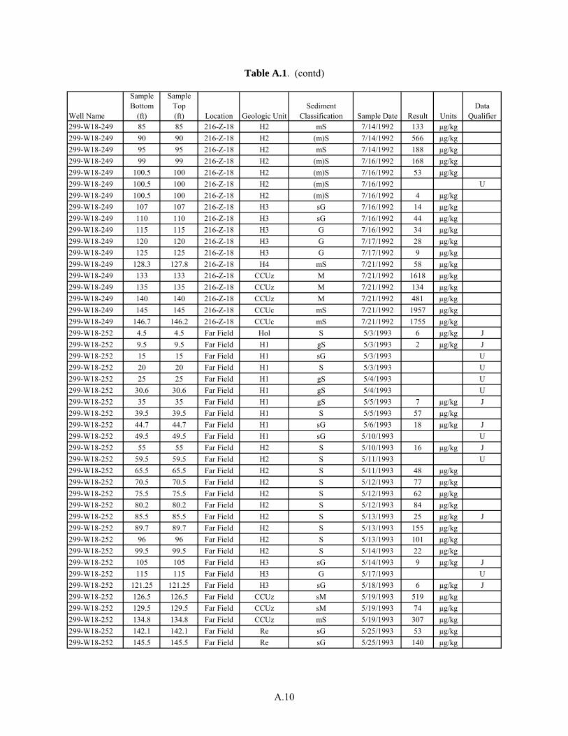
A.10

Table A.1. (contd)

Well Name

Sample Bottom

(ft)



DataQualifier

299-W18-249 85 85 216-Z-18 H2 mS 7/14/1992 133 µg/kg299-W18-249 90 90 216-Z-18 H2 (m)S 7/14/1992 566 µg/kg299-W18-249 95 95 216-Z-18 H2 mS 7/14/1992 188 µg/kg299-W18-249 99 99 216-Z-18 H2 (m)S 7/16/1992 168 µg/kg299-W18-249 100.5 100 216-Z-18 H2 (m)S 7/16/1992 53 µg/kg299-W18-249 100.5 100 216-Z-18 H2 (m)S 7/16/1992 U299-W18-249 100.5 100 216-Z-18 H2 (m)S 7/16/1992 4 µg/kg299-W18-249 107 107 216-Z-18 H3 sG 7/16/1992 14 µg/kg299-W18-249 110 110 216-Z-18 H3 sG 7/16/1992 44 µg/kg299-W18-249 115 115 216-Z-18 H3 G 7/16/1992 34 µg/kg299-W18-249 120 120 216-Z-18 H3 G 7/17/1992 28 µg/kg299-W18-249 125 125 216-Z-18 H3 G 7/17/1992 9 µg/kg299-W18-249 128.3 127.8 216-Z-18 H4 mS 7/21/1992 58 µg/kg299-W18-249 133 133 216-Z-18 CCUz M 7/21/1992 1618 µg/kg299-W18-249 135 135 216-Z-18 CCUz M 7/21/1992 134 µg/kg299-W18-249 140 140 216-Z-18 CCUz M 7/21/1992 481 µg/kg299-W18-249 145 145 216-Z-18 CCUc mS 7/21/1992 1957 µg/kg299-W18-249 146.7 146.2 216-Z-18 CCUc mS 7/21/1992 1755 µg/kg299-W18-252 4.5 4.5 Far Field Hol S 5/3/1993 6 µg/kg J299-W18-252 9.5 9.5 Far Field H1 gS 5/3/1993 2 µg/kg J299-W18-252 15 15 Far Field H1 sG 5/3/1993 U299-W18-252 20 20 Far Field H1 S 5/3/1993 U299-W18-252 25 25 Far Field H1 gS 5/4/1993 U299-W18-252 30.6 30.6 Far Field H1 gS 5/4/1993 U299-W18-252 35 35 Far Field H1 gS 5/5/1993 7 µg/kg J299-W18-252 39.5 39.5 Far Field H1 S 5/5/1993 57 µg/kg299-W18-252 44.7 44.7 Far Field H1 sG 5/6/1993 18 µg/kg J299-W18-252 49.5 49.5 Far Field H1 sG 5/10/1993 U299-W18-252 55 55 Far Field H2 S 5/10/1993 16 µg/kg J299-W18-252 59.5 59.5 Far Field H2 S 5/11/1993 U299-W18-252 65.5 65.5 Far Field H2 S 5/11/1993 48 µg/kg299-W18-252 70.5 70.5 Far Field H2 S 5/12/1993 77 µg/kg299-W18-252 75.5 75.5 Far Field H2 S 5/12/1993 62 µg/kg299-W18-252 80.2 80.2 Far Field H2 S 5/12/1993 84 µg/kg299-W18-252 85.5 85.5 Far Field H2 S 5/13/1993 25 µg/kg J299-W18-252 89.7 89.7 Far Field H2 S 5/13/1993 155 µg/kg299-W18-252 96 96 Far Field H2 S 5/13/1993 101 µg/kg299-W18-252 99.5 99.5 Far Field H2 S 5/14/1993 22 µg/kg299-W18-252 105 105 Far Field H3 sG 5/14/1993 9 µg/kg J299-W18-252 115 115 Far Field H3 G 5/17/1993 U299-W18-252 121.25 121.25 Far Field H3 sG 5/18/1993 6 µg/kg J299-W18-252 126.5 126.5 Far Field CCUz sM 5/19/1993 519 µg/kg299-W18-252 129.5 129.5 Far Field CCUz sM 5/19/1993 74 µg/kg299-W18-252 134.8 134.8 Far Field CCUz mS 5/19/1993 307 µg/kg299-W18-252 142.1 142.1 Far Field Re sG 5/25/1993 53 µg/kg299-W18-252 145.5 145.5 Far Field Re sG 5/25/1993 140 µg/kg

A.11

Table A.1. (contd)

Well Name

Sample Bottom

(ft)



DataQualifier

299-W18-252 149.7 149.7 Far Field Re S 5/26/1993 56 µg/kg299-W18-252 154.5 154.5 Far Field Re S 5/26/1993 281 µg/kg299-W18-252 159.5 159.5 Far Field Re sG 5/26/1993 205 µg/kg299-W18-252 164.5 164.5 Far Field Re gS 5/27/1993 177 µg/kg299-W18-252 164.5 164.5 Far Field Re gS 5/27/1993 377 µg/kg299-W18-252 172 172 Far Field Re G 5/28/1993 10 µg/kg J299-W18-252 175.5 175.5 Far Field Re sG 6/1/1993 116 µg/kg299-W18-252 191.7 191.7 Far Field Re sG 6/1/1993 8 µg/kg J299-W18-252 182 182 Far Field Re G 6/1/1993 U299-W18-252 185.1 185.1 Far Field Re S 6/1/1993 159 µg/kg299-W18-252 195.8 195.8 Far Field Re sG 6/3/1993 U299-W18-252 199.5 199.5 Far Field Re sG 6/3/1993 130 µg/kg299-W18-252 206.1 206.1 Far Field Re sG 6/7/1993 24 µg/kg J299-W18-252 211.1 211.1 Far Field Re sG 6/7/1993 U299-W18-252 214.7 214.7 Far Field Re sG 6/8/1993 U299-W18-252 220.2 220.2 Far Field Re sG 6/8/1993 U299-W18-252 225.6 225.6 Far Field Re sG 6/9/1993 U299-W18-27 142 140 Far Field H2/CCUz S/M 4/5/1991 5 µg/kg U299-W18-27 142 140 Far Field H2/CCUz S/M 4/5/1991 5 µg/kg U299-W18-27 81 Far Field H1 msG 4/10/1991 6 µg/kg U299-W18-27 81 Far Field H1 msG 4/10/1991 6 µg/kg U299-W18-27 102 100 Far Field H1/H2 sG 4/12/1991 5 µg/kg U299-W18-27 102 100 Far Field H1/H2 sG 4/12/1991 5 µg/kg U299-W18-27 121 119 Far Field H2 S 4/12/1991 5 µg/kg U299-W18-27 121 119 Far Field H2 S 4/12/1991 5 µg/kg U299-W18-27 161 159 Far Field Re gS 4/18/1991 5 µg/kg U299-W18-27 161 159 Far Field Re gS 4/18/1991 5 µg/kg U299-W18-27 185 183 Far Field Re sG 4/25/1991 5 µg/kg U299-W18-27 185 183 Far Field Re sG 4/25/1991 6 µg/kg U299-W18-27 201 198 Far Field Re gS 4/30/1991 5 µg/kg U299-W18-27 201 198 Far Field Re gS 4/30/1991 6 µg/kg U299-W18-28 27 Far Field H1a (g)S 4/9/1991 5 µg/kg U299-W18-28 27 Far Field H1a (g)S 4/9/1991 5 µg/kg U299-W18-28 47 Far Field H1a S 4/10/1991 5 µg/kg U299-W18-28 47 Far Field H1a S 4/10/1991 5 µg/kg U299-W18-28 69 67 Far Field H1 G 4/11/1991 5 µg/kg U299-W18-28 69 67 Far Field H1 G 4/11/1991 5 µg/kg U299-W18-28 89 87 Far Field H2 (m)S 4/15/1991 6 µg/kg U299-W18-28 89 87 Far Field H2 (m)S 4/15/1991 6 µg/kg U299-W18-28 114 112 Far Field H2 S 4/16/1991 5 µg/kg U299-W18-28 114 112 Far Field H2 S 4/16/1991 6 µg/kg U299-W18-28 135 133 Far Field H2 mS 4/17/1991 6 µg/kg U299-W18-28 135 133 Far Field H2 mS 4/17/1991 6 µg/kg U299-W18-28 155 153 Far Field CCUc sG 4/23/1991 5 µg/kg U299-W18-28 155 153 Far Field CCUc sG 4/23/1991 6 µg/kg U299-W18-28 174 173 Far Field Re gS 4/26/1991 6 µg/kg U299-W18-28 174 173 Far Field Re gS 4/26/1991 5 µg/kg U

A.12

Table A.1. (contd)

Well Name

Sample Bottom

(ft)



DataQualifier

299-W18-28 195 193 Far Field Re sG 4/30/1991 5 µg/kg U299-W18-28 195 193 Far Field Re sG 4/30/1991 6 µg/kg U299-W18-28 130 Far Field H2 mS 5/6/1991 6 µg/kg U299-W18-28 130 Far Field H2 mS 5/6/1991 5 µg/kg U299-W18-29 80 Far Field H3 sG 4/5/1991 5 µg/kg U299-W18-29 80 Far Field H3 sG 4/5/1991 5 µg/kg U299-W18-29 100 Far Field H3 sG 4/9/1991 5 µg/kg U299-W18-29 100 Far Field H3 sG 4/9/1991 5 µg/kg U299-W18-29 120 Far Field H4 S 4/10/1991 6 µg/kg U299-W18-29 120 Far Field H4 S 4/10/1991 6 µg/kg U299-W18-29 128 Far Field CCUz M 4/11/1991 22 µg/kg299-W18-29 128 Far Field CCUz M 4/11/1991 23 µg/kg299-W18-29 131 129 Far Field CCUz sM 4/11/1991 4 µg/kg J299-W18-29 131 129 Far Field CCUz sM 4/11/1991 4 µg/kg J299-W18-29 133 131 Far Field CCUz sM 4/12/1991 6 µg/kg U299-W18-29 133 131 Far Field CCUz sM 4/12/1991 6 µg/kg U299-W18-29 135 133 Far Field CCUz sM 4/12/1991 5 µg/kg J299-W18-29 135 133 Far Field CCUz sM 4/12/1991 4 µg/kg J299-W18-29 152 150 Far Field Re (m)sG 4/23/1991 6 µg/kg U299-W18-29 152 150 Far Field Re (m)sG 4/23/1991 6 µg/kg U299-W18-40 7 0 Far Field Bf mS 9/19/2001 6 µg/kg U299-W18-40 230 218 Far Field Re msG 9/19/2001 8 µg/kg U299-W18-40 230 218 Far Field Re msG 4/16/2002 0.9 µg/kg U299-W18-96 84.5 84 216-Z-18 H2 S 2/10/1993 89 µg/kg299-W18-96 86.5 86.5 216-Z-18 H2 S 2/11/1993 93 µg/kg299-W18-96 86.5 86.5 216-Z-18 H2 S 2/11/1993 79 µg/kg299-W18-96 90 90 216-Z-18 H2 S 2/12/1993 440 µg/kg299-W18-96 90 90 216-Z-18 H2 S 2/12/1993 332 µg/kg299-W18-96 92.35 92.35 216-Z-18 H2 S 2/12/1993 99 µg/kg299-W18-96 92.35 92.35 216-Z-18 H2 S 2/12/1993 56 µg/kg299-W18-96 95 95 216-Z-18 H2 (m)S 2/12/1993 124 µg/kg299-W18-96 98 98 216-Z-18 H2 (m)S 2/12/1993 111 µg/kg299-W18-96 98 98 216-Z-18 H2 (m)S 2/12/1993 193 µg/kg299-W18-96 100.5 100.5 216-Z-18 H2 (gm)S 2/12/1993 242 µg/kg299-W18-96 100.5 100.5 216-Z-18 H2 (gm)S 2/12/1993 127 µg/kg299-W18-96 104 104 216-Z-18 H2 gS 2/12/1993 140 µg/kg299-W18-96 110.15 110.15 216-Z-18 H3 sG 2/16/1993 10 µg/kg J299-W18-96 110.15 110.15 216-Z-18 H3 sG 2/16/1993 4 µg/kg J299-W18-96 116 116 216-Z-18 H3 sG 2/16/1993 12 µg/kg299-W18-96 119 119 216-Z-18 H3 sG 2/17/1993 6 µg/kg J299-W18-96 120 120 216-Z-18 H3 sG 2/17/1993 2 µg/kg J299-W18-96 120 120 216-Z-18 H3 sG 2/17/1993 7 µg/kg J299-W18-96 123.5 123.5 216-Z-18 H3 G 2/17/1993 52 µg/kg299-W18-96 123.5 123.5 216-Z-18 H3 G 2/17/1993 41 µg/kg299-W18-96 125.5 125.5 216-Z-18 H3 G 2/18/1993 41 µg/kg299-W18-96 125.5 125.5 216-Z-18 H3 G 2/18/1993 68 µg/kg299-W18-96 125.5 125.5 216-Z-18 H3 G 2/18/1993 8 µg/kg J

A.13

Table A.1. (contd)

Well Name

Sample Bottom

(ft)



DataQualifier

299-W18-96 125.5 125.5 216-Z-18 H3 G 2/18/1993 5 µg/kg J299-W18-96 129 129 216-Z-18 H4 mG 2/22/1993 43 µg/kg299-W18-96 129 129 216-Z-18 H4 mG 2/22/1993 65 µg/kg299-W18-96 129 129 216-Z-18 H4 mG 2/22/1993 39 µg/kg299-W18-96 129 129 216-Z-18 H4 mG 2/22/1993 28 µg/kg299-W18-96 130.5 130.5 216-Z-18 H4 mG 2/22/1993 16 µg/kg299-W18-96 130.5 130.5 216-Z-18 H4 mg 2/22/1993 5 µg/kg J299-W18-96 130.5 130.5 216-Z-18 H4 mG 2/22/1993 4 µg/kg J299-W18-96 130.5 130.5 216-Z-18 H4 mG 2/22/1993 14 µg/kg299-W18-96 134.5 134.5 216-Z-18 H4 sM 2/22/1993 111 µg/kg299-W18-96 134.5 134.5 216-Z-18 H4 sM 2/22/1993 17 µg/kg J299-W18-96 136.5 136.5 216-Z-18 H4 sM 2/23/1993 786 µg/kg299-W18-96 136.5 136.5 216-Z-18 H4 sM 2/23/1993 759 µg/kg299-W18-96 138.5 138.5 216-Z-18 CCUz M 2/24/1993 334 µg/kg299-W18-96 138.5 138.5 216-Z-18 CCUz M 2/24/1993 494 µg/kg299-W18-96 143.84 143.84 216-Z-18 CCUz M 2/25/1993 861 µg/kg299-W18-96 143.84 143.84 216-Z-18 CCUz M 2/25/1993 626 µg/kg299-W18-96 143.84 143.84 216-Z-18 CCUz M 2/25/1993 714 µg/kg299-W18-96 144.45 144.45 216-Z-18 CCUz M 2/25/1993 28 µg/kg299-W18-96 144.45 144.45 216-Z-18 CCUz M 2/25/1993 24 µg/kg J299-W18-96 146.5 146.5 216-Z-18 CCUc Caliche 2/25/1993 33 µg/kg299-W18-96 146.5 146.5 216-Z-18 CCUc Caliche 2/25/1993 33 µg/kg299-W19-34B 170.5 168 Far Field 4/14/1994 11 µg/kg U299-W19-34B 170.5 168 Far Field 4/14/1994 11 µg/kg U299-W19-34B 188.5 186 Far Field 4/18/1994 11 µg/kg U299-W19-34B 244.5 242.5 Far Field 4/26/1994 16 µg/kg U299-W19-34B 334 332 Far Field 6/1/1994 12 µg/kg UJ299-W19-34B 417.5 416 Far Field 6/30/1994 12 µg/kg U299-W19-34B 442 440 Far Field 8/1/1994 12 µg/kg U299-W19-34B 462 460 Far Field 8/5/1994 12 µg/kg U299-W19-34B 481.5 480.5 Far Field 8/11/1994 13 µg/kg U299-W19-34B 531.3 530 Far Field 8/24/1994 11 µg/kg U299-W19-35 160.5 158 Far Field 3/7/1994 12 µg/kg U299-W19-35 181 179 Far Field 3/8/1994 11 µg/kg U299-W19-35 238.5 236 Far Field 3/16/1994 10 µg/kg U299-W19-35 238.5 236 Far Field 3/16/1994 10 µg/kg U299-W19-35 247 245 Far Field 3/18/1994 11 µg/kg U299-W19-43 25 Far Field 7/2/2001 6 µg/kg U299-W19-43 25 Far Field 7/2/2001 6 µg/kg U299-W19-43 262 260 Far Field 7/17/2001 5 µg/kg U299-W19-44 233 Far Field 8/30/2001 6 µg/kg U299-W19-44 50 Far Field 8/30/2001 5 µg/kg U299-W19-44 245 233 Far Field 4/16/2002 0.8 µg/kg U299-W19-45 Far Field 8/17/2001 6 µg/kg U299-W19-45 Far Field 8/17/2001 6 µg/kg U

A.14

Table A.1. (contd)

Well Name

Sample Bottom

(ft)



DataQualifier

299-W19-45 234 228 Far Field 4/16/2002 1 µg/kg U299-W19-46 267 260 Far Field 11/20/2002 6 µg/kg U299-W19-46 30 0 Far Field 12/2/2002 5 µg/kg U299-W19-48 290 285 Far Field 11/24/2004 2 µg/kg U299-W19-48 340 Far Field 12/9/2004 2.4 µg/kg U299-W19-48 340 Far Field 12/9/2004 2.3 µg/kg U299-W19-48 407 402 Far Field 12/13/2004 2.4 µg/kg U299-W19-48 429 424 Far Field 12/15/2004 2.5 µg/kg U299-W19-94 32 30 Far Field 11/15/1993 25 µg/kg U299-W19-94 6 4 Far Field 12/3/1993 11 µg/kg U299-W19-94 17.5 15.5 Far Field 12/6/1993 11 µg/kg U299-W19-94 36 33.5 Far Field 12/8/1993 25 µg/kg U299-W19-94 40 38 Far Field 12/13/1993 13000 µg/kg U299-W19-94 59.5 57.5 Far Field 12/14/1993 5100 µg/kg U299-W19-94 50 48 Far Field 12/14/1993 4900 µg/kg U299-W19-94 70 68 Far Field 12/15/1993 10 µg/kg U299-W19-94 91.5 89.5 Far Field 12/16/1993 1300 µg/kg U299-W19-94 116 114 Far Field 1/3/1994 12 µg/kg U299-W19-94 130 128 Far Field 1/4/1994 11 µg/kg U299-W19-94 150 148 Far Field 1/6/1994 10 µg/kg U299-W19-94 150 148 Far Field 1/6/1994 10 µg/kg U299-W19-94 167.5 165.5 Far Field 1/7/1994 11 µg/kg U299-W19-94 167.5 165.5 Far Field 1/7/1994 11 µg/kg U299-W19-94 189 187 Far Field 1/13/1994 11 µg/kg U299-W19-94 199 197 Far Field 1/17/1994 13 µg/kg U299-W19-95 16.5 14.5 Far Field 9/3/1993 11 µg/kg U299-W19-95 32.5 30 Far Field 9/7/1993 11 µg/kg U299-W19-95 47.5 45 Far Field 9/8/1993 11 µg/kg U299-W19-95 62.5 60 Far Field 9/9/1993 11 µg/kg U299-W19-95 77.3 74.8 Far Field 9/10/1993 10 µg/kg U299-W19-95 92.25 90.25 Far Field 9/13/1993 11 µg/kg U299-W19-95 107.5 105 Far Field 9/15/1993 10 µg/kg U299-W19-95 107.5 105 Far Field 9/15/1993 11 µg/kg U299-W19-95 142.5 140 Far Field 9/16/1993 11 µg/kg U299-W19-95 122.5 120 Far Field 9/16/1993 11 µg/kg U299-W19-95 167.5 165 Far Field 9/16/1993 12 µg/kg U299-W19-95 182 181 Far Field 9/20/1993 10 µg/kg U299-W19-95 171.5 169 Far Field 9/20/1993 10 µg/kg U299-W19-95 171.5 169 Far Field 9/20/1993 11 µg/kg U299-W19-96 6 4 Far Field 11/5/1993 10 µg/kg U299-W19-96 17 15 Far Field 11/10/1993 5 µg/kg U299-W19-96 24 22 Far Field 11/12/1993 5 µg/kg U299-W19-96 27 24.5 Far Field 11/15/1993 20 µg/kg U299-W19-96 29.5 27 Far Field 11/16/1993 21 µg/kg U299-W19-96 32 29.5 Far Field 11/17/1993 23 µg/kg U299-W19-96 42.5 40.5 Far Field 12/9/1993 13000 µg/kg U299-W19-96 52 50 Far Field 12/13/1993 10 µg/kg U

A.15

Table A.1. (contd)

Well Name

Sample Bottom

(ft)



DataQualifier

299-W19-96 62 60 Far Field 12/15/1993 10 µg/kg U299-W19-96 82 80 Far Field 12/16/1993 10 µg/kg U299-W19-96 101.5 99.5 Far Field 12/20/1993 11 µg/kg U299-W19-96 122 120 Far Field 1/3/1994 12 µg/kg U299-W19-96 142 140 Far Field 1/3/1994 11 µg/kg U299-W19-96 142 140 Far Field 1/3/1994 11 µg/kg U299-W19-96 170 168 Far Field 1/5/1994 10 µg/kg U299-W19-96 168 166 Far Field 1/5/1994 12 µg/kg U299-W19-96 168 166 Far Field 1/5/1994 12 µg/kg U299-W19-96 161 159 Far Field 1/5/1994 11 µg/kg U299-W19-96 177 175 Far Field 1/11/1994 10 µg/kg U299-W19-97 6 4 Far Field 9/7/1993 11 µg/kg U299-W19-97 22.5 20 Far Field 9/8/1993 11 µg/kg U299-W19-97 32 30 Far Field 9/8/1993 10 µg/kg U299-W19-97 12.5 10 Far Field 9/8/1993 11 µg/kg U299-W19-97 52.5 50 Far Field 9/10/1993 12 µg/kg U299-W19-97 72.5 70 Far Field 9/13/1993 11 µg/kg U299-W19-97 103.3 101 Far Field 9/15/1993 11 µg/kg U299-W19-97 103.3 101 Far Field 9/15/1993 11 µg/kg U299-W19-97 132.5 130 Far Field 9/16/1993 11 µg/kg U299-W19-97 148.5 146 Far Field 9/17/1993 11 µg/kg U299-W19-97 148.5 146 Far Field 9/17/1993 11 µg/kg U299-W19-97 158.5 156 Far Field 9/17/1993 12 µg/kg U299-W19-97 170 167.5 Far Field 9/20/1993 12 µg/kg U299-W19-97 177 175.7 Far Field 9/21/1993 11 µg/kg U299-W19-98 5.4 4.4 Far Field 1/13/1994 11 µg/kg U299-W19-98 13.5 11 Far Field 3/2/1994 10 µg/kg U299-W19-98 17.25 15 Far Field 3/3/1994 11 µg/kg U299-W19-98 26.5 24 Far Field 3/4/1994 10 µg/kg U299-W19-98 49 47 Far Field 3/8/1994 10 µg/kg U299-W19-98 62.2 60 Far Field 3/9/1994 11 µg/kg U299-W19-98 82.1 80 Far Field 3/10/1994 10 µg/kg U299-W19-98 102.5 100 Far Field 3/14/1994 11 µg/kg U299-W19-98 132 130 Far Field 3/15/1994 11 µg/kg U299-W19-98 175.3 172 Far Field 3/17/1994 11 µg/kg U299-W19-98 185.5 183.5 Far Field 3/17/1994 11 µg/kg U299-W19-98 175.3 173 Far Field 3/17/1994 11 µg/kg U299-W19-98 185.5 183.5 Far Field 3/17/1994 11 µg/kg U299-W19-98 193 191.1 Far Field 3/22/1994 10 µg/kg U

A.16

Table A.2. Compilation of Modeled (Murray et al. 2006) and Measured (HEIS) Concentrations of Carbon Tetrachloride in Groundwater Beneath the Disposal Areas (ND = No data)

Depth BelowWater Table

(m)

Modeled CTat 216-Z-9

(ppb)

Modeled CTat 216-Z-1A

(ppb)

Modeled CTat 216-Z-18

(ppb)

Measured CTat 216-Z-9

(ppb)

0 663 93 54 ND2.5 800 127 78 3305 389 120 80 1600

7.5 110 89 95 010 96 100 82 115

12.5 92 92 95 72015 116 95 97 3800

17.5 98 97 83 ND20 920 120 96 2200

22.5 720 139 86 27025 460 145 78 ND

27.5 330 116 44 ND30 186 66 26 110

32.5 110 23 17 nd35 95 25 16 29

37.5 99 29 17 nd40 190 47 29 250

42.5 534 68 36 ND45 690 76 26 1025

47.5 460 46 17 47050 147 26 13 ND

52.5 61 16 9 8.755 46 11 6 ND

57.5 75 8 4 ND60 93 4 1 190

PNNL-16198

Distr.1

Distribution No. of Copies OFFSITE Wes Bratton Vista Engineering 8203 West Quinault Avenue Kennewick, WA 99336 Rick Dinicola U.S. Geological Survey Washington Water Science Center 1210 Pacific Avenue, Suite 600 Tacoma, WA 98402 ONSITE 6 DOE Richland Operations Office B. L. Foley* A6-38 J. G. Morse* A6-38 K. M. Thompson* A6-38 A. C. Tortoso* A6-38 Public Reading Room (2*) H2-53 11 Fluor Hanford, Inc. J. V. Borghese E6-35 M. E. Byrnes E6-35 D. B. Erb E6-35 T. W. Fogwell* E6-35 B. H. Ford E6-35 D. S. Miller* E6-35 S. W. Petersen E6-35 V. J. Rohay (2*) E6-35 A. F. Shattuck* E6-35 L. C. Swanson E6-35 M. E. Todd-Robertson* E6-35

No. of Copies U.S. Environmental Protection Agency D. A. Faulk* B1-46 Washington State Department of Ecology D. Goswami* H0-57 15 Pacific Northwest National Laboratory R. W. Bryce E6-35 A.R. Felmy K8-96 M. D. Freshley K9-33 N.J. Hess K8-96 C. T. Kincaid K9-33 G. V. Last* K6-81 M. Oostrom (2*) K9-33 M. L. Rockhold* K9-36 P. D. Thorne* K9-33 M. J. Truex* K6-96 S. B. Yabusaki K9-33 M. D. White K9-33 Hanford Technical Library (2*) P8-55

*Hard copy distribution; all others receive electronic file.

carbon tetrachloride flow and transport in the subsurface ...pnnl-16198 carbon tetrachloride flow...

Documents