carbon pricing with output-based subsidies discussion pa
TRANSCRIPT

1616 P St. NW Washington, DC 20036 202-328-5000 www.rff.org
June 2012 RFF DP 12-27
Carbon Pricing with Output-Based Subsidies
Impact on U.S. Industries over Multiple Time Frames
Liw ayw ay Adk ins , R ichar d Gar bacc io , M un Ho,
E r ic M oor e , and Richard Morgenstern
DIS
CU
SS
ION
PA
PE
R

© 2012 Resources for the Future. All rights reserved. No portion of this paper may be reproduced without
permission of the authors.
Discussion papers are research materials circulated by their authors for purposes of information and discussion.
They have not necessarily undergone formal peer review.
Carbon Pricing with Output-Based Subsidies: Impacts on U.S.
Industries over Multiple Time Frames
Liwayway Adkins, Richard Garbaccio, Mun Ho, Eric Moore, and Richard Morgenstern
Abstract
The effects of a carbon price on U.S. industries are likely to change over time as firms and
customers gradually adjust to new prices. The effects will also depend on offsetting policies to
compensate losers and the number of countries implementing comparable policies. We examine the
effects of a $15/ton CO2 price, including Waxman-Markey-type allocations, on a disaggregated set of
industries, over four time horizons—the very-short-, short-, medium-, and long-runs—distinguished by
the ability of firms to raise output prices, change their input mix, and reallocate capital. We find that if
firms cannot pass on higher costs, the loss in profits in a number of energy-intensive, trade-exposed
(EITE) industries will be substantial. When output prices can rise to reflect higher energy costs, the
reduction in profits is substantially smaller, and the offsetting policies in H.R. 2454 reduce output and
profit losses even more. Over the medium- and long-terms, however, when more adjustments occur, the
impact on output is more varied due to general equilibrium effects. We find that the use of the output-
based rebates and other allocations in H.R. 2454 can substantially offset the output losses over all four
time frames considered. Trade or "competitiveness" effects from the carbon price explain a significant
portion of the fall in output for EITE sectors, but in absolute terms, the trade impacts are modest and can
be reduced or even reversed with the subsidies. The subsidies are less effective, however, in preventing
emissions leakage to countries not adopting carbon policies. Roughly half of U.S. trade-related leakage to
non-policy countries can be explained by changes in the volume of trade and the other half by higher
emissions intensities induced by lower world fuel prices.
Key Words: carbon price, competitiveness, input-output analysis, computable general
equilibrium models, output-based allocations, carbon leakage
JEL Classification Numbers: F14, D 21, D57, D58, H23

Contents
I. Introduction ......................................................................................................................... 1
II. Other Studies with Detailed Industry Impacts ............................................................... 5
III. Implementation: Data and Model Construction ........................................................... 7
IV. Output-Based Rebates under H.R. 2454 ...................................................................... 10
V. Effects of Carbon Pricing with H.R. 2454 Subsidies over Multiple Time Horizons .. 12
Effects on Industry Prices: Very-Short-Run Horizon ....................................................... 12
Effects on Costs: Very-Short-Run Horizon ...................................................................... 13
Effects on Output: Very-Short-Run and Short-Run Horizons .......................................... 15
Effects on Profits: Very-Short-Run and Short-Run Horizons .......................................... 16
Comparing Effects on Output over the Short-, Medium-, and Long-Run Horizons ........ 17
VI. Trade and Leakage ......................................................................................................... 19
Trade Impacts.................................................................................................................... 19
Emissions Leakage at the Industry Level ......................................................................... 21
Aggregate Leakage ........................................................................................................... 22
Comment on Leakage Rates ............................................................................................. 23
VII. Conclusions .................................................................................................................... 24
References .............................................................................................................................. 27
Figures and Tables ................................................................................................................ 28
Resources for the Future Adkins et al.
1
Carbon Pricing with Output-Based Subsidies: Impacts on U.S.
Industries over Multiple Time Frames
Liwayway Adkins, Richard Garbaccio, Mun Ho, Eric Moore, and Richard Morgenstern
I. Introduction
Despite the failure to enact cap and trade legislation in the 111th Congress, analysis of
the specific proposals advanced in the debate can provide important lessons for the future
consideration of economy-wide carbon pricing, via either cap and trade or taxation. In whatever
form it takes, pricing carbon emissions will not only adversely affect electricity and primary
energy producers, but may also hurt the competitive position of industries that consume large
amounts of energy. Energy-intensive, trade-exposed (EITE) sectors, such as metals and
chemicals, could be especially impacted under such a policy. This situation gives rise to two
overarching concerns. First, some domestic industries will be disproportionately burdened if
carbon pricing policies affect their operations but not those of their international competitors.
Second, some of the environmental benefits will be eroded if increases in U.S. manufacturing
costs from uneven international carbon pricing cause economic activity and the corresponding
emissions to ―leak‖ to nations with weaker or no carbon pricing policies.
Industry-level impacts are fundamentally tied to the carbon intensity of producers, the
degree to which they can pass costs to consumers, and their ability to substitute away from
carbon-intensive energy. The strength of competition from imports and consumers’ ability to
substitute other, less carbon-intensive alternatives for a given product also play crucial roles in
determining the ultimate impacts on domestic production and employment.
The most effective approach to reduce the disproportionate impacts of domestic carbon
pricing is to ensure comparable action by other countries. In the absence of global action, the
Liwayway Adkins is an economist in the Office for Climate Change Policy and Technology in the U.S.
Department of Energy. Richard Garbaccio is an economist in the U.S. Environmental Protection Agency’s National
Center for Environmental Economics. Mun Ho is a visiting scholar at Resources for the Future. Eric Moore is a
graduate student at the University of Pennsylvania and was previously a research assistant at Resources for the
Future. Richard Morgenstern is a senior fellow at Resources for the Future. The authors gratefully acknowledge
financial support from both the National Commission on Energy Policy and the Doris Duke Charitable Foundation.
All views expressed in this article are those of the authors and do not reflect the opinions of the U.S. Environmental
Protection Agency or the U.S. Department of Energy. This paper is also published in the EPA’s National Center for
Environmental Economics Working Paper Series.

Resources for the Future Adkins et al.
2
U.S. Congress has considered proposals to reduce the impacts of domestic carbon pricing,
including the free allocation of emissions allowances to the most affected sectors. If these free
allowances, or rebates, are updated on the basis of recent output levels as prescribed, for
example, in the House-passed American Clean Energy and Security Act of 2009 (H.R. 2454),
firms would be able to maintain sales in the face of policy-induced cost increases while
sustaining incentives created by the emissions cap to reduce the carbon intensity of production.
Importantly, the per-unit allowance allocation would not be based on the firm’s emissions but on
a sector-based intensity standard, thus creating incentives for within-sector market shares to shift
toward firms with low emissions intensity.
Computable general equilibrium (CGE) models allow for the estimation of long-run
industry-level and consumer welfare impacts of carbon pricing policies after firms have adjusted
by using new technologies and the market has established new import patterns. Most of these
analyses assume fully mobile factors in which workers and producers are assumed to shift
seamlessly between sectors. Such long-run studies, however, fail to capture the short-run impacts
of carbon pricing policies or the reality that available mitigation options will change over time. A
steel mill faced with higher energy costs cannot immediately and costlessly convert to more
energy-efficient methods. If it leaves its output price unchanged, the higher input costs will lower
profits. If it tries to raise prices to cover the higher costs, it will face lower sales. Stakeholders
will likely oppose a carbon policy that does not fairly address these impacts.1
This paper advances the study of competitiveness and leakage issues by examining the
impacts of domestic carbon pricing policies on a highly disaggregated set of industries over
multiple timeframes, with special focus on the suite of subsidies to vulnerable industries
contained in H.R. 2454. This includes the output-based rebates for EITE industries to lessen
adverse impacts and the special treatment of the refining sector as well as electricity and gas
local distribution companies (LDCs). We do not analyze the effects of the border adjustments
scheduled to begin in 2020 under the legislation. The revenues raised by the cap and trade
system that are not explicitly allocated to these sectors are returned to households to partially
offset the higher prices as envisaged in these proposals. The analysis is based on an economy-
wide carbon dioxide (CO2) price of $15/ton, which is broadly consistent with projections of
1 Dynamic general equilibrium models do take some time-relevant adjustments into account, although such models
are usually highly aggregated and generally ignore potentially important differences among major energy-
consuming sectors.
Resources for the Future Adkins et al.
3
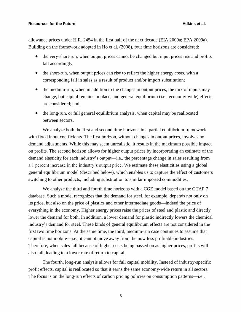
allowance prices under H.R. 2454 in the first half of the next decade (EIA 2009a; EPA 2009a).
Building on the framework adopted in Ho et al. (2008), four time horizons are considered:
the very-short-run, when output prices cannot be changed but input prices rise and profits
fall accordingly;
the short-run, when output prices can rise to reflect the higher energy costs, with a
corresponding fall in sales as a result of product and/or import substitution;
the medium-run, when in addition to the changes in output prices, the mix of inputs may
change, but capital remains in place, and general equilibrium (i.e., economy-wide) effects
are considered; and
the long-run, or full general equilibrium analysis, when capital may be reallocated
between sectors.
We analyze both the first and second time horizons in a partial equilibrium framework
with fixed input coefficients. The first horizon, without changes in output prices, involves no
demand adjustments. While this may seem unrealistic, it results in the maximum possible impact
on profits. The second horizon allows for higher output prices by incorporating an estimate of the
demand elasticity for each industry’s output—i.e., the percentage change in sales resulting from
a 1 percent increase in the industry’s output price. We estimate these elasticities using a global
general equilibrium model (described below), which enables us to capture the effect of customers
switching to other products, including substitution to similar imported commodities.
We analyze the third and fourth time horizons with a CGE model based on the GTAP 7
database. Such a model recognizes that the demand for steel, for example, depends not only on
its price, but also on the price of plastics and other intermediate goods—indeed the price of
everything in the economy. Higher energy prices raise the prices of steel and plastic and directly
lower the demand for both. In addition, a lower demand for plastic indirectly lowers the chemical
industry’s demand for steel. These kinds of general equilibrium effects are not considered in the
first two time horizons. At the same time, the third, medium-run case continues to assume that
capital is not mobile—i.e., it cannot move away from the now less profitable industries.
Therefore, when sales fall because of higher costs being passed on as higher prices, profits will
also fall, leading to a lower rate of return to capital.
The fourth, long-run analysis allows for full capital mobility. Instead of industry-specific
profit effects, capital is reallocated so that it earns the same economy-wide return in all sectors.
The focus is on the long-run effects of carbon pricing policies on consumption patterns—i.e.,

Resources for the Future Adkins et al.
4
households and other components of final demand switching to less energy-intensive products.
This switch in final demand changes the structure of production and total energy consumption,
and changes the cost of capital relative to labor.2
The four horizons considered in this paper can be summarized in the following table: Very-Short-Run Short-Run Medium-Run Long-Run
Input price effects X X X X
Demand adjustments X X X
Input substitution X X
Sectoral capital mobility X
This four horizon framework allows us to capture the complex, often opposing
adjustments occurring over time. On the one hand, producers of energy-intensive goods
gradually can substitute toward cheaper, less carbon-intensive inputs over time, thereby
dampening the initial price shock and decline in sales. On the other hand, the consumers of such
energy-intensive goods also are gradually substituting toward alternative inputs and capital and
reducing the quantities demanded. The net effect of these long-run adjustments is not clear a
priori. Indeed, our results show that both influences are at work.
Assumptions about climate policies adopted in other countries are also clearly important
in understanding competitiveness and leakage issues. Although we present some results for the
case of unilateral U.S. action, our principal analysis assumes comparable actions in other Annex
I nations, which account for roughly half of U.S. trade in energy-intensive goods. We examine
leakage of U.S. emissions that are due to changes in trade with countries that are not undertaking
carbon pricing policies, and also due to increased fossil fuel consumption in these same countries
that now face lower fuel prices because of reduced demand in Annex I.
The focus of this paper is on a sequence of transparent steps designed to estimate the
impacts of carbon pricing with and without rebate policies over the different time horizons.
Impacts are measured in terms of output, profits, and trade and leakage effects. Following this
introduction, Section II reviews a number of previous studies that have examined
competitiveness issues surrounding carbon pricing at a detailed, industry-specific level. We
2 While the ―long-run‖ may be defined in a variety of ways, our definition uses a one-period model in which the
supply of capital is given exogenously. A model with intertemporal features that determines savings endogenously
will identify an effect not considered here: how the total stock of capital responds to the changes in prices due to a
carbon tax.

Resources for the Future Adkins et al.
5
particularly focus on the analyses that have incorporated output-based rebate mechanisms of the
type contained in H.R. 2454. Section III describes the basic modeling approaches and data
sources. Section IV describes output-based rebates and other targeted allowance allocations to
vulnerable industries under H.R. 2454. Section V describes the principal results for output and
profits across multiple time horizons. Section VI addresses trade and leakage impacts. Section
VII offers some overall conclusions.
II. Other Studies with Detailed Industry Impacts
The literature on industry impacts of carbon policies is based largely on simulation
modeling, although a number of papers involve direct econometric estimation, e.g. Aldy and
Pizer (2011). The simulation analyses include both short-term partial equilibrium assessments as
well as long-term CGE modeling. Ho et al. (2008) review more than a dozen prior U.S. and
European analyses and report a series of estimates based on an earlier version of the current
modeling framework. With the exception of papers by Fischer and Fox (2007, 2009), however,
none of the earlier literature estimates the combined effects of carbon pricing and output-based
rebating. Starting in 2009, with the passage of H.R. 2454, a number of such analyses have been
performed, albeit on a more aggregated basis.
Fischer and Fox (2007) examine how the outcome of carbon policies is affected by
alternative permit allocation mechanisms: auction, grandfathering, output-based allocation tied to
emissions, and output-based allocation tied to value added. Using a static CGE model based on
GTAP 6 data (2001 base year), they report impacts on 18 non-energy and 5 energy sectors. In a
policy scenario that reduces emissions by about 14 percent below baseline, they estimate a
reduction in overall output on the order of 0.34 percent for the output-based allocations tied to
emissions, rising to as much as 0.51 percent for the other mechanisms. Overall, output declines
consistently for the alternative allocation mechanisms across most industries examined. The
hardest-hit manufacturing industries are chemicals and iron and steel, at about 1 percent each.
All other manufacturing industries report output declines that are generally 0.5 percent or less.
Fischer and Fox estimate an aggregate leakage of 12–15 percent, that is, the share of total U.S.
emissions reductions that are offset by increases in the rest of the world. At the industry level,
the implied leakage rate for the energy-intensive industries is on the order of 40–45 percent.3
3 See also Fischer and Fox (2009).

Resources for the Future Adkins et al.
6
An assessment by the U.S. Energy Information Administration (EIA), using its NEMS
model, finds that the rebate mechanisms contained in H.R. 2454 result in smaller-percentage
output reductions for the EITEs than for the manufacturing sector as a whole (EIA 2009a). An
analysis of H.R. 2454 by the U.S. Environmental Protection Agency (EPA), using the ADAGE
model, estimates that without the output-based rebate provisions, production in the energy-
intensive manufacturing industries decreases by 0.3 percent in 2015 and by 0.7 percent in 2020
(EPA 2009a). With the output-based rebates, the EPA estimated that energy-intensive
manufacturing output would increase by 0.04 percent in 2015 and fall by only 0.3 percent in
2020. Unfortunately, the models used by the EIA and EPA do not disaggregate industry impacts
to any significant extent.
An interagency report on the competitiveness impacts of H.R. 2454 conducted by
multiple executive branch agencies (EPA 2009b), uses on an updated version of the Fischer-Fox
(2007) model. Specifically, output-based rebates were modeled for 5 aggregated sectors,
incorporating 37 of the 43 six-digit NAICS EITE industries deemed to be presumptively eligible
for rebates. For three of the five sectors analyzed, the combined effect of the direct allocations to
EITEs, plus those to LDCs, offset virtually all of the incremental costs associated with the
carbon pricing. For two sectors—chemicals and plastics; pulp, paper, and print—the allocations
actually reduce production costs compared to the case without any carbon pricing. One issue of
interest is the relative importance of the direct allocations to EITEs versus those to LDCs. For
the five industry groups examined in the interagency report, the LDC rebates constitute a
relatively small share of the total cost reductions compared to the consistently larger effect of the
direct industry rebates.
The interagency report also considers the impacts of the rebate programs on trade flows
giving rise to emissions leakage. Here, it is useful to recall the two main sources of emissions
leakage: 1) changes in trade flows and 2) global substitutions in production processes associated
with changing fuel and raw material prices induced by the domestic carbon policy. Fischer and
Fox (2007, 2009), and Boehringer et. al (2010) find the latter to be a significant source of
emissions leakage. However, because trade flows are more readily influenced by policy
measures than global fuel or resource substitutions, and because they are an important proxy for
domestic output and employment losses, the interagency report focuses solely on trade flows as
the metric of impacts.
Although the European Union Emissions Trading Scheme (EU ETS) does not use an
output-based rebate system, several recent studies have examined the possible impacts of such a
mechanism on specific industries in the European Union. Demailly and Quirion (2006) find that

Resources for the Future Adkins et al.
7
if EU cement producers received output-based allocations at a rate equal to 90 percent of the
industry’s historical emissions intensity, imports to the European Union would be insignificantly
impacted under an EU cap-and-trade program, even if allowance prices reached as high as 50
euros per ton of CO2. Similarly, an analysis by the Carbon Trust (2008) found that output-based
allocations to steel and other energy-intensive sectors could significantly reduce increases in
imports that could otherwise result from the EU ETS.
III. Implementation: Data and Model Construction
The very-short-run and short-run models developed in this paper are based on a fixed
coefficient, input–output (I-O) framework of the U.S. economy, disaggregated to 52 NAICS
industries (listed in Table 2). Alternatively, we could have imposed appropriate constraints on
the CGE model to simulate the more inflexible conditions represented in the very-short- and
short-runs, but we would not have been able to conduct the analysis at a sufficient level of
industry disaggregation (a limitation of all the simulation models discussed in the previous
section). To represent the very-short-run, where output prices cannot be changed but input prices
rise and profits fall, the effect of a carbon tax is computed using a method that explicitly
recognizes that some fuel inputs are not combusted but converted to other products and hence
should not be subject to the CO2 price. The details of our methodology are given in Adkins et al.
(2010). Two cases are considered, one without the H.R. 2454 subsidies in the U.S. and one with
them. The starting point for the analysis is the value data for industry output and intermediate
inputs for the 65 industries in the 2006 annual U.S. I-O tables (BEA 2008), supplemented by
details from the 427 industries in the 2002 benchmark I-O tables.
To compute the carbon emissions from combustion and electricity use in each industry,
we rely on multiple data sets, including the Annual Energy Review (EIA 2009c), the
Manufacturing Energy Consumption Survey (EIA 2006), and the I-O value totals. Process
emissions from cement production, limestone consumption, and natural gas production, together
accounting for 87 percent of the total 104 million tons of CO2 from process emissions in 2008,
are also included.4 For the short-run analysis, where output prices can rise to reflect higher
energy costs, with corresponding declines in sales as a result of product and/or import
substitution, the I-O model is supplemented with demand elasticities. In the absence of
4 A detailed description of the data construction is given in Appendix B of Adkins et al. (2010). Process emissions
are taken from Table 15 of EIA 2009b.

Resources for the Future Adkins et al.
8
comprehensive, consistent estimates of such elasticities for all industries, we simulate them using
our CGE model, described below.
To estimate the demand elasticity for each industry, we simulate a one percent tax on that
industry's output and record the resulting effect on its sales. For energy-producing industries,
such as coal and oil, we apply the same tax to imports because the goal is to price the
consumption of fossil fuels. Estimating the demand curve for coal is a more delicate exercise. A
price of $15 per ton of CO2 would almost double the price of coal at the mine mouth. As a result,
we need to estimate the demand curve over a large range of prices and should not expect a linear
assumption to be valid for the whole range. In this case, we simulate the demand elasticity by
applying a 75 percent tax on coal. Since the CGE model is more aggregated than our I-O model,
the elasticity estimated, for example, for chemicals, is applied to all six sub-industries in the
chemicals group. This simulation procedure is applied to all industries except petroleum refining,
for which we impose a short-run demand elasticity that is smaller than that generated with the
CGE model, based on the work of Hughes et al. (2006).
H.R. 2454 has provisions to return the revenue from the sales of permits back to
households, that is, the revenue left over after providing for the rebates to the LDCs and EITE
industries. Economists debate how households dispose of such transfers. Are they regarded as
temporary and thus mostly saved, or are they regarded as permanent allowing a higher level of
consumption indefinitely? If the latter, do they change the spending habits within our ―short-
run‖ horizon? Since the carbon prices and transfers are part of a long-run policy horizon that
lasts many years into the future, we make the simple assumption that all of the transfers will be
spent in the short-run. For the short-run horizon we adopt a ―partial equilibrium‖ approach,
where the change in sales of each commodity is estimated using the simulated elasticities. We do
not aim for general equilibrium completeness here and estimate the household consumption
change due to the transfers by proportionally scaling the base case expenditures.
In the I-O framework, the value of output for each industry is equal to the sum of the
intermediate inputs, compensation of employees, indirect business taxes, and other value added,
which is often referred to as capital compensation.5 We use the term ―profits‖ to refer to this
other value added; it includes the conventional pre-tax profits and the value of depreciation.
5 This ―other value added‖ includes the value added of proprietorships, which compensates for both capital and
labor of the proprietors.

Resources for the Future Adkins et al.
9
To analyze the medium- and long-run, we use a multi-country CGE model with global
coverage that allows us to capture both the input substitution and trade effects. For the long-run
scenario, we simulate a carbon tax and use the model to estimate the effects on the outputs and
inputs of each industry, allowing for a full set of substitutions within each region. For the
medium term, capital is assumed to be fixed and cannot be re-allocated among industries. In all
cases, factors are assumed to be immobile across borders.
The CGE model, an updated version of Adkins and Garbaccio (2007) based on the GTAP
7 database (2004 base year), identifies 8 regions: the United States, Canada, Mexico, China,
India, the rest of Annex I, oil-exporting countries, and the rest of the world. The 29 sectors
identified (listed in Table 6) include 15 manufacturing sectors and 6 energy sectors: coal, oil
mining, gas mining, gas distribution, petroleum and coal products, and electricity. The 29 sectors
are aggregates of the 52 sectors in the I-O model. The production functions are nested constant
elasticity of substitution functions, where capital, energy and labor form a ―KLE‖ aggregate
input that is combined with a Leontief nesting of material inputs. Within the KLE bundle there is
substitution between capital and energy; and within the energy bundle the electricity input is
substitutable with non-electricity inputs. Imports are imperfect substitutes for domestic varieties.
The labor supply is elastic for all but the lowest income regions (China, India, and rest of the
world). The model calculates the effects of the CO2 tax on industry-specific exports and imports,
where the tax is defined as a levy on both domestic fuel producers and importers.
For all four horizons, we consider two policies, one with a carbon tax only and one with a
carbon tax combined with the H.R. 2454 subsidies. In the model simulations, these subsidies are
applied to the industry output prices so that producers receive more than what consumers pay.
Although the legislation provides for a gradual phase-out of these subsidies, in our simulation,
we consider only the impact of the initial, maximum level of subsidies. As a result, our ―long-
run‖ scenario should not be interpreted as the simulated effect of the legislation in year 2030 but
as an indication of the effects of capital adjustment to the subsidies.6
The issue of how the new revenue from a carbon tax, or sales of permits, is used is an
important one that is addressed in the literature on revenue recycling and tax interaction effects.
Revenues that are recycled back through reductions in other tax rates will reduce pre-existing tax
6 As noted previously, the border adjustment in H.R. 2454, scheduled to begin in 2020, is not explicitly considered
in this analysis.
Resources for the Future Adkins et al.
10
distortions, and thus the overall cost of the program, while revenues recycled as lump-sum
transfers will not. Revenues that are used for new government spending may provide new public
goods. For our analysis of the longer horizons we use the option that is clearest to analyze — a
reduction in tax rates on labor income. That is, in our simulations, any new revenue that is not
rebated back as output subsidies is used to reduce the labor tax, keeping government
expenditures and deficits the same as the base case. For the short-run (no substitution) horizon,
these revenues dampen the fall in real consumption expenditures.7
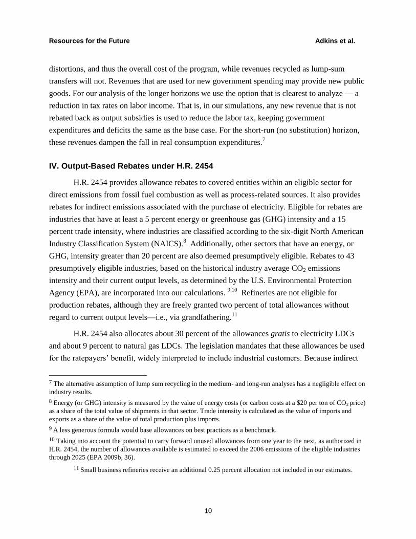
IV. Output-Based Rebates under H.R. 2454
H.R. 2454 provides allowance rebates to covered entities within an eligible sector for
direct emissions from fossil fuel combustion as well as process-related sources. It also provides
rebates for indirect emissions associated with the purchase of electricity. Eligible for rebates are
industries that have at least a 5 percent energy or greenhouse gas (GHG) intensity and a 15
percent trade intensity, where industries are classified according to the six-digit North American
Industry Classification System (NAICS).8 Additionally, other sectors that have an energy, or
GHG, intensity greater than 20 percent are also deemed presumptively eligible. Rebates to 43
presumptively eligible industries, based on the historical industry average CO2 emissions
intensity and their current output levels, as determined by the U.S. Environmental Protection
Agency (EPA), are incorporated into our calculations. 9,10
Refineries are not eligible for
production rebates, although they are freely granted two percent of total allowances without
regard to current output levels—i.e., via grandfathering.11
H.R. 2454 also allocates about 30 percent of the allowances gratis to electricity LDCs
and about 9 percent to natural gas LDCs. The legislation mandates that these allowances be used
for the ratepayers’ benefit, widely interpreted to include industrial customers. Because indirect
7 The alternative assumption of lump sum recycling in the medium- and long-run analyses has a negligible effect on
industry results.
8 Energy (or GHG) intensity is measured by the value of energy costs (or carbon costs at a $20 per ton of CO2 price)
as a share of the total value of shipments in that sector. Trade intensity is calculated as the value of imports and
exports as a share of the value of total production plus imports.
9 A less generous formula would base allowances on best practices as a benchmark.
10 Taking into account the potential to carry forward unused allowances from one year to the next, as authorized in
H.R. 2454, the number of allowances available is estimated to exceed the 2006 emissions of the eligible industries
through 2025 (EPA 2009b, 36).
11 Small business refineries receive an additional 0.25 percent allocation not included in our estimates.

Resources for the Future Adkins et al.
11
emissions from electricity consumption are an important component of total emissions of the
eligible sectors, the LDC provisions were expected to mitigate a significant portion of the policy-
induced costs to the eligible sectors. The allocations to natural gas LDCs are likely to have a
smaller impact.12
Table 1 displays our estimates of the dollar value of the EITE allocations and the implied
subsidy rates for our 29- and 52-sector aggregations. While the refining industry is not
technically eligible for the output-based rebates, we include the value of their grandfathered
rebates in the table.13
The LDC allocations for electric and gas utilities are also translated into
output subsidy rates and included in the table. Of the 33 manufacturing industries in the more
disaggregated I-O model, 21 are eligible for at least some rebates. The manufacturing sectors
receiving the largest subsidies (by value) are in the petroleum refining, ferrous metals, and
chemicals industries. We compute the subsidy rate as the ratio of the industry rebate value to the
industry output value. These subsidy rates vary considerably among sectors, ranging from 0.001
percent for food manufacturing to 4.38 percent for cement.
The last column of Table 1 gives the qualifying industry share, that is, the portion of
industry output presumptively eligible for rebates under H.R. 2454. The last column of Table 1
gives the qualifying industry share, that is, the portion of industry output presumptively eligible
for rebates under H.R. 2454. Thus, sectors such as pulp mills and other industries identified at
the six-digit NAICS level qualify for rebates on 100 percent of their output. Sectors such as
fertilizer, not comprised entirely of presumptively eligible six-digit NAICS industries, have
qualifying shares of less than 100 percent.
Of the 15 manufacturing industries represented in the 29-sector CGE model, nine are
eligible for subsidies (including the allocation to refining). In general, the greater level of
aggregation means that for most qualifying sectors, both the average subsidy rate and qualifying
share of output go down, masking some of the impact of the subsidies. For example, in the more
aggregated chemicals, rubber, and plastics sector, the average subsidy rate is 0.241 percent with
a qualifying share of output of 30.7 percent. However, in the 52 sector model, petrochemical
manufacturing by itself had a subsidy rate of 1.226 percent and a 100 percent qualifying share of
12 The natural gas LDC allocations only indirectly benefit the relatively small number of EITE industries that
receive their gas from LDCs and whose emissions are not directly regulated under H.R. 2454.
13 H.R. 2454 grants 2.25 percent of the total allowances to the refining sector; within our industry disaggregation
this is allocated to the sectors ―Refining-LPG‖ ($114.1 million) and ―Refining-Other‖ ($1,905.8 million).

Resources for the Future Adkins et al.
12
output. In the 52-sector model, cement had the highest subsidy rate of all sectors, 4.381 percent.
However, in the 29-sector model, it is subsumed within the non-metallic mineral products sector,
which has a subsidy rate of only 0.489 percent.
V. Effects of Carbon Pricing with H.R. 2454 Subsidies over Multiple Time Horizons
This section presents the results of our four modeling frameworks designed to represent
the very-short-, short-, medium-, and long-run time horizons. To illustrate the effects of an
economy-wide carbon pricing policy, we simulate a carbon tax of $15 per ton of CO2 (2006$)
with and without the accompanying subsidies specified in H.R. 2454, i.e. the output-based
rebates for EITE industries as well as the free allowance allocations for electricity and gas LDCs
and petroleum refining. The most comprehensive results are presented for industrial output,
while sector-specific estimates for prices, costs, and profits are presented for some of the
modeling horizons. We note that the case with subsidies generates a smaller reduction in CO2
emissions. Achieving the same emissions reduction with the subsidies would require a slightly
higher carbon price.
Effects on Industry Prices: Very-Short-Run Horizon
As noted, the very-short-run horizon was designed to facilitate a hypothetical, worst-case
assessment of the maximum damages affected industries might claim. In this scenario, we allow
the carbon policy to raise the prices of intermediate inputs; however, we assume that producers
cannot raise prices, adjust output levels, change their input mix, or adopt new technologies in
response to these higher costs. When calculating the effect on profits, output prices are assumed
to remain unchanged. In other words, it is assumed that buyers of an industry’s output must pay
the carbon tax-inclusive output price (net of any subsidies) but that the producer continues to
receive the pre-tax price. There is thus an inherent inconsistency in this very-short-run analysis:
firms pay more for their inputs but are unable to recoup the added costs from their customers.
The results are therefore valid taken one industry at a time, but they cannot be regarded as
applicable simultaneously. An additional value of this exercise is the comparison with the short-
run results below where we highlight the importance of output price increases in offsetting reductions
in profits.
Resources for the Future Adkins et al.
13
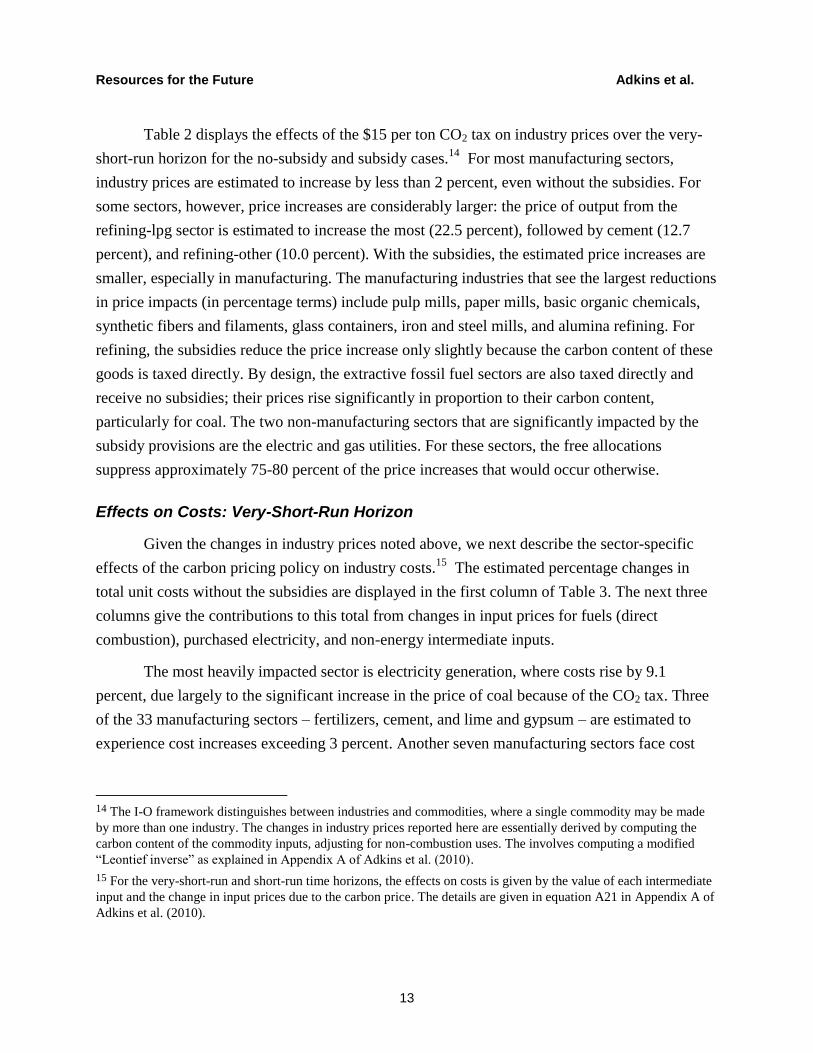
Table 2 displays the effects of the $15 per ton CO2 tax on industry prices over the very-
short-run horizon for the no-subsidy and subsidy cases.14
For most manufacturing sectors,
industry prices are estimated to increase by less than 2 percent, even without the subsidies. For
some sectors, however, price increases are considerably larger: the price of output from the
refining-lpg sector is estimated to increase the most (22.5 percent), followed by cement (12.7
percent), and refining-other (10.0 percent). With the subsidies, the estimated price increases are
smaller, especially in manufacturing. The manufacturing industries that see the largest reductions
in price impacts (in percentage terms) include pulp mills, paper mills, basic organic chemicals,
synthetic fibers and filaments, glass containers, iron and steel mills, and alumina refining. For
refining, the subsidies reduce the price increase only slightly because the carbon content of these
goods is taxed directly. By design, the extractive fossil fuel sectors are also taxed directly and
receive no subsidies; their prices rise significantly in proportion to their carbon content,
particularly for coal. The two non-manufacturing sectors that are significantly impacted by the
subsidy provisions are the electric and gas utilities. For these sectors, the free allocations
suppress approximately 75-80 percent of the price increases that would occur otherwise.
Effects on Costs: Very-Short-Run Horizon
Given the changes in industry prices noted above, we next describe the sector-specific
effects of the carbon pricing policy on industry costs.15
The estimated percentage changes in
total unit costs without the subsidies are displayed in the first column of Table 3. The next three
columns give the contributions to this total from changes in input prices for fuels (direct
combustion), purchased electricity, and non-energy intermediate inputs.
The most heavily impacted sector is electricity generation, where costs rise by 9.1
percent, due largely to the significant increase in the price of coal because of the CO2 tax. Three
of the 33 manufacturing sectors – fertilizers, cement, and lime and gypsum – are estimated to
experience cost increases exceeding 3 percent. Another seven manufacturing sectors face cost
14 The I-O framework distinguishes between industries and commodities, where a single commodity may be made
by more than one industry. The changes in industry prices reported here are essentially derived by computing the
carbon content of the commodity inputs, adjusting for non-combustion uses. The involves computing a modified
―Leontief inverse‖ as explained in Appendix A of Adkins et al. (2010).
15 For the very-short-run and short-run time horizons, the effects on costs is given by the value of each intermediate
input and the change in input prices due to the carbon price. The details are given in equation A21 in Appendix A of
Adkins et al. (2010).

Resources for the Future Adkins et al.
14
increases between 2 and 3 percent. For the EITE sectors as a whole, the average cost increase is
1.4 percent (shown in the bottom row).16
The composition of the cost increases vary widely by
sector, with some industries most affected by the changes in fuel costs (e.g., petrochemical
manufacturing), purchased electricity costs (e.g., aluminum), or indirect costs (e.g., fabricated
metals). We note that because of the fixed input coefficients assumption, the costs are
proportional to the CO2 tax. A CO2 price twice as large would double the costs.17
The last column in Table 3 shows that total cost impacts are significantly reduced after
the subsidies are applied. Only one manufacturing industry, cement, experiences a cost increase
greater than 3 percent, and one other industry, lime and gypsum, experiences a cost increase
between 2 and 3 percent. The average cost increase for the EITE sectors drops by nearly one half
to 0.7 percent (although the EITE average obscures a wide range in reductions across the
individual EITE industries). For the non-manufacturing sectors, the introduction of the subsidies
also mutes the increases in costs from the CO2 tax.
Columns 2-4 of Table 3 provide some explanation of the pattern of reductions in the cost
impacts with the subsidies. Since primary energy inputs are taxed directly and receive no direct
subsidies, the greater the amount of an industry’s total cost increase that can be explained by
direct fuel purchases, the less effective the subsidies are at reducing the cost increase. Examples
include refining, cement, and air transportation, which see their cost increases reduced only
about 20 percent. Similarly, electric utilities experience a negligible reduction in their cost
increase, since the free allocations they receive do nothing to dampen the increase in their fuel
costs. In contrast, aluminum experiences a net cost increase that is more than 75 percent smaller
with the subsidies. This is because purchases of electricity are a relatively large share of the
original cost increase; thus aluminum benefits from the relatively high subsidy to electric LDCs.
At the same time, some of the industries that benefit most are those for which indirect costs are a
relatively high share of the pre-subsidy cost impact; examples include machinery, miscellaneous
16 While not labeled as an EITE in the interagency report, we include it in our calculations of EITE averages.
17 Calculations for the very-short- and short-run analyses can be readily scaled up or down to reflect different
assumptions about CO2 prices, since they based on relatively simple linear models. In contrast, modeling of the
medium- and long-run horizons explicitly involve nonlinearities that cannot be so readily scaled. However, even for
the short-run case, one has to be careful about extrapolating to large CO2 price changes, since the calculated demand
elasticities, which are based on the multi-sector global CGE model, are strictly intended for marginal analysis. How
the system would respond to large increases in prices in the short-run is an issue that must be carefully considered.

Resources for the Future Adkins et al.
15
manufacturing, and gas utilities. The increases in their electricity costs are now significantly
dampened.
Effects on Output: Very-Short-Run and Short-Run Horizons
As discussed above, in our very-short-run horizon, output levels are fixed and there is an
inherent inconsistency between the individual sector results and those for the full set of
industries. In contrast, in our short-run horizon the treatment of input and output prices is
consistent. In the short-run, we assume that producers can raise prices to cover their higher unit
costs, with resulting reductions in sales and output as customers switch to alternative goods or
imports.18
Here, any revenues not rebated to industries are recycled to households, preserving
the equality between expenditures and receipts.
Table 4 displays the short-run changes in output with and without the subsidies. Without
the subsidies, three manufacturing sectors incur output reductions of two percent or more: lime
and gypsum (2.3 percent), alumina refining (2.3 percent), and cement (4.8 percent). The
relatively large declines in output in these sectors arise from the combined effects of large cost
increases and the relatively high demand elasticities estimated for these industries with the CGE
model. Consistent with the results shown in Table 3, the subsidies reduce the output losses
substantially for many industries. The output loss for cement is reduced by almost one half. For
lime and gypsum the output loss is reduced by about one quarter while for alumina refining,
which benefits from the substantial allocations to LDCs, the output loss is effectively eliminated.
On average, across all EITE industries, the H.R. 2454 subsidies reduce short-run output losses by
almost one half.
For the non-manufacturing sectors, the declines in output are generally smaller than for
the manufacturing sectors, with a few notable exceptions. As shown in Table 2, coal and other
fuel-producing industries saw the biggest increase in prices (for the purchaser, not the producer).
Not surprisingly, in Table 4 they now experience the biggest declines in sales, once we account
for the effect that these price increases will have on the derived demand for these products. In the
case of coal, the output decline is calculated to be more than 30 percent. Electric and gas utilities
experience moderate declines in output when the carbon price is introduced but see those losses
cut by 80 percent when the subsidies are included. The service sectors, which gain slightly in the
18 As noted in Section III, to determine the sales response, we estimated the elasticity of demand for each industry
using the 29-sector, multi-region global model. These elasticities are given in Table B1 in Adkins et al. (2010).

Resources for the Future Adkins et al.
16
no-subsidy case, gain less with the subsidies, as the amount recycled back to households is
halved, limiting the amount of expenditure switching to less carbon intensive commodities.
Effects on Profits: Very-Short-Run and Short-Run Horizons
Table 5 displays the effects of the carbon pricing policy on profits in the very-short-run
and short-run horizons, both with and without the subsidies. The effects are particularly
pronounced in our very-short-run scenario, since by assumption firms have no recourse but to
absorb the full impact of these cost increases as reductions in profits.19
Looking first at the
bottom row, which gives the weighted average results for the EITEs plus petroleum refining
sectors, we see that the imposition of a $15 per ton carbon price reduces profits by an average of
almost 12 percent. In the short-run, when we allow firms to increase their output prices and
introduce downward sloping demand curves for their products, the average reduction in profits
for this group falls 96 percent to less than half a percent. The H.R. 2454 subsidies reduce the
profit reduction by an additional 50 percent (comparing the second and fourth columns in Table
5).
A similar story applies to most individual industries. For example, without the subsidies,
fertilizers, artificial and synthetic fibers and filaments, and other basic organic chemicals
experience declines in profits of 78.7, 62.7, and 54.5 percent, respectively, in the very-short-run
when the output price is fixed vs. 1.5, 0.5, and 1.1 percent declines when they are free to raise
output prices. With the H.R. 2454 subsidies, the profit declines are further reduced by another
65-85 percent.
Among the non-manufacturing sectors, in the very-short-run, several industries
experience profit declines over 5 percent, with significantly higher losses for air transportation
and electric utilities. However, in our short-run case, once output prices are allowed to rise, only
electric and gas utilities and the fossil fuel producing sectors experience impacts on profits
greater than one percent. Once the subsidies are applied, this is limited to only the fossil fuel
producing sectors, given the relatively generous allocation to LDCs.
19 We define profits as the gross return to capital – i.e. sales revenue plus any applicable rebates, minus purchases of
intermediate inputs and labor costs. See Appendix A in Adkins et al. (2010).

Resources for the Future Adkins et al.
17
Comparing Effects on Output over the Short-, Medium-, and Long-Run Horizons
We next compare the short-run effects on output to those over our medium- and long-run
horizons. As noted in Section III, the global CGE model used to consider the latter two horizons
identifies 29 industries. In order to compare the estimates across the three horizons, we first
aggregate the results for the 52 industries used in the short-run analysis into the corresponding 29
industry categories using output values as weights. We focus on the case where a $15 per ton
CO2 (2006$) price is adopted in all Annex I nations (as opposed to unilateral U.S. action).
Table 6 displays the effects on output of the carbon pricing policy across the three
modeling horizons both with and without the H.R. 2454 subsidies.20
Figure 1 shows the effects
in the three horizons for the manufacturing sectors in the no-subsidy case. Recall that in the
medium term, producers may substitute among all inputs except capital. Thus, firms may
substitute labor for energy or gas for coal. However, only in the long-run can firms move capital
between sectors and/or substitute it for energy or labor. Furthermore, in the general equilibrium
framework, both producers and consumers are changing their behavior in response to a price on
carbon, and these may have opposing effects on output over time. On the one hand, producers
are substituting inputs to reduce the cost impact and hence prices; i.e. shifting the supply curve
back out. Over time, these lower prices should help raise sales and output. On the other hand,
customers are making substitutions to avoid higher prices for carbon intensive products, reducing
their demands (shifting the demand curve back), and thereby reducing sales and output of these
products.
Looking across the first three columns of Table 6, we see these competing effects at work
in the no-subsidy case. Results for the manufacturing sectors are also presented in Figure 1.
While most of the manufacturing sectors see reductions in output with the CO2 tax in the short-
run, the magnitude of the decline in the medium-run may be greater or smaller in comparison.
However, for the EITE sectors as a group, the average output decline is twice as great in the
medium-run (bottom row of Table 6). For the non-manufacturing sectors, the differences
between short- and medium-runs is mixed. For the coal and gas mining sectors, the decline in
20 Not surprisingly, the impact of carbon pricing policies on output levels is quite sensitive to the breadth of the
industrial categories considered: the more narrowly the categories are defined, the greater the variation in impacts.
For example, the short-run output decline is 64 percent larger for inorganic chemicals (column one of Table 4) than
it is for chemicals, rubber, and plastics (column one of Table 6). Although the availability of consistent information
dictated our present choice of aggregation, in earlier work, Morgenstern et al. (2004) found that sub-industry
impacts estimated at a four-digit SIC (Standard Industrial Classification) level can be an order of magnitude larger
those estimated at a two-digit level.

Resources for the Future Adkins et al.
18
output is much smaller in the medium-run. For the transportation sector the results are the
opposite, with a much greater decline in the medium-run. A number of the remaining non-
manufacturing sectors see small increases in output as households substitute into less carbon
intensive goods.
In contrast to the medium-run, the long-run allows for substitution of capital for other
inputs. For the most part, the differences between the medium- and long-run changes in output
are smaller than when comparing the short- and medium-runs. For the manufacturing sectors, the
reduction in output in the petroleum and coal products sector is significantly greater in the long-
run as the economy continues to adjust away from carbon intensive goods. For the nonferrous
and ferrous metals sectors the effect is the opposite, with reductions in output smaller in the
long-run. For the EITE sectors as a group, the average decline increases from 0.9 to 1.0 percent.
Coal, gas, and oil mining all see greater declines in output in the long-run.
For those sectors receiving them, the H.R. 2454 subsidies can have significant effects on
output across all of the horizons. As show in Table 6, the average decline in output for the EITEs
drops from 0.5 percent without the subsidies to 0.2 percent with the subsidies in the short-run,
from 0.9 to 0.3 percent in the medium-run, and from 1.0 to 0.3 percent in the long-run. Figure 2
shows the long-run effect of the subsidies on all of the sectors that receive allocations. They are
particularly significant for the electric utilities sector, which goes from a significant decline in
output to a small increase. Both the nonferrous and ferrous metals sectors also see significant
reversals with the subsidies. Of the sectors that do not receive subsidies, the coal mining sector is
the biggest beneficiary.
Beyond these results for carbon pricing across all Annex I countries, it is also instructive
to consider the impacts of unilateral action by the U.S. Clearly, the output losses under unilateral
action would be larger, since roughly half of U.S. trade in energy intensive goods is with other
Annex I nations. To examine this issue, we simulate the models covering all three timeframes
under the assumption that only the U.S. imposes a $15 per ton carbon price. Without the H.R.
2454 subsidies, the average output losses for all EITE industries plus petroleum products are 1.4,
0.4, and 0.4 times larger than the case of multilateral action, for the short-, medium-, and long-
run horizons, respectively (the details are given in Adkins et al. 2010). With the H.R. 2454
subsidies, the output losses in the unilateral scenario are 0.8, 1.4 and 1.1 times larger. Thus, even
though we are dealing with relatively small impacts, especially once the subsidies are applied,
we see the importance of multilateral action in attenuating losses.
Resources for the Future Adkins et al.
19
VI. Trade and Leakage
A sub-global carbon pricing policy will not only affect firms’ costs, output, and short-run
profits, but will also impact international trade, relocating economic activity from high
regulatory cost to low regulatory cost nations. These trade impacts, also known as
competitiveness effects, can lead to emissions leakage.21
Beyond the direct trade impacts,
ensuing changes in world fuel prices can further alter relative costs across countries, changing
the carbon-intensity of production and leading to additional leakage. Here we estimate the trade-
related impacts of our Annex I-wide carbon pricing policy and the implications for emissions
leakage on a sectoral basis. We examine leakage attributable to changes in trade volumes as well
as leakage related to differences in the carbon-intensity of production in different regions. We
also explore the impacts of the policies on aggregate leakage from the U.S. and other Annex I
countries with carbon policies, accounting for leakage at both the industry and household levels.
Trade Impacts
In previous sections, we estimated the changes in domestic output induced by the
imposition of a domestic carbon pricing regime with and without the subsidies incorporated in
H.R. 2454. Yet these production changes do not necessarily impact domestic consumption on a
one-for-one basis because some of the output reductions may be made up for through changes in
trade. Specifically, the change in domestic production of commodity i ( ) can be decomposed
into the changes in consumption plus exports minus imports22
:
(1)
The trade impact of the policies can then be defined as the share of the change in output due to
the changes in exports and imports23
:
(2) Trade Impact
Table 7 presents the results of the decompositions of the changes in output for the
medium-run, both with and without the subsidies. Table 8 presents the results for the long-run.
21 Note that these trade impacts are consistent with the well-known pollution-haven hypothesis (Jaffee et al., 1995).
22 Ignoring changes in inventories, which are not modeled here.
23 Aldy and Pizer (2011) define the ―competitiveness effect‖ as the percentage change in net imports.
Resources for the Future Adkins et al.
20
Figure 3 shows the decompositions for the manufacturing sectors in the medium-run without the
subsidies. We can see how the decompositions operate by taking the chemicals, rubber, and
plastics sector as an example. In the medium-run, following the imposition of the carbon tax
without subsidies, sectoral output falls by 1.55 percent (Table 7). Domestic consumption,
however, falls by less, as exports fall and imports rise to make up the difference. The decrease in
consumption contributes 0.55 percentage points to the change in output, the decrease in exports
0.79 percentage points, and the increase in imports 0.21 percentage points. Filling in equation (1)
we can confirm that: - 1.55 = (- 0.55) + (- 0.79) - (0.21). Taking the component due to changes in
trade alone, the trade impact for the chemicals, rubber, and plastics sector is 64 percent of the
total decline in output, i.e., [(- 0.79) – (0.21)]/(- 1.55).
As can be seen in Figure 3, in addition to the chemicals, rubber, and plastics sector, trade
impacts explain a significant portion of the fall in output for the nonferrous metals, non-metallic
mineral products, and ferrous metals sectors, accounting for 61, 56, and 53 percent, respectively,
of the fall in their output in the medium-run. For the petroleum refining sector, by contrast, the
decline in domestic consumption comprises the bulk of the output decline, with only 13 percent
of the total coming from changes in trade. For the EITE sectors as a whole, in the medium-run,
the trade or competitiveness accounts for 46 percent of the fall in output. As can be seen in
Figure 3, the trade effects can also work in the opposite direction. For example, in the machinery
sector, a decrease in domestic consumption is largely offset by the combined effects of an
increase in exports and a decrease in imports.
Without the subsidies, the composition of the changes in sectoral output in the long-run is
similar to those in the medium-run. However, in the long-run, the ability of capital to migrate
between sectors reduces international cost disparities and attenuates some of the trade impacts.
Thus, the trade impacts for the EITEs fall from 46 percent in the medium-run to 33 percent in the
long-run.24
As we saw in the previous section, for sectors that receive them, the subsidies
significantly reduce the declines in output that accompany imposition of the carbon tax (or in
24 Aldy and Pizer (2011), using an econometric approach, estimate short-run (one year) competitiveness effects for
more than 400 U.S. manufacturing industries. Although their methodology is not directly comparable with ours, it is
worth pointing out that where sectoral dissagreagtion is roughly similar, our change in net imports is comparable
with theirs. However, the estimated changes in their output measure is in all cases significantly larger than in our
simulation results. The net effect is that our trade impact measure is much larger than their comparable measure. For
example, their competitiveness effect for their chemicals sector is 1.3 percent. For the medium-run, our comparable
measure is 1.0 percent. However, Aldy and Pizer estimate a 3.4 percent fall in output, while our simulation result is
a fall of 1.6 percent.

Resources for the Future Adkins et al.
21
several cases actually increase sectoral output). With the subsidies spurring increases in exports
and decreases in imports for several sectors, the net effect is a decrease in trade impacts for the
EITE sectors. In the long-run, with the subsidies in place, the impact for the EITE sectors falls to
3 percent. This is a much stronger effect than in the medium-run, where the subsidies reduce the
trade impacts for the EITE sectors from 46 to 37 percent.
Emissions Leakage at the Industry Level
We now move beyond our examination of the trade impacts on U.S. industrial output to
estimate trade-related emissions leakage at the industry level. The $15 per ton CO2 price in
Annex I countries can be anticipated to cause emissions to leak to non-policy countries outside
Annex I, due in part to changes in trade flows. Here we decompose sectoral leakage from the
U.S. to non-Annex I countries into components that arise from changes in the volume of trade
with the U.S. and changes in the carbon-intensity of that trade. Table 9 presents calculations for
the long-run case without subsidies for the manufacturing sectors.
The first column of Table 9 shows the estimated change in U.S. CO2 emissions by sector,
which includes both direct emissions and indirect emissions from the use of electricity. Columns
2-4 decompose the change in non-Annex I emissions, i.e. leakage, by sector. The second and
third columns show the changes in non-Annex I emissions related to changes in exports to and
imports from the U.S. The fourth column shows the change in Annex I emissions related to the
change in the carbon intensity differential of production between the U.S. and its non-Annex I
trading partners. The final column gives the estimated sectoral trade-related leakage rates. Figure
4 shows the sectoral leakage rates and their trade- (i.e., net export) and intensity-related
components, computed from Table 9.
The highest estimated trade-related leakage rate is 27.1 percent for the petroleum refining
sector. Almost 40 percent of the increase in emissions there is due to the change in the emissions
intensity differential between the U.S. and its non-Annex I trading partners. Four other sectors,
all EITEs, have trade-related leakage rates greater than 5 percent. For the EITEs as a group, the
estimated leakage rate is 8.5 percent. Seven of the fifteen manufacturing sectors actually have
negative trade-related leakage rates. If we were to exclude the change in the carbon intensity
differential between the policy and non-policy countries, the trade-related leakage rate for the
EITEs would fall to 3.9 percent.
For the manufacturing sectors, Table 10 compares the emissions changes and trade-
related leakage rates from Table 9 with estimates that include the subsidies. As discussed
Resources for the Future Adkins et al.
22
previously, with the subsidies and the same $15/ton tax, the total emissions reduction in the U.S.
will be lower than in the case with the tax alone. This is evident at the sectoral level when
comparing columns 2 and 4 in Table 10. Both the numerator and denominator for the leakage
estimates may change when the subsidies are applied. In this case, the leakage rate for the
petroleum refining sector goes up, while the estimates for the other four sectors which previously
had leakage rates over 5 percent all go down. At the same time, leakage rates for a number of
sectors that do not receive subsidies go up.
Overall, the trade-related leakage rate for the EITEs goes down to 5.3 percent. Although
we saw earlier that the subsidies were generally effective at reducing or even reversing sectoral
output losses (Table 6), they reduce less than 40% of trade-related leakage in our estimates. This
contrasts with the interagency report discussed earlier, which ignores how the carbon pricing
policy will alter the differential in the carbon intensity of trade between the U.S. and non-policy
countries. In that analysis, allocations to LDCs and trade-vulnerable industries virtually
eliminated leakage in each of the five EITE sectors examined.
Aggregate Leakage
We now look at changes in emissions in all countries and regions in our CGE model and
calculate the aggregate leakage rates. We decompose the changes in emissions into components
for industry and households. We further decompose industry changes into components for output
and emissions intensity. Table 11 presents the decompositions for countries adopting carbon
pricing policies and for the non-policy countries. Estimates are presented for the cases both with
and without subsidies in the U.S. We focus here on the long-run (i.e., mobile capital) case.
The first column of Table 11 displays the base year level of emissions. In 2004, the
United States emitted 6,070 million tons of CO2, 23 percent of global emissions. In the no-
subsidy case, U.S. emissions fall by 518 million tons (8.6 percent). Emissions in the other Annex
I countries implementing the same carbon price (i.e., Canada and Rest of Annex I) fall by 648
million tons, resulting in total Annex I reductions of 1,167 million tons. Emissions in the non-
policy (i.e., non-Annex I) countries rise by 103 million tons for an aggregate leakage rate across
Annex I nations of 8.8 percent.
When the subsidies are introduced, U.S. output falls by somewhat less than in the no-
subsidy case, and so do corresponding emissions, by 441 million tons. Total Annex I reductions
also fall somewhat less, by 1,064 million tons. At the same time, the smaller reduction in U.S.
output leads to a smaller drop in international fuel prices compared to the no-subsidy case, and

Resources for the Future Adkins et al.
23
non-Annex I emissions increase less, by 92.4 million tons. The result is a slightly smaller leakage
rate of 8.7 percent. Mathematically, both the numerator and denominator of the leakage rate are
reduced, with the denominator decreasing relatively less.
We next look more deeply into the sources of changes in country emissions. For the U.S.
and the rest of the world we decompose emissions changes into those from industry and
households. For industry we decompose the changes further, into those resulting directly from
changes in sectoral output levels and those resulting from changes in emissions intensity:
(3) ,
where is the change in country or region emissions, is sector i output in country r, and
is the emissions intensity of output for sector I in country r. The superscripts 0 and P denote the
variables for the base and policy cases. Changes in are driven by substitution among fuel
inputs, resulting directly from the carbon policies and indirectly from changes in world fuel
prices.
The bottom two panels of Table 11 show the results of the decompositions of the
emissions changes in the U.S. and elsewhere. With the carbon tax imposed in the U.S. and other
Annex I countries (without any subsidies in the U.S.), the change in emissions directly attributed
to changes in household consumption is 13.3 percent for the U.S. and 19.0 percent outside of the
U.S. The change in input mix is the largest contributor to the change in emissions in both the
U.S. and abroad, accounting for 62.4 percent and 74.7 percent of the totals, respectively.
Changes in industrial output levels (weighted by the sectoral emissions coefficients), accounts
for the rest of the changes, at 24.4 percent in the U.S. and 6.3 percent abroad. With the subsidies
in place in the U.S., sectoral output changes less than in the no-subsidy case and the change in
emissions attributable to output changes falls to 4.5 percent, with that from input substitution
rising to 81.5 percent.
Comment on Leakage Rates
A number of factors influence industry and aggregate leakage rates. Burniaux and
Oliveira Martins (2000) use a simplified CGE model to look for key determinants of the
magnitude of leakage rates. Of the mechanisms they examine, they find that the supply elasticity
of coal and the model’s production structure have the most influence on leakage rates. With their
preferred parameter values and model structure, they find generally low aggregate leakage rates.
Resources for the Future Adkins et al.
24
Model closure, wherein exchange rates adjust to ―close‖ the foreign trade account, also
may have some influence on leakage rates. In our static model, the trade balance is assumed
unchanged by the carbon policy and an exchange rate closes this account. A dynamic model with
a transition period that allows trade balances to adjust would likely produce different changes in
trade flows and leakage rates in the short-run.
Industry leakage is also sensitive to the choice of import elasticities. The elasticities in
our global CGE model are drawn from the GTAP 7 database. While relatively disaggregated for
a global CGE model, many of the manufacturing sectors are averages across heterogeneous
products. In turn, the elasticities are averages and may not reflect well the import responses for
certain subsectors. If we were able to use the same set of sectors in our global model that are
available in the more disaggregated I-O model, import responses and leakage likely would be
greater for some sectors and smaller in others.
VII. Conclusions
Inevitably, any broad-based carbon pricing policy will have disproportionate impacts on
certain industries. Some of the key challenges to developing a CO2 pricing policy addressed in
this paper include: 1) identifying which industries face the greatest impacts and evaluating how
these impacts may change over time as producers and consumers adjust; 2) estimating the
associated trade (i.e., competitiveness) impacts and emissions leakage; and 3) assessing to what
extent the various impacts can be mitigated by offsetting policies, such as the output-based
rebates and free allowance allocations of the type contained in H.R. 2454.
In this paper we introduce a multi-horizon methodology that tries to address the dynamic
adjustment issue: (1) the very-short-run examines the maximum losses that industries might try
to claim, assuming that sellers are not able to pass through their cost increases; (2) the short-run
allows for cost pass-through but assumes no input substitution; (3) the medium-run allows for
cost pass-through and incorporates input substitution except for capital; (4) the long-run allows
for cost pass-through and substitution among all inputs. In order to identify the hardest hit
industries we developed a U.S. input-output model with 52 sectors, some at a highly
disaggregated level, for analyzing the first two time horizons. For the third and fourth horizons
we use a 29 sector global CGE model to assess the key impacts, including trade effects. The
effectiveness of the offsetting policies contained in H.R. 2454—translated into their subsidy
equivalents—is considered in all four horizons.
Resources for the Future Adkins et al.
25
With this methodology we are able to derive some results generally not available in other
studies. First, we identify the industries most affected by a carbon price at a disaggregated level.
Second, we show how output and profit losses may change substantially over time when output
prices can adjust and producers can substitute inputs. These dynamic results should allow a more
nuanced and critical discussion of industry claims of damages; losses may increase or decrease
over time and may require a more complex compensation strategy. Third, we show that the
subsidies substantially reduce losses for the industries directly affected, and for other industries
through the inter-industry framework. We also show how these subsidies affect trade flows and
examine their effectiveness at addressing competitiveness and leakage impacts of subglobal
carbon pricing. Fourth, we examine emissions leakage on both aggregate and industry levels and
decompose them into various components.
Examination of the results of our simulations of a $15/ton CO2 price across Annex I
countries, combined with the H.R. 2454 subsidies in the U.S., yields a number of observations:
Focusing on the short-run, when certain simplifying assumptions allow for a more
disaggregated analysis, we observe that the most pronounced impacts are concentrated in
particular sub-segments of the EITE industries. Without the subsidies, the biggest short-
run output losses in manufacturing occur in the cement, aluminum, and lime and gypsum
sectors. With the subsidies, on average, short-run losses for the EITE industries are cut in
half.
A reduction in output losses does not always occur as we move through successively
longer time frames in the analysis, suggesting that the passage of time by itself may not
be sufficient to attenuate the impacts. However, we do find that use of the H.R. 2454
subsidies can significantly offset output losses in each of the four time frames considered.
Within manufacturing, with the exception of petroleum and coal products, the subsidies
keep output losses under 0.6 percent in the short-run and under 0.5 percent in the
medium- and long-runs. In the non-manufacturing sector, the output losses of the electric
and gas utilities sectors shrink even more dramatically as a result of the allocations to
local distribution companies.
In the near-term, EITE industries’ ability to raise prices in the face of the domestic carbon
pricing policy is key to their sustained profitability. The average loss of profits in the
EITE industries shrinks by more than 25-fold when output prices are allowed to rise (the
short-run) – even without the subsidies – compared to the case where output prices are
fixed (the very-short-run). Indeed, on average we find that the ability of firms to raise

Resources for the Future Adkins et al.
26
prices is considerably more important in stemming profit losses for EITEs than the
application of the subsidies alone. When price increases are combined with the subsidies,
profit losses in the EITE industries fall by another half to an average of 0.23 percent.
We find that without subsidies, the increase in net imports for individual EITE sectors is
generally less than one percent, and shrinks when moving from the medium- to long-run.
Applying the subsidies either reduces the increase in net imports or reverses its sign. On
average, without the subsidies, trade or "competitiveness" impacts explain 46 percent of
the decline in EITE output in the medium-run and 33 percent in the long-run. With the
subsides, trade impacts for the EITEs fall to 37 percent in the medium-run and 3 percent
in the long-run; for some of the EITEs, the trade impacts actually increase sectoral
output.
We estimate that about half of trade-related leakage from the U.S. to non-policy countries
is due directly to changes in the volume of trade, and the other half to higher emissions
intensities in non-Annex I trading partners induced by lower world fuel prices. While the
H.R. 2454 subsidies are generally effective in reducing output losses for targeted sectors,
they are less effective in reducing leakage.
Overall, while some of our estimates are sensitive to the inevitable modeling
assumptions, we believe that our main conclusions regarding the most affected industries and the
effects of the rebates are robust. The dynamic effects are subject to greater uncertainty and
highlight the importance of more research into adjustment costs and the degree of input
substitution.

Resources for the Future Adkins et al.
27
References
Adkins, Liwayway, and Richard Garbaccio. 2007. ―Coordinating Global Trade and
Environmental Policy: The Role of Pre-Existing Distortions.‖ Paper prepared for the
Tenth Annual Conference on Global Economic Analysis, Purdue University.
Adkins, Liwayway, Richard Garbaccio, Mun Ho, Eric Moore, and Richard Morgenstern. 2010.
―The Impact on U.S. Industries of Carbon Prices with Output-Based Rebates over
Multiple Time Frames.‖ Discussion paper 10-47. Washington, DC: Resources for the
Future.
Aldy, Joseph, and William Pizer. 2011. ―The Competitiveness Impacts of Climate Change
Mitigation Policies.‖ NBER Working Paper no. 17705.
BEA (U.S. Bureau of Economic Analysis). 2008. Annual Industry Accounts: Input-Output (I-O)
Accounts, 1998-2006. Available from: http://www.bea.gov/industry/io_annual.htm.
Boehringer, Christoph, Carolyn Fischer, and Knut Einar Rosendahl. 2010. ―The Global Effects
of Subglobal Climate Policies.‖ The B.E. Journal of Economic Analysis and Policy, vol
10, no. 2, article 13.
Burniaux, Jean-Marc, and Joaquim Oliveira Martins. 2000. ―Carbon Emission Leakages: A
General Equilibrium View.‖ Economics Department Working Papers 242. Paris:
Organisation for Economic Co-operation and Development.
Carbon Trust. 2008. ―EU ETS Impacts on Profitability and Trade, a Sector by Sector Analysis.‖
Paper CTC 728. London: Carbon Trust.
Demailly, D., and P. Quirion. 2006. ―CO2 Abatement, Competitiveness, and Leakage in the
European Cement Industry under the EU ETS: Grandfathering vs. Output-based
Allocation.‖ Climate Policy 6: 93–113.
EIA. (U.S. Energy Information Administration). 2006. Manufacturing Energy Consumption
Survey (MECS). Washington, DC: EIA.
———. 2009a. Energy Market and Economic Impacts of H.R. 2454, the American Clean Energy
and Security Act of 2009. SR-OIAF/2005-05. Washington, DC: EIA.
———. 2009b. Emissions of Greenhouse Gases in the United States 2008. DOE/EIA-
0573(2008). Washington, DC.
———. 2009c. Annual Energy Review 2008. Washington, DC: EIA.

Resources for the Future Adkins et al.
28
EPA (U.S Environmental Protection Agency). 2009a. Analysis of the American Clean Energy
and Security Act of 2009 H.R. 2454 in the 111th Congress. Washington, DC: EPA.
Available at:
<http://www.epa.gov/climatechange/economics/pdfs/H.R.2454_Analysis.pdf>.
———. 2009b. The Effects of H.R. 2454 on International Competitiveness and Emission
Leakage in Energy-Intensive Trade-Exposed Industries: An Interagency Report
Responding to a Request from Senators Bayh, Specter, Stabenow, McCaskill, and Brown.
Washington, DC: EPA. Available at:
<http://www.epa.gov/climatechange/economics/pdfs/InteragencyReport_Competitiveness
&EmissionLeakage.pdf>.
Fischer, Carolyn, and Alan K. Fox. 2007. ―Output-Based Allocation of Emissions Permits for
Mitigating Tax and Trade Interactions.‖ Land Economics 83(4): 575–599.
———. 2009. ―Comparing Policies to Combat Emissions Leakage.‖ Discussion paper 09-02.
Washington, DC: Resources for the Future.
Ho, Mun, Richard Morgenstern, and Jhih-Shyang Shih. 2008. ―Impact of Carbon Price Policies
on U.S. Industry.‖ Discussion paper 08-37. Washington, DC: Resources for the Future.
Hughes, Jonathan E., Christopher R. Knittel, and Daniel Sperling. 2006. ―Evidence of Shift in
the Short-Run Price Elasticity of Gasoline Demand.‖ Energy Journal 29(1): 93–114.
Jaffe, Adam B., Steven R. Peterson, Paul R. Portney, and Robert N. Stavins. 1995.
―Environmental Regulation and the Competitiveness of U.S. Manufacturing: What Does
the Evidence Tell Us?‖ Journal of Economic Literature 33(1): 132-163.
Morgenstern, Richard D., Mun Ho, Jhih-Shyang Shih, and Xuehua Zhang. 2004. ―The Near-
Term Impacts of Carbon Mitigation Policies on Manufacturing Industries.‖ Energy
Policy 32(16): 1825–42.
Figures and Tables
See following pages.

Resources for the Future Adkins et al.
29
-3.5 -3.0 -2.5 -2.0 -1.5 -1.0 -0.5 0.0 0.5 1.0 1.5
Petroleum and Coal Products
Chemicals, Rubber, and Plastics
Nonferrous primary metals
Non-Metallic Mineral Products
Ferrous Metals
Wood
Textiles
Fabricated Metal Products
Paper and Publishing
Transportation Equipment
Food, Beverages, and Tobacco
Electronic equipment
Machinery
Wearing Apparel and Leather
Other Manufacturing
Short-Run Medium-Run Long-Run
Figure 1: Short-, Medium-, and Long-Run Effects on Output of a $15/ton CO2 Tax (% change)
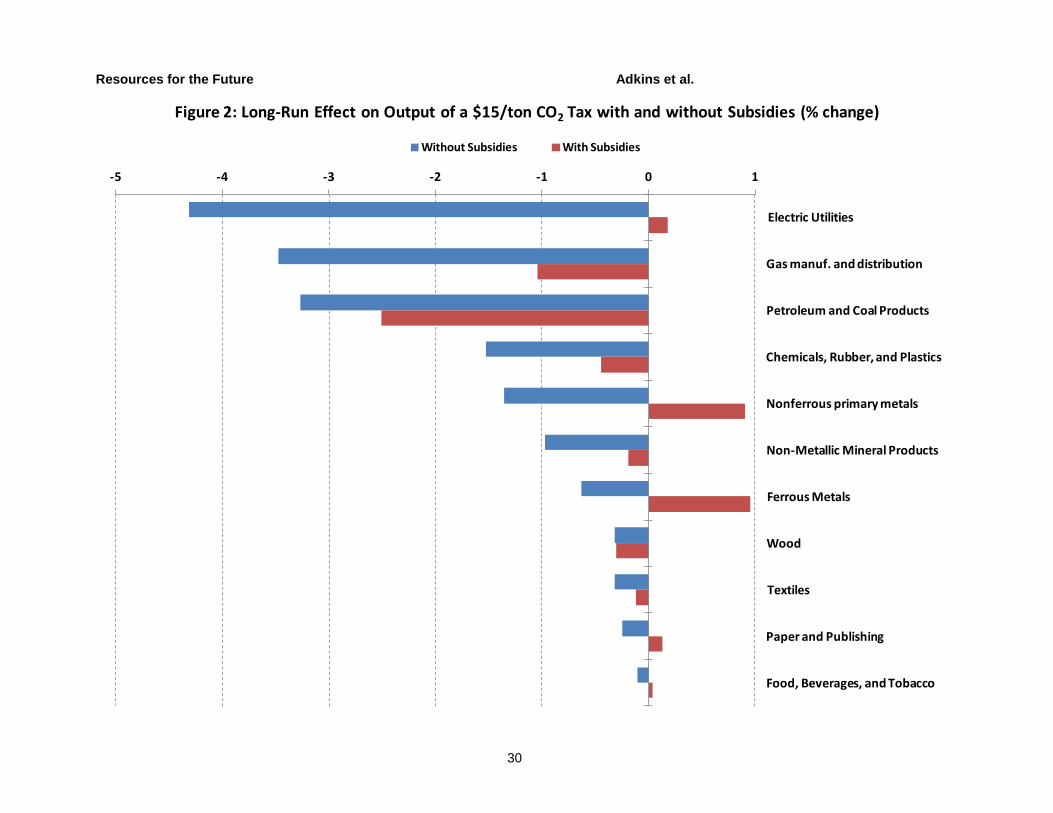
Resources for the Future Adkins et al.
30
-5 -4 -3 -2 -1 0 1
Electric Utilities
Gas manuf. and distribution
Petroleum and Coal Products
Chemicals, Rubber, and Plastics
Nonferrous primary metals
Non-Metallic Mineral Products
Ferrous Metals
Wood
Textiles
Paper and Publishing
Food, Beverages, and Tobacco
Without Subsidies With Subsidies
Figure 2: Long-Run Effect on Output of a $15/ton CO2 Tax with and without Subsidies (% change)
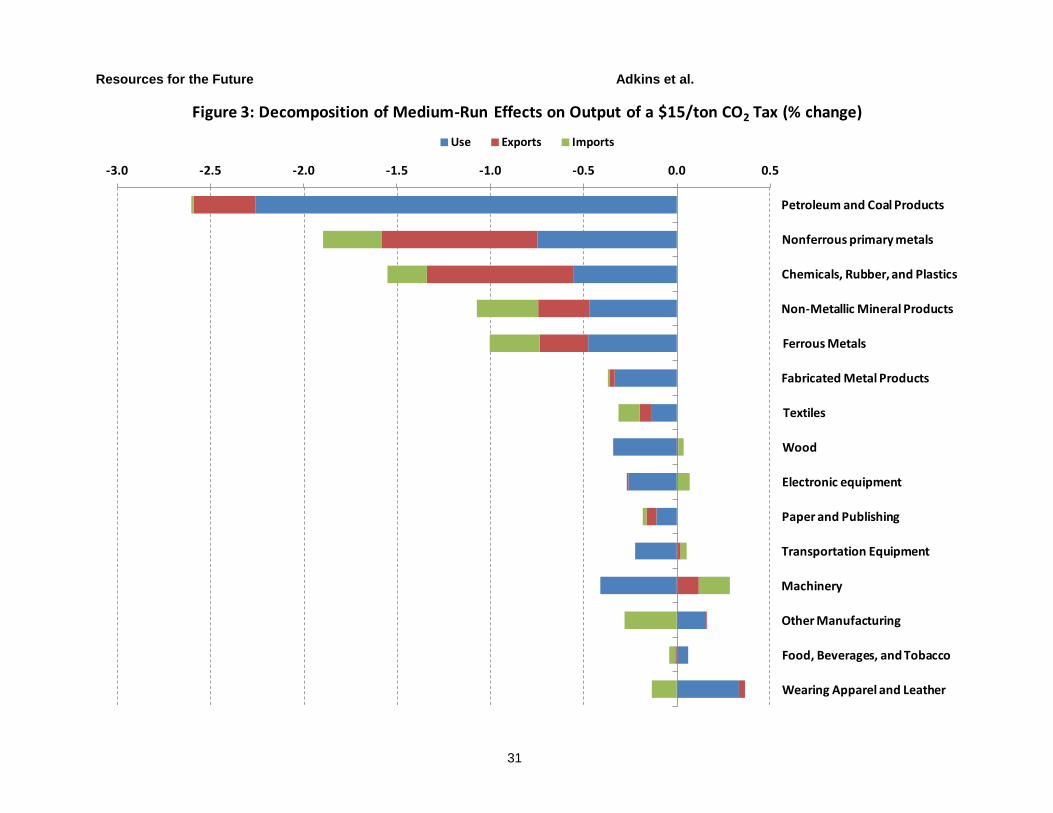
Resources for the Future Adkins et al.
31
-3.0 -2.5 -2.0 -1.5 -1.0 -0.5 0.0 0.5
Petroleum and Coal Products
Nonferrous primary metals
Chemicals, Rubber, and Plastics
Non-Metallic Mineral Products
Ferrous Metals
Fabricated Metal Products
Textiles
Wood
Electronic equipment
Paper and Publishing
Transportation Equipment
Machinery
Other Manufacturing
Food, Beverages, and Tobacco
Wearing Apparel and Leather
Use Exports Imports
Figure 3: Decomposition of Medium-Run Effects on Output of a $15/ton CO2 Tax (% change)
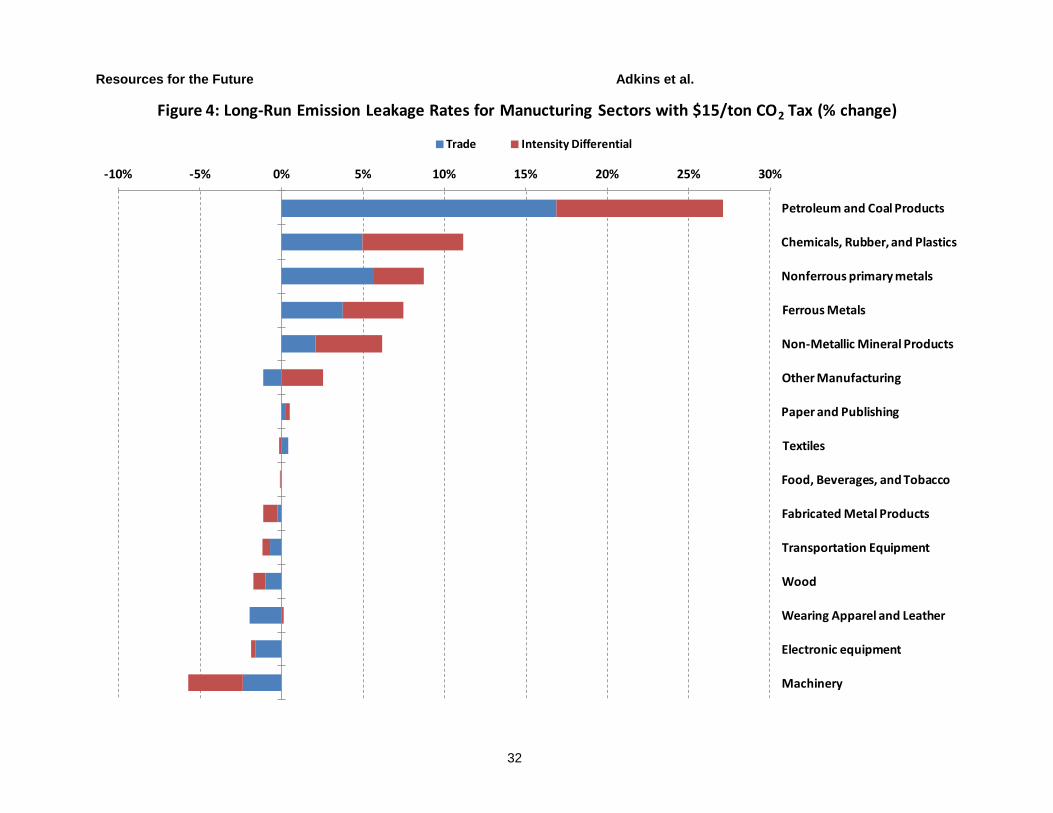
Resources for the Future Adkins et al.
32
-10% -5% 0% 5% 10% 15% 20% 25% 30%
Petroleum and Coal Products
Chemicals, Rubber, and Plastics
Nonferrous primary metals
Ferrous Metals
Non-Metallic Mineral Products
Other Manufacturing
Paper and Publishing
Textiles
Food, Beverages, and Tobacco
Fabricated Metal Products
Transportation Equipment
Wood
Wearing Apparel and Leather
Electronic equipment
Machinery
Trade Intensity Differential
Figure 4: Long-Run Emission Leakage Rates for Manucturing Sectors with $15/ton CO2 Tax (% change)
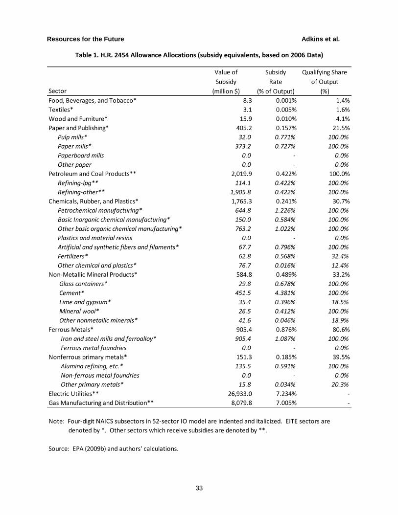
Resources for the Future Adkins et al.
33
Table 1. H.R. 2454 Allowance Allocations (subsidy equivalents, based on 2006 Data)
Value of Subsidy Qualifying Share
Subsidy Rate of Output
Sector (million $) (% of Output) (%)
Food, Beverages, and Tobacco* 8.3 0.001% 1.4%
Textiles* 3.1 0.005% 1.6%
Wood and Furniture* 15.9 0.010% 4.1%
Paper and Publishing* 405.2 0.157% 21.5%
Pulp mills* 32.0 0.771% 100.0%
Paper mills* 373.2 0.727% 100.0%
Paperboard mills 0.0 - 0.0%
Other paper 0.0 - 0.0%
Petroleum and Coal Products** 2,019.9 0.422% 100.0%
Refining-lpg** 114.1 0.422% 100.0%
Refining-other** 1,905.8 0.422% 100.0%
Chemicals, Rubber, and Plastics* 1,765.3 0.241% 30.7%
Petrochemical manufacturing* 644.8 1.226% 100.0%
Basic Inorganic chemical manufacturing* 150.0 0.584% 100.0%
Other basic organic chemical manufacturing* 763.2 1.022% 100.0%
Plastics and material resins 0.0 - 0.0%
Artificial and synthetic fibers and filaments* 67.7 0.796% 100.0%
Fertilizers* 62.8 0.568% 32.4%
Other chemical and plastics* 76.7 0.016% 12.4%
Non-Metallic Mineral Products* 584.8 0.489% 33.2%
Glass containers* 29.8 0.678% 100.0%
Cement* 451.5 4.381% 100.0%
Lime and gypsum* 35.4 0.396% 18.5%
Mineral wool* 26.5 0.412% 100.0%
Other nonmetallic minerals* 41.6 0.046% 18.9%
Ferrous Metals* 905.4 0.876% 80.6%
Iron and steel mills and ferroalloy* 905.4 1.087% 100.0%
Ferrous metal foundries 0.0 - 0.0%
Nonferrous primary metals* 151.3 0.185% 39.5%
Alumina refining, etc.* 135.5 0.591% 100.0%
Non-ferrous metal foundries 0.0 - 0.0%
Other primary metals* 15.8 0.034% 20.3%
Electric Utilities** 26,933.0 7.234% -
Gas Manufacturing and Distribution** 8,079.8 7.005% -
Note: Four-digit NAICS subsectors in 52-sector IO model are indented and italicized. EITE sectors are
denoted by *. Other sectors which receive subsidies are denoted by **.
Source: EPA (2009b) and authors' calculations.
Table 1. H.R. 2454 Allowance Allocations (subsidy equivalents, based on 2006 Data)

Resources for the Future Adkins et al.
34
Table 2. Very-Short-Run Effect of $15/ton CO2 Tax on Industry Output Prices (% change) Table 2. Very-Short-Run Effect of $15/ton CO2 Tax on Industry Output Prices (% change)
Without With
H.R. 2454 H.R. 2454
Sector Subsidies Subsidies
Food 0.98% 0.40%
Textiles 1.56% 0.44%
Apparel 0.52% 0.16%
Wood & Furniture 1.00% 0.42%
Pulp Mills 1.89% 0.21%
Paper Mills 1.96% 0.13%
Paperboard Mills 2.51% 1.12%
Other Paper 1.06% 0.28%
Refining-LPG 22.53% 21.72%
Refining-Other 9.98% 9.19%
Petrochemicals 2.70% 0.52%
Basic Inorganic Chemicals 1.78% 0.13%
Other Basic Organic Chemicals 2.33% 0.40%
Plastics and Material Resins 1.77% 0.76%
Artificial & Synthetic Fibers, Filaments 2.27% 0.16%
Fertilizer 3.05% 0.85%
Other Chemicals & Plastics 1.05% 0.31%
Glass Containers 2.23% 0.00%
Cement 12.65% 6.99%
Lime and Gypsum 6.24% 4.68%
Mineral Wool 1.72% 0.18%
Other Nonmetallic Minerals 1.93% 0.87%
Iron and Steel Mills and Ferroalloys 2.31% 0.19%
Alumina Refining, Primary & Secondary Aluminum 2.50% 0.02%
Ferrous Metal Foundries 1.59% 0.56%
Non-Ferrous Metal Foundries 1.34% 0.28%
Other Primary Metals 1.65% 0.37%
Fabricated Metals 1.12% 0.20%
Machinery 0.83% 0.18%
Computer & Electrical Equipment 0.55% 0.15%
Motor Vehicles 0.98% 0.25%
Other Transportation Equipment 0.65% 0.16%
Miscellaneous Manufacturing 0.64% 0.18%
Agriculture 1.13% 0.60%
Forestry, Fishing, etc 0.42% 0.21%
Oil Mining 16.32% 16.14%
Gas Mining 9.07% 8.90%
Coal Mining 131.96% 131.61%
Other Mining Activities 1.19% 0.75%
Electric Utilities 9.11% 1.73%
Gas Utilities 9.45% 2.23%
Construction 0.72% 0.35%
Trade 0.34% 0.14%
Air Transportation 2.28% 1.74%
Truck Transportation 1.31% 0.90%
Other Transportation 0.81% 0.57%
Information 0.36% 0.12%
Finance and Insurance 0.17% 0.06%
Real Estate and Rental 0.38% 0.11%
Business Services 0.30% 0.13%
Other Services 0.40% 0.14%
Government 0.73% 0.41%
Source: Authors' calculations.
Man
ufac
turi
ng In
dust
ries
No
n-M
anuf
actu
ring
Indu
stri
es
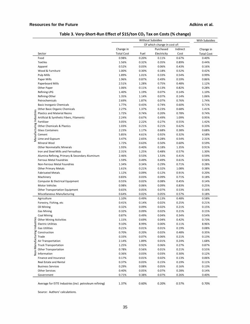
Resources for the Future Adkins et al.
35
Table 3. Very-Short-Run Effect of $15/ton CO2 Tax on Costs (% change) Table 3. Very-Short-Run Effect of $15/ton CO2 Tax on Costs (% change)
With Subsidies
Change in Purchased Indirect Change in
Sector Total Cost Fuel Electricity Cost Total Cost
Food 0.98% 0.20% 0.11% 0.67% 0.40%
Textiles 1.56% 0.32% 0.35% 0.89% 0.44%
Apparel 0.52% 0.03% 0.06% 0.43% 0.16%
Wood & Furniture 1.00% 0.30% 0.18% 0.52% 0.42%
Pulp Mills 1.89% 1.01% 0.33% 0.54% 0.99%
Paper Mills 1.96% 0.87% 0.49% 0.59% 0.86%
Paperboard Mills 2.51% 1.28% 0.75% 0.48% 1.12%
Other Paper 1.06% 0.11% 0.13% 0.82% 0.28%
Refining-LPG 1.40% 1.19% 0.07% 0.14% 1.10%
Refining-Other 1.35% 1.14% 0.07% 0.14% 1.06%
Petrochemicals 2.69% 1.87% 0.07% 0.76% 1.74%
Basic Inorganic Chemicals 1.77% 0.43% 0.74% 0.60% 0.71%
Other Basic Organic Chemicals 2.27% 1.37% 0.23% 0.68% 1.41%
Plastics and Material Resins 1.72% 0.74% 0.20% 0.78% 0.74%
Artificial & Synthetic Fibers, Filaments 2.24% 0.67% 0.49% 1.09% 0.95%
Fertilizer 3.05% 2.22% 0.27% 0.55% 1.42%
Other Chemicals & Plastics 1.03% 0.21% 0.21% 0.62% 0.33%
Glass Containers 2.23% 1.17% 0.68% 0.38% 0.68%
Cement 5.85% 4.61% 0.92% 0.32% 4.58%
Lime and Gypsum 3.47% 2.65% 0.28% 0.54% 2.31%
Mineral Wool 1.72% 0.63% 0.50% 0.60% 0.59%
Other Nonmetallic Minerals 1.93% 0.40% 0.18% 1.35% 0.91%
Iron and Steel Mills and Ferroalloys 2.31% 1.25% 0.48% 0.57% 1.30%
Alumina Refining, Primary & Secondary Aluminum 2.46% 0.53% 1.53% 0.41% 0.59%
Ferrous Metal Foundries 1.59% 0.49% 0.49% 0.61% 0.56%
Non-Ferrous Metal Foundries 1.34% 0.34% 0.29% 0.71% 0.28%
Other Primary Metals 1.61% 0.21% 0.32% 1.08% 0.38%
Fabricated Metals 1.12% 0.09% 0.12% 0.91% 0.20%
Machinery 0.83% 0.03% 0.09% 0.71% 0.18%
Computer & Electrical Equipment 0.55% 0.02% 0.08% 0.45% 0.14%
Motor Vehicles 0.98% 0.06% 0.09% 0.83% 0.25%
Other Transportation Equipment 0.65% 0.05% 0.07% 0.53% 0.16%
Miscellaneous Manufacturing 0.64% 0.02% 0.05% 0.57% 0.18%
Agriculture 1.10% 0.49% 0.13% 0.48% 0.58%
Forestry, Fishing, etc 0.41% 0.14% 0.02% 0.25% 0.21%
Oil Mining 0.32% 0.09% 0.02% 0.21% 0.15%
Gas Mining 0.32% 0.09% 0.02% 0.21% 0.15%
Coal Mining 0.87% 0.49% 0.04% 0.34% 0.54%
Other Mining Activities 1.15% 0.69% 0.04% 0.42% 0.73%
Electric Utilities 9.10% 8.99% 0.00% 0.11% 8.96%
Gas Utilities 0.21% 0.01% 0.01% 0.19% 0.08%
Construction 0.70% 0.20% 0.02% 0.48% 0.35%
Trade 0.33% 0.07% 0.06% 0.21% 0.13%
Air Transportation 2.14% 1.89% 0.01% 0.24% 1.68%
Truck Transportation 1.25% 0.92% 0.06% 0.27% 0.87%
Other Transportation 0.78% 0.56% 0.01% 0.21% 0.55%
Information 0.36% 0.03% 0.03% 0.30% 0.12%
Finance and Insurance 0.17% 0.01% 0.02% 0.13% 0.06%
Real Estate and Rental 0.37% 0.03% 0.15% 0.19% 0.11%
Business Services 0.29% 0.08% 0.05% 0.16% 0.13%
Other Services 0.40% 0.05% 0.07% 0.28% 0.14%
Government 0.71% 0.38% 0.07% 0.26% 0.40%
Average for EITE Industries (incl. petroleum refining) 1.37% 0.60% 0.20% 0.57% 0.70%
Source: Authors' calculations.
Man
ufa
ctur
ing
Ind
ust
ries
No
n-M
anu
fact
urin
g In
du
stri
es
Without Subsidies
Of which change in cost of:
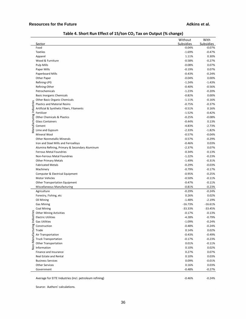
Resources for the Future Adkins et al.
36
Table 4. Short Run Effect of 15/ton CO2 Tax on Output (% change) Table 4. Short Run Effect of 15/ton CO2 Tax on Output (% change)
Without WithSector Subsidies SubsidiesFood -0.04% -0.07%
Textiles -1.69% -0.47%
Apparel 1.11% 0.30%
Wood & Furniture -0.58% -0.27%
Pulp Mills -0.08% 0.07%
Paper Mills -0.19% 0.07%
Paperboard Mills -0.43% -0.24%
Other Paper -0.04% 0.00%
Refining-LPG -1.24% -1.43%
Refining-Other -0.40% -0.56%
Petrochemicals -1.23% -0.20%
Basic Inorganic Chemicals -0.82% 0.00%
Other Basic Organic Chemicals -1.11% -0.16%
Plastics and Material Resins -0.75% -0.37%
Artificial & Synthetic Fibers, Filaments -0.51% 0.16%
Fertilizer -1.52% -0.42%
Other Chemicals & Plastics -0.25% -0.08%
Glass Containers -0.44% 0.13%
Cement -4.83% -2.73%
Lime and Gypsum -2.33% -1.82%
Mineral Wool -0.57% -0.04%
Other Nonmetallic Minerals -0.57% -0.29%
Iron and Steel Mills and Ferroalloys -0.46% 0.03%
Alumina Refining, Primary & Secondary Aluminum -2.37% 0.07%
Ferrous Metal Foundries -0.34% -0.13%
Non-Ferrous Metal Foundries -1.22% -0.23%
Other Primary Metals -1.49% -0.31%
Fabricated Metals -0.29% -0.03%
Machinery -0.79% -0.17%
Computer & Electrical Equipment -0.95% -0.25%
Motor Vehicles -0.50% -0.11%
Other Transportation Equipment -0.47% -0.11%
Miscellaneous Manufacturing -0.81% -0.23%
Agriculture -0.29% -0.24%
Forestry, Fishing, etc 0.26% 0.02%
Oil Mining -1.48% -2.19%
Gas Mining -16.73% -16.61%
Coal Mining -33.33% -33.45%
Other Mining Activities -0.17% -0.13%
Electric Utilities -4.28% -0.79%
Gas Utilities -1.09% -0.24%
Construction -0.48% -0.24%
Trade 0.14% 0.02%
Air Transportation -0.43% -0.49%
Truck Transportation -0.17% -0.23%
Other Transportation 0.01% -0.11%
Information 0.10% 0.02%
Finance and Insurance 0.27% 0.07%
Real Estate and Rental 0.10% 0.03%
Business Services 0.09% -0.01%
Other Services 0.16% 0.03%
Government -0.48% -0.27%
Average for EITE Industries (incl. petroleum refining) -0.46% -0.24%
Source: Authors' calculations.
Man
ufa
ctur
ing
Ind
ust
ries
No
n-M
anu
fact
urin
g In
du
stri
es
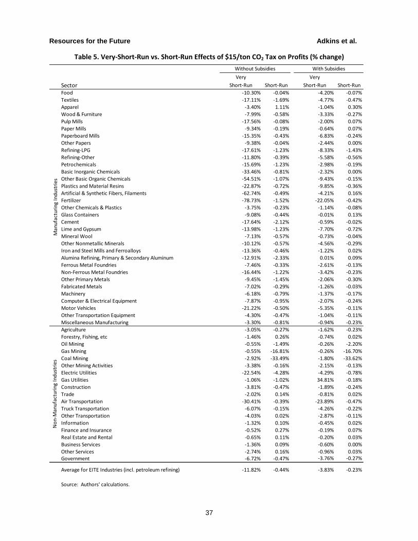
Resources for the Future Adkins et al.
37
Table 5. Very-Short-Run vs. Short-Run Effects of $15/ton CO2 Tax on Profits (% change) Table 5. Very-Short-Run vs. Short-Run Effects of $15/ton CO2 Tax on Profits (% change)
Very Very
Sector Short-Run Short-Run Short-Run Short-Run
Food -10.30% -0.04% -4.20% -0.07%
Textiles -17.11% -1.69% -4.77% -0.47%
Apparel -3.40% 1.11% -1.04% 0.30%
Wood & Furniture -7.99% -0.58% -3.33% -0.27%
Pulp Mills -17.56% -0.08% -2.00% 0.07%
Paper Mills -9.34% -0.19% -0.64% 0.07%
Paperboard Mills -15.35% -0.43% -6.83% -0.24%
Other Papers -9.38% -0.04% -2.44% 0.00%
Refining-LPG -17.61% -1.23% -8.33% -1.43%
Refining-Other -11.80% -0.39% -5.58% -0.56%
Petrochemicals -15.69% -1.23% -2.98% -0.19%
Basic Inorganic Chemicals -33.46% -0.81% -2.32% 0.00%
Other Basic Organic Chemicals -54.51% -1.07% -9.43% -0.15%
Plastics and Material Resins -22.87% -0.72% -9.85% -0.36%
Artificial & Synthetic Fibers, Filaments -62.74% -0.49% -4.21% 0.16%
Fertilizer -78.73% -1.52% -22.05% -0.42%
Other Chemicals & Plastics -3.75% -0.23% -1.14% -0.08%
Glass Containers -9.08% -0.44% -0.01% 0.13%
Cement -17.64% -2.12% -0.59% -0.02%
Lime and Gypsum -13.98% -1.23% -7.70% -0.72%
Mineral Wool -7.13% -0.57% -0.73% -0.04%
Other Nonmetallic Minerals -10.12% -0.57% -4.56% -0.29%
Iron and Steel Mills and Ferroalloys -13.36% -0.46% -1.22% 0.02%
Alumina Refining, Primary & Secondary Aluminum -12.91% -2.33% 0.01% 0.09%
Ferrous Metal Foundries -7.46% -0.33% -2.61% -0.13%
Non-Ferrous Metal Foundries -16.44% -1.22% -3.42% -0.23%
Other Primary Metals -9.45% -1.45% -2.06% -0.30%
Fabricated Metals -7.02% -0.29% -1.26% -0.03%
Machinery -6.18% -0.79% -1.37% -0.17%
Computer & Electrical Equipment -7.87% -0.95% -2.07% -0.24%
Motor Vehicles -21.22% -0.50% -5.35% -0.11%
Other Transportation Equipment -4.30% -0.47% -1.04% -0.11%
Miscellaneous Manufacturing -3.30% -0.81% -0.94% -0.23%
Agriculture -3.05% -0.27% -1.62% -0.23%
Forestry, Fishing, etc -1.46% 0.26% -0.74% 0.02%
Oil Mining -0.55% -1.49% -0.26% -2.20%
Gas Mining -0.55% -16.81% -0.26% -16.70%
Coal Mining -2.92% -33.49% -1.80% -33.62%
Other Mining Activities -3.38% -0.16% -2.15% -0.13%
Electric Utilities -22.54% -4.28% -4.29% -0.78%
Gas Utilities -1.06% -1.02% 34.81% -0.18%
Construction -3.81% -0.47% -1.89% -0.24%
Trade -2.02% 0.14% -0.81% 0.02%
Air Transportation -30.41% -0.39% -23.89% -0.47%
Truck Transportation -6.07% -0.15% -4.26% -0.22%
Other Transportation -4.03% 0.02% -2.87% -0.11%
Information -1.32% 0.10% -0.45% 0.02%
Finance and Insurance -0.52% 0.27% -0.19% 0.07%
Real Estate and Rental -0.65% 0.11% -0.20% 0.03%
Business Services -1.36% 0.09% -0.60% 0.00%
Other Services -2.74% 0.16% -0.96% 0.03%Government -6.72% -0.47% -3.76% -0.27%
Average for EITE Industries (incl. petroleum refining) -11.82% -0.44% -3.83% -0.23%
Source: Authors' calculations.
Man
ufac
turi
ng In
dust
ries
No
n-M
anuf
actu
ring
Indu
stri
es
With SubsidiesWithout Subsidies

Resources for the Future Adkins et al.
38
Table 6. Short-, Medium-, and Long-Run Effects of a $15/ton CO2 Tax on Output (% change) Table 6. Short-, Medium-, and Long-Run Effects of a $15/ton CO2 Tax on Output (% change)
Sector Short-Run Medium-Run Long-Run Short-Run Medium-Run Long-Run
Food, Beverages, and Tobacco -0.04 0.02 -0.10 -0.07 0.16 0.04
Textiles -1.69 -0.31 -0.31 -0.47 -0.10 -0.12
Wearing Apparel and Leather 1.11 0.23 0.18 0.30 0.26 0.20
Wood -0.58 -0.31 -0.32 -0.27 -0.29 -0.31
Paper and Publishing -0.11 -0.18 -0.24 -0.01 0.20 0.13
Petroleum and Coal Products -0.44 -2.61 -3.27 -0.61 -1.89 -2.51
Chemicals, Rubber, and Plastics -0.50 -1.55 -1.52 -0.12 -0.46 -0.45
Non-Metallic Mineral Products -1.06 -1.07 -0.97 -0.59 -0.28 -0.19
Ferrous Metals -0.44 -1.00 -0.63 0.00 0.61 0.96
Nonferrous primary metals -1.69 -1.90 -1.35 -0.19 0.40 0.91
Fabricated Metal Products -0.29 -0.37 -0.28 -0.03 -0.16 -0.09
Transportation Equipment -0.49 -0.17 -0.18 -0.11 -0.11 -0.13
Electronic equipment -0.95 -0.20 -0.03 -0.25 -0.23 -0.08
Machinery -0.79 -0.12 0.08 -0.17 -0.17 0.00
Other Manufacturing -0.81 -0.12 0.22 -0.23 -0.10 0.19
Agriculture -0.29 0.06 -0.02 -0.24 0.01 -0.07
Coal -33.33 -13.86 -16.47 -33.45 -11.78 -14.25
Oil mining -1.48 -1.33 -1.93 -2.19 -1.22 -1.93
Gas mining -16.73 -2.48 -3.58 -16.61 -2.45 -3.49
Other Minerals -0.17 -0.99 -0.81 -0.13 -0.15 0.01
Electric Utilities -4.28 -3.81 -4.32 -0.79 0.69 0.18
Gas manuf. and distribution -1.09 -3.27 -3.48 -0.24 -0.83 -1.04
Construction -0.48 -0.36 -0.40 -0.24 -0.33 -0.37
Trade 0.14 0.05 -0.07 0.02 0.24 0.12
Transportation Services -0.13 -1.26 -1.54 -0.22 -1.05 -1.32
Communications 0.10 0.16 0.05 0.02 0.30 0.18
Finance and Insurance 0.27 0.14 0.01 0.07 0.27 0.14
Services (inc real estate) 0.12 0.02 -0.08 0.02 0.07 -0.02
Owner-occupied Dwellings - 0.49 0.28 - 0.77 0.57
Average for EITE Inudstries (incl. petroleum refining) -0.45 -0.90 -0.96 -0.19 -0.25 -0.31
Source: Author's calculations.
Without Subsidies With SubsidiesM
anuf
actu
ring
Indu
stri
esN
on-
Man
ufac
turi
ng In
dust
ries

Resources for the Future Adkins et al.
39
Table 7. Decomposition of Medium-Run Effects of a $15/ton CO2 Tax on Output (% change)
Table 7. Decomposition of Medium-Run Effects of a $15/ton CO2 Tax on Output (% change)
Base Case
Domestic
Consumption Δ in Δ in Δ in Δ in Δ in Δ in Δ in Δ in
Sector (billion $) Output Use Exports Imports Output Use Exports Imports
Food, Beverages, and Tobacco 685 0.02 0.06 -0.01 0.03 0.16 0.23 -0.02 0.05
Textiles 147 -0.31 -0.14 -0.06 0.12 -0.10 0.09 -0.04 0.15
Wearing Apparel and Leather 159 0.23 0.33 0.03 0.13 0.26 0.72 -0.01 0.45
Wood 275 -0.31 -0.34 0.01 -0.03 -0.29 -0.23 -0.01 0.05
Paper and Publishing 394 -0.18 -0.11 -0.05 0.02 0.20 0.17 0.02 -0.01
Petroleum and Coal Products 310 -2.61 -2.26 -0.34 0.01 -1.89 -1.67 -0.25 -0.03
Chemicals, Rubber, and Plastics 733 -1.55 -0.55 -0.79 0.21 -0.46 -0.09 -0.33 0.04
Non-Metallic Mineral Products 123 -1.07 -0.47 -0.28 0.33 -0.28 -0.24 -0.04 0.00
Ferrous Metals 150 -1.00 -0.48 -0.26 0.27 0.61 -0.10 0.32 -0.39
Nonferrous primary metals 117 -1.90 -0.75 -0.84 0.32 0.40 -0.01 0.10 -0.31
Fabricated Metal Products 303 -0.37 -0.33 -0.03 0.01 -0.16 -0.19 0.01 -0.02
Transportation Equipment 766 -0.17 -0.22 0.02 -0.03 -0.11 -0.05 0.00 0.06
Electronic equipment 561 -0.20 -0.26 -0.01 -0.07 -0.23 -0.18 -0.05 0.00
Machinery 863 -0.12 -0.41 0.12 -0.17 -0.17 -0.25 0.02 -0.06
Other Manufacturing 116 -0.12 0.16 0.00 0.28 -0.10 0.50 -0.10 0.50
Agriculture 245 0.06 -0.01 0.07 0.00 0.01 0.08 -0.04 0.04
Coal 39 -13.86 -15.90 1.44 -0.61 -11.78 -12.99 0.72 -0.48
Oil mining 202 -1.33 -7.59 0.00 -6.26 -1.22 -5.51 0.00 -4.30
Gas mining 36 -2.48 -4.71 6.51 4.28 -2.45 -3.05 6.19 5.59
Other Minerals 32 -0.99 -0.99 -0.11 -0.11 -0.15 -0.17 -0.03 -0.05
Electric Utilities 301 -3.81 -3.73 -0.09 0.00 0.69 0.66 0.03 0.00
Gas manuf. and distribution 86 -3.27 -3.26 -0.01 0.00 -0.83 -0.88 0.04 0.00
Construction 1,390 -0.36 -0.36 0.00 0.00 -0.33 -0.33 0.00 0.00
Trade 2,420 0.05 0.04 0.00 0.00 0.24 0.24 0.00 0.00
Transportation Services 789 -1.26 -0.74 -0.34 0.18 -1.05 -0.46 -0.37 0.22
Communications 437 0.16 0.15 0.01 0.00 0.30 0.30 0.00 0.01
Finance and Insurance 1,728 0.14 0.11 0.02 -0.01 0.27 0.28 0.00 0.01
Services (inc real estate) 6,567 0.02 0.01 0.01 0.00 0.07 0.09 -0.01 0.01
Owner-occupied Dwellings 1,188 0.49 0.49 0.00 0.00 0.77 0.77 0.00 0.00
Average for EITE Industries (incl. petroleum refining) -0.90 -0.49 -0.30 0.11 -0.25 -0.16 -0.10 0.00
Source: Author's calculations.
With H.R. 2454 Subsidies
Contribution (ΔQ=ΔU+ΔX-ΔM):
Man
ufa
ctur
ing
Ind
ust
ries
No
n-M
anu
fact
urin
g In
du
stri
esWithout H.R. 2454 Subsidies
Contribution (ΔQ=ΔU+ΔX-ΔM):

Resources for the Future Adkins et al.
40
Table 8. Decomposition of Long-Run Effects of a $15/ton CO2 Tax on Output (% change)
Table 8. Decomposition of Long-Run Effects of a $15/ton CO2 Tax on Output (% change)
Base Case
Domestic
Consumption Δ in Δ in Δ in Δ in Δ in Δ in Δ in Δ in
Sector (billion $) Output Use Exports Imports Output Use Exports Imports
Food, Beverages, and Tobacco 685 -0.10 -0.09 -0.01 0.01 0.04 0.09 -0.02 0.03
Textiles 147 -0.31 -0.24 -0.06 0.01 -0.12 -0.02 -0.04 0.06
Wearing Apparel and Leather 159 0.18 0.01 0.03 -0.13 0.20 0.42 -0.01 0.21
Wood 275 -0.32 -0.43 0.01 -0.10 -0.31 -0.32 0.00 -0.01
Paper and Publishing 394 -0.24 -0.21 -0.04 -0.01 0.13 0.06 0.03 -0.04
Petroleum and Coal Products 310 -3.27 -2.94 -0.40 -0.07 -2.51 -2.30 -0.31 -0.10
Chemicals, Rubber, and Plastics 733 -1.52 -0.67 -0.72 0.13 -0.45 -0.20 -0.27 -0.03
Non-Metallic Mineral Products 123 -0.97 -0.51 -0.23 0.23 -0.19 -0.29 0.01 -0.09
Ferrous Metals 150 -0.63 -0.33 -0.16 0.13 0.96 0.03 0.42 -0.51
Nonferrous primary metals 117 -1.35 -0.50 -0.68 0.18 0.91 0.21 0.25 -0.45
Fabricated Metal Products 303 -0.28 -0.34 0.00 -0.05 -0.09 -0.21 0.04 -0.08
Transportation Equipment 766 -0.18 -0.37 0.05 -0.14 -0.13 -0.19 0.02 -0.04
Electronic equipment 561 -0.03 -0.27 0.06 -0.18 -0.08 -0.20 0.01 -0.11
Machinery 863 0.08 -0.48 0.26 -0.29 0.00 -0.32 0.14 -0.18
Other Manufacturing 116 0.22 -0.19 0.16 -0.25 0.19 0.17 0.04 0.02
Agriculture 245 -0.02 -0.10 0.05 -0.02 -0.07 0.00 -0.05 0.02
Coal 39 -16.47 -17.35 0.35 -0.53 -14.25 -14.72 0.03 -0.44
Oil mining 202 -1.93 -9.43 0.00 -7.50 -1.93 -7.22 0.00 -5.29
Gas mining 36 -3.58 -8.05 1.36 -3.11 -3.49 -6.60 1.08 -2.03
Other Minerals 32 -0.81 -0.88 -0.09 -0.15 0.01 -0.07 -0.01 -0.09
Electric Utilities 301 -4.32 -4.23 -0.09 0.00 0.18 0.15 0.03 0.00
Gas manuf. and distribution 86 -3.48 -3.47 0.00 0.00 -1.04 -1.09 0.05 0.00
Construction 1,390 -0.40 -0.41 0.00 0.00 -0.37 -0.37 0.00 0.00
Trade 2,420 -0.07 -0.08 0.00 -0.01 0.12 0.12 0.00 0.00
Transportation Services 789 -1.54 -0.96 -0.39 0.18 -1.32 -0.68 -0.42 0.23
Communications 437 0.05 0.02 0.02 -0.01 0.18 0.18 0.01 0.00
Finance and Insurance 1,728 0.01 -0.02 0.02 -0.01 0.14 0.15 0.00 0.00
Services (inc real estate) 6,567 -0.08 -0.10 0.01 -0.01 -0.02 -0.01 -0.01 0.00
Owner-occupied Dwellings 1,188 0.28 0.28 0.00 0.00 0.57 0.57 0.00 0.00
Average for EITE Industries (incl. petroleum refining) -0.96 -0.64 -0.28 0.04 -0.31 -0.30 -0.07 -0.06
Source: Author's calculations.
No
n-M
anuf
actu
ring
Indu
stri
esM
anuf
actu
ring
Indu
stri
esWithout H.R. 2454 Subsidies With H.R. 2454 Subsidies
Contribution (ΔQ=ΔU+ΔX-ΔM): Contribution (ΔQ=ΔU+ΔX-ΔM):

Resources for the Future Adkins et al.
41
Table 9. Decomposition of Long-Run Emissions Leakage Due to a $15 ton CO2 Tax (1000 tons)
Table 9. Long-run Industry CO2 Emissions Leakage resulting from a $15 ton CO2 Tax (1000 tons)
Change in Higher Lower Change in Leakage
U.S. CO2 Exports Imports Carbon Intensity Rate
Sector Emissions to U.S. from U.S. Differential Total (%)
Food, Beverages, and Tobacco -17,241 -8 0 -3 -11 -0.1
Textiles -3,639 4 11 -5 10 0.3
Wearing Apparel and Leather -1,448 -26 -3 2 -27 -1.9
Wood -4,627 -43 -3 -33 -79 -1.7
Paper and Publishing -24,537 27 43 52 121 0.5
Petroleum and Coal Products -10,495 1,125 647 1,074 2,846 27.1
Chemicals, Rubber, and Plastics -51,630 1,155 1,419 3,196 5,770 11.2
Non-Metallic Mineral Products -17,187 261 100 701 1,061 6.2
Ferrous Metals -15,843 457 142 586 1,186 7.5
Nonferrous primary metals -14,636 566 254 462 1,283 8.8
Fabricated Metal Products -4,496 -9 -2 -39 -50 -1.1
Transportation Equipment -7,253 -36 -16 -34 -86 -1.2
Electronic equipment -6,484 -89 -15 -18 -122 -1.9
Machinery -8,773 -106 -103 -296 -504 -5.7
Other Manufacturing -1,647 -12 -6 42 24 1.5
Average for EITE Industries (incl. petroleum refining) 8.5
Authors' calculations.
Change in Non-Annex I emissions
Due to:
Man
ufac
turi
ng In
dust
ries

Resources for the Future Adkins et al.
42
Table 10. Long-Run Trade-Related Emissions Leakage Rates Due to a $15/ton CO2 Tax
Table 10. Long-Run Trade-Related Emissions Leakage Rates Due to a $15/ton CO2 Tax
Change in U.S. Change in U.S.
Subsidy Emissions Leakage Emissions Leakage
Rates (1000 tons CO2) Rate (1000 tons CO2) Rate
Food, Beverages, and Tobacco 0.001% -17,241 -0.1% -14,680 0.1%
Textiles 0.005% -3,639 0.3% -2,812 0.7%
Wearing Apparel and Leather 0.000% -1,448 -1.9% -1,114 1.4%
Wood 0.010% -4,627 -1.7% -3,657 -1.5%
Paper and Publishing 0.157% -24,537 0.5% -20,052 -0.1%
Petroleum and Coal Products 0.422% -10,495 27.1% -7,720 34.1%
Chemicals, Rubber, and Plastics 0.241% -51,630 11.2% -40,274 9.2%
Non-Metallic Mineral Products 0.489% -17,187 6.2% -15,087 2.6%
Ferrous Metals 0.876% -15,843 7.5% -10,310 -3.7%
Nonferrous primary metals 0.185% -14,636 8.8% -9,351 3.5%
Fabricated Metal Products 0.000% -4,496 -1.1% -3,504 -2.5%
Transportation Equipment 0.000% -7,253 -1.2% -5,725 -1.0%
Electronic equipment 0.000% -6,484 -1.9% -5,126 -1.3%
Machinery 0.000% -8,773 -5.7% -7,046 -4.7%
Other Manufacturing 0.000% -1,647 1.5% -1,323 6.9%
Average for EITE Industries (incl. petroleum refining) 8.5% 5.3%
Source: Author's calculations.
Without Subsidies With SubsidiesM
anuf
actu
ring
Indu
stri
es

Resources for the Future Adkins et al.
43
Table 11. Long-Run Aggregate Effects of Annex I Carbon Price Policies (% change)
Table 11. Long-Run Aggregate Effects of Annex I Carbon Price Policies (% change)
2004 CO2 Without With
Emissions Subsidies Subsidies
(mil. tons) in U.S. in U.S.
Change in CO2 Emissions
US 6,070 -8.55% -6.77%
Canada 566 -8.43% -8.78%
Mexico 407 0.45% 0.38%
China 4,414 0.48% 0.41%
India 1,059 0.84% 0.77%
Rest of Annex I 7,669 -7.83% -7.87%
Oil Exporters 1,994 1.42% 1.29%
Rest of the World 3,814 1.12% 1.02%
Total 25,994 -4.09% -3.74%
Annex I Leakage Rate (%) 8.80% 8.69%
Decomposition of Change in U.S. Emissions
Industry - Input substitution 62.4% 81.5%
Industry - Output level 24.4% 4.5%
Household 13.3% 13.9%
Decompostion of Change in Non-U.S. Emissions
Industry - Input substitution 74.7% 72.8%
Industry - Output level 6.3% 8.6%
Household 19.0% 18.6%
Source: GTAP 7 data base and authors' calculations.