Carbon-based biosensors

Fortgeschrittenen-Praktikum (Anleitung von: Lucas Hess, Felix Buth)

1. Introduction/abstract

In recent years there have been tremendous efforts to combine biological with electronic systems. The most used semiconductor material, Si, which serves so well in electronics, happens to have rather poor properties when it comes to biological environments. In salty solutions and especially with applied potentials Si becomes easily corroded. This opens the stage for new and seemingly exotic materials: carbon based semiconductors. Carbon is one of the main elements in organic chemistry, which concerns materials ranging from plastic foils to biological systems like enzymes or even cells. Most of these materials are well known for being stable in aqueous environments. Therefore, the use of carbon based semiconductors is a natural choice when it comes to in-electrolyte operation. Furthermore, the chemical similarity between the semiconductor and biological systems facilitates their interfacing. This potentially enables devices which are able to monitor the quality of drinking water and food or more sophisticated ones like implants to monitor the glucose content of blood or even brain implants for deaf or blind people. In the course of this lab class you will investigate solution-gated field-effect transistor (FET) sensors made from graphene and the organic semiconductor sexithiophene (6T). The latter serves as a model system for water stable organic semiconductors. This class of materials attracts a lot of attention since they offer the possibility of low-cost production of large scale and/or flexible devices, which makes them interesting for disposable bio-/chemical sensors. Graphene, which proved to be very stable in the harsh biological environments, is a very promising candidate for in-vivo sensors or to interface living tissue and electronic circuitry. Additionally, graphene has electronic properties which are advantageous for this kind of applications: it features high charge carrier mobilities and a high interfacial capacitance promising a very high sensitivity to electrical or chemical changes in its surrounding. In the lab class the basic properties of these solution-gated transistors will be investigated and compared to the characteristics of the transistors operated with a solid-state gate. Subsequently, the effect of electrolyte properties (pH and total ionic strength) on the transistors will be investigated. The two materials’ performance shall be compared. In a last step, the penicillin concentration of a test solution will be measured.

2. Materials

2.1 Sexithiophene

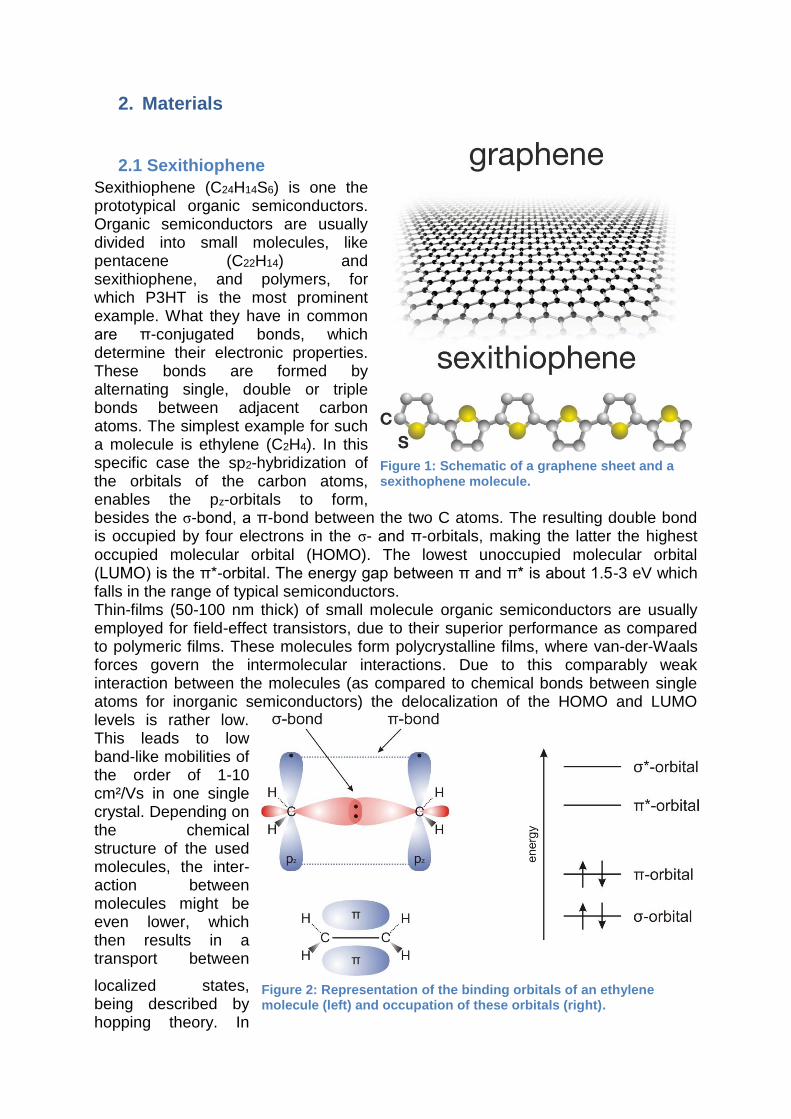
Sexithiophene (C24H14S6) is one the prototypical organic semiconductors. Organic semiconductors are usually divided into small molecules, like pentacene (C22H14) and sexithiophene, and polymers, for which P3HT is the most prominent example. What they have in common are π-conjugated bonds, which determine their electronic properties. These bonds are formed by alternating single, double or triple bonds between adjacent carbon atoms. The simplest example for such a molecule is ethylene (C2H4). In this specific case the sp2-hybridization of the orbitals of the carbon atoms, enables the pz-orbitals to form, besides the σ-bond, a π-bond between the two C atoms. The resulting double bond is occupied by four electrons in the σ- and π-orbitals, making the latter the highest occupied molecular orbital (HOMO). The lowest unoccupied molecular orbital (LUMO) is the π*-orbital. The energy gap between π and π* is about 1.5-3 eV which falls in the range of typical semiconductors. Thin-films (50-100 nm thick) of small molecule organic semiconductors are usually employed for field-effect transistors, due to their superior performance as compared to polymeric films. These molecules form polycrystalline films, where van-der-Waals forces govern the intermolecular interactions. Due to this comparably weak interaction between the molecules (as compared to chemical bonds between single atoms for inorganic semiconductors) the delocalization of the HOMO and LUMO levels is rather low. This leads to low band-like mobilities of the order of 1-10 cm²/Vs in one single crystal. Depending on the chemical structure of the used molecules, the inter-action between molecules might be even lower, which then results in a transport between

localized states, being described by hopping theory. In

Figure 1: Schematic of a graphene sheet and a sexithophene molecule.

Figure 2: Representation of the binding orbitals of an ethylene molecule (left) and occupation of these orbitals (right).

this case, the charge carrier mobility is in the order of 10-5 to 1 cm²/Vs. The grain boundaries present in polycrystalline films might further lower the effective field-effect mobility as extracted from transistor transfer curves. Like most organic semiconductors 6T is a hole conductor, which results from the efficient trapping of electrons by the most common defects encountered in organic semiconductors.

2.2 Graphene

Single layers of sp2 carbon, known as graphene, were experimentally obtained not until 2004. Similar to graphite, the atoms are arranged in a honeycomb lattice. The p-orbitals of the sp2 configuration are oriented perpendicular to the atomic plane and

form a delocalized -bond system (much like in the case of organic semiconductors, however much larger in real space). These delocalized states govern the electronic transport resulting in electronic properties that differ largely from all other known materials. In graphene, the conduction and valence band touch at certain points in k-space, known as Dirac-points which makes graphene a zero-gap semiconductor. Additionally, for both holes and electrons, a linear dispersion relation is observed in the close vicinity of the Dirac point resulting in charge carriers with an effective mass of zero. Therefore, these carriers can be described as quasi-relativistic particles. Due to this, the scattering of the charge carriers is reduced in graphene leading to very high mobilities of several 10.000 cm2/Vs (even up to 2·106 cm2/Vs for freely suspended graphene at low temperatures, typical values for Si: several 100 cm2/Vs). Besides these interesting electronic properties, graphene offers several very advantageous chemical qualities. As it is chemically very stable, it can be used for sensors operating in rather demanding conditions such as biological environments. In addition, it has been shown, that graphene is a rather biocompatible material, making it suitable for biosensor applications.

3. The solid/liquid interface

3.1 A short introduction to electrochemistry

In the lab class the transistors under study will be investigated in aqueous environments in this lab class. Thus, it is necessary to understand the basics of the interface between a solid and an electrolyte solution, which is an ion conductive medium (in our case a water-salt mixture). When bringing an ion in contact with an aqueous solution the water molecules close to the ion will orient themselves according to their dipole moment and the charge of the ion. This leads to an attractive interaction between the ion and the surrounding water molecules and leads to the so-called solvation shell of the ion. The charge carriers in the solid electrode as well as in the electrolyte solution are characterized by their electrochemical potentials 𝜇𝑖

∗, which are sums of their chemical

E k

x

ky

Energy Dispersion

Figure 3: Plot of the energy dispersion of ideal graphene. The inset shows a zoom-in into one of the Dirac points.

𝜇𝑖 and electric potentials φ. The electrochemical potentials correspond to the energy that is necessary to bring an additional charge carrier from the force-free state into the system (at constant pressure and temperature). As the electrolyte solution consists of positive and negative ions, one can easily imagine that a charged electrode in the solution will lead to an accumulation of the ionic species with a charge opposite to that of the electrode. The distribution of ions at the interface is as follows. Directly adsorbed at the electrode surface, and therefore without their solvation shell, are the ions forming the inner Helmholtz plane (IHP). These specifically adsorbed ions may be of any charge regardless of the charge of the electrode. In the outer Helmholtz

plane (OHP) one finds the ions constituting the counter charge to the electrode charge. They are not specifically adsorbed and therefore retain their solvation shell, which limits their closest approach to the electrode surface. Towards the bulk of the electrolyte follows the diffuse layer, where charge compensation in the electrolyte takes place. So far we did not account for chemical reactions that might occur in the electrolyte, or to chemical groups attached to the surface of the electrode. One typical class of reactions that are quite commonly encountered in electrochemistry is the redox reaction of the type:

𝑂𝑥 + 𝑒− ↔ 𝑅𝑒𝑑 (1) where the species Ox is reduced to Red or vice versa with the help of an electron. By changing the electronic potential of the electrode with respect to the electrolyte via an external voltage source, one can adjust the electrochemical potential of the electrons in the electrode such that it becomes favorable for an electron to cross the electrode/electrolyte interface and reduce the species Ox to Red. Typical examples in aqueous based electrolytes would be the generation of hydrogen and oxygen via the

following reactions: 𝐻3𝑂+ + 𝑒− ↔ 𝐻2 + 𝐻2𝑂 and 𝑂2 + 2𝐻2𝑂 + 4𝑒− ↔ 4𝑂𝐻−. Since the

redox reactions change the charge state of a species, the electrochemical potential of the redox couple (being the sum of the chemical and electric potential) depends on the concentrations of the reduced and oxidized species. The electric potential φ is described by the Nernst equation:

Figure 4: Schematic of the Helmholtz model of the solid-liquid interface.

𝜑 = 𝜑00 +𝑅𝑇

𝑧𝐹𝑙𝑛

𝑎𝑜𝑥

𝑎𝑟𝑒𝑑 (2)

with R being the gas constant, z the valency of the ions, F the Faraday constant, T the temperature and φ00 is the potential at standard conditions. a stands for the activity of the relevant species and is an adjustment to the concentration of the species in order to accompany for the force a particle feels due to other particles present. For infinitely diluted solutions the activity approaches the concentration. The Faraday constant F is the product of elementary charge and Avogardo constant, since the gas constant is the product of Boltzmann constant k and Avogardo constant, the term RT/zF can be written as kT/ze. If we furthermore convert the natural logarithm to a logarithm the base of 10 and insert all constants into the equation we are left with:

𝜑 = 𝜑00 +59𝑚𝑉

𝑧𝑙𝑜𝑔

𝑎𝑜𝑥

𝑎𝑟𝑒𝑑 (2b)

3.2 pH-/ion-sensitivity and the site-binding model

The pH-sensitivity of electrodes in contact with a solution is usually described by the site-binding model and the Nernst equation given in Eq. (2). This model assumes that the surface of the electrode contains groups which can be protonated or deprotonated depending on the pH of the electrolyte. A typical example is OH-groups on oxide surfaces. If the surface contains atoms X which are oxidized to X-OH, then these groups can be deprotonated to X-O- or protonated to become X-OH2

+, the pH at which this happens is determined by the Ka value of the surface group defined as:

K𝑎 =[𝐻+]𝑠𝑢𝑟𝑓∙𝑁𝑋−𝑂−

𝑁𝑋−𝑂𝐻 (3)

where NX-O- and NX-OH denote the density of the respective groups on the surface and [H+]surf is the concentration of protons close to the surface. These surface groups can be treated like the redox couple in the previous chapter, with the electric potential φ being the surface potential φ0. The pH close to the electrode surface differs from the bulk pH due to the electrostatic interactions between the positively charged protons and the charge at the electrode’s surface, described by a Boltzmann factor:

[𝐻+]𝑠𝑢𝑟𝑓 = [𝐻+]𝑏𝑢𝑙𝑘exp(−𝑒𝜑0

𝑘𝑇⁄ ) (4)

The charged surface groups give rise to a surface charge density

𝜎𝑠𝑢𝑟𝑓 = 𝑒(𝑁𝑋−𝑂𝐻2+ − 𝑁𝑋−𝑂−) (5)

As previously mentioned the surface charge is usually counter balanced by the ions in the diffuse layer. This charge is for a symmetrical salt (anion and cation have the same valency z) described by the Grahame equation:

𝜎𝑑𝑖𝑓𝑓 = (8𝑘𝑇𝜀0𝜀𝑟𝑐)1/2𝑠𝑖𝑛ℎ(

𝑧𝑒𝜑0

2𝑘𝑇) (6)

with ε0 being the vacuum permittivity and εr the relative permittivity of water, c is the salt concentration (if c is given in mol/L, the value has to be divided by 1000 to

convert from L=dm3 to cm3, in case the charge density is given in Ccm-2). In case of a semiconductor or a metal, we have to consider an additional electronic charge in the electrode σe, which is given by the potential drop over the double-layer capacitance CDL: 𝜎𝑒 = 𝐶𝐷𝐿(𝑈𝐺𝑆 − 𝑈𝐷

𝑇⁄− 𝜑0) (7)

where UGS is the gate voltage and 𝑈𝑇/𝐷 the threshold (6T) or Dirac (graphene)

voltage (which will be discussed in more detail in the following chapter). To ensure overall charge neutrality these charges have to sum up to zero: 𝜎𝑑𝑖𝑓𝑓 + 𝜎𝑠𝑢𝑟𝑓 + 𝜎𝑒 = 0 (8)

For given electrolyte conditions (c and pH=-log[H+]bulk), this set of equations can be numerical solved to obtain φ0 and thus the change in conductivity (given by σeμE) via Eq. 7. Since the surface potential φ0 depends logarithmically on the bulk proton concentration [H+]bulk (see Eq. 4) while the pH is defined as the negative logarithm of the proton concentration, we obtain a linear relation between the surface potential and the pH of the electrolyte. The change of potential with pH is generally used to characterize the pH sensitivity, with a theoretical limit of 59 mV/pH given by the Nernst equation (Eq. 2b). In order to attain this theoretical value the density of the surface bound groups has to be high enough. In addition, the surface charge might have different origins like specific adsorption of certain ions to the surface, as is

the case for the organic films. The general treatment however remains similar as discussed here. The sensitivity of the electrode towards the salt concentration c results from Eqs. 6 and 8. When c is increased, the diffuse charge close to the electrode increases and therefore the electronic charge has to decrease in order to fulfill the charge neutrality condition in Eq. 8, since the pH dependent surface charge σsurf remains constant. In analogy to the pH sensitivity also the ion sensitivity for monovalent salts is usually quantified in mV per decade salt concentration.

4. The ion sensitive field-effect transistor After having discussed the general properties of electrodes in contact with an electrolytic solution we can now focus on the special case where this solution is used to gate a semiconductor-based transistor. If a semiconductor is immersed into an electrolyte solution, a potential can be applied at this electrode versus the vacuum

Figure 5: Plot of the potential distribution (upper part) and the charge distribution (lower part) for a ISFET using a simplified Helmholtz model. The red lines/areas correspond to an electrolyte with higher ionic strength.

level, thereby moving the system (semiconductor in electrolyte solution) out of equilibrium. This means the Fermi level in the semiconductor can be shifted up or down and thereby the carrier density in the semiconductor close to the interface can be modulated. As the number of carriers changes, the conductivity changes as well. This opens the possibility for a transistor gated via an aqueous electrolyte, comparable to standard MOSFET devices. A drain-source voltage is applied between two contacts on the surface of the semiconductor electrode, while the electrolyte solution acts as a gate electrode. The potential of the electrolyte is controlled by an Ag/AgCl reference electrode. Since the

conductivity is also sensitive to changes in pH and ionic strength of the solution, these devices are commonly called ion sensitive field effect

transistor (ISFET). The dependence of the drain-source current 𝐼𝐷𝑆 on the drain-source voltage and the gate voltage is given by

𝐼𝐷𝑆 ≈𝑊

𝐿𝜇𝑛𝑈𝐷𝑆 (9)

µ is the mobility and n the density of the carriers, W and L the width and length of the

conducting channel, and 𝑈𝐷𝑆 the drain-source voltage. The charge carriers’ density n can be estimated by a MOSEFT-like model

𝑛 =𝑞

𝑒𝐶(𝑈𝐺𝑆 −𝑈𝑇/𝐷) (10)

where C is the capacitance of the gate, q/e equals the sign of the charge carriers, 𝑈𝐺𝑆

is the gate voltage, and 𝑈𝑇/𝐷 the threshold (6T) or Dirac (graphene) voltage, which

depends also on the gate/solution interface. For graphene, this equation holds for both electrons and holes and the sum of charge carriers has to be considered. In the case of a MOSFET the capacitance C is the capacitance of the gate dielectric (e.g. SiO2); in the case of an ISFET, the effective capacitance CDL of the electrical double layer, resulting from the series of capacitances of the inner and outer Helmholtz plane. The threshold voltage UT is the voltage were the Fermi level at the semiconductor/electrolyte interface is sufficiently close to the HOMO level or the valence band of an inorganic semiconductor to accumulated a substantial amount of mobile charge carriers for the drain-source current to increase significantly. Since graphene ideally has no bandgap the carrier Fermi level usually lies inside one of the bands and thus a substantial amount of mobile carriers is always present. Only if the Fermi-level is situated at the K-point the conductivity goes through a minimum and the carrier type is changed from holes to electrons or vice versa. The gate voltage necessary to shift the Fermi-level to the K-point is called Dirac voltage UD. Figure 7 depicts exemplary transistor curves for a 6T-based ISFET. The output curve is a plot of the drain-source current against the drain-source voltage for multiple gate voltages (in the example presented in Fig.7a the gate voltage is varied between 0

Figure 6: Schematic of the ISFET layout and wiring.

and -0.7V). Taking from this plot only the current values at a constant drain-source potential (here -50 mV) and plotting them against the gate potential yields the so-called transfer plot (Fig. 7b). For low UGS below the threshold IDS is negligible, if enough carriers are accumulated the transistor starts to turn on and enters a regime where the current is linearly proportional to UGS (following Eq. 9 and 10). The slope of

this line if the so-called transconductance 𝑔𝑚 =𝑊

𝐿𝜇𝐶𝑈𝐷𝑆. The intercept of the fit with

the UGS-axis yields the threshold voltage UT.

Figure 7: a) Output characteristic of a 6T-based ISFET. b) According transfer curve, including a fit to the linear region and the resulting threshold voltage.

5. Enzyme-modified ISFETs The surface of ISFETs can be modified by immobilizing enzymes on it. If the chemical reaction catalyzed by these enzymes produces a change in pH, this reaction can also be detected by the FET. That way the remarkable characteristics of enzymes, like their specificity towards certain analytes, can be used to enhance the capabilities of this sensor device. As already mentioned in the introduction, organic thin films can be easily modified with enzymes by simple physisorbtion. In this lab class, we will use penicillinase modified 6T ISFETs to detect penicillin. Penicillinase is an enzyme responsible for the resistance of some bacteria towards the antibiotic penicillin, since it catalyzes the decomposition of penicillin into penicilloic acid and a proton. This proton is locally changing the pH, which is detected by the transistor. Since the relation between the proton concentration and the surface potential is logarithmic we would expect a logarithmic shift of the potential with an increasing penicillin concentration in the electrolyte. However, in reality a linear response is observed for low penicillin concentrations. This results from the fact that the buffer present in the electrolyte counteracts the change in pH, by taking up protons. In addition, the diffusion of

Figure 8: Calibration curve of a penicillinase modified 6T ISFET. The dashed line represents the expected response if the

influence of the buffer is neglected.

penicillin towards the transistor surface and protons away from the surface influence the transistor response. The interplay of these different processes leads to the linear response observed for the conditions present in our measurements.

6. Experimental instructions

6.1 Cyclic voltammetry

Cyclic voltammetry is a standard electrochemical characterization technique, where the voltage of the electrode (in our case the transistor) is cyclically varied between two turnaround potentials. The variation is carried out with a constant speed, the scan speed, and the current through the electrode is recorded. In the case where no charge transfer occurs across the interface, the charge of the electrode is met by an opposite charge across the interface in the electrolyte. This arrangement acts as a capacitor and therefore a change in the potential results in a charging or discharging current. With a constant scan speed the result is a constant current. Draw the cyclic voltammogram (current vs. voltage plot) you would expect for a pure capacitor. How does the electrode response change, when a resistor is connected in parallel? If no charge transfer across the interface contributes to this part of the electrode response, which is referred to as “non-faradaic current”. When there is charge transfer across the interface, the corresponding currents are called “faradaic currents” and are superimposed on the non-faradaic current in a cyclic voltammogram. Such charge transfer happens when components of the electrolyte solution get oxidized or reduced at the interface, because the potential of the electrode is above or below the electrochemical potential of this component. This happens according to the discussed Nernst equation. Assuming a redox couple in the solution with a certain ratio of oxidized versus reduced species and in equilibrium with the electrode, a shift of the electrode potential to higher values will lead to a oxidation of the reduced state, producing more oxidized species until the system is in equilibrium again. Both parts of the electrode response (faradaic and non-faradaic current) can be qualitatively and quantitatively analyzed to yield parameters such as reaction potentials, reaction constants or the double layer capacitance. In the case of the transistor we can use this technique to analyze the potential window (potential interval) in which the gate voltage applied to the transistor causes no current to flow across the semiconductor/electrolyte interface. Such currents correspond to leakage currents across the gate dielectric in conventional MOSFETs. Sweep the potential between the transistor and the electrolyte from +0.5 V to -0.7 V (gate electrode vs. source and drain electrode). For this purpose, short-circuit the source and drain electrodes of the transistor and set them to ground, while applying the potential to the electrode. This is in contrast to the standard electrochemical convention, but is more suitable for the transistor context necessary here. Conduct this measurement for both transistors with scan rates of 10, 50 and 200 mV/s in 75 ml PBS buffer.

6.2 Transistor characterization

Use the computer connected to the source meters to scan the transistor current. Use gate voltages between -0.5 V and +0.5 V with steps of 50 mV and drain-source voltages between -0.1 V and +0.1 V and steps of 10mV for the graphene devices. For the 6T devices, use gate voltages between 0 V and -0.7 V with steps of 20 mV and drain-source voltages between 0V and -0.2 V with steps of 10 mV for the 6T devices. The gate voltage is applied between the reference electrode and the source contact.

6.3 Ion sensitivity

Adjust the ion concentration of the electrolyte by adding small amounts of a 3 M KCl solution, while monitoring the current of the two devices. Concentrations of 5 mM, 10 mM, 20 mM, 50 mM, 100 mM, 200 mM will be tested. Use a source-drain voltage of -0.1 V and choose from the transistor characteristics obtained earlier suitable gate voltages for both devices (such that the drain-source current becomes as sensitive as possible to changes in the gate potential). Apply now the gate voltage to the source contact while keeping the reference electrode at ground (this is in contrast to the previous measurements. How do you need to change the wiring and the potential with respect to the previous measurement?). Attention: Calculate the added amounts of KCl solution per volume of the original solution that have to be added in order to obtain desired concentrations before the lab class! The original electrolyte has an ion concentration of 5 mM.

6.4 pH titration Adjust the pH of the electrolyte by adding small amounts of a 1 M KOH solution. You should reach pH between 3 (initial buffer) to 7 in steps of 0.5. Use the same setup and potentials as in 6.3. Attention: The change of pH is not linear to the amount of KOH added. Start with small amounts at each step. Increase the amount only after analyzing the response of the electrolyte’s pH to the added solution.

6.5 Penicillin sensing Using a penicillinase modified 6T sample and the corresponding untreated reference sample, measure the transistor curves as done in 6.2. in 0.5 mM Na-based PBS buffer solution at pH 7. Afterwards, measure the transistor curves with the same parameters in the test solution and determine the penicillin content of the test solution.

7. Evaluation

7.1 Cyclic voltammograms

Plot the cyclic voltammograms and compare the potential windows (potential interval where no Faradaic currents occur) of the 6T and the graphene transistors. Calculate the double layer capacitance of the two different materials. The dimensions (W/L) are 30x40 µm² in the case of the graphene devices and 98000x20 µm² for the 6T devices.

7.2 Transistor characteristics

Plot the source drain current versus the applied source-drain voltage for different gate voltages. Describe and explain the qualitative differences. Plot for the drain source voltage of -0.1 V the transconductance gm (derivative of Ids with respect to Ugs) against Ug. Calculate the mobility from gm of both devices using equations (9) and (10) and the capacitance calculated in 7.1.

7.3 Sensitivity to the ionic strength and the pH of the electrolyte

Plot the current vs. the salt concentration and the pH (for the salt concentration use a scale corresponding to the one used in the current vs. pH plot). Explain the behavior of the device upon a variation of the salt concentration and extract from the ion sensitivity measurements the sign of the surface charge. Use the transconductance (from 7.2) to calculate the pH sensitivity in mV/pH and compare the obtained values to the theoretical limit.

7.4 Penicillin sensing

Use the calibration curve in Fig. 8 to estimate the penicillin concentration in the test solution. Take into account, that the pH and the salt concentration of the test solution are also unknown.

Further reading:

Organic semiconductors:

- M.Pope and C.E. Swenberg, Electronic Processes in Organic Crystals and Polymers, Oxford University Press, New York, Oxford 1999.

- H. Klauk, Organic Electronics: Materials, Manufacturing and Applications, Wiley-VCH, Weinheim, 2006

Graphene:

- A. K. Geim, K. S. Novoselov, Nature Materials 2007, 6, 183 – 191 - A.H. Castro Neto, F. Guinea, N.M.R. Peres, K.S. Novoselov, A.K. Geim,

Reviews of Modern Physics 2009, 81, 109-162 Electrochemistry:

- A. J. Bard, L. R. Faulkner, Electrochemical methods and applications, Wiley-Interscience, New York, London 2000.

ISFETs:

- M. J. Schöning, A. Poghossian, Analyst 2002, 127, 1137. - P. Fromherz, Phys. Status Solidi A 2012, DOI: 10.1002/pssa.201127766