capturing and predicting the integration process of an
TRANSCRIPT

Capturing and Predicting theIntegration Process of an Embedded
Software Company
Improving and automating a maturity-, progression- and feasibility
model
Martijn Reijerse


Capturing and Predicting theIntegration Process of an Embedded
Software Company
THESIS
submitted in partial fulfillment of therequirements for the degree of
MASTER OF SCIENCE
in
COMPUTER SCIENCE
by
Martijn Reijerseborn in Gouda, the Netherlands
Software Engineering Research GroupDepartment of Software TechnologyFaculty EEMCS, Delft University of TechnologyDelft, the Netherlandswww.ewi.tudelft.nl
TomTom International B.V.Integration Department
Oosterdoksstraat 114Amsterdam, the Netherlands
www.tomtom.nl

c© 2010 Martijn Reijerse. Cover picture: Customized PND.

Capturing and Predicting theIntegration Process of an Embedded
Software Company
Author: Martijn ReijerseStudent id: 1263137Email: [email protected]
Abstract
In 2009 TomTom developed a model, called the MFM-model, which should re-flect the maturity, feasibility and progression of a Personal Navigation Device softwareintegration project. However, this model did not reflect all required aspects of the in-tegration project and therefore was unable to correctly reflect the maturity, feasibilityor progression. Furthermore, creating and maintaining this model proved to be tootime-consuming. In this thesis we identify the problems of this model, propose a num-ber of improvements to eliminate this problems and explain how these improvementshave been implemented. In addition, we discuss how the model can be automaticallygenerated from Jira and Perforce in order to reduce the required effort for creatingand maintaining it. As an end result, this thesis will deliver a MFM 2.0 prototypewhich is an automated and improved version of the initial model. We will review thisprototype by comparing survey-results taken at the initial situation and the improvedsituation. To further inspect this prototype, a small case-study is performed to analyzethe accuracy, usage and importance of it.
Thesis Committee:
Chair: Prof. Dr. A. van Deursen, Faculty EEMCS, TU DelftUniversity supervisor: Prof. Dr. Ir. R. van Solingen, Faculty EEMCS, TU DelftCompany supervisor: Mr. J. Santiago-Nunez, TomTom International B.V.Committee Member: Dr. Ir. M.F.W.H.A. Janssen, Faculty TBM, TU Delft


Preface
This thesis is the final work of my Masters study Computer Science at the Delft Universityof Technology. It was conducted between February 2010 and October 2010 in collaborationwith TomTom. The graduation project that is described in this thesis has been a valuableexperience for me. It provided me with insights on project management and has widenedmy view on embedded software development.
I would like to express my gratitude to everybody who contributed to this thesis. In thefirst place I would like to thank Rini van Solingen, my daily supervisor, for supporting methroughout this graduation project. I would also like to thank Kevin Dullemond and Benvan Gameren for their critical, but extremely useful, feedback on this thesis.
A special thanks goes to TomTom for providing me with this opportunity. More in par-ticular, I would like to thank Jose Santiago-Nunez and Shay Perlstein for their support andvaluable insights during this project. They really helped me to feel at home at TomTomand were always willing to help in case I needed them. In addition, I would like to thankthe involved persons from the integration department for their valuable ideas and trust in me.
At last, I would like to say a special thanks to my parents, my sister and my girlfriendfor supporting me and helping me to take my mind off things every once in a while.
Martijn ReijerseAmsterdam, the Netherlands
September 24, 2010
iii


Contents
Preface iii
Contents v
List of Figures ix
List of Tables xi
I Introduction 1
1 Introduction 31.1 Context . . . . . . . . . . . . . . . . . . . . . . . . . . . . . . . . . . . . 31.2 Problem Description . . . . . . . . . . . . . . . . . . . . . . . . . . . . . 41.3 Goal, Research Questions and Approach . . . . . . . . . . . . . . . . . . . 41.4 Relevance for TomTom and TU-Delft . . . . . . . . . . . . . . . . . . . . 61.5 Thesis Overview . . . . . . . . . . . . . . . . . . . . . . . . . . . . . . . 7
II Current situation & observation 9
2 Current Situation 112.1 Organization . . . . . . . . . . . . . . . . . . . . . . . . . . . . . . . . . . 112.2 Development process . . . . . . . . . . . . . . . . . . . . . . . . . . . . . 122.3 Tooling . . . . . . . . . . . . . . . . . . . . . . . . . . . . . . . . . . . . 152.4 MFM model . . . . . . . . . . . . . . . . . . . . . . . . . . . . . . . . . . 162.5 Analysis of current situation . . . . . . . . . . . . . . . . . . . . . . . . . 18
3 T0 Measurement 213.1 Approach . . . . . . . . . . . . . . . . . . . . . . . . . . . . . . . . . . . 213.2 Findings . . . . . . . . . . . . . . . . . . . . . . . . . . . . . . . . . . . . 23
v

CONTENTS
3.3 Additional problems . . . . . . . . . . . . . . . . . . . . . . . . . . . . . 293.4 Validity . . . . . . . . . . . . . . . . . . . . . . . . . . . . . . . . . . . . 30
III Proposed solution 31
4 Improvements 334.1 Prerequisites for improving and automating the model . . . . . . . . . . . . 334.2 CMMI & Taking measurements . . . . . . . . . . . . . . . . . . . . . . . 344.3 Identifying additional improvements . . . . . . . . . . . . . . . . . . . . . 354.4 Proposed improvements . . . . . . . . . . . . . . . . . . . . . . . . . . . . 37
5 Proposed solution 395.1 Understanding the integration process . . . . . . . . . . . . . . . . . . . . 395.2 Predicting and controlling the integration process . . . . . . . . . . . . . . 455.3 Improving the integration process . . . . . . . . . . . . . . . . . . . . . . 555.4 Improved MFM 2.0 proposal . . . . . . . . . . . . . . . . . . . . . . . . . 55
6 Prototype of MFM 2.0 576.1 Overall System . . . . . . . . . . . . . . . . . . . . . . . . . . . . . . . . 576.2 Data Sources Layer . . . . . . . . . . . . . . . . . . . . . . . . . . . . . . 586.3 Data Processing Layer . . . . . . . . . . . . . . . . . . . . . . . . . . . . 616.4 Data Presentation Layer . . . . . . . . . . . . . . . . . . . . . . . . . . . . 686.5 Testing . . . . . . . . . . . . . . . . . . . . . . . . . . . . . . . . . . . . . 74
7 Evaluation 797.1 MFM Goals Reviewed . . . . . . . . . . . . . . . . . . . . . . . . . . . . 797.2 T1 Measurement . . . . . . . . . . . . . . . . . . . . . . . . . . . . . . . 807.3 Reliability of Predictions . . . . . . . . . . . . . . . . . . . . . . . . . . . 847.4 Review of a single project . . . . . . . . . . . . . . . . . . . . . . . . . . . 877.5 Overall Evaluation . . . . . . . . . . . . . . . . . . . . . . . . . . . . . . 89
IV Conclusions 91
8 Conclusions and Future Work 938.1 Contributions . . . . . . . . . . . . . . . . . . . . . . . . . . . . . . . . . 938.2 Conclusions . . . . . . . . . . . . . . . . . . . . . . . . . . . . . . . . . . 948.3 Discussion/Reflection . . . . . . . . . . . . . . . . . . . . . . . . . . . . . 958.4 Future work . . . . . . . . . . . . . . . . . . . . . . . . . . . . . . . . . . 96
Bibliography 99
A Glossary 103
B Interview Protocol 105
vi

C Detailed results of T0 interview 107
D Detailed results of T1 interview 111
E Entry criteria of internal milestones 115
F Details of MFM Webpages 119
vii


List of Figures
2.1 Organization of involved departments . . . . . . . . . . . . . . . . . . . . . . 122.2 The development milestones within TomTom . . . . . . . . . . . . . . . . . . 122.3 Milestones between TT3 and TT2 . . . . . . . . . . . . . . . . . . . . . . . . 14
4.1 Three purposes of taking measurements . . . . . . . . . . . . . . . . . . . . . 35
5.1 Hierarchy of GQM steps [26] . . . . . . . . . . . . . . . . . . . . . . . . . . . 415.2 Chosen metrics for MFM 2.0 model . . . . . . . . . . . . . . . . . . . . . . . 425.3 Artificial Neural Network . . . . . . . . . . . . . . . . . . . . . . . . . . . . . 485.4 Example rule for RI . . . . . . . . . . . . . . . . . . . . . . . . . . . . . . . . 495.5 CBR Cycle . . . . . . . . . . . . . . . . . . . . . . . . . . . . . . . . . . . . 505.6 Overview of proposed solution . . . . . . . . . . . . . . . . . . . . . . . . . . 56
6.1 Overall System Layout . . . . . . . . . . . . . . . . . . . . . . . . . . . . . . 576.2 Current Setup of Jira . . . . . . . . . . . . . . . . . . . . . . . . . . . . . . . 596.3 New Setup of Jira . . . . . . . . . . . . . . . . . . . . . . . . . . . . . . . . . 596.4 Abstract Class Diagram of MFM data Collector . . . . . . . . . . . . . . . . . 626.5 Database design diagram . . . . . . . . . . . . . . . . . . . . . . . . . . . . . 656.6 MFM Summary Graph During a Project . . . . . . . . . . . . . . . . . . . . . 666.7 MFM Summary Graph of Immature Project . . . . . . . . . . . . . . . . . . . 666.8 MFM Summary Graph of Mature Project . . . . . . . . . . . . . . . . . . . . 676.9 Explanation of Numbers in the MFM-Summary . . . . . . . . . . . . . . . . . 676.10 Zend Framework Structure . . . . . . . . . . . . . . . . . . . . . . . . . . . . 696.11 Use-Case Diagram of Web frontend . . . . . . . . . . . . . . . . . . . . . . . 706.12 Wireframe of Web frontend . . . . . . . . . . . . . . . . . . . . . . . . . . . . 716.13 Regression Prediction Technique . . . . . . . . . . . . . . . . . . . . . . . . . 726.14 Two variants of CBR progress predictions . . . . . . . . . . . . . . . . . . . . 75
7.1 Results of questions 7 to 18 . . . . . . . . . . . . . . . . . . . . . . . . . . . . 827.2 Results of questions 19 to 22 . . . . . . . . . . . . . . . . . . . . . . . . . . . 837.3 Project A at IS milestone . . . . . . . . . . . . . . . . . . . . . . . . . . . . . 88
ix

LIST OF FIGURES
7.4 Project A at IC milestone . . . . . . . . . . . . . . . . . . . . . . . . . . . . . 887.5 Project A at FC milestone . . . . . . . . . . . . . . . . . . . . . . . . . . . . . 89
F.1 MFM Graphical Summary Screenshot . . . . . . . . . . . . . . . . . . . . . . 119F.2 Detailed information of an axis . . . . . . . . . . . . . . . . . . . . . . . . . . 120F.3 Defects per state over time . . . . . . . . . . . . . . . . . . . . . . . . . . . . 121F.4 Defects per type over time . . . . . . . . . . . . . . . . . . . . . . . . . . . . 121F.5 Open time per defects . . . . . . . . . . . . . . . . . . . . . . . . . . . . . . . 122F.6 Regression prediction on defects . . . . . . . . . . . . . . . . . . . . . . . . . 123F.7 Regression prediction on defects for BC / MMT issues . . . . . . . . . . . . . 124F.8 CBR: planned vs realistic . . . . . . . . . . . . . . . . . . . . . . . . . . . . . 125F.9 Details of CBR prediction . . . . . . . . . . . . . . . . . . . . . . . . . . . . 125
x

List of Tables
2.1 Layered product model . . . . . . . . . . . . . . . . . . . . . . . . . . . . . . 14
3.1 Positions of interviewees . . . . . . . . . . . . . . . . . . . . . . . . . . . . . 223.2 Results of questions 1 to 4 . . . . . . . . . . . . . . . . . . . . . . . . . . . . 243.3 Results of questions 5 to 6 . . . . . . . . . . . . . . . . . . . . . . . . . . . . 243.4 Results of questions 7 to 8 . . . . . . . . . . . . . . . . . . . . . . . . . . . . 253.5 Results of questions 9 to 10 . . . . . . . . . . . . . . . . . . . . . . . . . . . . 253.6 Results of questions 11 to 12 . . . . . . . . . . . . . . . . . . . . . . . . . . . 263.7 Results of questions 13 to 14 . . . . . . . . . . . . . . . . . . . . . . . . . . . 263.8 Results of questions 15 to 16 . . . . . . . . . . . . . . . . . . . . . . . . . . . 263.9 Results of questions 17 to 18 . . . . . . . . . . . . . . . . . . . . . . . . . . . 273.10 Results of questions 19 to 22 . . . . . . . . . . . . . . . . . . . . . . . . . . . 273.11 Results of questions 23 to 24 . . . . . . . . . . . . . . . . . . . . . . . . . . . 283.12 Result of question 25 . . . . . . . . . . . . . . . . . . . . . . . . . . . . . . . 293.13 Result of question 26 . . . . . . . . . . . . . . . . . . . . . . . . . . . . . . . 29
4.1 Improvement i1 . . . . . . . . . . . . . . . . . . . . . . . . . . . . . . . . . . 344.2 Improvements i2 to i6 . . . . . . . . . . . . . . . . . . . . . . . . . . . . . . . 364.3 Improvement i7 . . . . . . . . . . . . . . . . . . . . . . . . . . . . . . . . . . 374.4 Improvement i8 . . . . . . . . . . . . . . . . . . . . . . . . . . . . . . . . . . 37
5.1 Template for defining measurement goals . . . . . . . . . . . . . . . . . . . . 415.2 Defined questions and metrics for evaluating goals. . . . . . . . . . . . . . . . 415.3 Example of Rule Induction cases . . . . . . . . . . . . . . . . . . . . . . . . . 495.4 Most accurate prediction technique, Shepperd and Kadoda [41] . . . . . . . . 525.5 Rating of prediction techniques, Mair, Shepperd and Kadoda [29] . . . . . . . 525.6 Explanatory value and configurability, Mair, Shepperd and Kadoda [29] . . . . 53
6.1 Mapping of priorities, statuses and layers . . . . . . . . . . . . . . . . . . . . 606.2 Weight calculation of issues . . . . . . . . . . . . . . . . . . . . . . . . . . . 606.3 Example of wrong regression calculations . . . . . . . . . . . . . . . . . . . . 73
xi

LIST OF TABLES
6.4 Pages of MFM Website . . . . . . . . . . . . . . . . . . . . . . . . . . . . . . 77
7.1 New results of questions 1 to 4 . . . . . . . . . . . . . . . . . . . . . . . . . . 807.2 New results of questions 5 to 6 . . . . . . . . . . . . . . . . . . . . . . . . . . 817.3 New results of questions 7 to 18 . . . . . . . . . . . . . . . . . . . . . . . . . 817.4 New results of questions 19 to 22 . . . . . . . . . . . . . . . . . . . . . . . . . 827.5 New results of questions 23 to 24 . . . . . . . . . . . . . . . . . . . . . . . . . 837.6 New results of question 25 . . . . . . . . . . . . . . . . . . . . . . . . . . . . 847.7 Results of question about overall happiness . . . . . . . . . . . . . . . . . . . 847.8 Results of regression evaluation . . . . . . . . . . . . . . . . . . . . . . . . . 85
C.1 T0: Detailed results of questions about effort (1 to 4) . . . . . . . . . . . . . . 107C.2 T0: Detailed results of questions abourt effort (5 to 6) . . . . . . . . . . . . . . 107C.3 T0: Detailed results of questions about accuracy (7 to 18) . . . . . . . . . . . . 108C.4 T0: Detailed results of questions about interpretation (19 to 22) . . . . . . . . . 108C.5 T0: Detailed results of questions about accessibility (23 to 24) . . . . . . . . . 108C.6 T0: Detailed results of question about usage (25) . . . . . . . . . . . . . . . . 109C.7 T0: Detailed results of question about overall happiness (26) . . . . . . . . . . 109
D.1 T1: Detailed results of questions about effort (1 to 4) . . . . . . . . . . . . . . 111D.2 T1: Detailed results of questions abourt effort (5 to 6) . . . . . . . . . . . . . . 111D.3 T1: Detailed results of questions about accuracy (7 to 18) . . . . . . . . . . . . 112D.4 T1: Detailed results of questions about interpretation (19 to 22) . . . . . . . . . 112D.5 T1: Detailed results of questions about accessibility (23 to 24) . . . . . . . . . 112D.6 T1: Detailed results of question about usage (25) . . . . . . . . . . . . . . . . 113D.7 T1: Detailed results of question about overall happiness (26) . . . . . . . . . . 113
xii

Part I
Introduction
1


Chapter 1
Introduction
Feasibility analysis and frequent progress updates can reduce the amount of project failures,because insight is gained into the development process. In 2009 TomTom created the Ma-turity Feature Matrix (MFM) model that reflects the maturity, feasibility and progression ofa software integration project. However, this model does not reflect all necessary aspects ofan integration project. Furthermore, creating and maintaining such a model proves to be tootime-consuming. This graduation project will focus on improving and automatically gener-ating this model. In section 1.1 we will sketch the context in which the graduation projectis performed. The problems that need to be solved can be found in section 1.2. Finding asolution for these problems will be guided by defining research questions, setting our goalsand describing our approach; These research questions, goals and approach are presentedin section 1.3. In section 1.4 we will discuss the relevance for TomTom and TU-Delft. Inthe last section of this introduction, section 1.5, we will give an overview of the remainderof this thesis.
1.1 Context
This graduation project is carried out at TomTom International B.V. TomTom is a digitalmapping and routing company that focuses on car navigation. The products they developare: Portable Navigation Devices (PND’s), line fitted in-dash navigation solutions and soft-ware for use on PDA’s and smartphones. Through the Tele-Atlas unit, TomTom also sup-plies digital maps that enable routing guidance. Software engineering is involved in all ofthese products, and thus this company can provide an appropriate place to carry out a Com-puter Science graduation project. This graduation project is performed at the integrationdepartment for PND’s at TomTom, and therefore, this report will focus on the activities inthis department.
MFM-model
The initial MFM-model gives an overview of the current state of defects and features in acertain embedded PND software integration project. The initial MFM-model is a textuallist of all the defects/features. In this list, all detected defects of all developed components
3

1. INTRODUCTION
(hardware/software) with their current status (open, in progress, resolved) are listed for thewhole project. Furthermore, an overview is presented where the total number of defects andfeatures can be found, stored as a Microsoft Excel file. It should be noted however, that thismodel is not used at the typical software engineering department. Instead it is used at anintegration department, where software packages together with hardware components aredelivered in order to be integrated into a navigation device. The amount of newly writtencode is therefore significantly less than in a traditional software engineering department. Asan effect, the MFM model is intended to reflect the maturity and feasibility of a project atthe start of the project, based on how much defects are present in the delivered packages andhardware components. During the integration phase of the project, the model will reflectthe maturity, feasibility and progression of the project itself, based on how the integrationis succeeding. A detailed overview of the initial MFM-model is presented in section 2.
Jira
Currently, the defects and features are stored in an issue tracker system called Jira [5] whichprovides the ability to keep track of various issues within defined projects. At TomTom,direct access to the Jira database is not allowed for other systems than Jira itself, neverthelessa Simple Object Access Protocol (SOAP) protocol is supported in order to communicatewith Jira. The Excel-file of the MFM-model provides macros to import defects by theSOAP protocol.
1.2 Problem Description
In every project at the integration department of TomTom, various departments are involved.For development of a simple PND product, departments such as hardware development,software development, management, sales play a role during the whole development cycle.This raises the complexity of a project significantly. Furthermore, TomTom is active in afast-changing market where fast product development is needed in order to make profit.TomTom focuses heavily on the rapid development of products, and it is one of the pillarson which the company is built [19]. Due to this rapid development, the creation of appro-priate models to estimate maturity and progress is performed poorly. The main problemTomTom has at this moment can be defined as follows:
The MFM-model does not give a complete overview of progress and maturity to performfeasibility studies or to check upon the progress of a project; furthermore, it proves to betime consuming to fill in the model.
This problem is subdivided into smaller sub problems, which are discussed in section 2.5
1.3 Goal, Research Questions and Approach
In this section we will define our goal, research questions and plan of approach in order tocomplete this project. The goal of this project can be defined as follows:
4

Goal, Research Questions and Approach
Goal: develop a MFM 2.0 model which is an improved version in comparison with thecurrent model and automatically generate this model
In order to reach this goal, a couple of research questions need to be answered. There-fore we will define the following research questions.
Improvements
To improve the current model, we first need to analyze which improvements need to bemade. Our first research question will therefore be:
RQ1: Which improvements should be made to the current MFM model in order to fulfillthe needs of TomTom?
Some additional questions need to be answered in order to find improvements and under-stand the whole picture in which this project is performed. It is, for instance, required toidentify the stakeholders in the organization of TomTom, to understand the different needsfor the MFM-model. Furthermore, it is necessary to investigate which information is presentin Jira [5] and how this information should be entered, to retrieve essential information forthe model.
Finding a solution
After possible improvements have been identified, we should consider how these improve-ments can be implemented. Therefore our second research question will be:
RQ2: Which technologies and methods are appropriate to realize the improvements foundwith RQ1?
Approach
In order to find a solution for the problems of TomTom in a structured manner, we willdefine an approach in this section.
First of all we will analyze the current situation and the initial MFM-model. We will dothis to identify the stakeholders and to understand the integration process. In addition wewill identify the problems of the MFM-model which we have to face during this project.Subsequently, we will perform a T0-measurement for two reasons. The first reason is to ratethe initial MFM-model to be able to measure our improvement when this project is finished.The second reason is to identify additional problems which we need to solve.
After we finished our analysis and T0-measurement, we will define the improvements wewant to implement. These improvements are closely linked to our identified problems.Then we will conduct research to find appropriate theories and techniques to implement our
5

1. INTRODUCTION
improvements. The founded theories and techniques will be used to define our proposedsolution.
When the theoretical research is performed, we will start with the description of the MFM2.0 prototype, which represents the practical part of this project. This prototype incorporatesour proposed solution and describes how these techniques are translated into a practical so-lution.
In order to review our prototype we will evaluate it in different ways. First, we will performa T1 measurement, which we can compare with our T0 measurement in order to reveal ourimprovements. Furthermore, we will perform measurements on existing project-data in or-der to see the accuracy of our project-predictions. At last, we will informally discuss theinvolvement of the MFM-model in the decisions made by the program manager.
We will finish our project by describing our contributions, conclusions, discussion and fu-ture work.
1.4 Relevance for TomTom and TU-Delft
TomTom indicated that the model should be improved and if possible be generated automat-ically. Improving the MFM-model is a scientifically challenging assignment and providesthe necessities for a Msc. graduation project. The relevance for science is present, becauseexisting research and theories will be translated into practical solutions to improve the situ-ation at TomTom. Furthermore, the relevance for society is also present, since this projectwill create experiences, which can possibly be applied to other similar companies. For in-stance when the model proves to be a success, it can be applied to other embedded softwareintegration departments. When prediction techniques prove to be accurate, they can be ap-plied to other companies as well. It will be challenging to define correct measures; selectand implement appropriate prediction techniques and to fully automate the creation of themodel. Research needs to be performed to explore the possibilities for improvement. Inaddition, for TomTom it is interesting because the model can create a better understandingof the process and it can help to control and predict this process. As a consequence, thismodel can help to develop products faster, reduce project costs and maintain a higher prod-uct quality. However limitations are present which will define constraints in terms of limitedpossibilities to propose technical changes to existing systems. Furthermore, the integrationdepartment of TomTom has unique characteristics, which make the whole process of findinga solution far from straightforward. These characteristics include: the dependency on manyother departments working with different methodologies, the type of embedded product thatis developed, and the required speed for product deliveries.
It can be seen that the relevance for both TomTom and TU-Delft are present. On one handTomTom will benefit from the process and final product. On the other hand, it will berelevant for the TU-Delft, because of the existing relevance for science and society.
6

Thesis Overview
1.5 Thesis Overview
This report is divided into four parts: introduction, current situation & observation, pro-posed solution and conclusions. The introduction part contains the current section and givesan introduction to the graduation project.
The second part is divided into two sections: in section 2 will we provide some back-ground information for this thesis and describe the problems which are experienced in thecurrent situation. In section 3 we will describe the structure, results and conclusions of theconducted interviews, which are performed to rate the current situation and to complete theproblem description.
The third part, which describes our proposed solution, is divided into four parts. In thefirst part, section 4, the required improvements are revealed and RQ1 will be answered. Inthe second part, section 5, the methods for implementing the required improvements willbe described in order to answer RQ2. Subsequently we will describe our proposed solutionfor the MFM 2.0 prototype in section 6, which is followed up by the evaluation of this pro-totype in section 7.
The fourth part is the conclusion of our master graduation project. Here in section 8, wewill discuss our contributions, describe our conclusions, mention our limitations and pro-pose interesting areas for further research.
7


Part II
Current situation & observation
9


Chapter 2
Current Situation
In order to fully understand what the goal of this project is, a clarification of the organi-zation and development process at TomTom is needed. In this section we will show theorganization of TomTom and explain the development process that is used. Furthermore,we will give a detailed overview of the initial MFM-model with its inputs and outputs,supplemented with an analysis of the initial MFM-model and its shortcomings.
2.1 Organization
TomTom (TT) is known for its personal navigation devices (PND); however the TomTomGroup is active on more than one market. The TomTom Group consists of four pillars: Tom-Tom PND, TomTom Work, Automotive and TeleAtlas. Except for TomTom PND the exactpurposes of the pillars are irrelevant for this thesis. TomTom PND is the department wherethis thesis is performed. TT-PND is responsible for creating personal navigation devicesand in order to understand what this gradation project deals with, it is necessary to give anoverview of TT-PND. Only then one can understand the interactions between the relevantdepartments. This thesis is carried out at the software integration department of TT-PND.In figure 2.1 the involved departments of this project are drawn. On top of the chart theVice President (VP) is drawn, which is the board of TT-PND. They are responsible for theupper-level decisions in the organization. One of their goals is to maximize revenue byselling navigation devices. The amount of devices TomTom can sell is dependent on whatcustomers want and what kind of devices TomTom can offer. Investigating the needs of thecustomers is the task of the sales department, which will advise to the VP. Together theyindicate to the project managers what kind of devices need to be developed. The demandedtechnologies for that project will be developed by various departments such as: user experi-ence, software technology and hardware development. The task of the software integrationdepartment is to integrate the various technologies into the final product. This raises somechallenges caused by compatibility issues between software and hardware, capacity issuesand time issues which will affect the feasibility of the project. Before TomTom came upwith the MFM-model it was almost impossible to identify these challenges and to check thematurity at the start of the project. Without this information various demands of the depart-
11

2. CURRENT SITUATION
Figure 2.1: Organization of involved departments
ments towards the integration department could not be withheld. Now, with the model it ispossible to show to some extend that demands are infeasible within the given constraints.
2.2 Development process
It is important to understand the development process structure, because the MFM-model(explained in following sections) is used in various phases of this process. Two differenttypes of structures can be identified: the overall TomTom development process and the in-ternal integration process of the integration department.
The development process of TomTom is organized around a traditional waterfall model[45, 14], where stages succeed each other in a sequential way. In this model no iterationsare made and six milestones ranging from ’start of project’ to the ’end of lifecycle’ canbe identified. These milestones are numbered TT5 until TT0 and are used throughout thewhole of TT-PND. The model is drawn in figure 2.2The project will start in TT5. Between TT5 and TT4 the feasibility of the project will be
Figure 2.2: The development milestones within TomTom
estimated by every involved department (user experience, hardware engineering, softwaretechnology and integration) based on experiences from previous projects. When the projectreaches TT4, the feasibility analysis is passed, and the project definition will be created. In
12

Development process
this stage user stories will be created. Between TT3 and TT2 the actual development willtake place. This phase will be treated in the next section. From TT2 the product is readyto be sold. Between TT2 and TT1 updates will be distributed to customers, so softwareengineering can still be involved. After TT1 the product reaches its end of live cycle andthe product will not be supported anymore.
Software integration process
Between TT3 and TT2 the actual integration takes place and additional milestones can beidentified. These milestones are used within the integration department, which will take careof integrating the various software components onto the hardware of a PND. Five milestonescan be identified (outlined in figure 2.3):
• IS - Integration start
• IC - Integration complete
• FC - Functional complete
• MC - Master candidate
• GM - Gold master
For the integration two project leaders will be appointed. One is responsible for the integra-tion of the components: the ’tech lead’. And the other leader is responsible for the testingduring the project which is the ’test lead’. Together they are responsible for the project.
From IS onwards the components will be integrated in the build for the product. Whenthe project reaches IC all the components are integrated, possibly with defects. At the startof IS there needs to be a working sample of the hardware; however the final hardware canbe different. One of the criteria to reach IC is that every feature is testable, despite thedefects that are present. Furthermore, the delivered hardware needs to be feature completeand testable. From IC onwards, the integration will be tested, which will result in defects.In the phase developers are starting with solving defects. At the beginning of FC the defectswill be stabilized. In this phase all of the defects that have a rating of critical or blockerneed to be resolved. Tech lead and test lead need to agree upon the non blocking/criticaldefects that are still present in the build to decide which defects will be solved and whichdefects will be waived. Also at the beginning of FC the final hardware needs to be ready.When integration is complete and no blocking/critical defects are open, the build will gointo the Master Candidate phase. After the MC milestone the product will be tested withthe final hardware, which will result in new issues. When testing is completed and all block-ing/critical issues are resolved the product will reach the GM milestone. From this pointonwards the product can be sold. A more detailed description of the entry criteria of everymilestone can be found in appendix E.
From IS to GM the SCRUM [38, 2, 7] methodology is partly used. The only aspect
13

2. CURRENT SITUATION
Figure 2.3: Milestones between TT3 and TT2
that is currently used from SCRUM is the daily stand-up, which will help team members toinform each other of their progression. There is no clear sprint identification; the internalmilestones are used for determining in which phase the project is.
Product layers
The software development of a PND project is done with the use of a layered-model. Thismodel is used to estimate the complexity of integrating a component into the software build.The lower the layer that is affected by integrating a component, the higher the complexitybecomes. This is quite logical, because changes in lower layers can affect behavior of com-ponents in higher layer, whereas the opposite almost never occurs. Besides, bugs in lowerlevels can block multiple components in higher layers. The model that is used divides thesoftware product in five layers, which can be seen in table 2.1. The lowest layer is the
Feature setNavigation Framework
Platform servicesKernel
Hardware
Table 2.1: Layered product model
hardware layer, which consists of the software-related hardware. This layer can contain forexample the Bluetooth chips or Processing Unit. Hardware which is not software related,such as the housing of the device is excluded in this layered-model. The next layer is the ker-nel layer which takes care of the interaction between hardware (HW) and software (SW).Examples are: interaction with the GPS module. The platform services layer (PS-layer)provides system functionality to the layer lying above the PS-layer. Such functionality canconsist of: positioning functionality, RDS functionality, audio functionality. The navigationframework layer facilitates the features that are implemented in the upper-layer. Examplesare: map rendering, web-based framework.The feature set layer adds the features in orderto let the customer enjoy his navigation device. Examples are: fuel-prices or a Chinesekeyboard
14

Tooling
Existing documentation on an integration project
At the integration department of TomTom different facets are documented about the project.We will give a description of these facets, because in coming sections we will verify whetherthe current MFM-model reflects all these facets correctly.
Two different types of requirements will be prepared for a PND-project. First of all, aset of features is composed at the start of a project which describes all possibilities of thenew product. Some features are hardware related. These features are tracked separatelyas hardware issues. In order to keep track of the quality of the product key-performance-indicators (KPI) are used. These KPIs describe a measurable target for a specific propertyof the product, for instance the frames per seconds (fps) of the screen of a device.
Furthermore, a risk list is maintained to identify the dangers that are present and whichproblems can occur during the project.
TomTom also keeps track of defects. Every defect that is found in the product is loggedinto an issue tracking system. Before a product is released the amount of defects should bereduced to a certain specified level.
2.3 Tooling
Various tools are used within the organization of TomTom. Two of them are relevant ofthis graduation project and we will discuss them in this section. Furthermore we will give adescription which strategy is used to setup the integration project software-wise.
Jira
An issue tracker called Jira is used to keep track of all defects and functional requirements.Projects can be defined within Jira where issues can be logged. Every issue has differentstates depending on the progress on the issues. Such states include: opened, in progress,ready for testing, closed and reopened. In addition to that, an issue will have a certain prior-ity which is ordered from high to low as: blocker, critical, major, minor, trivial. At TomTomthe tech/test leads (TL) are responsible for the correct administration and the assignment ofthese issues.
Perforce
A versioning control system called Perforce is used to version the software code. Withperforce, depots can be created where code can be stored. Multiple projects can be storedin the same depot, but can have different branches in order to differentiate the code of aspecific project.
15

2. CURRENT SITUATION
Branching
Most integration projects are not started from scratch. In most cases TomTom will developa main-branch in which a basic set of features is integrated. From this main-branch thedevelopment for multiple PND projects can be started by selecting a set of features whichneed to be present in that particular project/device. From this starting point, the remainderof the features will be integrated into project build. The main-branch is never a project thatis directly targeted for a PND, however it is the biggest project at the integration department.Requirements for this project are a composition of the requirements for the projects that arebranched from it.
2.4 MFM model
In 2009, TomTom came up with the MFM-model which should reflect the maturity of theproduct and the integration process during all phases of the project. Before the integrationstart (IS), it should be possible to do a feasibility analysis with the MFM-model. Duringthe project the MFM-model should give information about the progress and the feasibilityto reach certain deadlines. The MFM-model was designed with three purposes in mind. Wewill assign identifiers to these purposes for later use in this report.
• P1: Analyze maturity of the integration project
• P2: Monitor progression of the integration project
• P3: Predict progression of the integration project to check upon the feasibility
The first purpose is about analyzing how mature the delivered components are at the startof the project, in order to estimate the amount of work that needs to be done. During theproject the maturity of the integrated product and process are displayed. The second pur-pose is about monitoring the progression to see if the project is on track. The third purposeis about predicting the project progress to see if it can be finished within the given timeconstraints.
TomTom already indicated that the initial MFM-model is unable to provide all this in-formation, however this section is not intended to define all the shortcomings but merelyto explain the current state of the model. The problem definition and shortcomings of theinitial MFM-model can be found in the next section.
Currently, in TT4 the initial MFM-model is used to display the maturity of the project. Withthis maturity it is possible to estimate the feasibility to some extent, because the amount ofwork can be estimated. When the maturity is low and the planning of the development cy-cle is short, the project will tend to be infeasible. Whenever the maturity is high and thedevelopment cycle is long, the project tends to be more feasible. An exact indication of thefeasibility cannot be given with the initial model.After TT4 the integration process will start, and the MFM-model is used to keep track ofthe project. This is only possible, of course, when the model is updated frequently, which
16

MFM model
is impossible due to the time that is needed to do so. However, the idea is that outcomes ofthe MFM-model are used in weekly/monthly reports to provide information about the stateof the project. Besides, it is also used, during the integration face, to identify the quality ofthe product to some extent in terms of the existing defects. When the integration process isfinished, the MFM-model is not used anymore.
The initial MFM-model arose after a number of iterations. The first MFM-model includedtoo many aspects, which made it impossible to fill-in manually. Gradually the MFM-modelwas adapted until the initial version which is a textual list of user-stories, risks and bugstogether with a summary of those three aspects.
User-stories are listed as follows:
• Description
• Jira Link: link to Jira page where user-story can be found
• Ranking: unique rank assigned by Jira
• Last updated
• Owner
• Status
Risks are listed with the following fields:
• Description
• Linked User-story: Identifies relation between user-story and risk
• Comments: Not present in Jira, but manually entered in MFM. Used for entering themitigation of the risk
Defects are listed with the following fields:
• Priority: Type of defect from Jira
• Description
• Issue key: Assigned by Jira
• Component: Component where defect has been found
• Remarks: Not present in Jira, but manually entered in MFM
• Weight: Not present in Jira, but manually entered in MFM
17

2. CURRENT SITUATION
User stories can be imported from Jira, these are all the functional requirements for theproject. The description field of the user-story, together with the ranking, date of last up-date, owner, status and a link to Jira are shown in the list. Risks are listed as a descriptionand a link to the user-story which is linked to it. The risks need to be entered manually,since they are not maintained in Jira. Defects can be imported to some extend from Jira.The description and issue key fields can be imported from Jira, but the priority-, weight-,component- and remarks fields should be entered manually. Importing from Jira can bedone by selecting a single filter which returns a list of issues. At the beginning of the grad-uation project, the MFM-model was stored as a Microsoft Excel file with macros enablingimporting from Jira.
An overview of these three aspects is presented in the cover section of the model. Herethe number of user-stories, risks and bugs are shown. Furthermore, the number of bugswith a certain priority (blocker, critical, major and others) is shown as well. The summaryof the three lists is presented as follows:
• Number of user-stories
• Number of open user-stories
• Number of user-stories without owners
• Number of risks
• Average risk (based on type: blocker, critical, majors etc)
• Number of mitigations
• Number of open defects per weight (per type: blocker, critical, majors and others)
• Total defect weight
Performing maturity and feasibility analyses given this data can be difficult. With this modelit is possible to inspect the total volume of user-stories, risks and defects, which gives infor-mation about the project size and complexity. Together with the amount of open user-storiesand open defects, conclusions can be drawn on the current level of integration. However,information is missing and the indicated progress can be misleading, therefore we need toimprove this model.
2.5 Analysis of current situation
The main goal of this master graduation project is to improve the initial MFM-model. Im-proving is only possible if current problems are identified. Only then one can know whichaspects need to be improved. In this section we will analyze the initial MFM-model and de-fine the shortcomings of it, by looking at the three purposes of the MFM-model, describedin last section. By comparing a purpose of the MFM-model with the possibilities of theinitial model, one can identify whether the model fulfills this purpose. In cases when thepurpose can not be fulfilled with the model we will identify the underlying problems.
18

Analysis of current situation
Absence of feasibility studies
Feasibility studies are not commonly performed at the start of the project, because the fastchanging environment demands for immediate action. Without feasibility studies, problemscan arise during development when certain aspects of the project prove to be infeasible.Currently, at the start of a new project the software development manager, who will indicatethis to the board of TomTom, estimates the feasibility. As one can see, in this situationthe board will depend on the ability of the development manager to estimate the feasibilitycorrectly. In addition to that, the development manager depends on his persuasiveness toconvince the board of his/her estimations. At this moment it is possible to see to someextend the maturity of project from the initial MFM-model, but it is not possible to do afeasibility study. Predictions for a certain project cannot be made with the model, becausethe time constraints and predictions are neglected. TLs are using the maturity from themodel together with their experience to estimate the feasibility.
Absence of predictions
It is not possible to construct any predictions about the project evolution with the initialmodel. Predictions are important when management wants to know the project completionat a certain date in the future or to identify problems in an early stage in general. Fur-thermore, when predictions are constructed in an early phase of the project, it will giveadditional information about feasibility, in terms of the possibility to finish a project in acertain time span.
Progress not indicated
At this moment, it is also difficult to see the progression during the project. With Jira it ispossible to see to some extend what the progress is, but most of the progression indicatorsare not included. However, with the MFM-model it should be possible to inspect progresswhen the model is updated frequently. At the beginning of our project, the MFM-modelsare created manually or imported from the Jira Issue Tracker with macros. However, not allinformation is retrieved or present in Jira and therefore it is required to manually enter themajority of the information. A completely filled in MFM-model can provide data to supportclaims about the feasibility of a project, however at this moment it is a time consuming jobto fill it in. Evolution of a MFM-model can provide insight in the progress made in a projectat a certain moment. With historical information about the MFM-models created in the past,the progress can be measured and predicted for the future. However, it is then required thatthe MFM-models are updated frequently. At this moment it is virtually impossible to updatethe MFM-models frequently due to the time that is needed for updating it.
Incorrect equal share of issues
Another limitation of the MFM is that, when the MFM is updated, the progress indicationscan be misleading. The features maturity is given on scale from 0% to 100% and every fea-
19

2. CURRENT SITUATION
ture represents an equal share on this scale. But, in reality, not every feature is implementedwith the same amount of effort. The same is true for defects, KPIs and risks.
Macros unable to import whole project
With macros it is possible to import features and defects from Jira by entering a singlefilter which returns the desired issues. However, most PND projects are branched off themain-branch project. The result is that some issues are entered into the main-branch projectbecause they are shared throughout multiple projects, but other issues are entered into thePND project itself because they are unique for that project. In Jira it is not possible tocreate a filter which returns issues from multiple projects; therefore multiple filters shouldbe defined to cover the whole project. The problem is that in the MFM-model only one filtercan be used resulting in an incomplete coverage of the project.
20

Chapter 3
T0 Measurement
In this section we will discuss our T0 measurement, which is performed with a survey. Withinterviews we wanted to identify additional problems for the MFM-model and to rate theinitial MFM-model, in order to reveal our improvements in later stages. In this section, theapproach of the interviews will be discussed, along with its findings.
3.1 Approach
In this section the approach of the interviews is discussed. The following aspects will bediscussed: goals, population & samples, interview questions, interview structure and theinterview protocol.
Goals
The interviews were conducted to reach two goals:
• Be able to rate the current MFM-model to measure our improvements of our proposedsolution.
• Be able to identify additional problems of the current MFM-model
Population and samples
The interviewees were selected using the purposive sampling method [13]. With this methodsubjects will be selected based on a certain characteristic. The characteristic used for theseinterviews is:
The subject has to have experience with the initial MFM-model. Moreover, the subjecthas to have it filled in at least once.
Four interviewees were selected based on this method. Their positions in the integrationdepartment are outlined in table 3.1. It can be seen that there is diversity in the sample size,because every interviewee has a different position. Furthermore, these positions represent
21

3. T0 MEASUREMENT
Program ManagerTeam LeadTest Lead
Technical Lead
Table 3.1: Positions of interviewees
all positions that need to work with the MFM-model in the integration department and cantherefore represent the population.
We choose to use a survey, because every characteristic is related to user experience andthe most appropriate way to gather data on these characteristics is to use interviews [20].
Interview structure
There are two types of interviews in general: structured interviews and unstructured inter-views. The difference between the two is that, in structured interviews the questions are inthe hand of the interviewer and the interviewee response rests with the interviewee, whereas in unstructured interviews, the interviewer will adjust the questions to the answers of theinterviewee to be able to investigate the matter in detail. So, basically, the questions, aswell as the answers, are in hands of the interviewee. In fully-structured interviews everyanswer can be quantified. Because of the goals of the interviews and the need to quantifythe answers, a structured interview was used [39]. To quantify the answers a Likert-scaleis used for every question [11],except for the questions about the effort characteristic. Thereason for this exception is that effort is easily measurable on a time-scale, whereas accu-racy, accessibility and ease of interpretation are more difficult to measure, because a scaleto value these aspects is hard to find. With this structure every answer can be quantified.
When a Likert-scale was used, five answers were possible (the score of each answer isgiven between the brackets): totally disagree (1), disagree (2), neutral (3), agree (4) andtotally agree (5). To obtain a single score for every thesis, we will take the average of theanswers.
Example: 2 interviewees answered totally agree (5) and 1 interviewee answered neutral(3).
Outcome :2∗5 + 1∗3
3= 4,3
To obtain a score for the effort theses, a slightly different method is used since the answersare defined as a range. In this case the lower bounds and higher bounds will be calculatedseparately to define a range as the outcome.
Example: 2 interviewees answered (10-20 hours) and 1 interviewee answered (5-10 hours).
22

Findings
Outcome :2∗ (10−20hours)+ 1∗ (5−10hours)
3= 8−16hours
In the following sections the possible answers are abbreviated as follows: totally disagree(–), disagree (-), neutral (+/-), agree (+), totally agree (++).
Interview Questions
A couple of characteristics or measures were selected on which the model is valued [9, 11].The following characteristics were chosen:
• Effort
• Accuracy
• Accessibility
• Ease of interpretation
The effort will represents the value of how much effort it takes to create and update themodel, where as accuracy indicates the match between the real-world and the model. Fur-thermore, it is important, how stakeholders can access the model to inspect it, therefore avalue about accessibility is also included. The last characteristic is the ease of interpreta-tion, which represents the difficulty of the readers to understand the model.For every characteristic multiple indicators were defined to reduce errors and increase thevalidity of the measurements [11]. When taken together, these indicators will give a valueto the characteristic. To create the list of interview questions, every indicator is convertedinto a question. An example of such a conversion is given below:
• Characteristic: Effort
• Indicator: Filling in the MFM-model
• Resulting question: How much time does it take to fill-in the MFM-model at thestart of the project?
Interview Protocol
The protocol of the interviews can be found in appendix B.
3.2 Findings
The results of the interviews will be discussed here. More detailed results can be found inappendix C.
23

3. T0 MEASUREMENT
3.2.1 Effort
The current version of the MFM-model will be created by user input and data from Jira. Tomeasure the total effort needed to create the model we must measure the effort to fill in Jiraand the effort to create the model. Indicators for measuring the effort to create the modelare:
• Time to fill in Jira at start project
• Time to fill in MFM at start project
• Time to update Jira during project per week
• Time to update MFM during project per week
• Amount of double entered information
These indicators are directly mapped to a question. So every indicator will be representedby a question. One additional question was added to obtain the opinion of the intervieweesabout the required effort.There are slight differences between the answers of the interviewees, but in general theyagree on this topic. On average, the interviewees need 10 to 20 hours to fill in Jira at startof the project and more than 3 to 7 hours to update it. In addition, they also need 6 to 9hours to fill in the MFM at the start of the project and 2 to 4 hours to update it. We willget the results outlined in table 3.2, when we multiply the average value of every answerwith the number of interviewees that gave this answer. The opinions differ when we look
Indicator ResultTime to fill in Jira at start of project 10-20 hoursTime to fill in MFM at start of project 6-9 hoursTime to update Jira during the project per week 3-7 hoursTime to update the MFM during the project per week 2-4 hours
Table 3.2: Results of questions 1 to 4
at the double entered information. One interviewee indicated that almost all informationis entered twice; the other three indicated that there was less than some amount of doubleentered information. However all interviewees agreed on the fact that it takes them toomuch time to fill in the MFM. The results of these questions are outlined in tables 3.3.Possible answers to this thesis are: almost noting, not much, some amount, much and almosteverything. The overall effort required to fill-in the model seems to be high according to the
Indicator ScoreWhat is the amount of double entered information in Jira,and MFM-MODEL?
3.25
It takes me too much time filling in the MFM-MODEL 4.75
Table 3.3: Results of questions 5 to 6
24

Findings
interviewees. This is confirmed with the number of hours for filling-in the model. Thereforeautomation of the model, thus reducing the effort to create a model, seems to be desirableby the interviewees and for having regular updates of the model.
3.2.2 Accuracy
Another aspect of a certain model is the accuracy. A model can be understandable, explain-able and up-to-date, but when it is not accurate the value of it is limited. Fourteen theseswere proposed to assess this accuracy. Only the documented properties of an integrationproject are assessed, which are defects, features, hardware, risks and kpis.
Overall
For the overall accuracy the theses outlined in table 3.4 were proposed. It can be seen fromthe results that the opinion on accuracy is rather neutral with a slight deviation towards thenegative side.
Indicator ScoreThe MFM-model reflects the maturity of a project clearly inTT4
2.75
The MFM-model reflects the current status of a projectclearly during the project?
3.0
Table 3.4: Results of questions 7 to 8
Defects
Five aspects of a project were proposed by management that should be included in a MFM-model: defects, features, hardware components, risks, kpis. Each of these aspects is as-sessed by different theses to determine its accuracy.
For the defects the theses outlined in table 3.5 were used. It can be seen that the resultsare positive, with overall scores of 3.25 and 4 respectively.
Indicator ScoreThe MFM-model reflects the current state of the defects cor-rectly at the start of the project
3.25
The MFM-model reflects the current state of the defects dur-ing the project
4
Table 3.5: Results of questions 9 to 10
25

3. T0 MEASUREMENT
Risks
The second aspect that was assessed were the risks of a project. The theses outlined in table3.6 were proposed to the interviewees. It can be seen that the opinions on risks are mixed.Two interviewees totally disagreed with both questions and two interviewees were neutralor positive. The overall results of both scores lean towards the negative site, both receiveda 2.25.
Indicator ScoreThe MFM-model reflects the current state of the risks cor-rectly at the start of the project
2.25
The MFM-model reflects the current state of the risks duringthe project
2.25
Table 3.6: Results of questions 11 to 12
KPIs
The third aspect that was assessed was the key-performance-indicators. The theses outlinedin table 3.7 were proposed. It can be seen that the interviewees indicated that the accuracyof the KPIs is low. All, except one, interviewees strongly disagreed with both theses. Theoverall score is 1.25 for both of theses.
Indicator ScoreThe MFM-model reflects the current state of the kpis cor-rectly at the start of the project
1.25
The MFM-model reflects the current state of the kpis duringthe project
1.25
Table 3.7: Results of questions 13 to 14
Features
The fourth aspect that was assessed was: software features. The theses outlined in table 3.8were proposed. From this table it can be seen that the results are on the positive side. Atthe start of the project the average result on accuracy was 3.5 and during the project it isslightly higher at 3.75.
Indicator ScoreThe MFM-model reflects the current state of the features cor-rectly at the start of the project
3.5
The MFM-model reflects the current state of the features dur-ing the project
3.75
Table 3.8: Results of questions 15 to 16
26

Findings
Hardware
The final aspect that was assessed was: hardware components. The theses outlined in table3.9 were proposed. From this table it can be seen that the results are negative. On boththeses the average result is 1.5.
Indicator ScoreThe MFM-model reflects the current state of the hardwarecorrectly at the start of the project
1.5
The MFM-model reflects the current state of the hardwareduring the project
1.5
Table 3.9: Results of questions 17 to 18
Conclusions on effort
It can be seen from the previously described results that not all of the available project in-dicators are included in the model. Even though risks are included, the model does notreflect the current state of the risks according to the interviewees. The overall reflectionof the state of the project is less then average, which indicates that improvements are de-sirable. Especially, the inclusion of kpis en hardware related issues seems an appropriateimprovement.
3.2.3 Interpretation
Accuracy of a model is just one aspect of good model. The ability to interpret a model isanother aspect which is important to understand the model and draw conclusions upon it.Four theses, outlined in table 3.10 were proposed to the interviewees to identify the ease ofinterpretation of the current model. It can be seen that the results are mixed. On the first
Indicator ScoreThe MFM-MODEL gives a clear picture of the maturity ofthe project
2.5
The MFM-MODEL gives a clear picture of the current statusof the project
2.5
I can convince PMs / other stakeholders to take action basedon the current status of the project identified with the currentMFM-MODEL
3.5
I can convince PMs / other stakeholders about the feasibilityof the project with the current MFM-MODEL
3.5
Table 3.10: Results of questions 19 to 22
two theses interviewees disagreed and two were neutral, which results in an average scoreof 2.5. On the second theses the overall result is the same, but the variance between theanswers is much higher. On the next two thesis the results are more positive, both having anaverage of 3.5. It can also be seen that the third result of the third thesis have a remarkable
27

3. T0 MEASUREMENT
outlier. The reason for this outlier can be explained by the fact that the interviewees wereworking on different projects with different importance.
The average result on interpretation is average, therefore improvement regarding these as-pects is desirable, but does not have the highest priority.
3.2.4 Accessibility
Various stakeholders within the organization of TomTom have the desire to inspect themodel to keep track of projects. Therefore it is desired that the model is easily accessiblefor these people. To assess the accessibility of the MFM-model we proposed two theses,outlined in table 3.11, to the interviewees. On both theses the score is around neutral, only
Indicator ScoreThe MFM-MODEL is easily accessible for every stake-holder
3
It is easy to modify the MFM-MODEL and make the updatesavailable for other stakeholders
2.5
Table 3.11: Results of questions 23 to 24
with a slight deviation towards the negative side with the second thesis. This can be ex-plained by the fact that, currently, the model is stored as a Microsoft Excel file which needsto be saved, shared by Microsoft SharePoint or e-mail, downloaded and opened before onecan view it. Whenever the model is updated, the whole cycle needs to be executed again.Therefore, it is desirable to improve the accessibility.
Usage
An indicator for the success of the model can be the usage. Since a bad model will not beused in many projects, it means that whenever the new model is widely adopted, it indicatesa success. Therefore we asked the interviewees about the usage of the models in ongoingprojects. The result is outlined in table 3.12. Possible answers to this thesis were:
1. 0% - 20
2. 20% - 40
3. 40% - 60
4. 60% - 80
5. 80% - 100
It can be seen that in the model is not used in the majority of the projects.
28

Additional problems
Indicator ScoreIn which percentage of the projects is the MFM-MODELcurrently used?
15%-35%
Table 3.12: Result of question 25
Overall Happiness
Another indicator for the success of the model is can be the overall feeling of the involvedpeople. Therefore one additional question was asked. The questions with the result areoutlined in table 3.13. Possible answers are: Totally unhappy (1), Unhappy (2), Neutral (3),Happy (4), Totally happy (5). It can be seen that the interviewees were close to unhappy
Indicator ScoreWhat is your overall happiness of the current incarnation ofthe MFM-MODEL?
2.25
Table 3.13: Result of question 26
with the initial MFM-model.
3.3 Additional problems
One of the purposes of these interviews was to identify additional problems. In this sectionwe will summarize this problems and complete the problem description from chapter 2.
Too much time for filling in the model
It takes interviewees 8,25 hours on average to fill in the MFM-model and another 3 hoursper week to update it. For a project that takes five months to complete, it comes down toalmost 75 hours of effort to create and maintain the model. This is too much time accordingto the interviewees.
Difficult interpretation of the model
Furthermore, the interpretation of a MFM-summary requires some analytical ability. It isdifficult to see in a split-second if a project is feasible or not. Interviewees were negativeto neutral on the fact that the current model gives a clear picture of the current state of theproject.
Accessibility of the model
Another aspects which was questioned, was the accessibility of the model. On average theinterviewees were neutral about this aspect. Therefore this is not a strength nor a weaknessof the model, but improvement seems to be possible.
29

3. T0 MEASUREMENT
3.4 Validity
A couple of steps were taken to preserve the validity of the interviews and the conclusionswhich are based on it. First of all, the samples were carefully selected with the purposivesampling method. Secondly, the conceptualization principle described in [3] was followedin order to define correct indicators and thereby derive a list of questions. Furthermore theanswers of every interview were validated by the interviewee to guarantee that the interviewtaker noted the correct answers. At last, structured interviews with Likert-scales were usedin order to quantify every answer and avoid vague and immeasurable answers.
30

Part III
Proposed solution
31


Chapter 4
Improvements
The goal of this section is to define an answer to our first research question:
RQ1: Which improvements should be made to the current MFM-model in order to fulfilthe needs of TomTom?
Before these improvements can be found, we will first look at the prerequisites for im-proving the model.
4.1 Prerequisites for improving and automating the model
In our goal definition of this project, two aspects are named: improving the model and au-tomating the model. This is only possible when certain prerequisites are met. Automatinga model is, for instance, impossible when there are no support systems from where infor-mation can be retrieved. Therefore we will define a list of prerequisites which need to bemet before we can automate or improve the model. We will use this list as a quick check toinspect whether our assignment will be feasible. Therefore the list only contains the mostimportant conditions.
1. Inputs for a project should be defined, because these inputs identify the state of theproject. Without these inputs, the process and product are immeasurable.
2. Schedule constraints need to be set. Without having schedule constraints, no state-ments can be made whether the project is on track, since there is no deadline. Phasesare desirable, since it will help to analyze whether the project is on track during theproject.
3. Support systems, such as issue trackers or versioning systems, need to be presentin order to retrieve information from. Information about the project/process can beretrieved from these support systems when the model needs to be automated.
4. Formalization needs to be present such as weekly progress update report. Without thisprerequisite, improving and automating the model is still possible, but the beneficial
33

4. IMPROVEMENTS
value of it will be lower. This prerequisite is added to the list since it provides apurpose (using the outcome of the model in weekly reports) of the model.
When we inspect the process of TomTom, we can see that all prerequisites are met (outlinedbelow). This means that the fundamentals are in place for improving and automating theMFM-model.
1. Inputs are defined: risks, kpis, feature requirements and hardware requirements aredefined.
2. Schedule constraints are defined between TT5 and TT4. Phases exist and have indi-vidual milestone dates.
3. Support systems are present. Jira is used for tracking issues and Perforce is used forversioning the source-code.
4. Formalization is present. Weekly progress reports are presented to higher layers ofthe organization.
4.2 CMMI & Taking measurements
When the prerequisites list of previous section is inspected, it can be seen that there are sim-ilarities with the characteristics of the maturity levels in the CMM(I) framework [21, 34, 12,35, 36, 40] which helps to identify the maturity of an organization and is used by many soft-ware development organizations [16]. The five maturity levels in the CMMI model, rangingfrom immature to mature, are: Initial, Managed, Defined, Quantitatively Managed and Op-timizing [35, 36]. Our perquisites are part of the characteristics of different maturity levels.All of them are part of the defined or quantitatively managed level. This does not necessar-ily mean that TomTom process maturity is one of the two levels, since other characteristicmay be missing. One of the characteristics that is missing, is to take measurements of theprocess and product. This characteristic is part of what the MFM-model is supposed to do:take measurements. It can be seen from the problem description, that the current MFM-model already takes measurements. However they do not cover everything that needs to bemeasured. We will therefore define our first improvement as outlined in table 4.1. When we
Id Improvementi1 Define metrics in order to inspect maturity
Table 4.1: Improvement i1
have defined the metrics, we should investigate what these measurements can do for Tom-Tom. According to literature, measurements can provide information, that can be appliedfor three different purposes [16, 44, 32] outlined in figure 4.1:
1. understanding the process
2. predicting & controlling the process
34

Identifying additional improvements
3. improving the process.
Figure 4.1: Three purposes of taking measurements
There is an order between these purposes. First the process needs to be understood; thenwith the provided measurement information, the process can be predicted and controlled.Only when the process is controlled, it can be improved.
4.3 Identifying additional improvements
In this section we will identify additional improvements, guided by the three purposes oftaking measurements (defined in previous section) and our problem description (describedin section 2).
Understanding the integration process
The first purpose of taking measurements, understanding the process, can be mapped ontotwo of the three purposes of the MFM-model: Analyze the maturity (P1) and monitor pro-gression (P2). The current model failed to display the maturity and progression correctly,and therefore we were not able to understand the process. Our problem description andinterviews illustrate the shortcomings of the current model.
Our second improvement arises from the fact that interviewees indicated that too muchtime was needed to create the MFM model. This opinion is supported by the amount of
35

4. IMPROVEMENTS
time that the average user needed to fill in the model. Therefore our second improvementwill be:i2: Reduce the effort to create the MFM model
The following improvement comes from our problem description: not every issue is im-plemented with the same effort, although the current MFM-model suggests so. Thereforethe improved MFM-model should take into account the required effort of every issue. Wedefine our third improvement as:i3: Balance the share of issues in order to reflect the real world effort
In our problem description it is described that progress is not visible, because the modelis not updated frequently. This means that the MFM-model is always reflection a past stateof the project. Whenever the model is update frequently we are able to show the progress,because comparisons can be made with previous models. Therefore we add a fourth im-provement as follows:i4: Indicate progress
Interpretation was an aspect that was questioned in the interviews. Results suggested thatthe interpretation was average for the current model. Still, improvements are perhaps pos-sible, therefore we will add a fifth improvement:i5: Increase the ease of interpretation of the model
The last improvement comes from the fact that interviewees indicated that the accessibilityof the model was around average. It can be seen from the flow of distributing the MFM-model, that some required steps are taken to distribute the model. Perhaps these steps canbe reduced and this way the accessibility can be increased. Therefore we will add a sixthimprovement:i6: Increase the accessibility of the model
When we summarize the discussed improvements, we get the results as outlined in table4.2
Id Improvementi2 Reduce the effort to create the MFM-modeli3 Balance the share of issues in order to reflect the real-world efforti4 Indicate progressi5 Increase the ease of interpretationi6 Increase the accessibility of the model
Table 4.2: Improvements i2 to i6
Predicting and controlling the process
Another purpose for taking measurements, suggested by [16, 44, 32], is to be able to predictthe process. The current MFM-model is unable to predict the progress. However, still
36

Proposed improvements
the third purpose (P3) of the model is to predict progression to check upon the feasibility.Without predictions, it is difficult to perform any feasibility analysis, because certain aspectssuch as time, progress are not available. This fact is supported by our problem description,which states that currently it is impossible to perform feasibility studies with the MFM-model. Therefore we will add the following improvement, outlined in table 4.3
Id Improvementi7 Predict the integration process
Table 4.3: Improvement i7
Improving the process
Improving is only possible when the first two steps are correctly performed, and it is onlypossible whenever one knows what the current situation is and what the past situation was.Only then one can evaluate whether the situation is improved. Keeping data of past projectsis therefore essential. That is why we will add the improvement outlined in table 4.4.
Id Improvementi8 Store data of past projects and provide possibility to inspect this data
Table 4.4: Improvement i8
4.4 Proposed improvements
The goal of this section was to provide an answer for our first research question:
RQ1: Which improvements should be made to the current MFM-model in order to fulfilthe needs of TomTom?
By looking at the current problems experienced by members of the TomTom organizationand by looking at literature for identifying why measurements should be taken, we couldidentify eight improvements. These eight improvements will form the answer to our firstresearch question.
The next question we have to answer is: which techniques are appropriate to implementthese improvements. This question will be answered in the next sections.
37


Chapter 5
Proposed solution
The goal of this section is to identify appropriate techniques for implementing our proposedimprovements. By doing this, we will answer our second research question:
RQ2: Which technologies and methods are appropriate to realize the improvements foundwith RQ1?
With the principle of the Goal-Question-Metric (GQM) it is possible to define metrics ina structured manner for a measurement program [6, 16, 15, 8, 33, 44]. Therefore we willuse this principle to define a properly formed goal and define the questions that come withit, in order to select the measures to implement our first improvement i1.To find techniquesfor the remaining improvements, we will perform research to identify existing techniques inorder to compare them. Then, we will select the techniques that seem the most appropriatefor the MFM-model. The structure of this chapter is formed around the three purposes oftaking measurements and our defined improvements:
• Understanding: i1, i2, i3, i4, i5 and i6
• Predicting and Controlling: i7
• Improving: i8
5.1 Understanding the integration process
Defining measurements: i1
Many metric tools capture what is easy to measure, instead of measuring what is needed.The result is that these tools fail, because the measured data is not useful [16]. The Goal-Question-Metric method, developed in 1984 by Basili and Weiss, helps us to identify whichmetrics need to be captured to reach our defined goals. We choose to use the principle of theGQM-method to help us define which measurements we should take for our MFM-model.Therefore we use the GQM principle only, for realizing our first improvement (defining cor-rect measures), because the GQM is suited for that purpose. Of course, we have a planning,
39

5. PROPOSED SOLUTION
requirements and objectives, but these are applicable to the whole Msc. graduation projectand not only to i1. However, the principle of the GQM is about defining metrics by defininggoals and questions, which is exactly what we need to do to realize improvement i1. In thesubsequent chapters the data-collecting is described, by explaining the MFM data collector.Also, we will evaluate our defined GQM-goal in the evaluation chapter to see whether wechoose the correct metrics.
The full GQM method consists of four phases [44]:
1. Planning phase: the measurement project is defined, characterized and planned, re-sulting in a project plan.
2. Definition phase: the measurement program is defined and documented, which con-sist of goal, questions and metrics.
3. Data Collection phase: the data according to the measurement program is collected
4. Interpretation phase: data is processed into measurement goals to provide an answerto the defined questions after which the goals can be evaluated.
In our case we are performing the definition phase, in which we will define our metrics. Ourprototype will collect the data which is normally done in the Data Collection Phase. Andwe evaluate our GQM-goal in the evaluation chapter (chapter 7) which is normally done inthe Interpretation Phase.
The GQM-principle involves three steps: [16, 44, 15]:
1. List the measurement goals
2. Ask questions how these goals would be achieved
3. Determine metrics that show whether the goals are achieved.
The hierarchal structure is outlined in figure 5.1. By defining metrics in this way, it is clearwhich purpose the metrics have. It can be seen from figure 5.1 that multiple metrics can bedefined for a single question or goal.
The idea behind the GQM-method is that one first defines the measurement goals. Thesegoals are the targets one wants to achieve with your measurement program. The next stepis to ask several key questions which need to be answered in order to evaluate the definedgoals. Defining a goal is bounded to a couple of guidelines proposed by Basili in 1994.They should be clearly structured and understandable. Therefore a template can be used toachieve this by specifying the purpose, perspective and environment/context [16, 44]. Thetemplate is outlined in table 5.1. With this template we will define a goal for the MFM 2.0:
1. Analyze the integration process for understanding the maturity with respect to theproduct measures from the viewpoint of project management in the context of theintegration department of TomTom.
40

Understanding the integration process
Figure 5.1: Hierarchy of GQM steps [26]
Analyse The object under measurementWith respect to The quality focus of the object that measurement focuses onFrom the viewpoint of The people that measure the objectIn the context of The environment in which measurements take place
Table 5.1: Template for defining measurement goals
With this goal, we are able to define questions which help to evaluate our goals. By answer-ing the defined questions one should be able to evaluate whether a goal is reached and oneshould be able to determine metrics based on these questions. Therefore, the questions needto be of an intermediate level of abstraction. The questions we will define are outlined intable 5.2. With these questions, we can define metrics which will answer these questions.
QuestionWhat is the maturity of the software?What is the maturity of the hardware?What is the maturity of the process?What is the complexity of the project?
Table 5.2: Defined questions and metrics for evaluating goals.
For every question we asked ourselves which metrics would help us to answer that particu-lar question. The metrics that are chosen are illustrated in figure 5.2. With these metrics theMFM 2.0 will be created.
Reducing effort: i2
Highly automated creation of models can be efficient, however one should be careful notto automate too much [15]. At TomTom, the organization seems to be ready for automa-tion, because the prerequisites we defined are met and the interviewees indicate that filling
41

5. PROPOSED SOLUTION
Figure 5.2: Chosen metrics for MFM 2.0 model
42

Understanding the integration process
the models manually is too time-consuming. The reach our goal we want to generate theimproved MFM-model automatically for two reasons:
• Reduce effort to create the MFM-model and thereby increasing the efficiency of thesoftware measuring process [15]
• Build up historic data and publish updates of the model frequently to stakeholders
Reducing effort is required since it is part of our problem description, because it takestoo much time filling in the model manually as indicated by the interviewees in section3. Therefore we propose to use the existing data sources at TomTom for gathering dataabout the integration process. These data sources include Jira and Perforce. Some data,for instance the KPI’s, Risks, are not entered in Jira, but are maintained separately. Ourproposal is that Jira is to be used to enter these issues, instead of separate documents. Itis also possible that other issues have properties which are missing in Jira. Therefore weshould define for each issue which properties need to be present in Jira.
Balancing the share of issues: i3
Currently, every issue has the same weight. However in the real-world, not every issueis implemented with the same amount of effort, has the same complexity or has the sameimpact. Therefore we propose to add a weight to each issue. The weight of the issue can bebased on:
• Priority of the issue (Blocker, critical, major, minor, trivial)
• Affected layer (More information in section 2)
• Status (Open, reopened, in progress, ready for testing, done)
Each priority/layer/status will get a value assigned to it. For instance: blocker (5), critical(4), major (3), minor (2), trivial (1).
For issues like risks and KPI’s, other factors will influence the weight. We propose toadd two properties to a risk:
• Severity (Impact if risk becomes reality)
• Probability (Chance that risk becomes reality)
We propose that both fields are entered on a scale from 1 to 5. Where 1 means that theseverity/probability is high. The total weight of the risk can then be determined as:
Weight = priority∗ (100
severity∗ probability)
Note, that the layer field is not used for a risk, becomes in many cases it is not possible tomap a risk to a layer. For instance the following risk cannot be mapped to a specific layer:
43

5. PROPOSED SOLUTION
The product integration will not be finished in time because of the summer holidays.
We propose to add four properties to a KPI:
• Target value (what should the property be in MC?)
• Current value (what is the property at this moment?)
• Direction (Should the current value be more (>) or less (<) than the target value?)
• Unit (unit of measurement, such as frames per second)
Depending on the direction of the KPI, the total weight can be determined as follows:
Weight(<) = (priority∗ status)∗ (currentvaluetargetvalue
)
Weight(>) = (priority∗ status)∗ (targetvaluecurrentvalue
)
This way, the KPI’s will represent a value which indicates how many times the product de-viates from the target. Again, the layer function is not used for the weight of a KPI, becauseit is often unclear which aspect is influencing the kpi. For instance, when we have the fol-lowing kpi, it can be unclear which layer is affecting the performance:
The screen should update with 15 frames per second.
In this case it can be the hardware which is affecting the framerate, but it can also be thekernel, or even a feature.
Indicating progress: i4
Indicating progress is rather easy when the models are generated automatically and theissues are weighted. Frequently regenerating the model and keeping data of past situations,is all that is needed to indicate progress. Progress can be inspected by stating what specificmetrics were from past situations and what metrics are currently.
Visualization: i5
Interpreting pure tables of data can be much harder than interpret graphs. It is difficultfor most people to make sense of numerical information [46]. However, just representingdata in graphs, is not guaranteed to be successful. Tufte provides guidelines to create wellconstructed graphs [46, 47]. More in particular, he defined six principles, which will helpto construct graphs:
1. Show comparisons, contrasts, differences
2. Show causality, mechanism, explanation, systematic structure
44

Predicting and controlling the integration process
3. Show multivariate data, that is, show more than 1 or 2 variables
4. Completely integrate words, numbers, images and diagrams
5. Provide documentation
6. Analytical presentations ultimately stand or fall depending on the quality, relevance,and integrity of their content
Our proposal is to visualize an overview of the MFM-model in a graph, designed with thesesix principles in mind. It should reflect the five aspects of the MFM and differences fromprevious moments. Furthermore, the graph should be easily interpretable by using shortindicators of units of measurements/values and a separately accessible full documentation.
Human eyes are sensitive of color variations. Limited usage of colors can increase theclarity of the graph. Especially when pure, bright colors are used sparingly on dull back-ground tones [46]. Therefore we propose to use these colors in the graph to indicate goodand bad values.
Increasing accessibility: i6
Currently, the MFM-model is maintained as a Microsoft Excel file, which makes it difficultto distribute the model to all stakeholders. An internal website which is accessible for everyTomTom member with a PC is making distribution of the model easier. Then every membercan access the model at every moment. Therefore we propose to develop an internal websiteto represent the gathered data.
To increase the accessibility even further, we will also develop a stripped-down mobilephone version of the MFM-model with which the overview graphs can be inspected; and aTV-version which will be able to show a slideshow presentation of the overview of multipleprojects. The TV-slideshow will increase the awareness about the ongoing projects, sinceeveryone will be confronted with the MFM-summary when they walk past the TV.
5.2 Predicting and controlling the integration process
The goal of this section is provide reasoning for the selection of one or more of the discussedprediction techniques. Over the past years software engineering projects faced numerousproblems with overrun budgets and schedules caused by difficulties to estimate softwaredevelopment effort. Making estimation models remains a complex problem because of themany factors that are affecting progress and effort. Examples of these factors can be thescarcity of data on past projects or the complexity of this data because of many underlyingdimensions. In this section we will compare various predictions models and discusses the(dis)advantages of it. Then we will analyze various aspects, such as accuracy, configurabil-ity and explanatory value, in order to make a selection for our MFM-model/
45

5. PROPOSED SOLUTION
Predicting the integration process: i7
One of the requests from TomTom, regarding the MFM-model, is to extend it with pre-dictions about how a project will evolve. Furthermore, it is also an improvement we havedefined in previous sections. Despite a big amount of research effort over the past 30 yearsthere is no single model which works perfectly in all environments [29, 41]. Research haspointed out that certain models may only be successful in certain environments [29, 41].Hence, the selection of a successful model for TomTom will be a challenge.
The goal of a model is to simulate the development process of the software project. Withprocess we mean the systematic series of actions by people and technology directed to cre-ate a software product. The model itself is a simplified representation of the process itself.It should display the characteristics and features of the process. Besides, the model can bea simulation, which is a generated representation of the process before or during the actualprocess takes place.
Models based on code size
Numerous models have been proposed in the last 30 years to predict effort estimation.These models include Boehms COCOMO model [10], Function Point Analysis (FPA) byAlbrecht-Gaffney [4] and the model of Putnam-Fitzsimmons [37] which are all based oncode-size together with a large number of cost drivers to predict effort and duration ofa project. Unfortunately there is little evidence that these models give consistent results[18, 24, 23]. Furthermore, these models only predict a set of values, such as predicted de-velopment effort, while we are trying to find a model which can predict the whole evolutionof defects during a project.
Regression Models
Another technique that is used is regression. This attempts to find a relationship, mostlya line, between points from a dataset. Simple local models, such as least-square linearregression (LSR) or step-wise-regression (SWR) models have proven to have some successin predicting progress [28, 41]. LSR models attempt to minimize the square of errors acrossthe range of data points in the dataset.
f (x,b) = β0 + β1x
Where β0 and β1 can be defined as:
β0 = y−β1x
β1 =∑((xi− x)(yi− y))
∑(xi− x)
x and y are the averages of x and y respectively.
With the coefficient of determination (R2) the accuracy of the prediction can be indicated.
46
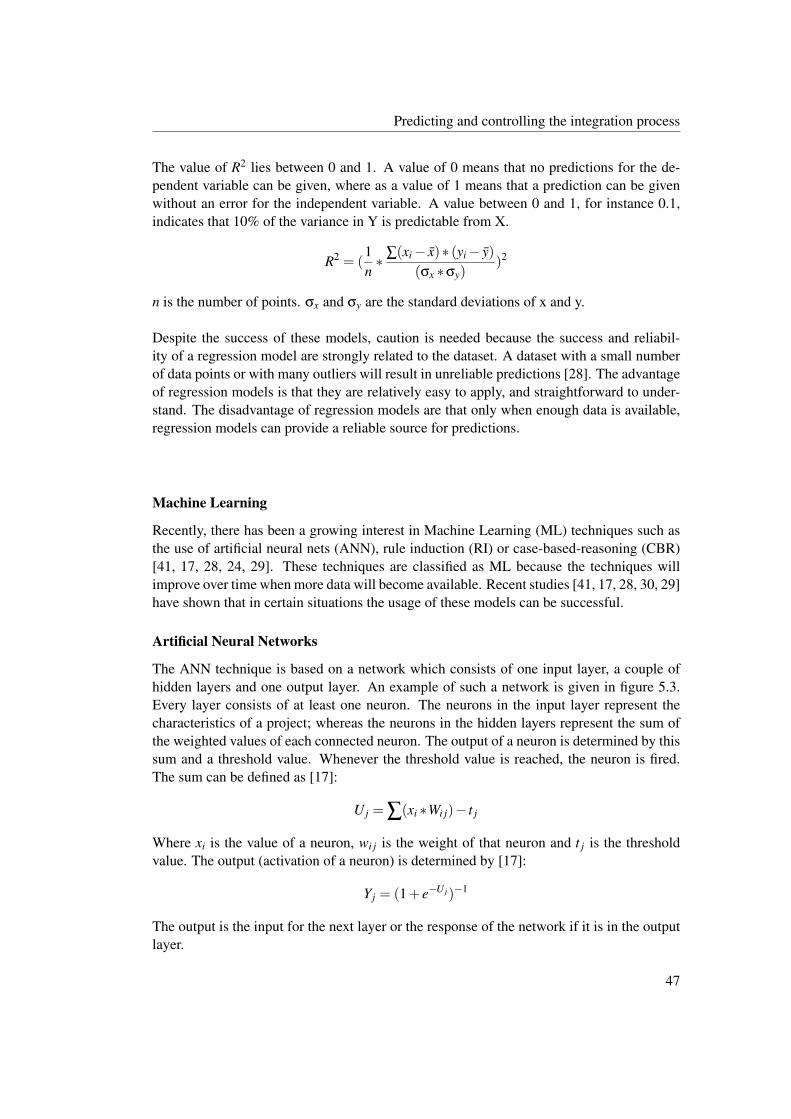
Predicting and controlling the integration process
The value of R2 lies between 0 and 1. A value of 0 means that no predictions for the de-pendent variable can be given, where as a value of 1 means that a prediction can be givenwithout an error for the independent variable. A value between 0 and 1, for instance 0.1,indicates that 10% of the variance in Y is predictable from X.
R2 = (1n∗ ∑(xi− x)∗ (yi− y)
(σx ∗σy))2
n is the number of points. σx and σy are the standard deviations of x and y.
Despite the success of these models, caution is needed because the success and reliabil-ity of a regression model are strongly related to the dataset. A dataset with a small numberof data points or with many outliers will result in unreliable predictions [28]. The advantageof regression models is that they are relatively easy to apply, and straightforward to under-stand. The disadvantage of regression models are that only when enough data is available,regression models can provide a reliable source for predictions.
Machine Learning
Recently, there has been a growing interest in Machine Learning (ML) techniques such asthe use of artificial neural nets (ANN), rule induction (RI) or case-based-reasoning (CBR)[41, 17, 28, 24, 29]. These techniques are classified as ML because the techniques willimprove over time when more data will become available. Recent studies [41, 17, 28, 30, 29]have shown that in certain situations the usage of these models can be successful.
Artificial Neural Networks
The ANN technique is based on a network which consists of one input layer, a couple ofhidden layers and one output layer. An example of such a network is given in figure 5.3.Every layer consists of at least one neuron. The neurons in the input layer represent thecharacteristics of a project; whereas the neurons in the hidden layers represent the sum ofthe weighted values of each connected neuron. The output of a neuron is determined by thissum and a threshold value. Whenever the threshold value is reached, the neuron is fired.The sum can be defined as [17]:
U j = ∑(xi ∗Wi j)− t j
Where xi is the value of a neuron, wi j is the weight of that neuron and t j is the thresholdvalue. The output (activation of a neuron) is determined by [17]:
Yj = (1 + e−U j )−1
The output is the input for the next layer or the response of the network if it is in the outputlayer.
47

5. PROPOSED SOLUTION
Figure 5.3: Artificial Neural Network
The network will improve itself by continuously determining the difference between theactual and desired value. This error is then propagated backwards into the network, in or-der to adapt the weights of each neuron. The performance of an ANN is depending onthe architecture and parameters of the network. Unfortunately, there is no ideal theory ofdetermining the architecture or to calculate the perfect parameters, which results in a trail-and-error process to configure the network. Even slight changes in parameters can havelarge influences on the whole network [17, 29].
The advantage of neural networks is that they are able to adjust automatically based onthe predicted data and retrieved data. This will ensure that predictions will become moreand more accurate. Disadvantages are that handling scope changes is difficult, because thenthe setup of the network needs to be changed. The effect will be that the adjustments haveto be reset, and the accuracy of the model is thereby reduced. Furthermore, these modelscan be difficult to apply when the process is not fully understood. Another disadvantage isthat configuring an ANN is a trial and error process.
Rule induction
Rule induction is a technique that tries to identify relations between specific cases in order toderive rules with which new cases can be predicted. These rules are organized into decisiontrees, which are used to classify unknown cases [27, 41, 29]. An example of cases is givenin table 5.3. From these cases the rule outlined in 5.4 can be derived. The advantage of rule-induction is that the method will get smarter when more cases are added. More accurate
48

Predicting and controlling the integration process
Measurement Case1 Case2 Case3Code size (kLoc) 25 30 35Experience of Manager (years) 3 2 1Interfaces 250 250 250Effort (man-months) 10 14 20
Table 5.3: Example of Rule Induction cases
If Codesize ≤ 25 andExperienceManager ≥ 3
Then Effort = 10
Figure 5.4: Example rule for RI
predictions can be made when more and more cases are added. A disadvantage is that,in order for this method to be effective, it is required to have a large set of cases. With aminimal number of cases only a minimum amount of rules can be derived, which results ina low coverage of the spectrum of new cases. Furthermore, the case set from which rules arederived, should have large differences between them in order to derive a large set of rules.It can occur that cases contradict each other; in this case the most encountered value is usedas the outcome. For instance, when from three cases the same rule is derived, but the thirdcase shows a different outcome value, then the outcome value of the first two cases is used.This results in an accuracy of 67% (two out of three).
Case-Based Reasoning
Case-Based Reasoning is a technique also known as estimation by analogy, which is com-parable with applying experience to new cases [42, 15]. It attempts to simulate a project bymapping similar past projects from the case base on to the target project. Each project ischaracterized by multiple general system characteristics (gsc), such as the number of inter-faces or the amount of reusable code. By determining the gsc’s for a new project, a similarcase can be selected from the case-base. Whenever a project is completed, it will be addedto the case-base. The processes in CBR can be defined as follows [43, 1], and are outlinedin figure 5.5:
• Retrieve the most similar cases
• Reuse the cases to attempt to solve the problem
• Revise the proposed solution if necessary
• Retain new solution as part of new case
The CBR technique can be effective whenever the domain is not fully understood; espe-cially, when it is unclear which factors in the development process have influence on eachother. In the older projects there can be unclear factors as well, but still, we can learn from
49

5. PROPOSED SOLUTION
Figure 5.5: CBR Cycle
these projects and use the experiences for new projects [25]. A commonly used algorithmto select a similar case is nearest neighbor selection for a p-dimensional space, where p isequal to the number of gsc’s. This algorithm is fairly straightforward when generic featuresor a low number of features are chosen, however when cases have different features or alarge set of features, a feature subset selection problem arises. The feature subset problemis a well-known problem in software engineering and is proven to be NP-hard, because acase with N features results in 2N feature subsets [50]. Revision is needed when the se-lected cases show differences with the target-case. Then the selected case will be adaptedwith adaptation rules. These rules are applied when prominent differences between gsc’soccur.
The advantage of the CBR-technique is that it usable when the process is not fully un-derstood. Furthermore, this technique is able to handle scope changes easily by selectingbetter fitted projects after the changes occur. Also the number of cases does not have tobe large, even with a limited amount of cases the technique can work effectively. A disad-vantage is that it is difficult to extrapolate the data when a new type of project is started,because no similar projects are available. Extrapolating is possible, but will take some time,since it requires having at least one finished project.
Selection criteria
Currently, the MFM-model is intended for project-management at the integration depart-ment. They are particularly interested in the progress and predictions of the project. Evenbefore the project is started (in TT4) and before data is gathered about the progress of it,
50

Predicting and controlling the integration process
they wish to be informed about estimations and predictions about the project. Thereforeonly showing trends based on gathered data or projects from history is insufficient to fulfilltheir needs. In order to make an appropriate selection of a model for TomTom, we first needto set the criteria, which should be fulfilled with our selection. The following criteria canbe defined:
• The model should give a prediction in TT4, before actual development starts
• The model should give a prediction for the whole duration of the project
• The predictions should reflect the defects.
• The model should fit within the development process of TomTom
• The model should be as accurate as possible
• The model should have a high explanatory value
• The model should be easily configurable
From the main-branch, a separate project is created. Every time a new PND project isstarted, it will be the successor of a current PND-device. All of these projects have a highdegree of complexity caused by the numerous interacting hardware components and newsoftware techniques. To make things even more complex: it can be the case that hardwarecomponents and software techniques are not yet available at the start of the project, but willbecome available during the project. Changing scopes during the project are therefore notuncommon. For this case, we will add an additional criterion:
• The model should be adaptable during the project when scope changes occur.
Direct comparison
In previous sections, the advantages and disadvantages are discussed, as well as the selectioncriteria. It can be seen that every technique has it strong points as well as its drawbacks. Inorder to make an appropriate selection we should evaluate these models in further detail. Inthis section we will compare every model with its counterparts on three aspects:
• Accuracy
• Configurability
• Explanatory value
In the past, case studies have been performed to assess prediction techniques on the listedaspects. Error measurements are used to assess the accuracy of the different techniques.In the discussed case studies the Mean Magnitude of Relative Error (MMRE) is used. TheMMRE value over n data points can be determined with the following formula:
MMRE = (∑n
estimate−actualactual
)÷n
51

5. PROPOSED SOLUTION
Where:estimate is the predicted valueactual is the actual encountered value
Based on the MMRE the models can be compared or rated. Two case-studies have beenfound that discuss the various models on accuracy. Shepperd and Kadoda [41] have countedwhich technique provides the most accurate prediction on various datasets. The results ofthis case study are outline in table 5.4. From these results it can be seen that CBR provides
Prediction Technique TotalSWR 10RI 7CBR 11ANN 4
Table 5.4: Most accurate prediction technique, Shepperd and Kadoda [41]
the most accurate results, closely followed by the SWR technique. Both RI and ANN pro-vide less accurate results. In contrast to these results, in a different case study performedby Mair and again Sheppard, Kadoda [29] other results were found. In this case study thetechniques are rated on a scale from 1 to 4. Where the rating of 1 stands for the most ac-curate results. The results of this study are outlined in table 5.5. It can be seen from the
Prediction Technique TotalLSR 2RI 4CBR 2ANN 1
Table 5.5: Rating of prediction techniques, Mair, Shepperd and Kadoda [29]
results that most values are corresponding with the previous mentioned results, except forthe ANN. In [41] the ANN technique was the least accurate technique, while in [29] it isthe most accurate technique. There is no clear explanation for this difference, besides thefact that in the research of [29] real data was used, while in [41] randomly generated datawas used.
Not only accuracy plays a role by selection a model. Explanatory value and configura-bility also have to be taken into account. When a model provides accureate predictions, butfor the users it is unclear how the model creates these predictions, it is difficult for them toaccept the predictions. However, when a model can be explained with reasons why certainpredictions are created, it is easier to accept it for users. The same holds for configurabil-ity; when a model is hard to configure or the configuration is unclear, users will hesitate toaccept predictions of the model. Furthermore, the model needs to be configured correctly,which is a difficult task when the configurability factor is low [29]. Both these two factorsare taken into account in the research of [29]. The results of this study are outlined in table5.6. It can be seen from the table that both LSR and CBR score the highest results on both
52

Predicting and controlling the integration process
Prediction Technique Explanatory value ConfigurabilityLSR 1 1RI 1 3CBR 1 1ANN 4 4
Table 5.6: Explanatory value and configurability, Mair, Shepperd and Kadoda [29]
aspects. RI is following with a lower configurability, where as ANN is worst in both cate-gories.
When we take all three aspects into account we can see that both LSR and CBR havethe most potential for being a good prediction technique. SWR also seems to be accurate,but it is not applicable for TomTom needs, because it only provides a single outcome basedon a set of defined variables. Both ANN and RI are showing lower results, although theaccuracy results for ANN are contradicting each other. However, when accuracy results areneglected, ANN still performs worse than LSR, RI or CBR.
Scope changes
With both LSR and CBR, scope changes can be handled. With CBR, scope changes willaffect the selection of similar projects. Whenever scope changes occur, other projects willbe selected to base predictions on it. Manual intervention is needed to handle scope changesin LSR. Then a particular subset of the data needs to be selected in order to calculate thecorrect regression line.
Model Selection
Two important aspects for selecting a model will be discussed: the characteristics of themodels and the applicability into the organization of TomTom.
Models based on code-size are not suited for TomTom, since they predict only a singleeffort value instead of predicting the whole evolution of a project. Furthermore, there is noevidence that these models are reliable. Therefore we will reject this technique.
Regression techniques are straightforward, easy to apply and can be effective. However,data need to be present in order to calculate the regression lines. One of the criteria we set isto be able to create predictions before actual development starts. In these phases, the datasetof the new project is (almost) empty and therefore regression models cannot be used. Nev-ertheless, in later phases of the project, when the dataset is filled with data, these modelscan provide a source for predictions. Therefore we will use this technique for predicting thedefects in the MFM-model
Artificial Neural Networks can provide a reliable source for effort predictions; however,developing the network architecture and determining the neuron parameters is a complex
53

5. PROPOSED SOLUTION
task. In general, this task has to be performed only once, however in the case of Tom-Tom these parameters should be adaptable constantly due to the changing scopes during theprojects. In addition to that, the output of an ANN is a couple of values, which can be forinstance the required effort for the project. In our case we are interested in the expectedproject evolution and for this purpose an ANN is less effective. Furthermore, studies havereported mixed results with it [41, 23]. Determining the right values of parameters will taketime, especially when they have to be adapted regularly. Therefore ANN seems unsuitablefor the defect predictions of TomTom.
Rule-induction can be effective when a large set of case are present, however at TomTomit will take a lot of time to gather these cases, since the average project duration is severalmonths. Furthermore, the accuracy and explanatory value of the RI-technique is low, as weshowed in previous section. Therefore this technique seems to be inappropriate for Tom-Tom as well.
Because of the categorization and the iterative nature of the projects at TomTom, the case-based-reasoning model can be a reliable prediction model. For instance: after a high-endPND project is finished, a new high-end PND project will be started to create a new de-vice. Between those projects there will be similarities in relation to the amount of the newlyadded hardware components and software techniques. Furthermore the CBR-technique canmodel multiple output-variables as long as the projects in the case base contain these vari-ables. In addition to that: projects from the case-base can be adapted with adaptation rules,even during the project to handle changing scopes. However, one drawback is that in orderfor this model to work, the case-base need to contain cases. Thus, it will take some timebefore this model can correctly be applied. Another drawback is that there exists no generaltheory to determine the gsc’s. On the other hand, the developed MFM tool stores exactly theinformation which is required for the case base of the CBR-technique. It namely stores allrequired facets over multiple points in time during projects. It therefore can provide infor-mation about the trends of past projects, no matter what the trend-curve is of these projects.This information is valuable for future projects. Therefore the CBR-technique seems to beappropriate for the defects predictions. We will use this technique as a supplement to theregression technique.
When we look at a single project at TomTom, it can be seen that in the beginning ofproject there is a high degree of uncertainty. In later phases this uncertainty is decreased be-cause data is gathered about the effort and progress. In these phases regression models cangive consistent predictions with the gathered data. Because of the possibilities of changingscopes at TomTom, these regression models should be able to cope with these changes. Inaddition to the regression technique, we choose to use the CBR-technique, because Tom-Tom will have similar past-cases stored with the MFM tool. The output can consist ofcontinuous values and the model is able to cope with scope changes easily. Another aspectis that with CBR, we can also see in which phases the historical project is and in whichphase the current project should be. Especially when we consider that with the MFM toolthe crucial information for a case-base is stored, the CBR technique seems to appropriate.
54

Improving the integration process
Only LSR and CBR show consistent accurate results and both have the highest score forexplanatory value and configurability. Furthermore, these two techniques can supplementeach other. At the beginning of the project when no data of the current project is availablethe CBR technique can be used. Whenever data of the current project is available the re-gression technique can be used. Therefore, we propose to use two prediction techniques:LSR and CBR.
Remaining open questions for predicting defects
A selection has been made about the predicting techniques; however a couple of open ques-tions still remain for these techniques. These questions are outlined below and will beanswered in section 6.
• How should the reliability of the regression be indicated to the user?
• Which parameters should be used to select similar cases with the CBR-technique?
• How many similar cases should be selected with the CBR-technique?
5.3 Improving the integration process
In order to improve the process, one needs to know the current situation and past situation.In previous section we added improvement 8 (i8) which states that historic data need to bestored.
Keeping historic data: i8
The MFM 2.0 prototype will keep historic data in order to be able compare old projects withcurrent projects. The prototype will use a metric database to store all data in an organizedfashion.
5.4 Improved MFM 2.0 proposal
Our proposed solution incorporates the techniques and improvements that are described inprevious sections. The improved MFM 2.0 model will show the recorded values of thefollowing aspects, both numerical and graphical:
• Software features
• Hardware components
• Key Performance Indicators
• Risks
• Defects
55

5. PROPOSED SOLUTION
All issues divided over these aspects will have weights to simulate real-world effort andcomplexity. Furthermore, aspects as complexity and project-size based on lines of codeshould be included as well.
The MFM 2.0 prototype is able to generate an improved MFM 2.0 model and present thismodel in various formats through different platforms. The overview of the whole system isillustrated in figure 5.6. The data sources layer contains all the data sources that are required
Figure 5.6: Overview of proposed solution
for creating the MFM-models. These are Jira and Perforce. The data-gatherer in the dataprocessing layer will collect data from the data sources layer and pass it through to the dataconverter. The data-converter converts the data into a usable format for the MFM-modeland stores it into a metric database. The data presentation layer will retrieve data from themetric database and present it on a website, mobile phone or television.
In the next section the prototype will be discussed in detail. Here the various design de-cisions will be discussed as well as the final prototype itself.
56

Chapter 6
Prototype of MFM 2.0
In this section we will describe the technical implementation of the MFM 2.0 prototype.First we will give an overview of the overall system. In the subsequent chapters will wediscuss the various layers of the prototype to get an in-depth view.
6.1 Overall System
The overall system consists of three layers, outlined in figure 6.1.The same layer division isused as in previous sections. The Data Sources Layer of the prototype consists of Jira and
Figure 6.1: Overall System Layout
Perforce together with their communication protocols. Jira is used to retrieve all issues fromand Perforce is used to retrieve the amount of kLoc (kilo lines of code). A more detaileddescription of the data sources layer can be found in section 6.2.
The Data Processing Layer consists of the MFM Data Collector which is responsible forprocessing and converting the input. Furthermore the MFM Data Collector stores the con-
57

6. PROTOTYPE OF MFM 2.0
verted data into a database and generates the MFM-summary graphs and feedback reports.A more detailed description of this layer will be given in section 6.3.
The Data Presentation Layer consists of the MFM Viewer which will present the modelto the user. The MFM Viewer is connected to both Jira and Perforce in order to authenticateusers and to retrieve filter/depot information. The viewer can present the MFM-model inthree formats:
• Normal website
• Smartphone website
• TV Presentation Slideshow
A more detailed description of this layer is given in section 6.4
6.2 Data Sources Layer
As indicated before, the MFM 2.0 Prototype uses two inputs: Jira and Perforce. The fol-lowing limitations are present for both of these inputs:
• Storage of these data sources cannot be accessed directly.
• Only a minimum amount of changes to the data sources can be applied
The development support department of TomTom is responsible for the functioning of bothPerforce and Jira. No direct access is granted to the storage of these data sources for theMFM-data collector, thus different protocols need to be used to gather data from thesesources. Furthermore, the development support department is undermanned, and thereforethe data sources should be used with a minimal amount of required changes.
Jira
Retrieving issues from Jira can be done by the Simple Object Access Protocol (SOAP) [49],which is a protocol for exchanging structured information in the XML format. Because thisprotocol is used, we are limited in our possibilities to retrieve issues from Jira. Atlassian[5], the developer of Jira, provides SOAP support to communicate with Jira. However, withthe current version 3.1, it is only possible to retrieve issues per filter (defined in Jira). Re-trieving, for instance, only updated issues is not possible. The development department ofTomTom extended the SOAP functionality by providing an extension. With this extensionit possible to retrieve the history of every issue is to some extent. However, it is still notpossible to retrieve only the updated issues or to execute any custom operations on Jira.
Although a minimum amount of changes can be applied, a few changes must be applied,because with the current setup it is impossible to enter all required issues. At this moment,it is possibly to store defects and user-stories only. The current setup is outlined in figure6.2. With two small changes the setup of Jira is changed to be able to log and retrieve allrequired issues. The following changes were made:
58

Data Sources Layer
Figure 6.2: Current Setup of Jira
• User-stories will get the following subtypes: functional requirement, kpi and risk
• Functional requirements will get one additional field: layer. Values of the layer fieldcan be:
– Feature set
– Navigation Framework
– Platform services
– Kernel
– Hardware
With these changes the setup of Jira will become as shown in figure 6.3. Now, it is possible
Figure 6.3: New Setup of Jira
to retrieve all values as discussed in section 4, although it seems that the severity, probabil-ity, direction, current value and target value are missing. These values will be entered in the
59

6. PROTOTYPE OF MFM 2.0
description field with the use of a template. The template of risks will be:
Severity:Probability:
For both the probability and severity, a number needs to be filled in, ranging from 1 (mostsevere/probable) to 5 (least severe/probable). Besides the keywords: high, medium and lowcan be used as well, which will be translated to 1,3 and 5 respectively. For kpis the sameprinciple is applied. The template will be:
Target value:Curent value:Direction:
Both the target value and current value will be any (fractional) number. The direction willbe either < or >, indicating whether the current value needs to be less or more than thetarget value. Entered values in the description field will be extracted with the use of RegularExpressions (described in following section).
The remaining fields (priority, status and layer) can be extracted directly; however a map-ping to a measureable number still needs to be applied. The mapping outlined in tables 6.1is used.
(a) Weights of priorities
Priority WeightBlocker 5Critical 4Major 3Minor 2Trivial 1
(b) Weights of statuses
Status WeightOpen 1Reopened 1In Progress 0.75Ready for testing 0.5In Testing 0.25Closed 0
(c) Weights of layers
Priority WeightFeature 1Nav Services 2Platfrom Services 3Kernel 4Hardware 5
Table 6.1: Mapping of priorities, statuses and layers
With this setup it is possible to enter and retrieve all required values as proposed in sec-tion 4. The weight of each issue will be determined as shown in table 6.2. Note that the
Issue type FormulaDefect Status∗PriorityRisk Status∗ 100
Severity∗ProbabilityKPI Status∗Priority∗DeviationFeature (Functional requirement where layer 6= hardware) Status∗Priority∗LayerHardware (Functional requirement where ≡ hardware) Status∗Priority∗5
Table 6.2: Weight calculation of issues
60

Data Processing Layer
priority field is not used for risks; this is because the priority for a risk is expressed in termsof probability and severity.
Perforce
Perforce is a versioning system which is based around changelists. Whenever new codeis submitted to the perforce repository a changelist with additional comments is created.Direct access to the perforce storage is not granted by TomTom, however with the PerforceCommand-line interface it is possible to retrieve information about the depots. With thisinterface it is possible to retrieve all changelist for a certain depot and collect the number ofadded, changed and deleted kLocs.
6.3 Data Processing Layer
The Data Processing Layer (DPL) consists of four parts. First there is the MFM-data collec-tor which is responsible for gathering information from the inputs, translate it accordingly,create feedback reports, store the translated issues in the database and create the MFM-summary graphs. The feedback reports are the second part of the DPL; these reports provideinformation to the owner of the project about which issues are not correctly filled in Jira.The database is the third part of the DPL and provides storage for all information whichneeds to be present in the MFM-model. At last there is the storage for the MFM-summarygraphs, these are created by the MFM-data collector.
MFM Data Collector Classes
This section will give an overview on a high abstract level of the MFM Data collector andthe various involved parts of it. The MFM Data collector is an application written in C#, be-cause these applications can be pre-compiled, targeting the development of load-intensiveapplications and both the standard Jira Soap Client and the extended TomTom Jira clientwere already available in the form of a C# class. In figure 6.4 the main classes with themost important methods are shown. Less important methods and classes are omitted for thesake of simplicity.
The basic flow of the data collector can be described as follows. By the command-lineinterface the user can influence the setup of the MFM-data collector. Once the collector isstarted, a new execution is created which is used as reference to the time and date when themodel was generated. Then both Jira and Perforce are approached in order to retrieve infor-mation. Information is gathered from Jira by the SOAP client and will first be parsed andconverted in the right format, before it is stored in the database. Information from Perforcecan be stored directly. After all information is stored, the MFM-summary graph will begenerated by the chart-class. If during any operation errors occur, or when required infor-mation could not be retrieved, errors will be logged in a feedback report by the logger-class.
At every start of the collecting phase a new execution with the current date and time will
61

6. PROTOTYPE OF MFM 2.0
Figure 6.4: Abstract Class Diagram of MFM data Collector
be inserted in the database, to which the model is connected. If for instance, the collectoris started three times on the same project, three executions are created, resulting in a model
62

Data Processing Layer
with three snapshots. The purpose of doing is that when the MFM-model is updated with acertain time interval, for instance once a day, it is possible to view the history of the project.
Furthermore, at the start of the collecting phase, a flag will be set in the database. Afterall operations are completed the flag will be removed. Models which still have a flag willnot be shown to the user. This will ensure that only finished models will be shown to theuser. Therefore, mechanic failures or any other type of interruptions on the generation willhave only a small effect: the user will need to restart the collector manually. In the nextsubsections, the various elements will be described in more detail.
Commandline Interface
By the command-line interface the user can set-up the configuration for the creation of theMFM-model. The following inputs are possible:
• Create models for all active projects.Command: MFM-generation.exe mfmgen
• Create model for specific projectCommand: MFM-generation.exe mfmgenpr projectid
• Create model for specific project from every day during a specific timespan,resultingin multiple snapshotsCommand: MFM-generation.exe mfmgenpr projectid start(dd-mm-yyyy hh:mm)end(dd-mm-yyyy hh:mm)
The functionality to create a model for a specific timespan is limited, because historicprojects will only have a limited amount of valid information. Issues like risks, kpis, andfunctional requirements are not stored in the correct format in these projects. Thereforeonly the defects will be parsed correctly.
Parser
The goal of the parser is to translate the information of Jira into our defined format. Themain tasks the parser performs are:
• Select the values of the required fields of the issues
• Perform the mapping outlined in table 6.1
• Parse description fields for severity, probability, direction, current value and targetvalue.
• Execute the formulas outlined in table 6.2.
Parsing the description field is done with the use of Regular Expressions together witha pattern which is used to retrieve parts of a string. The regular expressions are looselydefined in order to provide a better user experience. The following formats of entering anyof the mentioned fields are valid:
63

6. PROTOTYPE OF MFM 2.0
• target: 15
• target 15
• The target value of the kpi is 15
• target (any word, besides the keywords) 15
In addition to that, the keywords are case-insensitive. The mapping of the fields, as de-scribed in table 6.1, is stored in the database and can be altered when required.
Feedback reports
The logger will create a feedback report if, at any time during the generation, errors occur.However, in most cases no errors occur, but feedback reports are still created. In these casesthe feedback report provides information about which issues are not entered correctly intoJira. The following lines can be part of a feedback report:
3/30/2010 16:28:27: PROJ-1700: Unknown user-story type from remote issue, willuse functional requirement
3/30/2010 16:28:29: PROJ-588: Customfield does not exist - layer, will use value 0
3/30/2010 16:28:26: PROJ-2413: Cannot fetch target or current values from de-scription
Messages about incorrect entered issues are provided in a format of: date and time, theJira-key of the issue and the message. The first line indicates that user-story with keyPROJ-1700 is found, but no subtype (functional requirement, risk or kpi) is defined. Inthis case the system will store it as a functional requirement. The second line indicates thatfunctional requirement PROJ-588 is found, but no layer is defined. The system will use thefeature-layer. The last line indicates that KPI PROJ-2413 is found, but no information aboutthe target- or current values can be found. In this case the KPI is omitted, because a defaultvalue is difficult to assign (deviation is not bounded).
Database
In figure 6.5, the relational database schema is given. It can be seen that everything isformed around a project and an execution. Entries in the summary table are updated by theMFM data collector at runtime. The purpose of this table is to improve performance whena user wants to view the MFM-summary data.
MFM-Summary Chart Creation
The MFM-summary graph is created by the MFM-Data Collector, because we wanted todisplay a non-typical graph which could not be generated at runtime by the various libraries
64

Data Processing Layer
Figure 6.5: Database design diagram
available on the internet. The graph shown in figure 6.6 shows the graph that is used as theMFM-summary. The final setup of the graph arose after a number of iterations of improve-ments.
Vibrant colors are used to mark the elements one should reduce and increase. The redpart represents the elements you want to reduce (open defects, deviation of KPIs and openrisks). The smaller the red part the better it is, therefore this side is named: the immature
65

6. PROTOTYPE OF MFM 2.0
Figure 6.6: MFM Summary Graph During a Project
side. The green part represents the elements you want to increase (implemented featuresand hardware) and therefore this side is named: the mature side. At the start of the projectwhen no risks, KPIs and defects are entered, and no features/hardware are implemented yet,the summary will be shown as in figure 6.7. It represents an immature project.
Figure 6.7: MFM Summary Graph of Immature Project
Whenever a project finished completely successfully, the summary will look as outlinedin figure 6.8. Although this is not realistic, because in almost every project some defectswill remain, kpis will not be reached or features/hardware could not be fully integrated.
66

Data Processing Layer
Only showing a red and green surface is not revealing enough information, since the vol-
Figure 6.8: MFM Summary Graph of Mature Project
ume of all open issues is not presented. Therfore, various numbers are shown along theaxis to indicate the exact volume and progress of a specific issue-type. In figure 6.9 thesenumbers are explained.
Figure 6.9: Explanation of Numbers in the MFM-Summary
Because no existing library provides the functionality to create such graphs, we developedthis functionality. One of the requirements was that the graphs were scalable without any
67

6. PROTOTYPE OF MFM 2.0
loss of image-quality, because then the graphs can also be used on high-resolution televisiondisplays. The solution we came up with was to use a Scalable Vector Graphics (SVG) [48]image, with which it is possible to create a vector-based image, stored in a XML format.However, one drawback of SVG is that it is not supported by all web browsers. For instance,Microsofts Internet Explorer does not support SVG. Therefore the final SVG-image is con-verted to a Portable Networks Graphic (PNG), in order to display it on all web browsers.
For creating the SVG we developed a SVG-template, which will be filled in by the MFMData Collector. The following elements in the SVG-template need to be filled in:
• Numbers on every axis (volumes and progress)
• Position of the endpoints of the red/green surfaces
• Position of progress labels
In order to fill in the right values at the right place in the template, we created placeholdersfor these values in the following format:
< %%VolumeO f De f ects%% >
Every name between < %% and %% > is a placeholder for a coordinate or a value. Inthis manner the volumes and progression values can be easily filled in. Positioning the end-points of the red/green surfaces is a bit harder to accomplish. However, when one knowsthe center point of the graph together with every ending point of the axes and the progressthat needs to be shown, it becomes relatively easy to calculate the coordinates for the points.The MFM Data Collector retrieves the coordinates of the center point and end points of theaxes from the database, calculates the required coordinates, and fills these coordinates inthe template. Positioning the labels near the points has become an easy task as well. Witha defined offset (stored in the database) these coordinates can be calculated in the same way.
After the template is completely filled-in, it is stored as a separate SVG-file with the follow-ing name:
ch12-123.svg
The first number being the id of the project, and the second number being the id of theexecution, referencing to the time and date when the model was generated. After the SVGis stored, it is converted twice to a PNG by the InkScape [22] converter: one for the MFM-viewer website (low resolution) and one for the television slideshow (high resolution).
6.4 Data Presentation Layer
The Data Presentation Layer (DPRL) contains the MFM-viewer that represents the MFM-model in various formats to the user. Furthermore, it provides the functionality to add/remove
68

Data Presentation Layer
projects for automatically creating MFM-models. In the following sections, all the aspectsof this DPRL will be described.
Zend Framework
All formats of the DPRL are webbased and developed on the Zend Framework (ZF) withthe usage of Asynchronous Javacrips And XML (AJAX) to dynamically update the pages.The Zend Framework is a PHP based framework which provides a Model-View-Controller(MVC) approach for building web applications. The flow of the application along it variouselements in the framework can be illustrated as shown in figure 6.10. It can be seen from
Figure 6.10: Zend Framework Structure
this figure that functionality, layout and database logic are strictly divided. For our purposeof developing various formats of the MFM-model, this is an advantage, because now onlythe layout has to be changed in order to develop a different format. The database logic andfunctionality can remain the same for all three formats.
Normal website
The normal website represents the full MFM-model to the users. Here, the MFM-summary,but also the details about the different issue-types can be inspected. Furthermore, the web-site also provides the predictions and information about the kLOCs. In addition to that, it isalso possible to configure the data collector. In figure 6.11 the use-case diagram is shown.Three types of users can be distinguished:
69

6. PROTOTYPE OF MFM 2.0
Figure 6.11: Use-Case Diagram of Web frontend
• SiteOwner, the person responsible for the MFM Prototype
• Project Administrators, being the technical-/test leads
• TomTom Stakeholders, anyone who is interested in the generated models
Both the SiteOwner and Project Administrators are able to login to the system with their Jiracredentials after which the project administration pages are shown. Only the SiteOwner canadd/remove users who are eligible to login. Both the SiteOwner and Project Administratorscan add/edit/remove projects for the creation of MFM-models. When adding a project thefollowing details need to be filled in:
• Project name, can be anything the user wants
• Milestones dates, the dates of IS, IC, FC, MC and GM
• Number of devices, used for CBR predictions
• Filters of Jira, the filters that will return all required issues
70

Data Presentation Layer
• Perforce depots and keyword; the depots where the sourcecode of the project is stored.Keyword is used for filtering the changelists of the depots
Adding filters is rather easy. A list of their favorite marked filters from Jira will be shownfrom which the project administrator can select the appropriate ones. Adding a depot is a bitmore difficult, since the project administrator needs to know the name of depots, howeverit is possible to inspect the returned changelists to check whether the depots are correctlyfilled in.
Whenever all this information is provided, the MFM Data Collector can create the MFM-models. Every night at 3.00 PM a MFM-model is automatically created for all the activeprojects. In addition to that, it is also possible to generate a MFM-model for a specificmodel on demand by clicking the generate-button from the project administration. Afterthe model is generated on-demand, the user will be taken to the page where the generatedmodel is shown.
All users are able to view the generated MFM-models. In figure 6.12 the wireframe ofthe MFM-summary page is drawn. On the left-side the menu is drawn, from which the
Figure 6.12: Wireframe of Web frontend
various pages of the model can be selected. In the top bar, the administration menu isshown, whenever a user is logged in. In the middle information is displayed. Three typesof information can be displayed in this part of the page:
• MFM-summary graphs with a slider to advance through all historic situations
• Data table representing the underlying data of graphs
• Charts displaying information about specific issue-types
71

6. PROTOTYPE OF MFM 2.0
The pages outlined in table 6.4 are available for inspecting the MFM-model. In appendix Fan example is shown several mentioned pages from the table.
Defect Predictions
When the user selects the defect-prediction page, two types of predictions can be chosen:regression and CBR. Both are predicting progress on defects until the GM milestone. How-ever there is a difference, as mentioned in previous sections, about how these predictions arecalculated. The default prediction technique with which the user is presented is regression.The second prediction technique is case based reasoning. Both predictions are calculatedon demand, and are adjustable without the interference of the MFM-data collector.
The regression predictions are based on all data retrieved since IS. However, it is possibleto adjust the amount of data that needs to be used as a user. To reach 100% of completionon defects, all found defects need to be closed, which means that no unclosed blockers,criticals, majors, minors and trivials are present anymore. Therefore, a separate regres-sion equation is calculated for each type of issue. After which all these equations are(weighted) accumulated into one graph. The process of this method is outlined in figure6.13. Calculating just one regression line, based on the combined progress-data, will lead
Figure 6.13: Regression Prediction Technique
to incorrect predictions, as illustrated in table 6.3. It can be seen from the table, that everyweek 33% progression is made. However, stating that progress is 100% at week 4 is incor-rect, since still one minor-issue is open. This effect is caused by the fact that it is presumedthat one can keep on solving trivial issues. However, the reality is that only a limited amountof trivials can be closed, and after that, only minors remain, which will affect the progressspeed. The correct progress at week 4 should therefore be 83%. Note that in this examplethe weights of the trivials and minors are 1 and 2 respectively.
72

Data Presentation Layer
Week Trivials (Open/Total) Minors (Open/Total) Progress1 4/4 4/4 0%2 2/4 3/4 33%3 0/4 2/4 67%4 -2/4 1/4 100%
Table 6.3: Example of wrong regression calculations
The equation of the accumulated regression line is composed of the individual regressionequations. The regression equation of a single line will have the form of:
progress = max(ax + b,100)
Then the accumulated regression line is a summation of all individual equations in thefollowing way:
y = ∑trivial,minor,ma jor,critical,blocker
weight ∗max(ax + b,100)
The bends in the regression line can now be explained by the fact, that at some point one ofthe issues is maxed out at 100%.
The other selectable prediction technique is case based reasoning, with which similar projectsare selected based on the following aspects:
• Number of devices (number of software-versions that need to be made)
• Volume of KPI
• Volume of features
• Volume of hardware (number of hardware components that need to be used for inte-gration)
• Volume of risks
All of these aspects are known in TT4, which makes them usable for CBR-predictions inTT4. Furthermore, the aspects are independent of one another, which make them appropri-ate for using in the CBR-predictions. Together, these indicators will indicate the project sizeand complexity. To calculate the predictions, all finished projects will be selected, all valueswill be standardized and the differences between the new project and the past projects willbe calculated. Handling scope changes is possible, because these changes are reflected inthe aspects that are used for selecting similar projects. Whenever the scope of a projectchanges, other past projects will be selected.
Literature indicated that predictions based on three or four projects will work best [41].In our case, the three most closely related projects are selected by a 3-Nearest-Neighbor
73

6. PROTOTYPE OF MFM 2.0
algorithm; however this amount is adjustable by the user. After the projects are selected,the distance between these projects and the current project is calculated, based on the dif-ferences. This distance will be used as a weight. Just plotting the weighted average of theselected project seems to be incorrect, since the selected projects have different durationsof their phases. Different activities take place in the various phases, resulting in differentcurves of progression. Therefore a mapping of the phases of the selected projects ontothe new project is required. Two different types of mappings for the CBR-predications aremade: a planned progress prediction (how much progress should we make to finish theproject on time) and a realistic progress prediction (how much progress are we most likelyto make, based on previous projects). The process of calculating both CBR-predictions isoutlined in figure 6.14. In the left path of the figure, the phases of the selected projects aremapped onto the duration of the phases of the new project. Thus, density of the data inthese phases gets adjusted. Now, a prediction can be made with the weighted average of thethree adjusted projects. In the right path of the figure, the average duration of the phases ofthe selected projects is calculated and the projects are mapped onto this new phases. Again,the density of the data is adjusted. A prediction can be made with the weighted average.When these two predictions are plotted against each other, one is able to see if the requiredprogress (planned prediction) of the new project corresponds with the progress made in pastprojects (realistic prediction). In the example given in figure 6.14, the planned prediction isfinished in week 12, however the realistic prediction is finished in week 14.
When the CBR page is loaded, three projects are automatically selected. However, it can bethe case that a user knows which projects are similar. Therefore an option is included wherea user can select a number of similar projects with which the predictions then are made.
Smartphone viewer
The smartphone website is a website optimized for small-screens. Only TT-stakeholderusers are the users of this website: it is only possible to view MFM-summary graphs. Theuser can inspect the MFM-summary graph by selecting a project and time of execution.
Television Slideshow
The television slideshow is an application which is able to show any webpage during aselectable amount of time. In the database the pages together with their duration can beentered. Currently, the television slideshow is used on large screen at the integration depart-ment to raise awareness of the ongoing projects.
6.5 Testing
During development the prototype is tested in various ways. First of all, the Data ProcessingLayer has been unit tested with nUnit [31]. Secondly, the Data Processing Layer togetherwith the Data Presentation Layer have been tested within a controlled environment. In Jiraa separate project was created for testing purposes where a controlled amount of issues was
74

Testing
Figure 6.14: Two variants of CBR progress predictions
entered. An MFM-model was generated from this project which was validated after gen-eration. Then a pre-defined set of issues was changed and the model was generated again.After which it was checked again to make sure the MFM-model reflected the changes in theissues. These steps were repeated a couple of times to make sure the implementation wasperformed correctly.
In order to test the predictions, data of eleven projects was generated. These eleven projectsconsisted of one target project and ten case-base projects. Manually regressions and CBR-
75

6. PROTOTYPE OF MFM 2.0
predictions were made in order to compare these predictions with the generated predic-tions from the MFM 2.0 prototype. By comparing the predictions we were able to validatewhether the implementation of the predictions was correctly performed.
76

Testing
Page Content of pageMFM-Summary graph The graphical representation of the MFM-summary. With a slider and controls
on both sides of the graph, historic models can be selectedMFM-Summary data The numerical representation of the MFM-summary. With the controls on both
sides of the tables historic models can be selectedDefects Graphical representation of the following aspects:
• Unclosed defects per priority over time
• Defects per status over time
• Progress on defects over time (weighted)
• Closed defects versus unclosed defects over time (weighted)
Four pages: Features, Hard-ware, KPIs and Risks
Graphical representation of the following aspects:
• Progress on issues over time (weighted)
• Closed issues versus unclosed issues over time (weighted)
Defect Predictions Graphical representation of regression predictions in the following ways:
• Overall predictions with inclusion of milestones
• Predictions for Blockers and Critical
• Predictions for Majors, Minors and Trivials
Graphical representation of CBR predictions in the following ways:
• Realistic versus planned progression
• Planned progression mapped from selected projects
• Realistic progression mapped from selected projects
Complexity Graphical representation of the following aspects:
• Open time of unclosed defects
• Open time of closed defects
• Number of times that defect is reopened (accumulated) for unclosed de-fects
• Number of times that defect is reopened (accumulated) for closed defects
Numerical representation of the following aspects:
• Average open time of unclosed defects
• Average open time of closed defects
• Average number of times that defect is reopened for unclosed defects
• Average number of times that defect is reopened for closed defects
Klocs Graphical representation of the following aspects:
• Accumulated kLOC over time per type: added, changed and deleted lines
• Blocking defects per kLOC
• Non Blocking defects per kLOC
• Total volume of defects per kLOC
Table 6.4: Pages of MFM Website
77


Chapter 7
Evaluation
In this section we will evaluate the MFM 2.0 prototype in three ways. First of all wewill review the MFM Goals and check whether the prototype is able to reach those goals.Secondly, we will perform a T1 measurement in order to measure our improvement sincethe T0 measurement. At last we will review the accuracy of the predictions.
7.1 MFM Goals Reviewed
Our main question we will try to answer in this section is:
Did we select the correct metrics to reach the three goals of the MFM-model:
• P1: Analyze maturity of the integration project
• P2: Monitor progression of the integration project
• P3: Predict progression of the integration project to check upon the feasibility
It is difficult to directly give an answer to this question, however the MFM 2.0 prototypeprovides the technical possibilities, independently to the information that is shown, to:
• Retrieve information and present a maturity-model (P1)
• Update the models frequently to show progression (P2)
• Predict defect progress for feasibility purposes (P3)
So, basically we can see that the MFM 2.0 prototype provides the functionalities to reachthe three goals of the MFM: it can show information in various formats to reach thosethree goals. However, we do not know yet whether the MFM 2.0 model shows the correctinformation to be able to analyze the maturity or to really predict the progression. Therefore,we will conduct a series of interviews to evaluate these aspects.
79

7. EVALUATION
7.2 T1 Measurement
After finishing the MFM 2.0 prototype a new series of interviews were conducted. Theseinterviews were conducted along the same interview protocol (appendix B), with the samequestions and with the same interviewees. Interviewees were not confronted with theirprevious answers to ensure valid measurements. This way we can evaluate our prototypeby checking whether we improved the situation according to the interviewees. In the resultswe will mark previous results as T0 and results of the new interviews as T1. More detailedresults of T1 can be found in appendix D.
Effort
The MFM 2.0 model is generated from Jira, which means that almost no effort is required tocreate the model. For the model to be a success effort-wise it is important that the requiredeffort to fill in Jira is about the same as with the previous MFM model. Therefore we againasked questions about the four areas of effort, together with questions about double enteredinformation and a opinion on the required effort.
• Time to fill in Jira at start project
• Time to fill in MFM at start project
• Time to update Jira during project per week
• Time to update MFM during project per week
• Amount of double entered information
In table 7.1, the results of previous interviews and current interviews are shown. The re-
Indicator T0 T1Time to fill in Jira at start of project 10-20 hours 10-20 hoursTime to fill in MFM at start of project 6-9 hours 0.1 0.6 hoursTime to update Jira during the project per week 3-7 hours 3-7 hoursTime to update the MFM during the project per week 2-4 hours 0.1-0.6 hours
Table 7.1: New results of questions 1 to 4
sults show that the required effort to fill in Jira remains the same, but the effort to createand update the MFM-model is greatly reduced. The time to create the model is reduced bya factor of 15 and the time to update the model is reduced by a factor of 6. This meansthat a technical lead or test lead saves between 2 and 3,5 hours every single week by gen-erating the model automatically. Effort-wise the MFM 2.0 prototype seems to be successful.
The results on the double entered information differed from previous results, as well as theopionion whether the MFM-model takes too much time to fill in. The results are outlined intable 7.2 The results show that the amount of double entered information has become less.Currently interviewees indicated that the amount is between almost nothing and not much.
80

T1 Measurement
Indicator T0 T1What is the amount of double entered information in Jira,and MFM-MODEL?
3.25 1.5
It takes me too much time filling in the MFM-MODEL 4.75 1.5
Table 7.2: New results of questions 5 to 6
The opinion on the required effort shifted as well. Previously interviewees indicated that ittook them too much time to fill in the MFM-model. Now they almost totally disagree withthis thesis. Therefore we can conclude that our second improvement (i2: reducing effort),has been successfully implemented.
Accuracy
Reducing effort is meaningless whenever the quality of the model decreases. Thereforewe will also evaluate the perceived accuracy of the model by asking the same questionsas with the previous interviews. The questions that were asked with their results are listedin table 7.3 and figure 7.1. It can be seen that on every single aspect the results were
Indicator T0 T1The MFM-model reflects the maturity of a project clearly inTT4
2.75 3.75
The MFM-model reflects the current status of a projectclearly during the project?
3.0 4.25
The MFM-model reflects the current state of the defects cor-rectly at the start of the project
3.25 4.25
The MFM-model reflects the current state of the defects dur-ing the project
4 4.75
The MFM-model reflects the current state of the risks cor-rectly at the start of the project
2.25 4.75
The MFM-model reflects the current state of the risks duringthe project
2.25 4.75
The MFM-model reflects the current state of the kpis cor-rectly at the start of the project
1.25 5
The MFM-model reflects the current state of the kpis duringthe project
1.25 4.75
The MFM-model reflects the current state of the features cor-rectly at the start of the project
3.5 4.75
The MFM-model reflects the current state of the features dur-ing the project
3.75 5
The MFM-model reflects the current state of the hardwarecorrectly at the start of the project
1.5 3.75
The MFM-model reflects the current state of the hardwareduring the project
1.5 4.25
Table 7.3: New results of questions 7 to 18
better. Sometimes even improving from almost a minimal score (1.5) to a maximum score(5). Therefore we can conclude that the perceived accuracy has improved and that our
81

7. EVALUATION
Figure 7.1: Results of questions 7 to 18
improvements i3 and i4 have been implemented successfully, according to the interviewees.Furthermore, interviewees indicated two important aspects:
• They were positive on the fact that the MFM-model reflects the maturity
• They were positive on the fact that the model reflected the progression (current state)
Those answers of the interviewees indicate that it is possible to reach P1 and P2 with theimproved MFM-model.
Interpretation
Besides effort and accuracy, interpretation was assessed as well. Again we used the samequestions as in previous interviews. The results are outlined in table 7.4 and shown in figure7.2. It can be seen from the results that the interpretation-wise the MFM model has im-
Indicator T0 T1The MFM-MODEL gives a clear picture of the maturity ofthe project
2.5 4.5
The MFM-MODEL gives a clear picture of the current statusof the project
2.5 4.5
I can convince PMs / other stakeholders to take action basedon the current status of the project identified with the currentMFM-MODEL
3.5 4.25
I can convince PMs / other stakeholders about the feasibilityof the project with the current MFM-MODEL
3.5 4
Table 7.4: New results of questions 19 to 22
proved as well. The scores increased on every aspect. Also, with the new model it is easierto convince stakeholders to take action, according to the interviewees. Therefore we can
82

T1 Measurement
Figure 7.2: Results of questions 19 to 22
conclude that our fifth improvement (i5: visualization) has been successfully implemented,according to the interviewees.
Accessibility
Again, two theses were proposed to evaluate the accessibility of the model. The theses withtheir results are outlined in table 7.5. The accessibility of the model seems to have increases
Indicator T0 T1The MFM-MODEL is easily accessible for every stake-holder
3 4.75
It is easy to modify the MFM-MODEL and make the updatesavailable for other stakeholders
2.5 4.75
Table 7.5: New results of questions 23 to 24
as well. Especially, distributing updates of the model gained improvement, since it movedfrom an insufficient score to almost a perfect score. Therefore we can conclude that oursixth improvement (i6: accessibility) has been successfully implemented, according to theinterviewees.
Usage
Another aspect that was evaluated was the usage of the model. The question and results areoutlined in table 7.6. It can be seen that the usage increased with 50% to a total of 65% -85%. The usage of this model in 65%-85% of the ongoing projects is a great improvementand it indicates that the model is successful in the eyes of the adopters.
83

7. EVALUATION
Indicator T0 T1In which percentage of the projects is the MFM-MODELcurrently used?
15% - 35% 65% - 85%
Table 7.6: New results of question 25
Overall Happiness
To summarize the overall opinion of the interviewees of the improved MFM-model, weasked one additional question. The results are outlined in table 7.7. In the first series ofinterviews the average was 2,25 which lies between unhappy and neutral. In the secondseries of interviews the average increased to 4,25 which lies between happy and totallyhappy.
Indicator T0 T1What is your overall happiness of the current incarnation ofthe MFM-model??
2.25 4.25
Table 7.7: Results of question about overall happiness
Conclusions on user experience
It can be seen from previous section that the situation improved on every single aspects, ex-cept the effort needed to fill-in Jira. One some occasions the situation improved (accordingto the interviewees) drastically from the minimum score to almost the maximum score.
7.3 Reliability of Predictions
Regresion
From one month onwards into this graduation project we started to collect data. Morespecifically, for three projects we have all defect-data for nearly the whole project duration.These projects are two PND-projects and one main-branch project, with which we will eval-uate the regression technique.
There are three questions on which we will use to evaluate the regression predictions:
1. Is there a visible fit between the regression line and actual line?
2. What is the value of R2 when:
• all available data is used?
• a subset of the data is used (from one month before IC)?
3. What is the maximum deviation between the regression line and actual line.
84

Reliability of Predictions
For question 2 we choose to use data from one month before IC, because after IC decisionsare made about which defects will be solved, resulting in a different pattern of progres-sion. Furthermore, one month was chosen, because the most common IS-IC duration is onemonth. The three projects are renamed for confidentiality reasons:
• ProjectA (PND)
• ProjectB (PND)
• ProjectC (Main-branch)
The projects were in the following phases during the time of evaluating these projects:
• ProjectA (FC)
• ProjectB (GM)
• ProjectC (MC)
On the prediction pages three graphs are shown:
• Overall graph composed from blocker/critical graph and major/minor/trivial graph
• Blocker and critical graph
• Major, minor and trivial graph
We will evaluate the blocker/critical graph (BC) and the major/minor/trivial (MMT) graph,since those two graphs are determining how the overall graph will look like. When the maxi-mum deviation is calculated based on data before IC, the regression line is extrapolated ontoall retrieved data in order to evaluate the accuracy of the predictions. The numbers of themaximum deviation are percent points. The results of these questions are outlined in table7.8. It can be seen from the table the blocker/critical predictions always have a visible fit,
Project Type Visible fit r2 all r2 subset Max dev.all
Max dev.subset
ProjectA BC Yes 0.8584 0.8606 2% 5%ProjectA MMT Yes, until IC. No, from IC onwards 0.1140 0.2645 3% 5%ProjectB BC Yes 0.9324 0.8543 5% 6%ProjectB MMT Yes, until halfway after IC. No, from
that point onwards0.7891 0.5756 7% 5%
ProjectC BC Yes 0.9285 0.8602 3% 5%ProjectC MMT Yes, until halfway after IC. No, from
that point onwards0.7175 0.5369 9% 9%
Table 7.8: Results of regression evaluation
the value of R2 is always above .85 and the maximum deviation is no more than 5%. How-ever, the predictions for the major/minor/trivial issues are less accurate and do not alwayshave a visible fit between predictions and the data. Especially after IC, the predictions are
85

7. EVALUATION
not accurate anymore. This effect can be explained with the description we presented aboutthe integration process, because after IC, the focus on the defects shifts towards solving theblocker/critical issues only. Moreover, blocker/critical will sometimes change into a major-issue, resulting in a stagnating progression of the MMT-data. Therefore, the predictions arenot accurate anymore, because these are extrapolated from the phase where MMT-issuesare solved as much as the BC-issues.
The mixed results of the regression predictions are in fact not a worrying result, since thepredictions are accurate in moments when the focus is on a particular subset of issues. TheMMT-predictions are accurate in the phase when these issues are important. After that,when the focus shifts towards the BC-issues, the predictions are less accurate. The focus onthe BC-issues is present during the whole project and the BC-predictions are also accuratethroughout the whole project. Therefore we can conclude that the regression prediction canbe useful to predict the progress on defects.
Case Based Reasoning
Evaluating the accuracy of the CBR predictions is difficult, since the case-base contains nofinished projects. With the MFM-data collector it is possible to import older project to fillthe case-base, but this functionality is limited. Older project do not contain all requiredinformation such as kpis, risks, features and hardware issues. Still, we imported two suc-cessful old projects, because we can then at least inspect the defects.
When we tried to predict an ongoing project with the two projects in case-base, we real-ized that TomTom recently adapted a different integration methodology. Previously, withthe two projects in the case base, TomTom started the integration from scratch, resulting at0% progress on defects at IS. However, recently they started the integration progress with abranch from the main-branch, resulting in a high defect progress at IS. Therefore predictingthe ongoing project, with these two case-base projects was not making any sense.
Another approach we thought of was to predict a finished project with other finished projects.All projects would then be performed with the same methodology, resulting in more accu-rate predictions. Another advantage of this approach is that we could verify the accuracyof the technique, since we already know the exact outcome of the project. However, wesoon realized that these finished projects did not have any values on kpis, risks, features andhardware, on which our selection mechanism is based. This means that it is impossible tomeasure the similarities between the projects, resulting in inaccurate predictions, since theprediction are based on the wrong projects. Nevertheless, we could use the manual selec-tion method to select similar projects. However we have only two projects in the case-base,which means that the project will be predicted based on a single project, which does notmake sense either.
Therefore, evaluating the accuracy of the CBR prediction technique was impossible forus to do. Only after some time, when the current ongoing projects are finished, we can
86

Review of a single project
really evaluate this prediction technique.
Overall evaluation of predictions
Unfortunately, we were only able to evaluate the regression predictions, since there wasnot enough data available to evaluate the CBR-technique. Nevertheless, the results of theregression predictions were positive. Therefore we can conclude that our implementationof the seventh improvement (i7: predictions) has partly be implemented successfully andtherefore goal P3 can be partly reach successfully. Only after time we can conclude whetherthe improvements has been fully implemented successfully.
7.4 Review of a single project
In this section we will review one project in particular. Here, we will show the differentMFM-summaries in different phases and explain what these summaries mean. Furthermorewe will describe the decisions that are made based on the MFM-model by the programmanager.
Project A in detail
The project A is the same project as described in previous sections: it is a PND-projectand currently (at the time of writing) reached milestone FC. Therefore we will describethis project until FC. We could have chosen project B, since it is in more advanced state(GM), however for TomTom this is not desirable because it will reveal information aboutthe project near launch date, which TomTom wants to avoid.
In figure 7.3 project A is shown at the IS milestone. Since the project is branched offthe main-branch, defects and some features are present. It should be the case that all as-pect (defects, risks, kpis, features and hardware) are filled in at this milestone. However,the MFM-data collector was ready just before IS and the planning of the project was donewithout the new MFM model, resulting in separate documents for these missing aspects.In figure 7.4 project A is show at the IC milestone. All requirements are entered into Jirawhich can be seen at the axes of the summary. Absolute progress on defect is nearly made.However the total volume of the defects has increased with more than 40%. The most no-table change in the graph is the progress on features which increased by almost 70%. Thiscorresponds with the activities between IS and IC: integration of the components to create afully feature testable device. Hardware issues are also being entered, but not much progressis being made. Risks and KPIs are also filled in. In figure 7.5 project A is show at the FCmilestone. The most notable change is the progress on hardware which is expected sincetowards the end of the project the hardware will become more mature. Furthermore, thevolume of defects increased again, but the progress remained about the same, meaning thatintroducing and solving defects occurs at almost the speed. No progress is being made onthe risks and kpis. This comes from the fact that these issues are not updated in this project.
87

7. EVALUATION
Figure 7.3: Project A at IS milestone
Figure 7.4: Project A at IC milestone
Decisions taken based on MFM-model 2.0
Good indicators for the success of the model are the decisions which are made with it.Although it is difficult to really measure this indicator, we asked the program managerabout these decisions. We asked two questions:
• Which decisions are made based on the MFM-model?
• Would these decisions have been made without the MFM-model?
On the first question the program manager indicated that two types of decisions are currentlybeing made based on the MFM-model:
• Changes in milestone dates
• Changes in the number of developers/testers
Of course, these types of decisions are made in almost any project and are not unique forthe MFM-model. However the moment at which these decisions are made can be different.The program manager answered the following:
88

Overall Evaluation
Figure 7.5: Project A at FC milestone
“These decisions would have been made without the model as well, but at a different time.With the model we get indications for these decisions earlier, which gives us the possibilityto make these decisions earlier. Often, this is a great advantage, because it is more effectiveto, for instance, add/remove developers in earlier stages.”
The conclusion we can draw from the answers is that the MFM-model can help to makedecisions earlier. It is a tool which can indicate or prediction problems in early phase whichenable stakeholders to quickly react and intervene to solve these problems.
7.5 Overall Evaluation
In this chapter we evaluated the MFM 2.0 prototype in three ways:
• Evaluate the technical functionalities of the prototype
• Evaluate the model with a series of interviews
• Evaluate the accuracy of the predictions
From these three evaluations it can be seen that the model is a success. The intervieweesindicated that the model is able to show the maturity and progression of a project, which isa fulfillment of two of the three MFM goals: P1 and P2. Furthermore, the overall opinion ofthe interviewees on the MFM-model increased on every single question. More importantly:the opinion increased to a positive value for every single question.The evaluation of the last MFM goals (P3: predict progression), could not be done for allprediction techniques, nevertheless the regression technique seems to be a success.Another positive indicator for the success of the MFM 2.0 model is that the model is nowused in the majority of the projects. This indicates that the adopters see the importance ofthis model. Currently, it is even adopted at several other departments, who apparently seethe possibilities of the model as well.
89

7. EVALUATION
Recommendations for TomTom
One important phase of the GQM-method used in section 5 is the interpretation phase.In this phase the data is interpreted and appropriate actions for process improvement aretaken based on this data. The MFM 2.0 prototype is only the tool which gathers data andpresents it in certain format. TomTom however should take it further by evaluating how theintegration process can be improved based on this data.
90

Part IV
Conclusions
91


Chapter 8
Conclusions and Future Work
In this section we will give an overview of the project’s contributions towards the orga-nization of TomTom and to existing research. Subsequently, we will review our researchquestions by answering them with the results presented in previous sections. Furthermore,we will reflect on this project and discuss the limitations of our work. Finally, we will makesome recommendations for further research.
8.1 Contributions
In this project we tried to find and implement improvements for TomToms Maturity FeatureMatrix Model. This is useful, since TomTom will benefit from an improved model, whichhelps them to understand the integration process better. But it is also useful for the body ofresearch, where our approach can be used for similar problems.
First we started by reviewing the organization of TomTom PND, followed up by a seriesof interviews to identify current problems and to take measurements of the current situa-tion. Then we started to answer our research questions, which led us to develop a MFM 2.0prototype. After evaluating the MFM 2.0 model, it can be seen that the model has improved.In addition, a couple of other systems have now been replaced by the MFM-model, since itprovides a more complete overview of the required information. Therefore we contributedto the integration department of TomTom by improving the MFM-model.
Furthermore, we contributed to other departments of TomTom as well. Near the end ofthe project, interests from other departments grow and it was asked whether it was allowedfor them to start using the model as well. Now, after finishing the project, other depart-ments are using the model with some slight modifications and extensions in order to adaptit to their purposes.
Not only did we contribute to the organization of TomTom, but we also contributed to thebody of research concerning measuring project maturity and feasibility. We used existingtheories and techniques and translated them into practical solutions. Thus, our approach
93

8. CONCLUSIONS AND FUTURE WORK
can be used by other similar organizations as well, because it can be seen from the resultsthat the situation at TomTom improved. Furthermore the approach has a foundation of sci-entific literature. Furthermore we contributed to the body of research concerning projectpredictions. Although not all predictions techniques could be evaluated, the way that theregression technique has been implemented seems to be successful.
8.2 Conclusions
The main goal we wanted to achieve during this project was:
Develop a MFM 2.0 model which is an improved version in comparison with the currentmodel and automatically generate this model
In order to reach our goal, we defined two research questions. The first research ques-tion we attempted to answer is:
RQ1: Which improvements should be made to the current MFM model in order to fulfillthe needs of TomTom?
We answered this question by investigating the current situation with the help of a seriesof interviews, in order to define the current problems of the MFM. Subsequently we trans-lated our defined problems into improvements. Eight improvements have been found toanswer RQ1.
The second research question we attempted to answer was:
RQ2: Which technologies and methods are appropriate to realize the improvements foundwith RQ1?
We answered this question by investigating existing techniques to implement our proposedimprovements. In addition to that we proposed a solution to generate the improved MFMmodel automatically, resulting in the MFM 2.0 prototype. During this project this prototypewas implemented and evaluated. A particular challenging area for improvements was tocreate predictions of the project. We implemented two types of predictions in order to coverall facets of the project. During the evaluation of this prototype and the MFM 2.0 model,it became clear that the situation improved greatly. We can conclude that the MFM 2.0 is asuccess for four reasons:
• The required effort to create and maintain a MFM-model has been reduced
• The user-satisfaction is increased. On every aspect the MFM 2.0 received a score ofat least 3.75.
• The usage of the model in ongoing project increased by 50%, indicating the impor-tance of it.
94

Discussion/Reflection
• Multiple departments are now making use of the MFM-model
In addition, the program manager of the integration department indicated that it is possiblewith the MFM-model to take important project management decisions in an earlier stage.Therefore the value of the model is to gain insight into the integration process and be ableto faster react on the situation at hand. All of this can now be done with a minimum amountof effort.
8.3 Discussion/Reflection
The first limitation of our project is that we only took the currently documented projectproperties into account. Only these properties were included in the improved MFM 2.0 pro-totype. It is however, possible that more properties exist, which are not documented at thismoment that can help to identify the maturity or feasibility of a project. Due to the limitedtime available for this project, we were unable to perform research in this direction.
The second limitation of our project concerns that we did not investigate advanced predic-tion techniques based on project-size. With the combination of defect-data and kloc-data, itis possible to construct defect predictions as well. When one knows the average amount ofdefects per kloc, one can predict how many defects should be found whenever a new pieceof code is submitted. However this prediction technique reveals other information thanthe currently used techniques and therefore it should be seen as a complement to the cur-rently implemented techniques. We attached more importance to the currently implementedtechniques, since these techniques can predict the overall project evolution for defects. Fur-thermore, this kloc-defect technique is not as simple as it seems, since several other aspectsare determining the amount of defects as well, such as the complexity of the submitted code.Therefore, to perform these predictions, extensive data-mining should be applied in orderto reveal relations between defects and lines of code. This is a research project on its ownand is therefore not performed during this project.
The third limitation concerns that our implemented prediction techniques do not take theamount of developers or testers into account. For the regression technique this does notreally matter, because predictions are calculated on its own project data. Only when duringthe project the amount of developers or testers is changed, it will result in inaccurate pre-dictions. However, this can be fixed by selecting data from the change onwards to base thepredictions on. Therefore the effect of changing the amount of developers and testers canbe reduced to a minimum.For the CBR-technique it is more difficult. Since the predictions are based on previousprojects. It should therefore be known what the amount of developers/testers was at anymoment during these projects. Only then one can clarify why a certain progression is made:is it because more developers are added? Or is it because they were more productive?However, entering this information is serious challenge, since it is often unclear how manydevelopers and testers are working full-time on the project. Furthermore, the effect of re-ducing/increasing the amount of developers is rather unclear. Adding more developers in
95

8. CONCLUSIONS AND FUTURE WORK
the beginning of the project will possibly increase the progression, however adding moredevelopers near the end of the project can have the opposite effect. Also, when similarprojects are selected for the predictions, there are no general rules for mapping the differ-ences of developers/testers onto the new project, since the effect of these differences areunknown. Therefore we choose to not include the amount of developers/testers in our pre-dictions, because it makes them overcomplicated and therefore reduces the accuracy andexplainability. Furthermore, within one organization the differences of developers/testers insimilar projects will be small, and the effect will thereby be small as well.
The fourth limitation concerns our method to calculate the progress on KPIs. We assumedthat the progression on a KPI is linear, but in practice this could be different. Often it iseasier to reduce the first 50% of the deviation, than it is to reduce the last 50% and therebyreducing the deviation to 0. This makes sense, since in the beginning of the process it is eas-ier to find optimizations then at later stages of the project, when already many optimizationshave been found. However in our project, progress is not only measured with the deviationof the KPI, but also with the current status. Therefore the impact of this deviation-progresscalculation is limited.
Finally, the overall limitation of our project is that we could only investigate and implementa small portion of the many possibilities for improving and automating the MFM model.Due to the limited time available for this project, we created an extensive framework onlyfor generating an improved MFM 2.0 model. However, there are more possibilities whichwill improve the MFM 2.0 model further.
8.4 Future work
During this project described in this report, several interesting areas for further researchhave emerged. One of the areas for further research is to investigate whether there are ad-ditional project properties which help to identify the project maturity and estimating theproject feasibility, in order to improve the MFM 2.0 model. We only used the currentlydocument properties, however it is certainly possible that more indicators can be used.
Another interesting area for further research is to strengthen the combination of defect-data and kloc-data by investigating the relation between the two. With this relation otherpredictions can be created, but more importantly, product quality can be measured as well,since one knows how many defects should be present in the product and how many are al-ready found and solved.
Evaluating the accuracy of the implemented prediction techniques over time when moreproject are finished, can be an interesting area of further research as well. Currently, wewere unable to evaluate all prediction techniques, however over time this is possible, sincethe case-base will then be filled with projects. Additionally, the predictions can be improvedwith experiences from this evaluation.
96

Future work
Overall, perhaps the most interesting area for further research is to develop a general matu-rity, progression and feasibility model which can be applied to similar organizations, basedon the experiences of this project. Research is needed to adapt it and make it applicableto other organizations. Then the value of this project increases because it is beneficial tomultiple organizations.
97


Bibliography
[1] Agnar Aamodt and Enric Plaza. Case-based reasoning: foundational issues, method-ological variations, and system approaches. AI Commun., 7(1):39–59, 1994.
[2] Pekka Abrahamsson, Outi Salo, and and Jussi Ronkainen. Agile Software Develop-ment Methods. VTT Publications, 2002.
[3] Robert Adcock and David Collier. Measurement validity: A shared standard for qual-itative and quantitative research. American Political Science Review, 95(03):529–546,2001.
[4] A. J. Albrecht and J. E. Gaffney. Software function, source lines of code, and de-velopment effort prediction: A software science validation. IEEE Trans. Softw. Eng.,9(6):639–648, 1983.
[5] Atlassian. Bug, issue and project tracker, July 2010.
[6] Victor R. Basili and David M. Weiss. A methodology for collecting valid softwareengineering data. 1982.
[7] Mike Beedle, Martine Devos, Yonat Sharon, Ken Schwaber, and Jeff Sutherland.Scrum: An extension pattern language for hyperproductive software development,2000.
[8] Patrik Berander and Per Jonsson. A goal question metric based approach for effi-cient measurement framework definition. In ISESE ’06: Proceedings of the 2006ACM/IEEE international symposium on Empirical software engineering, pages 316–325, New York, NY, USA, 2006. ACM.
[9] B. W. Boehm, J. R. Brown, and M. Lipow. Quantitative evaluation of software quality.In ICSE ’76: Proceedings of the 2nd international conference on Software engineer-ing, pages 592–605, Los Alamitos, CA, USA, 1976. IEEE Computer Society Press.
[10] Barry W. Boehm. Software engineering economics. pages 641–686, 2002.
[11] Alan Bryman. Social Research Methods. Oxford University Press, 2008.
99

BIBLIOGRAPHY
[12] CORPORATE Carnegie Mellon University. The capability maturity model: guidelinesfor improving the software process. Addison-Wesley Longman Publishing Co., Inc.,Boston, MA, USA, 1995.
[13] M. Coleman. Research Methods In Educational Leadership And Management. SAGEPublications Ltd, 2007.
[14] A.M. Davis, E.H. Bersoff, and E.R. Comer. A strategy for comparing alternativesoftware development life cycle models. IEEE Transactions on Software Engineering,14:1453–1461, 1988.
[15] Christof Ebert, Reiner Dumke, Manfred Bundschuh, Andreas Schmietendorf, andRainer Dumke. Best Practices in Software Measurement. SpringerVerlag, 2004.
[16] Norman E. Fenton. Software Metrics: A Rigorous Approach. Chapman & Hall, Ltd.,London, UK, UK, 1991.
[17] G. R. Finnie, G. E. Wittig, and J-M. Desharnais. A comparison of software effort esti-mation techniques: Using function points with neural networks, case-based reasoningand regression models. Journal of Systems and Software, 39(3):281 – 289, 1997.
[18] G. R. Finnie, G. E. Wittig, and J. M. Desharnais. Estimating software developmenteffort with case-based reasoning. In ICCBR ’97: Proceedings of the Second Interna-tional Conference on Case-Based Reasoning Research and Development, pages 13–22, London, UK, 1997. Springer-Verlag.
[19] Harold Goddijn. Tomtom group strategy. Internal Presentation Slides, 2008.
[20] Siw Elisabeth Hove and Bente Anda. Experiences from conducting semi-structuredinterviews in empirical software engineering research. In METRICS ’05: Proceedingsof the 11th IEEE International Software Metrics Symposium, page 23, Washington,DC, USA, 2005. IEEE Computer Society.
[21] Watts S. Humphrey. Managing the software process. Addison-Wesley Longman Pub-lishing Co., Inc., Boston, MA, USA, 1989.
[22] Inkscape. Open-source svg editor and converter, August 2010.
[23] Gada Kadoda, Michelle Cartwright, Liguang Chen, and Martin Shepperd. Experiencesusing case-based reasoning to predict software project effort. 2000.
[24] Colin Kirsopp, Martin Shepperd, and John Hart. Search heuristics, case-based reason-ing and software project effort prediction. 2002.
[25] Janet L. Kolodner. An introduction to case-based reasoning. Artificial IntelligenceReview, 6(1):3–34, 1992.
[26] Heiko Koziolek, editor. Dependability Metrics. Springer, 2008.
100

[27] Pat Langley and Herbert A. Simon. Applications of machine learning and rule induc-tion. Commun. ACM, 38(11):54–64, 1995.
[28] Stephen G. MacDonell and Martin J. Shepperd. Combining techniques to optimizeeffort predictions in software project management. Journal of Systems and Software,66(2):91 – 98, 2003.
[29] Carolyn Mair, Gada Kadoda, Martin Lefley, Keith Phalp, Chris Schofield, MartinShepperd, and Steve Webster. An investigation of machine learning based predictionsystems. Journal of Systems and Software, 53(1):23 – 29, 2000.
[30] Tridas Mukhopadhyay, Steven S. Vicinanza, and Michael J. Prietula. Examining thefeasibility of a case-based reasoning model for software effort estimation. MIS Q.,16(2):155–171, 1992.
[31] nUnit. nunit, unit-testing framework for .net languages, September 2010.
[32] Paul W. Oman and Shari L. Pfleeger, editors. Applying Software Metrics. IEEE Stan-dards Office, New York, NY, USA, 1997.
[33] Robert Park, Wolfhart Goethert, and William Florac. Goal-Driven Software Measure-ment - A Guidebook. CMU/SEI, 1996.
[34] Mark C. Paulk, Thomas R. Miller, and Lt Col. A comparison of iso 9001 and the capa-bility maturity model for software. Technical report, Software, Software EngineeringInstitute, 1994.
[35] CMMI product team. Capability maturity model integration (cmmism), version 1.1.2001.
[36] CMMI product team. Cmmi for development, version 1.2. 2006.
[37] L.H. Putnam and A. Fitzsimmons. Estimating software costs. Datamation, pages189–198, 1979.
[38] Ken Schwaber. Scrum development process. In Proceedings of the 10th Annual ACMConference on Object Oriented Programming Systems, Languages, and Applications(OOPSLA, pages 117–134, 1995.
[39] Carolyn B. Seaman. Qualitative methods in empirical studies of software engineering.IEEE Transactions on Software Engineering, 25:557–572, 1999.
[40] SEI. Software engineering institute, July 2010.
[41] Martin Shepperd and Gada Kadoda. Comparing software prediction techniques usingsimulation. IEEE Trans. Softw. Eng., 27(11):1014–1022, 2001.
[42] Martin Shepperd and Chris Schofield. Estimating software project effort using analo-gies. IEEE Trans. Softw. Eng., 23(11):736–743, 1997.
101

BIBLIOGRAPHY
[43] M.J. Shepperd. Case-based reasoning and software engineering. Springer, 2003.
[44] Rini van Solingen and Egon Berghout. The Goal/Question/Metric Method: a practicalguide for quality improvement of software development. McGraw-Hill, 1999.
[45] Ian Sommerville. Software process models. ACM Comput. Surv., 28(1):269–271,1996.
[46] Edward Tufte. Envisioning information. Graphics Press, Cheshire, CT, USA, 1990.
[47] Edward R. Tufte. Beautiful Evidence. Graphis Pr, 2006.
[48] W3C. Scalable vector graphics version 1.1 specification, August 2010.
[49] W3C. Simple object access protocol version 1.2 specification, August 2010.
[50] Ning Zhong, Juzhen Dong, and Setsuo Ohsuga. Using rough sets with heuristics forfeature selection. J. Intell. Inf. Syst., 16(3):199–214, 2001.
102

Appendix A
Glossary
In this appendix we give an overview of frequently used terms and abbreviations.
AJAX : Asynchronous Javascript And XML
ANN : Artificial Neural Network
CBR : Case Based Reasoning
CMM : Capability Maturity Model
DPL : Data Processing Layer
DPRL : Data Presentation Layer
FC : Funcitonal Complete
GM : Gold Master
GQM : Goal-Question-Metric
IS : Integration Start
IC : Integration Complete
kLoc : Kilo (1000) lines of code
KPI : Key Performance Indicator
LSR : Least Square Regression
MC : Master Candidate
MFM : Maturity Feature Matrix
ML : Machine Learning
MMRE : Mean Magnitude of Relative Error
103

A. GLOSSARY
PHP : PHP: Hypertext Preprocessor
PND : Personal Navigation Device
PNG : Portable Network Graphics
Sei : Software Engineering Institute
RI : Rule Induction
SOAP : Simple Object Access Protocol
SVG : Scalable Vector Graphic
SWR : Step-Wise Regression
TT : TomTom
ZF : Zend Framework
104

Appendix B
Interview Protocol
1. Approach of TLs and Project ManagersIdentified the persons who worked with the MFM-model and sent them an invitationfor the interview
2. Making appointmentContact the selected persons. Try to make an appointment if they want to cooperate.
3. Take interview on location total duration: 30 min
a) Introduction of interviewer to interviewee – 2 minShort introduction of the interviewer
b) Give background information on project - 4 minExplain the research and explain to which part they are useful
c) Structure of interview – 2 minExplain the different steps that are taken in the interview
d) Questions - 20 minAsk the interview questions. To write down the answers of the closed questionsa form is used.
e) Successive steps - 2 minExplain which successive steps are taken after the interview
f) Thank the interviewee
4. Validate answersValidate answers of interviewee in order to reduce errors of interview taker
5. Examine all the answersAll answers should be examined and process to create an overview of all data
6. Analyze all interviewsData should be analyzed to see which claims are supported and which are not
105

B. INTERVIEW PROTOCOL
7. Draw conclusionsBy analyzing data conclusions can be drawn
106

Appendix C
Detailed results of T0 interview
The results of the interviews will be discussed here. Possible answers
• –: Totally disagree or almost nothing
• -: Disagree or not much
• +/-: Neutral or some amount
• +: Agree or much
• ++: Totally agree or almost everything
C.0.1 Effort
Indicator ResultTime to fill in Jira at start of project 10-20 hoursTime to fill in MFM at start of project 6-9 hoursTime to update Jira during the project per week 3-7 hoursTime to update the MFM during the project per week 2-4 hours
Table C.1: T0: Detailed results of questions about effort (1 to 4)
Indicator – - +/- + ++ OverallWhat is the amount of double entered information in Jira,and MFM-MODEL?
0 1 2 0 1 3.25
It takes me too much time filling in the MFM-MODEL 0 0 0 1 3 4.75
Table C.2: T0: Detailed results of questions abourt effort (5 to 6)
107

C. DETAILED RESULTS OF T0 INTERVIEW
Indicator – - +/- + ++ OverallThe MFM-model reflects the maturity of a project clearly inTT4
0 2 1 1 0 2.75
The MFM-model reflects the current status of a projectclearly during the project?
0 2 0 2 0 3.0
The MFM-model reflects the current state of the defects cor-rectly at the start of the project
0 1 2 0 1 3.25
The MFM-model reflects the current state of the defects dur-ing the project
0 0 1 2 1 4
The MFM-model reflects the current state of the risks cor-rectly at the start of the project
2 0 1 1 0 2.25
The MFM-model reflects the current state of the risks duringthe project
2 0 1 1 0 2.25
The MFM-model reflects the current state of the kpis cor-rectly at the start of the project
3 1 0 0 0 1.25
The MFM-model reflects the current state of the kpis duringthe project
3 1 0 0 0 1.25
The MFM-model reflects the current state of the features cor-rectly at the start of the project
0 2 0 3 0 3.5
The MFM-model reflects the current state of the features dur-ing the project
0 1 0 2 1 3.75
The MFM-model reflects the current state of the hardwarecorrectly at the start of the project
2 2 0 0 0 1.5
The MFM-model reflects the current state of the hardwareduring the project
2 2 0 0 0 1.5
Table C.3: T0: Detailed results of questions about accuracy (7 to 18)
Indicator – - +/- + ++ OverallThe MFM-MODEL gives a clear picture of the maturity ofthe project
0 2 2 0 0 2.5
The MFM-MODEL gives a clear picture of the current statusof the project
1 1 1 1 0 2.5
I can convince PMs / other stakeholders to take action basedon the current status of the project identified with the currentMFM-MODEL
1 0 0 2 1 3.5
I can convince PMs / other stakeholders about the feasibilityof the project with the current MFM-MODEL
0 0 2 2 0 3.5
Table C.4: T0: Detailed results of questions about interpretation (19 to 22)
Indicator – - +/- + ++ OverallThe MFM-MODEL is easily accessible for every stake-holder
0 2 0 2 0 3
It is easy to modify the MFM-MODEL and make the updatesavailable for other stakeholders
0 3 0 1 0 2.5
Table C.5: T0: Detailed results of questions about accessibility (23 to 24)
108

Indicator ł20% 20%-40%
50%-60%
60%-80%
ł80% Overall
In which percentage of the projects is the MFM-MODELcurrently used?
1 3 0 0 0 15%-35%
Table C.6: T0: Detailed results of question about usage (25)
Indicator – - +/- + ++ OverallWhat is your overall happiness of the current incarnation ofthe MFM-MODEL?
1 1 2 0 0 2.25
Table C.7: T0: Detailed results of question about overall happiness (26)
109


Appendix D
Detailed results of T1 interview
The results of the interviews will be discussed here. Possible answers
• –: Totally disagree or almost nothing
• -: Disagree or not much
• +/-: Neutral or some amount
• +: Agree or much
• ++: Totally agree or almost everything
D.0.2 Effort
Indicator ResultTime to fill in Jira at start of project 10-20 hoursTime to fill in MFM at start of project 6-9 hoursTime to update Jira during the project per week 3-7 hoursTime to update the MFM during the project per week 2-4 hours
Table D.1: T1: Detailed results of questions about effort (1 to 4)
Indicator – - +/- + ++ OverallWhat is the amount of double entered information in Jira,and MFM-MODEL?
3 1 0 0 0 1.5
It takes me too much time filling in the MFM-MODEL 3 0 1 0 0 1.5
Table D.2: T1: Detailed results of questions abourt effort (5 to 6)
111

D. DETAILED RESULTS OF T1 INTERVIEW
Indicator – - +/- + ++ OverallThe MFM-model reflects the maturity of a project clearly inTT4
0 0 1 3 0 3.75
The MFM-model reflects the current status of a projectclearly during the project?
0 0 0 3 1 4.25
The MFM-model reflects the current state of the defects cor-rectly at the start of the project
0 1 0 0 3 4.25
The MFM-model reflects the current state of the defects dur-ing the project
0 0 0 1 3 4.75
The MFM-model reflects the current state of the risks cor-rectly at the start of the project
0 0 0 1 3 4.75
The MFM-model reflects the current state of the risks duringthe project
0 0 0 1 3 4.75
The MFM-model reflects the current state of the kpis cor-rectly at the start of the project
0 0 0 0 5 5
The MFM-model reflects the current state of the kpis duringthe project
0 0 0 1 3 1.25
The MFM-model reflects the current state of the features cor-rectly at the start of the project
0 0 0 1 3 4.75
The MFM-model reflects the current state of the features dur-ing the project
0 0 0 0 4 5
The MFM-model reflects the current state of the hardwarecorrectly at the start of the project
0 1 0 2 1 3.75
The MFM-model reflects the current state of the hardwareduring the project
0 0 0 1 3 4.25
Table D.3: T1: Detailed results of questions about accuracy (7 to 18)
Indicator – - +/- + ++ OverallThe MFM-MODEL gives a clear picture of the maturity ofthe project
0 0 0 2 2 4.5
The MFM-MODEL gives a clear picture of the current statusof the project
0 0 0 2 2 4.5
I can convince PMs / other stakeholders to take action basedon the current status of the project identified with the currentMFM-MODEL
0 0 0 3 1 4.25
I can convince PMs / other stakeholders about the feasibilityof the project with the current MFM-MODEL
0 0 1 2 1 4
Table D.4: T1: Detailed results of questions about interpretation (19 to 22)
Indicator – - +/- + ++ OverallThe MFM-MODEL is easily accessible for every stake-holder
0 0 0 1 3 4.75
It is easy to modify the MFM-MODEL and make the updatesavailable for other stakeholders
0 0 0 1 3 4.75
Table D.5: T1: Detailed results of questions about accessibility (23 to 24)
112

Indicator ł20% 20%-40%
50%-60%
60%-80%
ł80% Overall
In which percentage of the projects is the MFM-MODELcurrently used?
0 0 0 2 2 60%-80%
Table D.6: T1: Detailed results of question about usage (25)
Indicator – - +/- + ++ OverallWhat is your overall happiness of the current incarnation ofthe MFM-MODEL?
0 0 1 1 2 4.25
Table D.7: T1: Detailed results of question about overall happiness (26)
113


Appendix E
Entry criteria of internal milestones
These are the entry criteria of every internal milestone between TT3 and TT2.
IS (Integration Start)
• Final product brief
• Full prioritised backlog
• Working sample of hardware
• First full build available (device + emulator)
• Disk image with build and content available
• Testable content available (map, voices, POIs)
• Project plan available with dates on IC, IS, FC, MC; hardware delivery dates; contentdelivery dates
• Test plan based on project plan
• Development and testing resources available; committed for at least the IS phase
• Test lead / tech lead / program manager / user experience responsible assigned andavailable
• Agreed upon test/development approach for the IS phase
IC (Integration Complete)
• Full specifications for all features
• Hardware available (feature complete and testable hardware)
• All accessories available
115

E. ENTRY CRITERIA OF INTERNAL MILESTONES
• All features available and verified
• Final SKU list available
• Functionally complete and verified testable content available
• One server for test environment available to develop/test with all functionally com-plete and verified testable on all target hardware SKUs.
• Complete set of test cases available
• All planned automated tests available and working
• Finalised commercial name
• Beta test planned and can be started
• IS testing completed
FC (Function Complete)
• Final hardware units of all SKUs available
• All non critical/blocker issues waived
• Limited number of criticals/blockers
• Test / Tech lead agree on which issues are to be fixed until MC
• Final test cases available
• Final content available
• All bugs/issues identified unless introduced by changes in the last week
• All resolved issues which are available in a build are retested
• Full beta test running / started
• IC testing completed
MC (Master Candidate)
• All open issues waived / conceded
• All resolved issues available in a build and retested
• All final images available
• Live server environment with all features available
• Planned FC testing completed
116

GM (Gold Master)
• New issues found since MC waived
• Planned MC testing completed
117


Appendix F
Details of MFM Webpages
MFM Graphical Summary
The graphical representation of the MFM-summary. Historic situations can be inspected bysliding the slider to another date.
Figure F.1: MFM Graphical Summary Screenshot
119

F. DETAILS OF MFM WEBPAGES
Detailed information about the five axes
On every detail page of the axes, the following two graphs are presented. The first oneshowing the volume of unclosed issues versus the volume of closed issues. The second oneshowing the progress of closing the issues.
Figure F.2: Detailed information of an axis
120

Information about defects
The following graphs are presented on the defects-page: an overview of defects per stateover time and an overview of defects per type over time.
Figure F.3: Defects per state over time
Figure F.4: Defects per type over time
121

F. DETAILS OF MFM WEBPAGES
Complexity
One of the graphs presented on the complexite page is the open time per defect.
Figure F.5: Open time per defects
122

Predictions
The first graph shows the regression prediction. The second graphs shows the regressionlines of the blocker/critical issues and the major/minor/trivial issues. The third graph showsthe planned-cbr-prediction versus the realistic-cbr-prediction. The fourth graph show detailsabout the cbr-predictions.
Figure F.6: Regression prediction on defects
123

F. DETAILS OF MFM WEBPAGES
Figure F.7: Regression prediction on defects for BC / MMT issues
124

Figure F.8: CBR: planned vs realistic
Figure F.9: Details of CBR prediction
125