Machine Learning Engineer Nanodegree

Capstone Project: Detecting Melanoma with Machine Vision Utilizing the Inception-v3 Convolutional Neural Network to Identify Melanoma in Moles

Ryan Ferrin

January 23, 2017

I. Definition

Project Overview

Skin cancer is the most common form of cancer in the United States.1 In fact, according to the American

Academy of Dermatology (AAD), 20% of Americans will develop skin cancer during their lifetime.

Furthermore, the AAD estimates that more than 8,500 people in the U.S. are diagnosed with skin cancer

every day.2 This amounts to approximately 5.5 million skin cancer diagnoses, in 3.4 million Americans

annually. The vast majority of these incidents are basal and squamous cell skin cancers rather than the

most dangerous form, melanoma, which accounts for slightly more than 75,000 cases annually.2

While melanoma accounts for a small amount, ~1%, of skin cancer cases, it results in over 70% of skin

cancer deaths. Of the approximately 13,500 annual deaths from skin cancer in the United States,

melanoma results in 10,000. Aside from the tragic loss of life due to skin cancer there is also an enormous

economic impact. It is estimated that the treatment of skin cancers in the U.S. costs $8.1 billion annually,

with melanoma accounting for $3.3 billion of that cost.3 While melanoma rates doubled in the U.S. from

1982 to 2011, there is reason to be optimistic. If detected early enough, almost all skin cancers, including

melanoma, can be cured if treated properly. In fact, the five-year survival rate of melanoma victims is

98% if it is detected and treated before it spreads to the lymph nodes. The survival rate decreases

drastically if the melanoma is detected and treated in later stages. 1

Ultimately, while skin cancer is the most common form of cancer in the United States, it is also easily

cured if detected and treated early enough. This means that early detection has the potential to save tens

of thousands of lives and billions of dollars in healthcare expenditures annually.

The recent advances in image recognition machine learning algorithms make the early detection of all

skin cancers an achievable goal. Skin cancer is primarily diagnosed visually, signs include: Changes in

size, shape or color of a mole or skin lesion, the appearance of a new growth on the skin, or a sore that

does not heal.4 All of these signs are visual features that can easily be identified, tracked, and monitored

by machine vision image recognition algorithms.

The ultimate goal of this project is to aid in the identification of skin cancer, specifically, melanoma, by

utilizing computer vision machine learning techniques. While it would be irresponsible, and likely illegal,

1 https://www.cdc.gov/cancer/skin/statistics/ 2 https://www.aad.org/media/stats/conditions/skin-cancer 3 http://www.cancer.org/cancer/cancercauses/sunanduvexposure/skin-cancer-facts 4 https://www.aad.org/media/stats/conditions/skin-cancer

to claim that this tool is a diagnostic tool, its purpose is to assist with early detection, not replace the

advice from a licensed medical professional.

This project will be focused on detecting melanoma in moles utilizing the Inveption-v3 image recognition

algorithm. This algorithm will be trained on open-source pre-labeled images of both benign and

malignant (melanoma) moles. Upon completion of the model, an image of any mole, ideally taken from a

smartphone app, can be evaluated by the model, and a probability will be provided for whether or not the

mole is malignant or benign.

Problem Statement

The ultimate goal of this project is to develop an image recognition model that can identify whether a

mole is benign or malignant (with melanoma). Such a model would allow people to use a device such as a

smartphone, in the comfort of their homes, to aid in the detection of melanoma by simply uploading a

photo for analysis. Skin cancer is the most common form of cancer in the United States. Therefore, this

model has the potential to save thousands of lives and billions of dollars annually.

The project strategy is as follows:

1. Obtain and pre-process open-source labeled photos of benign and malignant moles.

2. Retrain the Incpetion-v3 model to create a model for analyzing these images.

3. Evaluate the model performance.

4. Adjust the model to improve detection accuracy.

While achieving an extremely high level of accuracy is unlikely at this point, the goal is to achieve above

human-level diagnostic accuracy, the determination for this accuracy level is discussed in greater detail in

the Benchmark section.

Metrics

For the metrics used in this project it is necessary to understand some the performance measures used

when evaluating a model. There are four such measures which will be used to calculate the metrics. See

Figure 1.

tp: True Positive

tn: True Negative

fp: False Positive

fn: False Negative

Figure 1. The four measures are as follows. True positive: When melanoma is predicted and it the actual

diagnosis is melanoma. False positive: When melanoma is predicted but the actual diagnosis is benign.

False negative: When benign is predicted but diagnosis is melanoma. True negative: When benign is

predicted and when diagnosis is benign.

Accuracy:

For many models accuracy is a valuable metric to determine the model’s predictive power. However, for

reasons described below, it will only be used for informative purposes and not legitimate model

evaluation.

Precision: 5

For this project precision will be the fraction of accurate melanoma predictions out of all the actual

melanoma diagnoses.

Recall:6

Recall is the fraction of melanoma cases that were predicted out of all of the melanoma cases.

F1 Score:7

The F1 score is used to account for both precision and recall. The F1 score is essentially a weighted

average of precision and recall. It allows for a view of how accurate the model is with respect to the two

error types discussed above.

5 https://en.wikipedia.org/wiki/Precision_and_recall 6 https://en.wikipedia.org/wiki/Precision_and_recall 7 https://en.wikipedia.org/wiki/F1_score

Primary Model Evaluation Metric: Recall

Because the purpose of this project is to diagnose melanoma, there are several factors that need to be

taken into consideration. The first is the potential errors that can be made by the model. These errors are

known as type I and type II errors.8 A type I error is associated with false positives; in this project it is

when melanoma is diagnosed when the mole is actually benign. This is measured by precision; the greater

the number of type I errors the lower the precision. Type II errors are associated with false negatives. In

this project it is when a mole is diagnosed as benign but actually has melanoma. These errors are

measured by recall; the more type II errors the lower the recall will be and vice versa.

With respect to diagnosing diseases, generally both types of error can lead to significant concerns. In the

event that a treatment is dangerous and costly, it can be of great concern to make a type I error and

recommend treatment when it is not necessary. If the disease is dangerous and requires treatment, it is

also of great concern if a type II error is made and treatment is not recommended when it should be.

In the case of mole biopsy/excision, the treatment is not costly and it is relatively safe. Therefore, type I

errors are not generally an issue. Whereas, if melanoma is not detected, it can be life-threatening. This

makes type II errors far more dangerous in skin cancer diagnosis. Due to this fact, recall (also known as

sensitivity) will be used as the primary metric for measuring the models accuracy and comparing it to the

benchmark discussed in the Benchmark section.

II. Analysis

Data Exploration

The dataset used for this project is a collection of 2,000 mole images. The images were obtained from the

International Society for Digital Imaging of the Skin’s website. They were curated for the International

Skin Imaging Collaboration: Melanoma Project (ISIC). The goal of ISIC is to develop standards for

dermatological imaging. To further this goal, ISIC has developed an open source public access archive of

skin images which can be used for testing and developing automated diagnostic systems.9 The 2000

images were prepared from the archive of more than 13,000 images.10

The dataset consists of 2,000 mole images. The composition of the dataset is represented in Figure 2.

Diagnosis # of Images % of Total

Benign 1372 68.6%

Melanoma 374 18.7%

Seborrheic Keratosis (Benign) 254 12.7%

Figure 2. Image dataset composition. This is the number of images and the percentage of the total dataset

for the benign, melanoma, and seborrheic keratosis (benign) categories.

Benign: indicates that there is no cancer or other abnormalities present.

8 https://en.wikipedia.org/wiki/Type_I_and_type_II_errors 9 http://isdis.net/isic-project/ 10 https://challenge.kitware.com/#challenge/n/ISIC_2017%3A_Skin_Lesion_Analysis_Towards_Melanoma_Detection

Melanoma: Indicates that the mole is malignant with melanoma.

Seborrheic Keratosis (Benign): Indicates that the mole is not cancerous but does have an

abnormality known as Seborrheic Keratosis.

All of the images have been submitted to ISIC by leading clinical centers and have been labeled

according to a professional diagnosis. In total, there are 2000 partially standardized images. The majority

of the images (70%) are benign moles, with melanoma accounting for about 20%, and Seborrheic

Keratosis (SK) accounting for about 13%.

The images are partially standardized with respect to the formatting and photographic techniques.

However, there are some images that lack consistency and have variations in formatting (Figure 3 and

Figure 4 below).

Benign Melanoma Seborrheic Keratosis (Benign)

Figure 3. Partially standardized images. The majority of images in the dataset are formatted in this manner.

The mole is centered in the image with no other objects or markings present.

Figure 4. Abnormal images found in the dataset. A portion of the images contain nonstandard elements.

Above from left to right: the image has markings surrounding the mole. The image has a black ring

surrounding it as a result of the imaging device. The image has a circular sticker located near the mole.

The reason behind some inconsistencies in standardization is that a wide variety of different institutions

have contributed the images to the ISIC archive. Many of these institutions have unique imaging practices

that do not necessarily reflect the ISIC practices. These abnormalities may present complications into the

image recognition algorithm. For example, the black ring or the sticker in the images may be identified as

a feature by the algorithm. This may be problematic because it does not necessary reflect any type of

diagnosis however, it may negatively influence the algorithm to think that it has relevancy that does not

exist.

Exploratory Visualization

Sticker

Markings

Black Ring

Because the image data was collected from a variety of sources it was necessary to examine the quality of

the data and determine if it was consistent. This evaluation was conducted based on the abnormalities

within the dataset that were discussed above.

There are three major forms of abnormality, the first is a circular sticker in the image. This is a small

sticker located next to the mole. The second is markings drawn near or surrounding the mole. The third is

a black circular ring surrounding the image These abnormalities may adversely affect the image

recognition algorithm. This is because the abnormality may be identified as a feature of one of the

diagnosis types, and subsequently impact how the algorithm labels images that are processed through it.

Because of this fact it was necessary to analyze all of the pictures and identify whether the abnormalities

were associated with any particular diagnosis. If the abnormalities are randomly distributed throughout

the images then this would not be a concern, because it would have an equal impact on all of the classes.

However, if it is determined that the abnormality is associated with a specific class, then all of the images

with that abnormality will have to be removed to prevent bias from developing in the model. It is crucial

to analyze this characteristic of the data as the entire model could be compromised if it is not resolved.

Figure 5 displays the results of the analysis. The graph displays the type of abnormality, measured by

count. With the proportion of each diagnosis associated with the abnormality identifies by color.

Figure 5. Abnormalities displayed by diagnosis type. From the figure it is evident that bias would be

introduced into the model if some images are not removed, specifically the images with stickers in them.

It is clear that the abnormalities are not distributed evenly throughout the classes. Some images will have

to be removed to prevent the introduction of bias into the model. The sticker abnormality is only present

in benign images. This indicates that the sticker would most certainly be recognized as a feature of being

benign. Of course this not actually the case and it will not generalize to unseen data. The images with

stickers were likely all contributed from one institution, so the stickers are an artifact of their imaging

techniques and of course not an actual indication of being benign. When images that did not come from

this institution are tested, the sticker feature will not generalize to the new images. There is a similar

situation for the circular ring abnormality, there is no SK present with this abnormality. The marker seems

to be representative of the actual proportions of diagnoses in the dataset and therefore does not need to be

addressed. Ultimately, there are abnormalities in the data that will need to be addressed prior to

generating the model

0

50

100

150

200

250

300

Total Sticker Markings Black Ring Other

# o

f Im

age

s

Diagnosis

Type of abnormal image by diagnosis type

Benign Melanoma Seborrheic Keratosis (Benign)

Algorithms and Techniques

The analysis will be conducted using a convolutional neural network(CNN). A CNN is a machine

learning technique that loosely emulates the way in which the human brain functions. A CNN takes

inputs, and through its connections makes a prediction of what class the input belongs to. Based on the

accuracy of the prediction, the connections will be updated to improve the prediction in the future. CNNs

consists of a network with units (neurons) which have learnable weights and biases. Each neuron

receives inputs, for this project the inputs are raw image pixels. Convulsions then compute the outputs of

the neurons which is generated by performing a dot product based on the neuron’s weight and the region

they are connected to. The neurons are arranged in layers’ referred to as “hidden layers”. The

calculations performed on the input in the hidden layers can then be sent through additional layers such as

“pooling layers” examples are MaxPool and AvgPool (Figure 6), which are used to reduce the spatial

size of the representation which reduces the amount of computation and parameters in the network. Also

fully connected layers can contain neurons connected to all the neurons in the previous layer. A loss

layer such as Softmax (Figure 6) penalizes the model based on the deviation between the predicted and

true labels. This information is then sent via a backpropagation algorithm to update the neuron weights

based on the error made in the prediction. The whole network expresses a single differentiable score

function. This score can then be used to improve the model by learning which inputs map to which class

through this iterative process. 11

CNNs perform extraordinarily well for image recognition tasks and are the basis of most state-of-the-art

computer vision models.12 The goal of using a CNN is that it builds many layers of feature detectors

which can account for the spatial arrangement of pixels in an image. In the context of neural networks,

convolutional neural networks can be thought of as using many identical copies of the same neuron. This

provides the benefit of a network that has an extensive number of neurons, which express a

computationally large model, while limiting the number of parameters (the values which describe how the

neurons behave) to a fairly small amount. This makes it easier for the CNN to learn the model and

reduces errors.13

The specific CNN algorithm that will be used is known as the Inception-v3 algorithm. Inception-v3 was

selected for several reasons. First, upon its release in December of 2015, it demonstrated substantial gains

over the state-of-the-art computer vision algorithms. Second, it is developed for computational efficiency

and low parameter count which enables its use in a wider range of applications such as big data and

mobile vision. Finally, through the TensorFlow library, Google has released the capability to retrain just

the final layer of the Inception-v3 algorithm through a process known as transfer learning. The Incpetion-

v3 architecture can be seen in Figure 6.14

Without the ability to retrain just the final layer of the algorithm its use would not be feasible for this

project. It would require weeks of constant processing to train the model because it has millions of

parameters. Ultimately, the process of transfer learning allows for the use of a trained Inception-v3 model,

which retains all of its feature weights, and applies them to the new classes (images of moles) through a

retraining process. This allows for the use of one of the best models available, with a personal computer

and a relatively short amount of time.

11 http://cs231n.github.io/convolutional-networks/#fc 12 Szegedy, C., Vanhoucke, V., & E. (2015, December 02). Rethinking the Inception Architecture for Computer Vision. Retrieved January 01, 2017, from https://arxiv.org/abs/1512.00567 13 http://colah.github.io/posts/2014-07-Conv-Nets-Modular/ 14 https://arxiv.org/pdf/1310.1531v1.pdf

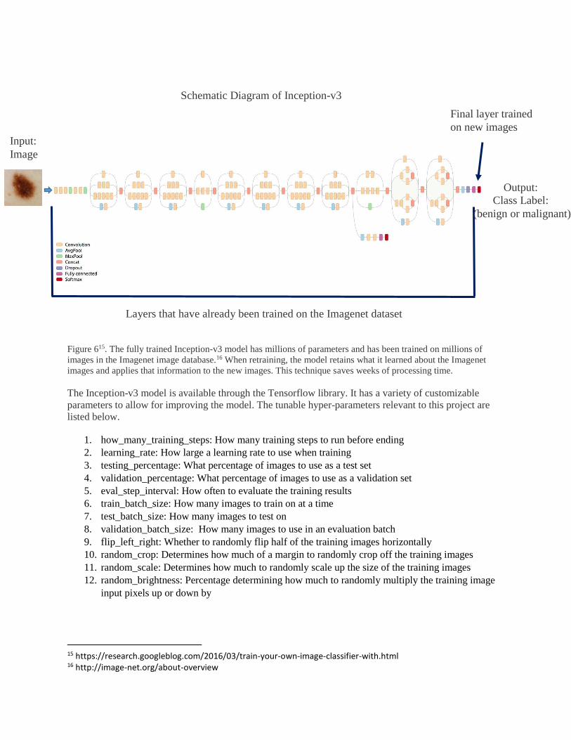
Figure 615. The fully trained Inception-v3 model has millions of parameters and has been trained on millions of

images in the Imagenet image database.16 When retraining, the model retains what it learned about the Imagenet

images and applies that information to the new images. This technique saves weeks of processing time.

The Inception-v3 model is available through the Tensorflow library. It has a variety of customizable

parameters to allow for improving the model. The tunable hyper-parameters relevant to this project are

listed below.

1. how_many_training_steps: How many training steps to run before ending

2. learning_rate: How large a learning rate to use when training

3. testing_percentage: What percentage of images to use as a test set

4. validation_percentage: What percentage of images to use as a validation set

5. eval_step_interval: How often to evaluate the training results

6. train_batch_size: How many images to train on at a time

7. test_batch_size: How many images to test on

8. validation_batch_size: How many images to use in an evaluation batch

9. flip_left_right: Whether to randomly flip half of the training images horizontally

10. random_crop: Determines how much of a margin to randomly crop off the training images

11. random_scale: Determines how much to randomly scale up the size of the training images

12. random_brightness: Percentage determining how much to randomly multiply the training image

input pixels up or down by

15 https://research.googleblog.com/2016/03/train-your-own-image-classifier-with.html 16 http://image-net.org/about-overview

Schematic Diagram of Inception-v3

Final layer trained

on new images

Layers that have already been trained on the Imagenet dataset

Input:

Image

Output:

Class Label:

(benign or malignant)

Benchmark

A typical assessment of a machine learning model’s effectiveness is whether or not it is better than a

human performing the same task. In the case of a model focused on diagnosing skin cancer this is a

logical strategy. In order for the model to be valuable it likely needs to be at least as effective as the

average human physician.

According to a study conducted by Rolfe17, which analyzed the accuracy of 6546 skin biopsies/excisions,

physicians had a diagnostic sensitivity (recall) of 76% with respect to melanoma diagnoses. As discussed

in the Metrics section, recall will be used as the primary evaluation metric. Therefore, the benchmark for

this model is:

Recall > 76%

III. Methodology

Data Preprocessing

Step 1: Remove unnecessary items from the dataset

For the ISIC dataset superpixel images for all of the mole images were provided. Since these will not be

necessary for generating this model, they all had to be removed (Figure 7).

Step 2: Remove abnormal pictures

As discussed in the Exploratory Visualization section, there were abnormal pictures that could potentially

bias and compromise the model. These images were all identified and removed. This amounted to 229

images being removed from the dataset. (Figure 8).

Step 3: Divide the images into three separate folders based on their diagnoses. Benign, Melanoma

and Seborrheic Keratosis.

The implementation of the Inception-v3 model being used analyzes images within folders and classifies

each image as the name of the folder. Therefore, all of the images for each specific diagnosis need to be

within the same folder.

Step 4: Remove the Seborrheic Keratosis folder from the analysis

Because the goal of this project is to determine whether a mole is benign (without any abnormality) or

malignant (with melanoma, the Seborrheic images will add unnecessary complexity to the model.

Step 5: Reduce the number of images in each image directory

After removing the superpixel images, the dataset of 2000 mole images is ~8GB. While more data is

almost always superior to less data for machine vision tasks, it was not feasible to work with such a large

dataset due to limited computational capabilities and need to transfer the files for submission.

300 training images and 30 test images, were randomly selected from the dataset for both of the classes,

660 total. The final file size is ~2GB. This allows for more manageable model building and evaluation.

17 https://www.ncbi.nlm.nih.gov/pubmed/22571558

Step 6: Split images into training, testing and validation sets

When the model is initialized it analyzes the folders in the image directory and splits the images into

training, testing and validation sets prior to analyzing them. 10% are divided to test, 10% to validation

and 80% to training. After these preprocessing steps have completed the analysis can begin.

Figure 7 (left). An example superpixel image from the dataset. While superpixel images can be valuable

for other analyses, they are not necessary for this project, therefore, they were removed.

Figure 8 (right). A collection of abnormal images that had to be removed from the dataset in order to

prevent bias. In this example, all of the stickers were found in benign images.

Implementation

Upon completion of the Tensorflow setup (see Read Me file), the model can be initiated using the

example retrain.py file. This python file contains all of the necessary components and calculations to run

the algorithm and analyze images. Alterations to the retrain.py file were necessary to meet the goals of

this project. These steps are as follows:

Step 1: Calculate true positive, false positive, false negative and true negative measures

The model only calculates accuracy by default. Because the goal is to measure the model’s performance

using recall, it was necessary to calculate the tp, fp, fn, tn, measures so that they could be utilized to calculate

recall.

Step 2: Display the hyper-parameters being adjusted each time the model is ran

Because the goal is to optimize the model with the highest recall possible, it is useful to have all of the

hyper-parameters being used and with their respective values. The model does not do this by default so it

was necessary to develop and implement this functionality.

Step 3: Display the measures: true positive, false positive, false negative and true negative

It was also necessary to display the measures in order to help model optimization.

Superpixel Image Abnormal Images Removed from Dataset

Step 4: Calculate & display model metrics performance: precision, recall, f1 and accuracy

With respect to overall model performance the only metric provided by default is accuracy. As mentioned

previously, accuracy is not a useful metric to use with this project because it will be skewed by true

negatives. Therefore, calculations were implemented for precision, recall, f1, and accuracy (in order to

verify consistency with the model’s accuracy)

Step 5: Append all performance metrics and hyper-parameters to a CSV file for analysis

Because it is necessary to run many trials with many variants of hyper-parameter settings to optimize the

model, all the metrics and hyper-parameter information is appended to a CSV file which can be analyzed

for optimal parameter tuning.

Running the Incpetion-v3 model.

After all of the necessary installation and setup steps are complete the process for analyzing images with

the model is relatively simple. The steps below outline how the process/model function.

1. Navigate to the tensorflow directory.

2. Run the appropriate code directed to the images that will be analyzed.

3. The retrain.py file will be called and begin the analysis on the selected images.

4. The latest version of the inception-v3 model will be downloaded

5. The model calculates “bottleneck” values for each image, these are the values the model uses to

classify the image.

6. The images are randomly divided into training, testing and validation sets.

7. The model begins training: the model predicts which class the image belongs to, compares the

prediction to the actual label, and updates the final layer’s weight using the backpropagation

process. The validation images are used during this step (Figure 9).

8. Finally, the test images, those that did not contribute to the model training, are analyzed. The

predictions made for these images determine the overall model accuracy.

9. The model displays the results including all of the customized metrics and values (Figure 10).

Figure 9 (above). The Inception-v3 model displays output for three

of the training processes. First, train accuracy shows what percent

of images in the current batch were predicted correctly. Second, cross

entropy is a loss function that demonstrates how well the learning process

is progressing because the objective of training is to minimize the loss function.

Finally, the validation accuracy represents how well the model predicts randomly-

selected images from different batches.

Figure 10 (left). Output after training is complete. This output was

obtained from running the model with all default values for the hyper-parameters,

except test_batch_size which was manually set at 10% of the dataset (60).

Top, the overall accuracy of the model. Middle, the hyper-parameters and their values.

Bottom, the metrics demonstrating the model’s performance.

Recall is 67.9%, the average of three trials with default values was 70.9%. This leaves

much room to improve the model to achieve a performance greater than the 76%

benchmark.

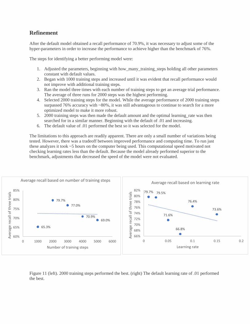
Refinement

After the default model obtained a recall performance of 70.9%, it was necessary to adjust some of the

hyper-parameters in order to increase the performance to achieve higher than the benchmark of 76%.

The steps for identifying a better performing model were:

1. Adjusted the parameters, beginning with how_many_training_steps holding all other parameters

constant with default values.

2. Began with 1000 training steps and increased until it was evident that recall performance would

not improve with additional training steps.

3. Ran the model three times with each number of training steps to get an average trial performance.

The average of three runs for 2000 steps was the highest performing.

4. Selected 2000 training steps for the model. While the average performance of 2000 training steps

surpassed 76% accuracy with ~80%, it was still advantageous to continue to search for a more

optimized model to make it more robust.

5. 2000 training steps was then made the default amount and the optimal learning_rate was then

searched for in a similar manner. Beginning with the default of .01 and increasing.

6. The default value of .01 performed the best so it was selected for the model.

The limitations to this approach are readily apparent. There are only a small number of variations being

tested. However, there was a tradeoff between improved performance and computing time. To run just

these analyzes it took ~5 hours on the computer being used. This computational speed motivated not

checking learning rates less than the default. Because the model already performed superior to the

benchmark, adjustments that decreased the speed of the model were not evaluated.

Figure 11 (left). 2000 training steps performed the best. (right) The default learning rate of .01 performed

the best.

65.3%

79.7%

77.0%

70.9%69.0%

60%

65%

70%

75%

80%

85%

0 1000 2000 3000 4000 5000 6000

Ave

rage

rec

all o

f th

ree

tria

ls

Number of training steps

Average recall based on number of training steps

79.7% 79.5%

71.6%

66.8%

76.4%

73.6%

66%

68%

70%

72%

74%

76%

78%

80%

82%

0 0.05 0.1 0.15 0.2

Ave

rage

rec

all o

f th

ree

tria

ls

Learning rate

Average recall based on learning rate

IV. Results

Model Evaluation and Validation

As discussed a process of trial and error was conducted to generate a model that consistently performs

superior to humans at diagnosing melanoma. The only hyper-parameter that required adjustment to

overcome the benchmark of 76% recall was the number of training steps. However, training steps alone

did not make the model sufficiently robust, so learning rate was also adjusted until the model consistently

performed above 76% recall.

In order to evaluate the models’ robustness, 60 new images (10% the size of the dataset) were

incorporated into the dataset. If the model was overfitting to the data, introducing these new images

should have had an effect on the performance. This is exactly what was seen. After introducing the new

images, the average recall of the model dropped to about 72%. With the new images, further model tuning

may be necessary.

That being said, the model’s results probably should not be trusted for a variety of reasons. First, the

dataset is very small and it was collected in an uncontrolled manner (it was self-submitted) so there are

possibly biases in the data, such as lighting, camera focus, angles, camera distance from mole, etc. The

model may be detecting these subtle differences in photographic technique rather than true features of

melanoma. While it would be fantastic if a diagnostic model superior to human physicians could be

generated from 600 images, this simply does not seem plausible. These results should probably not be

taken for true diagnostic accuracy, but rather features of the data and the limited number of images.

Justification

Ultimately, the final solution does provide results that are consistently superior to the benchmark.

However, for the reasons discussed above these results should probably not be trusted. Performing a

legitimate statistical test for significance is not feasible on these results due to the small sample size of

trials and the methodological differences between this project and the research paper from which the

benchmark was generated. To conduct a legitimate test for statistical significance, such as a t-test, many

more analyses would be needed, which would take a prohibitively large amount of time with the current

computing resources. The model demonstrates promise and the potential for a sophisticated diagnostic

model in the future. But there just simply is not enough evidence to demonstrate that the model generated

in this project is superior to human diagnostic abilities.

V. Conclusion

Free-Form Visualization

After the Inception-v3 model is completely trained, it can evaluate new images and provide a probability

that the image belongs to each of the classes in the training dataset, for this project that is whether the

mole in the image has melanoma or is benign. In Figure 12 three images have been evaluated by the

model. Two of the images are moles located on my stomach, both of which are almost certainly benign.

The third is a scar that formed after a mole was excised. This scar is located near the other moles being

analyzed on my stomach.

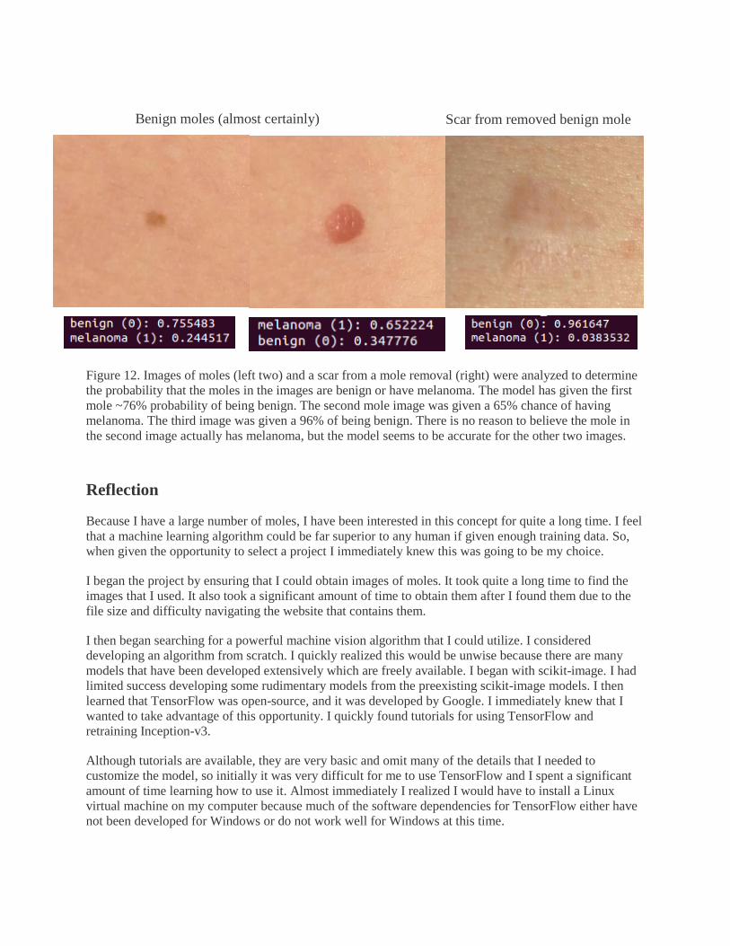
Figure 12. Images of moles (left two) and a scar from a mole removal (right) were analyzed to determine

the probability that the moles in the images are benign or have melanoma. The model has given the first

mole ~76% probability of being benign. The second mole image was given a 65% chance of having

melanoma. The third image was given a 96% of being benign. There is no reason to believe the mole in

the second image actually has melanoma, but the model seems to be accurate for the other two images.

Reflection

Because I have a large number of moles, I have been interested in this concept for quite a long time. I feel

that a machine learning algorithm could be far superior to any human if given enough training data. So,

when given the opportunity to select a project I immediately knew this was going to be my choice.

I began the project by ensuring that I could obtain images of moles. It took quite a long time to find the

images that I used. It also took a significant amount of time to obtain them after I found them due to the

file size and difficulty navigating the website that contains them.

I then began searching for a powerful machine vision algorithm that I could utilize. I considered

developing an algorithm from scratch. I quickly realized this would be unwise because there are many

models that have been developed extensively which are freely available. I began with scikit-image. I had

limited success developing some rudimentary models from the preexisting scikit-image models. I then

learned that TensorFlow was open-source, and it was developed by Google. I immediately knew that I

wanted to take advantage of this opportunity. I quickly found tutorials for using TensorFlow and

retraining Inception-v3.

Although tutorials are available, they are very basic and omit many of the details that I needed to

customize the model, so initially it was very difficult for me to use TensorFlow and I spent a significant

amount of time learning how to use it. Almost immediately I realized I would have to install a Linux

virtual machine on my computer because much of the software dependencies for TensorFlow either have

not been developed for Windows or do not work well for Windows at this time.

Benign moles (almost certainly) Scar from removed benign mole

After countless hours of learning how to use Tensorflow, I finally was able to get it to function. I then

cleaned the image data, randomized and separated it into smaller classes for the analysis. I then began

analyzing the data and adjusting the hyper-parameters to optimize the model. The Inception-v3 model is

an extraordinarily effective model and it was great getting the opportunity to utilize it for this project. I

still feel slightly skeptical of the great results I obtained for only having 600 images in the dataset,

however it definitely is cause for optimism with respect to machine vision capabilities.

Improvement

There are two fundamental limitations to the model which, if overcome, would likely improve it

substantially. The first is a lack of computing resources. The second is lack of data.

Need for more computational resources

Although the retrained model only requires a fraction of the time to use when compared to training from

scratch, it still requires a substantial amount of time and computational resources. Testing different

variations of hyper-parameters requires an extensive amount of time. Also, some of the distortions simply

could not be used because the time necessary was prohibitive. The model is equipped with four

distortions which can be used to randomly distort the photos, which can help the model generalize to

unseen data more effectively.

The distortions are:

1. flip_left_right

2. random_crop

3. random_scale

4. random_brightness

These parameters are described in more detail in the Algorithms and Techniques section. All of the

parameters manipulate the photos in some manner, which can help remove potential bias from an image

class. Unfortunately, when attempting to utilize these distortions the computer being used was not

powerful enough to make it practical. It took several minutes just to analyze one batch, as opposed to

several batches per second when the distortions were not used. That being said, these distortions could

potentially improve the model. It just was not practical to use them for this project.

Lack of image data

For developing an effective machine vision model, 600 images is likely far too few. Of course, the

number of images was limited in an effort to reduce evaluation time and make transferring files simpler.

However, even the total 13,000 images available on the ISIC website is likely far too small. For

something as nuanced as mole features, it will possibly take millions of labeled images to develop a truly

effective human-level model. More images would almost certainly improve the model even if nothing

else was adjusted. Ultimately, there are ways in which this model could be improved greatly. I believe

that in the not too distant future there will be machine learning algorithms that are superior to humans

with respect to diagnosing melanoma.