capital flows to emerging markets: causes, consequences...
TRANSCRIPT

Capital Flows to Emerging Markets: Causes, Consequences and Policy Options
Aquiles Rocha de Farias – Banco Central do Brasil
June 2016

The views expressed here are those of the author and do not necessarily reflect those of the Banco Central do Brasil or its members.

Cause Quantitative easing policies in AEs causes capital inflows
Monetary policy normalization in AEs causes capital outflows
Effect Sudden flood increases vulnerability (amplification mechanisms: excessive appreciation, borrowing, current account deficits, consumption, and again)
Given vulnerability, may put in motion sudden stop (amplificationmechanism: excessive depreciation, deleveraging, current account surplus, recession, and again)
Policy Smooth the upturn with (i) forex buy [lean against the wind and accumulate reserves], (ii) higher capital inflow taxes, (iii) tighter macroprudential policy, (iv) tighter monetary and fiscal policy [carefully: it is a pull factor and appreciation increases risk‐taking], (v) tighterfiscal policy
Smooth the downturn with (i) forex sell [hedge first], (ii) lower capital inflow taxes, (iii) easier macroprudential policy, (iv) easier monetary policy [carefully: it is a pull factor, depreciation can be at once contractionary and inflationary], (v) easier fiscal policy (if possible)
This cause is on top of other push [eg risk aversion] and pull [interest rate and growth]. e.g. Ahmed (2014).
Cause – Effect - Policy

Cause: Quantitative Easing
According to the Bernanke (2012), portfolio rebalancing is an important part of the transmission mechanism of the LSAP (that is, QE policies).
The argument goes back to Tobin (1969, 1982). Reduced supply of long‐term treasuries reduces marginal benefit of short term treasuries, pressures long term bond prices and moves investors towards other assets.
Suppose we can observe how US investors would respond to QE if they lived abroad and were therefore less directly affected. Then we could easily see if QE policies affects their behavior.
Of course, we cannot observe this. It is a counterfactual. But we can observe the next best thing: how ROW foreign investors behave during QE.
To make this even better, let’s focus on capital flows to the same recipient economy, and let’s control for different environments in US and ROW.
This section is based on “Quantitative Easing and United States Investor Portfolio Rebalancing Towards Foreign Assets” available as BCB WP n420

‐6
‐4
‐2
0
2
4
6
8
10
May‐03
Oct‐03
Mar‐04
Aug‐04
Jan‐05
Jun‐05
Nov
‐05
Apr‐06
Sep‐06
Feb‐07
Jul‐0
7
Dec‐07
May‐08
Oct‐08
Mar‐09
Aug‐09
Jan‐10
Jun‐10
Nov
‐10
Apr‐11
Sep‐11
Feb‐12
Jul‐1
2
Dec‐12
May‐13
Oct‐13
CreditDebt AbroadDebt in the countryEquityTotal (‐direct)
[QE3,.)[QE2,QE3)[QE1,QE2)
Capital Flows from ROW to Brazil
USD bn, 6 mma

‐3
‐2
‐1
0
1
2
3
4May‐03
Oct‐03
Mar‐04
Aug
‐04
Jan‐05
Jun‐05
Nov
‐05
Apr‐06
Sep‐06
Feb‐07
Jul‐0
7
Dec‐07
May‐08
Oct‐08
Mar‐09
Aug
‐09
Jan‐10
Jun‐10
Nov
‐10
Apr‐11
Sep‐11
Feb‐12
Jul‐1
2
Dec‐12
May‐13
Oct‐13
CreditDebt AbroadDebt in the countryEquityTotal (‐direct)
[QE3,.)[QE2,QE3)[QE1,QE2)
Capital Flows from US to Brazil
USD bn, 6 mma

We build a unique dataset of capital flows to Brazil from the US and ROW.
We build a similar but less comprehensive and homogeneous dataset of capital flows to 17 EMEs from the US and ROW.
Both datasets show that more than 50% of US flows to EMEs during theQE policies were actually caused by QE policies (between 50 and 80 USD billion in the case of Brazil).
We break this into types of flows; portfolio flows are particularly sensitive.
We break into QE rounds; results are basically the same and equally distributed around QE policy rounds.
We break into sectors; bank flows are not the major share of the effect.
Overall, very strong evidence that QE cause portfolio rebalancing.
This section is based on “Quantitative Easing and United States Investor Portfolio Rebalancing Towards Foreign Assets” available as BCB WP 420
Cause: Quantitative Easing: Summary of Results

Effect: Expansion, Appreciation, Vulnerability
Consider the Claim: QE sudden floods put in motion a feedback loop with asset price appreciation, lower credit constraints, higher indebtedness, higher consumption, higher growth, and so a new round of effects.
Most policymakers in EMEs would agree with this claim. Yet there is surprisingly little credible evidence about this for the QE‐specific floods.
Suppose we observe how capital flows to a recipient economy would be if the Fed had not implemented QE policies. Then we could infer the effects implied by structural economic models.
Of course, we cannot observe this. It is a counterfactual. But we can forecast what would happen under many scenarios, and consider robust results.
Moreover, we propose a structural model and a decomposition method that allows measuring the contribution of capital flows to the effects.
This section is based on “Quantitative Easing and Related Capital Flows into Brazil: measuring its effects and transmission channels” available as BCB WP 313

Ex Ante Effect = relative to dotted line
Ex Post Effect = relative to actual series
LHS = Full Sample
RHS = Crisis Sample
** = sign at 5%* = sign at 10%o = not sign
Range of Effects for Core Variables
(+) from 1.8% to 5.4% (**)ie. 10 bn to 25 bn USD
(‐) from 3.3% to 10.1% (*)
(+) from 0.4% to 1.3% (*)
(‐) from 4.0% to 11.7% (**)
(+) from 4.2% to 12.5% (**)ie. 30 bn to 100 bn USD
(+) from 1.0% to 2.9% (**)
Based on the previous section, now know effects are closer to the right end of the intervals in the full sample (left end, crisis sample) More than we knew in 2014!

Effect: Expansion, Appreciation, Vulnerability: Summary
QE causes the following effects on the Brazilian economy:
Capital inflows
Exchange rate appreciation
Economic activity impulse
Stock market price increases
Consumption growth
Credit market boom
Robust to more variables in the global scenario (e.g. China activity, Euro monetary policy), and domestic variables in core model (e.g. public credit).
Capital flows is the only consistently significant (economically and statistically) across variables, samples, scenarios and models.
This section is based on “Quantitative Easing and Related Capital Flows into Brazil: measuring its effects and transmission channels” available as BCB WP 313
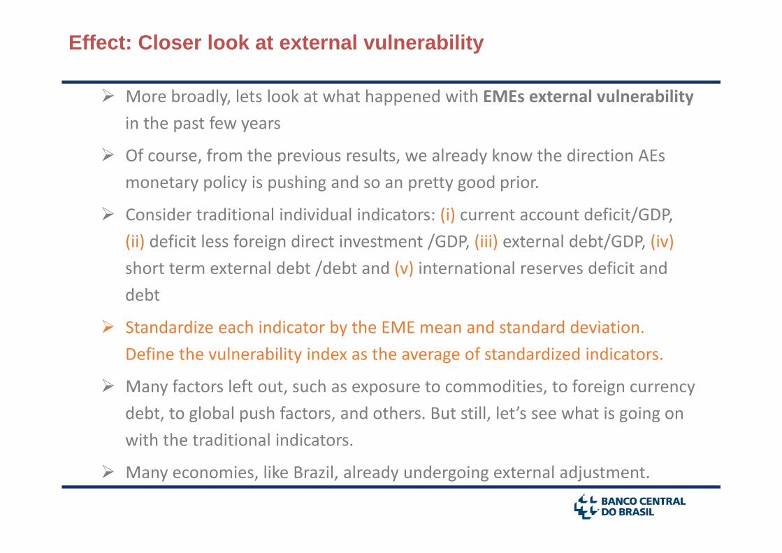
Effect: Closer look at external vulnerability
More broadly, lets look at what happened with EMEs external vulnerability in the past few years
Of course, from the previous results, we already know the direction AEs monetary policy is pushing and so an pretty good prior.
Consider traditional individual indicators: (i) current account deficit/GDP, (ii) deficit less foreign direct investment /GDP, (iii) external debt/GDP, (iv)short term external debt /debt and (v) international reserves deficit and debt
Standardize each indicator by the EME mean and standard deviation. Define the vulnerability index as the average of standardized indicators.
Many factors left out, such as exposure to commodities, to foreign currency debt, to global push factors, and others. But still, let’s see what is going on with the traditional indicators.
Many economies, like Brazil, already undergoing external adjustment.

External Vulnerability Index
In standard deviation of vulnerability units
‐0.6
‐0.4
‐0.2
0
0.2
0.4
0.6
2002 2003 2004 2005 2006 2007 2008 2009 2010 2011 2012 2013 2014 2015
75% percentile
25% percentile
median Brazil

Policy: Foreign Exchange Intervention
Foreign exchange intervention is useful to lean against the wind of (i) appreciation that increases vulnerability and (ii) depreciation that may trigger sudden stops.
Ironically, because of this, it is hard to assess its effectiveness. It is like saying police causes crime, because high crime cities have a large police force.
Suppose we have an observable random variable that affects intervention but that is not correlated with the exchange rate variation. This solves the problem, because we can isolate a ‘random part’ of the intervention.
It is very hard to find such a variable. Except in financial markets!
I have shown elsewhere that realized volatility (and other similar observable variables) fits the requirements by purely formal reasoning. A very clean identification strategy.
This section is based on “Realized Volatility as an Instrument to Official Intervention” available as BCB WP 363

‐4500
‐3500
‐2500
‐1500
‐500
500
1500
2500
3500
4500
11/07/20
07
11/09/20
07
11/11/20
07
11/01/20
08
11/03/20
08
11/05/20
08
11/07/20
08
11/09/20
08
11/11/20
08
11/01/20
09
11/03/20
09
11/05/20
09
11/07/20
09
11/09/20
09
11/11/20
09
11/01/20
10
11/03/20
10
11/05/20
10
11/07/20
10
11/09/20
10
11/11/20
10
11/01/20
11
11/03/20
11
11/05/20
11
11/07/20
11
11/09/20
11
11/11/20
11
SPOT SWAP
USD million
Foreign Exchange Interventions in Brazil
This section is based on “Realized Volatility as an Instrument to Official Intervention” available as BCB WP 363

0
20
40
60
80
100
120
140
1
1.2
1.4
1.6
1.8
2
2.2
2.4
11/07/20
07
11/09/20
07
11/11/20
07
11/01/20
08
11/03/20
08
11/05/20
08
11/07/20
08
11/09/20
08
11/11/20
08
11/01/20
09
11/03/20
09
11/05/20
09
11/07/20
09
11/09/20
09
11/11/20
09
11/01/20
10
11/03/20
10
11/05/20
10
11/07/20
10
11/09/20
10
11/11/20
10
11/01/20
11
11/03/20
11
11/05/20
11
11/07/20
11
11/09/20
11
11/11/20
11
Realized Variance
BRL/USD
BRL % %
Foreign Exchange Interventions in Brazil
This section is based on “Realized Volatility as an Instrument to Official Intervention” available as BCB WP 363

Policy: Foreign Exchange Intervention: Summary
The average impact effect of a 1 billion USD sell or buy intervention is around 0.50% depreciation or appreciation, respectively.
The estimate is a bit lower controlling for swaps (0.30%), which suggests intervention policies are complementary.
The analogous effects from swap operations is around (.25%), but this was not statistically significant in our sample. But the direction is consistent with other sources of evidence of swap effectiveness.
This section is based on “Realized Volatility as an Instrument to Official Intervention” available as BCB WP 363

Policy: Macroprudential Policy
Emerging markets have made intense use of macroprudential policy to smooth the credit cycle. A case in point is reserve requirement (RR)policy.
The argument for effectiveness goes back to Stein (1998). A change in funding composition towards or away from reservable (and usually insured) liabilities affects funding costs and then credit supply.
Suppose we had bank specific shocks to reserve requirements during a certain time period. This allows us to identify the effect of the shock and how it relates with variables of interest.
From 2008 to 2014 the BCB provided us with many policy shocks! We used loan level data from the “Sistema de Informação de Crédito” (SCR) to measure the impact of the shocks on credit supply.
This section is based on “Credit Supply Responses to Reserve Requirement: Evidence from credit registry and policy shocks” available upon request

Reserve Requirements in Brazil
Counterfactual based on regulation in place before September 2008
This section is based on “Credit Supply Responses to Reserve Requirement: Evidence from credit registry and policy shocks” available upon request

Policy: Macroprudential Policy
The evidence is suggestive that RR policy impact credit supply in the expected direction, that is, RR easing increases credit, while RR tightening decreases credit supply.
Interaction results are sensitive to specifications. But overall we find that
Banks with higher liquidity and capital ratios mitigate the impact
Monetary policy is a complement to RR policy in the sense that tightening one policy increases the effect of the other on credit
During economic expansions the impact of RR is somewhat weaker
Riskier borrowers receive less credit during tightening
This section is based on “Optimal Capital Flow Taxes in Latin America” available upon request
Policy: Capital Flow Management
Capital flow management makes sense when too much borrowing today makes the adjustment harder in the future, but economic agents don’t care.
The severity of future external adjustment depends on how badly needed is foreign funding
The amplification of the adjustment depends on how much harder to get foreign funding once there is recession and depreciation.
The likelihood of the adjustment depends on how much borrowing has been done in the past and on the willingness to lend to the country
To make agents care about borrowing to exact extent that they should, set
optimal capital flow tax = severity * amplification * likelihood
This section is based on “Optimal Capital Flow Taxes in Latin America” available as BCB WP 268
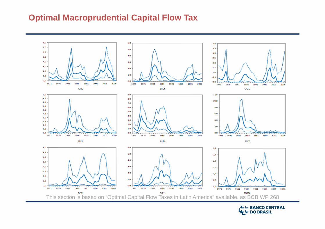
Optimal Macroprudential Capital Flow Tax
This section is based on “Optimal Capital Flow Taxes in Latin America” available. as BCB WP 268

Rule of thumb for optimal tax
Optimal tax is proportional to the square of the crisis probability
This section is based on “Optimal Capital Flow Taxes in Latin America” available as BCB WP 268
Summary
Conventional and unconventional monetary policy in AEs is the most important driver of capital inflows into EMEs.
Accounts for more than 50% of the inflows during QE.
Emerging markets that borrow abroad face an amplification mechanism.
sudden floods: excessive appreciation, consumption and liability growth
sudden stops: excessive depreciation, recession and external adjustment
We show evidence of the mechanism operating during the sudden flood of QE periods. By the historical record, it is possible it operates in reverse now.
The policy options involve smoothing the amplification mechanisms.
We show (i) foreign exchange intervention is effective, (ii) macroprudential policy is effective, (iii) capital flow tax is a feasible option, as far as choosing the tax rate goes.

Capital Flows to Emerging Markets: Causes, Consequences and Policy OptionsAquiles Rocha de Farias