Capital Controls in Chile: Effective? Efficient? †

Francisco Gallego*

Leonardo Hernández♣♣

Klaus Schmidt-Hebbel*

AbstractNew empirical evidence with regards to the effectiveness and efficiency of Chile’s capital controlsis provided here, based on more and better data on the range of controls and a broad assessment oftheir costs and benefits. The paper concludes that capital controls have been partially effective byraising the wedge between domestic and foreign interest rates, reducing aggregate net capitalinflows, and changing the debt composition toward longer maturities, without significantly alteringthe real exchange rate. Part of these effects is temporary as the effectiveness of controls is erodedover time for a given interest rates differential. Controls may have been crucial by contributing toChile’s lower exposure to short-term foreign liabilities at the time of the 1997-98 internationalfinancial turmoil. However, achieving temporary macroeconomic benefits by relying on capitalcontrols involves incurring in financial and growth effects that raise concerns about theirefficiency. The costs that resulted from the policy mix that comprised the capital controls, in termsof quasi-fiscal losses and lower investment and growth, were probably not negligible.

ResumenEste trabajo presenta nueva evidencia empírica sobre la efectividad y eficiencia de los controles decapital en Chile. La evidencia se basa en más y mejores datos sobre estos controles y en unaestimación aproximada de algunos de sus costos y beneficios potenciales. En el trabajo se concluyeque los controles de capital han sido parcialmente efectivos en aumentar la diferencia entre lastasas de interés internas y externas, reducir los flujos netos de capitales, y cambiar la madurez delos pasivos externos, aunque sin afectar significativamente al tipo de cambio real. El efecto sobre lamadurez de los pasivos externos (hacia plazos más largos) pudo haber jugado un rol trascendentedurante la crisis financiera internacional de 1997-98. Sin embargo, parte de estos efectos sontransitorios debido a que la efectividad de los controles se erosiona a través del tiempo por laexistencia de diferenciales positivos de tasas de interés. Los controles de capitales, no obstantegenerar beneficios macroeconómicos transitorios, también producen efectos financieros y sobre elcrecimiento, los que deben ser tomados en cuenta para evaluar su eficiencia. Existen costosimportantes, en términos de déficits cuasi-fiscales y menores tasas de inversión y crecimiento,resultantes de la combinación de políticas de las cuales el encaje es parte integrante.

JEL classification: E52, F21, F32, F36, F41

† The authors are very grateful to Pamela Mellado for excellent research assistance and to María T. Cofré for

kindly providing the raw data used in this study. The authors also thank Mario Blejer, Salvador Valdés-Prieto and Rodrigo Valdés for their comments to an earlier version of this paper, and to Miguel Fonseca andAngel Salinas for explaining to us crucial aspects of capital account regulations in Chile. Only the authorsare responsible for the findings and opinions presented here. This paper does not reflect the views of theCentral Bank of Chile or its Board of Directors.Authors’ email: fgallego@condor.bcentral.cl; lhernandez3@imf.org; kschmidt@condor.bcentral.cl

* Research Department, Central Bank of Chile♣ International Monetary Fund- Central Bank of Chile

1

1. Introduction

Controls on international capital flows have no place in a world without policy distortionsand market failures. However, even in the presence of policy distortions and market failures, it isdifficult to argue for imposing second-best measures such as capital controls. Here the conventionalargument applies that a better alternative to capital controls is to address directly the distortionsthat render capital flows ‘excessive’. These distortions comprise inadequate regulation andsupervision of the financial and corporate sectors, policy-induced moral hazard created, forinstance, by the provision of foreign-exchange insurance, etc. However, one may argue thatinternational distortions affecting the supply of capital –ranging from the existence of contagionand bandwagon effects in private markets, to moral hazard problems derived from the existence ofinternational rescuers of last resort– are not removable by recipient countries. Therefore, theargument follows, international distortions in the supply of capital should be offset by imposingdomestic capital controls aimed at limiting excessive capital inflows in good times, hence reducingthe likelihood of a solo or a twin crisis in bad times.

Chile’s long experience with capital controls—of both the administrative and thequantitative sort—has caught the interest of both policy makers and academics in a world of highlyvolatile capital flows, especially since Mexico’s crisis in 1994-95. An increasing number of recentstudies has provided an empirical evaluation of the macroeconomic effects of Chile’s quantitativerestriction on capital inflows—the unremunerated reserve requirement imposed by the CentralBank of Chile on selective (mostly short-term or financial) capital inflows during 1991-1998. Thispaper extends this literature in three directions: first, it provides an alternative measure of thefinancial cost of the reserve requirement, that differs significantly in both magnitude and effectsfrom conventional measures used in previous research; second, it broadens the study of capitalcontrols to include other administrative controls on capital flows and their effects; and third, itevaluates various potential “social” costs of capital controls (more precisely, of the policy mix thataccompanied the controls).

Section 2 provides a brief review of existing empirical studies on Chile. Subsequently, bothquantitative and administrative controls on capital flows in Chile are described and measured.Section 4 presents a simple dynamic model to analyze the effects of capital controls onmacroeconomic and financial aggregates. Regression results for the macroeconomic and financialeffects of all categories of capital controls are reported for monthly data covering the 1989-1998decade in section 5. A discussion of the quasi-fiscal, financial, and growth costs of capital controlstakes place in section 6. The paper concludes with a brief summary of benefits and costs of Chile’scapital controls presented in section 7.

2. Previous Findings and Remaining Questions

The experience of Chile since controls to capital inflows were imposed in the early 1990s,in the form of an unremunerated reserve requirement –URR–, has been studied in a number ofpapers. This section sets the stage by summarizing this literature and its main findings, and listingsome of the questions that have not been answered and, therefore, should be addressed in futureresearch. A more detailed review of the literature is provided in Annex 1.

Starting with the study by Soto and Valdés (1996), the growing literature on the Chileanexperience with capital controls during the 1990s has addressed three related questions, namely:

2

1. Has the URR increased the effectiveness of monetary policy, in an environment where theexchange rate is semi-fixed (i.e., where it fluctuates within a narrow band set by the authority)?

2. Has the URR allowed for a lower real exchange rate—a more depreciated currency—than itwould have been the case otherwise?

3. Has the URR contributed to a sounder—less risky—inflow composition, in the sense ofinducing inflows of longer maturity?

These questions arise directly from the reasons argued by the authority to impose andmaintain the URR in place from June 1991 through September 19981.

The existing research on this subject has addressed these questions using twocomplementary approaches, namely:

A. Single equation models (SEMs) in which the domestic interest rate (id), the real exchange rate(RER), and the composition of flows are regressed against the URR and other explanatoryvariables, and

B. Vector auto-regressive (VAR) models.

The SEMs are aimed at identifying and measuring the direct effect of the URR—controlling for other determinants—on any of the three dependent variables (id, RER, and thecomposition of flows). One disadvantage of this approach is that it requires strong assumptionsregarding the functional form of the equations to be estimated (i.e., the relationship among thedifferent variables) and exogeneity of the right hand side variables. Furthermore, there is a risk ofan estimation bias because of missing variables. The VAR approach, on the other hand, addressesthese problems since it identifies the dynamic relationship existing among the variables, imposingonly minimum identification restrictions. However, it does not provide a direct measure of theeffect of the URR on the variables of interest, nor does it identify the channel through which theURR works.

Using quarterly data for 1987-96 and the SEM approach, Soto and Valdés (1996) andValdés and Soto (1998) conclude that the imposition of the URR did not alter the appreciatingtrend observed in the real exchange rate during the 1990s. However, these authors conclude that theURR changed the composition of inflows, reducing the share of taxed flows in total short-termcredit. This effect was stronger (albeit marginally significant) during 1995-96, when the URR washigher, and when a non-linear single equation model is used in the estimations. Also using a SEMapproach but monthly data for 1991-96, Eyzaguirre and Schmidt-Hebbel (1997) reach a similarconclusion regarding the composition of inflows; in particular, they find that the URR reduces theshare of short-term flows and increases that of long-term flows. Also, the latter find that the URRincreases the effectiveness of monetary policy—the URR permits a higher interest rate differentialwith foreign rates—and depreciates the real exchange rate, albeit on a temporary basis. However,their findings show that the latter two effects are rather weak and not robust to differentspecifications for the estimated equations.

Conversely, using quarterly data for 1985-94 and a SEM, Laurens and Cardoso (1998)conclude that the URR had no effect on the composition of inflows, and assert that the URR did

1 The URR was not abolished, but its rate was dropped to zero in September 1998. Thus, the authority kept

the option to use the instrument in the future.

3

affect neither the real exchange rate nor the interest rate differential. However, the way this modelis estimated and the sample period used cast some doubts about these conclusions2.

The main weaknesses of the preceding studies is that the estimations do not control forchanges in other capital account regulations, namely, the liberalization of capital outflows andinflows, and for changes in the URR other than the tax rate (i.e., coverage and presence ofloopholes)3. The recent paper by De Gregorio, Edwards and Valdés (1999) addresses the latterlimitation by including a new variable aimed at measuring the presence of loopholes (an indexmeasuring the power of the URR). Using a SEM and quarterly data for 1987-96, they conclude thatthe URR gave the monetary authority additional room to maneuver—permitted a higher domesticinterest rate—and changed the composition of inflows toward long-term flows. However, likeprevious studies, they are still unable to find any significant effect on the real exchange rate (RER)and on total inflows.

The latter result regarding the RER presents a puzzle, since the higher level of the domesticinterest rates—supported by the URR—should lead to lower domestic spending and hence to amore depreciated real exchange rate. The reason that this effect has not been found in the empiricalpapers based on the SEM approach is most likely due to mispecification problems. This iscorroborated by the results reported in the two studies that use the VAR approach, Soto (1997) andDe Gregorio, Edwards and Valdés (1999). Indeed, using monthly data for 1991-96 and 1991-98,respectively, these authors find that a shock on the URR causes a transitory real exchange ratedepreciation. Furthermore, Soto (1997) finds that increases in the URR leads to a reduction in thevolatility of the RER. These papers also confirm the previous findings regarding the level ofdomestic interest rates and the composition of inflows.

In sum, there is robust evidence showing that the URR has led to higher domestic interestrates—or a larger differential with international interest rates—and a composition of inflows biasedtowards longer maturities. However, the effect of the URR on the real exchange rate—or its path—has proved to be more difficult to uncover, most likely due to the difficulties in finding the correctmodel that relates these two (and other) variables. This issue requires additional research.

Additional methodological aspects remain to be addressed in future empirical research.Among these are the need to properly control for the liberalization of capital inflows andoutflows—something we attempt to do here—, and permitting other functional forms for therelationship between the URR and the variables of interest4. Also, there is the need to consider thesocial costs and welfare implications of the URR, something we also attempt to do—albeitindirectly—in this paper (see section 6).

2 The capital control —or URR— index used in this regression is positively correlated with the dependent

variable (inflows) by construction, biasing its estimated coefficient upwards. In particular, the capitalcontrol index is measured as the URR tax-rate times the tax base. The latter, in turn, is constructed as thecumulative capital inflows since 1985. This puts the contemporaneous inflow variable on both sides of theestimated equation. In addition, the sample period comprises years when capital inflows were not entirelyvoluntary—voluntary flows to Chile resumed only in 1989.

3 For a critical review of the literature—without rigorous empirical analysis—see Nadal-De Simone andSorsa (1999).

4 It is plausible that the URR affects the inflow of capital—through the interest rates differential—in a non-linear way, especially since it puts a wedge separating the decision to borrow from abroad from that ofinvesting abroad (the URR separates the two conditions of arbitrage). It is worth noting that none of theempirical papers exploring this relationship allows for a non-linear specification in this regard.

4

3. Capital Controls in Chile during the 1990s

Trends of Capital Controls worldwide and in Chile

While controls on inflows and outflows can be equivalent under steady-state conditions (asargued by Laban and Larraín, 1997), they are very different under non-stationary conditions and, inparticular, in a crisis situation. Indeed, controls on inflows (like Chile’s 1991-98 reserverequirement) are imposed ex-ante in a preventive way, while controls on outflows are typicallyimposed as ex-post measures to stem capital outflows (like Chile’s 1982 and Malaysia’ 1997controls). As a change in the rules of the game that amounts at least to a temporary expropriation,controls on outflows are much more costly to foreign investors and to the countries that imposethem. In addition, the international evidence suggests that controls on outflows are easier to evadethan those on inflows. Finally, controls on inflows are pro-cyclical (they are imposed when theworld supply of capital increases), while controls on outflows are anti-cyclical.

Chile is no exception to this world experience, with a long history of controls on capitalaccount flows and transactions that started in the 1930s and continued through the mid-1970s.Controls were gradually liberalized in the late 1970s and early 1980s, but were tightened again inthe aftermath of the Latin American debt crisis of the 1980s.

The resumption of voluntary capital flows to emerging markets coincided in time with newcapital inflows starting coming to Chile in 1988. After a growing tide of inflows during 1988-1990,the CBCh imposed new quantitative restrictions in the form of an unremunerated reserverequirement on selective inflows in 1991 (that lasted through September 1998), and beganliberalizing old administrative controls on outflows. At the same time, however, other quantitativeand administrative controls on capital inflows were also lessened. We review the specificrestrictions and their changes observed during the last decade next (see Table 3.1 and annexes 2, 3and 4).

The unremunerated reserve requirement (URR) on selective capital inflows

The URR is a requirement to hold an unremunerated fixed-term (mostly 1-year) reserve atthe Central Bank, equivalent to a fraction of capital inflows of selective categories. Hence the URRis equivalent to a tax per unit of time that declines with the permanence or maturity of the affectedcapital inflows. The quantitative nature of this restriction, i.e. its tax equivalence, is made explicitby its alternative form: foreign investors are alternatively entitled to pay an up-front fee determinedby the product of the relevant foreign interest rate (i*) and the fraction of capital subject to therestriction.

Various features of the URR were altered during the June 1991–September 1998 period ofits existence at non-zero rates. As summarized in Annex 2, the CBCh introduced changes in the rateor fraction of deposit, the coverage of capital inflow categories, the foreign currency denominationfor the reserve deposit and fee payment, the holding period, the restrictions to rollover maturinginvestments, and other administrative requirements related to the URR.

A simple equation that reflects the cost of the URR (urr) is the following:

5

(3.1) ( )urr =

−∗τ

τ1

h

k i

where τ is the fraction of deposit of the capital inflow at the CB; h is the required holding period; kis the average maturity of the foreign investment for which the urr is calculated (equal to 6 monthsin the empirical application); and i* is the equivalent foreign interest cost for a k-month operation5.

Similar measures to the urr defined above have been used in previous empirical studies.They can be termed “naive“ in the sense that they do not reflect the option value of reinvesting orrolling over the capital after maturity, as calculated by Herrera and Valdés (1998). However, in1996 the CBCh restricted the possibility of rolling over maturing investments, reducing therelevance of this option value.

The resulting time series for urr (Fig. 3.1) reflects both changes introduced by the CBCh(affecting τ, h/k, and the applicable i*), and changing market conditions (affecting i*). Starting witha tax rate of 20% in June 1991, τ was raised to 30% in 1992 and maintained throughout June 1998,when it was reduced to 10%, followed by a further reduction to zero in September 1998. Otheradministrative changes introduced by the CBCh affected the maturity (h/k) and the relevant i*6,albeit the latter was also affected by changing market conditions. (See Annex 5 for a detaileddescription of how urr and its components are measured in this paper.) The resulting urr series (Fig.3.1) shows a growing trend until late 1997, largely explained by the rising share of up-front feepayments7. From June 1991 through September 1998, the urr averaged 4.24% per year with astandard deviation of 2.14%. Its maximum was 7.7% in November 1997.

An indirect measure of how binding the URR was for capital inflows to Chile is providedby the total amount collected as deposits. The latter is comprised by the actual capital stockdeposited as required reserve at the CB, and the capital stock equivalent to the up-front feepayments made in lieu of the reserve deposit. At its peak in August 1997, the URR implied a totalamount of US$ 2,237 million equivalent to reserve deposits, comprised by US$ 825 million ofactual deposits and US$ 1,412 million of fee-equivalent deposits (Figure 3.2). This is a sizableamount, equal to 2.9% of 1997 GDP or 30.0 % of that year’s net capital inflow. During the wholeJune 1991-September 1998 period, the total equivalent reserve deposit attained an average of 2.0%average GDP, or 40% of the average capital-account surplus.

However, as in the case of any other tax, the URR provides an incentive for tax elusion andtax evasion.8 Comparing actual and required total reserve deposits provides a measure of the URRtax effectiveness or power, pow. The latter is estimated by the ratio between the flows that wereactually taxed with the URR –either by making a deposit or paying the equivalent up-front fee– andthe total amount of new flows that were potentially subject to the URR (see annex 5 for a detailed

5 For details on the applicable i* see annex 5.6 The CBC changed from the Yen i* to the Dollar i* in November 1994. See annex 2 for details.7 The fee-option appears to be more expensive than making the deposit with the CB, because of the spread

of 2.5% (and 4%) applied to it on top of the foreign interest rate i* (see annex 2). However, this result is inpart due to having underestimated in our calculations the true (country and other) risk premia charged byforeign lenders, which we estimated as being nearly constant at around 1% throughout the period.

8 Le Fort and Sanhueza (1997) provide a good description of the elusion that occurred during the periodwhen the URR was in effect.

6

discussion of this and related measures). The estimation is made with monthly flows as shown inequation (3.2)

(3.2) pow t= (actual flows paying the URR)t / (potential taxable flows)t

where the potential taxable flows are derived after adjusting the recorded capital inflows for the re-labeling that occurred through the different loopholes9.

The resulting time series (figure 3.4) suggests that the URR gained effectiveness throughtime, although this occurred because of the authorities constant effort to close loopholes in URRregulations—the latter was partly achieved by increasing its coverage. For instance, in January1992, 6 months after its introduction, the URR power index was at 0.50, mainly because of theincreasing re-labeling of several forms of capital inflows as dollar denominated deposits. Then,when dollar denominated deposits became subject to the URR in February 1992, the power indexincreased to 0.78 (though other loopholes were discovered and used by arbitrageurs). This patternis shown in the figures 3.3 and 3.4. In the former figure it is possible to observe that the share ofeffectively affected inflows in the total increased in time up to 1995, next there is a transitorydecline in this share in 1996, and a further increase in 1997. A more formal analysis to explain thebehavior of the power of the URR is presented in section 5 below.

Combining the simple measure of the cost of the URR (urr), adjusted for changes in thecoverage of the capital base on which the URR is required (cov), and the effectiveness or power ofthe tax (pow), allows to obtain a measure of the effective cost of the reserve requirement (err):

(3.3) err = urr * cov * pow

Figure 3.4 depicts the time pattern of all three variables urr, pow, and err. All of them showa rising trend until late 1997, leading to an err with a sample average of 3.84% and a standarddeviation of 2.30%.

Administrative controls on selective capital inflows and capital outflows

During the last decade the CBCh has liberalized to a large extent administrative restrictionson both capital inflows and outflows. This can be seen both as part of the country’s overall trend ofeconomic liberalization and a (temporary) substitution of quantitative restrictions on inflows (theURR) for administrative controls.

Regarding capital inflows, the two main quantitative restrictions are minimum solvencyrequirements on domestic issuers of foreign liabilities (bonds and ADRs) and size requirements onissues of foreign liabilities by corporations and banks. The solvency requirements impose minimumrating levels provided by risk-rating agencies to corporations that issue equity and bondsinternationally. Size requirements refer to floors regarding absolute amounts on any issue of stocksand bonds. Both restrictions were partly liberalized during the last decade, as reflected by theircombined measure –ix_issues– depicted in Fig. 3.5.

Minimum permanence requirements before repatriation of capital and profits may beinterpreted as restrictions on both capital inflows and outflows. Technically they affect outflows ofcapital because they are imposed on capital that has flown in at some point in time–they restrict the

9 See annex 5 for more details on the construction of the relabeled flows.

7

repatriation of principal and cumulative profits accrued on past investments. However, in an ex-ante sense they will deter additional foreign investment, hence negatively affecting future capitalinflows (Labán and Larraín, 1997).

Permanence requirements on foreign investment—both portfolio and FDI—were reducedfrom an average of 8 to 3 years in 1991, and further to 2.5 and 1.0 years in 1992 (ix_remit in Fig.3.5). This liberalization was implemented in an ex-post way—i.e. old capital inflows could flow outafter complying with the new shorter permanence period. For this reason one may expect a largercapital outflow in the short run—as intended by the CB—and this is the reason why we classifythis is a capital outflow restriction. At the same time, however, this outflow liberalization providesan incentive for larger inflows, implying that the overall effect on net capital flows is ambiguous.

Other regulations on capital outflows that were liberalized during the last decade includeceilings on foreign asset holdings by financial institutions—banks, insurance companies, andpension funds—relative to their capital. Further restrictions on outflows that were lifted arerequirements imposed on exporters to surrender their export proceeds to the CB (these were fullyabolished in July 1995). An aggregate index for the two latter regulations and a host of othersecondary administrative controls on outflows as described in annex 4 is depicted as ix_other inFig. 3.5.

The specific indexes in Fig. 3.5 show significant and simultaneous progress in theliberalization of both capital inflows and outflows largely concentrated during 1991-1995—this issummarized by the (simple) average of the three indexes, ix_comp, in the figure. Towards late 1998a significant number of restrictions had been either scrapped or significantly lessened. Collinearityamong the three quantitative restrictions is very high during the whole sample period asliberalization was implemented across all categories of restrictions10.

4. A Simple Model of the Macro-Financial Dynamics of Capital Controls

Do capital controls affect macroeconomic aggregates and financial variables –and if theydo, are they temporary or permanent effects? How does a tax on capital account transactions affectdomestic interest rates, the real exchange rate, and capital inflows? In which direction do impactand long-term effects go? We address these questions next with the help of a simple, reduced-form,and qualitative open-economy model. The setup is in the tradition of the Australian two-sectorsmall open economy equilibrium complemented by a conventional portfolio equation that reflectsimperfect substitution between foreign and domestic assets. Goods and asset markets clearinstantaneously and forwarding-looking behavior is characterized by perfect foresight.

The government establishes an ad-valorem tax on the stock of net foreign assets (liabilities)held (issued) by domestic residents. The tax is symmetric in the sense that it affects both capitaloutflows and inflows; thus, no distinction is made here between taxes on outflows and inflows. Thetax is independent of both the type of capital inflow transaction and its maturity. The tax iscollected by the government –consolidated with the central bank– from domestic (foreign) holders

10 Pairwise correlation coefficients between the aggregate indexes for capital inflow restrictions (ix_issues),

permanence requirements (ix_remit), and other capital outflows restrictions (ix_other) are 0.85, 0.96, and0.88 for the first and second, first and third, and second and third. The standard deviation for all threecorrelation coefficients is 0.089.

8

of foreign (domestic) assets, and returned to the domestic private sector in lump-sum fashion. Theexchange rate is fully flexible and the consolidated public sector does not hold any foreign assets.

Imperfect asset substitution between domestic government bonds and net foreign assets isreflected in a standard portfolio equation. A particular functional form of the latter, consistent withstandard Brainard-Tobin portfolio equilibrium features, can be rewritten as an international interestarbitrage condition for the (expected equal actual) rate of depreciation of the real exchange rate:

(4.1)

e e

er tax

b e k

e kt t

tt t t

t t t

t t

+ − −

−

−= − − −

+

+

1 1 1

1 r

*

( )

ρ

where e is the real exchange rate (up is down and down is up, in the confusing LDC tradition11), ris the domestic real interest rate, r* is the foreign real interest rate, tax is the tax on foreign capitalholdings, b is outstanding domestic government debt in real domestic-currency units, k isoutstanding net foreign assets in real domestic-currency units, and ρ is a risk-premium function thatdepends positively on domestic debt relative to foreign assets. Stocks are dated at end of period,sub-index t denotes the time period, and a sign under a variable denotes the sign of thecorresponding partial derivative.

Net foreign asset accumulation is determined by the current account surplus, itself afunction of the determinants of the excess supply of traded goods net of foreign factor receipts (i.e.the excess of saving over investment). Its determinants comprise standard variables such as the realinterest rate, the real exchange rate, net foreign assets, the terms of trade (tot), and governmentspending (g):

(4.2)( )

)( )( )( )( )(

, , , , 11

−+−++=− −− ttttttt gtotkercaskk

Non-traded goods equilibrium relates the equilibrium real exchange rate to non-tradedsupply and demand determinants, similar to those included in the preceding equation. To takeaccount of the Balassa-Harrod-Samuelson effect of larger relative productivity growth in thetraded-goods sector on the real exchange rate, the relative traded/non-traded sector productivity oflabor (rlpt) is included. Solving the non-traded goods equilibrium condition as an implicit functionfor the real interest rate yields:

(4.3)( )

)( )( )( )( )(

, , , , 1

+++++

= − tttttt rlptgtotkerr

Substituting the real interest rate from eq. (4.3) into equations (4.1) and (4.2) yields asystem of two reduced-form difference equations for the real exchange rate and the stock of netforeign assets:

11 In other words, an increase is a depreciation.

9

(4.4)

( )

)( )( )( )( )( )(

b , , , ,

1

11-t*1

1

++++++

+−−−=

−

−

−−

+

tt

ttttttttt

t

tt

ke

ketaxrrlptgtotker

e

eeρ

(4.5)( )

)( )( )( )( )(

, , , , 11

+++++=− −− ttttttt rlptgtotkecaskk

where sign dependencies in equation (4.5) assume that coefficient signs in the non-tradedequilibrium condition (4.3) dominate those in the net foreign asset accumulation equation (4.2).

Imposing stationary equilibrium conditions on equations (4.4) and (4.5) yields long-termequilibrium values for the state variable k and the jumping variable e, and (by substituting the twolatter into equation 4.1 or 4.3) for r. Dynamic equilibrium exhibits saddle-path stability as depictedin Fig. 4.1.

Now consider a rise in the tax on foreign asset holdings (Fig. 4.2). The tax imposes a long-term wedge between domestic and foreign arbitrage interest rates, encouraging a portfolio shiftfrom domestic to foreign assets (i.e., lower foreign indebtedness). Net foreign assets are higher andthe equilibrium real exchange rate (as a result of larger net private wealth) is more appreciated inthe long-term, as reflected by the new steady-state equilibrium at point C (Fig. 4.2, higher panel)12.On impact the real exchange rate depreciates (point B), starting a subsequent process of realexchange rate appreciation and net foreign asset accumulation toward point C.

The long-term interest rate will be higher than the initial rate (at point C, lower panel) if thetax wedge effect on the domestic rate dominates the decline in country risk premium that arisesfrom the larger net foreign assets. This is likely if domestic and foreign assets are relatively closesubstitutes—i.e., when the risk premium ρ is not excessively sensitive to changes in the relativeholdings of domestic and net foreign assets. On impact the real interest rate will increase by thesum of the tax increase (positive) and the real exchange rate depreciation (which is negative). If thepositive tax effect dominates, the interest rate could rise on impact (to points B or B’, lower panel).In the (unlikely) opposite case, the interest rate could fall (point B’’) on impact.

This simple framework suggests that a tax on foreign asset holdings can have very differentimpact and long-term effects. While it contributes to a short-term real exchange rate depreciation,in the long-term the tax may appreciate the real exchange rate as a result of lower net foreignindebtedness. The current account (capital account) exhibits a temporary surplus (deficit). Realinterest rates are raised in the short-term by the direct effect of the tax, but lowered by thetemporary real exchange rate expected appreciation. The long-term domestic interest rate is likelyto be higher after the tax under conditions of empirically reasonable (high) asset substitutability.

12 Note that this simple framework abstracts from further wealth effects that could arise from an endogenous

response of domestic real capital to a permanently higher interest rate by implicitly assuming anendowment economy. In addition the possible inconsistency between permanent changes in the differencebetween the domestic interest rate and the subjective discount rate is not addressed here. Taking account ofthe latter would require developing a micro-founded small open economy model, which is beyond thescope of this paper.

10

5. Empirical Results for Chile

This section reports estimation results for two sets of variables. First we specify andestimate equations to explain the measures of quantitative and administrative capital controls. Theirspecifications attempt to reflect the motivation of the Central Bank of Chile in setting the URR taxand the average level of administrative controls. Next we specify the effect of capital controls onthe relevant macroeconomic and financial variables, following the model spelled in section 4.

We start by analyzing empirically the behavior of Chile’s capital controls and their power,to turn next to their effect on the relevant macro and financial variables.

Sample period, data, and estimation strategy. We fully exploit the 1989-1998:II sample periodduring which Chile had relatively unhindered access to voluntary foreign capital inflows, and the1998:7-1999:6 period when voluntary flows to emerging market economies became more scarce.During this decade, Chile liberalized gradually its administrative restrictions on both capitalinflows and outflows and, from June 1991 through September 1998, imposed the URR discussed insection 3. We use monthly data for all regressions, implying a maximum sample of 126observations. Data definitions and sources are discussed in Annex 6.

Specification of equations encompasses the simple equations of the model discussed above.Here we extend the specification by including variables that reflect non-instantaneous marketclearing in goods and asset markets—a relevant feature of high-frequency data like ours.Estimation is by individual equations. The estimation strategy addresses potential econometricproblems derived from spurious correlation, endogeneity of right-hand side regressors, andinefficient estimation due to residual heteroscedasticity and autocorrelation, by conductingappropriate diagnostic tests and using appropriate estimation techniques.

Diagnostic Tests. The order of integration of individual variables varies between 0 to 1. Asignificant number of variables are I(1) justifying estimation in first differences. When appropriate,cointegration tests were conducted with generally acceptable results13.

5.1 Capital controlsWe start by studying the effectiveness of the URR. For this purpose we estimate an equation forpow against those variables that would induce arbitrageurs to by-pass the reserve requirement, plusthe different policies implemented to reduce the evasion or elusion. The results are presented inTable 5.1

As expected, URR effectiveness rises with changes in its coverage and other regulationsaimed at reducing its elusion and evasion. This is shown by the positive and significant coefficientsreported for the different dummies in Table 5.1, which correspond to regulatory changes affectingdollar denominated deposits (D922), the currency denomination of the required deposit at the CB(D941), the issue of secondary ADRs (D957), and requirements to classify inflows as FDI (D9610).All these changes had permanent effects on the effectiveness of the URR.

More importantly, the results also show that the effectiveness of the URR decreased withthe differential between domestic and foreign interest rates (adjusted by country risk), and with thelevel of the tax rate, τ (a Laffer-like effect for the reserve requirement, tax). These results havestatistical significance and economic importance. For instance, for an interest rate differential of

13 Unit root and co-integration test results are available upon request.

11

4.5% –equal to the sample period average–, by the time τ was dropped to zero in September of1998, the URR would have lost –ceteris paribus– about 72 percent of its initial power. This resultshows that the URR cannot be used to sustain an interest rate differential on a permanent basis.

According to the discussion in section 3, the urr was imposed in 1991 in order to retain controlof monetary policy (for achieving the inflation target), to reduce external vulnerability (bystemming the growing tide of capital inflows, particularly of the short-term or financial types), andto maintain external competitiveness (by reducing the deviation of the real exchange rate from itslong-term equilibrium level). Further changes in urr and its coverage were imposed by the CentralBank to stem the loss of power due to evasion and elusion by private market participants.

Based on our measures for the urr and the effective cost of the reserve requirement (err)reported in section 3, we now proceed to estimate equations for each of them. They are based on aspecification that is common to both of them, illustrated here for the former:

(5.1)

( )

( )

+

+

+

+++++

−

++

+

+−+=

−

−

−−

- - -

)()(

+

-

1

18

1*

17*

654

3210

t

t

tttttt

tt

t

t

t

ttttt

wy

wfk

rrpowPDLe

eePDL

kf

kflPDL

y

kfePDLPDLurr

α

ραρααα

ααπτπαα

where (π - πτ) is the difference between actual and target inflation, e is the real exchange rate,(w)kf is total net capital inflows (to all developing countries), kfl is long-term net capital inflows, yis real domestic output, pow is our measure of power of the reserve requirement, r* is the externalinterest rate, and ρ is the country risk premium. The specification is restricted to include onlysimple lags or polynomial distributed lags (PDLs) of right-hand side variables, reflecting that onlypast variables are taken into account by the CB when setting the current (monthly) URR level.Expected coefficient signs are positive for the inflation differential, the ratio of total net capitalinflows to GDP, the contemporaneous external interest rate adjusted by country risk, and the totalinflows to developing countries, and negative for the ratio of long-term net capital inflows tooutput, the real exchange rate depreciation, the lag of external interest rate adjusted by country riskand the power index—pow enters as a regressor only in the equation for the urr since by definitionit is part of err.

The results in Tables 5.2 and 5.3 confirm the relevance of equation (5.1) to explain theCBCh’s use of the URR. In both measures for the cost of the URR (urr and err), all variables havethe expected signs and most of them are statistically significant at conventional levels. The CBChraised the URR in response to larger capital inflows but lowered it in response to higher long-terminflows—the implication is that the Central Bank responded quite strongly and significantly to anincrease in short-term inflows. In addition, the URR was altered in response to changing conditionsin world capital markets—it was raised with the overall availability of funds and reduced with the

12

(past) cost of funding (r*+ρ)-1 14. Also, the URR was raised in response to a higher rate of exchange

rate appreciation, reflecting the CB concern with deterioration in foreign competitiveness. (In oneof the equations in table 5.3, we also find—with a marginally significant coefficient—that the CBraised the URR in response to a larger actual-target inflation differential, reflecting its concern withprice stability.)

It is also interesting to note that urr falls with its own power (Table 5.2). Thus, the CBChraised the extent of the URR in response to a loss in power or efficiency due to evasion/elusion ofthe reserve requirement.

In the 1990s, the Central Bank started lifting administrative controls on both capital inflowsand outflows. Because of the strong observed correlation of controls on inflows and outflows notedin section 3, we construct an aggregate index of administrative controls on the capital account(ix_comp). An increase in the index means a more restrictive regime—i.e., a less open capitalaccount. Next, we explore the reasons that the authorities may have had to liberalize capital inflowsand outflows. The estimated model is depicted in equation (5.2).

(5.2) ( )tt

tt

t

ttt errPDL

e

eePDL

y

kfePDLcompix

t t _ 5

1

143

2210 ββββββ +

−+

+++=

−

−

– ? – + +

The expected coefficients are negative for total net capital inflows (as a ratio of GDP) andpositive for the rate of depreciation of the real exchange rate. These expected signs imply that inthe short run the authorities expected a greater liberalization would lead to lower net inflows, thusreducing the risks of overheating. For err the expected coefficient is positive (negative) if theadministrative controls on capital flows and the URR were used as substitutes (complements) forthe purpose of reducing overheating. The trend is expected to be negative as Chile lessened itscapital account regulations.

The results in Table 5.4 confirm expected coefficient signs at conventional significancelevels for all variables other than the depreciation of the real exchange rate. The results show thatliberalization increased through time following a worldwide trend, though at a decreasing path.Also, as expected, capital account liberalization increased with the pace of net capital inflows andwith the loss of effectiveness of the URR, validating the notion that both instruments (the URR andthe administrative controls on capital flows) were aimed at the same goal.

5.2 Macroeconomic and Financial VariablesDomestic real interest rates. The specification for interest rates assumes imperfect internationalinterest arbitrage, so that both external arbitrage and domestic market conditions affect interestrates in the short run. The general specification that nests an equation for the Central Bank policyrate and for the banking deposit rate is the following:

14 Note that the positive coefficients for the contemporaneous cost of funding (r*+ρ)t in tables 5.2 and 5.3 do

not have a meaningful interpretation; i.e., (r*+ρ)t is included in the regressions to control for the fact that itis part of urrt.

13

(5.3)

( )ttt

t

t

tt

t

t

t

t

t

ttttt

ett

y

m

y

gtot

y

y

y

cas

y

leoutflowsixerrer

πτπγγγγγγ

γγργγγγγ

−+

+

++

+

++++++=

−

−∗

+

_ ˆ r

121

1110987

16543210t

The first four regressors represent cost-equivalent components of international arbitrageconditions: the real international interest rate (r*), the expected real exchange rate depreciation (êe),the URR policy (err), and a measure of the country risk premium (ρ). We also include the index ofadministrative controls on capital outflows (ix_outflows)15 to check for a possible effect from theincreasing financial integration. The ratio of the outstanding stock of net external liabilities (l) tooutput is also included, to reflect a combination of the positive country-risk effect and the negativeeffect on the domestic credit demand due to lower private financial wealth. An additional domesticprivate credit demand determinant is captured by the foreign terms of trade (tot). Policy variablesinclude the ratios of aggregate government spending (g) and real M1 (m) to output. As three mainarguments of the monetary policy reaction function we also include the difference between actualand target inflation, the ratio of actual to full-employment output, and the current account surplus.These were the main concern of the CB throughout the sample period.

Expected coefficient signs are positive for the first four components of the internationalarbitrage condition, government spending, the actual-target inflation difference, and the business-cycle effect. However, expected coefficients are negative for money, the current account surplus,and the index of administrative controls on capital outflows. The expected sign is ambiguous forthe GDP ratio of net external liabilities and for the terms of trade—in the latter case depends onwhether shocks are permanent or transitory.

Two variants of equation (5.3) are implemented: one for cbr, the Central Bank policy realrate of interest16 and the other for rdep, the 91-365 day banking-sector real deposit rate. The centralbank rate is expected to have a strong effect on the deposit rate (but not the reverse). Both rates arehighly correlated but the central bank shows lower variation17. In the spirit of a monetary policyreaction function, we estimate the equation for cbr controlling for imperfect interest rate arbitrage,as a function of standard monetary policy objectives. The cbr is specified as depending only onlagged variables or polynomials as the Central Bank makes decisions based on information with alag of 1 month or more. The second variant, for rdep, is in the spirit of an imperfect internationalarbitrage model a la Edwards-Khan (1985), where both foreign arbitrage and domestic creditdemand variables determine this rate. We have added to the latter the Central Bank policy rate.Potential regressors include both contemporaneous and lagged variables.

The results in Table 5.5 for the CB policy rate show that all policy function determinants(π, y and cas) explain significantly the Bank’s policy stance, implying that the CB raises its policyrate whenever the economy shows signs of overheating. Regarding the foreign interest arbitragecondition, none of its determinants appear to be significant (possibly due to the use of highfrequency data). More interesting are the results regarding the URR policy. No significant effect is

15 This is a combined measure of ix_remit and ix_other.16 On 90-day maturity instruments until 1995; overnight rate afterwards.17 For monthly observations from 1989.1 through 1999.6 the following results are obtained. The

contemporaneous correlation between both variables is 0.86, with a standard deviation of 0.089. Thestandard deviation of each variable separately is 0.0122 for cbr and 0.0178 for rdep.

14

found for any of the measures of the financial cost of the URR (urr, err) or some combination ofthem and the determinants of the interest arbitrage condition. However, when analyzing thedifferent elements comprising the URR policy it appears that its power matters for setting thepolicy rate; i.e., the role of the URR policy in permitting higher domestic interest rates was dueprimarily to its power rather than the rate (tax). On average during 1991-98, the URR efficiency (orpower) –kept at about 0.8 by some combination of increasing coverage and cracking down onevasion/elusion– permitted a rise in the Bank’s policy rate of about 9 basis points.

As argued above, for the banking deposit rate (rdep) we include the imperfect interestarbitrage components, the CB policy rate cbr, and potential credit demand determinants. Theresults in Table 5.6 show that all components of the foreign interest arbitrage variable, includingthe different elements of the URR, do not attain conventional significance levels. It is notsurprising that their role in determining the deposit rate is completely dominated by the CB policyrate. Thus, the market has fully internalized the fact that the CB uses its policy rate to controlaggregate demand and contain overheating pressures.

The fiscal policy stance, the domestic economic cycle, and the liberalization of capitaloutflows all exert a strong positive effect on the banking deposit rate. A higher stock of net foreignliabilities and improving terms of trade both reduce the deposit rate, suggesting that the wealtheffect dominates the risk effect and transitory effects dominate permanent effects in the former andlatter case, respectively.

Real exchange rate. The equation estimated for the real exchange rate differs from the simplespecification of the model presented above in several respects. In particular, we solve equation 4.4for the contemporaneous level of the real exchange rate –implying that most coefficients changesign– and include other variables that influence the equilibrium in non-traded goods (like the phaseof the cycle). In addition, we consider temporary effects of asset-market pressures –captured by thedomestic-foreign interest rate differential– and nominal exchange rate pressures. The broaderequation that we estimate is the following:

(5.4)

11111091,87

65431

21

ˆ

+ log

−−+∗

−

∆+∆+∆+∆+∆+

∆

∆+∆+

∆+

∆+∆+=∆

ttte

ttt

tt

tt

t

t

t

tttot

Eerrer

ry

ytot

y

g

y

lerlpte

δρδδδδ

δδδδδδδ

The first 6 regressors reflect the short and long-term influence on the real exchange rate ofchanges in non-traded goods market conditions. However, they also include the GDP ratio of netforeign liabilities (l) and the domestic interest rate (r) since both have a role on long-terminvestment-saving decisions and on temporary portfolio shifts that influence net capital inflows.The four following regressors reflect the temporary influence of asset market pressures arisingfrom the components of foreign interest rate arbitrage. The final variable reflects the temporaryinfluence of a nominal devaluation –E is the nominal exchange rate level consistent with thedefinition of e– while ∆ stands for the difference operator.

Expected coefficient signs are positive for the GDP ratio of net foreign liabilities, thecomponents of the foreign interest arbitrage expression, and the lagged nominal exchange ratedepreciation, while expected coefficients are negative for the relative traded/non-traded sector

15

labor productivity, government spending, the business cycle, the terms of trade, and the domesticinterest rate18.

We proceed in two steps. First, a co-integration relationship was found among a smallnumber of I(1) variables that are potentially linked by a long-term relationship (bottom of Table5.7). The co-integration vector for the log of the real exchange rate is comprised of the GDP ratioof government spending, the GDP ratio of net foreign liabilities, the relative traded/non-tradedlabor productivity, and the terms of trade, and displays significant expected signs for all but the lastvariable. Next, we include the lagged residual from the cointegration relationship in a standarderror-correction model that considers as regressors many other short-term determinants of theexchange rate devaluation (top of Table 5.7)19. Among the determinants of the non-traded goodsmarket equilibrium are selective lags of the business cycle and the traded/non-traded sector laborproductivity. However, neither the domestic interest rate nor the components of the foreign interestarbitrage condition –except for the country risk premium (ρ)– affect the real exchange rate. Thus,as previous research has shown, neither measure of the cost of the URR –urr, nor err–exerted astatistically significant influence on the real exchange rate.

Total net capital inflows. As in the case of the preceding equation, the specification for net capitalinflows reflects both the permanent influence of the determinants of the goods-markets equilibrium(i.e., the current account), and the temporary influence of asset-market pressures (captured by thedomestic-foreign interest rate arbitrage condition). The estimated equation is the following:

(5.5)

t

ttt

t

ttt

ettttt

t

t

t

tt

t

tto

t

tt

wy

wfkissuesixremitix

k

kserr

errey

y

y

gtot

y

le

y

kfe

__

ˆ +

1413121

111109

1,87654321

1

λλλλρλλ

λλλλλλλλλ

++++++

+++

+++

+=

−

−

+∗−

The first 6 regressors reflect the influence of the determinants of the current account deficiton capital inflows. They are identical to the long-term fundamentals of the real exchange rate inequation (5.5), except for the exclusion of the traded/non-traded labor productivity (rlpt) and theinclusion of the real exchange rate (e). The latter variable is expected to reduce the current accountdeficit, hence, net capital inflows.

The domestic interest rate (r) has a double role: it influences long-term investment-savingdecisions and affects temporary portfolio shifts that influence net capital inflows. We assume thatthe latter effect dominates. The five following regressors reflect the influence of the foreign interestrate parity. Among them is the ratio of short-term to total outstanding net foreign liabilities (ks/k)that should increase the country risk premium. Furthermore, we include both the indexes ofadministrative controls on remittances of past investment and profits, and of new internationalissues (with expected coefficients of different sign), and a measure of the relative world supply ofcapital flows to developing countries, wfk/wy, to capture international push factors.

18 We assume that the negative effect through portfolio shifts (i.e., the interest rate arbitrage condition)

dominates the positive effect through investment- saving decisions (i.e., the expenditure channel).19 We have also included a term for the rate of depreciation between periods 5 and 6 as expected at period t-

1, to make the actual 1-month devaluation horizon consistent with the six-month maturity of all relevantinterest rates included in the regression.

16

Expected coefficient signs are positive for the GDP ratio of government spending, thebusiness cycle variable, the index of administrative controls on remittances, the domestic interestrate, and the relative supply of foreign capital to developing countries. Expected coefficients arenegative for the terms of trade, the ratio of short-term to total net foreign liabilities, the level of thereal exchange rate, the index of administrative controls on international issues, the components ofthe foreign interest rate parity condition including the country risk (ρ) and the URR, and the GDPratio of net foreign liabilities.

The overall results in table 5.8 are mixed. The two measures of the cost of the URR, urrand err, have the correct sign, but only the latter is statistically significant. This implies that theURR is effective in reducing the flow of foreign capital but only to the extent that its power is noteroded. Thus, increasing the err in 100 basis points per year –through some combination ofincreasing its coverage and cracking down evasion/elusion– reduces total inflows by about 1percent of GDP, and affected inflows by about 2 percent of GDP, implying a substitution of not-affected for affected flows. However, the results regarding other regressors are less satisfactory.Only the determinants of country risk –net foreign liabilities over GDP and the share of short-termdebt in the total– and the index of administrative controls on new international issues show thecorrect sign and attain statistical significance at conventional levels. On the contrary, all thedeterminants of the current account and the interest rate differential show the wrong sign (and someof these coefficients are statistically significant). This leads us to believe that a more serious biasproblem may be present in the results reported in table 5.8.

To check the robustness of these results we run the same regressions but using the currentaccount deficit as a regressior instead of its determinants. The results, reported in Table 5.9, showthat all the coefficients have the correct sign, and except for the index of administrative controls onnew international issues, all attain statistical significance at standard levels. Most important, againthe effective cost of the URR (err) appears to play a marginally significant –albeit small– negativerole in total net capital inflows. Thus, the result that increasing the err in 100 basis points reducesnet capital inflows by about one percentage point of GDP in the short-term still holds. This is againa temporary effect as the power of the URR (and hence err itself) declines over time for a giveninterest rates differential. However, the result regarding the substitution between non-affected andaffected flows does not appear so clearly as before. We address this issue using a differentapproach next.

Composition of total net foreign liabilities. As a substitute for the preceding result about thecomposition of net capital inflows, we test for the effect of capital controls on the composition ofoutstanding total net foreign liability stocks, controlling for other return and risk variables that mayaffect portfolio composition. We specify the following equation for the ratio of short-term tooverall net foreign liabilities:

(5.6)

++++++= −∗

t

tttt

ettto

t

t

y

leix_remiterrerr

l

ls 1654321

ˆ µµµµµµµ

The portfolio share of short-term debt in total net foreign liabilities is expected to rise withthe domestic to foreign interest rate differential (because the latter attracts short-term flows).Similarly, a more restrictive environment for the remittance of past investments and accrued profitsshould lead (in the short run) to a decrease in the share of short-term debt (ls) in total liabilities (l).Country risk –or its determinants– will affect negatively both short-term and long-term foreigninward investment. Hence, expected coefficient signs are positive for the domestic interest rate,

17

ambiguous for total net foreign indebtedness, and negative for the index of administrative controlson remittances, the foreign interest rate, the expected rate of depreciation, the effective cost of theURR, and the marginal product of capital. Only lagged values or PDLs enter the specification.

Results in table 5.10 are relatively disappointing, however, as a few variables do not exhibitexpected signs or acceptable significance levels. This result notwithstanding, both measures of thecost of the URR unambiguously reduce the share of short-term debt in net foreign liabilities. Also,as expected, lessening the conditions for the remittance of foreign capital led to a larger share ofshort-term foreign liabilities in the total.

Conclusions. We have gone a long way in testing for the macroeconomic and financial effects ofChile’s capital controls. We derive various conclusions from our empirical estimations.

Capital controls themselves have been highly responsive to the domestic and internationalmacro-financial environment. The Central Bank of Chile put the URR into place for a combinationof reasons: to retain monetary control, to stem overall capital inflows and, in particular, short-termand financial inflows, and to maintain international competitiveness. Our results confirm thesemotives. Both the simple measure (urr) and the effective measure (err) of the cost of the ChileanURR increased with total capital inflows, the level of short-term flows, and the level of exchangerate appreciation (and err also responded to the difference between actual and target inflationlevels). In addition the CB responded to the decline in tax power due to evasion and elusion byraising the cost and coverage of the URR through various changes in its administration. Separatelywe have also obtained results for the intensity of administrative controls on capital outflows: theytend to respond to similar variables as the URR and, in addition, seem to have been used as acomplement to the latter.

A monetary policy function, complemented by imperfect foreign interest arbitrage, wasestimated for the CBCh’s policy rate. Controlling for the significant influence of policy objectives,the power of the URR has had a significant positive effect on the CBCh’s policy rate –but we didnot find any direct effect of the cost measures urr and err. Subsequently we focused on the realbank deposit rate, finding the CBCh’s rate to be a main determinant. No separate direct effectswere found for either err or urr. Hence err has exerted only an indirect, albeit significant, influenceon the bank deposit rate. This stands in contrast to controls on outflows: lowering the latterthroughout the 1990s has helped in raising the bank deposit rate.

An error-correction model for the real exchange rate that reflects temporary and permanentinfluences of both short and long-run non-traded goods market equilibrium determinants andtemporary asset-market equilibrium forces did not yield significant effects of Chile’s capitalcontrols. This may be due to the offsetting short and medium-term effects of larger capital controlson the real exchange rate, as suggested by the model sketched in section 4.

A similar model –reflecting the influence of short and long-term effects of variablesaffecting investment-saving decisions and temporary effects due to domestic-foreign interest ratedifferentials– was specified and run for net capital inflows. Total net inflows were reducedsignificantly by the err (but not by the alternative urr). Moreover, there is some evidence (albeitweak) that the err reduced proportionately more some type of flows, implying some kind ofsubstitution between tax-exempt flows and short-term and URR-affected flows.

An alternative portfolio composition equation for the share of short-term in total net foreignliability stocks shows a significant negative effect of both urr or err. Hence the Chilean URR has

18

unambiguously changed the composition of total net foreign liability flows and stocks away fromshort-term (or affected) and toward medium and long-term (or not affected).

6. Potential costs of the URR

The existing research has focused on the macroeconomic aspects of the URR and itseffects, neglecting all microeconomic considerations. However, there are strong reasons to addressmicroeconomic and welfare implications of the URR. Indeed, the finding reported aboveconcerning the URR’s positive (direct and indirect) effect on the level of domestic interest rates,suggests that some costs may have been paid in Chile since 1991, due to the reallocation ofresources induced by the higher prevailing interest. Among these are the use of resources in thesearch for loopholes and, associated to it, the cost of uncovering and closing these loopholes(incurred by private investors and the authorities, respectively). In this section we discuss the mostimportant costs derived from the URR and the policy mix that accompanied it, and to the extentallowed by the data, attempt to quantify them.

6.1 Non-measurable costs

Market segmentation. The most obvious cost arises from the fact that the URR discriminatesamong investors with different access to capital markets, and between investment projects withdifferent expected productive lives. Since information asymmetries play a crucial role in financialmarkets, and there are fix costs—i.e., economies of scale—of overcoming them, usually smallborrowers have limited access to capital markets and, like short-term investors, must rely largely onbank lending to fund their operations. To the extent that it is more difficult for the banking systemto elude the URR, either because it is closely monitored by the authorities or due to the nature of itsbusiness, small investors (and projects with a shorter life) will bear a proportionately larger cost ofthe URR. Thus, it is expected that the URR will represent a larger tax for small and medium sizeenterprises, deterring their growth and giving a competitive advantage to larger enterprises withdirect access to international capital markets.

Also, the existence of the URR, especially if it is in place for a long period, may exacerbatethe process of financial desintermediation. This will occur since companies with access to long-term funding through the issue of primary ADRs (and long-term bonds) will have an additionalincentive not to finance their investments through the banking system. This will also occur in themedium-term, as the search for loopholes in URR regulations will lead to the development of new(and less efficient) forms of financing (i.e., through direct credit from foreign suppliers). In sum,the URR will, at the margin, exacerbate the asymmetries existing in financial markets betweensmall and large businesses, while artificially discriminating against short-term projects (those thatare more heavily taxed) and promoting the development of less efficient ways of financing.

Search for loopholes. To the extent that the URR creates profitable arbitrage opportunities, a resultthat depends on the monetary policy stance followed after imposing the URR, businessmen willallocate resources to the search of loopholes in URR regulations. The resources spent in thesesearch activities, as well as those spent by the authorities in detecting and closing loopholes, are aclear deadweight for the society as a whole. These search losses are dependent on the URR leadingto higher domestic interest rates, something that has been convincingly proved in this and previousresearch as occurring in Chile. Moreover, the microeconomic distortions referred above will bemore acute if because of the URR, short-term interest rates increase proportionately more thanlong-term rates, a likely result considering the nature of the Chilean URR.

19

Indirect evidence. It is important to note that the extent of these distortions and their associatedcosts are proportional to the interest rate differential with abroad, itself a result of the monetarypolicy applied after imposing the URR. In the case of Chile the CB increased short-term interestrates to dampen aggregate demand and avoid overheating several times before and after imposingthe URR—in fact the URR was introduced in an attempt to increase the effectiveness of a tightmonetary policy. An indirect manner to assess the extent of the distortion introduced with the URRis by looking at changes in the slope of the term-structure.

Figure 6.1 shows the differential between long- and short-term CB interest rates throughthe late 1980s and 1990s, and highlights (gray areas) the periods when the CBCh tightenedmonetary policy in order to dampen aggregate demand. During the periods when the CB’s policyrate was relatively high, the short-term rate was higher than the long-term rate—i.e., the term-structure was negatively sloped. A similar conclusion follows when looking at the term-structure ofinterest rates constructed from the yields observed in the secondary market; i.e., the term-structurewas negatively sloped several times during the 1980s and 1990s (figure 6.2)20.

It is important to note that the term structure had a negative slope—indicative of the degreeof microeconomic distortion—at times when the monetary policy was tightened, but not necessarilywhen the URR was raised. This is clearly seen in figure 6.1 that shows a normal (positively sloped)term-structure during 1992, the year when the URR rate was increased from 20 to 30 percent. Thisfinding is confirmed by regressing the difference between long- and short-term interest ratesagainst the URR and the CB’s policy rate. Table 6.1 shows that the CB’s monetary policy ratereduced the slope of the term structure, whereas the URR had no significant effect on it.

Thus, the URR affected the level of domestic interest rates—especially short-term rates—and lead to resource misallocation only indirectly through the tight monetary policy applied by theauthority. This is consistent with the findings in section 5—and in previous research21—regardingthe different coefficients found for the URR and the CB’s rate in the regression that explainsmarket deposit rates (see table 5.6).

6.2 Measurable costs

Given the result above, it can be argued more generally that the potential costs are not dueto the URR per se, but to the macroeconomic policy stance that accompanied and was supported byit, namely, a tighter monetary policy, a more expansionary fiscal policy, and a less flexibleexchange rate policy than otherwise. This policy-mix proved to be costly to the extent that it led tohigher domestic interest rates and the CB holding a larger stock of international reserves. In whatfollows we attempt to measure the costs associated with these outcomes.

A simple look at the data shows that during the 1990’s relatively high interest ratesprevailed. For instance, Loayza and Gallego (1999) compare the US T-bill 3-month rate with the

20 The rates used in figures 6.1 and 6.2 are not comparable because the former are risk-free rates from CB

securities (at the time of issue), while the latter are an average of the yields in corporate bonds, mortgagesand CB securities takem from the secondary market.

21 De Gregorio, Edwards and Valdés (1999) report that the URR is more important than foreign rates (i*) inexplaining the level of domestic interest (id) rates, though in their model the two variables enter theestimated equation linearly and could be added. They explain this finding by arguing that the URR actsindirectly by permitting the authority to raise domestic rates.

20

rate in the CBCh 3-month notes during 1991:6 and 1997:12. They conclude that the averageinterest rate differential was about 4.62 percent per year. Of this, about 0.68 percent can beexplained by the sum of country risk, foreign exchange risk, and exchange rate depreciation22,while about 3.94 percent can be explained by the authorities’ attempt to dampen aggregate demandby maintaining a tight monetary policy.23

Lower investment and growth. In addition to the misallocation of resources discussed above, theeconomy as a whole paid a cost derived from the lower investment and growth that resulted fromthe higher interest rates prevailing during the period. To assess this effect we proceed as follows:first we construct an estimate for the interest rate that would have prevailed without the URR.Next, relying on previous research on the determinants of aggregate investment and the stock ofcapital in Chile, we estimate the rate of investment and growth that would have existed without theURR. Though the exercise is done for each year during 1991-97, the discussion that follows refersto the average for the entire period.

Using actual data on foreign interest rates, foreign inflation, and the country riskpremium24, and assuming that the real exchange rate was expected to appreciate by 2 percent peryear25, we estimated a proxy for the real interest rate that would have prevailed in Chile during1991-97. The resulting series, however, underestimated the rate that would have prevailed becauseof the foreign exchange (and possibly other) risk premium. We solved this by taking the differencebetween the resulting series and the actual deposit rates that prevailed in Chile during the 8 monthsimmediately preceding the introduction of the URR. As this difference largely exceeds anyplausible estimate of the exchange rate risk premium—mainly because the period prior tointroducing the URR was one of monetary tightness—we interpret it as a measure of the‘unexplained interest differential’ (UID) that comprises the effect of both, the tight monetary policyapplied and the FX risk premium. Based on these estimates we took four possible measures26 forthe UID, and proceeded to estimate the interest rate differentials for subsequent years that werecaused and/or supported by the URR27. The results are reported in table 6.2 at the end. Theestimates show that the increase in interest due or induced by the URR is in the range of 2 to 3

22 Note that during this period the real exchange rate steadily appreciated.23 Of this amount about 3.0 percent can be attributed directly to the URR, while 0.94 percent to other capital

inflow taxes (Herrera and Valdés, 1997). Regarding the latter figure, there is a stamp-tax of 0.1 percent permonth, with a ceiling of 1.2 percent (or twelve months), on all domestic credits. This was extended toforeign credits in mid 1990 (see annex 2).

24 For the foreign interest rate we used the dollar 180-days LIBOR, for foreign inflation we took the 6-month(forward) change in the US WPI, and for country risk premium we used the average of the actual spreadscharged in bond issues by Chilean firms each year.

25 This rate corresponds to the (long-term) slope of the nominal exchange rate band announced by theauthorities—the middle-point of this band moved by the difference between domestic and foreign inflation,minus an adjustment of 2 percent equal to the relative gain in productivity in the Chilean tradable sector. Itis important to note that the assumption regarding the level of this rate is irrelevant for our purposes, sinceany measurement error in it carries on into the estimate for the UID.

26 This difference fluctuated widely between October 1990 and May 1991, because in the months prior to theintroduction of the URR the Central Bank tightened (and then relaxed) monetary policy. In all calculationsthe domestic rate is the deposit real rate for similar maturities.

27 Since the base period—last quarter of 1990 through first half of 1991—was one of tight monetary policy(see figure 6.1), most likely the effect on interest rates attributed to the monetary policy stance will beoverestimated for subsequent years. Hence, the effect on interest rates attributed to the URR andaccompanying policies will tend to be biased downwards.

21

percent per year. These figures are fully consistent with those given in previous research based on adifferent approach28.

Next, we use these interest differentials to estimate the effect on aggregate investment andeconomic growth. Based on the findings of Bustos et al. (1998), we estimate the capital-output ratiothat would have existed in the absence of the URR29. Similarly, we also used the results reported byLehmann (1991) to compute the new levels of aggregate investment that would have taken place ifthe interest rates had been lower30. Using these results and an Incremental Capital Output Ratio of4.0—equal to the actual mean ICOR observed in Chile during 1991-97—we computed the cost interms of lower growth31. The results are presented in table 6.3 at the end.

Overall, in the absence of the URR and the accompanying policy mix the Chilean economywould have grown by about half of a percentage point per year more than it actually did. Thecompound lost in output growth during the whole 1991-97 period fluctuates between 3.2 and 5.8percent, depending on which results are used for the calculations32. Finally, the model estimated byLehmann (1991) permits the computation of a social cost á la Harberger—that is, the deadweightmeasured as the area under the demand for investment. Measured in terms of the average GDPduring 1991-97, this cost was about 1.56 percent per year (a cumulative cost of about 11 percent ofGDP for the entire period).

Quasi fiscal losses. The tight monetary policy applied to dampen aggregate demand, jointly withthe attempt to avoid a sharp appreciation of the real (and nominal) exchange rate, led to a large andrapid accumulation of international reserves at the CB through the 1990s. Thus, the stock ofinternational reserves increased from US$ 2.5 billion (six months of imports) in 1988, to US$ 17.8billion (11 months of imports) in 1997. Figure 6.3 shows the monthly percentage changes in thestock of international reserves and domestic credit from March 1989, through June 1998. It is clearthat the monetary authority attempted through the decade to sterilize the increases in the monetarybase caused by the surge in inflows (itself partly induced by the high interest rates).

Holding this stock of reserves—and financing it by the issue of domestic debt—imposed animportant burden on the Central Bank’s budget. However, the cost that could be attributed to thepolicy-mix chosen by the authority refers only to the stock of reserves held in excess by the CentralBank. This potential cost is equal to the reserves held in excess—in turn, the difference betweenthe actual and the optimum level of reserves—times the difference in returns on domestic debt andthat on foreign assets. To assess this cost we constructed two measures of the optimum level ofreserves, each based on a different assumption. The first measure assumes that there is an optimumratio between reserves and monthly imports, while the second assumes an optimum ratio betweeninternational reserves and domestic credit, the other component of the monetary base. We estimatedthese two equilibrium ratios using the average figures of monthly imports, international reserves, 28 The estimates given in the literature are based on the URR formula presented in equation 3.1 for different

investment maturities.29 Using data for 1980-95, Bustos et al. (1998) estimate a model for the long-term capital-output ratio for the

Chilean economy. Among the determinants in their model is the real interest rate.30 Using Chilean data for 1981-89, Lehmann (1991) estimates a model for the level of total productive

investment.31 In the case of the model by Bustos et al. we also assumed that the investment rate changes in the same

proportion than the capital-output ratio. This seems a reasonable assumption given that their model is validfor the long-term.

32 These results are consistent with lower investment rates—as a share of GDP—of about 1.23 and 3.2percent per year, respectively.

22

and domestic credit for 1985-88. Figure 6.4 shows the actual level of reserves, and the reservesheld in excess during 1990-98 (measured as a share of the actual stock).

It is clear from figure 6.4 that the stock of reserves held by the CB through the 1990s wassignificantly higher than the optimum—on average, using the optimum average of 6.9 months ofimports, about 37 percent of the stock held was excessive (52 percent if using the estimate based onthe optimum composition of monetary base). The financial cost of holding the excess reserves wascomputed by taking the difference between the real interest paid on CB instruments, and LIBORplus the change in the nominal exchange rate and minus domestic inflation. This difference wasabout 6.7 percent per year on average during 1990-98. Figure 6.5 shows the cost of holding excessreserves measured as a share of each year GDP. The estimated cost is not negligible; using thelowest estimate it averaged about 0.6 percent per year, and amounted to about 5.2 per cent of GDPon a cumulative basis (the corresponding figures for the highest estimate are about 0.8 and 7.2percent, respectively). To calculate the overall financial cost for the CB, however, we need tosubtract from this figure the proceeds received for the inflows that did not make a deposit with theCB, but preferred to take the fee option described earlier in the paper. The latter was on averageabout 0.11 percent of GDP per year during the period. Thus, the net cost for the CB represented aflow of about 0.5 percent of GDP per year on average, still a non-negligible amount.

It is important to note that the monetary cost of holding excess reserves do not necessarilymean a net social cost. If the agents bringing capital in are residents, then the CB losses representjust a transfer among nationals, but if the agents doing the arbitrage are non-residents, then the CBlosses become a social cost. It is impossible to know the nationality of the counterparts of the CBlosses. Thus, the figures calculated above need to be used with caution if they are interpreted as asocial cost. Nevertheless, to the extent that these losses put in jeopardy the autonomy of the CentralBank—which will occur in the long-term if losses are sustained because of the erosion in CB’sequity—there is a social cost associated to them (though the latter is not easily measured).

7. Pros and Cons of the URR, conclusions and overall assessment.

In this paper we have analyzed the Chilean experience with capital controls during the1990s, extending the existing literature on the subject in three dimensions. First, we broadened theconcept of the URR to take into account changes in its effectiveness through time; second, weconstructed indicators for other administrative measures aimed at liberalizing the capital account;third, we attempted to estimate the economic costs associated to the URR in terms of growth andquasi-fiscal losses; finally, we extended the sample period to include the last year when the URRrate was reduced to zero.

From our analysis of the Chilean experience we briefly summarize and conclude next onthe pros and cons of capital controls. Since our findings are based on a single country experience,our final remarks will refer to the potential risks associated with using the same type of capitalcontrols in other countries.

Potential benefits of the URR

(i) Monetary independence. The URR can be beneficial for a country like Chile because it permitsa greater degree of monetary autonomy. Since it introduces a wedge between domestic and foreigninterest rates, the URR provides more space for the use of monetary policy to accommodatedifferent shocks. Our results show that this benefit was achieved in the case of Chile. However, we

23

also found that the interest rate differential supported by the URR –more precisely by its power–was, on average, relatively small (9 basis points).

(ii) Real Exchange Rate. The URR should lead –in the short run– to a less appreciated realexchange rate and, therefore, a more competitive export sector. However, our results do not supportthis view. The Chilean experience shows that the introduction of the URR did not affect the realexchange rate.

(iii) External indebtedness. The URR is expected to lead to smaller capital inflows, thereforereducing the country’s overall indebtedness. Our results validate this view for the case of Chile. Wefind that the URR led to a fall in capital inflows, although this effect is of a transitory nature due tothe URR loss of power.

(iv) Composition of inflows. The URR is expected to change the composition of capital inflowstoward longer maturities, making the recipient country more resilient to shocks. Our resultsindirectly show that this result was attained in the case of Chile. The introduction of the URR led toa distribution of external liabilities that was skewed towards long-term stocks.

Overall, through channels (iii) and (iv) above the URR allowed the Chilean economy toattain better economic fundamentals than otherwise. This very likely reduced the risk of suffering asudden reversal of flows—and eventually a recession and financial crisis—when externalconditions changed in 1997-98, even if the reversal of flows could have been caused by purecontagion or bandwagon effects. This benefit should not be overlooked despite the difficultiesassociated with measuring it (something that we do not attempt in this paper). It should beemphasized that the negative effects on short, medium and long-term growth of an episode ofcapital flight and a disruption in the access to international capital markets, may be quitesubstantial. The latter was shown by the experience of Latin America after the debt crisis of theearly 1980s.

However, when trying to draw the relevant policy lessons it should be kept in mind thatthese benefits are of a temporary nature, and can be realized only if the central bank is very activein maintaining the effectiveness of the URR. The speed at which the URR loses its effectivenessindicates that economic fundamentals will start deteriorating shortly after the URR has beenintroduced if the central bank fails in doing its job.

24

Potential costs of the URR

(i) Quasi-fiscal losses. The URR can lead to large quasi-fiscal losses, mainly because it loses itseffectiveness through time and, for a given interest rate differential sought by the authorities, mayinduce a rapid accumulation of reserves. The Chilean experience shows that the net cost associatedwith funding the excess of reserves is not negligible, reaching about 0.5 percent of GDP per year.

(ii) Misallocation of resources. Since the URR tends to increase short-term interest ratesproportionately more, or because banks are more tightly monitored, it will lead to an inefficientallocation of resources. In particular, the URR will discriminate against short-term projects andthose sectors that are more dependent on bank financing. In addition, there are costs associated tothe search for loopholes and their closure. Although this cost could not be measured in the case ofChile, it is likely that its burden has fallen proportionately more on the small and medium sizeenterprises.

(iii) Investment and growth. The higher level of domestic interest rate caused by the URR reducesinvestment and long-term growth. This cost is dependent on the interest elasticity of investment. Inthe case of Chile this cost is non-negligible. Our results show that without the URR –and thepolicy stance that accompanied it– the Chilean economy could have grown by about half of apercentage point more than it did during the 1990s.

Some final remarks

Before closing it is important to keep in mind that the effectiveness of the URR in the caseof Chile is due, to a large extent, to the high enforcement capacity of the CB, the long tradition ofcompliance with the law, and a relatively low degree of corruption. Thus, in countries operatingwith a weaker institutional and legal environment, a reserve requirement of the sort used by Chilecould be less effective and, in the extreme, lead to more corruption.

Similarly, the URR used in Chile has to be understood as a complementary policy aimed atimproving the trade-off between monetary and exchange rate policies. However, it is not aimed atsubstituting for a sound fiscal stance or an appropriate regulatory and prudential framework for thefinancial system. It is possible that in many instances the URR could be wrongly used as an excuseto delay the implementation of important reforms in the financial system or the fiscal front. Thishas not been the case in Chile as the country has a solid, highly capitalized and well-regulatedfinancial sector, and has maintained a largely sound fiscal stance since the mid-1980s.

Despite of the difficulties in assessing its net benefits or costs, the URR should beunderstood as part of a policy mix where the exchange rate was allowed to move within pre-specified bounds. However, in the long run adequate regulation of banks and corporations andavoidance of government guarantees that lead to excessive foreign indebtedness could replacecapital controls, in particular within a context of a floating exchange rate system.

25

References

Bustos, A., E. Engel and A. Galetovic (1998) “Impuestos y demanda por capital en Chile, 1980-1995”, Manuscript, Centro de Economía Aplicada, Universidad de Chile, March.

De Gregorio, J., S. Edwards and R. Valdés (1999), “Capital Controls in Chile: An Assessment”.Manuscript, Central Bank of Chile, March.

Edwards, S. and M. Khan (1985) “Interest Rate Determination in Developing Countries: AConceptual Framework”, IMF Staff Papers, pp 377-403, September.

Eyzaguirre, N. and K. Schmidt-Hebbel (1997), “Encaje a la Entrada de Capitales y AjusteMacroeconómico”. Manuscript, Central Bank of Chile, May.

Herrera, L.O. and R. Valdés (1997) “The Effects of Capital Controls on Interest RateDifferentials”. Manuscript, Central Bank of Chile.

IADB (1997) Economic and Social Progress in Latin America, IADB Annual Report.

Labán, R. and F. Larraín (1997) “Can a Liberalization of Capital Outflows Increase Net CapitalInflows?, Journal of International Money and Finance 16 (3), pp 415-31, June.

Laurens, B. and J. Cardoso (1998), “Managing Capital Flows: Lessons from the Experience ofChile”. IMF Working Paper 168, December.

Le Fort, G. and G. Sanhueza (1997), “Flujo de Capitales y Encaje en la Experiencia Chilena de los90”. Manuscript, Central Bank of Chile, May.

Lehmann, S. (1991) “Investment under Uncertainty: A Theoretical Model and Empirical Analysisfor Chile”, Colección de Estudios CIEPLAN 33, December.

Loayza, N. and F. Gallego (1999) “La tasa de interés neutral en Chile: Marco conceptual y algunasestimaciones”, Manuscript, Central Bank of Chile, January.

Milesi-Ferretti, G.M. (1998) “External Sustainability: A Study of Chile”, Manuscript, Central Bankof Chile, January.

Nadal De-Simone, F. and P. Sorsa (1999), “Capital Account Restrictions in Chile in the 1990s”.Mimeo, IMF, January.

Soto, C. (1997) “Controles a los Movimientos de Capital: Evaluación Empírica del Caso Chileno”,Manuscript, Central Bank of Chile.

Soto, M. and S. Valdés-Prieto (1996), “¿Es el Control Selectivo de Capitales Efectivo en Chile? SuEfecto Sobre el Tipo de Cambio Real”. Cuadernos de Economía, 33 (98) 77-104, April.

Valdés, R. and V. Délano (1999) “Productividad y Tipo de Cambio Real de Largo Plazo” Revistade Análisis Económico 14 (1), June.

Valdés-Prieto, S. y M. Soto (1998), “The Effectiveness of Capital Controls: Theory and Evidencefrom Chile”. Empirica, 25 (2).

i

Annex 1 Empirical Studies: summary of results and methodologies usedStudy by S. Valdés & M. Soto

(1998)Comments Laurens & Cardoso

(1998)Comments C. Soto (1997) Comments

Frequency, period Quarterly 1987-96 Comprises part of theperiod when inflowswere not voluntary(1987-88)

Quarterly, 1989-1994 and 1985-94

Comprises part of theperiod when inflowswere not voluntary(1985-88)

Monthly, 1991-96

Theoretical model Yes; partialequilibrium, singleequation

Use back of theenvelope (simple)formula;URR enters in a non-linear way in theestimation

NO; partialequilibrium, singleequation

URR enters in a non-linear way in theestimation

Structural VAR Use back of theenvelope (simple)formula

Empirical modelControls for Variables included

are: - sterilization YES Change in CB’s NFA

as share of GDPNO - Domestic interest

rate - scale flow variable C.A balance for LAC

countriesAs a share of Chile’sGDP

NO - Capital controlindex

- capital outflowliberalization

NO NO - RER

- trade volume(credit)

YES NO - RER volatility

- country risk rating Use S&P rating Take values 1 wheninvest. grade and 0otherwise

NO - Capital flows, leveland composition

- domestic interestrate set by the CB

YES This is endogenousand its rationale alsocombine with changein NFA

use interest ratedifferential fromabroad

Dependent variable Short-term creditflows from BoP netof URR plusEE&OO

EE&OO capturesexempt flows

total flows, short-andlong-term flowsseparately

All of the above

Hypothesis tested URR on ST flows Whether flows

ii

(and on the RER inprevious paper)

respond to the URR

Main Pitfalls Endogeneity issue Use instrumentalvariables

URR index inducesmisleadingconclusions

Main argument Substitution betweendifferent flow types

Conclusion Ineffective (exceptmarginally for highURR rates; i.e., in1995-96, in previousversions)Previous studies findno systematic effecton RER

- Does not controlfor re-labeling- Does not controlfor loopholes closing(intensity andeffectiveness of theURR)

No long-term effecton total capitalinflows, theexchange rate, orinterest rates (thoughno formal test isprovided for theclaim on the lattertwo variables);short-term negativeimpact on totalflows; results aremixed regarding thecomposition of flowssince a drop in short-term flows reversesafter a few quarters(but a chart shows adecrease in the shareof short-term flowsin the total)

The way the model isset casts seriousdoubts on thevalidity of theauthors’ results. Thecapital controlindex—right handside variable—hasthe dependentvariable on it: it iscalculated as flowstimes the tax rate.- Same pitfalls as inValdés&Sotoregarding loopholesand re-labeling

URR affects, thoughin a small amountand on a transitorybasis:- the domesticinterest rate (higher)- the nominal (andreal) exchange rate(depreciates)- and real exchangerate volatility (lower)

In the long-term theURR affects flowscomposition (skewedtoward longer term)

iii

Study by De Gregorio, Edwards andValdés (1999)

Comments Eyzaguirre & Schmidt-Hebbel(1997)

Comments

Frequency, period Quarterly 1987-96 andMonthly 1991-98

Monthly, 1991-1996

Theoretical model Yes, for the derivation of theURR formula

In the empirical part use a simple back of theenvelope calculation; also a power indexaimed at capturing the lack (or presence) ofloopholes is used;

YES; portfolio equilibrium (macro)model

Empirical model one equation models in all casesplus VARs, linear effect

URR enters linearly in all the equations one equation model in all cases;URR enters the equations linearly

Treats URR as anendogenous variable(estimates an equation forthis purpose)

Controls for - sterilization NO Does it indirectly by putting the CB

set rate as an explanatory variablein the interest rate equation

- scale flow variable yes, but resulted being non-significant

NO

- capital outflowliberalization

NO NO

- trade volume(credit)

- country risk rating YES (relative to other countries) NO- domestic interest

rate set by the CB(used as a dependent variable inthe interest rate equation)

Control for the determinants of the CB policy(domestic inflation) instead

YES (see above)

Dependent variable Interest rates; total and shortterm-flows; real exchange rate

Short-term interest rate; flowcomposition; RER and URR (also∆NFA)

Hypothesis tested URR on interest rates, flows(composition), and the RER

Main Pitfalls Endogeneity issue Use IvsMain argument The URR gives the authority

some room to meneuver;substitution between capitalflows occurs

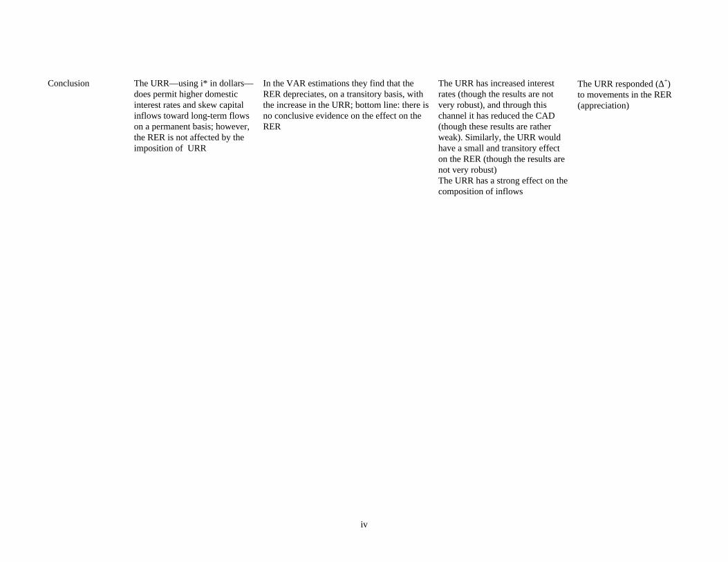
iv

Conclusion The URR—using i* in dollars—does permit higher domesticinterest rates and skew capitalinflows toward long-term flowson a permanent basis; however,the RER is not affected by theimposition of URR

In the VAR estimations they find that theRER depreciates, on a transitory basis, withthe increase in the URR; bottom line: there isno conclusive evidence on the effect on theRER

The URR has increased interestrates (though the results are notvery robust), and through thischannel it has reduced the CAD(though these results are ratherweak). Similarly, the URR wouldhave a small and transitory effecton the RER (though the results arenot very robust)The URR has a strong effect on thecomposition of inflows

The URR responded (∆+)to movements in the RER(appreciation)

v

Annex 2 URR: changes in coverage, rates, and methodologyDate Event Commentsmid-1990 Stamp tax of 1.2% (max.) extended to all foreign creditsJune 15, 1991 20 percent URR was introduced to new foreign borrowing

RR is in the same currency than the creditApply to foreign loans to banks and non-banksexcept direct trade credit, with the restrictionthat shipment must occur within six months.Holding period was equal to the loan maturitywith a minimum of 3 months and a maximum ofone year

June 27, 1991 URR can be exchanged for a paid up front fee, equal to thefinancial cost of the URR (using LIBOR for the calculation)URR is extended to all credits whose disbursement occursabroad and those that will be used abroadURR is also extended to those credits that are linked to FDIprojects

As these flows were exempt from the URR, thiscloses a loophole

January 23, 1992 URR extended to foreign exchange denominated term depositsheld at commercial banks by domestic and foreign residents

Closes a loophole

May 28 1992 URR is increased to 30 percent, except for direct borrowingby firms which remains at 20% Holding period was set at oneyear for all flows

Cost increased proportionately more for banksthan for non-bank borrowers

August 19, 1992 URR is set uniformly at 30 percentPaid-up front fee calculated at LIBOR + 2.5%

October 30 1992 Paid-up front fee increased to LIBOR + 4%October 1993 Shipment of merchandise using trade credit (exempt from

URR) must occur within 300 daysThis enlarges the loophole of using trade creditto bypass the URR

November 1994 Up front fee becomes payable only in dollarsJuly 4, 1995 Secondary ADRs become subject to the URR, since these are

not longer considered as FDI.Other inward financial—non-FDI and non- primary ADRs—become subject to the URR.

Closes a loophole. (Note: since primary ADRswere considered capital additions, they werenever subject to the URR.)

vi

September 14,1995

Period to purchase foreign exchange after selling ADRs in thedomestic market is shortened to 5 days

Prior to this date, there was not a regulationforcing foreigners to take their capital out of thecountry after selling their stock holdings

December 1995 New foreign borrowing to prepay other loans is exemptedfrom URR, when the new loan is of equal or shorter maturitythan the remaining maturity of the (old) loan to be repaid

June 1996 Foreign credits cannot be rolled over more than once within ayear

Closes a loophole

October 23, 1996 FDI classifies as such—and is exempt from URR—only if itincreases productive capacity

The FDI committee is in charge of determiningwhether the attempted investment classifies asFDI.

December 5,1996

Foreign borrowing for up to US$ 200,000 (or US$ 0.5 MMper year) is exempted from URR

March 1997 Minimum amount for exemption of the URR is reduced toUS$ 100,000 in 12 months

April 18, 1997 The remittance of funds—principal and profits—frominvestments by Chileans abroad is exempt from URR.

September 22,1997

The proceeds from closing positions in derivatives (options) inforeign markets becomes exempt from the URR

June 1998 URR was reduced to 10 percent, except for credit lines andforeign currency denominated deposits

August 1998 URR was eliminated for secondary ADRs. This had the objective of recovering liquidity forADRs, and reversing the declining volume oftransactions in the local stock market.

September 16,1998

URR was reduced to 0 percent

vii

Annex 3 Other measures aimed at liberalizing capital inflowsDate Event Comments

May 1992 Minimum solvency required to all financial and non-financialcorporations aiming to issue bonds internationally (minimum solvencyof A or higher)

The investment grade is given by thenational risk classification commission(refers to a domestic rating)

October 1992 International issue of convertible bonds is authorizedJune 1993 The requirement for the issue of bonds was modified in the sense that

rating from an international agency was requiredRating had to be equal or higher thansovereign risk

April 1994 Non-financial corporations have to be classified at least as BBB+ inorder to issue bonds internationally; for banks the classification must beBBB or higher (prior classification was A for both)The minimum issue size is set at US$ 25 MM (reduced from US$50MM) for non-banks; it stays at US$50 MM for banks

September 1994 Financial corporations had to be classified at least as BBB+ to issuestock internationally; for debt the classification must be A/B or higher(BBB+ for subordinated debt)

September 1994 Requirements for ADR issues are reduced from A to BBB+ and from aminimum of US$ 50 MM to US$ 25 MM (for first issues)

November 1995 For firms issuing ADRs for a second time the minimum size is set atUS$ 10 MM (from US$ 25 MM)

Prior to this date there was no rulereferring to second issues (the same asfirst issues applied)

September, 1996 Requirements for minimum size of internationally issued bonds of non-financial corporations are reduced to US$ 10 MM.

April, 1998 Requirements for minimum size of internationally issued bonds of non-financial corporations are reduced to US$ 5 MM. The minimumclassification was reduced to BBB-

June, 1999 Minimum maturaty requirements on internationally issued bonds ofnon-financial corporations are eliminated. The minimum rating for bothbonds and ADR issues was lessened. Requirements of previousauthorization for international bond issues are eliminated for bothfinancial and (some) non-financial corporations

Prior to this date the minimum maturitywas 4 years

viii

Annex 4 Capital outflow liberalizationDate Event Comments

February 1991 - Commercial banks were permitted to increase external trade financing and useup to 25 per cent of FX time deposits for foreign trade financing- Joint-venture rules were simplified- Procedures for direct investment abroad by corporates was simplified

April 1991 Waiting period for capital remittances for inward investment under debt-equityswap mechanism (chapter XIX) was shortened from 10 to 3 years

The waiting period could be reducedafter paying a fee proportional to thediscount at which the debt instrumentsused in the swap operation had beenbought in the international market.

April 1991 Banks can invest abroad up to 40% of the funds collected as term depositsdenominated in FX

April 1991 Outward FDI by Chileans financed with foreign exchange acquired in theinformal market is authorized.The period to surrender capital and profits from this investment abroad isextended from 3 to 4 months.

The only requirement for investors isto inform the CB about the transaction

March 1992 - Limit on net foreign exchange holdings by commercial banks was doubled;- Exports receipts exempt from surrender requirements were increased from 15%to 50%

- Allocations of foreign exchange for a variety of payments abroad wereincreased

- Period of advance purchase of foreign exchange for debt service was extendedMay 1992 Pension funds were allowed to invest up to 1.5% abroad. Investment grade assets only (BBB or

higher)May 1992 It was established that between May 1992 and April 1993, the cumulative profits

up to December 1992 of all foreign investments taken under chapter XIX (debt-equity swaps) could be repatriated.

Part of it could be repatriated untilApril 1993, and the rest within 270days after that date.

August 1992 It was established that the capital of chapter XIX investments could berepatriated after paying a fee equal to 3% of the capital.

August 1992 Pension funds were allowed to invest up to 3% of their portfolio abroad.

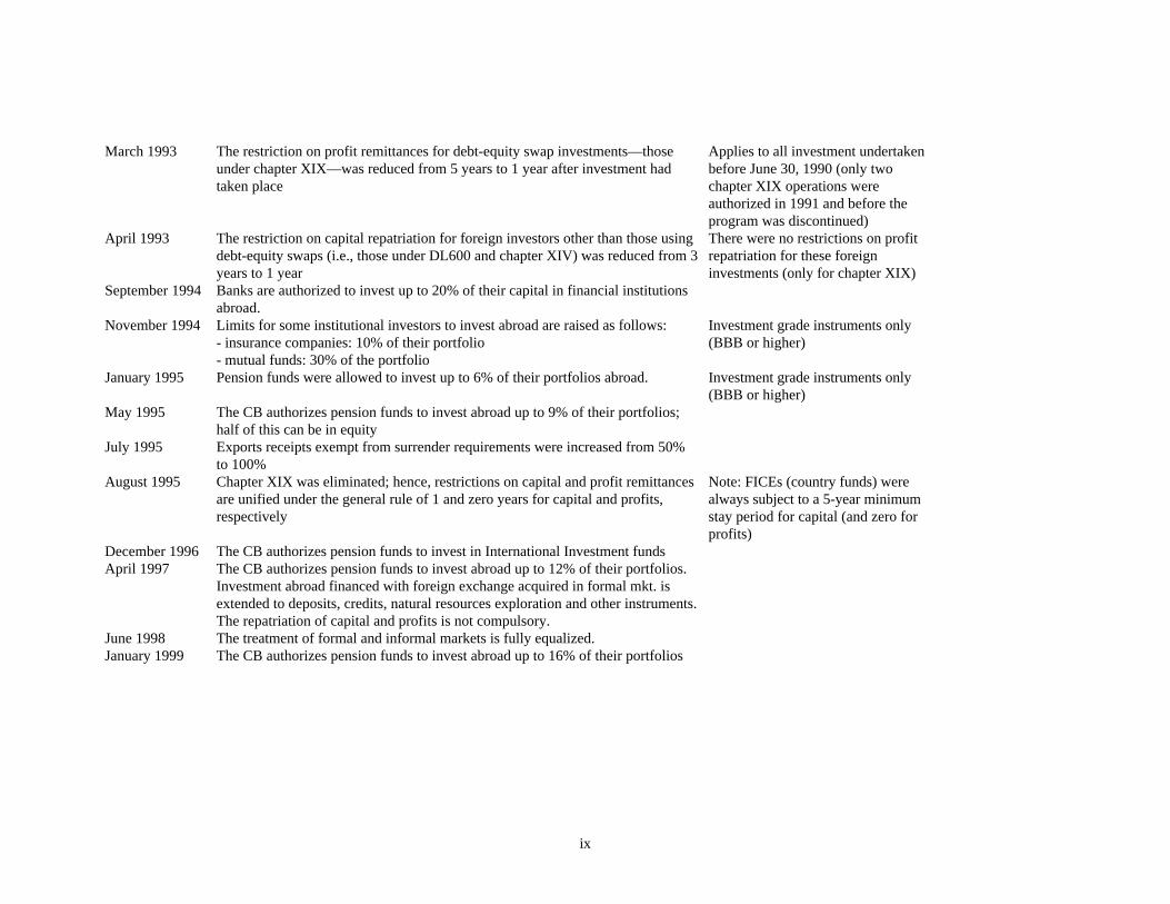
ix

March 1993 The restriction on profit remittances for debt-equity swap investments—thoseunder chapter XIX—was reduced from 5 years to 1 year after investment hadtaken place

Applies to all investment undertakenbefore June 30, 1990 (only twochapter XIX operations wereauthorized in 1991 and before theprogram was discontinued)

April 1993 The restriction on capital repatriation for foreign investors other than those usingdebt-equity swaps (i.e., those under DL600 and chapter XIV) was reduced from 3years to 1 year

There were no restrictions on profitrepatriation for these foreigninvestments (only for chapter XIX)

September 1994 Banks are authorized to invest up to 20% of their capital in financial institutionsabroad.

November 1994 Limits for some institutional investors to invest abroad are raised as follows:- insurance companies: 10% of their portfolio- mutual funds: 30% of the portfolio

Investment grade instruments only(BBB or higher)

January 1995 Pension funds were allowed to invest up to 6% of their portfolios abroad. Investment grade instruments only(BBB or higher)

May 1995 The CB authorizes pension funds to invest abroad up to 9% of their portfolios;half of this can be in equity

July 1995 Exports receipts exempt from surrender requirements were increased from 50%to 100%

August 1995 Chapter XIX was eliminated; hence, restrictions on capital and profit remittancesare unified under the general rule of 1 and zero years for capital and profits,respectively

Note: FICEs (country funds) werealways subject to a 5-year minimumstay period for capital (and zero forprofits)

December 1996 The CB authorizes pension funds to invest in International Investment fundsApril 1997 The CB authorizes pension funds to invest abroad up to 12% of their portfolios.

Investment abroad financed with foreign exchange acquired in formal mkt. isextended to deposits, credits, natural resources exploration and other instruments.The repatriation of capital and profits is not compulsory.

June 1998 The treatment of formal and informal markets is fully equalized.January 1999 The CB authorizes pension funds to invest abroad up to 16% of their portfolios

x

Annex 5. Construction of the control variables1

In this paper we aim to overcome some of the limitations of previous research bycontrolling the empirical estimations for the changes in capital account regulations, others than theimposition of the URR in 1991 and its modifications thereafter. In particular, we constructedindicators of the regulations affecting capital outflows and inflows in regards with:

(i) Mandatory period of permanence and minimum number of years before the remittances ofprincipal and profits from foreign investment in Chile is permitted;

(ii) Solvency requirements and minimum issue size affecting Chilean corporates taping theinternational capital markets through the issue of bonds and shares (ADRs);

(iii) Other regulations affecting capital outflows. These include restrictions (ceilings) affectingforeign investment by Chilean pension funds, banks and insurance companies, surrenderrequirements for Chilean exporters, and other minor regulations.

Restrictions on remittances

The first index (i) was constructed as follows. Since the repatriation requirements for the principal(and profits) were different for those investments that occurred under the debt-equity swapmechanisms, we took a weighted average of the years of minimum permanence that applied to eachtype of flow. The weights used were the corresponding share of each type of foreign investment(debt-equity swap versus non-debt equity swaps) in the total during 1985-1991:Q1. The resultingindex starts at 8 in 1989, drops to 3 in 1991, and continues falling to reach 1 at the end of thesample period. In the empirical analysis we use a normalized index (Figure 3.5). The normalizationprocedure consists of setting the highest value (the most restrictive stage) of each index at 1, andthe smallest value at 0 (the less restrictive stage). This methodology is the same as the one used byBID (1997) among others.2

Solvency and size restrictions on international issues

The second index (ii) is constructed by multiplying two sub-indices, one referring tominimum solvency requirements and the other to minimum size issue. The latter was constructedby taking the ratio between the size issue required at each time, and the minimum over the wholesample period—thus, this ratio fluctuated between 1 (end of the sample period) and 10 (beginningof the sample period). Since different types of issues (ADRs, bonds by banks, and bonds by non-banks) have different requirements, the share of each type of issue in the total weighted theresulting numbers during 1997-983. The minimum solvency requirements (AAA, BBB+, etc.) weretranslated into a numerical scale by decreasing the index in 1.0 each time that the restrictions wererelaxed. The starting value (when issues were prohibited) was set equal to 10, and intermediatevalues were found by fixing the end value—when restrictions were the lowest—in 1.0 and workingbackwards. The resulting index starts at 100 and drops to 1.7 towards the end of the sample period(Figure 3.4).

Restrictions on other capital outflows

1 The information needed for constructing some of the indices described below is reported in Annexes 2, 3

and 4.2 This procedure is also used in the next indexes.3 We used 1997-98 to calculate the weights because did not have data on primary ADRs for previous years.

xi

The third index (iii) was constructed by fixing the starting value at 11, and decreasing theindex each time that a significant change occurred. This methodology is the same than the one usedby Cardoso and Goldfajn (1997) when constructing a capital control index for the case of Brazil.The resulting index decreases to 1.0 towards the end of the sample period.

Composed indexes of restrictions on capital flowsThe fourth index (used in the empirical part of this paper) is a composed index of all the

restrictions on capital flows (inflows or outflows), and was constructed as the simple average of thethree normalized indexes mentioned above.

Power Index

Following De Gregorio et.al (1999), in this paper we included a power index aimed atmeasuring the effectiveness of the URR—alternatively, the difficulties encountered when trying toelude or bypass it. However, instead of using a qualitative index as in De Gregorio et.al (1999), weconstructed an index based on flows that paid the URR and flows that were relabeled. For this westarted by identifying the kind of flow and the period when the relabeling took place. Next, westudied the behavior of each flow in the months before and after the relabeling occurred, and usingthis information projected the relabeled flows. Finally, we constructed the power index as the ratiobetween the flows that actually paid the URR and the potentially affected flows (estimated as thesum of the flows that paid URR, the relabeled flows, and errors and omissions). The resultingpower index is shown in figure 3.3.

Coverage

The coverage index constructed in this paper, used in the regression analysis and in theestimation of the power index, is a step function that increases from 1.0 to 1.17 in June 1995, andfalls back to 1.0 in June 1998. The increase (and drop) reflects the inclusion of secondary ADRs inthe URR, and is proportional to the share of this type of inflows in the total during 1989:1-1991:6.

Relevant foreign interest rate (i*)

The relevant foreign interest rate is a weighted average of the dollar-LIBOR (id) and theYen-LIBOR (iy). This is used to reflect the option that investors had to choose the currency of theirdeposits at the CB. The weights are taken from the actual currency composition of reserve depositsin each period. Also, the foreign currency rates used (id, iy) are a weighted average of LIBOR + ρand LIBOR + ψ, where ψ is the premium charged on the up front fee (see annex 2), and ρ is anestimation of the country risk premium paid by Chilean corporations during the sample period.

xii

Annex 6. Data Sources and Frequency

VARIABLE SOURCE DESCRIPTIONEffective andUnremunerated ReserveRequirement

Author’s Elaboration. See below for details on each component of this variable

Actual and target inflation Central Bank of Chile. The Central Bank of Chile’s target inflation is set for December of each year. So, we constructthe monthly target using the lineal combination of each couple of two consecutive targets.

Real exchange rate Central Bank of Chile.Policy Interest Rate Central Bank of Chile. This variable is the PRBC rate up to 1995, and the overnight rate since.Deposit Interest Rate Central Bank of Chile This rate is the one paid on 91-365 days depositsCapital Flows to Chile Balance of Payment Department,

Central Bank of Chile.Capital Flows to theEmerging Markets

Author’s elaboration based on theIMF International Finance Statistics.

We construct this variable using the quarterly capital account deficits for the OECD countriesover the GDP of OECD countries, next we interpolate the quarterly data to monthly frequencyusing standard RATS routines.

Power Index Author’s elaboration. See annex 5 for more details.Capital Account Indexes Author’s elaboration. See annex 5 for more details.International Interest Rate Central Bank of Chile. This rate corresponds to the LIBOR-180 days.Expected Exchange RateDepreciation

Author’s elaboration. This variable is constructed as the projection from rolling regressions for the 6 months exchangerate depreciation. This methodology is the same than the one used by De Gregorio et al. (1999)

Country Risk Author’s elaboration, Central Bankof Chile and EMBI.

This variable is the premium charged on international bond issued by Chilean corporations.

GDP Author’s elaboration and CentralBank of Chile

This variable was constructed using the IMACEC (monthly aggregate production index) totransform the quarterly GDP into a monthly basis.

Terms of Trade Central Bank of Chile We interpolate the quarterly data to monthly frequency using standard RATS routines.Government Expenditure Ministry of Finance and author’s

elaborationM1 Central Bank of ChileRlpt Author’s elaboration in base of data

obtained form Central Bank of Chileand National Institute of Statistics

This variable is constructed with the same methodology used by Valdés and Délano (1999)

Nominal Exchange rate Central Bank of ChileOutput gap Author’s elaboration We estimated the potential GDP using a HP Filter.Net Foreign Liabilities Authors’s elabotation This variable was constructed adding the monthly flows to the figures estimated by Milessi-

Ferretti (1998) for December of 1988

Table 3.1 Restrictions on Capital Flows in Chile, 1989-1998

On Capital Inflows On Capital Outflows

Quantitative Restrictions Unremunerated reserverequirement (URR) on selectivecapital inflows

—

Administrative Restrictions Minimum solvencyrequirements on domesticissuers of foreign liabilities(bonds and ADRs)

Minimum permanencerequirements beforerepatriation of capital andprofits

Size requirements on issues offoreign liabilities

Ceilings on foreign assetholdings relative to capital forfinancial institutionsSurrender requirements ofexport proceeds

Table 5.1Power of the URR

Dependent Variable: D(power)Sample 1991:07-1998:08

C 0.004(1.54)

D(tax) -0.11(5.78)

r- r *- ee -ρ -0.0011(1.73)

D922 0.27(102.44)

D941 0.02(2.83)

DYEN 0.01(1.33)

D957 0.02(3.99)

D(T957) -0.001(0.24)

D9610 0.01(3.20)

D(T9610) -0.00(0.05)

D(power-1) 0.23(2.09)

Adjusted R2 0.78Durbin’s h 0.26

Estimation Technique LSNewey-West consistent t-statistics in parenthesis.

Table 5.2Cost of the URR

Dependent Variable: D(urr) Dependent Variable: D(urr)Sample 1991:06-1998:09 1991:06-1998:09

D(r) + D(ρ) 0.73(5.61)

0.77(5.92)

D(r *-1) -0.03(0.16)

-

D(ρ−1) -1.15(1.56)

-

D(r *-1)+ D(ρ−1) - -0.17(1.69)

D(1

1

−

−

wy

wfk)

30.00(1.82)

39.10(1.95)

PDL(t

tt

y

lfle;-3;-14;1)

-7.98(6.11)

-7.33(5.88)

PDL(t

tt

y

lfe;-6;-9;2)

2.84(3.78)

2.87(3.55)

PDL(D(1

1

−

−−

t

tt

e

ee);-2,-8,2)

-42.26(3.48)

-53.60(5.28)

PDL(D(power(-1)),9,3)) -3.13(2.51)

-4.29(2.78)

π−πτ 0.03(0.50)

0.04(0.77)

D(urr(-1)) 0.44(2.08)

0.46(2.04)

Adjusted R2 0.51 0.46

Durbin’s h 0.1 0.2

Estimation Technique LS LS

Newey-West consistent t-statistics in parenthesis, constants not reported.PDL (X;,A,B,C) stands for a polynomial distributed lag for the X variable, where A and B are the first and lastlag, respectively, while C is the order of the polynomial.

Table 5.3Effective Cost of the URR

Dependent Variable: D(err)Sample 1991:06-1998:09

D(r *) + D(ρ) 0.63(5.26)

0.70(5.82)

D(r *-1) -0.02(0.07)

-

D(ρ−1) -1.17(2.46)

-

D(r *-1)+ D(ρ−1) - -0.23(1.06)

D(1

1

−

−

wy

wfk)

36.31(1.72)

33.32(1.46)

PDL(t

tt

y

lfle;-3;-14;1)

-4.14(1.98)

-4.57(1.99)

PDL(t

tt

y

lfe;-6;-9;2)

2.05

(1.77)

2.50(1.89)

PDL(D(1

1

−

−−

t

tt

e

ee);-2,-8,2)

-33.39(2.04)

-45.43(2.04)

π−πτ 0.15(1.59)

0.07(1.04)

D(err(-1)) 0.51(2.01)

0.43(2.46)

Adjusted R2 0.39 0.33Durbin’s h 0.48 0.37

Esmation Technique LS LSNewey-West consistent t-statistics in parenthesis, constants not reported.PDL (X;,A,B,C) stands for a polynomial distributed lag for the X variable, where A and B are the first and lastlag, respectively, while C is the order of the polynomial.

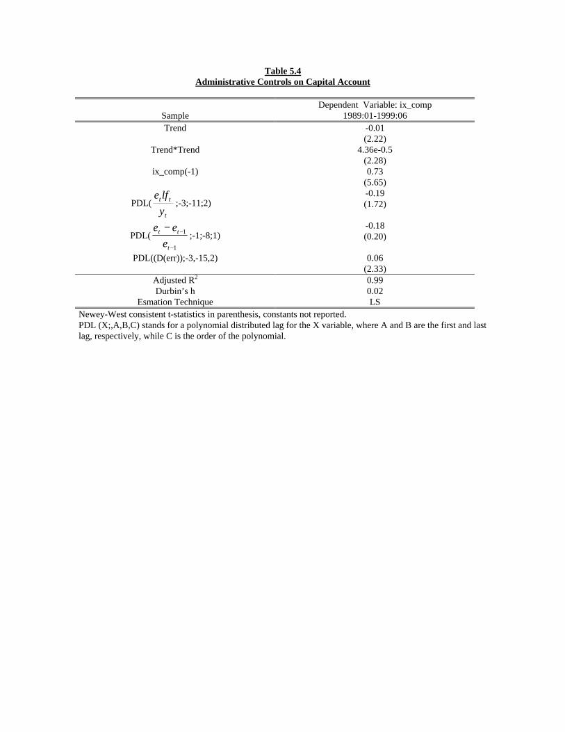
Table 5.4Administrative Controls on Capital Account

Dependent Variable: ix_compSample 1989:01-1999:06Trend -0.01

(2.22)Trend*Trend 4.36e-0.5

(2.28)ix_comp(-1) 0.73

(5.65)

PDL(t

tt

y

lfe;-3;-11;2)

-0.19(1.72)

PDL(1

1

−

−−

t

tt

e

ee;-1;-8;1)

-0.18(0.20)

PDL((D(err));-3,-15,2) 0.06(2.33)

Adjusted R2 0.99Durbin’s h 0.02

Esmation Technique LSNewey-West consistent t-statistics in parenthesis, constants not reported.PDL (X;,A,B,C) stands for a polynomial distributed lag for the X variable, where A and B are the first and lastlag, respectively, while C is the order of the polynomial.

Table 5.5Central Bank Policy Real Rate of Interest

Dependent Variable: D(rcb)Sample 1989:01-1998:08D(r*) -0.04

(1.16)-0.04(1.18)

- - - - -0.04(1.18)

-0.04(1.17)

D( ee ) 0.01(0.77)

0.01(0.77)

- - - - 0.01(0.81)

0.01(0.78)

D(ρ) 0.02(1.12)

0.02(1.15)

0.02(0.87)

0.02(0.86)

0.02(0.89)

0.02(0.90)

0.02(1.18)

0.02(1.17)

D(err) -0.01(0.24)

- -0.02(0.47)

- - - - -

D(urr) - 0.00(0.09)

- -0.03(0.57)

- - - -

D(ext) - - 0.01(0.61)

0.01(0.62)

- - - -

D(err)+D(ext) - - - - 0.00(0.51)

- - -

D(urr)+D(ext) - - - - - 0.00(0.47)

- -

D(tax) - - - - - - 0.08(1.46)

-

D(power-1) - - - - - - - 0.11(1.97)

D((π−πτ)−4) 0.07(2.99)

0.07(2.93)

0.08(2.97)

0.08(2.98)

0.08(2.98)

0.08(2.99)

0.07(3.00)

0.08(3.00)

D(y

cas-1)

-0.55(1.66)

-0.56(1.72)

-0.54(1.65)

-0.53(1.68)

-0.56(1.62)

-0.56(1.67)

-0.60(1.67)

-0.61(1.70)

PDL(

t

t

y

y;-1;-2;1)

2.02(2.19)

2.00(2.17)

2.11(2.18)

2.12(2.18)

2.10(2.20)

1.99(2.18)

1.99(2.18)

1.99(2.19)

D(rcb-1) 0.16(3.37)

0.16(3.32)

0.17(3.47)

0.17(3.49)

0.17(3.45)

0.16(3.35)

0.16(3.35)

0.16(3.38)

Adjusted R2 0.13 0.13 0.14 0.14 0.14 0.14 0.14 0.14Durbin’s h 0.02 0.01 0.16 0.14 0.15 -0.01 -0.01 -0.03EsmationTechnique

LS LS LS LS LS LS LS LS

Newey-West consistent t-statistics in parenthesis, constants not reported.

D (ext) = D ( r * ) + D( ete )

PDL (X;,A,B,C) stands for a polynomial distributed lag for the X variable, where A and B are the first and lastlag, respectively, while C is the order of the polynomial.

Table 5.6Deposit Real Rate of Interest

Dependent Variable: D(rdep)Sample 1989:01-1998:06D(r*) 0.01

(0.04)0.07

(0.37)- - - - -0.10

(0.39)-0.04(0.41)

D( ee ) -0.01(0.96)

-0.01(1.05)

- - - - -0.01(0.97)

-0.01(0.98)

D(ρ) 0.24(0.66)

0.18(0.53)

0.23(0.66)

0.17(0.50)

0.16(0.45)

0.17(0.48)

0.11(0.31)

0.11(0.30)

D(err) -0.11(0.55)

- -0.09(1.02)

- - - - -

D(urr) - -0.25(1.03)

- -0.17(1.82)

- - - -

D(ext) - - -0.01(0.77)

-0.01(0.61)

- - - -

D(err)+D(ext) - - - - -0.01(1.26)

- - -

D(urr)+D(ext) - - - - - -0.01(0.98)

- -

Durr - - - - - - 0.08(0.48)

-

D(power) - - - - - - - 0.11(0.53)

D(rcb) 0.62(3.04)

0.63(2.97)

0.62(3.07)

0.63(3.08)

0.63(3.12)

0.63(2.80)

0.62(2.97)

0.62(2.88)

D(y

el 1− )-6.24(1.67)

-6.84(1.88)

-6.05(1.94)

-5.96(1.99)

-5.85(1.84)

-5.87(1.74)

-5.79(1.73)

-5.84(1.73)

D(tot(-3)) -4.27(2.53)

-4.40(2.63)

-4.26(2.59)

-4.33(2.63)

-4.15(2.61)

-4.42(2.61)

-4.36(2.35)

-4.36(2.40)

D(y

g)

4.71(1.61)

5.70(1.93)

4.53(1.20)

4.74(1.27)

4.43(1.17)

4.42(1.05)

3.97(1.23)

3.95(1.22)

D(y

m 1− )-11.33(0.87)

-12.33(0.97)

-11.53(0.88)

-13.10(1.02)

-10.44(0.84)

-10.31(0.88)

-11.14(0.86)

-11.19(0.87)

d(

t

t

y

y)

2.33(2.12)

2.51(2.21)

2.34(2.06)

2.52(2.18)

2.25(2.08)

2.24(2.07)

2.26(2.12)

2.27(2.13)

0.5*[D(ix_remit)+D(ix_other)]

-1.16(2.02)

-1.39(2.14)

-1.15(2.29)

-1.27(2.43)

-1.08(2.38)

-1.08(2.89)

-1.16(2.08)

-1.17(2.13)

D(rdep-1) 0.16(1.97)

0.16(2.01)

0.16(1.98)

0.16(1.97)

0.17(2.04)

0.17(0.93)

0.16(1.76)

0.16(1.73)

Adjusted R2 0.35 0.36 0.35 0.36 0.36 0.36 0.35 0.35Durbin’s h 0.34 0.54 0.33 0.49 0.14 0.13 0.16 0.18EsmationTechnique

LS LS LS LS LS LS LS LS

Newey-West consistent t-statistics in parenthesis, constants not reported.

D (ext) = D ( r * ) + D( ete )

Table 5.7Real Exchange Rate

A. Error Correction ModelDependent Variable: D(rer)

Sample 1989:01-1998:12Ucoint(-1) -0.02

(2.05)-0.02(1.96)

-0.02(2.17)

-0.02(2.18)

D(rlpt(-9)) -0.08(2.41)

-0.08(2.42)

-0.07(2.49)

-0.07(2.50)

D(3

3

−

−

t

t

y

y)

-0.10(2.29)

-0.10(2.30)

-0.11(2.53)

-0.11(2.53)

D(4

4

−

−

t

t

y

y)

-0.11(2.18)

-0.12(2.20)

-0.13(2.73)

-0.13(2.73)

D(Et-1) 0.29(2.18)

0.29(3.83)

0.28(3.44)

0.28(3.43)

D(rcb) 0.00(0.24)

0.00(0.32)

- -

D(r*) 0.00(1.06)

0.01(1.29)

- -

D(ee +6)

0.00(1.17)

0.00(1.18)

- -

D(ρ) 0.03(3.21)

0.03(3.33)

- -

D(err) -0.01(1.00)

- - -

D(urr) - -0.01(1.34)

- -

D(gapext)-D(err) - - -0.00(1.28)

-

D(gapext)-D(urr) - - - -0.00(1.20)

Adjusted R2 0.22 0.23 0.21 0.21DW 2.00 2.01 2.00 2.00

Estimation Technique LS LS LS LS

Newey-West consistent t-statistics in parenthesis, constants not reported. D (gapext)=D (rcb) - D (r*) - D(ete 6ˆ + )

B. Cointegration VectorVariable Dependent Variable (Rer)

Coefficients

t

t

y

g -5.12(1.57)

-6.46(1.82)

t

tt

y

le 0.63(0.28)

0.64(0.32)

Rlpt -1.40(0.43)

-1.48(0.43)

Tot 0.14(0.20)

-

Log likelihood 1619.5 1310.8Estimation Technique Johansen Johansen

Standard errors in parenthesis, constant not reported.

Table 5.8Capital Inflows

Dependent VariableSample 1989:01-1999:06

D(TotalFlows/GDP)

D(Short TermFlows/GDP)

D(AffectedFlows/GDP)

D (rcb) - D (r*)

- D( ete 6ˆ + )-D(ρ)

-0.00(1.03)

-0.00(1.08)

-0.00(1.03)

-0.00(1.67)

0.00(0.69)

0.00(0.45)

D(err) -0.014(1.78)

- -0.014(1.78)

- -0.024(2.57)

-

D(urr) - -0.013(0.66)

- -0.019(0.82)

- -0.028(1.47)

D(t

tt

y

le 1− )-4.04(3.10)

-4.00(3.05)

-4.07(2.92)

-4.01(2.89)

-1.86(1.99)

-1.55(1.78)

D(1

1

−

−

t

t

l

ls)

-3.91(3.22)

-3.96(3.22)

-5.61(3.66)

-5.72(3.62)

-1.97(2.38)

-1.92(2.31)

D(wy

wfk)

1.30(1.23)

1.31(1.25)

1.85(1.56)

1.86(1.58)

0.64(0.62)

0.60(0.61)

D(ix_remit) 0.52(7.31)

0.52(7.32)

- - 0.33(2.19)

0.30(1.87)

D(ix_issues) 0.02(0.28)

0.02(0.25)

- - -0.01(0.11)

-0.02(0.21)

D(ix_comp) - - 0.57(1.47)

0.57(1.49)

- -

D(rer) 1.44(1.63)

1.45(1.61)

1.71(1.80)

1.73(1.76)

0.24(0.26)

0.19(0.21)

D(tot) 0.26(0.69)

0.27(0.72)

0.56(1.65)

0.58(1.68)

0.38(1.58)

0.39(1.59)

D( )y

g -1.37(1.19)

-1.37(1.19)

-0.79(0.80)

-0.79(0.81)

-1.10(1.24)

-1.04(1.18)

D( )y

y -0.50(2.52)

-0.51(2.42)

-0.40(1.92)

-0.41(1.92)

-0.51(2.06)

-0.52(1.95)

Adjusted R2 0.55 0.54 0.53 0.52 0.49 0.47DW 1.98 1.98 1.97 1.97 2.11 2.08

Estimation Technique TSLS TSLS TSLS TSLS TSLS TSLSNewey-West consistent t-statistics in parenthesis, constants not reported.The instrumented variables are real exchange rate, the ratio of actual output to potential output. Theinstruments are lags of each variable.

Table 5.9Capital Inflows

Dependent VariableSample 1989:01-1999:06

D(Total Flows/GDP)

D(Short Term Flows/GDP)

D(Affected Flows/GDP)

D (rcb) - D (r*)

- D( ete 6ˆ + )-D(ρ)

0.002(2.00)

0.002(1.47)

0.001(1.06)

0.00(0.75)

0.002(1.79)

0.002(1.48)

D(err) -0.0178(2.07)

- -0.0183(2.10)

- -0.0136(2.31)

-

D(urr) - -0.023(1.32)

- -0.025(1.42)

- -0.019(1.48)

D(t

tt

y

le 1− )-1.23(2.12)

-1.34(2.25)

-1.17(1.84)

-1.13(2.78)

-0.21(0.73)

-0.12(0.43)

D(1

1

−

−

t

t

l

ls)

-1.73(3.85)

-1.87(3.87)

-3.19(5.17)

-3.41(5.30)

-0.06(0.22)

-0.17(0.57)

D(wy

wfk)

1.65(2.17)

1.48(2.02)

1.62(1.62)

1.49(1.56)

1.08(1.40)

1.06(1.41)

D(ix_remit) 0.06(0.65)

0.05(0.44)

- - 0.04(0.96)

0.03(0.64)

D(ix_issues) -0.11(1.92)

-0.11(2.12)

- - -0.10(1.70)

-0.10(1.67)

D(ix_comp) - - -0.13(0.63)

-0.12(0.61)

- -

D( )y

cas -1.09(5.51)

-1.06(5.39)

-0.99(5.06)

-0.98(5.07)

-0.98(12.03)

-0.99(11.16)

Adjusted R2 0.70 0.69 0.66 0.66 0.59 0.57DW 1.91 1.90 1.97 1.97 1.71 1.66

Estimation Technique TSLS TSLS TSLS TSLS TSLS TSLSNewey-West consistent t-statistics in parenthesis, constants not reported.The current account surplus is instrumented using: lags of itself, the terms of trade, the ratio of governmentexpenditure to GDP, and lags of exchange rate and the ratio of actual output to potential output.

Table 5.10Portfolio Share of Short-Term Net Foreign Liabilities in Total Net Foreign Liabilities

Dependent VariableSample 1989.01-1999:06

PDL(D(rcb));-1,-5,2) 0.00(0.46)

0.01(0.69)

PDL(D( r* ));-1,-5,2)-0.00(0.01)

0.00(0.29)

PDL(D(D(D( ee )));-1,-5,2) 0.00(0.64)

0.00(0.71)

PDL(D(err));-1,-5,2) -0.01(2.81)

-

PDL(D(urr));-1,-5,2) - -0.01(1.91)

PDL(D(t

tt

y

le 1− );-5,-10,3)-0.31(1.66)

-0.28(1.48)

PDL(D(ix_remit);-1,-12,3) -0.10(2.79)

-0.11(3.24)

Adjusted R2 0.17 0.16DW 1.81 1.78

Estimation Technique LS LS

Newey-West consistent t-statistics in parenthesis, constants not reported.PDL (X;,A,B,C) stands for a polynomial distributed lag for the X variable, where A and B are thefirst and last lag, respectively, while C is the order of the polynomial.

Table 6.1: Regression of interest rate differentials on URR and CB’s policy rate

Dependent variable: ilong-term – ishort-term

CB’s securities rates Secondary Market Rates

Constant 2.25(3.63)

2.52(3.23)

2.89(6.21)

1.60(1.84)

err 0.004(0.06)

0.01(0.17)

-0.004(-0.15)

0.03(0.64)

Central Bank’spolicy rate

-0.33(-4.65)

-0.39(-3.75)

-0.45(-5.97)

-0.27(-1.79)

AR(1) 0.95(31.2)

0.94(25.1)

-- --

Adjusted R² 0.94 0.93 0.23 0.021Durbin-Watson -- -- 1.73 1.74Period 1988:2-1997:12 1991:1-1997:12 1988:1-1997:12 1991:1-1997:12N 119 84 120 84T tests are in parenthesis.

Table 6.2: Interest rates differential due to the URR (1991-1997)Interest Rate Differential (%)

Year (Unexplained differential per year)2.67 2.50 2.00 1.50

1991 0.63 0.80 1.30 1.801992 2.85 3.02 3.52 4.021993 4.09 4.26 4.76 5.261994 2.28 2.45 2.95 3.451995 0.58 0.74 1.24 1.741996 2.32 2.49 2.99 3.491997 0.90 1.07 1.57 2.07

Average 1.95 2.12 2.62 3.12

Table 6.3: Lower economic growth due to the URR-induced interest rate differentialsLower growth: 1991-97 average

Average interest differential Lehmann (1991) Bustos et.al. (1998)(% per year) (% per year)

1.95 0.36 0.642.12 0.39 0.702.62 0.49 0.863.12 0.58 1.03

Average 0.46 0.81

Figure 3.1URR Tax Rate and URR Cost (%)

0%

5%

10%

15%

20%

25%

30%

35%

Jun-91 Dic-91 Jun-92 Dic-92 Jun-93 Dic-93 Jun-94 Dic-94 Jun-95 Dic-95 Jun-96 Dic-96 Jun-97 Dic-97 Jun-98 Dic-98

0

1

2

3

4

5

6

7

8

9

URR TaxRate (t)

URR Cost (urr)

urr

Tax Rate

Figure 3.2URR Deposits at the Central Bank (mmUS$)

0

500

1000

1500

2000

2500

E-93

M-93

M-93

J-93

S-93

N-93

E-94

M-94

M-94

J-94

S-94

N-94

E-95

M-95

M-95

J-95

S-95

N-95

E-96

M-96

M-96

J-96

S-96

N-96

E-97

M-97

M-97

J-97

S-97

N-97

E-98

M-98

M-98

J-98

S-98

Actual URR Deposits

Fee Equivalent URR Deposits

Figure 3.3Potentially Affected Flows and Share of Effectivelly Affected Flows

0%

10%

20%

30%

40%

50%

60%

70%

80%

90%

100%

1991 1992 1993 1994 1995 1996 1997 1998

0

1000

2000

3000

4000

5000

6000

7000

8000

Share of Effectively Affected Potentially Affected

MM of US$

Figure 3.4URR Cost, URR Power, and URR Effective Cost (%)

0%

10%

20%

30%

40%

50%

60%

70%

80%

90%

100%

Jul-9

1

Ene

-92

Jul-9

2

Ene

-93

Jul-9

3

Ene

-94

Jul-9

4

Ene

-95

Jul-9

5

Ene

-96

Jul-9

6

Ene

-97

Jul-9

7

Ene

-98

Jul-9

8

0

1

2

3

4

5

6

7

8

9

Power urr err

Power(pow)

URR, ERR

0

0.1

0.2

0.3

0.4

0.5

0.6

0.7

0.8

0.9

1

E-89

M-8

9S-8

9E-9

0M

-90

S-90

E-91

M-9

1S-9

1E-9

2M

-92

S-92

E-93

M-9

3S-9

3E-9

4M

-94

S-94

E-95

M-9

5S-9

5E-9

6M

-96

S-96

E-97

M-9

7S-9

7E-9

8M

-98

S-98

E-99

M-9

9

ix_remit ix_other ix_issues ix_comp

Figure 3.5Administrative Controls in Capital Inflows and Capital Outflows

Figure 4.1

Long-Run Equilibrium in a Small Open Economy

Real interestrate (r)

r r errb e k

e k= + +

+

* ρ

Realexchangerate (e)

∆ k = 0

∆ e = 0

Net foreign assets (k)

Net foreign assets (k)

Figure 4.2

Dynamic Response to a Higher Tax on Net Foreign Assets

A

B

C

S'

k1k0

e

e '0

e 0

e 1

S'

( )∆ e = 0 ( )∆ e = 0 '

( )∆ k = 0

r

r1

r0

k0 k1 k

( )r err* + +0 ρ

r err* + +

1 ρ b + e k

e k

B'

B

A

B''

C

k

Figure 6.1

3

4

5

6

7

8

9

Q 11987

Q 11988

Q 11989

Q 11990

Q 11991

Q 11992

Q 11993

Q 11994

Q 11995

Q 11996

Q 11997

%

-1.5

-1.0

-0.5

0.0

0.5

1.0

1.5

2.0

2.5

3.0

%

Policy rate(Left hand side)

8yr. rate minus 90 days rate (r ight hand side)

tight monetary policy

Figure 6.2

Term Structure of Interest Rates for Selected Periods

6.3

6.5

6.7

6.9

7.1

7.3

7.5

0.0-2.0 2.1 - 5.0 5.1 - 8.0maturity (years)

Inte

rest

rat

e (%

)

Average of Tight Monetary Policy Periods

Average of Non-Tight Monetary Policy Periods

Tight Monetary Policy Periods comprise: 2nd. sem. of 1989, 1995; 1st. sem. of 1991 and the first three quarters of 1993. Non-tight periods comprise the remaining months of each year.

Figure 6.3

-50%

-40%

-30%

-20%

-10%

0%

10%

20%

30%

40%

mar-89 mar-90 mar-91 mar-92 mar-93 mar-94 mar-95 mar-96 mar-97 mar-98

Change in Int'l Reserves

Change in Domestic Credit

Figure 6.4

2000

4000

6000

8000

10000

12000

14000

16000

18000

1990 1991 1992 1993 1994 1995 1996 1997 1998

US$

mill

ions

20%

25%

30%

35%

40%

45%

50%

55%

60%

(Sha

re o

f ac

tual

res

erve

s)

RI mill US$ Excess reserves 1

Excess reserves 2

Right-hand side axis

Right-hand side axis

Note: Excess reserves 1 refers to the estimate based on the months of imports, while excessreserves 2 refers to the optimum based on the composition of the monetary base.

Figure 6.5

-0.2%

0.0%

0.2%

0.4%

0.6%

0.8%

1.0%

1.2%

1.4%

1.6%

1.8%

1990 1991 1992 1993 1994 1995 1996 1997 1998

As

a s

hare

of

GD

P

Cost 1 Cost 2

Note: Cost 1 refers to the estimate based on months of imports, while cost 2 refers to the estimatebased on the optimum composition of the monetary base.