capital budgeting
TRANSCRIPT


This page intentionally left blank

Capital Budgeting
This book explains the financial appraisal of capital budgeting projects.The coverage extends from the development of basic concepts, princi-ples and techniques to the application of them in increasingly complexand real-world situations. Identification and estimation (including fore-casting) of cash flows, project appraisal formulae and the applicationof net present value (NPV), internal rate of return (IRR) and otherproject evaluation criteria are illustrated with a variety of calculationexamples. Risk analysis is extensively covered by the use of the risk-adjusted discount rate, the certainty equivalent, sensitivity analysis,simulation and Monte Carlo analysis.
The NPV and IRR models are further applied to forestry, propertyand international investments. Resource constraints are introduced incapital budgeting decisions with a variety of worked examples usingthe linear programming technique.
All calculations are extensively supported by Excel workbookson the Web, and each chapter is well reviewed by end-of-chapterquestions.
DON DAYANANDA is Senior Lecturer in the School of Commerce atCentral Queensland University.
RICHARD IRONS is Lecturer in the School of Commerce at CentralQueensland University.
STEVE HARRISON is Associate Professor in the School of Economicsat the University of Queensland.
JOHN HERBOHN is Senior Lecturer in the School of Natural and RuralSystems Management at the University of Queensland.
PATRICK ROWLAND is Senior Lecturer in the Department of PropertyStudies at Curtin University of Technology.


Capital Budgeting
Financial Appraisal ofInvestment Projects
Don Dayananda,
Richard Irons, Steve Harrison,
John Herbohn and Patrick Rowland

The Pitt Building, Trumpington Street, Cambridge, United Kingdom
The Edinburgh Building, Cambridge CB2 2RU, UK40 West 20th Street, New York, NY 10011-4211, USA477 Williamstown Road, Port Melbourne, VIC 3207, AustraliaRuiz de Alarcón 13, 28014 Madrid, SpainDock House, The Waterfront, Cape Town 8001, South Africa
http://www.cambridge.org
First published in printed format
ISBN 0-521-81782-X hardbackISBN 0-521-52098-3 paperback
ISBN 0-511-03064-9 eBook
Don Dayananda, Richard Irons, Steve Harrison, John Herbohn and Patrick Rowland
2002
(Adobe Reader)
©

Contents
List of figures page xiiiList of tables xivPreface xvii
1 Capital budgeting: an overview 1Study objectives 2Shareholder wealth maximization and net present value 3Classification of investment projects 4The capital budgeting process 5Organization of the book 9Concluding comments 10Review questions 11
2 Project cash flows 12Study objectives 14Essentials in cash flow identification 14Example 2.1 15Example 2.2 16Asset expansion project cash flows 23Example 2.3. The Delta Project 27Asset replacement project cash flows 31Example 2.4. The Repco Replacement Investment Project 32Concluding comments 34Review questions 35
3 Forecasting cash flows: quantitative techniques and routes 37Study objectives 39Quantitative techniques: forecasting with regression analysis;
forecasting with time-trend projections; forecasting usingsmoothing models 39
v

vi Contents
More complex time series forecasting methods 49Forecasting routes 51Concluding comments 52Review questions 53
4 Forecasting cash flows: qualitative or judgemental techniques 55Study objectives 56Obtaining information from individuals 56Using groups to make forecasts 60The Delphi technique applied to appraising forestry projects 64Example 4.1. Appraising forestry projects involving new species 65Example 4.2. Collecting data for forestry projects involving new
planting systems 66Scenario projection 69Example 4.3. Using scenario projection to forecast demand 70Concluding comments: which technique is best? 71Review questions 73
5 Essential formulae in project appraisal 74Study objectives 75Symbols used 75Rate of return 76Example 5.1 76Note on timing and timing symbols 76Future value of a single sum 77Example 5.2 77Example 5.3 78Present value of a single sum 78Example 5.4 78Example 5.5 79Future value of a series of cash flows 79Example 5.6 79Present value of a series of cash flows 80Example 5.7 80Example 5.8 80Present value when the discount rate varies 81Example 5.9 81Present value of an ordinary annuity 81Example 5.10 82Present value of a deferred annuity 83Example 5.11 83Example 5.12 83

Contents vii
Perpetuity 84Net present value 85Example 5.13 85Net present value of an infinite chain 85Internal rate of return 86Example 5.14 86Loan calculations 87Example 5.15 87Loan amortization schedule 89Concluding comments 89Review questions 90
6 Project analysis under certainty 91Study objectives 92Certainty Assumption 92Net present value model 93The net present value model applied 95Other project appraisal methods 96Suitability of different project evaluation techniques 97Mutual exclusivity and project ranking 102Asset replacement investment decisions 108Project retirement 109Concluding comments 111Review questions 111
7 Project analysis under risk 114Study objectives 115The concepts of risk and uncertainty 115Main elements of the RADR and CE techniques 116The risk-adjusted discount rate method 118Estimating the RADR 118Estimating the RADR using the firm’s cost of capital 119Example 7.1. Computation of the WACC for Costor Company 120Estimating the RADR using the CAPM 120The certainty equivalent method 126Example 7.2. Computing NPV using CE: Cecorp 127The relationship between CE and RADR 128Example 7.3. Ceradr Company investment project 128Comparison of RADR and CE 129Concluding comments 130Review questions 130

viii Contents
8 Sensitivity and break-even analysis 133Study objectives 133Sensitivity analysis 134Procedures in sensitivity analysis 135Sensitivity analysis example: Delta Project 135Developing pessimistic and optimistic forecasts 138Pessimistic and optimistic forecasts of variable values for the
Delta Project example 141Applying the sensitivity tests 144Sensitivity test results 145Break-even analysis 149Break-even analysis and decision-making 150Concluding comments 150Review questions 151
9 Simulation concepts and methods 153Study objectives 154What is simulation? 154Elements of simulation models for capital budgeting 156Steps in simulation modelling and experimentation 158Risk analysis or Monte Carlo simulation 162Example 9.1. Computer project 163Design and development of a more complex simulation model 171Example 9.2. FlyByNight project 171Deterministic simulation of financial performance 175Example 9.3. FlyByNight deterministic model 175Stochastic simulation of financial performance 177Example 9.4. FlyByNight stochastic simulation 177Choice of experimental design 179Advantages and disadvantages of simulation compared with other
techniques in capital budgeting 179Concluding comments 180Review questions 180Appendix: Generation of random variates 181
10 Case study in financial modelling and simulation of aforestry investment 185Study objectives 185Key parameters for forestry models 186Sources of variability in forestry investment performance 187Methods of allowing for risk in the evaluation of forestry investments 189Problems faced in developing forestry financial models 190Developing a financial model: a step-by-step approach 191

Contents ix
Example 10.1. Flores Venture Capital Ltd forestry project 192Comparing forestry projects of different harvest rotations 199Example 10.2. FVC Ltd: comparison of one-stage and two-stage
harvest options 199Risk analysis or Monte Carlo analysis 200Example 10.3. Simulation analysis of FVC Ltd forestry project 200Concluding comments 202Review questions 203
11 Resource constraints and linear programming 204Study objectives 206LP with two decision variables and three constraints 206Example 11.1. Roclap: product mix problem 206Investment opportunities and by-product constraints 212Example 11.2. Capital rationing problem 212LP and project choice 214Example 11.3. Project portfolio selection problem 215Concluding comments 217Review questions 217
12 More advanced linear programming concepts and methods 219Study objectives 219Basic LP assumptions and their implications for capital budgeting 220Expanding the number of projects and constraints 221Example 12.1. Power generator’s decision problem 222Indivisible investments and integer activity levels 224Example 12.2. Resort development problem 225Borrowing and capital transfers 226Example 12.3. Borrowing and capital transfer problem 226Contingent or dependent projects 228Example 12.4. Infrastructure problem 228Mutually exclusive projects 229Example 12.5. Sports gear problem 230Some other LP extensions for capital budgeting 231Concluding comments 233Review questions 234
13 Financial modelling case study in forestry project evaluation 236Study objectives 237Forestry evaluation models: uses and user groups 237Financial models available to evaluate forestry investments 238The Australian Cabinet Timbers Financial Model (ACTFM) 239Review of model development and design options 246

x Contents
Concluding comments 249Review questions 250
14 Property investment analysis 251Study objectives 252Income-producing properties 252Example 14.1. Property cash flows from the industrial property 256Example 14.2. Equity cash flows before tax from the industrial property 258Example 14.3. Equity cash flows after tax from the industrial property 261Corporate real estate 263Example 14.4. Acquiring the industrial property for operations 263Example 14.5. Leasing or buying the industrial property for operations 266Development feasibility 268Example 14.6. Initial screening of an industrial building project 268Example 14.7. Project cash flows from a property development 270Example 14.8. Equity cash flows from the development project 271Concluding comments 272Review questions 272
15 Forecasting and analysing risks in property investments 274Study objectives 275Forecasting 275Example 15.1. Forecasting operating cash flows for the industrial
property 278Example 15.2. Forecasting resale proceeds for the industrial property 283Example 15.3. Forecasting development cash flows for a
residential project 285Risk analysis 288Example 15.4. Net present value of the industrial property – sensitivity
analysis 289Example 15.5. Overbuilding for the industrial property – scenario
analysis 290Example 15.6. Development risks – Monte Carlo (risk) simulation 293Concluding comments 293Review questions 295
16 Multinational corporations and international project appraisal 297Study objectives 298Definition of selected terms used in the chapter 298The parent’s perspective versus the subsidiary’s perspective 299Example 16.1. Garment project 301Exchange rate risk 303Country risk 304

Contents xi
A strategy to reduce a project’s exchange rate and country risks 305Other country risk reduction measures 309Incorporating exchange rate and country risk in project analysis 310Concluding comments 311Review questions 311
References 313Index 316


Figures
1.1 Corporate goal, financial management and capital budgeting page 21.2 The capital budgeting process 53.1 Forecasting techniques and routes 394.1 Major steps in the survey and data analysis process 574.2 A simple model for appraising investment in forestry projects 644.3 Modified extract of survey form used in stage 1 of Delphi
survey in Example 4.1 666.1 Net present value profiles for projects A and B 1007.1 Main features of RADR and CE techniques 1178.1 Project NPV versus unit selling price 1488.2 Project NPV versus required rate of return 1488.3 Project NPV versus initial outlay 1489.1 Cumulative relative frequency curve for NPV of computer project 169
10.1 NPV and LEV profiles of FVC Ltd forestry investment 19710.2 Cumulative relative frequency distribution for forestry
investment for FVC Ltd 20211.1 Graphical solution to the product mix problem 20711.2 Product mix problem: iso-contribution lines and optimal product mix 20813.1 Schematic representation of the structure of the ACTFM 24013.2 ACTFM: example of plantation output sheet 24213.3 Prescriptive costs sheet 24413.4 Costs during plantation sheet 24413.5 Annual costs sheet 24415.1 Trend in industrial rents per square metre 28115.2 Distribution of possible net present values 29416.1 A strategy for an MNC to reduce a host country project’s
exchange rate and country risks 306
xiii

Tables
2.1 Delta Corporation’s historical sales page 272.2 Delta Project: cash flow analysis 282.3 Repco Replacement Investment Project: initial investment 332.4 Repco Replacement Investment Project: incremental operating cash flows 332.5 Repco Replacement Investment Project: terminal cash flow 342.6 Repco Replacement Investment Project: overall cash flow 343.1 Desk sales and number of households 403.2 Desk sales, number of households and average household income 433.3 Household and income projections, 2002–2006 443.4 Desk sales forecasts using two-variable and multiple regressions 443.5 Desk sales forecasts using time-trend regression 463.6 Hypothetical sales data and calculation of simple moving average 473.7 Forecasts using exponential smoothing model 493.8 Ticket sales, households and household income 544.1 Planting and harvesting scenario for a maple and messmate mixture 674.2 Estimates of model parameters for a maple and messmate mixed plantation 685.1 First three months of a loan amortization schedule 896.1 Delta Project: annual net cash flow 956.2 Cash flows, NPV and IRR for projects Big and Small 1036.3 Cash flows, NPV and IRR for projects Near and Far 1046.4 Cash flows, NPV and IRR for projects Short and Long 1046.5 Replication chain cash flows as an annuity due 1056.6 Cash flows within timed replication chains 1076.7 Calculated individual NPVs for various replication cycle
lengths within a chain 1086.8 Calculated total NPVs for perpetual replacement over various
replication cycle lengths within a chain 1096.9 Repco Replacement Investment Project: incremental cash flows 109
6.10 Cash flow forecasts for various retirement lives 1106.11 Operational cash flows 1127.1 Stock-market index Value and Delta Company share price 122
xiv

List of tables xv
7.2 Stock-market index and share price returns 1237.3 Cecorp: CE coefficients and cash flows 1277.4 CapmBeta Company stock returns and stock-market index returns 1317.5 CapmBeta Company: forecasted project cash flows 1318.1 Pessimistic, most likely and optimistic forecasts 1448.2 Results of sensitivity tests 1459.1 Computer project: pessimistic, modal and optimistic values for selected
cash flow variables 1649.2 Computer project: random numbers and generated values under
triangular distributions for the four stochastic variables 1679.3 Computer project: Annual net cash flows and NPVs for first five replicates 1689.4 Computer project: ordered NPVs and cumulative relative frequencies 1689.5 FlyByNight: parameters of the basic model 1739.6 FlyByNight: output from the basic model simulation run 1749.7 FlyByNight: NPV levels from the deterministic simulation 1769.8 FlyByNight: NPV estimates for individual replicates
and mean of replicates 1789A.1 Probability distribution of number of tickets sold 1829A.2 Cumulative probability distribution of number of tickets sold,
and ranges of random numbers 18310.1 Sources of risk in farm forestry 18810.2 FVC Ltd forestry project: Main cash categories and predicted timing 19310.3 FVC Ltd forestry project: Cash outflows and timing associated with
a two-species plantation 19410.4 Estimated cash inflows for 1,000 ha plantation 19510.5 NPV calculations for FVC Ltd forestry project 19610.6 FVC Ltd forestry project: parameters selected for sensitivity analysis 19810.7 NPVs for FVC Ltd forestry investment 19810.8 Impact of harvesting all trees at year 34 compared with the
two-stage harvest in Example 10.1 20010.9 Calculation of random values used in NPV calculations 20111.1 Initial tableau for the product mix problem 20911.2 Revised LP tableau after solution for the product mix problem 21111.3 Sensitivity report for the product mix problem 21111.4 LP tableau after solution for the capital rationing problem 21411.5 Sensitivity report for the capital rationing problem 21411.6 NPVs, cash outflows and available capital in the project portfolio
selection problem 21511.7 LP model for the project portfolio selection problem 21612.1 Power generator’s decision problem: alternative technologies 22212.2 LP tableau for power generator problem after solution 22312.3 LP tableau and optimal plan for property developer decision problem 22612.4 Property developer decision problem: alternative solution methods 226

xvi List of tables
12.5 Tableau after solution for borrowing and capital transfer problem 22712.6 Tableau with solution for coal-miner’s example 22912.7 Tableau and solution for sports gear problem 23012.8 Capital expenditure for alternative hotel designs 23513.1 Estimated harvest ages, timber yields and timber prices for
eucalypt and cabinet timber species in North Queensland 24313.2 Modelling options for forestry investments 24714.1 Operating cash flows before tax 25314.2 Property cash flows before tax 25714.3 Equity cash flows before tax 25914.4 Equity cash flows after tax (an Australian example) 26214.5 Evaluating moving to new premises 26514.6 The costs of leasing or buying 26714.7 Preliminary analysis of a property development 26914.8 Project cash flows from a property development 27014.9 Equity cash flows from a property development 27115.1 Forecasting rent from leased properties 27815.2 Lease rent for the industrial property 27915.3 Industrial property market statistics 28015.4 Operating cash flows for the industrial property 28215.5 Property cash flows before tax for the industrial property 28415.6 Development project cash flows before tax 28615.7 Sensitivity table for net present value 29015.8 Cash flows and returns from contrasting scenarios 29115.9 Monte Carlo simulation of office development 29215.10 Lease terms for suburban office building 29515.11 Market data for suburban offices 29516.1 Analysis of the proposed garment project 302
Preface
Capital budgeting is primarily concerned with how a firm makes decisions on sizable invest-ments in long-lived projects to achieve the firm’s overall goal. This is the decision area of fi-nancial management that establishes criteria for investing resources in long-term real assets.
Investment decisions (on sizable long-term projects) today will determine the firm’sstrategic position many years hence, and fix the future course of the firm. These investmentswill have a considerable impact on the firm’s future cash flows and the risk associatedwith those cash flows. Capital budgeting decisions have a long-range impact on the firm’sperformance and they are critical to the firm’s success or failure.
One of the most crucial and complex stages in the capital budgeting decision process is thefinancial or economic evaluation of the investment proposals. This ‘project analysis’ is thefocus of this book. Project analysis usually involves the identification of relevant cash flows,their forecasting, risk analysis, and the application of project evaluation concepts, techniquesand criteria to assess whether the proposed projects are likely to add value to the firm. Whenthe project choice is subject to resource constraints, mathematical programming techniquessuch as linear programming are employed to select the feasible optimal combination ofprojects.
Motivation for the book
The writing of this book was motivated by the lack of a suitable capital budgeting textbookwith the following desirable features and coverage:
� Analysis and applications based on sound conceptual and theoretical foundations withpedagogical tools appropriate for capital budgeting
� Cash flow forecasting� Project choice under resource constraints� Comprehensive illustrations of concepts, methods and approaches for project analysis
under uncertainty (or risk), with applications to different industries� Preparing the reader for actual project analysis in the real world which involves volu-
minous, tedious, complex and repetitive computations and relies heavily on computerpackages.
xvii

xviii Preface
The book bridges this gap in the market by including these features and areas of coverage.
Distinctive features and areas of coverage
Distinctive features include:
� Practical approach with applications based on sound and appropriate concepts and theory� Concepts, techniques and applications are illustrated by worked examples, tables and
charts� Worked examples are extensively supported with live Excel workbooks easily accessible
on the Web� Use of pedagogical tools – such as Excel spreadsheet calculations accessible on the
World Wide Web – to help the users of the book grasp important and difficult conceptsand calculations, and make them clear, useful, attractive and sometimes fun by the use oftechnology (computer packages)
� Complex and difficult topics are explained intuitively with tableaux rather than in termsof algebra.
Areas of coverage include:
� Quantitative and qualitative techniques for cash flow forecasting� Application of mathematical programming techniques such as linear programming for
decision support when the project choice is subject to resource constraints� Sensitivity and break-even analysis and simulation – with applications to various industries
such as the computer, airline, forestry and property industries, each of which has its uniquecharacteristics
� As well as the standard industrial investment examples, the exotic and environmentallysensitive area of forestry investment and the increasingly demanding area of propertyinvestment are analysed with examples and case studies. The intricacies of investmentacross international borders are also discussed.
All of this material is reinforced with some challenging end-of-chapter review questions.Solutions to all the calculation questions are fully worked on Excel spreadsheets and areavailable on the Web.
Organization of the book
This book follows a natural progression from the development of basic concepts, principlesand techniques to the application of them in increasingly complex and real-world situations.Identification and estimation of cash flows are important initial steps in project analysis andare dealt with in Chapters 2 to 4. Once the cash flows have been estimated, investment pro-posals are subjected to project evaluation techniques. The application of these techniquesinvolves financial mathematics (Chapter 5). Chapter 6 uses the cash flow concepts and

Preface xix
the formulae (from Chapters 2 and 5) to evaluate case study projects using several projectevaluation criteria such as net present value (NPV), internal rate of return (IRR) and paybackperiod, and demonstrates the versatility of the NPV criterion. This basic model is then ex-panded to deal with risk (or uncertainty of cash flows) through the use of the risk-adjusted dis-count rate and certainty equivalent methods (Chapter 7), sensitivity and break-even analyses(Chapter 8) and risk simulation methods (Chapter 9). These concepts and methods are thenapplied in a case study involving the evaluation of a forestry investment in Chapter 10. Re-source constraints on the capital budgeting decision are considered in Chapters 11 and 12 byintroducing the basics of linear programming (LP), applying the LP technique for selectionof the optimal project portfolios and presenting extensions to the LP technique which makethe approach more versatile. A number of special topics in capital budgeting are coveredtowards the end of the book. They include forestry investment analysis (Chapter 13), prop-erty investment analysis (Chapters 14 and 15) and evaluation of international investments(Chapter 16).
Joint authorship
The positive side of joint authorship has been the rich interplay of ideas and lively debateon both conceptual and applied matters. The book has certainly benefited from this spiritedinterplay of ideas. Keeping five academics working, and working towards a common goal,an integrated exposition, has been a challenging management task. We have all benefitedfrom the discipline of a common goal and pressing deadlines.
Intended audience
We have endeavoured in this text to make the capital budgeting concepts, theory, techniquesand applications accessible to the interested reader, and trust that the reader will garner abetter understanding of this important topic from our treatment. This book should suitboth advanced undergraduate and postgraduate students, investment practitioners, financialmodellers and practising managers. Although the book relies on material that is covered incorporate finance, economics, accounting and statistics courses, it is self-contained in thatprior knowledge of those areas, while useful, is not essential.
Teaching and learning aids
Excel workbooks referred to in the text are accessible on the Web (at http://publishing.cambridge.org/resources/052181782x/). They provide details relating to calculations andthe student can use the examples provided to practise various computations. Estimating re-gression equations, performing sensitivity and break-even analyses, conducting simulationexperiments and solving linear programming problems are all done using Excel and theyare all provided on the Web for the readers of this book to experiment with.
An Instructor’s Manual includes answers to end-of-chapter review questions.

xx Preface
Acknowledgements
We have benefited from the encouragement and support of colleagues, family and friends.We particularly acknowledge the support given by Kathy Ramm, Head of the Schoolof Commerce, Central Queensland University. We are also grateful to the talented staffat Cambridge University Press, especially Ashwin Rattan (Commissioning Editor, Eco-nomics and Finance), Chris Harrison (Publishing Director, Humanities and Social Sciences),Robert Whitelock (Senior Copy-Editorial Controller, Humanities and Social Sciences),Chris Doubleday (commissioned copy-editor for this book), Karl Howe (Production Con-troller) and Deirdre Gyenes (Design Controller).
A final word
We have significant combined research, teaching and industry experience behind us, andtrust that this understanding of the learning process shines through in the text. Corporatefinancial management is not a process to be lightly embarked upon, but we hope yourjourney can be made more rewarding by the way in which this book has been presented.

1 Capital budgeting: an overview
Financial management is largely concerned with financing, dividend and investment deci-sions of the firm with some overall goal in mind. Corporate finance theory has developedaround a goal of maximizing the market value of the firm to its shareholders. This is alsoknown as shareholder wealth maximization. Although various objectives or goals are pos-sible in the field of finance, the most widely accepted objective for the firm is to maximizethe value of the firm to its owners.
Financing decisions deal with the firm’s optimal capital structure in terms of debt andequity. Dividend decisions relate to the form in which returns generated by the firm arepassed on to equity-holders. Investment decisions deal with the way funds raised in financialmarkets are employed in productive activities to achieve the firm’s overall goal; in otherwords, how much should be invested and what assets should be invested in. Throughoutthis book it is assumed that the objective of the investment or capital budgeting decision isto maximize the market value of the firm to its shareholders. The relationship between thefirm’s overall goal, financial management and capital budgeting is depicted in Figure 1.1.This self-explanatory chart helps the reader to easily visualize and retain a picture of thecapital budgeting function within the broader perspective of corporate finance.
Funds are invested in both short-term and long-term assets. Capital budgeting is primar-ily concerned with sizable investments in long-term assets. These assets may be tangibleitems such as property, plant or equipment or intangible ones such as new technology,patents or trademarks. Investments in processes such as research, design, development andtesting – through which new technology and new products are created – may also be viewedas investments in intangible assets.
Irrespective of whether the investments are in tangible or intangible assets, a capitalinvestment project can be distinguished from recurrent expenditures by two features. Oneis that such projects are significantly large. The other is that they are generally long-livedprojects with their benefits or cash flows spreading over many years.
Sizable, long-term investments in tangible or intangible assets have long-term conse-quences. An investment today will determine the firm’s strategic position many years hence.These investments also have a considerable impact on the organization’s future cash flowsand the risk associated with those cash flows. Capital budgeting decisions thus have a long-range impact on the firm’s performance and they are critical to the firm’s success or failure.
1

2 Capital Budgeting
Investmentdecision
Long-terminvestments
Short-terminvestments
CAPITAL BUDGETING
Financingdecision
Dividenddecision
GOAL OF THE FIRM
Maximize shareholder wealth or value of the firm
Figure 1.1. Corporate goal, financial management and capital budgeting.
As such, capital budgeting decisions have a major effect on the value of the firm and itsshareholder wealth. This book deals with capital budgeting decisions.
This chapter defines the shareholder wealth maximization goal, defines and distinguishesthree types of investment project on the basis of how they influence the investment decisionprocess, discusses the capital budgeting process and identifies one of the most crucialand complex stages in the process, namely, the financial appraisal of proposed investmentprojects. This is also known as economic or financial analysis of the project or simply as‘project analysis’. This financial analysis is the focus of this book.
Actual project analysis in the real world involves voluminous, tedious, complex andrepetitive calculations and relies heavily on computer spreadsheet packages to handle theseevaluations. Throughout this book, Excel spreadsheets are used to facilitate and supplementvarious calculation examples cited. These calculations are provided in workbooks on theCambridge University Press website. Those workbooks are identified at the relevant placesin the text.
Study objectives
After studying this chapter the reader should be able to:
� define the capital budgeting decision within the broader perspective of financial manage-ment
� describe how the net present value contributes to increasing shareholder wealth� classify investment projects on the basis of how they influence the investment decision
process

An overview 3
� sketch out a broad overview of the capital budgeting process� identify the financial appraisal of projects as one of the critically important and complex
stages in the capital budgeting process� appreciate the importance of using computer spreadsheet packages such as Excel for
capital budgeting computations� gain a broad overview of how the material in this book is organized.
Shareholder wealth maximization and net present value
The efficiency of financial management is judged by the success in achieving the firm’sgoal. The shareholder wealth maximization goal states that management should endeavourto maximize the net present (or current) value of the expected future cash flows to theshareholders of the firm. Net present value refers to the discounted sum of the expectednet cash flows. Some of the cash flows, such as capital outlays, are cash outflows, whilesome, such as cash proceeds from sales, are cash inflows. Net cash flows are obtained bysubtracting a given period’s cash outflows from that period’s cash inflows. The discountrate takes into account the timing and risk of the future cash flows that are available froman investment. The longer it takes to receive a cash flow, the lower the value investors placeon that cash flow now. The greater the risk associated with receiving a future cash flow, thelower the value investors place on that cash flow.
The shareholder wealth maximization goal, thus, reflects the magnitude, timing and riskassociated with the cash flows expected to be received in the future by shareholders. In termsof the firm’s objective, shareholder wealth maximization has been emphasized because thisbook has a corporate focus.
For a simplified case where there is only one capital outlay which occurs at the beginningof the first year of the project, the net present value (NPV) is calculated by subtracting thiscapital outlay from the present value of the annual net operating cash flows (and the netterminal cash flows). If the capital outlay occurs only at the beginning of the first year ofthe project then it is already a present value and it is not necessary to discount it any further.The formula for the NPV in such a simplified situation is:
NPV =n∑
t =1
Ct
(1 + r )t− CO
where CO is the capital outlay at the beginning of year one (or where t = 0), r is the discountrate and Ct is the net cash flow at end of year t.
For example, suppose project Alpha requires an initial capital outlay of $900 and willhave net cash inflows of $300, $400 and $600 at the end of years 1, 2 and 3, respectively.The discount rate is 8% per annum. The net present value is:
NPV = 300
(1.08)+ 400
(1.08)2+ 600
(1.08)3− 900 = 197.01
Project Alpha will add $197.01 to the firm’s value.
4 Capital Budgeting
Classification of investment projects
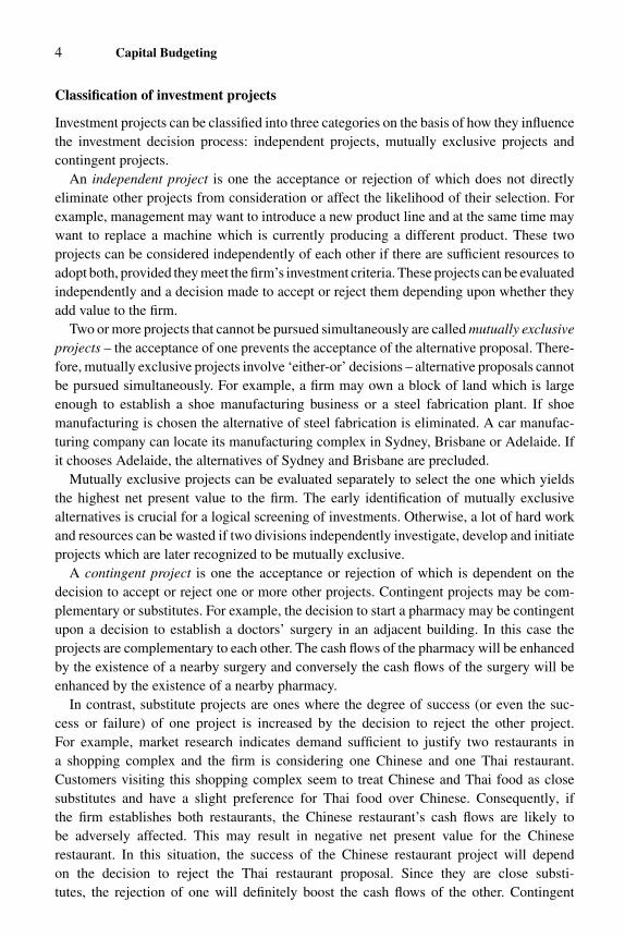
Investment projects can be classified into three categories on the basis of how they influencethe investment decision process: independent projects, mutually exclusive projects andcontingent projects.
An independent project is one the acceptance or rejection of which does not directlyeliminate other projects from consideration or affect the likelihood of their selection. Forexample, management may want to introduce a new product line and at the same time maywant to replace a machine which is currently producing a different product. These twoprojects can be considered independently of each other if there are sufficient resources toadopt both, provided they meet the firm’s investment criteria. These projects can be evaluatedindependently and a decision made to accept or reject them depending upon whether theyadd value to the firm.
Two or more projects that cannot be pursued simultaneously are called mutually exclusiveprojects – the acceptance of one prevents the acceptance of the alternative proposal. There-fore, mutually exclusive projects involve ‘either-or’ decisions – alternative proposals cannotbe pursued simultaneously. For example, a firm may own a block of land which is largeenough to establish a shoe manufacturing business or a steel fabrication plant. If shoemanufacturing is chosen the alternative of steel fabrication is eliminated. A car manufac-turing company can locate its manufacturing complex in Sydney, Brisbane or Adelaide. Ifit chooses Adelaide, the alternatives of Sydney and Brisbane are precluded.
Mutually exclusive projects can be evaluated separately to select the one which yieldsthe highest net present value to the firm. The early identification of mutually exclusivealternatives is crucial for a logical screening of investments. Otherwise, a lot of hard workand resources can be wasted if two divisions independently investigate, develop and initiateprojects which are later recognized to be mutually exclusive.
A contingent project is one the acceptance or rejection of which is dependent on thedecision to accept or reject one or more other projects. Contingent projects may be com-plementary or substitutes. For example, the decision to start a pharmacy may be contingentupon a decision to establish a doctors’ surgery in an adjacent building. In this case theprojects are complementary to each other. The cash flows of the pharmacy will be enhancedby the existence of a nearby surgery and conversely the cash flows of the surgery will beenhanced by the existence of a nearby pharmacy.
In contrast, substitute projects are ones where the degree of success (or even the suc-cess or failure) of one project is increased by the decision to reject the other project.For example, market research indicates demand sufficient to justify two restaurants ina shopping complex and the firm is considering one Chinese and one Thai restaurant.Customers visiting this shopping complex seem to treat Chinese and Thai food as closesubstitutes and have a slight preference for Thai food over Chinese. Consequently, ifthe firm establishes both restaurants, the Chinese restaurant’s cash flows are likely tobe adversely affected. This may result in negative net present value for the Chineserestaurant. In this situation, the success of the Chinese restaurant project will dependon the decision to reject the Thai restaurant proposal. Since they are close substi-tutes, the rejection of one will definitely boost the cash flows of the other. Contingent

An overview 5
Corporate goal
Strategic planning
Investment opportunities
Preliminary screening
Financial appraisal, quantitative analysis,project evaluation or project analysis
Qualitative factors, judgements and gut feelings
Accept /reject decisions on the projects
Accept Reject
Implementation
Facilitation, monitoring, control and review
Continue, expand or abandon project
Post-implementation audit
Figure 1.2. The capital budgeting process.
projects should be analysed by taking into account the cash flow interactions of all theprojects.
The capital budgeting process
Capital budgeting is a multi-faceted activity. There are several sequential stages in theprocess. For typical investment proposals of a large corporation, the distinctive stages inthe capital budgeting process are depicted, in the form of a highly simplified flow chart, inFigure 1.2.
Strategic planning
A strategic plan is the grand design of the firm and clearly identifies the business the firm isin and where it intends to position itself in the future. Strategic planning translates the firm’scorporate goal into specific policies and directions, sets priorities, specifies the structural,

6 Capital Budgeting
strategic and tactical areas of business development, and guides the planning process inthe pursuit of solid objectives. A firm’s vision and mission is encapsulated in its strategicplanning framework.
There are feedback loops at different stages, and the feedback to ‘strategic planning’ atthe project evaluation and decision stages – indicated by upward arrows in Figure 1.2 – iscritically important. This feedback may suggest changes to the future direction of the firmwhich may cause changes to the firm’s strategic plan.
Identification of investment opportunities
The identification of investment opportunities and generation of investment project pro-posals is an important step in the capital budgeting process. Project proposals cannot begenerated in isolation. They have to fit in with a firm’s corporate goals, its vision, missionand long-term strategic plan. Of course, if an excellent investment opportunity presentsitself the corporate vision and strategy may be changed to accommodate it. Thus, there is atwo-way traffic between strategic planning and investment opportunities.
Some investments are mandatory – for instance, those investments required to satisfyparticular regulatory, health and safety requirements – and they are essential for the firm toremain in business. Other investments are discretionary and are generated by growth oppor-tunities, competition, cost reduction opportunities and so on. These investments normallyrepresent the strategic plan of the business firm and, in turn, these investments can set newdirections for the firm’s strategic plan. These discretionary investments form the basis ofthe business of the corporation and, therefore, the capital budgeting process is viewed inthis book mainly with these discretionary investments in mind.
A profitable investment proposal is not just born; someone has to suggest it. The firmshould ensure that it has searched and identified potentially lucrative investment opportuni-ties and proposals, because the remainder of the capital budgeting process can only assurethat the best of the proposed investments are evaluated, selected and implemented. Thereshould be a mechanism such that investment suggestions coming from inside the firm, suchas from its employees, or from outside the firm, such as from advisors to the firm, are‘listened to’ by management.
Some firms have research and development (R&D) divisions constantly searching forand researching into new products, services and processes and identifying attractive invest-ment opportunities. Sometimes, excellent investment suggestions come through informalprocesses such as employee chats in a staff room or corridor.
Preliminary screening of projects
Generally, in any organization, there will be many potential investment proposals generated.Obviously, they cannot all go through the rigorous project analysis process. Therefore, theidentified investment opportunities have to be subjected to a preliminary screening processby management to isolate the marginal and unsound proposals, because it is not worthspending resources to thoroughly evaluate such proposals. The preliminary screening may

An overview 7
involve some preliminary quantitative analysis and judgements based on intuitive feelingsand experience.
Financial appraisal of projects
Projects which pass through the preliminary screening phase become candidates for rigorousfinancial appraisal to ascertain if they would add value to the firm. This stage is also calledquantitative analysis, economic and financial appraisal, project evaluation, or simply projectanalysis.
This project analysis may predict the expected future cash flows of the project, analysethe risk associated with those cash flows, develop alternative cash flow forecasts, examinethe sensitivity of the results to possible changes in the predicted cash flows, subject the cashflows to simulation and prepare alternative estimates of the project’s net present value.
Thus, the project analysis can involve the application of forecasting techniques, projectevaluation techniques, risk analysis and mathematical programming techniques such as lin-ear programming. While the basic concepts, principles and techniques of project evaluationare the same for different projects, their application to particular types of projects requiresspecial knowledge and expertise. For example, asset expansion projects, asset replacementprojects, forestry investments, property investments and international investments have theirown special features and peculiarities.
Financial appraisal will provide the estimated addition to the firm’s value in terms of theprojects’ net present values. If the projects identified within the current strategic frameworkof the firm repeatedly produce negative NPVs in the analysis stage, these results send amessage to the management to review its strategic plan. Thus, the feedback from projectanalysis to strategic planning plays an important role in the overall capital budgeting process.
The results of the quantitative project analyses heavily influence the project selection orinvestment decisions. These decisions clearly affect the success or failure of the firm and itsfuture direction. Therefore, project analysis is critically important for the firm. This bookfocuses on this complex analytical stage of the capital budgeting process, that is, financialappraisal of projects (or simply, project analysis).
Qualitative factors in project evaluation
When a project passes through the quantitative analysis test, it has to be further evaluatedtaking into consideration qualitative factors. Qualitative factors are those which will have animpact on the project, but which are virtually impossible to evaluate accurately in monetaryterms. They are factors such as:
� the societal impact of an increase or decrease in employee numbers� the environmental impact of the project� possible positive or negative governmental political attitudes towards the project� the strategic consequences of consumption of scarce raw materials� positive or negative relationships with labour unions about the project

8 Capital Budgeting
� possible legal difficulties with respect to the use of patents, copyrights and trade or brandnames
� impact on the firm’s image if the project is socially questionable.
Some of the items in the above list affect the value of the firm, and some not. The firmcan address these issues during project analysis, by means of discussion and consultationwith the various parties, but these processes will be lengthy, and their outcomes oftenunpredictable. It will require considerable management experience and judgemental skillto incorporate the outcomes of these processes into the project analysis.
Management may be able to obtain a feel for the impact of some of these issues, byestimating notional monetary costs or benefits to the project, and incorporating those valuesinto the appropriate cash flows. Only some of the items will affect the project benefits; mostare externalities. In some cases, however, those qualitative factors which affect the projectbenefits may have such a negative bearing on the project that an otherwise viable projectwill have to be abandoned.
The accept/reject decision
NPV results from the quantitative analysis combined with qualitative factors form the basisof the decision support information. The analyst relays this information to management withappropriate recommendations. Management considers this information and other relevantprior knowledge using their routine information sources, experience, expertise, ‘gut feeling’and, of course, judgement to make a major decision – to accept or reject the proposedinvestment project.
Project implementation and monitoring
Once investment projects have passed through the decision stage they then must be imple-mented by management. During this implementation phase various divisions of the firm arelikely to be involved. An integral part of project implementation is the constant monitor-ing of project progress with a view to identifying potential bottlenecks thus allowing earlyintervention. Deviations from the estimated cash flows need to be monitored on a regularbasis with a view to taking corrective actions when needed.
Post-implementation audit
Post-implementation audit does not relate to the current decision support process of theproject; it deals with a post-mortem of the performance of already implemented projects.An evaluation of the performance of past decisions, however, can contribute greatly tothe improvement of current investment decision-making by analysing the past ‘rights’ and‘wrongs’.
The post-implementation audit can provide useful feedback to project appraisal or strat-egy formulation. For example, ex post assessment of the strengths (or accuracies) andweaknesses (or inaccuracies) of cash flow forecasting of past projects can indicate the level

An overview 9
of confidence (or otherwise) that can be attached to cash flow forecasting of current invest-ment projects. If projects undertaken in the past within the framework of the firm’s currentstrategic plan do not prove to be as lucrative as predicted, such information can promptmanagement to consider a thorough review of the firm’s current strategic plan.
Organization of the book
This book follows a natural progression from the development of basic concepts, principlesand techniques to the application of them in increasingly complex and real-world situations.
An important and initial step in project analysis is the estimation of cash flows. Chapter 2commences with the basic concepts and principles for the identification of relevant cashflows followed by illustrative cash flow calculation examples for both asset expansion andasset replacement projects. All the cash flows for project evaluation are expected futurecash flows. Estimation of cash flows, therefore, involves forecasting. Quantitative and qual-itative ( judgemental) methods useful for forecasting project cash flows are discussed, withexamples, in Chapters 3 and 4.
Once the cash flows are estimated, projects are subjected to project evaluation techniques.The application of these techniques involves financial mathematics. Frequently encounteredformulae in capital budgeting are illustrated with simple examples in Chapter 5. A thoroughunderstanding of the application of these formulae provides a springboard for the projectanalysis material in the remainder of the book.
Chapter 6 uses the cash flow concepts and the formulae (from Chapters 2 and 5) toevaluate the projects using several criteria, such as net present value, internal rate of returnand payback period, and demonstrates the versatility of the net present value criterion.Project appraisal is carried out in Chapter 6 under the following assumptions:
� a single goal of wealth maximization for the firm� capital expenditures and cash flows known with certainty� no resource constraints (all the profitable projects can be accepted).
This basic model is then expanded to deal with risk (or uncertainty of cash flows) inChapters 7 to 10. Chapter 7 discusses, with illustrative examples, the risk-adjusted dis-count rate and certainty equivalent methods for incorporating risk. Chapter 8 illustrates theuse of sensitivity and break-even analyses as tools for aiding the decision-makers to makeinvestment decisions under uncertainty. Project risk analysis is further extended by intro-ducing simulation concepts and methods in Chapter 9 and then applying those concepts andmethods to a case study in evaluation of a forestry investment in Chapter 10.
Resource constraints on the capital budgeting decision are considered in Chapter 11 byintroducing the basics of linear programming (LP) and applying the LP technique for selec-tion of the optimal project portfolios. Chapter 12 presents extensions to the LP techniquewhich make the approach more versatile.
A number of special topics in capital budgeting are covered towards the end of the book.They include property investment analysis (Chapters 14 and 15), and evaluation of inter-national investments (Chapter 16). Capital budgeting decisions under resource constraints

10 Capital Budgeting
analysed in the two linear programming chapters (11 and 12) also provide a number ofspecial cases in project analysis. Simulation and financial modelling in forestry projectevaluation as discussed in Chapters 10 and 13 may also be viewed as special topics incapital budgeting because they apply to specific type of investments, namely investmentsin forestry.
Using Excel for computations
As mentioned earlier, actual project analysis in the real world involves voluminous, tedious,complex and repetitive calculations and relies heavily on computer packages. Capital bud-geting concepts, processes, principles and techniques can be made clear by words, graphsand numerical examples. Numerical examples – particularly those which involve repeated,complex, tedious or large calculations – are made simple, clear, useful, attractive and some-times fun by the use of such computer packages.
In this book, the Excel spreadsheet package is used, wherever appropriate, for calcula-tions in examples. Excel workbooks are held on the Cambridge University Press website(http://publishing.cambridge.org/resources/052181782x/). For convenience, the relevantExcel workbook is indicated with a marker at the appropriate places in the text.
This book is written in such a way that the materials can be studied independently ofthe Excel workbooks or computer access. However, Excel workbooks will help in under-standing the computations and may facilitate the clarification of any computational queriesfor which answers cannot be found in the text. The many Excel workbooks may be viewedas supplementary or complementary to the discussion in the text. These workbooks willaid in working through problems and will provide templates that may be applied in thiswork.
Concluding comments
This introductory chapter has set the capital budgeting decision within the broader perspec-tive of the finance discipline and its financial management context. A broad overview of thecapital budgeting process was presented in Figure 1.2. The financial appraisal of projects,which is the focus of this book, was identified as one of the critically important and complexstages in the capital budgeting process. The financial appraisal is often known in simpleand general terms as ‘project analysis’.
Emphasis has been placed on shareholder wealth maximization as the firm’s goal (i.e. thebook has a corporate focus).
The use of Excel as a teaching and learning aid in this book and then as a practical toolfor real-world project analysis has been emphasized.
The flow of materials in this book follows a natural progression from the developmentof basic concepts, principles and techniques to the application of them in increasinglycomplex and real-world situations. With this background, the main areas covered in thevarious chapters have been outlined, together with their relationships to one another.

An overview 11
Review questions
1.1 In finance theory, what is the most widely accepted goal of the firm? How does the netpresent value of a project relate to this goal?
1.2 Discuss the relationships between the firm’s goal, financial management and capitalbudgeting.
1.3 Present two examples for each of the following types of investment projects:(a) independent projects(b) mutually exclusive projects(c) contingent projects.
1.4 Should relatively small capital expenditures be subjected to thorough financial appraisaland the other key stages of a typical capital budgeting process?
1.5 Briefly discuss the main stages of a typical, well-organized capital budgeting processin a large corporation.

2 Project cash flows
An important part of the capital budgeting process is the estimation of the cash flowsassociated with the proposed project. Any new project will cause a change in the firm’scash flows. In evaluating an investment proposal, we must consider these expected changesin the firm’s cash flows and decide whether or not they add value to the firm. Success-ful investment decisions will increase the shareholders’ wealth through increased cashflows.
Valuing projects by estimating their net present values (NPV) of future cash flows is ameans of gaining an idea of their expected addition to shareholder wealth. Correct iden-tification of the relevant cash flows associated with an investment project is one of themost important steps in the calculation of NPV or in the project appraisal. Cash flow is avery simple concept, although it is easily confused with accounting profit or income. Cashflows are simply the dollars received and dollars paid out by the firm at particular points intime.
The focus of project analysis is on cash flows because they easily measure the impactupon the firm’s wealth. Profit and loss in financial statements do not always represent the netincrease or decrease in cash flows. Cash flows occur at different times and these times areeasily identifiable. The timing of flows is particularly important in project analysis. Someof the figures in standard financial statements, such as income statements or profit and lossaccounts, may not have a corresponding cash flow effect for the same period; some of theiractual cash flows may occur in the future or might already have occurred in the past. Forexample, a sale on credit is recorded as occurring on the day the transaction takes placewhile the actual cash inflow may occur many weeks or months later.
In order to evaluate a project, the cash flows relevant to the project have to be identified.In simple terms, a relevant cash flow is one which will change (decrease or increase) thefirm’s overall cash flow as a direct result of the decision to accept the project. Relevant cashflows thus deal with changes or increments to the firm’s existing cash flows. These flowsare also known as incremental or marginal cash flows.
Project evaluation rests upon incremental cash flows. Incremental cash flows are the cashinflows and outflows traceable to a given project, which would disappear if the projectdisappeared. The incremental cash flows can be measured by comparing the cash flowsof the firm ‘with’ the project and the cash flows of the firm ‘without’ the project. It is a
12

Project cash flows 13
marginal, or incremental, analysis comparing two situations. Erroneous comparisons suchas ‘before versus after’ should be avoided.
For example, suppose a new manufacturing plant uses land that could otherwise be soldfor $500,000. The firm owns the land ‘before’ the project and the firm still owns the land‘after’ the project. Therefore, if a ‘before versus after’ comparison is used, the cash flowattributed to the manufacturing project will be zero. However, the land is a valuable resourceand it is not free. It has an opportunity cost which is the cash it could generate for the firm ifthe project were rejected and the land sold or put to some other productive use. Therefore,‘without’ the project, the firm could generate $500,000 cash if the land is sold (and someother amount if the land is put to some other use). ‘With’ the project, the firm wouldnot be able to generate this cash inflow. Therefore, $500,000 is assigned to the proposedmanufacturing project as a cash outflow.
For analytical purposes project cash flows may be separated into two categories: capitalcash flows and operating cash flows. Capital cash flows may be disaggregated into threegroups: (1) the initial investment (2) additional ‘middle-way’ investments such as upgradesand increases in working capital investments, and (3) terminal flows. These are all cashflows and the distinctions among them are only to facilitate the convenient identification ofthe different categories.
The largest single capital flow is traditionally the initial investment. This is also called the‘initial capital outlay’ or just ‘capital expenditure’. Initial capital outlay generally involvesthe cash outflows required to start a project by purchasing or creating assets and puttingthem into working order. As such, the necessary expenditures to establish sufficient workingcapital for the project and the installation costs of the machines purchased are included inthe initial capital outlay. The word ‘initial’ is quite important. It denotes both the amountto ‘initiate’ or ‘start’ the project, and the time at which this outlay occurs.
Once the initial investment is made and the project is in operation, the project is expectedto generate cash flows over its economic life. These flows are called operating cash flowsand include: cash inflows from sales, cash outflows for advertising and marketing, paymentsfor wages, heating and lighting bills, and purchases of raw materials.
At the end of the project’s economic life there will be another set of capital flows. Theseare generally known as terminal cash flows. For example, the terminal cash inflows could bethe sale of the project as a going concern, the salvage value of the asset net of tax, and recoveryof any remaining working capital. Terminal cash outflows could be, for example, the costof asset disposal or demolition, the cost of environmental rehabilitation, and redundancypayments to employees.
It is important to classify the investment decision correctly as this will help with cashflow identification. Investment projects are generally of two types: asset expansion projectsand asset replacement projects. Asset expansion projects are those that propose to investin additional assets in order to expand an existing product or service line, enter a newline of business, increase sales or reduce costs etc. Asset replacement decisions involveretiring one asset and replacing it with a more efficient asset. This category of decisionalso encompasses asset retirement, asset abandonment and asset replication over the longerterm.

14 Capital Budgeting
In projects generally, the relevant cash flows will be easy to identify. These will be thestraightforward amounts for the initial outlay, ongoing receipts of cash from sales, ongoingcash expenditures on production costs and individual asset termination flows. However,there are some cash flows that are not so straightforward, and are sometimes difficult toidentify. These include synergistic effects and opportunity costs.
This chapter will provide guidelines for identifying a project’s incremental cash flows,with illustrative examples. The discussion includes the stand-alone project principle, indirector synergistic effects, the opportunity cost principle, the sunk cost concept, overhead costallocation, the treatment of working capital, taxation, depreciation, investment allowances,financing (debt and interest) flows and inflation and timing of cash flows. Cash flow es-timation of asset expansion projects and asset replacement projects will be illustrated bycalculated examples.
Study objectives
After studying this chapter the reader should be able to:
� identify a project’s incremental cash flows� calculate initial investment outlay, operating cash flows, and terminal cash flows for asset
expansion and asset replacement projects� determine the effects of depreciation on after-tax cash flows� separate the investment decision from the financing decision and distinguish between
project flows and financing flows� calculate after-tax cash flows to be used in project valuation� gain an insight into the differences between accounting income and cash flows
Essentials in cash flow identification
In estimating the relevant cash flows, a number of principles and concepts are employed.
Principle of the stand-alone project
A project’s incremental cash flows can be calculated by comparing the total future cash flowsof the firm ‘with’ and ‘without’ the project. In practice, this would be very cumbersome,particularly for large firms with many different product lines. Fortunately, it is not generallynecessary to do this because once the effect of undertaking the proposed project on thefirm’s cash flows has been identified, only that project’s incremental cash flows need to beconsidered.
This marginal form of analysis suggests that we can view the proposed project as a kindof ‘mini-firm’ with its own future capital expenditures and operating cash flows. Thus, whatthe stand-alone principle says is that we will be evaluating the proposed project purely onits own merits, in isolation from any other activities or projects of the firm, but includingits incidental or synergistic effects.

Project cash flows 15
Indirect or synergistic effects
All the indirect or synergistic effects of a project should be included in the cash flow calcu-lation. Synergistic effects can be negative or positive. For example, if a car manufacturingcompany considers introducing a new model called, say, Mako, which is a close substitutefor an existing model called Raptor, then there could be a fall in sales of Raptors due tothe new model Mako. Let us suppose that the Raptor sales are expected to decrease by$25 million over the project’s life from this effect. This negative effect would then have tobe counted as an incremental cost of the proposed Mako project. The rationale is that ‘with-out’ the Mako project, the firm’s future cash flows would have been higher by $25 million.In other words, ‘with’ the Mako project, the firm’s Raptor cash flow would be reduced by$25 million. The $25 million reduction is calculated into the Mako project by reducing itsfuture net cash flows by this amount.
As another example, assume that a proposed project introduces a new product or servicewhich is complementary to an existing product or service of the firm and consequently willenhance the sales of the existing product. Establishing a pharmacy adjacent to an existingdoctor’s surgery is likely to have a favourable impact on the surgery’s cash flows. Patientnumbers may increase at the surgery because of the convenience of a pharmacy next door.This positive flow-on effect should be included in the proposed pharmacy project’s cashinflow.
The rationale for the incorporation of these indirect effects has its base in the opportunitycost principle.
Opportunity cost principle
When a firm undertakes a project, various resources will be used and not be available forother projects. The cost to the firm of not being able to use these resources for other projectsis referred to as an ‘opportunity cost’. The value of these resources should be measured interms of their opportunity cost. The opportunity cost, in the context of capital budgeting, isthe value of the most valuable alternative that is given up if the proposed investment projectis undertaken. This opportunity cost should be included in the project’s cash flows. Let usconsider two examples.
Example 2.1
A proposed project involves the establishment of a production facility. This facility willbe located within a factory the firm already owns. The estimated rental value of the spacethat the production facility will occupy is $29,000 per year. The space has not been rentedin the past, but the firm expects to rent it in the future. Then, the firm will lose $29,000‘with’ the project because that space will be used for the project. Therefore, the opportunitycost is $29,000 per year in rent forgone and it should be included as a cash outflow. Thisexample also illustrates that even when no cash changes hands, there could be an opportunitycost. Why does this not contradict the principle that we should only consider cash flows?

16 Capital Budgeting
The reason is that opportunity cost of the space measures an extra cash flow that would begenerated (for the firm) ‘without’ the project.
Suppose that this space has not been rented in the past and there is no intention to rent,sell or use for any other purpose in the future. In this case, there is no opportunity cost ifthe resource is used for the proposed project. Therefore, in this situation, the $29,000 willnot be included as a cash outflow.
Example 2.2
A project under consideration involves the use of an existing building to set up a fac-tory to produce shoes. The market value of this building is $200,000. If the project isundertaken, there will be no direct cash outflow associated with purchasing the buildingsince the firm already owns it. In evaluating the proposed shoe-manufacturing project,should we then assume zero cost for the building? Certainly not. The building is not a‘free’ resource for the project because if the building was not used for this project itcould be used for some other purpose; for example, it could be sold to generate cash.Using the existing building for the proposed shoe project thus has an opportunity cost of$200,000.
Sunk costs
Another key concept used in identifying relevant cash flows is the notion of sunk costs. Asunk cost is an amount spent in the past in relation to the project, but which cannot nowbe recovered or offset by the current decision. Sunk costs are past and irreversible. Theyare not contingent upon the decision to accept (or reject) a proposed project. Therefore,they should not be included in the cash flows. To illustrate the concept, two excellentreal-world examples are reproduced in the following paragraphs from Brealey, Myers,Partington and Robinson (2000, p. 133) and Moyer, McGuigan and Kretlow (2001, p. 307)respectively.
In 1971 Lockheed sought a United States federal government guarantee for a bank loanto continue development of the TriStar aeroplane. Lockheed and its supporters argued thatit would be silly and imprudent to abandon a project on which nearly $1 billion had alreadybeen spent. Some of the opponents argued that it would be equally silly and imprudent tocontinue with a project that offered no prospect of a satisfactory return on that $1 billion.Both groups were wrong. The $1 billion was spent in the past and it was a sunk cost,irrelevant to the investment analysis. The TriStar project has been analysed by Reinhardt(1973) and that analysis does not include $1 billion as an opportunity cost.
In 1999, the Chemtron Corporation was considering a project to construct a new chemicaldisposal facility. Two years earlier, the corporation had hired the R.O.E. Consulting Groupto make an environmental impact study of the proposed site at a cost of $500,000. Thismoney cannot be recovered whether the proposed project (being considered in 1999) isundertaken or not. Therefore, it should not be included in the project’s cash flows.

Project cash flows 17
Overhead costs
Two examples of overhead costs are utilities (such as electricity, gas and water) and executivesalaries. Cost accounting is in part concerned with the appropriate allocation of variousoverhead costs to particular production units. In the project evaluation, however, the issueis not the allocation of overheads to production units, but the identification of incrementaloverhead costs. Very often, overhead expenses would occur ‘with’ or ‘without’ the proposedproject; they occur whether or not a given project is accepted or rejected. There is often not asingle specific project to which the overhead costs can be allocated. Thus, the question is notwhether or not the proposed project would benefit from the overhead facilities, but whetheror not the overhead expenses are incremental cash flows associated with the proposedproject.
In project appraisal, the decision as to what overheads should be allocated to a proposedproject’s cash flows can be guided by the opportunity cost and sunk cost principles. Onlythe incremental cash flows resulting from changes in overhead expenses should be includedin evaluating a project proposal. If the expenses are already being incurred, a proportionshould not be allocated to the new project.
For example, Cedar Ltd currently incurs utility overheads of $500,000 from the operationof its main office complex, which it allocates to the production departments on the basis offloor space. Suppose Cedar Ltd is considering extending its factory in order to manufacturea new product. In doing so, a new production department will be created which will takeup 20% of the available floor space of the factory. The new project is not expected to affectmain office utility overheads. The firm’s management accountant, employing accepted costaccounting principles, would allocate $100,000 (being 20% of a $500,000 utilities costincurred in the last year) as an expense associated with the new project. While it wouldbe tempting to include this overhead expense in the evaluation of the proposed project, itwould be incorrect to do so. From a project evaluation perspective, this utilities overheadwould not be included in the project analysis, because this cost is not an incremental costto the project; ‘with’ or ‘without’ the project, this utilities cost is incurred.
Continuing with the previous example, Cedar Ltd also allocates executive salaries to theproduction department, based on the floor space. The firm’s management accountant, usingthe same cost accounting principles, would allocate $160,000 (being 20% of the $800,000chief executive’s salary) as an expense associated with the new project. Again, while it wouldbe tempting to include this overhead expense in the evaluation of the proposed project, itwould be incorrect to do so, because this cost is not an incremental cost to the project; ‘with’or ‘without’ the project, this salary is paid. If, however, 25% of the chief executive’s timeis spent on the project causing a decrease in the productivity of the firm’s other activitiesthen this would be considered an opportunity cost of the proposed project and included inthe analysis.
Alternatively, if additional staff (costing $200,000) were recruited to look after the firm’sexisting business (thus preventing possible adverse effects on the productivity of the firm’sother activities), then the $200,000 would be an increment to the project and should beincluded in its evaluation.

18 Capital Budgeting
Treatment of working capital
More often than not, new projects will involve additional investments in working capital.Working capital is equal to a firm’s current assets minus its current liabilities. Cash, in-ventories of raw materials and finished goods, and accounts receivable (customers’ unpaidbills) are examples of current assets. Current liabilities include accounts payable (the firm’sunpaid bills) and wages payable.
When a new project starts, it may be necessary to increase the amount of cash held asa float to accommodate more transactions. Further inventories of raw materials may berequired to run the new production lines smoothly. Additional investment in finished goodsinventories may be necessary to handle increased sales. When the finished product is sold,customers may be slow to pay, thus causing an increase in accounts receivable. All of thesechanges require increased working capital investment.
Increases in working capital requirements are considered cash outflows even though theydo not leave the firm. For example, an increase in inventory is considered a cash outfloweven though the goods are still in store, because the firm does not have access to the cashvalue of that inventory. Consequently, the firm cannot use that money for other investments.That is, an increase in working capital represents an opportunity cost to the firm. Productionand sales fluctuate during the project’s progress and accordingly cash may flow into or outof working capital. When the project terminates, any working capital recovered is treatedas a cash inflow.
The flows of working capital must be treated as capital flows and not operational flows.Because working capital is allied to sales, you might be tempted to consider such flows asincome or expense flows. This is not the case: working capital represents a pool of fundscommitted to the project in the same manner as is fixed capital. The fixed capital cost isaccounted for as an opportunity cost in the NPV discounting process, and so too is theworking capital pool.
After-tax cash flows
Tax is a cash payment to a government authority. If the project generates tax liabilities, thenthe tax payable is relevant to the project, and must be accounted for as a cash outflow.
Corporate tax is a cash outflow. If the tax were levied on net cash inflow and paid at thesame time as cash was received, then the after-tax net cash flow would be easily calculated.However, tax is not based on net cash flow, but on taxable income.
Taxable income is defined by the relevant taxation legislation and does not necessarilymean the same thing as net cash flow or even accounting income or accounting profit.Taxable income is generally calculated by subtracting allowable deductions from assessableincome. These terms are specific to particular tax acts, and are not easily dealt with in ageneral context. However, project evaluation needs to be able to accord some treatment tothis calculation to determine after-tax cash flows. In this book, a simple flat rate (e.g. 30%)of tax is applied to illustrate the after-tax cash flow calculations in examples.
The tax definition of ‘deductions’ treats some non-cash items as allowable expenses. Onesuch item frequently encountered in project analysis is asset depreciation.
Project cash flows 19
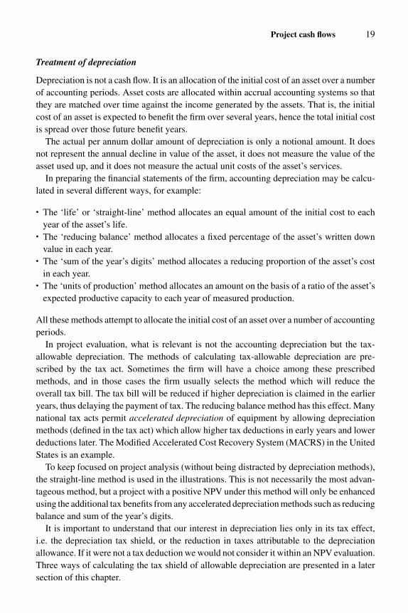
Treatment of depreciation
Depreciation is not a cash flow. It is an allocation of the initial cost of an asset over a numberof accounting periods. Asset costs are allocated within accrual accounting systems so thatthey are matched over time against the income generated by the assets. That is, the initialcost of an asset is expected to benefit the firm over several years, hence the total initial costis spread over those future benefit years.
The actual per annum dollar amount of depreciation is only a notional amount. It doesnot represent the annual decline in value of the asset, it does not measure the value of theasset used up, and it does not measure the actual unit costs of the asset’s services.
In preparing the financial statements of the firm, accounting depreciation may be calcu-lated in several different ways, for example:
� The ‘life’ or ‘straight-line’ method allocates an equal amount of the initial cost to eachyear of the asset’s life.
� The ‘reducing balance’ method allocates a fixed percentage of the asset’s written downvalue in each year.
� The ‘sum of the year’s digits’ method allocates a reducing proportion of the asset’s costin each year.
� The ‘units of production’ method allocates an amount on the basis of a ratio of the asset’sexpected productive capacity to each year of measured production.
All these methods attempt to allocate the initial cost of an asset over a number of accountingperiods.
In project evaluation, what is relevant is not the accounting depreciation but the tax-allowable depreciation. The methods of calculating tax-allowable depreciation are pre-scribed by the tax act. Sometimes the firm will have a choice among these prescribedmethods, and in those cases the firm usually selects the method which will reduce theoverall tax bill. The tax bill will be reduced if higher depreciation is claimed in the earlieryears, thus delaying the payment of tax. The reducing balance method has this effect. Manynational tax acts permit accelerated depreciation of equipment by allowing depreciationmethods (defined in the tax act) which allow higher tax deductions in early years and lowerdeductions later. The Modified Accelerated Cost Recovery System (MACRS) in the UnitedStates is an example.
To keep focused on project analysis (without being distracted by depreciation methods),the straight-line method is used in the illustrations. This is not necessarily the most advan-tageous method, but a project with a positive NPV under this method will only be enhancedusing the additional tax benefits from any accelerated depreciation methods such as reducingbalance and sum of the year’s digits.
It is important to understand that our interest in depreciation lies only in its tax effect,i.e. the depreciation tax shield, or the reduction in taxes attributable to the depreciationallowance. If it were not a tax deduction we would not consider it within an NPV evaluation.Three ways of calculating the tax shield of allowable depreciation are presented in a latersection of this chapter.

20 Capital Budgeting
Tax payable
Tax payable is a cash outflow. The form of tax encountered in project analysis is corporatetax. It is calculated as a percentage of taxable income. The rate of corporate tax is usuallya fixed rate for every dollar of taxable income.
Taxation is a very volatile area, and tax rules are constantly changing. In any situationwhere a project may be subject to particular and special tax laws or rulings, expert taxadvice must be sought. Even this help may not afford sufficient protection, as tax lawscan be changed retrospectively or they can change from time to time after the project hascommenced. The best course to follow in this situation is to ensure that the project is notdependent upon tax savings or tax shields for its success.
Investment allowance
Governments often provide special temporary incentives to the private sector to encourageinvestments in selected industries. These incentives normally take the form of a tax benefitwhere a given percentage of the cost of investment is assigned as an allowable deductionfor arriving at taxable income. This kind of investment allowance normally does not affectthe allowable depreciation of the asset, which is based on the full cost of the investmentbefore the investment allowance.
The tax rules attached to these sorts of schemes are quite complex, so when using theseschemes clarifications must be sought from appropriate tax experts. These incentives doenhance the NPVs of projects and should be incorporated into the analysis where necessary.
Financing flows
Treatment of financing flows is an area of confusion and sometimes a source of error inproject analysis. It is important to distinguish between project cash flows and financingcash flows. For the purpose of identifying the relevant cash flows for project evaluation,the investment decision (project) must be separated from its financing decision. The fi-nancing decision concerns the relative proportions of the project’s capital expenditures tobe provided by debt-holders and equity-holders respectively. The decision about the par-ticular mixture of debt and equity used in financing the project is a management decisionconcerning the trade-off between financial risk and the cost of capital. This debt–equitymixture determines how the resultant project cash flows are divided between debt-holdersand equity-owners. By contrast the investment evaluation decision determines whether theproject’s discounted cash flows exceed the initial capital outlay (investment), and so adds(net present) value to the firm.
Generally, interest charges or any other financing costs such as dividends or loan re-payments are not deducted in arriving at cash flows, because we are interested in the cashflow generated by the assets of the project. Interest is a return to providers of debt capital.It is an expense against the income generated to equity-holders, and as such is deductedin the determination of accounting profit. However, it is not included in project cash flowanalysis, as the discount rate employed in the NPV analysis accommodates the required
Project cash flows 21
returns to both equity and debt providers. Therefore, inclusion of interest charges in cashflow calculations would result in a double counting of the interest cost.
Interest is tax deductible, and therefore provides a tax shield for any investment. Thisbenefit is also accounted for in the discount rate, as the rate employed in project analysis isan ‘after-tax’ rate. Accordingly, tax savings on interest expenses are not included in projectcash flow analysis.
Almost always there are exceptions to general rules or practices and this is the case forthe general rule for the treatment of financing flows. There are situations where interestcharges are explicitly incorporated into the cash flows. The question here is not whetherit is right or wrong to incorporate financing flows into the cash flow analysis, but whetherthat incorporation is done correctly or incorrectly. If it is necessary to show the financingflows explicitly in the cash flows, as is often preferred by non-financial managers and chiefexecutives, it is quite possible to do this in a correct and consistent manner without distortingthe final results.
In property investment analysis, ‘property’ cash flows are distinguished from ‘equity’ cashflows. Property cash flows are the equivalent of ‘project’ cash flows discussed in this chapter.Property cash flow calculations do not include loan repayments and interest charges asdeductions. This approach is consistent with the general cash flow definition in this chapter.‘Equity’ cash flow calculations, in contrast, deduct loan repayments and interest expenses.
One of the objectives of property investment analysis is to evaluate the return to theinvestor under different debt and tax situations. A mortgage is for one particular property,rather than being an unidentified part of the capital structure of a corporation. Some in-vestment in property is to gain tax advantages from interest deductions associated withdebt financing. For these reasons, in property investment analysis, equity cash flows arecalculated after deducting loan repayments (principal plus interest) from other cash inflowsto enable the effects of borrowing and taxation to be evaluated. This is explained fully whenreal estate investments are described and analysed in Chapter 14.
Within-year timing of cash flows
Normally, cash flows occur at various points of time within a year. The standard practice incapital budgeting is to assume that capital expenditures occur at the beginning of the yearand all other cash flows occur at the end of the year. This assumption simplifies cash flowtiming and to some degree imitates reality. The yearly time frame is assumed because largecapital projects have very long lives, and the loss of within-year cash flow timing detail isnot material.
To maintain consistency for calculation purposes, the points in cash flow timing are setat the end of each year. Flows which would normally occur at the start of any year will betimed as occurring at the end of the immediately preceding year. For example, an initialcapital outlay of $200 at the start of year 1 will be timed as occurring at the end of year 0.The idea of a year 0 should not introduce any confusion. Year 0 simply means that therehas been some notional historical time which has now elapsed, and we now stand ‘at theend of year 0’. The end of year 0 is in fact the start of year 1. The notion of a year 0 is used

22 Capital Budgeting
so that we can maintain a consistent set of acronyms: the points in time are often tallied asEOY 0, EOY 1, EOY 2 and so on. Equivalently, we may use Y0, Y1, Y2 and so on. Capitalexpenditure at the start of the project is timed as occurring at EOY 0. Operating cash flowsin the first year are timed as occurring at EOY 1. Subsequent operating cash flows are timedat EOY 2, EOY 3 and so on.
The standard practice in capital budgeting assumes that capital expenditures occur atthe beginning of a year and all other cash flows occur at the end of a year. The capitalexpenditure occurring at the ‘start of year 3’, for example, would be netted out against theother cash flows as occurring at the ‘end of year 2 (EOY 2)’ since we have no timing positioncalled ‘start of year 3’, and in any case, the ‘end of year 2’ and the ‘start of year 3’ are thesame point in time.
The timing of tax payments may vary. In some tax jurisdictions, tax payable is assessedat the end of a year, and actually paid in the subsequent year. If this is the case, then thetax outflow will have to be shown as a delayed payment in the following year. In other taxjurisdictions, tax is paid progressively on quarterly or half-yearly earnings, or on estimatedyearly earnings. In these cases, the tax is paid within the current year. The treatment of taxwill thus depend upon the tax situation in a particular country. So that we can concentrateon the analytical side of project appraisal, we assume tax payments are made in the sameyear in which taxable income is generated, unless specifically noted otherwise.
Inflation and consistent treatment of cash flows and discount rates
Inflation will have an effect on the expected cash flows of a project. Both cash inflows andoutflows could be affected by inflation. Market rates, such as interest rates and equity returns,in general will also rise when the expected inflation rate is high. As the market rates rise,the required rate of return by investors will also rise. To deal with inflation appropriately,the project analysis must recognize expected inflation in the forecast of future cash flowsand use a discount rate that reflects investors’ expectations of future inflation.
If all cash flows as well as the discount rate are equally affected by expected inflation,the net present value is the same whether inflation is included or excluded. However, mostprojects consist of a multitude of cash flows over a number of years and it would be erroneousto assume that all of these cash flows will increase by exactly the same rate each year, orto assume the same effect on the discount rate. Some cash flows are unaffected by inflationwhile other cash flows are affected to varying degrees by inflation.
An outstanding example of the differential impact of inflation on a project’s cash flowis the ‘depreciation tax shield’ (or the tax saving from the tax-allowable depreciation).Tax-allowable depreciation is totally unaffected by inflation. Depreciation tax shields arecalculated on the basis of the historical costs of the assets at the time of their acquisition.Similarly, a long-term raw-material contract or the purchase of a commodity in the forwardor futures markets may lock in the present prices, thereby insulating the cash flow frominflationary effects.
Given the differential impact of inflation on various cash flow components, cash flowforecasts in nominal terms, i.e., incorporating the inflationary effect, have an advantage over

Project cash flows 23
cash flow forecasts in real terms, i.e., excluding the inflationary effects. That is, nominalcash flow forecasts can incorporate potentially different inflationary trends in selling prices,labour costs, material costs and so on, into cash flow estimates by applying different inflationrates for different components of the cash flow.
The required rate of return used for discounting cash flows is normally derived fromobserved market rates such as interest rates and returns on equity. These observed marketrates usually have the expected annual inflation rates built in and are usually quoted innominal terms (as opposed to real terms). Observed market rates expressed in nominal termscan, if necessary, be converted into real terms using the algebraic relationship expressed inthe Fisher effect. The Fisher equation is:
(1 + n) = (1 + r )∗(1 + p)
where:
n = the annual nominal interest rate (expressed as a decimal value)r = the annual real interest rate (expressed as a decimal value)p = the expected annual inflation rate
From the above equation the real interest rate can be easily derived:
r = (1 + n)
(1 + p)− 1
Consistency in the discounted cash flow analysis requires that if a project’s cash flows are innominal terms, they should be discounted by nominal discount rates, and if a project’s cashflows are in real terms they must be discounted by real discount rates. Real and nominalquantities should not be mixed.
As we see later in Chapters 6 and 7, the interest rate used for discounting cash flows isnormally derived from observed market rates. In an efficient financial market, investors’required rate of return will include a component, (1 + p), to compensate for expectedinflation. The use of observed market-required rates then implies that we should incorporateinflation into cash flows to be consistent. On rare occasions (such as the computer projectexample in Chapter 9), real cash flows are appropriate in the analysis. In such situations, thereal discount rate can be calculated from market (nominal) rates using the Fisher equationpresented above.
Asset expansion project cash flows
Principles, concepts and the treatments relating to cash flow calculation were discussed inthe preceding section. This section presents suitable formats for calculating the three maincomponents of cash flows: initial investment, net operating cash flows and terminal cashflows. Brief discussions or illustrations are provided where necessary.
The basic formats for determining initial investment, operating cash flows, and terminalcash flows of an asset expansion project are outlined below.

24 Capital Budgeting
Initial investment
The initial net investment in an asset expansion project is defined as the project’s initialcash outflow, that is, the capital outlay (or capital expenditure or capital outflow) at thebeginning of the project. It is calculated using the following typical format:
Cost of new asset(s)+ Installation and shipping costs+ Initial investment in working capital= Initial investment
It is worth noting here that for the purpose of tax-allowable depreciation, working capitalis not an allowable item. The asset cost plus installation and shipping costs form the basisupon which depreciation is computed. The typical wording of a tax act covering the valueof depreciable items says: ‘the cost of plant and equipment installed ready for use’. Thisdefinition does not include working capital.
Net operating cash flows
A project’s after-tax net operating cash flows for any given year during the economic lifeof the project may be calculated using the following typical format. To focus on the formatwithout being distracted by the details of the timing of cash flows for sales and cost ofgoods sold, it is assumed that they are all cash flows received or paid during the year. Moreexplicitly, it is assumed that all sales are for cash and that opening and closing inventoriesremain unchanged (hence, the cost of goods sold equals purchases) and that all purchasesare in cash. In fact, the forecasts of sales revenues and costs of goods sold are generallydone on a cash basis and the distinction between cash and non-cash values for a given yearis not an issue.
Cash inflow from sales− Cost of goods sold− Selling, general, administrative and other expenses− Depreciation= Taxable income− Tax payable= Net income (after tax)+ Depreciation= After-tax net operating cash flow
This method ‘adds back’ the amount of depreciation. This is quite common, and is correct.An alternative approach which isolates the cash flows from the non-cash flows is shownbelow.
Cash inflow from sales− Cost of goods sold− Selling, general, administrative and other expenses= Net cash income

Project cash flows 25
− Depreciation= Taxable income
Net cash income− Tax payable= After-tax net operating cash flow
Another format which identifies the ‘tax shield of allowable depreciation’ explicitly is:
Cash inflow from sales− Cost of goods sold− Selling, general, administrative and other expenses= Net cash income− Tax on net cash income= Net after-tax cash income+ Tax shield of allowable depreciation= After-tax net operating cash flow
where tax shield of depreciation = (depreciation × tax rate).Any of these formats can be used depending upon the circumstances.If there are net ‘losses’ (as opposed to net income), their tax treatment may vary un-
der different tax rules for different industries in different countries. Two possible generaltreatments of losses may be:
� Carry forward the losses to future years of the project until there is sufficient income tooffset the losses, or
� Deduct the losses from the firm’s other business activities (which include projects otherthan the project being considered) thus realizing tax benefits for the firm ‘with’ theproject.
In the latter case, such tax benefits may be treated as a cash inflow of the proposed project,because ‘without’ the proposed project the firm’s cash flows would be reduced by thatamount.
Terminal cash flow
In the final year of a project’s economic life, there is another cash flow on top of the normalannual operating cash flows. This is termed the terminal cash flow. Typically, it has twocomponents: the recovery of the working capital and the recovery of the after-tax salvagevalue of the assets.
The typical format for calculating the terminal cash flow is:
Proceeds from sale of assets− Taxes on sale of assets= After-tax salvage value+ Recovery of working capital= Terminal cash flow

26 Capital Budgeting
Taxes on the sale of an asset
Whenever an asset is sold, there are tax consequences which will affect the net proceedsfrom the sale. These tax rules vary not only among different countries but also over timewithin a single country. Therefore, expert tax advice ought to be sought at the time ofevaluating the project. However, for analytical purposes, as well as to become familiar withthe different possible tax situations, the tax treatment on ‘sale of assets’ may be categorizedinto four cases.
Case 1: Sale of an asset for its tax book-value. Normally if an asset is sold for an amountexactly equal to its tax book-value, there will be no tax consequences as there will be nogain or loss on the sale. Tax book-value is equal to the installed cost of the asset minusaccumulated tax depreciation.
Case 2: Sale of an asset for less than its tax book-value. In this case there will be a loss, whichis equal to sale proceeds minus tax book-value. This loss may be treated as an operatingloss, thus reducing the total tax payment.
Case 3: Sale of an asset for more than its tax book-value but less than its original cost. Inthis case the amount equal to the book-value may be treated as a tax-free cash flow whilethe remainder which is in excess of the book-value may be taxed at the same rate as thatapplied to the operating income.
Case 4: Sale of an asset for more than its original cost. In this case part of the gain maybe treated as ordinary income and part may be treated as capital gain. The part treated asordinary income may be equal to the difference between the original cost and the currenttax book-value. The capital gain portion may be the amount in excess of the original assetcost. The tax rates for the two components may be different.
In all four cases the tax book-value will be equal to the ‘written down book-value’, amore commonly used accounting term. Since we are using tax-allowable rates and methodsof depreciation for our analyses, these amounts will be the same.
To concentrate on the analytical side of project evaluation, we adopt only the simplesttax treatment. We assume that a single flat corporate tax rate applies, and that it applies bothto taxable income from operations and to any gain (or loss) from the sale of assets. Gain(or loss) from the sale of assets is defined, for simplicity, as being equivalent to the saleproceeds minus tax book-value.
Recovery of working capital
Normally the total value of the pool of working capital is assumed to be recovered atthe termination of the project. This is a capital cash inflow and has no taxation impli-cations.

Project cash flows 27
Table 2.1. Delta Corporation’s historicalsales
Year Sales (units)
1990 500,0001991 550,0001992 540,0001993 560,0001994 565,0001995 590,0001996 600,0001997 610,0001998 615,5591999 669,0002000 700,000
Example 2.3. The Delta Project
This example illustrates the calculation of after-tax cash flows for an asset expansion project.It will be used again in later chapters with appropriate modifications. The after-tax cashflows obtained here are used in Chapter 6 to illustrate the application of capital budgetingtechniques to project appraisal under the assumption of certainty. An extended version ofthe same example is used in Chapter 7 to illustrate the incorporation of risk into projectappraisal. This extended version is used again in Chapter 8 to illustrate sensitivity andbreak-even analysis for decision support under risk.
The proposalDelta Corporation is considering an investment proposal (the Delta Project), to expand oneof its product lines. The project is planned to start at the beginning of the year 2001 (denotedEOY 0, which in this case is the end of 2000). Capital outlay in the first year is $1 million.At the end of year 3, another capital expenditure of $0.5 million is required for an upgrade.The economic life of the project is estimated to be eight years. The level of working capitalfor the project is tabulated below.
Year 0 1 2 3 4 5 6 7 8
Working Capital ($) 2,000 2,500 3,100 3,600 4,000 4,300 4,500 3,000 0
The salvage value of the total capital expenditure ($1.5 million) at the end of the eighthyear is estimated as $16,000. The depreciation rate for the initial investment, for tax purposes,is 12.5% per annum. The upgrade depreciates at $100,000 per year for years 4 to 8.
The forecast sales for the project are to be based on a time-trend regression on thecompany’s last eleven years of sales, shown in Table 2.1.

Tabl
e2.
2.D
elta
Pro
ject
:ca
shflo
wan
alys
is($
)
Cal
enda
rye
ar20
0020
0120
0220
0320
0420
0520
0620
0720
08E
ndof
notio
naly
ear
01
23
45
67
8
Cap
ital
flow
s1.
Cap
italo
utla
y−1
0000
002.
Upg
rade
−500
000
3.A
fter
-tax
salv
age
valu
e11
,200
4.W
orki
ngca
pita
l−2
000
−500
−600
−500
−400
−300
−200
1500
3,00
05.
Cas
hflo
w:c
apita
l−1
,002
,000
−500
−600
−500
,500
−400
−300
−200
1,50
014
,200
Ope
rati
ngflo
ws
6.Fo
reca
stsa
les
units
691,
106
707,
812
724,
518
741,
224
757,
931
774,
637
791,
343
808,
049
7.E
xtra
sale
sun
its50
0,00
050
0,00
050
0,00
050
0,00
050
0,00
08.
Tota
lsal
esun
its69
1,10
670
7,81
272
4,51
81,
241,
224
1,25
7,93
11,
274,
637
1,29
1,34
31,
308,
049
9.U
nits
ellin
gpr
ice
0.50
0.50
0.50
0.50
0.50
0.75
0.75
0.75
10.S
ales
inco
me
345,
553
353,
906
362,
259
620,
612
628,
965
955,
978
968,
507
981,
037
11.U
nitc
ost
0.10
0.10
0.10
0.10
0.10
0.10
0.10
0.10
12.P
rodu
ctio
nco
st69
,111
70,7
8172
,452
124,
122
125,
793
127,
464
129,
134
130,
805
13.O
ther
cost
50,0
0050
,000
50,0
0050
,000
50,0
0055
,000
55,0
0055
,000
14.T
otal
cost
119,
111
120,
781
122,
452
174,
122
175,
793
182,
464
184,
134
185,
805
15.D
epre
ciat
ion
initi
al12
5,00
012
5,00
012
5,00
012
5,00
012
5,00
012
5,00
012
5,00
012
5,00
016
.Dep
reci
atio
nup
grad
e10
0,00
010
0,00
010
0,00
010
0,00
010
0,00
017
.Tax
able
inco
me
101,
442
108,
125
114,
807
221,
490
228,
172
548,
514
559,
373
570,
232
18.T
axpa
yabl
e30
,433
32,4
3734
,442
66,4
4768
,452
164,
554
167,
812
171,
070
19.N
etin
com
e71
,010
75,6
8780
,365
155,
043
159,
721
383,
960
391,
561
399,
162
20.C
ash
flow
:ope
ratio
ns19
6,01
020
0,68
720
5,36
538
0,04
338
4,72
160
8,96
061
6,56
162
4,16
2
21.N
etca
shflo
w−1
,002
,000
195,
510
200,
087
−295
,135
379,
643
384,
421
608,
760
618,
061
638,
362

Project cash flows 29
Forecast sales obtained from the time-trend regression are to be adjusted from year 4onwards to account for the increased sales resulting from the upgrade, which are estimatedas 500,000 units per year.
The selling price of the product is expected to be 50 cents per unit for the first five years,and 75 cents thereafter. The production cost is estimated to be 10 cents per unit. Otheroperating costs (which do not include depreciation) are $50,000 per year for the first fiveyears and $55,000 per year for the rest of the project life. The corporate tax rate is 30%.
Delta Project: cash flow analysis
Workbook2.1
A detailed cash flow analysis which distinguishes between capital flows and operatingflows is shown in Table 2.2. Definitions of some of the items in the table are provided below.
Calendar year and notional year are recorded in the table for illustrative purposes. Theinitiation of the project is denoted as end of notional year 0, and the end of the first year isdenoted as end of notional year 1. These will correspond to the end of calendar year 2000(or the beginning of 2001) and the end of 2001, respectively.
The capital outlay row records $1 million initial capital expenditure under year 0, as thecapital outlays are normally assumed to occur at the beginning of the relevant year. Thishas occurred in year 1 and to place it at the beginning of year 1, we insert it in the column‘end of notional year 0’.
The working capital row records the change in working capital (or the incremental workingcapital) calculated from the level of working capital given in the example. Investmentsin working capital, just like investment in plant and equipment, require a cash outflow.Disinvestments in working capital produce a cash inflow. The investment in workingcapital at the beginning of the project is $2,000. This capital outflow is placed underyear 0. The amount of working capital required increases by $500 from year 0 to year 1(i.e. from $2,000 to $2,500). This is shown under year 1. Up to year 6, working capitalrequirements increase annually, thus tying more cash into working capital. In years 7and 8, working capital is recovered. In year 7, working capital requirements decrease by$1,500 from $4,500 to $3,000, thus releasing cash tied up in the working capital. At theend of the project’s life, the remaining $3,000 in the pool of working capital is recoveredand generates a positive cash inflow.
Initial investment in the Delta Project example is equal to initial capital outlay ($1 million)plus the investment in working capital at the beginning of the project ($2,000). Thus it is$1,002,000.
Upgrade of equipment is to occur at the end of year 3. Since it is specifically stated thatit is to occur at the end of year 3 (as opposed to during year 3), it is timed as at the end

30 Capital Budgeting
of year 3. If we were told, however, that the upgrade is to occur in year 3, then followingthe standard practice that capital expenditures are assumed to occur at the beginning ofthe year, we would have timed it as at the end of year 2 so that it is treated as a capitalexpenditure at the beginning of year 3. Recall the general principle for timing of thecapital expenditures stated in a previous subsection titled ‘Within-year timing of cash flows’.
After-tax salvage value is calculated following the typical format for calculating the terminalcash flow described earlier. It is equal to ‘proceeds from sale of assets’ ($16,000) minus‘taxes on sale of assets’ ($4,800): $11,200.
‘Taxes on sale of assets’ is equal to:
(Sale proceeds − Tax book-value) × Tax rate = (16,000 − 0) × 0.3 = $4,800
Tax book-value = Cost − Tax-allowable accumulated depreciation
= 1,000,000 − (1,000,000 × 0.125 × 8) = 0
Forecast sales units are obtained by running a regression on the historical sales units ofthe company for the past eleven years. The annual sales figure is the dependent variableand the year number is the independent variable. For the independent variable, time, thenumbers 1 to 11 are used to represent the years 1990 to 2000. The estimated regressionequation is then used to forecast sales for the next eight years.
Forecasting using regression analysis is discussed in Chapter 3, where quantitativeforecasting techniques are presented. An example of a time-trend regression is givenin Workbook 3.3. You will become familiar with time-trend regression forecasting inChapter 3. Until then, you may take the figures for ‘forecast sales units’ in Table 2.2 as given.
Total sales units are obtained by adding the extra sales units (expected to be generatedfrom the equipment upgrade) to forecast sales units.
Sales income is obtained by multiplying the total sales units by the unit selling price.
Production cost is obtained by multiplying total sales units by the unit cost.
Total cost is equal to production cost plus other costs.
Depreciation initial is the 12.5% per annum depreciation of the $1 million initial investment.
Depreciation upgrade is the additional $100,000 depreciation allowable per annum for thefinal five years beginning in year 4. Year 4 is the first full year of production after theinstallation of the upgrade at the end of year 3. Under some tax jurisdictions, the first full$100,000 of depreciation may be claimable on the last day of year 3, if the equipment was‘installed ready for use’ at the close of business that day. This point highlights the fact thattaxation is a complex area, and the need to seek expert help in any detailed tax analysis.

Project cash flows 31
Taxable income is equal to sales income less total cost and total depreciation.
Tax payable is calculated by applying the 30% tax rate to taxable income. In computerizedcalculations it is important to set up the logic in such a way that tax is not paid on negativeincome.
Net income is equal to taxable income minus tax payable.
Net operating cash flow is calculated by adding back total depreciation to net income.In the table this amount is called ‘cash flow: operations’ to distinguish between capitalflows and operating flows while at the same time highlighting the fact that they both arecash flows. Net operating cash flow can also be calculated by netting out the cash flows,rather than by adding back total depreciation. Three ways to incorporate the tax effect ofallowable depreciation were described in an earlier subsection.
Net cash flow is the overall annual total flow, capital plus operating, and is the figure used inproject evaluation. These net cash flows will be used in Chapter 6 to illustrate the applicationof four project evaluation criteria for decision support.
Asset replacement project cash flows
The previous example (the Delta Project) took the life of the plant and equipment (includedin the project’s capital expenditure) as fixed. In many cases, the point at which equipmentis replaced reflects economics, not physical collapse. The decision-makers decide when toreplace the machines; the machines will rarely decide for the decision-maker.
The basic principles and procedures involved in determining initial investment, incre-mental operating cash flows and terminal cash flow of an asset replacement project areoutlined below by presenting the appropriate formats for their computation.
Initial investment
Cost of new asset+ Installation costs− Proceeds from sale of old asset+ Taxes on sale of old asset+ Initial investment in working capital= Initial investment
Incremental operating cash flows
Operating cash flow new asset− Operating cash flow old asset= Incremental cash flow of the proposed replacement project

32 Capital Budgeting
Terminal cash flow
Proceeds from sale of new asset− Proceeds from sale of old asset− Taxes on sale of new asset+ Taxes on sale of old asset+ Recovery of working capital= Terminal cash flow
The application of these formats is illustrated in the following Repco Corporationexample.
Example 2.4. The Repco Replacement Investment Project
Repco Corporation is considering a replacement investment. The machine currently inuse was purchased two years ago (in 1999) for $49,000. Depreciation for tax purposes is$9,800 per year for five years. The market value of this machine today (at the beginningof year 2001) is $35,000. The new machine will cost $123,000 and requires $3,000 forinstallation. Its economic life is estimated to be three years and tax-allowable depreciationis $42,000 per year for three years. If the new machine is acquired, the investment inaccounts receivable is expected to rise by $8,000, the inventory by $25,000 and accountspayable by $13,000. The annual income before depreciation and taxes is expected to be$65,000 for the next three years (2001, 2002 and 2003) with the old machine, and $122,000,$135,000 and $130,000 for the 1st, 2nd and 3rd years, respectively, with the new machine.The salvage values of the old and new machines three years from today (end of 2003) isexpected to be $3,500 and $4,000, respectively. The income tax rate is 25%. This incometax applies to operating income as well as to the book gains or losses on the machinery.Book gain or loss is defined as the difference between market value and the tax book-valueof the machine. Book-value for taxation purposes is the original cost minus accumulateddepreciation.
Tables 2.3 to 2.6 provide the calculation of initial investment, incremental operating cashflows, terminal cash flows and overall cash flows for the proposed Repco ReplacementInvestment Project.
For replacement projects, we need to include proceeds from both the new asset and theold asset. The rationale for each of these flows is:
� At the termination of the project the new machine will be sold for its salvage value and acash inflow will occur.
� The proceeds from the sale of the old machine are subtracted in arriving at the terminalcash flow of the proposed replacement investment, because if the replacement projectcommenced (at the beginning of year 2001), the old asset would have been sold at thattime. The proceeds from the sale of the old machine at that time were $35,000. Thiswas treated as a capital outflow in calculating the initial investment value of the pro-posed replacement investment project. The $3,500 salvage value of the old machine

Project cash flows 33
Table 2.3. Repco Replacement Investment Project: initial investment
Cost of new machine 123,000 (depreciable outlay)+ Installation 3,000 (depreciable outlay)− Proceeds from sale of old machine 35,000+ Taxes on sale of old machine 1,400+ Change in net working capital
(8,000 + 25,000 −13,000) 20,000Initial investment $112,400
Taxes on sale of old machine = (Sale proceeds − Book-value ) × Tax rate= (35,000 − 29,400) × 0.25= $1,400
Book-value = Cost − Tax-allowable accumulated depreciation= 49,000 − (9,800 × 2)= $29,400
Table 2.4. Repco Replacement Investment Project: incremental operatingcash flows ($)
EOY 1 EOY 2 EOY 3
New machine1. Operating income 122,000 135,000 130,0002. Depreciation 42,000 42,000 42,0003. Income before tax ((1) − (2)) 80,000 93,000 88,0004. Tax @ 25% 20,000 23,250 22,0005. Income after tax ((3) − (4)) 60,000 69,750 66,0006. Operating cash inflows ((5) + (2)) 102,000 111,750 108,000
Old machine1. Operating income 65,000 65,000 65,0002. Depreciation 9,800 9,800 9,8003. Income before tax ((1) − (2)) 55,200 55,200 55,2004. Tax @ 25% 13,800 13,800 13,8005. Income after tax ((3) − (4)) 41,400 41,400 41,4006. Operating cash inflows ((5) + (2)) 51,200 51,200 51,200
Incremental1. New machine 102,000 111,750 108,0002. Old machine 51,200 51,200 51,2003. Proposal’s incremental cash inflows ((1) − (2)) 50,800 60,550 56,800
at the end of 2003 is included as a terminal cash outflow as it represents an opportu-nity cost. That is, the old machine’s sale proceeds of $3,500 (which would have beena terminal cash inflow ‘without’ the proposed project) are now lost ‘with’ the proposedproject. Therefore, that amount is attributed as a cash outflow for the proposed replacementproject.

34 Capital Budgeting
Table 2.5. Repco Replacement Investment Project: terminal cash flow
Proceeds from sale of new machine 4,000− Proceeds from sale of old machine 3,500− Taxes on sale of new machine 1,000+ Taxes on sale of old machine 875+ Recovery of working capital 20,000
$20,375
Taxes on sale of new machine = (Sale proceeds – Book-value ) × Tax rate= (4,000 − 0) × 0.25= $1,000
Book-value = Cost − Tax-allowable accumulated depreciation= 126,000 − (42,000 × 3) = 0
Taxes on sale of old machine = (Sale proceeds − Book-value ) × tax rate= (3,500 − 0) × 0.25= $875
Tax book-value = Cost − Tax-allowable accumulated depreciation= 49,000 − (9,800 × 5) = 0
Table 2.6. Repco Replacement Investment Project: overall cash flow ($)
EOY 0 EOY 1 EOY 2 EOY 3
Initial investment −112,400Terminal cash flow 20,375Operating cash flows 50,800 60,550 56,800
Total cash flow −112,400 50,800 60,550 77,175
The two capital flow components – the initial investment and the terminal cash flow –and the operating cash flow component represent a project’s overall cash flows. These aresummarized in Table 2.6.
Concluding comments
Cash flow estimation is a complex task. The question to be asked when defining these cashflows is: what will the firm’s cash flows be like ‘with the project’ and ‘without the project’?Each individual case will have idiosyncratic flows, and only persistent application of theprinciple of comparing the situations ‘with’ and ‘without’ the project will help to define therelevant cash flows. All relevant cash flows are future cash flows – sunk costs are not relevantin capital budgeting. Estimation of cash flows, therefore, involves forecasting. The next twochapters discuss selected quantitative and qualitative forecasting methods. Chapter 6 showshow to evaluate projects by applying the NPV and other project valuation criteria to cashflows to facilitate decision-making on proposed projects.

Project cash flows 35
Review questions
2.1 A simplified hypothetical accounting income statement for XYZ Company is givenbelow.
Income Statement for XYZ Company, year ending 31 December 2002
$ millions
Sales 45,000Cost of goods sold 14,000Other expenses 350Selling, general and administrative expenses 12,455Depreciation 2,500Earnings before interest and taxes (EBIT) 15,695Interest expense 495Taxable income 15,200Tax payable @ 30% 4,560Net income (after tax) 10,640
Further information:
Sales: It is reasonable to assume that approximately 50% of sales are on credit. Thecredit terms are 90 days. For simplicity, assume all credit customers take the full 90 daysto pay.
Cost of goods sold: In addition to the cost of goods sold given in the table, inventoriesincreased $60 million in this year.
Selling, general, administrative and other expenses: The XYZ Company has 90 daysto pay on all accounts and the company takes full advantage of this facility.(a) What is the difference between the ‘sales’ in this financial statement and in what
would be recorded as a project’s cash flow? What is the cash inflow from sales forXYZ?
(b) How is the ‘cost of goods sold’ recorded in financial statements? Can the cost ofgoods sold and its cash flow be easily reconciled? Is it really necessary to reconcilethese two in order to arrive at cash outflow related to cost of goods sold for projectcash flow analysis?
(c) What is the cash flow related to the ‘selling, general, administrative and otherexpenses’ of XYZ?
(d) Distinguish between ‘accounting depreciation’ and ‘tax-allowable depreciation’and explain why only tax-allowable depreciation has implications for project cashflows.
(e) What is ‘EBIT’ and why is it not used in project cash flows?(f) Why is ‘interest expense’ and its tax savings not included in project cash flow
analysis?

36 Capital Budgeting
(g) In the context of project cash flow analysis, define ‘taxable income’.(h) Define ‘tax payable’ in the context of project cash flow analysis.(i) Define ‘net income’.(j) Derive the year’s cash flow from the XYZ Income Statement after considering the
points discussed in the answers to previous parts.2.2 Kajukotuwa Corporation is considering the purchase of a new item of equipment to
replace the current one. The new equipment will cost $100,000 and requires $7,000 ininstallation costs. It will be depreciated using the straight line method over a five-yearperiod. The old equipment was purchased for $40,000 five years ago. It was beingdepreciated using the straight line method over a five-year economic life. The oldmachine’s market value today is $45,000. As a result of the proposed replacement thecorporation’s investment in working capital is expected to increase by $12,000. Thetax rate is 30%.(a) Calculate the book-value of the old machine.(b) Calculate the taxes, if any, attributable to the sale of the old machine.(c) Determine the initial investment associated with the proposed equipment
replacement.

3 Forecasting cash flows:quantitative techniquesand routes
Forecasting is important in all facets of business. A supermarket needs to forecast the demandfor different types of cleaning agents, soft drinks and meat products. A car manufacturerhas to forecast the demand for the different types of cars it produces. A farmer must forecastthe demand for a variety of crops when deciding what to plant next spring. A governmentmust forecast its tax revenue in order to design its budget each year. A business corporationneeds to forecast the future requirement of different types of labour inputs, raw materials,machines and buildings as an integral part of its business processes. All business firmshave to plan for the future. The success of a business firm is closely related to how wellmanagement is able to anticipate the future and develop suitable strategies. No businessorganization can function effectively without forecasts for the goods and services it providesand the inputs it purchases.
In project evaluation, the ‘cash flows’ of a proposed project refer to expected future cashflows of that project. The reference is not to past or historical data, but to future data expectedfrom the proposed project. Perhaps the most critically important task in project appraisal isthe forecasting of expected cash flows. The cash flows form the basis of project appraisal.If the cash flow estimates are not reliable, the detailed investment analyses can easily lead,regardless of the sophisticated project appraisal techniques used, to poor business decisions.Therefore, reliable estimates of cash flows by careful and diligent forecasting are criticallyimportant.
The estimation of cash flows for project appraisal may be viewed as having four mainstages:
� forecasting the capital outlays and operating cash inflows (e.g. cash proceeds from productsales) and outflows (e.g. expenses) of the proposed project;
� adjusting these estimates for tax factors, and calculating the after-tax cashflows;� determining the variables which have the greatest impact on the project’s net present value
(sensitivity analysis); and� allocating further resources, if necessary, to improve the reliability of the critical variables
identified in the preceding stage.
37

38 Capital Budgeting
Capital outlays of the project may be relatively easy to estimate. In many cases, they aremade during the first year or the first few years of the project in its establishment stages.
Sales and operating expenses normally occur throughout the planning period for theproject analysis. From the sales and operating expenses, net operating cash flows canbe derived. By adjusting these estimates for tax factors, the after-tax cash flows can becalculated.
It is also important to identify all the variables that determine the cash flows and toassess which of those variables have the greatest influence on cash flows. These variables(which have the greatest influence on cash flows and hence on the project’s net presentvalue) are usually called critical variables, because the values of these variables are criticalto the project’s success or failure. An unexpected change in values of these variables canconsiderably affect the project’s expected NPV, turning a viable project into a non-viableone. Sensitivity analysis, which will be discussed in Chapter 8, is used to determine whichvariables have a pronounced effect on the project’s NPV.
Once these critical variables are identified, further resources may, if warranted, be allo-cated to obtaining more reliable forecasts of their future values. These variables require closemonitoring both during the data acquisition process and after the project’s implementation,with a view to early intervention if necessary.
Managers can use sound judgement, intuition and awareness of the state of the economyto obtain an idea or a ‘gut feeling’ of what is likely to happen in the future. However,translating this feeling into numbers which can be used to represent the next five years’sales, the next years’ raw material requirements, or the next ten years’ cash flows is oftendifficult. Knowledge of suitable forecasting methods and the ability to apply them can helpmanagers to estimate future values now. Since the interest in capital budgeting is in medium-to long-term investment projects, the focus is on annual cash flow forecasts (and not onweekly, monthly or quarterly forecasts).
Forecasting is a highly complex and detailed subject. Some forecasting techniques involvea rigorous, formal methodology while some are more informal and subjective. Entire bookshave been written about forecasting, and a large number of forecasting techniques areavailable.
An analyst, who will use a selected technique or combination of techniques, may(depending upon the nature of the project) use different routes (or paths or procedures)to arrive at a set of forecasts. Selected techniques and routes which are widely used incapital budgeting forecasts are sketched in Figure 3.1.
Selected techniques (or methods) have been classified into two main groups, namely,quantitative and qualitative. As the ways of thinking for forecasting, two routes have beenidentified, i.e. top-down and bottom-up. This chapter will discuss the quantitative tech-niques and routes listed in Figure 3.1. Chapter 4 will discuss qualitative (or judgemental)techniques, examples of which are again listed in Figure 3.1. Given the special featuresassociated with forestry projects and property investments, cash flow forecasts will be re-visited in the specific contexts of forestry project evaluation, in Chapters 10 and 13, andproperty investment analysis, in Chapter 15.

Forecasting cash flows: quantitative techniques 39
Techniques Routes
Top-down routeBottom-up routeQuantitative Qualitative
Simple regressionsMultiple regressionsTime trendsMoving averages
Delphi methodNominal group techniqueJury of executive opinionScenario projection
Figure 3.1. Forecasting techniques and routes
Study objectives
After studying this chapter the reader should be able to:
� evaluate the suitability of several quantitative forecasting techniques for a given project� employ a selected technique or combination of techniques to forecast cash flows for a
given project� identify a suitable forecasting route for estimating cash flows for a given project.
Quantitative techniques
Quantitative techniques can be used when (1) past information about the variable beingforecast is available, and (2) information can be quantified. These techniques use quantitativedata and quantitative methods to estimate relationships between variables or to identify thebehaviour of a single variable over a period of time. These relationships or behaviours arethen used for making forecasts.
Forecasting with regression analysis
Regression equations attempt to explain the behaviour of a selected dependent variableby the behaviour of one or more independent (or explanatory) variables. For example, thebehaviour of sales (units) of a particular brand of car may be dependent on four explanatoryvariables – personal income, the price and advertising expenditure of that brand and theprice of its closest substitute brand.
In order to forecast the future values using an estimated regression equation, it is firstnecessary to identify the variables which explain the historical behaviour of the depen-dent variable. If the historical values for the relevant variables can be collected, an appro-priate regression equation can be estimated using, for example, the ordinary least squares(OLS) technique. If the future values of the explanatory (or independent) variables of

40 Capital Budgeting
Table 3.1. Desk sales and numberof households
Desks sold Number of householdsYear Y X
1992 50,010 26,5001993 47,500 26,6001994 53,410 27,0001995 56,005 27,8001996 52,605 28,3001997 58,015 29,0101998 61,900 31,5001999 66,005 32,3002000 72,200 32,9002001 68,000 33,100
this regression equation can be predicted, those values can then be used to forecast thefuture values of the dependent variable. For example, car sales can be forecast by substi-tuting the future values of the explanatory variables into the estimated car sales regressionequation.
When the dependent variable being forecast is largely influenced by a single explana-tory variable, the two-variable regression model – one explanatory variable explaining thebehaviour of the dependent variable – is used. When the variable being forecast is influ-enced by two or more explanatory variables, the multiple regression model – two or morevariables explaining the behaviour of the dependent variable – is used.
The two-variable regression modelTwo-variable (or simple) regression analysis is best explained using an example. A desk-manufacturing company, Top Desk Inc., has experienced, over the last decade or so, agradual increase in demand for its desks. The company finds that this increase is causedby the gradual increase in the number of households in the region over time. Desk salesand number of households for the period 1992–2001 are presented in Table 3.1. Top Desk’sresearch and development department has access to a set of reliable population projectionsfor the next five years and believes that the past pattern of increase in the number of house-holds in the region will continue over the next five years. Research also suggests that no(desk-manufacturing) competitor is expected to enter this particular market for at leastthe next five years provided Top Desk continues to satisfy the market. The company isconsidering expanding its capacity to meet the increasing demand by investing a consid-erable sum of capital. This is the proposed project for which cash flow forecasts are beingsought. As a first step, Top Desk wants to forecast the demand for its desks for the next fiveyears.
Since the past trend is expected to continue in the future and one single variable (thenumber of households) seems to influence the desk sales, the project analyst would use

Forecasting cash flows: quantitative techniques 41
simple regression analysis. In this case, the form of the regression equation is:
Y = α + β X + U
where:
Y = the dependent variable, which is Top Desk’s annual desk salesX = the independent (or explanatory) variable, which is the number of house-
holds in the region.α = a parameter of the regression equation called the regression interceptβ = a parameter of the regression equation called the regression slope or
regression coefficientU = stochastic disturbance, or error term.
The error term U is also called the random (or stochastic) disturbance since it disturbs anotherwise deterministic relation. This error term is a surrogate for all those variables whichmay have negative and positive influences on Y. The expected (or average) value of theseinfluences is assumed to be zero.
The values of the two parameters in the above regression equation can be estimated usingthe ordinary least squares (OLS) regression technique, which is widely used in statisticalestimation and forecasting. The data set in Table 3.1 is used for illustration.
Workbook3.1
The regression function in Excel is used for estimating the regression equation with thedata in Table 3.1. This function is found in Excel under the Tools, Data Analysis menu.Following the insertion of appropriate data for input Y and input X, regression analysis canbe performed. The Excel regression output is held in Workbook 3.1. Using selected datafrom the Excel output, the regression equation (along with relevant test statistics) can bewritten as:
Y = −28,326 + 2.945 X R2 = 0.92
(−3.2) (9.9)
The values in parentheses are t values, which are used to test whether the coefficient estimatesare statistically significant. R2 is a measure of overall ‘goodness of fit’ of the regressionequation.
The estimated value of α, the regression intercept, is −28,326, and β, the regressionslope is 2.945.
The details pertaining to various statistical significance tests of regression models arefound in most statistics and econometric textbooks. Two examples are Kmenta (1990) andGujarati (1995). In this capital budgeting textbook, it is not intended to go into the details ofstatistics. As a rule of thumb, for samples of more than ten observations, it is quite safe toassume that if the t value is greater than two, the coefficient is statistically significant, and ifit is less than two, the relevant coefficient is not statistically significant (meaning it cannot

42 Capital Budgeting
be declared different from zero).1 For example, the t value for the coefficient estimate 2.945is 9.9, suggesting the estimate is strongly (statistically) significant.
The t value for the intercept estimate −28,326 is −3.2, indicating that the estimate isstatistically significant. The value of the intercept indicates the average level of desk saleswhen the number of households is zero. However, this is a mechanical interpretation of theintercept term and, in regression analysis, such literal interpretation of the intercept term maynot always be meaningful. Very often we cannot attach any physical meaning to the intercept(Gujarati, 1995, pp. 82–4). Except in cases where the regression analysis is deliberatelyset up to emphasize the intercept value, statistical significance tests on the intercept orinterpretation of its value are not generally important or relevant. In our example, it doesnot make much sense to interpret the intercept value. The sample range of the explanatoryvariable (number of households) does not include zero as one of the observed values.
For the purpose of forecasting, the statistical significance of individual coefficients isnot as important as the regression equation as a whole. To test the statistical significanceof the regression equation as a whole, we can look at the value of R2, the coefficient ofdetermination. A regression with an R2 value close to 1 is preferred. As a rough guide,regressions with R2 greater than 0.6 are accepted as reasonable for forecasting purposes inindustrial research.
The (adjusted) R2 value of 0.92 says that 92% of the variation in the dependent (orexplained) variable Y is explained by the independent (or explanatory) variable X, numberof households.
The estimated equation (presented above) can be used to forecast sales of desks. Thiswill be illustrated later in this section.
The multiple regression modelIn the two-variable regression model, there was only one independent (or explanatory)variable. In many situations, the behaviour of a given variable is explained not by a singleindependent variable but by a number of variables. An example is the sales of a particularbrand of car, mentioned earlier. Also in the Top Desk example, the desk sales may beinfluenced not only by the number of households but also by household income.
Here we consider the multiple regression model which enables the incorporation of morethan one explanatory variable in the regression. A multiple regression equation has onedependent variable (Y ) and two or more explanatory variables. For example, a multipleregression equation with two explanatory variables may be written in the form:
Y = α + β1 X1 + β2 X2 + U
A multiple regression equation with three explanatory variables may be written in the form:
Y = α + β1 X1 + β2 X2 + β3 X3 + U
1 More precisely, the critical value of the t-statistic for rejecting the null hypothesis that a parameter differs fromzero (in a two-tailed test) approaches 1.96 as the sample size approaches infinity. If the null hypothesis is rejected,it may be concluded (though some uncertainty still remains) that the coefficient in the underlying time series‘population’ is not zero.

Forecasting cash flows: quantitative techniques 43
Table 3.2. Desk sales, number of households andaverage household income
Desks sold Number of households Income ($)Year Y X1 X2
1992 50,010 26,500 39,3001993 47,500 26,600 36,6001994 53,410 27,000 40,0001995 56,005 27,800 40,5001996 52,605 28,300 41,4501997 58,015 29,010 43,5001998 61,900 31,500 42,5001999 66,005 32,300 47,2002000 72,200 32,900 51,4002001 68,000 33,100 49,000
Let us now estimate a three-variable multiple regression (which has one dependent vari-able and two explanatory variables). To illustrate a multiple regression and, at the sametime, to show how the regression coefficient values change when another variable is added,another variable, household income, is added as X2 to the data in Table 3.1. The new dataset is presented in Table 3.2.
Workbook3.2
Again, Excel’s regression function is used to estimate the regression. The full Excelregression output can be viewed in Workbook 3.2.
Using selected Excel output, the regression equation (along with the relevant test statis-tics) can be written as:
Y = −24,237 + 1.426 X1 + 0.944 X2 R2 = 0.96
(−3.86) (2.67) (3.09)
Notice the change in the X1 slope coefficient (from 2.945 to 1.426). Compared to the two-variable regression estimate, the multiple regression seems to improve slightly the R2 (from0.92 to 0.96) as a result of the addition of another explanatory variable. Both regressionestimates are highly statistically significant. In this case, either of the two equations can beused for forecasting purposes. The assumption, of course, is that population and incomeprojections are available.
Forecasting using regression resultsAssume that the company wants to forecast desk sales for the next five years, 2002–2006,and the relevant household and income projections are available. These data are presentedin Table 3.3.

44 Capital Budgeting
Table 3.3. Household and incomeprojections, 2002–2006
Number of households Income ($)Year X1 X2
2002 35,000 52,0002003 35,990 54,1002004 37,000 55,0002005 38,500 56,9702006 39,800 58,000
Table 3.4. Desk sales forecasts using two-variable andmultiple regressions
Sales forecasts using
Household projections Household and income projectionsYear X1 X1 and X2
2002 74,749 74,7612003 77,665 78,1552004 80,639 80,4452005 85,057 84,4442006 88,885 87,270
Using either the two-variable or the multiple regression analysis, the expected numberof desk sales can be forecast. The results from Workbook 3.2 are reproduced in Table 3.4.As an illustration of the mechanics of producing these forecasts, the estimation of the firstfigure using both one-variable and multiple regressions is shown below:
Workbook3.2
Forecast for year 2002 using two-variable regression:
Y = −28,326 + 2.945 (35,000) = 74,749
Forecast for year 2002 using multiple regression:
Y = −24,237 + 1.426 (35,000) + 0.944 (52,000) = 74,761
The two forecasting models provide similar estimates in this particular case and, there-fore, either set of forecasts can be chosen. In reality, however, forecasts produced fromtwo models can vary considerably. In such situations, the two sets of forecasts can beused in two alternative scenarios of the project when a project is analysed under differentscenarios.

Forecasting cash flows: quantitative techniques 45
The reliability of the forecast values depends on the reliability of the predicted valuesfor the explanatory variables. Often, the values for the predictors are readily available. Forexample, population and household income projections as well as other leading statisticalindicators of the economy or industrial performance are readily available from reliablesources for most of the countries in the world.
If the past pattern is expected to continue into the future, regression models can providereasonable forecasts for the key cash flow variables. It is also worth noting here that ifturning points in the predictors can be foreseen, then turning points in cash flow variablescan also be predicted.
Forecasting with time-trend projections
One basic requirement when using regression analysis for forecasting is the availability ofpredictions for the explanatory variable or variables. In the preceding example, predictionswere available for both the number of households and income. When such predictions arenot available and when the time series exhibits a long-term trend, time-trend projectionscan be used for forecasting. Time-trend projections are flexible and may be used both forshort-term or long-term forecasts. Time-trend forecasts are particularly suitable for timeseries which exhibit a consistent increase or decrease over time and where the past patternis expected to continue in the future.
The time-trend method may be viewed as a special case of simple regression analysiswhere the independent variable is ‘time’. Since the desk sales for Top Desk seem to have anoverall upward trend, that time series (from Table 3.1) can be used to estimate a time-trendregression equation. This equation can then be used to forecast desk sales for the next fiveyears (2002–2006).
Workbook3.3
Again, the Excel regression function is used. To represent time (years 1992–2001), thevalues 1 to 10 are used. Time is the explanatory variable; the number of desks sold is theexplained (or dependent) variable. The full Excel output can be viewed in Workbook 3.3.Using selected Excel output, the estimated regression equation can be written as:
Y = 44,535.67+2,550.788 T R2 = 0.87
where T is the explanatory variable, time.Desk sales forecasts for the five years 2002–2006 can be obtained by substituting values
of 11 to 15 for T. These calculations are shown in Workbook 3.3. The final results arereproduced in Table 3.5.
Forecasting using smoothing models
The earlier discussion of regression and time-trend models applies to situations where thehistorical time series exhibits a trend. However, there are situations where the historicaltime series does not exhibit a significant trend.

46 Capital Budgeting
Table 3.5. Desk sales forecasts using time-trend regression
Values for time-trend variable (T )(corresponding to years 2002–2006) Forecast desk sales
11 72,59412 75,14513 77,69614 80,24715 82,797
In such cases, smoothing models can be used for forecasting because these models adaptwell to changes in the level of the time series. These models are particularly suitable forsituations where the more recent observations are more indicative of future values. Thisis because these techniques can assign greater weight to the most recent observations ofthe time series in making forecasts. In some smoothing models, such as ‘simple movingaverage’, the average of the last three or four observations is used as the forecast for thenext period. This may result in loss of information. However, if the historical data seriesdoes not exhibit a trend and if the decision-makers believe that only the most recent dataare relevant, the loss of information pertaining to past periods, which are many years beforethe current period, is irrelevant.
Smoothing models are easy to use and generally provide reasonable forecasts for theshort- to medium-term forecasting periods, for example, the next two to three years. Adisadvantage of smoothing models is that they will not catch turning points since the basisof the forecast is nothing but a weighted average of the historical data. Smoothing modelsare also not suitable for a project concerned with a new product, as the moving averagesare based on historical data for an existing product.
This subsection will illustrate the application of three smoothing-based forecasting meth-ods: simple moving average, weighted moving average and exponential smoothing.
Simple moving averageConsider the hypothetical sales data for the past twelve years in Table 3.6, column 2.There is no trend apparent in these data. The data are used to demonstrate the calcula-tion of the simple moving average (SMA) and its associated test statistic, the mean stan-dard error (MSE). This test statistic is also called the root mean square error, becausethe square root is taken in calculating the mean standard error from the mean squarederrors.
Workbook3.4
The simple moving average (SMA) uses the average of the n most recent values in thetime series as the forecast for the next period. Choosing n = 3, three-year moving averageshave been calculated using Excel and are shown in Table 3.6. Column 3 presents the simple

Forecasting cash flows: quantitative techniques 47
Table 3.6. Hypothetical sales data and calculation of simple moving average
Year Sales units Three-year SMA Errors = (2) − (3) Squared errors(1) (2) (3) (4) (5)
1 39,0002 30,5003 45,000 38,167 6,833 46,694,4444 50,000 41,833 8,167 66,694,4445 59,000 51,333 7,667 58,777,7786 40,000 49,667 −9,667 93,444,4447 38,000 45,667 −7,667 58,777,7788 35,000 37,667 −2,667 7,111,1119 45,000 39,333 5,667 32,111,111
10 50,000 43,333 6,667 44,444,44411 41,000 45,333 −4,333 18,777,77812 49,000 46,667 2,333 5,444,444
Sum of squared errors = 432,277,778Mean standard error = 6,575
moving average values, column 4 the difference between the actual sales and the SMAvalues, and column 5 the squared errors which are used to calculate the mean standarderror (MSE). The data in Table 3.6 along with the formulae to calculate the MSE can beviewed in Workbook 3.4. The MSE is calculated by taking the square root of the mean ofthe squared errors.
The first three-year moving average is calculated as:
SMA = 39,000 + 30,500 + 45,000
3= 38,167
The next moving average is calculated by dropping year 1 and adding year 4, as follows:
SMA = 30,500 + 45,000 + 50,000
3= 41,833
As the term moving suggests, the average keeps on moving by dropping the oldest obser-vation and adding the next new observation for each new calculation. Proceeding this way,the last three-year moving average is calculated as:
SMA = 50,000 + 41,000 + 49,000
3= 46,667
In terms of forecasting for future periods, the last moving average value (46,667 fromTable 3.6, column 3) can be taken as the forecast for the next period (i.e. for year 13). Aforecast for year 14 may be arrived at by obtaining the three-year moving average of the year11 and 12 actuals (from Table 3.6, column 2) and year 13 forecast (46,667). It is 45,555. Aforecast for year 15 may be arrived at by obtaining the three-year moving average of year12 actual (49,000) and year 13 and 14 forecasts (46,667 and 45,555). It is 47,074. These

48 Capital Budgeting
forecasts can be viewed in Workbook 3.4. The moving average method may not be suitablefor any forecasts beyond two to three future periods.
How to choose the value of n? If four-year moving averages are used, different forecastswill be obtained. In practice, values of n in the range three to five are often used. TheExcel spreadsheet facility makes it easy to obtain sets of moving averages using differentvalues for n. Then, the n which yields the minimum MSE can be selected for calculatingthe moving averages.
Weighted moving averageIn SMA, each observation in the calculation receives equal weight. For example, in thethree-year SMA example, all three selected observations have equal weights of one-third.In the weighted moving average (WMA), different weights are assigned to the values inthe time series. For example, if the decision-maker believes that recent values are moreimportant than less recent ones in arriving at forecasts, greater weight can be given to these.The weights must add up to 1.
For example, using the sales data set in Table 3.6, the sales for year 13 could be forecastby taking the three-year WMA. The allocation of weights is as follows: a weight of 0.6 forthe most recent observation (which is 49,000), 0.3 for the next older observation (which is41,000) and 0.1 for the oldest observation (which is 50,000). Then the three-year WMA forthe period of years 10–12 is:
WMA = 50,000 (0.1) + 41,000 (0.3) + 49,000 (0.6) = 46,700.
This forecast is different from the three-year SMA forecast which was 46,667. Dependingupon the weights, this difference can be smaller or greater. Allocation of weights is largelya matter of judgement. If decision-makers believe that the recent past is a better predictorof the future than the distant past, then larger weights can be allocated to more recentobservations.
Forecasting for future periods can be done following the same procedure as for SMA.To determine whether one particular combination of n and a set of weights is betterthan another combination, a number of combinations may be tested on an Excel spread-sheet; the combination which produces the smallest MSE may be chosen for forecastingpurposes.
Exponential smoothingThis may be viewed as a special case of the weighted moving average method in whichonly one weight – the weight for the most recent observation – is selected. The weightassigned to this most recent observation is called the smoothing constant, α. The weightsfor the past data are computed according to a formula which assigns smaller and smallerweights as the observations move farther into the past. In other words, the weightassigned to past observations declines exponentially. The basic exponential smoothingmodel is:
Ft + 1 = αYt + (1 − α)Ft

Forecasting cash flows: quantitative techniques 49
Table 3.7. Forecasts using exponential smoothing model
Year Calculation Forecast
13 Reproduced from Workbook 3.5 43,99514 0.2 ×49,000 + (1 − 0.2) × 43,995 = 44,99615 0.2 ×49,000 + (1 − 0.2) × 44,996 = 45,797
where:
Ft+1 = forecast value for period t + 1Ft = forecast value for period tYt = actual value for period tα = the smoothing constant (0 < α < 1)
The calculations are demonstrated in Workbook 3.5. The sales data set is repeated fromTable 3.6. The chosen value for α is 0.2.
Workbook3.5
The formula for exponential smoothing shows that a forecast can be constructed for onlyone period ahead of the final actual value. Using the above formula, the forecast for year13 is calculated as 43,995 units. Calculation details can be viewed in Workbook 3.5. An adhoc method for forecasting values for years 14 and 15 is illustrated in Table 3.7. A forecastfor year 14 can be made using the actual value in year 12 (49,000), for Yt and the year13 forecast for Ft . The forecast for year 15 is made using the same actual value in year12 (49,000) for Yt and the year 14 forecast for Ft . In the absence of a technically andconceptually correct approach, this ad hoc method may provide an acceptable forecast foryears 14 and 15.
There is no hard and fast rule for determining the value for α. It could be anywherebetween 0 and 1. In practice the values between 0.1 and 0.3 are more frequently used. Thecloser α is to 0, the less influence the current observation has on the forecast. When α isnear 1, the current observation has the greatest impact on the forecast.
In general, if the time series contains substantial random variability, a small value of thesmoothing constant is favoured. If there is substantial variability, much of the forecast erroremanates from that random variability. In such situations, it is not appropriate to overreactand adjust the forecasts too much. Hence, a smaller value for the smoothing constant isfavoured. On the other hand, if the time series has relatively little variability, larger valuesof the smoothing constant lead to greater adjustments in the forecasts, thus allowing theforecast to react faster to changing conditions.
More complex time series forecasting methods
This chapter so far has illustrated the application of ordinary least squares regres-sion (OLS) analysis – simple regressions, including time-trend projections, and multiple

50 Capital Budgeting
regressions – and three types of moving average (or smoothing) model for forecasting cashflows. These methods combined with the qualitative methods discussed in Chapter 4 may beadequate for forecasting cash flows in most cases. It is worth noting, however, that a varietyof statistical techniques for forecasting using time series methodologies are available. Theclassical time series approach is to separate an observed series for a variable into the compo-nents of trend, cyclical variation, seasonal movements and random variation. Various formsof relationship can be assumed among these components, e.g. the additive and multiplicativemodels, represented respectively by Y = T + C + S + I and Y = T × C × S × I ,where T is trend (which could be linear or non-linear), C is cycle, S is season and I is irreg-ular movement. These models can be estimated by least squares regression, including useof dummy or 0–1 variables for seasonal components of the additive model and logarithmsof components in the multiplicative model.
The classical method may be extended to determine causal relationships between timeseries variables by adding further explanatory variables (in addition to time). For example,quarterly housing starts may be explained by the four components above, and also byhousehold formation (e.g. number of marriages), average household income, mortgageinterest rate and other variables.
Various more modern time series analysis techniques are available, some of which adopta rather mechanical (as distinct from causal) approach to forecasting. These techniques,and the statistical tests that accompany them, are referred to by a collection of acronyms,e.g. ARCH, GARCH, ARIMA, VAL and ADL. These stand for autoregressive conditionalheteroscedasticity, generalized autoregressive conditional heteroscedasticity, autoregressiveintegrated moving average, vector autoregression and autoregressive distributed lag models,respectively. They often involve differencing a series to remove trend, and calculating arange of autocorrelation coefficients to determine lag structures. These can be powerfulmethods for detecting statistically significant patterns in time series data that may notbe apparent from visual inspection of a graphed series. Techniques are also available toexamine the relationship between two time series (referred to as cointegration techniques),which may assist in forecasting one variable when information is available about anothervariable.
In the context of forecasting variables determining cash flows for projects with moderateto long planning horizons, more advanced time series forecasting methods suffer from anumber of limitations:
� they normally require a large number of observations of the variable or variables� they tend to be more suitable for explaining the behaviour of, and relationship between,
time series in the past than for predicting their future behaviour� accuracy can be high for short-term forecasts (e.g. the next two quarters), but forecasts
tend to fluctuate wildly when extrapolated over a number of years into the future� future patterns in the behaviour of time series variables may differ from those observed
in the past� where a mechanical, as distinct from causal, model is used, which lacks economic logic,
it can be difficult to convince a decision-maker of the reliability of the forecasts

Forecasting cash flows: quantitative techniques 51
� a time series analysis specialist is generally required to use these techniques, or at leastto check that they have been applied, and the findings interpreted, in a valid manner.
This is not to say that sophisticated time series forecasting techniques should be ignored.Various excellent books are available on these techniques (e.g. Mills, 1993; Hamilton, 1994),and they will not be discussed further here.
Forecasting routes
There are various paths that an analyst can follow to obtain a set of cash flow forecastsfor a proposed project. These are different ways of thinking about the forecasting process;they are not the ways in which the forecast will be expressed or modelled. The kind ofpath an analyst will take is determined by the nature of the project. For example, for aproject dealing with an internationally traded commodity, it may be better to start fromthe global macro level, say by reviewing international economic conditions, in order toarrive at a set of forecasts for the individual firm’s proposed project at the micro level.This is called a top-down route. On the other hand, for a relatively small project aimedat a local or regional market, it may be better to start at the micro level with the individ-ual firm and then refine the forecasts to take into account possible national and interna-tional influences, if any. This is known as a bottom-up route. In both routes, one can use asingle technique, or more often a combination of techniques, to obtain suitable cash flowforecasts.
Forecasting by the top-down route
Consider the example of a new investment in a copper-mining project. Copper is an in-ternationally traded commodity. International economic conditions strongly influence thedemand for copper and world copper prices. Therefore, the first step in forecasting copperprices may be to form a view about likely international economic conditions. World Eco-nomic Outlook, normally published twice a year by the International Monetary Fund, is agood source of international economic and financial forecasts. Such information may helpthe formation of a view about the international economic outlook and its impact on worldcopper demand and prices. Within the broader context of the world economic outlook,this publication provides, among other things, details on commodity price developments,including those for copper. These details may provide a basis for the proposed copperproject’s price forecasts. These data may be combined with the project analyst’s own trendprojections (obtained from moving averages or regression analysis) and qualitative (expert)judgement to arrive at a final set of copper price forecasts. On the other hand, the analystmay choose to use more sophisticated econometric models of the world copper market toforecast world copper demand and prices.
Once the copper price (P) forecasts have been prepared, the next step may be to estimatethe quantities (Q) of copper that the proposed project is going to produce over the planninghorizon. These estimates may be obtained from geological engineers and other experts

52 Capital Budgeting
working on the project. Sales revenue can then be obtained by multiplying P by Q. Thisis just a simple example to give an idea of how to obtain forecasts of sales revenues in aparticular case.
The sales forecasts have to be followed by operational expenditure forecasts for theproject, for example of wages, raw materials and travel expenses. By deducting these ex-penditures from the sales revenues, the net operating cash flows can be obtained. Aftermaking appropriate adjustments for tax factors, the net after-tax operating cash flows canbe estimated.
If a firm acts without an appreciation of macro events, it will become reactive rather thanproactive, and will be at the mercy of wider market forces which it has not recognized andfor which it is not equipped to deal.
Forecasting by the bottom-up route
It is not necessary for all projects to start with an examination of international economicand financial developments. For example, consider a relatively small project to expand anexisting local business by undertaking an additional investment. In such a case, the trendin the past sales of the existing business may be used to forecast the expected sales of theproposed investment.
Instead of starting from the international economic and financial outlook, this processbegins by examining the firm’s existing business trends and then adjusting these trends tosuit the changing conditions in the industry and the economy, if necessary. This approachis suitable for a project which is an expansion of existing business activities and is rela-tively small such that the project will not have a great impact on the aggregate industrysupply and price. The Top Desk project introduced previously in this chapter is a goodexample.
Time-trend projections estimated from the historical data of the existing business canproduce an initial set of forecasts for selected variables such as unit price, unit sales,production labour cost and sales expenses. These values can then be adjusted, if necessary, tosuit the changing conditions in the industry and the economy by using qualitative judgement.For example, the firm’s historical data on production labour cost, sales expenses and othervariable costs may suggest that they are gradually increasing over time. The trends inthese variables can be estimated by fitting simple time-trend regressions to each of thesehistorical data sets. They can then be extrapolated for future periods to obtain an initial setof forecasts. These forecasted values can then be modified to suit the expected changes inindustrial relations (which may change wages and salaries), raw material prices, fuel prices,industry and general economic prospects. The more the future is expected to differ fromthe past, the more judgement should be incorporated into the forecasted values.
Concluding comments
This chapter has illustrated regression models (two-variable and multiple regressions andtime-trend projections) and smoothing models as quantitative techniques for forecasting

Forecasting cash flows: quantitative techniques 53
cash flows. In regression and time-trend models, the trend line for forecasting is computedusing all the available data in the time series with equal weight given to all the past obser-vations. Regression and time-trend models are suitable for forecasting project cash flowsprovided that the historical relationship among the variables will continue into the future andforecasts for the predictors are available. In smoothing models, greater weight is assignedto more recent periods. Smoothing models are suitable for forecasting cash flows of short-term projects, when the historical time series do not exhibit trends and the decision-makersbelieve that greater weight should be assigned to more recent years’ data values.
Given the detailed and complex nature of quantitative forecasting techniques, the discus-sion of such techniques in this chapter is not complete. Entire books can be written on thesubject and still not do it justice. The objective in this chapter has been to provide insightinto some of the techniques more frequently used in capital budgeting cash flow forecasts.Regardless of which technique is considered, their success is determined by two criticalfactors: (1) how well the model fits the historical time series, and (2) how much the futuretime series looks like the past.
Two paths (or routes) that analysts frequently adopt in approaching a forecasting task,but which are not normally documented in the literature, have been identified as top-downand bottom-up routes.
Decision-makers generally combine various forecasting techniques (quantitative andqualitative) and use suitable forecasting routes to arrive at a final forecast. In the largemajority of cases, some form of quantitative technique is used to arrive at a base forecast,which is then adjusted through a qualitative judgement process. The next chapter willextend the discussion of forecasting techniques to a number of qualitative (or judgemental)methods such as the Delphi method, the nominal group technique and the jury of executiveopinion.
Review questions
3.1 What role does forecasting play in capital budgeting?3.2 Explain the terms: quantitative techniques, qualitative techniques, top-down route,
bottom-up route.3.3 Two calculation methods are included within ‘quantitative techniques’. These are ‘re-
gression analysis’ and ‘smoothing models’. Explain the processes of each, and theirseparate applications.
3.4 Silver Screen Inc. is a movie distribution company. It has kept records of total annualmovie ticket sales for one community over ten years. These data have been related toother publicly available data as shown in Table 3.8.For these data:(a) Plot the data so that you can advise Silver Screen’s management on a predictive
model for movie ticket sales for the next few years.(b) Discuss the relative merits of various regression and smoothing models with
reference to the available data.(c) Calculate both simple and multiple regressions.

54 Capital Budgeting
Table 3.8. Ticket sales, households and household income
Average householdYear Ticket sales Households income ($/year)
1992 75,000 20,000 32,2501993 82,000 20,850 34,8251994 81,100 22,000 37,5801995 85,250 21,800 42,0151996 94,350 21,450 41,8701997 92,700 22,100 44,2801998 95,280 23,750 47,8501999 96,480 24,100 49,2502000 94,300 24,800 51,3802001 97,800 25,370 54,890
(d) Calculate moving average, weighted moving average and exponential smoothingmodels.
(e) Establish three-year forecasts under each of the above models.(f) Advise management as to the suitability and reliability of forecasts established
under each model.3.5 Should Silver Screen Inc. be concerned with the world-wide or country-wide economic
situation when it is making predictions of movie ticket sales for the given community?

4 Forecasting cash flows:qualitative or judgementaltechniques
In a perfect world, all cash flows associated with a project would be known with certainty.However, this obviously is not the case, and it is common for estimates of parametersdetermining cash flows to be derived by a number of techniques. In Chapter 3, the importanceof forecasting cash flows was discussed and a number of quantitative means of estimatingcash flows were outlined.
Quantitative forecasting techniques can be used when (1) past information about thevalues being forecast is available, and (2) this information can be quantified. Past informationis not, however, always available or relevant. For example, for a new product, there are nodata on sales on which to base estimates of future sales. Similarly, past sales of a productmight not be relevant if a competitor launches a new product with superior features orperformance. In other situations, there is insufficient time to obtain data or use quantitativetechniques, or circumstances are changing so rapidly that a statistically based forecastwould be of little guidance. Even when statistical techniques are available there is strongevidence that human judgement is the overwhelming choice of managers for forecasting.Further, managers appear to be more comfortable dealing with their own judgements or withthose of a colleague, than with forecasts generated via a computer package and lackingtransparency. Even when quantitative techniques are used, estimates may be combinedwith qualitative judgements, or supplemented, reviewed or screened by subjecting them toqualitative judgements.
It has been suggested that the widespread use of human judgement in making businessforecasts can be rationalized in two ways. The first is that, in comparison with statisticalmodels, people might be better able to detect changing patterns in time series which exhibitconsiderable random variation. The second rationale for the use of human judgement isthat people might be able to integrate external (i.e. non-time series) information into theforecasting process. A number of qualitative forecasting techniques have been developedto provide estimates of key parameters for use in financial analysis in such situations. Qual-itative forecasts can be obtained from individuals (usually experts) or by groups of peoplecombining their judgements. In some situations, such as sales estimates, stated preferencesof consumers undertaken as part of market research may be used to provide estimates.
This chapter extends the discussion of the techniques available to estimate cash flowsto a number of qualitative (or judgemental) methods used either by individuals or through
55

56 Capital Budgeting
group processes. The use of surveys and interviewing to gather expert judgement or theopinions of individuals is first examined. A number of group techniques – including theDelphi method, the nominal group technique and the jury of executive opinion – are thenexplained. Two applications of the Delphi method to forecasting parameters in forestryprojects are then presented.
Study objectives
After studying this chapter the reader should be able to:
� evaluate the suitability of several qualitative techniques for forecasting cash flows in agiven project
� employ a selected technique or combination of techniques to forecast cash flows in a givenproject
� recognize the limitations of qualitative forecasting techniques.
Obtaining information from individuals
Once it has been decided that qualitative estimates are required, the analyst is faced witha number of options. For instance, the analyst must decide whether to seek estimates fromindividuals or from groups, and once this is decided, how to go about collecting the informa-tion. This section will discuss how qualitative estimates can be obtained from individuals,while the following section will deal with the collection of information from groups.
Information or estimates from individuals can be obtained in a number of ways. If theinformation requirements are simple, such as an estimate of the fuel efficiency of a particularvehicle under a particular circumstance, then a simple telephone call or email to someonewith the appropriate expertise will suffice. This type of informal information gatheringis undertaken on a routine basis and warrants little further discussion. There are, however,cases where the information requirements are more complex and require careful elicitation ofprofessional or expert judgement. In such cases, more formal techniques for data collectionare warranted, the most common of which is the sample survey. Hence it is appropriate hereto review some aspects of the application of sample surveys in obtaining information forforecasting purposes.
Conducting a survey
The survey process for generating forecasts may be thought of as both the developmentand administration of a questionnaire or survey instrument, and the analysis of the surveydata. That is, a survey is a process with a series of steps linked with one another. The majorsteps involved in the survey process are set out in Figure 4.1. The decisions made in theearly stages will affect the choices at the later stages – thus the forward links in Figure 4.1.For instance, the information needs specified at the start will affect the choice of samplingdesign, the way in which the questionnaire is structured and the selection of data analysis

Forecasting cash flows: qualitative techniques 57
Identify information needs
Sampling design
Develop questionnaire
Collect data
Analyse data
Write report
Forward links
Backward links
Figure 4.1. Major steps in the survey and data analysis process. (Source: Based on Alreck andSettle, 1995, p. 26.)
techniques. If there were only forward links in the process then a survey could be developedone step at a time, completing each step before considering the next. Implicit in this ‘singledirection’ approach is the assumption that there are no limiting factors in later steps. Thisis seldom, if ever, the case. For instance there are often limitations on data collection ordata processing resources, i.e. a budget. These limitations restrict the alternatives availableat earlier steps; these backward linkages are indicated in Figure 4.1 by dotted lines runningupwards. Backward links run from the ‘Collect data’ and ‘Analyse data’ boxes back to the‘Develop questionnaire’ and ‘Sampling design’ boxes. This illustrates that major decisionsconcerning data collection and analysis should always be considered before selecting asample and designing a questionnaire.
The amount of information that can be collected about a project is almost unlimited.However, because time and resources are limiting, it is necessary to prioritize the informationneeds. Information needs can be categorized into three levels of importance: (1) absolutelyessential, constituting the reason for the survey (in the case of project appraisals, these dataare required for the appraisal to be undertaken), (2) highly valuable for making importantdecisions, and (3) supporting data which clarifies the picture but is not essential. Caremust be taken to group questions logically, and to identify the most important questions tobe put to respondents, and to place these appropriately within the questionnaire, e.g. at apoint where rapport has been established with the respondent. More intrusive or personalquestions are often placed near the end of the questionnaire.

58 Capital Budgeting
A crucial part of any survey is deciding what group of people or objects is to be surveyed;this group is commonly referred to as the reference population. When seeking estimatesfor input into project appraisals it is critical to ask the people who have the experience,knowledge and skills to be able to provide reliable estimates. There is no point askingpeople in production to make estimates about likely sales of a new product; this question isbest addressed to either marketing staff or customers. In the case of gathering judgementalestimates used in project appraisals, the population is likely to comprise a small number ofexperts or semi-experts.
In such cases, it is feasible to distribute questionnaires to all members of the population,i.e. to carry out a census. Where the population is of a size that does not permit everymember to be contacted, within the budget and time frame of the forecasting effort, achoice needs to be made regarding the basic sampling design. Here the typical choices arebetween probability (random) or non-probability sampling. If random sampling is chosenthen further choices need to be made between sampling designs, the typical contenders beingsimple random sampling, stratified sampling and multi-stage sampling. As a rule of thumb,the less expert or focused the population with respect to the parameters being estimated(often corresponding to a large population), the shorter should be the questionnaire. Longquestionnaires distributed to groups with little or no interest in the outcomes of the surveywill result in low response rates. Long questionnaires are also more expensive to produceand analyse and are thus highly costly when large numbers are distributed.
Questionnaire development usually proceeds through a number of drafts. As part of thisprocess the instrument may be tested on a small sub-sample in a pilot survey; this usuallyleads to some revision of questions. It is also critical to ensure the questionnaire is designedto elicit all the information required and that no redundant information is sought. This isbest done by reference back to the previously identified information needs.
Implementation of the survey may be through personal interview, telephone interview,drop-off-and-collect or by post. Personal interviews are generally expensive and time-consuming and are suited to the situation where the target or reference population is smalland not widely dispersed. Non-response bias is generally not a problem because of highparticipation rates generally associated with this method. This is especially so if respondentsare being interviewed as part of their employment duties, which is sometimes the case wheninformation is being collected as input into project appraisal. Telephone interviewing can beeffective, especially where the information required is straightforward, but is not suitable forthe collection of information that is complex and requires detailed thought or calculations.Postal surveys are usually undertaken when large sample numbers are required with amodest survey budget. Non-response bias is an issue that needs to be considered no matterwhat method is used; however, it is especially a concern with postal surveys.
Data analysis is the process through which the survey responses are summarized intodescriptive statistics and graphs, and perhaps subjected to inferential statistical methodssuch as multivariate analysis and significance tests. In a highly structured questionnaire,highly specific information is sought. Respondents are required to provide specific estimates,such as estimates of sales quantity of a new product or the date that an event is likely to

Forecasting cash flows: qualitative techniques 59
occur. Alternatively, respondents may be required to choose one option from a discrete set ofoptions or to rank a particular statement on a predetermined scale. In such cases, descriptivestatistics such as means, medians and standard errors can be easily calculated and usedin project appraisal. Open-ended questions within a questionnaire allow respondents theopportunity to answer the question in their own words, and relay their particular perceptions,which can provide insights into specific issues and problems, but also poses challenges whenanalysing the responses.
Report generation produces a permanent record of the data collection process and find-ings. When the information is being collected for internal use – often the case in projectappraisal – the report, if prepared at all, may be rudimentary and involve simple summarytables and only brief discussion of the data.
The preceding material is a brief outline of some of the major elements of undertaking asurvey. A number of texts are available which provide more detail on the survey process. Anexcellent survey research resource is The Survey Research Handbook (Alreck and Settle,1995).
Surveys and market-research-based assessments
Consumer surveys, which seek to identify the purchasing intentions of consumers, are com-mon and may provide useful data for forecasting. Forecasters may rely on data from surveysundertaken by research-based organizations that publish indices relating to consumer senti-ment and consumer buying plans. From these, some indication may be gained about likelyincreases or decreases in the sales of a company’s products, and this may be useful inthe forecasting process. An alternative to these published surveys is for the company orforecaster to conduct their own survey.
The sales force composite method
This method is commonly used in the manufacturing and retailing sector to forecast sales.The method involves seeking the views of individual salespersons and sales management asto the sales outlook. The technique can be divided into three general categories, namely the‘grass-roots approach’, the ‘sales management technique’ and the ‘distributor approach’.
The grass-roots approach is based around the collection of estimates of sales by eachsalesperson for a company, either on forms submitted to the central office or given to theregional or district sales manager who then forwards them to the central office. These es-timates are often collected at an annual budgeting exercise using a bottom-up budgetingapproach. The only real quality control over this process is the judgement and assessmentby top management of the reasonableness of estimates by local sales people. Sometimescorporate staff may make independent estimates which are then used to check the figuresobtained by aggregating the estimates provided by local salespeople. Proponents of thegrass-roots approach maintain that its main strengths are (1) the use of the specialist knowl-edge of those closest to the market-place (2) the placing of responsibility on those who can

60 Capital Budgeting
most affect the actual results, and (3) that it lends itself to the easy breakdown of forecastsinto categories, such as by salesperson, region and product line. The major criticism of thetechnique is that salespeople are actually often unaware of the broader economic factorsthat drive demand and are thus poor forecasters of future sales activity.
The sales management technique and the wholesaler or distributor approach are alterna-tives to the grass-roots approach that also rely on forecasts by people involved in the salesprocess. With the sales management approach, the sales executives rather than individualsalespersons make forecasts. The rationale for this is that sales executives have a greaterappreciation of the broader economic factors that affect the demand for particular prod-ucts, as well as having almost the same level of appreciation of on-ground sales patternsas individual sales staff. This method reduces the number of people involved in providingforecasts but has the disadvantage of sales staff not being committed to achieving the salesforecast because they were not involved in its development. The wholesaler, or distributor,approach is based on obtaining forecasts from distributors of products. This is usually donewhen a manufacturing company uses independent distribution channels rather than directsales to end-users of their products.
Using groups to make forecasts
Evidence suggests that forecasts produced by groups offer greater forecasting accuracythan those derived from an individual. Groups also provide more information, althoughthe marginal increase in information content decreases as group size increases. The use ofgroups also provides an opportunity to gain more information about the range of possibleoutcome values, hence giving an insight into the risk associated with the estimates. Froma behavioural perspective, it is also likely that a group responsible for implementing aproject will have greater commitment to it if they are also involved in providing estimatesof variables used in the financial analysis leading up to a decision to proceed.
When group members are allowed to interact, this may be in a structured or unstructuredmanner. Group processes, particularly those that are unstructured (also referred to as ‘inter-acting groups’), also have a number of shortcomings (Janis and Mann, 1977; Lock, 1987),namely:
(1) Group think: In meetings, one idea is often pursued for a considerable period of timeand thinking consequently becomes narrow or confined. This often reflects a commoninformation base of group members and a desire for and encouragement of conformity.
(2) Inhibition of contributors: Within groups there are often power differentials and mem-bers of a group may be unwilling to contradict a superior, or even express an opinion.Also, dominant personalities may reduce the willingness of others to contribute.
(3) Premature closure: There often is a tendency for the group to adopt the first satisfactoryoption or estimate without fully exploring other options or possibilities.
A number of structured group techniques have been developed which aim to minimizethese social and psychological difficulties. Some of these structured techniques will nowbe examined.

Forecasting cash flows: qualitative techniques 61
The jury of executive opinion
This technique is one of the simplest and most widely used forecasting approaches. In itsmost basic form it simply involves executives meeting and deciding on the best estimate forthe item being forecast. As a precursor to the meeting, it is common to provide backgroundinformation to executives.
A major drawback of this approach is that it places those making the forecasts in directcontact with each other thus allowing ad hoc and uncontrolled interaction. The potentialexists for problems of group interactions (e.g. dominance of individuals and group think)to arise. In particular, the weight attached to the opinion of a particular individual is likelyto be determined by the position of that individual in the organization and their personality.The views of executives with the best information or in the best position to make an accurateforecast are not necessarily given sufficient weight.
One variation of this approach involves the jury periodically submitting estimates inwriting, which are then reviewed by the president or some other senior member. The personreviewing the individual forecasts will sometimes make a final assessment based on theopinions expressed. In doing so, this person will often call on past experience to take intoaccount which executives are biased, and in which direction, and then weight each individ-ual’s estimate accordingly. Alternatively, the individual estimates can be averaged to derive aforecast which is considered to be a forecast representative of the group. The latter approachcould almost be considered an informal variant of the Delphi method discussed below.
The Delphi method
The Delphi method was originally developed by the Rand Corporation in the 1950s toobtain consensus among experts. Since that time it has been refined further and appliedto gain information in a wide range of fields. These fields are as diverse as regional eco-nomic development, health care policy, sociology, environmental risks, prediction of fruitprices, tourism and recreation, forestry and advanced manufacturing techniques. The Delphitechnique may be particularly useful in situations where strictly objective data are scarce.
The Delphi method is designed to elicit estimates from experts within a group or panelwithout allowing interaction between individuals on the panel, thus avoiding problemswith dominant members. Experts do, however, have the ability to revise their estimateson the basis of group views. Such an option is not available using the traditional surveymethod. This technique proceeds through a series of data collection rounds. In a classicDelphi survey, the first round is unstructured, allowing panellists to identify freely andelaborate on the issues that they consider important. These are consolidated into a singleset by the monitors, who then produce a structured questionnaire designed to elicit theviews, opinions and judgements of the panellists in a quantitative form. The consolidatedlist of scenarios is presented to the panellists in the second round, at which time they placeestimates on key variables, such as the time an event will occur. These responses are thensummarized and the summary information is presented to the panellists, who are invited toreassess their original opinions in the light of anonymous individual responses. In addition, if
62 Capital Budgeting
panellists’ assessments fall outside the upper or lower quartiles, they may be asked to providejustification of why they consider their estimates are more accurate than the median values.Further rounds of collection of estimates, compiling summary information and invitingrevisions continue until there is no further convergence of expert opinion. Experience revealsthis usually occurs after two rounds, or at the most four rounds (Janssen, 1978).
There are a number of variants on the classic Delphi method. When the issues are welldefined, a clearly specified scenario can be developed by the monitoring team. In suchcircumstances, it is common to replace the unstructured first round with a highly structuredset of questions through which specific estimates of parameters are obtained. A statisticalsummary of all responses is then provided to the panel for the second round, rather than thethird. In such cases, it is common for the Delphi method to include only one or two iterations.
The classic Delphi method is conducted through a combination of a polling procedureand a conference. However, communication between conference panellists is restricted andundertaken through the monitoring team. Even though panellists are at the same physicallocation, there is no face-to-face contact. A variant is the ‘paper’ Delphi (sometimes alsoknown as a ‘paper-and-pencil Delphi poll’) that is conducted entirely by mail. Anothervariant is the ‘real time’ Delphi in which feedback is provided by computer and final resultsare usually available at the end of the session.
The quality of forecasts provided by the Delphi method (and other forecasting techniques)very much depends on how the technique is applied. The following list of suggestions onhow best to apply the Delphi method are primarily those of Parente, Anderson, Myers andO’Brien (1984) with a few additions from other sources:
(1) The criteria for the selection of panellists (education, experience) should be carefullydetermined and clearly communicated.
(2) A minimum of ten panellists after dropout is recommended, although it is sometimessuggested that five is sufficient.
(3) Commitment to serve on the panel should be secured before the first round of forecastsis requested. This will improve motivation and ensure a balanced sample if dropoutis likely. Time should be taken to explain the Delphi technique and the informationprovided.
(4) A range of forecast problems may be presented, although these should be less thantwenty-five in number. Where appropriate, the main forecast should be broken downinto sub-problems. Alternatively, different outcomes might be presented and their like-lihood requested. Either way, the forecast will be useless unless the right problems arepresented, hence effort needs to be put into framing the problem. Some pretesting maybe appropriate, especially if the Delphi survey is being undertaken through the post.
(5) Problem statements should not be longer than twenty words and should use quantitativedata (e.g. ‘50% increase’) rather than fuzzy language (e.g. ‘considerable increase’).
(6) Guidelines for good questionnaire design should be applied to the presentation ofproblems. These include avoiding compound sentences.
(7) If the purpose of the Delphi process is to generate forecast problems then it issuggested that examples of attractive and undesirable scenarios be presented.

Forecasting cash flows: qualitative techniques 63
(8) Whatever the means of administering the Delphi technique – mail, a networked com-puter or a face-to-face meeting – the same steps are involved in the process. Factorssuch as cost, the need for timely information or the availability of experts to attenda face-to-face meeting may determine the appropriate method.
(9) The principle of anonymity should be ensured. The organiser’s opinions on the forecastshould not be communicated to the panellists.
(10) The amount and form of the feedback will need to be carefully managed. The numberof rounds will depend on the panellists and the manner in which the Delphi survey isconducted (e.g. the choice of stage at which to distribute a highly structured question-naire). The general advice is that more rather than fewer rounds, as well as descriptivefeedback, are preferable. Medians should be provided.
(11) Extreme responses should be screened for the panellist’s expertise. If the expert hasrelatively low expertise, then the response might be discounted.
(12) If the Delphi survey is directed to research applications, a detailed report of the processshould be published to allow replication by other researchers at a later time. The rangeof responses should be published to demonstrate the degree of consensus.
The nominal group technique
The nominal group technique (NGT) uses the basic Delphi structure but in face-to-facemeetings which allow discussion among participants. A meeting with NGT starts withoutany interaction, with individuals initially writing down ideas or estimates related to theproblem or scenario. Each individual then presents their ideas or estimates, with no discus-sion until all participants have spoken. Then each idea or estimate is discussed. The processis then repeated. For this reason, NGT is sometimes known as the ‘estimate–talk–estimate’procedure. In practical terms, like Delphi, the framing of the questions or the scenario iscrucial for the success of the process. Also, ideally, the leader or moderator of the discussionshould come from outside the group.
Other group techniques
A number of other group techniques are available. The Devil’s advocate and dialecticalinquiry involve individuals or small groups taking a ‘devil’s advocate’ role or using thedialectic approach (presenting multiple views) to explore alternative options. Both methodsare considered to be ways of overcoming the problem of ‘group think’ discussed earlier.
Lock (1987) has also outlined a further approach to group judgemental forecasting whichdraws upon elements of the nominal group technique and inquiry systems. Inquiry systems,according to Lock, are simply philosophical systems that underlie different approaches toanalysing or investigating particular phenomena. This approach consists of seven phases:
(1) problem/task definition(2) pre-collection of estimates of the variable of interest and the reasoning behind the
estimates

64 Capital Budgeting
(3) sharing of the estimates and clarification of the reasoning behind them(4) discussion of underlying reasoning(5) encouragement of multiple advocacy (dialectical inquiry)(6) individual revision of estimates(7) synthesis of estimates
This approach recognizes the benefits of communication among group members.
The Delphi technique applied to appraising forestry projects
In this section, the Delphi technique is illustrated in the context of collecting informationfor a financial analysis of forestry projects. The illustration is based on two real-life Delphisurveys undertaken in northern Australia.
A simple model for appraising forestry investment
A simple model for appraising investment in forestry projects is illustrated in Figure 4.2. Thisdiagram illustrates the key parameters which need to be estimated in evaluating forestryprojects, namely harvest volumes and stumpage prices for the various types of timberharvested, and input costs. It is also critical to have estimates of the timing of these itemsthroughout the plantation life, or ‘rotation length’. The estimates made at the time of plantingbecome forecasts for deriving cash flows for the various years throughout the plantation’slife. This information can then be entered onto a spreadsheet in which annual net cash flows
Volume at harvest(m3/ha)
Stumpageprice ($/m3)
Cash inflows fromfinal harvest ($) at tn
Establishmentcosts ($) at t0
On-goingmaintenancecosts ($) at tn
Cash inflowsfrom thinnings($) at tx, ty, etc.
Net cashflowsfrom
plantation at tn
Financial performancecriterion, e.g. NPV
Figure 4.2. A simple model for appraising investment in forestry projects.

Forecasting cash flows: qualitative techniques 65
and financial performance criteria are derived. Performance estimates are typically madeon a one-hectare basis, and then aggregated to the plantation size.
For a traditional exotic conifer plantation such as radiata or Caribbean pine, it is rela-tively easy to obtain estimates of the various parameters of the model. For example, costs ofestablishment, ongoing maintenance and non-commercial thinning are easily obtained, forexample from contractors. Yield estimates, along with final harvest price, are the two key pa-rameters in determining final harvest revenue. For pine plantations there are well-developedstand growth models, based on many years of past growth data, that can provide accurate pro-jections of likely yield. The following two examples, on the other hand, apply to situationswhere non-traditional species are grown, and hence little stand growth data are available.
Example 4.1. Appraising forestry projects involving new species
In recent years there has been a move away from traditional silviculture systems involvingmonocultures of a small number of mostly softwood species. In Australia, for example,plantations of native hardwoods, including many rainforest species, have been established.In the case of native timber species for which little is known about their cultivation, it isextremely difficult to obtain estimates of growth rates that can be accepted with a highdegree of confidence. The Delphi technique is a convenient way of obtaining estimatesof the expected growth and the harvest age of native species for which there exist nogrowth models based on past performance or physiological characteristics. This was thecase recently in tropical Australia, where it was necessary to obtain estimates of growthrates and harvest ages for thirty-one species (Herbohn, Harrison and Emtage, 1999). Inthis case, the Delphi method proved to be an effective method of collecting the plantationproductivity data necessary for the financial appraisal.
This project used the Delphi method to provide estimates of (1) mean annual incrementor MAI (m3/ha/yr) and (2) time to harvest (years) of thirty-one species. Harvest age andMAI are the key biological parameters needed to estimate yield and harvest scheduling foruse in financial models. In this case the species for which information was sought, wereones that had been either widely planted in the area or included in a previous Delphi survey.
Opinions were sought from thirteen individuals with extensive experience in the growingof Australian tropical and sub-tropical rainforest species for either timber production orreforestation. Individuals generally either had extensive field experience or had undertakenresearch involving native rainforest and tropical eucalypt species.
Panellists were provided with a table listing the thirty-one selected species and asked toprovide their ‘best guess’ of the optimal rotation period (in years) for each species, alongwith estimates of ‘shortest time to harvest’ and ‘longest time to harvest’. Also requestedwas their ‘best guess’ for expected yield (in m3/ha/yr) based on the ‘best guess’ rotationperiod, along with estimates of ‘highest expected yield’ and ‘lowest expected yield’. Inthis section, participants were asked to assume that the trees would be planted on relativelyfertile basaltic soils, that average annual rainfall would be in the range 1500–2000 mm,that initial planting density would be around 660 stems per hectare and suitable thinningregimes would be applied.

66 Capital Budgeting
Optimal rotation period(years)
Yield based on 'best guess'rotation period(m3/ha/yr)
Species Commonname
Best guess (years)
Shortest time toharvest (years)
Longesttime toharvest (years)
Best guess
Highest expectedyield
Lowest expectedyield
Acacia mangium
Acacia melanoxylon
Black-
Wattle
wood
Agathisrobusta
Kauri pine
Araucariacunninghamii
Hoop pine
Beilschmiedabancroftii
Yellow walnut
Blepharocaryainvolucrigera
Rose butternut
Cardwelliasublimis
Northernsilky oak
Castano-spermumaustrale
Black bean
Eucalyptuscloeziana
MapleFlindersiabrayleana
Messmate
Figure 4.3. Modified extract of survey form used in stage 1 of Delphi survey in Example 4.1.
Questionnaires were distributed to participants and a visit was later made by one ofthe research team. Responses for the estimates of growth rates and harvest ages of thethirty-one selected species were then collated and averages calculated. A summary tableincluding the group averages was prepared and distributed to participants along with theiroriginal estimates. In this second round of the Delphi survey, participants were given theopportunity to review their original estimates of growth rates and harvest ages in the lightof the group averages and to provide any appropriate revisions or comments. Few revisionswere received in this second round and the Delphi process was terminated. An extract ofthe survey form used in the first round of the Delphi survey is provided in Figure 4.3. In thesecond round, a similar table was compiled with the averages of estimates provided by allpanellists, along with the estimates from that particular panellist.
The outcome of this Delphi survey was a table of harvest ages and yields, where for eachvariable the group mean and highest and lowest estimates were recorded.
Example 4.2. Collecting data for forestry projects involving new planting systems
In north Queensland it has become a common practice to plant Flindersia brayleana (maple)with Eucalyptus cloeziana (messmate) and many potential investors are interested in the

Forecasting cash flows: qualitative techniques 67
Table 4.1. Planting and harvesting scenario for a maple and messmate mixed plantation
Estimates requested fromDensity after treatment participants in Delphi survey
Stage and activity (stems/ha) of reforestation experts
1. Plant alternating rows ofmaple and messmate at3m × 5m spacing.
660 (330 maple, 330messmate)
2. Thin to waste every secondtree when maple reaches18 cm dbh.
340 (170 maple, 170messmate)
Age at which maple expectedto reach 18 cm dbh.
3. Thin every secondmessmate to waste or forstrainer posts. Thin whenmaple reaches 32 cm dbh.
255 (170 maple, 85 messmate) Age at which maple expectedto reach 32 cm dbh. Boledbh, small-end diameter,bole length of messmate atthis age.
4. Remove every secondmaple for strainer posts orsmall diameter logs.
170 (85 maple, 85 messmate)
5. Remove remainingmessmate for poles.
85 maple Ages at which messmateexpected to reach fivespecified pole dimensions
6. Harvest every second maplewhen crowns touch (50 cmdbh).
43 maple Age at which maple expectedto reach 50 cm dbh.Small-end diameter andbole length at this time.
7. Harvest remaining maple(81 cm dbh).
Nil Age at which maple expectedto reach 81 cm dbh.Small-end diameter andbole length at this time.
Note: dbh = diameter breast height.
possible financial returns from such a plantation. There is, however, a lack of growth modelsfor this mixture. Maple exhibits marked crown shyness (i.e. it stops growing when the leavesin its crown touch the leaves in the crown of another tree). There is also a simple relationshipbetween crown diameter and the diameter of the stem. These two characteristics make it veryeasy to develop a well-structured plantation scenario involving the two species. A Delphisurvey was carried out to obtain information for the development of a financial model forthe two-species mixture (Herbohn and Harrison, 2001).
A planting and harvesting scenario was developed for a 50:50 mixture of maple andmessmate (Table 4.1). Thinning and harvesting regimes are timed to occur just as maplecrowns touch, at which time lock-up of growth would be expected to occur.
Personal interviews were conducted with five north Queensland forestry experts chosenfor their familiarity with the species being modelled. At the commencement of interviews

68 Capital Budgeting
Table 4.2. Estimates of model parameters for a maple and messmatemixed plantation
Parameter estimate fromDelphi survey
Stage Parameter average range
2 Age at which maple expectedto reach 18 cm dbh
8.6 years 7–10 years
3 Age at which maple expectedto reach 32 cm dbh
17.6 years 15–20 years
4 At this age, the following areexpected for messmate
bole dbh 41.4 cm 35–50 cmsmall-end diameter 26.2 cm 15–35 cmbole length 16.4 m 12–20 m
5 Age at which messmate ex-pected to reach specified di-mensions for:
pole 1 17.4 10–25 yearspole 2 17.6 11–25 yearspole 3 21.0 12–30 yearspole 4 24.2 14–35 yearspole 5 25.6 15–35 years
6 Age at which maple expectedto reach 50 cm dbh
34 years 25–40 years
Expected small-end diam. atthis age
33 cm 30–40 cm
Expected bole length at this age 14.8 m 6–20 m
7 Age when maple expected toreach 81 cm dbh
60 years 50–65 years
expected small-end diam.at this age
57 cm 45–60 cm
expected bole length atthis age
16.6 m 10–20 m
Note: dbh = diameter breast height.
the plantation system was outlined and the requirements for information stated. Panellistswere provided with a table, similar to Table 4.2 but with the data columns blank, in which torecord their estimates. After collation of estimates, outliers were identified and clarificationwas sought from participants. The final estimates of the parameters that were used as inputsto the financial analysis are shown in Table 4.2. In this instance, the Delphi method proved tobe a timely and cost-effective means through which to collect the information and forecastsnecessary to construct the financial model.

Forecasting cash flows: qualitative techniques 69
While it is difficult to judge the accuracy and quality of the forecast information obtainedin Examples 4.1 and 4.2, the Delphi surveys provided information without which the con-struction of a financial model would have been impossible. The stimulus for choosing toundertake a Delphi survey was the fact that forecasts of tree growth and harvest age frommodels based on quantitative growth data will not be available until recent plantings usingthis species mix reach harvest age, and efforts to develop suitable quantitative models basedon physiological and environmental parameters had been unsuccessful.
Scenario projection
What will the transport infrastructure requirements in a major city like London be in twenty-five years? What will electricity demand be within a region in ten years and how muchelectricity will be generated from renewable resources such as the sun and the wind? Whatdemands will the increasing number of retired persons place on health services in a city intwenty years’ time? What are the long-term market prospects of a new product requiringlarge-scale research and development expenditure? All of these questions are important forcapital budgeting purposes.
For instance, infrastructure for transport, electricity and health services requires long leadtimes to develop. In deciding whether to build a new hospital, expand electricity generationcapacity or build a new freeway, it is first necessary to estimate demand for those servicessome time in the future. Scenario projection provides a convenient technique to do this.
Scenarios have been described as ‘descriptions of alternative hypothetical futures’. Sce-narios can be used to describe what potential futures we might expect, depending on whetheror not major events come to pass. Generating scenarios can be a useful tool in capital bud-geting.
While the term ‘scenario’ is used with various meanings, there are several features whichcharacterize scenarios:
� A scenario is hypothetical – it describes some possible future.� A scenario is selective – it represents one possible state of some complex future.� A scenario is bound – it consists of a limited number of states, events, actions and conse-
quences.� A scenario is connected – its elements are related, that is each element is conditional on
or caused by other elements.� A scenario is assessable – it can be judged with respect to its probability or desirability.
Ducot and Lubben (1980) suggest that scenarios can be classified in a number of differentways:
� Exploratory vs anticipatory: Exploratory scenarios start with some known or assumedstates or events and explore what might result i.e. they are forward-looking. Anticipatoryscenarios start with some assumed final state of affairs and look at what preconditions(events or actions) could produce this state of affairs i.e. they are backward-looking.

70 Capital Budgeting
� Descriptive vs normative: Descriptive scenarios present a possible future irrespective ofits desirability or otherwise. Normative scenarios take values and goals explicitly intoaccount.
� Trend vs peripheral: A trend scenario extrapolates the normal, surprise-free course ofevents that might be expected if nothing out of the ordinary was to happen or no particularcourse of action taken. A peripheral scenario depicts radical, trend-breaking or improbabledevelopments.
Based on practical experience, Schoemaker (1991) provides some guidelines for dealingwith scenarios:
(1) Develop an understanding of any issues thought important, especially in terms of theirhistory, to get a feel for the degrees of uncertainty.
(2) Identify the major stakeholders who would be interested in these issues. Both thosewith power and those influenced should be noted to clarify their roles, interests andexact power.
(3) Make a list of current trends that might affect the issues. Explain how these trends mightimpact on the issues.
(4) Identify key uncertainties and explain how they matter.(5) Construct two ‘forced’ scenarios by placing all the positive outcomes in one scenario
and all the negative outcomes in the other.(6) Assess the plausibility of these ‘forced’ scenarios.(7) Eliminate impossible combinations. These revised ‘forced’ scenarios might be called
‘learning-only’ scenarios.(8) Reassess the stakeholders in the learning scenarios. Identify and study topics for further
consideration.(9) Develop outline plans based on what has been learned so far. Communicate desired
scenarios to responsible managers.
Example 4.3. Using scenario projection to forecast demand
As an example of scenario projection, suppose the planning department of a company inthe electricity generation and wholesale sector wishes to forecast electricity demand in tenyears’ time to assist in deciding whether to construct a new coal-fired power station. Thefirst seven steps in scenario development might proceed as follows:
(1) Understanding of issues and history. Develop an understanding of any issues thoughtimportant, especially in terms of their history, to get a feel for the degrees of uncertainty.These demands have been growing, but there have been some unrealistically highdemand forecasts in the past which have led to excessive capital outlays, and to criticismby environmentalists.
(2) Identify major stakeholder groups. The major stakeholders are other electricity gen-erators, electricity consumers (industrial, commercial and domestic) and consumer

Forecasting cash flows: qualitative techniques 71
advocates (sensitive to price increases), and environmental groups (concerned aboutincreasing greenhouse-gas emissions).
(3) Identify current trends. Electricity demand is increasing steadily on account of increasedpopulation through natural increase and interstate migration, and increasing adoption ofair conditioning. A campaign has been undertaken by government to encourage adoptionof more energy-efficient household appliances, including solar hot-water systems. Thenet impact is likely to be increased electricity demand until air conditioning reachessaturation, then a decline as energy efficiency is pursued.
(4) Identify key uncertainties. On the supply side, other generators may install new plant.On the demand side, it is possible that an alumina smelter will be constructed and majorrail electrification projects will proceed, but the boom in construction of office blockscould come to an end. These events could lead to major changes in overall generationcapacity, and in industrial and commercial demand.
(5) Identify two ‘forced’ scenarios. The most favourable scenario for the generator wouldbe where there is little increase in generation capacity, but a large increase in demand.The most negative outcome would be where other generators rush to build new plant,but the expected increase in demand does not occur. Demand and supply quantitiesin megawatt hours would need to be placed on these scenarios, and price impactsinferred. Experience indicates that both extremes are possibilities, although installationof competing new plant, a moderate increase in industrial demand and little increase incommercial demand over the forecast period appear more probable.
(6) Reassessment of the stakeholders in the learning scenarios. Identify and study topics forfurther consideration. Here, further investigation might be undertaken into how researchdevelopments in the field of renewable energy might affect household consumption andhow the capacity for export of energy from co-generation of small electricity producerssuch as cane mills might change with developing technology.
(7) Develop outline plans, and communicate scenarios to management. The ‘most probable’forecast and some comments on alternative outcomes would form the core information.
Further information on scenario projections, including scenario projections in the energyindustry, can be found in Jungermann and Thuring (1987) and Vlek and Otten (1987).
Concluding comments: which technique is best?
In this chapter a number of techniques useful for estimating future values of key variables asinput to financial appraisals have been outlined. Let us now look critically at the reliabilityof each of the techniques, and the circumstances which favour the choice of one methodover another.
Which method provides the most reliable estimates?
A few studies have been conducted which have compared forecasting techniques. Of partic-ular interest is a recent study by Rowe and Wright (1999) in which they critically reviewed

72 Capital Budgeting
the Delphi technique as a forecasting tool. They also compared the accuracy of the Delphimethod with the other main techniques available, namely staticized groups (aggregation ofestimates from individuals), interacting groups and other procedures, such as NGT. Theseauthors found that the accuracy of Delphi forecasts tends to increase with the number ofrounds of revision undertaken. Also, the Delphi method proved more accurate than staticizedgroups (aggregation of individual estimates) which only have one round of estimates.
The Delphi method is a structured process for collecting information (e.g. using a ques-tionnaire). Estimates generated by Delphi panels were found to be more accurate thanthose of unstructured interacting groups (i.e. groups that simply meet and talk withoutany structure to their interactions). The nominal group technique (NGT), like Delphi, isa structured method, but differs from Delphi in that it involves face-to-face meetings thatallow discussion between rounds. There is some evidence to suggest that the discussion inthese face-to-face meetings improves the accuracy of forecasts. NGT groups thus tend tomake more accurate judgements than Delphi groups, although the evidence is somewhatmixed. In comparisons of other structured techniques (e.g. the dialectic procedure) with theDelphi method, there have been few studies that have found any substantial differences inaccuracy.
Which method to choose?
From the preceding subsection, the overall impression gained from the critical assessmentof the accuracy of the Delphi technique is that it is better than techniques that involvestaticized or unstructured groups. In most situations Delphi is at least as accurate as mostof the alternative structured techniques that are available, with the exception of NGT.
So why not always use NGT? Why worry about Delphi or these other techniques at all?The answer to this question lies in the old adage ‘horses for courses’. Some techniques arebetter suited to certain circumstances. For instance, if accuracy is of paramount importanceand cost not a major consideration, then NGT would probably be the favoured technique.However, bringing a group of experts together for a face-to-face meeting, as is required forNGT or classic Delphi, may be both difficult and expensive. In such cases, a postal Delphimay be the most appropriate technique to use. Staticized group techniques are often evensimpler and less costly to apply and may be considered if the trade-off with slightly reducedaccuracy is thought appropriate. Staticized group estimates can also be compiled quicklyand may be considered when time is short. Furthermore, when there is the potential formajor or discrete changes, the use of scenarios is a technique that provides a convenientframework for assessing the potential impact of these.
No matter what technique is selected, it is important to recognize the limitations of thetechnique, as these will impact on how the technique is applied and the quality of theforecasts obtained. Furthermore, with any technique that involves the collection of data itis essential to proceed in an orderly and considered manner. Sometimes there is a tendencyto collect information first and then worry about how it is to be used. The starting point,however, should be to clearly identify what information is needed, decide on the most

Forecasting cash flows: qualitative techniques 73
appropriate technique to collect the data (in the context of the resources, time and otherlimitations) and only then commence collection.
Review questions
4.1 Under what circumstances is the use of qualitative forecasting techniques appropriate?4.2 Outline the steps involved in undertaking a survey to collect forecast estimates from
individuals. Outline the advantages and disadvantages of using groups, as opposed toindividuals, to provide forecasts.
4.3 What are the steps normally applied when undertaking a Delphi survey? What aresome of the variants of this method?
4.4 How is the nominal group technique (NGT) different from the Delphi method?4.5 Outline the ‘jury of expert opinion’ method. How does this differ from the Delphi
method?4.6 A company offering eco-tourism adventures wishes to forecast the numbers of annual
tourists of various types coming to a region five years from now, and chooses theDelphi method to develop its forecasts.(a) Explain how a panel of appropriate experts could be selected.(b) Suggest how the information given to the panel and the questions could be framed.(c) How many rounds of data collection would you expect to undertake? Discuss how
these would proceed.4.7 The management of a coal-fired electricity generation station is concerned that new
technology to reduce carbon dioxide emissions will be required to offset emissions,and measures such as purchase of carbon credits will be required if the nationalgovernment signs up to the Kyoto Protocol. The severity of adjustment for the companywill depend on the extent of reduction in greenhouse-gas emissions agreed to by thenational government. Explain how scenario forecasting could be used to aid decision-making by the company.
4.8 A company engaged in sugar refining and export wishes to make medium-term pro-jections of international sugar prices. Suggest a method that could be used to makethese forecasts.

5 Essential formulae inproject appraisal
One of the most important principles of finance is that money has a time value. In the mostgeneral sense this refers to the fact that a dollar today is worth more than a dollar in oneyear’s time. One reason for this is that a dollar today can earn interest while waiting forone year. This means that a given sum of money (say a cash flow of $5,500) should bevalued differently, depending on when the cash flow is to occur. If the interest rate is 10%per annum, the present value of $5,500 received at the end of the first year is $5,000. Thisis because, $5,000 today can be invested at 10% to earn $500 interest at the end of the year.If the $5,500 is received at the end of two years from today, its present value is smaller than$5,000; it is approximately $4,546.
Capital budgeting decisions deal with sizable investments in long-lived projects. Asdiscussed in Chapter 2, the cash flows of a project are spread over many years. In manycases, large sums of money are invested in the first year and net operating cash flows arereceived over a number of years. At the termination of the project, terminal cash flowsare realized. In addition to the initial investment in the first year of the project, capitalexpenditures may occur at later stages of the project, for example, upgrades to the plant andequipment. The cash flows occurring at different times have to be converted to a commondenominator to assess if the cash inflows exceed the cash outflows.
This can be done by translating all the cash flows into either their present or future valuesusing a suitable ‘rate’ to represent the time value of money. A suitable proxy for the timevalue of money can be obtained from risk-free asset returns such as government bond yieldsor insured banks’ term deposit rates. These rates of return are generally termed ‘risk-freerates’. Using a risk-free rate, the cash flows occurring at different points of time can beconverted into their present values at the beginning of the current year or future values atthe end of the final year of the project’s planning horizon. The commonly used method infinance is to convert all the values into their present values using an appropriate discountrate (or interest rate) to represent the time value. The other method is to convert all thevalues into their future values, again using an appropriate interest rate to represent the timevalue of money. Whilst the present-value approach is the norm in project appraisal, thefuture-value approach may be useful at times.
74

Essential formulae in project appraisal 75
In property investment analysis, discussed in Chapter 14, loan calculation formulae areused in the process of arriving at equity cash flows for the investment. These calculationsalso involve present- and future-value concepts.
This chapter briefly presents the essential formulae involved in project appraisal andmortgage loan calculations, with examples. It is not intended to be a detailed coverage ofstandard financial mathematics, but rather a quick illustration of the application of essentialproject appraisal and loan calculation formulae to facilitate the understanding of the projectappraisal content of this book. The underlying philosophy of this chapter is to learn by doing.The emphasis is on problem-solving. Readers are urged to make full use of writing pads,pens, calculators and computers (in particular, the Excel workbooks provided on the Web).
Study objectives
After studying this chapter the reader should be able to:
� apply a discounting rate to cash flows occurring at different points in time to translatethem into a common measure of value
� calculate present value, net present value (NPV) and internal rate of return (IRR) from agiven cash flow series
� calculate monthly loan (mortgage) repayments, their interest and principal componentsand the loan balance of a mortgage loan
� understand the financial mathematics involved in the discounted cash flow techniques(such as NPV and IRR) and mortgage loans
� apply the relevant annuity formulae for project appraisal
Symbols used
t time periodr discount rateC cash flowCt cash flow at end of period tCOt capital outlays at the beginning of period tAnr present value of an annuity (of $1 per period) with the payments being made
at the end of each period. The number of periods is n and the discount rate is r .(1 + r )−t present value of a dollar to be received at the end of period t using a discount
rate of r .PV present value of a cash flow stream where:
PV =n∑
t=1
(1 + r )−t Ct
FV future value of a cash flow stream at the end of period n where:
FV =n∑
t=1
(1 + r )n − t Ct , or FV = PV (1 + r )n

76 Capital Budgeting
NPV net present valueIRR internal rate of return
Rate of return
The rate of return (ROR) is a basic concept in finance. If there are only two cash flows, acash outlay or an investment at the beginning of the year and a cash inflow or the realizationof the investment at the end of the year, the rate of return is usually measured by:
r = C1 − C0
C0
The symbol, r, used for the discount rate is also employed for the rate of return to alert thereader that the discount rate is a rate of return.
Workbook5.1
Example 5.1
Suppose you invest $1,000 at the beginning of the year and receive a total of $1,100 at theend of the year. The rate of return is:
r = 1,100 − 1,000
1,000= 0.1 or 10% per annum.
Note on timing and timing symbols
In Example 5.1, the initial cash outlay occurs at the start of the year, and the cash inflowoccurs at the end of the year. This structure reflects the standard timing assumptions withinfinancial analysis. These are that cash flows occur at particular points of time, rather thanwithin time periods, and that the initial investment (or capital outlay) occurs at the beginningof the period and subsequent cash flows occur at the end of the relevant time periods.
The length of the time period adopted is related to the analysis in hand. In a capitalbudgeting analysis, cash flows are assumed to occur yearly, as the project will usuallyextend over many years. In a short-term financial analysis, such as that of liquid cashmanagement, the timing period may be shortened to a day or a week.
In stating when a particular flow is to occur, the convention is to use EOY as an acronymfor ‘end of year’, although the symbol Y is also commonly used. Similarly EOM or M isused to denote ‘end of month’. The symbol used will be appropriate to the context. Each ofthese acronyms has a trailing digit which identifies the period. For example, EOY 1, or Y1,is ‘end of year 1’, and EOY 2, or Y2, is ‘end of year 2’.
It is important to note that cash flows occurring at the start of a project are denoted byEOY 0, or Y0. This timing structure allows all cash flows, including the present one, to beexpressed as ‘end of year’ flows. The EOY 0 concept is that year 0 has just come to an end

Essential formulae in project appraisal 77
today, and that year 1 will start tomorrow. Thus EOY 0 may be interpreted as the beginningof year 1.
In project analysis it is particularly important to identify and assign the cash flows totheir relevant periods accurately. This means that the analyst must become adept at using theappropriate timing symbols. Correct nomenclature is vitally important in setting the analysisup for computer calculation, because the various computational routines, as in Excel forexample, require particular classification of the cash flows. The workbooks accompanyingthe examples in this chapter demonstrate how to do this.
Future value of a single sum
The future value is the amount to which a present sum (such as a fixed term deposit placedwith a bank) will grow at a future date, through the operation (or the add-on effect) ofinterest. Suppose you invest $1,000 today (EOY 0) for a period of two years at an interestrate of 10% per annum, with interest paid at the end of each year. At the end of the first year(EOY 1), you would have accumulated $1,100 (i.e. the original sum of $1,000 plus $100(1,000 × 10%) interest). Assume that this interest is reinvested, thus increasing the level ofinvestment to $1,100 at EOY 1. At EOY 2, the $1,100 would have increased to $1,210 (i.e.$1,100 plus $110 (1,100 × 10%) interest). The $1,210 is the future value of $1,000 investedat 10% per annum for two years.
The interest has been compounded annually. Compound interest simply means ‘interestearned on interest’. In the example above, $100 interest has been received at EOY 1. This$100 has been reinvested to receive $10 (100 × 10%) interest at EOY 2 thus bringing theinterest for year 2 to $110 (1,000 × 10% + 100 × 10%). Compound interest is the normin financial calculations and compound interest is assumed throughout this book, unlessotherwise stated.
Future value is calculated using the following formula:
FV = PV (1+ r )n
Here, PV may be interpreted as the principal (or initial amount) invested in, for example, aterm deposit. For simplicity, r may be viewed as the interest rate. For example, if the interestrate is 10% per annum, r is equal to 0.10.
Example 5.2
You place $1 in a term deposit at the beginning of year 1 for a period of six years at acompound interest rate of 10% per annum. How much will you get at the end of six years?
Workbook5.2
The same question can be stated in the context of capital budgeting as follows. Thecapital outlay of a project incurred at the beginning of year 1 (that is, at EOY 0), is $1.The economic life of the project is six years. Assuming an annual return of 10%, what is

78 Capital Budgeting
the future value of this $1 investment at the end of year 6? The answer is:
FV = 1.00 × (1.10)6 = $1.771561 ≈ $1.77
Example 5.3
Instead of $1, suppose you deposited $2,000 (or incurred a capital expenditure of $2,000).Then, the future value of this investment is:
Workbook5.3
FV = 2,000 × (1.10)6 = 2,000 × (1.771561) = $3,543.12
Present value of a single sum
Present value is the opposite of future value. The formula for the future value presentedpreviously can be rearranged to calculate the present value of a future cash flow:
PV = FV
(1 + r )n
If we use symbol Cn (instead of FV ) to denote the cash flows at the end of period n, then:
PV = Cn
(1 + r )n
Recall that:
1
(1 + r )n= (1 + r )−n
Then:
PV = Cn(1 + r )−n
1(1+ r )n or (1 + r )−n is called the ‘present value factor’.
Example 5.4
In Example 5.2, the future value of $1 in six years’ time, at an interest rate of 10%, wasapproximately $1.77. Now, let us ask the question the other way round: what is the presentvalue of $1.771561 (≈$1.77) to be received in six years’ time, if the time value of money(or the appropriate discount rate) is 10% per annum?
Workbook5.4
PV = $1.771561 × (1 + 0.10)−6 = $1.771561 × (0.56447393) = $1.00
We now end up with $1.00. Note that rounding errors can make a small difference.The present value factor in this example is 1
(1+r )6 = 1(1.1)6 = 1
1.771561 = 0.56447393

Essential formulae in project appraisal 79
Example 5.5
The future-value question in Example 5.3 can be turned around to convert it to a questionof present value.
Workbook5.5
What is the present value of $3,543.12 to be received at the end of a six year period, ifthe time value of money is 10% per annum?
PV = 3,543.12 × (1.1)−6 = 3,543.12
(1.1)6= $1,999.999 = $2,000
This $2,000 was the initial investment in Example 5.3, which grew to a future value of$3,543.12 in six years.
Future value of a series of cash flows
So far, the calculations have involved a single sum. Project analysis normally involves aseries of cash flows occurring at different points in time. Therefore, an understanding ofthe calculation of future and present values of a series of cash flows is desirable. The futurevalue of a series of cash flows is calculated using the formula:
FV =n∑
t=1
Ct (1 + r )n−t
Example 5.6
It is estimated that an investment project will receive net cash inflows at the end of each ofthe first five years. They are $10,000, $20,000, $30,000, $45,000 and $60,000. What is thefuture value of these cash flows at the end of year 5, if the time value of money is 20% perannum?
Workbook5.6
FV = 10,000 × (1.2)5−1 + 20,000 × (1.2)5−2 + 30,000 × (1.2)5−3
+ 45, 000 × (1.2)5−4 + 60,000 × (1.2)5−5
= 10,000(1.2)4 + 20,000(1.2)3 + 30,000(1.2)2
+ 45,000(1.2)1 + 60,000(1.2)0
= 20,736 + 34,560 + 43,200 + 54,000 + 60,000
= $212,496

80 Capital Budgeting
Note that a number raised to power 0 is equal to 1. So (1.2)0 equals 1. The timing of thecash flows is important in setting up the correct powers in this example. The first cash flowoccurs at EOY 1. It has then only four years to run until the end of the project. The powervalue is thus 4. The power value of 4 for the first cash flow is shown in the calculation as(5−1) to demonstrate that, even though the project is for five years overall, the cash flowoccurs when the project has only four years to run.
Present value of a series of cash flows
Project analysis normally estimates the present value of a series of future cash flows in theprocess of computing the project’s net present value. The present value of a series of futurecash flows is calculated using the formula:
PV =n∑
t=1
Ct
(1 + r )t=
n∑
t=1
Ct (1 + r )−t
Example 5.7
What is the present value of the three cash flows $100, $200 and $600, to be received atEOY 1, EOY 2 and EOY 3, respectively, if the time value of money (or discount rate) is10% per annum?
Workbook5.7
PV = 100
(1.1)+ 200
(1.1)2+ 600
(1.1)3
= 90.91 + 165.29 + 450.79 = $706.99
Example 5.8
What is the present value of three cash flows $100, $200 and $600, to be received at EOY 1,EOY 3 and EOY 6, respectively, if the time value of money is 10% per annum?
Workbook5.8
PV = 100
(1.1)+ 200
(1.1)3+ 600
(1.1)6
= 90.91 + 150.26 + 338.68 = $579.85
In these examples, the first cash flow occurs at EOY 1. As its present value is beingcalculated, it must be discounted for one full year. Its power value is 1. The other powervalues are applied accordingly.

Essential formulae in project appraisal 81
Present value when the discount rate varies
Generally, the cash flows of future years are converted to present values by applying asingle discount rate to all the cash flows. There are circumstances, however, where theuse of different rates for different periods is justified. For example, when the discount rateis adjusted to incorporate a risk premium and if the degree of uncertainty of annual cashflows varies from year to year, the use of different discount rates for different periods maybe warranted. It must be noted that when the discount rate includes a risk premium forthe uncertainty of the cash flows, that discount rate is greater than the interest rate usedto represent just the time value of money. These distinctions are considered in detail inChapter 7. In this chapter, the focus is on illustrating computation formulae.
Example 5.9
Assume cash flows at the end of years 1, 2, 3, 4 and 5 are $100, $300, $400, $500 and $10,respectively.
The relevant interest rates (or discount rates) for different periods are:
Year 1: 10%Year 2: 5%Year 3: 10%Year 4: 12%Year 5: 11%
Then the present value is calculated as follows:
Workbook5.9
PV =[
100
(1.1)
]+
[300
(1.1)(1.05)
]+
[400
(1.1)(1.05)(1.1)
]
+[
500
(1.1)(1.05)(1.1)(1.12)
]+
[10
(1.1)(1.05)(1.1)(1.12)(1.11)
]
= $1,023.20
Present value of an ordinary annuity
Annuity formulae are useful in NPV calculations in which the value of the cash flows is thesame for a number of years.
To use the ordinary annuity formula, the following conditions should be satisfied:
� the value of the cash flows in each period is the same; for example,$500 at end of year 1$500 at end of year 2$500 at end of year 3, etc.

82 Capital Budgeting
� the period or the interval for the cash flows remains unchanged; for example, if they areannual, they have to remain annual; if they are six-monthly, then they have to remain assix-monthly periods; if they are monthly, then they have to remain as monthly etc.
� the receipt/payment of the cash flows should occur at the end of each regular period; forexample, end of each year or end of each month, as the case may be.
The present value of a $1 annuity is:
Anr = 1−(1 + r )−n
r
The present value of an annuity of C dollars thus becomes:
PV = C × Anr = C
[1−(1 + r )−n
r
]
This can also be written as:
PV = C
r
[1− 1
(1 + r )n
]
Example 5.10
A project is expected to have an economic life of five years. The value of this project’s netcash inflows is estimated to be $2,000 for each year and this is to be received at the end ofeach year. The appropriate discount rate is 15% per annum. What is the present value ofthis project’s cash inflows?
Workbook5.10
PV = 2,000 ×[
1−(1.15)−5
0.15
]
= 2,000 ×
1− 1
(1.15)5
0.15
= 2,000 ×[
1−0.49717
0.15
]
= 2,000 ×[3.3522]
= $6,704.40
A note on financial tables
Many corporate finance textbooks produce tables giving the present values of ordinaryannuities, along with present values and future values of $1 at different interest rates for

Essential formulae in project appraisal 83
different time periods. These tables are useful quick references for common interest ratesand common time periods. The ranges that they present are, however, limited. These financialtables are artefacts of past times when electronic calculators and spreadsheets, which allowrapid and easy calculation of these factors, were not available. In this text, such tables arenot included.
Present value of a deferred annuity
This is also useful in reducing the number of steps in calculating the NPV in project eva-luations.
Deferred annuity means that the annuity starts not from the end of the first year (or period)but from a few years (or periods) later. The present value of such an annuity can be found by atwo-stage process. First, the present-value concept is applied to find the value of the annuityat the beginning of the first annuity period. Then this single sum is discounted to the present,using the formula introduced in the earlier section, titled ‘Present value of a single sum’.
PV = C ×[
1 − (1 + r )−n
r
]× (1 + r )−t
Example 5.11
There is an annuity payment of $60 per year for twenty years, but the first payment is atthe end of year 10. The interest rate is 10% per annum. What is the present value of thesetwenty payments?
Workbook5.11
PV = 60 × 1 − (1.1)−20
0.1× 1.1−9
The index t has the value 9 because the normal present-value annuity formula has alreadycalculated the present value to the beginning of the tenth year, that is, to the end of the ninthyear.
PV = 60 × 8.5136 × 0.4241 = $216.64
Next, we will give another example, repeating some of these figures, but applying themto a case of project evaluation where the wording differs so as to give a different meaning.Compare and contrast the previous example with the next example to understand moreclearly the meanings and applications of a deferred annuity in NPV calculations.
Example 5.12
A project’s annual net cash inflows (to be received at the end of each year) are estimated asfollows. For the first nine years the project does not generate any cash inflow. For the next

84 Capital Budgeting
eleven years (i.e. from the tenth to the twentieth years inclusive), it generates $60 per year.The discount rate is 10% per annum. What is the present value of this project’s cash inflows?
Workbook5.12
PV = 60 × 1 − (1.1)−11
0.1×1.1−9
= 60 × 6.4951 × 0.4241
= $165.27
To understand this properly, recalculate this using the formula for the present value of aseries of individual future cash flows:
PV = 0
(1.1)+ 0
(1.1)2+ 0
(1.1)3+ 0
(1.1)4+ 0
(1.1)5+ 0
(1.1)6+ 0
(1.1)7+ 0
(1.1)8
+ 0
(1.1)9+ 60
(1.1)10+ 60
(1.1)11+ 60
(1.1)12+ 60
(1.1)13+ 60
(1.1)14+ 60
(1.1)15
+ 60
(1.1)16+ 60
(1.1)17+ 60
(1.1)18+ 60
(1.1)19+ 60
(1.1)20
= 0 + 0 + · · · + 0 + 23.13 + 21.03 + 19.11 + 17.38 + 15.80 + 14.36
+ 13.06 + 11.87 + 10.79 + 9.81 + 8.92
= $165.26
This is the same answer as obtained by using the deferred annuity formula.
Perpetuity
A perpetuity is a special case of an annuity in which the number of equal cash flows isinfinite. Because the cash flows go on forever, we cannot calculate the future value ofa perpetuity; a perpetuity does not have an end of life. Hence, a future value cannot becalculated. The formula for the present value of a perpetuity is:
PV = Ct
r
This formula is adapted from the annuity formula used in Example 5.10, which is repeatedhere:
PV = C
r
[1 − 1
(1 + r )n
]
In a perpetuity, n is infinite. In the limit, as n approaches infinity,[
1(1+r )n
]approaches zero,
so the overall equation becomes PV = Cr .

Essential formulae in project appraisal 85
The application of this formula is straightforward and does not require an example.
Net present value
The net present value (NPV) of a project is calculated by subtracting the present valueof the capital outlays from the present value of the cash inflows. If the capital outlayoccurs only at the beginning of year 1, that is, at EOY 0, then it is already at a presentvalue and it is not necessary to discount it any further. The formula for the NPV in suchsituations is:
NPV =n∑
t=1
Ct
(1 + r )t− CO
CO is the capital outlay at the beginning of year 1, where t = 0.If capital outlays occur in different years, the relevant formula is:
NPV =n∑
t=1
Ct
(1 + r )t−
n∑
t=0
COt
(1 + r )t
Example 5.13
Net cash inflows of a project are estimated as: EOY 1 $3,000; EOY 2 $4,000; and EOY3 $8,000. Capital outlays for the project will occur during the first and second years andthey are estimated as $2,000 and $1,500, respectively. They are assumed to occur at thebeginning of each period. The timing notation for the correct discounting of these will be:EOY 0 $2,000; and EOY 1 $1,500. The discount rate is 10% per annum.
Workbook5.13
NPV = 3,000
(1.1)+ 4,000
(1.1)2+ 8,000
(1.1)3− 2,000
(1.1)0− 1,500
(1.1)1
= 2,727.27 + 3,305.79 + 6,010.52 − 2,000 − 1,363.64
= 12,043.58 − 3,363.64 = $8,679.94
Net present value of an infinite chain
When mutually exclusive projects have unequal lives, net present value cannot be useddirectly to compare the projects. In such cases it is appropriate to calculate NPVp, which issimply the net present value of an infinite series of identical projects. The formula appliedin each case is that for a ‘perpetuity due’, that is, the formula for the present value of anordinary perpetuity, with the addition of the initial NPV as at today:
NPVp = NPVr + NPVn[(1 + r )n − 1
]

86 Capital Budgeting
where,
NPVp = NPV at the present time of all the NPVs in the replicating
stream to perpetuity
NPVr = NPV of the initial replication
NPVn = NPV of each replication at year n[(1 + r )n−1
] = periodic interest rate for each replication length
This formula is used in Chapter 6 where the ‘replacement chain’ method is applied tocompare projects with unequal lives. NPVp is particularly useful for comparing forestryprojects of different durations, and will be used in the forestry case study in Chapter 10.NPVp when applied to forestry is often referred to as the land expectation value (LEV),which is the net present value of an infinite sequence of identical timber rotations. LEV issimply a special case of NPVp which is used when comparing projects of unequal duration.For short rotations, the LEV will be considerably higher than the NPV, but for long rotationswill differ little from the NPV.
Internal rate of return
The internal rate of return is an alternative measure for evaluating projects. It is the calculatedrate of return (or discount rate) r at which the NPV will be equal to zero. In project evaluationthis rate has to be equal to or greater than the required rate of return for the project to beacceptable. It is calculated manually by trial and error, or by a special routine in computerizedspreadsheets. In our example, it would be set up as:
Example 5.14
Workbook5.14
0 = 3,000
(1 + r )+ 4,000
(1 + r )2+ 8,000
(1 + r )3− 2,000
(1 + r )0− 1,500
(1 + r )
Net cash flows are represented as occurring at the end of each year. The second outlayof cash, $1,500, as capital, occurs at the start of year 2. For timing purposes, as explainedabove, this is discounted as occurring at EOY 1. Hence, after collecting up like-timed valuesthe equation becomes:
0 = 1,500
(1 + r )+ 4,000
(1 + r )2+ 8,000
(1 + r )3− 2,000
(1 + r )0
Solving by trial and error, or electronically, r (as the IRR) = 133.76%. At this rate theproject’s NPV will be equal to zero. Arriving at the IRR solution will involve a number ofiterations, so where there are more than two cash flows, a computer package (such as Excel)or a financial calculator (with an IRR function) is recommended.

Essential formulae in project appraisal 87
Note on the calculation of IRR
There are several points that are worth noting in IRR calculations:
� There are as many possible solutions for the IRR as there are changes of sign. In ourexample there is one change of sign. This means there can be either no solution or justone solution. With more changes of sign there can be more solutions.
� A particular structure of cash flows may have no IRR solution.� When using hand-held calculators it is important to ensure that the correct cash flow signs
are entered.� Some hand-held calculators require a ‘seed’ rate of return to be entered to start the
calculation.� The Excel calculation of IRR has specific rules. A perusal of the workbook example
provided on the Web will help in setting up an IRR problem on an Excel spreadsheet. Theuse of the Excel Help facility can ensure the correct setting up of the problem for an IRRcalculation.
Loan calculations
Monthly or annual loan instalments (or repayments), interest and principal components ofa loan instalment, loan balances at different points in a series of repayments, and so on,are involved in the real estate property investment analysis in Chapter 14. Present-valueand annuity formulae form the basis of the financial mathematics of loan calculations. It isimportant to understand how the present-value and annuity formulae are manipulated to dovarious loan calculations. This is now illustrated using an example which assumes equalloan payments.
Example 5.15
� A loan of $150,000 is amortized monthly over ten years at an interest rate of 11% perannum. What is the monthly repayment?
� If the loan is fully paid off prior to the completion of the ten-year term, a prepayment feeof three months’ interest is charged. Assume that the loan is fully repaid after six years.What is the principal outstanding after six years? What is the early redemption fee? Whatis the total charge to redeem the loan?
In terms of present-value formulae, the amount borrowed under the loan is the presentvalue. This relationship between the present value and the set of repayments is constantthroughout the life of the loan, and the general expression of this rule is ‘The balance ofthe loan outstanding at any time is the present value of the remaining payments.’ The loanamount may be denoted as PV or L.
The equal periodic payments (monthly loan instalments) are the equal cash flows in theordinary annuity formula. We used the symbol C in our present-value and annuity formulae.In loan calculations, the abbreviation PMT (payment) is commonly used for this; either C

88 Capital Budgeting
or PMT may be used. The symbol r , interest rate per compounding period, has the samemeaning as used in present-value and annuity calculations. The symbol n is used to denotethe number of periods over which the loan is amortized.
Workbook5.15
PV = L = $150,000
n = 120 (12 months × 10 years)
r = 0.11
12= 0.009166667
C = PMT = ?
By algebraic manipulation of the formula for the present values of an annuity:
C = PV ×[
r
1−(1 + r )−n
]or PMT = L ×
[r
(1−(1 + r )−n
]
PMT = 150,000 × 0.009166667
1−(1.009166667)−120
PMT = 150,000 ×[
0.009166667
1−(1/2.989149721)
]= 150,000 ×
[0.009166667
1−0.334543296
]
= 150,000 ×[
0.009166667
0.665456704
]
PMT = 150,000 × 0.013775001
= $2,066.25
This is the monthly loan repayment.What is the amount of the loan outstanding (OL) at the end of six years? It will be the
present value of the remaining four years of payments. This amount is equal to the presentvalue of an annuity of 48 (4 × 12) monthly payments of $2,066.25.
OL = PMT ×[
1−(1 + r )−m
r
]
where m = number of periods outstanding (120 − 72 = 48)
OL = 2,066.25 ×[
1−(1 + 0.009166667)−(120−72)
0.009166667
]
= 2,066.25 × 38.69142085
= $79,946.15
This is the loan amount outstanding after six years of repayments.The early redemption fee is equal to three months’ interest. The three months’ interest
defined in this loan contract is the sum of the interest components of each of the three

Essential formulae in project appraisal 89
Table 5.1. First three months of a loan amortization schedule ($)
Repayment Repayment Interest Principal Balancenumber amount component component outstanding
0 150,000.001 2,066.25 1,375.00 691.25 149,308.752 2,066.25 1,368.66 697.59 148,611.163 2,066.25 1,362.27 703.98 147,907.18
repayments that would have followed the payment due at the early redemption date. Theamount of interest in each of these three months is calculated as follows:
Loan balance outstanding after 72 payments 79,946.15Interest due in PMT 73: 79,946.15 × 0.009166667 732.84Principal paid in PMT 73: 2,066.25 − 732.84 = 1,333.41 −1,333.41Loan balance outstanding after 73 payments 78,612.74Interest due in PMT 74: 78,612.74 × 0.009166667 720.61Principal paid in PMT 74: 2,066.25 − 720.61 = 1,345.63 −1,345.63Loan balance outstanding after 74 payments: 77,267.11Interest due in PMT 75: 77,267.11 × 0.009166667 708.28
Therefore, the total three months’ penalty interest is 732.84 + 720.61 + 708.28= $2,161.73
The total amount required to redeem the loan after six years is:Loan balance + early redemption fee = 79,946.15 + 2,161.73 = $82,107.88.
Loan amortization schedule
In analysing annuity-type loans, it is useful to lay out fully the interest, principal andprincipal reduction in each of the repayments over the life of the loan. This layout is knownas a loan amortization schedule. These are tedious to do by hand, but are easily automatedin Excel. The first few lines of a schedule for Example 5.15 is given in Table 5.1. The fullschedule is held in the Excel workbook.
Workbook5.16
Concluding comments
In this chapter, we illustrated the application of frequently encountered formulae in capitalbudgeting with simple calculated examples. Understanding them provides a good spring-board for the project analysis material in the remainder of the book.

90 Capital Budgeting
Review questions
5.1 What is the basic principle underlying the conversion of cash flows into their presentvalues using a suitable discount rate? Give two aspects of the rationale for thisprinciple.
5.2 Explain the difference between present value and future value.5.3 A company invests $400,000 at the beginning of the year and receives $450,000 at
the end of the year. What is the rate of return?5.4 What are the basic conditions that should be satisfied to enable the use of the ordinary
annuity formula?5.5 An investment costs $2,000 and pays $200 per annum in perpetuity. If the interest rate
is 8% per annum, what is the NPV?5.6 If you invest $500 at the end of each of the next five years at an interest rate of 12%
per annum, how much will you have at the end?5.7 An investment of $250 will produce $350 in two years. What is the annual interest
rate?5.8 If the present value of $145 is $125, what is the discount factor over one year?5.9 A project’s capital outlay is $2,500. It produces net cash inflows of $450, $3,000,
$2,500 and $300 in years 1, 2, 3 and 4 respectively. The discount rate is 8% perannum. What is the NPV? What is the IRR?
5.10 Recalculate the NPV of the project in Question 5.9 with the discount rates now varyingbetween years: Y1, 9.2%; Y2, 10.5%; Y3, 11.7%; Y4, 8.62%.
5.11 Refer to the information in Example 5.15. What is the amount of the loan outstandingafter seven years of repayments?
5.12 Refer to Example 5.15. Demonstrate that you can arrive at the same answer for thethree months’ penalty interest (early redemption fee) by an alternative calculationprocedure. Go through the following steps:(a) Calculate the principal outstanding after six years.(b) Calculate the principal outstanding after six years and three months.(c) Subtract (b) from (a).(d) Calculate the amount equal to three monthly payments.(e) Take away the answer to (c) from (d).

6 Project analysis under certainty
In the previous chapters, we have discussed the identification and estimation of projectcash flows and illustrated the mathematical formulae essential for project evaluation. Thischapter now uses these elements for investment analysis. There are two groups of projectevaluation techniques: discounted cash flow (DCF) analysis and non-discounted cash flow(NDCF) analysis. The first group includes the net present value (NPV) and the internal rateof return (IRR). The second group includes the payback period (PP) and the accountingrate of return (ARR).
Generally, DCF analysis is preferred to NDCF analysis. Within DCF analysis, the theo-retical and practical strengths of NPV and IRR differ. Theoretically, the NPV approach toproject evaluation is superior to that of IRR. The NPV technique discounts all future projectcash flows to the present day to see whether there is a net benefit or loss to the firm frominvesting in the project. If the NPV is positive, then the project will increase the wealth ofthe firm. If it is zero, then the project will return only the required rate of return, and will notincrease the firm’s wealth. If the NPV is negative, then the project will decrease the valueof the firm and should be avoided.
In spite of the theoretical superiority of the NPV technique, project analysts and decision-makers sometimes prefer to use the IRR criterion.The preference for IRR is attributable tothe general familiarity of managers and other business people with rates of return ratherthan with actual dollar returns (values). Since interest rates, profitability, investment incomeand so on are normally expressed as annual rates of return, the use of IRR makes sense tofinancial decision-makers. They find it easy to understand, and useful for comparing theprofitability of alternative investments. Decision-makers and other business people tend tofind NPV more difficult to use because it does not really measure benefits relative to theamount invested in terms of a rate of return that they are familiar with.
The computational method for IRR can be modified so that particular algebraic pitfallswithin the IRR analysis can be avoided. In these cases the IRR technique is safe to use, sothe widespread use of IRR should not be viewed as reflecting a lack of sophistication onthe part of project analysts and financial decision-makers.
This chapter illustrates the application of the four project evaluation criteria using thecash flow estimates of the Delta Project example introduced in Chapter 2. The chaptercontent assesses the suitability of the four criteria, explains why the DCF techniques are
91
92 Capital Budgeting
better than the NDCF techniques and shows that within the DCF techniques NPV is superiorto IRR.
Project ranking and choice is discussed for mutually exclusive projects using both NPVand IRR. The versatility of the NPV criterion is also demonstrated within this discussion.For example, it is demonstrated that the NPV model can be used to aid project ranking inthe context where projects have size disparities, time (or cash flow pattern) disparities orunequal lives. Two methods for handling problems encountered in ranking projects withunequal lives – replacement chain and equivalent annual annuity – are illustrated withcalculated examples. These two methods are adaptations of the basic NPV rule. All thesediscussions relate to asset expansion projects.
Asset replacement decisions are also important and they are illustrated using the cashflow data from the Repco Project example in Chapter 2. While management’s primary focusis on investing in new opportunities to generate more cash flows and increase the value ofthe firm, existing projects ought also to be constantly reviewed to ensure that they are stillviable. Non-viable assets should be retired. The asset retirement decision is discussed witha simple calculated example towards the end of the chapter.
The analysis in this chapter is carried out under the following assumptions:
� a single goal of wealth maximization for the firm� all the cash inflows and outflows of the project are known with certainty� there are no resource constraints (all the profitable projects can be accepted).
Study objectives
After studying this chapter the reader should be able to:
� use the NPV model to evaluate projects under certainty� apply the net present value, internal rate of return, payback period and accounting rate of
return criteria for investment decision-making under certainty� understand the reasons why the NPV criterion is generally the method of choice for project
evaluation� apply the NPV criterion for ranking mutually exclusive projects and project retirement
and replacement decisions� use the NPV model to evaluate replacement chain decisions.
Certainty Assumption
In every field of human endeavour, decision-making occurs within a complex environment.In order to proceed, all decision-making relies on simplified models of the complex realworld. Financial decision-making is no different. Finance theory and the financial analystextract from the real world only those items which are immediately relevant to the decision athand, and attempt to ignore or freeze into position those variables which may be too complexor difficult to handle. The simplest financial models operate within a very restricted world

Project analysis under certainty 93
view. These models make three highly simplifying assumptions:
� financial decision-makers are rational, i.e. they are risk-averse wealth maximizers� the financial market is perfectly competitive and efficient, i.e. there are no taxes, transaction
costs or information costs� the future is certain, i.e. future events and the outcomes of all decisions are known today
with certainty.
Net present value model
The formula for the computation of net present value has been stated in Chapter 5. The NPVof a project is calculated by subtracting the present value of cash outflows from the presentvalue of cash inflows. The difference between cash inflows and outflows is the net cashflow. Therefore, alternatively expressed, the NPV is calculated by discounting a project’snet cash flows at a specified rate. This rate – often called the discount rate, opportunity costor cost of capital – refers to the minimum return that must be earned on a project in orderto leave the firm’s market value unchanged.
The primary model for investment decision-making is the net present value model. Ini-tially, the model is built and applied under the three assumptions of rationality, perfectmarkets and certainty. Once the structure and application of the model has been illustratedwith this simplified version, the assumptions are relaxed to see how both the model andthe results behave within the complex real world. One assumption – perfectly competitiveefficient markets – is partially relaxed immediately by incorporating tax into the very firstexample. The analysis of the implications of relaxing other assumptions follows in laterchapters. However, the assumption of investor rationality is not normally relaxed. Withoutthis assumption there is no need for any decision-making. A totally irrational investor, whoignores risk completely, would be happy with any decision, or any chance outcome.
For conventional investments where there is only one capital outlay which occurs at thebeginning of the first year of the project, the NPV model calculates the increase or decreasein the firm’s current wealth by discounting all future net operating and terminal cash flowsand netting them out against the initial capital outlay. For example: Project Alpha requiresan initial outlay of $900, will have cash inflows of $300 in year 1, $400 in year 2 and $600in year 3. The discount rate is 8% per annum. The calculation is:
NPV = −900 + 300
(1.08)1 + 400
(1.08)2 + 600
(1.08)3
= $197.01
This positive result means that, by undertaking the project, the firm’s wealth will increaseby $197.01. Based on the NPV decision rule, the project should be undertaken.
We have made several assumptions in formulating and using this NPV model and decision:
� the amounts of the initial cash outflow and all future cash flows are known with certainty� the discount rate is constant and known with certainty

94 Capital Budgeting
� the initial capital outlay occurs at the beginning of year 1� all operating cash flows occur at year end� cash outflows from the firm are treated as negative; cash inflows are treated as positive� there are no constraints on the supply of capital, or on other resources� the firm will accept all positive NPV projects.
Certainty means that although future flows must be forecast or estimated, the estimated am-ounts will be received at the times they are expected to occur. Certainty makes the decisionsimple to model, and the outcome easy to accept.
The rate of discount is also an estimate. It will be 8% per annum, and it will remainconstant, with certainty. Under the assumption of certainty, future cash flows are to be dis-counted at a rate which represents the time value of money. Returns on risky assets suchas stock-market investments contain not only a rate for the time value of money but alsoa component (a risk premium) to compensate for the risk (or uncertainty) of the expectedreturn. Rates of return on ‘risk-free assets’ are expected to reflect only the time value ofmoney. Therefore, the appropriate discount rate for discounting certain cash flows is a suit-able risk-free rate. Examples of risk-free assets in the economy are government bonds andinsured banks’ term deposits. Rates of returns on these assets, where their terms to maturityare commensurate with the planning horizon of the project, can be selected as discountrates.
Since capital projects extend over many years, the telescoping of within-year progressivecash flows into year-end cash flows is a reasonable assumption. It makes for less detailedcomputation without significant loss of information. Cash flows are timed at yearly intervalsfor ease of discounting, as the discount rate is expressed as a yearly rate. The name of eachtime point is known as ‘end of year’. The time point of ‘today’ or ‘now’ is known as theend of year 0, and subsequent yearly time points count from this value. The usual cash flowtable timing layout is thus:
EOY 0 EOY 1 EOY 2 EOY 3 . . .
This layout may also be written as:
Y 0 Y 1 Y 2 Y 3 . . .
Capital outlays which occur in any year after year 0 are subtracted from the relevant end-of-year cash flows. If a future capital outlay occurs at the immediate start of any year, itis usually included with the previous end-of-year cash flows to ensure it is correctly timedfor discounting. In Project Alpha above, for example, we might have an upgrade outlay of$120 planned for the start of year 3. The $120 would be subtracted from the end-of-yearflows for year 2. The cash flow table would be:
EOY 0 EOY 1 EOY 2 EOY 3
−900 300 280 600
The decision criterion in an NPV analysis is the change in a firm’s current wealth.Cash flowing into the firm increases wealth; cash flowing out of the firm decreases wealth.

Project analysis under certainty 95
Table 6.1. Delta Project: annual net cash flow
EOY 0 EOY 1 EOY 2 EOY 3 EOY 4 EOY 5 EOY 6 EOY 7 EOY 8
−1,002,000 195,510 200,087 −295,135 379,643 384,421 608,760 618,061 638,362
This rule holds for both capital and operational flows. In defining the cash flows, then, itis important to apply the correct sign, plus or minus, and to make sure the correct signis employed in any computerized calculation. Some computer packages have implied cashflow signs within NPV formulae, but some do not.
The amount of an NPV represents the addition to a firm’s value. Rational managementwill accept all projects with a positive NPV and reject all those with a negative NPV. Theassumption of rationality implies that projects with only $1 of positive NPV will be acceptedalong with projects of $1,000,000 of positive NPV. The assumption here is that capital forinvestment is freely available, and that projects do not have to be ranked in order of relativebenefit to the firm. In conjunction with the assumption of perfect markets, this assumptionwill always be tenable. The ‘market’ will recognize the firm’s beneficial project and willprovide the necessary capital to the firm.
Under the assumption of certainty, a project with an NPV of $1 is perfectly acceptable.Without certainty, this small NPV may not provide an adequate buffer against errors inforecasts.
The net present value model applied
In Chapter 2, the Delta Project example was introduced to illustrate the project cash flowanalysis, with Table 2.2 showing the calculation of cash flows for the project. The essentialfinal row of data from that table, the annual net cash flow, is reproduced here as Table 6.1.
The NPV of this project can be computed by evaluating the cash flows. They begin withthe initial outlay of $1,002,000 at EOY 0 and continue until EOY 8, at which time the assetsalvage value is included. The NPV computation is:
NPV = −1,002,000 + 195,510
(1.05)1 + 200,087
(1.05)2 + −295,135
(1.05)3 + 379,643
(1.05)4
+ 384,421
(1.05)5 + 608,760
(1.05)6 + 618,061
(1.05)7 + 638,362
(1.05)8
= $1,049,852
With this positive NPV, the project is acceptable.We have used the risk-free rate of 5% per annum as the required rate of return here, as
the cash flows are assumed to be certain.
Workbook6.1

96 Capital Budgeting
This calculation is also shown in the Excel workbook 6.1, where the NPV function isapplied.
Other project appraisal methods
While the NPV criterion is the most appropriate method in most cases, the other discountedcash flow technique, the internal rate of return (IRR), is also frequently used, sometimesas a supplementary measure to NPV. Non-discounted cash flow methods such as paybackperiod (PP) and accounting rate of return (ARR) have a number of serious defects butare still being used in practice in some situations. Sometimes PP is used in conjunctionwith NPV, particularly in making risky investment decisions. It is useful to understandthese methods and their drawbacks so that the most appropriate method can be used forinvestment evaluation.
Internal rate of return
The IRR is the rate of discount which returns an NPV of zero. The IRR can thus be definedas the highest rate at which the future cash flows can be discounted making the project’sNPV equal to zero. Since the IRR is a rate of return, the decision rule for project acceptanceis: accept the project if its IRR is higher than the required rate of return.
Since the IRR cannot be expressed in terms of a solvable mathematical formula forprojects, the economic life of which extends over a number of years, this rate is normallycalculated by a trial-and-error process using a computer package. Using i to represent theIRR, the equation for the IRR calculation using the same cash flows as employed in theNPV calculation (Table 6.1) is:
$0 (as NPV ) = −1,002,000 + 195,510
(1 + i)1 + 200,087
(1 + i)2 + −295,135
(1 + i)3
+ 370,643
(1 + i)4 + 384,421
(1 + i)5 + 608,760
(1 + i)6 + 618,061
(1 + i)7 + 638,362
(1 + i)8
Workbook6.1
The solution for i, calculated by the Excel IRR function, is 19.80%. Since this rate is abovethe required rate of 5%, the project is acceptable.
Accounting rate of return
The accounting rate of return uses accounting income data to calculate a ratio which isused as a decision variable. It is worth noting that, as discussed in Chapter 2, accountingincome is different from cash flow. The ARR ratio is the annual average accounting incomedivided by an asset value. For example, an outlay of $1,000 may earn $200, $500 and $700

Project analysis under certainty 97
as accounting income over three years. The ARR is calculated as:
ARR = [(200 + 500 + 700)/3] /1000
= 46.66%
Workbook6.1
For the Delta Project example in Chapter 2, the accounting rate of return can be calcu-lated by dividing the average net income by the initial outlay of $1,002,000. The aver-age net income ($214,564) is obtained by summing the net income for the eight years(71,010 + · · · + 399,162) and dividing the sum (1,716,509) by eight. The ARR for theDelta Project is approximately 21%. If this rate is higher than a pre-determined requiredrate, then the project is acceptable.
There is no standard way to calculate the ARR, and this makes the definition of the ratioambiguous. This drawback of the ARR definition is discussed later in the chapter.
Payback period
Payback period is the period of time over which the accumulated cash flows will equal theinitial outlay. For example, an outlay of $1,200 may generate cash inflows of $820, $450and $300 over three years. The total cash inflow to the end of year 2 is $1,270, so thepayback period would be within two years. There is no objective time criterion associatedwith payback, but a period of two to three years would be generally acceptable.
Workbook6.1
In the Delta Project example, the operating cash flows accumulate progressively to$864,526 at EOY 5 and $1,473,825 at EOY 6. As the initial outlay is $1,002,000, thepayback will occur within year 6.
Suitability of different project evaluation techniques
The previous section illustrated four criteria for investment decision-making. This sectionbriefly discusses their relative merits and demerits, and the discussion leads to the conclu-sion that NPV is the most suitable criterion; it can be applied in all cases and overcomesthe problems of other criteria. This does not necessarily mean that the other criteria arecompletely irrelevant and useless. They may be used as supplementary measures to NPVto facilitate the relevant decision-making.
Net present value
The net present value model is the only decision technique which links the goal of the firmto the calculated output. The calculated NPV is the actual dollar amount by which the firm’s
98 Capital Budgeting
current wealth will increase if the project is undertaken. Its calculation accounts for thetime value of money at the required rate of return, and uses this as a data input, rather thanas a decision output. The weaknesses and problems of the other three criteria, as discussedin the following three sections, demonstrate the superiority of the NPV criterion.
Internal rate of return
The IRR is the financial equivalent of an algebraic problem. The problem is: given a valuefor Y , what is the solution for x in the following equation?
Y = C
(1 + x)1 + C
(1 + x)2 + C
(1 + x)3 + · · ·
This geometric progression has the same structure as a set of discounted cash flows, wherethe numerator of the equation is the set of cash flows, and the x value is an interest rate.In algebra this equation has meaning. Unfortunately, when it is transferred to finance it isnot economically relevant. In finance, the role of x cannot be clearly defined. In the NPVmodel, the NPV is clearly defined. In the IRR equation, however, it is difficult to define IRRin its own terms, because it effectively means something like: ‘the rate of return at which allfunds, if borrowed at the IRR, could be repaid from the project, without the firm having tomake any cash contribution’. The IRR criterion does not measure the project’s contributionto the firm’s value.
The IRR remains in use because decision-makers are used to dealing in ‘rates of return’rather than the more esoteric NPV. The IRR measure is useful for easily comparing the rateof return from the project being considered with various alternative returns.
Workbook6.2
There are a number of conceptual and computational problems with using IRR. Forexample, the IRR calculation implicitly assumes that cash earned can be reinvested at thecalculated IRR. The NPV calculation employs this assumption too, but it is probably moretenable there as it is likely that investment opportunities will be available at the generalrequired rate of return, more so than at the unique IRR. A ‘modified IRR’ (MIRR) has beendeveloped to overcome this problem. The modified IRR computational measure allows fora ‘reinvestment rate’ to be input to the calculation to derive the MIRR. The use of Excel’sMIRR function is demonstrated in Workbook 6.2. With an assumed reinvestment rate of8.25% per annum for the Delta Project example, the MIRR is 17.69%. This is, of course,less than the original IRR of 19.8%. The resulting MIRR figure may be defined as ‘theearning rate of the project if it is assumed that funds when received are reinvested at theforecast reinvestment rate’.
Workbook6.3

Project analysis under certainty 99
There may be one or many solutions for the IRR. According to Descartes’ rule of sign,there can be as many positive solutions for the IRR as there are changes of sign in thecash flows. For example, a series of flows of −$190, +$455, +$270 can have at most onesolution for the IRR, which is 189%. But, if the series is −$190, +$455, −$270, there canbe up to two positive solutions for the IRR. There are, in fact, two solutions, and these are8.49% and 31%. Only the first solution is given by the Excel calculation. The second oneis read off from the created chart, shown in Workbook 6.3. The difficulty in using the IRRas a decision-making tool in this case is that both are correct calculations, and thus both areacceptable solutions. If the required rate of return, for example, is 14% per annum, then oneIRR is below and the other is above the required rate; we can come to no sensible decisionas to whether the project should be accepted or rejected.
Workbook6.4
There may be no solution for the IRR. For example, given the set of cash flows, −$210,+$455, −$270, there is no IRR solution, even though at an assumed required rate of14% per annum, there is a valid NPV solution of −$18.63. As shown on the graph onWorkbook 6.4, there is no IRR solution, as the NPV profile line does not intersect thex-axis and the NPV is always negative.
The IRR decision can also conflict with the NPV decision for certain projects. Thisconflict is especially important where only one from two or more mutually competingprojects can be selected. For example, let us assume Project A has cash flows of −$2,000,+$200, +$3,700 and Project B has cash flows of −$2,000, +$2,000 and +$1,480. The twoprojects differ only in the timing of the cash inflows; their initial outlays and overall livesare similar. Both have a required rate of return of 9% per annum. The outcomes from thesetwo projects are:
A B
IRR 41.11% 49.50%NPV at 9% per annum $1,297.70 $1,080.55
A decision conflict arises here. Using the IRR, Project B should be selected; using the NPV,Project A should be selected. In such cases the NPV rule should be used, as it alone measuresthe absolute contribution to the firm’s value made by the project. The IRR measures onlythe relative rates of return and not the projects’ contributions to the value of the firm.Additionally, the IRR must be compared to the required rate for a decision to be made.This implies that the required rate must be known, and if it is known, then the NPV can becalculated using that rate anyway. Under certainty, as is assumed here, the required rate isknown, so the NPV is easily calculated.
The ranking conflict between the NPV and the IRR for competing projects can be high-lighted in an NPV profile chart (Figure 6.1). This chart shows the NPVs of both projects atvarious required rates of return (discount rates). The NPV schedules intersect at one point.This crossover point is known formally as the ‘Fisher Intersection’. In this particular case

100 Capital Budgeting
−500
0
500
1,000
1,500
2,000
2,500
10 20 30 40 50 60
Required Rate of Return (%)
Net
pre
sen
t va
lue
($)
Project A
Project B
Figure 6.1. Net present value profiles for projects A and B.
its value is given in Workbook 6.5 as approximately 23%. If the appropriate discount ratehappens to be lower than this crossover rate, there is a conflict in project ranking betweenNPV and IRR. For example, a discount rate of 9% will produce conflicting rankings underthe two criteria. The NPV criterion ranks A above B while the IRR criterion ranks B aboveA. If the appropriate discount rate happens to be higher than the crossover point, for example35%, then both criteria produce the same ranking – B is preferred to A.
Workbook6.5
Payback period
Payback period (PP) is a measure of the time taken to recoup the initial outlay. Sup-pose for example that Project C has the following yearly cash flows: −$280, +$120,+$140, −$60, +$90. The progressive sum of the cash flows after the initial outlay is:$120, $260, $200, $290. The payback occurs in year 4. There are several problems with thismeasure:
� The cash flows are not discounted. As the time value of money is not taken into account,the future cash flows cannot be related to the initial outlay.
� The data outcome ‘four years’ is not a decision variable. It does not relate to the firm’sgoal of wealth maximization.
� There is no objective measure of what constitutes an acceptable payback period.Management may set an ad hoc target of say three years, but this value is not objectivelyrelated to the firm’s goal.
� Cash flows occurring after the payback period are ignored. In the case where large outflowsmay occur on the termination of the project, such as the cost of rehabilitation of a minesite, a project may be erroneously accepted on the basis of a short payback term.

Project analysis under certainty 101
Payback is a very unsophisticated and misleading measure, and it is not recommended asa criterion for accepting or rejecting projects. It may be useful as a support measure to theNPV criterion, as an aid and comfort to some decision-makers when considering very riskyprojects. For example, suppose that a large natural resource project is to be establishedin a foreign country which is subject to unstable government and tribal fighting. In sucha case a short payback period may be desirable to ensure that the capital expenditure isquickly recovered and repatriated so that if something goes wrong and the project has tobe abandoned, at least the initial investment will have been recovered. In other words, PPmay be an additional consideration for very risky foreign investments in politically andsocially unstable countries. Additional risk factors in foreign investments are discussed inChapter 16.
Accounting rate of return
The accounting rate of return (ARR) is the ratio of average accounting income to investmentvalue. For example, suppose we have an initial outlay of $200, and subsequent annualaccounting income figures of $80, $110, $70 and $120. The average annual accountingincome would be (80 + 110 + 70 + 120)/4 = $95, and the ARR would equal 95/200, or47.5%.
Unfortunately, there are several variations on this simple measure. The divisor can takeon several meanings and values. Examples of three of these are:
� Average of opening and closing book-values. With an opening book-value of $200, wemight assume a closing written down book-value of $40. The ‘average’ value thus com-mitted to the investment is (200 + 40)/2 = $120. The ARR is thus 95/120, or 79.16%.
� Average of net opening and closing book-values. Given the values of $200 and $40, the‘net’ average value is (200 − 40)/2 = $80, and thus the ARR is $95/80, or 118.75%.
� Average of progressive written down book-values. Written down book-values at the endof each year are: $160, $120, $80 and $40. The average is (160 + 120 + 80 + 40)/4 =$100, and thus the ARR is 95/100, or 95%.
Each of the four calculated ARR values, 47.5%, 79.16%, 118.75% and 95% is ‘correct’.The ARR is obviously not a reliable measure.
It also suffers other conceptual drawbacks: it does not account for the time value ofmoney; it uses accounting data which is not directly related to the wealth of the firm; and ithas no objective decision criterion. The decision criterion usually employed is a comparisonof the ARR with the required rate of return. As we have seen, the ARR is only an accountingratio; it is not a time value of money measure. It should not be compared to the time valuerequired rate of return.
ARR is a very unsophisticated, vague and misleading measure. ARR is not recom-mended as a capital budgeting decision-making criterion. The ARR may play a role asan aid and comfort measure for supporting a project which is acceptable under the NPVcriterion.

102 Capital Budgeting
Summary of the suitability of the four criteria
Both the payback period and the accounting rate of return ignore the time value of money.Neither of these criteria gives an acceptable approach to the investment decision problem.
Both the NPV and the IRR acknowledge the time value of money and are worthy ofconsideration. Of these, the IRR technique suffers from both conceptual and computationaldrawbacks, and should not be the primary decision criterion. Only the NPV method relatesthe time value of money to the cash flows, and measures the project’s direct impact on thefirm’s goal of wealth maximization. It is the investment model of choice. The IRR methodmay be used in specialized and restricted cases.
Mutual exclusivity and project ranking
The decision criterion for independent, single, stand-alone projects, such as the DeltaProject, is straightforward. Projects with positive net present value or an internal rate ofreturn greater than the required rate of return are accepted. However, this acceptance is notalways possible. Firms often need to make investment decisions in the context of mutuallyexclusive investments where only one has to be selected from among a number of projectswith positive NPVs.
As an example, consider the case of buying a machine to produce either 2,000 or 5,000units a year. Since only one machine can be chosen, these assets are mutually exclusive. Notonly does the NPV criterion have to determine whether each machine is viable in its ownright, it must also provide a reliable ranking of the two assets for the investment choice.
In this case, both the size of the initial outlays and the length of the useful lives couldbe different, raising the question as to whether the NPV criterion will actually compare‘apples with apples’. It could be expected that the smaller machine would be cheaper andmay need to be replaced every three years, whilst the larger machine would cost more, butneed to be replaced only every five years. Fortunately, the NPV model can be adapted fordecision support in ranking mutually exclusive projects.
Mutual exclusivity occurs when the acceptance of one project will exclude all competingrivals. This occurs when a number of investment proposals perform essentially the sametask. For example, suppose a regional airline is considering buying a new aircraft. The choicecould be between a Boeing 747 and a Boeing 737. Would these be mutually exclusive? No,the choice would depend upon the intended use. The 400-plus-seat 747 is designed for long-haul routes, whilst the 737 is designed for short-haul routes with a passenger load factor ofabout 100. The 747 would be uneconomical for low-load, short-haul routes. It is thus nota competing project. But an Airbus A-320, having similar range and seat characteristics tothe 737, would be a competitor. In this case, these two planes would have to be directlycompared and ranked.
The exclusion is based on physical factors, such as limitations of space, small marketsize, specialist production or integration with other parts of the production process. It isimportant to note that exclusion is not based on financial factors, such as having a negativerather than a positive NPV, or limitations of available capital. In the case of negative NPV,such projects exclude themselves, and in the case of resource constraints, other specialist

Project analysis under certainty 103
Table 6.2. Cash flows, NPV and IRR for projects Big and Small
EOY 0 ($) EOY 1 ($) EOY 2 ($) EOY 3 ($)
B −100,000 0 0 147,000S −100 0 0 350
Workbook6.6
Results NPV ($) IRR (%)
B 10,443 13.7S 163 51.83
approaches, such as linear programming, are required. The point is that if competing assetsall have positive NPVs, then they must be ranked in order of their added value to the firm,so that the firm can make a rational choice.
Mutually exclusive projects may have various differences in project size, the timing ofcash flows (or cash flow patterns) and economic life. The standard NPV model can be usedto rank correctly projects with size disparities or projects with cash flow timing disparities,while the use of IRR may result in incorrect ranking. Projects with unequal lives can beranked appropriately by using extended versions of the basic NPV model. For example,replacement chain and equal annual annuity criteria used in ranking projects with unequallives may be viewed as tailor-made extensions of the basic NPV model.
Projects with size disparities
Mutually exclusive projects with large differences in size (capital expenditures) can beranked appropriately using the NPV criterion, while the application of the IRR method isprone to error and misinterpretation. For example, consider projects B(ig) and S(mall) withthe following cash flows and a required rate of 10% per annum (Table 6.2).
On the NPV criterion, Project B is preferred, but on the IRR criterion, Project S shouldbe chosen. The scale of the investments causes a ranking problem, depending upon thecriterion used.
The asset choice should be based on the NPV rule, since the NPV gives an absoluteamount of increase in wealth, whereas the IRR gives only a relative measure. When onlyone of these assets can be chosen, it is better for the firm to increase its wealth by $10,443,rather than to earn 51.83% on only $100.
Projects with cash flow timing pattern disparities
A second ranking problem occurs with projects which are equal in scale, but which havedifferent cash flow timing patterns. The timing of competing cash flows is critical in project

104 Capital Budgeting
Table 6.3. Cash flows, NPV and IRR for projects Near and Far
EOY 0 ($) EOY 1 ($) EOY 2 ($) EOY 3 ($)
N −1,150 1,000 400 100F −1,150 100 500 1,150
Workbook6.6
Results NPV ($) IRR (%)
N 165 21.48F 181 16.5
Table 6.4. Cash flows, NPV and IRR for projects Short and Long
EOY 0 ($) EOY 1 ($) EOY 2 ($) EOY 3 ($)
S 1,100 1,900 0 0L 1,100 0 0 3,570
Results NPV ($) IRR (%)
S 627 73L 1,582 48
ranking, because of the discounting process. For example, consider projects N(ear) andF(ar) with identical outlays and lives, and a required rate of 10% per annum (Table 6.3).
Again, the choice of method (NPV or IRR) leads to a difference in ranking. The NPVcriterion is preferred as it shows the absolute addition to the value of the firm.
Projects with unequal lives
Assume projects S(hort) and L(ong) have the cash flow patterns shown in Table 6.4, anda required rate of 10% per annum. The results with the two criteria again conflict. Thisranking inconsistency is caused by the different life-spans of the two projects. Ranking bythe NPV criterion (as opposed to the IRR criterion) will not solve the problem.
A serious conceptual problem arises when mutually exclusive projects have differinglife-spans. The projects are not comparable on an NPV basis because the firm will be indifferent financial positions according to which one is selected. If Project S has a life-spanof one year, and Project L has a life-span of three years, the question arises as to what willbe the firm’s position at the end of Project S. Project S has the lower NPV, but it will givethe firm the opportunity to reinvest the released resources for years 2 and 3, whereas theacceptance of Project L will exclude this possibility. Therefore, the comparison of the twoprojects by their NPVs is not a fair comparison; the ranking by NPV is not correct.

Project analysis under certainty 105
Table 6.5. Replication chain cash flows as an annuity due ($)
EOY 0 EOY 1 EOY 2 EOY 3
S 627 627 627L 1,582
Workbook6.8
Two ways of handling this ranking problem have been developed by extending the basicNPV model. They are the replacement chain and equivalent annual annuity methods. Theassumption underlying these methods is that the firm’s reinvestment opportunities in thefuture will be similar to the current ones.
Replacement chainsThe replacement chain method replicates each of the individual investments until the lowestcommon multiple life-span is reached. In our example this means that the one-year project,Project S, would be replicated three times, to equate it to one life-span of the three-yearproject, Project L.
The assumptions made to drive this idea are:
� the projects are repeated exactly at their replication dates� the projects are repeated with the same physical characteristics� the outflow and inflow streams for each project remain the same at each replication� the discount rate is constant.
Each replication is treated as if the initial NPV is received at the repetition date of eachproject, and this stream of NPVs is discounted to the present day to give a ‘common-lifeNPV’. The decision is then made on these current NPVs.
To compare projects S and L under this approach, we would replicate Project S threetimes, and compare it to one life-span of Project L (Table 6.5). The three NPVs of Project Sform an annuity due, with an annual rate of 10% per annum. The present value of thisannuity, which is the NPV of a three-time replication of Project S, is $1,715. As this NPVis more than the $1,582 of one replication of Project L, Project S should be chosen.
The algebraic layout of this calculation is:
NPVShort = 627 + 627
(1.10)+ 627
(1.10)2
= $1, 715
A valid comparison of two chains of replacement can only be made when the chains areof equal length. If one project has a life of thirteen years and the other sixteen years, thelowest common denominator is 208 (i.e. 13 × 16). At this point, the first project has been

106 Capital Budgeting
undertaken sixteen times and the second project thirteen times. Thus, this approach becomescumbersome as the number of replications increases.
This problem can be overcome by assuming that both chains continue indefinitely andthen replicating the projects in perpetuity. The relevant calculating formula is that for aperpetuity due. That is, the formula for the present value of an ordinary perpetuity, withthe added value of the initial NPV as at today. This formula can be expressed in twoforms:
NPVp = NPVr + NPVn
[(1 + r )n − 1]= NPVr
[( 1 + r )n
( 1 + r )n − 1
]
where:
NPVp = the NPV at the present time of all the NPVs in the replicatingstream to perpetuity.
NPVr = the NPV of the initial replicationNPVn = the NPV of each replication at year n.[
(1 + r )n − 1] = the periodic interest rate for each replication length.
For example, assume that Project E(ight) has an eight-year life, and Project T(hirteen) hasa thirteen-year life with a common required rate of 10% per annum. As these projects havea lowest common multiple life-span of 8 × 13 = 104 years, we can emulate the presentNPV calculations by assuming project replication in perpetuity. If Project E has an NPVof $432 occurring every eight years, and Project T has an NPV of $517 occurring everythirteen years, then the respective NPVs are:
E: NPVp = 432 + 432[(1.10)8 − 1]
= $810
T: NPVp = 517 + 517[(1.10)13 − 1]
= $728
In this mutually exclusive situation, Project E ought to be chosen.In practice, the replacement chain method could be used where firms are likely to continue
to produce the same product with the same production technology. The perennial woodenmousetrap is a classic example.
Equivalent annual annuityTo allow for an easier visualization of the benefits afforded by the infinitely replicatingchains, the present total NPVs can be re-expressed as streams of equivalent annual benefits.The dollar value of each amount in the stream is known as the equivalent annual annuity,or the equivalent annual value. The annual cash flows are simply those of a yearly ordinaryperpetuity giving NPVp at the required annual rate r . The formula is NPVp = EAA
r .

Project analysis under certainty 107
Table 6.6. Cash flows within timed replication chains ($)
Year Annual net cash flows Salvage value
1 11,000 19,0002 9,750 16,5553 8,120 12,8004 7,500 9,1755 6,320 6,950
In our example the equivalent annual annuities will be:Project E:
810 = EAA
0.10
EAA = $81
Project T:
728 = EAA
0.10
EAA = $72.80
As the equivalent annual annuity for Project E, $81, is greater than that for Project T, $72.80,E should be chosen.
The EAA method should be useful where decision-makers are able to relate more readilyto a constant annual stream measure than to the total NPV value of an irregularly replicatedchain.
Timing within a replacement chainA second benefit of the EAA method is that it provides a way of determining the optimumtime to replace assets, where those assets do form a natural chain. For example, a firm hiringout cars needs to know whether its fleet should be replaced every two, three or four years.It may be tenable here to assume that technological changes are irrelevant, as the firm isnot producing a tangible product, but rather selling mobility. Of course, the updating cyclemay be driven more by marketing requirements than by technical issues, but, even so, someanalysis needs to be done to identify an optimum replacement cycle, given operational data.
Assume a new car costs the firm $25,000 and that its life can be predicted in terms of itspositive cash inflows (net of increasing annual maintenance costs) and second-hand salvagevalues over a five-year life. The data are shown in Table 6.6.
The required rate of return is 10% per annum. The NPV for each of the separate holdingperiods is calculated as, for example:
One-year life cash flows:
EOY 0 EOY 1
−25,000 11,000 + 19,000

108 Capital Budgeting
Table 6.7. Calculated individual NPVs for variousreplication cycle lengths within a chain ($)
Replication cycle length NPV0
One year 2,273Two years 6,740Three years 8,775Four years 10,719Five years 12,692
Workbook6.9
NPV0 = 30,000
1.10− 25,000
= $2,272
Five-year life cash flows:
EOY 0 EOY 1 EOY 2 EOY 3 EOY 4 EOY 5
−25,000 11,000 9,750 8,120 7,500 6,320 + 6,950
NPV0 = 11,000
1.10+ 9,570
(1.10)2 + 8,120
(1.10)3 + 7,500
(1.10)4 + 13,270
(1.10)5
= $12,692
The NPVs for each of the singular holding periods are listed in Table 6.7.These results are then converted to the equivalent present NPV, NPVp, as if the assets
were to be replaced at the respective intervals in perpetuity. The ‘perpetuity due’ formulais used for this conversion:
NPVp = NPV0 + NPVn[(1+r )n−1]
The final results are presented in Table 6.8 and indicate that the rental cars should be replacedevery second year in perpetuity.
Asset replacement investment decisions
As discussed in Chapter 2, two types of investment project are asset expansion projectsand asset replacement projects. The discussion so far in this chapter has related to assetexpansion investment projects. Replacement chains discussed previously should not beconfused with asset replacement projects. The replacement chain technique is simply usedto rank mutually exclusive asset expansion projects so that the best project can be chosen.

Project analysis under certainty 109
Table 6.8. Calculated total NPVs for perpetual replacementover various replication cycle lengths within a chain ($)
Replication cycle length Overall NPV (NPVp)
One year 25,000Two years 38,833Three years 35,287Four years 33,814Five years 33,480
Workbook6.10
Table 6.9. Repco Replacement Investment Project: incremental cash flows ($)
EOY 0 EOY 1 EOY 2 EOY 3
Net cash outlay −112,400Operating inflows 50,800 60,550 56,800Terminal cash flow 20,375
This section discusses the accept/reject decision for an asset replacement project.An incremental cash flow calculation for an asset replacement project was illustratedin Chapter 2 with the Repco Project example, and the relevant cash flows are reproduced inTable 6.9.
The NPV of this replacement project is:
NPV = −112,400 + 50,800
(1.10)+ 60,550
(1.10)2 + 77,175
(1.10)3 = $41,805
As the NPV is positive, management should go ahead with the planned replacement invest-ment proposal.
There is no difference in the application of the NPV or IRR techniques between assetreplacement and asset expansion projects. The difference is in the calculation of the cashflows. The cash flow calculation for an asset replacement project, which involves additionalsteps, has been illustrated in Chapter 2 in the Repco Project example.
Project retirement
Although management’s primary focus is on making new investments, existing assets alsoought to be constantly reviewed to ensure that they are still viable. Non-viable assets shouldbe retired so that their capital can be reallocated to more efficient assets.
The retirement decision must be differentiated from the replacement decision. The formermeans that the asset is sold and not replaced, and the capital is re-employed elsewhere; thelatter means that the capital is re-employed on similar productive capacity, provided there is

110 Capital Budgeting
Table 6.10. Cash flow forecasts for various retirement lives ($)
End of year Net operating inflow Salvage value
5 — 22,0006 7,000 17,5007 6,400 14,3758 4,250 8,980
a need for such production. In reviewing an asset for retirement, management must compareits current cash salvage value against its current NPV as operating in place. Only relevant –future, changeable – flows are analysed; sunk costs must be ignored.
Assume that Torch Ltd has an asset with about three years of physical operating liferemaining, today being the end of the asset’s fifth year. The relevant cash flow forecasts arepresented in Table 6.10.
The decision at the end of year 5 is to compare the opportunity of the available salvagevalue now of $22,000, with the discounted value at 10% per annum of the net operatinginflow and salvage value in year 6. The computation is:
NPV = 7,000 + 17,500
1.10
= $22,272
As this NPV is positive, the asset should be kept at least one more year.We can also determine whether the asset should be kept until the end of year 7 or year 8
by the same approach. The relevant NPVs are:
Hold to year 7: NPV = 7,000
1.10+ 6,400 + 14,375
(1.10)2
= $23,533
Hold to year 8: NPV = 7,000
1.10+ 6,400
(1.10)2 + 4,250 + 8,980
(1.10)3
= $21,593
These calculations show that the asset should be kept until the end of year 7.An additional case for which the retirement technique can be employed is that of deter-
mining an optimal year of harvest for a long-term growing crop. Let’s assume that WoodlandInc. has a stand of timber. Woodland Inc. has no plans to grow a second crop after this cropis harvested. The projections for harvest income cash flows are as follows:
EOY 0 EOY 1 EOY 2 EOY 3 EOY 4 EOY 5 EOY 6 EOY 7
$M 0 0 0 80 100 120 130 135

Project analysis under certainty 111
Woodland Inc. has a required rate of return of 12% per annum.The NPV of the cash flow at each harvest date is calculated as, for example:
Harvest at EOY 3:
NPV0 = 80
(1.10)3
= $56.95M
Harvest at EOY 5:
NPV0 = 120
(1.10)5
= $68.09M
The NPVs of the various harvest flows are:
EOY 0 EOY 1 EOY 2 EOY 3 EOY 4 EOY 5 EOY 6 EOY 7
$M 0 0 0 56.95 63.55 68.09 65.86 61.07
The optimal harvest time is at the end of year 5.
Concluding comments
This chapter has dealt with the central issue in capital budgeting: the primacy of the netpresent value model as the decision model in all circumstances. The NPV is preferred to itsdiscounted cash flow counterpart, the internal rate of return, and both of these methods arefar more desirable than the non-discounted cash flow methods, the accounting rate of returnand the payback period. The primacy of the NPV model derives from its direct relationshipto the firm’s goal of wealth maximization.
This direct linkage between model output, the decision criterion and the goal of thefirm, allows us to employ the NPV in unusual project evaluation tasks. These tasks in-clude the choice among mutually exclusive projects, the setting up of asset replacementchains, the calculation of an optimum replacement cycle and the decision to retire existingassets.
In this chapter we have demonstrated the useful versatility of the NPV model, underthe restrictive assumption of certainty. We relax this assumption in the following chaptersto look at investment decisions under risk. The assumption of ‘no resource constraints’ isrelaxed in Chapters 11 and 12.
Review questions
6.1 Explain and define the terms: net present value, internal rate of return, modifiedinternal rate of return, accounting rate of return and payback period.
6.2 Explain the role of ‘certainty’ in project evaluation decisions.

112 Capital Budgeting
Table 6.11. Operational cash flows
Year Annual net cash flows ($M) Salvage value ($M)
0 23.00 (Cost)1 4.865 21.02 3.956 18.73 2.875 16.14 2.115 14.35 1.875 12.8
6.3 Assume that Anvil Inc. has estimated the following annual data for the introductionof a new product, Ranch Hand:
EOY 0 EOY 1 EOY 2 EOY 3 EOY 4 EOY 5Cash flows −14,250 3,700 2,980 6,540 7,810 6,320
Accounting income 2,870 2,540 5,890 6,720 5,780
Required rate of return: 14% per annumReinvestment rate of return: 12% per annum(a) For Ranch Hand calculate NPV, IRR, MIRR, ARR and payback period.(b) Based on the calculations in part (a), make a recommendation to Anvil’s manage-
ment about the introduction of Ranch Hand.6.4 With respect to investment decisions, explain the terms: mutual exclusivity, replace-
ment decisions, retirement decisions.6.5 Discuss the difference in the usage of the terms ‘asset replacement’ and ‘asset repli-
cation’.6.6 The formula to arrive at an NPV for asset replication in perpetuity is:
NPVp = NPVr + NPVn
[(1 + r )n − 1]= NPVr
[(1 + r )n
(1 + r )n − 1
]
Explain how this formula works, and show how it can be set up as a generic calculationwithin an Excel spreadsheet.
6.7 Assume that White Knuckle Airlines Inc. operates a regional fifty-seat jet aircraftfleet. White Knuckle expects that there will be a constant demand for this type offlight service, and that the model of aircraft employed will remain in production forthe foreseeable future. White Knuckle has predicted the set of operational cash flowsshown in Table 6.11 for each aircraft.If White Knuckle Inc. has a required rate of return of 12% per annum, determine theoptimal aircraft replacement cycle time, in perpetuity.
6.8 Kandy Corporation is considering a replacement investment. The machine currentlyin use was originally purchased two years ago for $65,000. Tax-allowable depreciationis $13,000 per year for five years. The current market value of this machine is $23,000.

Project analysis under certainty 113
The new machine being considered would cost $140,000, and require $4,000 shippingcosts and $2,000 installation costs. The economic life of the machine is estimated asthree years. Tax-allowable depreciation is $70,000 per year for the first two years.If the new machine is acquired, the investments in accounts receivable is expected toincrease by $9,000, the inventory by $13,000, and accounts payable by $15,000. Thebefore-tax net operating cash flow is estimated as $120,000 per year for the next threeyears with the old machine and $143,000 per year for the next three years with thenew machine. The expected resale value of the old and new machines in three years’time would be $4,000 and $6,600, respectively. The corporate tax rate is 30%.(a) Calculate the initial investment associated with the proposed replacement
decision.(b) Calculate the incremental operating cash flows of the proposed replacement
decision.(c) Calculate the terminal cash flows associated with the proposed replacement
decision.(d) Compute the NPV of the replacement project assuming a discount rate of 6%
per annum.(e) What is the proposed investment’s IRR?(f) Use the computed IRR and NPV results and discuss the project accept/reject
decision.

7 Project analysis under risk
The previous chapter discussed project analysis under certainty, i.e. in a no-risk situation.In reality, however, the future cash flows of a project are not certain. Cash flows cannot beforecast with absolute accuracy. These are estimates of what is expected in the future, notnecessarily what will be realized in the future. Sometimes, even the initial capital outlaycan be uncertain and subject to high estimation errors. For example, in 1987 the cost of theChannel Tunnel (between Britain and France) was estimated to be $12 billion, but later thiswas increased to about $22 billion. The Sydney Opera House is another famous exampleof a large cost increase over the initial estimate.
In the previous chapter, one single series – the best estimate of the project’s future cashflows – was used to compute the net present value. This series may be viewed as the bestestimate of a range of possible outcomes. For example, in Chapters 2 and 6, the DeltaProject was considered and its first year’s sales were expected to be $345,553. This wasthe best estimate. But this amount could eventually prove to have been under or over theactual sales that the project generated. This sales forecast was arrived at by estimating thesales units on the basis of past sales and assuming a unit selling price of $0.50. However,the actual selling price might be different to this forecast value. A change in selling pricecould subsequently generate a different cash flow as the project proceeds. For example, acompetitor might unexpectedly open a similar business a few months later, or the economymight slow down (or go into a recession), leading to lower sales than expected. Thus, thereis a risk or uncertainty associated with this cash flow. Similarly, all the forecasted cash flowshave a risk or uncertainty attached to them.
Measuring the risk associated with the expected cash flows of the project and incorporat-ing this risk into the determination of the net present value (NPV) is essential for any real-world project evaluation. There are various ways in which risk can be incorporated into theNPV computation and capital budgeting decision support. These include the risk-adjusteddiscount rate, the certainty equivalent, sensitivity and break-even analysis and simulation.
This chapter relaxes the certainty assumption and incorporates risk into project analysis.Risk and uncertainty are briefly discussed and two approaches to incorporating risk intoproject analysis – the risk-adjusted discount rate and the certainty equivalent – are discussedand applied. Another two approaches – sensitivity analysis and simulation – are discussedand applied in Chapters 8 to 10.
114

Project analysis under risk 115
One way to estimate the risk-adjusted discount rate (RADR) is to use the cost of capital.This is briefly reviewed in this chapter. Another way to estimate the RADR is to use thecapital asset pricing model (CAPM). Estimation of the risk premium using the CAPM,calculation of the RADR using that risk premium and application of the RADR to capitalbudgeting is illustrated using an extended version of the Delta Project example, which wasfirst introduced in Chapter 2 to illustrate project cash flows and then used in Chapter 6 forcapital budgeting decision support under certainty.
Study objectives
After studying this chapter the reader should be able to:
� define risk and understand the measurement of risk in finance� evaluate capital investment proposals using the risk-adjusted discount rate (RADR) and
certainty equivalent (CE) methods to incorporate risk� define and estimate the cost of capital to be employed as the RADR in project analysis� estimate the parameters of the capital asset pricing model (CAPM) and use the results to
calculate the RADR� understand the relationship between the CE coefficient and the RADR� appreciate the relative merits and demerits of RADR and CE methods in the context of
incorporating risk into project appraisal.
The concepts of risk and uncertainty
The term ‘risk’ is generally used to mean exposure to the chance of an injury or loss. Infinance, the term is used in general to refer to the chance of the loss of money or of receivingless than was expected. In common-sense terms, the chance of receiving more than wasexpected is not considered as risk. Statistical risk measurements in finance and economics,however, do not exclude these ‘better than expected outcomes’ as they measure both theupside and downside variability (or fluctuations) around the expected outcome. For example,widely used risk measurements in finance and economics are based on statistical measuressuch as variance – or its square root, the standard deviation – covariance and correlation, allof which deal with variability around the expected outcome or ‘mean’. The beta risk factorin the capital asset pricing model, estimated later in this chapter, is an example.
In the finance and economics literature dealing with risk and uncertainty, the term ‘prob-ability’ is often encountered. When managers refer to the chances of something occurring,they are using probability in their decision-making process. The decision-makers are es-tablishing in their minds the probability that some result will occur if a particular action istaken. The probability of an occurrence is the likelihood of that event expressed as a ratio orpercentage. For example, an investment manager, after analysing the available information,may feel that there is a 75% chance that his proposed investment in a new car manufacturingproject will earn a net cash inflow in the range of $5,000,000–$6,000,000 in its first yearof operation and 25% chance that it could earn only $750,000 or less. These percentages,

116 Capital Budgeting
or probabilities, reflect the manager’s expectations about the chances of the two outcomesoccurring.
A distinction is sometimes drawn between the terms ‘risk’ and ‘uncertainty’. ‘Uncer-tainty’ is used to describe situations in which the probabilities of outcomes are not known.Thus, uncertainty is defined as random variability for which it is not possible to specify theparameters of probability distributions; for example, when there is no history of observa-tions upon which to draw. ‘Risk’, on the other hand, is used to describe those situations inwhich the probabilities of all outcomes are known. For example, these probabilities mayhave been estimated on the basis of past records.
In practice, the distinction between risk and uncertainty does not seem to have anyrealistic meaning for two reasons. First, the term ‘risk’ is used in ordinary conversationto refer to any situation involving the possibility of an undesired outcome (which meansonly downside risk), whether or not probabilities are known. Second, there is hardly ever areal-world environment, other than the gaming table, in which probabilities are known. Inpractice, most past events are non-repeatable and therefore accurate estimation or derivationof probability distributions of expected future outcomes of, say, project cash flows, is notpossible. There is uncertainty about the accuracy of these estimates.
Nowadays, the terms risk and uncertainty are often used interchangeably. In this book,both risk and uncertainty are used in the more general sense to cover situations in whichthe outcomes are not known with certainty, irrespective of whether or not their probabilitiesare known.
Risk is a complex and multi-faceted problem. There have long been attempts to reducerisk measurements to a solid single measure. Unfortunately, however, such a single measure,which could adequately describe and assess risk in every situation, has not yet been devel-oped and it is highly unlikely that such a measure could be developed in the years to come.Investment analysts often look at more than one risk measure in the process of incorporatingrisk into their project evaluation. In this book, four widely used quantitative methods forappraising projects under risk are discussed and applied. They are the risk-adjusted discountrate, the certainty equivalent, sensitivity and break-even analysis and simulation.
Although those quantitative approaches to incorporating risk into project analysis arediscussed in detail, it should never be forgotten that the simplest risk analysis is qualitativeand subjective and all the quantitative methods involve, at some stage or another, someelement of judgement. In the simplest form of qualitative risk analysis, things that mightgo wrong are identified, and decision-makers are left to form their own judgement as to theimportance of these things in terms of the likelihood of occurrence or the significance ofthe consequences. The most basic risk analysis, then, may simply involve statements suchas: ‘This project’s estimated cash flows may not be realized if a civil war spreads’; or ‘Whatwould happen to our projected sales if a competitor suddenly enters the market?’
Main elements of the RADR and CE techniques
The main elements of the risk-adjusted discount rate (RADR) and certainty equivalent (CE)methods as well as their similarities and disparities are depicted in Figure 7.1.

Project analysis under risk 117
Obtain k using CAPM
Risk-adjusted NPV techniques
Certaintyequivalent
Risk-adjusteddiscount rate
Cash flows: Ct, COt
Forecasted cashflows converted to
their certaintyequivalents using bt
Forecasted cashflows
Discount rate
rrisk-free rate
kRADR
Obtain k using cost ofcapital (WACC)
Figure 7.1. Main features of RADR and CE techniques.
The algebraic symbols in this flow chart are defined as follows:
k = r + u + ar = risk-free rateu = average risk premium for the firma = an additional risk factor to account for the difference in the risk between
that faced by the firm and that of the proposed project; a could be positive,negative or zero, depending upon whether the project has greater, lower orthe same risk as the average risk of the firm’s existing business
bt = certainty equivalent coefficient
The flow chart serves as a convenient reference point for understanding the linkages of thematerial presented in this chapter. The RADR method involves an adjustment for risk inthe denominator of the NPV equation while the CE method makes the adjustment in thenumerator of the NPV equation.

118 Capital Budgeting
The risk-adjusted discount rate method
This seems to be the method most frequently employed by practitioners. A discount ratehigher than the risk-free rate is used to allow for the project’s risk. Other than that thereis no conceptual difference between the basic NPV formula under certainty (presented inChapter 6) and the NPV formula under uncertainty which uses the RADR to incorporaterisk into the project analysis.
The basic NPV formula, reproduced from Chapters 5 and 6, is:
NPV =n∑
t=1
Ct
(1 + r )t − C O
The NPV formula under RADR is:
NPVradr =n∑
t=1
Ct
(1 + k)t − C O
The only difference is that r is replaced with k. Here, k is the required rate of return (RROR)for the proposed project which takes into account the time value of money as well as the riskassociated with the project’s expected cash flows. Thus, conceptually and computationally,the NPV formulae under certainty and uncertainty are quite similar. However, the estimationof k is an extremely difficult task.
Conceptually, k has three components:
� a risk-free rate (r ) to account for the time value of money� an average risk premium (u) to compensate investors for the fact that the company’s assets
(or investments) are risky; in other words, a risk premium to account for the business riskof the firm’s existing business
� an additional risk factor (a), which could be zero, negative or positive to account for thedifference in the risk between the firm’s existing business and the proposed project.
Thus, conceptually, k may be expressed in an algebraic equation form as:
k = r + u + a.
If the risk of the proposed project is the same as the average risk of the firm’s existingprojects, the additional risk factor a is zero. The required rate of return (or the RADR) tobe employed as the discount rate for projects of average risk, therefore, is (r + u).
Estimating the RADR
How will we arrive at an estimate for k to be employed as the discount rate in the projectanalysis? It has three components, although, as we will see later, the three different compo-nents may not always be estimated separately and then summed to arrive at k. For example,if the cost of capital is used to estimate the RADR, then we usually arrive at a single valuefor (r + u), and then add to it or subtract from it a value to account for a. On the other hand,

Project analysis under risk 119
if the capital asset pricing model (CAPM) is used to estimate the RADR, then we will haveseparate values for r, u and a.
The risk-free discount rate, r
The risk-free rate may be arrived at by considering government bond yields or insuredbanks’ term deposit rates. By examining data published in the financial press, a suitablefigure for r can easily be chosen. Term deposits and bonds have different terms to maturity.The yield of those government bonds which have terms to maturity similar to the project lifeof the capital investment should be selected. For example, the yield on five-year governmentbonds can be used for projects with a five-year time frame.
The average risk premium for the firm, u
This may be estimated using the firm’s cost of capital. The weighted average cost of capital(WACC) is usually used for calculating this. Another approach to estimating u is to use thecapital asset pricing model (CAPM). Illustration and application of these involve relativelylengthy calculations. Therefore, for reasons of clarity and continuity, we will introduce thethird component of the RADR before illustrating WACC and CAPM.
The additional risk factor, a
The forecast cash flows from the project may have greater or lower risk than the firm’saverage risk, or they may be in the same risk class as the firm. If the perceived risk of theproject is greater or lower than the average risk, we need to add to or subtract from theaverage risk an additional risk factor to account for the difference between the average riskand that of the proposed project.
The additional risk factor applied to individual projects is usually established subjectively.For example, some firms establish a number of risk classes and then apply a different factorto each class. Projects with above-average risk, such as the expansion of existing facilitiesand product lines, might be assigned a value in the range 0.02 to 0.03 (i.e. 2% to 3%) for a.High-risk projects, such as investments in entirely new lines of business or the introductionof new products and services, might be assigned a value in the range 0.04 to 0.07 (i.e.4% to 7%) for a. Below-average-risk projects, such as plant and equipment replacements,might be assigned a value in the range −0.02 to −0.03 (i.e. −2% to −3%) for a. Average-risk projects, such as plant and equipment modifications, might be assigned a value ofzero for a.
Estimating the RADR using the firm’s cost of capital
The cost of capital is the rate of return required by investors in the firm’s debt and equity.Since investors require a higher rate of return from a risky company, risky firms will have ahigher cost of capital. Similarly, less risky firms will have a lower cost of capital. Therefore,

120 Capital Budgeting
the cost of capital may be used as the RADR for projects which have the same average riskas that of the firm’s existing business. In other words, the cost of capital, which is equal to(r + u), is the required return for the firm’s average-risk projects.
How do we estimate the cost of capital? Capital that a firm has or will use to finance newprojects usually comes from more than one source. Possible sources include common stock,preferred stock, retained earnings and debt. The appropriate cost of capital figure has to beweighted by the proportions of the various capital components in the firm’s target capitalstructure. Therefore, this figure is called the weighted average cost of capital. The basiccalculation of a WACC is illustrated for a highly simplified case in the following example.
Example 7.1. Computation of the WACC for Costor Company
Costor Company has a target capital structure consisting of 50% common stock, 40% debtand 10% preferred stock. The marginal cost of common stock has been estimated to be10%; the marginal cost of preferred stock is 8%; pre-tax marginal cost of debt is 7%. Thecompany tax rate is 30%.
The weighted average cost of capital for Costor is:
WACC = 0.5 × 0.10 + 0.10 × 0.08 + 0.40 × 0.07 (1 − 0.30)
= 0.05 + 0.008 + 0.0196
= 0.0776 = 7.76%
Often the (debt and equity) proportions of the firm’s long-term capital structure are notknown with certainty. The best approximation in such situations may be to use the existingcapital structure for allocating weights. The marginal cost of each debt and equity componentis approximated by the relevant current market rates. For example, the pre-tax cost of debtmay be approximated by the relevant market interest rates for similar debts.
The marginal cost of common stock, ke is calculated from the dividend growth model ofshare valuation:
P0 = D0 (1 + g)
(ke − g)
where:
P0 = current share priceD0 = current dividend per shareke = investors’ required rate of return on common stockg = annual expected growth rate of dividends.
Estimating the RADR using the CAPM
It was mentioned that one approach to incorporating risk into project analysis is to discountthe forecasted cash flows by a risk-adjusted discount rate, k. An important component of k

Project analysis under risk 121
is the average risk premium, u. One way to estimate u is to resort to the widely used capitalasset pricing model (CAPM). This section will:
� state the basic CAPM equation� extend the previously introduced Delta Project to demonstrate the application of the RADR
to project analysis� estimate the CAPM’s beta risk coefficient using hypothetical financial market data, which
are introduced to the extended Delta Project example� estimate the CAPM and the RADR for the extended Delta Project example, and� compute NPV for the extended Delta Project example using the RADR estimated from
the CAPM.
The basic CAPM equation
The basic CAPM equation may be written as:
ri = r f + (rm − r f )βi
where:
ri = expected (average) return on individual firm i’s sharesr f = risk-free rate (of assets from which the expected returns are certain)rm = expected (average) return on the market portfolioβi = the beta risk factor of firm i’s stock returns
In concept, the market portfolio represents the total value of all stocks listed on the stockexchange on which firm i is listed. In practice, this (market) portfolio is represented andmeasured by a representative stock market index. Beta measures the degree of systematicrisk of firm i’s stock returns relative to the risk of the (stock) market portfolio’s returns. Forexample, if β is equal to 1, firm i’s stock returns have the same risk as that of the marketportfolio’s returns; if β is less than 1, say 0.5, the risk of firm i’s stock returns is about halfthat of the market portfolio. If β is greater than 1, say 2, firm i’s stock returns are twice asrisky as the market portfolio’s returns. β measures the extent to which the firm i’s returnsare correlated with the market portfolio’s returns.
The CAPM measures the expected rate of return on an asset commensurate with its riskrelative to market-wide risk. An asset with returns which are expected to be more volatilethan expected market returns will attract a required rate higher than that for the marketin general. Conversely, an asset with returns which are expected to be less volatile thanexpected market returns will attract a required rate lower than that for the market.
The part (rm − r f ) βi of the basic CAPM equation above is the average risk premiumfor the firm’s existing business, which we denoted as u. (Recall that k = r + u + a.) Theterm r f in the basic CAPM equation is the risk-free rate, which was denoted as r earlier.

122 Capital Budgeting
Table 7.1. Stock-market index value and DeltaCompany share price
Year Stock-market index Share price ($)
1990 2005 5.001991 2201 5.501992 2410 5.751993 2520 5.901994 2602 6.001995 2835 6.101996 2650 6.001997 2502 5.901998 2854 6.501999 3210 7.002000 3420 7.25
Estimation of the CAPM and its application to capital budgeting: extensionof the Delta Project example
The Delta Project example was introduced in Chapter 2 for project cash flow identification,and was used subsequently for demonstrating the NPV calculations under certainty inChapter 6. It is now extended to incorporate risk into project analysis. Two further sets ofdata are now added into the Delta example. They are the historical data on Delta’s share priceand a stock-market index. Year-end prices of the Delta Company’s shares and a country’sstock-market index values are presented in Table 7.1. A relevant stock-market index inAustralia would be the All Ordinaries Index, whilst in the United States it would be theDow-Jones Industrial Average, or the New York Stock Exchange Index.
The CAPM equation is expressed in terms of market and individual-company stockreturns. Therefore, the first step is to calculate returns from the stock-market index valuesand share prices.
Calculation of returns from stock-market index values and share pricesReturns can be calculated in two ways. To allow their straightforward identification by twoconvenient terms, they are defined here as ‘arithmetic returns’ and ‘logarithmic returns’.
The formula for arithmetic returns on firm i’s shares is:
rit = Pit − Pit−1
Pit−1= Pit
Pit−1− 1
where:
rit = return on firm i’s shares over time period tPit = price of firm i’s shares at end of time t
Pit−1 = price of firm i’s shares at end of time t − 1.

Project analysis under risk 123
Table 7.2. Stock-market index and share price returns
Year Stock-market Index Returns (rmt ) Share price returns (rit)
1991 0.0977 0.10001992 0.0949 0.04541993 0.0456 0.02601994 0.0325 0.01691995 0.0895 0.01661996 −0.0652 −0.01631997 −0.0558 −0.01661998 0.1406 0.10161999 0.1247 0.07692000 0.0654 0.0357
Average 0.0570 0.0386
Workbook7.1
Arithmetic returns on the stock-market index can be expressed in the same way, but withdifferent symbols. As a way of demonstrating the arithmetic return calculation, the returnsfor the first full year in the data set, year-end 1991 to year-end 1992, will be:
Stock market Delta Company
rmt = Imt − Imt−1
Imt−1rit = Pit − Pit−1
Pit−1
= 2201 − 2005
2005= 5.50 − 5.00
5.00= 0.0977, or 9.77% = 0.10, or 10%
Returns for each of the subsequent years are calculated in the same way, and the full set ofannual returns over the ten years for the stock market and the Delta Company are providedin Table 7.2. The return calculations can be viewed in Workbook 7.1.
The formula for logarithmic returns on firm i’s shares is:
rit = lnPit
Pit−1= lnPit − lnPit−1
where ln denotes natural logarithms.
Workbook7.1
The calculation of logarithmic returns is demonstrated in Workbook 7.1 and is reviewed inthe questions at the end of the chapter. There is no significant difference between logarithmicand arithmetic returns except when the index values or share prices vary substantially

124 Capital Budgeting
between the time periods. Logarithms are often taken to convert skewed distributions toapproximately normal distributions. For the purpose of illustrations in the Delta Projectexample, arithmetic returns are used.
Estimating β
The value of β can be estimated as the regression coefficient of a simple regression model:
rit = a + birmt + uit
where:
rit = rate of return on firm i’s shares at time trmt = rate of return on the market portfolio at time tuit = random error term (as defined in regression analysis)
The random error term may include other factors which have negative and positive influenceson the individual firm’s stock return; the expected value of these influences is assumed tobe zero. With this standard regression assumption, the estimated regression equation canbe written as:
rit = α + β rmt
The value of the coefficient β can be estimated by ordinary least squares (OLS) regres-sion of observed values for the dependent variable rit on the independent variable rmt .The mathematical formula for estimating β can be expressed in various forms. Torelate the regression formula to the statistical measurement of risk in finance and toprovide an intuitive explanation of what is involved in the CAPM β, the calculationmay be expressed in terms of covariance and variance or correlation and standarddeviations:
β = cov (ri , rm)
var (rm)= ρi,mσi
σm
where:
cov (ri , rm) = covariance between the rate of return on firm i’s shares andthe rate of return on the market portfolio
var (rm), or σ 2m = variance of the rate of return on the market portfolioρ = correlation between the rates of return from firm i’s shares
and from the market portfolioσi = standard deviation of the rate of return on firm i’s sharesσm = standard deviation of the rate of return on the market portfolio
The computation of the regression coefficient is based on variations about the means of thetwo variables. Therefore, the β risk factor is a statistical measurement dealing with variations

Project analysis under risk 125
around the means of the individual company stock returns and the market portfolio returns,and with their association (covariance or correlation) with one another.
Workbook7.1
The regression equation is estimated using the Excel regression function and the detailscan be viewed in Workbook 7.1. The estimated regression equation is:
rit = 0.0083 + 0.532 rmt
Excel provides various test statistics useful for assessing the reliability of the esti-mates. Two such measures relevant in the context of β estimation are the t value of theβ coefficient and the R2 value for the regression equation. For the current example, the tvalue is 5.04 and the adjusted R2 value is 0.73. These values suggest that the β estimate ishighly significant statistically and that the goodness of fit of the regression equation is quiteacceptable: the explanatory variable – market returns – explains approximately 73% of thevariation in the explained variable – returns on the firm’s shares.
Estimating the CAPM and the RADR for the Delta Project
The parameter needed from the regression equation to establish the required rate of returnin the CAPM is the value for β (i.e. 0.532). This value is substituted into the CAPM with agiven risk-free rate of 5% per annum, giving the required rate of return of 5.37%. This rateis commensurate with the risk of the firm’s existing business.
ri = r f + (rm − r f )β
ri = 0.05 + (0.0570 − 0.05) × 0.532 = 0.0537
An additional risk factor, a, can be added to this rate to allow for the additional risk ofthe project, if the proposed project’s risk is above the average risk of the firm’s existingprojects. The Delta Project is said to have the same risk as that of the firm’s existing projects.Therefore the value of a is zero. Thus, the RADR to be applied to the Delta Project will be5.37% per annum.
The next step is to use the estimated k as the discount rate and compute the NPV for theDelta Project.
NPV computation for the Delta Project using the RADR estimate from the CAPM
Discounting the Delta Project’s cash flows (which were estimated in Chapter 2), bythe RADR estimated from the CAPM, an estimate of the net present value under risk

126 Capital Budgeting
can be obtained.
NPVradr, capm = −1,002,000 + 195,510
(1.0537)+ 200,087
(1.0537)2− 295,135
(1.0537)3+ 379,643
(1.0537)4
+ 384,421
(1.0537)5+ 608,760
(1.0537)6+ 618,061
(1.0537)7+ 638,362
(1.0537)8
= $1,008,826
Workbook7.2
The NPV in Workbook 7.2 is $1,008,457. The negligible difference (which is less than0.04%) between the manual and Excel calculations is due to rounding errors in the manualcalculation. The NPV under certainty (which was calculated using a risk-free discount rateof 5% in Chapter 6), was $1,049,852. The slightly lower NPV now is due to the marginallyhigher discount rate applied to allow for the risk. In this particular example, the β value wasapproximately 0.5 suggesting the risk of the firm’s existing business is about half of that ofthe stock market. Thus, the average risk of the firm’s business is relatively low. It was alsoassumed in the example that the proposed project is not expected to have any greater riskthan the firm’s average risk. Therefore, the RADR (of 5.37%) was only marginally higherthan the risk-free rate (of 5%). Consequently, the risk-adjusted net present value is slightlylower than the risk-free level.
The certainty equivalent method
Up to this point, risk has been incorporated into project appraisal by employing the risk-adjusted discount rate. The project’s expected cash flows were discounted using the RADR,where adjustments were made to the denominators of the NPV equation.
The certainty equivalent (CE) method is an alternative approach to incorporating risk intoproject analysis. This approach incorporates risk into the analysis by adjusting the expectedcash flows rather than the discount rate. The CE approach thus involves adjustments to thenumerator of the NPV equation.
The basic formula for the calculation of NPV using the certainty equivalent method is:
NPVce =n∑
t=1
bt Ct
(1 + r )t − CO
where:
NPVce = net present value calculated using the certainty equivalent approachCt = expected (risky) net cash inflow in period tbt = certainty equivalent coefficient which converts the expected risky cash
flows (Ct ) into their perceived certainty equivalent valuesr = risk-free rate (assumed to remain constant over the life of the project)n = number of years in the project’s economic life
C O = capital outlay

Project analysis under risk 127
Table 7.3. Cecorp: CE coefficients and cash flows
End of year bt Expected cash flows ($)
0 1 −3,500 (capital outlay)1 0.8 2,5002 0.7 3,3003 0.65 4,000
Compared to the basic NPV formula under certainty, the only difference in the certaintyequivalent method’s NPV formula is the term bt . In the certainty equivalent method, theuncertain cash flows are first converted into their certainty equivalents using CE coefficients.These certainty equivalent cash flows are then discounted by a risk-free rate.
A certainty equivalent may be defined as the certain amount we would be willing toaccept in exchange for an expected uncertain cash flow. For example, if the expected un-certain cash flow in the first year of the project is $20,000 and if, in exchange for this,we are prepared to accept $15,000 with certainty, then the certainty equivalent of an un-certain $20,000 is $15,000. The CE coefficient bt in this case is 0.75 (which is equal to15,000/20,000).
Estimation of CE coefficients
The certainty equivalent coefficient bt ranges from 0 to 1. The greater the certainty of theexpected cash flows, the higher the value of the CE coefficient. Conversely, the greaterthe uncertainty, the lower the value of the coefficient. For example, 0.9 for a particularyear’s cash flow suggests a lower risk associated with that year’s cash flow than does 0.2for another year’s cash flow. A value of 1 implies that there is no risk associated with thatcash flow.
CE coefficients reflect subjective management perceptions of the degree of risk of thecash flows. In more formal words, they reflect the decision-makers’ perception of the degreeof risk associated with the forecasted cash flow distribution and their degree of aversion toperceived risk. The product of the expected cash flow and the coefficient bt represents theamount that management would be willing to accept for certain in each year of the project’slife as opposed to accepting the cash flow distribution and its associated risk. Thus, thevalues for bt are essentially subjective and the management will determine these valuesbased on their experience and expert knowledge.
Example 7.2. Computing NPV using CE: Cecorp
The Cecorp Company is evaluating an investment proposal. CE coefficients and the expectedcash flows are presented in Table 7.3. Government bond yield is a suitable proxy for therisk-free rate. Data in the financial press indicate that the government bond yield for two- tofive-year maturities is around 6% per annum. In this example, the CE coefficients decline

128 Capital Budgeting
into the future. This reflects the fact that most cash flows are viewed as being more riskythe further into the future they are forecasted to occur.
Expected cash flows are converted to their certainty equivalents and then discounted atthe risk-free rate.
NPVce = 2,500 × 0.8
(1.06)1 + 3,300 × 0.7
(1.06)2 + 4,000 × 0.65
(1.06)3 − 3,500 × 1
(1.06)0
= 1,886.79 + 2,055.89 + 2,183.01 − 3,500 = $2,625.69
The certainty equivalent NPV for the project is $2,625.69, and the project is thereforeacceptable.
The relationship between CE and RADR
In discounting forecasted uncertain cash flows to their present values, two factors are takeninto account: time and risk. The CE method first converts the forecasted uncertain cash flowsinto their certainty equivalents and then discounts them using a risk-free rate to allow forthe time value of money. The RADR method, on the other hand, discounts the forecasteduncertain cash flows using a risk-adjusted discount rate, which comprises a risk-free ratefor the time value of money and a risk premium to account for the uncertainty of the futurecash flows.
Theoretically, if all variables are correctly specified, the present value calculated from anyfuture cash flows must be identical in the RADR and CE methods. Therefore, the followingcondition must hold:
Ct
(1 + k)t= bt Ct
(1 + r )t, and, therefore, bt = (1 + r )t
(1 + k)t
This concept is illustrated with a calculation in Example 7.3.
Example 7.3. Ceradr Company investment project
Ceradr is considering an investment project with an initial capital outlay of $250,000 andforecast cash flows of $150,000, $100,000 and $120,000 at the end of years 1, 2 and 3, respec-tively. The risk-free rate is 5% and the estimated risk premium (u + a) for the project is 3%.
The RADR in this case is 8% (i.e. 5% + 3%).
NPVradr = −250,000 + 150,000
(1.08)+ 100,000
(1.08)2+ 120,000
(1.08)3
= −250,000 + 138,889 + 85,734 + 95,260 = $69,883
Certainty equivalent coefficients, bt , are calculated as:
b1 = 1.05
1.08= 0.972222, b2 = (1.05)2
(1.08)2= 0.945216,
b3 = (1.05)3
(1.08)3= 0.918960

Project analysis under risk 129
Using these, the certainty equivalent NPV is calculated as:
NPVce = −250,000 + 150,000 × 0.972222
1.05+ 100,000 × 0.945216
(1.05)2
+ 120,000 × 0.91896
(1.05)3
= −250,000 + 138,889 + 85,734 + 95,260 = $ 69,883
The NPV under each method is the same. If all the relevant variables are properly specifiedand estimated, the two methods should yield the same NPV. Thus, on the face of it, thereappears to be no reason for preferring one method to the other. However, in reality, wecannot specify all the variables properly and estimate the relevant certainty equivalent ratesaccurately. All those rates – whether they are risk premiums, risk factors, risk-free rates orcertainty equivalent coefficients – are only best estimates.
There are also other considerations which will make the two methods different and onemethod can be more suitable than the other in particular circumstances. We now discussthese differences and the suitability of each method.
Comparison of RADR and CE
When discounting cash flows, it is necessary to account for the time value of money andrisk. In the RADR technique, this is done by adding a risk premium to the risk-free rate.This may produce a present value factor which is not highly meaningful, because the riskpremium component is also increasing exponentially. To allow for the time value of money,only the risk-free rate component needs to be increased exponentially. The exponentialincrease in the risk-free component, r, of the discount rate may be viewed as:
1
(1 + r ),
1
(1 + r )2 , . . . ,1
(1 + r )n
For the RADR, however, both the risk-free rate and the risk premium component, whichis equal to (u + a), increase exponentially, as k contains both these components (r and(u + a)). This can be demonstrated mathematically as:
1
(1 + k),
1
(1 + k)2 , . . . ,1
(1 + k)n ,
or1
(1 + r + u + a),
1
(1 + r + u + a)2, . . . ,
1
(1 + r + u + a)n
The use of a discount rate which is higher than the risk-free rate over the project’s entireeconomic life implies that the project’s risk is increasing over time exponentially. However,this may not be the case. The project’s risk structure may be such that the uncertainty ofthe cash flows may remain constant over time, increase exponentially over time, graduallydecrease over time, or dramatically decrease after a given critical time period has passed.Different projects can have different risk profiles over time. The RADR is suitable onlywhen the project’s risk increases over time exponentially.

130 Capital Budgeting
In contrast to this, the CE method discounts cash flows using a risk-free rate and theadjustment for risk is made by applying appropriate certainty equivalent coefficients toforecast cash flows. Therefore, it correctly allows for the time value of money by applyingan exponentially increasing risk-free rate to discount the future cash flows, after convert-ing the uncertain cash flows into their certainty equivalents. The CE method permits thedecision-maker to adjust separately each period’s cash flows to account for the specific riskof those cash flows. It thus allows for different time patterns of a project’s risk to be analysedaccording to their risk levels. Therefore, the CE method is most suitable when a project’srisk varies over time. The CE method is, however, not popular in practice, although it isconceptually superior to the RADR method. The main reason for this is that a satisfac-tory procedure has not yet been developed to generate the necessary certainty equivalentcoefficients.
Readers who wish to find more about the relationship between the certainty equiva-lent and risk-adjusted discount rate methods and the conceptual problems in the use ofthe RADR method will find a Journal of Finance article by Robichek and Myers (1966)interesting.
Concluding comments
This chapter has focused on two approaches to incorporating risk into project analysis.They are the risk-adjusted discount rate and certainty equivalent methods. Although the CEmethod is conceptually and theoretically superior to the RADR method, the CE methodis not widely used in practice owing to the lack of a satisfactory objective quantitativeprocedure for the estimation of certainty equivalent coefficients. On the other hand, well-established quantitative approaches are available for the estimation of a risk-adjusted dis-count rate. The capital asset pricing model and the weighted average cost of capital aretwo such methods discussed in this chapter. It may be noted that even when using thesequantitative methods, the estimation of the final discount rate does (and always should)involve some subjective judgements by the decision-makers about the risk of the proposedproject.
Another two approaches to incorporating risk into project analysis, sensitivity andbreak-even analysis and simulation, will be discussed with applications in Chapters 8, 9and 10.
Review questions
7.1 The CapmBeta Company is considering a new capital investment proposal. Thisproject’s risk structure is very similar to that of the company’s existing business. Re-turns for this company’s stock for the past ten years are given in Table 7.4, togetherwith returns for a country’s stock-market index (e.g. the All Ordinaries Index in Aus-tralia or the S&P Index in the United States). The government treasury bill rate wasaround 5.6% per annum. The total capital outlay of the proposed project is estimated

Project analysis under risk 131
Table 7.4. CapmBeta Company stock returns and stock-market index returns
Year Company’s stock returns (rit) Stock-market index returns (rmt)
1992 0.09 0.071993 0.10 0.091994 0.10 0.101995 0.11 0.121996 0.10 0.111997 0.11 0.101998 0.11 0.101999 0.10 0.092000 0.09 0.082001 0.07 0.07
Table 7.5. CapmBeta Company: forecastedproject cash flows
Year Net cash inflows ($ million)
1 252 2,0003 4,0004 6,0005 6,500
as $3,000 million and it is to be incurred at the beginning of year 1. The forecastedafter-tax net cash inflows of the project are provided in Table 7.5.(a) Compute the average stock-market (index) return.(b) Compute the average company stock return.(c) Compute the variance and standard deviation of the stock-market return: var(rm),
or σ 2m , and SD(rm), or σm .
(d) Compute the variance and standard deviation of the company stock return: var(ri ),or σ 2
i , and SD(ri ), or σi .(e) Compute the covariance between company stock return and stock-market index
return.(f) Compute the correlation between company stock return and stock-market index
return.(g) Estimate beta as βi = cov(ri ,rm )
var(rm )(h) Estimate beta as βi = ρi,mσi
σm
(i) Calculate the average risk premium, u, for the firm.( j) Estimate the RADR to be used as the discount rate for this project.(k) Compute the project’s NPV using this RADR.

132 Capital Budgeting
(l) Compute the certainty equivalent coefficients using the relevant information fromthe question under the condition that if risk adjustments are made correctly, thenet present value calculated from any given future cash flows must be identical inthe RADR and CE methods.
(m) Calculate the NPV using the RADR and CE methods to show the answer is thesame under both methods.
7.2 What are the relative merits and demerits of the RADR and CE methods of incorporatingrisk into project analysis.
7.3 Describe the relationship between the RADR and the CE coefficient.

8 Sensitivity and break-evenanalysis
In Chapter 7, two methods of dealing with risk in investment analysis were covered. Thesefocused on capturing risk by using an appropriate discount rate, or by employing a certaintyequivalent coefficient. The risk-adjusted discount rate method sought to find a discountrate that reflected the comparative risk of the project. The presumption in this type of riskmeasurement is that the higher the risk, the higher the required rate of return. The certaintyequivalent method sought to convert all uncertain future cash flows to their equivalentamounts to be received with certainty, and then to discount these flows at the risk-free rate.
This chapter introduces two mechanical methods for analysing projects under risk. Theaim of these methods is to discover which variables (or parameters) have the greatestimpact on the project’s outcome. The first method is known as sensitivity analysis. In thisprocess, individual forecasted variables are progressively stepped through their pessimistic,most likely and optimistic levels, to determine which variables cause the largest shifts in theproject’s net present value. For example, management may wish to know whether optimisticor pessimistic unit sales prices have greater impacts than optimistic and pessimistic valuesof sales growth rates.
The second method is known as break-even analysis. This process determines how lowan income variable can fall, or how high a cost variable can rise, before the project breakseven at a net present value of zero. For example, management may wish to know how lowa product’s price could go in a price war before the project becomes uneconomic.
Information about the critical variables allows management to make decisions at twopoints in time in the investment analysis. During the planning phase, management cancommit extra funds to develop more reliable forecasts for variables which will be critical tothe venture’s success. Decisions made at this stage are known as ex ante (before the event)decisions. In the operating phase, management can pay special attention to the behaviour ofidentified critical variables so that the project behaves as expected. Decisions made duringthis phase are known as ex post (after the event) decisions.
Study objectives
After studying this chapter, the reader should be able to:
� define ‘sensitivity analysis’ and ‘break-even analysis’
133

134 Capital Budgeting
� understand the role of these analyses in project evaluation� understand methods by which variables within a project may be selected for sensitivity
and break-even analysis� discuss the establishment of pessimistic, most likely and optimistic forecasts for variables
of interest� calculate net present values for a project under pessimistic, most likely and optimistic
values for the set of selected variables� calculate the break-even values for the set of selected variables� report the relevant calculations to management� make appropriate recommendations to assist management in decision-making.
Sensitivity analysis
There are numerous ways to analyse projects for risk. One of these is to evaluate the projectunder various scenarios in which selected variables are stepped through their pessimistic,most likely and optimistic values. In this analysis, only one variable at a time is changed.The resulting set of net present values for the project will show management which variableshave material impact on the financial outcome. Management can then decide either to investtime and effort in establishing more reliable forecasts for these variables, or to abandon theproject because of excessive risk.
Terminology used within sensitivity analysis
The terminology used within sensitivity analysis is neither unique nor exclusive. This chap-ter uses the following definitions to avoid confusion.
� Sensitivity analysis: the process of analysing risky projects by estimating a net presentvalue for each of the pessimistic, most likely and optimistic values for each variable underconsideration. Only one variable at a time is analysed, and all other variables are heldat their most likely value1 whilst this one variable is analysed. The process is designedto set apart those variables which have material impacts on the project’s estimated netpresent value. The term ‘sensitivity analysis’ here encompasses other common, similarterms such as ‘scenario analysis’ and ‘what-if analysis’.
� Sensitive variables: variables which return wide ranges of estimated net present values,or which return negative net present values, and hence are those most likely to receivemanagement’s attention. Since all variables are forecast variables, all will have someimpact on the project’s estimated net present value. Those which have the largest relativeimpacts are known as the sensitive variables.
� Optimistic, most likely and pessimistic values: these are estimated values at three identifiedpoints along the range of possible forecast values for the variables under consideration.The terms, ‘optimistic’ and ‘pessimistic’ are used in the context of impact on net cashflows and the positive wealth of the firm. For example, an optimistic unit sales price will
1 The term ‘most likely value’ is used here to refer to the best-guess level of a variable or parameter, and couldcorrespond with either the expected value (mathematical expectation) or the modal value.

Sensitivity and break-even analysis 135
be above the most likely unit sales price, whilst an optimistic unit production cost will bebelow the most likely unit production cost.
� Best case, base case and worst case results: the name of each individual net present valueestimate when the optimistic, most likely and pessimistic forecast value for an individualvariable is used in calculation. The terms are sometimes used to define the three individualspecial cases when all the optimistic, all the most likely, or all the pessimistic values areused in calculation. That meaning is not used in this book, as the term ‘sensitivity analysis’has been restricted to the analysis of individual variables one at a time. The term ‘results’here encompasses other common, like terms such as ‘scenario’, ‘outcome’, ‘output’ and‘solution’.
Procedures in sensitivity analysis
The steps in the analysis are:
(1) Calculate the project’s net present value using the most likely value estimated for eachvariable.
(2) Select from the set of uncertain variables those which management feels may have animportant bearing on predicted project performance.
(3) Forecast pessimistic, most likely and optimistic values for each of these variables overthe life of the project.
(4) Recalculate the project’s net present value for each of the three levels of each variable.While each particular variable is stepped through each of its three values, all othervariables are held at their most likely values.
(5) Calculate the change in net present value for the pessimistic to optimistic range of eachvariable.
(6) Identify the sensitive variables.
It is important to note that most textbooks treat sensitivity analysis as a mere mechanicalprocedure. That is, in working examples, little attention is paid to the selection of appropriatevariables, and to the setting up of the relevant pessimistic and optimistic values for theselected variables. This book attempts to redress that situation by discussing ways in whichmanagement might go about identifying important variables and establishing valid upperand lower forecast values.
Sensitivity analysis example: Delta Project
In Chapter 7, the Delta Project proposal was evaluated using the most likely values for allvariables. The resulting net present value was $1,008,457. This project is now subjected tosensitivity analysis.
The variables
In this project the forecast variables, expressed at their most likely values, are:
� initial outlay: $1,000,000

136 Capital Budgeting
� upgrade cost: $500,000 at the end of year 3� project life: eight years� various outlays of working capital after year 0� total asset salvage value: $16,000 at the end of year 8� tax depreciation rate: 12.5% per annum� time-trend forecast of sales volume: an upward trend beginning with 691,106 units
in the first year of operations, plus an additional 500,000 units per year following theupgrade
� predicted selling price: $0.50 per unit, rising to $0.75 per unit after the first five years� predicted production cost: $0.10 per unit� predicted other costs: $50,000 per annum, rising to $55,000 per annum after five years� company tax rate: 30% per annum� estimated required rate of return: 5.37% per annum.
Considerations in the selection of variables for sensitivity analysis
In this simple example, it may be practicable to analyse all the variables for sensitivity ofproject performance. In a larger, more complex project, it may not be practicable to do so,given the time available for the analysis and the number of variables in the model. Thereare five characteristics which management could consider in choosing a set of variables foranalysis.
Ability of management to control variablesManagement may feel confident of controlling variations in some variables but not inothers. For example, internal variables, such as unit production cost and the timing ofthe upgrade, will be subject to some control, whilst external variables, such as the unitselling price and the company tax rate, will not be controllable. Sensitivity analysis wouldthen be undertaken only on the uncontrollable variables, because management would feelconfident in being able to respond positively ex post to changes in levels of the controllablevariables.
The project’s economic setting will influence the distinction between controllable anduncontrollable variables. For example, in a monopoly supply situation, management willhave control over the unit selling price or the volume made available for sale. In a perfectlycompetitive market, management will not be able to control these variables. In both cases,management is likely to have control over the physical production processes and the scaleof production.
Conversely, in some projects management may not have control over the required rate ofreturn. Even though management sets a required rate of return for determining the project’sinitial economic viability, this rate is subject to general rises and falls in interest rates inthe economy as the project unfolds. Management may be restricted in its ability to react tothese changes ex post.
In the Delta Project, the controllable variables would include: initial outlay, upgrade cost,project life, outlays of working capital and the other costs. The uncontrollable variables

Sensitivity and break-even analysis 137
might include: total asset salvage value, tax depreciation rate, forecast unit sales, requiredrate of return and the company tax rate. Since management might feel comfortable inexercising control over the controllable variables whatever the future brings, sensitivityanalysis would be conducted on the uncontrollable variables only.
Management’s confidence in forecasts of variablesIf management is confident that forecasts for some variables are reasonably reliable, thenthese variables could be left out of the analysis. All others could be included. For example, theforecasts about which management might feel confident, and the reasons for this confidence,are:
� initial outlay – probably an agreed contract price; management is also likely to have agood estimate of the figure as information is readily available and the outlay occurs in thefirst year
� tax depreciation rate – historically relatively stable� company tax rate – historically usually varies within a narrow range� unit production cost – the engineering costs and labour costs for physical production are
generally well known from experience, or from engineering studies.
Historical experience held by managementManagement may be aware from experience that new capital projects tend to be championedby promoters who traditionally downplay the extent of investment required and are overlyoptimistic about future returns. Management may also know that cash flow forecasts forelements of production such as unit costs for physical facilities and outlays of workingcapital are not as important as forecasts of unit sales and unit selling prices. With the benefitof such experience, management might judge that the only variables that it is necessary totest are:
� initial outlay� forecast sales� unit selling price
Variables which give rise to extrinsic project benefitsIncome from private sector projects is taxable. Tax savings against this income are availablein the form of plant and equipment depreciation, and plant and equipment salvage valuetax adjustments. Whilst these are beneficial to the project, the project ought not to rely onthem for viability. One way of testing this attribute is to remove or reduce these tax savingsby setting their benefits at a pessimistic level.
Some projects also rely heavily on recovering a substantial portion of the capital outlaysas salvage values at the end of the project. This reliance can be misplaced, as salvage valueforecasts are for the very long term and assume that the assets will still have some value ina technologically advancing market. A pessimistic treatment of such benefits ensures thatthe project is accepted on its operating viability.

138 Capital Budgeting
Time available for analysis and cost of analysisIn an ideal world, all forecast variables in a project would be subject to sensitivity analysis.With practical constraints on time and cost, only those variables which can be investigatedquickly and cheaply will be investigated. While the actual mechanical analysis using aspreadsheet is relatively trivial, the time and effort involved in establishing pessimistic andoptimistic values for some variables is not. This constraint might rule out variables such asforecast unit sales and forecast unit selling price, as these may require extensive empiricaldata-gathering and detailed economic analysis. Unfortunately, these may also turn out tobe the critical variables.
The actual choice of variables for sensitivity analysis
The choice of variables should be based on mature and experienced judgement combinedwith a knowledge of the sensitivity analysis process. The choice ought to be made bymanagement in conjunction with the project analyst.
In the Delta Project example, any suite of variables could be chosen. The following sethas been chosen as a demonstration of the selection procedures just discussed, and as ademonstration of how the values for different forecasts can be established:
� initial outlay: $1,000,000� total asset salvage value: $16,000 at the end of year 8� time-trend forecast of sales volume: an upward trend beginning with 691,106 units in
the first year of operations, plus an additional 500,000 units per annum following theupgrade
� predicted selling price: $0.50 per unit, rising to $0.75 per unit after the first five years� Predicted production cost: $0.10 per unit� Predicted other costs: $50,000 per annum, rising to $55,000 per annum after five years� Estimated required rate of return: 5.37% per annum.
Developing pessimistic and optimistic forecasts
There are two general methods by which pessimistic and optimistic values for the variablesof interest can be established. The first of these treats the establishment of such values asan extension of formal forecasting techniques. The method places emphasis on the actualvariable-estimating process, and in that sense attempts to arrive at values which representforeseeable events.
The second method uses a more mechanical approach, in which the upper and lower levelsof variables for sensitivity analysis are chosen in an ad hoc manner without reference toany knowledge about their likely future values. Rather, the level of each variable of interestis allowed to vary by plus or minus a constant percentage of the most likely value, forexample plus or minus 20%, or plus or minus 30%. The idea here is to highlight ‘sensitivity’without reference to expectations of what levels might occur as obtained within a formalforecasting framework. In that the same percentage variation is adopted for each variable,

Sensitivity and break-even analysis 139
the changes in NPV can be examined to express sensitivity in the form of ‘elasticities’,i.e. percentage change in NPV relative to percentage change in the level of the variable orparameter.
Developing pessimistic and optimistic values by using the forecasting approach
By definition, the static set of values adopted in the initial project analysis represents themost likely values for each variable. The discussion of forecasting in Chapters 3 and 4demonstrates that these values will be the averages, smoothed values or extrapolated valuesfrom historical patterns, or will be the consensus of opinion from various experts. Toestablish pessimistic and optimistic limits around these central values, it is necessary toreturn to that discussion.
Pessimistic and optimistic values established from average valuesIf the forecast is a set of extrapolated averages, upper and lower bounds could be set aroundthis central value by allowing for plus or minus a fixed number of standard deviations aroundthe mean. This of course assumes that the distribution of historical observations is normal,and that the forecasts have been established on a formal statistical footing. The mean valueplus or minus two standard deviations, which provides a range between optimistic andpessimistic values covering 95% of the area under the normal curve, provides a suitableforecast range. Taking one standard deviation above and below the mean would generatea more narrow range, of 68% of the area under the normal curve. As a rule of thumb, thefirst of these two ranges is to be recommended since it provides a high probability thatthe realized value will fall in the forecast range. Where the forecast mean value has beenestablished by moving average, weighted moving average or exponential smoothing, thenpessimistic and optimistic values would be set up by guided guesswork. For example, witha moving average forecast, the pessimistic and optimistic range might be the lowest andhighest values within the series. A similar approach could be used for both weighted averageand exponentially smoothed series.
Pessimistic and optimistic values established from extrapolated valuesSome forecasts have been set up by extrapolating trend lines fitted to historical data sets.The trends have been established by simple or multiple linear regressions. The statisticaloutput from the regression analysis will include the standard error of the estimate, and amultiple of this figure can be used to create pessimistic and optimistic limits around theforecast values. The calculated variations around the trend line are known as the predictioninterval. Again, plus or minus two standard deviations could be used to give the pessimisticand optimistic forecasts at the upper and lower prediction interval values respectively.
Pessimistic and optimistic values established by using expert opinionThis approach does not necessarily employ any statistical inference techniques. In theabsence of any core values with attendant boundaries, the pessimistic and optimistic valuescould be set up as the lower and upper values given by expert opinions.

140 Capital Budgeting
Pessimistic and optimistic values established by using management inputPessimistic and optimistic forecasts can be made by following the above methods. In prac-tice, each of these will be adapted by management opinion. Where management has hadexperience in similar projects, or where management is experienced in risk analysis gener-ally, pessimistic and optimistic values could be established by experience.
Pessimistic and optimistic values established by physical constraintsWhere there are physical limitations to production and sales levels, these limits couldbecome the lower and upper bounds. For example, the optimistic value for annual outputcould be set by the upper level of physical capacity. This could be either machine capacity(after allowing for downtime) or shipping capacity. The pessimistic value could be set asthe minimum throughput required to keep the physical process operating.
Developing pessimistic and optimistic values by using the ad hoc approach
Pessimistic and optimistic values are sometimes set by selecting a standard positive andnegative percentage change around the forecast value. For example, standard values of plusor minus 20%, or plus or minus 30% of the forecast values could be used. The selection ofthe actual percentage variation may be based on experience or in accord with management’swishes. In some cases, such as in a consulting arrangement, the client may require a standardapproach to all analyses from various consultants. In such cases, the client will specify aparticular variation. A figure of plus or minus 30% is often used.
As this adjustment is applicable to all variables, and is simply mechanically applied,detailed forecasts of the pessimistic and optimistic values are not required. The process doesnot require any justification for any particular extreme value so created. In the computationalsense, these sensitivity analyses are relatively simple and straightforward.
Comparison of the forecasting approach and the ad hoc approach
A choice between these two approaches can be made by evaluating the cost and benefits ofeach method.
Forecasting approachThis approach has the following benefits:
� emphasizes the process of forecasting� emulates expected real-world behaviour� forces identification of physical sales and production limits� forces a selection from the full range of variables which might be considered
and these costs:
� consumes time and resources in creating special forecasts� may develop extremes that are highly unlikely
Sensitivity and break-even analysis 141
� may erroneously select variables that are not material� may omit material variables� may cause repeated analyses as forecasts are continually refined� may paralyse decision-making by excessive analysis.
Ad hoc approachThis approach has the following benefits:
� simple to apply� time efficient� easily applicable to all variables� can be used as an indirect test of the model� may give some relative comparability across the range of variables� may allow clients to compare consultants’ reports
and these costs:
� selection of the variation percentage is not guided by what is likely to be experienced� particular variation percentage may not discover sensitive variables� extreme values cannot be logically justified� some variables with fixed future values may be erroneously tested� percentage change is relative; variables with a small base value may not capture real
extremes� extensive analysis of all variables could waste resources.
Pessimistic and optimistic forecasts of variable values for the Delta Project example
The pessimistic and optimistic forecasts for each of the variables to be analysed are set outbelow. The rationale for these forecasts is also given.
Initial outlay, for the fixed asset: Pessimistic $1,200,000; optimistic $800,000. With a fixedasset, the initial outlay is usually a fixed contractual amount, and there should not be muchvariation in its value. The value can vary when there are time delays in delivery, or in theconstruction of specialized equipment which has not been proven. Management experiencewith projects similar to the Delta Project suggests that this range should incorporate mostforeseeable values.
There have been many celebrated cases of construction cost blowouts in large projectsaround the world. Two classic examples were the Sydney Opera House and the Mon-treal Olympic Stadium. In the analysis of a large, unproven project, especially wherethere is some public or political component, a large variation in initial cost should be in-cluded.
Total asset salvage value: Pessimistic $0; optimistic $32,000. The most likely value hasbeen estimated at $16,000. This is a forecast for eight years forward for an asset depreciating

142 Capital Budgeting
at 12.5% per annum. It is highly unlikely that any such forecast figure could be regarded as‘reliable’, particularly in a world where technology is changing so rapidly. A wide variation,of plus or minus 100%, has been chosen to demonstrate this point. Again, this adjustmentis based on management experience.
In this particular project, given an initial outlay of $1,000,000, a salvage value of only$16,000 is immaterial. The salvage value has been included in the analysis to demonstratetesting of salvage values generally. A pessimistic value of $0 has been chosen to emphasizethe point that any project should not rely on a salvage value for its viability.
Time-trend sales volume: Pessimistic: minus one standard error of the regression; optimistic:plus one standard error of the regression. This adjustment, of 16,701 per annum, is appliedto the sales forecast given by the regression equation. The adjustment amount of plus orminus one standard deviation has been chosen because management is confident the trendwill fall within this range.
The sales forecast of an extra 500,000 units for year 4 onwards should be adjusted also. Thissales forecast is only a management expectation and is not supported by any formal analysis.In the absence of a formal forecast, management feels that a variation of plus or minus 20%around the most likely value should cover all foreseeable variations. This variation will beequal to plus or minus 100,000 units per year. As a comparison, the standard error of theregression for the original sales units is 16,701 units, which is only 2.4% of the forecastvalue of 691,106 units for the first year. This variation is relatively small as the R2 valuefor the regression is relatively high at 0.92.
Unit selling price: In many capital budgeting analyses, this variable will be the one ofmost concern. It represents the firm’s interactive face with the consumer, is not subject tomanagement control and is at the mercy of competitors. Initial product pricing is a decisionof management in consultation with the production and marketing departments, and willalways be a difficult figure to determine. Additionally, it is this estimate which is most likelyto vary in response to changes in the market-place. For these reasons, the figure should becarefully tested for sensitivity.
The lowest (i.e. pessimistic) price which can be set is equal to the direct costs of pro-duction. This value allows production to proceed by covering merely the direct costs oflabour and materials, without contributing to fixed costs or wealth creation. Obviously,this is a figure which can be maintained only over the shortest possible term. In the ex-ample, this figure is $0.10. However, this is not a sensible value for a sensitivity testbecause it cannot be maintained over the full life of the project. An alternative valueof $0.30 per unit is chosen as the pessimistic value for the test, because it can be as-sumed to represent the lowest price a competitor could set to drive the product from themarket.
The highest (or optimistic) figure which can be set is the price which the market willbear. There is no direct information about this value in the example. In practice, it could

Sensitivity and break-even analysis 143
be equal to the highest price being charged by a competing product. A value of $0.90 isassumed for the analysis.
In both the pessimistic and optimistic cases, the price tested is held constant over the fulllife of the project. That is, the price increase expected to take place in year 5 is ignored.The expected price increase could be tested for sensitivity, but that extra effort might notbe worthwhile as it would probably only confirm the discovered degree of price sensitivity.
In using the pessimistic and optimistic prices in the sensitivity analysis, it is assumedthat the price variation will not affect the sales forecast. Forecast sales units and forecastsales price will be inversely related variables. The only way in which these can be analysedindependently is to assume that at the sales and price levels chosen the interdependencies willbe small. If it is known that the relationship will be material, then an algebraic price/volumecalculation will have to be set up to allow the analysis to proceed. If that is the case, thenindependent sensitivity tests for each variable cannot be undertaken.
Unit production cost: The figure given as the most likely value ($0.10 per unit) shouldbe reasonably stable because it represents the consensus of production and cost account-ing opinion. It should be reasonably accurate. As extremes around this value, it is as-sumed that the accounting and engineering staff have arrived at a pessimistic value of$0.13 and an optimistic value of $0.08 per unit. These are changes of +30% and −20%respectively.
Other costs: The values here, $50,000 per annum rising to $55,000 per annum after fiveyears, are probably global values representing ‘overhead’. The amounts should be reason-ably accurate since they are engineering/production oriented. Again, it is assumed that therelevant professionals have developed a forecast pessimistic value of $70,000 per annum,and a forecast optimistic value of $35,000 per annum, over the project’s life. These figuresrepresent a rise of 40% and a fall of 30% respectively. These values are held constantover the whole life of the project, and are assumed to encompass the step increase atyear 6.
Estimated required rate of return of 5.37% per annum: In addition to sales volume and salesprice, this variable is subject to considerable change due to macro-economic influences. Itis usually well tested in sensitivity analyses because of the traditional belief that the firmshould have a reasonable buffer against unexpected upward shifts in the required yield.Management feels that current interest rates are at a historically low value, and that interestrates are likely to rise. To accommodate these changes, the interest rates chosen for thesensitivity analysis are an optimistic value of 4% per annum and a pessimistic value of12% per annum. The pessimistic level is relatively high compared to the most likely rate.However, management feels that it is a valid expectation.
Workbook8.1

144 Capital Budgeting
Table 8.1. Pessimistic, most likely and optimistic forecasts
Pessimistic Most likely Optimistic
Initial outlay $1,200,000 $1,000,000 $800,000Total asset salvage value $0 $16,000 $32,000Sales forecast by regression −16,701 units regressed value +16,701 unitsExtra sales 400,000 units 500,000 units 600,000 unitsUnit selling price $0.30 $0.50 $0.90Unit production cost $0.13 $0.10 $0.08Other costs $70,000 $50,000; 55,000 $35,000Required rate of return 12% 5.37% 4%
The values discussed are summarized in Table 8.1. They are held, together with all theirrelevant calculated sensitivity tests, in Workbook 8.1.
Applying the sensitivity tests
There are important points to bear in mind when applying the sensitivity tests:
� Results of the test are measured against the objective of the project. This is the project’snet present value.
� Changes in the variables are made over the whole project life. It is difficult to interpretthe sensitivity results for variables changed for, say, only one or two years within aneight-year project.
� Each variable is stepped through its range individually while other variables are held attheir most likely values.
� It may not be feasible to test variables which are interdependent. For example, an op-timistically high selling price per unit ought to be associated with a moderate or lowsales volume. If interdependent variables are tested, then some assumptions have to bemade about the relationship between their values. These assumptions could be that theone variable will assume a value proportionate to the other, or that one variable will beheld at its most likely level provided the other variable changes within a limited range.Interdependent variables can be fully examined within a multi-variable simulation test.This type of test is demonstrated in the following chapter.
� Optimistic and pessimistic values are not necessarily achievable targets; they are onlyexpected extreme values on a forecast variable. In that sense, they cannot be used as goalswhich have to be achieved so that a project can proceed. In other words, the project shouldnot be accepted by arguing that it would be viable ‘if only sales could be made to reachthat high level’.
� Sensitivity testing only provides information for guiding management decision-makingabout the variables identified as ‘sensitive’. Management must use the outcomes to guideex ante decisions about the search for better forecasts, and/or the ex post management ofcontrollable variables as the project unfolds.

Sensitivity and break-even analysis 145
Table 8.2. Results of sensitivity tests
Sheet Pessimistic OptimisticVariable number NPV ($) NPV ($) Range ($)
Initial outlay 2(1,2) 856,208 1,160,706 304,498Total asset salvage value 2(3,4) 1,001,089 1,015,825 14,736Sales forecast by regression 2(5,6) 972,600 1,044,314 71,714Extra sales 2(7,8) 869,480 1,147,434 277,954Unit selling price 2(9,10) −431,798 2,379,109 2,810,907Unit production cost 2(11,12) 870,393 1,100,500 230,107Other costs 2(13,14) 926,608 1,082,594 155,986Required rate of return 2(15,16) 427,220 1,166,326 739,106
Sensitivity tests are performed on each variable in turn, while all other variables are heldconstant at their most likely values. There will be sixteen net present value outcomes sincethere are eight variables to be tested.
The tests could be performed using the initial spreadsheet by changing the relevantvariables one at a time. These findings could then be merged into an overall tableau byusing Excel’s Sensitivity, Merge command. However, some of the analytical detail is lostif this method is used. It is better to run the sensitivity test over sixteen copies of theoriginal worksheet. Each one of these sheets then becomes a record of a test. This methodprovides an audit trail for later follow-up of particular results. Sensitivity analysis canalso be performed using Excel’s Scenario function. This produces a summary table and alsoprovides sufficient information for an audit trail. Chapter 10 uses this function for sensitivityanalysis. The Table function in Excel can be set up to perform all the sensitivity tests withinthe same spreadsheet run.
Workbook8.1
Outcomes from each of the sixteen tests are given in Table 8.2.
Sensitivity test results
The coverage of variables here is quite extensive. Using the guidelines above, it may bepossible to reduce the number of variables subject to testing. With experience in sensitivitytesting, it may become apparent that only a few variables, such as forecast sales units,selling price, production cost and required rate of return, need to be routinely tested. In thisexample, it is useful to test most of the variables to observe their behaviour.
Individual spreadsheets have been used here for each test. Alternatively, the test couldhave been run on the main spreadsheet, with individual answers being recorded after eachtest. The use of individual spreadsheets gives a reliable audit trail, and allows for follow-uptesting.

146 Capital Budgeting
Identification of the sensitive variables
Naturally, all the variables will have some impact on the project’s net present value. Manage-ment is concerned with those having the largest impacts. The sensitivity test results showthat the rank ordering of these by the dollar size of the range is:
� forecast unit selling price� required rate of return� initial outlay.
Other variables such as the sales forecast (in units) and the unit production cost are alsoimportant.
The rank ordering is useful in that it focuses management attention on variables whichhave large dollar impacts on the net present value result. When the extremes of the values(i.e. pessimistic and optimistic values of each variable) have been determined using the fore-casting approach (rather than the ad hoc approach) discussed previously, the rank orderingcan indicate the ‘relative importance’ of the variables. This is because the extremes of thevalues have been based on forecasts of what the likely extremes could be. As such, the rangeof the NPVs that result when the pessimistic and optimistic values are used represents areasonable estimate of the likely extremes of discounted cash flows. In contrast, the ad hocapproach uses arbitrary percentage variations to set the pessimistic and optimistic values.The resulting range of NPVs using arbitrarily determined pessimistic and optimistic valuesis not necessarily indicative of the likely range of discounted cash flows that are possible.Hence, the rank order of the dollar impacts on NPVs produced using an ad hoc approachto sensitivity analysis are less useful in indicating the relative importance of the variables.
The variable having the largest dollar impact on the calculated net present value is theforecast unit selling price. It has an NPV range of over $2,810,907. If the forecasts of apessimistic price of $0.30 and an optimistic price of $0.90 are realistic, then this variable willbe critical to the project’s viability. Management can take three approaches to this problem ofexpected price variation:
(1) Be confident that the unit price in the market-place will rarely fall to $0.30 and thenonly for a short period. If the price remains high for the rest of the investment period,then this variable will be immaterial. Additionally, management might be confident thatthe price will seldom rise to $0.90 per unit, and even if it does, the project will be highlybeneficial anyway. In other words, the prices of $0.30 and $0.90 are only extreme valuesand are unlikely to occur. Management may expect prices to vary, but only across amoderate range.
(2) Go ahead with the project as it stands, and resolve to monitor closely the selling pricethroughout the project’s life. This would be an ex post solution to the problem. If the unitprice falls in future, management can alter production to suit market conditions in theshort term. Alternatively, if management believes it can exert some control over pricein the market-place, then price can be increased to enhance the project’s net presentvalue. However, if the product’s price is subject to market forces, price manipulationmay not be a realistic option.

Sensitivity and break-even analysis 147
(3) Expend further resources now to develop more accurate price forecasts. This wouldbe an ex ante solution to the problem. The expected price range of $0.30 to $0.90 perunit may be only a coarse approximation which could be refined by expert marketknowledge. The sensitivity test could be rerun with a more ‘accurate’ range.
In the tests of price sensitivity, it has been assumed that price variations will not affect salesvolume. If volume and price are interdependent variables, then the test may not be reliable.
Variations in the required rate of return also have material impacts on the project’s netpresent value. Within the given range of rate of return values of 4% per annum to 12% perannum, the NPV shifts from $1,166,326 to $427,220, a range of $739,106. The good newsabout this is that at all rates of return, even at the extremely high rate of 12% per annum,the NPV is positive. The bad news is that management has no control over this variable, asit will be subject to macro-economic forces.
There are various ways to insulate a project from rate of return changes. These are:including the project within a broad portfolio, employing sophisticated financing techniquessuch as forward rate agreements and options or setting up secured financing with fixed ratesof return. These are financing techniques which may or may not be applicable to this orany particular project. The problem with such techniques is that they are likely to be moreshort-term than long-term, and are likely to be expensive to set up and maintain.
The third variable which has a strong impact on project performance is the initial outlay.Initial outlay estimates range from $1,200,000 to $800,000. This variation gives an NPVrange of $856,208 to $1,160,706. If the forecast extreme costs are valid, this variable is aproblem for the project. Again, the good news is that under all variations, the project NPVremains positive. Further good news is that management will have some control over thisvariable. It is possible that the start-up costs could be reviewed, construction contracts relet orthe production processes redesigned to reduce the initial outlay. Additionally, managementshould spend further time in examining the range of expected outlay levels, because thisrange seems quite wide for such a near term expenditure.
Further analysis of the identified sensitive variables
The above analysis shows how the singular extreme values of the sensitive variables affectthe project’s NPV. It is also worthwhile to analyse the behaviour of the project over the fullpessimistic–optimistic range of these variables. This analysis is usually done with NPVprofile charts. The variable of interest is plotted on the horizontal (x) axis and the NPVis plotted on the vertical (y) axis. This type of chart is most commonly used in plottingNPV behaviour with respect to required rate of return. It is particularly useful for analysingmutually exclusive projects, because it normally reveals a crossover in ranking between theprojects at a particular rate of return.
NPV profile charts have been drawn for the three variables which have been identifiedas sensitive: forecast unit selling price, required rate of return and forecast production costper unit. They have been drawn on independent worksheets within the sensitivity analysis,and are reproduced in Figures 8.1–8.3.

148 Capital Budgeting
−2
−1
0
1
2
3
4
0.5 1 1.5
Unit selling price ($)
NP
V (
$M)
Figure 8.1. Project NPV versus unit selling price (from Worksheet 2(17)).
−0.6−0.4−0.2
00.20.40.60.81.01.21.4
5 10 15 20 25 30 35
Required rate of return (%)
NP
V (
$M)
Figure 8.2. Project NPV versus required rate of return (from Worksheet 2(18)).
0.80
0.85
0.90
0.95
1.00
1.05
1.10
1.15
1.20
−1.5 −1.0 −0.5 0
Initial outlay ($M)
NP
V (
$M)
Figure 8.3. Project NPV versus initial outlay (from Worksheet 2(1)).
Other sensitive variables which may be investigated
The rank ordering of variable impacts reveals that forecast extra sales units and unit produc-tion cost are also material variables in project viability. Management may wish to expendsome effort in obtaining better forecasts of these variables, or in allowing for their closemonitoring during project set-up and execution. The point is that management ought to be

Sensitivity and break-even analysis 149
aware that these (and other) variables will have an impact on project performance, and thatthey should be carefully planned and managed.
Break-even analysis
Break-even analysis is a special application of sensitivity analysis. It endeavours to find thevalue of individual variables at which the project’s NPV is zero. For example, managementmay wish to know how low the unit selling price can fall before the project becomesunsuccessful. If managers know that this ‘cut-off’ price is likely to be reached, then theymay decide not to proceed with the project. In common with sensitivity analysis, variablesselected for break-even analysis can be tested only one at a time. Management can selectthe particular variables by following the guidelines given for sensitivity analysis.
The calculations may be carried out using one of the following methods:
(1) Creation of a data table for a range of values from which is read the appropriate valueat a zero NPV;
(2) Trial-and-error substitution of variable values within a spreadsheet;(3) Use of the Excel Tools, Goal Seek function.
Method 1: Figures 8.1 and 8.2 demonstrate this first approach. The graphs for unit sellingprice and required rate of return both show zero NPVs for particular values of the variable.As the graphs use large scales, the actual break-even values must be read from the relevantdata table. From Worksheet 2(17) the break-even unit selling price lies between $0.35and $0.40. Limited trial-and-error substitution within this range reveals a break-even unitselling price of $0.3830. A special worksheet, 2(20), has been created for this calculation.The analysis assumes that this price is constant through the whole life of the project. Theoriginal projection was that the price would rise in year 6.
Workbook8.1
The break-even value for the required rate of return is, by definition, the internal rate ofreturn (IRR). The value calculated in the initial sheet, 2, is 19.8% per annum. This rate canbe also interpolated from the data table on Worksheet 2(18). The original required rate ofreturn was 5.37% per annum, so the high ‘cut-off’ rate of 19.8% allows for large rises inmacro-economic rates of return before the project becomes untenable.
Method 2: Production cost per unit has been identified as the third critical variable. Thecalculated data table on Worksheet 2(19) does not extend far enough to find a zero NPV.On this sheet, various values which are greater than $0.20 for unit production cost can besubstituted to find a zero NPV. The substitution process reveals the break-even unit costto be $0.3084. When using trial-and-error substitutions within a worksheet it is importantto ensure that the original values are reinstated to restore the worksheet to its originalresult.

150 Capital Budgeting
Method 3: To demonstrate the Tools, Goal Seek function, a non-critical variable, forecastsales units, has been chosen. This variable is used so that the NPV does not fall below zerobefore the break-even sales level has been achieved. Within Excel, the Goal Seek functionalters one cell to accord with the desired outcome in the target cell. In this case, the targetcell will be the NPV value. The variable ‘forecast sales units’ runs across eight cells, withone value for each year. To make the Goal Seek function work, the cell value for each yearis set equal to the initial year’s cell value, and only this one initial cell is altered. The resultsare shown on Worksheet 2(21). The break-even sales level per year is 613,272 units. Thisis a constant figure for all years, and includes the notional 500,000 extra units in years 6,7 and 8. In this analysis, the originally expected price rise from $0.50 to $0.75 per unit inyears 6, 7 and 8 has been maintained.
Break-even analysis and decision-making
Management can use the break-even results in two ways. Initially, management can decideto abandon the project if forecasts show that below break-even values are likely to occur.Later, management can prepare for a worst-case scenario involving the investigated variablesbeing realized during the project’s life. This action could be to suspend production, to tryto make production more efficient or to adjust the unit selling price.
In using the figures the following points must be borne in mind:
� The variables have been adjusted one at a time. It is unlikely in reality that only onevariable will change during the tenor of the project. If decisions are made by observingthe behaviour of only one variable, then those decisions may be invalid.
� Variables have been analysed as if they are independent. Pairs of variables such as salesvolume/sales price and production volume/production cost are not independent. Break-even figures are only reliable if it is assumed that the range over which the variableschange is sufficiently modest so as not to affect the related variable.
� Any project ought to be reviewed at regular points during its life. Analyses taken atparticular points in time must refer only to future events, and not to past ones. Thus, break-even values calculated at the outset may not be accurate, and they should be recalculatedat the chosen point in time.
� Break-even analysis is essentially pessimistic. Management should be interested in break-even figures only as a last line of defence in project analysis.
Concluding comments
Numerous analyses of the original project can be carried out using the flexibility andpower of spreadsheeting. These analyses should be guided by rational predictions, andshould be able to be sensibly interpreted by management. Analysts should be aware thattoo much analysis overwhelms management decision-making, although too little analysismay provide management too few options. Further, analysts must be careful to maintain the

Sensitivity and break-even analysis 151
integrity of the original calculated spreadsheet result, and to avoid inadvertent errors. Anaudit trail can be maintained and computational errors minimized if multiple spreadsheets(or, alternatively, the Excel Scenario or Table functions) are used.
Sensitivity analysis is designed to identify those variables which have a material dollarimpact on the project’s calculated net present value. The identification of these variablesshould help management to refine its forecasting function, or to plan for more detailedmanagement of those variables as the project unfolds.
In comparing the fixed percentage change (say plus or minus 20%) and pessimistic–optimistic range approaches to sensitivity analysis, the latter can be seen to provide greaterinformation to the decision-maker. Using the fixed percentage approach, it is necessary tointerpret the extent of change in the performance variable in the light of uncertainty in theparameter estimates. Using the pessimistic–optimistic approach, this uncertainty is to someextent built into the sensitivity analysis.
Both sensitivity and break-even analyses add to the strength of project investigation, andshould be carried out to the satisfaction of both management and analyst. Both of theseanalytical methods are limited in their scope because each method alters only one variableat a time, while all other variables are held at their most likely values. In a dynamic world,many variables will be changing in different directions at the same time. This dynamicworld is investigated through the methods of simulation and Monte Carlo analysis inChapter 9.
Review questions
8.1 Define and discuss the following terms:
� sensitivity analysis� break-even analysis� base-case solution� optimistic and pessimistic forecasts� ex ante and ex post management decision-making.
8.2 Pacific Products Inc. is considering the introduction of a new product, Alpha. The firmhas gathered the following information relevant to the project:
Initial fixed capital outlay: $120,000Initial working capital outlay: $9,800Life of the project: 5 yearsCapital recovery at project end: fixed $18,000; working $7,200Sales units forecast: 50,000 units in year 1, growing at 6% per annum thereafterUnit selling price: $2.75Unit production cost: $1.28Annual fixed overhead cost: $35,000Annual tax rate of depreciation claimable: 20% per annum

152 Capital Budgeting
Annual income tax rate: 38%Required rate of return: 9% per annumFor these data:
(a) Calculate an NPV for the project under the given base-case scenario.(b) Perform sensitivity analyses on the following variables: initial fixed capital outlay,
unit selling price, annual sales growth rate, unit production cost.(c) By the use of Data Tables and appropriate graphs, calculate the break-even points
for unit production cost and the required rate of return.(d) Advise management of the analyses regarding the new product Alpha, and make
appropriate investment recommendations.
8.3 Compare and contrast sensitivity and break-even analyses with other risk analysismethods such as the risk-adjusted discount rate and the certainty equivalent approach.Describe how each of these methods might influence management decision-making.

9 Simulation conceptsand methods
The term ‘simulation’ is widely used nowadays, and most people have their own view ofits meaning. In general, to ‘simulate’ means to mimic or capture the essence of something,without attaining reality. In management applications, simulation typically involves devel-oping a model of a business or economic system, and then performing experiments usingthis model to predict how the real system would behave under a range of managementpolicies. In that financial models have been used repeatedly in earlier chapters, the impor-tance of modelling will come as no surprise here. But when discussing simulation, attentionto aspects of modelling becomes even more important since simulation models are oftenhighly complex representations of business systems.
While many quantitative techniques take a well-recognized form, simulation differs in itsgreat flexibility, variety of applications and variations in form. These features, while highlyvaluable for modelling complex business systems, make this a difficult methodology toexplain and to comprehend. In fact, simulation has been described as ‘more art than science’.Proficiency with this technique cannot readily be gained in the classroom. Considerablehands-on experience from repeatedly designing, developing and performing experimentswith a number of different models is also necessary. But even for readers who will notbe engaged in developing complex models, an understanding of simulation concepts isindispensable because of the widespread use of this methodology.
The financial models encountered in earlier chapters, typically developed on a spread-sheet, may be regarded as a form of simulation. These simulate or mimic the financialperformance of a project, including the annual cash flows, so as to predict performancemeasures such as net present value. However, for the purposes of this book, we will takea somewhat narrower view, and place particular emphasis on stochastic simulation mod-els, i.e. that form of simulation modelling which explicitly makes allowance for financialrisk by generating random observations of uncertain cash flow variables during simulationexperiments.
The four methods for dealing with project risk discussed in Chapters 7 and 8 – risk-adjusted discount rate, certainty equivalent, sensitivity analysis and break-even analysis –provide additional information for the decision-maker with regard to acceptance or rejectionof a single project. In this chapter, it will be seen that simulation can provide a powerful
153

154 Capital Budgeting
approach to measurement of project risk. This application is known as risk analysis, risksimulation or Monte Carlo simulation.
A further role of simulation is to aid in the design of projects and the choice between var-ious resource commitments within the project alternatives. For example, it may be possibleto identify a number of decision variables in the design of a project, such as the output quan-tity for a new product or the price to charge for a commodity or service. If the relationshipbetween the levels of these decision variables and the project cash flows can be determined,simulation experiments may be used to assist in the design as well as the evaluation of theproject.
This chapter will demonstrate the use of simulation to aid two types of decision: (1)whether to accept or reject a given project; and (2) choice of the best combination ofresource commitments from among various alternatives. In this chapter, some of the basicconcepts of the so-called ‘systems approach’ and the steps fundamental to simulation studieswill be reviewed, with particular attention to model development, performing experimentsand testing the reliability of the model. This is followed by a risk analysis example (of acomputer project). The use of simulation as a planning technique is then demonstrated byexperimenting with a deterministic and a stochastic simulation using the same data for asingle project (FlyByNight).
Study objectives
After studying this chapter the reader should be able to:
� have a general appreciation of the ‘systems method’ and ‘simulation models’ in capitalbudgeting
� understand the application of simulation to the evaluation of project risk� recognize the difficulties in developing and testing simulation models� understand the basic concepts of carrying out computer-based experiments with simulation
models� recognize the range of experimental designs which may be appropriate for simulation
experiments.
What is simulation?
Simulation consists of a number of disparate concepts and techniques, with different ter-minologies adopted by different disciplines. Hence it is useful to establish the terminologywhich will be adopted in this discussion of the application of simulation in capital budget-ing. The essence of simulation is the development of a model to represent a real system,and then the performance of experiments using this model to gain an understanding of howthe real system would behave under a variety of circumstances.
Various terminologies have been adopted in presentations of simulation methodology.In particular, the terms systems analysis, systems research and simulation have been usedinterchangeably. The term ‘systems research’ is typically applied to describe all the steps

Simulation concepts and methods 155
in the study of an organized system. ‘Systems analysis’ was originally used in this broadcontext, but is now more often applied to just one step in systems research, viz. that ofidentifying the boundaries, elements and interrelationships of a system prior to modellingit. The term ‘simulation’ is sometimes applied to the overall procedure of developing amodel and generating decision support information, but sometimes to the experimentationstage only. In this chapter, the term ‘simulation’ will be used in the broader context, as asynonym for systems research.
The systems philosophy
Proponents of simulation usually subscribe to what is called the ‘systems approach’. Ac-cording to Shannon (1975), a system is ‘a group of objects united by some form of interactionor interdependence to perform a specified function’. In other words, any system consists ofa number of interrelated and interacting parts; further, these parts should not be studied inisolation but rather in the context of the overall system and its complex interdependencies.The whole is more than just the sum of the parts, and any change to one part of the systemmay cause unexpected changes elsewhere.
As the body of scientific knowledge has increased, there has been a tendency for greaterspecialization of research, with a loss in overall perspective and loss of communicationbetween researchers in different disciplines. This ‘spread of specialized deafness’ has led tothe study of more narrowly defined systems. However, from a management point of view, anholistic view of the system under study is required. The ‘system’ in which we are interestedis usually the level of aggregation at which planning and control decisions are made, whichis often that of an overall business firm. Various human, institutional, technical and financialsub-systems and interactions take place at this level of aggregation.
Practitioners of the systems approach need to have a clear understanding of the overallsystem, and the ability and willingness to consult with experts on various aspects of thesystem. In fact, systems research is often conducted by groups or teams rather than indi-viduals, since these can take on board a broader range of expertise on various aspects of thesystem.
Simulation tends to be used where a solvable model is not available (i.e. would notrepresent the system adequately). The simulation experiments may be likened to observinghow the real system would perform if particular management policies were to be adopted,except that the real system is not interfered with, real resources are not used (apart fromcomputing resources) and time is greatly compressed. Computer simulation experiments canprovide a great deal of information about how an actual system would behave, under a hostof different policies or assumptions, and this may provide a greatly improved understandingof how best to manage the system.
The nature of simulation models
Opting for a systems approach begs the question of how a complex real-world system canbe represented by an abstract model, and how we can define the relevant system, e.g. what

156 Capital Budgeting
are the boundaries and what are the important variables and relationships. From a capitalbudgeting perspective, the models we are interested in are usually algebraic models ofbusiness systems. The model is an abstract representation of the business system underinvestigation. The real system under study could be a factory, transport system, hydropowerplant, recreation resort, information system, accounting process and so on.
Nowadays, people are familiar with building algebraic models, through the widespreaduse of spreadsheets. Any spreadsheet – including one to derive the NPV of a project – is ineffect an algebraic model. Implicitly or explicitly, models have been used throughout theprevious chapters. In this chapter, we will refer to simulation models, though it should beborne in mind that they share the features of financial models in general. What is differenthere is that greater emphasis is placed on the characteristics of these models, and the way inwhich models can be used as both planning and evaluation tools. A further distinguishingfeature of simulation models is that they are often stochastic – i.e. have the random variabilityin one or more variables built into the model – and indeed this is one of the features forwhich simulation is particularly well suited.
Performing experiments
The model once developed is used to simulate or mimic how the real system would behaveunder particular circumstances, by conducting experiments on a computer using the model.In these experiments, measures of system performance are generated for various levels ofthe input variables. In this way, an understanding is gained of how the real system wouldperform under a variety of situations, which provides guidance to management about thelikely outcomes of various policies. Were such experiments performed on the real system,they would be time-consuming and costly to conduct, and could have extreme adversefinancial outcomes; on a computer, in contrast, they may involve just a few seconds ofprocessor time. ‘Running’ a spreadsheet of a project evaluation model may be thought ofas a form of experiment in which ‘what if’ questions can be asked by varying the inputparameters and observing how this affects the performance estimates. However, the formof simulation experiments can become much more complex than the simple examples wehave seen in earlier chapters.
Elements of simulation models for capital budgeting
In a simulation model for capital budgeting, the investment project becomes the ‘system’under study, and we wish to mimic all those inputs and outputs and expenditures and receiptswhich are associated with the incremental cash flows for the project. These are representedby a set of equations or relationships between variables, in a discrete multi-year symbolicmodel. The model may be deterministic or stochastic. In a deterministic model, single-point estimates are made of the values of variables and parameters. These best-guess valuesare typically the expected value or most likely value.1 In stochastic models, probability
1 Technically, the expected value is the mean, while the most likely value is the mode, and these may differ for anon-symmetric distribution.

Simulation concepts and methods 157
distributions are attached to one or more variables or parameters. It is generally consideredthat a refinement in modelling introduces a need to incorporate uncertainty. That is, as wemove to model a business or economic system in more detail, one of the important aspectsto consider is the introduction of stochastic variables.
The discussion of simulation models becomes easier if we introduce some terminologyto describe the various elements of these models. A convenient classification (drawing ona book by Naylor, Banintfy, Burdick and Chu (1966), written when simulation first startedto be used as a management tool) is given in the following subsections.
Components of the simulation model
These are the basic building blocks of the model, which may be identified in order to breakthe model-building task into workable sub-tasks. They may form relatively self-containedmodules in a computer implementation of the model. For example:
� a construction project could include components of design, construction and utilizationof the facility
� a transport project could include components of equipment acquisition, maintenance andreplacement, or of transport demand and logistics management
� a retailing project could include components of staffing, premises, inventory and financialcontrol.
Variables in the model
These may be divided into exogenous variables, the levels of which are determined outsidethe system, endogenous variables, the levels of which are determined within the system, andstatus variables, which describe the state of the system. Exogenous variables may be underthe control of management (decision or policy variables) or not controllable (environmentalvariables). Thus, the level of capital outlays is typically a controllable decision variable, themarket demand for a product when a particular price is set is an exogenous non-controllablevariable and net cash flow is an endogenous variable.
In simulation experiments, exogenous variables form the inputs which drive the model.Those variables under the control of management form the decision or policy instruments,the levels of which are adjusted during simulation experiments. Non-controllable exoge-nous, or environmental, variables may be modelled as either fixed values (or predeterminedtime series) or as probability distributions from which random values are generated.
The desirability of particular management policies is assessed in terms of one or moremodel outputs or levels of endogenous performance variables. In capital budgeting, netpresent value is typically adopted as the performance variable, though other discountedcash flow performance criteria such as internal rate of return may also be considered. Aswell, some measure of overall investment risk may be used as a performance criterion.
Status variables record the state of the system at each period in time. Examples for anindividual firm include amounts of inventory, cash and debts. The level of a status variablein any time period will depend on its level in the previous time period (a feedback loop).

158 Capital Budgeting
Functional relationships
These indicate how variables are interrelated, e.g. by linear or non-linear equations, andwith or without time lags. Included are identities and operating characteristics. Identitiesare true by definition, e.g.
Net cash flow = Annual cash inflow − Capital outlays − Operating costs
An operating characteristic is a hypothesized relationship between two or more variables,which may be estimated by statistical analysis or subjectively, e.g. the trend in productdemand over time at a fixed price:
Demand = Current level + (Trend coefficient × Time)
Functional relationships give the system its unique behaviour, and needless to say thereliability of any systems model depends vitally on how accurately the relationships areidentified and estimated.
Parameters of the model
These are the coefficients of the operating characteristics, values of which can only be esti-mated within given confidence levels. The constant (i.e. Current level) and trend coefficientin the above demand equation are examples of parameters.
Given this terminology, any systems model may be summarized by the following symbolicrelationship:
Z = f (X, Y, S, A)
where:
Z is a set of performance variablesX is a set of policy variablesY is a set of environmental variablesS is a set of initial levels or status variables (including initial resource
endowments)A is a set of parameter valuesf signifies that a functional relationship exists between the variables in the
various sets (i.e. f represents the model).
Steps in simulation modelling and experimentation
Having explored the nature of models in some detail, let us now look more closely at theprocedures of model construction and experimentation. Carrying out a simulation study islike carrying out any other quantitative study (though sometimes slightly more complicated).The ‘scientific method’ is employed, which means a series of steps are performed in a logical

Simulation concepts and methods 159
fashion to achieve the overall task. The terminology for simulation steps varies betweenexperts, but the following is a workable classification:
(1) identification of the problem(2) analysis of the system(3) system synthesis(4) programming the model on a computer(5) testing the model(6) experimentation with the model(7) interpretation of results, and reporting to the relevant authority.
These steps are performed in the sequence listed, except that there is usually some cyclingbetween them, e.g. testing the model may reveal the need to modify the structure and thenrevise the computer program. Each of the individual steps will now be discussed briefly.
Identification of the problem
It is most important to identify clearly the study objectives in terms of the research ormanagerial problem which is being examined. The nature of the model to be developedwill depend on the problem to be analysed. Is the objective to understand the system or toprescribe management policies? If the latter, who is responsible for the system, what aretheir goals and what is wrong with present policies?
Analysis of the system
Once the problem is identified, the systems analysis stage can be performed, in which theboundaries of the system, the relevant variables and their interrelationships are identified.This may involve drawing various charts or diagrams of the system.
System synthesis
The next step, ‘system synthesis’, consists of expressing the relationships between variablesin symbolic form and estimating the parameters of these relationships. Because of the highdegree of flexibility possible, it is difficult to lay down rules for this major step, thoughsome guidelines can be given. Where possible, statistical (including econometric) tech-niques should be used to estimate relationships between variables. Distributions or randomvariables can be obtained by testing the goodness of fit of alternative probability modelsusing, say, the chi-squared test. Where historical data are scarce or are not considered rele-vant to future behaviour of the system, subjective estimation by people regarded as expertson the system may be preferable. It is usually recommended to start with a relatively simplemodel, and gradually extend and refine it. To the extent that sub-systems are sufficientlyindependent, the model should be constructed in the form of a number of relatively self-contained modules, which can then be programmed and tested separately. Existing models

160 Capital Budgeting
of similar systems should be examined for relevance, since it may be possible to obtainideas or even adapt modules from them.
Programming the model on a computer
Once a prototype version of the model has been constructed, computer programmingcan commence, using a spreadsheet package or – if the model is too complex for this –using a computer programming language such as Visual Basic, FORTRAN, C, Stellar orSimile.
Testing the model
In simulation, rather than using an off-the-shelf software package implementing a well-known solution algorithm, a model is conceived and developed by the analyst. This placesgreater responsibility on analysts to ensure and to demonstrate to others that their creationis structurally sound and the predictions it produces are reliable; that is, some amount oftesting of the model is necessary.
There is far from general agreement on how systems models should be tested, but aworkable approach is to divide testing into verification, validation and sensitivity analysis.Verification is the process of testing whether the model takes its intended structure, i.e.whether the model is free of logical errors and whether the computer program performs asintended. Validation examines the broader question of whether the intended structure trulyrepresents the real system, and often leads to further refinement of the model.
Once a model has been validated as far as practicable, the effect of remaining errorson parameter estimates may be assessed through sensitivity analysis. If the purpose of themodel is to identify optimal management policies, errors in estimates of performance dueto inaccurate parameter values may not be of concern unless they lead to identification ofinferior policies as optimal. That is, we are not concerned with the predictive ability ofthe model in absolute terms so much as the model’s ability to correctly rank alternativemanagement policies. For this reason, it is desirable to include a sensitivity analysis withrespect to optimal values of decision variables.
Sensitivity analysis as a stage in model-testing involves adjusting parameter values bysmall amounts and calculating various sensitivity criteria. Sensitivity may be expressedquantitatively in terms of ‘elasticity’ of performance with respect to parameter levels, orelasticity of optimal management policies with respect to parameter values. High sensitiv-ities (elasticities) give cause for concern about the reliability of a model.
The most difficult part of model-testing is normally validation. A variety of statisticaltests have been proposed for this purpose, in which output from the model is compared withthat of the real system for the same levels of decision and environmental variables. However,in practice it has been found that often the assumptions underlying these statistical testsare violated, and that confidence in a model is typically built up over time, as the modelproceeds through a number of prototypes and is exposed to various users.

Simulation concepts and methods 161
Performing experiments
Once sufficient confidence has been gained in a model, a variety of simulation experimentsmay be conducted. Typically, these experiments provide predictions of the performancevariable (or variables), for various levels of one or more decision variables. Where there aretwo or more decision variables, care may be needed to adopt a suitable experimental designto provide meaningful decision support information without using excessive computer timeor generating excessive computer output.
In the language of experimental design, the performance variable is known as theresponse variable, the decision variables are known as experimental factors, and anycombination of levels of these factors (i.e. any management policy) is known as a treatment.A computer run in which a number of treatments are evaluated is known as a simulationexperiment. If random variability is built into the model (i.e. if the model is stochastic),then it is necessary to evaluate each treatment or policy under a number of differentenvironments, i.e. to include replication of each treatment in the simulation experiment.Experiments conducted on a computer also have important differences from real-worldexperiments. Three main sources of difference arise.
(1) Compression of time. Because of the speed of computing and the low cost of computertime, it is usually possible to include a larger number of treatments and a greater degree ofreplication.
(2) Sequential processing. Traditionally, each of the treatments in a real-system exper-iment is evaluated at the same time. For example, in a crop fertilizer experiment, thecomplete experimental design is decided, then the plots of land for each combinationof fertilizer levels are all planted on (or as near as possible to) the same day, all plotsare cultivated on the same day, and so on for watering, spraying and harvesting. Theobjective here is to minimize the effect of influences other than the experimental factorson the response variable. On the other hand, because a computer is a sequential processor,treatments are evaluated sequentially in a computer simulation experiment. This means thatwe know the performance level for the first treatment before the second is evaluated, andwe know the performance for the first and second treatments before evaluating the third,and so on. Sequential processing opens the opportunity to use information gained fromearlier treatments to adjust factor levels in later treatments within the same experiment,giving rise to what are known as ‘optimum-seeking’ experimental designs.
(3) Control over experimental variability. In a computer simulation experiment, the vari-ability in the ‘environment’ is under the control of the researcher. A random number gen-erator is used to produce numbers between 0 and 1, and these are transformed to randomobservations from the distributions specified for the random variables. If the random num-ber generator is given the same seed for each treatment then the treatments are evaluatedunder the same sequences of random numbers, i.e. under the same environments. This re-duces random variability in response levels between treatments compared to the alternative

162 Capital Budgeting
of independent seeding (i.e. not reseeding the random number generator). The result isgreater power to detect differences between treatments for a given sample size (or numberof replicates).
Analysis and interpretation of computer output
Simulation experiments often generate large volumes of information, and this output mustbe distilled and interpreted to a form usable by managers to assist their decision-making.In the case of stochastic simulation models, which indicate a range of possible outcomes,estimated performance levels should be thought of in a probability distribution context.
Risk analysis or Monte Carlo simulation
A relatively simple application of simulation is to the evaluation of investment projects thereturns from which are subject to a high level of uncertainty. Here, probability distributionsare attached to a number of non-controllable exogenous variables which determine annualnet cash flows, and synthetic sampling from these distributions is carried out on the computer,so as to generate the probability distribution of one or more financial performance criteria.This overall distribution (of, say, net present value or internal rate of return) is then presentedto the decision-maker, perhaps with some summary information, to aid in making a projectaccept/reject decision.
This technique is known by a variety of names, including risk analysis, venture analysis,risk simulation and Monte Carlo simulation. There is lack of agreement on the name, sincein a general sense any method of measuring the risk of a project could be referred to as riskanalysis. The term venture analysis is perhaps inappropriate, since in this context ‘venture’is simply a synonym for ‘project’, though there is an implication that the project is a riskyone. Risk simulation is in a sense an abbreviation of the concept of ‘project performancesimulation taking into account risk in cash flow variables’. The term Monte Carlo simulationor Monte Carlo method arises because of the historical association of gambling and roulettewheels, to which the generation of random values of cash flow variables is likened, withthe city of Monte Carlo. Two factors favouring use of the name risk analysis are the useof the term by David Hertz in his 1960s pioneering work on allowing for project risk, andthe adoption of the term in the software add-on to the Microsoft Excel and Lotus 1-2-3spreadsheet packages known as @RISK.
Risk analysis differs from other forms of treatment of risk in project evaluation, wheresources of variability are recognized but point values are used for the variables without anyattempt to attach a probability estimate to the likelihood of these values. The probabilitydistributions fitted in risk analysis can be discrete or continuous distributions, although inpractice continuous distributions are normally used. Various forms of probability distribu-tions could be specified for these variables, e.g. normal, log normal, beta, gamma, expo-nential, uniform, triangular. Some of these distributions require specification of parametervalues, e.g. mean and variance. Others require estimation of specific points, e.g. lowerand upper extremes (uniform distribution), or pessimistic, modal and optimistic levels

Simulation concepts and methods 163
(beta distribution, triangular distribution). The normal distribution takes the familiar bell-shaped symmetric curve. In the log normal distribution, large values are compressed morethan small values so that a positive skew is compressed, which is a better representationof the distribution for some variables. The beta distribution allows both positive and nega-tive skew and has been found particularly useful for fitting to task durations in the projectmanagement tool, program evaluation and review technique (PERT); hence, it is sometimesreferred to as the PERT beta distribution.
Risk analysis is best explained through a worked example. The following example ofinvestment in the highly volatile computer industry, in which technology change is rapidand the failure rate of firms high, illustrates the modelling, simulation process and outputof this technique.
Example 9.1. Computer project
A personal computer dealer is planning to introduce a new and more stylish model, andwould like to know the likely financial performance and the extent of financial risk ofthis investment. Initial outlays of $50,000 are required in arranging contracts for the sup-ply of components, tooling up and hiring computer technicians who would assemble thenew PCs.
Computer components are to be imported from various sources. There is sufficientunderutilized workshop space to assemble the PCs. No reduction is planned in other prod-uct lines at present. Component costs are falling over time, but this trend is expected tobe offset by the need to increase the performance specifications each year. Landed costsof components will also fluctuate with the exchange rate. Because the PC market is highlycompetitive, the firm has limited discretion in price-setting, and has to match closely thegoing market price. The number of units which will be sold through the firm’s three outletsis uncertain.
Management of the computer firm has identified four uncertain variables which will beimportant in determining the performance of this project, viz. annual sales quantity, marketprice, component cost and labour cost. As well as these items, it is estimated that overheadand marketing costs will amount to $500 per unit sold. Management considers that afterfive years the particular style of PC will have run its useful life, and hence adopts a planninghorizon of five years for the project. A discount rate of 7% is judged appropriate.
Management of the computer firm has heard that the triangular distribution has provedquite useful in risk analysis and is relatively easy to specify, and has decided that this is anacceptable approximation for the cash flow variables. The financial analyst, in consultationwith the head of the new project section, has specified three levels for each of the fouruncertain cash flow variables, as indicated in Table 9.1. These three levels are the pessimisticvalue, the modal (or most likely) value and the optimistic value. As discussed in Chapter 8,the pessimistic value is that value which would lead to the poorest investment outcome(e.g. the lowest product price or highest input cost), while the optimistic value is the mostfavourable value in terms of investment outcome. These may not be absolute extremes suchthat it is not possible to experience values outside them, but the probability of a value more

164 Capital Budgeting
Table 9.1. Computer project: pessimistic, modal and optimistic values for selectedcash flow variables
Pessimistic level Modal value Optimistic level
Sales quantity (no./year) 50 100 130Market price ($/unit) 2,200 2,500 3,000Component costs ($/unit) 1,200 1,000 900Labour cost ($/unit) 350 300 200
extreme than either should be not more than about 0.01 or 1%. The modal value representsthe highest point in the probability distribution, and for a discrete variable would be themost likely value.2
It should be noted that these levels of the uncertain variables, and hence the probabil-ity distributions, have been estimated subjectively. This has involved management usingjudgement and intuition, drawing on its past experience and knowledge of the PC market.Of course, it would be preferable to use objective probabilities. However, unfortunately,there is not likely to be a history of relevant sales records to draw upon (the new PC modelmay have different style and performance characteristics to previous models) and marketconditions in the future will not necessarily mirror closely those of the past.
Workbook9.1
In specifying the probability distributions, it is not necessary that these distributionsbe symmetric in shape. In Example 9.1, the sales quantity distribution is skewed to theleft (the modal value is towards the upper end of the distribution), while market price isskewed to the right (the longer tail of the distribution is in the higher range of values of thevariable).
Since probability distributions have been specified for only four of the variables deter-mining annual cash flows, not all of the performance variability for the project has beencaptured. In practice, probability distributions are usually specified for only the most impor-tant cash flow variables, but it is hoped that these capture most of the investment uncertainty.If levels of cash flow variables are expected to have clear trends over time, e.g. if there islikely to be an increasing or decreasing trend in the number of computers sold each year,then the strength of the trend can also be included as one of the uncertain cash flow variables.The choice of which variables to treat as stochastic in the risk analysis, and the estimationof their optimistic and pessimistic values, is essentially the same challenge as faced whenapplying sensitivity analysis to examine project risk.
2 For a continuous variable, the probability that any exact value will be realized approaches zero as the width ofinterval under the probability distribution approaches zero, hence it is not statistically meaningful to speak ofthe ‘most likely value’.

Simulation concepts and methods 165
Derivation of annual net cash flow and NPV under modal values
The cash flow model for each year of the project life is:
NCFt = REVt − COt − OCt
where:
REVt = PRICEt × QTYt
OCt = QTYt × (COMPt + LABt + OTHERt )
and:
NCFt = net cash flowREVt = gross sales receipts from computer sales
PRICEt = sale price per unitQTYt = quantity sold in the yearCOt = capital outlayOCt = annual operating cost
COMPt = component cost per unitLABt = labour cost per unit
OTHERt = overhead and marketing costs per unit.
Net present value (NPV) is determined in the usual way as:
5∑
t = 0
NCFt/(1 + r )t
where r is the discount rate. The NPV for the project could be obtained using the modalvalues of each of the uncertain cash flow variables (sales of 100 units, priced at $2,500, withper unit component and labour costs of $1,000 and $300, respectively). If NPV is found tobe positive, the project would be judged acceptable, assuming that the cash flow variablesexperienced modal values. It should be noted that the discount rate r does not include anallowance for risk aversion, since risk is measured explicitly in the analysis and quantifiedin the output; hence the decision-maker is able to consider risk explicitly.
Replicated sampling
Workbook9.1
Using modal values of the uncertain variables would provide only a single NPV value,or point estimate, of financial performance of the project. In contrast, in the risk analysis,the cash flow variables are allowed to take random values from within their triangularprobability distributions during the project evaluation. This is achieved by sampling, orgenerating, sets of values for each of the random variates for each year of the project life,and then computing the NPV for each series of cash flows obtained.

166 Capital Budgeting
Table 9.2 presents the random numbers and generated values of the four random variablesfor the first five replicates of the risk analysis. In each column (i.e. for each replicate),20 random numbers and then 20 corresponding random observations of the variables arepresented. The random numbers, which range between 0 and 1, are generated using the Excelrandom number generator, and these numbers are applied to the triangular distributions toobtain the random observations of the cash flow variables using the method explained in theappendix to this chapter. Specifically, for a triangular distribution with three points labelleda (lowest value), b (modal value) and c (largest value), a random value y is obtained usingthe formulae:
For r ≤ d : y = a +√
r (c − a)(b − a)
For r > d : y = c −√
(1 − r )(c − a)(c − b)
where d = (b − a)/(c − a), and r is a random number from the uniform distribution withrange 0 to 1.3
As an example, consider the sales quantity variable. The parameter d for this variable –which measures the proportion of the area under the probability distribution to the left ofthe mode – is obtained as
d = (100 − 50)/(130 − 50) = 50/80 = 0.625
In Table 9.2, the first random number for sales quantity is 0.2546. Since this is less than 0.625,the generated value for sales quantity is less than the modal quantity and is obtained as:
y = 50 +√
0.2546 (130 − 50)(100 − 50) = 81.91
which on rounding to the nearest integer becomes 82, as reported in the table.The sales quantities for years 2 to 5 in the first replicate are obtained in the same way.
Sales quantities in this first replicate over the five-year planning horizon range between 63and 112 units. Similarly, observations for the other three uncertain cash flow variables havebeen generated in the Replicate 1 column. This procedure has been repeated 100 times, i.e.there have been 100 replicates of the DCF analysis.4
Applying the above annual cash flow model, the values of the cash flow variables forReplicate 1 in Table 9.2 have been used to obtain the net cash flows for this repli-cate in Table 9.3. The net cash outflow in year 0 is simply the project set-up cost of$50,000. For year 1, the revenue is REV1 = 2,636 × 82 = $216,152 and the operating costis OC1 = 82 × (988 + 299 + 500) = $146,534, hence NCF1 = $69,618. Net cash flows forsubsequent years are derived in the same manner.
Table 9.3 presents the corresponding annual net cash flows and NPV estimates for thefirst five replicates. The initial capital outlay is timed for year 0 and other net cash flows are
3 More precisely, r is a pseudo-random number, and is obtained in Excel by the call to the random numbergenerator ‘=rand()’.
4 Often the term iteration is used to represent the process of obtaining a set of random variates from each ofthe probability distributions and deriving a point estimate of the performance criterion. Technically, this is notcorrect since an iteration is more precisely a set of steps in the solution procedure for a mathematical techniquesuch as linear programming.
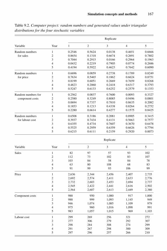
Simulation concepts and methods 167
Table 9.2. Computer project: random numbers and generated values under triangulardistributions for the four stochastic variables
Replicate
Variable Year 1 2 3 4 5
Random numbers 1 0.2546 0.5624 0.0138 0.4651 0.6666for sales 2 0.8654 0.1318 0.6674 0.2691 0.7802
3 0.7044 0.2915 0.0166 0.2964 0.19634 0.0432 0.2219 0.7905 0.0774 0.26865 0.4194 0.5922 0.4623 0.7642 0.6090
Random numbers 1 0.6696 0.0859 0.2738 0.1789 0.8249for price 2 0.7634 0.5465 0.1862 0.6624 0.8751
3 0.8199 0.6051 0.2669 0.7659 0.82684 0.4823 0.2060 0.2418 0.6317 0.37935 0.5247 0.6133 0.6252 0.2579 0.1353
Random numbers for 1 0.2562 0.0837 0.7600 0.0093 0.3327component costs 2 0.2580 0.3249 0.8085 0.9496 0.0801
3 0.0694 0.7337 0.7810 0.8635 0.20824 0.1853 0.1213 0.4338 0.8264 0.27525 0.2280 0.6614 0.4277 0.1575 0.8425
Random numbers 1 0.6508 0.3186 0.2081 0.8905 0.3415for labour cost 2 0.3937 0.7434 0.4131 0.5663 0.7577
3 0.6355 0.4734 0.7607 0.3670 0.64784 0.5525 0.2959 0.6359 0.6626 0.77945 0.6215 0.6111 0.2159 0.2920 0.0073
Replicate
Variable Year 1 2 3 4 5
Sales 1 82 97 57 93 1022 112 73 102 83 1073 103 84 58 84 784 63 80 108 68 835 91 99 93 106 99
Price 1 2,636 2,344 2,456 2,407 2,7352 2,692 2,574 2,411 2,633 2,7763 2,732 2,603 2,453 2,694 2,7374 2,545 2,422 2,441 2,616 2,5025 2,564 2,607 2,613 2,449 2,380
Component costs 1 988 950 1,080 917 1,0002 988 999 1,093 1,145 9493 946 1,074 1,085 1,109 9794 975 960 1,016 1,098 9915 983 1,057 1,015 969 1,103
Labour cost 1 299 269 256 321 2722 277 306 279 292 3073 298 284 308 274 2994 291 267 298 300 3095 297 296 257 266 210

168 Capital Budgeting
Table 9.3. Computer project: annual net cash flows and NPVs for first five replicates
Net cash flow ($)
Year (EOY) Replicate 1 Replicate 2 Replicate 3 Replicate 4 Replicate 5
0 −50,000 −50,000 −50,000 −50,000 −50,0001 69,618 60,625 35,340 62,217 98,2262 103,824 56,137 54,978 57,768 109,1403 101,764 62,580 32,480 68,124 74,8024 49,077 55,600 67,716 48,824 58,2665 71,344 74,646 78,213 75,684 56,133
NPV($) 277,125 202,414 164,986 205,422 282,661
Table 9.4. Computer project: ordered NPVs and cumulative relative frequencies
NPV ($) 155,421 155,930 157,449 165,138 183,182 . . . 315,975 321,943 323,975Cum. rel. freq. 0.01 0.02 0.03 0.04 0.05 . . . 0.98 0.99 1
assumed to take place at the end of the relevant years. The NPV estimates range between$165,000 and $282,000. The random numbers, generated values for uncertain variables andNPV calculations for the full 100 replicates are provided in Workbook 9.1.
The cumulative relative frequency distribution
The relative frequencies of financial performance could be summarized in the form of ahistogram. However, it is more useful to express these in cumulative relative frequencies.The set of 100 NPVs has been sorted into ascending order. Table 9.4 presents some of theseNPV values; to save space these are reported for the lower and upper ends of the distributiononly. The lowest NPV is $155,421 and the highest is $323,975, indicating a wide range ofpossible payoff levels. Cumulative relative frequencies are also provided in the table, ob-tained simply by dividing the rank position by the total sample size (100).
The full cumulative relative frequency curve is shown in Figure 9.1. For any NPV valuealong the horizontal axis, the vertical axis indicates the estimated probability that the NPVwill be this value or less. The graph has end points with cumulative relative frequencies ofnear zero (0.01 to be precise) and 1.0, and provides estimates of the likelihood, or probability,that the project if implemented would yield NPVs of less than the various levels within therange $155,421 and $323,975.
The curve of Figure 9.1 may be viewed as an estimate of the cumulative (probability)density function (CDF) of the performance variable, here NPV. The term ‘estimate’ is usedbecause it is derived from sampling, not from a precise knowledge of the overall behaviourof NPV (the statistical concept of a ‘population’). However, in practice we may refer to the

Simulation concepts and methods 169
0.0
0.2
0.4
0.6
0.8
1.0
100,000 150,000 200,000 250,000 300,000 350,000
Net present value ($)
Cum
. rel
. fre
quen
cy
Figure 9.1. Cumulative relative frequency curve for NPV of computer project.
curve, if somewhat loosely in statistical terms, as the CDF. Note that the CDF is raggedrather than smooth in shape. The degree of smoothness is a function of sample size (numberof replicates). The larger this number the more smooth this curve will become. For example,a sample of size 5,000 could be taken. However, this would yield little if any additionalinformation to that provided in Figure 9.1.
The CDF curve provides us with a good deal of information about the likely financialperformance of the project. The estimated probability of various ranges of performancelevels can be read from this graph. For the computer investment project, it would appearthat a payoff of less than $200,000 is highly unlikely, with an estimated probability ofonly about 0.1. Also, because the probability of a payoff of less than $300,000 is about0.95, a payoff of more than $300,000 is extremely unlikely (estimated as 1−0.95 or 0.05).The median payoff (middle of the distribution or probability of 0.5) appears to be about$240,000. In fact, it can be found from the spreadsheet that the median NPV (the averageof the 50th and 51st values of the ordered set) is about $238,500. The symmetrical shape ofthe CDF (i.e. similar slopes at the lower and upper ends) suggests the mean payoff will besimilar to the median value; the mean as computed from the spreadsheet is, in fact, $239,141.
Determining whether a project is financially acceptable
In discounted cash flow analysis as presented in earlier chapters, the output of the analysis isa single, or point, estimate of one or more performance criteria, e.g. the NPV or IRR of theproject. It is then a simple task to say, for example, the NPV is positive at the chosen discountrate or the IRR exceeds the required rate of return so the project is financially acceptable.While risk analysis provides information about the overall distribution of project payoffto the decision-maker, this makes the assessment of project acceptability somewhat moredifficult, precisely because of the greater amount of information to assimilate. Risk analysishas sometimes been criticized for this reason. The decision-maker obviously cannot take inall of the, say, 100 point estimates of project performance. The expected (i.e. average) or

170 Capital Budgeting
median NPV could be provided (and will usually be printed as part of the computer outputanyway), but reverting to a point estimate undermines the very purpose of risk analysis. Sowhat is management likely to glean from the CDF? In practice, the decision-maker mayhave some reference points in mind, and may be interested for example in the estimatedprobability of making a loss (NPV negative), or of making less than a notionally acceptablepayoff (say $200,000 or more) or of making a very high payoff (say $300,000 or more).
Comparing alternative projects
While risk analysis is typically used to determine whether a single project is financiallyviable, the approach can of course be applied to two or more competing projects or twoor more alternative ways of carrying out the same project. When using point estimates of,say, NPV, it is a relatively simple matter to compare the payoffs of alternative investmentoptions. Comparing overall CDFs can be more difficult. When the CDFs of two projects areplotted on the same graph, if the CDF of one is entirely to the right of another, then it can besaid that the former project has superior financial performance over the entire probabilityrange. But if the CDFs cross over it becomes more difficult to make a judgement betweenthe projects. A technique known as stochastic dominance analysis (not discussed here) willin some cases allow one project to be judged as superior to another when the CDFs cross.
Independent versus correlated sampling of cash flow variables
In the above risk analysis, the cash flow variables have been sampled independently, i.e. noallowance has been made for correlations in their levels, in the same time period. In practice,it is likely that some cash flow variables will be positively correlated, for example pricelevels of inputs and outputs. Also, some may be negatively correlated, for example the pricecharged for the PCs and the number sold. Further, the levels of individual random variablesare likely to be correlated between years within the planning horizon. For example, if thelabour cost is higher than the median level of the estimated distribution in year 1, then itwould tend to be higher than the median level in year 2.
Methods of generation of correlated random variates are available, so that if the ana-lyst can estimate the degree of association between cash flow variables then this can bebuilt into the analysis. Some software packages for risk analysis allow correlations to bespecified between cash flow variables, e.g. @RISK. In general, if cash flow variables arepositively correlated then overall project performance variability will be increased; if theyare negatively correlated then it will be decreased. However, this pattern will be influencedby which cash flow variables are correlated with which others. For example, if cash inflowand cash outflow variables were negative correlated, this would lead to increased variabilityin overall financial performance.
Software packages available
Various software packages have been developed for risk analysis. For example, the pack-ages @RISK and Insight have been designed as add-on software for spreadsheet programsincluding Excel. Some risk analysis packages are relatively expensive, and often it is

Simulation concepts and methods 171
possible to perform risk analysis simply using the facilities of the spreadsheet program(as in the example presented here).
Design and development of a more complex simulation model
A more complex example of simulation modelling is now presented to illustrate some ofthe more advanced features of simulation methodology. This example initially involvesa multi-period deterministic financial model of an airline investment. The model is thenextended to a stochastic format, and the nature of simulation experiments is illustrated.
Example 9.2. FlyByNight project
The FlyByNight airline company is planning to introduce a new country run, to providetwo return services a week (104 per year) to a rural city with a population of 30,000 persons.This project is named FlyByNight. The airline will use a forty-passenger aircraft, whichit can purchase for $4.5M. An airstrip owned by the local government in the rural area isavailable without charge, but the company will have to carry out restoration of the disusedairstrip and terminal at a cost of $200,000. A financial model is to be developed to simulatethe cash inflows and outflows from this venture over a ten-year period, and to provide anestimate of the net present value of the investment.
Other relevant information for model development includes:
� Passenger demand: This is predicted to be initially 5,000 passengers per year (in one-wayflights), increasing at the rate of 300 per year.
� Mail service revenue: In addition to passenger services, the company has a contract totransport mail to the rural city for a fixed annual payment of $200,000.
� Annual fixed costs: The annual cost of the air crew is $200,000 and that of ground staff is$50,000. The annual maintenance cost for the aircraft is 7% of the initial price.
� Fuel cost: Aviation fuel costs $800 per flight, plus $10 per passenger.� Handling cost: The cost of booking and other services is $15 per passenger flight.� Air fares: A charge of $280 is made for each one-way flight ($560 return).� Company tax is 30% of the annual operating surplus; the aircraft and ground facilities
can be depreciated at a rate of 10% per annum for taxation purposes.� After ten years, the aircraft has a salvage value of $1M.� The appropriate discount rate is 8%.
Development of the FlyByNight basic simulation model
Given the above information, a model may be set up which predicts the cash surplus eachyear t:
NPV = � ASt/(1 + r )t , t = 0 to 10
ASt = ARt − COt − ACt − TAXt
ARt = NPASt × FAREt + MAILt
ACt = MAINTt + STAFFt + FUELt + HANDt + ADVt

172 Capital Budgeting
NPASt = 5000 + 300 t
TYt = ARt − ACt − DEPNt + SALVt
TAXt = ARTt × TYt
where:
ASt = annual net cash flowARt = annual revenue from passenger and mail servicesCOt = capital outlayACt = annual costs
TAXt = annual company tax payable less tax benefit arising from deprecia-tion allowances, in relation to this investment.
FAREt = fare per passenger per flightMAILt = annual revenue from mail servicesNFLTt = number of one-way flights per yearNPASt = number of passengers per year
MAINTt = annual maintenance expenditure on the aircraft (purchase price ×maintenance rate)
STAFFt = annual wage bill (air crew and ground staff wages)FUELt = annual expenditure on aircraft fuel (fixed component × no. of
flights + variable component × number of passengers)HANDt = annual passenger handling cost (number of passengers × handling
cost per passenger)ADVt = annual advertising cost (zero in the initial model)
DEPNt = annual depreciation allowance (capital invested × depreciation rate)SALVt = end-of-project salvage value on capital outlays (fully taxable)
TYt = annual taxable incomeARTt = average rate of tax
r = annual real rate of interestt = time in years.
The model has been implemented on the computer as an Excel spreadsheet.
Workbook9.2
Structure of the FlyByNight basic model
In terms of the earlier discussion of elements of a model, it may be noted:
� Aircraft costs, passenger numbers, taxation etc. could be treated as separate componentsof the model, or modules of the computer implementation. In this case, the model isrelatively simple so it is not necessary to break it down into components.
� The performance or response variable is NPV.

Simulation concepts and methods 173
Table 9.5. FlyByNight: parameters of the basic model
Cost of aircraft $4,500,000Restoration of airstrip and terminal $200,000Seating capacity 40Number of one-way flights per year 208Initial passenger number 5,000Annual increase in passengers 300Mail service revenue per year $200,000Annual aircraft maintenance cost (% of cost) 7%Air crew cost per year $200,000Ground staff cost per year $50,000Fuel cost, fixed per flight $800Fuel cost, variable per passenger carried $10Handling cost per passenger $15Air fare (per passenger per flight) $280Income tax rate 30%Aircraft salvage value at year 10 $1,000,000Required rate of return (per annum) 8%
� Examples of identities, which are true by definition, include the definitions of annualsurplus and annual project revenue (taxable income):
ASt = ARt − COt − ACt − TAXt
TYt = ARt − ACt −DEPNt + SALVt
� An example of an operating characteristic is the equation for predicting passengernumbers:
NPASt = 5000 + 300 t
� Various parameters are present in the model, as summarized in Table 9.5. These are listedat the top of the spreadsheet, making the assumptions clear to the viewer and making forease of adjustment of parameters in sensitivity analysis.
� Values of various endogenous variables are generated in the simulation experiment.� The fare per flight is a controllable exogenous, or decision, variable, but has been set at
a fixed level ($280).� The model as formulated here has no non-controllable exogenous, or environmental,
variables.
Testing the FlyByNight basic simulation model
Before using a model such as this to derive quantitative decision support information, sometesting would be highly desirable. In this context the model would first be verified bytesting that it had been programmed correctly on the computer, which means checking thatthe logic and formulae in the spreadsheet conform with the model design. For this model,which involves only a few equations, verification is a relatively simple task.

Tabl
e9.
6.F
lyB
yNig
ht:
outp
utfr
omth
eba
sic
mod
elsi
mul
atio
nru
n(a
llca
shflo
ws
indo
llar
s)
Yea
r(e
ndin
g)0
12
34
56
78
910
Cap
ital
outl
ays
Initi
alou
tlay
4,70
0,00
0Sa
lvag
eva
lue
1,00
0,00
0
Pro
ject
reve
nue
Num
ber
ofpa
ssen
gers
5,00
05,
300
5,60
05,
900
6,20
06,
500
6,80
07,
100
7,40
07,
700
Fare
reve
nue
1,40
0,00
01,
484,
000
1,56
8,00
01,
652,
000
1,73
6,00
01,
820,
000
1,90
4,00
01,
988,
000
2,07
2,00
02,
156,
000
+M
ailr
even
ue20
0,00
020
0,00
020
0,00
020
0,00
020
0,00
020
0,00
020
0,00
020
0,00
020
0,00
020
0,00
0=
Tota
lrev
enue
1,60
0,00
01,
684,
000
1,76
8,00
01,
852,
000
1,93
6,00
02,
020,
000
2,10
4,00
02,
188,
000
2,27
2,00
02,
356,
000
Ope
rati
ngco
sts
Air
craf
tmai
nten
ance
315,
000
315,
000
315,
000
315,
000
315,
000
315,
000
315,
000
315,
000
315,
000
315,
000
+A
ircr
ewco
st20
0,00
020
0,00
020
0,00
020
0,00
020
0,00
020
0,00
020
0,00
020
0,00
020
0,00
020
0,00
0+
Gro
und
staf
fco
st50
,000
50,0
0050
,000
50,0
0050
,000
50,0
0050
,000
50,0
0050
,000
50,0
00+
Fuel
cost
216,
400
219,
400
222,
400
225,
400
228,
400
231,
400
234,
400
237,
400
240,
400
243,
400
+H
andl
ing
cost
75,0
0079
,500
84,0
0088
,500
93,0
0097
,500
102,
000
106,
500
111,
000
115,
500
+A
dver
tisin
gco
st0
00
00
00
00
0=
Tota
lcos
ts85
6,40
086
3,90
087
1,40
087
8,90
088
6,40
089
3,90
090
1,40
090
8,90
091
6,40
092
3,90
0
Tax
calc
ulat
ions
Net
oper
atin
gre
venu
e74
3,60
082
0,10
089
6,60
097
3,10
01,
049,
600
1,12
6,10
01,
202,
600
1,27
9,10
01,
355,
600
1,43
2,10
0−
Dep
reci
atio
n47
0,00
047
0,00
047
0,00
047
0,00
047
0,00
047
0,00
047
0,00
047
0,00
047
0,00
047
0,00
0=
Not
iona
ltax
able
273,
600
350,
100
426,
600
503,
100
579,
600
656,
100
732,
600
809,
100
885,
600
962,
100
inco
me
+Sa
lvag
eva
lue
tax
1,00
0,00
0ad
just
men
t=
Tota
ltax
able
inco
me
273,
600
350,
100
426,
600
503,
100
579,
600
656,
100
732,
600
809,
100
885,
600
1,96
2,10
0Ta
xpa
yabl
e82
,080
105,
030
127,
980
150,
930
173,
880
196,
830
219,
780
242,
730
265,
680
588,
630
Net
cash
flow
−4,7
00,0
0066
1,52
071
5,07
076
8,62
082
2,17
087
5,72
092
9,27
098
2,82
01,
036,
370
1,08
9,92
01,
843,
470
NPV
=1,
454,
148

Simulation concepts and methods 175
Second, the model would be validated by checking whether the overall behaviour of themodel corresponds with that which would take place in the real system (i.e. the airline). Inother words, the validity of the structure and relationships in the model – such as the traveldemand function – would be checked. This might involve examining the costs, demand andsales receipts experience of previous airline operators on this run, or those of other airlineswith similar characteristics. If possible, data used for model validation should exclude thatused in constructing the model. If the purpose of the model is to compare managementpolicies, then checking of the ranking of policies is more important than checking theability to predict NPV accurately.
Once the model had been validated as far as possible, sensitivity analysis would be used todetermine what effects inaccuracies in parameter estimates would have on NPV estimatesfrom the model, and on the ranking of management policies (experimental treatments)compared in the simulation experiments. Sensitivity analysis will indicate which parameterswarrant further estimation efforts.
Workbook9.2
Since the model is implemented on a spreadsheet (Workbook 9.2) the simulation isperformed automatically when the formulae in the spreadsheet are executed to generate thecell values. Running this model on the computer may be thought of as simulating passengernumbers and hence financial performance over the ten-year planning horizon. Output fromthis model is presented as Table 9.6. The lower part of the table presents the annual cashflow estimates. The NPV function of the spreadsheet is used to derive net present value forthe investment in the final line of output.
Deterministic simulation of financial performance
Simulation has been defined as modelling and performing experiments with the model (on acomputer). In this example, it may seem odd to describe estimation of project performanceby simply evaluating each of the spreadsheet formulae as an ‘experiment’. Only one set ofvalues is used for the variables, and this is in fact a standard NPV calculation. However, withminor modification, the financial model may be used to carry out more complex experimentsso as to improve the understanding by management about the behaviour of the system whichis being modelled.
Example 9.3. FlyByNight deterministic model
Suppose that the airline wishes to increase seat sales, and has identified two methods bywhich this can be achieved, viz. advertising or price discounting. Research indicates that:
(1) the number of passengers in any year, NPASt , is related to the advertising expenditurein that year (x1, in thousands of dollars) by the quadratic function with linear coefficient50 and quadratic coefficient −1.4;

176 Capital Budgeting
Table 9.7. FlyByNight: NPV levels from the deterministic simulation ($M )
Annual expenditure on advertising ($)
0 8,000 16,000 24,000
Price discount ($/flight) 0 1.45 1.79 1.91 1.8120 1.94 2.19 2.27 2.1940 2.02 2.15 2.17 2.1160 1.65 1.66 1.62 1.58
(2) the number of passengers in any year increases linearly by 500 for each $10 decreasein fare (x2).
This information has been built into the operating characteristics for passenger numbers:
NPASt = (5000 + 300 t) + 50 x1 − 1.4 x 21 + 500 x2
where x1 is expenditure on advertising in thousands of dollars and x2 is the price discountin $10 steps. In addition, there is a capacity constraint that NPASt ≤ 8,320 (208 flights of 40passengers). For simplicity, it has been assumed that any advertising or discounting policywill be employed throughout the whole ten-year period. (Allowing these to vary each yearwould lead to a very large number of decision variables.) Flight operations over ten yearshave been simulated for the following promotion policies: advertising expenditures of 0,$8,000, $16,000 and $24,000; price discounting of 0, $20, $40 and $60.
Workbook9.3
Note that each advertising level is to be combined with each price discount level. Anycombination of levels of each variable may be thought of as a treatment in the simulationexperiment; the simulation experiment therefore involves 4 × 4, or 16, treatments. In Excel,the Data Table function is used to evaluate these combinations of factor levels, producing theNPV levels shown in Table 9.7. The spreadsheet employed to produce this table, indicatingall of the calculations involved, is provided as Workbook 9.3. Details of how to use theData Table function are provided in the Excel Help files. (Advertising is treated as therow variable and price discount as the column variable, and a table frame with selectedtreatments or combinations of levels of these is set up before the Data Table function isused.)
The figures in the body of Table 9.7 may be thought of as points on an NPV responsesurface in two dimensions. It is apparent that NPV – which was $1.45M in Table 9.6 – canbe increased considerably by the promotion activities. The optimal levels of the decisionvariables can be read off as approximately x1 = $16,000 and x2 = $20, i.e. spend $16,000annually on advertising the airline and discount fares by $20 per flight. This informationwould be conveyed to management.

Simulation concepts and methods 177
Stochastic simulation of financial performance
The above examples relied on a deterministic simulation model. In practice, simulationmodels are often stochastic in nature, i.e. they include random variates, the values of whichare obtained through some random variate generator; this is sometimes referred to as MonteCarlo sampling. The use of such models is referred to as stochastic simulation or MonteCarlo simulation.
Example 9.4. FlyByNight stochastic simulation
Suppose that the number of passengers – the main source of uncertainty for the airline – canbe represented by the demand function of Example 9.3, but with the addition of a randomcomponent, y:
NPASt = (5000 + 300 t) + 50 x1 − 1.4 x 21 + 500 x2 + y
where this random component has a normal distribution with a mean of 0 and standarddeviation of 500 passengers. The financial model may now be used to conduct a simulationexperiment in which the demand function includes this non-controllable environmentalvariable. Every time the program is run on the computer (each encounter with the model)a different set of demand levels is generated, and hence a different NPV obtained. For thisreason, it is necessary to include in the simulation experiment a number of replicates andto average NPV performance over these replicates, if we are to gain a sound comparison oftreatments or sales promotion policies.
A method of generating normal random variables is explained in the appendix to thischapter. Random variates from the N(0,500) distribution of this example are obtained as
y = (�12ri − 6
) × 500
where the twelve ri values are observations from a uniform distribution with range 0 to 1(i.e. the spreadsheet random number generator).
Workbook9.4
A simulation experiment is performed with the same sixteen treatments as above, andwith four replicates, and NPV estimates are reported in Table 9.8. The spreadsheet usedto produce Table 9.8 is provided as Workbook 9.4. For this experiment, the levels of therandom demand variable have been obtained using the above procedure for generatingnormal variates and the random number generator of the spreadsheet package. The set ofrandom numbers to generate annual demand for air flights for one of the encounters withthe model is indicated in this workbook. An alternative approach to generating randomvariates is to use purpose-built risk analysis software, such as the @RISK add-on packagefor Excel.

178 Capital Budgeting
Table 9.8. FlyByNight: NPV estimates for individual replicates and meanof replicates ($M )
Annual expenditure on advertising ($)
Rep. 1 0 8,000 16,000 24,0000 1.55 1.50 1.79 1.90
Price discount ($/flight) 20 1.61 2.29 1.93 2.2440 1.86 2.15 2.24 2.2060 1.59 1.64 1.61 1.52
Rep. 2 0 8,000 16,000 24,0000 1.08 1.54 1.63 1.93
20 1.85 2.08 2.23 2.2240 1.97 1.90 2.19 1.9860 1.51 1.62 1.60 1.58
Rep. 3 0 8,000 16,000 24,0000 1.81 1.64 1.90 2.09
20 2.05 1.97 2.34 2.1640 2.18 2.16 2.25 2.0060 1.63 1.62 1.58 1.49
Rep. 4 0 8,000 16,000 24,0000 1.27 1.54 1.97 1.82
20 2.09 2.00 1.87 1.9440 1.86 2.06 1.98 2.0260 1.61 1.66 1.59 1.48
Means 0 8,000 16,000 24,0000 1.43 1.55 1.82 1.93
20 1.90 2.08 2.09 2.1440 1.97 2.07 2.16 2.0560 1.58 1.63 1.59 1.52
It is notable that there is considerable variation in performance among replicates. Forexample, NPV is highest for advertising expenditure of $16,000 a year in replicates 2 and 3but for expenditure of only $8,000 in replicates 1 and 4. Averaging the NPV values over thefour replicates removes some of the variation between treatments found when individualreplicates are compared. The NPV values for the highest fare discount rate exhibit littlevariation, because the capacity constraint is reached early in the project life. The fact thatthe optimal policy is to spend $8,000 to $16,000 a year on advertising and to discount pricesby $20 to $40 would be conveyed to management. But as well, some information could beconveyed on the extent to which the NPV for a particular policy varies among replicates,and the extent to which the optimal policy varies among replicates.

Simulation concepts and methods 179
Choice of experimental design
In the simulation experiment producing the response data of Table 9.8, each level of each ex-perimental factor (decision variable) was combined with each level of the other experimentalfactor, giving rise to what is known as a full factorial design. There are four replicates inthis experiment, hence 4 × 4 × 4, or 64, encounters with the model are required. If there is agreater number of decision variables, the number of treatments can become unmanageable.For example, if there are six factors, each at four levels, and four replicates, then the num-ber of encounters with the model is 47, or over 16,000. In such cases, it may be necessaryto resort to alternative experimental designs to reduce the overall number of treatmentsand associated computer time and amount of computer output. Alternative types of designinclude:
� Incomplete factorial designs: here some of the combinations of factor levels are omittedso as to reduce computing time.
� Optimum-seeking designs: in these designs, the factor levels are decided within the com-puter run (simulation experiment) rather than prior to it. As each treatment is evaluated,the response level is compared with that of previous treatments, and the next treatment isstrategically placed so as to seek a higher NPV performance level. In this way, it is oftenpossible to identify near optimal management policies with a relatively small number oftreatments.
Advantages and disadvantages of simulation compared with other techniquesin capital budgeting
In the sense that simulation is both a project evaluation and project planning tool, it maybe compared with other approaches in both these areas. Various methods of incorporat-ing risk in project evaluation models were discussed in earlier chapters, including therisk-adjusted discount rate, the certainty equivalent, and sensitivity and break-even analy-sis. Risk analysis, or risk simulation, is an alternative to these approaches which providesmore information to the decision-maker. For example, compared to sensitivity analysis notonly is the range of possible outcomes indicated, but also probabilities are attached to theseranges. Further, the variables are allowed to vary simultaneously, to yield a probabilitydistribution of overall project performance. In this sense, a more comprehensive measureof risk is obtained. From the CDF, the decision-maker can gain an idea of the overall rangeover which project financial performance is likely to vary, and can read off probabilityestimates for various sub-ranges of project performance.
On the other hand, more information is required to carry out risk analysis, and the com-puter modelling can be more demanding (though availability of spreadsheet add-on softwarefor risk analysis tends to overcome this problem). As mentioned above, interpretation ofthe computer output becomes more complex, and this may be a drawback for managerswho are not familiar with this form of information. Perhaps a more serious concern is thatof the additional effort estimating correlations between cash flow variables over time. In

180 Capital Budgeting
cases when these are high, this additional effort may be worthwhile to provide an improvedpicture of project risk.
As a project planning tool, simulation may be compared with other planning and re-source allocation techniques, for example linear programming. Since this technique is notdiscussed until Chapters 11 and 12, little can be said about the comparison at this stage.Experience indicates that simulation has the advantage of providing much greater flexibilityin modelling, in terms of being able to represent complex systems in a realistic way. Thedisadvantage is that often much greater model development and testing effort is required.
Concluding comments
This chapter has introduced some of the concepts and methods of the technique of computersimulation, as it is applied to capital budgeting decisions. Computer simulation relies on atotal systems philosophy, which asserts that components of a system should not be viewedin isolation but rather in terms of the complex interrelationships and interactions amongvariables. An attempt is made to analyse carefully all the components of the system andtheir interrelationships, and to represent these in a simplified and abstract model. This modelis used to conduct experiments in which the behaviour of the system is simulated undervarious assumptions or management policies.
This is a highly flexible technique, where the analyst has the ability to develop a complexmodel, using a spreadsheet package or computer programming language, and to use thismodel to mimic the behaviour of a real system over time. With the flexibility comes therequirement for testing of the model to ensure it is a realistic representation of the realsystem. In general, adopting the ‘systems philosophy’ tends to impose greater discipline onmodel development and testing.
While many simulation models are deterministic in nature, including random variatesto represent the major sources of uncertainty in project performance generates additionalinformation for the decision-maker concerning the level of uncertainty of project perfor-mance. Risk or venture analysis is sometimes used when probability distributions can beattached to the variables governing cash flows for a prospective investment. Simulationexperiments with a stochastic model superimpose decision variables on this risk analysis,so that project planning as well as evaluation becomes possible.
Review questions
9.1 Explain the basic steps in risk analysis or Monte Carlo simulation.9.2 Suppose the number of customers at a proposed restaurant is expected to follow a
triangular distribution with pessimistic, modal and optimistic levels of 40, 60 and 100,respectively, on weeknights and 60, 90 and 140, respectively, on weekends. Usingthe random number generator on your computer spreadsheet, generate a sample ofcustomer numbers for a two-week period.
9.3 Is risk analysis a complement or an alternative to sensitivity analysis? Discuss.9.4 Consider the Delta Project example of Chapter 2. Suppose probability distributions have
been estimated in terms of pessimistic, modal and optimistic values as in Table 8.2 of

Simulation concepts and methods 181
Chapter 8. Develop a simulation model to derive a cumulative relative frequency curvefor this project.
9.5 Develop a simulation model in an area in which you are familiar, along similar linesto that of Example 9.2. Incorporate two or more decision variables in this model, andconduct a deterministic experiment to identify the optimal management policy. Explainhow this model could be made into a stochastic simulation model.
Appendix: Generation of random variates
A critical step in any stochastic simulation model is to generate values of random (stochastic)variables or ‘variates’. In Example 9.1, annual demand was recognized as a random variable,and values were obtained by sampling from the demand distribution using random numbers.In simulation practice, variables are frequently recognized as stochastic. It has been saidthat a refinement in modelling introduces a need for stochasticity. A wide variety of formsof probability distributions have been recognized as reflecting the behaviour of particularrandom variables. Three examples will be presented here.
The starting point for producing (or ‘generating’ or ‘sampling’) values from any form ofprobability distribution is to use a random number from a known distribution. In practice,this is usually a number from a uniform distribution over the range 0 to 1, as illustratedbelow. ‘Uniform’ implies that the probabilities over the range are equal. Since the areaunder a probability function must be unity, the height of this curve is also 1. When a randomnumber generator is called in a computer spreadsheet or programming language (e.g. usingthe statement ‘= rand()’ in Excel) a number from this distribution is obtained. The procedureused on the computer is typically to divide a very large number by another large number, andto take the remainder as a fraction of the divisor (hence yielding a number between 0 and 1).As well, the remainder is multiplied by a third large number, and the product divided by theoriginal divisor. By repeating this process, a series of random numbers can be generated.The numbers are sometimes called ‘pseudo-random’ because given the same three largenumbers (and the same computer accuracy), the same series will always be produced.
0 1
1
Generating uniform variates over a specified range
Perhaps the simplest form of continuous probability distribution used in simulation modelsis the uniform distribution, as illustrated in the following diagram. Here a is the smallestvalue and b the largest value that the variable is expected to take. Since the area under a

182 Capital Budgeting
Table 9A.1. Probability distribution of number of tickets sold
Number of tickets sold 3,000 4,000 5,000 6,000Probability 0.2 0.3 0.3 0.2
probability function must be unity, and the range of values of the variable is b − a, theheight of the curve must be 1/(b − a).
a b
1/(b − a)
A value y from a uniform distribution can be generated by taking a random number r andapplying the expression:
y = a + r (b − a)
i.e. the lower limit plus the random number times the distance between the upper and lowernumbers. To obtain a series of values on the random variable, simply repeat this process anumber of times (on your computer).
Generating values from an empirical probability distribution(discrete probability table)
Suppose it has been found from experience that a random variable (say airline ticket sales)can be described by the distribution shown in Table 9A.1.
This distribution may be converted into cumulative form, and random numbers attachedto demand levels, as shown in Table 9A.2.
It is now a relatively simple task to obtain a series of random numbers in the range 0 to1, and to use these to ‘look up’ demand levels. Suppose the sequence of random numbers0.2765, 0.8346, 0.1207, 0.4533 and so on has been obtained. The first of these numbersfalls in the range 0.2 to 0.4999, hence demand of 4,000 seats is generated. The secondrandom number falls in the range 0.8 to 0.9999, corresponding to a demand of 6,000 seats.Proceeding in this way, a random series of demand levels is generated, in which the relativefrequency in each demand class will approximate the estimated probability.

Simulation concepts and methods 183
Table 9A.2. Cumulative probability distribution of numberof tickets sold, and ranges of random numbers
Demand level Probability of this demand Range of random(tickets sold) level or greater number
3,000 0.2 0.0–0.19994,000 0.2 + 0.3 = 0.5 0.2–0.49995,000 0.2 + 0.3 + 0.3 = 0.8 0.5–0.79996,000 0.2 + 0.3 + 0.3 + 0.2 = 1.0 0.8–0.9999
Generating normal variates
The normal distribution is widely recognized in statistical methods as a commonly occurringor approximated distribution. Further, many distributions can be converted to approximatelynormal distributions by applying a suitable transformation, e.g. by taking of logarithms orsquare roots.
There are several methods for generating normal random variates (values from a normaldistribution). The simplest is to take the sum of 12 random values from a uniform 0–1distribution (e.g. a computer random number generator), subtract six, then multiply by thetarget standard deviation (500) and add the target mean (0), i.e. to derive:
y = (�12 ri − 6
)500,
where the twelve ri values are observations from a uniform distribution with range 0 to 1(e.g. from a spreadsheet random number generator). Since the expected value of a singleuniform 0–1 random number is 0.5, the expected sum is 6, hence (�12 ri − 6) has anexpected value of 0. Further, it can be shown that the variance of a single uniform 0–1number is 1/12, hence the sum of twelve independent numbers from this distribution has avariance of 1.0 (and this is unaffected by subtracting 6). The sum of twelve numbers fromthe same distribution will approach a normal distribution, especially if the distribution is notheavily skewed – this follows from the Central Limit Theorem. It follows that (�12 ri − 6)is approximately a standard normal or N(0, 1) variable.
Any normal variable can be converted to a standard normal variable by subtracting themean and dividing by the standard deviation. Conversely, a standard normal variate z canbe converted to a value from a target normal distribution by multiplying by the standarddeviation and adding the mean. That is, if y is a normal variable, and z = (y−µ)/σ , theny = zσ +µ must be a normal variate from the target distribution.
Generating values from a triangular distribution
The triangular distribution is popular since it is often easy for people to make estimates ofthe most pessimistic, most likely (modal) and most optimistic values of a random variable.

184 Capital Budgeting
For any variable, these values (denoted a, b and c, respectively) can be used to define atriangular distribution as in the following diagram.
a b c
If a distance parameter d is defined as d = (b − a)/(c − a), then, using a random numberr, a value from this distribution y can be generated by applying the formulae:
For r ≤ d y = a +√
r (c − a)(b − a)
For r > d y = c −√
(1 − r )(c − a)(c − b)

10 Case study in financialmodelling and simulationof a forestry investment
Forestry projects are a form of capital investment with a particularly long time horizon,and as such present an interesting case of capital budgeting. In many countries, plantationforestry has traditionally been the domain of government agencies, e.g. the national ForestryCommission in the UK and the various state forestry services in Australia. Timber wasconsidered to be a critical economic resource but the long production period meant that onlygovernments had the long-term perspective and capacity to enter into forestry investments.This situation has changed markedly in the past fifty years, with probably the bulk of forestryinvestment in most countries being undertaken by private companies and individuals. Theneed for the establishment of plantations has been stimulated by decreasing supplies oftimber from native forests through unsustainable logging practices, and the withdrawal oflarge areas from logging because of their being set aside as protected areas, particularly intropical counties.
An integral component of investment in forestry is the need for financial informationabout the likely cash flows associated with the establishment, management and finalharvest of a plantation. This chapter uses the development of a financial model forforestry investment as a case study of financial modelling. The financial evaluationof forestry projects poses many challenges and this chapter examines the key parametersfor forestry appraisal and some of the problems faced by developers of financial models.The development of a model for the evaluation of forestry projects is outlined, followingthe step-by-step approach which was actually used by the model developers. This basicmodel framework is then used to illustrate how to undertake a sensitivity analysis and risksimulation.
Study objectives
After studying this chapter the reader should be able to:
� appreciate the need for estimates of forestry returns� identify the problems encountered in developing a forestry financial model� appreciate the difficulty in establishing cash flow estimates for long-lived forestry projects� discuss the methods of allowing for risk in the evaluation of forestry projects
185

186 Capital Budgeting
� develop a simple forestry model� apply sensitivity and risk simulation to forestry projects.
Key parameters for forestry models
The most common cash outflows associated with forestry operations include establishmentcosts (e.g. land and site preparation such as clearing, fencing and preparing the soil; purchaseof planting stock; planting, mulching and watering), weed control, fertilization, pruningand thinning to waste, and commercial harvesting. The major cash inflows come fromthe sale of commercial thinnings and the final harvest, and perhaps tree residues such asfirewood. In some situations, revenues are also derived from non-wood forest products suchas wild berries, mushrooms, honey and hunted game, all of which are made possible by theenvironment created by the forest.
Cash flow estimates of growing native timbers as a business enterprise will vary dependingon a variety of factors, some of the more important of which are:
� Site characteristics (e.g. climate, soil, aspect)� Species mixture� Silvicultural system (e.g. planting density, weed control and pruning)� Harvest age and harvest scheduling� Final yield or mean annual increment of individual species� Interactions between species in mixed-species plantations� Stumpage price (affected by a number of supply and demand factors)� Costs (land preparation, planting and establishment, maintenance, harvesting)� Amount of government assistance� Harvest rights (buffer zones, harvest on steep land, roading permission)� Taxation regime (deductions allowable, treatment of harvest revenue)� Allowance for non-wood benefits� Discount rate
In principle, a spreadsheet could be devised which incorporates each of these factors. Onefactor that can have a major impact on eventual cash flows is timber yield from plantations.Yield is commonly expressed as ‘mean annual increment’ (MAI) which is the aggregatevolume of harvestable timber produced in a year from the growth of trees in a plantation. Itis usually expressed as cubic metres of timber produced per hectare per year. Other factors,such as site productivity, species mixture, harvest ages and timber prices (usually expressedas $ per cubic metre) may also strongly affect eventual cash flows.
As well as direct and measurable financial benefits, forests provide a variety of non-market services that are more difficult to quantify in terms of cash flows. These include:crop benefits (e.g. windbreaks, insect control); visual amenity, including wildlife viewing;environmental products and services (e.g. carbon sequestration, erosion control, wildlifehabitats, biodiversity); soil protection and stream bank stability; improvements in waterquality; and acting as a store of wealth for the owner. In some cases, forestry activities may

Financial modelling and simulation of a forestry investment 187
impose non-wood costs such as the opportunity cost associated with conversion of croplandto forest, increased fire risk for adjacent properties, and crop damage from feral or nativeanimals using the forest as a habitat. Non-wood benefits and costs may be private (i.e. borneby the company or individual) or social (public). Private non-wood benefits and costs arerelevant to the private capital budgeting process and investment decision and hence shouldbe included in a financial model for a forest company, though their estimation often presentsconsiderable difficulty.
In general, social (or public) non-wood benefits and costs are not included in forestryfinancial analysis. However, they are sometimes included in more extended economic anal-ysis, such as a governmental economic cost/benefit analysis. The importance of these non-market benefits is apparent when it is realized that trees are often grown to obtain thesebenefits with no intention of logging. Furthermore, in some cases the multiple uses of forestshave a direct impact on management or harvesting practices and need to be incorporated inthe financial analysis.
The choice of an appropriate discount rate is a contentious issue. For example, in Australia,the Queensland state forest agency (Department of Primary Industries), which is required tomake a commercial return on plantations under its control, currently uses a rate of 7% whenassessing their industrial softwood plantations. It is sometimes argued that a lower rate (suchas 3% or 4%) is more appropriate for assessing forestry activities, to allow for the importantnon-wood benefits produced by growing trees. Whilst some government initiatives can beinvestigated by adjusting the discount rate in this manner, discount rate adjustment as amethod of benefit incorporation is not usual in commercial projects generally. Forestryinvestments judged not viable at the commercial rate may become acceptable using alower rate. This is particularly important for forestry investments under consideration bygovernment, which must satisfy multiple objectives when establishing and managing forests.
Sources of variability in forestry investment performance
Plantation forestry is not a risk-free investment. A variety of factors contributes to theuncertainty in revenue generated. Most cash inflows from plantations occur with the finalharvest of trees when they reach maturity, although some additional cash inflows may begenerated from the sale of trees that are thinned as part of the normal management practices.Typically it is thirty or more years until plantations are ready for final harvest, hence long-term predictions of physical and financial performance have to be made. The main sourcesof variability in the financial performance of forestry are summarized in Table 10.1.
Most of the costs of establishing forestry are incurred in the first few years of plantationlife and are reasonably predictable. Contract rates for the various plantation operations aregenerally well known. The cost of land preparation can vary to some extent, depending onsite characteristics. Seedling costs should be known in advance, as well as initial fertilizercosts. Weed control practices and labour requirements can be predicted within a narrowrange. Should unusually dry weather be experienced after planting, there may be additionalcosts in watering and replanting lost trees.

188 Capital Budgeting
Table 10.1. Sources of risk in farm forestry
Risk category Major sources
Risk of poor establishment Dry weather, poor weed control
Production (timber yield) risk Storm or cycloneFirePest (insect, disease)Unsuitable species or mixture for the siteCollateral damage at harvest
Timber quality and product type risk Inappropriate pruning and thinning regimeInsect damageProduct type and fashion changes in demand
Sovereign risk Regulatory changes concerning machinery use and roadingChanges in taxation arrangementsUncertain harvest rights and compensation
Market risk Uncertain future timber prices
Plantation establishment success and growth rates are less predictable, particularly whenspecies are used for which only limited experience has been gained. Even with the best ofintentions, there is no guarantee that thinning and pruning will be carried out at optimaltimes. The type of product which will be produced is also uncertain: high-quality poles arelikely to be more profitable than sawlogs due to earlier harvest and favourable prices.
With mixed-species plantings and differing harvest ages for different species, there isa risk of damaging retained trees at the various harvest stages. This is overcome to someextent by planting whole rows of individual species, but even then it presents problems inthat growth within rows will not be uniform and it may be desired to retain some individualtrees. Helicopter or balloon lifting at harvest is highly expensive, but financially viable forhigh-value trees.
Sovereign risk relates to changes by government in the rules relating to farm forestry.Over the life of a plantation, it is probable that there will be numerous changes in taxationarrangements. Also, environmental regulations have a tendency to become more stringentover time, and these could increase management and harvesting costs or even lead to theoutlawing of harvest. The extent to which compensation will be provided for such limitationson property rights is quite unpredictable.
In general, these sources of risk do not pose a threat of total crop loss. Even with severestorm damage or fires, it is usually possible to salvage a considerable proportion of thetimber.
In summary, a variety of sources of risk arise with respect to timber quantity, qualityand price. Superimposed upon the various risk components, landholders often have lit-tle information about likely plantation performance and payoff. This is particularly thecase for species which have not been widely used in industrial forestry, and for whichlittle ‘growth curve’ data are available. In Australia, most industrial forestry relies on

Financial modelling and simulation of a forestry investment 189
exotic conifers, and there is little information available about growth rates of nativetree species, even though these species are increasingly being favoured by growers andmarkets. One native conifer species which is widely grown in plantations is hoop pine(Araucaria cunninghamii), but this is limited to favourable sites in terms of soil fertility andclimate.
Some opportunity exists to minimize these risks. While plantation insurance is not nor-mally taken out, the relatively non-perishable nature of the product allows harvesting tobe timed for when timber prices are relatively high. Also, forestry may be conducted as arisk-reducing business diversification, with harvesting when other income is low. In fact,forestry is sometimes viewed as a form of superannuation or savings, with harvest whenthere is a particular need for cash, say to assist in intergenerational property transfer or tobuy out the equity shares of siblings.
Methods of allowing for risk in the evaluation of forestry investments
It is typical of projects spanning a number of years into the future that costs and benefits(especially the latter) are estimated subject to a high degree of uncertainty. That is, thecash flow estimates are simply best-guess point values arising from (unknown) probabilitydistributions of random cost and benefit variables. This is certainly the case with forestryinvestments. Some of the methods used to deal with investment risk in forestry are nowoutlined.
Taking conservative benefit estimates. This is probably the simplest and most widely adoptedmethod of allowing for risk in forestry projects. However, benefits tend to be adjusted in arather arbitrary manner, and the approach provides little information to the decision-makerabout the extent of risk faced. The emphasis is on protection against ‘downside risk’, andno recognition is given to the possibility of payoffs above the single-point estimates. As aresult, projects which are financially sound could easily be rejected.
Requiring a short payback period. Sometimes projects are favoured because they lead torecovery of expenditure in a relatively short period. The payback period in forestry is usuallythe number of years from plantation development to clearfell (i.e. when all remaining maturetrees are harvested at the same time), since thinnings (even the later commercial thinnings)cannot be expected to recover plantation establishment costs. Favouring a short paybackperiod usually means adopting a short rotation system such as production of pulpwood fromeucalypts with harvest after about seven to ten years. A shortened payback period meansthat there is less uncertainty about whether a market will exist for the timber harvested and,associated with this, the stumpage price which will be achieved.
Including a risk margin in the discount rate. In Chapter 7 we discussed how the discountrate (k) has three components, i.e.:
k = r + u + a

190 Capital Budgeting
where r is the risk free rate, u is the average risk premium for the firm and a is an additionalrisk factor to account for the difference between the average risk faced by the firm and therisk of the proposed project.
Adjusting a to reflect the additional riskiness of forestry would result in an appropriatediscount rate commensurate with the risk of the investment project being considered.
Sensitivity analysis can be employed to measure the investment risk for forestry projects.Timber yield (progressively calculated through mean annual increment in total cubic metres)at a nominated harvest age and timber price are frequently subjected to sensitivity analysis.These parameters may be defined for a number of product lines from the same plantation, e.g.thinnings and final harvest, or poles, peelers (high-quality logs used to produce veneer) andsawlogs. It is also usual to test sensitivity with respect to the discount rate, or alternativelyto plot the NPV profile with respect to discount rate.
Risk or venture analysis. This is sometimes carried out (e.g. Harrison, Herbohn and Emtage,2001) to provide an overall estimate of project risk (this compares with sensitivity analysiswhich is usually designed to estimate risk with respect to one variable at a time). Riskanalysis provides an estimate of the probability that a plantation will be profitable (positiveNPV or required rate of return achieved), which can be particularly useful information fordecision-makers. Commonly, Monte Carlo simulations are used here.
Problems faced in developing forestry financial models
There are numerous problems that may be encountered in developing financial models forassessing forestry investments. These problems usually arise from the particular nature offorestry – a long investment period over which world timber prices are likely to fluctuate,combined with the multiple-use nature of forests and the interaction of forestry with otherventures in a diversified firm.
Forestry is a long-term activity. Typically it takes twenty to thirty years for pine plantationsto mature in temperate countries such as Australia and New Zealand. In Europe, rotations(the time taken from planting to final harvest of plantations) are typically fifty to eighty yearsfor pines and up to two hundred years for broad-leaf species such as English oak. At theopposite end of the scale are some fast-growing hardwoods that can be harvested after onlyeight to ten years in some tropical countries. The long investment period typical of forestryprojects provides a number of challenges when developing financial models. In particular,timber prices are likely to fluctuate over this period and it is difficult to predict the price thatwill be obtained for timber when it is harvested. The problems with forecasting timber pricesthus pose a challenge in estimating cash inflows as part of the financial modelling process.Timber prices may increase over time in real terms, i.e. the price increase may be greater thanthe rate of inflation. For example, an annual increase in the real price of timber of 1.3% hasbeen suggested (Russell et al., 1993). Furthermore, there is a risk that technological changeor fashion change could result in weak demand for some timber types (e.g. satellite

Financial modelling and simulation of a forestry investment 191
communications reducing demand for poles for phonelines, consumer preferences for woodcolour changing over time). Regulatory change in response to changing community attitudescould increase costs and restrict areas which can be harvested.
The long time required for trees to grow also means that there is sometimes a lack ofbiological growth data that can be used to predict growth rates (and hence timber yield).Timber yield and harvest timing are critical variables in forestry financial models. The lackof such data is most critical when new (non-traditional) species for which there is no pasthistory of cultivation are being used in plantations. As seen in Chapter 4, the Delphi andother group forecasting methods can be used to develop estimates of growth and harvestages which can be used in financial models.
The multiple-use nature of forests has also been recognized in the management of largeindustrial and government plantation estates. These management practices can have directimpact on the financial performance of the investment and thus should be considered in theappraisal process. For example in Finland, when a plantation estate is harvested, a numberof habitat trees must be retained. The failure to harvest these trees directly reduces cashinflows to the investor. Similarly in the United Kingdom, there is recognition that nativeScots pine and native broad-leaf species provide greater non-timber benefits than the exoticSitka spruce. The result has been the harvesting of Sitka spruce plantations earlier than theiroptimal rotation age and their subsequent replacement with plantations of Scots pine andbroad-leaf species. In many countries there are also large incentives provided to establishplantations, ranging from tax benefits to direct cash payments. Where they exist, these alsoneed to be incorporated in the appraisal.
As with any appraisal of a capital project, it is necessary to gain an understanding ofthe social environment in which the project is being undertaken. In the case of a forestryinvestment, the way in which a forest is managed, and the ultimate quantity of timber whichcan be harvested, can be greatly affected by the increasing need for forests to be managedfor multiple uses.
Developing a financial model: a step-by-step approach
As with any project appraisal, undertaking a financial analysis of a forestry project can bebroken down into a number of individual and relatively simple steps:
(1) Identify the forestry system to be adopted – for example, the type of trees to be plantedand at what density, when they will be pruned, the types of product intended (e.g.sawlogs, veneer logs, pulpwood, poles, or some combination of these) and when har-vesting is likely to occur.
(2) Estimate the likely cash outflows.(3) Estimate the cash inflows from harvest.(4) Develop the financial model and estimate financial performance measures.(5) Evaluate investment risk.
These steps will now be illustrated with respect to a case study.

192 Capital Budgeting
Example 10.1. Flores Venture Capital Ltd forestry project
Example 10.1 (see Box 1 for the relevant background) will be used as a case study toillustrate the development of a financial model to assess investment in establishment of alarge plantation estate.
Box 1. Background to the case study forestry project
Flores Venture Capital Ltd (FVC Ltd) is considering diversifying its operations intoforestry. It has been presented with a proposal involving the establishment of a plan-tation estate of 1,000 ha in an area with suitably high rainfall and soil quality. Toencourage investment in the region, a local government has offered the required landrent-free for the period of the project on the condition that native species are usedrather than an exotic pine. The company has decided to establish a mixed species(eucalypt and rainforest species) plantation. The finance department of FVC Ltd hasindicated that a rate of return of 7% is required for the project.
Step 1: Identifying the forestry system
In Chapter 4 it was demonstrated how the Delphi method could be used to develop estimatesof key parameters. The example used was of a forestry project involving the use of twospecies for which little quantitative growth and harvest age data existed. In this section wedemonstrate how a forestry financial evaluation can be undertaken using similar data. Theexample in Chapter 4 was based on a real-life Delphi survey and the associated financialanalysis was quite complicated; the basic information from that example will be used here,but will be simplified in a number of ways. The forestry system to be adopted is outlined inBox 2.
Box 2. Identification of the FVC Ltd forestry system
FVC Ltd has engaged a forestry consulting company to provide technical adviceon the project. Because there was no past experience in growing native species in theregion, the consulting company has used the Delphi method to develop an appropriatesilviculture (tree-growing) system. Based on the results of their investigation, it isrecommended that trees be planted at a density of 660 stems per hectare. It is expectedthat extensive weed control will need to be undertaken in the first year, with furtherweed control required in the second and third years. Pruning of the trees to ensuregood form will be required in years 2, 4 and 6. A number of experts involved inthe Delphi survey indicated that the amount of pruning required is difficult to estimatebecause no one knows how much branching will occur on the sites and it could range

Financial modelling and simulation of a forestry investment 193
from minimal to requiring high labour inputs. The consultants explain that pruningis crucial because it ensures that the trees produce a straight, knot-free log for whichhigh prices can be obtained. It was also recommended that each pruning event shouldbe certificated by an external party because this will increase the likelihood of beingable to obtain a premium price for knot-free wood. A non-commercial thin is requiredat year 8, at which time 320 trees per hectare will be removed.
The first revenue from the plantation will come when a commercial thinning occursat the end of year 17, at which time about eighty-five trees will be harvested. Atyear 26, eighty-five further trees will be cut and sold for telephone and electricitypoles. The best eighty-five trees will be left to grow until year 34, when about half(forty-two) will be cut for sawlogs. The remaining trees will be allowed to grow toyear 60, when they will be harvested and sold as high-quality veneer logs.
From the information about the plantation system contained in Box 2, the major cashoutflow and inflow categories have been identified, and these are listed in Table 10.2.
Table 10.2. FVC Ltd. forestry project: main cash categories and predicted timing
Cash flow category Nature of cash flow Timing (year)
1. Establishment (capital) costs Planning and design 0Incidental clearing 0Site preparation and cultivation 0Cover crop establishment 0Pre-plant weed control 0Cost of plants 0Planting and refilling 0Fertilizer 0Fencing 0
2. Maintenance costs Post-plant weed control (1) 1Post-plant weed control (2) 2Post-plant weed control (3) 3First prune (plus certification) 2Second prune (plus certification) 4Third prune (plus certification) 6Thinning – non-commercial 8
3. Annual costs Protection and managementLand rental (if applicable)
4. Cash Inflows Thinning revenue 18Revenue from poles 26Revenue from first harvest 34Revenue from second harvest 60

194 Capital Budgeting
Table 10.3. FVC Ltd. forestry project: cash outflows and timing associated with atwo-species plantation
Cash outflow category Nature of cash outflow Timing (year) Cost ($/ha)
1. Establishment costs Planning and design 0 74Incidental clearing 0 158Site preparation and cultivation 0 265Cover crop establishment 0 88Pre-plant weed control 0 92Cost of plants 0 450Planting and refilling 0 645Post-plant weed control 0 540Fertilizer 0 83Fencing 0 560Sub-total 2,955
2. Maintenance costs Post-plant weed control (1) 1 1,300Post-plant weed control (2) 2 800Post-plant weed control (3) 3 200First prune (plus certification) 2 600Second prune (plus certification) 4 600Third prune (plus certification) 6 600Thinning – non-commercial 8 500
3. Annual costs Protection and management 40Land rental 0
Step 2: Estimating cash outflows
Estimates are now made of the likely amount of the cash outflows associated with thecategories of Table 10.2. This has drawn on information from a number of sources, e.g.quotes sought for the cost of establishing the plantation; pruning costs based on past expe-rience. Table 10.3 provides the financial estimates of each of these activities provided bythe consultant. For convenience, all estimates are expressed on a per hectare basis.
Step 3: Estimating cash inflows
Table 10.4 presents the estimated cash inflows. Cash inflows arise from the harvest of thetrees. Harvest revenue is determined by the volume of timber produced (typically measuredin cubic metres) multiplied by the stumpage price paid per cubic metre. For example, if acommercial thinning occurs at year 17 (as in the current example) and yields 170 m3 oftimber with an estimated sale (stumpage) price of $30/m3, this will result in estimated cashinflows of $5,100 per hectare.
Estimates of cash inflows are particularly difficult to make for forestry investments. Thelong production cycle means that it is difficult to estimate what stumpage prices will bemany years in the future. In rare cases, long-term supply contracts may be signed with a

Financial modelling and simulation of a forestry investment 195
Table 10.4. Estimated cash inflows for 1,000 ha plantation
Year of No. Yield Stumpage RevenueActivity resulting in cash inflow harvest stems/ha (m3/ha) ($/m3) ($’000)
First thinning 17 170 170 30 5,100Second thinning (poles) 26 85 — 148 per pole 12,580First harvest (sawlogs) 34 42 100 200 20,000Second harvest (sawlogs/veneer logs) 60 43 270 300 81,000
guaranteed sale price. Even in these circumstances the uncertainty associated with harvestvolumes means there is still considerable uncertainty when estimating cash inflows fromharvests. Some revenues may be obtained from commercial thinnings part way through theproduction cycle, though stumpage price is usually low because of the small diameter ofthese trees and the low quality of the timber. Typically there is no market for thinnings of avery young age, in which case the thinning process results in a net cash outflow. This is thecase in year 8 of the current example where a non-commercial thin was required costing anestimated $500.
The largest cash inflows from plantations will come at the end of the production cycle.In the current example, final harvest revenue is obtained after sixty years, although anothersignificant harvest occurs at thirty-four years. For this case study, estimates of harvest vol-umes and timing were collected as part of the Delphi survey undertaken by the consultants.These estimates, combined with estimates of future timber prices (in nominal dollars andalso collected as part of the survey) can be used to estimate cash inflows (Table 10.4). Theexpert panel used in the Delphi survey thought high-quality sawlogs of a native hardwoodproduced at year 34 would achieve a price of $200/m3. Furthermore, it was thought that itwas likely that logs harvested at year 60 would be suitable for the production of veneer, andattract a premium of 50% above the price of high-quality sawlogs.
Step 4: Developing the financial model
Workbook10.1
The Excel spreadsheet program provides a convenient platform for financial analysis withthe object of calculating key financial parameters such as NPV and IRR. Such a spreadsheetis provided in Workbook 10.1.
The tax component of the analysis has been simplified. It is assumed that all cash outflowsare fully allowable as deductions in the year that they are paid. In most years there isno revenue from the plantation against which to offset these tax losses. It is, however,assumed that FVC Ltd will be able to claim these losses against income generated fromother operations. As such, these losses produce a tax benefit equivalent to the amount of thenet cash outflows multiplied by the prevailing tax rate (30%). The results of this analysisfrom Workbook 10.1 are provided in Table 10.5.

Tabl
e10
.5.N
PV
calc
ulat
ions
for
FV
CL
tdfo
rest
rypr
ojec
t($’
000)
Tim
ing
ofca
shflo
w(e
ndof
year
)
Cas
hflo
wite
m0
12
34
56
78
9–16
1718
–25
2627
–33
3435
–59
60
1.E
stab
lishm
entc
osts
(cap
italc
osts
)−2
955
2.O
pera
ting
cost
sPo
st-p
lant
wee
dco
ntro
l−1
300
−800
−200
Firs
tpru
ne(p
lus
cert
ifica
tion)
−600
Seco
ndpr
une
(plu
sce
rtifi
catio
n)−6
00
Thi
rdpr
une
(plu
sce
rtifi
catio
n)−6
00
Thi
nnin
g(n
on-c
omm
erci
al)
−500
Ann
ualp
rote
ctio
nan
dm
anag
emen
t−4
0−4
0−4
0−4
0−4
0−4
0−4
0−4
0−4
0−4
0−4
0−4
0−4
0−4
0−4
0−4
0
Tota
lope
ratin
gex
pens
es−1
340
−144
0−2
40−6
40−4
0−6
40−4
0−5
40−4
0−4
0−4
0−4
0−4
0−4
0−4
0−4
03.
Ope
ratin
gre
venu
eT
hinn
ing
reve
nue
1(y
ear
17)
5,10
0T
hinn
ing
reve
nue
2(y
ear
26)
12,5
80H
arve
stre
venu
e1
(yea
r34
)20
,000
Har
vest
reve
nue
2(y
ear
60)
81,0
00To
talo
pera
ting
reve
nue
00
00
00
00
00
5,10
00
12,5
800
20,0
000
81,0
00Ta
xpa
idor
tax
bene
fit(3
0%)
886.
540
243
272
192
1219
212
162
12−1
,518
12−3
,762
12−5
,988
12−2
4,28
8N
etca
shflo
ws
(Ope
ratin
gre
venu
e−
Cap
italo
utla
ys−
Ope
ratin
gco
sts)
−2,0
68.5
−938
−1,0
08−1
68−4
48−2
8−4
48−2
8−3
78−2
834
52−2
88,
778
−28
13,9
72−2
856
,672
Net
pres
entv
alue
ofca
shflo
ws
atdi
scou
ntra
tesp
ecifi
ed
−58.
214
Inte
rnal
rate
ofre
turn
6.96
%

Financial modelling and simulation of a forestry investment 197
−5,000
0
5,000
10,000
15,000
20,000
3 84 5 6 7 10
NPV
LEV
Rate of return (%)
$’00
0
9
Figure 10.1. NPV and LEV profiles of FVC Ltd forestry investment.
Step 5: Undertake a sensitivity analysis
Once the financial model has been set up, it is a simple task to examine the effect of changesin parameter levels on the project performance criteria. This includes analysis with respectto the required rate of return and with respect to parameters which are not under the controlof FVC Ltd.
The Excel Table function has been used to derive NPV values for a range of discountrates, and these have been plotted in Figure 10.1. Note that the IRR is the discount rate forwhich the net present value is zero, i.e. the point where the curve crosses the x-axis.
This analysis suggests that the project is marginal in terms of financial acceptability. Atthe rate of return of 7% required by management, the NPV for the project is −$58,214,and the IRR is just below 7% (6.96%). Figure 10.1 also presents the land expectation value(LEV) or site value for the project, which was defined in Chapter 5. This is the NPV foran infinite sequence of identical rotations, and is useful for comparing projects of unequalduration. The LEV will be considerably higher than the NPV for short rotations, but forlong rotations (such as is the case with the investment under consideration by FVC Ltd)LEV will differ little from the NPV.
Parameters outside the control of FVC Ltd. which are likely to have most effect on NPVhave been identified, and pessimistic, most likely and optimistic levels identified for each,as in Table 10.6.
The spreadsheet used in the calculation of NPV and IRR for the most likely values inStep 4 has been used to recalculate these values for the optimistic and pessimistic valuesfor each of the parameters of Table 10.6.
Only one variable is changed at a time, while the other variables are held at their mostlikely values. The Scenario function within Excel allows multiple scenarios to be developedand the results reported in a table in a separate spreadsheet. This function has been usedin Workbook 10.1 to undertake the sensitivity analysis, results of which are reported inTable 10.7.
The results of the sensitivity analysis could now be used by FVC Ltd to guide it in whichvariables it may need to investigate further. From the sensitivity analysis it is clear that the

198 Capital Budgeting
Table 10.6. FVC Ltd forestry project: parameters selected for sensitivity analysis
Uncontrollable variable Pessimistic Most likely Optimistic
Stumpage price, first thinning ($/m3) 25 30 35Stumpage price, poles ($/pole) 110 148 200Stumpage price, first harvest ($/m3) 100 200 300Stumpage price, second harvest ($/m3) 150 300 450Yield, first thinning (m3/ha) 120 170 190Yield, poles (number/ha) 70 85 85Yield, first harvest (m3/ha) 80 100 150Yield, second harvest (m3/ha) 220 270 350Establishment costs ($/ha) 3,455 2,955 2,655Post-plant weed control, year 1 ($/ha) 1,800 1,300 1,000Post-plant weed control, year 2 ($/ha) 1,100 800 600Post-plant weed control, year 3 ($/ha) 400 200 0Pruning, years 2, 4, 6 ($/ha) 1,000 600 500Thinning costs, year 8 ($/ha) 800 500 400
Workbook10.1
Table 10.7. NPVs for FVC Ltd forestry investment ($’000)
Parameter Pessimistic estimate Optimistic estimate Range Rank
Stumpage price, first thinning ($/m3) −247 130 377 10Stumpage price, poles ($/pole) −448 475 922 4Stumpage price, first harvest ($/m3) −760 643 1,403 1Stumpage price, second harvest ($/m3) −547 431 978 3Yield, first thinning (m3) −391 75 465 9Yield, poles (number) −326 −58 268 12Yield, first harvest (m3) −339 643 982 2Yield, second harvest (m3) −239 232 471 8Establishment costs ($) −408 152 560 6Post-plant weed control, year 1 ($) −385 138 523 7Post-plant weed control, year 2 ($) −242 64 306 11Post-plant weed control, year 3 ($) −172 56 229 13Pruning, years 2, 4, 6 ($) −703 103 806 5Thinning costs, year 8 ($) −180 −17 163 14
stumpage prices for the first and second harvests and for the poles, along with the yieldfor the first harvest are the variables that have the greatest effect on the net present valueof the project. After identifying the variables causing most impact on NPV, FVC Ltd mayinvestigate ways to reduce their impact, such as through investing further resources intodeveloping more accurate yield predictions or investigating further projections of future

Financial modelling and simulation of a forestry investment 199
timber prices. It may also use the existing data to undertake an investigation of the threevariables for a greater number of values within the range from pessimistic to optimistic.
Comparing forestry projects of different harvest rotations
In Example 10.1, NPV was the appropriate criterion for FVC Ltd to judge whether it shouldinvest in establishing 1,000 ha of trees. The project involved a decision either to plant thetrees on a sixty-year rotation or not to proceed. This analysis indicated that the projectwas marginal, with the NPV being negative but with an IRR almost equal to the requiredrate of return. NPV does, however, have its limitations when comparing alternative forestryinvestments or comparing forestry with other uses of the land that have different projectlives. In such cases, LEV is the appropriate means by which to compare projects.
Example 10.2. FVC Ltd: comparison of one-stage and two-stage harvest options
Consider an extension of the scenario introduced in the previous example. The counciloffering FVC Ltd free use of the 1000 ha for the plantation project considers that there isgreat potential for forest-based recreation activities in the plantations after about thirty years.By this stage the remaining trees will be quite large and be somewhat irregularly spacedbecause of past thinning and harvesting patterns. It is also likely that a diverse understorey ofnative plants and shrubs will have grown under the remaining trees, which will attract manybirds and other native wildlife. For this reason, a two-stage harvest at years 34 and 60 is thepreferred harvesting option of the council, although under the terms of the agreement thiscannot be enforced. What are the alternative NPVs for FVC Ltd for a preliminary harvestat year 34 and final harvest at year 60; or for all the trees to be harvested at year 34.
Workbook10.2
The material in Example 10.2 describes two mutually exclusive projects, one involvinga two-stage harvest (at years 34 and 60) and the other a one-stage harvest with all the treesbeing harvested at year 34. The first scenario has already been analysed in Example 10.1.The NPV coming from that analysis is −$58,214. The spreadsheet used in Example 10.1can be easily modified to analyse Example 10.2 by simply adjusting the amount of timber tobe harvested at year 34 (i.e. a doubling) and deleting the income stream from the subsequentharvest at year 60 (see Workbook 10.2). The most likely values used in Example 10.1 werealso used in this second analysis. The results of this new cash flow structure are summarizedin Table 10.8. The results clearly indicate that it is better for FVC Ltd to harvest completelyat year 34 as the LEV is positive at $481,000, or in other words, there is a financial costin delaying harvest, the LEV of the project decreasing by some $540,000 (i.e. −$59,000−$481,000). Thus FVC Ltd would choose to harvest the plantations at year 34 as this wouldresult in the higher LEV. Another option would be if the council decided that the recreationand wildlife benefits provided by delaying the harvest were so great that they were willing

200 Capital Budgeting
Table 10.8. Impact of harvesting all trees at year 34 compared with the two-stageharvest in Example 10.1
Scenario NPV ($’000) LEV ($’000) IRR (%)
Two-stage harvest, with half the trees harvestedat year 34 and remaining trees at year 60 −58 −59 7.0
One-stage harvest with all trees harvested at year 34 433 481 7.3
to compensate FVC Ltd. for delaying the harvest and granting access to the sites. In thiscase, FVC Ltd would be indifferent from a financial perspective if it received $540,000 asan upfront cash payment from the council to alter the harvest strategy to include a two-stageharvest.
Note also that the difference between NPV and LEV is more marked in the shorterrotation option of thirty-four years. This illustrates the previous observation that LEV willbe considerably higher than NPV for short rotations, but will differ little from NPV for longrotations.
Risk analysis or Monte Carlo analysis
As discussed in Chapter 9, risk analysis is an extension of DCF analysis in which thevariability of performance of a project is estimated by fitting probability distributions torisky cash flow parameters, and subsequently estimating the probability distributions ofperformance criteria. Random observations may be drawn from a variety of probabilitydistributions, e.g. the normal, triangular, beta, exponential and Poisson distributions. In thefollowing example, the triangular distribution is used.
Example 10.3. Simulation analysis of FVC Ltd forestry project
The estimates of pessimistic, most likely and optimistic values of the sensitive variablesgiven in Table 10.6 are used to define a triangular distribution for a simulation analysis.
Workbook10.3
Workbook 10.3 has been set up to undertake the simulation analysis. This spreadsheetis a modified version of the spreadsheet used for Example 10.1, in which the ‘most likely’values for the uncontrollable variables have been replaced by values for these variablesdrawn randomly from a triangular distribution defined at the lower and upper limits by thepessimistic and optimistic values in Table 10.6. The following steps are used to undertakea simulation analysis involving 500 replicates.
For each of the 500 replicates, parameter values are generated for the relevant yearsof the project life. Each replicate sets up one static picture of the project over its whole

Financial modelling and simulation of a forestry investment 201
Table 10.9. Calculation of random values used in NPV calculations
Pessimistic Modal Optimistic Random Value ofVariable (a) (b) (c) number random variate
Stumpage price, firstthinning ($/m3)
25 30 35 0.35161 29
Stumpage price, poles($/pole)
110 148 200 0.050347 123
Stumpage price, firstharvest ($/m3)
100 200 300 0.66567 218
Stumpage price, secondharvest ($/m3)
150 300 450 0.649968 324
Yield, first thinning (m3) 120 170 190 0.3696 156Yield, poles (number) 70 85 85 0.052963 73Yield, first harvest (m3) 80 100 150 0.752005 121Yield, second harvest (m3) 220 270 350 0.546859 281Establishment costs ($) 3,455 2,955 2,655 0.911398 3,309Post-plant weed control,
year 1 ($)1,800 1,300 1,000 0.632912 1,503
Post-plant weed control,year 2 ($)
1,100 800 600 0.036198 674
Post-plant weed control,year 3 ($)
400 200 0 0.345005 166
Pruning, years 2, 4, 6 ($) 1,000 600 500 0.712976 878Thinning costs, year 8 ($) 800 500 400 0.505055 646
Net present value 8,796
life-span; each year of the life-span is not separately replicated. The random values used inthe simulation are derived in exactly the same way as in the example in Chapter 9. An exam-ple of the results of the calculation of one set of random values is presented in Table 10.9. Thefigures seen in Workbook 10.3 are not the same as the results shown in Table 10.9, becauseevery time a simulation is run, different random numbers are generated. Even when someoneuses the same Workbook 10.3 on one of their computers (which is different to what we used)the resulting output may not be the same because of the different random numbers used inthe analysis. This process is repeated 500 times with a new random number being generatedfor each replicate, which in turn produces a new random value for each of the variables.
A macro has been written and used in Workbook 10.3 to automate this process. Thismacro generates a series of random numbers, which are then used to calculate the valuesof each of the variables (highlighted in blue in the spreadsheet). The NPV returned for theset of values of the variables listed in Table 10.8 is $8,796,000. The cells containing thesevariables are referenced in the calculation of NPV. In the spreadsheet, the cells referencedback to the table of variables are highlighted in yellow. Thus each set of values of thevariables is used to calculate a unique NPV. This NPV is then copied and pasted in anoutput row as a value. Another set of random numbers is then generated and the process

202 Capital Budgeting
0
0.2
0.4
0.6
0.8
1
2,500 4,500 6,500 8,500 10,500 12,500 14,500NPV ($,000)
Pro
bab
ility
Figure 10.2. Cumulative relative frequency distribution for forestry investment for FVC Ltd.
is repeated, these steps being carried out 500 times. The macro then sorts the values inascending order and plots them as a cumulative distribution function, which is shown inFigure 10.2.
The CDF curve in Figure 10.2 provides a good deal of information about the likelyfinancial performance of the project. The estimated probability of various ranges of perfor-mance levels can be read from this graph. For example the downside risk of the project canbe expressed as the likelihood of achieving an NPV of less than a specified amount. Forthe forestry investment project, it would appear that there is a probability of less than 5%that the project will return a payoff of $5.9 million or less. The upside risk of the projectcan be expressed as a likelihood of achieving a result greater than a specified amount. Forexample, there is a likelihood of less than 5% (i.e. those amounts falling in the area of thecurve beyond 0.95 on the x-axis) that the project will achieve an NPV of more than $11.3million. The median payoff (middle of the distribution, or probability of 0.5) appears to beabout $8.48 million. The symmetrical shape of the CDF (similar slopes at lower and upperends) suggests the mean payoff will be similar to the median value; the mean as computedin Workbook 10.3 is, in fact, $8.50 million. It should be noted that this mean NPV is signif-icantly larger than the NPV for the project calculated in Workbook 10.1. This is because arisk-free discount rate of 4% has been used in Workbook 10.3 while a risk-adjusted discountrate of 7% was used in Workbook 10.1. The long time-span over which cash flows occurmeans that a lower (higher) discount rate will result in a significant increase (decrease) inNPV. This is illustrated in Figure 10.1.
Concluding comments
This chapter has presented a case study of the financial evaluation of a forestry project, inwhich a long list of sources of uncertainty in cash flows can be identified. Investment riskhas been assessed using both sensitivity analysis and risk analysis.

Financial modelling and simulation of a forestry investment 203
Risk analysis has been demonstrated to provide greater information about investmentrisk for the decision-maker, integrating the measures of risk from various sources in theestimation of the probability distribution of net present value. The triangular distributionhas been used as a relatively simple form of probability distribution for cash flow variables.
The choice of discount rate can present problems in the evaluation of forestry investments.A particular feature of forestry, particularly government-owned and small-scale plantations,is management for a variety of objectives, including non-wood benefits. It is sometimesargued that indirect allowance can be made for multiple use of forestry by downwardadjustment of the discount rate. However, this is a rather arbitrary and unsystematic method,and inferior to estimation of the private non-wood benefits to the forest-owner or social non-wood benefits in the case of government-owned plantations.
While the analysis has been couched in terms of a forestry investment, the approach isrelevant to other forms of long-term investment. Notably, the risk analysis has been per-formed using the capabilities of the Excel spreadsheet program, with macros for generationof random variates, rather than requiring special-purpose risk analysis software such as@RISK or Insight.
Review questions
10.1 What are some of the difficulties in establishing cash flow estimates for long-livedforestry projects?
10.2 What methods are available to allow for risk in the evaluation of forestry projects?Which of these methods are preferred?
10.3 In Example 10.1, the land used for the plantations was made available by a localcouncil for FVC Ltd to use at no cost (see Box 1). Assume now that FVC Ltd had topay rental on the land from the council at the rate of 4% of the land value per annum.(a) Using Workbook 10.1, recompute the NPV assuming that FVC Ltd had to pay an
annual land rental and that the land value on average was $2,000 per ha.(b) What effect has payment had on IRR?(c) Using the Goal Seek function of Excel, calculate the final stumpage price that
FVC Ltd must receive in order to achieve an NPV of 0.

11 Resource constraints andlinear programming
So far we have assumed that the firm’s market value or the shareholders’ wealth is maximizedby accepting every investment project that has a positive NPV. In the real world, however,there are limitations on the investment programme that prevent the firm from undertakingall such projects. There may, for example, be a limit on the amount of funds available forfinancing investment projects. This is often called capital rationing.
Clearly, capital rationing does exist in the real world. If projects have positive NPVsand both management and financiers are happy with the NPV estimates, then, in an effi-cient capital market, one would expect funds to be available for all positive NPV projects.Under these circumstances, capital rationing is irrational. Nevertheless, two types of capi-tal rationing are often encountered. Sometimes, management imposes capital expenditurelimits; this is called soft capital rationing. Sometimes, a firm is unable to raise fundsto undertake all positive NPV projects, and this is referred to as hard capital rationing.Various reasons have been advanced as to why hard or soft capital rationing might exist(Weingartner, 1977).
Apparently viable projects can also be rejected because firms face various other resourceconstraints, such as the availability of particular types of labour and raw material. Govern-ment regulations or marketing strategies may also impose restrictions.
Specific methods such as the profitability index, which involve ‘juggling’ positive NPVproject expenditures to ensure that total combined NPV is maximized from the invest-ment decision, can handle decisions associated with a single constraint. However, whentwo or more constraints are present, mathematical programming techniques such as linearprogramming become very handy.
Linear programming (LP) is a mathematical technique for choosing the optimal com-bination from a set of alternatives when the decision-maker has to operate within certainlimitations or constraints. For example, a firm considering output levels for two productsmay wish to find out the product mix which maximizes the total dollar contribution tothe firm’s cash flow subject to particular constraints. These constraints may be imposedby limited supplies of capital and raw materials. There may be other requirements whichnecessitate the firm producing a minimum number of units of a given product, e.g. tosatisfy the demand from certain customer groups or to satisfy the firm’s minimum produc-tion agreements with, say, the government.
204

Resource constraints and linear programming 205
The optimal combination depends on the objective and the constraints. An objective issomething management wishes to achieve, for example to maximize the total cash flow orNPV, or to minimize the total cost. The variables in the objective function are referred to asdecision variables. Their values will be determined by the model as the optimal solution.The optimal solution will be obtained from maximizing (or minimizing) the objective giventhe limitations set by the constraints.
The objective function and constraints are stated in terms of a set of linear equations,defined in terms of decision variables and input parameters. The input parameters are valuesspecified by the decision-maker to describe the characteristics of the system. For example,the dollar contributions per unit of each product to total cash flow can be the input parametersof the objective function. Technical (or input-output) coefficients(e.g. the amount of labourhours or the amount of each raw material required to produce one unit of each product) andthe resource supply levels (sometimes called right-hand sides) can be the input parametersof the constraints.
In developing and applying an LP model for problem-solving or decision support, anumber of steps are involved. They are:
(1) Formulation of the problem. This involves the translation of relevant information intothe LP framework. We need to specify input parameters and decision variables, theobjective function, and all relevant constraints.
(2) Solving the problem. Simple two-variable problems can be solved graphically. Thegraphical method is very good for understanding the LP concept and gaining an insightinto what is involved in the solution procedure. Whenever there are more than twodecision variables, or if there are numerous constraint equations, the graphical methodis of limited value. These problems can be solved using suitable LP software packages.We use Excel Solver.
(3) Interpretation of the optimal solution. It is necessary to understand what the optimalsolution values mean for decision-making. The optimal solution also provides shadowprices. They show the maximum amount that the decision-maker should be willing topay to acquire one additional unit of each resource or to have a minimum requirementrelaxed by one unit that is constrained in the problem. These are important for decision-making.
(4) Performing sensitivity analysis. A sensitivity analysis on the optimal solution can beperformed to determine ranges for each of the input parameters wherein the optimalsolution remains valid. Shadow prices remain valid only within the specific range ofinput parameters. Sensitivity analysis can suggest these ranges.
This chapter will illustrate and discuss LP concepts, problem formulation, graphical andcomputer solution approaches, and interpretation of the optimal solution, with worked ex-amples. Since the shadow prices provided in the optimal solution are important for decisionsupport, they are discussed in the decision support context. The sensitivity analysis providesadditional information for decision-makers.
We begin with a simple LP resource allocation problem, where the decision is to choosethe product mix which will maximize the total cash flow subject to two resource constraints

206 Capital Budgeting
and one minimum production requirement constraint. Next, a decision problem is discussedwhere the decision is to allocate capital between two investment divisions of a firm tomaximize the total NPV subject to the limited investment opportunities and a by-productrequirement. Application of LP to project choice (or project portfolio selection) is thendiscussed using a two-period capital rationing model. These examples will familiarize thereader with the concept and application of the LP technique. With that familiarity, theassumptions underlying the LP technique and its limitations will be reviewed and moreadvanced LP concepts and methods discussed in Chapter 12.
Study objectives
After studying this chapter the reader should be able to:
� understand the general purpose and structure of linear programming models� formulate an LP problem from relevant information� solve an LP problem on a computer, i.e. obtain the optimal solution� interpret the optimal solution and associated shadow prices� determine the combination of projects which maximizes the total NPV for the firm in
relatively simple portfolio selection situations.
LP with two decision variables and three constraints
Let us begin with a simple problem in which a firm must deal with two resource con-straints and a minimum contractual requirement, while seeking to maximize total dollarcontribution.
Example 11.1. Roclap: product mix problem
Roclap Inc. manufactures two products, the production levels of which will be referredto as x1 and x2. It has been estimated that contribution margins per unit of product 1 andproduct 2 (to the firm’s cash flow) are $3.00 and $4.50, respectively. Roclap wants tomaximize the total dollar contribution, but the production is limited by certain constraints.The availability of raw material, used for the production of the two output lines, is limitedto 80 tonnes. The firm uses 0.05 tonnes of raw material to produce one unit of product 1 and0.1 tonnes for one unit of product 2. Products 1 and 2 require one kilogram of a particularingredient for each single unit of output. The maximum amount of this ingredient available is1,000 kilograms. Roclap is bound by a legal contract with the government to produce aminimum of 300 units of product 2. The firm wishes to find out the product mix whichmaximizes the total dollar contribution subject to these constraints.
This problem can easily be solved using LP. The LP formulation is as follows:
maximize total dollar contribution Z = 3.00x1 + 4.50x2

Resource constraints and linear programming 207
subject to:
availability of raw material 0.05x1 + 0.1x2 ≤ 80availability of ingredient 1x1 + 1x2 ≤ 1,000minimum contractual requirement x2 ≥ 300non-negativity condition x1, x2 ≥ 0
The optimal solution to this simple two-variable problem can be arrived at graphically orusing an LP software package such as Excel Solver. The graphical solution will be explainedfirst.
Graphical solution to the product mix problem
Figure 11.1 presents Roclap’s decision problem in graphical form. The vertical axis repre-sents the number of units of product 1 (i.e. x1) and the horizontal axis represents the numberof units of product 2 (i.e. x2). Each of the three constraints and the non-negativity conditionscan be entered as straight lines. For example, sufficient raw material is available to produce1,600 units of product 1 or 800 units of product 2. The non-negativity conditions simplyrepresent the vertical and horizontal axes. The area in Figure 11.1 labelled ‘feasible region’
0
200
400
600
800
1000
1200
1400
1600
1800
0 200 400 600 800 1,000 1,200
x2
x1
Feasible region
C1
x2 ≥ 300
Raw material A
Ingredient B
C2
.05x1 + .1x2 ≤ 80
1x1 + 1x2 ≤ 1,000
C3C4
Figure 11.1. Graphical solution to the product mix problem.

208 Capital Budgeting
consists of all possible x1 and x2 values that simultaneously satisfy all the four constraints.This consists of points below or to the left of ‘≤’ and above or to the right of ‘≥’ constraints.We do not need to evaluate all of these possible combinations to determine the optimal so-lution because the optimal solution can only occur at an extreme or boundary point of thefeasible region – here C1, C2, C3 or C4 – or occasionally along a straight line joining twoboundary points.
Figure 11.1 reveals the physical production possibilities. To determine the optimal pro-duction levels, it is necessary to consider also the per unit contributions of the two products($3 for product 1 and $4.50 for product 2). A diagram can be drawn, as in Figure 11.2,displaying levels of each product which will result in equal total contributions. Suppose1,800 units of product 1 but none of product 2 were to be produced (this is an arbitraryand, in fact, infeasible level). The total contribution would then be $3 multiplied by 1,800or $5,400. The same contribution could be achieved by producing $5400/$4.50 or 1,200units of product 2. Also, any combination on the straight line joining these two outputmixes would generate a total contribution of $5,400; thus the line can be referred as the$5,400 iso-contribution line (where ‘iso’ simply means equal). Any other iso-contributionline will have exactly the same slope as the $5,400 iso-contribution line. The further theline from the graph origin, the higher the total contribution. Hence the optimal productmix can be determined by moving the arbitrarily chosen iso-contribution line inwards oroutwards in a parallel fashion until the point of greatest payoff is located. In Figure 11.2,
1,600
1,000
300 800 1,000
$5,400 iso-contribution line
C1
C4
C2
C3
x1
x2
1,800
1,200
$3,900 iso-contribution line
Figure 11.2. Product mix problem: iso-contribution lines and optimal product mix.

Resource constraints and linear programming 209
Table 11.1. Initial tableau for the product mix problem
A B C D E F
1 Roclap decision problem
2
3 Constraint or objective Product 1 Product 2 Resource use Sign Resource supply
4 Activity level 0 0
5 Raw material 0.05 0.1 0 ≤ 80
6 Ingredient 1 1 0 ≤ 1,000
7 Contract 1 0 ≥ 300
8 Total dollar contribution 3 4.5 0
this turns out to be at point C2. The optimal product mix can thus be read off the graphas approximately x1 = 400, x2 = 600, with a corresponding objective function value ofZ = 3x1 + 4.5x2 = $3,900.
Whenever there are more than two decision variables (almost always in practice), it isnot possible to obtain the optimal solution by graphical means. These cases can be solvedby using a suitable LP software package.
Finding optimal activity levels for the product mix problem with Excel Solver
The LP problem may be entered onto an Excel spreadsheet and the optimal solution obtainedusing Solver, a mathematical programming solution algorithm provided in Excel. Somespecial features are required in the way the initial tableau for the decision problem isarranged, so that it will be amenable to solving. The solution is provided in a revisedtableau, as well as in some associated reports.
The initial tableau for the product mix problem is presented as Table 11.1. This andother tableaux are included on the website as workbooks, with numbers indicated above thetableaux (in this case, Workbook 11.1). The activities are represented across the columnsof the tableau (columns B and C), and the resources down the rows (rows 5 to 7), with theobjective function as row 8. The technical coefficients form the body of the tableau (cellsB5 to C7). Column F lists the initial resource supplies and other constraint right-hand sides.
Workbook11.1
Prior to using Excel Solver, it is necessary to introduce a row for activity levels (row 4);these activity levels are initially set at zero. It is also necessary to introduce a columnfor resource use (column D). As well, a column for signs of the constraints is introduced

210 Capital Budgeting
(column E), in this case containing both ≤ and ≥ signs. (If not available in the Excel version,these symbols may be copied and pasted from a word processor file.)
The most complex step in setting up the initial tableau is to enter formulae in the ‘Resourceuse’ column, i.e. column D.
(1) The resource use for the raw material constraint (cell D5) is entered as the formula‘=SUMPRODUCT(B$4:C$4,B5:C5)’. This initially takes a level of zero, because theactivity levels in row 4 are zero. Note that absolute cell references are required forrow 4.
(2) The contents of cell D5 are then copied to cells D6 to D8. The coefficients in cellsD5 to D7 represent ‘resource use’ with respect to the other constraints, while the valuein cell D8 is the level of the objective function. Initial values in these cells are againzero.
Note that, ignoring row 4 and column D, this tableau formulation is exactly equivalent tothe algebraic formulation of the decision problem. Here row 4 represents the level of eachactivity, rows 5 to 7 represent the constraints, and row 8 represents the objective function.
Once these data have been entered onto the spreadsheet, Solver can be used to further setup the problem for solution. Solver is to be found under the Tools menu of Excel. (If it isnot currently available, seek assistance on how to access it.)
Note that the general form of the Solver window is:
Set Target Cell:Equal to:By Changing Cells:Subject to the Constraints:
The target cell is the total net revenue cell, here D8. Under the ‘Equal to:’ option, themaximization is chosen. Cells B4 to C4 are selected as the changing cells. When addingconstraints, select corresponding cells in columns D and F. It is also necessary to addnon-negativity constraints. Each of these selections has been added in Workbook 11.1.
The Solve option within Solver may now be used to obtain the optimal product mix. Thefigures in row 4 and column D will now change to those of Table 11.2, and these providesolution information. According to row 4, the solution is to produce 400 units of product 1and 600 units of product 2, generating a total contribution of $3,900, which agrees with thegraphical solution. Comparing columns D and F, all of the raw material and ingredient areused up, and the contract is more than met.
Sensitivity or post-optimality analysis
On solving the problem, some further report information is generated if required. Three typesof reports which may be selected are Answer, Sensitivity and Limits. The Answer report

Resource constraints and linear programming 211
Table 11.2. Revised LP tableau after solution for the product mix problem
A B C D E F
1 Roclap decision problem
2
3 Constraint or objective Product 1 Product 2 Resource use Sign Resource supply
4 Activity level 400 600
5 Raw material 0.05 0.1 80 ≤ 80
6 Ingredient 1 1 1,000 ≤ 1,000
7 Contract 1 600 ≥ 300
8 Total dollar contribution 3 4.5 3,900
Table 11.3. Sensitivity report for the product mix problem
Adjustable cells
Cell Name Final value Reduced gradient
$B$4 Activity level, Product 1 400 0$C$4 Activity level, Product 2 600 0
Constraints
Cell Name Final value Lagrange multiplier
$D$5 Raw material, Resource use 80 30$D$6 Ingredient, Resource use 1000 1.5$D$7 Resource use 600 0
provides little information beyond that in Table 11.2. The Sensitivity report is illustratedin Table 11.3. This repeats the optimal solution, in the Adjustable Cells section, of x1 =400 and x2 = 600. The ‘reduced gradient’ for these activities is zero. For an activity notin the optimal solution, the ‘reduced gradient’ would indicate the increase in contributionrequired for the activity to enter the optimal solution.
Under the Constraints section, Table 11.3 reports shadow prices (under the heading‘Lagrange multiplier’) associated with the three constraints. For constraints on resourcesupplies of the ‘less than or equal to’ type, the shadow price indicates the amount bywhich the value of the objective function would increase (in a maximization problem) ifthe original right-hand side (RHS) value associated with the slack-variable constraint wereincreased by one unit. In other words, the shadow price is the maximum additional amountthe firm should be willing to pay to acquire one additional unit of a resource so as to expand
212 Capital Budgeting
output. The two resources of raw material and ingredient are fully used up in the optimalsolution. Raw material has a shadow price of $30 per unit, and the ingredient has a shadowprice of $1.50 per unit. Hence the firm should be willing to pay up to a maximum of $30(in addition to the current price it pays) to acquire one tonne of additional raw material.If the firm currently pays, say, $60 per tonne, it is worthwhile to pay a maximum of$90 (= 60 + 30) per tonne to acquire additional amounts of raw material. For acquiringadditional amounts of ingredient, it is worthwhile to pay up to a maximum of $1.50 per kg(in addition to the current price it pays).
For ‘greater than or equal to’ constraints (in this case the contract constraint), the shadowprice indicates the amount by which the objective function would increase if the originalRHS value associated with the constraint were decreased by one unit. Since this constraintis not binding in the optimal solution (a minimum level of only 300 was required, comparedwith the optimal level of 600), it would not make sense to pay money to relax the minimumrequirement, so the shadow price is zero.
A further form of sensitivity analysis, not available in the Solver reports, is contributionranges for solution stability. LP packages often provide this information. For example,solving this decision problem with another package revealed that the contribution for product1 can range between $2.25 and $4.50 without the optimal solution changing, if all other inputparameters remain fixed. Similarly, the contribution for product 2 can range between $3and $6, ceteris paribus, without the optimal solutions changing. If contributions fall belowtheir lower limits, then the level of that activity in the solution will fall; if contributionsincrease to above the upper limit then the level will increase. Some packages also reportthe new solution level for the activity.
There is in effect no limit on the number of activities and constraints which may beincluded in a linear programming model. For example, a model may be set up in which thereare several thousand activities and several thousand constraints. This, of course, requires aconsiderable time input in setting up and checking the initial tableau.
Investment opportunities and by-product constraints
By going through a simple resource allocation problem, the previous section has providedfamiliarization with the concepts of linear programming, and illustrated how to formulatean LP problem, obtain the solution and interpret it. This section will discuss a simple capitalbudgeting decision problem involving capital rationing and proportionality requirement fortwo investments.
Example 11.2. Capital rationing problem
Capitol Inc. faces one-period capital rationing. The firm is subject to capital rationing now,but this is not anticipated in future years. Capitol has two divisions, between which it mustallocate capital. For every dollar invested in Division 1, $0.25 of NPV is created, and forevery dollar invested in Division 2, $0.35 of NPV is created. Total investment opportunities

Resource constraints and linear programming 213
in Divisions 1 and 2 are limited to $3,000 and $1,900, respectively. A by-product fromDivision 1 is used in Division 2, so the amount of investment in Division 1 must be atleast twice that in Division 2. The firm wishes to decide how much to invest in eachdivision.
Let us translate this information into an LP problem. How will we translate the by-productcondition into a linear constraint? Denoting the amount of investment in Divisions 1 and 2(the decision variables) as x1 and x2, the condition may be stated in mathematical termsas:
x1 ≥ 2x2
To fit into the standard LP formulation, this can be rewritten as
−x1 + 2x2 ≤ 0
The LP problem can now be expressed as:
maximize NPV Z = 0.25x1 + 0.35x2
subject to:
investment in division 1 x1 ≤ 3,000investment in division 2 x2 ≤ 1,900by-product constraint −x1 + 2x2 ≤ 0non-negativity condition x1, x2 ≥ 0
The input parameters for this LP problem are as follows:
objective function coefficients: 0.25 and 0.35right-hand sides: 3,000 and 1,900 (capital supplies) and 0 (by-productconstraint)technical coefficients: 1 (investment in each division), −1 and 2(by-product constraint)
The Excel Solver solution to this problem is held in Workbook 11.2. Selected extracts fromthe solution are presented in Tables 11.4 and 11.5.
Workbook11.2
The optimal solution is to invest $3,000 in Division 1 and $1,500 in Division 2. Thisallocation of capital will yield a total NPV of $1,275. This is the maximum NPV thatCapitol can obtain while operating within the limited investment opportunities in the twodivisions and, at the same time, satisfy the by-product requirement of the two divisions.
The shadow price for the Year 1 Capital constraint is $0.425, indicating that each extradollar in capital available for investment in Division 1 would raise the overall contributionby 42.5 cents.

214 Capital Budgeting
Table 11.4. LP tableau after solution for the capital rationing problem
A B C D E F
1 Capitol’s decision problem
2
3 Constraint or objective Division 1 Division 2 Resource use Sign Supply
4 Activity level 3,000 1,500
5 Div. 1 investment 1 3,000 ≤ 3,000
6 Div. 2 investment 1 1,500 ≤ 1,900
7 By-product requirement −1 2 0 ≤ 0
8 Total dollar contribution 0.25 0.35 1,275
Table 11.5. Sensitivity report for the capital rationing problem
Adjustable cells
Cell Name Final value Reduced gradient
$B$4 Activity level, Division 1 3,000 0$C$4 Activity level, Division 2 1,500 0
Constraints
Cell Name Final value Lagrange multiplier
$D$5 Div. 1, Resource use 3,000 0.425$D$6 Div. 2, Resource use 1,500 0$D$7 By-product requirement,
Resource use 0 0.175
How should the shadow price associated with the by-product constraint be interpreted?Its value (from Table 11.5) is 0.175. This suggests that if the requirement can be slightlyrelaxed such that the investment in Division 1 must be at least ‘twice the investment inDivision 2 less one dollar’, the total NPV can be increased by $0.175. In other words, ifthe investment in Division 2 is increased from $1,500 to $1,501, all other parameters beingunchanged, the total NPV will be $1,275.175.
LP and project choice
To illustrate the application of the LP technique to project portfolio selection, the Lorie andSavage (1955) nine-project, two-period capital rationing problem will be considered. Thisproblem is now regarded as a classic LP example in capital budgeting.

Resource constraints and linear programming 215
Table 11.6. NPVs, cash outflowsand available capital in the projectportfolio selection problem ($)
Cash outflow
Project NPV Period 1 Period 2
1 14 12 32 17 54 73 17 6 64 15 6 25 40 30 356 12 6 67 14 48 48 10 36 39 12 18 3
Capital available 50 20
Example 11.3. Project portfolio selection problem
NPVs for the nine projects, their cash outflows for periods 1 and 2 and the capital availablein periods 1 and 2 (in current dollars) are presented in Table 11.6.
In this model, the values in the capital constraints have not been discounted back to year 0(or the beginning of year 1) since the funds available are expressed in current dollars. Notethat additional constraints have been imposed on each project j such that:
0 ≤ x j ≤ 1
The constraint ‘≤ 1’ is used to place upper limits. Each project can have a maximum valueof 1, i.e. can be fully accepted. The condition in the above equation allows the fractionalacceptance of projects. A value of zero indicates non-acceptance of the project, and a valuebetween 0 and 1 represents the acceptance of a fraction of the project.
The Excel worksheet to solve this problem can be viewed in Workbook 11.3. The LPtableau after solution is presented in Table 11.7 and the corresponding Sensitivity report inWorkbook 11.3.
Projects 1, 3, 4 and 9 have levels of one unit in the optimal solution, i.e. they are acceptedin full. Only partial acceptance, of approximately 97% and 4.5%, is suggested for Projects6 and 7. The optimal level for Projects 2, 5, and 8 is zero, indicating the complete rejectionof these three projects. Fully and partially accepted projects generate a total combined NPVof $70 ($70.2727 in Table 11.7).
Final values of $50 and $20 for the two capital constraints (in Table 11.7) suggest thatthe entire budget allotment of $50 in year 1 and $20 in year 2 has been fully exhausted bythe optimal solution. Therefore, both these constraints have become binding at the optimalsolution. Their shadow prices reproduced from Workbook 11.3 sensitivity report are about$0.14 and $1.86. If the capital available in year 1 is increased by $1, the value of the objective

Tabl
e11
.7.L
Pm
odel
for
the
proj
ectp
ortf
olio
sele
ctio
npr
oble
m
Proj
ectp
ortf
olio
sele
ctio
npr
oble
m
Con
stra
into
rob
ject
ive
Proj
.1Pr
oj.2
Proj
.3Pr
oj.4
Proj
.5Pr
oj.6
Proj
.7Pr
oj.8
Proj
.9R
esou
rce
use
Sign
Supp
ly
Act
ivity
leve
l1
01
10
0.96
970.
0454
50
1
Cap
ital,
year
112
546
630
648
3618
50≤
50
Cap
ital,
year
23
76
235
64
33
20≤
20
Max
.pro
ject
11
1≤
1
Max
.pro
ject
21
0≤
1
Max
.pro
ject
31
1≤
1
Max
.pro
ject
41
1≤
1
Max
.pro
ject
51
0≤
1
Max
.pro
ject
61
0.96
97≤
1
Max
.pro
ject
71
0.04
545
≤1
Max
.pro
ject
81
0≤
1
Max
.pro
ject
91
1≤
1
Net
pres
entv
alue
1417
1715
4012
1410
1270
.272
7
Wor
kboo
k11
.3

Resource constraints and linear programming 217
function will increase by $0.14. Therefore, the firm may consider paying an interest rate ofup to 14% to increase year 1 capital. Following the same logic, it may be worthwhile forthe firm to pay an interest rate of 186% to raise new capital in year 2. This, of course, is anunusually high cost of capital. This interest rate applies only within certain limits.
It is notable that this solution involves the acceptance of fractional projects. While thismay be appropriate in specific situations, it would not generally be the case. For example, ifa project represents an investment in 2,500 m2 of warehouse space or 2,500 tonnes of steelplate, it may be quite possible to accept 2,000 m2 or 2,000 tonnes and reasonably assume thatcash flow will be reduced proportionately. For investment projects such as a huge shoppingcomplex, a jumbo jet, a copper mine or an oil well, such fractional investments make littlesense. If the decision-maker is compelled to consider accepting only full projects, the integerprogramming technique, which will be discussed in the next chapter, can be used.
Concluding comments
This chapter has demonstrated that linear programming is a powerful and versatile tech-nique for providing decision support information in resource allocation problems, includ-ing capital budgeting decisions. Problem formulation, graphical and computerized solutionapproaches, interpretation of the optimal solution and associated shadow prices have allbeen discussed and illustrated with examples.
When it is realized that LP models may have several thousand activities and constraints,the potential uses of this technique become more apparent. The technique is, of course,subject to some limitations, for example with respect to the linear nature of the objectivefunction and constraints, the fact that activities (including project levels) are allowed to takefractional levels, difficulties in including multiple time periods and capital accumulationover time, and failure to allow for project risk. Even these kinds of limitations can beovercome with sufficient ingenuity, as will be discussed in Chapter 12.
Review questions
11.1 Refer to Example 11.1 (product mix problem).(a) Demonstrate that the optimal values for x1 and x2 in the solution satisfy the original
constraints by substituting the values into the three constraints.(b) Write the raw material A constraint by increasing its RHS value by 1 from 80 to
81, while keeping the other values in the problem unchanged. Solve the resultingnew LP problem and demonstrate that the value of the objective function increasesby the amount of the relevant shadow price, which is 30, from 3,900 to 3,930.
11.2 Refer to Example 11.2 (capital rationing problem).(a) Represent the problem in graphical form and find the optimal solution using the
graphical method.(b) Solve the capital rationing problem using Excel Solver and compare your results
with the solution details provided in Workbook 11.2.

218 Capital Budgeting
(c) Confirm that the objective function increases by the value of the shadow price ofthe by-product requirement constraint (0.175) by appropriately reformulating thecapital rationing problem and solving it.
11.3 Refer to Example 11.3 (project portfolio selection problem).(a) Formulate the problem as an LP problem by specifying the information in terms
of a set of linear equations.(b) Solve the problem and compare your results with those provided in Workbook
11.3.

12 More advanced linearprogramming conceptsand methods
Selecting a portfolio of investment projects from a larger group of potential projects isa common decision problem in capital budgeting. The basic concepts and applicationsof linear programming were introduced with reference to simple resource allocation andcapital budgeting problems in Chapter 11. This chapter explores further the application oflinear programming (LP) to capital budgeting, and demonstrates the power and versatilityof the technique.
Recall from Chapter 11 that linear programming requires that the decision problem be rep-resented within a mathematical framework of optimizing a linear objective function of activ-ity levels subject to a set of linear constraints. In this context, the investment projects becomeactivities, the levels of which are restricted by limited capital and other resource constraints.The objective function represents the total payoff from the investment portfolio, typicallyin terms of net present value. LP problems are invariably solved using a computer package.
A number of restrictive assumptions were made in the examples in Chapter 11 so that theywould conform to the LP framework. The current chapter first reviews the nature of these as-sumptions, and the limitations they impose on the formulation of capital budgeting problems.Various model formulation approaches to overcome these limitations are then explained, andexamples presented in the form of LP tableaux. The specific extensions presented include:expanding the model for greater numbers of activities and constraints; modelling indivisibleinvestments; allowing for borrowing and transferring resources between years; represent-ing interdependent projects; specifying investments as mutually exclusive; and dealing withthreshold investment levels, economies of scale, multiple goals and investment risk. Generalconcepts are presented for each type of extension, with simple examples and interpretivecomments provided in most cases. Tableau constructions for the examples are presented asimages of Excel Solver spreadsheets, for which files are provided on the website.
Study objectives
After studying this chapter the reader should be able to:
� recognize some of the main limitations of the standard LP formulation in the context ofcapital budgeting
219

220 Capital Budgeting
� create mixed integer linear programming tableaux to accommodate investments involvingindivisible assets
� incorporate borrowing and capital transfers in linear programming models� incorporate interactions between projects, including contingent projects and mutual
exclusion between projects, in a linear programming model� understand in general terms how to deal with threshold investment levels, economies and
diseconomies of size, multiple goals and risk in a mathematical programming framework.
Basic LP assumptions and their implications for capital budgeting
The limitations of the basic linear programming model as developed in Chapter 11 de-rive from the assumptions of additivity and divisibility within activities, independence ofactivities, single-valued expectations and a linear one-dimensional objective function.
Additivity within activities
The amount of each resource used per unit of each activity is assumed to be constant re-gardless of the level at which the activity is conducted. In practice, an investment projectcan typically be designed with a number of alternative sizes and configurations, and theproportionate use of land, capital and other resources is likely to vary between these alter-natives. Large plants tend to benefit from economies of scale or size, that is, a large plantmay generate more revenue or a greater NPV per dollar invested.
Divisibility within activities
This implies that we can implement a fraction of a project, e.g. 70% or 25% of a newhotel, power station or manufacturing plant could be constructed. While variation in thesize of investment is sometimes possible, most frequently the task is to choose betweendiscrete alternatives. Thus a number of facility sizes may be nominated, on the basis ofengineering, economic and planning factors, and capital budgeting applied to each of thesenominated alternatives. Management is not likely to be impressed if the capital budgetinganalyst comes back with the recommendation that none of these designs exactly fits theoptimal investment mix as identified by the computer and a different set of project sizesshould therefore be investigated. Admittedly, LP can sometimes be used within limits toinvestigate the optimal sizes of investment projects under resource and other constraints.
Independence of activities
A standard assumption in LP is that whether one activity enters the optimal plan does notdepend on what other activities enter the plan; there is no interaction between projects.In practice, some investment projects provide infrastructure or intermediate products tosupport others. Also, projects are sometimes incompatible or mutually exclusive. For ex-ample, a developer may have a building site, and has to choose among construction of a

More advanced linear programming concepts and methods 221
five-star hotel, casino, home-unit complex or sporting facility. Since these alternativeprojects compete for the same site, only one can be chosen. More complex situations arisewhere groups of activities are complementary or incompatible, e.g. firms will want to investin particular project areas because it is easier to build up expertise and business alliances inmore specialized areas.
Modelling of multi-period decision problems
The simplest type of LP model is one which applies to a single time period, e.g. choiceof enterprises for a firm to maximize aggregate annual net revenue subject to a number ofresource constraints. Example 11.3 illustrated how capital constraints for two separate yearscould be included in an LP model. For more serious multi-period modelling, a means fortransferring supplies of unused capital and other resources between years is required. Also,if a project has positive net cash flows, it is desirable to be able to make these funds availablefor use in later years. This introduces another aspect of interdependence of activities, since,over time, one project can generate resources to support another activity.
Single-valued expectations
Typically, in LP applications, point estimates are made of capital outlays and operating costsand of product or service prices, though partial recognition of cost and price uncertainty maybe made through sensitivity analysis. In the case of long-term investments, cost and price un-certainty are often high, as are technical, legal and institutional uncertainty. Taking accountof uncertainty raises an additional challenge for mathematical programming methods.
Linear one-dimensional objective function
In the examples presented here, the objective will generally be to maximize the total NPV,i.e. the aggregate NPV over the set of projects selected. Variations of this objective are some-times warranted. For example, a measure of investment risk may be included in the objectivefunction to allow for a risk-averse decision-maker. Also, additional goals are sometimesapparent, such as paying high dividends, achieving recognition as being environmentallyresponsible, or being recognized as a significant source of employment.
In summary, the assumptions of the basic LP model as developed in Chapter 11 do not,in general, match well with all the realities, complexities and requirements of capital bud-geting. Hence there is a need to explore ways in which the limitations imposed by theseassumptions may be overcome.
Expanding the number of projects and constraints
Linear programming provides a general approach to solving project selection problems,which is applicable regardless of the number of projects from which to choose and thenumber of limited resources or inputs which constrain the choice. Larger choice sets and

222 Capital Budgeting
Table 12.1. Power generator’s decision problem: alternative technologies
Natural gas, Natural gas, SolarConstraint or objective Hydropower site A site B Windfarm Biofuel panels
Capital outlay ($M) 400 170 150 100 50 120Power output (MW) 420 250 200 70 50 90NPV ($M) 180 100 80 50 7 20
more constraints may be incorporated in the analysis simply by adding more activity columnsand constraint rows, respectively, in the initial tableau. The following decision problemfor an electricity generation company illustrates how a number of investments may berepresented in LP format, and optimal solutions derived on the computer.
Example 12.1. Power generator’s decision problem
A company in a privatized electricity supply industry is planning the construction of newgeneration plant. The company has identified alternative generation technologies and NPVpayoffs, for which suitable sites are available. The relevant data are presented in Table 12.1.
The industry regulator has directed that at least 100 MW have to be produced fromrenewables and at least 200 MW from natural gas. The company is constrained by cash andcredit access of $700M. Determine the construction portfolio which maximizes total NPVunder the capital and output constraints.
In setting up this decision problem as an LP model, a series of constraints have been addedto ensure that the maximum level of each project is one unit. (Without these constraints,the hydropower and natural gas A projects would form the solution, each at greater thanone unit.) This model has been entered onto an Excel spreadsheet, and the optimal activitymix obtained using Solver. The method of setting up the Excel spreadsheet was outlined inChapter 11. Table 12.2 presents the spreadsheet after the problem has been solved, optimalactivity levels being indicated in row 4. This LP tableau is included on the website asWorkbook 12.1.
Workbook12.1
According to Table 12.2, the solution is to develop the two natural gas projects and thewindfarm, and to develop a 70% scale hydropower station, with a total NPV of $356M.The scaling down of the hydro plant may or may not be acceptable to the power company.Column H indicates that all capital is used, and the renewable and natural gas targets aremore than met.
There is in effect no limit on the number of activities and constraints which may beincluded in a linear programming model. For example, a model may be set up in whichthere are several thousand activities and several thousand constraints. This, of course, leads

Tabl
e12
.2.L
Pta
blea
ufo
rpo
wer
gene
rato
rpr
oble
maf
ter
solu
tion
AB
CD
EF
GH
IJ
1Po
wer
gene
rato
r’s
deci
sion
prob
lem
2
Nat
ural
gas,
Nat
ural
gas,
Res
ourc
eR
esou
rce
3C
onst
rain
tor
obje
ctiv
eH
ydro
pow
ersi
teA
site
BW
indf
arm
Bio
fuel
Sola
rpa
nels
use
Sign
supp
ly
40.
71
11
00
5C
apita
lout
lay
($M
)40
017
015
010
050
120
700
≤70
0
6R
enew
able
sou
tput
(MW
)42
070
5090
364
≥10
0
7N
at.g
asou
tput
(MW
)25
020
045
0≥
200
8M
ax.h
ydro
pow
er1
0.7
≤1
9M
ax.n
at.g
asA
11
≤1
10M
ax.n
at.g
asB
11
≤1
11M
ax.w
indf
arm
11
≤1
12M
ax.b
iofu
el1
0≤
1
13M
ax.s
olar
10
≤1
14N
PV($
M)
180
100
8050
720
356
Wor
kboo
k12
.1

224 Capital Budgeting
to a considerable time input in setting up and checking the initial tableau. In practice, thenumber of alternative investment activities in which management is interested is usuallyrelatively small. On the other hand, it can be useful to include other types of informationwhich substantially increase tableau size. For example, resource constraints may be includedfor each of a number of years, and various activities other than those representing investmentprojects may be added, as discussed below.
Indivisible investments and integer activity levels
As noted in the above example, a solution to an LP problem is often generated whichcontains activity levels in fractional values.
Where the activities are discrete investment projects, this is often unsatisfactory, sincethere are sound technical reasons why a particular scale of investment is chosen. Also, onceall the planning has been carried out for a particular-sized project, management would notbe impressed by investment department advice that a 70% project should be implemented!Obviously, some mechanism is needed to ensure that projects can only enter the optimalmix at exactly one unit, or a 100% level, of the design size. The maximum-level constraintsin Example 12.1 ensured that a one-unit level for each activity could not be exceeded, butdid not prevent undersized projects from entering the solution.
Fortunately, a method has been developed, known as mixed integer linear programming(MILP), for overcoming this problem. This allows specific activities in the tableau to beflagged as integer (taking levels of 0, 1, 2, 3, etc.) or as binary (a special type of integerwhich can take levels of 0 or 1 only). The former would be appropriate when multiple unitscould be developed; the latter implies the project is a ‘take it or leave it’ investment, whichis probably most often the case. The approach is called mixed integer programming becauseit is possible to force some activities to take integer levels while allowing others to havecontinuous levels.
Various computer solution algorithms have been developed for solving MILP problems,the most popular of which is the branch-and-bound method. MILP is automatically availablein Excel Solver; when setting up a problem it is simply necessary to add ‘bin’ or ‘int’constraints. (These choices appear in the sign box of the constraints window of Solver.) Themechanics of MILP need not concern us here, but a few implications of using this solutionprocedure need to be noted:
(1) MILP is much more computer-intensive than normal LP. Rather than solve one LPproblem, the algorithm requires that a large number of LP problems be set up, withdifferent combinations of integer constraints added, and that each (or at least many)of these individual LP problems be solved. In effect, a partial evaluation of all thecontender integer combinations of activity levels is evaluated. For large tableaux, thiscan increase computing time substantially.
(2) For very large tableaux, the solution method is not always totally reliable, in terms ofidentifying the exact optimal solution, although at least a near-optimal solution can beexpected.

More advanced linear programming concepts and methods 225
(3) The sensitivity or post-optimality analysis (contribution ranges, shadow prices) pro-vided in the Report sheets accompanying the Answer sheet generated by Excel Solverceases to have any economic or business logic, because of the artificial nature of theconstraints which are added to force activities to take integer levels.
Because binary and integer activity levels are particularly relevant in the application oflinear programming to project selection, it is appropriate to examine this solution approachbefore proceeding to more advanced problem formulations. Also, as will soon be seen, theability to confine activities to binary levels is a critical ingredient in other extensions to thelinear programming approach to capital budgeting.
Example 12.2. Resort development problem
A Majorca-based property developer plans to construct luxury hotels at beach resorts innorth-east Australia. He has identified sites where well-located land is available and thelocal government is extending a welcoming hand, on the Gold, Sunshine, Capricorniaand Cassowary Coasts. The predicted capital investments for the four locations are $20M,$18M, $19M and $24M respectively, and the estimated NPV payoffs are $12M, $10M,$9M and $14M respectively. A total investment budget of $50M is available. Anotherconstraint concerns the time required by the specialist resort architect to design the hotels.He can spend up to 1,000 hours on designs and modifications for the approval process. Eachhotel will be unique in design, and respective time requirements are 250 hours, 180 hours,320 hours and 400 hours. Obviously there will be various other constraints, but these willnot be considered here.
This decision problem can be set up with a tableau containing four activities for the fourhotel sites, and two resource constraints (capital and architect’s time). Each of the activitiesis flagged to take binary (0–1) levels only. This is achieved by adding further constraints withrespect to the changing cells. Specifically, in the spreadsheet (Table 12.3), the constraints areadded that ‘B4=bin’, ‘C4=bin’, ‘D4=bin’ and ‘E4=bin’. The optimal solution, indicatedin row 4 of Table 12.3, is: x1 = 1, x2 = 0, x3 = 0, x4 = 1, total NPV = $26M. That is, thedeveloper would be advised to proceed with the Gold Coast and Cassowary Coast resorts.
Workbook12.2
It is informative to compare the optimal solutions obtained in Table 12.3, with the solutionwhich would have been obtained from continuous LP, both without and with upper boundson activity levels (Table 12.4). Where no upper limits are imposed on activity levels, multipleunits of the Gold Coast development are selected. Placing an upper bound of one unit oneach activity leads to selection of the Gold Coast and Cassowary Coast sites, but also toa fraction of the Sunshine Coast site. Under MILP, the latter site is eliminated, and someresources ($44M in capital and 350 hrs in design development) are left idle. Notably, whenusing MILP, not only is a more precise solution obtained, but tableau formulation is simplersince it is not necessary to add the upper activity level constraints.

226 Capital Budgeting
Table 12.3. LP tableau and optimal plan for property developer decision problem
A B C D E F G H
1 Property developer decision problem
2
Gold Sunshine Capricornia CassowaryConstraint or Coast site Coast site Coast site Coast site Resource Resource
3 objective (bin) (bin) (bin) (bin) use supply
4 Activity level 1 0 0 1
5 Capital ($M) 20 18 19 24 44 ≤ 50
6 Design devpt (hrs) 250 180 320 400 650 ≤ 1,000
7 NPV ($M) 12 10 9 14 26
Table 12.4. Property developer decision problem: alternative solution methods
Gold Coast Sunshine Coast Capricornia Coast Cassowary CoastSolution method (x1) (x2) (x3) (x4)
Continuous 2.5 0 0 0Upper bounds 1 0.3333 0 1MILP 1 0 0 1
Borrowing and capital transfers
Capital budgeting involves investments which generate cash flows over time. The LP modelsdiscussed above are not well suited to handling this time dimension. It would be morerealistic to take account of the amount of financial capital required by a project in each yearfor which the net cash flow is negative. Further, it would be useful to allow for borrowingfunds, and for carrying forward cash reserves to meet negative cash flows after the firstyear. This becomes possible when two further types of activities are introduced into theLP toolkit, namely activities for borrowing financial capital and activities for transferringunused funds from one time period to the next. These are illustrated in Example 12.3.
Example 12.3. Borrowing and capital transfer problem
An entrepreneur is considering two projects, namely purchase of an airport and constructionof a light rail line to provide a transport service to the airport. The airport purchase projectrequires capital of $120M in the first year and $25M in the second year. Construction ofthe light rail facility requires $20M in the first year and $10M in the second year. After thesecond year, both projects will yield a positive net cash flow and no further borrowing willbe required. The entrepreneur has $130M available to invest, and can borrow up to $10M

More advanced linear programming concepts and methods 227
Table 12.5. Tableau after solution for borrowing and capital transfer problem
A B C D E F G H I
1 Borrowing and capital transfers
2
Airport Light rail Borrow, Borrow, Transfer cash,3 (bin) (bin) year 1 year 2 yr 1 to yr 2
4 1 0 4.2857 10 14.2857
5 Capital, yr 1 120 20 −1 1 130 ≤ 130
6 Max. loan, yr 1 1 4.2857 ≤ 10
7 Capital, yr 2 25 10 −1 −1.05 0 ≤ 0
8 Max. loan, yr 2 1 10 ≤ 10
9 NPV 80 4 −1 −0.8696 0 67.02
a year, at an interest rate of 15% per annum. Funds carried forward will earn 5% per yearnet of tax. Determine whether the entrepreneur should proceed with either or both projects.
To set up this problem in tableau form (Table 12.5), two columns are used for the twoprojects, which are flagged to take binary values, and two rows are used to specify theyear 1 and year 2 capital constraints. An activity is then set up for borrowing in year 1.This activity supplies funds at the beginning of year 1. Note that a supply activity has anegative coefficient for the resource it supplies, hence the –1 in cell D5. This activity cantake continuous values, defined in units of $1M. A maximum loan constraint is added, witha unit entry in the borrow funds column, to limit the amount borrowed in year 1 to not morethan $10M. Similarly, an activity is added for borrowing funds at the beginning of year 2,and a constraint is placed to limit the amount borrowed in year 2 to not more than $10M.
Finally, a transfer activity is set up to carry unused funds in year 1 through to year 2,also defined in units of $1M. This demands unused funds in year 1 and supplies funds inyear 2. The amount demanded in year 1 is represented by +1 in units of $M transferred.These funds are released in year 2, with the addition of interest earned net of tax, assumedhere to be 5%, hence the coefficient of –1.05.
With regard to the objective function, borrowing funds at the beginning of year 1 generatesa debt in terms of NPV. If the discount rate is taken as the borrowing rate, the present valueof the debt is equal to the amount borrowed at the beginning of year 1 (assuming no capitalredemption). On the other hand, each $1M of debt incurred at the beginning of year 2 has apresent value of minus $0.8696M; this is based on an interest rate of 15%, i.e. 1/1.15. Thepresent value of interest due at the end of year 2 (−0.15/1.152) could also be included inthe NPV row for the two borrowing activities.
The solution to this problem is to purchase the airport only, and use both borrowing andtransfer of funds to year 2 to meet the second-year capital outflow. $4.29M is borrowed in

228 Capital Budgeting
year 1, and this and the unused $10M of the firm’s own capital are transferred forward, tosupply $15M in year 2, which is supplemented by a further $10M in year 2 borrowings.Additional loan funds would need to be available to proceed with the light rail project. Itwould be possible to introduce further borrowing and capital transfer activities, perhaps withdifferent interest rates, if additional sources of external finance were required to supportthis investment.
Workbook12.3
Contingent or dependent projects
Sometimes it is not possible to proceed with one project unless another project on which itdepends, but which is defined as a separate investment, is also implemented. For example,one project may provide the infrastructure needed for another project. In this case, the twoprojects – infrastructure construction and infrastructure use – could be treated as a singlecombined activity. But what if there were several projects which could all make gainful useof the infrastructure, but not all of which need to be implemented? In this case, it is bestto treat the infrastructure development as a discrete project, and to treat all the potentialprojects which depend on this infrastructure as distinct activities.
The LP model for this type of problem again requires binary, or 0–1 activity levels.As well, permission constraints must be used, such that only if the investment is made inthe infrastructure can the profitable dependent investments be undertaken. Infrastructureinvestments supply units of a permission resource for dependent investments.
Example 12.4. Infrastructure problem
A coal-mining company wishes to open up new mines in an area where large coal depositshave been proven by geological survey. Mines at three sites – labelled Mine A, Mine Band Mine C – are being considered. Respective predicted capital outlays are $20M, $18Mand $12M, and the company has $70M available for investment. To allow rail transportof coal to an export port on the coast, a railway line extension to the area at an outlayof $25M in present value terms is required. While accommodation already exists at minesites A and B, Mine C would require a town development project costing $15M in presentdollars. Predicted NPV payoffs from the three sites are $19M for Mine A, $17M for Mine Band $28M for Mine C. Markets exist for up to 45,000 tonnes (45 kt) of coal per year, andpredicted mine outputs are 18, 16 and 24 kt/year respectively.
The LP tableau including solution is presented as Table 12.6. Railway construction,development of the town, and the three mine site options are each set up as activities thatcan take only binary levels. Capital and market constraint rows are included.
Two permission constraints have been added. The first is the rail–mine tie. Here therailway construction activity supplies three units of permission for mine site development.A unit of this permission is an essential resource for any mine site to proceed. The secondpermission constraint is the town–mine tie, whereby development of the town supplies an

More advanced linear programming concepts and methods 229
Table 12.6. Tableau with solution for coal-miner’s example
A B C D E F G H I
1 Coalminer’s decision problem
2
Construct DevelopConstraint or railway town Mine A Mine B Mine C Resource Resource
3 objective (bin) (bin) (bin) (bin) (bin) use Sign supply
4 1 0 1 1 0
5 Capital ($M) 25 15 20 18 12 63 ≤ 70
6 Market (kt/yr) 18 16 24 34 ≤ 45
7 Rail–mine tie −3 1 1 1 −1 ≤ 0
8 Town–mine tie −1 1 0 ≤ 0
9 NPV ($M) −25 −15 19 17 28 11
essential resource for Mine C. Note that the initial supplies of these permission resources arezero, so it is only by development of the rail line and town that all three mine developmentprojects become feasible.
Workbook12.4
For simplicity, the capital costs of the two infrastructure development projects are taken aspresent values. In the objective function, these become negative NPVs such that the optimalsolution takes into account the impact on total NPV of the infrastructure development.
The solution to this problem (row 4) is that the railway but not the town be constructed(x1 = 1, x2 = 0), and Mines A and B but not C be constructed (x3 = 1, x4 = 1, x5 = 0).Some capital is unused and some market opportunity is sacrificed; total NPV is $11M.
Mutually exclusive projects
Sometimes there are various ways in which a project can be undertaken, and a choice mustbe made between these. For example, a processing plant, office block or recreation resortof various discrete sizes could be constructed on a given site. Here, only one of the projectscould be implemented. In more complex situations, a firm may have a number of competingproject proposals, but wishes to limit the choice to a sub-set of these for reasons whichcannot be specified conveniently as resource constraints. An example could be where a firmconsiders it should choose projects of a similar nature, because this will allow specializationof its managerial staff.

230 Capital Budgeting
Table 12.7. Tableau and solution for sports gear problem
A B C D E F G H
1 Sports gear
2
Cricket Golf Hockey Baseball Resource Resource3 Constraint or objective (bin) (bin) (bin) (bin) use Sign supply
4 1 1 0 1
5 Capital ($M) 4 8 3 3.5 15.5 ≤ 16
6 Mut. excl. overall 1 1 1 1 3 ≤ 3
7 Hockey–baseball mut. excl. 1 1 1 ≤ 1
8 NPV ($M) 3 5 2 2.2 10.2
Example 12.5. Sports gear problem
A sporting goods manufacturer is considering introducing a number of new product lines,namely cricket, golf, hockey and baseball equipment. Respective capital requirements forestablishment of these product lines in $M are 4, 8, 3 and 3.5, and capital of up to $16M isavailable. NPV payoffs in $M are predicted to be 3, 5, 2 and 2.2. Because of the need forspecialization to become technically efficient, the manufacturer decides to limit productionto at most three product lines. Also, he does not wish to produce both hockey and baseballequipment, owing to lack of expertise in these product lines.
The LP tableau after solution to this decision problem is presented in Table 12.7.Production of each of the four types of sporting goods is represented as an activity, thelevel of which is confined to a binary value. The capital constraint is added. Two mutualexclusion rows are then included. The first has a coefficient of +1 for each activity, anda right-hand side of +3. Since the activities can only take values of 0 or 1, at most threeactivities at the level of one unit can enter the solution. The second mutual exclusion rowhas unit coefficients in the hockey and baseball columns and a right-hand side value of +1,ensuring that only one of these activities can enter the solution.
The solution to this decision problem is to produce cricket, golf and baseball equipment(row 4, read x1 = 1, x2 = 1, x3 = 0, x4 = 1). A small amount of capital is unused; themutual exclusion ‘resources’ are fully used. Note that it would also be possible to have asolution in which less than three activities are present, including the case where neitherhockey nor baseball equipment is selected.
Workbook12.5

More advanced linear programming concepts and methods 231
Closer inspection of this example reveals that the first mutual exclusion constraint is notneeded. If hockey and baseball equipment cannot both be included, then not more than threeproduct lines can be selected. This is an example of a redundant constraint, which can bedeleted from the formulation.
Some other LP extensions for capital budgeting
The range of tableau construction devices to make mathematical programming more flexibleis indeed great, the above examples illustrating but a few of the possibilities. In this section,some further modelling constructs will be introduced briefly, without presenting exampletableaux.
Threshold investment levels
Sometimes it is an acceptable approximation to allow an investment project to be treatedas a continuous activity, i.e. to let the optimal size of investment be determined in the LPsolution. However, technical issues frequently dictate that the investment is not worthwhileunless it is undertaken at a sufficiently large scale to warrant particular types of equipmentand tooling-up steps. In such case, a minimum threshold level for the investment may beformulated as an activity which can only take a binary level, with this activity, if selected,providing permission for further units (i.e. a larger size) of the investment. The modellingapproach here is similar to that in Example 12.4 for infrastructure projects.
Plant size and economies of scale
Different project sizes can lead to differences in efficiency of resource use, i.e. projects maynot be additive within activities.The term economies of scale is widely used in referenceto the relationship between long-run output quantity (related to plant size) and long-runaverage cost of production. Strictly speaking, scale relationships refer to the case where allinputs – not just plant but also labour and other inputs – are adjusted in fixed proportions;if quantities of some inputs are increased by relatively greater amounts than others then asize rather than scale relationship is observed. Economic theory suggests that the long-runaverage cost curve, or planning curve, is downward-sloping with respect to plant size, atleast up to some large size where management control becomes difficult.
Size economies are an important reason why it is inappropriate to allow activities toenter the solution at continuous levels, i.e. to assume additivity within activities. Rather, ina capital budgeting context it is preferable to define a number of discrete investment sizesand associated resource demands.
As an example of economies of size, suppose a resort developer plans to construct a newhotel. Three size options are being examined for the site, viz. small (200 rooms), moderate(400 rooms) and mega-sized (1,000 rooms). The larger the hotel, the greater the resourcedemand in terms of capital, architectural design, staff required and so on. On the other hand,

232 Capital Budgeting
the mega-sized hotel may be able to form business links with airlines to attract extra patrons,support auditoria which can attract international conferences, and have its own travel, legal,laundry and other services rather than contracting out. In this way, the mega-hotel maygenerate a greater NPV payoff per $1,000 invested than a small one. To determine the sizechoice with linear programming, it is necessary to specify each of the hotel sizes as separateactivities, and flag these as taking binary levels.
Dealing with multiple goals
Often, management of the firm will have multiple goals. The simplest approach for dealingwith these is to use constraint goals. For example, if it is a goal of management that theprojects selected must have a total NPV of at least $20M, create 200 jobs, ensure that a 6%dividend can be paid, or restrict the area of native vegetation which must be disturbed to20 ha, these requirements can be included as constraints in the same way as resource supplyor market size constraints. If it turns out that these constraints cannot be met in a profitableinvestment mix, then the constraint levels will have to be reviewed.
A more systematic way of dealing with multiple goals is through goal programming (GP).Here, a number of goals are identified, and a target or aspiration level is specified for each.For example, the firm may aspire to generate a total NPV of $20M, a dividend rate of 6%,and so on, as in the above constraint levels. Deviational activities are then introduced in thetableau to allow for underachievement or overachievement of goals relative to the aspirationlevels. In particular, an underachievement activity is introduced for each aspiration floor,such as total NPV. On the other hand, an overachievement activity is introduced for eachaspiration ceiling, e.g. area of native vegetation cleared. A series of constraints are againset up for the goals, but with equality rather than inequality signs. For example, the constraintfor total NPV states that the NPVs of the investments plus NPV underachievement mustequal the aspiration level of NPV.
In the objective function for goal programming, the coefficients are not the project NPVpayoffs. Rather, they are the costs of underachievement and overachievement of goalsrelative to the aspiration levels. The objective function now states that the sum of shortfallsand over-runs, with appropriate coefficients for each, be minimized.
Because of the presence of deviational variables in goal programming, the constraints arereferred to as soft constraints, cf. the hard constraints for resource limits. Even if some orall the aspiration levels cannot be met, the problem will not be found to be infeasible (withan error message when an attempt is made to find the optimal solution). Rather, levels ofthe deviational variables in the solution will indicate the extent to which it is not possibleto meet the goal targets.
The question arises as to what coefficients or weights to place on the deviational activities.Shortfalls can be expressed in a variety of different units, such as dollars, rate of return as apercentage, jobs and hectares. One approach would be to place a weight on each deviationalvariable to represent the cost of goal underachievement or overachievement. Applying asystem of weights to these is known as weighted goal programming. In practice, expressingthe deviations in a common unit – say dollars – may be difficult and unnecessary.

More advanced linear programming concepts and methods 233
Often a priority ordering can be established between goal dimensions, referred to aslexicographic or pre-emptive goal programming. For example, the requirement may be toachieve the target dividend rate first, then NPV payoff, then the job creation goal, and finallythe environmental requirement. This could be achieved by placing weights of different ordersof magnitude on the shortfall activities. However, software has been developed in whichthe priority ordering is stated as input data and the solution algorithm ensures this priorityordering of goals. Often, it is possible to solve lexicographic goal programming problemsby using an appropriate system of weighting on deviational variables (e.g. $1M per unitshortfall for top priority goals, $0.1M for second priority goals and so on).
Incorporating risk in mathematical programming models
Keeping financial risk to an acceptable level is often considered an explicit goal of man-agement, along with NPV maximization. The simplest way to limit exposure to risk is toavoid projects with highly uncertain payoffs. For example, if particular types of projectsare known to be speculative but could create financial embarrassment for the firm, then thenumber of projects of this type could be limited in the project mix, through use of a mutualexclusion constraint.
A more effective but more data-demanding approach to limiting the selection of riskyprojects is to use quadratic programming (QP). Here, typically the expected payoff (NPV)and the variance of payoff for each project, and the covariance between payoffs for all pairsof projects, is estimated, often by subjective means. The model is then formulated with theobjective function being the minimization of project risk, where risk is defined in terms ofthe variance of the total NPV, which is a quadratic function of activity (project) levels. Atarget level of NPV is specified as a constraint.
The quadratic programming model can be solved for various target levels of total NPV,and from the results a graph can be drawn relating level of payoff (total NPV) to level ofrisk (variance of NPV), enabling the decision-maker to choose their preferred trade-offpoint. Excel Solver can deal with quadratic programming problems. The major difficultyis, of course, to estimate the variance-covariance matrix for the payoff criterion.
Concluding comments
The various forms of mathematical programming provide a powerful means of selecting anoptimal combination of investment projects subject to capital and other constraints. Whilethe linear programming formulation appears to impose a number of limitations on the flex-ibility with which a model of the decision problem can be specified, in practice it is arelatively simple matter to develop a formulation which overcomes these restrictions. Forexample, indivisible investments can be modelled as binary variables using a mixed integersolution facility. Binary activity levels in turn can be used to model investment in infras-tructure to support revenue-generating activities, threshold activity levels and mutual ex-clusion between activities. Inclusion of supply activities (particularly borrowing activities)and transfer activities allows more realistic multi-period models to be developed. Goal

234 Capital Budgeting
and quadratic programming allow multiple goals of management including risk aversionto be taken into consideration. In most cases, the decision models formulated for capitalbudgeting can be solved using widely available computer software, such as Excel Solver.
Review questions
12.1 With regard to Example 12.1:(a) solve this problem using MILP, with each generation project specified as a binary
activity;(b) solve the problem using MILP, with the requirement that only one natural gas
project can be selected, and at least two of the windfarm, biofuel and solar panelprojects should be included. (Hint: Mutual inclusion requires similar formulationto mutual exclusion, except for the direction of the inequality sign.)
12.2 Suppose in Example 12.5 that the manufacturer wishes to restrict the selection to onlytwo product lines, and that either hockey or baseball equipment is to be included inthe optimal plan. Modify the model and determine which product lines constitute theoptimal mix.
12.3 A gas company is planning a natural gas export project. This involves three componentprojects, namely to develop the gas field, construct a pipeline to a large coastal city,and develop a gas liquidification and export facility at the end of the pipeline. In thefirst case, gas would be sold on-site to another company. If the pipeline is constructed,the company could find domestic markets for all its production. A gas liquidifica-tion and export facility would allow substantially higher gas prices to be obtainedthrough exporting. $160M is available for investment. Gas-field development wouldcost $50M, pipeline construction $60M, and development of a liquidification plantand an export facility $45M. Respective NPV payoffs are $20M if gas is sold on-site,$10M for sales domestically and $30M if gas is exported. Set up a MILP model andsolve this problem, taking account of the contingency relationship between the threecomponent projects.
12.4 A fisherman is considering expansion of his operations. He has the opportunity topurchase a new fishing boat and net licence, to set up an on-shore fish processingdepot and to build a fish canning operation. His current scale of operation does notwarrant setting up the processing plant. The canning operation cannot proceed unlesson-shore processing is carried out. The net present values for the three projects are$2M, $1M and $1.5M. Year 1 and year 2 capital outlays for the new boat and licenceare $400,000 and $200,000, for the processing plant $300,000 and $300,000, andfor the canning plant $200,000 and $300,000. The fisherman has $800,000 in cashreserves, and can borrow money in years 1 and 2, of up to $1M in total, at a 12%interest rate. Set up these investment opportunities as a linear programming model,and determine the optimal investment portfolio.
12.5 A developer is planning to construct a new five-star hotel on a prime inner city site.Three alternative design and size options are under consideration, with net capital

More advanced linear programming concepts and methods 235
Table 12.8. Capital expenditure for alternative hotel designs
Design 1 Design 2 Design 3
Capital expenditure, EOY 0 ($M) 2 5 3Capital expenditure, EOY 1 ($M) 12 15 11Capital expenditure, EOY 2 ($M) 4 6 8
outlays in the first three years as shown in Table 12.8, after which the hotel should beself-funding.The developer has $20M in readily available funds, and can borrow further financeof up to $5M at an interest rate of 14%. The three designs have estimated net presentvalues over twenty years of $10M, $17M and $9M. Set up a linear programmingmodel which can be used to assist in project choice.

13 Financial modelling case studyin forestry project evaluation
This chapter presents a case study of the structure and application of financial models forthe evaluation of investment projects in forestry. Forestry projects provide a good exampleof capital budgeting in that forestry is a very long-term investment, i.e. one with substantialinitial outlays but with main cash inflows typically more than thirty years later. The casestudy illustrates principles which would apply equally well to other forms of long-terminvestment, e.g. in mining, energy, tourism or manufacturing.
While one-off models can be developed to evaluate individual forestry projects, thecash outflows and inflows of all forestry projects have much in common, giving rise tothe opportunity to develop a generic model which can be used to evaluate a variety ofseparate investment projects by a variety of users. Generic models are often large andcomplex, and involve considerable development effort. A generic model has importantadvantages over a one-off model for investment areas where projects with similar featuresrepeatedly arise. Development costs can be spread over a number of applications or users.Greater expertise can be brought to bear in the design, development and testing of themodel, and it is often possible to include a greater range of features or capabilities in themodel.
When designing and developing a generic model, a number of important questions needto be addressed: What is the model to be used for? Who is going to use the model? How isit to be used? What are the most appropriate design features? How will the model be testedfor validity and user friendliness? Who will be responsible in the future for making changesto the model to accommodate unanticipated or novel applications? Who will be responsiblefor handling user queries and training?
This chapter examines the various questions and issues in the development and ap-plication of generic models for project evaluation. As a way of illustrating some ofthese issues, a financial model which has been developed to evaluate forestry investmentsusing native tree species in eastern Australia is reviewed. Attention is paid to user groups,choice of model type, computing platform, model design options, and model testing andmaintenance.
236

Financial modelling in forestry project evaluation 237
Study objectives
After studying this chapter the reader should be able to:
� appreciate the benefits which can arise from the availability of a generic model for financialevaluation of investments in a particular field
� understand the various design objectives which may be involved in developing a genericfinancial model to evaluate investment projects in a particular area
� identify a number of financial models available to evaluate forestry investments� recognize the uses and user groups of forestry evaluation models� understand how models evolve through a number of versions over time and are progres-
sively refined, generalized and made easier to use� appreciate the high resource requirements involved in the design, development, testing
and maintenance of generic project evaluation models.
Forestry evaluation models: uses and user groups
The traditional use of financial models is to assess simply the financial viability of a proposedinvestment. As well as deriving single-point estimates of financial performance criteria,sensitivity analysis and risk simulation may be performed to explore the impact of variationsfrom the core assumptions. Models can also be used to explore investment alternatives. Forinstance, forestry models applied to joint ventures can be used to explore the impact on cashflows of different equity participation arrangements. Large pastoral companies can also usefinancial models to explore the impact that forestry may have on their overall business risk.The way in which a model is to be used is a crucial consideration in design of the model.
Commonly, financial models are constructed to investigate a specific capital budgetingproject, which may be independent of other projects under consideration or one of a numberof mutually exclusive projects. Previous chapters have demonstrated that spreadsheets areconvenient and powerful tools that can be used in the analysis of capital projects. Often thenature of the analysis means that novel spreadsheets are developed each time a new projectis assessed. Because of the structured nature of project evaluation, these spreadsheets areoften quite similar in nature. This is certainly true for forestry investments, where particularcategories of costs and revenue are recognizable for any investment.
Recall the example in Chapter 10, where a spreadsheet was used to evaluate the 1,000 haforestry proposal of FVC Ltd. For the company, this would have been a one-off appraisal ofa forestry investment, or at most one of a limited number of forestry projects. Developinga spreadsheet model that only applied to the particular investment under consideration wasthus an appropriate and cost-effective option. If, however, FVC Ltd were a promoter offorestry schemes, it would likely be undertaking such analyses on a regular basis. In suchcases, it would be appropriate to develop a more generic model which could be used toassess a range of forestry investments.
Forestry financial models can potentially be used by a number of different groups andfor a number of different purposes. For instance, a company which frequently promotesforestry schemes to investors would require a model that could be easily adapted to new

238 Capital Budgeting
areas and different tree species. Alternatively, a government department promoting jointventure arrangements involving only one or two species but which involve different equity-sharing arrangements with private landholders would need a model that was flexible in adifferent way. In both cases, it would be inefficient to develop a new spreadsheet-basedmodel for each new situation.
Globally, forestry is a major economic activity at the farm level and can be a significantcontributor to gross domestic product (GDP), particularly in many European countries. Farmoperations, however, are highly diverse in terms of area planted (thousands of hectares downto very small plots), species chosen, management regime, harvest age and other variables.Forestry is also only part of the overall business undertaking of the landowner, and must beconsidered in this context.
Farmers also often lack the skills to develop financial models capable of modelling theiractivities. The provision of models to be used as a tool to undertake this type of analysisis often done as a form of assistance or extension service by governments. In such cases,models need to be highly flexible and often also take into account the impact that forestryhas on the overall operations of the farm, particularly cash flows. The impact that forestryhas on the farm financial structure and cash flows can be critical. In such cases, a project witha positive NPV may be rejected because it cannot be accommodated within the financialstructure of the business (i.e. the question of how, if at all, the project can be financedbecomes critical).
Forestry financial models are also useful for land valuers, real estate agents and lendingagencies, who often have a need to place a value on immature forests when estimatingmarket values or evaluating loan proposals for rural properties. They also have a role intraining foresters and as a teaching device.
Financial models available to evaluate forestry investments
A number of publicly available models have been developed for evaluation of forestryinvestments. Of particular interest here are several large generic models developed recentlyin Australia and New Zealand.
The FARMTREE model (Loane, 1994) contains considerable detail on tree growth rates,product recoveries and stock shelter effects for Pinus radiata grown in parts of southernAustralia. The Agroforestry Estate Model (Middlemiss and Knowles, 1996) is a whole-farmmodel in which estimates of timber yields are provided by the user. This is a commercialsoftware package, used under licence, which is regularly maintained and has user supportmechanisms in place, hence the adoption rate has been high. It is also actively marketed bythe developers, so it has a higher adoption rate than the other models mentioned here.
The AGROFARM spreadsheet models have been developed for research and extensionpurposes by the Centre for Agricultural and Regional Economics (CARE) Pty Ltd and havea focus on northern New South Wales. These whole-of-business models include taxationand allow for joint-venture arrangements. Risk can be added to the model structure usingthe @RISK or Insight add-in for Excel.

Financial modelling in forestry project evaluation 239
The Australian Cabinet Timbers Financial Model, or ACTFM (Herbohn, Harrison andEmtage, 1999), estimates NPV and LEV for forestry investments in northern Australiainvolving non-traditional eucalypt and rainforest timber species. The Australian FarmForestry Financial Model, or AFFFM (Emtage et al., 2001) involves a combination ofthe features of the CARE AGROFARM models and the ACTFM model. The objectivewith AFFFM was to develop a stand-alone whole-farm model for use by researchers andforestry advisers, with a geographic focus on northern New South Wales and south-easternQueensland.
While these models have much in common, each has been developed to meet a particularneed. The Australian Cabinet Timbers Financial Model is now examined in greater detail,as a case study in the development of a generic forestry evaluation model.
The Australian Cabinet Timbers Financial Model (ACTFM)
The Australian Cabinet Timbers Financial Model has been developed as a flexible anduser-friendly computer-based model suitable for assessing the financial viability of timberplantations using Australian native eucalypt and cabinet species in North Queensland. Littlepublished information exists on growth rates of many of these native tree species. To provideinformation for the model about the growth rates and optimal harvest ages for the thirty-one species included in the model, it was necessary to undertake a Delphi survey of expertson North Queensland forestry. Details of this study are provided in later subsections.
The model contains a number of linked sheets in an Excel workbook format. Sheets areused to store or display data or information about the program, and to perform calculationsof the value of the plantation scenario established by the user. The model was developed onExcel (version 7.0) software and contains a collection of Visual Basic macros. It requires theExcel program to operate. To navigate between various data input and model output screens,a system of ‘button bars’ is provided. Notably, the model was developed by researchers andnot professional computer programmers. A schematic representation of the structure of themodel is provided in Figure 13.1.
The model has been set up with an attractive opening sheet, which indicates the modelname, the names of the developers and the version of the model, and acknowledges theagencies providing financial support for model development. From the title page access isgained to the Plantation Output summary sheet (Figure 13.2) by clicking on a Start button.This in turn is linked to the various other sheets in the workbook, which provide default dataand instructions and other information to the user, to allow calculation of net present valueand the internal rate of return. The menu system to allow the user to move freely betweensheets in the ACTFM workbooks consists of a series of buttons, on which the user simplyclicks the computer mouse. The various sheets provide:
� information about the program� data relating to mean annual increments (MAI), stumpage prices, and harvest ages of
thirty-one different cabinet timber species

240 Capital Budgeting
1.Species
selection
2.Growth
parameters
Common names
Species
(up to 5 species
selected out of 31)
Site Performance Index
Harvest age
MAI
5.Costs
Costs
Year of cost
Costs 6.Calculates
harvestvalues
Harvest values7.Generates
cashflows foreach year
Cash flowsCash flows
8.CalculatesNPV foreach year
11. ReturnsIRR forhighest
harvest age
10. Sumsup andreturns
NPV forhighest
harvest age
9.Calculates
IRR
NPV
IRR
NPV IRR
3.Economicparameters
Timber price Discount rateTimber price change Index
4.Plantationoutput –summary
sheet
Plantation output – values
12.Output /recomm-endations
Figure 13.1. Schematic representation of the structure of the ACTFM.

Financial modelling in forestry project evaluation 241
� data relating to establishment and maintenance costs� tables for the entry of alternative MAI, price, costs and harvest age data, and� pages containing Visual Basic code.
Users can see and access all the information about a plantation scenario with up to fivespecies on one sheet (Figure 13.2). Users can also choose to select default data to run themodel, or may enter their own growth, cost and price data.
The main outputs of the model are summarized in the Plantation Output sheet in orderto make it easy to see what is happening in terms of the volumes of timber produced, thevalue of the harvest and the timing of returns. This sheet also assists in understanding theeffects of changing each variable on the overall financial performance of the plantation.More detailed output from the financial analysis is displayed in the Economic Summarysheet which can be accessed from the Plantation Output sheet by a button bar.
Default values of the model
The model contains embedded estimates for a number of parameters used in the calcu-lation of NPV and IRR, some of which are presented in Table 13.1. Default values forMAI and harvest ages were derived from a Delphi survey of experts on North Queenslandforestry undertaken for thirty-one cabinet timber species in 1996–7, and are probably thebest projections currently available of future growth of many of the species. They are,however, for restricted growth conditions (relatively fertile basalt derived soils in areas of1,600–2,000 mm rainfall) and so users may wish to enter site-specific values. This needis to some extent overcome by the inclusion of a site index variable, which allows theuser to vary the MAI (growth) data for all species in a scenario according to the con-ditions for which the model is being used relative to those specified for the estimates.If, for example, the soils are less fertile than basalt-derived soils or the site under con-sideration receives less rainfall, then the site productivity index can be set at less than100%, reducing the estimated volume of timber produced in the scenario. However, ifthe rainfall regime in the area for which the plantation scenario is established is greaterthan 2,000 mm per year and on fertile soil, or irrigation of the plantation is planned, thenthe site productivity index may be set at greater than 100%. The maximum allowablevalue for the index is 150%, and the minimum 50%. The default value for the index is100%.
The default values for the costs of establishing and maintaining a plantation that aresupplied with the model are those for Community Rainforest Reafforestation Program(CRRP) plantings in the Atherton Tablelands region. Cost items include land preparationand planting, pruning and certification of pruning, weeding, fertilizers and fencing. Also,allowance is made for the opportunity cost of financial returns to the land foregone withplantation establishment, and for insurance and road maintenance. It is arguable whether aland rental amount should be included as part of the cost of the plantation, particularly inthe case of degraded or otherwise unproductive land.

Fig
ure
13.2
.A
CT
FM:e
xam
ple
ofpl
anta
tion
outp
utsh
eet.

Financial modelling in forestry project evaluation 243
Table 13.1. Estimated harvest ages, timber yields and timber prices foreucalypt and cabinet timber species in North Queensland
Harvest age Yield Timber priceSpecies (yrs) (MAI in m3/ha) ($/m3)
Acacia mangium 23.9 20.6Acacia melanoxylon 29.5 10.8 299Agathis robusta 46.2 15.3Araucaria cunninghamii 43.8 19.4Beilschmieda bancroftii 102.0 2.9Blepharocarya involucrigera 47.9 8.7Cardwellia sublimis 58.1 7.5 317Castanospermum australe 66.7 5.9 280Cedrela odorata 37.5 10.3 242Ceratopetalum apetalum 113.3 5.0 355Elaeocarpus angustifolius 33.8 16.9 317Endiandra palmerstonii 156.0 4.5 653Eucalyptus camalduensis 28.1 17.0Eucalyptus citriodora 32.0 16.1Eucalyptus cloeziana 35.5 17.2 47Eucalyptus cloeziana (poles) 25.5 15.8Eucalyptus drepanophylla 44.4 10.8Eucalyptus grandis 31.4 20.6Eucalyptus microcorys 30.6 15.8Eucalyptus pellita (resinifera) 30.6 16.3 75Eucalyptus tetreticornis 31.7 16.0Flindersia australis 57.5 355Flindersia bourjotiana 52.5 10.3 373Flindersia brayleana 43.0 13.5 205Flindersia iffliana 56.7 8.0 243Flindersia pimenteliana 55.0 9.0 317Flindersia schotiana 48.3 8.5 467Gmelina fasciculiflora 54.2 8.6 280Grevillia robusta 35.0 8.0 149Melia azedarach 31.1 13.7 243Paraserianthes toona 55.0 7.1Toona cilata (australis) 48.8 8.9 336
Notes: Assumed biophysical conditions: basalt-derived soils, annual rainfall 1,600–2,000 mm per year. Price estimates were not available for some uncommon species.
Timber prices and price changes over time
The generic stumpage price of $100/m3 has been used as a default value, being the ap-proximate royalty received by the state forest service for plantation hoop pine at the timeof model development. The model allows users the option of selecting their own genericstumpage price. Stumpage prices have a major influence on estimates of NPV and IRR,hence sensitivity analysis is reported in the Economic Summary sheet.

Figure 13.3. Prescriptive costs sheet. Additional prescriptive costs can be added by entering thecost type and amount under section 2. They will be added to the sub-total.
Figure 13.4. Costs during plantation sheet. Additional plantation costs can be added by entering costtype, year of cost and the amount under ‘Additional costs during plantation’. They will be includedin the calculations in the spreadsheet.
Figure 13.5. Annual costs sheet. Additional annual costs can be added by entering the cost typeand amount. They will then be included in ‘Total annual costs’.
Figures 13.3–13.5. Default costs (CRRP costs) from the Australian Cabinet Timbers FinancialModel.

Financial modelling in forestry project evaluation 245
Given that most of the species being planted are premium cabinet timbers it is likely thatthe average stumpage received for these will be considerably higher than that for hoop pine.The only available estimates of future stumpage price for many of the species in the modelhave been derived by a commercial consultant and are reported in Russell et al. (1993). Nodefault price is supplied for species not examined by these authors. Users can set their owntimber prices by selecting the Set Timber Prices button on the front sheet, and selecting theSet Own Timber Prices checkbox in the dialogue box that is subsequently displayed. Thiswill result in a new table being displayed, showing the species and their prices, that can bealtered individually by users.
A number of studies on the future of the timber trade in Australia and overseas havesuggested that it is likely that cabinet timber prices will increase in real terms in the foresee-able future as world supplies from native forests diminish and the demand for such timbersincreases.
The rate at which timber prices change per year can be set in the ACTFM by selecting thebutton Set Timber Price Change Rate. Russell et al. (1993) suggested a possible increaseof up to 1.3% per annum in timber prices, which is considered conservative by the authorswhen it is compared to a number of long-term forecasts. The default value for the model is0% although the option is available to set a real price change between +5% and −5%.
Output values generated by the ACTFM
The ACTFM calculates the financial returns that may be expected from a hypotheticaleucalypt or cabinet timber plantation, expressed in the form of net present value (NPV)and internal rate of return (IRR) per hectare of the plantation. The NPV of a plantation inthe model is the financial return that can be expected from harvesting the trees for timberin today’s values. The model adopts a 7% discount rate, but also provides NPV estimateswith the discount rate varied by +1% and −1%. Outputs from the model are displayed onscreen, but a Print button is available to generate a hard-copy version.
Further comments about the model
ACTFM takes into account only financial benefits, and does not include non-wood benefits tothe firm or agency establishing the plantations. If, for example, carbon credits were availablefrom growing the trees, then this additional income could be included in the model.
The model assumes fixed harvest ages (default values or entered by the user) and doesnot directly allow for a trade-off between harvest age and timber revenue. However, theuser could enter their own estimates of harvest age and timber price, and could rerun themodel with different combinations. The model does not allow directly for any interactionbetween species in mixed species plantings, although again the user could adjust timberyields if they were confident about estimates of interactions.
A stochastic version of this model has also been developed (Harrison, Herbohn andEmtage, 2001), while other versions have had other features added such as the calculationof LEV and the ability to add new species for use in specific financial analyses. It has been

246 Capital Budgeting
used by a variety of forestry stakeholders, including forestry investors, consultants, farmforestry advisers, by researchers and students, by corporate users, and by valuers and realestate agents.
Evolutionary development of the ACTFM
Development of the ACTFM commenced with a very simple financial model which hadbeen produced in a national forestry inquiry. Even though the ACTFM represents theculmination of several years of model development, it is still recognized to have limitationsin terms of its suitability for evaluating a wide range of forestry investment projects. Expe-rience in developing and trialling the ACTFM led to recognition of a need for some usersto model the impact of forestry on the wider business activities, along with a more robustmodelling framework not dependent on Excel. In response to this, the whole-farm planningcomponents of the CARE Pty Ltd financial model and the ACTFM financial model havebeen integrated in a user-friendly stand-alone Visual Basic programmed package, known asthe Australian Farm Forestry Financial Model (AFFFM). This model is designed to evaluateforestry investment proposals on mixed farming properties in eastern Australia.
Review of model development and design options
The above case study has provided insights into a number of decisions which have tobe made in relation to the nature of the financial model to be used for the evaluation offorestry investment proposals in a practical setting. Similar decisions would arise in projectevaluation in other investment areas, such as mining or tourism. Some of the options areindicated in Table 13.2.
The issue of one-off versus generic models was discussed above. This is basically aquestion of cost-effectiveness. If a model is to be used repeatedly, then greater effort inmodel development is warranted. It may be that a generic model is already available, whichhas been developed elsewhere. Regardless of whether this is ‘freeware’ or moderatelyexpensive to acquire, it may be in the best interests of the firm to gain access to such apackage rather than commit staff time to developing its own model.
No matter whether the model framework is acquired from external sources or developedin-house, an important consideration when planning the evaluation of a forestry project iswhether the assessment is to be undertaken for the individual investment in isolation or inthe context of the overall business operations and cash flows. Small-scale forestry is often anincremental investment with relatively small impact on the firm’s cash flow pattern. Largeforestry investments may have a severe adverse impact on the time pattern of cash flows,warranting consideration in a whole-of-business context.
Well-designed generic models can cope with a wide range of investment circumstances.However, it is not possible to predict all of the situations in which people may wish to usea model. In the design of a generic model, it is critical to give consideration to the degreeof flexibility that is required for changes to be made, the availability of skilled modellersto make changes in the model to accommodate novel or unforeseen applications, and the

Financial modelling in forestry project evaluation 247
Table 13.2. Modelling options for forestry investments
Characteristic of model Options
Model complexity and resource demands One-off or genericModel property rights Developed by investor or off-the-shelfLevel of business activity Forestry enterprise or whole-of-businessLevel of flexibility Narrow to wide range of applicationsModelling platform Spreadsheet programs (e.g. Excel), program-
ming languages (e.g. C++, Visual Basic) orsimulation languages (e.g. Stella, Simile)
Type of yield modelling Growth curves, growth simulations usingpackages such as Plantgro, discrete harvestage and MAI
Source of input data Default (trial-based, subjectively estimated,simulated) vs user-provided
User interface Menu system, button barsChoice of project benefit categories Wood only vs wider benefits (financial vs
economic)Representation of investment risk RADR, sensitivity analysis, risk analysisChoice of project performance variables NPV vs LEV, IRR, not payback periodUser support None, access to technical assistance, package
maintenance
choice of computing platform to suit user needs. This can also be a major influence on thesoftware used to develop the model.
For a large and complex generic model, a spreadsheet platform may not be suitable. Insuch cases, it may become necessary to resort to programming languages such as VisualBasic or C++. In other cases, modelling environments such as Simile, which have beenspecifically developed for use in developing models for complex resource managementdecisions (as are often required in forestry projects) may be appropriate.
When traditional timber species are grown, the growth curve (yield vs age) is generallyavailable, but this is not the case for non-traditional species such as Australian eucalypts andcabinet timbers. In this case, it may be necessary to settle for point estimates of plantationharvest age and yield (MAI) based on expert opinion. Alternatively, models such as Plantgroand other physiological models may be used to estimate the yield based on key determinantsof growth such as soil type, rainfall and temperature.
In general, the user has to enter a variety of input data into the model relating to theirparticular investment situation. However, to the extent that forestry parameters are relativelyconstant between sites, a model may be made much easier to use if a variety of default dataare embedded in it. Such data could include, for example, cost estimates for operationssuch as site development and planting, fertilizer, weed control and thinning, and estimatesof growth rates and timber prices for a variety of tree species. If these default data canreadily be viewed by the user, then the user can decide whether to accept them or entermore precise case-specific values.

248 Capital Budgeting
For these generic models to be used by a variety of stakeholders, most of whom havelittle understanding of the mechanics of the model, the user interface, or series of screensfor data input and output, has proved to be a critical design factor. Also, ease of navigationaround the model is critical, and a convenient way to provide this is through button barswhich are clickable with the mouse.
While plantations are often established primarily for timber production, the owners mayhave an interest in multiple-use forestry, and in fact government-owned plantations are usu-ally managed from this perspective in almost all countries. As well as returns from timbersales, a forest owner may gain income, status or pleasure out of having a standing forest.Income opportunities could arise from allowing the forest to be used for recreation pur-poses such as hunting, berry and mushroom collecting or tramping (bushwalking). Thereis also a developing market for the sale of carbon fixed by trees (commonly known as‘carbon credits’), with at least one futures market already operating through the SydneyFutures Exchange. Company or personal status benefits could arise from being regarded asundertaking environmentally responsible activities (contributing to carbon sequestration,watershed protection, flood mitigation or the provision of wildlife habitats). Personal plea-sure may arise from improved landscape appearance or the increased presence of nativebirds and animals. In the last two decades, much research has been carried out on the inclu-sion of these non-wood forest benefits (NWFBs) in the evaluation of forestry investments.The continued access to land on which to grow trees and the ability to harvest trees whenmature are also often dependent on plantations being managed for multiple uses.
Forestry investments by their long-term nature and various sources of uncertainty (asdiscussed in Chapter 10) are relatively high-risk investments. In practice, sensitivity analysisand sometimes risk analysis are used to examine project risk. Inclusion of NWFBs in theevaluation may reduce the estimated investment risk.
The investment performance criterion advocated in earlier chapters has generally beenthe net present value. While NPV is often the appropriate criterion for judging forestryinvestments, it has limitations when comparing alternative forestry investments or compar-ing forestry with other land uses. For example, suppose we wish to compare an eight-yearwoodchip project and a thirty-year lumber project. It could be that the lumber project has ahigher NPV per hectare of plantation. However, once the woodchip stand is harvested, a newtree crop may be planted or the land may be used for pasture or other profitable purposes.This alternative earning opportunity is not possible for many years with the longer-rotationlumber project. Use of the NPV criterion fails to take account of the future land use underdifferent project lives. The calculation of the NPV of an infinite series of identical rota-tions is one way to overcome this problem of comparing plantations with different rotationlengths. The resulting value is often referred to as the land expectation value (LEV) or sitevalue. LEV is simply a specialist case of NPV, which is used when comparing projects ofunequal duration. Adopting the LEV criterion assumes the land will be used permanentlyfor forestry, and removes any need to consider future alternative land uses. The LEV willbe considerably higher than the NPV for short rotations, but for long rotations will dif-fer little from the NPV. The IRR is again appropriate for forestry investments. There is

Financial modelling in forestry project evaluation 249
normally little purpose in calculating the payback period for forestry projects, because thisis typically the age of final harvest.
Where the model developer and user are different people within an organization, or arein different organizations, then the availability of technical support for users and furtherdevelopment of the model becomes important. Some problems invariably arise when aperson is using a model they did not develop, and users will quickly lose confidence andabandon a computer package for which technical support is inadequate. If an existing modelis used which has been developed external to the investor, then access to help in using themodel (documentation within the package, user manual, help line) and the maintenance ofthe model become important factors.
Concluding comments
The development of a forestry financial model (the ACTFM) illustrates some of the issueswhich arise when developing a generic model for evaluation of proposed investments in aparticular sector. It was soon found that a spreadsheet-based model was not adequate fordealing with a complex biological and financial analysis, because of capacity constraintsand slow runtime. Development or purchase of generic models becomes cost-effective whenone is faced with repeated decisions about investments of a similar nature. In any particularapplication area (such as forestry investment), there tends to be a variety of generic modelsavailable, and spending a little time investigating the accessibility and features of existingmodels can save a lot of time in ‘reinventing the wheel’.
Both activity-specific and whole-of-business models appear to fill a need for forestryinvestors, the relative suitability depending on the magnitude of the forestry investmentrelative to other activities of the firm. The business has to be able to support the cash flowpattern and long payback period of forestry. In this context, it may be critical to know theimpact of a forestry project on annual cash flows of the business.
The experience of developing these models has highlighted the fact that large multi-userfinancial models are not constructed in a single stage. There are always features which onewould like to add to a financial model. If the model is proving useful, and there is continuedenthusiasm by the developers, and someone is prepared to provide funding, then the modelmay keep evolving and improving. This has been the case with financial models for theevaluation of plantations of Australian native tree species. Hence, generic models typicallyevolve through a number of versions over time, as continued design work, modelling andtesting take place and the variety of potential uses becomes clearer. In general, large modelsmake use of components or modules developed in previous modelling efforts.
A critical stage in the development of large financial models is ‘field testing’ whererepresentatives of the various potential user groups make trial runs and provide feedbackon the usefulness, the user interfaces, the apparent validity of estimates and any computingproblems experienced.
In terms of testing, rather than having a set of validity tests, confidence is built up in amodel over time as it is used by a variety of people in a variety of applications and proceeds

250 Capital Budgeting
through a number of versions. The ACTFM has undergone this progressive developmentand testing.
It has also been evident that a commitment to the construction of a large and generic modelhas substantial resource implications. The ACTFM required about two full-time person-years in programming and evaluation of prototypes by various users. Similar inputs wererequired for the AFFFM model, in addition to which a professional programmer was hiredto make final revisions for programming efficiency and ease of use. The cost of developinga generic model to a standard where it may be used as a commercial product will typicallybe over $100,000, and further maintenance costs will arise.
With a generic model, it is important to clarify the legal responsibility of the modeldeveloper in relation to commercial decisions taken using information generated by themodel. Normally, the developer cannot reasonably be held responsible for commercialdecisions which turn out to be less successful than anticipated, and in this context it isimportant to issue a clear disclaimer of this responsibility.
Review questions
13.1 Consider an investment area with which you are familiar. What (if any) softwarepackages are available designed specifically for financial analysis in this area? Whatfeatures do these packages possess which you consider useful for project evaluation?
13.2 Consider an investment area with which you are familiar. Suppose that developmentof a financial model which can be used to evaluate a range of investment proposals isbeing contemplated.(a) Identify some of the uses to which such a model could be put.(b) Which financial performance criteria would you consider to be most appropriate
for these types of applications? Explain your logic.(c) How would you suggest the generic model should be designed? Suggest a model
structure and set of features, and illustrate with diagrams.(d) What default data do you think would be useful to include in this model?(e) Develop designs for:
(i) the opening computer screen for the model(ii) data input screens(iii) data output screens.
(f) Explain how such a model could be tested and how it might be maintained.

14 Property investment analysis
Property (or real estate) is any interest in land and its buildings. Purchasing or leasing aproperty is a capital budgeting decision that can be evaluated in the ways described inthe preceding chapters. In many ways, the decision is no different to acquiring any assetthat is expected to provide returns in the future. We apply all the usual principles of capitalbudgeting but there are some features of property investments and developments that requirespecial care.
There are four main features of properties that distinguish them from most other assets.First, buying a property is an ‘all-or-nothing’ decision with limited choice at any time.Investors must often compromise in their search for the right property and yet the outlay isoften the largest made by both private investors and businesses. Properties are not uniform,partial acquisitions are generally impractical and there are sizable transaction costs. Exceptfor property developments, the only way to alter the scale of the investment is to changethe financing arrangements.
A second distinction of properties is that each is financed separately, rather than drawingon a pool of company funds. Typically, the financing may be with a mortgage securedover the legal interest of the investor or company. This is one reason why the propertyand its financing are commonly evaluated together. This is a significant departure from thecorporate approach explained in Chapter 2, in which it was pointed out that properties arecommonly evaluated by working out their ‘equity’ cash flows. The details and rationale forthis are explained later in this chapter.
Thirdly, there are distinct patterns in the cash flows from properties that influence the wayin which rents, expenses and values are forecast. Rents fixed for several years are commonfor non-residential properties, which makes the leases important in forecasting rents. Theresale value or terminal value is often the most important element of the projected cashflows and hence needs special consideration. Rather than being a residual, the resale valuemay be the rationale for the acquisition. Severe cycles in property markets are seeminglyunavoidable and must be incorporated into forecasts of rents and values. These issues and theimportance of local knowledge in property forecasts are explored more fully in Chapter 15,together with the related analysis of the uncertainty of the cash flows.
Fourthly, most tax systems have special rules for real estate. Depreciation for tax pur-poses separates land, buildings, plant within buildings and acquisition costs although they
251

252 Capital Budgeting
are one asset. There are often special rules for calculating taxable capital gains from thesale of properties. Passive investors (those who acquire properties to receive rent) may betreated differently to businesses occupying properties. All these complications emphasizethe importance of analysing cash flows after tax.
This chapter illustrates capital budgeting for three types of property decision. The first isthe acquisition of an income-producing property by an investor. The objective of buying theproperty is to earn investment returns in the form of rent and/or capital gain. The investormay be a private entity, a public company or an institutional fund. The property is evaluatedas an addition to the investor’s portfolio, rather like a company acquiring an asset for itsincremental effects on cash flows. As we saw in Chapters 2 and 6, an acceptable project hascash flows with a present value greater than the initial outlay.
The second illustration is the evaluation of premises to be used by a business. Many ofthese capital budgeting decisions are the same as the examples in previous chapters. Theycan be settled by estimating the incremental effects of acquiring the property. As well assimple decisions on whether to expand into new premises or not, businesses are confrontedwith choices of properties and timing choices. Sometimes, the critical choice is in the natureof a financial issue: should the business lease or buy the property? All of these are termedcorporate real estate decisions.
The third and final illustration in this chapter is the development of a site for a new use.Typically, this involves the creation of an asset over many periods. The project is generallybased on the acquisition of a vacant (or redevelopment) site and then a series of cash outflowswhilst a building is constructed or infrastructure is provided. Upon the completion of thedevelopment, the property may be sold or retained for its use or income-producing potential.
An industrial property, which could be in virtually any metropolitan area, is used toexplain these three common decisions about properties. Although the type of property islargely irrelevant to the analysis, it is helpful to have a tangible property in mind whengrappling with the dollars it generates. All the examples in this chapter are based upona modern industrial property. As with most industrial properties, it is little more than anenclosed tall space with an ancillary office or showroom at the front of the building. Thereis sufficient land on the site for car parking and truck deliveries. The property is locatedamongst similar buildings, close to major roads and a rail terminal.
Study objectives
After studying this chapter the reader should be able to:
� apply the usual methods of capital budgeting to property decisions� work out both property cash flows and equity cash flows and know when to use each� evaluate properties on behalf of investors, corporations and developers.
Income-producing properties
Income-producing properties are acquired by investors for their rents and growth in value. Inessence, the present value of these two elements, discounted at a rate that reflects the risk of

Property investment analysis 253
Table 14.1. Operating cashflows before tax
Gross rent as if fully letless
vacancy allowanceoperating expenses
Operating cash flows before tax
not receiving them, is compared with the initial outlay on the property, based upon the askingprice (as in Chapter 6). The steps in building a cash flow model to evaluate income-producingproperties in this way are described here and illustrated using the industrial property.
The period of analysis
Property investments are almost always evaluated over a period that is less than the life ofthe asset. Their lives are much longer than our ability to forecast returns from the properties.As a general rule, property investments should be evaluated over a five-year period, or lessif the investor plans to sell sooner. Some investors may have no clear idea of how longthey plan to retain a property. Some may express intentions of holding onto propertiesfor ten years or more. However, given the volatility of property markets and their links tothe regional and national economy, there is little point in projecting cash flows beyond afive-year horizon (although some analysts do attempt ten- or fifteen-year projections).
For a five-year analysis, annual intervals are normally sufficient, although quarterly oreven monthly analysis is relatively easy using a computer spreadsheet. If the intervals are lessthan annual, yearly summaries are essential to be able to review the expected performanceof the investment.
Establishing the operating cash flows before tax
The owner of an income-producing property receives rent and any other charges paid by theoccupants, less any loss to vacancies and less the recurrent operating expenses. The calcu-lation of the operating cash flows for each year (or shorter interval) is shown in Table 14.1(the terminology may vary in other markets). Operating cash flows from properties aretermed ‘net income’ (in the UK and Australia) or ‘net operating income’ (in the USA).As explained in Chapter 2, income is an accounting or accrual concept that may reflectnon-cash items such as depreciation.
The operating cash flows before tax during the first period can be assessed by checkingthe following three sources of information:
� the lease, which establishes the terms of occupation and responsibilities of the landlord;� the current state of the rental market for the type of the property, which indicates potential
rents and losses to vacancies; and

254 Capital Budgeting
� the building management records, which confirm the recent operating expenses of theproperty.
The lease(s)If the property is currently occupied, a copy of the lease(s) should be available to potentialpurchasers. The critical details from the lease are the current rent, when it was set, when itwill be adjusted and whether there are other payments by, or responsibilities of, the tenant(s).Leases of non-residential premises often include provision for the rent to be adjusted dur-ing the lease by one or more means. The adjustment is often by a fixed percentage, bythe rate of consumer price inflation, by a portion of turnover in shops or by adopting themarket rent at that time. For a property with several tenants, a tenancy schedule sum-marizing this information should be available from the owner, selling agent or propertymanager.
A lease may be on a gross basis, under which the tenant pays rent and the landlord isresponsible for all the operating expenses. Alternatively, the tenant may be responsible forrunning the property or reimbursing some or all of the landlord’s operating expenses byway of what is commonly called a service charge or recovery of outgoings. The provisionsof a lease on a net or partially net basis must be checked carefully to work out the operatingcash flows before tax.
The current marketInvestigations into current conditions in the specific market for the property are importantto several elements of the analysis. The terms and volume of recent leases in the same orsimilar buildings must be ascertained. If leases have been granted for several years, the rentsbeing paid when the property is evaluated may be well above or below the rent that a newtenant would agree to pay. If parts of the building are empty or if leases are due to expireshortly or have imminent rent reviews to market levels, current market rents are a betterguide to net income for the first year than the lease rent.
The amount of competing vacant space will determine how quickly vacant portions ofthe property are leased as well as the likely ongoing loss to vacancies and bad debts.Loss to vacancy is usually expressed as a percentage of the potential gross income if theproperty were fully occupied. The usual practice is therefore to show the gross income asif the property were fully let and deduct the expected loss to vacancy during the year. Thevacancy allowance should reflect the history of the building and the current balance betweensupply and demand in the locality.
The building management recordsTo ascertain the net income from a property, the operating expenses for which the landlordis responsible are deducted from the rent paid by the tenant(s). The categories of operatingexpenses vary slightly depending on the type of property and the country in which it islocated. The operating expenses can be grouped as property taxes (taxes on ownershipas distinct from taxes on income and capital gains received by the owner), insurances,maintenance and management. Typical categories of expenses are:

Property investment analysis 255
� goods and services tax (GST), value-added tax (VAT) or similar taxes on rents collected(less any input tax credits on qualifying expenses)
� local council, water authority or other government rates and charges for services or con-sumption
� land tax, property tax or other taxes on ownership� insurances against damage to the building and public liability claims� repair and maintenance of the building and upkeep of other improvements and landscaping� contracts for servicing and maintenance of plant, such as air-conditioning and lifts, clean-
ing common areas of the building and security services� provision of power and fuel for shared services such as heating, cooling and ventilation
systems� wages and salaries of caretakers, security and other staff� wages or fees paid to property managers and leasing fees paid to find new tenants and
negotiate new leases.
It is important for the potential purchaser or analyst to make sure that no items havebeen omitted and that the recurrent amounts are realistic. In some countries, standard chartsof property accounts are used by property managers and these can be used as a checklist.Comparisons with the costs of running similar properties and, if possible, the operatingexpenses in previous years help to confirm whether the reported amounts are realistic. Manyproperty investments have not lived up to expectations because the past or quoted operatingexpenses did not allow for the full costs of running the property, thereby overstating theoperating cash flows. On the positive side, good management may achieve efficiencies thatlower costs without lowering rents or future capital value.
The gross income, vacancy rates and operating expenses must be forecast for each yearof the period of analysis. These projections are the most difficult part of the evaluation ofproperty (and most other) investments and are always critical to the ultimate success of theinvestment. They are described further in Chapter 15. At this point, it should simply be notedthat the operating cash flows before tax for all the periods of analysis must be estimated byprojecting changes in the rent that tenants are willing to pay, the related changes in vacancyand the changes in operating expenses.
Estimating the resale proceeds before tax
The proceeds from the sale of the property before tax form part of the property flowsat the end of the final year of the analysis. The resale proceeds are the estimated resalevalue less the selling costs. The resale value can be only roughly estimated because ofthe uncertainties in forecasting a market value many years in the future. Sometimes, theresale value is computed by applying a compound growth rate to the purchase price orcurrent value of the property. In those markets where investors dominate, the resale valueis generally estimated as the present value of the stabilized expected net income in the yearafter the period of analysis. This will be explained further in Chapter 15. The selling costsusually comprise the fees of a real estate agent and a legal representative to arrange for theconveyance of the property.

256 Capital Budgeting
Setting out the property cash flows before tax
The typical property cash flows before tax comprise a large initial outlay, a series of smallerinflows and a large terminal inflow. The property cash flows are the equivalent of theproject cash flows before tax, as described in earlier chapters, and are not adjusted for loanpayments.
The initial outlay on the property at the start of the analysis is made up of the purchaseprice of the property and the acquisition costs. In most instances, real estate prices arenegotiable and the cash flows will reflect either the asking price or a realistic bid for theproperty. The acquisition or buying costs are made up of any government transfer duty(often called stamp duty) and legal and other professional fees incurred by the buyer toconfirm that the building is in reasonable condition.
The subsequent flows from an income-producing property are the operating cash flowsduring each year of the analysis, with the resale proceeds added in the final year. Followingthe usual capital budgeting rules, operating cash flows during each year are treated as thoughthey are received at the end of the year.
Example 14.1. Property cash flows from the industrial property
The derivation of the property flows before tax for an industrial property is shown inTable 14.2 (and more fully in the accompanying Workbook 14.1). An investor is consideringthe acquisition of a modern property that is available at a price of $2,150,000. Buying costsof 4% of the price would also be incurred, making a total outlay on the property of$2,236,000. This outlay is the property outflow at the end of year 0 (EOY 0), which isthe beginning of year 1.
During the first year after the purchase, the tenant will pay a gross rent of $302,500. As aprecaution, some allowance for possible losses to vacancy during the period of analysis willbe made. Although this is unlikely to be the same in each year, 5% per annum of gross rentwill be allowed in this and subsequent years. Careful investigations suggest that operatingexpenses will total $95,000 in the first year of ownership. The operating cash flow to theend of year 1 (EOY 1) is therefore $192,375.
Initial market research suggests that the gross rent is likely to increase at 5% per annum(to $317,625 for EOY 2, $333,506 for EOY 3 etc.) and that operating expenses are likelyto increase at 2% per annum during the period of analysis (to $96,900 for EOY 2, $98,838for EOY 3 etc.). Table 14.2 shows the operating cash flows in each year to be the grossrent less vacancy and operating expenses ($204,844 for EOY 2, $217,993 for EOY 3, etc.).Whilst the period of analysis is only five years, the resale proceeds have been calculated, inthis instance, by projecting the operating cash flows to a sixth year ($261,884) and dividingthis amount by the expected market yield of 9.5%, giving a resale value of $2,756,673, andthen deducting selling costs of 3% of the value, leaving $2,673,971. The rationale for thiscalculation is explained in Chapter 15.
The property cash flows before tax are made up of the initial outlay and the operatingcash flows for each year, with the resale proceeds added in the fifth year.
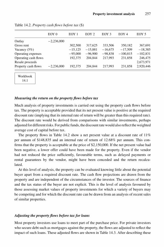
Property investment analysis 257
Table 14.2. Property cash flows before tax ($)
EOY 0 EOY 1 EOY 2 EOY 3 EOY 4 EOY 5
Outlay −2,236,000Gross rent 302,500 317,625 333,506 350,182 367,691Vacancy (5%) −15,125 −15,881 −16,675 −17,509 −18,385Operating expenses −95,000 −96,900 −98,838 −100,815 −102,831Operating cash flows 192,375 204,844 217,993 231,858 246,475Resale proceeds 2,673,971Property cash flows −2,236,000 192,375 204,844 217,993 231,858 2,920,446
Workbook14.1
Measuring the return on the property flows before tax
Much analysis of property investments is carried out using the property cash flows beforetax. The property is acceptable provided that its net present value is positive at the requireddiscount rate (implying that its internal rate of return will be greater than this required rate).The discount rate would be derived from comparisons with similar investments, perhapsadjusted for different risks. For public funds, the discount rate would also reflect the weightedaverage cost of capital before tax.
The property flows in Table 14.2 show a net present value at a discount rate of 11%per annum of $148,835 and an internal rate of return of 12.68% per annum. This con-firms that the property is acceptable at the price of $2,150,000. If the net present value hadbeen negative, a lower offer could have been made for the property. Even if the vendorhad not reduced the price sufficiently, favourable terms, such as delayed payments orrental guarantees by the vendor, might have been conceded and the return recalcu-lated.
At this level of analysis, the property can be evaluated knowing little about the potentialbuyer apart from a required discount rate. The cash flow projections are drawn from theproperty and are independent of the circumstances of the investor. The sources of financeand the tax status of the buyer are not explicit. This is the level of analysis favoured bythose assessing market values of property investments for which a variety of buyers maybe competing and for which the discount rate can be drawn from an analysis of recent salesof similar properties.
Adjusting the property flows before tax for loans
Most property investors use loans to meet part of the purchase price. For private investorswho secure debt such as mortgages against the property, the flows are adjusted to reflect theimpact of such loans. These adjusted flows are shown in Table 14.3. After describing these
258 Capital Budgeting
adjustments, the reasons for deviating from the usual practice of separating the project andfinancing decisions are explained.
The initial capital outlay is reduced by the loan amount, net of any fees required toestablish the loan. The loan is a positive flow to the investor, making the outlay smaller.The net income is reduced by the loan payments (and possibly service or ‘line’ fees). Theresale proceeds are reduced by any outstanding loan balance, together with any prepaymentpenalties charged by the lender for redeeming a loan before its full term. These penaltiesare prescribed in the loan contract and may be a specified number of months of payments,months of interest, a percentage of the outstanding balance or other compensation for thelender’s losses.
Example 14.2. Equity cash flows before tax from the industrial property
The calculations in Table 14.3 are based upon a loan of $1,505,000, being 70% of the price.There will be loan establishment fees of $6,000, meaning that the initial outlay is reducedfrom $2,236,000 to $737,000 (i.e. $2,236,000 − ($1,505,000 − $6,000)). The investor canborrow on a monthly amortizing loan over fifteen years at an interest rate of 7.25% perannum, fixed for the first five years of the loan. This would require total annual paymentsof $164,863. This and the other calculations for amortizing loans are explained in Chapter 5.In the final period, the outstanding balance of $1,170,227 is repaid, together with a prepay-ment fee of $27,477 (being two monthly payments).
With a required return on equity of 16% per annum, the net present value of the equitycash flows before tax is $129,194 and the internal rate of return is 20.10% per annum.These are positive signals for the acquisition of this property at this level of borrowing.The higher discount rate for the equity flows compared to that for the property reflects therisks of using debt.
Reasons for analysing project and financing flows together
The use of equity cash flows to analyse property investments enables us to evaluate theproperty and its sources of finance together. Private property investors are generally wellserved by a model that explicitly shows cash flows as the return on their equity. They cansee clearly their yearly cash receipts and any shortfall between rent and loan payments.Generally, private investors do not use many sources of funds; they use only a mortgageand their own savings as equity. It is unnecessary to amalgamate the sources and termsof finance into a weighted average cost of capital to discount the property cash flows (seeChapter 7). Further, if each property is held in isolation, with debt secured against it, anygrowth in value or loan amortization will change the debt-to-value percentage, making itimpractical to use a weighted average cost of capital.
On the other hand, public corporations and funds are more likely to evaluate propertycash flows. Public funds can estimate the return required by their investors and subscribers.This required return can be based on recent capital issues or can be imputed from the currentprices of shares or units in the companies or funds or in their competitors. Public companies

Property investment analysis 259
Table 14.3. Equity cash flows before tax ($)
EOY 0 EOY 1 EOY 2 EOY 3 EOY 4 EOY 5
Property cash flows −2,236,000 192,375 204,844 217,993 231,858 2,920,446Payment −164,863 −164,863 −164,863 −164,863 −164,863Loan 1,505,000 Outstanding balance −1,170,227Loan initial fee −6,000 Prepayment penalty −27,477Equity cash flows −737,000 27,512 39,981 53,130 66,995 1,557,879
Workbook14.1
and funds typically have a target debt percentage without necessarily allocating debt toparticular assets. They can combine the required returns of investors and the current costsof borrowing to determine their weighted average cost of capital, which can be used todiscount the property flows. This approach is illustrated later in this chapter in the contextof corporate real estate decisions.
It is important to understand that these two approaches (discounting the equity cash flowsat a required return on equity and discounting the property cash flows at a weighted averagecost of capital) are not inconsistent. However, whenever the debt-to-value percentagechanges during the investment, the two approaches may support slightly different prices.As a general rule, equity cash flows are more meaningful for private investors andproperty cash flows are more appropriate for property decisions by public corporationsand investment funds.
Adjusting the cash flows for income and capital gains tax
Both property and equity cash flows should be adjusted for the effects of income and capitalgains tax, unless the investor’s tax status is not known or the investor does not pay tax.Listed property trusts and pension funds are major property investors that do not pay tax insome countries.
Whether evaluating property flows or equity cash flows, the expected liability for tax caninfluence the outcome from property investments. Although savings in tax rarely justifybuying properties, tax liability may influence the choice and pricing of properties. Becausethe same portion of tax is not deducted from all properties, it is important to incorporatethe tax liability when evaluating investments.
This chapter does not attempt to explain the details of any tax system. The tax rules varyaround the world and change over time within countries. The following brief description ofthe typical features of tax laws that influence returns from income-producing properties isprovided in order to demonstrate how after-tax cash flows are established and evaluated.
Rents and operating expensesRents and almost all other recurrent receipts from property investments are assessableincome for taxpayers. As operating expenses are tax-deductible, it is usual to begin the

260 Capital Budgeting
calculation of tax liability with the operating cash flows or ‘net income’. On rare occasions,some expenses are not tax-deductible (for example, property taxes in a few countries andmoney paid into sinking funds for future expenses).
Depreciation allowancesThe two principal differences between cash flows and taxable income from property in-vestments are depreciation allowances and deductions for loan interest. Depreciation andinvestment allowances on some elements of the purchase of a property may be permitted fortax purposes. This will often require an apportionment of the purchase price between land,buildings, plant within the buildings and acquisition costs. Some tax systems permit theapportionment of the acquisition costs between the other three elements. The land cannot bedepreciated for tax purposes although, in a few countries, investment allowances are givento those who purchase industrial land.
In some countries, buildings can be depreciated for tax purposes if the owner is usingthem to earn taxable income. This would normally be at a prescribed rate per annum, whichmay be faster than the actual rate of depreciation. Accelerated depreciation rates for taxare used by governments to encourage the purchase or construction of particular types ofproperty. The plant within buildings may be depreciable in the same way as other plantused to make profits. Items of plant within buildings can include the heating and coolingequipment, lifts, carpets and other fittings. Plant depreciation can be claimed under mosttax regimes and is usually allowable at considerably higher rates than depreciation forbuildings.
Tax deductions for depreciation are attractive to tax-paying investors when the rates ofdepreciation are faster than the decline in value of the asset. It is often difficult to tell howthe land and buildings are separately changing in value over time but certainly a propertymay be increasing in value whilst the owner is claiming substantial depreciation allowances.However, many tax systems have devised ways in which excess depreciation deductions arereclaimed when the property is sold. The recapture of excess depreciation may be either byan adjustment to taxable income in the year that the property is sold or by increasing thetaxable capital gain on resale.
Loan interestIf we are carrying out an equity cash flow analysis, the effects of the sources of financeupon the tax liability should be incorporated. This is not the case if we are analysing theproperty or project cash flows.
Interest paid on loans taken out to purchase property investments is generally tax-deductible. In some countries, the interest deduction cannot exceed the net rental incomefrom the property (additional interest payments are carried forward as losses until the in-vestment or pool of investments earns taxable income). Elsewhere, investors are able tooffset tax payable on salaries and other sources against tax losses generated by propertyinvestments. Generally, the loan must have been taken out to earn investment income to giverise to a tax deduction, although in some countries the tax deduction may be regardless ofthe purpose of the loan. The loan principal within each payment of an amortizing loan does

Property investment analysis 261
not give rise to a tax deduction. Loan establishment fees are either deductible immediatelyor apportioned over several years.
Capital gainCapital gains on the resale of a property investment are generally taxed differently torecurrent income, unless the investor is deemed to be running a business buying and sellingproperties for profit. In most countries, capital gains are taxed leniently. Under some taxsystems, capital gains are taxed at a lower rate than income; other systems tax only a portionof the capital gain; sometimes the portion taxed declines if the property is held for longer;some systems only tax the gain if the property is held by a business. The capital gain iscalculated after allowing for acquisition and selling costs. It is calculated on the gain invalue of the asset, irrespective of the equity.
After-tax equity cash flow analysis
These features of the tax system are used to calculate the taxable income and gain as ifthe property is added to the investor’s other income. Usually a marginal tax rate is used todetermine the expected tax liability although it is possible to use a progressive tax scaleto calculate the liability more accurately. The marginal tax rate is the rate that would beapplied to additional income (or would have applied to taxable income that is sheltered bylosses generated by the property). The tax liability is deducted from the cash flows beforetax to arrive at the cash flows after tax (or tax savings generated by the property are addedback to the cash flow before tax).
Example 14.3. Equity cash flows after tax from the industrial property
Table 14.4 illustrates how the tax liability, including the tax deduction for loan interest, isdeducted from the equity cash flow before tax to arrive at the equity cash flow after tax. Theexample is based upon the tax regime in Australia at the time of writing. The net incomein working out the tax liability from the property is the same as the operating cash flowsbefore tax. Tax deductions for elements of the loan and for depreciation are used to computethe taxable income. In this example, the investor’s tax rate is 40% on taxable income andtaxable capital gain.
The interest portion of the annual loan payments is tax-deductible (Chapter 5 explains howthis is calculated). Initial fees to establish loans are deductible over the first five years of theloan. The building attracts a ‘capital allowance’ of 2.5% per annum of its construction costof $1,500,000. Items of plant within the building, with a value of $400,000, are depreciableover an average effective life of nine years. Depreciation for these items is calculated ona straight-line basis. During the first year, the taxable income is $2,008, of which 40% ispaid in tax. This tax liability of $803 is subtracted from the equity cash flow before tax of$27,512 to arrive at the equity cash flow after tax in the first year of $26,709.
In the final year, the tax consequence of selling the property must be incorporated inthe analysis. The balancing adjustment (an amount added to the taxable income based on

262 Capital Budgeting
Table 14.4. Equity cash flows after tax (an Australian example) ($)
EOY 0 EOY 1 EOY 2 EOY 3 EOY 4 EOY 5
Equity cash flows −737,000 27,512 39,981 53,130 66,995 1,557,879
Tax liabilityNet income 192,375 204,844 217,993 231,858 246,475Loan interest −107,222 −102,901 −98,257 −93,264 −87,897Loan initial fee −1,200 −1,200 −1,200 −1,200 −1,200Building allowance −37,500 −37,500 −37,500 −37,500 −37,500Plant depreciation −44,444 −44,444 −44,444 −44,444 −44,444Balancing adjustment 22,222Taxable income 2,008 18,798 36,592 55,449 97,655Income tax payable (40%) −803 −7,519 −14,637 −22,180 −39,062Capital gains tax −125,094Equity cash flows after tax −737,000 26,709 32,462 38,493 44,815 1,393,722
Workbook14.1
the resale value of the plant) and the capital gains tax payable under current Australianrules are rather complex and are calculated in the accompanying Workbook 14.1. Theserules ensure that if the building and the plant have been written down for tax purposesto less than their resale values, the excess depreciation is recaptured when the propertyis sold. Their effects on the equity cash flow after tax in the final year are shown inTable 14.4.
The after-tax cash flows have an internal rate of return of 16.77% per annum and a netpresent value of $159,440 at a discount rate of 12% per annum – positive signals for theacquisition at this level of borrowing after adjusting for expected tax liability. This methodof evaluating property investments shows the effects of growth in rents and value, theeffects of borrowing and the effects of tax. It requires careful consideration of the investor’scircumstances and likely cash flows generated by the property. Although it is never easy tomake the necessary forecasts, the calculations can be set up as a proforma for use with anyproperty, as in the accompanying workbook.
Because some elements of the after-tax cash flows are derived from the purchase price, itwould be incorrect to conclude in this example that the investor could pay $159,440 morethan the existing price to earn exactly 12% per annum. Increasing the price will alter thetransfer costs, the capital gains tax and possibly the loan amount if this is a percentage of theprice. The exact price that will earn this discount rate can be determined using the Goal Seekcommand provided in Excel (by setting the NPV to zero and varying the purchase price).In this example, a purchase price of $2,363,127 would earn a 12% per annum after-taxreturn on equity. Using the workbook will confirm that with a loan of $1,654,189, being70% of this purchase price, the initial equity is $809,463 including $6,000 initial loan feesand buying costs of $94,525.

Property investment analysis 263
Corporate real estate
Decisions by businesses to occupy additional properties or move to a new location arecritical to their operations and profitability. A wide range of decisions can be evaluatedwithin the capital budgeting framework expounded in this book. In essence, the premisesare an expense of operating the business and contribute to the value of the firm. Corporateproperty decisions are made as part of the overall strategy by which the business maximizesits value. The details of such analysis can vary with the circumstances and scale of theproperty investment. Two typical decisions are illustrated – the choice to move premisesand the choice between leasing and buying a property – and other corporate propertydecisions that can be evaluated similarly are mentioned.
Moving to new premises
Small firms and sole traders considering new premises might evaluate their whole businessin a potential new location: would the business be more profitable in the new property?For larger firms, it is generally possible to identify the specific effects of operating fromdifferent facilities or location. The effect on profitability is weighed against the initial outlayand running costs of the property. Occasionally, new premises are required solely for oneproject, in which case the costs of the property can be evaluated as outflows within thatproject. However, new premises are usually required for general expansion or change ofdirection for the firm and obtaining a new property is itself a project.
This is best evaluated by measuring the differences in the inflows and outflows resultingfrom the move to the new property. These are known as incremental, or differential, cashflows. The principles are the same as those illustrated in replacing a machine in Table 2.4in Chapter 2. The initial outlay is the difference between the costs of purchasing the newproperty and the amount that can be realized from a sale of the existing property. During theinterim periods of the analysis, there may be higher profits and different costs in operatingfrom the new property than from the existing one. The period of analysis cannot extendbeyond realistic projections for the business. In the final year of analysis, the differencebetween the likely resale proceeds from the new and existing properties should be added tothe other flows.
Example 14.4. Acquiring the industrial property for operations
The following example shows how a firm might evaluate the decision to sell an existingproperty in order to purchase a larger property. The period of analysis is four years. The largerproperty is the same industrial building used in the previous examples but now assumed to bevacant and available for occupation. The move would enable the firm to make savings in itstransport costs and expand its business to meet unsatisfied demand. The savings in transportcosts have been identified to be about $15,000 during the first year, growing at 4% perannum in later years. The expansion of the business is estimated to increase net cash flows(excluding the property expenses and transport savings) by $20,000 in the first year and

264 Capital Budgeting
$65,000 in the second year, while the new operations are being established, and $105,000and $110,000 in the third and fourth years. These items would be estimated in consultationwith the works and transport managers for the company. In practice, this analysis shouldalso show the differences in the tax shelter from the new and existing properties but, toillustrate the principles, the cash flows before tax suffice.
The purchase of the new property for $2,150,000 requires an outlay, including buyingcosts, of $2,236,000. From market enquiries, it is believed that the existing property couldrealize $1,410,000, net of selling costs, if sold today. The operating expenses of the newproperty are estimated to be $95,000 in the first year, growing at 2% per annum. Theoperating expenses of the existing property are estimated to be $64,000 in the first year,growing at 2.5% per annum (a slightly higher percentage increase as costs are likely toincrease faster for older buildings).
If it is assumed that the new property will increase in value at 5% per annum, it will havea value of $2,613,338 at the end of the fourth year. From this, selling costs of 3%, being$78,400, are deducted, giving resale proceeds of $2,534,938. The existing property is olderand assumed to be growing in value at a slower rate than the new one, suggesting resaleproceeds, less selling costs, of $1,600,000.
Table 14.5 calculates the differential flows created by acquiring and moving to the newproperty and selling the existing one. The differential cash flow today (EOY 0) is an outflowof $826,000, being the difference between the costs of acquiring the new and the proceeds ofselling the existing property. The differential cash flow in subsequent years is the sum of anyfinancial benefits from the new property and savings resulting from the sale of the existingproperty (positive amounts at EOY 1 and subsequently), less any costs of the new propertyand benefits given up by selling the existing property (negative amounts at EOY 1 andsubsequently). In the final year (EOY 4), the differential cash flow includes the potentialresale proceeds of the new property, $2,534,938, and an opportunity cost of $1,600,000because the existing property would not be available for sale.
For corporations, the effects of loans would not normally be shown. However, the discountrate is based upon the firm’s weighted average cost of capital before tax (see Chapter 7).In this example, the firm aims to retain about 40% debt and can borrow at 7% per annum.Shareholders require about a 15% per annum return. This suggests a discount rate of 11.8%per annum, being 40% of the 7% per annum cost of debt and 60% of the 15% per annumcost of equity. In this example, the net present value of the differential flows is negative,suggesting that the purchase of these new premises is not justified.
Differential cash flow analysis such as this can be used in several ways. If the businessis renting premises, the analysis would show the rent and operating expenses of the newproperty compared to those of the old one, rather than the acquisition and resale values. Ifa mortgage were secured on the new property, it would be legitimate to reflect the new andexisting loans and loan payments in the differential flows (as in Table 14.3 above). If equitycash flows are used, the discount rate should be the required return on equity (as the cost ofdebt is explicit in the loan payments).
Sometimes, a business is committed or obliged to move and wishes to choose betweenalternative premises. Occasionally, the alternative premises do not have major effects on the

Property investment analysis 265
Table 14.5. Evaluating moving to new premises ($)
EOY 0 EOY 1 EOY 2 EOY 3 EOY 4
Purchase price, plus costs −2,236,000Sale of existing property 1,410,000Operating expenses −95,000 −96,900 −98,838 −100,815
(of new property)Operating expenses 64,000 65,600 67,240 68,921
(of existing property)Savings in transport costs 15,000 15,600 16,224 16,873Net increments from 20,000 65,000 105,000 110,000
expanded businessResale proceeds from new 2,534,938
propertyResale proceeds from existing −1,600,000
propertyDifferential cash flows −826,000 4,000 49,300 89,626 1,029,917
Net present value at a weighted average cost of capital of 11.8% −59,616
Workbook14.2
operations of the business and the analysis is simplified to the selection of the premises withthe lowest net present value of the costs of occupation. More often, however, the choiceof premises will lead to differences in transport costs, labour costs and property operatingexpenses; larger premises might also enable a larger scale of operations or accommodatefuture expansion. Each alternative can be evaluated separately, seeking the one with thehighest net present value. Or, one of the possible new properties can be used as a benchmarkagainst which to evaluate the alternatives, as in Table 14.5.
Lease or buy
Businesses can often choose between buying and leasing their premises. In recent years,many companies have sold their properties and leased them back, freeing capital for theiroperations. Leasing gives the company more flexibility but less control over their premises.Although, in theory, leasing and buying should be financially equivalent (Miller and Upton,1976), firms often maintain that they can take advantage of market conditions to enhancethe value of their business by the appropriate choice of tenure.
The choice is best evaluated by comparing the net present value of the costs of buying withthe net present value of the costs of leasing. The costs of buying are the initial outlay andthe subsequent expenses of operating the property (less tax deductions for those operatingexpenses). The resale value of the property is added to the final year’s property flows. Thecosts of leasing are the rent payable in each year (less tax deductions for the rent). Thecheaper option is the one with the smaller (negative) net present value.

266 Capital Budgeting
It is generally important to incorporate the tax implications of buying, which may pro-vide depreciation allowances, and leasing, which gives tax deductions for the rent. Thefinancing can either be reflected in the after-tax cost of debt within the discount rate orby adjusting the property flows for the loan, its repayments and the tax deduction forinterest.
Example 14.5. Leasing or buying the industrial property for operations
Using the same industrial property as in the previous examples, the costs of buying orleasing can be compared. This example is calculated after tax, using a company tax rate of30%, and is based upon the property cash flows (in other words, before financing). We firstconsider the costs of buying, as set out in the top part of Table 14.6. The initial outlay is theprice of $2,150,000 plus the acquisition costs, totalling $2,236,000. The operating expensesin the first year of $95,000 are reduced to their after-tax cost of $66,500 because they willgive rise to tax deductions of $28,500 (being 30% of the expenses). These expenses havebeen increased at 2% per annum as in the earlier example.
As a tax-paying owner, the company would be able to claim $37,500 per annum as abuilding allowance and $44,444 per annum as plant depreciation (explained in Example14.3). This provides a tax deduction or tax shield of 30% of the claims, being $24,583. If itis assumed that the property will increase in value at 5% per annum, it will have a value of$2,613,338 at the end of the fourth year. From this, selling costs of 3%, being $78,400, arededucted and capital gains tax of $134,681. The resale proceeds of $2,400,257 are addedto the final year’s property cash flow after tax.
We then consider the costs of leasing, as set out in the bottom part of Table 14.6. The grossrent in the first year of $302,500 would be based upon the asking rent and rents recentlyagreed for similar premises nearby. The rent will be deductible for tax purposes and henceis reduced by 30% to its after-tax cost of $211,750 in the first year. Growth in rents hasbeen projected at 5% per annum, which is consistent with the growth applied to the valueof the property.
These alternative property cash flows after tax are discounted to their net present valuesusing the weighted average cost of capital, adjusted from the previous example to an after-taxcost (see Chapter 7). The cost of debt has been reduced to an after-tax rate of 4.9%, beingan interest rate of 7% per annum, less 30% tax deduction. This suggests a discount rate of10.96% per annum, being 40% of the 4.9% per annum cost of debt and 60% of the 15% perannum cost of equity. Table 14.6 shows that the net present value of leasing is less than thenet present value of buying, and leasing would therefore be preferred.
A similar conclusion would be derived from evaluating the purchase as an investmentoutlay that leads to savings in rent and an asset with a residual value. These flows wouldbe rather like those of purchasing an income-producing property (see Table 14.3 above)and could be adjusted similarly for the tax deductions created by depreciation allowancesand the tax deductions forgone on the rent. However, the comparison between leasing andbuying is less clear if set out in this manner.

Property investment analysis 267
Table 14.6. The costs of leasing or buying ($)
EOY 0 EOY 1 EOY 2 EOY 3 EOY 4
Costs of buyingPurchase price plus costs −2,236,000Operating expenses after −66,500 −67,830 −69,187 −70,570
tax deductionResale proceeds, net of costs 2,400,257
and gains taxTax shield of depreciation 24,583 24,583 24,583 24,583
allowancesProperty cash flows after tax −2,236,000 −41,917 −43,247 −44,604 2,354,270
Net present value at 10.96% −788,453
Costs of leasingRent after tax deduction −211,750 −222,338 −233,454 −245,127
Net present value at 10.96% −704,009
Workbook14.2
Sale and leaseback of a property
A property strategy that has been followed by many companies in recent years is to sell theirreal estate. This is generally done to free up capital for other investments. As such, it is afinancial decision similar to the choice between leasing and buying. A sale and leaseback of aproperty results in inflows and outflows that are the inverse of the purchase of a property. Thesale is an initial inflow and the rent a subsequent outflow. Depreciation allowances are givenup but the rent will provide tax deductions. In evaluating the consequences of selling theproperty now, it must not be forgotten that the company gives up an asset. The analysis mustshow a further outflow in the final year that is the estimated resale proceeds had the propertybeen retained. If this incremental cash flow is discounted at a rate reflecting the costs ofalternative sources of capital, a positive net present value suggests that the property shouldbe sold (because selling the property is a cheaper source of capital than the alternatives).
Workbook14.2
A wide variety of corporate real estate decisions can be analysed by estimating either theincremental or differential effects of acquiring, selling or leasing suitable premises. Some ofthese decisions may appear complex but, provided the analysis of alternatives is consistentin its treatment of inflows and outflows, financing, tax and discount rates, the usual capitalbudgeting rules can be adopted.

268 Capital Budgeting
Development feasibility
The purchase and development of sites is an entrepreneurial activity like any other business.The business produces completed buildings or subdivided parcels of land for sale. Propertydevelopment may be undertaken by trading companies or investors intending to retain thecompleted building but the development phase is generally evaluated separately. The cashflows and the risks during this phase are quite distinct from those when operating theproperty.
Any property development has four principal elements. These are the site and its ancillarypurchase and holding costs, the construction costs and related professional fees, the returnfor the risks taken, and the value of the completed property. In simple terms, the developmentis viable if the completed value is greater than the sum of the other three elements. Typically,a developer evaluates a project to determine either how much can be paid for the site or,if the price is not negotiable, whether the estimated return is sufficient. Many differentversions of the project may be considered, such as buildings of different size and quality, orperhaps various sites might be considered for the same project. Many development projectsare speculative (that is, they are built on the expectation that occupants will be found) andthe eventual selling price of the completed development is the key to the success of theproject. Some projects are only undertaken if the completed buildings have been ‘pre-let’or ‘pre-sold’. Some projects are completed by corporations for their own occupation.
In this section, a preliminary method to screen development projects is contrasted withan evaluation of the project cash flows. The preliminary method, or some variation of it,is so widely used that it needs to be demonstrated. However, it is not consistent with therules of capital budgeting, as will be evident when the same project is shaped into a cashflow model. The preliminary evaluation ignores the time value of money but gives a roughindication of whether the project is worthy of detailed investigation. This preliminary or‘static’ analysis calculates a notional ‘profit’ as a percentage of the total expenditure. Itapproximates holding or opportunity costs whilst the site is not producing income by asimple interest calculation. Provided that this form of analysis is done using current costsand values, its assumptions will tend to be more conservative than a cash flow model.However, the way that it allows for ‘profit’ and interest means that the results cannot bedirectly compared with a cash flow analysis of the project.
Example 14.6. Initial screening of an industrial building project
Let us imagine that a developer is considering putting up an industrial building on a vacantsite adjoining the property illustrating earlier examples in this chapter. On completion ofa new but otherwise similar building to the adjoining one, the developer might anticipateselling the property for $2,400,000, less selling costs of about 5% of the price. Planningapprovals for the building would take two months and construction a further seven months.Design and engineering fees of $130,000 would be payable in the second month and con-struction costs of $1,100,000 spread evenly over the remaining seven months. The site canbe acquired for $550,000, plus 4% buying costs. The developer can utilize funds that cost11% per annum for both the acquisition and the development.

Property investment analysis 269
Table 14.7. Preliminary analysis of a property development ($)
Sale of the completed property 2,400,000less Costs of sale −120,000Net proceeds of sale 2,280,000Purchase price of land, plus buying costs −572,000Holding costs of land −47,190Construction costs and design fees −1,230,000Opportunity or financing costs on construction −39,463Total outlays on development −1,888,653‘Profit’ on total outlays 391,347‘Profit’ as a percentage of total outlays 21%
Workbook14.3
Table 14.7 shows these items in the typical preliminary format. The net proceeds of saleare expected to be $2,280,000. Holding costs on the site cost of $572,000 at 11% per annumfor nine months are shown as $47,190. Opportunity cost for half of the construction costsand design fees of $1,230,000 at 11% per annum for seven months are shown as $39,463 (thehalving approximates the gradual use of these funds during the construction period). Thepreliminary analysis shows a ‘profit’ of $391,347, or 21% of the total outlay of $1,888,653.The development would be further investigated if this ‘profit’ is considered to be a sufficientpercentage to justify the risks. Bearing in mind that speculative property development ishighly risky, a required percentage ‘profit’ on outlay of 20–30% is typical.
More thorough evaluation of development projects uses cash flow models. In fact, it is dif-ficult in many countries to obtain funds for development without detailed cash flow analysisof the project. Property developments that can be completed in about one year are usuallyevaluated on a monthly basis. Longer projects may be evaluated quarterly and extended,staged projects over five or more years may be evaluated annually. All the revenue andexpenses are allocated to their expected time during the project. This is one of the main ben-efits of projecting cash flows rather than relying on the preliminary screening in Table 14.7.The discount rate would reflect both the opportunity cost of money involved in the projectand a return for the risks taken.
There is likely to be a series of outflows during most of the project, starting with thepurchase of the site, followed by design fees, construction costs and concluding with mar-keting costs (if the project is a speculative one). The components of the construction costsare often shown in great detail to ensure that no items are overlooked in assessing the feasi-bility of the development. Later, there will be one or possibly more inflows, which estimatethe consequences of the sale of the completed property or properties. If the property is tobe retained by a long-term investor or for occupation by a company, it can be shown in theproject cash flows as a notional transfer on completion.

270 Capital Budgeting
Table 14.8. Project cash flows from a property development ($)
EOQ 0 EOQ 1 EOQ 2 EOQ 3 EOQ 4
Sale of completed property 2,400,000Costs of sale −120,000Land plus buying costs −572,000Design fees −130,000Construction costs −157,143 −471,429 −471,429Project cash flows before tax −572,000 −287,143 −471,429 −471,429 2,280,000
Workbook14.3
Example 14.7. Project cash flows from a property development
Using the same project as in the previous example, Table 14.8 shows the quarterly devel-opment flows for the industrial property. These would generally be calculated monthly butthe principles are clearer if the cash flows are displayed quarterly. The flows have beencalculated by allocating the expected revenue and costs to the quarter when they are likelyto be received or paid. The initial outlay is the purchase of the site at the start of the firstquarter (EOQ 0). This is followed by payments for design and then construction paymentsover seven months in the first to third quarters. It is assumed that the property will be soldin the quarter following its completion (EOQ 4).
A net present value has been computed based on the quarterly project flows before tax ata discount rate of 9% per quarter. The positive net present value of $18,954 indicates thatthe development shows sufficient return. The high discount rate is indicative of the degreeof risk that developers take. The risks of property development without a commitment ofa purchaser upon completion (without what is referred to as a ‘take-out’) can be seen assimilar to venture capital or trading in futures contracts.
Basic NPV sensitivity analysis for a property development
Alternative schemes can be tested to see if variations in the value on completion, theconstruction costs or the price offered for the land might result in a higher net presentvalue. On the accompanying spreadsheet (Workbook 14.3), the Goal Seek commandcan be used to set the NPV to zero by changing one of these three elements. Theland value is often treated as a residual and the cash flow model can be used to workout the most that the developer can bid for the site whilst earning the required rate ofreturn.
The ability to adjust the components of the project flows to show the effects of differenttiming during the development makes this form of analysis much more realistic and moreflexible than the preliminary screening in Table 14.7. The tax consequences of the devel-opment project can also be incorporated, although development for sale does not usuallyattract depreciation allowances. Project cash flow analysis can be extended to show the

Property investment analysis 271
Table 14.9. Equity cash flows from a property development ($)
EOQ 0 EOQ 1 EOQ 2 EOQ 3 EOQ 4
Project cash flows before tax −572,000 −287,143 −471,429 −471,429 2,280,000Loan drawdowns 211,600 287,143 471,429 471,429Cumulative loan 211,600 504,562 989,866 1,488,516 0Loan repayments −1,529,450Equity cash flows before tax −360,400 0 0 0 750,550
Workbook14.3
effects of borrowing upon the developer’s return and liquidity. Much property developmentis carried out by small businesses and individuals who learn more from a ‘bottom line’ thatshows their equity than from the project flows.
Funding for development is offered by financial institutions on different terms than mort-gages for long-term property acquisitions. It is often available on terms that enable thedeveloper to draw down portions of a loan when they are required to pay for stages ofthe construction. Typically, the developer is expected to contribute all the equity beforeany portion of the loan is taken and to repay all the loan before receiving any of the salesrevenue. Some lenders will lower their interest rate if they are given an equity stake in theproject. The equity cash flows from these and other joint ventures can be made explicit,showing the returns to each party.
Example 14.8. Equity cash flows from the development project
Assuming that the developer has arranged a loan facility for 80% of the estimated projectcosts (excluding the costs of sale), Table 14.9 extends the project cash flows from Table 14.8to calculate the equity cash flows before tax. The developer will be required to contributethe first 20% (the equity cash outflow of $360,400 at EOQ 0) of the estimated total projectcosts of $1,802,000. The balance of the project costs will be covered by drawing downthe loan in stages. Interest on the cumulative amounts borrowed will be charged at a rateof 2.75% per quarter (one quarter of 11% per annum) and added to the cumulative loan.For example, the cumulative loan at the end of the first quarter is $504,562, being the totalloan from the previous quarter ($211,600) plus interest at 2.75% ($5,819), plus the amountdrawn down ($287,143).
The loan has the first claim over the proceeds of selling the completed industrial building.In this case, the net proceeds of sale of $2,280,000 at the end of the fourth quarter are usedto pay off the accumulated debt of $1,529,450 (being the debt of $1,488,516 plus interestof 2.75%, $40,934). This shows an equity cash flow at EOQ 4 of $750,550.
A net present value has been computed based on the quarterly project flows before tax ata discount rate of 20% per quarter. The positive net present value of $1,555 indicates that theequity contributed to the development shows sufficient return. The discount rate has beenincreased considerably to reflect the volatility of the equity cash flows when large loans

272 Capital Budgeting
have prior claims on the project. The degree of risk is evident if you consider a decline inthe industrial property market. If property prices should fall 15% (which is quite possible),the developer will get the initial equity back and nothing more. Further risks of propertydevelopment are described in Chapter 15.
One of the benefits of working out the equity cash flows is to be able to see the timingand magnitude of the developer’s contribution. The equity cash flows in Table 14.9 showquite a different pattern to the project cash flows.
Concluding comments
This chapter has applied capital budgeting techniques to three types of property decision.It has been shown that the evaluation of properties requires particular attention to someelements of the cash flows that might be unnecessary for many other capital outlays. Theallowance for financing should be given careful attention as, in many instances, the practicevaries from other uses of capital budgeting techniques. There are four ways of constructingcash flows from properties – before and after financing and before and after tax. The chapterhas shown that each may be suitable under different circumstances and each will require adifferent discount rate.
It should be evident that the evaluation always depends upon forecasting flows from theproperty in the foreseeable future. The techniques are only as reliable as the forecasts. Thefollowing chapter considers how to make these forecasts and how to measure the risks thatarise because the forecasts are inherently uncertain.
Review questions
14.1 Consider an office building which is available for sale at $3,200,000, plus $150,000of acquisition costs. The property is leased to a variety of tenants under short leaseswhich permit regular reviews of rent to the current market level. Fully leased, thebuilding would earn rents of $287,000 in the first year but the current vacancy levelof 4% is likely to be typical over the holding period. Operating expenses, includingproperty taxes and management fees, are estimated to be $76,000. Market rents areexpected to increase at 6% per annum for the next four years. Operating expenses areexpected to increase at 3% per annum during the period of analysis.
The property is entitled to depreciation allowances for tax purposes of $94,000 perannum which will not be reclaimed upon resale of the property. It is believed that theproperty will be saleable after three years for $3,750,000, less selling costs of 1.5%of the resale price.(a) Use the equity cash flows after tax to evaluate the returns over the next three years,
assuming that $1,340,000 is borrowed on a monthly amortizing loan over fifteenyears at an interest rate of 8% per annum with no loan fees. The investor pays taxat a rate of 30% and has a required return on the equity after tax of 9%. Shouldthe investor proceed with the acquisition at this price?

Property investment analysis 273
(b) Now, assume that the building can be acquired vacant and is suitable for theoccupation of a company in need of this additional accommodation. The prices,rental value and resale value are as above.
Apply the company’s weighted average cost of capital after tax to the propertycash flows after tax over the next three years to evaluate the purchase of theproperty over a three-year period of analysis. The company plans to retain itscurrent 40% debt-to-asset values. It can borrow at an effective fixed interest rateof 8% per annum. It can issue shares provided that investors believe they will earn11% per annum. The company pays tax at a rate of 30%.
Given these assumptions, would it be better to lease the property rather thanbuy it?

15 Forecasting and analysing risksin property investments
Property investments put capital at risk. The outcomes almost always vary from the bestestimates that we make when evaluating the property. Forecasting outcomes and gauging therisks of not achieving those outcomes are critical in applying capital budgeting techniquesto property decisions. This chapter can therefore be seen as a supplement to Chapter 14which illustrated the methods of property investment analysis.
The early part of Chapter 15 provides guidelines for forecasting cash flows arising fromproperty investments. There will always be doubts about the reliability of forecasts ofproperty rents, operating expenses and capital values, but what is the alternative to fore-casting? Purchasing (or leasing) real estate without forecasting cash flows would requirethat the company or other investor accept the asking or market price (or rent). The ‘goingprice’ is derived from other people’s opinions of the prospects and worth of the prop-erty to them. Thus, however difficult forecasting may be, it is surely better than investingblind. The solution lies in selecting the information and methods of forecasting that aremost likely to help in estimating cash flows. The most reliable forecasts for real estateoften combine the use of quantitative techniques (Chapter 3) and judgemental techniques(Chapter 4).
The later part of this chapter describes ways in which we can assess the risks of notachieving the investment objectives. Risk analysis is needed because of the uncertainty ofthe cash flows that we forecast. The risks can be revealed by testing the sensitivity of theinvestment to variations in the cash flows (as in Chapter 8) and simulating the alternativeoutcomes (as in Chapter 9). Having assessed the risks of a property investment, we candetermine whether the investment shows sufficient return. This might lead us to reject theinvestment or adjust the discount rate, changing the present value.
The examples used in this chapter illustrate forecasting and risk analysis for thethree types of property decision described in Chapter 14. Most of this chapter is de-voted to forecasting for, and the risks of purchasing, income-producing properties. Sim-ilar cash flow forecasts are required for corporate real estate decisions, but develop-ment feasibility requires a slightly different approach to forecasting. The risks of eachtype of property decision are somewhat different although the methods of analysingthem are the same. The examples in the text are available in the accompanying Excelworkbooks.
274

Forecasting and analysing risks in property investments 275
Study objectives
After studying this chapter the reader should be able to:
� identify the typical factors that determine cash flows from property investments� make forecasts combining past data with judgement about the future direction of the
specific property market� identify the main risks that property investors face and incorporate them in the analysis
of properties.
Forecasting
There are no sure ways to forecast cash flows from properties with complete accuracy ifthey are leased or traded in open markets. The problems of any economic forecast arecompounded by the lack of reliable data and the local variations. Information about pastchanges in rents and values may only be available as broad averages across the region and thisis sometimes of limited relevance to the property in question. Therefore, forecasting tendsto be largely judgemental, supported by aggregate data, trends and local market knowledge.The difficulties of forecasting are the main reason why Chapter 14 recommends that werestrict cash flow models for property analysis to five years.
Judgemental forecasts are based upon a sound understanding of the factors that causechanges in rents and values. These are often referred to as market drivers. This sectionsuggests an approach to forecasting property cash flows that makes use of available infor-mation about these market drivers, whilst leaving room for qualitative adjustments to suitcurrent local conditions. The stages in forecasting operating cash flows before tax, generallytermed ‘net income’ in property circles, are described in this chapter. Each stage is thendemonstrated by refining the projected cash flows for the property used as an example inChapter 14.
Rent under the lease
For properties acquired with existing tenants, there is reasonable certainty about the rentunder the terms of the lease. Therefore, the starting point in forecasting the rents fromleased properties is a study of the covenants in the lease. Most leases of commercial andindustrial properties are granted for several years. The leases fix the rent but often containmechanisms for the rent to be adjusted occasionally. The typical provisions for changingrent during the lease are:
� fixed percentage changes or dollar adjustments on the anniversary of the start of the lease� adjustments each year in line with the rate of increase in an index of consumer prices or
construction costs (as published by government statisticians)� less frequent reviews to the then current market rent, as agreed by the parties or indepen-
dently assessed� additional rent as a percentage of the turnover of shops.

276 Capital Budgeting
For an income-producing property, the rent is projected in accordance with the leaseterms. If the rent is adjusted during the year, the lease rent may comprise some months atone level and the remainder of the year at a different level. It is relatively easy to modelcash flows to this degree of accuracy when using computerized spreadsheets.
Forecasting the operating expenses
The lease also dictates which party is responsible for the various expenses of runningthe property. Each of the expenses (itemized in Chapter 14) can be projected separatelyif there are foreseeable changes or if major outlays are required to keep the property ingood condition. Sometimes, changes to property taxes, insurance premiums or servicingcontracts are announced and can therefore be built into the projections. Sometimes, it maybe necessary to upgrade a property to retain tenants or to renew plant at the end of itseconomic life. If there are no obvious irregular or unusual outlays, it may be adequate toassume that operating expenses will change at the rate of increase of an index of consumerprices (obtained from government sources or economic forecasting groups).
Estimating market rents
For a leased property, the rent collected will be adjusted to the prevailing market level foreach tenancy either at a ‘market rent review’ during the lease or at the expiry of the lease.Estimating rent at these times is a two-stage process. The first stage is to establish the marketrent today and the second stage (described later) is to forecast what the market rent will be atthe time of the market rent review. To establish the market rent today, we must compare theproperty with other similar ones that have been leased recently. The objective is to estimatewhat a likely tenant would pay if the property were offered for lease today. Because of thedistinct characteristics of each property, this may require a careful investigation of recentrents paid for similar premises. Rents are not generally public information and rents forcomparable properties can only be gathered by personal enquiries of those involved in thedeals. Commercial and industrial properties are not uniform, nor are their leases, makingcomparisons awkward.
The common practice of granting new tenants hidden incentives to sign leases (such asgranting periods free of rent or paying to fit out the premises to the tenant’s specification) canmake it more difficult to estimate market rents. The practice of granting leasing incentivesis common in many markets for commercial and industrial properties. It adds to the dangersof buying income-producing properties by assessing only the initial rent being paid by thetenant(s) – this rent should always be checked against current market rents. Because ofleasing incentives and changes in the market since the premises were leased, there are oftensubstantial differences between the rent fixed under the lease and the rent that would beagreed if the premises were available to lease.
Allowing for vacancy
Both the loss of rent arising from vacancy at the end of the lease and any monetary incentivesto attract new tenants should be built into the forecast of operating cash flows. The loss will

Forecasting and analysing risks in property investments 277
be determined by the suitability of the property for occupants and by market conditionswhen the lease expires. Typically, this will be expressed as months without rent and costsof attracting new tenants. The alternative (which is commonly used when there are manytenants) is to subtract an annual average loss to vacancy as a percentage of the lease rent.
Determinants of market changes
To estimate market rent when the review will occur and loss to vacancy when the leaseexpires, we must forecast changes in the state of the market for the type of property.Although long-term trends in past average rents can be measured as compound growthrates or by using statistical methods such as regression analysis, these are of limited helpin monitoring rental changes. There are two reasons for this. Long-term trends in rents andproperty values are heavily influenced by consumer price inflation. Therefore, past growthrates can only be used to forecast future trends if the rate is adjusted to reflect likely inflationrates in the future. The second (and more important reason) is that property markets arestrongly cyclical, often displaying startling booms followed by equally startling but moresobering contractions. Forecasts over a five-year period of analysis cannot afford to ignorethe likely movement through a cycle that will occur.
Much has been written about the persistence of property cycles. They are tied to cy-cles in the national and regional economy and to the long lead-time between decisionsto build more space and its availability for occupation. Smoothing techniques can helpto reveal the cycles more clearly than a time series of rents. For the analyst forecastingchanges in market rents (and property values), there are some signs to observe. The va-cancy rate is the unoccupied percentage of the stock of a certain type of property within adefined geographic area. Some vacancy is necessary to enable occupants to move. Whenvacancy rates decline below this ‘equilibrium’ or ‘natural’ vacancy level, rents are likelyto rise as occupants compete for limited supply. When vacancy rates are above this level,rents are likely to be stable or declining. In many markets, there is published data indi-cating vacancy rates in recent years for particular types of property and the trends can bemonitored.
Changes in vacancy rates are brought about by changes in supply and/or demand. It ispossible to anticipate most changes in supply because of the length of time to develop newbuildings. Buildings under construction are evident and market enquiries will reveal howmuch of this new space is already committed to occupants. Local government authoritiesmaintain records of building approvals (which in some countries are collated and publishedby government statistics offices) and generally monitor how much land is suitable but notyet approved for development.
It is more difficult to anticipate changes in demand. Past absorption rates (being theamount of additional property occupied per period) are indicative of average expansion indemand. However, the demand for properties is derived from various economic and socialfactors that are themselves difficult to predict. For example, the demand for further dwellingsin a city is determined by household formation, job security, interest rates and many otherfactors. The demand for offices is determined by growth in employment in professions andservices, business confidence and gradual shifts in the required floor area per person.

278 Capital Budgeting
Table 15.1. Forecasting rent from leased properties
EOY 1 EOY 2, EOY 3 etc.
Market rent From comparisons with Forecasts based on market dynamicsrecent lettings
Lease rent From lease(s) Changes based on lease Market rent whenprovisions lease permits
Vacancy Loss to vacancy and reletting costs at lease expiryOperating expenses Allowance for operating expenses for which the landlord is responsibleOperating cash flows Lease rent, less vacancy and operating expenses
It is helpful to have available both the aggregate regional data for any of these factors andlocal data. Property markets operate locally and we often observe slightly different patternsin rents and values in different suburbs for commercial and residential properties. However,because occupants and suppliers can switch localities, regional trends cannot be ignored inprojecting market rents in one locality.
The sources of the forecasts of rent to derive the operating cash flows (before tax) and therelationship between changing market rents and lease rents are summarized in Table 15.1.
Combining judgement and statistics in forecasts
Despite much research, property analysts have been unable to establish any consistentlyreliable quantitative relationships between rents (and prices) and vacancy rates, supply anddemand. Therefore, most forecasts of rents are made by assembling data that show how themarket has changed in recent years and using this data informally to develop judgementalforecasts. The judgement of someone with wide experience may recognize turning pointsand idiosyncrasies in markets that most statistical techniques do not detect. Experiencealso makes it easier to detect differences between average rents and the likely changesin the particular property under scrutiny. However, forecasts based on judgement wouldundoubtedly benefit from formalizing the process (as described in Chapter 4), as casualapproaches to qualitative forecasting are open to bias and may simply reinforce passingmarket sentiment.
Example 15.1. Forecasting operating cash flows for the industrial property
This example illustrates one method of forecasting the rent from the industrial propertydescribed in Chapter 14. The approach uses averages and trends to support judgementabout the direction of the market and the particular characteristics of the property beingevaluated.
The lease rentTo show the relationship between the lease rent and the market rent, it is assumed inthis chapter that the property was leased one year ago for five years at a gross rent of

Forecasting and analysing risks in property investments 279
Table 15.2. Lease rent for the industrial property
EOY 1 EOY 2 EOY 3 EOY 4 EOY 5
Lease rent $283,250 $291,748 Market rent 3% increase Market rent
$275,000 per annum in the first year. The lease specifies that the rent will increase by 3%per annum at the end of the first and second years (hence the rent during the first year ofour evaluation (EOY 1) is $283,250 per annum and will increase to $291,748 per annumfor the third year of the lease, being EOY 2).
The lease states that at the end of the third year the rent is to be renegotiated to the thenmarket rent (with provision for independent opinion to settle any dispute). Therefore, therent during year 3 will be the market rent at that time. The lease specifies a further 3%increase at the end of the fourth year of the lease (which will apply during year 4). At theend of the lease, the parties are free to terminate their agreement or to negotiate a new lease.Therefore, the rent during year 5 will be the market rent as agreed for a new lease witheither the existing tenant or someone else. Table 15.2 shows the rent that can be expectedunder the lease and after it expires.
The market rentTo forecast the future market rent first requires an estimate of the market rent today, whichcan be ascertained by research into recent lettings of similar properties and under similarterms. In this case, rents in the range $50–$60/m2 per annum are currently being agreedfor similar premises nearby. Although this property is on a main road (an advantage forindustrial properties), it has a low roof height, a small portion laid out as offices and ashort road frontage (all disadvantages). On balance, its current market rent is estimated tobe $55/m2 per annum, equating to $302,500 per annum. This is 10% higher than the rentagreed when this property was leased last year, which is consistent with the average changein industrial rents since last year in this neighbourhood.
We must now consider how market rents are likely to change between now and when themarket rent can be collected from the tenant. This property is similar to others in the area(average rents in the current year are $58/m2 per annum). From statistics, such as thoseshown in Table 15.3, we can form a picture of the direction of the market, supported bycommentary from real estate managers and agents who are active in the area.
In the last two years, rents for industrial premises in this neighbourhood have increasedsubstantially, after many years of largely stable rents. A boom in the need for indus-trial premises can be attributed to the expansion of the minerals sector of the regionaleconomy with the discovery of valuable deposits in the hinterland where mining hasbegun. As a response to increased demand and higher rents, there has been a substan-tial increase in the construction of industrial buildings in the last two years with pro-jected completions of new buildings next year well above the annual average. The resultis that the percentage of vacant space is currently edging upwards, perhaps indicatingthat increased demand has largely been satisfied. Although the regional economy is still

280 Capital Budgeting
Table 15.3. Industrial property market statistics
Time trend Difference fromGross rents in rents time trend Estimated New building
Year ($/m2 p.a.) ($/m2 p.a.) ($/m2 p.a.) vacant (%) (m2)
−10 37.00 37.14 −0.14 4 27,000−9 41.00 38.67 2.33 6 13,000−8 44.00 40.21 3.79 9 47,000−7 42.00 41.75 0.25 14 58,000−6 41.00 43.28 −2.28 18 21,000−5 42.00 44.82 −2.82 15 8,000−4 44.00 46.35 −2.35 14 15,000−3 44.00 47.89 −3.89 6 6,000−2 47.00 49.43 −2.43 3 18,000−1 53.00 50.96 2.04 4 24,000
0 58.00 52.50 5.50 9 29,000
1 54.04 37,0002 55.57 12,0003 57.114 58.655 60.18
Workbook15.1
buoyant and benefiting from the mining expansion, it seems likely that only moderate,if any, growth in rents can be expected whilst the new buildings are absorbed into themarket.
These directions are confirmed by simple quantitative analysis. A time trend regression(as explained in Chapter 3) shows that 73% of the change in rents can be explained bystraight-line growth of $1.54/m2 per annum. A continuation of this linear growth for thenext five years would show the levels of rent in bold type in Table 15.3 and represented bythe straight line in Figure 15.1.
It is probable that adjustments to this linear projection will improve the accuracy of aforecast of rents. First, we should check prevailing levels of inflation during the last tenyears. The gross rents in the second column of Table 15.3 have grown at an average annualcompound rate of 4.6% per annum during a period when the rate of inflation averagedaround 4% per annum. As economists are predicting lower rates of inflation in the next fewyears (the consensus is about 2% per annum), our trend line should be tempered to reflectlower expected inflation during the next five years.
Second, it is evident that rents increased rapidly in some years but were stable or declinedslightly in other years. The ten-year pattern of rents looks to be a little more than one cyclein this market, as is evident in Figure 15.1 and in the differences between the actual rentsand the time trend in Table 15.3. With data that spreads over several cycles, we might be

Forecasting and analysing risks in property investments 281
30
40
50
60
�10 �9
�8
�7
�6
�5
�4
�3
�2
�1 0 1 2 3 4 5
Typ
ical
gro
ss r
ent
($/m
2 p
.a.)
Time trend rentsActual gross rents
Years
Figure 15.1. Trend in industrial rents per square metre.
able to build a cyclical index (as described in most business statistics primers as an elementin time series decomposition). With one cycle only, a less formal adjustment to the timetrend is all that is practicable. This can be based on three series in Table 15.3: the differencefrom the time trend (the regression residuals); the estimated vacancy percentage; and thenew building completions.
Such adjustments to the trend are partly subjective. They are incorporated in this exampleinformally prior to considering whether this approach to forecasting could be enhanced bythe recognized techniques described in Chapters 3 and 4. Current rents are $5.50/m2 perannum above their long-term trend. This is the furthest above the trend that they have beenduring the last ten years. The vacancy rates in Table 15.3 have an average of 9.1%. In theprevious cycle, when vacancy reached this percentage, rents in the following year actuallydeclined. Average new building over the last eleven years has provided a further 24,182/m2
per annum. In the previous cycle, construction reached more than twice this average. Theforecast construction for the next two years does not show anywhere near this amount ofnew space in the pipeline.
Distilling this information and discussing the implications with local professionals, typ-ical rents are forecast to rise by 3% next year in this neighbourhood. For the followingtwo years, market rents are expected to be stable (as the market absorbs substantial newconstruction) and thereafter 4% per annum growth is projected in a gradually recoveringmarket (2% per annum above expected inflation).
In applying these forecasts to the property in question, some comments from real estateagents concerning its favourable position lead to a final adjustment. Work has started ona new road link that is due for completion in two years and this will provide substantiallyquicker access from the property to the city and the freight terminals. Real estate agentsbelieve that this will create a preference for those industrial buildings that will benefit fromthis road link over other buildings in the neighbourhood. For this reason, the forecast forthe rent that might be achieved for this property is adjusted upwards by 2% to 5% next year(to $317,625 during year 2 to year 4).

282 Capital Budgeting
Table 15.4. Operating cash flows for the industrial property ($)
EOY 1 EOY 2 EOY 3 EOY 4 EOY 5
Market rent 302,500 317,625 317,625 317,625 330,330
Lease rent 283,250 291,748 317,625 327,154 330,330Vacancy −110,110Operating expenses −95,000 −96,900 −98,838 −100,815 −102,831Operating cash flows 188,250 194,848 218,787 226,339 117,389
Workbook15.1
Operating expensesIn this case, operating expenses are forecast to grow at the same rate as consumer priceinflation (estimates of 2% per annum over the next three years were obtained from gov-ernment sources and economic forecasting groups). As this property is leased to a singletenant, vacancy is allowed by way of a period of four months without rent at the end ofthe lease (an amount of $110,110 deducted from the lease rent during year 5). The lengthof this potential vacancy at the end of the lease is one of the risks considered later in thechapter. Vacancy and operating expenses are deducted from the lease rent to calculate theoperating cash flows in Table 15.4.
More formal methods of incorporating these effects on forecast rents
There are many ways in which forecasts of rents can be made more sophisticated than in theabove example. However, none is suitable for all occasions. A few alternative approachesare outlined but a business statistics primer should be consulted for details.
There are inconsistencies between linear growth (as predicted by regression) and com-pound growth. Because rental growth is more likely to compound year by year, it may beappropriate to use the natural logarithms of the rents in a simple regression with time as theindependent variable.
The strength of the negative relationship between rental growth and the vacancy rate inprevious years can be tested in a simple regression with vacancy as the independent variable.For the data in Table 15.3, the vacancy rate in one year explains 47.5% of the rate of rentalgrowth in the following year. Lagged dependent variables such as this can help in makingshort-term projections but the strength of the relationships is rarely sufficient to forecastrents accurately.
In gathering the opinions of those active in the market, property analysts rarely followthe guidelines suggested for the qualitative forecasting methods described in Chapter 4.When collecting information for the analysis of a single property, opinions are virtuallynever sought by formal surveys (although these are occasionally used to uncover generalmarket perceptions). Few analysts would rely on the opinions of one market expert but

Forecasting and analysing risks in property investments 283
would consider both published commentary and discussions with several experts. Many ofthe experts in each local property market are involved in the sales, leasing or management ofthose properties. The analyst must guard against their bias (typically to ‘talk up the market’).Analysts must avoid being overly influenced by passing waves of market sentiment that tendto assume that the current direction of the market will continue indefinitely. If there is ateam of experts employed by the property investor, more structured group approaches toqualitative forecasts might be utilized (such as the Delphi technique explained in Chapter 4)but these are often impracticable if the analyst seeks the advice of outsiders for their localmarket knowledge. Nevertheless, some elements of structured group forecasting may lessenbias and careless aggregation of inconsistent opinions. For example, using a proforma witha set of questions when discussing market influences and trends will make the opinionseasier to synthesize. Discussing the local market with four or five experts will avoid givingtoo much weight to one opinion. Probing to establish the reasons for stated opinions canhelp to reconcile their differences.
The choice of forecasting technique is a trade-off between reliability and convenience.Property markets differ in the availability of data for statistical analysis and the reliabilityof independent local experts. To some extent, the factors that determine changes in rentsalso vary with the type and locality of the property. Forecasting techniques must thereforebe varied to suit the circumstances, aiming to utilize accessible, relevant data that canimprove projections.
Forecasting the resale proceeds
The final year of the analysis of an income-producing property requires an estimate of itsresale value, which is then reduced by the costs of sale. The value of the property at theend of the final year is added to the operating cash flow in the final year. The value must bedrawn from an assessment of the likely strength of the market at that time.
In many markets for property investments, the capitalization rate is the prevailing unit ofcomparison. The capitalization rate is a simple measure of the initial return on a propertyinvestment, being the initial operating cash flow divided by the purchase price. In similarfashion, the resale value can be estimated by dividing the operating cash flow in the monthafter sale by a resale capitalization rate. We use the operating cash flows after the periodof analysis as they will be the first available to a purchaser. Capitalization rates have beenrelatively stable over time in most markets, increasing up to 2% in times when investorsare pessimistic and increasing gradually as a property ages. The stability of capitalizationrates over time explains the preference for forecasts of values that are linked to changes inrents.
Example 15.2. Forecasting resale proceeds for the industrial property
As we can only guess at the terms under which this property might be leased for the fifthyear of the period of analysis, it will be assumed that the market rent can be obtained inthe month after resale. Using 4% growth in the market rent in year 5 in Table 15.4 gives a

284 Capital Budgeting
Table 15.5. Property cash flows before tax for the industrial property ($)
EOY 1 EOY 2 EOY 3 EOY 4 EOY 5
Operating cash flows 188,250 194,848 218,787 226,339 117,389Resale proceeds 2,261,411Property cash flows 188,250 194,848 218,787 226,339 2,378,800
Workbook15.1
sixth year’s rent of $343,543, less an average vacancy allowance of 5% and operatingexpenses of 2% more than in year 5 (being $104,888 in the sixth year). This leaves aninitial annual operating cash flow or ‘net income’ available to a buyer of $221,478. This iscapitalized to indicate a resale value.
The capitalization rate if this property is purchased now for $2,150,000 is 8.8%, being$188,250 divided by $2,150,000. As the market for these types of property is currentlybuoyant, capitalization rates are towards the low end of their range. In calculating resalevalue, a capitalization rate of 9.5% is used. This suggests a resale value at the end of the fifthyear of $2,331,351, being the operating cash flow of $221,478 divided by 9.5%. Sellingcosts of 3% are deducted to give resale proceeds of $2,261,411, as shown in Table 15.5.
Table 15.5 can be compared with the assumed constant rental growth used to demonstratethe principles of cash flow analysis in Table 14.2 in Chapter 14.
Forecasting for corporate real estate decisions
Although corporate real estate is not acquired for the same reasons as income-producingproperties, it requires forecasts of similar elements of the property market. Evaluatingcorporate real estate requires projections of either the likely rent under the typical leasingarrangements that the company could negotiate or the likely resale or residual value of aproperty that is acquired. This would follow the market-based methods described above.
If the company is evaluating the advantages of moving premises, it may be necessary toestimate increased revenue or cost savings in the new premises. Many of these changes canbe estimated by those who manage the existing operations, using the techniques describedin Chapters 3 and 4.
Forecasting development cash flows
Cash flows from development projects are quite different to those from other properties.As pointed out in Chapter 14, the cash flows are generally assigned to months or quartersand the development phase evaluated separately from the subsequent use of the completedbuilding(s). The critical but most difficult element is the assessment of the sales price(s)or value(s) of a completed development. Much property development is speculative, whichmeans that it is commenced without a commitment from users or buyers. If a speculative

Forecasting and analysing risks in property investments 285
development cannot be sold (or at least rented) reasonably quickly for roughly the amountestimated, it is unlikely to show an acceptable return.
The first skill lies in imagining the amount for which buildings on a currently vacant sitewould sell or rent if they were completed today. This is done by researching current pricesfor similar properties and adjusting them to reflect the superior and inferior features andlocation of the proposed development. In many markets dominated by investors (rather thanowner-occupiers) prices are set by capitalizing the initial operating cash flow (as explainedin the subsection ‘Forecasting the resale proceeds’ earlier in this chapter). In these markets,the value on completion is found by estimating the likely rent and dividing this by the goingcapitalization rate that investors are paying for similar income-producing properties.
The second skill lies in adjusting these prices or rents for changes between today and whenthe buildings will be sold either to owner-occupiers or to investors (after finding tenants).Because property development is carried out in dynamic and highly competitive markets,it is common for opportunities to be recognized by several developers simultaneously. As aconsequence, today’s shortage can lead to a glut of new buildings offered at about the sametime. The importance of monitoring other development activity is obvious. This is usuallydone from records of development approvals, visits to competing development sites andenquiries into sales activity and vacancy levels.
A speculative development often creates several properties for sale, such as a group ofdwellings or commercial or industrial buildings which are sub-divided for sale as individ-ually titled units. Forecasts of the rate of sale are made, based on past ‘take-up rates’ forsimilar projects and the likely state of the market when the development nears completion.The speed at which the completed properties are sold can make a considerable differenceto the viability of the development. Simplistic forecasts of constant growth in prices in thefuture can mask this, because the delay will appear to be offset by higher expected prices.In reality, sluggish sales may force the developer to reduce asking prices, may incur moreloan interest and consequently lower the present value of the cash flows.
The outflows in a development project are the construction costs and the purchase ofa site. Construction costs are generally estimated by specialists, except in preliminaryevaluations, which may utilize published costs per square metre or other unit rates. Mostbuilding contracts involve payments by the developer at the completion of each stage. Forcash flow analysis, each stage payment is allocated to its likely month or quarter. Somebuilding contracts have fixed prices for each stage and penalties for delays beyond givendates. Others are adjusted at each stage for interim changes in the prices of materials andlabour and are less stringent in the imposition of penalties for time and cost over-runs.Because the decision whether to develop will generally precede the signing of a buildingcontract, some assumptions must be made about likely or typical building contracts that thedeveloper will be able to negotiate and the probable construction time.
Example 15.3. Forecasting development cash flows for a residential project
To illustrate project cash flows when a series of sales occurs in more than one period,a project to develop and sell a group of five townhouses is introduced. The developer is

Tabl
e15
.6.D
evel
opm
entp
roje
ctca
shflo
ws
befo
reta
x($
)
End
ofm
onth
01
23
45
67
89
1011
1213
14
Sale
sof
tow
nhou
ses
283,
500
284,
850
286,
200
287,
550
288,
900
Cos
tsof
sale
−25,
000
−10,
000
−10,
000
−10,
000
−10,
000
Lan
dpl
usbu
ying
cost
−234
,000
Des
ign
fees
−60,
000
Site
wor
ks−4
5,33
8B
uild
ing
cost
s−1
57,8
13−1
58,5
94−1
59,3
75−1
60,1
56L
ands
capi
ng−3
2,80
0Pr
ojec
tcas
hflo
ws
−234
,000
0−6
0,00
0−4
5,33
8−1
57,8
130
−158
,594
0−1
59,3
750
65,5
4427
4,85
027
6,20
027
7,55
027
8,90
0
Wor
kboo
k15
.2

Forecasting and analysing risks in property investments 287
considering buying a site for $225,000, plus 4% acquisition costs. Zoning would permitthe construction of five townhouses. From comparisons with similar townhouses currentlyselling nearby, it is estimated that these could be sold for $270,000 each if available today.Prices in this market are rising at 6% per annum and it is likely that one townhouse could besold per month upon completion. The developer anticipates paying initial marketing feesof $15,000 and then $10,000 in brokerage and legal fees on the sale of each townhouse.
Current building costs for the townhouses would be $625,000, paid in quarterly stagesover an eight-month building period starting after two months. This excludes design andplanning fees of $60,000, preliminary site works of $45,000 and landscaping of $32,000.These expenses are currently increasing at about 3% per annum. The construction contractwould be let on a basis which adjusts each of the stage payments for any changes in thecosts of building materials or wage rates since the signing of the contract.
Table 15.6 shows how these inflows and outflows would be allocated to months and the(net) project cash flows before tax is calculated. Land and buying costs are an outlay today(end of month 0). Design fees are an outlay in the second month. All construction costsare inflated by one-twelfth of 3% per annum to the month when they will be incurred. Forexample, the site works, which would cost $45,000 today, will be carried out in three months;the cost is increased by 0.75% to $45,338. Similarly, the first payment of one quarter of thebuilding contract is increased from $156,250 by 1% (because of the contractual adjustment)to $157,813 in the fourth month.
The sales of the townhouses have been allocated to the months in which they are expectedto be settled. Their prices are inflated by one-twelfth of 6% per annum to their month of sale.For example, the first sale is expected in the month that construction is completed; the currentprice of $270,000 is increased by 5% to $283,500 in the tenth month. The initial marketingfees of $15,000 would be payable at about the time the townhouses are ready for sale. Thebrokerage and legal fees, totalling $10,000, are allocated to each of the months of sale.
These projects are very risky, compared with other small business activities, and a requiredrate of return might be 4% per month. The net present value of these project cash flowsat 4% per month is $16,607 (and the internal rate of return is 4.27% per month). The netpresent value indicates that the scheme is viable and that the developer could even increasethe initial outlay on land and buying costs by $16,607 to $250,607.
Adjusting for tax and financing
The effects of taxation on a property investment, corporate real estate or a developmentare forecast using the current tax laws and therefore follow directly from the forecasts ofincome, expenses and sales. Most changes to tax systems are prospective, meaning that therelevant rules for tax assessment are those prevailing when the property is acquired. Everytax system has its tax shields and anomalies that should be incorporated in the after-taxcash flows. Depreciation and investment allowances, being major items that distinguishcash flows from taxable income, are built into the analysis. Announced changes to taxrules and rates can be accommodated if they will apply to properties that are already heldby investors and companies.

288 Capital Budgeting
Whenever the equity cash flows are used to evaluate investments, the potential changesin loan interest rates should be considered. For loans at variable interest rates, the expectedchanges can be projected and the sensitivity of the investment to different interest ratescan be tested. For investors and developers using high levels of debt, the projected equitycash flows provide a clear indication of any shortfalls in rent and sales revenue in the earlyperiods of the investment.
Risk analysis
Because forecasts of cash flows from real estate are largely determined by our interpretationof the direction of the specific, local market, there is inevitably scope for inaccuracy in ourprojections. We should not despair of the forecasts but rather gauge the scale of the poten-tial variations in the investment outcomes. Measuring the range of foreseeable outcomesindicates the extent of risks to the investor or company. This section describes the typicalrisks that may affect the returns from income-producing properties, corporate real estateand development projects. They are accompanied by one example of each of four forms ofrisk analysis: sensitivity analysis, scenario analysis, break-even analysis and simulation, asexplained in Chapters 8 and 9.
Risks of income-producing properties
Most of the risks in purchasing an income-producing property are based on four relatedconcerns:
� default by the tenant� the uncertainty of changing market rents� losses caused by vacancy� the uncertainty of the resale value.
After it has been shown how these risks are linked, the industrial property from earlierin this chapter and Chapter 14 will be used to illustrate the sensitivity of the property tochanges in the forecast cash flows. Further risks arise from such factors as unexpectedexpenses in running the property, increasing interest rates, regulations limiting the use ofthe premises and retrospective tax changes.
Default by the tenantThere is a risk that the tenant may default on lease payments. The lease is rather like abond issued by the tenant agreeing to pay rent until the lease expires. The default risk ispartly gauged by credit checks on the tenant before acquisition. However, the differencebetween the market rent and the lease rent influences the likelihood of default by the tenant.Whenever the lease rent is greater than the market rent, there is an incentive for the tenant toavoid the commitment. Whenever the lease rent is below the market rent, there is a reductionin the risk of default.

Forecasting and analysing risks in property investments 289
The uncertainty of changing market rentsIn most cases, the market rent today can be assessed with reasonable accuracy. It is muchharder to forecast changes in the market rent. If the growth potential of a property is asignificant reason for its acquisition, the uncertainty of future market rents is the biggestrisk for property investors.
If the market rent is below the lease rent when the lease expires, the tenant will argue fora rent reduction on renewal of the lease. Given the cyclical nature of property markets, thismay occur if the lease expires during a trough in the market. If the market rent is above thelease rent at the end of the lease, the risk lies in any doubts over the ability of the currenttenant to afford a higher rent.
Losses caused by vacancyWhen the lease expires, there is the risk that the tenant may not renew the lease and thepremises may sit empty, not producing rent. This is most likely to occur during a troughin the market. At such times, vacancy rates may already be high if firms have been givingup surplus space, households avoiding new commitments or if new construction from aprevious boom has not been fully absorbed. It is therefore likely that decisions not to renewleases will coincide with periods when it is difficult to attract new tenants. The owner isthen confronted with the choice of prolonged vacancy or locking into an unattractive rent(in order to receive sufficient income to meet commitments such as loan payments).
The uncertainty of the resale valueBecause the resale value of the property generally accounts for more than half of the presentvalue of the cash flows, it is critical to the performance of the investment. The amount andtiming of the resale are dependent upon the state of the market several years away, posinga considerable risk to the owner.
The resale value of a property investment is usually tied to its potential rental income. If themarket for the property has contracted, rental growth will be lower than expected, depressingthe resale value. This in turn may adversely affect investors’ beliefs about future growthpotential and capitalization rates may increase, further lowering resale values. Similarly,if interest rates rise, not only will equity cash flows decline but capitalization rates mayincrease, again lowering resale values.
Example 15.4. Net present value of the industrial property – sensitivity analysis
Using the industrial property that was described in Chapter 14 as available for sale asan income-producing property, we can test the sensitivity of the net present value of theproperty cash flows before tax using the Excel Data, Table command. Table 15.7 showsoutput on the changes to the net present value that would occur if:
(1) the rental growth rate per annum varies from the original forecast of 5% per annum(2) annual loss to vacancy varies from the original forecast of 5% of the gross rent.
The variations across the columns are greater than the variations down the rows.Therefore, the table suggests that the uncertainty of rental growth is of more concern than

290 Capital Budgeting
Table 15.7. Sensitivity table for net present value ($)
Rental growth rate (%)
Vacancy loss (%) 0 3 5 7 10
2 −343,525 3,190 255,709 526,464 969,0154 −402,545 −62,906 184,460 449,689 883,2095 −432,055 −95,954 148,835 411,302 840,3066 −461,565 −129,001 113,211 372,914 797,4038 −520,585 −195,097 41,962 296,140 711,596
Workbook15.3
the portion of rent lost to vacancy, provided that the ranges for the inputs are realistic. Theproduction of these tables in a computer spreadsheet (such as in Workbook 15.3) permitsone to vary the inputs and observe the effect on the outcome from the investment instantly.
It is evident that the above four risks are related and it may be misleading to measure theeffects on the investment of one or two variables at a time. A change in one is likely to leadto a change in some or all the others (as described in relation to the uncertainty of resalevalues). It may be more realistic to carry out a simulation of an alternative scenario and itssimultaneous effects on all of these concerns.
Example 15.5. Overbuilding for the industrial property – scenario analysis
A downturn in the market brought about by overbuilding of competing industrial propertiesin the region and the locality is often a scenario which causes concern. The example in Table15.8 is based upon a scenario for the industrial property which recognizes its vulnerabilityin the event of an increase in the level of construction. The outcomes from the scenariowere calculated using the Excel Scenario Manager (found under the Tools command).
The three variables that would be affected by overbuilding were re-estimated, showinglower rental growth of 2% per annum over the period of analysis, increased vacancy of10% of rent and a higher resale capitalization rate of 10.5%. The combined effect of thesechanges upon the property cash flows before tax, the internal rate of return and the netpresent value are shown in Table 15.8.
It is evident from Table 15.8 that the effects of overbuilding would be to make theinvestment a poor one. The net present value at the discount rate of 11% per annum wouldbecome negative (−$484,083) and the internal rate of return would drop to 4.75% perannum. The likelihood of such a scenario occurring must be assessed to determine whetherit is an unacceptable risk.
Buying versus leasing – break-even analysis
Businesses acquiring or renting properties for their use are exposed to the uncertainty ofchanges in market rents and capital values but not the risks of tenant default and vacancy.

Forecasting and analysing risks in property investments 291
Table 15.8. Cash flows and returns from contrasting scenarios
Scenarios
Uncertain variables Market overbuilding Expected outcome
Rental growth (%) 2.0 5.0Vacancy loss (%) 10.0 5.0Resale capitalization rate (%) 10.5 9.5
Varying outcomes
Cash flowsEOY 1 $177,250 $192,375EOY 2 $180,795 $204,844EOY 3 $184,411 $217,993EOY 4 $188,099 $231,858EOY 5 $1,999,741 $2,920,446
IRR 4.75% per annum 12.68% per annumNPV −$484,083 $148,835
Workbook15.3
To illustrate the use of break-even analysis for corporate real estate managers, the choicebetween buying and leasing is used. One of the critical unknown factors that influences thischoice is the consequence of changing levels of rental growth. In the example in Table 14.6in Chapter 14, leasing showed a lower cost over the four-year analysis than buying. Thiswas based upon an assumption that rents would grow at 5% per annum if the property wasleased, as would the resale value if the property was acquired. If both grow at a higher (butthe same) rate per annum, leasing will become less attractive. We can answer the question,at what rate of rental (and capital) value growth will leasing no longer be cheaper? The fullcalculations are shown in Workbook 15.4, which uses the Excel Goal Seek command toconfirm that, if the rental growth rate is 6.53% per annum, leasing and buying cost the same.At this growth rate, the net present values of leasing and buying are the same and, if the rentgrows faster than this rate, buying would be cheaper. This indicates how much margin forerror there is in our forecast before the decision to lease becomes the more costly alternative.
Workbook15.4
Risks in property development
The typical risks of property development fall into three categories. First, the completeddevelopment may prove harder to sell than expected. This may result in lower prices anda protracted selling period. This may be caused by more severe competition from newbuildings than was anticipated; or, it may follow a decline in demand for the completed

Tabl
e15
.9.M
onte
Car
losi
mul
atio
nof
offic
ede
velo
pmen
t
Stoc
hast
icva
riab
les
Det
erm
inis
ticva
riab
les
Net
rent
Tri
angu
lar
dist
ribu
tion
Min
imum
$110
,000
,mos
tlik
ely
Mar
ketin
gco
sts
8%of
rent
$130
,000
and
max
imum
$140
,000
Let
ting
peri
odU
nifo
rmdi
stri
butio
nM
inim
umof
1m
onth
and
max
imum
of6
mon
ths
Cap
italiz
atio
nra
teT
rian
gula
rdi
stri
butio
nM
inim
umof
9%,m
ostl
ikel
yC
osts
ofsa
le3%
ofth
epr
ice
9.5%
and
max
imum
10.5
%
Bui
ldin
gco
sts
Nor
mal
dist
ribu
tion
Mea
nof
$600
,000
and
Des
ign
fees
10%
ofbu
ildin
gst
anda
rdde
viat
ion
of$5
0,00
0co
st
Bui
ldin
gpe
riod
Dis
cret
edi
stri
butio
n5%
chan
ceof
finis
hing
inSi
tepu
rcha
se$2
50,0
00pl
us4%
7m
onth
s,5%
in8
mon
ths,
buyi
ngco
sts
40%
in9
mon
ths,
30%
in10
mon
ths
and
20%
in11
mon
ths
Sum
mar
yof
resu
ltsof
sim
ulat
ion
(with
500
repl
icat
ions
(ite
ratio
ns))
Exp
ecte
dne
tpre
sent
valu
e$1
20,6
90St
anda
rdde
viat
ion
ofne
tpre
sent
valu
e$8
3,93
4M
inim
umne
tpre
sent
valu
e−$
140,
331
Max
imum
netp
rese
ntva
lue
$332
,104
Perc
enta
geof
nega
tive
netp
rese
ntva
lues
8%
Wor
kboo
k15
.5

Forecasting and analysing risks in property investments 293
properties that is attributed to changes in economic conditions or tastes. Second, the de-velopment may become more expensive than the budgeted cost or the building period mayoverrun. Third, the development may suffer because its costs of finance have increased.Because developers typically use a high proportion of debt finance, their projects areparticularly susceptible to increases in interest rates.
A combination of these three adverse outcomes can be enough to halt work on half-completed buildings and to bankrupt developers. Because property development is such anuncertain enterprise, it is suitable for demonstrating a form of computer-based risk analysisknown as Monte Carlo simulation (which was explained in Chapter 9).
Example 15.6. Development risks – Monte Carlo (risk) simulation
This example evaluates the risks of developing an office building for lease and sale. Detailsare in Workbook 15.5. Possible distributions are defined for five critical random variables.These are the net rent, the number of months to find a tenant, the capitalization rate to beapplied to the net rent on sale of the development, the building costs and the number ofmonths taken to build the offices. The type of distribution applied to each of these stochasticvariables is shown in Table 15.9, together with the deterministic variables. A computerworksheet has been used to calculate the project flows for 500 replications, selecting atrandom from the distributions of the stochastic variables. The lower part of Table 15.9shows a summary of the output from the Monte Carlo simulation.
The Monte Carlo simulation can be viewed and rerun in Workbook 15.5. The use ofExcel to achieve the random generation of values and the calculation of the distribution ofnet present values and some further statistics is explained in the workbook.
The combination of random values led to an average (or expected) net present valueof $120,690 and only 8% of the runs through the project resulted in negative net presentvalues. The potential variations in the outcome from the development are displayed in theprobability distribution of net present values in Figure 15.2.
Despite the ease with which computers can generate these variations in possible outcomesfrom a development, Monte Carlo simulation is rarely used in development feasibility. Thismay be because of the difficulties of specifying the distributions for the critical inputs.However, random simulations such as this are one way of gauging the effects of uncertaintyin property developments.
Concluding comments
This chapter illustrates the forecasting of cash flows from properties and the measurementof the risks to those cash flows. It suggests that the best methods of forecasting propertycash flows are a mixture of quantitative analysis and judgement. It demonstrates that wecan assess the main risks by testing how much they affect the forecast outcomes.
However, the evaluation of a property should not stop when it is acquired or leased.Opportunities for enhanced returns emerge and unforeseen problems must be tackled.

294 Capital Budgeting
0
5
10
15
20
25
�14
0,000
�93
,000
�46
,000
1,000
48,00
0
95,00
0
142,0
00
189,0
00
236,0
00
283,0
00
330,0
00
377,0
00
Pro
bab
ility
(%
)
Net present value ($)
Figure 15.2. Distribution of possible net present values.
Consequently, the initial capital budgeting decision should be reviewed regularly as thecircumstances of the investor and the market change, using revised forecasts and perhapsrevised discount rates. This is part of the function of good property management.
As well as measuring risks that arise in property decisions, it should not be forgottenthat properties are active investments, for which the risks can be anticipated and controlledto some extent. Properties only perform well if they are managed well. A few exampleswill suffice to illustrate this point. For owners of income-producing properties, the risksof vacancy are limited by renegotiating leases well before expiry; the risks of rapid ob-solescence can be anticipated by timely renovations; the risks of rising interest rates canbe removed by choosing fixed rates or hedging against rising rates. For both investorsand corporate real estate owners, good management will minimize operating expensesby avoiding waste, negotiating favourable service contracts and reviewing other chargescarefully.
For corporate real estate owners, the risks of acquiring properties include the possibilitiesthat they will be unsuitable for the operations of the company, unduly expensive to operateor difficult to resell. Good management will ensure that the premises are fully utilized andmaintained in good order to minimize these risks.
Properties acquired for development are inherently risky propositions. However, devel-opers can lower some of the risks by arranging buyers or tenants prior to commencingconstruction, by using fixed-price building contracts with penalties for delayed comple-tion and by reacting to competing developments quickly through changes to marketingstrategies.

Forecasting and analysing risks in property investments 295
Table 15.10. Lease terms for suburban office building
Floor area Current gross rentTenants (m2) ($) Lease terms
First floor 321.7 67,500 Leased three years ago for a fixed rent; leaseexpires at the end of next year.
Second floor 460.4 87,500 Leased last year for five years; with a fixed 10%increase at the end of this year and a marketrent review at the end of next year.
Table 15.11. Market data for suburban offices
Gross rents Time trend in rents Difference from time Estimated New buildingYear ($/m2 p.a.) ($/m2 p.a.) trend ($/m2 p.a.) vacant % (m2)
−10 165.00 173.41 −8.41 12 7,000−9 165.00 176.73 −11.73 11 11,000−8 170.00 180.05 −10.05 8 8,000−7 180.00 183.36 −3.36 3 9,000−6 200.00 186.68 13.32 4 21,000−5 215.00 190.00 25.00 7 29,000−4 215.00 193.32 21.68 9 36,000−3 205.00 196.64 8.36 12 19,000−2 195.00 199.95 −4.95 17 17,000−1 190.00 203.27 −13.27 11 6,000
0 190.00 206.59 −16.59 8 7,000
1 12,0002 9,000
Workbook15.6
Review questions
15.1 Assess the property cash flows before tax of a leased suburban office building that aninvestor is considering buying with a view to holding for five years. The property isleased to two tenants on the terms shown in Table 15.10.
Study the data for the suburban office market in Table 15.11. It can be used tohelp in forecasting market rents for the office building. Assume that this building istypical of those in the suburb and has a current gross market rent of about $190/m2
per annum.(a) What has been the compound growth rate in office rents in the last ten years?
During this period, the rate of increase in the index of consumer price inflation

296 Capital Budgeting
has averaged 2% per annum. Economic forecasters are predicting an average rateof inflation of about 4% per annum for the coming years. How might this impactyour forecast for the next five year’s rental growth?
(b) Work out the linear trend in rents over the next five years using simple regressionto extend the time trend of the past ten years. How much of the past variation inrent is explained by the trend line?
(c) Study the table above to estimate how market cycles might influence the rent overthe next five years. Consider the relationship between construction, vacancy andrental changes. Suggest a pattern for market rents over the next five years. Usethis pattern and the details about the existing leases to project lease rents for afive-year analysis.
(d) The landlord is currently paying $68/m2 per annum in operating expenses for theproperty. These can be assumed to increase at the projected rate of inflation. Allowfor six months’ loss of rent (or an equivalent leasing incentive of six months’ rent-free at the start of each new lease). Using this information, work out the operatingcash flows before tax.
(e) The property can be acquired for $1,200,000, plus 4% buying costs. It is believedthat the property should be saleable at the end of the fifth year at a capitalizationrate of 8.5% applied to the sixth year’s forecast operating cash flows before tax(less 3% costs of sale). Using this information, work out the property cash flowsbefore tax. At a discount rate of 12% per annum on the property cash flows beforetax, would you recommend the purchase?

16 Multinational corporations andinternational project appraisal
So far in this book, investment projects have been analysed on the understanding thatthey were domiciled completely within a single country. This approach has allowed thediscussion to proceed in the absence of the extra layer of analysis that is required wheninvestments are located outside a firm’s home country. In this chapter, we will relax thisassumption and investigate the situation where a firm is considering investing in a projectin another country.
Multinational corporations (MNC) frequently invest in foreign countries through theirsubsidiaries established in those foreign countries (also called ‘host countries’). Thesesubsidiaries may be viewed as the MNCs’ ‘investment arms’, or ‘business arms’, in hostcountries.
Multinational corporations’ foreign investment analysis is complicated by a variety offactors and risks that are not encountered by purely domestic firms or purely nationalinvestments. These complicating factors and risks stem from:
� involvement of more than one company – the existence of parent and subsidiary� involvement of more than one country – home (or parent’s) country and host (or foreign
or subsidiary’s) country� tax differentials between home and host countries� requirement to convert funds from one currency to another currency and the associated
risks due to unpredictable exchange rate movements� country risk: the host country’s political, social, economic and financial risk factors.
The basic concepts, principles and techniques of project analysis still apply to multi-national corporations’ foreign investments. The net present value concept and criterion arestill valid, but the analysis required for the application of the NPV criterion to foreigninvestments is usually more complicated.
This chapter defines and clarifies the terms often used in multinational foreign investmentanalysis. A distinction is made between cash flows to the subsidiary and to the parentcompany, and an analysis of a foreign investment is illustrated from the view points of boththe parent and the subsidiary. Two risks in foreign investments are ‘exchange rate risk’and ‘country risk’. These are briefly discussed and strategies to reduce them are reviewed.These strategies can reduce the exchange rate and country risks but cannot eliminate them.
297

298 Capital Budgeting
Therefore, foreign investments, unlike other risky investments, need to be evaluated takingaccount of exchange rate and country risks. Techniques for incorporating these risks intothe foreign investment analysis are reviewed towards the end of the chapter. Throughout thischapter, for clarity and ease of comprehension, a number of selected countries, currenciesand financial institutions are sometimes used.
Study objectives
After studying this chapter the reader should be able to:
� define an international investment project from the perspectives of both an MNC (parentcompany) and its local subsidiary
� analyse the investment project from these parent company and subsidiary perspectives� identify and incorporate into the analysis the additional computational steps associated
with foreign investments� comprehend the additional risk factors involved in international investments� identify and define exchange rate risk� identify the more common forms of country risk for MNCs’ foreign investments� review strategies to reduce the impact of these additional risks.
Definition of selected terms used in the chapter
Terms often used in this chapter are now defined.
Host country and home country
The host country is the country in which a subsidiary of an MNC carries out its localinvestment projects. For the discussion in this chapter, Asia-Pacific nations are selected ashost countries (e.g. Sri Lanka, Singapore, Malaysia and Thailand). The home country is thehome of the MNC (or the parent company) where the MNC’s headquarters are located. Theone specific home country used as an example is the United States.
Parent and subsidiary
‘Parent’ refers to the parent company, which is the MNC with its headquarters in the homecountry (here, the United States). The subsidiary firms are domiciled in the named hostcountries such as Sri Lanka and Singapore. Subsidiaries are the host country investmentarms of the MNC. Local investment projects are carried out through the MNC’s subsidiariesestablished in the host countries.
Local currency
In this chapter, local currency specifically refers to the currency of the host country con-cerned – for example, the Sri Lankan rupee (SLRs.) or Singapore dollar (SIN$). This is to dis-tinguish host country currencies from MNCs’ home country currencies (e.g. the US dollar).

MNCs and international project appraisal 299
The parent’s perspective versus the subsidiary’s perspective
The issue of whether a foreign investment project should be evaluated from the subsidiary’sor the parent’s viewpoint arises because the project’s net after-tax cash flows to the subsidiaryare different from those to the parent. The parent does not receive (or have access to) allof the project cash flows which are received by the subsidiary. As a result, a project whichproduces a positive NPV for the subsidiary may have a negative NPV for the parent; aproject acceptable from the subsidiary’s point of view may not be acceptable from theparent’s point of view.
Given the differences between project and parent cash flows, the question arises as towhat is the relevant perspective from which a multinational corporation’s internationalinvestment in a subsidiary’s project should be evaluated. If the subsidiary is wholly ownedby the parent company and the project is wholly financed by the parent, the owners of theproject are the parent company’s shareholders. Therefore, each project, whether foreign ordomestic, should ultimately generate sufficient NPV to the parent in order to increase itsshareholder wealth.
If the foreign subsidiary is not wholly owned by the parent and the foreign project ispartially financed with retained earnings of the parent and of the subsidiary then both theparent and subsidiary perspectives need to be considered. The project must increase thewealth of both shareholder groups. In such situations, the NPVs from the perspectives ofboth the subsidiary and the parent need to be positive for the project to be acceptable.
Differences in cash flows to the subsidiary and the parent are caused by tax differentials,exchange controls, exchange rate movements, management fees and royalties.
Host and parent country tax differentials
Various taxes result in a difference between the cash flows received by the subsidiary andthose received by the parent. The subsidiary’s after-tax cash flows are those cash flowswhich remain following the payment of host country corporate tax. If these cash flowsare remitted to the parent, a host country withholding tax might also apply. This tax, tobe paid to the host country taxing authority, will reduce the cash flow to the parent. Thecash flows received by the parent after these two taxes may be subjected to a third taxin the home country. Despite double-taxation agreements, income received by the par-ent may be subjected to another tax in the home country in the form of some corporatetax. Thus, the after-tax cash flow to the parent can be substantially lower than that to thesubsidiary.
Management fees and royalties charged by the parent company
Administration of the foreign project is generally carried out by the subsidiary. Sometimes,the parent company may facilitate the project with the provision of advice, guidance andsupervision. For these services the parent company may charge a service fee. At times,management may be highly centralized at the parent’s headquarters and the subsidiary may

300 Capital Budgeting
be charged excessively high administration fees. These fees are classed as expenditures(cash outflows) by the subsidiary, and as revenues (operating cash inflows) by the parent.The fee revenue received by the parent may well exceed the actual cost of managing thesubsidiary, the result being higher net cash flows for the parent and lower net cash flows forthe subsidiary.
Remittance restrictions in the host country
As part of the permission to operate, a host country government may limit the outward flowof a subsidiary’s earnings to the parent. This restriction may be employed to encourage theMNC to lengthen the time period of the project’s operation within the host country. If onlya fraction of a subsidiary’s cash flows can be remitted to the parent, it will take a longerperiod to generate a positive NPV for the parent. Accordingly, the local project has to becontinued for a longer period of time.
The parent will have no access to these restricted funds, which could have been used fordistribution as dividends to the home country shareholders, repayment of debts sourced fromthe home country, reinvestment in the home country, or reinvestment in another subsidiarylocated in a different country. When there are remittance restrictions, a project viable fromthe subsidiary’s perspective may become non-viable from the parent’s perspective, becausethe cash flows to the parent can be considerably less than those to the subsidiary.
A possible strategy to overcome this problem is for the subsidiary to obtain a considerableproportion of funds for the project from within the host country, for example in the form oflocal currency debt. Cash flows from the project that cannot be remitted to the parent (andretained in the subsidiary within the host country) can be used to repay the local currencydebt and its interest. As discussed later in this chapter, it is quite possible for subsidiariesin some countries, such as Singapore, to raise considerable funds within the host countryat competitive rates. This strategy of local-currency borrowing also helps to reduce foreignexchange risk (which is discussed later in this chapter).
Exchange rate movements
When funds are remitted to the parent, they are converted from the host country currencyto the parent country currency. The amount received by the parent is therefore affected bythe exchange rate at the time of transfer. If the host country currency depreciates over thelife of the project, the amount received by the parent will decrease.
For example, assume that the parent country is the United States and the local projectis in the host country of Sri Lanka. At the time of project evaluation, the exchange rateis US$1 = Rs.100. The Sri Lankan rupee now depreciates over time and when the fundsare to be remitted – say at the end of the project’s third year – the actual exchange rateis US$1 = Rs.120. If the amount of funds being transferred is Rs.120 million, the parentwill receive US$1 million (Rs.120 million/exchange rate 120). If the Sri Lankan rupeehas not depreciated, the parent would receive US$1.2 million (Rs.120 million/exchangerate 100).

MNCs and international project appraisal 301
If a host country currency is expected to depreciate considerably over time, a projectwhich is viable from the subsidiary perspective can become non-viable from the parentperspective.
Parent perspective versus subsidiary perspective: an example
To illustrate how a project analysis may vary depending upon whether the project is evaluatedfrom the perspective of the subsidiary or the parent, consider the following example.
Example 16.1. Garment project
Durango Corporation, a US-based MNC, has a subsidiary in Sri Lanka called Lekano.A new line of business, a garment manufacturing project, is being considered for Lekano.The following data have been compiled for the analysis.
� The initial capital outlay is estimated as SLRs.800 million. At the existing exchange rateof 80 rupees per US dollar, this converts to US$10 million.
� The projected net operating cash flow of the proposed garment project is SLRs.500 millionper year for three years.
� According to contractual agreements with the Sri Lankan government, the garment projectwill have to be handed over to the Sri Lankan government in three years’ time; no com-pensation will be paid. In return for this concession, the Sri Lankan government will taxonly the funds remitted to the US parent at a rate of 20%. This can be called a ‘withholdingtax’ in the sense that this tax encourages the funds to be withheld in the host country.
� The exchange rate forecasts are SLRs.85, 95 and 102 per US dollar at the end of the first,second and third years, respectively, of the project.
� The US government will tax any dollar earnings received by the parent company at a 15%rate.
� The required rate of return for the project is 22% per annum.� The subsidiary is wholly owned by the parent company and the project is wholly financed
by the parent.
The project analysis, conducted in terms of NPV, from the perspective of the subsidiaryand the parent company is presented in Table 16.1.
The NPV of the project, from the subsidiary’s perspective, is a positive SLRs.220 millionwhilst it is a negative US$2.48 million from the parent’s perspective.
There are three main causes for this discrepancy. They are withholding tax, depreciationof the host country local currency (rupee) and US government taxes. This example showsthat while a project may be acceptable when analysed from a subsidiary’s perspective, itmay not be acceptable from the parent’s perspective. In this example, the subsidiary iswholly owned by the parent and the project is wholly financed by the parent. Therefore, therelevant perspective is the parent’s. Since the NPV from the parent perspective is a negativeUS$2.48 million, the project is not acceptable.

302 Capital Budgeting
Table 16.1. Analysis of the proposed garment project (SLRs. millionsor US$ millions)
Cash flow item EOY 0 EOY 1 EOY 2 EOY 3
From subsidiary’s perspectiveCapital outlay Rs.800Operating cash flows Rs.500 Rs.500 Rs.500Present values (at 22%) Rs.800 Rs.409 Rs.336 Rs.275Net present value Rs.220
From parent’s perspectiveCapital outlay $10Total operating cash flows
from project Rs.500 Rs.500 Rs.500Withholding tax if cash flows
were remitted to parent (at 20%) Rs.100 Rs.100 Rs.100Remitted funds after withholding tax Rs.400 Rs.400 Rs.400Exchange rate (Rs. per $) 85 95 102Funds to parent company $4.71 $4.21 $3.92US government taxes (at 15%) $0.71 $0.63 $0.59After-tax funds to parent company $4.00 $3.58 $3.33Present values (at 22%) $10 $3.28 $2.41 $1.83Net present value −$2.48
Workbook16.1
Possible alternative arrangements to make the project viable to both parentand subsidiary
Workbooks16.2 and 16.3
The project may become viable for both parties if some expenses such as managementand administrative fees are paid by Lekano to Durango and are treated as non-taxableincome in the United States. Alternatively, or additionally, Durango could negotiate with theSri Lankan government to provide compensation to Durango when the project is handed overto the Sri Lankan government in year 3. Some examples of such calculations are presentedin Workbooks 16.2 and 16.3. These computations may be viewed as an application of thesimulation of alternative combinations (as in the airline example illustrated in Chapter 9),but here the process is designed to provide to the MNC’s management some points ofnegotiation on the project, rather than as an assessment of risk.
Workbook 16.2 demonstrates an alternative analysis, with a single change to Exam-ple 16.1. The change is that the Lekano subsidiary pays a management fee of SLRs.200million a year for three years to Durango. These fees are remitted to Durango and theyare not subject to any tax. In this situation, the NPV from the subsidiary’s point of view

MNCs and international project appraisal 303
becomes negative (SLRs.187.33 million) and from the parent’s point of view also it isnegative (US$1.07 million).
Workbook 16.3 provides calculations with the following changes to Example 16.1.
� The Sri Lankan government pays SLRs.200 million compensation at the end of year 3to Lekano. This is repatriated to Durango without any tax from the Sri Lankan and USgovernments.
� Lekano pays a management fee of SLRs.200 million a year for three years to Durango.These fees are remitted to Durango and they are not subject to any tax by the Sri Lankanand US governments.
In this situation, the NPV from Lekano’s point of view is negative (SLRs.77.19 million)and from Durango’s perspective it is positive (US$0.01 million). The purpose of thesecalculations is to demonstrate that simulation experiments can be performed under variousalternative scenarios to assess the conditions under which Durango can implement theproject in Sri Lanka, the information from which can be used as a basis for negotiatingthe terms and conditions for the project with the Sri Lankan government. If the projectcreates great employment opportunities for Sri Lankans and helps maintain the political,social, financial and economic stability of the country, then the Sri Lankan government mayconsider providing various incentives for the project.
Exchange rate risk
Exchange rate risk is usually a major concern in foreign investments. Exchange rate risk incapital budgeting can be broadly defined as the risk that a project’s performance or NPV willbe affected by unexpected movements in exchange rates. Exchange rates cannot be forecastwith a high degree of reliability. Generally, the longer the forecasting period the higher theforecasting errors. Hedging methods to reduce exchange rate risk, such as forward exchangecontracts, futures and options, are generally not available for long time horizons. The largerthe amount of foreign exchange and the longer the period of time involved, the greater therisk. MNCs’ international investments involve not only the conversions of large amounts offoreign currencies but also very long-term debt financing. For example, in 1993, the largeDutch consumer electronics company, Philips Electronics NV, borrowed US$500 millionby selling US$250 million in ten-year notes and US$250 million in twenty-year bonds inUS capital markets. In such situations, the exchange rate risk is further compounded by theMNCs’ long-term borrowings of large sums for foreign investment projects.
This exchange rate risk (associated with foreign debt) stems from the ‘transaction expo-sure’. This is defined as future exchange gains or losses on foreign currency denominatedtransactions or financial obligations already committed. Suppose a US-based MNC financesits Sri Lankan subsidiary project with a US$100 million borrowing converted to rupees atthe exchange rate of US$1=SLRs.95. The US dollar debt is equivalent to Rs.9,500 million.If the rupee depreciates over time and the exchange rate at the time of debt repayment isUS$1=SLRs.150, the subsidiary needs Rs.15,000 million. This is Rs.5,500 million morethan the rupee equivalent of the borrowing. The currencies of many developing countries,

304 Capital Budgeting
where multinationals operate their subsidiaries, often depreciate dramatically and unex-pectedly. This subjects the debt repayments to considerable transaction exposure and theassociated exchange rate risk.
Country risk
One of the country risks faced by an MNC is the political risk. An extreme form of politicalrisk is expropriation. Expropriation is the seizure of the subsidiary’s assets by the hostcountry’s governments (or an illegal regime), with or without compensation. In a situationof expropriation, the cash flows to the subsidiary and parent diverge. With expropriation,a project which was viable from the perspectives of both the subsidiary and the parent caneasily become non-viable from the parent’s perspective. For example, suppose a project’scumulative net present value will not turn positive until well after its fourth year of operation.Should expropriation occur at some point during the first four years, it is unlikely thatthe project will ever be viable from the parent’s perspective unless the compensation issufficiently great.
At times, some host countries become hostile to the presence of multinationals and sud-denly block the repatriation of funds. Fund transfers from the subsidiaries to the parent areoften required for dividend repatriation, loan repayments, purchases of supplies, manage-ment fees and other purposes. If the fund transfers are unexpectedly restricted or completelyblocked, a project which was initially viable may become non-viable for the parent. In theevent of these blocked funds, the project would be viable (in the face of this risk) only ifthe blocked funds could earn an adequate return (in the host country) to compensate theopportunity cost of these funds.
Wars, tribal clashes and civil armed conflicts can cause both the project and parent cashflows to decrease or even disappear. Such circumstances may even require the sudden aban-donment of the project. In the 1990s, some tribes in Papua New Guinea armed themselvesand rebelled against the operation of the Bougainville mine, one of the largest gold andcopper mines in the world. This rebellion caused a dramatic loss of cash flows to the parentcompanies’ consortium, and to the national government of Papua New Guinea. The ter-rorist attack on 11 September 2001 on New York’s World Trade Center and the followingAfghanistan war (or the war against terrorism), caused disruptions not only in New Yorkand Afghanistan, but all around the world. Thus, in assessing country risks, both the par-ticular host country’s current and future state of affairs and the global economic, politicaland financial conditions have to be taken into consideration.
Bureaucratic ‘red tape’ and corrupt practices in some countries can cause considerabledelay and interruption to normal cash flows. For example, necessary approvals may bedeliberately delayed by bureaucrats seeking unethical inducements (i.e. bribes) and thismay hinder the efficient and smooth implementation of projects. All these country riskscan be reduced if the project has considerable participation from within the host coun-try and will contribute to the host country’s development. Examples of measures whichcan have a favourable influence in securing support for the project include: host coun-try government involvement in terms of partial equity injections and the appointment of

MNCs and international project appraisal 305
directors to the subsidiary’s board; debt financing for the project from influential host coun-try financial institutions; considerable employment of skilled and unskilled host countrylabour; and large use of host country raw materials as inputs for the final product of theproject.
Many host country governments are sceptical about MNCs’ contribution to the hostcountry’s socio-economic development. Host countries would like to see that the MNCs’investment projects contribute to employment creation, financial stability, foreign exchangeand balance-of-payments enhancement, worker-skill development and infrastructure devel-opment. Host countries would like to see these MNCs as friendly, contributory and helpfulorganizations, well assimilated and integrated into the host country’s socio-economy (asopposed to being alien and exploitative). Therefore, a strategy which includes these elementswould contribute to reducing country risk.
A strategy to reduce a project’s exchange rate and country risks
MNCs’ foreign exchange risk management has been discussed in the international financialmanagement literature, e.g. Madura (1995) and Shapiro (1996). The elements of some ofthese risk management techniques include local-currency borrowing and reinvestment. Astrategy which can reduce foreign exchange risk and financing cost has been presented in theform of a ‘model for thought’ in Dayananda (1999). This strategy can also help to reducethe country risk, because operation of the strategy involves local-currency borrowing fromthe host country’s most respected and influential financial institutions, and an increased‘presence’ of the MNC in the host country as a friendly, contributory and helpful organiza-tion, well assimilated and integrated into the host country’s socio-economy.
A strategy (to reduce exchange and country risks) is outlined using a model which hasthree basic participants: (1) MNCs (2) host country national provident funds (NPF), and(3) host countries. These three participants, along with their preferences or characteristicspertaining to the model operation, are placed in the three boxes in Figure 16.1. The mainflows between the MNC subsidiary and the other two participants in the model are depictedby arrows linking to and from the MNC.
NPFs in Asia-Pacific host countries may be viewed as equivalent to superannuation ormutual funds in the Western countries (such as the USA, Australia and the UK). The NPFsare government-sponsored institutions which operate the compulsory national superannu-ation schemes. In the model, the host country’s NPF acts as a lender to the MNC’s sub-sidiary in the host country. This financial flow is shown in the figure by the arrow labelled‘borrow’. The Central Provident Fund (CPF) of Singapore and the Employee ProvidentFund (EPF) of Malaysia are two examples of Asia-Pacific host country NPFs. Reference isprimarily made to the CPF in the illustrations. These NPFs are located in the middle box inFigure 16.1.
Asia-Pacific countries are identified in this model as host countries, and from this groupof countries, Singapore, Malaysia and Thailand are selected for illustrative purposes, withthe primary focus being on Singapore. These host countries are placed in the upper box ofthe figure.

306 Capital Budgeting
sales revenue in local currencies
invest, produce, sellbo
rrow
debt
ser
vice
in lo
cal c
urre
ncie
s
.
Host country: an Asia-Pacific natione.g. Singapore, Malaysia, Thailand
Benefits to host country from the strategy: improve managerial and technical skills of local workers increase economic growth..increase employment
MNC-subsidiary: borrower and investorLarge sums of funds required for long-terminvestmentsPartly finance local projects byborrowing from NPF
Benefits to MNC from the strategy:reduce exchange rate riskreduce country riskreduce financing costs
...
Asia Pacific NPFs – lenders to MNCe.g. CPF in Singapore EPF in Malaysia.large sums of funds available for long-term
investments.wish to finance local projects.need a return no less than their current investment portfolio return at no greater risk
-
Figure 16.1. A strategy for an MNC to reduce a host country project’s exchange rate and countryrisks.
The chosen MNC in the model has subsidiaries in Asia-Pacific countries, particularlyin Singapore, Malaysia and Thailand. The MNC is a US-based company and therefore theparent’s home country is the USA. The MNC and its subsidiary in the host country arerepresented in the lower box of Figure 16.1.
Basic elements and operational features of the strategy
The basic activities and operational flows of the strategy (to reduce country and exchange raterisks) are outlined below using the MNC as the main actor in the model. The main featuresof this strategy are depicted in Figure 16.1. For clarity and to allow a quick grasp of theoverall strategy, in points 6–9 below, references are made only to particular host countries –Singapore being the focus host country, and Malaysia and Thailand being mentioned whereit is necessary to refer to another host country. Also a specific national provident fund, the

MNCs and international project appraisal 307
CPF, and a specific home country, the USA, are used in points 6–9. These points can begeneralized without loss of validity.
(1) Carefully select the projects such that they will greatly contribute to the host country’seconomic growth, employment creation and social development. These investments in thehost country are shown by the arrow going from the MNC-subsidiary box to the host countrybox labelled ‘invest, produce, sell’, meaning the MNC will invest in projects which willbenefit the host country and produce and sell in the host countries. Product may also be soldin other countries, such as that exported to the home country (e.g. the United States).
(2) Hire local labour to the maximum extent possible and contribute to the development ofthe skills of the local labour force. This action of the MNC will benefit the host country andtherefore it is listed as a benefit in the host country box.
(3) Use raw materials from within the host country or other countries in the region whichmaintain close commercial and social ties with the host country.
(4) Finance a considerable proportion of the project funding by direct local-currency bor-rowing from the host country NPF, for example from the CPF in Singapore dollars. Theseborrowings can include large amounts of long-term debt. This project financing flow isdepicted by the arrow labelled ‘borrow’ in Figure 16.1. The arrow runs from the NPF boxto the MNC-subsidiary box.
(5) Invest these borrowings (along with other capital from the MNC) in projects in the hostcountry from which the local currency is borrowed (i.e. in Singapore if Singapore dollarsare borrowed from the CPF), and also, if desirable, in another host country in the region(e.g. Malaysia). This is shown by the arrow titled ‘invest, produce, sell’ going from theMNC-subsidiary box to the host country box.
(6) Export, at least partly, the final product from the MNC’s Malaysian sub-sidiary’s project to Singapore. Sell the final product from the Singaporean project inSingapore, Malaysia or other Asia-Pacific countries and in the USA.
(7) Price the product sold in different countries in the local currency of the country of sale.For example, exports from Malaysia to Singapore are priced in Singapore dollars, as isproduct made and sold in Singapore.
(8) Receive Singapore dollars from the portion of product made and sold in Singapore andthe portion of product made in Malaysia and exported to Singapore. This flow is shown inFigure 16.1 by the arrow running from the host country box to the MNC-subsidiary boxlabelled ‘sales revenue in local currencies’.
(9) Use these Singapore dollars to service the debt to the CPF. This flow is shown inFigure 16.1 by the arrow running from the MNC-subsidiary to the NPF box labelled ‘debtservice in local currencies’.
(10) Maintain close business and social ties with the host country NPF, e.g. borrowingconsiderable sums on a long-term basis from the NPF, consulting the NPF in relation to the

308 Capital Budgeting
MNC’s investment decisions in the host country, allowing NPF representation (as a directoror simply as an observer) in the MNC’s subsidiary in the host country.
How the strategy reduces host country risk
National provident funds are highly regarded in the host countries and therefore their in-volvement in financing the MNC’s projects in the host country (point 4 above) and theMNC’s close business and social ties (through the subsidiary) with the NPF (point 10above) can reduce country risk. For example, a host country government would be reluctantto take any actions such as expropriation or blocking the repatriation of funds if the NPFhad provided considerable finance to the MNC’s projects in the host country or if the NPFhad close and friendly business and social ties with the MNC subsidiary in the host country.Under these situations, the NPF may pressure the host government to avoid possible‘takeover’ or ‘block fund’ actions.
Country risk is reduced because both the NPF and the host country will have a positivesocial attitude to the MNC’s project. This positive attitude stems from the fact that the MNCborrows from the NPF and invests in projects which benefit the host country (point 1 above).For example, the CPF in Singapore is highly valued by the nation and its government andmost, if not all, workers in the country contribute to the CPF. If the Singapore subsidiaryborrows from the CPF, the country risk of potential government takeover will be reducedto a minimum because of the considerable influence the CPF has on the nation and itsgovernment. Generally, all the features in the strategy (points 1–10) help to reduce theproject’s country risk, because they all contribute to the host country’s socio-economicdevelopment and skill development.
How the strategy reduces a project’s exchange rate risk
The proposed strategy will reduce transaction exposure and the associated exchange raterisk, because the NPF loans are denominated in local currencies and debt is serviced usinglocal currency earned from sales in the host countries. For example, a CPF loan to theMNC is denominated in Singapore dollars and the debt is serviced from Singapore dollarsearned by sales in Singapore. If the MNC had borrowed in US dollars (or UK pounds) andconverted them into local currency (e.g. Singapore dollars) for investing in the host country(e.g. Singapore), then the subsidiary would face the foreign exchange risk of the value oflocal currency depreciating over time. This is because the amount of local currency requiredfor the repayment of a given amount of US dollar-denominated debt would increase. Thisis particularly so for long-term (say, twenty-year) loans, because the value of many Asia-Pacific currencies has depreciated in the past and is expected to depreciate in the future.
Is it feasible to obtain a considerable amount of finance for a host countryproject from an NPF?It is quite possible because the NPFs (e.g. CPF or EPF) have large sums of accumulatedfunds which can be lent for long terms as long as they can earn risk-adjusted returns similarto those from their current investment.

MNCs and international project appraisal 309
Can the NPFs earn risk-adjusted returns similar to their current investments?Current NPF investments are mostly in government securities and bank term deposits.Considering the rates of return on government securities and term deposits, the MNCsshould be able to pay comparable (if not higher) rates to NPF monies used for a hostcountry project. The MNCs largely borrow through financial intermediaries. Therefore, bydirect lending/borrowing between the NPF and an MNC, it is possible for the NPF to earna return at least equal to what it earns from its current investment portfolio and at the sametime for the MNC to pay an interest not greater than what it otherwise pays. Financialintermediaries always retain a margin when lending their depositors’ money to borrowers.This difference between the financial intermediary’s ‘average lending rate’ and its ‘averageborrowing rate’ is called the financial intermediary’s ‘spread’. The direct lending/borrowingbetween an NPF and an MNC avoids the intermediary, and therefore the ‘spread’ of thefinancial intermediary can be shared between the NPF and the MNC. The transaction cost ofNPF–MNC direct lending/borrowing is minimal, because the amount involved in a singledebt transaction is large and it is arranged for a considerably long period of time (e.g. fifteento twenty years). Therefore, direct lending/borrowing can be beneficial to both the NPF andthe MNC.
It may also be argued that the risk associated with these loans is not greater than that of theNPFs’ current investment portfolios, because the project will mimic current investments,and the MNC’s investments will be larger, and thus more internationally diversified, thanthe host country’s traditional investments. One may also argue that an NPF’s investmentswith an MNC (in terms of loans to the MNC) are safer than the term deposit investmentswith host country banks, because many MNCs are large and have a diversified portfolio ofinvestments spread over different industries and countries. Many MNCs may be prudentiallymore sound than many host country banks.
Other country risk reduction measures
The most serious country risk is that of a host government takeover of the subsidiary (whichmeans the takeover of an MNC’s projects in the host country run through the subsidiary).Blockage of fund transfers (by imposing ‘exchange controls’ or through direct and specificgovernment orders), civil or international wars, terrorism and host country governmentbureaucracy can also cause unexpected adverse outcomes for the project’s NPV. In somesituations, projects will have to be abandoned, causing major losses.
Insurance against country risks
Purchasing insurance against selected country risks may also be considered as part of acomprehensive risk reduction strategy. Some home countries have insurance schemes whichprovide cover for several country risks. For example, the US government has been providinginsurance through the Overseas Private Investment Corporation (OPIC) to cover the riskof expropriation. Many home countries of MNCs have investment guarantee programmesthat partly insure the risks of host country government takeovers, wars or blockage of

310 Capital Budgeting
fund transfers. An important point to remember is that even if a subsidiary qualifies forinsurance, the insurance policies usually cover only a portion of the country risk and there is acost to the MNC in terms of an insurance premium. A subsidiary must weigh the benefitsof the insurance against the cost of the policy’s premiums and potential losses in excess ofthe coverage. While the insurance may reduce the risk at a cost, it does not by itself preventlosses arising from host country risk factors (Madura, 1995, pp. 593–4).
Using a short-term planning horizon for the project
The payback period for project evaluation was discussed in Chapter 6. Payback period mayprovide supplementary decision support (in addition to NPV) in selecting projects in hostcountries. A shorter payback period is helpful for recovering cash flows quickly, so that inthe event of expropriation or war, losses are minimized.
Incorporating exchange rate and country risk in project analysis
Standard NPV risk adjustment methods, such as the risk-adjusted discount rate (RADR) andthe certainty equivalent (CE) approaches, can be applied to international projects. However,the estimation of RADR and CE coefficients becomes more difficult.
There is no precise formula for adjusting the discount rate to incorporate country riskand exchange rate risk. One way to arrive at a suitable discount rate is to first estimate adiscount rate for a similar domestic project and then to add a risk premium to represent addedexchange rate and country risks. This basically involves the inclusion of a high ‘additionalrisk premium’ in the discount rate. In Chapter 7, we discussed how the RADR has threecomponents, i.e.
k = r + u + a
where r is the risk-free rate, u is the average risk premium for the firm and a is an additionalrisk factor to account for the difference between the average risk faced by the firm and thatof the proposed project.
Adjusting a to reflect the additional risk of foreign investments stemming from exchangerate and country risks would result in an appropriate discount rate for use in foreign invest-ment analysis. In arriving at a suitable estimate for a, at least some of the information canbe collected using the Delphi method discussed in Chapter 4. For example, independentopinions on country risk can be collected without group discussion by expert assessors.The assessors may be the corporation’s employees or outside consulting firms which haveestablished networks for collecting the relevant country risk information. The MNC canaverage the country risk scores provided by several independent assessors and, if necessary,establish the degree of disagreement by measuring the dispersion of opinions.
The certainty equivalent approach allows the analyst to adjust each annual cash flow bytaking into account the potential impact on the cash flow of each different risk factor. Forexample, if there is a high degree of risk that the cash flows will be adversely affected in thesecond year of the project because of the eruption of a civil war or a tribal fight, that year’s

MNCs and international project appraisal 311
estimated cash flows can be multiplied by a relevant certainty equivalent factor, say 0.5.This will halve the value of that year’s estimated cash flow.
Sensitivity analysis and the simulation methods discussed in Chapters 8 and 9 can be usedto obtain more information to aid the decision-maker, and to highlight variables which shouldbe monitored during a project’s operation with the aim of early intervention. For example(using sensitivity analysis as discussed in Chapter 8), alternative NPV estimates can be pre-pared on the basis of various scenarios for volatile variables such as the exchange rate andpolitical risk. Scenario projection, discussed in Chapter 4, is also useful for preparing alter-native estimates under selected possible circumstances and for preparing contingency plans.
In the face of potential risks of takeovers, wars and blocked funds, the NPV analysismay be used in conjunction with a payback period to determine a suitable approach for aninternational investment project. When faced with these additional risks, shorter paybackperiods become an important consideration.
Concluding comments
The basic concepts, principles, techniques and methods of project evaluation do not differbetween domestic and international investment projects. The application of these concepts,principles, techniques and methods becomes more complex, detailed, lengthy and cumber-some in the case of international projects. The additional complications and risks emanatefrom the involvement of more than one country and more than one currency.
Given the additional risk factors and the greater uncertainty associated with the expectedcash flows, the challenge in multinational capital budgeting revolves around making reliableforecasts of the parameter values relevant to the project evaluation. If poor data (inaccurateforecasts) are input into the analysis, then the output generated will also be poor; the financialperformance estimates will be unreliable. Consequently, an MNC might wrongly go aheadwith a project. Most international investment projects are irreversible and decisions whichseem right at the time they are made, turn out to be unfavourable. Therefore, MNCs’ foreigninvestment projects need thorough evaluation and considered judgement by experiencedproject analysts well conversant with exchange rate and country risk analysis.
Review questions
16.1 Define the following terms:� international investment� multinational corporation� home country� host country� exchange rate risk� political risk� expropriation� transaction exposure
16.2 What are the benefits of international investment for the two main parties involved,the MNC and the host country.

312 Capital Budgeting
16.3 Explain why the host country as an entity is recognized as a party to internationalinvestment, whilst the home country is not.
16.4 By performing simulation experiments with alternative combinations of parametervalues and introducing new variables (or conditions) to Example 16.1, establish amix of cash flows to Lekano and Durango which would result in a positive NPVfor both parties. In your experiments, possible compensation payments to Lekano bythe Sri Lankan government and US government tax exemption for Durango may beconsidered.
16.5 Assume that Lekano in Example 16.1 can raise SLRs.600 million of the requiredinitial SLRs.800 million from the country’s national provident fund as a loan at11% per annum. Explain how this new financing arrangement would affect the cal-culated NPV results, and discuss how Lekano’s transaction exposure to possibleSri Lankan rupee depreciation would be reduced.
16.6 Explain how both the RADR and the CE approaches might be employed to assess aproject under an international risk scenario.

References
Alreck, P.L. and Settle, R.B. (1995), The Survey Research Handbook: Guidelines and Strategies forConducting a Survey, Chicago: Irwin Professional Publishing.
Brealey, R., Myers, S., Partington, G. and Robinson, D. (2000), Principles of Corporate Finance,Sydney: Irwin McGraw-Hill.
Byrne, P. (1996), Risk, Uncertainty and Decision-Making in Property Development, 2nd edn, London:Spon.
Carn, N., Rabianski, J., Racster, R. and Seldin, M. (1988), Real Estate Market Analysis – Techniquesand Applications, Englewood Cliffs: Prentice-Hall.
Dayananda, D. (1999),‘Reducing multinational corporations’ foreign exchange risk and financingcost by sourcing debt from Asia Pacific national provident funds: a model for thought’, inT. Fetherston and T. Bos (eds.), Advances in Pacific Basin Financial Markets, vol. V, Greenwich,Conn.: JAI Press, pp. 135–43.
DiPasquale, D. and Wheaton, W.C. (1996), Urban Economics and Real Estate Markets, EnglewoodCliffs: Prentice-Hall.
Ducot, C. and Lubben, G.J. (1980), ‘A typology of scenarios’, Futures 12: 51–7.Emtage, N., Harrison, S., Herbohn, J., Davidson, J. and Thompson, D. (2001), ‘The Australian Farm
Forestry Financial Model: a software package developed for the Rural Industries Research andDevelopment Corporation’, draft report, Brisbane.
Gujarati, D.N. (1995), Basic Econometrics, 3rd edn, New York: McGraw-Hill.Hamilton, J.D. (1994), Time Series Analysis, Princeton: Princeton University Press.Harrison, S.R., Herbohn, J.L. and Emtage, N.F. (2001), ‘Estimating investment risk in small-scale
plantations of rainforest cabinet timbers and eucalypts’, in S.R. Harrison and J.L. Herbohn (eds.),Sustainable Farm Forestry in the Tropics: Social and Economic Analysis and Policy, Cheltenham:Edward Elgar, pp. 47–60.
Herbohn, J.L. and Harrison, S.R. (2000), ‘Assessing financial performance of small-scale forestry’, inS.R. Harrison, J.L. Herbohn and K.F. Herbohn (eds.), Sustainable Small-Scale Forestry: Socio-Economic Analysis and Policy, Cheltenham: Edward Elgar, pp. 39–49.
(2001), ‘Financial analysis of a two-species farm forestry mixed stand’, in S.R. Harrison and J.L.Herbohn (eds.), Sustainable Farm Forestry in the Tropics: Social and Economic Analysis andPolicy, Cheltenham: Edward Elgar, pp. 39–46.
Herbohn, J.L., Harrison, S.R. and Emtage, N. (1999), ‘Potential performance of rainforest and eucalyptcabinet timber species in plantations in North Queensland’, Australian Forestry 62: 79–87.
Hertz, D.B. (1964), ‘Risk analysis in capital investment’, Harvard Business Review 42: 95–106.Jaffe, A.J. and Sirmans, C.F. (1995), Fundamentals of Real Estate Investment, 3rd edn, Englewood
Cliffs: Prentice-Hall.Janis, I.L. and Mann, L. (1977), Decision Making, New York: Free Press.
313

314 References
Janssen, H. (1978), ‘Application of the Delphi method to short-range price predictions on the fruitmarket’, Acta Horticulturae 77: 223–30.
Jungermann, H. and Thüring. M. (1987), ‘The use of mental models for generating scenarios,’ inG. Wright and P. Ayton (eds.), Judgmental Forecasting. Chichester: Wiley, pp. 245–66.
Kmenta, J. (1990), Elements of Econometrics, 2nd edn, New York: Macmillan.Loane, B. (1994), ‘The FARMTREE model: computing financial returns from agroforestry’, paper to
conference Faces of Farm Forestry, Australian Forest Growers, Launceston, Tasmania.Lock, A. (1987), ‘Integrating group judgements in subjective forecasts’, in G. Wright and P. Ayton
(eds.), Judgmental forecasting, Chichester: Wiley, pp. 109–27.Lorie, J.H. and Savage, L.J. (1955). ‘Three problems in rationing capital’, Journal of Business 28:
229–39.Louviere, J.J., Hensher, D.A. and Swait, J.D. (2000), Stated Choice Methods: Analysis and Applica-
tions, Cambridge: Cambridge University Press.Madridrakos, S., Wheelwright, S.C. and McGee, V.E. (1983), Forecasting Methods and Applications,
2nd edn, Chichester: Wiley.Madura, J. (1995), International Financial Management, 4th edn, St Paul, Minn.: West Publishing
Company.Metcalfe, M. (1995). Forecasting Profit, Boston: Kluwer Academic Publishers.Middlemiss, P. and Knowles, L. (1996), AEM Agroforestry Estate Model, User Guide for v. 4.0,
Rotorua: New Zealand Forest Research Institute.Miles, M E., Haney, R.L. and Berens, G. (1996), Real Estate Development – Principles and Practices,
2nd edn, Washington: Urban Land Institute.Miller, M.H. and Upton, C.W. (1976), ‘Leasing, buying and the cost of capital Services’, Journal of
Finance 31: 761–86.Mills, T.C. (1993), The Econometric Modelling of Financial Time Series, Cambridge: Cambridge
University Press.Moyer, R., McGuigan, J. and Kretlow, W. (2001), Contemporary Financial Management, 8th edn,
Cincinnati: South-Western College Publishing.Mueller, G. (1997), ‘Cycle theories’, Property Australia 11(5): 10–13 & 11(6): 8–9.Naylor, T.H., Banintfy, J.L., Burdick D.S. and Chu, K. (1966), Computer Simulation Techniques, New
York: Wiley.Nourse, H.O. (1990), Managerial Real Estate, Englewood Cliffs: Prentice-Hall.Parente, F.J., Anderson, J.K., Myers, P. and O’Brien, T. (1984), ‘An examination of factors contributing
to Delphi accuracy’, Journal of Forecasting 3: 173–82.Pyhrr, S.A., Cooper, J.R., Wofford, L.E., Kapplin, P.K. and Lapides, S.D. (1989), Real Estate Invest-
ment Strategy Analysis Decisions, 2nd edn, New York: Wiley.Reinhardt, U. (1973), ‘Break-even analysis for Lockheed’s TriStar: an application of financial theory’,
Journal of Finance 28: 821–38.Robichek, A. and Myers, S. (1966), ‘Conceptual problems in the use of risk-adjusted discount rates’,
Journal of Finance 21: 727–30.Rowe, G. and Wright, G. (1999), ‘The Delphi technique as a forecasting tool: issues and analysis’,
International Journal of Forecasting 15: 353–75.Rowland, P.J. (1997), Property Investments and Their Financing, 2nd edn, Sydney: LBC Information
Services.Royal Institution of Chartered Surveyors (1994), Understanding the Property Cycle, London: Royal
Institution of Chartered Surveyors.Russell, J.S., Cameron, D.M., Whan, I.F., Beech, D.F., Prestwidge, D.B. and Rance, S.J. (1993),
‘Rainforest trees as a new crop for Australia’, Forest Ecology and Management 60: 41–58.Schoemaker, P.J.H. (1991), ‘When and how to use scenario planning: a heuristic approach with
illustration’, Journal of Forecasting 10: 549–64.

References 315
Shannon, R.E. (1975), Systems Simulation: the Art and the Science, Englewood Cliffs: Prentice-Hall.Shapiro, A. (1996), Multinational Financial Management, 5th edn, Englewood Cliffs: Prentice-Hall.Thompson, D. (2001), Personal communication, CARE Pty Ltd., Armidale.Vlek, C. and Otten, W. (1987), ‘Judgmental handling of energy scenarios’, in G. Wright and P. Ayton
(eds.), Judgmental Forecasting, Wiley Chichester: 267–89.Weingartner, H.M. (1977), ‘Capital rationing: n authors in search of plot’, Journal of Finance 32:
1403–32.Whigham, D. (1998), Quantitative Business Methods Using Excel, New York: Oxford University
Press.Wright, G. and Ayton, P. (1987), ‘The psychology of forecasting’, in G. Wright and P. Ayton (eds.),
Judgmental Forecasting, Chichester: Wiley, pp. 83–104.

Index
accept/reject decision, 8, 109additional risk factor, 119additivity within activities, 220AGROFARM models, 238annuity formulae, 81–4, 87–9, 106–7arithmetic returns, 122–3ARR (accounting rate of return), 91, 96–7, 101–2asset depreciation, see depreciationasset expansion projects, 13–14, 23–5, 27–31asset replacement projects, 13–14, 31–4, 107, 108–9asset retirement projects, 109–11assets, 1, 18, 26, 94, 120–6Australian Cabinet Timbers Financial Model
(ACTFM), 239–46Australian Farm Forestry Financial Model (AFFFM),
239, 250average risk premium, 119, 121
base case, 135best case, 135beta risk factor, 121, 124–5blocked funds, 304book-value, 26borrowing and capital transfer, 226–8bottom-up route, 38–9, 52branch and bound method, 224break-even analysis, 149–50, 290–1buildings, 254–5, 260by-product constraints, 212–14
capital budgeting process, 5–9capital, cost of, 119–20capital expenditure, see initial capital outlaycapital gains tax, 261capital outflows, forecasting, 37–8capital rationing, 204, 212–14, 214–17capital transfer and borrowing, 226–8capitalization rates, 283CAPM (capital asset pricing model), 120–6
cash flow identification, 14–23asset expansion projects, 23–6asset replacement projects, 31–2categories of cash flow, 13
cash flowsestimation, 12, 37–8non-cash flows, 24–5overall cash flows, 34real cash flows, 23–4series of, 79–80see also timing of cash flows
CDF (cumulative density function), 168–70, 202Central Limit Theorem, 183certainty
ARR (accounting rate of return), 96–7, 101asset replacement projects, 108–9asset retirement projects, 109–11certainty assumption, 92–5IRR (internal rate of return), 96, 98–100methods compared, 97–102NPV (net present value), 93–6, 97–8PP (payback period), 97, 100–1project ranking, 102–8
certainty equivalent (CE) method, 116–17, 126–30,128–30, 310–11
cointegration techniques, 50complementary projects, 4compound interest, 77conservative benefit estimates, 189constraints
by-product constraints, 212–14capital rationing problem, 214–17constraint goals, 232expansion of, 221–4in graphical solutions, 206–9greater than or equal to, 212in linear programming, 204permission constraints, 228–9using Excel Solver, 209–10, 224
316

Index 317
contingent projects, 4, 228–9contribution ranges, 212corporate real estate decisions
acquiring the property, 263–7buying versus leasing, 290–1equity cash flows after tax, 287–8forecasting for, 284lease or buy decision, 252, 265–7moving to new premises, 263–5resale proceeds before tax, 284risk analysis, 294tax and financing, 287–8
correlation, 124, 170cost of capital, 119–20country risk, 304–10covariance, 124critical variable, 38cumulative frequency distribution, 168–9, 182cyclical indices, 281
DCF (discounted cash flow) analysisadjusted rates, 187, 189–90under certainty, 91–2, 93equity and debt, 20–1and inflation, 22–3in international projects, 310–11nominal and real, 23see also IRR (internal rate of return)
debt–equity mixture, 20debt-to-value percentage, 259decision variables, 157, 161, 173, 205Delphi method of forecasting, 61–5, 72demand, forecasting, 70–1dependent projects, see contingent projectsdependent variables, 39–40, 41depreciation
initial depreciation, 30in net operating cash flows, 24–5in property investment, 260and tax, 22, 24, 25treatment of, 19upgrade, 30
deterministic models, 156, 175–7deviational activities, 232Devil’s advocate technique, 63–4dialectical inquiry technique, 63–4distributor approach, 60dividends, 20divisibility within activities, 220
EAA (equivalent annual annuity), 106–7early redemption fees, 88–9economies of scale, 231–2endogenous variables, 157, 173EOY (end of year), 22, 76–7
equity cash flows, 20–1after tax, 261–3, 287–8before tax, 258–9
Excel, 10Data, 289Goal Seek function, 150, 291IRR (internal rate of return), 87regression equation, 41, 125Scenario function, 145, 197, 290Solver algorithm, 209–10, 224; Answer report,
210–11, 225; Limits report, 210–11;Sensitivity report, 210–11, 214
exchange rates, 300–1, 303–4, 305–8executive opinion, jury of, 61exogenous variables, 157, 173experimental design, 161, 161–2, 179explanatory variables, see independent variablesexpropriation, 304
factorial designs, 179feasible regions, 207–8financial appraisal, 7financial tables, 82–3financing flows, 20–1Fisher equation, 23, 99–100forecasting
complex methods, 50–1development cash flows, 284–5importance of, 37regression analysis, 39–45rents under lease, 275–83resale proceeds before tax, 283–5routes, 38–9, 51–2smoothing models, 45–9techniques, 38, 71–3time–trend projections, 45
foreign investment analysiscomplicating factors, 297country risk, 304–5discount rates, 310–11exchange rate risk, 303–4parent versus subsidiary perspective, 299–301reducing exchange rate and country risk, 305–8
forestry modelsavailability of, 238–9cash flows estimation, 194–5comparison of projects, 199–200default values, 244, 247Delphi technique, 64–9design options, 246–9development problems, 190–1discount rates, 187, 189–90, 203field testing of models, 249generic models, 236, 237–8, 246–9identification of system, 192–4

318 Index
forestry models (cont.)non-wood forest benefits (NWFB), 248NPV (net present value), 194–5, 248parameters, 186–7performance variables, 187–9risk analysis, 189–90, 200–2sensitivity analysis, 197–9steps in modelling, 191uses and user groups, 237–8see also Australian Cabinet Timbers Financial
Model (ACTFM)fractional projects, 217, 220functional relationships, 158future values, 74, 75, 77–8, 79–80
generic models, 236availability of, 238–9design options, 246–9development of, 249–50uses and user groups, 237–8
goal programming (GP), 150, 232, 233, 291goals, 1–2goods and services tax (GST), 255grass-roots approach, 59–60group think, 60–9, 72
hard constraints, 204home country, 298, 299host country, 298, 299, 300, 304–5
identities, 158, 173income statements, 12income-producing properties, 275–8
cash flows before tax, 253–5, 285–8equity cash flows after tax, 261–3equity cash flows before tax, 258–9income and capital gains tax, 259–61period of analysis, 253property cash flows before tax, 256–8resale proceeds before tax, 255, 283–4risk analysis, 288–9, 294sensitivity analysis, 289–90tax and financing, 287–8
incremental cash flows, 12, 17, 31–2, 263independence of activities, 220independent projects, 4independent variables, 39–40, 41indirect effects, 15individuals, obtaining information from, 56–60, 72indivisible investment projects, 224–6, 233inflation, 22–3information needs, 57initial capital outlay, 13
asset replacement projects, 31, 32cash flow calculations, 24
impact on NPV, 147management experience of, 137pessimistic and optimistic forecasts, 141profile charts, 148
intangible assets, 1interest rates, see DCF (discounted cash flow)
analysisinvestment allowance, 20investment projects
accept/reject decision, 8by-product constraints, 212–14classification of, 4–5, 13–14decisions about, 1financial appraisal of, 7identification of, 6preliminary screening of, 6–7
IRR (internal rate of return), 86–7calculation involving, 96in discounted cash flow (DCF) analysis, 91modified IRR (MIRR), 98problems with, 98–100, 102, 103
iso-contribution lines, 208
judgemental techniques, see qualitative analysis
leases, 254operating expenses, 276lease or buy decision, 265–7rent under lease, 275–6
LEV (land expectation value), 86, 197, 199–200, 248lexicographic goal programming, 233life-spans of projects, differing, 104–8linear programming (LP), 7
assumptions in, 220–1borrowing and capital transfer, 226–8contingent projects, 228–9expanding projects and constraints, 221–4extensions, 231–3graphical solutions, 207–9indivisible projects, 224–6investment opportunities, 212–14limitations of, 217, 220, 233mixed integer LP (MILP), 224–6mutually exclusive projects, 230–1project choice, 214–17risk analysis, 233sensitivity analysis, 210–12steps in, 205
loan repaymentsamortization schedule, 89calculations, 87–9equity cash flows, 20interest, 260–1property cash flows, 20before tax, 257–8

Index 319
local currency, 298, 305logarithmic returns, 122–3long-term investments, 1losses, 25
MAI (mean annual increment), 65, 186, 241market drivers, 275market portfolio, 121market rates, 23market rents, forecasting, 279–82market research, 59MILP (mixed integer linear programming), 224–6modal values, 163–4modified internal rate of return (MIRR), 98monitoring of projects, 8Monte Carlo simulation, 162–3, 293most likely values, 134, 163MSE (mean standard error), 46–8multi-period modelling, 221multiple regression model, 42–3mutually exclusive projects, 4, 85–6, 102–8,
147–8
net cash flows, 31, 165–8net income, 31, 253net operating cash flows, 24–5, 31net operating income, 253NGT (nominal group technique), 63, 72nominal cash flow forecasts, 22–3non-cash flows, 24–5non-discounted cash flow (NDCF) analysis, 91,
96–7, 100–2non-market benefits, 186–7, 248NPF (national provident funds), 305, 307–9NPV (net present value)
assumptions in, 93–4compared with IRR, 99–100in discounted cash flow (DCF) analysis, 91estimation of, 12formula for, 3, 85of an infinite chain, 85–6limitations of, 248under modal values, 165pessimistic and optimistic forecasts, 146–8profile charts, 147–9and ranking projects, 102–8replacement chains, 105–6in replicated sampling, 165–8, 177–8, 201–2response surface, 176under risk, 125–6, 126–30sensitivity analysis, 37–8, 135and shareholder wealth maximization, 3in stochastic models, 177–8suitability of, 97–8, 111using RADR, 118, 125–6
objective function, 205, 221operating cash flows, 13, 24–5operating cash inflows, 37–8operating characteristics, 158, 173opportunity cost principle, 15–16, 18optimal solution, 205optimistic values, 134, 138–41, 163–4optimum-seeking experimental designs, 179ordinary least squares technique (OLS), 39–40, 41, 47overachievement activities, 232overhead costs, 17
parent company, 298, 299–300performance variables, 157, 161, 187–9permission constraints, 228–9perpetuity formulae, 84, 106PERT (program evaluation and review technique), 163pessimistic values, 134, 138–41, 163–4planning curves, 231plant depreciation, 260plant size, 231–2Plantation Output summary sheet, 239, 241, 242portfolio selection, 214–17post-implementation audit, 8–9PP (payback period), 91, 97, 100–1, 102, 189preliminary screening, 6–7, 268–70present value
of a deferred annuity, 83in loan calculations, 87–9of money, 74, 75of an ordinary annuity, 81–2of a series, 80of a single sum, 78–9with variable discount rates, 81
private investors, 258–9probability, 115probability distributions, 162, 164, 181–2, 183,
183–4production costs, 30profile charts, 147–8profit and loss accounts, 12, 20profitability index, 204project cash flows, components of, 13project implementation, 8property accounts, 255property cycles, 277property development
cash flow forecast for a residential project, 285–8cash flow forecasts, 284–5cash flows after tax, 287–8cash flows before tax, 270–2equity cash flows, 288feasibility, 268–70risk analysis, 291–3, 294tax and financing, 287–8

320 Index
property investmentequity cash flows, 21, 288features of, 251–2forecasting, 275–8income-producing properties, 252–62market, 254, 280property development, 268–72see also corporate real estate decisions
QP (quadratic programming), 233qualitative analysis, 7–8
methods compared, 71–3scenario projection, 69–71surveys, 56–60using groups, 60–4
quantitative analysis, 38–51regression techniques, 39–42smoothing models, 45–51time-trend projections, 45when to use, 55
questionnaires, 58, 66
random error, 124random number generation, 161, 166, 201random variates, 177, 181–4ranking projects, 99–100, 102–8rate of return (ROR), 76
capital asset pricing model (CAPM), 120–6impact on NPV, 146–7pessimistic and optimistic forecasts, 143–4profile charts, 148risk-free assets, 94risk-free rates, 74see also IRR (internal rate of return)
rates on properties, 255raw materials, 18redemption fees, 88–9reduced gradient, 211reference population, 58regression analysis, 39–40
capital asset pricing model (CAPM), 124–5multiple regression model, 45smoothing models, 45–9time-trend regression, 45two-variable regression model, 40–2
rents under lease, 275–6forecasting operating cash flows, 278–83market rents, 276, 277–8operating cash flows, 282operating expenses, 259–60vacancies, 276–7
replacement chains, 105–6, 107–8replicated sampling, 165–8, 177, 200–2reports, 59, 210–11, 214, 225resale proceeds before tax, 255, 283
response variables, 161retirement projects, 109–11@Risk, 170, 177risk-adjusted discount rate (RADR)
and CE, 128–30estimating, 118–19estimating using CAPM, 120–6estimating using cost of capital, 119–20in international projects, 310main elements, 116–17method, 118
risk analysiscertainty equivalent (CE) method, 126–30concepts of risk, 115–16in forestry models, 190, 238Monte Carlo simulation, 162–3, 200–2in property investment, 288–93and sensitivity analysis, 202–3
risk premium, 129risk-free discount rate, 119
salaries, 17sale and leaseback, 267sales expenses, 38sales forecasts, 30, 59–60, 137, 142, 165–8sales income, 30sales management technique, 60salvage value, 30, 110, 141–2sampling, 58, 165–8, 170scenario projection, 69–71, 311screening, 6–7, 268–70sensitive variables, 134, 136–8, 146–8sensitivity analysis, 37–8
contribution ranges, 212model-testing, 160pessimistic and optimistic forecasts, 138–41procedures, 134and risk analysis, 202–3sensitivity tests, 144–9terminology, 134–5variables, selection of, 135–8, 197–8
sequential processing, 161shadow prices, 205, 211–12, 213shareholder wealth maximization, 1, 3short-term assets, 1short-term financial analysis, 76short-term projects, 53Simile, 247simulation models
advantages of, 179–80components of, 157decision making, 169–70deterministic models, 156, 175–7elements of, 156–8experiments, 161–2

Index 321
explanation of, 154–6nature of, 155–6parameters of, 158, 173programming, 160role of, 153–4software packages, 170–1steps in modelling, 158–62, 191stochastic models, 156–7, 177–8system synthesis, 159–60terminology, 154–5testing, 160–1, 173–5validation, 160, 175variables in, 157
single-valued expectations, 221site development, 252site value, see LEV (land expectation value)size disparities in projects, 103slack-variable constraints, 211–12SMA (simple moving average), 46–8smoothing models, 45–9social benefits, 186–7soft constraints, 204, 232sovereign risk, 188stand-alone project principle, 14standard deviation, 124statistical significance, 41–2status variables, 157stochastic models, 41, 156–7, 170, 177–8stock-market index, 121–4strategic planning, 5–6subsidiary company, 298substitute projects, 4sunk costs, 16supply activities, 227surveys, 56–60, 66–7synergistic effects, 15systems analysis, 154–5, 159systems research, see simulation models
t values, 41–2tangible assets, 1tax
after-tax cash flows, 18on asset sales, 26, 30goods and services tax (GST), 255interest charges, 21, 260–1tax benefits, 20tax payable, 20, 31tax shield, 22, 25taxable income, 18, 31timing of payments, 22
technical coefficients, 209terminal cash flows, 13, 25, 32, 34threshold investment levels, 231time compression, 161time series projections, 49–51time-trend projections, 52, 142time-trend regression, 45, 280–1time value of money, 74, 102, 129timing of cash flows, 3, 12
in mutually exclusive projects, 103–8and symbols, 76within-year, 21–2, 30, 94–5
top-down route, 38–9, 51–2total costs, 30total sales, 30transaction exposure, 303transfer activities, 227treatment, 161two-variable regression model, 40–2
uncertainty and risk, concepts of, 115–16underachievement activities, 232unequal lives of projects, 104–8unit production cost, 143unit selling price
impact on NPV, 146–7management experience of, 137pessimistic and optimistic forecasts, 142–3profile charts, 148
uses and user groups, 237–8utilities, 17
vacancies, 276–7, 281, 282validation of the model, 160, 175value-added tax (VAT), 255variables
forestry models, 187–9identification of, 146–7independent variables, 39–40, 41independent versus correlated, 170performance variables, 157, 161, 187–9selection of, 135–8, 197–8
variance, 124venture analysis, 162verification of the model, 160
weighted average cost of capital (WACC), 119–20weighted goal programming, 232WMA (weighted moving average), 48working capital, 18, 24, 26worst-case scenario, 135, 150