capacity constrained assortment optimization under the...
TRANSCRIPT
Submitted to Operations Research
manuscript (Please, provide the manuscript number!)
Capacity Constrained Assortment Optimizationunder the Markov Chain based Choice Model
Antoine DesirDepartment of Industrial Engineering and Operations Research, Columbia University, [email protected]
Vineet GoyalDepartment of Industrial Engineering and Operations Research, Columbia University, [email protected]
Danny SegevDepartment of Statistics, University of Haifa, Haifa 31905, Israel, [email protected]
Chun YeDepartment of Industrial Engineering and Operations Research, Columbia University, [email protected]
Assortment optimization is an important problem that arises in many practical applications such as retailing
and online advertising. In such settings, the goal is to select a subset of items to offer from a universe of
substitutable items in order to maximize expected revenue when consumers exhibit a random substitution
behavior. We consider a capacity constrained assortment optimization problem under the Markov Chain
based choice model, recently considered in Blanchet et al. (2016). In this model, the substitution behavior of
customers is modeled through transitions in a Markov chain. Capacity constraints arise naturally in many
applications to model real-life constraints such as shelf space or budget limitations. We show that the capacity
constrained problem is APX-hard even for the special case when all items have unit weights and uniform
prices, i.e., it is NP-hard to obtain an approximation ratio better than some given constant. We present
constant factor approximations for both the cardinality and capacity constrained assortment optimization
problem for the general Markov chain model. Our algorithm is based on a “local-ratio” paradigm that
allows us to transform a non-linear revenue function into a linear function. The local-ratio based algorithmic
paradigm also provides interesting insights towards the optimal stopping problem as well as other assortment
optimization problems.
Key words : Assortment optimization, choice models, approximation algorithms, Markov chain
1. Introduction
Assortment optimization problems arise widely in many practical applications such as retailing and
online advertising. In this problem, the goal is to select a subset from a universe of substitutable
items to offer to customers in order to maximize the expected revenue. The demand of any item
depends on the substitution behavior of the customers that is captured mathematically by a choice
model that specifies the probability that a random consumer selects a particular item from any
1

Desir, Goyal, Segev, Ye: Capacity Constrained Assortment Optimization under the Markov Chain based Choice Model2 Article submitted to Operations Research; manuscript no. (Please, provide the manuscript number!)
given offer set. The objective of the decision maker is to identify an offer set that maximizes
expected revenue.
Many parametric choice models have extensively been studied in the literature in diverse areas
including marketing, transportation, economics, and operations management. The Multinomial
logit (MNL) model is by far the most popular model in practice due to its tractability (Talluri
and Van Ryzin 2004). However, some of the simplifying assumptions behind this model, such as
the Independence of Irrelevant Alternatives property, make it inadequate for many applications.
Consequently, more complex choice models have been developed to capture a richer class of sub-
stitution behaviors. Such models include the nested logit model (Williams 1977) and the mixture
of Multinomial logit model (McFadden et al. 2000). Nonetheless, the increase in model complexity
makes their estimation and assortment optimization problems significantly more difficult. Hence,
one of the key challenges in assortment planing is choosing a model that strikes a good balance
between its predictability and tractability, as there is a fundamental tradeoff between these desir-
able properties.
In a recent paper, Blanchet et al. (2016) consider a Markov chain based choice model. Here,
customer substitution is captured by a Markov chain, where each item (including the no-purchase
option) corresponds to a state, and substitutions are modeled using transitions in the Markov
chain. The authors show that this model provides a good approximation in choice probabilities
to a large class of existing choice models, allowing it to circumvent the model selection problem.
In particular, the Markov chain choice model is a generalization of several known choice models
in the literature including MNL, Generalized Attraction Model (GAM) (Gallego et al. (2015)),
and the exogenous demand model (Kok and Fisher (2007)). Furthermore, Blanchet et al. (2016)
show that the unconstrained assortment optimization problem under the Markov chain model is
polynomial time solvable. Zhang and Cooper (2005) also consider the Markov chain model in the
context of airline revenue management, and present a simulation study. In a recent paper, Feldman
and Topaloglu (2014b) study the network revenue management problem under the Markov chain
model and give a linear programming based algorithm.
In this paper, we consider the capacity constrained assortment problem under the Markov chain
model. In this problem, every item i is associated with a weight wi, and the decision maker is
restricted to selecting an assortment whose total weight is at most a given bound, W . Therefore,
we can formulate the capacity constrained assortment optimization problem as
maxS⊆N
{
R(S) :∑
i∈S
wi ≤W
}
, (Capacity-Assort)
where N denotes the universe of substitutable items and R(S) denotes the expected revenue for
any assortment S ⊆N under the Markov chain model. For the special case of uniform item weights
Desir, Goyal, Segev, Ye: Capacity Constrained Assortment Optimization under the Markov Chain based Choice ModelArticle submitted to Operations Research; manuscript no. (Please, provide the manuscript number!) 3
(i.e. wi = 1 for all i), the capacity constraint reduces to a constraint on the number of items in
the assortment. We refer to this setting as the cardinality constrained assortment optimization
problem:
maxS⊆N
{R(S) : |S| ≤ k} . (Cardinality-Assort)
The cardinality and capacity constraints on assortments arise naturally in many applications, allow-
ing one to model practical scenarios, such as a shelf space constraint or budget limitations. Capacity
constrained assortment optimization has been studied in the literature for many parametric choice
models. Davis et al. (2013) give an exact algorithm for MNL under cardinality constraint, and
more generally, under totally-unimodular constraints. Gallego and Topaloglu (2014) propose an
exact algorithm for the cardinality constrained problem for a special case of the nested logit model.
More recently, Feldman and Topaloglu (2014a) present an exact algorithm for the latter model
when the cardinality constraint is across different nests. Rusmevichientong et al. (2010) devise a
polynomial-time approximation scheme (PTAS) for the cardinality constrained assortment prob-
lem under a mixture of MNL choice model. Desir and Goyal (2014) propose a fully polynomial-time
approximation scheme (FPTAS) for the capacity constrained assortment problem under both the
nested logit and the mixture of MNL models.
1.1. Our contributions
Hardness of Approximation. We show that the capacity constrained assortment optimization
problem under the Markov chain model is NP-hard to approximate within a factor better than some
given constant, even when all items have uniform prices and unit weights. In this case, the capacity
constraint reduces to a bound on the number of items, i.e. to a cardinality constraint. It is interesting
to note that, while the unconstrained assortment optimization problem under the Markov chain
choice model can be solved optimally in polynomial time, the cardinality constrained problem is
APX-hard. In contrast, in both the MNL and Nested logit models, the unconstrained assortment
optimization and the cardinality constrained assortment problems have the same complexity.
We also consider the case of totally-unimodular (TU) constraints on the assortment. Note that
a cardinality constraint is a special case of TU constraints. These capture a wide range of practical
constraints such as precedence, display locations, and quality consistent pricing constraints (Davis
et al. (2013)). We show that the assortment optimization problem under general totally-unimodular
(TU) constraints for the Markov chain choice model is hard to approximate within a factor of
O(n1/2−ε) for any fixed ε > 0, where n is the number of items. This result drastically contrasts that
of Davis et al. (2013), who prove that the assortment optimization problem with TU constraints
for the MNL model can be solved in polynomial time.
Desir, Goyal, Segev, Ye: Capacity Constrained Assortment Optimization under the Markov Chain based Choice Model4 Article submitted to Operations Research; manuscript no. (Please, provide the manuscript number!)
Approximation Algorithms: Uniform Prices. The above hardness results motivate us to
consider approximation algorithms for the capacity constrained assortment optimization problem
under the Markov chain choice model. For the special case, when all item prices are equal, we
show that the revenue function is submodular and monotone. Therefore, we can obtain a (1−1/e)-
approximation for the cardinality constrained problem using a greedy algorithm (Nemhauser and
Wolsey (1978)). In fact, for this special case of uniform prices, we can get a (1−1/e)-approximation
for more general constraints such as a constant number of capacity constraints (Kulik et al. (2013))
and matroid constraint (Calinescu et al. (2011)).
It is worth mentioning that, from a practical point of view, the uniform-price setting turns the
objective function into that of maximizing sales probability. This scenario is very common when
products are horizontally-differentiated, i.e., differ by characteristics that do not affect quality or
price, such as iPads coming in a variety of colors, or yogurt with different amounts of fat-content.
Approximation Algorithms: General Prices. For the general case of non-uniform item prices,
the revenue function is neither submodular nor monotone. Moreover, the performance of the greedy
algorithm can be arbitrarily bad even for the cardinality constrained problem. Our main contribu-
tion in this paper is to present a “local-ratio” based algorithm to obtain a (1/2− ε)-approximation
for the cardinality constrained assortment optimization problem under the Markov chain model.
The running time of our algorithm is polynomial in the input size and 1/ε. The algorithm is based
on a “local-ratio” paradigm that builds the solution iteratively. In each iteration, the algorithm
makes an appropriate greedy choice and then constructs a modified instance such that the final
objective value is the sum of the objective value of the current solution and the objective value
of the solution in the modified instance. Therefore, the local-ratio paradigm allows us to cap-
ture the externality of our action in each iteration on the remaining instance by constructing an
appropriate modified instance; thereby, linearizing the revenue function even though the original
objective function is non-linear. This technique may be of independent interest. We also obtain
a (1/3− ε)-approximation for the general capacity constrained assortment optimization problem
using the local-ratio paradigm. Our approach also provides an alternative strongly-polynomial
exact algorithm for the unconstrained assortment optimization problem under the Markov chain
model.
Computational Results. We conduct a computational study to compare the numerical per-
formance of our algorithm. We focus on two particular issues: performance and computational
efficiency. We present an exact mixed-integer programming (MIP) formulation of the problem to
compute the exact optimal solution for comparison. In the numerical experiments, we observe
Desir, Goyal, Segev, Ye: Capacity Constrained Assortment Optimization under the Markov Chain based Choice ModelArticle submitted to Operations Research; manuscript no. (Please, provide the manuscript number!) 5
that the practical performance of our algorithm is significantly better than its worst-case theo-
retical guarantee. Specifically, although the theoretical guarantee is (1/2− ε) for the cardinality
constrained problem, we observe that the approximation ratio is 0.97 on average and at least 0.77
across all instances considered in our experiments. With respect to computational efficiency, our
algorithm is scalable and terminates in a few seconds, and in fact, within one minute in the worst
case over all large instances tested. On the other hand, the MIP does not terminate even within a
time limit of 2 hours on most of these large instances (n= 200).
1.2. The Markov chain model and Notations
We denote the universe of n products by the set N = {1,2, . . . , n} and the no-purchase option by
0, with the convention that N+ = N ∪ {0}. We consider a Markov chain M with states N+ to
model the substitution behavior of customers. This model is completely specified by initial arrival
probabilities λi for all states i ∈ N+ and the transition probabilities ρij for all i ∈ N+, j ∈ N+. If
a retailer chooses to offer a subset of products S to consumers, then the corresponding states in
S of the Markov chain become absorbing states. A customer arrives in state i with probability
λi if the state is absorbing. Otherwise, the customer transitions to a different state j 6= i and the
process continues until the customer reaches an absorbing state. In other words, the probability of
a random customer purchasing product i with S being the offer set of products is the probability
that the customer reaches state i before any other absorbing states in the underlying Markov chain.
Following Blanchet et al. (2016), we assume that for each state j ∈N , there is a path to state 0
with non-zero probability. For a given offer set S ⊆N , let π(i, S) be the choice probability that item
i is chosen when the assortment S is offered. Let pi denote the price of item i. For any assortment
S, the expected revenue can be written as
R(S) =∑
i∈S
π(i, S) · pi.
For any (possibly empty) pairwise-disjoint subsets U,V,W ⊆N+, let Pj(U ≺ V ≺W ) denote the
probability that starting from j, we first visit some state in U before visiting any state in V ∪W ,
and subsequently visit some state in V before visiting any state inW , with respect to the transition
probabilities of M. Let P(U ≺ V ≺W ) =∑n
j=1 λjPj(U ≺ V ≺W ). Note that with this notation, we
can write π(i, S) = P(i≺ S+\{i}) where S+ = S ∪{0} for all S ⊆N (in this case, W = ∅).
1.3. Outline
The remainder of this paper is organized as follows. In Section 2, we present the hardness results for
the constrained assortment optimization problem under the Markov chain model. We present the
special case of uniform price items in Section 3. We also illustrate why several greedy algorithms,
Desir, Goyal, Segev, Ye: Capacity Constrained Assortment Optimization under the Markov Chain based Choice Model6 Article submitted to Operations Research; manuscript no. (Please, provide the manuscript number!)
including the one that is provably good for uniform prices, do not provide good approximations
for arbitrary prices. In Sections 4 and 5, we present the local-ratio paradigm and our algorithm
for the cardinality constrained problem. We present the generalization to the capacity constrained
problem in Section 6. Finally, the computational study is presented in Section 7.
2. Hardness of Approximation
In this section, we present our hardness of approximation results for the constrained assortment
optimization problem under the Markov chain choice model.
2.1. APX-hardness for cardinality constraint with uniform prices
We show that Cardinality-Assort is APX-hard, i.e., it is NP-hard to approximate within a given
constant. In particular, we prove this result even when all items have uniform prices.
Theorem 1. Cardinality-Assort is APX-hard, even when all items have equal prices.
Our proof is based on gap preserving reduction from the minimum vertex cover problem on
3-regular (or cubic) graphs, to which we refer to as VCC. This problem is known to be APX-
hard (see Alimonti and Kann (2000)). In other words, for some constant α > 0, it is NP-hard to
distinguish whether the minimum-cardinality vertex cover is of size at most k or at least (1+α)k
for cubic graphs. Given any instance I of the VCC problem with a cubic graph G = (V,E) and
k > |E|/3, we construct an instance M(I) of Cardinality-Assort as follows. We consider a Markov
chain with states corresponding to each vertex in G and an additional state 0 corresponding to the
no-purchase item 0. Each state has a transition to state 0 with probability 1/4. In addition, each
state has transitions to the states corresponding to their neighbors in G with probability 1/4 each
(since G is a 3-regular graph, the sum of transition probabilities out of any state is one).
To prove the hardness result, we establish the following two properties: i) if the minimum vertex
cover of instance I has size at most k, then the optimal expected revenue for instance M(I) is at
least(34+ k
4n
), and ii) if the minimum vertex cover of instance I has size at least (1+α)k, then the
optimal expected revenue for instance M(I) is at most(34+ k
4n− α
16
). Therefore, there is a constant
gap between the optimal objective value for instance M(I) of Cardinality-Assort for the two cases.
Since it is NP-hard to distinguish between the two cases for instance I, this implies that it is NP-
hard to approximate Cardinality-Assort better than some constant (strictly smaller than 1); thereby,
proving the APX-hardness of Cardinality-Assort. We would like to note that Cardinality-Assort is
APX-hard even for the special case of uniform item prices. Furthermore, our hardness reduction
provides interesting insights towards the structure of difficult instances of the problem.
We present a detailed proof of Theorem 1 in Appendix A.
Desir, Goyal, Segev, Ye: Capacity Constrained Assortment Optimization under the Markov Chain based Choice ModelArticle submitted to Operations Research; manuscript no. (Please, provide the manuscript number!) 7
2.2. Totally-unimodular constraints
We consider the assortment optimization under the Markov chain model for the more general case
of totally-unimodular constraints. Let xS ∈ {0,1}|N | denote the incidence vector for any assortment
S ⊆N where xSi = 1 if i ∈ S and xS
i = 0 otherwise. The assortment optimization problem subject
to a totally-unimodular constraint can be formulated as follows:
maxS⊆N
{R(S) :AxS ≤ b
}. (TU-Assort)
Here, A is a totally-unimodular matrix, and b is an integer vector. Note that the cardinality
constraint in Cardinality-Assort is a special case of TU-Assort. We show that TU-Assort is NP-hard
to approximate within factor O(n1/2−ε), for any fixed ε > 0 for the Markov chain model. This result
drastically contrasts that of Davis et al. (2013), who proved that the assortment optimization
problem with totally-unimodular constraints can be solved in polynomial time when consumers
choose according to the MNL model.
To establish our inapproximability results for TU-Assort, we demonstrate that totally-unimodular
constraints in the Markov chain model capture the distribution over permutations model as a
special case. Aouad et al. (2015) show that even unconstrained assortment optimization under a
general distribution over permutations (or rankings) model is hard to approximate within factor
O(n1−ε) for any fixed ε > 0 (n is the number of substitutable items). In an instance of the assortment
optimization problem over the distribution over permutations model, we are given a collection of
items N = {1, . . . , n} with prices p1 ≤ · · · ≤ pn, respectively. In addition, we are given an arbitrary
(known) distribution on K preference lists, L1, . . . ,LK , each of which specifies a subset of the items
listed in decreasing order of preference. A customer with a given preference list selects the most
preferred item that is offered (possibly the no-purchase item) according to his/her list. The goal is
to find an assortment such that the expected revenue is maximized.
Theorem 2. TU-Assort cannot be approximated in polynomial-time within a factor O(n1/2−ε), for
any fixed ε > 0, unless P =NP .
We present the proof in Appendix A.
3. Special Case: Uniform Price Items
In this section, we consider a special case of Cardinality-Assort when item prices are uniform, and
prove that this setting can be efficiently approximated within factor 1− 1/e.
Desir, Goyal, Segev, Ye: Capacity Constrained Assortment Optimization under the Markov Chain based Choice Model8 Article submitted to Operations Research; manuscript no. (Please, provide the manuscript number!)
3.1. Constant factor approximation algorithm
When all prices are equal, we show that the revenue function is submodular and monotone. Using
the classical result of Nemhauser and Wolsey (1978), we have that a greedy algorithm guarantees a
(1−1/e)-approximation for Cardinality-Assort for this special case of uniform prices. We start with
a few definitions.
Definition 1. A revenue function R : 2N → R+ is monotone when for all S ⊆N and i ∈ N , we
have R(S ∪{i})≥R(S).
Definition 2. A revenue function R : 2N → R+ is submodular when for all S ⊆ T ⊆ N and i ∈
N\T , we have R(S ∪{i})−R(S)≥R(T ∪{i})−R(T ).
Theorem 3. When all items have uniform prices, the revenue function R(·) is submodular and
monotone.
Proof. Let p be the price of every item in N . Since item prices are identical, for every subset
S and item i∈N\S, we have
R(S ∪{i}) =R(S)+ p ·P(i≺ 0≺ S).
Recall that P(i≺ 0≺ S) is the probability that the Markov chain visits state i and then visits state
0 without visiting any state in S. When all prices are equal, the marginal increase in revenue by
adding item i is only due to the additional demand that item i is able to capture. Consequently,
R(·) is monotone as the quantity p ·P(i≺ 0≺ S) is non-negative. Moreover, the submodularity of
R follows from the fact that for all S ⊆ T , we have
R(S ∪{i})−R(S) = p ·P(i≺ 0≺ S)≥ p ·P(i≺ 0≺ T ) =R(T ∪{i})−R(T ).
�
Therefore, from the classical result of Nemhauser and Wolsey (1978) for maximizing a monotone
submodular function subject to a cardinality constraint, we know that the greedy algorithm gives
a (1− 1/e)-approximation bound for Cardinality-Assort with uniform prices. Algorithm 1 describes
this procedure in detail. Note that for uniform prices, when |S|< k < n, the condition in Step 2
that there exist i ∈N\S such that R(S ∪ {i})−R(S)≥ 0 is redundant as the revenue function is
monotone, which is not necessarily true for the case of arbitrary prices. Therefore, we include this
condition to describe the greedy algorithm for the general case to discuss implications for arbitrary
prices.
Desir, Goyal, Segev, Ye: Capacity Constrained Assortment Optimization under the Markov Chain based Choice ModelArticle submitted to Operations Research; manuscript no. (Please, provide the manuscript number!) 9
Algorithm 1 Greedy Algorithm
1: Let S be the set of states picked so far, starting with S = ∅.
2: While |S|< k and there exists i∈N\S such that R(S ∪{i})−R(S)≥ 0,
(a) Let i∗ be the item for which R(S ∪{i})−R(S) is maximized, breaking ties arbitrarily.
(b) Add i∗ to S.
3: Return S.
More General Constraints for Uniform Prices. For the special case of uniform prices, since
the revenue function is monotone and submodular, we can exploit the existing machinery for
approximately maximizing submodular monotone functions subject to a wide range of constraints
(see, for instance, Lee et al. (2010), Buchbinder et al. (2014), Kulik et al. (2013), Calinescu et al.
(2011)). This way, constant-factor approximations can be obtained for the assortment optimization
under the Markov chain model for more general constraints. For instance, Kulik et al. (2013)
give a (1− 1/e)-approximation algorithm for maximizing a monotone submodular function under
a fixed number of knapsack (capacity) constraints, and Calinescu et al. (2011) give a (1− 1/e)-
approximation for maximizing a monotone submodular function under a matroid constraint.
3.2. Bad examples for arbitrary prices
The approximation guarantees we establish for uniform prices do not extend to the more general
setting with arbitrary prices, even for Cardinality-Assort. In what follows, we point out the drawbacks
of the natural greedy heuristics, including Algorithm 1, in approximating Cardinality-Assort for
arbitrary prices. Intuitively, the performance of Algorithm 1 for general prices can be bad since it
can make a low-price item absorbing that subsequently blocks all probabilistic transitions going
into high price items. We formalize this intuition in the following lemma.
Lemma 1. For arbitrary instances of Cardinality-Assort with a cardinality constraint of k, Algo-
rithm 1 can compute solutions whose expected revenue is only O(1/k) times the optimum.
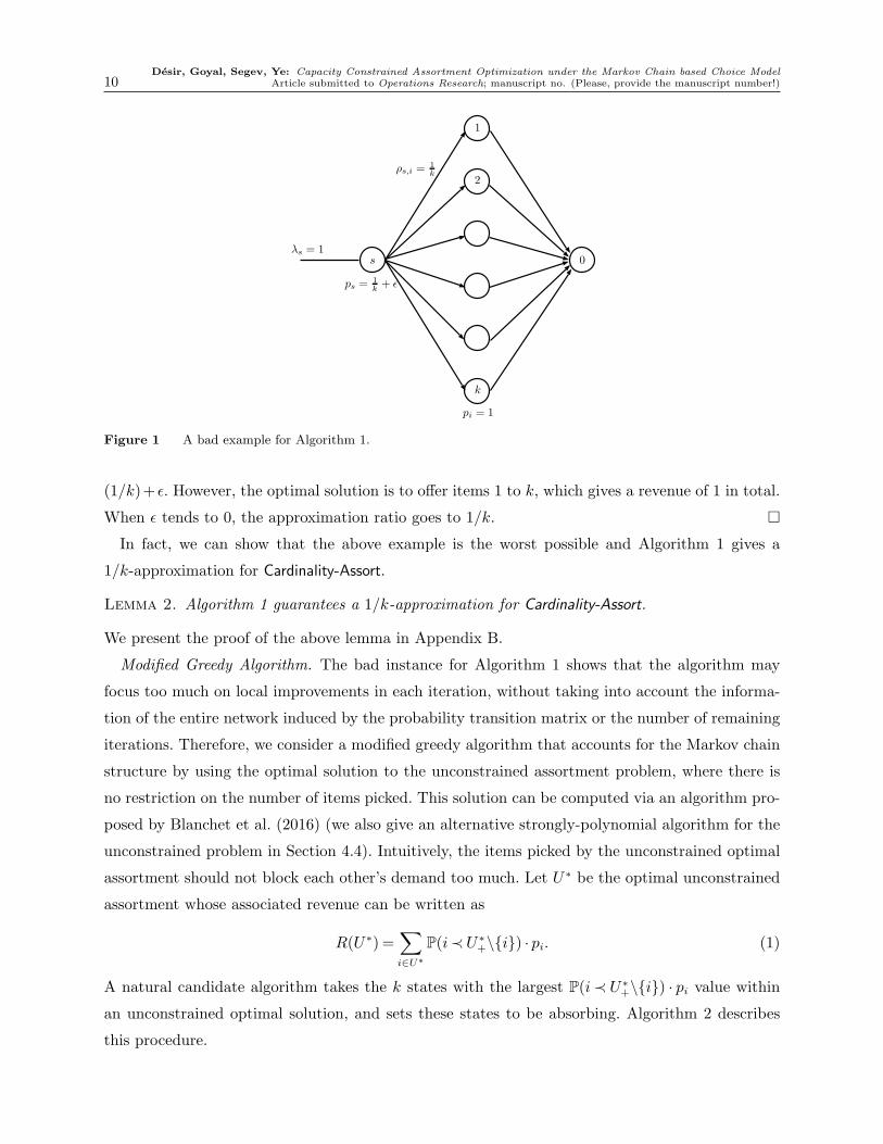
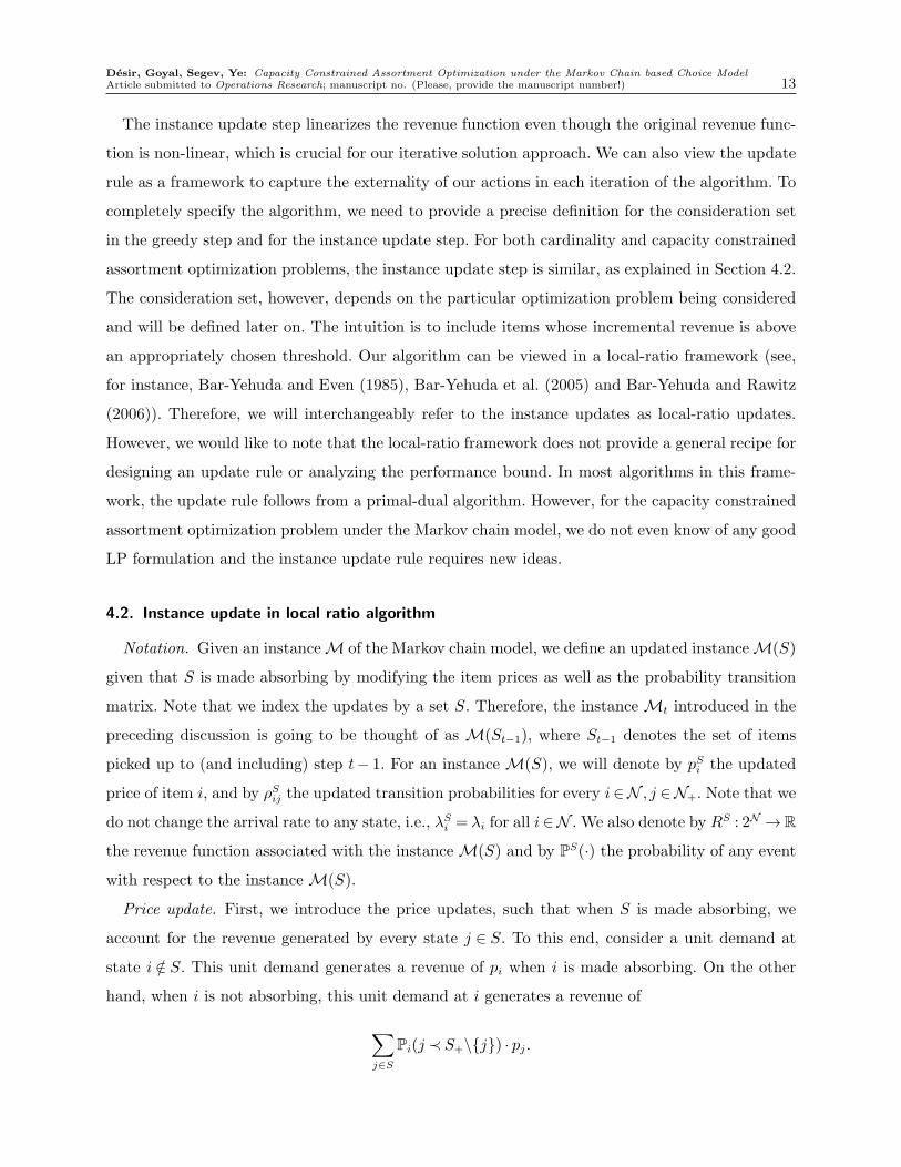
Proof. Consider the following instance of Cardinality-Assort with n= k+1 items, where k is the
upper bound specified by the cardinality constraint. We have a state s and states i= 0, . . . , k. The
arrival rates are all equal to 0, except for λs which is equal to 1. Moreover
pi =
{(1/k)+ ε if i= s
1 if i= 1, . . . , k,ρij =
1/k if i= s and j = 1, . . . , k1 if i= 1, . . . , k and j = 00 otherwise,
where ε≤ 1/(2k). Figure 1 provides a graphical representation of this instance. Algorithm 1 first
picks item s as R({s}) = (1/k) + ε while R({i}) = (1/k), for i= 1, . . . k. Once s is selected, adding
any other state cannot increase the revenue. Therefore, the greedy algorithm gives a revenue of
Desir, Goyal, Segev, Ye: Capacity Constrained Assortment Optimization under the Markov Chain based Choice Model10 Article submitted to Operations Research; manuscript no. (Please, provide the manuscript number!)
s
1
2
k
0
ps =1k + ε
ρs,i =1k
pi = 1
λs = 1
Figure 1 A bad example for Algorithm 1.
(1/k)+ ε. However, the optimal solution is to offer items 1 to k, which gives a revenue of 1 in total.
When ε tends to 0, the approximation ratio goes to 1/k. �
In fact, we can show that the above example is the worst possible and Algorithm 1 gives a
1/k-approximation for Cardinality-Assort.
Lemma 2. Algorithm 1 guarantees a 1/k-approximation for Cardinality-Assort.
We present the proof of the above lemma in Appendix B.
Modified Greedy Algorithm. The bad instance for Algorithm 1 shows that the algorithm may
focus too much on local improvements in each iteration, without taking into account the informa-
tion of the entire network induced by the probability transition matrix or the number of remaining
iterations. Therefore, we consider a modified greedy algorithm that accounts for the Markov chain
structure by using the optimal solution to the unconstrained assortment problem, where there is
no restriction on the number of items picked. This solution can be computed via an algorithm pro-
posed by Blanchet et al. (2016) (we also give an alternative strongly-polynomial algorithm for the
unconstrained problem in Section 4.4). Intuitively, the items picked by the unconstrained optimal
assortment should not block each other’s demand too much. Let U∗ be the optimal unconstrained
assortment whose associated revenue can be written as
R(U∗) =∑
i∈U∗
P(i≺U∗+\{i}) · pi. (1)
A natural candidate algorithm takes the k states with the largest P(i≺ U∗+\{i}) · pi value within
an unconstrained optimal solution, and sets these states to be absorbing. Algorithm 2 describes
this procedure.

Desir, Goyal, Segev, Ye: Capacity Constrained Assortment Optimization under the Markov Chain based Choice ModelArticle submitted to Operations Research; manuscript no. (Please, provide the manuscript number!) 11
Algorithm 2 Greedy Algorithm on Optimal Unconstrained Assortment
1: Let U∗ be an optimal solution to the unconstrained problem.
2: Sort items of U∗ in decreasing order of P(i≺U∗+\{i}) · pi.
3: Return S = {top k items in the sorted order}.
We show in the following lemma that even Algorithm 2 performs poorly in the worst case. In
fact, we present an example where every subset of k items of the optimal solution U∗ has revenue
a factor k away from the optimal.
Lemma 3. There are instances where the revenue obtained by Algorithm 2 is far from optimal by
a factor of k/|U∗| where k is the upper bound in the cardinality constraint.
Proof. Consider the following instance of the problem with n+ 2 items (or states). We have
a state s and states i= 1, . . . , n and state 0 corresponding to the no-purchase option. The arrival
rates are all equal to 0, except for λs which is equal to 1. Moreover
pi =
{1− ε if i= s1 if i= 1, . . . , n,
ρij =
1/n if i= s and j = 1, . . . , n1 if i= 1, . . . , n and j = 00 otherwise,
where ε > 0. Figure 2 provides a graphical representation of this instance. For this example, the
s
1
2
n
0
ps = 1− ε
ρs,i =1n
pi = 1
λs = 1
Figure 2 A bad example for Algorithm 2.
unconstrained optimal assortment is U∗ = {1, . . . , n}, and the greedy algorithm on U∗ selects k
items among U∗, meaning that a total revenue of k/n is obtained. However, the optimal solution
of the constrained problem is to only offer item s, which gives a revenue of 1− ε. As ε tends to 0,
the approximation ratio goes to k/|U∗|. �
Desir, Goyal, Segev, Ye: Capacity Constrained Assortment Optimization under the Markov Chain based Choice Model12 Article submitted to Operations Research; manuscript no. (Please, provide the manuscript number!)
The poor performance of Algorithm 2 on the above example illustrates that an optimal assort-
ment for the constrained problem may be very different from that of its unconstrained counterpart.
Hence, searching within an unconstrained optimal solution for a good approximate solution to the
constrained problem can be unfruitful in general. It is worth noting that the lower bound of k/|U∗|
for Algorithm 2 is tight, as stated in the following lemma, whose proof is given in Appendix C.
Lemma 4. Algorithm 2 guarantees a k/|U∗|-approximation algorithm to Cardinality-Assort.
The analysis of the two greedy variants for the cardinality constrained assortment optimization
under the Markov chain model provides important insights that we use towards designing a good
algorithm for the problem.
4. Local Ratio based Algorithm Design
In this section, we present the general framework of our approximation algorithm for the cardinality
and capacity constrained assortment optimization under the Markov chain model.
4.1. High-level ideas
As the example in Figure 1 illustrates, Algorithm 1 could end up with a highly suboptimal solution
due to picking items that cannibalize, i.e. block, the demand for higher price items. Picking the
highest price item will eliminate such a concern. However, a high price item might only capture
very little demand, and therefore, generate very small revenue as illustrated in the example in
Figure 2. When there is a capacity constraint on the assortment, picking such items may not be an
optimal use of the capacity. This motivates us to choose the highest price item in an appropriate
consideration set. Intuitively, the consideration set will consist of items that generate sufficiently
high incremental revenue.
We first give a high-level description of our algorithm that builds the solution iteratively. Let
Mt denote the problem instance in any iteration t. The algorithm (ALG) considers the following
two steps in each iteration t:
1. Greedy Selection. Define an appropriate consideration set Ct of items, and pick the “highest
price” item from Ct.
2. Instance Update. Construct a new instance, Mt+1, of the constrained assortment optimization
problem with appropriately modified item prices and transition probabilities such that
ALG(Mt) =∆t +ALG(Mt+1),
where ALG(·) is the revenue of the solution obtained by the algorithm on a given instance, and ∆t
is the incremental revenue in the objective value from the item selected in iteration t.
Desir, Goyal, Segev, Ye: Capacity Constrained Assortment Optimization under the Markov Chain based Choice ModelArticle submitted to Operations Research; manuscript no. (Please, provide the manuscript number!) 13
The instance update step linearizes the revenue function even though the original revenue func-
tion is non-linear, which is crucial for our iterative solution approach. We can also view the update
rule as a framework to capture the externality of our actions in each iteration of the algorithm. To
completely specify the algorithm, we need to provide a precise definition for the consideration set
in the greedy step and for the instance update step. For both cardinality and capacity constrained
assortment optimization problems, the instance update step is similar, as explained in Section 4.2.
The consideration set, however, depends on the particular optimization problem being considered
and will be defined later on. The intuition is to include items whose incremental revenue is above
an appropriately chosen threshold. Our algorithm can be viewed in a local-ratio framework (see,
for instance, Bar-Yehuda and Even (1985), Bar-Yehuda et al. (2005) and Bar-Yehuda and Rawitz
(2006)). Therefore, we will interchangeably refer to the instance updates as local-ratio updates.
However, we would like to note that the local-ratio framework does not provide a general recipe for
designing an update rule or analyzing the performance bound. In most algorithms in this frame-
work, the update rule follows from a primal-dual algorithm. However, for the capacity constrained
assortment optimization problem under the Markov chain model, we do not even know of any good
LP formulation and the instance update rule requires new ideas.
4.2. Instance update in local ratio algorithm
Notation. Given an instanceM of the Markov chain model, we define an updated instanceM(S)
given that S is made absorbing by modifying the item prices as well as the probability transition
matrix. Note that we index the updates by a set S. Therefore, the instance Mt introduced in the
preceding discussion is going to be thought of as M(St−1), where St−1 denotes the set of items
picked up to (and including) step t− 1. For an instance M(S), we will denote by pSi the updated
price of item i, and by ρSij the updated transition probabilities for every i∈N , j ∈N+. Note that we
do not change the arrival rate to any state, i.e., λSi = λi for all i∈N . We also denote by RS : 2N →R
the revenue function associated with the instance M(S) and by PS(·) the probability of any event
with respect to the instance M(S).
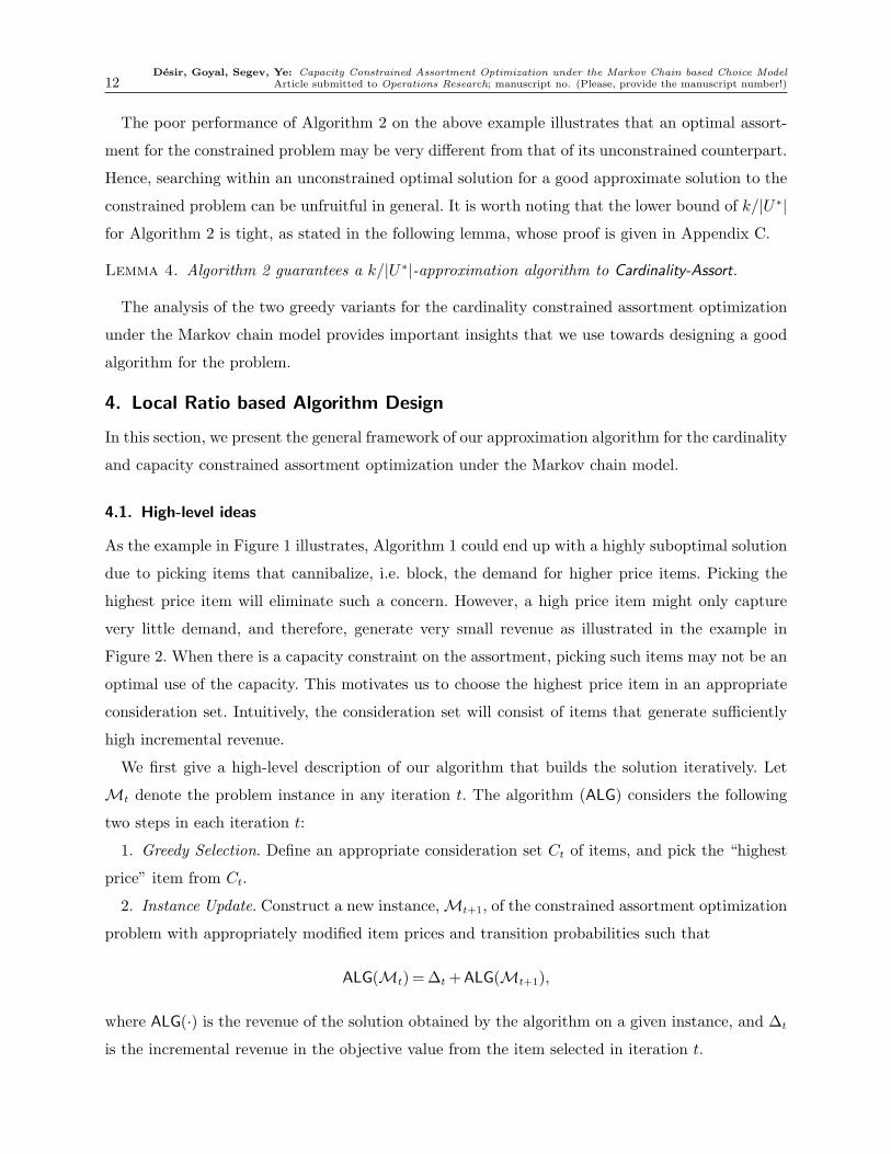
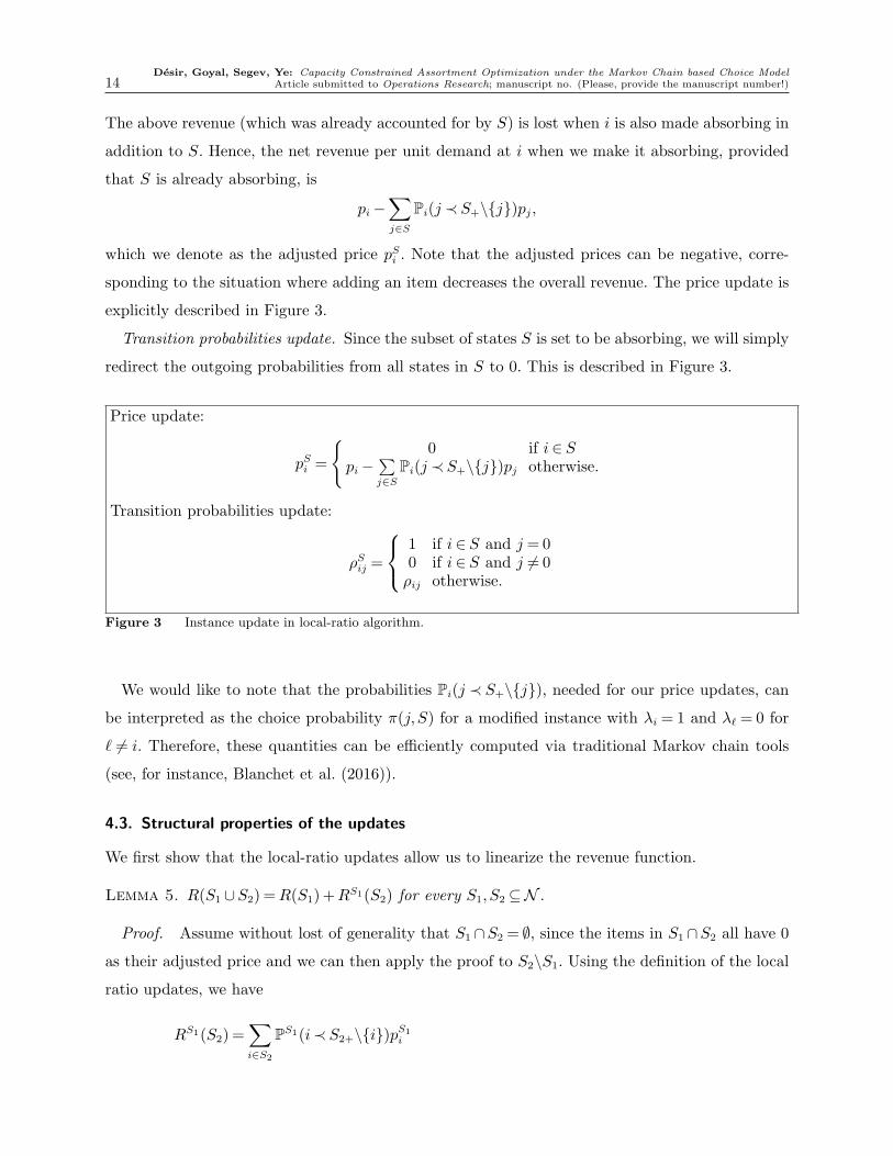
Price update. First, we introduce the price updates, such that when S is made absorbing, we
account for the revenue generated by every state j ∈ S. To this end, consider a unit demand at
state i /∈ S. This unit demand generates a revenue of pi when i is made absorbing. On the other
hand, when i is not absorbing, this unit demand at i generates a revenue of
∑
j∈S
Pi(j ≺ S+\{j}) · pj.
Desir, Goyal, Segev, Ye: Capacity Constrained Assortment Optimization under the Markov Chain based Choice Model14 Article submitted to Operations Research; manuscript no. (Please, provide the manuscript number!)
The above revenue (which was already accounted for by S) is lost when i is also made absorbing in
addition to S. Hence, the net revenue per unit demand at i when we make it absorbing, provided
that S is already absorbing, is
pi −∑
j∈S
Pi(j ≺ S+\{j})pj,
which we denote as the adjusted price pSi . Note that the adjusted prices can be negative, corre-
sponding to the situation where adding an item decreases the overall revenue. The price update is
explicitly described in Figure 3.
Transition probabilities update. Since the subset of states S is set to be absorbing, we will simply
redirect the outgoing probabilities from all states in S to 0. This is described in Figure 3.
Price update:
pSi =
{0 if i∈ S
pi −∑
j∈S
Pi(j ≺ S+\{j})pj otherwise.
Transition probabilities update:
ρSij =
1 if i∈ S and j = 00 if i∈ S and j 6= 0ρij otherwise.
Figure 3 Instance update in local-ratio algorithm.
We would like to note that the probabilities Pi(j ≺ S+\{j}), needed for our price updates, can
be interpreted as the choice probability π(j,S) for a modified instance with λi = 1 and λ` = 0 for
` 6= i. Therefore, these quantities can be efficiently computed via traditional Markov chain tools
(see, for instance, Blanchet et al. (2016)).
4.3. Structural properties of the updates
We first show that the local-ratio updates allow us to linearize the revenue function.
Lemma 5. R(S1 ∪S2) =R(S1)+RS1(S2) for every S1, S2 ⊆N .
Proof. Assume without lost of generality that S1 ∩S2 = ∅, since the items in S1 ∩S2 all have 0
as their adjusted price and we can then apply the proof to S2\S1. Using the definition of the local
ratio updates, we have
RS1(S2) =∑
i∈S2
PS1(i≺ S2+\{i})pS1
i
Desir, Goyal, Segev, Ye: Capacity Constrained Assortment Optimization under the Markov Chain based Choice ModelArticle submitted to Operations Research; manuscript no. (Please, provide the manuscript number!) 15
=∑
i∈S2
PS1(i≺ S2+\{i})
(
pi −∑
j∈S1
Pi(j ≺ S1+\{j})pj
)
=∑
i∈S2
PS1(i≺ S2+\{i})pi −∑
j∈S1
∑
i∈S2
PS1(i≺ S2+\{i})Pi(j ≺ S1+\{j})pj.
With the definition of ρS1 , note that all items of S1 are redirected to 0. This, together with the
fact that S1 ∩S2 = ∅ implies that for all i ∈ S2, we have PS1(i≺ S2+\{i}) = P(i≺ (S2 ∪S1)+\{i}).
Consequently,
R(S1)+RS1(S2) =∑
j∈S1
(
P(j ≺ S1+\{j})−∑
i∈S2
P(i≺ (S2 ∪S1)+\{i})Pi(j ≺ S1+\{j})
)
pj
+∑
i∈S2
P(i≺ (S2 ∪S1)+\{i})pi
=∑
j∈S1
(P(j ≺ S1+\{j})−P(S2 ≺ j ≺ S1+\{j}))pj
+∑
i∈S2
P(i≺ (S2 ∪S1)+\{i})pi
=∑
j∈S1
P(j ≺ (S2 ∪S1)+\{j})pj +∑
i∈S2
P(i≺ (S2 ∪S1)+\{i})pi
=R(S1 ∪S2),
where the second equality holds since
∑
i∈S2
P(i≺ (S2 ∪S1)+\{i})Pi(j ≺ S1+\{j}) = P(S2 ≺ j ≺ S1+\{j}),
as by the Markov property, both the left and right terms in the above equality denote the probability
that we will visit some state in S2 before any state in S1+, followed by state j ∈ S1 before any other
state in S1+. �
The next lemma shows that the composition of two local ratio updates over subsets S1 and S2
is equivalent to a single local ratio update over S1 ∪ S2. This property is crucial for repeatedly
applying local-ratio updates.
Lemma 6. Let S1 ⊆N be some assortment, and let M1 =M(S1). For any S2 with S1 ∩ S2 = ∅,
the instance M1(S2) is identical to the instance M(S1∪S2) in terms of item prices and transition
probabilities.
It suffices to verify that (pS1
i )S2 = pS1∪S2
i for all S1,S2 and i /∈ S1∪S2, as the above identity clearly
holds for the transition matrix updates. The proof is similar to that of Lemma 5, and is presented
in Appendix D. Putting the previous two lemmas together gives the following claim.
Lemma 7. RS1(S2 ∪S3) =RS1(S2)+RS1∪S2(S3) for any pairwise-disjoint sets S1, S2, S3 ⊆N .
Desir, Goyal, Segev, Ye: Capacity Constrained Assortment Optimization under the Markov Chain based Choice Model16 Article submitted to Operations Research; manuscript no. (Please, provide the manuscript number!)
4.4. Warm-up: Exact algorithm for the unconstrained problem
As a warmup, we first present an alternative exact algorithm for the unconstrained assortment
optimization problem under the Markov chain model by using the local-ratio framework. Our
algorithm is based on the observation that it is always optimal to offer the highest price item for the
unconstrained problem, as it does not cannibalize the demand of other items. The latter property is
implied by a slightly more general claim, formalized as follows. For any x∈R, let [x]+ =max(x,0).
Lemma 8. Let S ⊆N . For any item i /∈ S with price pi ≥ [maxj∈S pj]+, we have R(S∪{i})≥R(S).
Proof. From Lemma 5, we have that
R(S ∪{i}) =R(S)+RS({i}) =R(S)+PS(i≺ 0) · pSi .
Now, pi ≥ [maxj∈S pj]+ and
pSi = pi −∑
j∈S
Pi(j ≺ S+ \ {j}) · pj ≥ 0,
which implies R(S ∪{i})≥R(S). �
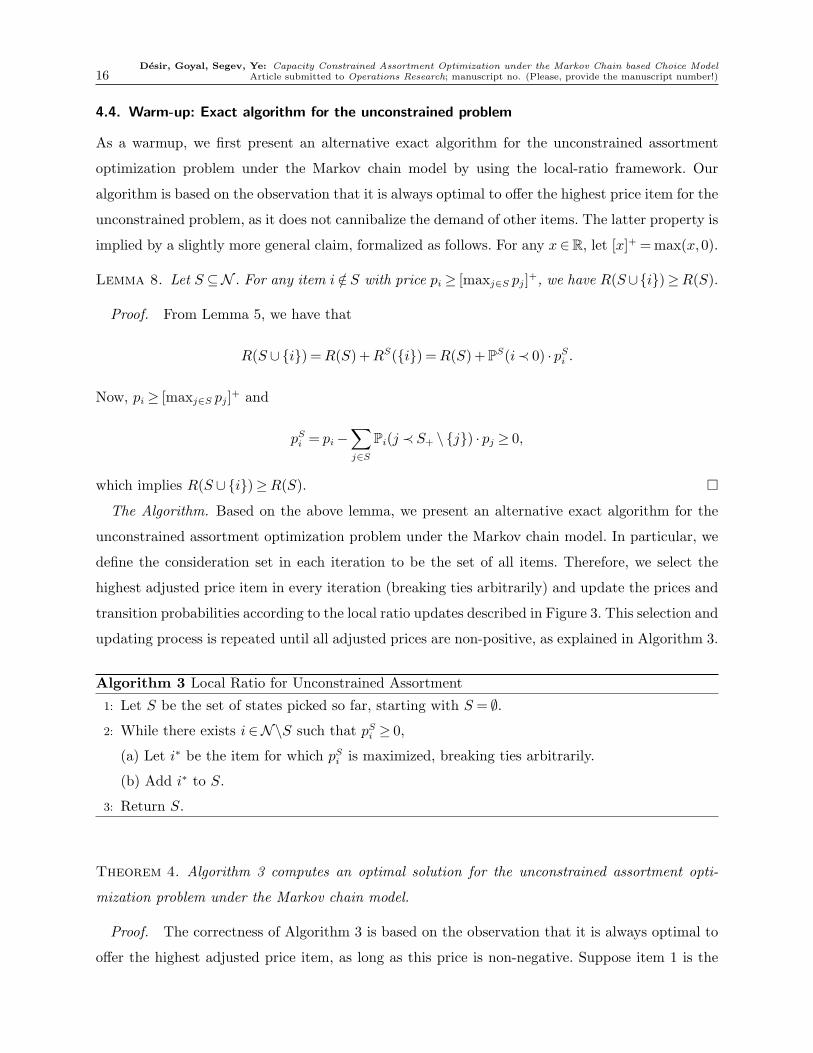
The Algorithm. Based on the above lemma, we present an alternative exact algorithm for the
unconstrained assortment optimization problem under the Markov chain model. In particular, we
define the consideration set in each iteration to be the set of all items. Therefore, we select the
highest adjusted price item in every iteration (breaking ties arbitrarily) and update the prices and
transition probabilities according to the local ratio updates described in Figure 3. This selection and
updating process is repeated until all adjusted prices are non-positive, as explained in Algorithm 3.
Algorithm 3 Local Ratio for Unconstrained Assortment
1: Let S be the set of states picked so far, starting with S = ∅.
2: While there exists i∈N\S such that pSi ≥ 0,
(a) Let i∗ be the item for which pSi is maximized, breaking ties arbitrarily.
(b) Add i∗ to S.
3: Return S.
Theorem 4. Algorithm 3 computes an optimal solution for the unconstrained assortment opti-
mization problem under the Markov chain model.
Proof. The correctness of Algorithm 3 is based on the observation that it is always optimal to
offer the highest adjusted price item, as long as this price is non-negative. Suppose item 1 is the

Desir, Goyal, Segev, Ye: Capacity Constrained Assortment Optimization under the Markov Chain based Choice ModelArticle submitted to Operations Research; manuscript no. (Please, provide the manuscript number!) 17
highest price item. From Lemma 8, we get R(S ∪{1})≥R(S) for any assortment S. Therefore, we
can assume that item 1 belongs to the optimal assortment. From Lemma 5, we can write
maxS⊆N
R(S) =R({1})+ maxS′⊆N\{1}
R{1}(S′).
It remains to show that, when we get to an iteration where our current absorption set is X, and the
adjusted price of every state in the modified instance M(X) is non-positive, then X is an optimal
solution to M. To see this, by repeated applications of Lemmas 5 and 6, we have
maxS⊆N
R(S) =R(X)+ maxS′⊆N\X
RX(S′).
However, since the adjusted price of every state in the instance M(X) is non-positive, we must
have RX(S′)≤ 0 for all S′ ⊆N\X. Hence, it is optimal not to make any state in M(X) absorbing,
which implies that X is an optimal solution to M. �
Implications. Our algorithm for the unconstrained assortment optimization over the Markov
chain model provides interesting insights for some known results about the optimal stopping prob-
lem and the assortment optimization over the MNL model. Blanchet et al. (2016) relate the uncon-
strained assortment problem to the optimal stopping time on a Markov chain (see Chow et al.
(1971)). In this problem, we need to decide at each state i whether to stop and get the reward pi,
or transition according to the transition probabilities of the Markov chain. Moreover, there is an
absorbing state 0 with price p0 = 0. Algorithm 3 for the unconstrained assortment optimization
problem gives an alternative strongly polynomial time algorithm for the optimal stopping problem.
Blanchet et al. (2016) prove that the MNL choice model is a special case of the Markov chain
based choice model. Therefore, by analyzing Algorithm 3 to solve the assortment optimization over
the MNL model, we can recover the structure of the optimal assortment being nested by prices, i.e.,
the optimal assortment consists of the ` top-priced items for some `. We give an explicit expression
for our local ratio updates when the underlying choice model is MNL in Appendix E.
5. Cardinality Constrained Assortment Optimization for General Case
In this section, we present a (1/2− ε)-approximation for the cardinality constrained assortment
optimization under the Markov chain model, for any fixed ε > 0. Following the local-ratio framework
described in Section 4, our algorithm for the cardinality constrained case also selects a state with
high adjusted price in each step from an appropriate consideration set. The consideration set is
defined to avoid picking states that have a high adjusted price but capture very little demand. In
particular, the consideration set includes only items whose incremental revenue is at least a certain
threshold.
Desir, Goyal, Segev, Ye: Capacity Constrained Assortment Optimization under the Markov Chain based Choice Model18 Article submitted to Operations Research; manuscript no. (Please, provide the manuscript number!)
The Algorithm. Our algorithm is iterative and selects a single item in each step. Let St be the
set of selected items by the end of step t, starting with S0 = ∅. We use σt to denote the item picked
in step t, meaning that St = {σ1, . . . , σt}. At every step t≥ 1, we select the highest adjusted price
item (with respect to pSt−1 , breaking ties arbitrarily) among items in the following consideration
set:
Ct =
{
i∈N\St−1 :RSt−1({i})≥ α
R(S∗)
k
}
,
where S∗ is the optimal solution, k is the cardinality bound, and α ∈ (0,1) is a parameter whose
value will be optimized later. Note that Ct is defined at the beginning of step t, whereas St is
defined at the end of step t, and includes the item selected in this step. Once the item σt is selected,
we recompute the adjusted prices via the local ratio update described in Figure 3, and update the
consideration set to get Ct+1. The algorithm terminates when either k items have already been
picked (i.e., upon the completion of step k), or when the consideration set Ct becomes empty.
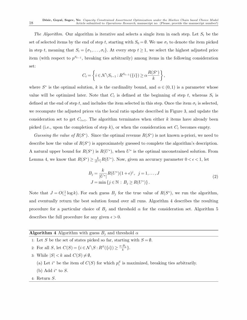
Guessing the value of R(S∗). Since the optimal revenue R(S∗) is not known a-priori, we need to
describe how the value of R(S∗) is approximately guessed to complete the algorithm’s description.
A natural upper bound for R(S∗) is R(U∗), when U∗ is the optimal unconstrained solution. From
Lemma 4, we know that R(S∗)≥ k|U∗|
R(U∗). Now, given an accuracy parameter 0< ε< 1, let
Bj =k
|U∗|R(U∗)(1+ ε)j, j = 1, . . . , J
J =min{j ∈N : Bj ≥R(U∗)} .
(2)
Note that J = O( 1εlogk). For each guess Bj for the true value of R(S∗), we run the algorithm,
and eventually return the best solution found over all runs. Algorithm 4 describes the resulting
procedure for a particular choice of Bj and threshold α for the consideration set. Algorithm 5
describes the full procedure for any given ε > 0.
Algorithm 4 Algorithm with guess Bj and threshold α
1: Let S be the set of states picked so far, starting with S = ∅.
2: For all S, let C(S) = {i∈N\S :RS({i})≥α·Bj
k}.
3: While |S|< k and C(S) 6= ∅,
(a) Let i∗ be the item of C(S) for which pSi is maximized, breaking ties arbitrarily.
(b) Add i∗ to S.
4: Return S.
Desir, Goyal, Segev, Ye: Capacity Constrained Assortment Optimization under the Markov Chain based Choice ModelArticle submitted to Operations Research; manuscript no. (Please, provide the manuscript number!) 19
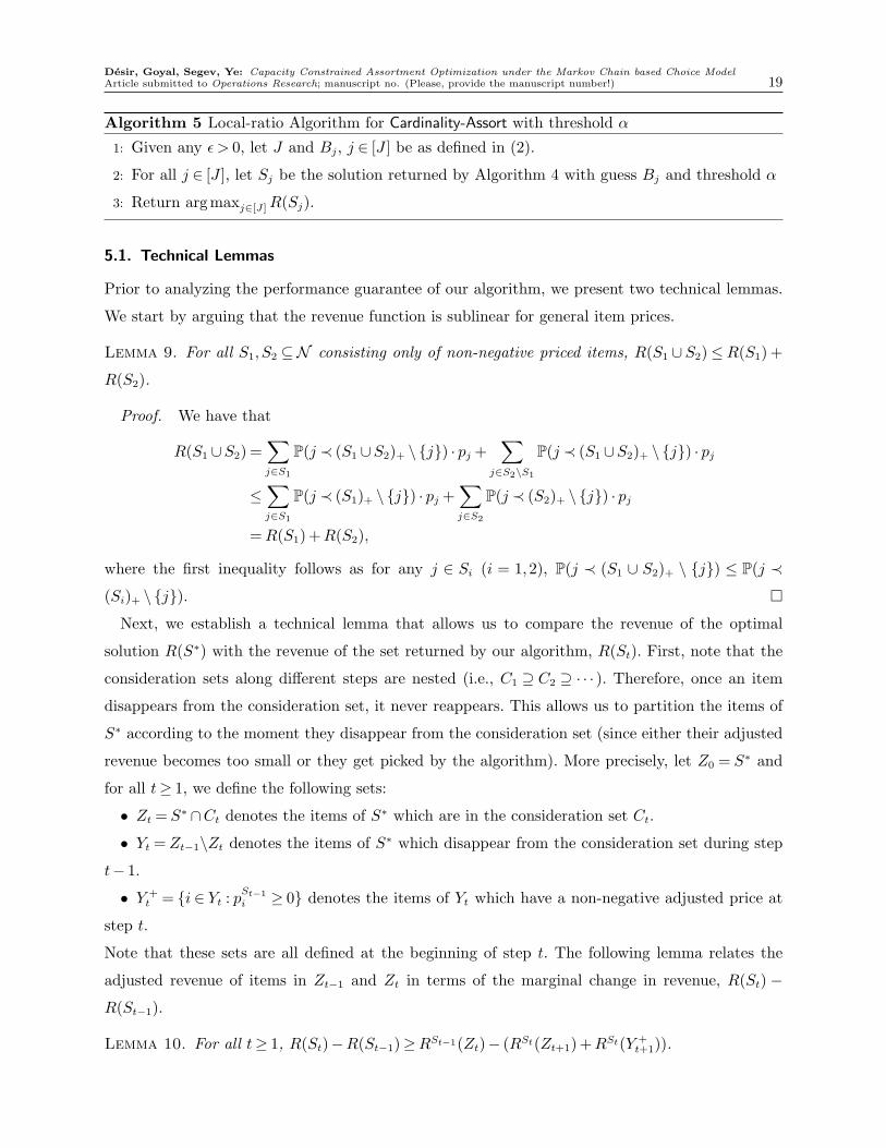
Algorithm 5 Local-ratio Algorithm for Cardinality-Assort with threshold α
1: Given any ε > 0, let J and Bj, j ∈ [J ] be as defined in (2).
2: For all j ∈ [J ], let Sj be the solution returned by Algorithm 4 with guess Bj and threshold α
3: Return argmaxj∈[J]R(Sj).
5.1. Technical Lemmas
Prior to analyzing the performance guarantee of our algorithm, we present two technical lemmas.
We start by arguing that the revenue function is sublinear for general item prices.
Lemma 9. For all S1, S2 ⊆N consisting only of non-negative priced items, R(S1 ∪ S2)≤R(S1) +
R(S2).
Proof. We have that
R(S1 ∪S2) =∑
j∈S1
P(j ≺ (S1 ∪S2)+ \ {j}) · pj +∑
j∈S2\S1
P(j ≺ (S1 ∪S2)+ \ {j}) · pj
≤∑
j∈S1
P(j ≺ (S1)+ \ {j}) · pj +∑
j∈S2
P(j ≺ (S2)+ \ {j}) · pj
=R(S1)+R(S2),
where the first inequality follows as for any j ∈ Si (i = 1,2), P(j ≺ (S1 ∪ S2)+ \ {j}) ≤ P(j ≺
(Si)+ \ {j}). �
Next, we establish a technical lemma that allows us to compare the revenue of the optimal
solution R(S∗) with the revenue of the set returned by our algorithm, R(St). First, note that the
consideration sets along different steps are nested (i.e., C1 ⊇ C2 ⊇ · · · ). Therefore, once an item
disappears from the consideration set, it never reappears. This allows us to partition the items of
S∗ according to the moment they disappear from the consideration set (since either their adjusted
revenue becomes too small or they get picked by the algorithm). More precisely, let Z0 = S∗ and
for all t≥ 1, we define the following sets:
• Zt = S∗ ∩Ct denotes the items of S∗ which are in the consideration set Ct.
• Yt =Zt−1\Zt denotes the items of S∗ which disappear from the consideration set during step
t− 1.
• Y +t = {i ∈ Yt : p
St−1
i ≥ 0} denotes the items of Yt which have a non-negative adjusted price at
step t.
Note that these sets are all defined at the beginning of step t. The following lemma relates the
adjusted revenue of items in Zt−1 and Zt in terms of the marginal change in revenue, R(St) −
R(St−1).
Lemma 10. For all t≥ 1, R(St)−R(St−1)≥RSt−1(Zt)− (RSt(Zt+1)+RSt(Y +t+1)).

Desir, Goyal, Segev, Ye: Capacity Constrained Assortment Optimization under the Markov Chain based Choice Model20 Article submitted to Operations Research; manuscript no. (Please, provide the manuscript number!)
Proof. Recall that, by definition, Zt contains the items of S∗ that are in the consideration set
at the beginning of step t. Since our algorithm picks the highest adjusted price item, σt, in the
consideration set Ct, we have pSt−1σt ≥ p
St−1
i ≥ 0 for all items i∈Zt. Therefore, by Lemma 8,
RSt−1(Zt)≤RSt−1(Zt ∪{σt}). (3)
We now consider two cases, depending on whether the item σt appears in the optimal solution S∗
or not.
Case (a): σt /∈ S∗. From Lemma 7, RSt−1(Zt∪{σt}) =RSt−1({σt})+R
St(Zt). Consequently, from
inequality (3), we have
RSt−1(Zt)≤RSt−1({σt})+RSt(Zt)
=RSt−1({σt})+RSt(Zt+1 ∪Yt+1)
≤RSt−1({σt})+RSt(Zt+1 ∪Y+t+1)
≤RSt−1({σt})+RSt(Zt+1)+RSt(Y +t+1),
where the second inequality holds since removing all negative adjusted price items can only increase
net revenue, and the last inequality follows from Lemma 9. Adding R(St−1) on both sides of the
inequality yields the desired inequality by Lemma 5.
Case (b): σt ∈ S∗. From Lemma 7, RSt−1(Zt) =RSt−1({σt})+R
St(Zt\{σt}). Then, similar to the
previous case, we have
RSt(Zt\{σt})≤RSt((Zt+1 ∪Y+t+1)\{σt})≤RSt(Zt+1)+RSt(Y +
t+1\{σt}).
Note that RSt(Y +t+1\{σt}) =RSt(Y +
t+1) since pStσt= 0 and σt is an absorbing state in M(St). Adding
R(St−1) on both sides of the inequality concludes the proof. �
From the above result, we obtain the following claim.
Lemma 11. For all t≥ 0, we have R(St)≥R(S∗)− (RSt(Zt+1)+∑t+1
j=1RSj−1(Y +
j )).
Proof. By summing the inequality stated in Lemma 10 over j = 1, . . . , t, we obtain a telescopic
sum which yields
R(St)≥R(Z1)−
(
RSt(Zt+1)+t+1∑
j=2
RSj−1(Y +j )
)
.
Since every item in S∗ must have non-negative price and S∗ = Z1 ∪ Y1 by definition, we have
R(S∗)≤R(Z1) +R(Y1) by sublinearity of the revenue function (see Lemma 9). Combining these
two inequalities concludes the proof. �
Desir, Goyal, Segev, Ye: Capacity Constrained Assortment Optimization under the Markov Chain based Choice ModelArticle submitted to Operations Research; manuscript no. (Please, provide the manuscript number!) 21
5.2. Analysis of the Local-Ratio Algorithm
We show that the local-ratio algorithm gives a (1/2− ε)-approximation for Cardinality-Assort for
any fixed ε > 0. In particular, we have the following theorem.
Theorem 5. For any fixed ε > 0, Algorithm 5 gives a (1/2 − ε/2)-approximation for
Cardinality-Assort. Moreover, the running time is polynomial in the input size and 1/ε.
Proof. For a fixed ε > 0, let j∗ be such that R(S∗)
1+ε≤Bj∗ ≤R(S∗). Let B =Bj∗ and consider the
solution returned by Algorithm 4 with guess B and threshold α. We consider two cases based on
the condition by which the algorithm terminates.
Case 1. If the algorithm stops after completing step k, then by linearity of the revenue when
using the local ratio updates (Lemmas 5 and 6), the resulting solution Sk has a revenue of
R(Sk) =k∑
t=1
RSt−1({σt})≥ αB ≥α
1+ ε·R(S∗)≥ (1− ε)αR(S∗),
where the above inequality holds since the item σt belongs to the consideration set Ct, and therefore
RSt−1({σt})≥ αB/k.
Case 2. Now, suppose the algorithm stops at the end of step k′ < k, after discovering that
Ck′+1 = ∅. From Lemma 11, we get
R(Sk′)+RSk′ (Zk′+1)≥R(S∗)−k′+1∑
j=1
RSj−1(Y +j ).
Now, since Ck′+1 = ∅, this implies that Zk′+1 = ∅. Moreover, from Lemma 9, we also have
RSj−1(Y +j )< |Y +
j | ·α ·B/k for all j = 1, . . . , k′ +1. Therefore,
k′+1∑
j=1
RSj−1(Y +j )≤ α ·
B
k·k′+1∑
j=1
|Y +j | ≤ αB ≤ αR(S∗),
where the second inequality holds since∑k′+1
j=1 |Y +j | ≤ k and the last inequality holds as B ≤R(S∗).
Therefore,
R(Sk′)≥R(S∗)−αR(S∗) = (1−α) ·R(S∗).
This shows that the approximation ratio attained by our algorithm is
min{(1− ε)α, 1−α} .
Picking α= 1/2 we obtain a (1/2− ε/2)-approximation for Cardinality-Assort.
Running time. Algorithm 5 considers J =O( 1εlogn) guesses for R(S∗). For any given guess Bj,
the running time of Algorithm 4 is polynomial in the input size. Therefore, the overall running
time of Algorithm 5 is polynomial in the input size and 1/ε. �
Desir, Goyal, Segev, Ye: Capacity Constrained Assortment Optimization under the Markov Chain based Choice Model22 Article submitted to Operations Research; manuscript no. (Please, provide the manuscript number!)
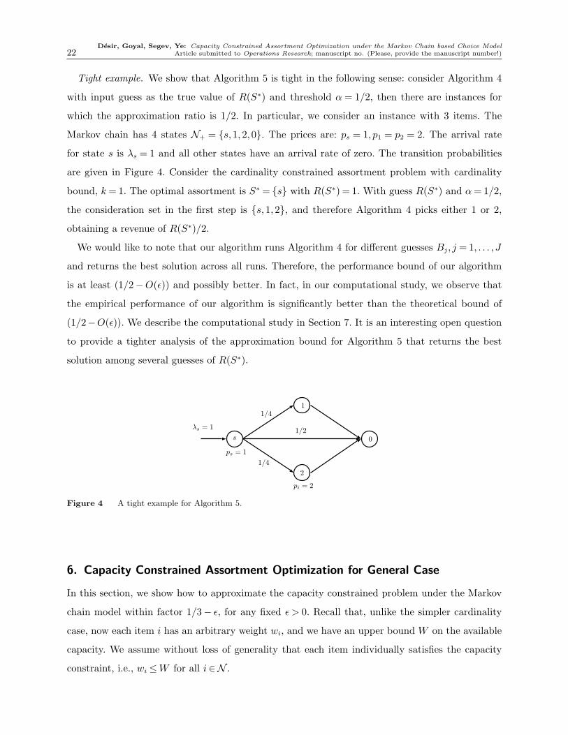
Tight example. We show that Algorithm 5 is tight in the following sense: consider Algorithm 4
with input guess as the true value of R(S∗) and threshold α = 1/2, then there are instances for
which the approximation ratio is 1/2. In particular, we consider an instance with 3 items. The
Markov chain has 4 states N+ = {s,1,2,0}. The prices are: ps = 1, p1 = p2 = 2. The arrival rate
for state s is λs = 1 and all other states have an arrival rate of zero. The transition probabilities
are given in Figure 4. Consider the cardinality constrained assortment problem with cardinality
bound, k= 1. The optimal assortment is S∗ = {s} with R(S∗) = 1. With guess R(S∗) and α= 1/2,
the consideration set in the first step is {s,1,2}, and therefore Algorithm 4 picks either 1 or 2,
obtaining a revenue of R(S∗)/2.
We would like to note that our algorithm runs Algorithm 4 for different guesses Bj, j = 1, . . . , J
and returns the best solution across all runs. Therefore, the performance bound of our algorithm
is at least (1/2−O(ε)) and possibly better. In fact, in our computational study, we observe that
the empirical performance of our algorithm is significantly better than the theoretical bound of
(1/2−O(ε)). We describe the computational study in Section 7. It is an interesting open question
to provide a tighter analysis of the approximation bound for Algorithm 5 that returns the best
solution among several guesses of R(S∗).
λs = 1
ps = 1
1/41
2
pi = 2
0s
1/4
1/2
Figure 4 A tight example for Algorithm 5.
6. Capacity Constrained Assortment Optimization for General Case
In this section, we show how to approximate the capacity constrained problem under the Markov
chain model within factor 1/3− ε, for any fixed ε > 0. Recall that, unlike the simpler cardinality
case, now each item i has an arbitrary weight wi, and we have an upper bound W on the available
capacity. We assume without loss of generality that each item individually satisfies the capacity
constraint, i.e., wi ≤W for all i∈N .
Desir, Goyal, Segev, Ye: Capacity Constrained Assortment Optimization under the Markov Chain based Choice ModelArticle submitted to Operations Research; manuscript no. (Please, provide the manuscript number!) 23
The Algorithm. We describe a local-ratio based algorithm, similar in spirit to the one for the
cardinality constrained problem, by suitably adapting the way consideration sets are defined. For
this purpose, instead of considering items whose incremental absorption revenue exceeds a certain
threshold, we only consider items whose incremental absorption revenue per unit of weight exceeds
a certain threshold.
Again, our algorithm selects a single item in each step. Let St be the set of selected items by the
end of step t, starting with S0 = ∅. We use σt to denote the item picked in step t, meaning that
St = {σ1, . . . , σt}. At every step t ≥ 1, we select the highest adjusted price item (with respect to
pSt−1 , breaking ties arbitrarily) among items in the following consideration set:
Ct =
{
i∈N\St−1 :RSt−1({i})
wi
≥ αR(S∗)
W
}
,
where S∗ is the optimal solution, W is the capacity bound, and α ∈ (0,1) is a parameter whose
value will be optimized later. Once the item σt is selected, we recompute the adjusted prices via the
local ratio update described in Figure 3. This selection and update process is repeated in every step
until either the consideration set becomes empty or adding the current item violates the capacity
constraint. Let t′ be such a step. In the former case, we stop and return St′−1. In the latter case,
we take either St′−1 or {σt′}, depending on which of these sets has a larger total revenue.
Guessing R(S∗). As in the case of cardinality constraints, since the value of R(S∗) is unknown,
we need to approximately guess the value R(S∗). We will use a procedure similar to the one given
in Section 5, with the exception of utilizing 1|U∗|
R(U∗) as a lower bound (see proof of Lemma 2
in Appendix B), where U∗ is the optimal unconstrained solution. In particular, we consider the
following guesses for R(S∗).
Bj =1
|U∗|R(U∗)(1+ ε)j, j = 1, . . . , J
J =min{j ∈N : Bj ≥R(U∗)} .(4)
Note that J =O( 1εlogn). Algorithm 6 provides a description of our approximation algorithm for
Capacity-Assort, given a particular guess Bj for R(S∗) and threshold α, while Algorithm 7 describes
the complete procedure.
6.1. Analysis
To analyze the above algorithm, it is convenient to have a technical lemma similar to Lemma 11.
By defining the same sets Yt and Zt with respect to the optimal assortment S∗ to Capacity-Assort
and the adapted consideration sets Ct, the exact same lemma holds. We therefore do not restate
this claim and its proof, as these are identical to those of Lemma 11. The following theorem shows
that the local-ratio algorithm gives a (1/3− ε)-approximation for Cardinality-Assort for any fixed
ε > 0.
Desir, Goyal, Segev, Ye: Capacity Constrained Assortment Optimization under the Markov Chain based Choice Model24 Article submitted to Operations Research; manuscript no. (Please, provide the manuscript number!)
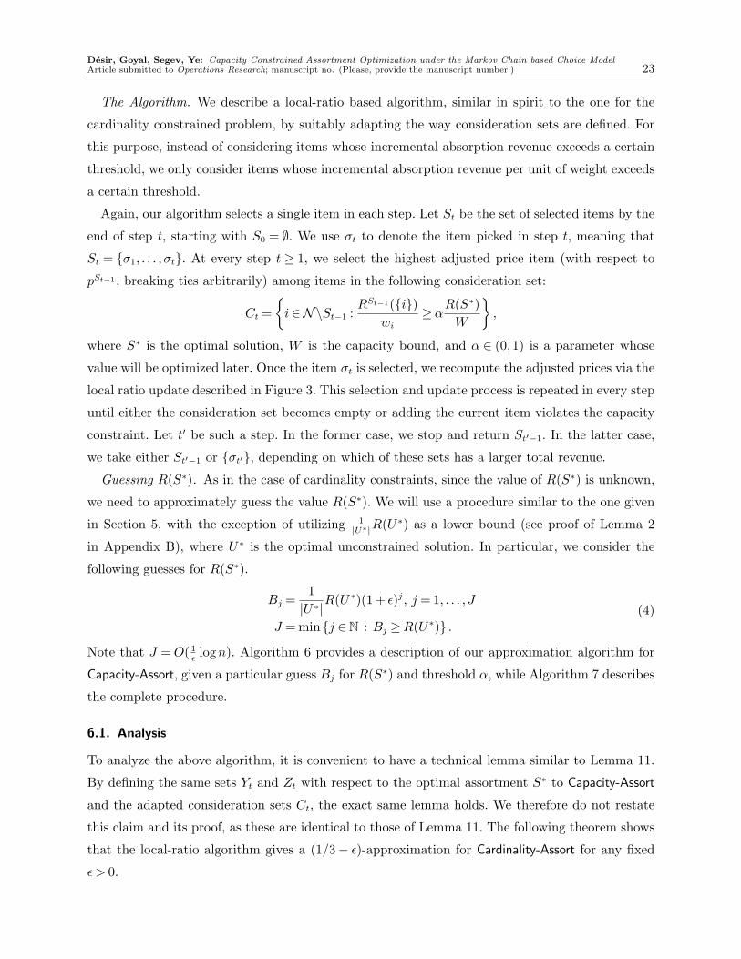
Algorithm 6 Algorithm with guess Bj and threshold α
1: Let S be the set of states picked so far, starting with S = ∅.
2: For all S, let C(S) = {i∈N : RS({i})wi
≥ α ·Bj
W}.
3: While∑
i∈S wi <W and C(S) 6= ∅,
(a) Let i∗ be the item of C(S) for which pSi is maximized, breaking ties arbitrarily.
(b) If∑
i∈S∪{i∗}wi <W , add i∗ to S.
(c) Else return the highest revenue set among {i∗} and S.
4: Return S.
Algorithm 7 Local-ratio Algorithm for Capacity-Assort with threshold α
1: Given any ε > 0, let J and Bj, j ∈ [J ] be as defined in (4).
2: For all j ∈ [J ], let Sj be the solution returned by Algorithm 6 with guess Bj and threshold α
3: Return argmaxj∈[J]R(Sj).
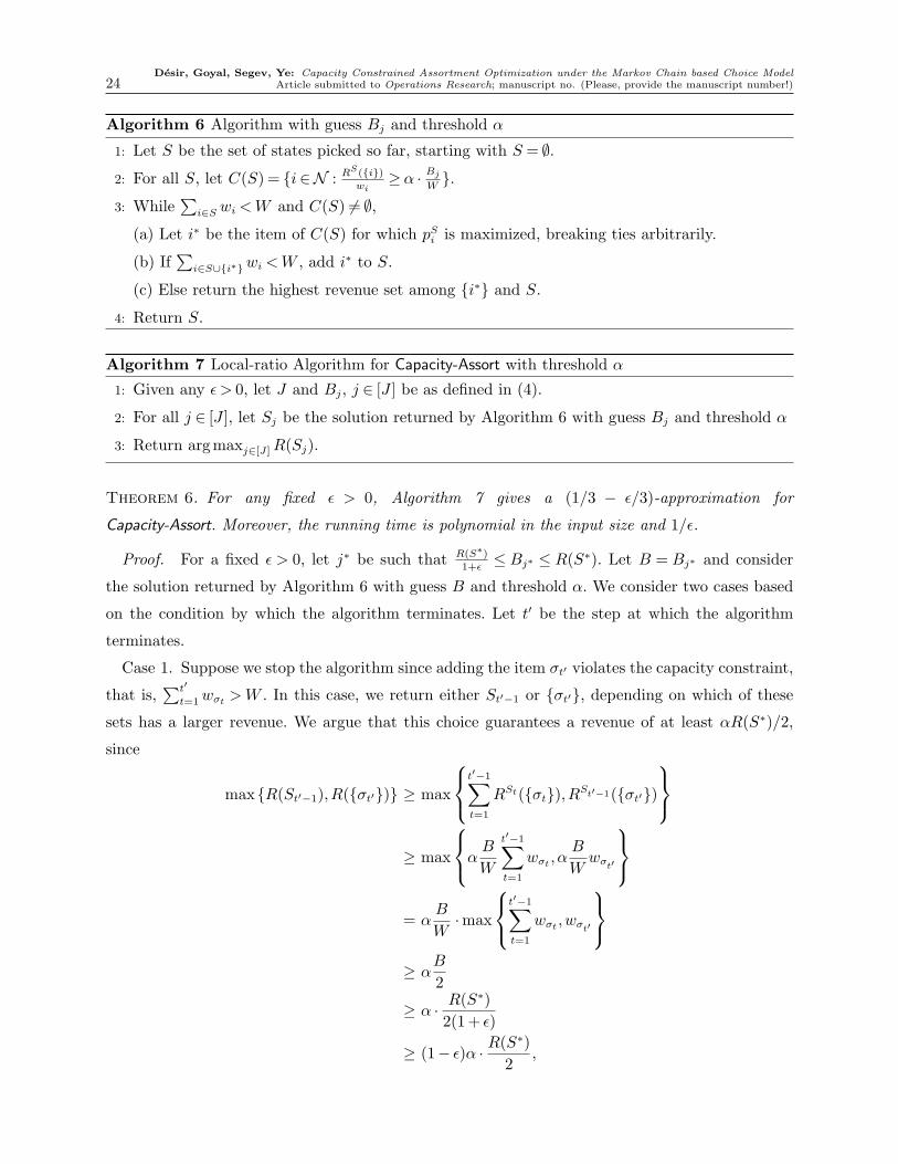
Theorem 6. For any fixed ε > 0, Algorithm 7 gives a (1/3 − ε/3)-approximation for
Capacity-Assort. Moreover, the running time is polynomial in the input size and 1/ε.
Proof. For a fixed ε > 0, let j∗ be such that R(S∗)
1+ε≤ Bj∗ ≤ R(S∗). Let B = Bj∗ and consider
the solution returned by Algorithm 6 with guess B and threshold α. We consider two cases based
on the condition by which the algorithm terminates. Let t′ be the step at which the algorithm
terminates.
Case 1. Suppose we stop the algorithm since adding the item σt′ violates the capacity constraint,
that is,∑t′
t=1wσt>W . In this case, we return either St′−1 or {σt′}, depending on which of these
sets has a larger revenue. We argue that this choice guarantees a revenue of at least αR(S∗)/2,
since
max{R(St′−1),R({σt′})} ≥ max
t′−1∑
t=1
RSt({σt}),RSt′−1({σt′})
≥ max
αB
W
t′−1∑
t=1
wσt, α
B
Wwσt′
= αB
W·max
t′−1∑
t=1
wσt,wσt′
≥ αB
2
≥ α ·R(S∗)
2(1+ ε)
≥ (1− ε)α ·R(S∗)
2,
Desir, Goyal, Segev, Ye: Capacity Constrained Assortment Optimization under the Markov Chain based Choice ModelArticle submitted to Operations Research; manuscript no. (Please, provide the manuscript number!) 25
where the third to last inequality holds since max{∑t′−1
t=1 wσt,wσt′
} ≥W/2 and the second to last
inequality follows as B ≥R(S∗)/(1+ ε).
Case 2. On the other hand, suppose the algorithm terminates since Ct′+1 = ∅. Using Lemma 11
adapted to the capacitated case, we have
R(St′)+RSt′ (Zt′+1)≥R(S∗)−t′+1∑
j=1
RSj−1(Y +j ).
Since Ct′+1 = ∅, this implies that Zt′+1 = ∅. Moreover, from Lemma 9, for all j = 1, . . . , t′ + 1, we
have
RSj−1(Y +j )<αB ·
∑
i∈Y +
jwi
W.
Since our algorithm stopped prior to reaching the capacity constraint, we have∑t′+1
j=1
∑
i∈Y +
jwi ≤
W . Consequently,∑t′+1
j=1 RSj−1(Y +
j )<αB ≤ αR(S∗), and therefore,
R(St′)≥R(S∗)−αR(S∗) = (1−α)R(S∗).
As a result, the approximation ratio attained by our algorithm is
min{
(1− ε)α
2, 1−α
}
.
By setting α= 2/3, we obtain an approximation factor of (1/3− ε/3).
Running Time . Algorithm 7 considers J =O( 1εlogn) guesses of R(S∗). Each run of Algorithm 6
for a given guess is polynomial time. Therefore, the overall running time of Algorithm 7 is polyno-
mial in the input size and 1/ε. �
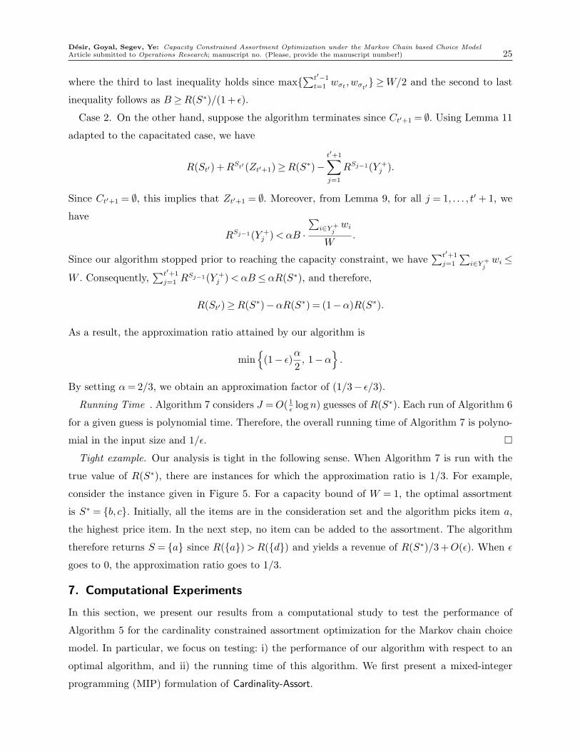
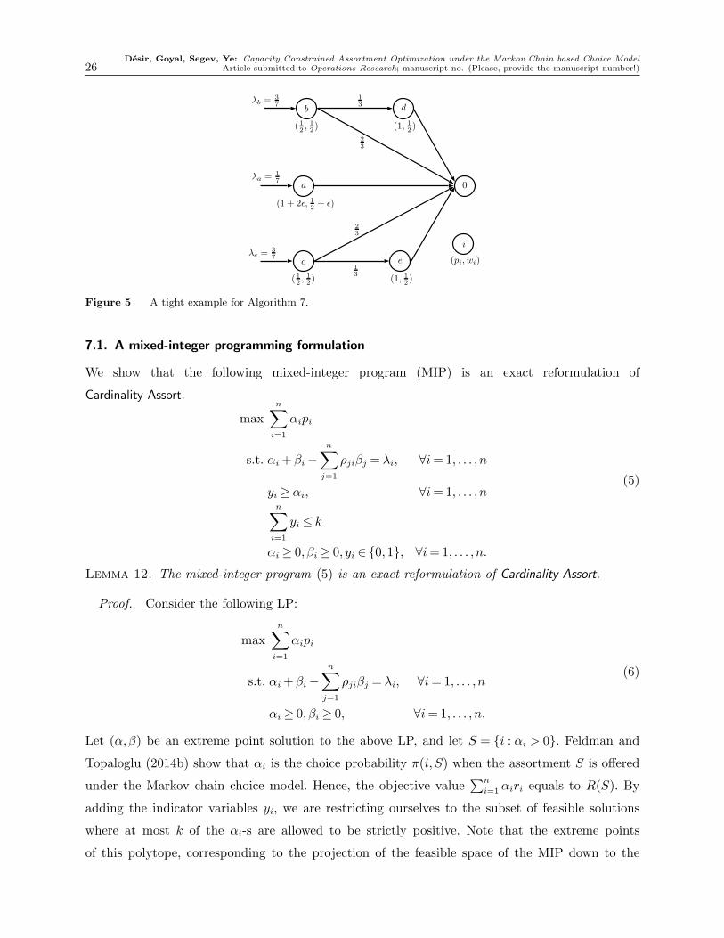
Tight example. Our analysis is tight in the following sense. When Algorithm 7 is run with the
true value of R(S∗), there are instances for which the approximation ratio is 1/3. For example,
consider the instance given in Figure 5. For a capacity bound of W = 1, the optimal assortment
is S∗ = {b, c}. Initially, all the items are in the consideration set and the algorithm picks item a,
the highest price item. In the next step, no item can be added to the assortment. The algorithm
therefore returns S = {a} since R({a})>R({d}) and yields a revenue of R(S∗)/3+O(ε). When ε
goes to 0, the approximation ratio goes to 1/3.
7. Computational Experiments
In this section, we present our results from a computational study to test the performance of
Algorithm 5 for the cardinality constrained assortment optimization for the Markov chain choice
model. In particular, we focus on testing: i) the performance of our algorithm with respect to an
optimal algorithm, and ii) the running time of this algorithm. We first present a mixed-integer
programming (MIP) formulation of Cardinality-Assort.
Desir, Goyal, Segev, Ye: Capacity Constrained Assortment Optimization under the Markov Chain based Choice Model26 Article submitted to Operations Research; manuscript no. (Please, provide the manuscript number!)
a
c e
0
(1 + 2ε, 12 + ǫ)
(12 ,12 ) (1, 12 )
23
13
λa = 17
λc =37
b d
(12 ,12 ) (1, 12 )
13λb =
37
23
i
(pi, wi)
Figure 5 A tight example for Algorithm 7.
7.1. A mixed-integer programming formulation
We show that the following mixed-integer program (MIP) is an exact reformulation of
Cardinality-Assort.
maxn∑
i=1
αipi
s.t. αi +βi −n∑
j=1
ρjiβj = λi, ∀i= 1, . . . , n
yi ≥ αi, ∀i= 1, . . . , nn∑
i=1
yi ≤ k
αi ≥ 0, βi ≥ 0, yi ∈ {0,1}, ∀i= 1, . . . , n.
(5)
Lemma 12. The mixed-integer program (5) is an exact reformulation of Cardinality-Assort.
Proof. Consider the following LP:
maxn∑
i=1
αipi
s.t. αi +βi −n∑
j=1
ρjiβj = λi, ∀i= 1, . . . , n
αi ≥ 0, βi ≥ 0, ∀i= 1, . . . , n.
(6)
Let (α,β) be an extreme point solution to the above LP, and let S = {i : αi > 0}. Feldman and
Topaloglu (2014b) show that αi is the choice probability π(i, S) when the assortment S is offered
under the Markov chain choice model. Hence, the objective value∑n
i=1αiri equals to R(S). By
adding the indicator variables yi, we are restricting ourselves to the subset of feasible solutions
where at most k of the αi-s are allowed to be strictly positive. Note that the extreme points
of this polytope, corresponding to the projection of the feasible space of the MIP down to the

Desir, Goyal, Segev, Ye: Capacity Constrained Assortment Optimization under the Markov Chain based Choice ModelArticle submitted to Operations Research; manuscript no. (Please, provide the manuscript number!) 27
(α,β) coordinates, are exactly the set of assortments S with cardinality at most k. Hence, (5) is a
mixed-integer formulation of the cardinality constrained assortment optimization problem. �
7.2. Settings tested
We proceed by describing the families of random instances being tested in our computational
experiments. Here, each item’s price pi is uniformly distributed over the interval [0,1]. Note that
since we present statistics regarding approximation factors, any constant here will give identical
results, so the choice of 1 is arbitrary. In each instance, we compute the optimal unconstrained
assortment U∗ using the LP given by Blanchet et al. (2016). We then choose the cardinality
constraint k uniformly between 1 and |U∗|/2. For the transition probabilities ρij and the arrival
rates λi, we test our algorithm on three different settings:
1. We generate n2 independent random variables Xij, each picked uniformly over the interval
[0,1]. We then set ρij = Xij/∑n
j=0Xij for all i, j such that i 6= j. Since we do not allow self-
loops (i.e. ρii = 0), the number of random variables needed is n2. For the arrival rates, we then
generate n independent random variables Yi, each picked uniformly over the interval [0,1], and set
λi = Yi/∑n
j=1 Yj for all i 6= 0.
2. In this setting, we sparsify the transition matrix of setting 1. More precisely, we additionally
generate n2 independent random variable Zij, each following a Bernoulli distribution with param-
eter 0.2. For all i, j such that i 6= j, we set ρij = ZijXij/∑n
j=0ZijXij, where Xij are generated as
in setting 1. This is equivalent to eliminating each transition (i, j) with probability 0.8 and then
renormalizing. The arrival rates are generated similarly to setting 1.
3. The transition matrix in this last setting is one of a random walk. More precisely, we generate
n2 independent random variable Xij, each following a Bernoulli distribution with parameter 0.5.
We then set ρij =Xij/∑n
j=0Xij for all i, j such that i 6= j. We also generate n random variables Yi,
each following a Bernoulli distribution with parameter 0.5, and set λi = Yi/∑n
j=1 Yj for all i 6= 0.
7.3. Results
We examine how our algorithm performs in term of both approximation and running time. Table 1
shows the approximation ratio of Algorithm 5 (with ε = 0.1) for the different settings and the
different values of n. We use the MIP formulation given in (5) to compute the optimal assortment.
As can be observed, the actual performance of our algorithm is significantly better than its worst
case theoretical guarantee. Indeed, in all settings tested, the average approximation ratio is always
above 0.97. Moreover, the worst approximation ratio over all instances is above 0.77.
The running time of our algorithm also scales nicely. Table 2 shows the performance of Algo-
rithm 5 in terms of running time for setting 2. The running times are very similar for the other
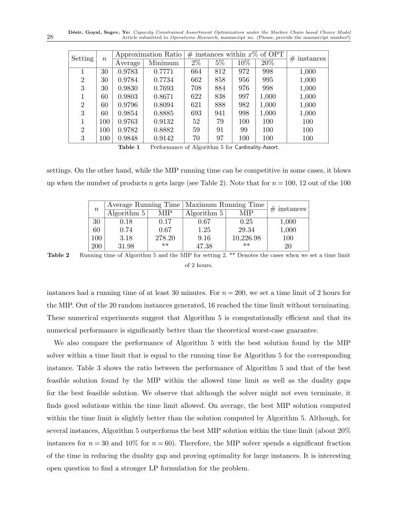
Desir, Goyal, Segev, Ye: Capacity Constrained Assortment Optimization under the Markov Chain based Choice Model28 Article submitted to Operations Research; manuscript no. (Please, provide the manuscript number!)
Setting nApproximation Ratio # instances within x% of OPT
# instancesAverage Minimum 2% 5% 10% 20%
1 30 0.9783 0.7771 664 812 972 998 1,0002 30 0.9784 0.7734 662 858 956 995 1,0003 30 0.9830 0.7693 708 884 976 998 1,0001 60 0.9803 0.8671 622 838 997 1,000 1,0002 60 0.9796 0.8094 621 888 982 1,000 1,0003 60 0.9854 0.8885 693 941 998 1,000 1,0001 100 0.9763 0.9132 52 79 100 100 1002 100 0.9782 0.8882 59 91 99 100 1003 100 0.9848 0.9142 70 97 100 100 100
Table 1 Performance of Algorithm 5 for Cardinality-Assort.
settings. On the other hand, while the MIP running time can be competitive in some cases, it blows
up when the number of products n gets large (see Table 2). Note that for n= 100, 12 out of the 100
nAverage Running Time Maximum Running Time
# instancesAlgorithm 5 MIP Algorithm 5 MIP
30 0.18 0.17 0.67 0.25 1,00060 0.74 0.67 1.25 29.34 1,000100 3.18 278.20 9.16 10,226.98 100200 31.98 ** 47.38 ** 20
Table 2 Running time of Algorithm 5 and the MIP for setting 2. ** Denotes the cases when we set a time limit
of 2 hours.
instances had a running time of at least 30 minutes. For n= 200, we set a time limit of 2 hours for
the MIP. Out of the 20 random instances generated, 16 reached the time limit without terminating.
These numerical experiments suggest that Algorithm 5 is computationally efficient and that its
numerical performance is significantly better than the theoretical worst-case guarantee.
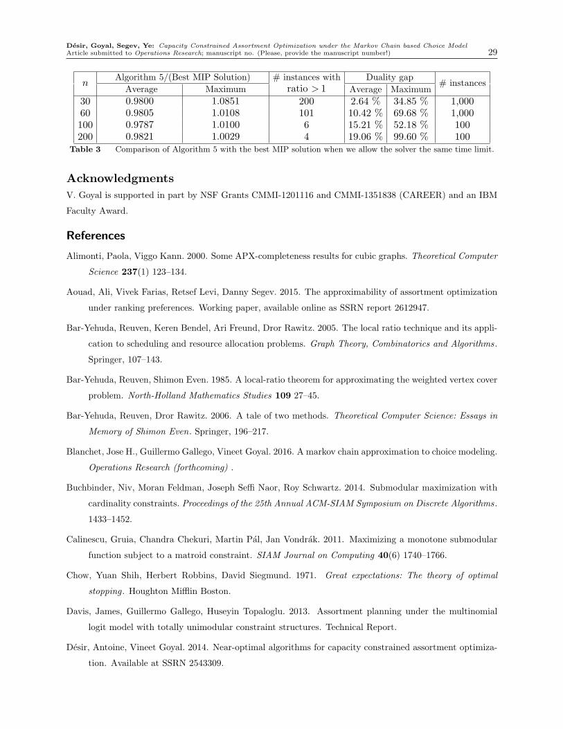
We also compare the performance of Algorithm 5 with the best solution found by the MIP
solver within a time limit that is equal to the running time for Algorithm 5 for the corresponding
instance. Table 3 shows the ratio between the performance of Algorithm 5 and that of the best
feasible solution found by the MIP within the allowed time limit as well as the duality gaps
for the best feasible solution. We observe that although the solver might not even terminate, it
finds good solutions within the time limit allowed. On average, the best MIP solution computed
within the time limit is slightly better than the solution computed by Algorithm 5. Although, for
several instances, Algorithm 5 outperforms the best MIP solution within the time limit (about 20%
instances for n= 30 and 10% for n= 60). Therefore, the MIP solver spends a significant fraction
of the time in reducing the duality gap and proving optimality for large instances. It is interesting
open question to find a stronger LP formulation for the problem.
Desir, Goyal, Segev, Ye: Capacity Constrained Assortment Optimization under the Markov Chain based Choice ModelArticle submitted to Operations Research; manuscript no. (Please, provide the manuscript number!) 29
nAlgorithm 5/(Best MIP Solution) # instances with
ratio > 1Duality gap
# instancesAverage Maximum Average Maximum
30 0.9800 1.0851 200 2.64 % 34.85 % 1,00060 0.9805 1.0108 101 10.42 % 69.68 % 1,000100 0.9787 1.0100 6 15.21 % 52.18 % 100200 0.9821 1.0029 4 19.06 % 99.60 % 100
Table 3 Comparison of Algorithm 5 with the best MIP solution when we allow the solver the same time limit.
Acknowledgments
V. Goyal is supported in part by NSF Grants CMMI-1201116 and CMMI-1351838 (CAREER) and an IBM
Faculty Award.
References
Alimonti, Paola, Viggo Kann. 2000. Some APX-completeness results for cubic graphs. Theoretical Computer
Science 237(1) 123–134.
Aouad, Ali, Vivek Farias, Retsef Levi, Danny Segev. 2015. The approximability of assortment optimization
under ranking preferences. Working paper, available online as SSRN report 2612947.
Bar-Yehuda, Reuven, Keren Bendel, Ari Freund, Dror Rawitz. 2005. The local ratio technique and its appli-
cation to scheduling and resource allocation problems. Graph Theory, Combinatorics and Algorithms.
Springer, 107–143.
Bar-Yehuda, Reuven, Shimon Even. 1985. A local-ratio theorem for approximating the weighted vertex cover
problem. North-Holland Mathematics Studies 109 27–45.
Bar-Yehuda, Reuven, Dror Rawitz. 2006. A tale of two methods. Theoretical Computer Science: Essays in
Memory of Shimon Even. Springer, 196–217.
Blanchet, Jose H., Guillermo Gallego, Vineet Goyal. 2016. A markov chain approximation to choice modeling.
Operations Research (forthcoming) .
Buchbinder, Niv, Moran Feldman, Joseph Seffi Naor, Roy Schwartz. 2014. Submodular maximization with
cardinality constraints. Proceedings of the 25th Annual ACM-SIAM Symposium on Discrete Algorithms.
1433–1452.
Calinescu, Gruia, Chandra Chekuri, Martin Pal, Jan Vondrak. 2011. Maximizing a monotone submodular
function subject to a matroid constraint. SIAM Journal on Computing 40(6) 1740–1766.
Chow, Yuan Shih, Herbert Robbins, David Siegmund. 1971. Great expectations: The theory of optimal
stopping . Houghton Mifflin Boston.
Davis, James, Guillermo Gallego, Huseyin Topaloglu. 2013. Assortment planning under the multinomial
logit model with totally unimodular constraint structures. Technical Report.
Desir, Antoine, Vineet Goyal. 2014. Near-optimal algorithms for capacity constrained assortment optimiza-
tion. Available at SSRN 2543309.
Desir, Goyal, Segev, Ye: Capacity Constrained Assortment Optimization under the Markov Chain based Choice Model30 Article submitted to Operations Research; manuscript no. (Please, provide the manuscript number!)
Feldman, Jacob B, Huseyin Topaloglu. 2014a. Capacity constraints across nests in assortment optimization
under the nested logit model. Technical report, Cornell University, School of Operations Research and
Information Engineering.
Feldman, Jacob B, Huseyin Topaloglu. 2014b. Revenue management under the markov chain choice model.
Gallego, Guillermo, Richard Ratliff, Sergey Shebalov. 2015. A general attraction model and sales-based
linear program for network revenue management under customer choice. Operations Research 63(1)
212–232.
Gallego, Guillermo, Huseyin Topaloglu. 2014. Constrained assortment optimization for the nested logit
model. Management Science 60(10) 2583–2601.
Kok, A. Gurhan, Marshall L. Fisher. 2007. Demand estimation and assortment optimization under substitu-
tion: Methodology and application. Operations Research 55(6) 1001–1021. doi:10.1287/opre.1070.0409.
Kulik, Ariel, Hadas Shachnai, Tami Tamir. 2013. Approximations for monotone and nonmonotone submod-
ular maximization with knapsack constraints. Mathematics of Operations Research 38(4) 729–739.
Lee, Jon, Maxim Sviridenko, Jan Vondrak. 2010. Submodular maximization over multiple matroids via
generalized exchange properties. Mathematics of Operations Research 35(4) 795–806.
McFadden, Daniel, Kenneth Train, et al. 2000. Mixed mnl models for discrete response. Journal of applied
Econometrics 15(5) 447–470.
Nemhauser, G. L., L. A. Wolsey. 1978. Best algorithms for approximating the maximum of a submodular
set function. Mathematics of Operations Research 3(3) 177–188.
Rusmevichientong, Paat, Zuo-Jun Max Shen, David B Shmoys. 2010. Dynamic assortment optimization
with a multinomial logit choice model and capacity constraint. Operations research 58(6) 1666–1680.
Schrijver, Alexander. 1986. Theory of Linear and Integer Programming . John Wiley & Sons, Chichester.
Talluri, K., G. Van Ryzin. 2004. Revenue management under a general discrete choice model of consumer
behavior. Management Science 50(1) 15–33.
Williams, H.C.W.L. 1977. On the formation of travel demand models and economic evaluation measures of
user benefit. Environment and Planning A 3(9) 285–344.
Zhang, Dan, William L Cooper. 2005. Revenue management for parallel flights with customer-choice behav-
ior. Operations Research 53(3) 415–431.
Appendix A: Proofs of Theorems 1 and 2
Proof of Theorem 1. Consider an instance I of VCC, consisting of a cubic graph G= (V,E) on
n vertices V = {v1, . . . , vn}. We can assume that k > |E|/3, or otherwise, the distinction between
the two cases above is easy. We construct an instance M(I) of Cardinality-Assort as follows. Each
vertex vi ∈ V corresponds to an item i of N . In addition, we also have the no-purchase item 0.
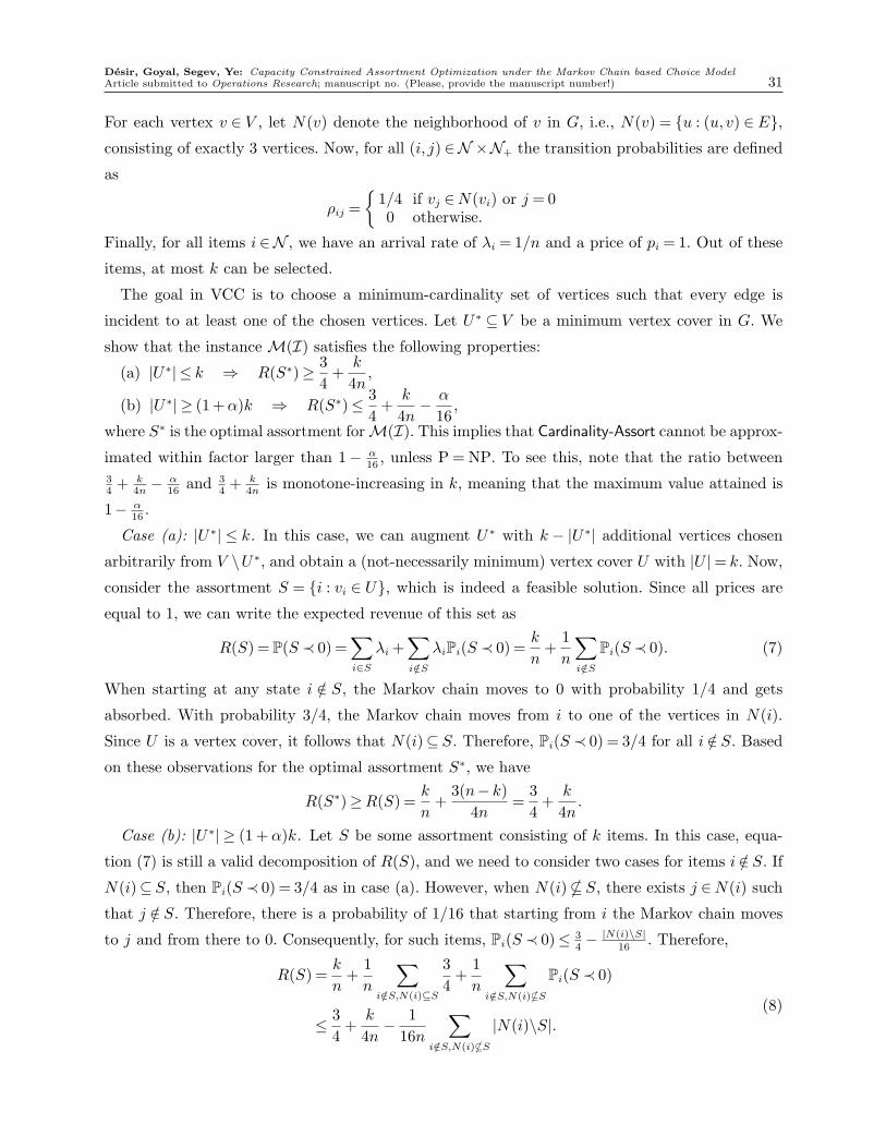
Desir, Goyal, Segev, Ye: Capacity Constrained Assortment Optimization under the Markov Chain based Choice ModelArticle submitted to Operations Research; manuscript no. (Please, provide the manuscript number!) 31
For each vertex v ∈ V , let N(v) denote the neighborhood of v in G, i.e., N(v) = {u : (u, v) ∈ E},
consisting of exactly 3 vertices. Now, for all (i, j)∈N ×N+ the transition probabilities are defined
as
ρij =
{1/4 if vj ∈N(vi) or j = 00 otherwise.
Finally, for all items i ∈N , we have an arrival rate of λi = 1/n and a price of pi = 1. Out of these
items, at most k can be selected.
The goal in VCC is to choose a minimum-cardinality set of vertices such that every edge is
incident to at least one of the chosen vertices. Let U∗ ⊆ V be a minimum vertex cover in G. We
show that the instance M(I) satisfies the following properties:
(a) |U∗| ≤ k ⇒ R(S∗)≥3
4+
k
4n,
(b) |U∗| ≥ (1+α)k ⇒ R(S∗)≤3
4+
k
4n−α
16,
where S∗ is the optimal assortment forM(I). This implies that Cardinality-Assort cannot be approx-
imated within factor larger than 1− α16, unless P = NP. To see this, note that the ratio between
34+ k
4n− α
16and 3
4+ k
4nis monotone-increasing in k, meaning that the maximum value attained is
1− α16.
Case (a): |U∗| ≤ k. In this case, we can augment U∗ with k − |U∗| additional vertices chosen
arbitrarily from V \U∗, and obtain a (not-necessarily minimum) vertex cover U with |U |= k. Now,
consider the assortment S = {i : vi ∈ U}, which is indeed a feasible solution. Since all prices are
equal to 1, we can write the expected revenue of this set as
R(S) = P(S ≺ 0) =∑
i∈S
λi +∑
i/∈S
λiPi(S ≺ 0) =k
n+
1
n
∑
i/∈S
Pi(S ≺ 0). (7)
When starting at any state i /∈ S, the Markov chain moves to 0 with probability 1/4 and gets
absorbed. With probability 3/4, the Markov chain moves from i to one of the vertices in N(i).
Since U is a vertex cover, it follows that N(i)⊆ S. Therefore, Pi(S ≺ 0) = 3/4 for all i /∈ S. Based
on these observations for the optimal assortment S∗, we have
R(S∗)≥R(S) =k
n+
3(n− k)
4n=
3
4+
k
4n.
Case (b): |U∗| ≥ (1 + α)k. Let S be some assortment consisting of k items. In this case, equa-
tion (7) is still a valid decomposition of R(S), and we need to consider two cases for items i /∈ S. If
N(i)⊆ S, then Pi(S ≺ 0) = 3/4 as in case (a). However, when N(i)* S, there exists j ∈N(i) such
that j /∈ S. Therefore, there is a probability of 1/16 that starting from i the Markov chain moves
to j and from there to 0. Consequently, for such items, Pi(S ≺ 0)≤ 34− |N(i)\S|
16. Therefore,
R(S) =k
n+
1
n
∑
i/∈S,N(i)⊆S
3
4+
1
n
∑
i/∈S,N(i)*S
Pi(S ≺ 0)
≤3
4+
k
4n−
1
16n
∑
i/∈S,N(i)*S
|N(i)\S|.(8)
Desir, Goyal, Segev, Ye: Capacity Constrained Assortment Optimization under the Markov Chain based Choice Model32 Article submitted to Operations Research; manuscript no. (Please, provide the manuscript number!)
To upper bound the latter term, let V (S) be the set of vertices of V corresponding to S, i.e.,
V (S) = {vi : i ∈ S}. Let E(S) be the set of edges that are not covered by V (S). We have (2 ·
|E(S)|) =∑
i/∈S,N(i)*S |N(i)\S|. The important observation is that |E(S)| ≥ αk. Otherwise, V (S)
can be augmented to a vertex cover via the addition of fewer than αk vertices, contradicting
|U∗| ≥ (1+α)k. Now,
|E(S)| ≥ αk≥α
3· |E|=
αn
2,
where the second inequality follows from k > |E|/3, and the last equality holds since |E|= 3n/2,
as G is cubic. By inequality (8), we have
R(S)≤3
4+
k
4n−
|E(S)|
8n≤
3
4+
k
4n−α
16.
Since the above upper bound on R(S) holds for any assortment S of k items, this must also be
true for the maximum-revenue one, S∗. �
Proof of Theorem 2. Aouad et al. (2015) show that unconstrained assortment optimization over
the distribution over permutations model is hard to approximate within factor O(n1−ε) for any
fixed ε > 0 even for the case where the number of preference lists is equal to the number of items,
i.e., K = n.
We consider an instance I of the assortment optimization problem over distribution over permu-
tations model with n preference lists: L1, . . . ,Ln. We construct a corresponding instance M(I) of
the assortment optimization under the Markov chain model as follows. Each of the original items
in N has a separate copy as a state in M(I) for every list that contains it. More precisely, for every
list Li and for every 1≤ j ≤ |Li|, we have a state (j, i) corresponding to the j-th most preferred
item in Li. In addition, there is a state 0 corresponding to the no-purchase option. Therefore, the
set of states is:
S = {0}∪ {(j, i) : i= 1, . . . , n, j = 1, . . . , |Li|}.
The transition probabilities between these states are given by:
ρ((j,i),s) =
1 if j < |Li| and s= (j+1, i)1 else if j = |Li| and s= 00 otherwise.
In other words, for each list there is a directed path (with transition probabilities 1) over its
corresponding states in decreasing order of preference, ending at the no-purchase option. This is
illustrated in Figure 6. Finally, the arrival rates are defined by
λ(j,i) =
{ψi if j = 10 otherwise,

Desir, Goyal, Segev, Ye: Capacity Constrained Assortment Optimization under the Markov Chain based Choice ModelArticle submitted to Operations Research; manuscript no. (Please, provide the manuscript number!) 33
λ(1,1) = ψ1
λ(1,2) = ψ2
λ(1,4) = ψ4
1, 1 2, 1 3, 1 4, 1
1, 2 2, 2
1, 4
1, 3
2, 4
2, 3
3, 2
3, 4
0
λ(1,3) = ψ3
Figure 6 Sketch of our construction for an instance on 4 items, where L1 = (1 � 2 � 3 � 4), L2 = (1 � 3 � 4),
L3 = (2� 3), and L4 = (1� 2� 4). Note, for example, that the state (2,2) corresponds to the second
item of L2, but actually corresponds to item 3.
where ψi is the probability of list Li. With this construction, each row corresponds to a list, and
each column correspond to an item.
In order to obtain a one-to-one correspondence between the solutions to I and M(I), it remains
to ensure that, when item i is offered in I, all of its corresponding copies (appearing in the same
column) are offered in M(I), and vice versa. This restriction can be captured by the constraints
x(j,i) = x(k,`), for every i, ` ∈ {1, . . . , n} such that j ≤ |Li|, k ≤ |L`| and such that the jth item in
Li is the kth item in L`. This way, we guarantee that each column is either completely picked or
completely unpicked in the instance M(I). The resulting set of inequalities specifies a constraint
matrix with a single appearance of +1 and −1 in each row, where all other entries are 0. Such
matrices are well-known to be totally-unimodular (see, for example, Schrijver (1986)).
To complete the proof, note that the original instance I consists of n items and n preference
lists and therefore, the Markov chain instance M(I) has O(n2) states. Since the former problem
is NP-hard to approximate within factor O(n1−ε), for any fixed ε > 0, it follows that TU-Assort
cannot be efficiently approximated within O(n1/2−ε), unless P =NP . �
Appendix B: Proof of Lemma 2
This result is an immediate corollary of the following (more general) claim: Let Sg be the solution
returned by Algorithm 1, and let S be any subset of states. Then,
R(Sg)≥R(S)
|S|.
Desir, Goyal, Segev, Ye: Capacity Constrained Assortment Optimization under the Markov Chain based Choice Model34 Article submitted to Operations Research; manuscript no. (Please, provide the manuscript number!)
To prove this claim, let g be the first item selected by Algorithm 1, which necessarily exists
as long as there is an item i with pi > 0. Then, by definition of the greedy algorithm, we have
R({g})≥R({i}) for every item i∈ S. Therefore,
R(Sg)≥R({g})≥1
|S|·∑
i∈S
R({i})≥R(S)
|S|,
where the last inequality follows from the sublinearity of the revenue function (Lemma 9).
Appendix C: Proof of Lemma 4
Let Sgu be the set of states selected by Algorithm 2. Note that for every i ∈ Sgu, we have that
P(i≺ Sgu+ \{i})≥ P(i≺U∗
+\{i}) since Sgu is a subset of U∗. Thus,
R(Sgu) =∑
i∈Sgu
P(i≺ Sgu+ \{i})pi
≥∑
i∈Sgu
P(i≺U∗+\{i})pi
≥k
|U∗|
∑
i∈U∗
P(i≺U∗+\{i})pi
=k
|U∗|R(U∗)
≥k
|U∗|R(S∗),
where S∗ is the optimal solution to Cardinality-Assort. Here, the second inequality holds due to
picking the top k states in terms of P(i≺U∗+\{i}) values. The last inequality holds since the optimal
unconstrained revenue provides an upper bound on the optimal revenue in the constrained case.
Appendix D: Proof of Lemma 6
It suffices to verify that (pS1
i )S2 = pS1∪S2
i for all S1,S2 and i /∈ S1 ∪S2, as the above identity clearly
hold for the transition matrix updates. We have
(pS1
i )S2 =pS1
i −∑
j∈S2
PS1
i (j ≺ S2+\{j})pS1
j
=pi −∑
l∈S1
Pi(l≺ S1+\{l})pl
︸ ︷︷ ︸
A
−∑
j∈S2
PS1
i (j ≺ S2+\{j})pS1
j
︸ ︷︷ ︸
B
.
Using the definition of the updated prices,
B =∑
j∈S2
PS1
i (j ≺ S2+\{j})pj −∑
j∈S2
PS1
i (j ≺ S2+\{j})∑
l∈S1
Pj(l≺ S1+\{l})pl
=∑
j∈S2
Pi(j ≺ (S2 ∪S1)+\{j})pj −∑
j∈S2
PS1
i (j ≺ S2+\{j})∑
l∈S1
Pj(l≺ S1+\{l})pl
︸ ︷︷ ︸
C
.
Desir, Goyal, Segev, Ye: Capacity Constrained Assortment Optimization under the Markov Chain based Choice ModelArticle submitted to Operations Research; manuscript no. (Please, provide the manuscript number!) 35
We can now combine A and C,
A−C =∑
l∈S1
(
Pi(l≺ S1+\{l})−∑
j∈S2
Pi(j ≺ (S2 ∪S1)+\{j})Pj(l≺ S1+\{l})
)
pl
=∑
l∈S1
(Pi(l≺ S1+\{l})−Pi(S2 ≺ l≺ S1+\{l}))pl
=∑
l∈S1
Pi(l≺ (S2 ∪S1)+\{j})pl.
Putting everything together, we get
(pS1
i )S2 = pi −∑
j∈(S2∪S1)
Pi(j ≺ (S2 ∪S1)+\{j})pj = pS1∪S2
i .
�
Appendix E: Application of Algorithm 3 to MNL
In the MNL model, we are given a collection of items, 1, . . . , n, along with the no-purchase option,
which is denoted by item 0. Each item i has a utility parameter ui and a price pi. Without loss of
generality, we can assume that∑n
i=0 ui = 1. For any given assortment S, each item i∈ S is picked
with probability
π(i, S) =ui
u0 +∑
i∈S ui
,
making the expected revenue
R(S) =∑
i∈S
ui
u0 +∑
`∈S u`
pi.
Blanchet et al. (2016) prove that the MNL choice model is a special case of the Markov chain
model. More precisely, when ρij = uj for all j and λi = ui for all i, the choice probabilities of the
two models are identical. In this special case, our local ratio updates can be written as
pSi =
0 if i∈ S
pi −∑
j∈S
uj
u0 +∑
`∈S u`
pj otherwise.
Note that in the above update, the subtracted term is independent of i. Therefore, the ordering of
the prices does not change after each update. Since we are picking the highest adjusted price item
at each step, it follows that the optimal assortment is nested by price, i.e., consists of the top `
priced items, for some `. This is a well known structural property that we recover here as a direct
consequence of our algorithm. Moreover, the updated prices provide a criteria for when to stop
adding items to the assortment.