canx-4/-5: mission simulation, intersatellite separation - t-space
TRANSCRIPT

CanX-4/-5: Mission Simulation, Intersatellite Separation System, Hardware Integration and Testing
by
Jakub Urbanek
A thesis submitted in conformity with the requirements for the degree of Master of Applied Science
Institute for Aerospace Studies University of Toronto
© Copyright by Jakub Urbanek 2011

ii
CanX-4/-5: Mission Simulation, Intersatellite Separation System,
Hardware Integration and Testing
Jakub Urbanek
Master of Applied Science
Institute for Aerospace Studies University of Toronto
2011
Abstract
The CanX-4/-5 mission currently under development at the Space Flight Laboratory will
demonstrate sub-metre formation control in four separate formations consisting of two
nanosatellites. Formation maintenance is performed using a propulsion payload providing one
axis of thrust, resulting in frequent slewing to meet thrust targets. Navigation is GPS dependent,
with both satellites equipped with a receiver and antenna pair. Presented is a mission simulation
developed for evaluating formation flying algorithm performance and the effects of frequent
slewing on GPS coverage. CanX-4 and CanX-5 will be joined for commissioning prior to
commencing formation flying via a mechanism, the Intersatellite Separation System. Details
regarding the performance testing and troubleshooting of the system are described. Integration
and testing of CanX-4/-5 flight hardware into a functional “FlatSat” is presented. Additionally, a
description of satellite operations for two nanosatellites is given, with an emphasis on the
relevance to the work performed for the CanX-4/-5 mission.
iii
Acknowledgments
I would like to thank Dr. Robert Zee for the opportunity to be part of the Space Flight
Laboratory and his guidance throughout my thesis. Also, thank you to Cordell Grant, the CanX-
4/-5 Project Manager, for his tutelage, insights and advice. Your top-down perspective on
project decisions often served to direct my work in the most sensible direction. Daniel Kekez
and Karan Sarda deserve some sort of special trophy for their time, patience and ability to
endure many inquiries about the particulars of CanX-2, NTS and ground station software and
hardware. Thank you also to Niels Roth for your continuous feedback and encouragement for
investigation of details that I had not yet considered. Finally, a sincere thank you to all staff and
students at the Space Flight Laboratory for your valuable advice on various matters.
To my parents, this thesis would not exist were it not for your hard work, advice and support
that have allowed me to be where I am. All that you’ve done is appreciated every day. A special
recognition to Courtney, who should simultaneously graduate with a Master Degree in “How to
Date Someone Pursuing a Master Degree”. Without your help, I would likely be graduating
haggard and malnourished.

iv
Table of Contents
Acknowledgments ......................................................................................................................... iii
Table of Contents ............................................................................................................................ iv
List of Tables ............................................................................................................................... viii
List of Figures .................................................................................................................................. x
List of Acronyms ......................................................................................................................... xiii
Chapter 1: Introduction ............................................................................................................. 1
Chapter 2: Satellite Operations .................................................................................................. 5
2.1 Canadian Advanced Nanospace Experiment - 2 ................................................................. 5
2.1.1 Background .............................................................................................................. 5
2.1.2 Applicability to Other Work .................................................................................... 6
2.1.3 Operational Description ........................................................................................... 7
2.1.3.1 Satellite Health .......................................................................................... 7
2.1.3.2 GPS Occultation and Atmospheric Spectrometer ..................................... 7
2.1.3.3 SFL Engineering Experiments .................................................................. 8
2.1.3.3.1 Nanosatellite Propulsion System Experiments ......................... 8
2.1.3.3.2 Monochrome Imaging Experiments ....................................... 10
2.1.3.3.3 GPS Engineering Experiments ............................................... 12
2.2 Nanosatellite Tracking Ships ............................................................................................. 15
2.2.1 Background ............................................................................................................ 15
2.2.2 Applicability to Other Work .................................................................................. 16
2.2.3 Operational Description ......................................................................................... 16
2.2.3.1 Satellite Health ........................................................................................ 16
2.2.3.2 Payload Operations ................................................................................. 16

v
Chapter 3: Mission Simulation for Formation Flying Nanosatellites ..................................... 18
3.1 Background ........................................................................................................................ 18
3.2 Simulation Architecture ..................................................................................................... 19
3.2.1 Steps Required for GPS Coverage Determination and Evaluation of FIONA Performance ........................................................................................................... 19
3.2.2 C++ Code ............................................................................................................... 20
3.2.2.1 Re-Initialization of Mission Simulation .................................................. 24
3.2.2.2 Errors ....................................................................................................... 24
3.2.3 Formation Flying Algorithm and Relative Navigation .......................................... 25
3.2.4 Satellite Tool Kit ................................................................................................... 26
3.2.4.1 Connect .................................................................................................... 27
3.2.4.2 Astrogator ................................................................................................ 27
3.2.4.2.1 Initial State .............................................................................. 28
3.2.4.2.2 Propagate ................................................................................ 28
3.2.4.2.3 Maneuvers .............................................................................. 29
3.2.4.3 Online Attitude Representation and GPS Coverage Determination ....... 30
3.2.5 OASYS .................................................................................................................. 31
3.2.6 Attitude Simulation, GPS Coverage Determination and Post-Processing............. 31
3.2.6.1 Delays and Minimum Satellites .............................................................. 31
3.2.6.1.1 Delay-to-Lock ......................................................................... 32
3.2.6.1.2 Delay-to-Acquire .................................................................... 33
3.2.6.1.3 Minimum Number of GPS Satellites Required for Solution .. 34
3.2.6.1.4 Delay for Transition to Fine Formation Control .................... 34
3.2.6.2 Approach Utilized ................................................................................... 34
vi
3.2.7 CanX-4/-5 STK Model .......................................................................................... 36
3.3 GPS Antenna Pointing Considerations .............................................................................. 37
3.3.1 Pointing in Direction of an Orbital Axis................................................................ 37
3.3.2 Limited Slew Rate ................................................................................................. 39
3.3.3 Thrust Pointing Leading to Poor Antenna Pointing .............................................. 41
3.3.4 Effect of Consecutive Slews .................................................................................. 42
3.3.5 Reducing Overall Slewing of Antenna Boresight ................................................. 46
3.4 Results ............................................................................................................................... 46
3.4.1 GPS Coverage for Iteration # 1 .............................................................................. 48
3.4.2 GPS Coverage with Blackouts Supplied ............................................................... 51
3.4.3 GPS Coverage without Limited Slew Rate ........................................................... 54
3.4.4 Recommendations ................................................................................................. 56
Chapter 4: Intersatellite Separation System ............................................................................ 58
4.1 Background ........................................................................................................................ 58
4.2 Prototype Model ................................................................................................................ 60
4.2.1 Overview ............................................................................................................... 60
4.3 Flight Model ...................................................................................................................... 61
4.3.1 Overview ............................................................................................................... 61
4.3.2 Arming Procedure .................................................................................................. 64
4.3.3 Initial Flight ISS Testing ....................................................................................... 67
4.4 Flight ISS Troubleshooting ............................................................................................... 67
4.4.1 New Epoxy ............................................................................................................ 67
4.4.2 Epoxy Batch, Preparation and Curing ................................................................... 67
4.4.3 Differences between Prototype and Flight Models ............................................... 68
4.4.4 Review of Load Calculations................................................................................. 69
4.4.5 Load Testing of Belleville Washers and Compression Spring .............................. 71

vii
4.4.6 Investigated Modifications to the Flight ISS ......................................................... 72
4.4.6.1 Flight Spring, Belleville Washers and O-Ring ........................................ 72
4.4.6.1.1 Sensitivity to Compression ..................................................... 73
4.4.6.2 Satellite Face Deflection ......................................................................... 74
4.4.6.3 Surface Area of Cup and Cone Bond ...................................................... 76
4.4.7 Epoxy Strength Testing ......................................................................................... 77
4.4.8 Additional Challenges ........................................................................................... 81
4.4.8.1 Separation Telemetry Microswitch ......................................................... 81
4.4.8.2 Premature Separation .............................................................................. 82
4.4.8.3 Delays in Testing ..................................................................................... 83
4.5 Next Steps .......................................................................................................................... 84
4.6 Recommendations ............................................................................................................. 84
Chapter 5: CanX-4 FlatSat Assembly, Integration and Testing .............................................. 85
5.1 Background ........................................................................................................................ 85
5.2 Power Board Functional Test ............................................................................................ 86
5.2.1 Procedure Creation ................................................................................................ 86
5.2.2 Tested Functionality .............................................................................................. 87
5.2.3 Results, Issues Found and Solutions ...................................................................... 88
5.3 Wire Harness ..................................................................................................................... 89
5.4 Populating Remaining Components .................................................................................. 90
5.5 Lessons Learned ................................................................................................................ 94
5.6 Next Steps .......................................................................................................................... 95
Chapter 6: Conclusions ........................................................................................................... 96
References...................................................................................................................................... 98
viii
List of Tables
Table 1: Standard Deviations and Biases used for Errors in Simulation ..................................... 25
Table 2: FIONA Modes Exercised in Simulations ...................................................................... 25
Table 3: STK Mission Simulation Propagator Details ................................................................ 28
Table 4: STK CNAPS Engine Model Parameters ....................................................................... 29
Table 5: Summary of Delays Used in Simulation and GPS Coverage Determination ................ 32
Table 6: GPS Coverage Percentage; Averaged over Ten Simulation Runs ................................ 49
Table 7: Total Displacement of Antenna Boresight; Averaged over Ten Simulation Runs ....... 50
Table 8: Fuel Use and Tracking Errors; Averaged over Ten Simulation Runs ........................... 51
Table 9: GPS Coverage Percentage; Averaged over Four Iterations with Blackouts ................. 52
Table 10: Total Displacement of Antenna Boresight; Averaged over Four Iterations with
Blackouts ..................................................................................................................................... 53
Table 11: Fuel Use and Tracking Error Data; Averaged over Four Iterations with Blackouts ... 53
Table 12: GPS Coverage Percentage with and without Slew Rate Limit; Averaged over Five
Simulation Runs .......................................................................................................................... 55
Table 13: Total Displacement of Antenna Boresight with and without Slew Rate Limit;
Averaged over Five Simulation Runs (Ave. Dis. = Average Displacement; Std. Dev. = Standard
Deviation) .................................................................................................................................... 55
Table 14: Recommended Attitude Pointing Methods for Each Phase of Formation Flying ....... 57
Table 15: ISS Requirements – Taken from [33] .......................................................................... 59
Table 16: Summary of Differences between Prototype and Flight ISS Models.......................... 63
Table 17: ISS Calculated Parameter Changes ............................................................................. 70
ix
Table 18: ISS Calculated Parameter Changes and Load Test Results......................................... 72
Table 19: Sensitivity to Calculated Load and Separation Velocity for Desired Load and ±
0.2 mm ......................................................................................................................................... 74
Table 20: Original and Proposed Cone Plunger Dimensions ...................................................... 77
Table 21: Epoxy Strength Testing Results (PS = Premature Separation) ................................... 80
Table 22: Main Power Board Tests and their Importance ........................................................... 88
x
List of Figures
Figure 1: Visualization of Successive Thrust Vectors ................................................................... 2
Figure 2: CanX-4 and CanX-5 Satellite (Left: from +Y direction, Right: from –Y direction) [12]
....................................................................................................................................................... 2
Figure 3: Images of SFL Ground Station Area .............................................................................. 5
Figure 4: CanX-2 Solid Model [2]................................................................................................. 6
Figure 5: Image of CanX-2 Payloads ............................................................................................ 8
Figure 6: Solid Model View of NANOPS [3] ............................................................................... 9
Figure 7: Visualization of STK Scenario for CanX-2 GPS Warm Start ..................................... 13
Figure 8: Image of NTS [10] ....................................................................................................... 16
Figure 9: Simulation and GPS Coverage Determination Steps for Each Iteration ...................... 20
Figure 10: Mission Simulation Flow Chart ................................................................................. 21
Figure 11: Block Diagram for C++ Code .................................................................................... 22
Figure 12: Typical Astrogator Mission Sequence for Deputy Satellite ....................................... 28
Figure 13: CanX-4/-5 STK Visualization Model ........................................................................ 36
Figure 14: GPS Satellites above Antenna Plane for Constant Zenith Pointing ........................... 37
Figure 15: GPS Satellites above Antenna Plane for Constant Orbit Normal Pointing ................ 38
Figure 16: GPS Satellites above Antenna Plane for Constant Velocity Pointing ....................... 38
Figure 17: Desired Zenith Pointing Attitude Alignment (Local Horizontal Plane in Grey;
Attitude Sphere Shown for Reference) ........................................................................................ 39
Figure 18: Antenna Pointing Close to Nadir – Body X Axis is Thrust Direction ....................... 41

xi
Figure 19: GPS Antenna Slewing Example for Both Antenna Pointing Methods – Body X Axis
is Thrust Direction ....................................................................................................................... 45
Figure 20: Relative Position of CanX-4/-5 in Each Formation and Reconfiguration ................. 47
Figure 21: Relative Position of CanX-4/-5 in Each Formation and Reconfiguration –
Components ................................................................................................................................. 48
Figure 22: Prototype ISS Model .................................................................................................. 60
Figure 23: Flight ISS Solid Model .............................................................................................. 61
Figure 24: Compressing ISS Spring using Loading Screws (Image from [36]) .......................... 64
Figure 25: Inserting ISS Loading Spacer and Removing Loading Screws (Image from [36]) ... 64
Figure 26: Lunchbox Setup for Flight ISS Testing (Top-End, Front and Top-Back Panels
Removed) ..................................................................................................................................... 65
Figure 27: ISS Load Test Setup ................................................................................................... 71
Figure 28: Belleville Washer Stack on Flight ISS ....................................................................... 73
Figure 29: FEA of Satellite Face Deflection ............................................................................... 75
Figure 30: Depiction of Standoffs to Eliminate Satellite Face Deflection .................................. 76
Figure 31: Flight ISS Cup after Separation ................................................................................. 76
Figure 32: Solid Model of Current Flight Cone .......................................................................... 76
Figure 33: Solid Model of Proposed Flight ISS Cone Plunger ................................................... 77
Figure 34: Prototype ISS Structure Assembled with Flight Plungers and Springs ..................... 78
Figure 35: Epoxy Strength Testing Setup .................................................................................... 79
Figure 36: Separation Telemetry Microswitch ............................................................................ 81
Figure 37: Power Board, HKC and ADCC ................................................................................. 85

xii
Figure 38: Subset of Assembled Wiring Harness ........................................................................ 89
Figure 39: CNAPS Electronics Board on FlatSat ........................................................................ 90
Figure 40: GPS Board on FlatSat ................................................................................................ 91
Figure 41: Reaction Wheels without (Left) and with (Right) Protective FlatSat Cover ............. 92
Figure 42: Solar Cell Coupon in Protective Case ........................................................................ 93
Figure 43: CanX-4 FlatSat ........................................................................................................... 94

xiii
List of Acronyms
ADCC Attitude Determination and Control Computer ADCS Attitude Determination and Control System AGI Analytical Graphics, Inc. AIS Automatic Identification System AIT Assembly, Integration and Testing ATO Along Track Orbit BCDR Battery Charge and Discharge Regulator CanX Canadian Advanced Nanospace EXperiment CDR Critical Design Review CNAPS Canadian Nanosatellite Advanced Propulsion System COTS Commercial Off-The-Shelf DMM Digital MultiMeter DRDC Defence Research and Development Canada ESD ElectroStatic Discharge FEA Finite Element Analysis FFC Formation Flying Computer FIONA Formation Flying Integrated Onboard Nanosatellite Algorithm FOV Field Of View FPGA Field-Programmable Gate Array GNB Generic Nanosatellite Bus GPS Global Positioning System GSE Ground Support Equipment HKC House Keeping Computer IC Integrated Circuit ISL InterSatellite Link ISS Intersatellite Separation System LEO Low Earth Orbit LFFT Long Form Functional Test MOBC Main On Board Computer MOST Microvariability and Oscillations of STars NANOPS NANOsatellite Propulsion System NTS Nanosatellite Tracking Ships OASYS On-orbit Attitude SYstem Software OBC On-Board Computer PCO Projected Circular Orbit POBC Payload On Board Computer PSLV Polar Satellite Launch Vehicle RIC Radial, In-Track, Cross-Track SFL Space Flight Laboratory STK Satellite Tool Kit SEU Single Event Upset TLE Two-Line Element UTIAS University of Toronto Institute for Aerospace Studies

1
Chapter 1: Introduction
Satellite formation flying has the potential to greatly enhance space based capability for observation,
monitoring and experimentation. Distributed sensing is a prime example, where a number of satellites
flying in formation can create larger effective apertures than a single satellite could. Satellite formation
flight often entails a passive chief satellite and one or more deputies that maintain a predefined relative
position with respect to the chief. Specialized hardware for relative state estimation and actuation for
formation maintenance is required.
Continued miniaturization of hardware coupled with specialized design philosophy has pushed the
technological envelope, redefining what is capable on a nanosatellite platform. Small, low-cost platforms
allow for quicker development and more customer accessibility than traditional satellites. One of the
logical directions for development is nanosatellite formation flying. The challenges in developing
nanosatellites capable of formation flight are a consequence of the stringent limitations on power, mass
and volume available, directly impacting the hardware and software required for estimation and actuation.
Among the missions that the Space Flight Laboratory (SFL) has undertaken is a nanosatellite formation
flying capability demonstrator comprised of two satellites, Canadian Advanced Nanospace
Experiment (CanX) - 4 and CanX-5. The satellites, based on the Generic Nanosatellite Bus (GNB)
developed at SFL, are equipped with a GPS receiver and antenna pair, an intersatellite communication
system and a propulsion payload, the Canadian Nanosatellite Advanced Propulsion System (CNAPS).
CNAPS provides one axis of thrust. The three-axis attitude determination and control system augments
this under-actuated state to provide thrusting capability in any direction.
Four formations will be flown, a 1000 m and 500 m Along Track Orbit (ATO) and a 50 m and 100 m
Projected Circular Orbit (PCO). Sub-metre formation control will be demonstrated in all four formations
[11]. This fine degree of control enables applications that require precise positioning for remote
observation. Frequent thrusting to maintain this fine degree of control is needed, resulting in frequent
attitude slews. A visualization of the successive thrust vectors is shown in Figure 1, where the green
vectors show the thrust and the red vectors represent the orbital frame at each thrust. The ATO and PCO
formations are tracked using a linear quadratic regulator (LQR) controller [26].

2
Figure 1: Visualization of Successive Thrust Vectors
CanX-4/-5 navigation is performed via carrier-phase differential GPS, necessitating continuous – or near
continuous – GPS coverage during formation flying phases. GPS coverage, in this sense, refers to not
simply the visibility of GPS satellites, but the availability of a solution. For example, large slews will
result in losing sight of GPS satellites that were previously tracked. Even though new satellites will now
be visible, there will likely be a delay before a GPS solution is again acquired. The frequent slewing
necessary to meet thrust targets presents a complex, unique challenge in maintaining GPS coverage.
The GPS antenna is located on the +Y face of the spacecraft, as shown in Figure 2. Formation keeping
thrusts require that the thrust axis (+X face of the spacecraft) be aligned with the desired thrust vector,
since the CNAPS thrust nozzles are located on the –X face. This significantly inhibits constant ideal
antenna pointing in a given direction, such as zenith. However, since the thruster nozzles and GPS
antenna boresight are on geometrically perpendicular faces, the latter is rotated about the former in an
effort to point the GPS antenna as close as possible to a desired direction.
Figure 2: CanX-4 and CanX-5 Satellite (Left: from +Y direction, Right: from –Y direction) [12]

3
It was necessary to determine how often a GPS solution would be lost as a result of frequent slewing or
poor GPS antenna pointing. These lapses in GPS solution are required to be both few in occurrence and
short in duration such that the formations do not drift apart as a result. The exact frequency and duration
of acceptable lapses in solution is dependent on relative state estimation at the time of the dropouts, which
can vary, making the problem challenging to analyze.
The analysis can be performed in a solely software based simulation or with hardware-in-the-loop,
incorporating the GPS receivers, signal simulators and the relative navigation algorithm. The software
and hardware required for the latter were not yet available. Hardware-in-the-loop testing also had the
restriction of being real-time. As a result, the author pursued the development of a comprehensive
software based mission simulation that would resolve a number of unknowns about dropouts in the GPS
solution and their effect on maintaining desired formations. When a hardware-in-the-loop simulation
setup is developed in the future, the software-based approach will retain its ability to provide
representative analyses quicker than real-time.
Formation flying requires a number of satellite systems to be functioning correctly in unison.
Commissioning these systems on-orbit is crucial in ensuring a successful mission. Accordingly, a
mechanism to hold CanX-4 and CanX-5 together post deployment had been developed to allow
completion of commissioning prior to the commencement of formation flying. When ready, the ground
station issues a command for the mechanism to release the two satellites. A prototype model of the
mechanism had shown promising results. Testing and characterization of the flight model was required to
ensure correct, reliable performance and attain metrics about separation times and velocities, as well as a
refinement of the arming procedure.
Finally, as part of the assembly, integration and testing (AIT) stages that the CanX-4/-5 mission is
currently in, a “FlatSat”, short for flat satellite, was required. This consists of an integrated set of
hardware that is either designated for flight or flight representative, positioned and connected on a flat
panel that allows access to all elements for testing and debugging. A FlatSat is crucial in ensuring proper
functionality of the satellite at a system level, prior to the assembly of the satellite. A FlatSat is also useful
in later stages of the mission for testing operations prior to executing them on-orbit, as well as for
debugging anomalies that occur.
The objectives of this thesis are to simulate and study GPS coverage for the CanX-4 and CanX-5 mission
using a software approach, determine if formations are maintained with the resulting level of GPS
coverage, as well as test and modify attitude strategies that have been created to assist with maintaining a
GPS solution. Further, the mechanism for joining CanX-4 and CanX-5 for commissioning and separating

4
them for formation flying is tested and evaluated. Finally, the CanX-4 FlatSat is assembled into a
functioning unit. These tasks are supported by operation of two nanosatellites currently in orbit.
Specifically, satellite operations assisted in quantifying simulation parameters related to GPS satellite
acquisition and timing of the separation mechanism.
This document is organized into sections based on the projects performed. Where appropriate, the projects
and their associated tasks are tied in to each other and explained where they fit in the context of the
overall thesis topic.

5
Chapter 2: Satellite Operations
Satellite operations are a key component of any mission, the culmination of satellite design effort and, put
simply, the execution of tasks for which the satellite was conceived. The author is privileged to have the
opportunity to operate two SFL spacecraft CanX-2 and CanX-6, the latter more commonly referred to as
Nanosatellite Tracking Ships (NTS). The following sections provide an overview of each mission and
describe operations performed during the time of the author’s involvement.
All operations take place at SFL. The hardware infrastructure is located on site. Figure 3 shows images of
the SFL ground station area.
Figure 3: Images of SFL Ground Station Area
2.1 Canadian Advanced Nanospace Experiment - 2
2.1.1 Background
The CanX-2 nanosatellite is a 3.5kg triple CubeSat. It is a technology demonstrator and precursor to the
CanX-4/-5 formation flying mission. CanX-2 was launched Apr. 28, 2008 from India as one of the
secondary payloads aboard a Polar Satellite Launch Vehicle (PSLV) rocket. It has a Sun-synchronous
orbit with an altitude of 635 km and a descending node of 9:30 am [1]. The CanX-2 bus is shown in
Figure 4.

6
UHF Antennae (4)
S-Band PatchAntennae (2)
AtmosphericSpectrometer
PropulsionThruster (2)
GPS Antenna
Materials ScienceExperiment
Magnetometer
X
Y
Z
UHF Antennae (4)
S-Band PatchAntennae (2)
AtmosphericSpectrometer
PropulsionThruster (2)
GPS Antenna
Materials ScienceExperiment
Magnetometer
X
Y
Z
X
Y
Z
Figure 4: CanX-2 Solid Model [2]
CanX-2 has a total of 4 experimental payloads onboard: a GPS receiver and antenna for radio occultation
and positioning experiments led by the University of Calgary, an atmospheric spectrometer for measuring
greenhouse gases led by York University, a propulsion system developed at SFL (discussed further in
Section 2.1.3.3.1) and a materials experiment led by the University of Toronto. The first three payloads
listed require operator interaction to set the spacecraft attitude, upload and schedule experiment scripts
and download resulting data. The last is a passive experiment that collects long term telemetry which is
autonomously downloaded as part of normal telemetry downloads.
The author was part of the operations team for the duration of his thesis and was involved in all duties
associated with the operation of CanX-2. Each member of the operations team is part of a rotating
schedule that includes three satellite contacts in the morning/early afternoon and another three contacts in
the evening/early night, as well as weekend and holiday monitoring.
2.1.2 Applicability to Other Work
In a general sense, knowledge of satellite operations is very useful for understanding mission level
concepts and architecture. It requires a good understanding of the satellite’s various operational modes
and how to safely transition between them. These have to be understood in detail to run standard
experiments, create custom ones and to troubleshoot anomalies. This knowledge is naturally transferred to
planning the concept of operations for other missions and is an asset in planning discussions for CanX-4/-
5 formation flying and the transitions between formations, as well as commissioning activities.

7
More specifically, CanX-2 GPS engineering experiments directly supported CanX-4/-5 work, allowing
for a better understanding of GPS satellite acquisition. This assisted in quantifying parameters in the
mission simulation for CanX-4/-5. They also helped in adapting the approach in [5] for warm starting the
receiver, as well as allowed for testing acquisition times and getting acquainted with the receiver’s
function and performance.
Finally, familiarity with tasks required during satellite contacts assisted in the timing of the separation of
CanX-4 and CanX-5 using the satellite separation mechanism.
2.1.3 Operational Description
2.1.3.1 Satellite Health
A crucial component of satellite operations is continuous monitoring of satellite health. To assist in this,
telemetry data is polled from sensors on the satellite every minute and stored in memory. This data buffer
is downloaded autonomously at the beginning of each contact with the ground station. The operator then
inputs all the telemetry into a database that allows for reviewing the data, flagging anomalies and
unexpected telemetry readings, as well as monitoring short and long-term trends in satellite health.
On occasion, anomalies in telemetry are observed. Alternatively, a satellite alarm may be triggered by
anomalous behavior or conditions. During such periods, it is the operator’s responsibility to efficiently
and correctly investigate the cause of the anomaly and carry out the appropriate action to recover the
satellite to the nominal operational state. The author was involved in numerous such events and acted
together with the rest of the operations team to resolve the issues. Often, corrective actions are captured in
existing contingency procedures. Otherwise, the satellite operator, in consultation with the operations and
project managers, will devise and carry out a new contingency procedure.
These tasks assisted with preliminary planning of CanX-4/-5 operations, specifically in terms of re-
acquiring a GPS solution after one was lost as well as handling of the separation sequence of the two
satellites.
2.1.3.2 GPS Occultation and Atmospheric Spectrometer
CanX-2 is on a rotating experiment schedule. Each of the onboard experiments is operated for a month at
a time. From an operations standpoint, occultation and positioning experiments for the University of
Calgary and spectrometer experiments for York University are similar. A photograph of the payloads is
shown in Figure 5. Each experiment requires scripts created by the respective Co-Investigator’s science
team. These scripts are uploaded and scheduled by the satellite operator. Additionally, the attitude of the

8
spacecraft is set to point the respective payloads in desired directions. This involves changing Attitude
Determination and Control System (ADCS) settings and uploading and scheduling an additional script,
responsible for transitioning CanX-2 into an attitude mode that allows the use of its wheel to align the
payload with a vector in the orbital plane. Once the experiment has executed, the operator downloads the
data. This process is repeated for the duration of an experiment campaign. The data is compiled and sent
to the Co-Investigator’s team for analysis.
The ability to script and time-tag commands is crucial to the CanX-4/-5 mission since ground station
contact is limited to a maximum of six times per day. In between contacts, the satellites will have to
continue autonomous formation flying without ground station input. An example of an important scripted
task would be a GPS receiver warm start after a lapse in solution.
Figure 5: Image of CanX-2 Payloads
2.1.3.3 SFL Engineering Experiments
There is time in the rotating experiment schedule dedicated to SFL engineering experiments on-orbit.
These consist of Nanosatellite Propulsion System (NANOPS), optical imaging, or GPS experiments, and
are discussed below. As the engineering experiments involve more operator involvement than the
aforementioned experiments, the following sections provide more depth where necessary.
2.1.3.3.1 Nanosatellite Propulsion System Experiments
NANOPS experiments are similar in procedure to the aforementioned GPS and spectrometer experiments,
except that they require additional operator interaction to pressurize NANOPS prior to thrusting. Also,
attitude scripts are not required for NANOPS testing. A solid model view of the NANOPS assembly is
Atmospheric Spectrometer GPS Antenna
GPS Receiver
Materials Experiment

9
shown in Figure 6. It is a self contained unit that is assembled prior to integration with the satellite. The
system has a mass of approximately 576 grams and uses sulfur hexafluoride as its fuel [3].
Figure 6: Solid Model View of NANOPS [3]
Before each test thrust is scheduled, the pressure in the secondary volume on NANOPS is polled allowing
the operator to calculate how long the regulator valve needs to be opened for the pressure in the secondary
volume to reach the desired setpoint. An expected increase per unit time is known and used to attain the
desired pressure. The difference in temperature between the time of pressurizing and the expected
temperature at the time of the experiment has to be taken into account.
As shown in Figure 4, the NANOPS nozzle is located on the –X face toward the +Y end. Since, the thrust
nozzle is located away from the centre of mass of the satellite, when fired, the thruster will cause a
rotation of the satellite. The body rates will be determined by the attitude determination system and the
induced spin is used to characterize NANOPS performance.
In order to avoid damping the body rates right away, CanX-2 is put into Passive Attitude Mode prior to
the experiment. In this state, attitude determination is performed, but no control is actuated. Additionally,
since the body rates induced are not large, it is desired that the body rates prior to the experiment are low.
For this reason, CanX-2 remains in B-Dot Attitude Mode during the NANOPS campaign, except during
experiments, to allow for rate damping. B-Dot is a control mode that uses the satellite’s magnetometer to
measure the local magnetic field of Earth and magnetorquers to interact with the magnetic field to reduce
the spin rate on each body axis. After an experiment has been executed and enough body rate data has

10
been gathered to analyze the NANOPS thrust, B-Dot Mode is again set either autonomously by the
experiment script or by an operator.
During the author’s time as an operator, a number of NANOPS campaigns were performed. The telemetry
attained assisted in the design of the propulsion system for CanX-4/-5. Performance metrics for this
system were needed for accurate representation of the thruster model in the mission simulation for CanX-
4/-5.
2.1.3.3.2 Monochrome Imaging Experiments
CanX-2 has both a colour and monochrome imager. The colour imager is located on the Main On-Board
Computer (MOBC) and the monochrome on the Payload On-Board Computer (POBC). The colour
imager has never been used in space. The MOBC cannot be power cycled and there is a risk that the
voltage drop from the colour imager would result in a brownout state, affecting satellite function as a
whole. As a result, all space based imaging campaigns thus far have focused on the monochrome imager.
Both imager payloads onboard CanX-2 were additional experimental payloads and were not critical to
meeting any main mission requirements. Any images attained were considered to be an additional benefit
of the mission. As this payload was not mission critical, time constraints during development prevented
extensive testing of the imager in a representatively illuminated environment prior to launch.
The author was an operator during a lengthy and detailed campaign, performed by the CanX-2 operations
team, to attain an image with the monochrome imager. It is a National Semiconductor LM9638 CMOS
array imager with a Sunex DSL901 lens [4]. There is no neutral density filter on this unit and the
challenge in attaining an image is oversaturation of the CMOS array. An extensive FlatSat and on-orbit
bracketing study was performed under various conditions. First, FlatSat imager bracketing was carried out
by the operations team indoors. Not all imager parameters are accessible in the flight code. The
parameters that are likely to affect imager saturation and are accessible were tested. It was found that
those directly related to the integration time, gain and size of the image had the most effect. A successful
image of the FlatSat room ceiling was captured [4].
When outdoor imaging with the FlatSat was attempted, it was found that even when all settings related to
integration time and gain were set to their minimums, images would be completely over-saturated (all
white). With no filter on the lens, outdoor light intensity was large enough to exceed the limits of the
imaging sensor. Attempting to gradually reduce the window size, it was found that in one step size
change, the image would transition from completely over-saturated to completely under-saturated (all
black). At this point, the image was less than 10 × 10 pixels in size. The small image size coupled with
low integration time and gains did not allow any light to be registered on the sensor. Increasing other

11
parameters while maintaining this window size was found to transition the image from completely under-
saturated to completely over-saturated in one step of a parameter. When a neutral density filter was placed
over the imager, a successful outdoor image was attained [4].
On-orbit testing was performed, applying the experience gained from FlatSat trials and performing
comprehensive bracketing tests. Imaging times were limited to when the satellite was in contact with the
ground station, as the imaging commands cannot be time-tagged. Daylight images were completely over-
saturated and one step change in settings would result in complete under-saturation, similarly to the
outdoor FlatSat testing. Imaging during eclipse occasionally resulted in some visible features, but it was
shortly found that these were similar no matter where over Earth the image was taken. Consequently, this
was attributed to sensor noise. Imaging while coming out of eclipse was also attempted, with the prospect
of having favourable lighting conditions while flying through the penumbra, the transitional region
between full eclipse and full illumination. Unfortunately, the penumbra transition for a Low Earth Orbit
(LEO) satellite is very short (on the order of seconds) and images taken were still subjected to light
intensity high enough to result in the same aforementioned behaviour [4]. It is worth noting that an image
of the Moon was attained, but this was prior to the author’s thesis. Additional time had not been allotted
to capturing another Moon image prior to the writing of this document.
Earth limb and star field images did not yield successful results. Additionally, imaging over bright cities
during eclipse was attempted, but city choices were limited by the satellite having to be in contact with
the SFL ground station. Unfortunately, no successful images were attained during these trials [4].
In the end, the efforts were analyzed and summarized and it was concluded that under the current
infrastructure, all reasonable attempts had been made to capture a successful image with the monochrome
imager. Supplementary experimentation with this imager would require potential code changes to allow
access to more imager parameters. This required substantial changes to both onboard and ground station
software, as well as comprehensive testing on the CanX-2 FlatSat prior to uploading the updates to the
satellite. This is to find any bugs contained in updated operating code that could result in anomalous
satellite behaviour. In a worst case, this could lead to the end of the mission. Since imaging is not a
mission critical task and since there is no guarantee of successful results with operating code changes, this
task was deemed not critical enough at that time to justify the effort and risk involved. It was left as a
potential task for the future.
Colour imaging may be more successful due to the Bayer filter on the colour imager. However, as
previously stated, the colour imager is on the MOBC. Experimenting with it carries potential risk to the

12
mission and a comprehensive FlatSat study should first be performed. This remains as a potential future
task for CanX-2 operations.
Much was learned about the imager itself during this test campaign. Furthermore, this was the author’s
first campaign as an operator and the operation of CanX-2 for imaging requires a comparatively large
amount of operator input. Consequently, good experience with the satellite and its functions was gained
through these experiments. This is beneficial in planning the satellite separation sequence for CanX-4/-5
as well as providing input to the operations concept for this mission.
2.1.3.3.3 GPS Engineering Experiments
In addition to using the CanX-2 GPS receiver and antenna for University of Calgary occultation
experiments, SFL performed engineering experiments to assist in predicting and simulating GPS
performance for CanX-4/-5. The receiver and antenna models for CanX-4/-5 are not the same. However,
at the time, these were the best metrics that were available. This was later supplemented by test results
that became available from signal simulator testing [9]. Engineering experiments provide the operator
with the opportunity to design, execute and analyze CanX-2 operations. This is unique compared to other
CanX-2 activities that nominally involve the operator in mainly the execution stage.
It had been found that cold starting the CanX-2 receiver could take almost twenty minutes to attain a GPS
solution in some cases. This was much too long to recover from GPS dropouts for CanX-4/-5. It was
known that the University of Calgary used a receiver warm start procedure for occultation experiments. It
involved a priori knowledge of satellite position when the receiver is turned on, which GPS satellites
would be in the antenna field of view and what their Doppler shifts would be [5]. The University of
Calgary had developed their own software for generating the experiment scripts containing the
appropriate receiver warm start commands. The author developed an in-house method for doing this using
a combination of Satellite Tool Kit (STK) and Microsoft Excel. The resulting warm start script was very
similar to that of the occultation scripts, but tailored for the desired SFL engineering experiments. Outside
of the method of script generation, the major difference was that after acquiring a GPS solution, all
receiver channels would be set to automatic tracking. It was found that the GPS solution in this process
was lost only very briefly before the channels would automatically lock onto satellites and continue their
own tracking algorithms for the remainder of the experiment. On-orbit testing of these scripts showed that
with zenith pointing, warm starts were typically attained in approximately 2 min. This was a significant
improvement over the cold start and provided values used as a basis for CanX-4/-5 GPS acquisition
timing in mission simulations.
The warm start script was created as follows [6]:

13
1.) A scenario is created in STK that contains the CanX-2 satellite based on an up-to-date Two-Line
Element (TLE) set. A simple GPS antenna is created (boresight towards +Z body axis) and the GPS
constellation is loaded (STK uses the SEM Almanac by default [41]). The attitude is set to correspond
to the desired warm start pointing. Figure 7 shows the final setup, where CanX-2 is the green point,
GPS satellites are white points and green lines shows access to GPS satellites from the CanX-2
antenna. The green plane represents the sensor field of view (FOV). It is a plane because a
hemispherical antenna was used as an approximation. GPS satellites near this plane would likely have
low signal-to-noise ratios and satellites with higher elevations were preferred for the warm start script.
Figure 7: Visualization of STK Scenario for CanX-2 GPS Warm Start
2.) The approximate time is calculated using the format of GPS week followed by seconds from the
beginning of the week. It is preferable, but not necessary, to perform GPS experiments while the
satellite is in sunlight due to onboard power constraints. These times are found using the “Sun Start”
and “Sun Stop” reports in the STK scenario.
3.) The receiver requires an approximate position input in the format of latitude, longitude and height. A
custom report is created in the STK simulation to attain this data for a chosen time period.
4.) GPS satellites in view at the time of the experiment are found and assigned to specific GPS receiver
channels, providing an expected Doppler offset. The Doppler offset, ƒDO, is calculated using range rate
information from STK and according to [6]:

14
fct
Rf DO
(1)
where: ∆R is the change in range
∆t is the time between the two range values
c is the speed of light
f is the frequency of the GPS signal being used (1575.42MHz)
An error window for the Doppler offset is supplied. The maximum value of 10,000Hz is used [7].
The warm start script that is uploaded to the satellite is in a format in accordance with the script
convention developed at SFL for communicating with payload devices on CanX-2 [8].
These warm starts were performed with the GPS antenna pointing to zenith. Warm starting with the
antenna pointing to either velocity or anti-velocity was also attempted with the same procedure employed.
This was found to be unsuccessful, likely due to the more quickly changing Doppler shifts of the GPS
satellites than those closer to zenith. Due to experiment schedule constraints, further experiments to test
warm starting performance were not performed. Later, results from signal simulator testing performed by
an SFL member showed more applicable performance in terms of hardware to the CanX-4/-5 mission [9].
However, the experiments performed on CanX-2 resulted in a familiarity with warm starting and vital
knowledge for mission simulations performed.
Since CanX-4/-5 will be slewing frequently to meet thrust targets, it was desired to study GPS receiver
ability to maintain a solution while slewing. CanX-2 has the ability to slew around the orbit normal,
allowing to point the GPS antenna in the velocity/anti-velocity, zenith and nadir directions and anywhere
in between. An attitude control mode named Wheel Pitch is set for slewing. This allows the momentum
wheel to change speed such that the satellite slews to, and holds, a certain pointing. A script to transition
CanX-2 in and out of this mode is used and can be time-tagged to start at any point in the orbit. However,
the attitude control setting that determines where the satellite will point in Wheel Pitch Mode cannot be
time-tagged and can only be changed during a pass by an operator. This limitation dictates a certain
operational approach when performing any experiments that require a slew. The experiment procedure is
set up as follows:
1.) A GPS warm start script is created that:
a. Performs a GPS receiver warm start a few minutes prior to a satellite contact;

15
b. Assigns all receiver channels to track automatically a few minutes after the warm start was
initiated to give the receiver enough time to attain a solution;
c. Continues logging for at least the duration of the satellite contact.
2.) This script is uploaded on a pass prior to the one where the slew experiment will be performed.
3.) The script is scheduled along with an attitude script that will switch the mode to Wheel Pitch for the
duration of the experiment.
4.) During the next contact, the operator waits until the desired time. The GPS receiver should be on and
have a solution and the attitude mode should be set to Wheel Pitch already by the time-tagged script.
The slew is performed by the operator changing the appropriate attitude control settings.
5.) The experiment is given time to finish. The GPS data log is downloaded in the following contact.
Over a full 180 ° slew, the set of GPS satellites visible would change almost completely, giving a good
indication of how well the receiver handles such changes. To avoid unnecessary slewing as well as
pointing the antenna at the ground, the experiment could be set up such that the antenna is initially
pointed at anti-velocity and slewed around to velocity, or vice-versa. The challenge is that this implies a
warm start pointing at either velocity or anti-velocity. To avoid this, a 90 ° slew, warm started at zenith
was also attempted. Unfortunately, an error caused the satellite to slew 270 ° degrees, pointing the antenna
at the ground in the process and losing GPS lock. Only a few slewing experiments were conducted overall
due to time constraints of the operations schedule. It was also discovered that data logging issues caused
the logs from some of the experiments to be cut off prematurely, rendering them unusable for analysis.
Unfortunately, due to operational time constraints, further experiments that avoided these complications
were not pursued during the time of the author’s thesis. Future signal simulator testing will be used to
attain representative performance metrics for the CanX-4/-5 mission.
2.2 Nanosatellite Tracking Ships
2.2.1 Background
CanX-6, more commonly known as NTS, is a small cube measuring 20 cm on each side with a mass of
6.5 kg. It houses an Automatic Identification System (AIS) payload and antenna built by COM DEV and
was intended to test this technology in space. It was launched in 2008, along with CanX-2, and is still
operational. An image of NTS is shown in Figure 8.

16
The author was a member of the operations team for NTS, performing regular telemetry monitoring and
payload operations, as well as troubleshooting when necessary. In much the same way as CanX-2, the
operators work on a rotating schedule, though NTS payload operations
are largely autonomous. This was useful experience because many
operations on CanX-4/-5 will have to be autonomous, since the satellites
will be formation flying whether or not they are in contact with the
ground station.
2.2.2 Applicability to Other Work
In addition to further experience with satellite operation and familiarity
with the functions of on-orbit satellite systems, NTS provided good
background for the concept and setup required for autonomous spacecraft
operations. The day-to-day tasks were significantly different than for
CanX-2 and the varied experience between the two satellites provided for
more complete education in spacecraft operations. Additionally, since
NTS was tracked by more than one ground station and controlled remotely from SFL, operations
provided experience that may be useful to CanX-4/-5 if more contact time is required for the satellite.
2.2.3 Operational Description
2.2.3.1 Satellite Health
Similarly as for CanX-2, satellite health is monitored for both short and long-term trends. In addition to
regular telemetry, errors in the experimental Static Random Access Memory (SRAM) onboard NTS are
actively monitored. These errors change periodically as a result of Single Event Upsets (SEUs). Error
detection and correction (EDAC) in the form of triple voting can handle an error at a certain location in
one memory bank. However, if there are errors in the same locations of more than one memory bank,
erroneous data results and incorrect instructions can be attempted by the spacecraft. Additional scans can
be performed to check if memory error locations overlap. Also, change in MOBC current accompanies
changes in the amount of memory bank errors. As long as the current remains within a given threshold,
this does not affect satellite operations. Active monitoring is performed to study how often errors change
and how large the associated current changes are.
2.2.3.2 Payload Operations
The AIS payload is proprietary to COM DEV. Observation scripts are sent to SFL and prepared for
upload by the operator. Autonomous operations set up for NTS allow for the script file to be prepared
Figure 8: Image of NTS [10]

17
prior to the pass and set to upload. The upload happens autonomously and the experiments execute in a
time-tagged manner.
Once the experiment has executed, download of payload telemetry and data can also be set up to run
autonomously, with the operator on duty being on-call to respond if anything goes wrong. Status emails
are sent to Blackberry devices carried by operations staff. All upload and download operations can also be
performed manually if necessary.
For certain observation campaigns, the downlink was through a ground station run by DRDC Ottawa.
This facility allowed for quicker data downloads, making possible more frequent NTS observations. Also,
for a period of time, NTS operations were performed remotely through ground stations in Tromsø and
Andøya, Norway. The high latitude location of these stations allowed for useful contacts for almost every
orbit, allowing for a larger data throughput. Though mostly autonomous, these observation campaigns
still required a higher degree of operator involvement to manage contact through multiple stations, as well
as to prepare the larger amount of scripts executed during these campaigns. A similar approach with
multiple ground stations and increased contact time could be sought for CanX-4/-5 if it was deemed
necessary to mission success. The experience acquired through NTS operations would be beneficial in
operating under this infrastructure.

18
Chapter 3: Mission Simulation for Formation Flying Nanosatellites
3.1 Background
Mission simulation can be tackled through various approaches. The most complete and representative
simulators are those that incorporate mission representative hardware and software. An example is
NASA’s Goddard Space Flight Center (GSFC) Guidance, Navigation and Control Center’s (GNCC) work
on a testbed that combines an orbital simulator (VirtualSat Pro) with GPS receivers and RF simulators
[13]. Stanford University has also developed two and three dimensional simulation platforms [13], [14].
Other hardware-in-the-loop simulations have been developed at various facilities around the world as well
[15], [16], [17]. Such simulators are highly beneficial in developing formation flying missions.
For software based simulations, an approach commonly encountered in publications is testing of the
formation control algorithms using an orbital propagation program written specifically for that purpose
[18], [19]. STK is often employed in mission simulation, but not always found integrated with external
software like MATLAB or C++ for more customized simulation. Examples of cases where integration
was present, either through Connect (see Section 3.2.4.1) or STK’s scripting capability, are given in [20],
[21], [22], [23], [24], [25]. While these examples are not all related to formation flying, they do
incorporate some similar functionalities utilized in the simulations described herein.
The purpose of the software based simulation for CanX-4/-5 is to investigate a number of unknown
questions in regards to GPS coverage and formation flying algorithm performance when a GPS solution is
not available. Specifically:
Taking into consideration the attitude constraints imposed on the deputy by frequent thrusts, what
level of GPS coverage can be expected?
Can the attitude controller function be adjusted to improve GPS coverage?
Are the spacecraft expected to stay in formation with the calculated level of GPS coverage, or
will they drift apart due to the lapses in highly accurate relative solutions (available only when
carrier-phase differential GPS can be employed)?
Is sub-metre formation control achieved?

19
3.2 Simulation Architecture
3.2.1 Steps Required for GPS Coverage Determination and Evaluation of FIONA Performance
It was desired to use STK for the simulation environment since it contains built in high fidelity orbital
propagators as well as useful tools for analysis, such as determination of access intervals to a number of
assets. This avoids the need for re-writing software necessary for high fidelity propagation and supporting
functionality. Simulation capability in STK can be highly customized by linking to external software to
control STK functions and access data. The Formation Flying Integrated Onboard Nanosatellite
Algorithm (FIONA) is written in C. A simulation environment was created that interfaced FIONA and
STK, allowing the two to exchange information online.
First, FIONA executes a time step. The outputs determine STK action for that time step, i.e. will there be
a new thrust target, is it time to execute a thrust or is there just a propagation for a duration of the time
step? Once STK has performed the appropriate action, the absolute and relative state of chief and deputy
are polled and supplied to FIONA for the next iteration. The simulation continues in this fashion for a
duration set by the user. Within this setup, attitude representation is performed by creating Eigen-axis
slews based on the thrust targets calculated by FIONA. While providing representative attitude, this does
not capture hardware performance or features of the actual attitude controller. This is ultimately desired
for accurate determination of GPS coverage. Unfortunately, incorporating the attitude controller and
hardware representation, as well as determining GPS solution availability online was not possible (see
Section 3.2.4.3 for details). Instead, the attitude profile and resulting GPS coverage are determined after
the STK/FIONA simulation. In order to capture the effect of GPS blackouts (periods of time where a GPS
solution is not available), the calculated coverage is supplied to a subsequent simulation. During GPS
blackouts, FIONA does not command actuation. GPS blackouts will result in a different ephemeris and
attitude profile and, as a result, potentially different GPS coverage. This coverage can again be supplied
to a subsequent simulation. This iterative process allows for GPS coverage determination, verifying that
GPS blackouts are short and infrequent enough that the formations do not experience significant drift, as
well as examining FIONA performance metrics when lapses in GPS solution occur. Multiple iterations of
this process confirm that the results attained do not diverge. Figure 9 shows the procedure for determining
GPS coverage and assessing FIONA performance for each iteration.

20
Run STK with FIONA, assuming no GPS
blackouts
Use STK ephemeris data to generate TLE
Run attitude simulator with TLE and desired
attitude scheme
Use ephemerides and simulated attitude to
create satellites in STK, with simple GPS
antennas
Use STK Chain Access to determine which GPS satellites are in view of antennas at
each time step
Post-process the result, adding desired delay
times
Create a GPS blackout flag for each time step
Run STK with FIONA and GPS blackouts
Figure 9: Simulation and GPS Coverage Determination Steps for Each Iteration
The post processing software generates what has been called the “blackout vector”. It is a text file filled
with 1s and 0s. Each entry represents a time step of the simulation. A 1 means there was a GPS blackout
and a 0 that a GPS solution was available. This file is provided as an input to a new simulation. It is read
in as an array and referenced at each time step. Based on the input, a flag is sent to FIONA signalling
whether or not a GPS lock exists. FIONA performs operations accordingly.
This method of supplying a blackout vector that was generated based on the actual GPS constellation,
actual CanX-4 and CanX-5 positions and actual attitude allows for a very realistic representation of
expected gaps in GPS solution and, as such, is likely the most representative way of studying and
verifying FIONA performance using only software methods. The desired next step of performing similar
trials with a hardware-in-the-loop setup that includes the actual GPS receivers and a GPS signal simulator
is being pursued by another SFL member. While testing with hardware and the relative navigation
algorithm has many benefits, the downside of this approach is that the signal simulator implies real-time
simulation. The speed of the software based mission simulation is platform dependent. Using a desktop
computer with common commercial specifications, speeds of approximately ten times faster than real-
time are attained.
The following sections describe the components of the mission simulation in detail.
3.2.2 C++ Code
The C++ architecture provides a skeleton for the simulation and facilitates data exchange between
FIONA and STK. It also monitors that data and responds accordingly to create the desired mission
sequence. Propagation, thrust and slew maneuvers, as well as custom engines, are all created and
commanded from functions within the C++ mission simulation code. The flow chart for the mission

21
simulation is shown in Figure 10. Note that the Formation Flying Algorithm component is called from
C++, but is actually written in C.
Figure 10: Mission Simulation Flow Chart
The attitude slews referred to are the Eigen-axis slews being created online in STK. As mentioned
previously, the actual attitude controller and hardware representation is incorporated after the online
FIONA and STK simulation. Data required for post-processing is written to files. This task is also
handled by the C++ architecture. Errors are added to data in appropriate locations.
Figure 11 shows the block diagram describing the C++ architecture, along with what data is passed
between the separate functions. The blocks are briefly described below.
-FIONA

22
Figure 11: Block Diagram for C++ Code
A brief description of each block is given:
CanX45MissionsInit – Initializes the mission scenario, simulation settings and time in STK and
creates the satellites and their properties. The initial separation maneuver is also created,
representative of the separation using the Intersatellite Separation System.
CanX45MissionReInit – Re-initializes the mission simulation periodically. See Section 3.2.2.1 for
details.
23
VectorToPass – Gathers all data required by FIONA in each time step and sets the appropriate
values in the FIONA data exchange structure. The relative state in the Radial, In-Track, Cross-
Track (RIC) reference frame is polled from a custom STK report.
fiona_deputy – This is the formation flying algorithm that is called in each time step. It accesses
its data exchange structure, performs its computations and outputs to its data exchange structure.
AddAttitudeSegment – Performed if a new attitude target is output by FIONA. A representative
attitude slew is created in STK as an Eigen-axis slew that has a given amount of time to complete.
For the purposes of this approximated attitude, the slew duration is set to the full amount of time
before the next thrust. Error is added to the target given by FIONA to account for expected ADCS
errors.
AddThrusterModel – Performed as part of the main mission sequence if a new upcoming thrust is
output by FIONA. Creates and adds a thruster to the STK scenario that resembles CNAPS
performance. A thrust magnitude error is added to the nominal thrust expected from CNAPS.
PropCanX4 – Creates a propagation segment in the Astrogator mission sequence using the
propagator outlined in Section 3.2.4.2.2, for a duration of one time step. CanX-4 is the chief in the
scenario.
CanX5Thrust – Creates a thrust maneuver in the Astrogator mission sequence. Thrust direction is
as specified by FIONA, but with errors added to account for ADCS errors. For a specific thrust,
the attitude (with errors) is the same as the attitude at the end of the aforementioned slew created
by the AddAttitudeSegment function. Calibration will be performed to characterize and handle
possible thruster misalignment, thus an additional error to account for this is not added in
simulations. The thrust duration is set as requested by FIONA and the already created CNAPS
thruster model is utilized. CanX-5 is the deputy in the scenario.
PropCanX5 – Creates a propagation segment in the Astrogator mission sequence using the
propagator oulined in Section 3.2.4.2.2, for a duration of one time step. Alternatively, if there was
a thrust commanded in the same time step and it was shorter in duration than one time step, the
deputy is propagated for a duration that completes the time step. For example, if the time step is 5
seconds and a 2 second thrust was commanded, a 3 second propagate will follow.

24
3.2.2.1 Re-Initialization of Mission Simulation
It was found that simulations would slow down significantly as they were continuously propagated. Much
time was spent timing functions to track down possible sources, as well as making certain operations, like
accessing STK reports, more efficient. The most likely explanation for the progressive slow down that
still exists is the accessing of data in STK using Connect with a quickly growing and changing Astrogator
sequence, a factor that cannot be controlled by the user. Eventually, the simulation slows down to the
point of being greater than real-time, significantly reducing its utility. To manage this, the state of the
satellites is periodically saved, the scenario closed and then restarted using the saved states. This is done
automatically at set intervals and does not require user interaction.
3.2.2.2 Errors
The assumption that errors are Gaussian and white is made. In reality, the errors will likely not be
randomly distributed. Biases will also be present and their expected magnitude has been taken into
account where possible, as shown in Table 1. Systemic errors will likely be present and should largely be
handled through calibration. At the current time, more detailed characterization of remaining errors is
pending and as a result, a Gaussian representation was chosen, with a standard deviation based on best
current knowledge of each respective system. Errors are added to the following quantities:
Absolute and relative states of the satellites – The truth model, STK, is polled for absolute and
relative states of CanX-4 and CanX-5. To provide more representative values to FIONA, noise is
added to the states. A standard deviation and bias is chosen based on initial signal simulator
testing of the relative navigation algorithm [9]. The random number generator is seeded based on
time, ensuring that the generated errors are different between simulations. This was a desired
condition in order to assess the performance of FIONA and GPS coverage with different errors.
As the random number generator is called very often, it is re-seeded periodically based on time,
as a precaution for longer simulations.
Satellite attitude – Errors exist associated with attitude pointing and, therefore, thrusting. These
stem from both the attitude software and hardware. The standard deviation for the error is an
assumed worst case for the CanX-4/-5 attitude control system.
Thrust magnitude – Thrust magnitude errors are also applied using an assumed worst case
standard deviation for the CNAPS thruster system.
The standard deviations and biases for each error are given in Table 1.

25
Parameter Standard Deviation Bias Satellite Absolute Position Error 8 m 2 m Satellite Absolute Velocity Error 0.04 m/s 0.01 m/s Satellite Relative Position Error 0.01 m 0.03 m Satellite Relative Velocity Error 0.0005 m/s 0 m/s Angular Error for Pointing and Thrusting (per Axis)
1.7 ° 0 °
Thrust Magnitude Error 10 % of thrust magnitude 0 % of thrust magnitude
Table 1: Standard Deviations and Biases used for Errors in Simulation
There was no bias added to the relative velocity because the bias observed in signal simulator testing was
negligible [9]. Also, the pointing and thrust magnitude errors do not have added bias because no data to
the contrary was available.
3.2.3 Formation Flying Algorithm and Relative Navigation
FIONA, is tasked with computing control thrust directions and durations that maintain desired relative
satellite formation or perform reconfiguration maneuvers between them. A brief description of the
relevant elements is given here. Details regarding FIONA can be found in [26].
FIONA, written in C, will nominally run on the Formation Flying Computer of the deputy satellite. For
the purposes of simulation and testing, it is run on the same desktop computer as the remainder of the
simulation components. FIONA receives absolute and relative state information for chief and deputy via a
data exchange structure. Depending on the availability of GPS solutions, the FIONA modes that are
exercised in the simulations described herein are given in Table 2. Details about modes and possible
transitions can be found in [27].
Mode Description
Fine At least four common GPS satellites are visible to the two antennas. Carrier phase differential GPS can be performed. Representative state errors are applied that are smaller than those in Coarse Mode.
Coarse
Both satellites have a GPS solution, but not from the same set of satellites. Alternatively, when four common GPS satellites become available, FIONA remains in this mode for a set period of time prior to entering Fine mode to allow the navigation filter to converge. The latter was exercised in the simulations (see Section 3.2.6.1.4). Navigation based on differencing of absolute positions is performed in Coarse mode. Representative state errors are applied that are larger than in Fine mode.
Blackout No GPS solution is available for at least one satellite or the satellites cannot exchange information. FIONA propagates a solution based on the last known state, but no actuation is performed.
Table 2: FIONA Modes Exercised in Simulations

26
Transitions between formations and reconfigurations are performed based on time-tagging, i.e. FIONA
performs the transition autonomously after a user defined number of orbits in each stage.
FIONA had been tested in a MATLAB environment with a custom made simulator by another SFL
member. Its performance had been examined under various conditions. However, these tests were limited
by the fidelity of the propagator, as well as GPS blackout representation. A series of blackouts had been
supplied, but they were constructed in a random way to match a postulated statistic and satellite attitude
was not taken into consideration. The mission simulation described herein provides a much higher degree
of realism and simulation accuracy in representing the orbital environment and the GPS blackouts based
on the positions of the actual GPS satellites and representative attitude. Formation control is also
examined in this environment, with GPS blackouts taken into account.
The attitude control system requires time to meet a requested thrust target. The thrusting frequency during
formation keeping is referred to as the control period, details of which can be found in [28]. During
formation keeping, thrusts are performed every 75 seconds, a value determined through the
aforementioned MATLAB simulations to work well for maintaining sub-metre formation control. The
same testing has shown that seven thrust maneuvers work well for reconfiguring between formations.
The relative navigation algorithm, known as RelNav, is a separate entity that will calculate the relative
state of the CanX-4/-5 satellites based on real-time GPS information and supply this information to the
FIONA data exchange structure. FIONA autonomously decides what, if any, control action to take based
on the supplied information. RelNav can be tested and verified via hardware-in-the-loop GPS signal
simulator testing [9]. Most of the simulation work described herein was performed before RelNav existed.
Accordingly, the requirements for the mission simulation are to test FIONA performance with and
without GPS blackouts in a software environment, without GPS signal simulators. Absolute and relative
state estimation is polled from STK and populated into the data exchange structure. Noise representative
of absolute and relative state estimation is added to exercise FIONA with realistic inputs. Further
information in regards to errors is provided in Section 3.2.2.2. An additional benefit of having a
simulation that does not involve RelNav and a signal simulator is that analysis can be performed faster
than real-time, a useful feature to support future on-orbit operations.
3.2.4 Satellite Tool Kit
The existing capability of STK is employed as the backbone for mission simulations. The mission
scenario is built and propagated using the Astrogator interface and custom reports are used for outputs.
27
The Chain Access Tool is employed to find which GPS satellites are visible in each time step. The
following sections describe the relevant STK components.
3.2.4.1 Connect
STK Connect is a module that allows external programs to control STK functions. It is useful in creating
customized scenarios, especially in cases where the scenario depends on other programs or pieces of code
[29]. For this simulation, the development of the mission sequence depends on the outputs of a FIONA
control cycle. The next control cycle, in turn, depends on the inputs supplied to FIONA from the last
segment of the mission sequence added. This coupled nature makes Connect an ideal utility to build the
developing mission sequence online, passing information back and forth between STK and FIONA after
each completes its cycle. Setting satellite properties, simulation parameters and creating and updating the
mission sequence is all performed via Connect commands created in the C++ architecture.
3.2.4.2 Astrogator
Astrogator is a module that allows for construction and customization of a specialized scenario that can
involve maneuvers and custom engines, critical to simulating CanX-4/-5 [30]. The mission sequence
shown in Figure 12, consists mainly of alternating propagate and maneuver segments and is typical of the
deputy satellite that is performing regular thrusting to remain in formation and maintain sub-metre
control. The right side of Figure 12 shows the details for Maneuver 2. The desired thrust direction is set in
the visible tab. The thruster model is specified in the Engine tab, while the Propagator tab allows for
selection of a propagator and specifying the duration of the thrust. All segments shown were created
online through Connect, based on desired thrusting calculated by FIONA. Three types of mission
sequence segments are used. They are briefly described in the following sections.

28
Figure 12: Typical Astrogator Mission Sequence for Deputy Satellite
3.2.4.2.1 Initial State
The initial state of both satellites is set using Keplerian orbital elements. Satellite properties such as mass
and drag area are specified. CanX-4 and CanX-5 are created to be identical. An initial separation
maneuver is programmed, with a given magnitude and opposite in direction for the two satellites. The
magnitude of the velocity is representative of expected separation velocity from the Intersatellite
Separation System, an overview of which can be found in Section 4.3.1.
3.2.4.2.2 Propagate
The propagate segments specify the duration to propagate the satellite as well as a propagator. A built-in
“Earth Full” propagator is used as it provides high fidelity gravity and atmospheric density models. The
initial time step of the propagator is modified to be a constant 5 seconds, corresponding to the simulation
time step. The parameters for this propagator, given in Table 3, were left unchanged from the STK default
settings.
Parameter Description Gravity Model JGM2 (Degree: 21, Order: 21) Atmospheric Density Model Jacchia-Roberts Solar Radiation Pressure Model Spherical Third Body Effects Sun, Moon Numerical Integrator RKV8th9th
Table 3: STK Mission Simulation Propagator Details

29
3.2.4.2.3 Maneuvers
Maneuver segments specify reconfiguration and formation keeping thrusts. When a thrust is calculated
and requested by FIONA, a new “engine” is created in STK to represent the CNAPS thrusters. Gaussian
white noise (see Section 3.2.2.2) is added to the thrust magnitude to account for expected variation. The
Astrogator mission sequence functions such that a change in any of the components causes a re-
propagation of all segments that are affected by the change. If only one CNAPS model was created, then
every time the thrust magnitude was changed, all thrust segments using that model would be re-
propagated. The overall result would be that all thrusts are performed with the same thrust magnitude. To
avoid this, a new CNAPS model is created for each thrust, allowing for a different thrust magnitude error
to be applied and resulting in more realistic performance.
CNAPS has four nozzles arranged in a cruciform centred around the middle of the –X face, as was shown
in Figure 2. The centre of mass of the satellite will not be exactly at its centre and a spin on the satellite
will be induced by a thrust. If only three nozzles are selected for each thrust, the offset between the thrust
vector and centre of mass changes depending on the chosen nozzle set, resulting in a set of possible spins
that will be induced. As a result, the satellite will have to slew to maintain the desired direction
throughout the thrust. By cleverly selecting which three nozzles are used, forcing the attitude control
system to slew can be used to dump momentum from the reaction wheels [39]. This approach has been
adopted for the mission. Each nozzle is expected to produce 5 mN of thrust. CNAPS engine model
parameters are given in Table 4. The specific impulse, Isp, is a quantity that indicates the efficiency of the
fuel used [31]. NANOPS, the technology demonstrator for CNAPS, was tested on-orbit to assess
performance. The current Isp value is based on NANOPS results.
Parameter Description Thrust Magnitude 15 mN (before adding error) Isp 35 sec
Table 4: STK CNAPS Engine Model Parameters
Gaussian white noise (see Section 3.2.2.2) is also added to the desired thrust direction to represent ADCS
pointing errors. A thrust maneuver is set up in the mission sequence in STK using the thrust vector with
errors, the CNAPS model, a thrust duration specified by FIONA and a propagator. The same propagator
as outlined in Section 3.2.4.2.2 is used.

30
3.2.4.3 Online Attitude Representation and GPS Coverage Determination
Originally, the simulation architecture that was designed called for online determination of whether a
GPS solution existed and delivery of this information to FIONA for the following time step.
Unfortunately, this approach had to be modified for two reasons:
1.) It was discovered that a bug in STK caused the software to crash and close when an Access call
was made for a satellite with a specific mission sequence in Astrogator (specifically, it contained
an alternating sequence of maneuvers and propagates, where the first propagate was a place
holder to allow for easier insertion of subsequent segments). This sequence was necessary and
unavoidable for this application. STK technical support was able to re-create the problem and
have it flagged as a required fix. Unfortunately, the timeframe for an expected fix was not known.
2.) The SFL attitude controller simulation software, written in MATLAB/Simulink, is not designed
to interface with other software online in its current state. Two possible solutions were:
a. Augmenting this capability into the MATLAB/Simulink attitude simulator.
b. Implementing the attitude controller and representative hardware models as an STK
script
Option ‘a’ is a major project in itself and was deemed outside of the requirements and scope of
this simulation. Option ‘b’, while also a major project, was more feasible to accomplish within
the scope and would have been pursued further if the aforementioned STK bug did not exist or
had been resolved. However, since the time for a solution was unknown, an alternative approach
was pursued.
The simulation does contain attitude representation via time-tagged Eigen-axis slews in STK, created
online at the same time as the mission sequence is being created. This approach provides representative
attitude, but lacks details required for more realistic GPS coverage determination. Certain OASYS –
SFL’s attitude determination and control software (see Section 3.2.5) – features, like the limited slew rate,
as well as attitude hardware performance representation are not captured. The actual attitude controller
along with hardware models is ultimately desired.
Consequently, the simulation architecture was changed to incorporate attitude profiles and GPS coverage
determination after the online STK/FIONA simulation. Iteration is used to study FIONA performance
with GPS blackouts, as described in Section 3.2.1.
31
3.2.5 OASYS
The On-orbit Attitude System Software (OASYS) is the attitude control software used on SFL satellites
and is customized for the needs of specific missions. OASYS is linked to a simulation environment,
Mirage, created in MATLAB/Simulink. It contains models of attitude hardware to allow for
representative attitude simulation and testing. Satellite location in Mirage is calculated using a Simplified
General Perturbations (SGP4) propagator and a TLE set that is supplied by the user.
As discussed in Section 3.2.4.3, Mirage is not designed to interface with other simulation software online.
Augmenting this functionality into Mirage is a major project in itself. It not only requires adding
capability to read input directly from STK or a file at specified intervals, but appropriate timing of
calculation, read and write operations such that an iteration of FIONA is followed by an iteration of STK,
followed by an iteration of OASYS/Mirage. This was deemed outside the requirements and scope of the
mission simulation.
Internal STK attitude definitions, however, cannot accurately capture the slew paths between changing
targets or the performance of attitude hardware. The possibility of scripting in STK was examined. This
would require a complete recreation of the attitude algorithms and hardware models. This duplication,
while possible, was not necessary because an iterative approach was nevertheless required due to the STK
bug discussed in Section 3.2.4.3. Accordingly, attitude simulation is integrated after the initial
STK/FIONA online simulation and iteration is used to fully simulate the effects of GPS blackout.
3.2.6 Attitude Simulation, GPS Coverage Determination and Post-Processing
3.2.6.1 Delays and Minimum Satellites
In order to represent more realistic behaviour in terms of the receiver acquiring GPS satellites, two delays
were studied and implemented. The first is the delay required to transition from a GPS blackout to a GPS
solution with the receiver being in “Fine” state, where the clock error is ± 1 μ sec [7]. This allows for
relative navigation accurate enough to meet the sub-metre tracking error requirement. The second is the
delay in declaring a GPS satellite visible when a GPS solution already exists. This is meant to account for
the fact that a GPS satellite that just comes into view of a simulated hemispherical antenna will in reality
not be acquired until the signal-to-noise ratio is sufficiently high. It is unlikely that a satellite will stay at a
very low elevation with respect to the antenna plane because of the relative motion of CanX-4 and CanX-
5 with respect to the GPS constellation, as well as the fact that CanX-4 and CanX-5 are slewing
frequently. The term “delay-to-lock” will be used for the former and “delay-to-acquire” for the latter.

32
Table 5 presents a brief summary of the delays and the following sections provide more details about each
one.
Delay Summary Value Source
Delay-to-lock Time to reacquire a GPS solution after a blackout.
210 seconds CanX-2 GPS experiments
Delay-to-acquire
Time to acquire new GPS satellites that come into view when a GPS solution already exists.
60 seconds CanX-2 GPS experiments
Delay for transition to Fine formation control
Time for FIONA to remain in Coarse mode before transitioning to Fine mode after a GPS blackout. Serves to give the relative navigation filter time to converge.
600 seconds FIONA testing in MATLAB
Table 5: Summary of Delays Used in Simulation and GPS Coverage Determination
3.2.6.1.1 Delay-to-Lock
When a GPS solution is lost in orbit, either due to pointing close to nadir, a large slew or a
software/hardware issue, reacquiring a GPS solution might be quick if the dropout was not long. The
receiver will have a good idea of where it is, how quickly it is moving and which GPS satellites to look
for. If the dropout is longer, the receiver will have a valid almanac, but its initial conditions (position and
velocity) might not be accurate enough because the commercial off-the-shelf (COTS) receiver was not
intended for use in space and the dynamics used for propagation do not reflect orbital motion. As a result,
attaining a solution could mean effectively cold starting the receiver. CanX-2 GPS experiments have
shown that this can sometimes take upwards of 15 minutes. An automated receiver warm start could be
used to expedite this process. The warm start method was tested on CanX-2 as described in Section
2.1.3.3.3. It showed that, typically, a warm start of approximately two minutes is possible. Experiments
have shown that once a solution is computed, there is an additional delay time for the receiver to
transition from “Coarse” to “Fine” state that takes approximately 45 seconds.
Accordingly, the delay-to-lock used in determining GPS coverage was set to 210 seconds. If less than
four common satellites become visible, the GPS solution is deemed not available. Once at least four of the
same GPS satellites are visible to both satellites’ hemispherical antennas, a flag telling FIONA that a GPS
solution exists will not be set until 210 seconds later.
33
3.2.6.1.2 Delay-to-Acquire
When a GPS satellite comes into view of an antenna, the satellite will likely not be acquired
instantaneously. Additionally, the STK simulation assumes an ideally hemispherical antenna pattern,
where in reality, GPS satellites that are at low elevations to the antenna plane may have a low signal-to-
noise ratio. Analysis of GPS data from CanX-2 experiments has shown that satellites coming into view of
the expected antenna pattern tend to be acquired within a period of 20 to 40 seconds [32]. This is an
approximation because a precise antenna pattern is unknown. At the time, however, these were the best
metrics available.
There are additional, more subtle considerations for this delay as well. The chief satellite in the formation
will mimic the attitude of the deputy using a target attitude sent to it by the deputy. First, this implies that
there may be a short delay in when the chief starts slewing compared to the deputy, which will have a
small effect on exactly what parts of the sky are visible by the two satellites’ antennas. Second, by nature
of the separation of the chief and deputy, pointing in the same desired direction will result in slightly
different parts of the sky being visible, an effect most pronounced in the 1000 m ATO. Lastly, small
differences in the performance of attitude hardware will cause the antenna boresights not to point in
exactly the same directions, again opening the possibility for the aforementioned effect of GPS satellite
visibility. These complexities will only affect the visibility of GPS satellites that are on the fringes of the
antenna patterns, but might cause some situations where a certain GPS satellite comes into view of the
deputy slightly sooner than the chief, or a number of similar scenarios. These subtle factors are not
expected to cause any significant differences in GPS coverage, but as a precaution, minor potential effects
can be captured by an acquisition delay.
Since all aforementioned effects depend on a currently unknown exact antenna pattern, and because they
will vary depending on the exact attitude slews which are different from simulation to simulation due to
randomized errors and GPS blackouts, the complete effect is currently not possible to characterize. To
account for it, this additional delay in the time to acquire new satellites can be added.
The delay chosen to encompass all possible effects described in this section is the high end of the
aforementioned CanX-2 acquisition time (i.e. 40 seconds) and an additional margin for unknown effects
is added. The total value chosen is 60 seconds and can be refined as more information is attained from
signal simulator testing. Once a GPS satellite is reported to be in view of both satellites’ hemispherical
antennas, it will not actually be acknowledged as in view for another 60 seconds.

34
3.2.6.1.3 Minimum Number of GPS Satellites Required for Solution
The usual number of GPS satellites required to attain a solution is four. However, with more satellites
used to calculate a solution, the error will likely be lower. More importantly, the ability to calculate a
solution and the associated errors is dependent on the geometric distribution of the GPS satellites. This is
not directly considered in determining if a GPS solution exists. Instead, four satellites are used as a
minimum and errors are accounted for in other ways. However, the parameter is easily configurable.
3.2.6.1.4 Delay for Transition to Fine Formation Control
When a GPS blackout period finishes and a solution is attained, especially if the GPS blackout was
relatively long, the formation tracking filter needs some time to converge prior to being able to enter fine
formation control from coarse formation control. Based on FIONA testing in MATLAB performed by an
SFL member, a good delay time was deemed to be 600 seconds. This value was used in the simulations
and is easily configurable, if needed.
3.2.6.2 Approach Utilized
Outputs from the STK/FIONA simulation are examined with a suite of custom MATLAB functions.
Relative position, tracking performance, tracking and parameter errors, formations and FIONA modes
(coarse and fine formation keeping and blackouts) can be examined to ensure expected performance or
investigate anomalous behaviour.
An ephemeris file containing the position and velocity of each satellite at every simulation time step is
generated. The TLE creator in STK is used to create a TLE that is passed to OASYS/Mirage for the
attitude simulation. Detailed thrust maneuvers are not captured in this process, but comparing the
generated TLE to the ephemeris position has shown that it is within 1 km for an eight orbit simulation
(one orbit in each formation and one orbit for each reconfiguration). Affected are the determination of
vectors that change throughout the orbit, such as the local zenith. However, the difference is small and not
of significant concern in this application.
The chief mimics the attitude of the deputy to increase the likelihood of seeing the same GPS satellites, a
condition required for carrier-phase differential GPS. The target attitude can be passed from the deputy to
the chief in one of two ways: as a thrust target or as a quaternion representing the body axis orientation
with respect to an inertial reference frame. The former will result with the chief and deputy trying to align
their respective antennas with their own local vectors (such as zenith) which will differ slightly due to the
separation of the two satellites. This difference will be quite small and is not of significant concern.
Alternatively, in the latter method, the deputy determines a target quaternion and the chief slews to match

35
it. As a result, the chief will be trying to align its antenna with vectors specified in the deputy’s orbital
frame. The latter was chosen for simulation purposes. Since the deputy is determining a target quaternion
and passing it to the chief, only one TLE and set of attitude targets is input to Mirage. Not captured are
differences in attitude of the two satellites due to differences in ADCS performance, but these again are
negligible and not of significant concern for the purpose of determining the GPS coverage. The attitude
simulation generates an output file containing a set of quaternions for each time step compatible for use as
an input file to STK.
Along with the ephemeris for each satellite, the attitude file is used to fully define CanX-4 and CanX-5 in
STK. Simple hemispherical GPS antennas are created for each satellite. It is expected that GPS satellites
that are close to the antenna plane will not have strong signal-to-noise ratios. Whether or not they will be
usable in determining a GPS solution remains to be confirmed via signal simulator testing. Furthermore,
CanX-2 GPS experiments performed by the University of Calgary found that some GPS satellites below
the antenna plane were tracked by the receiver [5]. The expected signal-to-noise ratio for this case with
CanX-4/-5 hardware remains to be determined through future signal simulator testing. The hemispherical
antenna plane was chosen as an approximation. If a GPS satellite is at low elevation angles with respect to
the antenna plane and the signal-to-noise ratio is too low to use the satellite for a solution, there will
essentially be a delay until the satellite reaches a higher elevation. Alternatively, if the GPS satellite is just
barely rising above the antenna plane and dropping below it shortly after, then it will likely not be used in
calculating a GPS solution. To handle these cases, a delay in GPS satellite acquisition is implemented in
post-processing as discussed earlier. The result is that a satellite has to be in the FOV for longer than the
acquisition delay in order to be declared available to use in a solution.
The GPS constellation is loaded into the STK scenario (STK uses the SEM Almanac by default [41]) and
the Chain Access Tool is used to determine which GPS satellites are visible to each antenna at every time
step.
A MATLAB script reads the resulting Access file for CanX-4 and CanX-5 and parses all the visible
satellites into arrays. A comparison is performed to determine which satellites are visible to both antennas
at each time step and for how long. At least four GPS satellites have to be common for a duration greater
than or equal to the delay-to-lock before a GPS solution is declared. Once a lock is attained, each new
GPS satellite that comes into view has to be common for a duration greater than or equal to the delay-to-
acquire before the number of visible satellites is increased. If the number of common satellites drops
below four, GPS lock is lost. Four common satellites must again be visible for a duration greater than or
equal to the delay-to-lock prior to a GPS solution being deemed available. An array with flags is set for

36
each time step depending on whether a GPS solution exists or not. This array is used in subsequent
STK/FIONA simulations, as described in Section 3.2.1.
FIONA propagates satellite state during blackouts. At the time of this thesis, it is unknown how long the
propagation is accurate enough to allow for reliable formation keeping. The relative navigation algorithm
is being tested with the CanX-4/-5 GPS receivers and GPS signal simulators by an SFL staff member to
attain these metrics. For the purposes of this simulation, it was decided that no thrusts would be
performed when a GPS solution is not available.
FIONA performance is different when there are times that it does not thrust due to blackouts. There is
also a new set of randomized errors. FIONA calculations and commands are coupled to GPS coverage.
Hence, without online determination of attitude and GPS availability, the response and performance of
FIONA cannot be studied without iteration. Each subsequent iteration is analyzed in the same way as the
first and an array of blackout flags is attained that is used in the next simulation. Confidence in successful
formation flying and reconfigurations is attained if GPS coverage, fuel use and formation tracking error
do not diverge over a number of iterations of the cycle shown in Figure 9.
3.2.7 CanX-4/-5 STK Model
In order to assist attitude visualization, as well as for enhancing presentations on the subject, a visual
model of the CanX-4/-5 satellite bus was created for STK in the required “.mdl” file format. This is
purely a visual representation of the bus. Satellite properties are specified irrespective of the visualization
file employed. The model is shown in Figure 13 and has been used by a number of SFL members for
visualization purposes.
Figure 13: CanX-4/-5 STK Visualization Model

37
3.3 GPS Antenna Pointing Considerations
Continuous GPS coverage is highly desirable for formation flying navigation. Attaining constant
coverage may not be possible. A high degree of coverage, however, can be attained by studying the
factors involved and tailoring the attitude scheme appropriately.
Since the antenna boresight is perpendicular to the thrust vector, thrust axis alignment is not violated by
slewing around it, opening the possibility for an attitude scheme that will provide sufficient levels of GPS
coverage.
The following sections present and discuss these considerations.
3.3.1 Pointing in Direction of an Orbital Axis
With CanX-4/-5 flying in LEO, it can be postulated that GPS coverage would be best if the antenna
boresight was pointing to zenith throughout the orbit. Figure 14, Figure 15 and Figure 16 are based on an
STK simulation of a satellite in a CanX-4/-5 orbit maintaining constant pointing to zenith, orbit normal or
velocity, respectively. The antenna has no mask, thus the graphs show all satellites visible above the
antenna plane for a one day period.
Figure 14: GPS Satellites above Antenna Plane for Constant Zenith Pointing
Time (Hours)
Num
ber
of G
PS
Sat
ellit
es in
Vie
w

38
Figure 15: GPS Satellites above Antenna Plane for Constant Orbit Normal Pointing
Figure 16: GPS Satellites above Antenna Plane for Constant Velocity Pointing
As expected, these figures indicate that there are greater odds of seeing more GPS satellites while
pointing at zenith. Comparatively, orbit normal and velocity pointing have similar results. Velocity
pointing sometimes results in fourteen satellites being visible, but other times there are as little as six.
Compared to orbit normal, there are more times when only seven are visible. While all three pointing
cases never drop below the minimum four satellites required for a solution, with CanX-4/-5 constantly
slewing, it will be beneficial to try and point the antenna to directions that have more satellites visible in
general. While the coverage shown above is for a specific Sun-synchronous LEO, similar results can be
expected for other Sun-synchronous LEOs of similar altitude due to the symmetrical distribution of the
GPS constellation. More importantly, as long as the orbit is a LEO, constant pointing towards zenith will
Num
ber
of G
PS
Sat
ellit
es in
Vie
w
Time (Hours)
Time (Hours)
Num
ber
of G
PS
Sat
ellit
es in
Vie
w

39
be beneficial and constant pointing towards orbit normal will tend to be better than constant pointing to
velocity, where the relative velocity of the LEO satellite and the GPS satellite would be higher.
Since the deputy for the CanX-4/-5 mission is constrained to point the thrust axis in some direction,
constant antenna pointing cannot be maintained. However, by rotating around the thrust axis, the GPS
antenna boresight can be pointed "as close as possible" to a desired direction. Figure 17 shows this for the
desired zenith pointing case. With the desired thrust being near the local horizontal plane, the antenna can
point very close to zenith. Often, this will not be possible. For the purposes of the attitude pointing
method study, trying to point the antenna to either zenith or orbit normal (while still meeting all thrust
vectors) was chosen due to the aforementioned reasons. It is important to note, however, that the optimal
solution may lie somewhere in between, though it may not be necessary if requirements are met
otherwise.
Figure 17: Desired Zenith Pointing Attitude Alignment (Local Horizontal Plane in Grey; Attitude Sphere Shown for
Reference)
3.3.2 Limited Slew Rate
To increase the chances of maintaining at least four GPS satellites in view and reduce the chances of
dropping satellites in some of the worst case slews, a limited slew rate about the thrust axis was studied
and implemented in OASYS by another SFL student. A description of the concept and implementation is
provided here for completeness as it affects GPS coverage results.

40
The concept is that if thrust targets are still being satisfied, the satellites can slew the antenna around the
thrust axis at a rate lower than some predefined value. This rate can be chosen such that there should
always be at least four satellites in view, i.e. if only four satellites are visible, a new one enters the FOV
of the antenna before one of the four is lost.
The limited slew rate was determined using STK. A satellite was set up with an attitude such that the GPS
antenna boresight would rotate in the local horizontal plane. The slew rate was altered and GPS coverage
was examined for different values until a suitable rate was determined. A delay to acquire new satellites
was taken into consideration. See [32] for more details.
With one axis limited, satellite slewing is no longer around the Eigen-axis but follows a somewhat more
complex path, with more degrees slewed overall. As a result, changes in GPS coverage could be due to
slower slewing or a different slew path. Conversely, it is possible that the different slew path causes GPS
satellites to be dropped. The effect of the slower slew vs. the different slew path on GPS coverage has not
been decoupled or analyzed in detail.
It is also important to note that the slew used for determining the rate is a specific case and does not
guarantee that there will always be four GPS satellites in view when any arbitrary slew is considered.
Furthermore, the two dimensional slew analysis used to determine the slew rate limit does not directly
carry over to a three dimensional slewing case. An additional consideration is that with a limit on one
axis, it must be confirmed that thrust targets are being met at the time of the thrust.
If trying to align to a certain direction, the antenna boresight should never drop below the plane
perpendicular to that direction. However, the attitude controller does allow the antenna axis to drop below
that plane during slews. For example, if trying to align the antenna to zenith, pointing below the local
horizontal plane is still possible during a slew. Lastly, it is also important to note that while pointing in
the thrust direction at the time of the thrust is guaranteed (except for error), pointing the antenna as close
to the desired direction as possible is not guaranteed at the time of the thrust. Thus, the antenna could still
be slewing around the thrust axis at the time of the thrust and never reach is final desired pointing before a
new thrust direction is requested. This could throw off the reaction wheel momentum dumping scheme
discussed in Section 3.2.4.2.3.
These factors and their possible effects were presented to the appropriate SFL members by the author for
further consideration. In terms of the mission simulation described herein, the limited slew rate was
treated as a feature that can be turned on or off in the OASYS controller and its effect was studied as a
whole.

41
The simulations have shown that the limited slew rate is beneficial in certain circumstances. Its utility is a
function of the formation being maintained and the attitude scheme being employed. Section 3.4.3
presents simulation results with and without the limited slew rate.
3.3.3 Thrust Pointing Leading to Poor Antenna Pointing
The interaction of thrust pointing and desired antenna pointing can lead to poor FOV for the antenna for
certain thrust targets. Poor, in this sense, is defined as directions known to have low likelihood of tracking
many GPS satellites. An extreme and obvious case of this is the antenna pointing close to nadir. For
example, this condition can be encountered when trying to align the antenna axis with orbit normal and
the desired thrust is near the orbit normal slightly above the local horizontal plane, or negative orbit
normal, slightly below the local horizontal plane. The latter is as shown in Figure 18. If trying to point the
antenna boresight at zenith, a similar case would result in pointing the antenna boresight towards either
velocity or anti-velocity.
Zenith Pointing Orbit Normal Pointing
Figure 18: Antenna Pointing Close to Nadir – Body X Axis is Thrust Direction
(Left: Desired Zenith, Right: Desired Orbit Normal)
If the thrust directions in a certain formation coupled with the desired antenna pointing often result in
poor antenna pointing orientations, GPS blackouts become more likely. With random errors being applied
to simulation parameters, no two simulations are likely to be the same and each will provide a somewhat
different set of thrust vectors. However, the ATO and PCO formations will require formation keeping
thrusts that will likely not be randomly or evenly distributed over 4π steradians. It is possible that, as a
result, certain attitude antenna pointing methods and formation combinations may result in frequent poor
antenna pointing. Conversely, with proper selection, antenna pointing can be improved.

42
3.3.4 Effect of Consecutive Slews
The most significant effect seen to influence GPS coverage in simulations to-date is large consecutive
GPS antenna slews. Depending on the desired antenna pointing selected, a relatively small change in
thrust direction can cause a large change in antenna pointing direction for one desired pointing method,
while causing a small change for another. An example of this is shown in Figure 19, where the antenna
pointing is demonstrated for the desired zenith (left) and desired orbit normal (right) methods over a nine
minute period. The thruster direction is the body X axis. It can be seen that while the antenna boresight is
moving in both cases, the desired zenith pointing causes the antenna to slew over a significantly larger
portion of the sky during this period. Further support for this effect is in the metrics showing how much
the antenna slewed in each formation, given in Section 3.4.
Zenith Pointing Orbit Normal Pointing

43

44

45
Figure 19: GPS Antenna Slewing Example for Both Antenna Pointing Methods – Body X Axis is Thrust Direction
(Left: Desired Zenith, Right: Desired Orbit Normal)
This effect is challenging to predict and analyze. One or a series of large antenna slews could cause
numerous and/or lengthy GPS dropouts. Furthermore, since errors are randomized causing each
simulation's attitude profile to be somewhat different and because GPS blackouts change thrust times and
directions, consecutive antenna slews will not be identical from simulation to simulation.
However, numerous simulations have shown that even with random errors and GPS blackouts, there is a
statistical correlation between large antenna slews, the desired antenna pointing method and the formation
being maintained. In addition, the total angular distance slewed by the antenna boresight axis for each
formation was recorded for each simulation. It was found that certain antenna pointing method and
formation combinations had significantly more antenna slewing than others. This can be used as a metric.
The less GPS antenna slewing, the less likely that GPS dropouts will occur.

46
3.3.5 Reducing Overall Slewing of Antenna Boresight
Since antenna slewing is the main contributor to losing GPS lock, the amount of slewing performed by
the antenna boresight axis provides important information in regards to maintaining GPS coverage. If the
assumptions made with regards to the delay times prove to be inaccurate based on signal simulator
testing, then the GPS coverage statistics would change. This is especially true for orbits where the antenna
axis performed a large amount of slewing.
Consequently, it is important to consider the overall amount of antenna boresight slewing, especially in
cases where the difference in GPS coverage between desired zenith and orbit normal pointing methods is
small. If, for instance, two desired pointing schemes result in very similar GPS coverage, but the total
angular displacement slewed by the antenna boresight in one case is significantly smaller than in the
other, this should factor into the decision for which strategy to use for that formation or reconfiguration.
Simulations have shown that this is indeed the case. These results will be examined in Section 3.4.
There are two additional arguments in support of choosing antenna pointing methods that reduce the
overall displacement of the antenna boresight. First, more antenna slewing implies GPS satellites moving
in and out of the FOV more frequently. Even if the number of GPS satellites remains high enough to
maintain a solution, new GPS satellites will likely initially cause undesired state estimation effects from
new states being added to the navigation filter. Therefore, reducing the amount of times new satellites
enter the FOV is desired. Second, more slewing implies increased wear of attitude hardware. This factor
has not been investigated as part of this work, but if significant enough, should be considered in the
selection of antenna pointing methods.
3.4 Results
A summary of the key simulation results is presented in the following sections. It is separated into three
categories. These are intended to present information about some of the main aspects of attaining a degree
of GPS coverage high enough to meet mission requirements.
As described in Section 3.2.6.2, the first simulation iteration is performed without any blackouts. This
results in uninterrupted fine formation flying for each formation. The ephemeris and attitude resulting
from this first iteration are used to evaluate how often GPS coverage would have been lost as a result of
the slewing commanded by FIONA and performed by the ADCS.
The blackout flags that are generated are then supplied to subsequent simulations, interrupting fine
formation flying when GPS blackouts occur. This again results in an ephemeris and attitude profile that is

47
used to calculate what the GPS coverage would have been in that case. The new blackouts are then
supplied to FIONA for the next iteration. This iterative process is important to note for the following
sections. It was found that GPS coverage, fuel use and tracking error were stable from iteration to
iteration.
For reference, the relative motion of CanX-4 and CanX-5 is shown in Figure 20. One orbit in each
formation and one orbit used for each reconfiguration are simulated. The satellites have an initial
separation of 0 m in each component. The RIC reference frame is employed. Figure 21 shows the same
results but in component form. The formation and reconfigurations are visible in the relative distance of
each component.
Figure 20: Relative Position of CanX-4/-5 in Each Formation and Reconfiguration
Separation
Reconfiguration
Reconfiguration
Reconfiguration
Start Point
End Point

48
Figure 21: Relative Position of CanX-4/-5 in Each Formation and Reconfiguration – Components
It is important to note two additional things. First, in order to ensure the possibility for comparison, these
simulations were run for the same Sun-synchronous LEO orbit that is being used for other simulations
related to CanX-4/-5 by other SFL members. Due to the geometrical distribution of the GPS constellation
as well as the relative altitude compared to LEO, the GPS coverage, fuel use and tracking error statistics
are not expected to be significantly different. Second, GPS coverage is needed during reconfigurations
orbits as well because the reconfiguration thrusts are recalculated throughout the orbit based on the
relative state.
3.4.1 GPS Coverage for Iteration # 1
The errors on absolute and relative position and velocity, attitude pointing and thrust magnitude are
randomized. The random number generator is seeded based on time, so the errors from simulation to
simulation are different. As a result, each simulation will be different even though all other parameters are
the same. The randomized errors can cause different slews and blackouts to occur that are unique to that
specific simulation. Therefore, general conclusions about attitude pointing schemes cannot be made based
on only one simulation run. While the random number generator could be seeded with the same seed
every time, the desire is to capture the effects of unexpected errors, so a constant seed resulting in one set
of errors for all simulations would not reflect this. The standard deviation and bias for the errors has been
refined over time and current estimates are based on research and signal simulator testing performed by
an SFL member and described in [9].
Separation 1000 m ATO Reconfiguration 500 m ATO Reconfiguration 50 m PCO Reconfiguration 100 m PCO
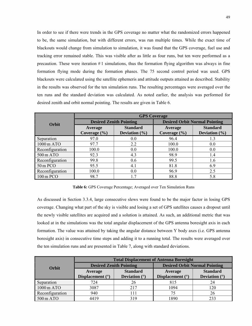
49
In order to see if there were trends in the GPS coverage no matter what the randomized errors happened
to be, the same simulation, but with different errors, was run multiple times. While the exact time of
blackouts would change from simulation to simulation, it was found that the GPS coverage, fuel use and
tracking error remained stable. This was visible after as little as four runs, but ten were performed as a
precaution. These were iteration # 1 simulations, thus the formation flying algorithm was always in fine
formation flying mode during the formation phases. The 75 second control period was used. GPS
blackouts were calculated using the satellite ephemeris and attitude outputs attained as described. Stability
in the results was observed for the ten simulation runs. The resulting percentages were averaged over the
ten runs and the standard deviation was calculated. As noted earlier, the analysis was performed for
desired zenith and orbit normal pointing. The results are given in Table 6.
Orbit
GPS Coverage Desired Zenith Pointing Desired Orbit Normal Pointing
Average Coverage (%)
Standard Deviation (%)
Average Coverage (%)
Standard Deviation (%)
Separation 97.0 0.0 96.4 1.3 1000 m ATO 97.7 2.2 100.0 0.0 Reconfiguration 100.0 0.0 100.0 0.0 500 m ATO 92.3 4.3 98.9 1.4 Reconfiguration 99.8 0.6 99.5 1.6 50 m PCO 95.5 4.1 81.8 6.9 Reconfiguration 100.0 0.0 96.9 2.5 100 m PCO 98.7 1.7 88.8 5.8
Table 6: GPS Coverage Percentage; Averaged over Ten Simulation Runs
As discussed in Section 3.3.4, large consecutive slews were found to be the major factor in losing GPS
coverage. Changing what part of the sky is visible and losing a set of GPS satellites causes a dropout until
the newly visible satellites are acquired and a solution is attained. As such, an additional metric that was
looked at in the simulations was the total angular displacement of the GPS antenna boresight axis in each
formation. The value was attained by taking the angular distance between Y body axes (i.e. GPS antenna
boresight axis) in consecutive time steps and adding it to a running total. The results were averaged over
the ten simulation runs and are presented in Table 7, along with standard deviations.
Orbit
Total Displacement of Antenna Boresight Desired Zenith Pointing Desired Orbit Normal Pointing
Average Displacement (°)
Standard Deviation (°)
Average Displacement (°)
Standard Deviation (°)
Separation 724 26 815 24 1000 m ATO 3087 217 1094 120 Reconfiguration 940 111 75 26 500 m ATO 4419 319 1890 233

50
Reconfiguration 811 65 693 56 50 m PCO 3822 281 4629 537 Reconfiguration 576 47 1053 96 100 m PCO 2705 247 3822 339
Table 7: Total Displacement of Antenna Boresight; Averaged over Ten Simulation Runs
The resulting coverage shows that there are orbits that benefit from desired zenith pointing and others that
benefit from desired orbit normal pointing. There is clear benefit from as little GPS dropouts as possible
when it comes to precise formation flying. Switching between pointing schemes is not complicated,
whether it is done via operations or autonomously via FIONA settings. These results indicate that there
would be benefit in employing a combination of desired antenna pointing schemes.
Additionally, Table 7 shows that for some orbits, one pointing method results in much more antenna
boresight slewing than the other. For example, in the 1000 m ATO, the coverage is only a few percent
better when desired orbit normal pointing is used, but the antenna boresight axis slewed approximately
three times less. Another example is the reconfiguration orbit from the 1000 m ATO to the 500 m ATO.
The coverage in both cases is 100 %, but the antenna boresight axis slews approximately twelve times
more when desired zenith pointing is used.
Attitude pointing schemes that result in less antenna boresight slewing are more reliable to maintain GPS
coverage. Additionally, simulation inaccuracies due to assumptions and approximations will likely have
less effect on coverage for orbits that have less slewing overall. Also, if there are any undesired transient
effects in GPS solution due to acquiring or dropping satellites without actually losing the GPS solution,
the amount of times this happens is reduced when the antenna FOV is slewing less.
Additional benefits of selecting pointing schemes that have less slewing are those on attitude hardware
and power consumption. The magnitude of these has not been examined as part of this work and will not
be discussed here.
Finally, three other values of interest were monitored:
Fuel Use – The FIONA calculated ΔV.
Tracking Error – The difference between the reference trajectory and the relative state.
Tracking Error after Delays – The same as above, except that, to account for formation insertion
errors, there is a delay after reconfiguration before the error is considered (see Section 3.4.2 for
details).

51
The results, averaged over ten simulation runs, are shown in Table 8. Since only the attitude was changed
for desired zenith/orbit normal pointing, the first iteration values are the same for both attitude schemes.
Parameter Average Standard Deviation Fuel Use 0.611 m/s 0.008 m/s Tracking Error 0.763 m 0.149 m Tracking Error after Delays 0.769 m 0.045 m
Table 8: Fuel Use and Tracking Errors; Averaged over Ten Simulation Runs
The fuel use shown is a total for the complete simulation. When broken down into formation and
reconfiguration segments, it can be shown that at least ten orbits in each formation can be demonstrated,
satisfying mission requirements.
As shown, the tracking errors meet the sub-metre requirement. Of specific note, however, is the fact that
the tracking error is slightly higher after the aforementioned delays are considered. The reason for this is
that in some simulations, the tracking error after insertion into a formation is low and sub-metre tracking
is attained quickly. Consequently, the delay time after insertion actually encompasses a large segment
where sub-metre tracking was being demonstrated. However, some relatively larger tracking errors
(though still sub-metre) existed at other points of formation flying. When the tracking error was tallied
without using a delay time, the sub-metre tracking portions that would otherwise fall inside the delay
assisted in bringing down the overall tracking error. The lesson learned is that the delay time being used is
likely too large in a number of simulations and needs to be refined. For the ten simulations used to attain
the aforementioned results, the tracking error calculated without a delay was lower in six of them.
3.4.2 GPS Coverage with Blackouts Supplied
Iteration # 1 results are used to attain GPS coverage metrics as described in Section 3.2.6. These are used
in Iteration # 2, whose metrics are used in Iteration # 3 and so on.
When a formation is entered after a reconfiguration, there is an initial spike in the tracking error due to the
difference between desired and actual relative state as a result of formation insertion error. Also, a period
of changing magnitude in tracking error is encountered when the transition is made from coarse to fine
formation control after a blackout. Since this is unavoidable, SFL staff made the decision to introduce a
delay after these periods before sub-metre formation control can be demonstrated. It is important to note
that mission requirements are not violated by having this delay time after transitions. Based on the
duration of these effects, the delays can be adjusted. The following values were determined empirically to
encompass the aforementioned transitional periods:

52
Delay after Reconfiguration: 1200 sec – Value based on simulation testing of FIONA.
Delay after Transition to Fine Tracking: 1200 sec – Value based on simulation testing of FIONA.
As discussed in Section 3.2.6, the data processing generates a series of 1s and 0s, one for each time step
of the simulation, where a 1 means there is a GPS blackout and a 0 means there is not. Note that the
abovementioned delays do not affect the GPS blackout times.
The simulation is repeated with the same parameters (except for the randomized errors) but with the
calculated GPS blackouts supplied. FIONA will now miss thrusts due to lapses in GPS solution and will
also be toggled between coarse and fine modes. The ephemeris generated is again used with
OASYS/Mirage to determine an attitude profile. The ephemeris and attitude are then used to calculate the
GPS coverage resulting from this iteration.
This process results in another unique set of GPS blackouts, which is supplied into the next iteration. Five
iterations were performed, where Iteration #1 did not have blackouts, but was used to generate a set for
Iteration # 2, resulting in a total of four iterations with GPS blackouts. After these four iterations, stability
in the GPS coverage, fuel use and tracking error was observed. The averaged GPS coverage along with
standard deviation is given in Table 9.
Orbit
GPS Coverage Desired Zenith Pointing Desired Orbit Normal Pointing
Average Coverage (%)
Standard Deviation (%)
Average Coverage (%)
Standard Deviation (%)
Separation 97.0 0.0 94.0 0.0 1000 m ATO 95.8 4.2 97.8 2.6 Reconfiguration 99.8 0.5 100.0 0.0 500 m ATO 98.3 2.1 100.0 0.0 Reconfiguration 100.0 0.0 100.0 0.0 50 m PCO 98.3 2.1 93.0 5.2 Reconfiguration 100 0.0 98.0 2.4 100 m PCO 99.3 1.5 93.5 6.4
Table 9: GPS Coverage Percentage; Averaged over Four Iterations with Blackouts
The GPS antenna total displacement results along with standard deviations are given in Table 10.
Orbit
Total Displacement of Antenna Boresight Desired Zenith Pointing Desired Orbit Normal Pointing
Average Displacement (°)
Standard Deviation (°)
Average Displacement (°)
Standard Deviation (°)
Separation 778 47 838 76 1000 m ATO 3275 308 1518 381

53
Reconfiguration 921 69 76 18 500 m ATO 4198 410 1998 270 Reconfiguration 774 72 713 65 50 m PCO 3635 220 3318 161 Reconfiguration 589 86 1021 146 100 m PCO 2745 177 3203 245
Table 10: Total Displacement of Antenna Boresight; Averaged over Four Iterations with Blackouts
These results generally agree with those from Iteration # 1 in terms of which antenna pointing method
benefits which formation.
Fuel use and tracking error data are given in Table 11. Note that each attitude scheme resulted in a
different set of GPS blackouts. Each of these was run in a separate subsequent simulation. Hence, the
following results are separate for desired zenith and desired orbit normal pointing. They are totals for the
whole simulation.
Parameter
Value Desired Zenith Pointing Desired Orbit Normal Pointing
Average Standard Deviation
Average Standard Deviation
Fuel Use 0.703 m/s 0.024 m/s 0.769 m/s 0.027 m/s Tracking Error 1.39 m 0.21 m 1.63 m 0.07 m Tracking Error after Reconfiguration Delays
1.85 m 0.22 m 2.20 m 0.22 m
Tracking Error after Reconfiguration and Fine Transition Delays
0.799 m 0.08 m 0.796 m 0.12 m
Percent of Time in Formations Used to Calculate Error with All Delays
60.8 % 5.9 % 49.0 % 4.0 %
Percent of Simulation Time Spent in Fine Mode
93.7 % 1.6 % 88.0 % 3.5 %
Table 11: Fuel Use and Tracking Error Data; Averaged over Four Iterations with Blackouts
The fuel use is a simulation total value and includes reconfigurations as well as formation flying in coarse
and fine modes. As in Iteration # 1, if broken down, it can be shown that at least ten orbits in each
formation can be demonstrated with the available fuel margin.
Of specific note are the tracking errors. Unlike in Iteration #1, the tracking error when transitional effects
are included does not meet sub-metre control requirements. While mission requirements do not stipulate
that sub-metre tracking has to be demonstrated during GPS blackouts, these higher errors are an indirect
result of lapses in GPS solution. After a blackout, when a solution is reacquired, FIONA spends 600
seconds in coarse mode to allow for relative state estimates to converge. When the transition is made to

54
fine mode and the controller gains are changed, the tracking error requires a finite amount of time to drop
to the sub-metre level. This transitional period significantly increases the overall tracking error to more
than one metre.
When the tracking error is calculated with the reconfiguration delay to account for formation insertion
errors, the same effect as described in Iteration #1 takes place. Further empirical evidence from signal
simulator testing will aid in confirming this effect and all results will be used to adjust the delay time.
Finally, when the fine mode transition delay is introduced, the resulting tracking error is representative of
fine formation flying during periods where a GPS solution has been available long enough for transitional
periods to be complete. It is demonstrated that sub-metre tracking errors are achievable under these
conditions. Of the time spent in formations, 60.8 % and 49.0 % of time was spent in fine formation mode
and outside of transitional periods for desired zenith and desired orbit normal pointing, respectively. The
lower time for desired orbit normal pointing is a result of the lower GPS coverage for the PCOs compared
to desired zenith pointing. The fractions of time would be maximized with a combination of GPS antenna
pointing methods based on the formation being maintained.
The above percentages do not include reconfiguration orbits. The total time spent in fine mode for both
formation and reconfiguration orbits, including transitional periods, is 93.7 % and 88.0 % of the total
simulation time for desired zenith and desired orbit normal pointing, respectively. It is worth noting that
there are no requirements for tracking accuracy during reconfigurations.
3.4.3 GPS Coverage without Limited Slew Rate
To quantify the effect of the limited slew rate, the thrust targets and TLEs attained for five simulation
runs of Iteration # 1 were supplied to OASYS/Mirage with the slew rate limit removed. Stability was
observed. The results were averaged and standard deviations were found. The results from the first five
simulation runs of Iteration # 1 with the slew rate limit in place are provided for comparison. The
coverage results are given in Table 12.
Orbit
GPS Coverage Desired Zenith
Pointing Desired Orbit Normal
Pointing Slew Rate
Limit No Slew Rate
Limit Slew Rate
Limit No Slew Rate
Limit Ave. Cov. (%)
Std. Dev. (%)
Ave. Cov. (%)
Std. Dev. (%)
Ave. Cov. (%)
Std. Dev. (%)
Ave. Cov. (%)
Std. Dev. (%)
Separation 97.0 0.0 97.0 0.0 96.4 1.3 96.4 1.3 1000 m ATO 98.0 1.9 94.4 4.2 100.0 0.0 100.0 0.0

55
Reconfiguration 100.0 0.0 100.0 0.0 100.0 0.0 100.0 0.0 500 m ATO 92.2 3.3 84.2 6.7 99.0 1.4 99.4 1.3
Reconfiguration 100.0 0.0 99.8 0.4 99.0 2.2 99.8 0.4 50 m PCO 93.6 5.1 93.0 5.4 78.8 5.7 83.0 1.0
Reconfiguration 100.0 0.0 100.0 0.0 97.8 1.3 98.4 1.7 100 m PCO 98.0 1.9 97.6 2.5 85.6 6.5 85.0 9.4
Table 12: GPS Coverage Percentage with and without Slew Rate Limit; Averaged over Five Simulation Runs
(Ave. Cov. = Average Coverage; Std. Dev. = Standard Deviation)
The slew rate limit provides some benefit when trying to point the antenna towards zenith in the ATOs.
However, trying to point the antenna towards orbit normal results in better coverage for the ATOs than
either of the desired zenith pointing cases. For the PCOs, the limited slew rate did not make a noticeable
difference when trying to point the antenna towards zenith. For desired orbit normal pointing, the slew
rate limit resulted in marginally worse coverage for the 50 m PCO and did not make a noticeable
difference for the 100 m PCO. Overall, trying to point the antenna towards zenith for the PCOs resulted in
better GPS coverage, a result consistent with previous observations. Finally, for the reconfigurations, the
limited slew rate did not have a noticeable effect.
The GPS antenna boresight slewing results are given in Table 13.
Orbit
Total Displacement of Antenna Boresight Desired Zenith
Pointing Desired Orbit Normal
Pointing Slew Rate
Limit No Slew Rate
Limit Slew Rate
Limit No Slew Rate
Limit Ave. Dis. (°)
Std Dev. (°)
Ave. Dis. (°)
Std Dev. (°)
Ave. Dis. (°)
Std Dev. (°)
Ave. Dis. (°)
Std Dev. (°)
Separation 728 23 718 22 817 26 818 23 1000 m ATO 3054 164 3004 179 1109 90 1128 83 Reconfiguration 941 159 922 138 63 21 65 26 500 m ATO 4288 357 4222 316 1972 229 1944 211 Reconfiguration 793 82 780 67 706 48 693 46 50 m PCO 3756 351 3732 358 4778 546 4582 493 Reconfiguration 553 38 562 41 1042 59 1016 28 100 m PCO 2778 233 2762 226 3998 352 3880 357
Table 13: Total Displacement of Antenna Boresight with and without Slew Rate Limit; Averaged over Five
Simulation Runs (Ave. Dis. = Average Displacement; Std. Dev. = Standard Deviation)
The slew rate limit does not have a major noticeable difference on the overall amount of slewing.

56
3.4.4 Recommendations
Simulation testing has shown that trying to point the GPS antenna towards zenith is beneficial for the
PCOs. Trying to point the antenna towards orbit normal results in better coverage for the ATOs. This is
supported by significantly less antenna boresight slewing in the ATOs when desired orbit normal pointing
is employed and vice-versa for the PCOs.
The slew rate limit improves GPS coverage only for desired zenith pointing in the ATOs, but coverage is
still lower than with desired orbit normal pointing. As a result, the slew rate limit does not provide better
GPS coverage overall.
For the reconfiguration orbits, in general, it makes sense to choose desired zenith pointing since there are
long periods without thrusting during which the GPS antenna can be tracking zenith, not just trying to
point close to it. A contrary case may be the 1000 m ATO to 500 m ATO reconfiguration, where in the
iterated cases, there was no noticeable difference in the GPS coverage, but there was over ten times more
slewing of the antenna boresight when trying to point to zenith. As previously discussed, less antenna
slewing is preferable as it decreases the likelihood of losing GPS lock on orbit. It also decreases the
frequency of changing which GPS satellites are being tracked by the receiver.
It is important to recognize that GPS coverage and slewing results are dependent on the attitude controller
being employed. Any changes that result in different slew paths will have an effect on GPS coverage.
Lastly, it is worth noting that in preparation for further signal simulator testing at SFL by a staff member,
an independent simulation verified that the desired thrusts in an ATO tend to allow antenna slewing to be
reduced when trying to align the antenna with orbit normal. This is because many of the thrusts fall
relatively close to the orbital frame, allowing the antenna to slew less. To elucidate this point, a simplified
example is that of a two thrust sequence. The first is in the orbital plane, in a direction 45 ° away from
zenith towards the velocity direction. The second is also in the orbital plane, but 45 ° away from zenith
towards the anti-velocity direction. Since the GPS antenna boresight is perpendicular to the satellite thrust
axis, if the antenna is trying to align with orbit normal (in this case it would be pointing exactly towards
orbit normal) the slew can occur around the boresight and the antenna pointing will not change at all. If
the antenna was trying to point towards zenith, a substantial antenna slew would have resulted. While this
is an oversimplified case, since seldom does a thrust occur exactly in the orbital plane, the reasoning
applies to a broader range of slews that are near the orbital plane.
A similar argument can be made for the PCOs and trying to point the antenna towards zenith. Here, many
thrust targets will be near the local horizontal plane.

57
The recommended pointing methods are summarized in Table 14.
Formation Flying Phase Attitude Pointing Method
Along track orbits Desired orbit normal pointing Without slew rate limit
Projected circular orbits Desired zenith pointing Without slew rate limit
Reconfigurations
Zenith tracking in between thrusts Desired zenith pointing when thrusting Possible exception of reconfiguration from
1000 m ATO to 500 m ATO due to significantly more GPS antenna boresight slewing
Without slew rate limit
Table 14: Recommended Attitude Pointing Methods for Each Phase of Formation Flying
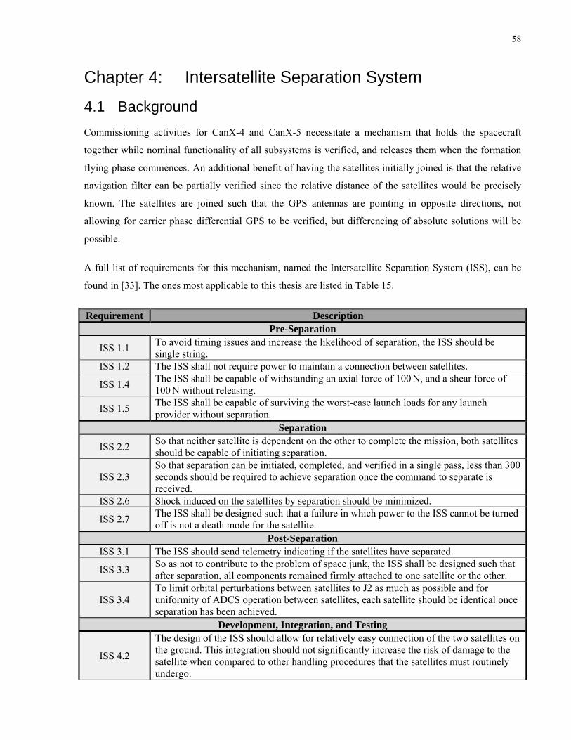
58
Chapter 4: Intersatellite Separation System
4.1 Background
Commissioning activities for CanX-4 and CanX-5 necessitate a mechanism that holds the spacecraft
together while nominal functionality of all subsystems is verified, and releases them when the formation
flying phase commences. An additional benefit of having the satellites initially joined is that the relative
navigation filter can be partially verified since the relative distance of the satellites would be precisely
known. The satellites are joined such that the GPS antennas are pointing in opposite directions, not
allowing for carrier phase differential GPS to be verified, but differencing of absolute solutions will be
possible.
A full list of requirements for this mechanism, named the Intersatellite Separation System (ISS), can be
found in [33]. The ones most applicable to this thesis are listed in Table 15.
Requirement Description Pre-Separation
ISS 1.1 To avoid timing issues and increase the likelihood of separation, the ISS should be single string.
ISS 1.2 The ISS shall not require power to maintain a connection between satellites.
ISS 1.4 The ISS shall be capable of withstanding an axial force of 100 N, and a shear force of 100 N without releasing.
ISS 1.5 The ISS shall be capable of surviving the worst-case launch loads for any launch provider without separation.
Separation
ISS 2.2 So that neither satellite is dependent on the other to complete the mission, both satellites should be capable of initiating separation.
ISS 2.3 So that separation can be initiated, completed, and verified in a single pass, less than 300 seconds should be required to achieve separation once the command to separate is received.
ISS 2.6 Shock induced on the satellites by separation should be minimized.
ISS 2.7 The ISS shall be designed such that a failure in which power to the ISS cannot be turned off is not a death mode for the satellite.
Post-Separation ISS 3.1 The ISS should send telemetry indicating if the satellites have separated.
ISS 3.3 So as not to contribute to the problem of space junk, the ISS shall be designed such that after separation, all components remained firmly attached to one satellite or the other.
ISS 3.4 To limit orbital perturbations between satellites to J2 as much as possible and for uniformity of ADCS operation between satellites, each satellite should be identical once separation has been achieved.
Development, Integration, and Testing
ISS 4.2
The design of the ISS should allow for relatively easy connection of the two satellites on the ground. This integration should not significantly increase the risk of damage to the satellite when compared to other handling procedures that the satellites must routinely undergo.

59
ISS 4.4 It shall be possible to set and reset the ISS with no disassembly of either satellite.
ISS 4.5 The potential for damage to the satellite during reset of the ISS shall be minimized. GSE that allows access to the ISS but protects exposed and sensitive areas of the satellite will be implemented to protect the satellite during reset of the ISS.
Table 15: ISS Requirements – Taken from [33]
Prior to the author beginning his Master studies at SFL, a trade study that considered power, thermal,
mechanical, testing and operational requirements concluded with a design based on an electrically
debonding epoxy [34]. The ISS consists of two almost identical units, shown in Figure 23. Each unit is
housed within one satellite, with the bonding element protruding from the -Y spacecraft face. One bond is
shaped as a cup, the other as a cone; the only difference between the two units. The cup and cone are held
together by the epoxy. Internal to the satellite, a compression spring on each unit provides a force along
the bond axis, with the intent of pulling the ISS apart. The spring is chosen such that the load applied is
less than the full strength of the epoxy. When a voltage is applied across the bond surface, the strength of
the epoxy is significantly reduced and the spring provides the required force to break the bond, separating
the spacecraft.
The ISS is connected to the Payload Power Board, an electronic board designed for the CanX-4/-5
mission and responsible for providing power to not only the ISS, but also to CNAPS, the intersatellite
communication system and the payload computer. The Payload Power Board supplies 12.5 V directly
across the epoxy bond to weaken it. The epoxy is expected to debond along the anode interface [35]. It is
possible to initiate separation from either satellite. The Payload Power Board is designed in such a way as
to provide a ground path no matter which satellite initiates the separation. Further to the redundancy
provided, an added benefit of this is the capability to alternate the direction of applied voltage as a
contingency to nominal separation.
Prior to the author’s efforts, a prototype model had been used to perform a concept verification for the
epoxy. The prototype model is flight representative in the sense that the separation mechanism is a cup
and cone, bonded together with epoxy, with a spring based load that tries to separate the bond. There are,
however, several differences between the prototype and flight models. The two models and their
differences are presented in the following sections.
The author’s tasking was to assemble the flight model and integrate it with the satellite structures and
Payload Power Board. Functional testing, thermal acceptance testing and calibration were to be
performed, along with attaining performance metrics. This was under the assumption that the flight ISS
would function consistently as designed, based on the prototype proof of concept. Unfortunately, it was

60
found that the flight model did not function as expected. As a result, the tasking changed to
troubleshooting and testing the design and determining recommendations as to its further development.
The following sections outline both prototype and flight models, the initial observations made, the
strategies adopted to troubleshooting the mechanism and, finally, the recommended changes to the design.
The arming procedure for the system is also detailed.
4.2 Prototype Model
4.2.1 Overview
The prototype model is shown in Figure 22 in its separated state with cup and cone retracted. Cured
epoxy can be seen on the surface of the cone.
Figure 22: Prototype ISS Model
Most flight model components are similar to those shown on the prototype and an explanation of the
purpose of each component is given in Section 4.3.1. The Belleville washers, which provide the
separation spring force, are not compressed in the unarmed state.
When arming the ISS, one set of screws holding the “satellite faces” and the spacers together is removed
to allow access to the cup. The pull plates are then pulled down until a 1 mm metal spacer can be inserted
between the cup and the Delrin base. The same is done for the cone. The Belleville washer stack fits
snugly between the Delrin base and the pull plate. As a result of inserting the spacer, the stack is
compressed by 1 mm. The epoxy is then applied into the cup, the two sides of the ISS fixed to their
respective “satellite faces” are joined back together using screws. The epoxy is allowed to cure.
When the spacers are removed, the epoxy holds the cup and cone together and the Belleville washers
remain compressed, applying a force across the bond that is not large enough to break the full strength of

61
the epoxy. For separation, a power supply is connected to the pull plates and 12.5V are applied. The
epoxy weakens due to the applied potential, allowing the force from the Belleville washers to overcome
the epoxy bond strength and separate the ISS.
Testing prior to the author’s involvement had shown that the prototype model had reasonable success and
trials would usually result in separation as expected.
4.3 Flight Model
4.3.1 Overview
The flight ISS solid model is shown in Figure 23. The components are described below, followed by a
comparison of the prototype and flight models in Table 16.
Figure 23: Flight ISS Solid Model
The key components and features are outlined:
Pull plate – Assists in arming the device and provides a surface to compress the spring. The pull
plate is pulled down using screws that are inserted from the outside of the satellite face for
arming. The spacer plate is inserted as in the prototype model and the screws are removed prior to
joining the satellites for curing.
Microswitch – Provides separation telemetry. The push button at the bottom of the switch is
depressed against the Delrin base when armed. It is meant to disengage when the ISS separates.
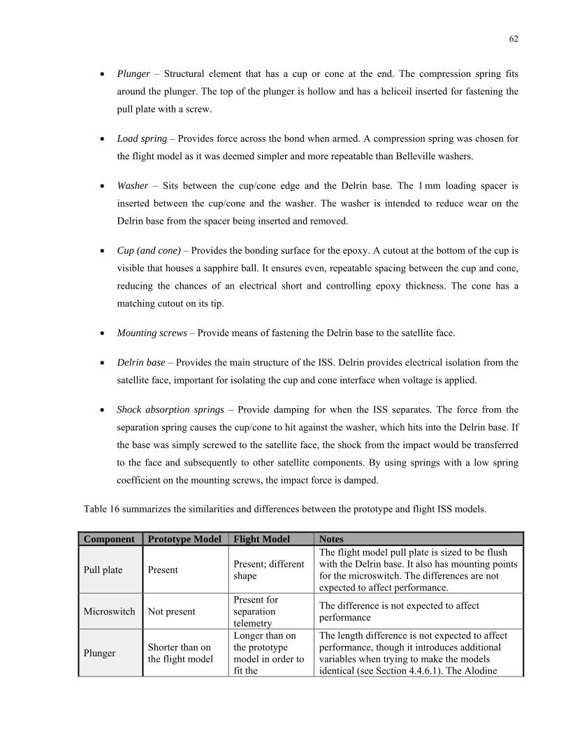
62
Plunger – Structural element that has a cup or cone at the end. The compression spring fits
around the plunger. The top of the plunger is hollow and has a helicoil inserted for fastening the
pull plate with a screw.
Load spring – Provides force across the bond when armed. A compression spring was chosen for
the flight model as it was deemed simpler and more repeatable than Belleville washers.
Washer – Sits between the cup/cone edge and the Delrin base. The 1 mm loading spacer is
inserted between the cup/cone and the washer. The washer is intended to reduce wear on the
Delrin base from the spacer being inserted and removed.
Cup (and cone) – Provides the bonding surface for the epoxy. A cutout at the bottom of the cup is
visible that houses a sapphire ball. It ensures even, repeatable spacing between the cup and cone,
reducing the chances of an electrical short and controlling epoxy thickness. The cone has a
matching cutout on its tip.
Mounting screws – Provide means of fastening the Delrin base to the satellite face.
Delrin base – Provides the main structure of the ISS. Delrin provides electrical isolation from the
satellite face, important for isolating the cup and cone interface when voltage is applied.
Shock absorption springs – Provide damping for when the ISS separates. The force from the
separation spring causes the cup/cone to hit against the washer, which hits into the Delrin base. If
the base was simply screwed to the satellite face, the shock from the impact would be transferred
to the face and subsequently to other satellite components. By using springs with a low spring
coefficient on the mounting screws, the impact force is damped.
Table 16 summarizes the similarities and differences between the prototype and flight ISS models.
Component Prototype Model Flight Model Notes
Pull plate Present Present; different shape
The flight model pull plate is sized to be flush with the Delrin base. It also has mounting points for the microswitch. The differences are not expected to affect performance.
Microswitch Not present Present for separation telemetry
The difference is not expected to affect performance
Plunger Shorter than on the flight model
Longer than on the prototype model in order to fit the
The length difference is not expected to affect performance, though it introduces additional variables when trying to make the models identical (see Section 4.4.6.1). The Alodine
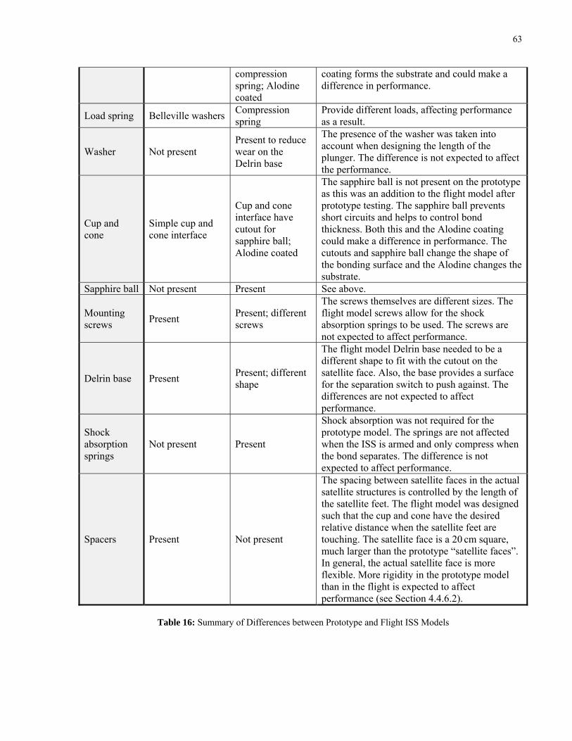
63
compression spring; Alodine coated
coating forms the substrate and could make a difference in performance.
Load spring Belleville washers Compression spring
Provide different loads, affecting performance as a result.
Washer Not present Present to reduce wear on the Delrin base
The presence of the washer was taken into account when designing the length of the plunger. The difference is not expected to affect the performance.
Cup and cone
Simple cup and cone interface
Cup and cone interface have cutout for sapphire ball; Alodine coated
The sapphire ball is not present on the prototype as this was an addition to the flight model after prototype testing. The sapphire ball prevents short circuits and helps to control bond thickness. Both this and the Alodine coating could make a difference in performance. The cutouts and sapphire ball change the shape of the bonding surface and the Alodine changes the substrate.
Sapphire ball Not present Present See above.
Mounting screws
Present Present; different screws
The screws themselves are different sizes. The flight model screws allow for the shock absorption springs to be used. The screws are not expected to affect performance.
Delrin base Present Present; different shape
The flight model Delrin base needed to be a different shape to fit with the cutout on the satellite face. Also, the base provides a surface for the separation switch to push against. The differences are not expected to affect performance.
Shock absorption springs
Not present Present
Shock absorption was not required for the prototype model. The springs are not affected when the ISS is armed and only compress when the bond separates. The difference is not expected to affect performance.
Spacers Present Not present
The spacing between satellite faces in the actual satellite structures is controlled by the length of the satellite feet. The flight model was designed such that the cup and cone have the desired relative distance when the satellite feet are touching. The satellite face is a 20 cm square, much larger than the prototype “satellite faces”. In general, the actual satellite face is more flexible. More rigidity in the prototype model than in the flight is expected to affect performance (see Section 4.4.6.2).
Table 16: Summary of Differences between Prototype and Flight ISS Models

64
4.3.2 Arming Procedure
Existing procedures for arming the ISS were consolidated, expanded and modified based on experience
gained throughout testing. The revised arming procedure is outlined below:
Load the ISS:
1.) Clean the cup and cone bonding surfaces and the sapphire ball:
a.) Scrape off large remaining pieces of epoxy from previous tests using a scalpel. Avoid
scratching the bonding surfaces as much as reasonably possible.
b.) Clean small remaining bits of epoxy using acetone and a plastic applicator.
c.) Examine the cup, cone and sapphire ball under a microscope to ensure all surfaces are
clean and free of old epoxy.
d.) Wipe off all surfaces thoroughly using isopropyl alcohol. Wear gloves to avoid leaving
any skin oils on the surfaces.
2.) Load the springs using the loading screws, as shown in Figure 24. Compress the ISS only until
the spacer can be inserted. Compressing more than this can result in damage to the push pin
mechanism in the microswitch.
Figure 24: Compressing ISS Spring using Loading Screws (Image from [36])
3.) Insert the loading spacer between the cup/cone and the washer as shown in Figure 25.
4.) Ensure the microswitch is depressed using a digital multimeter
(DMM). This step applies to testing. When arming the ISS with
assembled satellites, the switch will not be accessible as it is housed
within the satellite structure. The state of the microswitch after the
arming procedure will have to be checked via telemetry when the
satellites are on.
5.) Remove the loading screws as shown in Figure 25.
6.) Ensure the microswitch is still depressed using a DMM. This step
applies to testing. When arming the ISS with assembled satellites, the
Figure 25: Inserting ISS
Loading Spacer and
Removing Loading Screws
(Image from [36])

65
switch will not be accessible. Again, its state can be verified after the arming procedure when the
satellites are on.
Prepare the epoxy:
7.) Dispense the two part mixture into a mixing dish. The dispenser ensures the proper 1 to 4 ratio.
8.) Gently mix until uniform. A smell akin to ammonia should be apparent. This has been found to
happen within no more than 2 minutes. Therefore, the recommended mixing time is 2 minutes.
9.) Degas the mixed epoxy for approximately13 minutes in the bell jar. This will remove air in the
epoxy that could weaken the bond. Testing has shown that after 13 minutes, most of the visible
air has escaped from the epoxy and the bell jar is evacuated to approximately 200 milliTorr, as
low as it can go in the current setup.
10.) In the remaining steps, do not vigorously stir or scoop the epoxy to avoid introducing air bubbles.
Join the satellites:
11.) From the Lexan satellite lunch box, remove one entire long face, the top panel from the opposing
long face and one end panel to allow easy access for sliding the satellites in and to leave room for
the protruding loading spacers. Place the remaining lunch box structure vertically. This setup is
shown in Figure 26.
Figure 26: Lunchbox Setup for Flight ISS Testing (Top-End, Front and Top-Back Panels Removed)
12.) Place the satellite with the cup interface into the lunch box with the cup (-Y face) facing upwards
and the loading spacer protruding from the completely removed long face of the lunch box.
13.) Place the sapphire ball into the cutout in the cup.
Removed

66
14.) Apply the epoxy into the cup using a plastic applicator. The sapphire ball will stick to the epoxy
and any slight motion will tend to displace it. Hold the sapphire ball in place using another plastic
applicator to prevent this. Take care to avoid creating air pockets when applying the epoxy.
15.) Let the epoxy settle and even out, but make sure not to exceed the pot life of 30 minutes [35].
16.) Slide the other satellite down the lunch box rails with the cone (-Y face) facing downwards. Both
loading spacers should be protruding from the same side of the lunch box. Gently allow the cone
to settle inside the cup and ensure that the legs of the satellites are properly lined up and touching.
17.) Use a DMM to ensure that a short circuit does not exist across the bond.
18.) Fasten the top Lexan panel on the opposite side of the protruding loading spacers. Fasten the end
panel to the lunch box as well.
Cure the epoxy:
19.) Let cure for 2 days at room temperature or 3 hours at 80 °C. When using the assembled satellites,
the curing will have to be at room temperature as the chamber temperature is too high to subject
all satellite components to. The data sheet specifications state 1 day at room temperature or 1
hour at 80 °C, but it was found that the likelihood of the ISS separating prematurely when the
spacers are removed was higher if these times were used. If a thermal chamber was used for
curing, allow the system to cool to room temperature before moving to the next step. Also, in the
thermal chamber, count curing time from when the cup and cone interface reaches 80 °C, not
when the chamber does. Due to thermal mass of the structures, the epoxy may not be at 80 °C at
the same time as the chamber.
20.) Check for a short circuit across the bond using a DMM.
21.) Remove the spacer plates. Use caution as there will be resistance and when they do come out, it
will likely be abrupt. Extreme care must be taken to avoid damage to the satellite, especially
when solar cells will be present on the satellite face. In this case, use protective Ground Support
Equipment (GSE) for the solar cells (to be developed).
22.) Check for a short circuit across the bond using a DMM.
23.) Ensure the microswitch is depressed. This step applies to testing. When arming the ISS with
assembled satellites, the switch will not be accessible. As before, microswitch telemetry can be
checked once the satellites are turned on.
24.) Remove the lunchbox panels and gently remove the joined satellites. Ensure that the bond has not
been broken in this process by visual inspection, as well as a resistance measurement using a
DMM. The resistance should be very high, but finite (on the order of tens of MΩ).

67
Note that checking for a short circuit across the bond, verifying microswitch telemetry and ensuring that
the bond has not broken should also be performed after spacecraft vibration testing, as well as at the
launch site.
4.3.3 Initial Flight ISS Testing
The flight ISS had not been tested previously. The model was assembled and integrated with the
unpopulated satellite structure, with the exception of the Payload Power Board. A number of separation
tests were attempted, but the flight ISS did not separate nominally. Extended periods of voltage and
switching the direction of applied voltage occasionally led to separation, but consistency was not
observed.
4.4 Flight ISS Troubleshooting A troubleshooting strategy based on engineering principles was established to isolate the possible causes.
The following sections describe the steps taken to troubleshooting the device and isolating the reasons for
it not functioning.
4.4.1 New Epoxy
The epoxy used in the unsuccessful trials was acquired approximately two years prior. It was stored
refrigerated, increasing its shelf life, but after two years, performance could have been degraded. A few
preliminary tests with the prototype models resulted in successful separation. However, a new epoxy
sample was acquired from EIC Laboratories in Massachusetts, U.S.A, the creators of the epoxy. This
batch was used in subsequent trials to eliminate the possibility that expired product was contributing to
improper function.
The manufacturer recommended shelf life when stored at room temperature is 6 months and it increases
to greater than a year when refrigerated [35]. New epoxy was ordered as needed, though subsequent
orders were placed with a distributor in Sweden named Exonera. Shipping regulations made it easier to
ship the epoxy from Europe.
4.4.2 Epoxy Batch, Preparation and Curing
Possible variation in the epoxy batch, preparation procedure or curing process was investigated. To
provide a control sample for each test, epoxy from the same batch was applied to a prototype model as
well as the flight model and the units were cured together under the same conditions. Separation of the
prototype model was performed prior to every flight model test. A successful separation was indicative of
no issues being present with the epoxy batch, preparation procedure and curing process.

68
Typically, it was found that the prototype model would separate as expected within a few minutes of
voltage being applied, leading to the initial assumption that the epoxy or preparation procedure was not
the root cause of the issue.
4.4.3 Differences between Prototype and Flight Models
Several differences exist between the prototype model and the flight model as previously described in
Table 16. The flight model testing setup also included the Payload Power Board. Since the prototype
model had demonstrated separation, a logical approach was to remove the differences in the flight model
one-by-one, until it matched the prototype as closely as possible. Exact matching was not possible due to
the inherent differences of the two designs.
The test setup for the flight ISS included the Payload Power Board. It was verified that the proper
potential was being generated and applied. In case of more subtle effects, the Payload Power Board was
removed from the testing setup. This had the additional benefit of simplifying test preparation and
satellite handling as there were no electronic components involved. For all subsequent testing, the voltage
across the bond was directly applied using a programmable power supply. As expected, removal of the
Payload Power Board did not yield successful flight ISS separation.
The sapphire ball that helps prevent electrical shorts and controls bond thickness is not present in the
prototype model. This ball directly interfaces with the epoxy and bond surface, adding a different material
to the substrate as well as geometrically complicating the bond surface. The sapphire ball was removed.
To prevent shorting, small spacers were inserted between the feet of the two satellites when they were
joined together in the lunch box to provide additional space in the cup and cone interface, while ensuring
that the cone lowered into the epoxy still had a significant bonding surface. Removal of the sapphire ball
did not produce successful separation. The cutout in the cup and cone for the sapphire ball was still
present. However, the prototype cup has a hole-like irregularity that has not been found to impede
performance. Consequently, the cutout is not expected to affect separation, but complete confirmation of
this would require newly machined plungers that do not have any cutouts (not available) as well as a new
method for preventing shorts and ensuring consistency in bond thickness. This would introduce new
variables into the system.
The flight plungers, including cup and cone, are Alodine coated. The bonding substrate is, therefore, not
aluminum but Alodine. Alodine is conductive though the resistance is marginally larger than across just
aluminum. Unfortunately, not enough is known about the proprietary epoxy and the chemical process it
undergoes when a voltage is applied. Consequently, it is unknown whether an Alodine substrate may lead
to undesired effects during the debonding process. Aluminum was listed as a recommended substrate by

69
the manufacturer [35], but information about a specific coating, such as Alodine, was not available. To
make the flight model more representative of the prototype and eliminate any potential unknown effects,
the Alodine coating was removed from the bonding surface with a fine grade of sandpaper. Inspection
under a microscope of the cup and cone ensured that the aluminum was exposed over the entire surface
area. Subsequent testing of the flight ISS did not result in separation.
The remaining difference between the prototype and flight ISS models was the spring that provides the
load. Belleville washers provide the separation force for the prototype model, while a compression spring
is employed on the flight model. The cured flight ISS was dismantled while keeping the cup and cone
bonded. Shims were added around the plunger, providing additional compression on the spring. The load
was increased incrementally, with voltage applied between each shim addition. Eventually, the ISS
opened. While bond strength could not be inferred from the spring compression employed because the
bond would have been weakened from a number of separation attempts and assembly/disassembly cycles,
the indication was that the load being applied by the compression spring was not sufficient to break the
bond. Consequently, a detailed review of load calculation for both prototype and flight models was
required.
It is important to note that while changing a number of the above elements did not result in successful
separation of the flight ISS, it is not necessarily true that these factors were not contributing to improper
function. When troubleshooting and modifications are complete, the components will have to be
introduced to the system one-by-one and shown not to impede proper operation.
4.4.4 Review of Load Calculations
A compilation of past calculations for both prototype and flight models was created. The result was a
depiction of how the separation system evolved. It was found that each iteration corrected an error or
updated the previous one as new information became available. The author created a final version that
verified calculations and provided updates. In summary, the following was determined:
Prototype:
1.) Initial calculations had an error in calculating the potential energy, resulting in an incorrect ΔV.
This was corrected in the second iteration.
2.) Spacer plate was assumed to be 1.0 mm thick. When measured it is 1.1 mm thick. The 0.1 mm
makes a noticeable difference in resulting load and separation velocity calculations.

70
3.) The Belleville washers were ordered from a company called Spaenaur. The pound force at a
given deflection for the Belleville washers was incorrectly copied from the Spaenaur catalogue.
This affected the spring stiffness calculation, which was then propagated into an error in the
expected load from the Belleville stack.
4.) Satellite mass had been taken to be 6 kg. It was updated to 7 kg.
Flight:
1.) Spacer plate was assumed to be 1.0 mm thick.
Table 17 shows the resulting changes in calculated load and separation velocity.
Prototype Model Parameter Initial Updated
Load across Bond (N) 71 97 Separation Velocity (cm/s) 6.6 10.0
Flight Mode Parameter Initial Updated
Load across Bond (N) 43 49 Separation Velocity (cm/s) 6.5 7.5
Table 17: ISS Calculated Parameter Changes
The overall finding was that the load across the prototype model bond and resulting separation velocity
were larger than originally assumed during the design process. The implications are that firstly, there is
actually more force being applied to separate the bond than expected and secondly, the separation velocity
will be higher than quoted in other calculations and documents.
More significantly, it was found that the load across the bond had been decreased to approximately 40 to
50 N for the flight models using the compression spring chosen for the design. While the exact reasoning
for this change is undocumented, to the author’s best current knowledge, this value was at the time
deemed enough to separate the bond with what was then known about the epoxy strength.
To verify the calculations, and since there was doubt whether the Belleville washers and compression
spring were being used in the regime where spring stiffness is linear (a key factor in the calculations), a
basic load test was performed and is described in Section 4.4.5.
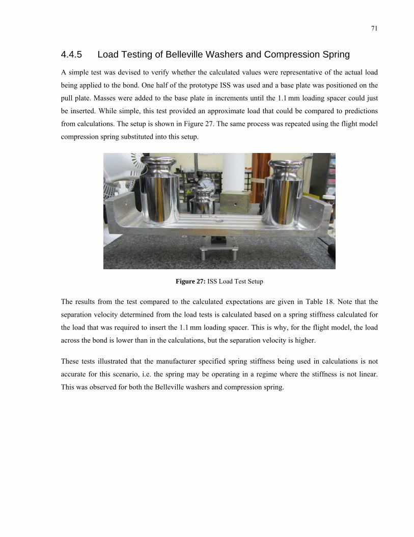
71
4.4.5 Load Testing of Belleville Washers and Compression Spring
A simple test was devised to verify whether the calculated values were representative of the actual load
being applied to the bond. One half of the prototype ISS was used and a base plate was positioned on the
pull plate. Masses were added to the base plate in increments until the 1.1 mm loading spacer could just
be inserted. While simple, this test provided an approximate load that could be compared to predictions
from calculations. The setup is shown in Figure 27. The same process was repeated using the flight model
compression spring substituted into this setup.
Figure 27: ISS Load Test Setup
The results from the test compared to the calculated expectations are given in Table 18. Note that the
separation velocity determined from the load tests is calculated based on a spring stiffness calculated for
the load that was required to insert the 1.1 mm loading spacer. This is why, for the flight model, the load
across the bond is lower than in the calculations, but the separation velocity is higher.
These tests illustrated that the manufacturer specified spring stiffness being used in calculations is not
accurate for this scenario, i.e. the spring may be operating in a regime where the stiffness is not linear.
This was observed for both the Belleville washers and compression spring.

72
Prototype Model Parameter Initial Updated Tested
Load across Bond (N) 71 97 123 Separation Velocity (cm/s) 6.6 10.0 11.2
Flight Model Parameter Initial Updated Tested
Load across Bond (N) 43 49 40 Separation Velocity (cm/s) 6.5 7.5 8.0
Table 18: ISS Calculated Parameter Changes and Load Test Results
In summary, the load on the prototype model, thought to be approximately 70 N, is actually
approximately 120 N. The load on the flight model was shown to be approximately 40 N. The separation
velocity based on the spring stiffness calculated from the load test is 11.2 cm/s for the prototype model
and 8.0 cm/s for the flight model.
With the prototype model having demonstrated separation, it can be inferred that approximately 120 N are
required to break the bond when voltage is applied and only 40 N are applied in the flight model.
4.4.6 Investigated Modifications to the Flight ISS
The following sections outline modifications to the flight ISS that have been proposed and investigated.
4.4.6.1 Flight Spring, Belleville Washers and O-Ring
Increasing the deflection of the flight compression spring in order to attain 120 N was not possible.
Unfortunately, no other non-custom made, off-the-shelf compression springs were found that suited the
requirements for size and spring stiffness. To avoid the need for a custom spring, other options were
investigated.
The first and obvious option was to use Belleville washers, as with the prototype ISS. The ones for the
prototype are made from chrome vanadium steel, but stainless steel washers are required for flight. Very
similar stainless steel Belleville washers were available. Their size and spring constant were only
marginally different and calculations were performed to confirm that the resulting load attained was
representative of the prototype model. Other sizes of Belleville washers were also available, making
customization possible if it was needed in the future. For the purposes of this testing, however, other sizes
were not considered to avoid introducing new variables into the testing process.
Another alternative was using an o-ring that would fit around the plunger and be compressed in the
direction perpendicular to its opening to provide the desired load. This option was explored and a

73
candidate o-ring was found. However, since the prototype model had demonstrated successful separation,
it was reasonable to select the former alternative, which also had the added benefit of allowing for much
more customization of spring load than an o-ring would.
It was decided to use the same stack configuration as was being used on the prototype model to avoid
introducing new variables in the testing process. However, since the shaft of the plungers is longer in the
flight model (to accommodate the original compression spring), “filler” spacers (washers and shims) were
needed to fill up the additional room between the Delrin base and the pull plate. This setup is shown in
Figure 28. A potential challenge with Belleville washers arranged in series is that if the edges of a washer
do not sit flush with the adjacent washer, the compression of the stack may be altered. To reduce the
chance of this happening, the “filler” shims being used to fill the extra space on the plunger were placed
between adjacent Belleville washers.
Figure 28: Belleville Washer Stack on Flight ISS
With shims that were 0.1 mm in thickness, a fairly good control of stack height could be achieved. The
largest uncertainty came from the height of each Belleville washer. This would affect whether the
installed stack was compressed prior to inserting the spacer or if there was unoccupied space between the
pull plate and Delrin base. The former results in more compression than expected, while the latter results
in less. Care was taken to avoid either case.
After this modification, the flight ISS was tested, but successful separation was still not observed. Other
stack combinations were not pursued because it was found through calculations that the original stack
employed in the prototype model worked comparatively well for attaining the desired load and no
advantage of using other stack combinations was found.
4.4.6.1.1 Sensitivity to Compression
Calculations for the Belleville washer stack have shown that the load and separation velocity are quite
sensitive to stack compression. This was observed for various Belleville stack configurations with series
Belleville Washer “Filler” Shim
“Filler” Washer
Pull Plate
Delrin Base

74
and parallel elements. Shown in Table 19 are results from calculations assuming specifications for the
stainless steel Belleville washers that are a candidate for the flight ISS. The same stack configuration as
for the prototype ISS is assumed, though this behaviour was not specific to this configuration.
Parameter -0.2 mm -0.1 mm Desired +0.1 mm +0.2 mm Load (N) 91 104 117 130 143 Separation Velocity (cm/s) 9.6 11.0 12.3 13.7 15.0
Table 19: Sensitivity to Calculated Load and Separation Velocity for Desired Load and ± 0.2 mm
It can be seen that 0.1 mm of deflection results in a difference of 13 N in load and1.3 to 1.4 cm/s in
separation velocity. The shims that could be used to tune the device have a 0.1 mm thickness, allowing for
the precision desired. However, it is difficult to accurately measure the entire stack compression to an
accuracy of 0.1 mm with common tools because the pull plate can be sitting at a slight angle. As a result,
it is likely that in future modification and tuning, estimated load values will have to be confirmed
empirically. Once tuned, if the assembly and components of each side of the ISS do not change, the
performance metrics attained should be repeatable.
4.4.6.2 Satellite Face Deflection
When the loading spacers are removed after curing, the compression springs or Belleville washers will try
to return to an uncompressed state. They will push against the pull plates and the Delrin base. Since the
epoxy is holding the pull plates at a fixed distance, the springs cannot extend in that direction. However,
by pushing against the Delrin base, they are pushing against the satellite face as well. The satellite feet are
pressed against each other at the corners of the faces and as a result, each satellite face deflects at the
centre, in the direction away from the spring and towards the other satellite face. This allows the spring to
partially uncompress, resulting in a loss of force across the bond surface. Prior to the author’s work, a
simple finite element analysis (FEA) using FEMAP Express on a solid model of the satellite face was
performed using the originally assumed 40 N load. The worst case deflection at the centre of the face was
shown to be approximately 0.1 mm. With an initial compression of 1.1 mm from the loading spacer, this
results in approximately a 9 % reduction in load across the bond. This had been taken into account in the
flight ISS design [36]. Since the prototype “satellite faces” are much closer together, the prototype
structure is more rigid and this deflection would not be present.
Since the aforementioned testing indicated that a load of 120 N was likely necessary to separate the
weakened bond, the FEA was repeated using this load. As expected, the worst case deflection was
approximately 3 mm, representing a reduction in load of approximately 27 %. The FEA result is shown in

75
Figure 29. This is a substantial fraction of the overall load applied and needs to be considered in spring
and compression selection.
Figure 29: FEA of Satellite Face Deflection
A more subtle effect, not captured in the static FEA, is that as the plate deflects and the spring
uncompresses, the force from the spring that deflects the plate is reduced. It is therefore expected that the
actual worst case deflection will be less than 0.3 mm. A basic test to measure the deflection was attempted
by fixing an additional metal plate as a reference point to the satellite face and measuring its deflection
using 0.1 mm shims. Unfortunately, the simple nature of this test setup did not allow for a reliable
measurement of this precision. Equipment required to perform such a measurement accurately was not
available on hand and the test was not critical enough to acquire new equipment.
An alternative solution to tailoring spring selection and compression is the inclusion of physical standoffs
between the satellite faces. These would have a length corresponding to the space between the centre of
the faces when the satellite feet are flush. Two or four standoffs could be used, fastened to the ISS
mounting screws whose length can be chosen such that they protrude from the satellite face. Standoffs
could all be mounted to one satellite or split between the two. When the loading spacers are removed and
the satellite faces would otherwise deflect, the standoffs would physically prevent this from occurring.
Figure 30 depicts the desired effect. The red lines in the left image show exaggerated satellite face
deflection. The red arrows in the right image demonstrate the effect of the standoffs to prevent deflection.
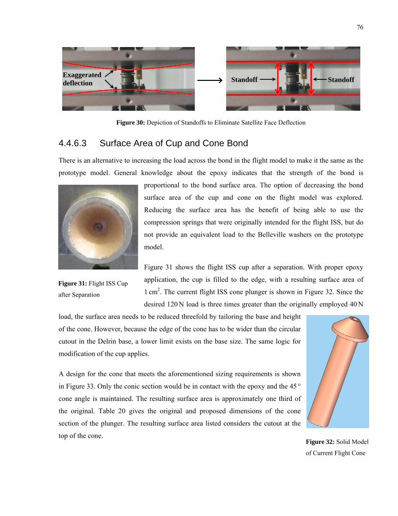
76
Figure 30: Depiction of Standoffs to Eliminate Satellite Face Deflection
4.4.6.3 Surface Area of Cup and Cone Bond
There is an alternative to increasing the load across the bond in the flight model to make it the same as the
prototype model. General knowledge about the epoxy indicates that the strength of the bond is
proportional to the bond surface area. The option of decreasing the bond
surface area of the cup and cone on the flight model was explored.
Reducing the surface area has the benefit of being able to use the
compression springs that were originally intended for the flight ISS, but do
not provide an equivalent load to the Belleville washers on the prototype
model.
Figure 31 shows the flight ISS cup after a separation. With proper epoxy
application, the cup is filled to the edge, with a resulting surface area of
1 cm2. The current flight ISS cone plunger is shown in Figure 32. Since the
desired 120 N load is three times greater than the originally employed 40 N
load, the surface area needs to be reduced threefold by tailoring the base and height
of the cone. However, because the edge of the cone has to be wider than the circular
cutout in the Delrin base, a lower limit exists on the base size. The same logic for
modification of the cup applies.
A design for the cone that meets the aforementioned sizing requirements is shown
in Figure 33. Only the conic section would be in contact with the epoxy and the 45 °
cone angle is maintained. The resulting surface area is approximately one third of
the original. Table 20 gives the original and proposed dimensions of the cone
section of the plunger. The resulting surface area listed considers the cutout at the
top of the cone.
Standoff Standoff Exaggerated deflection
Figure 31: Flight ISS Cup
after Separation
Figure 32: Solid Model
of Current Flight Cone

77
Cone Plunger Radius (mm) Height (mm) Surface Area (mm2) Original 5.00 3.50 approx. 101 Proposed 3.00 3.00 approx. 30.0
Table 20: Original and Proposed Cone Plunger Dimensions
The protruding disc is the same width as the base of the cone in the original design. The height of the
section in between the cone and the disc ensures that the length of the new design matches the old, such
that the cup and cone maintain the same proximity as before. In order to confirm and approve any design
changes prior to implementing them, a comprehensive epoxy strength test was undertaken using the
original cup and cone. It is described in Section 4.4.7.
Figure 33: Solid Model of Proposed Flight ISS Cone Plunger
4.4.7 Epoxy Strength Testing
There were no records found of prior strength testing for the prototype or flight ISS and to the author’s
best knowledge, assumptions and calculations were based on data sheet values. In order to confirm
calculations and assist in developing a modified cup and cone, a comprehensive strength testing campaign
was undertaken.
It was desired to capture any possible effects on the strength of the bond from the presence of the sapphire
ball. Hence, the flight plungers were used for strength testing. There were two sets of flight plungers. In
order to expedite the testing process, both were used. However, only one set of satellite structures is
available. Furthermore, time constraints for other projects resulted in the thermal chamber not being
available for curing. A process oven was available, but would not fit a set of satellite structures. It was
decided to use the two prototype ISS structures to cure the two sets of flight plungers. Since strength
testing would require mechanical separation of only the plungers, the structure used for curing was

78
inconsequential. As mentioned earlier, the flight plungers are longer to accommodate the compression
spring, which is longer than the Belleville stack. In order to avoid “filling” spacers, the flight spring was
used. An additional benefit of this is that since the flight springs provides less load, the chances of
premature separation were reduced (see Section 4.4.8.2). The load does not affect the curing process
because the structure and loading spacers govern the relative distance of the cup and cone. As before,
since strength testing requires mechanical separation of only the plungers, the load used for curing is
inconsequential.
An image of the flight components assembled with the prototype structure is shown in Figure 34.The
preparation and curing procedure was kept constant for all trials. Two types of tests were performed: full
strength with no voltage applied and reduced strength with voltage applied.
Figure 34: Prototype ISS Structure Assembled with Flight Plungers and Springs
Due to chamber availability, the epoxy was cured in a process oven for these tests. The ISS was then
disassembled carefully to avoid breaking the bond. The strength testing setup is shown in Figure 35 and a
description follows.
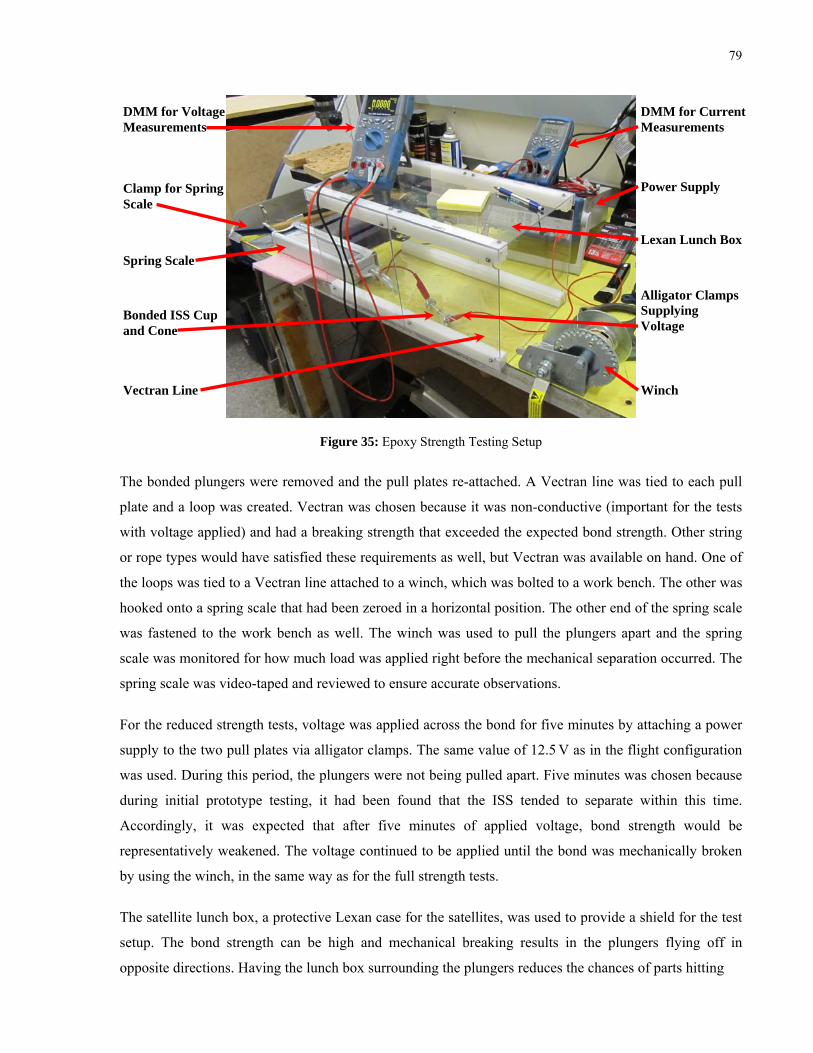
79
Figure 35: Epoxy Strength Testing Setup
The bonded plungers were removed and the pull plates re-attached. A Vectran line was tied to each pull
plate and a loop was created. Vectran was chosen because it was non-conductive (important for the tests
with voltage applied) and had a breaking strength that exceeded the expected bond strength. Other string
or rope types would have satisfied these requirements as well, but Vectran was available on hand. One of
the loops was tied to a Vectran line attached to a winch, which was bolted to a work bench. The other was
hooked onto a spring scale that had been zeroed in a horizontal position. The other end of the spring scale
was fastened to the work bench as well. The winch was used to pull the plungers apart and the spring
scale was monitored for how much load was applied right before the mechanical separation occurred. The
spring scale was video-taped and reviewed to ensure accurate observations.
For the reduced strength tests, voltage was applied across the bond for five minutes by attaching a power
supply to the two pull plates via alligator clamps. The same value of 12.5 V as in the flight configuration
was used. During this period, the plungers were not being pulled apart. Five minutes was chosen because
during initial prototype testing, it had been found that the ISS tended to separate within this time.
Accordingly, it was expected that after five minutes of applied voltage, bond strength would be
representatively weakened. The voltage continued to be applied until the bond was mechanically broken
by using the winch, in the same way as for the full strength tests.
The satellite lunch box, a protective Lexan case for the satellites, was used to provide a shield for the test
setup. The bond strength can be high and mechanical breaking results in the plungers flying off in
opposite directions. Having the lunch box surrounding the plungers reduces the chances of parts hitting
Lexan Lunch Box
Vectran Line
DMM for Current Measurements
Power Supply
Winch
Alligator Clamps Supplying Voltage
Clamp for Spring Scale
Spring Scale
Bonded ISS Cup and Cone
DMM for Voltage Measurements

80
the tester or lab equipment when the bond breaks. Strength
test results are given in Table 21.
The entries that show the “>” symbol mean that the force was
at the given value when something happened to the test setup.
Examples of this are the Vectran line snapping or the clamp
holding the spring scale coming loose. The test setup was
checked prior to each trial, but with high loads, occasional
anomalies would occur. When the setup was corrected, the
epoxy would break at a lower force, as it was likely weakened
from the previous trial or from physical impact when the
Vectran line snapped.
It is important to note that all epoxy preparation and test
execution variables in these tests were kept as consistent as
possible with the equipment available.
The inconsistency of results makes it impossible to draw any
conclusions. The bond strength is hard to determine because of
the spread of results. There is some consistency in the voltage
applied strength for the # 1 set of plungers, though it is highly unexpected that these values tend to be
higher than the full strength values. Furthermore, the reason for regular premature separation for flight
plunger set # 2 is undetermined. The plungers were tried with both prototypes models; the springs and
loading spacers were exchanged as well. The epoxy preparation and curing procedure remained constant
to the extent possible with the available equipment. Examples of limitations include the measurement of
very small amounts of epoxy and perfectly level curing in the process oven.
The bonding surfaces on plunger set # 2 are smoother due to the fact that they have not been through as
many testing and cleaning cycles. This is not expected to be a concern since plunger set # 1 did not exhibit
regular premature separation at any point during its use.
The variability of the results lends to the fact that there are many inherent variables that are difficult to
control to the accuracy desired for this system with the tools available. Furthermore, there are still
unknowns as to why some anomalies occur in the system. Lastly, some variability can reasonably be
expected as a natural consequence of using epoxy for this purpose. Nevertheless, the strength test results
do not serve to provide a basis for cup and cone surface area modification, or for a reliable
characterization of full and weakened bond strength.
Flight Plunger Set #
Load Applied at Separation (N)
Full Strength – No Voltage Applied 1 491 2 PS 1 > 402 2 98 1 177 2 PS 1 177 2 PS
Reduced Strength – Voltage Applied 1 186 2 PS 1 392 2 PS 1 520 2 PS 1 451 2 PS 1 >510 2 PS
Table 21: Epoxy Strength Testing Results
(PS = Premature Separation)

81
However, the strength testing serves as another strong indicator that the separation system in its current
state is not reliable.
4.4.8 Additional Challenges
4.4.8.1 Separation Telemetry Microswitch
Satellite separation can be sensed in various indirect ways, for example sun sensor readings or power
generation on the faces that were previously joined. Precise GPS positioning would also confirm
successful separation. These methods, however, require time to confirm. Ultimately, the desire is to
initiate, attain and confirm separation within one contact of the ground station. Assuming a high elevation
pass with good contact and subtracting the time for initial telemetry checks, a time of 8-10 min can be
assumed. Accordingly, an instantaneous method of attaining separation telemetry had been implemented
as a microswitch, shown in Figure 36.
Figure 36: Separation Telemetry Microswitch
The switch is attached to the pull plate and when the ISS is armed, the push pin presses against the Delrin
base and engages the switch. When the ISS releases and the pull plate moves to its neutral position, the
switch is disengaged. The setup was shown in Figure 23.
It was found that that there was not enough clearance between the bottom of the switch and the Delrin
base. When the flight ISS was armed, the push pin was driven too far into the housing, resulting in
damage. Measurements were made and the surface of the Delrin base that contacts the push pin was
milled to provide the desired clearance.
Arming with the modified base was successful. However, when the spacers are removed after curing, the
deflection of the panels (see Section 4.4.6.2) causes the relative distance between the pull plate and Delrin
base to increase. This increase is enough to disengage the switch prior to actual ISS separation, resulting
in incorrect telemetry.

82
The travel distance of the push pin on the microswitch is not very large and it may prove to be a challenge
to attain the desired function with the current setup. This remains as an issue to be solved after the
separation issues are resolved.
4.4.8.2 Premature Separation
After some time of testing, the prototype model began separating prematurely, without any voltage being
applied. This behaviour was first observed with the Belleville washers. For strength testing, the flight
spring was used, reducing the load applied, but this behaviour continued. The premature separation was
observed for the newer set of flight plungers initially, hence exceeding the parts’ life cycles is unlikely.
This set had smoother bonding surfaces because it had not undergone as many testing and cleaning
cycles. However, in earlier testing when the other set had smoother bonding surfaces, this was not
observed to be a problem. This would indicate that surface roughness is not the likely issue.
The amount of testing performed would not have exceeded the life of the springs. However, even if this
was possible, the spring would provide less load, not more, and hence is unlikely to be the cause of
premature separation.
The preparation and curing procedure was kept mostly consistent throughout, though some changes were
made. Three unavoidable examples are new epoxy being used, the process oven being used for curing and
sometimes marginally different amounts of epoxy being used (on the order of a few hundredths of a
gram) due to limitations in the measuring equipment available.
To confirm that the issue was not related to the prototype structure used with flight plungers and springs,
the prototype models were assembled and armed in their original form, with Belleville washers and
prototype plungers. The same preparation and curing procedure was used. Both prototype models
separated prematurely, suggesting that the structural elements are not the issue.
It is possible that a new batch of epoxy was different in some way from previously acquired batches or
that the temperature ramp rate of the process oven has an effect on epoxy strength. However, if such
factors are causing issues then the complexity and requirements for arming a successful ISS increase. If,
for example, the manufacturer has changed the process for manufacturing the epoxy, then all previous
testing, even if the ISS was separating as expected, is then invalidated. This could present a major
complication in the future as CanX-4 and CanX-5 approach their launch date.
Furthermore, if marginal changes in the quantity of epoxy or its distribution, or the alignment of a
Belleville washer or compression spring are enough to make the difference between the ISS functioning

83
and not functioning, then the lack of robustness in the system may prove to be a major difficulty in the
future.
Alternatively, if successful separation is indeed highly dependent on factors such as surface roughness of
the substrate, precise curing temperature (which will be at ambient for the assembled satellites), or some
subtle and currently unknown considerations in the preparation and application of the epoxy, then there is
much left to be learnt about making ISS performance successful and repeatable for both prototype and
flight models.
Final arming of the system for flight will likely be susceptible to a number of the aforementioned
variables and, hence, a mission critical system that is affected by them carries with it considerable risk. It
has been proven to be challenging to control all variables of this system and to ensure that preparation and
curing is identical between trials with the equipment available. It is highly desirable that any
modifications made to the ISS ensure that the system becomes robust to a reasonable amount of variation
in the preparation and curing procedure.
4.4.8.3 Delays in Testing
An additional hindrance in the testing and troubleshooting of the ISS has been delay due to factors
external to the ISS itself. Room temperature curing of the epoxy is recommended for 24 hours, but to
account for fluctuations in laboratory ambient temperature and because premature separation was initially
observed after a 24 hour cure, this time was increased to 48 hours. Needless to say, this is a long time for
one test and so curing at 80 °C was the preferred method. However, a chamber is often in use or
undergoing servicing, causing delays. A nominal test can take 24 hours, when curing, cooling and
ensuring premature separation does not occur are taken into account. As a result, characterizing system
performance is a lengthy process, especially when numerous trials are needed to attain statistics.
Furthermore, acquisition of new epoxy can be challenging as there are only two known suppliers
worldwide, one of which is subject to restrictive export regulations.
The reason for these considerations being important in this design are that they can cause unexpected and
possibly complex problems at critical times in this project. Proper steps should be taken to minimize the
chances of this happening.

84
4.5 Next Steps
A comprehensive test campaign has been completed, supported by performance calculation and
discussion with the epoxy supplier. Further testing is possible, the direction of which is pending further
consultation with the Project Manager.
4.6 Recommendations
It is likely that further testing will assist in isolating the factors responsible for anomalous ISS operation.
However, if it does not after a reasonable amount of testing, or alternatively, if the root cause will require
a complete overhaul of the system or a lengthy and complex arming procedure, it is the author’s
recommendation that alternative designs be at the very least investigated. A trade study was initially
performed, but after extensive testing effort for the current design, much better knowledge of the system’s
benefits and limitations is available, allowing for the consideration of factors that were initially unknown.
The current design has numerous benefits in terms of its size, power consumption and relative simplicity.
It is important to note, however, that many engineering hours have been utilized in testing and
troubleshooting the system. The cost versus benefit of further decisions regarding the development of the
ISS will have to be considered in selecting the optimal next steps.
There is a need for a recovery plan in case the satellites separate prematurely, either pre- or post-
deployment. A method of well timed thrusts that bring the drifted satellites back into formation, leaving
enough fuel to still meet mission requirements is to be investigated, regardless of the aforementioned ISS
results. If it is shown that such a recovery is possible without significantly affecting the mission overall,
then it should be considered whether the ISS should join the satellites at all. Malfunction of the ISS in a
closed state automatically prevents mission requirements from being met. Malfunction of the ISS in an
open state requires the aforementioned contingency and is equivalent to the case of not having an ISS.
There is the disadvantage of not being able to perform commissioning with the satellites together,
however this may be outweighed by removing a mission critical system that carries with it inherent risk.

85
Chapter 5: CanX-4 FlatSat Assembly, Integration and Testing
5.1 Background
A “FlatSat” is an integrated set of ideally identical hardware and software to that which makes up the
actual satellite, but laid out on a flat structure allowing easy access to all components for testing and
troubleshooting purposes. It is standard SFL practice to have a FlatSat for each satellite that will be
launched. FlatSats are useful in the development stage where component and system level testing is being
performed. FlatSat components are considered flight components and will usually be integrated into the
satellite. Another FlatSat will then be integrated using spare flight components. Once the satellite is
launched, a FlatSat is useful for testing new procedures and experiments prior to performing them on-
orbit and for troubleshooting anomalies that occur on-orbit.
The author was tasked to continue CanX-4 FlatSat AIT along with another SFL student. At the time the
author became involved, the FlatSat had an Attitude Determination and Control Computer (ADCC) and
House Keeping Computer (HKC), both of which had undergone a Long Form Functional Test (LFFT).
The LFFT is a comprehensive test to verify the correct functionality of a unit or system. The FlatSat also
had a Power Board for which the functional test had just been started. Figure 37 shows these three
components.
Figure 37: Power Board, HKC and ADCC
ADCC
HKC
Power Board

86
5.2 Power Board Functional Test
Correct power distribution is critical to the success of satellite missions. The vast majority of systems,
whether they are payloads or serve a purpose native to the satellite bus, require power to perform their
functions. The GNB Power Board is tasked with distributing power generated by the solar cells and stored
in the battery to all systems when they need it. For all GNB missions, the Power Board provides a 3 V and
5 V rail. A third rail is customizable to either 10 V or 3.3 V, the latter being used for the CanX-4 and
CanX-5 satellites to power the GPS receivers [40].
When performing GNB FlatSat AIT, the first step is to perform functional testing of the On-Board
Computers (OBCs), namely the HKC and ADCC, as they are needed to perform the Power Board
functional test. With this complete, Power Board functional testing is the next critical step. All other
satellite components are dependent on the Power Board and their integration follows a successful
functional test.
Functional testing is an important part of AIT. The system undergoing testing is exercised in a manner
representative of how it will be used at the system level and in orbit. Component level testing serves two
purposes. First, it ensures that the component performs as expected and when connected to other
components, will not cause any damage. Second, it makes the overall testing process more manageable. If
all functional testing was performed at the system level when all components are integrated, finding the
source of any problems that arise would be more difficult and time consuming and, as a result, more
costly.
Often, functional tests are performed more than once. This can occur, for example, if a component needs
to be tested at various temperatures. Alternatively, if part of the component was modified, like a swapped
integrated circuit (IC) on an electronics board, the entire board would need to be re-tested to ensure that
no adverse effects resulted. System level functional tests are also performed a number of times, usually
after undergoing testing stages like vibration or thermal vacuum.
Functional tests for certain components can be involved. As a result, a clear, organized procedure is
required to expedite the testing process and ensure accurate testing.
5.2.1 Procedure Creation
A comprehensive test procedure for executing a Power Board functional test was required, the basis for
which was an existing outline of testing steps. The end users of this document are SFL members, as well
as SFL partners that may need to perform a Power Board test for joint projects in their own facilities.

87
Through hands-on practice and SFL staff tutelage, familiarity with the Power Board itself, the existing
testing outline and the details of the tasks required for a comprehensive functional test was acquired. The
functional test procedure was created incrementally prior to each testing step and augmented, during and
after, with appropriate additions and corrections. The resulting procedure was used to efficiently perform
a subsequent full Power Board test after the modifications outlined in Section 5.2.3 were made. This final
round of testing served as an assessment of the clarity and utility of the document. The final product
allowed for efficient, accurate testing.
5.2.2 Tested Functionality
Table 22 outlines the importance of the main tests contained within the Power Board functional test
procedure. This testing list is not exclusive. There are a number of other components that are checked to
ensure correct functionality and the full procedure is given in [37]. Also, additional verification might be
required if potentially anomalous behaviour is observed. This is done at the discretion of the tester.
Test Importance
Power consumption
The test is performed with the Power Board isolated from other components. Incorrect power consumption is a general indicator of underlying issues.
Solar panel diode circuits The diodes are verified to allow current flow only in the correct direction. Reverse current can cause damage to the cells.
Separation switches
These switches ensure that the satellite is off until it is deployed. This is a safety precaution during the launch to prevent individual satellites causing interference that could affect the launch vehicle.
S-Band transmitter
The transmitter is critical for sending experiment data to the ground station. This test verifies that the switch is working and the transmitter can be turned on and off, a function that happens for every ground station contact.
Battery Charge and Discharge Regulator (BCDR) toggle
The BCDR, as its name suggests, controls the charging and discharging of the spacecraft batteries. There are two batteries on a GNB spacecraft, each with its own BCDR. The second battery is a spare and toggling between the two is required in case of anomalies.
Switches
The ground station software that allows the operator to control Power Board functions is called GNB Control. The switch tests verify that toggling components in GNB control turns the corresponding switches on and off on the Power Board.
Magnetorquer drivers The Power Board supplies current to the magnetorquers which provide attitude actuation.

88
The magnetorquers are critical in de-spinning the spacecraft and dumping momentum from the reaction wheels. This test verifies that the current requested is supplied to each torquer.
Loadshed functionality
If the bus voltage drops below a certain level indicating anomalous function of one or more components, the loadshed functionality will turn off all components, with the exception of the OBCs and UHF receiver [40]. When this happens, satellite operators must investigate the cause prior to returning to nominal operations. This test verifies that the loadshed functionality works as expected. It also checks to ensure that when the voltage increases, a latch remains set to indicate that a loadshed occurred. This latch must be manually cleared by the operator.
Firecode functionality
A firecode is a command that power cycles or resets a component. It is critically important in space hardware to deal with Single Event Upsets or potential software problems [38]. This test verifies that the programmed firecode successfully resets the Power Board.
Switch over-current limits
An increased current that is beyond expectations for a given component is an indicator of anomalous behaviour. As a safety precaution, switches on the Power Board have limits as to how much current is allowed for each component. This test verifies that if the current limit is exceeded, the switch is automatically turned off.
Table 22: Main Power Board Tests and their Importance
5.2.3 Results, Issues Found and Solutions
The functional test performed on the CanX-4 FlatSat Power Board flagged three issues that required
further investigating and debugging. The first two were related to the magnetorquers. Two magnetorquer
driving circuits were not functioning correctly, i.e. the current commanded was not being supplied. The
circuits were traced component-by-component, comparing the voltage measurements at each step to the
magnetorquer circuit that was functioning correctly.
This allowed for localizing the area of concern on the Power Board. A physical examination under a
microscope found that one magnetorquer circuit was not functioning correctly due to a cold solder on a
resistor. The other was missing solder on a pin of an IC. These issues were corrected by an SFL
technician. The magnetorquers were re-tested and shown to work as expected.

89
The third flagged issue was the inability to firecode the Power Board. All firecoding GSE was verified to
be working correctly and sending the intended firecode. The Field-Programmable Gate Array (FPGA),
however, was not being reset. After significant effort in debugging and attempting possible firecodes, it
was deemed that the likely cause was an error in the documentation for the correct firecode when it had
been programmed. The FPGA firecode cannot be reprogrammed. The most reasonable solution was to
replace the FPGA with a newly programmed one. This was performed by SFL staff.
Any modification of an electronic board component requires complete re-testing of the board.
Accordingly, the entire functional test was repeated for the Power Board. The firecode test was
successful, as were the other tests.
5.3 Wire Harness
The wire harness facilitates the connection of all satellite and FlatSat components. The FlatSat harness is
essentially the same as the flight harness, with minor exceptions for components that require a longer
harness on the FlatSat than they will in the spacecraft. Examples of this are the connections between the
Power Board and the HKC and ADCC.
The wire harness for the GNB, and for CanX-4/-5 specifically, had already been designed. Cutting and
crimping of harness wires is outsourced. Hence, to finish the wiring harness, the crimped wires must be
assembled with the designated DF11 sockets based on the wiring harness schematic for CanX-4/-5. A
safe-to-mate of all harness components must be performed, a critically important step in ensuring safe
integration of electronic boards and hardware. A subset of the assembled wiring harness is shown in
Figure 38.
Figure 38: Subset of Assembled Wiring Harness

90
5.4 Populating Remaining Components
As previously noted, the majority of FlatSat components are considered to be flight components. The first
FlatSat, once tested, is assembled into the satellite and the second FlatSat is integrated using flight spare
components.
During FlatSat integration, minor modifications can be required to properly and safely integrate
components with the FlatSat panel. A brief description of the CanX-4 components and any modifications
that were required during AIT are listed below:
Formation Flying Computer (FFC) – This is the OBC that will run FIONA and the relative
navigation algorithm.
Payload Power Board (PayPow) – Provides power to the FFC, ISS, CNAPS and the intersatellite
communication system.
CNAPS Electronics Board – Controls CNAPS function. The FlatSat panel requires modification
for mounting the CNAPS board, as the design has changed since the manufacturing of the panel.
New mounting points can be created to accommodate and safely attached the board to the FlatSat.
As a result, the originally designated location for the rate sensors is moved. All modifications can
be performed in-house. An image of the mounted board is shown in Figure 39. The cutouts on the
left hand side are where part of the old board would have been.
Figure 39: CNAPS Electronics Board on FlatSat
GPS Board – This is the GPS receiver that will be used to track GPS satellites for the purposes of
navigation. Similar to the CNAPS electronics board, FlatSat panel modification is needed to

91
integrate the GPS Board. The original cutout and mounting points were designed for a different
board than is currently being used for the mission. Small metal panels can be cut and drilled in-
house and fixed to the original mounting points. The GPS board is mounted to these panels as
shown in Figure 40.
Figure 40: GPS Board on FlatSat
Magnetorquers – Provide attitude actuation through the interaction of a generated magnetic field
with Earth’s magnetic field. Three torquers are present on the satellite, mounted on orthogonal
faces. The ones used for the FlatSat are not flight components or flight spares because they are an
incorrect size. Wire leads are required for connecting to the FlatSat wire harness. The torquers are
also wrapped in protective wipes.
Reaction Wheels – Provide attitude actuation by varying wheel speed. Three reaction wheels are
present on the satellite, mounted on orthogonal faces. This allows for three-axis control. The
reaction wheels designated for the FlatSat are flight components and are sensitive to dust. A cover
is required to protect them from dust and other particle contamination. Figure 41 shows the
wheels before and after the protective cover is affixed.

92
Figure 41: Reaction Wheels without (Left) and with (Right) Protective FlatSat Cover
Sun Sensors – Provide attitude determination by enabling calculation of the Sun vector based on
illumination on a set of sensors. Six sensors are present on the satellite, one on each spacecraft
face.
Magnetometer – Provides attitude determination by sensing Earth’s magnetic field. The
magnotemeter is designed for three axis sensing. It is situated in a boom that extends from the
spacecraft bus. This assists in isolating it from local magnetic fields generated by the spacecraft.
Rate Sensor – Provides attitude determination by tracking body rates in all three spaceraft axes.
UHF Radio – Used for the spacecraft uplink.
S-Band Radio – Used for the spacecraft downlink.
Intersatellite Link (ISL) – This is a radio specifically designed for the CanX-4/-5 mission to
enable position and attitude data exchange between the two satellites.
Separation Switches – Ensure that the satellite is off during launch to avoid interfering with the
launch vehicle. The satellite turns on when it is ejected from the deployer. For FlatSat integration,
wire leads are soldered per connection specifications and DF11 connectors are attached for
integration with the flight harness. The separation switches themselves are attached to the FlatSat
panel as well.

93
Solar Cell Coupon – Solar cells provide power generation for the spacecraft. The solar cell
designated for the FlatSat is a slightly scratched, non-flight cell. A protective housing is made in-
house to protect the cell from further damage. It is shown in Figure 42.
Figure 42: Solar Cell Coupon in Protective Case
BCDRs – The battery charge and discharge regulators are responsible for controlling battery
activity. There are two on the satellite, each with an integrated battery. One of the BCDRs serves
as a backup.
Wire Harness – As mentioned previously, the wire harness allows for integration of all satellite
and FlatSat components.
An image of the whole FlatSat is shown in Figure 43. The rate sensor is not present as it was not available
for integration at the time of writing this thesis. The integrated wire harness is visible.

94
Figure 43: CanX-4 FlatSat
5.5 Lessons Learned
FlatSat assembly, like satellite operations, is a very effective way of gaining knowledge about the system
level function and interaction of a satellite. Furthermore, with the Power Board playing a central role,
performing its functional test allows for exposure to some of the more subtle behaviours and properties of
not just the board, but the satellite as a whole.
The FlatSat assembly and integration process is well organized. Integration of most components is
straightforward. As discussed, certain modifications were required, but these were not possible to foresee
when the FlatSat panel was manufactured. The modifications and protective casings that were needed are
easy and quick to construct in-house. In terms of the wiring harness, outsourcing the cutting, stripping and
crimping saves a great deal of effort during assembly.
A place for improvement in the integration process arises during the integration of the wiring harness.
The flight harness is used to connect FlatSat components as well. This harness is designed for the relative
positions of components in the satellite, not on the FlatSat panel. As a result, many of the connectors
require extensions for the FlatSat. While this is unavoidable, wire harness integration could be simplified
and expedited in two ways. First, a standard for wire arrangement and routing on the FlatSat panel would
assist in organizing the large amount of wires that can quickly become disordered. Second, if a standard
for wire routing existed, the number and lengths of required extensions could easily be determined in
advance. As a result, they could be outsourced along with the flight harness or made in-house at one time.
Separation Switches
Payload Power Board
GPS Board
Reaction Wheels
ADCC
Power Board
Magnetometer
BCDRs
CNAPS Electronics Board
FFC
Solar Cell Coupon
HKC
Sun Sensors
ISL
Magnetorquers
UHF Radio
S-Band Radio

95
This standardization would accelerate the assembly and integration process for all future GNB FlatSats. It
would also result in more organized wiring, which is beneficial for any testing that is performed on the
FlatSat.
5.6 Next Steps
After integrating the wiring harness and connecting all FlatSat components, the system level LFFT for the
FlatSat will be performed. Once the CanX-4 FlatSat is fully functional, the CanX-5 FlatSat will be built
following the same steps outlined herein. Eventually, the two FlatSats will be used in a mission style
simulation. The satellite designated to be the deputy will run FIONA on its FFC. The GPS receivers will
be connected to signal simulators and the relative navigation algorithm will also be running on the FFC of
the deputy. The CanX-4 and CanX-5 FlatSats will exchange relative position, attitude and thrusting
information using the ISL.

96
Chapter 6: Conclusions
This thesis describes the contribution of the author to the CanX-4/-5 formation flying mission, an exciting
and ambitious project to demonstrate formation flying with sub-metre formation control on a nanosatellite
platform.
With on-board resources allowing for one axis of thrust and one GPS antenna, strict pointing
requirements place challenges on maintaining GPS coverage, required for navigation, while meeting
frequently changing thrust targets. The satellite was designed in such a way that the GPS antenna is
positioned on a face perpendicular to the thrust nozzles, enabling the possibility for limited antenna
slewing while meeting targets. To study and evaluate the effect of these constraints, the author designed
and created a comprehensive mission simulation environment that facilitated online interaction between
STK and the formation flying algorithm. Representative attitude was incorporated using SFL’s attitude
simulator offline and an iterative method for studying GPS coverage and its effects was developed. The
architecture allowed for determining the expected level of GPS coverage and testing of formation flying
algorithm performance when lapses in GPS solution are present. Two GPS antenna pointing methods
were explored, one trying to point the antenna towards zenith, the other orbit normal, while meeting all
commanded thrust vectors. It was shown that with the attitude controller employed, the former was
beneficial for projected circular formations, while the latter for along track formations. With the two
methods of pointing, a level of GPS coverage high enough to meet mission requirements was achieved.
Specifically, the formations were maintained, reconfigurations were successful and sub-metre formation
control was demonstrated.
To assist with commissioning and prepare CanX-4 and CanX-5 for formation flying, a system had been
designed to hold the satellites together until formation flying was to commence. A trade study performed
prior to the author’s thesis led to the selection of a system based on an electrically debonding epoxy. A
prototype model had been developed and had been used to test the validity of this solution. The flight
model had been developed based on this prototype. The author conducted comprehensive testing of the
flight model and found that a number of issues existed that were previously unknown. Detailed and
systematic troubleshooting led to a conclusion that the system in its current state is unreliable. A number
of modifications to the current design were explored and presented. Implementation of these or other
changes, as well as any future troubleshooting, should take into account the engineering hours dedicated
to these efforts and the cost versus benefit of pursuing this design versus other options. While the current
design has a number of benefits in terms of size, power consumption and relative simplicity, it has been
shown that factors difficult to foresee in the initial trade study could have resulted in a different design
selection. This should be considered for future effort dedicated to the separation system. Finally, with the

97
need for a contingency procedure in case of prolonged, uncontrolled drift, the benefits of using a
separation system may be outweighed by reducing the mission risk associated with it, provided that a
feasible contingency procedure exists.
As part of satellite assembly, integration and testing, a FlatSat allows for system level testing and
debugging both before and after the satellite is launched. The author was involved in assembly and
integration of the CanX-4 FlatSat. These activities commenced with testing of the CanX-4 FlatSat Power
Board and the creation of the associated procedure. Several issues were discovered and debugged in this
process. The final assembly of the wiring harness followed and all available components were integrated.
System level testing of the integrated FlatSat will follow.
Finally, the author was a member of the operations teams for the CanX-2 and NTS satellites. In addition
to regular operations tasks and performing experiments in accordance with a rotating schedule, the author
was involved in numerous contingency operations. Further to this, an extensive imager bracketing
campaign and GPS receiver warm start trials were performed. Operations efforts supported the CanX-4/-5
mission simulation development in that GPS satellite acquisition delay times and warm start times were
determined. These parameters were used in determining expected GPS coverage.
The projects and initiatives regularly undertaken at SFL serve as an excellent training ground for
developing engineers in the field. Working on the CanX-4/-5 formation flying mission has provided
unrivaled experience at the Master level. The author hopes that the work described herein continues to be
useful in developing CanX-4/-5 and contributes to overall mission success.

98
References
[1] Sarda, Karan, et. al., “Canadian Advanced Nanospace Experiment 2 Orbit Operations: One Year of Pushing the Nanosat Performance Envelope”, 23rd Annual Small Satellite Conference, Logan, Utah, U.S.A., 2009-08-11
[2] Callibot, Eric, “CanX-2 System Overview”, University of Toronto Institute for Aerospace Studies, Space Flight Laboratory, Internal Document, SFL-CX2-CDR-D004-0.1, 2007-04-16
[3] Mauthe, Stephen, Pranajaya, Freddy, Park, Sangtak, “NANOPS – Nano Propulsion System Payload – Critical Design Review Document”, University of Toronto Institute for Aerospace Studies, Space Flight Laboratory, Internal Document, SFL-CX2-CDR-D008-1.2, 2005-07-29
[4] Sarda, Karan, “Technical Memo – CanX-2 POBC Imager Orbit Experimentation Interim Summary”, University of Toronto Institute for Aerospace Studies, Space Flight Laboratory, Internal Document, SFL-CX2-OPS-TM012-1.3, 2009-10-05
[5] Kahr, E., O’Keefe, K., Skone, S., “Optimizing Tracking and Acquisition Capabilities for the CanX-2 Nanosatellite’s COTS GPS Receiver in Orbit”, Institute of Navigation GNSS Conference, Portland, Oregon, U.S.A., September 2010
[6] Urbanek, J., “CanX-2 GPS Receiver Warm Start: Methods, Experiments & Results”, University of Toronto Institute for Aerospace Studies, Space Flight Laboratory, Internal Document, SFL-CX2-OPS-TM013-1.0, 2010-02-26
[7] NovAtel, Inc. “OEM4 Family of Receivers – User Manual – Volume 2 – Command and Log Reference”, Publication Number: OM-20000047, Revision Level: 12, Revisions Date: 2003-07-31, Copyright 2003
[8] Tuli, Tarun, Orr, Nathan, “CanX-2 GPS Script Command Summary”, University of Toronto Institute for Aerospace Studies, Space Flight Laboratory, Internal Document, First Written: Jan 30, 2006, Draft 0.1, Modified: June 20, 2007, Version 1.0
[9] Roth, Niels H., “GPS Signal Simulator Testing for the CanX-4/-5 Formation Flying Mission”, University of Toronto Institute for Aerospace Studies, Space Flight Laboratory, Internal Document, SFL-CX4-GPS-TM002-1.0, 2011-03-28
[10] “CanX-6 – NTS”, University of Toronto Institute for Aerospace Studies, Space Flight Laboratory, Website, http://www.utias-sfl.net/nanosatellites/CanX6/, Copyright 2011
[11] Zee, R. E., Grant, C., “Generic Nanosatellite Mission Requirements Document Supporting CanX-4, CanX-5, BRITE”, University of Toronto Institute for Aerospace Studies, Space Flight Laboratory, Internal Document, SFL-GNB-SYS-R001-1.8.3, 2007-04-02
[12] Foisy, D., Grant, C., Tuli, T., Orr, N., Deschamps, N., “CanX-4/-5 Systems Overview”, University of Toronto Institute for Aerospace Studies, Space Flight Laboratory, Internal Document, SFL-CX4-CDR-D008-1.0, 2007-04-03
[13] Bauer, Frank H., et. al., “Enabling Spacecraft Formation Flying through Spaceborne GPS and Enhanced Automation Technologies”, Institute of Navigation GPS Conference, Nashville, Tennessee, U.S.A., 1999-09-15
[14] Kitts, Christopher, “Emerald: A Low-Cost Spacecraft Mission for Validating Formation Flying Technologies”, Space Systems Development Laboratory, Stanford University, Space Systems Development Laboratory, Santa Clara University, Aerospace Robotics Laboratory, Santa Clara Remote Extreme Environment Mechanisms Laboratory, 1999

99
[15] Leung, Sunny, Montenbruck, Oliver, “Real-Time Navigation of Formation-Flying Spacecraft Using Global-Positioning-System Measurements”, Journal of Guidance, Control, and Dynamics, Vol. 28, No. 2, March-April, 2005
[16] Hilstad, Mark Ole, “A Multi-Vehicle Testbed and Interface Framework for the Development and Verication of Separated Spacecraft Control Algorithms”, Massachusetts Institute of Technology, Department of Aeronautics and Astronautics, Master of Science Thesis, Copyright 2002
[17] Ferguson, Philip Andrew, “Distributed Estimation and Control Technologies for Formation Flying Spacecraft”, Massachusetts Institute of Technology, Department of Aeronautics and Astronautics, Master of Science Thesis, Copyright 2003
[18] Naasz, Bo J., Karlgaard, Christopher D., Hall, Christopher D., “Application of Several Control Techniques for the Ionospheric Observation Nanosatellite Formation”, Virginia Polytechnic Institute and State University, Department of Aerospace and Ocean Engineering, 2002
[19] Campbell, Mark E., Schetter, Thomas, “Formation Flying Mission for the UW Dawgstar Satellite”, University of Washington, Department of Aeronautics and Astronautics, 2000
[20] Roberts, Jennifer A., Roberts, Peter C. E., “The Development of High Fidelity Linearized J2 Models for Satellite Formation Flying Control”, Cranfield University, Space Research Centre, Cranfield University, 2004
[21] Kumar, Balaji, Ng, Alfred, “Japan Canada Joint Collaboration Satellite – Formation Flying (JC2Sat-FF) Mission Design”, STK Users’ Conference, 2008
[22] Cleaves, David W., et. al., “Design of a Simulation Environment for Space-Based Information Management and Distribution”, Proceedings of the 2008 IEEE Systems and Information Engineering Design Symposium, University of Virginia, Charlottesville, Virginia, U.S.A., 2008-04-25
[23] Guzman, Jose J., Dunham, David W., Sharer, Peter J., “STEREO Mission Design: Exploiting Matlab, Connect, and Astrogator”, AGI User Exchange, Washington, D.C., U.S.A., 2007
[24] Carrico, Timothy, et. al., “Proximity Operations for Space Situational Awareness – Spacecraft Closed-Loop Maneuvering Using Numerical Simulations and Fuzzy Logic”, Advanced Maui Optical and Space Surveillance Technologies Conference, Wailea, Maui, Hawaii, U.S.A., September 2006
[25] Folta, David, Lowe, Jonathan, “Formation Flying of a Telescope/Occulter System with Large Separations in an L2 Libration Orbit”, 59th International Astronautical Congress, Glasgow, United Kingdom, IAC-08-C1.6.2, 2008/09
[26] Roth, Niels Henrik, “Navigation and Control Design for the CanX-4/-5 Satellite Formation Flying Mission”, University of Toronto Institute for Aerospace Studies, Master of Applied Science Thesis, Copyright 2010
[27] Bradbury, L., Roth, N., “Technical Memo – CanX-4 & CanX-5 Operational Modes Update”, University of Toronto Institute for Aerospace Studies, Space Flight Laboratory, Internal Document, SFL-CX4-SYS-TM004, 2011-02-11
[28] Eyer, J., “Formation Flying Control Algorithm”, University of Toronto Institute for Aerospace Studies, Space Flight Laboratory, Internal Document, SFL-CX4-CDR-D002-1.0, 2007-03-23
[29] “External Control using Connect – Introduction”, Analytical Graphics, Inc., Satellite Tool Kit 9.2.2, Website, http://www.stk.com/resources/help/online/stk/source/extfile/connect/ theverytop.htm, Copyright 2011
[30] “STK/Astrogator”, Analytical Graphics, Inc., Satellite Tool Kit, Website, http://www.agi.com/ products/by-product-type/applications/stk/add-on-modules/stk-astrogator/, Copyright 2011

100
[31] Wertz, James R., Larson, Wiley J., “Space Mission Analysis and Design”, Third Edition, Microcosm, Inc., 2003
[32] Johnston-Lemke, B., Zee, R. E., “Attitude Manoeuvring Under Dynamic Path and Time Constraints for Formation Flying Nanosatellites”, 24th Annual AIAA/USU Conference on Small Satellites, SSC10-XI-6, Logan, Utah, U.S.A., 2010
[33] Grant, C., “CanX-4 and CanX-5 Satellite Separation System Requirements Document”, University of Toronto Institute for Aerospace Studies, Space Flight Laboratory, Internal Document, SFL-CX4-SYS-R001-1.3.2, 2007-05-09
[34] Larouche, Benoit P., “Design, Simulation, and Testing of the Structural & Separation System for the CanX-3 & CanX-4/-5 Nanosatellite Missions”, University of Toronto Institute for Aerospace Studies, Master of Applied Science Thesis, Copyright 2008
[35] “ElectRelease-E3 – Electrically Debonding Adhesive – Data Sheet”, Rev. 1, EIC Laboratories, Norwood, Massachusetts, U.S.A., 2007-12-15
[36] Grant, C., “CDR – Intersatellite Separation System for CanX-4/CanX-5”, University of Toronto Institute for Aerospace Studies, Space Flight Laboratory, Internal Document, SFL-CX4-CDR-D001-1.0, 2007-04-02
[37] Bonin, G., Bradbury, L., Urbanek, J., “GNB Power Board Acceptance Test Procedure”, University of Toronto Institute for Aerospace Studies, Space Flight Laboratory, Internal Document, SFL-GNB-PWR-TP003-2.0, 2011-03-06
[38] Kekez, Daniel David, “Development of Flight Software and Communication Systems for the CanX-2 Nanosatellite”, University of Toronto Institute for Aerospace Studies, Master of Applied Science Thesis, Copyright 2006
[39] Grant, C., “Technical Memo – Momentum Management with CNAPS Thrusters”, University of Toronto Institute for Aerospace Studies, Space Flight Laboratory, Internal Document, SFL-CX4-SYS-TM001-1.1, 2008-10-21
[40] Bonin, Grant Raymond Robert, “Power System Design, Analysis, and Power Electronics Implementation on Generic Nanosatellite Bus (GNB) Spacecraft”, University of Toronto Institute for Aerospace Studies, Master of Applied Science Thesis, Copyright 2009
[41] “GPS Propagator”, Analytical Graphics, Inc., Satellite Tool Kit, Help Files, Copyright 2011