can tax simplification help lower tax corruption? · can tax simplification help lower tax ....

Policy Research Working Paper 6988

Can Tax Simplification Help Lower Tax Corruption?

Rajul AwasthiNihal Bayraktar

Governance Global Practice GroupJuly 2014

WPS6988P

ublic

Dis

clos

ure

Aut

horiz

edP

ublic

Dis

clos

ure

Aut

horiz

edP

ublic

Dis

clos

ure

Aut

horiz

edP

ublic

Dis

clos

ure

Aut

horiz

edP

ublic

Dis

clos

ure

Aut

horiz

edP

ublic

Dis

clos

ure

Aut

horiz

edP

ublic

Dis

clos

ure

Aut

horiz

edP

ublic

Dis

clos

ure

Aut

horiz

ed

Produced by the Research Support Team

Abstract

The Policy Research Working Paper Series disseminates the findings of work in progress to encourage the exchange of ideas about development issues. An objective of the series is to get the findings out quickly, even if the presentations are less than fully polished. The papers carry the names of the authors and should be cited accordingly. The findings, interpretations, and conclusions expressed in this paper are entirely those of the authors. They do not necessarily represent the views of the International Bank for Reconstruction and Development/World Bank and its affiliated organizations, or those of the Executive Directors of the World Bank or the governments they represent.

Policy Research Working Paper 6988

This paper is a product of the Governance Global Practice Group. It is part of a larger effort by the World Bank to provide open access to its research and make a contribution to development policy discussions around the world. Policy Research Working Papers are also posted on the Web at http://econ.worldbank.org. The authors may be contacted at [email protected].

This paper seeks to find empirical evidence of a link between tax simplification and corruption in tax administration. It attempts to do this by first defining “tax simplicity” as a measurable variable and exploring empirical relationships between simpler tax regimes and corruption in tax adminis-tration. Corruption in tax administration is calculated with data series from the World Bank’s Enterprise Survey Data-base. The focus is on business taxes. The study includes 104 countries from different income groups and regions of the world. The time period is 2002–12. The empirical findings support the existence of a significant link between the mea-sure of tax corruption and tax simplicity, so a less complex

tax system is shown to be associated with lower corruption in tax administration. It is predicted that the combined effect of a 10 percent reduction in both the number of payments and the time to comply with tax requirements can lower tax corruption by 9.64 percent. Some interesting regional differences are observed in the results. Similarly, the income level of countries plays an important role in determining the impact of tax simplification on tax cor-ruption; specifically, the link is stronger for lower-income level countries. The positive link between tax simplicity and lower tax corruption has useful policy implications.

Can Tax Simplification Help Lower Tax Corruption? *1

Rajul Awasthi** and Nihal Bayraktar, Ph.D.***

**Senior Public Sector Specialist Tax Policy and Revenue Administration, Governance Global Practice

TheWorld Bank 1818 H St Washington DC USA 20433

E-mail: [email protected]

***Associate Prof. of Economics Penn State University – Harrisburg, School of Business Administration

777 W. Harrisburg Pike, Middletown PA 17057 Tel: +1-240-461-0978; e-mail: [email protected]

Key words: taxes; tax corruption; tax simplification; tax administration; tax compliance

JEL Codes: H2; D73

* We thank Blanca Moreno-Dodson, Najy Benhassine, Syed Akhtar, Ana Goicoechea, Sebastian James, Peter Ladegaard, Senay Agca, Indrit Hoxha, Zeynep Kalaylioglu, and the attendees at the 13th EBES Conference in Istanbul for helpful comments and suggestions. Errors remain our own.

mailto:[email protected]

mailto:[email protected]

1. Introduction

The tax administration of a country plays a central role in raising much needed revenues to

finance government expenditures. No state can exist without taxes. In today’s world taxes go

beyond merely raising revenues; they signify the “fiscal contract” between society and its

government, the so-called “price for civilization” (attributed to Oliver Wendell Holmes, Jr.,

1904). The willingness for people of a country to pay tax relates very strongly with their

identification with the state as citizens of the country they live in. This intrinsic willingness to

pay tax – also referred to as tax morale – is higher where taxpayers have more confidence in

the integrity of government, and more specifically, the integrity of the tax administration.

Therefore, a corruption-free tax administration is the basis for establishing good governance,

the foundation on which a strong fiscal contract can be built, and determines the extent to

which people are happy to voluntarily comply with their tax duties.

Corruption in tax administration is as old as the system of collecting taxes itself. It finds

reference in ancient treatises, for example, in the Arth Shastra, written by Kautilya in India as

far back as the third century B.C. (see, for example, one translation, “Kautilya’s Arthashastra”,

Kautilya, 1915). Chapter VIII of Book II of the book is entitled, “Detection of What Is Embezzled

by Government Servants Out of State Revenue”. The chapter lists several ways in which

revenues can be compromised by corrupt officials, and specifies penalties to be imposed. The

chapter starts with the following statement, which underscores the importance of tax revenues

and recognizing the possibility of corruption:

“ALL undertakings depend upon finance. Hence foremost attention shall be paid to the

treasury.”

The interesting point is that as far back as the third century B.C., there was a realization that

corruption in tax administration is a real risk.

Intuitively, there is an understanding that complexity of the tax system gives rise to

corruption: the more complex a tax regime, the greater the opportunity for corruption.

Complexity in tax law leads to opportunities for multiple interpretations of tax statutes, giving

rise to incentives for choosing the lowest-tax options. Whether a tax official accepts the low-tax

2

interpretation or not is at their discretion. Given that significant monetary stakes could be

involved, this provides rent seeking opportunities to tax officials. But, even at a more basic

service-delivery level, tax corruption from complexity can arise. Complex declaration forms,

high costs of compliance, and intricate compliance procedures may provide rent seeking

opportunities to tax officials that “facilitate” tax compliance for a “fee.” Both these types of

complexity exist in varying degrees in tax administrations around the world, but typically in

developing countries with low levels of “maturity” of tax administrations, complex tax

administrations abound. And, consequently, corruption in tax administrations is seen as a

serious problem in developing countries, with a detrimental impact on tax collections, and on

tax morale.

This paper attempts to answer the question of whether or not there is empirical

evidence that would link tax complexity and corruption in tax administrations. In the literature

there are several studies, investigating the link between tax corruption and taxes2 and also the

link between tax complexity and taxes.3 But, there are only a very limited number of empirical

studies on the relationship between tax corruption and tax complexity which can be considered

as an important component of the transmission mechanism between tax complexity and taxes.

None of these studies on tax corruption and tax complexity involve a cross-country dimension.

For example, Obwona and Muwonge (2002) and Kasimbazi (2003) find tax complexity and lack

of transparency leads to tax corruption in Uganda, but focus only on one country in their

analysis.

In this paper, tax corruption is measured directly by using firm-level data from 104

different countries. Given data availability, we focus only on business taxes (corporate taxes,

2 For example, Tanzi and Davoodi (2002) studies corruption, growth, and public finances, Friedman, Johnson, Kaufmann, and Zoido-Lobaton (2000) studies determinants of unofficial activity in 69 countries, Crandall and Bodin (2005) and Imam and Jacobs (2007) focus on the effect of corruption on tax revenues; and Purohit (2007) studies corruption in tax administration. 3 Some papers on the impact of complex tax systems on tax cost: Heyndels and Smolders (1995), Cuccia and Carnes (2001), Evans (2003), Dean (2005), Mulder, Verboon and De Cremer (2009), Saad (2009), Alm (1999), Paul (1997), Oliver and Bartley (2005), Quandt (1983), Alm, Jackson and Mckee (1992), Picciotto (2007). Some studies on how tax complexity may lead to lower taxes: Milliron (1985), Mills (1996), Spilker, Worsham and Prawitt (1999), Forest and Sheffrin (2002), Kirchler, Niemirowski and Wearing (2006), Richardson (2006), and Slemrod (2007). There are some controversial studies, indicating that tax complexity may lead to higher taxes: Scotchmer (1989), White, Curatola and Samson (1990).

3

value added tax, and labor taxes) and exclude personal income tax. The main data source is the

World Bank’s Enterprise Survey Database. The dataset covers the years from 2002 to 2012. Tax

complexity is measured with two alternative variables: time to comply with tax requirements

and the number of tax payments, both of which are from the World Bank’s Doing Business

database. In this paper we try to identify empirical determinants of tax corruption, including tax

complexity indicators, through different regression analyses. In the benchmark regression

specification, tax corruption is the dependent variable, while tax complexity indicators and

control variables are included as independent variables. The control variables include political

and institutional determinants of tax corruption, as well as judicial determinants. A GMM

technique is applied to investigate the impact of these variables on tax corruption due to the

possibility of an endogeneity problem.

The regression findings support the existence of a strong link between tax corruption

and the indicators of tax complexity. After obtaining the estimated coefficients, different

experiments are run to understand the economic significance of the tax simplification variables

on tax corruption. The results show that while a 10 percent drop in the number of tax payments

leads to an approximately 4 percent cut in tax corruption, the same amount of decrease in the

hours to comply with tax requirements reduces tax corruption by 6 percent. The combined

effects of the two tax simplification variables (10 percent cuts in both variables) are predicted

to be even stronger, leading to a 9.6 percent cut in tax corruption. To check for robustness,

regional differences and the income level of countries are controlled.

We find that tax corruption responds more to the changes in the tax simplification

variables in the Latin America and Caribbean and Sub-Saharan African regions. Similarly, a

stronger positive link is observed between tax corruption and tax simplification for lower-

income countries. The empirical results, indicating that tax simplification has a strong impact on

tax corruption, have important policy implications. Lowering corruption in tax administration is

possible by simplifying the tax regime, often in various easy, non-controversial ways, many of

which do not even need legislative changes. The paper attempts to provide a road map for tax

4

simplification; steps that can be taken both in tax laws and tax administration which would

move a tax administration towards simplification, and hence on a path of lower tax corruption.

Section 2 gives information on the measurement of the tax corruption variable, as well

as the indicators of tax complexity. Section 3 focuses on regression analyses and experiments.

Section 4 presents some policy implications of the empirical results and includes suggestions on

how to simplify taxes. Section 5 concludes.

2. Tax Simplification and Tax Corruption: Data Issues

2.1 Measuring Tax Simplicity

As the intuitive analysis tells us, a simpler tax system creates fewer chances for rent seeking

and lowers the opportunity for corruption in the tax system. The question arises, how does one

define “tax simplicity”, particularly in a way that would allow comparisons on an international

level and across a time period? The only viable option available is to use the Doing Business

reports produced by the World Bank Group. The Doing Business reports measure the ease of

doing business as reflected in 10 indicators, including one on complying with the tax system:

Paying Taxes. 2 sub-indicators of the Paying Taxes indicator are: Time to Comply and Number

of Payments. The premise is that the lower the time taken to comply with the tax system and

the fewer the number of payments, the easier it is for businesses to comply with their tax

paying obligations. Based on the definitions of the sub-indicators and the methodology of

collecting data around them, it appears that for the purposes of this paper, the sub-indicators,

Time to Comply (TAXTIME) and Number of Payments (TAXPAY), are the best suited measures of

“tax simplicity”. It may be noted that these two variables are also used to measure the

complexity of tax systems by Lawless (2013). That paper investigates the impacts of changing

tax complexity on foreign direct investment flows. The definitions and methodologies as set out

in the Doing Business reports are provided in Appendix 1 (Doing Business Paying Taxes, 2013).

The TAXTIME indicator measures the time it takes to prepare and file tax returns for the

three major taxes that impact an average medium-sized business, and the time taken to make

the payments of these taxes. The preparation time includes the time taken to collect all

5

information and data needed to calculate the tax liability and to fill out the declaration forms. If

the tax regime has complex provisions which impose requirements to provide information that

may not be available to a business in the normal course of carrying on its business, or in its

usual financial accounting, this adds to the time taken to comply. Finally, the time taken to

actually complete declaration forms is also included, and so is the time taken to make the

payments. If the declaration forms are complex, long, and tedious, that would result in a higher

time to comply. And if payment procedures are inconvenient and not streamlined, time to

comply increases. All of these raise compliance costs for taxpayers. This provides businesses

with the incentives to accede to rent-seeking tax officials who may be able to help cut down on

the time and cost of tax filing and payments in return for an appropriate rent. This represents

one link between tax complexity and tax corruption.

Secondly, if the tax laws contain provisions that provide special tax concessions or

exemptions based on a business fulfilling certain conditions, such as, maintaining special

documentation or accounts to comply with the tax regime, and avail those concessions, the

extra time that requires is also factored in. This not only increases the time to comply, but it

can also lead to tax corruption in that the concessions are wrongly claimed, the provisions are

deliberately misused, false claims are made, and incorrect documents submitted, in collusion

with some corrupt officials. Thus, a complex regime has the potential to engender rent seeking

behavior, and time to comply is a good proxy of the complexity or simplicity of the tax regime.

Similarly, TAXPAY is a good measure of the ease of payment procedures of taxes. In

inefficient tax administrations, taxpayers often face onerous payment procedures, have limited

options in terms of where the payments can be made, and may have to stand in long lines to

submit their tax payments. The Doing Business methodology captures all this, and in addition,

it factors in the benefits of electronic filing and payments. In fact, the Doing Business

methodology assigns a higher weight to e-filing and e-payment systems: where these systems

are widely prevalent, it assumes only one payment, even though businesses may make more

frequent payments. Therefore, it implicitly assumes that e-filing and e-payment systems

significantly reduce compliance burdens. Electronic tax systems thus get a disproportionately

6

high weight, and rightly so. It is seen around the world that successfully operating e-systems

have been extremely useful to tax administrations in reducing tax compliance time and cost for

tax payers and direct contact between taxpayers and tax officials. So, the Doing Business’s

paying taxes sub-indicator is also useful in judging a tax system’s simplicity.

Based on this reasoning, the two sub-indicators chosen as proxies for a measure of tax

simplicity are TAXTIME and TAXPAY. As the data analysis shows in the following sections, while

each of these indicators by themselves have a positive relationship with tax corruption, jointly

they further strengthen the relationship.

It should be noted that the Doing Business (DB) reports come out with a lag of two

years. For example, a DB 2010 report reflects the measures of various indicators as were

recorded for the year 2008. Accordingly, the year 2008 data points of all other variables used in

the paper correspond to “DB year” 2010; care has been taken in ensuring that the data for the

same years have been matched for each country.

The Doing Business indicators have been criticized as they are not considered the most

robust of measures, especially in the case of the Paying Taxes indicators. The methodology and

the presentation of the data collected have also been questioned. However, the point is, they

are the only available set of data points that provide an objective, world-wide comparison of

indicators of the complexity or simplicity of tax regimes.

The Doing Business report has recently been reviewed by an independent panel4

constituted by the President of the World Bank. This panel has also relied, among others, on a

study carried out by the International Tax Dialog (ITD) in 2008, which made various suggestions

on improving the DB Paying Taxes indicator.5

In general, the recommendations conclude that “the Panel accepts the need for tax

indicators as a measure of the ease of doing business for small and medium-sized enterprises. It

4 Independent Panel Review of the Doing Business Report, June 2013, http://www.dbrpanel.org/sites/dbrpanel/files/doing-business-review-panel-report.pdf 5 The International Tax Dialog brings together the Inter-American Center of Tax Administrations, European Commission, Inter-American Development Bank, IMF, OECD, United Nations, and the World Bank.

7

also notes that there have been examples of where the indicators have helped governments

identify and implement best practices. For this reason, the Panel supports continuing the tax

indicator in a modified form, either in the context of the present framework but with a different

approach, or in the context of a new framework” (Independent Panel Report, 2013 page 40).

The panel did raise questions about the methodology for all the 10 indicators used in

the Doing Business report, including Paying Taxes. Specifically, on the Paying Taxes, they have

criticized most the Total Tax Rate (TTR) indicator, saying it is not indicative of the ease of doing

business at all. We agree with this view and in this paper we do not use the TTR measure for

tax simplicity.

Even though the independent panel report criticizes Time to Comply (TAXTIME) due to

its subjectivity, they agree (as does the ITD) that this indicator is a good, useful measure of the

compliance burden of a tax system.

On the third sub-indicator, the Panel has recommended that the Number of Payments

(TAXPAY) measure be dropped or modified, as the number of times a firm needs to make

payments may not represent simplicity or lower compliance burdens, in their view. They also

question the validity of assuming one payment in case electronic filing and payment systems

are being used. On this, our view is a bit different. As discussed above, we believe that the

indicator is a useful measure of simplicity. Moreover, it gives a higher weight to electronic filing

and payments systems, which help reduce opportunities for tax corruption. On both these

counts, we see this indicator to be useful for this paper.

2.2 Measuring Tax Corruption

The World Bank’s Enterprise Surveys (www.enterprisesurveys.org) offers an expansive array

of economic data on 130,000 firms in 138 countries. An Enterprise Survey is a firm-level survey

of a representative sample of an economy's private sector. The surveys cover a broad range of

business environment topics including access to finance, corruption, infrastructure, crime,

competition, and performance measures.

8

http://www.enterprisesurveys.org/

Firm-level surveys have been conducted since 2002 by the World Bank. The raw

individual country datasets, aggregated datasets (across countries and years), panel datasets,

and all relevant survey documentation are publicly available (see Appendix 2 for a description

of the methodology). The Enterprise Surveys (ES) data used for this paper is for 138 countries

which have a non-zero number for the measure of the tax corruption indicator. These surveys

are conducted between the years 2002 and 2013.

In the questionnaire administered by the Enterprise Surveys, the following questions are asked

about corruption in tax administration:

• “J3 question” from the survey: over the last 12 months, was this establishment visited

or inspected by tax officials?

• “J5 question” from the survey: in any of these inspections or meetings was a gift or

informal payment expected or requested?

Based on the response, the measure of percent of firms giving gifts to tax officials is computed.

More specifically, for each country, the tax corruption indicator is defined as the ratio of the

number of "yes" answers to “J5 question” to the total number of "yes" answers to “J3

question”. This is a direct measure of corruption in tax administrations.

It is worth noting that while calculating the tax corruption ratios, we do not use any

aggregate data from the Enterprise Surveys Database. The tax corruption ratio is constructed by

using firm-level data from the database; and then we calculate country averages by using this

series based on firm-level data. The detailed information on firms from each country is

presented in Table A1 in the Annex. It can be seen in the table that the number of firms

interviewed is large and it includes firms with different characteristics. Thus it can be concluded

that firms included in the Enterprise Surveys Database represent the average position of

countries because the database covers a broad range of firms. The response rates on tax

corruption are reasonably large in many countries. The size characteristics of firms are well-

distributed. Almost 53 percent of firms are small firms, which are defined as having fewer than

9

https://www.enterprisesurveys.org/Portal/

20 employees. About 31% of the firms are medium size (with between 20 and 99 employees),

while the share of large firms is 16 percent (more than 99 employees). There are representative

firms from each sector: 40 percent of the firms are from the manufacturing sector; 17 percent

from the retail sector; 25 percent of firms are from the other service sectors; 2 percent of firms

are from other sectors; and the remaining sectors are not identified.

One of the limitations of the ES database is that it does not cover all countries (about 60

less than the Doing Business for the years in consideration). Therefore, we do not get a

worldwide dataset. Another limitation is that the ES does not do a survey in each country every

year, the way the Doing Business is conducted. This fact requires using a technique to fill out

missing data points for the missing years from the ES database.

Databases based on survey studies may have incomplete data points. Such missing

information raises uncertainty associated with data aggregation and negatively affects the

possibility of obtaining proper conclusions. Several techniques are suggested in the literature to

estimate incomplete data points. In this paper the data imputation technique of expectation

maximization is exploited (Dempster, Laird, and Rubin, 1977; Anderson, Basilevsky, and Hum,

1983; Rubin, 1987; Ruud, 1991; and Honaker and King, 2010). This technique estimates missing

data points with the help of a predictive model that incorporates the available information, and

any prior information on the data, as well as relationships between variables included in the

process. The imputation technique is a two-stage iterative method. In the first stage, called the

expectation stage, a log-likelihood function for missing data points is formed and their

expectations are taken. In the second stage, which is named as the maximization stage, the

expected log-likelihood from the first stage is maximized. Before the imputation is applied, all

variables used in the process are standardized to enhance the distributional features of the

series. If there are any negative numbers in the series, a constant number is added to data

points to guarantee that the imputation of negative values can be realized.

The data imputation technique of expectation maximization requires including different

related variables as predictors of series that needs to be completed. In this paper, because the

tax corruption ratio is the variable with missing data points, the candidates of predictors must

10

be related to the tax corruption series. They must also be as complete as possible in terms of

both time and cross-section dimensions. A general corruption index is picked as the predictor,

because it is the most related to the tax corruption ratio and at the same time their numbers of

observations are mostly complete. The general corruption index used in the imputation process

is “Control of Corruption” from the World Bank Institute’s Worldwide Governance Indicators

Database. It is defined as “measuring perceptions of the extent to which public power is

exercised for private gain, including both petty and grand forms of corruption, as well as

‘capture’ of the state by elites and private interests” (Thomas, 2010). After the imputation

process, the tax corruption ratio has been transformed to its original scale.

While extending the tax corruption series by using the available information for

predicted values of missing years, it should be noted that its statistical features have not been

changed. The already available data points in the series are taken as is and the remaining data

points are predicted. The descriptive statistics for the tax corruption series before and after

data extension show that its average value was 23.1 before the extension and it is 22.1 after

the extension. The median value of the tax corruption series was 18.7 before the extension of

the series, and it becomes 18.1 after the extension. Similarly, the before-extension and after-

extension standard deviations are very close as well: 19.1 and 18.8, respectively.

2.3 Sample Selection

The distribution of the tax corruption series among countries indicates that some

cultural perception issues play an important role in how firms define bribery or corruption in

their countries. As presented in Table 1, while most Latin American countries have an

unexpectedly low tax corruption ratio, some high-income or upper middle-income countries

face a relatively high tax corruption ratio. These findings of the Enterprise Surveys appear to be

contrary to anecdotal and other observations in these countries. Such low ratios may possibly

be explained by an observation that in some countries gift demands by tax inspectors may not

be considered corruption. Another explanation could be that our definition of tax corruption

calculated from the Enterprise Surveys, i.e., the ratio of the number of "yes" answers to the “J5

question” to the total number of "yes" answers to the “J3 question”, would not cover cases

11

such as, payments of bribes for obtaining a tax clearance certificate or a tax refund, or for

preventing a tax audit from taking place.

In order to eliminate possible negative impacts of such cross-country differences, fixed

country effects are introduced in regression analyses. In addition to this measure, some

countries are eliminated if their tax corruption ratio is unexpectedly high or low. For this

purpose, two country rankings are compared to each other: the ranking based on the tax

corruption ratio calculated from the Enterprise Survey database as defined above and the

ranking based on the bribery index from the Global Competitiveness Index Database. Because

the series from the Enterprise Survey Database include subjective elements, it is helpful to

compare country rankings by using the two variables on corruption to identify countries with

“unexpected” data. The tax corruption ratio is between 0 and 100 where higher numbers

indicate higher corruption. The bribery index, which is defined as irregular payments and

bribes, is an index between 1 and 7, where lower numbers indicate higher corruption.6 Each of

the 138 countries from our initial dataset is ranked based on these two measures, and then

these two rankings are compared to each other for each country. If the absolute value of the

6 The definition in World Economic Forum (2013) is “average score across the five components. The question is: In your country, how common is it for firms to make undocumented extra payments or bribes connected with (a) imports and exports; (b) public utilities; (c) annual tax payments; (d) awarding of public contracts and licenses; (e) obtaining favorable judicial decisions.” In each case, the answer ranges from 1 (very common) to 7 (never occurs).

12

Table 1 - County Averages: Tax Corruption and Tax Simplification (2002-2012)

Source: Authors’ calculations based on series from the World Bank’s Enterprise Survey and Doing Business Databases.

Tax corruption (demand for bribery % of

total tax visits)

Tax Payments

(number per year)

Tax Time (hours per

year)

Tax corruption (demand for bribery % of

total tax visits)

Tax Payments (number per

year)

Tax Time (hours per

year)Albania 47.8 44 364 Lebanon 24.5 19 180Angola 18.9 30 276 Lesotho 4.2 33 379Armenia 33.6 40 527 Liberia 62.5 33 155Azerbai jan 50.8 25 491 Lithuania 18.3 12 170Bahamas 12.4 18 58 Macedonia , FYR 23.1 37 150Bangladesh 59.6 20 335 Madagascar 9.9 24 241Belarus 14.3 79 773 Malawi 12.7 25 247Bel ize 6.2 37 147 Mal i 25.7 55 270Benin 19.1 56 270 Mauri tania 43.1 37 696Bhutan 3.3 19 274 Mauri tius 1.2 8 160Bosnia and Herzegovina 39.3 52 401 Mexico 6.8 15 454Botswana 6.5 34 145 Moldova 39.7 48 224Brazi l 9.7 9 Mongol ia 12.9 41 197Bulgaria 26.7 18 567 Montenegro 6.4 67 359Burkina Faso 17.8 45 270 Mozambique 10.6 37 230Burundi 26.8 30 193 Namibia 2.7 37 333Cambodia 72.1 41 157 Nepal 14.5 34 365Cameroon 40.2 44 651 Niger 15.4 41 270Cape Verde 5.3 38 186 Nigeria 26.8 38 1003Centra l African Republ ic 20.9 56 499 Pakis tan 56.0 47 562Chad 19.6 54 732 Panama 4.7 53 486Chi le 2.3 8 310 Paraguay 24.3 34 345China 19.1 17 533 Peru 5.0 9 372Congo, Dem. Rep. 48.8 32 322 Phi l ippines 23.9 46 195Congo 20.7 60 606 Poland 24.4 33 362Costa Rica 2.0 36 304 Romania 22.9 95 205Côte d'Ivoi re 19.6 64 270 Russ ia 34.4 8 342Croatia 25.1 31 196 Rwanda 6.6 22 152Czech Republ ic 29.4 12 670 Samoa 17.7 37 224Dominica 13.9 37 127 Senegal 14.5 59 674Ecuador 4.2 8 624 Serbia 20.1 66 279Egypt 28.5 33 517 Sierra Leone 9.3 30 375Gabon 13.4 26 488 Slovak Republ ic 26.2 29 273Gambia, The 12.8 50 376 Slovenia 23.0 20 260Ghana 21.5 33 251 South Africa 2.1 9 250Greece 60.8 12 231 Sri Lanka 4.0 62 251Guatemala 4.6 28 341 St. Lucia 5.15 32 82Guinea 57.3 57 419 St. Vincent and the Grenadines 2.90 36 100Guinea-Bissau 25.2 46 208 Swazi land 3.6 33 105Honduras 4.2 47 291 Tanzania 19.7 48 172Hungary 13.5 13 310 Timor-Leste 3.08 13 438India 60.2 49 260 Togo 8.4 50 270Indones ia 28.3 51 332 Trinidad and Tobago 7.8 40 210Iraq 32.1 13 312 Turkey 19.0 11 231Jamaica 4.6 64 404 Uganda 11.4 31 210Jordan 0.5 26 141 Ukra ine 41.4 118 1115Kazakhstan 43.6 8 243 Uruguay 0.8 49 320Kenya 37.0 41 389 Vanuatu 5.0 31 120Kosovo 0.9 33 163 Vietnam 36.6 32 986Kyrgyz Republ ic 63.4 64 205 Yemen 44.8 44 248Lao PDR 28.8 34 487 Zambia 8.7 38 183Latvia 21.1 9 288 Zimbabwe 10.6 50 242

13

difference between the two rankings for any country is larger than 70, that country is excluded

from the sample. After this elimination process, 104 countries are left in the dataset.

2.4 Tax Simplification and Tax Corruption: Country Averages

Table 1 presents the average values of the two tax simplification variables and the tax

corruption indicator for 104 countries included in the dataset over the period of 2002 to 2012.

It can be seen that the tax corruption ratio changes significantly across countries and its range

is large. Liberia has the highest ratio at 62.5%, while Jordan has the lowest tax corruption ratio,

which is equal to 0.5%. The dataset includes countries from different regions of the world.

Representatives of each income group are also present in the dataset. The maximum average

number of tax payments per year is 118, and it belongs to Ukraine. Chile has the minimum

number of tax payments; 8 times. The country with the highest average value of tax hours per

year is Uruguay (1,115 hours), while the country with the lowest tax hours is the Bahamas (58

hours). It should be noted that Brazil’s time to comply taxes is excluded in the study because of

its obvious outlier value at 2,600 hours.

It is interesting to first view the data in the form of scatter plots – the tax corruption

ratio plotted against tax payments (TAXPAY) or tax time (TAXTIME). In Figure 1, a specific linear

trend cannot be immediately observed. But as time to comply and tax payments increase, there

is a tendency that the tax corruption ratio increases. So there is a positive correlation between

the two. The correlation coefficient between time to comply and tax corruption is 0.13, while

the correlation coefficient between tax payments and tax corruption is 0.17. These correlations

are low, but statistically significant at the 1 percent level, given the large number of

observations included in the study (close to 1000 data points). One important point is that the

correlation between the tax simplification indicators and tax corruption can appear to be low,

but it should be noted that country specific features are not considered in these correlation

measures. As noted above, each country, based on their cultural values, can have a different

perception of corruption concept. This fact may prevent us from seeing the actual link between

tax simplification and tax corruption which can be more obvious when country differences are

controlled. Thus regression analysis gives a better idea of the link between tax simplification

14

Figure 1- Country Averages: Tax Corruption and Tax Simplification (2002-2012)

Source: Authors’ calculations based on series from the World Bank’s Enterprise Survey and Doing Business Databases.

0

20

40

60

80

100

120

140

0 20 40 60 80 100

Tax

Paym

ents

(num

ber p

er y

ear)

Tax corruption (%)

Country averages: Tax Corruption and Tax Payments (2002-2012)

0

200

400

600

800

1000

1200

0 20 40 60 80 100

Tax

Tim

e (h

ours

per

yea

r)

Tax corruption (%)

Country averages: Tax Corruption and Tax Time (2002-2012)

15

and tax corruption, because it allows us to introduce fixed country effects to control for

observed country differences. It can be also added that when the time dimension is taken into

account instead of using only country averages, the correlation between the tax corruption

ratio and tax simplification is much higher at the country level.

2.5 Dual Causality Tests between Tax Simplification and Tax Corruption

Dual granger causality tests are run between the tax corruption ratio and the two

alternative definitions of tax simplification by using panel data. The test results are presented in

Table 2. The upper panel is for time to comply taxes and the lower panel is for the number of

tax payments as two indicators of tax simplification. In the upper panel, the first null hypothesis

is time to comply (TAXTIME) does not cause tax corruption, while the second one states tax

corruption does not cause time to comply. 5 different lag values are applied for each test. The

first test results for TAXTIME indicates that TAXTIME causes tax corruption with the lag

numbers 2 or higher. As the tax time to comply changes, it causes changes in the tax corruption

variable, and the impact lasts a couple of years. Any causality from tax corruption to TAXTIME

cannot be identified as presented in the table. It means that any changes in tax corruption do

not cause changes in tax time to comply. The test result is robust to the different number of

lags. This last result confirms that there is no dual causality between two variables, and the

direction of causality is only from TAXTIME to tax corruption.

The same set of tests is repeated for the number of tax payments (TAXPAY). The results

are shown in Table 2 in the lower panel. As can be seen in the results, TAXPAY is not as

successful as TAXTIME in causing tax corruption. When the numbers of lags are 2 and 3, the null

hypothesis of TAXPAY not causing tax corruption is rejected. It indicates causality moving from

TAXPAY to tax corruption. This causality is not observed when the number of lags is equal to 1,

4, or 5. Similar to the TAXTIME tests, no causality in the direction of tax corruption to TAXPAY is

detected. The test results show that there is no dual causality between TAXPAY and tax

corruption. The absence of dual causality is important for regression analyses, which are

presented in the following section.

16

3. Tax Simplification and Tax Corruption: Regression Results

In the paper, the starting point of regression analyses is an initial regression

specification which regresses the tax corruption ratio on the tax simplification variables

(TAXTIME and/or TAXPAY) and on different sets of control variables, consisting of variables

which are thought to be affecting tax corruption.

Dos Santos (1995), Tanzi (1998), and Keen (2003) investigate possible causes of tax

corruption. In addition to behavioral and cultural determinants of tax corruption, they also list

factors related to the tax system and tax Administration: 1) Complex tax systems: Tax auditors

can collect bribes from taxpayers by taking advantage of complex rules or unclear laws,

regulations, and procedures. The taxpayer, who wants to evade taxes, can choose to bribe the

tax auditor. 2) Time-consuming and costly dispute resolution: the taxpayer might choose to

bribe to get things done. 3) Complex declaration forms, high costs of compliance, and intricate

Table 2 – Panel Data: Dual Granger Causality Tests

Source: Authors’ calculations.

Panel Data: Dual Granger Causality Tests between Tax Time (hours per year) and Tax Corruption

Number of lags

Number of observations F-Statistic Prob. Result F-Statistic Prob. Result

LAG 1 903 0.014 0.905 Fail to reject H0 0.177 0.674 Fail to reject H0

LAG 2 745 2.468 0.085 Reject H0 0.656 0.471 Fail to reject H0




Panel Data: Dual Granger Causality Tests between Tax Payments (number per year) and Tax Corruption

Number of lags

Number of observations F-Statistic Prob. Result F-Statistic Prob. Result






H 0 : TAXTIME does not Granger Cause CORRUPTION

H 0 : CORRUPTION does not Granger Cause TAXTIME

H 0 : TAXPAY does not Granger Cause CORRUPTION

H 0 : CORRUPTION does not Granger Cause TAXPAY

17

compliance procedures. 4) High tax rates may lead to more corruption by increasing the

incentive for taxpayers to evade them; however, there is no clear evidence to either validate or

refute this (there is no clear support in the literature; for example, Ivanova, Keen, and Klemm,

2005). 5) Lack of sanctions is another important factor stimulating corruption. In the regression

specification, tax simplification variables are included to capture Factors 1 and 2. Judicial

determinants are included for Factor 5. We try to capture possible behavioral and cultural

factors with political, economic and geographical determinants.

Based on the literature on corruption, the regression specification is defined as:

𝑇𝑎𝑥 𝑐𝑜𝑟𝑟𝑢𝑝𝑡𝑖𝑜𝑛𝑖𝑡= 𝛼0 + 𝛼1. log (𝑡𝑎𝑥 𝑠𝑖𝑚𝑝𝑙𝑖𝑓𝑖𝑐𝑎𝑡𝑖𝑜𝑛)𝑖𝑡 + 𝛼2. 𝑒𝑐𝑜𝑛𝑜𝑚𝑖𝑐 𝑑𝑒𝑡𝑒𝑟𝑚𝑖𝑛𝑎𝑛𝑡𝑠𝑖𝑡+ 𝛼3.𝑝𝑜𝑙𝑖𝑡𝑖𝑐𝑎𝑙 𝑑𝑒𝑡𝑒𝑟𝑚𝑖𝑛𝑎𝑛𝑡𝑠𝑖𝑡 + 𝛼4. 𝑗𝑢𝑑𝑖𝑐𝑖𝑎𝑙 𝑑𝑒𝑡𝑒𝑟𝑚𝑖𝑛𝑎𝑛𝑡𝑠𝑖𝑡

+ 𝛼5.𝑔𝑒𝑜𝑔𝑟𝑎ℎ𝑖𝑐𝑎𝑙 𝑑𝑒𝑡𝑒𝑟𝑚𝑖𝑛𝑎𝑛𝑡𝑠𝑖𝑡 +∈𝑖𝑡

In the regression specification for each set of determinants, different control variables

are tried to see which ones can explain tax corruption best. Most of these control variables

have already been introduced in the literature as possible determinants of general corruption in

different countries. . Some papers investigating determinants of general corruption are listed

below, while explaining control variables used in the regression analyses.7

As possible economic determinants of corruption, the following variables are

introduced in our regression analyses: index for wastefulness of government spending and

global competitiveness index, both of which are from Global Competitiveness Index Database;

real GDP per capita, real GDP growth rate, and the share of taxes in GDP, all of which are from

the World Bank’s World Development Indicators. There are several empirical studies supporting

the negative link between general corruption and market competitiveness.8 Similarly, in the

literature the negative link between the level of income and general corruption has been

7 Seldadyo and de Haan (2006) present a good literature review of empirical studies on corruption. 8 See, for example, Iwasakia and Suzukib (2012), Shabbir and Anwar (2007), Park (2003), Kunicova and Ackerman (2005), Gurgur and Shah (2005), and Graeff and Mehlkop (2003).

18

studied extensively.9 Other studies find a negative link between economic growth and

corruption,10 while some find a negative link between the share of tax revenue in GDP and

corruption.11

In our regression analyses with tax corruption, even though the estimated coefficients

of the economic determinants present the expected negative sign, no statistically significant

coefficient is observed for this set of variables. The only exception to this is the share of taxes in

GDP which has a significant coefficient with the expected negative sign. Unfortunately, this

series has many missing data points which lower the total number observations by more than

half. Since the real GDP per capita series fails the unit root test and, thus, is non-stationary, it is

not included in the specification. Given that the estimated coefficients of tax simplification

variables are robust to the regression specifications with or without the economic variables, we

excluded them in the final benchmark regression specification. The results with omitted

economic variables are presented in Table A2 in Annex.12 Column (1) presents the estimation

results of one of the regression specifications of the benchmark empirical model. In columns

(2)-(5) the results with the variables which are omitted from the benchmark specification are

presented. It is worth noting that political determinants are highly correlated with

macroeconomic indicators. As a result, the inclusion of political determinants of tax corruption

in the regression specification partially captures the effects of economic determinants on tax

corruption anyway. In addition to that the inclusion of country fixed effects is also helpful to

control for omitted economic determinants of tax corruption.

In the second set of control variables, different political and institutional determinants

of corruption are introduced and their statistical significance in determining tax corruption is

determined. The variables in this group are:

9 Some examples are Serra (2006), Shabbir and Anwar (2007) Treisman (2000), Kunicova and Ackerman (2005), Braun and di Tella (2004), Alt and Lassen (2003), Graeff and Mehlkop (2003), Persson and Tabellini (2003), Tavares (2003), Fisman and Gatti (2002), Paldam (2002), Abed and Davoodi (2000), and Rauch and Evan (2000). 10 Evrensel (2010) and Isse and Ali (2003). 11 Goel and Nelson (2010). 12 It should be noted that many different specifications are estimated with these omitted variables. Only selected results are presented in Table A2 because of space limitation. The complete results are available upon request.

19

• From International Country Risk Guide Database: bureaucracy quality; civil disorder;

democratic accountability; political risk rating.

• From the World Bank Institute’s Worldwide Governance Indicators Database: voice and

accountability; political stability and absence of violence/terrorism; government

effectiveness; regulatory quality.

• From Global Competitiveness Index Database: transparency of government policy

making; burden of government regulation.

In the literature there are many studies focusing on the link between general corruption

and its political and institutional determinants. Several studies find a negative link between

corruption and bureaucracy quality,13 while democratization has been identified as one of the

main factors determining corruption.14 The link is found to be negative. According to several

empirical studies the link between corruption and political stability is also negative.15 According

to Tanzi (1998), higher transparency of government lowers corruption. Voice and accountability

are significant determinants of corruption and as voice and accountability improve, corruption

declines.16

Since all these indexes indicate improvements with higher values, in our regression

specifications the expected sign of all these variables’ estimated coefficients is negative as is

the case in the literature. The regression results indicate that only bureaucracy quality,

democratic accountability, government effectiveness, and burden of government regulation are

statistically significant determinants of tax corruption. In columns (6)-(11) of Table A2 in Annex,

the results with the omitted political and institutional variables are reported. It can be seen

that the estimated coefficients of the tax simplification variables, which are the main interests

of our paper, is robust to the presence or absence of the insignificant determinants. Thus, only

13 For example, Tanzi (1998), Gurgur and Shah (2005), Brunetti and Weder (2003), and van Rijckeghem-Weder (1997). 14 Iwasakia and Suzukib (2012), Revier and Elbahnasawy (2012) Shabbir and Anwar (2007), Treisman (2000), Tanzi (1998), Kunicova and Ackerman (2005), Braun and di Tella (2004), Knack and Azfar (2003), Paldam (2002), Swamy, Knack, Lee, and Azfar (2001), Wei (2000), and Goldsmith (1999). 15 Serra (2006), Evrensel (2010), and Park (2003). 16 Revier and Elbahnasawy (2012), Shabbir and Anwar (2007), Lederman, Loayza, and Soares (2005), and Brunetti and Weder (2003).

20

bureaucracy quality, democratic accountability, government effectiveness, and burden of

government regulation are included in the final benchmark regression specification. Due to the

presence of high correlation among variables, government effectiveness and burden of

government regulation are included alone in regression specifications.

Two variables are included to control judicial determinants of corruption in our regression

analyses: “law and order” from International Country Risk Guide Database and “rule of law”

from the World Bank Institute’s Worldwide Governance Indicators Database. In the literature,

several studies find a negative link between corruption and judicial determinants.17 Since these

variables are close substitutes, they are included one at a time in the initial regression

specification. In our regression outcomes, given that higher values of these indexes indicate an

improvement, both variables have the expected negative sign. But only the “rule of law” index

has a statistically significant coefficient. Given that these two variables are close substitutes,

only “rule of law” is included in the benchmark specification.

In the last set of control variables, geographical determinants of tax corruption are

considered. In our regression analysis the variable included in this group is total natural

resources rents (% of GDP) from The World Bank’s World Development Indicators. The link

between corruption and natural resources has not been extensively researched. In one

example, Leite and Weidmann (1997) present a negative relationship between corruption and

the share of natural resources in GDP. In our regression results, the variable has an expected

positive sign but its estimated coefficient is not statistically significant. Because the estimated

coefficients of the tax simplification variables are robust to the inclusion or exclusion of the

variable which captures natural resources rents, they are excluded in the benchmark regression

specifications. The estimated coefficients are reported in column (12) of Table A2 in Annex.

As pointed out in the previous section, the value of tax corruption changes significantly

across countries, even if they take place in the same income groups. Thus, country fixed effects

17 Iwasakia and Suzukib (2012), Revier and Elbahnasawy (2012), Evrensel (2010), Tanzi (1998), Damania, Fredriksson, and Mani (2004), Herzfeld and Weiss (2003), Broadman and Recanatini (2000), and Ades and di Tella (1997).

21

are introduced to control for country differences. Similarly, time dummies are included in the

regression analyses to control for time effects on tax corruption.

After dropping the insignificant control variables, which do not affect the robustness of

the estimated coefficients, the final benchmark regression specification becomes:

𝑇𝑎𝑥 𝑐𝑜𝑟𝑟𝑢𝑝𝑡𝑖𝑜𝑛𝑖𝑡 = 𝛽0 + 𝛽1. log (𝑡𝑎𝑥 𝑠𝑖𝑚𝑝𝑙𝑖𝑓𝑖𝑐𝑎𝑡𝑖𝑜𝑛𝑖𝑡) + 𝛽2. 𝑏𝑢𝑟𝑒𝑎𝑢𝑐𝑟𝑎𝑐𝑦 𝑞𝑢𝑎𝑙𝑖𝑡𝑦𝑖𝑡 +

𝛽3.𝑑𝑒𝑚𝑜𝑐𝑟𝑎𝑡𝑖𝑐 𝑎𝑐𝑐𝑜𝑢𝑛𝑡𝑎𝑏𝑖𝑙𝑖𝑡𝑦𝑖𝑡 + 𝛽4.𝑔𝑜𝑣𝑒𝑟𝑛𝑚𝑒𝑛𝑡 𝑒𝑓𝑓𝑒𝑐𝑡𝑖𝑣𝑒𝑛𝑒𝑠𝑠𝑖𝑡 +

𝛽5. 𝑏𝑢𝑟𝑑𝑒𝑛 𝑜𝑓 𝑔𝑜𝑣𝑒𝑟𝑛𝑚𝑒𝑛𝑡𝑖𝑡 + 𝛽6. 𝑟𝑢𝑙𝑒 𝑜𝑓 𝑙𝑎𝑤𝑖𝑡 + 𝑐𝑜𝑢𝑛𝑡𝑟𝑦 𝑓𝑖𝑥𝑒𝑑 𝑒𝑓𝑓𝑒𝑐𝑡𝑠 +

𝑡𝑖𝑚𝑒 𝑓𝑖𝑥𝑒𝑑 𝑒𝑓𝑓𝑒𝑐𝑡𝑠 + 𝜀𝑖𝑡

(1)

The tax corruption ratio and the two tax simplification variables are defined in the

previous section. TAXTIME and TAXPAY are included one by one as well as together in the

regression analyses. In the regression specification regional dummies are also included in some

regression analyses.

Bureaucracy quality (BUREAUC) is taken from the International Country Risk Guide

Database and it is defined as: “Institutional strength and quality of the bureaucracy is a shock

absorber that tends to minimize revisions of policy when governments change.” It is an index

number between 1 and 6, where 6 corresponds to the highest quality. Thus the expected sign

of the estimated coefficient is negative.

Democratic Accountability (DEMOC) is also from the International Country Risk Guide

Database. The database defines the series as: “A measure of, not just whether there are free

and fair elections, but how responsive government is to its people. The less responsive it is, the

more likely it will fall. Even democratically elected governments can delude themselves into

thinking they know what is best for the people, regardless of clear indications to the contrary

from the people.” The series consists of index numbers taking a value between 1 and 6. 6

represents the highest democratic accountability. Its sign is expected to be negative.

22

Government effectiveness (EFFECTIVE) and rule of law (RULE) are from the World Bank

Institute’s Worldwide Governance Indicators Database. Government effectiveness is

“measuring the quality of public services, the quality of the civil service and the degree of its

independence from political pressures, the quality of policy formulation and implementation,

and the credibility of the government’s commitment to such policies” (Thomas, 2010). Rule of

law captures “perceptions of the extent to which agents have confidence in and abide by the

rules of society, and in particular the quality of contract enforcement, the police and the courts,

as well as the likelihood of crime and violence” (Thomas, 2010). The measure of both variables

for each country is a point in the range of -2.5 (lowest effectiveness or rule of law) to 2.5

(highest effectiveness or rule of law). As a result, the expected sign of both variables is

negative.

Burden of government regulation (BURDEN) is from Global Competitiveness Database

and it measures “how burdensome is it for businesses in your country to comply with

governmental administrative requirements (e.g., permits, regulations, reporting)? [1 =

extremely burdensome; 7 = not burdensome at all]” (World Economic Forum, 2013). Similar to

other control variables the expected sign is negative.

23

The descriptive statistics of the variables used in the regression analysis are summarized

in Table 3. The pairwise correlation matrix is given in Table 4. All correlation coefficients are

significant at least at a 5 percent significance level. The correlations present the expected signs.

Since the correlation of BURDEN and EFFECTIVE with other independent variables is high, these

two variables are introduced alone in the regression specifications.

Before running regression analyses, panel unit root tests have been conducted. The test

results infer that the null hypothesis of unit root non-stationarity is rejected at the 1 percent

level of significance for each variable used in the regression analyses.

Hausman endogeneity tests are run to understand whether any statistically significant

endogeneity problem is observed. Such a problem may lead to inconsistencies in estimated

coefficients if a panel least squared technique is used for regression analyses. The null

hypothesis of exogeneity is rejected, indicating a presence of an endogeneity problem which is

Table 3 –Descriptive Statistics


Table 4 –Correlation Matrix


BURDEN BUREAUC DEMOC EFFECTIVE RULE TAX CORRUP TAXPAY TAXTIME

Mean 3.218 1.981 4.079 -0.350 -0.399 22.047 36 344Median 3.195 2.000 4.000 -0.443 -0.470 18.172 35 274Standard Deviation 0.579 0.988 1.494 0.662 0.704 18.741 21 119Minimum 1.847 0.000 0.000 -1.877 -1.924 0.398 6 58Maximum 5.297 4.000 6.000 1.263 1.367 81.667 147 1585Count 839 1230 1230 1064 1069 1107 882 873

BURDEN BUREAUC DEMOC EFFECTIVE RULE TAX CORRUP TAXPAY TAXTIMEBURDEN 1.000BUREAUC 0.654 1.000DEMOC 0.587 0.310 1.000EFFECTIVE 0.517 0.638 0.561 1.000RULE 0.101 0.244 0.314 0.408 1.000TAX CORRUP -0.141 -0.164 -0.218 -0.259 -0.306 1.000TAXPAY 0.070 -0.165 -0.082 -0.324 -0.286 0.132 1.000TAXTIME -0.090 -0.101 -0.233 -0.189 -0.253 0.172 0.315 1.000

24

most probably caused by omitted variables. For consistent estimation coefficients, that

problem has to be corrected. The Generalized Method of Moments is one of the most

commonly used regression techniques to handle endogeneity problems (Arellano and Bond,

1991; Arellano and Bover, 1995; and Blundell and Bond, 1998). This methodology requires

introduction of instrumental variables. In the regression analyses below, instrumental variables

are defined as the first lagged values of the right-hand-side variables of the benchmark

regression specification.

3.1 Panel Regression Results: Determinants of Tax Corruption

The benchmark regression specification of the results presented in Table 5 is Equation

(1). In the specifications, the tax simplification variables are used one by one, as well as

together. Since the tax simplification variables are in levels while the rest of the variables are in

percent or index numbers, TAXPAY and TAXTIME are expressed in log terms in the equations.

The results in columns (1), (2), (4) and (6) include the specifications with only TAXPAY or

only TAXTIME. In the rest of the specifications they are introduced together. In each

specification either no control variables are included or different sets of control variables are

involved. The control variable sets are determined based on their statistical significance and the

correlation coefficients between them. Bureaucracy quality can match with democratic

accountability and rule of law variables, since the correlation coefficients among these variables

are relatively low as presented in Table 4. On the other hand, the government effectiveness and

burden of government regulation variables are introduced one by one due to the presence of a

collinearity problem. In each specification, country and time fixed effects are introduced to

control for country and time effects, successively.

25

Depe

nden

t var

iabl

e: T

ax c

orru

ptio

n(1

)(2

)(3

)(4

)(5

)(6

)(7

)(8

)(9

)(1

0)(1

1)

Cons

tant

term

12.4

09-1

2.12

5-1

6.98

822

.675

10.6

4410

.676

4.08

22.

97-3

.136

2.28

78.

205

(3.6

98)*

**(-

1.79

7)*

(-2.

368)

**(5

.663

)***

(1.4

18)

(1.3

23)

(0.5

06)

(0.3

23)

(-0.

421)

(0.3

07)

(1.0

77)

Tax

sim

plifi

catio

nlo

g(Ta

x pa

ymen

ts)

2.81

91.

937

2.45

12.

611

2.53

52.

967

2.36

22.

243

(2.9

18)*

**(1

.97)

**(2

.444

)***

(2.0

11)*

*(2

.555

)***

(1.9

22)*

*(2

.337

)***

(2.2

36)*

**

log(

Tax

time)

6.02

35.

712

2.31

65.

317

4.86

65.

206

4.23

93.

102

4.70

2(5

.101

)***

(4.8

03)*

**(1

.876

)*(1

.872

)*(3

.137

)***

(3.8

65)*

**(3

.56)

***

(2.5

82)*

**(3

.352

)***

Polit

ical

and

Pol

itica

l Ins

titut

ion

Dete

rmin

ants

of C

orru

ptio

nBu

reau

crac

y Q

ualit

y (h

ighe

r bet

ter q

ualit

y)-0

.772

-0.5

56-0

.555

-0.5

99-0

.772

(-1.

881)

*(-

1.70

3)*

(-1.

799)

*(-

1.96

4)**

(-1.

995)

**

Dem

ocra

tic A

ccou

ntab

ility

(hig

her b

ette

r)-1

.543

-1.2

98-1

.298

-1.9

2-1

.891

(-2.

937)

***

(-2.

429)

**(-

2.41

8)**

(-3.

603)

***

(-3.5

48)*

**

Gove

rnm

ent E

ffect

iven

ess

(hig

her b

ette

r)-6

.508

(-6.

244)

***

Burd

en o

f gov

ernm

ent r

egul

atio

n, 1

-7 (b

est)

-4.5

58(-

3.60

5)**

*Ju

dici

al a

nd B

urea

ucra

tic D

eter

min

ants

of C

orru

ptio

nRu

le o

f Law

(hig

her b

ette

r)

-6.7

75-6

.492

-6.4

95-7

.434

(-6.

449)

***

(-6.

296)

***

(-6.

041)

***

(-7.

73)*

**

No.

of o

bser

vatio

ns88

187

287

285

684

784

786

063

485

985

986

0J-

stat

istic

s2.

897

2.93

93.

193

3.13

12.

527

3.26

13.

316

3.16

82.

781

2.79

53.

233

Arel

lano

-Bon

d se

rial c

orre

latio

n te

st A

R(1

)0.

182

0.18

60.

187

0.22

40.

229

0.23

10.

228

0.23

20.

250

0.22

10.

245

Arel

lano

-Bon

d se

rial c

orre

latio

n te

st A

R(2

)0.

871

0.89

00.

950

0.83

20.

851

0.89

10.

884

0.84

90.

838

0.99

41.

041

Jarq

ue-B

era

norm

ality

test

1.45

21.

550

1.35

01.

421

1.41

91.

487

1.47

31.

415

1.39

71.

406

1.42

2

Tabl

e 5

- Pan

el R

egre

ssio

n: D

eter

min

ants

of T

ax C

orru

ptio

n (S

ampl

e 20

02-2

012)

Not

e: Th

e es

timat

ion

met

hod

is a

pane

l -GM

M. A

nnua

l dat

a are

use

d. t-

stat

istic

s are

give

n in

par

enth

esis.

* in

dica

tes 1

0% si

gnifi

canc

e le

vel,

** in

dica

tes 5

% si

gnifi

canc

e le

vel, a

nd **

* in

dica

tes 1

% si

gnifi

canc

e le

vel.

Thes

e sig

nific

ance

leve

ls ar

e eq

ual t

o on

e m

inus

the

prob

abili

ty o

f rej

ectin

g the

nul

l hyp

othe

sis o

f zer

o co

effic

ient

s. J-

test

is fo

r ove

riden

tific

atio

n pr

oble

m w

here

H0:

ther

e is

no

over

iden

tific

atio

n pr

oble

m.

For s

eria

l cor

rela

tion

z-te

sts,

H0 is

"the

re is

no

seria

l cor

rela

tion"

; and

for n

orm

ality

test

, H0 i

s "no

rmal

dis

trib

utio

n".

26

When the estimated coefficients are checked in Table 5, it can be seen that the signs

associated with the coefficients of both measures of tax simplification, TAXTIME and TAXPAY,

are consistent with the hypothesis that there exists a positive relationship between the tax

corruption measure and tax simplification. Furthermore, the t-statistics of the estimated

coefficients indicate the statistical significance of the relationship. TAXTIME and TAXPAY are

significant at the 1 percent level in most specifications. So the results indicate that there exists

a positive link between the percent of firms expected to provide gifts during tax inspections and

the number of tax payments and hours to comply. This result is robust to the inclusion of

different sets of control variables. The magnitudes of the estimated coefficients are large as

well. The experiments presented below indicate that the tax corruption ratio drops by around

0.3 percent with a 1 percent improvement in the number of tax payments and around 0.5

percent with a 1 percent lower time to comply with tax requirements.

When the estimated coefficients of the control variables are investigated in Table 5, it

can be seen that all variables have negative coefficients and are statistically significant at least

at the 10 percent level. Given that an increase in any of these control variables indicates

improvement conditions, the negative link between the tax corruption ratio and the control

variables is the expected result. This is especially true for the index for democratic

accountability and rule of law which are highly significant determinants of tax corruption. The

results indicate that as democratic accountability increases and the law is enforced more

strictly, tax corruption declines as a response to these improvements. Conversely, as countries’

democratic accountability and rule of law indicators decrease, they start facing larger tax

corruption issues. The index measuring bureaucracy quality also has an important negative

impact on tax corruption. As expected, the higher the quality, the lower is tax corruption. The

burden of government regulation is an index measure with higher values indicating lower

government burdens. Thus the negative estimated coefficient of this variable produces the

expected result. As the government’s burden declines, tax corruption incidents tend to decline

with it. The effectiveness of government is another variable significantly determining tax

corruption. As the government effectiveness indicator improves, tax corruption issues lessen.

27

All of these results related to the control variables support previous empirical findings in the

literature as explained in the prior subsection.

Different tests are included with each regression result. Given that the use of the GMM

regression technique in the regression analysis requires introducing instruments, it is important

to test the validity of these instruments. J-statistics reported with the regression results are the

test statistics for the overidentification test of all instruments used in the regression

specifications. The null hypothesis is “overidentification problem does not exist.” We fail to

reject the null hypothesis for every signal regression specification. The first and second order

Arellano-bond correlation tests (AR(1) and AR(2)) are also calculated for each regression

specification. They are z-tests and the null hypothesis for each test is “serial correlation does

not exist.” Similar to the J-test results, the null hypothesis is failed to reject, indicating that no

serial correction problem is observed. The last test statistic reported in the regression results is

Jarque-Bera normality test. The null hypothesis is defined as “series have normal distributions.”

We fail to reject the null hypothesis in each case. So the test results support the validity of the

regression analysis.

3.2 Experiments

The empirical specification given in Equation (1) is a powerful predictor of significant

gains in reducing tax corruption through tax simplification. This can be confirmed with different

experiments measuring the economic significance of tax simplification for tax corruption. In the

experiments it is asked how much tax corruption is expected to drop if the complexity of tax

systems is reduced, corresponding to the lower values of TAXPAY and TAXTIME. For the

experiments, the predicted values of the tax corruption ratio are computed for different values

of the tax simplification variables, as well as the control variables. While calculating the

predicted values of tax corruption, the estimated coefficients of tax simplification variables and

the control variables are taken from different empirical specifications of Table 5. The predicted

values of improvements in the tax simplification variables are also computed using the same

estimated coefficients from the regression outcomes presented in Table 5, keeping the values

of all other variables in the specifications constant.

28

The experiments are based on three different equations: TAXTIME individually; TAXPAY

individually; both together. The decision on picking up the regression specifications is

determined by the significance level of the tax simplification variables and the control variables.

Columns (4) and (7) from Table 5 are used for TAXPAY experiments, while TAXTIME

experiments are based on the specifications presented in columns (11) and (7). The

experiments for the combined effect of the two simplification measures are based on the

estimated coefficients of column (7). The experiment outcomes are presented in Table 6. A 10

percent drop in the number of tax payments leads to a 3.8 percent cut in tax corruption

according to the estimated coefficients given in column (4) of Table5. The drop in tax corruption

is 3.3 percent if using the estimated coefficients of column (7) of Table 5. Instead if we reduce

the hours to comply with tax requirements by 10 percent, the model predicts a reduction of

5.87 percent in the level of administrative corruption according to column (11) of Table 5 and a

reduction of 6.34 percent with the parameters of column (7) of the same table. When these

two individual effects are compared to each other, it can be concluded that a cut in TAXTIME

has a stonger positive impact on tax corruption. As expected, the combined effect of TAXPAY

and TAXTIME is even stronger. The model presented in column (7) of Table 5 predicts a 9.64

percent drop in tax corruption with the combined effect of 10 percent drops in both TAXPAY

and TAXTIME at the same time.

Table 6 - Experiments: Impact of Tax Simplification on Tax Corruption (in percentage terms)

Source: Authors' calculation.

10% drop in tax payments

10% drop in tax time

10% drop in tax payments and tax time

Equation (4) from Table 5 -3.883 .. ..

Equation (11) from Table 5 .. -5.866 ..

Equation (7) from Table 5 -3.303 -6.341 -9.644

29

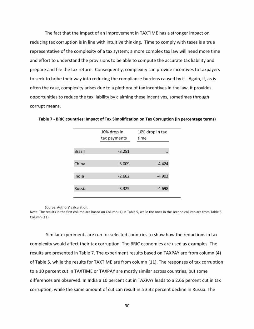
The fact that the impact of an improvement in TAXTIME has a stronger impact on

reducing tax corruption is in line with intuitive thinking. Time to comply with taxes is a true

representative of the complexity of a tax system; a more complex tax law will need more time

and effort to understand the provisions to be able to compute the accurate tax liability and

prepare and file the tax return. Consequently, complexity can provide incentives to taxpayers

to seek to bribe their way into reducing the compliance burdens caused by it. Again, if, as is

often the case, complexity arises due to a plethora of tax incentives in the law, it provides

opportunities to reduce the tax liability by claiming these incentives, sometimes through

corrupt means.

Similar experiments are run for selected countries to show how the reductions in tax

complexity would affect their tax corruption. The BRIC economies are used as examples. The

results are presented in Table 7. The experiment results based on TAXPAY are from column (4)

of Table 5, while the results for TAXTIME are from column (11). The responses of tax corruption

to a 10 percent cut in TAXTIME or TAXPAY are mostly similar across countries, but some

differences are observed. In India a 10 percent cut in TAXPAY leads to a 2.66 percent cut in tax

corruption, while the same amount of cut can result in a 3.32 percent decline in Russia. The

Table 7 - BRIC countries: Impact of Tax Simplification on Tax Corruption (in percentage terms)

Source: Authors' calculation. Note: The results in the first column are based on Column (4) in Table 5, while the ones in the second column are from Table 5 Column (11).



Brazil -3.251 ..

China -3.009 -4.424

India -2.662 -4.902

Russia -3.325 -4.698

30

effects of cuts to the number of tax payments on tax corruption are similar in China and Brazil.

The response of tax corruption to cuts in TAXTIME is strongest in India, where a 10 percent

decline in TAXTIME lowers tax corruption by 4.90 percent. In China the same experiment

produces a 4.4 percent cut in tax corruption, while it is 4.7 percent in Russia.

It should be noted that since only business taxes are included in this study, the

magnitude of the impacts of tax simplification on tax corruption, as calculated above, can be

considered partial. In a study where personal income taxes are taken into account as well, the

overall impact of tax simplification on tax corruption is expected to be stronger.

3.3 Importance of Regional Differences in Determining Tax Corruption

As presented in section 2 of the paper, significant differences in the tax corruption

measure are observed across regions. For example, while Latin American and South Asia

countries tend to report lower measures of tax corruption, countries from Eastern Europe and

Central Asia present much higher tax corruption ratios. These results are not entirely in line

with observed instances of tax corruption. For example, it is generally expected that tax

corruption is higher in South Asia than ECA. Our surmise is that two factors may be responsible

for the slightly unexpected results: first, the cultural factors which may have an influence on the

responses to the Enterprise Survey questions on tax corruption, and, second, the fact that tax

corruption data are not collected from all countries. Nevertheless, there is value in exploring

regional dimensions to gain some understanding of the dynamics of tax simplification and

corruption in a region.

In order to understand the impact of regional differences on the link between tax

simplification and tax corruption, the benchmark regression specification is run separately for

each region. The regions included in the study are: Europe and Central Asia (ECA), Sub-Saharan

Africa (SSA), Latin America and Caribbean (LAC), South Asia (SASIA), East Asia and Pacific (EAP),

and the Middle Eastern and North Africa region (MENA). Due to data limitations, some regions

are combined. Countries from SASIA and EAP are pooled together. Similarly, MENA and ECA

countries form one group.

31

Table 8 presents the regression results for different regions. When the results in Table 5

and Table 8 are compared to each other, it can be seen that the results are consistent and

robust, but still some regional differences are observed. The estimated coefficients of the two

tax simplification variables are statistically significant and have the expected positive sign. The

control variables also have the expected sign and are statically significant determinants of tax

corruption. The exception is the SASIA and EAP region. The statistical significance level of the

Table 8 –Regional Differences in Tax Corruption (2002-2012)

Dependent variable: Tax corruption (1) (2) (3) (4)

SSAEAP and SASIA LAC

MENA and ECA

Constant term -21.308 46.893 53.717 13.975(-2.342)** (1.384) (7.391)*** (0.845)

Tax simplificationlog(Tax payments) 4.574 2.855 6.357 3.254

(3.222)*** (1.624) (6.165)*** (2.065)**

log(Tax time) 3.802 2.106 4.857 2.017(2.674)*** (1.747)* (1.85)* (1.837)*

Political and Political Institution Determinants of CorruptionBureaucracy Quality (higher better quality) -0.846 -3.101 -0.338 -1.411

(-1.707)* (-1.682)* (-1.524) (-0.733)

Democratic Accountability (higher better) -1.45 -1.2 -2.023 -1.157(-1.733)* (-1.816)* (-3.807)*** (-1.754)*

Judicial and Bureaucratic Determinants of Corruption -11.184 -20.703 -1.864 -9.483Rule of Law (higher better) (-8.511)*** (-5.619)*** (-2.509)** (-3.929)***

No. of observations 340 126 124 257J-statistics 2.485 2.556 2.649 2.487Arellano-Bond serial correlation test AR(1) 0.460 0.414 0.474 0.461Arellano-Bond serial correlation test AR(2) 0.888 0.908 0.878 0.889Jarque-Bera normality test 1.264 1.297 1.246 1.267

Note: The estimation method is a panel - GMM. Annual data are used. t-statistics are given in parenthesis. * indicates 10% significance level, ** indicates 5% significance level, and *** indicates 1% significance level. These significance levels are equal to one minus the probability of rejecting the null hypothesis of zero coefficients. J-test is for overidentification problem where H0: there is no overidentification problem. For serial correlation z-tests, H0 is "there is no serial correlation"; and for normality test, H0 is "normal distribution".

32

estimated coefficients of this region is lower (see column (2)). In column (1) only SSA countries

are included. The estimated coefficients of both TAXTIME and TAXPAY are highly significant.

The magnitude of the coefficients of the tax complexity indicators is high as well. LAC countries

present a similar result. As can be seen in column (3) the estimated coefficients of both

TAXTIME and TAXPAY are significant and their size is large. Column (4) combines the MENA and

ECA countries in our dataset. The size of estimated coefficients is low, but statistically

significant.

The economic significance of the estimated coefficients can be better understood with

the help of experiments run with hypothetically changing values of the tax complexity variables.

Experiment outcomes are presented in Table 9. The predicted changes are generated using the

regression specifications given in Table 8’s corresponding columns, based on which region is

analyzed in the experiments. For each region three experiments are run. First the impact of a

10 percent drop in TAXPAY on tax corruption is investigated. Then the effect of a 10 percent

drop in TAXTIME is studied. The combined effects of 10 percent cuts in TAXPAY and TAXTIME

are reported in the last column of Table 9. A 10 percent decrease in TAXPAY or TAXTIME has

the highest impact on tax corruption in the LAC region, where the cut in tax corruption is

predicted to be 6.2 percent for TAXPAY and 4.7 percent for TAXTIME. When two effects are

combined, 10 percent declines in TAXTIME and TAXPAY lead to almost 11 percent decline in tax

Table 9 - Regions: Impact of Tax Simplification on Tax Corruption (in percentage terms)

Source: Authors' calculation. Note: The outcomes are calculated using the estimated coefficients reported in Table 8.




ECA+MENA -2.817 -1.746 -4.563

SSA -5.362 -4.457 -9.819

LAC -6.224 -4.756 -10.980

EAP+SASIA -1.480 -1.092 -2.572

33

corruption. SSA countries follow LAC countries in terms of the economic significance of tax

simplification on tax corruption. In the SSA region, a 10 percent drop in TAXPAY and TAXTIME

causes a 5.4 percent and 4.5 percent decline in tax corruption, successively. The combined

effect of two cuts on tax corruption is close to -10 percent. The impact of tax simplification on

tax corruption is more limited in the ECA and MENA regions. While a 10 percent cut in TAXPAY

leads to a 2.8 percent drop in tax corruption, the same amount of cut in TAXTIME leads to only

a 1.8 percent cut. When two effects are combined, the total impact on tax corruption is

predicted to be -4.6 percent for these countries. The weakest economic significance is observed

in the SASIA and EAP regions. Even the combined effects of 10 percent cuts in TAXPAY and

TAXTIME lead to only a 2.6 percent decline in tax corruption.

3.4 Importance of Development Levels of Countries in Determining Tax Corruption

In order to understand the importance of the development level of countries in

determining tax corruption, the countries included in the study are split into two groups. In the

first group, low-income and lower middle-income countries are included. While identifying the

countries’ income group, the World Bank’s classifications are taken into account. 56 countries

of the dataset belong to the first set. The second group consists of upper middle-income and

high-income countries; there are 48 countries in this group. The descriptive statistics associated

with these two groups are presented in Table 10. The lower-income group has larger tax

corruption ratios on average and their tax systems are more complex, which is measured by the

time to comply with tax requirements and the number of tax payments.

34

The regression results for these two groups of countries are presented in Table 11. The

outcomes in the first 6 columns are for the lower-income group, while the estimated

coefficients obtained from the higher-income group are presented in columns (7)-(12). When

the findings are compared to each other, it can be seen that significant differences are

observed between two income groups. Tax corruption is more responsive to changes in the

level of tax complexity of lower-income countries. The estimated coefficients of both TAXTIME

and TAXPAY are highly significant and the coefficients’ economic significance is higher for this

group. The regression results obtained from the combined panel set (Table 5) indicate that the

economic significance associated with TAXTIME is higher than the significance of TAXPAY. But in

Table 11 TAXPAY presents higher estimated coefficients for the lower-income group than

TAXTIME. Given that it is relatively easier to reduce the number of tax payments than cutting

TAXTIME, it is an encouraging result for policy makers of lower-income countries, where tax

corruption issues tend to be more severe. The findings indicate that the control variables are

statistically significant and have the expected negative signs for the lower-income group.

The estimated coefficients for the higher-income group show that the impact of tax

simplification on tax corruption is more limited. The coefficients of TAXPAY and TAXTIME are

Table 10 – Income Groups: Descriptive Statistics

Source: Authors’ calculation.


Mean 3.302 1.732 3.795 -0.670 -0.674 24.620 42 358Median 3.316 2.000 4.000 -0.655 -0.685 19.595 41 270Standard Deviation 0.577 1.045 1.446 0.451 0.545 19.182 17 145Minimum 2.129 0.000 0.000 -1.769 -1.855 0.398 7 104Maximum 5.297 4.000 6.000 0.733 1.083 96.667 147 1585Count 450 684 684 612 615 629 499 499


Mean 3.121 2.294 4.435 0.082 -0.025 18.661 29 325Median 3.069 2.000 5.000 0.127 -0.074 14.757 22 292Standard Deviation 0.567 0.811 1.479 0.656 0.724 17.600 24 102Minimum 1.847 0.000 0.000 -1.877 -1.924 0.410 6 58Maximum 4.408 4.000 6.000 1.263 1.367 95.276 125 1000Count 389 546 546 452 454 478 383 374

LOW-INCOME AND LOWER MIDDLE-INCOME COUNTRIES

UPPER MIDDLE-INCOME AND HIGH-INCOME COUNTRIES

35

lower and at the same time their statistical significance is around the 10 percent level. For this

group of countries the control variables have the expected negative signs and are statistically

significant.

Overall the estimated coefficients are higher for tax simplification variables in the lower-

income group. This difference between the two groups is reflected in experiments. Table 12

presents the economic significance of the estimated coefficients of the tax simplification

variables. The economic significance of both indicators of tax complexity is higher for the lower-

income set. In lower-income countries, the effect of reducing the number of tax payments by

10 percent is expected to lower tax corruption by 11 percent, a higher effect than reducing tax

time. Reducing the time taken to comply for taxes by 10 percent is expected to cut tax

corruption by 8 percent. In a regression specification where the two measures of tax

simplification are included together, a 10 percent drop in TAXPAY leads to a 8.4 percent cut in

tax

36

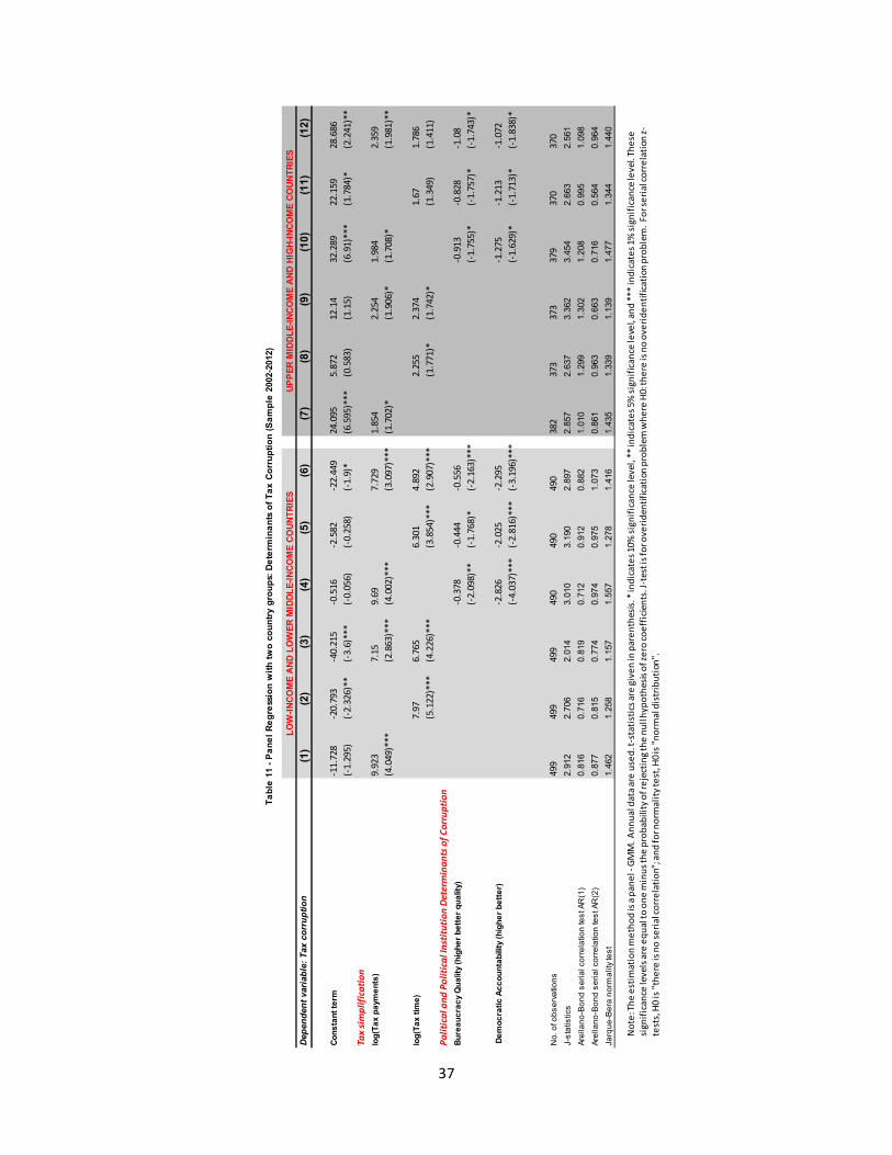
Depe

nden

t var

iabl

e: T

ax c

orru

ptio

n(1

)(2

)(3

)(4

)(5

)(6

)(7

)(8

)(9

)(1

0)(1

1)(1

2)

Cons

tant

term

-11.

728

-20.

793

-40.

215

-0.5

16-2

.582

-22.

449

24.0

955.

872

12.1

432

.289

22.1

5928

.686

(-1.

295)

(-2.

326)

**(-

3.6)

***

(-0.

056)

(-0.

258)

(-1.

9)*

(6.5

95)*

**(0

.583

)(1

.15)

(6.9

1)**

*(1

.784

)*(2

.241

)**

Tax

sim

plifi

catio

nlo

g(Ta

x pa

ymen

ts)

9.92

37.

159.

697.

729

1.85

42.

254

1.98

42.

359

(4.0

49)*

**(2

.863

)***

(4.0

02)*

**(3

.097

)***

(1.7

02)*

(1.9

06)*

(1.7

08)*

(1.9

81)*

*

log(

Tax

time)

7.97

6.76

56.

301

4.89

22.

255

2.37

41.

671.

786

(5.1

22)*

**(4

.226

)***

(3.8

54)*

**(2

.907

)***

(1.7

71)*

(1.7

42)*

(1.3

49)

(1.4

11)

Polit

ical

and

Pol

itica

l Ins

titut

ion

Dete

rmin

ants

of C

orru

ptio

nBu

reau

crac

y Q

ualit

y (h

ighe

r bet

ter q

ualit

y)-0

.378

-0.4

44-0

.556

-0.9

13-0

.828

-1.0

8(-

2.09

8)**

(-1.

768)

*(-

2.16

3)**

*(-

1.75

5)*

(-1.

757)

*(-

1.74

3)*

Dem

ocra

tic A

ccou

ntab

ility

(hig

her b

ette

r)-2

.826

-2.0

25-2

.295

-1.2

75-1

.213

-1.0

72(-

4.03

7)**

*(-

2.81

6)**

*(-

3.19

6)**

*(-

1.62

9)*

(-1.

713)

*(-

1.83

8)*

No.

of o

bser

vatio

ns49

949

949

949

049

049

038

237

337

337

937

037

0J-

stat

istic

s2.

912

2.70

62.

014

3.01

03.

190

2.89

72.

857

2.63

73.

362

3.45

42.

663

2.56

1Ar

ella

no-B

ond

seria

l cor

rela

tion

test

AR

(1)

0.81

60.

716

0.81

90.

712

0.91

20.

882

1.01

01.

299

1.30

21.

208

0.99

51.

098

Arel

lano

-Bon

d se

rial c

orre

latio

n te

st A

R(2

)0.

877

0.81

50.

774

0.97

40.

975

1.07

30.

861

0.96

30.

663

0.71

60.

564

0.96

4Ja

rque

-Ber

a no

rmal

ity te

st1.

462

1.25

81.

157

1.55

71.

278

1.41

61.

435

1.33

91.

139

1.47

71.

344

1.44

0

LOW

-INCO

ME

AND

LOW

ER M

IDDL

E-IN

COM

E CO

UNTR

IES

UPPE

R M

IDDL

E-IN

COM

E AN

D HI

GH-

INCO

ME

COUN

TRIE

S

Tabl

e 11

- Pa

nel R

egre

ssio

n w

ith tw

o co

untry

gro

ups:

Det

erm

inan

ts o

f Tax

Cor

rupt

ion

(Sam

ple

2002

-201

2)

Not

e: Th

e es

timat

ion

met

hod

is a

pane

l -GM

M. A

nnua

l dat

a are

use

d. t-

stat

istic

s are

give

n in

par

enth

esis.

* in

dica

tes 1

0% si

gnifi

canc

e le

vel,

** in

dica

tes 5

% si

gnifi

canc

e le

vel, a

nd **

* in

dica

tes 1

% si

gnifi

canc

e lev

el. T

hese

si

gnifi

canc

e le

vels

are

equa

l to

one

min

us th

e pr

obab

ility

of r

ejec

ting t

he n

ull h

ypot

hesis

of z

ero

coef

ficie

nts.

J-te

st is

for o

verid

entif

icatio

n pr

oble

m w

here

H0:

ther

e is

no

over

iden

tifica

tion

prob

lem

. For

seria

l cor

rela

tion

z-te

sts,

H0 is

"the

re is

no

seria

l cor

rela

tion"

; and

for n

orm

ality

test

, H0 i

s "no

rmal

dis

trib

utio

n".

37

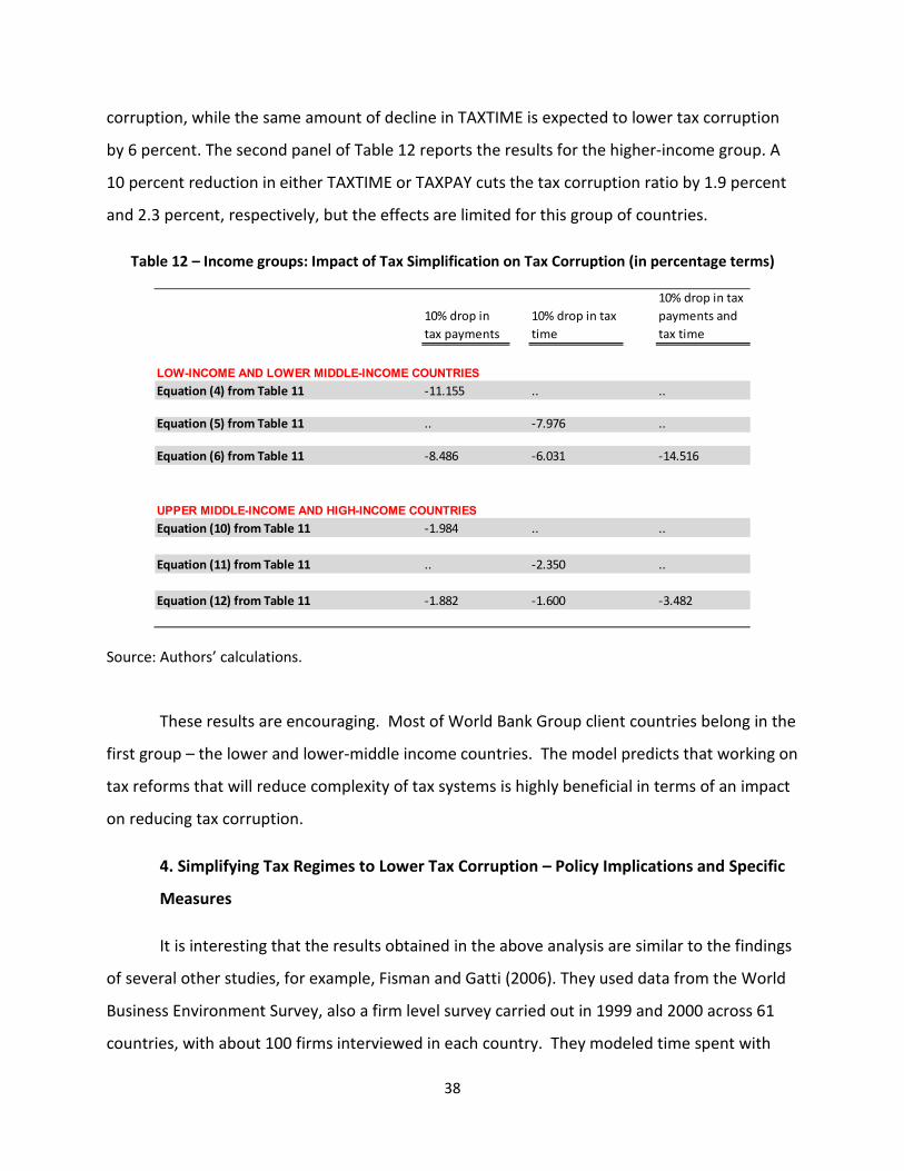
corruption, while the same amount of decline in TAXTIME is expected to lower tax corruption

by 6 percent. The second panel of Table 12 reports the results for the higher-income group. A

10 percent reduction in either TAXTIME or TAXPAY cuts the tax corruption ratio by 1.9 percent

and 2.3 percent, respectively, but the effects are limited for this group of countries.

These results are encouraging. Most of World Bank Group client countries belong in the

first group – the lower and lower-middle income countries. The model predicts that working on

tax reforms that will reduce complexity of tax systems is highly beneficial in terms of an impact

on reducing tax corruption.

4. Simplifying Tax Regimes to Lower Tax Corruption – Policy Implications and Specific

Measures

It is interesting that the results obtained in the above analysis are similar to the findings

of several other studies, for example, Fisman and Gatti (2006). They used data from the World

Business Environment Survey, also a firm level survey carried out in 1999 and 2000 across 61

countries, with about 100 firms interviewed in each country. They modeled time spent with

Table 12 – Income groups: Impact of Tax Simplification on Tax Corruption (in percentage terms)





LOW-INCOME AND LOWER MIDDLE-INCOME COUNTRIESEquation (4) from Table 11 -11.155 .. ..



UPPER MIDDLE-INCOME AND HIGH-INCOME COUNTRIESEquation (10) from Table 11 -1.984 .. ..



38

bureaucrats against bribes paid, and further included in the regression a variable that measures

the extent to which firms know in advance how much these irregular payments will be, and

interact it with bribes. The estimated relationship between time and corruption is positive in

their study as well. So, the more time it takes to comply with various regulations – in their

study “time” is a variable which respresents senior management time spent with government

officials in general, not just tax officials – the more the amount of irregular payments made. In

our analysis presented above, the findings are on the same lines, are robust, are specific to

corruption related to tax administration, and provide a clear policy prescription – if you want to

reduce tax administration related corruption, simplify the tax regime.

A sizeable body of research on the economics of corruption has come to similar

conclusions, that regulatory complexity in general, and tax complexity in particular, engenders

corruption and rent-seeking behavior. Lambsdorff (2006) lists “regulatory quality” as one of the

main causes of corruption. He recommends that reform should “avoid complicated rules and

those that are difficult to administer, and should design individual incentives to promote honest

decision making.” Clearly, he is in favor of simple laws and regulations that are easier to comply

with. Obwona and Muwonge (2002) pointed out how in the case of Uganda, despite changes in

the tax regime, “the tax system is still complicated and non-transparent.” These conditions

prevented the reduction of corruption in the Uganda Revenue Authority. In another study of

Uganda, Kasimbazi (2003) refers to unclear tax legislation which led to random and partly ad

hoc collection procedures which gave wide discretionary powers to taxpayers and tax

inspectors interpret tax laws. He recommends that the income tax laws should be simplified.

As our model above shows, lowering tax corruption is linked to tax simplification. We

defined our “simplicity” variables as time to comply and number of payments. The model

therefore, guides us to look for ways to reduce the time it takes to comply with the tax regime

and reduce the number of payments taxpayers need to make. A set of such measures is

outlined here.

It is important to note that there is a large literature on corruption in tax administrations

and strategies to tackle it. This section does not attempt to summarize all of those efforts.

39

Rather, the emphasis here is to highlight those actions that can be taken which specifically help

in improving “tax simplicity” as defined in this paper, i.e. measures that help to reduce the time

to comply and the number of payments.

A distinction needs to be made between tackling the motives for corruption and tackling

the opportunities for corruption.18 Measures focused on improving tax simplicity generally

would help reduce opportunities for corruption in tax administrations. According to Das-Gupta,

Engelschalk, and Mayville (1999), “tax simplification is perhaps the most important method of

limiting opportunity, and can also increase economic efficiency…” They list a set of measures,

inter alia, which would help address opportunity for corruption. The measures that also impact

favorably the time to comply and number of payments variables are listed below:

• Low and few rates and limited exemptions;

• Withholding and presumptive taxes, particularly for small businesses;

• Nondiscretionary penalties;

• Limited contact between taxpayers and tax officials;

• Computerization and automation.

In addition to the above, A Handbook for Tax Simplification, prepared by the Investment

Climate Advisory Services (2009), provides a list of good practices to be followed by tax

administrations to help reduce corruption. These include the following points which are

specifically related to tax simplification:

• the tax administration, as far as possible, limits direct contact with taxpayers;

• where concessions or any type of clearances need to be granted, they must be

granted by means of “transparent, nondiscretionary, and auditable written rules and

procedures;”

18 See for example, Das-Gupta, Engelschalk, and Mayville (1999).

40

• specific provisions such as levy of interest, penalties, or collection of delinquent

taxes should be nondiscretionary and implemented via transparent rules and

procedures;

• presumptions that reduce computation and record keeping needs are helpful in

simplifying tax provisions.

One of the key measures that helps reduce tax complexity is computerization. Most

modern tax administrations rely heavily on computer systems – for the purposes of their own

internal data collection and analysis, and also in their interactions with taxpayers. In mature tax

systems taxpayers are almost entirely able to interact with the tax authority electronically – to

file returns, make payments, obtain refunds, etc. These systems reduce human interaction,

thereby significantly reducing the opportunities for corruption. Investment Climate Advisory

Services (2009) highlights the role of technology in reducing corruption and describes various

ways in which it helps. IT technology can automatically record the receipt of different

documents and requests for service. This reduces the scope for “out of turn” favors and makes

service delays conspicuous and easy to monitor. IT systems also make it possible to set up

nondiscretionary and standardized procedures for various activities such as creating tax

demands, issuing notices, and processing refunds. In the case of audit procedures, using IT

driven risk based audit systems can eliminate discretion in selection of cases for audit. All of

these measures help reduce corruption. In terms of the variables of tax simplicity in our model

here, IT systems help reduce the number of payments, especially as for the purpose of the

Doing Business computation, if e-payments exist for the majority of taxpayers, the number of

payments is taken as “1”, even if there are more tax payments. So, in the measure of the

number of tax payments, an extra weightage is provided for e-systems. This variable succeeds

in capturing the IT-related tax simplification measures which also impact corruption.

Two other measures can help to reduce the time to comply:

• time limitations on provision of taxpayer services; and

• a well-oiled tax dispute resolution institution.

41

Setting time limitations on provision of specific taxpayer services help to ensure that the

time to comply with the tax regime is kept within limits. It also helps keep tax corruption in

check as delays in taxpayer services – such as, taxpayer registration, or issuance of tax refunds –

can be monitored and corrupt practices identified and checked. An effective and efficient tax

dispute resolution mechanism increases taxpayer confidence in the objectivity of the tax

system and helps reduce the time to comply with the tax system by resolving disputes quickly.

Some of the measures described above need legislative amendments, changes in tax

laws, but most of them are in the nature of improvements in the administration of the tax

regime, and hence are easier to carry out. Experience shows that changes in tax laws, especially

those aimed at reducing tax rates and getting rid of tax exemptions, are difficult and time

consuming to make as they may negatively impact the economic interests of some taxpayers.

On the contrary, several of the measures described above are in the nature of “win-win”

propositions that improve the efficiency of the tax administration and impact positively all

taxpayers. These measures do not need long drawn out legislative procedures. They are

relatively simple ways to simplify tax regimes and reduce tax corruption.

5. Conclusion

This study tries to construct an empirical link between tax simplification and tax

corruption in tax administrations. The measure of tax corruption and the two alternative

measures of tax complexity (the time to comply with tax requirements and the number of tax

payments) are calculated using the World Bank’s databases. The study includes 104 countries

from different regions and income groups and covers the period of 2002-2012. After identifying

the statistically significant determinants of tax corruption, experiments are run to understand

the economic significance of tax simplification in this process. The regression findings support

the existence of a strong link between tax corruption and the indicators of tax complexity. The

link is both statistically and economically significant. The tax complexity indicators are robust to

the inclusion of a different set of country-level variables. It is predicted that a 10 percent drop

in TAXTIME leads to an approximately 4 percent decline in tax corruption, while the same about

42

of decline in TAXPAY leads to a roughly 6 percent improvement in tax corruption. The results

indicate some differences across regions, as well as income groups. The combined effect of 10

percent declines in TAXTIME and TAXPAY is a 9.6 percent cut in tax corruption.

These empirical findings have important policy implications. There are different ways of

reducing tax complexity and simplification of tax systems is useful in the process of fighting tax

corruption.

It is worth noting that, in order to draw country-specific, detailed recommendations

regarding tax simplification issues, the findings of our cross-country study should be followed

by additional country-specific empirical studies, which should consider country specific

characteristics that would affect tax corruption and tax simplification at the country level. Our

study is not a substitute for such detailed country-level analysis. Each country has different

features and it may require country specific analysis to have more detailed conclusions.

Unfortunately such country-level studies focusing on the link between tax corruption and tax

simplification are very limited, mainly, due to lack of data information on tax corruption. As far

as we know, even though it is not perfect, the Enterprise Surveys Database is the only database

which includes some data information on tax corruption. Thus, we believe that our panel-data

analysis presents useful information on the link between tax corruption and simplification,

which has been rarely investigated empirically in the literature.

43

References

Abed, George T. and Hamid R. Davoodi (2000) "Corruption, Structural Reforms, and Economic Performance in the Transition Economies,” IMF Working Paper WP/00/132 (July).

Ades, Alberto and Rafael Di Tella (1999) "Rents, Competition, and Corruption,” American Economic Review, Vol. 89 (4), pp. 982-992.

Alm, James (1999) “Tax compliance and administration”, Public Administration and Public Policy, Vol. 72, pp. 741-768.

Alm, James, Betty Jackson, and Michael Mckee (1992) “Institutional uncertainty and taxpayer compliance”, The American Economic Review, Vol. 82, No. 4, pp. 1018-1026.

Alt, James E. and David Dreyer Lassen (2003) "The Political Economy of Institutions and Corruption in American States,” Journal of Theoretical Politics, Vol. 15 (3), pp. 341-365.

Anderson, Andy B., Alexander Basilevsky, and Derek P. J. Hum (1983) “Missing Data: A Review of the Literature,” in Rossi, Peter H., James D. Wright and Andy B. Anderson, ed., Handbook of Survey Research, (Boston: Academic Press, Inc.).

Arellano, Manuel and Stephen Bond (1991) “Some Tests of Specification for Panel Data: Monte Carlo Evidence and an Application to Employment Equations,” Review of Economic Studies, Vol. 58 (2), pp. 277-297.

Arellano, Manuel and Olympia Bover (1995) “Another Look at the Instrumental Variables Estimation of Error-Components Models,” Journal of Econometrics, Vol. 68, pp. 29-51.

Blundell, Richard and Stephen Bond (1998) “Initial Conditions and Moment Restrictions in Dynamic Panel Data Models,” Journal of Econometrics, Vol. 87, pp. 115-143.

Braun, Miguel and Rafael Di Tella (2004) "Inflation, Inflation Variability, and Corruption,” Economics and Politics, Vol. 16, pp. 77-100.

Broadman, Harry G. and Francesca Recanatini (2000) "Seed of Corruption: Do Market Institutions Matter?” The World Bank Policy Research Working Paper No. 2368 (November).

Brunetti, Aymo and Beatrice Weder (2003) "A Free Press is Bad News for Corruption,” Journal of Public Economics, Vol. 87, pp. 1801-1824.

Crandall and Bodin (2005) Crandall, William, and Jean-Paul Bodin (2005) “Revenue Administration Reform in Middle Eastern Countries, 1994–2004,” IMF. Working Paper No. WP/05/203.

Cuccia, Andrew D. and Gregory A. Carnes (2001) “A closer look at the relation between tax complexity and tax equity perceptions”, Journal of Economic Psychology, Vol. 22, No. 2, pp. 113-140.

44

Damania, Richard, Per Fredriksson, and Muthukumara Mani (2004) "The Persistence of Corruption and Regulatory Compliance Failures: Theory and Evidence,” Public Choice, Vol. 121, pp. 363-390.

Das-Gupta, Arindam, Michael Engeschalk, and William Mayville (1999) “An Anticorruption Strategy for Revenue Administration.” The World Bank: Washington, DC.

Dean, Steven A. (2005) “Attractive complexity: Tax deregulation, the check-the-box election, and the future of tax simplification”, Hofstra Law Review, Vol. 34, pp. 405-467.

Dempster, Arthur P., Nan M. Laird, and Donald B. Rubin (1977) “Maximum Likelihood from Incomplete Data via the EM Algorithm,” Journal of the Royal Statistical Society. Series B (Methodological), Vol. 39, pp. 289-309.

Dos Santos, Paulo Sergio (1995) “Corruption in Tax Administration,” presented at the Twenty-Ninth Annual Assembly of the CIAT, Lima, Peru, March 29, 1995.

Evans, Chris (2003) “Studying the studies: An overview of recent research into taxation operating costs”, eJournal of Tax Research, Vol. 1, No. 1, pp. 64-92.

Evrensel, Ayşe Y. (2010) “Institutional and Economic Determinants of Corruption: a Cross-Section Analysis,” Applied Economics Letters, Vol. 17 (4/6), pp. 551 – 554.

Fjeldstad, Odd-Helge (2006) "Corruption in Tax Administration: Lessons from Institutional Reforms in Uganda," in Rose-Ackerman, Susan, ed., International Handbook on the Economics of Corruption, (Northampton: Edward Elgar Publishing, Inc.).

Fisman, Raymond J. and Roberta Gatti (2002) "Decentralization and Corruption: Evidence across Countries,” Journal of Public Economics, Vol. 83, pp. 325-345.

Fisman, Raymond J. and Roberta Gatti (2006) "Bargaining for Bribes: the Role of Institutions," in Rose-Ackerman, Susan, ed., International Handbook on the Economics of Corruption, (Northampton: Edward Elgar Publishing, Inc.).

Forest, Adam and Steven M. Sheffrin (2002) “Complexity and compliance: An empirical investigation”, National Tax Journal, Vol. 55, No. 1, pp. 75-88.

Friedman, Eric, Simon Johnson, Daniel Kaufmann, and Pablo Zoido-Lobaton (2000) “Dodging the Grabbing Hand: The Determinants of Unofficial Activity in 69 Countries“ Journal of Public Economics, Vol. 76, pp. 459-493.

Goel, Rajeev K. and Michael A. Nelson (2010) “Causes of Corruption: History, Geography and Government,” Journal of Policy Modeling, Vol. 32 (4), pp. 433 – 447.

Goldsmith, Arthur A. (1999) "Slapping the Grasping Hand: Correlates of Political Corruption in Emerging Market,” American Journal of Economics and Sociology, Vol. 58(4), pp. 865-883.

45

Goolsbee, Austan (2004) "The TurboTax Revolution: Can Technology Solve Tax Complexity?" in Aaaron, Henry J. and Joel Slemrod, eds., The Crisis in Tax Administration, (Washington, DC: Brookings Institution Press).

Graeff, Peter and Guido Mehlkop (2003) "The Impacts of Economic Freedom on Corruption: Different Patterns for Rich and Poor Countries,” European Journal of Political Economy, Vol. 19, pp. 605-620.

Gurgur, Tugrul and Anwar Shah (2005) "Localization and Corruption: Panacea or Pandora’s Box,” World Bank Policy Research Working Paper 3486 (January).

Herzfeld, Thomas and Christoph Weiss. (2003) "Corruption and Legal (In)-Effectiveness: An Empirical Investigation,” European Journal of Political Economy, Vol. 19, pp. 621-632.

Heyndels, B. and C. Smolders (1995) “Tax complexity and fiscal illusion”, Public Choice, Vol. 85, No. 1, pp. 127-141.

Honaker, James and Gary King (2010) “What to do about Missing Values in Time Series Cross-Section Data,” American Journal of Political Science, Vol. 54 (3), pp. 561-581.

Imam, Patrick A. and Davina F. Jacobs (2007) “Effect of Corruption on Tax Revenues in the Middle East,” IMF Working Paper No: WP/07/270 (November).

Independent Panel (2013) Independent Panel Review of the Doing Business Report (June 2013). World Bank: Washington D.C. [http://www.dbrpanel.org/sites/dbrpanel/files/doing-business-review-panel-report.pdf ]

Investment Climate Advisory Services (2009) "A Handbook for Tax Simplification." Washington, DC: The World Bank Group.

Isse, Hodan Said and Abdiweli M. Ali (2003) “Determinants of Economic Corruption: a Cross-Country Comparison,” The Cato Journal, Vol. 22 (3), pp. 449 - 466.

Ivanova, Anna, Keen, Michael, and Klemm, Alexander (2005) “The Russian Flat Tax Reform,” IMF Working Paper No. WP/05/16.

Iwasakia, Ichiro and Taku Suzuki (2012) “The Determinants of Corruption in Transition Economies,” Economics Letters, Vol. 114 (1), pp. 54–60.

Kasimbazi, Emmanuel (2003) "Taxpayers’ Rights and Obligations: Analysis of Implementation and Enforcement Mechanisms in Uganda." Danish Institute for International Studies: Copenhagen.

Kautilya (1915) Kautilya’s Arthashastra, translated by R. Shamasastry, Bangalore Government Press. http://www.columbia.edu/itc/mealac/pritchett/00litlinks/kautilya/index.html

Keen, Michael (2003) Changing Customs: Challenges and Strategies for the Reform of Customs Administrations (Washington, DC: International Monetary Fund).

46

Kirchler, Erich, Apolonia Niemirowski, and Alexander Wearing (2006) “Shared subjective views, intent to cooperate and tax compliance: Similarities between Australian taxpayers and tax officers”, Journal of Economic Psychology, Vol. 27, No. 4, pp. 502-517.

Knack, Stephen and Omar Azfar (2003) "Trade Intensity, Country Size and Corruption,” Economics of Governance, Vol. 4, pp. 1-18.

Kunicova, Jana and Susan Rose-Ackerman (2005) "Electoral Rules and Constitutional Structures as Constraints on Corruption,” British Journal of Political Science, Vol. 35 (4), pp. 573-606.

Lambsdorff, Johann Graf (2006) "Causes and Consequences of Corruption: What do We Know from a Cross Section of Countries?" in Rose-Ackerman, Susan, ed., International Handbook on the Economics of Corruption, (Northampton: Edward Elgar Publishing, Inc.).

Lawless, Martina (2013) “Do Complicated Tax Systems Prevent Foreign Direct Investment?” Economica, Vol. 80, pp. 1–22.

Lederman, Daniel, Norman V. Loayza, and Rodrigo R. Soares (2005) "Accountability and Corruption: Political Institutions Matter,” Economics and Politics, Vol. 17, pp. 1-35.

Leite, Carlos A. and Jens Weidmann (1999) "Does Mother Nature Corrupt? Natural Resources, Corruption, and Economic Growth,” International Monetary Fund Working Paper WP/99/85, (July).

Milliron, V.C. (1985) “A behavioral study of the meaning and influence of tax complexity”, Journal of Accounting Research, Vol. 23, No. 2, pp. 794-816.

Mills, Lilian F. (1996) “Corporate tax compliance and financial reporting”, National Tax Journal, Vol. 49, pp. 421-436.

Mulder, Laetitia B., Peter Verboon, and David De Cremer (2009) “Sanctions and moral judgments: The moderating effect of sanction severity and trust in authorities”, European Journal of Social Psychology, Vol. 39, No. 2, pp. 255-269.

Obwona, Marios and Abdu Muwonge (2002) "The Efficiency and Effectiveness of the Revenue Administration in Uganda." Report developed for the Taxation, aid and democracy project (draft). Institute for International Studies (IIS), Copenhagen.

Oliver, Tracey and Scott Bartley (2005) “Tax system complexity and compliance costs—some theoretical considerations”, Economic Roundup, Winter, Vol. 2005, pp. 53-68.

Owens, Jeffrey and Stuart Hamilton (2004) "Experience and Innovations in Other Countries," in Aaaron, Henry J. and Joel Slemrod, eds., The Crisis in Tax Administration, (Washington, DC: Brookings Institution Press).

Paldam, Martin (2002) “The Cross-Country Pattern of Corruption: Economics, Culture and the Seesaw Dynamics,” European Journal of Political Economy, Vol. 18, pp. 215-240.

47

Park, Hoon (2003) "Determinants of Corruption: A Cross-National Analysis", Multinational Business Review, Vol. 11 Iss: 2, pp.29 - 48

Paul, Deborah L. (1997) “Sources of tax complexity: How much simplicity can fundamental tax reform achieve”, North Carolina Law Review, Vol. 76, p. 151-221.

Persson, Torsten and Guido Tabellini (2003) The Economic Effects of Constitutions, (Cambridge: MIT Press).

Picciotto, Sol (2007) “Constructing compliance: Game playing, tax law, and the regulatory state”, Law & Policy, Vol. 29, No. 1, pp. 11-30.

Purohit, Manesh C. (2007) “Corruption in Tax Administration.” In Shah, A. (Ed.) Performance, Accountability and Combating Corruption. Washington, D.C., International Bank for Reconstruction and Development/The World Bank.

Quandt, Richard E. (1983) “Complexity in regulation”, Journal of Public Economics, Vol. 22, No. 2, pp. 199-214.

Rauch, James and Peter Evans (2000) “Bureaucratic Structure and Bureaucratic Performance in Less Developed Countries,” Journal of Public Economics, Vol. 75, pp. 49-71.

Revier, Charles F. and Nasr G. Elbahnasawy (2012) “The Determinants of Corruption: Cross-Country-Panel-Data Analysis,” The Developing Economies, Vol. 50 (4), pp. 311 – 333.

Richardson, Grant (2006) “Determinants of tax evasion: A cross-country investigation”, Journal of International Accounting, Auditing and Taxation, Vol. 15, No. 2, pp. 150-169.

Rubin, Donald B. (1987) Multiple Imputations for Nonresponse in Surveys, (New York : Wiley).

Ruud, Paul A. (1991) “Extentions of Estimation Methods using the EM Algorithm,” Journal of Econometrics, Vol. 49, pp. 305-341.

Saad, Natrah (2009) “Fairness perceptions and compliance behaviour: The case of salaried taxpayers in Malaysia after implementation of the self-assessment system,” eJournal of Tax Research, Vol. 8, pp. 32-63.

Scotchmer, Suzanne (1989) “Who profits from taxpayer confusion?” Economics Letters, Vol. 29, No. 1, pp. 49-55.

Seldadyo, Harry and Jakob de Haan (2006) “The Determinants of Corruption: A Literature Survey and New Evidence,” Paper presented at the EPCS Conference, Turku, April 20-23.

Serra, Danila (2006) “Empirical Determinants of Corruption: A Sensitivity Analysis,” Public Choice, Vol. 126 (1/2), pp. 225-256.

48

Shabbir, Ghulam and Mumtaz Anwar (2007) “Determinants of Corruption in Developing Countries,” Hamburg Institute of International Economics HWWI Research Working Paper No: 2-11, (November).

Slemrod, Joel (2004) "Small Business and the Tax System," in Aaaron, Henry J. and Joel Slemrod, eds., The Crisis in Tax Administration, (Washington, DC: Brookings Institution Press).

Slemrod, Joel (2007) “Cheating ourselves: The economics of tax evasion”, The Journal of Economic Perspectives, Vol. 21, No. 1, pp. 25-48.

Spilker, Brian C., Ronald G. Worsham, and Douglas F. Prawitt (1999) “Tax professionals' interpretations of ambiguity in compliance and planning decision contexts”, The Journal of the American Taxation Association, Vol. 21, No. 2, pp. 75-89.

Swamy, Anand, Stephen Knack, Young Lee, and Omar Azfar (2001) “Gender and Corruption,” Journal of Development Economics, Vol. 64, pp. 25-55.

Tanzi, Vito (1998) “Corruption Around the World: Causes, Consequences, Scope, and Cures,” IMF Working Paper No. 98/63 (May).

Tanzi, Vito and Hamid R. Davoodi (2002) “Corruption, Growth, and Public Finances,” in Governance, Corruption, and Economic Performance, ed. by George T. Abed and Sanjeev Gupta (Washington, DC: International Monetary Fund).

Thomas, Melissa A. (2010) “What do the Worldwide Governance Indicators Measure?” European Journal of Development Research, Vol. 22, pp. 31–54.

Treisman, Daniel (2000) "The Causes of Corruption: A Cross-National Study," Journal of Public Economics, Vol. 76, pp. 399-457.

Tavares, Jose (2003) “Does Foreign Aid Corrupt?” Economic Letters, Vol. 79, pp. 99-106.

Van Rijckeghem, Caroline and Beatrice S. Weder (1997) “Corruption and the Rate of Temptation: Do Low Wages in the Civil Service Cause Corruption?” IMF Working Paper WP/97/73, (July).

Wei, Shang-Jin (2000) "Local Corruption and Global Capital Flows,” Brookings Papers on Economic Activity, Vol. 31 (2), pp. 303-354.

White, Richard, Anthony Curatola, and William Samson (1990) “A behavioral study investigating the effect of knowledge of income tax laws and tax policy on individual perceptions of federal income tax fairness”, Advances in Taxation, Vol. 3, pp. 165-185.

World Economic Forum (2013) The Global Competitiveness Report. Geneva: World Economic Forum.

49

Appendix 1

Time to comply (TAXTIME): Time is recorded in hours per year. The indicator measures the time taken to prepare, file and pay three major types of taxes and contributions: the corporate income tax, value added or sales tax, and labor taxes, including payroll taxes and social contributions. Preparation time includes the time to collect all information necessary to compute the tax payable and to calculate the amount payable. If separate accounting books must be kept for tax purposes - or separate calculations made - the time associated with these processes is included. This extra time is included only if the regular accounting work is not enough to fulfill the tax accounting requirements. Filing time includes the time to complete all necessary tax return forms and file the returns at the tax authority. Payment time considers the hours needed to make the payment online or at the tax authorities. Where taxes and contributions are paid in person, the time includes delays while waiting.

Number of payments (TAXPAY): The tax payments indicator reflects the total number of taxes and contributions paid, the method of payment, the frequency of payment, the frequency of filing, and the number of agencies involved for this standardized case study company during the second year of operation. It includes taxes withheld by the company, such as sales tax, value added tax and employee-borne labor taxes. These taxes are traditionally collected by the company from the consumer or employee on behalf of the tax agencies. Although they do not affect the income statements of the company, they add to the administrative burden of complying with the tax system and so are included in the tax payments measure. The number of payments takes into account electronic filing. Where full electronic filing and payment is allowed and it is used by the majority of medium-size businesses, the tax is counted as paid once a year even if filings and payments are more frequent (emphasis added). For payments made through third parties, such as tax on interest paid by a financial institution, or fuel tax paid by a fuel distributor, only one payment is included even if payments are more frequent.

50

Appendix 2

The current survey instruments and manuals are available on the website: www.enterprisesurveys.org.

Firm-level surveys have been conducted since 2002 by different units within the World Bank. Since 2005-06, most data collection efforts have been centralized within the Enterprise Analysis Unit. Earlier data from differing survey instruments have been matched to an older standard instrument for dissemination on the website. The raw individual country datasets, aggregated datasets (across countries and years), panel datasets, and all relevant survey documentation are publicly available. All surveys have country-specific questions; therefore the aggregated dataset across countries does not include these country-specific questions.

Surveys implemented by the Enterprise Analysis Unit follow the Global Methodology, which is outlined on this page. Note that data users should exercise caution when comparing raw data and point estimates between surveys that did and did not adhere to the Enterprise Surveys Global Methodology.

Who conducts the surveys:

Private contractors conduct the Enterprise Surveys* on behalf of the World Bank. Due to sensitive survey questions addressing business-government relations and bribery-related topics, private contractors, rather than any government agency or an organization/institution associated with government, are hired by the World Bank to collect the data.

Confidentiality of the survey respondents and the sensitive information they provide is necessary to ensure the greatest degree of survey participation, integrity and confidence in the quality of the data. Surveys are usually carried out in cooperation with business organizations and government agencies promoting job creation and economic growth, but confidentiality is never compromised.

Who is surveyed:

The Enterprise Survey is answered by business owners and top managers. Sometimes the survey respondent calls company accountants and human resource managers into the interview to answer questions in the sales and labor sections of the survey. Typically 1200-1800 interviews are conducted in larger economies, 360 interviews are conducted in medium-sized economies, and for smaller economies, 150 interviews take place. The Sampling Note provides the rationale for these sample sizes.

The manufacturing and services sectors are the primary business sectors of interest. This corresponds to firms classified with ISIC codes 15-37, 45, 50-52, 55, 60-64, and 72 (ISIC Rev.3.1). Formal (registered) companies with 5 or more employees are targeted for interview. Services firms include construction, retail, wholesale, hotels, restaurants, transport, storage, communications, and IT. Firms with 100% government/state ownership are not eligible to participate in an Enterprise Survey. Occasionally, for a few surveyed countries, other sectors are included in the companies surveyed such as education or health-related businesses. In each country, businesses in the cities/regions of major economic activity are interviewed.

51

http://www.enterprisesurveys.org/

In some countries, other surveys, which depart from the usual Enterprise Survey methodology, are conducted. Examples include 1) Informal Surveys- surveys of informal (unregistered) enterprises, 2) Micro Surveys- surveys fielded to registered firms with less than five employees, and 3) Financial Crisis Assessment Surveys- short surveys administered by telephone to assess the effects of the global financial crisis of 2008-09.

Structure of the surveys:

The Enterprise Surveys Unit uses two instruments: the Manufacturing Questionnaire and the Services Questionnaire. Although many questions overlap, some are only applicable to one type of business. For example, retail firms are not asked about production and nonproduction workers.

The standard Enterprise Survey topics include firm characteristics, gender participation, access to finance, annual sales, costs of inputs/labor, workforce composition, bribery, licensing, infrastructure, trade, crime, competition, capacity utilization, land and permits, taxation, informality, business-government relations, innovation and technology, and performance measures.

Over 90% of the questions objectively ascertain characteristics of a country’s business environment. The remaining questions assess the survey respondents’ opinions on what are the obstacles to firm growth and performance. The mode of data collection is face-to-face interviews.

Sampling and weights:

The sampling methodology for Enterprise Surveys is stratified random sampling. In a simple random sample, all members of the population have the same probability of being selected and no weighting of the observations is necessary. In a stratified random sample, all population units are grouped within homogeneous groups and simple random samples are selected within each group. This method allows computing estimates for each of the strata with a specified level of precision while population estimates can also be estimated by properly weighting individual observations. The sampling weights take care of the varying probabilities of selection across different strata. Under certain conditions, estimates' precision under stratified random sampling will be higher than under simple random sampling (lower standard errors may result from the estimation procedure).

The strata for Enterprise Surveys are firm size, business sector, and geographic region within a country. Firm size levels are 5-19 (small), 20-99 (medium), and 100+ employees (large-sized firms). Since in most economies, the majority of firms are small and medium-sized, Enterprise Surveys oversample large firms since larger firms tend to be engines of job creation. Sector breakdown is usually manufacturing, retail, and other services. For larger economies, specific manufacturing sub-sectors are selected as additional strata on the basis of employment, value-added, and total number of establishments figures. Geographic regions within a country are selected based on which cities/regions collectively contain the majority of economic activity.

Ideally the survey sample frame is derived from the universe of eligible firms obtained from the country’s statistical office. Sometimes the master list of firms is obtained from other government

52

agencies such as tax or business licensing authorities. In some cases, the list of firms is obtained from business associations or marketing databases. In a few cases, the sample frame is created via block enumeration, where the World Bank “manually” constructs a list of eligible firms after 1) partitioning a country’s cities of major economic activity into clusters and blocks, 2) randomly selecting a subset of blocks which will then be enumerated. In surveys conducted since 2005-06, survey documentation which explains the source of the sample frame and any special circumstances encountered during survey fieldwork are included with the collected datasets.

Obtaining panel data, i.e. interviews with the same firms across multiple years, is a priority in current Enterprise Surveys. When conducting a new Enterprise Survey in a country where data was previously collected, maximal effort is expended to re-interview as many firms (from the prior survey) as possible. For these panel firms, sampling weights can be adjusted to take into account the resulting altered probabilities of inclusion in the sample frame.

53

Table A1 - Firm Characteristics from Enterprise Surveys

Tax corruption

(demand for bribery % of

total tax visits)

Total number of

firms interviewed

Total number of firms

which answer "yes" to visits of tax officials

Total number of firms answering

"yes" to whether any bribery is

demanded during the visits % small % medium % large

% Manufacturing % Retail

% Other Services % Others

%Sector information unavailable

Albania 47.8 678 603 288 53.52 36.23 10.25 12.17 8.22 12.94 0.00 66.67Angola 18.9 785 534 101 67.32 25.72 6.96 39.78 20.83 28.64 4.17 6.59Armenia 33.6 896 682 229 48.93 33.77 17.30 10.07 10.96 12.30 0.00 66.67Azerbai jan 50.8 900 684 347 45.78 36.68 17.54 10.53 10.53 12.28 0.00 66.67Bahamas 12.4 150 24 3 46.67 36.67 16.67 28.00 18.00 53.33 0.67 0.00Bangladesh 59.6 2505 1857 1107 29.19 30.59 40.23 85.90 2.79 6.72 4.59 0.00Belarus 14.3 958 570 82 42.44 34.49 23.06 23.53 22.96 20.18 0.00 33.33Bel ize 6.2 150 122 8 52.67 40.67 6.67 48.00 16.00 36.00 0.00 0.00Benin 19.1 347 258 49 70.00 23.33 6.67 48.00 12.00 36.67 3.33 0.00Bhutan 3.3 250 188 6 48.40 37.60 14.00 37.60 12.00 49.60 0.80 0.00Bosnia and Herz. 39.3 743 466 183 41.35 31.68 26.69 11.63 9.42 12.19 0.09 66.67Botswana 6.5 610 293 19 54.94 30.67 14.39 32.52 32.23 30.71 0.00 4.53Brazi l 9.7 3444 988 96 27.80 47.79 24.23 90.75 2.33 6.52 0.09 0.30Bulgaria 26.7 2401 1607 429 44.94 33.40 21.40 19.26 8.99 11.75 0.00 60.00Burkina Faso 17.8 533 391 69 66.81 23.42 9.77 30.40 46.12 23.48 0.00 0.00Burundi 26.8 270 230 62 81.11 15.56 3.33 37.78 28.15 20.37 0.00 13.70Cambodia 72.1 503 142 102 40.44 30.48 29.08 26.89 10.16 48.01 14.94 0.00Cameroon 40.2 535 500 201 46.30 33.45 20.24 48.61 32.09 18.87 0.43 0.00Cape Verde 5.3 254 152 8 61.03 30.44 8.52 44.24 35.96 19.29 0.51 0.00Centra l African Rep. 20.9 150 135 28 66.00 26.67 7.33 24.67 27.33 48.00 0.00 0.00Chad 19.6 150 137 27 51.33 36.00 12.67 40.00 20.67 38.67 0.67 0.00Chi le 2.3 2998 1890 44 30.35 40.60 29.05 71.43 11.52 16.41 0.10 0.54China 19.1 6648 5052 966 21.96 40.04 38.00 62.63 5.37 31.89 0.11 0.00Congo, Dem. Rep. 48.8 699 630 307 72.62 19.91 7.47 39.74 22.78 30.88 0.28 6.32Congo 20.7 151 127 26 55.63 33.77 10.60 20.53 11.92 62.91 4.64 0.00Costa Rica 2.0 881 247 5 50.13 32.61 17.26 29.93 9.29 10.78 0.00 50.00Côte d'Ivoi re 19.6 526 296 58 71.67 19.58 8.75 39.73 18.44 41.83 0.00 0.00Croatia 25.1 1056 444 111 47.41 27.25 25.07 21.64 6.27 5.42 0.00 66.67Czech Republ ic 29.4 861 448 132 39.78 34.81 25.41 29.33 15.47 21.87 0.00 33.33Dominica 13.9 150 93 13 68.67 28.67 2.67 18.67 15.33 66.00 0.00 0.00Ecuador 4.2 1477 598 25 39.14 38.29 22.57 47.08 24.56 28.29 0.00 0.08Egypt 28.5 977 907 259 36.14 33.66 30.20 74.84 0.52 23.99 0.13 0.52Gabon 13.4 179 143 19 63.69 25.70 10.61 13.97 12.85 66.48 6.70 0.00Gambia, The 12.8 174 137 17 69.54 26.44 4.02 18.97 27.01 35.06 0.00 18.97Ghana 21.5 494 465 100 74.49 19.03 6.48 59.11 20.85 20.04 0.00 0.00Greece 60.8 546 397 241 73.99 14.84 11.17 0.00 0.00 0.00 0.00 100.00Guatemala 4.6 1567 836 38 38.84 34.55 26.61 60.53 16.42 22.00 1.05 0.00Guinea 57.3 223 185 106 88.34 8.52 3.14 60.54 21.97 16.59 0.00 0.90Guinea-Bissau 25.2 159 136 34 85.53 13.21 1.26 31.45 33.96 15.09 0.00 19.50Honduras 4.2 796 507 21 48.90 30.32 20.77 56.55 16.18 27.27 0.00 0.00Hungary 13.5 1151 633 85 36.98 35.41 27.22 13.29 6.99 12.94 0.11 66.67India 60.2 4113 1748 1051 69.63 18.40 8.57 52.55 46.01 0.00 0.83 0.61Indones ia 28.3 2157 527 149 56.09 24.24 19.67 82.20 7.83 9.76 0.00 0.21Iraq 32.1 756 389 125 78.31 20.77 0.93 62.83 5.56 31.61 0.00 0.00Jamaica 4.6 470 156 7 37.23 44.95 17.82 32.18 33.51 34.31 0.00 0.00Jordan 0.5 503 410 2 35.19 39.76 25.05 32.80 0.00 13.12 37.18 16.90Kazakhstan 43.6 1379 923 402 34.04 40.98 24.97 11.27 10.17 11.89 0.00 66.67Kenya 37.0 941 720 266 46.88 33.18 19.94 60.27 19.18 15.22 0.00 5.33Kosovo 0.9 270 241 2 70.00 24.81 5.19 38.15 23.33 38.52 0.00 0.00Kyrgyz Republ ic 63.4 712 638 405 37.80 39.35 22.85 9.89 5.64 9.36 0.11 75.00Lao PDR 28.8 839 680 196 50.04 34.38 15.58 38.13 24.17 37.51 0.18 0.00Latvia 21.1 652 379 80 48.49 24.89 26.63 11.32 11.07 10.95 0.00 66.67

Size Sector

54

Table A1 - Firm Characteristics from Enterprise Surveys (continued)

Tax corruption

(demand for bribery

% of total tax visits)

Total number of

firms interviewe

d

Total number of firms

which answer "yes" to visits

of tax officials

Total number of firms answering

"yes" to whether any bribery is

demanded during the visits % small % medium % large

% Manufacturing % Retail

% Other Services % Others

%Sector information unavailable

Lebanon 24.5 354 211 52 48.43 36.65 13.09 44.76 7.07 29.06 17.80 1.31Lesotho 4.2 226 152 6 50.33 29.14 20.53 35.10 23.84 34.44 6.62 0.00Liberia 62.5 150 138 86 78.67 14.67 6.67 14.00 10.00 41.33 34.67 0.00Lithuania 18.3 920 482 88 37.97 38.70 23.22 9.15 6.52 9.15 0.18 75.00Macedonia , FYR 23.1 736 482 111 46.38 31.14 22.19 11.66 8.47 12.93 0.27 66.67Madagascar 9.9 738 377 37 38.20 44.72 17.08 45.84 17.98 36.18 0.00 0.00Malawi 12.7 310 268 34 30.00 36.00 34.00 47.33 15.33 32.67 4.67 0.00Mal i 25.7 1005 696 179 76.35 21.26 2.38 53.21 20.33 26.46 0.00 0.00Mauri tania 43.1 237 213 92 78.90 18.99 2.11 33.76 19.41 26.58 0.00 20.25Mauri tius 1.2 610 179 2 52.26 33.17 14.57 55.28 21.11 22.86 0.75 0.00Mexico 6.8 2960 1119 77 41.89 31.08 27.03 77.64 7.87 13.21 0.03 1.25Moldova 39.7 990 767 305 37.93 36.08 25.99 7.44 9.23 8.33 0.00 75.00Mongol ia 12.9 557 415 53 39.50 40.88 19.61 35.91 23.48 40.61 0.00 0.00Montenegro 6.4 216 106 7 51.72 34.48 13.79 32.76 35.34 31.03 0.86 0.00Mozambique 10.6 479 354 38 63.88 29.65 6.47 71.19 22.13 6.68 0.00 0.00Namibia 2.7 329 76 2 69.60 24.92 5.47 32.22 33.43 20.36 0.00 13.98Nepal 14.5 850 617 89 55.58 34.68 9.74 43.72 26.43 29.72 0.14 0.00Niger 15.4 275 197 30 63.40 31.33 5.27 31.47 7.80 23.33 1.00 36.40Nigeria 26.8 1891 1527 409 77.26 20.41 2.33 50.13 20.89 21.68 0.00 7.30Pakis tan 56.0 1900 714 400 60.75 23.53 15.72 83.85 6.31 9.84 0.00 0.00Panama 4.7 969 401 19 46.40 37.12 16.48 36.42 26.84 30.87 0.00 5.88Paraguay 24.3 1587 580 141 45.86 41.20 12.94 58.55 17.89 18.48 0.18 4.89Peru 5.0 2208 927 47 36.79 38.81 24.41 66.56 14.93 18.51 0.00 0.00Phi l ippines 23.9 2042 1532 366 31.60 42.99 25.41 74.21 12.82 12.82 0.15 0.00Poland 24.4 2038 924 225 46.17 31.85 21.89 8.02 6.76 9.78 0.44 75.00Romania 22.9 1396 963 221 34.18 36.57 29.25 11.83 9.37 12.14 0.00 66.67Russ ia 34.4 6331 3486 1201 38.75 36.31 24.86 25.76 5.52 18.39 0.32 50.00Rwanda 6.6 453 328 22 57.38 31.17 11.45 30.72 17.85 49.31 0.00 2.12Samoa 17.7 109 56 10 63.30 32.11 4.59 24.77 22.94 44.95 0.92 6.42Senegal 14.5 768 556 81 80.83 14.82 4.35 51.19 20.55 28.26 0.00 0.00Serbia 20.1 1346 812 164 42.86 25.26 31.68 11.60 8.51 13.23 0.00 66.67Sierra Leone 9.3 150 137 13 74.00 18.00 8.00 32.00 17.33 37.33 13.33 0.00Slovak Republ ic 26.2 665 343 90 41.88 29.61 28.14 10.67 8.97 13.33 0.36 66.67Slovenia 23.0 687 189 44 49.81 24.06 26.12 12.80 6.52 13.89 0.12 66.67South Africa 2.1 1540 753 16 38.53 40.13 21.34 72.57 15.05 12.38 0.00 0.00Sri Lanka 4.0 1062 529 21 51.97 29.18 18.85 59.34 19.84 20.82 0.00 0.00St. Lucia 5.15 150 97 5 52.67 36.67 10.67 42.00 24.67 33.33 0.00 0.00St. Vincent and the Gre. 2.90 154 69 2 71.43 24.68 3.90 31.82 29.87 38.31 0.00 0.00Swazi land 3.6 307 237 8 69.71 18.89 11.40 22.80 40.07 25.41 0.00 11.73Tanzania 19.7 1114 972 191 62.29 26.97 10.74 65.16 15.51 16.23 0.00 3.10Timor-Leste 3.08 150 65 2 65.33 28.67 6.00 42.00 8.00 48.00 2.00 0.00Togo 8.4 155 99 8 58.71 29.03 12.26 22.58 12.26 57.42 3.23 4.52Trinidad and Tobago 7.8 370 166 13 44.86 27.84 27.30 32.70 31.89 34.86 0.54 0.00Turkey 19.0 3546 1679 319 35.87 37.29 26.22 19.90 2.02 3.02 0.07 75.00Uganda 11.4 863 712 81 65.90 27.53 6.57 54.53 21.67 19.01 0.00 4.80Ukra ine 41.4 1908 1216 503 42.29 34.90 22.81 22.68 4.78 5.84 0.04 66.67Uruguay 0.8 1228 499 4 43.93 35.97 20.09 61.26 17.97 18.68 0.08 2.01Vanuatu 5.0 128 96 5 63.28 35.16 1.56 11.72 36.72 51.56 0.00 0.00Vietnam 36.6 2203 1589 582 21.84 40.93 37.23 73.98 8.64 16.43 0.95 0.00Yemen 44.8 477 389 174 62.05 27.04 10.90 52.62 18.03 29.35 0.00 0.00Zambia 8.7 690 551 48 55.17 31.61 13.22 62.81 23.97 13.22 0.00 0.00Zimbabwe 10.6 600 506 54 38.73 36.89 24.37 62.77 14.86 22.37 0.00 0.00

Size Sector

55

Table A2 - Panel Regression with omitted variables for robustness check: Determinants of Tax Corruption

Dependent variable: Tax corruption (1) (2) (3) (4) (5) (6) (7) (8) (9) (10) (11) (12)

Constant term 10.676 11.13 13.781 10.004 13.96 13.029 8.701 12.783 14.903 12.006 13.215 10.983(1.323) (2.801)*** (1.593) (1.239) (2.733)*** (1.548) (1.109) (1.59) (2.787)*** (1.466) (3.645)*** (1.293)

Tax simplificationlog(Tax payments) 2.611 2.852 2.328 2.802 1.949 3.112 2.954 2.746 2.724 3.106 3.149 3.197

(2.011)** (2.762)*** (2.985)*** (1.913)** (1.755)* (2.507)*** (1.835)* (2.706)*** (2.232)** (2.101)** (2.033)** (1.944)**

log(Tax time) 5.317 5.297 4.961 5.142 3.207 4.928 5.644 4.736 4.471 5.418 5.488 4.611(1.872)* (1.892)* (2.426)** (1.716)* (2.210)** (1.841)* (1.948)* (1.698)* (2.009)** (1.873)* (1.939)* (2.527)**

Economic Determinants of CorruptionWastefulness of government spending, 1-7 (best) 3.249

(0.878)

Global Competitiveness Index, 1-7 (best) -1.137(-0.647)

GDP per capita growth (annual %) -0.225(-1.372)

Tax revenue (% of GDP) -0.567(-3.896)***

Political and Political Institution Determinants of CorruptionBureaucracy Quality (higher better quality) -0.555 -0.396 -0.454 -0.673 -0.208 -0.536 -0.225 -0.669 -0.389 -0.695 -0.526 -0.549

(-1.799)* (-1.821)* (-2.168)** (-1.844)* (-1.995)* (-2.203)** (-2.291)** (-1.847)* (-2.544)** (-1.861)* (-2.261)** (-2.111)**

Civil Disorder (higher low disrder) -1.174(-0.981)

Political Stability and Absence of Violence/Terrorism (higher better) -6.909(-1.002)

Democratic Accountability (higher better) -1.298 -1.387 -1.211 -1.311 -0.707 -1.241 -1.354 -1.785 -0.995 -1.634 -1.587 -1.526(-2.418)** (-2.132)** (-1.639)* (-2.438)** (-2.016)** (-2.299)** (-2.596)*** (-3.233)*** (-1.842)* (-2.538)** (-2.446)** (-2.68)***

Regulatory Quality (higher better) -6.135(-1.406)

Political Risk Rating (higher value, lower risk) -0.325(-1.492)

Voice and Accountability (higher better) 1.504(0.946)

Transparency of government policymaking, 1-7 (best) -5.566(-0.863)

Judicial and Bureaucratic Determinants of CorruptionRule of Law (higher better) -6.495 -4.82 -5.68 -6.557 -7.424 -6.362 -5.491 -5.081 -4.979 -7.634 -3.883 -5.943

(-6.041)*** (-3.83)*** (-4.258)*** (-6.096)*** (-4.057)*** (-5.871)*** (-5.341)*** (-6.447)*** (-4.337)*** (-4.73)*** (-2.977)*** (-4.841)***Cultural and Geographical Determinants of CorruptionTotal natural resources rents (% of GDP) 0.05

(1.075)

No. of observations 847 613 613 840 473 847 846 847 847 847 613 749J-statistics 3.261 4.104 3.104 3.427 2.802 3.409 3.415 2.229 3.909 2.409 3.404 3.392Arellano-Bond serial correlation test AR(1) 0.231 0.242 0.355 0.875 0.981 0.879 0.381 0.766 0.752 0.879 0.148 0.868Arellano-Bond serial correlation test AR(2) 0.891 0.803 0.803 0.887 1.015 0.883 0.453 0.673 0.883 0.863 1.103 0.989Jarque-Bera normality test 1.487 1.004 1.204 1.146 1.358 1.138 1.438 1.238 1.238 1.108 1.004 1.348

Note: The estimation method is a panel - GMM. Annual data are used. t-statistics are given in parenthesis. * indicates 10% significance level, ** indicates 5% significance level, and *** indicates 1% significance level. These significance levels are equal to one minus the probability of rejecting the null hypothesis of zero coefficients. J-test is for overidentification problem where H0: there is no overidentification problem. For serial correlation z-tests, H0 is "there is no serial correlation"; and for normality test, H0 is "normal distribution". Column (1) presents the estimation results of the benchmark regression specification. In the remaining columns the results with the variables omitted from the benchmark model are presented.

56

can tax simplification help lower tax corruption? · can tax simplification help lower tax ....

Documents