Can Commitment Resolve Political Inertia?

An Impossibility Theorem∗

Christian Roessler† Sandro Shelegia‡ Bruno Strulovici§

November 22, 2014

Abstract

Dynamic collective decisions often suffer from severe political inertia and other

inefficiencies. This paper investigates whether long-term commitment can resolve this

problem, and provides a mostly negative answer: whenever a long-term commitment is

socially preferred to the dynamic voting equilibrium, there must be a social-preference

cycle among all long-term commitments which includes both the equilibrium and

the commitment preferred to it. Allowing commitment thus replaces an inefficiency

problem by one of indeterminacy. The result holds for general stochastic shock and

decision rule processes under a power consistency condition linking social preferences

over commitments to the power structure in the dynamic game. Applications include

the provision of a public good, the avoidance of beneficial reforms, the stability of

unpopular dictatorships, and efficiency failures on the job market.JEL: D70, H41,

C70

1 Introduction

The inefficiency of dynamic equilibria, in the form of political inertia and other distortions,

is a pervasive and severe problem for policymaking. It affects fiscal and monetary policy,

the feasibility of major reforms such as trade liberalization and privatization, the stability

of institutions and the structure of “clubs” and other organizations.1 Committing at the

outset to a long-term, state-contingent policy can often improve efficiency and resolve

political inertia. It is therefore of prime importance to understand when commitment

should be considered, encouraged, and guaranteed by institutions.

Many studies of dynamic collective decision making have ignored the possibility of

commitment on the ground that commitments are either rarely observed in practice or

∗We thank John Duggan, Wiola Dziuda, Georgy Egorov, Jeff Ely, Daniel Garcia, Michael Greinecker,Matt Jackson, Karl Schlag, Stephen Schmidt, Joel Watson, and numerous seminar participants for theircomments.†California State University, East Bay‡University of Vienna§Northwestern University1See, e.g., Kydland and Prescott (1977) and Battaglini and Coate (2008) for macroeconomic applica-

tions, Fernandez and Rodrik (1991), Strulovici (2010), Bai and Lagunoff (2011), and Acemoglu et al. (2012)for reform adoption, Barbera and Jackson (2004) for the stability of voting rules, and Roberts (1999) forthe theory of clubs. Other examples of inefficiencies resulting from dynamic voting include Roberts (2007)and Penn (2009), who show that a static Condorcet winner may not be chosen in a dynamic voting game.

1

infeasible.2 The infeasibility argument is based on the observation that policymakers often

have opportunities to modify their policy, or are replaced by other policymakers who can

ignore or undo the resolutions of their predecessors.

However, commitment may be imposed in ways such that breaking it requires the con-

sent of all or multiple parties with potentially conflicting interests. Most policies create

winners and losers, and it is a rare situation in which all parties involved may benefit

from reneging on a previous commitment. Parties in favor of the commitment may hold

other parties accountable for breaking their promise. For instance, countries of a mon-

etary union or military organization may take sanctions against any member violating

the statute of the union or organization. Constitutions are one form of commitment that

takes a supermajority to undo. Policymakers, such as central banks and other regulators,

may also be concerned about their reputation, so that reneging on a previous commitment

would entail an important political cost.3 In general, sophisticated contracts and agree-

ments can be written and enforced, and if commitments were highly valuable, institutions

guaranteeing their enforcement could be strengthened or developed.4

This paper provides an alternative explanation for the ineffectiveness and paucity

of commitment to resolve political inefficiency. We address, specifically, the following

puzzle: when a decisive group of voters prefers some long-term to policy to the equilibrium

resulting from successive short-term collective decisions (often, some status quo), why

doesn’t it adopt the better policy as a law or contingent measure? Our main result shows

that, whenever committing to a state-contingent policy is socially preferred to the dynamic

collective decision equilibrium without commitment, there must exist a Condorcet cycle

among all such policies, assuming that the relative power of the decision makers satisfies

some consistency condition.5 That cycle includes both the equilibrium policy and the

policy that dominates it. As a result, there cannot exist any Condorcet winner among

state-contingent policies.

2Among recent contributions on this topic, Gomes and Jehiel (2005) observe that “long-term contractsare (so) rare in political contexts” and argue that “[I]n the real world, legislators do not stay in officeforever, and even if they do stay in office for a few legislatures, it is hardly conceivable that they couldcommit to some political actions to be taken next when there is some uncertainty as to whether they willstill be in office.” (Footnote 20). Acemoglu et al. (2012) motivate the assumption of a high discount factorby the observation that “a new state, involving a different configuration of political power, can be changedimmediately by those who have the power” and base their approach on the “natural lack of commitment indynamic decision-making problems. Some papers, such as Strulovici (2010) and Dziuda and Loeper (2014)observe that some commitment can improve upon the inefficiency arising in the equilibrium, but they donot consider the set of all possible commitments and the potential cycles among them.

3Many of the models cited above focus on Markov Perfect Equilibria, which de facto rule out reputation-based equilibria and the endogenous commitment that they imply. While this modeling choice can bemotivated by tractability and other considerations, it cannot serve as a normative basis for rejectingcommitment.

4Another potential argument against the consideration of long-term commitments is the complexitythat may involve. However, in many settings (some described in the paper) commitments improvingupon the equilibrium are quite simple to describe. Moreover, the first-order social gains provided by suchcommitments should likely exceed any complexity-related cost associated with them.

5Any pair of policies is associated with a set of winning coalitions able to determine the relative socialranking of those two policies. While the simplest instance of this is the simple majority rule, applicationsoften involve other decision rules. The pairwise comparisons and cycles analyzed here are similar to thosedefined in Assumption 2, i) of Acemoglu et al. (2012). The objects being compared are quite different(state-contingent policies vs. per-period states) but can be brought closer in a specialized setting of ourpaper (see Section D.1).

2

Allowing commitments thus replaces a problem of inefficiency by one of indeterminacy.

Intuitively, allowing commitments may enrich the collective decision problem in such a

way as to make it impossible to agree on a long-term (possibly state-contingent) policy:

given any policy X, there is another policy that Y is preferred to X by a decisive group of

individuals. At it turns out, this problem arises if and only if the equilibrium is dominated

in the social preference relation by some other policy (the interesting direction being the

“if” part). In important cases (some related to the setting studied by Acemoglu et al.

(2012)), the equilibrium is efficient. We provide conditions under which this happens in

Appendix D.

Consider the following illustration, developed later in the paper. In Rome, there is a

broad agreement that the metro system is underdeveloped, but attempts at further de-

velopment have been stalled.6 Roman officials have explained the difficulties they face as

follows:7 Building a new metro line is likely to result in the discovery of antique ruins,

which a blocking majority of citizens may find too valuable to destroy, causing construc-

tion to be abandoned. The threat of such a shift of political power may deter those citizens

who value the metro but not additional ruins in the city from supporting costly metro

construction.8 Political inertia in the ‘Roman metro problem’ could seemingly be resolved

by an unconditional commitment to finishing the metro regardless of what is found un-

derground.9 As it turns out, such a commitment is majority-preferred to the status quo

if and only if it is itself beaten by the state-contingent policy to start the metro line, but

then abandon it, should valuable ruins be uncovered by construction. That policy is, in

turn, dominated by the status quo, generating a Condorcet cycle.

Our main result is formulated in the context of a dynamic collective decision game with

finitely many periods and binary decisions in each period, which guarantees equilibrium

existence and (generic) uniqueness.10 Our focus on binary decisions eliminates “local”

Condorcet cycles and thus also an important potential source of indeterminacy which

may confuse the message of our theorem.11 Otherwise, the analysis is completely general:

6The Roman underground has two lines, 49 stations, that serve a metropolitan area of 3.4 millionresidents, and 9 million annual visitors. Berlin is similar in size, but has 173 subway stations. Madrid,which is about one-and-a-half times as large as Rome, has 300. Even in Oslo, where less than a millionpeople live, the subway has 105 stops.

7The chairman of Roma Metropolitane SpA, Enrico Testa, was quoted saying: “There are treasuresthat are underground that would stay buried forever, but as soon as we uncover them, our work getsblocked.” (Kahn (2007))

8Clearly, we are oversimplifying: there is a difference between being unaware of ruins underground anddestroying ruins that have been unearthed. These complications are somewhat unique to the Roman metroexample, which is merely illustrative of the type of voting problem we have in mind.

9One could preserve the most valuable pieces; in fact, the argument does not rely on the destruction ofany ruins, as long as preservation is costly.

10As usual with voting models, we only consider equilibria that eliminate weakly-dominated strategies.The logic of our main result also applies to infinite horizon settings, particularly Markovian settings inwhich the state converges to absorbing states, from which one can proceed by backward induction. While afull blown analysis of infinite horizon models is beyond the scope of this paper, Appendix E illustrates thisin the context of a model od reform adoption based on Strulovici (2010). Acemoglu et al. (2014) considera setting in which only a fixed, finite number of shocks can occur. Backward induction techniques can beapplied from the last shock, and the analysis of the present paper could likely be extended to a model withthis feature.

11Thanks to this assumption, the cycles which may arise among state-contingent policies have nothingto do with possible cycles in any given period. Equilibrium inefficiency is also unambiguous, since theequilibrium is uniquely defined.

3

players’ payoffs may arbitrarily depend on past decisions. Stochastic states, such as beliefs

about the value of a reform, can follow general processes. The power of each individual,

as captured by the set of winning coalitions that determine the binary decision in any

period, can also depend in arbitrary ways on the current state.12

The paper first considers, for clarity, a setting in which all decisions (for both the dy-

namic binary-decision game and the pairwise comparisons of policies) are made according

to the simple majority rule. The theorem is then extended to general voting rules under

a novel power consistency condition, which plays a key role in the analysis. The condition

says the following: Consider two policies that are identical except for the decision made

at a given period and state (or subset of states) in that period. Then, the relative social

ranking between these two policies must be determined by the same set of winning coali-

tions as the one arising in the dynamic game when that binary decision is reached. Power

consistency is not only sufficient, but also necessary for the result: without it, one may

find a preference profile and a policy that is socially preferred to the equilibrium (strictly)

and to any other policy.

Power consistency has several normative and positive interpretations discussed in Sec-

tion 5. For example, if some decisions concern only a minority of agents, or even a single

individual, a form of liberalism would require that the relative social ranking of the corre-

sponding alternatives follow the preferences of this minority. This may of course lead to

trade-offs between equilibrium efficiency and liberalism, and we establish a link between

the power consistency and Amartya Sen’s notion of liberalism (Sen (1970)). As another

example, power consistency may also be justified based on fairness toward future deci-

sion makers. The condition then “prohibits” current society members from committing to

principles that are contrary to the interests of future society members.

We discuss other applications of our results to policy reforms (examining both exper-

imentation and slippery slope mechanisms), decisions by recruiting committees, and the

stability of unpopular regimes. In addition to some proofs, the appendix describes an

infinite horizon setting where the main idea of our theorem can be applied, as well as

“single-crossing” settings in which the equilibrium policy is guaranteed to be the Con-

dorcet winner.

2 Outline of the Arguments

To explain the logic of our main theorem, it is useful to break down the presentation into,

first, a deterministic setting with the simple majority rule, and then explain the significant

changes that come with adding uncertainty and more flexible decision rules.

4

Vote

Vote

a1 b1

b2a2

Vote

a'2 b'2

Figure 1: A two-stage voting game. Decisions are indicated by solid nodes and madeaccording to the simple majority rule.

2.1 Deterministic Setting

I. Simple Majority Rule

Consider the binary decision tree of Figure 1, which has two periods. A complete plan

of action at all nodes will be called a policy or commitment. In the deterministic case,

each policy is outcome-equivalent to a path of the decision tree and we may identify each

policy with its path. Using this reduction, there are four possible policies: a1a2, a1b1, b1a′2,

and b1b′2. We assume without loss that the equilibrium (eliminating weakly dominated

strategies) generates the decision sequence a1a2.

Getting to the point of our paper, suppose that a majority prefers a different policy

over the equilibrium. That policy cannot start with a1 since, conditional on a1, equilibrium

voting has revealed that the majority preferred a1a2 to a1b2. Therefore, the policy must

start with b1. Without loss, suppose that this policy is b1b′2. Since b1 was not chosen in

equilibrium, the majority must prefer the continuation a′2 over b′2. Otherwise, b1b′2 would

be the continuation equilibrium following b1, and since a majority prefers b1b′2 to a1a2,

it would have supported b1 over a1 initially. Summarizing these observations, the social

preferences ≺ based on simple majority voting satisfy

a1a2 ≺ b1b′2 ≺ b1a′2.

Since the majority could obtain b1a′2 if they started with b1, and instead chose a1 in

equilibrium, one must also have b1a′2 ≺ a1a2. This, together with the previous inequalities,

completes a Condorcet cycle. Since the argument holds for any configuration, we conclude

that whenever a policy (such as b1b′2) is majority-preferred to the equilibrium, there must

be Condorcet cycle among policies.

To interpret this result and provide a first concrete application of the theorem, one

may think of a1a2 as the status quo, and b1 as being a moderate reform. Following

12The restriction to binary choices may be relaxed as long as larger one-period decision problems do notinvolve cycles. In that case, those larger decision problems can be broken down into sequences of binarydecisions and fit into the framework of the paper.

5

b1, society can hold on to this moderate reform (action b′2) or implement a more extreme

reform (action a′2). The above example can be interpreted as follows: a majority prefers the

moderate reform over the status quo, but that reform is not implemented due to a slippery

slope logic: if the moderate reform was implemented, it would give way to the more

extreme reform (preferred to the moderate one by a majority of individuals), something

that a majority of voters wish to avoid ex ante.13 A commitment to the moderate reform,

if possible, would be majority preferred to the status quo. However, if all commitments are

allowed, society cannot unambiguously decide on a course of action, since the moderate

reform loses against the extreme reform, which loses against the status quo.

II. Beyond the Simple Majority Rule : Consistency and Fairness

Actual decision procedures often deviate from the simple majority rule. For example,

the binary decision {a2, b2} might be made by a small committee of experts, or based on

some supermajority rule. As it turns out, the previous analysis does not hinge on the

particular procedure, or on how it varies over time or depends on the issue at stake or

on the current state of the world, as long as some power consistency condition holds. In

the expert committee example, the condition requires that the experts deciding between

a2 and b2 be also the ones to determine the pairwise social ranking of any two policies

differing only with respect to {a2, b2} – and with the same voting rule for the committee.

Under this condition, the argument of the previous section goes through and the same

cycle arises in the social preferences and comparisons of policies. It does not matter who

makes the choice: the cycle arises as long as the choice is made consistently in the two

settings.

A violation of power consistency distorts the representativeness of the commitment

decision. To illustrate this, suppose that the only difference between a2 and b2 concerns

the rights of a minority which would, in the dynamic game, be free to choose between a2

and b2. Then, power consistency requires that the same minority also be decisive when

comparing commitment plans that differ only with respect to a2 and b2.14

2.2 Voting with Uncertainty

When uncertainty is resolved over time, a policy can no longer be identified by a single

endpoint of the decision tree; it has to be described by a full-blown state-contingent plan.

This difference creates a wedge between the usual agenda setting literature, in which

alternatives correspond to terminal nodes of the successive decisions set by the agenda,

and the present setting. This difference is not innocuous. With uncertainty, there may be

a Condorcet cycle among policies even when there is no cycle among terminal outcomes.

13Some voters preferring the extreme reform to the moderate one must have initially opposed the mod-erate reform and must therefore have non-monotonic preferences, prefer no reform at all or a radical oneto a mild compromise.

14Another interpretation of power consistency is in terms of future generations: the “minority” may bevoters in the second period, who are only born if a1 was chosen in the first period. This idea is developedin Section 5.

6

Moreover, the equilibrium policy can be Pareto dominated (not just majority dominated)

by some other policy, something which never happens in the agenda setting literature.15

12-2

000

12-2

-231

Vote

Y N

Nature

antiquityfound

nothingfound

M T

Vote

Figure 2: The Roman Metro Game. At the circular nodes, decisions are made accordingto voting majorities. The square node is a chance node.

As a first illustration of these ideas, we return to the Roman metro problem mentioned

in the introduction. Consider the game of Figure 2. There are two periods and two states,

and voters are equally split into three types, I, II, and III. The population first decides

whether to dig a metro (‘Y’es or ‘N’o). If they decide to do so, some antiquity may be

discovered with probability q. In this case, the population chooses whether to pursue

the ‘M’etro or preserve the antique ‘T’reasure. All decisions are made according to the

simple majority rule (Theorem 2 encompasses more realistic portrayals of this application,

allowing decisions by expert committees, subsets of constituents, etc). Terminal payoffs

for the three types are indicated on Figure 2.

As mentioned earlier, in deterministic settings policies can be identified with terminal

nodes, so there is a cycle among policies if and only if there is a cycle among terminal

nodes. In particular, the equilibrium policy can be majority-dominated by another policy

if and only if there is a cycle among terminal nodes. Here, there is no cycle among terminal

payoffs.16

For q ∈ (1/3, 2/3), it is easy to check (and shown in Appendix A) that the equilib-

rium policy is the status quo (‘N’), despite the fact that it is majority dominated by a

commitment to dig the metro and build it regardless of whether an antiquity is found

(YM).17

15The recruiting application of Section 6 and the example of Appendix A. In the standard agendasetting framework, (sophisticated) equilibrium play must belong to the Banks and uncovered sets and thusbe Pareto undominated (see Shepsle and Weingast (1984) and Banks (1985)).

16There are four terminal nodes, but for simplicity we treat completion of the metro line as the sameoutcome regardless of whether anything was discovered or not.

17Intuitively, Type I voters knows there is significant risk that ruins will be found and the metro will be

7

Moreover, despite the fact that there is no cycle among terminal payoffs, there is a

Condorcet cycle among policies. Indeed, since Y T has the majority support (from types

II and III) over YM ,18 there is a Condorcet cycle: YM is beaten by Y T that is itself

beaten by N that in turn is beaten by YM . Of course, for extreme values of q there is no

Condorcet cycle. For example, if q = 1 the antiquity is found for sure and Types II and

III impose the equilibrium policy Y T . More formally, we have the following result, which

holds true for all values of q.

Proposition 1. In the Roman metro game, a majority opposes the construction project

if and only if there exists a Condorcet cycle over the set of all policies.

Proof. If a Condorcet cycle exists, it must take the following form: YM is majority-

preferred to N , Y T is majority-preferred to YM , and N is majority-preferred to Y T .

Indeed, YM delivers the metro line with certainty, and by assumption a majority prefers

ending up with the metro line over nothing. Moreover, Y T is a lottery between the metro

line and the antiquity, which is majority-preferred to YM because a majority prefers

ending up with the antiquity over the metro line. The only way to get a Condorcet cycle

is then for N to beat Y T in majority voting. But this is precisely the choice voters make

in the Roman metro game when they forego the project. Conversely, if a majority opposes

the project, then N is majority-preferred to Y T . Because Y T is majority-preferred to

YM , and YM is majority-preferred to N from the assumptions, we have a Condorcet

cycle.

A final note on the Metro problem, related to efficiency: for any q, the total expected

utility from the project is 2q+ 1− q = 1 + q, which is always positive. A utilitarian social

planner would therefore want to start the project regardless of q, and stop if an antique

treasure were found. By construction, total utility is aligned with majority preference,

and therefore preserving the antiquity if discovered is in every sense a valuable option - a

majority prefers it to the metro line, and moreover it offers higher total utility.19 Paradox-

ically, when the option to abandon the metro line for “something better” is introduced,

the majority shifts its support from the metro project to the inefficient status quo (at

intermediate values of q).20

abandoned, so they don’t want to start digging, while Type III voters find the probability of ruins to lowto justify digging the metro, which they do not value.

18These two policies differ only if ruins are found, in which case a majority prefers the policy thatpreserves them.

19Although the status quo is Pareto-efficient here, the outcome of the dynamic voting equilibrium isPareto-dominated by another policy in other cases; see Example 1 in Section 5.

20This three-type example can easily be extended to an arbitrary number of types where a majorityprefers metro over status quo, and antiquity over metro. It is crucial that the majority that favors metroover status quo can have a different composition from the majority that prefers antiquity over metro. Ifa majority of citizens individually preferred both metro and antiquity over status quo, the initial votewould clearly be in favor of the project. Changing voting blocks result directly from the admission of newvoting members in Barbera et al. (2001) and Jack and Lagunoff (2006). This too can lead to inefficiency,when intrinsically less desirable newcomers are allowed in because of their expected voting behavior in thefuture.

8

2.3 Relation to the agenda-setting literature

When the game is deterministic and all decisions are made according to the simple major-

ity rule, there is a formal correspondence between our study of the value of commitments

and the existence of a Condorcet winner over simple alternatives, because any “commit-

ment” reduces to choosing a terminal node of the dynamic game. It is well-known and

straightforward to show21 that if the winner of a sequence of binary majority votes depends

on the order in which alternatives are compared, then there is no Condorcet winner.22

With uncertainty, however, the correspondence breaks down. As illustrated by the

Roman metro problem, the standard agenda setting literature has in fact little to say about

dynamic games in which there is a precise, logical ordering of physical decisions. Reverting

the order of decisions - the core of the agenda setting approach - is a different operation

here. For instance, one cannot decide to preserve the antiquity even before observing

whether such antiquity exist. Of course, it is possible to decide first whether to preserve

the ruins conditional on finding them. However, doing so amounts to a strong form of

commitment (assuming that this decision is indeed binding and meaningful), which is the

focus of the present paper but a consideration absent from the agenda setting literature.

Moreover, it is possible to find two-period examples, similar to the Metro problem but with

more states of the world (see Appendix A) in which reverting the order of voting decisions

has no impact on equilibrium payoffs, even though the equilibrium is Pareto dominated

by some other policy. In such examples, the standard trick of reordering decisions will not

allow to pick up the optima policy, nor will it detect that the equilibrium is dominated or

that there exists a Condorcet cycle.

With uncertainty, there are generally many more conditional decisions than there are

physical periods, and unpacking all those decisions would be tantamount to unpacking the

decision of choosing among commitment policies, which is a different problem from the

dynamic voting game and far beyond the usual meaning of “agenda setting” for such a

voting game.

Another way to see this is that a state-contingent policy now corresponds to a proba-

bility distribution over terminal nodes, and agents do not have rich enough choices, in the

dynamic voting game, to express preferences amongst all these distributions. Put in the

more formal language of tournaments, the choice process along the dynamic game may not

be summarized by a complete algebraic expression for comparing all policies (see Laslier

(1997)), which explains why the agenda setting literature does not encompass our setting.

Indeed, our method of proof for establishing our main theorem is quite different from and

more involved than the one used in deterministic settings to show that the equilibrium is

dominated if and only if there is no Condorcet winner among alternatives.

Allowing arbitrary, history-dependent power structures extends the agenda setting

and, more generally, the tournament literature in another direction. This literature has

21See, e.g., Miller (1977).22In a static choice problem, Zeckhauser (1969) and subsequently Shepsle (1970) study the existence of

Condorcet winners in voting over certain alternatives and lotteries. Zeckhauser shows that, if all lotteriesover certain alternatives are in the choice set, no Condorcet winner can be found, even if there is such awinner among certain alternatives. In a comment on Zeckhauser, Shepsle demonstrates that a lottery canbe a Condorcet winner against certain alternatives that cycle.

9

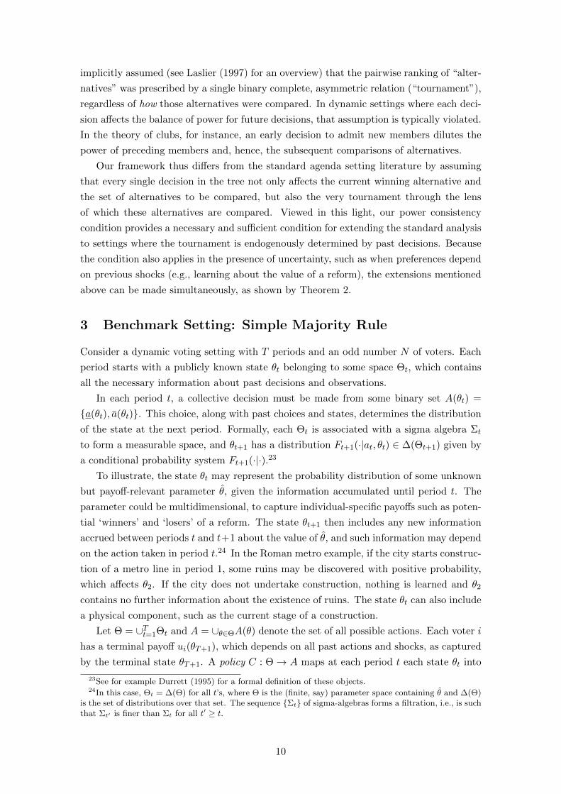
implicitly assumed (see Laslier (1997) for an overview) that the pairwise ranking of “alter-

natives” was prescribed by a single binary complete, asymmetric relation (“tournament”),

regardless of how those alternatives were compared. In dynamic settings where each deci-

sion affects the balance of power for future decisions, that assumption is typically violated.

In the theory of clubs, for instance, an early decision to admit new members dilutes the

power of preceding members and, hence, the subsequent comparisons of alternatives.

Our framework thus differs from the standard agenda setting literature by assuming

that every single decision in the tree not only affects the current winning alternative and

the set of alternatives to be compared, but also the very tournament through the lens

of which these alternatives are compared. Viewed in this light, our power consistency

condition provides a necessary and sufficient condition for extending the standard analysis

to settings where the tournament is endogenously determined by past decisions. Because

the condition also applies in the presence of uncertainty, such as when preferences depend

on previous shocks (e.g., learning about the value of a reform), the extensions mentioned

above can be made simultaneously, as shown by Theorem 2.

3 Benchmark Setting: Simple Majority Rule

Consider a dynamic voting setting with T periods and an odd number N of voters. Each

period starts with a publicly known state θt belonging to some space Θt, which contains

all the necessary information about past decisions and observations.

In each period t, a collective decision must be made from some binary set A(θt) =

{a(θt), a(θt)}. This choice, along with past choices and states, determines the distribution

of the state at the next period. Formally, each Θt is associated with a sigma algebra Σt

to form a measurable space, and θt+1 has a distribution Ft+1(·|at, θt) ∈ ∆(Θt+1) given by

a conditional probability system Ft+1(·|·).23

To illustrate, the state θt may represent the probability distribution of some unknown

but payoff-relevant parameter θ, given the information accumulated until period t. The

parameter could be multidimensional, to capture individual-specific payoffs such as poten-

tial ‘winners’ and ‘losers’ of a reform. The state θt+1 then includes any new information

accrued between periods t and t+1 about the value of θ, and such information may depend

on the action taken in period t.24 In the Roman metro example, if the city starts construc-

tion of a metro line in period 1, some ruins may be discovered with positive probability,

which affects θ2. If the city does not undertake construction, nothing is learned and θ2

contains no further information about the existence of ruins. The state θt can also include

a physical component, such as the current stage of a construction.

Let Θ = ∪Tt=1Θt and A = ∪θ∈ΘA(θ) denote the set of all possible actions. Each voter i

has a terminal payoff ui(θT+1), which depends on all past actions and shocks, as captured

by the terminal state θT+1. A policy C : Θ→ A maps at each period t each state θt into

23See for example Durrett (1995) for a formal definition of these objects.24In this case, Θt = ∆(Θ) for all t’s, where Θ is the (finite, say) parameter space containing θ and ∆(Θ)

is the set of distributions over that set. The sequence {Σt} of sigma-algebras forms a filtration, i.e., is suchthat Σt′ is finer than Σt for all t′ ≥ t.

10

an action in A(θt). Similarly, a voting strategy for voter i is defined by a policy Ci, which

describes his voting decisions.

Given a policy C and a state θt, voter i’s expected payoff, seen from period t, is

V it (C|θt) = E[ui(θT+1)|θt, C].

Definition 1 (Voting Equilibrium). A profile {Ci}Ni=1 of voting strategies forms a Voting

Equilibrium in Weakly Undominated Strategies if the following conditions hold for each

θt ∈ Θ:

• The resulting collective decision Z satisfies Z(θt) = a ∈ A(θt) if and only if |Ci(θt) =

a| ≥ N/2.

• Ci(θt) = arg maxa∈A(θt) Vit (a ◦ Z|θt)

The first condition describes simple majority voting: at each time, society picks the

action that garners the most votes. The second condition corresponds to the elimination

of weakly dominated strategies. In each period t, voter i, taking as given the continuation

of the collective decision process from period t+1 onwards that will result from state θt+1,

votes for the action that maximizes his expected payoff as if he were pivotal.

We assume for simplicity25 that for each period t, state θt, and policy C, each voter

has a strict preference for one of the two actions in A(θt). That is, we rule out situations

in which

V it (a(θt) ◦ C|θt) = V i

t (a(θt) ◦ C|θt)

for some i, where a(θt) ◦ C denotes the policy equal to C on Θ \ {θt} and equal to a(θt)

for θt, with a similar definition for a(θt) ◦ C.

Because indifference is ruled out and the horizon is finite, this defines a unique voting

equilibrium, by backward induction.

Proposition 2. There exists a unique voting equilibrium.

3.1 Commitment and Voting Cycles

Given two policies Y and Y ′, say that Y dominates Y ′, written Y � Y ′, if there is a

majority of voters for whom V i1 (Y |θ1) > V i

1 (Y ′|θ1). A Condorcet cycle is a finite list of

policies Y0, . . . , YK such that Yk ≺ Yk+1 for all k < K, and YK ≺ Y0. A policy X is

a Condorcet winner if for any policy Y , either X � Y , or X and Y induce the same

distribution over ΘT+1.

Theorem 1. Let Z denote the equilibrium policy.

i) If there exists Y such that Y � Z, then there is a Condorcet cycle that includes Y

and Z.

25This is a standard assumption in the tournament literature, where the preference relation acrossalternatives is assumed to be asymmetric. See Laslier (1997). Without this strictness assumption, most ofTheorem 1 still applies to “weak” Condorcet winner and cycle. See Remark 1.

11

ii) If there exists a policy X that is a Condorcet winner among all policies, then X and

Z induce the same distribution over ΘT+1.

Remark 1. If ties in voters’ preferences are allowed, Part i) of the theorem still goes

through with a weak Condorcet cycle: there is a finite list of policies Y0, . . . , YK such that

Yk � Yk+1 for all k < K, and YK ≺ Y0. Similarly, as the proof makes clear, the equilibrium

Z continues to be a Condorcet winner in the following sense: there does not exist another

policy Y such that Z ≺ Y .

The cycles predicted by Theorem 1, whenever they occur, may be interpreted as follows:

If the population were allowed, before the dynamic game, to commit to a policy, it would

be unable to reach a clear agreement, as any candidate would be upset by some other

proposal. If one were to explicitly model such commitment stage, the outcome of that

stage would be subject to well-known agenda setting and manipulation problems, and the

agenda could in fact be chosen so that the last commitment standing in that stage be

majority defeated by the outcome of the dynamic game (i.e., the equilibrium policy).26

In many applications, such as the Roman metro example of Section 2, the terminal

payoffs and probability distribution for the state process are described by a few parameters,

and the set of parameters can be partitioned into two nontrivial subsets according to

whether the equilibrium is dominated by some other policy.27 Seen this way, Theorem 1

states that this partition also characterizes the existence of a Condorcet winner among all

policies and, in the absence of such a winner, shows that any policy is part of Condorcet

cycle that includes the equilibrium policy.

Another, more positive, interpretation of Theorem 1 is that even when the equilibrium

policy is majority-dominated by another policy, it must belong to the top cycle of the social

preferences based on majority ranking. However, the equilibrium policy may be Pareto

dominated by another policy, as in the recruiting application described in Section 6.28

The proof, below, may be outlined as follows: If Y is different from Z, then Y takes

an action somewhere that the majority opposes. This allows us to construct a sequence

of policies, starting from Y , where we switch actions to those preferred by a majority,

thus always defeating the previous policy, until we recover Z, which was defeated by the

original alternative Y . The proof collects states according to the (finitely many) winning

coalitions, because individual states may (and often do) have zero probability. Because

we group states by all possible majorities, and then switch actions for each majority,

the switch is guaranteed to have the support of that particular majority. Proceeding by

backward induction on the decision tree, this sequence of transformations recovers the

equilibrium policy Z. Thus, we get a Condorcet cycle if, initially, Y � Z.

26In fact, one could formally incorporate such commitment decisions into the dynamic game, with thestate θt encoding whether a commitment has been chosen before period t (and if so, which). From anormative standpoint, another interpretation of the theorem is of course that the social preferences are not“rational” (i.e., transitive) in such case, which creates the usual problem of interpreting those preferences.

27In settings satisfying some single-crossing condition, the equilibrium is always undominated, as shownby Appendix D. Moreover, one can always choose common payoffs for all players, in any setting, toguarantee that the equilibrium Pareto dominates any other policy. A related payoff construction is usedin the proof of Theorem 3.

28Unlike the agenda setting literature, the equilibrium need not belong to the Banks set, because not allpolicy comparisons occur in the dynamic game. See the first paragraph of Section 2.2.

12

Proof. We fix any policy Y and let S denote the set of coalitions with at least N/2

voters. For each θt, a ∈ A(θt) and policy X, let S(a|θt, X) denote the set of voters

who strictly prefer a to the other action in A(θt), given the current state θt and given

that the continuation policy from t+ 1 onwards is X. The set ΘT can be partitioned into

AT ∪(∪S∈SBT (S)), where BT (S) = {θT ∈ ΘT : ZT (θT ) 6= YT (θT ) and S(ZT (θT )|θT , Z)) =

S} and AT consists of all remaining states in ΘT . In words, BT (S) consists of all the states

at the beginning of period T for which the set of voters who strictly prefer the action

prescribed by Z over the one prescribed by Y is equal to S.29 AT consists of all the states

for which YT and ZT coincide.30 We will index the coalitions in S from S1 to Sp, where

p is the cardinal of S. Consider the sequence of policies {Y pT }

pp=1, defined iteratively as

follows:

• Y 1T is equal to Y for all states except on BT (S1), where it is equal to Z.

• For each p ∈ {2, . . . , p}, Y pT is equal to Y p−1

T for all states except on BT (Sp), where

it is equal to Z.

By construction, Y 1T � Y because the policies are the same except on a set of states

where a majority of voters prefer Z (and, hence, Y 1T ) to Y . Moreover, because voters are

assumed to have strict preferences over actions, the social preference is strict if and only if

BT (S1) is reached with positive probability under policy Y : Y 1T � Y ⇔ Pr(BT (S1)|Y ) > 0.

If Pr(BT (S1)|Y ) = 0, Y 1T = Y with probability 1.

Therefore, either Y and Y 1T coincide, or Y 1

T � Y . Similarly, Y pT � Y p−1

T for all p ≤ p,

and Y pT � Y

p−1T if and only if Y p

T 6= Y p−1T with positive probability. This shows that

Y pT � · · · � Y

1T � Y,

and at least one inequality is strict if and only if the set of states in ΘT over which ZT

and YT are different is reached with positive probability under Y . By construction, Y pT

coincides with Z on ΘT : Y pT (θT ) = Z(θT ) for all θT ∈ ΘT .

We now extend the construction by backward induction to all periods from t = T − 1

to t = 1. For period t, partition Θt into At∪(∪S∈SBt(S)), where At consists of all θt’s over

which Yt and Zt coincide, and Bt(S) = {θt : Zt(θt) 6= Yt(θt) and S(Zt(θt)|θt, Z)) = S}.That is, Bt(S) consists of all states in Θt for which the set of voters who strictly prefer

the action prescribed by Z over the one prescribed by Y , given that Z is used for all

subsequent periods, is equal to S.31 Y pt is defined inductively as follows, increasing p

within each period t, and then decreasing t: for each t,

• For p = 1, Y 1t is equal to Y p

t+1 for all states, except on Bt(S1), where it is equal to

Z.

• For p > 1 Y pt is equal to Y p−1

t for all states, except on Bt(Sp) where it is equal to Z.

29In particular, YT (θT ) 6= ZT (θT ) for all those states.30Because Z is the equilibrium policy, the set of voters who prefer Y over Z at time T must always form

a minority, so AT and ∪S∈SBT (S) exhaust all states in ΘT .31Again, by definition of Z, there cannot be a majority who prefer Yt over Zt, given the continuation

policy {Z′t}t′≥t, so At ∪ (∪S∈SBt(S)) = Θt.

13

By construction, Y p+1t � Y p

t for all t and p < p and Y 1t � Y p

t+1 for all t. Moreover, the

inequality is strict if and only if the policies being compared are not equal with probability

1 on the set of states reached by either of them.

Finally, observe that Y p1 = Z. Let {Yk}Kk=1, K ≥ 1, denote the sequence of distinct

policies obtained, starting from Y , by the previous construction, iterating from t = T and

p = 1 down to t = 1 and p = p.32

If Y 6= Z with positive probability, then K ≥ 2. Moreover,

Y = Y1 ≺ Y2 · · · ≺ YK = Z. (1)

Therefore, we get a voting cycle if Z ≺ Y , which concludes the proof of part i).

Since Z can never be defeated without creating a cycle, we can characterize a Condorcet

winner out of all policies, if it (they) exists, and ii) follows. As mentioned in Remark 1, the

entire proof goes through if one drops the assumption that voters have strict preferences.

The only difference now is that (1) only holds with weak inequalities.

In the Roman metro game, payoffs were such that the equilibrium was inefficient in a

utilitarian sense. As usual with majority voting, however, there are situations in which the

equilibrium is a Condorcet winner but inefficient in a utilitarian sense, and other situations

in which it maximizes utilitarian welfare and is nonetheless part of a Condorcet cycle.

Theorem 1 implies, as an immediate corollary, a link between (strict) Pareto inefficiency

of the equilibrium and the existence of a Condorcet cycle: if the equilibrium policy is

strictly Pareto dominated by some other policy (i.e., all voters strictly prefer it to the

equilibrium), then there is a Condorcet cycle including the equilibrium and that Pareto-

improving policy, and no Condorcet winner can exist in such configuration.

4 General Case: State Dependent Rules and Power Consis-

tency

Collective decisions often deviate in essential ways from majority voting. In the Roman

metro problem, some stakeholders (archeologists) have a special say over preserving an-

tiquities. In other settings, power might rest with institutions that can be swayed only

by the preferences of a supermajority of ordinary citizens. This section shows that our

main result still holds when the decision rule is extended beyond simple majority, under

a power consistency condition whose relevance is discussed in detail below.

The formal environment is the same as before, except for the power structure of the

collective decision process.33 In each period t, given state θt, action a(θt) might, for

instance, impose a particular quorum or require the approval of certain voters (veto power)

to win over a¯(θt). Moreover, the decision rule may depend on the current state. Some

32We call two policies distinct if they induce different distributions over ΘT . Policies that differ only atstates that are never reached are not distinct.

33The number of voters need not be odd any more. We do maintain the assumption that decisions arebinary in each period to avoid the complications arising from coalition formation with more choices andequilibrium multiplicity.

14

voters may be more influential than others, because they are regarded as experts on the

issue under consideration, or because they have a greater stake, or simply because they

have acquired more influence.

Each state θt is associated with a set S(θt) of coalitions which may impose a(θt), in

the sense that if all individuals in S ∈ S(θt) support a(θt), given state θt, then a(θt) is

implemented in that period. Likewise, there is a set S(θt) of coalitions which may impose

a¯(θt).

34 A coalition S belonging to W (θt) = S(θt)⋃S(θt) will be called a winning coalition

and, whenever necessary, we will specify which action(s) S can impose. The collective

decision is always well defined.35 We require the following monotonicity condition: For

any ordered coalitions S ⊂ S′ and state θt, S ∈ S(θt)⇒ S′ ∈ S(θt). With this restriction,

individuals have a clear dominant strategy, which is to support the action that they prefer,

because they can never weaken the power of their preferred coalition by joining it.

A coalitional strategy Ci for individual i is, like the policies defined earlier, a map from

each state θt to an action in A(θt). It describes which action, a¯(θt) or a(θt), i supports.

Given a coalitional strategy profile C = (C1, . . . , CN ), let a(C, θt) denote the action

corresponding to the winning coalition: a(C, θt) = a(θt) if {i : Ci(θt) = a(θt)} ∈ S(θt)

and a(C, θt) = a¯(θt) if {i : Ci(θt) = a

¯(θt)} ∈ S(θt).

36

Given a policy C and state θt, i’s expected payoff, seen from period t, is

V it (C|θt) = E[ui(θT+1)|θt, C].

Definition 2 (Coalitional Equilibrium). A profile {Ci}Ni=1 of coalitional strategies forms

a Coalitional Equilibrium in Weakly Undominated Strategies if the following conditions

hold for all θt ∈ Θ:

• The resulting policy Z satisfies Z(θt) = a(C, θt))

• Ci(θt) = arg maxa∈A(θt) Vit (a ◦ Z|θt)

The first condition describes coalitional power: in each period, society picks the action

supported by the strongest coalition. The second condition corresponds to the elimina-

tion of weakly dominated strategies. In each period t, individual i, taking as given the

continuation of the collective decision process from period t + 1 onwards that will result

from state θt+1, joins the coalition whose preferred action maximizes his expected payoff,

as if he were pivotal.

We maintain the assumption of the previous section that each voter has, for any policy

and state θt, a strict preference for one of the two actions in A(θt). Because indifference

is ruled out and the horizon is finite, this defines a unique coalitional equilibrium, by

backward induction.

Proposition 3. There exists a unique coalitional equilibrium.

34Precisely, S(θt) contains all coalitions such that their complement is not in S(θt) and is thus in factredundant: S(θt) suffices to describe the power structure in state θt.

35For example, with simple majority voting and an even number of voters, a could require at least 50%of the votes. In that case, W(θt), but also S(θt) and S(θt), consists of all sets with at least N/2 voters.

36As explained earlier, exactly one of these cases must occur: the coalition of individuals preferring a(θt)can impose it if and only if its complement cannot impose a

¯(θt).

15

4.1 Commitment and Indeterminacy

Now suppose that, instead of playing the political equilibrium, society members are given

a chance to collectively commit to a policy at the outset. The objective of this section

is to determine whether a coalition can form to support some policy, which cannot be

challenged by any other policy.

Given any two policies Y and Y ′, say that S is a winning coalition for Y over Y ′ if

Y � Y ′ whenever all members of S support Y over Y ′ when the two policies are pitted

against each other. A power structure specifies the set of winning coalitions for every single

pair of alternatives. Given a power structure and individual preferences over alternatives,

we obtain a social preference relation, or pairwise ranking of every pair of alternatives:

Y � Y ′ if and only if there is a winning coalition S for Y over Y ′ all of whose members

prefer Y to Y ′.37

Given the social preference relation �, say that a policy Y is a Condorcet winner if

there is no other policy Y ′ strictly preferred over Y by a winning coalition.38 A Condorcet

cycle is a defined as in the previous section with the only difference that � is used instead

of the simple majority preference relation.

Specifying a power structure is generally demanding: it requires specifying the set of

winning coalitions for every single pair Y, Y ′. Fortunately, our main theorem requires a

condition that concerns a much smaller subset of those pairs.39

Definition 3 (Power Consistency). If i) Y and Y ′ differ only on a set Θt(Y, Y′) of states

corresponding to some fixed period t and ii) S is a winning coalition imposing the action

corresponding to Y for all states in Θt(Y, Y′), then S is also a winning coalition imposing

Y over Y ′.

Section 5 provides several interpretations of the condition and discusses when it is likely

to hold or to fail. Owing to the generality of the setting, the discussion encompasses not

only time-varying voting rules, but also situations in which new generations are born after

the beginning of the dynamic game, the case of a single time-inconsistent agent playing a

game with his future selves, agents who may die after some shocks, or gain political power

over time, etc.

Theorem 2. Let Z denote the equilibrium of the coalitional game and assume that power

consistency holds. Then,

i) If there exists Y such that Y � Z, then there is a Condorcet cycle that includes Y

and Z.

37Although individuals have strict preferences across any two actions in the dynamic game, they will beindifferent between two policies that take exactly the same actions except on a set of states that is reachedwith zero probability under either policy. We view such policies as identical and say that they “coincide”with each other.

38This generalization to non-majority voting is standard in the tournament literature. See, e.g., Laslier(1997).

39Remark: One could define consistency for each state θt rather than for a set of states Θt(Y, Y′). Because

individual states may have zero probability (e.g., with Gaussian uncertainty), it is more appropriate todefine it for sets of states. See the proof of Theorem 2.

16

ii) If some policy X is a Condorcet winner among all policies, then X and Z must

induce the same distribution over ΘT+1.

Proof. See Appendix.

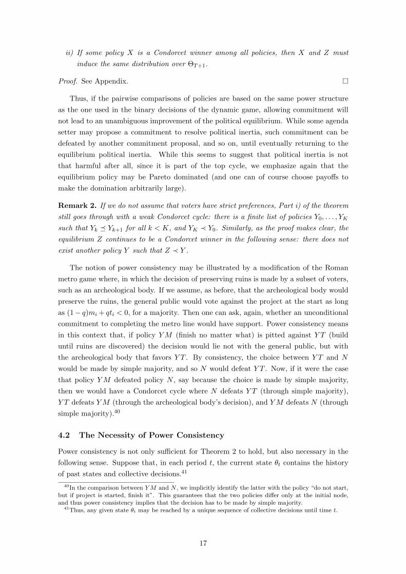
Thus, if the pairwise comparisons of policies are based on the same power structure

as the one used in the binary decisions of the dynamic game, allowing commitment will

not lead to an unambiguous improvement of the political equilibrium. While some agenda

setter may propose a commitment to resolve political inertia, such commitment can be

defeated by another commitment proposal, and so on, until eventually returning to the

equilibrium political inertia. While this seems to suggest that political inertia is not

that harmful after all, since it is part of the top cycle, we emphasize again that the

equilibrium policy may be Pareto dominated (and one can of course choose payoffs to

make the domination arbitrarily large).

Remark 2. If we do not assume that voters have strict preferences, Part i) of the theorem

still goes through with a weak Condorcet cycle: there is a finite list of policies Y0, . . . , YK

such that Yk � Yk+1 for all k < K, and YK ≺ Y0. Similarly, as the proof makes clear, the

equilibrium Z continues to be a Condorcet winner in the following sense: there does not

exist another policy Y such that Z ≺ Y .

The notion of power consistency may be illustrated by a modification of the Roman

metro game where, in which the decision of preserving ruins is made by a subset of voters,

such as an archeological body. If we assume, as before, that the archeological body would

preserve the ruins, the general public would vote against the project at the start as long

as (1− q)mi + qti < 0, for a majority. Then one can ask, again, whether an unconditional

commitment to completing the metro line would have support. Power consistency means

in this context that, if policy YM (finish no matter what) is pitted against Y T (build

until ruins are discovered) the decision would lie not with the general public, but with

the archeological body that favors Y T . By consistency, the choice between Y T and N

would be made by simple majority, and so N would defeat Y T . Now, if it were the case

that policy YM defeated policy N , say because the choice is made by simple majority,

then we would have a Condorcet cycle where N defeats Y T (through simple majority),

Y T defeats YM (through the archeological body’s decision), and YM defeats N (through

simple majority).40

4.2 The Necessity of Power Consistency

Power consistency is not only sufficient for Theorem 2 to hold, but also necessary in the

following sense. Suppose that, in each period t, the current state θt contains the history

of past states and collective decisions.41

40In the comparison between YM and N , we implicitly identify the latter with the policy “do not start,but if project is started, finish it”. This guarantees that the two policies differ only at the initial node,and thus power consistency implies that the decision has to be made by simple majority.

41Thus, any given state θt may be reached by a unique sequence of collective decisions until time t.

17

Theorem 3. Suppose that there exist policies Y and Y ′, and a coalition S such that i)

Y and Y ′ differ only through the actions taken in some period t and only for θt lying in

some subset Θt of Θt, ii) Θt is reached with positive probability under policy Y (and hence

Y ′), iii) S is a winning coalition for any θt ∈ Θt implementing the action prescribed by Y ′

(instead of Y ’s) for all those states, iv) S is not a winning coalition for Y ′ over Y in the

power structure used for the pairwise comparison of policies.42 Then, there exists a payoff

profile for all individuals and terminal states and a policy X that strictly dominates the

equilibrium Z and X is a Condorcet winner.

Proof. See the Appendix.

5 Interpreting Power Consistency

Consider, first, a setting with time-consistent agents who are all present at the commit-

ment stage (this setting rules out the possibility of future generations). Intuitively, all

agents have a say, at least in principle, on all decisions, and a well-defined preference over

those. To go beyond the simple majority rule, which clearly satisfies power consistency,

consider the following scenarios:

Expertise Rule: Some issues require specific expertise (energy policy, international con-

flicts, monetary policy, etc.). The relative social ranking of policies that differ only on

those issues should be based on the preferences of experts, just like the corresponding bi-

nary action in the dynamic game. Power consistency thus holds, and puts higher political

weight on those experts.

Minority Rule: Some decisions concern specific groups and should be decided by those

groups, in both dynamic and commitment settings. A particularly simple example is

provided by the notion of “liberalism” studied by Sen (1970) and discussed further in Sec-

tion 5.1. Besides individual liberalism, this rule may be applied to study various minority

rights.

Importance Rule: Decisions that require supermajority rules, such as the two-thirds ma-

jority rule or the unanimity rule, are often of particular importance for society and may

trigger radical changes. The use of such supermajority at some node of the dynamic game

may reflect this importance, in which case it is also natural to incorporate that rule in the

social comparisons of policies.

In several policy applications, such as problems with intergenerational transfers of

resources, long-lasting environmental decisions, and major international treaties, commit-

ments involve generations which are unborn at the time of commitment. Whether power

consistency holds depend on how one treats those generations in the social preference re-

lation. This leads to two different rules:

42Equivalently, its complement S can impose Y over Y ′

18

Virtual Minority Rule: This is a variation of the Minority Rule, in which the issue at

stake concerns some future generation(s). In that case, the social preference concerning

policies that mainly affect future generations may, normatively, include their preferences,

even though the minority is absent at the time of commitment. This rule incorporates the

preferences (well being) of future generations in the social preference relation. Today’s gen-

erations take on a social planner role which entails some form of intergenerational altruism.

Irrelevance Rule: Reciprocally, some agents may die or more generally leave the dynamic

game following some actions or exogenous shocks. It seems reasonable, at least in the

context of policymaking, to ignore them when comparing policies that differ only with

respect to decisions arising after they left the game.

An alternative, more selfish view of future generations, is to simply ignore them in the

social preference. In that case, power consistency will be violated.

Myopic Rule: The current generation ignores the welfare and preferences of future gen-

erations. Power consistency is violated when the preferences of future generations are in

conflict with those of the commitment-making generation.

The selfish generation rule is an example of what may broadly be described as a time

inconsistency problem: The preferences of future decision makers are not reflected in

today’s preferences.

The link with time inconsistency and Theorem 2 is intuitively clear: It is well known, in

particular, that a time-inconsistent agent values commitment. Time-inconsistent agents

violate power consistency because their initial ranking of social alternatives is not rep-

resentative of their preferences when they make future decisions. One may think of a

time-inconsistent agent as a succession of different selves, or agents, each with their spe-

cific preferences. At time t, the t-self of the agent is in power; he is the dictator and the

unique winning coalition. When considering commitment at time 0, however, the initial

preferences of the agent are used for all policy comparisons, and this violates power con-

sistency.

Time Inconsistency (Single agent): Commitment is valuable to time-0 agent. He ignores

the preferences of his future selves.

One should emphasize that, while commitment is valuable to a time-inconsistent agent,

it is only because his future preferences are not directly taken into account in the social

ranking.43 Of course, the last observation is by no means limited to a single agent. A set

of perfectly identical but time inconsistent agents would face the same issue, regardless of

the voting rule adopted in each period. Again, power consistency is violated when one ap-

43The agent’s preferences in the first period may incorporate his future preferences, and this very factmay be the source of the agent’s time inconsistency, as in Galperti and Strulovici (2014). The point hereis that the future preferences of the agent do not directly affect the ranking of commitment policies whenthe agent chooses among them at time 1.

19

propriately treats the future selves of those agents as different agents. A similar source of

time inconsistency concerns institutions whose directors change over time, bringing along

different preferences.

Time inconsistency (Successive Agents): While formally similar, this context applies to

governments and regulators: Old governments are replaced by new governments, or old

governments’ preferences can change over time. Commitments made by early govern-

ments ignore future governments and thus violate power consistency. When governments

are elected, their time inconsistency may reflect the time inconsistency of the electorate.

Another form of time inconsistency arises when some agents become more politically

powerful over time, to where they can influence future decisions above and beyond their

power at the commitment stage.

Power Rule: Agents’ individual power varies over time. These power changes may be

foreseeable or random, depending on the economic or political fortunes of individuals at

time zero. Regardless of the cause, commitment may be valuable at the outset, as a way

to insulate future decisions from the excessive power gained by a small minority. Power

consistency is violated because the evolution of individual power is not included in the

commitment decision.

The entire analysis so far has considered the value of commitments, assuming that

they were feasible. In practice, some commitments are infeasible, because future decision

makers have the power to revoke previous laws or ignore resolutions made by their pre-

decessors. These considerations must be clearly separated from any analysis of the value

of commitment, assuming it were available. However, it is easy to formally incorporate

in the analysis such limitations on the commitment power of decision makers at time 0.

In fact, those limitations are exactly captured by power consistency: In all of the above

settings where power consistency is violated, one can restore it by putting restrictions on

commitment, as follows:

Limited Commitment Rule: Whoever is in power in period t and state θt also dictates

the social preference for policies differing only in that period. This incorporates the power

of future decision makers into the social preference relation, as a way of recognizing impor-

tant practical limitations of the commitments that may credibly be considered in period 0.

Of course, if the limited commitment rule is applied to all periods and states, it is

not surprising that commitment is ineffectual at improving the equilibrium, because the

rule has essentially emptied commitment of its content. However, when the limited com-

mitment rule is only applied to a subset of future decisions, our main theorem may be

interpreted as follows: to the extent that some commitments are feasible, they can improve

upon the dynamic equilibrium without commitment if and only if there is indeterminacy

20

among feasible commitments.

Choosing How to Choose

The discussion so far has purposely ignored collective decisions that determine the voting

rule of ulterior decisions. Such decisions are, of course, allowed by the general framework

of this paper: the state θt can include any past decision, and determines the set of win-

ning coalitions at time t. They are also relevant: In many settings, the future allocation

of political power is determined by current agents. This arises in the theory of clubs

(e.g., Barbera et al. (2001) study how voters decide on immigration policies that expand

their ranks), or when voters decide today on voting rules that will be used in the future

(Barbera and Jackson (2004)).

This omission was made to avoid confusion, because early decisions that set voting

rules for later ones have the flavor of commitment, but they are distinct from the kind of

commitment over entire policies that is the focus of this paper. We discuss whether power

consistency holds and interpret our theorem in such a context.

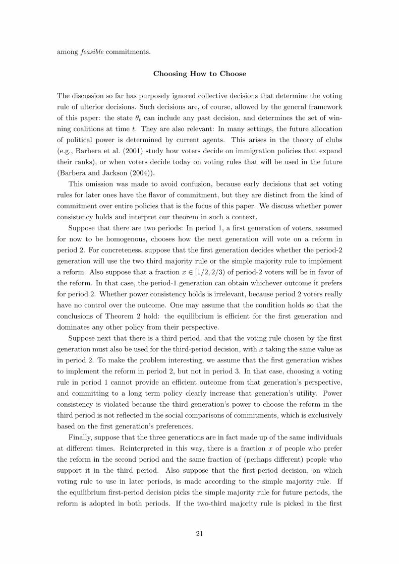
Suppose that there are two periods: In period 1, a first generation of voters, assumed

for now to be homogenous, chooses how the next generation will vote on a reform in

period 2. For concreteness, suppose that the first generation decides whether the period-2

generation will use the two third majority rule or the simple majority rule to implement

a reform. Also suppose that a fraction x ∈ [1/2, 2/3) of period-2 voters will be in favor of

the reform. In that case, the period-1 generation can obtain whichever outcome it prefers

for period 2. Whether power consistency holds is irrelevant, because period 2 voters really

have no control over the outcome. One may assume that the condition holds so that the

conclusions of Theorem 2 hold: the equilibrium is efficient for the first generation and

dominates any other policy from their perspective.

Suppose next that there is a third period, and that the voting rule chosen by the first

generation must also be used for the third-period decision, with x taking the same value as

in period 2. To make the problem interesting, we assume that the first generation wishes

to implement the reform in period 2, but not in period 3. In that case, choosing a voting

rule in period 1 cannot provide an efficient outcome from that generation’s perspective,

and committing to a long term policy clearly increase that generation’s utility. Power

consistency is violated because the third generation’s power to choose the reform in the

third period is not reflected in the social comparisons of commitments, which is exclusively

based on the first generation’s preferences.

Finally, suppose that the three generations are in fact made up of the same individuals

at different times. Reinterpreted in this way, there is a fraction x of people who prefer

the reform in the second period and the same fraction of (perhaps different) people who

support it in the third period. Also suppose that the first-period decision, on which

voting rule to use in later periods, is made according to the simple majority rule. If

the equilibrium first-period decision picks the simple majority rule for future periods, the

reform is adopted in both periods. If the two-third majority rule is picked in the first

21

period, no reform is adopted in later periods. Suppose without loss that the two-third

majority rule is chosen, so that the equilibrium preserves the status quo. This means that

there is a majority of individuals who dislike the reform in at least one period, so much so

that they prefer the status quo to having the reform in both periods, even though there is

also a majority (x) of people who, in each period, prefer the reform to be implemented in

that period.44 If we use the simple majority rule when comparing any pair of policies other

than the pairs differing only at one period, there is a cycle across commitment policies: a

majority of people prefer no reform at all (Z) to both reforms (Y), but a majority prefers

reform in period 1 only (X) to Z, and a majority prefers reform in both periods (Y) to

X, so that Y � X � Z � Y . Power consistency is reasonable in this setting: whatever

decision is made in the dynamic game reflects the preferences of the population at the

beginning of the game. The theorem applies and, since the equilibrium is dominated by

reform in either period, we get a Condorcet cycle.

5.1 An example: Sen’s Impossibility of a Paretian Liberal

Sen (1970) has demonstrated that a social decision function cannot be both efficient (in

the strict Pareto sense) and satisfy what Sen calls “Minimal Liberalism”: for at least

two individuals there exists a pair of alternatives, one pair for each individual, such that

these individuals are decisive over their pair. By linking social preferences to individual

decisions in a dynamic game, power consistency can capture Sen’s notion of liberalism as

a particular case.

Sen’s setting concerns a static social choice problem, in which alternative entails a

complete description of all decisions in society. When these decisions (collective or indi-

vidual) can be represented as a deterministic dynamic game, Sen’s alternatives correspond

to the policies studied in the previous sections, and there are natural settings in which

power consistency corresponds to liberalism.

To illustrate, consider Sen’s main example which concerns two individuals, 1 (a ‘per-

vert’) and 2 (a ‘prude’), and a book, Lady Chatterly’s Lover. The prude player does not

want anyone to read the book but, should the book be read by someone (for simplicity,

Sen does not allow both individuals to read the book), he prefers to be the one who reads

it. The pervert individual, by contrast, would like someone to read the book, and would

also prefer the prude read it, rather than he himself (the rational being that he enjoys

the idea of the prude having to read this subversive book). Let x, y, and z respectively

denote the following alternatives: 2 reads the book; 1 reads the book; no one reads the

book. The situation is embedded in a dynamic game, illustrated on Figure 3, in which 1

decides first whether to read the book, followed by 2.45

Power consistency implies that player 2 has the right to choose between reading the

book or not. Player 1, too, is entitled to reading the book, regardless of what player

44For example, suppose that x = 3/5 and the 2/5 who oppose the reform in any given period dislikeit much more than they value the reform in the other period. By taking the sets of reform opponents tobe completely disjoint across periods, we get 4/5 of agents against simple majority rule in period 1, as itwould lead to reform being implemented in both periods.

45The reverse sequence of moves yields outcome x (the prude player reads the book) and thus does notcapture the tension contained in Sen’s theorem.

22

Player 2

z

Player 1

x

y

Read Don't

Read Don't

Player 2: z, x, yPlayer 1: x, y, z

Individual rankings

Figure 3: A representation of Sen’s game. Individual preferences are indicated from themost preferred to the least preferred alternative.

2 does. Thus, power consistency and Sen’s version of liberalism are equivalent in this

setting. In the coalitional equilibrium of this game, the pervert reads the book and the

prude does not (y). If, moreover, the Pareto condition of Sen’s analysis may be encoded by

requiring the unanimity rule for x to win against y. Because x Pareto dominates y given

the players’ individual preferences, the equilibrium y is defeated by the commitment to a

policy in which the pervert does not read the book and the prude does (x). Theorem 2

then triggers a Condorcet cycle, leading to the impossibility of Paretian liberalism.

6 Applications

Pareto Inefficiency on the Job Market

In this first application, an economics department must decide whether to fly out a

job candidate and, if so, whether to make her an offer. The faculty initially doesn’t know

whether the candidate’s primary interest lies in macroeconomics or labor economics, but

this uncertainty will be resolved during the flyout, should it take place. In effect, the faculty

decides whether to “experiment” with a new candidate (N). In case the department cannot

agree on the flyout, some “status quo” candidate (S) will get the position (alternatively

no one will be hired); however, there is a shared feeling among the faculty that more

information should be gathered before making the offer. Hence, there is an inherent

preference for a flyout.

Once N ’s field is known, the faculty will vote on whether to hire her or S. The

department is split according to the following preferences. To a third of the faculty (group

I), it is important to hire a candidate who will exclusively work on macroeconomics; these

members would prefer to make an offer to S over a labor economist. Another third (group

II) is already convinced about N and willing to make an offer to N over S, regardless of

whether she is macro or labor economist. The remaining third (group III) will vote for N

only if she is a labor economist, and otherwise prefer S. Figure 4 displays this game. The

utility from the status quo candidate is normalized to zero, and the flyout is inherently

desirable in that hiring S yields a greater payoff after N ’s flyout. The total utility from

23

inviting the new candidate and making an offer is always positive; furthermore, there is

always a majority that would support an offer to N .

Figure 4 goes here.

flyout status quo

macro labor

offer offer status quo status quo

000

111

111

22-3

-322

Nature

Vote

Vote Vote

Figure 4: Job Market Game

Still, groups I and III both refuse to fly her out, for different reasons. I fears that N is

found to be a labor economist, and II and III then align to make her an offer. III worries

that N could turn out to be a macroeconomist and would then be supported by I and II.

Hence, the candidate may fail to get the flyout, even though, regardless of what the flyout

reveals, a majority would vote to make her an offer (and the benevolent department head

would do the same). Moreover, in this case the choice not to fly the candidate out is Pareto

inefficient, since a strictly superior outcome can be guaranteed for everyone (hiring S is

always possible and valued more after the flyout). In these circumstances, commitment

is a tempting solution. For instance, commitment to only hire a labor economist has

majority support over the status quo, because it results in a lottery between the status

quo candidate and a labor economist, whom a majority prefers. This means, however,

that Theorem 1 applies: since there is a policy that defeats the status quo, voting on

policies must be subject to a Condorcet cycle.46

An interesting aspect of this job market example is that, while decision makers have

no clear way out of an inefficient choice, the candidate could fix the problem by revealing

her type. By positioning herself clearly as a macroeconomist or a labor economist, she

46The cycle works as follows. Take, for example, the Pareto improvement over the status quo: flyingN out, but hiring S in any case. This policy defeats the status quo, but is itself beaten by a policy tomake an offer to N only if she is a labor economist, which is preferred by II and III. This policy, however,is rejected by a majority in favor of hiring N in any case, since this yields better outcomes for I and II.But flying N out and hiring her cannot defeat the status quo, since the expected payoff for I and III isnegative.

24

can remove any uncertainty, in which case the department will invite her. This rational-

izes the advice job candidates often get from their advisors to avoid mixing fields. The

corresponding action in the Roman metro game would be to locate ruins prior to deciding

on the project, so that the uncertainty is resolved. Unfortunately, this is not feasible in

practice.

Experimenting with Reforms: An Argument in Favor of Anonymous Policies

A common source of political inertia concerns the avoidance of socially valuable reforms

who carry uncertain outcomes and, hence, political risk. We first apply Theorem 1 to show

how commitment may fail to resolve political inertia, and then show how the Condorcet

cycle predicted by that theorem can be destroyed by focusing on anonymous policies. This

application provides a cautious source of optimism in settings where agents are sufficiently

symmetric ex ante.

The application builds on the two-stage experimentation setting of Fernandez and

Rodrik (1991). In the first stage, the citizens of a country decide whether to institute a

trade reform. If the reform is undertaken, each individual learns whether he is a “winner”

or “loser” from the reform. In the second stage, citizens vote on whether to continue the

reform (or implement it, they hadn’t done so in the first period). A simplified version

of this application is depicted on Figure 5. The reform imposes a (sunk) cost c on each

individual that must be borne once, regardless of the duration of the reform. Voters are

split into three groups (I, II, and III) of equal size, and one of the groups is randomly

(with uniform probability) chosen as the sole winner from the reform. Individuals in the

winning group get a payoff of g per period for the duration of the reform, while remaining

individuals lose l per period. If the reform is implemented in the first period and continued

in the second, we call it a long-term reform, whereas if it is revoked in the second period,

it is a short-term reform.

Figure 5 goes here.

Provided that g is sufficiently larger than l, the long-term reform is socially valuable. It

provides a higher expected payoff to everyone, relative to the status quo (not implementing

the reform in either period), and committing to the long-term reform is thus majority

preferred to the status quo. However, any initial reform must be revoked in the second

period, because two out of three groups find out that they are losers of the reform and

have an incentive to end it in the second period. We will say that a status quo bias arises

if the reform is not implemented at all in equilibrium even though committing to it would

be socially beneficial.47

Theorem 1 implies that, whenever status quo bias arises, there must be a Condorcet

cycle over policies involving the status quo and long-term experimentation. The status quo

47While there is no unanimously accepted and rigorous definition of status quo bias, the fact that asocially beneficial reform is not implemented despite having a positive expected payoff relative to thestatus quo captures the intuitive meaning of this expression. In the context of social reforms, Strulovici(2010) decomposes the notion of status quo bias into “loser trap” and “winner frustration” effects whichare formally defined relative to the policy that each agent would follow had he had the sole control overexperimentation.

25

R S

R S

First period vote

Nature picks the winner

Second period vote

R SR S

A B CR S

Second period vote

2g-c-2l-c-2l-c

g-c-l-c-l-c

A B C

000

Nature picks the winner

-2l-c2g-c-2l-c

-l-cg-c-l-c

-2l-c-2l-c2g-c

-l-c-l-cg-c

g-c-l-c-l-c

-l-cg-c-l-c

-l-c-l-cg-c

Figure 5: Reform game from Fernandez and Rodrik (1991) for three voters and onewinner from the reform.

occurs in equilibrium when g < 2l + 2c, because the expected payoff from the short-term

reform (the reform is ended the moment two losers are identified) is negative for every

type. The expected payoff from the long-term reform is simultaneously positive for each

type, provided that g > 2l + 1.5c. Other possible commitments, to short-term reform or

to delayed reform in the second period, yield identical negative expected payoffs. Among

these, long-term reform is a Condorcet winner, which seems to contradict Theorem 1.

How to explain this paradox?

In Theorem 1, the Condorcet cycle over policies is constructed over the full set of

feasible policies: any plan of action that conditions on states where voting takes place is

under consideration. While natural in many contexts, such as the Roman metro game,

this may be too demanding in others. Here, it makes little sense to let policies depend on

the identity of the winner and losers. It is the anonymity of policies, implicitly assumed

in the previous paragraph, which allows the long-term reform to be a Condorcet winner.

Without imposing anonymity that policy is no longer a Condorcet winner. For example,

it is defeated by the following policy: start with reform initially, and revoke it only if I

is the winner. Note that II and III strictly prefer this policy to unconditional long-term

reform, since they will be losers in that particular state of the world. In turn, commitment

to long-term reform except when I is the winner is beaten by commitment to long-term

reform unless I or II is the winner. This differs from the previous policy only when II is

the winner, and in that state of the world I and III benefit from ending the reform, so

their expected payoffs increase. Now that I and II are at best temporary winners, both

prefer the status quo (recall that the expected payoff from short-term reform is negative).

This yields a cycle: Unconditional commitment to a long-term reform defeats the status

quo and unconditional commitment to temporary reform, but loses to long-term reform

26

unless I is the winner, which in turn loses to long-term reform unless I or II is the winner,

which in turn loses to commitment to the status quo.

The Stability of Unpopular Regimes

Dictators are sometimes able to stay in power despite widespread dissatisfaction, partly

because the opposition, while united in wishing to depose the current government, is

fragmented by conflicting goals and mutual distrust. One may reasonably expect those

groups to understand that the political situation following the fall of such a regime will

not necessarily be an improvement of their current situation.48 Suppose that there are

three groups: the elite, who benefits from the current dictatorship (the “status quo”), as

well as secular and religious factions. A revolt against the status quo is successful if it is

supported by a majority of the population.49 Three outcomes are then possible: religious,

secular, and bipartisan regimes. In the bipartisan regime, power is shared between the

religious and secular groups and the elite loses its privileges. While the religious and

secular groups both want to remove the dictator, they favor radically opposite regimes,

following an uprising. We suppose that each constitutes 49% of the population, so that

the elite, representing the remaining 2% of the electorate, plays the role of a swing voter.50

The elite is interested in preserving some degree of power and might side with either the

religious or the secular group, depending on how the uprising unfolds. Finally, we assume

that the elite supports each group with equal probability, but always prefers a religious or

a secular regime to a bipartisan one, in which it loses all influence.

Figure 6 depicts an instance of this application, where the payoffs are given in the

following order: religious, secular, and elite. While the population has the choice between

three distinct outcomes (regimes) after the uprising, we can easily redefine the decision as

a series of binary choices, so as to fit the framework of Theorem 1.51

Figure 6 goes here.

Since the elite lends its support to either the religious or the secular group, revolting

amounts to a lottery between a religious or a secular regime, and has an expected payoff of

zero for both of these groups - less than the status quo payoff. The dictator, whom 98% of

the population would like to depose, can therefore hold on to power because of the elite’s

pivotal role. Yet, commitment to an uprising and subsequent bipartisan government has

a higher payoff and is therefore majority-preferred to the status quo.

48This application was suggested to us by Stephen Schmidt, in reference to the Arab Spring civil upris-ings.

49Voting is here a metaphor for collective action. Alternatively, one may invoke Theorem 2 and require,say, 90% support to overthrow the dictator.

50This percentage is meant to capture the qualitative feature that no group can single-handedly imposeits most preferred regime, and that the elite can play a pivotal role. The “vote” that follows an uprising isa stylization of the struggle for power that leads to an uprising, and the percentages represent the relativestrength of each group in that fight.

51More generally, it is possible to accommodate voting over three or more alternatives (at each stage), aslong as expected payoffs are such that, for any continuation play, there exists a Condorcet winner amongthem. However, we did not include this possibility in the statement of Theorem 1, to avoid confusion fromtalking about Condorcet winners at different decision levels.

27

uprising status quo

Nature

elite sideswith S

elite sides with R

secular state

-10102

550

1110

Vote

Vote Vote

bipartisansolution

religiousstate

10-102

Figure 6: Dictator game

Theorem 1 implies that there does not exist a Condorcet winner among ways to commit.

What is the predicted cycle that upsets the bipartisan solution, preferred by 98% over

dictatorship? We have already seen why the dictatorship is preferred to the fair lottery that

results in a partisan (secular or religious) regime, depending on whom the elite supports.

In turn, this lottery is majority-preferred over the policy which imposes the religious

regime if supported by the elite, but imposes the bipartisan regime if the elite supports

the secular one. Such commitment is, in turn, majority-preferred (by the religious faction

and the elite) to commitment to a bipartisan government. This yields the cycle that is

required by our result. The implication is that a successful opposition to the dictator

cannot necessarily be organized through an ex ante agreement. Since the uprising also

fails in the absence of agreements, the unpopular dictatorship seems stable, even if the

population has the capacity to commit to a specific plan.

In addition to the uncertainty stemming from the random support of the elite, one

may add other realistic shocks, such as an individual probability of incurring injury or

death as a result of the uprising. As long as those shocks do not completely reverse the

allocation of power among each group, the analysis goes through.

7 Concluding Remarks

Can political inertia and inefficient equilibria be resolved through the use of commitments?

It turns out, unfortunately, that committing to some policy will improve upon the equi-

librium policy only if there is a disagreement among decisive factions of society regarding

which commitment to choose. Allowing commitments thus transforms any inefficiency

problem into one of indeterminacy. This finding holds for general state processes and

utility functions, allowing social learning, experimentation, and arbitrarily heterogeneous

payoffs. When the power structure underlying collective decisions is extended beyond

28

the simply majority rule, possibly accounting for the time-and state-dependence of those

rules, or for changes in the nature of the decisions faced by society, our theorem relies on a

power consistency condition which may reflect representativeness, stability, or fairness of

the commitment decision rule, depending on the setting. When power consistency is vio-

lated, the value of commitment may be restored, often at the expense of decision makers,

such as unborn generations, who are poorly or not at all represented at the commitment

stage. One may be tempted to circumvent the theorem by placing a priori restrictions on

the set of commitments to consider. For example, when the decision problem is ex ante

perfectly symmetric across voters, one may restrict attention to anonymous or symmetric

policies, as illustrated in Section 6. In general, however, voters have heterogeneous pref-

erences from the very beginning of the dynamic problem, which limits the applicability of

the anonymity criterion. It is also helpful in some applications to restrict commitments to

policies which are Pareto undominated. Exploring such restrictions may help restore the

viability of commitments as a way to resolve the inefficiency of political equilibria, and

constitutes a natural and important question for future research.

We conclude this section with some extensions and further interpretations of our re-

sults.

Random proposers

In well-known agenda-setting protocols, voters may take turns to make collective pro-

posals, and may be chosen deterministically or stochastically to do so. Those protocols

are compatible with the setting of this paper. For example, for t odd, the state θt may

include, as well as past information, the identity of a proposer, who chooses between two

collective proposals. At the next, even, period, the new state θt+1 includes the proposal

just made by the proposer at time and society decides whether to accept the proposal or

to hold on for now to the status quo, given the possibility of future proposals.

Non-binary decisions

The analysis has focused on sequences of binary decisions. As explained at the outset,

this restriction avoids Condorcet cycles at the myopic, periodic level of the dynamic game,

shutting an obvious source of indeterminacy which would obfuscate the nature of the main

result. Many political problems do in fact have this binary structure. Particularly when

direct democracy is applied, choices such as referenda and initiatives almost always take

the form of a binary decision. Similarly, lawmakers introduce bills and amendments as

“yes” or “no” choices. This approach also appears in the explicit protocol proposed by

Acemoglu et al. (2012) (p. 1458).52

52While collective decisions are all binary, that paper allows a player to make proposals among all possiblestates. In the present setting, this can be easily replicated by a sequence of at most S periods (where Sis the number of states) in which each period corresponds to a new state being presented to the proposer,who makes a “no” decision until being presented by the state that he wants to propose to the group, atwhich point he votes “yes” and the proposal is made to the group. The total number T of periods, whilefinite, can be arbitrarily large, and any form of discount function may be included in the setting, whichmakes this extensive form rigorously equivalent to a direct choice among the S states.

29

With three or more alternatives to choose from at any time, it is worth emphasizing that

any attempt to resolve the potential Condorcet cycles through a “binarizing” procedure

will be subject to the theorem of this paper. Either turning the problem into a sequence of

binary choices leads to an equilibrium that is undominated among state-contingent plans

(so it not only resolves local indeterminacies but also yields majority-preferred outcomes),

or it leads to indeterminacies in the class of state-contingent policies.

Transfers

Although transfers were not explicitly considered, they are accommodated to some

extent in the present setting. For instance, one may include particular periods at time t,

at may correspond to a specific transfer from i to a player j, and a¯t

to the absence of a

transfer. Of course, i is a ‘dictator’ over that decision, and the state θt must keep track

of all past transfers to determine players’ payoffs at the end of the game.

Utility Functions: Non Separability, Past Dependence, etc.

The utility functions are arbitrary functions of past states and decisions. For exam-

ple, they allow complementarities across periods, and many forms of past-dependence,

such as habit formation, addiction, taste for varieties, utility from memories, learning by

experimentation, learning by doing, etc.53

53With such features, one must be careful to correctly interpret power consistency, as discussed in Section5.

30

Appendices

A Omitted proofs and examples of Section 2

A.1 Analysis of the Roman metro example

We solve the game by backward induction, using elimination of weakly dominated strategies as a

refinement. If construction takes place, the ruins are discovered, and a majority consisting of types

II and III votes to preserve them at the expense of the metro. Anticipating this, type-I voters

initially vote for the project if:

E(uI) = −2q + 1− q ≥ 0 ⇐⇒ q ≤ 1

3.

II votes for the project regardless of q, because II benefits whether or not an antiquity is found.

Type-III voters support the project if:

E(uIII) = q − 2 (1− q) ≥ 0 ⇐⇒ q ≥ 2

3.

Overall, there is a majority in favor of the project at the outset if q ≤ 1/3 (in which case, it is

supported by types I and II) or q ≥ 2/3 (then, the project is supported by types II and III). But

in case 1/3 < q < 2/3, types I and III join forces, so that a majority opposes the project.

A.2 Example showing that reverting the order of decisions does not

improve the equilibrium and does not reveal that the equilibrium

is Pareto dominated

There are two decisions i) U or D and ii) L or R, and three voters. The decisions can be made in

any order and are made according to the simple majority rule. The state of the world is revealed

between the decisions. The state of the world can take six possible values with probability 1/6

each, and broken down into two components: the role played by each decision (2 possibilities) and,

independently, which player is the “sucker” (3 possibilities). We index the states as θωi where i

indicates the sucker and ω ∈ {A,B} indicates the role of decisions. The payoff structure is as

follows:

In state θAi, all players get a payoff of 1 if L is chosen regardless of the other decision (U or

D). If R is chosen, then all players get a payoff of 2 if D is chosen, while player i gets −100 and

other players get 3 if U is chosen. Importantly, these payoffs do not depend on the other in which

the actions (U/D and L/R) are chosen.

In state θBi, the role of actions is reversed as follows: all players get a payoff of 1 if U is chosen,

regardless of the other decision (L or R). If D is chosen, then all players get a payoff of 2 if R is

chosen, while player i gets −100 and other players get 3 if L is chosen. Again, these payoffs do not

depend on the other of decisions (U/D and L/R).

The game is constructed in such a way that there is a commitment problem: players would ex

ante all prefer to get the payoff of 2, which is always achievable by committing to the action profile

(D,R), regardless of the order of these decisions. Without commitment however, there is always

a probability 1/2 that in period 2, two players gain by imposing the actions that gives them 3 and

gives the other player −100. For example, if L/R is the first decision, then if players choose action

R and the action state ω is A, then two players impose U in the second period and the other one

gets −100. If instead they choose action L and the action state ω is B, then two players impose

action D in the second period. Because of this, players’ expected payoff in equilibrium is order the

order of −100/6 ∼ −15.

31

By symmetry, players get exactly the same expected payoffs if instead the action U/D is made

in the first period.

In contrast, committing to (D,R) yields a payoff of 2, regardless of the state of the world.

Thus, reordering actions per se does not reveal the value of commitment. Of course, as implied by

Theorem 1, there is a cycle among commitment policies, as is easily checked.

B Proof of Theorem 2

Fix any policy Y , let ΘT denote the set {θT ∈ ΘT : ZT (θT ) 6= YT (θT )}. For θT ∈ ΘT , let ST (θT )

denote the coalition of individuals who prefer ZT (θT ) to YT (θT ). Since Z is the coalition equilibrium

policy, ST (θT ) must be a winning coalition given state θT . Let ST = {ST (θT ) : θT ∈ ΘT } denote

the set of all such coalitions and pT denote the (finite) cardinality of ST . We index coalitions in

ST arbitrarily from S1 to SpT. For each p ≤ pT , let Θp

T denote the set of θT ∈ ΘT for which the

coalition of individuals who prefer ZT (θT ) to YT (θT ) is equal to Sp and for which Sp is a winning

coalition. By construction ΘpT is nonempty. Consider the sequence {Y p

T }pT

p=1 of policies defined

iteratively as follows.

• Y 1T is equal to Y for all states except on Θ1

T , where it is equal to Z.

• For each p ∈ {2, . . . , pT }, Y pT is equal to Y p−1

T for all states except on ΘpT , where it is equal

to Z.

By construction, Y 1T � Y because the policies are the same except on a set of states where a

winning coalition prefers Z (and, hence, Y 1T ) to Y , and, by power consistency, they can impose

Y 1T over Y in the commitment stage because for all states in Θ1

T , S1 is a winning coalition, it has

to be a winning coalition when comparing Y 1T to Y . The winning coalition’s preference is strict if

and only if Θ1T is reached with positive probability under policy Y .

Therefore, either Y and Y 1T coincide (i.e., take identical actions with probability 1), or Y 1

T � Y .

Similarly, Y pT � Y p−1

T for all p ≤ pT , and Y pT � Y p−1

T if and only if Y pT 6= Y p−1

T with positive

probability. This shows that

Y pT � · · · � Y

1T � Y,

and at least one inequality is strict if and only if the set of states ΘT is reached with positive

probability under Y . By construction, Y pT

T coincides with Z on ΘT : Y pT

T (θT ) = Z(θT ) for all

θT ∈ ΘT .

Proceeding by backward induction, we extend this construction to all periods from t = T − 1

to t = 1. For period t, let Θt = {θt ∈ Θt : Zt(θt) 6= Yt(θt)}. For θt ∈ Θt, let St(θt) denote

the coalition of individuals who prefer Zt(θt) to Yt(θt). Given the continuation policy Z from

time t + 1 onwards, St(θt) is a winning coalition, since Z is the coalitional equilibrium. Also let

St = {St(θt) : θt ∈ Θt}. Letting pt denote the cardinality of St, we index coalitions in St arbitrarily

from S1 to Spt. Let Θp

t denote the set of θt’s in Θt for which the coalition of individuals who prefer

Zt(θt) to Yt(θt) is equal to Sp and for which this coalition wins. Θpt is nonempty, by construction

of Sp. Consider the sequence {Y pt }

pt

p=1 of policies defined iteratively as follows, increasing p within

each period t, and then decreasing t: for each t,

• For p = 1, Y 1t is equal to Y

pt+1

t+1 for all states, except on Θ1t , where it is equal to Z.

• For each p ∈ {2, . . . , pt}, Y pT is equal to Y p−1

T for all states except on Θpt , where it is equal

to Z.

All the constructed policies have Z as their continuation from period t+1 onwards. By construction,

Y p+1t � Y p

t for all t and p < pt and Y 1t � Y

pt+1

t+1 for all t. Moreover, such inequality is strict unless

the set of states over which they differ is reached with zero probability.

32

By construction, the last policy Y p1

1 generated by this algorithm is equal to Z. Let {Yk}Kk=1,

K ≥ 1, denote the sequence of distinct policies obtained, starting from Y , by the previous con-

struction.54

If Y 6= Z with positive probability, then K ≥ 2. Moreover,

Y = Y1 ≺ Y2 · · · ≺ YK = Z.

Therefore, we get a voting cycle if Z ≺ Y , which concludes the proof of part i).

Since Z can never be defeated without creating a cycle, we can characterize a Condorcet winner

out of all policies, if it (they) exists, and ii) follows.

C Proof of Theorem 3

We set the terminal payoffs equal to 0 for all policies, except when i) the action sequence until time

t has followed policy Y (and hence Y ′) and ii) the state θt reached at time t belong to Θt. In that

case, members of coalition S (its complement S) get 100 (10) if the time t action prescribed by Y ′

is played and followed by the continuation of policy Y (and hence Y ′), with the reverse payoffs if

instead the action prescribed by Y is played at time t and followed by the continuation of policy

Y . If θt /∈ Θt, everyone’s payoff is set to some small ε > 0 for the common continuation of Y and

Y ′, and to zero for all other continuations.55

Let Z denote the equilibrium policy. Z must coincide with Y and Y ′ until period t since it is

the only way, for any player, to get a nontrivial payoff. If the state θt ∈ Θt, coalition S imposes

at time t the action prescribed by Y ′, so as to achieve its highest possible payoff of 100, and it is

in everyone’s interest to implement the continuation corresponding to Y ′ from time t+ 1 onwards,

so that even members of S get their second highest payoff of 10. Even if θt /∈ Θt, it is also in

everyone’s interest to follow the common continuation of Y and Y ′ so as to get ε. This shows that

Z coincides to Y ′.

We now consider the social comparisons of policies. Clearly, S imposes Y � Y ′ since it has

the power to do so and this achieves it maximal expected payoff. Moreover, there cannot be any

cycle among policies, since Y and Y ′ Pareto dominate all other policies. Thus, Y is the Condorcet

winner56 among all commitments plans.

D Existence of a Condorcet Winner

Theorems 1 and 2 establish an equivalence between the existence of a Condorcet winner (in either

the usual or the coalitional sense) and the non-dominance of the equilibrium policy. When the set

of policies is large, one may legitimately wonder how likely the existence of a Condorcet winner is

in such setting. As it turns out, there are natural conditions under which a Condorcet winner does

exist. This section provides two routes for establishing such a result. For simplicity the analysis

of this section is focused on deterministic settings.

D.1 Terminal States

The setting is specialized as follows: there is finite set S of alternatives. The dynamic game starts

with some status quo alternative s0. Thereafter, in each period, a new alternative in S is proposed

54We call two policies distinct if they induce different distributions over ΘT+1. Policies that differ onlyat states that are never reached are not distinct.

55Although this is largely irrelevant to the gist of the present argument (see Remark 2), one may addarbitrarily small, action-dependent payoffs to break ties at all points of the game for all histories as requiredby the non-indifference assumption of Theorem 2.

56Any other Condorcet winner X must be identical to Y except on a set of histories which has probability0 when Y (or, equivalently, X) is followed.

33

against the last accepted alternative. If the challenger is accepted, it becomes the new ‘status quo.’

Otherwise, the previous status quo is pitted against a new challenger. The state θt corresponds

to the current status quo. So, without loss, θt ∈ S. It is assumed that the proposal protocol is

flexible enough so as to guarantee that each possible sequence of S states may arise under some

policy as the succession of status quo. This is achieved for instance if the states are ordered from

s1 to sS and, the number T of periods is such that T > S2, and at each time t ≤ T the challenger

is the state sk where k is the remainder in the Euclidean division of t by S.

The payoff of each player i is determined by the state s at the end of the last period. Formally,

i’s payoff ui is a map from S to R. Therefore, any policy reduces, in terms of payoffs, to the

last alternative. In particular, there is a Condorcet winner among policies if and only if there

is a Condorcet winner among states. As it turns out, this exact condition has been studied by

Acemoglu et al. (2012), hereafter (AES). In particular, part i) of their Assumption 2 is identical to

ruling out Condorcet cycle.57 Theorem 4 in AES provide sufficient conditions for acyclicity. By a

direct translation of their result, we obtain a sufficient condition for the existence of a Condorcet

winner. For completeness, we recall the assumptions of AES:

Say that a set C of coalitions is regular if it satisfies the following properties: i) For any W ∈ Cand W ⊂W ′, we have W ′ ∈ C, ii) For any W,W ′ ∈ C, W ∩W ′ 6= ∅.

For the sufficient condition, we order the set of players from 1 to N . The preference profile

{ui(·)}i∈N obeys the single-crossing property if for any ordered states s < s′ and ordered players

i < j, ui(s′) ≥ (>)ui(s) implies uj(s

′) ≥ (>)uj(s).

Proposition 4. Suppose the players satisfy the single-crossing property and that for each state s,

the set of winning coalitions is regular. Then, the equilibrium of the coalitional game selects the

unique Condorcet winner among the S alternatives.

Proof. The assumptions of Theorem 4 in AES are satisfied.58 Theorem 4 then implies acyclicity

of coalitional preferences which in turn guarantees the existence of a Condorcet winner s∗ among

alternatives and, by equivalence, among plans. Theorem 2 then implies that the equilibrium selects

that policy and hence s∗ as the terminal outcome.

Remark 3. AES also has a result based on single-peaked preferences and another nonempty in-

tersection condition for winning coalitions across different states. We refer the reader that paper.

Theorem 3 in that paper provides a condition under which the stable set is Pareto efficient. This

condition can readily be adapted to the setting of the present paper to guarantee that the equilibrium

yields a Pareto efficient outcome (regardless of whether it is a Condorcet winner).

D.2 Policy-based single-crossing property

The previous section established the existence of a Condorcet winner by first simplifying the setting

to one in which the payoffs only depend on the terminal state and applying single crossing to those

states. In many settings, the entire decision process, not just the final outcome, affects policies.

For example, consider a succession of decisions which affect a specific policy, such as gun laws,

gay marriage, or climate policy. Every single binary decision along the dynamic game can be

interpreted as going left or right along this policy spectrum. Interpreting a¯t (resp., at) as a move

to the left (right), a policy is thus a succession of moves on one dimensional policy spectrum. It is

clear, then, that the policy a¯1, a¯2 in a two-period problem is more to the left than the policy a1, a2.

Comparing a¯1, a2 with a1, a

¯2 is harder as it depends on the relative importance of first and second

move. However, in some settings there is a clear ranking of these magnitudes. For example, the

first decision may be of first importance, and followed by refining decisions of a less magnitude. In

such circumstance policies may be ranked unequivocally from left to right, and the single crossing

property may be imposed. If the simple majority rule is used throughout, then the median voter

57In both settings, the set of winning coalitions only depend on the current state.58The assumption, maintained throughout the present paper, that players are never indifferent across

actions implies that Assumption 6 in AES is satisfied.

34

theorem applies and guarantees the existence of a Condorcet winner. To illustrate, suppose that

policies are ranked lexicographically as follows: for any distinct policies Y, Y ′, Y ≺ Y ′ if at the first

period t for which there exists a state θt such that Yt 6= Y ′t , we have Yt = a¯t and Y ′t = at for all

the states of period t on which Y and Y ′ are distinct. This ordering captures the idea that earlier

decisions matter more for the policy than later refinements. Having a total order on policies one

can then apply the single crossing property.

E Voting Cycles with Experimentation over an Infinite Hori-

zon

A similar argument to the one used to prove Theorem 1 may be employed to Markovian settings

where backward induction can be applied to the underlying state, rather than time. We illustrate

this idea by revisiting the model of Strulovici (2010) for the case of three voters. Time is continuous

and voters, choose, at each instant, between a risky action (the “reform”) and a safe action (the

“status quo”). While the reform is implemented, each voter can receive good news revealing that

the reform benefits him, in which case he becomes a “winner” of the reform. Voters who do not

receive such news, called “unsure voters”, become more pessimistic about the value of the reform

and eventually want to abandon it and return to the status quo, if they still form a majority at

that time. Owing to the Markovian structure of the model, if the safe action is implemented once,

it is then implemented forever and social experimentation if abandoned.

In the model, the utilitarian policy, denoted by Y , is ex ante strictly preferred by all voters

to the equilibrium policy, Z, by Theorem 6 of Strulovici (2010).59 The equilibrium policy is

characterized by cutoffs p(0) > p(1) such that experimentation stops when the probability p of

success for unsure voters reaches p(k) if and only if k winners or less have been reached by that

time (Theorem 1). Similarly, the utilitarian policy is determined by thresholds q(k) (Theorem 2).

From Theorem 3, q(k) < p(k) for k = 0, 1: intuitively, social experimentation is more valuable to

a social planner who takes into account the utility of winners, and also has a higher option value

of experimentation than individual voters who have to share power. Suppose that q(1) = 0, which

means that it is socially efficient to play the risky action forever from the moment that one winner

has been observed. This condition is equivalent to g ≥ 3s, by Theorem 2, and this parametric

condition is imposed in what follows.

The thresholds p(1) and q(0) respectively solve the following equations, which come from

indifference conditions:60

p(1) =µs

µg + (g − s) + p(1)g − s(2)

and

q(0) =µs

µg + (g − s) + 2(q(0)g − s). (3)

Because p(1) and q(0) are strictly below the myopic cut-off s/g (Theorem 1), this implies that

q(0) > p(1).61 All the above implies p(0) > q(0) > p(1).

We now construct a cycle, based on the following modifications of the utilitarian policy. Let

Y1 denote the policy that coincides with the social optimum, Y , except that experimentation stops

at the threshold p(1) if the only winner observed by that time is Voter 1. That policy is strictly

preferred by Voters 2 and 3 over the utilitarian policy: conditional on Voter 1 being the only

winner by the time q(0) is reached, the policy that maximizes Voters 2 and 3’s common expected

59We refer the reader to the original paper for the results and notation used in this section. Theoremnumbers also refer to the original paper

60See Equation (17), p. 964 with N = 3 and kN = 1 and, respectively, Equation (7) on p. 947 withN = 3, k = 0, and W (1, p) = 1

3( gr

+ 2p gr).

61If p(1) ≥ q(0), then we would have p(1)g − s ≥ q(0)g − s > 2(q(0)g − s), where the strict inequalitycomes from q(0) < s/g. This would imply that the RHS of (2) is strictly smaller than the RHS of (3) and,hence, that p(1) < q(0).

35

utility consists precisely in stopping experimentation at the cutoff p(1) if none of them has become

a winner by then and, otherwise, in playing the risky action forever. To see this, notice that the

utilitarian cutoff q for Voters 2 and 3, starting from q(0), and given that any winner will cause L

to be played forever, is characterized by the indifference equation62

qg + 2qλ

(1

2

(gr

+ qg

r

)− s

r

)= s.

The first term of the LHS is the average flow payoff for Voters 2 and 3 when the risky action

is played. The second term of the left-hand side is their average jump in utility if one of them

becomes a winner, multiplied by the flow probability of that event. The right-hand side is the flow

payoff if the safe action is chosen instead (in that case, nothing is learned, so there is no jump in

utility).

After rearrangement, this equation is identical to (2) and thus yields the same cut-off.63 There-

fore, Y1 � Y . Similarly, consider the policy Y2 that is identical to Y1 except that experimentation

stops at p(1) if only Voter 2 has become a winner by that time. This policy is preferred by Voters 1

and 3 over Y1, by the same reasoning, so Y2 � Y1. Also construct Y3 by modifying Y2 so that

experimentation stops at p(1) if only Voter 3 is a winner by that time. Y3 � Y2.

By construction, Y3 stops experimentation if a single winner has been observed by the time

p(1) is reached, as does the equilibrium policy Z. The only difference between Y3 and Z is that

Z stops experimentation earlier, at the threshold p(0) > q(0), if no winner has been observed,

whereas Y3 stops experimentation at q(0).

However, subject to the constraint that experimentation stops at p(1) if only one winner has

been observed by that time, and continues forever otherwise, the socially optimal policy is actually

to stop at p(0), not q(0). To see this, notice that, due to the constraint, the continuation value of a

voter who becomes a winner is precisely the continuation value w under the equilibrium policy, and

the continuation value for unsure voters when another voter becomes a winner is the equilibrium

continuation value, u.

Formally, the socially optimal cut-off q for stopping experimentation when no winner has been

observed, given the constraint on continuation play, solves the indifference equation

3q + 3λq(w(1, q) + 2u(1, q)− 3

s

r

)= 3s.

The first term of the LHS is the aggregate expected flow payoff for the three voters if L is played,

and the second term is their aggregate jump in utility if one of them becomes a winner, multiplied

by the flow probability of this happening. The right-hand side is the aggregate flow payoff if the

safe action is played instead. Dividing by 3, one obtains exactly the characterization of the cut-off

p(0).64 This shows that Z � Y3 and yields the voting cycle Z ≺ Y ≺ Y1 ≺ Y2 ≺ Y3 ≺ Z.

The logic of the Roman metro example can be extended to an infinite-horizon model. In particular,

Strulovici (2007) studies experimentation between several restaurants, including a Singaporean

restaurant which, in addition to serving Indian cuisine, can teach “voters” about Chinese cuisine.

Reinterpreting that example in the context of the Roman metro problem, we obtain the following

setting.

There are three alternatives: S: do not start construction; M : build the metro, even if some

ruins are discovered; P : start construction and preserve ruins if some are discovered (do not finish

construction). There are also three voters, with the following preferences: Voter 1 cares only about

the metro; Voter 2 prefers restoring the ruins to building the metro, and building the metro to not

digging at all; Voter 3 does not care about the metro, and prefers restoring the ruins if some are

found.

62See Equation (7) on p. 947 with N = 2 and k = 0, and W (1, p) = 1/2(g/r + pg/r).63It is easily checked that Equation (2) has a unique positive solution (the left-hand side is increasing in

p which the right-hand side is decreasing p).64See Equation (20), p. 965, with N = 3 and kN = 1, and replacing the factor N − kN − 2 by N − kN ).

36

Finally, the flow payoffs are as follows. The flow payoff for not starting the project is normal-

ized to 1 for all constituents. If the metro is built, Voters 1 and 2 get a flow payoff of 2, while

Voter 3 gets 0. If the ruins are restored, Voter 1 gets a flow payoff of −9, Voter 2 gets 2.1 and

Voter 3 gets 1.1.

Let p denote the ex ante probability of finding some ruins. The analysis of Strulovici (2007) implies

the following result.

Proposition Absent P , M is implemented by the only Majority Voting Equilibrium (MVE). If P

is added to the set of feasible alternatives and p ∈ (0.1, 0.8), S is implemented forever by the only

MVE.

Proof. In the example analyzed by Strulovici, Voter 3 gets a payoff g = 0.1 under M if some

ruins are discovered but the metro is built nonetheless (action M). The analysis of that example

is identical for all g ∈ [0, 0.1], and in particular for the value g = 0 used in the Roman Metro

example.65

References

Acemoglu, D., Egorov, G., and Sonin, K. (2012). Dynamics and stability of constitutions, coalitions,

and clubs. American Economic Review, 102(4):1446–1476.

Acemoglu, D., Egorov, G., and Sonin, K. (2014). Political economy in a changing world.

Bai, J. H. and Lagunoff, R. (2011). On the faustian dynamics of policy and political power. Review

of Economic Studies, 78(1):17–48.

Banks, J. S. (1985). Sophisticated voting outcomes and agenda control. Social Choice and Welfare,

1(4):295–306.

Barbera, S. and Jackson, M. (2004). Choosing how to choose: Self-stable majority tules and

constitutions. The Quarterly Journal of Economics, 119(3):1011–1048.

Barbera, S., Maschler, M., and Shalev, J. (2001). Voting for voters: A model of electoral evolution.

Games and Economic Behavior, 37(1):40–78.

Battaglini, M. and Coate, S. (2008). A dynamic theory of public spending, taxation, and debt.

American Economic Review, 98(1):201–36.

Durrett, R. (1995). Probability: Theory and Examples. Duxbury Press, Belmont, CA.

Dziuda, W. and Loeper, A. (2014). Dynamic collective choice with endogenous status quo.

Fernandez, R. and Rodrik, D. (1991). Resistance to reform: Status quo bias in the presence of

individual-specific uncertainty. American Economic Review, 81(5):1146–55.

Galperti, S. and Strulovici, B. (2014). Forward-looking behavior revisited: A foundation of time

inconsistency.

Gomes, A. and Jehiel, P. (2005). Dynamic processes of social and economic interactions: On the

persistence of inefficiencies. Journal of Political Economy, 113(3):626–667.

Jack, W. and Lagunoff, R. (2006). Dynamic enfranchisement. Journal of Public Economics, 90(4-

5):551–572.

65A possible interpretation of a positive g, in the context of the Roman Metro, is that Voter 3 gets asmall positive payoff in case ruins are discovered, even the metro ends up being built. The paradox appliesto that case too.

37

Kahn, G. (January 27, 2007). When rome builds a subway, it trips over archaeologists. The Wall

Street Journal, Sec. A p. 1.

Kydland, F. and Prescott, E. (1977). Rules rather than discretion: The inconsistency of optimal

plans. Journal of Political Economy, 85(3):473–491.

Laslier, J.-F. (1997). Tournament Solutions and Majority Voting. Springer, Berlin.

Miller, N. R. (1977). Graph-theoretical approaches to the theory of voting. American Journal of

Political Science, pages 769–803.

Penn, E. M. (2009). A model of farsighted voting. American Journal of Political Science, 53(1):pp.

36–54.

Roberts, K. (1999). Dynamic voting in clubs. http://ssrn.com/abstract=1160966.

Roberts, K. (2007). Condorcet cycles? a model of intertemporal voting. Social Choice and Welfare,

29(3):383–404.

Sen, A. (1970). The impossibility of a paretian liberal. Journal of Political Economy, 78(1):152–157.

Shepsle, K. A. (1970). A note on zeckhauser’s “majority rule with lotteries on alternatives”: The

case of the paradox of voting. Quarterly Journal of Economics, 84(4):705–09.

Shepsle, K. A. and Weingast, B. R. (1984). Uncovered sets and sophisticated voting outcomes with

implications for agenda institutions. American Journal of Political Science, 28(1):49–74.

Strulovici, B. (2007). Voting and experimentation. Working paper, Oxford University.

Strulovici, B. (2010). Learning while voting: Determinants of collective experimentation. Econo-

metrica, 78(3):933–971.

Zeckhauser, R. (1969). Majority rule with lotteries on alternatives. Quarterly Journal of Eco-

nomics, 83(4):696–703.

38