can a little ice age climate signal be detected in the
TRANSCRIPT

The University of MaineDigitalCommons@UMaine
Electronic Theses and Dissertations Fogler Library
8-2001
Can a little ice age climate signal be detected in thesouthern alps of New Zealand?Jessica L. Black
Follow this and additional works at: http://digitalcommons.library.umaine.edu/etd
Part of the Climate Commons, Environmental Monitoring Commons, and the GlaciologyCommons
This Open-Access Thesis is brought to you for free and open access by DigitalCommons@UMaine. It has been accepted for inclusion in ElectronicTheses and Dissertations by an authorized administrator of DigitalCommons@UMaine.
Recommended CitationBlack, Jessica L., "Can a little ice age climate signal be detected in the southern alps of New Zealand?" (2001). Electronic Theses andDissertations. 523.http://digitalcommons.library.umaine.edu/etd/523

CAN A LITTLE ICE AGE CLIMATE SIGNAL BE DETECTED IN THE SOUTHERN
ALPS OF NEW ZEALAND?
BY
Jessica L. Black
B.S. University of St. Andrews, 1998
B.A. Wellesley College, 1999
A THESIS
Submitted in Partial Fulfillment of the
Requirements for the Degree of
Master of Science
(in Quaternary and Climate Studies)
The Graduate School
The University of Maine
August, 2001
Advisory Committee:
George H. Denton, Professor of Geological Sciences and Quaternary and Climate Studies, Advisor Thomas V. Lowell, Professor of Geology, University of Cincinnati Kirk A. Maasch, Associate Professor of Geological Sciences and Quaternary and Climate Studies William A. Halteman, Associate Professor of Mathematics and Statistics James Fastook, Professor of Computer Science and Quaternary and Climate Studies

CAN A LITTLE ICE AGE CLIMATE SIGNAL BE DETECTED IN THE
SOUTHERN ALPS OF NEW ZEALAND?
By Jessica L. Black
Thesis Advisor: Dr. George H. Denton
An Abstract of the Thesis Presented in Partial Fulfillment of the Requirements for the
Degree of Master of Science (in Quaternary and Climate Studies)
August, 2001
The Little Ice Age (LIA) was a late Holocene interval of climate cooling
registered in the North Atlantic region by expansion of alpine glaciers and sea ice (Grove,
1988). Here the LIA includes an early phase from about AD 1280 to AD 1390, along
with a main phase from about AD 1556 to AD 1860, followed by warming and ice retreat
(Holzhauser and Zumbiihl, 1999a). It has recently been demonstrated from records of
North Atlantic ice-rafted debris that the LIA is the latest cooling episode in a pervasive
1500-year cycle of the climate system that may lie at the heart of abrupt climate change
(Bond et al., 1999). This raises the question of whether the LIA climate signal is globally
synchronous (implying atmospheric transfer of the climate signal) or out of phase
between the polar hemispheres (implying ocean transfer of the climate signal by a bipolar
seesaw of thennohaline circulation) (Broecker, 1998). New Zealand is ideally situated to
address this problem as it is located on the opposite side of the planet from the North
Atlantic region where the classic LIA signal is registered so clearly.
Due to high precipitation and ablative activity gradients, glaciers in the Southern
Alps of New Zealand respond to climate change on a decadal timescale (Chinn, 1996).

Therefore, moraine sequences deposited during oscillations of these glaciers are ideal for
determining the character of the LIA signal in this portion of the Southern Hemisphere.
The chronology of the late Holocene moraine sequences fronting Hooker and Mueller
Glaciers in the Southern Alps is controversial. Initial dating of these moraines from
historical records, as well and from lichenometric and tree-ring analyses (Lawrence and
Lawrence, 1965; Burrows, 1973), pointed to deposition in the LIA, indicating a global
near-synchronous climate signal. In contrast, a subsequent chronology based on
weathering rinds of surface clasts suggested that most of the late Holocene moraines
antedate the LIA (Gellatly, 1984), implying lack of a classic LIA climate signal in this
portion of the Southern Hemisphere. To resolve this dilemma, a new and detailed
chronology of the Hooker and Mueller Holocene moraine systems was constructed in this
study by using geomorphologic maps, historical records, and the FALL lichenometry
technique.
A major result of this study is that most of the Holocene moraines fronting
Mueller and Hooker Glaciers were deposited during the main phase of the LIA as defined
in the North Atlantic region. The glacier advances recorded by these moraines are about
equivalent in age with those in the North Atlantic region. The magnitude and timing of
the LIA climate signal is nearly the same in the two regions. The collapse of Hooker and
Mueller Glaciers in the last 140 years is also approximately synchronous with retreat of
glaciers in the North Atlantic region. Therefore, the LIA climate signal occurs in the
atmosphere as far south as New Zealand, on the other side of the planet from the North
Atlantic region.

ACKNOWLEDGMENTS
There are many people who have contributed to this thesis. Foremost, my advisor
George Denton for his endless patience with my creative grammar, for his generous
support throughout this incredible project, and for his guidance during my time in Maine.
My committee members have all been very helpful and encouraging. Kirk Maasch and
Tom Lowell provided much needed assistance for this thesis and offered valuable
insights. Bill Halteman’s contribution to this thesis was exceptional - his experience with
statistics, his gift for teaching, and his willingness to go beyond what was expected of
him led to a significantly stronger thesis. Debbie and Nancy - this thesis could not have
been finished without you both - thank you so much for your support. This thesis was
funded by NOAA and the Lamont Consortium for Abrupt Climate Change.
I thank my parents for always encouraging me to try, and then helping to support
me along the way. My Aunt Veronica and her family provided a much needed refuge for
me during my time in the east. They helped smooth out all the rough patches, and
celebrate all the victories. My friends in Orono are the reason why my stay in Maine was
so special. Thank you Robin and Nazife for being such special friends and always
listening, Mike - you’re drawings are exceptional and have added so much to my thesis,
Nate - the blinding moon of the geology department, Heather- I’ll eat ice cream anytime.
Ben, Becky, Julia, Doug, Adam, Wendy - you’ve all been extraordinarily patient - thank
you. I would also like to thank those that helped me in the final preparations - Nancy,
Mom, Ethan, Robin, and Corinn - you are all incredible.
.. 11
TABLE OF CONTENTS
.. ACKNOWLEDGMENTS ............................................................................................. 11
LIST OF TABLES ........................................................................................................ v
LIST OF FIGURES ...................................................................................................... vi
I . Introduction ............................................................................................................ 1
The Problem .............................................................................................................. 1
The Strategy .............................................................................................................. 2
North Atlantic Type Region .................................................................................... 3
Swiss Glacier Record of the Little Ice Age ............................................................. 7
Little Ice Age . Early Phase (-AD 1280-1290 to 1390) ......................................... 7
Inter-Little Ice Age Warm Period (-AD 1390 to 1555) .......................................... 8
Main Phase of Little Ice Age (-AD 1556 to 1850-1860) ........................................ 8
New Zealand ........................................................................................................... 13
Mueller Valley ....................................................................................................... 20 Hooker Valley ....................................................................................................... 24
II . Previous Work ..................................................................................................... 28
Initial Studies of Holocene Moraines Fronting Hooker and
Mueller Glaciers ..................................................................................................... 28
Recent Studies of Holocene Moraines Fronting Hooker and
Mueller Glaciers ..................................................................................................... 30
III . Glacial Geomorphology .................................................................................... 33
Mueller Morphosequences .................................................................................... 34
Morphosequence M-A1 ......................................................................................... 34
Morphosequence M.A2 ......................................................................................... 35
Morphosequence M-B ........................................................................................... 35
Morphosequence M-D ........................................................................................... 38
Morphosequence M-E ........................................................................................... 40
Morphosequence M-F ........................................................................................... 40
Morphosequence M-C ........................................................................................... 37
... 111

Hooker Morphosequences ..................................................................................... 4 1
Morphosequence H-A ........................................................................................... 41
Morphosequence H-B ........................................................................................... 42
Morphosequence H-C ........................................................................................... 43
IV . Historical Records .............................................................................................. 45
V . Chronology of Mueller and Hooker Morphosequences .................................. 101
Lichenometry ........................................................................................................ 101
Lichen Selection. Ouality. and Measurement ..................................................... 105
Site Selection ....................................................................................................... 111
Statistical Analysis . FALL Method of Bull and Brandon (1998) ...................... 114
Statistical Analysis . Modified FALL Method ................................................... 125
FALL Chronology of Mueller Morphosequences ............................................. 130
Unfiltered FALL Chronology of Mueller Morphosequences ............................. 131
Filtered FALL Chronology of Mueller Morphosequences Using ANOVA
Tests .................................................................................................................... 133
Gumbel Chronology of Mueller Morphosequences ............................................ 135
FALL Chronology of Hooker Morphosequences .............................................. 138
Unfiltered FALL Chronologv . of Hooker Morphosequences .............................. 139
Filtered FALL Chronology of Hooker Morphosequences Using ANOVA
Tests .................................................................................................................... 141
Gumbel Chronology of Hooker Morphosequences ............................................ 142
Comparison of Mueller and Hooker Chronologies ........................................... 144
VI . Discussion ......................................................................................................... 146
VII . Conclusions ..................................................................................................... 153
References ................................................................................................................ 154
Appendix A: Mueller Lichenometry Results ....................................................... 161
Appendix B: Hooker Lichenometry Results ......................................................... 170
Appendix C: Mueller Site Descriptions and Lichen Measurements CD ....... pocket
Appendix E: S-Plus Script for Mulitmodal Normal Distributions ..................... 174
BIOGRAPHY OF THE AUTHOR ........................................................................... 175
Appendix D: Hooker Site Descriptions and Lichen Measurements CD . . . . . . . .p ocket
iv

LIST OF TABLES
Table 1.
Table 2.
Table 3.
Table 4.
Table 5.
Table 6.
Table 7.
Table 8.
Comparison of the timing of glacier advances in New Zealand and the Swiss Alps during the LIA ........................................................................ 30
Comparison between the different ages from the same Holocene moraines fronting Mueller Glacier derived from lichenometric and weathering-rind methods.. ......................................................................... 32
Results of a replication experiment testing for significant variance in replicate counts done by the same operator measuring the same transect in a channel ................................................................................ 109
Results of a replication experiment testing for significant variance between operators measuring the same section of a landform ................ 110
The weighted mean and standard deviation for the multimodal FALL distribution from the M-62 lichen site, located on a historically dated moraine.. .................................................................................................. 123
Ages and means from lichenometry of the morphosequences in the Mueller forefield ..................................................................................... 137
Ages and means from lichenometry of the morphosequences in the Hooker forefield ...................................................................................... 143
Comparison of the ages and means from lichenometry of equivalent morphosequences from the Mueller and Hooker forefields .................... 145
Table A. 1 FALL means and ages of sites in the Mueller Glacier forefield ............. 161
Table A.2 Gumbel means of sites in the Mueller Glacier forefield ......................... 165
Table B.l FALL means and ages of sites in the Hooker Glacier forefield .............. 170
Table B.2 Gumbel means of sites in the Mueller Glacier forefield ......................... 172
Tables C. 1-C.90
Tables D. 1-D.31
Mueller Site Descriptions and Raw Data ................................ pocket
Hooker Site Descriptions and Raw Data ................................. pocket
V

LIST OF FIGURES
Figure 1.
Figure 2.
Figure 3.
Figure 4.
Figure 5.
Figure 6.
Figure 7.
Figure 8.
Figure 9.
The record of hematite-stained grains that record millennial-scale oscillations of surface circulation in the North Atlantic Ocean from core VM23-8 1 ........................................................................................................ 1
The location of the four representative glaciers in the Swiss Alps: Lower Grindelwald, Rhone, Grosse Aletsch, and Gorner Glaciers ........................... 4
Oscillations of the Rhone, Grosse Aletsch, Gorner, and Lower Grindelwald Glaciers during the LIA ............................................................. 5
The sea ice and temperature record from Iceland compared to the LIA fluctuations of Gorner Glacier in Switzerland ............................................. 6
Fluctuations of the Rhone Glacier terminus during the main phase of the LIA in Switzerland ....................................................................................... 10
Variations in Grosse Aletsch Glacier from AD 1860 to AD 1977 ............... 11
A map of the South Island of New Zealand ................................................. 14
A glacial sedimentary basin typical of those in the Swiss Alps of Europe and the Southern Alps of New Zealand ....................................................... 16
Map of the boundary of Mount Cook National Park, located east of the Main Divide, in the central section of the Southern Alps, New Zealand ..... 18
Figure 10. Site map of the field area, located in Mount Cook National Park southeast of the Main Divide in the central section of the Southern Alps ................... 19
Figure 11. Aerial photograph of the Mueller Glacier forefield, which is divided into nine areas ...................................................................................................... 22
Figure 12. Aerial photograph of the Hooker Glacier forefield, which is divided into five areas ............................................................................................... 26
Figure 13. Geomorphic map of the Mueller and Hooker Glacier forefields ...........p ocket
Figure 14. Morphosequence map of the Mueller and Hooker Glacier forefields.. ........................................................................................... ....p ocket
Figure 15. Summary diagram of the areas of Mueller Forefield depicted in Figures 18 to 26 ........................................................................................................ 46
vi

Figure 16. Summary diagram of the areas of Mueller Forefield depicted in Figures 27 to 33 and Figure 37 ................................................................................. 47
Figure 17. Summary diagram of the areas of Hooker Forefield depicted in Figures 34 to 36 ........................................................................................................ 48
Figure 18. Photograph by E.P. Sealy in AD 1867 of the Moorhouse Range with the Sefton Peak and the terminal face of the Mueller Glacier ........................... 50
Figure 19. Sketch map by H.G. Wright of the Mueller Glacier forefield in AD 1884, showing three frontal moraines west of Hooker River ................................ 55
Figure 20. Map of Mueller and Hooker Glaciers of Mount Cook by T.N. Brodrick in AD 1889, and printed in Ross (1892) .......................................................... 60
Figure 2 1. Photograph by Joseph James Kinsey in AD 1890 of the southern wire- bridge across the Hooker River .................................................................... 62
Figure 22. Black and white diagram drawn by T.N. Brodrick, showing the positions of numbered stones on the surface of Mueller Glacier in AD 1889, 1890, and 1893. ...................................................................................................... 64
Figure 23. Color diagram drawn by T.N. Brodrick showing positions of numbered stones on the Mueller Glacier surface in AD 1889, 1890, 1893, 1895, and 1898 .............................................................................................................. 66
Figure 24. Color diagram drawn by M. Ross showing positions of numbered stones on the Mueller Glacier surface in AD 1889 and 1890, based on work by Brodrick in AD 1890 ................................................................ 68
Figure 25. A compass map that Brodrick drew in his field notebook of the Mueller Glacier terminus on October 1 lth, 1890 ......................................... 70
Figure 26. Photograph by Joseph James Kinsey in AD 1895 of a view from the top of Mount Ollivier, looking out west over the Mueller and Hooker Glaciers, towards the Liebig Range ................................................ 72
Figure 27. Photograph by Malcolm Ross in AD 1896 of Cook Spur and Leibig Range from Sealy Range .................................................................. 74
Figure 28. A compass map Brodrick drew in his field notebook of the northeastern margin of the Mueller Glacier terminus on October 1 lth, 1890 ...................................................................................................... 77
vi i

Figure 29. Photograph by Joseph James Kmey in 1896 of the Hooker River and the terminal face of Mueller Glacier near the Northern Lobe and Eastern Margin areas in AD 1896 ........................................................ 79
Figure 30. Photograph by Thomas Pringle in AD 1905 of Mount Cook (12349 ft) from the Mueller Glacier ......................................................................... 82
Figure 31. A section of the map of the Southern Alps of New Zealand constructed from a government survey, with additions by E.A. Fitzgerald in AD 1896 .................................................................................. 85
Figure 32. Photograph by F.G. Radcliffe of Mount Sefton and the Footstool, with the terminus of Mueller Glacier visible in the foreground, taken about AD 1910 ....................................................................................................... 87
Figure 33. Photograph of Hooker River and the Mueller Glacier terminus by F.G. Radcliffe about 1910 ............................................................................ 89
Figure 34. Photograph by E. Wheeler and Sons in AD 1888 of Hooker Glacier .......... 92
Figure 35. Photograph by F.G. Radcliffe of Hooker Glacier taken around AD 1910 ... 94
Figure 36. Sketch map of the Hooker Glacier forefield by H.G. Wright in AD 1884 .. 97
Figure 37. Photograph by Arthur Seymour Sutton-Turner of the old Hermitage at some time after its construction in AD 1884 and before its destruction in AD 1913 ....................................................................................................... 99
Figure 38. Best-fit solution for the lichen-growth equation showing the colonization time, great growth phase, and linear growth phase .................................... 103
Figure 39. Calibration results for the lichen growth equation of Bull and Brandon (1998) shown above in Fig. 38 ................................................................... 104
Figure 40. A large, high-quality Rhizocarpon subgenus Rhizocarpon lichen being measured with digital calipers .......................................................... 106
Figure 41. The H-22 lichen site is located on a lateral moraine in the Hooker forefield ...................................................................................................... 112
Figure 42. Sketch of the M-50 and M-34 lichen sites, located on frontal moraines in the Central Arm of the Memorial area in the Mueller forefield ...................................................................................................... 113
Figure 43. Cross-section of a partially overridden moraine adapted from Figure 8 of KarlCn (1973) ........................................................................... 114
viii

Figure 44. Probablility density plots of FALL sizes for lichens growing on moraine slopes in the Mueller (A) and Tasman (B) forefields .................. 116
Figure 45. Three perched boulders (A, B, and C) from three different moraines in two different glacier forefields ............................................................... 119
Figure 46. Frequency plot of the measurements from the H-1 1 lichen site located in an abandoned outwash channel .................................................................. 122
Figure 47. Probability density plot of the multimodal M-28 site on a moraine historically dated to AD 1890-1905 ........................................................... 124
Figure 48. Histogram of lichen measurements from a single boulder from Classen forefield ...................................................................................................... 128
Figure 49. Lichen site map for the Mueller and Hooker forefields ......................... pocket
Figure 50. Map of weighted means from unfiltered FALL method for each lichen site in the Mueller and Hooker forefields ............................................... pocket
Figure 51. Map of ages from unfiltered FALL method for each lichen site in the Mueller and Hooker forefields .....................................................................
Figure 52. Map of weighted means from filtered FALL method for each lichen site in the Mueller and Hooker forefields ............................................... pocket
Figure 53. Map of ages from filtered FALL method for each lichen site in the Mueller and Hooker forefields ............................................. ..................p ocket
Figure 54. Map of means from unfiltered Gumbel method for each lichen site in the Mueller and Hooker forefields . . . . . . . . . . . . . . . . . . . . . . . . . . . . . . . . . . . . . . . . . . . . . . . . . . . . . . . . . . . . . . .p ocket
Figure 55. Map of means from filtered Gumbel method for each lichen site in the Mueller and Hooker forefields . . . . . . . . . . . . . . . . . . . . . . . . . . . . . . . . . . . . . . . . . . . . . . . . . . . . . . . . . . . . . . .p ocket
Figure 56. Oscillations of Mueller Glacier terminus during the main phase of the LIA ............................................................................................................. 138
Figure 57. Oscillations of the Hooker Glacier terminus during the main phase of the LIA ....................................................................................................... 143
Figure 58. Comparison of oscillations of the termini of Mueller, Hooker, and Rhone Glaciers during the main phase of the LIA ..................................... 150
Figure 59. Comparison of oscillations of the termini of Mueller, Hooker, and Lower Grindelwald Glaciers during the main phase of the LIA ................ 151
ix

I. Introduction
The Problem
The millennial-scale oscillations detected in Greenland ice cores (Dansgaard et
al., 1993) and North Atlantic sediment records (Bond et al., 1993, Bond and Lotti, 1995)
are thought to be the building blocks of abrupt climate change (Fig. 1; Bond et al., 1999).
A fundamental 1500-year cycle of such oscillations is pervasive in both glacial and
interglacial climates regimes, with the Little Ice Age (LIA) being the latest cold pulse
(Bond et al., 1999). The basic question of the extent, magnitude, and phasing of the LIA
climate signal across the planet must be addressed to clarify the nature of the cold pulses
of the 1500-year cycle.
Figure 1. The record of hematite-stained grains that record millennial-scale oscillations of surface circulation in the North Atlantic Ocean from core VM23-81 (adapted from Bond et al., 1999). The percentage of this petrologic tracer found within ice-rafted debris is considered a sensitive indicator of climate change in the subpolar North Atlantic Ocean. The 1000-2000-year oscillations were present throughout both glacial and interglacial climates since 80,000 ka.
YD H1 H2 H3 H4 H5 H6 51 I 30, L'A

The LIA was a late Holocene interval of climatic cooling, registered by the
expansion of European alpine glaciers and North Atlantic sea ice. In this sector of the
planet, the LIA was a low-amplitude climatic event, resulting in a snowline depression of
90 m and a temperature decline of 0.5-0.7"C compared to present-day (Maisch, 1999).
This subtle climate oscillation occurred in two phases. The first phase started in the 13"
and 14" centuries, bringing the Medieval Climatic Optimum to a close (Porter, 1986).
The main phase of the LIA began with glacier advances in the mid-16" century and
persisted through the mid-19" century (Grove, 1988). European glaciers have since
collapsed in response to a warming trend and consequent snowline rise that began around
AD 1860. Although there have been several brief periods of climatic cooling lasting only
a few years to a decade since the main phase of the LIA came to an end, the overall trend
has been one of warming in the North Atlantic region (Grove, 1988).
The Strategy
Late Holocene moraine records are compared for alpine glaciers in two regions:
the Swiss Alps in Europe at about 45"N latitude and the Southern Alps in New Zealand at
about 45"s latitude. These regions were chosen because they have mountain ranges of
similar magnitude with temperate alpine glaciers that respond quickly to climate change.
The North Atlantic is the type region for the LIA, with an excellent chronology
established for the two phases of climatic cooling. The Southern Alps of New Zealand
are situated on the opposite side of the planet from the North Atlantic region. This
location makes New Zealand ideal for investigating the global extent of the LIA, as well
as the timing and magnitude of the climate signal.

North Atlantic Type Region
The North Atlantic region is unique because the full LIA sequence, as registered
by fluctuations in alpine glaciers and sea ice, was recorded by extensive historical
observations, in addition to tree-ring chronologies and radiocarbon dating of glacier
advances. Late Holocene fluctuations of Swiss alpine glaciers are particularly well
documented, especially during the LIA (Grove, 1988). The four premier LIA
chronologies in the Swiss Alps come from the Rhone, Grosse Aletsch, Gorner, and
Lower Grindelwald Glaciers (Holzhauser and Zumbiihl, 1999b; Figs. 2, 3). These four
glaciers are here taken to represent the European Alps.

2 i
0 3.
4
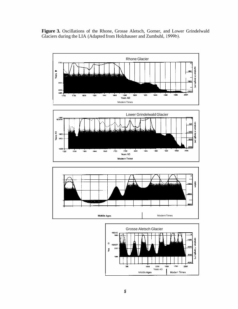
Figure 3. Oscillations of the Rhone, Grosse Aletsch, Gorner, and Lower Grindelwald Glaciers during the LIA (Adapted from Holzhauser and Zumbuhl, 1999b).
Rhone Glacier
Mlddle Ages
1781
0 .l
g P 1921
1955
1968
Years AD
Modern Times
Modern Times I
Lower Grindelwald Glacier
Grosse Aletsch Glacier 1w-m
1Bg)
2 I s 0
192W27
1957 3
3 B - 3 - 1996
IWO 1250 1 5 2 4 1750 2wo Years AD
Middle Ages I ModernTimes
5

The response of sea ice to the shifting North Atlantic polar front is an equally
sensitive indication of LIA climate change. The glacier oscillations in the Swiss Alps
mirror the changes in the extent of sea ice in the North Atlantic (Fig. 4). Therefore,
glacier records from the Swiss Alps are considered to be representative of climate change
in the North Atlantic region as a whole. Although there is some variation in the timing of
the oscillations of individual Swiss glaciers (Figs. 3-4), the regional trends of the glacier
fluctuations are coherent (Holzhauser, 1997; Figs. 3-6).
Figure 4. The sea ice and temperature record from Iceland compared to the LIA fluctuations of Gorner Glacier in Switzerland (adapted from Bergthorsson, 1969 and Holzhauser and Zumbiihl, 1999b). See Figure 2 for location of Gorner Glacier.
1859.65
1880 I920
8 g 1954 r
19%
Gorner Glacier
I I I T I 1 I I r I I
’7” l8O0 l9O0 1300 1400 1500 IMK) 900 loo0 1100 ’’ YearsAD
Middle Ages I I Mldern Times
I I
6

Swiss Glacier Record of the Little Ice Age
Little Ice Age - Earlv Phase (-AD 1280-1290 to 1390)
The beginning of the LIA is coincident with alpine glacier advance at the end of
Medieval Climatic Optimum (AD 1090-1230) (Porter, 1986). The early phase began
around AD 1280-1290 and extended to the end of the 15" century (Holzhauser, 1984,
1995). The Rhone Glacier achieved its maximum position of the LIA about AD 1350
(Zumbuhl and Holzhauser, 1988; Holzhauser and Zumbuhl, 1999b). The Grosse Aletsch
Glacier also advanced during the 13d1 and 14d1 centuries (Holzhauser, 1997). Historical
documents indicate that the Oberriederi (a system of three irrigation conduits) was
destroyed between AD 1200 and 1350 by the expanding ice front (Lamb, 1985).
Likewise, radiocarbon dates and dendrochronological cross-correlation of larch stumps
located in situ in the present-day forefield indicate a major advance of the Grosse Aletsch
Glacier from about AD 1300 to 1369 (Holzhauser, 1984; Holzhauser and Zumbuhl,
1999a).
Kill dates from larch stumps found in situ in the Gorner Glacier forefield were
tied into an absolute tree-ring chronology from larches that overlap from AD 1100 to the
present (Holzhauser, 1997). Therefore, the exact year that a larch tree died due to a
readvance of the glacier terminus is known as far back as AD 1100 (Holzhausesr, 1997).
The larch chronology indicates a significant advance between AD 1322 and AD 1327.
The glacier then continued to expand slowly until AD 1341 (Holzhauser, 1997). The
maximum extent of the Gorner Glacier during the early phase of the LIA occurred in AD
1385, and was close to the overall LIA maximum. A dendrochronological date from an
overrun fossil trunk of an Alpine stone pine in the forefield of the Lower Grindelwald
Glacier indicates a major extension of the glacier terminus about AD 1338 (Holzhauser
7

and Zumbuhl, 1996). However, the fossil trunk was not in situ, so the exact magnitude of
the advance cannot be determined.
Inter-Little Ice Age Warm Period (-AD 1390 to 1555)
The brief period of warming recorded by glacier retreat from AD 1390 to AD
1550 was not intense enough to cause shrinkage to the retracted positions of the Medieval
Climatic Optimum. The in-situ stumps of larch trees overrun by the advancing Grosser
Aletsch Glacier in the 12* century did not reappear from under retreating ice until AD
1940 (Ladurie, 1971). A forest killed by expansion of Lower Grindelwald Glacier in the
13" century did not regenerate in this warm interval, even though the area again became
ice-free (Lamb, 1985). Thus, although a period of glacier retreat is recorded in the Swiss
Alps during the Inter-LIA warm period, it was short-lived and of low magnitude.
Main Phase of Little Ice Age (- AD 1556 to AD 1850-1860)
Prolonged climatic deterioration during the main phase of the LIA followed the
brief inter-LIA warm interval. The most severe cooling occurred between AD 1556 and
1700, and was registered by numerous advances of Swiss glaciers (Lamb, 1968;
Holzhauser and Zumbuhl, 1999a). The Hochstand (the High Stand, or last major advance
of glaciers during the LIA) occurred at AD 1850 to 1860. Following this 19" century
advance, all Swiss glaciers have experienced significant retreat and volume loss (Maisch,
1999).
The Rhone Glacier is one of the most closely observed glaciers in the world, as a
result of numerous travelers passing over the Grimsel and Furks Passes (Grove, 1988).
The chronology of the terminal fluctuations of Rhone Glacier has been reconstructed
8
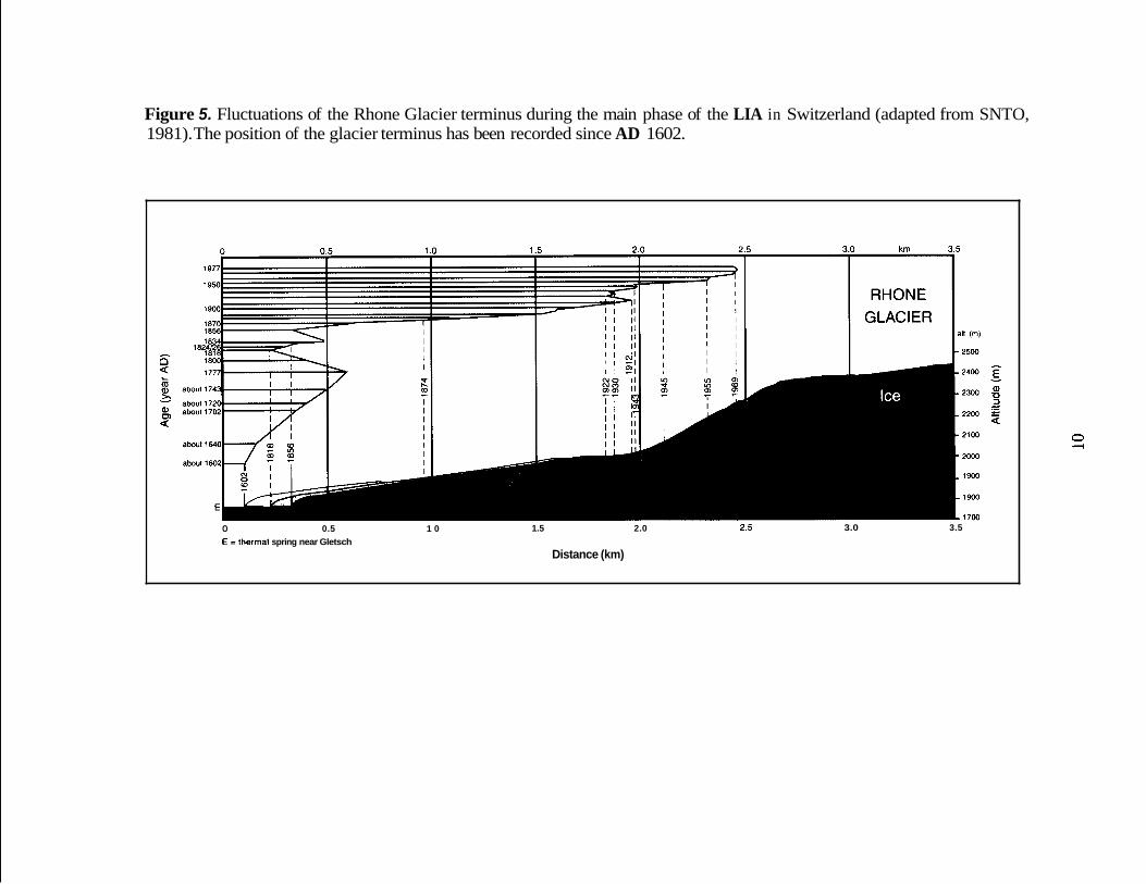
Figure 5. Fluctuations of the Rhone Glacier terminus during the main phase of the LIA in Switzerland (adapted from SNTO, 1981). The position of the glacier terminus has been recorded since AD 1602.
0 0.5 1 0 E =thermal spring near Gletsch
1.5 2.0
Distance (km)
2.5 3.0 3.5

Grosse Aletsch Glacier experienced two major periods of advance during the
main phase of the LIA (Holzhauser, 1997). The first extension around AD 1650-1678
finally ended the use of the Oberriederi irrigation system (Holzhausser and Zumbuhl,
1999b). The second period of extension was in the 19” century, initially about AD 1820
and then again about AD 1859/60 (Holzhauser, 1997). The glacier began to retreat after
the Hochstand of about AD 1859, and has continued to do so with only minor readvances
or stillstands through to the present day (Fig. 6).
Figure 6. Variations in Grosse Aletsch Glacier from AD 1860 to AD 1977 (adapted from SNTO, 1981). The light blue color in the diagram of the glacier represents the area abandoned by ice since AD 1860. The dark blue color in the diagram represents the surface area of ice in AD 1977. The graph illustrates the rate of retreat of the Grosse Aletsch terminus from AD 1860 to AD 1977.
J u n g f r a u j E h b
+- 1860 0 2 4 6 Bkm , “ “ “ ‘ I
Years AD

Gorner Glacier began to expand rapidly at the end of the 16" century (Holzhauser,
1997). Based on dendrochronological kill dates of overrun fossil larch trees in its
forefield, Gorner Glacier advanced in AD 1623 and reached a maximum position for the
17" century in AD 1669/70 (Holzhauser, 1997). Historical reconstructions indicate that
Gorner Glacier was in an advanced position about AD 1791 to 1859. Extensive damage
to buildings and farmland by the advancing ice front occurred during this time (Tyndall,
1898). Gorner Glacier began retreating around AD 1860 to 1865, and has receded over
2600 m since the Hochstand of AD 1859 (Holzhauser and Zumbuhl, 1999a).
The advance of Lower Grindelwald Glacier during the main phase of the LIA was
one of the most extensive in the Swiss Alps (SNTO, 1981). This glacier was commonly
visited, resulting in a large number of visual and written accounts of the changing
terminus.
There is documentary evidence that Lower Grindelwald Glacier destroyed some
houses during a readvance around AD 1600 (Lamb, 1985). Kill dates of fossil wood in
two paleosols in lateral moraines of Lower Grindelwald Glacier indicate that, during an
advance in the late 16'' century, the terminus reached its maximum position for the main
phase of the LIA about AD 1600 (Holzhauser and Zumbiihl, 1996). In the 18" and 19"
centuries there were several advances of Lower Grindelwald Glacier to near maximum
positions, notably around AD 1719/20 to 1743, AD 1768, AD 1778/79, between AD
1814 and 1820/22, from AD 1826 to 1838/39, and during the Hochstand in AD 1855/56
(Holzhauser and Zumbiihl, 1996). Since the Hochstand in AD 1855/1856, the glacier
terminus has retreated more than two kilometers (Holzhauser and Zumbiihl, 1999a).
12

New Zealand
Determining the extent of the LIA and its underlying cause is an important
component of paleoclimate research. To address this problem, the project reported here
focused on glacier fluctuations in the Southern Alps of New Zealand in order to establish
whether the LIA climate signal is regional or global. New Zealand is located in the South
Pacific Ocean, in the band of westerlies on the opposite side of the world from the North
Atlantic target region (Fig. 7). The mountain ranges of New Zealand are high enough to
intersect the snowline, leading to numerous temperate mountain glaciers. Most of these
glaciers terminate on land and are sensitive to climate change, responding as quickly as
the glaciers of the Swiss Alps (Chinn, 1996). The New Zealand glaciers are of a
comparable size, and their lower reaches are situated in glacial sedimentary basins of
similar morphology, to those in the Swiss Alps.

Figure 7. A map of the South Island of New Zealand. The field area of this study is located near Mount Cook in the central portion of the Southern Alps, on the eastern side of Main Divide. See Figures 9 and 10 for a more detailed map of the field area.
'E LL
North
NEW ZEALAND
174'E 70"E
_- STEWART *
ISLAND - '
0 100 200 km I I
I I I I I
166"E 17CPE 174'E
42"s
44's
46"s
4 8 3
14

The similar geometry of glacial sedimentary basins in the two target areas is
important, as the fluctuations in the glacier termini that track climate change occur within
these basins (Fig. 8). Such sedimentary basins consist of high lateral moraine walls that
confine the glaciers in the upper part of the ablation zones. These moraine walls are
steep. The lateral moraines have a complex stratigraphy and morphology because the
glacier repeatedly expanded into the walls, smearing deposits both into and on top the
high lateral moraines. This stratigraphy may well record some advances into or over
moraine walls that can be radiocarbon or dendrochronologically dated from wood in
overrun soils. However, in the absence of detailed dendrochronologic control, it is very
difficult to match up these advances with those represented by the frontal moraines.
15

Figure 8. A glacial sedimentary basin typical of those in the Swiss Alps of Europe and the Southern Alps of New Zealand. In this study, the model of a sedimentary basin applies largely to Mueller Glacier. The high lateral moraine walls constrain the glacier along most of its path. These moraine walls form the margins of the glacier sedimentary basin. During an advance, a bulge of thickening ice forms in the upper reaches of the glacier and moves down toward the terminus, funneled by the moraine walls. This bulge can rise up high on the lateral walls, or even overtop them. However, when the ice bulge reaches the glacier terminus, it can in some cases cause only a relatively small readvance. The glaciers thus commonly increase in volume in a vertical direction before there is much expansion in the horizontal direction. Unless specific organic layers with dendrochronologic cross-correlation of fossil trees can be traced from the inside of the moraine wall to underneath a distinct lateral moraine, and then around to a frontal moraine, the ages derived from these organic layers cannot be related to specific glacier frontal advances (sketches drawn by M.Y. Horesh).
Plan View Glacier
Moraine Walls + Frontal Moraines
Cross Sectional View
Moraine Walls
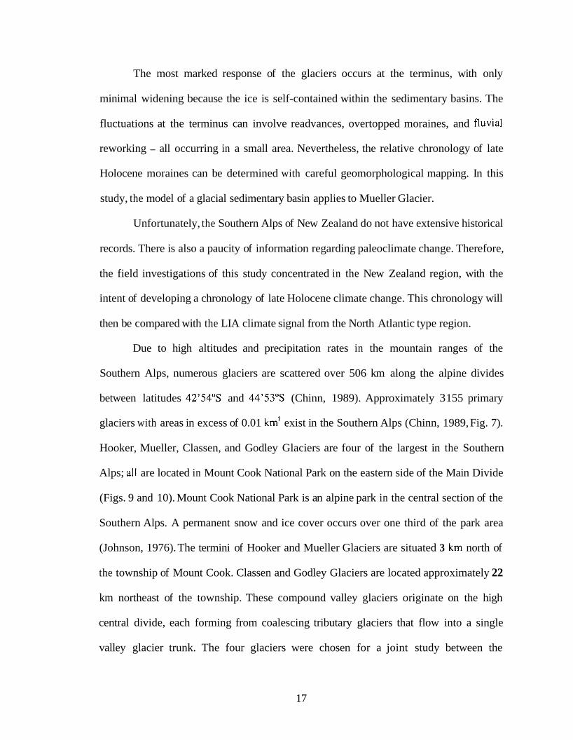
The most marked response of the glaciers occurs at the terminus, with only
minimal widening because the ice is self-contained within the sedimentary basins. The
fluctuations at the terminus can involve readvances, overtopped moraines, and fluvial
reworking - all occurring in a small area. Nevertheless, the relative chronology of late
Holocene moraines can be determined with careful geomorphological mapping. In this
study, the model of a glacial sedimentary basin applies to Mueller Glacier.
Unfortunately, the Southern Alps of New Zealand do not have extensive historical
records. There is also a paucity of information regarding paleoclimate change. Therefore,
the field investigations of this study concentrated in the New Zealand region, with the
intent of developing a chronology of late Holocene climate change. This chronology will
then be compared with the LIA climate signal from the North Atlantic type region.
Due to high altitudes and precipitation rates in the mountain ranges of the
Southern Alps, numerous glaciers are scattered over 506 km along the alpine divides
between latitudes 42'54"s and 44'53"s (Chinn, 1989). Approximately 3 155 primary
glaciers with areas in excess of 0.01 km2 exist in the Southern Alps (Chinn, 1989, Fig. 7).
Hooker, Mueller, Classen, and Godley Glaciers are four of the largest in the Southern
Alps; all are located in Mount Cook National Park on the eastern side of the Main Divide
(Figs. 9 and 10). Mount Cook National Park is an alpine park in the central section of the
Southern Alps. A permanent snow and ice cover occurs over one third of the park area
(Johnson, 1976). The termini of Hooker and Mueller Glaciers are situated 3 km north of
the township of Mount Cook. Classen and Godley Glaciers are located approximately 22
km northeast of the township. These compound valley glaciers originate on the high
central divide, each forming from coalescing tributary glaciers that flow into a single
valley glacier trunk. The four glaciers were chosen for a joint study between the
17
University of Maine and the University of Cincinnati for their sensitivity to climate
change, their size, the excellent preservation of the Holocene moraines fronting the
glaciers, and the large amount of available historical documents. The Holocene
fluctuations of the Hooker and Mueller Glacier termini were analyzed at the University of
Maine, while the fluctuations of Classen and Godley Glacier termini were studied by
Katherine Schoenenberger at the University of Cincinnati. Only results from Hooker and
Mueller Glaciers are reported in this paper.
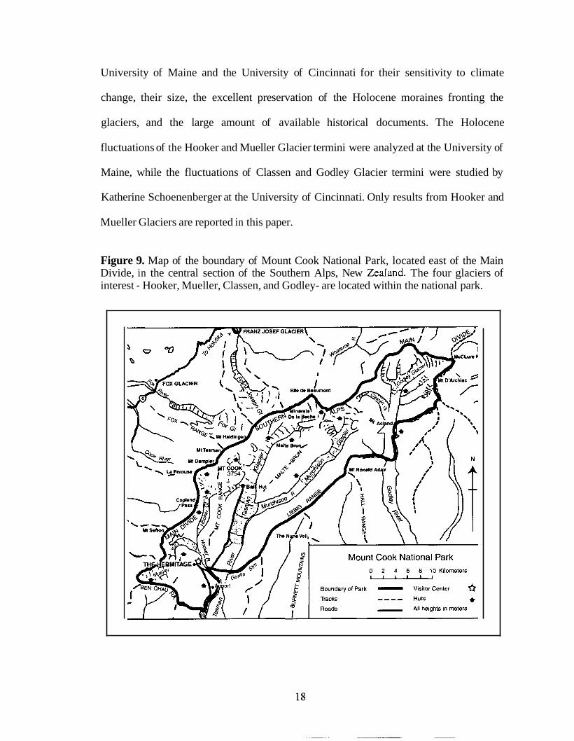
Figure 9. Map of the boundary of Mount Cook National Park, located east of the Main Divide, in the central section of the Southern Alps, New Zealand. The four glaciers of interest - Hooker, Mueller, Classen, and Godley- are located within the national park.

Figure 10. Site map of the field area, located in Mount Cook National Park southeast of the Main Divide in the central section of the Southern Alps. Hooker and Mueller Glaciers are fully contained within the southern section of the Mount Cook National Park, and are located north of the town of Mount Cook and southwest of the peak of Mount Cook - the highest mountain in the Southern Alps.
170'WE 170'05'E
43'408'
43'455
170'00.E 170'05€
-43'40.8
-43'455

The Southern Alps has a humid, mesothemal climate, with mean annual
precipitation in the high mountain environments ranging from about 800 to 15,000 mm
(Griffiths and McSaveney, 1983). The Southern Alps intercept the prevailing westerly
winds off the Pacific Ocean, creating a steep, precipitation gradient rising eastward, along
with a strong fohn effect on the west and south side (Chinn, 1989). Therefore, there are
high levels of precipitation along the Main Divide of the Southern Alps. Mount Cook
Village receives 4000 mm of precipitation annually, with rainfalls of up to 537 mm
recorded in a 24 hour period (Dennis and Potton, 1983). Local climatic conditions can
vary significantly. Kirkbride (1988) suggested that there was an increase in annual
rainfall of half a centimeter for every ten steps from Mount Cook Village toward Mueller
and Hooker Glaciers and the Main Divide.
The vegetation on the floors of Hooker and Mueller Valleys is composed mainly
of herbfields, sub-alpine scrub, and alpine grasslands (Dennis and Potton, 1983). The
bedrock in the eastern Mount Cook region is predominantly Tertiary quartz-felspathic
greywacke, together with slate and schist (Maizels, 1989). These are middle to upper
Triassic and Permian low-grade, well-indurated sandstones and mudstones of the
Torlesse Supergroup and Haast Schist Group (Suggate, 1978).
Mueller Valley
Mueller Valley encompasses Mueller Glacier, the Holocene moraine systems
deposited by the glacier, the large outwash plain south of these moraines, and Mount
Cook Village. Mueller Glacier is confined along the narrow upper Mueller Valley for
most its length.

Mueller Glacier is fronted by a series of well-preserved Holocene moraines, all
within 2 km of the present-day terminus. The Holocene moraines were deposited where
the valley widens near the current ice terminus. For the purpose of this study, Mueller
Glacier forefield has been divided into nine areas (Fig. 11): 1) the White Horse Flood
area, 2) the Kea Lobe area, 3) the White Horse Valley Spillover area, 4) the Idyllic
Valley area, 5 ) the Western Arm of the Memorial area, 6 ) the Central Arm of the
Memorial area, 7) the Eastern Margin area, 8) the Northern Lobe area, and 9) the
Southern Hooker Valley area. Each contains a series of moraines, ice-contact and
outwash channels, and ice-marginal terraces. The high lateral wall on the northeastern
portion of Mueller Valley blocks the southern outlet of Hooker Valley to the north.
Mueller proglacial lake is actively forming in the newly deglaciated basin fronting
Mueller Glacier. This lake is bounded by high lateral moraine walls that form the Mueller
sedimentary basin, and by late Holocene frontal moraines along the southern margin of
the lake. The outlet of Mueller proglacial lake, located in the southeast comer of the lake,
feeds the Hooker River, which flows south along the eastern valley wall to the junction
with the Tasman River farther downvalley.
21


23

Mueller Glacier is fed from several sources. Most of the ice that makes up the
terminus of upper Mueller Glacier originates from Huddleston Glacier, a tributary that
descends from Mount Footstool into Mueller Glacier (Fig. 10). Other tributaries are
Frind, Bannie, and Welchman Glaciers. Another source is from ice cliffs at 2300-2600 m
elevation on the east face of Mount Sefton. This steep face promotes periodic ice
avalanches that nourish Mueller Glacier (Kirkbride, 1988). Just as with many other
glaciers east and south of the Main Divide, Mueller Glacier has thick debris mantling its
surface and insulating the ice. Most of this debris originates in rockfalls from the cliffs at
1200-2300 m elevation beside the Main Divide (Kirkbride, 1988). Significant amounts of
debris are also deposited on the surface of Mueller Glacier from avalanche activity on
Frind and Huddleston Glaciers. Avalanches from the ice cliffs on the east face of Mount
Sefton are also a source of debris.
Hooker Valley
Hooker Valley encompasses Hooker Glacier, the Holocene moraine systems
deposited by the glacier, and the outwash plain south of these moraines. The northern
lateral moraine wall of Mueller Glacier delimits Hooker Valley in its southern end.
Hooker Valley is predominantly a linear glacial valley, trending north-south. Hooker
Glacier differs significantly from Mueller Glacier in that it is confined by a narrow, cliff-
bound valley along its entire length (Burrows, 1973).
Hooker Glacier is fronted by a series of well-preserved Holocene moraines, all
within 4 km of the present-day terminus. The lateral moraines of Hooker Glacier are well
preserved. Unlike the situation alongside Mueller Glacier, each Hooker lateral moraine is
a distinct entity rather than part of a massive moraine wall (Burrows, 1973). The lateral
24
moraines are discrete ridges arrayed on the valley wall, rather than one massive ridge
with a steep proximal moraine wall, as at Mueller Glacier. The Hooker lateral moraines
are successively older with increasing elevation on the valley wall. Some of the laterals
are as much as 3 km long, and are cut only by stream courses, avalanche chutes, or
alluvial fans. Many of the lateral and frontal Hooker moraines have been dissected by
meltwater flowing from Eugenie and Stocking (Tewaewae) Glaciers, both of which
originate on the Main Divide along the western wall of Hooker Valley.
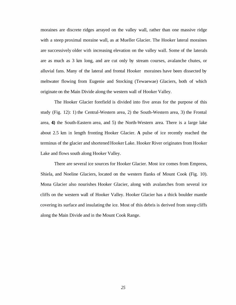
The Hooker Glacier forefield is divided into five areas for the purpose of this
study (Fig. 12): 1) the Central-Western area, 2) the South-Western area, 3) the Frontal
area, 4) the South-Eastern area, and 5) the North-Western area. There is a large lake
about 2.5 km in length fronting Hooker Glacier. A pulse of ice recently reached the
terminus of the glacier and shortened Hooker Lake. Hooker River originates from Hooker
Lake and flows south along Hooker Valley.
There are several ice sources for Hooker Glacier. Most ice comes from Empress,
Shiela, and Noeline Glaciers, located on the western flanks of Mount Cook (Fig. 10).
Mona Glacier also nourishes Hooker Glacier, along with avalanches from several ice
cliffs on the western wall of Hooker Valley. Hooker Glacier has a thick boulder mantle
covering its surface and insulating the ice. Most of this debris is derived from steep cliffs
along the Main Divide and in the Mount Cook Range.
25

27

11. Previous Work
There are two different categories of ages previously assigned to the late
Holocene moraines in the forefields of Mueller and Hooker Glaciers, both of which drain
from the Main Divide of the Southern Alps into the upper reaches of Tasman Valley.
Based on tree-ring analysis and lichenometry, the early studies indicated that most of the
late Holocene moraines formed within the LIA interval as recognized in the North
Atlantic region (Lawrence and Lawrence, 1965; Burrows and Lucas, 1967; Burrows,
1973). In sharp contrast, a more recent study based on weathering-rind analysis and
radiocarbon dates gave very different results. The same Holocene moraines previously
placed within the LIA interval were reassigned significantly older ages, spanning more
than 7000 yrs (Gellatly, 1984, 1985a). The implication of this latter study is that a large
fraction of the Holocene moraines system formed prior to the LIA. The widely differing
moraine chronologies that emerge from using these differing techniques need to be
resolved before any conclusions can be made regarding the presence of a LIA signal in
the Southern Alps. Reconstructions of former equilibrium line altitudes were made using
Holocene moraine sets from this region (Porter, 1975). The Holocene ELAs were
depressed approximately 140 m below the levels of AD 1974.
Initial Studies of Holocene Moraines Fronting Hooker and Mueller Glaciers
A late Holocene chronology based on the ages of trees growing on and beside the
Holocene moraines indicate that recent variations in Mueller Glacier closely paralleled
the LIA main phase of Europe (Lawrence and Lawrence, 1965). The trees chosen for this
study were strategically located on the moraine ridges. The ages reported represent the
28
minimum time since the ice receded. This tree-ring chronology suggested that Mueller
Glacier underwent advances in the 17" and 18" centuries, with the outermost extension
occurring about AD 1730 and 1745. Mueller Glacier remained at or close to its maximum
position from AD 1745 to 1785. Slightly less extensive readvances and stillstands
occurred in the 19"' century, with a major period of recession beginning about AD 1890.
The first chronologies of late Holocene moraines derived from lichenometry also
indicated that advance phases of Hooker and Mueller Glaciers were roughly synchronous
with the early and main phases of the LIA in the Swiss Alps (Burrows and Lucas, 1967;
Burrows, 1973). Although several advances were postulated to have taken place in the
12m, 13tl' and 15" centuries, the most significant expansions were in the 17" and 18"
centuries (Burrows, 1973). The LIA maximum was around AD 1740, and was followed
by a series of smaller advances and stillstands from the late AD 1700s until AD 1890
(Burrows, 1973). The historically documented AD 1890 moraine (Brodrick, 1894)
represents the last advance prior to a major collapse of Mueller and Hooker Glaciers
(Gellatly, 1985b). Although brief halts in recession (or even minor expansion) occurred
in the 20" century, the overall pattern for the Mt. Cook glaciers was one of retreat
(Wardle, 1973; Gellatly, 1982a). These early studies were consistent in showing a general
trend of glacier expansion during the LIA (Table 1). Nearly all ages assigned to the late
Holocene moraines in Table 1 place the most recent period of glacier advance within the
two phases of the LIA as recognized in the North Atlantic region.
29

Table 1. Comparison of the timing of glacier advances in New Zealand and the Swiss Alps during the LIA (Burrows, 1973; Lawrence and Lawrence, 1965; Holzhauser and Zumbuhl, 1996).
Lichenometry at Mueller Glacier, NZ (Burrows, 1973)
years (AD)
Tree-Ring Analysis at Mueller Glacier, NZ (Lawrence and Lawrence, 1965), years (AD)
1 z5n < 1445
Tree-ring Analysis and Historical Records at Lower Grindelwald
Glacier, Switzerland (Holzhauser and Zumbiihl, 1996), years (AD)
1338
1580 I 1588
Recent Studies of Holocene Moraines Fronting Hooker and Mueller Glaciers
A date of 1010k50 14C years B.P. (NZ4507) of a buried soil horizon in a lateral
moraine of Mueller Glacier was taken to indicate that previous lichenometric analysis had
underestimated the ages of the frontal late Holocene moraines (Burrows, 1980). Similar
radiocarbon dates from Hooker Glacier lateral moraine walls also were taken to imply
that the frontal moraine sets were significantly older than previously indicated (Gellatly
et al., 1985; Burrows, 1980, 1989). In addition, one of the historical ages used for the
lichenometry calibration curve (Burrows, 1973) was found to be incorrect (Gellatly,
1983). Photographs of the Mueller Glacier terminus by J. Kinsey in AD 1895 and M.
Ross in AD 1896 show that the moraine thought to have formed in AD 1931 (Burrows,
1973) was already in existence by AD 1895 (Kinsey, 1895; Ross, 1896; Gellatly,
1982a,b). However, it should be pointed out that the radiocarbon-dated stratigraphic units
in the steep moraine walls of Mueller and Hooker Glaciers cannot be traced to specific
165011655
17 10/1720- 1740/1750
1770- 1790/ 1795
183511 840- 1850 1805l18 10
30
----
1719/20 1730 1743 1754 1768 1745-1785 1778179
1838/39 1838139 18551%
4804, <1808 18 14- 1820122

moraine ridges in their forefields, and therefore by themselves do not invalidate the tree
ring or lichenometry chronologies constructed for the Holocene moraines fronting these
glaciers
In sharp contrast to the lichenometric data, weathering-rind analysis of clasts on
moraines in the forefields of Hooker and Mueller Glaciers suggested a mid-and-late
Holocene age (Gellatly, 1984). The mid-Holocene moraines at Mueller Glacier were
thought to range in age from 7200 to 1150 years B.P. Late Holocene moraines were
postulated to have formed during six major periods of ice expansion between 1100 and
100 years B.P. (Gellatly, 1985a). Mid-Holocene moraines of Hooker Glacier were
inferred to have formed from 4200 to 1150 years B.P. (Gellatly, 1984). The late Holocene
moraines of Hooker Glacier had a similar sequence to those in the Mueller Glacier
forefield. The greatest glacier expansion in the last millennium, according to the
interpretation of weathering-rind data, occurred at 1 100-950 years B .P. (Gellatly, 1985a).
Radiocarbon data from the Mount Cook region were used to confirm the validity of the
weathering-rind chronologies (Gellatly, 1984). However, as mentioned above, the
individual radiocarbon dates are from the lateral moraine walls of Hooker and Mueller
Glaciers, and cannot yet be related to specific moraine ridges in the glacier forefields.
Therefore, such radiocarbon evidence is unrelated to the weathering-rind data, which
comes from clasts on frontal moraines.
In the early lichenometry studies the oldest moraine in the Holocene set of
Mueller Glacier was found to have formed about 700 years ago (Burrows, 1973),
compared to the weathering-rind date of 7000 years B.P. (Gellatly, 1984). Thus there is a
major disparity between the lichenometric and weathering-rind dating methods (Table 2).
The only aspect of the glacier chronologies that is consistent in the two schemes is the
31

marked recession that began about AD 1890 in the Mount Cook region - a conclusion
that is based on historical records and not on different dating methods.
Table 2. Comparison between the different ages from the same Holocene fronting Mueller Glacier derived from lichenometric and weathering-rind (adapted from Gellatly, 1984; Burrows, 1973).
moraines methods
Moraine
1 2 3 4 5 6 7 8 9 10 11
Lichenometry Burrows (1973)
(yrs before AD 1984) 50 90 130 210-190 250-230 ca. 300 ca. 350 Ca. 450 550 ca. 630 undated
Weathering-Rind Analysis Gellatly (1984) (Y rs before AD 1984)
135535 340+88 580+150 I 840+2 18
2540+660 33505870 4200+ 1090 7200k1870
32

111. Glacial Geomorphologv
A glacial geomorphic map was constructed for the Mueller and Hooker moraine
sequences (Fig. 13). The map forms the basis of the interpretations concerning mid-to-
late Holocene glacier oscillations. Morphologic units were stressed in order to delineate
the glacial geomorphic forms that result from ice-marginal fluctuations. The map depicts
morphosequences of time-equivalent groups of landforms. A classic morphosequence of
glacial deposits is made up of a moraine belt with a steep ice-contact slope on the
proximal side of the belt, an outwash plain that grades to the distal side of the moraine
belt, and ice-contact terraces and channels of the same age. Ice-contact slopes can also
occur at the head of outwash terraces and along the proximal side of channels. Ice-contact
slopes, terraces, and channels link moraine belts to individual ice-marginal positions.
Channels commonly dissect the morphosequences. A lichenometric chronology was then
developed, with the maps serving to tie the dating results to the glacial morphology.
The initial step was the construction of a preliminary geomorphic map of Hooker
and Mueller moraine systems from analysis of aerial photographs (Fig. 13). The maps
were then corrected by extensive fieldwork and morphosequences delineated for the
Hooker and Mueller forefields. The resulting array of geomorphic features depicted in the
maps include main and subsidiary outwash plains; moraine belts composed of ridges,
hills and hummocks; ice-contact terraces and slopes; ice-marginal channels; meltwater
spillways; deltas; alluvial fans; and rockfall deposits. The legend in Figure 13 gives a
description of these major geomorphic features.
The extensive supraglacial debris cover on Mueller and Hooker Glaciers
promoted the formation of large, complex moraines (Burrows, 1973). In some places the
33

moraines are incompletely preserved, due to modification, partial destruction, or burial by
deposits of subsequent glacier advances. Both the Hooker and the Mueller moraine
systems have also been modified by outwash streams from glaciers on adjacent valley
walls. In most places, however, there is extremely good preservation of moraine systems,
with ridges and relict channels extending nearly unmodified for several kilometers.
Mueller Morphosequences
The geomorphic analysis revealed six main morphosequences (A-F) in the
Mueller Glacier forefield (Fig. 13). The morphosequences are defined on the basis of
time-equivalent morphologic characteristics, illustrated in the glacial geomorphic map in
Figure 13 and the morphosequence map in Figure 14. The FALL ages and Gumbel means
of lichens sampled from the landforms are assigned to the morphologic morphosequences
for the Mueller late Holocene moraines (Figs.50-55). Figure 49 is the map of the lichen
sample sites.
Morphosequence M-A1
Morphosequence M-A1 is the outermost and therefore the oldest
morphosequence. It consists of several small moraine remnants. The Foliage Hill moraine
remnant, along with the moraine remnant near the shelter in the Mueller Glacier
campground (Fig. l l ) , are part of Morphosequence M-A1. The moraine remnants have
weathered boulders on their surfaces, in contrast to the fresh boulders in the other areas of
the Mueller forefield. These remnants are therefore interpreted to be significantly older
than the other moraines fronting Mueller Glacier, and hence were not sampled. The
moraine fragments of Morphosequence M-A1 may have been deposited at different
34

times. However, the relative ages of these fragments cannot be determined on the basis of
weathering characteristics alone.
Morphosequence M-A2
White Horse Hill (WHH) was also not sampled (Fig. 11). WHH is proximal to
Morphosequence M-A1. Weathered boulders and a dense vegetation cover on parts of
WHH indicate WHH is significantly older than the other moraines fronting Mueller
Glacier. There is a historical photograph (Sutton-Turner, 1884-1913) showing that WHH
burned in the early 1900s (Fig. 37). Lichenometry cannot be applied to areas that have
experience snow or firelull. The lichen measurements will reflect the age of the fire, not
the age of deposition. It is not known when these moraines were deposited. The WHH
moraines are crosscut by a large channel (probably a former channel of Hooker River),
and also by the moraines of Morphosequence M-B.
Morphosequence M-B
Morphosequence M-B is proximal to Morphosequence M-A2. It is moderately to
heavily vegetated. The moraine belt of this morphosequence includes the outermost
moraines in the Central and Western Arms of the Memorial area (Fig. 11).
Morphosequence M-B moraine belts are large, broad features with multiple ridges. The
ridges are difficult to trace along the moraine belt. Some larger ridges crosscut smaller
moraines in the West Arm area. On the basis of this morphology the Mueller Glacier
terminus is interpreted to have been at this general position for an extended period, with
minor oscillations. The M-17 to M-23 lichen sites are situated on the moraines in the
35

West Arm area of Morphosequence M-B, and the M-31-32, M-35-40.3, and M-58-59
lichen sites are in the Central area of the moraine belt of Morphosequence M-B.
The moraine belt of Morphosequence M-B in the West Arm of the Memorial area
is cut by the present-day Hooker River. The moraine belt continues from the West Arm
of the Memorial area across Hooker River and then along the base of the eastern wall of
Mueller Valley. The moraines in the Eastern Margin area of Mueller Glacier are not as
massive as those in the Memorial area. Rather, they are smaller and better-defined
individual ridges. In the Eastern Margin area, the moraine ridges are heavily vegetated
and extend partly up the wall of Mueller Valley. The M-53 through M-56 lichen sites are
located on moraine ridges from Morphosequence M-B. Morphosequence M-B moraine
ridges on the north end of the Eastern Margin area are cut by the present-day Hooker
River. The moraine ridges continue from the Eastern Margin area across the Hooker
River to the Northern Lobe area of the Mueller forefield. The M-67 and M-68 lichen sites
are on two of the outermost moraine ridges in the Northern Lobe area. These outermost
ridges are heavily vegetated.
The moraines in the Kea Lobe area represent a separate lateral lobe of Mueller
Glacier. The outermost moraines in the Kea Lobe area are part of Morphosequence M-B.
They are heavily vegetated and of a similar character to the moraines on the wall of
Mueller Valley in the Eastern Margin area. The M-9 through M-16 lichen sites are on
moraine ridges of Morphosequence M-B. These ridges are part of a single, massive belt
along most of their length. In places, the massive belt branches into several smaller ridges
that curve around the front of the former glacier terminus. The lichen sites from
Morphosequence M-B are located on these smaller branching ridges. It is likely that the
outer moraines of the White Horse Spillover area also belong to Morphosequence M-B,
36

as they are heavily vegetated and similar in both size and morphology to the
Morphosequence M-B moraines of the Kea Lobe area.
Morphosequence M-C
Morphosequence M-C is located proximal to Morphosequence M-B. A moderate
vegetation cover, heavily dissected morphology, and indistinct margins of individual
morainal features characterize Morphosequence M-C. In the Central Arm of the
Memorial area, Morphosequence M-C is moderately to heavily vegetated, with a grass
and low bush cover on an outwash plain leading up to hillocky, boulder-strewn morainal
topography. The hummocky terrain slopes upward toward remnants of several moraine
ridges. The M-34 lichen site is on one such small remnant in the eastern side of the
Central Arm of the Memorial area, and the M-48 and M-80 lichen sites are on small
moraine remnants on the western side of the Central Arm area. The moraines are too
dissected to determine the number of ridges in the Central Arm area of Morphosequence
M-C. However, there are at least two moraine ridges in this area. The moraine fragments
with the M-34 and M-48 lichen sites on them were partially overridden by a glacier
advance (e.g. Figs. 114, 115). The moraine hillock with the M-48 lichen site is
particularly heavily vegetated. The M-80 lichen site is on a small moraine fragment on
the distal side of this hillock.
The moraine ridge at the inner margin of Morphosequence M-C in the Central
Arm of the Memorial area is continuous with a small, heavily vegetated moraine hillock,
located just north of the southern wire-bridge (Figs. 11, 13) in the Eastern Margin area.
The M-51 lichen site is on this hillock. Morphosequence M-C in the Eastern Margin area
consists of a complex series of both small and large channels, elevated ice-contact
37
terraces, moraine fragments, and hummocky terrain that stretches northward to the
Hooker River. The moraines of Morphosequence M-C are moderately to heavily
vegetated. The M-57 lichen site is located in the middle of the hummocky terrain in the
north part of the Eastern Margin area, whereas the M-41 and the M-52 lichen sites are
situated in channels that crosscut Morphosequence M-B. There is no clear morphological
continuity for Morphosequence M-C between the northern end of the Eastern Margin
area and the Northern Lobe area of the Mueller forefield. In the Kea Lobe and White
Horse Spillover areas, there is also not a distinct manifestation of Morphosequence M-C.
It is possible that some of the moraines in the Kea Lobe and White Horse Spillover areas
can be attributed to Morphosequence M-C, but in these areas there is not a clear
morphologic break to distinguish Morphosequence M-B from Morphosequence M-C.
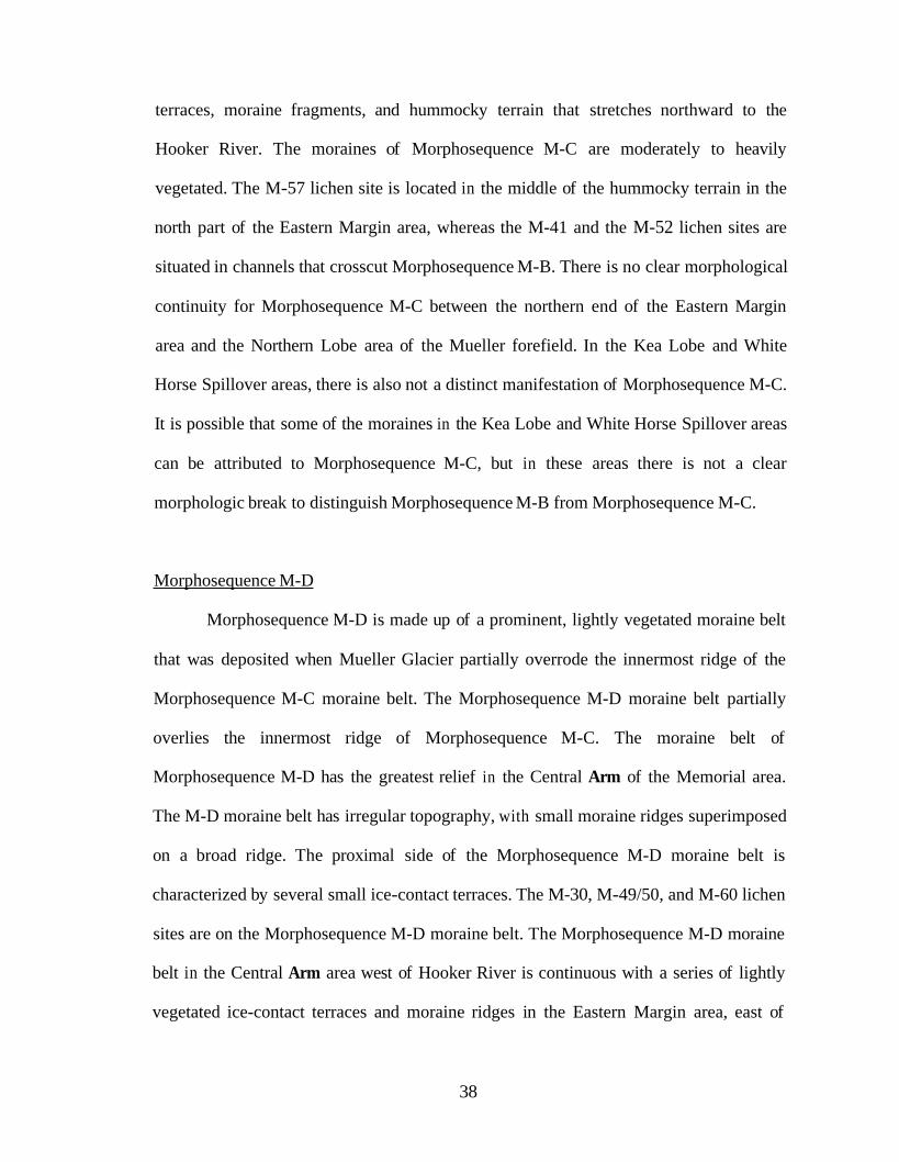
Morphosequence M-D
Morphosequence M-D is made up of a prominent, lightly vegetated moraine belt
that was deposited when Mueller Glacier partially overrode the innermost ridge of the
Morphosequence M-C moraine belt. The Morphosequence M-D moraine belt partially
overlies the innermost ridge of Morphosequence M-C. The moraine belt of
Morphosequence M-D has the greatest relief in the Central Arm of the Memorial area.
The M-D moraine belt has irregular topography, with small moraine ridges superimposed
on a broad ridge. The proximal side of the Morphosequence M-D moraine belt is
characterized by several small ice-contact terraces. The M-30, M-49/50, and M-60 lichen
sites are on the Morphosequence M-D moraine belt. The Morphosequence M-D moraine
belt in the Central Arm area west of Hooker River is continuous with a series of lightly
vegetated ice-contact terraces and moraine ridges in the Eastern Margin area, east of
38

Hooker River. The M-44 and M-65-66 lichen sites are located on the Morphosequence
M-D moraine complex. On the distal side of the Morphosequence M-D moraine complex
is an abandoned channel of the Hooker River, which has been partially covered by the
Morphosequence M-D complex. The M-47 lichen site is on the former river channel. The
M-45 and M-46 lichen sites are located on ice-contact terraces that formed at the same
time as the moraine complex of Morphosequence M-D.
The prominent, lightly vegetated moraine complex in the Northern Lobe area of
Mueller Glacier is also part of Morphosequence M-D. This moraine complex is located
just south of the moraine ridge with the M-68 lichen site. The Morphosequence M-D
moraine complex has its highest relief in the Northern Lobe area, and is composed of
several small ridges. The M-69 through M-71 lichen sites are located on this moraine
complex. In the Kea Lobe area, a prominent, lightly vegetated moraine abuts the margin
of the heavily vegetated Morphosequence M-B moraine complex. The Morphosequence
M-D moraine complex does not extend south into the Kea Lobe area like the
Morphosequence M-B moraines, but rather crosses the mouth of Kea Lobe area. The M-8
and M-77 through M-79 lichen sites are situated on the Morphosequence M-D moraine
complex in the Kea Lobe area. Several small ridges make up this complex. On the
proximal side of the Morphosequence M-D moraine complex is a series of ice-contact
terraces. In the White Horse Spillover area, there is a ridge located high on the Mueller
Glacier lateral moraine wall. The M-24 lichen site is on this small, lightly vegetated
moraine ridge in the White Horse Spillover area. The ridge with the M-24 lichen site may
be part of Morphosequence M-D.
39

Morphosequence M-E
The moraines and ice-contact terraces that make up Morphosequence M-E
represent a minor readvance of Mueller Glacier, followed by a stillstand of the terminus.
A small, prominent moraine on the southern margin of Mueller Lake partially covers an
outwash plain, recording a readvance of Mueller Glacier. This small moraine is part of
Morphosequence M-E, and is in the Central Arm of the Memorial area. The
Morphosequence M-E moraine has only one sharp ridge crest, has steep slopes, and is
almost completely unvegetated. Lichen sites M-28, M-29, and M-62 are on this moraine.
In the Eastern Margin area of Mueller Glacier, a series of low moraine ridges, small
channels, and ice-contact terraces comprise Morphosequence M-E. These features have
only a light grass cover. The M-42, M-43, M-63, and M-64 lichen sites are on landforms
of Morphosequence M-E.
On the Northern Lobe area of Mueller Glacier, the low-lying glacial features that
form a series of small moraine ridges, ice-contact terraces, and channels are proximal to
the Morphosequence M-D moraine complex, and therefore are attributed to
Morphosequence M-E. The glacial features of Morphosequence M-E in the Northern
Lobe area are almost completely unvegetated. There is also a series of ice-contact
terraces on the Kea Point area. These ice-contact terraces are lightly vegetated and may
be part of Morphosequence M-E.
Morphoseauence M-F
The only feature that is part of Morphosequence M-F is the island moraine in
Mueller Lake. This moraine formed during a minor stillstand of the Mueller Glacier, in
the midst of overall collapse. The M-33 lichen site is on this moraine. The moraine is on
40

an island subsiding today because of a melting ice core. There is a significant spatial gap
between the Morphosequence M-F ridge and the Morphosequence M-E moraine belt.
Hooker Morphosequences
There are three main morphologic Morphosequences (A-C) in the Hooker Glacier
forefield, defined by the time-equivalent morphologic characteristics illustrated in the
glacial geomorphic map of Figure 13 and the morphosequence map of Figure 14. These
morphosequences are similar to those at Mueller Glacier. The lichen sample sites are
shown in Figure 49, while the five different areas of Hooker Glacier forefield are shown
in Figure 12.
Momhosequence H-A
Morphosequence H-A, the outermost, is heavily dissected by fluvioglacial
processes. The dense vegetation cover, the moderate weathering of boulders on the
moraine belt, and the lack of younger crosscutting moraines indicate that this is the oldest
morphosequence in Hooker Valley. Moraines in Morphosequence H-A in the South-
Western area are characterized by very large boulders. The moraine belt includes the
largest and uppermost of the lateral moraines on both the east and the west valley walls.
Lichen sites H-1 and H-24 are on lateral moraines of Morphosequence H-A. Lateral and
frontal moraines of the H-A Morphosequence have been heavily dissected by
fluvioglacial processes. In particular, the meltwater streams from Stockmg and Eugenie
Glaciers are heavily eroding the lateral moraines in the Central-Westem area.
Fluvioglacial fan deposits are accumulating on the upper lateral moraines. The frontal
moraines have been largely eroded by Hooker River. Only the small moraine remnants at
41
the H-23 lichen site and at the southern tip of the disintegration terrain (located south of
the H-13 lichen site) remain. The moraines in the South-Western area are part of the
outermost H-A Morphosequence. These moraines have also experienced significant
amounts of fluvioglacial alteration. Many of these moraine ridges have been eroded on
both their proximal and their distal sides by streams.
A large region of disintegration terrain in the Frontal area of the Hooker forefield
separates Morphosequence H-A from Morphosequence H-B. Downwasting of Hooker
Glacier leaves the stagnant ice responsible for the disintegration terrain. On the western
side of the valley, an outwash plain separates the moraines in the South-Western area
from those in the Central-Western area. This plain can be traced across the current
Hooker River to the area of disintegration terrain. There is no distinct break between
Morphosequences H-A and H-B in the Hooker lateral moraines. Morphosequence H-A
and H-B moraines are closely spaced, with no large gaps between them.
Momhosequence H-B
Morphosequence H-B also includes a heavily vegetated moraine belt, although
the cover is generally not as dense as on deposits of Morphosequence H-A. Directly
south of the moraine belt is a large former river channel that separates the hummocky
terrain of Morphosequence H-A from the deposits of Morphosequence H-B. There are
four main ridges in the Frontal area of the Morphosequence H-B moraine belt. The
outermost moraine of Morphosequence H-B was overrun by a readvance of Hooker
Glacier. At least two moraines deposited during the readvance partially cover the
outermost moraine. The innermost moraine of Morphosequence H-B is steep and narrow,
and has been partly overrun by a readvance of Hooker Glacier that deposited the moraine
42

belt of Morphosequence H-C. Any former corresponding moraines on the other side of
Hooker River in the Central-Western area have been covered by alluvial fans from
meltwater of Eugenie Glacier. The H-10 lichen site is located on one of these alluvial
fans. Lateral moraines of Morphosequence H-B can be traced along the eastern wall of
Hooker Valley. Here the dividing line between Morphosequence H-A and
Morphosequence H-B lateral moraines is not clear. The erosion by glaciofluvial streams,
the active alluvium partly deposited over the moraines, the heavy vegetation cover of
both morphosequences, and the non-linear trend of the moraines together result in an
indistinct border between the two morphosequences.
Morphosequence H-C
Morphosequence H-C abuts Morphosequence H-B without an intervening
outwash plain. Morphosequence H-C consists of a largely unvegetated moraine belt. This
is the youngest of the morphosequences deposited prior to the collapse of Hooker Glacier
that led to the formation of Hooker Lake. The outermost unvegetated moraine in the
Frontal area is also the largest. This moraine is interpreted to represent a readvance of the
Hooker terminus that partly overrode the innermost moraine of Morphosequence H-B.
The moraine belt of Morphosequence H-C has a broad and irregular surface. There are
several ridges in parts of this broad belt, but these ridges are not clearly delineated in the
Frontal area. This broad belt continues on the western side of Hooker River in the North-
Western area. The H-5 and H-4 lichen sites are on two ridges of Sequence H-C in the
North-Western area. The lateral moraines of Morphosequence H-C can be traced through
the Mid- and South-Eastern areas. Most Morphosequence H-C moraines are removed by
43

erosion in the North-West area. The H-17, H-25, and H-26 lichen sites are all located on
lateral moraines of Morphosequence H-C.
44

IV. Historical Records
Historical records for the Mount Cook region were used to help constrain the
chronology of Mueller and Hooker morphosequences. Records exist from AD 1862 to the
present. Written accounts, rough sketches, survey maps, and photographs make up the
collection of historical material for Mueller and Hooker Glaciers. All historical
information found in this study was from the Alexander Turnbull Library in Wellington,
the Canterbury Museum in Christchurch, the University of Canterbury in Christchurch,
and the Hocken Library in Dunedin. Figures 15, 16 and 17 are summary diagrams of the
areas covered by each historical photograph and map in the Mueller and Hooker
forefields. The earliest recorded observations of Mueller and Hooker Glaciers were by
Julius Haast in AD 1862 (Haast, 1879).
45
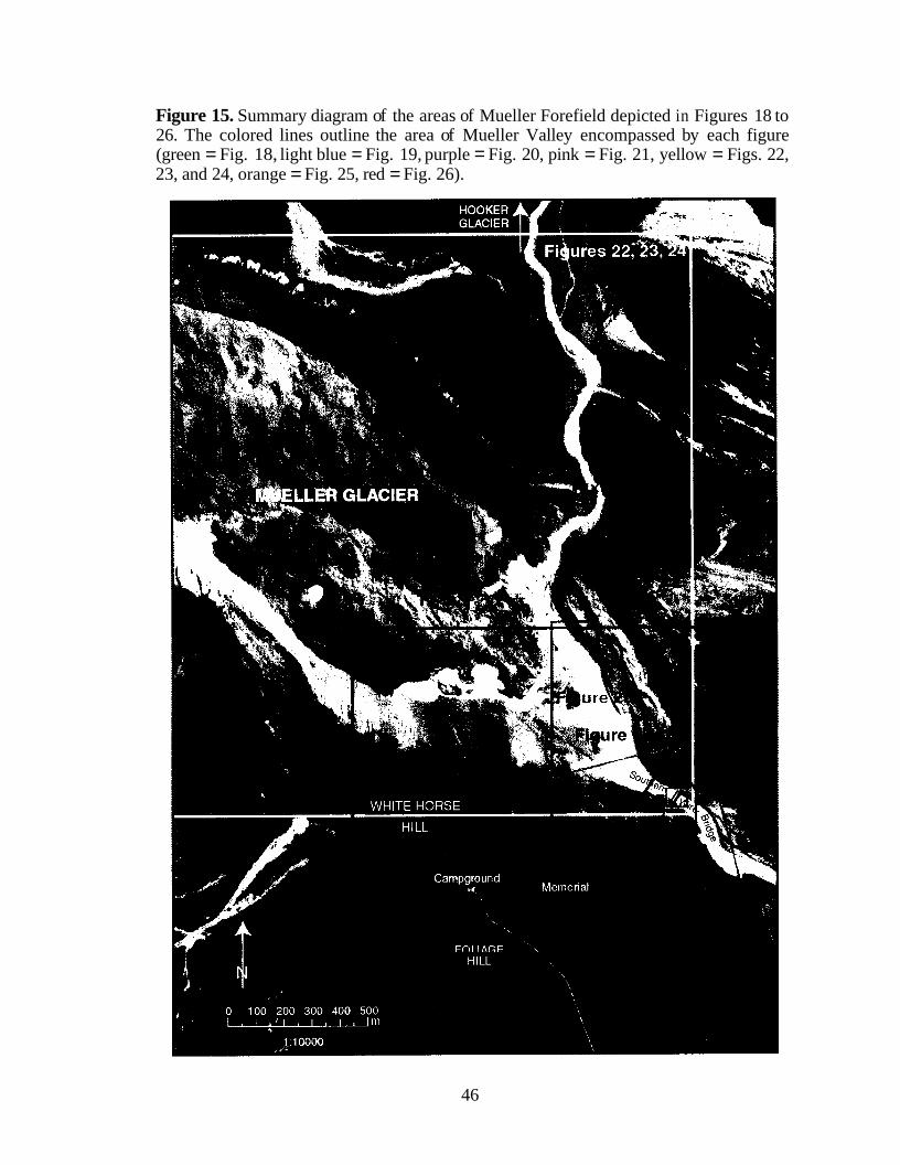
Figure 15. Summary diagram of the areas of Mueller Forefield depicted in Figures 18 to 26. The colored lines outline the area of Mueller Valley encompassed by each figure (green = Fig. 18, light blue = Fig. 19, purple = Fig. 20, pink = Fig. 21, yellow = Figs. 22, 23, and 24, orange = Fig. 25, red = Fig. 26).
46

Figure 16. Summary diagram of the areas of Mueller Forefield depicted in Figures 27 to 33 and Figure 37. The colored lines outline the area of Mueller Valley encompassed by each figure (orange = Fig. 27, light blue = Fig. 28, green = Fig. 29, pink = Fig. 30, purple = Fig. 31, yellow = Fig. 32, dark blue = Fig. 33, red = Fig. 37).
47
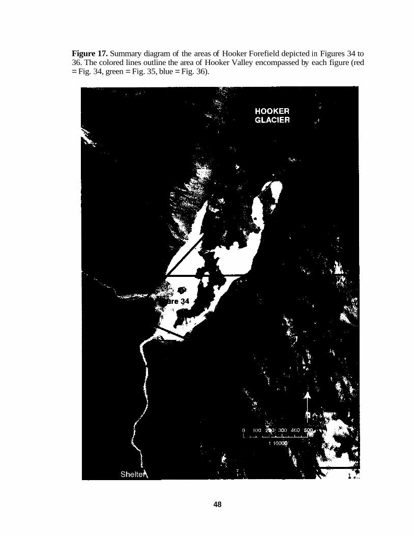
Figure 17. Summary diagram of the areas of Hooker Forefield depicted in Figures 34 to 36. The colored lines outline the area of Hooker Valley encompassed by each figure (red = Fig. 34, green = Fig. 35, blue = Fig. 36).
48

Using records by Julius Haast (1879) and photographs by E.P. Sealy (1867), F.A.
Coxhead (pre-AD 1886), Burton Brothers (c. AD 1875), Wheeler (AD 1888), and Morris
(c. AD 1880s), Gellatly (1982a) reconstructed the position of the Mueller Glacier
terminus in AD 1862. The terminus was about 30 m upstream (north) from where the
southern wire bridge is located (There are two wire bridges in the Mueller Glacier
forefield, a southern and a northern bridge and the locations of each bridge are marked in
Figures 11, 13 and 16). After analyzing a photograph by E.P. Sealy in AD 1867 (Haast,
1879; Fig. IS), I am in agreement with Gellatly's (1982a) positioning of the Mueller
Glacier terminus. Therefore, the ice margin was located proximal to the moraine with
lichen site M-34, in the Central Arm of the Memorial area, and this moraine was
deposited prior to AD 1862.
49

Figure 18. Photograph by E.P. Sealy in AD 1867 of the Moorhouse Range with the Sefton Peak and the terminal face of the Mueller Glacier (Haast, 1879). The position of the Mueller terminus is estimated to be approximately 30m north of the southern wire- bridge. See Figure 15 for specific area of Mueller Valley depicted in photograph.
50

1s

Reports from Haast (1879) indicate that Mueller Glacier had been downwasting
for some time prior to his visit in AD 1862.
"It was here two lateral moraines, of which the outer one, standing more than a hundred feet above the glacier itself, is densely covered with sub- alpine vegetation" (Haast, 1879, p. 32).
The lateral moraines, located about 30 m (looft) above the glacier surface (probably on
WHH), were already heavily vegetated and stranded above the ice when Haast visited the
area in AD 1862. The glacier surface near these lateral moraines lowered at least 45 m
between AD 1862 and AD 1982 (Gellatly, 1982a). In AD 1862, the elevation of the
terminal face of Mueller Glacier was also measured at 2851 ft (819 m) by Haast (1879).
Gellatly (1982a) remeasured the height at 762 m. Therefore, the Mueller Glacier terminal
face downwasted about 57 m between AD 1862 and 1982. Downwasting of Mueller
Glacier has been significant since AD 1862.
The eastern margin of Mueller Glacier extended to the valley wall as late as the
mid-19" century. Haast (1879, p.32-33) described the eastern margin of Mueller Glacier
in AD 1862:
"The glacier abuts, as before mentioned, against the south-westem spur of the Mount Cook range, and 1 now thought that the outlet of the Hooker glacier would have sufficient power to destroy its terminal face so effectually, that it would not reach the rocky mountain side. However, as I observed that the outlet kept more towards the centre of the valley, finding its way some 150 yards from the foot of the range below the Mueller glacier, and issuing with the outlet of the latter from a magnificent ice vault".
A photograph by E.P. Sealy from AD 1867, published in the Geology of Canterbury and
Westland (Fig. 18; Haast, 1879), shows Mueller Glacier nearly abutting the Mount Cook
Range, separated from the bedrock wall by a single moraine. Mueller Glacier either
52
retreated from its position against the south-western spur of the Mount Cook range or
Haast (1879) missed the moraine seen in the AD 1867 Sealy photograph (Haast, 1879).
Regardless, most landforms in the Eastern Margin area of the Mueller forefield were
deposited after AD 1862.
The interval between AD 1862 and AD 1888 was marked by significant
downwasting and retreat of the eastern margin of Mueller Glacier. Hutton (1888) noted
that by AD 1888 the terminal face of Mueller Glacier had retreated approximately 250 to
300 yards from the AD 1862 position (a retreat of 100-150 m). Each summer sheep of
Birch-Hill Station were driven across glacier bridges spanning Hooker River so that they
could graze in Hooker Valley (Hutton, 1888). Fluctuations of the Hooker River, along
with retreat of the Mueller Glacier terminus, led to the collapse of the ice bridges, thus
cutting off easy access to Hooker Valley. A large flood in AD 1868 caused the ice
covering Hooker River to begin to collapse (Hutton, 1888, p. 438). By AD 1878, the last
ice-bridge gave way and the practice of using the Hooker Valley flats as a summer
grazing place for the sheep was temporarily ended. The Rev. W.S. Green made note of
this during his trip to the Mount Cook area in 1882:
"...for years it had been customary to send a mob of about 2,000 sheep across the Hooker to Mount Cook for the summer months, but this year, owing to some ice bridges in the Hooker Glacier having given way, they were unable to cross, and all this fine pasture was going to waste" (Green, 1883, p. 157).
Hooker River had many shifts in path from AD 1862 to AD 1888 (Hutton, 1888).
Variations in melt rates and storm events resulted in unstable behavior of the river and
the Mueller ice terminus. Hutton (1888) observed that by 1884, Hooker River was again
flowing under Mueller Glacier:
53

"At the end of 1884, when Mr. Huddleston arrived and built the Hermitage, the Hooker River skirted the whole breadth of the glacier, but in March 1885, it again cut its way under the northern comer of the glacier. It entered by an ice-cave just below the north lateral moraine of the Mueller, and came out again by another cave about two-thirds of the way across the face" (Hutton, 1888, p. 438).
However, this situation did not last long, and the final ice collapse was in January of
1888, when "the whole of the ice over the Hooker disappeared" (Hutton, 1888, p. 438).
In AD 1884, H.G. Wright drew sketch maps of the forefields of Mueller and
Hooker Glaciers (Wright, 1884; Fig.19). Wright noted only the coarsest geomorphic
features and the vegetation cover in the forefields. Wright sketched three parallel frontal
moraines in the Mueller Glacier forefield. The eastern margin of each of these three
moraine ends near the Hooker River. The most distal moraine appears slightly longer on
its eastern margin than the middle moraine. However, it is the proximal moraine that
reaches closest to the Hooker River. The geometry of the eastern margins of the three
frontal moraines matches the geometry of the long, outermost moraine in the Central Arm
of the Memorial area with lichen site M-31, the shorter, and partially overrun moraine
with the M-34 lichen site, and the younger moraine that is closest to the Hooker River,
with lichen sites M-50 and M-30. On the eastern margin of the Central Arm of the
Memorial area, the partially overrun moraine is a distinct ridge, separate from the
younger moraine ridge with the M-50 and M-30 lichen sites. Farther to the west, these
two moraines merge and are indistinguishable.
54


56

The proximal moraine drawn in the sketch by Wright (1884) appears to
correspond to a moraine fragment east of Hooker River. In the geomorphic map of the
Mueller forefield in Figure 13, the young moraine with the M-30 lichen site can be traced
northeast across the Hooker River to a corresponding moraine ridge in the Eastern
Margin area. However, the innermost moraine from Wright's (1884) sketch cannot be the
lakeside moraine with lichen sites M-28 and M-29, as this moraine does not correspond
to any moraines east of the Hooker River. Because there is not a fourth moraine ridge
drawn in Wright's sketch close to the ice margin, the lakeside moraine did not exist at that
time. The lakeside moraine is a small but prominent feature that certainly would have
been noted if it existed.
In the Central Arm of the Memorial area of the Mueller forefield, Hutton (1888,
p. 436) noted the presence of only two distinct frontal moraines, unlike Wright (1884),
who sketched in three distinct moraine ridges:
"The Mueller Glacier, at present, forms no terminal moraine, for the Hooker River carries all the debris away. But lower down in the valley, bending round in the usual way, may be seen two old terminal moraines, about 150 yards apart, and corresponding with, or rather passing into, the two inner lateral moraines. These terminal moraines are not large nor high. Still lower down the valley is Mogo Hill (Foliage Hill), rising about 100 feet above the plain.. . "
The 'two old terminal moraines' in Wright's quoted description correspond to the two
moraines belts of Sequence M-B and M-D in the Central Arm of the Memorial area of the
Mueller forefield. One of the sketched moraines is certainly the outermost moraine of the
Memorial Moraines section with lichen site M-31. A distance of about 150 yards (137 m)
from the outermost Memorial Moraine to a proximal moraine could correspond either to
57

the partially overrun moraine with the M-34 lichen site, or to the younger moraine with
the M-30 lichen site that was deposited on top of part of the older moraine. The partially
overridden moraine is only distinguishable on the extreme western and eastern sides of
the forefield, and is heavily dissected by outwash streams in the central section. Without
close observation, the two moraines appear to be a single feature. Wright (1884) observed
the eastern margin of the frontal moraines, where the partially overridden moraine is
clearly a separate ridge. I think that Hutton (1888) only noted the gross features, and was
unable to distinguish the fragments of the partially overridden moraine. Therefore, the
description of 'two old terminal moraines' (Hutton, 1888) probably relates to the
outermost Memorial Moraine, along with a composite moraine feature made up of both
the overridden moraine with lichen site M-34 and the younger moraine with lichen site
M-30 proximal to it.
Hutton's (1888) written account does not mention a small but prominent,
unvegetated moraine, proximal to and northwest of the two older terminal moraines. In
fact, Hutton (1888) stated that moraines were not being deposited on or near the
innermost moraine, as the Hooker River carried away all sediments. Based on Hutton's
(1 888) description of the Mueller Glacier forefield, this prominent, unvegetated moraine
with the M-28 and M-29 lichen sites did not exist in AD 1888, nor was it in the process
of being deposited.
A readvance of Mueller Glacier began in AD 1888 (Gellatly, 1992a). By AD
1896 enough ice had built up over Hooker River to allow sheep to cross again onto
Hooker Flats, as Fitzgerald (1896, p. 112) observed shepherds:
58

' I . . .drove their sheep as far as the snout of the Hooker Glacier. The glacier served as a bridge to carry the flock to the other side of the stream where they are left to feed upon the scanty snowgrass during the summer months" (Gellatly (1982a) noted that in many old accounts Mueller Glacier was referred to incorrectly as Hooker Glacier. Fitzgerald (1896) very likely made this mistake here).
The changing margin of Mueller Glacier was also documented by T. N. Brodrick,
a government surveyor sent to prepare topographic maps of the Mount Cook region (Fig.
20). He surveyed the Mueller district in AD 1889, recording the terminal face of Mueller
Glacier in detail during this initial survey, and again in AD 1890 (Brodrick, 1890, 1894,
1905). In AD 1889 the ice terminus was about 160 m upstream of the southern wire-
bridge across Hooker River. In AD 1890, the terminus retreated to 200-220 m from the
southern wire-bridge (Kinsey, 1890; Fig. 21). In AD 1890, Brodrick (1890) surveyed in a
small moraine hillock between the AD 1889 and 1890 terminal positions. Therefore, this
hillock was deposited between AD 1889 and 1890 either during a small readvance during
that period or during a stillstand of the glacier as it retreated. The moraine hillock is about
160 m northwest of the southern wire-bridge across Hooker River according to the survey
map (Figs. 22-24). This location corresponds to the lakeside moraine in the Mueller
forefield, with lichen sites M-28 and M-29. A compass map that Brodrick drew in his
field notebook of the Mueller Glacier forefield on October 11", 1890 (Brodrick, 1890;
Fig. 25) marks the position of the moraine hillock and has notes about a 'lead moraine'.
The lead moraine without vegetation except for "weeds here and there" (Brodrick, 1890)
is here interpreted to be the moraine with lichen sites M-30 and M-50 in the Central Arm
of the Memorial Area. The lakeside moraine can also be seen in two photographs taken
by Kinsey in AD 1895 (Kinsey, 1895; Fig. 26) and Ross in AD 1896 (Ross, 1896; Fig.
27).
59
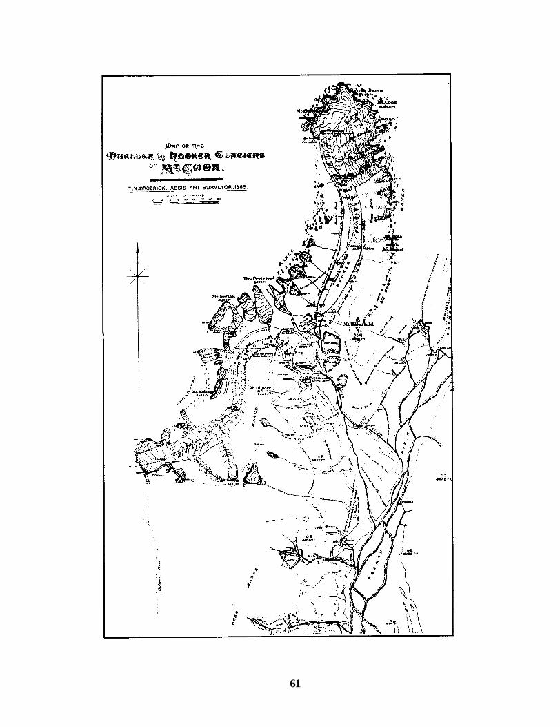
61


r
63


65
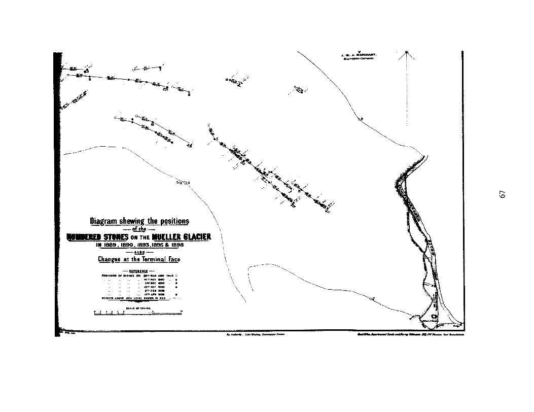


69


73


Brodrick (1890) also surveyed the northeastern face of the Mueller terminus (Fig.
28). Based on the location of the ice margin drawn on Brodrick’s maps (Figs. 22-24), ice
still occupied the Northern Lobe area in AD 1890. A photograph confirms that the
terminus near the Northern Lobe was still quite high in AD 1896 (Kinsey, 1896, Fig. 29).
This photograph also shows the position of Hooker River in AD 1896 when it entered
Mueller Valley.
76
Figure 28. A compass map Brodrick drew in his field notebook of the northeastern margin of the Mueller Glacier terminus on October ll"', 1890 (Brodrick, 1890). The northern lateral moraine, ice margin, and Hooker River are marked on this map. See Figure 16 for specific area of Mueller Valley depicted in photograph.
77

FIELD BOOK, No.
!
f ,. i
I I
1 i \ I
i
1
I
!
1
i I
6' I
S u rv o y o I:
78


7- I-
80

Beginning in AD 1889 (Brodrick, l890), certain boulders on the surface of
Mueller Glacier were numbered and their positions recorded. In succeeding years, the
changing positions of these boulders were recorded by Brodrick (1894, 1905; Figs. 22
and 23), Baker (1891), and Ross (1892; Fig. 24), who among them constructed four
different maps of the changing positions of the numbered boulders. All four show the AD
1889 and 1890 positions of the Mueller Glacier terminus mapped by Brodrick (1890).
Marshall (1907, p. 289) traversed Mueller Glacier in 1905 and noted two main
outwash channels:
"...at the present day the Mueller Glacier has a second outlet. The main stream flows from its terminal face; but a mile above this there is an outlet through the southern lateral moraine. Down this channel torrents of water flow in continuous wet weather after the glacier has filled up".
I believe that the second outlet refers to the stream channel draining the Kea Lobe area. If
so, the ice margin must have been at least as high as the surface of Kea Lobe in order for
meltwater from Mueller Glacier to drain through this outlet. A photograph by Thomas
Pringle in AD 1905 shows the Mueller Glacier terminus close to its position of the AD
1890s (Pringle, 1905; Fig. 30). Gellatly (1982a) interpreted the passage by Marshall
(1907) and the photograph by Pringle (1905) to indicate a slight advance of the glacier
terminus. While possible, there is insufficient evidence to validate this claim. Today,
there is no recognizable moraine in the central area of Mueller Glacier forefield that can
be attributed to this advance.
81


83

In 1913 the old Hermitage, located alongside White Horse Hill, was destroyed by
a flood from Kea Lobe. Frida du Faur (1915, p. 123) described the event:
'I In fine weather there is a tiny lake at the junction of the Kea Point and the old grass-covered moraine besides which the Hermitage is built. The lake is usually only a few feet deep, and sometimes dries up altogether. The last fornight's deluge, besides being of considerable volume itself, was a warm rain that had melted the snow in all directions; these conditions caused the lake, which is a well that receives a large portion of the lake drainage of the Mueller Moraine, to rise about 20 feet, then the pressure of the water burst the bank of the moraine separating the lake from the valley".
Mueller Glacier was already in retreat by AD 1913 (Gellatly, 1982a). The location of the
old Hermitage is shown in a map by E.A. Fitzgerald in AD 1896 (Fig. 31). Photographs
from the late 19'' century through to the present-day indicate that, once it began in the late
AD 1800s and early AD 1900, collapse of the glacier proceeded with few interruptions
(Table 3 in Gellatly, 1984). Initially Mueller Glacier downwasted, losing significant
volume. The terminus itself did not retreat quickly, but remained fairly stationary through
the AD 1910s. Photographs taken by F.G. Radcliffe about AD 1910 show the Mueller
Glacier terminus close to its position of the AD 1890s (Radcliffe, 1910-1919a,b; Figs. 32
and 33).
84


86


88


A
90

There are few historical records of Hooker Glacier. One of the earliest
photographs of the glacier margin was taken in AD 1888 by E. Wheeler of Christchurch
(Wheeler, 1888; Fig. 34). Hutton (1888) reported that E. Wheeler photographed the
Mueller and Hooker Glaciers in AD 1888. In AD 1888 the Hooker River outlet was in the
same position it is today, namely on the southwestern margin of the glacier forefield
(Wheeler, 1888). Hooker Glacier reached higher up on valley sides in AD 1888,
compared to its position shown in a photograph by F.G. Radcliffe about AD 1910
(Radcliffe, 1910-1919c; Fig. 35). Therefore, Hooker Glacier downwasted between AD
1888 and AD 1910.
91


€6


95

A sketch map made by H.G. Wright in AD 1884 of Hooker Valley affords
excellent information about the vegetation present at that time (Wright, 1884). In
particular, burnt areas in the Hooker Glacier forefield are marked (Fig. 36). A photograph
by A.S. Sutton-Turner (1884-1913) of White Horse Hill taken around AD 1910 shows
the entire slope covered with burnt vegetation (Fig. 37).
96


98


100

V. Chronology of Mueller and Hooker Morphosequences
Lichenometry
Lichenometry is defined as the use of lichens to estimate the relative and absolute
ages of substrates on which they are growing. Lichenometry is applied in this study for
two main purposes: 1) to correlate substrates by comparing lichen size or cover, regarded
as a relative dating technique, and 2) to date surfaces by creating a lichen growth curve
that relates lichen size to age, regarded as an absolute dating method. The Fixed Area
Largest Lichen or FALL lichenometry method used in this study was adapted from Bull
and Brandon (1998). The FALL method requires the measurement of the longest axis of
the largest lichen in each of 100 or more sampling sites of approximately the same area
on a given morphologic feature (Bull and Brandon, 1998).
The FALL method is thought to average out the effects of locally variable
colonization times and growth rates, taxonomic misidentification, and measurements of
inherited lichens and composite thalli of merged lichens (Bull and Brandon, 1998). With
the large sample sizes required for the FALL method, evaluation of possible snowlull and
firekill events at lichenometry sites is also possible. Six factors are considered necessary
in order to use the FALL method of lichenometry to date geomorphic events of the past
500 years (Bull and Brandon, 1998): 1) using digital calipers to make FALL
measurements in order to increase precision while reducing bias, 2) measuring the long
axis of elliptical thalli on the premise that they record optimal lichen growth, 3)
measuring only exposed lichens in order to reduce the effects of microclimate on growth
rates, 4) measuring large FALL data sets of greater than 100 measurements if possible, 5 )
calibrating lichen growth rates with control sites dated to the year or day, and 6 )
101

determining the spatial validity for calibration of lichen growth rates by comparing FALL
distributions on substrates formed at the same time at different altitudes and climate
settings and on varying rock lithologies.
The FALL method was developed for use on landslides and rockfall deposits in
order to date and estimate the magnitude of paleoseismic events in the South Island of
New Zealand (Bull and Brandon, 1998). The lichenometry measurements reflect the
timing of the landslide or rockfall event (Bull and Brandon, 1998). In the study reported
here, the FALL lichenometry method is adapted for use on glacial geomorphic features.
The FALL lichenometry measurements reflect the age of deposition. In some areas, the
FALL measurements may not indicate the true age due to post-depositional alteration of
the moraines. These alterations include settling of ice-cored moraines, slumping of
moraines, and glaciofluvial erosion. However, with careful geomorphic mapping, the
areas of post-depositional alteration were largely avoided.
The study reported here was conducted in the general region of the South Island
where Bull and Brandon (1998) developed their lichen growth curve for the Rhizocarpon
subgenus Rhizocarpon lichens (Fig. 38). Thus the same calibration curve that they
developed for rockfalls was also used to date moraines in the Hooker and Mueller
Valleys. The colonization times or growth rates of most species of Rhizocarpon subgenus
Rhizocarpons do not vary with substrate lithology and smoothness, mean annual
precipitation and temperature, or length of growing season (Bull and Brandon, 1998).
This precludes the need for the calibration of lichen growth for each individual study
area. Bull and Brandon (1998) estimated the variance associated with their lichen growth
curve, finding that sample sizes of 100 lichen measurements or more, had an error of f 6
years for the historical period of the last 150 yrs (Fig. 39).
102

Figure 38. Best-fit solution for the lichen-growth equation showing the colonization time, great growth phase, and linear growth phase (adapted from Fig. 16 of Bull and Brandon, 1998).
30
25
20 -
15 - 10 -
5 -
0 25 50 75 100 125 150
Surface Age (yr)
103

Figure 39. Calibration results for the lichen growth equation of Bull and Brandon (1998) shown above in Fig. 38 (adapted from Fig. 20 in Bull and Brandon, 1998). Bull and Brandon (1998) restricted the data to sites older than AD 1956 to ensure that the calibration was entirely within the uniform-growth phase. Note that the heavy gray line in parts A and C shows the 4-parameter growth curve of Fig. 15. A) Calibration using eight historic calibration points spanning 150 years. The plot symbols are larger than the two standard error uncertainties for age and FALL size. B) The 95 percent confidence interval for an estimated lichenometry age using the calibration in part A. The contoured values 25, 100, and 500 refer to the number of FALL measurements used to estimate the FALL peak to be dated. C) Calibration using a combined data set of 19 calibration points, both historic and prehistoric, spanning a 1000 years. Error bars show the one standard error uncertainties. D) The 95 percent confidence interval for an estimated lichenometry age. The contoured values 25, 100, and 500 refer to the number of FALL measurements used to estimate the FALL peak to be dated.
30
25
- 20 E E v
.B 15
2 10
u) J -I
5
n 7840 1880 1920 1960 2000
Calendar Age BP
30
- 20 i > v - 9 10 Q)
C - .-
g o a z
$
c
-10
Ic)
-20
-30 i400 1 ~ 0 0 1600 1700 1800 1900 2000
Calendar Age BP
200
175
150
125
100
75
50
25
0 - 1000 1200 1400 1600 1800 2000
Calendar Age BP
" " " ' " " ' " 1 1 ' " ' ' "
L 4 k-1 ............ , ................ : 00 ;
10
................ I 25 ; -20 c. . . ' -.. .L.
-30 1000 1200 1400 1600 1800 2000
Calendar Age BP
104

Lichen Selection, Quality, and Measurement
The yellow-green Rhizocarpon subgenus Rhizocarpon is the slowest growing of
New Zealand lichens, and therefore is best suited for dating geomorphic surfaces (Bull
and Brandon, 1998). These lichens are also easily identified in the field, and they are
common in the alpine environments of the Mount Cook region. Although each section of
Rhizocarpon subgenus Rhizocarpon has many species, the majority of sections have
similar growth rates (Bull and Brandon, 1998). This precluded the need for laboratory
identification of each measured lichen (Bull and Brandon, 1998). The underlying
assumptions of the FALL measurements are that: 1) the largest lichen was the first to
colonize the boulder, 2) the lichen growth since deposition of the boulder has been
unconstrained, and 3) the rate of growth for each measured lichen is similar to the
average rate of Rhizocarpon subgenus Rhizocarpons lichens.
Most FALL measurements of the yellow-green Rhizocarpon subgenus
Rhizocarpon lichens were made with digital calipers (Fig. 40). Vernier calipers were used
only during rain storms. There are three main factors that need to be considered in lichen
measurements (Bull and Brandon, 1998): 1) is the lichen a single thallus or a composite
of several thalli? 2 ) are the margins, long axis, and degree of circularity of the thallus of a
good enough quality? And 3) is the substrate smooth and planar enough to allow a
precise measurement?
105
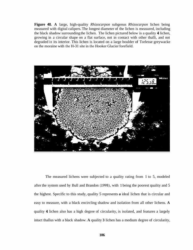
Figure 40. A large, high-quality Rhizocarpon subgenus Rhizocarpon lichen being measured with digital calipers. The longest diameter of the lichen is measured, including the black shadow surrounding the lichen. The lichen pictured below is a quality 4 lichen, growing in a circular shape on a flat surface, not in contact with other thalli, and not degraded in its interior. This lichen is located on a large boulder of Torlesse greywacke on the moraine with the H-31 site in the Hooker Glacier forefield.
The measured lichens were subjected to a quality rating from 1 to 5, modeled
after the system used by Bull and Brandon (1998), with 1 being the poorest quality and 5
the highest. Specific to this study, quality 5 represents a ideal lichen that is circular and
easy to measure, with a black encircling shadow and isolation from all other lichens. A
quality 4 lichen also has a high degree of circularity, is isolated, and features a largely
intact thallus with a black shadow. A quality 3 lichen has a medium degree of circularity,
106
is isolated, and has a mostly distinguishable thallus with a black shadow. A quality 2
lichen has medium-to-low degree of circularity, is partially disintegrated, and has at least
half the circumference of the thallus distinguishable. A quality 1 lichen is considered too
poor to include in the data set. Generally, such poor lichens have less than half a thallus,
are extremely disintegrated, and are in contact with other lichens.
The FALL method requires a small fixed area for each lichen measurement site.
In this study, we set the minimum size to be a boulder that was 0.256 m or greater along
its intermediate axis. If the boulder was greater than 2.5 m2 in area, the exposed surface of
the boulder was divided into smaller sample areas of 2.5 m2 each. The largest single
lichen was measured in a fixed area in each of 100 sites along a transect of a geomorphic
feature such as a moraine.
A slight variation of the FALL lichenometric methodology was used for the first
57 of the 82 sample sites in the Mueller forefield. The longest axis of the largest lichen on
each of 100 or more blocks was measured when possible. However, lichens were
measured on every rock, regardless of size. There was no defined fixed area. Therefore, a
small bias towards sampling larger lichens was introduced. Five sites dated using this
slightly modified FALL method were remeasured using the FALL method of Bull and
Brandon (1998). The mean quantitative difference between the two methods is 2.24 mm,
which corresponds to an age of 12 to 14 years using the linear portion of the Bull and
Brandon (1998) growth curve. The difference is small, and close to the average 9.3
year/mm calculated variance associated with most site measurements (the variance for
each site was calculated). Therefore, the quantitative difference between the two
variations of the FALL lichenometric method is negligible. The FALL lichenometry
method outlined above was used for the rest of the study at Mueller and Hooker Glaciers.
107
The lichen measurements themselves can introduce a source of error. Digital
calipers were used to reduce this error. Bull and Brandon (1998) found that the
measurement-related standard deviation of 0.47 mm from a single operator using digital
calipers is equivalent to a variation of 2.8 years, using their growth rate. This is an
insignificant and acceptable level of error. The use of digital calipers also reduces bias
introduced by the individual operators when making lichen measurements. An operator
does not know the size of the thallus until after the measurement is made and the value
read from the caliper. On the other hand, measurements with rulers and dial calipers are
not as precise as those with digital calipers. They also introduce a bias for thallus size
when the operator estimates the value from the instruments. A klmm reading error was
estimated for ruler measurements (Bull and Brandon, 1998), which is a significant level
of error for slow-growing lichens. Calipers must be maintained in good working
condition in order to ensure continuing precision of measurements. Therefore, the
calipers were oiled every 2-3 days, ensuring ease of movement of the components.
Replicate experiments were conducted to estimate individual operator error, as
well as variations in measurements among operators. Each of these experiments was
conducted at several different locations and at various times. The data were tested for
significant variance between operator measurements using the Two-Sample Komogorov-
Smirnov Test (Table3). This statistical test searches for the maximum difference between
two samples. The test assesses the probability of finding a particular maximum difference
when the underlying distribution for each sample is the same. The first replication
experiment tested operator error by having operators measure two different samples
along the same transect of a channel. All operators were able to replicate their
108

measurements, indicating consistency and precision in measurements for each individual
operator.
Site Number Landform
Table 3. Results of a replication experiment testing for significant variance in replicate counts done by the same operator measuring the same transect in a channel. The Two- Sample Komogorov-Smirnov Test was used, where Ho = two samples are the same and Ha = two samples are not the same. If the P-Values are below 0.05, then Ha is concluded and the two samples tested are significantly different from each other.
Operator P-Value Significantly Different
C-59-6 1 Abandoned Colby vs. Colby 0.7096 No outwash channel
Jessica vs. Jessica 0.6863 No Katie vs. Katie 0.3783 No
The second replication experiment tested the variation among operators at three
different locations (Table 4). Each operator measured the same area of a moraine or an
outwash channel. For the C-59-61 and M-54 lichen sites, only the measurements of the
operator Katie are significantly different. However, for the G-1 lichen site, the
measurements of the operator Jessica are significantly different from the those of the
other operators. There is not a systematic difference between one particular operator and
the other operators, implying that the lichenometric data collection was not standardized.
The maximum difference between two significantly different operators is 10.66 mm. To
correct for differences in data collection, Analysis of Variance (ANOVA) tests were run
on each site. If the measurements taken by a specific operator were found to be
significantly different from the others, then that operator's measurements were removed
109

from the data set. ANOVA tests were also used to account for variations in slope stability
and surface exposure, described in a later section.
Site Number Landform Operators
C-59-61 Abandoned Colby vs. Katie outwash channel
Colby vs. Jessica Jessica vs. Katie
M-54 Older, moraine Adam vs. Colby fragment
Adam vs. Jessica
Table 4. Results of a replication experiment testing for significant variance between operators measuring the same section of a landform. The Two-Sample Komogorov- Smirnov Test was used, where Ho = the two samples are the same, and Ha = the two samples are not the same. If the P-Values are below 0.05, then Ha is concluded and the two samples tested are significantly different from each other.
P- Value Significantly Different
0.0194 Yes
0.9185 No 0.5246 No 0.7088 No
0.2456 No Adam vs. Katie 0.0001 Colby vs. Jessica 0.1478 Colbv vs. Katie 0.0001
Yes No Yes
~
G- 1 Jessica vs. Katie 0.0210 Yes
Young, distinct Colby vs. Katie 0.4695 No
I Jessica vs. Katie I 0.0000 I Yes
moraine ridge Colby vs. Jessica
110
0.0061 Yes

Site Selection
Site selection is very important, as it has a large influence on the precision of age
estimates and hence on the resolution of closely spaced geomorphic events (Bull and
Brandon, 1998). Important factors that need to be considered include the diversity and
frequency of geomorphic processes, the lichen species and abundance present, the quality
of thalli, the smoothness of substrates, the sizes of rockfall or moraine blocks, and the
ability to recognize old blocks that were deposited beyond the time range of the FALL
lichenometry technique (Bull and Brandon, 1998). In addition, the distal side of moraines
are generally more stable than the proximal sides, because they have lower slope angles.
Sampling was concentrated as much as possible on these distal slopes. When the distal
slopes either are not available for sampling or else have an insufficient number of lichens,
sampling took place on the ridge crests and proximal slopes of the moraines. The
geomorphic maps created for Hooker and Mueller Valleys were used to select which
landforms should be sampled in order to create a relative and absolute chronology.
Significantly modified or heavily vegetated siteswere avoided. Modification of
moraine systems in glacial forelands can occur by subsidence of glacial ice-cores, by
fluvial erosion, by readvance of glaciers, by landslides, and by rockfalls. Some
geomorphic features are located very close together, and care must be taken when
choosing which boulders to sample. Lichens were measured only on the boulders that
were clearly associated with a specific geomorphic feature. One example of this is a
Hooker Glacier lateral moraine on the eastern valley wall (lichen site H-22) that is being
covered by an active alluvial fan (Fig. 41). It is commonly possible to discern which
boulders are part of the original deposit and which boulders have since fallen down from
the fan above, as the original boulders are weathered and embedded in the vegetation
111
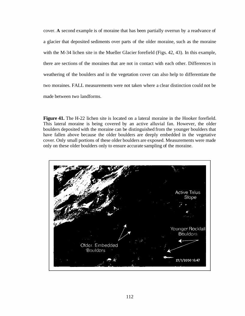
cover. A second example is of moraine that has been partially overrun by a readvance of
a glacier that deposited sediments over parts of the older moraine, such as the moraine
with the M-34 lichen site in the Mueller Glacier forefield (Figs. 42, 43). In this example,
there are sections of the moraines that are not in contact with each other. Differences in
weathering of the boulders and in the vegetation cover can also help to differentiate the
two moraines. FALL measurements were not taken where a clear distinction could not be
made between two landforms.
Figure 41. The H-22 lichen site is located on a lateral moraine in the Hooker forefield. This lateral moraine is being covered by an active alluvial fan. However, the older boulders deposited with the moraine can be distinguished from the younger boulders that have fallen above because the older boulders are deeply embedded in the vegetative cover. Only small portions of these older boulders are exposed. Measurements were made only on these older boulders only to ensure accurate sampling of the moraine.
112

Figure 42. Sketch of the M-50 and M-34 lichen sites, located on frontal moraines in the Central Arm of the Memorial area in the Mueller forefield. The moraine with the M-34 lichen site was partially covered with a moraine deposited during a readvance of Mueller Glacier. The moraine with lichen site M-50 was deposited during this readvance, and is easily distinguishable from the overridden moraine as it is only lightly vegetated in comparison with the older, moderately vegetated moraine. Only the easternmost section of the overridden moraine with the M-34 lichen site remains undisturbed. Measurements were restricted to the portions of the moraine clearly not in contact with, or having been altered by, the larger and younger moraine with the M-50 lichen site. Figure sketched by M.Y. Horesh.
Older Moraine Completely Covered
by Younger Moraine
Lichen '\a,,
Transect , '. \ -
Partially Overridden Older Moraine
Younger Moraine Deposited by a Readvance
of the Glacier
113

Figure 43. Cross-section of a partially overridden moraine adapted from Figure 8 of KarlCn (1973). The initial moraine ridge was overrun by a glacier re-advance, during which a younger moraine was deposited over the distal slope of the initial ridge.
I Younger
Glacier
Statistical Analysis - FALL Method of Bull and Brandon (1998)
Bull and Brandon (1998) found that the FALL distributions from single-event
deposits (seismically induced rockfalls) commonly had one major bell-shaped peak. The
peak was normally distributed (Bull and Brandon, 1998). Probability density plots were
constructed for each FALL distribution. The mean and standard deviation of the peak was
determined using a peak-fitting program applied to the probability density plots. The
peak was interpreted to represent a geologic event - in most cases a seismic event. The
means from each major peak were used together with the growth curve constructed by
Bull and Brandon (1998) to determine the age of the seismic events that caused the
rockfall. Bull and Brandon (1998) appear to have considered each of the FALL
distributions for their calibration sites from the historical period (last 150 yrs) to have
formed during a single geological event, and therefore each distribution from a
calibration site had a single peak. The mean of that single peak was calculated and this
value was used to construct their growth curve.
114

For some of their lichen sites, Bull and Brandon (1998) considered the large
variance in the FALL distrubutions to have resulted from a mixture of normal
distributions. Therefore, the large, bell-shaped peak was actually made up of several
smaller peaks in these broad lichen distribution. Probability density plots were
constructed for each FALL distribution, with Gaussian kernal sizes (defines the width of
the unit Gaussian used in constructing the plot) chosen specifically to minimize noise and
maximize the rockfall peaks. A peak-fitting program was then used to determine the
mean and standard deviation of each peak in the mulitmodal distribution (Bull and
Brandon, 1998). It was assumed that each smaller peak in these multimodal distributions
could be represented by a single Gaussian. The mean of each peak, used together with the
lichen growth curve, was interpreted to be the age of an individual seismically induced
rockfall event during which boulders were disturbed. The size of the peak was inferred to
be a function of the intensity of the seismic event at each site (Fig. 44). Several of the
FALL distributions of Bull and Brandon (1998) were skewed. This was interpreted to
give information about the life expectancy of lichens, illustrating that older lichen died at
a faster rate than younger lichens (Bull and Brandon, 1998).
115

Figure 44. Probablility density plots of FALL sizes for lichens growing on moraine slopes in the Mueller (A) and Tasman (B) forefields (reproduced from Fig. 3 in Bull and Brandon, 1998). The vertical lines mark individual FALL peaks that are thought to represent regional rockfall events that occurred at both sites.
100 I 1 0 120 130 140 150 Largest lichen maximum diameter (mm)
The data sets of FALL lichen measurements from forefields of both Mueller and
Hooker Glaciers collected during this study were predominantly multimodal. In
accordance with the Bull and Brandon (1998) interpretation of multimodal data sets, each
peak within a data set was assumed to follow a Gaussian distribution. A statistical
program, written by W.A. Halteman for S-Plus, separated out each individual peak in the
multimodal FALL distributions. The program randomly computed the mean, standard
deviation, and relative weighting of each peak. The weighted mean and standard
deviation for each data set were also calculated. All data sets from the Mueller and
Hooker Glacier forefields were analyzed using this program. The weighted mean for each
116

complete data set was used together with the growth curve constructed by Bull and
Brandon (1998) to determine the age of the glacial geomorphic feature.
Analysis of Variance (ANOVA) tests are tools for studying the statistical
relationship between a response variable (lichen diameters) and one or more explanatory
or predicator variables (aspect, operator) (Neter et al., 1996). ANOVA tests do not
require any assumptions about the nature of the statistical relation between the response
and the explanatory variables, nor do they require that the explanatory variables be
quantitative. Each data set was analyzed using ANOVA tests for significant differences
between the different explanatory variables (aspect and operator) and the response
variable (lichen diameters). If there were any significantly different explanatory
variables, such as a certain aspect or a particular operator, that variable was removed
from the FALL data set. The significantly different aspects or operators indicate
anomalous lichen growth conditions, including variations in slope stability and exposure
to the sun and wind.
The FALL method of Bull and Brandon (1998) was developed for assessing the
ages of rockfalls associated with seismic events. The FALL method was adopted in this
study for assessing the age of glacial geomorphic landforms fronting Mueller and Hooker
Glaciers. The geomorphic landforms are not formed during a rapid 'single-event' such as
a rockfall. Rockfalls occur abruptly, whereas the moraines were deposited while the ice
margin was in a particular position for some length of time. Many of the moraines were
formed during a single advance or stillstand of the glacier margin, but over a greater
period of time than the rockfalls. Those moraines that were affected by multiple
advances, or that were subsequently altered by fluvial erosion, were identified through
117

geomorphic mapping of the forefield of the two glaciers (see attached geomorphic map;
Fig. 13).
The major point of the following discussion is that the individual peaks that
emerge from the lichen data sets are not used in the same manner of Bull and Brandon
(1998). Rather, an overall mean of the lichen population, either a weighted mean or a
gumbel mean, was used to calculate the lichen numbers for each distribution. The
presence of perched boulders, multiple peaks in former outwash channels, and anomalous
peaks in a historically dated moraine led to conclusion that individual peaks do not
represent specific geologic events.
Perched boulders occur on moraines in the Hooker and Classen forefields (Figs. 9,
45; personal communication 2001, K. Schoenenberger and T.V. Lowell). The perched
boulders were deposited directly by glacier ice, which subsequently melted away. The
presence of precariously perched boulders on relatively old and distinct moraine ridges
implies that these moraines have not experienced significant shaking movement during
any seismic events subsequent to their formation. Therefore, the individual peaks found
in the multimodal data sets for Hooker and Mueller Glacier forefields cannot represent
individual seismic events of varying magnitude, as assumed by Bull and Brandon (1998)
for their data sets.
118

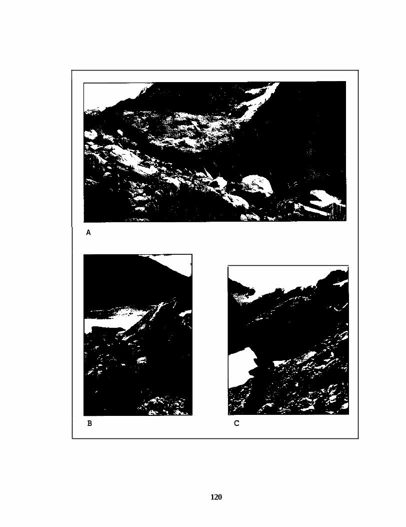
A
B C
120

Many of the moraines were (and some still are) ice-cored. As the ice melted, the
moraines settled accordingly. Geomorphic analyses of the structure of the moraines
inidcated that the majority of these features formed at one time, and subsequently have
not been significantly disturbed. It is possible to distinguish in the field those glacial
landforms that have experienced alterations, and the lichen sites were chosen to be on a
single feature of the same geomorphic age (Figs. 13, 14). Therefore, the multimodal
distributions cannot be attributed to multiple times of formation.
Distributions of FALL data from sites located in former stream channels were
also multimodal (Fig. 46). Former stream channels within a glacial sequence are single-
age events such as a rockfall. Once water flow ceases, lichens can colonize blocks on the
channel floor. If water begins flowing again in the channel, any lichens growing on the
boulders in the channel will die. There is no stabilization factor, because the original
topography of channel floors is fairly flat. The channel with the H-11 lichen site occurs
inside, and is therefore younger than, the proximal margin of the lateral moraine with the
perched boulder (Fig. 45). Therefore, the peaks in the H-11 FALL data set cannot be
attributed to seismically induced disturbances of the boulders on which the lichens grew.
121

Figure 46. Frequency plot of the measurements from the H-11 lichen site located in an abandoned outwash channel. The H-11 distribution is clearly multimodal. This site is located closer to the Hooker ice margin, and consequently is younger than, the high lateral moraine that features a perched boulder on its surface. Therefore, seismic activity cannot have caused the peaks seen in this distribution.
H-11 Channel
2
0 30 60 90 Diameter (mm)
A further argument against the individual peaks in multimodal FALL distributions
being caused by seismic activity comes from a site on a historically dated moraine. The
M-28 site is on a moraine has been dated between AD 1890 and AD 1905 through
historical documents listed previously (Kinsey, 1895; Ross, 1896; Brodrick, 1905 Fig. 23,
122

26, 27). This site is multimodal, with three of the six peaks (Peaks 4-6) having ages that
Peak
are older than AD 1890 using the growth curve of Bull and Brandon (1998; Table 6, Fig.
Weighted Standard n Composite Mean Deviation Weight
47). Such literal application of each peak to the lichen growth curve of Bull and Brandon
1 2
(1998) gives ages that are too old. Therefore, these peaks cannot reflect seismic events
11.22 2.23 23 0.15 16.01 1.14 32 0.21
that would have to have occurred before the moraine was deposited in AD 1890.
4 5
Table 5. The weighted mean and standard deviation for the multimodal FALL distribution from the M-62 lichen site, located on a historically dated moraine. The moraine was deposited between AD 1890 and AD 1905 according to survey maps, written accounts, and numerous photographs of the glacier margin during this time (Fitzgerald, 1896; Marshall, 1907; Gellatly, 1982a; Fig. 18, 22, 23). This FALL data set has six peaks, numbered 1 - 6. Peak 1 has the smallest mean and is therefore interpreted to be the youngest peak. Peak 6 has the largest mean and is the oldest peak. Using a literal interpretation of the Bull and Brandon (1998) approach of assuming that each peak indicates a geologic event, Peaks 4, 5 , and 6 correspond to periods of formation prior to AD 1890-1905, and are therefore older than the historical age of the moraine. Peak 6 is approximately 78 years older, Peak 5 is 44 years older, and Peak 4 is 21 years older than the true age of the moraine. Peaks 4, 5 and 6 clearly cannot represent seismic events as the boulders on the moraine were not yet deposited by that time. Peaks 4, 5 and 6 also do not represent periods of stabilization or any other form of alteration of the moraines as again, the moraines did not exist. Therefore, I conclude these peaks do not represent geologic events.
23.89 0.831 251 0.17 27.32 0.911 191 0.13 1846
1812 6
25
31 19.67) 1.031 35) 0.23
61 32.52) 3.781 161 0.11
Age (years AD) based on growth curve
from Bull and Brandon, (1 998)
(+/- Years
j l 1869
123

Figure 47. Probability density plot of the multimodal M-28 site on a moraine historically dated to AD 1890-1905 (Fitzgerald, 1896; Marshall, 1907; Gellatly, 1982).
M-62 Moraine
I I I I
1897
0 10 20 30 40 50 Diameter (mm)
The Bull and Brandon (1998) method of analysis of the FALL measurements
requires that each peak in the mulitmodal data set represents a specific coseismic rockfall
event or are in a series of multiple ice advances. Each peak is assumed to be normally
distributed. However, as demonstrated above, these multiple peaks are not a result of
geologic processes. The peaks could represent a biological process such as varying
growth rates of lichens within a population, variation in the post-depositional
modification of the glacial feature that affects lichen colonization or, as discussed below,
an artifact of the sampling procedure. Therefore, instead of an individual peak, the

weighted mean for the entire FALL data set was used in this study, together with the
growth curve of Bull and Brandon (1998), to determined the age of the geomorphic
features (Tables A . l and B.l). Bull and Brandon (1998) gave the impression that each of
their lichen calibration sites had a single peak, and they used the mean of the single peak
from each of their young lichen calibration sites to construct the historical portion of the
lichen growth curve. Bull and Brandon (1998) did not seem to encounter multimodal
distributions for the calibration sites dating to the historical period. The use of a single
overall peak for each of the lichen sites in the Mueller and Hooker forefields, instead of
the mean of each individual peak to calculate the age of the landforms, is therefore
comparable to the approach of Bull and Brandon (1998) for the young portion of their
curve. The unfiltered FALL measurements from the historically dated AD 1890 moraine
(lichen site M-62) have a weighted mean of 20.6k0.7 mm. This mean corresponds to an
age of deposition of AD 189024. Using the weighted mean of the FALL distributions
together with the growth curve of Bull and Brandon (1998) appears to result in an
accurate age of the moraines.
Statistical Analysis - Modified FALL Method
The major assumptions of the original FALL method were re-examined, leading
to a different interpretation of FALL measurements on Holocene moraines. It was
assumed that if the largest lichen was the first to colonize a boulder, the subsequent
lichen growth and colonization were unconstrained and the growth rate for each lichen
measured was similar to the average rate of the Rtzizocnrpoiz subgenus Rhizocarpon
125

lichens. Therefore, it is possible that the lichens on a single boulder are a representative
sample of the total lichen population of a moraine.
Lichen colonization of a boulder probably occurs either continuously, or in pulses
following the initial colonization period, as demonstrated by the wide range of lichen
diameters found on most boulders. Many lichens observed on boulders on the Mueller
and Hooker moraines were barely large enough to be seen by eye. Other lichens were
noted growing over older, larger lichens. This implies that boulders on the moraines may
have experienced more than one pulse of lichen colonization. However, there are
insufficient data to determine whether lichen colonization occurred continuously or in
pulses.
There is not enough information about the biological controls of lichen
colonization to make the assumption that lichens inhabited an area uniformly. However,
field observations do not support the concept of uniform colonization. Boulders on
individual glacial geomorphic features in the Mueller and Hooker forefields do not have
identical lichen covers. Bull and Brandon (1998) found that the microclimate, involving
shelter from the sun and wind, had large effects on the lichen growth rates. These same
microclimatic factors could also have affected the colonization pattern of lichens. On a
typical moraine in the Mueller and Hooker forefields, some boulders have no lichens,
whereas others located nearby have fairly dense populations. Thus, there is clearly an
uneven distribution of lichens on boulder surfaces. Although lichens colonized the
boulders unevenly due to such random environmental influences or to unknown
biological factors, it is likely that the Hooker and Mueller forefields were exposed to the
same amounts of lichen spores at the same times. If all the lichens on a boulder are
126

measured, and the samples pooled for a selection of the boulders, a distribution of the
lichen population will be obtained for a specific geomorphic feature. The distribution of
lichen population may be a mixture of normals (as implied by Bull and Brandon (1998)
for the FALL distributions), or even normal with a large variance. The implication is that
in each area (or boulder), there is a single population of lichens. We see this in our data,
as tests done on single boulders show single peaks (Fig.48). However, our sampling
technique, in which only the largest lichen measurement from each boulder is combined
with other largest lichen measurements from other boulders on the same moraine, leads to
an extreme-value distribution.
127
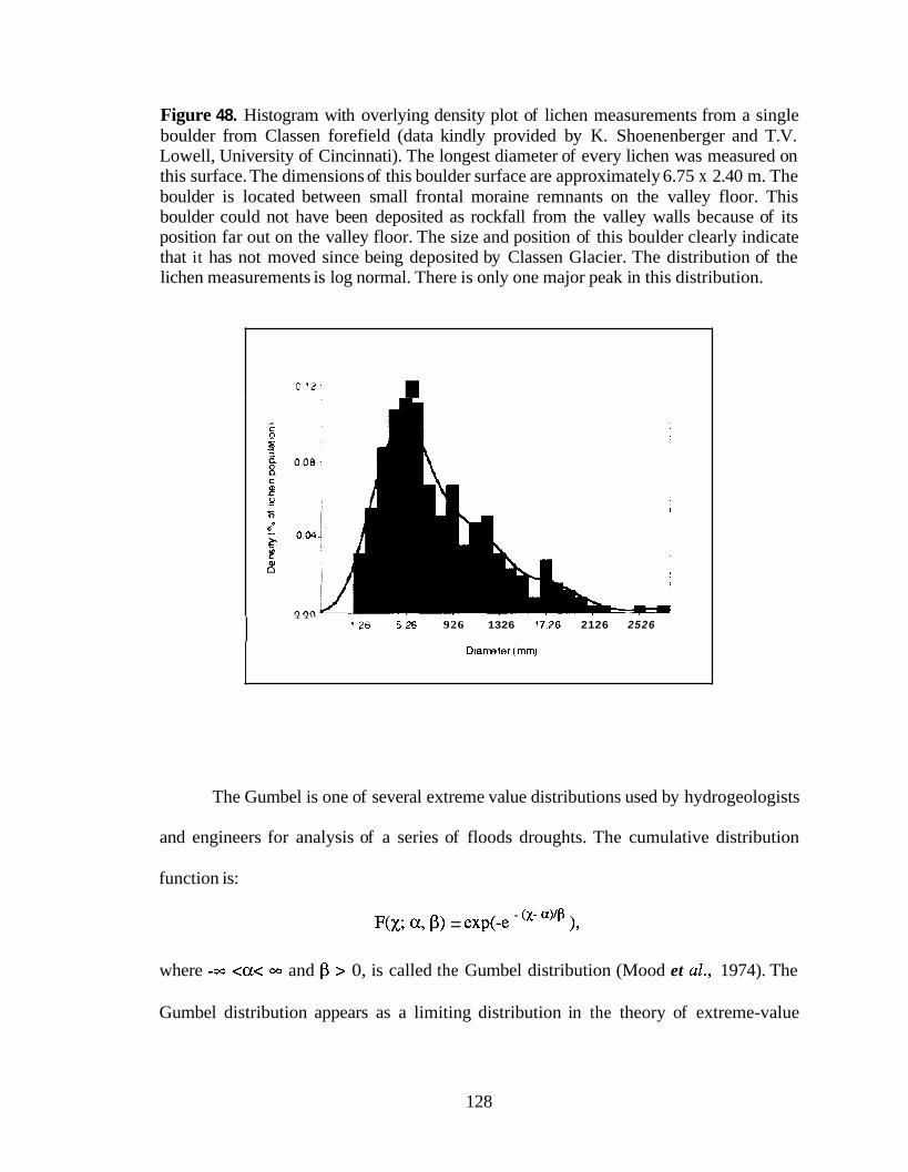
Figure 48. Histogram with overlying density plot of lichen measurements from a single boulder from Classen forefield (data kindly provided by K. Shoenenberger and T.V. Lowell, University of Cincinnati). The longest diameter of every lichen was measured on this surface. The dimensions of this boulder surface are approximately 6.75 x 2.40 m. The boulder is located between small frontal moraine remnants on the valley floor. This boulder could not have been deposited as rockfall from the valley walls because of its position far out on the valley floor. The size and position of this boulder clearly indicate that it has not moved since being deposited by Classen Glacier. The distribution of the lichen measurements is log normal. There is only one major peak in this distribution.
I C ' 2 .
I I"
'26 5 2 6 926 1326 7726 2126 2526 I
The Gumbel is one of several extreme value distributions used by hydrogeologists
and engineers for analysis of a series of floods droughts. The cumulative distribution
function is:
1, - (x- a)@ F(x; a, PI = exp(-e
where -00 <a< 00 and P > 0, is called the Gumbel distribution (Mood et al., 1974). The
Gumbel distribution appears as a limiting distribution in the theory of extreme-value
128

statistics. We used a sampling technique similar to the analysis of floods when we made
FALL lichen measurements. We recorded the largest lichen diameter in a specific area on
a boulder surface. We repeated this for approximately 100 separate areas (or boulders).
Therefore, we collected - 100 extreme values for each geomorphic landform. The
assumptions associated with the Gumbel distribution in this study area are that: 1) a
random process produced a population of observations, 2) the sampling process collects
samples and extracts the maximum value from each, and 3) the number of observations in
each sample is large. The data from each transect were analyzed to see if they followed
the Gumbel distribution by testing whether a Q-Q plot of the data against quantiles from
a Gumbel distribution produced a straight line. The Gumbel mean for each FALL transect
was then calculated and used to estimate the relative age of a depositional event. Not
enough calibration points were measured in this study to construct a growth curve for use
with the Gumbel means for each lichen population on a geomorphic landform. Therefore,
only a relative chronology of landforms could be constructed. The lichens have a life
expectancy of about 500-1000 years (Bull and Brandon, 1998). Therefore the chronology
constructed for sampled Mueller and Hooker moraines is limited to 1000 years or
younger.
The data sets follow the Gumbel extreme value distribution and are not normally
distributed as concluded by Bull and Brandon (1998). Therefore, the multiple peaks
recorded by the FALL measurements are artifacts of the sampling technique. The
multiple peaks seen in the FALL data sets from the glacial landforms are not produced by
either a geological or biological process, but by selectively sampling the extreme values
of a lichen population.
129

FALL Chronology of Mueller Morphosequences
An important test for the consistency of the FALL method is to determine
whether the lichen measurements from each of the sites reflect the relative age of the
morphosequences determined from field mapping. The means for the FALL lichen sites
from the various glacial geomorphic features in Mueller forefield correspond reasonably
well to the relative ages of the morphosequences (Figs. 49-55; Table Al). With only a
few exceptions, the means are largest on the outermost morphsequences, and become
progressively smaller on morphosequences closer to the present-day glacier margin.
There are four separate chronologic maps for the Mueller forefield. Figure 50
shows the unfiltered weighted means (data sets not split using ANOVA tests) plotted at
each lichen site. Figure 51 illustrates the ages of the landforms based on the unfiltered
weighted means from each lichen site, used together with the lichen growth curve of Bull
and Brandon (1998). The data sets for each of these lichen sites are unfiltered. Figure 52
shows the means of the glacial landforms determined after the data sets have been filtered
using ANOVA tests. The ANOVA tests filtered out the effects of slope instability and
exposure to elements such as the sun and wind. The filtered chronology is regarded as the
most accurate representation of ages of moraines and channels in the Mueller forefield.
The fourth map (Fig. 53) shows the ages of the glacial landforms once the data set has
been filtered. For all chronologies, Morphosequence M-A1 is considered to be beyond
the range of lichenometry and therefore remains undated. Morphosequence M-A2 was
not sample because of the heavy vegetation cover and evidence from historical accounts
that the WHH area burned in the early 1900s (Fig. 37). The moraine belt of
Morphosequence M-B crosscuts the moraines in the White Horse Hill area
(Morphosequence MA-2). If the WHH moraines were deposited during the LIA, they
130
were formed prior to - AD 1740, which is the approximate age of the outermost moraine
ridge in Morphosequence M-B.
Unfiltered FALL Chronolow of Mueller Morphosequences
The moraine complex of Morphosequence M-B is a large, broad feature with
many surface ridges. This complex is the outermost feature on the Mueller forefield that
can be dated with lichenometry. The outer ridge on the M-B moraine complex is dated to
about AD 1740-1775 (means = 38.3-42.8 mm) (Figs. 50 and 51, Table 6). This outer
ridge exhibits the largest lichen diameters in the Kea Lobe, White Horse Spillover,
Memorial, and Eastern Margin areas. The innermost ridge of the moraine complex has
smaller means, and was deposited in the early AD 1800s (means = 31.5-38.8 mm). The
Mueller Glacier terminus was at the Morphsequence M-B position for approximately 30
to 50 years, an extended period reflected by the complex geomorpholgy of the
Morphosequence M-B moraine belt in the Western and Central Arms of the Memorial
area. The implication is that, during the deposition of the Morphosequence M-B moraine
belt between AD 1750 and AD 1818, the Mueller Glacier terminus was at its outermost
extent of the LIA.
Morphosequence M-C can not be distinguished from Morphosequence M-B by
lichenometry. The moraine fragments sampled in the Central Arm of the Memorial area
have varying ages of deposition, ranging from AD 1786 to AD 1832 (means = 29.5 to
36.6 mm). The moraine fragments from Morphosequence M-C have all been exposed to
glaciofluvial erosion, which on parts of the moraine fragments may have reset the ages of
lichens to the time of the latest period of erosion. In the Eastern Margin area, the moraine
fragments range in age from AD 1740 to AD 1837 (means = 43.5 to 28.8 mm). Historical
131

records indicate that the Eastern Margin area was ice covered as late as AD 1862 (Haast,
1879). Therefore, the hummocky terrain in the northern part of the Eastern Margin area
was deglaciated after AD 1862. However, the age of deposition determined by
lichenometry is AD 1740. This anomalous age could be the result of an accelerated
pocket of lichen growth on the hummocky terrain, or possibly due to a very short
stabilization period of flatter hummocky terrain compared to moraine ridges. Pockets of
accelerated lichen growth on glacial geomorphic landforms are not common, and appear
to be limited to small hollows. One other such pocket was identified in the Hooker
forefield (site H-31).
There is a clear difference in the ages of Morphosequences M-B and M-D. FALL
means from sites on the Morphosequence M-D moraine belt in the Central Arm of the
Memorial, Eastern Margin, Kea Lobe, and White Horse Spillover areas reflect an age of
deposition between AD 1825 and AD 1840 (means = 28.2 to 30.5 mm). A reconstruction
of the Mueller Glacier margin in the Central Arm of the Memorial area from records of
Haast's visit in AD 1862 (Haast, 1879), shows that the M-D moraine complex had
already been deposited by that time. Most of the lichenometry results for the Central Arm
area are in accordance with historical records.
Lichen sites on the Morphosequence M-E moraine complex in the Central Arm of
the Memorial area and in the Northern Lobe area show an age of deposition of these
ridges and ice-contact terraces of about AD 1868 to AD 1890 (means = 21.0 to 24.2 mm).
The Eastern Margin area yielded a wide range of ages of deposition from AD 1853 to AD
1941 (means = 13.0 to 26.2 mm) for the glacial features of Morphosequence M-E. This
result was expected, because historical documents (Radcliffe, 1910-1919) indicate that
the Hooker River oscillated throughout the Morphosequence M-E section of the Eastern
132
Margin area during the late AD 1800s to at least the AD 1920s, and possibly even later
(Gellatly, 1982b).
The Morphosequence M-F moraine has an age of deposition of AD 1912 (17.3
mm). This fits well in comparison to the M-E Morphosequence, whose glacial features
were deposited around AD 1884 to AD 1904 (means =21.0 to 24.2 mm). The means of
the lichen sizes become progressively smaller closer to the glacier margin. These
lichenometry results also correspond well with known historical observations of the
Mueller Glacier terminus (Gellatly, 1982a; Radcliffe, 1910-1919).
Filtered FALL Chronolonv of Mueller Morphosequences Using. ANOVA Tests
A chronology was constructed with data from lichen sites that were first filtered
with ANOVA tests described earlier. Lichen means from operators that sampled unstable
portions of moraine slopes, or from lichens facing a particular aspect that led to
anomalous growth conditions on the boulders, were removed. Instability and excessive
exposure lead to slower growth of lichens or an inability for lichens to colonize an area.
A chronology filtered for these variations in growth conditions generally yields
maximum age estimates for deposition of glacial features.
The filtered chronology is not very different from the unfiltered chronology. In
general, the filtered FALL ages are older than the filtered ages by about 10 to 20 years
(means = 2 to 3 mm) (Fig. 52, 53; Table Al) . The outer ridge on the M-B moraine
complex has the largest lichens in the Kea Lobe, White Horse Spillover, Memorial, and
Eastern Margin areas, and is dated to AD 1729 to AD 1771 (means = 45.0 to 36.4 mm),
with most ages centered around AD 1740 to AD 1750. The filtered chronology indicates
that Mueller Glacier terminus was most extended about AD 1740 to AD 1750. The
133

innermost moraine of the Morphosequence M-B belt was formed around AD 1788 to AD
1818 (means = 36.2 to 31.5 mm), with most of the ages about AD 1790 to AD 1800. As
in the case of the unfiltered FALL chronology, the Mueller terminus was extended to the
Morphosequence M-B moraine belt for approximately 50 years.
Morphosequence M-C moraine belt cannot be distinguished from either the M-B
or the M-D Morphosequences on the basis of the filtered chronology. The ages of the
sites range from AD 1788 to AD 1821 (means = 36.7 to 31.1 mm), with no noticeable
trend. Disturbance of the sampled moraine segments is a possible reason for the large
range of ages. There is a clear age difference between Morphosequences M-B and M-D.
The Morphosequence M-D moraine belt were deposited between AD 1800 to AD 1840
(means = 34.4 to 28.2 mm), with most of the ages clustered around AD 1820 to AD 1850.
The filtered lichenometry results are in accordance with the position of the Mueller
Glacier margin in AD 1862, constructed by Gellatly (1982a) for the Central Arm area
from accounts by Haast (1 879).
The Morphosequence M-E moraine complex in the Central arm of the Memorial
area and in the Northern Lobe area has an age of AD 1868 to AD 1892 (means = 23.1 to
21.0 mm). The lakeside moraine in the Central Arm area is historically dated to AD 1890
(Broderick, 1890, Gellatly, 1982a), and the ages from measurements at lichen sites on
this moraine are AD 186856 (mean = 23.1k0.9 mm) and AD 188855 (mean = 21.0k0.7
mm). The Morphosequence M-F moraine is the innermost in the Mueller forefield, and
appropriately has a recent age of AD 1919 (mean = 16.4 mm). Overall, the filtered FALL
lichenometry method affords moraine ages that correspond well with those derived from
historical records.
134

Gumbel Chronology of Mueller Momhosequences
The Gumbel and FALL means for the Mueller forefield are nearly identical for
both the filtered and unfiltered lichen data sets. The Gumbel means are slightly larger
than the FALL means (Figs. 54, 55; Table A2). The difference between the Gumbel and
FALL means for individual sites is only 0.15-0.2 mm. Because a lichen growth curve was
not constructed for Gumbel means, absolute ages cannot be assigned to the landforms.
Therefore the Gumbel moraine chronology is relative. The same morphosequences were
registered using Gumbel means, as were found using means from the FALL method. The
means for individual lichen sites were similar for the two methods. Therefore, the
chronology described for the FALL results, as well as the manner in which the FALL
means from each lichen site relate to the morphosequences of the Mueller forefield, is the
same as that for the Gumbel means, but the age assignment awaits a suitable calibration
curve. A description of how the FALL means (both filtered and unfiltered) from the
lichen sites in the Mueller forefield relate to the morphosequences is given in the sections
above. The same descriptions apply for the Gumbel means of both the filtered and the
unfiltered data sets. Even though the Gumbel means are so similar to the FALL means,
they were derived from very different statistical distributions. Therefore, the growth
curve of Bull and Brandon (1998), constructed for FALL lichen measurements analyzed
as normal distributions, cannot be used with lichen data sets analyzed using the Gumbel
distribution. Only the relative chronologies (Gumbel and FALL) can be compared. They
give nearly identical results.
For the unfiltered Gumbel chronology, Morphosequence M-B is characterized by
Gumbel means of 38.5 to 42.9 mm on the outer ridge, and Gumbel means of 31.6 to 34.0
mm on the inner ridge. Morphosequence M-C cannot be distinguished from
135

Morphosequences M-B or M-D by unfiltered Gumbel means. The Morphosequence M-D
moraine belt has Gumbel means of 28.3 to 30.6 mm. Morphosequence M-E has Gumbel
means of 21.1 to 24.2 mm, and the Morphosequence M-F moraine has a Gumbel mean of
17.4 mm.
In the filtered Gumbel chronology, lichen sites on the Morphosequence M-B
moraine belt have Gumbel means of 45.2 to 39.0 mm on the outer ridge, and Gumbel
means of 36.5 to 31.6 mm on the inner ridge. Morphosequence M-C cannot be
distinguished from either Morphosequence M-B or Morphosequence M-D by filtered
Gumbel means. Morphosequence M-C has Gumbel means ranging from 36.9 to 31.3 mm.
The Morphosequence M-D moraine belt has Gumbel means of 34.4 to 28.3 mm. The
sites on the Morphosequence M-E moraine complex have Gumbel means between 23.3
and 21.1 mm, and the Morphosequence M-F moraine has a Gumbel mean of 16.4 mm.
The lichenometry results from the Mueller forefield are summarized in Table 6. Figure 56
illustrates the oscillations of the Mueller terminus during the main phase of the LIA as
derived from these lichenometry results and from the geographic position of the dated
morphosequences.
136
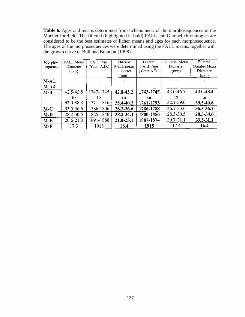
Table 6. Ages and means determined from lichenometry of the morphosequences in the Mueller forefield. The filtered (highlighted in bold) FALL and Gumbel chronologies are considered to be the best estimates of lichen means and ages for each morphosequence. The ages of the morphosequences were determined using the FALL means, together with the growth curve of Bull and Brandon (1998).
137

Figure 56. Oscillations of the Mueller Glacier terminus during the main phase of the LIA.
1743
1850
0 1890 a E 9 m
2000 1750 1800 1850 1900 1950 2
Years AD
Mueller Glacier
30
FALL Chronology of Hooker Morphosequences
The major differences between the morphosequences from the Mueller and
Hooker Valleys are the presence of significantly older moraines in the Mueller forefield.
The Hooker forefield does not exhibit these old features, perhaps because they are
covered by younger morphosequences. Likewise, the youngest moraines of the Hooker
forefield have probably been eroded into Hooker lake or else have been covered by rising
lake water. The other major difference is an additional morphosequence in Mueller
forefield. Mueller Morphosequence M-D falls between Hooker Morphosequences H-B
and H-C. Each glacial valley has a different geometry, so it is not surprising that the
morphosequences are not identical.
138

The main test for the consistency of the FALL method is to determine whether the
lichen dates from each of the sites are consistent with the relative positions of the
morphosequences. In general, the two data sets are consistent. The largest means (and
therefore dates) are located on the outer moraines, whereas the smallest means (and
therefore youngest dates) are from the innermost moraine of the Hooker forefield (Figs.
49-53).
Unfiltered FALL Chronology of Hooker Morphosequences
The unfiltered FALL chronology (Figs. 50 and 51; Table B l ) does not distinguish
Morphosequence H-A from Morphosequence H-B. Site ages range from the early AD
1700s to the AD 1780s for the moraine belt in Morphosequence H-A. The moraine ridges
in the Frontal and South-Eastern areas of Morphosequence H-A have reasonably
consistent ages of about AD 1759 to AD 1769 (means = 40.7 to 39.1 mm). The Frontal
area moraine complex in Morphosequence H-B has ages of AD 1765 to AD 1789 (means
= 39.8 to 36.1 mm). Hence, the ages of the moraine complexes in the two
morphosequences appear to be similar. However, Morphosequences H-A and H-B
delimit two ice-marginal positions that the Hooker termini occupied during two distinct
periods, suggested that the ages of the two morphosequences should be different. Two of
the lichen sites (H-1 and H-24) on the Frontal and Mid-Eastern areas of the
Morphosequence H-A are on lateral moraines. The H-1 lichen site has a low sample size
of 42, and the H-24 lichen site is located below an alluvial fan. It is possible that these
factors affected the lichen means at these lichen sites. The remaining locality in the
Frontal area Morphosequence H-A is the H-23 lichen site, which is located on a moraine
139

fragment that has been altered by glacial outwash on all sides. Although care was taken
with sampling, it is possible that fluvial alteration led to an age that is slightly too young.
In contrast, the South-Western area of the Morphosequence H-A moraine belt is
significantly older than the Frontal and South-Eastern areas. The ages of the moraine
ridges in the belt range from AD 1637 to AD 1743 (means = 59.5 to 43.1 mm). The H-31
lichen site, situated in a hollow between two moraines in the South-Western area of the
Morphosequence H-A moraine belt, has a mean of 59.5 mm, corresponding to an age of
AD 1637. The hollow of the H-31 lichen site abuts a moraine ridge on its proximal side.
This proximal ridge features the H-30 lichen site, with a mean of 43.1 mm and an age of
AD 1743. There is more than 100 years age difference between these two lichen sites,
and yet there are no intervening morphological breaks. Lichen sites H-30 and H-31 are
located on glacial features that are part of the same morphosequence. The H-31 site is
located in a moist, sheltered hollow, which possibly caused accelerated growth of the
lichens. Because of these discrepancies, the age from the H-31 site is disregarded.
The range of ages from the South-Western area of Morphosequence H-A is AD 1696 to
AD 1743 (means = 50.4 to 43.1 mm) when the H-31 site is not included. The outermost
moraine in the belt in the South-Westem area has an age of AD 1709 5 20.1 (mean =
48.4 k 3.1), the next proximal ridges sampled have ages of AD 1725 & 20.6 to AD 1743
f 20.0 (means = 45.9 f 3.2 to 43.1 k 3.1 mm). This innermost ridge of the
Morphosequence H-A moraine belt (site H-6) has an age of AD 1696 (mean = 50.4 mm).
Such a date is anomalous, and may possibly be due to accelerated growth conditions in
the transect sampled on the ridge. The H-6 site is disregarded. The ridges in the South-
Western area of the Morphosequence H-A get progressively smaller in the proximal
direction, and were deposited primarily between AD 1724 to AD 1759 (means = 48.4 to
140

43.1 mm). In the South-Westem area of the Hooker forefield, a lichenometric distinction
can be made between the moraine belts of Morphosequence H-A and Morphosequence
H-B. Morphosequence H-A was deposited about AD 1709 to AD 1743 (means = 48.4 to
43.1 mm), and Morphosequence H-B was dated at AD 1765 to AD 1805 (means = 39.8
to 36.1 mm).
Morphosequence H-B is distinguishable from Morphosequence H-C in the
Frontal area of the Hooker forefield. The moraine belt of Morphosequence H-C was
deposited around AD 1910 (means = 17.7 mm). There are several young ages (e.g. AD
1932 and AD 1940) in the Frontal area and South-Eastern and North-Eastern areas of
Morphosequence H-C. The ridges these lichen sites are located on are unstable and
exposed to the wind and sun (sites H-14, H-18, H-25, and H-26).
The sites on the lateral moraine ridges in the North-Eastem area date to the mid
AD 1800s, and do not seem to correspond to either Morphosequence H-A or H-B. It is
possible that these moraine ridges are part of a different morphosequence not
distinguishable in the Hooker forefield.
Filtered FALL Chronology of Hooker Morphosequences Using ANOVA Tests
The filtered FALL chronology is similar to the unfiltered FALL chronology (Figs.
52, 53, Table B 1). Morphosequence H-A is only distinguishable from Morphosequence
H-B in the South-Western area. Morphosequence H-A in the South-Westem area ranges
in age from AD 1709 to AD 1743 (means =48.4 to 43.1 mm).
The moraine belt of Morphosequence H-B was deposited between AD 1735 and
AD 1764 (means = 44.4 and 39.3 mm). Morphosequence H-B is distinguishable from
Morphosequence H-C in the filtered data from the FALL method. The moraine belt of
141
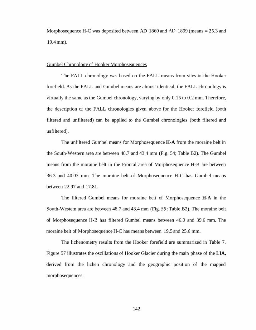
Morphosequence H-C was deposited between AD 1860 and AD 1899 (means = 25.3 and
19.4 mm).
Gumbel Chronology of Hooker Morphoseauences
The FALL chronology was based on the FALL means from sites in the Hooker
forefield. As the FALL and Gumbel means are almost identical, the FALL chronology is
virtually the same as the Gumbel chronology, varying by only 0.15 to 0.2 mm. Therefore,
the description of the FALL chronologies given above for the Hooker forefield (both
filtered and unfiltered) can be applied to the Gumbel chronologies (both filtered and
un fi 1 tered).
The unfiltered Gumbel means for Morphosequence H-A from the moraine belt in
the South-Western area are between 48.7 and 43.4 mm (Fig. 54; Table B2). The Gumbel
means from the moraine belt in the Frontal area of Morphosequence H-B are between
36.3 and 40.03 mm. The moraine belt of Morphosequence H-C has Gumbel means
between 22.97 and 17.81.
The filtered Gumbel means for moraine belt of Morphosequence H-A in the
South-Westem area are between 48.7 and 43.4 mm (Fig. 55; Table B2). The moraine belt
of Morphosequence H-B has filtered Gumbel means between 46.0 and 39.6 mm. The
moraine belt of Morphosequence H-C has means between 19.5 and 25.6 mm.
The lichenometry results from the Hooker forefield are summarized in Table 7.
Figure 57 illustrates the oscillations of Hooker Glacier during the main phase of the LIA,
derived from the lichen chronology and the geographic position of the mapped
morphosequences.
142

Table 7. Ages and means from lichenometry of the morphosequences in the Hooker forefield. The filtered FALL and Gumbel chronologies (highlighted in bold) are considered to be the best estimates of lichen means and ages for each morphosequence. The ages of the morphosequences were determined using the FALL means, together with the growth curve of Bull and Brandon (1998).
Morphos FALL Mean FALL Age equence Diameter (Years A.D.)
(mm)
H-A 48.4-43.1 1709-1742
Flitered Filter FALL Gumbel Mean FALL mean Age (Years, Diameter
Diameter A.D.) (mm)
48.4-43.1 1709-1743 43.4-48.7 (mm)
H-B H-C
Filtered Gumbel Mean
Diameter
363 -39.8 1765- 1789 39.3-39.8 1765-1768 36.3-40.0 14.4-21.8 1883-1932 19.4-25.3 1860-1899 17.8-22.0
Figure 57. Oscillations of the Hooker Glacier terminus during the main phase of the LIA.
1780 1876 1730m
n a r 9 m
2000
Hooker Glacier
1750 1800 1 850 1900 1950 Years AD
143

Comparison of Mueller and Hooker Morphosequence Chronologies
The Morphosequence H-A matches up well with the outer ridge of the
Morphosequence M-B moraine belt (Table 8). Morphosequence H-B has similar ages to
the innermost moraine of Morphosequence M-B. Morphosequence H-C corresponds to
Morphosequences M-E and M-F. The Mueller forefield has three additional
morphosequences that are not present in the Hooker forefield. Hooker Glacier is in a
valley with a morphology different from that of Mueller Valley, so small variations were
expected. However, there is a good overall match between the glacial advances recorded
by the moraine belts in the Mueller and Hooker forefields. Both glaciers advanced
between the mid- to late AD 1700s and the early AD 1800s, and again in the AD 1890s.
Mueller Glacier also expanded during the mid- AD 1800s. This advance may be recorded
in the moraine ridges of the North-Eastern area of Hooker forefield. Lichen samples from
additional moraine ridges are needed to determine if there was a Hooker advance during
the mid-AD 1800s.
144
Table 8. Comparison of the ages and means from lichenometry of equivalent morphosequences from the Mueller and Hooker forefields. The ages are based on the filtered FALL means and the filtered Gumbel means. The ages of the morphosequences were determined using the FALL means, together with the growth curve of Bull and Brandon (1998).
Mueller Mo rp ho- sequences
M-A
M-B - distal ridge
ridge M-B -proximal
M-C M-D
M-E and M-F
Filtered FALL Filtered Hooker Filtered Filtered Age (Years, Gumbel Morpho- FALL Age Gumbel
A.D.) Mean sequence (Years, A.D.) Mean (mm) (mm)
- - - -
1743-1745 43 .O-43.4 H-A 1709-1743 43.4-48.7
1761-1793 33.5-40.6 H-B 1765-1768 39.6-40.0
1786-1788 36.5-36.7 -
1800-1856 28.3-34.6 - - -
1874-1887, 23.3-21.1, H-C 1860-1899 19.6-25.6 1918 16.4
145

VI. Discussion
The FALL chronology of morphosequences in the Mueller and Hooker forefields
shows ice advances in the mid-AD 1700s to about AD 1800, and again in the mid-to late
1800s. These dates fall within the main phase of the LIA as documented in the Swiss
Alps, implying at least a near-synchronous LIA signal between the Southern Alps in New
Zealand and the Swiss Alps in Europe. The filtered FALL chronology agrees with the
results of earlier lichenometry investigations by Burrows (1973), as well as with a tree-
ring chronology constructed by Lawrence and Lawrence (1965) for the Mueller and
Hooker forefields. There is no agreement with the weathering-rind analyses done by
Gellatly (1984).
Burrows (1973) concluded that the most significant advances of Mueller Glacier
occurred between AD 1700 and AD 1890, the FALL results from this study. Using the
single largest lichen diameter method, Burrows (1973) concluded that the moraine belt of
Morphosequence M-B in the Central Arm of the Memorial area was deposited in AD
1750. The filtered FALL chronology placed the outer ridge of this moraine belt between
AD 1743 and AD 1745. Burrows (1973) also dated a small moraine hillock that forms
part of the innermost moraine ridge of Morphosequence M-C to AD 1790. The filtered
FALL chronology indicate that this hillock was deposited about AD 1785. Overall, there
is strong agreement between the results of the two lichenometry studies.
Using tree-ring analysis, Lawrence and Lawrence (1965) found that the Mueller
Glacier terminus advanced to the outer ridge of the Sequence M-B moraine belt in the
Memorial area before AD 1761, and that the ice receded by AD 1793. The results from
the filtered FALL chronology are in accord with this conclusion. The older ages from the
outer ridge of the Sequence M-B moraine belt indicate that the glacier advanced about
146

AD 1743 to AD 1745, and that the terminus remained extended until about AD 1790 to
AD 1800. These results fit well with the tree-ring chronology of Lawrence and Lawrence
(1965). On the Eastern Margin area of the Mueller Glacier forefield, Lawrence and
Lawrence (1965) concluded that the ice margin extended to the valley wall in the Eastern
Margin area from AD 1745 to AD 1785, and that retreat had occurred by AD 1804 to AD
1808. The filtered FALL chronology indicated that several moraines along the base of the
valley wall of the Eastern Margin area were deposited between AD 1746 and AD 1752,
reflecting the same advance as recorded by Lawerence and Lawrence (1965). Lawrence
and Lawrence (1965) ascertained that the innermost moraine ridge of the
Morphosequence M-C was formed by AD 1838-1839. Filtered FALL measurements
from the same sampling areas used in the tree-ring analysis of Lawrence and Lawrence
(1965) indicate that the innermost moraine was deposited around AD 1786 to AD 1788.
Here, the chronology constructed using tree-ring analysis is consistent with that for the
filtered FALL dating method.
None of the chronologies constructed in this study agrees with the weathering-
rind chronologies. Using weathering-rind analysis, Gellatly (1984) considered the outer
ridge of the Morphosequence M-B moraine belt to be 2940 years old. The inner ridge of
the same moraine belt was assigned an age of 1490 years, implying that the glacier was
extended for 1500 years. My study, using the FALL method to date these same moraines,
concluded that the glacier was extended to these ridges for 50 years between AD 1743 to
AD 1790. Gellatly (1984) did not find a LIA signal in the Mueller and Hooker forefields.
Rather, almost all moraine ages determined by weathering-rind analysis for the Mueller
and Hooker forefields are significantly older than the LIA. These old dates determined
from weathering-rind analysis do not agree either with the younger ages determined from
147

the lichenometric studies presented here or by Burrows (1973), or from the tree-ring
chronology of Lawrence and Lawrence (1965). I consider that the weathering-rind
chronology overestimates the true ages of the moraines, commonly by about 1000 years.
Hooker and Mueller Glaciers do not have exactly the same response time to
climate forcing. Howerver, chronologies constructed for the Hooker and Mueller
forefields are not expected to match in every detail. For example, during the first phase of
the LIA in the Swiss Alps, tree-ring chronologies, together with radiocarbon dates of
glaciers, also record a range in response times (Holzhauser and Zumbuhl, 1999b). An
advance in AD 1300 has a spread of approximately 85 years in Switzerland. During the
main phase of the LIA, historical information shows a spread in response times of Swiss
glaciers ranging from only a few years to about 30 years (Holzhauser and Zumbuhl,
1999b). Assuming moraines are not missing and all advances were recorded for both
phases of the LIA in the Swiss Alps, variation of up to 85 years is expected in glacier
response times.
The glaciers and the basin geometries are similar in the Swiss Alps and the
Southern Alps in New Zealand. Therefore, variations in response times of New Zealand
glaciers also are expected. Factors that can affect glacier response times include the
length of forcing, the snowline position on the glacier during forcing (i.e., where in the
geometry of the glacier basin), the shape of the glacier basin, and the amount of rock
cover on the glaciers. In addition, not every moraine was sampled in the lichenometry
study of Mueller and Hooker forefields. There were time constraints and not every
moraine was suitable for lichen measurement. In particular, Hooker forefield has an
incomplete lichenometry coverage. It is likely that several advances of Hooker Glacier
were missed, accounting for some of the difference between oscillations of Hooker and
148
Mueller Glaciers. However, although specific details may vary, the broad agreement of
the Hooker and Mueller chronologies is striking.
The dated advances of the Hooker and Mueller Glaciers are near synchronous to
those in Swiss Glaciers for the main phase of the LIA (Figs. 58, 59). Advances registered
in the Mueller and Hooker Glacier forefields nearly correspond to advances of the Lower
Grindelwald Glacier during the mid- AD 1700's, and also during the mid- to late AD
1800's. Gorner Glacier registered an advance during the late AD 1800's, along with the
Rhone (Fig. 58) and Grosse Aletsch Glaciers. Although the advances of New Zealand
and Swiss Glaciers are not in perfect agreement, the major trends of glacier expansion
and retreat during the main phase of the LIA are evident in both areas.
149
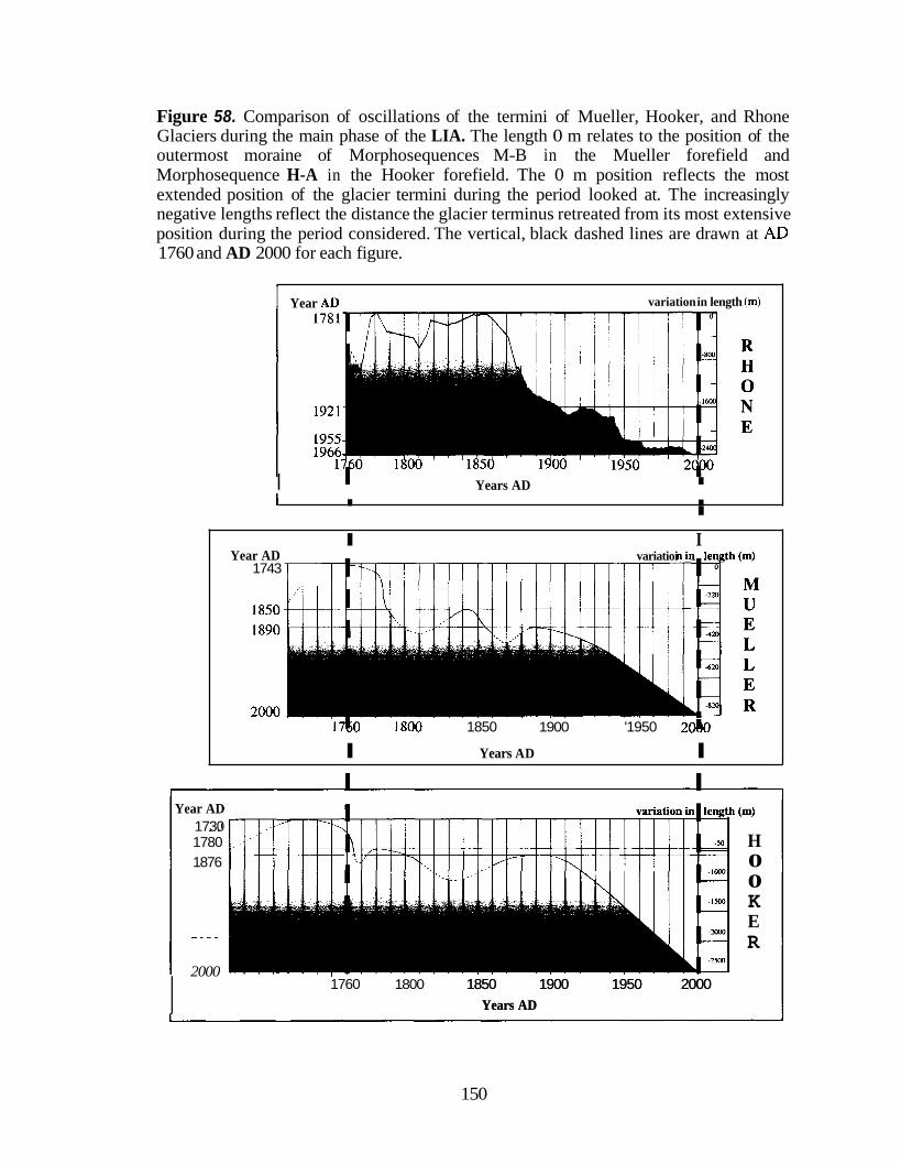
Figure 58. Comparison of oscillations of the termini of Mueller, Hooker, and Rhone Glaciers during the main phase of the LIA. The length 0 m relates to the position of the outermost moraine of Morphosequences M-B in the Mueller forefield and Morphosequence H-A in the Hooker forefield. The 0 m position reflects the most extended position of the glacier termini during the period looked at. The increasingly negative lengths reflect the distance the glacier terminus retreated from its most extensive position during the period considered. The vertical, black dashed lines are drawn at AD 1760 and AD 2000 for each figure.
I Year AD variation in length (m)
I I Years AD 1 I I
I
I I Year AD variatioi
I I I I I l l l l l l l l l l 1 l l 1743 I
'1%0 I800 1850 1900 '1950 2 0
I Years AD I
Year AD 1730 1780 H 1876 0
0 K E R
2000 1760 1800 1850 1900 1950 2000
Years AD I ----
1850 1900 1950 2000 Years AD
150

Figure 59. Comparison of oscillations of the termini of Mueller, Hooker, and Lower Grindelwald Glaciers during the main phase of the LIA. The length 0 m relates to the position of the outermost moraine of Morphosequences M-B in the Mueller forefield and Morphosequence H-A in the Hooker forefield. The 0 m position reflects the most extended position of the glacier termini during the period looked at. The increasingly negative lengths reflect the distance the glacier terminus retreated from its most extensive position during the period considered. The vertical, black dashed lines are drawn at AD 1760 and AD 2000 for each figure.
variation in length (m) Year AD 1600
1882 195 1
1996
Years AD
M U E L L E R
I Years AD
I
1780 H 0 0 K E R
1876 -
1850 1900 1950 2000 Years AD
151

Porter (1975) calculated a 140 m snowline depression for the LIA advances of
several small glaciers in the central region of the Southern Alps of New Zealand. As the
moraines of Morphosequences M-B through M-F, and H-A through H-B were deposited
during the main phase of the LIA, a 140 m snowline depression can be associated with
that time period. This corresponds to a drop in temperature of less than 1 "C during the
LIA, assuming that the effects of changing precipitation were not important (Porter,
1975). Maisch (1999) calculated a snowline lowering of 90 m and a 0.5-0.7 "C
temperature depression in the Swiss Alps. Thus the snowline depression in New Zealand
and Switzerland were nearly identical during the main phase of the LIA.
The early phase of the LIA was not detected in the Mueller and Hooker forefields,
but without a tree-ring chronology coupled with radiocarbon dates such as in the Swiss
Alps of Europe, this is not surprising. The early phase of the LIA in New Zealand likely
was not as large in magnitude as during the main phase of the LIA. The glacier advances
during main phase of the LIA probably destroyed almost all evidence of earlier advances
during the LIA, covering over any deposits.
152

VII. Conclusions
The main phase of the LIA signal is nearly synchronous between the North Atlantic
region in the Northern Hemisphere and the temperate latitudes of the South Pacific
sector of the Southern Hemisphere. The LIA signal in the Southern Alps of New
Zealand closely parallels the main phase of the LIA in the North Atlantic region. The
beginning of the collapse of the New Zealand glaciers is approximately synchronous
with that of the Swiss glaciers.
The response of the New Zealand glaciers was of a similar magnitude to that of the
Swiss glaciers during the LIA. The similarity in the geometry of the glacial
sedimentary basins and the equivalent drop in snowline elevation during the main
phase of the LIA suggest comparable atmospheric forcing of glaciers systems in the
two different regions.
The LIA snowline lowering represents at least a near-global climate signal that must
have been transferred through the atmosphere in order for the LIA to occur
simultaneously on opposite sides of the planet. There is no interhemispheric seesaw
of thermohaline circulation between the Northern Hemisphere, and at least 45"s
latitude (Broecker, 1998), during the main phase of the LIA.
153

References
Baker, J.H., 1891. On Mount Cook glacier motion: Report of Australasian Association for Advancement of Science, v. 3, p. 153-161.
Bergthdrsson, P., 1969. An estimate of drift ice and temperature in Iceland in 1000 years: Jijkull, V . 19, p. 94-101.
Bond, G. and R. Lotti, 1995. Iceberg discharges into the North Atlantic on millennia1 time scales during the last glaciation: Science, v. 267, p. 1005-1010.
Bond, G., W. Broecker, S. Johnsen, J. McManus, L. Labeyrie, J. Jouzel, and G. Bonani, 1993. Correlations between climate records from North Atlantic sediments and Greenland ice: Nature, v. 65, p. 143-147.
Bond, G.C., W. Showers, M. Elliot, M. Evans, R. Lotti, I. Hajdas, G. Bonani, and S. Johnsen, 1999. Tracing the North Atlantic's -1.5 kyr climate cycle to 80 k yrs B.P. - relationship to Heinrich Events, DansgaardOeschger Cycles and the Little Ice Age. In Mechanisms of Millennial-scale Global Climate Change, Webb et al. (eds). Geophysical Monograph 112, p. 35-58.
Brodrick, T.N., 1890. Timaru Field Note Book no. 387, 1890-1891. New Zealand Department of Lands and Survey, Christchurch.
Brodrick, T.N., 1894. Ice motion of the Canterbury Glaciers: New Zealand Alpine Journal, v. 1, p. 307-316.
Brodrick, T.N., 1905. Mueller Glacier. Appendix to the Journals of the House of Representatives of New Zealand: C-1, p. 112-1 13.
Broecker, W.S., 1998. Paleocean circulation during the last deglaciation: A bipolar seesaw?: Paleoceanography, v. 13, p. 119-121.
Bull, W.B. and M.T. Brandon, 1998. Lichen Dating of Earthquake-Generated Regional Rockfall Events, Southern Alps, New Zealand: GSA Bulletin, v. 110, p. 60-84.
154

Burrows, C.J., 1973. Studies of some glacial moraines in New Zealand - 2: Ages of moraines of the Mueller, Hooker and Tasman Glaciers: New Zealand Journal of Geology and Geophysics, v. 16, p. 831-855.
Burrows, C.J., 1980. Radiocarbon dates for post-Otiran glacial activity in the Mount Cook region, New Zealand: New Zealand Journal of Geology and Geophysics, v. 23, p., 239-248.
Burrows, C.J., 1989. Aranuian radiocarbon dates from moraines in the Mount Cook region, New Zealand: New Zealand Journal of Geology and Geophysics, v. 32, p. 205-2 16.
Burrows, C.J. and J. Lucas, 1967. Variations in two New Zealand glaciers during the past 800 years: Nature, v. 216, p. 467-468.
Chinn, T.J., 1996. New Zealand glacier responses to climate change of the past century: New Zealand Journal of Geology and Geophysics, v. 39, p. 415-428.
Chinn, T.J.H., 1989. Glaciers of Irian Jaya, Indonesia, and New Zealand - Glaciers of New Zealand - Satellite image atlas of glaciers of the world. (eds) Williams, R.S. Jr. and J.G. Ferrigno. U.S. Geological Survey Professional Paper 1386-H-2.
Dansgaard, W.S., H.B. Johnsen, D. Clausen, D. Dahl-Jensen, N.S. Gundestrup, C.V. Hammer, C.S. Hvidberg, J. Steffensen, Sveinbjornsdottir, J. Jouzel, and G. Bond, 1993. Evidence for general instability of past climate from a 250-kyr ice core record: Nature v. 364, p. 218-220.
Dennis, A. and C. Potton, 1983. The Alpine World of Mount Cook National Park. Department of Conservation and Cobb/Horwood Publications, Aukland, New Zealand. 97p.
Du Faur, F., 1915. The conquest of Mount Cook and other climbs: An account of four seasons’ mountaineering on the Southern Alps of New Zealand. George Allen and Unwin Ltd., London.
Fitzgerald, E.A., 1896. Climbs in the New Zealand Alps. Being an Account of Travel and Discovery. Unwin, London. 363p.
155
Gellatly, A.F., 1982a. Holocene glacial activity in Mt Cook National Park, New Zealand. Unpublished Ph.D. thesis, lodged in the library, University of Canterbury, Christchurch, New Zealand.
Gellatly, A.F., 1982b. Lichenometry as a relative-age dating method in Mount Cook National Park, New Zealand: New Zealand Journal of Botany, v. 20, p. 343-353.
Gellatly, A.F., 1983. Revised dates for 2 recent moraines of the Mueller Glacier, Mt Cook National Park (Note): New Zealand Journal of Geology and Geophysics, v. 26, p. 311-315.
Gellatly, A.F., 1984. The use of rock weathering-rind thickness to redate moraines in Mount Cook National Park, New Zealand: Arctic and Alpine Research, v. 16, p. 225 -23 2.
Gellatly, A.F., 1985a. Glacial fluctuations in the central Southern Alps, New Zealand: documentation and implications for environmental change during the last 1000 years: Zeitschrift fur Gletscherkunde und Glazialgeologie, v. 21, p. 259-264.
Gellatly, A.F., 1985b. Historical records of glacier fluctuations in Mt Cook National Park, New Zealand: A century of change: The Geographical Journal, v. 151, p. 86-99.
Gellatly, A.F., F. Rothlisberger, and M.A. Geyh, 1985. Holocene glacier variations in New Zealand (South Island): Zeitschrift fur Gletscherkunde und Glazialgeologie, V. 21, p. 265-273.
Green, W.S., 1883. The high Alps of New Zealand or A trip to the glaciers of the Antipodes with an ascent of Mount Cook. Macrnillan and Co., London, 350p.
Griffiths, G.A. and M.J. McSaveney, 1983. Distribution of mean annual precipitation across some steepland regions of New Zealand: New Zealand Journal of Science, V. 26, p. 197-209.
Grove, J.M., 1988. The Little Ice Age. Methuen, New York, New York, 498 p.
156

Haast, J. von, 1879. Geology of the provinces of Canterbury and Westland, New Zealand: A report comprising the results of official explorations. Times Office, Chri stc hurc h, New Zeal and, 486p.
Holzhauser, H., 1984. Zur Geschichte der Aletsch - und des Fieschergletschers: Physical Geography, v. 13.
Holzhauser, H., 1995. G1etscherschwankungen innerhalb der letzten 3200 Jahre am Beispiel des Groben Aletsch - und des Gornergletschers. Neue Ergebnisse. In Gletscher im standigen Wandel: Publikationen der Schwiezerischen Akademie der Naturwissenschaften (SANW/ASSN), 6 vdf Hochschulverlag AG an der ETH Zurich.
Holzhauser, H., 1997: Fluctuations of the Grosser Aletsch Glacier and the Gorner Glacier during the last 3200 years: new results. In: Frenzel, B.(Hrsg.): Glacier fluctuations during the Holocene. PalaoklimaforschungRalaeoclimate Research, Vol. 24, p. 35-58. Special Issue: ESF Project European Palaeo-climate and Man 16. Gustav Fischer Verlag Stuttgart, Jena, Lubeck, Ulm.
Holzhauser, H. and H.J. Zumbuhl, 1996. To the history of the Lower Grindelwald Glacier during the last 2800 years - palaeosols, fossil wood and historical pictorial records - new results. Zeitschrift fur Geomorphologie N.F., Supp1.-Bd. 104, pg. 95-127.
Holzhauser, H. and H.J. Zumbuhl, 1999a. Glacier fluctuations in the western Swiss and French Alps in the 16"' Century: Climatic Change, v. 43, p. 223-237.
Holzhauser, H. and H.J. Zumbuhl, 1999b.Holocene glacial fluctuations, In Hydrological Atlas of Switzerland: Geographisches Institut der Universitat Bern - Hydrologie.
Hutton, F.W., 1888. Notes on the Mueller glacier, New Zealand: Proceedings of the Linnean Society of New South Wales, v. 3, p. 429-442.
Johnson, G.W., 1976. Mount Cook National Park. The Microtone Colour Book SeriesBascands Ltd., Christchurch, New Zealand.
157

Kinsey, J.J., 1890. The 220ft span wire suspension bridge across the Hooker River, about 10 chains below the terminal face of the Mueller Glacier. Albumen print 99x152 mm mounted on album page. Joseph Kinsey Collection, Alexander Turnbull Library, National Library of New Zealand, Te Puna Matauranga o Aotearoa, Reference Number: PA1-q-137-13-2.
Kinsey, J.J., 1895. View from the top of Mount Ollivier, looking west over the Mueller and Hooker Glaciers towards the Liebig Range. The Hermitage is at the bottom of the photograph. Alexander Turnbull Library, National Library of New Zealand, Te Puna Matauranga o Aotearoa, Reference Number: PA1-q-137-21.
Kinsey, J.J., 1896. The Hooker River and the terminal face of the Mueller Glacier. Albumen print 148x201 mm mounted on album page. Joseph Kinsey Collection, Alexander Turnbull Library, National Library of New Zealand, Te Puna Matauranga o Aotearoa, Reference Number: PA1-q-137-76-2.
Kirkbride, M.P., 1988. Glaciers of the Tasman Valley and Mount Cook National Park, supplement to the guidebook for the International Glaciological Society Post- Symposium Tour, New Zealand, 13p.
Ladurie, E.L.R., 1971. Times of Feast, Times of Famine: A History Of Climate Since the Year 1000. Doubleday & Company, Inc., Garden City, New York, 426 p.
Lamb, H.H., 1968. The Changing Climate. Methuen & Co. Ltd., London, England, 236 p.
Lamb, H.H., 1985. Climatic History and the Future. Princeton University Press, Princeton, New Jersey, 835 p.
Lawrence, D.B. and E.G. Lawrence, 1965. Glacier studies in New Zealand: Mazama, v. 47, p. 17-27.
Maisch, M., A. Wipf, B. Denneler, J. Battaglia, and C. Benz, 1999. Die Gletscher der Schweizer Alpen - Gletscherhochstand 1850 Aktuelle Vergletscherung Gletscherschwund-Szenarien - 2.Auflage. Schlussbericht NFP 3 1 v/df Hochschulverlag AG an der ETH Zurich.
Maizels, J.K., 1989. Differentiation of late Pleistocene terrace outwash deposits using geomorphic criteria: Tekapo Valley, South Island, New Zealand: New Zealand Journal of Geology and Geophysics, v. 32, p. 225-241.
158

Marshall, P., 1907. Notes on glaciation in New Zealand: Report of Australasian Association for Advancement of Science, v. 11, p. 283-289.
Mood, A.M., F.A. Graybill, and D.C. Boes, 1974. Introduction to the theory of statistics, 31d edition. McGraw-Hill Book Company, New York.
Neter, J, M.H. Kutner, C.J. Nachtscheim, W. Wasserman, 1996. Applied Linear Statistics Models Fourth Edition. WCB McGraw-Hill, Boston, 1408 p.s
Porter, S.C., 1975. Equilibrium-Line Altitudes of Late Quaternary Glaciers in the Southern Alps, New Zealand: Quaternary Research, v. 5, p. 27-47.
Porter, S.C., 1986. Pattern and Forcing of Northern Hemisphere Glacier Variations during the Last Millennium: Quaternary Research, v. 26, p. 27-48.
Pringle, T., 1905. Mount Cook, 12349 ft, from the Mueller Glacier. A.E. Birch Collection, Alexander Turnbull Library, National Library of New Zealand, Te Puna Matauranga o Aotearoa, Reference Number: G- 695 1-1/1-, Collection Reference Number: PAColl-178 1.
Radcliffe, F.G., 1910-1919a. Mount Sefton and the Footstool, Southern Alps, New Zealand. F.G. Radcliffe Collection, Alexander Turnbull Library, National Library of New Zealand, Te Puna Matauranga o Aotearoa, Reference Number: G- 7557- 1/2 -, Collection Reference Number: PAColl-4950.
Radcliffe, F.G., 1910-1919b. The Hooker River and the Stocking Glacier, Southern Alps, New Zealand. F.G. Radcliffe Collection, Alexander Turnbull Library, National Library of New Zealand, Te Puna Matauranga o Aotearoa, Reference Number: G- 7550- 1/2 -, Collection Reference Number: PAColl-4950.
Radcliffe, F.G., 1910-1919c. View of the Hooker Glacier. F.G. Radcliffe Collection, Alexander Turnbull Library, National Library of New Zealand, Te Puna Matauranga o Aotearoa, Reference Number: G- 7549- 1/2-, Collection Reference Number: PAColl-4950.
Ross, M., 1892. Aorangi; or the Heart of the Southern Alps, New Zealand. Government Printers, Wellington, New Zealand, 64 p.
159

Ross, M., 1896. Cook Spur and Liebig Range from Sealy Range. Ross Collection, Alexander Turnbull Library, National Library of New Zealand, Te Puna Matauranga o Aotearoa, Reference Number: G- 17590-1/4-, Collection Reference Number: PAColl-5 192.
Schoenenberger, K., and T.V. Lowell, 2001. Personal communication.
Suggate, R.P., 1978. Torlesse supergroup. In The Geology of New Zealand (R.P. Suggate, G.R. Stevens, and M.T. Te Punga, eds.), V. 1, p. 254-255. Government Printer, Wellington, New Zealand.
Sutton-Turner, A.S., 1884-1913. The old Hermitage, with Mount Sefton and The Footstool in the background. Silver gelatin print 113x157 mm mounted on album page, Alexander Turnbull Library, National Library of New Zealand, Te Puna Matauranga o Aotearoa, Reference Number: PA1-0-485-02.
Swiss National Tourist Office (SNTO), 1981. Switzerland and her Glaciers - From the Ice Age to the Present. Kummerly and Frey, Geographical Publishers Berne, Switzerland.
Tyndall, J., 1898. Die Gletscher der Alpen. Deutsche Ausgabe des Werkes von 1860, Vieweg und Sohn, Braunschweig, 550p.
Wardle, P., 1973. Variations of the Glaciers of the Westland National Park and the Hooker Range, New Zealand: New Zealand Journal of Botany, v. 11, p. 349-388.
Wheeler, E., 1888. (Aorangi) Mt Cook and Hooker Glacier. E. Wheeler and Son photograph, Broadhead Collection, Canterbury Museum, Reference Number: 16522.
Wright, H.G., 1884. Timaru Field Book no. 212. Corresponding File R2652. New Zealand Department of Lands and Survey, Christchurch.
Zumbuhl, H.J. and H. Holzhauser, 1988. Alpengletscher in der Kleinen Eiszeit - Sonderheft zum jahrigen Jubilaum des SAC. Herausgegeben vom Schweizer Alpen-Club. Die Alpen (3. Quartal). Bern.
160

Appendix A: Mueller Lichenometry Results
Table A . l FALL means and ages of sites in the Mueller Glacier forefield. Use <1848 for all ages younger than AD 1848. Use >1848 for all ages older than AD 1848 (Bull and Brandon, 1998). Bull and Brandon's (1998) growth curve was used to calculate all ages. The table includes the unaltered data sets for each site as well as the split data sets from the ANOVA tests. F indicates the specific site used for the filtered FALL distribution.
161
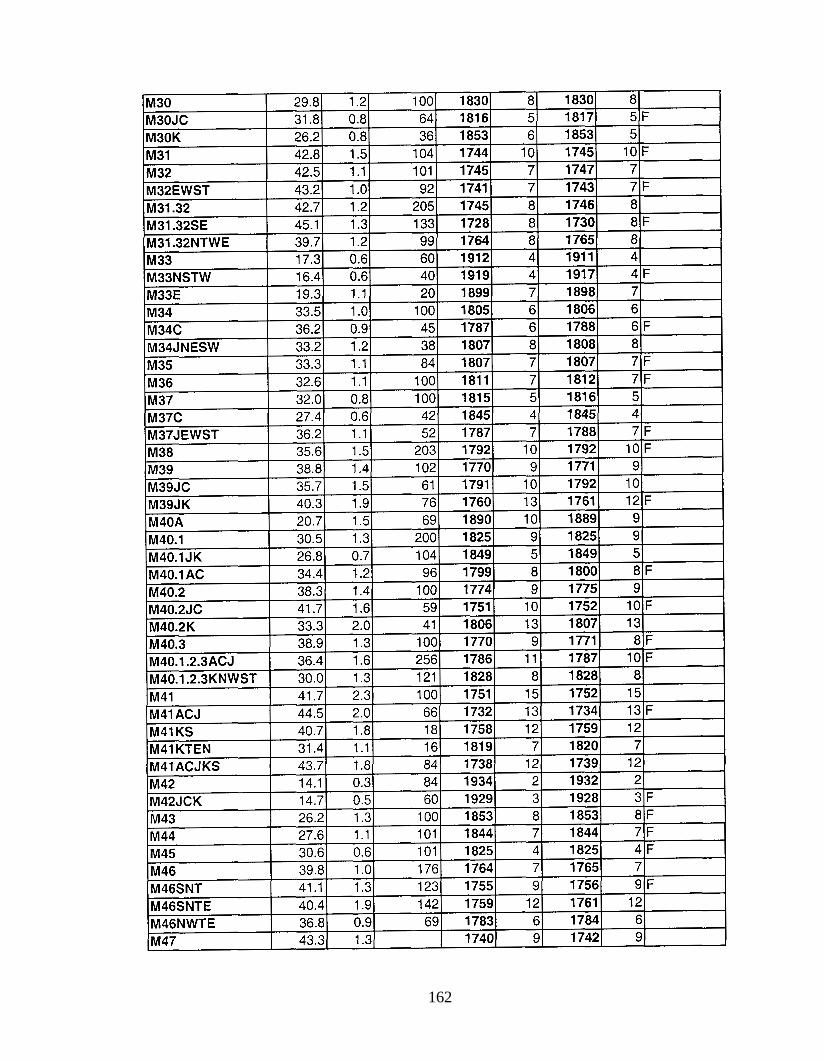
162

163

The letters in the Site name indicate which aspects and operators are included in the data set for that site. The unaltered data sets for each site only have the site number - e.g. M34. H=Hooker Site, N= north, E = east, T=top, S = south, W = west, J= Jessica, C = Colby, K= Katie, T=Tom, A=Adam.
164
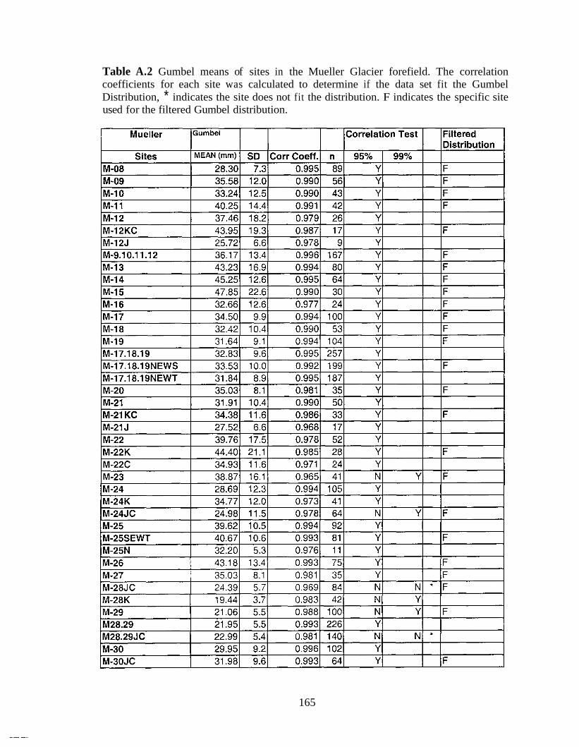
Table A.2 Gumbel means of sites in the Mueller Glacier forefield. The correlation coefficients for each site was calculated to determine if the data set fit the Gumbel Distribution, * indicates the site does not fit the distribution. F indicates the specific site used for the filtered Gumbel distribution.
165

166

L
167

168

The letters in the Site name indicate which aspects and operators are included in the data set for that site. The unaltered data sets for each site only have the site number - e.g. M34. H=Hooker Site, N= north, E = east, T=top, S = south, W = west, J= Jessica, C = Colby, K= Katie, T=Tom, A=Adam.
169

Appendix B: Hooker Lichenometry Results
Hl9SJ 14.5 0.9 34 1931 5.6 1930 5.5 Hl9KST 33.9 2.6 28 1803 17.1 1803 16.8 F H20 31.1 1.9 100 1821 12.4 1821 12.2 F H21 15.9 1.0 100 1922 6.8 1921 6.6
---------.
Table B.l FALL means and ages of sites in the Hooker Glacier forefield. Use 4 8 4 8 for all ages younger than AD 1848. Use >1848 for all ages older than AD 1848 (Bull and Brandon, 1998). Bull and Brandon's (1998) growth curve was used to calculate all ages. The table includes the unaltered data sets for each site as well as the split data sets from the ANOVA tests. F indicates the specific site used for the filtered FALL distribution.
170

H30 H31
The letters in the Site name indicate which aspects and operators are included in the data set for that site. The unaltered data sets for each site only have the site number - e.g. M34. H=Hooker Site, N= north, E = east, T=top, S = south, W = west, J= Jessica, C = Colby, K= Katie, T=Tom, A=Adam.
43.1 3.1 100 1742 20.3 1743 20.01F 59.5 3.1 100 1633 20.5 1637 20.21F
171

Table B.2 Gumbel means of sites in the Mueller Glacier forefield. The correlation coefficients for each site was calculated to determine if the data set fit the Gumbel Distribution, * indicates the site does not fit the distribution. F indicates the specific site used for the filtered Gumbel distribution.
L
H-20 31.3 H-21 16.0
16.91 0.9891 1001Y I IF 6.81 0.9851 1001N IY I I
172

The letters in the Site name indicate which aspects and operators are included in the data set for that site. The unaltered data sets for each site only have the site number - e.g. M34. H=Hooker Site, N= north, E = east, T=top, S = south, W = west, J= Jessica, C = Colby, K= Katie, T=Tom, A=Adam.
173

Appendix E: S-Plus Script for Mulitmodal Normal Distributions
comp <- 5 diameter <- WHF.TomDiams n <- nrow(diameter) data <- cbind(diameter,floor(runif(n, 1, (comp + 0.999)))) dimnames(data) [ [2]] <- c("X","comp")
i <- 0 repeat C unstack <- menuUnstackColumns(target = unstack, target.col.spec = list("<ENDz"), source = data, source.col.spec = list("X"), type = "Group Column", group = "comp" means<-menuDescribe (unstack) [c ( 3 , 9 , 7 ) , I comp <- ncol(means) p <- matrix(O,n,comp) for(j in 1:comp) p[,j] <- dnorm(data[,l],means[l,jl,means[2,jl) p.max <- t(apply(p,l,order)) data[,2l~-p.max[,compl den i- t(apply(p,l,sort)) [,compl loglike <- log(prod(den)) AIC <- loglike - 2*comp + 1 BIC <- loglike - (2*comp + l)*log(n)/2 remove (c ( "unstack" ) ) i < - i + l if (i > 20 I I abs(A1C - AIC.old) < 0.01)
break
AIC.Old <- 0
AIC.Old <- AIC 1
comprop <- means[3,]/n weightmean <- sum(comprop*means[l,1) weightsd <- sqrt(sum((~omprop*means[2,])~2)) 1 i s t ( It A1 C It =A1 C , Is B 1 C I' = B I C , 'I i 'I = i , 'I C omp We i gh t s 'I = c ompr op , I' Means I' =means ,
"WeightAve"=weightmean,"WeightSD"=weightsd)
174

BIOGRAPHY OF THE AUTHOR
Jessica L. Black was born in Tacoma, Washington, on August 11, 1976. She was
raised in Washington; Connecticut; Sydney, Australia; Manila, Philippines; and
Sunnyside, Washington. She graduated from The Taft School in Watertown, Connecticut,
in 1994. Jessica received a Bachelor of Science degree in Geography from the University
of St Andrews in St Andrews, Scotland, in 1998. Jessica also received a Bachelor of Arts
degree in Geology from Wellesley College in Wellesley, Massachusetts, in 1999. After
travelling in Central America, Jessica enrolled in the University of Maine, Orono, and
served as a Research Assistant in the Institute for Quaternary and Climate Studies. Jessica
is a candidate for the Master of Science degree in Quaternary and Climate Studies from
The University of Maine in August, 2001.
175