camera study for mammalian carnivore presence across

Camera Study for Mammalian Carnivore

Presence across Seasons in Montana de Oro State

Park, San Luis Obispo County, CA

Senior Project

Presented to Dr. John D. Perrine

Biological Sciences Department

California Polytechnic State University

San Luis Obispo, CA

In Partial Fulfillment

of the Requirements for the Degree

Bachelor of Science

Environmental Management and Protection

by

Samuel R. Young

Natural Resource Management Department

California Polytechnic State University

San Luis Obispo, CA

June 13, 2011

© 2011 Young

i

Abstract

Montana de Oro (MDO) is one of the largest state parks in California. Little

is known however about its wildlife or their habits. Large predators such as

mountain lion (Puma concolor) and black bear (Ursus americanus), and non–native

species such as red fox (Vulpes vulpes) and feral pig (Sus scropha) are of

management concern because of their potentially dramatic ecological roles.

Cameras were deployed at 5 sites along the Coon Creek hiking trail in spring (May

3–June 7), summer (July 15–August 19), and fall (October 10–November 23)

sessions with the goal of collecting a minimum of 28 survey nights of data. From

this data species richness, latency to first detection, and activity patterns were

examined. Overall, 19 different species of terrestrial vertebrates were detected: 8

species of birds, 11 species of mammals, and 7 species of mammalian carnivores

(including the Virginia opossum (Didelphis virginiana), an introduced marsupial).

Mountain lion was the only species of management concern detected, and it was only

detected once during the summer session. ANVOA testing found no significant

difference in species richness between seasons (α=0.05, P>0.05). Latency to first

detection was too variable for statistical analysis, and there was no apparent trend

for seasonal effect within any species. Daily activity patterns were analyzed using a

chi–squared goodness of fit test (α=0.05) for striped skunk (Mephitis mephitis)

(Pspring=0.41, n=8), mule deer (Odocoileus hemionus) (Pfall=0.03, n=10), and gray fox

(Urocyon cinereoargenteus) (Pspring=0.032, n=16; Psummer<0.001, n=89; Pfall<0.001,

n=59). All tests yielding significant P–values also indicated a preference for

crepuscular activity. Contingency table analysis indicated there was an interaction

between time of day and season for gray fox (P<0.001), with the strongest effect in

dawn and spring, and night and fall. This interaction is unexplained. Lack of

detection of black bear, red fox, and feral pig suggest that they are not present

within the Coon Creek watershed of MDO. Additional studies on a larger spatial

scale are required to determine their status throughout the park. Mountain lion

likewise require further study on a larger scale to determine how they are using

MDO habitat.

ii

Table of Contents

I. Introduction and Purpose ........................................................................ 1

Project Area ......................................................................................... 2

Mountain Lion ..................................................................................... 3

Black Bear............................................................................................ 3

Red Fox ................................................................................................ 4

Feral Pig ............................................................................................... 5

II. Methods ...................................................................................................... 5

Project Development ........................................................................... 5

Site selection ........................................................................................ 5

Camera Deployment ........................................................................... 7

Data Collection .................................................................................... 9

Data Analysis ....................................................................................... 10

III. Results ........................................................................................................ 11

Species Richness .................................................................................. 11

Camera Efficiency ............................................................................... 17

Latency Periods ................................................................................... 18

Activity Patterns.................................................................................. 20

IV. Discussion................................................................................................... 24

Species Richness .................................................................................. 24

Latency Periods ................................................................................... 25

Activity Patterns.................................................................................. 26

V. Conclusions ................................................................................................ 26

VI. Acknowledgments ..................................................................................... 27

VII. Literature Cited ........................................................................................ 28

VIII. Appendices ................................................................................................. 30

Appendix A: Maps .............................................................................. 30

Appendix B: Detection Event and Habitat Utilization Tables ........ 33

1

I. Introduction and Purpose

Montana de Oro (MDO) is one of the larger California Department of Parks and

Recreation (State Parks) properties at more than 8,000 acres in size, and located on

California’s Central Coast in San Luis Obispo County. There is a long history of grazing in

MDO dating back to the 19th century. In 1892 Alden B. Spooner Jr. purchased the land

around Islay Creek; ending a long regime of grazing sheep and ushering in cattle grazing and

dairy operations on the coastal bluffs. In the early 20th century, Alexander S. Hazard who

owned the property just north from the Spooner family planted a Eucalyptus forest in hopes

of producing timber. Unfortunately the timber was unfit for commercial use and was never

harvested. The evidence of Mr. Hazard’s failed venture is still observable today by park

visitors driving through those Eucalyptus rows. Oscar Fields bought the Spooner and Hazard

properties in 1940, and primarily used the area as range land. In 1950 Mr. Fields sold the

properties to Irene McAllister who named the area “Montana de Oro” for the golden wild

flower shows observable during the spring season. In 1965 State Parks purchased the land

from Ms. McAllister and turned it into the state park it is today (Sierra Club, 2010).

The MDO landscape is characterized by rugged sea bluffs, marine terraces, and steep

terrain supporting a variety of vegetation communities from sage brush scrub and chamise

chaparral to dense riparian corridors and coast live oak forests. Access to the inland portions

of the park is primarily limited to a small number of hiking trails (Sierra Club, 2010). The

inland park boundaries border private rural land holdings which continue through steep hilly

terrain vegetated by coastal scrub and coast live oak woodland to the Irish Hills Open Space

managed by the city of San Luis Obispo. Due to constraints of funding availability and task

priority, little research has been performed on the wildlife inhabiting the park or on their

potential movement through the region (Andreano personal com., 2010). State Parks has an

interest in increasing knowledge on wildlife utilization of MDO and their regional

movements with particular regard to large carnivores such as mountain lion (Puma concolor)

and black bear (Ursus americanus) (Andreano personal com., 2010). Mountain lion have

been previously documented within MDO whereas black bear have not (Sierra Club, 2010).

There are unconfirmed observations of black bear sign in private land holdings bordering the

Irish Hills Open Space which has generated interest in determining whether bears are actively

moving between higher elevations of the Coast Ranges where they are known to occur and

areas such as the Irish Hills and MDO (Andreano personal com., 2010). This camera study is

2

intended to function as a pilot to future study with the goals of assessing which species of

mammalian carnivores are present in MDO, whether species richness varies across seasons,

what time period is appropriate for detecting MDO carnivores by camera, and whether

activity patterns in MDO carnivores vary across seasons. Special emphasis is placed on

species of management concern including large predators (mountain lion and black bear) and

non–native species (red fox (Vulpes vulpes) and feral pig (Sus scropha).

Project Area

Map 1. Project area in the Coon Creek Watershed within Montana de Oro

State Park, San Luis Obispo County, CA.

3

The Coon Creek Watershed (Map 1) is a narrow riparian zone bordered by steep

slopes, located in the southern end of MDO. Vegetation consists of coastal scrub

transitioning to semi–closed canopy coast live oak woodland with increasing distance

from the coast on south aspect slopes and low elevations near the riparian corridor.

Riparian areas are densely vegetated by arroyo willow (Salix lasiolepis), American

dogwood (Cornus sericea), and other woody, thicket–forming species. As such mobility

in these areas is likely restricted to breaks in vegetation by larger mammals such as black

bear and mountain lion. Areas characterized by oak woodland or coast scrub do not pose

such barriers to movement, though game trails are observable through the vegetation.

This indicates that there are preferred routes for wildlife movement even through open

coastal scrub vegetation and understory areas in oak woodland.

Mountain Lion

Mountain lions are the largest of California’s cats. They are capable of surviving

in a wide range of habitats and at one time were distributed throughout the Americas

(Verts and Carraway, 1998). Mountain lions have large home ranges (up to 50km2)

making them an excellent umbrella species for conservation planning (Verts and

Carraway, 1998; Thorne, 2006). The public perception that mountain lions pose a danger

to humans is largely exaggerated – there were only ten attacks on humans between 1986

and 1995 in California (Ginsberg, 2001). In reality these large predators tend to avoid

areas of frequent human activity. Muhly et. al. (2011) found that lions (among other

predators) in Alberta, Canada avoided areas that had more than eighteen human visits per

day regardless of prey density. Mountain lions are therefore particularly vulnerable to

habitat fragmentation as urban expansion restricts home range size, habitat connectivity,

and dispersion.

Black Bear

Black bears are associated with early seral stage forest habitats (Verts and

Carraway, 1998). They are known to occur along Santa Lucia Range in San Luis Obispo

County and have been documented utilizing coast live oak and blue oak woodland, mixed

evergreen and coniferous forest, and chamise chaparral as habitat (Forbes, 1982). Black

4

bear did not historically occupy San Luis Obispo County until the early part of the 20th

century after the grizzly bear (Ursus arctos californicus) had been extirpated from the

region (Forbes, 1982). The expansion of the black bear’s range in California has been

largely attributed to relocations of bears by the California Department of Fish and Game

(DFG) particularly in the southern part of the state (Forbes, 1982). The San Luis Obispo

County bear population may originate from natural expansion of bears introduced in

Santa Barbara and/or Monterey Counties; however unauthorized relocation of game for

recreational hunting also may have occurred (Forbes, 1982). Genetic testing has shown

that black bears in the central coast area are most closely related to those of the southern

Sierra Nevada (Brown et al., 2009). This corroborates the findings of Forbes’ (1982)

research on the origins of black bear in coastal California, however Brown (2009) et al.

note that natural expansion (due to competitive release from the extirpation of the grizzly

bear) of black bear range may have had a greater contribution to the central coast

population than artificial relocation. In this scenario maintaining migration corridors

through the central Coast Ranges and the Transverse Ranges is essential to maintaining

the genetic diversity of bears in the central coast region (Brown et al., 2009). Bears are

not currently legal game in San Luis Obispo County, though the DFG is reviewing the

possibility of opening a black bear season (Perrine, personal com, 2010).

Red Fox

Red fox is the most widely distributed terrestrial mammal species second only to

humans (Verts and Carraway, 1998). The European red fox is difficult to distinguish

from the native red fox, usually requiring genetic analysis for distinction (Verts and

Carraway, 1998). Non–native populations can have strongly deleterious impacts on

native prey items, particularly rodents and birds. Top predators such as black bear and

mountain lion are often absent in highly fragmented habitat, which removes competitive

and predation pressure from foxes in these environments. (Harding, 2001). Release from

such biological constraints allows red fox populations to grow larger than they would

otherwise, increasing the impact foxes have on native prey.

5

Feral Pig

Pigs have been introduced worldwide as a popular food item (Waithman et. al.,

1999). Feral pigs are a hybrid between escaped domestic pigs brought by the Spanish in

the 1700s and the Eurasian wild boar which was first introduced to Monterey County in

1925 as game. Introduction of Eurasian wild boar continued in other parts of California

through the 1950s (Waithman et. al., 1999). Feral pigs are particularly damaging to

indigenous communities in that they are vectors of disease, contribute competitive

pressure to native herbivores, and destroy habitat through rooting activity (Waithman et

al., 1999). They have a high reproductive potential and are difficult to track, which

makes eradication efforts challenging (Waithman et al., 1999).

II. Methods

Project Development

The project was developed through scoping project scale and design with Dr.

John D. Perrine, Biological Sciences Department, California Polytechnic State

University; Lisa Andreano, State Parks Resource Ecologist; and Vince Cicero, State

Parks Resource Ecologist. This project consisted of five Cuddeback Excite cameras

placed within the Coon Creek Watershed in MDO. Cameras were placed at strategic

sites along and in the vicinity of the Coon Creek hiking trail for a period of four to six

weeks in spring (May 3 – June 7), summer (July 15 – August 19) and fall seasons

(October 10 – November 23) of 2010. Dates were selected based on operator and camera

availability within the seasons of interest and such that those deployment sessions were at

least four weeks apart. Variation in deployment time was at the discretion of the

operator, with the goal of collecting 28 survey nights of data.

Site Selection

Camera placement sites were established through several preliminary surveys of

the study area. Criteria for site selection consisted of probable detection of mammals

(PDM), feasible operator accessibility (FOA), and low probability of detection by

recreational users of the Coon Creek Trail (LPDP). PDM was evaluated by presence of

6

game trails, abundance of tracks, scat or other sign, and sufficient substrate to

inconspicuously position cameras. FOA was determined by accessibility without

significant risks to the health of the operator, and by spatial proximity such that weekly

data collection was possible within the sunlit hours of a single day. LPDP was assessed

by the ability to place cameras sufficiently high or low such that they remained outside of

a person’s normal field of vision, and sufficient vegetative cover and/or distance from

hiking trails to hide cameras from view.

During preliminary surveys, all mammal sign observed was recorded using a

global positioning system (GPS) capable Topcon unit running Windows CE. GPS data

was taken in the field and placed into an ArcPad map as separate shape files for differing

sign which was later transposed into an ArcGIS layout (Appendix A: Map 2). Photos

were taken at the majority of GPS points recorded. Sites meeting the above criteria were

shown to project advisor Dr. John D. Perrine in the field, who then approved seven of

them as suitable for camera placement (Appendix A: Map 3). These seven sites were

assigned relative index ranks between one and ten based on how well they fit each

criterion in a matrix analysis (Table 1). The top five scoring sites were selected

(Appendix A: Map 4).

Game trails were favored disproportionately to presence of other sign within the

PDM criterion because they indicate regular use over time. Tracks, scat, and browsing

damage to vegetation do not provide such indication if surveys are few in number and are

close in temporal proximity (such as preliminary surveys performed for this study).

Cameras were placed low to the ground and out of site. Vegetative cover was used to

obscure camera position where possible.

7

Table1. Matrix analysis of camera site criteria: probable detection of

mammals (PDM), feasible operator accessibility (FOA), and low probability of

detection by recreational users (LPDP). Each potential site was assigned an index

value between 1 and 10 to rate how well it fit ideal site criteria (1 being poor and 10

being ideal). Index values were summed across categories to generate a suitability

score. The top 5 scoring sites were selected for the study.

PDM FOA LPDP Subtotal Selected

Sites

Potential Site

1

5 7 4 16 Not Selected

Potential Site

2

5 6 8 19 Camera

Site 1

Potential Site

3

8 8 5 21 Camera

Site 2

Potential Site

4

8 8 5 21 Camera

Site 3

Potential Site

5

5 10 3 18 Camera

Site 4

Potential Site

6

5 4 8 17 Camera

Site 5

Potential Site

7

5 3 8 16 Not Selected

Camera Deployment

At each site cameras were fixed to trees by screw fastenings or by stem mounts

fastened to trees. Occasionally brush needed to be cleared for camera installment,

improvement of photo quality, and operator access (specifically regarding sites where

poison oak (Toxicodendron diversilobum) was abundant). This was done such that the

impact to the site was minimal. Clearing did not significantly widen trails, and percent

vegetative cover was not reduced by more than five percent within a fifty foot radius of

the clearing activity.

8

Camera site 1 was located approximately 0.85 miles east from the Coon Creek

trailhead (35º15’14.667”N, 120º52’44.954”W) (WGS 1984). The site was

approximately 17 ft at S50ºW (230º azimuth, declination 14.5º E) from the main hiking

trail along a small obscure game trail characterized by a narrow path through the

understory marked by broken vegetation through a dense semi closed canopy arroyo

willow (Salix lasiolepis) riparian corridor. Vegetation was scattered on the trail,

becoming denser off the trail where black berry (Rubus ursinus) became abundant.


trail head (WGS 84: 35º15’10.337”N, 120º52’31.391”W). The site was approximately

100 ft at N15ºW (345º azimuth, declination 14.5º E) from the main hiking trail along a

well-developed game trail. This trail was one of several that meander through the low

herbaceous understory of the semi closed canopy coast live oak (Quercus agrifolia)

forest, repeatedly intersecting each other. Vegetation was scattered on the game trails

developing close to one hundred percent cover in some off trail areas. False solomon’s

seal (Maianthemum racemosum) was dominant among understory vegetation. Poison oak

(Toxicodendron diversilobum) was also abundant. The camera was installed

approximately 2ft above ground level on a tree trunk (facing away from the main hiking

trail) adjacent to the main game trail.


trailhead (35º14’50.375”N, 120º51’45.512”W). The site was located approximately 330

feet from the main hiking trail at N08ºE (azimuth 8º, declination 14.5ºE). Interweaving,

well developed game trails meandered through the semi closed canopy coast live oak

forest, as observed at camera site 2. Poison oak was dominant among the understory in a

scattered distribution. The camera was installed one to two feet above ground level on a

tree adjacent to the game trail.


trailhead (35º14’43.596”N, 120º51’26.598”W). The site was located approximately 33ft

at S02ºW (azimuth 182°, declination 14.5° E) from the main hiking trail in a small coast

live oak thicket within a clearing vegetated largely by European annual grasses.

Understory within the thicket was sparse with yerba buena (Clinopodium douglasii)

9

forming carpets at the thicket edge. The camera was installed at 1ft above ground level

such that thicket foliage obscured it from the view of the hiking trail.


trailhead (2.51 miles according to sign at trailhead) (35º14’46.215”N, 120º51’19.908”W).

The site was located approximately 330ft at N80ºE from the main hiking trail’s end at the

old Spooner Homestead marked by a grove of Monterey Cypress (Hesperocyparis

macrocarpa). The area was characterized by very steep west and southwest aspect slopes

with interweaving game trails through semi closed canopy coast live oak woodland.

Upper portions of the slope are marked by a sharp ecotone where the coast live oaks give

way to California sagebrush scrub. The camera was placed off of any well-developed

game trails as evidence of human activity was noted during preliminary survey. The

camera was installed less than two feet above ground level to keep it out of the normal

range of view for humans, and was positioned such that the tree trunk obscures it from

view of the nearby game trails. This site was more than 100ft away from the nearest

observed anthropogenic sign.

Data Collection

Cameras were checked on a weekly basis for number of images recorded and

battery life. Compact Flash (CF) Cards containing digital image data were collected from

each camera at each check and replaced with a blank CF card. If battery charge was less

than 75 percent, new batteries were installed. Images were downloaded and examined

for detection event, species detected, number of individuals, date and time of event,

problems with camera position, camera obstructions, indications to camera malfunction

(corrupted files, scrambled images, etc).

Camera sites 4 and 5 were baited with cat food because they were not on a

discernable game trail as the other sites were. Baiting these sites increased the

probability of detecting animals utilizing the local area by attracting them to a sites they

may only visit infrequently otherwise. Other camera sites were located on game trails,

which were assumed to be least cost paths and therefore would concentrate animal

movement making baiting unnecessary. During the summer deployment session data

10

collectors changed the baiting regime to include all sites. The fall deployment session

resumed the former baiting regime.

Data Analysis

Image information was recorded into a Microsoft Excel spreadsheet and sorted by

camera station, species, and time photo was taken. Images of the same species at the

same station that occurred within one hour of each other were considered pseudo–

replicates of the same detection event. The image with the earliest time stamp was used

to represent the event and all other pseudo–replicates were removed from further analysis

unless there were obvious features such as variations in size or markings that

differentiated individuals. Images with multiple individuals were considered to be more

representative of the event than earliest time and were selected for analysis where they

occurred.

Species richness was represented by total number of vertebrate species detected,

number of mammals detected, and by number of carnivores detected. ANOVA and

Tukey Multiple Comparison Test were utilized to test for significant difference in each

category between seasons. Habitat utilization was reported both in terms of number of

detections (after removing pseudo–replicate data) and number of detections per survey

night to standardize data for differences in camera operating time between sites.

Survey nights were determined by subtracting time periods where cameras where

inactive from total deployment time. Inactivity periods were estimated by time

difference between the last clear image to next clear image (or time of camera

replacement) where problems were observed with camera function.

The number of survey nights to first detection (latency period) was calculated for

each species at each station by subtracting time of camera deployment from time of first

detection per species per station. Inactivity periods were accounted for if they occurred

between deployment and first detection. Latency to detection were only calculated for

mammalian carnivores and mule deer.

Detection events were plotted by time (rounded to the nearest hour) for each

species where numbers where large enough for statistical analysis (n2/k > 10) (Zar, 2010).

Plots were generated for striped skunk (Mephitis mephitis) detections during the spring

11

deployment session because number of detections was close to large enough for

meaningful statistical analysis (n2/k = 8). Chi squared goodness of fit was used to assess

whether there were differences in amount of activity between time of day by “dawn”,

“day”, “dusk”, and “night” categories per species. Dawn and dusk were defined as the

time period within two hours on either side of sunrise or sunset respectively. Day and

night were calculated by the amount of time from end–dawn to start–dusk and end–dusk

to start–dawn respectively. Sunrise and sunset times were taken from National Oceanic

and Atmospheric Administration (NOAA) model (NOAA, 2011). Differences in time

category preference between seasons were assessed by a 3x4 contingency table per

species (α=0.05, n/rk>6). Only mammalian carnivores and mule deer were examined for

statistical significance (opossum considered a “carnivore” for the purposes of this

analysis).

IV. Results

Species Richness

Across all seasons 19 different species of vertebrates were detected: 8 species of

birds and 11 species of mammals – 7 of which were mammalian carnivores. Black bear,

red fox, and feral pig were not detected at all. Mountain lion was detected once at site 3

(July 22, 2010 – 1:27) during the summer camera deployment session. All 7 species of

carnivores were detected during the summer deployment session, where as only 3 were

detected during spring and fall sessions (Tables 3–6). Spring and summer sessions

detected 6 to 7 more species than the fall session, but many of these were bird species

(spring birds = 7; summer birds = 5; fall birds = 1) (Tables 3–6).

12

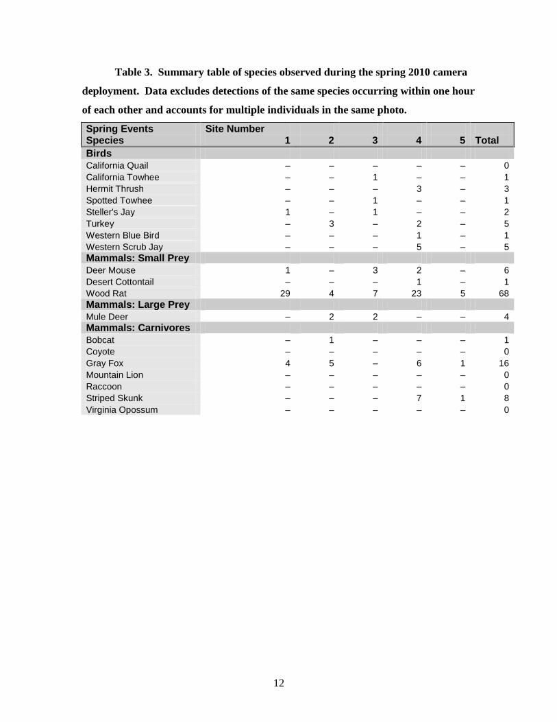
Table 3. Summary table of species observed during the spring 2010 camera

deployment. Data excludes detections of the same species occurring within one hour

of each other and accounts for multiple individuals in the same photo.

Spring Events Site Number Species 1 2 3 4 5 Total

Birds

California Quail – – – – – 0

California Towhee – – 1 – – 1

Hermit Thrush – – – 3 – 3

Spotted Towhee – – 1 – – 1

Steller's Jay 1 – 1 – – 2

Turkey – 3 – 2 – 5

Western Blue Bird – – – 1 – 1

Western Scrub Jay – – – 5 – 5

Mammals: Small Prey

Deer Mouse 1 – 3 2 – 6

Desert Cottontail – – – 1 – 1

Wood Rat 29 4 7 23 5 68

Mammals: Large Prey

Mule Deer – 2 2 – – 4

Mammals: Carnivores

Bobcat – 1 – – – 1

Coyote – – – – – 0

Gray Fox 4 5 – 6 1 16

Mountain Lion – – – – – 0

Raccoon – – – – – 0

Striped Skunk – – – 7 1 8

Virginia Opossum – – – – – 0

13

Table 4. Summary table of species observed during the summer 2010

camera deployment. Data excludes detections of the same species occurring within

one hour of each other and accounts for multiple individuals in the same photo.

Summer Events Site Number Species 1 2 3 4 5 Total

Birds

California Quail 1 – – – – 1

California Towhee – – – – – 0

Hermit Thrush 2 – – 14 – 16

Spotted Towhee – – 3 1 – 4

Steller's Jay – – 1 – – 1

Turkey – – – – – 0

Western Blue Bird – – – – – 0

Western Scrub Jay – – 2 1 – 3

Mammals: Small Prey

Deer Mouse – – 4 1 – 5

Desert Cottontail – – – – – 0

Wood Rat 16 – 21 21 – 58

Mammals: Large Prey

Mule Deer – 9 3 – – 12

Mammals: Carnivores

Bobcat 2 – – – – 2

Coyote – 1 – – – 1

Gray Fox 12 26 27 14 13 92

Mountain Lion – – 1 – – 1

Raccoon 4 – – – – 4

Striped Skunk – – – 1 – 1

Virginia Opossum – – – 5 – 5

14

Table 5. Summary table of species observed during the fall 2010 camera

deployment. Data excludes detections of the same species occurring within one hour

of each other and accounts for multiple individuals in the same photo.

Fall Events Site Number Species 1 2 3 4 5 Total

Birds

California Quail – – – – – 0

California Towhee – – – – – 0

Hermit Thrush 3 – – 3 – 6

Spotted Towhee – – – – – 0

Steller's Jay – – – – – 0

Turkey – – – – – 0

Western Blue Bird – – – – – 0

Western Scrub Jay – – – – – 0

Mammals: Small Prey

Deer Mouse 1 – – – – 1

Desert Cottontail – – – 1 – 1

Wood Rat 20 1 – 2 1 24

Mammals: Large Prey

Mule Deer – 5 1 – 4 10

Mammals: Carnivores

Bobcat 1 – – – – 1

Coyote – – – – – 0

Gray Fox 18 14 2 10 15 59

Mountain Lion – – – – – 0

Raccoon 2 – – – – 2

Striped Skunk – – – – – 0

Virginia Opossum – – – – – 0

15

Table 6. Summary table of number of detections by species per season.

Species Spring Summer Fall

Mammals: Carnivores

Bobcat 1 2 1

Coyote – 1 –

Gray Fox 16 92 59

Mountain Lion – 1 –

Raccoon – 4 2

Striped Skunk 8 1 –

Virginia Opossum – 5 –

Mammals: Large Prey

Mule Deer 4 12 10

Mammals: Small Prey

Deer Mouse 6 5 1

Desert Cottontail 1 – 1

Wood Rat 68 58 24

Birds

California Quail – 1 –

California Towhee 1 – –

Hermit Thrush 3 16 6

Spotted Towhee 1 4 –

Steller's Jay 2 1 –

Turkey 5 – –

Western Blue Bird 1 – –

Western Scrub Jay 5 3 –

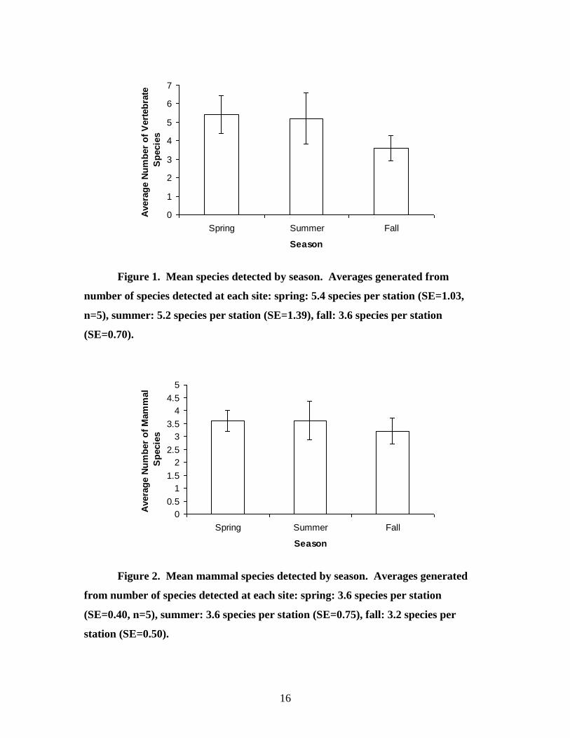
A two–factor ANOVA (α=0.05) was run on species richness between seasons and

time of day. High P–values were yielded for total species (P1=0.33), mammal species

(P2=0.84), and mammalian carnivore species (P3=0.28) between seasons. High P–values

were also generated in each of these categories between time categories (P1=0.13,

P2=0.39, P3=0.40).

16

0

1

2

3

4

5

6

7

Spring Summer Fall

Season

Avera

ge N

um

ber

of

Vert

eb

rate

Sp

ecie

s

Figure 1. Mean species detected by season. Averages generated from

number of species detected at each site: spring: 5.4 species per station (SE=1.03,

n=5), summer: 5.2 species per station (SE=1.39), fall: 3.6 species per station

(SE=0.70).

0

0.5

1

1.5

2

2.5

3

3.5

4

4.5

5

Spring Summer Fall

Season

Avera

ge N

um

ber

of

Mam

mal

Sp

ecie

s

Figure 2. Mean mammal species detected by season. Averages generated

from number of species detected at each site: spring: 3.6 species per station

(SE=0.40, n=5), summer: 3.6 species per station (SE=0.75), fall: 3.2 species per

station (SE=0.50).

17

0

0.5

1

1.5

2

2.5

3

Spring Summer Fall

Season

Avera

ge N

um

ber

of

Carn

ivo

re

Sp

ecie

s

Figure 3. Mean mammalian carnivore species detected by season. Averages

generated from number of species detected at each site: spring: 1.4 species per

station (SE=0.40, n=5), summer: 2.2 species per station (SE=0.37), fall: 1.4 species

per station (SE=0.40).

Table 7. Summary table of total number of detected vertebrate species, total

number of mammal species, and total number of mammalian carnivore species and

percentages relative to absolute total number detected across all seasons.

Season Total Species

Percent of Total (n=19) Mammals

Percent of Total (n=11) Carnivores

Percent of Total (n=7)

Survey Nights

Spring 14 73.68% 7 63.64% 3 42.86% 144

Summer 15 78.95% 10 90.91% 7 100% 162

Fall 8 42.11% 7 63.64% 3 42.86% 153

Camera Efficiency

Camera efficiency was high in all seasons, never falling below 50% (Table 7).

Deployment time was extended for cameras that were determined to be inactive to

attempt to collect data a minimum of 28 survey nights. This was not achieved at station 1

where only 23 survey nights of data were collected during the summer deployment

session and at station 4 where only 9 survey nights of data were collected.

18

Table 7. Camera efficiency at each station by season.

Spring

Station Total Events

Carnivore Events Deployed Retrieved Inactive

Survey Nights

Total Nights Efficiency

1 35 4 5/3/2010 5/31/2010 0 28 28 100.0%

2 15 6 5/3/2010 5/31/2010 0 28 28 100.0%

3 15 0 5/3/2010 5/31/2010 0 28 28 100.0%

4 50 13 5/3/2010 6/7/2010 6 30 36 83.3%

5 7 2 5/3/2010 5/31/2010 0 28 28 100.0%

Summer



Survey Nights


1 37 18 7/15/2010 8/19/2010 12 23 35 64.6%

2 36 27 7/15/2010 8/19/2010 1 34 35 97.1%

3 62 28 7/15/2010 8/19/2010 0 35 35 100.0%

4 58 20 7/15/2010 8/19/2010 0 35 35 100.0%

5 13 13 7/15/2010 8/19/2010 0 35 35 100.0%

Fall



Survey Nights


1 45 21 10/10/2010 11/16/2010 0 37 37 100.0%

2 20 14 10/10/2010 11/16/2010 0 37 37 100.0%

3 3 2 10/10/2010 11/23/2010 15 29 44 65.5%

4 16 10 10/10/2010 10/19/2010 0 9 9 100.0%

5 20 15 10/10/2010 11/16/2010 0 37 37 100.0%

Latency Periods

Latency periods ranged from as low as 1 survey night (multiple species, all

camera deployment sessions) to 28 survey nights (Virginia opossum, summer

deployment session). In the spring deployment session 4 of the 8 species examined were

detected, 3 of which were detected within one survey night (Table 4). Gray fox (Urocyon

cinereoargenteus) latency ranged from 1 to 13 survey nights (16 detection events at 4

sites), mule deer (Odocoileus hemionus) from 1 to 3 survey nights (4 detection events at 2

sites), and striped skunk from 1 to 25 survey nights (8 detection events at 2 sites). Bobcat

(Lynx rufus) was only represented by one detection event (4 days to detection).

The summer deployment session detected all 8 of the species examined, only one

of which was detected within one survey night (Table 5). Mountain lion was detected

after 7 survey nights at site 3, but was not detected again. Only gray fox and mule deer

19

were detected at more than one site with ranges in latency from 2 to 5 (89 events at 5

sites) and 1 to 4 survey nights (10 events at 2 sites) respectively.

The fall deployment session detected 4 of the eight species examined with 2 of

them occurring within one survey night (Table 6). Only gray fox and mule deer were

detected at more than one site with ranges in latency from 1 to 10 (59 events at 5 sites)

and 1 to 21 survey nights (10 events at 3 sites) respectively.

Table 4. Latency to first detection for the spring camera deployment session.

Nights inactive occurred between May 4 and 9 before the first detection of striped

skunk at site 4.

Nights to First Detection

Site Number

Species 1 2 3 4 5 Average SD Min Max

Bobcat - 4 - - - 4.00 - 4 4

Coyote - - - - - - - - -

Gray Fox 3 2 - 1 13 4.75 5.56 1 13

Mountain Lion - - - - - - - - -

Mule Deer - 1 3 - - 2.00 1.41 1 3

Raccoon - - - - - - - - -

Striped Skunk - - - 1 25 13.00 16.97 1 25 Virginia Opossum - - - - - - - - -

Table 5. Latency to first detection for the summer camera deployment

session. Nights inactive occurred between July 19 and 23 before the first detection

of bobcat at site 1, and between July 19 and 23, July 23 and 27, and July 28 and

August 2 before first detection of raccoon at site 1.


Site Number

Species 1 2 3 4 5 Average SD Min Max

Bobcat 5 - - - - 5.00 - 5 5

Coyote - 4 - - - 4.00 - 4 4

Gray Fox 5 2 2 2 4 3.00 1.41 2 5

Mountain Lion - - 7 - - 7.00 - 7 7

Mule Deer - 4 1 - - 2.50 2.12 1 4

Raccoon 14 - - - - 14.00 - 14 14

Striped Skunk - - - 13 - 13.00 - 13 13 Virginia Opossum - - - 28 - 28.00 - 28 28

20

Table 6. Latency to first detection for the fall camera deployment session.

Nights inactive occurred between October 26 and November 10 before the first

detection of mule deer at site 3.


Site Number

Species 1 2 3 4 5 Average SD

Min

Max

Bobcat 5 - - - - 5 - 5 5

Coyote - - - - - - - - -

Gray Fox 1 4 5 1 10 4.2 3.70 1 10

Mountain Lion - - - - - - - - -

Mule Deer - 1 21 - 2 8 11.27 1 21

Raccoon 14 - - - - 14 - 14 14

Striped Skunk - - - - - - - - -

Virginia Opossum - - - - - - - - -

Activity Patterns

Mountain Lion was only detected once at site three at 1:27. No further analysis

could be performed.

Spring detections of striped skunk met chi–squared goodness of fit test

assumptions, but was found not to differ significantly from expected frequency by time of

day (P=0.41, n=8).

Mule deer only had a large enough number of detections to meet goodness of fit

test assumptions during the summer and fall seasons (n=10 for both seasons). No

significant deviation from the expected frequency by time of day was found for the

summer deployment session (P=0.196), however goodness of fit test on fall detection did

have observed values that significantly deviated from the expected frequency (P=0.031).

The largest contributing factors were “Night” (χ2 = 4.615, observed greater than

expected) and “Day” (χ 2

= 4.105, observed lower than expected).

21

0.0%

5.0%

10.0%

15.0%

20.0%

25.0%

30.0%

0:00 2:00 4:00 6:00 8:00 10:00 12:00 14:00 16:00 18:00 20:00 22:00

Time of Day

Percen

t o

f V

isit

ati

on

Even

ts

Figure 4. Number of striped skunk visitation events detected during the

spring deployment session. Activity appears to be concentrated in “dawn”

(2:53<t<6:53), “dusk”(17:00<t<21:00), and “night”(t<2:53, t>21:00) time categories,

with one detection in “day” (6:53<t<17:00). Goodness of fit test suggests no

significant difference from random selection of time period (P=0.41, n=8).

0.0%

5.0%

10.0%

15.0%

20.0%

25.0%

30.0%

0:00 2:00 4:00 6:00 8:00 10:00 12:00 14:00 16:00 18:00 20:00 22:00

Time of Day

Pe

rcen

t o

f V

isit

ati

on

Ev

en

ts

Fall

Summer

Spring

Figure 5. Mule deer activity by time of day for each seasonal camera

deployment session. There is no significant difference in frequency distribution

between time categories except for during fall deployment (P=0.0313, n=10).

22

Gray fox was the only species examined with high enough detection event counts

to meet the assumptions for performing chi squared goodness of fit test for time of day

preference for all three seasons. Spring, summer, and fall detections for gray fox were

found to be different from the expected occurrence frequency by time of day

(Pspring=0.032, n=16; Psummer<0.001, n=89; Pfall<0.001, n=59). Contributing factors to

deviation from expected frequency somewhat varied across seasons (“Day” second

largest contributor in all seasons). The largest contributing factors during the spring

deployment session were “Dawn” (χ 2

= 4.167, observed greater than expected) and

“Day” (χ 2

= 3.34, observed lower than expected), summer were “Dusk” (χ 2

= 11.687,

observed greater than expected) and “Day” (χ 2

= 9.402, observed less then expected), and

fall were “Night” (χ 2

= 13.734, observed greater than expected) and “Day” (χ 2

= 9.837,

observed less than expected).

0.0%

5.0%

10.0%

15.0%

20.0%

25.0%

0:00 2:00 4:00 6:00 8:00 10:00 12:00 14:00 16:00 18:00 20:00 22:00

Time of Day

Pe

rcen

t o

f V

isit

ati

on

Ev

en

ts

Fall

Summer

Spring

Figure 6. Gray fox activity by time of day. Activity measured by number of

detection events rounded to the nearest hour. Seasons tend to follow similar

patterns with all having lowest values during “Day” (4:18<t<8:18) and peak activity

occurring in “Dawn” (2:53<t<6:53) during spring, “Dusk” (17:01<t<21:01) during

summer, and “Night” (t<4:18, t>19:10) during fall.

23

Only gray fox detection had large enough value (n=164) to meet the assumptions

for running a chi–squared contingency table analysis. An interaction was detected

between time of day and season variables. The largest contributing factors to this were in

“Dawn” and spring (χ 2

= 6.92, observed greater than expected) and in between “Night”

and fall (χ 2

= 4.72, observed greater than expected).

Table 7. Contingency table assessing interdependence of the variables time

of day and season for gray fox. Low P–value indicates that there is an interaction

between the two (α=0.05). χ2

values indicate that the dawn in spring and night in fall

are the strongest contributors to this effect.

Gray Fox Dawn Day Dusk Night Total Proportion

Observed

Spring 6 2 2 6 16 0.098

Summer 10 18 28 33 89 0.543

Fall 6 4 9 40 59 0.360

Total 22 24 39 79 164 1

Proportion 0.134 0.146 0.238 0.482 1

Expected

Spring 2.146 2.341 3.805 7.707 16

Summer 11.939 13.024 21.165 42.872 89

Fall 7.915 8.634 14.030 28.421 59

Total 22 24 39 79 164

P 0.0004

X^2

Spring 6.919 0.050 0.856 0.378 8.203

Summer 0.315 1.901 2.208 2.273 6.696

Fall 0.463 2.487 1.804 4.718 9.472

Total 7.697 4.438 4.867 7.369 24.371

Gray fox were documented to prey upon wood rat (Neotoma spp.) and deer mouse

(Peromyscus spp.) during the study. To attempt to explain the interaction between time

of day and season variables described above, wood rat and deer mouse detections were

lumped together as “rodent” detections and tested using chi–squared goodness of fit test

for activity preference by time of day and for and interaction between season and time of

day variables. Goodness of fit testing yielded significant deviation from the expected

distribution of detections (Pspring<0.001, n=71; Psummer<0.001, n=62; Pfall<0.001, n=25)

with “night” being the largest contributing factor (χ2

spring=85.7, χ2

summer=66.6, χ2

fall=36.1).

Observed detections at night were much greater than expected in all seasons.

24

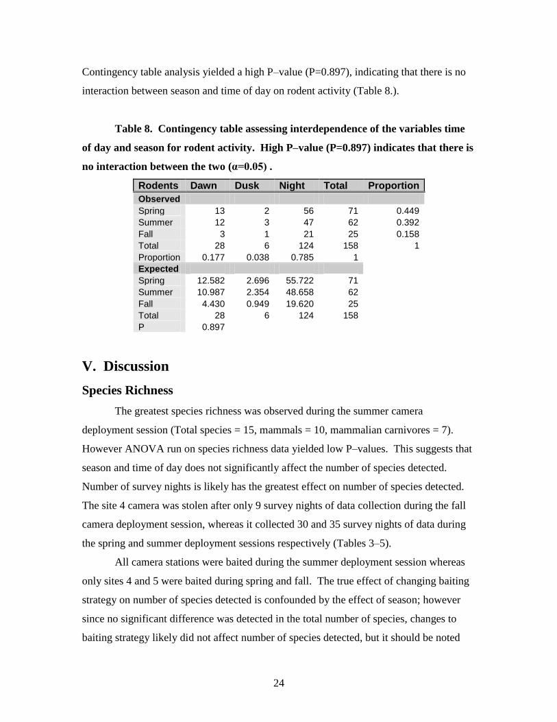
Contingency table analysis yielded a high P–value (P=0.897), indicating that there is no

interaction between season and time of day on rodent activity (Table 8.).

Table 8. Contingency table assessing interdependence of the variables time

of day and season for rodent activity. High P–value (P=0.897) indicates that there is

no interaction between the two (α=0.05) .

Rodents Dawn Dusk Night Total Proportion

Observed

Spring 13 2 56 71 0.449

Summer 12 3 47 62 0.392

Fall 3 1 21 25 0.158

Total 28 6 124 158 1

Proportion 0.177 0.038 0.785 1

Expected

Spring 12.582 2.696 55.722 71

Summer 10.987 2.354 48.658 62

Fall 4.430 0.949 19.620 25

Total 28 6 124 158

P 0.897

V. Discussion

Species Richness

The greatest species richness was observed during the summer camera

deployment session (Total species = 15, mammals = 10, mammalian carnivores = 7).

However ANOVA run on species richness data yielded low P–values. This suggests that

season and time of day does not significantly affect the number of species detected.

Number of survey nights is likely has the greatest effect on number of species detected.

The site 4 camera was stolen after only 9 survey nights of data collection during the fall

camera deployment session, whereas it collected 30 and 35 survey nights of data during

the spring and summer deployment sessions respectively (Tables 3–5).

All camera stations were baited during the summer deployment session whereas

only sites 4 and 5 were baited during spring and fall. The true effect of changing baiting

strategy on number of species detected is confounded by the effect of season; however

since no significant difference was detected in the total number of species, changes to

baiting strategy likely did not affect number of species detected, but it should be noted

25

that baiting may significantly affect individual species. A paired study is required to

truly assess the effect of baiting on camera efficacy and efficiency in MDO.

Mountain lion was the only species of management concern detected during the

study. It was only detected once during the summer camera deployment session. It is

unclear whether coon creek contains part of the mountain lion’s home range or if this was

an individual which just happened to be passing by. Further study on a larger spatial

scale is required to gather more information on mountain lion use on MDO habitat.

Black bear were not detected during any of the camera deployment sessions. This

suggests that black bear are at least not present in the Coon Creek Watershed area of

MDO. There are a number of barriers such as highway 101, and dense scrub and

chaparral vegetation separating MDO from the nearest known population in the Santa

Lucia range. This makes unassisted dispersal of black bear into MDO seemingly

unlikely, however modeling is required to support this hypothesis. Red fox and feral pigs

were likewise not detected during the study, possibly for the similar reasons.

Latency Periods

Of the 19 species detected only 8 were analyzed for seasonal patterns in latency to

first detection. This included all 7 mammalian carnivores and mule deer. Latency

varied so widely within each species that meaningful statistical analyses could not be

performed. Of the 8 mammal species examined, only three were detected in each

deployment session: bobcat, gray fox, and mule deer. Latency to detection appeared to

be longer generally in the fall than the summer or spring (Figures 6–8). There was no

clear trend to variation between summer and spring, indicating that change in baiting

regime may not have improved survey efficiency for these species. Differences between

summer and fall are confounded as to whether variations latency periods were due to the

changed baiting regime or time of year. Spring latency periods tended to be shorter than

in fall with the same baiting regime in each session, which suggests greater efficiency

may be achieved by spring deployment rather than fall. Further study is needed to collect

a robust enough data set to test for statistically significant seasonal difference in latency

to detection.

26

Activity Patterns

Numbers of detection events were generally too low for statistical tests for

activity preference by time of day, except for the striped skunk, mule deer, and gray fox.

Gray fox was the only species with a sufficiently large number of detections for

contingency table analysis and is therefore the focus for discussion. Findings suggested

preference for dawn in spring, dusk in summer, and night in fall. All gray fox

demonstrated avoidance of activity during the day time. This matches with the known

crepuscular habits of the grey fox (Verts and Carraway, 1998). Contingency table

analysis indicated there was an interaction between the time of day and season variables

with the strongest effects contributed by an interaction of “dawn” and “spring” and in

“night” and “fall”. This may represent a seasonal shift in resources such as prey, changes

to competitive and/or predation pressure. Gray fox were documented to use rodents as

prey items, so rodent detections were examined to attempt to account for seasonal

variation in activity preference by time of day. Contingency table analysis of rodent

(woodrat and deer mouse) detections by time of day yielded a large P–value (P=0.897),

indicating that there is not an interaction between season and time of day for rodent

activity. There may be a food source preferred over rodents that becomes less available

over the course of the year from spring to fall. Preference for dawn in the spring may

also have a reproductive motivation. There may also be shifts in competitive pressure

from other canids/predation pressure from larger carnivores across seasons, however

there were too few detection events to perform analysis on seasonal activity for other

carnivore species. Further study is needed to comprehensively assess the observed

interaction between season and time of day for gray fox.

VI. Conclusions

Detection of seasonal patterns in species richness, latency periods, and shits in

activity–time preference require a larger data set for most species. Seasonal activity

analysis for gray fox was possible because they are common enough to detect with a

small number of cameras (n=5) within a small area (within 100m of the Cook Creek

Trail). Such data sets may be collected through deployment of more cameras distributed

over a larger area. Multiple data collection techniques may also improve detection

27

efficiency. Using other tools, such as track plates, in conjunction with cameras will

likely improve detection efficiency which can be calibrated between media by

comparison of latency to first detection (Gompper et al., 2006).

Black bear, red fox and feral pig are likely not present in the coon creek

watershed, and mountain lion likely only visit the area infrequently. Expanding the study

across multiple watersheds and incorporating multiple detection tools as recommended

by Gompper et al. (2006) will yield more conclusive information on if and how these

species are utilizing MDO habitat.

VII. Acknowledgements

Materials and guidance for this project were provided by Dr. John D. Perrine who

was the principle advisor for the project. Lisa Andreano and Vince Cicero (State Parks

Resource Ecologists) provided support and consult during project design and

implementation. Sarah Snyder (California Polytechnic State University graduate student)

and Stephanie Klein (State Parks intern) were primary data collectors during the summer

deployment session, which would not have been possible without their help.

28

VIII. Literature Cited

(Anonymous). Montana de Oro State Park. 2010. Sierra Club Santa Lucia Chapter. 9

May 2010 <http://santalucia.sierraclub.org/mntdeoro.html#intro>.

(Anonymous). Solar Calculation Details. 2011. National Oceanic and Atmospheric

Administration. 9 May 2011.

<http://www.srrb.noaa.gov/highlights/sunrise/calcdetails.html>

Brown, Sarah K., Hull, Joshua M., Updike, Douglas R., Fain, Steven R., Ernest, Holly B.

2009. “Black Bear Population Genetics in California: Signatures of Population

Structure, Competitive Release, and Historical Translocation.” Journal of

Mammalogy. 90 (5):1066–1074.

Forbes, Gregory A. 1982. The Black Bear (Ursus americanus) in California. Thesis. San

Luis Obispo: California Polytechnic State University.

Ginsberg, Joshua R. 2001. “Setting Priorities for Carnivore Conservation: What Makes

Carnivores Different?.” Carnivore Conservation. Ed. John L. Gittleman, Stephen

M. Funk, David Macdonald, and Robert K. Wayne. Cambridge: Cambridge

University Press. 498-523.

Gompper, Matthew E, Kays, Roland W., Ray, Justina C., Lapoint, Scott D., Bogan,

Daniel A., Cryan, Jason R. 2006. “A Comparison of Non– Invasive Techniques

to Survey Carnivore Communities in Northeastern North America.” Wildlife

Society Bulletin. 34(4): 1142-1151.

Harding, Elaine K, Daniel F. Doak, and Joy D. Albertson. 2001. “Evaluating the

Effectiveness of Predator Control: the Non–Native Red Fox as a Case

Study.” Conservation Biology 15(4): 1114-1122.

Muhly, Tyler B., Semeniuk, C., Massolo, A., Hickman, L., Musiani, M. 2011. “Human

Activity Helps Prey Win the Predator–Prey Space Race.” PLos ONE. 6(3):

e17050.doi:10.1371/journal.pone.0017050.

http://santalucia.sierraclub.org/mntdeoro.html#intro

http://www.srrb.noaa.gov/highlights/sunrise/calcdetails.html

29

Thorne, James H, Dick Cameron, and James F. Quinn. 2006. “A Conservation Design for

the Central Coast of California and the Evaluation of Mountain Lion as an

Umbrella Species.” Natural Areas Journal. 26(2): 137-148.

Verts, B. J and Leslie N. Carraway. 1998. Land Mammals of Oregon. Berkeley:

University of California Press.

Waithman, John D., Sweitzer, Richard A., van Vuren, Dirk, Drew, John D., Brinkhaus,

Amy J., Gardner, Ian A., Boyce, Walter M. 1999. “Range Expansion, Population

Sizes, and Management of Wild Pigs in California.” The Journal of Wildlife

Management. 63(1): 298-308

Zar, Jerrold H. 2010. Biostatistical Analysis 5th Ed.. Upper Saddle River, New Jersey:

Pearson.

30

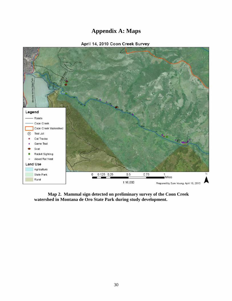
Appendix A: Maps

Map 2. Mammal sign detected on preliminary survey of the Coon Creek

watershed in Montana de Oro State Park during study development.

31

Map 3. Potential camera sites examined in the Coon Creek watershed in

Montana de Oro State Park during placement site selection. Sites 2 through 6 were

selected for the study based on matrix analysis of attributes (Table 1.)

32

Map 4. Camera sites selected for the study within the Coon Creek watershed

in Montana de Oro State Park.

33

Appendix B: Site Utilization Data

0

0.5

1

1.5

Mule

Dee

r

Bob

cat

Coy

ote

Gra

y Fo

x

Mou

ntain

Lion

Rac

coon

Stri

ped

Sku

nk

Virg

inia O

poss

um

Species

Dete

cti

on

s/S

urv

ey N

igh

t

Sping

Summer

Fall

Figure 7. Average site utilization in each season by species. Utilization

measured in number of individual detections divided by the number of survey

nights the camera was collecting data for.

Table 9. Site utilization by species per station during the spring 2010

deployment session. Utilization measured in number of individual detections

divided by the number of survey nights the camera was collecting data for.

Site Number

Species 1 2 3 4 5 Total Average SD SE

Bobcat 0 0.034 0 0 0 0.034 0.011 0.016 0.007

Coyote 0 0 0 0 0 0 0 0 0

Gray Fox 0.138 0.172 0 0.200 0.036 0.546 0.182 0.178 0.079

Mountain Lion 0 0 0 0 0 0 0 0 0

Mule Deer 0 0.069 0.071 0 0 0.140 0.047 0.052 0.023

Raccoon 0 0 0 0 0 0 0 0 0

Striped Skunk 0 0 0 0.233 0.036 0.269 0.090 0.115 0.052 Virginia Opossum 0 0 0 0 0 0 0 0 0

34

Photo1. Bobcat detected at site 2 during the spring camera deployment

session. This was the only bobcat detection in the spring session

Table 10. Site utilization by species per station during the summer 2010



Site Number


Bobcat 0.087 0 0 0 0 0.087 0.029 0.041 0.018

Coyote 0 0.029 0 0 0 0.029 0.010 0.014 0.006

Gray Fox 0.522 0.765 0.771 0.400 0.371 2.829 0.943 0.858 0.384

Mountain Lion 0 0 0.029 0 0 0.029 0.010 0.013 0.006

Mule Deer 0 0.265 0.086 0 0 0.350 0.117 0.140 0.063

Raccoon 0.174 0 0 0 0 0.174 0.058 0.082 0.037

Striped Skunk 0 0 0 0.029 0 0.029 0.010 0.013 0.006 Virginia Opossum 0 0 0 0.143 0 0.143 0.048 0.067 0.030

35

Photo 2. Mountain Lion detected at site 3 during the summer camera

deployment session. This was the only mountain lion detected during the entire

study.

Table 11. Site utilization by species per station during the fall 2010



Site Number


Bobcat 0.026 0 0 0 0 0.026 0.009 0.012 0.006

Coyote 0 0 0 0 0 0 0 0 0

Gray Fox 0.474 0.368 0.069 1.000 0.395 2.306 0.769 0.741 0.331

Mountain Lion 0 0 0 0 0 0 0 0 0

Mule Deer 0 0.132 0.034 0 0.105 0.271 0.090 0.095 0.042

Raccoon 0.053 0 0 0 0 0.053 0.018 0.025 0.011

Striped Skunk 0 0 0 0 0 0 0 0 0

Virginia Opossum 0 0 0 0 0 0 0 0 0

36

Photo 3. Gray fox detected at site 1 during the fall camera deployment

session. Gray fox was the most commonly detected carnivore in the study, and the

second most commonly detected mammal.

camera study for mammalian carnivore presence across

Documents