cambridge-inet institute · cambridge-inet institute faculty of economics . information acquisition...

Cambridge-INET Working Paper Series No: 2015/23

Cambridge Working Paper in Economics: 1566

INFORMATION ACQUISITION AND EXCHANGE IN

SOCIAL NETWORKS

Sanjeev Goyal Stephanie Rosenkranz Utz Weitzel Vincent Buskens (University of Cambridge) (Utrecht University) (Utrecht University) (Utrecht University)

A central feature of social networks is information sharing. The Internet and related computing technologies define the relative costs of private information acquisition and forming links with others. This paper presents an experiment on the effects of changing costs. We find that a decline in relative costs of linking makes private investments more dispersed and gives rise to denser social networks. Aggregate investment falls, but individuals access to investment remains stable, due to increased networking. The overall effect is a significant increase in individual utility and aggregate welfare.

Cambridge-INET Institute

Faculty of Economics

Information Acquisition and Exchange in

Social Networks

Sanjeev Goyal∗ Stephanie Rosenkranz†

Utz Weitzel‡ Vincent Buskens§

September 6, 2015

A central feature of social networks is information sharing. The Internetand related computing technologies de�ne the relative costs of private infor-mation acquisition and forming links with others. This paper presents anexperiment on the e�ects of changing costs.

We �nd that a decline in relative costs of linking makes private invest-ments more dispersed and gives rise to denser social networks. Aggregateinvestment falls, but individuals access to investment remains stable, due toincreased networking. The overall e�ect is a signi�cant increase in individualutility and aggregate welfare.

∗Faculty of Economics and Christ's College, University of Cambridge. Email:[email protected]†Department of Economics, Utrecht University. Email: [email protected]‡Department of Economics, Utrecht University, and Department of Economics, Rad-

boud University Nijmegen. Email: [email protected]§Department of Sociology, Utrecht University. Email: [email protected]

We are grateful to the Editor, Martin Cripps, and three anonymous referees for commentsthat have signi�cantly improved the paper. We also thank Nicolas Carayol, Syngjoo Choi,Matthew Elliott, Edoardo Gallo, Ben Golub, Friederike Mengel, Francesco Nava, RomansPancs, Pauline Rutsaert, Vessela Daskalova and seminar participants at ASSET 2012,Stockholm, ESA 2012, Cologne, Bordeaux, Cambridge, Rotterdam and Cape Town forhelpful comments. The paper was circulated as a working paper in 2012 with the title"Individual search and social communication".

1 Introduction

Individuals (and organizations) acquire information privately and by form-ing communication links with others. Private acquisition of information iscostly; similarly, creating and maintaining personal contacts takes time andresources. The development of modern information technology creates a plat-form for extensive on-line social engagement: it has a major impact on therelative cost of these two ways of accessing information. The goal of thispaper is to empirically study the economic e�ects of this change.1

We use laboratory experiments to study this trade-o� as they allow usto control the main variables directly: the costs and bene�ts of linking andof individual public good provision. We can study causal determinants ofthe processes at work. Moreover, we can measure the provision of the publicgood and the welfare implications explicitly.

The theoretical framework for our experiment is taken from Galeotti andGoyal (2010). In their model, individuals choose a level of investment givenby xi, and the number of links with others, given by ηi. Investments take ona general form and are naturally interpreted as a local public good.2 Indi-vidual investment is costly: each unit of investment costs c > 0. Similarly,linking activity is costly: each link costs k > 0. Furthermore, investmentactivity of di�erent individuals is substitutable: the marginal utility of owninvestment is falling in the investment level of connected others. De�ne y asthe investment an isolated individual would make.

Galeotti and Goyal (2010) show that every (strict) Nash equilibrium ofthis game is characterized by investment sharing. The theory yields sharppredictions on some dimensions: every individual must access y investment(own investment and investment from others) and total investment by soci-ety must also be equal to y, independently of the linking costs. The theoryis permissive on other dimensions: a variety of networks and distribution ofindividual investments levels can be sustained in equilibrium. For instance,at low costs of linking, there exists an equilibrium with a single hub playeracquiring y and all other players forming links to him/her. But there is

1For a wide ranging overview of the economics of modern information technology, seePeitz and Waldfogel (2012). For a study of the information �ows and their impact oninter�rm collaboration links, see Frankort et al (2012).

2This framework combines an approach to network formation introduced in Goyal(1993) and Bala and Goyal (2000) with a model of local public good provision in �xednetworks taken from Bramoulle and Kranton (2007).

1

another equilibrium in which all players make investments and are fully con-nected with each other. On the other hand, at high costs of linking, only thesingle hub outcome is sustainable in equilibrium. One of the main questionsof interest is the impact of changing linkage costs on welfare. It is easy to seethat welfare impact depends crucially on which equilibrium is played at lowcosts. Roughly speaking, the welfare improvements are larger if the singlehub equilibrium is played across the di�erent linkage costs, but are mutedif the multiple hub equilibrium is played at low costs.3 This multiplicity inequilibrium outcomes is thus an important motivation for our experimentalwork.

We conduct a range of experiments with groups of four subjects. To ac-commodate the complexity of the strategic structure of the game and to giveplayers ample opportunities for learning we run the experiment in continuoustime. Subjects can make choices and revise them over time and we have arandom termination time.

We start with homogenous costs of investment, c, and low costs for links,k. We then compute the level of y. In the experiment, we �nd that allsubjects indeed have access to y units of investment. Total investment insociety is much lower than 4× y: so there is extensive sharing of investments.In line with theory, individual investments and the number of in-coming linksare positively correlated.

We then turn to the e�ects of changing costs of linking. As we raiselinking costs, the theory predicts that y remains unchanged. However, at ahigher linking cost, a person must obtain more investment for the link to bejusti�ed. Given that total investment is constant (across linkage costs), thisimplies that there will be fewer hubs and also fewer links. In the experiment,we �nd that subjects act very much in line with each of these predictions:the number of hubs and links fall as we raise linking costs, while hubs raisetheir investment. Individuals access y units of investment on average, at allcost levels.

Next we consider a setting with heterogeneity in costs of investment. Thelow-cost player i's stand-alone optimal investment is y1 > y. The uniqueequilibrium network has the star architecture with the low-cost player asthe hub, independently of the linking costs. In the experiment we randomly

3We note that equilibrium total investment is constant across linkage costs, but thatthe number of links vary from n − 1 (in the hub-spoke (star) network) all the way ton(n− 1)/2 (in the fully connected (complete) network).

2

determined one player in each group to have lower costs. We see indeed thatthis low-cost player is more likely to be the hub and that individuals access y1units of investment on average, at all cost levels. The macroscopic patternswith regard to linking costs exhibit the same pattern as in the homogenoustreatments: the number of hubs and links fall as we raise linking costs, whileaverage investment by hubs rises.

One important prediction of the theory, in both the homogenous and theheterogeneous cost treatments, is that total investment acquired is invariantwith respect to linking costs. In the experiment, we �nd that aggregateinvestment is higher than predicted and that it increases with linking costs.We develop an explanation for these two departures from the theory. The�rst point to note is that in the original model of Galeotti and Goyal (2010),players make their choices simultaneously. By contrast, in the experiment,players make choices sequentially and repeatedly, and there is an uncertainend point. We focus on this di�erence: the main idea we explore is that,toward the end of the game, players explore small and local moves to improvetheir payo�s. A strategy pro�le is said to be stable if there exists no smalland local deviation that is pro�table, in this sense.

An important feature of the equilibrium outcome in the static game is thatthe hub player makes large investments while the peripheral nodes make zeroinvestments and form links with the hub. In a dynamic setting, the hub canshade his investment downward, in anticipation of a potential upward shiftin the investment by the peripheral player. The extent of downward shadingis constrained by the threat of a link deletion by peripheral player. Ouranalysis explores the bounds on the shading and the level of investments bythe peripheral players. We note that in this situation, the peripheral playerwill choose an investment level that is optimal given the hub's investmentchoice (so investment accessed by the peripheral player must be y). On theother hand, as the hub potentially has access to multiple peripheral players,he/she accesses investment in excess of the static equilibrium level y. Thisprovides an account for higher than static equilibrium investments in theexperiment. Building on these considerations, we also show that higher costsof linking imply higher aggregate investments.

The �nal major �nding concerns the welfare implications of changes incosts of links. In the homogenous cost case (when all players have the samecosts of investment), at high linking costs, there is a unique equilibrium witha single hub. However, at lower linking costs in addition to the single huboutcome, there also exist other equilibrium outcomes, with multiple hubs

3

and more links. So the theoretical predictions on individual and aggregatewelfare are a priori ambiguous. The data from the experiment yields twoclear cut �ndings. Aggregate earnings are below the (least e�cient) Nashequilibrium prediction in all cases. However, they are falling signi�cantly inlinking costs.4

To summarize, our experimental subjects behave in line with the predic-tions of the theory with regard to total investment accessed by an individualplayer and on the presence of signi�cant linking and investment sharing. Theexperiment, however, goes beyond the theory in one important dimension:it shows that as linking costs fall, investment is more dispersed and it is ac-companied by denser social networks. This has interesting and large e�ectson welfare. Finally, the experiment also yields an important departure fromthe theory: aggregate investment is sensitive to costs of linking.

Our paper is a contribution to the literature on public goods and net-works. In the literature on public goods experiments, an important general�nding is that individuals contribute more than what theory predicts thoughthey contribute less than the �rst best; for surveys, see Ledyard (1995), Cro-son (2010), and Holt and Laury (2012). Thus individual utility is generallyhigher than the Nash equilibrium level. The principal novelty in the presentpaper is that individual choices determine whether their actions and oth-ers' actions become public goods or remain `private'. This is accomplishedthrough the formation of links. The experiment reveals that this `endogene-ity' of public goods has important implications for behavior and welfare.With increasing linking costs the aggregate investment in the `public' goodrises, but due to lower linking, every individual has access to the same amountof it. Moreover, in all treatments, endogeneity of links leads to outcomes thatare worse than the worst Nash equilibrium (in terms of aggregate welfare).

Our paper is also a contribution to the study of social networks. Thereis now a large theoretical literature on social networks but the empiricalassessment of networks in economic activity remains a challenge. This moti-vates the recent experiments on networks (Charness, Corominas-Bosch andFrechette (2007), Cassar (2007), Callander and Plott (2005), Burger andBuskens (2009), Goeree et al. (2009), Falk and Kosfeld (2012), Rosenkranzand Weitzel (2012), Charness, Feri, Melendez-Jimenez, Sutter (2014), andVan Dolder and Buskens (2014)). This work considers either games on �xed

4We observe very similar patterns with regard to welfare in the heterogenous costtreatments.

4

networks or pure network formation games. The novelty in the present paperis that we combine both activities and focus on the trade-o� between pri-vate investments and linking activity. Two recent papers, Rong and Houser(2012) and Leeuwen, O�erman and Schram (2013) also report experimentson the Galeotti and Goyal (2010) paper. The distinctive feature of our paperis the focus on the relative costs of social linking and the empirical �ndingsrelating to the large economic e�ects of such changes.The rest of the paperis organized as follows: Section 2 describes the theoretical model. Section3 presents the experimental design. Section 4 presents and discusses theexperimental �ndings. Section 5 concludes.

2 The network game

The following model is taken from Galeotti and Goyal (2010). Supposethere is a set of agents N = {1, 2, ..., n} with n ≥ 3 and let i and j bemembers of this set. Let each player i choose xi ∈ X with X ∈ [0, X](denoting agent i's e�ort level on the production of a local public good, anda set of links represented as a vector gi = (gi1, ..., gii−1, gii+1..., gin), wheregij ∈ {0, 1}, for each j ∈ N\{i}. If gij = 1, agent j has a link with playeri and bene�ts directly from agent i's e�ort, and gij = 0 otherwise. Supposethat gi ∈ Gi = {0, 1}n−1.

The set of strategies of player i is denoted by Si = X × Gi. Let S =S1 × ...× Sn to be the set of strategies of all players. A strategy pro�le s =(x, g) ∈ S speci�es the investment made by each player, x = (x1, x2, ..., xn),and the network of links g = (g1, g2, ..., gn). The network of links g is adirected graph; let G be the set of all possible directed graphs on n vertices.

De�ne Ni(g) = {j ∈ N : gij = 1} as the set of players with whomi has formed a link, and let ηi(g) = |Ni(g)|, the number of links formedby i. The closure of g is an undirected network denoted g = cl(g) wheregij = max{gij, gji} for each i and j in N, re�ecting the bilateral nature ofexchange between two players. De�ne N i(g) = {j ∈ N : g ıj = 1} as the setof players directly connected to i.

The core-periphery network plays a prominent role in our analysis. Wenow de�ne it formally: There are two groups of players, N1(g) and N2(g),with the feature that Ni(g) = N2(g) for all i ∈ N1(g), and Nj(g) = N\{j}for all j ∈ N2(g). We will refer to nodes which have n− 1 links as as hubs,while we will refer to the complementary set of nodes as peripheral nodes or

5

as spokes.The payo� to player i under strategy pro�le s = (x, g) is:

Πi(s, g) = f(xi +∑

j∈Ni(g)

xj)− cxi − ηi(g)k (1)

Costs of investment are represented by c > 0, while linking costs are rep-resented by k > 0. The payo� function represents the tradeo� described inthe introduction and the local public good character of private investment.The bene�t f(y) of a player depends on the aggregate investment by her di-rect neighbors, which is not necessarily identical to the aggregate investmentavailable in the network.

For the experiment we assume that f(y) is twice continuously di�eren-tiable, increasing, and strictly concave in y, and that f(0) = 0, f ′(0) > c andf ′(X) = z < c. Under these assumptions there exists a number y ∈ (0, X),such that y = arg maxy∈X f(y)− cy.

De�ne I(s) = {i ∈ N |xi > 0} as the set of players who make positiveinvestments. Galeotti and Goyal (2010) prove:Proposition 1 Suppose payo�s are given by ( 1) and k < cy. In everystrict equilibrium s = (x, g): (1.)

∑i∈N xi = y, and (2.) the network has a

core-periphery architecture. Hubs make positive investments and peripheralplayers make no investments.

They show that as the relative linking costs k/c grow, the number of hubsdecreases, each hub player makes larger investments, and the total numberof links decreases. In particular, if k/c ∈ (y/2, y), then there is only one hub,and the communication structure takes the form of a periphery sponsoredstar. Note that in every strict equilibrium aggregate investment will be equalto y and is thus independent of the level of linking costs.

Suppose that there exists a small heterogeneity in costs of investment.Let ci = c for all i 6= 1 and c1 = c − ε, where ε > 0. De�ne y1 =arg maxy1∈X f(y1) − c1y. Proposition 3 of Galeotti and Goyal (2010) es-tablish:Proposition 2 Suppose that k < f(y1)− f(y) + cy.5 In every strict equilib-rium s∗ = (g∗, x∗), (i)

∑i∈N x

∗i = y1 (ii) the network is a periphery-sponsored

5The inequality gives us the upper bound on the cost of a link for a high cost player to

link with a low cost hub player.

6

star with player 1 as hub, and (iii) either x∗1 = y1 and x∗i = 0, for all i 6= 1,OR x∗1 = ((n− 1)y − y1)/(n− 2), and xi = (y1 − y)(n− 2), for all, i 6= 1.

Observe that a slight cost heterogeneity leads to the low-cost player be-coming the unique hub player; this illustrates the power of strategic reasoningin shaping networks and behavior.

3 The experimental design and hypotheses

In the experiment, subjects faced the decision problem characterizedabove: groups of N = 4 subjects chose a level of investment and, simul-taneously, they chose to which other players they wanted to be connected.The payo� is given by the following function (withX = 29):

πi = (xi +∑

j∈N(i;g)

xj)(29− (xi +∑

j∈N(i;g)

xj))− cixi − ηi(g)k.

This implies that (given the network) the optimal e�ort level xi for aplayer i is:

xi = (29− ci) /2−∑

j∈N(i;g)

xj.

Our design consists of two treatment variables: the linking costs k, andthe costs ci for investment. In the experiment, investments were constrainedto integers. Table 1 presents our treatments, which we label by roman num-bers in the following.

� Insert Table 1 here �

The baseline treatment

In the baseline treatment, we set c = 5 and k = 10. For these valuesy = 12, and the parameters satisfy k < cy. We refer to this as Treatment I.

Appendix I provides a proof that in every equilibrium the sum of totalinvestments is equal to 12.6 With this result on aggregate investment being

6The original results of Galeotti and Goyal (2010) apply to strict Nash equilibrium. Inour experimental treatments we assume that investments take on integer values only andthis restriction allows us to draw stronger implications and show that aggregate investmentis equal to y = 12 in every equilibrium (and not just in the strict equilibrium).

7

equal to y = 12, we then apply Proposition 1 in Galeotti and Goyal (2010)to provide a complete characterization of equilibria. Figure 1 presents thekey features of equilibrium outcomes.

� Insert Figure 1 here �

There are multiple equilibria possible but they share some key macro-scopic properties: there is investment sharing in all of them, every individ-ual accesses 12 units of investment, and aggregate investment in society isalso 12. There is positive correlation between level of individual investmentand the number of others who link with this person (her in-degree). The-ory also predicts individual earnings to vary greatly within an equilibriumand also across equilibria. Finally, aggregate earnings are predicted to alsovary greatly across equilibria (see Table 3). Due to the rather high level ofcomplexity in our experiment (groups of 4, two strategic variables, multipleequilibria) we do not expect subjects to easily coordinate on equilibria. Thisleads us to focus on the impact of relative cost of investments and linkingon individual investments and the macroscopic features of the network (thenumber of links and the welfare).

Linking costs

A key aspect of the model is the comparison of linking costs and the costsof investment. To explore the role of this comparison we vary the linkingcosts. We raise the costs from k = 10 to k = 24 and then to k = 36; werefer to these as Treatments II and III. Figure 1 provides a characterization ofequilibrium outcomes. In Treatment II, with k = 24, an equilibrium containseither 1 hub with 3 links or 2 hubs with 4 links. Investment by a hub mustbe at least 4.8 to justify linking by peripheral players. In Treatment III,with k = 36, an equilibrium contains 1 hub and 3 links. Investment by thehub must exceed 7.2. Across these cost levels, individuals access exactlyy = 12 units of investment and aggregate investment remains at 12. For easyreference all equilibrium values including earnings are presented in Table 3.

These observations yield our �rst hypothesis on the comparisons acrossTreatment I, II and III.

Hypothesis 1: With homogenous costs of investment an increase in link-ing costs (a) reduces the number of hubs, (b) raises investments by hubs,

8

and (c) reduces the number of links, while (d) aggregate investment remainsunchanged and (e) aggregate earnings fall.

Heterogeneity in costs of investment

To understand the importance of heterogeneity among players for theemergence of core-periphery structures, we consider the role of heterogeneityin costs for investment across individuals. Suppose ci = 5 for all i 6= 1 andc1 = c − ε, where ε = 2. We allow for the same three levels of linking costsas in the homogeneous treatments, i.e. k = {10, 24, 36}. We refer to theseheterogeneous treatments as Treatments IV-VI. It follows that the low-costplayer's stand-alone optimal investment is y1 = 13. Moreover, k < f(y1) −f(y)+cy, which in combination with the discrete action space implies that theunique equilibrium network is a periphery-sponsored star and the low-costplayer is the hub, investing y1, irrespective of the linking costs. The proof ofthis property is presented in Appendix I. Figure 1 provides a characterizationof equilibrium outcomes. Our second hypothesis operationalizes Proposition2 and refers to a comparison between Treatment I and IV (k = 10).7

Hypothesis 2: If linking costs are low (k = 10), heterogeneity with respectto costs of investment specialization: (a) the low-cost player is the hub. More-over, heterogeneity (b) reduces the number of hubs, (c) raises investment byhubs, and (d) lowers the number of links, and (e) raises aggregate investment.

Note that part (e) is a direct consequence of the fact that with heteroge-neous players the low-cost player is the unique hub whose optimal investment,which is identical to aggregate investment, is larger due to his lower costs.

3.1 Experimental procedures

The computerized experiment was designed using the software program z-tree (Fischbacher, 2007) and conducted in the Experimental Laboratory forSociology and Economics (ELSE) at Utrecht University. In total, eight exper-imental sessions of approximately one-and-a-half hours were scheduled and

7For Hypothesis 2, we focus on the benchmark cost k = 10; in other words, we comparetreatment I and IV. This comparison that o�ers the greatest contrast: with homogenouscosts networks with 1-4 hubs may arise in equilibrium while there is a network with aunique hub in the heterogenous costs case. For higher links costs, the impact of costheterogeneity is much smaller.

9

completed. Before the start of every experiment, general written instructionswere given, which were kept identical across sessions (see Appendix II).

Using the ORSEE recruitment system (Greiner, 2004), over 1000 poten-tial subjects were approached by e-mail to participate in the experiment. Atotal of 152 subjects (either 16 or 20 per session) participated. Each subjectplayed 24 rounds of a local public goods game with linking decisions. Sub-jects were informed about the fact that at the beginning of each round, theywere randomly allocated to a group together with three other participants.This resulted in 152/4 = 38 observations at the group level per round. Sub-jects were indicated as circles on the screen and could identify themselves bycolor: each subject saw him- or herself as a blue circle while all other mem-bers of the same group were represented as black circles (see screen shotsin Appendix II). In the heterogeneous treatments the low-cost player wasdetermined randomly at the beginning of reach round and on the screen thisplayer was marked with an additional square. Subjects could see investmentlevels and links as well as pro�ts of all other players all the time. The identityof the subjects was not identi�able between di�erent rounds or at the end ofthe experiment.8

In each session we ran every treatment. The order of the treatments wasbalanced across sessions.9 Each of the six treatments I - VI described inthe previous section was played for 4 rounds: 1 trial round and 3 paymentrounds. As we did not use the data of the trial round in our analysis, thisultimately led to 114 (= 38 groups × 3 rounds) observations at the grouplevel per treatment. Moreover, we obtained 456 (= 38 groups × 3 payedrounds × 4 players) observations at an individual level.

Every round had the same structure and lasted between 105 and 135seconds (on average 120.5 seconds). This was communicated to subjects atthe start of the experiment and again at the point of 105 seconds. Startingfrom a situation with no investments and no links, subjects indicated simul-taneously on their computer terminals (by clicking on one of two buttons atthe bottom of the screen) how much (expressed in "points") they wished toinvest. By clicking on one of the circles on the screen representing anotherparticipant, subjects could link to this other participant. A one-headed ar-row appeared to indicate the link and its direction. By clicking again on

8The aim of this allocation mechanism is to minimize the dependence across observa-tions (Falk and Kosfeld, 2012).

9See Table 9 in Appendix II for the sequence of the treatments.

10

the other participant the arrow and, thus, the link was removed again. Theparticipant who initiated this link had to pay some points for this link. Ifboth participants had clicked for a speci�c link a two-headed arrow appearedand both participants needed to pay points for this link.

We note that, during the experiment, full information about the invest-ments and linking decisions of all other subjects was continuously provided.Also, resulting payo�s of all participants could continuously be observed onthe screen. At the end of each round, subjects were informed about the num-ber of points earned with the investments and links as were on the screen atthe end of that round. In other words, subject earnings only depended onthe situation at the (random) end of every round.

It is important to clarify some aspects of the experimental design.Our �rst remark concerns the complexity of the game and the need for

trial time: Experience with previous experiments on network formation sug-gests that individuals �nd the decision problem to be very complex and thisinhibits behavior (Goeree et al., 2009; Falk and Kosfeld, 2012). Subjectsappear to need time to understand the game and to coordinate their actions.We address this issue in our design by having a trial round (non-payo� rele-vant) at the beginning of each treatment, and, in addition, by starting eachround with a trial period of 105 seconds where actions do not have payo�implications. Moreover, to facilitate activity, we allowed subjects to chooselinks and investment levels in continuous time.

Our second remark concerns the end of the time interval between 105 and135 seconds: while a random end may induce players in a disadvantageousequilibrium position to try to move play towards a more advantageous equi-librium if the interval is still long enough, a �xed end may turn the game intoan unpredictable waiting game in which players are likely to mis-coordinateduring the �nal stage. After an internal test session we considered the seconde�ect to be more severe.

The third set of remarks is about the relation between the theoreticalmodel discussed in Section 2, and the experimental design.

A general observation is that design departs in many ways from the staticmodel studied by Galeotti and Goyal (2010). This departure was in somecases motivated by considerations of complexity of the game, as discussedabove. But it is important to emphasize a more general methodologicalpoint: our goal in this paper is to examine the economic implications ofthe trade-o� between costs of linking and the costs of personal investmentas alternative routes to being well informed. Our view is that if the trade-

11

o�s identi�ed in the theoretical paper are robust then they should also bere�ected in an experimental design that departs in some dimensions from thestatic model. With this general observation in place, we now take up somemore speci�c points.

We may consider our experimental design as a sequence of simultaneousmove games, with a stochastic end stage, and only the last stage behaviorto be payo� relevant. In such an interpretation, it follows from standardarguments that any equilibrium of the stage game can be implemented inthe stage game of our experiment.

Players know that activity in the �rst 105 seconds has no (direct) payo�relevance: actions in this period may therefore be viewed as `cheap talk'. Thisraises the question of whether this cheap talk can select between di�erentequilibria of the stage game. There is a large literature on this subject: ageneral message is that cheap talk is more likely to be e�ective in equilibriumselection if equilibria are Pareto ranked (see e.g., Farrell and Rabin (1996)).In our setting, equilibria are not Pareto ranked. So we believe that cheaptalk is not helpful in selecting equilibria in our analysis.

The �nal remark is about the potential repeated game e�ects. The pe-riod from 105 seconds until the end of the game may be viewed as a typeof `repeated game', with an ending that is stochastic with a well de�ned�nite end point (at 135 seconds). From the work of Benoıt and Krishna(1985), we know that repetition may be used to select among di�erent stagegame equilibrium and indeed even go beyond stage game equilibrium � toPareto improving pro�les of actions. This is certainly a possibility in ourexperimental design. We come back to this issue in section 4.3. below.10

At the end of the experiment, points were converted to Euros at a rateof 200 points = Euro 1. The total was then rounded upwards to Euro 0.5.On average, the experiment lasted 80 minutes and subjects earned Euro14.40. At the end of the experiment, subjects were asked to �ll in a shortquestionnaire about their demographic pro�les.

10There is also the possibility that once play settles on a stage game equilibrium a playerwho is disadvantaged (such as the hub) may choose to signal a move to a di�erent stagegame equilibrium though a deviation in personal investment. This sort of dynamic canprobably be accommodated within an equilibrium but would require a much richer model.While this dynamic might be at work we believe that our main results � which pertain tothe e�ects of falling linking costs �are robust to this dynamic as it is common across allour treatments.

12

4 Experimental �ndings

4.1 Description of sample and variables

Table 2 describes the sample across all sessions and treatments.11 On average,a subject contributed 4.4 units, invested in 1.03 links to other players (out-degree) and had 1.03 other players linking to her (in-degree). On average, aperiod lasted 120.5 seconds during which a subject took 24.7 linking decisionsand 52 investment decisions. Thus, the experiment was characterized by highlevel of activity in both investment and linking decisions.


Table 3 provides a summary of investments and linking per treatment, andreports pro�ts at the individual and at the group level. In the followingsubsection, we use these variables and the di�erences between treatments,and report the relevant statistical analyses to test our hypotheses.12


With respect to individual investment, Table 3 shows that in line withtheory the median player accesses exactly 12 units of investment, while theaverage access is 12.693 units. Although this average access is statisticallydi�erent from y = 12 (two-tailed t-test, p < 0.01), its deviation is less than1 unit from the predicted value, which was the minimum increment in theexperiment. Also for the heterogeneous treatments, in line with theory weobserve that individuals, in the median, access 13 units of investment re-gardless of the level of linking costs.13 For the average we also �nd that itis statistically not di�erent from the theoretically predicted value of y1 = 13(two-tailed t-test, p = 0.229, in Treatment IV). In Table 3, we observe forthe baseline Treatment I, a mean total investment per group of 15.175 units,

11Approximately 65% of the 152 subjects participating in the experiment were femaleand 62% were Dutch. On average, a subject knew 0.7 other people in the lab by �rst name(`friends'), and was 21.3 years old.

12Treatments V and VI are robustness checks for Treatment IV.13Wilcoxon rank-sum tests for the equality of medians show that the accessed levels

of investment for k = 24 and k = 36 do not di�er signi�cantly (z = 0.455) and only atz = 0.093 for k = 10 and k = 24. Two-sample t-tests for a comparison of the averagesshow a similar pattern with a p = 0.438 for k = 24 versus k = 36, and p = 0.002 for k = 10versus k = 24.

13

which is signi�cantly higher than the theoretically predicted level of y = 12.14

Figure 2 presents the distribution of investments accessed in Treatments Iand IV.


While total investment in society is larger than predicted, it still is muchlower than 48 units, the level that would prevail if every individual wouldchoose its optimal level independently. As each individual, on average, hasaccess to approximately 12 units of investment, this means that there isconsiderable sharing of investment among individuals.

This insight is con�rmed by an analysis of the relation between an indi-vidual's investment and her in-degree, i.e. the number of directed, incominglinks from other individuals. Figure 3 presents a box plot on this relation, i.e.the average node investment (for xi < 19, corresponding to 99% of all obser-vations) per node in-degree (x-axis). Non-parametric and parametric testsof pairwise correlation show that investment is indeed signi�cantly higher forplayers with a higher in-degree.15


To get more insight into investment sharing we next analyze the networkstructure. A direct examination of linking patterns reveals that the networkis connected in over 90% of the cases, see Table 4. Table 2 shows that thereis signi�cant linking activity (in all treatments).16


14Our statistical tests (a two-tailed t-test, a Wilcoxon rank-sum (Mann-Whitney) testfor the equality of medians, and a Kolmogorov-Smirnov test for the equality of distributionfunctions) con�rm that aggregate investment is statistically signi�cantly higher than 12at a 99% level of con�dence.

15The Pearson correlation coe�cient between in-degree and investment at a 1% levelof statistical signi�cance (99% CI) is 0.4196 for the homogeneous Treatments I-III, and0.4409 for the heterogeneous Treatments IV-VI. The positive correlation between in-degreeand investment is also con�rmed in an OLS regression, with investment as the dependentvariable, and in-degree and all levels of linking costs k as independent variables. This isreported in Table 10, in Appendix II, where Model 1 in the �rst column presents the datafrom the baseline Treatment I (k = 10, c = 5).

16Although equilibrium outcomes arise very rarely in the laboratory, 25.4% of all groupsare in a network structure as described by equilibrium (for evidence on this refer to Table11 in Appendix II).

14

Taken together, these observations o�er strong support for investmentsharing in the laboratory. Finally, from Table 3 we note that aggregateearnings of subjects are typically lower than the lowest equilibrium payo�s.However, we do observe a signi�cant fall in aggregate earnings as we raisethe costs of linking from k = 10 to k = 36.

4.2 Hypotheses testing

We now turn to the central question regarding the impact of changinglinking costs. Hypothesis 1 predicts (for the homogeneous treatments) thatan increase in linking costs (a) reduces the number of hubs, (b) raises in-vestments by hubs, and (c) reduces the number of links, while (d) aggregateinvestment remains unchanged and (e) aggregate earnings fall.

The theory de�nes a hub as a player who invests xi > k/c, such that otherplayers �nd it worthwhile to link to this player. For k = 10, 24, 36 and c = 5,these critical investment levels are 2, 4.8, and 7.2, respectively. Note that, totest whether the investment by hubs increases with rising linking costs, weshould not use a de�nition that is based on rising investment thresholds, asthis would bias our estimates. We therefore use a de�nition that is based ona player's incoming links (in-degree). We de�ne someone as 'Hub2' if she hasan in-degree larger than or equal to 2, and someone as 'Hub3' if she has anin-degree larger than or equal to 3. While the �rst de�nition is in line withthe equilibrium predictions for the treatments k = {10, 24}, it is too lenientfor k = 36. The second de�nition is in line with the theoretical predictionsfor treatment k = 36. It also allows for a conservative test of our theorywhen applied to the other two treatments.

In Table 5, the columns 'Hub2' and 'Hub3' show the number of playersqualifying as a hub, as well as the average number of hubs per group. Overall,we �nd clear evidence for a decline in the number of hubs when linking costsincrease from k = 10 to k = 24 or k = 36 (Hub2) and from k = 10 or k = 24to k = 36 (Hub3), largely supporting Hypothesis 1(a).17

17Kolmogorov-Smirnov tests comparing the number of hubs in one treatment with theremaining two levels of k, show that there are signi�cantly more subjects with an in-degreeof at least 2 (Hub2) when k = 10 compared with k = 24 or k = 36 (statistically signi�cantwith a 99% CI). There is, however, no signi�cant di�erence between the treatments withk = 24 and k = 36. At the same time we �nd that signi�cantly fewer subjects had anin-degree of 3 (Hub3) when k = 36 compared with k = 24 or k = 10 (di�erences aresigni�cant with a 99% CI). We do not �nd a signi�cant di�erence between the treatments

15

Table 5 shows investment subjects that qualify as a Hub2 or as a Hub3:for both hub de�nitions investment levels for k = 24 and for k = 36 aresigni�cantly higher than for k = 10 (99% CI), while the investment levels fork = 24 and k = 36 do not di�er statistically.18 Thus, we interpret this assupport for Hypothesis 1(b).19


We next turn to the number of links. Table 3 on group descriptivesreports the mean (and median) number of directed ties per group. We seethat there are 5, 4 and 3 links as we vary costs of linking from k = 10 tok = 36. Con�rming Hypothesis 1(c), we �nd that higher levels of linkingcosts are associated with lower levels of linking.20

We next consider aggregate investment. Table 3 reveals that it is growingwith cost of linking: in the homogeneous treatments, it is, on average, 15.175at k = 10, rises to 17.588 at k = 24 and then rises further to 19.465 atk = 36. This rise of aggregate investment is statistically signi�cant at a95% level of con�dence (for t-tests, the Wilcoxon rank-sum tests as wellas a Kolmogorov-Smirnov tests across levels of k). With the same testswe also con�rm statistically that aggregate investment is higher than 12 ata 99% level of con�dence. This is a clear departure from the theoreticalprediction in Hypothesis 1(d). However, note that, as theoretically predicted(see Proposition 1 and Figure 1), the mean and median individually accessedinvestment does not change in the level of linking costs k.21 We provide an

with k = 10 and k = 24.18Table 10 in Appendix II shows a positive correlation between in-degree and investment

in general. Model 2 shows the estimations for the data from the heterogeneous TreatmentIV with k = 10, Model 3 for all data from the homogeneous Treatments I-III pooled,Model 4 for all data from the heterogeneous Treatments IV-VI, and Model 5 for all dataof the full sample (Treatments I-VI) pooled. In Models 3 to 5, dummies for the treatmentswith linking costs k = 10 and k = 36 are added. The results show that with lower linkingcosts, k = 10, individual investment is lower. The dummy for k = 36 in Model 3 is close tostatistical signi�cance with a t-value (p-value) of 1.565 (0.118) when compared to k = 24.

19Note that theory does not predict a speci�c slope for the increase of investments byhubs. According to Table 5 such a slope is likely to be concave: we �nd a signi�cantincrease in hub investments as costs of linking move from k = 10 to k = 24, which thenlevels out between k = 24 and k = 36.

20A Wilcoxon rank-sum test (and also the Kolmogorov-Smirnov test) shows that therespective di�erences are signi�cant for k = 24 (k = 36) and k = 10 (99% CI), and fork = 24 and k = 36 (95% CI).

21T -tests show p-values of 0.187 and 0.631 for a comparison of averages across levels of

16

explanation for the deviation concerning aggregate investment in Section 4.3below.

Finally, we consider aggregate earnings. Recall that at k = 10 and atk = 24 there are multiple equilibria (with possibly 1-4 hubs and 1-2 hubs,respectively), while at k = 36 there exists a unique equilibrium (with asingle hub). As aggregate investment is constant at 12 in all cases aggregateearnings are falling in the number of links in an equilibrium: the equilibriumwith a single hub is e�cient. If we focus on the e�cient equilibrium then itis easy to check that aggregate earnings will fall by 78 as the costs of linkingincrease from k = 10 all the way to k = 36. This is the maximum declinein equilibrium earnings possible as we raise costs of linking. On the otherhand, the minimum fall in earnings is 48 and corresponds to the case whenplayers choose the 4-Star equilibrium when k = 10. Table 3 reports themovement in aggregate earnings across di�erent linking cost treatments. We�nd a signi�cant drop in median earnings − from 680 to 611 − as we raisecosts from k = 10 to k = 36.22 Thus the experiment supports Hypothesis1(e), aggregate welfare are falling sharply in costs of linking.

We next turn to e�ects of heterogeneity in the costs of investment. Hy-pothesis 2 predicts that, if linking costs are low (k = 10), heterogeneity withrespect to costs of investment increases specialization: (a) the low-cost playeris the hub. Moreover, heterogeneity (b) reduces the number of hubs, (c) raisesinvestment by hubs, and (d) lowers the number of links when compared to thehomogeneous case, while (e) aggregate investment rises.

First we test whether the low-cost player is a hub player. Here we fol-low the theoretical prediction for the heterogeneous treatments and focuson Hub3 (someone who has an in-degree equal to 3), because the de�nitionof Hub2 would be too lenient and bias our results in favour of the theory.Table 6 presents logistic estimations for Treatment IV and for all heteroge-neous Treatments IV-VI with a dummy for Hub3 as the dependent variable(Columns 1 and 3). As our most important variable of interest we includea dummy for the low-cost player as explanatory variable.23 For robustness,

k = 10 and k = 24, and of k = 24 and k = 36, respectively. The corresponding z-valuesof Wilcoxon rank-sum tests for the equality of medians are z = 0.328 and z = 0.861,respectively.

22This fall of aggregate earnings is statistically signi�cant at a 99% level of con�denceacross all levels of k (Wilcoxon rank-sum test as well as a Kolmogorov-Smirnov test).

23All control variables of the econometric speci�cation in Table 10 are also included in

17

Table 6 also reports all estimations for Hub2 (Columns 2 and 4). The resultsof all econometric speci�cations clearly con�rm Hypothesis 2(a): for a low-cost player the odds of being a Hub3 (or Hub2) are 5.692 (or 4.152) timeslarger than for high-cost players.


We further examine the e�ect of cost heterogeneity on the number of hubs.Table 5 shows that the average number of players per group that qualify asa Hub3 in the heterogeneous Treatment IV is 0.693, but not signi�cantlylower than the corresponding average in the homogeneous baseline treatment(0.684). This also applies to Hub3-comparisons between heterogeneous andhomogeneous treatments for k = 24 (0.623 vs 0.614).24 Thus, Hypothesis2(b) is not con�rmed.

Despite the fact that investment by Hub3 players is lower than the theo-retically predicted level of 13, it is higher in the heterogeneous treatment thanin the homogeneous treatment.25 Moreover, the subgroup of Hub3 playersthat are also low-cost players in Treatments IV, V and VI invest signi�cantlymore than the Hub3 players in Treatments I, II and II respectively.26 Hence,overall, we �nd some support for Hypothesis 2(c).

Table 3 shows that networks in the heterogeneous Treatment IV withk = 10 have, on average, 4.965 directed links, which is more than theoreticallypredicted (3 links, for all heterogeneous treatments) and statistically notdi�erent from the average number of links in the corresponding homogenousTreatment I (4.842). Hence, we �nd no support for Hypothesis 2(d), whichpredicted a lower number of links in the homogeneous treatment.

Table 3 also reports equal aggregate investments in Treatment IV and

Table 6, with the exception of a dummy for c, as we focus on the heterogeneous sampleonly.

24For k = 36 theory predicts that there should not be a di�erence, and this is indeedcon�rmed (0.465 vs 0.412).

25A t-test comparing the mean investments of Hub3 players in the heterogeneous withthe homogeneous treatment (see Table 5) is signi�cant with p = 0.077 (one-tailed).

26A Wilcoxon rank-sum and two-tailed t-test (unreported) show that the investmentlevels of the subgroup of Hub3 players that are also low-cost players in Treatment IV aresigni�cantly higher (99% CI) than the investment levels of Hub3 players in the baselineTreatment I. This also applies to respective comparisons of Hub3 investment levels betweenTreatments II and V (95% CI), and between Treatments III and VI (99% CI).

18

Treatment I.27 In addition, the OLS analysis presented in the last columnof Table 10 in Appendix II (Model 5) reveals that individual investment isnot signi�cantly higher for heterogeneous treatments: the coe�cient of adummy for the homogeneous treatments is not signi�cantly di�erent fromzero. This also applies when we rerun Model 5 of Table 10 with TreatmentsI and IV only (unreported). Overall, we do not �nd any di�erence betweenheterogeneous and homogeneous low-cost treatments, and therefore also nosupport for Hypothesis 2(e).

Finally, we note that the theory predicts that with heterogeneous costs,the aggregate investment must remain constant with respect to costs of link-ing. An inspection of Table 3 reveals that aggregate investments are rising incosts of linking, from 14 all the way to 19, as we increase the costs of linkingfrom k = 10 to k = 36. Thus the experiment with heterogenous costs clearlyviolates this prediction of the theory.

Our experiments, both with the homogenous and the heterogenous costs,present one consistent violation of the theoretical prediction: aggregate in-vestments are rising in the costs of linking. The next section develops anexplanation for this violation.

4.3 Findings on aggregate investment

The results in the previous section revealed that, while the median subjectaccesses the theoretically predicted investment (see Section 4.1), the aggre-gate investment level is higher than y = 12 and is increasing with linkingcosts. This violates an important prediction of the theory (Hypothesis 1d).

We now propose a simple model to help us understand the patterns in ag-gregate investment. We start by noting that in the original model of Galeottiand Goyal (2010), players make their choices simultaneously. By contrast,in the experiment, players make choices sequentially and repeatedly, andthere is an uncertain end point. Given these signi�cant departures from themodel, we interpret the consistency between the theoretical predictions andthe data as strong support for key trade-o�s faced by individuals in privateinvestments and linking. There is, however, one important dimension � ag-gregate investment � on which there is clear di�erence between the theoreticalprediction and the experimental data. In what follows, we propose a simple

27Neither the medians (both 14 units) nor the means (15.386 for Treatment IV; 15.175for Treatment I) are statistically di�erent (Wilcoxon rank-sum and t-test).

19

notion of stability to explore the role of strategic posturing in a dynamicsetting.

The model we develop is an attempt at bridging the gap between thestatic theoretical model and the possibilities of strategic posturing createdby the dynamic game being played in the experiment. Our model builds onearlier work by Bramoulle and Kranton (2007) on the stability of investmentbehaviour on �xed networks, and Page and Wooders (2009) and Dutta et al.(2009) on the stability of network formation processes.

The main idea here is that, toward the end of the game, players exploresmall and local moves to improve their payo�s. In this exploration they takeinto account the possible response of other players but as time is short theydo not believe that it is worth working through the consequences of longsequences of moves and counter moves. More formally, given a pro�le s, aplayer i asks if she can change her investment or her linking and if that canconceivably improve her payo�s, given that possibly one other player mayhave a chance to respond. A strategy pro�le s is said to be stable if thereexists no small and local deviation that may be pro�table in this sense.

We start with an analysis of the stability of the equilibrium predictionsin the theoretical model. The �rst observation is that a hub player has anincentive to shade their investments: if the shading is very large peripheralplayer(s) will best respond by deleting links but if the shading is small thenthey will best respond by simply raising their investment correspondingly. Inthis situation, the payo�s of the hub player will de�nitely increase. We havethus shown that the equilibrium outcomes identi�ed in Treatments I-III arenot stable in a dynamic setting

We now turn to the study of stable outcomes. Following on the aboveargument, the next step is to develop bounds on the level of shading thatthe hub-player can practice. Our analysis of these bounds is summarized asfollows:

Observation: Fix a strategy pro�le s in which the network is a core-peripherynetwork with m hub players and n-m periphery players. Let xi denote invest-ment by a hub-player and xj the investment by a periphery player. Thispro�le is stable only if the investments respect the following restrictions:

xi =k

c+z∗

m; xj = y − mk

c− z∗,

20

with

y − (m+ 1) k

c≤ z∗ ≤ y − mk

c.

We note an important feature of these investment restrictions: a hub playeraccesses investments in excess of y, while periphery players access investmentsexactly equal to y.

The key step is the derivation of the bounds on z and we present it here;the rest of the derivation is presented in Appendix I. Consider the incentivesto reduce investments by the periphery: in the dynamic setting there is thepossibility that the hub player responds by raising her investment. We nowshow that if z is small then the hub is accessing su�cient investments and willnot raise his investment in response. To check this let us take the investmentof this one periphery player all the way down to 0. The hub will still access

m

(k

c+z

m

)+ (n−m− 1)

(y − mk

c− z)

And it may be checked that this is in excess of y if

z∗ ≤ y − mk

c

(for n−m ≥ 2).As periphery players get no incoming links, their investments must be

justi�ed (in themselves), and there must be no incentive to form a link withanother peripheral player. As aggregate investments accessed by a peripheralplayer are y, we only need to check the no-new-link constraint, i.e., xj < k/c.This is true if

z > y − (m+ 1)k

c

Putting together these two conditions gives us the required restrictions onz∗. We now illustrate the implication of these restrictions, for our di�erentcost treatments. To �x ideas we focus on the case of a single hub.

Consider the low cost case k = 10: we can compute the bounds for zto be 8 < z < 10. The hub player sets minimum possible investment andso we get xi = 10 and xj = 2. So aggregate investment is equal to 16. In

21

the medium costs case, k = 24, the bounds for z are 2.4 < z < 7.2. Thehub player sets xi = 7.2 and xj = 4.8. So aggregate investment is equal to21.6. Finally, consider the high cost case, k = 36. It is easy to compute that−2.4 < z < 4.8. The hub player sets minimum possible z, i.e., z = 0. Wethen get xi = 7.2 and xj = 4.8. So aggregate investment is equal to 21.6.We can use similar methods to compute the bounds on z for outcomes withmultiple hub players. They are presented in the appendix and indicate thataggregate investment will be lower in case there are multiple hubs.

Taken together, our computations demonstrate one, that aggregate in-vestments in a stable outcome in the dynamic model can be larger than theequilibrium investments in the original static model and two, that they areincreasing in linking costs. These two predictions are consistent with thepatterns observed in our experiment.

To close the circle, we now return to the data from our experimentsand show that an important prediction of this new model is also satis�ed:hubs typically overinvest relative to the static best response, while peripheryplayers roughly play a best response in investment levels.

Table 4 shows that in the baseline treatment the network is connectedin over 92.11% of the cases. Table 7 shows that in Treatments I and II thehub does indeed over-invest relative to the best response given his neighbors'choices, while the non-hubs choose actions roughly in line with their bestresponse.

� Table 7 here �

We conclude by showing that the investment shading practiced by thehubs has large payo� e�ects. Table 8 presents data on payo�s of hubs andperipheral players. Hubs earn signi�cantly more than peripheral players (99%CI); this order of earnings reverses the ranking of equilibrium payo�s in thestatic Galeotti-Goyal model!

� Table 8 here �

5 Conclusion

Individuals and organizations acquire information privately and also in-vest in links with others to access information indirectly. This paper presents

22

an experiment on the economic consequences of changes in the relative costof these two activities.

The experiment is based on a theoretical model of local public goodsand linking. We �nd that a decline in linking costs can have large e�ects.Individual investments in local public goods are more dispersed and they areaccompanied by greater linking activity and hence, denser social networks.Aggregate investment falls, but investment accessed by individuals remainsstable, due to increased networking. The overall e�ect is a signi�cant increasein individual utility and aggregate welfare.

Our experiment is conducted with 4 subjects. In future work, it wouldbe important to test the scope of the theory by conducting experiments onsigni�cantly lager groups.

References

[1] Aral, S. and D. Walker (2012). Identifying In�uential and SusceptibleMembers of Social Networks, Science, 337-341

[2] Bala, V. and Goyal, S., (2000). A Noncooperative Model of NetworkFormation. Econometrica 68, 1181-1229.

[3] Benoıt, J., and Krishna, V. (1985). Finitely repeated games. Economet-rica, 43, 4, 905-922.

[4] Bramoulle, Y., and R. Kranton (2007). Public Goods in networks, Jour-nal of Economic Theory, 135, 478-494.

[5] Burger, M., and V. Buskens (2009). Social Context and Network For-mation: An Experimental Study. Social Networks 31, 63-75.

[6] Cassar, A., (2007). Coordination and Cooperation in Local, Random andSmall World Networks: Experimental Evidence. Games and EconomicBehavior 58, 209-230.

[7] Callander, S. and Plott, C., (2005). Principles of network developmentand evolution: An experimental study. Journal of Public Economics 89,1469-1495.

23

[8] Charness, G. and Corominas-Bosch, M., Frechette, G. R., (2007). Bar-gaining and network structure: An experiment. Journal of EconomicTheory 136, 28-65.

[9] Charness, G., F. Feri, M. Melendez-Jimenez and M. Sutter, (2014) Ex-perimental Games on Networks: Underpinnings of Behavior and Equi-librium Selection. Econometrica, 82(5), 1615-1670

[10] Croson, R (2010). Public goods experiments, in Palgrave Dictionary ofEconomics, edited by, S. Durlauf and L. Blume.

[11] Dolder, D. van, and V. Buskens (2014). Individual Choices in Dy-namic Networks: An Experiment on Social Preferences. PloS ONE 9(4):e92276

[12] Dutta, B., Ghosal, S., & Ray, D. (2005). Farsighted network formation.Journal of Economic Theory, 122(2), 143-164.

[13] Falk, A., and Kosfeld, M., (2012). It's all about connections: Evidenceon network formation. Review of Network Economics 11(3), Article 2.

[14] Farrell, J., and M. Rabin (1996). Cheap Talk, Journal of EconomicPerspectives, 10, 3, 103-118.

[15] Fischbacher, U., (2007). Z-Tree. Zuerich Toolbox for Ready-Made Eco-nomic Experiments. Experimental Economics 10, 171-178.

[16] Frankort, H. T. W., J. Hagedoorn, and W. Letterie (2012). R&D Part-nership Portfolios and the In�ow of Technological Knowledge. Industrialand Corporate Change 21 (2), 507�37.

[17] Galeotti, A., and S. Goyal, (2010). The Law of the Few. American Eco-nomic Review 100, 1468-1492.

[18] Goeree, J. K., Riedl, A. and A. Ule, (2009). In Search of Stars: Net-work Formation among Heterogeneous Agents. Games and EconomicBehavior 67, 445-466.

[19] Goyal, S., (1993), Sustainable communication networks, Tinbergen In-stitute Discussion Paper, TI 93-250.

24

[20] Goyal, S., (2007), Connections: An Introduction to the Economics ofNetworks. Princeton University Press.

[21] Holt, C., and S. Laury (2012). Voluntary Provision of Public Goods:Experimental Results with Interior Nash Equilibria, forthcoming in theHandbook of Experimental Economic Results, (eds) C. Plott and V.Smith. New York: Elsevier Press.

[22] Kosfeld, M., (2004). Economic networks in the laboratory: A survey.Review of Network Economics 3, 20-42.

[23] Ledyard, J (1995). Public Goods: a survey of experimental research, inHandbook of Experimental Economics, edited by J. Kagel and A. Roth.

[24] Leeuwen, B. van, T. O�erman and A. Schram (2013). Superstars NeedSocial Bene�ts: An Experiment on Network Formation. Tinbergen In-stitute Discussion Paper 2013-112/I.

[25] Page, F. H., and Wooders, M. (2009). Strategic basins of attraction,the path dominance core, and network formation games. Games andEconomic Behavior, 66(1), 462-487.

[26] Peitz, M., and J. Waldfogel (2012). The Oxford Handbook of the DigitalEconomy, Oxford University Press.

[27] Rong, R. and D. Houser (2012). Emergent Star Networks with Ex AnteHomogeneous Agents. George Mason University Interdisciplinary Cen-ter for Economic Science Paper No. 12-33.

[28] Rosenkranz, S. and U. Weitzel, (2012). Network Structure and StrategicInvestments: An Experimental Analysis.Games and Economic Behavior75, 898-920.

[29] Varian, H. (2010). Computer Mediated Transactions, American Eco-nomic Review: Papers and Proceedings, 100, 2, 1-10.

25

Figure 1: Equilibrium con�gurations in Treatments I to VI.

Costs of information acquisitionk = 10 k = 24 k = 36

Homogeneous, c = 5 I II IIIHeterogeneous, ci = 3 IV V VI

Table 1: Treatments in the experiment

26

N* Mean SD Min MaxAge 152 21.368 2.454 17 31Friends in the lab 152 0.711 1.183 0 6Male 152 35.50% 0.48 0 1Foreign nationality 152 38.20% 0.487 0 1Investment (�nal decision) 2736 4.401 3.364 0 30In-degree (�nal decision) 2736 1.03 1.09 0 3Out-degree (�nal decision) 2736 1.03 0.841 0 3Linking decisions (per node, round) 38485 24.746 16.387 1 91Investment decisions (per node, round) 96166 52.015 32.434 1 241(N = 152 subjects multiplied by 18 non-trial rounds).

Table 2: Descriptive statistics of sample

Homogeneous, c = 5 Heterogeneous, ci = 3Treatment I II III IV V VI

k = 10 k = 24 k = 36 k = 10 k = 24 k = 36theory 5 4 3 3 3 3

Number of directed median 5 4 3 5 4 3ties per group mean 4.842 3.833 3.684 4.965 3.746 3.658

SD (1.252) (3.611) (1.826) (1.545) (0.870) (1.356)theory 12 12 12 13 13 13

Total investment median 14 17 19 14 17.5 19per group mean 15.175 17.588 19.465 15.386 18.491 19.509

SD (4.502) (4.560) (6.444) (4.586) (4.876) (6.886)theory 696-726 636-684 648 763 721 685

Total pro�t median 680 636 611 698 645 621.5per group mean 658.588 622.526 611.912 669.491 640.956 628.5

SD (54.843) (41.616) (56.702) (58.871) (37.813) (61.14)N 114 114 114 114 114 114theory 12 12 12 13 13 13

Individually median 12 12 12 13 13 13accessed investment mean 12.693 12.993 12.879 12.833 13.564 13.355

SD (2.942) (3.611) (3.557) (2.957) (3.958) (4.141)theory 144-194 130-180 164,198 169,196 169,184 169,172

Individual median 169 158 156.5 172.5 160 160pro�t mean 164.647 155.632 152.978 167.373 160.239 157.125

SD (20.209 ) (21.481) (23.915) (20.449) (20.809) (23.981)N 456 456 456 456 456 456

Table 3: Descriptive statistics at the group level

27

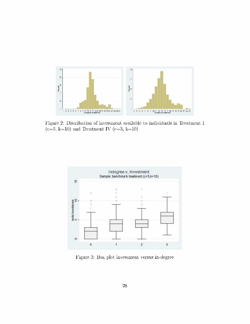
Figure 2: Distribution of investment available to individuals in Treatment I(c=5, k=10) and Treatment IV (c=3, k=10)

Figure 3: Box plot investment versus in-degree

28

Netw

ork

TreatmentI

TreatmentII

TreatmentIII

TreatmentIV

TreatmentV

TreatmentIV

structures

c=

5,k

=10

c=

5,k

=24

c=

5,k

=36

c i=

3,k

=10

c i=

3,k

=24

c i=

3,k

=36

Connected

105

109

81104

107

85(92.11%)

(95.61%)

(71.05%)

(91.23%)

(93.86%)

(74.56%)

1Isolate

44

186

414

(3.51%

)(3.51%

)(15.79%)

(5.26%

)(3.51%

)(12.28%)

2Isolates

00

50

02

(4.39%

)(1.75%

)Dyads

51

104

313

(4.39%

)(0.88%

)(8.77%

)(3.51%

)(2.63%

)(11.40%)

Total

114

114

114

114

114

114

Tablereportsnumber

ofobservationsand%

oftotal(inparentheses).

Table4:

Com

ponents

innetworks

29

Hub2

Hub3

Number

Investment

Number

Investment

Nn

avgn/grp

median

mean

navgn/grp

median

mean

(SD)

(SD)

(SD)

(SD)

Baseline

456

182

1.596***

5***

5.093***

780.684

6***

5.962***

c=

5,k

=10

(0.646)

(2.285)

(0.502)

(2.122)

TreatmentII

456

124

1.088

76.645

700.614

77.314

c=

5,k

=24

(0.556)

(2.516)

(0.487)

(1.822)

TreatmentIII

456

133

1.167

66.293

470.412***

77.362

c=

5,k

=36

(0.879)

(3.116)

(0.527)

(2.847)

TreatmentIV

456[114]

185[65]

1.623***

65.324***

79[42]

0.693

66.519***

c i=

3,k

=10

(0.755)

(2.865)

(0.58)

(2.717)

TreatmentV

456[114]

127[70]

1.114

77.039

71[41]

0.623

87.62

c i=

3,k

=24

(0.455)

(2.595)

(0.503)

(2.167)

TreatmentVI

456[114]

120[54]

1.053

77.058

53[33]

0.465***

88.226

c i=

3,k

=36

(0.687)

(3.733)

(0.499)

(3.93)

∗,∗∗

,∗∗∗

denote

p<

0.1,<

.05,<

0.01levelsofstatisticalsigni�cance

forTreatm

ents

I-IIIandIV

-VI,comparedwitheach

ofthere-

mainingtwolevelsofk.

Incolumnstwo,threeandseven

thenumber

oflow-cost

playersisgiven

insquare

brackets,in

columnthreetheasterisksreferto

a

Kolm

ogorov-Smirnov

test

forequality

ofdistributionfunctions,in

columnsfourandnineto

aWilcoxonrank-sum

(Mann-W

hitney)

test

forequality

ofmedians.

Mediansofk=

24andk=

36donotdi�er

statistically.

Incolumns�veandtenthey

referto

a

Kolm

ogorov-Smirnov

test

forequality

ofdistributionfunctions.

Meansanddistributionsofk=

24andk=

36donotdi�er

statistically.

Table5:

Number

ofhubsandinvestmentbyhubs

30

Hub3 Hub2 Hub3 Hub2Treatment IV Treatment IV Treatments IV-VI Treatment IV-VI

low-cost player 5.065*** 2.648*** 5.692*** 4.152***[5.349] [3.506] [9.529] [8.968]

k = 10 0.65 1.254[-0.352] [0.189]

k = 36 0.386 0.62[-0.772] [-0.398]

Period 0.808 1.145 1.123 1.144[-0.536] [0.603] [0.336] [0.390]

Session dummies yes yes yes yesPeriod dummies yes yes yes yesConstant 1.74 0.146 0.048 0.057

[0.116] [-0.709] [-1.026] [-0.962]No. observations 456 456 1368 1368No. clusters 114 114 342 342Log Likelihood -186.224 -282.441 -508.682 -779.102Pseudo R2 0.114 0.083 0.114 0.087χ2 49.899 167.07 112.034 160.553Prob > χ2 0.000 0.000 0.000 0.000Table reports odds ratios; z-values in parentheses; heteroskedasticity-consistent estimator of

of variance; standard errors corrected for intra-network correlation.* p < 0.1, ** p < 0.05, *** p < 0.01.

Table 6: Logistic estimation on the likelihood of being a hub (Treatment IV)

31

Homogeneous, c = 5 Heterogeneous, ci = 3Hub2 I II III IV V VI

k = 10 k = 24 k = 36 k = 10 k = 24 k = 36Hubs: investment 5.093 6.645 6.293 5.324 7.039 7.058

best-response 3.983 4.250 4.361 4.995 4.811 5.733z-value 0.000 0.000 0.000 0.292 0.000 0.000

Non-hubs: investment 2.930 3.557 4.279 2.838 3.689 4.098best-response 2.974 3.731 4.328 3.708 4.295 4.798z-value 0.604 0.595 0.918 0.000 0.000 0.000

Hub3 I II III IV V VIk = 10 k = 24 k = 36 k = 10 k = 24 k = 36

Hubs: investment 5.926 7.314 7.362 6.518 7.620 8.226best-response 4.410 3.743 4.766 5.860 4.141 6.321z-value 0.000 0.000 0.000 0.128 0.000 0.000

Non-hubs: investment 3.347 3.868 4.579 3.286 4.070 4.437best-response 3.164 3.896 4.288 3.888 4.494 4.876z-value 0.170 0.718 0.023 0.000 0.000 0.000

The z-values correspond to Wilcoxon rank-sum tests, signi�cance is also con�rmed

in two-tailed t-tests.

Table 7: Best-response for hubs and non-hubs

32

Costs

Hub1

NPro�t2

Pro�t±

2.58×S.E.

Theory

Theory

vs

(mean)

low

high

low

high

Sample

(P)

c=

5,no

274

158.8

155.3

162.3

154

194

154<P<

194

k=

10yes

182

173.5

171.1

175.8

144

184

144<P<

184

all

456

164.6

162.2

167.1

174

182

P<

174

c=

5,no

332

150.5

147.4

153.6

154

194

P<

154

k=

24yes

124

169.3

166.3

172.4

130

170

130<P

u17

0all

456

155.6

153.0

158.2

159

171

P<

159

c=

5,no

409

151.4

148.3

154.5

168

168

P<

168

k=

36yes

47166.9

161.2

172.7

144

144

144<P

all

456

153.0

150.1

155.9

162

162

P<

162

c i=

3,no

377

165.4

162.6

168.2

198

198

P<

198

k=

10yes

79176.8

172.4

181.2

169

169

169<P

all

456

167.4

164.9

169.8

190.75

190.75

P<

190.

75c i

=3,

no

385

156.2

153.6

158.8

184

184

P<

184

k=

24yes

71182.2

178.8

185.5

169

169

169<P

all

456

160.2

157.7

162.8

180.25

180.25

P<

180.

25c i

=3,

no

403

154.9

151.9

157.8

172

172

P<

172

k=

36yes

53174.4

164.8

184.0

169

169

169/P

all

456

157.1

154.2

160.0

171.25

171.25

P<

171.

251Hub2forTreatm

ents

IandII,Hub3forTreatm

ents

III-VI.

2Allhubpro�ts

are

greaterthannon-hubpro�ts

atacon�dence

level(C

I)of99%

(t-statistic,

2-tailed)formeansandWilcoxonranksum

test

formedians.

Table8:

Pro�ts

ofhubsandnon-hubs

33

Appendix I

1. In Treatments I-III, aggregate investments in equilibrium are equal to 12.

Proof: The proof exploits the assumption that investments take integervalues and that n = 4. First, we prove that in equilibrium the network isconnected. Suppose it is not connected then we need to consider networks ofone, two, three (and four) isolated players and networks with disconnectedpairs. Observe that no network with a single isolated player is an equilibrium:this is because the isolated player will optimally choose 12. But then fromGaleotti and Goyal (2010) we know that there must be only one hub, whichcontradicts the hypothesis that the player is isolated. So we need to considerthe case of two disconnected pairs only. When k = 10 or 24, in each pair thereis at least one player who chooses 6 or more. But then the larger investingplayer in one pair has an incentive to form a link with the larger investingplayers in the other pair. When k = 36, it follows that in each pair the higherinvesting player is choosing 8 or more. But then the higher investing playerin one pair has a strict incentive to form a link with the higher investingplayer in the other pair.

So consider connected networks. If only one player invests then it followsfrom optimality that this player must be investing 12. If only two playersare investing then it follows from arguments in Galeotti and Goyal (2010)that neither is investing 12. So they must be connected to each other. Thisimplies from optimality of individual actions that each of them must accessexactly 12. Consider next the case that 3 players are investing. Again all ofthem must be investing strictly less than 12. As everyone accesses 12, eachof them must access at least one other player. If a positive investing playeraccesses all three then the sum total investments must equal 12. So in thethree investors case we have proved that the sum of investments must equal12.

Finally, consider the case that all four players make positive investments.We �rst consider the case that a player with x is a leaf. Observe that in thiscase there is a player with y such that x + y = 12, However, as the networkis connected y must have one other link with someone with investment z. Sothere is a player who accesses x + y + z, where all investments are positive.From optimality of individual investments it follows that x+ y+ z = 12, butthis is a contradiction. So no player is a leaf. Similarly, we can show that anetwork in which a player has three links must imply that this player accesses

34

all investments, which must then be equal to 12. So the only possibility leftis that every player has two links. This means that the network is a ring.This means that all players must make equal investments and sum of threeinvestments must equal 12. In other words, every player invests 4. Thisis impossible if k = 24 or k = 36. If k = 10, then each player is strictlybetter o� cutting down own investment and linking with a new player. Thiscompletes the proof. QED

2. In Treatments IV-VI, in equilibrium all high-cost players choose 0 invest-ments.

Proof: The proof of connectedness is as in the previous result. So from nowon we restrict attention to connected networks.

We go through the di�erent cases with 1, 2, 3 and 4 contributors. Supposethere is 1 contributor. This contributor cannot be the high-cost (H) player ashe will choose 12; but then the low-cost (L) player will raise his investmentto a positive amount so that total investment accessed is 13.

Next consider the case of two contributors. If both players are high costand contributing then neither can be contributing 12. But then it followsfrom optimality of individual behavior that the sum of investments must be12. But then an L player will have a strict incentive to increase investmentto 1. So consider the case where one investor is Hand the other is L. Againit follows that the sum must be 13 and both players must access each other.But then, the H player is accessing too much investment.

Consider next the case of 3 contributors. We need to separately considerthe case of three H players, 2 H players and 1 L player. Straightforwardarguments exploiting the fact that an L player must access at least 13 andan active an H player must access exactly 12 imply imply that there is noequilibrium like that.

Finally, consider the case of 4 contributors. Here we follow the line ofargument in the previous result. We start by showing that a player cannotbe peripheral in an equilibrium network. We then consider networks in whichno player is peripheral. Here we take up networks in which some player has3 links. If this is an H player then it contradicts the requirement that anH player must access exactly 12, while there is an L player who is accessingexactly 13. Similarly, if the L player has 3 links then we need to consider arange of networks with 3, 4, 5 and 6 links and in each case we can use integerinvestments, and the requirement that the L player must access exactly 13,

35

while the H player accesses exactly 12, to show that this cannot be sustainedin equilibrium. This leaves only the case in which every player has exactly2 links. In the ring network, it can be checked that we run afoul of integerconstraints. So 4 contributors cannot be sustained in equilibrium. We areleft with only one option: one contributor who is of the low-cost type. QED

36

Proof of Observation: We start with incentives of the hub player.

• Adding a link to hub player: this would simply lower payo� by k andis clearly unpro�table.

• Cutting a link to hub player: this can potentially raise payo�s by k.

• Increasing information acquisition: the hub player already accesses in-vestments in excess y. All other players are already connected to thehub. So an increase in investment can only lead to lower investmentsby others and thus lower utility.

• Reducing information acquisition: we know that lower investmentsthan y − (m + 1)k/c will mean that periphery players invest in ex-cess of k/c and this will lead to switches between self investment andlinks with other peripheral players, thus destroying the core-peripherynetwork.

We next consider incentive of the periphery player:

• Severing the link to hub: this will clearly reduce payo�s since xi > k/cand aggregate investments accessed by periphery player are y.

• Adding a link to non-hub player: this is clearly unpro�table as xj < k/c.It will also not raise investments of the new neighbor as this player willthen accessing investments in excess of y.

• Reducing investments: this is unpro�table as total investments accessedare y and lower investment will not induce greater investment fromcurrent hub contacts. This was explained in the main text of the paperand de�nes the upper bound for z.

• Increasing investment: this is not by itself pro�table as periphery playeris accessing y in current pro�le. So the only incentive would be a linkfrom a periphery player. However, such a link would lead to thatnew contact lowering investment to 0. So again increasing investmentcannot be pro�table.

�

We now compute the bounds for z for the di�erent cost of linking and forthe di�erent core-periphery networks. The case with single hub has already

37

been presented in the main text. We now complete the other cases, k=24and m=2: The bounds for z are −2.4 < z < 2.4. So investment by a hubplayer is xi = 4.8 and by the periphery player is xj = 2.4. This means thataggregate investment is 14.4.Turning to the low cost case k = 10. For m = 2, we �nd the bounds for zare 6 < z < 8. The investment by the hub is xi = 5 and the investment bythe peripheral player is xj = 2. This means that the aggregate investment is14.

Appendix II

Session Treatments

1 I II III IV V VI

(k = 10, c = 5) (k = 24, c = 5) (k = 36, c = 5) (k = 10, ci = 3) (k = 24, ci = 3) (k = 36, ci = 3)2 III II I VI V IV

(k = 36, c = 5) (k = 24, c = 5) (k = 10, c = 5) (k = 36, ci = 3) (k = 24, ci = 3) (k = 10, ci = 3)3 IV V VI I II III

(k = 10, ci = 3) (k = 24, ci = 3) (k = 36, ci = 3) (k = 10, c = 5) (k = 24, c = 5) (k = 36, c = 5)4 VI V IV III II I

(k = 36, ci = 3) (k = 24, ci = 3) (k = 10, ci = 3) (k = 36, c = 5) (k = 24, c = 5) (k = 10, c = 5)5 I II III IV V VI

(k = 10, c = 5) (k = 24, c = 5) (k = 36, c = 5) (k = 10, ci = 3) (k = 24, ci = 3) (k = 36, ci = 3)6 III II I VI V IV

(k = 36, c = 5) (k = 24, c = 5) (k = 10, c = 5) (k = 36, ci = 3) (k = 24, ci = 3) (k = 10, ci = 3)

7 IV V VI I II III

(k = 10, ci = 3) (k = 24, ci = 3) (k = 36, ci = 3) (k = 10, c = 5) (k = 24, c = 5) (k = 36, c = 5)8 VI V IV III II I

(k = 36, ci = 3) (k = 24, ci = 3) (k = 10, ci = 3) (k = 36, c = 5) (k = 24, c = 5) (k = 10, c = 5)

Table 9: Sequence of treatments

38

Model 1 Model 2 Model 3 Model 4 Model 5Baseline Treatment IV Homogeneous Heterogeneous Full

Treatment I ci = 3, k = 10 Treatments I-III Treatments IV-VI Samplein-degree 1.367*** 1.574*** 1.316*** 1.528*** 1.413***

[13.501] [12.183] [18.549] [17.893] [25.094]k = 10 -0.868** -1.328*** -0.926**

[-2.493] [-3.581] [-2.364]k = 36 0.581 0.204 0.56

[1.565] [0.506] [1.423]Homogeneous costs -0.095

[-0.753]Round -0.088 -1.99 0.017 0.091 -0.079

[-0.510] [-0.735] [0.100] [0.496] [-0.376]Session dummies yes yes yes yes yesPeriod dummies yes yes yes yes yesConstant 1.911*** 1.770 2.962*** 3.048*** 3.325***

[2.805] [1.927] [6.241] [5.803] [9.473]No. observations 456 456 1368 1368 2736No. clusters 114 114 342 342 684R2(adj.) 15.261 13.090 16.953 16.467 26.872F 0.340 0.328 0.214 0.227 0.221Prob > F 0.000 0.000 0.000 0.000 0.000Table reports t-values in parentheses; heteroskedasticity-consistent estimator of variance; standard errors corrected

for intra-network correlation; period and session dummies incl. * p < 0.1, ** p < 0.05, *** p < 0.01.

Table 10: OLS regressions with individual investment as dependent variable,Treatments I - VI

39

Treatment I Treatment II Treatment III Treatment IV Treatment V Treatment VIc = 5, k = 10 c = 5, k = 24 c = 5, k = 36 ci = 3, k = 10 ci = 3, k = 24 ci = 3, k = 36

DataEquilibria 1 4 2 2 0 0

(0.8%) (3.4%) (1.7%) (1.7%)Equilibrium 29 34 17 5 22 14structures (25.4%) (29.7%) (14.9%) (4.4%) (19.29%) (12.28%)ChanceEquilibria < 0.01 < 0.01 < 0.01 < 0.01 < 0.01 < 0.01

(< 0.001%) (< 0.001%) (< 0.001%) (< 0.001%) (< 0.001%) (< 0.001%)Equilibrium 5.79 3.56 1.78 0.44 0.44 0.44structures (5%) (3.1%) (1.5%) (0.4%) (0.4%) (0.4%)Total 114 114 114 114 114 114Table reports number of observations and % of total (in parentheses).

Table 11: Frequencies and percentages of equilibria and equilibrium struc-tures

40

1

Experimental Laboratory for Sociology and Economics

- Instructions -

Please read the following instructions carefully. These instructions are equal for all the

participants. The instructions state everything you need to know in order to participate

in the experiment. If you have any questions, please raise your hand. One of the

experimenters will approach you in order to answer your question.

You can earn money by means of earning points during the experiment. The number of

points that you earn depends on your own choices and the choices of other participants.

At the end of the experiment, the total number of points that you earn during the

experiment will be exchanged at an exchange rate of:

200 points = 1 Euro

The money you earn will be paid out in cash at the end of the experiment without other

participants being able to see how much you earned. Further instructions on this will

follow in due time. During the experiment you are not allowed to communicate with

other participants. Turn off your mobile phone and put it in your bag. Also, you may

only use the functions on the screen that are necessary to carry out the experiment.

Thank you very much.

- Overview of the experiment -

The experiment consists of six scenarios. Each scenario consists again of one trial

round and three paid rounds (altogether 24 rounds of which 18 are relevant for your

earnings).

In all scenarios you will be grouped with three other randomly selected participants. At

the beginning of each of the 24 rounds, the groups and the positions within the groups

will be randomly changed. The participants that you are grouped with in one round are

very likely different participants from those you will be grouped with in the next round.

It will not be revealed with whom you were grouped at any moment during or after the

experiment.

The participants in your group will be shown as circles on the screen (see Figure 1).

You are displayed as a blue circle, while the other participants are displayed as black

circles. You will be able to connect to one or more other participants in your group

during each round. By clicking on one of the other participants, you become connected

to this other participant. An arrow appears to indicate the connection. By clicking again

on the participant the arrow and, thus, the connection is removed again. You are also

connected to another participant if this other participant clicks once on you. The

participant on whose side a one-sided arrow starts has initiated this connection and has

to pay some points for this connection. If both participants have clicked for a specific

connection a two-headed arrow appears and both participants need to pay points for this

connection. All participants that are connected to you by any kind of arrow will be

called your neighbors. Hence, in Figure 1 the participants with “75” and with “118” in

their circles are your neighbors.

2

Figure 1: Explanation of screen elements

You can earn points in a round by investing, but investing also costs points. The points

you receive in the end depend on your own investment and the investments of your

neighbors. By clicking on one of the two buttons at the bottom of the screen you

increase or decrease your investment. At the end of the round, you receive the amount

of points that is shown on the screen at that moment in time. In other words, your final

earnings only depend on the situation at the end of every round.

Each round lasts between 105 and 135 seconds. The end will be at an unknown and

random moment in this time interval. Therefore, different rounds will not last equally

long.

The points you will receive can be seen as the top number in your blue circle. The

points others will receive are indicated as the top number in the black circles of others.

Next to this, the size of the circles changes with the points that you and the other

participants will receive: a larger circle means that the particular participant receives

more points. The bottom number in the circles indicates the amount invested by that

participant.

Remarks:

It can occur that there is a time-lag between your click and the changes of the

numbers on the screen. One click is enough to change a connection or to change

your investment by one unit. A subsequent click will not be effective before the

previous click is effectuated.

Therefore wait until a connection is changed or your investment is adapted

before making further changes!

YOU

Click on other circles

to initiate or remove

connections

Click on red

buttons to change

investments

3

- Your earnings -

Now we explain in detail how the number of points that you earn depends on the

investments and the connections. Read this carefully. Do not worry if you find it

difficult to grasp immediately. We also present an example with calculations below.

Next to this, there is a trial round for each scenario to gain experience with how

connections and investments affect your earnings.

In all scenarios, the points you receive at the end of each round depend in a similar way

on two factors:

1. Every connection that you initiated yourself costs a given number of points

(this will be either 10, 24 or 36).

2. Every unit that you invest yourself will cost you 5 points most of the time; in

some scenarios, there is one participant in your group (maybe yourself) for

whom every unit investment costs only 3 points. This participant will be

displayed with an additional square around the circle (see Figure 3).

3. You earn points for each unit that you invest yourself and for each unit that

your neighbors invest (the earnings related to a neighbor’s investments do

not depend on whether an arrow points toward yourself, toward the

neighbor, or in both directions).

If you sum up all units of investment of yourself and your neighbors, the following table

gives you the points that you earn from these investments:

Your investment plus

your neighbors’

investments

0 1 2 3 4 5 6 7 8 9 10

Points 0 28 54 78 100 120 138 154 168 180 190

Your investment plus

your neighbors’

investments

11 12 13 14 15 16 17 18 19 20 21

Points 198 204 208 210 211 212 213 214 215 216 217

The higher the total investments, the lower are the points earned from an additional unit

of investment. Beyond an investment of 21, you earn one extra point for every

additional unit invested by you or one of your neighbors.

Note: if your and your neighbors’ investments add up to 12 or more, earnings

increase by less than 5 points for each additional unit of investment.

4

- Example shown in Figure 2 -

Suppose

1. initiating connections costs 24 points in this scenario;

2. you initiated one connection with one participant and one other participant

initiated a connection with you;

3. you invested 2 units;

4. one of your neighbors invested 3 units and the other neighbor invested 4 units.

Then you have to pay 24 points for the connection you initiated and 2 times 5 = 10

points for your own investments. Therefore, your total costs are 34 points.

The investments that you profit from are your own plus your neighbors’ investments: 2

+ 3 + 4 = 9 (see bottom numbers in the circles from you and your neighbors on the right

and on the left). In the table you can see that your earnings from this are 180 points.

In total, you would receive 180 − 34 = 146 points if this would be the situation at the

end of the round. Figure 2 shows this example as it would appear on the screen. The

investment of the fourth participant in your group (at the bottom of the screen) does not

affect your earnings. In the trial round before each scenario, you will have time to get

used to how the points you receive change with investments.

The participant on the left has initiated two connections, invests in 3 units himself and

profits from 3 + 2 + 1 = 6 units in total. Therefore, this participant receives in this

situation 138 (see table) − 2 24 − 3 5 = 75 points.

Figure 2: Numerical example

5

- Scenarios -

All rounds are basically the same. The things that change between scenarios are:

1. The costs for a connection will be 10, 24, or 36 points.

2. There might be one participant who pays only 3 points per unit of investment.

This participant is marked with an additional square. In Figure 3, this is the

participant on the left. This participant earns 6 points more than in Figure 2

because he pays 3 2 = 6 points less for his three units of investments, which

brings his total earnings to 138 − 2 24 − 3 3 = 81.

When a new scenario starts, you will get a message on the screen that describes the new

scenario. Please read these messages carefully. As indicated before each scenario starts

with a trial round. At the top of the screen you can also see when you are in a trial

round. Paying rounds are indicated by “ROUND” while trial rounds are indicated by

“TRIAL ROUND”.

Figure 3: Second example

- Questionnaire -

After the 24 rounds you will be asked to fill in a questionnaire. Please take your time to

fill in this questionnaire accurately. In the mean time your earnings will be counted.

Please remain seated until the payment has taken place.

cambridge-inet institute · cambridge-inet institute faculty of economics . information acquisition...

Documents