calpuff modeling of large electrical generating units and ... · calpuff simulates atmospheric...
TRANSCRIPT

2016 MANE-VU Source Contribution Modeling Report
CALPUFF Modeling of Large Electrical
Generating Units and Industrial Sources
April 4, 2017
2016 MANE-VU CALPUFF Point Source Contribution Modeling Analysis April 4, 2017
2
TABLE OF CONTENTS
Contents Acknowledgments........................................................................................................................... 3
Executive Summary ......................................................................................................................... 4
1.0 Introduction .............................................................................................................................. 5
2.0 CALPUFF Modeling System .................................................................................................. 6
2.1. The NHDES/VTDEC CALPUFF Modeling Platform Description ............................................. 7
2.2 CALMET Meteorological Modeling ....................................................................................... 8
2.3 Model Performance ............................................................................................................ 13
3.0 2016 MANE-VU Modeling Methodology ........................................................................... 14
3.1 Emission Source Selection .................................................................................................. 14
3.2 Development of CALPUFF Model Inputs ............................................................................ 14
3.2 Modeling Phases ................................................................................................................. 18
3.3 Output Processing ............................................................................................................... 19
3.4 Quality Assurance ............................................................................................................... 20
4.0 2016 MANE-VU Modeling Results ..................................................................................... 21
4.1 2011 Top-10 Visibility Impacting Units to Regional Class I Areas ....................................... 21
4.2 Top 25 2011 and 2015 Visibility Impacting EGU Units to Five MANE-VU and Two Nearby
Class I Areas .............................................................................................................................. 34
4.3 Top 25 2011 Visibility Impacting Industrial and Institutional Units to Five MANE-VU Class I
and Two Nearby Class I Areas ................................................................................................... 44
4.3 Sensitivity Analyses for Annual vs. 95th Percentile Emissions ............................................ 48
4.4 Effect of Meteorology ......................................................................................................... 50
4.5 State-by State EGU Visibility Extinction Percentages ......................................................... 54
5.0 Summary and Further Analysis .......................................................................................... 60
References .................................................................................................................................... 61
Appendix A (A.1): EGU Sources Modeled in Phases I-VI
Appendix B (B.1-B.4): EGU and Industrial/Institutional Source Parameters and Emissions
Appendix C (C.1-C.2): Distances from Facilities to Class I Areas
Appendix D (D.1-D.2): Parameter and Emission Assumptions
Appendix E (E.1): Output Processing Calculations
Appendix F (F.1-F.33): Ranking of Visibility-Impairing Sources to Class I Areas

2016 MANE-VU CALPUFF Point Source Contribution Modeling Analysis April 4, 2017
3
Acknowledgments
This study was made possible through the meteorological modeling efforts Dan Riley of the
Vermont Department of Environmental Conservation (VTDEC) , analysis and report drafting
efforts of Jessica Dunbar, David Healy, and Jeff Underhill of the New Hampshire Department of
Environmental Services (NHDES), the dispersion modeling efforts of NHDES interns Anthony
Picone and Maxwell Tuttle, and efforts from members of the MANE-VU Technical Support
Committee (and others) who provided comment on the technical analysis and the report.
2016 MANE-VU CALPUFF Point Source Contribution Modeling Analysis April 4, 2017
4
Executive Summary
New Hampshire Department of Environmental Services (NHDES) in conjunction with Vermont Department of Environmental Conservation (VTDEC) carried out air pollution transport modeling with the CALPUFF dispersion model, which was used to simulate sulfate and nitrate formation and transport in the Mid-Atlantic Northeast Visibility Union (MANE-VU) and nearby regions. This modeling effort focused on electric generating units (EGUs) and large industrial and institutional sources in the eastern and central United States. NHDES and VTDEC used the CALMET, CALPUFF and CALPOST programs to estimate pollutant concentrations and visibility impacts at eleven Class I areas in the northeastern U.S. Both groups completed different steps throughout the dispersion modeling process with quality assurance steps carried out by both parties. The VTDEC developed meteorological inputs for CALPUFF through the use of observation-based National Weather Service (NWS) inputs and application of CALMET. The resulting meteorological files were provided to NHDES, who developed hourly and annual sulfur dioxide and nitrogen oxide emissions inputs for CALPUFF. Emissions inputs for EGUs were derived from continuous emissions monitoring system (CEMS) data files. NHDES chose to model 95th percentile daily emissions in order to represent high end emission days but at the same time eliminate outlying high emissions due to occasional events such as start-ups and shut downs. Annual emissions were also modeled to provide a sense of how the predicted visibility impacts differ, especially for units that are infrequently operated. Emissions for industrial and institutional units were derived from reported annual emissions adjusted to a typical hourly emission estimate based on emission unit operational statistics. Calculated 95th percentile 2011 and 2015 EGU emissions for sulfur dioxide (SO2) and nitrogen oxides (NOX) were modeled for each day of the year to assess the maximum 24-hour impact to each of eleven Class I areas located in the northeastern United States. Similarly, annual 2011 and 2015 emissions were modeled by NHDES for the entire year for each Class I area. This process was carried out for each of the provided years of meteorology (2002, 2011, and 2015). The industrial and institutional typical hourly emission sources (2011 emissions) were modeled with 2002, 2011 and 2015 meteorology. The results (including 24-hour maximum sulfate [SO4] and nitrate [NO3] concentrations, extinction, and deciviews), were used to rank emission units by their extinction value at each Class I area. The resulting ranking tables revealed Ohio as the top contributing state to visibility impact at all Class I areas using 2011 95th percentile EGU emissions with meteorology from years 2002 and 2011. Ohio was also one of the top contributing states using 2015 meteorology. The results described in this report will assist MANE-VU and its member states in reaching the federal Regional Haze rule goal of improving visibility to natural/ambient levels at Class I areas. It should be noted that this analysis is intended to be a qualitative screening tool, to be used in conjunction with other techniques (e.g. emission to distance ratios and back-trajectory analyses), to rank emissions sources for further consideration as part of the larger MANE-VU consultation process.
2016 MANE-VU CALPUFF Point Source Contribution Modeling Analysis April 4, 2017
5
1.0 Introduction
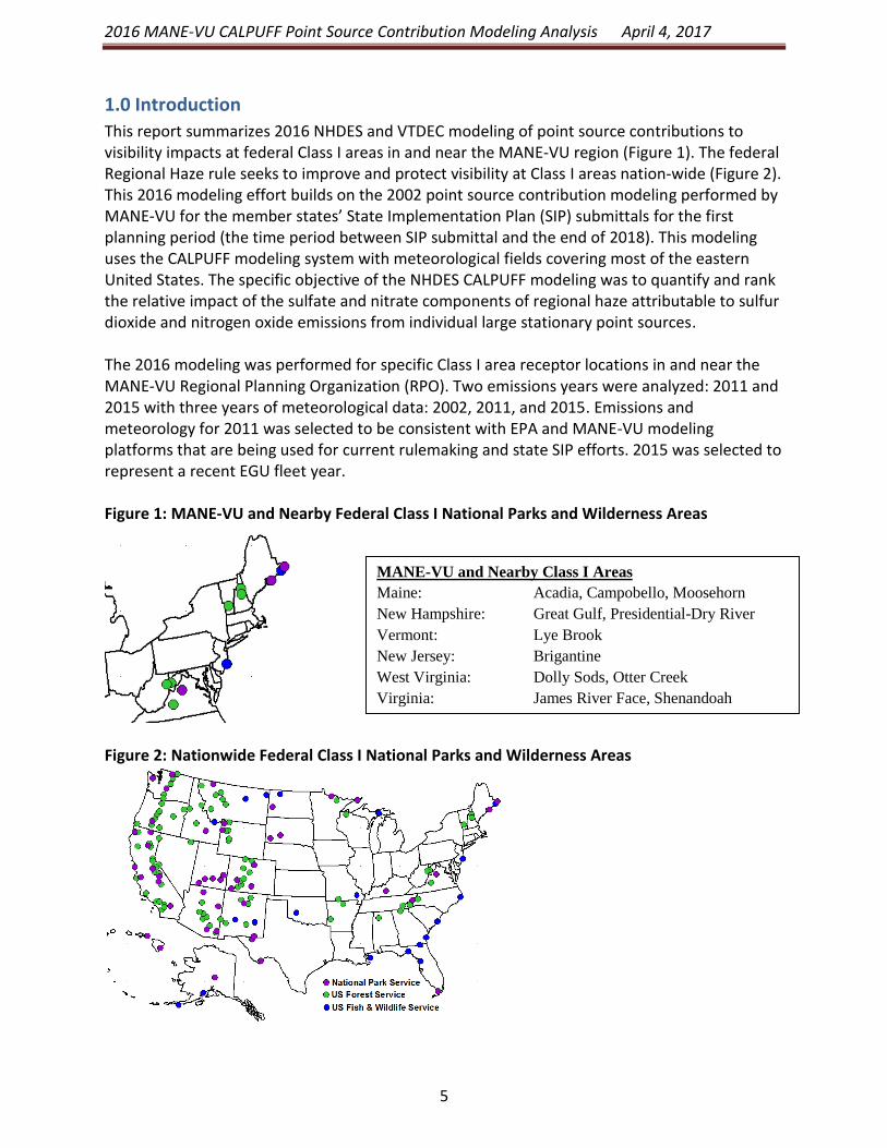
This report summarizes 2016 NHDES and VTDEC modeling of point source contributions to visibility impacts at federal Class I areas in and near the MANE-VU region (Figure 1). The federal Regional Haze rule seeks to improve and protect visibility at Class I areas nation-wide (Figure 2). This 2016 modeling effort builds on the 2002 point source contribution modeling performed by MANE-VU for the member states’ State Implementation Plan (SIP) submittals for the first planning period (the time period between SIP submittal and the end of 2018). This modeling uses the CALPUFF modeling system with meteorological fields covering most of the eastern United States. The specific objective of the NHDES CALPUFF modeling was to quantify and rank the relative impact of the sulfate and nitrate components of regional haze attributable to sulfur dioxide and nitrogen oxide emissions from individual large stationary point sources. The 2016 modeling was performed for specific Class I area receptor locations in and near the MANE-VU Regional Planning Organization (RPO). Two emissions years were analyzed: 2011 and 2015 with three years of meteorological data: 2002, 2011, and 2015. Emissions and meteorology for 2011 was selected to be consistent with EPA and MANE-VU modeling platforms that are being used for current rulemaking and state SIP efforts. 2015 was selected to represent a recent EGU fleet year. Figure 1: MANE-VU and Nearby Federal Class I National Parks and Wilderness Areas
Figure 2: Nationwide Federal Class I National Parks and Wilderness Areas
MANE-VU and Nearby Class I Areas
Maine: Acadia, Campobello, Moosehorn
New Hampshire: Great Gulf, Presidential-Dry River
Vermont: Lye Brook
New Jersey: Brigantine
West Virginia: Dolly Sods, Otter Creek
Virginia: James River Face, Shenandoah

2016 MANE-VU CALPUFF Point Source Contribution Modeling Analysis April 4, 2017
6
2.0 CALPUFF Modeling System
CALPUFF is a Lagrangian modeling system included in EPA’s Guideline on Air Quality Models (GAQM) as a recommended model for long-range transport, specifically to address the impacts of emissions from Prevention of Significant Deterioration (PSD) sources in Class I areas (note: EPA's most recent GAQM, effective May 22, 2017, no longer recommends one specific model for this purpose). CALPUFF simulates atmospheric transport, transformation, and dispersion through the treatment of air pollutant emissions from stacks or area sources as a series of discrete puffs. Each puff is tracked individually by the model until it leaves the modeling domain, and the contribution of each puff to receptor concentrations (or deposition fluxes) is calculated separately and can be used to create individual source impacts, or summed in different ways to create total impacts over source groups based on the user’s choices. The CALPUFF modeling system includes numerous related programs used to create inputs for the model and to extract and analyze model outputs. One key related program is CALMET, which is the meteorological processor that creates three-dimensional wind fields for the dispersion model CALPUFF. Another key related program is CALPOST, which performs a number of output post-processing functions. CALPUFF has seen wide use across the United States, providing estimated concentration and visibility impacts in Class I areas for numerous PSD applications for new power plants and other PSD sources. The use of CALPUFF for regional modeling at the scale of this contribution assessment (where transport distances exceed 1000 kilometers in some cases) has not been as widespread, and its performance at distances beyond 300 kilometers is subject to some uncertainty. The Interagency Workgroup on Air Quality Modeling (IWAQM) Phase II Report (USEPA, 1998) suggested, based on an analysis of the CAPTEX tracer study, that under-prediction of horizontal dispersion at greater than 300 kilometer transport distances could lead to an over-prediction of surface concentrations using CALPUFF. For the present study, this uncertainty is addressed through the emphasis on model performance (compared to measured data) documented in the 2006 MANE-VU modeling report, Contributions to Regional Haze in the Northeast and Mid-Atlantic United States (NESCAUM 31 August 2006). Further, the modeling results from this exercise will simply identify units that might undergo a more rigorous analysis for reasonable measures for visibility improvement. The CALPUFF modeling system was developed by Earth Tech and is now maintained and updated by Exponent Engineering and Scientific Consulting, and is publicly available. Model and support program executables, a graphical user interface, model and support program source code, examples, and users’ guides are available either through a link provided on EPA’s web site www.epa.gov/ttn/scram or directly from Exponent at http://www.src.com/. The CALMET meteorological processor is a key component of the CALPUFF modeling system. Its primary purpose is to prepare meteorological inputs for running CALPUFF, consisting nominally of three-dimensional wind fields, two-dimensional gridded derived boundary layer parameter fields (e.g. mixing depth, friction velocity, Monin Obukhov length, etc.), and two-dimensional gridded fields of surface measurements and precipitation rates (for use in calculating wet

2016 MANE-VU CALPUFF Point Source Contribution Modeling Analysis April 4, 2017
7
deposition fluxes). Inputs to CALMET consist of geophysical data (land use, terrain) and observations in the form of surface measurements, precipitation rates, and upper air rawinsonde soundings.
2.1. The NHDES/VTDEC CALPUFF Modeling Platform Description
Version 7.2.1 (Level 150816) of CALPUFF is an updated version of the model used for this exercise (Exponent 2011). This update includes changes to roadway inputs and the capability to use receptor group names. Output post processing was performed with CALPOST Version 7.1.0 (Level 141010) and meteorology was generated with CALMET Version 6.334 (Level 110421) (Scire, Robe, Fernau and Yamartino 1998). Modeling methodologies in this 2016 study generally replicate what was done for the regional haze SIP work for the first planning period. The MANE-VU CALPUFF and CALMET modeling domains use a Lambert Conformal Conic (LCC) projection consistent with the RPO modeling projections; namely, an origin of 40.0 degrees N and 97.0 degrees W and matching parallels of latitude at 33.0 and 45.0 degrees N. The vertical extent of the domain is set at approximately 3 km with different resolutions depending on the platform. Grid resolution for the VTDEC CALMET platform was set at 36 kilometers, which resulted in a grid size of 74 by 60 cells. The vertical grid structure for the NH/VT platform consisted of eight levels, specified to allow accurate representation of atmospheric conditions in the surface level, transition level, and the free atmosphere. A depiction of the domain used in these analyses is shown in Figure 3. Figure 3: MANE-VU (NH/VT) Modeling Domain

2016 MANE-VU CALPUFF Point Source Contribution Modeling Analysis April 4, 2017
8
2.2 CALMET Meteorological Modeling
VTDEC developed meteorological inputs for CALPUFF through the use of observation-based inputs (i.e., rawinsonde and surface measurements) from the National Weather Service (NWS) and application of CALMET. VTDEC previously developed CALMET files for the year 2002 with a 2003 beta test version of CALMET. The 2002 meteorological fields were used as-is for a portion of this 2016 CALPUFF modeling exercise. In addition, new meteorological fields were developed for 2011 and 2015 with CALMET 6.334 for the 2016 modeling exercise. In all cases, meteorology files include entire calendar years and reflect the domain shown in Figure 3. A detailed description of the methodologies that VTDEC used to generate the 2002 meteorological fields can be found in Section D.2.2 of Appendix D to NESCAUM’s 2006 MANE-VU modeling report, Contributions to Regional Haze in the Northeast and Mid-Atlantic United States.1 For this 2016 modeling effort, VTDEC used similar methodologies to generate the 2011 and 2015 meteorological fields. Meteorological data inputs for 2002 consisted of 684 surface stations, 27 radiosonde stations for upper air representation, 1037 precipitation measurement sites, and 5 overwater (buoy) sites (see Figure 4). For 2011 and 2015, data from 1,203 surface and precipitation sites and 27 radiosonde stations were used. The surface station data was extracted from the integrated surface hourly observations (ISHO) dataset compiled by the National Climatic Data Center (NCDC). For all three of the meteorological years, data was extracted and processed in four quarters to allow for reasonable CALMET run times. Figure 4: Surface (ASOS), and Upper Air (Radiosonde), Stations used in the 2002 CALMET runs
1 This report, Contributions to Regional Haze in the Northeast and Mid-Atlantic United States, may be found on the NESCAUM website at: http://www.nescaum.org/documents/contributions-to-regional-haze-in-the-northeast-and-mid-atlantic--united-states/.

2016 MANE-VU CALPUFF Point Source Contribution Modeling Analysis April 4, 2017
9
The CALMET modeling system uses a set of programs for preprocessing geophysical data such as land use and terrain elevations for the modeling domain. Figures 5 and 6 show example QA/QC plots of the terrain and land use output from these preprocessors. From this information, CALMET produces related physical fields that are necessary for the CALPUFF pollutant predictions including surface roughness, albedo, Bowen ratio, soil heat flux, and leaf area index. Figures 7 and 8 portray fields of surface roughness and leaf area index for the domain. Figure 5: Plot of Smoothed Terrain Heights (m) Used in the VTDEC CALMET Modeling
Figure 6: Plot of Land Use Used in the VTDEC CALMET Modeling
LEGEND
Terrain Height
(Meters)
36 KM. Resolution CALMET Domain in Lambert Conformal Projection
Terrain Heights
Terrain Derived from USGS and Smoothed for Domain
Ter. Ht. Plotted For : Month : Day : Hour :
0 to 10 m
10 to 50 m
50 to 100 m
100 to 200 m
200 to 300 m
300 to 400 m
400 to 500 m
500 to 600 m
LEGEND
Land Use
Categories
36 KM. Resolution CALMET Domain in Lambert Conformal Projection
Land Use
Landuse Derived from USGS Global Files
Landuse Plotted For : Month : Day : Hour :
Urban
Agricultural
Rangeland
Forestland
Water

2016 MANE-VU CALPUFF Point Source Contribution Modeling Analysis April 4, 2017
10
Figure 7: Plot of Surface Roughness Used in the VTDEC CALMET Modeling
Figure 8: Plot of Leaf Area Index Used in the VTDEC CALMET modeling
0.0 to 0.1 m
0.1 to 0.2 m
0.2 to 0.3 m
0.3 to 0.4 m
0.4 to 0.5 m
0.5 to 0.6 m
0.6 to 0.7 m
0.7 to 0.8 m
0.8 to 0.9 m
0.9 to 1.0 m
LEGEND
Sfc. Roughness
36 KM. Resolution CALMET Domain in Lambert Conformal Projection
Surface Roughness (Meters)
Surface Roughness Calculated Within CALMET
Sfc. Roughness Plotted For : Month : Day : Hour :
36 KM. Resolution CALMET Domain in Lambert Conformal Projection
Leaf Area Calculated by CALMET
0 to 1
1 to 2
2 to 3
3 to 4
4 to 5
5 to 6
6 to 7
7 to 8
8 to 9
LEGEND
Leaf Area Index

2016 MANE-VU CALPUFF Point Source Contribution Modeling Analysis April 4, 2017
11
VTDEC performed visual spot checks during the processing of the 2011 and 2015 meteorology, including visual plots to ensure that all components of the CALMET modeling system were working correctly. Examples of VTDEC’s QA/QC plots are shown in Figures 9 through 12. Figure 9: QA/QC Plot of Rainfall (mm/hr) for April 1, 2011, Hour 1
Figure 10: QA/QC Plot of Rainfall (mm/hr) for April 1, 2011, Hour 19
RPO Projection 36 KM. Grid Starts at 33.48N, 98.16W
Precipitation Rates (MM/HR)
With 1066 Precip Sites from ASOS Data
With Model Settings Defined in Appendix D Report
Isopleths Plotted For : Month : 4 Day : 1 Hour : 6
0.00 to 0.05
0.05 to 0.10
0.10 to 0.25
0.25 to 0.50
1.00 to 2.50
2.50 to 5.00
5.00 to 15.00
>15.00
LEGEND
Precip. Rates
(MM/HR)
RPO Projection 36 KM. Grid Starts at 33.48N, 98.16W
Precipitation Rates (MM/HR)
With 1066 Precip Sites from ASOS Data
With Model Settings Defined in Appendix D Report
Isopleths Plotted For : Month : 4 Day : 1 Hour : 19
0.00 to 0.05
0.05 to 0.10
0.10 to 0.25
0.25 to 0.50
1.00 to 2.50
2.50 to 5.00
5.00 to 15.00
>15.00
LEGEND
Precip. Rates
(MM/HR)

2016 MANE-VU CALPUFF Point Source Contribution Modeling Analysis April 4, 2017
12
Figure 11: QA/QC Plot of Wind Speed and Direction for April 1, 2011, Hour 1, Model Level 3
Figure 12: QA/QC Plot of Wind Speed and Direction for April 1, 2011, Hour 1, Model Level 1
RPO Projection 36 KM. Grid Starts at 33.48N, 98.16W
Winds at 750 meters Level 3
With 1067 ASOS Sfc. Stations, 27 Upper Air Stations.
With Model Settings Defined in Appendix D Report
Windfield Plotted For : Month : Day : Hour :
Speed Legend
Length of This Wind Barb = 5 M/S
RPO Projection 36 KM. Grid Starts at 33.48N, 98.16W
Winds at 750 meters Level 1
With 1067 ASOS Sfc. Stations, 27 Upper Air Stations.
With Model Settings Defined in Appendix D Report
Windfield Plotted For : Month : Day : Hour :
Speed Legend
Length of This Wind Barb = 5 M/S

2016 MANE-VU CALPUFF Point Source Contribution Modeling Analysis April 4, 2017
13
2.3 Model Performance
Appendix D to NESCAUM’s 2006 MANE-VU modeling report, Contributions to Regional Haze in the Northeast and Mid-Atlantic United States NESCAUM (2006), documents model performance for CALPUFF modeling with 2002 continuous emissions monitoring system (CEMS)-based emissions and CALMET 2002 meteorology. This analysis is not reproduced in this report, but serves as justification for using similar model options and methodologies in the current 2016 modeling exercise. Based on the conclusions from the model performance analysis in the 2006 NESCAUM report, the VTDEC CALPUFF modeling platform appears to be performing well enough to be used, at least in a relative sense, for replicating visibility impacts at northeastern Class I areas from modeled SO2 and NOX emissions.

2016 MANE-VU CALPUFF Point Source Contribution Modeling Analysis April 4, 2017
14
3.0 2016 MANE-VU Modeling Methodology
3.1 Emission Source Selection
Over the past ten years, there have been a number of SO2 emission reduction programs that have resulted in visibility improvements. Federal measures, including the Clean Air Interstate Rule (CAIR), the Cross State Air Pollution Rule (CSAPR), Boiler MACT, MATS, BART, and advancements in the economical production of natural gas are expected to reduce SO2 emissions by almost 70% in the eastern U.S. from 2002 to 2018. Because of this, there are fewer high emitting units remaining since many have applied emission controls or have shut down, and those that are still operating tend to operate fewer hours per year. EPA estimates that CSAPR (and other state rules) reduced EGU SO2 emissions by 73% between 2005 and 2014.
For the 2016 modeling effort, the MANE-VU Technical Support Committee (TSC) provided a preliminary list of EGU sources. This list was based on an enhanced Q/d analysis considering recent SO2 emissions in the eastern United States and an analysis that adjusted previous 2002 MANE-VU CALPUFF modeling by applying a ratio of 2011 to 2002 SO2 emissions (MANE-VU Technical Support Committee 6 April 2016). This list of sources was then enhanced by including the top five SO2 and NOX emission sources for 2011 for each state included in the modeling domain.
Once the list of EGUs for 2016 CALPUFF modeling was developed, 2011 and 2015 95th percentile and annual emissions for these sources were processed as described below. As mentioned earlier, the year 2011 was selected for current CALPUFF work to be consistent with the base year being used in EPA and OTC/MANE-VU photochemical modeling for regional haze (projected year 2028) and other efforts. The year 2015 was added to the analysis in order to represent the most recent available year, which recognizes changes in emission controls, fuel changes, changes in operations, and facility shutdowns that may have occurred since base year 2011.
The MANE-VU TSC also identified 82 industrial and institutional facilities located within the CALPUFF modeling domain that either have emissions similar in magnitude to the EGUs modeled in this exercise, or are close enough to a Class I area that they would have the potential for visibility impacts.
3.2 Development of CALPUFF Model Inputs
The following sections describe the CALPUFF model input development in further detail. A total of 311 EGU stacks and 82 industrial facilities were included in this modeling analysis.
EGU Emission Rates Because fewer high emitting EGU units are operating as base-loaded units, this 2016 CALPUFF modeling effort shifts from modeling annual emissions to a focus on peak actual operating conditions to determine potential effects on Class I area visibility. Daily EGU emissions (tons per day) were obtained from EPA’s Clean Air Markets Division (CAMD) database and processed to determine the 95th percentile daily SO2 and NOX emissions for a number of electric generating units for the years 2011 and 2015. This database compiles all data from the EPA Air Markets

2016 MANE-VU CALPUFF Point Source Contribution Modeling Analysis April 4, 2017
15
Program Database - https://ampd.epa.gov/ampd/ (US EPA 2015). The emissions can also be found at the EPA FTP site (ftp://ftp.epa.gov/dmdnload/emissions/daily/quarterly/). The emissions data downloaded from the EPA was in quarterly format but was saved by NHDES in an annual by-state spreadsheet format. From these annual state-by-state spreadsheets, maximums, averages, and 95th percentiles were calculated for each modeled facility. 95th percentile daily emissions were divided by 24 to obtain an hourly emission rate for input into the CALPUFF model.
The 95th percentile was selected to remove the influence of start-up and shut-down operations or other atypical outlier emissions events. However, the 95th percentile was felt to be representative of the emissions that could be expected on the highest typical operation days. Since the emission units could operate at any time of the year, they were modeled using 95th percentile emissions for all days of the year to identify the maximum potential 24-hour impact on the eleven modeled Class I areas. Thus, the model output represents the impact of a specific emission unit operating with worst case actual emissions for that year. This is a conservative (i.e. high bound) approach because it assumes that the modeled EGUs are emitting at the 95th percentile rate every day of the year. For the EGUs, 2011 annualized emissions were also modeled as a point of comparison with the 2011 95th percentile daily emissions.
2011 annual emissions for each modeled EGU were taken directly from MARAMA’s 2011 Beta modeling emissions inventory. Since the CALPUFF model allows emissions inputs of tons per year, the annual emission rates were entered directly into the model in those units. The model then assumes that those emissions are distributed evenly throughout the year. Figure 13 shows the 2011 and 2015 95th percentile daily SO2 and NOX emissions that were used in the modeling. Industrial/Institutional Source Emission Rates Because EPA CAMD does not track industrial and institutional source emissions on an hourly basis, another method was applied for calculating industrial source SO2 and NOX emissions. For this task, annual emissions were obtained from the MARAMA 2011 Beta base year emission inventory. Operating hours per year for each source were also obtained from the MARAMA inventory. Typical hourly emission rates for each device were produced by dividing annual emissions by the number of hours operated in 2011. Emissions from individual units were combined when vented through a common stack and then stacks with resulting 2011 SO2 emissions of greater than 200 pounds per hour were included in a Large Emitting Stack category for CALPUFF modeling. Large emitting stacks comprise 80 stacks at 60 (out of the 82 total) industrial/institutional facilities. Because 22 of the 82 facilities identified by MANE-VU for CALPUFF modeling were not included in the Large Emitting Stack category, another category was developed to model facility-wide emissions where no specific stack produced a large amount of emissions. In this category, Accumulated Emissions, facility-wide emissions for each of the 22 facilities not represented in the Large Emitting Stack category were modeled as hypothetically exhausting through a single stack. The stack used in each of these cases was the stack that exhausts the greatest portion of

2016 MANE-VU CALPUFF Point Source Contribution Modeling Analysis April 4, 2017
16
the applicable facility’s emissions. Additional Accumulated Emission sources included units located at 9 of the facilities already represented with a Large Emitting Stack, but which still had a large amount of emissions not being represented by a modeled stack. In these cases, the remaining emissions not already represented by a Large Emitting Stack were accumulated and hypothetically exhausted through a single dominant stack not already being modeled. Much like the conservative nature of using the 95th percentile emissions for EGU units, combining emissions from multiple units through a common stack assumes that all units run at the same time and adds a peak potential emission perspective to the analysis. Typical hourly SO2 and NOX emission rates for the industrial/institutional facilities are shown in Figure 14. The methodology for filling missing hourly operations data is provided in Appendix D.2. Figure 13: 2011 and 2015 95th Percentile Daily SO2 Emissions (a) and 2011 and 2015 95th Percentile Daily NOX Emissions (b) for the EGUs
2015 SO2
Emissions
2011 SO2
Emissions
2015 NOx
Emissions 2011 NOx
(a)
(b)

2016 MANE-VU CALPUFF Point Source Contribution Modeling Analysis April 4, 2017
17
Figure 14: 2011 Hourly SO2 Emissions (a) and 2011 Hourly NOX Emissions (b) for the Industrial Facilities
Industrial and institutional emissions modeled as Large Emitting Stacks and Small Accumulated Emissions reflect over 99% of the SO2 emissions from the 82 MANE-VU selected facilities, and more than 94% of the NOX emissions. Stack Parameters Stack parameters (stack height, diameter, exit velocity, exhaust temperature, and coordinates) were obtained from the MARAMA 2011 Beta modeling inventory (McDill, McCusker and Sabo 2016), NHDES used Google Earth to estimate base elevations using the latitude/longitude coordinates provided in the MARAMA inventory. A FORTRAN program was used to convert the latitude/longitude coordinates into X,Y coordinates consistent with the Lambert Conformal projection of the CALPUFF modeling platform. In some cases, several units emit through a single stack. In these instances, NHDES grouped these units to the one stack adding their emission values together to create a single model run for that stack. When the stack parameters or annual emissions for the EGU units were not found in the MARAMA Beta Inventory and/or when 95th emissions were not found in the CAMD database, assumptions and/or data alterations were made. All assumptions were documented and can be found in Appendix D. Background Ozone Data The MESOPUFF II chemistry scheme used in the CALPUFF modeling requires the specification of an ozone background level. For each of the meteorological years modeled, hourly background ozone data was compiled and input into the model by means of an external hourly ozone data file. Hourly ozone data sets for calendar years 2002, 2011 and 2015 were downloaded from EPA’s Technology Transfer Network Air Quality System - https://www.epa.gov/aqs (US EPA n.d.). 2002 ozone data was gathered from 425 stations; 615 stations were used for 2011, and 604 stations were used for 2015. Figure 15 displays the stations that were used to gather the 2015 background hourly ozone data.
(a) SO2 (b) NOx

2016 MANE-VU CALPUFF Point Source Contribution Modeling Analysis April 4, 2017
18
Figure 15: Ozone Monitoring Stations Used for 2015 Background Hourly Ozone Data
Meteorology Meteorology files for the years of 2002, 2011, and 2015 were created by VTDEC using
methodology the described in Section 2.2.
3.2 Modeling Phases
2016 CALPUFF modeling was performed in a total of seven phases to include different combinations of emission type (EGU 95th percentile or annual, industrial typical), emission years (2011 or 2015) and meteorological data (2002, 2011, or 2015). A summary of the emission sources that were included in each modeling phase can be found in Appendix A. Each individual phase is described in more detail below (the number of stacks modeled in each phase is shown in parentheses):
Phase I: A comprehensive list of all EGU emissions sources selected for 2016 CALPUFF modeling were modeled using 2011 95th percentile SO2 and NOX emissions, 2002 meteorology, and 2002 ozone background data. This phase was used as a screening test of sources to determine which sources should undergo further analyses. (308 Stacks)2
Phase II: A subset of EGU sources from Phase I were remodeled using 2011 annual emissions
(rather than the 95th percentile), 2002 meteorology, and 2002 ozone background data. It was expected that the results would differ significantly from Phase I in some cases because many sources do not run every day. (81 Stacks)
Phase III: A subset of EGUs was modeled that had modeled Phase I visibility extinctions at any
Class I area of one inverse megameters (Mm-1) or more (and had not shut down by
2 One stack is equal to one modeling run

2016 MANE-VU CALPUFF Point Source Contribution Modeling Analysis April 4, 2017
19
2016). Phase III used 2011 meteorology, 2011 ozone background data, and 2011 95th SO2 and NOX percentile emissions. These runs serve as the base for MANE-VU analyses. (163 Stacks)
Phase IV: This phase is similar to Phase II, using 2011 annual emissions but with 2011
meteorology. This phase compared with Phase II allows a comparison of meteorology changes occurring between 2002 and 2011. (127 Stacks)
Phase V: This phase used 2015 meteorology and 2011 95th percentile SO2 and NOX emissions.
This phase, when compared with Phases I and III serves as a comparison of meteorology changes occurring between 2002, 2011 and 2015. (132 Stacks)
Phase VI: The sixth phase of modeling pairs 2015 meteorology with 2015 95th percentile SO2
and NOX emissions to reflect most recent conditions. This phase includes the same sources modeled in Phase IV minus sources that have shut down or otherwise reduced SO2 emissions to levels below 10 lb/hr. This phase, when compared to Phase V serves as a comparison of emissions changes occurring between 2011 and 2015. (159 Stacks)
Phase VII: The seventh phase of modeling pairs 2002, 2011 and 2015 meteorology with 2011
estimated daily industrial and institutional SO2 and NOX emissions. This phase includes two groupings of facilities; the first includes Large Emitting Stacks consisting of industrial/institutional stacks with 200 lb/hr and greater of SO2 emissions. The second includes Accumulated Emissions consisting of facility-wide emissions (not included in the Large Stacks category). The groupings include consideration of not just large emitting stacks, but also over 99% of the SO2 emissions at 82 industrial/institutional facilities. (139 Stacks)
3.3 Output Processing
Once the dispersion modeling with CALPUFF was completed, the CALPOST post-processor was used to extract predicted sulfate and nitrate concentrations for a set of receptors covering eleven Class I areas in and near the MANE-VU region. The CALPOST output data is then imported into an Excel output processing spreadsheet created by NHDES that automatically finds the maximum 24-hour sulfate and nitrate modeling concentration for each of the eleven selected Class I areas.
A routine programmed into the Excel spreadsheet mathematically converts predicted sulfate concentrations to ammonium sulfate concentrations, and nitrate concentrations to ammonium nitrate concentrations. The spreadsheet also calculates an estimated change in light extinction for each modeled emission source based on its predicted ammonium sulfate and ammonium nitrate impacts at each Class I area. These calculations are based on FLAG guidance equations for reconstructed light extinction. Additional spreadsheet calculations include emission source relative visibility changes in deciviews for the 20% best and 20% worst visibility days for each Class I area. Average 20% best and 20% worst visibility extinction values were derived from 2011 IMPROVE data for each Class I area (note: On January 10, 2017, EPA published a final rule regarding amendments to state plans for protection of visibility (82 FR 3078). This rule

2016 MANE-VU CALPUFF Point Source Contribution Modeling Analysis April 4, 2017
20
incorporates a new methodology based on the 20% "most impaired" days. EPA also published an associated draft guidance for the second implementation period of the regional haze rule. However, EPA has not finalized this draft guidance. Therefore this 2016 CALPUFF analysis was based on the 20% "worst days" metric.). Visibility in deciviews was calculated with and without the modeled extinction increment, and the difference between the two provided an estimate for changes in deciviews under different visibility conditions. It should be noted that the methodology of using 95th percentile emissions produces a very conservative (i.e. high bound) impact assessment representing potential impact when certain conditions combine. The modeling results are even more conservative in that the 95th percentile daily NOX emissions and 95th percentile daily SO2 emissions may occur on different operational days for each EGU. Yet it is assumed in the modeling that both occur every day of the year so all meteorological conditions are considered with peak emissions.
Calculations for visibility extinction and deciviews can be found in Appendix E.
3.4 Quality Assurance
NHDES carried out quality assurance for every step of the modeling process. A second, and in some cases third, analyst reviewed and reproduced modeling input files and results. All modeling parameters and emissions were cross referenced for consistency.
To ensure accurate emissions, the ratio of annual emissions in tons per year divided by 365 was compared to 95th percentile emissions in tons per day (see equation below). By definition, the 95th percentile is the value below which 95 percent of the values lie; five percent of the values are above the 95th percentile. Therefore, the average daily emissions calculated from the annual emissions should never be greater than the 95th percentile. That is, the ratio derived from the equation below should be less than 1.00. When the ratio was above 1.00 or emissions seemed unrealistically high or low, analysts checked the 95th emissions and annual emissions for accuracy.
[(Annual Emission Value/365)] / (95th Percentile Emission Value) = X
Once all emissions and stack parameters were collected and organized, analysts entered these parameters into the input files with which CALPUFF is run. To confirm that this information and the meteorological data were entered correctly, a secondary analyst checked all input files completed by the first analyst. For some CALPUFF runs, one staff member acted as the primary analyst; for other runs, the staff members switched roles. In this manner, analysts did a fairly equal amount of run production and quality assurance.
With modeling runs complete, staff reviewed the results and looked for unexpectedly high or low values. Where outputs were questioned, the runs were redone. Furthermore, to catch any lingering mistakes in input files, output calculations, or other parts of the process, a third staff member independently recreated and reran all EGU modeling runs, compared the results with the original outputs, and corrected some minor differences. For the industrial runs, all runs were not redone, but input files were recreated and checked against the original files.

2016 MANE-VU CALPUFF Point Source Contribution Modeling Analysis April 4, 2017
21
4.0 2016 MANE-VU Modeling Results
This report section provides an overview of modeling results. Because of the large number of emission sources, scenarios, and Class I areas, there are many ways to review the results. This report focuses on basic reporting of the modeling performed. Future report addendums can be added to consider additional analyses. A complete list of modeling results for all sources and modeling phases can be found in Appendix F.
Section 4.1 below provides tables of top-ten 2011 and 2015 EGU emission sources and top-five 2011 ICI sources impacting each of the eleven regional Class I areas. Section 4.2 provides the top 25 impacting EGUs and ICI facilities for five MANE-VU and two nearby Class I areas in a graphical format; section 4.3 presents comparative information regarding 95th percentile and annual emissions; section 4.4 examines effects of meteorology; and section 4.5 presents visibility impacts to MANE-VU Class I areas by state.
4.1 2011 Top-10 Visibility Impacting Units to Regional Class I Areas
Tables 1 through 33 below list the top 10 contributors to the Class I areas modeled in Phases I, III, V, VI and VII (phases can be referenced in section 3.2). Rankings for the different phases are divided into three tables for each Class I area as follows.
The first table in each set gives the top 10 contributors based on maximum impacts among Phases I, III, and V; each of these phases represent 2011 95th percentile emissions impacts, but differ in the year of meteorology (2002, 2011, or 2015). For comparison, this table also provides modeling results (shown in red text) from Phase VI: 2015 95th percentile emissions with 2015 meteorology.
The second table in each set presents rankings based on modeling with 2015 emissions for all meteorology years. Note that only the 2015 meteorology year is based on modeled outputs (Phase VI); extinction values for the 2002 and 2011 meteorology years are estimated using emissions ratios. This table also compares these 2015 results to the maximum 2011 95th percentile emission impacts (shown in red text) among the three years of meteorology. This table is organized similarly to the first table, except that rankings are by impacts given 2015 emissions rather than 2011 emissions; likewise, the results for the top 10 2015 contributors are compared to those facilities’ maximum 2011 impacts, rather than vice versa.
The third table includes the top five ICI facilities modeled with 2011 typical emissions for all three years of meteorology (Phase VII). All three tables also provide the distance of each top ranking facility from the relevant Class I area.
To clarify how contributing facilities are ranked, the maximum values upon which each are ranked are bolded in blue font. The emission sources are in descending order according to the maximum visibility extinction for each 95th percentile emission source over three years of meteorology. For example, Table 1 shows that the Kyger Creek facility had the highest rank for Acadia for 2011 95th percentile emissions. This facility had a maximum predicted extinction value of 22.1 inverse megameters (Mm-1), which occurred for the 2002 meteorological year. The Muskingum River facility ranked second based on a maximum predicted extinction of 9.4 Mm-1, which also occurred for the 2002 meteorological year. Chesterfield Power Station ranked

2016 MANE-VU CALPUFF Point Source Contribution Modeling Analysis April 4, 2017
22
third based on a maximum predicted extinction of 9.3 Mm-1, which occurred for the 2015 meteorological year. Walter C Beckford Generating Station (Unit 6) ranked 10th based on a predicted maximum extinction of 6.3 Mm-1, which occurred for the 2002 meteorology year.

2016 MANE-VU CALPUFF Point Source Contribution Modeling Analysis April 4, 2017
23
Acadia, ME Table 1: 2011 Acadia National Park Top-10 Visibility Impairing EGU Point Sources
Facility Info Extinction Value (Mm-1)
Rank State Facility ORIS
ID Unit IDs
2002 Met 2011 95th
2011 Met 2011 95th
2015 Met 2011 95th
2015 Met 2015 95th
Distance (mi)
1 OH Kyger Creek 2876 1,2,3,4,5 22.1 19.8 13.9 1.2 806
2 OH Muskingum River 2872 1,2,3,4 9.4 7.5 4.8 2.3 762
3 VA Chesterfield Power Station 3797 5 6.2 7.4 9.3 0.2 677
4 MA Brayton Point 1619 3 6.4 8.9 5.8 0.8 234
5 NH Merrimack 2364 2 8.7 8.3 8.2 1.7 180
6 MI Monroe 1733 1,2 4.6 4.3 7.2 0.4 778
7 OH Avon Lake Power Plant 2836 12 5.2 4.8 7.1 9.1 723
8 PA Homer City 3122 2 6.6 2.9 3.0 8.1 616
9 PA Homer City 3122 1 6.6 2.9 3.0 9.3 616
10 OH Walter C Beckford
Generating Station 0 6 6.3 5.9 4.7 -- 904
Table 2: 2015 Acadia National Park Top-10 Visibility Impairing EGU Point Sources
Facility Info Extinction Value (Mm-1)
Rank State Facility ORIS
ID Unit IDs
Estimated 2002 Met 2015 95th
Estimated 2011 Met 2015 95th
Modeled 2015 Met 2015 95th
Maximum 2002,11,15
Met 2011 95th
Distance (mi)
1 PA Homer City 3122 1 9.3 4.0 4.2 6.6 616
2 OH Avon Lake Power Plant 2836 12 6.7 6.2 9.1 7.1 723
3 PA Homer City 3122 2 8.1 3.6 3.7 6.6 616
4 ME William F Wyman 1507 4 5.6 3.5 4.9 2.7 102
5 OH Muskingum River 2872 5 4.6 3.5 2.3 2.9 762
6 VA Yorktown Power Station 3809 3 4.4 3.2 4.1 1.3 652
7 MA Brayton Point 1619 4 2.6 4.3 2.8 1.4 234
8 PA Shawville 3131 3,4 3.3 2.2 1.6 3.5 560
9 MA Canal Station 1599 1 2.5 3.0 2.0 2.0 210
10 NH Newington 8002 1 2.8 2.5 2.8 2.7 152
Table 3: 2011 Acadia National Park Top-5 Visibility Impairing Industrial/Institutional Sources
Facility Info Extinction Value (Mm-1)
Rank State Facility ORIS
ID Unit IDs
2002 Met 2011 Emis
2011 Met 2011 Emis
2015 Met 2011 Emis
Distance (mi)
1 ME The Jackson Laboratory 7945211 All 9.0 5.7 5.8 4
2 MD Luke Paper Company 7763811 All 5.1 4.4 5.2 648
3 ME Sappi - Somerset 8200111 All 1.4 1.6 2.0 72
4 ME Woodland Pulp LLC 5974211 All 0.8 1.8 1.5 71
5 NY Lafarge Building Materials Inc. 8105211 All 1.7 1.5 1.0 306

2016 MANE-VU CALPUFF Point Source Contribution Modeling Analysis April 4, 2017
24
Brigantine, NJ Table 4: 2011 Brigantine National Wildlife Area Top-10 Visibility Impairing EGU Point Sources
Facility Info Extinction Value (Mm-1 )
Rank State Facility ORIS
ID Unit IDs
2002 Met 2011 95th
2011 Met 2011 95th
2015 Met 2011 95th
2015 Met 2015 95th
Distance (mi)
1 OH Kyger Creek 2876 1,2,3,4,5 41.7 32.5 18.1 2.3 417
2 OH Muskingum River 2872 1,2,3,4 9.8 17.7 8.3 4.4 390
3 VA Chesterfield Power Station 3797 5 14.3 16.4 12.1 0.5 217
4 NJ B L England 2378 1 12.0 4.2 2.4 -- 17
5 OH Walter C Beckford Generating Station
0 6 8.8 6.8 5.0 -- 532
6 MD Chalk Point 1571 1,2 4.2 5.0 7.9 1.5 138
7 VA Yorktown Power Station 3809 1,2 5.6 5.6 7.6 7.0 189
8 WV Harrison Power Station 0 1 (25%), 2 (20%)
1.3 6.7 1.9 7.0 319
9 PA Homer City 3122 2 3.9 5.5 6.2 8.1 267
10 NJ B L England 2378 2,3 6.1 1.9 1.2 5.6 17
Table 5: 2015 Brigantine Top-10 Visibility Impairing EGU Point Sources
Facility Info Extinction Value (Mm-1)
Rank State Facility ORIS
ID Unit IDs
Estimated 2002 Met 2015 95th
Estimated 2011 Met 2015 95th
Modeled 2015 Met 2015 95th
Maximum 2002,11,15
Met 2011 95th
Distance (mi)
1 VA Yorktown Power Station 3809 3 9.5 6.9 10.9 3.3 189
2 PA Homer City 3122 1 5.8 8.3 9.2 6.0 267
3 PA Homer City 3122 2 5.0 7.3 8.1 6.2 267
4 OH Muskingum River 2872 5 4.9 7.7 3.8 4.8 390
5 WV Harrison Power Station 0 1 (25%),
2 (20%) 1.3 7.0 2.0 6.7 319
6 VA Yorktown Power Station 3809 1,2 5.1 5.1 7.0 7.6 189
7 OH Avon Lake Power Plant 2836 12 3.5 6.4 6.7 5.2 429
8 NJ B L England 2378 2,3 5.6 1.7 1.1 6.1 17
9 OH Muskingum River 2872 1,2,3,4 2.5 4.4 2.1 17.7 390
10 PA Montour 3149 1 1.4 4.4 4.2 4.8 167
Table 6: 2011 Brigantine Top-5 Visibility Impairing Industrial/Institutional Sources
Facility Info Extinction Value (Mm-1)
Rank State Facility ORIS
ID Unit IDs
2002 Met 2011 Emis
2011 Met 2011 Emis
2015 Met 2011 Emis
Distance (mi)
1 MD Luke Paper Company 7763811 All 7.0 12.5 7.9 250
2 MD Sparrows Point, LLC 8239711 All 0.8 2.5 1.5 114
3 TN Eastman Chemical Company 3982311 All 1.4 1.0 2.2 488
4 VA Smurfit Stone Container Corp - West Point 4182011 All 1.3 2.1 1.7 185
5 NJ Atlantic County Utilities Authority Landfill 8093211 All 0.9 1.7 0.6 9

2016 MANE-VU CALPUFF Point Source Contribution Modeling Analysis April 4, 2017
25
Lye Brook, VT Table 7: 2011 Lye Brook Top-10 Visibility Impairing EGU Point Sources
Facility Info Extinction Value (Mm-1)
Rank State Facility ORIS
ID Unit IDs
2002 Met 2011 95th
2011 Met 2011 95th
2015 Met 2011 95th
2015 Met 2015 95th
Distance (mi)
1 OH Kyger Creek 2876 1,2,3,4,5 20.4 25.7 22.0 1.2 556
2 OH Muskingum River 2872 1,2,3,4 11.4 6.7 9.5 2.8 510
3 NH Merrimack 2364 2 5.5 11.0 2.3 3.3 79
4 VA Chesterfield Power Station 3797 5 3.5 4.2 7.7 0.2 459
5 OH Walter C Beckford Generating Station
0 6 7.7 6.0 5.6 -- 652
6 PA Homer City 3122 2 6.0 6.3 5.7 7.7 365
7 PA Homer City 3122 1 5.9 6.2 5.6 8.6 365
8 NY Cayuga Operating Company, LLC
0 1 (33%), 2 (33%)
2.2 5.8 2.6 1.9 186
9 OH Avon Lake Power Plant 2836 12 3.4 5.2 5.6 7.2 474
10 NH Merrimack 2364 1 2.7 5.3 1.1 1.3 79
Table 8: 2015 Lye Brook Top-10 Visibility Impairing EGU Point Sources
Facility Info Extinction Value (Mm-1)
Rank State Facility ORIS
ID Unit IDs
Estimated 2002 Met 2015 95th
Estimated 2011 Met 2015 95th
Modeled 2015 Met 2015 95th
Maximum 2002,11,15
Met 2011 95th
Distance (mi)
1 PA Homer City 3122 1 8.3 8.6 7.9 6.2 365
2 PA Homer City 3122 2 7.3 7.7 6.9 6.3 365
3 OH Avon Lake Power Plant 2836 12 4.3 6.7 7.2 5.6 474
4 OH Muskingum River 2872 5 5.6 3.7 5.1 3.4 510
5 VA Yorktown Power Station 3809 3 2.1 3.1 5.0 1.5 446
6 ME William F Wyman 1507 4 0.8 4.6 1.7 2.3 151
7 NH Merrimack 2364 2 1.6 3.3 0.7 11.0 79
8 PA Keystone 3136 1 2.7 3.2 2.8 4.2 366
9 KY Big Sandy 1353 BSU1,BSU2 2.2 2.9 3.1 3.6 607
10 PA Keystone 3136 2 2.6 3.1 2.7 4.2 366
Table 9: 2011 Lye Brook Top-5 Visibility Impairing Industrial/Institutional Sources
Facility Info Extinction Value (Mm-1)
Rank State Facility ORIS
ID Unit IDs
2002 Met 2011 Emis
2011 Met 2011 Emis
2015 Met 2011 Emis
Distance (mi)
1 MD Luke Paper Company 7763811 All 7.2 9.5 10.8 401
2 NY Lafarge Building Materials Inc. 8105211 All 3.0 8.1 2.8 59
3 NY Finch Paper LLC 8325211 All 5.2 7.6 4.6 33
4 ME Sappi - Somerset 8200111 All 0.5 1.8 1.0 201
5 IN Arcelormittal Burns Harbor Inc. 7376511 All 0.8 1.5 0.8 727

2016 MANE-VU CALPUFF Point Source Contribution Modeling Analysis April 4, 2017
26
Moosehorn, ME Table 10: 2011 Moosehorn Top-10 Visibility Impairing EGU Point Sources
Facility Info Extinction Value (Mm-1)
Rank State Facility ORIS
ID Unit IDs
2002 Met 2011 95th
2011 Met 2011 95th
2015 Met 2011 95th
2015 Met 2015 95th
Distance (mi)
1 OH Kyger Creek 2876 1,2,3,4,5 17.6 16.2 16.0 0.9 869
2 MI Monroe 1733 1,2 4.8 4.7 7.9 0.5 832
3 VA Chesterfield Power Station 3797 5 5.7 5.3 7.9 0.2 744
4 MA Brayton Point 1619 3 7.0 6.6 4.3 0.6 301
5 OH Muskingum River 2872 1,2,3,4 6.5 4.7 4.4 1.6 823
6 OH Walter C Beckford Generating Station
0 6 5.4 5.9 3.0 -- 964
7 NH Merrimack 2364 2 5.5 5.3 5.8 1.0 244
8 OH Avon Lake Power Plant 2836 12 5.2 3.5 4.6 6.8 779
9 IN Rockport 6166 MB1,MB2 4.1 2.8 2.5 2.8 1,129
10 PA Homer City 3122 2 3.9 3.0 2.6 4.8 678
Table 11: 2015 Moosehorn Top-10 Visibility Impairing EGU Point Sources
Facility Info Extinction Value (Mm-1)
Rank State Facility ORIS
ID Unit IDs
Estimated 2002 Met 2015 95th
Estimated 2011 Met 2015 95th
Modeled 2015 Met 2015 95th
Maximum 2002,11,15
Met 2011 95th
Distance (mi)
1 OH Avon Lake Power Plant 2836 12 6.8 4.5 6.0 5.2 779
2 PA Homer City 3122 1 5.6 4.2 3.7 3.8 678
3 ME William F Wyman 1507 4 5.1 3.6 3.2 2.5 166
4 PA Homer City 3122 2 4.8 3.7 3.3 3.9 678
5 VA Yorktown Power Station 3809 3 4.4 2.3 3.5 1.4 719
6 MA Brayton Point 1619 4 3.4 3.6 2.0 1.2 301
7 OH Muskingum River 2872 5 3.2 2.1 2.1 2.0 823
8 MA Canal Station 1599 1 2.3 2.8 1.6 1.9 277
9 IN Rockport 6166 MB1,MB2 2.8 1.9 1.7 4.1 1,129
10 MA Canal Station 1599 2 2.2 2.8 1.3 1.5 277
Table 12: 2011 Moosehorn Top-5 Visibility Impairing Industrial/Institutional Sources
Facility Info Extinction Value (Mm-1)
Rank State Facility ORIS
ID Unit IDs
2002 Met 2011 Emis
2011 Met 2011 Emis
2015 Met 2011 Emis
Distance (mi)
1 ME Woodland Pulp LLC 5974211 All 5.7 3.4 3.5 10
2 MD Luke Paper Company 7763811 All 3.8 4.5 3.3 712
3 ME Sappi - Somerset 8200111 All 1.6 1.1 0.8 117
4 NY Lafarge Building Materials Inc. 8105211 All 1.2 1.0 0.7 369
5 OH P. H. Glatfelter Company - Chillicothe Facility 8131111 All 1.1 0.7 0.7 892

2016 MANE-VU CALPUFF Point Source Contribution Modeling Analysis April 4, 2017
27
Campobello/Roosevelt International Park, ME/NS
Table 13: 2011 Campobello/Roosevelt International Park Top-10 Visibility Impairing EGU Point Sources
Facility Info Extinction Value (Mm-1)
Rank State Facility ORIS
ID Unit IDs
2002 Met 2011 95th
2011 Met 2011 95th
2015 Met 2011 95th
2015 Met 2015 95th
Distance (mi)
1 OH Kyger Creek 2876 1,2,3,4,5 17.6 16.8 14.3 0.9 880
2 VA Chesterfield Power Station 3797 5 5.3 5.0 8.2 0.2 750
3 MA Brayton Point 1619 3 7.9 5.3 4.1 0.7 305
4 MI Monroe 1733 1,2 4.1 3.8 7.4 0.4 847
5 OH Muskingum River 2872 1,2,3,4 6.8 4.8 3.7 1.7 835
6 OH Walter C Beckford Generating Station
0 6 5.2 5.4 3.0 -- 977
7 NH Merrimack 2364 2 5.2 5.1 4.6 1.0 254
8 OH Avon Lake Power Plant 2836 12 4.6 2.7 4.3 5.9 794
9 IN Rockport 6166 MB1,MB2 3.9 2.6 2.3 2.7 1,142
10 OH Eastlake 0 5 3.0 2.7 3.6 -- 760
Table 14: 2015 Campobello Top-10 Visibility Impairing EGU Point Sources
Facility Info Extinction Value (Mm-1)
Rank State Facility ORIS
ID Unit IDs
Estimated 2002 Met 2015 95th
Estimated 2011 Met 2015 95th
Modeled 2015 Met 2015 95th
Maximum 2002,11,15
Met 2011 95th
Distance (mi)
1 OH Avon Lake Power Plant 2836 12 5.9 3.5 5.6 4.6 794
2 PA Homer City 3122 1 5.1 3.7 3.4 3.6 690
3 VA Yorktown Power Station 3809 3 4.5 2.5 3.7 1.4 724
4 PA Homer City 3122 2 4.5 3.3 3.0 3.6 690
5 ME William F Wyman 1507 4 4.2 3.3 2.6 2.1 176
6 MA Brayton Point 1619 4 3.7 3.4 1.9 1.2 305
7 OH Muskingum River 2872 5 3.3 2.2 1.7 2.1 835
8 MA Canal Station 1599 1 2.9 2.4 1.9 2.0 279
9 PA Shawville 3131 3,4 2.7 1.9 1.2 2.8 633
10 IN Rockport 6166 MB1,MB2 2.7 1.8 1.5 3.9 1,142
Table 15: 2011 Campobello Top-5 Visibility Impairing Industrial/Institutional Sources
Facility Info Extinction Value (Mm-1)
Rank State Facility ORIS
ID Unit IDs
2002 Met 2011 Emis
2011 Met 2011 Emis
2015 Met 2011 Emis
Distance (mi)
1 MD Luke Paper Company 7763811 All 4.0 4.0 3.0 722
2 ME Woodland Pulp LLC 5974211 All 2.7 1.7 2.4 29
3 ME Sappi - Somerset 8200111 All 2.3 1.4 0.9 132
4 NY Lafarge Building Materials Inc. 8105211 All 1.3 1.0 0.7 380
5 OH P. H. Glatfelter Company - Chillicothe Facility 8131111 All 1.1 0.6 0.6 904

2016 MANE-VU CALPUFF Point Source Contribution Modeling Analysis April 4, 2017
28
Great Gulf, NH Table 16: 2011 Great Gulf Top-10 Visibility Impairing EGU Point Sources
Facility Info Extinction Value (Mm-1)
Rank State Facility ORIS
ID Unit IDs
2002 Met 2011 95th
2011 Met 2011 95th
2015 Met 2011 95th
2015 Met 2015 95th
Distance (mi)
1 OH Kyger Creek 2876 1,2,3,4,5 18.7 21.2 12.7 1.4 673
2 NH Merrimack 2364 2 3.3 7.2 6.4 2.9 81
3 OH Muskingum River 2872 1,2,3,4 6.4 7.2 5.0 1.8 627
4 OH Avon Lake Power Plant 2836 12 3.9 7.1 5.1 8.9 579
5 MI Monroe 1733 1,2 3.6 5.7 5.1 0.5 632
6 PA Homer City 3122 2 4.2 3.7 5.3 6.4 482
7 PA Homer City 3122 1 4.2 3.6 5.3 7.3 482
8 OH Eastlake 0 5 2.7 5.1 3.5 -- 546
9 IN Wabash River Gen Station 1010 2,3,4,5,6 3.6 3.3 4.5 2.6 893
10 OH Walter C Beckford Generating Station
0 6 4.4 4.5 3.0 -- 766
Table 17: 2015 Great Gulf Top-10 Visibility Impairing EGU Point Sources
Facility Info Extinction Value (Mm-1)
Rank State Facility ORIS
ID Unit IDs
Estimated 2002 Met 2015 95th
Estimated 2011 Met 2015 95th
Modeled 2015 Met 2015 95th
Maximum 2002,11,15
Met 2011 95th
Distance (mi)
1 OH Avon Lake Power Plant 2836 12 5.0 8.9 6.4 7.1 579
2 PA Homer City 3122 1 5.8 5.1 7.3 5.3 482
3 PA Homer City 3122 2 5.1 4.5 6.4 5.3 482
4 ME William F Wyman 1507 4 2.9 4.1 2.7 1.9 66
5 OH Muskingum River 2872 5 3.2 3.6 2.4 2.2 627
6 VA Yorktown Power Station 3809 3 2.1 1.4 3.6 1.1 560
7 KY Big Sandy 1353 BSU1,BSU2 2.2 2.9 1.7 2.6 726
8 NH Merrimack 2364 2 1.3 2.9 2.6 7.2 81
9 WV Harrison Power Station 0 1 (25%),
2 (20%) 1.0 2.8 1.3 2.7 578
10 GA Harllee Branch 709 3&4 2.8 0.9 1.6 3.2 1,003
Table 18: 2011 Great Gulf Top-5 Visibility Impairing Industrial/Institutional Sources
Facility Info Extinction Value (Mm-1)
Rank State Facility ORIS
ID Unit IDs
2002 Met 2011 Emis
2011 Met 2011 Emis
2015 Met 2011 Emis
Distance (mi)
1 MD Luke Paper Company 7763811 All 4.6 5.8 6.9 522
2 ME Sappi - Somerset 8200111 All 0.5 3.1 0.7 84
3 NY Finch Paper LLC 8325211 All 0.5 1.7 1.3 137
4 NY Lafarge Building Materials Inc. 8105211 All 1.4 0.9 1.4 179
5 ME Verso Paper - Androscoggin Mill 7764711 All 0.4 1.4 0.2 52

2016 MANE-VU CALPUFF Point Source Contribution Modeling Analysis April 4, 2017
29
Presidential Range/Dry River, NH Table 19: 2011 Presidential Range/Dry River Top-10 Visibility Impairing EGU Point Sources
Facility Info Extinction Value (Mm-1)
Rank State Facility ORIS
ID Unit IDs
2002 Met 2011 95th
2011 Met 2011 95th
2015 Met 2011 95th
2015 Met 2015 95th
Distance (mi)
1 OH Kyger Creek 2876 1,2,3,4,5 18.7 21.9 14.2 1.4 666
2 NH Merrimack 2364 2 4.9 7.9 7.0 3.1 72
3 OH Avon Lake Power Plant 2836 12 4.0 7.3 5.8 9.2 574
4 OH Muskingum River 2872 1,2,3,4 7.3 7.1 5.0 1.8 619
5 MI Monroe 1733 1,2 3.9 6.0 5.2 0.5 627
6 PA Homer City 3122 2 4.6 3.9 5.4 6.5 475
7 PA Homer City 3122 1 4.6 3.8 5.3 7.4 475
8 OH Eastlake 0 5 2.7 5.3 3.9 -- 540
9 OH Walter C Beckford Generating Station
0 6 4.8 4.3 3.7 -- 759
10 IN Wabash River Gen Station 1010 2,3,4,5,6 3.6 3.6 4.6 2.6 887
Table 20: 2015 Presidential Top-10 Visibility Impairing EGU Point Sources
Facility Info Extinction Value (Mm-1)
Rank State Facility ORIS
ID Unit IDs
Estimated 2002 Met 2015 95th
Estimated 2011 Met 2015 95th
Modeled 2015 Met 2015 95th
Maximum 2002,11,15
Met 2011 95th
Distance (mi)
1 OH Avon Lake Power Plant 2836 12 5.0 9.2 7.3 7.3 574
2 PA Homer City 3122 1 6.3 5.3 7.4 5.3 475
3 PA Homer City 3122 2 5.6 4.7 6.5 5.4 475
4 ME William F Wyman 1507 4 3.9 4.2 3.3 2.0 65
5 VA Yorktown Power Station 3809 3 2.4 1.5 3.7 1.1 551
6 OH Muskingum River 2872 5 3.6 3.6 2.4 2.2 619
7 NH Merrimack 2364 2 2.0 3.1 2.8 7.9 72
8 KY Big Sandy 1353 BSU1,
BSU2 2.3 3.1 1.8 3.6 718
9 IN Rockport 6166 MB1,MB2 2.0 3.0 1.4 4.2 924
10 WV Harrison Power Station 0 1 (25%),
2 (20%) 1.1 3.0 1.3 2.8 995
Table 21: 2011 Presidential Top-5 Visibility Impairing Industrial/Institutional Sources
Facility Info Extinction Value (Mm-1)
Rank State Facility ORIS
ID Unit IDs
2002 Met 2011 Emis
2011 Met 2011 Emis
2015 Met 2011 Emis
Distance (mi)
1 MD Luke Paper Company 7763811 All 5.5 6.4 7.3 514
2 ME Sappi - Somerset 8200111 All 0.5 3.5 1.2 90
3 NY Finch Paper LLC 8325211 All 0.5 2.1 1.3 130
4 NY Lafarge Building Materials Inc. 8105211 All 1.8 1.1 1.5 171
5 IN Arcelormittal Burns Harbor Inc. 7376511 All 0.4 1.0 1.2 818

2016 MANE-VU CALPUFF Point Source Contribution Modeling Analysis April 4, 2017
30
Dolly Sods, WV Table 22: 2011 Dolly Sods Top-10 Visibility Impairing EGU Point Sources
Facility Info Extinction Value (Mm-1)
Rank State Facility ORIS
ID Unit IDs
2002 Met 2011 95th
2011 Met 2011 95th
2015 Met 2011 95th
2015 Met 2015 95th
Distance (mi)
1 OH Kyger Creek 2876 1,2,3,4,5 77.3 61.3 49.4 5.1 150
2 OH Muskingum River 2872 1,2,3,4 24.3 18.2 25.0 6.3 130
3 OH Walter C Beckford Generating Station
0 6 14.4 11.2 7.4 -- 266
4 PA Cheswick 8226 1 12.1 11.0 9.3 4.1 106
5 KY Big Sandy 1353 BSU1, BSU2
11.8 11.0 8.1 10.3 187
6 PA Homer City 3122 2 11.3 11.2 9.4 14.3 102
7 PA Homer City 3122 1 11.2 11.0 9.2 16.3 102
8 IN Wabash River Gen Station 1010 2,3,4,5,6 9.2 11.1 9.0 6.3 433
9 MI Monroe 1733 1,2 8.1 11.0 11.0 1.1 288
10 OH Avon Lake Power Plant 2836 12 10.5 7.8 10.8 13.7 222
Table 23: 2015 Dolly Sods Top-10 Visibility Impairing EGU Point Sources Facility Info Extinction Value (Mm-1)
Rank State Facility ORIS
ID Unit IDs
Estimated 2002 Met 2015 95th
Estimated 2011 Met 2015 95th
Modeled 2015 Met 2015 95th
Maximum 2002,11,15
Met 2011 95th
Distance (mi)
1 PA Homer City 3122 1 16.3 16.1 13.5 11.2 102
2 PA Homer City 3122 2 14.3 14.2 11.9 11.3 102
3 OH Avon Lake Power Plant 2836 12 13.4 9.9 13.7 10.8 222
4 OH Muskingum River 2872 5 10.5 7.5 12.2 7.6 130
5 WV Harrison Power Station 0 1 (25%),
2 (20%) 11.4 9.1 9.7 10.8 58
6 KY Big Sandy 1353 BSU1,BSU
2 10.3 9.6 7.0 11.8 187
7 WV Kammer 3947 1,2,3 6.2 7.4 7.2 7.7 96
8 OH Conesville 2840 5,6 3.0 3.5 7.0 8.2 165
9 OH Gen J M Gavin 8102 1 6.8 5.1 6.5 5.0 149
10 OH Muskingum River 2872 1,2,3,4 6.1 4.6 6.3 25.0 130
Table 24: 2011 Dolly Sods Top-5 Visibility Impairing Industrial/Institutional Sources Facility Info Extinction Value (Mm-1)
Rank State Facility ORIS
ID Unit IDs
2002 Met 2011 Emis
2011 Met 2011 Emis
2015 Met 2011 Emis
Distance (mi)
1 MD Luke Paper Company 7763811 All 54.3 52.6 89.6 33
2 TN Eastman Chemical Company 3982311 All 3.1 4.0 3.6 247
3 OH P. H. Glatfelter Company - Chillicothe Facility 8131111 All 2.3 2.3 2.7 195
4 PA USS/Clairton Works 8204511 All 1.4 1.5 2.3 92
5 IN Arcelormittal Burns Harbor Inc. 7376511 All 1.6 1.9 1.4 448

2016 MANE-VU CALPUFF Point Source Contribution Modeling Analysis April 4, 2017
31
Otter Creek, WV Table 25: 2011 Otter Creek Top-10 Visibility Impairing EGU Point Sources
Facility Info Extinction Value (Mm-1)
Rank State Facility ORIS
ID Unit IDs
2002 Met 2011 95th
2011 Met 2011 95th
2015 Met 2011 95th
2015 Met 2015 95th
Distance (mi)
1 OH Kyger Creek 2876 1,2,3,4,5 76.6 70.3 51.7 4.9 134
2 OH Muskingum River 2872 1,2,3,4 34.2 19.7 24.0 8.7 117
3 OH Walter C Beckford Generating Station
0 6 14.3 15.0 8.5 -- 251
4 PA Homer City 3122 2 14.0 13.1 8.4 17.6 107
5 PA Homer City 3122 1 13.8 12.8 8.2 20.0 107
6 PA Cheswick 8226 1 13.5 12.1 9.2 5.1 106
7 KY Big Sandy 1353 BSU1, BSU2
12.3 12.7 9.6 11.1 171
8 MI Monroe 1733 1,2 9.3 12.0 11.4 1.1 279
9 IN Wabash River Gen Station 1010 2,3,4,5,6 9.7 11.5 9.2 6.5 419
10 OH Avon Lake Power Plant 2836 12 11.3 8.5 11.3 14.2 215
Table 26: 2015 Otter Creek Top-10 Visibility Impairing EGU Point Sources Facility Info Extinction Value (Mm-1)
Rank State Facility ORIS
ID Unit IDs
Estimated 2002 Met 2015 95th
Estimated 2011 Met 2015 95th
Modeled 2015 Met 2015 95th
Maximum 2002,11,15
Met 2011 95th
Distance (mi)
1 PA Homer City 3122 1 20.0 18.6 11.9 13.8 107
2 PA Homer City 3122 2 17.6 16.5 10.5 14.0 107
3 OH Muskingum River 2872 5 15.1 8.7 11.5 9.4 117
4 OH Avon Lake Power Plant 2836 12 14.2 10.7 14.1 11.3 215
5 WV Harrison Power Station 0 1 (25%),
2 (20%) 11.2 9.9 11.0 10.6 46
6 KY Big Sandy 1353 BSU1,BSU2 10.7 11.1 8.3 12.7 171
7 OH Muskingum River 2872 1,2,3,4 8.7 5.0 6.1 34.2 117
8 WV Kammer 3947 1,2,3 6.1 6.5 8.5 8.8 86
9 OH Gen J M Gavin 8102 1 7.6 6.1 7.1 5.4 134
10 OH Conesville 2840 5,6 2.8 4.0 7.2 8.4 145
Table 27: 2011 Otter Creek Top-5 Visibility Impairing Industrial/Institutional Sources Facility Info Extinction Value (Mm-1)
Rank State Facility ORIS
ID Unit IDs
2002 Met 2011 Emis
2011 Met 2011 Emis
2015 Met 2011 Emis
Distance (mi)
1 MD Luke Paper Company 7763811 All 46.7 30.9 50.2 45
2 TN Eastman Chemical Company 3982311 All 3.4 4.3 3.5 234
3 OH P. H. Glatfelter Company - Chillicothe Facility 8131111 All 2.2 2.5 2.6 181
4 PA USS/Clairton Works 8204511 All 1.9 1.1 2.2 91
5 IN Arcelormittal Burns Harbor Inc. 7376511 All 1.8 2.0 1.5 435

2016 MANE-VU CALPUFF Point Source Contribution Modeling Analysis April 4, 2017
32
James River Face, VA Table 28: 2011 James River Face Top-10 Visibility Impairing EGU Point Sources
Facility Info Extinction Value (Mm-1)
Rank State Facility ORIS
ID Unit IDs
2002 Met 2011 95th
2011 Met 2011 95th
2015 Met 2011 95th
2015 Met 2015 95th
Distance (mi)
1 OH Kyger Creek 2876 1,2,3,4,5 32.9 80.7 57.0 4.1 172
2 OH Muskingum River 2872 1,2,3,4 20.2 20.8 32.4 7.6 184
3 VA Chesterfield Power Station 3797 5 16.1 18.5 12.1 0.6 113
4 OH Walter C Beckford Generating Station
0 6 15.8 12.4 17.2 -- 281
5 PA Homer City 3122 2 3.8 9.7 7.1 12.1 202
6 PA Homer City 3122 1 3.7 9.6 7.0 13.8 202
7 OH Muskingum River 2872 5 5.5 5.6 9.1 14.9 184
8 GA Harllee Branch 709 3&4 9.0 3.9 4.6 7.9 373
9 KY Big Sandy 1353 BSU1, BSU2
7.4 9.0 4.3 7.6 178
10 OH Avon Lake Power Plant 2836 12 8.9 5.5 6.5 11.4 304
Table 29: 2015 James River Face Top-10 Visibility Impairing EGU Point Sources Facility Info Extinction Value (Mm-1)
Rank State Facility ORIS
ID Unit IDs
Estimated 2002 Met 2015 95th
Estimated 2011 Met 2015 95th
Modeled 2015 Met 2015 95th
Maximum 2002,11,15
Met 2011 95th
Distance (mi)
1 OH Muskingum River 2872 5 9.0 9.1 14.9 9.1 184
2 PA Homer City 3122 1 5.3 13.8 10.0 9.6 202
3 PA Homer City 3122 2 4.7 12.1 8.8 9.7 202
4 OH Avon Lake Power Plant 2836 12 11.4 7.1 8.3 8.9 304
5 GA Harllee Branch 709 3&4 7.9 3.4 4.0 9.0 373
6 KY Big Sandy 1353 BSU1,BSU2 6.3 7.6 3.7 9.0 178
7 OH Muskingum River 2872 1,2,3,4 4.7 4.9 7.6 32.4 184
8 WV Harrison Power Station 0 1 (25%),
2 (20%) 6.9 4.2 7.1 6.7 133
9 VA Yorktown Power Station 3809 3 4.8 6.8 3.8 2.1 166
10 OH Gen J M Gavin 8102 1 3.1 6.6 6.0 5.7 172
Table 30: 2011 James River Face Top-5 Visibility Impairing Industrial/Institutional Sources Facility Info Extinction Value (Mm-1)
Rank State Facility ORIS
ID Unit IDs
2002 Met 2011 Emis
2011 Met 2011 Emis
2015 Met 2011 Emis
Distance (mi)
1 MD Luke Paper Company 7763811 All 21.3 4.3 9.8 132
2 VA Gp Big Island LLC 4183311 All 12.7 13.6 11.5 6
3 OH P. H. Glatfelter Company - Chillicothe Facility 8131111 All 2.0 2.4 3.3 225
4 TN Eastman Chemical Company 3982311 All 2.7 2.8 2.5 186
5 IN Arcelormittal Burns Harbor Inc. 7376511 All 1.0 1.8 1.0 496

2016 MANE-VU CALPUFF Point Source Contribution Modeling Analysis April 4, 2017
33
Shenandoah National Park, VA Table 31: 2011 Shenandoah National Park Top-10 Visibility Impairing EGU Point Sources
Facility Info Extinction Value (Mm-1)
Rank State Facility ORIS
ID Unit IDs
2002 Met 2011 95th
2011 Met 2011 95th
2015 Met 2011 95th
2015 Met 2015 95th
Distance (mi)
1 OH Kyger Creek 2876 1,2,3,4,5 61.7 46.4 62.6 3.2 191
2 OH Muskingum River 2872 1,2,3,4 24.9 28.1 32.9 7.8 185
3 VA Chesterfield Power Station 3797 5 19.7 23.6 20.2 0.6 94
4 OH Walter C Beckford Generating Station
0 6 17.3 11.1 10.0 -- 307
5 MI Monroe 1733 1,2 5.7 14.8 8.1 1.3 350
6 MD Chalk Point 1571 1,2 7.8 10.8 11.7 2.0 109
7 IN Wabash River Gen Station 1010 2,3,4,5,6 7.6 11.6 6.5 6.6 478
8 PA Homer City 3122 2 7.6 7.9 9.4 12.0 156
9 OH W H Zimmer Generating Station
6019 1 9.3 6.8 5.5 6.9 302
10 OH Muskingum River 2872 5 7.2 8.3 9.3 15.2 185
Table 32: 2015 Shenandoah National Park Top-10 Visibility Impairing EGU Point Sources Facility Info Extinction Value (Mm-1)
Rank State Facility ORIS
ID Unit IDs
Estimated 2002 Met 2015 95th
Estimated 2011 Met 2015 95th
Modeled 2015 Met 2015 95th
Maximum 2002,11,15
Met 2011 95th
Distance (mi)
1 OH Muskingum River 2872 5 11.8 13.6 15.2 9.3 185
2 PA Homer City 3122 1 11.0 11.5 13.6 9.2 156
3 PA Homer City 3122 2 9.7 10.2 12.0 9.4 156
4 OH Avon Lake Power Plant 2836 12 10.6 8.3 11.9 9.2 285
5 VA Yorktown Power Station 3809 3 8.4 10.5 5.2 3.3 142
6 OH Muskingum River 2872 1,2,3,4 5.9 6.6 7.8 32.9 185
7 KY Big Sandy 1353 BSU1,BSU2 7.4 6.0 4.9 8.8 214
8 WV Harrison Power Station 0
1 (25%),
2 (20%) 6.4 5.3 7.0 6.6 117
9 OH W H Zimmer Generating
Station 6019 1 6.9 5.1 4.1 9.3 302
10 PA Brunner Island 3140 1,2 2.9 6.9 5.7 6.9 164
Table 33: 2011 Shenandoah Top-5 Visibility Impairing Industrial/Institutional Sources Facility Info Extinction Value (Mm-1)
Rank State Facility ORIS
ID Unit IDs
2002 Met 2011 Emis
2011 Met 2011 Emis
2015 Met 2011 Emis
Distance (mi)
1 MD Luke Paper Company 7763811 All 28.4 24.8 32.7 84
2 OH P. H. Glatfelter Company - Chillicothe Facility 8131111 All 3.6 2.5 3.7 242
3 TN Eastman Chemical Company 3982311 All 2.7 2.7 2.8 245
4 MD Sparrows Point, LLC 8239711 All 1.4 2.3 2.0 135
5 WV Capitol Cement - Essroc Martinsburg 4987611 All 2.2 1.9 1.2 87
2016 MANE-VU CALPUFF Point Source Contribution Modeling Analysis April 4, 2017
34
*Note: Top 100 contributors to each Class I areas can be found in Appendix B. **Note: All distances of EGUs to Class I areas can be found in Appendix C.
4.2 Top 25 2011 and 2015 Visibility Impacting EGU Units to Five MANE-VU and Two
Nearby Class I Areas
Figures 16-25 below display the top 25 EGU contributors to five MANE-VU Class I areas (Acadia, Brigantine, Great Gulf, Lye Brook, and Moosehorn) with modeled 2011 and 2015 95th percentile emissions. Figures 26-29 exhibit only MANE-VU EGU stack impacts on two nearby Class I areas (Dolly Sods and Shenandoah). As described in Section 4.1, only 2015 meteorology was modeled with 2015 95th percentile emissions; estimates for 2002 and 2011 meteorology with 2015 95th percentile emissions were calculated based on ratios determined with 2011 emission modeling. Each Class I area has two graphs, each of which represent a different emission year (2011 and 2015). This is done to highlight changes that occurred in actual emissions between the two years. The top 25 EGUs impacting each Class I area are sorted from the maximum on the left to the 25th maximum on the right.
The three colors in the graphs represent the range in predicted impacts due to the three years of meteorology. Colors represent the maximum (green), mid-range (red), and minimum (blue) impacts, but the year in which these occur may differ by facility and are not specified in the graph. That is, the green part of the bar always depicts the maximum impact for a given source, but that maximum impact may be based on 2002 meteorology for one source and based on 2011 meteorology for another source. The intent of the charts is not to point out the years of maximum impact, but to illustrate the range of impacts among the three years.
The closer these three colors are bunched, the less the variation due to meteorology; the more spread out, the greater the difference between the years of meteorology. As an example, for 2011 95th percentile emissions impacts at Acadia, Kyger Creek had a fair amount of variation between the meteorological years. The maximum predicted extinction was about 22 Mm-1 (for 2002, shown by green part of the bar), the minimum predicted extinction for the three years was about 14 Mm-1 (for 2015, shown by the blue part of the bar), and the mid-range of the three years was about 20 Mm-1 (for 2011, shown by the red part of the bar).

2016 MANE-VU CALPUFF Point Source Contribution Modeling Analysis April 4, 2017
35
Figure 16: Acadia Top 25 Visibility Impacting 2011 EGU Units
Figure 17: Acadia Top 25 Visibility Impacting 2015 EGU Units

2016 MANE-VU CALPUFF Point Source Contribution Modeling Analysis April 4, 2017
36
Figure 18: Brigantine Top 25 Visibility Impacting 2011 EGU Units
Figure 19: Brigantine Top 25 Visibility Impacting 2015 EGU Units

2016 MANE-VU CALPUFF Point Source Contribution Modeling Analysis April 4, 2017
37
Figure 20: Great Gulf Top 25 Visibility Impacting 2011 EGU Units
Figure 21: Great Gulf Top 25 Visibility Impacting 2015 EGU Units

2016 MANE-VU CALPUFF Point Source Contribution Modeling Analysis April 4, 2017
38
Figure 22: Lye Brook Top 25 Visibility Impacting 2011 EGU Units
Figure 23: Lye Brook Top 25 Visibility Impacting 2015 EGU Units

2016 MANE-VU CALPUFF Point Source Contribution Modeling Analysis April 4, 2017
39
Figure 24: Moosehorn Top 25 Visibility Impacting 2011 EGU Units
Figure 25: Moosehorn Top 25 Visibility Impacting 2015 EGU Units

2016 MANE-VU CALPUFF Point Source Contribution Modeling Analysis April 4, 2017
40
Figure 26: Dolly Sods Top 25 Visibility Impacting 2011 MANE-VU EGU Units
Figure 27: Dolly Sods Top 25 Visibility Impacting 2015 MANE-VU EGU Units

2016 MANE-VU CALPUFF Point Source Contribution Modeling Analysis April 4, 2017
41
Figure 28: Shenandoah Top 25 Visibility Impacting 2011 MANE-VU EGU Units
Figure 29: Shenandoah Top 25 Visibility Impacting 2015 MANE-VU EGU Units

2016 MANE-VU CALPUFF Point Source Contribution Modeling Analysis April 4, 2017
42
Table 34 provides a ranking of modeled EGU stacks with 2015 95th percentile emissions that considers impacts to all seven MANE-VU Class I areas. Each stack receives one point for each Class I area for which it has a modeled visibility extinction of 1.0 Mm-1 or greater. Since there are three years of meteorology, a stack may receive a maximum score of 21 if it has modeled visibility extinctions of 1.0 or greater for every Class I area for all three years. Also provided in this table is these sources’ impact on overall max extinction in MANE-VU and nearby areas; see Appendix F for source rankings by max extinction for each Class I area.
Table 34: Top Impacting EGU Stacks (2015 Emissions) to MANE-VU Class I Areas
Facility Info Overall Max
Extinction (Mm-1)
Rank State Facility Name Facility/ORIS ID Unit IDs
Stack CEMS Unit
MANE-VU
Score MANE-VU
Areas Nearby Areas
1 VA Yorktown Power Station 3809 3 D038093 21 10.93 10.55
2 PA Homer City 3122 1 D031221 21 9.29 19.98
3 OH Avon Lake Power Plant 2836 12 D0283612 21 9.20 14.20
4 PA Homer City 3122 2 D031222 21 8.14 17.61
5 OH Muskingum River 2872 5 D028725 21 7.68 15.18
6 PA Montour 3149 1 D031491 21 4.35 3.80
7 IN Rockport 6166 MB1,MB2 D06166C02 21 3.84 6.66
8 PA Shawville 3131 3,4 D03131CS1 21 3.60 5.13
9 KY Big Sandy 1353 BSU1,BSU2 D01353C02 21 3.52 11.07
10 OH Gen J M Gavin 8102 1 D081021 21 3.33 7.55
11 PA Keystone 3136 1 D031361 21 3.18 6.10
12 PA Keystone 3136 2 D031362 21 3.07 5.91
13 OH Gen J M Gavin 8102 2 D081022 21 3.07 6.89
14 IN Wabash River Gen Station 1010 2,3,4,5,6 D01010C05 21 2.61 6.60
15 OH W H Zimmer Generating Station 6019 1 D060191 21 2.55 6.90
16 NC L V Sutton 0 1, 2 D02713C02 20 6.94 2.36
17 OH Muskingum River 2872 1,2,3,4 D02872C04 20 4.44 8.69
18 MA Brayton Point 1619 4 x07 20 4.31 0.88
19 PA Montour 3149 2 D031492 20 4.10 3.58
20 MI Trenton Channel 1745 9A D017459A 20 2.55 4.22
21 VA Yorktown Power Station 3809 1,2 D03809CS0 19 6.98 4.99
22 MI St. Clair 1743 6 D017436 19 2.08 3.40
23 ME William F Wyman 1507 4 D015074 18 5.57 0.88
24 PA Brunner Island 3140 1,2 D03140C12 18 3.97 6.87
25 WV Kammer 3947 1,2,3 D03947C03 18 3.21 8.48
26 MI St. Clair 1743 7 D017437 18 2.82 3.49
27 NY Somerset Operating Company (Kintigh) 0 1 D060821 18 2.37 2.27
28 IN Tanners Creek 988 U4 D00988U4 18 2.19 6.39
29 WV Harrison Power Station 0 1 (25%), 2 (20%) D03944C01 17 7.02 11.42
30 MI Belle River 0 2 D060342 17 3.98 3.56
31 PA Brunner Island 3140 3 D031403 17 3.84 5.49
32 MI Belle River 0 1 D060341 17 3.69 3.28
33 NH Newington 8002 1 D080021 17 2.85 0.47
34 GA Harllee Branch 709 3&4 D00709C02 17 2.83 7.90
35 OH Killen Station 6031 2 D060312 17 2.43 5.33
36 PA Homer City 0 3 D031223 15 3.26 6.15

2016 MANE-VU CALPUFF Point Source Contribution Modeling Analysis April 4, 2017
43
Facility Info
Overall Max Extinction (Mm-1)
Rank State Facility Name Facility/ORIS ID Unit IDs
Stack CEMS Unit
MANE-VU
Score MANE-VU
Areas Nearby Areas
37 MI St. Clair 1743 1,2,3,4,...6 x09 15 3.14 2.71
38 MA Canal Station 1599 1 D015991 15 2.96 0.43
39 MA Canal Station 1599 2 D015992 14 2.98 0.44
40 IN Michigan City Generating Station 0 12 D0099712 14 1.88 2.15
41 NH Merrimack 2364 2 D023642 11 3.28 0.32
42 WV Pleasants Power Station 6004 2 D060042 10 2.77 7.48
43 OH Kyger Creek 2876 1,2,3,4,5 D02876C01 10 2.28 5.06
44 NY Oswego Harbor Power 2594 6 x15 10 2.27 1.12
45 WV Kanawha River 3936 1,2 D03936C02 9 2.26 6.85
46 KY Mill Creek 1364 1,2,3 x05 8 2.17 3.79
47 MD Herbert A Wagner 1554 3 D015543 7 3.83 4.61
48 WV Pleasants Power Station 6004 1 D060041 7 2.58 5.81
49 MI J H Campbell 0 3 (50%) D01710M3
A
7 1.78 3.77
50 IL Powerton 0 51,52,61,62 D00879C06 7 1.67 2.68
51 OH Conesville 2840 5,6 D02840C06 6 1.95 7.18
52 PA Martins Creek 3148 3,4 x21 6 1.86 0.81
53 TN Johnsonville 3406 1 thru 10 D03406C10 5 2.36 2.81
54 PA Cheswick 8226 1 D082261 5 1.50 5.15
55 NH Schiller 2367 6 0 5 1.38 0.14
56 NH Merrimack 2364 1 D023641 5 1.28 0.12
57 KY Ghent 1356 3,4 … (2,3) D01356C02 5 1.19 2.64
58 MD C P Crane 1552 2 D015522 4 2.62 3.25
59 MI J H Campbell 0 A,B,1,2 D01710C09 4 1.30 3.19
60 NJ B L England 2378 2,3 x12 3 5.64 1.40
61 GA Yates 0 Y6BR D00728Y6R 3 1.90 2.89
62 CT Bridgeport Harbor Station 568 BHB3 0 3 1.22 0.42
63 MD Brandon Shores 602 2 D006022 2 2.46 2.25
64 MD C P Crane 1552 1 D015521 2 1.54 1.90
65 NC Roxboro 2712 4A,4B D02712C04 2 1.53 3.88
66 TX Big Brown 3497 1 0 2 1.22 1.42
67 TX Big Brown 3497 2 0 2 1.18 1.37
68 IN Whitewater Valley 0 1, 2 D01040C12 2 1.14 2.62
69 NH Schiller 2367 4 0 2 1.14 0.12
70 IN IPL - Harding Street Station (EW Stout) 0 50 D0099050 2 1.04 2.45
71 MD Brandon Shores 602 1 D006021 1 2.31 2.07
72 NY Cayuga Operating Company, LLC 0 1 (33%), 2 (33%) D02535C01 1 1.93 0.80
73 NC Roxboro 2712 3A,3B D02712C03 1 1.60 4.09
74 MD Chalk Point 1571 1,2 D01571CE2 1 1.50 2.05
75 AL E C Gaston 26 1, 2 D00026CA
N
1 1.49 2.24
76 WV Mitchell (WV) 3948 1,2 D03948C02 1 1.44 3.52
77 MO Sibley 0 1, 2, 3 D02094C01 1 1.13 0.92
78 MI J C Weadock 0 7, 8 D01720C09 1 1.04 1.43
79 IN Gibson 6113 1,2,3 D06113C03 1 1.03 1.95
80 MD Morgantown 1573 1 D015731 1 1.00 2.10
81 IN Tanners Creek 988 U1,U2,U3 D00988C03 1 1.00 2.97

2016 MANE-VU CALPUFF Point Source Contribution Modeling Analysis April 4, 2017
44
4.3 Top 25 2011 Visibility Impacting Industrial and Institutional Units to Five MANE-VU
Class I and Two Nearby Class I Areas
Figures 30 to 34 below display the top 25 Industrial and Institutional contributors to five MANE-VU Class I areas (Acadia, Brigantine, Great Gulf, Lye Brook, and Moosehorn). Figures 35 and 36 display this information for two nearby Class I area (Dolly Sods and Shenandoah). The top 25 Industrial and Institutional contributors impacting each Class I area are sorted from the maximum on the left to the 25th maximum on the right. The three colors indicated in the graphs represent the range in predicted impacts due to the three years of differing meteorology. The closer these three colors are bunched, the less the meteorology variation, and the more spread out, the greater the difference between the years of meteorology. As an example, for 2011 typical emissions impacts at Acadia, Jackson Laboratories had a fair amount of variation between the meteorological years. The maximum predicted extinction was about 9 Mm-1 (for 2015, shown by green part of the bar), the minimum predicted extinction for the three years was about 5.7 Mm-1 (for 2011, shown by the blue part of the bar) and the mid-range of the three years was about 5.8 Mm-1 (for 2002, shown by the red part of the bar). Figure 30: Acadia Top 25 Visibility Impacting 2011 Industrial/Institutional Units

2016 MANE-VU CALPUFF Point Source Contribution Modeling Analysis April 4, 2017
45
Figure 31: Brigantine Top 25 Visibility Impacting 2011 Industrial/Institutional Units
Figure 32: Great Gulf Top 25 Visibility Impacting 2011 Industrial/Institutional Units

2016 MANE-VU CALPUFF Point Source Contribution Modeling Analysis April 4, 2017
46
Figure 33: Lye Brook Top 25 Visibility Impacting 2011 Industrial/Institutional Units
Figure 34: Moosehorn Top 25 Visibility Impacting 2011 Industrial/Institutional Units

2016 MANE-VU CALPUFF Point Source Contribution Modeling Analysis April 4, 2017
47
Figures 35 and 36 indicate the top 25 MANE-VI ICI facility impacts to nearby Class I areas. Figure 35: Dolly Sods Top 25 MANE-VU Visibility Impacting 2011 Industrial/Institutional Units
Figure 36: Shenandoah Top 25 MANE-VU Visibility Impacting 2011 Industrial/Institutional Units
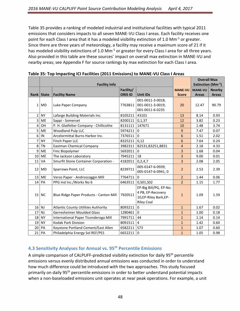
2016 MANE-VU CALPUFF Point Source Contribution Modeling Analysis April 4, 2017
48
Table 35 provides a ranking of modeled industrial and institutional facilities with typical 2011 emissions that considers impacts to all seven MANE-VU Class I areas. Each facility receives one point for each Class I area that it has a modeled visibility extinction of 1.0 Mm-1 or greater. Since there are three years of meteorology, a facility may receive a maximum score of 21 if it has modeled visibility extinctions of 1.0 Mm-1 or greater for every Class I area for all three years. Also provided in this table are these sources’ impact on overall max extinction in MANE-VU and nearby areas; see Appendix F for source rankings by max extinction for each Class I area. Table 35: Top Impacting ICI Facilities (2011 Emissions) to MANE-VU Class I Areas
Facility Info Overall Max
Extinction (Mm-1)
Rank State Facility Name Facility/ORIS ID Unit IDs
MANE-VU
Score MANE-VU
Areas Nearby Areas
1 MD Luke Paper Company 7763811 001-0011-3-0018, 001-0011-3-0019, 001-0011-6-0235
20 12.47 90.79
2 NY Lafarge Building Materials Inc. 8105211 43101 13 8.14 0.93
3 ME Sappi - Somerset 8200111 0,1,37 12 3.82 0.23
4 OH P. H. Glatfelter Company - Chillicothe Facility (0671010028)
8131111 147671 10 1.48 3.74
5 ME Woodland Pulp LLC 5974211 0 9 7.47 0.07
6 IN Arcelormittal Burns Harbor Inc. 7376511 0 6 1.51 2.02
7 NY Finch Paper LLC 8325211 0,12 6 7.64 0.24
8 TN Eastman Chemical Company 3982311 B2531,B3251,B831 4 2.18 4.33
9 ME Fmc Biopolymer 5692011 0 3 1.68 0.04
10 ME The Jackson Laboratory 7945211 18 3 9.00 0.01
11 VA Smurfit Stone Container Corporation - West Point
4182011 0,2,4,7 3 2.08 2.05
12 MD Sparrows Point, LLC 8239711 005-0147-6-0939, 005-0147-6-0941, 0
2 2.53 2.39
13 ME Verso Paper - Androscoggin Mill 7764711 0 2 1.44 0.06
14 PA PPG Ind Inc./Works No 6 6463511 0,S01,S02 2 1.15 1.77
15 NC Blue Ridge Paper Products - Canton Mill 7920511
EP-Big Bill/PG, EP-No. 4 PB, EP-Recovery 10,EP-Riley Bark,EP-Riley Coal
1 1.09 1.59
16 NJ Atlantic County Utilities Authority Landfill
8093211 0 1 1.67 0.02
17 NJ Gerresheimer Moulded Glass 12804611
0 1 1.00 0.18
18 NY International Paper Ticonderoga Mill 7991711 44 1 1.14 0.14
19 NY Kodak Park Division 8091511 4 1 1.42 0.60
20 PA Keystone Portland Cement/East Allen 6582211 S73 1 1.07 0.60
21 PA Philadelphia Energy Sol REF/PES 6652211 0 1 1.05 0.98
4.3 Sensitivity Analyses for Annual vs. 95th Percentile Emissions
A simple comparison of CALPUFF-predicted visibility extinction for daily 95th percentile emissions versus evenly distributed annual emissions was conducted in order to understand how much difference could be introduced with the two approaches. This study focused primarily on daily 95th percentile emissions in order to better understand potential impacts when a non-baseloaded emissions unit operates at near peak operations. For example, a unit

2016 MANE-VU CALPUFF Point Source Contribution Modeling Analysis April 4, 2017
49
that only operates 10 days out of the year would consider 95th percentile emissions during those days instead of evenly distributing the total emissions for those ten day over the full 365 days for the year. In the latter case, even distribution of annual emissions would be highly diluted from 355 days with zero emissions.
Even Distribution of Annual Emissions = Total Annual Emissions / 365 Days per Year
The following set of scatter plots (Figures 37-40) for five MANE-VU Class I areas compares model-predicted visibility extinction for the even distribution of annual emissions (x-axis) and the 95th percentile emissions (y-axis). Each plot includes about 100 EGU units that were modeled with both techniques. The full set of over 300 EGU units was not modeled in order to conserve resources. Instead, an illustrative subset was selected such that EGU units with relatively higher 95th percentile SO2 emissions were included with a good geographic distribution throughout the domain.
In each case, it is clear that potential peak visibility impairment is considerably understated when using an even distribution of annual emissions. The degree of understatement tracks with lowering operating hours.
Figure 37: Acadia EGU Visibility Extinction for 95th Percentile and Annual Emissions
Figure 38: Brigantine EGU Visibility Extinction for 95th Percentile and Annual Emissions
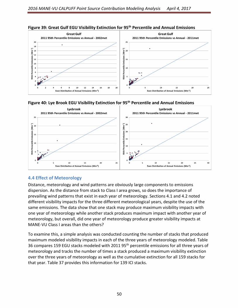
2016 MANE-VU CALPUFF Point Source Contribution Modeling Analysis April 4, 2017
50
Figure 39: Great Gulf EGU Visibility Extinction for 95th Percentile and Annual Emissions
Figure 40: Lye Brook EGU Visibility Extinction for 95th Percentile and Annual Emissions
4.4 Effect of Meteorology
Distance, meteorology and wind patterns are obviously large components to emissions dispersion. As the distance from stack to Class I area grows, so does the importance of prevailing wind patterns that exist in each year of meteorology. Sections 4.1 and 4.2 noted different visibility impacts for the three different meteorological years, despite the use of the same emissions. The data show that one stack may produce maximum visibility impacts with one year of meteorology while another stack produces maximum impact with another year of meteorology, but overall, did one year of meteorology produce greater visibility impacts at MANE-VU Class I areas than the others?
To examine this, a simple analysis was conducted counting the number of stacks that produced maximum modeled visibility impacts in each of the three years of meteorology modeled. Table 36 compares 159 EGU stacks modeled with 2011 95th percentile emissions for all three years of meteorology and tracks the number of times a stack produced a maximum visibility extinction over the three years of meteorology as well as the cumulative extinction for all 159 stacks for that year. Table 37 provides this information for 139 ICI stacks.

2016 MANE-VU CALPUFF Point Source Contribution Modeling Analysis April 4, 2017
51
Table 36: EGU Stack Cumulative Comparison for Three Years of Meteorology
# Maxima Cumulative Extinction
2002 2011 2015 2002 2011 2015
Acadia 80 41 38 280.8 255.7 235.5
Brigantine 38 66 55 332.3 395.1 350.5
Campobello 87 47 25 231.4 203.4 184.3
Great Gulf 47 72 40 192.0 232.6 201.2
Lye Brook 48 75 36 245.5 284.9 249.9
Moosehorn 77 48 34 237.4 214.9 199.8
Presidential Range
53 70 36 205.1 244.0 212.8
Total 430 419 264 1724.5 1830.6 1634
For EGU stacks (Table 36), 2002 meteorology emerged as worst case for the EGU stacks modeled in this analysis, and 2011 produced the greatest cumulative extinction. However, 2011 meteorology produced a similar number of EGU stacks with maximum visibility impacts, while the number of stacks providing maximum impacts during 2015 was about 40% lower than the rates experienced with 2002 and 2011 meteorology. Worst case visibility modeling for Acadia, Campobello, Moosehorn, Dolly Sods, and Otter Creek occurred with 2002 meteorology; worst case for Brigantine, Great Gulf, Lye Brook, Presidential Range, James River Face, and Shenandoah occurred with 2011 meteorology.
Table 37: ICI Cumulative Comparison for Three Years of Meteorology
# Maxima Cumulative Extinction
2002 2011 2015 2002 2011 2015
Acadia 53 44 40 37.8 35.4 36.5 Brigantine 12 58 67 30.2 45. 7 39.8
Campobello 63 46 28 25.2 22.6 21.5 Great Gulf 26 54 57 19.2 29.9 26.8 Lye Brook 21 68 48 31. 8 50.0 39.4
Moosehorn 62 46 29 30. 8 27.7 25.8 Presidential
Range 31 51 55 21.0 31.9 29.3
Total 268 367 324 195.9 243.2 219.0
Figures 41-52 present state-by-state extinction values for each MANE-VU Class I area based on modeling of 2011 emissions over the three years of meteorology. The extinction values for each state are the sum of the extinctions calculated for each source in the state. All results for 2011 95th emissions and 2002 meteorology are based on modeled results, but smaller subsets of sources were modeled for the later meteorology years (see discussion of phases in section 3.2). Therefore, extinction is calculated for the 2011 and 2015 meteorology years for some sources based on ratios developed from sources modeled over all three years.

2016 MANE-VU CALPUFF Point Source Contribution Modeling Analysis April 4, 2017
52
The three colors in the charts represent the minimum, middle, and maximum impacts from among the three meteorology years, but the year that corresponds to each of these categories may differ from state to state. The intent of the chart is not to show which meteorology year led to the maximum visibility impact, but to illustrate the variability in impacts over the three years from differing weather patterns.
To make this variability easier to distinguish, the data labels above each bar describe the maximum impact as a multiple of the minimum impact; that is, a value of 2.0 indicates that the maximum impact was twice the minimum impact. A value of 1.0 means there was no appreciable difference among the three years. States are ordered in decreasing order based on this multiplying factor, such that the leftmost states show the greatest percent increase from minimum to maximum (though the absolute difference may be small), and the rightmost states show the least difference due to changes in meteorology.
The variability of predicted visibility impacts due to changes in annual meteorology is significant and warrants additional analysis. There appears to be enough differences in modeled impacts and contributions introduced to suggest that modeling with one year of meteorology may not be sufficient to capture important transport patterns that may cycle more in some years and may be absent in others.

2016 MANE-VU CALPUFF Point Source Contribution Modeling Analysis April 4, 2017
53
Figure 41: Acadia NP – Variability in EGU Visibility Impact by State and Meteorology Year – 2011 95th Percentile Emissions with Three Years of Meteorology
Figure 42: Acadia NP – Variability in ICI Visibility Impact by State and Meteorology Year – 2011 Typical Emissions with Three Years of Meteorology

2016 MANE-VU CALPUFF Point Source Contribution Modeling Analysis April 4, 2017
54
Figure 43: Brigantine – Variability in EGU Visibility Impact by State and Meteorology Year – 2011 95th Percentile Emissions with Three Years of Meteorology
Figure 44: Brigantine – Variability in ICI Visibility Impact by State and Meteorology Year – 2011 Typical Emissions with Three Years of Meteorology

2016 MANE-VU CALPUFF Point Source Contribution Modeling Analysis April 4, 2017
55
Figure 45: Great Gulf – Variability in EGU Visibility Impact by State and Meteorology Year – 2011 95th Percentile Emissions with Three Years of Meteorology
Figure 46: Great Gulf – Variability in ICI Visibility Impact by State and Meteorology Year – 2011 Typical Emissions with Three Years of Meteorology

2016 MANE-VU CALPUFF Point Source Contribution Modeling Analysis April 4, 2017
56
Figure 47: Lye Brook – Variability in EGU Visibility Impact by State and Meteorology Year – 2011 95th Percentile Emissions with Three Years of Meteorology
Figure 48: Lye Brook – Variability in ICI Visibility Impact by State and Meteorology Year – 2011 Typical Emissions with Three Years of Meteorology

2016 MANE-VU CALPUFF Point Source Contribution Modeling Analysis April 4, 2017
57
Figure 49: Moosehorn – Variability in EGU Visibility Impact by State and Meteorology Year – 2011 95th Percentile Emissions with Three Years of Meteorology
Figure 50: Moosehorn – Variability in ICI Visibility Impact by State and Meteorology Year – 2011 Typical Emissions with Three Years of Meteorology

2016 MANE-VU CALPUFF Point Source Contribution Modeling Analysis April 4, 2017
58
4.5 State-by-State EGU Visibility Extinction Percentages
This section provides a state-by-state breakdown for EGU visibility extinction for 2011 and 2015 using 95th percentile emissions. Table 38 includes only those emission sources located within the modeling domain and modeled in this exercise. There are other emission sources in each state, including smaller EGUs not modeled in this analysis because it was assumed their impacts would be small based on the selection criteria used.
This table makes the rough assumption that extinction values for each modeled EGU within a state can be summed to give the state’s total impact and that the maximum of these total extinction values over the three years of meteorology provides an estimate of the state’s potential visibility impact to each regional Class I area. These total state contributions are ranked by the maximum extinction among each of the Class I areas and over the two emission years; this ranking becomes dominated by the 2011 extinction values for Brigantine, which produced the largest values overall.
The color scheme applies to all data in the table (inclusive of both 2011 and 2015 emission year data). The highest values are dark red, and the lowest values are dark blue, with both ends of the range gradating to white for middle values. The largest and smallest contributors are similar between the two emission years, but, as illustrated by the greater number of medium and dark blue cells, state contributions are lower overall with 2015 EGU emissions. The color scales also demonstrate that the relative rank of each state’s contributions is fairly similar from one Class I area to the next.
Note that the 2011 emissions year includes a much more robust set of sources than the 2015 emissions year (308 compared to 130). Also, for meteorology years without modeled outputs, extinction values are calculated from ratios. For 2015 emissions, sources were modeled only with 2015 meteorology; 2002 and 2011 meteorology year results are calculated (see also section 4.1). For 2011 emissions, some sources were modeled for all three years, but others were modeled using 2002 meteorology only. In the latter case, extinction ratios from those sources modeled for all three years were used to calculate extinction values for the 2011 and 2015 meteorology years.

2016 MANE-VU CALPUFF Point Source Contribution Modeling Analysis April 4, 2017
59
Table 38: State-by-State Contribution to Visibility Impairment at Class I Areas from Modeled EGUs (Expressed as Extinction in Mm-1 and Based on Maximum Extinction from 2002, 2011, and 2015 Meteorology with 2011 and 2015 95th Percentile Emissions)
State*
2011 EGUs 2015 EGUs
Moose-horn
Acadia NP
Great Gulf
Lye Brook
Brigan-tine
Moose-horn
Acadia NP
Great Gulf
Lye Brook
Brigan-tine
OH 56.1 68.2 68.3 70.8 95.3 18.9 22.7 26.7 24.7 33.0
PA 33.2 48.6 36.9 53.4 69.5 23.1 35.1 27.1 37.4 48.5
IN 28.4 30.7 31.6 35.2 46.3 12.5 13.6 12.9 12.4 18.6
MI 25.1 25.6 25.2 21.9 36.0 12.9 13.7 14.5 14.8 21.9
VA 18.2 21.6 16.2 21.8 33.1 5.3 7.0 6.1 7.9 14.4
MA 17.6 21.0 13.8 21.2 31.3 10.9 12.0 8.8 8.3 16.3
NH 12.5 18.1 12.6 19.7 30.4 6.9 7.2 7.4 7.9 16.0
MD 12.4 13.3 11.0 14.4 20.5 4.3 5.0 4.1 4.7 5.7
KY 10.6 13.0 10.8 12.8 20.2 5.0 5.9 5.0 5.8 6.5
WV 10.0 11.2 10.6 11.4 14.6 5.1 6.2 5.2 6.6 9.6
SC 9.9 11.1 9.7 11.1 14.2 0.4 0.4 0.4 0.4 0.4
NC 8.9 10.9 9.2 8.9 13.7 1.0 1.1 1.0 1.0 1.5
NY 8.0 10.0 7.0 8.5 13.6 2.7 3.0 3.7 4.6 3.8
TN 7.7 8.6 6.9 7.8 12.5 1.7 1.7 2.1 1.4 3.0
GA 7.3 8.5 6.7 6.9 12.1 3.4 3.8 3.9 4.7 5.7
IL 6.6 6.9 6.5 6.7 10.9 1.6 1.5 1.2 1.3 2.8
MO 5.9 6.2 6.2 6.4 10.8 1.1 1.2 1.0 1.2 1.6
TX 5.7 6.1 5.2 5.1 10.2 2.4 2.7 2.9 3.7 3.1
ME 3.4 4.0 3.6 4.0 4.7 4.9 5.6 4.8 5.1 6.3
AL 3.7 5.7 5.2 5.0 6.0 0.5 0.7 0.6 0.6 1.0
OK 3.5 4.0 4.2 4.7 5.0 1.0 0.9 0.9 1.0 1.4
IA 3.2 3.9 3.1 3.1 3.9 1.2 1.3 1.1 1.3 2.1
WI 3.0 3.5 2.8 3.0 3.8 0.3 0.3 0.3 0.3 0.4
NJ 2.8 3.4 2.8 2.8 3.1 0.7 0.9 0.9 0.9 1.2
AR 2.7 3.0 2.5 2.7 2.9 0.0 0.0 0.0 0.0 0.0
MN 2.7 2.1 2.2 2.6 2.1 0.4 0.4 0.5 0.4 0.5
KS 1.8 2.0 1.6 2.4 2.0 0.0 0.1 0.0 0.1 0.1
CT 1.8 1.9 1.5 2.2 1.5 0.7 0.9 0.8 0.7 1.1
DE 1.6 1.3 1.3 1.4 1.1 0.3 0.3 0.2 0.1 0.3
*States are ranked by maximum extinction among the five Class I areas and both emission years (2011 and 2015).

2016 MANE-VU CALPUFF Point Source Contribution Modeling Analysis April 4, 2017
60
5.0 Summary and Further Analysis
Modeling results provided in this report are not intended to provide policy recommendations. It
is anticipated that this data will subsequently be analyzed for better understanding and
potential policy development. While the MANE-VU states consider CALPUFF a good model for
this type of analysis, it is recommended that selection of emissions sources for any policy
recommendation be additionally based on further analyses such as a 4-factor analysis.
MANE-VU will review these modeling results in conjunction with other information about these
sources. This report by itself is not sufficient to indicate a need for controls on specific sources,
but rather is an indication that certain sources should be analyzed in more detail. Some of these
sources have shut down or reduced emissions considerably since 2011, while others have
increased emissions of SO2 and/or NOX. Similarly, this report will be used in conjunction with
other information about sources and their potential impacts and is not by itself sufficient to
identify where or when additional emission controls may be reasonable. MANE-VU will consult
with other states and regional organizations as it proceeds to consider what additional
emissions reductions are reasonable for improving visibility at MANE-VU Class I areas by 2028.
Observations resulting from this 2016 CALPUFF modeling exercise include:
1. Emissions of SO2 and NOX from EGUs are lower in 2015 compared to 2011 at many
EGUs, however some show some increased emissions.
2. Modeled sulfate, nitrate and visibility impacts for 95th percentile emissions produce
substantially different results than modeling with annual emissions, especially for units
with low operating hours.
3. The application of three different years of meteorology with identical emission rates can
provide differing maximum sulfate, nitrate and visibility impacts. In some cases, the
difference is substantial. Additional analysis of meteorological influence on emission
source impacts to downwind areas is highly recommended.
4. Emission sources located close to Class I areas typically show higher visibility impacts
than similarly sized facilities further away. But visibility degradation appears to be
dominated by more distant emission sources.
5. This analysis indicates that some industrial emissions sources other than EGUs may have
significant impacts on visibility at MANE-VU Class I areas. Several of these sources are
located in MANE-VU, while a few are located in nearby states.

2016 MANE-VU CALPUFF Point Source Contribution Modeling Analysis April 4, 2017
61
References
Exponent 2011, ‘CALPUFF Modeling System Version 6 User Instructions’.
MANE-VU Technical Support Committee 2016, MANE-VU Updated Q/d*C Contribution Assessment, accessed from <http://otcair.org/MANEVU/Upload/Publication/Reports/MANE-VU%20TSC%20-%20Updated%20QC%20over%20d%20Contribution%20Assessment%20-%20Final.pdf>.
McDill, J, McCusker, S and Sabo, E 2016, ‘Technical Support Document: Emission Inventory Development for 2011 for the Northeastern U.S. Beta Version’.
NESCAUM 2006, Contributions to Regional Haze in the Northeast and Mid-Atlantic United States, Boston, MA, accessed from <http://www.nescaum.org/documents/contributions-to-regional-haze-in-the-northeast-and-mid-atlantic--united-states/mane-vu_haze_contribution_asessment--2006-0831.pdf/>.
Scire, JS, Robe, F, Fernau, M and Yamartino, RJ 1998, ‘A user’s guide for the CALMET meteorological model (Version 5)’, Earth Tech, Inc. Concord, MA.
US EPA 2015, ‘Air Markets Program Data’, accessed from <http://ampd.epa.gov/ampd/>.
US EPA ‘AQS Data Mart’, accessed from <http://aqs.epa.gov/aqsweb/documents/data_mart_welcome.html>.