call center capacity planning
TRANSCRIPT
General rights Copyright and moral rights for the publications made accessible in the public portal are retained by the authors and/or other copyright owners and it is a condition of accessing publications that users recognise and abide by the legal requirements associated with these rights.
• Users may download and print one copy of any publication from the public portal for the purpose of private study or research. • You may not further distribute the material or use it for any profit-making activity or commercial gain • You may freely distribute the URL identifying the publication in the public portal
If you believe that this document breaches copyright please contact us providing details, and we will remove access to the work immediately and investigate your claim.
Downloaded from orbit.dtu.dk on: Feb 12, 2018
Call Center Capacity Planning
Nielsen, Thomas Bang; Nielsen, Bo Friis; Iversen, Villy Bæk
Publication date:2010
Document VersionPublisher's PDF, also known as Version of record
Link back to DTU Orbit
Citation (APA):Nielsen, T. B., Nielsen, B. F., & Iversen, V. B. (2010). Call Center Capacity Planning. Kgs. Lyngby, Denmark:Technical University of Denmark (DTU). (IMM-PHD-2009-223).

Ph.D. Thesis
Call Center Capacity Planning
Thomas Bang NielsenDTU
Kgs. LyngbyOctober 30, 2009
Technical University of DenmarkInformatics and Mathematical ModellingBuilding 321, DK-2800 Kongens Lyngby, DenmarkPhone +45 45253351, Fax +45 [email protected]
IMM-PHD-2009-223
Preface
This thesis has been prepared at the Technical University of Denmark, Departmentof Informatics and Mathematical Modelling in partial fulfilment of the requirementsfor obtaining the Ph.D. degree in engineering. The thesis consists of a summary re-port and a collection of three research papers written and submitted for publicationduring the period 2007–2009. The Ph.D. was funded by a university grant from theTechnical University of Denmark and carried out under the research school ITMAN.
First and foremost, I would like to thank my main supervisor Bo Friis Nielsen (DTUInformatics) for all his help during the three years and for believing in me. Also Iwould like to thank my co-supervisor Villy Bæk Iversen (DTU Fotonik) for his guid-ance. Additionally, I mention my colleagues at the Mathematical Statistics group,especially Jan Frydendall for sharing ups and downs in the office for the main part ofthe three years and Ellen-Marie Traberg-Borup for helping me with all the practicalmatters.
Next, I thank the operations management group at Danske Bank, in particularMette Willemoes Berg for her cooperation and for helping me gain insight into thecall center world.
I appreciate the OBP-group at the VU University Amsterdam for welcoming mein the fall of 2007. Especially I thank Ger Koole for letting me visit and for hisinvaluable help during the last years of my studies. Also thanks to Rene Bekker forhis close cooperation on a paper and Sandjai Bhulai for letting me attend his class.
My family played an important role. In particular I would like to thank myparents Sonja and John for their support throughout my studies and my brothersTorben and Jesper for their interest in my work.
Last, but not least I thank my wonderful girlfriend Sara for always being therefor me and making the last years much more enjoyable due to her love and cheerfulmind.
October 2009Thomas Bang Nielsen
iii


Summary
The main topics of the thesis are theoretical and applied queueing theory withina call center setting.
Call centers have in recent years become the main means of communica-tion between customers and companies, and between citizens and public in-stitutions. The extensively computerized infrastructure in modern call centersallows for a high level of customization, but also induces complicated oper-ational processes. The size of the industry together with the complex andlabor intensive nature of large call centers motivates the research carried outto understand the underlying processes.
The customizable infrastructure allows customers to be divided into classesdepending on their requests or their value to the call center operator. Theagents working in call centers can in the same way be split into groups basedon their skills. The discipline of matching calls from different customer classesto agent groups is known as skills-based routing. It involves designing therouting policies in a way that results in customers receiving a desired servicelevel such as the waiting time they experience. The emphasis of this thesis ison the design of these policies.
The first paper, Queues with waiting time dependent service, introduces anovel approach to analyzing queueing systems. This involves using the waitingtime of the first customer in line as the primary variable on which the analysis isbased. The legacy approach has been to use the number of customers in queue.The new approach facilitates exact analysis of systems where service dependson the waiting time. Two such systems are analyzed, one where a server canadapt its service speed according to the waiting time of the first customer inline. The other deals with a two-server setup where one of the servers is onlyallowed to take customers who have waited a certain fixed amount of time. Thelatter case is based on a commonly used rule in call centers to control overflowbetween agent groups.
v

Realistic call center models require multi-server setups to be analyzed. Forthis reason, an approximation based on the waiting time of the first in line ap-proach is developed in the paper Waiting time dependent multi-server priorityqueues, which is able to deal with multi-server setups. It is used to analyze asetup with two customer classes and two agent groups, with overflow betweenthem controlled by a fixed threshold. Waiting time distributions are obtainedin order to relate the results to the service levels used in call centers. Further-more, the generic nature of the approximation is demonstrated by applying itto a system incorporating a dynamic priority scheme.
In the last paper Optimization of overflow policies in call centers, overflowsbetween agent groups are further analyzed. The design of the overflow policiesis optimized using Markov Decision Processes and a gain with regard to servicelevels is obtained. Also, the fixed threshold policy is investigated and foundto be appropriate when one class is given high priority and when it is desiredthat calls are answered by the designated agent class and not by other groupsthrough overflow.

Resume
Hovedomraderne for denne afhandling er teoretisk og praktisk køteori anvendtinden for call centre.
Call centre har i de senere ar vundet frem som maden, hvorpa firmaer ogoffentlige institutioner kommunikerer med kunder og borgere. En omfattendecomputerstyret infrastruktur i moderne call centre giver mulighed for en højtilpasningsevne, men kan i samme omgang gøre driften særdeles kompleks.Størrelsen og den arbejdstunge karakter af call center industrien, samt de kom-plekse underliggende processer, gør call centre til et interessant forskningsemne.
Den computerstyrede infrastruktur betyder, at kunder kan deles op i forskel-lige klasser alt efter grunden til deres henvendelse eller efter deres værdi forcall center operatøren. Pa samme made kan medarbejderne i call centre delesop i grupper efter deres kvalifikationer. Problemet med at parre forskelligekundeklasser og medarbejdergrupper omtales som skills-based routing. Detteomfatter dirigering af opkald til de rette medarbejdere under hensyntagen tilden service kunderne skal have, herunder den ventetid de bliver udsat for.Denne afhandling omhandler design af disse regler for opkaldsdirigering.
Den første artikel, Queues with waiting time dependent service, introducereren ny tilgang til analyse af køsystemer. Denne tilgang tager udgangspunkt ibrugen af ventetiden for den forreste kunde i køen som den primære variabelanalysen baseres pa. Den traditionelle tilgang er at bruge antal kunder i kø somden primære variabel. Den nye tilgang gør det muligt at analysere systemer,hvor betjeningen afhænger af den tid, kunden forrest i køen har ventet. Tosadanne systemer bliver analyseret. I det første kan et betjeningssted tilpassebetjeningshastigheden som funktion af den tid, den forreste kunde i køen harventet. Det andet system, der analyseres, omfatter to servere, hvoraf den enekun ma tage kunder, der har ventet en given fast tid. Det sidste tilfælde erbaseret pa en regel, der ofte bruges i call centre til at styre opkald mellemmedarbejdergrupper.
vii
Realistiske call center modeller ma nødvendigvis kunne bruges pa systemermed flere betjeningssteder. Med udgangspunkt i dette, udvikles der en ap-proksimation i artiklen Waiting time dependent multi-server priority queues,der kan bruges pa sadanne systemer. Den bruges til at analysere en opsætningmed to kundeklasser og to medarbejdergrupper, hvor der desuden er mulighedfor at sende opkald i overløb mellem grupperne efter en regel baseret pa enfast grænseværdi pa ventetiden. Ydermere demonstreres approksimationensalsidighed ved at anvende den pa et system, hvor kunder prioriteres efter endynamisk regel.
I den sidste artikel, Optimization of overflow policies in call centers, ana-lyseres overløbet mellem medarbejdergrupper nærmere. Overløbet optimeresved hjælp af Markov beslutningsprocesser og det vises, at en forbedring afbehandlingen af kunder kan opnas. Desuden pavises det, at overløbsreglenbaseret pa en fast grænseværdi pa ventetiden er fordelagtig i tilfælde, hvor enkundeklasse tildeles høj prioritet, samt nar det tilstræbes, at kunder betjenesaf de rette medarbejdere, dvs. at de ikke sendes i overløb.
Contents
Preface iii
Summary v
Resume vii
Acronyms xi
1 Introduction 1
2 Call Center Basics 5
2.1 Background . . . . . . . . . . . . . . . . . . . . . . . . . . . . . . . . . . . . 5
2.2 Call Center Structure . . . . . . . . . . . . . . . . . . . . . . . . . . . . . . . 6
2.3 Service Measures . . . . . . . . . . . . . . . . . . . . . . . . . . . . . . . . . 9
3 Traffic Analysis 13
3.1 Traffic Characteristics . . . . . . . . . . . . . . . . . . . . . . . . . . . . . . 13
3.2 Data Collection . . . . . . . . . . . . . . . . . . . . . . . . . . . . . . . . . . 15
3.3 Forecasting . . . . . . . . . . . . . . . . . . . . . . . . . . . . . . . . . . . . 19
4 Call Center Capacity Planning 21
4.1 Resource Acquisition . . . . . . . . . . . . . . . . . . . . . . . . . . . . . . . 21
4.2 Staffing using Queueing Models . . . . . . . . . . . . . . . . . . . . . . . . . 22
4.3 Multi-Skill Call Centers . . . . . . . . . . . . . . . . . . . . . . . . . . . . . 29
4.4 Skills-Based Routing . . . . . . . . . . . . . . . . . . . . . . . . . . . . . . . 32
5 Waiting Time Based Routing Policies 35
5.1 An Analytical Approach . . . . . . . . . . . . . . . . . . . . . . . . . . . . . 37
5.2 The Erlang Approximation . . . . . . . . . . . . . . . . . . . . . . . . . . . 39
5.3 Optimization of Overflows . . . . . . . . . . . . . . . . . . . . . . . . . . . . 41
ix
6 Simulation Modelling 456.1 Discrete Event Simulation Basics . . . . . . . . . . . . . . . . . . . . . . . . 466.2 Choice of Software . . . . . . . . . . . . . . . . . . . . . . . . . . . . . . . . 496.3 Illustrative Simulation Example . . . . . . . . . . . . . . . . . . . . . . . . . 50
7 Discussion 53
Bibliography 55
Appendices 63
A Queues with waiting time dependent service 65A.1 Addendum . . . . . . . . . . . . . . . . . . . . . . . . . . . . . . . . . . . . . 83
B Waiting time dependent multi-server priority queues 99B.1 Addendum . . . . . . . . . . . . . . . . . . . . . . . . . . . . . . . . . . . . . 115
C Optimization of overflow policies in call centers 127
Acronyms
ACD Automatic Call Distributer
AE Average Excess
ANI Automatic Number Identification
ASA Average Speed of Answer
AWT Acceptable Waiting Time
CSR Customer Service Representative
CTI Computer Technology Integration
CTMC Continuous Time Markov Chain
DNIS Dialed Number Identification Service
FCFS First Come First Served
FCR First Call Resolution
FIL First In Line
IP Internet Protocol
IVR Interactive Voice Response
MDP Markov Decision Process
PABX Private Automatic Branch Exchange
PSTN Public Switched Telephone Network
QED Quality-Efficiency Driven
RPC Right Party Contact
RSF Rostered Staff Factor
SLA Service Level Agreement
SLT Service Level Target
TEA The Erlang Approximation
TSF Telephone Service Factor
xi


CHAPTER 1Introduction
Call centers are the preferred way for most major companies and public insti-tutions to interact with customers and citizens. The call center industry is byall measures large and still growing. As of 2006, 2.2 million jobs exist withinthe industry in the US alone (about 1.4% of the entire workforce) with anexpected growth of 25% in the period 2006-2016 [18]. Because of the size andlabour intensive character of the industry there is a large degree of motivationto understand the dynamics of call centers to ensure proper management andavoid unnecessary use of resources.
The main driving forces behind aggregating customer contact in call centersare economy of scale together with the possibility of having a higher degree ofconsistency in the interaction with customers. A large call center allows formore efficient operation, however, it also induces more complex operationalprocesses. Advanced mathematical methods are required to understand thedetails of the processes in order to optimize and improve the operations.
Management within the call center industry involves many areas of op-erations management such as forecasting, scheduling, capacity planning androuting optimization. In [21], call center management is described as a cir-cular iterative process. It starts out setting a desired service level target toaim for. The next element is data collection from which, forecasting can becarried out. After having forecasted the expected load, the required staff andphysical structures can be found taking shrinkage (e.g. absence of employees)
1

1. Introduction
into account. Finally the actual scheduling of agent work hours can be settledand the cost of the operation calculated. The process can then start over andthe service level can be adjusted to ensure that excessive costs are not spenton a too high service level or vice versa.
The above description of call center management is a very general presen-tation. The elements included in the planning process are described in furtherdetail in Chapter 2-6. Especially the advent of the highly computerized setupin modern call centers contributes to more complicated systems. The comput-erized setup allows a high degree of customization of how calls are handled.This means that customers can be treated in different ways and the agentscan be divided into groups according to their skills. Such arrangements arereferred to as multi-skill call centers. Within such a setting, the disciplines ofcall routing and prioritization become important.
The iterative planning process may be fine for smaller adjustments. How-ever, for larger changes to the infrastructure of call centers it is essential tounderstand what the consequences of these changes will be. By modelling thecall center setup, the effect of changes can be assessed without the risk ofimpairing the system during the process.
This thesis centers around routing and handling of calls and is arranged asfollows. A general introduction to the call center world is given in Chapter 2.This includes a description of the physical structure of call centers and thecentral concept of service levels.
Chapter 3 deals with analysis of traffic data. The characteristics of thetraffic to inbound call centers are described together with different aspectsthat may affect it. The importance of data collection for analysis of e.g. waitingtime, service time, and abandonment distributions is treated. Finally the useof historical data for forecasting purposes is described.
Key issues of capacity planning in call centers are treated in Chapter 4. Thisbasically involves having the right number of agents and the right use of theseto accommodate incoming calls in the desired way. All the different levels of theplanning hierarchy are treated, this ranges from resource acquisition, such asdesigning the physical surroundings and the hiring and firing of call center staffto the more detailed management issues. These include staffing and rosteringof agents, i.e. determining how many agents should be at work at a given timeand how the work schedules of the individual agents should be designed to bestcorrespond to the need while adhering to rules regarding work hours. Also thecomplex issue of call routing in multi-skill call centers is discussed.
In Chapter 5, routing policies based on the waiting time of the first customerin line are treated. The special case characterized by fixed thresholds is dealt
2

with in detail. This policy is used widely in multi-skill call centers for loadbalancing between different agent groups. The discussion in this chapter iscentered around the three papers presented in appendices A, B, and C, whichall deal with the analysis of thresholds.
The use of simulation for modelling call centers is treated in Chapter 6. Thisincludes a discussion of the benefits and disadvantages of using simulations ascompared to analytical models or approximations. At the end of the chapter,the possibilities of using simulation for modelling call center performance areillustrated through a concrete example.
Finally in the last chapter of the summary report, a short discussion ofthe contribution of the thesis is given. The main contribution of the thesis ispresented in the appendices in form of three journal papers.
In Appendix A a new approach to modelling queueing systems is presented.This involves using the waiting time of the first customer in line as the primaryvariable, which the analysis is based on. The approach is in many ways similarto the one used in [10], where the workload is considered. The new approachis especially convenient when queueing systems with operations that somehowdepend on the experienced waiting time of customers are considered. Two suchsystems are analyzed in Appendix A, one where the service rate of a server canbe adjusted according to the waiting time of the customer first in line. Theother analyzed system involves two servers, of which one is only allowed to takecustomers who have waited a certain fixed amount of time. The latter system isbased on a common rule used in call centers for skills-based routing, where callsare only allowed to overflow between different agent groups after having waiteda fixed amount of time. The analysis in Appendix A is elaborated further onin Appendix A.1 where an additional mathematical investigation regarding theindependence of a linear equation system from the paper is given.
A more application oriented approach is taken in the work presented inAppendix B. Here an approximation, based on the same approach of using thewaiting time of the customer first in line as the primary variable, is developed.The approximation is used to model a realistic call center multi-server setupwith two customer classes and two agent groups and overflow from one class tothe other. Furthermore, the general nature of the approximation is illustratedby modelling a dynamic priority system. In Appendix B.1 the validity of theapproximation in its simplest form is proven.
The last paper, presented in Appendix C, deals with optimization of over-flow. Again, the same approach of analyzing the waiting time of the firstcustomer in line is taken. The appropriateness of using the fixed thresholdpolicy is also examined.
3

CHAPTER 2Call Center Basics
The fundamental aspects of call centers and call center management are treatedin this chapter. This includes the background and motivation for using callcenters in Section 2.1 and the physical structure in Section 2.2. The use ofdifferent service measures is discussed in Section 2.3.
2.1 Background
The term call center covers a large variety of instances. Another often seenterm, is contact center, where the general consensus is that a call center onlycommunicates through phone calls whereas contact centers have multiple com-munication channels such as email or chat beside phone calls. The term callcenter may also be avoided in some cases due to it having a somewhat negativeconnotation. This may especially be the case for call centers with highly skilledemployees who want to differentiate their service from simpler ones often pro-vided by students working part time. The term call center is used throughoutthis thesis as mainly the discipline of handling calls is considered. See e.g. [15]for a treatment of contact centers with traffic composed of mixed mail andphone calls.
The main purpose of gathering customer contact in one central place iseconomy of scale, a large central unit is more efficient than multiple smallerunits. The simplest explanation for this is that the risk of one customer having
5

2. Call Center Basics
to wait at one place while capacity is available another place is eliminated.This is treated further in Section 4.2.
Call centers are divided into inbound and outbound depending on whoinitiate the calls. The term inbound call center is used for the case wherecustomers initiate calls, typically to obtain a service. Outbound refers to callcenters where agents call customers. The latter would typically be used to sella product or conduct a survey. Combinations of the two are of course alsopossible. Inbound call centers are the most interesting from a modelling pointof view as this is where most of the challenges are, due to the stochastic natureof incoming calls. Outbound call centers can to a large extent decide whencalls take place, whereas there is a large element of uncertainty associated withinbound call centers. For this reason, this thesis focuses solely on inbound callcenters. Optimization of a combination of in and outgoing traffic is treated in[11].
People can have many reasons for communicating with call centers. Themost obvious is a person calling a company he does business with, such as abank or a support hotline. For outbound call centers it can even be involun-tarily by salespersons calling and trying to sell services or goods, often at themost inappropriate of times. This may very well be one of the sources of thesomewhat bad reputation call centers can have. Emergency services, such as112 and 911 in the European Union and the United States respectively, alsofall under the category call centers. We will refer to people communicatingwith a call center as customers no matter the reason.
There is an abundance of general introductions to call centers and call centermanagement. Highly recommended for a lighter approach to call center man-agement is [21] whereas [25] gives a more mathematical introduction includingnumerous references.
2.2 Call Center Structure
The main resource of call centers is the employees responsible for the commu-nication with customers. The used terms for these employees are agents orCustomer Service Representatives (CSRs). The fact that salaries account for60-80% of total operating costs [50], [4] makes this by far the most importantsubject for optimization.
Operations in modern call centers are built around an extensively com-puterized setup as depicted in Figure 2.1. Call centers typically have theirown telephone exchange in the form of a Private Automatic Branch Exchange
6

Call Center Structure
(PABX) that connects phones internally and to the Public Switched TelephoneNetwork (PSTN) through trunk lines. For further details of the underlyingtelecom technology see e.g. [53].
ACD
CTIPSTN
PABX
Agent terminals
Call center
IVR
Trunk lines
Figure 2.1: The physical structure of a modern call center. Solid lines representvoice connections and dotted lines data connections.
The effect of limited computer system processing power is analyzed in [3]by treating the agent pool as a processor sharing unit. This case should reallybe avoided though, as payroll costs are generally dominant in call centers. Onecould maybe imagine cases in parts of the world where salaries are very low,where this would be relevant.
A central piece of equipment is the Automatic Call Distributer (ACD) whichdistributes incoming calls and collects call statistics. This makes it importantfor planning purposes. The distribution of calls is based on algorithms thatcan be designed to accommodate calls in desired ways. This topic is discussedfurther in Chapter 4.
Interactive Voice Response (IVR) is the technical term for the equipmentthat gives welcome messages, plays music, and informs about the caller’s placein queue, if these services are implemented. The IVR also allows users tointeract with the call center using the keypad of the phone. This includesletting the customer choose a desired service after hearing a message such as
7
2. Call Center Basics
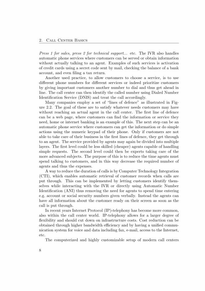
Press 1 for sales, press 2 for technical support... etc. The IVR also handlesautomatic phone services where customers can be served or obtain informationwithout actually talking to an agent. Examples of such services is activationof credit cards using a secret code sent by mail, checking the balance of a bankaccount, and even filing a tax return.
Another used practice, to allow customers to choose a service, is to usedifferent phone numbers for different services or indeed prioritize customersby giving important customers another number to dial and thus get ahead inline. The call center can then identify the called number using Dialed NumberIdentification Service (DNIS) and treat the call accordingly.
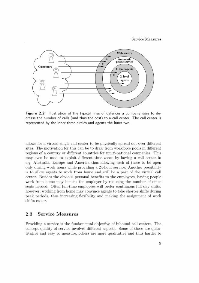
Many companies employ a set of “lines of defence” as illustrated in Fig-ure 2.2. The goal of these are to satisfy whatever needs customers may havewithout reaching an actual agent in the call center. The first line of defencecan be a web page, where customers can find the information or service theyneed, home or internet banking is an example of this. The next step can be anautomatic phone service where customers can get the information or do simpleactions using the numeric keypad of their phone. Only if customers are notable to take care of their business in the first lines of defence, they get throughto an agent. The service provided by agents may again be divided into multiplelayers. The first level could be less skilled (cheaper) agents capable of handlingsimple requests. The second level could then be experts taking care of themore advanced subjects. The purpose of this is to reduce the time agents mustspend talking to customers, and in this way decrease the required number ofagents and thus the expenses.
A way to reduce the duration of calls is by Computer Technology Integration(CTI), which enables automatic retrieval of customer records when calls areput through. This can be implemented by letting customers identify them-selves while interacting with the IVR or directly using Automatic NumberIdentification (ANI) thus removing the need for agents to spend time enteringe.g. account or social security numbers given verbally. Instead the agents canhave all information about the customer ready on their screen as soon as thecall is put through.
In recent years Internet Protocol (IP)-telephony has become more common,also within the call center world. IP-telephony allows for a larger degree offlexibility and should cut down on infrastructure costs. Cost reduction can beobtained through higher bandwidth efficiency and by having a unified commu-nication system for voice and data including fax, e-mail, access to the Internet,etc.
The computerized and highly customizable setup of modern call centers
8
Service Measures
2. levelagents
1. level agents
Automatic
Web service
phone service
Customers
Figure 2.2: Illustration of the typical lines of defences a company uses to de-crease the number of calls (and thus the cost) to a call center. The call center isrepresented by the inner three circles and agents the inner two.
allows for a virtual single call center to be physically spread out over differentsites. The motivation for this can be to draw from workforce pools in differentregions of a country or different countries for multi-national companies. Thismay even be used to exploit different time zones by having a call center ine.g. Australia, Europe and America thus allowing each of these to be openonly during work hours while providing a 24-hour service. Another possibilityis to allow agents to work from home and still be a part of the virtual callcenter. Besides the obvious personal benefits to the employees, having peoplework from home may benefit the employer by reducing the number of officeseats needed. Often full-time employees will prefer continuous full day shifts,however, working from home may convince agents to take shorter shifts duringpeak periods, thus increasing flexibility and making the assignment of workshifts easier.
2.3 Service Measures
Providing a service is the fundamental objective of inbound call centers. Theconcept quality of service involves different aspects. Some of these are quan-titative and easy to measure, others are more qualitative and thus harder to
9
2. Call Center Basics
measure.Call centers can be characterized by how they are operated, distinguished
by different regimes. Some call centers may have a very low agent utilizationmeaning that almost all calls are answered immediately, this is referred to asthe quality driven regime. At the other extreme we have the efficiency drivenregime where almost all customers have to wait before being served, here theagent utilization will be close to 100%. In between, and where most call cen-ters operate, is the rationalized regime where agent utilization is high (maybe90 − 95%), but many calls may still be answered immediately. This is madepossible by large call centers enjoying the benefits of economy of scale. Thedifferent regimes influence how system performance can be approximated. Theimportant rationalized regime was first thoroughly analyzed in [34] resultingin its alternative designation, the Halfin-Whitt regime. Sometimes it is alsoreferred to as the Quality-Efficiency Driven (QED) regime.
Service Levels
The quantitative service measures typically involve how long customers haveto wait before the call is answered by an agent. The simplest measure of this isAverage Speed of Answer (ASA), which is, as the term implies, just the meanof the time customers wait in queue. The measure used by itself is lackingin detail, as no information about the waiting time distribution is given otherthan its mean.
In in-house call centers the upper management typically sets a Service Level(SL) target for the operations manager to meet. For outsourced call centersthe call center operator and the company enter a contract in the form of aService Level Agreement (SLA). Service levels are common in the simple formof a specified percentage of calls that should be answered within a certain time,referred to as Acceptable Waiting Time (AWT) or Service Level Target (SLT).This is written as e.g. 80/20 which means 80% of calls should be answeredwithin 20s. This service measure is referred to as Telephone Service Factor(TSF).
Lost or abandoned calls are also normally considered. This measure wouldtypically be strongly correlated with the service levels. Customers may evenbe encouraged to abandon and call back while they are in queue if the systemis overloaded in order to improve service levels.
The TSF used in call centers varies greatly; 90/20, 85/15 or 90/15 wouldtypically be regarded as high service levels used in competitive businesses wherecustomers may take their business elsewhere if service is unsatisfactory. For
10
Service Measures
emergency services the demands may be even higher. A TSF of 80/20 is theclassic middle of the road choice often used in banks, insurance companies, andtravel agencies. In the lower end, service levels such as 80/300 may be usedby e.g. soft- and hardware support centers and governmental offices where youcan’t really take your business elsewhere [21].
Service levels have to be approached with some caution. TSF used by itselfactually motivates tossing customers out of the queue as soon as the time theyhave spent in the queue exceeds the threshold of the TSF. This approach willincrease the chance of serving other customers within the threshold. Anothersimilar approach would be to only serve customers which have exceeded thethreshold if no customers having waited less than the threshold are present inthe queue. In order to account for some of these discrepancies a new servicemeasure is suggested in [49]. The suggested service measure is called the Av-erage Excess (AE) and it is, as the name suggests, the average time, whichwaiting exceeds SLT.
It has been suggested to introduce a third term to TSF representing thepercentage of intervals where a percentage of calls are answered within a timelimit. E.g. 90/80/20 would mean that in 90% of time intervals 80% of callsshould be answered within 20s. The length of the time interval should also begiven.
The widespread use of TSF probably originates in how easily it is inter-preted. Despite this, less mathematically gifted management may still requirethe impossible of the operations management team, such as a 100% servicelevel with a low SLT for their most priced customers. It may seem appropriateto guarantee the most valued customers to be answered quickly, however theremust be room for exceptions as 100% service levels in principle require an agentsitting ready for each customer.
There is some discrepancy about how to calculate the performance measureTSF from data. This is discussed in [21] and involves how abandonments aredealt with. Sometimes abandoned calls are disregarded altogether, and TSFis calculated as the number of calls answered before the SLT divided by thetotal number of answered calls. Another option is to divide by the number ofoffered calls which will degrade the TSF if many calls abandon. Sometimesonly calls that abandoned before SLT are included. As such there is no uniqueright way to do it as long as it is clarified how it is done. However, the methodof dividing the sum of answered and abandoned calls within SLT by offeredcalls is recommended in [21].
Even taking the different ways to calculate TSF into account there is stillroom for more interpretations. The time period over which the TSF is mea-
11

2. Call Center Basics
sured, can have a major influence on the resulting values. If TSF is measuredover a short period, the percentage of calls answered within the time limit willvary much more than if longer periods are used. During a 24-hour period therequired number of calls may be answered within the time limit, however if thesame day is split into hourly intervals the TSF may be exceeded during someof the intervals.
Customer Satisfaction
The qualitative part of call center service is harder to measure. This includesthe customer’s impression of the conversation, such as politeness and com-petence of the agent. Agent competence plays a major factor in First CallResolution (FCR) which is important because it affects the number of calls acall center receives. Customers are likely to call back if their intent is not metthe first time.
Many call centers use the possibility of having supervisors or colleaguessitting next to them and listen in on the calls. In this way agents can receivefeedback on their performance and be coached into giving better service by thelistener-in. Some call centers also have supervisors listening in on calls to assessperformance without agents knowing it. This may not be a good practice froma work environment point of view, as agents may feel monitored.
The usual suspects when it comes to what determines service quality andcustomer satisfaction are ASA, abandonment rate, blocked calls, TSF, FCR,and talk time. The first three can be expected to be negatively correlated andthe latter three positively correlated to customer satisfaction.
A study in [23] shows a surprising lack of correlation between the usualperformance measures (ASA, abandonment rate, talk time, etc.) and customersatisfaction in banking/financial call centers, however, no explanation of whatdetermines satisfaction is given. This essentially highlights the issue of theassumption that satisfaction is correlated to what can easily be measured ratherthan harder to measure factors such as agent kindness, etc. An interestingresult of [23] is that correlation between the usual performance measures ismuch larger for call centers within other industries.
12

CHAPTER 3Traffic Analysis
The nature of call traffic to inbound call centers is highly stochastic. Alsothe duration of calls and the caller behavior with regard to patience and thetendency to redial, constitute interesting research topics which are discussedin this chapter.
3.1 Traffic Characteristics
The traffic to inbound call centers varies greatly with time. This variation canbe seen as a function of the time of day, day of the week, day of the month,month of the year, and even the year.
The most obvious variation is typically seen intra-day as calls depend on thework hours and daily routines of people. The business hours of a call center mayalso influence the pattern of arriving calls. This could be in the form of a peakjust after opening time. A pronounced variation over the week will also oftenbe seen, mostly with a distinction between weekdays and weekends. Variationover the month may especially be seen at the start and end of the monthas many bills have to be settled around this time. Also people may have atendency to spend more money on shopping on and just after payday, resultingin an increased call load to sales call centers. An intra-yearly variation willtypically result from people going on vacation during the summer, Christmas,etc. Inter-yearly variation can be assumed to come from a general trend in call
13

3. Traffic Analysis
loads originating in a changing number of customers or people’s disposition touse the call center. The possibility of identifying a general trend motivatessaving records of call volumes for a long time.
0 4 8 12 16 20 24Time of day
Off
ered
cal
ls
High priorityLow priority
5 10 15 20 25 30Day of the month
Off
ered
cal
ls
High priorityLow priority
Figure 3.1: Calls to an inbound call center during 15 minute intervals over a dayand daily intervals over a month. The number of calls are depicted on a linear axiswithout a scale as the intention is only to illustrate the patterns.
The number of calls a call center receives is referred to as offered calls.This can be considered over any given time interval, such as 15 minute ordaily intervals and includes all calls including both those whom are eventuallyserved and those whom abandon. Figure 3.1 shows an example of the patternof offered calls over a day and over a month for low and high priority calls. Thedaily variation is clearly seen with the highest load during work hours and inthe morning in particular. The weekly variation is also clear with fewest callsin the weekends and most on Mondays. The previously mentioned increasearound the turn of a month seems especially pronounced for the high prioritycustomers. Also the offered calls of high and low priority customers appearhighly correlated. Observations such as these should all be accounted for whendesigning forecasting models as described in Section 3.3.
Calls to an inbound call center are often assumed to arrive according toa Poisson process (i.e. times between calls are independent and exponentiallydistributed) with constant intensity within short time intervals. The rate atwhich calls arrive is generally denoted by λ. The reasoning behind this is thatthe total number of customers is assumed to be infinite, thus the intensity of
14

Data Collection
arriving calls does not depend on the active number of calls. This assumptionis appropriate as the customer base of call centers is normally quite large.
If the average service time of calls is also given, it makes sense to considerthe offered load. The offered load is measured in erlang (E), a dimensionlessunit, given by multiplying the mean arrival rate with the average service timeas
A = λµ−1,
where µ−1 is the average service time and A the offered load.Redials due to calls not being resolved during the first contact will violate
the Poisson assumption as the arriving calls will be dependent on the servicelevel and abandonment rate. This means that the way calls are served, influ-ences the offered traffic, contrary to what is normally assumed in most models,i.e. the offered traffic being independent of the service quality [37].
3.2 Data Collection
Collection of data in call centers is essential for planning purposes and foranalyzing performance. Large quantities of data are normally logged as datastorage capacity is relatively cheap. This includes number of calls, duration ofcalls, waiting times, abandoned calls, etc.
A widely used practice is only to log aggregated call data as this results inmuch less data compared to logging of individual calls. Aggregated data wouldtypically be the number of offered, abandoned, and answered calls during a 15minute period. Waiting time distributions can also be logged in an aggregatedform as number of calls served after having waited between 0 and 2 seconds, 2and 4 seconds, again during 15 minute intervals. In this way a lot of informationis discarded compared to logging call-by-call data.
The more detailed call-by-call data is e.g. required to analyze the arrivalprocess in order to investigate the assumption of it being Poisson in short timeintervals. Also call-by-call data could be used to estimate an arrival function,λ(t), which would be interesting for models dealing with non-stationary trafficas discussed in Chapter 4. The same goes for detailed analysis of the waitingtime distributions, both for those who are eventually served and those whoabandon. Aggregated data should be adequate for most forecasting purposesthough.
Another topic for which aggregated data cannot be used to examine is firstcall resolution. Call-by-call data should be more appropriate for this as the
15

3. Traffic Analysis
same caller calling multiple times within a short time may very well indicatethat his intent was not resolved by the first contact.
The literature dealing with statistical analysis of center data is not as abun-dant as it could be. This is to some extent probably due to the lack of reliablecall-by-call data. Exceptions are [16] and [17] where the same call-by-call datafrom an Israeli call center is analyzed.
Service time
For most analytical work, service times are assumed to be exponentially dis-tributed. This is often done for practical reasons as exponentially distributedholding times are easiest to deal with analytically even though it may not al-ways be the best representation of reality. It also means that only the mean ofthe service times needs to be used for modelling. The rate of which calls arehandled by agents is normally denoted µ, i.e. the mean service time is 1/µ.
A detailed analysis of call center service times can be found in [17], wherethe service times are shown to be very close to lognormally distributed. Themean service time was also shown to vary greatly over the 24-hour day withthe longest service times coinciding with the highest offered traffic in the latemorning and afternoon. This was especially the case for regular calls to thebank, but less so for internet support calls which had a more stable servicetime.
The problem of short service is also discussed in [17]. This involves agentshanging up on customers as soon as they are put through in order to increasethe number of calls the agent handles. This obviously decreases the meanhandling time, which is a part of how agents are evaluated. This issue stressesthe importance of not relying on too simple measures as these may be exploitedby the more scrupulous individuals. By considering the entire service timedistribution this issue was easily identified and appropriate measures could betaken.
Further analysis can be found in e.g. [13] which treats the holding (service)time of telephone calls as a mixture of different components. Also the humanperception of time is considered.
As calls constitute a dialogue, service time of a call is obviously dependenton both the caller and the agent. However, in most multi-skill models theservice time is bound to either the agent pool or the customer class, often outof convenience.
16
Data Collection
Customer Patience
Customers are in simpler models, such as the Erlang-C model treated in Sec-tion 4.2, assumed to be infinitely patient. This is however not realistic in acall center setting as customers get tired or annoyed and abandon the queue.Ignoring abandonments can actually lead to overstaffing as the carried load nolonger equals the offered load.
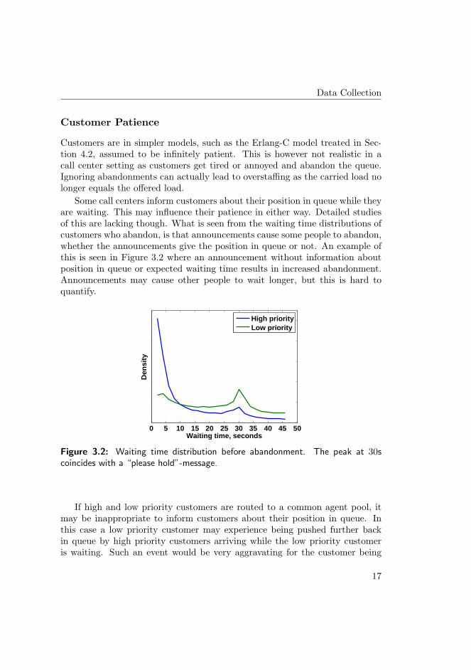
Some call centers inform customers about their position in queue while theyare waiting. This may influence their patience in either way. Detailed studiesof this are lacking though. What is seen from the waiting time distributions ofcustomers who abandon, is that announcements cause some people to abandon,whether the announcements give the position in queue or not. An example ofthis is seen in Figure 3.2 where an announcement without information aboutposition in queue or expected waiting time results in increased abandonment.Announcements may cause other people to wait longer, but this is hard toquantify.
0 5 10 15 20 25 30 35 40 45 50Waiting time, seconds
Den
sity
High priorityLow priority
Figure 3.2: Waiting time distribution before abandonment. The peak at 30scoincides with a “please hold”-message.
If high and low priority customers are routed to a common agent pool, itmay be inappropriate to inform customers about their position in queue. Inthis case a low priority customer may experience being pushed further backin queue by high priority customers arriving while the low priority customeris waiting. Such an event would be very aggravating for the customer being
17

3. Traffic Analysis
pushed back and probably not something call centers would expose even lowpriority customers to.
Another option is to give an estimate of the remaining waiting time. Thiscan obviously never be more than an estimate, however it actually gives morevaluable information to the customer than just giving the position in queue.For example being informed that you are number eight in queue may meanyou have to wait for a very long time if only one agent handles calls or a veryshort time if hundreds of agents are working. Prediction of waiting times isexamined in [74] where information such as the number of customers in queueand elapsed waiting time for non-exponential service times are used to improveestimates.
An interesting note is that in an M/M/n system with a First Come FirstServed (FCFS) policy and visible queue the waiting time a customer can expectto experience is gamma distributed, but if the queue is invisible then the waitingtime is exponentially distributed [37]. This is due to the fact that the expectednumber of waiting customers is geometrically distributed and a set of gammadistributions with shape parameters weighted by a geometric distribution doesindeed result in an exponential distribution.
An empirical analysis of abandonments is given in [78]. It is shown thatexperienced callers adapt their patience according to system performance evenif information about queue length is not given, they simply learn that at certaintimes they risk waiting a long time if not being served immediately.
What is often referred to as the Erlang-A model extends the Erlang-C modelby including abandonments. Analysis of models including abandonments wasfirst carried out in [60]. Erlang-A can be seen as a generalization of the Erlangmodels, with Erlang-B and Erlang-C being the two extremes with zero andinfinite patience of the customers.
Analysis of customer patience requires inference analysis because the pa-tience of those served is not known and is thus considered censored data. Em-pirical data of customer patience is examined in [16] and [17] and shown tohave a nearly constant hazard rate, i.e. the patience is nearly exponentiallydistributed. The main deviation from this comes from messages being an-nounced, stating that the customer is in queue. These messages seem to makecustomers abandon the queue, intentionally or not. Customer patience is fur-ther analyzed in [27] where a method based on boot strapping to determineconfidence intervals is presented.
18
Forecasting
3.3 Forecasting
The discipline of predicting the number of incoming calls to a call center isreferred to as forecasting. The importance of thorough forecasting cannot beoverestimated. Unprecise predictions of the call load lead to either over- orunderstaffing which in turn results in unnecessary pay costs or unsatisfactoryservice levels respectively.
In general, a forecast will be more precise, the shorter the time horizon.Forecasting with a horizon of a month or more is used to determine the requiredstaffing levels and from those, schedule the work hours of agents. Forecastingwith a shorter horizon of, say a few days, could be used to call in extra staff ifneeded.
It is often assumed that calls arrive according to a time-inhomogeneousPoisson process. The inhomogeneity stems from the fact that the probabilityof a customer making a call varies during the day, week, month and year. Therate of arrivals is normally denoted λ for time-homogeneous systems and λt orλ(t) for time-inhomogeneous systems.
The most common approach to forecasting call volumes is a simple top-down approach [25]. This approach starts with an estimate of the number ofcalls during a month or even a year from historical data. From this, weekly,daily and typically half-hourly estimates are made. As an example, assumethat a call center receives 1′000′000 calls in a year; from historical data it isknown that 10% of calls are made in May, of those, 20% of calls fall in thefirst week of the month, 25% of calls are made on Mondays and 5% are madebetween 10.00 and 10.30, then the estimated number of calls in the half-hourlyinterval would be 1000000 · 0.1 · 0.2 · .25 · 0.05 = 250. Due to the simplicity ofthis approach, one might expect that better results would be easily obtainable.Certain days such as national holidays will not follow this pattern and are oftendealt with from the past experience of an operations manager.
In [69], a number of different approaches to forecasting are examined usingunivariate time series methods. The result of this work indicates that a simpleapproach referred to as Seasonal mean is hard to beat when the horizon of thepredictions is more than a few days. Seasonal mean is just a moving averageover the same half-hour of the week of previous weeks. For shorter forecastswith a horizon of 1-2 days another method, Exponential Smoothing for DoubleSeasonality, was shown to perform better. This method assigns more weight tothe most recent observations and takes both intra-day and intra-week seasonalcycles into account.
Also of importance when forecasting is to take the expected service time
19

3. Traffic Analysis
into account. It has been observed that the average service time can increaseduring evenings, effectively making the call load higher, see [21] and [17]. Alsoa (positive) correlation between the call volume and mean service time has beenobserved as agents may become tired and less effective when they are stressed[16].
In [65] detection of outliers, data visualization, and determination of signif-icant features such as day of the week effect from noisy data are treated usingsingular value decomposition. This is used to develop a forecasting model andused for a test case based on data from an American financial company. Theoutliers are found to nicely correspond to holidays or days with system errorsand a day of the week dependence is identified, both contributing to improvingthe forecasts.
Computation of prediction intervals for the arrival rate is treated in [44]. Byusing Poisson mixtures to deal with overdispersion, the arrival rate is treatedas a random variable, i.e. the arrival rate λ is drawn from one distribution andthe number of calls in an interval is then drawn from a Poisson distributionwith parameter λ. This is necessary as the variance of observed data is oftenhigher than the mean, these should be even under the Poisson assumption.Call center performance is finally determined using the Erlang-C formula.
20

CHAPTER 4Call Center Capacity
Planning
The issue of determining the number of servers required to provide customerswith a desired service level can be very complicated due to the many factorsinvolved. This topic is treated in the following sections.
4.1 Resource Acquisition
A part of the physical structure to be dimensioned is the number of telephonetrunk lines. All active calls need a trunk line, both those queued, those usingthe IVR, and obviously those which have been put through to an agent. Inmost cases call centers ensure that there are simply enough trunk lines foralmost any scenario as the required hardware is relatively cheap compared toagent wages. The number of required trunk lines can be determined by usingthe Erlang-B formula [37] as calls are blocked if no line is available. This isfurther treated in Section 4.2
The hiring process of agents also falls within resource acquisition. Depend-ing on the required skill of agents, hiring and training a new agent may takedays, months or even years. This obviously calls for some long term planningtaking into account the expected growth of business, i.e. new customers or fu-ture acquisitions of other companies. Also people leaving for other jobs and
21

4. Call Center Capacity Planning
retiring must be considered. The hiring problem is not unique to the call centerindustry and is well described in the literature such as in [31].
Shrinkage
The number of agents required to man the phones at any given time does notequal the number of agents that needs to be scheduled for the given time.The actual number of available agents is decreased due to many causes suchas people calling in sick, needing breaks to go to the toilet and get coffee,lunch breaks, meetings, coaching, education, vacation, and more. Some factorscan be controlled to some extent as discussed in [1] while other may be moreproblematic.
Accounting for shrinkage is normally done by fairly simple methods suchas described in [21] and [20]. The procedure is to use Rostered Staff Factor(RSF) (also referred to as overlay) as a factor which describes the requiredoverstaffing needed to account for shrinkage. Not much work in the literaturetakes absenteeism into account for general models but [76] treats the numberof active agents, given the number of agents on job, as a random variable.
4.2 Staffing using Queueing Models
The fundamental aspect of staffing is to determine the minimum number ofagents required to satisfy service levels. Obviously overstaffing leads to in-creased costs and understaffing results in poorer than desired service. Thismeans that staffing is a key element in call center management, i.e. wheregreat savings can be made. In this way, a good result for an operations man-ager is not to have as many calls as possible answered within the TSF, butrather just the required percentage.
The many different issues related to the flow of calls through the call centerare illustrated in Figure 4.1. Most models only take some parts of the processinto account. This will often be due to necessity as models quickly become verycomplicated, however much insight can also be gained from simplified models.
The discipline of determining the required number of servers to offer incom-ing traffic a given service level is the most classic within queueing theory. It waspioneered by Agner Krarup Erlang while he worked at the Copenhagen Tele-phone Company with the aim of determining the number of required circuits toensure the desired telephone service. He also worked on determining how many
22

Staffing using Queueing Models
Retrials
Retrials
Agents
Served callsUnresolved calls, retrials
Queued calls
Answered calls
Offered calls
Lost calls
Abandoned calls
Lost calls
Blocked calls
Figure 4.1: Call center process diagram.
telephone operators should be working at cord boards used to switch telephonecalls in the early days of telephony. In many ways this can be seen as theancestral origin of modern call centers or indeed the mathematical aspects ofcall center management. Erlang’s work has proved extremely long-lasting andhis formulae are still widely used within the call center and telecommunicationworlds.
Erlang-C
The most used way of determining the number of agents needed, is by theErlang-C formula. The model behind the Erlang-C formula is M/M/n, Marko-vian arrivals and service completions (time between arrivals and service dura-tions are exponentially distributed) and n servers with infinite waiting positionsand infinitely patient customers. The formula gives the relation between thedelay probability (the probability of not being served immediately, P(W > 0))and the number of servers (n), arrival rate (λ) and service rate (µ). It is worthnoting that only the ratio between λ and µ matters, thus the offered traffic isintroduced as A = λ/µ. See for [37] for details and references on the original
23

4. Call Center Capacity Planning
work of Erlang.
P (W > 0) =
An
n!n
n−An−1∑i=0
Ai
i!+
An
n!n
n−A
.
Assuming that calls are handled on a first come, first served (FCFS) basis, thenthe waiting time distribution can be found as
P(W ≤ t) = 1− P (W > 0) · e−(nµ−λ)t, n > A, t > 0.
The use of the Erlang-C formula is fairly straightforward as it only requiresestimation of the arrival rate and mean service time, which should be availablefrom forecasts based on historical data. However, the Erlang-C model has someshortcomings. A major one being that it does not take customer abandonmentsinto account. This means that if the offered traffic exceeds n, then the queuebecomes unstable and grows towards infinity.
In order to have a stable system, i.e. the queue will not grow infinitely,the number of servers must be greater than the offered traffic for an M/M/nsystem. The number of servers beyond the offered traffic is referred to as safetystaffing and a well proven rule in this context is the square root safety staffingprinciple. In words, this rule dictates that in order to have approximately thesame service level, the number of additional servers beyond the offered trafficshould grow as the square root of the offered traffic. Put formally it becomes
n ≈ A + β√
A,
where n is the number of servers, A the offered traffic and β a coefficient relatedto the service level. The rule applies best to heavily loaded large systems. Theprinciple behind square root staffing has been known for long, as it is funda-mentally based on the central limit theorem. In fact Erlang used the principle,but it was formalized in the call center setting in [14]. The quality of the ap-proximation behind the square root principle is examined in [41] and shownto be very good even for moderate sized systems as long as abandonments areignored.
The square root safety staffing rule nicely illustrates the economy of scaleprinciple, one of the main driving factors of call centers. A simple example ofthis would be to consider a call center offered a load of 100 E compared to oneoffered 400 E. To obtain approximately the same service level (assume β = 1),
24
Staffing using Queueing Models
the smaller call center would require a safety staff of 10 agents compared to 20for the four times larger call center, i.e. only twice as many safety staff despitea fourfold larger traffic. Put in another way the utilization of agents increaseswith the size of call centers, given the same service level as described in [73].
Erlang-B
Also well known is the Erlang-B formula, which is based on a rejection model.This means that customers that are not served immediately are blocked andlost. Arrivals and service completions are assumed Markovian as for the Erlang-C formula. The Erlang-B formula gives the probability of being blocked, B [37]:
B =
An
n!n∑
i=0
Ai
i!
.
The Erlang-B formula is normally used for trunk capacity calculations [21] inthe call center world, that is how many phone lines should go into the callcenter.
Beyond Erlang
There is an abundance of more advanced queueing models in the literature. Asthe assumptions behind the Erlang-C model differ from real scenarios, thereshould be room for better models. The more advanced models typically takeabandonments, different distributions of service time or patience, varying load,etc. into account. Some of the literature on these models is discussed here.
A simple extension to the Erlang-C model is to limit the number of queue-ing positions which in practice is also the case in real call centers due to thelimited number of trunk lines. However, as the number of trunk lines is oftendimensioned generously, it may very well not be the most important exten-sion of the Erlang-C model to include, when considering call center cases. Theusual notation for this kind of system is M/M/n/k (given Markovian arrivaland service processes), where the k refers to the number of queueing positions.Some discrepancy exists in the literature whether to include the n servers inthe k queueing positions or not, something to be mindful of.
A more important extension is the inclusion of abandonments in the model.Neither the Erlang-B nor Erlang-C formula describes the dynamics of a call
25
4. Call Center Capacity Planning
center very well as people tend to have neither zero nor infinite patience. In thisway the Erlang formulas can be seen as two extremes. Many models tryingto fit in between these have been introduced. A simple way of introducingpatience is to assume customers have exponential patience, thus keeping theMarkovian property as done in [60]. This has later been referred to as theErlang-A model (A for abandonment) in [26] where the importance of takingabandonments into account when modelling call centers is examined. It isshown that ignoring abandonments can result in very significant overstaffing.The use of the square root safety staffing principle for the Erlang-A case isexamined in [77] and the addition of a correcting term is suggested.
The assumption of exponential service times in call centers does not fit wellwith empirical data as discussed in Section 3.2. This means that underlying as-sumptions of the analytically attractive Erlang-C, M/M/n model are violated.This calls for the use of the M/G/n model (G referring to general service times)which is less analytically attractive. It is known that the performance of sucha queueing system depends on the relation between the variation and the meanof the service time distribution. This relation is typically represented by thecoefficient of variation given by the standard deviation divided by the meanor the peakedness given by the variance divided by the mean. This relation isdescribed in [50], where a general introduction to call center queueing modelsis given. The relation is examined thoroughly in [73] and it is shown that froma performance perspective it is advantageous if the arrival process and servicetimes are of low variability.
As it is generally agreed upon that the service times are not exponential,many models taking this into account have been developed. Such a modelis presented in [68] where a general service time distribution is approximatedby mixed Erlang distributions (a subclass of phase-type distributions). Theapproximation takes abandonments, redials, and varying arrival intensities intoaccount.
In [72] it is claimed that an M/GI/s/r +GI model is the most appropriatefor call center modelling, where the two GI’s refer to general independent andidentically distributed service times and abandonments. The reasoning behindthis is that the service time and abandonment distributions have been shownto be non-exponential as discussed in Section 3.2. The “correct” model isapproximated by an M/M/s/r + M(n) model, where M(n) refers to a statedependent abandonment rate. The use of exponential service times is justifiedby a claim that service times mostly influence system performance through themean of the distribution, which is somewhat contradictive to the results in [73].
Another implementation taking customer impatience into account is pre-
26
Staffing using Queueing Models
sented in [54]. Here workload dependent balking (customers leaving immedi-ately before entering the queue) is used to emulate customers being told anexpected waiting time upon calling and hanging up based on this. Phase-typedistributions are used for the service time resulting in an M/PH/1 model,which is interesting as phase-type distributions can approximate log-normaldistributions quite well.
Time-varying Demand
As described in Section 3.1, the arrival rate of calls is far from constant. Thesimplest approach of assuming the arrival rate to be constant at all times has,not surprisingly, been shown to be a poor approach in almost all cases [29]. Thisapproach is often called the simple stationary approximation and is only reallyuseful in cases where the arrival rate fluctuates quickly compared to the servicerate without a general trend. Most often the call arrival process is assumed tofollow a Poisson process with constant rate, which may be adequate when ashort time interval is considered. This approach of having individual (constant)arrival rates for each interval works quite well for most cases [28] and is oftenreferred to as a point wise stationary approximation. However, in cases withlarge abrupt changes of the arrival rate it may not perform that well. Suchabrupt changes could occur just after a TV commercial promoting a productbeing sold by the call center or just after the call center opens. The latter isobviously not an issue for 24-hour operations, but could e.g. be relevant for callcenters selling tickets for concerts that are being put on sale at certain times.The results in [28] are based on arrival rates following a sinusoidal pattern, butshould be applicable to general arrival patterns.
Variations in call loads may lead to a build up of waiting customers in onetime interval, e.g. 15 minute interval, which is then carried over to the followingintervals. This could be the case during the absolute peak time of the day asthe call center may very well be slightly understaffed during this time, becauseit may not be possible to make rosters that exactly follow the traffic patternas most agents work full day shifts. This understaffing in one period may leadto further understaffing in the following time intervals as both the carried overcalls and the otherwise anticipated calls need to be served.
Fluid models are a useful tool for modelling overload situations. The prin-ciple behind fluid models is to consider both arriving calls and served calls asa continuous stream of work instead of individual entities. Fluid models of callcenters are treated and compared to queueing approaches in [5] and further de-veloped in [43]. Abandonments and retrials are also considered in [55] in a fluid
27
4. Call Center Capacity Planning
setting. The fluid models do not work well in underload situations however, asthe stochastic element is disregarded. Fluid models are used for a multi-serversetting with abandonments in [75]. Staffing of time-varying queues to achievetime-stable performance is treated in [24]. A fluid approximation that takesbalking, impatience, and retrials into account is presented in [2].
In [24] a simulation based approach is used to determine staffing levels forinhomogeneous Poisson arrivals, general service times and general customerabandonment rates, referred to as Mt/G/st + G. The presented iterative-staffing algorithm (ISA) involves running a series of simulations based on thetime-dependent arrival rate and iteratively adjusting the number of servers, st,according to a set target delay probability. The algorithm is shown to performwell for a realistic case.
Yet another approximation for systems with time varying arrival rates isgiven in [42], which uses a normal approximation and performs well for bothslowly and quickly changing rates.
Another approach is to use an effective arrival rate at certain time instantsdetermined by exponentially smoothing an estimated arrival rate. In this waysteps in the arrival rate function can be taken into account, which seem to yieldbetter results than the point wise stationary approximation. This is due to thefact that it can take the inertia of the system into account, i.e. after a step downin the arrival rate function, performance will be worse than the current ratewould otherwise suggest and vice versa for steps up. Abandonments, retrialswith some probability, and non-exponential service times (by using Erlangdistributions) are also treated in [68]. A similar system is treated in [55].
Scheduling
Having determined the number of required agents for each time frame (e.g.half hour period), the next step is scheduling, i.e. making work rosters for theindividual agents. This will often be done taking the employees preferencesinto account. Some may prefer to come in early in the morning while othersmay prefer working at night. Also breaks, seminars, and work-hour regulationsneed to be worked into the work schedule.
Scheduling is a well established and described discipline within operationsresearch and available in many commercial products. The mathematical meth-ods used for this purpose include simulated annealing, genetic algorithms, andother metaheuristics. The problems are often not solved to optimality due totheir complexity but suboptimal solutions are seen as adequate. Scheduling in-cluding breaks and reliefs is e.g. treated in [64] where schedules are first made
28

Multi-Skill Call Centers
without breaks, which are then included and additional agents added as nec-essary. Another approach based on simulation and cutting plane methods ispresented in [7] and [19].
Sometimes it may not be possible to make a schedule that matches therequired workforce for all time periods. However if short periods (e.g. 15 min-utes) are used for scheduling it may be acceptable to have a slight understaffingin a few periods, which may be made up for by overstaffing in other periods.To fully account for this, staffing and scheduling need to be considered as oneunified problem. This makes for very complex problems which may be difficultto solve for large systems. A fluid flow based model for staffing presented in[35] should be able to take possible schedules into account. Other work dealingwith combined staffing and scheduling is discussed in [25].
4.3 Multi-Skill Call Centers
With the advent of more advanced ACDs, the use of skills-based routing is nowthe norm in practically all but the smallest call centers. Agents are divided intodifferent groups according to their skills, e.g. the languages they speak, theirIT-competence or financial knowledge. Incoming calls have to be routed basedon some criteria such as the dialed number (by DNIS) or the number dialedfrom (by ANI). Another or additional way to determine how a call should berouted is from caller input into the IVR such as the customer entering his bankaccount number or choosing a desired service.
The reasons for implementing a multi-skill/class environment in a call centerare many. An obvious reason is a desire to differentiate customers and givethem different priorities. Examples of this are that some customers may bemore valuable than others to e.g. a bank and some agents may have bettercompetencies to handle the important customers. Another example is supportlines that have two numbers customers can call, one free of charge and anothercharged number, where customers willing to pay are put ahead in line.
An additional and perhaps even more important reason for having multi-skill call centers is that it allows for a higher level of specialization of theagents. Specialized people generally perform better within their speciality [66].However, dividing agents into smaller skill groups obviously negates some ofthe benefit gained by having a larger more effective unit. Allowing customersto be routed between the different skill groups based on a given policy can tosome extent alleviate this dilemma by introducing some flexibility.
29

4. Call Center Capacity Planning
The use of skills-based routing complicates most of the aspects of call centermanagement. As seen in Figure 4.2 the structural design of call centers canbecome very complicated indeed. Staffing becomes much more difficult as thenumber of agents assigned to one agent pool may influence the number of agentsneeded in another pool. Staffing of multi-skill call centers has experienced agrowing interest in the literature in recent years. This topic is dealt with ine.g. [71], [35], and [62], while a recent overview can be found in [51].
µ1 µ1 µ1
λ A
µ2 µ3µ2 µ2 µ3 µ3
1 2 n 31 2 n 2
λ B λ C λ D
1 2 n 1
Figure 4.2: Multi-skill call center. Solid lines represent default call routing, dottedlines alternative routes.
The general consensus is that simulation is the only feasible way to analyzemulti-skill call centers when they start to get just a little complicated, see e.g.[8]. The alternative approach to analyze more advanced routing schemes hasbeen to split them up into smaller parts and introduce a number of canonicaldesigns which are easier to deal with [25]. A number of canonical designs areshown in Figure 4.3.
While the canonical structures are often used to gain insight into parts ofa more complicated call center setup, it still remains to be investigated howlarge the effect of these simplifications is. The effect will obviously depend onthe individual setup, but caution should indeed be exercised when using thesesimplifications. This would be an interesting topic for a simulation study. Itwill depend on how large the influence of the ignored parts of the system is. Ifhigher priority calls routed to a considered agent pool are ignored, the effectmay very well be much larger than if lower priority calls are ignored. This istreated further in Section 6.3.
30

Multi-Skill Call Centers
A A B A B A B A B C A
"I" "V" "N" "X" "W" "M"
B
1 2 1 2 3212111
Figure 4.3: Canonical designs for skill-based routing as defined in [25].
The benefit of having cross-trained agents, such as in the “M”-design, hasbeen thoroughly studied in the literature. The general consensus is that a fewcross trained agents can make a system perform almost as well as a systemwith all cross trained agents [48]. This is a way to reduce costs as agents withmore skills can be assumed to be more expensive than those with less.
The “M”-design is also investigated in [67], where one customer class is givennon-preemptive priority over the other, when assigning calls to the generalists.Balking and abandonments are taken into account and simple performancemeasures calculated. A 4-dimensional state space is defined and the balanceequations are solved using the power method. This approach is limited tosmaller systems due to the curse of dimensionality problem.
In [59] it is shown that the Erlang-B formula is also valid for hyper-exponen-tial service time durations in loss systems, which may occur if calls originatefrom different types of customers. Indeed, the Erlang-B formula is valid for anyservice time distribution, as only the mean of the service duration affects theblocking probability [37]. Hyper-exponential service time durations in delaysystems are treated in [59].
A thorough treatment of multi-skill call centers is given in [61]. Limitedcomputer resources in a multi-skill environment are treated in [3]. A fluid ap-proximation to multi-server schemes with abandonments is presented in [75].As always the fluid model works best for heavily loaded systems and it is con-cluded that the service time distribution mostly affect performance through itsmean, whereas the abandonment (or patience) distribution affects performancethrough higher order moments to a higher degree. In [33] staffing of multi-classcall centers (one agent skill, multiple customer classes) is addressed and thefindings indicate that it may be enough to consider the total rate of incoming
31
4. Call Center Capacity Planning
calls.
4.4 Skills-Based Routing
In call centers with multiple customer classes and different agent skills, a centralproblem is how to route calls. This is often divided into call and agent selectionpolicies. Call selection being how agents select the next call when they havefinished serving a call, and agent selection being how incoming calls are routedif multiple agents are free.
Skills-based routing is obviously strongly intertwined with the other aspectsof call center planning. However, the discipline of agent/call selection undera given workforce and call load poses many interesting issues. Many differentrouting schemes are used in call centers, as illustrated in Figure 4.3, but theconsequence of using these are not fully understood.
The call selection and agent selection problems are treated in [6] for a skills-based setting. A system with one server pool and multiple customer classesis considered, where costs can be associated with different quantities such asqueue length, abandonment and number of customers in the system. In mostcases it is desirable to use a work conserving policy, however in certain casesit may indeed be desirable to have idle agents even while calls are waiting. InAppendix C it is shown that especially for the case where the cost functions arestep shaped, e.g. zero below a given value and non-zero above it may indeedbe advantageous to keep some servers free.
Agent Selection
Agent selection can further be divided into which agent pool calls are routedto and which individual agent in the pool gets the call. The most commonpractice in call centers is to route incoming calls to the agent who has waitedthe longest within an agent pool. This can be seen as the most fair policy forthe agents. However, in a contact center where agents have other tasks thananswering calls it may be better to use a different scheme in order to give agentsfewer but longer breaks. This would allow them better to be able to concentrateon other tasks (answering emails, etc.) and is certainly an interesting topic forfurther research.
Agent pool selection becomes relevant when calls are allowed to go to morethan one agent pool and agents are free in these. This could be incoming A-calls in the “N”-design, but not B-calls. Or B-calls, but not A- and C-calls
32
Skills-Based Routing
in the “W”-design. The standard way to implement agent pool selection is tohave a preferred agent pool for each call type, this could be pool number 1 forA-calls in the “N”-design. Often it would be preferable to send calls to agentswho are most specialized in order to let more generalized agents be availableto handle other call types. This means that A-calls should be sent to agentpool 1 and B-calls to agent pool 3 if possible in the “M”-design. Agents inpool 2 should thus only be assigned calls if none of the respective specializedagents are available. An approach for optimizing routing policies in complexsetups based on one-step policy improvement is presented in [12]. No queuesare allowed in the system thus the objective is to minimize blocked calls whichis effectively done.
Another implementation used in call centers is only to allow calls to go toa server group after a certain fixed time. The motivation for this type of setupcould be if a call center has a front and back office, where it is preferred thatfront office agents take the calls. Back office agents may have other tasks andonly be used when a queue builds up in order to improve the service levels.This type of policy is treated further in Chapter 5.
A multi-skill system without waiting room is treated in [52] in order toexamine the loss probability and overflow process. They treat setups withmany skills and customer types and come up with an approximation that isused to analyze the performance of different routing policies, i.e. the order ofwhich incoming calls select an agent type.
Call Selection
Call selection becomes relevant when an agent finishes serving a customer andis allowed to take multiple classes of calls, i.e. agents in the “V”-design or agentpool 2 in the “N”-design. Within each of the queues, the norm is to answercalls according to FCFS for fairness, even if other policies may improve servicelevels as discussed in Section 2.3.
A straightforward approach to call selection is to rank customers strictlyaccording to different priorities. Early work on this policy is presented in [22].This is also referred to as head-of-line prioritization, as high priority customersare allowed to get in front of lower priority customers. When an agent finishesa call, the next call routed to the agent will be the one waiting with the highestpriority. This policy may, however, lead to very long waiting times for lowerpriority customers, especially if the majority of customers are of high priority.
Using dynamic priority can to some extent overcome the risk of exceedinglylong waiting times for low priority customers. This prioritization scheme is
33

4. Call Center Capacity Planning
implemented by adding a constant, kX , dependent on the priority class, X,to the waiting time of customers. When an agent becomes free, the next callhe will receive, will be the one with the lowest combined value of the waitingtime and the constant. The added constant can in this way be seen as a targetwaiting time, and lower values of the constants correspond to higher priority.This policy was first described in [38] in its discrete form and is sometimes alsoreferred to as scheduling according to due date. The tail behavior is describedin [39] as being exponential, and the first part of the distribution is examinedusing The Erlang Approximation (TEA) in Appendix B.
Service according to the dynamic priority discipline is bounded by FCFSand head-of-line prioritization. If different classes have the same priority con-stant they will obviously be served according to FCFS. At the other extreme,if a customer class’ priority constant is allowed to tend to infinity, then it willalways get service before other classes, which would correspond to strict orhead-of-line prioritization.
The dynamic priority discipline is referred to as being endogenous [40],because the order in which customers are served not only depends on theirpriority class but also on the waiting time the individual customer has alreadyincurred. A prioritization scheme based on a somewhat similar principle isintroduced in [46] and further treated in [47]. Instead of adding/subtractingconstants as in dynamic priority, the waiting time is multiplied with differentfactors based on relative priority, and the customer with the highest productis chosen for service.
The fixed threshold policy discussed for agent selection also applies for callselection policies. It implies that agents are only allowed to take calls fromcertain queues that have waited at least the given threshold. This is typicallycombined with different priorities in the normal sense. An example could beto make agent pool 2 in the “N”-design of Figure 4.3 take B-calls, unless thereis a waiting A-call that has waited more than the given threshold. This is acommon policy in call centers, probably due to ease of implementation. Also itis convenient to relate the fixed thresholds to TSF, however this relation is notreally backed by anything but assumptions. Indeed it is not straightforward,and it is certainly not documented in the literature until now. It is treated inChapter 5 and Appendix C.
34

CHAPTER 5Waiting Time Based
Routing Policies
Routing policies based on a fixed or deterministic threshold on the waiting timeof the first customer in line are used widely in real call centers but the effectsof using these are not very well understood or described in the literature. Thethree papers in appendices A, B, and C examine routing policies with waitingtime based policies, in particular, fixed thresholds.
The reasons for using fixed thresholds may be many. One is prioritizationof calls by letting some calls wait longer than others, before overflow is allowed.The most obvious reason is probably in relation to service levels in the form ofTSF. In this way the fixed threshold can be used to send a call to another agentgroup, just before its waiting time reaches the SLT, in order to keep servicelevels high. The reasoning behind this is that a call has a certain amount oftime to be routed to the agent group for which it was intended, while stillkeeping the possibility of letting it overflow to avoid excessively long waitingtimes. The actual effects of using the policy are analyzed in Appendix C.
Fixed type threshold policies have been treated in the literature, howeverthe threshold has been based on the number of customers in queue rather thanon the waiting time. Such a setup is analyzed in [36]. There is an evidentadvantage to base the threshold on the waiting time of the first in line ascompared to the queue length. A queue-length based threshold is strongly
35

5. Waiting Time Based Routing Policies
dependent on the service times and number of servers. Take as an examplea threshold that allows overflow when 20 customers are waiting, this may notbe a strict threshold during peak hours where maybe 100 agents are working,whereas during the night where traffic is low and maybe only a few agents areon duty, the overflow threshold would be very high in terms of waiting time.
The lack of literature on fixed threshold policies based on the waiting timecan be ascribed to the difficulties of dealing with constant values in stochasticsystems. Most variables in models are normally assumed to follow the expo-nential distribution or other closely related distributions, because these areeasier to deal with due to the lack of memory property. As the policy is widelyused in call centers, it is essential to obtain a better comprehension of whatthe implications of using it are.
The natural and most used approach to model queueing systems, since thetimes of Erlang, has been to base the analysis on the number of customersin line. Indeed a fixed threshold overflow policy is analyzed in [9] based onthis approach. Here, states of the Markov chain correspond to the numberof customers in queue, and state dependent overflow probabilities are used toemulate a fixed threshold. The fixed threshold in this case determines whetheran incoming call is allowed to go to a back-office group of agents or not. Thedecision to allow overflow or not is thus taken immediately upon arrival froma straightforward presumption that the risk of having to wait more than thegiven threshold increases with the number of customers already in queue. Theapproach seems to work well and an approximation of the waiting time dis-tribution together with other performance measures are obtained. Apart from[9], the literature on fixed thresholds on the waiting time is non-existent.
The three papers presented in appendices A, B, and C deal with fixedthresholds on the waiting time and are all based on a novel approach. Insteadof considering the number of customers queued, the waiting time of the firstcustomer in line is used as the primary variable. This approach allows fixedthresholds to be dealt with directly, contrary to the usual approach. In allcases the waiting time distributions are derived or approximated. Obtainingthe waiting time distributions is essential to fully understand the dynamics ofthe system and to relate the results to the use of TSF as a performance measurein call centers.
The simple design of Figure 5.1a is analyzed analytically in Appendix Aand discussed in Section 5.1. An approximation capable of dealing with themore complex setup in Figure 5.1b is presented in Appendix B and discussed inSection 5.2. In Appendix C overflow in systems with “N”-design is optimized,this is also discussed in Section 5.3.
36

An Analytical Approach
λ
sµp µ
primary secondary
(a) “IV”-design
n b n a
µa µa µa µb µb µb
bλaλ
1 2 1 2
(b) “N”-design
Figure 5.1: The setups with fixed thresholds, which the work presented in ap-pendices A-C is centered around. The simpler setup in (a) is analyzed analyticallywhereas approximations are used for the more involved multi-server setup in (b).
5.1 An Analytical Approach
The simplest possible setup using the fixed threshold on the waiting time ofthe first customer in line (Wt) is analyzed in Appendix A. An illustration ofthe setup is shown in Figure 5.1a. Only having one primary server (front officeagent) and one secondary server (back office agent) allows an analytical solutionof the waiting time distribution to be found. Calls are only allowed to go to theback office (secondary) server when its waiting time has reached or surpasseda fixed value K. Both service times and arrivals are assumed Markovian.
Put briefly, the analysis is based on the evolution of the waiting time ofthe first customer in line. This First In Line (FIL) process is illustrated withan example in Figure 5.2. Wt obviously increases linearly with time, when atleast one customer is queued. Whenever customer i enters service, the waitingtime of the first customer in line decreases with an exponential value, Ai, asthe time between arrivals is exponential. If Wt in this way decreases to anegative value, it is taken as the customer who just initiated service was theonly one in the queue, and Wt is set to zero. This process is analyzed usingforward Kolmogorov equations and level crossing arguments. In this way eightlinear equations are produced. The solution to this equation system gives aset of constants, which are included in the final solution of the waiting time
37
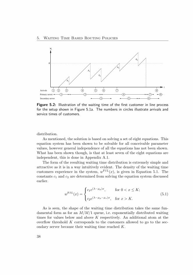
5. Waiting Time Based Routing Policies
Arrivals
5
A6
A3
A2
tW
1 2 4 7 8
3 5 6
75 643 81
t
2
Primary server
Secondary server
A4
A
K
Figure 5.2: Illustration of the waiting time of the first customer in line processfor the setup shown in Figure 5.1a. The numbers in circles illustrate arrivals andservice times of customers.
distribution.As mentioned, the solution is based on solving a set of eight equations. This
equation system has been shown to be solvable for all conceivable parametervalues, however general independence of all the equations has not been shown.What has been shown though, is that at least seven of the eight equations areindependent, this is done in Appendix A.1.
The form of the resulting waiting time distribution is extremely simple andattractive as it is in a way intuitively evident. The density of the waiting timecustomers experience in the system, wFIL(x), is given in Equation 5.1. Theconstants c1 and c2 are determined from solving the equation system discussedearlier.
wFIL(x) =
c1e(λ−µp)x, for 0 < x ≤ K;
c2e(λ−µp−µs)x, for x > K.
(5.1)
As is seen, the shape of the waiting time distribution takes the same fun-damental form as for an M/M/1 queue, i.e. exponentially distributed waitingtimes for values below and above K respectively. An additional atom at theoverflow threshold K corresponds to the customers allowed to go to the sec-ondary server because their waiting time reached K.
38

The Erlang Approximation
For the front and back office setup there is an interesting consequence ofthe fact that higher traffic is allowed than what the front office server canhandle. The consequence of this is that the waiting time distribution for valuesless than K becomes concave when λ > µp. This is illustrated in Figure 5.3a.If the primary server is highly overloaded and the overflow threshold is large,most calls will experience a waiting time close to K as illustrated in Figure 5.3b.Obviously the traffic must be less than the combined capacity of the two serversin order for the system to be stable as abandonments are not considered.
m p = 1, K = 1.5m p = 2, K = 1.0m p = 4, K = 0.5
x0 1 2 3
P( W
> x
)
0
0,2
0,4
0,6
0,8
1,0
(a) λ = 2, µs = 3
x0 5 10 15 20 25
P( W
> x
)
0
0,2
0,4
0,6
0,8
1,0
(b) λ = 2, µp = 1, µs = 3, K = 15
Figure 5.3: Analytically determined waiting times for the two server setup shownin Figure 5.1a.
Even though the direct practical use of this result may be limited, it istheoretically very interesting, as it may indicate that a similar simple resultwould apply to a multi-server setup. This hypothesis does require furtherresearch though. Also the results can be seen as a proof of concept of the FILapproach.
5.2 The Erlang Approximation
The analytical approach used for the two server setup treated in Appendix Ais not easily applicable to more complex setups, as the number of equationsand the resulting expressions increase very quickly with the complexity of the
39

5. Waiting Time Based Routing Policies
system. An example of this is that a 2-dimensional FIL process would need tobe analyzed, if a system with two queues was to be considered. In Appendix BThe Erlang Approximation (TEA), based on the same fundamental idea ofmodelling the waiting time of the customer first in line, is presented.
A discrete approximation of the FIL process is used, instead of modelling itexplicitly as in Appendix A. This allows the system to be modelled as a Contin-uous Time Markov Chain (CTMC) through which waiting time distributionscan be obtained. Besides modelling the waiting time of the first in line, thenumber of free servers is also included in the model thus allowing multi-serversetups to be treated.
The principle behind TEA is illustrated in Figure 5.4. Whenever servers arefree the system is modelled in the usual way of keeping track of the number offree servers, represented by negative indices. When customers start queueingup the FIL waiting time is modelled by states with positive indices. Tran-sitions with rate γ represent evolving time. The number of steps backward,when a customer goes into service, follows a truncated geometric distributionillustrated by the double arrows in Figure 5.4. These correspond to the ex-ponentially distributed jumps in the continuous representation described inSection 5.1. A truncated state space is used for the actual computations.
nµ nµ nµnµ−n 210−1−2
λ γ
µ(n−1)
λ λ γ3
Figure 5.4: The Erlang Approximation illustrated by states and transitions of theMarkov chain for the relatively simple M/M/n system.
The waiting time of customers is approximated by considering the statesfrom which customers enter service. For example, if a customer enters servicefrom state i, this corresponds to having waited a sum of i exponentially dis-tributed (with rate γ) time frames, i.e. a gamma distributed amount of time.The approach used to determine the waiting time distributions is described indetail in Appendix B.
When TEA is used for system with “N”-design, the underlying Markovchain becomes 2-dimensional. The combination of the number of free servers(negative indices) and the FIL waiting time (positive indices) in each dimensionhelps reduce the curse of dimensionality problem and makes the approximationof the “N”-design feasible. Systems with three or more server groups and
40

Optimization of Overflows
customer classes could in principle also be analyzed using TEA, but then thecurse of dimensionality would quickly become a problem.
TEA is shown to converge to the analytically correct solution when usedfor an M/M/1 system in Appendix B.1. It converges for γ → ∞ and whenthe number of states with positive indices representing the FIL waiting timeis infinite. This result nicely supports the fundamental approach of TEA.Simulations are used to verify TEA for the more complex setups.
TEA is first and foremost used to model the “N”-design shown in Figure 4.3and obtain the waiting time distribution from which relevant performance mea-sures such as ASA and TSF are easily calculated. An example of the waitingtimes as found through TEA is presented in Figure 5.5a and compared tosimulations.
The generic nature of TEA is also demonstrated in Appendix B by analyzingother models such as systems featuring dynamic priority, which were discussedin Section 4.4. A conjecture in [39] states that the tails of the waiting timedistributions have an exponential shape for a system based on the “V”-designwith dynamic priority. This is based on the fact that if customers arrive ata system where they can expect to wait a long time, then a B-customer thathas already waited (kA−kB) will receive the same service as a recently arrivedA-customer. The conjecture is illustrated in Figure 5.5b where a logarithmicplot is used to illustrate the exponential tails. TEA is shown to work bestfor the lower and most interesting part of the waiting time distribution. Thedeviation of the model from the simulations in the upper part is magnified bythe logarithmic plot.
5.3 Optimization of Overflows
The next obvious question is whether the fixed threshold policy is actuallyattractive and if it is, for which scenarios. This is treated in Appendix C,where the “N”-design from Appendix B is further analyzed. The approachused for the optimization is based on adding decisions to the states in theunderlying Markov chain of TEA. In this way it can be treated as a MarkovDecision Process.
The decisions subject to optimization are in regard to how agents in servergroup 2 of the “N”-design choose calls. When an agent in this group becomesfree and calls are waiting in both queues it must choose whether to take an A-or B-customer into service. Likewise, if only A-calls are waiting it must choosewhether to serve this or leave it. The reason for not taking an A-call, while no
41

5. Waiting Time Based Routing Policies
0 1 2 3 4 5 6 7 8
0.4
0.5
0.6
0.7
0.8
0.9
1
w / waiting time, minutes
P(W
<w)
A calls, PhT−modelB calls, PhT−modelSimulation meanSimulation 95% conf
(a) “N”-design, fixed overflow threshold.
0 0.5 1 1.5 2 2.5 3 3.5 4
0.20.4
0.6
0.8
0.9
0.95
0.98
0.99
0.995
w / waiting time, minutes
P(W
<w)
A calls, PhT−modelB calls, PhT−modelSimulation meanSimulation 95% conf
(b) “V”-design, dynamic priority.
Figure 5.5: Waiting time distributions found from The Erlang Approximation.
B-calls are waiting, would be to keep the group 2 server(s) reserved for futureB-calls.
In order to optimize the control of overflowing calls, costs must be assignedto certain events. In Appendix C this is done by imposing a cost whenevera call is taken into service after having waited in queue. The actual form ofthese cost functions depends on what service measures are prioritized such asASA and/or TSF. Costs can also be assigned to whenever an A-call is takenby a group 2 agent, i.e. when an overflow happens. Depending on how thecost functions are given, both A- and B-calls can be of higher priority than theother.
It is shown that the fixed threshold policy is in some cases nearly optimal.This is the case if ASA is considered and A calls are given higher priority thanB calls and an additional cost is assigned to overflowing calls.
The optimal policies when only considering ASA take some fairly simpleforms. In general there should almost never be free servers, if calls are waiting.If calls from both classes are waiting and an agent from pool 2 becomes free,he should generally take the customer having waited the longest. Differentparameters may affect the optimal policy in favour of either customer classthough.
When TSF is used as basis for the cost functions, the picture becomes muchmore involved. The optimal policies become rather complex, however, they canbe well explained by closer inspection as done in Appendix C.
An example of the optimal policy when the optimization is based on TSF
42

Optimization of Overflows
is seen in Figure 5.6a. Each marker corresponds to a state in the state spaceof the underlying Markov chain of TEA. The x-axis represent free servers inagent group 1 (negative indices) and the FIL waiting time of queue A (positiveindices), the y-axis represent server group 2 and the B-queue in the same way.Green markers mean that A-calls should be sent to server group 2, blue markersthey should not. The white areas show states where no decision is possible. Asis seen no decisions are possible when group 1 servers are vacant. Whenever A-calls are queued, decisions are tied to each state, except when all group 2 serversare occupied and no B-calls are waiting. This is due to a technical modellingissue explained in the detailed presentation of the optimization approach inAppendix C.
Figure 5.6b shows the resulting waiting time distribution of the optimizedpolicy compared to having a fixed threshold policy. It is seen that the tail ofthe optimized policy is larger than that of the fixed threshold policy for A-calls,but more calls are served within the SLT (the rightmost vertical dotted blackline) when using the optimized policy. As the optimization is only based onthe fraction of calls served within the SLT, this is as desired.
0 10 20 30 40 50 60
40
30
20
10
0
−10
i
j
a = 1a = 2
(a) Optimal policy.
0 0.5 1 1.5 20.3
0.4
0.5
0.6
0.7
0.8
0.9
1
Waiting time
P(W
<w)
A optimizedB optimizedA fixedB fixed
SLTb
SLTa
(b) Waiting time distributions.
Figure 5.6: The resulting policy from optimizing with regard to TSF (green meanssend A-call to server group 2, blue means do not) and the appertaining waitingtime distributions comparing fixed and optimized thresholds.
All in all, Appendix C shows that the fixed threshold policy may indeedbe attractive to use, however it can be improved by more complex policies inmost cases.
43


CHAPTER 6Simulation Modelling
The very complex nature of modern call centers makes it difficult if not im-possible to construct analytical models that describe their operation and per-formance in detail. Discrete event simulation is often mentioned as the onlyfeasible approach, when the performance of multi-skill call centers needs to beinvestigated [57], [25].
Modelling a call center by discrete event simulation enables very complexsetups to be analyzed. This includes call centers with multi-skill setups, generalservice time distributions, time varying arrival rates, and a varying number ofagents working during the day.
A detailed simulation model can in many cases represent a real scenariomore closely than analytical models, especially for complex setups. A simula-tion model built on a real scenario is thus suitable to analyze what happens if acertain parameter, such as the threshold determining when overflow is allowed,is tweaked. This may be the case even if the simulations are not capable ofreproducing the real performance data precisely, a general trend may still beeasily identifiable.
One of the drawbacks of simulations is that it can be hard to restrict theextent of the investigation to something that produces transparent and usefulresults due to the many parameters involved in complex models. In order tostructure the investigations, proper “design of experiments”-techniques shouldbe used, see [58] and [45] for exhaustive texts on this topic.
45
6. Simulation Modelling
Another drawback is that running a sufficient number of simulations toobtain reliable results can be time consuming even on high performance com-puters. Also the implementation of a complex model can require a lot of work.
There is an abundant amount of literature on discrete event simulation bothin the general setting and within the call center world. The role of simulationas a tool to aid in decision making within complex multi-skill call centers isdiscussed in [8]. The fundamental issues connected to call center simulationsuch as relevant inputs and outputs are described [57] and [56]. Simple exam-ples of the possibilities of simulation modelling that deal with cross training ofagents in multi-skill call centers are also given in both of these references.
A real-world scenario involving an outbound call center is analyzed usingsimulations in [32]. Three different call scheduling methods, including the oneactually used in the call center, are compared and it is shown that one of thealternative methods will result in more Right Party Contacts (RPCs).
Within this chapter the basic elements of discrete event simulation are de-scribed in Section 6.1. The different approaches that can be taken regardingthe use of software for simulation are discussed in Section 6.2. Finally in Sec-tion 6.3, an example is given of how simulations can be used to investigate theeffect of relying upon canonical model structures.
6.1 Discrete Event Simulation Basics
A realistic discrete event simulation model of a call center involves a lot ofparameters. Some of these are normally regarded as uncontrollable factors,such as call patterns and service times. Obviously measures can be taken tomodify these, but basically this involves much more than changing a parametersomewhere in the telephony system. On the other hand, controllable factorsinclude routing policies, agent schedules, and the assigned agent skills.
Based on these parameters, a discrete event simulation model simulatesthe operation of a call center down to the individual calls arriving, perhapswaiting, and finally being served by an agent or abandoning. An illustrationof how the handling of calls by individual agents proceed in a simulation ofa multi-skill call center is shown in Figure 6.1. The illustrated simulation isbased on a setting similar to the one in Figure 4.2, i.e. a setting with fourdifferent call types, three agent groups, and overflow between these. Figure 6.1also illustrates how a simulation model easily can be adapted to account fordifferent arrival and service rates, different number of agents in the groups, andspecific routing policies.
46

Discrete Event Simulation Basics
100 120 140 1601357
Time
Gro
up
3
A callsB callsC callsD calls
13579
Gro
up
1
1
3
5
Gro
up
2
Figure 6.1: Illustration of the details of agents’ work in a discrete event simulationof a multi-skill call center as the one seen in Figure 4.2. Each line corresponds toan individual agent, the circles show when agents pick up calls, and the lines tothe right of the circles show the service times.
The term discrete event simulation refers to how the software program takesall events into account. These events could include an arriving call, a call havingwaited a certain time that allows it to overflow, and agents finishing servinga call. The events are then typically simulated in the order they happen, andthe times at which they happen are updated and recorded for analysis.
Service and inter-arrival times are typically assumed to happen accordingto a given distribution from which the individual values for the calls are sam-pled. This sampling of values relies heavily on random number generation, thussimulations of the same system will give different results if not the same seed isused. This means that the more simulations are carried out, the more precisethe result can be assumed to be and indeed confidence intervals can and shouldbe determined. In this way simulations can be used to verify the correctness ofanalytical results as is done in the work presented in Appendix A. Simulationsare also often used to examine how good approximations are, examples of thisare seen in Appendix B and in [52].
Relevant data should be collected during the simulations in order to be
47

6. Simulation Modelling
able to assess the performance of the simulated system. Figure 6.2 shows thenumber of occupied agents and the number of different calls in queue for asimulation of a multi-skill system as an illustration of this.
0 5 10 150
5
10
15
Qu
eue
load
A queueB queueC queue
0 5 10 150
10
20
30
Arrival time
Ag
ent
load
Group 1Group 2
Figure 6.2: Illustration of the load on a simulated system and the transient thatneeds to be taken into account when starting with an empty system. Only eventswithin the vertical dotted lines should be used to calculate performance measures.
What is seen from Figure 6.2 is that it takes some time for the system toreach a steady phase. An often used approach is to start with an empty systemand disregard the transient phase until the system reaches a stable phase. Howlong this transient phase should be, is ambiguous, however, as a starting pointit is better to make it too long than too short. A somewhat similar modificationof the simulated data must be carried out at the end of the simulation. Hereit is appropriate to remove all events after the last arrival, as low priority callsqueued after this time instant will never be overtaken by high priority calls andthus in principle receive better service.
The collected data forms the basis for the outputs of the simulation such
48

Choice of Software
as TSF, ASA, and fraction of abandoned calls. These outputs can be used toexamine what effect different changes of the controllable factors will trigger.
6.2 Choice of Software
Simulation of call center performance can be approached in different ways. Afundamental decision is whether to build a simulation model from scratch oruse a commercial software package. Building a simulation model from scratchusing a programming language such as C, C++, Java, Matlab, etc. requires acertain level of familiarity with stochastic processes and discrete event simula-tion principles together with the obvious programming skill. Contrary to this,using a commercial software package such as Arena, Extendsim or OPNETshould be much more approachable, as these will typically provide a graphicaluser interface. It should also be taken into account that acquiring the licensefor a commercial software package can be quite costly.
In [70] simulation of a call center using C and Arena is compared. In generalthe C-implementation is favoured by the authors due to its faster performanceand better ability to deal with the finer details in a call center setup. Anexample of the difficulties of dealing with details in the commercial softwareis the possibility to assign calls to the free agent who has waited the longest,which proved troublesome in Arena but straightforward in C. However, formost call center managers’ point of view, Arena, or other dedicated commercialsimulation packages, may indeed be preferable due to the much faster and easiermodel building process. In this perspective it should also be pointed out thatmanagers in commercial call centers may not have the time and perhaps notthe skill to develop a simulation program from scratch.
The aforementioned possible lack of programming skills among call centermanagers is also addressed in [63] where an implementation of a simulationtool with an Excel interface is presented. The underlying simulation engineis based on a combination of Visual Basic and Arena. Despite the obviousadvantage of a familiar interface, the model only encompasses a single-skillcall center. Building a flexible multi-skill simulation tool in this way quicklybecomes much more involved than what is presented in [63]. Using such anapproach will also still require a costly license for the simulation software.
An in-between approach, between the full-blown commercial software pack-ages and from-the-scratch implementations, might be to have a dedicated sim-ulation model built, based on a given call center setup. This could eventuallyhave an Excel/VB interface as above combined with a dedicated program writ-
49
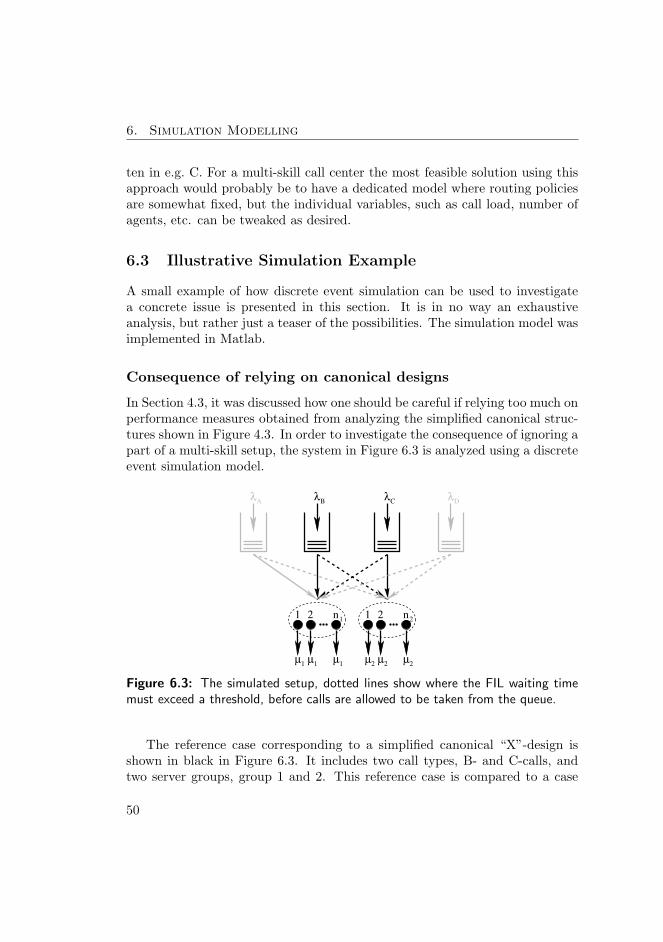
6. Simulation Modelling
ten in e.g. C. For a multi-skill call center the most feasible solution using thisapproach would probably be to have a dedicated model where routing policiesare somewhat fixed, but the individual variables, such as call load, number ofagents, etc. can be tweaked as desired.
6.3 Illustrative Simulation Example
A small example of how discrete event simulation can be used to investigatea concrete issue is presented in this section. It is in no way an exhaustiveanalysis, but rather just a teaser of the possibilities. The simulation model wasimplemented in Matlab.
Consequence of relying on canonical designs
In Section 4.3, it was discussed how one should be careful if relying too much onperformance measures obtained from analyzing the simplified canonical struc-tures shown in Figure 4.3. In order to investigate the consequence of ignoring apart of a multi-skill setup, the system in Figure 6.3 is analyzed using a discreteevent simulation model.
µ2
µ2
µ2
λB
λD
µ1
µ1
µ1
1 2 n2
λC
λA
1 2 n1
Figure 6.3: The simulated setup, dotted lines show where the FIL waiting timemust exceed a threshold, before calls are allowed to be taken from the queue.
The reference case corresponding to a simplified canonical “X”-design isshown in black in Figure 6.3. It includes two call types, B- and C-calls, andtwo server groups, group 1 and 2. This reference case is compared to a case
50

Illustrative Simulation Example
where lower priority calls are added to the system, referred to as D-calls andillustrated with grey in the right part of Figure 6.3. The last case examinedis one where high priority calls are added, corresponding to the A-calls in thefigure, also shown in grey. In this case no D-calls are present.
The parameters used for the simulation are given in Table 6.1. Arrivalrates, service times and abandonments are all assumed Markovian. The unitscan be arbitrary as long as they are consistent. In the call center setting theycould very well be minutes (and 1/minute). The arrival rate of calls of type i isgiven as λi, service rates of agents in group j as µj , number of agents in groupj as nj , abandonment rate of type i calls as αi and finally the fixed thresholdson the waiting time of the first in line before overflow is allowed for call type iis given as ki.
Table 6.1: Parameters for the simulation.
Parameter λA λB λC λD
Reference case 0 27 27 0Added low priority case 0 27 27 6Added high priority case 6 27 27 0
Shared parameters n1 = 30, n2 = 30,µ1 = 1, µ2 = 1,αA,...,D = 1
3 , kA,...,D = 15 .
As is seen, the three cases only differ in that a small amount of D-callsare added in the second case and a small amount of A-calls in the third case.In this way, the total traffic offered to the constant number of servers is notthe same in the reference case as in the other two cases. As the intent is toinvestigate the consequences of ignoring a part of the setup altogether, this isas it should be.
In all cases 200 iterations of 10′000 calls were simulated and the averagevalues of the performance measures calculated. This amount of simulationsgives only a small uncertainty on the last digit of the presented results. Inthis way, the uncertainties are nowhere near significant as compared to thedifferences between the service measures of the three cases.
The first output of the simulations is the percentage of calls served within1/3 time unit corresponding to 20s if minutes are used as time unit. The per-centage is calculated by taking the number of calls served within the time limit
51
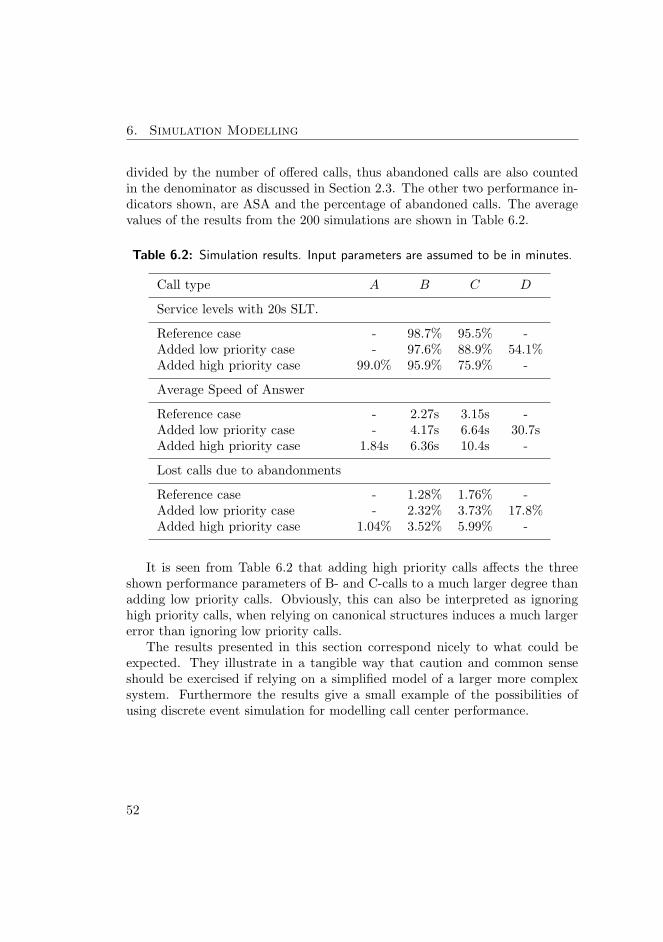
6. Simulation Modelling
divided by the number of offered calls, thus abandoned calls are also countedin the denominator as discussed in Section 2.3. The other two performance in-dicators shown, are ASA and the percentage of abandoned calls. The averagevalues of the results from the 200 simulations are shown in Table 6.2.
Table 6.2: Simulation results. Input parameters are assumed to be in minutes.
Call type A B C D
Service levels with 20s SLT.
Reference case - 98.7% 95.5% -Added low priority case - 97.6% 88.9% 54.1%Added high priority case 99.0% 95.9% 75.9% -
Average Speed of Answer
Reference case - 2.27s 3.15s -Added low priority case - 4.17s 6.64s 30.7sAdded high priority case 1.84s 6.36s 10.4s -
Lost calls due to abandonments
Reference case - 1.28% 1.76% -Added low priority case - 2.32% 3.73% 17.8%Added high priority case 1.04% 3.52% 5.99% -
It is seen from Table 6.2 that adding high priority calls affects the threeshown performance parameters of B- and C-calls to a much larger degree thanadding low priority calls. Obviously, this can also be interpreted as ignoringhigh priority calls, when relying on canonical structures induces a much largererror than ignoring low priority calls.
The results presented in this section correspond nicely to what could beexpected. They illustrate in a tangible way that caution and common senseshould be exercised if relying on a simplified model of a larger more complexsystem. Furthermore the results give a small example of the possibilities ofusing discrete event simulation for modelling call center performance.
52

CHAPTER 7Discussion
The content and contributions of this thesis are summarized and discussed inthis chapter.
In chapters 2-6 of the thesis, the fundamental methods and issues of call cen-ter management are treated. This spans from a general description of call cen-ters and their structure over data analysis to capacity planning using queueingmodels and simulations. A thorough literature review together with numerousreferences are given throughout these chapters.
The main part of the thesis is the three papers presented in appendicesA, B, and C. The background of this work and these papers is discussed inChapter 5.
The single main contribution is the development and use of the First InLine (FIL) analysis. This approach involves modelling the waiting time of thecustomer first in line as the main variable. This is a fundamentally new ap-proach to modelling queueing systems and opens up new possibilities regardinganalysis of certain queueing systems as discussed below.
The concept of FIL analysis is proven by the analytical approach taken inthe paper presented in Appendix A. Two different uses of the approach arepresented in this paper, one dealing with a single server that adapts its serviceaccording to the waiting time of the first in line. This analysis is interesting,because one could very well imagine a server that hurries up the current service,if a waiting customer becomes impatient after having waited a long time. The
53
7. Discussion
other use treats a two-server setup where the secondary server is only allowedto take jobs that have waited more than a given fixed time. The FIL approachenables exact analysis of this system, which was otherwise problematic dueto the inherent difficulties of dealing with deterministic entities in stochasticsystems. As a result, a very simple and attractive expression is found for thewaiting time distribution of customers in the latter system.
An approximation based on the FIL principle is developed in the paperpresented in Appendix B and referred to as The Erlang Approximation. Thisapproximation enables analysis of more complex systems than what is feasibleusing the exact approach of Appendix A. The versatility of TEA is demon-strated by approximations of the performance of different queueing systems,all where the waiting time of customers somehow plays an important role.Numerous suggestions for further uses are also discussed.
The last paper, presented in Appendix C, takes the use of the approachesdeveloped in the two former papers a step further. Here, the overflow betweenserver groups is optimized with regard to the service level measures used in thecall center industry. Furthermore the appropriateness of the often used fixedthreshold policy is verified and the implications of using it are discussed.
The work presented spans a nice range of research fields. From the veryanalytical approach in Appendix A, over the more application oriented ap-proximation of Appendix B, to optimization of concrete call center processesin Appendix C.
The FIL approach should be taken into consideration whenever queueingsystems, in which processes somehow depend on the waiting time of customers,are to be analyzed.
54
Bibliography
[1] The call center’s incredible shrinking day. Credit Union Executive Newslet-ter, 28(29):2, 2002.
[2] Salah Aguir, Fikri Karaesmen, O. Zeynep Aksin, and Fabrice Chau-vet. The impact of retrials on call center performance. OR Spectrum,26(3):353–376, 2004.
[3] O. Zeynep Aksin and Patrick T. Harker. Modeling a phone center: Anal-ysis of a multichannel, multiresource processor shared loss system. Man-agement Science, 47(2):324–336, 2001.
[4] Z. Aksin, M. Armony, and V. Mehrotra. The modern call center: a multi-disciplinary perspective on operations management research. Productionand Operations Management, 16(6):665–688, 2007.
[5] Eitan Altman, Tania Jimenez, and Ger Koole. On the comparison ofqueueing systems with their fluid limits. Probability in the Engineeringand Informational Sciences, 15(2):165, 2001.
[6] Rami Atar, Avi Mandelbaum, and Martin I. Reiman. Scheduling a multiclass queue with many exponential servers: Asymptotic optimality inheavy traffic. Annals of Applied Probability, 14(3):1084–1134, 2004.
[7] Julıus Atlason, Marina A. Epelman, and Shane G. Henderson. Call centerstaffing with simulation and cutting plane methods. Annals of OperationsResearch, 127(1-4):333–358, 2004.
[8] A.N. Avramidis and P. L’Ecuyer. Modeling and simulation of call centers.Winter Simulation Conference, 2005 Proceedings of the, page 9 pp., 2005.
55
Bibliography
[9] Wolfgang Barth, Michael Manitz, and Raik Stolletz. Analysis of two-levelsupport systems with time-dependent overflow - a banking application.Forthcoming in Production and Operations Management, available fromhttp://ideas.repec.org/p/han/dpaper/dp-399.html, 2009.
[10] Rene Bekker. Queues with state-dependent rates. PhD thesis, EindhovenUniversity of Technology, 2005.
[11] S. Bhulai and G. Koole. A queueing model for call blending in call centers.IEEE Transactions on Automatic Control, 48(8):1434–1438, 2003.
[12] Sandjai Bhulai. Dynamic routing policies for multiskill call centers. Prob-ability in the Engineering and Informational Sciences, 23(1):101, 2009.
[13] V.A. Bolotin. Telephone circuit holding time distributions. FundamentalRole of Teletraffic in the Evolution of Telecommunications Networks. Pro-ceeding of the 14th International Teletraffic Congress - ITC 14, 1:125–34vol.1, 1994.
[14] S. Borst, A. Mandelbaum, and M.I. Reiman. Dimensioning large callcenters. Operations Research, 52(1):17–34, 2004.
[15] Andreas Brandt and Manfred Brandt. On a two-queue priority systemwith impatience and its application to a call center. Methodology AndComputing In Applied Probability, 1(2):191–210, 1999.
[16] L. Brown, N. Gans, A. Mandelbaum, A. Sakov, H. Shen, S. Zeltyn, andL. Zhao. Statistical analysis of a telephone call center: A queueing-scienceperspective. Technical report, University of Pennsylvania, 2002. download-able at http://iew3.technion.ac.il/serveng/References/references.html.
[17] Lawrence Brown, Noah Gans, Avishai Mandelbaum, Anat Sakov, HaipengShen, Sergey Zeltyn, and Linda Zhao. Applications and case studies - sta-tistical analysis of a telephone call center: A queueing-science perspective.Journal of the American Statistical Association, 100(469):36–50, 2005.
[18] U.S. Department of Labor Bureau of Labor Statistics. Occupational Out-look Handbook, Customer Service Representatives. 2008-09 edition. Avail-able at http://www.bls.gov/oco/ocos280.htm.
[19] Mehmet Tolga Cezik and Pierre L’Ecuyer. Staffing multiskill call centersvia linear programming and simulation. Management Science, 54(2):310–323, 2008.
56

[20] Brad Cleveland. Where is everybody?! how to accurately predict scheduleshrinkage. Customer Management Insight, page 22, 2008.
[21] Brad Cleveland and Julia Mayben. Call Center Management on Fast For-ward: Succeeding in Today’s Dynamic Inbound Environment. Call CenterPress, first edition, 1997.
[22] Alan Cobham. Priority assignment in waiting line problems. Journal ofthe Operations Research Society of America, 2(1):70–76, 1954.
[23] Richard A. Feinberg, Leigh Hokama, Rajesh Kadam, and IkSuk Kim.Operational determinants of caller satisfaction in the banking/financialservices call center. International Journal of Bank Marketing, 20(4):174–180, 2002.
[24] Zohar Feldman, Avishai Mandelbaum, William A. Massey, and WardWhitt. Staffing of time varying queues to achieve time stable performance.Management Science, 54(2):324–338, 2008.
[25] Noah Gans, Ger Koole, and Avishai Mandelbaum. Telephone call cen-ters: Tutorial, review, and research prospects. Manufacturing and ServiceOperations Management, 5(2):79–141, 2003.
[26] O. Garnett, A. Mandelbaum, and M. Reiman. Designing a call center withimpatient customers. Manufacturing & Service Operations Management,4(3):208–27, 2002.
[27] Anders Gorst-Rasmussen and Martin B. Hansen. Asymptotic inferencefor waiting times and patiences in queues with abandonment. Communi-cations in Statistics - Simulation and Computation, 38(2):318–334, 2009.
[28] Linda Green and Peter Kolesar. The pointwise stationary approximationfor queues with nonstationary arrivals. Management Science, 37(1):84–97,1991.
[29] Linda Green, Peter Kolesar, and Anthony Svoronos. Some effects of non-stationarity on multiserver markovian queueing systems. Operations Re-search, 39(3):502–511 and 171403, 1991.
[30] Geoffrey Grimmett and David Stirzaker. Probability and Random Pro-cesses. Oxford University Press, third edition, 2001.
57

Bibliography
[31] R.C. Grinold and K.T. Marshall. Manpower planning models. ElsevierScience Publishing Co Inc., US, 1977.
[32] S. Gulati and S.A. Malcolm. Call center scheduling technology evaluationusing simulation. Proceeding of the 2001 Winter Simulation Conference(Cat. No.01CH37304), 2:1438–1442 vol.2, 2001.
[33] I. Gurvich, M. Armony, and A. Mandelbaum. Service-level differentiationin call centers with fully flexible servers. Management Science, 54:279–294,2008.
[34] Shlomo Halfin and Ward Whitt. Heavy-traffic limits for queues with manyexponential servers. Operations Research, 29(3):567–588, 1981.
[35] J.M. Harrison and Assaf Zeevi. A method for staffing large call centersbased on stochastic fluid models. Manufacturing & Service OperationsManagement, 7(1):20–36, 2005.
[36] T.-Y. Huang. Analysis and modeling of a threshold based priority queueingsystem. Computer Communications, 24(3-4):284–291, 2001.
[37] Villy Bæk Iversen. Teletraffic Engineering and Network Planning. COMCenter, Technical University of Denmark, 2006.
[38] James R. Jackson. Some problems in queueing with dynamic priorities.Nav. Res. Logistics Quart., 7:235–249, 1960.
[39] James R. Jackson. Queues with dynamic priority discipline. ManagementScience, 8(1):18–34 and 2627272, 1961.
[40] N.K. Jaiswal. Priority Queues. Academic Press, New York and Londons,1968.
[41] A.J.E.M. Janssen, J.S.H. van Leeuwaarden, and Bert Zwart. Refiningsquare root safety staffing by expanding erlang c. Working paper, Versionof December 20, 2008.
[42] Otis B. Jennings, Avishai Mandelbaum, William A. Massey, and WardWhitt. Server staffing to meet time-varying demand. Management Science,42(10):1383–1394, 1996.
[43] Tania Jimenez and Ger Koole. Scaling and comparison of fluid limits ofqueues applied to call centers with time-varying parameters. OR Spectrum,26(3):413–422, 2004.
58

[44] G. Jongbloed and G. Koole. Managing uncertainty in call centres usingpoisson mixtures. Applied Stochastic Models in Business and Industry,17(4):307–318, 2001.
[45] Jack P.C. Kleijnen. Design and Analysis of Simulation Experiments.Springer, 2008.
[46] Leonard Kleinrock. A delay dependent queue discipline. Naval ResearchLogistics Quarterly, 11(4), 1964.
[47] Leonard Kleinrock and Roy P. Finkelstein. Time dependent priorityqueues. Operations Research, 15(1):104–116, 1967.
[48] G. Koole, A. Pot, and J. Talim. Routing heuristics for multi-skill callcenters. Simulation Conference, 2003. Proceedings of the 2003 Winter,2:1813–1816, 2003.
[49] Ger Koole. Redefining the service level in call centers. Working paper,available from http://www.math.vu.nl/ koole/research/.
[50] Ger Koole and Avishai Mandelbaum. Queueing models of call centers: Anintroduction. Annals of Operations Research, 113(4):41–59, 2002.
[51] Ger Koole and Auke Pot. An overview of routing and staffing algorithmsin multi-skill customer contact centers. Submitted for publication, 2006,available from http://www.math.vu.nl/ koole/research/.
[52] G.M. Koole and J. Talim. Exponential approximation of multi-skill callcenters architecture. Proc. QNETs 2000, 23:1–10, 2000.
[53] Leon-Garcia and Widjaja. Communication Networks. McGraw Hill HigherEducation, second edition, 2001.
[54] Liqiang Liu and Vidyadhar G. Kulkarni. Explicit solutions for the steadystate distributions in m/ph/1 queues with workload dependent balking.Queueing Systems, 52(4):251–260, 2006.
[55] A. Mandelbaum, W.A. Massey, M.I. Reiman, and B. Rider. Time varyingmultiserver queues with abandonment and retrials. Teletraffic Engineer-ing in a Competitive World. Proceedings of the International TeletrafficCongress - ITC-16. Vol.3a, 1:355–64 vol.1, 1999.
59

Bibliography
[56] T.A. Mazzuchi and R.B. Wallace. Analyzing skill-based routing call cen-ters using discrete-event simulation and design experiment. SimulationConference, 2004. Proceedings of the 2004 Winter, 2:1812–1820 vol.2,2004.
[57] V. Mehrotra and J. Fama. Call center simulation modeling: methods,challenges, and opportunities. Simulation Conference, 2003. Proceedingsof the 2003 Winter, 1:135–143, 2003.
[58] Douglas C. Montgomery. Design and Analysis of Experiments. Wiley, 6thedition, 2008.
[59] Conny Palm. Inhomogeneous telephone traffic in full-availability groups.Ericsson Technics, (1), 1937.
[60] Conny Palm. Nagra undersokningar over vantetider vid telefonanlagg-ningar. Sartryck ur Tekn. Medd. fran Kungl. Telegrafstyrelsen, (7-9), 1937.
[61] Auke Pot. Planning and Routing Algorithms for Multi-Skill Contact Cen-ters. PhD thesis, Vrije Universiteit, 2006.
[62] Auke Pot, Sandjai Bhulai, and Ger Koole. A simple staffing method formultiskill call centers. Manufacturing and Service Operations Manage-ment, 10(3):421–428, 2008.
[63] R. Saltzman and V. Mehrotra. A manager-friendly platform for simula-tion modeling and analysis of call center queueing systems. SimulationConference, 2004. Proceedings of the 2004 Winter, 1, 2004.
[64] M. Segal. The operator-scheduling problem: A network-flow approach.Operations Research, 22(4):808–823, 1974.
[65] Haipeng Shen and Jianhua Z. Huang. Analysis of call centre arrival datausing singular value decomposition. Applied Stochastic Models in Businessand Industry, 21(3):251–263, 2005.
[66] Adam Smith. An Inquiry into the Nature and Causes of the Wealth ofNations. W. Strahan and T. Cadell, London, United Kingdom, 1776.
[67] Raik Stolletz and Stefan Helber. Performance analysis of an inbound callcenter with skills-based routing. OR Spectrum, 26(3):331–352, 2004.
60

[68] David Y. Sze. A queueing model for telephone operator staffing. Opera-tions Research, 32(2):229–249, 1984.
[69] James W. Taylor. A comparison of univariate time series methods for fore-casting intraday arrivals at a call center. Management Science, 54(2):253–265, 2008.
[70] R.B. Wallace and R.M. Saltzman. Comparing skill-based routing call cen-ter simulations using c programming and arena models. Proceedings of the2005 Winter Simulation Conference (IEEE Cat. No.05CH37732C), page9 pp., 2005.
[71] R.B. Wallace and W. Whitt. A staffing algorithm for call centers withskill-based routing. Manufacturing & Service Operations Management,7(4):276–294, 2005.
[72] W. Whitt. Engineering solution of a basic call-center model. ManagementScience, 51(2):221–235, 2005.
[73] Ward Whitt. Understanding the efficiency of multi-server service systems.Management Science, 38(5):708–723, 1992.
[74] Ward Whitt. Predicting queueing delays. Management Science, 45(6):870–888, 1999.
[75] Ward Whitt. Fluid models for multiserver queues with abandonments.Operations Research, 54(1):37–54, 2006.
[76] Ward Whitt. Staffing a call center with uncertain arrival rate and absen-teeism. Production and Operations Management, 15(1):88–102, 2006.
[77] Bo Zhang, Johan S.H. van Leeuwaarden, and Bert Zwart. Refined squareroot staffing for call centers with impatient customers. To appear in Man-ufacturing & Service Operations Management.
[78] Ety Zohar, Avishai Mandelbaum, and Nahum Shimkin. Adaptive behav-ior of impatient customers in tele-queues: Theory and empirical support.Management Science, 48(4):566–583, 2002.
61

Appendices
63


APPENDIX AQueues with waiting time
dependent service
65


Queues with waiting time dependent service
R. Bekker†, G.M. Koole†, B.F. Nielsen?, T.B. Nielsen?
†Dept. MathematicsVU University Amsterdam
De Boelelaan 1081, 1081 HV, the Netherlands.
?Dept. Informatics and Mathematical ModellingTechnical University of Denmark
Richard Petersens Plads, 2800 Kgs. Lyngby, Denmark.
Abstract
Motivated by service levels in terms of the waiting-time distribution seen in e.g. callcenters, we consider two models for systems with a service discipline that depends onthe waiting time. The first model deals with a single server that continuously adaptsits service rate based on the waiting time of the first customer in line. In the secondmodel, one queue is served by a primary server which is supplemented by a secondaryserver when the waiting of the first customer in line exceeds a threshold. Using levelcrossings for the waiting-time process of the first customer in line, we derive steady-state waiting-time distributions for both models. The results are illustrated withnumerical examples.
Keywords: Waiting-time distribution; Adaptive service rate; Call centers; Contactcenters; Queues; Deterministic threshold; Overflow; Level crossing.
1 Introduction
In service systems, the tail probability (or distribution function) of the waiting time ofcustomers is one of the main service-level indicators. For example, in call centers theservice level is generally characterized by the telephone service factor (TSF), i.e., thefraction of calls whose delay fall below a prespecified target. Typically, call centers use a80-20 TSF meaning that 80% of the calls should be taken into service within 20 seconds,see [12]. Motivated by performance measures in terms of tail probabilities of waiting times,we consider queueing systems where the service mechanism is based on waiting times ofcustomers. This type of control policy is commonly used in call centers [20], and indeedthe authors have often encountered it in various forms when working with call centers.However, the literature on it is limited. In the traditional queueing literature, routing andcontrol are commonly based on the number of customers present.The main goal of this paper is to find the steady-state waiting-time distribution for queue-ing systems where the service characteristics depend on the waiting time of the first cus-tomer in line. This type of service control seems to be new in the queueing literature,despite its widespread use in the industry. In the sequel we use FIL as an abbreviation offirst customer in line.
I
We consider two Markovian queueing models: (i) single-server queues with FIL waiting-time dependent service speed and (ii) a queue with two heterogeneous servers, where thesecondary server is only activated as soon as the FIL waiting time exceeds some targetlevel. For both models, the analysis is based on the waiting process of the first customerin line (FIL-process). Using level crossings, we find the steady-state distribution of theFIL-process and derive the waiting-time distribution as a corollary.First, in Section 2, we study the single-server model, where the service speed can becontinuously adapted based on the waiting time of the first customer in line. This modelis related to the study of dams and queueing systems with workload-dependent servicerates, see e.g. [4], [5], [16] or [24]. The difference is that the service speed here dependson the waiting time instead of the amount of work present.Second, in Section 3, we consider a system with a single queue and two heterogeneousservers, where the secondary server takes the first customer in line into service as soon ashis waiting time exceeds some threshold. The primary motivation for this model stemsfrom routing mechanisms in call centers with operators in front and back offices. Typically,the only task of operators in the front office would be to answer calls whereas operatorsin the back office would have other assignments and only answer calls under high load.A common problem is then how to meet the service level agreements while keeping thedisturbance of the back office operators to a minimum, see [12] and references therein.Overflow problems are in general difficult to analyze, see [11], because the overflow trafficis not Poisson; the deterministic threshold of this model only adds to this. We believethough that the model is of independent interest and has its applications in other areaswhere the service level involves the (tail) distribution of the waiting time, as in, e.g.,telecommunication and production systems.Related to the heterogeneous-servers model above is the slow-server problem, see [18],[19], [23] and [25]. In the slow-server model, a single queue is served by two heterogeneousservers with service rates µ1 and µ2, where µ1 > µ2. In [23], the author gives qualitativeand explicit quantitative results on when to maintain or discard the slow server. In themodels of [18] and [19], customers can be assigned to one of the servers depending on thenumber of customers present. There it was shown that the fast server should always beused and that the slow server should only be used if the number of customers exceeds somethreshold. This result was derived for an infinite waiting space. We note that in case of afinite queue length, the optimal policy is not necessarily of a threshold type, see [25].The literature on queueing models where the service time process depends on the waitingtime is limited. In [3], a system with time dependent overflow is approximated by aqueue-length dependent overflow. Prioritization based on adding different constants to thewaiting times of customers is introduced in [17] and referred to as dynamic prioritization.There are some studies of single-server queues where the service time depends on thewaiting time experienced by the customer in service (instead of the first customer in line),see [6], [22] and [26]. Furthermore, in [7] the authors consider an M/M/2 queue wherenon-waiting customers receive a different rate of service than customers who first wait inline. Their analysis is based on the “system point method” [8], which is closely related tothe level crossing equations [10] of Section 3.Some numerical results are presented in Section 4. Conclusions and topics for furtherresearch can be found in Section 5.
II

2 Single-server queue
In this section we consider a single-server queue where the service speed depends on thewaiting time of the first customer in line. In particular, we assume that customers arriveaccording to a Poisson process with rate λ and have exponentially distributed servicerequirements with mean 1/µ. The service discipline is assumed to be FIFO. Denote byWt the waiting time of the first customer in the queue at time t, with the convention thatWt = 0 if the queue is empty. Also, let Yt denote the number of customers in serviceat time t (thus Yt ∈ {0, 1}). The service speed depends on the waiting time of the firstcustomer in line and the service speed function is denoted by r(·). Let r(0) be the servicespeed for state (Wt, Yt) = (0, 1) and 0 be the speed for state (0, 0). For convenience, defineρ0 = λ/(µr(0)). We assume that r(·) is strictly positive, left-continuous, and has a strictlypositive right limit on (0,∞).The process {(Wt, Yt), t ≥ 0} can now be described as follows. Given that Wt0 = w > 0and the next service completion is at time t1 > t0, the waiting-time process of the firstcustomer in line during (t0, t1) behaves as Wt0+t = w + t and Yt0+t = 1. If Sw denotes thetime until the next service completion, conditioned on the initial waiting time w > 0, thenP(Sw > t) = exp
(−µ
∫ w+tw r(y)dy
). At the moment of a service completion, the second
customer in line (if there is any) becomes the first customer in line. Since the interarrivaltimes between customers are exponentially distributed, we have
Wt+1=
(Wt−1
−Aλ
)+, (1)
where (x)+ = max{x, 0} and Aλ denotes an exponential random variable of rate λ.It remains to specify the boundary cases of an empty queue. For (0, Yt0), the time untilthe next state transition has an exponential distribution with rate λ+µr(0)Yt0 . For (0, 1)the next state is (0, 0) with probability µr(0)/(λ+µr(0)), or Wt starts to increase linearlyas described above with probability λ/(λ + µr(0)). For (0, 0), the next state is (0, 1) withprobability one.Since the service requirements and interarrival times are exponentially distributed, theprocess {(Wt, Yt), t ≥ 0} is a Markov process. Assuming that the system is stable (see [9,Corollary 4.2] for stability conditions), the process is regenerative and thus has a stationarydistribution, see e.g. [2, Chapter VII]. Below, we determine the steady-state distributionof this process and derive from it the waiting-time distribution of an arbitrary customer.For this, we introduce the steady-state distribution of the FIL-process as WFIL(x) =limt→∞ P(Wt ≤ x) and the corresponding density as wFIL(x) = dWFIL(x)/dx. For theatom in zero, Yt is included in the notation as WFIL(0, y) = limt→∞ P(Wt = 0, Yt = y).
Theorem 2.1 We have WFIL(0, 1) = ρ0WFIL(0, 0). The density of the FIL-process is
wFIL(x) = λρ0WFIL(0, 0) exp
{∫ x
0(λ− µr(y))dy
},
where
WFIL(0, 0) =[1 + ρ0 + λρ0
∫ ∞
0exp
{∫ x
0(λ− µr(y))dy
}dx
]−1
.
It is instructive to derive the distribution of the FIL-process based on level crossing argu-ments. We refer to Remark 2.1 below for an alternative proof based on results in [5].
III
Proof For x > 0, using (1), the level crossing equations read
wFIL(x) =∫ ∞
y=xe−λ(y−x)µr(y)wFIL(y)dy. (2)
The left-hand side corresponds to upcrossings of level x and the right-hand side correspondsto the long-run average number of downcrossings through level x. Observe that we havecontinuous upcrossings of waiting-time levels and downcrossings by jumps, where thejump sizes correspond to interarrival times between successive customers (in contrast toworkloads in single-server queues). Taking derivatives on both sides of Equation (2) yields
ddx
wFIL(x) = λ
[∫ ∞
y=xe−λ(y−x)µr(y)wFIL(y)dy
]− µr(x)wFIL(x)
= (λ− µr(x))wFIL(x),
where the second step follows from (2). The solution of this first-order differential equationcan be readily obtained as
wFIL(x) = Cexp{∫ x
0(λ− µr(y))dy
}. (3)
Balancing the transitions between the interior part of the state space and the boundarypart, we have
λWFIL(0, 1) =∫ ∞
0e−λyµr(y)wFIL(y)dy.
Using the above and letting x ↓ 0 in (2) yields limx↓0 wFIL(x) = λWFIL(0, 1). Also, lettingx ↓ 0 in (3) determines the constant C = limx↓0 wFIL(x) = λWFIL(0, 1).Now, balancing the transitions between the two boundary states gives
λWFIL(0, 0) = µr(0)WFIL(0, 1),
which enables us to determine the three constants in terms of WFIL(0, 0). Finally, usingnormalization, we have
WFIL(0, 0) + WFIL(0, 1) + λWFIL(0, 1)∫ ∞
0exp
{∫ x
0(λ− µr(y))dy
}dx = 1.
Expressing WFIL(0, 1) in WFIL(0, 0) and solving for WFIL(0, 0) completes the proof.
To determine the waiting time, we only need to consider the FIL-process at specific pointsin time. We introduce the waiting time an arbitrary customer experiences as W and thedistribution of this as W (x) = P(W ≤ x). Using PASTA, it is easy to see that the atom inzero of the waiting time is given by P(W = 0) = WFIL(0, 0). In case of non-zero waitingtimes, the waiting times are given by the FIL-process embedded at epochs just beforedownward jumps.Let Ns(u, v) denote the number of customers taken into service during the interval (u, v].Consider an infinitesimal interval (t, t + h], h > 0. Then, P(Wt > x; Ns(t, t + h) = 1) =∫∞x µr(y)hwFIL(y)dy + o(h). Note that P(Ns(t, t + h) = 1)/h (for h → 0) is the rate at
IV

which customers are taken into service and, since every customer leaves the queue throughthe server and the system is stable, equals λ. Combining the above, we have
P(W > x) = limh→0
P(Wt > x | Ns(t, t + h) = 1)
= limh→0
P(Wt > x; Ns(t, t + h) = 1)P(Ns(t, t + h) = 1)
=1λ
∫ ∞
xµr(y)wFIL(y)dy.
The density of the steady-state waiting time, w(x), can be obtained by differentiating theabove:
Corollary 2.1 For the steady-state waiting time, we have P(W = 0) = WFIL(0, 0) anddensity
w(x) =µr(x)wFIL(x)
λ,
where WFIL(0, 0) and wFIL(·) are given in Theorem 2.1.
Remark 2.1 We note that the steady-state waiting time and FIL distributions take asimilar form as the steady-state workload distribution of an M/M/1 queue with workload-dependent arrival and/or service rate, see e.g. [4], [16] or [2], p. 388. Also related is theelapsed waiting time process in the M/G/1 queue [21].For positive values, the FIL-process is a special case of the model considered in [5], i.e.,an on/off storage system with state-dependent rates restricted to up intervals. Applying[5, Theorem 1] combined with [5, Section 6] and taking (in the notation of [5]) r0(x) ≡ 1,λ0(x) = µr(x) and λ1(x)/r1(x) ≡ λ with λ1(x) and r1(x) tending to infinity, directly yieldsthe FIL-density represented in (3). Furthermore, combining results on expected excursiontimes [5, Theorem 2] with standard renewal arguments provides the remaining constants.¦
Remark 2.2 For a renewal arrival process, the interior part of the state space can bestraightforwardly adapted. In particular, Wt is still a Markov process for positive waitingtimes and the level crossing equation (2) then reads
wFIL(x) =∫ ∞
y=xµr(y)wFIL(y)(1−A(y − x))dy,
where A(·) is the interarrival-time distribution. Note that the above equation can bewritten as a Volterra integral equation of the second kind, see e.g. [27]. For the FILprocess to be a Markov process, a supplementary variable is required to describe theelapsed interarrival time at the boundary of the state space, i.e., in case there is nocustomer in line. We note that Corollary 2.1 remains valid for a renewal process. ¦
Example 2.1 The results become even more tractable in various special cases. Here, weconsider the case of two service speeds determined by a threshold value of the waitingtime of the first customer in the queue. Specifically, we assume that
r(x) ={
r1, for 0 ≤ x ≤ K,r2, for x > K.
V
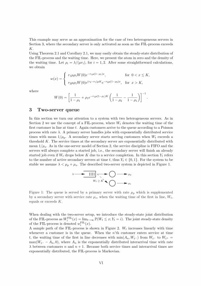
This example may serve as an approximation for the case of two heterogeneous servers inSection 3, where the secondary server is only activated as soon as the FIL-process exceedsK.Using Theorem 2.1 and Corollary 2.1, we may easily obtain the steady-state distribution ofthe FIL-process and the waiting time. Here, we present the atom in zero and the density ofthe waiting time. Let ρi = λ/(µri), for i = 1, 2. After some straightforward calculations,we obtain
w(x) =
r1µρ1W (0)e−r1µ(1−ρ1)x, for 0 < x ≤ K,
r2µρ1W (0)e(r2−r1)µKe−r2µ(1−ρ2)x, for x > K,
where
W (0) =[
11− ρ1
+ ρ1e−r1µ(1−ρ1)K
(1
1− ρ2− 1
1− ρ1
)]−1
.
3 Two-server queue
In this section we turn our attention to a system with two heterogeneous servers. As inSection 2 we use the concept of a FIL-process, where Wt denotes the waiting time of thefirst customer in line at time t. Again customers arrive to the queue according to a Poissonprocess with rate λ. A primary server handles jobs with exponentially distributed servicetimes with mean 1/µp. A secondary server starts serving customers when Wt exceeds athreshold K. The service times at the secondary server are exponentially distributed withmean 1/µs. As in the one-server model of Section 2, the service discipline is FIFO and theservers will always complete a started job, i.e., the secondary server will finish an alreadystarted job even if Wt drops below K due to a service completion. In this section Yt refersto the number of active secondary servers at time t, thus Yt ∈ {0, 1}. For the system to bestable we assume λ < µp + µs. The described two-server system is depicted in Figure 1.
Wt ≥ K
λ µp
µs
Figure 1: The queue is served by a primary server with rate µp which is supplementedby a secondary server with service rate µs, when the waiting time of the first in line, Wt,equals or exceeds K.
When dealing with the two-server setup, we introduce the steady-state joint distributionof the FIL-process as WFIL
i (x) = limt→∞ P(Wt ≤ x; Yt = i). The joint steady-state densityof the FIL-process is denoted wFIL
i (x).A sample path of the FIL-process is shown in Figure 2. Wt increases linearly with timewhenever a customer is in the queue. When the n’th customer enters service at timet, the waiting time of the first in line decreases with min(An, Wt−) from Wt− to Wt+ =max(Wt− − An, 0), where An is the exponentially distributed interarrival time with rateλ between customers n and n + 1. Because both service times and interarrival times areexponentially distributed, the FIL-process is Markovian.
VI

Arrivals
5
A6
A3
A2
tW
1 2 4 7 8
3 5 6
75 643 81
t
2
Primary server
Secondary server
A4
A
K
Figure 2: Elapsed waiting time of the first customer in line, Wt. The occupation of theservers are shown beneath the graph. Notice how Wt keeps increasing after customer #3finishes service as the secondary server is not allowed to start a new service until the levelK is reached.
The analysis of the system is based on the level crossing equations for the FIL-process.These are more involved, compared to those in Section 2, and are thus presented inLemma 3.1. From this, the steady state distribution of the FIL-process is determined andgiven in Theorem 3.1.
Lemma 3.1 We consider the level crossing equations with upcrossings of level x on theleft-hand side and downcrossings on the right-hand for three different cases.
(i) For x < K and an active secondary server we have
wFIL1 (x) + µsW
FIL1 (x) = µp
∫ ∞
y=xe−λ(y−x)wFIL
1 (y)dy
+ µs
∫ ∞
y=Ke−λ(y−x)wFIL
1 (y)dy
+ wFIL0 (K−)e−λ(K−x).
(ii) For x < K and an inactive secondary server
wFIL0 (x) = µp
∫ K
y=xe−λ(y−x)wFIL
0 (y)dy + µsWFIL1 (x).
(iii) For x > K the secondary server will always be active
wFIL1 (x) = (µp + µs)
∫ ∞
y=xe−λ(y−x)wFIL
1 (y)dy.
Proof Only case (i) is dealt with in detail as it is the most complicated. The levelcrossing equations are obtained from setting up forward Kolmogorov equations. For case
VII
(i) this becomes
P(Wt+dt ≤ x + dt; Yt+dt = 1)= (1− µpdt− µsdt)P(Wt ≤ x; Yt = 1)
+ µpdtP(Wt ≤ x + An; Yt = 1)+ µsdtP(K < Wt ≤ x + An; Yt = 1)+ (1− µpdt)P(Wt ∈ [K − dt,K];Wt ≤ x + An;Yt = 0) + o(dt).
Subtracting P(Wt ≤ x + dt;Yt = 1) from both sides, dividing by dt and letting dt → 0allows us to rewrite the term on the left side and the first term on the right side asderivatives with regard to t and x respectively. Moreover dt cancels from the rest of theterms except the last. Note that µpP(Wt ∈ [K − dt,K];Wt ≤ x + An; Yt = 0) → 0 fordt → 0. Hence,
ddtP(Wt ≤ x; Yt = 1)
=− ddxP(Wt ≤ x; Yt = 1)− (µp + µs)P(Wt ≤ x; Yt = 1)
+ µpP(Wt ≤ x + An; Yt = 1) + µsP(K < Wt ≤ x + An; Yt = 1)
+ limdt→0
P(Wt ≤ K; Yt = 0)− P(Wt ≤ K − dt; Yt = 0)dt
· P(An > K − x).
By letting t → ∞, the left side of the expression tends to zero. The probabilities can bewritten in form of density and distribution functions, using convolution for the probabilitiesinvolving An; e.g. P(Wt ≤ x + An; Yt = 1) = WFIL
1 (x) + P(x < Wt ≤ x + An, Yt = 1) =WFIL
1 (x)+∫∞y=x e−λ(y−x)wFIL
1 (y)dy. Using limdt→0,t→∞(P(Wt≤K;Yt=0)−P(Wt≤K−dt;Yt=0)
dt
)=
wFIL0 (K−), then leads to:
0 = − wFIL1 (x)− (µp + µs)WFIL
1 (x)
+ µp
(WFIL
1 (x) +∫ ∞
y=xe−λ(y−x)wFIL
1 (y)dy
)+ µs
∫ ∞
y=Ke−λ(y−x)wFIL
1 (y)dy
+ wFIL0 (K−)e−λ(K−x).
Finally, the level crossing equation for case (i) can be obtained by simply rearranging theabove terms.We now turn to case (ii). Following an approach similar to the one for case (i), the levelcrossing equation can be found from the initial Kolmogorov equation
P (Wt+dt ≤ x + dt; Yt+dt = 0) = (1− µpdt)P(Wt ≤ x; Yt = 0)+ µpdtP(Wt ≤ x + An; Yt = 0)+ µsdtP(Wt ≤ x; Yt = 1) + o(dt).
In case (iii) the Kolmogorov equation is of the following form
P(Wt+dt ≤ x + dt;Yt+dt = 1) = (1− µpdt− µsdt)P(Wt ≤ x; Yt = 1)+ (µp + µs)dtP(Wt ≤ x + An; Yt = 1) + o(dt).
Again, using the same approach as for case (i), the level crossing equation of Lemma 3.1,case (iii), can be obtained.
VIII
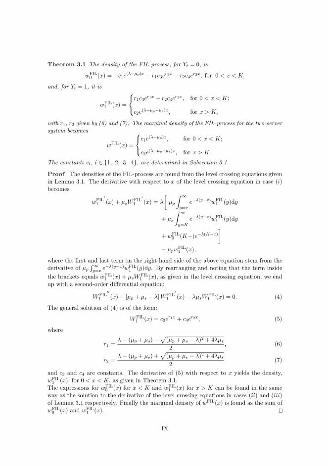
Theorem 3.1 The density of the FIL-process, for Yt = 0, is
wFIL0 (x) = −c1e
(λ−µp)x − r1c3er1x − r2c4e
r2x, for 0 < x < K,
and, for Yt = 1, it is
wFIL1 (x) =
r1c3er1x + r2c4e
r2x, for 0 < x < K;
c2e(λ−µp−µs)x, for x > K,
with r1, r2 given by (6) and (7). The marginal density of the FIL-process for the two-serversystem becomes
wFIL(x) =
c1e(λ−µp)x, for 0 < x < K;
c2e(λ−µp−µs)x, for x > K.
The constants ci, i ∈ {1, 2, 3, 4}, are determined in Subsection 3.1.
Proof The densities of the FIL-process are found from the level crossing equations givenin Lemma 3.1. The derivative with respect to x of the level crossing equation in case (i)becomes
wFIL′
1 (x) + µsWFIL
′1 (x) = λ
[µp
∫ ∞
y=xe−λ(y−x)wFIL
1 (y)dy
+ µs
∫ ∞
y=Ke−λ(y−x)wFIL
1 (y)dy
+ wFIL0 (K−)e−λ(K−x)
]
− µpwFIL1 (x),
where the first and last term on the right-hand side of the above equation stem from thederivative of µp
∫∞y=x e−λ(y−x)wFIL
1 (y)dy. By rearranging and noting that the term insidethe brackets equals wFIL
1 (x) + µsWFIL1 (x), as given in the level crossing equation, we end
up with a second-order differential equation:
WFIL′′
1 (x) + [µp + µs − λ] WFIL′
1 (x)− λµsWFIL1 (x) = 0. (4)
The general solution of (4) is of the form:
WFIL1 (x) = c3e
r1x + c4er2x, (5)
where
r1 =λ− (µp + µs)−
√(µp + µs − λ)2 + 4λµs
2, (6)
r2 =λ− (µp + µs) +
√(µp + µs − λ)2 + 4λµs
2(7)
and c3 and c4 are constants. The derivative of (5) with respect to x yields the density,wFIL
1 (x), for 0 < x < K, as given in Theorem 3.1.The expressions for wFIL
0 (x) for x < K and wFIL1 (x) for x > K can be found in the same
way as the solution to the derivative of the level crossing equations in cases (ii) and (iii)of Lemma 3.1 respectively. Finally the marginal density of wFIL(x) is found as the sum ofwFIL
0 (x) and wFIL1 (x).
IX

3.1 Constants and atoms
To fully describe the distribution of the FIL-process, the atoms in zero must be determinedtogether with the constants in Theorem 3.1. The atoms, corresponding to the queue beingempty, can be divided into four different boundary states; both servers are unoccupied(N), only the primary server is occupied (P), only the secondary server is occupied (S),and both servers are occupied (PS). The probabilities of being in these states are referredto as WFIL
N (0), WFILP (0), WFIL
S (0) and WFILPS (0), respectively.
Eight independent equations are needed to determine the eight constants; the probabilityof being in the four boundary states and the ci’s, i ∈ {1, 2, 3, 4}. Two equations followdirectly from the boundary states in 0, as N and S can only be entered and left from otherboundary states. Writing the rate out of the states on the left-hand side and the rate intothe states on the right-hand side gives
λWFILN (0) = µpW
FILP (0) + µsW
FILS (0) (8)
and
(λ + µs)WFILS (0) = µpW
FILPS (0). (9)
The rate out of P is λ + µp as this state can only be left by an arrival or a departurefrom the primary server. The state can be entered by an arrival in state N or a departurefrom the secondary server in state PS. P can also be entered from the FIL-process fornon-zero Wt given that Yt = 0 and Wt < An. This is represented by the second term onthe right-hand side in (10).
(λ + µp)WFILP (0) = λWFIL
N (0) + µp
∫ K
0+
e−λywFIL0 (y)dy + µsW
FILPS (0). (10)
The balance equation for WFILPS (0) is found in the same way:
(λ + µp + µs)WFILPS (0) = λWFIL
S (0) + µp
∫ ∞
0+
e−λywFIL1 (y)dy
+ µs
∫ ∞
Ke−λywFIL
1 (y)dy + wFIL0 (K−)e−λK . (11)
Three more equations can be obtained by considering boundary conditions. By lettingx ↓ 0 in (5) we have
WFILS (0) + WFIL
PS (0) = c3 + c4. (12)
Letting x ↑ K in the level crossing equation of case (ii) in Lemma 3.1 gives
wFIL0 (K−) = µsW
FIL1 (K)
= µs
[WFIL
S (0) + WFILPS (0) +
∫ K
0wFIL
1 (y)dy
], (13)
and the same limit in the level crossing equation of case (i) gives
wFIL1 (K−) + µsW
FIL1 (K) = wFIL
0 (K−) + (µp + µs)∫ ∞
y=Ke−λ(y−K)wFIL
1 (y)dy
= wFIL0 (K−) + c2e
(λ−µp−µs)K . (14)
X
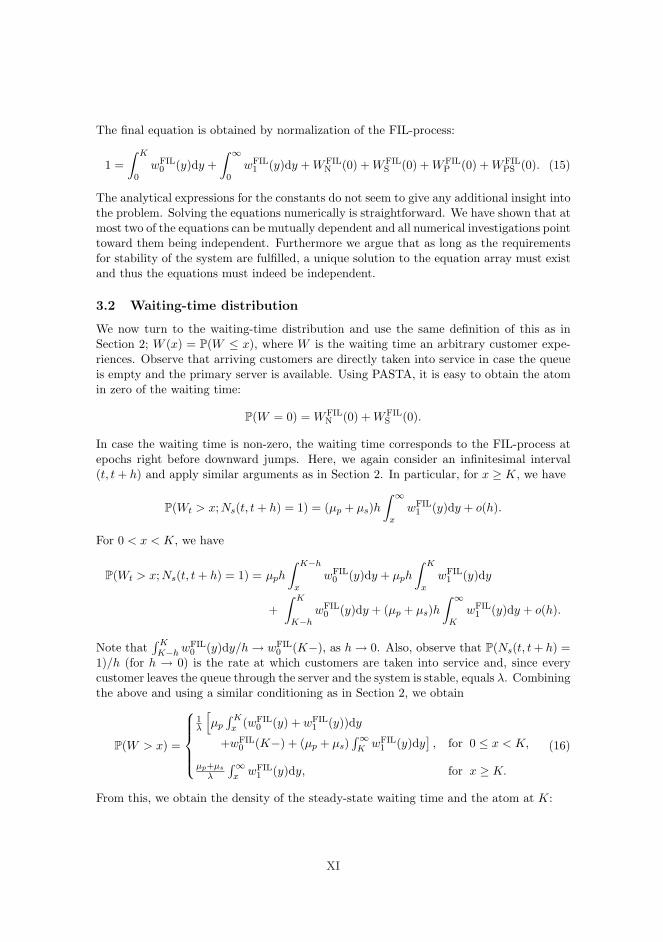
The final equation is obtained by normalization of the FIL-process:
1 =∫ K
0wFIL
0 (y)dy +∫ ∞
0wFIL
1 (y)dy + WFILN (0) + WFIL
S (0) + WFILP (0) + WFIL
PS (0). (15)
The analytical expressions for the constants do not seem to give any additional insight intothe problem. Solving the equations numerically is straightforward. We have shown that atmost two of the equations can be mutually dependent and all numerical investigations pointtoward them being independent. Furthermore we argue that as long as the requirementsfor stability of the system are fulfilled, a unique solution to the equation array must existand thus the equations must indeed be independent.
3.2 Waiting-time distribution
We now turn to the waiting-time distribution and use the same definition of this as inSection 2; W (x) = P(W ≤ x), where W is the waiting time an arbitrary customer expe-riences. Observe that arriving customers are directly taken into service in case the queueis empty and the primary server is available. Using PASTA, it is easy to obtain the atomin zero of the waiting time:
P(W = 0) = WFILN (0) + WFIL
S (0).
In case the waiting time is non-zero, the waiting time corresponds to the FIL-process atepochs right before downward jumps. Here, we again consider an infinitesimal interval(t, t + h) and apply similar arguments as in Section 2. In particular, for x ≥ K, we have
P(Wt > x;Ns(t, t + h) = 1) = (µp + µs)h∫ ∞
xwFIL
1 (y)dy + o(h).
For 0 < x < K, we have
P(Wt > x; Ns(t, t + h) = 1) = µph
∫ K−h
xwFIL
0 (y)dy + µph
∫ K
xwFIL
1 (y)dy
+∫ K
K−hwFIL
0 (y)dy + (µp + µs)h∫ ∞
KwFIL
1 (y)dy + o(h).
Note that∫ KK−h wFIL
0 (y)dy/h → wFIL0 (K−), as h → 0. Also, observe that P(Ns(t, t + h) =
1)/h (for h → 0) is the rate at which customers are taken into service and, since everycustomer leaves the queue through the server and the system is stable, equals λ. Combiningthe above and using a similar conditioning as in Section 2, we obtain
P(W > x) =
1λ
[µp
∫ Kx (wFIL
0 (y) + wFIL1 (y))dy
+wFIL0 (K−) + (µp + µs)
∫∞K wFIL
1 (y)dy], for 0 ≤ x < K,
µp+µs
λ
∫∞x wFIL
1 (y)dy, for x ≥ K.
(16)
From this, we obtain the density of the steady-state waiting time and the atom at K:
XI

Corollary 3.1 For the steady-state waiting time, we have two atoms
P(W = 0) = WFILN (0) + WFIL
S (0),
P(W = K) =wFIL
0 (K−)λ
,
and density
w(x) =
µp
λ c1e(λ−µp)x, for 0 < x < K,
µp+µs
λ c2e(λ−µp−µs)x, for x > K.
Remark 3.1 Note that the form of the steady-state waiting time density (and distribu-tion) is closely related to the density in Example 2.1, i.e., the single-server model with twoservice speeds determined by a threshold on the FIL-process. In particular, the parame-ters ri, i = 1, 2, and µ should be taken such that r1µ = µp and r2µ = µp +µs (for instance,let µ = µp, r1 = 1, and r2 = 1 + µs/µp). The main difference between the waiting-timedistributions concerns the atom at K. ¦
4 Numerical results
To illustrate the difference in behavior of the waiting-time distribution for the one serversystem of Example 2.1 and the two-server system treated in Section 3, a few numericalresults are shown in Figure 3. The parameters have been chosen such that the two casesare comparable.The waiting-time distributions in Figure 3b are found from Corollary 3.1 and the cor-responding eight constants, found with Maple, are given in Table 1. It is seen how therelation between λ and µp governs the shape of the distribution for x < K; it is convexfor λ < µp, concave for λ > µp and a straight line for λ = µp. Notable are also the atomsat K which are absent in the two-speed single server case of Figure 3a.The somewhat better performance of the two-server model can be explained by the sec-ondary server finishing an already started service when Wt drops below K, whereas thesingle server system of Example 2.1 will change the service speed to r1 immediately.
Table 1: Numerical results for common parameters λ = 2, µs = 3.
(µp = 1, K = 1.5) (µp = 2, K = 1.0) (µp = 4, K = 0.5)
WN 0.0470 0.2298 0.5318WP 0.0860 0.2181 0.2559WS 0.0027 0.0078 0.0133WPS 0.0135 0.0195 0.0166c1 0.1990 0.4751 0.5451c2 6.3453 2.9956 0.6123c3 -0.6401·10−4 -0.2673·10−3 -0.4749·10−3
c4 0.01626 0.0276 0.0304
In Figure 4 we compared the performance of the service mechism based on waiting times tothe control based on queue lengths, since the latter is common in the queueing literature.
XII

0 1 2 3 40
0.2
0.4
0.6
0.8
1
x
P(W
>x)
r1=1, r
2=4, K=1.5
r1=2, r
2=5, K=1
r1=4, r
2=7, K=0.5
(a) Waiting-time distributions for the single serversystem in Example 2.1 with two service speeds de-termined by different parameter values of r1, r2,and K. Shared parameters: λ = 2 and µ = 1.
0 1 2 3 40
0.2
0.4
0.6
0.8
1
xP(
W>
x)
µ
p=1, K=1.5
µp=2, K=1
µp=4, K=0.5
(b) Waiting-time distribution for the two-serversystem of Section 3 for 3 different values of µp andK and shared parameters λ = 2 and µs = 3.
Figure 3: Numerical comparison of the one and two-server models.
For the model with queue-length based control, the secondary server is only allowed totake customers into service when more than 30 and 3 customers, in Figures 4a and 4b,respectively, are waiting in the queue. These parameters have been chosen such that theresulting average waiting times are nearly identical for the two policies. The waiting-timedistribution for the queue-length based threshold is found by taking the average of 50simulations of 100.000 calls each. In this way the 95% confidence intervals become toonarrow to display in the figure. It is seen that the waiting-time based threshold results inless variation of waiting times which is preferable as the objective is to have more controlover the system. This reduction in variability of waiting times is accentuated for largerthreshold value as displayed in Figure 4a. The figure illustrates the interesting, but notsurprising, phenomenon of how the probability mass gathers around K for λ > µp, Klarge and waiting-time based control.Given the distribution of the waiting-time and FIL-process, most of the commonly usedperformance measures such as TSF are easily found. Other performance measures suchas the utilization of the servers can be found as
ap = 1−WN(0)−WS(0),
as = 1−WN(0)−WP(0)−∫ K
0wFIL
0 (y)dy,
where ap and as are the utilization of the primary and secondary server, respectively.
5 Conclusions and topics for further research
We have studied queueing systems where the provided service depends on the waiting timeof the first customer in line. This type of control is commonly used in call centers and has
XIII
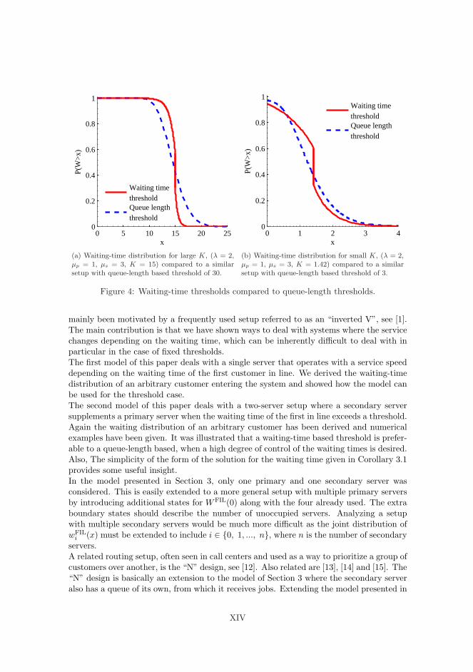
0 5 10 15 20 250
0.2
0.4
0.6
0.8
1
x
P(W
>x)
Waiting timethresholdQueue lengththreshold
(a) Waiting-time distribution for large K, (λ = 2,µp = 1, µs = 3, K = 15) compared to a similarsetup with queue-length based threshold of 30.
0 1 2 3 40
0.2
0.4
0.6
0.8
1
xP(
W>
x)
Waiting timethresholdQueue lengththreshold
(b) Waiting-time distribution for small K, (λ = 2,µp = 1, µs = 3, K = 1.42) compared to a similarsetup with queue-length based threshold of 3.
Figure 4: Waiting-time thresholds compared to queue-length thresholds.
mainly been motivated by a frequently used setup referred to as an “inverted V”, see [1].The main contribution is that we have shown ways to deal with systems where the servicechanges depending on the waiting time, which can be inherently difficult to deal with inparticular in the case of fixed thresholds.The first model of this paper deals with a single server that operates with a service speeddepending on the waiting time of the first customer in line. We derived the waiting-timedistribution of an arbitrary customer entering the system and showed how the model canbe used for the threshold case.The second model of this paper deals with a two-server setup where a secondary serversupplements a primary server when the waiting time of the first in line exceeds a threshold.Again the waiting distribution of an arbitrary customer has been derived and numericalexamples have been given. It was illustrated that a waiting-time based threshold is prefer-able to a queue-length based, when a high degree of control of the waiting times is desired.Also, The simplicity of the form of the solution for the waiting time given in Corollary 3.1provides some useful insight.In the model presented in Section 3, only one primary and one secondary server wasconsidered. This is easily extended to a more general setup with multiple primary serversby introducing additional states for WFIL(0) along with the four already used. The extraboundary states should describe the number of unoccupied servers. Analyzing a setupwith multiple secondary servers would be much more difficult as the joint distribution ofwFIL
i (x) must be extended to include i ∈ {0, 1, ..., n}, where n is the number of secondaryservers.A related routing setup, often seen in call centers and used as a way to prioritize a group ofcustomers over another, is the “N” design, see [12]. Also related are [13], [14] and [15]. The“N” design is basically an extension to the model of Section 3 where the secondary serveralso has a queue of its own, from which it receives jobs. Extending the model presented in
XIV

this paper to the “N” design, necessitates the use of a 2-dimensional FIL-process in orderto keep track of the waiting time of the first customer in line in both queues.There is still much to be done in relation to analysis of complex queueing systems suchas those seen in call centers. Even though simulation may remain the dominant way ofmodelling these systems, it is indeed worth pursuing analytical approaches to gain insightnot obtainable through simulation such as the result in Corollary 3.1.
References
[1] Armony, M. (2005). Dynamic routing in large-scale service systems with heterogeneous servers.Queueing Systems 51, 287–329.
[2] Asmussen, S. (2003). Applied Probability and Queues, Second Edition. Springer, New York.
[3] Barth, W., M. Manitz, R. Stolletz (2009). Analysis of Two-Level Support Systems with Time-Dependent Overflow - A Banking Application. Forthcoming in Production and Operations Man-agement.
[4] Bekker, R., S.C. Borst, O.J. Boxma, O. Kella (2004). Queues with workload-dependent arrivaland service rates. Queueing Systems 46, 537–556.
[5] Boxma, O., H. Kaspi, O. Kella, D. Perry (2005). On/off storage systems with state dependentinput, output and switching rates. Probability in the Engineering and Informational Sciences19, 1–14.
[6] Boxma, O.J., M. Vlasiou (2007). On queues with service and interarrival times depending onwaiting times. Queueing Systems 56, 121–132.
[7] Brill, P.H., M.J.M. Posner (1981). A two server queue with nonwaiting customers receivingspecialized service. Management Science 27, 914–925.
[8] Brill, P.H., M.J.M. Posner (1981). The system point method in exponential queues: a levelcrossing approach. Mathematics of Operations Research 6, 31–49.
[9] Browne, S., K. Sigman (1992). Work-modulated queues with applications to storage processes.Journal of Applied Probability 29, 699–712.
[10] Cohen, J.W., M. Rubinovitch (1977). On level crossings and cycles in dam processes. Mathe-matics of Operations Research 2, 297–310.
[11] Franx, G.J., G.M. Koole, S.A. Pot (2006). Approximating multi-skill blocking systems byhyperexponential decomposition. Performance Evaluation 63, 799–824.
[12] Gans, N., G.M. Koole, A. Mandelbaum (2003). Telephone call centers: tutorial, review, andresearch prospects. Manufacturing and Service Operations Management 5, 79–141.
[13] Gans, N., Y.-P. Zhou (2003). A call-routing problem with service-level constraints. OperationsResearch 51, 255–271.
[14] Gans, N., Y.-P. Zhou (2007). Call-routing schemes for call-center outsourcing. Manufacturingand Service Operations Management 9, 33–50.
[15] Gurvich, I., M. Armony, A. Mandelbaum (2008). Service-level differentiation in call centerswith fully flexible servers. Management Science 54, 279–294.
[16] Harrison, J.M., S.I. Resnick (1976). The stationary distribution and first exit probabilities ofa storage process with general release rule. Mathematics of Operations Research 1, 347–358.
[17] Jackson, J.R. (1960). Some problems in queueing with dynamic priorities. Naval ResearchLogistics Quarterly 7, 235–249.
XV

[18] Koole, G.M. (1995). A simple proof of the optimality of a threshold policy in a two-serverqueueing system. Systems & Control Letters 26, 301–303.
[19] Lin, W., P.R. Kumar (1984). Optimal control of a queueing system with two heterogeneousservers. IEEE Trans. Automat. Control 29, 696–703.
[20] Lucent Technologies (1999). CentreVu Release 8 Advocate User Guide. P.O. Box 4100, Craw-fordsville, IN 47933, U.S.A.: Lucent Technologies.
[21] Perry, D., L. Benny (1989). Continuous Production/Inventory Model with Analogy to CertainQueueing and Dam Models. Advances in Applied Probability 21, 123–141.
[22] Posner, M.J.M (1973). Single-server queues with service time dependent on waiting time.Operations Research 21, 610–616.
[23] Rubinovitch, M. (1985). The slow server problem. Journal of Applied Probability 22, 205–213.
[24] Scheinhardt, W.R.W., N. van Foreest, M. Mandjes (2005). Continuous feedback fluid queues.Operations Research Letters 33, 551–559.
[25] Stockbridge, R.H. (1991). A martingale approach to the slow server problem. Journal ofApplied Probability 28, 480–486.
[26] Whitt, W. (1990). Queues with service times and interarrival times depending linearly andrandomly upon waiting times. Queueing Systems 6, 335–351.
[27] Zabreiko, P.P, A.I. Koshelev, M.A. Krasnosel’skii; transl. and ed. by T.O. Shaposhnikova,R.S. Anderssen and S.G. Mikhlin (1975). Integral Equations: a Reference Text. Monographsand textbooks on pure and applied mathematics. Noordhoff, Leiden.
XVI

Addendum
A.1 Addendum
Independence of Equations
In this addendum to Appendix A, we examine the independence of the eightequations obtained for the two-server queue in the paper Queues with waitingtime dependent service. It is shown that at most two of the equations can bedependent, but all numerical investigations point towards all eight equationsbeing independent. The eight equations are re-listed below.
λWFILN (0) = µpWFIL
P (0) + µsWFILS (0), (A.1)
(λ + µp)WFILP (0) = λWFIL
N (0)
+ µp
Z K
0+e−λywFIL
0 (y)dy + µsWFILPS (0), (A.2)
(λ + µs)WFILS (0) = µpWFIL
PS (0), (A.3)
(λ + µp + µs)WFILPS (0) = λWFIL
S (0) + µp
Z ∞0+
e−λywFIL1 (y)dy
+ µs
Z ∞K
e−λywFIL1 (y)dy + wFIL
0 (K)e−λK , (A.4)
1 =
Z K
0
wFIL0 (y)dy +
Z ∞0
wFIL1 (y)dy + WFIL
N (0)
+ WFILS (0) + WFIL
P (0) + WFILPS (0), (A.5)
wFIL0 (K−) = µs
»WFIL
S (0) + WFILPS (0) +
Z K
0
wFIL1 (y)dy
–(A.6)
wFIL1 (K−) + µsW
FIL1 (K) = wFIL
0 (K) + c2e(λ−µp−µs)K , (A.7)
WFILS (0) + WFIL
PS (0) = c3 + c4, (A.8)
where
wFIL0 (x) = −c1e
(λ−µp)x − r1c3er1x − r2c4e
r2x, for 0 < x ≤ K,
wFIL1 (x) =
r1c3er1x + r2c4e
r2x, for 0 < x ≤ K;
c2e(λ−µp−µs)x, for x > K,
83

A. Queues with waiting time dependent service
with r1, r2 given by
r1 =λ− (µp + µs)−
√(µp + µs − λ)2 + 4λµs
2,
r2 =λ− (µp + µs) +
√(µp + µs − λ)2 + 4λµs
2.
Writing Equations (A.1)-(A.8) in matrix form as Ax = b where
x =
WFILN (0)
WFILP (0)
WFILS (0)
WFILPS (0)c3
c4
c1
c2
, b =
00001000
,
results in a rather complicated A-matrix, which should be non-singular forthe eight equations to be independent. We introduce the following matrixoperations:
• SwitchRow(a,b): Switches the position of rows a and b. For instance,SwitchRow(2,4) on rows numbered [1, 2, 3, 4] yields [1, 4, 3, 2].
• InsertRow(a,b): Inserts row a on row b’s position and shifts the otherrows as required. Example: InsertRow(2,4) on rows numbered [1, 2, 3, 4]yields [1, 4, 2, 3].
• Eliminate(a,b,c): Eliminates element (a, b) (row a, column b) of the ma-trix using element (c, b) and manipulates the remaining elements of rowa accordingly. The procedure can formulated as:
A(a, .) = A(a, .)− A(a, b)A(c, b)
A(c, .).
As an example, running Eliminate(2,1,3) on the matrix B yields C inEquation (A.9).
B =
1 2 34 5 67 8 9
, C =
1 2 30 3
767
7 8 9
(A.9)
84
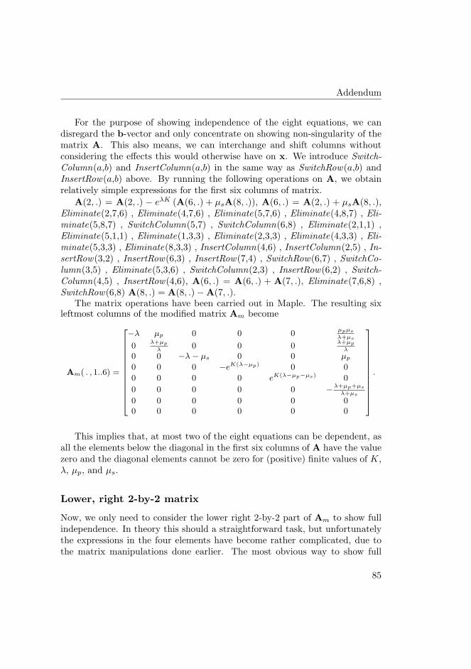
Addendum
For the purpose of showing independence of the eight equations, we candisregard the b-vector and only concentrate on showing non-singularity of thematrix A. This also means, we can interchange and shift columns withoutconsidering the effects this would otherwise have on x. We introduce Switch-Column(a,b) and InsertColumn(a,b) in the same way as SwitchRow(a,b) andInsertRow(a,b) above. By running the following operations on A, we obtainrelatively simple expressions for the first six columns of matrix.
A(2, .) = A(2, .) − eλK (A(6, .) + µsA(8, .)), A(6, .) = A(2, .) + µsA(8, .),Eliminate(2,7,6) , Eliminate(4,7,6) , Eliminate(5,7,6) , Eliminate(4,8,7) , Eli-minate(5,8,7) , SwitchColumn(5,7) , SwitchColumn(6,8) , Eliminate(2,1,1) ,Eliminate(5,1,1) , Eliminate(1,3,3) , Eliminate(2,3,3) , Eliminate(4,3,3) , Eli-minate(5,3,3) , Eliminate(8,3,3) , InsertColumn(4,6) , InsertColumn(2,5) , In-sertRow(3,2) , InsertRow(6,3) , InsertRow(7,4) , SwitchRow(6,7) , SwitchCo-lumn(3,5) , Eliminate(5,3,6) , SwitchColumn(2,3) , InsertRow(6,2) , Switch-Column(4,5) , InsertRow(4,6), A(6, .) = A(6, .) + A(7, .), Eliminate(7,6,8) ,SwitchRow(6,8) A(8, .) = A(8, .)−A(7, .).
The matrix operations have been carried out in Maple. The resulting sixleftmost columns of the modified matrix Am become
Am( . , 1..6) =
2666666666664
−λ µp 0 0 0µpµs
λ+µs
0λ+µp
λ0 0 0
λ+µp
λ
0 0 −λ− µs 0 0 µp
0 0 0 −eK(λ−µp) 0 0
0 0 0 0 eK(λ−µp−µs) 0
0 0 0 0 0 −λ+µp+µs
λ+µs
0 0 0 0 0 00 0 0 0 0 0
3777777777775.
This implies that, at most two of the eight equations can be dependent, asall the elements below the diagonal in the first six columns of A have the valuezero and the diagonal elements cannot be zero for (positive) finite values of K,λ, µp, and µs.
Lower, right 2-by-2 matrix
Now, we only need to consider the lower right 2-by-2 part of Am to show fullindependence. In theory this should a straightforward task, but unfortunatelythe expressions in the four elements have become rather complicated, due tothe matrix manipulations done earlier. The most obvious way to show full
85

A. Queues with waiting time dependent service
rank of the 2-by-2 matrix is to show the determinant cannot be 0. The fourexpressions are listed and simplified individually below.
Am(7, 7) =eK(r1−λ)µpr1 − µpr1 + r1µseK(r1−λ) − µseK(r1−λ)λ
r1 − λ
−λ2 + 2µsλ + µsµp + µ2
s
λ + µp + µs
=µpr1
`eK(r1−λ) − 1
´+ µseK(r1−λ)(r1 − λ)
r1 − λ−
(λ + µs)2 + µpµs
λ + µp + µs
=µpr1
`eK(r1−λ) − 1
´r1 − λ
+ µseK(r1−λ) −(λ + µs)2 + µpµs
λ + µp + µs
=(r1(µp + µs) − λµs)eK(r1−λ) − µpr1
r1 − λ−
(λ + µs)2 + µpµs
λ + µp + µs
=
„r1µp
r1 − λ+ µs
«eK(r1−λ) −
µpr1
r1 − λ−
(λ + µs)2 + µpµs
λ + µp + µs,
Am(7, 8) =eK(r2−λ)µpr2 − µpr2 + r2µseK(r2−λ) − µseK(r2−λ)λ
r2 − λ
−λ2 + 2µsλ + µsµp + µ2
s
λ + µp + µs
=µpr2
`eK(r2−λ) − 1
´+ µseK(r2−λ)(r2 − λ)
r2 − λ−
(λ + µs)2 + µpµs
λ + µp + µs
=µpr2
`eK(r2−λ) − 1
´r2 − λ
+ µseK(r2−λ) −(λ + µs)2 + µpµs
λ + µp + µs
=(r2(µp + µs) − λµs)eK(r2−λ) − µpr2
r2 − λ−
(λ + µs)2 + µpµs
λ + µp + µs
=
„r2µp
r2 − λ+ µs
«eK(r2−λ) −
µpr2
r2 − λ−
(λ + µs)2 + µpµs
λ + µp + µs,
86
Addendum
Am(8, 7)
=1
(r1 + µp − λ)(µ2p − λ2)
„µsµpλ
2 − µsµ3p + µsµ
3pe
K(r1+µp−λ) − λ2
µser1K
µp
+λ2(−r1µp + er1K r1µp − er1K r1λ − r1µs − µser1K λ + r1λ − r2
1 + µser1K r1 + µsλ + r21er1K )µp
r1 + µp − λ
+λ2(−r1µp + er1K r1µp − er1K r1λ − r1µs − µser1K λ + r1λ − r2
1 + µser1K r1 + µsλ + r21er1K )µ2
p
r1(r1 + µp − λ)
−2λ3(−r1µp + er1K r1µp − er1K r1λ − r1µs − µser1K λ + r1λ − r2
1 + µser1K r1 + µsλ + r21er1K )µp
r1(r1 + µp − λ)
−λ3(−r1µp + er1K r1µp − er1K r1λ − r1µs − µser1K λ + r1λ − r2
1 + µser1K r1 + µsλ + r21er1K )
r1 + µp − λ
+λ4(−r1µp + er1K r1µp − er1K r1λ − r1µs − µser1K λ + r1λ − r2
1 + µser1K r1 + µsλ + r21er1K )
r1(r1 + µp − λ)
«
+λ2 + 2µsλ + µsµp + µ2
s
λ + µp + µs
=1
(r1 + µp − λ)(µ2p − λ2)
»µsµpλ
2 − µsµ3p + µsµ
3pe
K(r1+µp−λ) − λ2
µser1K
µp
+
0@λ2
µp − λ3 +
λ2µ2p − 2λ3µp + λ4
r1
1A·
0@−r1µp + er1K r1µp − er1K r1λ − r1µs − µser1K λ + r1λ − r21 + µser1K r1 + µsλ + r2
1er1K
r1 + µp − λ
1A –
+(λ + µs)2 + µpµs
λ + µp + µs
=1
(r1 + µp − λ)(µ2p − λ2)
"µpµs
„λ2 “1 − e
r1K”
+ µ2p
„e
K(r1+µp−λ) − 1««
+ λ2 `
µp − λ´
1 +µp − λ
r1
!0@“1 − er1K
” `λµs + r1(λ − µp − µs − r1)
´r1 + µp − λ
1A#
+(λ + µs)2 + µpµs
λ + µp + µs
=µpµs
„λ2
“1 − er1K
”+ µ2
p
„e
K(r1+µp−λ) − 1««
(r1 + µp − λ)(µ2p − λ2)
+(λ + µs)2 + µpµs
λ + µp + µs
= −µpµsλ2
(r1 + µp − λ)(µ2p − λ2)
ekr1 +
µ3pµs
(r1 + µp − λ)(µ2p − λ2)
eK(r1+µp−λ)
−µpµs
r1 + µp − λ+
(λ + µs)2 + µpµs
λ + µp + µs,
87

A. Queues with waiting time dependent service
and
Am(8, 8)
=1
(r2 + µp − λ)(µ2p − λ2)
„µsµpλ
2 − µsµ3p + µsµ
3pe
K(r2+µp−λ) − λ2
µser2K
µp
+λ2(−r2µp + er2K r2µp − er2K r2λ − r2µs − µser2K λ + r2λ − r2
2 + µser2K r2 + µsλ + r22er2K )µp
r2 + µp − λ
+λ2(−r2µp + er2K r2µp − er2K r2λ − r2µs − µser2K λ + r2λ − r2
2 + µser2K r2 + µsλ + r22er2K )µ2
p
r2(r2 + µp − λ)
−2λ3(−r2µp + er2K r2µp − er2K r2λ − r2µs − µser2K λ + r2λ − r2
2 + µser2K r2 + µsλ + r22er2K )µp
r2(r2 + µp − λ)
−λ3(−r2µp + er2K r2µp − er2K r2λ − r2µs − µser2K λ + r2λ − r2
2 + µser2K r2 + µsλ + r22er2K )
r2 + µp − λ
+λ4(−r2µp + er2K r2µp − er2K r2λ − r2µs − µser2K λ + r2λ − r2
2 + µser2K r2 + µsλ + r22er2K )
r2(r2 + µp − λ)
«
+λ2 + 2µsλ + µsµp + µ2
s
λ + µp + µs
= −µpµsλ2
(r2 + µp − λ)(µ2p − λ2)
ekr2 +
µ3pµs
(r2 + µp − λ)(µ2p − λ2)
eK(r2+µp−λ)
−µpµs
r2 + µp − λ+
(λ + µs)2 + µpµs
λ + µp + µs.
We note the last part of each of the four expressions of Am(7..8, 7..8) areidentical. If we write the values as
Am(7, 7) = a− x,
Am(7, 8) = b− x,
Am(8, 7) = c + x,
Am(8, 8) = d + x,
the determinant, D, of Am(7..8, 7..8) becomes:
D = (a− x)(d + x)− (b− x)(c + x)= ad− bc + x(a− b + c− d), (A.10)
88

Addendum
where
a =
„r1µp
r1 − λ+ µs
«eK(r1−λ) −
µpr1
r1 − λ,
b =
„r2µp
r2 − λ+ µs
«eK(r2−λ) −
µpr2
r2 − λ,
c =−µpµsλ2
(r1 + µp − λ)(µ2p − λ2)
ekr1 +µ3
pµs
(r1 + µp − λ)(µ2p − λ2)
eK(r1+µp−λ) −µpµs
r1 + µp − λ,
d =−µpµsλ2
(r2 + µp − λ)(µ2p − λ2)
ekr2 +µ3
pµs
(r2 + µp − λ)(µ2p − λ2)
eK(r2+µp−λ) −µpµs
r2 + µp − λ,
x =(λ + µs)2 + µpµs
λ + µp + µs.
In order to make the above expressions appear nicer for further manipula-tions, we introduce:
P1 = µs + r1 = λ− µp − r2,
P2 = µs + r2 = λ− µp − r1,
R1 = λ− r1 = r2 + µp + µs,
R2 = λ− r2 = r1 + µp + µs
thus
a =(
µs −r1µp
R1
)e−kR1 +
µpr1
R1,
b =(
µs −r2µp
R2
)e−kR2 +
µpr2
R2,
c =µpµsλ
2
P2(µ2p − λ2)
ekr1 −µ3
pµs
P2(µ2p − λ2)
e−kP2 +µpµs
P2,
d =µpµsλ
2
P1(µ2p − λ2)
ekr2 −µ3
pµs
P1(µ2p − λ2)
e−kP1 +µpµs
P1,
x =(λ + µs)2 + µpµs
λ + µp + µs.
Now Equation (A.10) is considered piece by piece using the relations given
89
A. Queues with waiting time dependent service
at the end of this addendum. For the first part
ad =
„„µs −
r1µp
R1
«e−kR1 +
µpr1
R1
« µpµsλ2
P1(µ2p − λ2)
ekr2 −µ3
pµs
P1(µ2p − λ2)
e−kP1 +µpµs
P1
!
=
„µs −
r1µp
R1
«µpµsλ2
P1(µ2p − λ2)
e−K(µp+µs) −„
µs −r1µp
R1
«µ3
pµs
P1(µ2p − λ2)
e−K(λ+µs)
+
„µs −
r1µp
R1
«µpµs
P1e−kR1 +
µpr1
R1
µpµsλ2
P1(µ2p − λ2)
ekr2 −µpr1
R1
µ3pµs
P1(µ2p − λ2)
e−kP1
+µpr1
R1
µpµs
P1
=
µpµ2
sλ2
P1(µ2p − λ2)
−µpµsλ2
µ2p − λ2
!e−K(µp+µs) −
µ3
pµ2s
P1(µ2p − λ2)
−µ3
pµs
µ2p − λ2
!e−K(λ+µs)
+
„µpµ2
s
P1− µpµs
«e−kR1 +
µpµsλ2
µ2p − λ2
ekr2 −µ3
pµs
µ2p − λ2
e−kP1 + µpµs,
and
bc =
„„µs −
r2µp
R2
«e−kR2 +
µpr2
R2
« µpµsλ2
P2(µ2p − λ2)
ekr1 −µ2
p
P2(µ2p − λ2)
e−kP2 +µpµs
P2
!
=
„µs −
r2µp
R2
«µpµsλ2
P2(µ2p − λ2)
e−K(µp+µs) −„
µs −r2µp
R2
«µ3
pµs
P2(µ2p − λ2)
e−K(λ+µs)
+
„µs −
r2µp
R2
«µpµs
P2e−kR2 +
µpr2
R2
µpµsλ2
P2(µ2p − λ2)
ekr1 −µpr2
R2
µ3pµs
P2(µ2p − λ2)
e−kP2
+µpr2
R2
µpµs
P2
=
µpµ2
sλ2
P2(µ2p − λ2)
−µpµsλ2
µ2p − λ2
!e−K(µp+µs) −
µ3
pµ2s
P2(µ2p − λ2)
−µ3
pµs
µ2p − λ2
!e−K(λ+µs)
+
„µpµ2
s
P2− µpµs
«e−kR2 +
µpµsλ2
µ2p − λ2
ekr1 −µ3
pµs
µ2p − λ2
e−kP2 + µpµs.
Gathering the former two expressions eliminates all non-exponential ele-
90
Addendum
ments.
ad− bc =µpµ
2sλ
2
µ2p − λ2
(1P1
− 1P2
)e−K(µp+µs) −
µ3pµ
2s
µ2p − λ2
(1P1
− 1P2
)e−K(λ+µs)
+(
µpµ2s
P1− µpµs
)e−kR1 −
(µpµ
2s
P2− µpµs
)e−kR2
+µpµsλ
2
µ2p − λ2
ekr2 − µpµsλ2
µ2p − λ2
ekr1 −µ3
pµs
µ2p − λ2
e−kP1 +µ3
pµs
µ2p − λ2
e−kP2
=µsλ
2(r1 − r2)µ2
p − λ2e−K(µp+µs) −
µ2pµs(r1 − r2)
µ2p − λ2
e−K(λ+µs)
− µpµsr1
µs + r1e−kR1 +
µpµsr2
µs + r2e−kR2
+µpµsλ
2
µ2p − λ2
ekr2 − µpµsλ2
µ2p − λ2
ekr1 −µ3
pµs
µ2p − λ2
e−kP1 +µ3
pµs
µ2p − λ2
e−kP2
The expression inside the parenthesis in Equation (A.10) is now considered.First part by part
a− b =(
µs −r1µp
R1
)e−kR1 +
µpr1
R1−(
µs −r2µp
R2
)e−kR2 − µpr2
R2
=(
µs −r1µp
R1
)e−kR1 −
(µs −
r2µp
R2
)e−kR2 + r1 − r2,
and
c− d =µpµsλ
2
P2(µ2p − λ2)
ekr1 −µ3
pµs
P2(µ2p − λ2)
e−kP2
+µpµs
P2− µpµsλ
2
P1(µ2p − λ2)
ekr2 +µ3
pµs
P1(µ2p − λ2)
e−kP1 − µpµs
P1
=µpµs
µ2p − λ2
(λ2
P2ekr1 − λ2
P1ekr2 −
µ2p
P2e−kP2 +
µ2p
P1e−kP1
)+ r2 − r1,
which together becomes
a− b + c− d =(
µs −r1µp
R1
)e−kR1 −
(µs −
r2µp
R2
)e−kR2
+µpµs
µ2p − λ2
(λ2
P2ekr1 − λ2
P1ekr2 −
µ2p
P2e−kP2 +
µ2p
P1e−kP1
)
91

A. Queues with waiting time dependent service
The entire expression for the determinant becomes
D = ad− bc + x(a− b + c− d)
=µsλ
2(r1 − r2)
µ2p − λ2
e−K(µp+µs) −µ2
pµs(r1 − r2)
µ2p − λ2
e−K(λ+µs)
− µpµsr1
µs + r1e−kR1 +
µpµsr2
µs + r2e−kR2
+µpµsλ
2
µ2p − λ2
ekr2 − µpµsλ2
µ2p − λ2
ekr1 −µ3
pµs
µ2p − λ2
e−kP1 +µ3
pµs
µ2p − λ2
e−kP2
+(λ + µs)
2 + µpµs
λ + µp + µs
»„µs −
r1µp
R1
«e−kR1 −
„µs −
r2µp
R2
«e−kR2
+µpµs
µ2p − λ2
„λ2
P2ekr1 − λ2
P1ekr2 −
µ2p
P2e−kP2 +
µ2p
P1e−kP1
«–
=µsλ
2(r1 − r2)
µ2p − λ2
e−K(µp+µs) −µ2
pµs(r1 − r2)
µ2p − λ2
e−K(λ+µs)
+
»(λ + µs)
2 + µpµs
λ + µp + µs
„µs −
r1µp
R1
«− µpµsr1
µs + r1
–e−kR1
−»(λ + µs)
2 + µpµs
λ + µp + µs
„µs −
r2µp
R2
«− µpµsr2
µs + r2
–e−kR2
+µpµsλ
2
µ2p − λ2
„x
P2− 1
«ekr1 − µpµsλ
2
µ2p − λ2
„x
P1− 1
«ekr2
+µ3
pµs
µ2p − λ2
„x
P1− 1
«e−kP1 −
µ3pµs
µ2p − λ2
„x
P2− 1
«e−kP2
92

Addendum
Finally, inserting the expressions for R1, R2, P1 and P2 yield
D =µsλ
2(r1 − r2)µ2
p − λ2e−K(µp+µs)
−µ2
pµs(r1 − r2)µ2
p − λ2e−K(λ+µs)
+[(λ + µs)2 + µpµs
λ + µp + µs
(λµs − r1(µp + µs)
λ− r1
)− µpµsr1
µs + r1
]e−K(λ−r1)
−[(λ + µs)2 + µpµs
λ + µp + µs
(λµs − r2(µp + µs)
λ− r2
)− µpµsr2
µs + r2
]e−K(λ−r2)
+µpµsλ
2
µ2p − λ2
(λ2 + λµs
(λ + µp + µs)(µs + r2)− r2
µs + r2
)ekr1
− µpµsλ2
µ2p − λ2
(λ2 + λµs
(λ + µp + µs)(µs + r1)− r1
µs + r1
)ekr2
+µ3
pµs
µ2p − λ2
(λ2 + λµs
(λ + µp + µs)(µs + r1)− r1
µs + r1
)e−K(µs+r1)
−µ3
pµs
µ2p − λ2
(λ2 + λµs
(λ + µp + µs)(µs + r2)− r2
µs + r2
)e−K(µs+r2) (A.11)
In order to analyze the determinant further, we denote the eight lines inthe expression (A.11) as D(1) through D(8).
Numerical investigations
Numerical evaluations of the determinant given in (A.11) indicate that thedeterminant is always negative for valid values of K, λ, µp and µs (all should bepositive and finite). A more detailed numerical investigation of the individualelements of D is given in Table (A.1), where the rough magnitudes are shownfor different parameter values.
A pattern is seen in the signs of the individual elements of the determinantby looking at the values in Table A.1. This pattern is shown in Table A.2
Analysis of the determinant
By looking at the values of the determinant elements in the numerical investi-gation, it is seen, it should be possible to show that the determinant is always
93
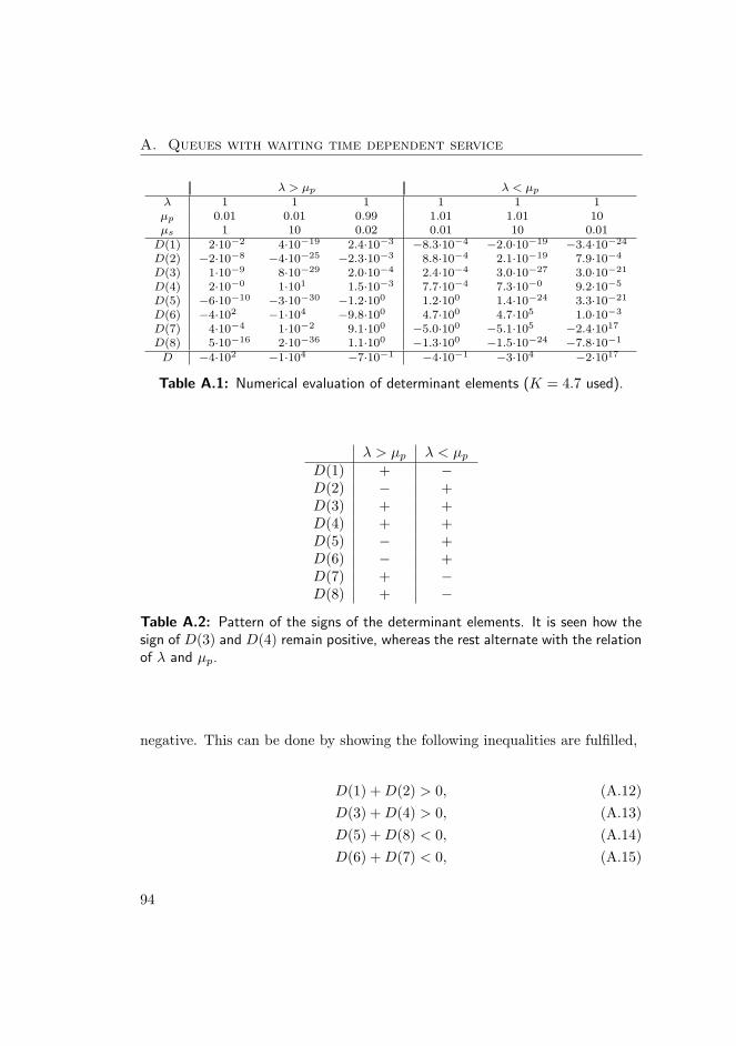
A. Queues with waiting time dependent service
λ > µp λ < µp
λ 1 1 1 1 1 1µp 0.01 0.01 0.99 1.01 1.01 10µs 1 10 0.02 0.01 10 0.01
D(1) 2·10−2 4·10−19 2.4·10−3 −8.3·10−4 −2.0·10−19 −3.4·10−24
D(2) −2·10−8 −4·10−25 −2.3·10−3 8.8·10−4 2.1·10−19 7.9·10−4
D(3) 1·10−9 8·10−29 2.0·10−4 2.4·10−4 3.0·10−27 3.0·10−21
D(4) 2·10−0 1·101 1.5·10−3 7.7·10−4 7.3·10−0 9.2·10−5
D(5) −6·10−10 −3·10−30 −1.2·100 1.2·100 1.4·10−24 3.3·10−21
D(6) −4·102 −1·104 −9.8·100 4.7·100 4.7·105 1.0·10−3
D(7) 4·10−4 1·10−2 9.1·100 −5.0·100 −5.1·105 −2.4·1017
D(8) 5·10−16 2·10−36 1.1·100 −1.3·100 −1.5·10−24 −7.8·10−1
D −4·102 −1·104 −7·10−1 −4·10−1 −3·104 −2·1017
Table A.1: Numerical evaluation of determinant elements (K = 4.7 used).
λ > µp λ < µp
D(1) + −D(2) − +D(3) + +D(4) + +D(5) − +D(6) − +D(7) + −D(8) + −
Table A.2: Pattern of the signs of the determinant elements. It is seen how thesign of D(3) and D(4) remain positive, whereas the rest alternate with the relationof λ and µp.
negative. This can be done by showing the following inequalities are fulfilled,
D(1) + D(2) > 0, (A.12)D(3) + D(4) > 0, (A.13)D(5) + D(8) < 0, (A.14)D(6) + D(7) < 0, (A.15)
94

Addendum
together with
−1 <D(1) + D(2) + D(3) + D(4)
D(6) + D(7)< 0. (A.16)
First, we show that D(1) + D(2) > 0:
D(1) + D(2) =µsλ
2(r1 − r2)µ2
p − λ2e−K(µp+µs) −
µ2pµs(r1 − r2)
µ2p − λ2
e−K(λ+µs)
=µs(r1 − r2)
µ2p − λ2
e−Kµs(λ2e−Kµp − µ2
pe−Kλ
).
The nominator of the fraction and the middle exponential term are alwaysnegative. For λ > µp, the denominator is negative and the expression insidethe parentheses is positive. When λ < µp, both of these change their sign,thus, the whole expression is always positive.
D(3) + D(4) is by far the least nice term because of the many r’s involvedin the expression. It appears to always be positive from the numerical results,this has not been verified analytically though:
D(3) + D(4) = +
»(λ + µs)
2 + µpµs
λ + µp + µs
„λµs − r1(µp + µs)
λ− r1
«− µpµsr1
µs + r1
–e−K(λ−r1)
−»(λ + µs)
2 + µpµs
λ + µp + µs
„λµs − r2(µp + µs)
λ− r2
«− µpµsr2
µs + r2
–e−K(λ−r2)
Now we look at D(5) + D(8), which seems to be negative judging from thenumerical experiments.
D(5) + D(8) =µpµsλ
2
µ2p − λ2
(λ2 + λµs
(λ + µp + µs)(µs + r2)− r2
µs + r2
)eKr1
−µ3
pµs
µ2p − λ2
(λ2 + λµs
(λ + µp + µs)(µs + r2)− r2
µs + r2
)e−K(µs+r2)
=µpµs
µ2p − λ2
λ2 + λµs − r2(λ + µp + µs)(λ + µp + µs)(µs + r2)
(λ2e−Kµp − µ2
pe−Kλ
).
In the expression for D(5) + D(8), the first fraction alternates with oppositesign compared to the last parentheses, with the relation between λ and µp,thus always creating a negative sign together. The nominator of the secondfraction seems to take both positive and negative values, this needs furtherinvestigation though.
95
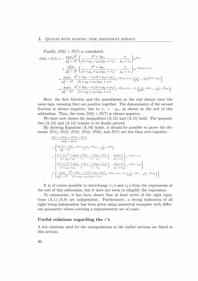
A. Queues with waiting time dependent service
Finally, D(6) + D(7) is considered.
D(6) + D(7) = −µpµsλ2
µ2p − λ2
„λ2 + λµs
(λ + µp + µs)(µs + r1)−
r1
µs + r1
«ekr2
+µ3
pµs
µ2p − λ2
„λ2 + λµs
(λ + µp + µs)(µs + r1)−
r1
µs + r1
«e−K(µs+r1)
=µpµs
µ2p − λ2
λ2 + λµs − r1(λ + µp + µs)
(λ + µp + µs)(µs + r1)e−K(µs+r1)
“µ2
p − λ2eK(λ−µp)”
=µpµs
µ2p − λ2
λ2 + λµs − r1(λ + µp + µs)
(λ + µp + µs)(µs + r1)e−K(µs+r1−λ)
“µ2
pe−Kλ − λ2e−Kµp
”Here, the first fraction and the parentheses at the end always have the
same sign, meaning they are positive together. The denominator of the secondfraction is always negative, due to r1 < −µs, as shown at the end of thisaddendum. Thus, the term D(6) + D(7) is always negative.
We have now shown the inequalities (A.12) and (A.15) hold. The inequali-ties (A.13) and (A.14) remain to be finally proved.
By showing Equation (A.16) holds, it should be possible to prove the ele-ments D(1), D(2), D(3), D(4), D(6), and D(7) are less than zero together.
D(1) + D(2) + D(3) + D(4)
D(6) + D(7)
=
(µs(r1 − r2)
µ2p − λ2
e−Kµs
“λ2e−Kµp − µ
2pe−Kλ
”
+
"(λ + µs)2 + µpµs
λ + µp + µs
„λµs − r1(µp + µs)
λ− r1
«−
µpµsr1
µs + r1
#e−K(λ−r1)
−"
(λ + µs)2 + µpµs
λ + µp + µs
„λµs − r2(µp + µs)
λ− r2
«−
µpµsr2
µs + r2
#e−K(λ−r2)
),(
µpµs
µ2p − λ2
λ2 + λµs − r1(λ + µp + µs)
(λ + µp + µs)(µs + r1)e−K(µs+r1−λ)
“µ2pe−Kλ − λ
2e−Kµp
”)
It is of course possible to interchange r1’s and r2’s from the expressions atthe end of this addendum, but it does not seem to simplify the expression.
To summarize, it has been shown that at least seven of the eight equa-tions (A.1)-(A.8) are independent. Furthermore, a strong indication of alleight being independent has been given using numerical examples with differ-ent parameter values covering a representative set of cases.
Useful relations regarding the r’s
A few relations used for the manipulations in the earlier sections are listed inthis section.
96

Addendum
r1 + µp − λ < 0
Proof
µp − λ +1
2
„λ− µp − µs −
q(−λ + µp + µs)2 + 4λµs
«< 0
1
2(−λ + µp − µs) <
1
2
q(−λ + µp + µs)2 + 4λµs
−λ + µp − µs <q
(−λ + µp + µs)2 + 4λµs
r2 + µp − λ > 0
Proof
µp − λ +1
2
„λ− µp − µs +
q(−λ + µp + µs)2 + 4λµs
«> 0
−λ + µp − µs +q
(−λ + µp + µs)2 + 4λµs > 0q(−λ + µp + µs)2 + 4λµs > λ− µp + µs
(−λ + µp + µs)2
+ 4λµs > λ2
+ µ2p + µ
2s − 2λµp + 2λµs − 2µpµs
λ2
+ µ2p + µ
2s − 2λµp − 2λµs + 2µpµs + 4λµs > λ
2+ µ
2p + µ
2s − 2λµp + 2λµs − 2µpµs
4µpµs > 0
r1 < 0
Proof
r2 + µp − λ > 0λ− µp − µs − r1 + µp + µp − λ > 0
−µs > r1
0 < r2 < λ
97

A. Queues with waiting time dependent service
r21 = (λ− µp − µs)r1 + λµs
r22 = (λ− µp − µs)r2 + λµs
r1r2 = −λµs
r1 + r2 = λ− µp − µs
R1R2 = λµp
R1P1 = (λ− r1)(µs + r1)
= −r21 + (λ− µs)r1 + λµs
= −(λ− µp − µs)r1 − λµs + (λ− µs)r1 + λµs
= µpr1
R2P2 = (λ− r2)(µs + r2)
= −r22 + (λ− µs)r2 + λµs
= −(λ− µp − µs)r2 − λµs + (λ− µs)r2 + λµs
= µpr2
1
P1− 1
P2
=P2 − P1
P1P2
=µs + r2 − µs − r1
(µs + r1)(µs + r2)
=r2 − r1
µ2s + µs(r1 + r2) + r1r2
=r2 − r1
µ2s + µs(λ− µp − µs) + 1
4((λ− µp − µs)2 − (λ− µp − µs)2 − 4λµs)
=r1 − r2
µpµs
98

APPENDIX BWaiting time dependent
multi-server priority queues
99


Waiting time dependent multi-server priority queues
G.M. Koole†, B.F. Nielsen?, T.B. Nielsen?
†Dept. MathematicsVU University Amsterdam
De Boelelaan 1081, 1081 HV, the Netherlands.
?Dept. Informatics and Mathematical ModellingTechnical University of Denmark
Richard Petersens Plads, 2800 Kgs. Lyngby, Denmark.
May 2, 2010
Abstract
We introduce a new approach to modelling queueing systems where the priority orthe routing of customers depends on the waiting time of the first customer in line. Theapproach uses the waiting time of the first customer in line as the primary variableand we obtain waiting time distributions for complex systems, such as the N-designrouting scheme widely used in e.g. call centers and systems with dynamic priorities.
Keywords: Waiting time distribution; Call centers; Priority queues; Deterministicthreshold; Erlang distribution; Dynamic priority; Due-date.
1 Introduction
The traditional approach to modelling queueing systems developed by Erlang, Engset,Fry and Molina has been to look at the number of customers in queue, see [8] for originalreferences. In this paper we introduce an alternative way of modelling queueing systemsuseful for priority rules often used in real scenarios.
Prioritization of customers in real queueing systems is often implemented as a functionof the waiting time of the customer first in line (FIL). This is for example used in callcenters to route calls between agent pools in order to meet service levels of differentcustomer classes [6]. The service levels are usually characterized by the telephone servicefactor (TSF), i.e. the fraction of calls answered within a certain time. The use of TSFthus motivates the examination of waiting time distributions rather than just averagevalues. Prioritization based on waiting times is also used in the health care sector for e.g.operating room scheduling [3].
The traditional approach of modelling the number of customers in a system is not usefulfor modelling these systems as no information about the FIL waiting time is inherent in thevariables. Instead we introduce the Erlang approximation (TEA) as a way of modellingthe waiting time of the customer first in line. We show how TEA can be used for findingthe waiting time distribution for different queueing systems.
I

The literature on this kind of prioritization is very limited despite its widespread usein the industry. In [2] a system is considered, where a single queue is served by twoservers of which one are only allowed to take in customers when they have waited a givenamount of time, and an expression for the waiting time distribution is found. In [1]a similar time-dependent overflow is approximated by a state-dependent overflow wherestates represent the number of customers in the system. Beside these, the literature islimited to less similar systems such as [14] where service times are exponentially distributedwith parameters which depend on the waiting time experienced by the customer enteringservice.
In Section 2 TEA is presented for the simple case of an M/M/n queue and it is shownhow the waiting time distribution can be found. The principles behind TEA are easier toexplain with this simple case and it also facilitates verification of the approximation bytheoretical values.
In Section 3 it is shown how TEA can be used for modelling the N-design system withdeterministic thresholds as shown in Figure 1a. The N-design is composed of a group offlexible servers and a group of specialized servers and two classes of customers. There existmultiple papers about the N-design; e.g. in [17] performance measures, such as averagequeueing delay and queue length distribution, are derived for a bilingual call center wherea fraction of the agents are bilingual and the rest unilingual. In [16] the N-design is alsoexamined and it is shown that a few flexible servers can improve performance significantly,when this is measured as the mean service time, however neither of these papers deal withthe deterministic overflow threshold.
Further possibilities of TEA are discussed in Section 4, including an example of how theapproach can be used for a system with low and high priority customers and schedulingaccording to due dates, also referred to as dynamic priority [11], [5]. Scheduling accordingto due date is a generalization of strict non-preemptive prioritization where high prioritycustomers are not always given service first. This prioritization scheme is for example usedfor operating rooms scheduling to ensure lower priority operations will not experienceexceedingly long waiting times while still keeping high priority patients’ waiting timesrelatively low [3].
n b n a
µa µa µa µb µb µb
bλaλ
1 2 1 2
>kWFIL
(a) N-design
λaλ
1 2
µ µ µ
b
n
a
FIL
bargmax{W −k ,W −k }ba
FIL
(b) V-design
Figure 1: Systems analyzed in Section 3 (Fig. 1a) and Section 4.1 (Fig. 1b).
Possible extensions of TEA are also discussed in Section 4. Only non-preemptive casesare considered here although the presented method could also be used for preemptive
II

(non-resume) prioritization. Finally a conclusion is given in Section 5.
2 The Erlang approximation
The fundamental idea of the Erlang approximation is to describe the FIL waiting time ina discretized form as states in a continuous time Markov chain (CTMC). The transitionrate diagram of the CTMC for TEA of an M/M/n queue is shown in Figure 2.
nµ nµ nµnµ−n 210−1−2
λ γ
µ(n−1)
λ λ γ3
Figure 2: Transition rate diagram for the Erlang approximation of the M/M/n system.
We define WFILt as the waiting time of the first customer in line at time t, with the
convention WFILt = 0 when the queue is empty. In TEA we let states numbered {1, 2, ...}
represent WFILt > 0. Transitions from state i to i+1 with rate γ represent the, in principle
linearly, increasing FIL waiting time in a discrete way.Whenever the queue is empty we have to differentiate between the number of free
servers. This is done by letting states with negative numbers represent the number of freeservers, thus state −n corresponds to all n servers being vacant and state 0 to all serversbeing busy and the queue being empty. Arrivals occur with rate λ and are only “seen”by the model when the queue is empty. In the negative states, i < 0, where servers areunoccupied an arrival just goes to a free server and i increases by one. In state i = 0,were all servers are busy and the queue empty, an arriving customer enters the queue andbecomes the first customer in line. This means WFIL
t starts to increase, represented by theγ-transitions. Customers arriving when i > 0 are not seen by the model as these arrivalsdo not affect WFIL
t .Service completions occur with rate nµ for i ≥ 0 and rate (n+i)µ for i < 0. Whenever a
service completion occurs at time t and the queue is not empty, the FIL waiting decreaseswith min{S,WFIL
t }, where S is a random variable describing the inter-arrival time ofcustomers. In the considered M/M/n queue, S is exponentially distributed as the inter-arrival times in a Poisson arrival process are exponential. This translates to a set oftransitions from state it− to states it+ , following a geometric distribution in the discretesetting of TEA as given in Theorem 2.1. Here t− and t+ refer to the time just before andjust after the transition at time t and it+ ∈ {0 ... it−} is the set of states from 0 to it− .These transitions are illustrated with the double arrows in Figure 2.
Theorem 2.1 The discretization of the interarrival distribution is given as:
P (It+ = it+ |It− = it−) =
1−it−−1∑
h=0
(λ
λ + γ
)(γ
λ + γ
)h
, for it+ = 0;
(λ
λ+γ
)(γ
λ+γ
)it−−it+, for it+ ∈ {1, .., it−}.
Proof The theorem follows directly from the geometric distribution, where the probabil-ity of having a γ-transition in a given state is γ/(λ + γ). This means that the probabilityof going from state it− to it+ equals the probability of having had it− − it+ , γ-transitions
III
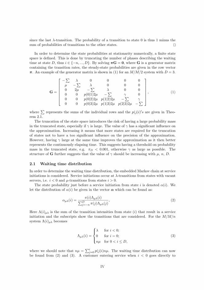
since the last λ-transition. The probability of a transition to state 0 is thus 1 minus thesum of probabilities of transitions to the other states.
In order to determine the state probabilities at stationarity numerically, a finite statespace is defined. This is done by truncating the number of phases describing the waitingtime at state D, thus i ∈ {−n, ..., D}. By solving πG = 0, where G is a generator matrixcontaining the transition rates, the steady-state probabilities are given in the row vectorπ. An example of the generator matrix is shown in (1) for an M/M/2 system with D = 3.
G =
−∑λ 0 0 0 0
µ −∑λ 0 0 0
0 2µ −∑λ 0 0
0 0 p(0|1)2µ −∑γ 0
0 0 p(0|2)2µ p(1|2)2µ −∑γ
0 0 p(0|3)2µ p(1|3)2µ p(2|3)2µ −∑
, (1)
where∑
represents the sums of the individual rows and the p(j|i)′s are given in Theo-rem 2.1.
The truncation of the state space introduces the risk of having a large probability massin the truncated state, especially if γ is large. The value of γ has a significant influence onthe approximation. Increasing it means that more states are required for the truncationof states not to have a too significant influence on the precision of the approximation.However, having γ large at the same time improves the approximation as it then betterrepresents the continuously elapsing time. This suggests having a threshold on probabilitymass in the truncated state, e.g. πD < 0.001, otherwise γ as large as possible. Thestructure of G further suggests that the value of γ should be increasing with µ, n, D.
2.1 Waiting time distribution
In order to determine the waiting time distribution, the embedded Markov chain at serviceinitiations is considered. Service initiations occur at λ-transitions from states with vacantservers, i.e. i < 0 and µ-transitions from states i > 0.
The state probability just before a service initiation from state i is denoted α(i). Welet the distribution of α(i) be given in the vector α which can be found as:
αµλ(i) =π(i)Λµλ(i)∑D
j=−n π(j)Λµλ(j), (2)
Here Λ(i)µλ is the sum of the transition intensities from state (i) that result in a serviceinitiation and the subscripts show the transitions that are considered. For the M/M/nsystem Λ(i)µλ becomes
Λµλ(i) =
λ for i < 0;0 for i = 0;nµ for 0 < i ≤ D,
(3)
where we should note that nµ =∑i
j=0 p(j|i)nµ. The waiting time distribution can nowbe found from (2) and (3). A customer entering service when i < 0 goes directly to
IV
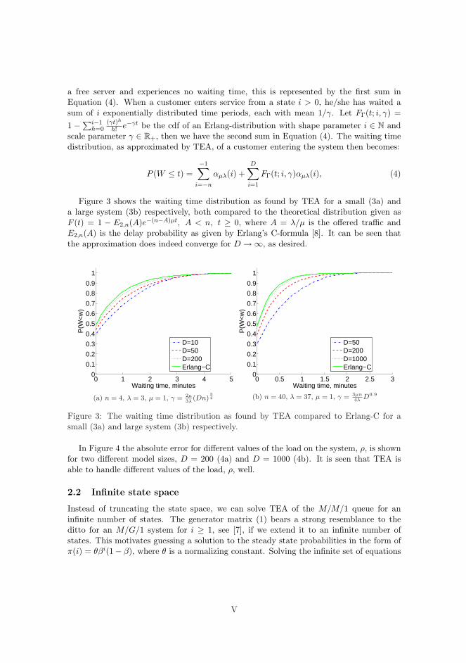
a free server and experiences no waiting time, this is represented by the first sum inEquation (4). When a customer enters service from a state i > 0, he/she has waited asum of i exponentially distributed time periods, each with mean 1/γ. Let FΓ(t; i, γ) =1 −∑i−1
h=0(γt)h
h! e−γt be the cdf of an Erlang-distribution with shape parameter i ∈ N andscale parameter γ ∈ R+, then we have the second sum in Equation (4). The waiting timedistribution, as approximated by TEA, of a customer entering the system then becomes:
P (W ≤ t) =−1∑
i=−n
αµλ(i) +D∑
i=1
FΓ(t; i, γ)αµλ(i), (4)
Figure 3 shows the waiting time distribution as found by TEA for a small (3a) anda large system (3b) respectively, both compared to the theoretical distribution given asF (t) = 1 − E2,n(A)e−(n−A)µt, A < n, t ≥ 0, where A = λ/µ is the offered traffic andE2,n(A) is the delay probability as given by Erlang’s C-formula [8]. It can be seen thatthe approximation does indeed converge for D →∞, as desired.
0 1 2 3 4 50
0.1
0.2
0.3
0.4
0.5
0.6
0.7
0.8
0.9
1
Waiting time, minutes
P(W
<w
)
D=10D=50D=200Erlang−C
(a) n = 4, λ = 3, µ = 1, γ = 2µ3λ
(Dn)34
0 0.5 1 1.5 2 2.5 30
0.1
0.2
0.3
0.4
0.5
0.6
0.7
0.8
0.9
1
Waiting time, minutes
P(W
<w
)
D=50D=200D=1000Erlang−C
(b) n = 40, λ = 37, µ = 1, γ = 3µn4λ
D0.9
Figure 3: The waiting time distribution as found by TEA compared to Erlang-C for asmall (3a) and large system (3b) respectively.
In Figure 4 the absolute error for different values of the load on the system, ρ, is shownfor two different model sizes, D = 200 (4a) and D = 1000 (4b). It is seen that TEA isable to handle different values of the load, ρ, well.
2.2 Infinite state space
Instead of truncating the state space, we can solve TEA of the M/M/1 queue for aninfinite number of states. The generator matrix (1) bears a strong resemblance to theditto for an M/G/1 system for i ≥ 1, see [7], if we extend it to an infinite number ofstates. This motivates guessing a solution to the steady state probabilities in the form ofπ(i) = θβi(1− β), where θ is a normalizing constant. Solving the infinite set of equations
V
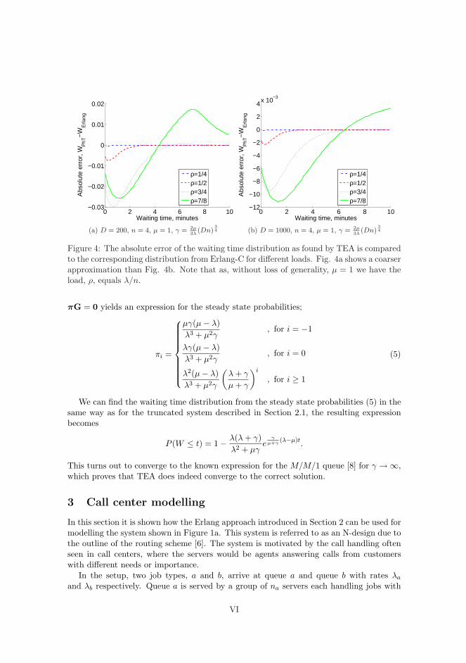
0 2 4 6 8 10−0.03
−0.02
−0.01
0
0.01
0.02
Waiting time, minutes
Abs
olut
e er
ror,
WP
hT−
WE
rlang
ρ=1/4ρ=1/2ρ=3/4ρ=7/8
(a) D = 200, n = 4, µ = 1, γ = 2µ3λ
(Dn)34
0 2 4 6 8 10−12
−10
−8
−6
−4
−2
0
2
4x 10⁻³
Waiting time, minutes
Abs
olut
e er
ror,
WP
hT−
WE
rlang
ρ=1/4ρ=1/2ρ=3/4ρ=7/8
(b) D = 1000, n = 4, µ = 1, γ = 2µ3λ
(Dn)34
Figure 4: The absolute error of the waiting time distribution as found by TEA is comparedto the corresponding distribution from Erlang-C for different loads. Fig. 4a shows a coarserapproximation than Fig. 4b. Note that as, without loss of generality, µ = 1 we have theload, ρ, equals λ/n.
πG = 0 yields an expression for the steady state probabilities;
πi =
µγ(µ− λ)λ3 + µ2γ
, for i = −1
λγ(µ− λ)λ3 + µ2γ
, for i = 0
λ2(µ− λ)λ3 + µ2γ
(λ + γ
µ + γ
)i
, for i ≥ 1
(5)
We can find the waiting time distribution from the steady state probabilities (5) in thesame way as for the truncated system described in Section 2.1, the resulting expressionbecomes
P (W ≤ t) = 1− λ(λ + γ)λ2 + µγ
eγ
µ+γ(λ−µ)t
.
This turns out to converge to the known expression for the M/M/1 queue [8] for γ →∞,which proves that TEA does indeed converge to the correct solution.
3 Call center modelling
In this section it is shown how the Erlang approach introduced in Section 2 can be used formodelling the system shown in Figure 1a. This system is referred to as an N-design due tothe outline of the routing scheme [6]. The system is motivated by the call handling oftenseen in call centers, where the servers would be agents answering calls from customerswith different needs or importance.
In the setup, two job types, a and b, arrive at queue a and queue b with rates λa
and λb respectively. Queue a is served by a group of na servers each handling jobs with
VI
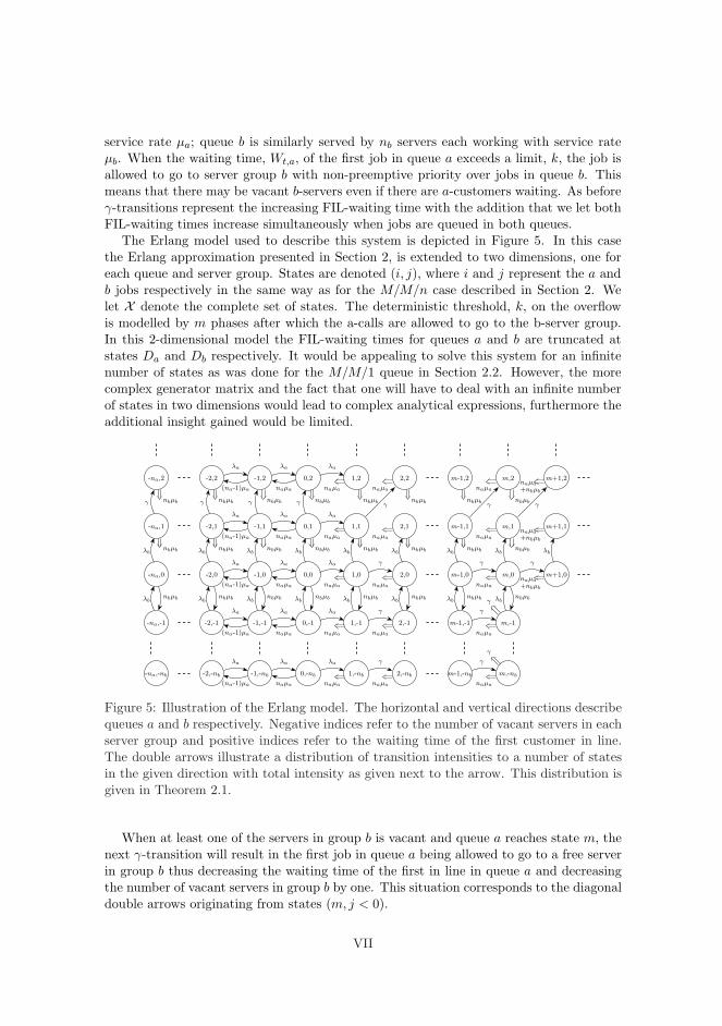
service rate µa; queue b is similarly served by nb servers each working with service rateµb. When the waiting time, Wt,a, of the first job in queue a exceeds a limit, k, the job isallowed to go to server group b with non-preemptive priority over jobs in queue b. Thismeans that there may be vacant b-servers even if there are a-customers waiting. As beforeγ-transitions represent the increasing FIL-waiting time with the addition that we let bothFIL-waiting times increase simultaneously when jobs are queued in both queues.
The Erlang model used to describe this system is depicted in Figure 5. In this casethe Erlang approximation presented in Section 2, is extended to two dimensions, one foreach queue and server group. States are denoted (i, j), where i and j represent the a andb jobs respectively in the same way as for the M/M/n case described in Section 2. Welet X denote the complete set of states. The deterministic threshold, k, on the overflowis modelled by m phases after which the a-calls are allowed to go to the b-server group.In this 2-dimensional model the FIL-waiting times for queues a and b are truncated atstates Da and Db respectively. It would be appealing to solve this system for an infinitenumber of states as was done for the M/M/1 queue in Section 2.2. However, the morecomplex generator matrix and the fact that one will have to deal with an infinite numberof states in two dimensions would lead to complex analytical expressions, furthermore theadditional insight gained would be limited.
naµa
+nbµb
naµa
+nbµb
naµa
+nbµb
naµanaµanaµa(na-1)µa naµa
naµanaµanaµa(na-1)µa naµa
-2,-1 -1,-1 0,-1
-2,0 -1,0 0,0
-2,1 -1,1 0,1
1,-1
1,0
1,1
2,-1
2,0
2,1
-2,2 -1,2 0,2 1,2 2,2
γ
λb
λb
λb
λb λb λb λb
λb λb λb
γ γ
λa λa λa
λa λa λa
λa λa λa γ
λa λa λa γ
(na-1)µa
(na-1)µa
(na-1)µa
naµa
naµa
naµa
naµa
naµa
naµa
naµa
naµa
naµa
nbµbnbµbnbµbnbµbnbµb
nbµb
nbµb
nbµbnbµbnbµbnbµb
nbµbnbµbnbµb nbµbγ
-2,-nb -1,-nb 0,-nb 1,-nb 2,-nb
λa λa λa γ
-na,-1
-na,0
-na,1
-na,2
λb
γ
λbnbµb
nbµb
nbµb
-na,-nb
m,-1
m,0
m,1m-1,1
m-1,0
m-1,-1
m+1,0
m+1,1
m,2m-1,2 m+1,2
λb λb
λb λb
γ
γ
γ
λb
γ
naµa
naµa
naµa
nbµb nbµb
γγnbµb
nbµb
nbµb
nbµb
m-1,-nb m,-nb
γ
γ
Figure 5: Illustration of the Erlang model. The horizontal and vertical directions describequeues a and b respectively. Negative indices refer to the number of vacant servers in eachserver group and positive indices refer to the waiting time of the first customer in line.The double arrows illustrate a distribution of transition intensities to a number of statesin the given direction with total intensity as given next to the arrow. This distribution isgiven in Theorem 2.1.
When at least one of the servers in group b is vacant and queue a reaches state m, thenext γ-transition will result in the first job in queue a being allowed to go to a free serverin group b thus decreasing the waiting time of the first in line in queue a and decreasingthe number of vacant servers in group b by one. This situation corresponds to the diagonaldouble arrows originating from states (m, j < 0).
VII
The use of Erlang distributions for approximating step functions in stochastic modelsoften suffers from the curse of dimensionality. This is to some extent avoided by combiningthe number of free servers and the waiting time of the first in line in one dimension foreach of the job types.
Extra care has to be taken when determining the waiting time distribution for thetwo job types. The transitions leading to service initiations in the N-design model areλa and λb-transitions from states with vacant servers, i.e. i < 0 and j < 0 respectively,γ-transitions from states where i = m and j < 0, and finally µa and µb-transitions fromstates i > 0 and j > 0 respectively.
Besides the obvious differentiation between service initiations for a and b jobs, it isalso necessary to deal with service initiations for a jobs due to γ transitions in a specialway. This is due to γ-transitions representing customers having waited exactly k and nota gamma-distributed amount of time.
The state probabilities just before service initiations are denoted α(i, j)a and α(i, j)b
for a and b-calls respectively. The distribution of α can be found as:
αaµλ(i, j) =
π(i, j)Λaµλ(i, j)∑
(i,j)∈X π(i, j)Λaµλγ(i, j)
, (6)
αaγ(m, j) =
π(m, j)Λaγ(m, j)∑
(i,j)∈X π(i, j)Λaµλγ(i, j)
, j < 0. (7)
Here Λa(i, j) is the sum of the transition intensities from state (i, j) that result in a serviceinitiation for a-calls. The subscripts on Λ are used to differentiate between the differenttransitions that lead to service initiations. For a-calls, Λ is given as:
Λaµλ(i, j) =
λa for i < 00 for i = 0naµa for 0 < i ≤ m
naµa + nbµb for m < i
(8)
Λaγ(i, j) =
{γ for i = m, j < 0;0 else.
(9)
Λaµλγ(i, j) = Λa
µλ(i, j) + Λaγ(i, j) (10)
For the b-calls the expressions are somewhat simpler:
Λbµλ(i, j) =
λb for j < 0, i ≤ m;nbµb for 0 < j, i ≤ m
0 else.
(11)
Using the same approach as in Section 2, the waiting time distribution for type a jobs
VIII
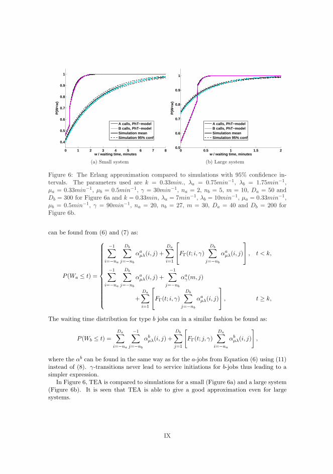
0 1 2 3 4 5 6 7 8
0.4
0.5
0.6
0.7
0.8
0.9
1
w / waiting time, minutes
P(W
<w)
A calls, PhT−modelB calls, PhT−modelSimulation meanSimulation 95% conf
(a) Small system
0 0.5 1 1.5 20.5
0.6
0.7
0.8
0.9
1
w / waiting time, minutes
P(W
<w)
A calls, PhT−modelB calls, PhT−modelSimulation meanSimulation 95% conf
(b) Large system
Figure 6: The Erlang approximation compared to simulations with 95% confidence in-tervals. The parameters used are k = 0.33min., λa = 0.75min−1, λb = 1.75min−1,µa = 0.33min−1, µb = 0.5min−1, γ = 30min−1, na = 2, nb = 5, m = 10, Da = 50 andDb = 300 for Figure 6a and k = 0.33min, λa = 7min−1, λb = 10min−1, µa = 0.33min−1,µb = 0.5min−1, γ = 90min−1, na = 20, nb = 27, m = 30, Da = 40 and Db = 200 forFigure 6b.
can be found from (6) and (7) as:
P (Wa ≤ t) =
−1∑
i=−na
Db∑
j=−nb
αaµλ(i, j) +
Da∑
i=1
FΓ(t; i, γ)
Db∑
j=−nb
αaµλ(i, j)
, t < k,
−1∑
i=−na
Db∑
j=−nb
αaµλ(i, j) +
−1∑
j=−nb
αaγ(m, j)
+Da∑
i=1
FΓ(t; i, γ)
Db∑
j=−nb
αaµλ(i, j)
, t ≥ k,
The waiting time distribution for type b jobs can in a similar fashion be found as:
P (Wb ≤ t) =Da∑
i=−na
−1∑
j=−nb
αbµλ(i, j) +
Db∑
j=1
[FΓ(t; j, γ)
Da∑
i=−na
αbµλ(i, j)
],
where the αb can be found in the same way as for the a-jobs from Equation (6) using (11)instead of (8). γ-transitions never lead to service initiations for b-jobs thus leading to asimpler expression.
In Figure 6, TEA is compared to simulations for a small (Figure 6a) and a large system(Figure 6b). It is seen that TEA is able to give a good approximation even for largesystems.
IX
4 Further possibilities of TEA
The possibilities of TEA are not limited to the N-design presented in Section 3. In thissection we show how a system with dynamic prioritization can be modelled using TEAand discuss how discretionary prioritization and the inclusion of abandonments in modelscould be approached. A setup with overflow to a back office, such as the one dealt within [1], could also be analyzed with TEA.
4.1 Dynamic prioritization
In this section we show how TEA, introduced in Section 2, can be used for a system withdynamic priority. In this case the next customer to be served when a server becomesavailable at time t, is selected from two queues, a and b, by max{Wt,a − ka,Wt,b − kb},where the k’s are constants and the Wt’s FIL-waiting times as previously. Arrivals areassumed to occur according to a Poisson process with rates λa and λb to the two queues.Jobs from both queues are served by a joint group of n servers that each handle the jobswith exponential service time with mean 1/µ. If one queue is empty, jobs from the otherwill always be taken into service immediately if a server is vacant. The system is illustratedin Figure 1b.
As is shown in [4], the average waiting time of the low priority customers in a staticpriority system with two classes grows quickly when the relative frequency of high-prioritycustomers increases. This prioritization scheme is thus desirable when exceedingly longwaiting times should be avoided for all classes while still giving some priority to certaincustomers.
The exact formulation of the additive prioritization scheme may vary as only the dif-ference of the constants matters, adding ka and kb to Wt,b and Wt,a respectively wouldbe equivalent. Here it is formulated by subtraction of a constant for each queue whichespecially for systems with more than two queues make things more clear as it can beinterpreted as a target waiting time for each queue.
This prioritization scheme was first introduced in [9] and is referred to as dynamicpriority or sequencing according to due-date in the literature. In [10], Jackson’s conjectureis given, stating that the tails of the waiting time distributions for the different priorityclasses are exponential with the same shape. Indeed the shape of the tails are the sameas for an FCFS system, only shifted ka − kb from each other. The conjecture doesn’t sayanything about the remaining, lower part of the distribution, which is where TEA cangive a good approximation.
The state space of TEA for the V-design system with dynamic priority becomes two-dimensional as the FIL-waiting times of both queues need to be taken into account. Statesi < 0 keep track of the number of vacant servers in the same way as for the M/M/n systemtreated in Section 2. Whenever a server finishes a job and i > 0, the next customer takeninto service must be chosen from max{Wt,a − ka, Wt,b − kb}. This is implemented in themodel by dividing the state space into two parts representing either option as illustratedin Figure 7 with the thick dotted line.
In Figure 8, a plot of the waiting time distribution for a dynamic priority two class sys-tem is shown as found by TEA. Customers are always taken immediately into service whena server is vacant, thus the distributions start at the same value in 0. Figure 8 illustratesJackson’s conjecture [10] as it plots the waiting time distributions on a logarithmic scale
X

-n
0,2
-2λa + λb
(n-1)µ-1
nµ
λa + λb
0,0λa
nµ1,0
nµ
γ
2,0
λb λbnµ λb
nµnµ0,1
λa
1,1 2,1
γ
nµnµ
γnµ
λa
γnµ nµ
γ
2,21,2
nµ1,3
λa
0,3 2,3
nµ
2,4
γnµnµ
0,4 1,4λa
γ
Figure 7: Transition rate diagram for modelling dynamic prioritization using TEA. Thedotted line divides the state space into sections determining from which queue the nextcustomer will be taken.
thus producing straight lines for the exponential tails. Simulation results with confidenceintervals are shown for validation.
A possible extension to the dynamic priority model would be to keep servers free tocater for potential a-customers even though b-customers may be in line. This could betreated as an optimization problem and approached using Markov Decision Processes. Itwould be somewhat analogous to the slow-server problem [12], [13] and [15].
4.2 Discretionary priority
The discretionary priority discipline is a mix of the preemptive and non-preemptive dis-ciplines, [11]. The idea is that high priority customers are only allowed to preempt lowerpriority customers under certain circumstances, e.g. that a low priority customer has juststarted service. In this case TEA could be used in an inverted way by modelling theelapsed service time of the last low priority customer who entered service and thus onlyallowing high priority customers to preempt when this value is under a given threshold.
4.3 Abandonments
The inclusion of abandonments is often considered essential when dealing with call centers[18]. It should be possible to extend the model to take abandonments into account byintroducing transitions representing abandonments of the FIL customer. Also a negativebinomial distribution should be used in Theorem 2.1 instead of the geometric distribu-tion in order to account for the possibility of customers further back in the line havingabandoned the system.
Including abandonments ought to improve the Erlang approximation as it will decreasethe risk of the truncation having a significant negative influence.
XI

0 0.5 1 1.5 2 2.5 3 3.5 40.5
0.6
0.7
0.8
0.9
1
w / waiting time, minutes
P(W
<w)
A calls, PhT−modelB calls, PhT−modelSimulation meanSimulation 95% conf
(a) Waiting time distribution.
0 0.5 1 1.5 2 2.5 3 3.5 4
0.20.4
0.6
0.8
0.9
0.95
0.98
0.99
0.995
w / waiting time, minutes
P(W
<w)
A calls, PhT−modelB calls, PhT−modelSimulation meanSimulation 95% conf
(b) Waiting time distribution, logarithmic plot.
Figure 8: The Erlang approximation compared to simulations for a system with dynamicpriority. The parameters used are ka = 0.25, kb = 1.25, λa = 3.5, λb = 2.5, µ = 1, n = 8,Da = 90, Db = 150, and γ = 60.
5 Conclusion
We introduced a new approach to modelling queueing systems by using the waiting time ofthe customer first in line. This has proved useful when dealing with systems where routingor priority of customers depends on this waiting time as seen in many real scenarios suchas call centers.
The Erlang approximation (TEA) was introduced in Section 2 and we showed thatthe resulting waiting time distribution indeed converges to the theoretical value when thestate space increases in size.
In Section 3 we implemented TEA for a N-design routing scheme with deterministicthreshold on the overflow between server groups, a design often used in call centers. Weshowed that it is possible to get a good approximation of the waiting time distribution andthat TEA can thus be an alternative approach to examining complicated systems wheresimulation studies have otherwise been seen as the only viable approach.
Further possibilities of TEA were discussed in Section 4 including how abandonmentscould be taken into account. We also showed how TEA can be used to model a systemwith dynamic priority, thus showing the flexibility of TEA.
References
[1] Wolfgang Barth, Michael Manitz, and Raik Stolletz. Analysis of Two-Level SupportSystems with Time-Dependent Overflow - A Banking Application. Forthcoming inProduction and Operations Management, 2009.
[2] Rene Bekker, Ger Koole, Bo Friis Nielsen, and Thomas Bang Nielsen. Queues withwaiting time dependent service. Submitted for publication, June 2009.
XII

[3] Margaret L. Brandeau, Franois Sainfort, and William P. Pierskalla. Operations Re-search and Health Care: A Handbook of Methods and Applications. Springer, illus-trated edition, 2004.
[4] Alan Cobham. Priority assignment in waiting line problems. Journal of the OperationsResearch Society of America, 2(1):70–76, 1954.
[5] Richard W. Conway, William .L. Maxwell, and Louis W. Miller. Theory of Scheduling.Addison-Wesley Publishing Company, 1967.
[6] Noah Gans, Ger Koole, and Avishai Mandelbaum. Telephone call centers: Tutorial,review, and research prospects. Manufacturing and Service Operations Management,5(2):79–141, 2003.
[7] Geoffrey Grimmett and David Stirzaker. Probability and Random Processes. OxfordUniversity Press, third edition, 2001.
[8] Villy Bæk Iversen. Teletraffic Engineering and Network Planning. COM Center,Technical University of Denmark, 2006.
[9] James R. Jackson. Some problems in queueing with dynamic priorities. Nav. Res.Logistics Quart., 7:235–249, 1960.
[10] James R. Jackson. Queues with dynamic priority discipline. Management Science,8(1):18–34 and 2627272, 1961.
[11] N.K. Jaiswal. Priority Queues. Academic Press, New York and Londons, 1968.
[12] G.M. Koole. A simple proof of the optimality of a threshold policy in a two-serverqueueing system. Systems & Control Letters, 26:301–303, 1995.
[13] W. Lin and P.R. Kumar. Optimal control of a queueing system with two heteroge-neous servers. IEEE Trans. Automat. Control, 29:696–703, 1984.
[14] M.J.M Posner. Single-server queues with service time dependent on waiting time.Operations Research, 21:610–616, 1973.
[15] M. Rubinovitch. The slow server problem. Journal of Applied Probability, 22:205–213., 1985.
[16] Robert A. Shumsky. Approximation and analysis of a call center with flexible andspecialized servers. OR Spectrum, 26(3):307–330, 2004.
[17] D.A. Stanford and W.K. Grassmann. The bilingual server system: a queueing modelfeaturing fully and partially qualified servers. INFOR, 31(4):261–277, 1993.
[18] W. Whitt. Engineering solution of a basic call-center model. Management Science,51(2):221–235, 2005.
XIII


Addendum
B.1 Addendum
Verification of TEA
In this addendum to the paper Waiting time dependent multi-server priorityqueues, The Erlang Approximation is verified by using it with an infinite statespace and finding the waiting time distribution of the M/M/1-queue. Thetransition rate diagram for this approximation is shown in Figure B.1
pµ 31
pµ 10 pµ 21 pµ 32
pµ 20 pµ 30
210−1γλ λ γ
3µ
Figure B.1: Transition diagram of TEA applied to the M/M/1-queue.
The generator matrix for TEA applied to the M/M/1-queue is given by:
G =
266666664
−λ λ 0 0 0 0 0µ −(λ + µ) λ 0 0 0 00 µp10 − (γ + µp10) γ 0 0 00 µp20 µp21 −
`γ + µ
P1i=0 p2i
´γ 0 0
0 µp30 µp31 µp32 −`γ + µ
P2i=0 p3i
´γ 0
.
.
....
. . .. . .
. . .. . .
. . .
377777775(B.1)
The steady state probabilities can be found from solving the equation array0 = πG, where π is a row vector containing the steady state probabilities. Theindividual equations of this array can be written out as
0 = −λπ−1 + µπ0
0 = λπ−1 − (λ + µ)π0 +∞∑
j=1
p0jµπj
0 = λπ0 − (γ + µp01)π1 +∞∑
j=2
p1jµπj
0 = γπi−1 −
γ + µi−1∑j=0
pij
πi +∞∑
j=i+1
pijµπj , for i ≥ 2,
115
B. Waiting time dependent multi-server priority queues
where
pji = P (It+ = i|It− = j) =
1−
j−1∑h=0
(λ
λ + γ
)(γ
λ + γ
)h
, for i = 0;(λ
λ + γ
)(γ
λ + γ
)j−i
, for i ∈ {1, .., j},
(B.2)are the probabilities describing the distribution of the transitions, whenever acustomer goes into service.
Now, inserting (B.2) in each of the above equations yields the followingequations:
0 = −λπ−1 + µπ0 (B.3)
0 = λπ−1 − (λ + µ)π0 + µ
∞∑j=1
(1− λ
λ + γ
j−1∑h=0
(γ
λ + γ
)h)
πj (B.4)
0 = λπ0 −(
γ + µ
(1− λ
λ + γ
))π1 + µ
(λ
λ + γ
) ∞∑j=2
(γ
λ + γ
)j−1
πj (B.5)
0 = γπi−1 −(
γ + µ
(1− λ
λ + γ
))πi
+ µ
(λ
λ + γ
) ∞∑j=i+1
(γ
λ + γ
)j−i
πj , for i ≥ 2 (B.6)
The structure of G, as seen in Equation (B.1), bears a strong resemblanceto the generator matrix of an M/G/1-system [30]. This resemblance motivatesguessing a solution of the form: πi = θβi(1 − β), for i ≥ 2, i.e. a geometricdistribution, where θ is a normalizing constant. Inserting this guess in Equa-tion (B.6) enables us to find an expression for β:
116

Addendum
0 = γθ(1− β)βi−1 −(
γ + µ
(1− λ
λ + γ
))θ(1− β)βi
+ µ
(λ
λ + γ
) ∞∑j=i+1
(γ
λ + γ
)j−i
θ(1− β)βj
0 = γβi−1 −(
γ +µγ
λ + γ
)βi +
µλ
λ + γ
∞∑j=i+1
(γ
λ + γ
)j−i
βj
0 = γ −(
γ +µγ
λ + γ
)β +
µλγ
(λ + γ)2β2 1
1− βγλ+γ
0 = γ − γ2
λ + γβ +
(−γ − µγ
λ + γ+
βγ2
λ + γ+
µβγ2
(λ + γ)2
)β +
µλγ
(λ + γ)2β2
0 = γ −(
γ +µγ + γ2
λ + γ
)β +
µλγ + γ2(λ + µ + γ)(λ + γ)2
β2
0 = γ(λ + γ)2 −(γ(λ + γ)2 + (λ + γ)(µγ + γ2)
)β + (λ + γ)(µγ + γ2)β2
0 = λ + γ − (λ + µ + 2γ)β + (µ + γ)β2,
thus
β = 1 ∧ β =λ + γ
µ + γ. (B.7)
Now we consider Equation (B.5) and insert the guess πi = θ(1 − β)βi, fori ≥ 2:
0 = λπ0 −„
γ +µγ
λ + γ
«π1 + µ
„λ
λ + γ
« ∞Xj=2
„γ
λ + γ
«j−1
θ(1− β)βj
0 = λπ0 −„
γ +µγ
λ + γ
«π1 + (1− β)
λµγθβ2
(λ + γ)21
1− γβλ+γ
0 =
„λ− λγβ
λ + γ
«π0 −
„γ +
µγ
λ + γ− γ2β
λ + γ− µγ2β
(λ + γ)2
«π1 + (1− β)
λµγθβ2
(λ + γ)2
0 =`λ(λ + γ)2 − λγβ(λ + γ)
´π0
−`γ(λ + γ)2 + µγ(λ + γ)− γ2β(λ + γ)− µγ2β
´π1 + (1− β)λµγθβ2
0 = λ(λ + γ) (λ + γ − γβ) π0 − γ(λ + µ + γ)(λ + γ − γβ)π1 + λµγθ(β2 − β3).(B.8)
117

B. Waiting time dependent multi-server priority queues
Inserting the non-trivial value of β from Equation (B.7) in Equation (B.8)yields
0 = λ(λ + γ)(
λ + γ − γλ + γ
µ + γ
)π0 − γ(λ + µ + γ)
(λ + γ − γ
λ + γ
µ + γ
)π1
+ λµγθ
((λ + γ
µ + γ
)2
−(
λ + γ
µ + γ
)3)
0 = λ(λ + γ)(
µ
µ + γ
)π0 − γ(λ + µ + γ)
(µ
µ + γ
)π1
+ λµγθ
(λ + γ
(µ + γ)2− (λ + γ)2
(µ + γ)3
)0 = λ(λ + γ)π0 − γ(λ + µ + γ)π1 + λγ
(λ + γ
µ + γ− (λ + γ)2
(µ + γ)2
)θ
0 =1γ
π0 −λ + µ + γ
λ(λ + γ)π1 +
µ− λ
(µ + γ)2θ (B.9)
By manipulating Equation (B.4) we get:
0 = λπ−1 − (λ + µ)π0 + µ
∞Xj=1
1− λ
λ + γ
j−1Xh=0
„γ
λ + γ
«h!
πj
0 = λπ−1 − (λ + µ)π0 + µ
∞Xj=1
0B@1− λ
λ + γ
1−“
γλ+γ
”j
1−“
γλ+γ
”1CAπj
0 = λπ−1 − (λ + µ)π0 + µ
∞Xj=1
„γ
λ + γ
«j
πj ,
and inserting the guess for πi yields
0 = λπ−1 − (λ + µ)π0 +µγ
λ + γπ1 + µ
∞Xj=2
„γ
λ + γ
«j
θ(1− β)βj
0 = λπ−1 − (λ + µ)π0 +µγ
λ + γπ1 + µθ(1− β)
∞X
j=0
„γβ
λ + γ
«j
− 1− γβ
λ + γ
!
0 = λπ−1 − (λ + µ)π0 +µγ
λ + γπ1 + µ(1− β)
1
1− γβλ+γ
− 1− γβ
λ + γ
!θ.
118
Addendum
The expression for β is inserted:
0 = λπ−1 − (λ + µ)π0 +µγ
λ + γπ1 + µ
„1− λ + γ
µ + γ
«0B@ 1
1−γ λ+γ
µ+γ
λ+γ
− 1−γ λ+γ
µ+γ
λ + γ
1CA θ
0 = λπ−1 − (λ + µ)π0 +µγ
λ + γπ1 + µ
„µ− λ
µ + γ
«„µ + γ
µ− µ
µ + γ
«θ
0 = λπ−1 − (λ + µ)π0 +µγ
λ + γπ1 +
γ(2µ + γ)(µ− λ)
(µ + γ)2θ (B.10)
We now consider Equations (B.3), (B.9), and (B.10) again:
0 = −λπ−1 + µπ0
0 =1γ
π0 −λ + µ + γ
λ(λ + γ)π1 +
µ− λ
(µ + γ)2θ
0 = λπ−1 − (λ + µ)π0 +µγ
λ + γπ1 +
γ(2µ + γ)(µ− λ)(µ + γ)2
θ
From Equation (B.3), we express π−1 by π0:
π−1 =µ
λπ0, (B.11)
By inserting the expression of Equation (B.11) in Equation (B.10), we get:
0 = λπ−1 − (λ + µ)π0 +µγ
λ + γπ1 +
γ(2µ + γ)(µ− λ)(µ + γ)2
θ
0 = λµ
λπ0 − (λ + µ)π0 +
µγ
λ + γπ1 +
γ(2µ + γ)(µ− λ)(µ + γ)2
θ
0 = λπ0 +µγ
λ + γπ1 +
γ(2µ + γ)(µ− λ)(µ + γ)2
θ (B.12)
Equation (B.9) is re-written as:
0 =1γ
π0 −λ + µ + γ
λ(λ + γ)π1 +
µ− λ
(µ + γ)2θ
π0 =(λ + µ + γ)γ
λ(λ + γ)π1 −
(µ− λ)γ(µ + γ)2
θ (B.13)
119

B. Waiting time dependent multi-server priority queues
Now, Equation (B.13) inserted in Equation (B.12) gives us an expression forπ1 by θ:
0 = λπ0 +µγ
λ + γπ1 +
γ(2µ + γ)(µ− λ)(µ + γ)2
θ
0 = λ
((λ + µ + γ)γ
λ(λ + γ)π1 −
(µ− λ)γ(µ + γ)2
θ
)+
µγ
λ + γπ1 +
γ(2µ + γ)(µ− λ)(µ + γ)2
θ
0 =(λ + 2µ + γ)γ
λ + γπ1 −
γ(λ + 2µ + γ)(µ− λ)(µ + γ)2
θ
0 =1
λ + γπ1 −
µ− λ
(µ + γ)2θ
π1 =(µ− λ)(λ + γ)
(µ + γ)2θ (B.14)
To obtain π0 given by θ; Equation (B.14) is inserted in Equation (B.13):
π0 =(λ + µ + γ)γ
λ(λ + γ)π1 −
(µ− λ)γ(µ + γ)2
θ
π0 =(
(λ + µ + γ)γλ(λ + γ)
)((µ− λ)(λ + γ)
(µ + γ)2θ
)− (µ− λ)γ
(µ + γ)2θ
π0 =(µ + γ)γ(µ− λ)
λ(µ + γ)2θ
π0 =γ(µ− λ)λ(µ + γ)
θ (B.15)
Next, π−1 is found by inserting Equation (B.15) in Equation (B.11):
π−1 =µ
λπ0
π−1 =µγ(µ− λ)λ2(µ + γ)
θ (B.16)
As the total probability mass of the states in equilibrium must sum to one, we
120
Addendum
get:
1 =∞X
i=−1
πi
1 =
"µγ(µ− λ)
λ2(µ + γ)+
γ(µ− λ)
λ(µ + γ)+
(µ− λ)(λ + γ)
(µ + γ)2+
∞Xi=2
„1−
λ + γ
µ + γ
«„λ + γ
µ + γ
«i#
θ
1 =
"µγ(µ− λ)
λ2(µ + γ)+
γ(µ− λ)
λ(µ + γ)+
(µ− λ)(λ + γ)
(µ + γ)2+
λ− µ
µ + γ
1 +
λ + γ
µ + γ−
1
1− λ+γµ+γ
!#θ
1 =
"µγ(µ− λ)
λ2(µ + γ)+
γ(µ− λ)
λ(µ + γ)+
(µ− λ)(λ + γ)
(µ + γ)2+
(λ + γ)2
(µ + γ)2
#θ
1 =µγ(µ− λ)(µ + γ) + γ(µ− λ)λ(µ + γ) + λ2(µ− λ)(λ + γ) + λ2(λ + γ)2
λ2(µ + γ)2θ
1 =(λ + µ)γ(µ− λ)(µ + γ) + λ2(λ + γ)(µ + γ)
λ2(µ + γ)2θ
1 =λ3 + µ2γ
λ2(µ + γ)θ
θ =λ2(µ + γ)
λ3 + µ2γ(B.17)
We can now find the explicit expressions for the steady state probabilities;first π−1:
π−1 =µγ(µ− λ)λ2(µ + γ)
θ
π−1 =(
µγ(µ− λ)λ2(µ + γ)
)(λ2(µ + γ)λ3 + µ2γ
)π−1 =
µγ(µ− λ)λ3 + µ2γ
, (B.18)
then π0:
π0 =γ(µ− λ)λ(µ + γ)
θ
π0 =(
γ(µ− λ)λ(µ + γ)
)(λ2(µ + γ)λ3 + µ2γ
)π0 =
λγ(µ− λ)λ3 + µ2γ
, (B.19)
121

B. Waiting time dependent multi-server priority queues
and π1:
π1 =(µ− λ)(λ + γ)
(µ + γ)2θ
π1 =(µ− λ)(λ + γ)
(µ + γ)2
(λ2(µ + γ)λ3 + µ2γ
)π1 =
λ2(µ− λ)(λ + γ)(µ + γ)(λ3 + µ2γ)
. (B.20)
Finally πi, for i ≥ 2:
πi = θ(1− β)βi, for i ≥ 2
πi =λ2(µ + γ)λ3 + µ2γ
(1− λ + γ
µ + γ
)(λ + γ
µ + γ
)i
, for i ≥ 2
πi =λ2(µ + γ)λ3 + µ2γ
(µ− λ
µ + γ
)(λ + γ
µ + γ
)i
, for i ≥ 2
πi =λ2(µ− λ)λ3 + µ2γ
(λ + γ
µ + γ
)i
, for i ≥ 2
We see that the expression for i ≥ 2 is also valid for i = 1. To sum up, thesteady state probabilities become:
πi =
µγ(µ− λ)λ3 + µ2γ
, for i = −1
λγ(µ− λ)λ3 + µ2γ
, for i = 0
λ2(µ− λ)λ3 + µ2γ
(λ + γ
µ + γ
)i
, for i ≥ 1
With the state probabilities settled, we can now determine the waiting-timedistribution. First we find the probabilities of having a service initiation froma state, i, given as αi:
αi =πiΛi∑∞
j=−1 πjΛj, (B.21)
122

Addendum
where
Λi =
λ for i < 0;0 for i = 0;µ for i ≥ 1,
is the transition intensity from each state that leads to a service initiation. Thedenominator in Equation (B.21) is common for all i, thus we start out withconsidering this:
∞∑j=−1
πjΛj = π−1λ +∞∑
j=1
πjµ
=µγ(µ− λ)λ3 + µ2γ
λ +∞∑
j=1
λ2(µ− λ)λ3 + µ2γ
(λ + γ
µ + γ
)i
µ
=λµγ(µ− λ)λ3 + µ2γ
+λ2µ(µ− λ)λ3 + µ2γ
λ + γ
µ + γ
µ + γ
µ− λ
=λµγ(µ− λ)λ3 + µ2γ
+λ2µ(λ + γ)λ3 + µ2γ
=λ3µ + λµ2γ
λ3 + µ2γ
From this, α−1 is determined to:
α−1 =πiΛi∑∞
j=−1 πjΛj,
=µγ(µ− λ)λ3 + µ2γ
λλ3 + µ2γ
λ3µ + λµ2γ
=λµγ(µ− λ)λ3µ + λµ2γ
=γ(µ− λ)λ2 + µγ
123
B. Waiting time dependent multi-server priority queues
Obviously α0 = 0 as Λ0 = 0. The αi’s, for i ≥ 1, are found as:
αi =πiΛi∑∞
j=−1 πjΛj,
=λ2(µ− λ)λ3 + µ2γ
(λ + γ
µ + γ
)i
µλ3 + µ2γ
λ3µ + λµ2γ
=λ2µ(µ− λ)λ3µ + λµ2γ
(λ + γ
µ + γ
)i
=λ(µ− λ)λ2 + µγ
(λ + γ
µ + γ
)i
Now, we have all the elements needed to find the waiting-time distribution.It is given as:
P (W ≤ t) = α−1 +∞∑
i=1
FΓ(t; , i, γ)αi,
where FΓ(t; i, γ) = 1−∑i−1
h=0(γt)h
h! e−γt is the cdf of an Erlang-distribution with
124

Addendum
shape parameter i ∈ N and scale parameter γ ∈ R+. Inserting the α’s yield:
P (W ≤ t) = α−1 +
∞Xi=1
FΓ(t; , i, γ)αi
=γ(µ− λ)
λ2 + µγ+
∞Xi=1
1−
i−1Xh=0
(γt)h
h!e−γt
!λ(µ− λ)
λ2 + µγ
„λ + γ
µ + γ
«i
=(µ− λ)
λ2 + µγ
"γ + λ
∞Xi=1
„λ + γ
µ + γ
«i
− λe−γt∞X
i=1
„λ + γ
µ + γ
«i i−1Xh=0
(γt)h
h!
#
=(µ− λ)
λ2 + µγ
"γ + λ
λ + γ
µ + γ
„µ + γ
µ− λ
«− λe−γt
∞Xi=1
„λ + γ
µ + γ
«i i−1Xh=0
(γt)h
h!
#
= 1− λ(µ− λ)
λ2 + µγe−γt
∞Xi=1
„λ + γ
µ + γ
«i i−1Xh=0
(γt)h
h!
= 1− λ(µ− λ)
λ2 + µγe−γt
∞Xh=0
(γt)h
h!
∞Xi=h+1
„λ + γ
µ + γ
«i
= 1− λ(µ− λ)
λ2 + µγe−γt
∞Xh=0
(γt)h
h!
„λ + γ
µ + γ
«h+1 ∞Xi=0
„λ + γ
µ + γ
«i
= 1− λ(µ− λ)
λ2 + µγe−γt
∞Xh=0
(γt)h
h!
„λ + γ
µ + γ
«h+1„µ + γ
µ− λ
«= 1− λ(λ + γ)
λ2 + µγe−γte
γt(λ+γ)µ+γ
= 1− λ2/γ
λ2/γ + µ− λ
λ2/γ + µe
γµ+γ
(λ−µ)t
which converges to P (W ≤ t) = 1 − λµe(λ−µ)t for γ → ∞. The Erlang
Approximation is verified by this result.
125


APPENDIX COptimization of overflow
policies in call centers
127


Optimization of overflow policies in call centers
G.M. Koole†, B.F. Nielsen?, T.B. Nielsen?
†Dept. MathematicsVU University Amsterdam
De Boelelaan 1081, 1081 HV, the Netherlands.
?Dept. Informatics and Mathematical ModellingTechnical University of Denmark
Richard Petersens Plads, 2800 Kgs. Lyngby, Denmark.
May 2, 2010
Abstract
We examine how overflow policies in a multi skill call center should be designedto accommodate different performance measures such Average Speed of Answer andTelephone Service Factor. This is done using a discrete Markovian approximation tothe waiting time of the first customers waiting in line. We show that the widely usedpolicy, of having a fixed threshold on the waiting time of the first customer in linedetermine when overflow is allowed, is far from optimal in many cases. Furthermorewe discuss in which cases this approach is indeed appropriate. The work is motivatedby call center applications but may be applicable to other fields such as health caremanagement and communication networks.
Keywords: Waiting time distribution; call center; priority queues; Markov DecisionProcesses; optimization; Dynamic Programming.
1 Introduction
In call centers a commonly used practice is to allow overflow of calls between differentagent pools. The purpose of this can be to reduce the risk of having calls waiting anexcessive amount of time in one queue while servers assigned to another queue may bevacant. There can obviously be restrictions on the overflow between groups, e.g., due toone group of agents not having the competence to answer all types of calls or simply basedon a wish of giving higher priority to one customer class.
The call routing structure of real call centers can often be very complicated with mul-tiple customer classes and agent/server groups. In order to analyze these setups an oftenused practice is to look at different canonical structures, such as the “V”, “N”, “X”, and“W” designs [4]. The system analyzed here is the one referred to as an N-design. Figure 1shows an illustration of this system. Two customer classes, a and b, are each served bytheir own server group. Furthermore a-calls can be routed to b-servers according to deci-sions based on the number of free servers and/or the waiting times of the first customersin line in the two queues. b-calls can never go to a-servers. Also, a-calls cannot preemptb-calls already being served. It should be noted that a-calls are not necessarily of higher
I

priority than b-calls, the fundamental difference lies only in the routing scheme. For ex-ample, if a-calls are of high priority, the overflow to b-servers could be used to reduce therisk of having important customers wait too long in the queue. In the case where b-callsare of higher priority, the overflow from the a-queue could allow any excess capacity in theb-server group to be utilized. The prioritization of calls will be based on cost functionsdiscussed later.
µa µa µa µb µb µb
bλaλ
1 2 1 2n a n b
Figure 1: The N-design. a-customers can be sent to b-servers according to decisions basedon the number of free servers and/or the waiting times of the first customers in line in thetwo queues.
An often used policy is to allow overflow after the waiting time of the first customer inline has reached a given fixed threshold, thus not taking into account if servers are vacantin the server group the overflow is directed to. This policy is examined in [3], [9] and [2].The idea behind keeping b-servers vacant even though a-customers are waiting, is to haveb-servers ready to answer incoming b-calls. However, the approach of letting the thresholdwhere overflow is allowed to be independent of the number of free servers, is intuitivelyunattractive as it might very well be better to allow overflow earlier if many b-serversare vacant and later if few b-servers are vacant. In this paper we examine how overflowpolicies can be designed to accommodate different performance measures in the best wayand thus avoid a waste of resources.
Different implementations of routing and call selection based on the waiting time ofcustomers have been examined in the literature, especially for the V-design where twocustomer classes share a server group. One simple approach is to assign an ageing factorthat grows proportionally with a customer’s waiting time and choose the customer withthe highest proportional waiting time. This approach was introduced in [8] and later alsoexamined in [10]. A similar approach is to add a constant to the waiting time for eachcustomer class and thus prioritize calls based on the values of the constant. This is oftenreferred to as scheduling according to due dates or dynamic prioritization and was firstexamined in [6] and [7].
In [5], call selection is optimized and average costs are given for a single server and twocustomer classes with switching costs and preemptive-resume service discipline using one-step optimization. Non-preemptive systems with multiple customer classes are normallyhard to analyze using Markov Decision Processes as knowledge of the customers currentlybeing served is required. This requirement is relaxed here by modelling the waiting timesof the first customers in line. As a result, the optimal policies will depend on the waitingtime of the longest waiting call. This makes sense both from a theoretical and a practical
II
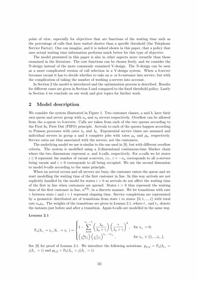
point of view, especially for objectives that are functions of the waiting time such asthe percentage of calls that have waited shorter than a specific threshold (the TelephoneService Factor). One can imagine, and it is indeed shown in this paper, that a policy thatuses actual waiting time information performs much better for this type of objective.
The model presented in this paper is also in other aspects more versatile than thoseexamined in the literature. The cost functions can be chosen freely, and we consider theN-design instead of the more commonly examined V-design. The N-design can be seenas a more complicated version of call selection in a V-design system. When a b-serverbecomes vacant it has to decide whether to take an a- or b-customer into service, but withthe complication of taking the number of working a-servers into account.
In Section 2 the model is introduced and the optimization process is described. Resultsfor different cases are given in Section 3 and compared to the fixed threshold policy. Lastlyin Section 4 we conclude on our work and give topics for further work.
2 Model description
We consider the system illustrated in Figure 1. Two customer classes, a and b, have theirown queue and server group with na and nb servers respectively. Overflow can be allowedfrom the a-queue to b-servers. Calls are taken from each of the two queues according tothe First In, First Out (FIFO) principle. Arrivals to each of the queues happen accordingto Poisson processes with rates λa and λb. Exponential service times are assumed andindividual servers in group a and b complete jobs with rates µa and µb, respectively.Service rates are thus associated with the servers, not the customers.
The underlying model we use is similar to the one used in [9], but with different overflowcriteria. The system is modelled using a 2-dimensional continuous-time Markov chainwhere the two dimensions represent a- and b-calls, respectively. For a-calls we let statesi ≤ 0 represent the number of vacant a-servers, i.e., i = −na corresponds to all a-serversbeing vacant and i = 0 corresponds to all being occupied. We use the second dimensionto model b-calls according to the same principle.
When an arrival occurs and all servers are busy, the customer enters the queue and westart modelling the waiting time of the first customer in line. In this way arrivals are notexplicitly handled by the model for states i > 0 as arrivals do not affect the waiting timeof the first in line when customers are queued. States i > 0 thus represent the waitingtime of the first customer in line, wFIL, in a discrete manner. We let transitions with rateγ between state i and i + 1 represent elapsing time. Service completions are representedby a geometric distributed set of transitions from state i to states {0, 1, ..., i} with totalrate naµa. The weights of the transitions are given in Lemma 2.1, where t− and t+ denotethe instants just before and after a transition. Again b-calls are modelled in the same way.
Lemma 2.1
Pa(It+ = it+ |It− = it−) =
1−it−−1∑
h=0
(λa
λa + γ
)(γ
λa + γ
)h
, for it+ = 0;
(λa
λa+γ
)(γ
λa+γ
)it−−it+, for it+ ∈ {1, .., it−}.
See [9] for proof of Lemma 2.1. We introduce the following notations: pa,ij = Pa(It+ =j|It− = i) and pb,ij = Pb(Jt+ = j|Jt− = i).
III
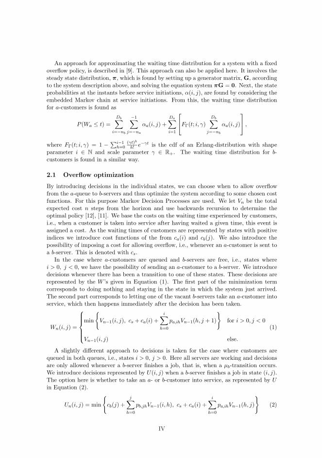
An approach for approximating the waiting time distribution for a system with a fixedoverflow policy, is described in [9]. This approach can also be applied here. It involves thesteady state distribution, π, which is found by setting up a generator matrix, G, accordingto the system description above, and solving the equation system πG = 0. Next, the stateprobabilities at the instants before service initiations, α(i, j), are found by considering theembedded Markov chain at service initiations. From this, the waiting time distributionfor a-customers is found as
P (Wa ≤ t) =Db∑
i=−nb
−1∑
j=−na
αa(i, j) +Da∑
i=1
FΓ(t; i, γ)
Db∑
j=−nb
αa(i, j)
,
where FΓ(t; i, γ) = 1 − ∑i−1h=0
(γt)h
h! e−γt is the cdf of an Erlang-distribution with shapeparameter i ∈ N and scale parameter γ ∈ R+. The waiting time distribution for b-customers is found in a similar way.
2.1 Overflow optimization
By introducing decisions in the individual states, we can choose when to allow overflowfrom the a-queue to b-servers and thus optimize the system according to some chosen costfunctions. For this purpose Markov Decision Processes are used. We let Vn be the totalexpected cost n steps from the horizon and use backwards recursion to determine theoptimal policy [12], [11]. We base the costs on the waiting time experienced by customers,i.e., when a customer is taken into service after having waited a given time, this event isassigned a cost. As the waiting times of customers are represented by states with positiveindices we introduce cost functions of the from ca(i) and cb(j). We also introduce thepossibility of imposing a cost for allowing overflow, i.e., whenever an a-customer is sent toa b-server. This is denoted with cs.
In the case where a-customers are queued and b-servers are free, i.e., states wherei > 0, j < 0, we have the possibility of sending an a-customer to a b-server. We introducedecisions whenever there has been a transition to one of these states. These decisions arerepresented by the W ’s given in Equation (1). The first part of the minimization termcorresponds to doing nothing and staying in the state in which the system just arrived.The second part corresponds to letting one of the vacant b-servers take an a-customer intoservice, which then happens immediately after the decision has been taken.
Wn(i, j) =
min
{Vn−1(i, j), cs + ca(i) +
i∑
h=0
pa,ihVn−1(h, j + 1)
}for i > 0, j < 0
Vn−1(i, j) else.
(1)
A slightly different approach to decisions is taken for the case where customers arequeued in both queues, i.e., states i > 0, j > 0. Here all servers are working and decisionsare only allowed whenever a b-server finishes a job, that is, when a µb-transition occurs.We introduce decisions represented by U(i, j) when a b-server finishes a job in state (i, j).The option here is whether to take an a- or b-customer into service, as represented by Uin Equation (2).
Un(i, j) = min
{cb(j) +
j∑
h=0
pb,jhVn−1(i, h), cs + ca(i) +i∑
h=0
pa,ihVn−1(h, j)
}(2)
IV

For i ≤ 0, we have no decisions to make as no a-calls are queued. For states i > 0, j = 0there is also no decision as no b-servers are free and if one becomes free a transition ismade to a state j = −1, which the next decision will be based on.
Having defined the decisions, we can now set up the equations for the backward recur-sion. Five different equations are needed due to the structure of the state space. Theseare given in Equations (3)-(7). In order to have the same average time between transitionsfrom each individual state we introduce uniformization terms. These are given in the lastline in each of the equations giving a uniformization rate of γ + λa + λb + naµa + nbµb.
Vn(i, j) = λaWn(i + 1, j) + λbVn−1(i, j + 1)+ µa(na + i)Vn−1(i− 1, j) + µb(nb + j)Vn−1(i, j − 1) (3)+ (−iµa − jµb + γ)Vn−1(i, j) for i ≤ 0, j ≤ 0
Vn(i, j) = γVn−1(i, j + 1) + λaVn−1(i + 1, j)
+ µa(na + i)Vn−1(i− 1, j) + µbnb
(cb(j) +
j∑
h=0
pb,jhVn−1(i, h)
)(4)
+ (λb − iµa)Vn−1(i, j) for i ≤ 0, j > 0
Vn(i, j) = γWn(i + 1, j) + λbWn(i, j + 1)
+ naµa
(ca(i) +
i∑
h=0
pa,ihWn(h, j)
)+ (nb + j)µbWn(i, j − 1) (5)
+ (λa − jµb)Vn−1(i, j) for i > 0, j < 0
Vn(i, j) = γVn−1(i + 1, j) + λbVn−1(i, j + 1)
+ naµa
(ca(i) +
i∑
h=0
pa,ihVn−1(h, j)
)+ nbµbWn(i, j − 1) (6)
+ λaVn−1(i, j) for i > 0, j = 0
Vn(i, j) = γVn−1(i + 1, j + 1)
+ naµa
(ca(i) +
i∑
h=0
pa,ihVn−1(h, j)
)+ nbµbUn(i, j) (7)
+ (λa + λb)Vn−1(i, j) for i > 0, j > 0
We let the value iteration algorithm run until Vn − Vn−1 converges as follows, where εis some small number, e.g. 10−9:
max(i,j)
{Vn(i, j)− Vn−1(i, j)} −min(i,j)
{Vn(i, j)− Vn−1(i, j)} < ε.
When the optimal policy has been determined through value iteration, we end up witha set of decisions, one for each of the states i > 0, j < 0 and i > 0, j > 0. A generatormatrix for the system can then be set up based on these decisions. This is requiredto determine the stationary distribution and from this, the waiting time distribution ofcustomers as described earlier in this section. Performance measures such as TSF andASA can readily be extracted from the waiting time distributions.
V

2.2 Performance measures
The prevalent way of measuring performance in call centers is to use Average Speed ofAnswer (ASA) and Telephone Service Factor (TSF), the latter being the percentage of callswhose waiting times fall below a service level target. The cost functions for a and b-callscan be designed to emulate either, or both of these. Furthermore it may be appropriate topenalize overflow as it might be desired that a-calls are assigned to a-servers and b-calls tob-servers. The actual form and value of the cost functions ca(i) and cb(j) together with theoverflow/switching cost cs will always be a managerial decision based on often subjectivepriorities.
One might choose ca(i) and cb(j) as step functions being 0 below a certain thresholdand some non-zero value above this threshold to represent a given TSF such as 80/20(percentage/service level target), where we introduce SLTa and SLTb as the service leveltargets for a- and b-customers respectively. Another possibility is to let the cost functionsincrease linearly, which would then correspond to having a performance measure basedon ASA. A combination of the two performance measures is of course also possible. Acall center manager might choose to value a-calls twice as much as b-calls and thus let thecost function for a-calls increase twice as fast. However, a-calls need not necessarily bethe high priority customers as discussed earlier.
The optimization of the routing policy is done under a given set of parameters, thusour target is not to dimension the system to fulfill a given TSF but rather doing as goodas possible under given conditions. That is, serving as many as possible within the timelimit in the TSF of the two customer classes with the possibility of having more weighton serving one class. Or, in the case where the cost functions are shaped to emulate anemphasis on ASA, trying to keep this as low as possible.
The way to relate states in the model to actual waiting times is to use the mean timespent in a state before a γ-transition happens, i.e., 1/γ. For example, if γ = 30 min−1
then being in state i > 0 will correspond to the first customer in line having waitedapproximately 2i seconds.
3 Results
In this section we illustrate the optimal policy for a number of different cases. The policiesare illustrated by plots of the state space with colors representing the optimal decision ineach state. In all cases a = 1 (blue) indicates that no action should be taken and a = 2(green) indicates that a call should be taken from the a-queue and assigned to a b-server.The white areas indicate that no decision is possible. The policy of allowing overflow aftera given fixed time would in this case correspond to the state space being divided in a bluesection to the left and green section to the right where the border would be a verticalline situated at the threshold value. No units are given on the parameters or results asthese can be chosen as desired. However, the values have been chosen such that they canrealistically be assumed to be in minutes (or min−1 for the intensities) in a call centercontext.
For all results, a larger than shown state space has been used in order to avoid theinfluence of the truncated state space. Typically a state space of size 120× 120 has beenused in the calculations to produce valid results for a state space of size 70 × 70. Theresults have been verified by setting cs = ∞, which leads to overflow never being allowed.This corresponds to having two independent M/M/n queues and the resulting waiting
VI

time distribution from the model can thus be compared to analytical results. The modelhas also been compared to the simulations used for verification of the fixed threshold casein [9], and again the results agree.
Figure 2a shows an optimal policy when the cost functions are based on minimizingASA and both types of calls are assigned the same weight or value. It is almost alwaysoptimal to route a-calls to b-servers when some of these are available, which makes senseas this minimizes the time servers are free while calls are waiting. When calls are waitingin both queues the optimal policy is in general to take the call that has waited the longestwith a small bias towards b-customers. This is due to that fact that it is not desirable toend up in a states i < 0 where some servers will not be working.
Figure 2b shows what happens when a penalty is given when calls are allowed tooverflow and the mean waiting time of a-calls are given triple weight compared to themean for b-customers. It is seen that the decision to allow overflow is only taken when thewaiting time of a-customers has reached a certain value. In this case the optimal policyactually bears some resemblance to the often used policy of allowing overflow after a fixedamount of time, with the difference that the border separating the areas with differentdecisions is not totally vertical.
0 10 20 30 40 50 60
60
50
40
30
20
10
0
i
j
a = 1a = 2
(a) Optimal policy, equal priority
0 10 20 30 40 50 60
60
50
40
30
20
10
0
i
j
a = 1a = 2
(b) High priority a-calls, penalty to overflow
Figure 2: Decisions based on optimization of ASA. Green shows where overflow is allowed.Unique parameters for Figure 2a are: ca(i) = i, cs = 0, and for Figure 2b ca(i) = 3i, cs =120. Shared parameters for the two figures are cb(j) = j, λa = 5; λb = 4; µa = 1; µb =1; na = 6; nb = 6; γ = 30; ε = 10−9.
The optimal policy when using TSF as performance indicator can take a rather com-plicated form as seen in Figure 3a. If lines are overlaid at SLTa, SLTb, i = 0, and j = 0,as is done with red dotted lines in Figure 3a, the picture becomes more clear. Within eachof these seven areas it can actually be seen that the decisions do indeed follow a monotonepattern.
The cost functions for Figure 3 have been chosen such that the b-customers are theones requiring shorter waiting times (below 10s) and a-customers are of lower priorityand can wait up to 20s before a penalty is given. In this case it can clearly be seen thatwhen a-customers have not waited for a long time, they should only be sent to b-serversif many of these are vacant. If customers are waiting in both queues, overflow should
VII
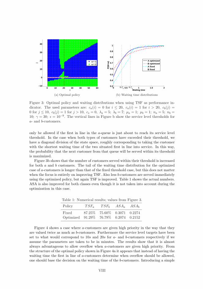
0 10 20 30 40 50 60
40
30
20
10
0
−10
i
j
a = 1a = 2
(a) Optimal policy
0 0.5 1 1.5 20.3
0.4
0.5
0.6
0.7
0.8
0.9
1
Waiting time
P(W
<w)
A optimizedB optimizedA fixedB fixed
SLTb
SLTa
(b) Waiting time distributions
Figure 3: Optimal policy and waiting distributions when using TSF as performance in-dicator. The used parameters are: ca(i) = 0 for i ≤ 20, ca(i) = 1 for i > 20, cb(j) =0 for j ≤ 10, cb(j) = 1 for j > 10, cs = 0, λa = 5; λb = 7; µa = 1; µb = 1; na = 5; nb =10; γ = 30; ε = 10−9. The vertical lines in Figure b show the service level thresholds fora- and b-customers.
only be allowed if the first in line in the a-queue is just about to reach its service levelthreshold. In the case when both types of customers have exceeded their threshold, wehave a diagonal division of the state space, roughly corresponding to taking the customerwith the shortest waiting time of the two situated first in line into service. In this way,the probability that the next customer from that queue will be served within its thresholdis maximized.
Figure 3b shows that the number of customers served within their threshold is increasedfor both a and b customers. The tail of the waiting time distribution for the optimizedcase of a-customers is longer than that of the fixed threshold case, but this does not matterwhen the focus is entirely on improving TSF. Also less b-customers are served immediatelyusing the optimized policy, but again TSF is improved. Table 1 shows the actual numbers.ASA is also improved for both classes even though it is not taken into account during theoptimization in this case.
Table 1: Numerical results; values from Figure 3.
Policy TSFa TSFb ASAa ASAb
Fixed 87.25% 75.60% 0.3071 0.2274Optimized 91.29% 76.79% 0.2074 0.2152
Figure 4 shows a case where a-customers are given high priority in the way that theyare valued twice as much as b-customers. Furthermore the service level targets have beenset to what would correspond to 10s and 20s for a- and b-customers respectively if weassume the parameters are taken to be in minutes. The results show that it is almostalways advantageous to allow overflow when a-customers are given high priority. Fromthe structure of the optimal policy shown in Figure 4a it appears that instead of having thewaiting time the first in line of a-customers determine when overflow should be allowed,one should base the decision on the waiting time of the b-customers. Introducing a simple
VIII
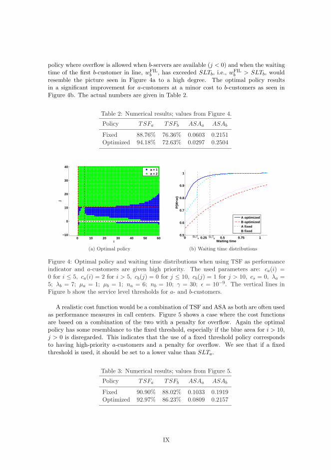
policy where overflow is allowed when b-servers are available (j < 0) and when the waitingtime of the first b-customer in line, wFIL
b , has exceeded SLTb, i.e., wFILb > SLTb, would
resemble the picture seen in Figure 4a to a high degree. The optimal policy resultsin a significant improvement for a-customers at a minor cost to b-customers as seen inFigure 4b. The actual numbers are given in Table 2.
Table 2: Numerical results; values from Figure 4.
Policy TSFa TSFb ASAa ASAb
Fixed 88.76% 76.36% 0.0603 0.2151Optimized 94.18% 72.63% 0.0297 0.2504
0 10 20 30 40 50 60
40
30
20
10
0
−10
i
j
a = 1a = 2
(a) Optimal policy
0 0.25 0.5 0.75 10.5
0.6
0.7
0.8
0.9
1
Waiting time
P(W
<w)
A optimizedB optimizedA fixedB fixed
SLTa SLT
b
(b) Waiting time distributions
Figure 4: Optimal policy and waiting time distributions when using TSF as performanceindicator and a-customers are given high priority. The used parameters are: ca(i) =0 for i ≤ 5, ca(i) = 2 for i > 5, cb(j) = 0 for j ≤ 10, cb(j) = 1 for j > 10, cs = 0, λa =5; λb = 7; µa = 1; µb = 1; na = 6; nb = 10; γ = 30; ε = 10−9. The vertical lines inFigure b show the service level thresholds for a- and b-customers.
A realistic cost function would be a combination of TSF and ASA as both are often usedas performance measures in call centers. Figure 5 shows a case where the cost functionsare based on a combination of the two with a penalty for overflow. Again the optimalpolicy has some resemblance to the fixed threshold, especially if the blue area for i > 10,j > 0 is disregarded. This indicates that the use of a fixed threshold policy correspondsto having high-priority a-customers and a penalty for overflow. We see that if a fixedthreshold is used, it should be set to a lower value than SLTa.
Table 3: Numerical results; values from Figure 5.
Policy TSFa TSFb ASAa ASAb
Fixed 90.90% 88.02% 0.1033 0.1919Optimized 92.97% 86.23% 0.0809 0.2157
IX
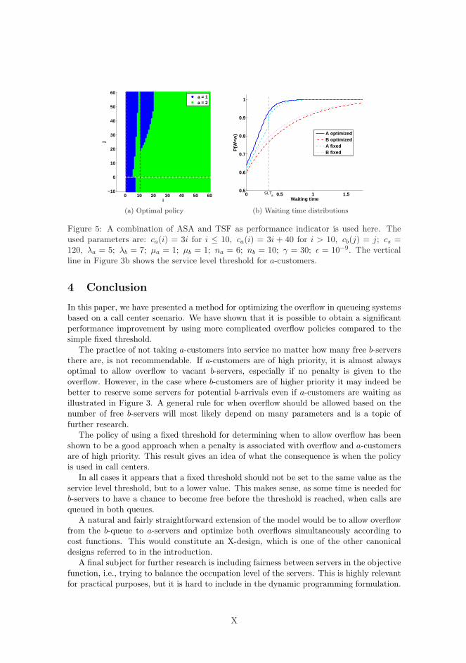
0 10 20 30 40 50 60
60
50
40
30
20
10
0
−10
i
j
a = 1a = 2
(a) Optimal policy
0 0.5 1 1.50.5
0.6
0.7
0.8
0.9
1
Waiting time
P(W
<w)
A optimizedB optimizedA fixedB fixed
SLTa
(b) Waiting time distributions
Figure 5: A combination of ASA and TSF as performance indicator is used here. Theused parameters are: ca(i) = 3i for i ≤ 10, ca(i) = 3i + 40 for i > 10, cb(j) = j; cs =120, λa = 5; λb = 7; µa = 1; µb = 1; na = 6; nb = 10; γ = 30; ε = 10−9. The verticalline in Figure 3b shows the service level threshold for a-customers.
4 Conclusion
In this paper, we have presented a method for optimizing the overflow in queueing systemsbased on a call center scenario. We have shown that it is possible to obtain a significantperformance improvement by using more complicated overflow policies compared to thesimple fixed threshold.
The practice of not taking a-customers into service no matter how many free b-serversthere are, is not recommendable. If a-customers are of high priority, it is almost alwaysoptimal to allow overflow to vacant b-servers, especially if no penalty is given to theoverflow. However, in the case where b-customers are of higher priority it may indeed bebetter to reserve some servers for potential b-arrivals even if a-customers are waiting asillustrated in Figure 3. A general rule for when overflow should be allowed based on thenumber of free b-servers will most likely depend on many parameters and is a topic offurther research.
The policy of using a fixed threshold for determining when to allow overflow has beenshown to be a good approach when a penalty is associated with overflow and a-customersare of high priority. This result gives an idea of what the consequence is when the policyis used in call centers.
In all cases it appears that a fixed threshold should not be set to the same value as theservice level threshold, but to a lower value. This makes sense, as some time is needed forb-servers to have a chance to become free before the threshold is reached, when calls arequeued in both queues.
A natural and fairly straightforward extension of the model would be to allow overflowfrom the b-queue to a-servers and optimize both overflows simultaneously according tocost functions. This would constitute an X-design, which is one of the other canonicaldesigns referred to in the introduction.
A final subject for further research is including fairness between servers in the objectivefunction, i.e., trying to balance the occupation level of the servers. This is highly relevantfor practical purposes, but it is hard to include in the dynamic programming formulation.
X
References
[1] Mor Armony and Nicholas Bambos. Queueing dynamics and maximal throughputscheduling in switched processing systems. Queueing Systems, 44(3):209–252, 2003.
[2] Wolfgang Barth, Michael Manitz, and Raik Stolletz. Analysis of two-level supportsystems with time-dependent overflow - a banking application. Forthcoming in Pro-duction and Operations Management, 2009, available fromhttp://ideas.repec.org/p/han/dpaper/dp-399.html.
[3] Rene Bekker, Ger Koole, Bo Friis Nielsen, and Thomas Bang Nielsen. Queues withwaiting time dependent service. Submitted for publication, 2009, available fromhttp://www.math.vu.nl/ koole/research/.
[4] Noah Gans, Ger Koole, and Avishai Mandelbaum. Telephone call centers: Tutorial,review, and research prospects. Manufacturing and Service Operations Management,5(2):79–141, 2003.
[5] Robin Groenevelt, Ger Koole, and Philippe Nain. On the bias vector of a two-classpreemptive priority queue. Mathematical Methods of Operations Research, 55(1):107–120, 2002.
[6] James R. Jackson. Some problems in queueing with dynamic priorities. Nav. Res.Logistics Quart., 7:235–249, 1960.
[7] James R. Jackson. Queues with dynamic priority discipline. Management Science,8(1):18–34 and 2627272, 1961.
[8] Leonard Kleinrock and Roy P. Finkelstein. Time dependent priority queues. Opera-tions Research, 15(1):104–116; 168514, 1967.
[9] Ger Koole, Bo Friis Nielsen, and Thomas Bang Nielsen. Waiting time depen-dent multi-server priority queues. Submitted for publication, 2009, available fromhttp://www.math.vu.nl/ koole/research/.
[10] M. Perry and A. Nilsson. Performance modelling of automatic call distributors:assignable grade of service staffing. International Switching Symposium 1992. ‘Diver-sification and Integration of Networks and Switching Technologies Towards the 21stCentury’ Proceedings, pages 294–8 vol.2, 1992.
[11] Martin L. Puterman. Markov Decision Processes. Discrete Stochastic Dynamic Pro-gramming. Wiley, second edition, 2005.
[12] Henk C. Tijms. A First Course in Stochastic Models. Wiley, second edition, 2003.
XI