Occasional Papers

California’s Economic Future and Infrastructure Challenges

David Neumark

June 2, 2005 The California 2025 project www.ca2025.org, conducted with support of the William and Flora Hewlett Foundation, addresses issues that will affect the state of the State in 2025. The Technical Report series provides more information on topics discussed in chapters of the project’s major report, California 2025: Taking on the Future (Hanak and Baldassare, eds., PPIC, 2005). This is a corrected version of the previous version of this paper posted June 2005.

Public Policy Institute of California

The Public Policy Institute of California (PPIC) is a private operating foundation established in 1994 with an endowment from William R. Hewlett. The Institute is dedicated to improving public policy in California through independent, objective, nonpartisan research. PPIC's research agenda focuses on three program areas: population, economy, and governance and public finance. Studies within these programs are examining the underlying forces shaping California’s future, cutting across a wide range of public policy concerns, including education, health care, immigration, income distribution, welfare, urban growth, and state and local finance. PPIC was created because three concerned citizens – William R. Hewlett, Roger W. Heyns, and Arjay Miller – recognized the need for linking objective research to the realities of California public policy. Their goal was to help the state’s leaders better understand the intricacies and implications of contemporary issues and make informed public policy decisions when confronted with challenges in the future. David W. Lyon is founding President and Chief Executive Officer of PPIC. Thomas C. Sutton is Chair of the Board of Directors.

Copyright © 2006 by Public Policy Institute of California All rights reserved San Francisco, CA Short sections of text, not to exceed three paragraphs, may be quoted without written permission provided that full attribution is given to the source and the above copyright notice is included. PPIC does not take or support positions on any ballot measure or on any local, state, or federal legislation, nor does it endorse, support, or oppose any political parties or candidates for public office. Research publications reflect the views of the authors and do not necessarily reflect the views of the staff, officers, or Board of Directors of the Public Policy Institute of California.

Summary

The development of California’s economy over the next two decades will help to shape the physical infrastructure and human capital investment challenges that the future holds. In particular, the changing industrial mix of the economy is likely to shift the demands placed on various components of the state’s infrastructure. While long-term economic projections are fraught with uncertainty, and the linkages between the changing economy and infrastructure needs are far from deterministic, the goal of this paper is to describe projected changes in California’s economy over the next couple of decades, and to assess the broad implications of these projected changes for infrastructure needs.

The description of likely changes in California’s economy is not based on an independent economic forecasting exercise, but instead on a synthesis of alternative economic forecasts for the state emanating from the private sector, the public sector, and the research community. The strategy can be viewed as taking the economic forecasts as “data” and then examining a number of questions concerning infrastructure challenges based on these “data.” The key results that emerge from synthesizing these forecasts is that there is general agreement regarding the broad directions of projected changes in the industry mix of California’s economy—strong declines in manufacturing employment and declines as well in transportation and utilities and perhaps construction, while the services industry is projected to grow strongly.

Based on these projections, the paper considers infrastructure needs along three dimensions. First, the geographic location of employment growth and population growth influences where infrastructure challenges relating to housing and transportation are likely to be more or less acute. Second, the industrial composition of economic activity has implications for infrastructure needs relating to energy, water, and transportation, as different industries make varying demands on non-labor resources, on the volume of goods that need to be transported and to where, and on the environment. Finally, and perhaps most important, the skill composition of the workforce needed to support this economic activity dictates the human capital that has to be supplied by the population, driving demands for education and training and the institutions that provide them. These analyses lead to three conclusions:

• The regional forecasts are sufficiently varied that it is not possible to make definitive statements regarding the geographic location of employment and population growth and implications for transportation infrastructure.

• The changing industrial mix of the economy away from goods-producing industries and towards service-producing industries is likely to prove less taxing on the physical infrastructure broadly defined.

• The forecasts of employment growth by industry indicate that the educational levels of the workforce will have to rise substantially, implying that the greatest challenge for public investment concerns human capital in the form of education. Encouraging California’s youths to increase educational attainment is particularly important in enabling them to enjoy high living standards in the evolving economy; and conversely, failure to do so is likely to increase difficulties posed by poor employability and low wages.

- i -

Contents

Summary i

Tables v

Acknowledgments vii

Introduction 1

ECONOMIC FORECASTS 3 Economic Forecasting 3

Econometric Models 3 Long-Term Extrapolation/Projection 4 Forecast Scenarios 5 Threats to the Forecasts 5

Economic Forecasts for California 7 Forecast Descriptions 7 Statewide and Regional Forecasts 8 Forecasts for Employment by Industry 9 Expert Assessments of Threats to the Forecast 11

IMPLICATIONS FOR INFRASTRUCTURE 13 Transportation and Housing: Employment versus Population Growth 13 Industrial Composition and the Use of Infrastructure Resources 14 Industrial Composition and Workforce Skill Needs 17

Changes in the Industrial Composition of Employment and Educational Levels of the Workforce 17 Educational Levels and Changes by Industry 18 Changes at the Regional Level 19 Adjustments of Educational Attainment Among California’s Workforce to Changing Educational Requirements 20

Conclusion 23

References 25

Appendix A. Foreign Economic Developments and Economic Forecasts 31 Howard J. Shatz, Research Fellow, Public Policy Institute of California

The End of Globalization 31 The Development of a Cheap, Alternative Fuel 31 Dramatic Mexican Economic Success 32 Zero Industrial and Agricultural Tariffs 33

- ii -

Appendix B. Technological Innovation and Uncertainty about the Future 35 Junfu Zhang, Research Fellow, Public Policy Institute of California

The Deepening of Internet Technology 35 The Advancement of Biotechnology 36 The Commercialization of Nanotechnology 36 Summary 36

Appendix C. Threats to Long-Term Economic Forecasts for California from Political Developments 37

Stephen Levy, Director and Senior Economist, Center for Continuing Study of the California Economy

Appendix D. Infrastructure Investment and Economic Growth 39 Christopher Thornberg, Senior Economist, UCLA-Anderson Forecast

- iii -

Tables

Table 1 Economic Forecasts for California

Table 2 Statewide Forecasts

Table 3 Regional Employment Forecasts, Level and Percentage Change from 2000

Table 4 Projected Changes in Non-Farm Employment by Industry

Table 5 Four Experts’ Views on Threats to the Forecasts

Table 6 Employment Versus Population Growth, Forecasted Percentage Changes, by Regions and Other County Aggregations

Table 7 Input Requirements from Transportation, Communications, and Utilities and Government Enterprises for Output from Other One-Digit Industries

Table 8 Implications of Industrial Composition of Employment for Educational Levels of Non-Farm Workers in California in 2000, 2010, and 2020

Table 9 Educational Levels Across Industries and Trends Within Industries

Table 10 Educational Levels and Changes by Services Subsector

Table 11 Projected Changes in Employment by Industry, Percentage Change in Share, 2000-2020, by COG Regions and Other County Aggregations

Table 12 Implications of Industrial Composition of Employment for Educational Levels of Workers in California, Statewide and by COG Regions and Other County Aggregations, Percentage Change in Share in Each Educational Level 2000-2020

Table 13 Implications of Industrial Composition of Employment for Educational Levels of Non-Farm Workers in California and United States

Table 14 Forecasted Changes in Employment by Industry, SIC

Table 15 Forecasted Changes in Employment by Industry, Later Forecasts, NAICS

- v -

Acknowledgments

I would like to thank Stephen Ciccarella, Jon Norman, and Douglas Symes for outstanding research assistance, and Amanda Bailey, Ellen Hanak, Doug Henton, Manuel Pastor, Deborah Reed, and Chris Thornberg for helpful comments.

- vii -

Introduction

This paper considers a set of forecasts or likely scenarios regarding California’s economy in the next couple of decades, with a particular emphasis on those features of the economy that are likely to influence infrastructure needs. The effort to envision California’s economic future draws on existing forecasts for the state to develop a sense of the state’s likely economic future. It then uses these forecasts combined with other data sources and predictions to consider the broad implications of these forecasts for some of the key infrastructure challenges the state is likely to face as 2025 approaches.

The analysis focuses on a few critical features of the economy that bear most strongly on infrastructure challenges. These include the following dimensions of the state’s economy:

• the level of economic activity, most important, employment;

• the geographic location of economic activity;

• the industrial composition of economic activity; and

• the skill composition of the workforce.

These dimensions are viewed as most important with respect to infrastructure challenges. The industrial composition of economic activity has implications for infrastructure needs relating to energy, water, and transportation, as different industries make varying demands on non-labor resources, on the volume of goods that need to be transported and to where, and on the environment. The geographic location of this activity influences where infrastructure challenges relating to housing and transportation are likely to be more or less acute and the nature of those challenges. Finally, and perhaps most important, the skill composition of the workforce that is needed to support this economic activity dictates the human capital that has to be supplied by the population, driving demands for education and training and the institutions that provide them. Consequently, the paper focuses on these features of the economic forecasts in making broad inferences about the infrastructure challenges the state is likely to face.

It is important to emphasize that the infrastructure and public investment challenges posed by changes in California’s economy are likely quite a bit less significant than those posed by a growing population overall, especially with regard to physical infrastructure. Many infrastructure needs grow approximately in line with the population, although with some influence from the age structure of the population. For example, a rising population implies growing strains on transportation and physical educational infrastructure as a result of simply more drivers and more students. Especially in a state like California with a population that is projected to grow rapidly (Johnson, 2005), the infrastructure challenges posed by economic change are almost surely secondary to those posed by a growing population.1 Nonetheless, economic changes have further implications that merit exploration—such as where challenges 1 As a consequence, it is not uncommon for long-term perspectives on future developments in a state to focus on population; for example, Murdock et al. (2002) focus exclusively on population in looking at challenges that Texas will face in the 21st century.

- 1 -

to transportation infrastructure are likely to be more or less acute because of changes in employment, or changes in the educational attainment that students may want or need to reach. These are most likely to be driven by changes in the composition of industries in which California’s workers are employed.

Moreover, an expanding population does not, in and of itself, necessarily call for changing skill levels in the workforce. Rather, the challenges regarding public investment in human capital are probably those that are most closely tied to changes in the economy. As a consequence, these human capital challenges receive a disproportionate share of attention in this paper. The focus on the “human” component of public investment, rather than physical infrastructure per se, is unconventional. “Infrastructure” is most commonly used to refer to physical components only, and typically refers to investments that society makes, but that are utilized by everyone, including businesses. But, thinking more broadly, society makes investments in assets that assist in the productivity of economic activity. Investments in humans, and the stock of human capital assets that such investments help to build up, can be thought of as parallel to infrastructure investment. As an example, a highly educated, technically literate workforce no doubt enhances the capacities of capital and labor to develop profitable high-tech enterprises.2 Thus, we think it important to focus as much on human capital as on physical infrastructure in considering the implications of future economic changes in California for infrastructure, in particular given that—as just argued—economic changes contribute in a unique way to human capital needs.3

It is also important to clarify what this paper does not do. First, it is not an economic forecasting exercise per se. Instead, it summarizes and synthesizes existing economic forecasts. Economic forecasting is a complex and expensive enterprise, and there are already a number of public and private bodies in the state that have developed the expertise and resources to engage in forecasting. In a sense, the strategy used in this study can be interpreted as using the economic forecasts as “data,” and then examining a number of questions using these data to makes inferences about California’s economic future. As with all empirical research, it is important to consider how robust these implications are. That is, if most of the forecasts point to the same conclusion regarding a particular implication, the conclusion can be drawn more strongly, whereas if the answer appears to vary with the different forecasts, then it may not be possible to draw firm conclusions.

Second, this paper is not an infrastructure planning exercise. Most important, it does not explicitly study needs for specific types of infrastructure associated with different industries and different regions. Rather, it focuses on trying to discern the general economic trends likely to influence the state over the next couple of decades and how they might influence infrastructure needs broadly defined. Other components of the “California 2025” project address in more detail spending on particular components of infrastructure and detailed assessment of infrastructure needs.

2 A telling example is provided by the growth of outsourcing of service-related work to India, which is greatly eased by the English language skills of its workforce. 3 Similar arguments are made in a 2001 report assessing investment needs in North Carolina looking forward 20 years (North Carolina Progress Board, 2001).

- 2 -

Economic Forecasts

Economic Forecasting

Econometric Models

The most venerable method of economic forecasting comes from econometric models. Econometric models used in forecasting typically combine economic theory and statistical methods to develop and estimate models for each industrial sector of the economy, the government, the labor market, and so on. Along with forecasts of many variables taken as exogenous to the economic model—frequently, for example, population—these models then produce forecasts for the path of numerous economic variables. Published forecasts typically also reflect a good deal of judgment on the part of forecasters. Such models are used by numerous institutions—including the Federal Reserve Board and its banks, private banks, and forecasting companies—to produce both national and state-level forecasts.

Forecasting based on econometric models has two strengths. First, while complicated, to a trained eye at least the models generate forecasts in a transparent fashion; the forecasts have a strong “mechanical” component and are easy to both understand and to critique. Second, good econometric models impose the consistency required by economic theory. In particular, built into their structure and therefore into the forecasts are requirements that markets are in equilibrium (demand equals supply) and that identities hold (for example, all income is either saved or spent). Thus, econometric models produce internally consistent forecasts and their logic is easily understood.

On the other hand, most economic forecasting based on econometric models is not very well-suited to our objectives because it focuses almost exclusively on the short or medium run. For example, the widely cited UCLA-Anderson forecast (see, for example, UCLA-Anderson Forecasting Project, 2002) focuses on a horizon of two years (and sometimes part of a third year). At the same time, long-run forecasts using these models are not unheard of. Periodically, the UCLA-Anderson forecast includes statewide projections with a 10-year or 20-year horizon. Similarly, an econometric model for county-level forecasts was developed to produce 20-year forecasts for purposes of transportation planning used by the California Department of Transportation (Schniepp, 2000).

There are multiple problems with generating longer-term predictions. First, there is the likelihood that the parameters of the model, which reflect underlying behavior or the state of technology, as well as government policy, may change over time in ways that the model will not capture. Second, many variables in econometric models are taken as exogenous and therefore have to be forecasted in a fashion that is often more ad hoc. Third, econometric models, especially the more complicated ones that try to more completely capture the structure of the economy, do not behave as well in predicting longer-term trends, most likely because estimates of their parameters and the implied economic structure come from shorter-term variation in the data. This is not to say that one cannot use these models to generate long-term forecasts. But professional forecasters are skeptical of such exercises, and the models typically have not been developed with an eye to long-term forecasting. At the same time, the

- 3 -

“consumers” of forecasts—such as financial investors or the Federal Reserve Board—are often primarily interested in short-term predictions.

Long-Term Extrapolation/Projection

Numerous government agencies with responsibilities that often bear on infrastructure, as well as other researchers, engage more explicitly in longer-term projections. For example, because transportation systems can take decades to develop and build, long-term forecasts of population and the demand for transportation are needed (see, for example, Transportation California, 2001). Similarly, agencies involved in manpower planning often try to project occupational needs over long horizons, both to assist students and counselors in career planning, and to ensure that adequate educational facilities such as community colleges or college campuses are being built. As examples, the State of California’s Employment Development Department produces employment projections by occupation and by industry at the state level with a horizon of about 10 years, and disaggregates this to the county level with a somewhat shorter horizon (California Employment Development Department, 2004a and 2004b). And California State University’s Long-Range Economic & Employment Projections program forecasts occupational and industry employment with a horizon of approximately five years (www.des.calstate.edu, viewed June 10, 2003). Finally, as an example of individual researchers focusing on the long term, the Center for Continuing Study of the California Economy (CCSCE) publishes an annual report that provides some employment and industry output forecasts with a horizon of about seven years, and growth forecasts with a horizon of about 20 years (for example, CCSCE, 2002a), as well as long-term projections of employment by county (for example, CCSCE, 2002b).

From the perspective of this paper, the strength of such projections is that they try to look much further out into the future than typical econometric forecasts. Given this goal, the methods used in such projections are more geared to the longer term, and hence may be more accurate than letting econometric models designed for short-term forecasting produce longer-term forecasts. Of course, these sorts of projections work better in some spheres than others. As an example, forecasting population and the age structure may be quite reliable because there is a large deterministic component to the process. If we ignore the effects of migration, everyone who will be aged 20-30 in 20 years has already been born, and barring some unforeseen disaster we can predict quite accurately how many will die during that 20-year period. But if we want to take account of immigration, then behavioral decisions (whether to immigrate to California from another country, whether to leave California for another state, and so on), and policy decisions (whether to attempt to reduce foreign immigration) become much more important, and much less predictable as they are in part driven by events that have not been anticipated, and in part driven by behavioral responses to other variables, such as economic conditions in California and elsewhere, that have to be predicted.

Aside from these considerations, there are two weaknesses of these types of long-term forecasts. First, they tend to be based principally on extrapolation of existing trends—that is, assuming that present growth rates will mechanically continue into the future. That is not always the case, of course, as experts who work in these areas often have in mind behavioral models that underlie the projections. And in econometric models used for forecasting, over the longer run the forecasts tend to converge to longer-run trends because of the structure of the

- 4 -

equations used in these models. Second, such projections are often done in isolation from what is or what might be happening in other sectors of the economy that might cause important interactions. They therefore do not always have imposed on them the same internal consistency and coherence that characterizes forecasts from more complete econometric models.

Forecast Scenarios

The preceding discussion should make two things clear. First, economic forecasting—even in the short run but especially in the long run—is far from an exact science. Second, there is unlikely to be any single method or approach that is uniquely suited to generating long-term forecasts regarding California’s economy. Therefore, rather than attempt to come up with a single “best” forecast, we regard it as more important to consider the overall qualitative conclusions that come from a variety of existing forecasts. In addition to reflecting what we believe to be some of the uncertainty surrounding long-range forecasting, this more eclectic approach will also provide a menu of economic scenarios that others can consider in relation to their implications for infrastructure.

Threats to the Forecasts

Even documenting the range of economic changes predicted by the various forecasts almost surely understates the uncertainty inherent in long-run forecasting. Most important, whether based on econometric models or longer-term extrapolation, such forecasts do not allow for wide-sweeping changes in technology, politics, foreign economic development, and so on, which may have profound impacts on the economy. As examples, California’s experiences with changes in military spending in the early 1990s and the technology boom of the late 1990s aptly demonstrate how government spending and technological innovation can have rather dramatic influences on the composition and location of economic activity.

Most important, perhaps, this paper focuses on long-run forecasts for the California economy and what these imply for infrastructure. However, because the infrastructure may also help lay the conditions for economic growth and development, there is potentially important feedback from infrastructure to the economy. For example, an economic future highly dependent on a well-functioning transportation network could be threatened by failure to develop the necessary transportation resources. The same goes for investment in human capital, as the evolution of the economy would likely be altered were severe shortages of educated workers to arise.

The question of the dependence of economic growth on infrastructure investment is a difficult one to answer. Some evidence points to the economically productive effects of public infrastructure investment. Aschauer (1989a) considers whether public infrastructure investment simply crowds out private investment as businesses react to the greater public investment in capital by investing fewer of their own resources in private capital investment. He notes, though, that public investments may increase the productivity of private capital, and furthermore that the public investments that do this may have to be publicly provided. Returning to the earlier example, a good transportation network may only be built by the public

- 5 -

sector because of the public goods nature of transportation and increasing returns to scale,4 and such a network may increase the productivity of investments that rely on transportation. He presents suggestive evidence for the United States—from time-series data—that the predominant effect of public investment is to increase the return to private investment and to increase private investment. 5 Consistent with this, he also finds (1989b) that it is investments in “core” infrastructure—streets and highways, airports, electrical and gas facilities, mass transit, water systems, and sewers—that have the greatest impact on economic productivity, in contrast to public investments in hospitals, other buildings, conservation and development structures, or the military.

On the other hand, subsequent work reported and summarized in Kelejian and Robinson (1997) raises serious questions about our ability to draw strong conclusions regarding the productivity of public capital, showing that such estimates are highly sensitive to variations in the econometric specification, and that estimates indicating no productive effect of this capital are common. As the authors note, “[O]ne would not seriously consider the possibility that overall productivity would be unaffected if all forms of public capital were to somehow disappear! However, the issue at hand … relates to the marginal productivity of public capital given the existing stock. Our results suggest that existing estimates of this marginal productivity may be naïve and seriously biased” (p. 128). This work might therefore be interpreted as suggesting that at least minor deviations from the path of infrastructure accumulation that is implicitly assumed in the economic forecasts would not pose major threats to the forecasts.

The econometric forecasts that are summarized in this paper tend to focus on “business as usual,” and do not attempt to predict or take account of unanticipated but important changes or “shocks” to the economic environment. In addition, they do not take account of the potential feedback effects from infrastructure to economic growth. As a consequence, it is important to supplement what the long-range forecasts might tell us with an informed, although also subjective and qualitative assessment of the potential for key developments (or lack thereof) to threaten the longer-run scenarios implied by the existing economic forecasts. In addition, therefore, to synthesizing econometric and long-range economic forecasts, we consider the potential for major changes or developments to chart a very different course for California’s economic future. Specifically, four individuals with expertise in areas that potentially pose

4 The public goods nature of roads arises because to some extent one person or business making use of the roads does not affect another person’s or business’s ability to use the roads; this is referred to as the “nonrival” nature of public goods. Of course at some point congestion may set in, in which case one person’s or business’s use has negative externalities. See, for example, Glomm and Ravikumar (1994) for a model of public investment that incorporates varying degrees of nonrivalry and congestion. 5 Conrad and Seitz (1994) and Seitz (1995) present similar evidence for West Germany that public investment increases the return to private capital, and increases investment in private capital, using both aggregate data by industry and a panel of data on cities with measures of local infrastructure investment. On the other hand, public investment may be labor saving—generating a higher capital-to-labor ratio by “crowding in” private investment. Their work on cities is of interest, because the most recent work for the United States (e.g., Haughwout, 2001) argues that the beneficial effects of infrastructure depend in part on its geographic concentration, asserting, in particular, that infrastructure investment in central cities can have a large positive impact by exploiting economies of agglomeration (that is, the advantages that businesses experience from location near many other businesses).

- 6 -

major “threats” or “challenges” to the forecast—in areas of technology, foreign economic relations, politics, and infrastructure—were consulted, and their views on what might be considered relatively unlikely but nonetheless high-impact changes are summarized in relation to the forecasts. Their responses help to flesh out the uncertainty surrounding long-term economic forecasts, and to provide a sense of possible alternative scenarios.

Economic Forecasts for California

Forecast Descriptions

Table 1 summarizes the economic forecasts used in this report, which are the main forecasts available in the state. In each case, in columns (1) and (2) we describe the geographic scope of the forecast, and the forecast horizon (the ending year of the forecast). In some cases, such as for the UCLA-Anderson forecast, there are multiple forecasts with different time horizons available. We always use the most recent forecast with the latest ending date, but in some cases there is an earlier forecast with a longer horizon, in which case we consider both forecasts because the more recent forecast, while having a shorter horizon, may reflect newer information. The shortest forecast horizon we consider is to 2010, and the longest available is to 2030. Column (3) of the table provides a brief description of the forecast model or methods. Note that in some cases this column simply indicates “proprietary;” this occurs for the two cases—UCLA-Anderson and CCSCE—of forecasts that are sold commercially, and for which the forecast models are therefore not publicly available.

As noted above, while these forecasts often cover a wide range of variables—especially the larger statewide forecasts—we are interested primarily in employment. We therefore provide a description of the employment information forecasted by each of these models, in column (5). Because some of our analysis focuses on employment relative to population, we also describe the population information available in these forecasts in column (4), although population variables are often exogenous inputs to the forecast or based on simple extrapolation rather than endogenous forecasts.

As the table shows, there are three sources of statewide forecasts—UCLA-Anderson, the California Employment Development Department (EDD), and the Center for Continuing Study of the California Economy (CCSCE). The Councils of Government (COGs) provide forecasts for their regions—covering the Bay Area, Sacramento, San Diego, and Los Angeles/Southern California. Finally, the California Department of Transportation (DOT) generates forecasts for all counties, as do EDD and CCSCE. The DOT county-level forecasts can be aggregated to generate yet another statewide forecast.6

6 There was no need to do this for the county-level EDD and CCSCE forecasts, since they already produce state-level forecasts. The COGs covered are: the Association of Bay Area Governments (ABAG); the Sacramento Area Council of Governments (SACOG); the San Diego Association of Governments (SANDAG); and the Southern California Association of Governments (SCAG).

- 7 -

Statewide and Regional Forecasts

Table 2 summarizes the results from the statewide forecasts, and Table 3 summarizes the results from the regional forecasts. Turning first to the statewide forecasts, columns (1)-(3) first summarize the population forecasts, including population forecasts that are independent of economic forecasts; the final rows provide the Department of Finance (DOF) forecasts and the PPIC population forecasts that are part of the California 2025 project (Johnson, 2005). For the 10-year horizon to 2010, the population forecasts that underlie the economic forecasts deviate little, projecting population growth of between 16 and 17 percent. Not surprisingly, the range of the forecasts to 2020 is wider, from 30 to 34 percent. Note that the population forecasts embedded in each of the economic forecasts are toward the high end of the range of population forecasts reported in the bottom panel of the table. To some extent, this reflects the economic forecasts using earlier DOF forecasts, which called for higher population growth (California DOF, 2004b).

The employment projections are reported in columns (4)-(6). The levels are not strictly comparable across all forecasts, because some cover payrolls (that is, wage and salary workers), and others all employment. The growth rates, however, are more comparable. The range of the forecasts for employment growth is considerably wider than that for population growth. For the period from 2000 to 2010, the range is from 13 to 23 percent. To some extent, those forecasts done at a later date project lower employment growth (the exception is the EDD forecast), presumably reflecting an accounting for the economic slowdown at the beginning of the decade. This is perhaps most apparent in comparing forecasts from the same group that were done at different dates; for example, the UCLA-Anderson forecast for employment growth for the 2000-2010 period fell from 21 to 15 percent between their 2002 and 2003 forecasts. There are fewer forecasts available for 2020. The DOT and CCSCE forecasts are for 32 to 34 percent employment growth, while the UCLA-Anderson forecast is for 41 percent employment growth from 2000 to 2020. Note, though, that the UCLA-Anderson and CCSCE projections come from their earlier forecasts, and as just noted later forecasts—although extending only through 2010—revised projected employment growth downward. Thus, we might expect somewhat lower employment growth over the long term than these latter two forecasts suggest. In addition, as noted above the employment forecasts are based on older DOF population forecasts that called for slightly faster population growth; were they based on the current population forecasts, they would presumably be a shade lower.

Table 3 reports the regional forecasts. Each of the four major COGs are covered in the table, including both their own forecasts and forecasts based on aggregating the DOT county-level forecasts for the corresponding region.7 In addition, forecasts for regional groupings of counties covering the rest of the state—North Coast and Mountains, Central Coast, Upper Sacramento Valley, and San Joaquin Valley—are also constructed based on aggregating the DOT forecasts. Turning first to the regions covered by the COGs, based on the DOT forecasts, there is considerable variation in predicted employment growth, with the figures lowest for the Bay Area, and highest for the San Diego region. However, with the exception of San Diego, the COG employment growth projections are always higher than the DOT projections. On the

7 CCSCE also constructs forecasts for the COG regions, and they can be constructed from EDD county-level forecasts, but only through 2010; they are therefore not reported in Table 3.

- 8 -

other hand, based on the COG forecasts projected employment growth is highest for the Sacramento region, and SANDAG forecasts much lower employment growth for its region than does the DOT. Among the other county groups, employment growth is projected to be near the state rate of growth for the North Coast and Mountains, and the Upper Sacramento and San Joaquin Valleys, but lower for the Central Coast.

In contrasting the COG and DOT forecasts for the regions covered by the COGs, it is important to realize that the COG forecasts are not necessarily intended to be simply the best projection of future trends, but also serve as the basis of regional plans. Thus, they may sometimes reflect the projected impact of desired policies, even though these policies may not be the most likely outcome. As an example, the 2003 ABAG projections are based upon “smart growth” principles, a model of planning adopted by ABAG in 2001 that calls for policies that increase housing density in cities and inner suburbs as well as greater reliance on public transportation by residents. In the assumptions that underlie its model, ABAG assumes that these policies are implemented (at least partially) by 2030 (ABAG, 2003). In contrast, ABAG’s 2002 forecast did not encompass these principles, and hence projected somewhat lower employment and population growth. But the adoption of the different principles in ABAG’s 2003 forecast does not necessarily imply that the likelihood that these principles would be adopted had greatly shifted, and in this sense the forecast does not necessarily represent the most likely paths of growth of population and employment. Furthermore, across the different COGs the forecast methods are quite different, and, frankly, we have less confidence in these forecasts than in the DOT forecasts. Because of all of these considerations, the COG projections have to be approached a bit more cautiously, and the commercial forecasts and the government forecasts given somewhat more credence in terms of best predicting the future course of the economy.

Forecasts for Employment by Industry

Finally, Table 4 provides information on the forecasted changes in employment by industry, from the three statewide forecasts that cover the industrial composition of employment.8 Because the projected changes in employment by industry are critical to the question of infrastructure challenges posed by the changing California economy, it is worth discussing in some detail what drives the industry forecasts.

According to the California Employment Development Department (2004a), industry projections are based on historical industry employment at the two- or three-digit SIC code in a geographic area. Historical data are used to project total industry employment for the area. In addition, the relationship between the historical and projected data in the geographic area is considered in comparison with the same data at the state level, and possible adjustments are made. The projections are then disaggregated into four-digit SIC components, and are then reviewed by local area analysts with specific knowledge of local trends and changes. We use 8 The industry forecasts reflect the change under way in the classification of industries from the SIC to the NAICS. The industry employment figures here are based on the earlier SIC codes, as most of the forecasts discussed to date use these codes. But the transition from SIC to NAICS codes is in progress, and in fact the UCLA-Anderson 2003 forecast uses NAICS codes, and in later tables we sometimes refer to forecasts based on NAICS codes. Because we simply summarize and synthesize existing forecasts, we report results based on the industry classifications used in the original forecasts.

- 9 -

projections that are then aggregated up to the one-digit SIC level. EDD is careful to emphasize that a number of key assumptions—which might best be characterized as “business as usual” —underlie their projections.9 In general, then, the EDD projections can be characterized as based in large part on past trends in employment data, with some scope for what are often called “judgmental” factors that might account for more recent developments.

According to the Department of Transportation, the largest factor influencing the mixture of industries in their forecasts for California is population, as the age distribution of the population has a large effect on which sectors thrive and which decline (personal communication, Mark Schniepp, May 18, 2004). This may be particularly true in the late 20th and early 21st century California economy, because it is dominated by service-sector jobs such as health care, education, and retail trade; the first of these is responsive to an aging population, and the latter two to increases in the youth population. Thus, aging combined with relatively high fertility will result in strong growth in many of these service sectors. The forecasts are also driven by projected technological change, such as growth in productivity in finance, insurance, and real estate that moderates employment increases. Of course, as with the EDD forecasts, past trends play a heavy role in these industry forecasts.

Finally, like the EDD forecast, the UCLA-Anderson forecast, despite using a full-blown econometric model, primarily reverts to relying on past trends to arrive at long-term future employment projections (personal communication, Joe Hurd, May 19, 2004). Again, productivity growth plays a role; for example, productivity growth from advances in technology contributes to declining employment in manufacturing.

Turning to the detailed forecasts for industry employment, two of the forecasts—the UCLA-Anderson forecasts and the aggregated DOT forecasts—extend to 2020, while the EDD forecast extends only to 2010. The industry projections across the three different forecasts have some common features. Most notable, perhaps, is the projected decline in manufacturing jobs, with the share of jobs in manufacturing predicted to decline by 15 to 24 percent as of 2010, and 29 to 36 percent by 2020 (see columns (6) and (7)). Note, though, that these are projected changes in the shares of employment, not the level of employment. Indeed for manufacturing, the projected levels of employment are about flat over the next two decades. In contrast, the industry projections point to sharp increases in employment in services, with the share growing by 7 to 11 percent by 2010, and 15 to 17 percent by 2020. Aside from these two major changes, the forecasts tend to point to declining employment shares of mining, construction, and transportation, communications, and public utilities. The projected trends in trade are sometimes positive and sometimes negative, and centered around zero, as are those for government, and for finance, insurance, and real estate.

9 In particular, they assume an absence of sharp changes in U.S. economic institutions; the continuation of recent technological and scientific trends; persistence of long-term employment patterns by industry; ongoing budgetary constraints for federal, state, and local government agencies; no events such as wars or other disasters that will significantly change the economy’s industrial or occupational structure or substantially change the long-term rate of growth; demographic developments not significantly different from the Department of Finance’s projections; and stable attitudes toward work, schooling, and income (California EDD, 2004a).

- 10 -

These forecasts are only at the one-digit industry level (using SIC codes), which is unfortunate because within one-digit industries, there are some quite different industries. For example, manufacturing extends from textile mills to electronic and electrical equipment, and services covers industries as disparate as business services, social services, and amusement and recreation services. To give some flavor of how more narrowly defined industries have been changing in the past, we examined changes in employment shares of two-digit industries from 1990 to 2000 at the national level. As noted above, long-term projections are strongly shaped by past trends, so these past changes would likely be reflected in any long-term projections of employment change at the level of two-digit industries. In manufacturing, the declines from 1990 to 2000 were widespread; every two-digit industry in manufacturing experienced a declining employment share, ranging from a 5.4 percent decline in rubber and plastics, to a 49.2 percent decline in apparel and textile products. In services, although most two-digit industries experienced growth, the employment share in personal services fell by 5.9 percent and the share in miscellaneous repair services fell by 18.2 percent. Growth was particularly strong in business services (59.3 percent), amusement and recreation services (32.9 percent), and social services (38.9 percent). When we discuss the implications of the changing industrial composition of employment for education, we will return briefly to the differential growth rates of industries within the broad services grouping. More generally, though, it is important to emphasize that changes in industrial composition at levels below the level of aggregation of one-digit industries may have implications for infrastructure. This may be particularly true at a regional level where economic activity in a narrower set of industries can loom larger.

As noted in the Introduction, the industrial composition of the state’s economy is probably the most important determinant of how the future course of the economy affects infrastructure needs. The most salient changes predicted by the economic forecasts—which are robust across the different forecasts—are the declines in manufacturing and perhaps also construction jobs, and the increases in services.10

Expert Assessments of Threats to the Forecast

Finally, we briefly depart from the formal economic forecasts to consider possible alternative developments that could have a major impact on the economic future of the state, and concomitant implications for infrastructure needs. Because these alternative developments are not quantified, we do not incorporate them into the discussion in the next section of the paper regarding the implications of future economic developments for infrastructure. However, we do think they serve as an important “backdrop” in clarifying the uncertainty that inevitably surrounds long-range economic forecasting, and in pointing out some of the possible ways in which both economic developments and infrastructure needs might diverge from the general trends drawn from the quantitative economic forecasts. The views of four experts asked to consider major threats to the forecast from the perspectives of international economic

10 Some caution is in order here, because industrial classifications are based on the final product of the firm to which establishments belong. As an example, auto manufacturers have some employees in Los Angeles, but many do design or management rather than production (Los Angeles County Economic Development Corporation, 2002), so the demands on the infrastructure generated by such employment may be more akin to those of service-producing industries.

- 11 -

relations, technological change, political decisions, and infrastructure investment and utilization are summarized in Table 5.

According to Howard Shatz, two of the four plausible threats to the forecasts related to international economic relations stem from sharp changes in trade patterns. Overall, more trade is viewed as implying higher economic growth, lower prices, and so on, and as benefiting export-oriented industries the most. The development of a cheap, alternative fuel would reshape economic relations between countries, but most likely generally benefit a state like California that is a large user of energy and that has strong economic ties with Asian countries that would gain from decreased reliance on petroleum. A dramatic change in economic growth in Mexico would be particularly important to California and other states with large immigrant (and especially illegal immigrant) populations.

Junfu Zhang considers the possible effects of sharp technological changes, and suggests that the growth and commercialization of the biotechnology and nanotechnology industries hold the potential to create in California developments echoing those spurred by the development of the computer industry in Silicon Valley, and to affect industries that might be particularly affected by these technologies, such as health and agriculture. Also, important advances in biotechnology could lead to declines in mortality with important implications for the future demographic structure of the state.

Stephen Levy weighs the possible consequences of political decisionmaking for the state’s economic future, in particular in relation to infrastructure. He raises concerns regarding insufficient attention to repair and maintenance as well as technological improvements, as opposed to new projects that largely replicate the existing stock of infrastructure, and paying excessive attention to the infrastructure needs of the manufacturing industry as opposed to other industries that may be more important to the state’s economic future. In addition, sharp changes in immigration policy could affect future demographic trends as well as educational levels of the workforce and population.

Finally, Chris Thornberg tries to assess the potential threats to the forecast stemming from the influence of infrastructure investment on economic growth. Although the evidence of the effects of infrastructure on economic growth is somewhat ambiguous, it is possible that insufficient infrastructure investment will restrict economic growth below what is projected. On the other hand, the ability of government and the private sector to adapt to infrastructure constraints should not be underestimated. This, combined with the weak evidence linking infrastructure to economic growth, suggests that at least moderate deviations of infrastructure investment from the trends that might be projected based on economic growth will not seriously threaten that growth. In the end, infrastructure investment may have more to do with maintaining the quality of life as economic growth occurs, rather than with economic growth per se; this does not minimize the importance of infrastructure investment, but it may influence how we think about the “need” for more investment.

- 12 -

Implications for Infrastructure

After synthesizing the forecasted changes in the state’s economy over the next two decades in the previous section, the paper now turns to the implications of these predicted economic changes for infrastructure needs.

Transportation and Housing: Employment versus Population Growth

The forecasts regarding employment growth by region can be contrasted with population projections by region to make inferences about the likely balance between the two. Imbalances have potentially important implications for transportation and housing infrastructure. For example, if a region is projected to have considerably higher employment growth than population growth, then unless there are substantial changes in work behavior—such as telecommuting or more generally work at home—the implication is that individuals residing in other areas will be commuting into and out of the region for work, suggesting a need for increased efforts to avoid traffic congestion or provide public transportation, with a particular focus on commuting from dispersed areas into the region.11 On the other hand, the population projections do not take into account possible sharp changes in housing availability. A region facing employment growth that outstrips population growth may be able to partially alleviate this problem by increasing housing availability.

Comparisons of employment and population projections are reported in Table 6. For the COG regions, both the forecasts from the COGs and from the DOT are used. The table shows the calculations using both DOF population forecasts (California DOF, 2004a) as well as the population forecasts that accompany the economic forecasts.12

These forecasts exhibit a fair amount of discrepancy. This is most apparent in looking at the columns for “Empl. − Pop.” (columns (3), (5), (8), (10), (13), and (15)), which address the imbalance with which this inquiry is most concerned. For each of the COGs, for at least one of the forecast ranges of 2000-2010 or 2000-2020 there are conflicting signs; for example, for SANDAG, using the COG/DOT population forecasts and looking at the projection for 2020, the COG forecast implies that employment growth will fall short of population growth by 4 percentage points, whereas the DOT forecast indicates that employment growth will outstrip population growth by 14 percentage points. It is difficult to characterize what drives these discrepancies. In some cases (such as SANDAG) the DOT forecast calls for considerably more

11 The Bureau of Labor Statistics (BLS) reported that in May 2001, 19.8 million persons, or 15 percent of the workforce, usually did some work at home (at least once a week) (U.S. Bureau of Labor Statistics, 2002). The National Household Travel Survey, carried out by the U.S. Department of Transportation, provides a lower number; our computations indicate that in 2001, 10.4 million workers telecommuted or otherwise worked from home, with about one-fifth of these working from home every day, one-third one day a week or more, and the rest less frequently (see http://nhts.ornl.gov/2001/index.shtml, available May 9, 2004). Unfortunately, there are no comparable survey results over time with which to track trends in telecommuting; there are only some small surveys carried out by private organizations that play advocacy roles (for example, the International Telework Association & Council). 12 The one exception is for SCAG, which extends to 2030 and for which there is no corresponding DOF population forecast.

- 13 -

employment growth than the COG forecast, while in others (such as SACOG) the reverse is true. The COGs do tend to project lower population growth than DOT, while the COG and DOT population growth projections are sometimes higher and sometimes lower than the DOF forecasts.

As a consequence of these differences, it appears to be impossible to draw firm conclusions from the economic and population forecasts regarding regions in which employment is likely to grow considerably faster or considerably slower than population, and the infrastructure challenges that such imbalances might generate. However, if we take the DOT forecasts as more credible, for reasons discussed above, then we can perhaps draw some inferences; these forecasts have been highlighted in the table to facilitate seeing the implications of the DOT forecasts. These figures show that in the SACOG region and in the San Joaquin Valley employment growth is expected to lag behind population growth by quite a bit, while in the SANDAG region, the North Coast and Mountains, and the Upper Sacramento Valley employment is expected to grow considerably faster than population. For the ABAG and SCAG regions as well as the Central Coast the numbers are somewhat more ambiguous and probably indicate relatively more balance between employment and population growth. All else the same, regions for which employment growth is projected to outstrip population growth are likely to face stronger infrastructure challenges involved with the transportation of distant commuters to work—challenges that can be addressed directly via transportation, and perhaps indirectly via increased housing availability. On the other hand, regions expecting relatively more population growth will likely face challenges associated with being “bedroom communities,” most important, those associated with a large share of residents commuting to work. Naturally, the transportation infrastructure needed for regions characterized by workers commuting into a region versus commuting out of a region may differ. And we re-emphasize that these conclusions are less robust than the others discussed in this paper, because of the discrepancies among forecasts when the COG forecasts are included.

Industrial Composition and the Use of Infrastructure Resources

The industrial composition of the economy also has potential direct implications for infrastructure because economic activity itself makes demands upon the state’s infrastructure. For example, some industries are more intensive users of transportation, water, electricity, and so on, than are others. To address the question of how the changing industrial structure affects infrastructure needs, we have developed an input-output table that highlights infrastructure demands by industry.

We focus on input requirements of each one-digit industry—for which we have employment forecasts—for the output of industries in the one-digit (SIC) industry “transportation, communications, and utilities,” and for the output of government enterprises. The two-digit industries that make up transportation, communications, and utilities include railroads and related services and passenger ground transportation; motor freight transportation and warehousing; water transportation; air transportation; pipelines, freight forwarders, and related services; communications; electric services; gas production and distribution; and water and sanitary services. Inputs from these industries do not necessarily constitute infrastructure per se, but they are often strongly associated with infrastructure demands. As an example, the purchase of inputs from the two-digit industry “motor freight

- 14 -

transportation and warehousing” is not going to capture all of the costs associated with highway use (wear and tear, congestion, and so on). Nonetheless, output from this industry will contribute to demands on the transportation infrastructure. Thus, if the industrial composition of the economy is shifting away from industries that use inputs from this particular industry, transportation infrastructure demands can reasonably be expected to fall in relative terms. We also focus on inputs from government enterprises, which may also help to pick up infrastructure demands. In the input-output accounts, this includes both federal enterprises—including the postal service, the Tennessee Valley Authority, other federal utilities, as well as military exchanges and restaurants—and state and local enterprises—including local transit, utilities, water and sanitation services, and parking (U.S. Department of Commerce, 1998).

There are a few potentially important qualifications to this analysis. First, the industry- level forecasts described above pertain to employment rather than output. If productivity growth is quite different across industries, then even though an industry’s employment share is falling, its relative demands on infrastructure may fall less or even rise. For example, if manufacturing employment falls by half but these workers continue to produce the same level of total output (with productivity doubling), then the decline in requirements for transportation infrastructure stemming from manufacturing industries will be seriously overstated by the decline in manufacturing employment. Unfortunately, however, the various economic forecasts do not project output by industry (or equivalently productivity growth by industry).

On the other hand, information available from the U.S. Bureau of Labor Statistics (2001a and 2001b) does point to higher productivity growth over the 1990s in the manufacturing sector. The figures for annual productivity growth over 1990-1999, for the broad industries for which they are reported, are mining, 3.0%; transportation, communications, and utilities, 2.9%; retail trade, 2.4%; finance and services, 1.8%; and manufacturing, 4.0%. Although productivity measurements in non-goods-producing sectors must be used cautiously, these figures suggest that insofar as it is manufacturing output rather than manufacturing employment that taxes physical infrastructure, the projected declines in manufacturing employment overstate the declines in infrastructure demands that changes in this sector will pose. Indeed, if productivity growth in manufacturing continues to run about one percentage point faster than in the other sectors, a good share of the projected 30 percent or so decline in the share of employment in manufacturing should be offset by rising productivity growth (as one percentage point faster productivity growth amounts to growth in output per worker of 22 percent over 20 years).

The second limitation to using input-output tables to assess the effects of changing industrial composition on infrastructure demands is that some industries pose infrastructure demands that are not reflected in the input-output table. For example, if businesses in a particular industry tend to draw consumers by car (for example, retail trade or tourism), then growth in this industry may increase demands on transportation infrastructure, but because this transportation is not a business-to-business (or business-to-government) transaction, it does not appear in the input-output tables. Third, some infrastructure needs are imposed by

- 15 -

California’s role as a major portal of imports and exports from other states13—demands that are not necessarily reflected in changes in California’s employment by industry.14

Finally, the fixed input requirements of input-output analysis may not hold over the longer run. As Chris Thornberg emphasizes in Appendix D, businesses and other agents may adapt to infrastructure shortages (or changes in the prices of infrastructure services), in which case industry input requirements could change. 15

To construct an input-output table that shows the input requirements of one-digit industries for the outputs of specific two-digit industries in transportation, communications, and utilities, we need to start with an input-output table at the two-digit industry level, and then aggregate input requirements to the one-digit industry level. This is done by weighting the input requirements in the two-digit industry-to-industry requirements table by the share of each two-digit industry in the one-digit industry’s output, based on the industry use table.16

The results of doing this are reported in Table 7, which shows the input requirements of one-digit industries from the two-digit industries in transportation, communications, and utilities (this latter one-digit industry is excluded from the columns of the table), and from federal and state and local government enterprises. For example, the 0.010 figure in the upper-left-hand corner implies that a dollar of output from the mining industry requires one cent of input from “railroads and related services; passenger ground transportation.” In the table, the input requirements for the three industries with the most strongly declining employment shares, and the one industry (services) with the fastest-growing share, are highlighted (the latter more darkly). The table shows that the declining industries (again, in relative terms) are the most intensive users of infrastructure from the transportation, communications, and utilities sector, while the services industry, which is the most rapidly growing industry, is one of the least intensive users of infrastructure from this sector. For example, the input requirements from “motor freight transportation and warehousing” for construction and manufacturing are around 0.04, compared with 0.013 for services. Input requirements for the services industry are also lower for “railroads and related services,” “water transportation,” “electric services” (except for construction), “gas production and distribution, “ and “water and sanitary services” (again, except for construction). On the other hand, with respect to output from government enterprises, the services sector is more in the middle.17

Thus, these input-output calculations indicate that, insofar as the changing industrial structure of the economy influences infrastructure needs, the future course of the economy is probably most likely to somewhat lighten infrastructure challenges relative to the economic

13 See Haveman and Hummels (2004). 14 Suppose a manufacturing industry that is a heavy user of these ports but is based in another state expands. Then even though manufacturing employment in California may be declining, manufacturing-related infrastructure demands could increase. 15 Finally, note that we have not discussed the role of agriculture, which is the predominant user of water resources. 16 These tables can be obtained from the web site of the Bureau of Economic Analysis, at http://www.bea.gov/bea/dn2/i-o_annual.htm. We use the 1999 tables. 17 The high input requirements from these enterprises for the government sector, in the last column, is not surprising, as this sector uses much of the output of government enterprises.

- 16 -

structure of the past. We again emphasize, however, that the increasing scale of economic activity with population growth implies that, overall, infrastructure challenges will nonetheless rise considerably, and the reductions in infrastructure challenges to which we refer are to be interpreted as reductions relative to what would be implied by population growth and the economic structure of the past. Moreover, given many of the limitations discussed above, there are numerous factors that may drive demand for transportation infrastructure, in particular, that are not captured via changing industrial composition and the input requirements of industries. As a consequence, other means of directly predicting transportation needs, which are discussed in Hanak and Barbour (2005), are probably more useful on this score. Nonetheless, the input-output analysis is useful in clarifying the role of the changing industry mix of the economy and at least some of the shifts in infrastructure needs that these changes imply.

Industrial Composition and Workforce Skill Needs

Finally, the changing economy poses challenges to “human” infrastructure needs. Different industries require different skills, and different skill levels. Although skills are multidimensional, one dimension of skill that is critical in the labor market, on which we have good data, and that is strongly influenced by public policy (as opposed to, say, job training), is education. The question we address in this section, therefore, is whether the educational needs that are likely to arise as California’s economy changes over the next couple of decades will be consonant with those that the population is likely to provide. This is a complicated question, so we address it in a series of steps. First, we discuss the implications of the changing industrial composition of employment in California for educational levels of the workforce at the state level. Second, we shed some light on these implications by providing information on educational levels of workers in different industries and changes in those educational levels over time. Third, we look at the implications of changes in the industrial mix of employment at the regional level. And finally, we discuss how educational attainment of workers in California is likely to adjust to changing requirements on the part of industry, and specifically consider the extent to which we might expect in-migration of workers with the educational qualifications that are likely to be needed over the next couple of decades.

Changes in the Industrial Composition of Employment and Educational Levels of the Workforce

First, given a set of projected changes in employment by industry, and given predictions of skill needs by industry, we can explore the implications of the changing industry composition of employment for skill needs. We have already described the projections of the industry composition of employment. To predict skill needs by industry, we consider two alternatives. First, we take the distribution of workers by education in each industry in 2002, and assume that in the future the educational distribution within each industry will be the same; we refer to this as the “static” scenario. (The information on education by industry comes from the Current Population Survey (CPS).) In this case, educational requirements of the workforce change only because of the changing industry mix of employment. Second, it is the case that in the workforce as a whole, as well as within industries, education has generally been rising, perhaps reflecting the greater skill needs posed by technological changes within industries. Consequently, we also consider a “dynamic” scenario in which education trends

- 17 -

within industries are projected to continue to follow the same path they have followed for the past decade—that is, from 1992 to 2002.18 In this case, educational requirements of the workforce are projected to change because of both the predicted changes in the industrial composition of employment and the continuation of past changes in education within industries.

The results are presented in columns (1)-(7) of Table 8. The first five columns are based on the UCLA-Anderson industry employment forecasts. In the static exercise, in the top panel, over the period 2000-2010 and more so 2000-2020, the projections indicate declines in the share of the workforce at low educational levels (with a high school diploma or less), and increases in the share with higher educational levels (bachelor’s degrees or higher). Columns (6) and (7) are based on the EDD forecast, and show quite similar results. In the dynamic exercise in the bottom panel, these changes are considerably more pronounced, with sharp projected increases in the share of workers with AA degrees or higher, and sharp projected declines in the share of workers with a high school diploma or less education. It seems more likely that past trends in education within industries will persist than that educational levels within industries will stagnate, so the projections in the bottom panel of Table 8 probably more closely reflect how demands are likely to change.

Educational Levels and Changes by Industry

These results may be viewed as surprising, given suggestions from some quarters that our economy is moving in the direction of low-wage, low-skill service jobs. For example, projections for the state of California based on the Bureau of Labor Statistics’ Occupational Projections and Training Data suggest that between 2000 and 2010, 43 percent of new job openings will be in jobs in which the most significant pathway to employment entails no more than 30 days of on-the-job training, rather than longer-term training or higher education (see U.S. Bureau of Labor Statistics, 2004; California Employment Development Department, 2003; and Pastor and Reed, 2005).

However, Table 9 provides some information on educational levels by industry, which should help to counter projections that the economy is creating vast numbers of unskilled jobs. The top panel shows the distribution of workers in each industry across education categories. This panel demonstrates that mining, construction, manufacturing, and trade use relatively less-educated workers, while services tend to use more-educated workers. For example, 27.2 percent of construction workers and 21 percent of manufacturing workers have less than a high school diploma, compared with 11.2 percent of service workers, while the services industries have the second highest share (25 percent) with a BA, AB, or BS degree; the highest share is in finance, insurance, and real estate. Moreover, services jobs are not becoming less skilled. The bottom panel shows the trends in education within industry. Here, we see that in most

18 Note that we use 1992-2002 rather than 1990-2000 because the classification of education in the Current Population Survey changed in 1992. See, for example, Jaeger (1997) .

- 18 -

industries educational levels are rising, but services exhibits relatively robust growth in the share with college degrees.19

Finally, to shed a bit more light on the services industry, Table 10 gives information on educational levels for the four sub-categories of services that were introduced with the NAICS—business and repair services, personal services, entertainment and recreation services, and professional and related services. The top panel of the table reveals that only the personal services industry is characterized by low educational levels, and the bottom panel reveals that the share with a four-year college degree has declined (slightly) in this industry. However, as the first column of the bottom panel shows, this is the one services industry that is in decline, while the other services industries—all of which use much more-educated workers—are growing. In sum, the services industry, which is the fastest growing, makes use of relatively more-educated workers, and the trend is toward increased education in this industry, which explains why the projected changes in the industry composition of employment imply rising educational levels.20

How can the projections of declining skill needs noted above be reconciled with the apparent rising educational levels by industry? The key distinction to note is that it is incorrect to interpret the projections based on the Occupational Projections and Training Data as measuring the education requirements for the job. Indeed the Bureau of Labor Statistics strongly cautions against this interpretation, as these data are explicitly not intended to capture educational requirements, writing: “… the link to the educational attainment preferences of employers is not automatic” (U.S. Bureau of Labor Statistics, 2004, Chapter 1, p. 2). And the rising observed educational levels, coupled with the general trend toward increased economic returns to education, suggest that employers are indeed requiring more-educated workers; in contrast, if workers were acquiring more education that was not valued by employers, we would expect the economic returns to education to be declining. In addition, the jobs with pathways entailing no more than 30 days of on-the-job training also entail higher turnover into other jobs (authors’ calculations based on California Employment Development Department, 2003); the higher turnover implies that job growth at this skill level overstates the number of new workers finding employment in these jobs, as workers tend to move on to other jobs with higher skill requirements.

Changes at the Regional Level

The discussion of skill needs has thus far been at the state level. Tables 11 and 12 use the DOT employment-by-industry forecasts—coupled with state-level data on education within industry—to consider the implications of the projected changes in employment by industry at the regional level for educational needs at the regional level. Table 11 first shows the projected changes in employment by industry at the regional level. The projected changes are qualitatively similar across regions, with declines in manufacturing and in mining and 19 Some of the percentage changes for mining are very large, reflecting changes relative to a very small base. 20 It is important to recognize, though, that wages in the services industry—for otherwise comparable workers—are lower than in manufacturing and construction (see, for example, Blackburn and Neumark, 1992). The issue of whether the state can or should try to encourage employment in higher-wage industries or take other steps to increase wage levels within industries is beyond the scope of this study.

- 19 -

construction, and increases in services. Table 12, which calculates the implied changes in educational levels of the workforce, echoes the statewide analysis, with projected declines in the number of workers with a high school diploma or less, and projected increases in the number of workers with an AA degree or higher. We should emphasize, though, that these projections in educational levels are based on information on education by industry at the state level rather than the regional level, because it is difficult to estimate these distributions reliably using the limited data available from the CPS. The main point of these two tables, then, is that at the regional level the qualitative direction of the changes in the industry composition of employment, and hence also of the likely changes in educational levels of the workforce, are similar to the projected statewide changes.21

Adjustments of Educational Attainment Among California’s Workforce to Changing Educational Requirements

To this point, the evidence based on the projected industrial composition of employment and the implied educational requirements of the workforce suggest strongly that the future course of California’s economy is going to require potentially large increases in educational levels. In that sense, perhaps the most serious public investment challenge posed by California’s economic future—aside from the simple scaling up of all infrastructure required by a growing population—is the need for a more-educated workforce, or investment in building up human capital.

It is important to recognize that a more-educated workforce may in fact be forthcoming. Over the 10 years 1990 to 2000,22 the following percentage changes in the share of the workforce at each educational level occurred: less than high school diploma, -9.6%; high school diploma, -16.4%; some college, 0.2%; AA degree, 12.4%; BA, AB, or BS degree, 18.6%; and MA, PhD, or professional degree, 22.5%. While these trends should continue, as documented in Johnson (2005), the changing demographic mix of the state’s population will work in the other direction, as population growth is concentrated among groups that have typically attained lower levels of education. Forecasts of the educational attainment likely to be supplied by the population, based on Johnson (2005), are reported in the final column of Table 8. Corresponding to the “demand-side” analysis in columns (1)-(7), the top panel reports forecasts based on a static scenario in which education by demographic group remains fixed, and the changes are driven by demographic shifts, while the bottom panel is dynamic and allows for the continuation of past trends in educational attainment (over the past decade) by demographic group. In either

21 The original version of this paper, published in June 2005, showed very different results for the North Coast and Mountains, slightly different results for the San Joaquin Valley, and different statewide estimates (which, for Table 11, should have matched those in the bottom panel of Table 4). Those estimates were incorrect, due to computer programming errors. Only for the North Coast and Mountain region are the results qualitatively different, and with the corrections made, the results for this region look much more like those for the other regions of the state. The same errors were reflected in Figures 3.9 and 3.10 and Table 3.5 of California 2025 (Baldassare and Hanak, 2005). None of the conclusions or implications regarding state policy in this paper or California 2025 are affected by these corrections. I am very grateful to Amanda Bailey for discovering and correcting these errors. 22 Formally, this calculation is done using the 1990 and 2000 industry distributions of employment, but the educational distribution by industry for 1992 and 2002, because 1992 is the first year with the required educational classification.

- 20 -

case, the figures suggest that the demand for educated workers presented by the economy of the future are likely to outstrip the supply that will be generated by the population, although in the dynamic exercise a good share of the predicted need for workers with a four-year college degree or higher is met.23

The growth in educational levels of the workforce in the dynamic scenario is driven by increases in educational levels since 1990. At the same time, Johnson (2005) emphasizes that one of the drivers behind this increase is in-migration of more-educated adults from other states, and out-migration of less-educated adults.24 If this migration pattern falters, the educational increases will be more moderate than those implied by the dynamic scenario in the bottom panel of Table 8, suggesting a greater shortfall of educated workers relative to demands for such workers created by economic change.

An obvious question is what we can do to encourage or create the supply of educated workers that the economy of the future will require, and which, on balance, seems unlikely to be met based solely on past trends and projected demographic changes. Aside from requiring attendance at school until age 18 in California, education is voluntary. Decisions to obtain more education are a function of the costs and quality of education, and the economic and other returns to acquiring education. Other components of the “California 2025” project address the question of physical infrastructure for education, and it seems plausible that a better infrastructure may help entice students to continue their education, and might also improve the quality of education. But it seems unlikely that this would be a major contributor to rising educational levels or educational quality, except in extreme cases such as, for example, excessive overcrowding of classrooms. In addition, though, these other components also address questions of access to higher education, which may be more pertinent to raising educational levels at least among some segments of the population.25

Of course, to the extent that students respond to labor market developments, rising demands for more-educated workers will likely help induce rising educational levels in the workforce, as individuals respond to the higher wages for more-educated workers that will ensue if demand for such workers rises without commensurate increases in supply. Certainly in California (and elsewhere) educational attainment levels rose for most groups as the economic returns to completing high school and obtaining college education increased in the latter part of the 20th century.26 Whether more proactive policies to encourage or induce higher educational attainment are necessary is an important question, and one that is difficult to answer.

Finally, it is conceivable that some of the more-educated labor will migrate to this state from other states. If such migration occurs, it is potentially advantageous because it can fulfill the needs of industry without requiring that the state “produce” as many educated workers as businesses require. On the other hand, thinking in the long run, current residents of the state

23 We only do this exercise corresponding to the trend calculations in the bottom panel of Table 8, since it seems nonsensical to assume that education levels within industries will remain constant while past trends in the supply of workers by education level will continue. 24 See also Betts (2000). 25 See Hanak and Barbour (2005) and Pastor and Reed (2005). 26 For evidence on increases in schooling attainment in California, see Reyes (2001).

- 21 -

would probably prefer that their offspring be educated to fulfill the educational requirements of the jobs of the future in the state, and hence have the opportunity to move into these higher-paying jobs. Irrespective of the advantages or disadvantages of meeting the need for more-educated workers via in-migration, the extent to which this in-migration is likely to occur depends in part on how demands for workers of different educational levels are likely to evolve in the rest of the country. The final three tables address this question.

Table 13 repeats the state-level projections of changes in the educational composition of the workforce, in the first two columns, and then reports the calculation for the country as a whole, in both cases based on the UCLA-Anderson forecast (2002). The dynamic exercise, in the bottom panel, suggests that changes nationwide will parallel those for California, with rather sharp decreases in the representation of less-educated workers, and conversely sharp increases in the representation of highly educated workers. The static exercise, however, points to considerably less-dramatic changes nationwide. As Table 14 shows (see the highlighted line), this is because the 2002 UCLA-Anderson forecast predicts considerably slower growth of employment in services nationwide than for California. However, this particular component of their national forecast seems somewhat of an anomaly. The last column of the table reports nationwide BLS industry employment projections through 2010 (they do not go out to 2020), which suggest much faster growth of services employment. And finally, as shown in Table 15, the more recent 2003 UCLA-Anderson forecast—which goes only through 2010 and uses the NAICS—also predicts faster growth of services employment, as does a slightly later BLS projection based on the NAICS. Thus, it seems safest to say that changes in the industry composition of employment—and the corresponding implications for educational levels of the workforce—will be qualitatively similar in California and the nation as a whole.

These results do not imply that more-educated workers will not tend to migrate to California. But it does suggest that there are likely to be similar demand pressures elsewhere, and therefore that the state’s economy is most likely going have to rely, in large part, on boosting educational levels among the California-born and California-educated population. Of course, insofar as the California-born and California-educated population is able to meet the needs of the economy of the future, the children of the state’s current population are more likely to share in the benefits of that economy, which implies that current residents have a strong interest in ensuring that the state is successful in producing the more-educated workers that will be needed in the future. Conversely, these projections and calculations suggest that if the state’s youths do not increase their educational attainment, they may increasingly find themselves facing employment difficulties and a lack of higher-paying jobs in the economy of the future, affecting their quality of life and most likely increasing burdens on the state’s social and income transfer programs.

- 22 -

Conclusion

The future course of the state’s economy can influence infrastructure needs, especially as the changing industrial mix of the economy makes different demands on the various components of the state’s infrastructure. While recognizing that long-term economic projections are fraught with uncertainty, and that the linkages between the changing economy and infrastructure needs are far from deterministic, this paper endeavors to describe likely changes in California’s economy over the next couple of decades, and then to make inferences about the infrastructure challenges these changes are likely to pose.

The descriptions of likely changes in California’s economy are based on a synthesis of a number of alternative economic forecasts for the state—forecasts emanating from the private sector, the public sector, and the research community. Aside from the overall scale of the economy, which is tied largely to population, the critical changes with regard to infrastructure are shifts in the industrial composition of the economy. The various forecasts are relatively uniform in pointing to strong declines in manufacturing employment and declines as well in transportation and utilities and perhaps construction. On the other hand, the services industry is projected to grow strongly.

The investment challenges based on these economic changes are examined with respect to demands on both physical infrastructure and human capital. With regard to physical infrastructure, one question is whether the distribution of employment and population is likely to change in ways that will pose challenges to transportation and housing infrastructure—as, for example, commuting flows into a region increase in areas with strong employment growth but slower population growth. The regional forecasts needed to assess this question are sufficiently varied, however, that it is not possible to draw definitive conclusions regarding this question.

The second question considered with respect to infrastructure is whether, overall, the changing industrial mix of the economy is likely to prove more or less taxing on the physical infrastructure broadly defined. Input-output tables that summarize the input requirements of each industry suggest that the shift away from goods-producing industries and towards service-producing industries will likely diminish demands on physical infrastructure including transportation, utilities, and energy. However, input-output tables do not capture all of the demands that economic activity places on the physical infrastructure, but rather only those reflected in purchases of goods and services.

The final question turns from physical infrastructure to human capital. In particular, based on forecasts of employment growth by industry and current and past information on the educational levels of the workforce in each industry, projections of the educational requirements of the economy of the future indicate that the workforce will have to be considerably more educated than it currently is. This result stems from projected declines in “heavy” industries that are relatively intensive users of less-educated labor, and the growth of service industries that rely on a more-educated workforce. There are important but unresolved questions concerning what policymakers can do to increase educational attainment among the workforce. But because of the projected growth in the economy’s need for educated workers,

- 23 -

encouraging or inducing California’s youths to increase educational attainment is particularly important in enabling them to enjoy high living standards in the evolving economy; and conversely, failure to do so is likely to increase difficulties resulting from poor employability and low wages, and the burden on public resources resulting from an inability of those without the requisite education to achieve acceptable living standards in the labor market.

Moreover, although the controversy regarding the contribution of physical capital to economic growth was discussed above, there is less controversy about the productive effects of human capital. There is long line of work that documents the role of education in economic growth. Motivated by the “Solow residual” (Solow, 1957), the early work on this topic included Schultz’s seminal work (1960, 1961) based on the human capital approach and Denison’s (1962) and Griliches’ (1960) research on the changing composition of the labor force, and extending to consideration of the complementarity of capital and skill by Griliches (1970). More modern research on economic growth also highlights the positive role of education, including not just the quantity of education but also its quality (for example, Barro, 2002). The implication of this long line of research is that investment in human capital can go above and beyond meeting the needs posed by the changing industrial composition of the economy, but can also build the foundation for stronger economic growth. But Barro’s work, in particular, emphasizes that efforts to increase educational attainment must not lose sight of continuing efforts to improve the quality of education.

To conclude, it is useful to revisit the relationship between population growth, economic change, and infrastructure. In thinking about physical infrastructure, the first-order demands are likely those posed by population growth, as many physical infrastructure needs such as those for schools, housing, and perhaps transportation, likely grow roughly proportionally with the population, although there are surely some changes associated with demographic changes such as a shifting age structure. Thus, with regard to physical infrastructure, the challenges that are likely to ensue from the changing industrial composition of the economy are likely to be of considerably less significance than those posed by population growth, although the analysis in this paper attempts to help understand which physical infrastructure challenges will become more or less acute because of economic changes. On the other hand, economic change, rather than population growth, is likely to be the main driver of human capital challenges in the form of increasing educational attainment of workers. Nothing about population growth per se generates this need; rather, it is generated by the projected shift of California’s economy towards industries that are more intensive users of highly educated workers. Thus, it seems likely that the principal infrastructure challenge posed by economic change in California over the next couple of decades is for increased investment in human capital, the component of infrastructure on which a modern, technologically advanced, and service-oriented economy increasingly depends.

- 24 -

References

Aschauer, David Alan, “Does Public Expenditure Crowd Out Private Capital?” Journal of Monetary Economics, Vol. 24, No. 2, September 1989a, pp. 171-188.

Aschauer, David Alan, “Is Public Expenditure Productive?” Journal of Monetary Economics, Vol. 23, No. 2, March 1989b, pp. 177-200.

Association of Bay Area Governments, “Forecasts for the San Francisco Bay Area to the Year 2030: Projections 2003,” Oakland, California, 2003.

Baldwin, Richard E., and Philippe Martin, “Two Waves of Globalization: Superficial Similarities, Fundamental Differences,” National Bureau of Economic Research Working Paper 7858, Cambridge, Massachusetts, January 1999.

Barro, Robert J., “Education as a Determinant of Economic Growth,” in Education in the Twenty-First Century, edited by Edward P. Lazear, Hoover Institution, Stanford University, Palo Alto, California, 2002, pp. 9-24.

Berman, Jay M., “Industry Output and Employment Projections to 2010,” Monthly Labor Review, November 2001, pp. 39-56.

Betts, Julian, The Changing Role of Education in the California Labor Market, Public Policy Institute of California, San Francisco, California, September 2000.

Blackburn, McKinley, and David Neumark, “Unobserved Ability, Efficiency Wages, and Interindustry Wage Differentials,” Quarterly Journal of Economics, Vol. 107, No. 4, November 1992, pp. 1421-1436.

California Department of Finance, “Population Projections by Race/Ethnicity, Gender and Age for California and Its Counties 2000-2050,” Sacramento, California, May 2004a.

California Department of Finance, Demographic Research Unit, “Interim County Population Projections: Estimated July 1, 2000 and Projections for 2005, 2010, 2015, and 2020,” available at http://www.dof.ca.gov/HTML/DEMOGRAP/P1.doc, May 14, 2004b.

California Department of Transportation, “Long-Term Socioeconomic Forecasts by County,” available at http://www.dot.ca.gov/hq/tpp/offices/ote/socio-economic.htm, January 22, 2004.

California Employment Development Department, “Table 6: Occupational Employment Projections 2000-2010,” available at http://www.calmis.cahwnet.gov/FILE/OCCPROJ/ Cal$TB6.XLS, August 12, 2003.

California Employment Development Department, “Labor Market Information,” available at http://www.calmis.ca.gov/file/indproj/0amethintx.htm, January 23, 2004a.

California Employment Development Department, “Labor Market Information: Employment Projections by Occupation,” available at http://www.calmis.ca.gov/htmlfile/subject/ occproj.htm, June 6, 2004b.

- 25 -

Center for Continuing Study of the California Economy, “Smart Public Investments for the California Economy,” Palo Alto, California, 1999.

Center for Continuing Study of the California Economy, “California Economic Growth, 2002 Edition,” Palo Alto, California, 2002a.

Center for Continuing Study of the California Economy, “California County Projections, 2002 Edition,” Palo Alto, California, 2002b.

Center for Continuing Study of the California Economy, “California Economic Growth, 2003 Edition,” Palo Alto, California, 2003a.

Center for Continuing Study of the California Economy, “California County Projections, 2003 Edition,” Palo Alto, California, 2003b.

Conrad, Klaus, and Helmut Seitz, “The Economic Benefits of Public Infrastructure,” Applied Economics, Vol. 26, No. 4, April 1994, pp. 303-311.

Denison, Edward F., “The Sources of Economic Growth in the United States and the Alternatives Before Us,” Supplementary Paper No. 13, Committee for Economic Development, New York, New York, 1962.

Easterly, William, The Elusive Quest for Growth: Economists’ Adventures and Misadventures in the Tropics, MIT Press, Cambridge, Massachusetts, 2002.

Glomm, Gerhard, and B. Ravikumar, “Public Investment in Infrastructure in a Simple Growth Model,” Journal of Economic Dynamics and Control, Vol. 18, No. 6, November 1994, pp. 1173-1187.

Griliches, Zvi, “Measuring Inputs in Agriculture: A Critical Survey,” Journal of Farm Economics, Vol. 42, No. 5, December 1960, pp. 1411-1427.

Griliches, Zvi, “Notes on the Role of Education in Production Functions and Growth Accounting,” in Education, Income, and Human Capital, edited by W. Lee Hansen, National Bureau of Economic Research, New York, New York, 1970, pp. 71-114.

Hanak, Ellen, and Elisa Barbour, “Sizing up the Challenge: California’s Infrastructure Needs and Trade-offs,” in Ellen Hanak and Mark Baldassare, eds., California 2025: Taking on the Future, Public Policy Institute of California, San Francisco, California, 2005.

Haughwout, Andrew F., “Infrastructure and Social Welfare in Metropolitan America,” Federal Reserve Bank of New York Economic Policy Review, December 2001, pp. 1-16.

Haveman, Jon D., and David Hummels, California’s Global Gateways: Trends and Issues, Public Policy Institute of California, San Francisco, California, 2004.

Horrigan, Michael W., “Employment Projections to 2012: Concepts and Context,” Bureau of Labor Statistics, Washington, D.C., February 2004.

Jaeger, David, “Reconciling the Old and New Census Bureau Education Questions: Recommendations for Researchers,” Journal of Business & Economic Statistics, Vol. 15, No. 3, July 1997, pp. 300-309.

- 26 -

James, Harold, The End of Globalization: Lessons from the Great Depression, Harvard University Press, Cambridge, Massachusetts, and London, England, 2001.

Johnson, Hans, “California’s Population in 2025,” in Ellen Hanak and Mark Baldassare, eds., California in 2025: Taking on the Future, Public Policy Institute of California, San Francisco, California, 2005.

Kelejian, Harry H., and Dennis P. Robinson, “Infrastructure Productivity Estimation and Its Underlying Econometric Specifications: A Sensitivity Analysis,” Papers in Regional Science, Vol. 76, No. 1, January 1997, pp. 115-131.

Los Angeles County Economic Development Corporation, “The Auto Industry in Southern California,” Los Angeles, California, 2002.

Martin, Philip, “Mexico-U.S. Migration,” Institute for International Economics, Washington, D.C., July 2003.

Munnell, Alicia H., “Why Has Productivity Growth Declined? Productivity and Public Investment,” New England Economic Review, January/February 1990, pp. 3-22.

Murdock, Steve H., Steve White, Md. Nazrul Hoque, Beverly Pecotte, Xiuhong You, and Jennifer Balkan, ”The Texas Challenge in the Twenty-First Century: Implications of Population Change for the Future of Texas,” The Center for Demographic and Socioeconomic Research and Education, Department of Rural Sociology, Texas A&M University System, Department Technical Report 2002-1, 2002.

North Carolina Progress Board, NC 20/20: A Report About the Future of North Carolina, Raleigh, North Carolina, 2001.

Pastor, Manuel, and Deborah Reed, “Understanding Equitable Infrastructure Investment for California,” in Ellen Hanak and Mark Baldassare, eds., California 2025: Taking on the Future, Public Policy Institute of California, San Francisco, California, 2005.

Reyes, Belinda I., editor, A Portrait of Race and Ethnicity in California: An Assessment of Social and Economic Well-Being, Public Policy Institute of California, San Francisco, California, 2001.

Sacramento Area Council of Governments, “Documentation: Projections for Population, Housing, Employment, and Primary/Secondary Students,” Sacramento, California, May 2001.

Sacramento Area Council of Governments, “A Bold First Step for Mobility in the Sacramento Region: Metropolitan Transportation Plan for 2025,” Sacramento, California, August 2002.

San Diego Association of Governments, “Preliminary 2030 Cities/County Forecast,” San Diego, California, April 2003.

Schniepp, Mark, “County Level Economic and Demographic Forecasts State of California: Methodology Report,” Office of Transportation Economics, California Department of Transportation, May 2000.

Schultz, T.W., “Capital Formation by Education,” Journal of Political Economy, Vol. 68, No. 6, December 1960, pp. 571-583.

- 27 -

Schultz, T.W., “Education and Economic Growth,” in Social Forces Influencing American Education, edited by N.B. Henry, University of Chicago Press, Chicago, Illinois, 1961.

Seitz, Helmut, “The Productivity and Supply of Urban Infrastructures,” Annals of Regional Science, Vol. 29, No. 2, May 1995, pp. 121-141.

Solow, Robert M., “Technical Change and the Aggregate Production Function,” Review of Economics and Statistics, Vol. 39, No. 3, August 1957, pp. 312-320.

Southern California Association of Governments, “2000-2030 Regional/County Employment Projections,” Los Angeles, California, September 2002.

Southern California Association of Governments, “Final Draft 2004 Regional Transportation Plan,” available at http://www.scag.ca.gov/committees/pdf/rc/2004/april/Draft% 20Final %202004%20RTP.pdf, May 7, 2004.

Transportation California, “California’s Roads and Highways: Conditions and Travel Trends,” Washington, D.C., 2001.

UCLA-Anderson Forecasting Project, “The UCLA Anderson Forecast for the Nation and California,” UCLA Anderson Graduate School of Management, Los Angeles, California, September 2003.

UCLA-Anderson Forecasting Project, “The UCLA Anderson Forecast for the Nation and California,” UCLA Anderson Graduate School of Management, Los Angeles, California, June 2002.

U.S. Bureau of Labor Statistics, “Productivity and Costs: Manufacturing Industries, 1990-99,” May 15, 2001a, available at ftp://ftp.bls.gov/pub/news.release/History/prin2.05152001.news, May 27, 2004.

U.S. Bureau of Labor Statistics, “Productivity and Costs: Service-Producing and Mining Industries, 1990-99,” June 6, 2001b, available at ftp://ftp.bls.gov/pub/news.release/History/ prin.06062001.news, May 27, 2004.

U.S. Bureau of Labor Statistics, “BLS Releases New Series on Productivity and Costs in Wholesale Trade Industries, 1990-2000,” June 20, 2002, available at ftp://ftp.bls.gov/ pub/news.release/History/prin2.06202002.news, May 27, 2004.

U.S. Bureau of Labor Statistics, “Occupational Projections and Training Data, 2004-2005 Edition,” available at http://www.bls.gov/emp/optd/home.htm, August 12, 2004.

U.S. Department of Commerce, “Benchmark Input-Output Accounts of the United States, 1992,” Economics and Statistics Administration, Bureau of Economic Analysis, Washington, D.C., September 1998.

U.S. Department of Energy, Energy Information Administration, State Energy Data 2000 Consumption, Washington, D.C., n.d.

U.S. Department of Energy, Energy Information Administration, The International Energy Outlook 2004, Washington, D.C., 2004.

- 28 -

U.S. International Trade Commission, Dataweb Version 2.7.0., Washington, D.C., 2005.

U.S. Trade Representative, 2003 Trade Policy Agenda and 2002 Annual Report of the President of the United States on the Trade Agreements Program, Washington, D.C., 2003.

- 29 -

Appendix A. Foreign Economic Developments and Economic Forecasts

Howard J. Shatz, Research Fellow, Public Policy Institute of California

Long-term projections are highly uncertain because of an apparent paradox: It is nearly impossible to predict specific unlikely events, yet unlikely events happen all the time. Most of these unlikely events have no effect on daily life. Some, however, have the potential to change history. Here are four unlikely developments in the international economy that could change the California economy dramatically, if they were to occur.

The End of Globalization

On some dimensions, the world economy before World War I was more globalized than today’s world economy. Yet by the mid-1930s, world trade and finance had collapsed, and the world was slinking toward global war.27 Around 1870, U.S. trade relative to U.S. gross domestic product (GDP) measured 14 percent. By 1950, it registered only 9 percent.28 What would such a collapse mean to California today? Trade in goods and services was worth almost 25 percent of U.S. GDP in 2004, and likely was worth as much or more of California gross state product. In addition, foreign-owned firms employ about 5 percent of all California workers, and California ports handle more than 20 percent (by value) of all U.S. international goods trade.

If world trade were to collapse through renewed trade barriers, California’s high-technology industries, which generally pay among the highest wages, would face tremendous financial difficulties, since they are among the most globalized. Port traffic would also slow, affecting dockworkers, the logistics industry, and the trucking industry. Further down the economic chain, wholesale and retail prices would rise, reducing the standard of living of many.

More perniciously, because trade is linked to global finance, many countries would have trouble paying their international debts, and global stock markets, including that of the United States, could fall dramatically, harming the retirement prospects of many. In sum, a collapse of world trade would decrease the size of the economy, blocking job prospects for new groups of workers entering the labor market and causing layoffs among experienced workers. The economy would eventually readjust to a new level, and eventually approach old levels of employment, but at lower wages and standards of living and a tremendous transition cost.

The Development of a Cheap, Alternative Fuel

In 2000, Californians used almost 9 percent of all the energy consumed in the United States, most of which came from natural gas and petroleum. The United States is the world’s top oil consumer and the world’s top net importer of oil. In 2004, the country imported $100 billion worth of crude petroleum, almost $20 billion worth of natural gas in gaseous form, and 27 A detailed account of this collapse can be found in James (2001). 28 Baldwin and Martin (1999).

- 31 -

almost $4 billion worth of liquefied natural gas, among other fuels. Worldwide, total consumption of commercial traded sources of energy is expected to rise by more than 50 percent between 2001 and 2025.29 What would happen if a new source of energy became available, especially one that was cheap and non-polluting?30 Three immediate economic changes would occur.

First, the cost of producing goods in energy-intensive industries would decline. This means a wider variety and a greater quantity of such goods could be produced, and that inflation would not be a threat. Deflation could even occur, helping lenders and hurting debtors. Second, transportation costs would fall, suggesting a rise in travel and perhaps even the development of new means of travel, but also a likely increase in travel congestion. Finally, countries dependent on oil exports for a large share of their national income or government budgets could suffer, or even collapse into chaos.

Close to home, oil-related revenues constitute one-third of Mexican government revenues, and the end of oil would spell great difficulties for that country, perhaps spurring new migration to the United States. Oil revenues are even more important for Venezuela. Further abroad, such a collapse might mean chaos for the countries of the Persian Gulf and would harm Russia’s economy as well. However, the workshops of oil-poor Asia would gain new efficiencies, likely leading to much higher levels of U.S.-Asia and California-Asia trade, higher levels of competition from Asian producers, and a greater availability of manufactured goods at lower prices.

Dramatic Mexican Economic Success

Mexico is struggling to bring its economy and society to the living standards of the most-developed countries. Although it has made many key economic reforms, it may not yet have attained a sustained growth path. If it succeeds, however—and it has a chance of doing so—the results may be surprising for California. Key to this surprise will be what is known as the migration hump.31 With luck and good policies, Mexico could narrow its per-person income relative to that of the United States from less to one-third to more than one-half by 2025. This could lead to three phenomena. First, illegal immigration from Mexico would slow, or even stop. California industries that depend on a steady flow of new illegal immigrants—agriculture, personal services, restaurants—would face higher labor costs. They could pass some on to customers, but others they would have to absorb, making it harder for them to compete. At the same time, any social ills caused by illegal immigration would lessen, saving the money now spent on their amelioration. Second, migration from Mexico could actually reverse, as it has in the case of other economically successful countries. This could lead to a slight lowering of the share of Mexican-origin residents of California. Finally, countries with more equal incomes tend to trade more with each other than do countries with large differences in income. If Mexico grew significantly, trade between the United States and Mexico would expand. This would not only further directly benefit workers in traded-goods industries, help 29 Information on California energy use is from the U.S. Department of Energy (n.d.); import data are from the U.S. International Trade Commission (2005); projections are from the U.S. Department of Energy (2004). 30 Some believe nuclear energy fits this description, although nuclear waste remains an issue. 31 Martin (2003).

- 32 -

consumers of traded goods, and lead to further overall growth, but it could lead to much more border congestion.

Zero Industrial and Agricultural Tariffs

Since the end of World War II, countries of the world have completed eight negotiating rounds that lowered tariffs and other barriers to trade. In addition, the number of countries signing these agreements, originally the General Agreement on Tariffs and Trade and now the agreements of the World Trade Organization, has grown remarkably, with 148 economies now members. Russia, the last major country not a member, may accede by the end of this decade. The world is now in the midst of a ninth negotiating round, and the United States has proposed eliminating all tariffs on industrial goods by 2015, and slashing agricultural tariffs with the aim of eventually eliminating them.32 The actual elimination of all tariffs is unlikely, but would have far-reaching consequences. From the California exporter’s standpoint, it would open up new markets to non-technology manufactured goods, which currently face high tariffs in large and growing Asian markets. It would also open the world to California agricultural goods to a degree they have not experienced. From the California non-exporting producer’s standpoint, it would introduce tough new competition, especially in agriculture. For other producers, it would make cheaper inputs available. Overall, it would force greater specialization, more efficiency in the economy, and likely more innovation—and therefore bring more wealth—but also bring possibly great transitional pain as businesses tried to fight off new sources of imports. From the consumer’s standpoint, it would greatly expand the choices available and keep a tough lid on prices, raising the overall level of consumption. It could also increase employment opportunities for the relatively well-educated, but further damage job prospects for the less-educated.

32 U.S. Trade Representative (2003).

- 33 -

Appendix B. Technological Innovation and Uncertainty about the Future

Junfu Zhang, Research Fellow, Public Policy Institute of California

As the famous Yogi Berra quote goes, “It’s tough to make predictions, especially about the future.” Yet the difficulty never prevents economists from trying. In fact, the economic forecaster has gained a reputation as “the only person who can make weathermen look good.”

This paper considers California’s infrastructure needs based on a set of forecasts for California’s economy in 2025. Those forecasts are derived from long-term extrapolation of econometric models. As the author points out, such forecasts do not allow for wide-sweeping changes in technology. However, in more than two decades, new technologies are bound to have profound effects on our economy. These changes, in turn, affect our infrastructure needs.

Technological developments often bring radical and discontinuous changes to the economy. They not only change the parameters of the forecasting models, but also alter the underlying functional forms. Long-term forecasts, which cannot incorporate such changes, will always be off-target. Such forecasts can be useful, but only as a set of benchmarks.

It is impossible to foresee all the important technological changes in the coming decades. In the early 1990s, even Bill Gates did not anticipate the Internet revolution that occurred only a few years later. Likewise, Ken Olson, the founder and chairman of Digital Equipment Corporation, was alleged to have said in 1977, “There is no reason anyone would want a computer in their home.” Even the most visionary minds often misjudge the direction of technological innovation.

Having said that, we identify three trends of technological progress that are likely to affect the course of economic development in the next two decades:

The Deepening of Internet Technology

Broadband and wireless Internet will continue to transform our economy and everyday life. The burst of the Internet bubble has diminished but not killed the broadband dream. In fact, it is coming true in countries like Japan and Korea, where a large proportion of the population is connected to broadband Internet. The United States is heading in the same direction, only not as fast as many people hoped. Wireless Internet is also growing, which will open many more economic opportunities.

Broadband and wireless Internet will change how and where people work. An increasing number of white-collar workers can already work from home, thanks to broadband technology. In 20 years, more than half of the workforce might work from home, coffee shops, or airports. That will change commuting patterns substantially and ease the burden on physical infrastructure. Broadband Internet also enables e-learning and long-distance education and makes more efficient use of existing schools. Such developments will also expand our

- 35 -

definition of infrastructure; our infrastructure needs will include not only physical roads and schools, but also the whole “information highway system.”

The Advancement of Biotechnology

In 20 years, biotechnology may indeed lead us to the “post-human future.” Soon we will be able to control our appearance, disposition, and health through genetic engineering. Many fatal diseases will be conquered, and agricultural production greatly increased. The technological capability that Aldous Huxley envisioned in his Brave New World may soon become reality.

Biotech is likely to expand our lifespan substantially once some of the most life-threatening diseases are under control. A flourishing biotech industry will change our economy and affect our infrastructure needs through the longer-lived population.

The Commercialization of Nanotechnology

Scientists and engineers may soon develop the techniques to manipulate matter at the nanometer (one-billionth of a meter) scale, atom by atom. That development will dramatically transform the high-tech industries, changing what products are produced and how they are manufactured. The California Council on Science and Technology has predicted that in the next 10 to 20 years, the nanotechnology revolution will take root.

California leads the nation in every area just mentioned. Econometric forecasting models cannot consider such technological developments, because no one knows how and when they will be realized. However, such developments will surely affect California’s economic future and thus our infrastructure needs.

Summary

This paper considers the future of California’s economy along different dimensions, including the level of economic activity, industry composition, and skill composition of the workforce. All these dimensions are subject to significant changes imposed by technological development. Silicon Valley’s experience in the past decade provides a good example. From 1990 to 2001, Silicon Valley’s software industry grew by 136 percent, making it the region’s number one industry in terms of employment, even larger than the semiconductor industry, from which Silicon Valley acquired its name. This was primarily a result of the commercialization of the Internet, which was not predicted by any econometric model. Such technological innovation raised the level of economic activity, altered the industrial composition of economic activity, and also changed the skill composition of the workforce. In two decades, biotech, nanotech, or another technology that has not already caught our attention may bring the same kind of revolution.

In short, we want to add a caveat that radical technological innovations imply a much broader range of scenarios than the economic forecasts cited in this paper could possibly predict. That caveat, of course, only makes it even more difficult to assess our future infrastructure needs in 2025.

- 36 -

Appendix C. Threats to Long-Term Economic Forecasts for California from Political Developments

Stephen Levy, Director and Senior Economist, Center for Continuing Study of the California Economy

This essay comments on the paper reviewing California growth forecasts with reference to the link with infrastructure investment. The first comment is that non-growth factors are very important with regard to infrastructure investment as explained in CCSCE’s Smart Public Investments report (CCSCE, 1999).

Repair and maintenance of roads, airports, water systems and port facilities are examples of non-growth investments. Moreover, global infrastructure “technology” advances, such as deep-water ports, may pose more competitive threats to California’s economic growth than any “errors” having to do with estimating population or job growth.

In addition, the structure of industry growth may have implications beyond mere growth in the number of jobs. This is particularly true of “quality-of-life” infrastructure affecting the competition for capital in key industries. Thus, another political threat to the forecast is that the state acts as though manufacturing is the only key industry and misses the opportunity to tailor infrastructure investment to new and emerging non-manufacturing sectors. The three major determinants of California population and job growth are: (1) national immigration trends and policies; (2) fertility rates in California; and (3) overall California economic competitiveness. Over 25 years, the impacts are somewhat muted, but as time passes, immigration alternatives make the biggest difference to overall U.S. and California population growth. Since immigration policy is distinctly “political,” major changes in immigration policy pose a “political” threat to growth forecasts in California.

However, there is a serious possibility of misinterpreting the immigration trends. If policymakers focus on population growth as the major determinant of infrastructure needs, they may alter infrastructure policy without taking account of the needs for (1) constant repair and maintenance and (2) the constant imperative to improve technology. For example, there is general agreement that California should implement new water safety technology even if population growth slows or is zero.

Political threats could raise or lower California’s share of U.S. job growth and, therefore, the future amount of job growth in the state. Failure to implement an aggressive infrastructure investment agenda would pose a threat to the projected growth.

In my view, the greatest uncertainty is about future real income growth—for example, uncertainties about the rate of productivity growth or the impact of global competition during the next 25 years.

The accepted theory about regional growth is that job growth drives population growth. All of the COG projections are done this way. So, ultimately these projections are about (1) U.S.

- 37 -

population and job growth and (2) each COG’s “share” of job growth, which depends on the industrial mix and regional competitive factors.

Another problem is that COG infrastructure plans are so underfunded that even if growth fell by 10 or 20 percent by 2025, the “practical” implementation of infrastructure policy would not change.

If the question is, in essence, are there threats that might influence policy, the answer is probably not any major credible threats relative to numerical growth forecasts but maybe some relative to the other factors mentioned above.

- 38 -

Appendix D. Infrastructure Investment and Economic Growth

Christopher Thornberg, Senior Economist, UCLA-Anderson Forecast

There has been increasing awareness of the lack of investment in California, both public and private. Increased congestion on the highways, poor outcomes in our public schools, the recent power crisis, and of course the housing crunch are all problems cited as examples of the state’s failure to invest in the future. Part of this problem is a lack of direct spending on public infrastructure goods (roads, power transmission systems, schools, and so on) that is due to lack of available funds or the reallocations of public funds to other uses. This should be distinguished from a lack of private investment—such as in power plants and housing—attributed to the burdensome public regulatory structure the state has in place.

As a forecaster I am often asked about what this investment gap implies for the growth of the state’s economy. My best answer to this question is that it is certainly a drag on growth, but exactly how much of a drag is unclear. In fact the role that regulation and public investment plays in overall economic growth is quite controversial in economics. This is not a new debate. The early years of the Clinton administration were marked by a very similar debate at the national level. This was sparked by a number of academic papers in the late 80s that claimed that the productivity slowdown of the early 70s was due in part to the slowdown in public spending on infrastructure that began in the late 60s.33

It may seem odd that there is such controversy over something that would seem so intuitively obvious. Yet what often seems obvious on the surface is in fact more complex. One ongoing cliché in economics is that there is no free lunch. What this implies is that an economy has a fixed amount of resources to devote to consumption and investment. It must be kept in mind that when the government invests more in public infrastructure, it can only do so by taxing or borrowing. In either case this process reduces the amount of private income that can be drawn upon by private investors. In short, government investment pushes out other forms of private investment.

This is not to say that government investment is unnecessary. There are some forms of investment that are characterized as being natural monopolies. The question is one of degree, however—the debate is over whether there has been enough investment, or perhaps even too much investment. Similarly, regulation raises the cost of doing some forms of investment, but the freed resources are often diverted to other uses ameliorating much of the economic loss. Furthermore, there are usually some public purposes to regulations such as environmental protection or preventing negative externalities that need to be factored into account as well.

33 Aschauer (1989b) and Munnell (1990) were two of the first papers released on this topic. There has also been vigorous debate about the role of public infrastructure investments in the growth of developing nations. At one point in time much of the aid provided by international relief agencies to developing countries centered on providing infrastructure to impoverished nations. For the most part this strategy, on its own, failed to spark the virtuous cycle of productivity gains and additional private investment hoped for (see Easterly, 2002).

- 39 -

A number of reports in recent years have proclaimed to estimate the “need” for infrastructure. These reports are generally flawed because they imagine some fixed usage ratio for a particular industry or the population overall. The idea, of course, is that if we do not provide a certain amount of necessary infrastructure, growth will stop or slow dramatically. The true relationship between infrastructure and growth is far more complicated than might immediately be imagined because firms and people can and do adjust behavior in response to external influences, thus confounding such simple mathematical estimates. Instead the usage of infrastructure assets adjusts to the prevailing conditions.

Examples of this process can go on and on. Firms that need more-educated workers than are available because of a weak local education system can substitute in-house training. High housing prices encourage households to become larger. Many public assets are overused because they are priced incorrectly, or not priced at all. Highways in California are free to use, thus encouraging “overuse” (where the marginal cost of consumption is larger than the marginal benefit). When these roadways started to become more expensive (in terms of time costs) to use because of congestion the response was predictable reallocation of use. Many firms began providing flexible hours to their employees in order to help them make their work commute in better times by driving in non-peak times. Bad traffic encourages people to live closer to their workplace, again a more efficient allocation.

Indeed many economists would argue that if a city never had congested roadways it has clearly overinvested in that particular infrastructure asset. Similarly for the California power “crisis,” the failure was one of pricing, not a real shortage. Had the Public Utilities Commission simply raised retail prices of electricity by 10 to 20 percent there would have been no need for rolling blackouts to occur, and the state would not have racked up billions in wholesale debt. The reality is that California does not have a housing shortage; we have high housing prices that force the poorest segments of our society to live in crowded conditions.

This is not to say that infrastructure investments do not have a substantial influence on growth—as all these effects raise the cost of doing business within a particular area, which can reduce total investment or drive investment to other locations. But these effects are incremental, not absolute, and the rising costs to businesses must be weighed against the costs of providing the infrastructure. Furthermore there is an element of our society that wants to discourage resources from moving into California—such no-growth mentality is often seen in many debates regarding regulations. In any case, the reality is that firms and workers can adjust their behavior on the basis of prevailing conditions. More highways encourage more commuting from farther away places. More water encourages greener lawns. Cheaper electricity encourages people to leave their air conditioning units on in the middle of the day when no one is home.

When confronted with such theoretical difficulties in trying to measure something, economists often turn to statistical evidence to help them along. Instead of trying to intuit the need, perhaps by directly measuring the relationship between investment and growth we can determine the necessary levels of investment. Here again economists find themselves stymied by a variety of problems that complicate their work. One of the largest is the issue of endogeneity, or what might be better labeled as dual-causation. One idea is that more public investment leads to higher productivity and hence faster growth. Alternatively, we might

- 40 -

- 41 -

postulate that when economies are growing faster they simply have more resources available for public investment. Either explanation is believable. Similarly, rapidly growing economies tend to quickly use all available capacity in their publicly provided assets. Hence we find highway congestion to be driven by economic growth, rather than the other way around.

Indeed it might be suggested that many forms of infrastructure investments pose more of a quality-of-life issue than a productivity growth issue, and point to the infrastructure-challenged yet rapidly growing cities in many parts of the world such as Seoul, Bangkok, or Mexico City. This leads to another quandary, particularly at the local level. Many investments might lead to growth not by making local private factors of production more productive but by simply encouraging the migration of resources from other communities. To this extent such investments may be greater than their efficient allocation simply on the basis of inter-regional competition—a sort of arms race.

All these empirical complications could be handled if the data were available, but more often than not the data are very limited and prone to containing many errors. Add to this the fact that infrastructure effects that occur over the long run are often swamped by short-term influences, as well as the mysteries of economic performance that still pervade the discipline, and you have all the makings for a substantial economic debate.

So regulation and a lack of investment do have an impact on the growth of the California economy, but we should be careful before we decide the degree to which it is a problem. It could be very large; it might not be large at all. One thing to keep in mind, however, is that a lack of infrastructure is an effect as much as it is a cause. Highways are crowded and housing prices are high in California in part because people want to live here and businesses want to locate here. As such, these impacts can only be a drag on positive growth, not cause the economy to shrink. If the economy did start to contract (as it does in a regional recession for example) the pressure on the infrastructure would be relieved, and thus mitigate the situation. Perhaps this is why infrastructure does not get the press it deserves: it simply is not dramatic enough.

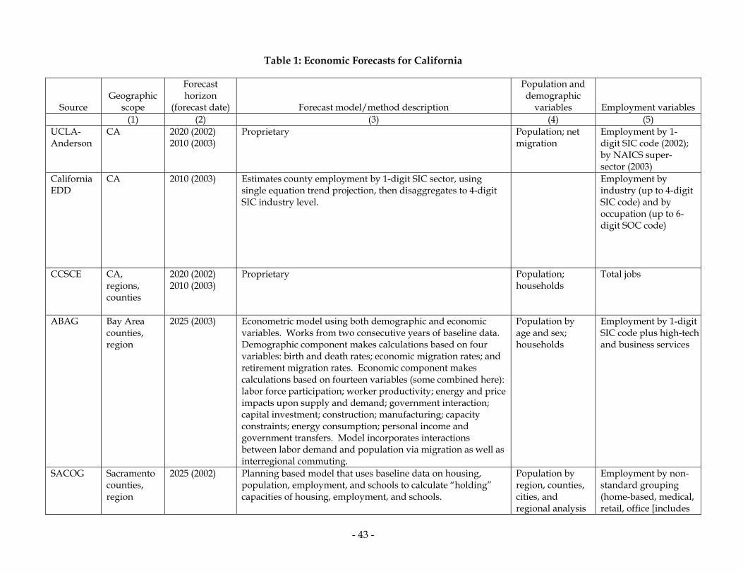
Source

Geographic

scope

Forecast horizon

(forecast date)

Forecast model/method description

Population and demographic

variables

Employment variables (1) (2) (3) (4) (5)

UCLA- Anderson

CA

2020 (2002) 2010 (2003)

Proprietary Population; net migration

Employment by 1-digit SIC code (2002); by NAICS super-sector (2003)

CaliforniaEDD

CA 2010 (2003) Estimates county employment by 1-digit SIC sector, using single equation trend projection, then disaggregates to 4-digit SIC industry level.

Employment by industry (up to 4-digit SIC code) and by occupation (up to 6-digit SOC code)

CCSCE

CA, regions, counties

2020 (2002) 2010 (2003)

Proprietary Population; households

Total jobs

ABAG

Bay Area counties, region

2025 (2003) Econometric model using both demographic and economic variables. Works from two consecutive years of baseline data. Demographic component makes calculations based on four variables: birth and death rates; economic migration rates; and retirement migration rates. Economic component makes calculations based on fourteen variables (some combined here): labor force participation; worker productivity; energy and price impacts upon supply and demand; government interaction; capital investment; construction; manufacturing; capacity constraints; energy consumption; personal income and government transfers. Model incorporates interactions between labor demand and population via migration as well as interregional commuting.

Population by age and sex; households

Employment by 1-digit SIC code plus high-tech and business services

SACOG

Sacramento counties, region

2025 (2002) Planning based model that uses baseline data on housing, population, employment, and schools to calculate “holding” capacities of housing, employment, and schools.

Population by region, counties, cities, and regional analysis

Employment by non-standard grouping (home-based, medical, retail, office [includes

Table 1: Economic Forecasts for California

- 43 -

- 44 -

Source

Geographic

scope

Forecast horizon

(forecast date)

Forecast model/method description

Population and demographic

variables

Employment variables (1) (2) (3) (4) (5)

districts; school-age population by levels

non-medical service workers], manufacturing, and other)

SANDAG

San Diego region, local areas

2025 (2003) Econometric model consisting of four related sub-models with feedback mechanisms between each: a demographic and economic forecasting model; an interregional commuting model; a cities/county urban development forecast model; and a transportation forecast model. All models use baseline data from 2000. The demographic and economic forecasting model uses a cohort survival model to forecast population by age, sex, and ethnicity, and also takes into account in- and out-migration. The economic component of the model is based on the general U.S. economy. The interregional commuting model predicts the residential location of workers inside and outside of the region. The urban development model is a land use model. The transportation model forecasts travel activity and transportation needs.

Population by age, gender, ethnic group; labor force

Total civilian and military employment

SCAG

Southern California region and counties

2030 (2004)

2020 (2002)

A projection (extrapolation) model that uses total number of jobs, population, and labor force participation rates to forecast future employment. National and regional data are used to compute future projections.

Population by region and counties

Employment by 1-digit SIC code for region (2020 forecast only)

DOT CA counties

2020 (2004) Econometric model including 70 California economic and demographic variables (from UCLA-Anderson Forecast), 22 national economic variables (from UCLA-Anderson Forecast), and 10 local county demographic variables from DOF. 35 stochastic equations and 20 deterministic equations (identities).

Population

Employment by 1-digit SIC code

SIC: Standard Industrial Classification NAICS: North American Industry Classification System SOC: Standard Occupational Classification The most recent SCAG forecast posted includes numbers from SCAG’s 1998 regional transportation plan (RTP). 2001 and draft 2004 RTPs are posted, but with very limited economic forecast information, and no detail about employment by industry. EDD’s initial forecasts are evaluated in light of CCSCE and UCLA-Anderson projections, and discussed with the California Department of Finance before publication. Their forecasts contain a large judgmental component (personal communication with James Booth at the Projections Unit at EDD, January 22, 2004). The documentation for the SACOG forecast is in SACOG (2001).

Table 2: Statewide Forecasts

Population (1000s) Employment (1000s) Forecast 2000 2010 2020 2000 2010 2020 Economic forecasts (1) (2) (3) (4) (5) (6) UCLA-Anderson (2002)

34,117 39,957 45,850 14,487 (payroll employment)

17,461

20,412

Percent change from 2000

17 34 21 41

UCLA-Anderson (2003)

34,036 39,670 14,488 (payroll employment)

16,711

Percent change from 2000

17 15

California EDD (2003)

14,488 (payroll employment)

17,709

Percent change from 2000

22

CCSCE (2002) 34,100 39,700 44,500 16,300 (total employment)

20,100 21,800

Percent change from 2000

16 30 23 34

CCSCE (2003) 33,872 39,710 16,200 (total employment)

19,090

Percent change from 2000

17 18

DOT aggregated counties (2004)

34,046 39,726 45,684 14,590 (payroll employment)

16,440

19,293

Percent change from 2000

17 34 13 32

Population forecasts DOF (2004a) 34,065 39,247 43,852 Percent change

from 2000 15 29

PPIC low alternative 34,065 38,469 42,197 Percent change

from 2000 13 24

PPIC high alternative

34,065 40,030 45,521

Percent change from 2000

18 34

The figures in the last row are population forecasts, included for purposes of comparison; they are reported in Johnson (2005). “Payroll employment” generally excludes self-employed, unpaid family workers, and household workers.

- 45 -

Table 3: Regional Employment Forecasts, Level and Percentage Change from 2000

Forecast 2000 2010 2020 2025 2030 (1) (2) (3) (4) (5) ABAG (2003) SF Bay Area

3,606 3,964 10%

4,544 26%

4,983 38%

DOT (2004) county forecasts, SF Bay Area

3,542 3,706 5%

4,271 21%

SACOG (2002) Sacramento region (6 county)

849 1,096 29%

1,295 52%

1,360 60%

DOT (2004) county forecasts, SACOG region

849 1,023 20%

1,176 39%

SANDAG (2003) San Diego region

1,385 1,529 10%

1,673 21%

1,824 32%

DOT (2004) county forecasts, San Diego county

1,205 1,487 23%

1,825 51%

SCAG (2004) Los Angeles region

10,527 38%

SCAG (2002) Los Angeles region

7,441 9,018 21%

10,574 42%

DOT (2004) county forecasts, SCAG region

6,830 7,723 13%

9,075 33%

DOT (2004) county forecasts, North Coast and Mountains

226 269 19%

312 38%

DOT (2004) county forecasts, Central Coast

565 629 11%

726 28%

DOT (2004) county forecasts, Upper Sacramento Valley

167 200 20%

231 39%

DOT (2004) county forecasts, San Joaquin Valley

1205 1403 16%

1677 39%

Note that the 2004 SCAG forecast contains no detail on the interim years. Also note that the SCAG and DOT-SCAG forecasts are computed for differing geographic regions. For the 2030 SCAG forecast, the percentage change is calculated relative to the 2000 numbers in SCAG (2002). Employment definitions are as follows: ABAG and SCAG—total employment; SACOG, SANDAG, and DOT—non-farm employment. The SANDAG forecast is limited to civilian jobs.

- 46 -

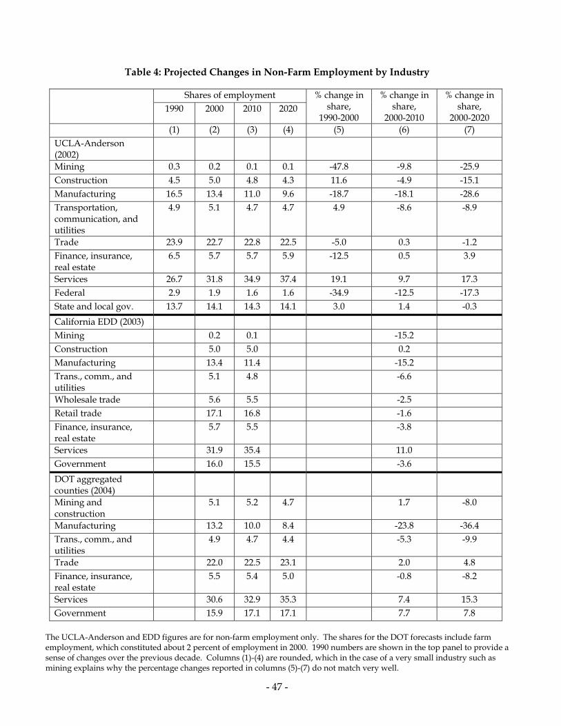
Table 4: Projected Changes in Non-Farm Employment by Industry

Shares of employment 1990 2000 2010 2020

% change in share,

1990-2000

% change in share,

2000-2010

% change in share,

2000-2020 (1) (2) (3) (4) (5) (6) (7) UCLA-Anderson (2002)

Mining 0.3 0.2 0.1 0.1 -47.8 -9.8 -25.9 Construction 4.5 5.0 4.8 4.3 11.6 -4.9 -15.1 Manufacturing 16.5 13.4 11.0 9.6 -18.7 -18.1 -28.6 Transportation, communication, and utilities

4.9 5.1 4.7 4.7 4.9 -8.6 -8.9

Trade 23.9 22.7 22.8 22.5 -5.0 0.3 -1.2 Finance, insurance, real estate

6.5 5.7 5.7 5.9 -12.5 0.5 3.9

Services 26.7 31.8 34.9 37.4 19.1 9.7 17.3 Federal 2.9 1.9 1.6 1.6 -34.9 -12.5 -17.3 State and local gov. 13.7 14.1 14.3 14.1 3.0 1.4 -0.3 California EDD (2003) Mining 0.2 0.1 -15.2 Construction 5.0 5.0 0.2 Manufacturing 13.4 11.4 -15.2 Trans., comm., and utilities

5.1 4.8 -6.6

Wholesale trade 5.6 5.5 -2.5 Retail trade 17.1 16.8 -1.6 Finance, insurance, real estate

5.7 5.5 -3.8

Services 31.9 35.4 11.0 Government 16.0 15.5 -3.6 DOT aggregated counties (2004)

Mining and construction

5.1 5.2 4.7 1.7 -8.0

Manufacturing 13.2 10.0 8.4 -23.8 -36.4 Trans., comm., and utilities

4.9 4.7 4.4 -5.3 -9.9

Trade 22.0 22.5 23.1 2.0 4.8 Finance, insurance, real estate

5.5 5.4 5.0 -0.8 -8.2

Services 30.6 32.9 35.3 7.4 15.3 Government 15.9 17.1 17.1 7.7 7.8

The UCLA-Anderson and EDD figures are for non-farm employment only. The shares for the DOT forecasts include farm employment, which constituted about 2 percent of employment in 2000. 1990 numbers are shown in the top panel to provide a sense of changes over the previous decade. Columns (1)-(4) are rounded, which in the case of a very small industry such as mining explains why the percentage changes reported in columns (5)-(7) do not match very well.

- 47 -

Table 5: Four Experts’ Views on Threats to the Forecasts

Unanticipated development

Likely major effects for California

International economic relations

End of globalization

● Reductions in demand facing high-tech industries. ● Slowing of port traffic, affecting dockworkers and logistics and

trucking industries. ● Increases in wholesale and retail prices. ● Declines in stock markets globally harming retirement prospects.

Development of cheap, alternative fuel

● Moderation of inflation pressures, or deflation. ● Declining transportation costs, spurring rise in travel or new

transportation modes, but increasing congestion. ● Potential economic and political difficulties in oil-exporting

countries, including Mexico and Venezuela, which could increase migration to United States.

● Economic gains for Asian producers, leading to more trade with Asia but also more competition from lower-priced manufactured goods.

Dramatic Mexican economic success

● Slowdown or halt to illegal immigration, harming industries such as agriculture, personal services, and restaurants, that rely on illegal labor, but reducing public spending on services for illegal immigrants. Possibly even reverse migration of immigrants from United States back to Mexico.

● Increasing trade between Mexico and United States as income levels converge, benefiting export-oriented industries but increasing competitive pressure on other industries, boosting growth, lowering prices, and increasing border congestion.

Elimination of industrial and agricultural tariffs

● Open up new markets for California exporters, especially in agriculture, but also increase competition faced by agriculture and other industries from imports.

● Lower input prices for other producers, leading to efficiency gains, and lower prices for consumers.

● Possible large transitional costs for industries harmed by increased trade.

● Likely increase in wages and employment prospects for more-educated workers, and declines in opportunities for less-educated workers.

Technological change

Deepening of Internet technology

● Change how and where people work, with large increases in work on-line from home or other locations, implying changes in commuting patterns that should reduce burden on physical infrastructure.

● More e-learning and long-distance education will increase efficiency of use of educational infrastructure.

● Require incorporating “information highway system” into definition of physical infrastructure.

Advancement of biotechnology

● Genetic engineering will lead to health increases and reductions in mortality, and increased agricultural production.

- 48 -

- 49 -

Unanticipated development

Likely major effects for California

Commercialization of nanotechnology

● State’s lead in nanotechnology implies that rapid commercialization of this technology can substantially broaden range of possible scenarios regarding both level of economic activity and its industrial composition, as well as skill composition of workforce.

Political decisions

Infrastructure investment directed to manufacturing industries

● Disadvantage emerging non-manufacturing sectors.

Changes in immigration policy

● Restrictions or expansions of immigration can lead to different population growth scenarios, including projected skill composition of the workforce.

Excessive focus on infrastructure-population relationship

● Insufficient attention to repair and maintenance of existing infrastructure.

● Insufficient attention to improving infrastructure technology.

Infrastructure investment and utilization

Economic growth depends in part on infrastructure investment

● Insufficient infrastructure investment could lead to lower economic growth, although evidence linking growth to infrastructure is subject to debate, and the effect is probably more incremental than absolute.

● Dependence of growth on infrastructure investment may be overstated because infrastructure use is adaptive, as businesses, workers, and others adjust behavior in response to congestion problems and other infrastructure shortages.

● Infrastructure may be more important as a determinant of quality of life than of economic growth, as witnessed by high-growth, low-infrastructure cities such as Seoul, Bangkok, and Mexico City.

See Appendices A-D for detailed discussions of threats to the forecasts.

Table 6: Employment Versus Population Growth, Forecasted Percentage Changes, by Regions and Other County Aggregations

2000-2010 2000-2020 2000-2025/2030 Population forecast: DOF COG/DOT DOF COG/DOT DOF COG/DOT

Empl.

Pop. Empl. –

Pop.

Pop. Empl. –

Pop.

Empl.

Pop. Empl. –

Pop.

Pop. Empl. –

Pop.

Empl.

Pop. Empl. –

Pop.

Pop. Empl. –

Pop. (1) (2) (3) (4) (5) (6) (7) (8) (9) (10) (11) (12) (13) (14) (15) ABAG SF Bay Area, COG

10 11 -1 11 -1 26 23 3 20 6 38 (2025)

29 9

25 13

ABAG SF Bay Area, DOT

5 11 -6 10 -5 21 23 -2 20 1

SACOG Sacramento region, COG

29 27 2 24 5 52 58 -6 43 9 60 (2025)

73 -13

49 11

SACOG Sacramento region, DOT

20 27 -7 25 -5 39 58 -19 47 -8

SANDAG San Diego region, COG

10 15

-5 14

-4 21 28

-7 25

-4 32 (2030)

35 -3

37 -5

SANDAG San Diego region, DOT

23 15 8 17 6 51 28 23 37 14

SCAG Los Angeles region, COG (2002)

21 15 6 15 6 42 25 17 31 11

SCAG Los Angeles region, COG (2004)

38 (2030)

35 3

SCAG Los Angeles region, DOT

13 15 -2 18 -5 33 25 8 36 -3

North Coast and Mountains, DOT

19 9 10 12 7 38 18 20 26 12

Central Coast, DOT 11 10 1 12 -1 28 20 8 28 0 Upper Sacramento Valley, DOT

20 14 6 15 5 39 30 9 33 6

San Joaquin Valley, DOT

16 23 -7 24 -8 39 50 -11 49 -10

The employment figures for COGs are based on COG projections or aggregated county-level DOT forecasts, as indicated. The employment figures for other county aggregations are based on aggregated county-level DOT forecasts. The DOF population entries are the disaggregated figures corresponding to the aggregate DOF forecasts reported in Table 2. The COG/DOT forecasts are from their economic forecasts. The end year for the last set of forecasts (in the final five columns) are given in column (11). For SCAG, the economic forecasts pertain to the Los Angeles region, while the population forecasts are for the entire region. For the 2030 SCAG forecast, there are no corresponding DOT forecasts, and the percentage changes for 2030 are calculated relative to the 2000 numbers in SCAG (2002).

- 50 -

Fastest-declining employment shares

Fastest-growing employment share

Mining

Construction

Manufacturing

Trade

Finance, insurance, and real estate

Services

Government

(1) (2) (3) (4) (5) (6) (7) Railroads and related services; passenger ground transportation

.010 .005 .009 .003 .002 .003 .010

Motor freight transportation and warehousing

.019 .038 .043 .011 .009 .013 .031

Water transportation .006 .002 .003 .001 .000 .001 .014 Air transportation .007 .006 .010 .007 .004 .007 .014 Pipelines, freight forwarders, and related services

.003 .003 .005 .003 .001 .003 .005

Communications, except radio and TV

.012 .015 .015 .028 .019 .022 .014

Radio and TV broadcasting .002 .002 .006 .010 .003 .005 .000 Electric services (utilities) .023 .009 .019 .013 .005 .011 .031 Gas production and distribution (utilities)

.053 .006 .014 .004 .002 .004 .036

Water and sanitary services .002 .001 .002 .001 .001 .001 .004 Federal government enterprises

.004 .005 .005 .009 .013 .009 .411

State and local government enterprises

.015 .005 .009 .006 .004 .006 .618

Input requirements are calculated from 1999 national input-output industry requirements table for two-digit industries. Industry input-output coefficients are aggregated weighting by share of two-digit industry in one-digit industry output, based on industry use table for two-digit industries. (See www.bea.gov.)

Table 7: Input Requirements from Transportation, Communications, and Utilities and Government Enterprises for Output from Other One-Digit Industries

- 51 -

Table 8: Implications of Industrial Composition of Employment for Educational Levels of Non-Farm Workers in California in 2000, 2010, and 2020

Based on UCLA-Anderson forecast

Based on EDD forecast

PPIC population forecasts, 25-64

year-olds

2000 2010 2020

2000 – 2010: % change in

share

2000 – 2020: % change in

share

2000 – 2010: % change in

share

2000 – 2020: % change in

share

2000 – 2020: % change in

share (1) (2) (3) (4) (5) (6) (7) (8)

“Static”

Less than high school diploma 14.0 13.7 13.5 -1.9 -3.6 -1.4 -4.4 21.3

High school diploma 22.1 21.8 21.6 -1.2 -2.2 -1.0 -1.1 5.3

Some college 23.5 23.5 23.6 0.2 0.2 -0.3 0.7

AA degree 10.1 10.1 10.1 0.3 0.4 -0.2 0.9 -7.7

BA, AB, BS degree 20.6 20.8 21.0 1.0 2.0 0.7 1.0

MA, PhD, or professional 9.7 10.0 10.2 2.8 5.1 2.8 3.5

-11.4

“Dynamic”

Less than high school diploma 14.2 12.8 11.4 -10.0 -19.9 -9.2 -18.2 -1.8

High school diploma 22.9 18.4 14.3 -19.6 -37.8 -19.4 -39.0 -9.1

Some college 23.5 23.6 23.7 0.6 0.8 0.0 2.7

AA degree 9.9 10.9 11.8 10.3 19.5 9.5 18.3 -10.3

BA, AB, BS degree 20.0 23.2 26.4 16.0 31.9 15.7 29.9

MA, PhD, or professional 9.5 11.0 12.4 16.4 31.6 16.3 31.6

19.3

Columns (1)-(7) are based on the economic forecasts. Figures for 2000 are based on the educational distribution of each industry in monthly CPS files for 1992 and 2002. In the static exercise, these are based on the 2002 educational distribution, and in the dynamic exercise the 2000 distribution is linearly interpolated from the 1992 and 2002 distributions. Figures for 2010 and 2020 are based on forecasts of employment by industry, coupled with the educational distribution of workers in each industry in 2002. In the bottom panel, there is an additional adjustment for the trend in the education level of workers in each industry from 1992 to 2002, which is applied to the subsequent years. If a trend projected a negative number of workers with a given educational level in an industry, that number was set to zero, and the additional workers implicitly added to that cell were removed from the other educational categories in that industry in proportion to their representation. PPIC population forecasts in column (8) are from Johnson (2005). The population forecasts are for somewhat more aggregated educational attainment categories.

- 52 -

- 53 -

Table 9: Educational Levels Across Industries and Trends Within Industries

Less than high school diploma

High school diploma

Some college

AA degree

BA, AB, BS degree

MA, PhD, or professional

(1) (2) (3) (4) (5) (6) 2002 share Mining 17.7 24.1 13.8 20.8 18.8 4.9 Construction 27.2 36.3 20.2 7.2 7.3 1.8 Manufacturing 21.0 24.8 18.2 8.4 19.8 7.7 Trans., comm., and utilities 9.9 29.0 26.6 11.4 17.8 5.8

Trade 21.1 29.0 25.9 7.3 14.3 2.5 Finance, insurance, real estate 5.1 19.6 28.3 10.4 28.1 8.5

Services 11.2 17.5 20.6 9.7 25.0 15.9 Public administration 4.0 13.3 28.8 16.3 24.1 13.6

1992-2002 % change in share

Mining 3.0 -46.0 -41.3 556.5 304.9 -29.3 Construction 11.3 -3.3 -10.6 15.5 0.4 -6.8 Manufacturing -17.9 -10.8 -1.4 34.2 23.5 33.6 Trans., comm., and utilities -16.4 -3.3 -6.2 1.7 15.2 53.6

Trade -1.9 -10.0 0.5 12.7 23.8 -1.9 Finance, insurance, real estate -2.7 -21.5 4.0 14.5 6.5 19.1

Services -16.0 -18.4 -0.2 10.9 19.4 7.6 Public administration 32.7 -38.8 6.3 2.8 9.2 31.5

Figures are from monthly CPS files for 1992 and 2002.

Table 10: Educational Levels and Changes by Services Subsector

Share of Services

Employment Share in Each Educational Category

Less than high school diploma

High school diploma

Some college

AA degree

BA, AB, BS degree

MA, PhD, or professional

(1) (2) (3) (4) (5) (6) (7) 2002 share Business and repair services 22.1 17.5 21.8 20.7 8.4 23.8 7.9

Personal services, incl. private household

9.6 30.0 26.0 20.2 11.1 10.3 2.4

Entertainment and recreation services 8.7 11.0 20.8 25.0 6.4 29.3 7.5

Professional and related services 59.6 6.0 14.1 20.0 10.5 27.1 22.2

1992-2002 change in share

Business and repair services 0.8 -0.1 -7.9 -1.3 0.0 6.6 2.8

Personal services, incl. private household

-2.7 -3.7 -2.5 1.4 4.2 -0.7 1.3

Entertainment and recreation services 1.5 -5.8 2.5 -3.1 -0.3 5.1 1.6

Professional and related services 0.4 -1.2 -3.4 0.8 2.2 7.7 0.3

Figures are from monthly CPS files for 1992 and 2002.

- 54 -

Table 11: Projected Changes in Employment by Industry, Percentage Change in Share, 2000-2020, by COG Regions and

Other County Aggregations

Statewide

ABAG

SACOG

SANDAG

SCAG

North Coast and Mountains

Central Coast

Upper Sacramento

Valley San Joaquin

Valley (1) (2) (3) (4) (5) (6) (7) (8) (9) Mining and construction -8.0 -5.6 -10.2 -6.4 -8.5 -10.6 -4.9 -11.0 -12.9

Manufacturing -36.4 -42.7 -18.4 -27.4 -37.7 -36.4 -26.2 -30.3 -20.8

Trans., comm., and utilities -9.9 -19.0 -13.8 -18.7 -4.1 -11.5 -19.1 -22.5 1.6

Trade 4.8 9.9 -4.8 -0.4 4.6 -3.7 4.6 5.8 6.7

Finance, insurance, real estate -8.2 -9.8 -17.5 -7.2 -10.2 7.0 3.4 39.5 14.0

Services 15.3 17.1 16.1 12.5 15.6 12.0 4.9 7.1 23.6

Government 7.8 2.0 2.7 4.7 8.2 10.3 14.3 4.2 13.3

All calculations are based on DOT employment forecasts.

- 55 -

- 56 -

Table 12: Implications of Industrial Composition of Employment for Educational Levels of Workers in California, Statewide and by COG Regions and Other County Aggregations, Percentage Change in Share in Each Educational Level

2000-2020

Statewide

ABAG

SACOG

SANDAG

SCAG

North Coast and Mountains

Central Coast

Upper Sacramento

Valley San Joaquin

Valley (1) (2) (3) (4) (5) (6) (7) (8) (9) “Static”: fixed education within industry

Less than high school diploma -5.7 -3.3 -3.7 -3.9 -4.7 -8.4 -7.8 -6.9 -15.7

High school diploma -2.0 -1.8 -2.3 -2.0 -2.1 -3.1 -1.8 -1.4 -1.7

Some college 1.1 0.8 -0.3 0.3 1.1 1.3 1.8 1.6 3.8

AA degree 1.7 0.4 0.9 1.0 1.4 3.0 3.1 1.6 6.3

BA, AB, BS degree 1.8 1.1 1.7 1.6 1.4 2.7 2.3 2.5 7.0

MA, PhD, or professional 5.1 4.4 5.1 4.5 4.8 5.8 4.2 3.3 11.5

“Dynamic”: trend education within industry

Less than high school diploma -20.8 -19.6 -14.7 -18.3 -20.7 -18.6 -21.4 -19.1 -29.0

High school diploma -37.7 -36.6 -42.6 -38.8 -37.1 -44.7 -37.9 -39.1 -37.3

Some college 2.8 1.3 2.1 1.4 2.0 4.8 7.6 5.0 10.1

AA degree 20.5 20.0 16.7 19.6 20.8 18.2 20.8 18.6 24.4

BA, AB, BS degree 31.8 31.4 29.1 31.0 31.6 30.3 32.7 31.6 38.9

MA, PhD, or professional 31.4 28.9 34.6 30.5 31.0 36.7 30.1 30.5 40.8

All calculations are based on DOT employment forecasts. See notes to Table 8 for description of calculations. Information on education distributions and trends is at the state level, not the county or COG level.

Table 13: Implications of Industrial Composition of Employment for Educational Levels of Non-Farm Workers in California and United States

California United States

2000 – 2010: % change in share in each

education level

2000 – 2020: % change in share in each

education level

2000 – 2010: % change in share in each

education level

2000 – 2020: % change in share in each

education level

(1) (2) (3) (4) “Static”: fixed education within industry

Less than high school diploma -1.9 -3.6 -0.1 -0.4

High school diploma -1.2 -2.2 -0.2 -0.9

Some college 0.2 0.2 0.1 0.1

AA degree 0.3 0.4 -0.1 0.1

BA, AB, BS degree 1.0 2.0 -0.1 0.4 MA, PhD, or professional 2.8 5.1 0.0 1.6

“Dynamic”: trend education within industry

Less than high school diploma -10.0 -19.9 -14.3 -28.6

High school diploma -19.6 -37.8 -14.3 -29.1

Some college 0.6 0.8 -0.1 -0.5

AA degree 10.3 19.5 21.1 42.1

BA, AB, BS degree 16.0 31.9 17.1 34.9 MA, PhD, or professional 16.4 31.6 11.9 25.7

The first two columns repeat the numbers from UCLA-Anderson forecast from Table 8. The last two columns present the same calculation, but for the UCLA-Anderson national forecast, and national data on educational levels and trends.

- 57 -

Table 14: Forecasted Changes in Employment by Industry, SIC

UCLA-Anderson, California

(2002)

UCLA-Anderson, United States

(2002)

BLS, United States

% change in share,

1990-2000

% change in share,

2000-2010

% change in share,

2000-2020

% change in share,

1990-2000

% change in share,

2000-2010

% change in share,

2000-2020

% change in share,

2000-2010 (1) (2) (3) (4) (5) (6) (8) Mining -47.8 -9.8 -25.9 -36.4 -15.0 -23.1 -33.3 Construction 11.6 -4.9 -15.1 7.9 8.2 2.9 -2.2 Manufacturing -18.7 -18.1 -28.6 -19.6 -9.1 -14.5 -11.4 Trans., comm., and utilities

4.9 -8.6 -8.9 1.1 5.0 -3.8 2.0

Trade -5.0 0.3 -1.2 -2.4 0.9 2.0 -3.5 Finance, insurance, real estate

-12.5 0.5 3.9 -6.2 3.5 3.6 -6.1

Services 19.1 9.7 17.3 20.3 0.6 4.7 13.2 Federal -34.9 -12.5 -17.3 -25.2 -13.6 -15.8 -18.8 State and local gov.

3.0 1.4 -0.3 -2.2 2.0 2.5 -4.2

First three columns repeat those in Table 4 for California. BLS projections are from Berman (2001).

- 58 -

- 59 -

Table 15: Forecasted Changes in Employment by Industry, Later Forecasts, NAICS

UCLA-Anderson, California (2003)

UCLA-Anderson, United States (2003)

BLS, United States

% change in share, 2000-2010

% change in share, 2000-2010

% change in share, 2002-2012

(1) (2) (3) Natural resources and mining -46.7 -23.6 -24.4 Construction 1.9 10.5 -1.2 Manufacturing -26.8 -23.7 -15.0 Trans., warehousing, and util. -4.4 6.3 1.6 Trade -1.2 -7.9 -2.9 Financial activities -11.3 -0.0 -3.6 Information 0.7 -5.8 1.7 Professional and business serv. 8.4 18.6 11.9 Education and health serv. 18.6 12.3 13.1 Leisure and hospitality serv. 5.4 4.0 1.1 Other serv. 6.3 -0.9 -0.7 All services 13.7 8.9 8.2 Federal -8.5 -11.5 -13.8 State and local gov. 3.7 0.9 -2.6

BLS projections are from Horrigan (2004).

PUBLIC POLICY INSTITUTE OF CALIFORNIA

Board of Directors

Thomas C. Sutton, Chair Chairman and Chief Executive Officer Pacific Life Insurance Company

Linda Griego President and Chief Executive Officer Griego Enterprises, Inc.

Edward K. Hamilton Chairman Hamilton, Rabinovitz & Alschuler, Inc.

Gary K. Hart Founder Institute for Education Reform California State University, Sacramento

Walter B. Hewlett Director Center for Computer Assisted Research in the Humanities

David W. Lyon President and Chief Executive Officer Public Policy Institute of California

Ki Suh Park Design and Managing Partner Gruen Associates

Constance L. Rice Co-Director The Advancement Project

Raymond L. Watson Vice Chairman of the Board Emeritus The Irvine Company

Carol Whiteside President Great Valley Center

Advisory Council

Stuart A. Gabriel Director and Lusk Chair Lusk Center for Real Estate University of Southern California

Clifford W. Graves

Elizabeth G. Hill Legislative Analyst State of California

Hilary W. Hoynes Associate Professor Department of Economics University of California, Davis

Andrés E. Jiménez Director California Policy Research Center University of California Office of the President

Norman R. King Director, University Transportation Center California State University, San Bernardino

Dean Misczynski Director California Research Bureau

Rudolf Nothenberg Chief Administrative Officer (Retired) City and County of San Francisco

Manuel Pastor Professor, Latin American & Latino Studies University of California, Santa Cruz

Peter Schrag Contributing Editor The Sacramento Bee

James P. Smith Senior Economist RAND Corporation

PUBLIC POLICY INSTITUTE OF CALIFORNIA 500 Washington Street, Suite 800 San Francisco, California 94111 Phone: (415) 291-4400 Fax: (415) 291-4401 www.ppic.org info@ppic.org