1

Box 1.1: Highlights of this report

The Northeast Pacific was dominated by the “warm blob”: record high sea surface temperatures that developed in the Gulf of Alaska and spread to the coast and southward.

Basin-wide indices trended from ENSO-neutral toward mild El Niño in the MEI, and the PDO and NPGO both shifted from conditions promoting high primary productivity to less productive conditions.

After a record strong year of coastal upwelling, conditions in 2014 returned to average or slightly below average upwelling. Coupled with the basin scale indices, this would suggest lower primary productivity.

After several relatively productive years, biomass of energy-rich northern copepod species declined sharply in the fall of 2014.

Several components of the forage base showed stable or high abundance in spring surveys in 2013 and 2014; it is unknown if the forage base has responded to the oceanographic changes outlined above.

Central Valley and Lower Columbia Chinook salmon have negative 10-year escapement trends, while trends elsewhere are stable or positive.

There are presently only 3 assessed groundfish that are in an “overfished” status (canary rockfish, yelloweye rockfish, Pacific ocean perch), and no recent indication of overfishing on groundfish.

Following an unusual mortality event (UME) of California sea lion pups in 2013, survival improved in 2014; however, pup weights are once again below average and another UME may be under way in 2015.

Although biomass trends of seabirds in the southern CCE have been stable or increasing, a large-scale mass mortality of Cassin’s auklets has been occurring since late 2014.

Commercial fishery landings increased from 2009-2013, driven largely by Pacific hake and coastal pelagic species; crab and shrimp landings also increased.

Diversification of fishing vessels continued its long-term decline throughout much of the fleet, which may indicate greater risk of highly variable annual revenue.

There is some evidence that catch shares have increased vessel safety in the fixed gear sablefish fleet.

CALIFORNIA CURRENT INTEGRATED ECOSYSTEM ASSESSMENT (CCIEA) STATE OF THE CALIFORNIA CURRENT REPORT, 2015

A report of the CCIEA Team (NOAA Northwest, Southwest and Alaska Fisheries Science Centers) to the Pacific Fishery Management Council, March 8, 2015

1 INTRODUCTION

Section 1.4 of the 2013 Fishery Ecosystem Plan (FEP) outlines a reporting process wherein NOAA provides the Council with a yearly update on the state of the California Current Ecosystem (CCE), as derived from environmental, biological and socio-economic indicators. NOAA’s California Current Integrated Ecosystem Assessment (CCIEA) team is responsible for this report. This marks our 3rd such report, with prior reports in 2012 and 2014.

The highlights of this report are summarized in Box 1.1. Sections below provide greater detail. In addition, a list of supplemental materials is provided at the end of this document, in response to previous requests from Council members or the Scientific and Statistical Committee (SSC) to provide additional information, or to clarify details within this short report.

2

1.1 NOTES ON INTERPRETING TIME SERIES FIGURES

Throughout this report, time series figures follow common formats, illustrated in Figure 1.1 for ease of interpretation; see the figure caption for details. Data in the most recent 5 years of the time series (indicated by green shaded areas) are the focus of status and trend analyses. Most plots show annual mean values relative to long-term means and standard deviations (s.d.). Where possible, we have added shaded areas (Fig. 1.1, right) that represent fitted estimates plus 95% confidence intervals, derived from a Multivariate Auto-Regressive State Space (MARSS) model. The addition of MARSS outputs follows the guidance of the SSC Ecosystem Subcommittee (SSCES; see advisory body reports at Agenda Item E.1.b., March 2015). In coming years we hope to include fits and error estimates for all indicator time series.

1.2 SAMPLING LOCATIONS

Figure 1.2 shows the CCE and major headlands that demarcate key biogeographic boundaries, in particular Cape Mendocino and Point Conception. We generally consider the region north of Cape Mendocino to be the “Northern CCE,” the region between Cape Mendocino and Point Conception the “Central CCE,” and the region south of Point Conception the “Southern CCE.” Points on the map indicate sampling locations for much of the regional oceanographic data (Section 3.2), zooplankton data (Section 4.1), and seabird data (Section 4.6) presented in this report. Sampling locations for other data are described within the sections of the report or in the Supplementary Materials.

Figure 1.1: Sample time series plots. Horizontal lines show the mean (dashed line) ± 1.0 s.d. (solid lines) of the full time series. Symbol at upper right indicates whether data over the last 5 years (green shaded areas) had a positive trend (), a negative trend (), or no trend (↔). Symbol at lower right indicates whether the mean over the past 5 years was greater than (), less than (–), or within 1 s.d. () of the mean of the full time series. Data points are annual means; the right panel also includes a fit with 95% confidence intervals, generated by a Multivariate Auto-Regressive State Space (MARSS) model (gray shaded area).

Figure 1.2. California Current Ecosystem (CCE), with key geographic features and oceanographic sampling locations labeled.

3

2. CONCEPTUAL MODELS OF THE CALIFORNIA CURRENT

The CCE is a socio-ecological system in which human and naturally occurring components and processes are inextricably linked. Recognizing ecosystem links is critical to understanding the dynamics of the CCE and to managing different resources, benefits and ecosystem services in an informed manner. We have developed a series of conceptual models to assist in prioritizing these links and communicating their importance to others.

Figure 2.1 shows a series of conceptual models developed specifically for groundfish in the CCE. The models provide simplified overviews and brief narratives of how environmental drivers, ecological interactions, and human activities affect different stages of groundfish life histories. The benefits of these conceptual models are multifold:

They facilitate discussion around which issues are thought to be most important in the CCE.

They can be readily simplified or made more in-depth and complex as desired.

Each box or line represents an ecosystem component or process that corresponds to one or more indicators that we are tracking; thus, the models help us put indicators into context.

Figure 2.1. Conceptual models of CCE groundfish in relation to their physical environments and habitats (upper left); their interactions with prey, predators, competitors and other members of their communities (upper right); and their interactions with humans (lower left). Models are presented in greater detail in the Supplementary Materials.

Similar models are available for other CCE components (see Supplementary Materials).

(Illustrations by Su Kim, NWFSC.)

4

Relating the focal component (e.g., groundfish in Fig. 2.1) to its linked components and processes may help us anticipate how changes in the ecosystem will affect managed species.

Conceptual models with up-to-date information on status and trends of relevant indicators will provide information for “ecosystem considerations” sections of stock assessments.

They serve as consistent reminders to account for human dimensions and potential management tradeoffs in different human sectors.

Higher-resolution versions of all models are available by contacting Su Kim (Su.Kim@noaa.gov) or Chris Harvey (Chris.Harvey@noaa.gov).

3 CLIMATE AND OCEAN DRIVERS

3.1 BASIN-SCALE CLIMATE INDICATORS

The El Niño/Southern Oscillation (ENSO) is the dominant mode of interannual variability in the equatorial Pacific, and has impacts throughout the Pacific Basin and CCE. There are several ENSO indices; in this report, we use the Multivariate ENSO Index (MEI), which is based on a set of six physical variables from the equatorial Pacific. Positive MEI values represent El Niño conditions, while negative values represent La Niña conditions. El Niño conditions in the CCE are associated with warmer surface water, weaker upwelling winds and lower nutrient availability at the surface; however, the effects of any given ENSO event are highly variable. The last El Niño event was in the winter of 2009/2010, followed by mild La Niña events in the summer of 2010 and the fall of 2011; otherwise the recent MEI index has been neutral (Fig. 3.1). There was speculation in early 2014 that a major El Niño would develop, but the MEI indicated ENSO-neutral conditions in the summer. At the end of the year the MEI was positive (0.578) but still ENSO-neutral.

The Pacific Decadal Oscillation (PDO) is a low-frequency signal of North Pacific sea surface temperatures (SSTs). Cold regimes (negative PDO values) are associated with enhanced productivity in the CCE. During positive PDO regimes, coastal SSTs in the Gulf of Alaska and the CCE tend to be higher, while those in the North Pacific Subtropical Gyre tend to be lower. The PDO values for 2014 were positive, which is a

Figure 3.1. Summer values of the Multivariate ENSO Index (MEI) in the Pacific Basin, 1950-2014. Lines, colors and symbols are as in Figure 1.1. Winter values are presented in the Supplementary materials.

Figure 3.2. Summer values of the Pacific Decadal Oscillation (PDO) index in the Pacific Basin, 1900-2014. Lines, colors and symbols are as in Figure 1.1. Winter values are presented in the Supplementary materials.

5

reversal from the cool regime experienced from the summer of 2010 to December of 2013 (Fig. 3.2). As of December 2014 the PDO value exceeded 2.5, one of the highest values ever measured.

The North Pacific Gyre Oscillation (NPGO) is a low-frequency signal of sea surface height, indicating variations in the circulation of the North Pacific Subtropical Gyre and Alaskan Gyre, which in turn relate to the source waters for the California Current. Positive values of the NPGO are linked with increased equatorward flow in the California Current, along with increased surface salinities, nutrients, and chlorophyll-a values. Negative NPGO values are associated with decreases in such values, inferring less subarctic source waters and generally lower productivity; for example the NPGO was strongly negative during 2005 and 2006, which in turn were associated with record-low levels of juvenile groundfish productivity and seabird reproductive success in parts of the CCE. The NPGO was positive from April 2007 through October 2013, indicating strong circulation in the North Pacific Subtropical Gyre. At the end of 2013 the NPGO switched from the positive values experienced over the previous 7 years to negative values, which resulted in a significant trend over the last five years (Fig 3.3).

The most prominent basin-scale hydrographic development was the highest recorded SSTs (time series 1982-2014) in the Gulf of Alaska, where anomalies were in excess of 1 to 2°C. This anomaly, referred to as the “warm blob,” developed in the summer of 2013 and has continued. Similarly warm waters were south of the Southern California Bight (Fig. 3.4, left). Summer SST anomalies were average to below average along the coast from Washington down to Monterey Bay. While this pattern is reflected in the reversals of the PDO and NPGO, it cannot be explained by the MEI or other climate indices. During the fall of 2014, the warm waters extended south in the northern and central CCE. Although West Coast summer SSTs have been below average (Fig. 3.4, middle), there is a strong summer warming trend in the northeast Pacific over the last five years (Fig. 3.4, right).

Figure 3.3. Summer values of the North Pacific Gyre Oscillation (NPGO) index in the Pacific Basin, 1950-2014. Lines, colors and symbols are as in Figure 1.1. Winter values are presented in the Supplementary materials.

Figure 3.4: Hadley Centre Sea Ice and Sea Surface Temperature (HadISST) SST products. Left: 2014 summer SST anomalies; a black X marks a cell where the 2014 anomaly was a record high. Middle: 2010-2014 summer SST means relative to the long-term s.d. Right: 2010-2014 summer SST trends relative to the long-term s.d. Values for cells in the mean/trend maps have been normalized by the long-term s.d. of the summer time series at that cell. In all maps, a gray dot marks a cell with an anomaly/mean/trend >1 s.d. from the long-term mean.

6

3.2 REGIONAL CLIMATE INDICATORS

Upwelling is critically important to productivity and ecosystem health in the CCE, as local wind fields that drive coastal upwelling ultimately drive primary production at the base of the food web. The most common metric of upwelling is the Bakun Upwelling Index (UI), which is a measure of the magnitude of upwelling anywhere along the coast. The timing, strength, and duration of upwelling in the CCE are highly variable, and are forced by large-scale atmospheric pressure systems. Here, we show plots of the cumulative upwelling index (CUI; Fig. 3.5). The CUI is the cumulative sum of the daily UI starting January 1 and ending on December 31. The CUI provides an estimate of the net influence of upwelling on ecosystem structure and productivity over the course of the year. While this report includes only the CUI, the full CCIEA and other reports often include variables on onset, length, and strength of the upwelling season. Any or all of these indices may relate more appropriately to the productivity of any particular region or population, although as with any climate index, such relationships can be complex. The highest values of the CUI for the entire record (1967-2014) occurred in 2013 for latitudes 39°N and northward. During 2014, upwelling was near the long-term mean for the first half of the year; after June, the CUI was slightly above the long-term mean to the north but slightly below the long-term mean at 33°N. The date of the 2014 spring transition was delayed from the mean date at 39 and 45°N. Despite the delayed 2014 spring transition it should be noted that the strength of the downwelling winds (negative UI) were anomously weak leading up to the spring transition date. The spring transition is defined as the date of the minimum CUI value in the first 150 days of the year.

Low dissolved oxygen (DO) concentrations in CCE coastal and shelf waters are an emerging concern. When DO levels fall below 1.4 ml L-1 (2 mg L-1; 64 μM), the waters are considered to be ‘hypoxic’ with limited oxygen available to organisms. DO concentrations in the ocean are dependent on a number of physical and biological processes, including circulation, ventilation, air-sea exchange, production and respiration. Off Oregon, upwelling transports offshore hypoxic waters onto productive continental shelves, where respiration can reduce water-column DO and thus subject coastal ecosystems to hypoxic or anoxic conditions. Declining DO is a concern for the CCE as it can result in habitat compression for pelagic and benthic species, more severe hypoxic events on

Figure 3.5: Cumulative Upwelling Index (CUI) at three latitudes in the CCE, 1967-2014. Black trend line = long-term mean; gray trend lines = 1967-2009; colored trend lines/symbols = 2010-2014. Dashed vertical lines mark the 2014 spring transition date; solid vertical lines mark the mean spring transition date. Dotted vertical lines mark the end of January, April, July and October.

7

the shelf, and resultant physiological stress or even die-offs for less mobile species. Off southern California, the boundary between oxygenated and hypoxic waters has shoaled in recent years, and DO values have been declining over the past 30 years for water near the core of the California Undercurrent. Figure 3.6 shows DO trends derived from offshore sampling station data at several locations. In the past five years, higher oxygen values have been observed at the offshore California stations (90.90), on top of a long-term declining trend. Nearshore DO values are almost always lower than those offshore (93.30 vs. 90.90). The two inshore stations in Oregon and Southern California had mean values of approximately 2.3 ml L-1 at 150 m. The DO time series presented above are from shelf and offshore waters (50 to 300 km from shore) and may not adequately correlate with nearshore hypoxic events, where Partnership for Interdisciplinary Studies of Coastal Oceans (PISCO) and Regional Association datasets may be more informative.

Ocean acidification (OA) is caused by increased concentration of carbon dioxide (CO2) in seawater, which changes in parallel with atmospheric concentrations. Increasing CO2 lowers pH, which may affect the metabolism or behavior of marine organisms. Increasing CO2 also lowers carbonate ion concentrations, which negatively affects organisms that rely on calcium carbonate for structures or shells (e.g., corals, oysters, urchins, etc.). An important indicator of OA effects is aragonite saturation state, a measure of how corrosive seawater is to organisms with shells made of aragonite (a form of calcium carbonate). Values <1.0 indicate conditions that are corrosive for aragonite, and have been shown to be stressful for many marine species, including oysters, crabs, and pteropods.

At sampling station NH05 off of Newport, OR, aragonite saturations <1.0 are seen throughout the upwelling season, most commonly in July and August (Fig. 3.7). Higher values are seen in winter, when the water column tends to be well mixed by winter storms (see Supplementary material). Conversely, at station NH25, aragonite saturation is always <1.0 at a depth of 150 m. It is noteworthy that water from this depth upwells onto the continental shelf in summer, thus it is the acidity of these source waters that contribute to low aragonite saturation on the continental shelf in summer. There is no clear temporal trend in aragonite saturation; however, we are already seeing

Figure 3.6. Dissolved oxygen (DO) at 150 m depth off of Oregon (Newport Line station NH25) and southern California (CalCOFI stations 93.30 and 90.90). Stations 93.30 and NH25 are <50 km from the shore, while station 90.90 is >300 km from shore. Dashed lines indicate data gaps >6 months. Lines, colors and symbols are as in Figure 1.1.

8

seasonal pulses of acidified water off Oregon and believe that this is of natural origin, caused by the decomposition of organic matter and CO2 release as it sinks toward the seafloor.

4 FOCAL COMPONENTS OF ECOLOGICAL INTEGRITY

4.1 NORTHERN COPEPOD ANOMALY

The northern copepod biomass anomaly time series represents interannual variation in biomass of “cold-water copepod” species, which are rich in wax esters and fatty acids that appear to be essential for pelagic fishes. Northern copepods usually dominate the Washington-Oregon coastal zooplankton community in summer, but this pattern is often altered during El Niño events and/or when the PDO is in a positive (warm) phase, leading to higher biomass of southern copepods that are of lower nutritional quality. Threshold values for the anomaly have not been set, but positive values in summer are correlated with stronger returns of fall and spring ocean-type Chinook salmon to Bonneville dam, and values greater than 0.2 are associated with better survival of coho salmon.

In the summer of 2014, the northern copepod anomaly was relatively high, ~1.0 s.d. above the long-term mean (Fig. 4.1, top). There were no short-term temporal trends. Overall the high anomalies in recent years, especially for the summer data, suggest that ocean conditions were in a generally productive state. However, in the fall of 2014 the northern copepods declined sharply while the southern copepod anomaly increased (Fig. 4.1, bottom), consistent with warm ocean conditions and a bioenergetically depleted state for pelagic fishes.

Figure 4.1. Monthly northern and southern copepod biomass anomalies from 1996-2014 in waters off Newport, OR. Lines, colors and symbols are as in Figure 1.1. Data courtesy of Bill Peterson.

Figure 3.7. Aragonite saturation in summer months off of Newport, OR, 1998-2014. Lines, colors and symbols are as in Figure 1.1. The time series is similar to data in Figure 2.4 because aragonite saturation is calculated in part from DO data.

9

4.2 REGIONAL FORAGE AVAILABILITY

This section describes trends in forage availability, based on research cruises in the central and northern portions of the CCE. These prey species represent a substantial portion of the available forage in the regions over which the cruises sample, and their variability is correlated with predator dynamics and environmental variability. Therefore, we consider these to be regional indices of forage availability and variability, but not indices of overall abundance of these species in the CCE; species abundance indices should derive from formal monitoring programs and stock assessments. Also, the regional forage time series represent different survey methods (e.g., selectivity, timing, frequency, and survey objectives). Therefore, the amplitudes of each time series are not necessarily comparable between regions. Central CCE: The annual geometric means of catch-per-unit effort (CPUE) are shown for seven key pelagic forage groups off of Northern California (Fig. 4.2), including all young-of-the-year (YOY) rockfish, market squid (multiple life stages), adult krill, YOY Pacific sanddab, adult Pacific sardine and adult Northern anchovy. Notably, 2013 and 2014 had among the highest observed densities of juvenile rockfish, sanddab and market squid, following an unusually stable trend of high krill abundance and very low abundance of Pacific sardine and northern anchovy in preceding years. Years associated with such high numbers of YOY groundfish, market squid and krill are generally associated with cooler ocean conditions and high levels of upwelling and productivity, which in turn are associated with greater breeding success and productivity of many of the higher trophic level predators that forage on this assemblage, such as seabirds and salmon. The lower abundance of anchovy and sardine during such years may reflect localized availability (these stocks may be distributed further south and/or offshore during high upwelling conditions) during the period (May-June) in which this survey operates.

Northern CCE: Geometric mean catch rates are shown by year for five key forage groups from Northern California Current (Fig. 4.3), including northern anchovy, Pacific sardine, herring, jack mackerel, and whitebait smelt. In 2014, anchovy and herring CPUE were second and first greatest in the time series respectively. Pacific sardine, jack mackerel, and whitebait smelt were at average

CentralCaliforniaCurrent

Figure 4.2: Geometric means of CPUE for seven forage groups in Central California Current. Lines and shading are as in Figure 1.1.

Central California Current

10

to below-average abundances over the last five years, although the long-term mean of whitebait smelt appears biased by the anomalously high catches in 2001.

4.3 SALMON: CHINOOK SALMON ABUNDANCE

For indicators of the abundance of Chinook salmon populations, we compare the trends in spawning escapement (which incorporates the cumulative effect of natural and anthropogenic pressures) along the CCE to evaluate the coherence in production dynamics, and also to get a more complete perspective of their health across the greater portion of their range. When available, we used the full time series back to 1985; however, some populations only had available data for a shorter time frame (Central Valley Spring starts 1995, Central Valley Winter starts 2001, and Coastal California starts 1991).

Figure 4.4 summarizes information from multiple time series. Generally, California Chinook salmon stocks were within 1 s.d. of their long-term average (since 1985). However, the last decade saw a significant decline in abundance of most California populations examined, with Central Valley Winter Run Chinook salmon at extremely low abundances from 2007-2011. Largely, though, this represents a return to previous values following high escapements in the early 2000s. For the northern Chinook salmon stocks, recent abundances were also close to average, except for a positive deviation for the Snake River Fall Run. There is a notable contrast in recent trends between steep declines in the lower Columbia River and Willamette River stocks and increases in

Figure 4.4. Chinook salmon escapement means and trends. All time series were first normalized to the same scale. “Recent Average” is mean escapement to natural spawning grounds (includes hatchery strays) of the last 10 years relative to the mean of the full time series. “Recent Trend” indicates if escapement increased or decreased significantly in the last 10 years. Dotted lines are ±1.0 s.d.

Northern California Current NorthernCaliforniaCurrent

Figure 4.3: Geometric means of CPUE for five forage groups in Northern California Current. Lines and shading are as in Figure 1.1.

11

the upper Columbia and Snake River stocks. Similar to the California stocks, the observed steep declines follow higher abundances in the early 2000s. This suggests that 10 years may be too short a time frame for evaluating status of these stocks.

4.4 GROUNDFISH

Approximately 1/3 of the managed species within the groundfish fishery management plan (FMP) have been evaluated (either recently or historically) for the overfished threshold based on stock assessment results. Most of the recently assessed groundfish species are above the biomass limit reference point, and are thus not in a depleted “overfished” status, and no overfishing occurred on these stocks prior to their most recent assessments (Fig. 4.5). The three assessed stocks currently in an overfished state are all rockfishes. Pacific hake biomass had recently been below BMSY, but increased sharply since the previous assessment (see the March 2014 CCIEA briefing). Individual trajectories for each stock are available in the stock assessments; the majority (albeit not all) of these species demonstrate stable or increasing abundance trends.

4.5 MARINE MAMMALS

California sea lions are permanent residents of the CCE, breeding on the Channel Islands and feeding throughout the CCE in coastal and offshore habitats. They are sensitive to changes on different temporal and spatial scales, and so are good indicators for the status of upper trophic levels in the CCE. Two particularly sensitive indicators of prey availability are pup production, which relates to prey availability and nutritional status of adult females from October of the previous year to June when pups are born; and pup growth, which is an index of energy transfer from mother to pup and is related to prey availability to adult females during the 11-month lactation period and to survival of pups after weaning.

In March 2013, an Unusual Mortality Event (UME) was declared for California sea lions in Southern California due to unprecedented numbers of pups from the 2012 cohort stranding along the coast between January and March, and poor condition of pups at San Miguel Island and other rookeries during the winter. By the onset of the reproductive season in June 2013, most population indices at San Miguel Island showed signs of improvement. Although the average number of live pups counted at San Miguel Island in July 2013 declined 27% from 2012 (Fig. 4.6, top), the pup growth indices indicated that the condition of dependent pups from the 2013 cohort had improved considerably from 2012. However, pup weights at 4 to 7 months of age, and growth rates to 7 months of age (Fig. 4.6, bottom), still remained below the long-term average. The decline in pup production reflects the inability of adult females to support pregnancies during the winter and spring of 2013 and coincides with a reduced availability of Pacific sardine and northern anchovy in

Figure 4.5. Stock status of CCE groundfish assessed since 2007. Horizontal line = overfishing threshold. Vertical lines = target biomass reference point (dashed line) and limit reference points indicating overfished status (purple for flatfishes; red for all other groundfishes). Symbols indicate the terminal year of the most recent assessment.

12

the spring of 2013 as indicated by surveys in central California in spring 2013. The improved condition of pups in 2013 suggests that foraging conditions improved for lactating females during the period of pup dependence.

In the late summer and early fall of 2014, weights of pups were once again below average at San Miguel Island. That trend has continued into winter, along with strandings of dead pups. It is possible that another UME will be declared soon in 2015.

4.6 SEABIRDS

Resident and migratory populations of >75 seabird species depend upon habitats and food webs in the CCE. Seabirds are excellent indicators of marine ecosystem variability, as they integrate marine resources over varying spatial and temporal scales. Here we report recent status and trends of at-sea density for two prominent species (sooty shearwaters and Cassin’s auklets) in springtime in the southern CCE; data from other seasons can be found in the Supplementary materials. Prior to plotting, time series data were normalized to place them on the same scale. Data are from the CalCOFI region (Fig. 1.2) and are courtesy of Dr. Bill Sydeman, with the support of the National Science Foundation, NOAA-IOOS, California Audubon, and the Marisla Foundation.

Sooty shearwater density in the southern CCE increased in recent spring surveys (Fig. 4.7, top). Shearwater abundance had declined in the central and southern CCE in earlier decades. The long-term variation may be due to shifting spatial distributions of shearwaters, changes in productivity of coastal pelagic fishes, changes in shearwater productivity on the breeding grounds, or a combination of factors. Cassin’s auklet densities have been near average levels in the southern CCE and have shown no trend in recent years (Fig. 4.7, bottom).

Figure 4.7. At-sea densities of sooty shearwaters (upper) and Cassin’s auklets (lower) in spring from 1987-2014 in the southern CCE. Data are shipboard counts, transformed as ln(bird density/km

2 +1). Lines,

symbols and shading are as in Figure 1.1.

Figure 4.6. California sea lion pup production across the CCE (upper) and predicted average (± 1 S.E.) daily growth rate of female (circle) and male (triangle) California sea lion pups between 4-7 months old at San Miguel Island, 1997-2013.

13

Although Cassin’s auklets appear stable in the CalCOFI region, highly successful breeding in 2014 from British Columbia to the Farallon Islands may have increased juvenile Cassin’s auklet density throughout the CCE. An exceptional mortality event of Cassin’s auklets, especially juveniles, has been observed along the much of the West Coast from October 2014 through January 2015 (see Supplementary information). Many dead auklets appear emaciated. Cassin’s auklets prey on zooplankton, and this die-off may be a leading indication of suboptimal feeding conditions, although the actual causes of the mortality event remain undetermined.

5 HUMAN ACTIVITIES

5.1 TOTAL LANDINGS BY MAJOR FISHERIES

The best source for information on stock-specific fishery removals is typically stock assessments that report landings, estimate amount of discard, and evaluate discard mortality, but these are only available for assessed species. For non-assessed stocks, fishery removal data are best summarized in the Pacific Fisheries Information Network (PacFIN, http://pacfin.psmfc.org) for commercial landings and in the Recreational Fisheries Information Network (RecFIN, http://www.recfin.org/) for recreational landings. Landings provide the best long-term indicator of fisheries removals.

Landings of groundfish (excluding hake) were at historically low levels from 2008-2013, while landings of Pacific hake were highly variable but increased overall (Fig. 5.1). Landings of coastal pelagic species were at historically high levels over the last five years, and highly migratory species

Figure 5.1. Annual landings of seven major West Coast commercial fisheries (data from PacFIN) and total landings from all commercial and recreational fisheries (data from PacFIN and RecFIN) from 1981-2013. Lines, symbols and shading are as in Figure 1.1.

14

landings were within historical levels. Landings of crab increased to historically high levels between 2008 and 2013, and shrimp landings increased over the short-term and may exceed historical levels if current trends of high landings continue into the future. Salmon landings had previously been at historically low levels, but landings are now within averages over the last 33 years. Fishery removals from all commercial and recreational fisheries in the CCE increased over the last five years, and appeared to be highly dependent on the trends in the landings of Pacific hake and coastal pelagic species, the two largest fishery sectors (Fig. 5.1). State-by-state breakdowns of landings are provided in the Supplementary Materials.

5.2 AQUACULTURE PRODUCTION

AND SEAFOOD DEMAND

Data from NOAA’s Fisheries of the United States annual reports were used to capture the trends in shellfish production in the CCE. The only marine net-pen finfish aquaculture operations in the CCE occur in Washington State and data came from the Washington Department of Fish & Wildlife (2014 data are preliminary). Shellfish aquaculture has increased over the last five years, and was more than 1 s.d. above the long-term average (Fig. 5.2). Finfish aquaculture has been stable over the last five years and was at the upper limits of historical averages. Demand for seafood products is increasingly being met through shellfish aquaculture practices; increases in finfish production have been relatively steady over the entire time series.

Seafood demand in the U.S. has been relatively constant from 2009-2013, but the average of total consumption in that time was above historical averages (Fig. 5.3). With total demand already at historic levels, increasing populations and recommendations by the U.S. Dietary Guidelines to increase seafood intake, total demand for seafood products will

Figure 5.3. a) Total and b) per-capita use of fisheries products in the U.S., 1962-2013. Lines, symbols and shading are as in Figure 1.1.

Figure 5.2. U.S. production of a) shellfish (clams, mussels and oysters; 1985-2012) and b) finfish (Atlantic salmon; 1986-2014) in marine waters of the CCE. Lines, symbols and shading are as in Figure 1.1.

15

Figure 5.4. Distance transited by commercial shipping vessels in the CCE, 2001-2012. Lines, symbols and shading are as in Figure 1.1.

Figure 5.5. Normalized index of the sum of nitrogen and phosphorus applied as fertilizers in WA, OR and CA from 1945-2010. Lines, symbols and shading are as in Figure 1.1.

likely continue to increase for the next several years. These data are based on total (imports and commercial landings) edible and nonedible seafood reported in NOAA’s “Fisheries of the United States” annual reports describing the utilization of fisheries products (http://www.st.nmfs.noaa.gov/st1/publications.html).

5.3 TRENDS IN SHIPPING ACTIVITY, NUTRIENT INPUT AND OFFSHORE OIL AND GAS ACTIVITY

Approximately 90% of world trade is carried by the international shipping industry and the volume of cargo moved through U.S. ports is expected to double (as compared to 2001 volume) by 2020. Fisheries impacts associated with increased commercial shipping include interactions between fishing and shipping vessels; ship strikes of protected species; underwater noise levels that impact fish spawning, migration, communicative, and recruitment behaviors.

Commercial shipping activity in the CCE was at historically low levels over the last five years of the dataset (Fig. 5.4). This contrasts with global estimates of commercial shipping activity increasing nearly 400% over the last 20 years. Regional differences, lagging economic conditions and different data sources may be responsible for the observed differences. Data come from the U.S. Army Corps of Engineers and integrate distance traveled of all port-to-port coastwise traffic for foreign and domestic vessels within the boundaries of the CCE.

Elevated nutrient concentrations are a leading cause of contamination in streams, lakes, wetlands, estuaries, and ground water of the United States. Excessive nutrients accelerate eutrophication, which produces a wide range of other impacts on aquatic ecosystems and fisheries, including: algae blooms; declines in aquatic vegetation; mass mortality of fish and invertebrates through poor water quality (e.g., via oxygen depletion and elevated ammonia levels); and alterations in long-term natural community dynamics.

Nutrient input declined over the last five years of the available dataset (2005–2010) but the short-term average was still greater than 1 s.d. above the long-term mean (Fig. 5.5). Overall, steep increases in the application of nitrogen and phosphorus occurred at the beginning of this time series until 1980 followed by a relatively sharp stepped increase in the 2000’s. However a large decrease occurred in 2009, leading to the short-term decline. Data consist of county-level inputs of nitrogen and phosphorus via fertilizers in Washington, Oregon and California (http://pubs.usgs.gov/sir/2006/5012/).

16

Environmental risks posed by offshore exploration and production of oil and gas include the loss of hydrocarbons to the environment, smothering of benthos, sediment anoxia, destruction of benthic habitat, and the use of explosives. Petroleum products, including PAHs, consist of thousands of chemical compounds which can be particularly damaging to marine fishes. Effects of exposure to PAHs in benthic species of fish include liver lesions, inhibited gonadal growth, inhibited spawning, reduced egg viability and reduced growth. The effects of oil rigs on fish stocks are less conclusive, as there may be some benefits associated with the structure associated with rigs.

Offshore oil and gas activity in the CCE occurs only off the coast of California and has been stable over the last five years, but the short-term average was more than 1 s.d. below the long-term average (Fig. 5.6). A rather steady decrease in oil and gas production has been occurring since the mid 1990’s. Data were retrieved from annual and monthly reports of the California State Department of Conservation’s Division of Oil, Gas, and Geothermal Resources and from the U.S. Energy Information Administration.

6. HUMAN WELLBEING

6.1 FLEET DIVERSITY INDICES

Catches and prices from many fisheries exhibit high interannual variability, leading to high variability in fishers’ incomes. In a previous analysis of >28,000 vessels fishing off the West Coast and Alaska, Kasperski (AFSC) and Holland (NWFSC) showed that variability of revenue can be reduced by diversifying fishing activities across multiple fisheries or regions. However, individuals may have good reasons to specialize, including reduced costs or greater efficiency; thus while diversification may reduce income variation, it does not necessarily promote higher average profitability. Diversification can be measured with the Herfindahl-Hirschman Index (HHI), which ranges from a high of 10,000 for a vessel that derives all its income from a single fishery and declines toward zero as revenues are spread more evenly across more fisheries.

Levels of diversification for groupings of vessels vary greatly and exhibit different trends over time (Fig. 6.1). The fleet of vessels fishing in West Coast and Alaska waters in 2013 was less diverse than at any point in the past 34 years. For all categories of vessels evaluated, there was a slight decrease in diversification (increase in HHI) in 2013 relative to 2012. Diversification declined in each West Coast state, most notably for vessels with Oregon revenues over $5K. The temporal trends are due both to entry and exit of vessels and to changes for individual vessels. Over time, less-diversified vessels have been more likely to exit, which increases the average diversification level (decreases HHI). However vessels that remain in the fishery have become less diversified, at least since the mid-1990s, and newer entrants generally have been less diversified than earlier entrants. The net result is a moderate decline in average diversification (increase in HHI) since the mid-1990s or earlier for most vessel groupings. Notwithstanding these trends in average diversification, there are wide ranges of diversification levels and strategies within as well as across vessel classes, and some vessels remain highly diversified.

Figure 5.6: Normalized index of the sum of oil and gas production from offshore wells in CA, 1974-2013. Lines, symbols and shading are as in Figure 1.1.

17

6.2. COASTAL COMMUNITY VULNERABILITY INDICES

Here we present a new set of human wellbeing indicators that relate to socioeconomic vulnerability of fishing-dependent coastal communities adjacent to the CCE. We used a set of variables drawn from extant community-level data and used factor analyses to generate vulnerability indices. This process determined which communities are potentially most dependent on fisheries and marine ecosystems, and which among these are the most socioeconomically vulnerable (see Supplementary Materials for more information). While this approach has been successfully developed and implemented for coastal communities on the East Coast, the method of measuring and evaluating socioeconomic resilience is still in the early stages of data collection, organization and analysis for the communities of the West Coast.

A factor analysis approach applied to available and relevant fisheries data for 2010 estimates the dependency of CCE communities upon commercial fishing. Dependence indices include a commercial fishing engagement index, which measures the fishing activity that takes place in a community, as well as a commercial fishing reliance index, which accounts for fishing activity

6,000

6,500

7,000

7,500

8,000

8,500

Ave

rage

Her

fin

dah

l-H

irsc

hm

an I

nd

ex

West Coast and AK Vessels with >$5K Average Revenue

>$5K 2013 FLEET 1981-2013 FLEET

6,000

6,500

7,000

7,500

8,000

8,500

Vessels with 2013 West Coast Revenue >$5K

2013 WA >$5K 2013 OR >$5K 2013 CA >$5K

4000

4500

5000

5500

6000

6500

7000

7500

8000

8500

9000

9500

Year

Vessels with 2013 West Coast Revenue >$5K

<41 Feet 41-80 Feet 81-125 Feet

5500

6000

6500

7000

7500

8000

8500

9000

9500

Ave

rage

Her

fin

dah

l-H

irsc

hm

an I

nd

ex

Year

Vessels with 2013 West Coast Revenue >$5K

$5K-$25K $25K-$100K >$100K

Figure 6.1. Trends in average diversification for U.S. West Coast and Alaskan fishing vessels from 1981-2013. Data are for all vessels with >$5K in average revenues (top left) and for vessels in the 2013 West Coast Fleet with >$5K in average revenues, broken out by state (top right), by average gross revenue classes (bottom left) and by vessel length classes (bottom right).

18

relative to a community’s population size (Fig. 6.2). We will next explore indices of social vulnerability (personal disruption, population composition, poverty, labor force structure, housing characteristics, housing disruption, and natural resource labor force) to better understand the social context within which reliance on commercial fishing is occurring in coastal communities.

6.3 VESSEL SAFETY IN THE FIXED GEAR SABLEFISH FLEET

Rights-based catch shares can change incentive structure of commercial fishing and decrease risk-taking behavior by fishers. Rather than evaluating the effect of catch shares on safety incidents, which is fraught with statistical problems, we empirically evaluated the underlying behavioral change that is hypothesized to occur: a reduction in individual, voluntary risk exposure due to the changed incentive structure. We estimated the impact of the change from a “race for fish” or limited season fishery to individual fishing quota (IFQ or catch shares) on risk-taking behavior using a particularly data-rich fishery, the West Coast limited entry fixed gear sablefish fishery.

Figure 6.2. Relative extents of commercial fishing dependence in coastal communities in Washington and Oregon (top) and California (bottom). Communities are arranged clockwise from north to south in each plot.

19

Specifically, we estimated the effect of the transition to catch shares on the probability that an individual fisherman takes a fishing trip on a high wind day. After catch shares were implemented, a high wind day caused a 76% decrease in the average fisher's probability of taking a fishing trip, compared to only 20% in the previous derby fishery (Fig. 6.3). Using complementary methods, we estimated that catch shares caused the overall average annual rate of fishing on high wind days to decrease by 85%, even accounting for the influence of safety trainings and other types of Coast Guard regulations that have varied over time. This is evidence that management structure changes can significantly reduce risk exposure and result in safer fisheries. The results of this paper are specific to the West Coast sablefish fixed gear tier limit fishery; on-going work will address similar issues in the West Coast groundfish trawl fishery and other fisheries.

7. LIST OF SUPPLEMENTARY MATERIALS

Appendix A: List of Acronyms

Appendix B: List of Contributors and Affiliations

Appendix C: Conceptual Models

Appendix D: Regional Climate Indicators, Winter

Appendix E: Fact Sheet on Cassin’s Auklet Mortality Event

Appendix F: State-by-State Fishery Landings

Appendix G: Coastal Community Vulnerability Indicators

0.2

.4.6

Pro

bab

ility

of sta

rtin

g trip

|Fix

ed

effect is

0

Pre-catch shares Post-catch shares

Fair weather High winds

Predictive Margins of Management Regime on the Probability of Fishing

Figure 6.3. Probability (± 95% confidence intervals) of starting a fishing trip on a high wind day compared to a fair weather day, before (1994-2000) and after (2001-2012) catch shares were implemented in the fixed gear sablefish fishery.

IEA S-1

SUPPLEMENTARY MATERIALS TO 2015 CCIEA PFMC REPORT

Appendix A. List of acronyms used in this report

ABC Allowable Biological Catch AFSC Alaska Fisheries Science Center BMSY Biomass when at Maximum Sustainable Yield CalCOFI California Cooperative Oceanic Fisheries Investigations CCLME California Current Large Marine Ecosystem CCIEA California Current Integrated Ecosystem Assessment CPS Coastal Pelagic Species CPUE Catch per Unit Effort CUI Cumulative Upwelling Index DO Dissolved Oxygen FEP Fishery Ecosystem Plan FMP Fishery Management Plan HHI Herfindahl-Hirschman Index IEA Integrated Ecosystem Assessment IFQ Individual Fishing Quota IOOS Integrated Ocean Observing System LST Longspine Thornyhead MARSS Multivariate Auto-Regressive State Space model MEI Multivariate El Niño Index NOAA National Oceanic and Atmospheric Administration NWFSC Northwest Fisheries Science Center OA Ocean Acidification PacFIN Pacific Fisheries Information Network PAH Polycyclic Aromatic Hydrocarbons PDO Pacific Decadal Oscillation PFMC Pacific Fishery Management Council PISCO Partnership for Interdisciplinary Studies of Coastal Oceans POP Pacific Ocean Perch RecFIN Recreational Fisheries Information Network SSC Scientific and Statistical Committee SSCES Scientific and Statistical Committee Ecosystem Subcommittee SST Sea Surface Temperature (in most occurrences) Shortspine Thornyhead (in Groundfish section, Figure 3.4) SWFSC Southwest Fisheries Science Center UI Bakun Upwelling Index UME Unusual Mortality Event YOY Young-of-the-Year

IEA S-2

Appendix B. List of contributors to this report, by affiliations

SWFSC, NOAA Fisheries

Dr. Newell (Toby) Garfield (co-editor; Toby.Garfield@noaa.gov) Dr. Steven Bograd Dr. John Field Dr. Elliott Hazen Dr. Andrew Leising Dr. Jessica Redfern Dr. Isaac Schroeder Dr. Brian Wells Dr. Thomas Williams Dr. Francisco Werner NWFSC, NOAA Fisheries

Dr. Chris Harvey (co-editor; Chris.Harvey@noaa.gov) Mr. Kelly Andrews Dr. Richard Brodeur Dr. Jason Cope Dr. Kurt Fresh Dr. Correigh Greene Dr. Thomas Good Dr. Melissa Haltuch Dr. Daniel Holland Ms. Su Kim Dr. Phil Levin Dr. Karma Norman Dr. William Peterson Dr. Lisa Pfeiffer Dr. Nick Tolimieri Ms. Anna Varney Dr. Thomas Wainwright Mr. Gregory Williams Dr. John Stein AFSC, NOAA Fisheries

Dr. Stephen Kasperski Dr. Jeff Laake Dr. Sharon Melin Farallon Institute

Dr. William Sydeman

Oregon State University

Ms. Caren Barcelo Dr. Jay Peterson Ms. Jennifer Fisher

IEA S-3

Appendix C. Conceptual models

The process of developing a science program in support of ecosystem-based management can benefit greatly from a set of conceptual models, perhaps as simple as box-and-arrow diagrams, that illustrate key ecosystem components, processes and connections. Such conceptual frameworks can help ensure that management goals and ecosystem properties are properly aligned and are associated with relevant indicators that can be monitored effectively (see Orians et al. 2012, http://www.washacad.org/about/files/WSAS_Sound_Indicators_wv1.pdf).

In 2013, the CCIEA team began developing a series of conceptual models related to the key drivers, habitats, ecosystem components, and human activities in the CCLME. We believe these conceptual models will help us to:

Synthesize and clarify our understanding of the structure and function of the CCLME; Present hypotheses, data, and modeling results in a clear and engaging manner; Illustrate and convey the context and importance of ecosystem indicators; Provide effective communication and outreach to stakeholders, managers and policy makers.

All images below were created by Su Kim (NWFSC) with input from the rest of the CCIEA team.

Integrated Socio-Ecological System conceptual model

The CCIEA team regards the CCLME as an integrated socio-ecological system (Fig. C1). The focal components that we value (aspects of ecological integrity and human wellbeing) are heavily influenced by drivers and pressures (climate systems, oceanography, social forces) that are mediated through different habitat types, human activities, and social systems. Moreover, there are interactions within and between these components; species interact, human sectors augment or compete with one another, climate patterns affect social forces, etc.

Figure C1. Conceptual model of the Socio-Ecological System of the California Current Large Marine Ecosystem.

IEA S-4

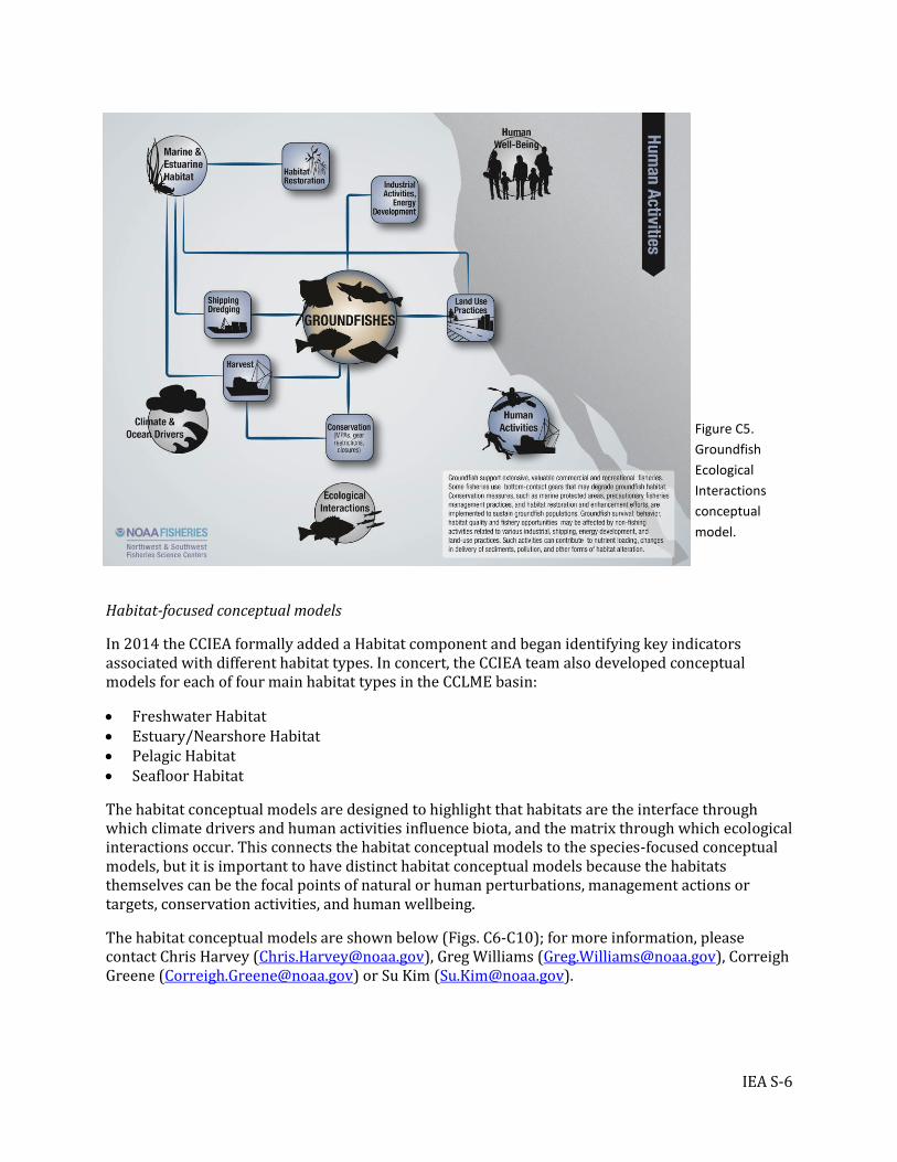
Species-focused conceptual models

We have developed a series of models that focus on several major species groups or niches within the CCLME. Focal groups are:

Coastal Pelagic Species Salmon Groundfish Marine mammals Seabirds

For each group, we developed 4 conceptual models:

1. Overview: a model linking the group to major drivers, pressures and ecosystem attributes; 2. Environmental Drivers: a model linking the group to physical processes, such as climate and

oceanography, with a brief narrative; 3. Ecological Interactions: a model linking the group to prey, predators, competitors, and other key

species groups, with a brief narrative; and 4. Human Activities: a model linking the group to key human activities and aspects of human

wellbeing, with a brief narrative. The groundfish conceptual models are shown below (Figs. C2-C5) in greater detail than in the main report; for other species group conceptual models, please contact Chris Harvey (Chris.Harvey@noaa.gov), Greg Williams (Greg.Williams@noaa.gov) or Su Kim (Su.Kim@noaa.gov).

Figure C2. Groundfish Overview conceptual model.

IEA S-5

Figure C3.

Groundfish

Environmental

Drivers

conceptual

model.

Figure C4.

Groundfish

Ecological

Interactions

conceptual

model.

IEA S-6

Habitat-focused conceptual models

In 2014 the CCIEA formally added a Habitat component and began identifying key indicators associated with different habitat types. In concert, the CCIEA team also developed conceptual models for each of four main habitat types in the CCLME basin:

Freshwater Habitat Estuary/Nearshore Habitat Pelagic Habitat Seafloor Habitat

The habitat conceptual models are designed to highlight that habitats are the interface through which climate drivers and human activities influence biota, and the matrix through which ecological interactions occur. This connects the habitat conceptual models to the species-focused conceptual models, but it is important to have distinct habitat conceptual models because the habitats themselves can be the focal points of natural or human perturbations, management actions or targets, conservation activities, and human wellbeing.

The habitat conceptual models are shown below (Figs. C6-C10); for more information, please contact Chris Harvey (Chris.Harvey@noaa.gov), Greg Williams (Greg.Williams@noaa.gov), Correigh Greene (Correigh.Greene@noaa.gov) or Su Kim (Su.Kim@noaa.gov).

Figure C5.

Groundfish

Ecological

Interactions

conceptual

model.

IEA S-7

Figure C6.

Habitat

Overview

conceptual

model.

Figure C7.

Freshwater

Habitat

conceptual

model.

IEA S-8

Figure C8.

Estuary/

Nearshore

Habitat

conceptual

model.

Figure C9.

Pelagic

Habitat

conceptual

model.

IEA S-9

Figure C10.

Seafloor

Habitat

conceptual

model.

IEA S-10

Appendix D. Climate and Ocean Indicators, Winter

Section 3 of the 2015 CCIEA State of the California Current report describes indicators of basin-scale and region-scale climate and ocean drivers. The plots in that section feature summertime measures of the indices, which are concurrent with the typical periods of maximum upwelling, productivity, and the potential for periods of hypoxia or reductions in pH. Here we present the wintertime indices to allow a more complete picture of these time series.

Figure D1. Winter values of basin-scale climate indicators used to assess environmental variability impacts in

the California Current ecosystem. The three time series are Multivariate ENSO Index (MEI), Pacific Decadal

Oscillation (PDO), and North Pacific Gyre Oscillation (NPGO). Lines, colors and symbols are as in Figure 1.1.

IEA S-11

Figure D2. Winter values of dissolved oxygen in the CCE. Lines, colors and symbols are as in Figure 1.1. Dissolved oxygen was measured at 150 m depth off of Oregon (Newport Line station NH25) and southern California (CalCOFI stations 93.30 and 90.90). Stations 93.30 and NH25 are located within 50 km from the shore, while station 90.90 is located over 300 km from shore. Note: the CalCOFI time series do not have 2014 values.

IEA S-12

Figure D3. Winter values of aragonite saturation in the northern CCE, 1998-2014. Lines, colors and

symbols are as in Figure 1.1 of the main document. The time series for station NH25 is similar to the DO

data shown in Figure D2 because aragonite saturation is calculated in part from oxygen data.

IEA S-13

Appendix E. Fact sheet for Cassin’s auklet mortality event

More information on the recent West Coast mortality event of Cassin’s auklets can be found at http://depts.washington.edu/coasst/news/breaking_news/Cassins%20Auklet%20factsheet%206Jan15.pdf.

IEA S-14

Appendix F. State-by-state fishery landings

At the CCIEA team’s presentation to the Council in March 2014, Council members requested that we include fishery landings data on a state-by-state basis. Those time series are presented here.

Total landings in California were available from PacFIN (Pacific Fisheries Information Network; http://pacfin.psmfc.org) for shoreside commercial landings and from RecFIN (Recreational Fisheries Information Network; http://www.recfin.org/) for recreational landings. Total fisheries landings in California varied within historical averages over the last five years and these patterns were driven almost completely by landings of coastal pelagic species (Fig. F1). Landings of groundfish (excluding hake) and recreational-caught species have been consistently at historically low levels over the last five years, while landings of Pacific hake have decreased to historically low levels and crab have increased to historically high levels over the last five years. Shrimp and salmon landings have increased over the last five years. Highly migratory species and other commercially-landed species have been relatively unchanged over the last five years.

Figure F1. Annual landings of eight major West Coast commercial fisheries, recreational landings, and total

landings from commercial and recreational fisheries (data: PacFIN and RecFIN) from 1981-2013 in California.

IEA S-15

Commercial and recreational fisheries landings in Oregon were available from PacFIN for shoreside commercial landings and from RecFIN for recreational landings. Total fisheries landings in Oregon increased over the last five years (Fig. F2). These patterns appear to be driven by interactions in landings of Pacific hake, which have increased over the last five years, and coastal pelagic species, which have been highly variable over the last five years. Landings of shrimp have increased to historically high levels over the last five years and landings of highly migratory species have been consistently at historically high levels over the last five years. Landings of groundfish (excluding hake), crab, salmon, other species, and recreationally-caught species have not changed over the last five years.

Figure F2. Annual landings of eight major West Coast commercial fisheries, recreational landings, and total

landings from commercial and recreational fisheries (data: PacFIN and RecFIN) from 1981-2013 in Oregon.

IEA S-16

Commercial and recreational fisheries landings in Washington were available from PacFIN (Pacific Fisheries Information Network; http://pacfin.psmfc.org) for shoreside commercial landings and from RecFIN (Recreational Fisheries Information Network; http://www.recfin.org/) for recreational landings. Total fisheries landings in Washington increased to historically high levels over the last five years (Fig. F3). These patterns were driven primarily by the interaction of landings of coastal pelagic species and Pacific hake. Landings of coastal pelagic species and other species increased to historically-high levels over the last five years, while landings of highly migratory species were consistently at historically-high levels and groundfish (excluding hake) were consistently at historically low levels. Landings of shrimp increased over the last five years. Landings of crabs and Pacific were highly variable but within historical averages, while landings of salmon and recreational catch were consistently within historical averages over the last five years.

Figure F3. Annual landings of eight major West Coast commercial fisheries, recreational landings, and total

landings from commercial and recreational fisheries (data: PacFIN and RecFIN) from 1981-2013 in Washington.

IEA S-17

Appendix G. Coastal community vulnerability indicators

Section 6.2 of the CCIEA Annual Ecosystem Summary described work on coastal community vulnerability indicators, and specifically presented information on the extent of dependence upon commercial fishing in coastal communities of Washington, Oregon and California. The sensitivity of any one of these communities to changes in commercial fishing conditions is not just a function of fishing dependence, however; fishing dependence in any coastal community occurs within the broader social context of that community. Thus, we must examine overall indices of community vulnerability in order to fairly assess the implications of fishery dependence.

In order to asses and track coastal community vulnerability for the inhabited shoreline areas adjacent to the California Current Large Marine Ecosystem (CCLME), this section uses a set of variables that were drawn from extant community-level data and subjected to factor analyses in generating vulnerability indices. This process determined which communities are potentially most dependent on fisheries and marine ecosystems, and which among these are the most socioeconomically vulnerable (Fig. G1). While this approach has been successfully developed and implemented for coastal communities on the U.S. East Coast (Jacob et al. 2012; Jacob et al. 2010; Colburn and Jepson 2012), the method of measuring and evaluating socioeconomic resilience is still in the early stages of data collection, organization and analysis for the communities of the U.S. West Coast (i.e. the coastal portion of the California Current Large Marine Ecosystem).

As shown in Section 5.2 of the main report, a factor analysis approach was applied to available and relevant fisheries data for 2010 to reveal which CCLME communities were relatively dependent on commercial fishing. Once a set of fishing dependent communities is established, the factor analysis approach pioneered by Jepson and Colburn (2013) allows for the use of sociodemographic data from the 2000 and 2010 censuses, as well as the annual American Community Survey (ACS) updates and other secondary sources, to develop indices of social vulnerability. For the major fishing dependent communities in each California Current state (WA, OR and CA), we can measure social vulnerability with respect to six relevant indices (personal disruption, population composition, poverty, labor force structure, housing characteristics, and housing disruption) and compare communities according to each index (Figs. G2-G8). Composite scores representing social vulnerability of communities were calculated by summing the factor scores (reversed factor scores were used for housing characteristics and labor force structure) and categorizing communities into low, moderate, and high levels of vulnerability based upon less than 20%, 20-80%, and greater than 80% percentiles, respectively. This approach follows that of the Hazards and Vulnerability Research Institute approach (2014) and Himes-Cornell and Kasperski (In Press), where counties or communities were classified as having vulnerability levels of low, medium, and high vulnerability as those in less than 20%, 20-80%, and greater than 80%

Commercial Fishing Dependence Indices

• Commercial Fishing Reliance

• Commercial Fishing Engagement

Social Vulnerability Indices

• Personal Disruption

• Population Composition

• Poverty

• Labor Force Structure

• Housing Characteristics

• Housing Disruptions

Figure G1. Indices of fishing dependence and social vulnerability for CCLME communities. Adapted from Jepson and Colburn (2013) by Miller (2014).

IEA S-18

percentiles in of the total distribution, respectively. A composite score for social vulnerability among West Coast coastal communities is represented in Figure G9. For more information, please contact Dr. Karma Norman, Karma.Norman@noaa.gov.

Figure G2. Relative comparisons for the personal disruption index among (top) Washington and Oregon

communities and (bottom) California communities.

IEA S-19

Figure G3. Relative comparisons for the population composition index among (top) Washington

and Oregon communities and (bottom) California communities.

IEA S-20

Figure G4. Relative comparisons for the poverty index among (top) Washington and Oregon communities and (bottom) California communities

IEA S-21

Figure G5. Relative comparisons for the labor force structure index among (top) Washington and Oregon communities and (bottom) California communities. For the Labor Force Structure and Housing Characteristics indices, the cardinality was reversed (higher employment and greater participation of females in the labor force is indicative of lower vulnerability in the Labor index and the higher housing characteristics are similarly associated with decreased vulnerability in the Housing index).

IEA S-22

Figure G6. Relative comparisons for the housing characteristics index among (top) Washington and Oregon communities and (bottom) California communities. For the Labor Force Structure and Housing Characteristics indices, the cardinality was reversed (higher employment and greater participation of females in the labor force is indicative of lower vulnerability in the Labor index and the higher housing characteristics are similarly associated with decreased vulnerability in the Housing index).

IEA S-23

Figure G7. Relative comparisons for the housing disruption index among (top) Washington and Oregon communities and (bottom) California communities.

IEA S-24

Figure G8. Relative comparisons for the labor force index among (top) Washington and Oregon communities and (bottom) California communities.

IEA S-25

Figure G9. Relative comparisons among (top) Washington and Oregon communities and (bottom) California communities according to an overall composite score for social vulnerability.

IEA S-26

Literature cited in Coastal Community Vulnerability analysis:

Colburn L.L., Jepson M. 2012. Social Indicators of Gentrification Pressure in Fishing Communities: A Context for Social Impact Assessment.Coastal Management 40:289-300

Hazards and Vulnerability Research Institute (HVRI). 2014. The Social Vulnerability Index (SoVI ®), 2006-2010, US County Level. Columbia, SC: University of South Carolina. Available from http://www.sovius.org.

Himes-Cornell, A. and S. Kasperski. In Press. Assessing climate change vulnerability in Alaska’s fishing communities. Fisheries Research. 162: 1-11.

Jacob, S., P. Weeks, B. G. Blount, and M. Jepson. 2010. Exploring fishing dependence in gulf coast communities. Marine Policy 34:1307-1314.

Jacob, S., P. Weeks, B. G. Blount, and M. Jepson. 2012. Development and Evaluation of Social Indicators of Vulnerability and Resiliency for Fishing Communities in the Gulf of Mexico. Marine Policy 26:16-22.

Jepson, M. and L.L. Colburn. 2013. Development of Social Indicators of Fishing Community Vulnerability and Resilience in the U.S. Southeast and Northeast Regions. U.S. Department of Commerce, NOAA Technical Memorandum NMFS-F/SPO-129, 64p.

Miller, S. 2014. Indicators of Social Vulnerability in Fishing Communities along the West Coast Region of the U.S. Master of Public Policy essay, Oregon State University, Corvallis, OR.