calibration processes for bruker...
TRANSCRIPT

Calibration Processes
with Bruker MS and Star Workstations
Randall Bramston-Cook Lotus Consulting, 5781 Campo Walk, Long Beach, Ca 90803 310/569-0128 [email protected]
January 19, 2014
Copyright 2014, Lotus Flower, Inc.


25.50 26.00 minutes
MC
ount
s
40
0
Standard = 1 ppmV Area: 2.559e+8
Sample Area: 1.488e+8
Quantitation of unknown samples in gas chromatography relies on establishing a correspondence between concentration and detector response. By measuring the detector signals for known standards, a response factor can be computed and applied to signals generated from unknowns examined under identical conditions. Detector response can be reported as peak height or peak area, using the appropriate parameter within the method. Peak area is inherently more inclusive of the response, as it incorporates more data points, especially with tailing or distorted peaks, to help improve the suppression of noise with the averaging of data points for the peak. Linearity over a wider range is the result.
The simplest computation merely compares a response from a standard with equivalent results from unknown samples, as depicted in Figure 1, commonly labeled as “external standard” calculation.1
Figure 1. The simplest computation of concentration is a ratio of area counts between the sample and standard, multiplied by the concentration for the standard.
This response factor for measurements involving external standard operations can be calculated as either:
RF = areastd/concentrationstd = 255,923,885 counts / 1 ppmV = 255,923,885 counts / ppmV (1)
with unknowns then reported as:
Concentrationunk = Areaunk/RF = 148,814,825 / 255,923,885 = 0.581 ppmV (2)
Or concentration can be determined by reciprocal operations:
RF = concentrationstd/areastd = 1 / 255,923,885 = 3.9078 X 10⁻⁹ (3)
with unknowns then reported as:
Concentrationunk = Areaunk*RF = 1.488 X10+8 * 3.9078 × 10-9 = 0.581 ppmV (4)
1 Another operation involves addition of a specific unknown compound directly into the sample to correct for effects in variations of injection volume, extraction or purging efficiencies. This computation is called “internal standard” and is not discussed here. Full discussion can be found in any basic GC textbook, www.chemistry.adelaide.edu.au/external/soc-rel/content/int-std.htm or en.wikipedia.org/wiki/Internal standard.

Calibration Curve ReportBenzene
Curve Fit: Linear, Origin: Force, Resp. Fact. RSD: 6.688%Coeff. Det.(r2): 0.999827y = +9.520109e+5x
Amount (ppbV)1 2 3 4 5
0
5
M C
ount
s
Use of either set of equations will yield the same results when a single point is used for each calibration level. However, answers can differ when multiple points for each level are employed.2 Each process has no significant merits over the other, and the choice of Equations 1 and 2 is by convention for Bruker Star and MS Workstations and matches most standard protocols.
The operator establishes response factors by injecting various concentrations of known standards over the expected amounts in the unknown samples.3 This is demonstrated visually with a calibration curve in Cartesian coordinates, as shown in Figure 2.
Figure 2. The conventional display of a calibration curve is
a plot of area counts (ordinate) versus concentration (abscissa).
2 The average response factors for multiple points at each level, using the two set of equations above, are different, as illustrated by the following. To simplify the mathematics, let’s say that we have areas of 2, 3 and 4 for three repeat measurements of a standard with a concentration of 1. For the calculation with Equation 1, the three runs give:
Average Response Factor = [2/1 + 3/1 + 4/1] / 3 = 3 If the unknown has an area of 3, then:
Concentrationunk = 3 / 3 = 1.000 Using Equation 3 gives the following:
Average Response Factor = [1/2 + 1/3 + 1/4] / 3 = 0.361 If the unknown area is the same 3, then:
Concentrationunk = 3 * 0.361 = 1.083 for a difference of 8.3%, based only on which calculation mode is used. For real samples, this difference is often small, but can still yield differing results. Most standard methods and most chromatographic data systems use the first approach. 3 The notable exceptions to this linearity are the flame photometric and pulsed flame photometric detectors operated in the sulfur mode. Their responses follow a quadratic relationship with concentration. To convert areas or heights into concentrations, the calculation for sulfur compounds must be performed by taking either the square root of the height, or fitting the calibration data to a quadratic equation.

Multi-Level Calibrations Most chromatographic detectors are linear over wide concentration range, but limits are imposed by the characteristics of the detector involved. Other processes can severely limit the usable range, including degradations in sample preparations and chromatography. The expected range must be authenticated with known standards over the anticipated range. Typically, for liquid samples, this validation process is best performed by processing a range of standards, usually by dilution of a higher concentration stock solution, and then analyzing the series consecutively. Their accuracies are very dependent on the quality of the preparation process. Often “ready-to-inject” standards can be procured,4 but add to the expense of the measurement, especially if they are certified to some standard measure. An alternative protocol for liquid standards is to inject a single standard with varying injection volumes. Many liquid automated samplers allow the operator to set the injection volume in a sample list, as shown in Figure 3. Care must be exercised to not exceed the limits of the injector system. Too large an injection volume may overload the chromatography process, and too small might introduce serious repeatability errors. Typically, the range is limited to a single decade in concentration range. For gases, preparation of multi-level standards is not nearly as easy as with liquids. Dilutions of a stock standard can be accomplished most readily by pressure dilutions into canisters. For example, 3 psiA5 of the stock standard is loaded into a total can pressure of 30 psiA; this process yields a 10:1 dilution of the stock standard. Alternatively, if injections are set with fixed volume sample loops, use of multiple loops with varying volumes can accomplish the multi-point calibration process. Manual switching out of these loops can be tedious. So to fully automate the process, valves can be employed to enable easy switching between loops. Figure 4 depicts a valving scheme to select three differing loops without any hardware changes. The precise volume of each loop must include volumes of the interconnecting tubing between the gas sampling valve (GSV) and the interport volumes between valves. Figure 5 illustrates the accumulation of volumes for Loop 3. Commonly, many of these volumes are either not correctly known or cannot be known accurately enough to maintain precision of the calibration process. The best mechanism to determine these volumes is to run all three loops individually with the same standard and compute their relative sizes by responses generated.
Additional loops can be installed by daisy-chaining more 6-port valves beyond Valve B in Figure 4, or a multi-position valve can be employed to allow up to 16-individual loops6 to be installed and readily accessed with Bruker Stream Selector Valve software. A typical set-up is shown in Figure 6.
4 See for example ts.nist.gov/srmors/view_detail.cfm?srm=2891 through =2899. 5 Pressure units of PSIA (pounds per square inch Absolute), or equivalent are used in this pressure labeling, and not psiG (pounds per square inch Gauge) to account for the starting point of a hard vacuum, or 0 psiA. 6 Multi-position valves are available to accommodate 4, 6, 8, 10, 12 or 16 loops.
Figure 3. Bruker WorkstationSampleList allows multiple liquidvolumes to be preprogrammed toperform a multi-point calibrationprocess with a single stock solutionby just altering the injection volume.

Carrier In
Sample Out
Sample In
Column Detector
Loop 1
Loop 2
Loop 3 GSV VA VB
Figure 4. Valving configuration for selection of three injection volumes by simple activation of valves, without hardware changes.
Carrier In
Sample Out
Sample In
Column Detector
Loop 1 GSV VA
Loop 4
Loop 3
Loop 2
Figure 5. Proper allocation of volume for Loop 3 includes all interconnecting volumes 1-9.
35
2 4
6
7
8
9
1
Carrier In
Sample Out
Sample In
Column Detector
Loop 1
Loop 2
Loop 3 GSV VA VB
6
4
Figure 6. Multi-position valve set up for selection of any one of four loops.

Several specific applications in gas analysis use a trapping scheme and a mass flow controller to load in a sample.7 By setting the sample flow rate with a flow controller and then directing flow through the concentrator trap for a predetermined time, the amount of sample loaded becomes the product of the sample flow rate and the time interval. For example, if the controller is set to 50 ml/min and the sample is loaded into the trap for 6 minutes, the sample volume trapped becomes 300 ml. Conveniently we can accomplish a multi-point calibration series by altering the time of sample loading and/or the sample flow rate. Table I and Figures 7 and 8 illustrate a typical setup to perform this task. Data plotted in Figure 2 is generated from such a procedure.
Sampling Time (min.)
Sample Flow Rate (ml/min)
Volume (ml) Relative
Concentration 12.00 50 600 2.00 6.00 50 300 1.00 3.00 50 150 0.500 1.50 50 75 0.250 1.00 50 50 0.167 0.50 50 25 0.0833 0.20 50 10 0.0333 0.10 50 5 0.0166
7 For examples, see USEPA Compendium “Method TO-15 - Determination of Volatile Organic Compounds (VOCs) in Air Collected in Specially-prepared Canisters and Analyzed by Gas Chromatography/Mass Spectrometry (GC/MS)”, www.epa.gov/ttn/amtic/files/ambient/airtox/to-15r.pdf. and California Air Resources Board SOP 066, “Standard Operating Procedure for the Determination of Oxygenates and Nitriles in Ambient Air by Capillary Column Gas Chromatography/Mass Spectrometry”. www.arb.ca.gov/aaqm/sop/sop_066.pdf.
Figure 7. Typical valving scheme for generating multiple level calibrations with a mass flow controller and trapping.
Carrier In
Sample In
VA VB
Purge Flow In
Mass Flow Controller Vacuum
Trap
Vent
Column Detector
Step A. Time 0.00, Valves VA and VB off. Sample flow off and trap cold.
Carrier In
Sample In
VA VB
Purge Flow In
Mass Flow Controller Vacuum
Trap
Vent
Column Detector
Step B. Time 0.01, Valve VA on. Sample flow on to purge line, but not to trap, and trap cold.

Step D. Time 7.00, Valve VA off. Sample flow off; purge flow to trap loading interval stops. Sampling time is 6.00 minutes.
Carrier In
Sample In
VA VB
Purge Flow In
Mass Flow Controller Vacuum
Trap
Vent
Column Detector
Step C. Time 1.00, Valve VB on. Sample flow on to trap; loading interval starts.
Carrier In
Sample In
VA VB
Purge Flow In
Mass Flow Controller Vacuum
Trap
Vent
Column Detector
Step E. Time 8.00, Valve VB off. Prepare to inject sample to column.
Carrier In
Sample In
VA VB
Purge Flow In
Mass Flow Controller Vacuum
Trap
Vent
Column Detector
Step E. Time 8.10, Heat up trap to desorb sample to column.
Carrier In
Sample In
VA VB
Purge Flow In
Mass Flow Controller Vacuum
Trap
Vent
Column Detector

Smaller volumes are readily achieved by adjusting Step C in Figure 12, in order to maintain the same timing for injection to the column. Volumes loaded with times less than 0.5 minutes should be fully validated to ensure accurate volumes are allocated, The volume contained in the interconnecting tubing between valves is not fully accounted in this process and can distort the perceived volume with low sample flows and low loading times. Large volumes, potentially as high as 2 liters, are possible by lengthening the loading time and/or increasing the sample flow rate. However, trap break-through with this large volume can degrade the calbration process. This loading may necessitate an alteration of times for Steps D, E and F, and result in a delay in the on-column injection and a consequent change in retention times.
Special Calibration Operations
Update Compound Table Parameters – The operator can choose what parameters can alter the peak table settings for retention times reference spectra or target ion ratios, as a result of calibration runs. For example, if peak retention times shift slightly, then these times in the peak table can be updated from the last standard. Occasionally, these updates can pick a closely eluting isomer as the target compound and adjust the identifying criteria based on this wrong peak. The user should be careful here and use a wider integration window to properly integrate the peak, but select a narrow identification window to only pick out the proper peak. Only the apex of the specified peak needs to be within the identification window to be chosen; any peak outside will not be considered. To ensure that a “normal” data set is used in this updating process and not an extreme one (either low or high), a calibration sequence should be performed with the mid-level standard as the last one. For example, the levels, in increasing concentrations, should be 1,2,4,5, then 3. Thus, the sequence would end with information that should apply to nearly all peak concentrations.
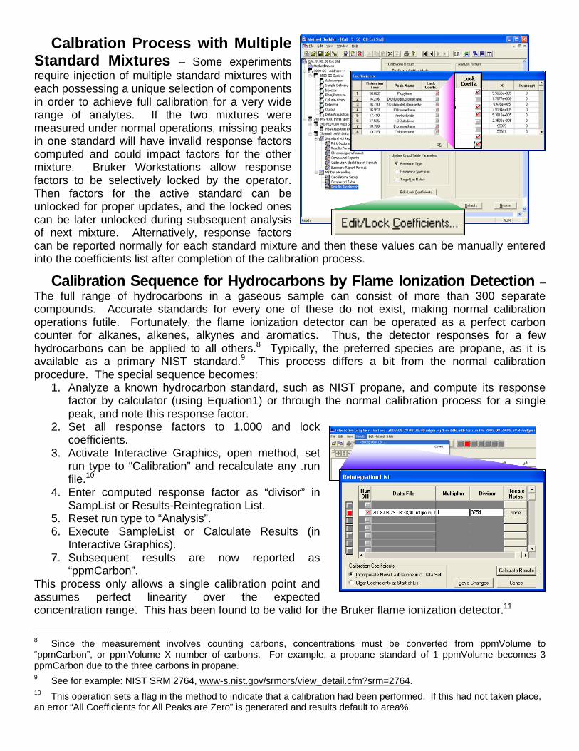
Calbration Process with Multiple Standard Mixtures – Some experiments require injection of multiple standard mixtures with each possessing a unique selection of components in order to achieve full calibration for a very wide range of analytes. If the two mixtures were measured under normal operations, missing peaks in one standard will have invalid response factors computed and could impact factors for the other mixture. Bruker Workstations allow response factors to be selectively locked by the operator. Then factors for the active standard can be unlocked for proper updates, and the locked ones can be later unlocked during subsequent analysis of next mixture. Alternatively, response factors can be reported normally for each standard mixture and then these values can be manually entered into the coefficients list after completion of the calibration process.
Calibration Sequence for Hydrocarbons by Flame Ionization Detection – The full range of hydrocarbons in a gaseous sample can consist of more than 300 separate compounds. Accurate standards for every one of these do not exist, making normal calibration operations futile. Fortunately, the flame ionization detector can be operated as a perfect carbon counter for alkanes, alkenes, alkynes and aromatics. Thus, the detector responses for a few hydrocarbons can be applied to all others.8 Typically, the preferred species are propane, as it is available as a primary NIST standard.9 This process differs a bit from the normal calibration procedure. The special sequence becomes:
1. Analyze a known hydrocarbon standard, such as NIST propane, and compute its response factor by calculator (using Equation1) or through the normal calibration process for a single peak, and note this response factor.
2. Set all response factors to 1.000 and lock coefficients.
3. Activate Interactive Graphics, open method, set run type to “Calibration” and recalculate any .run file.10
4. Enter computed response factor as “divisor” in SampList or Results-Reintegration List.
5. Reset run type to “Analysis”. 6. Execute SampleList or Calculate Results (in
Interactive Graphics). 7. Subsequent results are now reported as
“ppmCarbon”. This process only allows a single calibration point and assumes perfect linearity over the expected concentration range. This has been found to be valid for the Bruker flame ionization detector.11
8 Since the measurement involves counting carbons, concentrations must be converted from ppmVolume to “ppmCarbon”, or ppmVolume X number of carbons. For example, a propane standard of 1 ppmVolume becomes 3 ppmCarbon due to the three carbons in propane. 9 See for example: NIST SRM 2764, www-s.nist.gov/srmors/view_detail.cfm?srm=2764.
10 This operation sets a flag in the method to indicate that a calibration had been performed. If this had not taken place, an error “All Coefficients for All Peaks are Zero” is generated and results default to area%.

Scalars for Each Data Channel – Each “analysis” sample in the SampleList can possess a separate multuplier and divisor that apply the entered values to all results for that sample. These might be used to scale results for dilutions, or sample weights, or injection volumes. If multiple detectors are employed, these factors can be set separately for each detector. For example, if both a mass spectrometer and flame ionization detector were run simultaneously, each one can have independent multipliers and divisors, appropriately for each detector.
Unidentified Peak Factors – Normal operating
procedures mandate that a standard matching every analyte in unknowns be used to generate a response factor to yield concentrations for unknowns. With some situations, such as with hydrocarbons in gasoline, a standard is not available for every analyte. For analogous series, often a response for one can be applied to others that are not identified. The unidentified peak factor can be entered in the SampleList to apply to all other peaks not listed in the peak table.
Display of Calibration Data
Bruker Star and MS Workstations12 save all calibration data in the method, under Calibration Setup for Star Workstation and Compound Table for MS Workstation. The screen is very interactive and allows testing of different curve fits, origin treatment and regression weighting. Changes to any of these parameters generate an update to the curve fit and can be saved to the method.
Two operator selections of these parameters can be compared directly by selecting the “Overlay” button. Then both curves are shown along the fit data. The second choice can be selected to be saved to the method.
11 See for example: www.arb.ca.gov/msprog/levprog/cleandoc/clean_nmogtps_final.pdf.
12 Most operations discussed in this monograph are available in both Bruker Star and MS Workstation. All entry screens shown here apply to MS Workstation only; equivalent Star screens should be located with little difficulty.

To confirm the source of data points, each point can be highlighted with the mouse cursor. Then by selecting “Point Info” button, the data file location for that run, its raw data and its deviation from the curve are displayed. “Exclude Selected Point from Calculation” check box allows specific calibration points to be deleted from the curve generation, with the new fit automatically updated. Also points may be excluded from the calculations by right-clicking on the selected data points in the active plot. This is a toggle function. Right-clicking on an excluded point will include it again. The process of excluding data points does not remove the data points from the Compound Table. However, exclusion does affect the calibration calculation and the quantitation results.
To permit maximum flexibility in controlling the calibration process, coefficients determined during the calibration sequence can be presented and even altered by the operator by selecting new values and saving them to the method.
A built-in calculator allows the operator to enter either a
hypothetical concentration or area counts, and view the other, based on the active calibration fit. This operation is useful in anticipating a possible detection limit.
The calibration curve can be exported in a variety of formats for archiving or
display in publications such as this. This author used “To Picture File”.wmf to generate many figures in this monograph and then edited them through Word draw utilities.
Calibration data are commonly displayed in a
Cartesian plot, as shown in Figure 2, with concentration as the abscissa and area counts the ordinate. This works well for limited concentration ranges, say over one decade in concentration. Over a wider range, low concentrations are often too compressed to visually assess how well they fit to the curve. The Bruker MS Workstation offers an option to display the calibration plot as log[area counts] versus log[concentration]. Although this view allows better visualization of the wider concentration range, the log-log scale almost always shows the data points right on the curve, even when they stray away a bit.
Printing Calibration Data
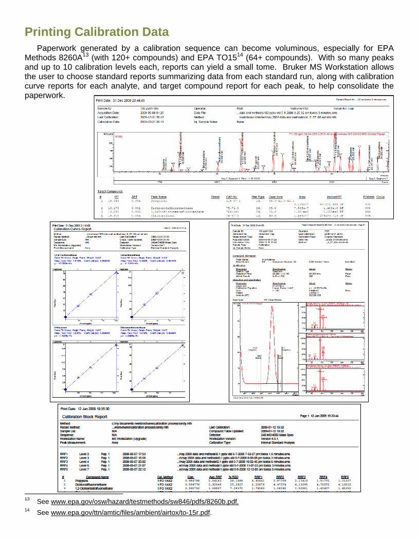
Paperwork generated by a calibration sequence can become voluminous, especially for EPA Methods 8260A13 (with 120+ compounds) and EPA TO1514 (64+ compounds). With so many peaks and up to 10 calibration levels each, reports can yield a small tome. Bruker MS Workstation allows the user to choose standard reports summarizing data from each standard run, along with calibration curve reports for each analyte, and target compound report for each peak, to help consolidate the paperwork.
13 See www.epa.gov/osw/hazard/testmethods/sw846/pdfs/8260b.pdf. 14 See www.epa.gov/ttn/amtic/files/ambient/airtox/to-15r.pdf.

Block reports for the calibration standards are formatted in the Method. A “standard” report lists specifics related to the calibration process and has the calibration equations with response factors for all calibration points. This abbreviated report normally prints out with just a few pages.

The “detailed” report gives all of the data from the standard report, as well as each level’s retention time, standard amount, area count, average response factor, standard deviation (if more than a single run is included for each level, %RSD, along with the equations for the fit. The data files used for each analytes level is included, with an indication if the point was excluded from the calibration process. This report can entail many pages; a report for 68 compounds with nine levels each can be 27 pages.

Also available are control charts for standards, verifications and samples. The user opts for parameters to be included in the control charts and for indicated control limits. The printouts can be generated from a Print Summary after Print Control Charts is checked.
Calibration data files employed in the generation of computed results for each unknown sample are automatically saved in a Calibration Log within the data file. This log can then be printed with every report when its box is checked. This log is accumulative, archives every calibration file applied to this analysis file, and cannot be altered.

Calibration Curve Fitting
With the Bruker Star and MS Workstation software15, the calibration data are plugged into a least squares fit16 to yield the slope and intercept of the plot, as well as a measure of the quality of the fit. Two numbers are reported by the Bruker Workstation packages - r2 and “Response Factor RSD”. 17 For r2, a value of one is a perfect fit,18 and any number less than one is measure of the misfit. Many established protocols have an acceptable value specified, either expressed as r or r2. The “Response Factor RSD” is a measure of outliers that that are far off the linear fit. A low number implies all data points are close to the curve fit. Caution must be applied to this value as the average may be skewed when most of the calibration points are close with one widely deviant value that still allows the average to be acceptable.
A simple least square fit, where all data points have equal weighting, suffers from several issues. Deviant points generated from errors in the measurement can radically skew the fit and generate unexpectedly low r2 and “Response Factor RSD” values. These outliers may not be due to random errors in the measurement nor from the true performance of the system, but instead could be attributed to a single flaw in the sampling process. Repeat runs with the same level can often establish the cause of the variation. Secondly, the conventional least square fit places more weight on the higher concentration levels, to the detriment of the lower levels, especially over a very wide concentration range. To correct for this predicament, Bruker has included a choice of weighting factors related to the concentration level either x
1 or 21x
, where x is the concentration for the
standard.
To yield better quality for fits with both extended calibration ranges and varying number of points per level, the Bruker Workstation software offers combined weighting factors of nx
1 and 21
nx, where n is
the number of replicate runs at the same calibration level.
Fortunately, most chromatographic detectors have very wide linear relationships between their responses and concentrations. If the detector response is known to be linear over the expected concentration range, a single calibration level can be sufficient to establish the response factor. However, many standard methods mandate use of multiple levels to ensure that linearity is validated.
Average Response Factor Fit
To perform Average Response Factor Fit to the calibration curve, the following parameters are set as listed:
Curve Fit = Linear Origin Point = Force Regression Weighting = 2
1x
or 21
nx
15 Most operations discussed here are derived from the Bruker MS Workstation. Equivalent Bruker Star Workstation screens are often slightly different or found in different sections of the method, but should be able to be located with little difficulty. 16 A full explanation of computing a least squares fit can be found at www.en.wikipedia.org/wiki/least_squares. 17 See, for example, computations for response factor RSD in EPA Method TO-15 at www.epa.gov/ttnamti1/files/ambient/airtox/to-15r.pdf, page 15-24. 18 Typical discussions of r2 can be found at www.en.wikipedia.org/wiki/Coefficient_of_determination.

Quality of Calibration Curve Fitting
The relative standard deviation of response factors is a common measure of the quality of the data and usually indicates if outliers are skewing a linear fit. Here the peak responses are divided by the corresponding concentrations to yield the response factor, and then all response factors for a given peak are averaged and the relative standard deviation is computed. A low number implies that all data points are close to a linear fit through zero. One caution here is when nearly all of the data points are perfectly on the linear curve, and one or two all wildly deviant. The relative standard deviation can still be quite low, but serious errors are concealed by the mathematics of averaging.
Figure 8. This artificially generated data set illustrates how one grossly deviate point at 67% away from the fit can still generate reasonable response factor relative standard deviation of 29%, while most of the other data points are nearly on top of the curve. Without the anomalous point, the RSD for the data set becomes 0.9%.
To better assess the quality of the fit, calibration data can be plotted as response factor versus concentration, or if the concentration range is over a wider range, then versus log[concentration], as shown in Figure 9. Abnormal points are now more readily identifiable, especially at low concentrations.
Figure 9. Data presented in Figure 3 is reformatted by plotting Response Factors vs. log[Concentration] to more readily demonstrate consistent response factors for most of the calibration levels, save one deviant point at 0.35 ppbV. The one outlier skews the average and standard deviation away from the more likely average value. The abscissa scale is displayed as log[concentration] to better illustrate the wide range in concentration and provide better visibility of the lower concentrations levels.
Res
po
nse
F
acto
r
Calibration Curve ReportTolueneCurve Fit: Linear, Origin: Force Resp. Fact. RSD: 29.20%
Coeff. Det.(r2): 0.930450y = +1.380812e+6x
Amount (ppbV)0.25 0.50 0.75 1.00
0.00
1.25
M C
ount
s
Calibration Curve Report
Curve Fit: Linear, Origin: Force, Weight: NoneResp. Fact. RSD: 14.03%Coeff. Det.(r2): 0.999996y = +1.49717e+5x
Amount0.010 0.020 0.030
0.0
10.0
Replicates 8
K C
ou
nts
Vinyl Acetate
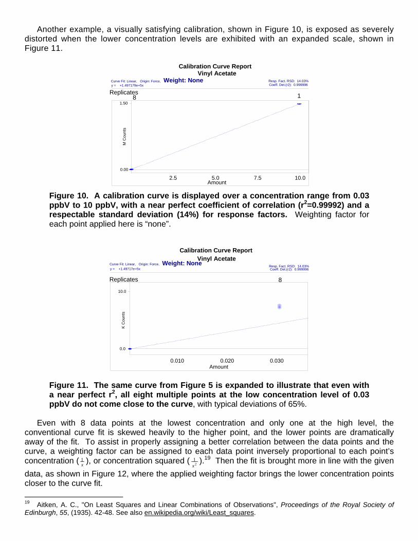
Another example, a visually satisfying calibration, shown in Figure 10, is exposed as severely distorted when the lower concentration levels are exhibited with an expanded scale, shown in Figure 11.
Figure 10. A calibration curve is displayed over a concentration range from 0.03 ppbV to 10 ppbV, with a near perfect coefficient of correlation (r2=0.99992) and a respectable standard deviation (14%) for response factors. Weighting factor for each point applied here is “none”.
Figure 11. The same curve from Figure 5 is expanded to illustrate that even with a near perfect r2, all eight multiple points at the low concentration level of 0.03 ppbV do not come close to the curve, with typical deviations of 65%.
Even with 8 data points at the lowest concentration and only one at the high level, the conventional curve fit is skewed heavily to the higher point, and the lower points are dramatically away of the fit. To assist in properly assigning a better correlation between the data points and the curve, a weighting factor can be assigned to each data point inversely proportional to each point’s concentration (
x1 ), or concentration squared ( 2
1x
).19 Then the fit is brought more in line with the given
data, as shown in Figure 12, where the applied weighting factor brings the lower concentration points closer to the curve fit.
19 Aitken, A. C., "On Least Squares and Linear Combinations of Observations", Proceedings of the Royal Society of Edinburgh, 55, (1935). 42-48. See also en.wikipedia.org/wiki/Least_squares.
Calibration Curve ReportVinyl Acetate
Curve Fit: Linear, Origin: Force, Weight: None Resp. Fact. RSD: 14.03% Coeff. Det.(r2): 0.999996y = +1.497179e+5x
Amount2.5 5.0 7.5 10.0
0.00
1.50
M C
ou
nts
Replicates 8 1

Calibration Curve ReportVinyl Acetate
Curve Fit: Linear, Origin: Force, Weight: 1/X2 Resp. Fact. RSD: 14.03% Coeff. Det.(r2): 0.999996y = +2.358558e+5x
Amount2.5 5.0 7.5 10.0
0.00
1.50
M C
ou
nts
Replicates 8 1
Calibration Curve Report
Curve Fit: Linear, Origin: Force, Weight: 1/X2Resp. Fact. RSD: 14.03%Coeff. Det.(r2): 0.999996y = +2.358558+5x
Amount0.010 0.020 0.030
0.0
10.0
Replicates 8
K C
ou
nts
Vinyl Acetate
Figure 12. With a weighting factor of 2
1x
applied to all data points in the fit,
the curve now nearly matches the location of the eight low level points.
Unfortunately, now the curve has radically departed away from the proximity of the high point with this new weighting factor (Figure 8). Table I summarizes the effect of choosing differing weighting factors for this data set.
Figure 13. Returning Figure 12 back to full scale to show the full range of the calibration, the curve now deviates significantly for the single high concentration point.
The calibration sequence with eight replicates at a low level and only one at the higher level is
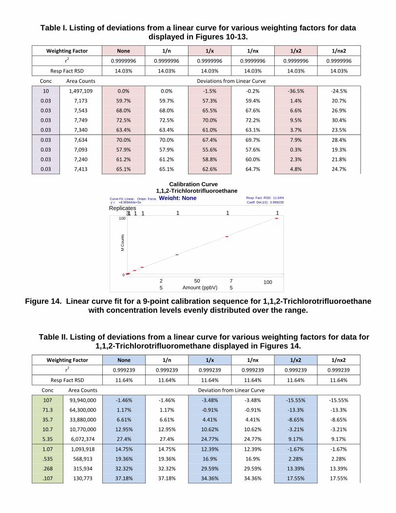
purposefully selected to illustrate dramatically the effects of the different weighting factors. A proper sequence should not contain this wide disparity in concentrations between calibration levels. A more suitable nine-point calibration is shown in Figure 14 for 1,1,2-Trichlorotrifluoroethane, and the effects of the various weighting factors are provided in Table II. The optimum choice of weighting factor is very dependent on the make-up of the data set, especially the concentration distribution and the number of replicate runs at each level. A judgment on the quality of the fit for all points must be made by the operator, often as a compromise.
Calibration Curve 1,1,2-Trichlorotrifluoroethane
Curve Fit: Linear, Origin: Force, Weight: None Resp. Fact. RSD: 11.64% Coeff. Det.(r2): 0.999239 y = +8.909444e+5x
Replicates 3 1 1 1 1 1 1
100
M C
ou
nts
25
50 75
100
0
Amount (ppbV)
Table I. Listing of deviations from a linear curve for various weighting factors for data displayed in Figures 10-13.
Weighting Factor None 1/n 1/x 1/nx 1/x2 1/nx2
r2 0.9999996 0.9999996 0.9999996 0.9999996 0.9999996 0.9999996
Resp Fact RSD 14.03% 14.03% 14.03% 14.03% 14.03% 14.03%
Conc Area Counts Deviations from Linear Curve
10 1,497,109 0.0% 0.0% ‐1.5% ‐0.2% ‐36.5% ‐24.5%
0.03 7,173 59.7% 59.7% 57.3% 59.4% 1.4% 20.7%
0.03 7,543 68.0% 68.0% 65.5% 67.6% 6.6% 26.9%
0.03 7,749 72.5% 72.5% 70.0% 72.2% 9.5% 30.4%
0.03 7,340 63.4% 63.4% 61.0% 63.1% 3.7% 23.5%
0.03 7,634 70.0% 70.0% 67.4% 69.7% 7.9% 28.4%
0.03 7,093 57.9% 57.9% 55.6% 57.6% 0.3% 19.3%
0.03 7,240 61.2% 61.2% 58.8% 60.0% 2.3% 21.8%
0.03 7,413 65.1% 65.1% 62.6% 64.7% 4.8% 24.7%
Figure 14. Linear curve fit for a 9-point calibration sequence for 1,1,2-Trichlorotrifluoroethane with concentration levels evenly distributed over the range.
Table II. Listing of deviations from a linear curve for various weighting factors for data for
1,1,2-Trichlorotrifluoromethane displayed in Figures 14.
Weighting Factor None 1/n 1/x 1/nx 1/x2 1/nx2
r2 0.999239 0.999239 0.999239 0.999239 0.999239 0.999239
Resp Fact RSD 11.64% 11.64% 11.64% 11.64% 11.64% 11.64%
Conc Area Counts Deviation from Linear Curve
107 93,940,000 ‐1.46% ‐1.46% ‐3.48% ‐3.48% ‐15.55% ‐15.55%
71.3 64,300,000 1.17% 1.17% ‐0.91% ‐0.91% ‐13.3% ‐13.3%
35.7 33,880,000 6.61% 6.61% 4.41% 4.41% ‐8.65% ‐8.65%
10.7 10,770,000 12.95% 12.95% 10.62% 10.62% ‐3.21% ‐3.21%
5.35 6,072,374 27.4% 27.4% 24.77% 24.77% 9.17% 9.17%
1.07 1,093,918 14.75% 14.75% 12.39% 12.39% ‐1.67% ‐1.67%
.535 568,913 19.36% 19.36% 16.9% 16.9% 2.28% 2.28%
.268 315,934 32.32% 32.32% 29.59% 29.59% 13.39% 13.39%
.107 130,773 37.18% 37.18% 34.36% 34.36% 17.55% 17.55%
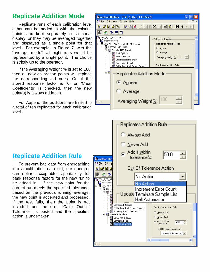
Replicate Addition Mode
Replicate runs of each calibration level either can be added in with the existing points and kept separately on a curve display, or they may be averaged together and displayed as a single point for that level. For example, in Figure 7, with the “average mode”, all eight runs would be represented by a single point. The choice is strictly up to the operator.
If the Averaging Weight % is set to 100, then all new calibration points will replace the corresponding old ones. Or, if the stored response factor is “0” or “Clear Coefficients” is checked, then the new point(s) is always added in. For Append, the additions are limited to a total of ten replicates for each calibration level.
Replicate Addition Rule
To prevent bad data from encroaching into a calibration data set, the operator can define acceptable repeatability for peak response factors for the new run to be added in. If the new point for the current run meets the specified tolerance, based on the previous running average, the new point is accepted and processed. If the test fails, then the point is not included, and the error “Calib. Out of Tolerance” is posted and the specified action is undertaken.
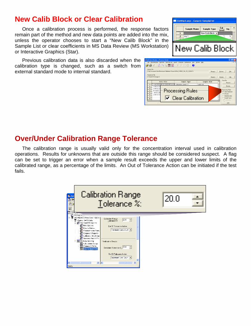
New Calib Block or Clear Calibration
Once a calibration process is performed, the response factors remain part of the method and new data points are added into the mix, unless the operator chooses to start a “New Calib Block” in the Sample List or clear coefficients in MS Data Review (MS Workstation) or Interactive Graphics (Star).
Previous calibration data is also discarded when the calibration type is changed, such as a switch from external standard mode to internal standard.
Over/Under Calibration Range Tolerance
The calibration range is usually valid only for the concentration interval used in calibration operations. Results for unknowns that are outside this range should be considered suspect. A flag can be set to trigger an error when a sample result exceeds the upper and lower limits of the calibrated range, as a percentage of the limits. An Out of Tolerance Action can be initiated if the test fails.

Lotus Consulting 310/569-0128 Fax 714/898-7461 email [email protected]
5781 Campo WalkLong Beach, California 90803
Screens are copyrighted by Bruker Inc., and are reprinted (reproduced) with the permission of Bruker, Inc. All rights reserved. Bruker and the Bruker logo are trademarks or registered trademarks of Bruker, Inc.
Verification of Calibration Process
Once a calibration operation is completed, the curve fit should be validated with a check sample to confirm performance of the standards. The expected answers are entered into the Compound Table, either as one of the standards or as a separate level amount. When a Sample Type is labeled as “Verification”, the generated results are compared with the expected ones. If the reported values exceed the tolerance specified, an error “Verification Failure” is generated.
Out of Tolerance Actions
Errors generated from tests for Replicate Addition, Calibration Range Tolerance, or Verification Results may be catastrophic when any occurs once, or an occasional miss could be tolerated. Each check allows the
operator to set the consequences of a failure, either “No Action”, “Increment Error Counter”, “Terminate Sample List”, or “Halt Automation”.
If Increment Error Count is selected, then the system monitors for problems of the same nature for each compound. If the number reaches the value entered into the Instrument Parameters screen in System Control, then the active SampleList is terminated.
Jan 02 17:03:29 Hexachloro-1,3-butadiene : Outside Calib. Range; No Recovery Action Specified Jan 02 17:03:29 Hexachloro-1,3-butadiene : Verification Failure; Incrementing Error Counter Jan 02 17:03:29 Naphthalene : Outside Calib. Range; No Recovery Action Specified Jan 02 17:03:29 Naphthalene : Verification Failure; Incrementing Error Counter Jan 02 17:03:50 Warnings were encountered. Jan 02 17:03:50 Error Counter at 3 Errors; Ended SampleList