calibration and validation of the ocean color version-3

Journal of Oceanography, Vol. 54, pp. 401 to 416. 1998

401Copyright The Oceanographic Society of Japan.

concentration) whose accuracy ranged from 30% (Vermonteand Saleous, 1993) to 220% (Chl-a was underestimated 45%compared to in situ data) (Arrigo et al., 1994). Since the CZCSwas terminated in 1986, ocean color users have long awaiteda spaceborne ocean color sensor.

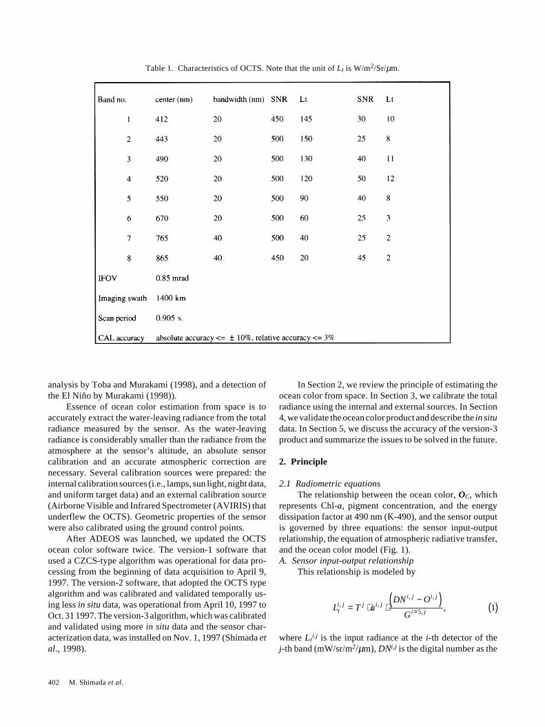
The Ocean Color and Temperature Scanner (OCTS),developed by the National Space Development Agency ofJapan (NASDA), was launched on Aug. 17, 1996, into an800 km polar orbit with a repeat cycle of 41 days and sub-repeat cycle of 3 days. It was carried by the Advanced EarthObserving Satellite (ADEOS), together with seven othersensors (Shimoda, 1997). OCTS consists of eight visible-and-near-infrared bands and four thermal-infrared bands(Table 1). Each band consists of ten detectors and achievesa 700 m resolution in nadir direction. Bandwidths rangefrom 20 nm in visible bands to 40 nm in near infrared bands.The OCTS became operational on Nov. 2, 1996, but it wasterminated due to the solar paddle breakdown on June 30,1997. The total amount of data acquired during the eightmonths exceeded 7 TB and OCTS data provided valuableinformation on the Earth change (e.g., the dynamics ofKuroshio Extension given by Toba (1998), a water mass

Calibration and Validation of the Ocean Color Version-3Product from ADEOS OCTS

MASANOBU SHIMADA1, HIROMI OAKU1, YASUSHI MITOMI2, HIROSHI MURAKAMI1,AKIRA MUKAIDA2, YASUHISA NAKAMURA1, JOJI ISHIZAKA3, HIROSHI KAWAMURA1,TASUKU TANAKA1, MOTOAKI KISHINO4 and HAJIME FUKUSHIMA5

1Earth Observation Research Center, National Space Development Agency of Japan, 1-9-9, Roppongi, Minato-ku, Tokyo 106-0032, Japan2Remote Sensing Technology Center of Japan, 1-9-9, Roppongi, Minato-ku, Tokyo 106-0032, Japan3Faculty of Fisheries, Nagasaki University, 1-14, Bunkyo, Nagasaki 852-8521, Japan4Institute of Physical and Chemical Research, 2-1, Hirosawa, Wako, Saitama 350-0106, Japan5School of High-Technology for Human Welfare, Tokai University, 317 Nishino, Numazu 410-0395, Japan

(Received 23 February 1998; in revised form 21 August 1998; accepted 24 August 1998)

We present calibration and validation results of the OCTS’s ocean color version-3product, which mainly consists of the chlorophyll-a concentration (Chl-a) and the nor-malized water-leaving radiance (nLw). First, OCTS was calibrated for the inter-detectorsensitivity difference, offset, and absolute sensitivity using external calibration source. Itwas also vicariously calibrated using in-situ measurements for water (Chl-a and nLw) andatmosphere (optical thickness), which were acquired synchronously with OCTS undercloud-free conditions. Second, the product was validated using selected 17 in-situ Chl-aand 11 in-situ nLw measurements. We confirmed that Chl-a was estimated with an ac-curacy of 68% for Chl-a less than 2 mg/m3, and nLw from 94% (band 2) to 128% (band4). Geometric accuracy was improved to 1.3 km. Stripes were significantly reduced bymodifying the detector normalization factor as a function of input radiance.

Keywords:⋅Ocean color,⋅ calibration,⋅validation,⋅ radiance,⋅ chlorophyll-a,⋅AVIRIS,⋅OCTS,⋅NASDA,⋅ADEOS.

1. IntroductionIt is very important to know the global and local

distribution of chlorophyll-a concentration (Chl-a) and seasurface temperature in different time scales because they areclosely related to the ocean productivity and may helpunderstanding the changing Earth environment. Globalwarming, which, we have been warned, will accelerate(IPCC, 1990; Uzawa, 1995), is strongly related to the air-seacarbon exchange and the ocean productivity. Thus, a need toestimate Chl-a as a carbon absorbent accurately has arisenin recent years (Saino, 1993).

In 1978, the Coastal Zone Color Scanner (CZCS), thefirst ocean color measuring sensor, was launched by NASAin a 955 km polar orbit. It has acquired a huge amount ofocean color with a 0.825 km resolution (local area coverage)and 4 km resolution (for global processing) during its nearlyeight years of operation (1978–1986) (Karma,1996). It wasoriginally a proof-of-mission-concept program, but it hassignificantly advanced the ocean color monitoring tech-nology, i.e., the atmospheric correction, sea truth measure-ment, and sensor calibration methodology, and achieved theaccurate measurement of Chl-a (more exactly, pigment

402 M. Shimada et al.

analysis by Toba and Murakami (1998), and a detection ofthe El Niño by Murakami (1998)).

Essence of ocean color estimation from space is toaccurately extract the water-leaving radiance from the totalradiance measured by the sensor. As the water-leavingradiance is considerably smaller than the radiance from theatmosphere at the sensor’s altitude, an absolute sensorcalibration and an accurate atmospheric correction arenecessary. Several calibration sources were prepared: theinternal calibration sources (i.e., lamps, sun light, night data,and uniform target data) and an external calibration source(Airborne Visible and Infrared Spectrometer (AVIRIS) thatunderflew the OCTS). Geometric properties of the sensorwere also calibrated using the ground control points.

After ADEOS was launched, we updated the OCTSocean color software twice. The version-1 software thatused a CZCS-type algorithm was operational for data pro-cessing from the beginning of data acquisition to April 9,1997. The version-2 software, that adopted the OCTS typealgorithm and was calibrated and validated temporally us-ing less in situ data, was operational from April 10, 1997 toOct. 31 1997. The version-3 algorithm, which was calibratedand validated using more in situ data and the sensor char-acterization data, was installed on Nov. 1, 1997 (Shimada etal., 1998).

Table 1. Characteristics of OCTS. Note that the unit of Lt is W/m2/Sr/µm.

In Section 2, we review the principle of estimating theocean color from space. In Section 3, we calibrate the totalradiance using the internal and external sources. In Section4, we validate the ocean color product and describe the in situdata. In Section 5, we discuss the accuracy of the version-3product and summarize the issues to be solved in the future.

2. Principle

2.1 Radiometric equationsThe relationship between the ocean color, OC, which

represents Chl-a, pigment concentration, and the energydissipation factor at 490 nm (K-490), and the sensor outputis governed by three equations: the sensor input-outputrelationship, the equation of atmospheric radiative transfer,and the ocean color model (Fig. 1).A. Sensor input-output relationship

This relationship is modeled by

Lti, j = T j ⋅ ai, j ⋅

DNi, j − Oi, j( )Gi=5, j , 1( )

where Lti,j is the input radiance at the i-th detector of the

j-th band (mW/sr/m2/µm), DNi,j is the digital number as the

Calibration and Validation of the Ocean Color Version-3 Product from ADEOS OCTS 403

Table 2. Aerosol models installed in OCTS software.

Fig. 1. Schematic view of the ocean color estimation.

sensor output, Oi,j is the offset, ai,j is the detector normal-ization factor (a ratio of gain at i-th detector to that at thereference detector, which is the fifth detector in a band),Gi=5,j is the absolute gain of the reference detector, and Tj isthe transmittance of the scanning mirror and is a function ofits temperature and the tilt angle. For simplicity, suffix i andj for radiance are omitted in later discussion except whentheir appearances are important.B. Atmospheric radiation equation

The input radiance to OCTS is modeled by

L̂t = Lm pr ,oz( ) + La atype , τ a( )+Lam atype , τ a( ) + t pr ,oz , τ a( ) ⋅ Lw OC( ) 2( )

where

L̂t = e j ⋅ Lt + f j 3( )

is a modified radiance so that Eq. (2) can be valid for thetruth data and the radiances obtained from Eq. (1). Here, twoparameters ej and fj are fitting factors, whose determinationmethod will be introduced later. Lm is the molecular radi-ance, La is the aerosol radiance, Lam is the radiance from theinteraction between the molecule and the aerosol, t is thetransmittance of the atmosphere, atype is the aerosol type,and Lw is the water-leaving radiance containing the oceancolor. pr is the surface atmospheric pressure, τa is the opticalthickness of the selected aerosol type, and oz is the total ozoneamount. The first three terms on the right hand side of Eq. (2)are calculated numerically. Ten aerosol models are preparedto enable Eq. (2) to describe the atmospheric radiativeproperties over various ocean areas (Table 2). More detailedinformation on the radiative transfer is provided by Nakajimaet al. (1986), Kishino et al. (1997), Fukushima and Toratani(1997), and Mitomi et al. (1998).C. Ocean color model

When Lw is calculated from Eq. (2), OC is estimated usingthe following empirical models given by Kishino (1994):

a) Chlorophyll-a (µgl–1)

Chl - a = 0.2818Lw4 + Lw5

Lw3

3.497

. 4.1( )


b) Pigment (µgl–1)

Pig = 1.568Lw2

Lw4

−2.079Lw3

Lw4

−3.498

. 4.2( )

c) K490 (m–1)

K490 = 0.0391Lw4 + Lw5

Lw2

1.691

. 4.3( )

Here, we clarify the water-leaving radiance, Lw, and nor-malized water-leaving radiance, nLw. The former is the ra-diance at the surface of the ocean. The latter is the radiancenormalized by the cosine of sun elevation angle (θsun_ele) andthe transmittance (t) between the sun and the ocean surface,and is expressed by nLw ≡ Lw/(cosθsun_ele·t).

2.2 Aerosol selection and calculation of water-leavingradianceWe adopted Gordon’s algorithm (1997) to select the

suitable aerosol type (atype) out of the ten models. The al-gorithm is summarized as follows. We assume that noradiances are radiated from the ocean surface towards thesky in near-infrared bands (band 6 to 8):

Lwj =6,7,8 OC( ) = 0. 5( )

This assumption becomes more valid for the longer wave-length (Kishino, 1994). For areas that contain turbid waterand the radiative particles, Eq. (5) can not be valid, and theproducts may be degraded. Radiance in band 7 is attenuatedby the oxygen’s absorption, and a correction algorithm isnecessary. Since the algorithm has not been prepared yet,the band 7 data are not used in this algorithm. Given anaerosol type (atype), Eq. (2) gives the optical thicknesses (τa)for bands 6 and 8. This means that ten possible aerosol typesgive ten different optical thicknesses for each band, and weneed a rule to choose the correct aerosol type. Here, γ, a ratioof the optical thickness at any band for a given aerosol typeto that at band 8, is introduced to express a dependence ofoptical thickness on the aerosol type. It is shown that, foradequately selected aerosol models, γs at band 6 distributeGaussian with a mean of (Fukushima and Toratani, 1997)

γ = 1N

τ aj =6

τ aj =8

ak

k =0

N −1

∑ , 6( )

where N is the number of aerosol types (N = 10), and ak is thek-th aerosol type. Then, the aerosol type is selected as amixture of two aerosol types whose γs are closest to

γ . Here,we sorted the ten aerosol types in descending order of γ. To

calculate the radiances from the aerosols, these two aerosolmodels are always used. For example, aerosol thickness at865 nm ( j = 8) is given by

τ aj =8 = 1 − r( ) ⋅ τ a, N =N1

j =8 + r ⋅ τ a, N =N2

j =8 , 7.1( )

r = γ − γ j =6

γ j =8 − γ j =6 , 7.2( )

where N1 and N2 are the selected aerosol type numbers, andr is the interior division ratio of three γs. The other quantities(i.e., optical thickness, transmittance, etc.) are also calcu-lated in this way. We show the typical relationships betweenγ and the band number for the ten aerosol types in Fig. 2. Lw

can be calculated using the given atmospheric pressure (anobjective analysis data provided by Japan MeteorologicalAgency) and total ozone amount provided from TOMS(Total Ozone Mapping Spectrometer on ADEOS):

Lw OC( ) = L̂t − Lm − La − Lam

t. 8( )

2.3 Accuracy considerationWe determine requirement for calibration accuracy

that corresponds to accuracy requirement for Chl-a esti-mation. Taylor expansion of Eq. (4.1) gives

∆Chl - a

Chl - a= b − ∆Lw3

Lw3

+ ∆Lw4 + ∆Lw5

Lw4 + Lw5

+ O higher( ), 9( )

Fig. 2. Dependence of γ on band number for ten aerosol models.


Table 3. Accuracy requirements.

where ∆-capped values are the measurement uncertaintiesand b is 3.497. This linearization can be valid when each∆Lwj/Lwj ( j = 3, 4, 5) is less than 0.3 with an error of 10%.For larger deviation of Lwj, we should consider the higher-order terms and Eq. (9) becomes nonlinear. When Eq. (9) isvalid, there are two requirements for ∆Lwj/Lwj to satisfy theChl-a requirement. According to Kishino (1994), we derivedthe normalized standard deviation of Chl-a model as 35%.Allowing almost the same uncertainty in the radiation model,here, we set the Chl-a requirement as 60%. And we alsoassume that Lw = 0.1·Lt. There are two cases that minimizeEq. (9).

First case (Case 1) minimizes each term of ∆-cappedvalues independently. The right hand side of Eq. (9) can beapproximated to 2b∆Lw3/Lw3. Finally, we allow measure-ment error for each Lw3 and Lw4 + Lw5 as 9% and that for Lt

as 0.9%. This requires high accuracies on Lt measurements.Second case (Case 2) is to minimize the total sum of the

error. The error is limited by the linearization limit of 30%for each term. Thus, the calibration accuracy will be relaxedto 3%. Note that this meets the Chl-a estimation require-ment, but it may leave a bias error for the water-leavingradiance.

As shown in Table 3, the calibration accuracy, ∆Lt, istwofold as 0.9% for the strict case and 3% for the relaxedcase. Since the pigment concentration and K-490 can not bevalidated in our experiments, accuracy consideration wasperformed only for Chl-a.

3. Calibration

3.1 Radiometric calibrationEquation (1) contains three factors to be determined:

the detector normalization factor, ai,j, offset, Oi,j, and theabsolute gain of the reference detector, Gi=5,j. The objectiveof the calibration is to validate Eq. (1) so that the correct Lt

can be obtained.

A. Relative calibration-detector normalizationIn general, it is very difficult to eliminate the stripes in

the radiometrically corrected images from a multi-detectorsensor. If all the detector sensitivities were well character-ized and the raw data were corrected by using these data, thecorrected data would not suffer from stripes. Many stripes,however, were visible in images when we applied Gi,j (thepreflight data) or relative gain derived from the lamp mea-surement, which is the output of OCTS in response to thelamp input. We guess that the reasons for this problem areas follows: i) the stripes are detectable even though thesensitivity difference is less than 0.5% although the instru-ment was built with a stability of less than 3%; and ii) theradiances from the lamp are not similar to the natural targets.The stripes remarkably degrade the image quality and deviatethe Chl-a values, therefore, destriping was a high-prioritytask. We used 62 spatially-uniform areas to determine thedetector normalization factors. These areas were selectedfrom the images acquired at various scanning and tilt angles.We developed the following model for the detector normal-ization:

ai, j =bi, j ⋅ Ltemp

i, j + ci, j Ltempi, j ≤ LC

i, j

bi, j ⋅ LCii, j + ci, j Ltemp

i, j ≥ LCi, j

, 10( )

where bi,j is the slope, Ltempi,j is the input radiance calculated

using the reference detector’s gain and each detector’soffset, ci,j is the offset, and LC

i,j is the criteria beyond whicha different normalization curve is selected. These coeffi-cients were determined in the least square way. A samplerelationship between ai,j and the input radiance for theseventh detector of band 8 is shown in Fig. 3.

The offset was determined by analyzing the short- andlong-term deviations of the night data (the data of band 8 areshown in Figs. 4 and 5). Because the data kept decreasinguntil 100 days after launch, the average of the data after that


time was calculated.The detector normalization function in version-2 was

constant. Version-3 modified it as a function of the inputradiance and reduced the stripes. This means that the relativesensitivity has a weak non-linearity of the input radiance.B. Absolute calibration

In addition to the preflight data, the lamp measurement,solar data, and AVIRIS underflight data were used as thereferences for the absolute calibration (Table 4).

(1) Preflight calibration dataOn the ground, an integration sphere with known

radiance gave the preflight gain of all the detectors,

Gi, j

(NASDA document, 1994). The integrating sphere ownedby Nihon Electric Cooperation (NEC) was maintained byusing the National Research Laboratory of Metrology(NRLM) lamp (Johnson et al., 1997).

(2) Lamp measurement and solar dataOne of the two halogen lamps were turned on one after

the other every 28 days or so. In this mode, direct emissionfrom the lamps was monitored and OCTS output were alsomeasured. These data were evaluated for short and long termstabilities. The lamp measurement decreased faster for shorterwavelengths and slower for longer wavelengths (Fig. 6).Because the calibration accuracy for the lamp was assuredto only 10% (Table 1) and the calibration accuracy couldhave been degraded by the satellite launch, the lamp is nota reliable source.

The OCTS output in response to sun light (solar data)was acquired when the satellite arrived at the north polarregion, and was a candidate for the OCTS calibration source.However, the following two difficulties made the solar dataunreliable: i) Guided solar light changed the incidence angleto the scanning mirror seasonally, but, the reflection prop-erty was not measured accurately, ii) a very small spot on themirror is illuminated by the guided solar light, and the localnonuniformity of the mirror reflectance caused to fluctuatethe output. Normal observation is different from the solar

Fig. 3. Detector normalization factor aij for 7th detector ofband 8.

Fig. 6. Temporal changes of lamp 1 output for each OCTS band.

Fig. 4. Long-term change of the night data at band 8.

Fig. 5. Short-term change of the night data at band 8. Here, rangein horizontal axis is 0.2 sec.


Fig. 7. OCTS image off California merged with AVIRIS.

Table 4. Summary of the calibration sources.


calibration mode (i.e., using full aperture of the mirror), soabove mentioned difficulties are not a concern for theobservation data.

(3) AVIRIS dataAVIRIS, owned by the Jet Propulsion Laboratory (JPL),

is a well calibrated airborne optical sensor installed an ER-2 jet plane. AVIRIS achieves high-resolution imaging (20m) for the medium image swath of 12 km at an altitude of20,000 m, and acquires the wide range spectrum of the targetfrom 400 nm to 2400 nm in 10 nm steps (a total of 224 10-nm channels). Since i) the atmospheric radiation loss betweenAVIRIS height and the OCTS height is small and the losscan be estimated accurately, and ii) OCTS visible bands, i.e.,from band 1 to band 8, are thoroughly covered by theAVIRIS, the AVIRIS data could be a good external cali-bration source if data from the two sensors were acquiredsimultaneously at the same place. Four experiments wereconducted from Nov. 1996 to May 1997 (Table 4), but onlythe one on May 20, 1997 was usable.

Figure 7 shows one of the OCTS data taken off Cali-fornia overlaid by two AVIRIS flight paths, a straight pathand a circular path. These two sensors have different groundspeeds and different viewing geometries. Thus, only a fewpixels have the same sun elevation and azimuth angles. Weassumed, therefore, that the ocean surface has theaxisymmetric reflection pattern around an axis of the sun-specular-reflection (Fig. 8). We matched up the two sensordata that have the same angle from the axis of sun-specular-reflection:

θ = cos−1 −rt ⋅rspec( ), 11( )

where rspec is the unit vector that shows a specular reflectionfor the sun at point p, and rt is the unit vector directing fromthe sensor to the target. Next, AVIRIS radiance was con-verted to simulated OCTS radiances in the following pro-cedure.

i) JPL calibrated the AVIRIS radiance using inter-nal lamp and calibration data measured on the landing strip,and extrapolated it to OCTS altitude by correcting for theozone and atmospheric attenuation between the two altitudes.

ii) NASDA generated a simulated OCTS radiance byconvolving the AVIRIS radiance with the OCTS spectralresponse (Oaku et al., 1998) by the following manner:

Lt ,OCTS j( ) = Lt ,AVIRIS i( )fOCTSdλ

λ i,min border

λ i,max border∫fAVIRISdλ

λ i,min

λ i,max∫i ⊆ OCTSbandj∑ , 12( )

where Lt,AVIRIS(i) is the AVIRIS radiance at i-th band, Lt,OCTS

( j) is the OCTS radiance at j-th band, fOCTS is the OCTS filterfunction, fAVIRIS is the AVIRIS filter function, λi,min border

and λi,max border are the AVIRIS crossover wavelengths be-tween two contiguous channels, λ i,max and λi,min are theAVIRIS maximum and minimum wavelengths of i-thchannel.

Error in correcting the attenuation by ozone is esti-mated to be less than 0.3% and the correction may not be amajor error source. The convolution accuracy heavily de-pends on the real spectrum of the surface reflectance.Nevertheless, we assumed that it was constant within aband. Figure 9 shows the radiances of the ocean measured bythe OCTS and the AVIRIS as a function of angle (θ) for band6 under the circle flight. Because the observation geometriesof both sensors differ, the overlapped angle area is limitedfrom 30 to 50 degree. This figure shows that the bothradiances agree very well. A bi-directional reflection distri-

Fig. 8. Coordinate system adopted for matching AVIRIS andOCTS data. θ is the angle from the axis of sun-specular-reflection.

Fig. 9. Comparison of the radiances measured by OCTS andAVIRIS. Data for band 6 are compared.


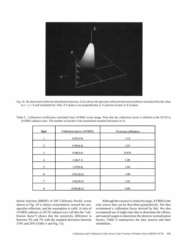
Fig. 10. Bi-directional reflection distribution function. Z axis shows the specular-reflection direction (radiance normalized by the valuein x = y = 0 and multiplied by 256). X-Y plane is set perpendicular to Z and Sun locates in X-Z plane.

Table 5. Calibration coefficients calculated from AVIRIS ocean image. Note that the calibration factor is defined as the OCTS toAVIRIS radiance ratio. The number in bracket is the normalized standard deviation in %.

bution function (BRDF) of Off California Pacific oceanshown in Fig. 10 is almost axisymmetric around the sun-specular-reflection, and the assumption is valid. A ratio ofAVIRIS radiance to OCTS radiance (we call this the “cali-bration factor”) shows that the sensitivity difference isbetween 3% and 7% with the standard deviation between3.9% and 26% (Table 5 and Fig. 11).

Although the variance is relatively large, AVIRIS is theonly source that can be described quantitatively. We thusrecommend a calibration factor derived by this. We alsorecommend use of night time data to determine the offsets,and natural targets to determine the detector normalizationfactors. Table 6 summarizes the data sources and theirreliabilities.


3.2 Geometric calibrationA. Offset of the attitude values

The geometric accuracy was improved to 1.31 km bytuning the three alignment angles (pitch, roll, and yaw)between OCTS and the satellite base plate, and three align-ment angles (pitch, roll, and yaw) in the OCTS scanningmirror so that the root-mean-squared difference betweenestimated ground points and the measured ground pointscould be minimized (Table 7). Here, 187 ground controlpoints were used for this tuning (NASDA, 1997).B. Registration parameters

The band-to-band registration is a key parameter forgenerating satisfactory products especially for land appli-cations. Because 1) the OCTS observes the earth surfacewith the scanning mirror, 2) viewing direction is slightlydifferent over twelve bands, and 3) the pixel resolutionchanges as a function of the scanning angle, it is difficult toachieve perfect image co-registration. The terrain heightalso makes the co-registration difficult.

Table 7. Geometric accuracy improvement by tuning the sensor alignment (km). 187 ground control points were used for this tuningand “cross” and “along” stands for cross track and along track, respectively.

Table 6. Summary of the correction tables.

Fig. 11. Comparison of the calibration factors derived fromAVIRIS and vicarious method. Vicarious data are based onCALCOFI (Nov. 1, 1996).


Fig. 12. Location of the acquired in situ data.

Table 8. Summary of in situ data collected for OCTS data validation.


4. Validation

4.1 Match-up datasetsProduct validation requires in situ data which are ac-

quired simultaneously with OCTS observation under cloud-free conditions. During the eight-month ADEOS life, morethan 1666 Chl-a and 496 nLw measurements were collectedthrough worldwide interagency cooperation (Fig. 12 andTable 8). The major sources of the measurements are mooredbuoys and ships. The representative buoys are NASDA’sbuoy at Yamato-bank in the Sea of Japan (Ishizaka et al., 1997;Kishino et al., 1997), and NASA’s buoy off Lanai Island,Hawaii (Clark et al., 1997). The ship measurements arerepresented by the off Sanriku campaign from May 1997 toJune 1997, UK’s campaign crossing the Atlantic ocean fromnorth to south, and the California Cooperative OceanicFisheries Investigations (CALCOFI) campaigns off Cali-fornia.

Strict match-up conditions on 1) time difference of lessthan 24 hours, 2) location difference of less than 700 m, and3) uniformity of OCTS image which does not containstripes, decreased the number of usable in situ data to 17 forChl-a and 11 for nLw. This means that it is extremely difficultto collect good in situ datasets co-registered with OCTS, anda good collection of in situ data cannot be obtained withoutthe cooperation of agencies worldwide.

A match-up dataset consists of OCTS radiances data(512 pixels by 512 lines for 12 bands), ancillary data(atmospheric pressure, wind speed, wind direction, totalozone amount, solar elevation and azimuth, satellite eleva-tion and azimuth, and a conversion table between the detectornumber and the image address), and the in situ data (e.g.,Chl-a, nLw, optical thickness, aerosol type, humidity, andlocation and the time of measurements). The radiance imageis a subset of Local Area Coverage (LAC).

4.2 Vicarious calibrationAccuracy of Chl-a depends on that of Lw, and thus

depends on the accuracies of Eq. (2) and Lt. While the Lw

shares only a few percent to 10% of Lt, the radiation model(Lm + La + Lam) contributes most regardless of the accuracy.Therefore, Eq. (2) should be well tuned so that the Lw can beconnected with Lt. We proposed a vicarious calibrationmethod that tuned ej and fj so as to statistically fit Lt with Eq.(2). Here, measurements of total ozone, atmospheric surfacepressure, water-leaving radiance, aerosol type, and humid-

ity, were used to determine

L̂t . The key parameter is theaerosol property, and the CALCOFI on November 1, 1997,only provides the aerosol property and the ocean property.We should note that this is not the calibration in a strictmeaning but a parameter fitting. For simplicity, we assumedfj = 0. The factors (ej) are listed in Table 5 in addition to theAVIRIS-based calibration factors.

4.3 EvaluationWe evaluated the accuracy of Chl-a in the Global Area

Coverage (GAC) and LAC products by comparing themwith the in situ data.A. GAC products

Figure 13 shows a scatterogram for Chl-a and in situdata. An use of relaxed condition on co-registration, i.e.,

Fig. 13. Estimated Chl-a of GAC products and in situ Chl-a.

Fig. 14. Comparison of the in situ Chl-a and estimated Chl-a.


Fig. 15. Comparison of estimated nLw and in situ data. a) band 1, b) band 2, c) band 3, d) band 4, and e) band 5.


location error of 27 km and time difference of 72 hrs,increased the number of data to 300. We confirmed that Chl-a is estimated with an accuracy of 68% for Chl-a less than2 mg/m3, and is underestimated after that. Here, the accu-racy is defined by

err = 1N

Chl - aesimated − Chl - a in-situ

Chl - a in-situ

2

i=0

N −1

∑ . 13( )

B. LAC productsFigure 14 shows the scatterogram for Chl-a and the in

situ data, which is screened by the most strict condition (700m distance and 24 hours time difference). The Chl-a slightlyexceeds the in situ data of less than 2 mg/m3 (the normalizederror of 68%) and is underestimated for the Chl-a more than2 mg/m3. The nLw, which is evaluated in the same way asChl-a, in bands 1 to 4 coincides well with the truth data, butnot so well for band 5 (Fig. 15). We understand that Chl-ais acceptable for use, but nLw is not (error of 94 to 129%except for nLw5) as seen in Table 9. The largest error, 416%,in band 5 should be reduced. This result implies that moreattempts on parameter fitting are necessary to reduce theerror in nLw. The reasons why error in Chl-a is much smallerthan that in nLw is that the errors in nLw deviate in the samedirection and the error in Chl-a is reduced (as the Case 2 ofSubsection 2.3).

5. Discussion and ConclusionsThe chlorophyll-a concentration is derived by manipu-

lating the equations for the instrument, the atmosphere, andthe ocean. As discussed in the accuracy consideration (Sub-section 2.3), the errors in total radiance (measurement) andthe atmospheric radiative equation degrade the Chl-a esti-mation. We would like to make conclusive comments for thefuture calibration and validation.

5.1 Calibration (AVIRIS)Absolute calibration can be performed only if we

prepare an accurate reference signal source. A calibratedairborne sensor flying at high altitude is a good source forthis purpose because the on-board sources (lamp and solardata) are inadequate in terms of stability and absolute value.We have conducted the AVIRIS underflights of OCTS overthe ocean area four times. However, the essential difficulties(e.g., i) less opportunities of collocation of two sensor datawhich have different moving speeds and observation geom-etry, ii) unknown radiometric spectrum of the target, and iii)possible temporal deviation of the OCTS filter function)still remain. Although the volume of collocated data wasincreased by assuming the axisymmetry of the oceanicBRDF, a slightly larger variation of the calibration factor atlonger wave length regions is a new problem. The bestaccuracy of 3% is almost acceptable from the hardwarepoint of view, however, it is not small enough to meet therequired accuracies of Chl-a and nLw. Achievement of 0.9%for ∆Lt is the goal for future calibration.

5.2 Radiation modelThe atmospheric radiation model is based on assump-

tions that the aerosols are spherical. The real aerosols havedifferent shapes, so some differences are unavoidable. Evenif the calibration is performed accurately, error of the radiationmodel degrades estimation of ocean color. Thus, the modelis hoped to be built more realistically. Although the modelis very complicated, simple parameterization that fits in thein situ atmospheric data is required.

5.3 Vicarious calibrationCurrently, absolute calibration using the reference

sources (e.g., AVIRIS underflights) does not meet the re-quirements, and the radiation model can not be modifiedeasily. Therefore, only vicarious calibration as a modelfitting can provide good parameters for estimating the Chl-a and nLw accurately. This is the parameter fitting, and the

modified radiance

L̂t is not the calibrated radiance but afitted radiance based on the assumed radiation model. Theideal is to calibrate and validate all three equations so that Lt,nLw, and Chl-a can be correct. This may be future goal.

5.4 In situ data acquisitionAlthough we acquired much in situ data during the eight

months (1666 Chl-a and 496 for water-leaving radiances asof Feb. 1, 1998, Table 8), the usable datasets were limiteddue to unacceptable differences in time and location, orcloud coverage, and the success ratio is only 1% (17 dividedby 1666). This shows that acquisition of matched-up datasetsis extremely difficult and the worldwide cooperation isnecessary.

Table 9. Accuracy of the Chl-a and nLw.


Fig. 16. Sample image of LAC data.


5.5 Towards the version-4 productWe recommend the following actions to improve the

version-3 product: 1) The ej for band 6 and band 8 should bedetermined using the reliable signal sources (i.e., OCTSdata over clear ocean area with no aerosols), and 2) those forthe remaining bands (1–5) should be determined by the leastsquare method.

We show a version-3 Chl-a image of April 26, 1997 inFig. 16. In this paper, we presented the calibration andvalidation results of the version-3 products, where Chl-a isestimated with an accuracy of 68%, water-leaving radiancein 92% at best, and geometric accuracy, 1.3 km. Error of68% meets the accuracy requirement for Chl-a and not farfrom the in situ measurement accuracy of 35%. Althoughthere are several items to be improved in these products, wemay say that the version-3 products can be usable for Earthenvironmental change study.

AcknowledgementsThe authors would like to thank all the members of the

NASDA’s OCTS CAL/VAL teams, and the supportingresearchers. We also thank all the agencies that collaboratedwith NASDA and provided the in situ data to NASDA.

ReferencesArrigo, K. R., C. R. McClain, J. K. Firestone, C. W. Sullivan and

J. C. Comiso (1994): A Comparison of CZCS and In SituPigment Concentrations in the Southern Ocean. NASA TM104566, Vol. 13, Case Studies for SeaWiFS Calibration andValidation, Part 1, Jan.

Clark, D. K., H. R. Gordon, K. J. Voss, Y. Ge, W. Broenkow andC. Trees (1997): Validation of atmospheric correction overthe ocean. J. Geophys. Res., 102, 17,209–17,217.

Fukushima, H. and M. Toratani (1997): Asian dust aerosol:Optical effect on satellite ocean color signal and a scheme ofits correction. J. Geophys. Res., 102, D14, 17,119–17,130.

Gordon, H. R. (1997): Atmospheric correction of ocean imageryin the Earth Observing System era. J. Geophys. Res., 102, D14,17,081–17,106.

IPCC (1990): IPCC Scientific Assessment. Cambridge UniversityPress, Cambridge.

Ishizaka, J., I. Asanuma, N. Ebuchi, H. Fukushima, H. Kawamura,K. Kawasaki, M. Kishino, M. Kubota, H. Masuko, S.Matsumura, S. Saitoh, Y. Senga, M. Shimanuki, N. Tomii andM. Utashima (1997): Time series of physical and opticalparameters off Shimane, Japan, during fall of 1993: Firstobservation by moored optical buoy system for ADEOS dataverification. J. Oceanogr., 53, 245–258.

Johnson, B. C., F. Sakuma, J. J. Butler, S. F. Biggar, J. W. Cooper,J. Ishida and K. Suzuki (1997): Radiometric measurementcomparison using Ocean Color Temperature Scanner (OCTS)visible and near infrared integrating sphere. J. Res. Natl. Inst.Stand. Technol., 106, 627.

Karma, H. J. (1996): Observation of the Earth and Its Environ-ment-Survey of Missions and Sensors. Springer, 239 pp.

Kishino, M. (1994): Development of In-Water Algorithm, contractreport to Remote Sensing Technology Center of Japan.

Kishino, M., J. Ishizaka, S. Saitoh, Y. Sennga and M. Utashima(1997): Verification plan of ocean color and temperaturescanner atmospheric correction and phytoplankton pigmentby moored optical buoy system. J. Geophys. Res., 102, D14,17,197–17,207.

Mitomi, Y., M. Toratani, M. Shimada, H. Oaku, H. Murakami, A.Mukaida, H. Fukushima and J. Ishizaka (1998): Evaluation ofOCTS standard ocean color products: comparison betweensatellite derived and ship measured values. PORSEC’98, July28–31, Qingao, China (to be submitted).

Murakami, H. (1998): El Niño found by OCTS. Proc. of ThirdADEOS Symposium, Sendai, Japan.

Nakajima, T., M. Tanaka, T. Hayasaka, Y. Miyake, Y. Nakanishiand K. Sasamoto (1986): Airborne measurements of the opti-cal stratification of aerosols in turbid atmospheres. AppliedOptics, 25(23), 4374-4381.

NASDA (1997): Initial Evaluation of OCTS, contract report byNEC.

NASDA Documents (1994): OCTS Description and Database,prepared by Mitsubishi Electric Cooperation.

Oaku, H., M. Shimada and R. Green (1998): OCTS absolutecalibration using AVIRIS. IGARSS’98, Seattle (to be pre-sented).

Saino, T. (1993): Satellite ocean color remote sensing and primaryproductivity in the ocean. Coastal Ocean Research Note, 31(1),129–152 (in Japanese).

Shimada, M. and NASDA OCTS Team (1998): A CAL/VAL reporton the OCTS version 3 products. NASDA documents, Jan. 26.

Shimoda, H. (1997): ADEOS Reference Nahdbook. NASDAdocument.

Toba, Y. (1998): Kuroshio, 3rd ADEOS workshop in Sendai, Jan.26–30.

Toba, Y. and H. Murakami (1998): Use of SST-chlorophylldiagrams for water mass analyses including biological pro-cesses. IEEE Geo. Science and Remote Sensing (submitted).

Uzawa, H. (1995): On Global Warming. Iwanami-Shinnsho, Ja-pan.

Vermonte, E. and N. E. Saleous (1993): Absolute calibration ofAVHRR channels 1 and 2. In Advances in the Use of NOAAAVHRR Data for Land Applications, edited by G. D’souza, A.S. Belward and J.-P. Malingreau, Kluwer Academic Publishers.