calibration and 3d model generation for a low-cost
TRANSCRIPT
Calibration and 3D Model Generation for
a Low-Cost Structured Light Foot Scanner
by
Navaneetha Kannan Viswanathan
A thesis
presented to the University of Waterloo
in fulfillment of the
thesis requirement for the degree of
Master of Applied Science
in
Mechanical Engineering
Waterloo, Ontario, Canada, 2012
© Navaneetha Kannan Viswanathan 2012

ii
AUTHOR'S DECLARATION
I hereby declare that I am the sole author of this thesis. This is a true copy of the thesis, including any
required final revisions, as accepted by my examiners.
I understand that my thesis may be made electronically available to the public.

iii
Abstract
The need for custom footwear among the consumers is growing every day. Serious research is being
undertaken with regards to the fit and comfort of the footwear. The integration of scanning systems in
the footwear and orthotic industries have played a significant role in generating 3D digital
representation of the foot for automated measurements from which a custom footwear or an orthosis
is manufactured. The cost of such systems is considerably high for many manufacturers due to their
expensive components, complex processing algorithms and difficult calibration techniques.
This thesis presents a fast and robust calibration technique for a low-cost 3D laser scanner. The
calibration technique is based on determining the mathematical relationship that relates the image
coordinates to the real world coordinates. The relationship is determined by mapping the known real
world coordinates of a reference object to its corresponding image coordinates by multivariate
polynomial regression. With the developed mathematical relationship, 3D data points can be obtained
from the 2D images of any object placed in the scanner.
An image processing script is developed to detect the 2D image points of the laser profile in a series
of scan images from 8 cameras. The detected 2D image points are reconstructed into 3D data points
based on the mathematical model developed by the calibration process. Following that, the output
model is achieved by triangulating the 3D data points as a mesh model with vertices and normals. The
data is exported as a computer aided design (CAD) software readable format for viewing and
measuring.
This method proves to be less complex and the scanner was able to generate 3D models with an
accuracy of +/-0.05 cm. The 3D data points from the output model were compared against a reference
model scanned by an industrial grade scanner to verify and validate the result. The devised
methodology for calibrating the 3D laser scanner can be employed to obtain accurate and reliable 3D
data of the foot shape and it has been successfully tested with several participants.

iv
Acknowledgements
I would like to offer my sincere gratitude to my supervisors, Dr. Jan Huissoon and Dr. Sanjeev Bedi
for supporting me throughout my thesis with patience and knowledge. I attribute the level of my
Masters degree to their encouragement and effort. Special thanks to Tezera Ketema for his strong
motivation and trust on me and this research.
I am thankful to Professor. Naveen Chandrashekar and Professor. Behrad Khamesee for agreeing to
read my thesis and for their valuable feedbacks towards the betterment of the thesis. I would like to
acknowledge Dr. Jonathan Kofman and Luigi Giaccari for sharing their knowledge and expertise in
computer vision systems and surface reconstruction.
I must also mention my gratitude to Sam Lochner for his friendly assistance and encouragement
throughout this journey. Special thanks to Dragos Besliu, Vinodhkumar and Sudipto Dolui for their
assistance in the laboratory.
I would like to thank my friend Teja Vajha for the many hours spent in the experiments and for his
priceless support and assistance. Finally, I thank my parents and my sister for their love and moral
support although I was miles away from them.

v
Dedication
To my Motherland and Manju

vi
Table of Contents
AUTHOR'S DECLARATION ............................................................................................................... ii
Abstract ................................................................................................................................................. iii
Acknowledgements ............................................................................................................................... iv
Dedication .............................................................................................................................................. v
Table of Contents .................................................................................................................................. vi
List of Figures ..................................................................................................................................... viii
List of Tables ......................................................................................................................................... x
Chapter 1 Introduction ........................................................................................................................... 1
1.1 Project Motivations ...................................................................................................................... 1
1.1.1 Shoe making .......................................................................................................................... 2
1.2 Current Research .......................................................................................................................... 5
1.3 Earlier Work................................................................................................................................. 6
1.4 Thesis Layout ............................................................................................................................... 8
Chapter 2 Literature Review .................................................................................................................. 9
2.1 Overview ...................................................................................................................................... 9
2.2 Basic foot geometry measurements ............................................................................................. 9
2.2.1 Linear Measurements .......................................................................................................... 10
2.2.2 Girth Measurements ............................................................................................................ 11
2.2.3 Plantar Shape Measurement ................................................................................................ 11
2.2.4 Dynamic Measurements ...................................................................................................... 12
2.3 Optical Scanning methods ......................................................................................................... 12
2.3.1 Optical 3D Measurement Techniques ................................................................................. 13
2.4 Calibration techniques ............................................................................................................... 18
2.4.1 Self-calibration and Reference-object based calibration ..................................................... 18
2.4.2 Single camera calibration .................................................................................................... 19
2.5 3D Laser Scanners ..................................................................................................................... 22
2.5.1 Generic Classification ......................................................................................................... 23
Chapter 3 System Description ............................................................................................................. 25
3.1 Scanner criteria .......................................................................................................................... 25
3.2 Overall constructional setup....................................................................................................... 26
3.2.1 Scanner criteria ................................................................................................................... 26
3.3 Hardware setup .......................................................................................................................... 27

vii
3.3.1 Overall Setup ....................................................................................................................... 27
3.3.2 Range-Sensor Platforms ...................................................................................................... 29
3.3.3 Motors and Drives ............................................................................................................... 31
3.3.4 Front-end interface .............................................................................................................. 33
Chapter 4 Optical Calibration of the Scanner ....................................................................................... 34
4.1 3D measurement process of the Foot scanner ............................................................................ 34
4.2 Optical Calibration ..................................................................................................................... 35
4.2.1 Choosing a calibration technique ........................................................................................ 35
4.3 Fast and Robust calibration technique ........................................................................................ 37
4.3.1 Depth Mapping - Multivariate Regression .......................................................................... 38
4.3.2 Computation ........................................................................................................................ 42
4.4 Experiments and Trials performed ............................................................................................. 47
4.5 Steps after Calibration ................................................................................................................ 53
Chapter 5 Implementation and Prototype Validation ........................................................................... 54
5.1 Range Image acquisition ............................................................................................................ 54
5.2 Image processing ........................................................................................................................ 55
5.3 Depth estimation and Post processing 3D data points ................................................................ 61
5.4 CAD model generation ............................................................................................................... 64
Chapter 6 Performance Verification and Results ................................................................................. 66
6.1 Scan results of Calibration Object .............................................................................................. 66
6.1.1 Description .......................................................................................................................... 66
6.1.2 Scanner 3D point cloud output ............................................................................................ 67
6.1.3 Basic dimensional check ..................................................................................................... 68
6.2 Scan results of Sock model......................................................................................................... 69
6.2.1 Comparison of Foot models by Registration ....................................................................... 69
6.3 Scan results of human foot ......................................................................................................... 74
Chapter 7 Conclusion and Future Work ............................................................................................... 75
7.1 Conclusion .................................................................................................................................. 75
7.2 Future Work ............................................................................................................................... 76
Appendix A Estimation of Goodness of Fit ......................................................................................... 78
Appendix B Calibration Chart for 8 Cameras ...................................................................................... 80
References ............................................................................................................................................ 81

viii
List of Figures
Figure 1-1 Plastic and wooden shoe last ................................................................................................ 2
Figure 1-2 Generic classification of footwear manufacturing ............................................................... 3
Figure 1-3 Schematic flow of footwear manufacturing integrated with a scanning system .................. 4
Figure 1-4 Research motive and Scope .................................................................................................. 5
Figure 1-5 Two-dimensional scanner for custom orthotic sandal developed at the University of
Waterloo [1, 2] ....................................................................................................................................... 7
Figure 1-6 Thesis organization .............................................................................................................. 8
Figure 2-1 Generic classification of foot geometry measurements ....................................................... 9
Figure 2-2 Brannock device [4] ........................................................................................................... 10
Figure 2-3 Three dimensional measuring techniques by optics [22] ................................................... 14
Figure 2-4 Classification of the camera parameters ............................................................................. 18
Figure 2-5 Pinhole camera model ........................................................................................................ 20
Figure 2-6 Checkerboard pattern to determine the camera parameters ............................................... 21
Figure 2-7 Classification of 3D laser digitizers [51] ............................................................................ 23
Figure 3-1 3D Foot scanner criteria ..................................................................................................... 26
Figure 3-2 CAD model of the 3D Foot scanner with conceptual laser plane ...................................... 27
Figure 3-3 3D Foot scanner - Working prototype ................................................................................ 28
Figure 3-4 Top view of the 3D Foot scanner ....................................................................................... 28
Figure 3-5 Range sensor head - Overview ........................................................................................... 29
Figure 3-6 From top to bottom (1) Range sensor head - Side platform (2) Range sensor head - Bottom
platform ................................................................................................................................................ 30
Figure 3-7 Control box ......................................................................................................................... 32
Figure 3-8 Hand-held controller .......................................................................................................... 32
Figure 3-9 Front-end Graphic User Interface ...................................................................................... 33
Figure 4-1 Basic steps in image-based 3D measurement ..................................................................... 34
Figure 4-2 Transformation of 2D image data points to world space ................................................... 37
Figure 4-3 Polynomial curves of various orders .................................................................................. 39
Figure 4-4 Conceptual diagram of laser ray over an object and its view in image plane .................... 40
Figure 4-5 Reference object used for calibration of 8 cameras ........................................................... 46
Figure 4-6 Calibration of camera 1 – Upper-left range sensor head .................................................... 48
Figure 4-7 Point cloud data acquired from the calibration frame of camera 1 – 411 points ................ 51

ix
Figure 4-8 Point cloud data acquired from 8 cameras - Calibration frame .......................................... 52
Figure 4-9 3D Foot scanning process after the calibration of scanner optical system ........................ 53
Figure 5-1 Matlab (R2010b) Image Acquisition Toolbox Environment .............................................. 55
Figure 5-2 Basic overview of image processing and associated operations ......................................... 56
Figure 5-3 Laser profile over the sock model...................................................................................... 57
Figure 5-4 Identification of laser profile in a scan image ..................................................................... 58
Figure 5-5 Laser profile with outliers removed .................................................................................... 59
Figure 5-6 Thinned laser profile ........................................................................................................... 59
Figure 5-7 Collection of extracted 2D image points from Camera 1 - Sock model (17 images) ........ 60
Figure 5-8 Input image coordinates for depth mapping ....................................................................... 61
Figure 5-9 3D Point cloud data of camera 1 - Sock model (Viewed in Meshlab environment) .......... 62
Figure 5-10 3D Point Cloud data with outliers – Viewed in Meshlab environment ............................ 63
Figure 5-11 3D Point cloud data of the scanned sock model ............................................................... 64
Figure 5-12 Triangulated 3D sock model from the 3D data points ...................................................... 65
Figure 6-1 Aluminum block (15 x 10 x 5 cm) ...................................................................................... 66
Figure 6-2 3D Point cloud of the block- Viewed in Meshlab .............................................................. 67
Figure 6-3 Reconstructed block as .stl file - Viewed in Meshlab ......................................................... 67
Figure 6-4 Length and width deviation study – Solidworks ............................................................... 68
Figure 6-5 Scan result of the Sock model - NDI, Waterloo [57] ......................................................... 69
Figure 6-6 Generated 3D .stl file of the Sock model ........................................................................... 70
Figure 6-7 Scanner output and reference model – CloudCompare [58] environment ......................... 70
Figure 6-8 Comparison of data points with the reference CAD file- CloudCompare [58] environment
.............................................................................................................................................................. 71
Figure 6-9 Cloud to Cloud distance between reference CAD model and scanner output model ......... 72
Figure 6-10 Cloud to Cloud distance comparison for 8 classes of data points .................................... 73
Figure 6-12 Foot models from the scanner ........................................................................................... 74

x
List of Tables
Table 3-1 Functional roles of the range sensor heads .......................................................................... 31
Table 4-1 Calibration chart- Depth mapping through a reference object of known geometry ............ 47
Table 4-2 Calibration chart of camera 1 .............................................................................................. 49
Table 4-3 Computed coefficients for 'Y' and 'Z'- Camera 1 ................................................................. 50
Table 6-1 Deviations with the actual CAD model and the output CAD model ................................... 68
Table 6-2 Results of Cloud to Cloud comparison ............................................................................... 73

1
Chapter 1
Introduction
The footwear industry serves billions of people across the globe every year and satisfying the needs
of every consumer has become an essential goal for the industry. The diverse industry produces
numerous varieties of everyday footwear for men, women, children as well as specialized products
like winter boots, athletic footwear, and protective footwear. The footwear industry remains a highly
specialized and competitive environment as it aims to satisfy consumers in terms of fitness and
comfort. Most footwear manufacturers need to be as efficient as possible while providing high quality
footwear for the majority of customers. In recent years, this drive for efficiency has increased due to
the rise in international trade and competition as well as increased consumer demand. As a result,
footwear manufacturers have found it crucial to adapt to the market conditions by providing footwear
with a wide variety of styles and sizes. Lately, the integration of computers and automation in the
footwear industry has been relatively limited compared to other fields due to the high costs of setup
and complex computations involved.
The research presented in this thesis focuses mainly on the software development for a proof-of-
concept three dimensional foot scanning system for custom shoe manufacturing. The scanner
presented in the thesis provides a solution to this need for improved productivity and efficiency due to
its low cost and reliable output.
1.1 Project Motivations
The following section reviews the shoemaking process and the role of optical scanning systems in the
footwear industry. The applications of two dimensional and three dimensional scanning systems for
integrated footwear manufacturing and custom orthoses are also discussed to understand the demand
for such systems.

2
1.1.1 Shoe making
A typical shoe maker starts the job with a last made traditionally from wood, but now often made of
plastic as shown in Figure 1-1. The design of the last represents the shape and measurement of the
customer’s foot. These measurements for the last are acquired through measuring sticks, measuring
tapes and calipers. The last is then used to cut the upper materials and the sole of the shoe. Following
that, the last is removed after the upper materials and the sole are sewn and nailed together. It is
naturally a tedious work to develop a last for each customer the shoe maker has to deal with. As a
result, the shoe lasts are typically made from a generic template and are pre-crafted for various
common sizes.
For un-common sizes or cases with some artifacts, new lasts are custom made. With the help of a last,
a mock shoe is made as per the quality and aesthetic requirements of the customer. The mock shoe is
then tested by the customer for fit and comfort. If necessary, the required changes are made in the last
and then the shoe is finally crafted.
Figure 1-1 Plastic and wooden shoe last
Since the process involves a lot of manual measurements, errors are significant. The entire process of
measuring, computing and manufacturing is laborious and time consuming. In addition, since the foot
measurement data is not common among manufacturers, the customers are constrained to approach
the same manufacturer each time they need new footwear.

3
On the whole, the process of shoemaking can be classified into two major types (as shown in Figure
1-2); conventional or traditional methods of manufacturing and custom manufacturing.
Figure 1-2 Generic classification of footwear manufacturing
While the custom footwear manufacturing industry had to rely on the conventional manual process;
commercial and mass manufacturing industry began to use the benefits of technological
advancements in automated manufacturing. The use of injection molding techniques, CNC based last
milling, pattern cutting and sewing had tremendous impact in optimizing the commercial shoe
manufacturing process.
Due to the absence of technological advancements in foot measuring techniques, custom
manufacturing has become relatively expensive in terms of time and cost. On average, a custom shoe
maker charges about two to three thousand dollars for a custom shoe and takes nearly 4 hours to
manufacture a last for the same [1]. So, any development or break-through in the process of
measurement and last manufacturing would drastically bring down the overall time.

4
Advancements in scanning systems have proven useful for obtaining a computerized model of a foot.
Figure 1-3 shows a c \onceptual flow diagram of a foot wear manufacturing system integrated with a
scanning system. This typically eliminates the laborious work involved in measuring the foot with
calipers, measuring sticks and measuring tapes. Hence, with the help of scanning systems, foot
measurements can be taken with ease and drastically reduce the manual error. This potential blend of
technology has developed an interest in the footwear and orthoses manufacturing industries to adopt
and stand-out in delivering products with a good fit and comfort for the customers.
Figure 1-3 Schematic flow of footwear manufacturing integrated with a scanning system
Although the integration of scanning systems in the footwear and the orthosis manufacturing
industries has many advantages, the high cost of implementing such systems in a retail store or a

5
clinic is still the biggest disadvantage. For example, a three dimensional foot scanning system in the
market costs in the range of $ 25,000 to $ 75,000 (Canadian dollars). Since only a few retailers can
afford to purchase such a scanning system, the majority of the retailers are in need of a low-cost
scanning system that suits their needs.
1.2 Current Research
As mentioned earlier, the research mainly focuses on the software developed for the scanning system
to digitize the foot and generate a measurable three dimensional CAD model using a fast and reliable
optical calibration technique. This enables last manufacturing in a shorter period of time and more
importantly without any human errors that result from manual methods. The CAD file of the foot data
can be easily shared and accessed through the internet which makes it easy for the consumer to order
footwear or make medical consultations with the click of a mouse. Also, for the orthotics industry and
foot clinics, the CAD file could be used by clinicians or practitioners to access the patient’s foot data
on their computer without the physical presence of the patient.
Figure 1-4 Research motive and Scope

6
1.3 Earlier Work
Prior to the research presented in this work, a 2D scanning system to produce a plantar shoe surface
was designed and deployed [1]. A brief overview of the system is presented in this section. The result
of the deployed 2D scanner inspired and motivated the development of a 3D scanning system that
could digitize the foot and produce a CAD model.
The first basic measurement step of a shoe maker is to start by tracing the perimeter of the foot, from
which the contours and sizing can be estimated. This preliminary measurement can be easily made
with a simple 2D scanning system, involving a camera and acquisition hardware. This method
enables capturing of the subject data with more accurate information on features and landmarks. This
has a significant impact in the making of plantar shoe surface. A step further, integration of
CAD/CAM with this system proves to be advantageous. As a result, an automated system for custom
orthotic sandals with a series of 2D scan images has been developed [2].
To stress the significance of the advantage of 2D scanning, the following is a brief insight on the
research done by Lochner [1] towards the development of custom orthotic sandal from 2D scan
images. The plantar regions of left and right foot of the customer are acquired by an off the shelf 2D
scanner. The acquired images are uploaded to a processing server, which enables the operator or
clinician to choose points on the image manually in order to estimate the length and width of the foot.
Additionally, key features like toe crest, ball joint and other distinct features can also be identified
and noted.
Once the landmarks are identified, programmed scripts would run the automatic contouring of the
foot. The images are placed in a 3D space where a custom orthotic is extrapolated with the Rhino API
script.

7
This research, with the help of an industrial partnership was applied to commercially manufacture
custom orthotic sandals. The CAD extrapolated sandal sole was then manufactured using ethylene
vinyl acetate material in a CNC mill. Following that, sole covers and upper straps are added to make
the finished product.
.
Figure 1-5 Two-dimensional scanner for custom orthotic sandal developed at the University of
Waterloo [1, 2]

8
1.4 Thesis Layout
The remainder of this thesis has the following layout.
Chapter 2 reviews the study of basic foot geometry, optical scanning methods, calibration techniques
of cameras and insight on three dimensional laser scanning systems.
Chapter 3 describes the three dimensional laser scanner devised to digitize the foot. Also, various
criteria and considerations are discussed in detail.
A detailed discussion on calibrating the laser scanner is presented in Chapter 4. Following that,
Chapter 5 presents the implementation and working of the laser scanner more elaborately. Chapter 6
presents the performance verification and results and Chapter 7 presents the conclusion,
recommendations and future work to be carried out in the system.
Figure 1-6 Thesis organization

9
Chapter 2
Literature Review
2.1 Overview
Computer vision and scanning systems have witnessed numerous improvements and innovations in
the field of shape measurements. This chapter of the thesis is intended to familiarize the reader with
four major segments that are essential for understanding 3D foot scanning techniques. The first
segment guides the reader through the basic foot geometry measurements essential for shoe last or
custom orthoses manufacturing. The second and third segments elaborate on various optical scanning
techniques applied to 3D object measurement and calibration methodologies for cameras used in the
scanning system. The 3D laser scanning technique is discussed in detail in greater fourth segment of
this chapter.
2.2 Basic foot geometry measurements
Figure 2-1 Generic classification of foot geometry measurements
Foot measurements
Linear measurements Girth measurements Plantar measurements

10
2.2.1 Linear Measurements
The most common foot measurement taken by a shoemaker or a retailer is the length of the foot, with
which the customers are given the closest fitting shoe off the shelf. These sizes are regulated and
defined by various national and continental sizing systems [3]. Depending on the
need/retailer/shoemaker/demography, the method of measurements is carried out. For example, use of
a Brannock device (shown in Figure 2-2) helps in measuring the length, the width and the arc length
of the foot.
Figure 2-2 Brannock device [4]
Witana et al. [5] and Liu et al. [6] present various methodologies for generating foot measurements
from a 3D scan data. The former used the 3D shape of the foot from a high-end 3D scanning system
that could generate 3D surface data along the length of the foot. Based on the linear measurements,
Krauss et al. [7] categorizes the human feet into different types: voluminous, flat-pointed and slender.
Various studies have been carried out to validate the results of linear measurements obtained by
Left heel cup
Right heel cup
Movable width bar
Moveable arc length
pointer

11
automated measurements to be in line with the results of earlier studies based on manual
measurements. Lou et al. [8] applied the 3D scanning technique to assess the differences in foot shape
with gender. The results were proven to be in line with the earlier study made by Wunderlich et al.
[9].
2.2.2 Girth Measurements
A step further to linear measurement of the foot, it was found necessary to have a detailed data on the
overall foot shape to manufacture shoe lasts (as discussed earlier in chapter 1). Development of shoe
lasts generally needs in depth foot measurements of the customer’s foot so as to manufacture
footwear with a good fit and comfort. Bao et al. [10] presented an integrated system for
manufacturing custom shoe lasts for the orthopedic shoe design. Witana et al. [5] and Nacher et al.
[11] used 3D scanners with girth measurement algorithms to measure the non-contact areas (due to
the irregular shape of the foot) and also investigated the quality of fit between the foot and shoe based
on the computed measurements. Wang [12] scanned 10 shoe lasts and developed a process for
selecting a last that would most suit for the individual based on various girth measurements like ball
girth, waist girth and instep girth of the foot.
2.2.3 Plantar Shape Measurement
Similar to linear and girth measurements, a lot of research has been carried out specifically in
measuring the plantar surface of the foot. This measurement is considered to be vital for any custom
orthosis manufacturing. It is proven that customers with custom orthosis enjoy a good fit and comfort
than preferring an off the shelf orthosis. Hawke et al. [13] conducted clinical trials and evaluated the
effectiveness of custom orthotics. Over the past decade, a large number of 2D scanning systems to
measure the plantar surface have evolved in the market.

12
Modern surface scanning techniques is integrated with the software packages to enable fast and
reliable orthosis design. Some notable software packages include, Orthomodel from Delcam PLC,
UK and PlantarScan, Precision 3D, UK.
An alternative method for obtaining the shape of the foot rather by casting or scanning is the
impression foam system [14]. The patient is made to stand with their foot pushed into a low density
foam box. As the foam collapses with the self-weight, a negative of the foot shape is achieved. The
box is either filled with plaster or scanned directly to obtain the positive cast.
2.2.4 Dynamic Measurements
The advancements in optical technologies provided ways to measure dynamic changes in foot shape
during walking and other actions [15]. The process is highly computational because of its complexity
and is expensive. Kimura et al. [16] uses 12 video cameras and a walkway for the study of dynamic
changes. Jezerek et al. [17] uses the multiple-laser-plane triangulation to measure the 3D geometry.
Recent advancements in this method include the pressure mapping and pin device systems to analyze
the variations in foot shape during various actions.
The extensive use of optical scanning systems is evident from the above study. The traditional manual
measurements are slowly being replaced by the advanced optical scanning instruments. The following
section presents a detailed study on various optical scanning methods for 3D shape measurements.
2.3 Optical Scanning methods
In the current industrial scenario, there is a need for accurate measurement of 3D objects to enhance
the speed of a product development along with the quality of manufacturing [18]. This technology is
more prevalent in reverse engineering, part inspections, dimension measurements, intelligent robots,
and obstacle detection for vehicle guidance.

13
With the rise of technological advancements in computer technology integrated with digital scanning
systems, 3D measuring systems/scanners have become commercially successful. Another major
advantage of these optical scanners is that it allows non-contact based measurement with a high
accuracy and denser data points, which carves the way for more research and analysis based on the
output data. The cost of such scanning systems becomes expensive due to the sophisticated optical
and electronic setup.
There have been many efforts to reduce the cost of a commercial foot scanner. Blais et al. [19]
designed 3 optical sensors to reduce the cost of foot scanner. Kouchi et al. [20] applied the concept of
homologous shape modeling and Leon Kos [21] introduced automatic landmark detection algorithm
to design a low cost foot scanner that generates a customized shoe last based on the extracted foot
shape.
However the cost of these scanners is still too high to be used in a conventional retail store/clinic, as
these scanners still implement the 3D measurement technique with expensive hardware setup.
2.3.1 Optical 3D Measurement Techniques
Over the past few years, a wide range of optical techniques have been applied to measure a 3D shape.
Figure 2-3 illustrates the generic classification of the 3D measurement techniques and a brief
overview of these techniques discussed in [22] is reviewed in this section of the thesis.

14
Figure 2-3 Three dimensional measuring techniques by optics [22]
2.3.1.1 Time/Light in flight
Time of flight based method of 3D measurement is based on estimating the depth information by
measuring the duration of flight of a light source from a source point to the receiver point [23].
During the measurement, the object pulse is reflected back to the receiver and is compared with the
reference pulse for the time difference. This difference is mathematically related to the distance. The
resolution of the device operating with this method purely depends on the high resolution electronics
and the pulse generation time [18]. This technique serves as the basic principle of operation for laser
range finders.
2.3.1.2 Laser speckle pattern sectioning
This method is purely based on the transformation relationship between the optical
wavelength/frequency space and the distance/range space to measure the shape of an object [24, 25,
26]. A speckle pattern is acquired and measured using a CCD array at various laser wavelengths, and
the individual frames are aggregated to generate a 3D data array. Following that, a 3D Fourier
transform is applied to this data array to obtain the 3D shape of an object. Some major advantages of
this technique are (1) the high flexibility of measurement range and (2) that it does not require phase
3D Measurement by Optics
Time/light in flight
Laser speckle pattern
Moiré method
Interferometry
Photogrametry
Structured light
Laser scanning

15
shifting as in the case of conventional interferometry. The time to acquire images with different
wavelengths was found to be too long for relatively large scale shapes and hence it is not preferred in
the industry [18].
2.3.1.3 Moiré method
The Moiré method can be divided into a projection of light and the shadow based method of
measurement. Takasaki[27] and Harding et al. [28] have elaborated more on the Moiré topography
and the application of Moiré method in visual inspection of machined parts . The technique uses two
gratings, namely a master grating and a reference grating, from which contour fringes can be
generated and resolved by a charge coupled device (CCD) camera. The Logic-Moiré method
discussed in [29, 30] employs a computer generated reference grating and a computer resolved master
grating. The complexity in construction, time and implementation becomes the drawback in industrial
and commercial applications. To overcome this drawback, various studies have been carried out and
use of multiple image fringe patterns with different phase shifts were then introduced to overcome the
environmental perturbations and to reduce the process time [18]. The comparison of high speed Moiré
methods, applications and related references can be found in [18, 31].
2.3.1.4 Interferometry
The basic idea behind interferometry based shape measurements is the formation of fringes by
varying the sensitivity matrix (usually controlled by computer) that relates the geometry of the
scanned object to the measured optical phases. The key variables of the sensitivity matrix are the
wavelength, refractive index and the illumination and direction of observation. Dalhoff et al. [32]
presented the double heterodyne interferometry using a frequency shift technique to measure 3D
shapes of high accuracy with 0.1mm resolution . It was also proven in the same research that the
integration of phase shifting technique with the interferometric method and the heterodyne technique
16
can have accuracies of 1/100 and 1/1000 of a fringe respectively. Some of the advanced methods of
Interferometry include, shearography, diffraction grating, digital wave front reconstruction and wave
length scanning and conoscopic holography [48].
2.3.1.5 Photogrammetry
Photogrammetric 3D reconstruction technique employs the bundle adjustment principle, where the
geometric model and the orientation of the bundles of light rays in a photogrammetric relationship is
developed analytically and is implemented by the least squares procedure [34]. It typically uses one
of the stereo techniques, defocus, shading or scaling to measure the 3D shape. Photogrammetry is
primarily used in the feature type 3D dimension measurement. It is carried out by having bright
markers on the surface of the object being measured. Extensive research has been carried out by
Fraser [35] to improve the accuracy of this method and proved to have high accuracy as one part in
100,000 or even one part in 1,000,000.
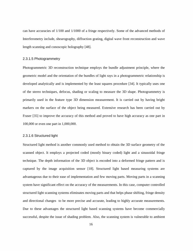
2.3.1.6 Structured light
Structured light method is another commonly used method to obtain the 3D surface geometry of the
scanned object. It employs a projected coded (mostly binary coded) light and a sinusoidal fringe
technique. The depth information of the 3D object is encoded into a deformed fringe pattern and is
captured by the image acquisition sensor [18]. Structured light based measuring systems are
advantageous due to their ease of implementation and few moving parts. Moving parts in a scanning
system have significant effect on the accuracy of the measurements. In this case, computer controlled
structured light scanning systems eliminates moving parts and that helps phase shifting, fringe density
and directional changes to be more precise and accurate, leading to highly accurate measurements.
Due to these advantages the structured light based scanning systems have become commercially
successful, despite the issue of shading problem. Also, the scanning system is vulnerable to ambient
17
light and becomes challenging to handle in a brighter environment. Some of its common applications
are discussed in [36].
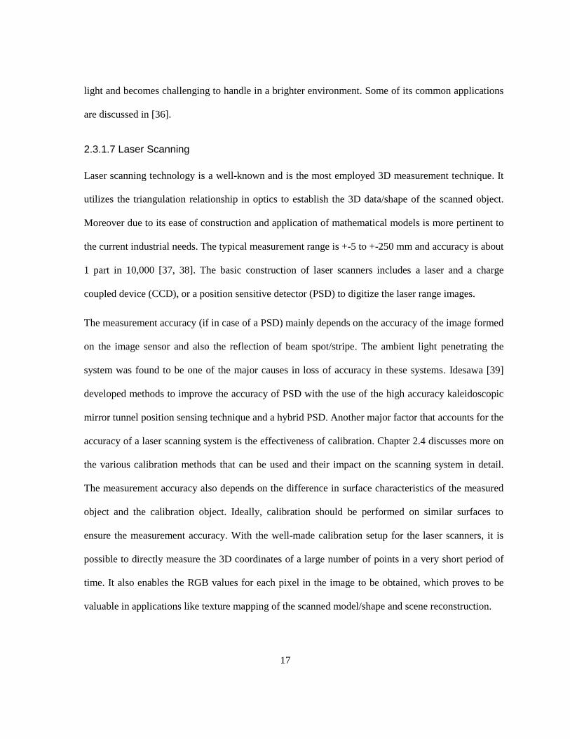
2.3.1.7 Laser Scanning
Laser scanning technology is a well-known and is the most employed 3D measurement technique. It
utilizes the triangulation relationship in optics to establish the 3D data/shape of the scanned object.
Moreover due to its ease of construction and application of mathematical models is more pertinent to
the current industrial needs. The typical measurement range is +-5 to +-250 mm and accuracy is about
1 part in 10,000 [37, 38]. The basic construction of laser scanners includes a laser and a charge
coupled device (CCD), or a position sensitive detector (PSD) to digitize the laser range images.
The measurement accuracy (if in case of a PSD) mainly depends on the accuracy of the image formed
on the image sensor and also the reflection of beam spot/stripe. The ambient light penetrating the
system was found to be one of the major causes in loss of accuracy in these systems. Idesawa [39]
developed methods to improve the accuracy of PSD with the use of the high accuracy kaleidoscopic
mirror tunnel position sensing technique and a hybrid PSD. Another major factor that accounts for the
accuracy of a laser scanning system is the effectiveness of calibration. Chapter 2.4 discusses more on
the various calibration methods that can be used and their impact on the scanning system in detail.
The measurement accuracy also depends on the difference in surface characteristics of the measured
object and the calibration object. Ideally, calibration should be performed on similar surfaces to
ensure the measurement accuracy. With the well-made calibration setup for the laser scanners, it is
possible to directly measure the 3D coordinates of a large number of points in a very short period of
time. It also enables the RGB values for each pixel in the image to be obtained, which proves to be
valuable in applications like texture mapping of the scanned model/shape and scene reconstruction.
18
2.4 Calibration techniques
The primary objective of calibration is to establish the projection from the 3D world coordinate
system to the 2D image coordinate system. With a known projection, 3D information can be inferred
from the 2D images acquired the by the laser scanner’s acquisition device. Zhang [40] classifies the
camera calibration techniques into two main categories: Reference-object based calibration and Self-
calibration.
2.4.1 Self-calibration and Reference-object based calibration
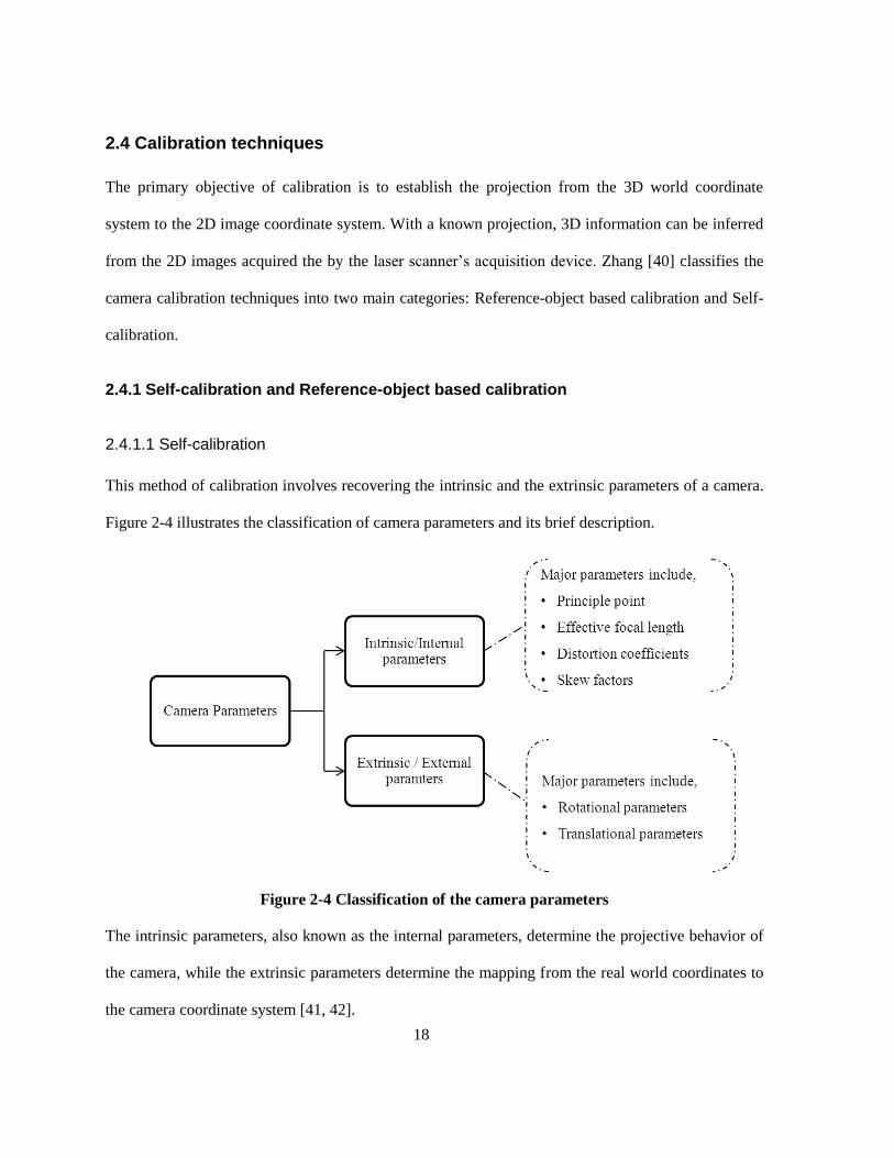
2.4.1.1 Self-calibration
This method of calibration involves recovering the intrinsic and the extrinsic parameters of a camera.
Figure 2-4 illustrates the classification of camera parameters and its brief description.
Figure 2-4 Classification of the camera parameters
The intrinsic parameters, also known as the internal parameters, determine the projective behavior of
the camera, while the extrinsic parameters determine the mapping from the real world coordinates to
the camera coordinate system [41, 42].

19
The intrinsic parameters of a camera include the details on principle point, effective focal
length, and distortion co-efficient and skew factor. The principle point of a camera is a
point where the optical axis coincides with the image plane or the image-sensor plane of a
camera. The effective focal length ‘ f ’ of camera is defined in two values along x-axis and
y-axis, namely, ‘xf ’ and ‘ y
f ’. Distortions in a camera are due to the optical aberrations in
the lens of the camera [42]. The skew factor of the camera is defined as the angle between
the pixels in the x-axis and y-axis respectively. Imperfections in manufacturing are the
main source of this factor.
The extrinsic parameters of a camera include three rotational parameters and three
translational parameters. The rotational parameters of a camera give the orientation of the
camera coordinate system in the world coordinate system, while the translation parameters
relate the origin of the camera coordinate system in the world coordinate system [42].
2.4.1.2 Reference object –based calibration
The camera calibration process is accomplished by observing a calibration object of precisely known
geometry in 3D world space. Usually the calibration object consists of two or three planes orthogonal
to each other in order to effectively extract the depth information from a 2D image.
2.4.2 Single camera calibration
With the images from camera of known internal parameters, correspondence between three images
can be used to recover internal and external parameter which allows in reconstructing 3D models
[40].
Clarke et al. [43] presented a detailed review of widely used camera models and calibration
techniques. The most commonly used camera model is the pinhole model. Various pinhole model

20
based algorithms for camera calibration are presented in [40, 44, 45]. In those models, the camera is
assumed to perform a perfect perspective optical transformation. Figure 2-5 illustrates the pinhole
camera model.
Figure 2-5 Pinhole camera model
The mapping from image coordinates to world coordinates can be written as [40]:
[ | ]sm A R T M
(2.1)
or, expanded as,
11 12 13 1
21 22 23 2
31 32 33 3
0
0
1 0 0 11
x x
y y
Xi f c r r r t
Ys j f c r r r t
Zr r r t
(2.2)
Where (X, Y, Z) are the 3D real world coordinates, (i, j) are the image coordinates. The image plane
is shown ahead of the projection center for better visualization and understanding, although it is
actually behind. In equations 2.1 and 2.2, ‘A’ represents the camera matrix, xc , yc are the principle

21
points along x and y directions respectively. xf and y
f are the focal lengths in x and y directions
respectively, expressed in pixel units. The joint rotation-translation matrix R|T is usually known as
the extrinsic matrix and describes the pose of the image plane in the camera to the real world
coordinates [41]. To consider lens distortion in the calibration process, parameters k1, k2 are
introduced to determine the radial distortions and p1, p2 for the tangential distortions. Tsai [47]
mentions that only radial distortion plays a significant role in machine vision applications.
The calibration techniques are usually based on known space coordinates/ geometry of a calibration
object (as mentioned in section 2.4.1.2). The calibration objects employed to recover the camera
parameters can be either a 2D [47] or a 3D [48] or a planar [40] object. The calibration method
presented in [40] uses a 2D planar calibration grid, which is placed at different positions and
orientations in front of the camera. The feature points of the planar checkerboard pattern are extracted
by image processing and the projective transformation between the image points of different images
and the corresponding 3D points are computed. Figure 2-6 shows a 7x6 checkerboard pattern.
Figure 2-6 Checkerboard pattern to determine the camera parameters

22
The camera’s intrinsic and extrinsic parameters are computed next by direct linear transformations.
Following to that, the radial distortion terms are computed by linear least squares and the re-
projection errors incurred in the process are minimized by using the Levenberg-Marquardt method
[49, 50].
2.5 3D Laser Scanners
As mentioned earlier in section 2.3.1.7, the 3D laser scanners are currently the pick among all the
other scanning systems, because of their high accuracy and precision with a low processing time.
Primarily, a laser scanner employs a laser diode, a capturing device (CCD or PSD) and a processing
system to acquire range images of the scan object in order to process the 2D images into 3D data
points. Extensive research has been carried out in this field of scanning systems to improve the
accuracy and precision of the output results. Improvements in the field of digital acquisition systems
have carved a way to much advancement in 3D laser scanning systems.
For example, increments in the frame grabbing rate of CCD cameras, usage of sophisticated PSD
devices and the development of smart sensors [50] that could produce 1000 images per second are a
few notable advancements in 3D laser scanning systems.
Telfer et al.[3] splits the technology of producing a 3D representation of a foot into two categories:
scanners and digitizers. Scanning is a process where 3D images are converted to digital form using
the optical setup; and digitizing involves tracing of a 3D object’s features and digitally stored on a
computer [3]. But, in modern systems, the line between the mentioned two methods has become
somewhat blurred and no particular distinction was drawn between the foot scanners using the
differing approaches.
Forest et al.[51] classifies the approach of 3D measurements and reconstruction using laser digitizers
based on raw acquisition, space encoding and smart sensor based. The proposed classification gives a

23
detailed understanding on the laser scanning 3D digitizers. A brief overview on the understanding is
summarized in the following section.
2.5.1 Generic Classification
Figure 2-7 Classification of 3D laser digitizers [51]
2.5.1.1 Raw Acquisition
The basic approach of acquiring a range image from image acquisition hardware once the laser beam
is passed on to the scene is widely known as raw acquisition. The number of raw images to be
acquired is decided based on the required accuracy of the scan data.
2.5.1.2 Space Encoding
This approach involves acquiring successively projected binary patterns on the scan object. The
number of patterns projected onto the scan object explicitly denotes the number of bits used in the
codification. The bright regions in the pattern are assigned the logic level ‘1’ and the dark regions are
Generic classification
of Laser Scanners
Raw Acquisition based
Space Encoding based
Smart Sensors based
1
2
3

24
assigned a level of ’0’. The projected patterns are assigned with different weights and thus the pixels
in the images acquired associate to a unique binary code. For every shutter period of the CCD, a new
pattern is projected onto the scan object. Yu et al. [52] demonstrated the use of space encoding
method and polygonal mirror in the laser scanning device and Hattori et.al [53] presented a new
approach using pattern shifting method. The method was tested with the objective of improving
accuracy at a cost of losing acquisition speed.
2.5.1.3 Smart Sensors
For the scanning systems with a rotating mirror setup, accurate position sensors are needed to
effectively control the hardware for best scan results. The rotating mirror’s motor was driven by the
position controllers based on the inputs by the external rotation sensor. This complex hardware was
simplified by replacing the external rotation sensor with a timer. Araki et al.[73] proposed a new
method for measuring the time at which the slit image projects onto a photosensitive cell of a
specifically designed discrete array. Each of the photosensitive cells has a time register associated and
is incremented till the image of the laser slit illuminates its corresponding photosensitive cell. Two
optical switches and a simple threshold circuit were used to trigger the start/stop process and to detect
laser stripe image respectively. After a complete scan, the registered array was configured to form a
bit-shift register.

25
Chapter 3
System Description
3.1 Scanner criteria
As mentioned previously, designing and constructing a prototype of a 3D foot scanner within a
budget of CAD 7,500 was the primary objective of this research. Along with the primary objective of
deploying a low cost 3D foot scanner, it was also necessary to have an output with a reasonable
accuracy level and generate an open source design in the construction of the system’s hardware and
software components. This would enable the scanner to achieve the secondary objectives, which
include sizing, feature detection and texture mapping. The following chapter describes the operations
of a 3D Foot scanner that produces a three dimensional point cloud representing a person’s foot.
Furthermore, the 3D data points in X, Y, Z world coordinate space are used to reconstruct a CAD
model.
The approximate budget for the development and construction of this 3D scanner was $ 7,500
(Canadian dollars), and compared to the professional industrial 3D foot scanners in the range of
$25,000 to $75,000. It is evident from the results that the scanner was able to generate results close to
the targeted accuracy level of less than 1 cm. Less computational process and simple construction
make the scanner more advantageous when compared to other 3D foot scanners that are on the
market.

26
3.2 Overall constructional setup
This section covers a brief introduction to the mechanical and electrical design of the 3D foot scanner.
The mechanical design of the scanner was made by Besliu [2] and the electrical design was carried
out by Jake Neilson, University of Waterloo.
3.2.1 Scanner criteria
Since the scanner was developed in collaboration with industrial sponsors, basic requirements, criteria
and specifications were considered as the baseline of work and thought process throughout the
hardware and software development. Some of these major criteria are discussed in this section.
Figure 3-1 3D Foot scanner criteria
Cost of development to be well under a
budget of $7,500
Scan time and Process time to be on par
with Industrial Scanners
COST
TIME

27
3.3 Hardware setup
3.3.1 Overall Setup
Laser- Camera range sensor setup of the scanner was designed and constructed based on the criteria
discussed in the previous section. The design ensured the required scan volume of 5.5 (140 mm)
inches in width, 4.5 inches (114 mm) in height and 15 inches (380mm) in depth.
In order to establish a 360 degree scan of the foot and to have a simple scanner
construction/assembly, use of multiple cameras was preferred instead of choosing a rotational mirror
setup or other methods that were mentioned earlier in Chapter 2. A CAD model of the developed
prototype is shown in Figure 3-2 and photo views are shown in Figure 3-3 and Figure 3-4.
Figure 3-2 CAD model of the 3D Foot scanner with conceptual laser plane
28
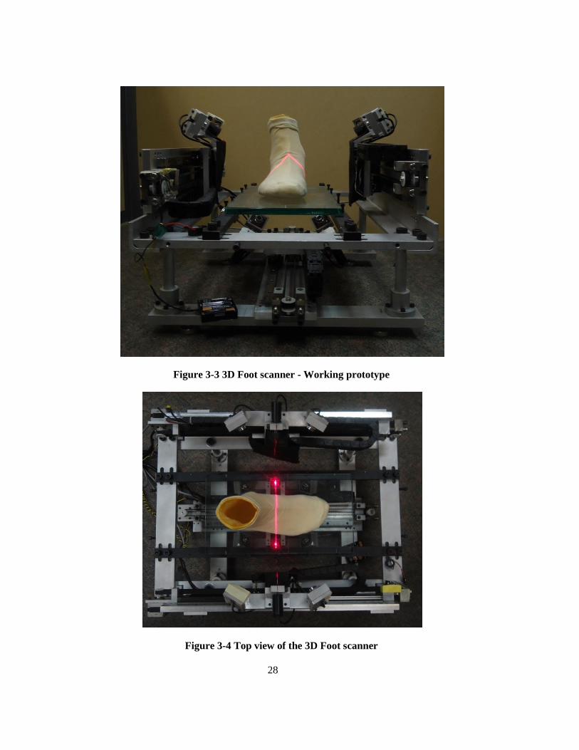
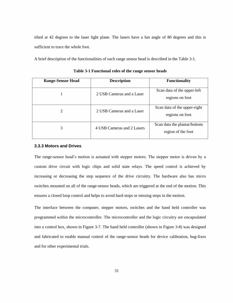
Figure 3-3 3D Foot scanner - Working prototype
Figure 3-4 Top view of the 3D Foot scanner

29
3.3.2 Range-Sensor Platforms
Considering the field of view of the camera and camera parameters, the scanner setup was finalized to
have 3 laser-camera range sensor heads to view the upper-left foot, upper-right foot and plantar
surfaces of the foot. Each of the range sensor head that scan the upper-left region and upper-right
region of the foot consists of two cameras and a laser, positioned with known geometry. The range
sensor set up for the plantar surface scan consists of 4 cameras and 2 lasers. Figure 3-5 illustrates the
three laser range-sensor heads in the scanner. More detailed construction is shown in Figure 3-6.
Figure 3-5 Range sensor head - Overview
Range-Sensor Head 1 Range-Sensor Head 2
Range-Sensor Head 3

30
Figure 3-6 From top to bottom (1) Range sensor head - Side platform (2) Range sensor head -
Bottom platform
All the range sensor heads utilize a compact 1.3MP PC USB 2.0 webcam and high powered (50mW)
red lasers. The chosen cameras fit well with the prototype design in terms of cost, resolution and size
constraints. Moreover, the camera also has an adjustable focal length which permits close range
measurements of 3 inches (76mm). The range sensor head was positioned such that the depth of field
is 3.5 inches (89mm). It can be noted from the figure that the cameras in the range sensor head are
Range-Sensor Head 1 –
Scanning Platform
Range-Sensor mounted with
USB cameras and Laser
Range-Sensor Head 3 with 4
USB Cameras and 2 Lasers
Range-Sensor field of view
designed to scan the
plantar/bottom surface of the
foot
Range-Sensor Head 3 –
Scanning Platform
Sock Model – Used for
experimental scans
31
tilted at 42 degrees to the laser light plane. The lasers have a fan angle of 80 degrees and this is
sufficient to trace the whole foot.
A brief description of the functionalities of each range sensor head is described in the Table 3-1.
Table 3-1 Functional roles of the range sensor heads
Range-Sensor Head Description Functionality
1 2 USB Cameras and a Laser Scan data of the upper-left
regions on foot
2 2 USB Cameras and a Laser Scan data of the upper-right
regions on foot
3 4 USB Cameras and 2 Lasers Scan data the plantar/bottom
region of the foot
3.3.3 Motors and Drives
The range-sensor head’s motion is actuated with stepper motors. The stepper motor is driven by a
custom drive circuit with logic chips and solid state relays. The speed control is achieved by
increasing or decreasing the step sequence of the drive circuitry. The hardware also has micro
switches mounted on all of the range-sensor heads, which are triggered at the end of the motion. This
ensures a closed loop control and helps to avoid hard stops or missing steps in the motion.
The interface between the computer, stepper motors, switches and the hand held controller was
programmed within the microcontroller. The microcontroller and the logic circuitry are encapsulated
into a control box, shown in Figure 3-7. The hand held controller (shown in Figure 3-8) was designed
and fabricated to enable manual control of the range-sensor heads for device calibration, bug-fixes
and for other experimental trials.

32
Figure 3-7 Control box
Figure 3-8 Hand-held controller
Control Box with embedded
micro-controllers and logic
circuitry
Communication Lines for
scan platform controls
Communication Line for
hand-held controller
USB Communication
Line for Front-End GUI

33
3.3.4 Front-end interface
All the hardware components mentioned in the previous sections are operated by several structured
classes written in C++. The interface between the user and scanner happens through a Visual Basic
Graphic User Interface. Figure 3-9 shows the GUI that runs the scanner. Subroutines scripted in
Visual Basic, communicate with the embedded microcontroller in the control box for each instruction
the user inputs. This concludes the overview of the electro-mechanical setup of the scanner.
Subsequent sections discuss the primary research of this thesis on 3D Foot model reconstruction from
the devised scanner.
Figure 3-9 Front-end Graphic User Interface

34
Chapter 4
Optical Calibration of the Scanner
4.1 3D measurement process of the Foot scanner
The measurement process can be represented in four major steps: Camera calibration, Image
acquisition, Digitization and 3D Reconstruction. The accuracy level and quality of these processes,
determines the precision of the output measurement. Figure 4-1 illustrates the process sequence to be
carried out for measuring a 3D object. The following section describes the first critical step of camera
calibration. The subsequent steps are discussed in Chapter 5 of the thesis.
Figure 4-1 Basic steps in image-based 3D measurement

35
4.2 Optical Calibration
Optical calibration or camera calibration deals with determining a mathematical relationship between
the 2D image points of an image to their corresponding 3D points in a space frame referenced to the
camera focal plane. With the known mathematical relationship, 3D data points can be acquired from
any 2D image points of the calibrated camera. As mentioned in the previous chapter, 8 cameras were
used in the foot scanner. This requires calibrating all 8 cameras with high precision to yield reliable
output.
As discussed in Chapter 2.4, the majority of the calibration of laser-scanner range sensor employed
triangulation techniques. The triangulation technique has proven to be effective, but the complexity in
computation and precise details on intrinsic and extrinsic parameters of the cameras used, makes it
more difficult to apply to this scanner setup. Based on the criteria devised for the scanner, it was
essential to apply a technique that yielded an accurate relationship between the input and output data
of the 8 cameras both quickly and with few computations.
4.2.1 Choosing a calibration technique
Choosing a calibration technique for the scanner was carried out purely based on the cameras used in
the device. For example, calibration method and complexity differs from cameras with known optical
parameters to cameras with unknown optical parameters. This study was carried out in two cases;
Calibration with known parameters and calibration with unknown camera parameters.
4.2.1.1 Known parameters
For cameras with known intrinsic, extrinsic parameters and setup parameters, 3D coordinates (X,Y,Z)
can be determined from geometric equations relating to the image coordinates (i,j) and (X,Y,Z) [67].
Intrinsic parameters of these cameras are known prior to the usage. Typically, these cameras are
36
referred to as ‘metric cameras’ whose parameters are estimated and well defined by the manufacturer.
Extrinsic parameters and setup parameters like distance and angles between cameras/laser are
computed and calibrated accordingly.
4.2.1.1.1 Drawbacks
Metric cameras are expensive.
Highly sensitive to setup parameters. Cameras using this method require extremely accurate
alignment of cameras in terms of angles and distances.
4.2.1.2 Unknown Parameters
These cameras are also referred to as ‘non-metric’ cameras. The camera parameters and setup details
are unknown and are determined by calibration routine rather than physical measurements. The
camera’s internal and setup parameters are usually determined implicitly or explicitly as mentioned in
section 2.4.2 of this thesis.
4.2.1.2.1 Major advantages
Measurement of camera angles, distances and other geometries are not required.
Less-expensive off-the shelf cameras can be used.
Easy handling and wider scope of applications.
Except for the setup parameters, intrinsic and extrinsic parameters of the 8 USB web cameras used in
the foot scanner were unknown. Moreover, the prototype was subjected to continuous alterations in
hardware as a part the research. Any disturbances in the optical setup after calibration would alter the
results and would require recalibration. This would furthermore increase the complexity of the

37
scanner in its real world application. Hence, a robust and quick calibration method was the need. This
motivated the design and use of a reference object based calibration method.
As mentioned earlier in section 2.4.1, a reference object based calibration method involves the optical
system observing an object of well-known geometry in world space and the corresponding
relationship is computed between the geometry of the object in the image coordinate system to that of
the world coordinate system.
4.3 Fast and Robust calibration technique
The mathematical relationship that relates the 2D image points to the 3D data points are estimated by
Multivariate polynomial regression. Figure 4-2 shows the basic transformation of 2D image data into
3D world space data. The following section discusses the mathematical approach for establishing the
relationship by the multivariate polynomial regression method in detail.
Figure 4-2 Transformation of 2D image data points to world space

38
4.3.1 Depth Mapping - Multivariate Regression
The entire process of calibration revolves around the mapping of image points (i, j) to real-world
coordinates (X, Y, Z). The mapping of these variables is achieved by the polynomial regression
method. The method is a form of linear regression that permits the output variable to be predicted by
decomposing the input variable into an nth order polynomial. This method is widely applied in fitting
nonlinear data into a least squares linear regression model.
Generally the regression model has the form:
2 3
0 1 2 3 .....k
kR p p p p (4.1)
Where,
0 , 1 ,
2 ,3 , ..
k - Polynomial coefficients
R - Output variable
p - Input variable
As the successive powers of the ‘ p ’ are added to the equation, the best fit line changes shape. As
such, it results in changes in input-output relationship as well.
For example,
0 1R p .. (Produces a straight line; Figure 4-3 (a))
2
0 1 2R p p .. (Quadratic: Produces a parabola; Figure 4-3 (b))
2 3
0 1 2 3R p p p ..(Cubic: Produces ‘s’ shaped curve; Figure 4-3 (c))
Figure 4-3 illustrates the variation of the relationship with the degree of the polynomial equation.
39
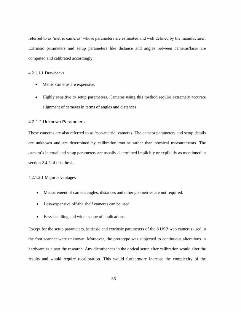
Figure 4-3 Polynomial curves of various orders
For mapping between the image coordinates and the real world coordinates, a quadratic polynomial
relationship is preferred as the foot profile data are of this type. The above discussed polynomial
yields the relationship for one input and one output. But, for calibrating 2D images into 3D real world
Figure 4-3 (d): Fourth degree polynomial
(permits more kinks and knots)
Figure 4-3 (b): Second degree polynomial
Figure 4-3 (a): First degree polynomial Figure 4-3 (c): Third degree polynomial

40
coordinates, where ‘i’ and ‘j’ are to be mapped to their corresponding ‘Y’ and ‘Z’ ( ‘X’ is fixed as the
range-sensor calibration is done in the YZ plane).
Figure 4-4 Conceptual diagram of laser ray over an object and its view in image plane
For this requirement, equation 4.2 shows an example of how the relationship is established based on
two inputs (p, q) and the output (R).
A second order polynomial function of two variables generally has the form,
2 2
1 2 3 4 5 6( , )R f p q p q p pq q (4.2)
Where,
1 , 2 ,3 , 4 , 5 , 6 - Polynomial coefficients
R - Output variable
,p q - Input variables

41
Extending equation 4.2 to ‘n’ data points 1{( , , )}n
k k kp q R , we obtain a model with ‘n’ equations
for six unknowns 6
1{ }l l
2 2
1 2 3 4 5 6k k k k k k kR p q p p q q (4.3)
Where, k= 1… n
Equation 4.3 is represented in matrix form as:
2 21 11 1 1 1 1 1
2 22 22 2 2 2 2 2
2 23 33 3 3 3 3 3
4
5
2 26
1
1
1
. . . . . . .
. . . . . . .
1n n n n n n n
R p q p p q q
R p q p p q q
R p q p p q q
R p q p p q q
(4.4)
which can be written as:
, .p qR M (4.5)

42
Where,
R
1
2
3
.
.
n
R
R
R
R
,p qM
2 2
1 1 1 1 1 1
2 2
2 2 2 2 2 2
2 2
3 3 3 3 3 3
2 2
1
1
1
. . . . . .
. . . . . .
1 n n n n n n
p q p p q q
p q p p q q
p q p p q q
p q p p q q
1
2
3
4
5
6
4.3.2 Computation
Equation 4.5 serves as the base to compute the mathematical relationship between the 2D image
points (i,j) and the real world coordinates (X, Y, Z). If R and ,p qM represent the real world
coordinates and the image coordinates respectively, ,p qM can be computed from the image data
points and with the known coefficient matrix , its corresponding R can be computed.
The image points of the laser profile to construct ,p qM are acquired through the image processing
module of the software (details in Chapter 5) and the coefficient matrix is obtained through the
range sensor calibration.
The calibration is carried out in the ‘YZ’ plane with a fixed ‘X’ coordinate. Hence, the polynomial
equation is extended for two variables ‘Y’ and ‘Z’. This allows computing the relationship of ‘Y’
coordinates and ‘Z’ coordinates with the 2D image points independently. The equations are
constructed as follows.

43
Equation to map ‘Y’ coordinates with the image points (i, j):
2 211 1 1 1 1 1 1
2 222 2 2 2 2 2 2
2 233 3 3 3 3 3 3
4
5
2 26
1
1
1
. . . . . . .
. . . . . . .
1
y
y
y
y
y
yn n n n n n n
Y i j i i j j
Y i j i i j j
Y i j i i j j
Y i j i i j j
(4.6)
The equation can be re-written as,
Pix . yY (4.7)
It should be noted that, the matrix Pix is similar to ,p qM . The notation is changed for better
understanding of computations involving image points (i,j).
Similar to equation 4.6, the equation to map ‘Z’ coordinates with the image points (i, j) can be
constructed as,
2 21 11 1 1 1 1 1
2 22 22 2 2 2 2 2
2 23 33 3 3 3 3 3
4
5
2 26
1
1
1
. . . . . . .
. . . . . . .
1
z
z
z
z
z
n zn n n n n n
Z i j i i j j
Z i j i i j j
Z i j i i j j
Z i j i i j j
(4.8)
44
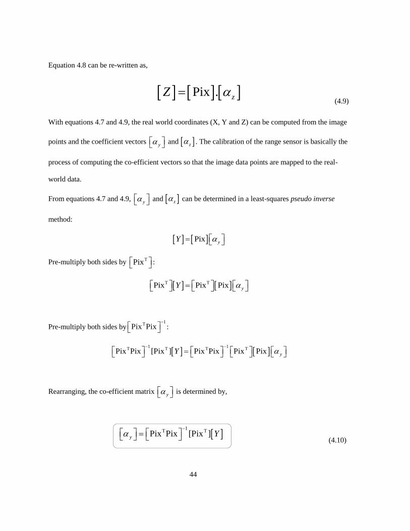
Equation 4.8 can be re-written as,
Pix .
zZ
(4.9)
With equations 4.7 and 4.9, the real world coordinates (X, Y and Z) can be computed from the image
points and the coefficient vectors y and z
. The calibration of the range sensor is basically the
process of computing the co-efficient vectors so that the image data points are mapped to the real-
world data.
From equations 4.7 and 4.9, y and z
can be determined in a least-squares pseudo inverse
method:
Pix yY
Pre-multiply both sides by T
Pix :
T TPix Pix Pix yY
Pre-multiply both sides by1
TPix Pix
:
1 1
T T T TPix Pix [Pix ] Pix Pix Pix Pix
yY
Rearranging, the co-efficient matrix y
is determined by,
1T T
Pix Pix [Pix ]y
Y
(4.10)

45
Similarly the co-efficient matrix z
is determined as,
1
T TPix Pix [Pix ]
zZ
(4.11)
4.3.2.1 Estimation of the Coefficient Matrix
Estimation of the co-efficient matrix results in a model that relates the image points to the 3D real
world data. To compute the co-efficient matrix, reference object based calibration needs to be carried
out.
A 3D object (as shown in Figure 4-5) of well-known geometry and high precision (+-0.001mm)
was manufactured for calibrating the cameras in the foot scanner. Control points with precisely
known real-world coordinates (X, Y, and Z) are chosen and marked on the 3D object. The object was
positioned in the scan volume of the scanner such that, the laser ray traces over the chosen control
points (Points on the reference object, that defines the relationship between the input and output
parameters). It was also ensured that the object was positioned the optimum field of view of all the
cameras. The setup was ensured to have no optical or physical disturbances, to minimize errors during
the process.

46
Figure 4-5 Reference object used for calibration of 8 cameras
Once properly setup, images are captured from all 8 cameras. The image points (i, j) of the control
points were identified and recorded from the captured images. It should be noted that, the precision of
identifying the image points has a significant effect on the accuracy of calibration. Algorithms for
image processing techniques like edge/blob detection; image segmentation and pattern recognition
can be of much help in getting to sub-pixel level accuracy of detecting the control points. Table 4-1
shows a typical calibration chart for a single camera.
The known real-world coordinates of the control points (in Y and Z) constitute Y , Z matrix and
the corresponding image coordinates are constructed as Pix matrix. With the known matrices, co-
efficient matrix is computed by the equations 4.10 and 4.11.

47
Table 4-1 Calibration chart- Depth mapping through a reference object of known geometry
Real World Coordinates Image Coordinates
Control
Point
Number
X Y Z Column
(i)
Row
(j)
P1
X
Y1 Z1 i1 j1
P2 Y2 Z2 i2 j2
P3 Y3 Z3 i3 j3
P4 Y4 Z4 i4 j4
P5 Y5 Z5 i5 j5
P6 Y6 Z6 i6 j6
4.4 Experiments and Trials performed
The reference object shown in Figure 4-4 was used to calibrate the range sensor heads of the scanner.
This involves a process of mapping of image points from all the 8 cameras to their corresponding real
world coordinates.
The reference object was placed on the scan volume of the scanner and the laser stripe was positioned
over the chosen control points on the object (as shown in Figure 4-6). Following this, images
representing the profile of the laser over the object were captured from all the cameras.
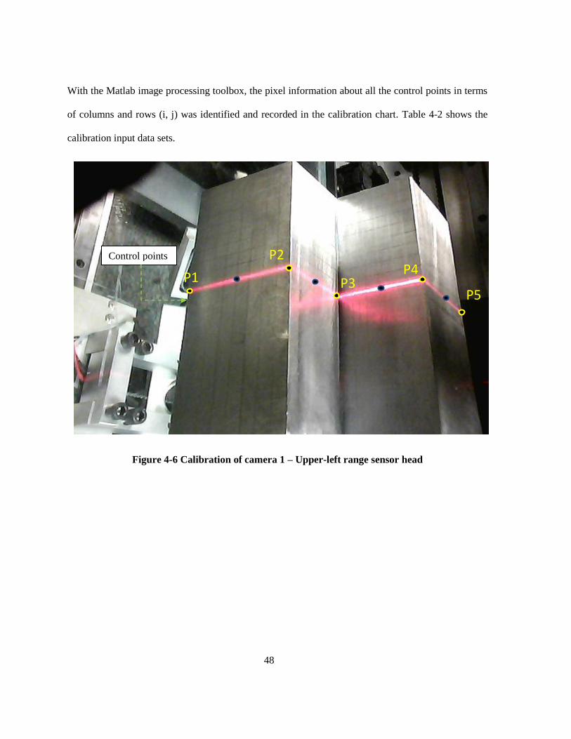
48
With the Matlab image processing toolbox, the pixel information about all the control points in terms
of columns and rows (i, j) was identified and recorded in the calibration chart. Table 4-2 shows the
calibration input data sets.
Figure 4-6 Calibration of camera 1 – Upper-left range sensor head
P1
P2
P3
P4
P5
Control points

49
Table 4-2 Calibration chart of camera 1
Control Point
Number
Real World Coordinates Image Coordinates
X Y Z Column
(i)
Row
(j)
P1
0
5 3 159 221
P2 5 7 318 170
P3 2 7 397 225
P4 2 10 530 192
P5 -2 10 591 255
Based on the tabulated data, the matrices[ ]Y , [ ]Z and [Pix] are constructed as shown below.
Real world data (column vectors):
5
5
[ ] 2
2
2
Y
3
7
[ ] 7
10
10
Z
Image points matrix:
2 2
2 2
2 2
2 2
2 2
1 159 221 159 (159*221) 221
1 318 170 318 (318*170) 170
[Pix]= 1 397 225 397 (397*225) 225
1 530 192 530 (530*192) 192
1 591 255 591 (591*255) 255
The above matrices are substituted in equation 4.10 and 4.11 to determine the coefficients. The result
is shown in Table 4-3.

50
Table 4-3 Computed coefficients for 'Y' and 'Z'- Camera 1
Camera 1
Real World Image Point Resultant Coefficients
Y Z i j y z
5 3 159 221 0.00000 0.00000
5 7 318 170 -0.02223 -0.00871
2 7 397 225 0.13790 0.08232
2 10 530 192 0.00000 0.00000
-2 10 591 255 0.00004 0.00011
-0.00048 -0.00036
With the computed coefficients, the mathematical model that maps the image points of camera 1 to
the world space can be formulated by substituting the determined coefficient values in the equations
4.7 and 4.9.
0
0.02223
0.13790Pix
0
0.00004
0.00048
Y
(4.12)
0
0.00871
0.08232Pix
0
0.00011
0.00036
Z
(4.13)

51
With the equations 4.12 and 4.13, any known image points of camera 1 can be mapped to real world
data. Figure 4-7 presents the 3D data points of the 2D image (calibration object) computed based on
the discussed mathematical model.
Figure 4-7 Point cloud data acquired from the calibration frame of camera 1 – 411 points
The coefficient of determination, R2
was computed for analyzing the goodness of the equations 4.12
and 4.13. R2
value ranges between 0 and 1; value closer to 1 indicates that the equation fits the data
well. The computations are explained in Appendix A and it was found that 92.17 % of the total
variance of ‘Y’ values and 100% of the total variance of ‘Z’ values are explained by variations in the
input data (i,j).

52
The calibration chart is extended for the remaining 7 cameras and is presented in Appendix B. The
data collected was loaded into the Matlab environment for computing the co-efficient matrix y
and z for all the cameras. The following table shows the consolidated results of the
y and
z for all the 8 cameras. With the computed co-efficient matrices; the captured calibration frames
from 8 cameras were processed to obtain a 3D point cloud data (shown in Figure 4-8). This step is
done to verify the accuracy and precision of the calibration process.
Figure 4-8 Point cloud data acquired from 8 cameras - Calibration frame
X
Y
Z

53
4.5 Steps after Calibration
On successful calibration of the foot scanner using the reference object, the scanner can now be used
to scan and measure the human foot. A brief description of the process is illustrated in Figure 4-9.
Figure 4-9 3D Foot scanning process after the calibration of scanner optical system
Chapter 5 discusses the real time data acquisition, image processing descriptions for acquiring the 2D
image coordinates of the laser profile, and reconstruction from the 3D data points of the foot scan into
a CAD model.
54
Chapter 5
Implementation and Prototype Validation
5.1 Range Image acquisition
Through calibration, a mathematical relationship between 2D image data coordinates and the 3D
world space coordinates was established. The next step was to acquire 2D range image data from all
the cameras in the scanning system. The following section describes the process of range image
acquisition of the 3D foot scanner.
Once the subject positions their foot over the base plate of the scanner in a semi-weight bearing
condition, the scanner is triggered through its GUI. The homing process takes place until all three
range sensor heads are aligned axially. On successful homing, a manual trigger is initiated to capture
range image data from the cameras. The Matlab Image acquisition toolbox is used to carry out the
data acquisition process. Figure 5-1 shows the Matlab Image Acquisition tool working environment.
Selection of cameras and defining the properties of acquisition are configured in this environment.
Avi files with 200 frames were acquired from all the cameras. Scan time for the range sensor head to
cover a span of 40 cm was recorded to be 11 seconds. The number of frames was decided based on
the scan area and control volume. On experimentation and trials, a collection of 200 frames was
found to be suitable for covering the scan length of 40 cm. The acquisition is triggered after the
successful homing operation of the range heads. The acquisition process ends after logging the set
200 frames. The file name and the logging options are configured in the acquisition tool.

55
Figure 5-1 Matlab (R2010b) Image Acquisition Toolbox Environment
5.2 Image processing
Efficient extraction of the 2D range data was the primary objective of the data. Range images
obtained in the earlier process are typically a series of 640x480 2D images with a laser stripe
corresponding to the foot profile. Robust and simple methods of extracting the laser stripe from the
range images were scripted in Matlab (R20120b) as it features a wide range of inbuilt Image
processing tools.
Raw chart of the image processing module is shown in Figure 5-2. The module starts by reading the
input AVI file and splitting this into frames. Following to this, frames are processed sequentially to
extract 2D pixel data (i,j).

56
Figure 5-2 Basic overview of image processing and associated operations
The basic extraction of the laser profile from the images is through identifying the pixels
corresponding to the highest intensity (255) in the red plane ie., (255,0,0). This operation is often
termed ‘thresholding’ in image processing applications. But during the application, identification of
the laser stripe could be a bit problematic, as the scanner was subject to varying ambient light
conditions and the use of high-powered lasers for a short range application.
The intensity of the lasers was tuned down during dark ambient conditions and while the scanner is
covered with its lid. But, for trials in ambient day light, the laser intensity was set to high so that the
Read frames from the input video file
Identify laser stripe in the image
Background noise and outlier elimination
Thinning of the identified laser stripe
Transformation of 2D image coordinates of
laser stripe to real world coordinates
Surface reconstruction module
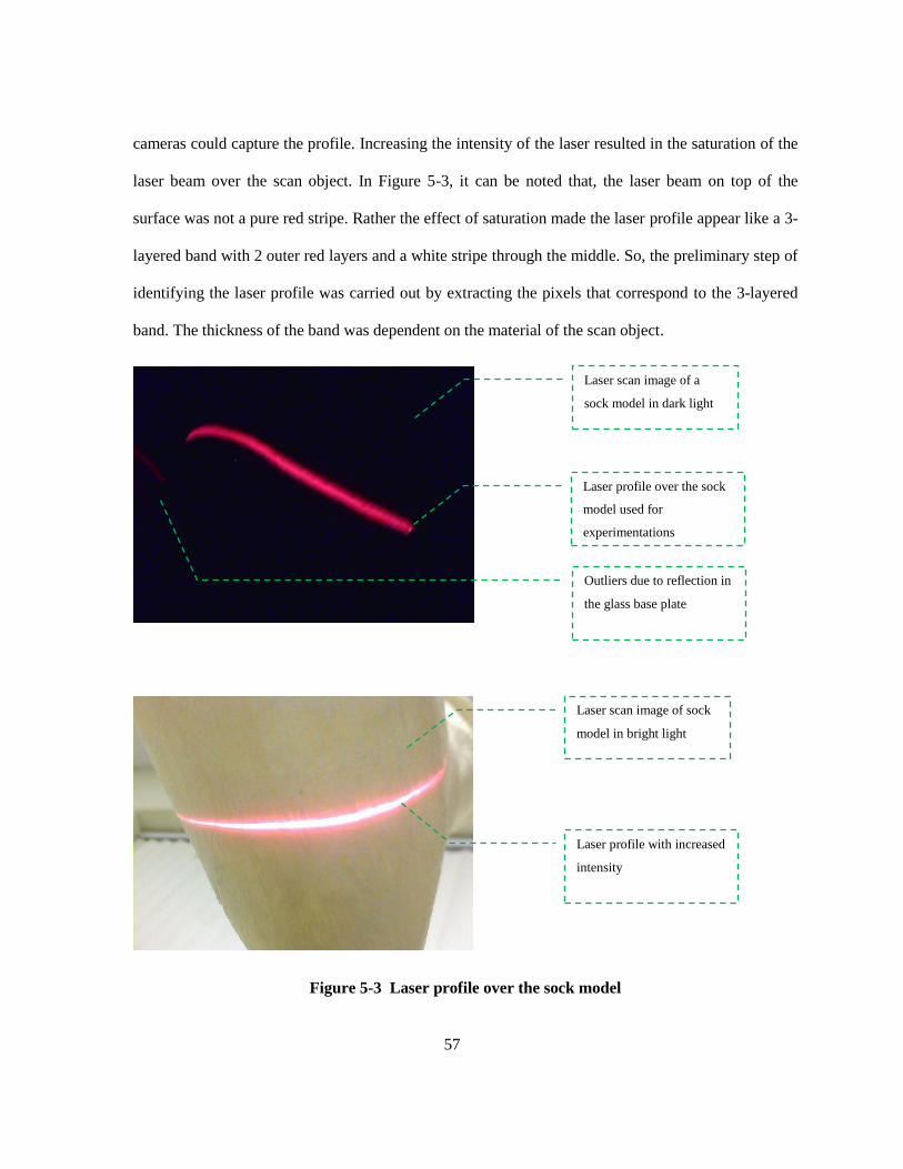
57
cameras could capture the profile. Increasing the intensity of the laser resulted in the saturation of the
laser beam over the scan object. In Figure 5-3, it can be noted that, the laser beam on top of the
surface was not a pure red stripe. Rather the effect of saturation made the laser profile appear like a 3-
layered band with 2 outer red layers and a white stripe through the middle. So, the preliminary step of
identifying the laser profile was carried out by extracting the pixels that correspond to the 3-layered
band. The thickness of the band was dependent on the material of the scan object.
Figure 5-3 Laser profile over the sock model
Laser scan image of a
sock model in dark light
Laser profile over the sock
model used for
experimentations
Outliers due to reflection in
the glass base plate
Laser profile with increased
intensity
Laser scan image of sock
model in bright light

58
Once the preliminary laser stripe is extracted, the RGB range images are converted to a binary image.
The pixels corresponding to brighter regions are coded ‘1’ and lower regions as ‘0’. Since, the pixels
in the region of laser are naturally bright in the image; they get encoded as regions of ‘1’. This step
also encoded the noise and outlier data pixels as ‘1’. At this point, a technique to isolate the
continuous laser stripe from the outliers was carried out. The continuous and non-discrete laser stripe
in the range image, helped to differentiate the laser stripe and the outliers.
Figure 5-4 Identification of laser profile in a scan image
Extracted laser profile
from the input 2D scan
image
Outliers along with the
actual laser profile
Outliers along with the
actual laser profile
Extracted 3-layered laser
profile

59
Following the encoding process, the encoded binary image was scanned and checked for connected
pixels. The region of binary image with laser stripe had more connected pixel components than other
regions. The pixels corresponding to large connectivity were then isolated to perform
‘thinning/eroding’. The functions ‘bwlabel’ and ‘bwconncomp’ in Matlab were employed for this
purpose.
Figure 5-5 Laser profile with outliers removed
Figure 5-6 Thinned laser profile
Dense laser profile of the
sock model
Outliers and background noise
eliminated by setting threshold
for connected components
Thinned laser profile by
median operation – To reduce
number of data points and
faster computation
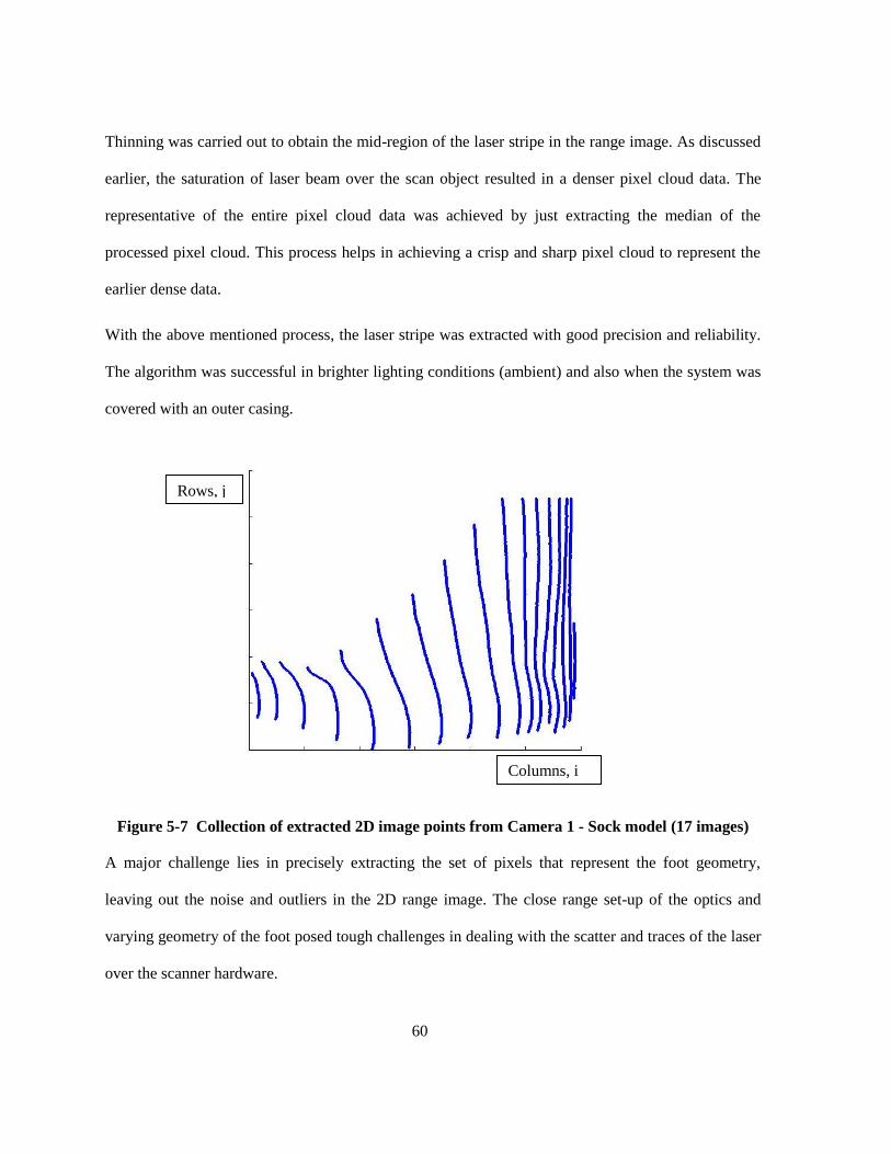
60
Thinning was carried out to obtain the mid-region of the laser stripe in the range image. As discussed
earlier, the saturation of laser beam over the scan object resulted in a denser pixel cloud data. The
representative of the entire pixel cloud data was achieved by just extracting the median of the
processed pixel cloud. This process helps in achieving a crisp and sharp pixel cloud to represent the
earlier dense data.
With the above mentioned process, the laser stripe was extracted with good precision and reliability.
The algorithm was successful in brighter lighting conditions (ambient) and also when the system was
covered with an outer casing.
Figure 5-7 Collection of extracted 2D image points from Camera 1 - Sock model (17 images)
A major challenge lies in precisely extracting the set of pixels that represent the foot geometry,
leaving out the noise and outliers in the 2D range image. The close range set-up of the optics and
varying geometry of the foot posed tough challenges in dealing with the scatter and traces of the laser
over the scanner hardware.
Columns, i
Rows, j

61
5.3 Depth estimation and Post processing 3D data points
The extracted image points (i,j) of the laser are transformed into real-world coordinates based on the
mathematical relationship established in section 4.3.2 of this thesis. Section 4.4 explains the
computation of mapping the 2D image points of the calibration object to the real world space with the
known coefficient matrices. The mapping for foot scan images in 3D space is also established by the
same method.
Figure 5-8 Input image coordinates for depth mapping
The image points of the laser stripe are used to construct the Pix matrix. Using the equations
transformation is computed for all the 8 cameras independently and the resultant 3D point cloud data
is carried over for post processing. Figure 5-8 shows the transformed point cloud data (42750
vertices) from camera1 in range sensor head 1.
Pixel data – Image coordinates of the laser
profile extracted to construct [Pix]

62
Figure 5-9 3D Point cloud data of camera 1 - Sock model (Viewed in Meshlab environment)
Point cloud data from the 8 cameras were stored as an nx2 Matlab array. Following the depth
estimation process, a third level of outlier elimination was carried out. This step was typically carried
out to eradicate the 3D points that are found to be extrapolated. The extrapolation in this algorithm
happens primarily due to pixel data that lies outside the control volume. Although the image
processing algorithms gave the best set of 2D data, it was necessary to have an algorithm to post
process the 3D points for more reliability. The algorithm checks for the closest Euclidean distance
between consecutive 3D data points and the data points that lie farthest away from the point cloud
data are eliminated. Figure 5-9 shows 3D point cloud data with prominent outliers.

63
Figure 5-10 3D Point Cloud data with outliers – Viewed in Meshlab environment
On successful elimination, point clouds of all 8 cameras are concatenated into a single array. This
array in the range of 50,000 elements represents the digitized foot. The point cloud data of the
scanned foot can be easily imported into CAD software as a .ply file. The typical point cloud result of
the scanner had 50,000 3D data points representing the scanned foot. The software proved highly
advantageous in having a dense point cloud for the low cost set-up.
The .ply format enables high portability of the 3D Data for less memory. So as to obtain the 3D
model of the foot, the following operations are carried out.

64
Figure 5-11 3D Point cloud data of the scanned sock model
5.4 CAD model generation
The reconstructed 3D point clouds were created into a mesh that represents the geometry of the
scanned object, in this case a human foot. The crust algorithm, developed by Amenta et al. [55] is the
most commonly preferred for surface reconstruction. For the given sample of points, the algorithm
creates a topologically correct surface with its geometry convergent to that of the original surface.
The algorithm mainly relies on Voronoi diagrams and Delaunay triangulation techniques. The
Voronoi diagrams help in decomposing a metric space into specific subspaces. The extension of the
Voronoi diagram to three dimensions is addressed and proposed workable solutions in the algorithm
are discussed in [55].
Delaunay triangulation involves triangulating a surface in such a way that no point on the surface is
encapsulated/lies inside the circumcircle of any triangle. This method helps in yielding a triangulated
surface with wide triangles (maximizing the minimum angle in the triangle) rather than skinny or

65
narrower triangles. The extension of Delaunay triangulation involves the use of circumspheres rather
circumcircles. The ‘robustcrust’ function developed by Luigi Giaccari based on the ball pivot
algorithm [56] is the most preferred for meshing 3D point clouds of a closed surface. A simple and
customized function based on ‘robustcrust’ was constructed and implemented to mesh the 3D point
cloud data of the foot. Vertices and normals of the triangulated surface are computed in this module.
The next step towards achieving a CAD model is to export the mesh model as a CAD readable
format. Standard formats that most CAD software packages and reverse engineering machines like
3D printers accept are .stl or .vrml. The final module of the software focuses on exporting the
generated mesh model into a .stl file, which makes it compatible for viewing in CAD software
packages and make it more efficient in data transfer.
Figure 5-12 Triangulated 3D sock model from the 3D data points

66
Chapter 6
Performance Verification and Results
This section of thesis documents the results from the scanner and evaluation of the output models in
terms of accuracy and precision. Comparison of the 3D foot scanner’s result against the scanned
result of an Industrial high-end Laser scanner at Northern Digital Inc., [57], was carried out for better
analysis. The section also provides an overview of various experiments and trials that were carried
out during the calibration process for improved accuracy and precision of the scanner.
6.1 Scan results of Calibration Object
6.1.1 Description
A 3D aluminum block of 15 cm x 10 cm x 5 cm was scanned using the 3D foot scanner to study the
accuracy of the scan output model. The block was modeled using Solidworks prior to manufacturing,
and its output scan was compared against the CAD model. Figure 6-1 shows some of the key points
observed.
Figure 6-1 Aluminum block (15 x 10 x 5 cm)

67
6.1.2 Scanner 3D point cloud output
The aluminum block was covered with two layers of mild-yellow colored cloth in order to avoid
reflections and scatter of the laser stripe over its surface. The scanner’s 3D point cloud output and the
reconstructed CAD file were viewed in Meshlab, which are presented in Figure 6-2 and 6-3.
Figure 6-2 3D Point cloud of the block- Viewed in Meshlab
Figure 6-3 Reconstructed block as .stl file - Viewed in Meshlab

68
6.1.3 Basic dimensional check
A straightforward comparative study of the dimensional differences between the actual CAD model
and the scanner generated CAD model was carried out. Table 6-1 shows the deviation in the
dimensions between the actual and acquired 3D model. The results show that the scanner could able
to generate output models with accuracy of +/-0.05cm.
Table 6-1 Deviations with the actual CAD model and the output CAD model
Length (cm) Width (cm) Height (cm)
Actual CAD model 15 10 5
Scanner CAD model 15.12 10.20 5.14
*The sock material thickness =0.15cm
Figure 6-4 Length and width deviation study – Solidworks

69
6.2 Scan results of Sock model
A sample plaster cast/sock-model of human foot was used for experiments and trials with the scanner.
To make a comparative study on the scanner’s accuracy, the sock model was scanned with a High-
end Industrial laser scanner at NDI, Waterloo [57]. The scanned CAD model was considered to be the
reference standard, to validate the foot scanner’s performance. Figure 6-5 shows the scanned sock-
model from NDI’s scanner.
Figure 6-5 Scan result of the Sock model - NDI, Waterloo [57]
The CAD model was highly precise, accurate and featured with high-definition ‘texture-mapping’.
The sock model was scanned in the 3D foot scanner with a resolution of 0.178cm and a CAD file in
.stl file format was generated for comparison with the reference model (shown in Figure 6-6).
6.2.1 Comparison of Foot models by Registration
The comparison between the reference model and the generated model was carried out using open
source software called ‘CloudCompare’ [58], which used point cloud data registration for the purpose
of comparing models. Point cloud registration within the software checks for correspondence between

70
data points by feature matching and by iterative transformations. The software also checks for
similarities in surface curvature among the data points and iterates the process until the features/data-
points match. Figure 6-7 illustrates the comparison of the two models using ‘CloudCompare’ [58].
Figure 6-6 Generated 3D .stl file of the Sock model
Figure 6-7 Scanner output and reference model – CloudCompare [58] environment

71
Figure 6-8 Comparison of data points with the reference CAD file- CloudCompare [58]
environment
View -1
View -2
Green regions correspond to
the reference CAD model
Pink regions correspond to the
generated CAD model
Deviation (approx. 0.07cm)
between reference and generated
data points
Max deviation (approx. 0.17cm)
between reference and generated
data points
Due to insufficient data points in the
generated model –
Cause: Complexity in laser stripe
identification at the convex region

72
The vertices of the scanner output model were sub-divided into 70 classes based on the distance from
its corresponding point in the reference model. The cloud to cloud distance was computed for the
models to determine more details on the error in terms of maximum distance, mean distance and
standard deviation. Figure 6-9 shows the spread of the data points and their distance from the
reference model. 56 classes of the output model’s data points were found to be well under 0.1cm (i.e.,
80% of the total data points), while the rest found to be under 0.2 cm.
Table 6-2 shows the error based on the cloud to cloud distance comparison. It was found that the
maximum distance was 0.310 cm and a mean distance of 0.035 cm.
Figure 6-10 presents the same cloud to cloud distance comparison for 8 classes of the data points.
Figure 6-9 Cloud to Cloud distance between reference CAD model and scanner output model

73
Table 6-2 Results of Cloud to Cloud comparison
Reference Vertices of Reference CAD model
Compared Vertices of Scanner Output Model
Minimum Distance (cm) 0
Maximum Distance (cm) 0.31032
Mean Distance (cm) 0.03532
Standard Deviation 0.3075
Figure 6-10 Cloud to Cloud distance comparison for 8 classes of data points

74
6.3 Scan results of human foot
In order to validate the scanner’s functionality of scanning a foot, numerous scans were performed
with various participants. The scanner was able to successfully generate accurate models of the
human feet that differed among various subjects in terms of length, width and girth sizes.
Figure 6-9 presents some of the 3D foot models of the participants.
Figure 6-11 Foot models from the scanner

75
Chapter 7
Conclusion and Future Work
7.1 Conclusion
Footwear manufacturing integrated with the scanning system is proven to reduce laborious manual
measurements and computations. Introduction of 2D scanning systems were effective in achieving
accurate information only on the features and the landmarks of a foot. However, it was limited to
manufacturing of the orthosis and for measuring basic plantar surface of the foot. On the other hand,
3D foot scanning systems have proven useful for capturing geometry for shoe last manufacturing and
for developing custom orthoses and footwear. However, the high cost of current 3D scanning systems
makes it unaffordable for many shoemakers and orthotic technicians. The solution for this is a low-
cost foot scanner. Digitization and 3D CAD model generation of the foot using such a low-cost
structured light scanner was the focus of this thesis.
A technique for optical calibration of the scanner and generation of CAD model was proposed,
implemented and tested in this work. The optical setup of the scanner requires calibration to measure
the real-world object effectively. The proposed method eliminates the need of complex and laborious
computations of the internal and the external parameters of a camera. Added to that, the method is
independent of lens distortions and other optical geometry as well, making it highly advantageous.
Computations that determine the relationship between 2D image points and 3D real world co-
ordinates serve to be memory efficient and possess quicker execution time.
With a computed relationship between the 2D image points and the real world coordinates, the
scanner was equipped to generate a 3D model of the foot. The images acquired by the cameras are
processed by the image processing script to extract the 2D points of the laser stripe. The image points

76
are subsequently mapped to their corresponding 3D coordinates. Input images from all the cameras
were processed and dense data points representing the scanned foot were obtained.
The 3D data points were triangulated by ball pivoting method to produce a 3D model. The output
model consisting of triangles and normals was constructed as a .stl file. This makes the output model
to be compliant with any CAD software. The algorithm for image processing and surface
reconstruction was tested and comparisons were made between the 3D reference models of known
geometry and their corresponding scanner output models. The resolution of the scanner was estimated
to be 0.178 cm. The mean error of the scanner’s output based on the comparison with the reference
sock model was 0.035 cm, which conforms to the target tolerance of less than +/- 0.05 cm. The
maximum error of 0.31 cm can be brought down by recalibrating the cameras with more control
points. Increasing the number of control points in the calibration process helps in achieving more
accurate mapping of 2D image points with the real world data points. The results of the experiments
and trials of various foot scans were encouraging and can be expanded in many ways.
7.2 Future Work
The short term objective of the scanner is to interface 8 USB cameras with the processing computer
for simultaneous data acquisition. The restricted USB bandwidth is likely to be the cause for this
issue. A possible solution for this issue is to loop the USB camera to effectively use the bandwidth
and also trials are being carried out using advanced Peripheral Component Interconnect (PCI) card to
interface USB ports with the computer. In addition to this, trials are being carried out using pinhole
camera-laser setup, to improve the quality of input scan images.
The long term objective of the scanner includes sizing, texture mapping and landmark detections
based on the generated 3D CAD model of the foot. Sizing is the most common requirement during a
footwear purchase. It can be estimated by measuring the basic geometries mentioned in Chapter 2

77
from the CAD model. Mondopoint is a well-known shoe sizing system which is preferred by the
footwear industry professionals for sizing measurements. This system involves the estimation of the
mean foot length and width of the foot which can be acquired through the measurable 3D CAD model
from the scanner. The sizing module could be incorporated into the surface reconstruction module so
that sizing measurements are achieved along with the CAD file. Similarly, incorporation of texture
mapping features in the CAD model would add the credibility of the scanner in terms of feature
detection, landmark identification and other clinical purposes.
Improvements in the calibration process in terms of (i) increasing the control points on the reference
object, (ii) ensuring higher order of control point measurement accuracy (to be greater than the target
accuracy of the scanner), and (iii) uniform distribution of control points over the scan volume would
serve to be a good starting point for any further experiments and trials.

78
Appendix A
Estimation of Goodness of Fit
Estimation of R2 to determine the total variation of ‘Y’ and ‘Z’ for the variations in the input data (i,j):
Yobs and Zobs are computed from the known image coordinates i, j and the coefficient matrix by
equations 4.12 and 4.13. With the known actual data and the observed data, R2
can be computed as
follows.
,2
,
,
1y z
y z
y z
SER
SV
The squared errors ,y zSE can be determined by,
SEy = (Yact - Yobs)2
SEz = (Zact - Zobs)2
And the Squared variations ,y zSV can be determined by,
SVy = ( Yact – MeanY )2
SVz = ( Zact – MeanZ )2
The following table is computed based on the above formula and the value of R2 is achieved.
Inputs Actual 'Y'
Yact
Observed 'Y'
Yobs
Squared Error
SEy
Squared Variation
SVy i j
159 221 5 4.9032 0.009 6.76
318 170 5 4.6643 0.113 6.76
397 225 2 1.4752 0.275 0.16
530 192 2 1.0706 0.864 0.16
591 255 -2 -3.1572 1.339 19.36
MeanY 2.4 Total YSE = 2.6 YSV = 33.2

79
Percentage of variation, not explained by the variations in input:
= Y
Y
SE
SV
= 2.6
33.2 = 0.0783 = 7.83%
Therefore, the percentage of total variations of ‘Y’ values explained by the variations in input can be
estimated as,
R2Y
= 1- 0.0783 = 0.9217 = 92.17%
Similarly, for estimating the goodness of the equation relating to ‘Z’ can be determined as,
Inputs Actual 'Z'
Zact
Observed 'Z'
Zobs
Squared Error
SEZ
Squared Variation
SVz i j
159 221 3 3.0000 0 19.36
318 170 7 6.9999 0 0.16
397 225 7 7.0000 0 0.16
530 192 10 10.0000 0 6.76
591 255 10 9.9999 0 6.76
MeanZ 7.4 Total zSE = 0 ZSV = 33.2
Percentage of variation, not explained by the variations in input:
= Z
Z
SE
SV
=
0
33.2 = 0 = 0 %
Therefore, the percentage of total variations of ‘Z’ values explained by the variations in input can be
estimated as,
R2z = 1- 0 = 1 = 100 %
It was found that, Yobs and Zobs varies with the increase in the significant digits of non-zero values in
the coefficients z and
y
respectively. The above computations were carried out with 5
significant figures. Results may vary for computations with any significant digit greater than 5.
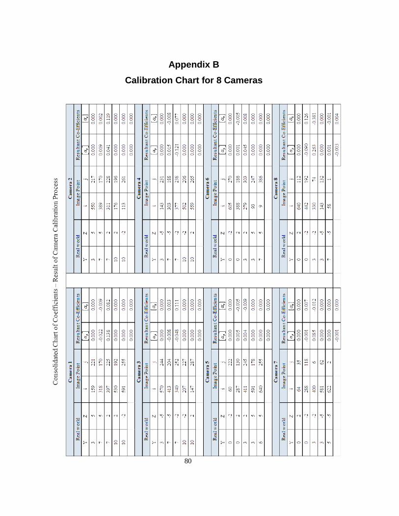
80
Appendix B
Calibration Chart for 8 Cameras

81
References
[1] S. J. Lochner, Automation of shoe last modification and tool path planning, Waterloo: University
of Waterloo, 2009.
[2] D. Besliu, Measurement Devices for Custom Shoe Manufacturing, Waterloo: University of
Waterloo, 2011.
[3] S. Telfer and J. Woodburn, "The use of 3D surface scanning for the measurement and
assessment of human foot," Journal of foot and ankle research, no. 10.1186/1757-1146-3-19, p.
3:19, 2010.
[4] T. B. D. Company, "The Brannock Device Co., Inc.," [Online]. Available:
http://brannock.com/brannock/images/brannock2.jpg. [Accessed 5 11 2012].
[5] C. Witana, S. Xiong, J. Zhao and R. Goonetilleke, "Foot measurements from 3 Dimensional
scans; a comparison and evaluation of different methods," Int J Ind Ergon, pp. 36:789-807,
2006.
[6] X. Liu, W. Kim and B. Drerup, "3D characterization and localization of anatomical landmarks of
the foot by FastSCAN," Realtime Imaging, pp. 10:217-228, 2004.
[7] I. Krauss, S. Grau, M. Mauch, C. Maiwald and T. Horstmann, "Sex-related differences in foot
shape.," Ergonomics, pp. 51:1693-1709, 2008.
[8] Lou G, Houston VL, Mussman M, Garbarini M, Beattie AC and Thongpop C, "Comparison of
male and female foot shape," J Am Podiat Med Assoc, pp. 99:383-390, 2009.
[9] Wunderlich RE and Cavanagh PR, "Gender differences in adult foot shape; Implications for shoe
design," Med Sci Sports Exerc, pp. 33:605-11, 2001.
[10] Bao HP, Soundar P and Yang T, "Integrated approach to design and manufacture of shoe lasts
for orthopeadic use," Comput Eng, pp. 26:411-421, 1994.
[11] Nacher B, Alemany S, Gonzalez JC, Alcantara E, Garcia-Hernandez J, Heras S and Juan A, "A
foot wear fit classification model based on anthropometric data," in 8th annual digital human
modelling for design and engineering symposium, Lyon, 2006.
[12] Wang C-S, "An analysis and evaluation of fitness for shoe lasts and human feet," Comput Ind,
pp. 61:532-540, 2010.

82
[13] Hawke F, Burns J, Radford JA and du Toit V, "Custom made foot orthotics for the treatment of
foot pain," Cochrane Database system Rev, p. 16:CD006801, 2008.
[14] Guldemond NA, Leffers P, Sanders AP, Emmen H, Schaper NC and Walenkamp GHIM,
"Casting methods and plantar pressure: effects of custom made foot orthoses on dynamic plantar
pressure distribution," J Am Pod Med Assoc, pp. 96:9-18, 2006.
[15] Coudert T, Vacher P, Smits C and Van Der Zande M, "A method to obtain 3D foot shape
deformation during the GAIT cycle," in 9th international symposium on the 3d analysis of
human movement, Valenciennes, June 2006.
[16] Kimura M, Mochimaru M and Kanade T, "3D measurement of feature cross-sections of foot
while walking," Mach Vis Appl.
[17] Jezerek M and Mozina J, "High-speed measurement of foot shape based on multiple-laser-plane
triangulation," Opt Eng, p. 48:113604, 2009.
[18] F. Chen, G. M. Brown and M. Song, "Overview of three-dimensional shape measurement using
optical methods," Optical Engineering, vol. 39, no. 1, pp. 293-312, 2000.
[19] Blais F, Bisson J.A, Williams S, Roberston N, Rozin S and Nelson A, "The ShapeGrabber
FootScanner: a low cost high accuracy 3D system for the acquisition of human feet," The
International society of Optical Engineering, vol. 3958, pp. 178-186, 2000.
[20] Kouchi M and Mochimaru M, "Development of a Low-cost footscanner foe a custom shoe
making system," in Proceedings of the 5th symposium on footwear boimechanics, Zuerich, 2001.
[21] Leon Kos, "A system for footwear fitting analysis," International design conference, pp. 1187-
1192.
[22] H.J.Tiziani, "Optical metrology of engineering surfaces-scope and trends," Optical measurement
techniques and applications, 1997.
[23] I.Moring, H.Ailisto, V.Koivunen and R.Myllyla, "Active vision ssystem for automatic model-
based shape inspection," Opt. Laser Eng., vol. 10, pp. 3-4, 1989.
[24] J.Y.Wang, "Imaging laser radar - an overview," in Processdings of 9th international conference
Laser, 1986.
[25] J.C.Marron and T.J.Schulz, "Three dimensional, fine resolution imaging using laser frequency
diversity," Opt. Lett, vol. 17, pp. 285-287, 1992.

83
[26] J.C.Marron and K.S.Schroeder, "Three dimensional lensless imaging using laser frequency
diversity," Appl. Opt., vol. 31, pp. 255-262, 1992.
[27] H.Takasaki, "Moire topography," Appl. opt, vol. 9, pp. 1467-1472, 1970.
[28] R.Harding and R.Tait, "Moire technique applied to automated inspection of machine parts," in
Proceedings SME vision, Detroit, 1986.
[29] A.Asundi, "Computer Aided Moire methods," Opt. Lasers Eng., vol. 17, pp. 107-116, 1993.
[30] C.M.Wong, "Image processing in experimental mechanics," M.Phil thesis, University of Hong
Kong, 1993.
[31] K.Bieman and K.Harding, "3D imaging using a unique refractive optic design to combine moire
and stereo," in Proceedings SPIE, 1997.
[32] E.Dalhoff, E.Fischer, S.Kreuz and H.J.Tiziani, "Double hetrodyne interferometry for high
precision distance measurements," in Proceeding SPIE, 1993.
[33] J.D.Trolinger, "Ultra-high resolution interferometry," in Proceedings SPIE, 1996.
[34] W.Wester-Ebbinghaus, "Analytics in non-topographic photogrametry," ISPRS Cong., Com.v.,
Kyoto, pp. 380-390, 1988.
[35] C.S.Fraser, "Photogrammetric measurement to one part in a million," Phtogramm. Eng Remote
sens, vol. 58, no. 3, pp. 305-310, 1992.
[36] E.Muller, "Fast three dimensional form measurement system," Opt.Eng, vol. 34, no. 9, pp. 2754-
2756, 1995.
[37] Z.Ji and M.C.Leu, "Design of optical triangulation devices," Opt. Laser Technol., vol. 21, no. 5,
pp. 335-338, 1989.
[38] C.P.Keferstein and M.Marxer, "Testing bench for laser triangulation sensors," Sens. Rev, vol. 18,
no. 3, pp. 183-187, 1998.
[39] M.Idesawa, "High precision image position sensing methods suitable for 3D measurements,"
Opt.Laser.Eng, vol. 10, pp. 3-4, 1989.
[40] Zhengyou Zhang, "A flexible new technique for camera calibration," IEEE transactions on
pattern analysis and machine intelligence, vol. 22, no. 11, pp. 1330-1334, 2000.
[41] C. Y.-l. Liu, Three-dimensional Hand tracking and Surface geometry measurement for a robot-
vision system, Thesis, University of Waterloo, 2008.

84
[42] J. Kofman, SYDE 625 computer vision and 3D Imaging, Graduate Course notes, 2012.
[43] T. Clarke and J. Fryer, "The Development of Camera Calibration Methods and Models," The
Photogrammetric Record, vol. 16, no. 92, pp. 293-312, 1998.
[44] J. Heikkila and O. Silven, "A four step calibration procedure with implicit image correction,"
IEEE computer society conference on computer vision and Pattern recognition, 1997.
[45] T. B, "Autocalibration from planar scenes," ECCV, pp. 89-105, 1998.
[46] R. Tsai, "A versatile camera calibration technique for high-accuracy 3D machine vision
metrology using the off-shelf TV cameras and lenses," IEEE journal of Robotics and
Automation, vol. 3, no. 4, 1987.
[47] O.Faugeras, Three Dimensional Computer Vision: a geometric viewpoint, MIT Press, 1993.
[48] K. Levenberg, "A method for the solution of certain problems in least squares,"
Quart.Appl.Math, vol. 2, pp. 164-168, 1994.
[49] D. Marquardt, "An algorithm for least squares estimation of non-linear parameters.," SIAM
J.Appl.Math, vol. 11, pp. 431-441, 1963.
[50] A.Yokoyama, K.Sato, T.Yoshigahara and S.Inokuchi, "Realtime range imaging using adjustment
free photo vlsi," in Proceedings of the IEEE/RSJ International conference on Intelligent robots
and systems, 1994.
[51] J. Forest and J. Salvi, "A review of laser scanning three-dimensional digitisers," in Proceedings
of the IEEE/RSJ International Conference on Intelligent robots and systems, Switzerland, 2002.
[52] Xiaoyang Yu, Jian Zhang, Liying Wu and Xifu Qiang, "Laser scanning device used in space
encoding rangefinder," Automated opt. Insp. for Industy, SPIE, pp. 490-495, 1996.
[53] Kazuyuki Hattori and Yukio Sato, "Handy rangefinder for active vision," In proceedings of IEEE
Int;. Conf on Robotics and Automation, pp. 1423-1428, 1995.
[54] Kazuo Araki, Yukio Sato and Srinivasan Parthasarathy, "High Speed rangefinder," In SPIE
Editor, Optics, Illumination and Image sensing, vol. 850, pp. 184-188, 1987.
[55] N Amenta, S.Choi and R.Kolluri, "The Power Crust," in ACM Symposium on Solid Modelling
and Applications, 2001.
[56] Fausto Bernardini; Joshua Mittleman; Holly Rushmeier; Claudio Silva; Gabriel Taubin;, "The
Ball-Pivoting algorithm for Surface Reconstruction," IBM Journal of Research and

85
Development.
[57] "Accurate Measurement Solutions for Industrial and Life Sciences Applications," NDI, [Online].
Available: http://www.ndigital.com/. [Accessed 21 11 2012].
[58] "CloudCompare - Open source Project," [Online]. Available: http://www.danielgm.net/cc/.
[Accessed 21 11 2012].