calibrating artificial neural networks by global optimization
TRANSCRIPT

Expert Systems with Applications 39 (2012) 25–32
Contents lists available at SciVerse ScienceDirect
Expert Systems with Applications
journal homepage: www.elsevier .com/locate /eswa
Calibrating artificial neural networks by global optimization
János D. Pintér ⇑Pintér Consulting Services, Inc., Halifax, NS, CanadaSchool of Engineering, Özyegin University, Istanbul, Turkey
a r t i c l e i n f o
Keywords:Artificial neural networksCalibration of ANNs by global optimizationANN implementation in MathematicaLipschitz Global Optimizer (LGO) solversuiteMathOptimizer Professional (LGO linked toMathematica)Numerical examples
0957-4174/$ - see front matter � 2011 Elsevier Ltd. Adoi:10.1016/j.eswa.2011.06.050
⇑ Address: School of Engineering, Özyegin Univers34662 Istanbul, Turkey.
E-mail address: [email protected]: http://www.ozyegin.edu.tr, http://www.pin
a b s t r a c t
Artificial neural networks (ANNs) are used extensively to model unknown or unspecified functional rela-tionships between the input and output of a ‘‘black box’’ system. In order to apply the generic ANN con-cept to actual system model fitting problems, a key requirement is the training of the chosen (postulated)ANN structure. Such training serves to select the ANN parameters in order to minimize the discrepancybetween modeled system output and the training set of observations. We consider the parameterizationof ANNs as a potentially multi-modal optimization problem, and then introduce a corresponding globaloptimization (GO) framework. The practical viability of the GO based ANN training approach is illustratedby finding close numerical approximations of one-dimensional, yet visibly challenging functions. For thispurpose, we have implemented a flexible ANN framework and an easily expandable set of test functionsin the technical computing system Mathematica. The MathOptimizer Professional global–local optimiza-tion software has been used to solve the induced (multi-dimensional) ANN calibration problems.
� 2011 Elsevier Ltd. All rights reserved.
1. Introduction
A neuron is a single nerve cell consisting of a nucleus (cell body,the cell’s life support center), incoming dendrites with endingscalled synapses that receive stimuli (electrical input signals) fromother nerve cells, and an axon (nerve fiber) with terminals that de-liver output signals to other neurons, muscles or glands. The elec-trical signal traveling down on the axon is called neural impulse:this signal is communicated to the synapses of some other neu-rons. This way, a single neuron acts like a signal processing unit,and the entire neural network has a complex, massive multi-pro-cessing architecture. The neural system is essential for all organ-isms, in order to adapt properly and quickly to their environment.
An artificial neural network (ANN) is a computational model �implemented as a computer program � that emulates the essentialfeatures and operations of neural networks. ANNs are used exten-sively to model complex relationships between input and outputdata sequences, and to find hidden patterns in data sets whenthe analytical (explicit model function based) treatment of theproblem is tedious or currently not possible. ANNs replace theseunknown functional relationships by adaptively constructedapproximating functions. Such approximators are typically de-signed on the basis of training examples of a given task, such asthe recognition of hand-written letters or other structures and
ll rights reserved.
ity, Kusbakisi Caddesi, No. 2,
terconsulting.com
shapes of interest. For in-depth expositions related to the ANN par-adigm consult, e.g. Hertz, Krogh, and Palmer (1991), Cichocki andUnbehauen (1993), Smith (1993), Golden (1996), Ripley (1996),Mehrotra, Mohan, and Ranka (1997), Bar-Yam (1999), Steeb(2005) and Cruse (2006).
The formal mathematical model of an ANN is based on the keyfeatures of a neuron as outlined above. We shall consider first asingle artificial neuron (AN), and assume that a finite sequence ofinput signals s = (s1, s2, . . . , sT) is received by its synapses: the sig-nals st t = 1, . . . , T can be real numbers or vectors. The AN’s infor-mation processing capability will be modeled by introducing anaggregator (transfer) function a that depends on a certain parame-ter vector x = (x1, x2, . . . , xn); subsequently, x will be chosen accord-ing to a selected optimality criterion. The optimization procedureis typically carried out in such a way that the sequence of mod-el-based output signals m = (m1, m2, . . . , mT) generated by the func-tion a = a(x, s) is as close as possible to the corresponding set(vector) of observations o = (o1, o2, . . . , oT), according to a given dis-crepancy measure. This description can be summarized symboli-cally as follows:
s! AN! m; ð1Þs ¼ ðs1; . . . ; sTÞ; mt ¼ aðx; stÞ; m ¼ mðxÞ ¼ ðm1;m2; . . . ;mTÞ;o ¼ ðo1; . . . ; oTÞ; t ¼ 1; . . . ; T:
Objective: minimize d(m(x), o) by selecting the ANN parameteriza-tion x.
A perceptron is a single AN modeled following the descriptiongiven above. Flexible generalizations of a single perceptron based
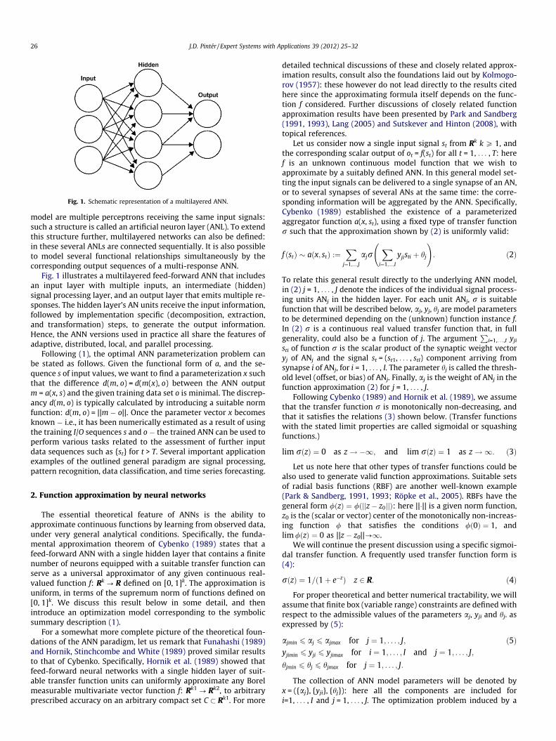
Fig. 1. Schematic representation of a multilayered ANN.
26 J.D. Pintér / Expert Systems with Applications 39 (2012) 25–32
model are multiple perceptrons receiving the same input signals:such a structure is called an artificial neuron layer (ANL). To extendthis structure further, multilayered networks can also be defined:in these several ANLs are connected sequentially. It is also possibleto model several functional relationships simultaneously by thecorresponding output sequences of a multi-response ANN.
Fig. 1 illustrates a multilayered feed-forward ANN that includesan input layer with multiple inputs, an intermediate (hidden)signal processing layer, and an output layer that emits multiple re-sponses. The hidden layer’s AN units receive the input information,followed by implementation specific (decomposition, extraction,and transformation) steps, to generate the output information.Hence, the ANN versions used in practice all share the features ofadaptive, distributed, local, and parallel processing.
Following (1), the optimal ANN parameterization problem canbe stated as follows. Given the functional form of a, and the se-quence s of input values, we want to find a parameterization x suchthat the difference d(m, o) = d(m(x), o) between the ANN outputm = a(x, s) and the given training data set o is minimal. The discrep-ancy d(m, o) is typically calculated by introducing a suitable normfunction: d(m, o) = ||m � o||. Once the parameter vector x becomesknown � i.e., it has been numerically estimated as a result of usingthe training I/O sequences s and o � the trained ANN can be used toperform various tasks related to the assessment of further inputdata sequences such as {st} for t > T. Several important applicationexamples of the outlined general paradigm are signal processing,pattern recognition, data classification, and time series forecasting.
2. Function approximation by neural networks
The essential theoretical feature of ANNs is the ability toapproximate continuous functions by learning from observed data,under very general analytical conditions. Specifically, the funda-mental approximation theorem of Cybenko (1989) states that afeed-forward ANN with a single hidden layer that contains a finitenumber of neurons equipped with a suitable transfer function canserve as a universal approximator of any given continuous real-valued function f: Rk ? R defined on [0, 1]k. The approximation isuniform, in terms of the supremum norm of functions defined on[0, 1]k. We discuss this result below in some detail, and thenintroduce an optimization model corresponding to the symbolicsummary description (1).
For a somewhat more complete picture of the theoretical foun-dations of the ANN paradigm, let us remark that Funahashi (1989)and Hornik, Stinchcombe and White (1989) proved similar resultsto that of Cybenko. Specifically, Hornik et al. (1989) showed thatfeed-forward neural networks with a single hidden layer of suit-able transfer function units can uniformly approximate any Borelmeasurable multivariate vector function f: Rk1 ? Rk2, to arbitraryprescribed accuracy on an arbitrary compact set C � Rk1. For more
detailed technical discussions of these and closely related approx-imation results, consult also the foundations laid out by Kolmogo-rov (1957): these however do not lead directly to the results citedhere since the approximating formula itself depends on the func-tion f considered. Further discussions of closely related functionapproximation results have been presented by Park and Sandberg(1991, 1993), Lang (2005) and Sutskever and Hinton (2008), withtopical references.
Let us consider now a single input signal st from Rk k P 1, andthe corresponding scalar output of ot = f(st) for all t = 1, . . . , T: heref is an unknown continuous model function that we wish toapproximate by a suitably defined ANN. In this general model set-ting the input signals can be delivered to a single synapse of an AN,or to several synapses of several ANs at the same time: the corre-sponding information will be aggregated by the ANN. Specifically,Cybenko (1989) established the existence of a parameterizedaggregator function a(x, st), using a fixed type of transfer functionr such that the approximation shown by (2) is uniformly valid:
f ðstÞ � aðx; stÞ :¼X
j¼1;...;J
ajrX
i¼1;...;I
yjisti þ hj
!: ð2Þ
To relate this general result directly to the underlying ANN model,in (2) j = 1, . . . , J denote the indices of the individual signal process-ing units ANj in the hidden layer. For each unit ANj, r is suitablefunction that will be described below, aj, yj, hj are model parametersto be determined depending on the (unknown) function instance f.In (2) r is a continuous real valued transfer function that, in fullgenerality, could also be a function of j. The argument
Pi=1,. . .,I yji
sti of function r is the scalar product of the synaptic weight vectoryj of ANj and the signal st = (st1, . . . , stI) component arriving fromsynapse i of ANj, for i = 1, . . . , I. The parameter hj is called the thresh-old level (offset, or bias) of ANj. Finally, aj is the weight of ANj in thefunction approximation (2) for j = 1, . . . , J.
Following Cybenko (1989) and Hornik et al. (1989), we assumethat the transfer function r is monotonically non-decreasing, andthat it satisfies the relations (3) shown below. (Transfer functionswith the stated limit properties are called sigmoidal or squashingfunctions.)
lim rðzÞ ¼ 0 as z! �1; and lim rðzÞ ¼ 1 as z!1: ð3Þ
Let us note here that other types of transfer functions could bealso used to generate valid function approximations. Suitable setsof radial basis functions (RBF) are another well-known example(Park & Sandberg, 1991, 1993; Röpke et al., 2005). RBFs have thegeneral form /ðzÞ ¼ /ðjjz� z0jjÞ: here ||�|| is a given norm function,z0 is the (scalar or vector) center of the monotonically non-increas-ing function / that satisfies the conditions /ð0Þ ¼ 1, andlim /ðzÞ ¼ 0 as ||z � z0||?1.
We will continue the present discussion using a specific sigmoi-dal transfer function. A frequently used transfer function form is(4):
rðzÞ ¼ 1=ð1þ e�zÞ z 2 R: ð4Þ
For proper theoretical and better numerical tractability, we willassume that finite box (variable range) constraints are defined withrespect to the admissible values of the parameters aj, yji and hj. asexpressed by (5):
ajmin 6 aj 6 ajmax for j ¼ 1; . . . ; J; ð5Þyjimin 6 yji 6 yjimax for i ¼ 1; . . . ; I and j ¼ 1; . . . ; J;
hjmin 6 hj 6 hjmax for j ¼ 1; . . . ; J:
The collection of ANN model parameters will be denoted byx = ({aj}, {yji}, {hj}): here all the components are included fori=1, . . . , I and j = 1, . . . , J. The optimization problem induced by a

J.D. Pintér / Expert Systems with Applications 39 (2012) 25–32 27
given approximator function form is to minimize the error of theapproximation (2), considering the training sequence (st, ot)t = 1, . . . , T, and using a selected norm function. In this study, weshall use the least squares error criterion to measure the qualityof the approximation. In other words, the objective function (errorfunction) e(x) defined by (6) will be minimized under theconstraints (5):
eðxÞ ¼X
t¼1;...;T
ðf ðstÞ � aðx; stÞÞ2: ð6Þ
Let us note that other (more general linear or nonlinear)constraints regarding feasible parameter combinations could alsobe present, if dictated by the problem context. Such situationscan be handled by adding the corresponding constraints to thebox-constrained optimization model formulation (5) and (6). Animportant case in point is to attempt the exclusion of identicalsolutions in which the component functions aj r(
Pi=1,. . .,I yji sti + hj)
of function a are, in principle, exchangeable. To break such symme-tries, we can assume, e.g. that the components of {aj} are orderedso that we add the constraints
aj P ajþ1 for all j ¼ 1; . . . ; J � 1: ð7Þ
One could also add further lexicographic constraints if dictated bythe problem at hand. Another optional – but not always applicable– constraint results by normalizing the weights {aj}, as shown below:
Xj¼1;...;J
aj ¼ 1; aj P 0 for all j ¼ 1; . . . ; J: ð8Þ
3. Postulating and calibrating ANN model instances
Cybenko (1989) emphasizes that his result cited here only guar-antees the theoretical possibility of a uniformly valid approxima-tion of a continuous function f, as opposed to its exactrepresentation. Furthermore, the general approximation result ex-pressed by (2) does not specify the actual number of processingunits required: hence, the key model parameter J needs to be setor estimated for each problem instance separately. Cybenko(1989) also conjectures that J could become ‘‘astronomical’’ inmany function approximation problem instances, especially sowhen dealing with higher dimensional approximations. Thesepoints need to be kept in mind, to avoid making unjustifiableclaims regarding the ‘‘universal power’’ of a priori defined (pre-fixed) ANN structures.
Once we select – i.e., postulate or incrementally develop – theANN structure to use in an actual application, the remaining essen-tial task is to find its parameterization with respect to a giventraining data set. The objective function defined by (6) makes thisa nonlinear model fitting problem that could have a multitude oflocal or global optima. The multi-modality aspect of nonlinearmodel calibration problems is discussed in detail by Pintér (1996,2003); in the context of ANNs, consult, e.g. Auer, Herbster, andWarmuth (1996), Bianchini and Gori (1996) and Abraham (2004).
Following the selection of the function form r, the number ofreal-valued parameters (i.e., the variables to optimize) is J(I + 2),each with given bound constraints. Furthermore, considering alsoboth (7) and (8), the number of optionally added linear constraintsis J. Since in the general ANN modeling framework the values of Iand J cannot be postulated ‘‘exactly’’, in many practical applica-tions one can try a number of computationally affordable combina-tions. In general, ANNs with more components can serve as betterapproximators, within reason and in line with the size T of thetraining data set that should minimally satisfy the conditionT P J(I + 2). At the same time, in order to assure the success of asuitable nonlinear optimization procedure and its software
implementation, one should restrict I and J to manageable values.These choices will evidently influence the accuracy of the approx-imation obtained.
Summarizing the preceding discussion, first one has to postu-late an ANN structure, and the family of parameterized transferfunctions to use. Next, one needs to provide a set of training data.The training of the chosen ANN is then aimed at the selection of anoptimally parameterized function from the selected family of func-tion models, to minimize the chosen error function.
The training of ANNs using optimization techniques is often re-ferred to in the literature as back-propagation. Due to the possiblemultimodality of the error function (6), the standard tools ofunconstrained local nonlinear optimization (direct search meth-ods, gradient information based methods, Newton-type methods)often fail to locate the best parameter combination. The multimo-dality issue is well-known: consult, e.g. Bianchini and Gori (1996),Sexton, Alidaee, Dorsey, and Johnson (1998), Abraham (2004) andHamm, Brorsen, and Hagan (2007). To overcome this difficulty,various global scope optimization strategies have been also usedto train ANNs: these include experimental design, spatial samplingby low-discrepancy sequences, theoretically exact global optimiza-tion approaches, as well as popular heuristics such as evolutionaryoptimization, particle swarm optimization, simulated annealing,tabu search and tunneling functions. ANN model parameterizationissues have been discussed and related optimization approachesproposed and tested, e.g. by Watkin (1993), Grippo (1994), Prechelt(1994), Bianchini and Gori (1996), Sexton et al. (1998), Jordanovand Brown (1999), Toh (1999), Vrahatis, Androulakis, Lambrinos,and Magoulas (2000), Ye and Lin (2003), Abraham (2004) andHamm et al. (2007).
4. The continuous global optimization model
Next we will discuss a global optimization based approach thatwill be subsequently applied to handle illustrative ANN calibrationproblems. In accordance with the notations introduced earlier, weuse the following symbols and assumptions:
x e Rn
n-dimensional real-valued vector of decisionvariables;e: Rn ? R
continuous (scalar-valued) objective function; D � Rn non-empty set of feasible solutions, a propersubset of Rn
The feasible set D is assumed to be closed and bounded: it is de-fined by
l e Rn, u e Rn
component-wise finite lower and upperbounds on x; andg: Rn ? Rm
an (optional) m-vector of continuousconstraint functionsApplying these notations, we shall consider the global optimizationmodel
Minimize eðxÞsubject to xeD :¼ x : l6 x6 u gjðxÞ6 0 j¼ 1; . . . ;m
� �:
ð9Þ
The concise model formulation (9) covers numerous special casesunder additional structural specifications. The model (9) also sub-sumes the ANN model calibration model statement summarizedby formulas (4)–(6), with the optionally added constraints (7)and/or (8). The analytical conditions preceding the GO model state-ment guarantee that the set of global solutions to (9) is non-empty,and the postulated model structure supports the application of

28 J.D. Pintér / Expert Systems with Applications 39 (2012) 25–32
properly defined globally convergent deterministic and stochasticoptimization algorithms. For related technical details that are out-side of the scope of the present discussion, consult Pintér (1996).For further comprehensive expositions regarding global optimiza-tion models, algorithms and applications, consult also Horst andPardalos (1995) and Pardalos and Romeijn (2002).
In spite of the stated theoretical guarantees, the numericalsolution of GO model instances can be a tough challenge, and evenlow-dimensional models can be hard to solve. These remarks ap-ply also to the calibration of ANN instances as it will be illustratedlater on.
5. The LGO software package for global and local nonlinearoptimization
The proper calibration of ANNs typically requires GO methodol-ogy. In addition, the ANN modeling framework has an inherent‘‘black box’’ feature. Namely, the error function e(x) is evaluatedby a numerical procedure that � in a model development and test-ing exercise, as well as in many applications � may be subject tochanges and modifications. Similar situations often arise in therealm of nonlinear optimization: their handling requires easy-to-use and flexible solver technology, without the need for modelinformation that could be difficult to obtain.
The Lipschitz Global Optimizer (LGO) solver suite has been de-signed to support the solution of ‘‘black box’’ problems, in additionto analytically defined models. Developed since the late 1980s,LGO is currently available for a range of compiler platforms (C,C++, C#, FORTRAN 77/90/95), with seamless links to several opti-mization modeling languages (AIMMS, AMPL, GAMS, MPL), MS Ex-cel spreadsheets, and to the leading high-level technical computingsystems Maple, Mathematica, and MATLAB. For algorithmic andimplementation details not discussed here, we refer to Pintér(1996, 1997, 2002, 2005, 2007, 2009, 2010a, 2010b, 2010c), Pintérand Kampas (2005) and Pintér, Linder, and Chin (2006).
The overall design of LGO is based on the flexible combination ofnonlinear optimization algorithms, with corresponding theoreticalglobal and local convergence properties. Hence, LGO – as a stand-alone solver suite – can be used for both global and local optimiza-tion; the local search mode can be also used without a precedingglobal search phase. In numerical practice – that is, in hardware re-source-limited and time-limited runs – each of LGO’s global searchoptions generates a global solution estimate(s) that is (are) refinedby the seamlessly following local search mode(s). This way, theexpected result of using LGO is a global and/or local search basedhigh-quality feasible solution that meets at least the local optimal-ity criteria. (To guarantee theoretical local optimality, standard localsmoothness conditions need to apply.) At the same time, one shouldkeep in mind that no global � or, in fact, any other � optimizationsoftware will ‘‘always’’ work satisfactorily, with default settingsand under resource limitations related to model size, time, modelfunction evaluation, or to other preset usage limits.
Extensive numerical tests and a growing range of practicalapplications demonstrate that LGO and its platform-specific imple-mentations can find high-quality numerical solutions to compli-cated and sizeable GO problems. Optimization models withembedded computational procedures and modules are discussed,e.g. by Pintér (1996, 2009), Pintér et al. (2006) and Kampas andPintér (2006, 2010). Examples of real-world optimization chal-lenges handled by various LGO implementations are cited herefrom environmental systems modeling and management (Pintér,1996), laser design (Isenor, Pintér, & Cada, 2003), intensity modu-lated cancer therapy planning (Tervo, Kolmonen, Lyyra-Laitinen,Pintér, & Lahtinen, 2003), the operation of integrated oil and gasproduction systems (Mason et al., 2007), vehicle component design(Goossens, McPhee, Pintér, & Schmitke, 2007), various packing
problems with industrial relevance (Castillo, Kampas, & Pintér,2008), fuel processing technology design (Pantoleontos et al.,2009), and financial decision making (Çaglayan & Pintér, submittedfor publication).
6. Numerical examples and discussion
6.1. Computational environment
The testing and evaluation of optimization software implemen-tations is a significant (although sometimes under-appreciated)research area. One needs to follow or to establish objectiveevaluation criteria, and to present fully reproducible results. Thesoftware tests themselves are conducted by solving a chosen setof test problems, and by applying criteria such as the reliabilityand efficiency of the solver(s) used, in terms of the quality of solu-tions obtained and the computational effort required. For examplesof benchmarking studies in the ANN context, we refer to Prechelt(1994) and Hamm et al. (2007). In the GO context, consult, e.g.Ali, Khompatraporn, and Zabinsky (2005), Khompatraporn, Pintér,and Zabinsky (2005) and Pintér (2002, 2007), with further topicalreferences. Here we will illustrate the performance of an LGOimplementation in the context of ANN calibration, by solving sev-eral function approximation problems. Although the test functionspresented are merely one-dimensional, their high-quality approx-imation requires the solution of induced GO problems with severaltens of variables.
The key features of the computational environment used andthe numerical tests are summarized below: the detailed numericalresults are available from the author upon request.
� Hardware: PC, 32-bit, Intel™Core™2 Duo CPU T5450 @1.66 GHz, 2.00 GB RAM. Let us remark that this is an averagelaptop PC with modest capabilities, as of 2011.� Operating system: Windows Vista.� Model development and test environment: Mathematica (Wol-
fram Research, 2011).� Global optimization software: MathOptimizer Professional (MOP).
MathOptimizer Professional is the product name (trademark) ofthe LGO solver implementation that is seamlessly linked toMathematica. For details regarding the MOP software, consult,e.g. Pintér and Kampas (2005) and Kampas and Pintér (2006).� ANN computational model used: 1-J-1 type feed-forward net-
work instances that have a single input node, a single outputnode, and J processing units. Recall that this ANN structuredirectly follows the function approximation formula expressedby (2). The ANN modeling framework, its instances and the testexamples discussed here have been implemented (by theauthor) in native Mathematica code.� ANN initialization by assigned starting parameter values is not
necessary, since MOP uses a global scope optimization approachby default. However, all LGO solver implementations also sup-port the optional use of initial values in their constrained localoptimization mode, without applying first a global search mode.� A single optimization run is executed in all cases: repetitions
are not needed, since MathOptimizer Professional produces iden-tical runs under the same initializations and solver options.Repeated runs with possibly changing numerical results canbe easily generated by changing several options of MOP. Theseoptions make possible, e.g. the selection of the global searchmode applied, the use of different starting points in the localsearch mode, the use of different random seeds, and the alloca-tion of computational resources and runtime.� In all test problems the optimized function approximations are
based on a given set of training points, in line with the modelingframework discussed in Section 2.

J.D. Pintér / Expert Systems with Applications 39 (2012) 25–32 29
� Simulated noise structure: none. In other words, we assumethat all training data are exact. This assumption could be easilyrelaxed, e.g. by introducing a probabilistic noise structure as ithas been done in Pintér (2003).� Key performance measure: standard error (the root of the mean
square error, RMSE) calculated for the best parameterizationfound. For completeness, recalling (6), RMSE is defined by theexpression (e(x)/T)1/2 = (
Pt=1,. . .,T (f(st) � a(x, st))2/T)1/2.
� Additional Mathematica features used: documentation and visu-alization capabilities related to the ANN models and tests dis-cussed here, all included in a single (Mathematica notebook)document.� Additional MOP features: the automatic generation of optimiza-
tion test model code in C or FORTRAN (as per user preferences),and the automatic generation of optimization input and resulttext files. Let us point out that these features can be put to gooduse (also) in developing and testing compiler code based ANNimplementations.
In the numerical examples presented below, our objective is to‘‘learn’’ the graph of certain one-dimensional functions defined onthe interval [0, 1], based on a preset number of uniformly spacedtraining points. As earlier, we apply the notation T for the numberof training data, and J for the number of processing units in the hid-den layer.
6.2. Example 1
The first (and easiest) test problem presented here has beenstudied also by Toh (1999), as well as by Ye and Lin (2003). Thefunction to approximate is defined as
f ðxÞ ¼ sinð2pxÞcosð4pxÞ; 0 6 x 6 1: ð10Þ
We set the number of training data as T = 100 and postulate thenumber of processing units as J = 7. Recalling the discussion of Sec-tion 2 (cf. especially formula (2)), this choice of J induces a non-triv-ial box-constrained GO model in 21 variables.
Applying first MOP’s local search mode (LS) only, we obtainedan overall function approximation characterized by RMSE�0.0026853412. With default MOP settings, the number of errorfunction evaluations is 60,336; the corresponding runtime is4.40 s. (The program execution speed could somewhat vary, ofcourse, depending on the actual tasks handled by the computerused.)
For comparison, next we also solved the same problem usingLGO’s most extensive global search mode (stochastic multi-start,MS) followed by corresponding local searches from the best pointsfound. This operational mode is referred to briefly as MSLS, and ithas been used in all subsequent numerical examples. In the MSLSoperational mode, we set (postulate) the variable ranges[lb, ub] = [�20, 20] for all ANN model parameters, and we set thelimit for the global search steps (the number of error function eval-uations) as gss = 106. Based on our numerical experience related toGO, this does not seem to be an ‘‘exorbitant’’ setting, since we have
0.2 0.4 0.6 0.8 1.0
1.0
0.5
0.5
1.0
Fig. 2. Function (10) and the list plot
to optimize 21 parameters globally. (For a simple comparison, if weaimed at just 10% precision to find the best variable setting in 21dimensions by applying a uniform grid based search, then thisnaïve approach would require 1021 function evaluations.)
Applying the MSLS operational mode, we received RMSE�0.0001853324. This means a significant 93% error reduction com-pared to the already rather small average error found using onlythe LS operational mode. The actual number of function evalua-tions is 1,083,311; the corresponding runtime is 77.47 s.
To illustrate and summarize our result visually, function (10) isdisplayed below: see the left hand side (lhs) of Fig. 2. This isdirectly followed by the list plot produced by the output of theoptimized ANN at the equidistant training sample arguments:see the right hand side (rhs) of Fig. 2.
Even without citing the actual parameter values here, it isworth noting that the optimized ANN parameterizations foundby the local (LS) and global (MSLS) search modes are markedly dif-ferent. This finding, together with the results of our further tests,indicates the potentially massive multi-modality of the objectivefunction in similar – or far more complicated – approximationproblems. Let us also remark that several components of theANN parameter vectors found lie on the boundary of the presetinterval range [�20, 20]. This finding indicates a possible needfor extending the search region: we did not do this in our limitednumerical study, since the approximation results are very satisfac-tory even in this case. Obviously, one could experiment further, e.g.by changing the value of J (the number of processing units), as wellas by changing the parameter bounds if these measures are ex-pected to lead to markedly improved results.
Let us also note that in this particular test example, we couldhave perhaps reduced the global search effort, or just use the localsearch based estimate which already seems to be ‘‘good enough’’.Such experimental ‘‘streamlining’’ of the optimization proceduremay not always work, however, and we are convinced that properglobal scope search is typically needed in calibrating ANNs. Hence,we will solve all further test problems using the MSLS operationalmode.
The numerical examples presented below are chosen to beincreasingly more difficult, although all are ‘‘merely’’ approxima-tion problems related to one-dimensional functions. (Recall atthe same time that the corresponding GO problems have tens ofvariables.) Obviously, one could ‘‘fabricate’’ functions, especiallyso in higher dimensions, that could become very difficult toapproximate solely by applying ANN technology. This commentis in line with the observation of Cybenko cited earlier, regardingthe possible need for ‘‘astronomical’’ choices of J. This caveatshould be kept in mind when applying ANNs to solve complicatedreal-world applications.
6.3. Example 2
In this example, our objective is to approximate the functionshown below:
f ðxÞ ¼ sinð2pxÞsinð3pxÞsinð5pxÞ; 0 6 x 6 1: ð11Þ
20 40 60 80 100
1.0
0.5
0.5
1.0
produced by the optimized ANN.

0.2 0.4 0.6 0.8 1.0
0.6
0.4
0.2
0.2
0.4
0.6
20 40 60 80 100
0.6
0.4
0.2
0.2
0.4
0.6
Fig. 3. Function (11) and the list plot produced by the optimized ANN.
0.2 0.4 0.6 0.8 1.0
0.2
0.1
0.1
0.2
0.3
0.4
20 40 60 80 100
0.2
0.1
0.1
0.2
0.3
0.4
Fig. 4. Function (12) and the list plot produced by a sub-optimally trained ANN.
30 J.D. Pintér / Expert Systems with Applications 39 (2012) 25–32
To handle this problem, we use again T = 100, but now assume(postulate) that J = 10. Notice that the number of processing unitshas been increased heuristically, reflecting our belief that function(11) could be more difficult to reproduce than (10). This settingleads to a 30-variable GO model: however, we keep the allocatedglobal search effort gss = 106 as in Example 1.
We conjecture again that the induced model calibration prob-lem is highly multi-extremal. The global search based numericalsolution yields RMSE �0.0002453290; the corresponding runtimeis 99.94 s spent on 1,013,948 function evaluations. For a visualcomparison, the function (11) is displayed below, directly followedby the list plot produced by the output of the trained ANN: see thelhs and rhs of Fig. 3, respectively.
6.4. Example 3
In the last illustrative example presented here, our objective isto approximate the function shown below by (12): here log denotesthe natural logarithm function.
f ðxÞ ¼ sinð5pxÞsinð7pxÞsinð11pxÞlogð1þ xÞ; 0 6 x 6 1: ð12Þ
As above, we set T = 100, J = 10, and use the MSLS search modewith 106 global search steps; furthermore, now we extend thesearch region to [�50, 50] for each ANN model parameter. Theresulting global search based numerical solution has an RMSE�0.1811353757 which is noticeably not as good as the previouslyfound RMSE values. The corresponding runtime is 111.61 s, spenton 1,130,366 function evaluations. For comparison, the function(12) is displayed by Fig. 4, directly followed by the list plot pro-
0.2 0.4 0.6 0.8 1.0
0.2
0.1
0.1
0.2
0.3
0.4
Fig. 5. Function (12) and the list plot prod
duced by the (sub-optimally) trained ANN. Comparing the lhsand rhs of Fig. 4, one can see the apparent discrepancy betweenthe function and its approximation: although the ANN output re-flects well some key structural features, it definitely misses someof the ‘‘finer details’’. This finding shows that the postulated ANNstructure may not be adequate, and/or the training set may notbe of sufficient size, and/or that the allocated global scope searcheffort may not be enough.
In several subsequent numerical experiments, we attempted toincrease the precision of approximating function (12), by increas-ing one or several of the following factors: the number of trainingdata T, the number of processing units J, the global search effort gss,and the solver runtime allocated to MOP. Obviously, all the abovemeasures could lead to improved results. Without going intounnecessary details, Fig. 5 illustrates that, e.g. the combinationT = 200, J = 20, gss = 3,000,000, and the LGO runtime limit set to30 min leads to a fairly accurate approximation of the entire func-tion: the corresponding RMSE indicator value is �0.0016966244.The total number of function evaluations in this case is3,527,313; the corresponding runtime is 1360.56 s. Again, increas-ing the sampling effort (T), and/or the ANN configuration size (J),and/or the search effort (gss) even better approximations couldbe found, if increased accuracy is required.
Our illustrative results demonstrate that GO based ANN calibra-tion can be used to handle non-trivial function approximationproblems, with a reasonable computational effort using today’saverage personal computer. Our approach (as described) is also di-rectly applicable to solve at least certain types of multi-input andmulti-response function approximation and related problems.
50 100 150 200
0.2
0.1
0.1
0.2
0.3
0.4
uced by the globally optimized ANN.

J.D. Pintér / Expert Systems with Applications 39 (2012) 25–32 31
Specifically, if the input data sequences can be processed by inde-pendently operated intermediate ANN layers for each function out-put, then the approach introduced can be applied (repetitively or inparallel) to such multi-response problems. However, if the inputsequences need to be aggregated, then in general this will lead toincreased GO model dimensionality. This remark hints at the po-tential difficulty of calibrating general multiple-input multiple-output ANNs.
7. Conclusions
Artificial neural networks are frequently used to model un-known functional relationships between the input and output ofsome system perceived as a ‘‘black box’’. The general functionapproximator capability of ANNs is supported by strong theoreticalresults. At the same time, the ANN framework inherently has ameta-heuristic flavor, since it needs to be instantiated and cali-brated for each new model type to solve. Although the selectionof a suitable ANN structure can benefit from domain-specificexpertise, its calibration often becomes difficult as the complexityof the tasks to handle increases. Until recently, more often than notlocal – as opposed to global scope – search methods have been ap-plied to parameterize ANNs. These facts call for flexible and trans-parent ANN implementations, and for improved ANN calibrationmethodology.
To address some of these issues, a general modeling and globaloptimization framework is presented to solve ANN calibrationproblems. The practical viability of the proposed ANN calibrationapproach is illustrated by finding high-quality numerical approxi-mations of visibly challenging one-dimensional functions. Forthese experiments, we have implemented a flexible ANN frame-work and an easily expandable set of test functions in the technicalcomputing system Mathematica. The MathOptimizer Professionalglobal-local optimization software has been used to solve the in-duced multi-dimensional ANN calibration problems. After definingthe (in principle, arbitrary continuous) function to approximate,one needs to change only a few input data to define a new sam-pling plan, to define the actual ANN instance from the postulatedANN family, and to activate the optimization engine. The corre-sponding results can be then directly observed and visualized, foroptional further analysis and comparison.
Due to its universal function approximator capability, the ANNcomputational structure flexibly supports the modeling of manyimportant research problems and real world applications. Fromthe broad range of ANN applications several areas are closely re-lated to our discussion: examples are signal and image processing(Masters, 1994; Watkin, 1993), data classification and pattern rec-ognition (Karthikeyan, Gopal, & Venkatesh, 2008; Ripley, 1996),function approximation (Toh, 1999; Ye & Lin, 2003), time seriesanalysis and forecasting (Franses & van Dijk, 2000; Kajitani, Hipel,& McLeod, 2005), experimental design in engineering systems(Röpke et al., 2005), and the prediction of trading signals of stockmarket indices (Tilakaratne, Mammadov, & Morris, 2008).
Acknowledgements
The author wishes to acknowledge the valuable contributions ofDr. Frank Kampas to the development of MathOptimizer Profes-sional. Thanks are also due to Dr. Maria Battarra and to the editorsand reviewers for all constructive comments and suggestionsregarding the manuscript.
This research has been partially supported by Özyegin Univer-sity (Istanbul, Turkey), and by the Simulation and OptimizationProject of Széchenyi István University (Gy}or, Hungary; TÁMOP4.2.2-08/1-2008-0021).
References
Abraham, A. (2004). Meta learning evolutionary artificial neural networks.Neurocomputing, 56, 1–38.
Ali, M. M., Khompatraporn, C., & Zabinsky, Z. B. (2005). A numerical evaluation ofseveral stochastic algorithms on selected continuous global optimization testproblems. Journal of Global Optimization, 31, 635–672.
Auer, P., Herbster, M., & Warmuth, M. (1996). Exponentially many local minima forsingle neurons. In D. Touretzky et al. (Eds.). Advances in neural informationprocessing systems (Vol. 8, pp. 316–322). Cambridge, MA: MIT Press.
Bar-Yam, Y. (1999). Dynamics of complex systems. Boulder, CO: Westview Press.Bianchini, M., & Gori, M. (1996). Optimal learning in artificial neural networks: A
review of theoretical results. Neurocomputing, 13, 313–346.Çaglayan, M. O., & Pintér, J. D. (2010). Development and calibration of a currency
trading strategy by global optimization. Research Report, Özyegin University,Istanbul. Submitted for publication.
Castillo, I., Kampas, F. J., & Pintér, J. D. (2008). Solving circle packing problems byglobal optimization: Numerical results and industrial applications. EuropeanJournal of Operational Research, 191, 786–802.
Cichocki, A., & Unbehauen, R. (1993). Neural networks for optimization and signalprocessing. Chichester, UK.: John Wiley & Sons.
Cruse, H. (2006). Neural networks as cybernetic systems (2nd revised ed.). Bielefeld,Germany: Brains, Minds and Media.
Cybenko, G. (1989). Approximation by superpositions of a sigmoidal function.Mathematics of Control, Signals, and Systems, 2, 303–314.
Franses, P. H., & van Dijk, D. (2000). Nonlinear time series models in empirical finance.Cambridge, UK: Cambridge University Press.
Funahashi, K. (1989). On the approximate realization of continuous mappings byneural networks. Neural Networks, 2, 183–192.
Golden, R. M. (1996). Mathematical methods for neural network analysis and design.Cambridge, MA: MIT Press.
Goossens, P., McPhee, J., Pintér, J. D., & Schmitke, C. (2007). Driving innovation: Howmathematical modeling and optimization increase efficiency and productivity invehicle design. Maplesoft, Waterloo, ON: Technical Memorandum.
Grippo, L. (1994). A class of unconstrained minimization methods for neuralnetwork training. Optimization Methods and Software, 4(2), 135–150.
Hamm, L., Brorsen, B. W., & Hagan, M. T. (2007). Comparison of stochastic globaloptimization methods to estimate neural network weights. Neural ProcessingLetters, 26, 145–158.
Hertz, J., Krogh, A., & Palmer, R. G. (1991). Introduction to the theory of neuralcomputation. Reading, MA: Addison-Wesley.
Hornik, K., Stinchcombe, M., & White, H. (1989). Multilayer feedforward networksare universal approximators. Neural Networks, 2, 359–366.
Horst, R., & Pardalos, P. M. (Eds.). (1995). Handbook of global optimization (Vol. 1).Dordrecht: Kluwer Academic Publishers.
Isenor, G., Pintér, J. D., & Cada, M. (2003). A global optimization approach to laserdesign. Optimization and Engineering, 4, 177–196.
Jordanov, I., & Brown, R. (1999). Neural network learning using low-discrepancysequence. In N. Foo (Ed.). AI’99, Lecture notes in artificial intelligence (Vol. 1747,pp. 255–267). Berlin, Heidelberg: Springer-Verlag.
Kajitani, Y., Hipel, K. W., & McLeod, A. I. (2005). Forecasting nonlinear time serieswith feed-forward neural networks: a case study of Canadian lynx data. Journalof Forecasting, 24, 105–117.
Kampas, F. J., & Pintér, J. D. (2010). Advanced nonlinear optimization in Mathematica.Research Report, Özyegin University, Istanbul. Submitted for publication.
Kampas, F. J., & Pintér, J. D. (2006). Configuration analysis and design by usingoptimization tools in mathematica. The Mathematica Journal, 10(1), 128–154.
Karthikeyan, B., Gopal, S., & Venkatesh, S. (2008). Partial discharge patternclassification using composite versions of probabilistic neural networkinference engine. Expert Systems with Applications, 34, 1938–1947.
Khompatraporn, Ch., Pintér, J. D., & Zabinsky, Z. B. (2005). Comparative assessmentof algorithms and software for global optimization. Journal of GlobalOptimization, 31, 613–633.
Kolmogorov, A. N. (1957). On the representation of continuous functions of manyvariables by superposition of continuous functions of one variable and addition.Doklady Akademii Nauk SSR, 114, 953–956.
Lang, B. (2005). Monotonic multi-layer perceptron networks as universalapproximators. In W. Duch et al. (Eds.). Artificial neural networks: Formalmodels and their applications – ICANN 2005, Lecture notes in computer science(Vol. 3697, pp. 31–37). Berlin, Heidelberg: Springer-Verlag.
Mason, T. L., Emelle, C., van Berkel, J., Bagirov, A. M., Kampas, F., & Pintér, J. D. (2007).Integrated production system optimization using the Lipschitz global optimizerand the discrete gradient method. Journal of Industrial and ManagementOptimization, 3(2), 257–277.
Masters, T. (1994). Signal and image processing with neural networks. New York: JohnWiley & Sons.
Mehrotra, K., Mohan, C. K., & Ranka, S. (1997). Elements of artificial neural nets.Cambridge, MA: MIT Press.
Pardalos, P. M., & Romeijn, H. E. (Eds.). (2002). Handbook of global optimization (Vol.2). Dordrecht: Kluwer Academic Publishers.
Pantoleontos, G., Basinas, P., Skodras, G., Grammelis, P., Pintér, J. D., Topis, S., &Sakellaropoulos, G. P. (2009). A global optimization study on the devolatilisationkinetics of coal, biomass and waste fuels. Fuel Processing Technology, 90, 762–769.
Park, J., & Sandberg, I. W. (1991). Universal approximation using radial-basis-function networks. Neural Computation, 3(2), 246–257.

32 J.D. Pintér / Expert Systems with Applications 39 (2012) 25–32
Park, J., & Sandberg, I. W. (1993). Approximation and radial-basis-functionnetworks. Neural Computation, 5(2), 305–316.
Pintér, J. D. (1996). Global optimization in action. Dordrecht: Kluwer AcademicPublishers.
Pintér, J. D. (1997). LGO � A program system for continuous and Lipschitzoptimization. In I. M. Bomze, T. Csendes, R. Horst, & P. M. Pardalos (Eds.),Developments in global optimization (pp. 183–197). Dordrecht: Kluwer AcademicPublishers.
Pintér, J. D. (2002). Global optimization: Software, test problems, and applications.In P. M. Pardalos & H. E. Romeijn (Eds.). Handbook of global optimization (Vol. 2,pp. 515–569). Dordrecht: Kluwer Academic Publishers.
Pintér, J. D. (2003). Globally optimized calibration of nonlinear models: Techniques,software, and applications. Optimization Methods and Software, 18(3), 335–355.
Pintér, J. D. (2005). Nonlinear optimization in modeling environments: Softwareimplementations for compilers, spreadsheets, modeling languages, andintegrated computing systems. In V. Jeyakumar & A. M. Rubinov (Eds.),Continuous optimization: Current trends and modern applications (pp. 147–173).New York: Springer Science + Business Media.
Pintér, J. D. (2007). Nonlinear optimization with GAMS/LGO. Journal of GlobalOptimization, 38, 79–101.
Pintér, J. D. (2009). Software development for global optimization. In P. M. Pardalos& T. F. Coleman (Eds.), Global optimization: Methods and applications. Fieldsinstitute communications (Vol. 55, pp. 183–204). Berlin: Springer.
Pintér, J. D. (2010a). LGO – A model development and solver system for nonlinear(global and local) optimization. User’s guide. (Current version) Distributed byPintér Consulting Services, Inc., Canada. <www.pinterconsulting.com>.
Pintér, J. D. (2010b). Spreadsheet-based modeling and nonlinear optimization withExcel-LGO. User’s guide. With technical contributions by B.C. S�al and F.J. Kampas(Current version) Distributed by Pintér Consulting Services, Inc., Canada;<www.pinterconsulting.com>.
Pintér, J.D. (2010c). MATLAB-LGO User’s Guide. With technical contributions by B.C.S�al and F.J. Kampas. (Current version) Distributed by Pintér Consulting Services,Inc., Canada. <www.pinterconsulting.com>.
Pintér, J. D., & Kampas, F. J. (2005). Nonlinear optimization in Mathematica withMathoptimizer Professional. Mathematica in Education and Research, 10(2), 1–18.
Pintér, J. D., Linder, D., & Chin, P. (2006). Global Optimization Toolbox for Maple: Anintroduction with illustrative applications. Optimization Methods and Software,21(4), 565–582.
Prechelt, L. (1994). PROBEN1 � A set of benchmarks and benchmarking rules for neuralnetwork training algorithms. Technical Report 21/94, Fakultät fur Informatik,Universität Karlsruhe, Germany.
Ripley, B. D. (1996). Pattern recognition and neural networks. Cambridge, MA:Cambridge University Press.
Röpke, K. et al. (Eds.). (2005). DoE – Design of experiments. Munich, Germany: IAVGmbH, Verlag Moderne Industrie. � sv Corporate Media, GmbH.
Sexton, R. S., Alidaee, B., Dorsey, R. E., & Johnson, J. D. (1998). Global optimization forartificial neural networks: A tabu search application. European Journal ofOperational Research, 106, 570–584.
Smith, M. (1993). Neural networks for statistical modeling. New York: Van NostrandReinhold.
Steeb, W.-H. (2005). The nonlinear workbook (3rd ed.). Singapore: World Scientific.Sutskever, I., & Hinton, G. E. (2008). Deep, narrow sigmoid belief networks are
universal approximators. Neural Computation, 20, 2629–2636.Tervo, J., Kolmonen, P., Lyyra-Laitinen, T., Pintér, J. D., & Lahtinen, T. (2003). An
optimization-based approach to the multiple static delivery technique inradiation therapy. Annals of Operations Research, 119, 205–227.
Tilakaratne, Ch. D., Mammadov, M. A., & Morris, S. A. (2008). Predicting tradingsignals of stock market indices using neural networks. In AI 2008: Advances inartificial intelligence. In W. Wobcke & M. Zhang (Eds.). Lecture notes in computerscience (Vol. 5360, pp. 522–531). Berlin, Heidelberg: Springer-Verlag.
Toh, K.-A. (1999). Fast deterministic global optimization for FNN training. InProceedings of IEEE international conference on systems, man, and cybernetics,Tokyo, Japan (pp. V413–V418).
Vrahatis, M. N., Androulakis, G. S., Lambrinos, J. N., & Magoulas, G. D. (2000). A classof gradient unconstrained minimization algorithms with adaptive stepsize.Journal of Computational and Applied Mathematics, 114, 367–386.
Watkin, T. L. H. (1993). Optimal learning with a neural network. Europhysics Letters,21(8), 871–876.
Wolfram Research (2011). Mathematica (Current version 8.0.1). Distributed by WRI,Champaign, IL.
Ye, H., & Lin, Z. (2003). Global optimization of neural network weights usingsubenergy tunneling function and ripple search. In Proceedings of the IEEE ISCAS,Bangkok, Thailand, May 2003 (pp. V725–V728.