calibrated american option pricing by stochastic linear programming
TRANSCRIPT

This article was downloaded by: [University of Stellenbosch]On: 09 October 2014, At: 12:11Publisher: Taylor & FrancisInforma Ltd Registered in England and Wales Registered Number: 1072954 Registeredoffice: Mortimer House, 37-41 Mortimer Street, London W1T 3JH, UK
Optimization: A Journal ofMathematical Programming andOperations ResearchPublication details, including instructions for authors andsubscription information:http://www.tandfonline.com/loi/gopt20
Calibrated American option pricing bystochastic linear programmingFabio Antonellia, Carlo Mancinia & Mustafa Ç. Pınarb
a DISIM, University of L’Aquila, L’Aquila, Italy.b Department of Industrial Engineering, Bilkent University, Ankara,Turkey.Published online: 09 Sep 2013.
To cite this article: Fabio Antonelli, Carlo Mancini & Mustafa Ç. Pınar (2013) Calibrated Americanoption pricing by stochastic linear programming, Optimization: A Journal of MathematicalProgramming and Operations Research, 62:11, 1433-1450, DOI: 10.1080/02331934.2013.833201
To link to this article: http://dx.doi.org/10.1080/02331934.2013.833201
PLEASE SCROLL DOWN FOR ARTICLE
Taylor & Francis makes every effort to ensure the accuracy of all the information (the“Content”) contained in the publications on our platform. However, Taylor & Francis,our agents, and our licensors make no representations or warranties whatsoever as tothe accuracy, completeness, or suitability for any purpose of the Content. Any opinionsand views expressed in this publication are the opinions and views of the authors,and are not the views of or endorsed by Taylor & Francis. The accuracy of the Contentshould not be relied upon and should be independently verified with primary sourcesof information. Taylor and Francis shall not be liable for any losses, actions, claims,proceedings, demands, costs, expenses, damages, and other liabilities whatsoever orhowsoever caused arising directly or indirectly in connection with, in relation to or arisingout of the use of the Content.
This article may be used for research, teaching, and private study purposes. Anysubstantial or systematic reproduction, redistribution, reselling, loan, sub-licensing,systematic supply, or distribution in any form to anyone is expressly forbidden. Terms &

Conditions of access and use can be found at http://www.tandfonline.com/page/terms-and-conditions
Dow
nloa
ded
by [
Uni
vers
ity o
f St
elle
nbos
ch]
at 1
2:12
09
Oct
ober
201
4

Optimization, 2013Vol. 62, No. 11, 1433–1450, http://dx.doi.org/10.1080/02331934.2013.833201
Calibrated American option pricing by stochastic linear programming
Fabio Antonellia, Carlo Mancinia∗ and Mustafa Ç. Pınarb
aDISIM, University of L’Aquila, L’Aquila, Italy; bDepartment of Industrial Engineering, BilkentUniversity, Ankara, Turkey
(Received 28 January 2013; accepted 14 July 2013)
We propose an approach for computing the arbitrage-free interval for the price ofanAmerican option in discrete incomplete market models via linear programming.The main idea is built replicating strategies that use both the basic asset andsome European derivatives available on the market for trading. This method goesunder the name of calibrated option pricing and it has given significant results forEuropean options. Here, we extend the analysis to American options showing thatthe arbitrage-free interval can be characterized in terms of martingale measuresand that it gets significantly reduced with respect to the non-calibrated case.
Keywords: American option; incomplete market; arbitrage-free interval;calibrated option pricing; dual theory; martingale measures
1. Introduction
In this work, we apply a linear programming method to price American options in a discreteand incomplete market model. The linear programming theory has been used in contexts ofcompleteness by Naik [1], Ortu [2] and by Baccara et al. [3]. As it is well known, we areno longer able to exhibit a unique price for derivatives. In the literature an arbitrage-freeinterval is usually given by characterizing its endpoints as infimum and supremum of theexpected values of the pay-off with respect to a family of martingale measures. Hence, anappropriate criterion to select a specific measure (minimal variance, minimal martingalemeasure etc.) is used (see Föllmer and Schweizer [4] and Frittelli [5]).
A possible alternative approach is to study the values of all possible admissible invest-ment strategies, trying to select those that replicate an arbitrage-free pricing of the derivative(see Cont [6]). This leads to setting up two optimization problems, known as the buyer’s andseller’s problem. The optimal values of these problems represent the maximum price andthe minimum price that allow, respectively the buyer and the seller of the contract to exploitan arbitrage opportunity. Once they pass these levels they are in no arbitrage conditions (seeKing [7]). The values of the optimal solutions of these two problems will give the endpointsof the arbitrage-free price interval for the considered derivative.
More precisely in incomplete arbitrage-free markets, the price of an option is not uniquebut should lie somewhere between the least cost of a super replication strategy (seller’s price)and the greatest amount that the buyer would pay for it without facing the risk of a negative
∗Corresponding author. Email: [email protected]
© 2013 Taylor & Francis
Dow
nloa
ded
by [
Uni
vers
ity o
f St
elle
nbos
ch]
at 1
2:12
09
Oct
ober
201
4

1434 F. Antonelli et al.
terminal wealth (buyer’s price). When frictionless trading is possible, these bounds can beexpressed as the supremum and infimum of the discounted expected future cash-flows of theoption on the set of all pricing measures. Having focused on strategies, linear programmingbecomes the natural tool to look for those values in finite-state discrete-time markets, alsoproviding a setting of easy implementation.
In practice, the resulting problems are often quite big and sometimes, even though thecomputational time is not high, they do not provide a significant outcome, meaning that thecomputed arbitrage-free interval is quite large.
To answer this problem, King et al. in [8] employ a modified approach, inspired bywhat actually happens in real financial markets. In conditions of incompleteness, since thebasic assets are not sufficient to devise a replicating strategy for each derivative, agentsincorporate derivatives in their hedging portfolios. Hence, King et al. introduce the so-called calibrated option pricing. In their work, for European options, they write new linearprogramming problems for the buyer and the seller, where they include in the hedgingstrategy the possibility of selling and buying other European options with respective bidand ask prices and maturities. The authors prove again that the optimal solutions may becharacterized in terms of the average values with respect to martingale measures that maybelong, now, to a much smaller set. This reduces sensibly the arbitrage-free interval and theadvantage of the method is illustrated numerically.
In this paper, the hedging problem is modelled as a stochastic problem using the math-ematical technique of conjugate duality or alternatively Lagrange duality (ref. Rockafellar[9]). The first to use this technique to price an American contingent claim in incompletemarkets were Pennanen and King [10] and Flåm [11]. Pennanen and King, in particular,studied the linear programming problems for the buyer’s and the seller’s prices, but inthe buyer’s case their proof is valid only for the American options, a more general proofwas given by Camci and Pinar [12] later on. The main contribution of the present paperis to show that the calibrated option bounds for American options can be computed bysolving two linear programming problems, improving the numerical results. Moreover,we show that the end points of the no arbitrage interval may be characterized again byinfimum and supremum of the expected pay-off with respect to an appropriate set ofmartingale measure. The main results are contained in Theorems 3.1 and 3.2. Especially,Theorem 3.1, while similar in spirit to the aforementioned results in the utilization of duality,requires a careful proof. We substantiate our results with numerical illustrations using realdata.
The outline of the paper is as follows. Section 2 describes the market model. In Section 3,we study the calibrated option bounds for American contingent claims pointing out therelations between hedging and martingale measures in incomplete markets. In Section 4,we present some numerical results applied to the pricing of S&P500 options. Section 5is devoted to the concluding remarks about the advantages and the weaknesses of themodel.
2. Discrete market models
We consider the same discrete finite-dimensional market model as in King [7]. There areJ + 1 securities tradable at discrete times k = 0, . . . , K . We denote by Sk = (S0
k , . . . , S Jk )
the price process, whose first component represents the price of the riskless asset, thus it isalways strictly positive. Thanks to this assumption, we can define the discount processes
Dow
nloa
ded
by [
Uni
vers
ity o
f St
elle
nbos
ch]
at 1
2:12
09
Oct
ober
201
4
Optimization 1435
βk = S00
S0k
. Moreover, Sk is adapted with respect to a given filtered probability space
(�,F , {Fk}, P), such that |�| < ∞.The market is arbitrage-free, frictionless and investors are small, comparatively to the
market dimension.To have a finite sample space, � simplifies the analysis and allows a natural description
of the market model in terms of a scenario tree. Here, we assume that the tree is non-recombinant, which might be important in incomplete markets, where trading strategies arein general path dependent. The atoms of Fk , denoted by Nk , are the nodes of the scenariotree at time k. At time 0, the set N0 consists of the root node n = 0; since the tree is non-recombinant, each outcome is uniquely identified by its path, the nodes n ∈ NK correspondone-to-one to the probability atoms ω ∈ �. The collection of all nodes will be denoted byN = ∪K
k=0Nk . Since the scenario tree is non-recombinant, we have that for k = 1, . . . , K ,each node n ∈ Nk comes from a unique element a(n) ∈ Nk−1, thus we can define theset C(n) = {m ∈ N |a(m) = n} ∈ Nk+1 of the first descendants of a node n ∈ Nk withk = 1, . . . , K . We denote by A(n) the collection of ascendant nodes or path history of nodeincluding n itself and D(n) the set of descendant nodes of n, again including n itself. Fromnow on, we focus our attention no longer on times but on nodes, hence we will denote bySn , n ∈ Nk the value of the assets at each single node of the tree at time k.
The probability measure P gives weight pKn > 0 to each node n ∈ NK so that∑
n∈NKpK
n = 1. The probability of each node n ∈ N \ NK is determined by conditioningso pk
n = ∑m∈C(n) pk+1
m for k = 0, . . . , K − 1. Hence, each non-leaf node has a probabilitymass equal to the combined mass of its child nodes. The expected value of Sk given P isgiven by the finite sum
EP[Sk] =∑
n∈NK
pkn Sn .
The conditional expectation of Sk+1 on Nk is hence obtained by
EP[Sk+1|Nk] =∑
m∈C(n)
pk+1m
pkn
Sm .
Definition 2.1 A probability measure Q = {q Kn }n∈NK , such that
βk Sk = EQ[βk+1Sk+1|Nk] (k ≤ K − 1)
is called a martingale probability measure.
A measure Q is said to be equivalent to P if qkn > 0. To simplify the notations, from
now on we write pn for the probability, i.e. we will omit the index k.A trading strategy is an RJ+1-valued {Fk}K
k=0-adapted process θ = (θ0k , . . . , θ J
k )Kk=0,
where the value of θj
k is the fraction of security j held in the portfolio during the period(k, k + 1]. The value of the portfolio θk = (θ0
k , . . . , θ Jk ) at time k is the scalar product
Sk · θk :=J∑
j=0
S jk θ
jk .
Dow
nloa
ded
by [
Uni
vers
ity o
f St
elle
nbos
ch]
at 1
2:12
09
Oct
ober
201
4

1436 F. Antonelli et al.
An arbitrage opportunity is the possibility to find a trading strategy which starts from zeroinitial wealth and whose final value is positive with positive probability. In mathematicalterms, this means that there exists a trading strategy θ such that
S0 · θ0 = 0,
Sk · (θk − θk−1) = 0, k = 1, . . . , K ,
SK · θK ≥ 0, P − a.s.,
EP[SK · θK ] > 0.
By the fundamental theorem of asset pricing (see [7]) the absence of arbitrage is equivalentto the existence of a martingale measure Q equivalent to P for the discounted prices βk Sk .We will denote the set of martingale measures for the discounted price processes by M.From [9] in an arbitrage-free market, the set of equivalent martingale measures is exactlythe relative interior, ri-M, of M.
3. The calibrated option bounds for American options
An American contingent claim associated with a real-valued stochastic processX = {Xk}K
k=0 is a security whose owner can, at any stage k = 0, . . . , K , choose to take Xk
euros, after which the security expires. Pennanen and King in [10] and Camci and Pinar in[12] characterize the end points of the arbitrage-free interval for an American contingentclaim with payoff X by appropriate linear programming problems constructed consideringthe point of view of the buyer and of the seller.
We want to evaluate an American option in a market where other European optionsare available for trading (using the same methodology introduced by King et al. in [8] forEuropean pricing problems). It is natural for an investor in a real market to try to includethese in the hedging strategies. If everything remains unchanged, this can only improve theinvestor’s situation. In particular, these tools should make the buyer’s price higher and theseller’s price lower, thus the arbitrage interval becomes smaller. With this in mind, let ussee how the linear programming problems produced in [10] have to be modified.
Let Gh , h = 1, . . . , H be European contingent claims with bid-ask prices Chb ≤ Ch
a andpay-offs Gh
n . The first step is to consider the buyer’s point of view, he is interested in findingthe maximum amount one could pay for it without the risk of having negative terminalwealth. If he includes those derivatives in the admissible hedging strategy, the price V canbe characterized by the following optimization problem:
maxV,θ,e,ξ+,ξ−
V
s.t. S0 · θ0 + Ca · ξ+ − Cb · ξ− = X0e0 − V,
Sn · (θn − θa(n)) = Gn · (ξ+ − ξ−) + Xnen n ∈ Nk, k ≥ 1
Sn · θn ≥ 0 n ∈ NK ,∑m∈A(n)
em ≤ 1 n ∈ NK
en ∈ {0, 1} n ∈ Nk, k ≥ 0,
ξ+, ξ− ≥ 0,
θ, e, ξ+, ξ− are Fk-adapted,
(1)
Dow
nloa
ded
by [
Uni
vers
ity o
f St
elle
nbos
ch]
at 1
2:12
09
Oct
ober
201
4

Optimization 1437
where ξ h+ and ξh− are the bought and sold amounts of the European option indexed h withpay-off Gh at time k >= 1 and ek denotes the amount of the American contingent claimexercised at time k. The constraints on e mean that the claim is exercised at most onetime. Every number below the optimal value of this problem is not an arbitrage-free price.Indeed, if the claim could be bought for a price lower than V , then the agent could pocketthe difference and, following the strategy of the optimal solution of (1), still obtain a non-negative terminal wealth. On the other hand, to buy the claim at a price above the optimalvalue does not lead to arbitrage opportunity, indeed this is the maximum price that allowsthe buyer to have a positive final wealth. The optimum value is called buyer’s price of X .
We can describe the exercise strategy for anAmerican contingent claim through stoppingtimes instead of using the variables e. The relation en = 1 for some n ∈ Nk ⇔ τn = k,defines a one-to-one correspondence between stopping times and processes e ∈ E , where
E =⎧⎨⎩e|e is Fk-adapted,
∑m∈A(n)
em ≤ 1 for all n ∈ NK and e ∈ {0, 1}P-a.s.
⎫⎬⎭ .
We will denote with T the set of all stopping times between 0 and K .It is possible to relax the problem (1) to have a convex optimization problem. Indeed,
if we replace the constraint en ∈ {0, 1} with en ≥ 0 we obtain
maxV,θ,e,ξ+,ξ−
V
s.t. S0 · θ0 + Ca · ξ+ − Cb · ξ− = X0e0 − V,
Sn · (θn − θa(n)) = Gn · (ξ+ − ξ−) + Xnen n ∈ Nk, k ≥ 1
Sn · θn ≥ 0 n ∈ NK ,∑m∈A(n)
em ≤ 1 n ∈ NK
e, ξ+, ξ− ≥ 0,
θ, e, ξ+, ξ− are Fk-adapted.
(2)
This is equivalent to ask that e ∈ E with
E ={
e|e is Fk-adapted,K∑
k=0
ek ≤ 1 and e ≥ 0 P-a.s.
}.
Note that E is the set of extreme points of E . The following result shows that this relaxationdoes not affect the buyer’s price. Indeed, we may view multiple fractional exercise as theexercise of more than one claim at different times by the buyer and the following theoremshows that this decision does not lead to pay a higher initial value.
Theorem 3.1
(a) The set of solutions of (2) contains at least a solution of (1). In particular, theoptimum value of (2) equals that of (1).
(b) In an arbitrage-free market, the buyer’s price of X can be expressed as:
maxτ∈T
minQ∈MC
EQ[βτ Xτ ] = minQ∈MC
maxτ∈T
EQ[βτ Xτ ],
Dow
nloa
ded
by [
Uni
vers
ity o
f St
elle
nbos
ch]
at 1
2:12
09
Oct
ober
201
4

1438 F. Antonelli et al.
where
MC ={
Q ∈ M|Chb ≤ EQ
[ K∑k=1
βk Ghk
]≤ Ch
a , h ∈ {1, . . . , H}}
.
In particular, the buyer’s price is finite if and only if MC = ∅.
Proof (a) We begin noting that if en = 0 for each n ∈ N at the optimal solution of (2)(relaxed problem), then this is automatically an optimal solution also for the non-relaxedproblem (1) and there is nothing to prove. Hence, we assume the en > 0 for at last onen ∈ N .
Keeping e fixed in (2) and maximizing only with respect to V and θ , we reduce (2) toa linear programming problem for the buyer of a European contingent claim with pay-offs{Xkek}K
k=0. Writing the Lagrangian of this problem (considering xn ≥ 0), we have:
L(V, θ, x, w) = V − w0(S0θ0 + Ca · ξ+ − Cb · ξ− − X0e0 + V )
−K∑
k=1
∑n∈Nk
wn
[Sn(θn − θa(n)) − Xnen − Gn(ξ+ − ξ−)
]+∑
n∈NK
xn Snθn
= (1 − w0)V +K∑
k=0
∑n∈Nk
wn Xnen
+∑
n∈NK
(xn − wn)Snθn −K−1∑k=0
∑n∈Nk
[Snwn −
∑m∈C(n)
wm Sm
]θn
+[ K∑
k=1
∑n∈Nk
wnGn − Ca
]ξ+ −
[ K∑k=1
∑n∈Nk
wnGn − Cb
]ξ−,
deducing that wn = xn for all n ∈ NK , we obtain the following dual problem
minw
K∑k=0
∑n∈Nk
wnen Xn
s.t. w0 = 1,
Snwn = ∑m A(n)
Smwm n ∈ Nk, k = 0, . . . , K − 1
∑n∈N
Ghnwn ≤ Ch
a h = 1, . . . , H,
∑n∈N
Ghnwn ≥ Ch
b h = 1, . . . , H,
wn ≥ 0 n ∈ NK .
The first and the fourth constraint imply that wn = βnqn , where βn is the discount factorand Q = {qn}n∈Nk ,k=0,...,K is a probability measure in MC .
Dow
nloa
ded
by [
Uni
vers
ity o
f St
elle
nbos
ch]
at 1
2:12
09
Oct
ober
201
4

Optimization 1439
Hence, minimizing on the admissible w is equivalent to minimizing on the probabilitymeasures Q ∈ MC , the optimum of the problem therefore can be written as:
minQ∈MC
EQ
[K∑
k=0
βk Xkek
].
We are interested in finding the optimal value of (2), but the values of the optimal solutionsof the primal and dual problems coincide therefore it can be written as:
maxe∈E
minQ∈MC
EQ
[K∑
k=0
βk Xkek
]. (3)
Since minQ∈MC EQ
[∑Kk=0 βk Xkek
]is continuous in en , we have that the component in
E of the optimal solution of (2) is given by
{e∗n}n∈N = arg max
Emin
Q∈MCEQ
[K∑
k=0
βk Xkek
]. (4)
We want to show that {e∗n} is in E . For this reason, we go back to the problem (2) and
construct its dual problem considering z, x ≥ 0 and writing the associated Lagrangian
L(V, θ, e, ξ+, ξ−, x, y, z)
= V − y0(S0θ0 + Ca · ξ+ − Cb · ξ− + V − X0e0)
−K∑
k=1
∑n∈Nk
yn[Sn(θn − θa(n)) − Gn · (ξ+ − ξ−) − Xnen
]
+∑
n∈NK
xn Snθn +∑
n∈NK
zn
(1 −
∑m∈A(n)
em
)
= V (1 − y0) +∑
n∈NK
(xn − yn)Snθn −K−1∑k=0
∑n∈Nk
θn
(Sn yn −
∑m∈C(n)
Sm ym
)
+∑n∈N
(yn Xn −
∑m∈D(n)∩NK
zm
)en +
( ∑n∈N
Gn yn − Ca y0
)· ξ+
−( ∑
n∈NGn yn − Cb y0
)· ξ−+
∑n∈NK
zn .
From the second term we deduce yn = xn and, since we know that xn ≥ 0 for all n ∈ NK ,we get the dual problem
Dow
nloa
ded
by [
Uni
vers
ity o
f St
elle
nbos
ch]
at 1
2:12
09
Oct
ober
201
4

1440 F. Antonelli et al.
minz,y
∑n∈NK
zn
s.t. y0 = 1,
Sn yn = ∑m∈C(n)
Sm ym n ∈ Nk, k = 0, . . . , K − 1,
yn Xn ≤ ∑m∈D(n)∩NK
zm n ∈ N ,∑n∈N
Ghn yn ≤ Ch
a h = 1, . . . , H,∑n∈N
Ghn yn ≥ Ch
b h = 1, . . . , H,
zn, yn ≥ 0 n ∈ NK .
(5)
Since the constraints are valid also for the riskless asset S0n > 0 for all n ∈ N and yn ≥ 0
for n ∈ NK , from the second constraint we find recursively that yn ≥ 0 for all n ∈ N . For
any n ∈ NK−1, we have yn =∑
m∈C(n) S0m ym
S0n
≥ 0 since m ∈ C(n) ⊆NK , on the other handstarting from n = 0 and and applying the first constraint for all k, there must be at least ann ∈ Nk such that yn > 0.
The constraints imply that if yn is part of an admissible solution, yn = βnqn , where βn
is the discount factor and Q = {qn}n∈Nk ,k=0,...,K is a martingale measure in MC . Thus,problem (5) becomes
minz,q
∑n∈NK
zn
s.t. q0 = 1,
Snβnqn = ∑m∈C(n)
Smβmqm n ∈ Nk, k = 0, . . . , K − 1,
βnqn Xn ≤ ∑m∈D(n)∩NK
zm n ∈ N ,
Q ∈ MC ,
zn ≥ 0 n ∈ NK .
Let us consider the optimal solution that contains the e∗ found before. From the initial partof the proof, we can suppose that e∗
n > 0 for some n ∈ N , we want to prove that e∗n = 1.
Let us denote by k′ the first time with some strictly positive e∗n and let us denote by n′ ∈ Nk′
one of the nodes where this happens. By the complementary slackness theorem, it holds⎛⎝βn′qn′ Xn′ −
∑m∈D(n′)∩NK
zm
⎞⎠ e∗
n′ = 0,
thus, since e∗n′ > 0, we have
qn′βn′ Xn′ =∑
m∈D(n′)∩NK
zm .
Therefore, the objective function verifies
minz,q
∑m∈NK
zm = minz,q
⎛⎝ ∑
m∈D(n′)∩NK
zm +∑
m∈NK \D(n′)zm
⎞⎠ (6)
= minz,q
⎛⎝qn′βn′ Xn′ +
∑m∈NK \D(n′)
zm
⎞⎠ .
Dow
nloa
ded
by [
Uni
vers
ity o
f St
elle
nbos
ch]
at 1
2:12
09
Oct
ober
201
4

Optimization 1441
Moreover, note that D(n) ∩ NK ⊂ D(n′) ∩ NK for all n ∈ D(n′) \ {n′}, so we can breakthe constraint βnqn Xn ≤ ∑
m∈D(n)∩NKzm n ∈ N in three pats
βn′qn′ Xn′ = ∑m∈D(n′)∩NK
zm
βnqn Xn ≤ ∑m∈D(n)∩NK
zm n ∈ D(n′) \ {n′}
βnqn Xn ≤ ∑m∈D(n)∩NK
zm n /∈ D(n′) \ {n′},
and we can eliminate the second constraint, since it is redundant it does not appear inthe objective function. Using complementary slackness again we conclude e∗
n = 0 forn ∈ D(n′) \ {n′}.
Let us consider k′′ the first time with some strictly positive e∗n in N \D(n′) (i.e. without
considering n′) and let n′′ ∈ Nk′′ be one of the nodes, such that e∗n′′ > 0. Applying the
slackness theorem, we can write (6) in the following form
minz,q
⎛⎝qn′βn′ Xn′ + qn′′βn′′ Xn′′ +
∑m∈NK \(D(n′)∪D(n′′))
zm
⎞⎠ ,
and as before we may say that e∗n = 0 for all n ∈ D(n′′) \ {n′′}.
Iterating our procedure, we find a finite set of nodes {n′, n′′, . . . , n(N )}, with N ≤ |N |,such that e∗
n = 0 for n ∈ ∪Ni=1(D(n(i)) \ {n(i)}). Since these are the nodes corresponding to
the first times with a strictly positive exercise, we can say that for n ∈ N \ (∪Ni=1D(n(i)))
there aren’t nodes such that e∗n > 0, that is e∗
n = 0 except the nodes in the set{n′, n′′, . . . , n(N )}. So we may conclude that (6) is equal to
minz,q
⎛⎜⎝ N∑
i=1
qn(i)βn(i) Xn(i) +∑
m∈NK \(∪Ni=1D(n(i)))
zm
⎞⎟⎠ .
Let us define the function v : N → {0, 1} by
vn ={
1 n ∈ {n′, n′′, . . . , n(N )}0 otherwise
,
substituting in (6) we obtain
minz,q
⎛⎝ N∑
i=1
qn(i)βn(i) Xn(i)vn(i) +∑
m∈NK \(D(n′)∪D(n′′))zm
⎞⎠ .
Let us note that {vn} ∈ E and, since e∗n = 0 except for the nodes in the set {n′, n′′, . . . , n(N )},
we have that for all n ∈ Ne∗
n = 0 ⇐⇒ v(n) = 0.
Considering expression (3), we find
maxe∈E
minQ∈MC
EQ
[K∑
k=0
βk Xkek
]= max
e∈Emin
Q∈MC
K∑k=0
∑n∈Nk
qnβn Xnen
= maxe∈E
minQ∈MC
K∑k=0
∑n∈Nk
qnβn Xnvnen = maxe∈E
minQ∈MC
N∑i=1
qnβn(i) Xn(i)vn(i)en(i) ,
Dow
nloa
ded
by [
Uni
vers
ity o
f St
elle
nbos
ch]
at 1
2:12
09
Oct
ober
201
4
1442 F. Antonelli et al.
but (6) and (3) must be equal (the solutions are the optimal value of the same linearprogramming problem), so
maxe∈E
minQ∈MC
N∑i=1
qn(i)βn(i) Xn(i)vn(i)en(i)
= minz,q
⎛⎝ N∑
i=1
qn(i)βn(i) Xn(i)vn(i) +∑
m∈NK \(D(n′)∪D(n′′))zm
⎞⎠
= minq
N∑i=1
qn(i)βn(i) Xn(i) = vn(i) + minz
∑m∈NK \(D(n′)∪D(n′′))
zm .
Since we know 0 ≤ en ≤ 1, it holds
maxe∈E
minQ∈MC
N∑i=1
qn(i)βn(i) Xn(i)vn(i)en(i) ≤ minQ∈MC
N∑i=1
qn(i)βn(i) Xn(i)vn(i) ,
thus
minq
N∑i=1
qn(i)βn(i) Xn(i)vn(i) + minz
∑m∈NK \(D(n′)∪D(n′′))
zm
≤ minQ∈MC
N∑i=1
qn(i)βn(i) Xn(i)vn(i) .
We must have∑
m∈NK \(D(n′)∪D(n′′)) zm = 0 (the constraints of the dual problem say thatthis quantity is non-negative), and it is also true that
minq
N∑i=1
qn(i)βn(i) Xn(i)vn(i)en(i) = minQ∈MC
N∑i=1
qn(i)βn(i) Xn(i)vn(i) ,
with vn ∈ {0, 1}, 0 ≤ e∗n ≤ 1, e∗
n = 0 ⇐⇒ v(n) = 0 and Xn, qn, βn ≥ 0, which finallyimplies en = vn for all n ∈ N .
We found there is an optimal solution for (2) that is admissible for (1), but the set definedby the constraints of (2) is larger than the set defined by the constraints of (1), so this mustbe also an optimal solution for (1). In conclusion we can write the optimal value of (1) as
maxe∈E
minQ∈MC
EQ
[K∑
k=0
βk Xkek
],
and the correspondence between stopping times and the processes e ∈ E gives the first partof the equality in (b).
(b) By Part (a), we can replace E by E without changing the value of (3). Both E and MC
are bounded convex sets, so we can change the order of max and min without affectingthe value in (3). For each fixed Q ∈ M, the objective function is linear in e, thus itsmax is achieved on the boundary of E that is for e ∈ E , yielding the second part of theequality. �
Dow
nloa
ded
by [
Uni
vers
ity o
f St
elle
nbos
ch]
at 1
2:12
09
Oct
ober
201
4

Optimization 1443
Let us consider the problem of the seller of the option, he wants to know what is the smallestamount of cash required by a strategy not allowing a loss. Moreover, he must hedge againstany future exercise that may result from the contract. For this reason he is interested in anoptimization problem given by
minV,θ,ξ+,ξ−
V
s.t. S0 · θ0 + Ca · ξ+ − Cb · ξ− = V,
Sn · (θn − θa(n)) = Gn · (ξ+ − ξ−) n ∈ Nk, k ≥ 1
Sn · θn ≥ 0 n ∈ NK ,
Sn · θn ≥ Xn n ∈ N ,
θ, ξ+, ξ− are Fk-adapted.
(7)
Thanks to the constraint Snθn ≥ Xn , the solution of this problem hedges against any futureexercise of the American contingent claim. The constraint Snθn ≥ 0 n ∈ NK implies thatany number below the optimum value of (7) is an arbitrage price for the seller. On the otherhand, selling X for a lower price does not lead to arbitrage opportunities, since the optimalvalue of (7) is the smallest price that allows to have an investing strategy θ∗ (that is a partof the optimal solution) that respects the constraint Snθn ≥ 0 n ∈ NK , i.e. selling X at alower price means to force the seller to construct an investing strategy that can lead to anegative terminal wealth with a positive probability. The optimal value of (7) will be calledthe seller’s price.
As before, convex duality yields the following expression for the seller’s price.
Theorem 3.2 In an arbitrage-free market, the calibrated seller’s price of the option canbe expressed as:
maxτ∈T
maxQ∈MC
EQ[βτ Xτ ] = maxQ∈MC
maxτ∈T
EQ[βτ Xτ ].
Proof We begin by writing the Lagrangian of problem (7)
L(V, θ, ξ+, ξ−, x, y, z)
= V + y0(S0θ0 + Ca · ξ+ − Cb · ξ− − V )
+K∑
k=1
∑n∈Nk
yn[Sn(θn − θa(n)) − Gn · (ξ+ − ξ−)
]
−∑
n∈NK
xn Snθn +K∑
k=1
∑n∈Nk
zn(Xn − Snθn)
= V (1 − y0) +∑
n∈NK
(yn − xn − zn)Snθn
+K∑
k=0
K−1∑n∈Nk
θn
⎛⎝Sn yn − Snzn −
∑m∈A(n)
Sm ym
⎞⎠
+(
Ca y0 −∑n∈N
Gn yn
)ξ+ −
(Cb y0 −
∑n∈N
Gn yn
)ξ−+
K∑k=0
∑n∈Nk
Xnzn,
Dow
nloa
ded
by [
Uni
vers
ity o
f St
elle
nbos
ch]
at 1
2:12
09
Oct
ober
201
4

1444 F. Antonelli et al.
where we are supposing that z, x ≥ 0, so we get the dual
maxy,z
K∑k=0
∑n∈Nk
Xnzn
s.t. y0 = 1,
Sn(yn − zn) = ∑m∈C(n)
Sm ym n ∈ Nk, k = 0, . . . , K − 1,
yn − zn ≥ 0 n ∈ NK ,∑n∈N
Gn yn ≤ Ca,∑n∈N
Gn yn ≥ Cb,
zn ≥ 0 n ∈ N .
(8)
Let us suppose that the set MC = ∅, thus there exists a strictly positive vector q , such thatSnqn = ∑
m∈C(n) Smqm . Then, we set yn = qn and zn = 0 for all n ∈ N . Multiplying theresulting pairs (y, z) by 1
y0one obtains a feasible solution of (8) that satisfies the strictly
inequality yn − zn > 0 for all n ∈ NK , moreover the positivity of S0 and the secondconstraint imply that yn − zn > 0 for all n ∈ N . Since the optimal solution of a linearprogramming problem is achieved at the extreme points of the set defined by the constraints,we get that the seller’s price equals the optimal value of
maxy,z
K∑k=0
∑n∈Nk
Xnzn
s.t. y0 = 1,
Sn = ∑m∈C(n)
ymyn−zn
Sm n ∈ Nk, k = 0, . . . , K − 1,∑n∈N
Gn yn ≤ Ca,∑n∈N
Gn yn ≥ Cb,
yn > zn ≥ 0 n ∈ N .
The second constraint means that there exists a Q ∈ riMC , such that
ym
yn − zn= qmβm
qnβn⇐⇒ ym
qmβm= yn
qnβn− zn
qnβn.
Applying the change of variables
fn = yn
qnβnand en = zn
qnβn,
we can express the seller’s price as
maxy,z
K∑k=0
∑n∈Nk
Xnqnβnen
s.t. f0 = 1,
fn = fa(n) − ea(n) n ∈ Nk, k = 1, . . . , K ,
fn > en ≥ 0 n ∈ N ,
Q ∈ riMC .
Dow
nloa
ded
by [
Uni
vers
ity o
f St
elle
nbos
ch]
at 1
2:12
09
Oct
ober
201
4

Optimization 1445
Table 1. European call and put options on the S&P500.
Call Put
STR MAT Cb Ca STR MAT Cb Ca
890 17 31.5 33.5 750 17 0.4 0.6900 17 24.4 26.4 790 17 1 1.3905 17 21.2 23.2 800 17 1.3 1.65910 17 18.5 20.1 825 17 2.5 2.85915 17 15.8 17.4 830 17 2.6 3.1925 17 11.2 12.6 840 17 3.4 3.8935 17 7.6 8.6 850 17 3.9 4.7950 17 3.8 4.6 860 17 5.5 5.8955 17 3 3.7 875 17 7.2 7.8975 17 0.95 1.45 885 17 9.4 10.4980 17 0.65 1.15 750 37 5.5 5.9900 37 42.3 44.3 775 37 6.9 7.7925 37 28.2 29.6 800 37 9.3 10950 37 17.5 19 850 37 16.7 18.3875 100 77.1 79.1 875 37 23 24.3900 100 61.6 63.6 900 37 31 33950 100 35.8 37.8 925 37 41.8 43.8975 100 26 28 975 37 73 75995 100 19.9 21.5 995 37 88.9 90.91025 100 12.6 14.2 650 100 5.7 6.71100 100 3.4 3.8 700 100 9.2 10.2
750 100 14.7 15.8775 100 17.6 19.2800 100 21.7 23.7850 100 33.3 35.3875 100 40.9 42.9900 100 50.3 52.3
The constraints on f and e mean that e ≥ 0 and∑
m∈A(n) en < 1 for n ∈ NK . Thus, wecan write the seller’s problem as
maxy,z
K∑k=0
∑n∈Nk
Xnqnβnen
s.t. f0 = 1,∑m∈A(n)
en < 1 n ∈ Nk, k = 1, . . . , K ,
fn > en ≥ 0 n ∈ N ,
Q ∈ riMC .
Since f is involved only in the third constraint and en must be necessarily less than 1, wecan impose fn = 1 without loss of generality.
Dow
nloa
ded
by [
Uni
vers
ity o
f St
elle
nbos
ch]
at 1
2:12
09
Oct
ober
201
4
1446 F. Antonelli et al.
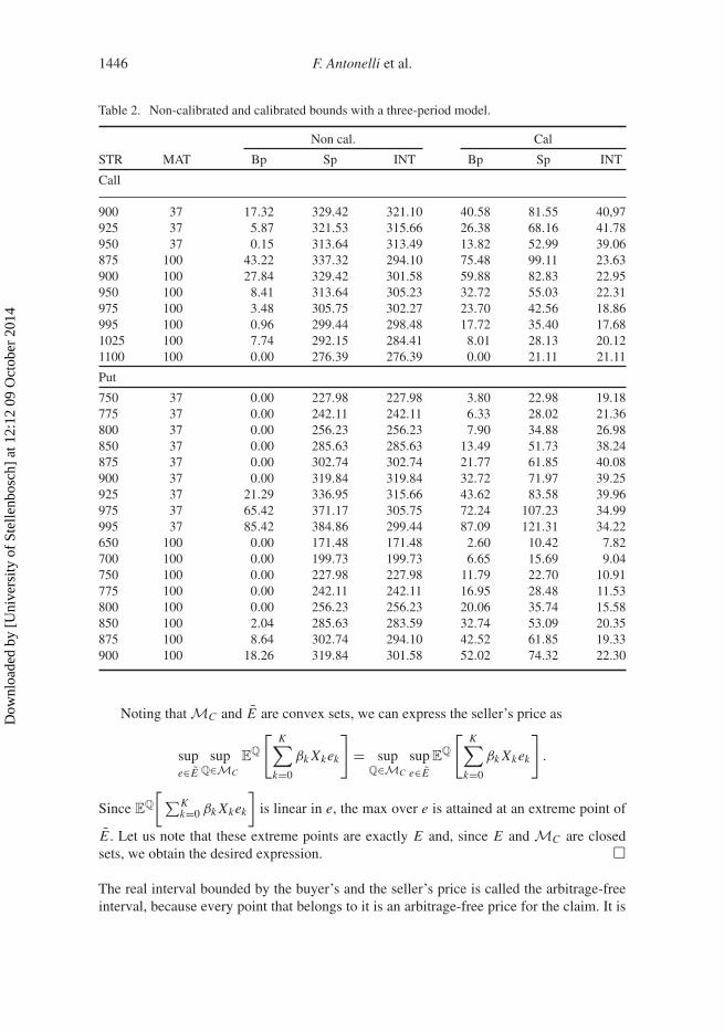
Table 2. Non-calibrated and calibrated bounds with a three-period model.
Non cal. Cal
STR MAT Bp Sp INT Bp Sp INT
Call
900 37 17.32 329.42 321.10 40.58 81.55 40,97925 37 5.87 321.53 315.66 26.38 68.16 41.78950 37 0.15 313.64 313.49 13.82 52.99 39.06875 100 43.22 337.32 294.10 75.48 99.11 23.63900 100 27.84 329.42 301.58 59.88 82.83 22.95950 100 8.41 313.64 305.23 32.72 55.03 22.31975 100 3.48 305.75 302.27 23.70 42.56 18.86995 100 0.96 299.44 298.48 17.72 35.40 17.681025 100 7.74 292.15 284.41 8.01 28.13 20.121100 100 0.00 276.39 276.39 0.00 21.11 21.11
Put
750 37 0.00 227.98 227.98 3.80 22.98 19.18775 37 0.00 242.11 242.11 6.33 28.02 21.36800 37 0.00 256.23 256.23 7.90 34.88 26.98850 37 0.00 285.63 285.63 13.49 51.73 38.24875 37 0.00 302.74 302.74 21.77 61.85 40.08900 37 0.00 319.84 319.84 32.72 71.97 39.25925 37 21.29 336.95 315.66 43.62 83.58 39.96975 37 65.42 371.17 305.75 72.24 107.23 34.99995 37 85.42 384.86 299.44 87.09 121.31 34.22650 100 0.00 171.48 171.48 2.60 10.42 7.82700 100 0.00 199.73 199.73 6.65 15.69 9.04750 100 0.00 227.98 227.98 11.79 22.70 10.91775 100 0.00 242.11 242.11 16.95 28.48 11.53800 100 0.00 256.23 256.23 20.06 35.74 15.58850 100 2.04 285.63 283.59 32.74 53.09 20.35875 100 8.64 302.74 294.10 42.52 61.85 19.33900 100 18.26 319.84 301.58 52.02 74.32 22.30
Noting that MC and E are convex sets, we can express the seller’s price as
supe∈E
supQ∈MC
EQ
[K∑
k=0
βk Xkek
]= sup
Q∈MC
supe∈E
EQ
[K∑
k=0
βk Xkek
].
Since EQ
[∑Kk=0 βk Xkek
]is linear in e, the max over e is attained at an extreme point of
E . Let us note that these extreme points are exactly E and, since E and MC are closedsets, we obtain the desired expression. �
The real interval bounded by the buyer’s and the seller’s price is called the arbitrage-freeinterval, because every point that belongs to it is an arbitrage-free price for the claim. It is
Dow
nloa
ded
by [
Uni
vers
ity o
f St
elle
nbos
ch]
at 1
2:12
09
Oct
ober
201
4

Optimization 1447
Table 3. Calibrated bounds with a 4-period model and branching structure (20, 10, 10, 10).
Call Put
STR MAT Bp Sp INT STR MAT Bp Sp INT
900 37 40.58 84.99 44.41 750 37 3.80 22.96 19.16925 37 26.38 70.57 44.19 775 37 6.33 26.30 19.97950 37 13.82 56.17 42.35 800 37 7.95 38.86 30.91875 100 75.48 105.50 30.02 850 37 13.25 55.44 42.19900 100 59.88 86.90 27.02 875 37 21.71 65.42 43.71950 100 31.97 58.19 26.22 900 37 32.72 75.41 42.69975 100 23.71 45.60 21.89 925 37 43.62 86.15 42.53995 100 17.50 38.13 20.63 975 37 72.27 110.28 38.011025 100 7.97 30.47 22.50 995 37 86.49 122.57 36.081100 100 0.00 22.58 22.58 650 100 2.60 10.30 7.70
700 100 6.65 16.45 9.80750 100 11.74 26.38 14.64775 100 16.95 32.42 15.47800 100 20.07 39.66 19.59850 100 32.74 56.95 24.21875 100 42.52 65.42 22.90900 100 52.02 80.34 28.32
not a priori clear whether the buyer’s and seller’s prices themselves are arbitrage-free or not.When problems (1) and (7) have the same optimal solution, the price of X is unique and theclaim is said to be replicable. Finally, let us note that the interval determined by the optimalsolutions of problems (1) and (7) is smaller than that defined by the non-calibratedAmericanprogramming problems in [10] and [12], since the set MC of calibrated martingale measuresis smaller than M. The keypoint is that the previous results hold and when we calibrate wefall into M, hence the set MC can be thought of as a set of martingale measures calibratedby the observed market prices.
4. Numerical tests with S&P500 options
In this section, we summarize the most meaningful numerical results obtained consideringthe 48 European option used by King et al. in their work. In particular, we consider the bidand ask closing prices of 21 European call and 27 European put options on the S&P500 indexon September 10, 2002, in turn one of the European options will be considered Americanand all the others used for calibrating. In Table 1, we summarize our data-set, the columnslabeled STR and MAT give the strike prices and maturities and those labeled with Ca and Cb
give the bid and ask prices. To price each ‘American’ we solve the seller’s and the buyer’sproblems 38 times, indeed we exclude the options with maturity 17 days because they areindistinguishable from the European case.
4.1. A three-period model
The risky asset is denoted by S1 and it is the S&P500 index, while we assume the risklessasset to be constant. The period structure in the model is chosen according to the maturitiesof the options. That is, we assume that trading occurs at 0,17,37, and 100 days, which
Dow
nloa
ded
by [
Uni
vers
ity o
f St
elle
nbos
ch]
at 1
2:12
09
Oct
ober
201
4

1448 F. Antonelli et al.
Table 4. Calibrated bounds with a 4-period model and branching structure (30, 10, 10, 10).
Call Put
STR MAT Bp Sp INT STR MAT Bp Sp INT
900 37 40.58 88.36 38.95 750 37 3.80 29.20 25.40925 37 26.58 73.96 41.78 775 37 6.33 35.09 28.76950 37 13.82 59.59 45.71 800 37 7.90 42.10 34.20875 100 75.48 109.85 34.37 850 37 13.26 58.74 45.48900 100 59.88 90.88 31.00 875 37 21.68 68.76 47.08950 100 31.91 61.60 29.69 900 37 32.72 78.78 46.06975 100 23.83 49.05 25.68 925 37 43.62 89.40 45.78995 100 17.74 41.26 23.52 975 37 72.51 113.73 41.221025 100 7.99 33.73 25.74 995 37 87.02 126.04 39.021100 100 0.00 26.08 26.08 650 100 2.60 11.33 8.73
700 100 6.65 19.58 12.93750 100 11.76 29.57 17.81775 100 16.95 35.64 18.69800 100 20.07 42.89 22.82850 100 32.74 60.45 27.71875 100 42.52 68.76 26.24900 100 52.02 84.64 32.62
are the expiration dates of the options in Table 1. The scenario tree is built by using theGauss-Hermite procedure. We choose the branching structure (50, 10, 10). All thecomputations have been performed in GAMS 23.7, using CPLEX for the numericalsolution and on a personal computer equipped with a Pentium Dual-Core 2.17 GHz and 3GB RAM.
We begin considering in Table 2 the Non-calibrated and calibrated option bounds forAmerican options. In the following table the columns Bp, Sp, INT give, respectively thebuyer’s price, the seller’s price and the length of the arbitrage free interval. We note thatthe non-calibrated arbitrage interval can be quite large.
Comparing the calibrated columns of Table 2 with the table for European options in thework by King et al. we note that the buyer’s problems have the same optimal value. Webelieve this happens because we are not considering in the money options, thus the buyerprefers to carry the options to maturity. If we observe the values of the variables en , wenotice that the number of nodes of early exercise is irrelevant compared to the total numberof nodes. It seems that the approximation works better with the negative moneyness, thatis to say the more out of the money the option is and the smaller the interval is. This is inline with the fact that the more out of the money the option is and more the behavior of theoption is similar to the European case.
In both calibrated and non-calibrated case the average time for the routines is about15 seconds for the buyer’s problem and about 10 seconds for the seller’s problem.
4.2. A four-period model
We also studied the calibrated problem in a four-step model (the steps are in the days 8th,17th, 37th and 100th). We considered the case of a scenario tree with a branching structure(20, 10, 10, 10) in Table 3 and (30, 10, 10, 10) in Table 4.
Dow
nloa
ded
by [
Uni
vers
ity o
f St
elle
nbos
ch]
at 1
2:12
09
Oct
ober
201
4
Optimization 1449
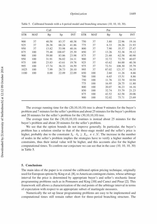
Table 5. Calibrated bounds with a 4-period model and branching structure (10, 10, 10, 30).
Call Put
STR MAT Bp Sp INT STR MAT Bp Sp INT
900 37 40.58 83.37 40.38 750 37 3.80 22.96 19.16925 37 26.38 68.24 41.86 775 37 6.33 28.26 21.93950 37 13.82 53.98 40.16 800 37 7.90 35.37 27.47875 100 75.48 100.87 25.39 850 37 13.26 52.38 39.12900 100 59.88 83.86 23.98 875 37 21.68 62.58 40.90950 100 31.91 56.02 24.11 900 37 32.72 72.79 40.07975 100 23.83 43.61 19.78 925 37 43.62 84.00 40.38995 100 17.74 36.33 18.59 975 37 72.51 108.30 35.791025 100 7.99 28.73 20.10 995 37 87.02 121.37 34.351100 100 0.00 22.09 22.09 650 100 2.60 11.26 8.66
700 100 6.65 15.51 8.86750 100 11.76 22.70 10.94775 100 16.95 28.75 11.80800 100 20.07 36.23 16.16850 100 32.74 53.79 21.23875 100 42.52 62.58 20.06900 100 52.02 75.71 23.69
The average running time for the (20,10,10,10) tree is about 9 minutes for the buyer’sproblem and 7 minutes for the seller’s problem and about 25 minutes for the buyer’s problemand 20 minutes for the seller’s problem for the (30,10,10,10) tree.
The average time for the (30,10,10,10) routines is instead about 25 minutes for thebuyer’s problem and about 20 minutes for the seller’s problem.
We see that the option bounds do not improve generally. In particular, the buyer’sproblem has a solution similar to that of the three-stage model and the seller’s price ishigher, probably due to the constraint Sn · θn ≥ Xn, n ∈ N . The increase in the numberof nodes in the seller’s problem implies the strategies have to verify a higher number ofconstraints, thus their initial value will be higher, and this accounts also for the highercomputational times. To confirm our conjecture we can see that in the case (10, 10, 10, 30)
in Table 5.
5. Conclusions
The main idea of the paper is to extend the calibrated option pricing technique, originallyused for European options by King et al. [8], toAmerican contingent claims, whose arbitrageinterval for the price is determined by appropriate buyer’s and seller’s stochastic linearprogramming problems such as in Pennanen and King [10] and Camci and Pinar [2]. Thisframework still allows a characterization of the end points of the arbitrage interval in termsof expectation with respect to an appropriate subset of martingale measures.
Numerically the set up linear programming problems are easy to be implemented andcomputational times still remain rather short for three-period branching structure. The
Dow
nloa
ded
by [
Uni
vers
ity o
f St
elle
nbos
ch]
at 1
2:12
09
Oct
ober
201
4
1450 F. Antonelli et al.
reduction of the arbitrage interval is remarkable and the endpoints in many cases mayprovide a satisfactory approximation of the actual price.
Unfortunately an increase of the number of time periods does not necessarily correspondto a further reduction in size of the arbitrage interval. This is probably due to the fact thatincreasing the time steps we are at the same time increasing the range of the underlying.Also, we pay this refinement of periods in terms of computational times.
It would be desirable to test the procedure against a data-set of prices of actually tradedAmerican options, but these data are hardly free to retrieve.
References
[1] Naik V. Finite state securities market models and arbitrage, in handbooks in operationsresearch and management science. Vol. 9, In: Finance, Jarrow RA, Maksimovic V, ZiembaWT. Amsterdam: Amsterdam Elsevier; 1995. p. 31–64.
[2] Ortu F. Arbitrage, linear programming and martingales in securities market with bid-ask spreads.Decisions Eco. Financ. 2001;24:79–105.
[3] Baccara M, Battauz A, Ortu F. Effective securities in arbitrage-free markets with bid-ask spreadsat liquidation: a linear programming characterization. J. Econom. Dynam. Control. 2006;30:55–79.
[4] Föllmer H, Schweizer M. Hedging of contingent claims under incomplete information in appliedstochastic analysis, stochastics monographs. Vol. 5, Davis MHA, Elliott RJ, editors. London:Gordon and Breach; 1989. p. 389–414.
[5] Frittelli M. The minimal entropy martingale measure, the valuation problem in incompletemarkets. Math. Finance. 2000;10:39–52.
[6] Cont R. Model uncertainty and its impact on the pricing of derivative instruments. Math. Finance.2006;16:519–547.
[7] King AJ. Duality and martingales: a stochastic programming perspective on contingent claims.Math. Program. Ser. B. 2002;91:543–562.
[8] King AJ, Koivu M, Pennanen T. Calibrated option bounds. Int. J. Theor. Appl. Finance.2005;8:141–159.
[9] Rockafellar TR. Convex analysis. Princeton (NJ): Princeton University Press; 1972.[10] Pennanen T, King A. Arbitrage pricing of American contingent claims in incomplete markets
– a convex optimization approach. Stochastic programming e-print series; 2006. Available athttp://edoc.hu-berlin.de/series/speps/2004-14/PDF/14.pdf
[11] Flåm SD. Option pricing by mathematical programming. Optimization. 2008;57:165–182.[12] Camci A, Pinar M. Pricing American contingent claims by stochastic linear programming.
Optimization. 2009;58:627–640.
Dow
nloa
ded
by [
Uni
vers
ity o
f St
elle
nbos
ch]
at 1
2:12
09
Oct
ober
201
4