calculus ii, second semester chapter 6. transcendental...
TRANSCRIPT

CALCULUS II, Second SemesterTable of Contents
Chapter 6. Transcendental Functions 1226.1. Inverse Functions 1226.2. The Inverse Trigonometric Functions 1276.3 First Order Differential Equations 130
Chapter 7. Techniques of Integration 1367.1. Substitution 1367.2. Integration by Parts 1397.3. Partial Fractions 1437.4. Trigonometric Methods 149
Chapter 8. Indeterminate Forms and Improper Integrals 1538.1. L’Hopital’s Rule 1538.2 Other Indeterminate Forms 1568.3 Improper Integrals: Infinite Intervals 1588.4 Improper Integrals: Finite Asymptotes 161
Chapter 9. Sequences and Series 1649.1. Sequences 1649.2. Series 1349.3. Tests for Convergence 1759.4. Power Series 1809.5. Taylor Series 184
Chapter 10 Numerical Methods 19110.1. Taylor Approximation 19110.2. Newton’s Method 19510.3. Numerical Integration 198
Chapter 11. Conics and Polar Coordinates 20311.1. Quadratic Relations 20311.2. Eccentricity and Foci 21011.3. String and Optical Properties of the Conics 21511.4. Polar Coordinates 21911.5. Calculus in Polar Corrdinates 225
Chapter 12. Second Order Linear Differential Equations 22812.1. Homogeneous Equations 22812.2. Behavior of the Solutions 23312.3. Applications 23512.4. The Inhomogeneous equation 238
i

CALCULUS I, Second Semester
VI. Transcendental Functions
6.1 Inverse Functions
The functions ex and lnx are inverses to each other in the sense that the two statements
y = ex , x = ln y
are equivalent. In general, two functions f, g are said to be inverse to each other when thestatements
(6.1) y = f(x) , x = g(y)
are equivalent for x in the domain of f , and y in the domain of g. Often we write g = f−1 andf = g−1 to express this relation. Another way of giving this citerion is
f(g(x)) = x g(f(x)) = x .
Example 6.1. Find the inverse function for f(x) = 3x− 7. We write y = 3x− 7 and solve for xas a function of y:
(6.2) x =y + 7
3.
The equations y = 3x − 7 and x = (y + 7)/3 are equivalent for all x and y, so (6.2) gives us theformula for the inverse of f : f−1(y) = (y + 7)/3. Since it is customary to use the variable x forthe independent variable, we should write:
f−1(x) =x + 7
3.
Example 6.2. Find the inverse function for
f(x) =x
x + 1.
We let y = x/(x + 1), and solve for x in terms of y:
(6.3) yx + y = x so that y = x(1− y) ,
so thatx =
y
1− y.
Thusf−1(x) =
x
1− x.
Notice that -1 is excluded from the domain of f , and 1 is excluded from the domain of f−1. Infact, we see that these substitutions in equations (6.3) lead to contradictions.
122

We have to be careful, in discussing inverses, to clearly indicate the domain and range, otherwisewe have ambiguities and make mistakes.
Example 6.3. x2 and√
x appear to be inverses since (√
x)2 = x. But since the symbol √ gives thepositive root,
√x2 = |x| which is not x when x is negative.This ambiguity is clarified by specifying
the domains of the functions. So, for x ≥ 0,√
x is the inverse of x2, but for x ≤ 0, −√
x is theinverse of x2. Finally,
√x is only defined for nonnegative numbers.
We illustrate this graphically in figure 6.1.
y = x2
-3 -2 -1 1 2 3
2
4
6
8
y =√
x
2 4 6 8
0.5
1
1.5
2
2.5
3
y = −√
x
2 4 6 8
-3
-2.5
-2
-1.5
-1
-0.5
Figure 6.1
In the first graph each horizontal line y = y0 intersects the graph in two points for y0 > 0, and inno points for y0 < 0. So the domain of an inverse function can contain no negative numbers, and
123

for positive numbers, there are 2 choices of inverse, one for the function x2, x nonnegative, andthe other for x2, x nonpositive.
In general, this provides a graphical criterion for a function to have an inverse:
Proposition 6.1. Let y = f(x) for a function f defined on the interval a ≤ x ≤ b. Let f(a) =α, f(b) = β. If, for each γ between α and β the line y = γ intersects the graph in one and onlyone point, then f has an inverse defined on the interval between α and β.
For if (c, γ) is the point of intersection of the graph with the line y = γ, define f−1(γ) = c.
For a continuous function, we know, from the Intermediate Value Theorem of Chapter 2, that eachsuch line y = γ intersects the graph in at least one point. Thus for continuous functions, we canrestate the proposition as
Proposition 6.2. Let y = f(x) for a continuous function f defined on the interval a ≤ x ≤ b. Letf(a) = α, f(b) = β. If the condition
(6.4) x1 6= x2 implies f(x1) 6= f(x2)
then f has an inverse defined on the interval between α and β.
For a differentiable function, it follows from Rolle’s theorem of chapter that condition (6.4) holdsif f ′(x) 6= 0 for all a ≤ x ≤ b.
Proposition 6.3. Let y = f(x) for a differentiable function f defined on the interval a ≤ x ≤ b.Let f(a) = α, f(b) = β. If f ′(x) 6= 0 in the interval, then f has an inverse defined on the intervalbetween α and β.
Example 6.4. Let f(x) = x2 − x. Find the domains for which f has an inverse, and find theinverse function.
First, differentiate: f ′(x) = 2x − 1. Thus f ′(x) < 0 for x < 1/2, and f ′(x) > 0 for x > 1/2, sowe should be able to find inverses for f on each of the domains (−∞, 1/2), (1/2,∞).To find theformula for the inverse, let y = x2 − x and solve for x in terms of y. To do this, we write theequation as x2 − x− y = 0, and use the quadratic formula:
x =−1±
√1 + 4y
2.
How convenient: we’re looking for two possible inverses, and here we have two choices. Notice firstthat because of the square root sign, the domain of y must be y ≥ −1/4. We conclude that, in thedomains x ≥ 1/2, y ≥ −1/4 the following statements are equivalent:
y = x2 − x , x =−1 +
√1 + 4y
2
and thus the inverse to f(x) = x2 − x on this domain is
(6.5) f−1(x) = (−1 +√
1 + 4x)/2 .
124
Similarly, in the domains x ≤ 1/2, y ≥ −1/4 the following statements are equivalent:
y = x2 − x , x =−1−
√1 + 4y
2
and thus the inverse to f(x) = x2 − x on this domain is f−1(x) = (−1−√
1− 4x)/2.
Example 6.5. Let
f(x) =ex − e−x
2.
This function is called the hyperbolic sine. The hyperbolic sine has an inverse function defined forall real numbers. First of all f ′(x) = (ex + e−x)/2 > 0 for all x, so f has an inverse function.Secondly,
limx→−∞
f(x) = −∞ and limx→∞
f(x) = ∞
so the range of f , and thus the domain of its inverse, is all real numbers. We now find a formulafor the inverse function. Let y = f−1(x), so that
x = f(y) =ey − e−y
2.
Multiply both sides of the equation by 2ex, giving
2xey = e2y − 1 or e2y − 2xey − 1 = 0 .
Using the quadratic formula we find
ey =2x±
√4x2 + 42
= x±√
x2 + 1 .
Since this is positive for all x, we must have ey = x +√
x2 + 1, and finally
y = ln(x +√
x2 + 1)
is the inverse hyperbolic sine.
Proposition 6.4. Suppose that f and g are inverse to each other in their respective domains. Lety = g(x). Then
(6.6) g′(x) = 1/f ′(y) .
To see this, differentiate the relations x = f(y), y = g(x) implicitly with respect to x:
1 = f ′(y)dy
dx,
dy
dx= g′(x) ,
sog′(x) =
dy
dx=
1f ′(y)
.
125

Example 6.6. Let us illustrate this proposition with the exponential and logarithmic functions.Recall that y = lnx is defined as being equivalent to x = ey. Differentiate that equation withrespect to x implicitly .
1 = ey dy
dxso that
dy
dx=
1ey
.
Since ey = x, we obtain the formula for the derivative of the logarithm:
d
dxlnx =
1x
.
Example 6.7. Let y = f−1(x) be the function defined on the domain x ≥ 2 which is inverse tof(x) = x2 − x (recall example 6.4). We find the derivative of f−1(x) .First, write:
y = f−1(x) is equivalent to x = y2 − y .
Differentiate implicitly:
1 = 2ydy
dx− dy
dxso that
dy
dx=
12y − 1
.
or
(6.7)d
dxf−1(x) =
12f−1(x)− 1
.
Since we have an explicit formula for f−1(x) (see equation (6.5)), we may substitute that in (6.7)to obtain
d
dxf−1(x) =
1√1 + 4x
.
Of course, in the above example the inverse functions are explicit, and so we can make a substitutionfor f−1(x) on the left side of (6.7), but that may not always be the case.
Example 6.8. Suppose that g is the inverse to the function f(x) = x2 − 4x− 44 for x > 2. Findg′(1).
Note, since the parabola has its vertex where x = 2, the function f does have an inverse in x > 2.Let y = g(x). Since g is inverse to f , x = f(y) = y2 − 4y − 44 and f ′(y) = 2y − 4, so
g′(x) =1
2y − 4.
To calculate g′(1) we find the value of y corresponding to x = 1 : 1 = y2−4y−44 has the solutions−9, 5. Since f is restricted to values greater than 2, we must have g(1) = 5. Now f ′(y) = 2y − 4,so
g′(1) =1
f ′(5)=
12(5)− 4
=16
.
Problems 6.1
1. Find the function inverse tof(x) =
2x + 1x− 3
.
126
2. Find the inverse function, and its domain, for
f(x) =ex + e−x
2.
If possible, find a formula for f−1.
3. Find g′((e + e−1)/2) where g is the inverse to the function of problem 2.
4. Show that f(x) = x3 + 3x + 1 has an inverse. Find
d
dxf−1(x)
∣∣x=1
.
5. Let f(x) = x lnx for x > 1. Show that f has an inverse g. Noting that f(e2) = 2e2, find g′(2e2).
6.2 Inverse Trigonometric Functions
In this section we use the ideas of the preceding section to define inverses for the trigonometricfunctions, and calculate their derivatives. Since the trigonometric functions are periodic, we willhave to restrict the domain of definition in order to obtain a well-defined inverse.
We start with the tangent function. Recall that tanx is strictly increasing on the interval (π/2, π/2)and takes every value between −∞ and ∞, and then repeats itself in intervals of length π. Thus,if we restrict the domain of the tangent to the interval (π/2, π/2), it has an inverse there, definedfor all real numbers.
Definition 6.1. The function y = arctanx is defined on the interval (−∞,∞), taking values in−π/2, π/2] .by the condition x = tan y.
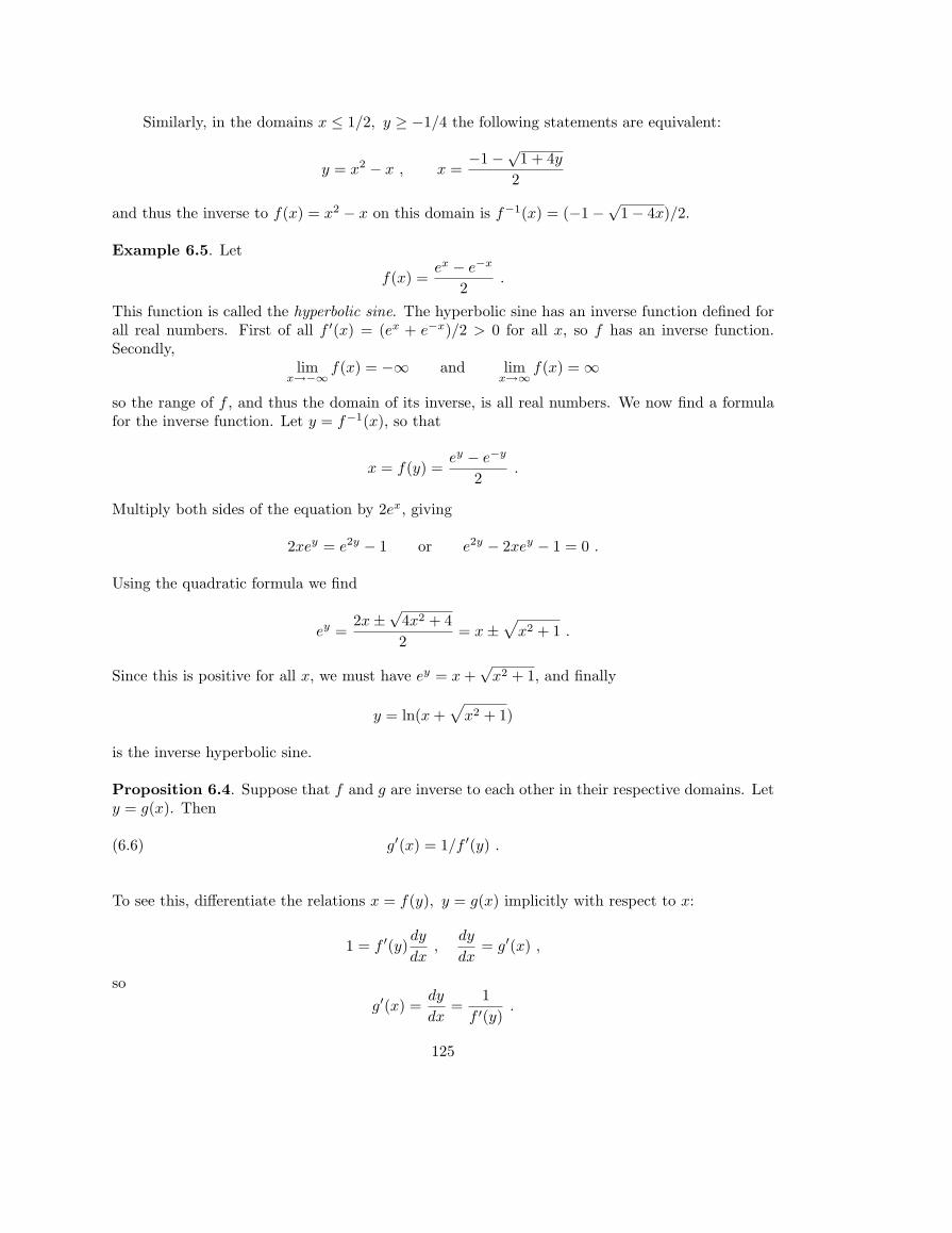
The inverse tangent (or arctangent) is sometimes denoted by y = tan−1(x). See figure 6.2 for thegraph of the inverse tangent.
�
� 1 � 5� 1
� 0 � 50
0 � 51
1 � 5
� 6 � 4 � 2 0 2 4 6
Figure 6.2
127
Proposition 6.5.d
dxarctanx =
1(1 + x2)
,
∫1
(1 + x2)dx = arctan x + C
To see this, we start with the equation x = tan y that defines y as the arctangent of x. We get:
1 = sec2 ydy
dx.
Now, since sec2 y = tan2 y + 1, we can replace sec2 y by x2 + 1, obtaining
1 = (x2 + 1)dy
dxor
dy
dx=
1x2 + 1
,
which is just the first equation. The second is a restatement in terms of integrals.
Similarly, we define y = arcsinx by the condition x = sin y. However, since the sine function isperiodic, the equation sin y = x has many solutions for x between −1 and 1. But, if we insistthat y be between −π/2 and π/2, there is only one solution. So, to pick a definite inverse forthe sine function, we specify that its domain is the interval [−1, 1], and its range (set of values) is[−π/2, π/2]. Then, with this specification, it is true that the equation sin y = x has one and onlyone solution. That solution we call the inverse sine function, denoted arcsinx or sin−1 x.
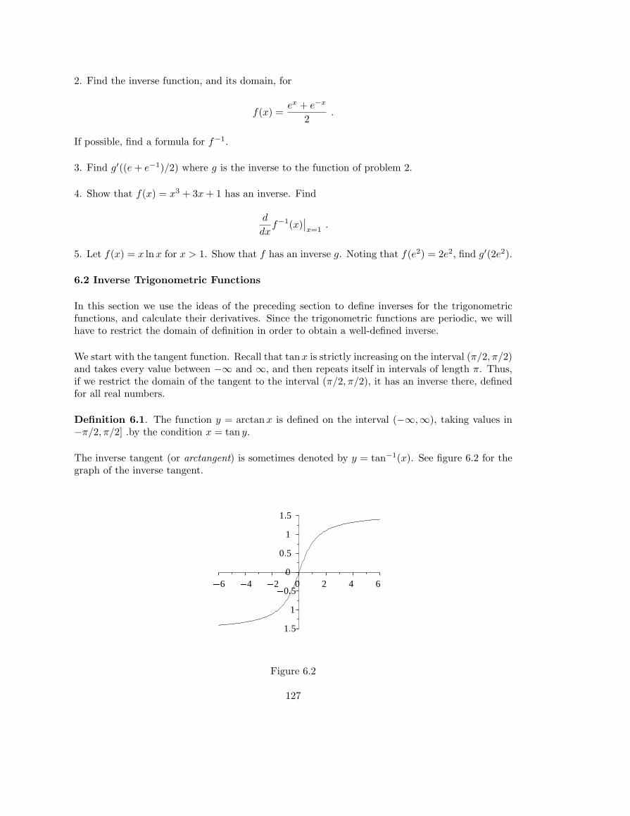
Definition 6.2. The function y = arcsinx is defined on the interval (−1, 1), taking values in−π/2, π/2] .by the condition x = sin y. See figure 6.3 for a graph of y = arcsinx.
� 2 � 1 � 5 � 1 � 0 � 5 0 0 � 5 1 1 � 5 2
� 1 � 5� 1
� 0 � 50
0 � 51
1 � 5
� 1 � 0 � 5 0 0 � 5 10
0 � 51
1 � 52
2 � 53
3 � 5
Figure 6.3 Figure 6.4
Proposition 6.6.d
dxarcsinx =
1√1− x2
,
∫1√
1− x2dx = arcsinx + C
Differentiate x = sin y implicitly:
1 = cos ydy
dx.
128

Now, since sin2 y + cos2 y = 1, writing this as x2 + cos2 y = 1, and thus replace cos y by√
1− x2:
1 =√
1− x2dy
dxor
dy
dx=
1√1− x2
.
We took the positive root for, in the chosen domain for arcsinx, it is increasing.
Turning to the cosine, since cos(−x) = cos(x), it is not possible to define an inverse if we takethe domain of cos to be any interval about 0. However, we note that since the cosine function isstrictly decreasing between 0 and π, we can define an inverse on the interval [−1, 1] taking valuesbetween 0 and π: this is the inverse cosine, denoted arccos x. (See figure 6.4 for the graph).
Definition 6.3. The function y = arccos x is defined on the interval (−1, 1), taking values in(0, π], .by the condition x = cos y.
Proposition 6.7.d
dxarccos x = − 1√
1− x2,
∫1√
1− x2dx = − arccos x + C
The verification is the same as that of proposition 6.6, except that this time, since the arccosine isdecreasing, we take the negative square root. Note that, for any acute angle α, its complementaryangle is π/2− α, thus sinα = cos(π/2− α). Letting x = sin α, so that α = arcsinx , this tells usthat arccos x = π/2−α = π/2−arcsinx, explaining the coincidence in the formulas of propositions6.6 and 6.7.
Example 6.9. Find ∫xdx
x4 + 1.
Make the substitution u = x2, du = 2xdx. This gives us
12
∫du
u2 + 1=
12
arctanu + C =12
arctan(x2) + C .
Example 6.10. Find, for any constant a: ∫dx
x2 + a2.
Make the substitution x = au, dx = adu. The integral becomes∫adu
a2u2 + a2=
1a
∫du
u2 + 1=
1a
arctanu + C =1a
arctan(u
a) + C .
Problems 6.2
1. tan(arccos x) =
2.1x2− tan2(arccos x) =
129

3. Show that arcsinx + arccos x is constant.
4. Differentiate : g(x) = arcsin(lnx) .
5. Differentiate : y = arccos√
x
6. Find the equation of the line tangent to the curve y = arctan x at the point (√
3, π/3).
7. Find all points at which the tangent line to the curve y = arcsinx has slope 4.
8. What is the maximum value of the derivative of f(x) = arccos x?
9.
∫xdx√1− x4
=
10. Show that f(x) = sec x has an inverse in the interval (0, π/2). The inverse is denoted y =sec−1 x (called the arcsecant). Find the formula for the derivative of the arcsecant.
11.
∫dx√
a2 − x2=
12. The curve y =1√
1 + x21 ≤ x ≤
√3
is rotated around the x-axis. Find the volume of the enclosed solid.
6.3 First Order Linear Differential Equations
Definition 6.4. A first order linear differential equation is a differential equation of the type
(6.8)dy
dx+ P (x)y = Q(x) .
It is said to be homogeneous if the function Q(x) is 0.
The equation is of “first order” since it involves only the first derivative, and linear since theequation expresses the first derivative of the unknown function y as a linear function of y.
If P and Q are constant functions we can easily solve the differential equation by separation ofvariables.
Example 6.11. To solve, saydy
dx= 2y − 3
we rewrite the equation in the form (2y−3)−1dy = dx. These differentials integrate to the relation
12
ln(2y − 3) = x + C or√
2y − 3 = Kex .
130

Squaring both sides and soving for y, we ge the general solution
(6.9) y =Ke2x + 3
2.
For example, to find the solution with initial value y(0) = 5, we first solve for K:
5 =Ke2(0) + 3
2,
so K = 7, and the particular solution is y = (7e2x + 3)/2.
The acute reader will object that the integral of (2y − 3)−1dy is (1/2) ln |2y − 3|, and if we followthrough with this, this seems to lead to the alternative solution
(6.10) y =3−Ke2x
2.
However, this is the same as (6.9), just with a different choice for the constant K. If we use (6.10)with the same initial conditions y(0) = 5, we find this K = −7, giving the same final answer. Forthis reason it is often the case that the absolute value is ignored.
Now, we note that the homogeneous equation (the case Q(x) = 0) is separable:
Example 6.12. Solve y′ − 2xy = 0, y(2) = 1.
We separate the variables: y−1dy = 2xdx and integrate:
ln y = x2 + C .
Substituting the initial condition allows us to solve for C : ln 1 = 4 + C, so C = −4. Thus theparticular solution is given by
ln y = x2 − 4
which exponentiates toy = ex2−4 .
Now, to solve the general equation, we make a crucial observation:
Proposition 6.8. Given the differential equation, y′ + P (x)y = Q(x), suppose that v solves thehomogeneous equation: v′ + Pv = 0. Then, making the substitution y = uv leads to a simpleintegration for the unknown function u.
Let’s make the substitution in the given equation. Since y′ = uv′ + u′v, we have
uv′ + u′v + Puv = Q , or u′v + u(v′ + Pv) = Q , or u′v = Q ,
since v′ + Pv = 0. But then u′ = Qv−1, and we find u by integration.
This leads to a method for solving the general first order differential equation
y′ + Py = Q .
131

1. Find a solution v of the corresponding homogeneous equation.2. Make the substitution y = uv, leading to an integration to find the new unknown function
u.
Example 6.13. Solvedy
dx=
y + 1x
, y(1) = 2 .
The homogeneous equation is y′ − x−1y = 0. which has the solution y = Kx. Try y = ux inthe given equation. This leas us to the equation u′x = x−1, or u′ = x−2, which has the solutionu = −x−1 + C. Thus the general solution is
y = ux = (−1x
+ C)x = −1 + Cx .
Now solve for C using the initial conditions y(1) = 2: 2 = −1 + C, so C = 3 and the solution isy = 3x− 1.
Now the solution of the homogeneous equation y′ + Py = 0 is e−∫
Pdx. With the substitutiony = ue−
∫Pdx, the terms involving an undifferentiated u disappear precisely because e−
∫Pdx solves
the homogeneous equation. For this reason e−∫
Pdx is called an integrating factor. This method iscalled that of variation of parameters; the idea being to first find the general solution of an easierequation, and then trying that in the original equation, but with the constant replaced by a newunknown function. This method is very productive in solving very general types of differentialequations.
Example 6.14. Solve y′ − 2xy = x, y(0) = 2 . First, as in example 6.12, solve the homogeneousequation y′ − xy = 0, leading to
y = Kex2.
Now substitute y = uex2into the original equation to obtain
u′ex2= x or u′ = xe−x2
.
This integrates to
u = −12e−x2
+ C ,
so that our general solution is y = uex2with this u:
y =(− 1
2e−x2
+ C)ex2
= −12
+ Cex2.
Notice that the constant function −1/2 (found by taking C = 0) is a solution of the differentialequation. However, this doesn’t satisfy our initial conditions: y(0) = 2. Those give us C = 2, sothe solution we seek is
y = −12
+ 2ex2.
Example 6.15. Find the general solution to xy′ − y = x2.
132

We first must put this in the form (6.8):
dy
dx+
y
x= x .
The solution to the homogeneous equation is y = Kx. So, we try y = ux, and obtain the equation
u′x = x ,
which has the general solution u = x + C. Thus the general solution to the original problem is
y = ux = (x + C)x = x2 + Cx .
Remember the steps to solve the equation y′ + P (x)y = Q(x):
1. Solve the homogeneous equation y′ + P (x)y = 0, obtaining y = e−∫
Pdx.
2. Try the solution y = ue−∫
Pdx, leading to the equation for u : u′e−∫
Pdx = Q(x), or u′ =
Q(x)e∫
Pdx.
Solve for u, and put that solution in the equation y = ue−∫
Pdx. If an initial value is specified,now solve for the unknown constant.
This can, of course, be summarized in a formula:
Proposition 6.9 The general solution of the first order linear differential equation
y′ + Py = Q
isy = e−
∫Pdx( ∫
Qe∫
Pdxdx + C) .
We strongly advise students to remember the method rather than this formula.
A useful fact to know about linear first order equations is that if we know one particular solution,then we only have to solve the homogeneous equation to find all solutions.
Proposition 6.10. Suppose that yp is a solution of the differential equation y′ + Py = Q. Thenevery solution is of the form
y = yp + Ke−∫
Pdx ;
that is, every solution is of the form yp + yh, where yh is a solution of the homogeneous equation.
For suppose that y is any solution of the equation: y′ + Py = Q. Then (y − yp)′ + P (y − yp) =(y + Py)− (yp + Pyp) = Q−Q = 0 so solves the homogeneous equation.
Example 6.16. Find the solution of the equation y′ − 2y + 5 = 0 such that y(0) = 1.
133

Now the constant function yp = 5/2 solves the equation, since y′p = 0. The general solution ofthe homogeneous equation is y = Ke2x, so the general solution of the original equation is of theform y = (5/2) + Ke2x. Substituting y = 1, x = 0, we find 1 = 5/2 + K, so K = −3/2, and theparticular solution we want is
y =12(5− 3e2x) .
Example 6.17. A body falling through a fluid is subject to the force due to gravity as well asa resistance, due to the viscosity of the fluid, proportional to its velocity. (Here we are assumingthat the density of the body is much higher than the density of the fluid, and that its shape isnot relevant). Let x(t) represent the distance fallen at time t and v(t) its velocity. The hypothesisleads to the equation
dv
dt= −kv + g
for some constant k (g is the acceleration of gravity), called the coefficient of resistance of thefluid. Notice that the constant v = g/k is a solution of the equation. This is called the “free fallvelocity”, and for any falling body it will accelerate until it reaches this maximum velocity. Byproposition 6.10, the general solution is
v(t) =g
k+ Ke−kt ,
for some constant k.
Example 6.18. Suppose a heavy spherical object is throuwn from an airplane at 10000 meters,and that the coefficient of resistance of air is k = 0.05. Find the velocity as a function of time.What is the free fall velocity? Approximately how long does it take to reach the ground?
Here g = 9.8 m/sec2, so the free fall velocity is vp = 9.8/(.05) = 196 meters/sec. The generalsolution to the problem is
v(t) = 196 + Ke−(.02)t .
At t = 0, v = 0, so 0 = 196 + K, and our solution is
v(t) = 196(1− e−(.02)t) .
To answer the last question, we have to find distance fallen as a function of time, by integratingthe above:
x(t) = 196(t + 50e−(.02)t) + C .
At t = 0, x = 0; this gives C = −196(50), and the solution for our particular object:
x(t) = 196(t + 50(e−(.02)t − 1)) .
Now we want to solve for t when x = 10, 000. For large t, the exponential term is negligible, so T ,the time to reach ground, is approximately given by the solution of
10, 000 = 196(T − 50)
so T = 101 seconds.
Problems 6.3
134

1. Solve the initial value problem xy′ + y = x, y(2) = 5.
2. Solve the initial value problem: y′ = x(5− y), y(0) = 1.
3. Solve the initial value problem (x + 1)y′ = 2y, y(1) = 1.
4. Solve the initial value problem xy′ − y = x3, y(1) = 2.
5. Solve the initial value problem y′ − 2xy = ex2, y(0) = 4.
6. Solve the initial value problem:
4y′ + 3y = ex , y(0) = 7 .
7. Solve the initial value problem:
xy′ − 3y = x2 , y(1) = 4 .
8. Solve the initial value problem y′ − 2xy = ex2, y(0) = 4.
9. Solve the initial value problem: y′ + y = ex, y(0) = 5.
10. Solve the initial value problem : y′ +y
x= x, y(1) = 2 .
135

VII. Terchniques of Integration
Integration, unlike differentiation, is more of an art-form than a collection of algorithms. Manyproblems in applied mathematics involve the integration of functions given by complicated formu-lae, and practitioners consult a Table of Integrals in order to complete the integration. There arecertain methods of integration which are essential to be able to use the Tables effectively. Theseare: substitution, integration by parts and partial fractions. In this chapter we will survey thesemethods as well as some of the ideas which lead to the tables. After the study of this material,students should be able to easily use any set of Integral Tables.
7.1 Substitution
This was introduced in section 4.1 (recall Proposition 4.5). To integrate a differential f(x)dx whichis not known to us, we seek a function u = u(x) so that the given differential can be rewritten asa differential g(u)du whose integral is known to us. Then, if
∫g(u)du = G(u) + C, we know that∫
f(x)dx = G(u(x)) + C. Finding and employing the function u often requires some experienceand ingenuity as the following examples show.
Example 7.1.∫
x√
2x + 1dx = ?
Let u = 2x + 1, so that du = 2dx and x = (u− 1)/2. Then∫x√
2x + 1dx =∫
u− 12
u1/2 du
2=
14
∫(u3/2 − u1/2)du ==
14(25u5/2 − 2
3u3/2) + C
=130
u3/2(3u− 5) + C =130
(2x + 1)3/2(6x− 2) + C =115
(2x + 1)3/2(3x− 1) + C ,
where at the end we have replaced u by 2x + 1.
Example 7.2.∫
tanxdx =?
Since this isn’t on our tables, we revert to the definition of the tangent: tanx = sinx/ cos x. Then,letting u = cos x, du = − sinxdx we obtain∫
tanxdx =∫
sinx
cos xdx = −
∫du
u= − lnu + C = − ln cos x + C = ln sec x + C .
Example 7.3.∫
sec xdx =?
This is tricky, and there are several ways to find the integral. However, if we are guided by theprinciple of rewriting in terms of sines and cosines, we are led to the following:
sec x =1
cos x=
cos x
cos2 x=
cos x
1− sin2 x.
Now we can try the substitution u = sinx, du = cos xdx. Then∫sec xdx =
∫du
1− u2.
136
This looks like a dead end, but a little algebra pulls us through. The identity
11− u2
=12( 11 + u
+1
1− u
)leads to ∫
du
1− u2dx =
12
∫ ( 11 + u
+1
1− u
)du =
12(ln(1 + u)− ln(1− u) + C .
Using u = sinx, we finally end up with∫sec xdx =
12(ln(1 + sin x)− ln(1− sinx) + C =
12
ln(1 + sin x
1− sinx) + C .
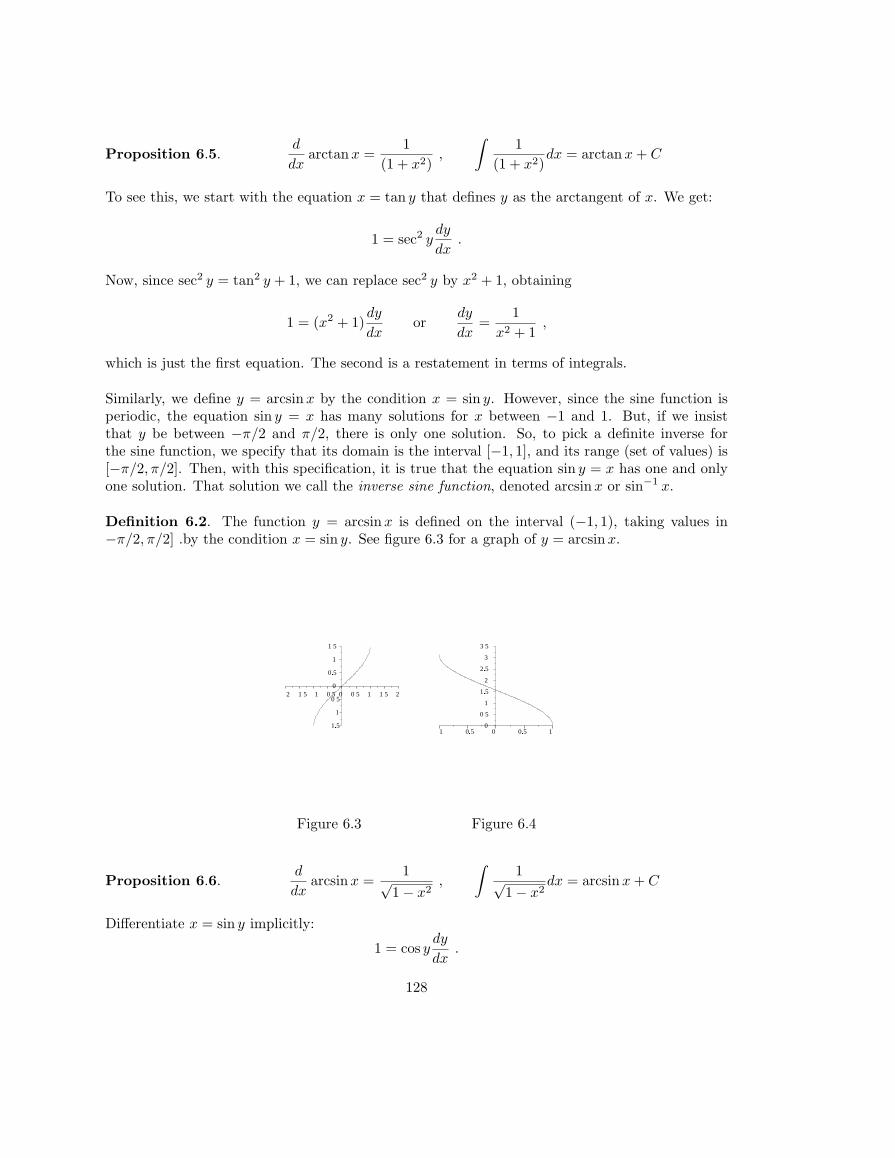
Example 7.4. As a circle rolls along a horizontal line, a point on the circle traverses a curve calledthe cycloid. A loop of the cycloid is the trajectory of a point as the circle goes through one fullrotation. Let us find the length of one loop of the cycloid traversed by a circle of radius 1.
Let the variable t represent the angle of rotation of the circle, in radians, and start (at t = 0) withthe point of intersection P of the circle and the line on which it is rolling. After the circle hasrotated through t radians, the position of the point is as given as in figure 7.1.
Figure 7.1
11
t
t
1 � cos t
t � sin tP
The point of contact of the circle with the line is now t units to the right of the original point ofcontact (assuming no slippage), so
x(t) = t− sin t , y(t) = 1− cos t .
To find arc length, we use ds2 = dx2 + dy2, where dx = (1− cos t)dt, dy = sin tdt. Thus
ds2 = ((1− cos t)2 + sin2 t)2dt2 = (2− 2 cos t)2dt2
so ds =√
2(1− cos t)dt, and the arc length is given by the integral
L =√
2∫ 2π
0
√1− cos tdt .
137
To evaluate this integral by substitution, we need a factor of sin t. We can get this by multiplyingand dividing by
√1 + cos t:
√1− cos t =
√1− cos2 t√1 + cos t
=| sin t|√1 + cos t
.
By symmetry around the line t = π, the integral will be twice the integral from 0 to π. Inthat interval, sin t is positive, so we can drop the absolute value signs. Now, the substitutionu = cos t, du = − sin tdt will work. When t = 0, u = 1, and when t = π, u = −1. Thus
L = −2√
2∫ −1
1
u−1/2du = 2√
2∫ 1
−1
u−1/2du = 2√
2(2u1/2)∣∣1−1
= 8√
2 .
Problems 7.1. Evaluate the Integrals.
1.
∫ 2
0
x
1 + x4dx
2.
∫dx
(1 + x)√
x
3.
∫2 + x
1 + xdx
4.
∫xdx
1 + 4x2=
5.
∫ 2
0
ex
1 + e2xdx
6.
∫arccos x√
1− x2dx
7.
∫(lnx + 1)2
xdx
8.
∫cos3 x sin2 xdx
9.
∫ 2
0
(x2 + 3x− 1)2(2x + 3)dx
138
10.
∫ 2
0
dx
x2 + 4x + 5
11.
∫ 2
0
xdx
1 + 4x2=
12.
∫ 2
0
dx
1 + 4x2=
13.
∫exdx
e2x + 1=
14.
∫dx
ex + e−x=
15.
∫dx√
5− 4x− x2=
16.
∫tan2 xdx =
17.
∫tan3 xdx =
18.
∫dx
x2 − 6x + 13=
7.2 Integration by Parts
Sometimes we can recognize the differential to be integrated as a product of a function that iseasily differentiated and a differential that is easily integrated. For example, if the problem is tofind
(7.1)∫
x cos xdx
then we can easily differentiate f(x) = x, and integrate cos xdx separately. When this happens,the integral version of the product rule, called integration by parts, may be useful, because itinterchanges the roles of the two factors.
Recall the product rule: d(uv) = udv + vdu, and rewrite it as
(7.2) udv = d(uv)− vdu
139

In the case of (7.1), taking u = x, dv = cos xdx, we have du = dx, v = sinx. Put this all in (7.2):
x cos xdx = d(x sinx)− sinxdx ,
and we can easily integrate the right hand side to obtain∫x cos xdx = x sinx−
∫sinxdx = x sinx + cos x + C .
7.1 Proposition (Integration by Parts). For any two differentiable functions u and v:
(7.3)∫
udv = uv −∫
vdu .
To integrate by parts:
1. First identify the parts by reading the differential to be integrated as the product of afunction u easily differentiated, and a differential dv easily integrated.
2. Write down the expressions for u, dv and du, v.
3. Substitute these epxressions in (7.3).
4. Integrate the new differential vdu.
Example 7.5. Find∫
xexdx.
Let u = x, dv = exdx. Then du = dx, v = ex. (7.3) gives us∫xexdx = xex −
∫exdx = xex − ex + C .
Example 7.6. Find∫
x2exdx.
The substitution u = x2, dv = exdx, du = 2xdx, v = ex doesn’t immediately solve the problem,but reduces us to example 7.5:∫
x2exdx = x2ex − 2∫
xexdx = x2ex − 2(xex − ex + C) = x2ex − 2xex + 2ex + C .
Example 7.7. To find∫
lnxdx, we let u = ln x, dv = dx, so that du = (1/x)dx, v = x, and∫lnxdx = x lnx−
∫x
1x
dx = x lnx−∫
dx = x lnx− x + C .
This same idea works for arctanx: Let
u = arctan x, dv = dx du =dx
1 + x2, v = x ,
140

and thus ∫arctanxdx = x arctanx−
∫x
1 + x2dx = x arctanx− 1
2ln(1 + x2) + C ,
where the last integration is accomplished by the new substitution u = 1 + x2, du = 2xdx.
Example 7.8. These ideas lead to some clever strategies. Suppose we have to integrate ex cos xdx.We see that an integration by parts leads us to integrate ex sinxdx, which is just as hard. Butsuppose we integrate by parts again? See what happens:
Letting u = ex, dv = cos xdx, du = exdx, v = sinx, we get
(7.4)∫
ex cos xdx = ex sinx−∫
ex sinxdx .
Now integrate by parts again: letting u = ex, dv = sinxdx, du = exdx, v = − cos x, we get∫ex sinxdx = ex cos x +
∫ex cos xdx .
Inserting this in (7.4) leads to∫ex cos xdx = ex sinx− ex cos x−
∫ex cos xdx .
Bringing the last term over to the left hand side and dividing by 2 gives us the answer:∫ex cos xdx =
12(ex sinx− ex cos x) + C .
Example 7.9. If a calculation of a definite integral involves integration by parts, it is a good ideato evaluate as soon as integrated terms appear. We illustrate with the calculation of∫ 4
1
lnxdx
Let u = ln xdx, dv = dx so that du = dx/x, v = x, and∫ 4
1
lnxdx = x lnx∣∣41−
∫ 4
1
dx = 4 ln 4− x∣∣41
= 4 ln 4− 3 .
Example 7.10.
∫ 1/2
0
arcsinxdx = ?
We make the substitution u = arcsinx, dv = dx, du = dx/√
1− x2, v = x. Then∫ 1/2
0
arcsinxdx = x arcsin x∣∣1/2
0−
∫ 1/2
0
xdx√1− x2
.
141
Now, to complete the last integral, let u = 1− x2, du = −2xdx, leading us to∫ 1/2
0
arcsin xdx =12(π
6) +
12
∫ 3/4
1
u−1/2du =π
12+ u1/2
∣∣3/4
1=
π
12+√
32− 1 .
Problems 7.2. Evaluate the Integrals.
1.
∫x(sinx)dx
2.
∫exxdx
3.
∫x ln(2x)dx
4.
∫ln(2x)
xdx
5.
∫tan2 xdx
6.
∫x(e2x + 1)dx
7.
∫x2 sinxdx
8.
∫(lnx)2dx .
9.
∫x2 lnxdx .
10.
∫arccos xdx .
11. If the region in the first quadrant bounded by the curves y = 1, y = ex and x = 1 is rotatedabout the y-axis, what is the volume of the resulting solid?
12.
∫sec3 xdx .
142

7.3. Partial Fractions
The point of the partial fractions expansion is that integration of a rational function can be reducedto the following formulae, once we have determined the roots of the polynomial in the denominator.
7.3. Proposition. a)∫
dx
x− a= ln |x− a|+ C ,
b)∫
du
u2 + b2=
1b
arctan(u
b) + C ,
c)∫
udu
u2 + b2=
12
ln(u2 + b2) + C .
These are easily verified by differentiating the right hand sides (or by using previous techniques).
Example 7.11. Let us illustrate with an example we’ve already seen(for example, in example7.3). To find the integral ∫
dx
(x− a)(x− b)
we check that
(7.5)1
(x− a)(x− b)=
1a− b
( 1x− a
− 1x− b
),
so that ∫dx
(x− a)(x− b)=
1a− b
(ln |x− a| − ln |x− b|) + C =
1a− b
ln |x− a
x− b|+ C .
The algebraic manipulation in (7.5) can be applied to any rational function. Any polynomial canbe written as a product of factors of the form x− r or (x− a)2 + b2, where r is a real root and thequadratic terms correspond to the conjugate pairs of complex roots. The partial fraction expansionallows us to write the quotient of polynomials as a sum of terms whose denominators are of theseforms, and thus the integration is reduced to Proposition 7.3.
Here is the partial fractions procedure.
1. Given a rational function R(x), if the degree of the numerator is not less than the degreeof the denominator, by long division, we can write
R(x) = Q(x) +p(x)q(x)
where now deg p < deg q.
2. Find the roots of q(x) = 0. If the roots are all distinct (that is, there are no multiple roots),express p/q as a sum of terms of the form
(7.6)p(x)q(x)
=A
x− r,
B
(x− a)2 + b2,
Cx
(x− a)2 + b2.
143

3. Find the values of A, B, C, . . .. This is done putting the expression on the right hand sideover a common denominator, and then equating coefficients of the numerators in the equation.
4. Integrate term by term using Proposition 7.3.
If the roots are not distinct, the expansion is more complicated; we shall resume this discussionlater. For the present let us concentrate on the case of distinct roots, and how to find the coefficientsA,B,C, . . . in (7.6).
Example 7.12. Integrate ∫xdx
(x− 1)(x− 2).
First we write
(7.7)x
(x− 1)(x− 2)=
A
x− 1+
B
x− 2.
Now multiply this equation by (x− 1)(x− 2), getting
x = A(x− 2) + B(x− 1) .
If we substitute x = 1, we get 1 = A(1− 2), so A = −1; now letting x = 2, we get 2 = B(2− 1, soB = 2, and (7.7) becomes
x
(x− 1)(x− 2)=
−1x− 1
+2
x− 2.
Integrating, we get∫xdx
(x− 1)(x− 2)= − ln |x− 1|+ 2 ln |x− 2|+ C = ln
(x− 2)2
|x− 1|+ C .
So, this is the procedure for finding the coefficients of the partial fractions expansion when theroots are all real and distinct:
1. Write down the expansion with unknown coefficients.
2. Multiply through by the product of all the terms x− r.
3. Substitute each root in the above equation; each substitution determines one of the coeffi-cients.
Example 7.13. Integrate ∫(x2 − 3)dx
(x2 − 1)(x− 3).
Here the roots are ±1, 3, so we have the expansion
(7.8)x2 − 3
(x2 − 1)(x− 3)=
A
x + 1+
B
x− 1+
C
x− 3
144

leading tox2 − 3 = A(x− 1)(x− 3) + B(x + 1)(x− 3) + C(x + 1)(x− 1) .
Substitute x = −1 : 1− 3 = A(−2)(−4), so A = −1/4.
Substitute x = 1 : 1− 3 = B(2)(−2), so B = 1/2.
Substitute x = 3 : 9− 3 = C(4)(2), so C = 3/4, and (7.8) becomes
x2 − 3(x2 − 1)(x− 3)
= (−14)
1x + 1
+ (12)
1x− 1
+ (34)
1x− 3
,
and the integral is∫(x2 − 3)dx
(x2 − 1)(x− 3)= −1
4ln |x + 1|+ 1
2ln |x− 1|+ 3
4ln |x− 3|+ C .
Quadratic Factors
Example 7.14.
∫dx
x2 − 4x− 5= ?
Here we can factor: x2 − 4x− 5 = (x + 1)(x− 5), so we can write
1x2 − 4x− 5
=A
x + 1+
B
x− 5
and solve for A and B as above: A = 1/6, B = −1/6, so we have
1x2 − 4x− 5
=16(
1x− 5
− 1x + 1
)
and the integral is ∫dx
x2 − 4x− 5=
16
ln |x− 5x + 1
|+ C .
Example 7.15.
∫dx
x2 − 4x + 5= ?
Here we can’t find real factors, because the roots are complex. But we can complete the square:x2 − 4x + 5 = (x− 2)2 + 1, and now use Proposition (7.3 b):∫
dx
x2 − 4x + 5=
∫dx
(x− 2)2 + 1= arctan(x− 2) + C .
Example 7.16.
∫(x + 3)dx
x2 − 4x + 5= ?
145

Here we have to be a little more resourceful. Again, we complete the square, giving
x + 3x2 − 4x + 5
=x + 3
(x− 2)2 + 1.
If only that x + 3 were x− 2, we could use Proposition 7.3c, with u = x− 2. Well, since x + 3 =x− 2 + 5, there is no problem:∫
(x + 3)dx
x2 − 4x + 5=
∫(x− 2)dx
(x− 2)2 + 1+
∫5dx
(x− 2)2 + 1=
12
ln((x− 2)2 + 1) + 5 arctan(x− 2) + C .
Example 7.17.
∫(2x + 1)dx
x2 − 6x + 14= ?
First, we complete the square in the denominator: x2 − 6x + 14 = (x − 3)2 + 5. Now, write thenumerator in terms of x− 3 : 2x + 1 = 2(x− 3) + 7. This gives the expansion:
(2x + 1)dx
x2 − 6x + 14=
7(x− 3)2 + 5
+ 2x− 3
(x− 3)2 + 5
so, using Proposition 7.3:∫(2x + 1)dx
x2 − 6x + 14= 7
∫dx
(x− 3)2 + 5+ 2
∫(x− 3)dx
(x− 3)2 + 5
=7√5
arctanx− 3√
5+ ln((x− 3)2 + 5) + C .
Example 7.18.
∫(x + 1)dx
x(x2 + 1)= ?
Here we have to expect each of the terms in Proposition 7.3 to appear, so we try an expression ofthe form
(7.9)x + 1
x(x2 + 1)=
A
x+
B
x2 + 1+
Cx
x2 + 1.
Clearing the denominators on the right, we are led to the equation
(7.10) x + 1 = A(x2 + 1) + Bx + Cx2 .
Setting x = 0 gives 1 = A. But we have no more roots to substitute to find B and C, so instead weequate coefficients. The coefficient of x2 on the left is 0, and on the right is A + C, so A + C = 0;since A = 1, we learn that C = −1. Comparing coefficients of x we learn that 1 = B. Thus (7.9)becomes
x + 1x(x2 + 1)
=1x
+1
x2 + 1− x
x2 + 1,
and our integral is ∫(x + 1)dx
x(x2 + 1)= ln |x|+ arctanx− 1
2ln(x2 + 1) + C .
146

Example 7.19.
∫(x2 + 1)dx
x(x2 − 4x + 5)= ?
The denominator is x((x− 2)2 + 1), so we expect a partial fractions expansion of the form
(7.11)x2 + 1
x(x2 − 4x + 5)=
A
x+
B
(x− 2)2 + 1+
C(x− 2)(x− 2)2 + 1
.
Clearing of denominators, we obtain the equation
x2 + 1 = A((x− 2)2 + 1) + Bx + C(x− 2)x .
For x = 0, we obtain 1 = A(5), so A = 1/5. Comparing coefficients of x2 we obtain 1 = A + C, soC = −1/5. Comparing coefficients of x we obtain 0 = −4A + B − 2C, so 0 = −4/5 + B + 2/5, soB = 2/5 and (7.11) becomes
x2 + 1x(x2 − 4x + 5)
= (15)1x
+ (25)
1(x− 2)2 + 1
− (15)
x− 2(x− 2)2 + 1
,
which we can integrate to∫(x2 + 1)dx
x(x2 − 4x + 5)=
15
ln |x|+ 25
arctan(x− 2)− 110
ln(x2 − 4x + 5) + C .
Multiple Roots
If the denominator has a multiple root, that is, there is a factor x− r raised to a power, then wehave to allow for the possibility of terms in the partial fraction of the form 1/(x − r) raised tothe same power. But then the numerator can be (as we have seen above in the case of quadraticfactors) a polynomial of degree as much as one less than the power. This is best explained througha few examples.
Example 7.20.
∫(x2 + 1)dx
x3(x− 1)= ?
We have to allow for the possibility of a term of the form (Ax2 +Bx+C)/x3, or, what is the same,an expansion of the form
(7.12)x2 + 1
x3(x− 1)=
A
x+
B
x2+
C
x3+
D
x− 1.
Clearing of denominators, we obtain
x2 + 1 = Ax2(x− 1) + Bx(x− 1) + C(x− 1) + Dx3 .
Substituting x = 0 we obtain 1 = C(−1), so C = −1. Substituting x = 1, we obtain 2 = D. Tofind A and B we have to compare coefficients of powers of x. Equating coefficients of x3, we have0 = A + D, so A = −2. Equating coeffients of x2, we have 1 = −A + B, so B = 1 + A = −1. Thusthe expansion (7.12) is
x2 + 1x3(x− 1)
= − 2x− 1
x2− 1
x3+
2x− 1
,
147

which we can integrate term by term:∫(x2 + 1)dx
x3(x− 1)= −2 ln |x|+ 1
x+
12x2
+ 2 ln |x− 1|+ C .
If the denominator has a quadratic factor raised to a power, the situation becomes much morecomplicated. If the quadratic factor has real roots, we can solve by partial fractions; otherwise weneed to turn to the methods of the next section.
Example 7.21.
∫dx
(1− x2)2= ?
Noting that 1− x2 = (1− x)(1 + x) we seek an expansion of the form
(7.13)1
(1− x2)2=
A
1− x+
B
(1− x)2+
C
1 + x+
D
(1 + x)2.
Clearing of denominators:
1 = A(1− x)(1 + x)2 + B(1 + x)2 + C(1− x)2(1 + x) + D(1− x)2 .
Evaluating at x = 1, we get B = 1/4; at x = −1, D = 1/4. Equating constant terms: 1 =A + B + C + D, and equating the coefficients of x3 gives −A + C = 0, so all coefficients are equalto 1/4. Now we easily integrate
(7.14)∫
dx
(1− x2)2=
14(− ln(1−x)+
11− x
+ln(1+x)− 11 + x
) =14
ln(1 + x
1− x)+
12(
x
1− x2)+C .
Problems 7.3 Evaluate the Integrals.
1.
∫dx
x2(x + 2)
2.
∫2 + x
1 + xdx
3.
∫ 4
2
dx
x(x− 1)
4.
∫ 2
1
x2 − 4x + 1x(x− 4)2
dx
5.
∫ 4
2
dx
x2 − 1
6.
∫ 2
1
dx
x2(x + 1)
148

7.
∫dx
x(x− 1)(x + 2)
8.
∫ 4
2
dx
x(x− 1)2
9.
∫dx
x2(x− 1)
10.
∫dx
x(x2 + 4x + 5)=
11.
∫(x + 1)dx
x(x + 3).
12.
∫(x + 1)dx
x2(x + 3).
13.
∫dx
(x− 1)(x + 2)2.
14.
∫(x2 − 1)dx
(x2 + 1)(x + 3).
15.
∫x2dx
(1− x2)2.
7.4 Trigonometric Methods
Now, although the above techniques are all that one needs to know in order to use a Table ofIntegrals, there is one form which appears so often, that it is worthwhile seeing how the integrationformulae are found. Expressions involving the square root of a quadratic function occur quitefrequently in practice. How do we integrate
√1− x2 or
√1 + x2 ?
When the expressions involve a square root of a quadratic, we can convert to trigonometric functionsusing the substitutions suggested by figure 7.2.
Figure 7.2
�1 � x2
1
1
x x
u u
(A) (B)
�1 � x2
149

Example 7.22. To find∫ √
1− x2dx, we use the substitution of figure 7.2A: x = sinu, dx =cos udu,
√1− x2 = cos u. Then ∫ √
1− x2dx =∫
cos2 udu .
Now, we use the half-angle formula: cos2 u = (1 + cos 2u)/2:∫ √1− x2dx =
∫1 + cos 2u
2du =
u
2+
sin 2u
4+ C .
Now, to return to the original variable x, we have to use the double angle formula: sin 2u =2 sinu cos u = x
√1− x2, and we finally have the answer:∫ √
1− x2dx =arcsinx
2+
x√
1− x2
4+ C .
Example 7.23. To find∫ √
1 + x2dx, we use the substitution of figure 7.2B: x = tanu, dx =sec2 udu,
√1 + x2 = sec u. Then ∫ √
1 + x2dx =∫
sec3 udu .
This is still a hard integral, but we can discover it by an integration by parts (see problem 12 ofsection 7.2) to be ∫
sec3 du =12(sec u tanu + ln | sec u + tanu|) + C .
Now, we return to figure 7.2B to write this in terms of x: tanu = x, sec u =√
1 + x2 . We finallyobtain ∫ √
1 + x2dx =12(x
√1 + x2 + ln |
√1 + x2 + x|) + C .
Example 7.24.
∫x√
1 + x2dx = ?
Don’t be misled: always try simple substitution first; in this case the substitution u = 1+x2, du =2xdx leads to the formula∫
x√
1 + x2dx =12
∫u1/2du =
23(1 + x2)3/2 + C .
Example 7.25.
∫x2
√1− x2dx = ?
Here simple substitution fails, and we use the substitution of figure 7.2A:
x = sinu, dx = cos udu,√
1− x2 = cos u .
150
Then ∫x2
√1− x2dx =
∫sin2 u cos2 udu .
This integration now follows from use of double- and half-angle formulae:∫sin2 u cos2 udu =
14
∫sin2(2u)du =
18
∫(1− cos(4u))du =
18(u− sin(4u)
4) + C .
Now, sin(4u) = 2 sin(2u) cos(2u) = 4 sinu cos u(1− 2 sin2 u) = 4x√
1− x2(1− 2x2). Finally∫x2
√1− x2dx =
arcsin x
8+
x√
1− x2(1− 2x2)2
+ C .
Example 7.26. Let’s do example 7.21 using these methods. We make the substitution of figure7.2A: x = sinu, dx = cos udu,
√1− x2 = cos u, leading to∫dx
(1− x2)2=
∫cos udu
cos4 u=
∫sec3 udu ,
which we found in problem 12 of section 7.2 to be
12
sec u tanu +14
ln1 + sin u
1− sinu+ C .
Substituting back from u to x, using figure 2a, we get (7.14).
Example 7.27.
∫dx
(1 + x2)2= ?
We use the substitution of figure 7.2B: x = tan u, dx = sec udu,√
1 + x2 = sec u This gives∫dx
(1 + x2)2=
∫sec2 udu
sec4 u=
∫cos2 udu =
12(u + sinu cos u) + C =
12(arctanx +
x
1 + x2) + C .
Problems 7.4
In this problem set, we not only have trigonometric substitutions, but also a variety of problemsusing methods from the entire chapter.
1.
∫x2dx√9− x2
.
2.
∫x2dx√9 + x2
.
3.
∫(x + 1)x12dx . .
151
4.
∫x(x + 1)12dx
5.
∫ e
1
x2 ln(2x)dx .
6.
∫xdx
(1− x2)2.
7.
∫x2dx
(1 + x2)2.
8.
∫ √x(x + 1)dx .
9. The curve y = cos x is revolved about the y-axis, for x running from o to pi/2. Find the volumeof the resulting solid.
10.
∫x3dx
(1 + x2).
152

VIII. Indeterminate Forms and Improper Integrals
8.1 L’Hopital’s Rule
In Chapter 2 we intoduced l’Hopital’s rule and did several simple examples. First we review thematerial on limits before picking up where Chapter 2 left off.
Suppose f is a function defined in an interval around a, but not necessarily at a. Then we write
limx→a
f(x) = L
if we can insure that f(x) is as close as we please to L just by taking x close enough to a. If f isalso defined at a, and
limx→a
f(x) = f(a)
we say that f is continuous at a . If the expression for f(x) is a polynomial, we found limits byjust substituting a for x; this works because polynomials are continuous.
But how do we calculate limits when the expression f(x) cannot be determined at a? For example,the definition of the derivative:
(8.1) f ′(x) = limx→a
f(x)− f(a)x− a
.
This is an example of an indeterminate form of type 0/0: an expression which is a quotient of twofunctions, both of which are zero at a. As for (8.1), in case f(x) is a polynomial, we found thelimit by long division, and then evaluating the quotient at a (see Theorem 1.1). For trigonometricfunctions, we devised a geometric argument to calculate the limit (see Proposition 2.7).
For the general expression f(x)/g(x) we have
Proposition 8.1 (l’Hopital’s Rule). If f and g have continuous derivatives at a and f(a) = 0and g(a) = 0, then
limx→a
f(x)g(x)
= limx→a
f ′(x)g′(x)
.
To see this we use the Mean Value Theorem, theorem 2.4. According to that theorem, we canwrite f(x) − f(a) = f ′(c)(x − a) for some c between x and a, and gx) − g(a) = g′(d)(x − a) forsome d between x and a. Since f(a) = 0 and g(a) = 0, we have
limx→a
f(x)g(x)
= limx→a
f ′(c)(x− a)g′(d)(x− a)
= limx→a
f ′(c)g′(d)
.
But now, by assumption the derivatives f ′ and g′ are continuous. So, since c and d lie between xand a, f ′(c) and g′(d) have the same limits as f ′(x) and g′(x) as x → a.
153

Example 8.1. limx→2
x3 − 3x + 2tan(πx)
=
After checking that the hypotheses are satisfied, we get
limx→2
x3 − 3x + 2tan(πx)
=l′H limx→2
3x2 − 3π sec2(πx)
=12− 9
π=
3π
.
The second limit can be evaluated since both functions are continuous and the denominatornonzero.
Example 8.2. limx→0
x2 + 23x2 + 1
=
Since neither the numerator nor denominator is zero at x = 0, we can just substitute 0 for x,obtaining 2 as the limit. However if we apply l’Hopital’s rule without checking that the hypothesesare satisfied, we get the wrong answer: 1/3.
Example 8.3. limx→0
cos(3x)− 1sin2(4x)
=
Both numerator and denominator are 0 at x = 0, so we can apply l’H (a convenient abbreviationfor l’Hopital’s rule):
limx→0
cos(3x)− 1sin2(4x)
=l′H limx→0
−3 sin(3x)8 sin(4x cos(4x)
= −38
limx→0
sin(3x)sin(4x)
limx→0
1cos(4x)
.
The last limit is 1, and the other limit can be calculated by l’Hopital’s rule:
limx→0
sin(3x)sin(4x)
=l′H limx→0
3 cos(3x)4 cos(4x)
=34
.
Thus the answer is −9/32.
l’Hopital’s rule also works when taking the limit as x goes to infinity, or the limits are infinite. Wesummarize all these rules:
Proposition 8.2. If f and g are differentiable functions, and suppose that limx→a f(x) andlimx→a g(x) are both zero or both infinite. Then
limx→∞
f(x)g(x)
= limx→∞
f ′(x)g′(x)
.
The limit point a can be ±∞.
Example 8.4. limx→π
2−
tanx
ln(π/2− x)=
154

The superscript “−” means that the limit is taken from the left; a superscript “+” means the limitis taken from the right. Since both factors tend to ∞, we can use l’Hopital’s rule:
limx→π
2−
tanx
ln(π/2− x)=l′H lim
x→π2−
sec2 x
−(π/2− x)−1= − lim
x→π2−
π/2− x
cos2 x.
Now, both numerator and denominator tend to 0, so again:
=l′H − limx→π
2−
−1−2 cos x sinx
= −∞ ,
since cos x sinx is positive and tends to zero. We leave it to the reader to verify that the limit fromthe right is +∞.
Example 8.5. limx→π
2−
tanx
sec x=
This example is here to remind us to simplify expressions, if possible, before proceeding. If we justuse l’Hopital’s rule directly, we get
limx→π
2−
tanx
sec x=l′H lim
x→π2−
sec2 x
sec x tanx= lim
x→π2−
sec x
tanx,
which tells us that the sought-after limit is its own inverse, so is ±1. We now conclude that sinceboth factors are positive to the left of π/2, then the answer is +1. But this would have all beeneasier to use some trigonometry first:
limx→π
2−
tanx
sec x= lim
x→π2−
sinx = 1 .
Example 8.6. limx→+∞
xn
ex=
Both factors are infinite at the limit, so l’Hopital’s rule applies. Let’s take the cases n = 1, 2 first:
limx→+∞
x
ex=l′H lim
x→+∞
1ex
= 0 ,
limx→+∞
x2
ex=l′H lim
x→+∞
2x
ex=l′H 2 lim
x→+∞
1ex
= 0 .
We see that for a larger integer n, the same argument will work, but with n applications ofl’Hopital’s rule. We say that the exponential function goes to infinity more rapidly than anypolynomial.
Example 8.7. limx→+∞
x
lnx=
limx→+∞
x
lnx=l′H lim
x→+∞
11/x
= limx→+∞
x = +∞ .
In particular, much as in example 8.6, one can show that polynomials grow more rapidly than anypolynomial in lnx.
155

Problems 8.1. Evaluate the limits.
1. limx→0
cos x− 1x2
=
2. limx→0
sinx− x
x(cos x− 1)=
3. limx→π
(x− π)3
sinx + x− π=
4. limx→0
ex − 1− x
x2=
5. limx→1
lnx
cos((π/2)x)=
6. limx→0+
(cos(
√x)− 1x
) =
7. limx→5
(5cos(πx) + x
x2 − 25) =
8. limx→∞
x√1 + x2
=
9. limx→∞
x lnx
x2 + 1=
10. limx→∞
x(x + 1)√x3 − 1
=
8.2 Other inderminate forms
Many limits may be calculated using l’Hopital’s rule. For example: x → 0 and lnx → −∞ asx → 0 from the right. Then what does x lnx do? This is called an indeterminate form of type0 · ∞, and we calculate it by just inverting one of the factors.
Example 8.9.
limx→0
x lnx = limx→0
lnx
1/x=l′H lim
x→0
1/x
−1/x2= − lim
x→0
x2
x= − lim
x→0x = 0 .
156

Example 8.10. limx→∞
x(π/2− arctanx) =
This is of type 0 · ∞, so we invert the first factor:
limx→∞
x(π/2− arctanx) = limx→∞
π/2− arctanx
1/x=l′H lim
x→∞
−1/(1 + x2)−1/x2
= limx→∞
x2
1 + x2
= limx→∞
11 + x−2
= 1 .
Another case, the indeterminate form ∞−∞, is to calculate limx→a(f(x)− g(x)), where both fand g approach infinity as x approaches a. Although both terms become infinite, the differencecould stay bounded, tend to zero, or also tend to infinity. In these cases we have to manipulatethe form algebraically to bring it to one of the above forms.
Example 8.11. limx→0
(1
sinx− 1
x) =
limx→0
(1
sinx− 1
x) = lim
x→0
x− sinx
x sinx=l′H lim
x→0
1− cos x
sinx + x cos x=l′H lim
x→0
sinx
2 cos x− x sinx= 0 .
Example 8.12. limx→∞
x−√
x2 + 20 =
Here we can change the subtraction of two positive functions to that of addition by remembering
x−√
x2 + 20 = (x−√
x2 + 20)x +
√x2 + 20
x +√
x2 + 20=
x2 − (x2 + 20)x +
√x2 + 20
=−20
x +√
x2 + 20,
limx→∞
x−√
x2 + 20 = limx→∞
−20x +
√x2 + 20
= 0 .
Finally, whenever the difficulty of taking a limit is in the exponent, try taking logarithms.
Example 8.13. limx→∞
x1/x =
Let’s take logarithms:
limx→∞
ln(x1/x) = limx→∞
1x
lnx = limx→∞
lnx
x=l′H lim
x→∞
1/x
1= 0 .
Now, exponentiate, using the continuity of exp:
limx→∞
x1/x = exp( limx→∞
ln(x1/x)) = e0 = 1 .
Problems 8.2: Find the limits.
1. limx→1
(1
lnx− 1
x− 1)
2. limx→∞
√1 + x2 − x
x
157

3. limx→∞
x(√
1 + x2 − x)
4. limx→π/2+
(tanx)(x− π/2)
5. limx→1+
(x− 1) ln(lnx)
8.3 Improper Integrals: Infinite Intervals
To introduce this section, let us calculate the area bounded by the x-axis, the lines x = −a, x = aand the curve y = (1 + x2)−1. This is∫ a
−a
dx
1 + x2= arctan x
∣∣a−a
= 2 arctan a .
Since arctan a is always less than π/2, this area is bounded no matter how large we choose a.In fact, since lima→∞ arctan a = π/2, the area under the total curve y = (1 + x2)−1 adds up to2(π/2) = π . We can write this in the form
(8.2)∫ ∞
−∞
dx
1 + x2= π ,
using the following definitions.
Definition 8.1. a ) Suppose that f(x) is defined and continuous for all x ≥ c. We define∫ ∞
c
f(x)dx = lima→∞
∫ a
c
f(x)dx
if the limit on the right exists. In this case we say the integral converges. If there is no limit onthe right, we say the integral diverges.
b) In the same way, if f(x) is defined and continuous in an interval x ≤ c, we define∫ c
−∞f(x)dx = lim
a→−∞
∫ c
a
f(x)dx
if the limit exists.
c) If f(x) is defined and continuous for all x. Then
(8.3)∫ ∞
−∞f(x)dx =
∫ 0
−∞f(x)dx +
∫ ∞
0
f(x)dx ,
if both integrals on the right side converge.
158
Note that it is insufficient to define (8.3) by the limit lima→∞∫ a
−af(x)dx, for this integral is always
zero for an odd function, say f(x) = x, and it would not be appropriate to say that such an integralconverges.
Example 8.14.
∫ ∞
0
e−xdx = 1 .
First we calculate the integral up to the positive number a:∫ a
0
e−xdx = −e−x∣∣a0
= 1− 1ea
.
Now, since e−a → 0 as a →∞, the limit exists and is 1.
Example 8.15.
∫ ∞
1
x−pdx converges for p > 1.
We calculate the integral over a finite interval:∫ a
1
x−pdx =1
−p + 1x−p+1
∣∣a1
=1
−p + 1(a−p+1 − 1) .
Now, if −p + 1 < 0, a−p+1 → 0 as a →∞, so our conclusion is valid, and in fact
(8.4)∫ ∞
1
dx
xp=
1p− 1
for p > 1 .
Also, if p < 1 then −p + 1 > 0, so a−p+1 becomes infinite with a, and thus
(8.5)∫ ∞
1
dx
xpdiverges for p < 1 .
The case p = 1 cannot be handled this way, because then −p + 1 = 0. But
Example 8.16.
∫ ∞
1
dx
xdiverges
We calculate over a finite interval: ∫ a
1
dx
x= lnx
∣∣a1
= ln a ,
which goes to infinity as a →∞.
Sometimes we can conclude that the improper integral converges, even though we cannot calculatethe actual limit. This is because of the following fact:
Proposition 8.3. Suppose that F is an increasing continuous function of x for all x ≥ c, andsuppose that F is bounded; that is, there is a positive number M such that M ≥ F (x) for all x.Then limx→∞ F (x) exists.
159

This is an important fact, known as the Monotone Convergence Theorem the proof of which dependsupon an axiomatic development of the real number system. To see why it is reasonable we considerthe least upper bound M0 of the set of values F (x). The relevant fact about real numbers is thatthere always is a least upper bound for any nonempty bounded set of real numbers. There mustbe values F (x) which come as close as we please to M0, for if not, the values of F stay away fromM0, so this could not be the least upper bound. But now, because F is increasing, that meansthat eventually all values come that close to M0.
Example 8.17.
∫ ∞
1
e−x2dx converges.
In this range, x2 ≥ x, so e−x2 ≤ e−x. So, for any a,∫ a
1
e−x2dx ≤
∫ a
1
e−xdx ≤ 1
by example 8.16. Thus the values of the integral are bounded by 1. But since the function isalways positive, the integrals increase as a increases. Thus by Proposition 8.3, the limit exists.
This example generalizes to the following
Proposition 8.4. (Comparison Test). Suppose that f and g are continuous functions definedfor all x ≥ c, and suppose that for all x, 0 ≤ f(x) ≤ g(x). Then
a) If∫ ∞
c
g(x)dx converges, then∫ ∞
c
f(x)dx converges .
b) If∫ ∞
c
f(x)dx diverges, then∫ ∞
c
g(x)dx diverges .
Example 8.18.
∫ ∞
1
| cos x|dx
x3/2converges.
Now, we don’t know how to integrate this function, but we do know that | cos x| ≤ 1. Thus theintegrand is always less than or equal to x−3/2, and so, by example 8.17 and proposition 8.6, wecan conclude that our integral converges.
Problems 8.3
In problems 1-6, determine whether or not the integral converges. If it does, try to find its value.
1.
∫ ∞
0
xe−x2dx =
2.
∫ ∞
0
x2
x3 + 1dx =
160

3.
∫ 1
0
dx
x9/10=
4.
∫ ∞
3
dx
x(lnx)2=
5.
∫ ∞
1/5
ln(5x)x2
dx =
6.
∫ ∞
−∞
dx
(1 + x2)3/2=
7. Find the area under the curve y = (x2 − x)−1, above the x-axis and to the right of the linex = 2.
8. The region in the first quadrant to the right of the line x = 1, and below the curve y = 1/x isrotated about the x-axis. Show that the resulting solid has finite volume.
9. Find the area under the curve y = (x2 − x)−1, above the x-axis and to the right of the linex = 2.
10. The equiangular spiral is the curve given parametrically by the equations
x = e−t cos t , y = e−t sin t , 0 ≤ t < ∞ .
Show that this curve crosses the x axis infinitely often, but is of finite length.
8.4 Improper Integrals: Finite Asymptotes
Now, it is also possible, for a function which has a vertical asymptote, that the values approachthe asymptote so fast that the area enclosed is finite.
Example 8.19. Consider y = x−1/2 for x positive. For a slightly larger than 0,∫ 1
a
x−1/2dx = 2x1/2∣∣1a
= 2(1−√
a) .
Now, as a → 0+, this converges to 2. Thus it makes sense to say that∫ 1
0x−1/2dx = 2, as we do
with this definition.
Definition 8.2. Let f(x) be defined and continuous for all x in an interval (c, b]. We define∫ b
c
f(x)dx = lima→c+
∫ b
a
f(x)dx
161

if the limit exists. Similarly if f(x) is defined and continuous for all x in an interval [b, c), we define∫ c
b
f(x)dx = lima→c−
∫ a
b
f(x)dx .
Example 8.20.
∫ 1
0
x−pdx converges for p < 1.
We calculate the integral over an interval (a, 1), with a > 0:∫ 1
a
x−pdx =1
−p + 1x−p+1
∣∣1a
=1
−p + 1(1− a−p+1) .
Now, if −p + 1 > 0, a−p+1 → 0 as a → 0, so our conclusion is valid, and in fact
(8.6)∫ 1
0
dx
xp=
11− p
for p < 1 .
Also, if p > 1 then −p + 1 < 0, so a−p+1 becomes infinite as a goes to zero, and thus
(8.7)∫ 1
0
dx
xpdiverges for p > 1 .
As for the case p = 1, since ∫ 1
a
dx
x= ln x
∣∣1a
= − ln a ,
this integral diverges to infinity as a → 0. However:
Example 8.21.
∫ 1
0
lnxdx converges .
By example 9 of chapter 7, for a positive and near 0,∫ 1
a
lnxdx = (x lnx− x)∣∣1a
= −1− (a ln a− a) .
By example 8.9, lima→0+ a ln a = 0, so the limit exists and is equal to -1.
Problems 8.4. Determine whether or not the integral converges. If it does, try to find its value.
1.
∫ π/2
0
dx
1− cos x=
2.
∫ 1
0
dx
(1− x)3/2=
162
3.
∫ 1/2
0
dx√x(1− x)
4.
∫ 2
0
dx√x
=
5.
∫ 1
0
dx
(x− 1)2=
6.
∫ 10
1
dx
x√
lnx=
7.The region in the first quadrant above the line y = 1, and left of the curve y = 1/x is rotatedabout the y-axis. Show that the resulting solid has finite volume.
163

IX. Sequences and Series
9.1 Sequences
The purpose of this chapter is to introduce a particular way of generating algorithms for findingthe values of a function defined, not by a formula, but by its properties. For example, the trigono-metric functions have been defined geometrically,and the exponential function as the solution of aparticular differential equations. This type of definition, while uniquely identifying the function,does not give a way to calculate its values at specific points. Such a way is given by the techniqueof Infinite Series. Computer algorithms for determining the value of a function are based on theusual arithmetic operations; thus an exact determination can only be achieved for those functionsexpressed explicitly in terms of the arithmetic operations: the rational functions (quotients ofpolynomials). If a function is transcendental, its values can only be approximated. For example,we have seen that
ex = limn→∞
(1 +x
n)n .
This expression tells us that, if for any n, we calculate the expression on the right, these numberswill, for n large enough, be close to the “true” value of ex. Now, it turns out that this is a veryinefficient way to calculate ex, and the expression as an infinite series (which we will discuss indepth later in this chapter)
(9.1) ex = 1 + x +x2
2!+
x3
3!+ · · ·+ xn
n!+ · · ·
is far better. Equation (9.1) is to be understood in this way: start with E0 = 1. To get E1 addx/1! to E0; now get E2 by adding x2/2! to E1, and so forth. That is, for every n ≥ 1 add xn/n!to En−1 to get En.Finally, if we take n large enough, we have a good approximation to ex, andas n increases the approximation gets better. Of course, it is important to have estimates on howgood this approximation is, as well as, in general, to have ways of discovering these approximatingsums. That is what we study in this chapter, starting with the idea of convergence in the sense of“good approximation”.
Definition 9.1. A sequence is a list of numbers, denoted {an}, where an is the nth term of thesequence.
A sequence may be defined by a specific formula or an algorithm for determining the members ofthe sequence successively.
Example 9.1. The formulae
(9.2) an = n , n ≥ 1 ; bn =n + 1n− 1
, n ≥ 2 ; cn = 3 + 2n, n ≥ 0
define the sequences, respectively:
1, 2, 3, . . . , n, . . . ;31,42,53, . . . ,
n + 1n− 1
, . . . ; 3, 5, 7, 9, . . . , 3 + 2n, . . .
A sequence is said to be defined recursively, or by a recursive algorithm when we are told thefirst member (or members) of the sequence; and then given an expression for determining the nthnumber, once we have calculated the first n− 1 numbers. For example, the data:
c0 = 3 ; and for n > 0, cn = cn−1 + 2
164

defines the last sequence of (9.2). Similarly, the first sequence of (9.2) is given by the recursiona1 = 1, an = an−1 + 1.
The symbol n! (read “n-factorial”) is used to denote the product of the first n integers. This alsohas the recursive definition: a0 = 1, and for n > 0, an = nan−1. (Note that we have taken 0! tobe 1).
We can also verify formulas or assertions about the positive integers by recursion. That is, supposethat P (n) represents an assertion for the integer n. If we can verify that (A): P (1) is true, and(B): the truth of P (n) follows from the truth of P (n − 1), then we can assert that P (n) is truefor all n. For, (A) tells us that P (1) is true, and so by (B) we conclude that P (2) is also true,and so, by (B) again, P (3) is true, and so also P (4), P (5) and so on. For any integer n, with napplications of (B), we verify the truth of P (n). For future reference we record this method as:
Proposition 9.1. (The Principle of Mathematical Induction). Let P (n) represent anassertion about the positive integer n. If we can verify P (1) and also show that the truth ofP (n− 1)implies the truth of P (n), then P (n) is true for all integers n.
Example 9.2. Consider the sequence defined recursively by a1 = 1, an = an−1 + n. Note thatthis equivalent to saying that an is the sum of the first n positive integers. Let’s show that
an =n(n + 1)
2.
Call this the assertion P (n). Clearly a1 = 1(2)/2, so P (1) is true. Now, let’s assume we know thetruth of P (n− 1), and verify it for n:
an = an−1 + n =(n− 1)n
2+ n =
n2 − n + 2n
2=
n2 + n
2=
n(n + 1)2
.
Example 9.3. Define the sequence recursively by c0 = 1, cn = 1 + rcn−1. Then
cn =1− rn+1
1− r.
The first case (n = 0) is certainly true:
c0 = 1 =1− r0+1
1− r.
Now, let’s verify that the truth for n− 1 implies that for n:
cn = 1 + rcn−1 = 1 + r1− rn
1− r=
1− r + r − rn+1
1− r=
1− rn+1
1− r.
Of the sequences described in (9.2), the first and the third clearly grow without bound, but thesecond is bounded; in fact, if we rewrite the general term as
bn =n + 1n− 1
=1 + 1
n
1− 1n
,
165
we see that the sequence bn approaches 1 as n gets larger and larger. We say that bn converges to1, as in the following definition.
Definition 9.2. A sequence {a1, a2, . . . , an, . . .} converges to a limit L, written
limn→∞
an = L ,
if, for every ε > 0, there is an n0 such that for all n ≥ n0 we have |an − L| < ε.
This just says that we can be sure that an is as close to L as we need it to be, just by takingthe index n large enough. We will rarely have to actually use this definition, relying more onunderstanding what it says, and known facts about limits. For example:
Proposition 9.2. If the general term an of a sequence can be expressed as f(n) for a continuousfunction f , then if we know that limx→∞ f(x) = L, then we can conclude that limx→∞ an = L.
As an application, using results from the preceding chapter, we have
Proposition 9.3.
(a) limn→∞
np = ∞ for p > 0 ,
(b) limn→∞
1np
= 0 for p > 0 ,
(c) limn→∞
A1/n = 1 if A > 0 .
Let p and q be polynomials.
(d) limn→∞
p(n)q(n)
= 0 if deg p < deg q, limn→∞
p(n)q(n)
= ∞ if deg p > deg q .
(e) If the polynomials p and q have the same degree, then
limn→∞
p(n)q(n)
=a
b,
where a and b are the leading coefficients of p and q.
(f) limn→∞
p(n)en
= 0 for any polynomial p .
(g) limn→∞
p(n)ln(n)c
= ∞ for any polynomial of positive degree and any positive c .
166

These can all be derived by replacing n by x, and using limit theorems already discussed (such asl’Hopital’s rule).
Example 9.4. limn→∞
n2
n2 + n + 1= 1 , by (e) above .
Example 9.5. limn→∞
(−1)n
n= 0 ,
since the numerator oscillates between -1 and 1, and the denominator goes to zero. We should notbe perturbed by such oscillation, so long as it remains bounded. For example we also have
limn→∞
sin(n)n
= 0 ,
since the term sin(n) remains bounded. The following propositions state the general rule forhandling such cases.
Proposition 9.4. a) (Squeeze theorem) Given three sequences an, bn, cn, if
an ≥ bn ≥ cn for all n , and limn→∞
an = limn→∞
cn = L ,
then alsolim
n→∞bn = L .
b) If an = bncn, the sequence bn is bounded, cn ≥ 0 and limn→∞ cn = 0, then also limn→∞ an = 0.
Let’s see why b) is true, using a). Let M be the bound of the |bn|. Then
Mcn ≥ bncn ≥ −Mcn
so a) applies and the conclusion follows.
In some cases where none of the above rules apply, we have to return to the definition of convergence.
Example 9.6. For any a > 0, limn→∞
an
n!= 0 .
To see why this is true, we think of the sequence as recursively defined: a1 = 1, and each an
is obtained by multiplying its predecessor by a/n. Now, eventually, that is, for n large enough,a/n < 1/2. Thus each term after that is less than half its predecessor. This now surely looks likea sequence converging to zero. To be more precise, let N be the first integer for which a/N < 1/2.Then for any k > 0,
aN+k
(N + k)!<
12k
aN
N !.
Now the sequence on the right is a fixed number (aN/N ! ) times a sequence (1/2k) which tends tozero. Thus our sequence converges to zero, also by the squeeze theorem (proposition 9.4a).
Note that in the above argument, we only had to show that the general term of our sequence isdominated by the general term of a sequence converging to zero from some point on. What happens
167

to any finite collection of terms of a sequence is not relevant to the question of convergence. Weshall use the word eventually to mean “from some point on”, or more precisely, “for all n greaterthan some fixed integer N”. We restate proposition 9.4, using the word ”eventually”:
Proposition 9.5. a) (Squeeze theorem) Given three sequences an, bn, cn, if eventually
an ≥ bn ≥ cn for all n , and limn→∞
an = limn→∞
cn = L ,
then alsolim
n→∞bn = L .
b) Suppose that an = bncn eventually, that is, for all n larger than some N . If the sequence bn isbounded, cn ≥ 0 and limn→∞ cn = 0, then also limn→∞ an = 0.
Example 9.7. For any positve integer p, limn→∞
np
n!= 0 .
The idea here is that the numerator is a product of p terms, whereas the denominator is a productof n terms, so grows faster than the numerator. To make this precise, write
np
n!=
n · · ·nn(n− 1) · · · (n− p + 1)
1(n− p)!
.
Now, if n is so large that n/(n− p) < 2 , (n > 2p will do), then the first factor is bounded by 2p.Thus, for n > 2p, that is, eventually,
np
n!< 2p 1
(n− p)!.
Since 1/(n− p)! → 0 asn n →∞, the result follows from the squeeze theorem.
An important fact that we will need is the following.
Proposition 9.6. A bounded monotonically increasing sequence converges.
Let’s make sure that the terms involved are clear. A sequence an is bounded if there is a numberM such that M ≥ an for all n. A sequence is monotonically increasing if, for all n, an ≤ an+1.
Proposition 9.6 follows from the fact about real numbers that any bounded nonempty set hasa least upper bound. So, for a the least upper bound of the given sequence {an}, we havelimnrightarrow∞ an = a. For if c is any number less than a, it is not an upper bound of thesequence, so there is anN such that c < aN < a. But now, since the sequence is monotonicallyincreasing, for every n ≥ N , we have c < an < a.
Finally, we note that the limit of a sum is the sum of the limits:
Proposition 9.7. If an = bn+cn, and the sequences bn and cn converge, then so does the sequencean, and
limn→∞
an = limn→∞
bn + limn→∞
cn .
Problems 9.1
168

Find the limits.
1. limn→∞
n
(lnn)15
2. limn→∞
nk
n!
3. limn→∞
(n + 1n
)2
4. limn→∞
(2n− 1)2
n2 − 3n + 1
5. limn→∞
(1 + n)n
n!
6. Show part c) of proposition 9.3:
limn→∞
A1/n = 1 if A > 0 .
7. Find limn→∞
n1/n .
8. Find limn→∞
√n2 + 1√n3 + 1
.
9. Define the sequence an recursively by
a1 = 1 , an =12(10 + an−1) .
Show that an converges to 10.
10. Let an = rn where
r =1 +
√5
2or r =
1−√
52
.
Show thatan+2 = an+1 + an for all n ≥ 2 .
9.2 Series
For many sequences, in fact, the most important ones, the general term is formed by addingsomething to its predecessor; that is, the sequence is formed by the recursion sn = sn−1 + an,
169

where an is from another sequence. Such a sequence is called a series. Explicitly, the terms of theseries are
a1, a1 + a2, a1 + a2 + a3, . . . , a1 + a2 + a3 + · · ·+ an, · · · .
It is useful to use the summation symbol:
a1 + a2 + a3 + · · ·+ an =n∑
k=1
ak .
Definition 9.3. The series∞∑
k=0
ak
is to be considered as the limit of the sequence
sn =n∑
k=0
ak .
If the limit L of the sequece {sn} exists, the series is said to converge, and L is called its sum. Ifthe limit does not exist, the series diverges. The terms of the sequence sn are called the partialsums of the series.
Example 9.8.∞∑
k=1
12k
= 1 .
Let’s look at a few partial sums:
12
,34
,78
,1516
, . . .
We see that, at least for the first four terms
(9.3) sn =2n − 1
2n.
Let’s now see that this is true for all n, using the principle of mathematical induction. Supposewe’ve verified (9.3) for all integers up to n − 1; we now verify this for n. By definition and (9.3)for sn−1:
sn = sn−1 +12n
=2n−1 − 1
2n−1+
12n
.
Putting this all over the denominator 2n, we obtain
sn =2n − 2 + 1
2n=
2n − 12n
,
which is just (9.3) for sn.
Now, by (9.3):∞∑
k=1
12k
= limn→∞
sn = limn→∞
2n − 12n
= limn→∞
(1− 12n
) = 1 .
170

Remember that the index is a way of relating the partial sums of the series to the general termfrom which it is defined, so if we change that relation consistently, we don’t change the series. Forexample,
∞∑k=1
ak =∞∑
n=1
an =∞∑
k=0
ak+1 =∞∑
m=9
am−8
and so forth. Each representation comes about by replacing the index with a new index. Forexample, if we substitute n for k, we get the first equality; if we substitute k + 1 for n we get thesecond equality, and if we replace k + 1 by m− 8, we get the last one. It is often useful to make achange of index as the next examples show.
Example 9.9.∞∑
k=0
12k
= 2 .
For∞∑
k=0
12k
= 1 +∞∑
k=1
12k
= 1 + 1 = 2 .
Example 9.10.
∞∑k=n
12k
=1
2n−1.
First, change the index by k = m + n, and then factor out 2−n:
∞∑k=n
12k
=∞∑
m=0
12m+n
= 2−n∞∑
m=0
12m
= 2−n · 2 = 2−n+1 .
Proposition 9.8 (Geometric Series) :
∞∑k=0
xk =1
1− xfor |x| < 1 ,
∞∑k=0
xk diverges for |x| ≥ 1 .
To show this, we obtain (by a clever little observation) a formula for the partial sums
sn =n∑
k=0
xk = 1 + x + x2 + · · ·+ xn .
Note thatsn+1 = (1 + x + x2 + · · ·+ xn) + xn+1 = sn + xn+1 and
(9.4) sn+1 = 1 + (x + x2 + · · ·+ xn+1) = 1 + xsn .
(Note that (9.4) is the recursive definition of the partial sums we’ve already seen in example 9.3).Equating these expressions for sn+1, we obtain sn + xn+1 = 1 + xsn. Solving this for sn:
171

sn =n∑
k=0
xk =1− xn+1
1− x,
so∞∑
k=0
xk = limn→∞
sn = limn→∞
1− xn+1
1− x,
which equals (1− x)−1 if |x| < 1 and diverges if |x| > 1.
We look at the cases x = ±1 separately. For x = 1, sn = n, so the series diverges. For x = −1,the sequence sn is the sequence 1, 0, 1, 0, 1, 0, . . ., so cannot converge to any particular number.
Example 9.11.∞∑
n=1
1k(k + 1)
= 1 .
We first use the fact that1
k(k + 1)=
1k− 1
k + 1.
Thus the partial sum sn can be calculated:
sn = (1− 12) + (
12− 1
3) + (
13− 1
4) + · · ·+ (
1n− 1
n + 1)
= 1 + (−12
+12) + (−1
3+
13) + (−1
4+
14)− · · ·+ (− 1
n+
1n
)− 1n + 1
= 1− 1n + 1
,
which converges to 1 as n goes to infinity. This is an example of a telescoping series.
We now observe that if a series converges, its general term must go to zero.
Proposition 9.9. If∞∑
k=0
ak converges, then limn→∞
ak = 0 .
To see this, let sn =∑n
k=0 ak, tn =∑n−1
k=0 ak. Then, since these are both sequences of the partialsums of the series, but indexed differently, limn→∞ sn = limn→∞ tn. Thus limn→∞(sn − tn) = 0.But sn − tn = an.
Be careful: there are many series whose general term goes to zero which do notconverge.
Proposition 9.5 for sequences translates to the following for series:
Proposition 9.10. If an = bn + cn, and the series∑
bn and∑
cn converge, then so does theseries
∑an, and ∑
an =∑
bn +∑
cn .
172

Absolute Convergence
There are new difficulties when we have to consider series including negative as well as positiveterms. For example, although the series
∑1/n diverges (as we’ll see below, example 9.16), if we
alternately change signs, the series converges.
Example 9.12. The series
1− 12
+13− 1
4+ · · · =
∞∑n=1
(−1)n+1
nconverges.
To see this, we start by looking at the sequences of even partial sums and odd partial sumsseparately. Since
s2(n+1) = s2n +1
2n + 1− 1
2n + 2> s2n
the sequence of even partial sums is increasing. Similarly,
s2(n+1)+1 = s2n+1 −1
2n + 2+
12n + 3
< s2n+1
tells us that the sequence of odd partial sums is decreasing. Now
(9.5) s2n+1 = s2n +1
2n + 1> s2n ,
that is, the odd partial sums are all greater than all the even partial sums. So both sequences aremonotonic and bounded, and thus converge. But, they converge to the same limit, as we see bytaking the limits in the expression (9.5):
limn→∞
s2n+1 = limn→∞
s2n + limn→∞
12n + 1
= limn→∞
s2n ,
since 1/(2n+1 → 0. Since the sequences of even partial sums and that of odd partial sums convergeto the same limit, the full sequence also converges, and to the same limit.
This argument actually generalizes to any alternating series, a series whose terms alternate in sign.
Proposition 9.11. If an is a decreasing sequence, and limn→∞ an = 0 then the series
∞∑n=1
(−1)nan
converges.
Definition 9.4 Given a sequence an, we say the series∑
an converges absolutely if, for the seriesformed of the absolute values |an|, we have convergence:
∑|an| < ∞.
Proposition 9.12. If a series converges absolutely, it converges. That is,
if∑
|an| < ∞ , then∑
an converges.
173

To see that, let sn be the nth partial sum of the sequence, pn the sum of all the positive termsmaking up sn, and qn the sum of the absolute values of all the negative terms. Then
sn = pn − qn .
Both sequences pn and qn are increasing, and bounded by∑|an|, so converge, to, say p, q respec-
tively. Then ∑an = lim
n→∞sn = lim
n→∞pn − lim
n→∞qn = p− q .
Problems 9.2
Does the series converge? If it does, try to find the sum.
1.
∞∑n=1
5n
8n+1
2.∞∑
n=1
5n
8n + 1
3.∞∑
k=1
1(2k)(2k + 2)
4.∞∑
n=1
(−1)n n
n + 21
5.
∞∑n=1
n
2n
Do these series converge:
6.
∞∑0
(−1)3n+1 n2
n3 − (−1)n.
7.∞∑0
2n + 3n+1
6n.
8. Let an be a sequence of positive numbers. Show that if∑
an converges then∑
a2n converges.
174
9.3 Tests for Convergence
Throughout this section, unless otherwise specified, we will be considering series, all of whose termsare positive. For such a series, the sequence of partial sums is increasing. If they remain bounded,then, by proposition 9.6, the sequence of partial sums will converge.
Proposition 9.13. If ak ≥ 0 for all k, and there is an M > 0 such that
n∑k=0
ak ≤ M for all n ,
then∞∑
k=0
ak converges .
Because of this proposition, for a series with positive terms, the statements∑
ak converges,∑
ak
diverges, are usually written simply as
(9.6)∞∑
k=0
ak < ∞ (converges) ,
∞∑k=0
ak = ∞ (diverges) .
Here is an important application of this proposition:
Proposition 9.14. (Comparison Test). Given two sequences ak, bk with 0 ≤ ak ≤ bk. Then
(a) if∑
bk < ∞ , then∑
ak < ∞ ,
(b) if∑
ak = ∞ , then∑
bk = ∞ .
As for (a), the sequence of partial sums of sn =∑n
0 ak is bounded by∑∞
0 bk, so converges byProposition 9.13. In the second case, since the sequence of partial sums
∑ak has no bound, neither
does the sequence of partial sums of∑
bk.
It is important to observe that it is not necessary that the inequalities in the hypothesis of propo-sition 9.14 hold for all k, only that they eventually hold. That is because the issue of convergenceseries is determined by the end of the series, and not affected by any finite number of terms.
Example 9.13.∑ 1
rk(r + 1)< ∞ if 0 < r < 1.
Since rk+1 < rk(r + 1),1
rk(r + 1)<
1rk+1
,
so the comparison test applies.
Example 9.14.∑ k
rk< ∞ if r > 1.
175
Now, here the trouble is that the numerator grows without bound - but it doesn’t grow as fast apower. So, what we do is borrow something from the denominator to compensate for the numerator.We note that eventually k/rk/2 < 1; in fact, this is true as soon as k > 2 ln k/ ln r (which eventuallyhappens, since k/ ln k →∞). Then for all k larger than this number
k
rk=
k
(√
r)k
1(√
r)k<
1(√
r)k.
Since r > 1, we also have√
r > 1, and so the series∑ 1(√
r)k
converges, and thus, by comparison, our original series converges.
Example 9.15.∞∑
n=0
1n2
< ∞ .
Now,1n2
<1
n(n− 1)=
1n− 1
− 1n
,
so our series is dominated by a telescoping series which converges (see example 9.11 above).
A very useful application of the comparison test is the following.
Proposition 9.15 (The Integral Test). Suppose that f is a nonnegative, nonincreasing functiondefined on an interval [M,∞). Suppose the an is a sequence such that for n > M , an = f(n).Then
(a) if∫ ∞
M
f(x)dx < ∞ then∞∑
n=0
an < ∞ ,
(b) if∫ ∞
M
f(x)dx = ∞ then∞∑
n=0
an = ∞ .
Let
bn =∫ n+1
n
f(x)dx .
Then, since the function is nonincreasing, f(n) ≥ bn ≥ f(n+1); that is an ≥ bn ≥ an+1 . Now, usethe comparison theorem. For example, if
∫f(x)dx < ∞, then
∑bn converges, so by comparison∑
an+1 also converges.
Example 9.16 (The harmonic series).
∞∑n=1
1n
= ∞ .
176

We apply the integral test using the function f(x) = 1/x. Since∫ ∞
1
dx
x= ∞ ,
as we saw in chapter 8, the result follows.
If we apply example 8.17 to series via the integral test we have a result which is very useful forcomparisons:
Proposition 9.16. Let p be a positive number.
(a)∞∑
n=1
1np
< ∞ if p > 1
(b)∞∑
n=1
1np
= ∞ if p ≤ 1
This follows from the facts (example 8.17):∫ ∞
1
dx
xp< ∞ if p > 1 and = ∞ if p ≤ 1 .
Example 9.17.
∞∑n=2
1n(lnn)p
.
The function f(x) = 1/x(lnx)p is decreasing. We integrate using the substitution u = ln x:∫ A
2
dx
x(lnx)p=
∫ ln A
ln 2
du
up.
We know (again from example 8.17) that this converges if p > 1, and otherwise diverges. Thus, bythe integral test,
∞∑n=2
1n(lnn)p
< ∞ if p > 1 ,
and otherwise diverges.
We now turn to a tool to test for convergence when we cannot realize the general term of the seriesin the form f(n) for some function f . For example, if the expression for an involves the factorial,we proceed to the following.
Proposition 9.17. (Ratio Test). Given the series∑
an, consider
liman+1
an= L ,
177

if the limit exists. If L < 1, the series converges; if L > 1, the series diverges. For the case L = 1,we can draw no conclusion.
Suppose that L < 1. Then there a number r with L < r < 1 such that eventually an+1/an < r.That is, there is an integer N such that an+1/an < r for all n ≥ N . We conclude
aN+1 < aNr , aN+2 < aN+1r < aNr2 , aN+3 < aN+2r < aNr3 ,
and so forth. Thus, we have, for all k ≥ 1, aN+k < aNrk, so by comparison with the geometricseries, our series converges.
If on the other hand, L > 1, there is a number r, L > r > 1, such that eventually an+1/an > r.Following the same argument but with the inequalities reversed, we conclude that for all k ≥ 1,aN+k/aNrk, so we have divergence by comparison with the geometric series. We can concludenothing if L = 1. This is the case for the all the series of the type
∑1/np, and as we have seen,
for some p we get convergence, and divergence for other p.
Example 9.18.
∞∑n=1
an
n!.
We try the ratio test.an+1
an=
an+1
(n + 1)!n!an
=a
n + 1→ 0
as n →∞, so the ratio test gives us convergence.
Example 9.19.∞∑
n=1
n2xn converges for − 1 < x < 1 .
Here we use the ratio test for the absolute values;
|an+1||an|
=(n + 1)2|x|n+1
n2|x|n= (
n + 1n
)2|x| → |x| .
Thus, we get convergence for x of absolute value less than 1.
Example 9.20.∞∑
n=1
2nn3
3n.
Try the ratio test:an+1
an=
2n+1(n + 1)3
3n+1
3n
2nn3=
23(n + 1
n)3 → 2
3
so we have convergence.
Example 9.21.∞∑
n=1
rn .
178

Here the ratio test givesan+1
an= r ,
so we conclude that the series converges if r < 1, and diverges if r > 1. This may seem to be asimplification of proposition 9.8, but in fact it is a fraud. The argument is circular, for we haveused proposition 9.8 to derive the ratio test.
Notice that we didn’t really need to know that the limit of an+1/an exists, only that eventuallythese ratios are either less than some number less than 1 to conclude convergence, or greater thansome number greater than 1, for divergence.
Problems 9.3
For each problem, determine whether or not the series converges or diverges. Give your reasoning.
1.∞∑
n=1
n + 1n3
2.
∞∑n=2
(n + 1)2
n3 lnn
3.∞∑
n=1
2n
n!
4.∞∑
n=1
ne
en
5.∞∑
n=1
n5/2
n4 − n3 + n2 + 1
6.∞∑
n=1
n!n(2n)!
7. Σ∞n=1
n2 + 1n3√
n
8.∞∑
n=1
lnn
n2
179
9.∞∑
n=1
2nn3
n!
10. For what positive integers k (if any) does the following series converge? Give your reasoning.
∞∑n=1
k!(n− k)!n!
9.4 Power series
Definition 9.5. A power series is a series of the form
(9.7)∞∑
n=0
an(x− c)n .
The point c is called the center of the power series.
A power series defines a function on the set of points for which it converges by
f(x) =∞∑
n=0
an(x− c)n .
The series provides an effective way of approximately evaluating the function f ; our goal in theselast sections is to show that the transcendental functions we’ve come across do have a power seriesrepresentation. We can use the ratio test to determine the question of convergence. We take theratio of successive terms of (9.7):
|an+1||x− c|n+1
|an||x− c|n=|an+1||an|
|x− c| → L|x− c| ,
if the limit L = limn→∞ |an+1|/|an| exists. In this case the series converges absolutely for |x− c| <1/L, and diverges for |x− c| > 1/L. It can be shown that, in general, even if the limit of the ratioof successive coefficients doesn’t exist, there is an interva, say of radius R, l centered at c in whichthe power series converges absolutely, and diverges outside that interval. R may be zero, in whichcase the series converges only for x = c, or we may have R = ∞ in which case the series convergesfor all real numbers. For other values of R, what happens at the endpoints of the interval needsto be determined independently. R is called the radius of convergence of the power series.
Proposition 9.18. Given the power series representation
f(x) =∞∑
n=0
an(x− c)n ,
there is a number R, 0 ≤ R ≤ ∞ such that we get absolute convergence for all x, |x− c| < R, anddivergence for all x, |x− c| > R. We have this value of R:
limn→∞
|an+1||an|
=1R
,
180
if the limit exists.
The first example of a power series representation is that of the geometric series:
Example 9.22.
∞∑n=0
xn =1
1− xfor |x| < 1
has the radius of convergence R = 1 (recall proposition 9.8).
Example 9.23.
∞∑n=0
nkxn converges for |x| < 1
for any number k. We use the ratio test. The ratio of successive coefficients
(n + 1)k
nk= (
n + 1n
)k → 1
as n →∞.
Example 9.24.∞∑
n=0
xn
n!has radius of convergence R = ∞ .
Using the ratio test:1
(n + 1)!/ 1
n!=
1n + 1
→ 0 ,
so R = ∞, and the series converges for all x. On the other hand, the ratio test shows us that theseries
∞∑n=0
n!xn
has radius of convergence R = 0, so converges only for x = 0.
Power series, like the geometric series, converge quite rapidly. To illustrate this, consider the series
∞∑n=0
1n!
.
By example 9.24, this converges, and as we shall see in example 9.29, the sum is e. We now seehow close to e the sum of the first k terms brings us. The difference between e and this sum is thesum of the remaining terms
∞∑n=k
1n!
=∞∑
m=0
1(m + k)!
,
by the substitution n = m + k. Now (m + k)! ≥ m!k!, since (m + k)! is m! times k terms, each ofwhich is greater than the corresponding term in k!. Thus
∞∑n=k
1n!≤
∞∑m=0
1k!m!
=1k!
∞∑m=0
1m!
=e
k!.
181

So, for example,
1 + 1 +12
+16
+124
is within 3/120 of e (using the simple estimate e ≤ 3).
Newton thought of power series as “generalized polynomials” - that is, as polynomials, only longer.This is justified, because we can operate with power series just as we operate with poynomials: wecan add, multiply, and substitute in them by doing so term by term.
Example 9.25.x
1− x=
∞∑n=0
xn+1 for R < 1 .
Forx
1− x= (x)
11− x
= x(1 + x + x2 + x3 + · · ·) = x + x2 + x3 + x4 + · · ·
Example 9.26.1
1− x2=
∞∑n=0
x2n ,1
1 + x2=
∞∑n=0
(−1)nx2n for |x| < 1 .
To see the first, we note that 1/(1−x2) is obtained from 1/(1−x) by substituting x2 for x. Thus,the power series representation is obtained in the same way. In the second, we have substituted−x2 for x.
Example 9.27. Find a power series expansion for 1/(5− 2x) centered at the origin. What is itsradius of convergence?
To solve a problem like this, we have to relate the function to another function, whose power serieswe know. In this case that would be 1/(1 − x). Now 5 − 2x = 5(1 − (2/5)x), so our function isobtained from 1/(1−x) by first replacing x by (2/5)x, and then dividing by 5. We follow the sameinstructions with the power series.
Start with :1
1− x=
∞∑n=0
xn .
Replace x by (2/5)x :1
1− (2/5)x=
∞∑n=0
(25x)n .
Divide by 5 and clean up :1
5− 2x=
15
∞∑n=0
(25x)n =
∞∑n=0
2nxn
5n+1.
We can calculate the radius of convergence using proposition 9.18, or we can reason as follows:since the series we started with converges for |x| < 1, our final series converges for |(2/5)x| < 1, or|x| < 5/2.
Finally, we can also integrate and differentiate power series term by term:
182

Proposition 9.19. Suppose that f(x) =∑∞
n=0 anxn has radius of convergence R. Then∫ x
0
f(t)dt =∞∑
n=0
an
n + 1xn+1 ,
f ′(x) =∞∑
n=1
nanxn−1 ,
and both have the same radius of convergence, R.
Example 9.28. arctanx =∞∑
n=0
(−1)n
2n + 1x2n+1 .
We know that the derivative of the arc tangent is 1/(1+x2). Now, in example 9.26, we have alreadyfound the power series representation of that function, so we obtain the power series representationof arctanx by integrating term by term.
Example 9.29. ex =∞∑
n=0
xn
n!for all x .
Let f(x) =∑∞
n=0 xn/n! Then, differentiating term by term, we find
f ′(x) =∞∑
n=1
nxn−1
n!=
∞∑n=1
xn−1
(n− 1)!=
∞∑n=0
xn
n!,
where the last equation is obtained by replacing the index n by n + 1. Thus f ′(x) = f(x), sosatisfies the differential equation, y′ = y, defining the exponential function. Since f(0) = 1 also, itis the exponential function.
Example 9.30. e−x2=
∞∑n=0
(−1)n x2n
n!for all x .
Just replace x in example 9.29 by −x2.
Problems 9.4
In problems 1-5 find the radius of convergence of the series:
1.∞∑
n=1
2n
(n + 1)!xn
2.
∞∑n=1
n
3nxn
3.∞∑
n=0
n(n− 1)(n− 2)(x
3)n
183
4.∞∑
n=1
(2n)!(n!)2
xn
5.∞∑
n=1
(n + 1)(n + 2)(n + 3)n!
xn
6. Let
f(x) =∞∑
n=0
(n + 2)(n + 1)n!
xn .
Find a formula for the function f .
7. We know that for r > 0, r < 1,∞∑
n=0
rk =1
1− r.
Show that the error made in summing just the first k + 1 terms is at most rk+1/(1− r).
8. Does the series converge or diverge? Give your reasoning.
a)∞∑
n=1
n2 + 1n4 − n2 + n
.
b)∞∑
n=1
n!en
c)∞∑
n=1
ecos(nπ)
n2
9. a) Let f(x) =∑∞
n=0(2n − 1)xn. What is the radius of convergence of the series?
b). Write f(x) in closed form (that is, as an algebraic expression).
9.5 Taylor series
Finally we tackle the question: how do we find the power series representation of a given function?Recalling that the purpose of the power series is to have an effective way to approximate the valuesof a function by polynomials, we turn to that question: what is the best way to so approximate afunction? We start with a function f that has derivatives of all orders defined in an interval aboutthe origin. To begin with, we recall the definition of the derivative in this context:
limx→0
f(x)− f(0)x
= f ′(0) .
184

If we rewrite this as
limx→0
f(x)− (f(0) + f ′(0)x)x
= 0 ,
we see that the linear function y = f(0) + f ′(0)x approximates f(x) to first order: f(0) + f ′(0)x iscloser to f(x) than x is to zero, and by an order of magnitude. We now ask, can we find a quadraticpolynomial which approximates f to second order? Let y = a + bx + cx2 be such a polymomial.Then we want
limx→0
f(x)− (a + bx + cx2)x2
= 0 .
We calculate this limit using l’Hopital’s rule. First of all, for l’Hopital’s rule to apply, we have tohave a = f(0). Then
limx→0
f(x)− (f(0) + bx + cx2)x2
=l′H limx→0
f ′(x)− (b + 2cx)2x
.
We can apply l’Hopital’s rule again, if we have b = f ′(0):
limx→0
f(x)− (f ′(0) + 2cx)2x
=l′H limx→0
f ′′(x)− 2c
2= 0
if c = f ′′(0)/2. We conclude that the polynomial
f(0) + f ′(0)x +f ′′(0)
2x2
approximates f to second order: this is closer to f(x) than x is to 0 by two orders of magnitude.Furthermore, it is the unique quadratic polynomial to do so.
We can repeat this procedure as many times as we care to, concluding
Proposition 9.19. The polynomial which approximates f near 0 to nth order is
f(0) + f ′(0)x +f ′′(0)
2x2 + · · ·+ f (n)(0)
n!.
Of course we can make the same argument at any point, not just the origin. To summarize:
Definition 9.6. Suppose that f is a function with derivatives at all orders defined in an intervalabout the point c. The Taylor polynomial of degree n of f , centered at c is
(T (n)c f)(x) =
n∑k=0
f (k)(c)k!
(x− c)k .
Proposition 9.20. The Taylor polynomial T(n)c f is the polynomial of degree n which approximates
f near c to nth order.
So, we can compute effective approximations to the values of f(x) near c by these Taylor polyno-mials; but the question is, how effective is this? More precisely, what is the error? We use thisestimate:
185

Proposition 9.21. Suppose that f is differentiable to order n + 1 in the interval [c − a, c + a]centered at the point c. Then the error in approximating f in this interval by its Taylor polynomialof degree n, T
(n)c f is bounded by
(9.8)Mn+1
(n + 1)!|x− c|n+1 ,
where Mn+1 is a bound of the values of f (n+1) over the interval [c − a, c + a]. To be precise, wehave the inequality
|f(x)− Tnc f(x)| ≤ Mn+1
(n + 1)!|x− c|n+1 .
In the first section of the next chapter we will show how the error estimate is obtained, and seehow to work with it. What we want now is to concentrate on the representation by series.
Definition 9.7. Let f be a function which is differentiable to all orders in a neighborhood of thepoint c. The Taylor series for f centered at c is
Tcf(x) =∞∑
n=0
f (n)(c)n!
(x− c)n
If c is the origin, this series is called the Maclaurin series for f .
Proposition 9.22. Suppose that f is a function which has derivatives of all orders in the interval(c− a, c + a). Let Mn be a bound for the nth derivative of f in the interval. If the sequence
(9.9)Mn
n!|x− c|n → 0,
converges to zero for all x in the interval, then f is given by its Taylor series:
f(x) =∞∑
n=0
f (n)(c)n!
(x− c)n
in (c− a, c + a).
This gives us another way of seeing that ex has the Maclaurin series
ex =∞∑
n=0
xn
n!,
since the nth derivative of ex is still ex, and its value at x = 0 is 1. By a parallel calculation weobtain the power series representation of ex centered at any point:
Example 9.31. For c any point, the function ex has the Taylor series representation centered atc:
ex =∞∑
n=0
ec
n!(x− c)n .
186

We do have to verify that the remainders converge to zero, that is, the terms (9.9) converge tozero. Since ex is an increasing function, its maximum in the interval [a− c, a + c] is at x = a + c,so we can take Mn = ea+c. Then, for the exponential function we have
limn→∞
Mn
n!|x− c|n = ea+c lim
n→∞
|x− c|n
n!= 0
by example 9.6.
It is useful to make the following observation
Proposition 9.22. Suppose that f has a power series representation:
(9.10) f(x) =∞∑
n=0
an(x− c)n .
Then, this is its Taylor series. More precisely:
an =f (n)(c)
n!.
This is easy to see; if we differentiate (9.10) k times we obtain:
f (k)(x) =∞∑
n=k
n(n− 1) · · · (n− k)an(x− c)n−k .
Now, let x = c: only the first term remains since all terms but the first have the factor x− c. Thuswe obtain f (k)(c) = k!ak,
So, if we have found a power series representative of a function, then that is automatically theTaylor series for the function.
Example 9.33. Find the Maclaurin series for the function f(x) = 1 − x + 5x2 − x3. Since apolynomial is already expressed as a sum of powers of x, that expression is a power series, andthus the Maclaurin series for the polynomial.
Example 9.34. Find the Taylor series centered at c = 1 for the function f(x) = 1− x + 5x2− x3.We have to find the values of the derivatives of f at c = 1:
f(1) = 4 ,
f ′(x) = −1 + 10x− 3x2 , so f ′(1) = 6 ,
f ′′(x) = 10− 6x , so f ′(1) = 4 ,
f ′′′(x) = −6 , so f ′(1) = −6 ,
and all higher derivatives are zero. Thus the Taylor series is
f(x) = 4 + 6(x− 1) +42!
(x− 1)2 − 63!
(x− 1)3 = 4 + 6(x− 1) + 2(x− 1)2 − (x− 1)3 .
187
We can find the Maclaurin series for many functions, so long as we know how to differentiate them.Following is a list of some important Maclaurin series.
Proposition 9.23.
(a)1
1− x=
∞∑n=0
xn, |x| < 1
(b) ex =∞∑
n=0
xn
n!
(c) cos x =∞∑
n=0
(−1)n
(2n)!x2n
(d) sinx =∞∑
n=0
(−1)n
(2n + 1)!x2n+1
(e) arctanx =∞∑
n=0
(−1)n
2n + 1x2n+1
We have already seen how to get (a), (b and (e). For the trigonometric functions, we proceed asfollows. First, the cosine:
f(0) = 1 ,
f ′(x) = − sinx , so f ′(1) = 0 ,
f ′′(x) = − cos x , so f ′(1) = −1 ,
f ′′′(x) = sin x , so f ′(1) = 0 .
f (iv)(x) = cos x , so f(iv)(1) = 1 .
Thus, up to four terms we have
cos x = 1− x2
2!+
x4
4!+ · · · .
But, now, since we have returned to cos x, the cycle {1, 0,−1, 0} repeats itself again and again. Weconclude that
cos x = 1− x2
2!+
x4
4!− x6
6!+
x8
8!· · · .,
which can be rewritten as (c) of proposition 9.23.
As another example, we calculate the Taylor series for lnx for x near 1, using the fact that lnx isthe integral of 1/x. Start with the geometric series
11− t
=∞∑
n=0
tn for |t| < 1 .
188
Substitute x = 1− t:
1x
=∞∑
n=0
(1− x)n =∞∑
n=0
(−1)n(x− 1)n for |x− 1| < 1 .
Integrate for the final result:
lnx =∞∑
n=0
(−1)n (x− 1)n=1
n + 1for |x− 1| < 1 .
Problems 9.5.
1. Find the Taylor series centered at the origin for the function
F (x) =∫ x
0
dt
1− t4.
2. Find the Taylor series centered at the origin for the antiderivative (indefinite integral) of
f(x) =e−x2 − 1
x.
3. Find the Taylor series centered at the origin for the function∫ x
0
1 + t2
1− t2dt .
4. Find the Taylor series centered at the origin for the function
1(1− x2)2
.
5. Find the Taylor expansion of x3 centered at the point -1.
6. Find the Taylor series centered at the origin for the function
coshx =ex + e−x
2
7. Find the first 5 coefficients of the Maclaurin series for f(x) = ex cos x.
8. Expand f(x) = 1 + x− 3x2 + x9 in a Maclaurin series.
9. For the Maclaurin series expansion:
t
2− t2=
∞∑n=0
antn
find the values of a0, a1, a2, a3.
189

10. Since the concept of convergence of a power series depends only on the notion of the distancebetween two numbers a, b, given by the absolute value |a − b|, we can consider series defined forcomplex numbers:
∞∑n=0
anzn where z = x + iy
with x and y real numbers, i =√−1 and |z| =
√x2 + y2. With this definition we see (with the
same proof) that the series∞∑
n=0
zn
n!
converges for all z. This we call the complex exponential ez. Show that, for real numbers x:
eix = cos x + i sinx .
190
X. Numerical Methods
10.1 Taylor Approximation
Suppose that f is a function defined in a neighborhood of a point c, and suppose that f hasderivatives of all orders near c. In section 5 of chapter 9 we introduced the Taylor polynomials forf :
Definition 10.1. The Taylor polynomial of degree n of f , centered at c is
(T (n)c f)(x) =
n∑k=0
f (k)(c)k!
(x− c)k .
We saw, in section 9.5, that the Taylor polynomial of degree n is for the best approximation nearc to f by a nth degree polynomial. We recall that fact:
Proposition 10.1. The Taylor polynomial T(n)c f is the polynomial of degree n or less that
approximates f near c to nth order.
This statement is not very useful without some estimate of the error bar in this approximation.This was stated in the preceding chapter without proof as:
Proposition 10.2. Suppose that f is differentiable to order n + 1 in the interval [c − a, c + a]centered at the point c. Then the error in approximating f in this interval by its Taylor polynomialof degree n, T
(n)c f is bounded by
(10.1)Mn+1
(n + 1)!|x− c|n+1 ,
where Mn+1 is a bound of the values of f (n+1) over the interval [c − a, c + a]. To be precise, wehave the inequality
|f(x)− Tnc f(x)| ≤ Mn+1
(n + 1)!|x− c|n+1 for all x between c− a and c + a .
Before demonstrating how to use this estimate, let us see how it comes about. To simplify thenotation, we shall take c to be the origin. First, a preliminary step:
Lemma. Suppose that f(0) = 0, f ′(0) = 0, . . . , f (n)(0) = 0. Then
|f(x)| ≤ Mn+1
(n + 1)!|x|n+1 .
First we show the case n = 1. We have |f ′′(s)| ≤ M2 for all s, 0 ≤ s ≤ x. So, for any t, 0 ≤ t ≤ x,we have
|f ′(t)| = |∫ t
0
f ′′(s)ds| ≤∫ t
0
|f ′′(s)|ds ≤ M2
∫ t
0
ds ≤ M2t .
But now,
|f(x)| = |∫ x
0
f ′(t)dt| ≤∫ x
0
|f ′(t)|dt ≤∫ x
0
M2tdt ≤ M2x2
2.
191

Of course, the same argument works for x negative, we just have to be careful with the signs.
Now, we show that if we assume the lemma for n − 1 we can show it for n, and then invoke theprinciple of mathematical induction. Suppose we have gotten to the (n − 1)th case. Then thelemma applies (at n− 1) to the derivative f ′; so we know that
|f ′(t)| ≤ Mn+1
n!|t|n for all t in the interval [−a, a] .
(We have Mn+1 because the nth derivative of f ′ is the (n + 1)th derivative of f). Now we argueindependently on each side of 0: for x > 0:
|f(x)| = |∫ x
0
f ′(t)dt| ≤∫ x
0
|f ′(t)|dt ≤∫ x
0
Mn+1
n!tndt ≤ Mn+1
n!tn+1
n + 1=
Mn+1
(n + 1)!|x|n+1 .
The argument for x < 0 is the same; just be careful with signs.
Now that the lemma is verified, we go to the proposition itself. Let g = f − T(n)c f Then g satisfies
the hypotheses of the lemma. Furthermore, since T(n)c f is a polynomial of degree n, its (n + 1)th
derivative is identically zero. Thus g(n+1) has the same bound, Mn+1. Applying the lemma to g,we have the desired result:
|f(x)− T (n)c f | ≤ Mn+1
(n + 1)!|x|n+1 .
If this error estimate converges to 0 as n →∞, then we saw that f is be represented by its Taylorseries:
f(x) =∞∑
n=0
f (n)(c)n!
(x− c)n
in the interval [c− a, c + a].
Before doing some examples, let’s review what has to be done. To use the Taylor polynomials tofind an approximation to the value to a function within some error bound, we first have to findbounds Mn for the successive derivatives of the function. Then we have to calculate the values of
(10.2)Mn
n!|x− c|n
for successive values of n until we have found one which is within the desired error. Then wecalculate using the Taylor polynomial of degree n− 1.
Example 10.1. Find√
e to within an error of 10−4.
This is e1/2, so we look at the function f(x) = ex. Since f (n)(x) = ex for all n, and the valuex = 1/2 is within 1 of 0, we can use the Maclaurin series for ex and the bounds Mn = e1. Since 3is more manageable than e, we take Mn = 3. Now we estimate the error (10.2) at stage n whichwe’ll call E(n). We have, in this example
E(n) =3n!
(12)n .
192

n = 1 : E(1) =32
n = 2 : E(2) =32
14
n = 3 : E(3) =36
18
=348
n = 4 : E(4) =324
116
=3
384
n = 5 : E(5) =3
120132
= 7.8× 10⁻⁴
n = 6 : E(6) =3
720164
< 10−4
Thus, we have our estimate to within 10−4 by taking the fifth Taylor polynomial:
T 50 (ex)(1/2) = 1 +
12
+12
14
+16
18
+124
116
+1
120132
= 1.6487
Example 10.2. Find sin(π/8) to within an error of 10−3.
Here we start with the Maclaurin series for sinx:
sinx = x− x3
6+
x5
120+ · · ·
Since the derivatives of sin x alternate between ± sinx and ± cos x, we may take Mn = 1 for all n.We need to choose n large enough that the Taylor error estimate E(n) satisfies
E(n) =1n!
(π
8)n <
1210−3 .
n = 1 : E(1) =π
8= .3927
n = 2 : E(2) =12(π
8)2 = .077
n = 3 : E(3) =16(π
8)3 = .010
n = 4 : E(4) =124
(π
8)4 = .0009
so we need only go to n = 3. The estimate is
T 30 (sinx)(π/8) =
π
8− 1
6(π
8)2 = .3826
or sin(π/8) = .383, correct to three decimal places.
Some Taylor series converge too slowly to get a reasonable approximation by just a few terms ofthe series. As a rule, if the series has a factorial in the denominator, this technique will workefficiently, otherwise, it will not.
193
Example 10.3. Use the Maclaurin series
ln(1 + x) =∞∑
n=1
(−1)n+1 xn
n
to estimate ln(1 + a) for a > 0 to within 4 decimal places.
First we calculate the successive derivatives of f(x) = ln(1+x) to obtain the bounds Mn. We have
f (n)(x) = (−1)n−1(n− 1)!(1 + x)−n
so we can take Mn = (n− 1)!. Thus we need, for x = a:
E(n) =(n− 1)!
n!an =
an
n< 10−4 .
If a = 1/10, then the estimate occurs at n = 4, so the first three terms will do. But if a = 1/2, wedon’t get this inequality until n = 12, so we’ll need 11 terms of the series.
Let’s close this section with a more direct argument for the Taylor estimate, proposition 10.2.Again we assume that f is differentiable of all orders in the interval [c − R, c + R], and that Mn
is an upper bound of |f (n)(x)| on that interval. We have to treat the cases x ≤ c and x ≥ cseparately. Here we demonstrate the proposition for x in the interval [c, c + R], the case of the lefthalf interval is the same, but with more care given to signs. First, we show the case n = 0. By thefundamental theorem of the calculus,
f(x)− f(c) =∫ x
c
f ′(t)dt .
Since f ′(t) ≤ M1 in that interval,
f(x)− f(c) ≤∫ x
c
M1dt = M1(x− c) .
We proceed now to the induction step: assume the theorem is true for all functions f and theinteger n − 1. Apply the theorem to the derivative f ′ of f and the integer n − 1. Now, for everyk, the k derivative of f ′ is the (k + 1)st derivative of f , so, in particular, the bound on the nthderivative of f ′ is Mn+1. The induction hypothesis is this:
f ′(x)−(f”(c) + f”(c)(x− c) +
f (3)(c)2!
(x− c)2 + · · ·+ f (n))(c)(n− 1)!
(x− c)n−1)≤ Mn+1
n!(x− c)n .
Integrate this inequality from c to x, obtaining
f(x)− f(c)−(f”(c)(x− c) + f”(c)
(x− c)2
2+
f (3)(c)2!
(x− c)3
3+ · · ·+ f (n)(c)
(n− 1)!(x− c)n
n
)≤ Mn+1
n!(x− c)n+1
n + 1,
which is the desired result.
194

10.2 Newton’s method
Suppose that we want to estimate the solution of the equation f(x) = 0. If this is a linear equation,there is no problem: we just look for the point at which the line crosses the x-axis. Newton’s ideais that, since the tangent line approximates the graph, why not take as the estimate the point atwhich the tangent line crosses the x-axis? Well, to make sense of this, let’s start at some value x0
and calculate y0 = f(x0). If that is 0, then we’re through. If not, let x1 be the point at whichthe tangent line at (x0, y0) crosses the x-axis. That is our first approximation. If it is not goodenough, replace x0 with x1, and repeat the process, over and over again, until the result is goodenough. Of course, the definition of “good enough” is to be determined by the degree of precisiondesired in the context of the problem at hand.
This process is illustrated in figure 10.1.
Figure 10.1
x0 x1 x2xHowever, it doesn’t always work so well, as figure 10.2 shows. The choice f x0 on the left works,but the choice on the right sets in motin a search for a root that doesn’t exist. The importantpoint is to start with a decent guess for x0, so that we start in a range of the function where theconcavity of the curve forces convergence of these successive approximations.
Figure 10.2
x0x0 x1x1 x2
( ) = = ( )( ; )195

Newton’s method thus, is a technique for replacing an approximation by a better one. Suppose westart with the function y = f(x), and have found an approximation x = a, with f(a) (relatively)close to zero. The slope of the tangent line at x = a is f ′(a), and the equation of the tangent lineis y − f(a) = f ′(a)(x− a). This intersects the x-axis where y = 0, so we have
(10.3) −f(a) = f ′(a)(x− a) which has the solution x = a− f(a)f ′(a)
We now replace a by this value, and repeat the process. That is, we define a sequence of approxi-mate solutions (hopefully converging to the root), using (10.3) as the recursion relation:
Newton’s Method. Given the differentiable function y = f(x), define a sequence recursively asfollows:
a0 = a good guess of the solution of f(x) = 0 ,
(10.4) an+1 = an −f(an)f ′(an)
.
If the guess is in an interval containing a root, and f ′(x) > 0 or f ′(x) < 0 in that interval, thenthe sequence an converges to a solution of f(x) = 0.
The criterion for convergence seems problematic, since we don’t know the root of the equation -we’re trying to find it. But, ordinarily the relation y = f(x) is one we can graph, and from thegraph we can see if the condition is satisfied, and make a good guess. How do we know when weare within an error e of the solution? This is a difficult question, and will be discussed in a coursein Numerical Analysis. For our purposes, in the presence of the criterion, we can stop as soon asthey are within e of each other.
Example 10.4. Find√
8 correct to within 4 decimal places.
Here we want to find the root of the equation f(x) = x2 − 8 = 0. Since f ′(x) = 2x, the criterionis satisfied so long as x > 0 Let’s start with x0 = 3, since 32 = 9 and 9 is close to 8. The nextestimate is
x1 = 3− 32 − 82× 3
= 2.8333
We now use this in the recursion, and continue until we reach stability in the first 4 decimal places:
x2 = 2.8333− (2.8333)2 − 82 · 2.8333
= 2.8284
x3 = 2.8284− (2.8284)2 − 82 · 2.8284
= 2.8284 ,
which we take as the estimate accurate to 4 decimal places.
Before going on to other examples, we summarize the process: To solve f(x) = 0:1. Graph y = f(x) to find plausible intervals in which to work.2. Calculate f ′(x), and determine an interval [a.b] in which f ′(x) does not change sign, but forwhich the signs of f(a) and f(b) differ.
196

3.. Select a first estimate a0 in [a, b] so that f(a0) is small..4. Calculate the recursion relation
x′ = x− f(x)f ′(x)
.
5. Find a1 from a0 by taking x = a0, x′ = a1 in the recursion relation.6. Repeat step 5 until the successive estimates are no further from each other than the desiredestimate.
Of course, in practice this is all done on the computer. Furthermore, the way the function isdefined may make it difficult, even impossible, to complete some of the steps. In such a case, picka starting point as best you can and calculate a number of terms. If they don’t seem to converge,try another starting point.
Example 10.5. Find the solutions of f(x) = x3 − 12x + 1 = 0 to three decimal places.
First we graph the function so as to make an intelligent first estimate.
-5 -4 -3 -2 -1 0 1 2 3 4 5
-15
-10
-5
5
10
15
Figure 10.3
We have f ′(x) = 3x2−12, so the local maximum and minimum of y = f(x) are at (-2,17), (2, -15).At x = 0, y = 1, and the graph is as shown in figure 10.3. There are three solutions; one close to0, another larger than 2, and a third less than -2
First, find the solution near zero. We see from the graph that the derivative is well away from zeroin a range including x = 0 and the solution, so we can take our first estimate to be x0 = 0. Nowwe calculate successive estimates:
x1 = 0− 1−12
=112
= .08333
x2 = .08333− (.08333)3 − 12(.08333) + 13(.08333)2 − 12
= .08338 ,
x3 = .08338
so this solution is x = .08338 up to four decimal places.
Now, to find the solution larger than 2, it will not do to take x0 = 2, since the derivative is 0 there.But if we take x0 = 3, we have f ′(3) = 15, a nice large number, so the recursion should work. Wefind
x1 = 3− 33 − 12(3) + 13(32)− 12
= 3− −815
= 3.5333 ,
197
x2 = 3.5333− (3.5333)3 − 12(3.5333) + 13(3.5333)2 − 12
= 3.4267
x3 = 3.4215 , x4 = 3.4215 ,
so this is our estimate to four decimal places. In the same way, starting at x0 = −3, we find thethird solution.
Example 10.6. Solve ex = x + 2 to three decimal places.
Here f(x) = ex − x − 2, f ′(x) = ex − 1. Since the derivative is increasing, and greater than 1 atx = 1, and f(1) < 0, while f(2) > 0, a good first estimate will be any number between 1 and 2.So, take x0 = 1. The recursion is
x′ = x− ex − x− 2ex − 1
=ex(x− 1) + 2
ex − 1.
We now calculate the successive estimates:
x1 = 1.16395 , x2 = 1.1464 , x3 = 1.1462 , x4 = 1.1462 ,
so this is the desired estimate. Notice that in this range, the derivative is not very large, so thatthe convergence is slower than in the preceding examples.
10.3. Numerical Integration
We have learned techniques for calculating definite integrals which are based on finding antideriva-tives of the function to be integrated. However, in many cases we cannot find an expression forthe antiderivative, and these techniques will not lead to an answer. For example f(x) =
√1 + x3.
No formula for the integral exists in any integral tables. In such a case, we have to return to thedefinition of the integral, and approximate the definite integral by the approximating sums. Toexplain this, we first review the definition of the definite integral.
10.4 Definition. Let y = f(x) be a function defined on the interval [a, b]. The definite integral isdefined as follows. A partition of the interval is any increasing sequence
{a = x0 < x1 < · · · < xn−1 < xn = b}
of points in the interval. The corresponding approximating sum is
(10.5)n∑1
f(x′i)∆xi
where ∆xi is the length xi − xi−1 of the ith interval, x′i is any point on that interval, and∑
indicates that we add all these products together (see Figure 10.4).
198

Figure 10.4: Approximation to the area under a curve.
a b
y = f (x)Z ( ) :[ ; ℄( ) = ( � ) ( ) (
If these approximating sums approach a limit as the partition becomes increasingly fine (the lengthsof the subdivisions go to zero), this limit is the definite integral of f over the interval [a, b], denoted∫ b
a
f(x)dx .
Thus, we can approximate a definite integral by the sums (10.5). One way to accomplish this is:Pick an integer N , and divide the interval [a, b] into N subintervals, all of size (b− a)/N . For eachsubinterval, evaluate the function at the right endpoint xi, and form the sum
(10.6)N∑1
f(xi)∆xi =(b− a)
N
N∑1
f(xi) (Approximating Rectangles)
Example 10.7. Let’s find an approximate value for∫ 1
0
√1 + x3dx this way. Let’s divide the
interval into 10 subintervals. Then the sum (7) is
110
(√
1 + (1/10)3 +√
1 + (2/10)3 +√
1 + (3/10)3 + · · ·√
1 + (10/10)3) =
=110
(1.0005 + 1.0040 + 1.0134 + 1.0315 + 1.0607 + 1.1027 + 1.1589 + 1.2296 + 1.3149 + 1.4142) =
= 1.1330 .
Of course these calculations are tedious if done by hand, but, by computer - completely trivial. Itis a good idea to try these using a spreadsheet, because there you get to follow the computation.If we take more subdivisions, we get a better approximation. For example, if we take N = 100 weget
1100
(√
1 + (1/100)3 +√
1 + (2/100)3 +√
1 + (3/100)3 + · · ·√
1 + (100/100)3) = 1.113528 ,
an apparently better approximation.
Example 10.8. Just to see how well this method is working, let us use it to approximate∫ 2
1x1.4dx,
which we know to be (22.4 − 1)/(2.4) = .1.782513 . . .. Let’s first take N = 10. The approximatingsum is
110
((1.1)1.4 + (1.2)1.4 + (1.3)1.4 + · · · (2)1.4)
199

=110
(1.1427 + 1.2908 + 1.4438 + 1.6017 + 1.7641 + 1.9309 + 2.1020 + 2.2771 + 2.4562 + 2.6390)
= 1.8648 .
For N = 100 we obtain the estimate 1.790712, which is better, but not great.
We can improve this method by improving the estimate in each subinterval. First, note that wehave estimated the integral in each subinterval by the area of the rectangle of height at the rightendpoint. If instead we estimate this area using the trapezoid whose upper side is the line segmentjoining the two endpoints (see figure 10.5), it makes sense that this is a better estimate.
Figure 10.5
y = f (x)a b( � )( ( )+ � ( )+ ( )) (( � )( ( )+ ( )+ ( )+ ( )+ � � �+ ( � )+ (
This comes down to
(10.7)(b− a)
2N(f(a) + 2
N−1∑1
f(xi) + f(b)) (Trapezoid Rule)
Going one step further, we might replace the upper curve by the best parabolic approximation.For N even, this leads to the rule
(10.8)(b− a)
3N(f(a) + 4f(x1) + 2f(x2) + 4f(x3) + · · ·+ 4f(xN−1) + f(b)) (Simpson′s Rule)
Let us now do the above examples using these two rules:
Example 10.9. The calculation of∫ 1
0
√1 + x3dx using the Trapezoidal rule and N = 10 gives us
120
(1 + 2(√
1 + (1/10)3 +√
1 + (2/10)3 +√
1 + (3/10)3 + · · ·√
1 + (9/10)3)
+√
2) =
=120
(1 + 2(1.0005 + 1.0040 + 1.0134 + · · ·+ +1.2296 + 1.3149
)+ 1.4142) =
= 1.0123 .
Example 10.10. Let’s compare the estimates of∫ 1
0x1.4dx with these two new methods.. First,
with N = 10, and the trapezoid rule:
120
(1 + 2((1.1)1.4 + (1.2)1.4 + (1.3)1.4 + · · · (1.9)1.4
)+ 21.4 =
200

=120
(1 + 2(1.1427 + 1.2908 + · · ·+ 2.2771 + 2.4562)
+ 2.6390) =
= 1.78288 (Trapezoid Rule) .
Now Simpson’s rule and N = 10:
=130
(1 + 4(1.1427) + 2(1.2908) + · · ·+ 2(2.2771) + 4(2.4562) + 2.6390)
= 1.782513 (Simpson′s Rule) .
In general, these estimate of a definite integral get better as N gets larger, and the trapezoid ruleis better than the rectangular sums, but not as good as Simpson’s rule, simply because the localapproximations to the curve are better. The question is, of course: how good are these rules: whatis the error for a given N and a given rule? The following proposition gives the estimates (theseare not easy to derive).
10.5 Proposition. Let f be a function defined on the interval [a, b], and let Mn be a bound on thenth derivative of f in this interval. Then, the approximations to
∫ b
af(x)dx using N subdivisions
are correct to within the error E(N) given by:
E(N) =(b− a)3
12N2M2 (Trapezoid Rule) ; E(N) =
(b− a)5
180N4M4 (Simpson′s Rule) .
Example 10.11. Let us calculate the error in the trapezoid estimate for∫ 1
0
√1 + x3dx given in
example 10.9. We first have to find a bound on the second derivative. Differentiating twice, wehave
f ′′(x) =3(2x + x4
2 )2(1 + x3)3/2
,
which is bounded in [0,1] by 15/4. Since N = 10, the error is less than
13
12(102)154
= .003125,
so the answer 1.0123 of example 10.9 is correct to two decimals.
Example 10.12. Now, let’s calculate the error in the use of Simpson’s rule in example 10, withN = 10. First we need to bound the fourth derivative of f(x) = x1.4 in the interval [1,2]. Acalculation leads to
|f (4)(x)| = |(−1.6)(−.6)(.4)(1.4)x−2.6| ≤ .5376
Thus the error is bounded by15
180(10)4(.5376) < 3× 10⁻⁸ ,
telling us that the calculation of example 10.10 is correct in all six decimal places.
Problems, Chapter 10.
1. Since tan(π/6) = 1/√
3,and therefore, π = 6 arctan(1/√
3) we can use the Taylor series for thearc tangent to estimate π. Do this, using the first three nonzero terms.
201

2. Since sin(π/6) = 1/2, we can also find π by solving the equation sinx = 1/2. We can ap-proximate the solution by replacing sin by an approximating Taylor polynomial, and then usingNewton’s method. Do this with the cubic Taylor polynomial for sinx.
3. Find a solution, by Newton’s method, of the equation
x5 − x4 + x3 − x2 = 4
correct to five decimal places.
4. Here is another way of estimating π. We know that
π/4 =∫ 1
0
dx
1 + x2.
Estimate this integral by the trapezoid rule, using steps of size 1/10. How many steps should wetake to be sure of an estimate correct to 4 decimal places?
5. Define
J0(x) =∞∑
n=0
(−1)nx2n
4n(n!)(n + 1)!.
Evaluate J0(1) correctly to 4 decimal places.
6. Find an estimate for ∫ 2
0
sinx
xdx
using Simpson’ s rule with N = 20 subdivisions.
202
XI. Conics and Polar Coordinates
11.1 Quadratic Relations
A quadratic relation between the variables x, y is an equation of the form
(11.1) Ax2 + Bxy + Cy2 + Dx + Ey = F so long as one of A,B,C is not zero .
If we substitute a number for x, we obtain a quadratic equation in y, which we can then solveby the quadratic formula. In this way (11.1) defines y as a function of x implicitly, although forsome x there may be two solutions or no solutions. In any event, the set of points in the x, y-planesatisfying equation (11.1) is a curve. These curves are called conics or conic sections, for theyrepresent, in suitably chosen coordinates, the curve on a cone in three dimensions cut out by aplane.
As a first example, consider the equation
(11.2) x2 + y2 = F .
This is the circle of radius√
F when F > 0, just the origin if F = 0, and has no points if F < 0.
We will see that in general, the curve defined by the quadratic relation (11.1) is one of these threecurves: a) parabola, b) ellipse, c) hyperbola. As we have seen in (11.2), for special values ofthe coefficients, there may be no curve. There are other possibilities; for example, the equationx2 − y2 = a describes a hyperbola if a 6= 0, but if a = 0, we get the two lines x = ±y.
First we list the standard forms of the basic curves. These are standard in the sense that any othercurve given by a quadratic equation is obtained from one of these by moving the curve in the planeby translating and/or rotating.
The Parabola. The standard form is one of these:
(11.3) y = ax2 , x = ay2
The sign of a determines the orientation of the parabola. This gives us four possibilities, the graphsof which are shown in figures 11.1-11.4.
203

Figure 11.1
1 x
y
a
Figure 11.2
1
x
y
a
Figure 11.3
1
x
y
a
Figure 11.4
1
x
y
a
j jj j+ =The magnitude of a determines the spread of the parabola: for |a| very small, the curve is narrow,
204

and as |a| gets large, the parabola broadens. The origin is the vertex of the parabola. In the firsttwo cases, the y-axis is the it axis of the parabola, in the second two cases it is the x-axis. Theparabola is symmetric about its axis.
The Ellipse. The standard form is
(11.4)x2
a2+
y2
b2= 1
The values x can take lie between −a and a and the values of y lie between −b and b.
If a > b (as shown in figure 11.5), the major axis of the ellipse is the x-axis, the minor axis is they-axis and the points (±a, 0) are its vertices. If a < b (as shown in figure 11.6), the major axis ofthe ellipse is the y-axis, the Ax-axis is the minor axis, and the points (0,±b) are its vertices.
Of course, if a = b, the curve is the circle of radius |a|, and there are no special vertices or axes.
Figure 11.5
a�a
b�b
Figure 11.6
a�a
b
�b
If a < b (as shown in figure 11.6), the major axis of the ellipse is they-axis,x = 0 is the minor axis,( ;� )= � = � = ;The Hyperbola. The standard form is one of these:
(11.5)x2
a2− y2
b2= 1
y2
b2− x2
a2= 1 ,
corresponding to the graphs (11.7),(11.8) respectively.
The x-axis is the axis of the hyperbola (11.7). The points (±a, 0) are the vertices of the hyperbola;for x between these values, there corresponds no point on the curve. Similarly for the hyperbola(11.8), the y-axis is its axis and the points (0,±b) are its vertices.
205

The linesy = ± b
ax
are the asymptotes of the hyperbola, in the sense that, as x →∞, the curve gets closer and closer tothese lines. We see this by multiplying the defining equation by b2/x2, and consider what happensas x →∞. For example, using the first equation of (11.5), we get
b2
a2− y2
x2=
b2
x2or
y2
x2=
b2
a2− b2
x2.
Thus, as |x| gets large, the hyperbola approaches the graph of
y2
x2=
b2
a2
which amounts to the two equations y = ±(b/a)x. The dotted lines of figures 11.7 and 11.8represent the asymptotes.
Figure 11.7
a�a
Figure 11.8
b�b(� ; )=� ! !Now, let’s return to the general quadratic relation (11.1), with C = 0:
Ax2 + By2 + Dx + Ey + F = 0 ,
and see how to relate the equation to the above standard forms. By completing the square in bothx and y we are led to an equation which looks much like one of the standard forms, but with the
206

center removed to a new point (x0, y0). If C 6= 0, the situation is more difficult: a rotation of thefigure is also required to get it into standard form. We leave that for a later discussion, and hereconsider only the case C = 0. First, some examples:
Example 11.1. Let’s graph the curve
3x2 − 30x− y + 73 = 0
We have to complete the square in x. We get
3(x2 − 10x + 25)− y + 73− 75 = 0
which can be rewritten in the standard form
y + 2 = 3(x− 5)2 ,
where the vertex is at (5,-2) rather than the origin (see figure 11.9).
Figure 11.9
a
bc
= � ;j j ==�( = )Example 11.2. Graph the curve
9x2 + 4y2 − 18x− 16y = 11
Completing the squares:
9(x2 − 2x + 1) + 4(y2 − 4y + 4) = 11 + 9 + 16 = 36 or
9(x− 1)2 + 4y − 2)2 = 36
which can be rewritten in standard form (with the point (1,2) replacing the origin):
(x− 1)2
22+
(y − 2)2
32= 1 .
See figure 11.10.
207
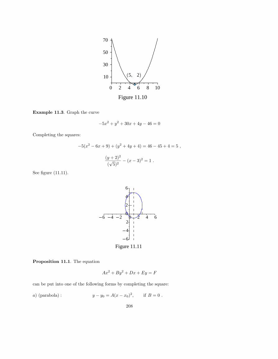
(5;�2)0 2 4 6 8 10
10
30
50
70
Figure 11.10( � +( �Example 11.3. Graph the curve
−5x2 + y2 + 30x + 4y − 46 = 0
Completing the squares:
−5(x2 − 6x + 9) + (y2 + 4y + 4) = 46− 45 + 4 = 5 ,
(y + 2)2
(√
5)2− (x− 3)2 = 1 .
See figure (11.11).
�6 �6
�4 �4
�2�20
02
2
4
4
6
6
Figure 11.11
� � � =+ )= + + = ;) = : � + + + � = :� ( � + )+( + + )= � + = ;( + )(p ) � ( � ) = :Proposition 11.1. The equation
Ax2 + By2 + Dx + Ey = F
can be put into one of the following forms by completing the square:
a) (parabola) : y − y0 = A(x− x0)2, if B = 0 .
208

The vertex of the parabola is at (x0, y0), and the axis is the line x = x0.
b) (parabola) : x− x0 = C(y − y0)2 if A = 0 .
The vertex of the parabola is at (x0, y0), and the axis is the line y = y0.
c) (ellipse) :(x− x0)2
a2+
(y − y0)2
b2= 1 if A and B are of the same sign .
The center of the ellipse is at (x0, y0), and its axes are the lines x = x0, y = y0.
d) (hyperbola) :(x− x0)2
a2− (y − y0)2
b2= 1 or
(y − y0)2
b2− (x− x0)2
a2= 1
if A and B are of different signs. The center of the hyperbola is (x0, y0), and its axes are the linesx = x0, y = y0.
e) If both A and B are zero, the curve is a line. The following degenerate cases may also result:
A(x− x0)2 + B(y − y0)2 ≤ 0 : no graph or just the point (x0, y0).
A(x− x0)2 −B(y − y0)2 = 0 : two lines crossing at (x0, y0).
Example 11.4. Finally, just to illustrate the situation of a quadratic whose coefficient of xy isnonzero, we consider the curve xy = 1. This curve is symmetric about the lines y = ±x, and hasthe asymptotes x = 0, y = 0. This appears to be a hyperbola with major axis the line x = y.In fact, if we make the linear change of variables x = u + v, y = u − v, this becomes the curveu2 − v2 = 1 in the new variables. (This change of variables represents a rotation by 45◦, with aslight change of scale.) See figure (11.12).
Figure 11.12
-2 -1 1 2
-40
-20
20
40
209
Problems 11.1
In problems 1-4 put the conic in standard form, and find the center and vertices. In the nextsection you will learn about foci of the conic sections. After reading that section, return to theseproblems and find the foci.
1. y − 8x2 + 32x− 29 = 0
2. 9x2 + 4y2 − 36x + 8y + 4 = 0
3. 4x2 − y2 + 2y = 5
4. x2 − 5y2 − 4x + 10y = 1
5. Find the equation of the parabola with vertex (2,5), axis y = 5 that goes through the point(4,2).
6. Find the equation of the ellipse with vertices (0,0), (0,10) that goes through the point (4,6).
7. Find the equation of the hyperbola with vertices at (3,0), (1,0) and asymptotes of slope ±5.
In problems 8-10 your are given the equation of a curve C and a point P on the curve. Find thepoint of intersection of the tangent line to C at P with the x-axis.
8. x2 + 5y = 0 , (10,−20) .
9. x2 + 4y2 = 16 , (2√
3, 1) .
10. 4x2 − y2 = 1 , (√
2/2, 1) .
11.2 Eccentricity and Foci
Curves described by quadratic equations are called the conic sections because they can be visualizedas the intersection of a cone with a plane. We shall now consider another definition, dating fromthe ancient Greeks, which leads to important properties of the conics.
Fix a point F and a line L in the plane such that L does not go through F .
Pick a positive number e. We consider the locus C of all points X in the plane such that
(11.6) |XF | = e|XL|
where |XY | means the distance from X to Y . e is the eccentricity of C; F the focus and L thedirectrix. Note that the curve C is symmetric about the line through the focus and perpendicular
210

to the directrix. This is the axis of the curve. There is one point between F and L on C which ison this axis; this point is the vertex of C. See figure 11.13.
Figure 11.13
L
V
mn
F
Xn = em
Figure 11.14
y
�p
X (x;y)F (p;0)L
V
= ( ; )j j= + = j j=p( � ) +p( � ) + = ( + = ) = + :=We now show that if e = 1, C is a parabola, if e < 1, C is an ellipse and if e > 1, C is a hyperbola.Let’s take the axis of C to be the x axis, and place the vertex at the origin, O. Then the focus issome point (p, 0); we take p > 0. Since |OF | = p, from (11.6) we find that the directrix is the linex = −p/e (see figure 11.14).
Now, for a point X = (x, y) on the curve, we have
|XL| = x + p/e and |XF | =√
(x− p)2 + y2
and so equation (11.6) in coordinates is given by
(11.7)√
(x− p)2 + y2 = e(x + p/e) = ex + p .
Case e = 1. Squaring both sides we get
x2 − 2px + p2 + y2 = x2 + 2px + p2 simplifying to y2 = 4px .
This of course is the standard form of a parabola. It also locates the focus (at (p, 0)) and thedirectrix (the line x = −p) of the parabola.
Proposition 11.2 . The focus of the parabola y2 = ax is a/4 units on one side of the vertex ofthe parabola along the axis, and and the directrix intersects the axis a/4 units on the other side.
211
Example 11.5. Find the vertex, focus and directrix of the parabola given by the equation
2x2 + 12x− y + 20 = 0
We put the equation in standard form. First we move the terms not involving x to the other side:
2x2 + 12x = y − 20 ,
and then, completing the square, we have
2(x2 + 6x + 9) = y − 20 + 18 , or (x + 3)2 =12(y − 4) .
Thus the vertex is at (−3, 4), axis of the parabola is the line y = 4 and the parabola opens up (since4p = 1/2 > 0). We have p = 1/8, so the focus is 1/8=.125 units above the vertex at (-3,4.125) andthe directrix is the line y = 3.875.
Example 11.6. Find the equation of the parabola whose vertex is at (4, 2) and whose directrix isthe line x = −1. Find the focus of this parabola.
Since the directrix is a vertical line, the axis is horizontal, so the equation has the form
(y − 2)2 = 4p(x− 4) ,
since the vertex is at (4, 2). Now p is the distance between the vertex and the directrix, sop = 4− (−1) = 5. Thus the equation of the parabola is
(y − 2)2 = 20(x− 4) .
The focus is 5 units to the right of the vertex, so is at (9, 2).
Example 11.7. Find the equation of the parabola whose focus is the origin and whose vertex isat the point (a, 0) with a > 0.
Since both the focus and vertex are on the x=axis, that is the axis of the parabola. Since thevertex is to the right of the focus, the parabola opens to the left. Thus the equation has the form
y2 = −4p(x− a) ,
where p is the distance between focus and vertex. But that is a, so the equation is
y2 = −4a(x− a) .
Case e 6= 1. Squaring both sides of (11.7) gives us
x2 − 2px + p2 + y2 = e2(x2 + 2px + p2)
which simplifies to
(11.8) (1− e2)x2 + y2 − 2p(1 + e)x = 0
212

Thus, if e < 1, this is an ellipse, and if e > 1 this is a hyperbola. Notice, because of symmetry inthe minor axis, ellipses and hyperbolas have two foci; one on each side of the minor axis.
We now want show how to locate the foci of an ellipse (e < 1) given in standard form. Thus westart by putting (11.8) in standard form, and then compare it to the formula of Proposition 11.1c).Dividing equation (11.8) by the coefficient of x2 gives us
x2 − 2p
1− ex +
y2
1− e2= 0
Now completing the square, we come to
(11.9) (x− p
1− e)2 +
y2
1− e2=
p2
(1− e)2
Comparing this to
(11.10)(x− x0)2
a2+
(y − y0)2
b2= 1
we see that the center of the ellipse is at (p/(1− e), 0) and a2 = p2/(1− e)2, b2 = a2(1− e2). Letc be the distance of the center from the focus. Since the focus is at (p, 0),
c =p
1− e− p = p(
11− e
− 1) = ep
1− e= ea
and c2 = e2a2 = a2 − b2. Summarizing
Proposition 11.3. If an ellipse is in standard form
(11.10)(x− x0)2
a2+
(y − y0)2
b2= 1 ,
with a > b, then the foci of the ellipse are on the major axis, c units away from the center where
c2 = a2 − b2
The eccentricity of the ellipse is given by the equations
b2 = (1− e2)a2 or e = c/a
A similar argument for the case e > 1, the hyperbola, leads to
Proposition 11.4 . If a hyperbola is in standard form
(11.11)(x− x0)2
a2− (y − y0)2
b2= 1
then the foci of the hyperbola are on the major axis, c units away from the center where
c2 = a2 + b2
213

The eccentricity of the hyperbola is given by the equations
b2 = (e2 − 1)a2 or e = c/a
Example 11.8. Find the foci of the conic given by the equation
x2 + 4y2 − 2x = 8 .
First, we complete the square to get the equation in standard form:
(x− 1)2
32+
y2
(3/2)2= 1 .
This conic is an ellipse centered at (1,0), with major axis the line x = 1, and a2 = 9, b2 = 9/4.Thus c2 = a2− b2 = 9(3/4), so c = (3/2)
√3. This is the distance of the foci from the center (along
the major axis), so the foci are at (1± (3/2)√
3, 0).
Example 11.9. Find the foci of the conic given by the equation
y2 − x2 + 4x = 13 .
Complete the squares, and get the standard form
y2
32− (x− 2)2
32= 1 .
This is a hyperbola with center at (2, 0), and major axis the line x = 2. We have c2 = a2 +b2 = 18,so c = 3
√2 is the distance of the foci from the center along the line x = 2. Thus the foci are at
(2,±3√
2. The vertices are at (2,±3).
Example 11.10. Find the equation of the ellipse centered at the origin, with a focus at (2, 0) anda vertex at (3, 0).
The equation of an ellipse centered at the origin is
x2
a2+
y2
b2= 1
we are given a = 3, c = 2. Thus b2 = a2 − c2 = 5, and the equation is
x2
9+
y2
5= 1
Problems 11.2.
1. Find the equation of the parabola whose vertex is at (0,2) and focus is the origin.
2. Find the vertex of the parabola with focus at (0,7) and passes through the points (±2, 7) and(±1, 5).
214

3. Find the equation of the parabola with focus at (2,3) and directrix the line y = −1.
4. Find the foci and eccentricity of the ellipse given by the equation
(x− 1)2
4+
y2
16= 1 .
5. A hyperbola has vertices at (±3, 0) and foci at (±4, 0). What are the equations of its asymptotes?
6. Find the foci and eccentricity of the hyperbola
(y − 2)2
25− (x + 1)2
16= 1 .
7. A hyperbola has asymptotes y − 1 = ±0.8(x + 2). What is its eccentricity?
In each of problems 8 thorugh 10, the curve described depends upon a parameter. Identify theparameter, and find the equation of the curve in terms of the parameter.
8. A parabola with axis the x-axis and focus at the origin.
9. A hyperbola with foci at (-1,0), (1,0).
10. An ellipse with foci at (-1,0), (1,0).
11. Show that the hyperbola and the ellipse of problems 9 and 10 intersect orthogonally; that is,at a point of intersection their tangent lines are orthogonal.
11.3 String and Optical Properties of the Conics
We have seen that the parabola can be defined as the locus of points X equidistant from a givenpoint F and a given line L. The ellipse and the hyperbola have similar definitions.
Proposition 11.5. Given two points F1 and F2 and a number a greater than half the distancebetween F1 and F2, the locus of points X such that
(11.13) |XF1|+ |XF2| = 2a
is an ellipse with foci at F1 and F2 and major axis of length 2a.
Choose coordinates so that the points F1 and F2 lie on the x-axis, equidistant from the origin.Then F1 has coordinates (−c, 0), and F2 has coordinates (c, 0) for some c < a. Let X have thecoordinates (x, y). Then (11.13) becomes√
(x + c)2 + y2 +√
(x− c)2 + y2 = 2a
Eliminate the radicals to verify that we end up with a quadratic equation which is that of anellipse.
We should point out that every ellipse has property (11.13). For there is only one ellipse withgiven foci and length 2a of the major axis. So, if we start with a given ellipse, and then constructthe curve satisfying (11.13) with the foci and major axis of the given ellipse, since that curve is anellipse, it is the given ellipse.
We have a similar description of the hyperbola:
215
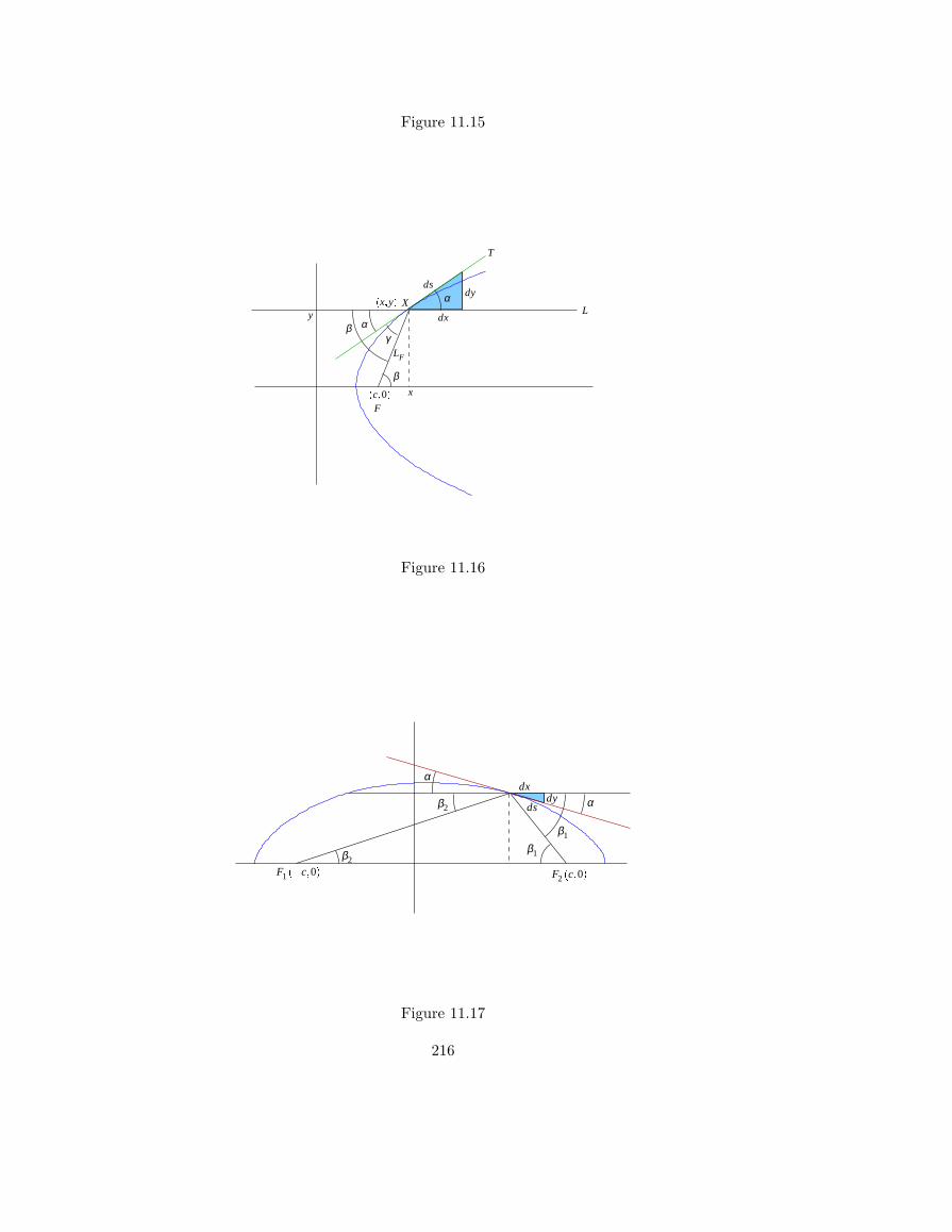
Figure 11.15
y
α
αβγ
β
F
ds
dx
dyX
x
(x;y)(c;0)
T
L
LF
=� = ( ; )Figure 11.16
dxdy
ds
β1
β1
β2
β2
α
α
F1 (�c;0) F2 (c;0)+ =( � ) = � =Figure 11.17
216

Figure 11.17:
α
α
F1 F2
L1 L2
T
x Proposition 11.6. Given two points F1 and F2 and a positive number a, the locus of points Xsuch that
(11.13) |XF1| − |XF2| = 2a
is a hyperbola with foci at F1 and F2.
Actually, this is just the branch of the hyperbola which wraps around the focus F2; the otherbranch is given by the equation
|XF2| − |XF1| = 2a
The optical properties of the conics follow from these string characterizations. Let’s start withthe parabola. Suppose that the parabola is coated with a light-reflecting material. The rays of abeam of light originating far away along the axis of the parabola will approach the parabola alonglines parallel to its axis. According to the physics of the situation, the angle of reflection off theparabola is equal to the angle of incidence. The optical property of the parabola is that thesereflected rays all meet at the focus. See figure 11.15.
Proposition 11.7. Let X be a point on the parabola, and T the tangent line to the parabola atX. Let LF be the line from the focus to X, and L the line through X parallel to the axis of theparabola. Then the angle between T and LF is equal to the angle between T and L.
What we want to show, referring to figure 11.15, is that γ = α. From the figure we see thatγ = β − α, so this amounts to showing that β − α = α.
Referring to figure 11.15, the focus-directrix definition of the parabola tells us that LF (the distancefrom the point X to the focus F ) is equal to x + c (the distance from X to the directrix). Thus
(11.15) LF = x + c .
Squaring this equation gives us(x− c)2 + y2 = (x + c)2 .
217

Differentiate this equation with respect to arc length and divide by 2 to get
(x− c)dx
ds+ y
dy
ds= (x + c)
dx
ds.
Now, divide by x + c = LF to get
(11.16)x− c
LF
dx
ds+
y
LF
dy
ds=
dx
ds.
From figure 11.15, we have
dx
ds= cos α ,
dy
ds= sinα ,
x− c
LF= sinβ ,
y
LF= cos β ,
so (11.16) becomes
sinβ cos α + cos β sinα = cos α , or cos(β − α) = cos α ,
from which we conclude that β − α = α, as desired.
The optical property of the ellipse is that a ray of light emanating from one focus reflects off theellipse so as to pass through the other focus (see figure 11.16).
Proposition 11.8. Let X be a point on the ellipse, and T the tangent line to the ellipse at X.Let L1 be the line from the focus F1 to X, and L2 the line from the other focus F2 to X. Thenthe angle between T and L1 is equal to the angle between T and L2.
What we want to show, referring to figure 11.16, is that β2 + α = β1−α. We start with the stringproperty, written in the coordinates as shown in the figure:√
(x + c)2 + y2 +√
(x− c)2 + y2 = 2a
Differentiate with respect to arc length to arrive at
x + c√(x + c)2 + y2
dx
ds+
y√(x + c)2 + y2
dy
ds+
x− c√(x− c)2 + y2
dx
ds+
y√(x− c)2 + y2
dy
ds= 0
Now make substitutions of the trigonometric functions, using the figure. We have to be careful: inour picture dy and x− c are negative, so since the sine and cosine are ratios of lengths, we have
cos β1 = − x− c√(x− c)2 + y2
sinα =∣∣dy
ds
∣∣ = −dy
ds.
Thus our equation becomes
cos β2 cos α + sinβ2(− sinα) + (− cos β1) cos α + sinβ1(− sinα) = 0
or(cos β2 cos α− sinβ2 sinα)− (cos β1 cos α + sinβ1 sinα) = 0
which is cos(β2 + α)− cos(β1 − α) = 0, so β2 + α = β1 − α as desired.
218

The optical property of the hyperbola is that a ray of light emanating from one focus reflects offthe opposite branch of the hyperbola so as to appear to have come from the other focus (see figure11.17).
Proposition 11.9. Let X be a point on the hyperbola, and T the tangent line to the ellipse atX. Let L1 be the line from the focus F1 to X, and L2 the line from the other focus F2 to X. Thenthe exterior angles between T and L1 and between T and L2 are equal.
The verification is a computation completely analogous to the one for the ellipse: differentiate thestring property, and then make the correct trigonometric substitutions
Problems 11.3
1. Find the point (x, y) on the parabola y2 = 12x for which the line from the focus meets thetangent line at an angle of 45◦.
2. Give a proof, using the optical properties of the conics that confocal hyperbolae and ellipsesintersect orthogonally. That is, suppose that H and E are respectively a hyperbola and an ellipse,and suppose that the have the same foci. Show that, at a point P of intersection of H and E thatthe curves have tangent lines which are perpendicular.
11.4 Polar Coordinates
Often a problem can be seen as that of understanding the motion of a particle in the plane relativeto a fixed point. In such a situation it is desirable to be able to describe a position in terms of thelength and the direction of the line between the two points. These are the polar coordinatesof the point. We consider the fixed point as the origin of these coordinates, and take the positivex-axis as the “zero” direction. Then any other direction is described by the angle between it andthe positive x axis, which we denote as θ. The distance of a point on this line from the origin isdenoted r. These equations relate the cartesian coordinates (x, y) with the polar coordinates r, θ:
(11.17) x = r cos θ , y = r sin θ , r =√
x2 + y2 , θ = arctany
x
See figure 11.18 to justify these formulas. Polar coordinates have two pecularities that need to bepointed out. Every value of (r, θ) determines a point in the plane. However, if r = 0, the pointis the origin, and θ doesn’t make sense. Secondly, the values (r, θ) and (r, θ + 2π), and in fact,(r, θ + 2nπ) for any n give the same point. This ambiguity is sometimes of value: for example,when discussing the motion of a particle, n tells us how many times the particle has wound aroundthe origin in the counterclockwise sense. Finally, it is also of convenience to let r take negativevalues, meaning a distance of |r| in the opposite direction of the ray θ. Thus (r, θ) and (−r, θ + π)determine the same point. We now consider the graphs of equations in polar coordinates.
219

x
y
r
θ
Figure 11.18 =( ; ) ( ; + )Figure 11.18
Example 11.11. The equation r = a, for a > 0 is satisfied by all points of distance a from theorigin, so is polar equation of the circle of radius a centered at the origin.
Example 11.12. The equation θ = θ0 is the line which makes an angle of θ0 with the x-axis.
Example 11.13. r = aθ describes the motion of a point which rotates around the origin at angularvelocity 1 while moving out along the ray at velocity a. This is the Archimedean spiral; seefigure 11.19.
θaθ
=== =Figure 11.19 Figure 11.20
Example 11.14. r = eaθ is another spiral, however, the point moves out along the ray at a rateexponential in the rate of rotation. This is the logarithmic spiral, depicted in figure 11.20.
220
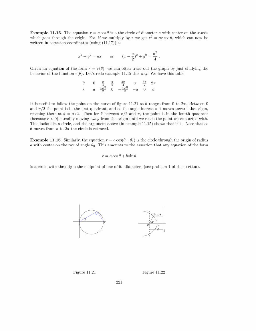
Example 11.15. The equation r = a cos θ is a the circle of diameter a with center on the x-axiswhich goes through the origin. For, if we multiply by r we get r2 = ar cos θ, which can now bewritten in cartesian coordinates (using (11.17)) as
x2 + y2 = ax or (x− a
2)2 + y2 =
a2
4.
Given an equation of the form r = r(θ), we can often trace out the graph by just studying thebehavior of the function r(θ). Let’s redo example 11.15 this way. We have this table
θ 0 π4
π2
3π4 π 3π
2 2π
r a a√
22 0 −a
√2
2 −a 0 a
It is useful to follow the point on the curve of figure 11.21 as θ ranges from 0 to 2π. Between 0and π/2 the point is in the first quadrant, and as the angle increases it moves toward the origin,reaching there at θ = π/2. Then for θ between π/2 and π, the point is in the fourth quadrant(because r < 0), steadily moving away from the origin until we reach the point we’ve started with.This looks like a circle, and the argument above (in example 11.15) shows that it is. Note that asθ moves from π to 2π the circle is retraced.
Example 11.16. Similarly, the equation r = a cos(θ−θ0) is the circle through the origin of radiusa with center on the ray of angle θ0. This amounts to the assertion that any equation of the form
r = a cos θ + b sin θ
is a circle with the origin the endpoint of one of its diameters (see problem 1 of this section).
aθ
Figure 11.22
X (x;y)r θ
F Vd L
Figure 11.21 Figure 11.22
221
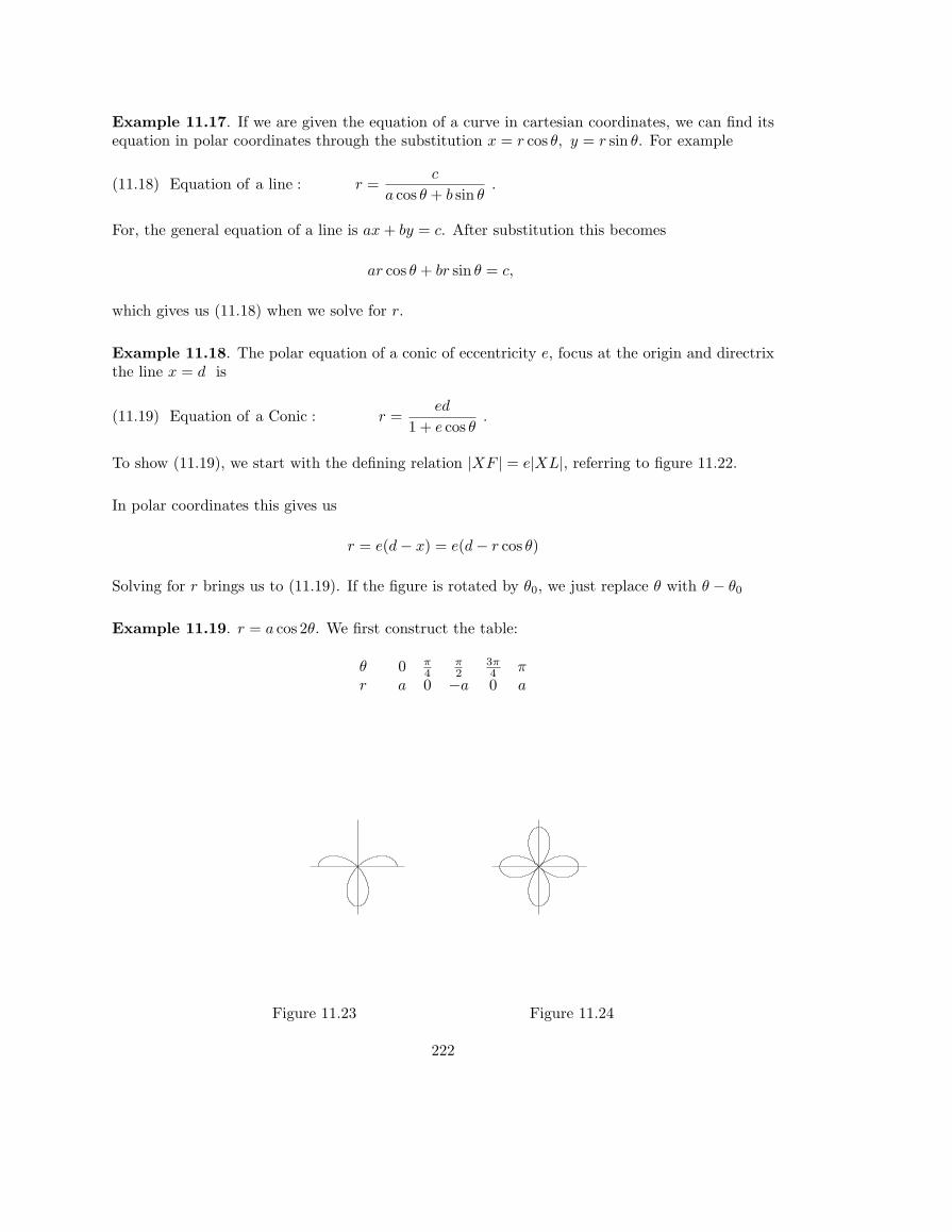
Example 11.17. If we are given the equation of a curve in cartesian coordinates, we can find itsequation in polar coordinates through the substitution x = r cos θ, y = r sin θ. For example
(11.18) Equation of a line : r =c
a cos θ + b sin θ.
For, the general equation of a line is ax + by = c. After substitution this becomes
ar cos θ + br sin θ = c,
which gives us (11.18) when we solve for r.
Example 11.18. The polar equation of a conic of eccentricity e, focus at the origin and directrixthe line x = d is
(11.19) Equation of a Conic : r =ed
1 + e cos θ.
To show (11.19), we start with the defining relation |XF | = e|XL|, referring to figure 11.22.
In polar coordinates this gives us
r = e(d− x) = e(d− r cos θ)
Solving for r brings us to (11.19). If the figure is rotated by θ0, we just replace θ with θ − θ0
Example 11.19. r = a cos 2θ. We first construct the table:
θ 0 π4
π2
3π4 π
r a 0 −a 0 a
= � �Figure 11.23 Figure 11.24
222
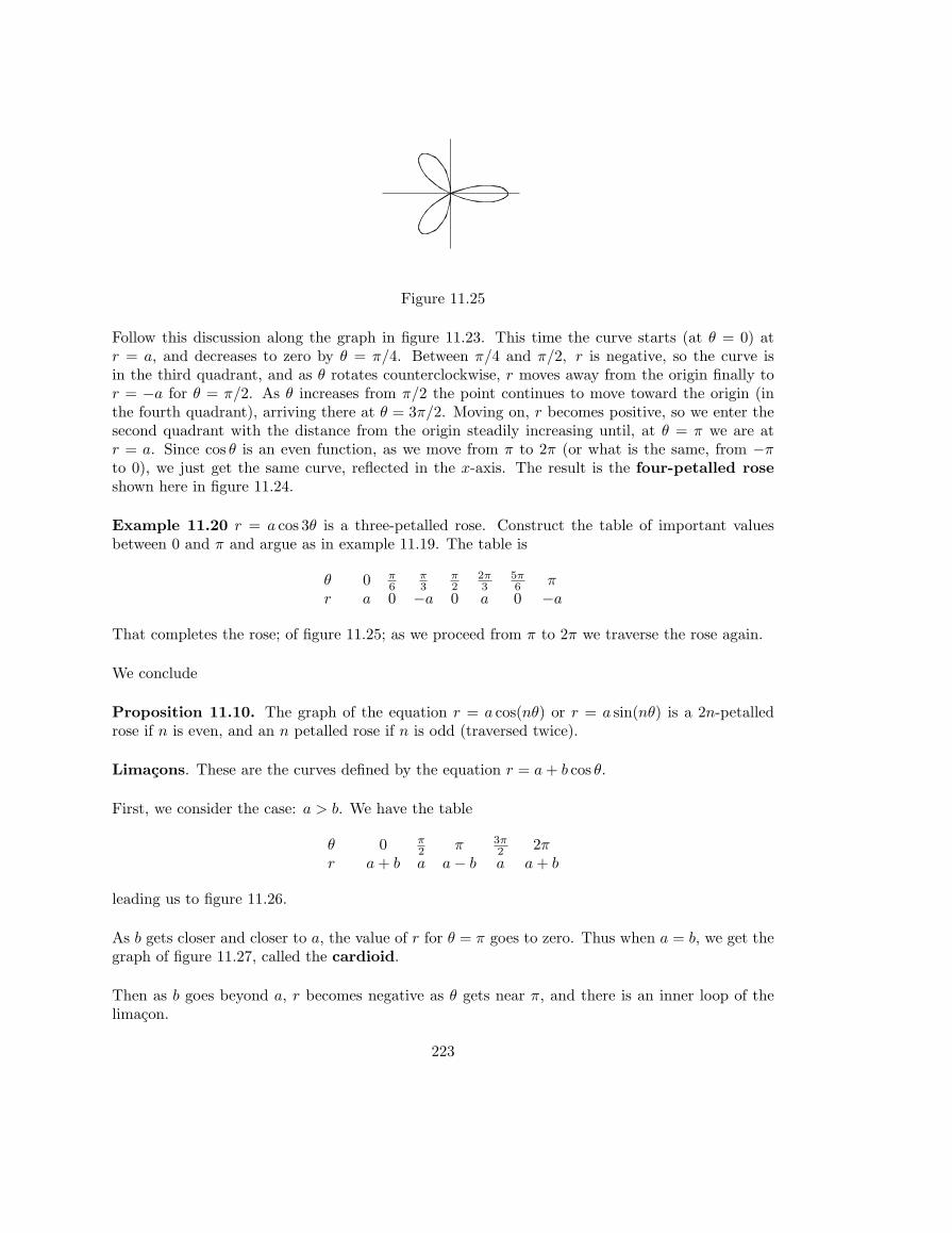
> +Figure 11.25
Follow this discussion along the graph in figure 11.23. This time the curve starts (at θ = 0) atr = a, and decreases to zero by θ = π/4. Between π/4 and π/2, r is negative, so the curve isin the third quadrant, and as θ rotates counterclockwise, r moves away from the origin finally tor = −a for θ = π/2. As θ increases from π/2 the point continues to move toward the origin (inthe fourth quadrant), arriving there at θ = 3π/2. Moving on, r becomes positive, so we enter thesecond quadrant with the distance from the origin steadily increasing until, at θ = π we are atr = a. Since cos θ is an even function, as we move from π to 2π (or what is the same, from −πto 0), we just get the same curve, reflected in the x-axis. The result is the four-petalled roseshown here in figure 11.24.
Example 11.20 r = a cos 3θ is a three-petalled rose. Construct the table of important valuesbetween 0 and π and argue as in example 11.19. The table is
θ 0 π6
π3
π2
2π3
5π6 π
r a 0 −a 0 a 0 −a
That completes the rose; of figure 11.25; as we proceed from π to 2π we traverse the rose again.
We conclude
Proposition 11.10. The graph of the equation r = a cos(nθ) or r = a sin(nθ) is a 2n-petalledrose if n is even, and an n petalled rose if n is odd (traversed twice).
Limacons. These are the curves defined by the equation r = a + b cos θ.
First, we consider the case: a > b. We have the table
θ 0 π2 π 3π
2 2πr a + b a a− b a a + b
leading us to figure 11.26.
As b gets closer and closer to a, the value of r for θ = π goes to zero. Thus when a = b, we get thegraph of figure 11.27, called the cardioid.
Then as b goes beyond a, r becomes negative as θ gets near π, and there is an inner loop of thelimacon.
223
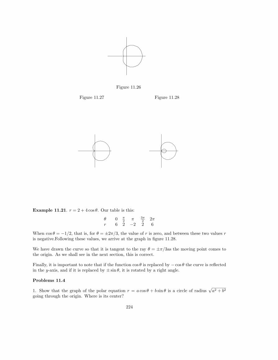
= ( ) = ( )= +> + � +Figure 11.26
Figure 11.27 Figure 11.28
= + �= � = = � ==� =Example 11.21. r = 2 + 4 cos θ. Our table is this:
θ 0 π2 π 3π
2 2πr 6 2 −2 2 6
When cos θ = −1/2, that is, for θ = ±2π/3, the value of r is zero, and between these two values ris negative.Following these values, we arrive at the graph in figure 11.28.
We have drawn the curve so that it is tangent to the ray θ = ±π/3as the moving point comes tothe origin. As we shall see in the next section, this is correct.
Finally, it is important to note that if the function cos θ is replaced by − cos θ the curve is reflectedin the y-axis, and if it is replaced by ± sin θ, it is rotated by a right angle.
Problems 11.4
1. Show that the graph of the polar equation r = a cos θ + b sin θ is a circle of radius√
a2 + b2
going through the origin. Where is its center?
224

2. Graph r = 3(cos θ +√
3 sin θ).
3. What is the polar equation of an ellipse, with one focus at the origin, corresponding directrixthe line x = −3 and corresponding vertex at the point (-1,0)?
4. Identify the curve: r = 2 sin(5θ).
5. Graph r2 = cos(2θ). This is called a lemniscate.
11.5 Calculus in polar coordinates
Arc length
Consider the curve given in polar coordinates by the equation r = r(θ). We can calculate thedifferential ds of arc length by the differential triangle in polar coordinates using the diagram infigure 11.29.
drds
rdt
r = r (t)dt r
= +Figure 11.29
The length of the arc of the circle of radius r subtended by the angle dθ is rdθ. The differentialtriangle is thus a right triangle with side lengths dr and rdθ. By the pythagorean theorem
(11.20) ds2 = dr2 + r2dθ2
Example 11.22. Find the length of the curve r = θ2 from 0 to 2π .
This curve is a spiral whose distance from the origin increases as the square of the angle. We havedr = 2θdθ, so
ds2 = dr2 + r2dθ2 = 4θ2dθ2 + θ4dθ2 = θ2(4 + θ2)dθ2
and thus the length is∫ 2π
0
ds =∫ 2π
0
θ√
4 + θ2dθ =13(4 + θ2)3/2)
∣∣2π
0=
13(4 + 4π2)3/2 − 43/2)
225

Area
To caculate the area enclosed by a curve given, in polar coordinates, by r = r(θ), we calculatethe differential of area, using figure 11.30
rdθ
rdθ
r = r (θ )= Z � (Figure 11.30
The area of the wedge given by the increment dθ is (1/2)r2dθ. To see this, we start with thearea of the circle of radius r : A = πr2. Now an angle α subtends a segment of the circle which isthe (α/2π)th part of the full circle, thus the area of that segment is (1/2)r2α. Thus, for α = dθ,we get
(11.21) dA =12r2dθ
Example 11.23. Find the area enclosed by the cardioid r = 3(1 + sin θ).
The area is
Area =12
∫ 2π
0
[3(1 + sin θ)2]dθ =92
∫ 2π
0
(1 + 2 sin θ + sin2 θ)dθ .
Now, we know that the integral of sin θ over an entire period is zero, so we can neglect the middleterm. We now use the double angle formula for the last term, and drop the integral of cos(2θ) forthe same reason:
Area =92
∫ 2π
0
(1 +1− cos(2θ)
2)dθ =
92
∫ 2π
0
32dθ =
272
π .
Example 11.24. Find the area inside one petal of the rose r = sin 3θ.
At θ = 0 we have r = 0, but then as the angle rotates, r increases to its maximum at 3θ = π/2,and then decreases back to zero for 3θ = π. Thus one petal is spanned as θ ranges from 0 to π/3.We now calculate;
Area =12
∫ π/3
0
sin2(3θ)dθ =12
∫ π/3
0
(1− cos(6θ)
2)dθ =
12(θ
2− cos(6θ)
12
∣∣π/3
0=
π
12.
226
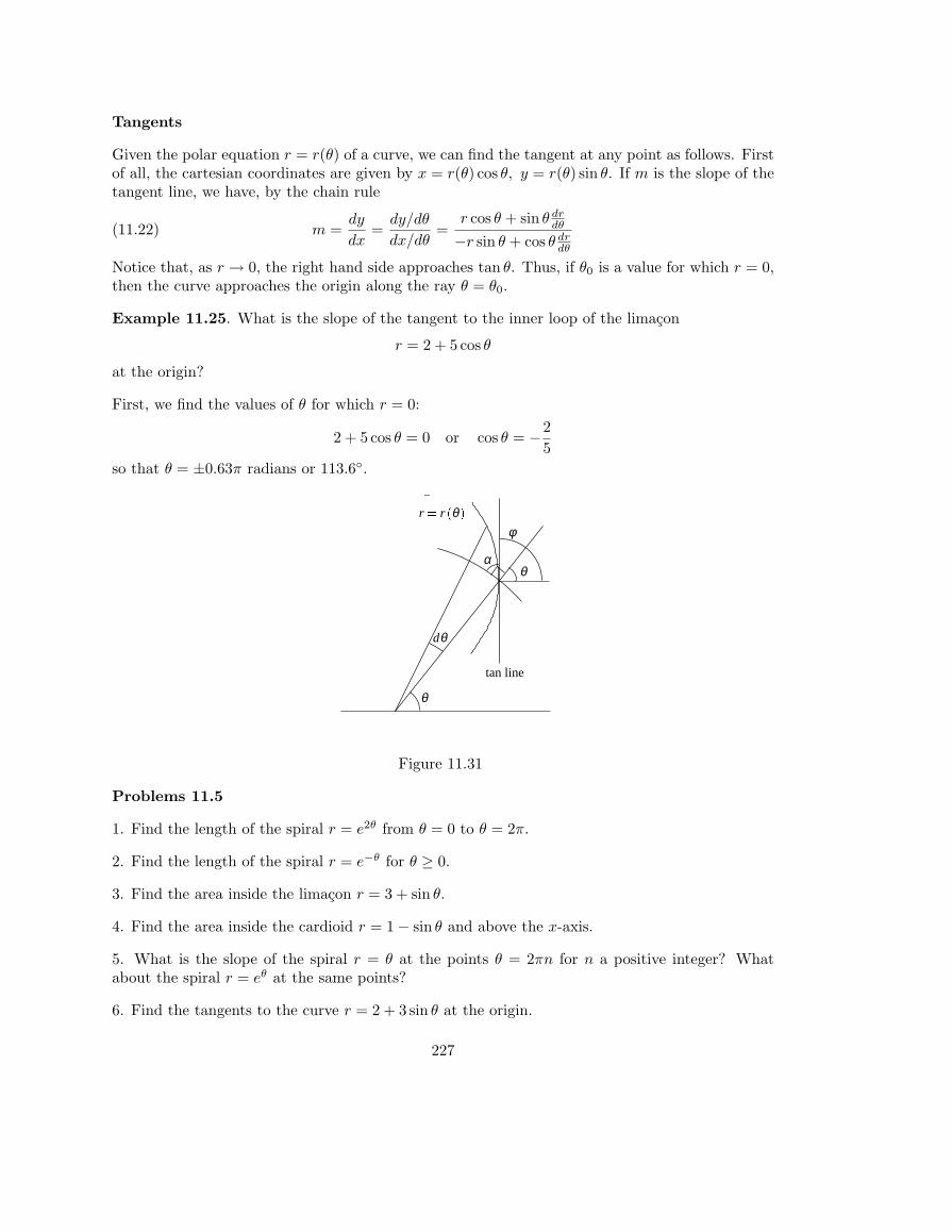
Tangents
Given the polar equation r = r(θ) of a curve, we can find the tangent at any point as follows. Firstof all, the cartesian coordinates are given by x = r(θ) cos θ, y = r(θ) sin θ. If m is the slope of thetangent line, we have, by the chain rule
(11.22) m =dy
dx=
dy/dθ
dx/dθ=
r cos θ + sin θ drdθ
−r sin θ + cos θ drdθ
Notice that, as r → 0, the right hand side approaches tan θ. Thus, if θ0 is a value for which r = 0,then the curve approaches the origin along the ray θ = θ0.
Example 11.25. What is the slope of the tangent to the inner loop of the limacon
r = 2 + 5 cos θ
at the origin?
First, we find the values of θ for which r = 0:
2 + 5 cos θ = 0 or cos θ = −25
so that θ = ±0.63π radians or 113.6◦.Figure 11.31
r = r (θ )φ
αθ
θ
dθ
tan line
= ( ) = ( ) ; = ( )= = == = +� +! =Figure 11.31
Problems 11.5
1. Find the length of the spiral r = e2θ from θ = 0 to θ = 2π.
2. Find the length of the spiral r = e−θ for θ ≥ 0.
3. Find the area inside the limacon r = 3 + sin θ.
4. Find the area inside the cardioid r = 1− sin θ and above the x-axis.
5. What is the slope of the spiral r = θ at the points θ = 2πn for n a positive integer? Whatabout the spiral r = eθ at the same points?
6. Find the tangents to the curve r = 2 + 3 sin θ at the origin.
227
XII. Second Order Linear Differential Equations
12.1 Homogeneous Equations
A differential equation is an equation involving variables x, y, y′, y′′, . . .. A solution is a functionf(x) defined in an interval I such that the substitution y = f(x), y′ = f ′(x), y′′ = f ′′(x), . . .becomes an identity for x in the interval I. The differential equation is said to be linear if itis linear in the variables y, y′, y′′, . . .. We first encountered solutions of differential equations insection 4 of Chapter 3, in the context of equations of the form f(y)dy = g(x)dx). In Chapter 6,section 3 we discussed the solution of first order linear equations (those in which only the variablesx, y, y′ appear). in this chapter we turn to second order linear equations with constant coefficients(those allowing also a second derivative). The general form of such an equation is
(12.1) y′′ + ay′ + by = g(x) ,
where a and b are constants, and g(x) is a differentiable function of x. In section 6.4, we saw that afirst order equation has a one-parameter family of solutions, and that the specification of an initialcondition y(x0) = y0 uniquely determines a solution. In the case of second order equations, thebasic theorem is this.
Theorem 12.1. Given x0 in the domain of the differentiable function g, and numbers y0, y′0,there is a unique function f(x) which solves the differential equation (12.1) and satisfies the initialconditions f(x0) = y0, f ′(x0) = y′0.
In this section we shall see how to completely solve equation (12.1) when the function on the righthand side is zero:
(12.2) y′′ + ay′ + by = 0 .
This is called the homogeneous equation. An important first step is to notice that if f(x) andg(x) are two solutions, then so is the sum; in fact, so is any linear combination Af(x) + Bg(x).Thus, once we know two solutions (they must be independent in the sense that one isn’t a constantmultiple of the other) we can solve the initial value problem in theorem 12.1 by solving for A andB.
Example 12.1. Solve. y′′ + y = 0 , y(0) = 4 , y′(0) = −1 .
Now, we know that cos x and sinx are solutions of the equation, so we try a solution of theform y(x) = A cos x + B sinx. Evaluating at x = 0, we find that A = 4. Differentiate, gettingy′(x) = −A sinx + B cos x, and evaluating at x = 0, we find B = −1. Thus the solution isy(x) = 4 cos x− sinx.
The reason the answer worked out so easily is that y1 = cos x is the solution with the particularinitial values y1(0) = 1, y′1(0) = 0 and y1 = sin x is the solution with y1(0) = 0. y′1(0) = 1 . Thenthe solution with initial values y(0) and y′(0) is
(12.3) y(x) = y(0) cos x + y′(0) sinx
Example 12.2. Solve y′′ − y = 0 , with given initial values y(0) , y′(0) .
228

Now ex and e−x are solutions of this differential equation, so the general solution is a linearcombination of these. But we won’t have as easy a time finding a solution like (11.3), since thesefunctions do not have the initial values 1, 0; 0, 1 respectively. However if we introduce the functions
coshx =12(ex + e−x) sinhx =
12(ex − e−x)
these do have the right initial values:
cosh 0 = 1 , sinh 0 = 0
(12.4)d
dx(coshx) = sinhx ,
d
dx(sinhx) = coshx
so (cosh)′(0) = 0, (sinh)′(0) = 1. Thus, the solution to our problem is
y(x) = y(0) coshx + y′(0) sinhx .
This particular differential equation comes up so often that it is important to remember thesefunctions, coshx, sinhx, called the hyperbolic functions and their basic properties: equation(12.4) and
(12.5) cosh2 x− sinh2 x = 1 .
Because of (12.5) these functions parametrize the standard hyperbola (and it is for this reason thatthey are called hyperbolic functions).
Using these examples as a guide, we return to the general second order equation.
Proposition 12.2. Let r be a root of the equation
(12.6) r2 + ar + b = 0 .
Then erx is a solution to the homogeneous equation:
(12.7) y′′ + ay′ + by = 0 .
Equation (12.6) is called the auxiliary equation of the differential equation (12.7). To verify theproposition, let y = erx so that y′ = rerx, y′′ = r2erx. Substituting into equation (12.7):
r2erx + arerx + berx = erx(r2 + ar + b) ,
and this is zero if and only if r is a root of the auxiliary equation.
Now unfortunately a quadratic equation does not necessarily always have two real roots, so wehave to examine the cases separately.
Case of two real roots. If the discriminant a2 − 4b > 0, then there are two real roots, and it isstraightforward to find the solution of the corresponding initial value problem.
Example 12.3. Solve : y′′ + 6y′ + 5y = 0 , y(0) = 4 , y′(0) = −1 .
229
The auxiliary equation, r2 + 6r + 5 = 0 has the roots r = −1,−5, so e−x and e−5x are solutions.The general solution is
y = Ae−x + Be−5x with derivative y′ = −Ae−x − 5Be−5x .
Evaluating at x = 0, we have 4 = A + B, −1 = −A − 5B. Solving this pair of equations, we getA = 19/4 and B = −3/4, so our solution is
y =194
e−x − 34e−5x
Example 12.4. A function x = x(t) satisfies the differential equation
x′′ − 2x′ − 15x = 0 .
Under what conditions on the values of x at t = 0 will this function decay to 0 as t →∞?
The auxiliary equation r2 − 2r − 15 has the roots r = −3, 5. Thus the general solution isx(t) = Ae−3t +Be5t. This will decay at infinity only if B = 0. Now, evaluating x and x′ at 0 givesus the equations
x(0) = A + B , x′(0) = −3A− 5B .
Setting B = 0, the condition becomes x′(0) + 3x(0) = 0.
Case of complex roots. If the discriminant a2−4b < 0, then the roots are two complex conjugatenumbers α + iβ, α− iβ.
Let’s look again at the case y′′ + y = 0. Then the roots of r2 + 1 = 0 are ±i, and we’d like to saythat the solutions are the functions eix, e−ix. This does work, and all the algebra in the case ofreal roots works just as well in this case, once we have given these expressions meaning. First ofall, remember equation (12.3): the general solution of y′′ + y = 0 is
(12.8) y(x) = y(0) cos x + y′(0) sinx
If y(x) = eix is to represent a solution of this differential equation, we have y(0) = e0 = 1, andy′(0) = ie0 = i, so we must have
(12.9) eix = cos x + i sinx
Notice that if we differentiate this expression, we get
− sinx + i cos x = i(cos x + i sinx) ,
so this expression is consistent with the differentiation rule for the exponential:
d
dxeix = ieix .
In fact, defining the complex exponential by (12.9) is consistent with all the rules of exponentials.In particular (recall problem 10 of section 9.5), if we substitute the Maclaurin series for all thefunctions in (12.9) we get an identity:
∞∑n=0
(ix)n
n!=
∞∑n=0
(−1)n x2n
(2n)!+ i
∞∑n=0
(−1)n x2n+1
(2n + 1)!.
230
Proposition 12.3. For a complex number α + iβ if we define the exponential function as
e(α+iβ)x = eαxeiβx = eαx(cos(βx) + i sin(βx)) ,
then all the usual laws of exponents carry through.
Now, of course, we are interested only in real-valued functions. What we have shown is that if α±iβare the roots of the equation r2 + ar + b = 0, then the functions e(α±iβ)x solve the differentialequation y′′ + ay′ + b = 0. But then the real and imaginary parts of this function satisfy theequation as well, which gives us the desired two real-valued solutions.
Proposition 12.4 . If the auxiliary equation for the differential equation
y′′ + ay′ + b = 0
has the complex roots α± iβ, then every solution of the differential equation is of the form
(12.10) Aeαx cos(βx) + Beαx sin(βx) = eαx(A cos(βx) + B sin(βx))
In solving initial value problems, we can work with the complex solutions or solutions of the form(12.10); usually the latter is more convenient.
Example 12.5. Find the general solution x = x(t) of
x′′ + a2x = 0 .
Since the roots of the auxiliary equation r2 = −a2 = 0 are ±ia, the general solution is
(12.11) x(t) = A cos at + B sin at
It is easy to see what this function looks like by defining
C =√
A2 + B2, γ = arctan(B/A)
Then (12.11) becomes
x(t) = C(cos γ cos at + sin γ sin at = C cos(at− γ) = C cos a(t− γ/a)) .
Thus the graph of x = x(t) is a simple cosine curve of amplitude C, and period 2π/a, shifted tothe right by the phase γ. (See figure 12.1).
Example 12.6. Find the solution y = y(x) of y′′ + 2y′ + 5y = 0, with initial values y(0) =2, y′(0) = −1.
The auxiliary equation r2 + 2r + 5 = 0 has the solutions r = −1 ± 2i. Thus the general solutionis y = e−x(A cos(2x) + B sin(2x)). To solve for A and B using the initial values we must firstdifferentiate y:
y′ = −e−x(A cos(2x) + B sin(2x)) + e−x(−2A sin(2x) + 2B cos(2x)) .
231
Substituting the initial values gives the equations A = 2, −A + 2B = −1, which has the solutionsA = 2, B = 1/2. The answer thus is
y = e−x(2 cos(2x) +12
sin(2x)) .
Case of a double root. If the discriminant a2− 4b = 0, then the auxiliary equation has one rootr, which gives us only one solution erx of the differential equation. We find another solution bythe technique of variation of parameters. We try y = uerx, where u is a new unknown function.Now, since the auxiliary equation has only the single root r, we have a = −2r and b = r2, so thedifferential equation can be written as:
y′′ − 2ry′ + r2y = 0 .
Substituting y = uerx in the left hand side, we get
y′′ − 2ry′ + r2y = erx[(u′′ + 2u′r + ur2)− 2r(u′ + ur) + r2u] = erxu′′ .
For this to be zero, we must have u” = 0, so that u = Ax + B.
Proposition 12.5 . If the auxiliary equation for the differential equation
y′′ + ay′ + b = 0
has only the root r, then every solution is of the form
(Ax + B)erx
Example 12.7. Find the solution of y′′ − 4y′ + 4y = 0 with initial values y(0) = 2, y′(0) = −1.
The auxiliary equation has just the root r = 2. The general solution is y = (Ax + B)e2x, withderivative y′ = 2(Ax + B)e2x + Ae2x. Substituting the initial conditions gives the equations
2 = B − 1 = 2B + A .
Thus A = −5, B = 2 and the answer is
y = (−5x + 2)e2x .
Problems 12.1
1. Solve y′′ − 5y = 0 with the initial values y(0) = 1, y′(0) = −1.
2. Solve y′′ + 5y = 0 with the initial values y(0) = 1, y′(0) = −1.
3. Solve y′′ − 5y′ + 6y = 0 with the initial values y(0) = 1, y′(0) = −1.
4. Solve y′′ + 4y′ + 5y = 0 with the initial values y(0) = 1, y′(0) = −1.
5. Solve y′′ − y′ = 0 with the initial values y(2) = 1, y′(2) = 2.
232

6. Solve y′′ + 2y′ + y = 0 with the initial values y(−1) = 1, y(1) = 1.
12.2 Behavior of the Solutions
When these differential equations come up in applications, one usually wants to have some ideaof the long term behavior of the solution. Since the roots of the auxiliary equation determine thesolutions, they also determine their behavior. Here we summarize the results.
Both roots positive. Except for the identically zero solution, all solutions grow exponentially.See figure 12.2.
Both roots negative. Except for the identically zero solution, all solutions decay exponentially.See figure 12.3.
Figure 12.2
−1
7
00
1
1
23457
0 � 2 0� 4 0� 6 0� 8
Figure 12.3
00
1
1
2
2
3
3
4
4
5
5
7
A negative and a positive root. All solutions grow exponentially, except for the multiples ofthe exponential with the negative root.
Both roots imaginary. In this case the equation is
y′′ + ω2y = 0 ,
As we saw in example 12.5, the general solution can be written as
y(x) = A cos ωx) + B sin(ωx) or y(x) = C cos(ωx− γ) ,
an oscillation of period 2π/ω, amplitude C and phase γ (see figure 12.1).
233
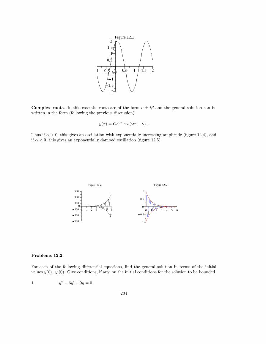
Figure 12.1
� 2
� 1 � 5� 1
� 1 � 0 � 5� 0 � 5 0
0
0 � 5
0 � 5
1
1
1 � 5
1 � 5
2
2
Complex roots. In this case the roots are of the form α ± iβ and the general solution can bewritten in the form (following the previous discussion)
y(x) = Ceαx cos(ωx− γ) .
Thus if α > 0, this gives an oscillation with exponentially increasing amplitude (figure 12.4), andif α < 0, this gives an exponentially damped oscillation (figure 12.5).
Figure 12.4
� 500
� 300
� 1000
0
100
300
500
1 2 3 4 5 6
Figure 12.5
00
1
1
2 3 4 5 6
� 1
� 0 � 5
0 � 5
Problems 12.2
For each of the following differential equations, find the general solution in terms of the initialvalues y(0), y′(0). Give conditions, if any, on the initial conditions for the solution to be bounded.
1. y′′ − 6y′ + 9y = 0 .
234

2. ′′ − 6y′ + 5y = 0 .
3. y′′ − y′ + 6y = 0 .
4. y′′ + 4y′ + 13y = 0 .
5. y′′ − 4y′ + 13y = 0 .
6. y′′ + 9y = 0 .
7. y′′ − 9y = 0 .
8. Find the solution of problem 3 with initial values y(0) = 3, y′(0) = −2.
9. Find the solution of problem 4 with initial values y(0) = 0, y′(0) = 1.
12.3 Applications
Springs
Suppose we place a mass m on the end of a vertically hanging spring, and then set it in motion;how can we describe the subsequent motion? As we have seen in chapter 5, section 4, the spring issubject to a restoring force proportional to its displacement from equilibrium. By Newton’s secondlaw of motion, this force is ma, where a is the acceleration of the mass m. Letting x represent thedownward displacement from equilibrium, we have a = x′′, and if the spring constant is k, thisgives us the equation
(12.12) mx′′ = −kx , or x′′ +k
mx = 0
Letting ω =√
k/m, this has the solution (see example 12.5)
x(t) = C cos(ωt− γ)
where C and γ are to be determined by the initial data.
We have to be a little careful about units. In the metric system, when m is measured in kilogramsand x in meters, then force is measured in newtons, and the units for the spring constant k arenewtons/meter. On a smaller scale, m is in grams, x in centimeters, force in dynes, and k indynes/meter. However, in the British system it is customary to refer to the weight w of the object(in pounds), rather than its mass. Then m = w/g, where g = 32 ft/sec2 is the acceleration due togravity. Finally, in the British system, the spring constant is given in lbs/foot.
Example 12.8. Suppose a mass of 10 g hangs from a spring with spring constant k = .4 dynes/cm.If the spring is extended an additional 8 cm. and then released, give the equation of subsequentmotion.
235
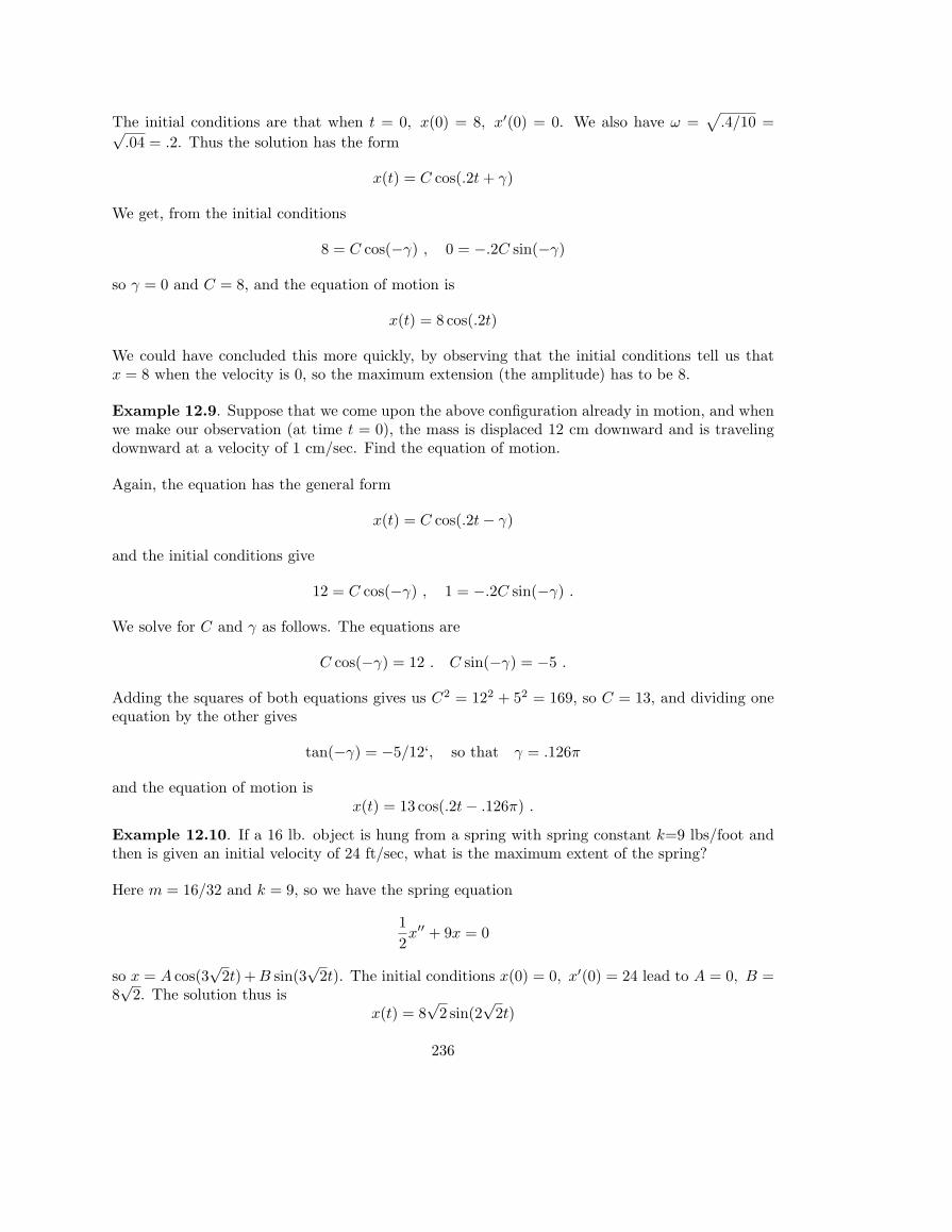
The initial conditions are that when t = 0, x(0) = 8, x′(0) = 0. We also have ω =√
.4/10 =√.04 = .2. Thus the solution has the form
x(t) = C cos(.2t + γ)
We get, from the initial conditions
8 = C cos(−γ) , 0 = −.2C sin(−γ)
so γ = 0 and C = 8, and the equation of motion is
x(t) = 8 cos(.2t)
We could have concluded this more quickly, by observing that the initial conditions tell us thatx = 8 when the velocity is 0, so the maximum extension (the amplitude) has to be 8.
Example 12.9. Suppose that we come upon the above configuration already in motion, and whenwe make our observation (at time t = 0), the mass is displaced 12 cm downward and is travelingdownward at a velocity of 1 cm/sec. Find the equation of motion.
Again, the equation has the general form
x(t) = C cos(.2t− γ)
and the initial conditions give
12 = C cos(−γ) , 1 = −.2C sin(−γ) .
We solve for C and γ as follows. The equations are
C cos(−γ) = 12 . C sin(−γ) = −5 .
Adding the squares of both equations gives us C2 = 122 + 52 = 169, so C = 13, and dividing oneequation by the other gives
tan(−γ) = −5/12‘, so that γ = .126π
and the equation of motion isx(t) = 13 cos(.2t− .126π) .
Example 12.10. If a 16 lb. object is hung from a spring with spring constant k=9 lbs/foot andthen is given an initial velocity of 24 ft/sec, what is the maximum extent of the spring?
Here m = 16/32 and k = 9, so we have the spring equation
12x′′ + 9x = 0
so x = A cos(3√
2t) + B sin(3√
2t). The initial conditions x(0) = 0, x′(0) = 24 lead to A = 0, B =8√
2. The solution thus isx(t) = 8
√2 sin(2
√2t)
236
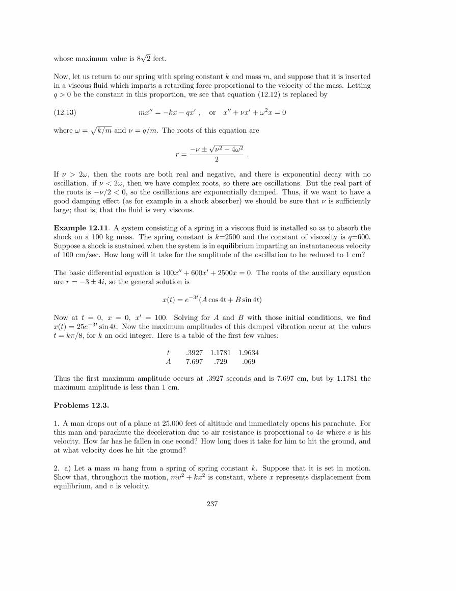
whose maximum value is 8√
2 feet.
Now, let us return to our spring with spring constant k and mass m, and suppose that it is insertedin a viscous fluid which imparts a retarding force proportional to the velocity of the mass. Lettingq > 0 be the constant in this proportion, we see that equation (12.12) is replaced by
(12.13) mx′′ = −kx− qx′ , or x′′ + νx′ + ω2x = 0
where ω =√
k/m and ν = q/m. The roots of this equation are
r =−ν ±
√ν2 − 4ω2
2.
If ν > 2ω, then the roots are both real and negative, and there is exponential decay with nooscillation. if ν < 2ω, then we have complex roots, so there are oscillations. But the real part ofthe roots is −ν/2 < 0, so the oscillations are exponentially damped. Thus, if we want to have agood damping effect (as for example in a shock absorber) we should be sure that ν is sufficientlylarge; that is, that the fluid is very viscous.
Example 12.11. A system consisting of a spring in a viscous fluid is installed so as to absorb theshock on a 100 kg mass. The spring constant is k=2500 and the constant of viscosity is q=600.Suppose a shock is sustained when the system is in equilibrium imparting an instantaneous velocityof 100 cm/sec. How long will it take for the amplitude of the oscillation to be reduced to 1 cm?
The basic differential equation is 100x′′ + 600x′ + 2500x = 0. The roots of the auxiliary equationare r = −3± 4i, so the general solution is
x(t) = e−3t(A cos 4t + B sin 4t)
Now at t = 0, x = 0, x′ = 100. Solving for A and B with those initial conditions, we findx(t) = 25e−3t sin 4t. Now the maximum amplitudes of this damped vibration occur at the valuest = kπ/8, for k an odd integer. Here is a table of the first few values:
t .3927 1.1781 1.9634A 7.697 .729 .069
Thus the first maximum amplitude occurs at .3927 seconds and is 7.697 cm, but by 1.1781 themaximum amplitude is less than 1 cm.
Problems 12.3.
1. A man drops out of a plane at 25,000 feet of altitude and immediately opens his parachute. Forthis man and parachute the deceleration due to air resistance is proportional to 4v where v is hisvelocity. How far has he fallen in one econd? How long does it take for him to hit the ground, andat what velocity does he hit the ground?
2. a) Let a mass m hang from a spring of spring constant k. Suppose that it is set in motion.Show that, throughout the motion, mv2 + kx2 is constant, where x represents displacement fromequilibrium, and v is velocity.
237
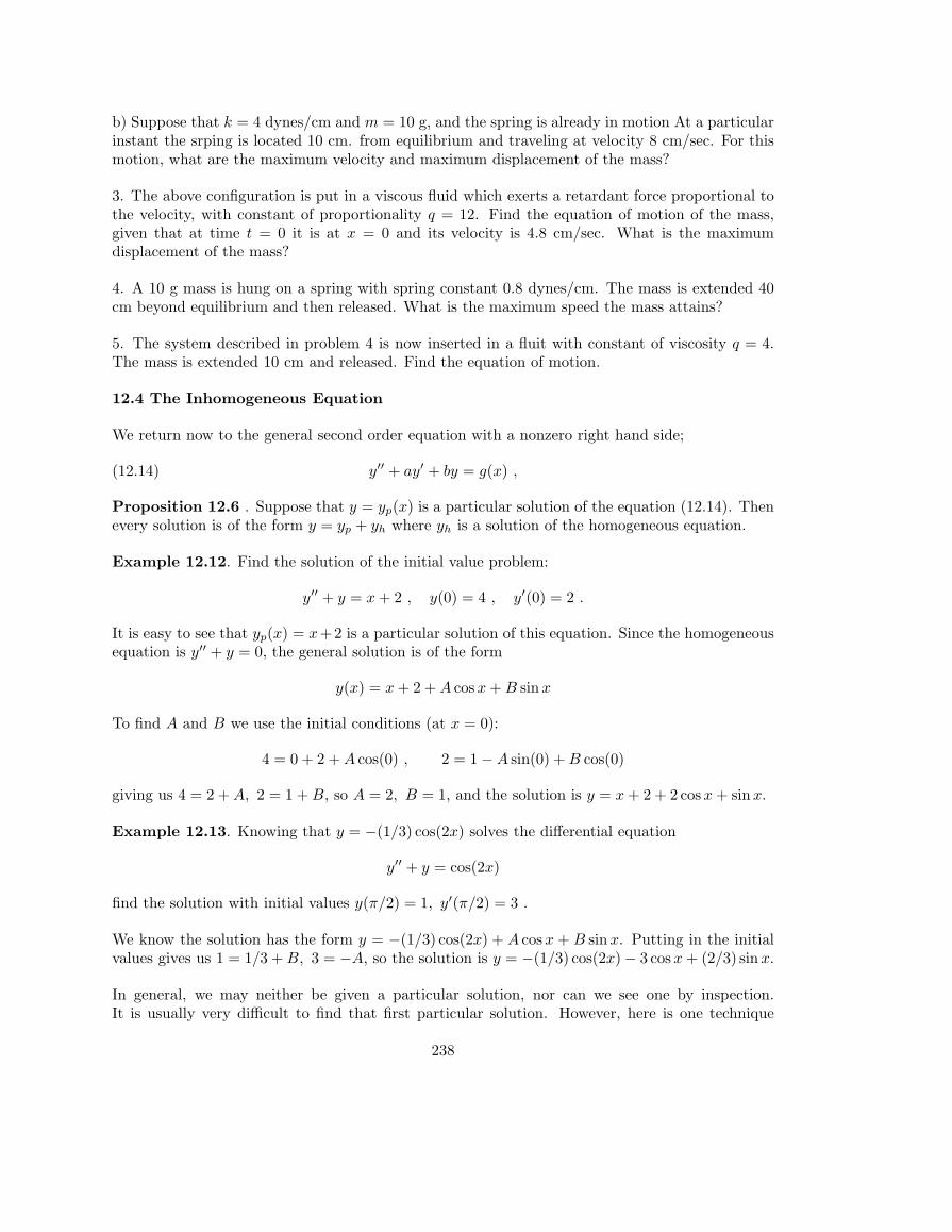
b) Suppose that k = 4 dynes/cm and m = 10 g, and the spring is already in motion At a particularinstant the srping is located 10 cm. from equilibrium and traveling at velocity 8 cm/sec. For thismotion, what are the maximum velocity and maximum displacement of the mass?
3. The above configuration is put in a viscous fluid which exerts a retardant force proportional tothe velocity, with constant of proportionality q = 12. Find the equation of motion of the mass,given that at time t = 0 it is at x = 0 and its velocity is 4.8 cm/sec. What is the maximumdisplacement of the mass?
4. A 10 g mass is hung on a spring with spring constant 0.8 dynes/cm. The mass is extended 40cm beyond equilibrium and then released. What is the maximum speed the mass attains?
5. The system described in problem 4 is now inserted in a fluit with constant of viscosity q = 4.The mass is extended 10 cm and released. Find the equation of motion.
12.4 The Inhomogeneous Equation
We return now to the general second order equation with a nonzero right hand side;
(12.14) y′′ + ay′ + by = g(x) ,
Proposition 12.6 . Suppose that y = yp(x) is a particular solution of the equation (12.14). Thenevery solution is of the form y = yp + yh where yh is a solution of the homogeneous equation.
Example 12.12. Find the solution of the initial value problem:
y′′ + y = x + 2 , y(0) = 4 , y′(0) = 2 .
It is easy to see that yp(x) = x+2 is a particular solution of this equation. Since the homogeneousequation is y′′ + y = 0, the general solution is of the form
y(x) = x + 2 + A cos x + B sinx
To find A and B we use the initial conditions (at x = 0):
4 = 0 + 2 + A cos(0) , 2 = 1−A sin(0) + B cos(0)
giving us 4 = 2 + A, 2 = 1 + B, so A = 2, B = 1, and the solution is y = x + 2 + 2 cos x + sinx.
Example 12.13. Knowing that y = −(1/3) cos(2x) solves the differential equation
y′′ + y = cos(2x)
find the solution with initial values y(π/2) = 1, y′(π/2) = 3 .
We know the solution has the form y = −(1/3) cos(2x) + A cos x + B sinx. Putting in the initialvalues gives us 1 = 1/3 + B, 3 = −A, so the solution is y = −(1/3) cos(2x)− 3 cos x + (2/3) sinx.
In general, we may neither be given a particular solution, nor can we see one by inspection.It is usually very difficult to find that first particular solution. However, here is one technique
238

(basically trial and error) which leads to a particular solution when the inhomogeneous function isan elementary function.
Undetermined coefficients. To solve y′′ + ay′ + by = g(x), try a function of the same form asg(x). More precisely:
If g is a polynomial of degree n, try the general polynomial of degree n.
If g is an exponential times a polynomial of degree n, try the general exponential times a polynomialof degree n.
If g is a cosine or a sine times a polynomial of degree n, try the general cosine and sine times apolynomial of degree n.
The reason this works is that successive differentiation keeps us in the same form, so we endup equating coefficients and solving for them. There is one caution: if g is a solution of thehomogeneous equation, this will fail In this case we replace the phrase “polynomial of degree n”by “polynomial of degree n or more”. Let us illustrate
Example 12.14. Find a particular solution of y′′ + 5y′ − y = x2 − 3x + 4.
We try y = ax2 + bx + c. First we calculate the first and second derivative: y′ = 2ax + b, y′′ = 2a.Substituting these in the given equation we obtain
2a + 5(2ax + b)− (ax2 + bx + c) = x2 − 3x + 4
This simplifies to−ax2 + (10a− b)x + 2a + 5b− c = x2 − 3x + 4
We now equate coefficients:
−a = 1 , 10a− b = −3 , 2a + 5b− c = 4
giving the solutions a = −1, b = −7, c = −41, so the answer is
y = −x2 − 7x− 41 .
Example 12.15. Find a particular solution of y′′ + y′ − y = xex.
Try y = (ax + b)ex. Differentiating, y′ = (ax + a + b)ex, y′′ = (ax + 2a + b)ex. Substituting in thegiven equation leads to
(ax + 2a + b)ex + (ax + a + b)ex − (ax + b)ex = xex ,
reducing to the equations a = 1, 3a + b = 0. Thus the answer is
y = (x− 3)ex
Example 12.16. Find a particular solution of y′′ + y = cos x.
239
Since cos x satisfies the homogeneous equation, we must try y = ax sinx + bx cos x. Then y′′ =2a cos x− 2b sinx− ax sinx− bx cos x, and we obtain the equation
2a cos x− 2b sinx = cos x
so a = 1/2, and the solution is y = (1/2)x sinx.
Problems 12.4
1. Solve y′′ + 2y′ + y = x with the initial values y(0) = 0, y′(0) = 0.
2. Find the general solution of y′′ + 2y′ + y = sinx.
3. Find the general solution of y′′ − 4y = sin(2x).
4. Find the general solution of y′′ + 4y = sin(2x).
5. A crystal glass consists of cells in a crystalline shape which oscillate at a natural frequency, sothe motion is governed by a differential equation x′′ + ω2
0x = 0 where 2π/ω0 is the frequency. Ifthe ambient air is vibrating at a frequency of ω/2π (due to a monotonal sound, perhaps), thenthe motion of a crystal is modified by the force of the air in motion so as to be governed by theinhomogeneous equation
x′′ + ω20x = A cos ωt
Find a particular solution of this differential equation. What happens as ω approaches ω0? (Thisphenomenon is called resonance.)
240