calculus i for engineers - faculty.uaeu.ac.aefaculty.uaeu.ac.ae/jaelee/class/1110/ln.pdf ·...
TRANSCRIPT

Calculus I for Engineers
My Students1
Fall 2010
1It is based mostly on the textbook, Smith and Minton’s Calculus Early Transcendental Functions, 3rd Ed and ithas been reorganized and retyped by Jae Lee.

Calculus I for Engineers Fall, 2010
Page 2 of 101

CONTENTS
1 Limits and Continuity 71.1 A Brief Preview of Calculus: Tangent Lines and the Length of a Curve . . . . . . . . . . . . 71.2 The Concept of Limit . . . . . . . . . . . . . . . . . . . . . . . . . . . . . . . . . . . . . . 71.3 Computation of Limits . . . . . . . . . . . . . . . . . . . . . . . . . . . . . . . . . . . . . 101.4 Continuity and Its Consequences . . . . . . . . . . . . . . . . . . . . . . . . . . . . . . . . 111.5 Limits Involving Infinity: Asymptotes . . . . . . . . . . . . . . . . . . . . . . . . . . . . . 13
1.5.1 Vertical Asymptote . . . . . . . . . . . . . . . . . . . . . . . . . . . . . . . . . . . 131.5.2 Horizontal Asymptote . . . . . . . . . . . . . . . . . . . . . . . . . . . . . . . . . 141.5.3 Slant Asymptote . . . . . . . . . . . . . . . . . . . . . . . . . . . . . . . . . . . . 15
1.6 Formal Definition of the Limit . . . . . . . . . . . . . . . . . . . . . . . . . . . . . . . . . 151.7 Limits and Loss–of–Significance Errors . . . . . . . . . . . . . . . . . . . . . . . . . . . . 15
2 Differentiation 172.1 Tangent Lines and Velocity . . . . . . . . . . . . . . . . . . . . . . . . . . . . . . . . . . . 172.2 The Derivative . . . . . . . . . . . . . . . . . . . . . . . . . . . . . . . . . . . . . . . . . . 17
2.2.1 Definition . . . . . . . . . . . . . . . . . . . . . . . . . . . . . . . . . . . . . . . . 172.2.2 Differentiability . . . . . . . . . . . . . . . . . . . . . . . . . . . . . . . . . . . . . 182.2.3 Meaning: Geometrical . . . . . . . . . . . . . . . . . . . . . . . . . . . . . . . . . 202.2.4 Alternative Derivative Notations . . . . . . . . . . . . . . . . . . . . . . . . . . . . 21
2.3 Computation of Derivatives: The Power Rule . . . . . . . . . . . . . . . . . . . . . . . . . 222.3.1 Power Rule . . . . . . . . . . . . . . . . . . . . . . . . . . . . . . . . . . . . . . . 222.3.2 General Derivative Rules: Linearity . . . . . . . . . . . . . . . . . . . . . . . . . . 222.3.3 Higher Order Derivatives . . . . . . . . . . . . . . . . . . . . . . . . . . . . . . . . 232.3.4 Physical Meaning of Derivative: Rate of Change . . . . . . . . . . . . . . . . . . . 23
2.4 The Product and Quotient Rules . . . . . . . . . . . . . . . . . . . . . . . . . . . . . . . . 242.4.1 Product Rule . . . . . . . . . . . . . . . . . . . . . . . . . . . . . . . . . . . . . . 242.4.2 Quotient Rule . . . . . . . . . . . . . . . . . . . . . . . . . . . . . . . . . . . . . . 242.4.3 Applications . . . . . . . . . . . . . . . . . . . . . . . . . . . . . . . . . . . . . . 24
2.5 The Chain Rule . . . . . . . . . . . . . . . . . . . . . . . . . . . . . . . . . . . . . . . . . 252.5.1 Prerequisite . . . . . . . . . . . . . . . . . . . . . . . . . . . . . . . . . . . . . . . 252.5.2 Chain Rule . . . . . . . . . . . . . . . . . . . . . . . . . . . . . . . . . . . . . . . 252.5.3 Derivative of Inverse Function . . . . . . . . . . . . . . . . . . . . . . . . . . . . . 26
2.6 Derivatives of Trigonometric Functions . . . . . . . . . . . . . . . . . . . . . . . . . . . . 272.6.1 Prerequisites: Basic Formulas . . . . . . . . . . . . . . . . . . . . . . . . . . . . . 272.6.2 Derivatives of Trigonometric Functions . . . . . . . . . . . . . . . . . . . . . . . . 272.6.3 Applications . . . . . . . . . . . . . . . . . . . . . . . . . . . . . . . . . . . . . . 28
2.7 Derivatives of Exponential and Logarithmic Functions . . . . . . . . . . . . . . . . . . . . 292.7.1 Prerequisites: Basic Formulas . . . . . . . . . . . . . . . . . . . . . . . . . . . . . 292.7.2 Derivatives of the Exponential Functions . . . . . . . . . . . . . . . . . . . . . . . 29
3

Calculus I for Engineers Fall, 2010
2.7.3 Derivative of the Natural Logarithm . . . . . . . . . . . . . . . . . . . . . . . . . . 302.7.4 Logarithmic Differentiation . . . . . . . . . . . . . . . . . . . . . . . . . . . . . . 31
2.8 Implicit Differentiation and Inverse Trigonometric Functions . . . . . . . . . . . . . . . . . 322.8.1 Implicit Differentiation . . . . . . . . . . . . . . . . . . . . . . . . . . . . . . . . . 322.8.2 Derivatives of the Inverse Trigonometric Functions . . . . . . . . . . . . . . . . . . 33
2.9 The Mean Value Theorem . . . . . . . . . . . . . . . . . . . . . . . . . . . . . . . . . . . 35
3 Applications of Differentiation 373.1 Linear Approximations and Newton’s Method . . . . . . . . . . . . . . . . . . . . . . . . . 373.2 Indeterminate Forms and L’Hopital’s Rule . . . . . . . . . . . . . . . . . . . . . . . . . . . 37
3.2.1 Introduction . . . . . . . . . . . . . . . . . . . . . . . . . . . . . . . . . . . . . . . 373.2.2 Indeterminate Forms: 0/0 and Infinity/Infinity . . . . . . . . . . . . . . . . . . . . 383.2.3 L’Hopital’s Rule . . . . . . . . . . . . . . . . . . . . . . . . . . . . . . . . . . . . 383.2.4 Other Indeterminate Forms . . . . . . . . . . . . . . . . . . . . . . . . . . . . . . . 39
3.3 Maximum and Minimum Values . . . . . . . . . . . . . . . . . . . . . . . . . . . . . . . . 403.3.1 Absolute Extrema . . . . . . . . . . . . . . . . . . . . . . . . . . . . . . . . . . . . 403.3.2 Local Extrema . . . . . . . . . . . . . . . . . . . . . . . . . . . . . . . . . . . . . 403.3.3 Critical Number . . . . . . . . . . . . . . . . . . . . . . . . . . . . . . . . . . . . 41
3.4 Increasing and Decreasing Functions . . . . . . . . . . . . . . . . . . . . . . . . . . . . . . 433.4.1 Increasing and Decreasing Functions . . . . . . . . . . . . . . . . . . . . . . . . . 433.4.2 Critical Point Classification . . . . . . . . . . . . . . . . . . . . . . . . . . . . . . 43
3.5 Concavity and the Second Derivative Test . . . . . . . . . . . . . . . . . . . . . . . . . . . 453.5.1 Concavity . . . . . . . . . . . . . . . . . . . . . . . . . . . . . . . . . . . . . . . . 453.5.2 Second Derivative Test . . . . . . . . . . . . . . . . . . . . . . . . . . . . . . . . . 46
3.6 Overview of Curve Sketching . . . . . . . . . . . . . . . . . . . . . . . . . . . . . . . . . . 473.7 Optimization . . . . . . . . . . . . . . . . . . . . . . . . . . . . . . . . . . . . . . . . . . 48
3.7.1 Guideline . . . . . . . . . . . . . . . . . . . . . . . . . . . . . . . . . . . . . . . . 483.7.2 Area . . . . . . . . . . . . . . . . . . . . . . . . . . . . . . . . . . . . . . . . . . . 483.7.3 Volume . . . . . . . . . . . . . . . . . . . . . . . . . . . . . . . . . . . . . . . . . 493.7.4 Closest Point to Curve . . . . . . . . . . . . . . . . . . . . . . . . . . . . . . . . . 493.7.5 Soda Can & Highway . . . . . . . . . . . . . . . . . . . . . . . . . . . . . . . . . 50
3.8 Related Rates . . . . . . . . . . . . . . . . . . . . . . . . . . . . . . . . . . . . . . . . . . 523.8.1 Spreading Oil . . . . . . . . . . . . . . . . . . . . . . . . . . . . . . . . . . . . . . 523.8.2 Ladder . . . . . . . . . . . . . . . . . . . . . . . . . . . . . . . . . . . . . . . . . 533.8.3 Car Speed . . . . . . . . . . . . . . . . . . . . . . . . . . . . . . . . . . . . . . . . 543.8.4 Economics . . . . . . . . . . . . . . . . . . . . . . . . . . . . . . . . . . . . . . . 553.8.5 Flying Jet . . . . . . . . . . . . . . . . . . . . . . . . . . . . . . . . . . . . . . . . 55
3.9 Rates of Change in Economics and the Sciences . . . . . . . . . . . . . . . . . . . . . . . . 56
4 Integration 574.1 Antiderivatives . . . . . . . . . . . . . . . . . . . . . . . . . . . . . . . . . . . . . . . . . 57
4.1.1 Antiderivative . . . . . . . . . . . . . . . . . . . . . . . . . . . . . . . . . . . . . . 574.1.2 Indefinite Integral . . . . . . . . . . . . . . . . . . . . . . . . . . . . . . . . . . . . 57
4.2 Sums and Sigma Notation . . . . . . . . . . . . . . . . . . . . . . . . . . . . . . . . . . . 604.3 Area . . . . . . . . . . . . . . . . . . . . . . . . . . . . . . . . . . . . . . . . . . . . . . . 604.4 The Definite Integral . . . . . . . . . . . . . . . . . . . . . . . . . . . . . . . . . . . . . . 614.5 The Fundamental Theorem of Calculus . . . . . . . . . . . . . . . . . . . . . . . . . . . . 62
4.5.1 The Fundamental Theorem of Calculus . . . . . . . . . . . . . . . . . . . . . . . . 624.5.2 Application of Fundamental Theorem of Calculus . . . . . . . . . . . . . . . . . . . 63
4.6 Integration by Substitution . . . . . . . . . . . . . . . . . . . . . . . . . . . . . . . . . . . 654.6.1 Introduction . . . . . . . . . . . . . . . . . . . . . . . . . . . . . . . . . . . . . . . 65
Page 4 of 101

Calculus I for Engineers Fall, 2010
4.6.2 Integration By Substitution . . . . . . . . . . . . . . . . . . . . . . . . . . . . . . . 664.6.3 Integration By Substitution in Definite Integral . . . . . . . . . . . . . . . . . . . . 67
4.7 Numerical Integration . . . . . . . . . . . . . . . . . . . . . . . . . . . . . . . . . . . . . . 674.8 The Natural Logarithm as an Integral . . . . . . . . . . . . . . . . . . . . . . . . . . . . . . 68
5 Applications of the Definite Integral 695.1 Area Between Curves . . . . . . . . . . . . . . . . . . . . . . . . . . . . . . . . . . . . . . 69
5.1.1 Region Bounded by Upper and Lower Curves . . . . . . . . . . . . . . . . . . . . . 695.1.2 Region Bounded by Right and Left Curves . . . . . . . . . . . . . . . . . . . . . . 71
5.2 Volume: Slicing, Disks and Washers . . . . . . . . . . . . . . . . . . . . . . . . . . . . . . 725.2.1 Volume by Slicing . . . . . . . . . . . . . . . . . . . . . . . . . . . . . . . . . . . 725.2.2 Method of Disks . . . . . . . . . . . . . . . . . . . . . . . . . . . . . . . . . . . . 745.2.3 Method of Washers . . . . . . . . . . . . . . . . . . . . . . . . . . . . . . . . . . . 76
5.3 Volume by Cylindrical Shells . . . . . . . . . . . . . . . . . . . . . . . . . . . . . . . . . . 775.4 Arc Length and Surface Area . . . . . . . . . . . . . . . . . . . . . . . . . . . . . . . . . . 785.5 Projectile Motion . . . . . . . . . . . . . . . . . . . . . . . . . . . . . . . . . . . . . . . . 785.6 Applications of Integration to Physics and Engineering . . . . . . . . . . . . . . . . . . . . 785.7 Probability . . . . . . . . . . . . . . . . . . . . . . . . . . . . . . . . . . . . . . . . . . . . 78
6 Integration Techniques 796.1 Review of Formulas and Techniques . . . . . . . . . . . . . . . . . . . . . . . . . . . . . . 796.2 Integration by Parts . . . . . . . . . . . . . . . . . . . . . . . . . . . . . . . . . . . . . . . 82
6.2.1 Integration by Parts: No Repetition . . . . . . . . . . . . . . . . . . . . . . . . . . 826.2.2 Integration by Parts: Repetition . . . . . . . . . . . . . . . . . . . . . . . . . . . . 846.2.3 Integration by Parts Formula for Definite Integrals . . . . . . . . . . . . . . . . . . 87
6.3 Trigonometric Techniques of Integration . . . . . . . . . . . . . . . . . . . . . . . . . . . . 886.3.1 Integrals Involving Powers of Trigonometric Functions . . . . . . . . . . . . . . . . 886.3.2 Trigonometric Substitution . . . . . . . . . . . . . . . . . . . . . . . . . . . . . . . 92
6.4 Integration of Rational Functions using Partial Fractions . . . . . . . . . . . . . . . . . . . 946.4.1 Division Algorithm . . . . . . . . . . . . . . . . . . . . . . . . . . . . . . . . . . . 946.4.2 Form I. S(x)
(ax+b)(cx+d) , where the degree of the polynomial S(x) is less than 2 . . . . . 94
6.4.3 Form II. S(x)(ax+b)n , where the degree of the polynomial S(x) is less than n . . . . . . . 98
6.4.4 Form III. S(x)(ax2+bx+c)(dx2+ex+ f ) , where the degree of S(x) is less than 4 . . . . . . . . 99
6.4.5 Brief Summary of Integration Techniques . . . . . . . . . . . . . . . . . . . . . . . 1016.5 Integration Tables and Computer Algebra Systems . . . . . . . . . . . . . . . . . . . . . . 1016.6 Improper Integrals . . . . . . . . . . . . . . . . . . . . . . . . . . . . . . . . . . . . . . . 101
Page 5 of 101

Calculus I for Engineers Fall, 2010
Page 6 of 101

Chapter 1
Limits and Continuity
§1.1 A Brief Preview of Calculus: Tangent Lines and the Length of a Curve.Skip. Please read the textbook.
§1.2 The Concept of Limit.Consider the function,
f (x) =x2 −4x−2
,
which has the domain all real numbers except 2, i.e., R−{2}.We raise a question: As x approaches 2, what value does f approach? We think of two ways: Graphical wayand Computational/Analytical way.
Figure 1.1: Graph of f (x) =x2 −4x−2
1. Graph (See the figure 1.1):(1) As x approaches 2 from the left, the graph shows that the values of f are closer to 4.(2) As x approaches 2 from the right, the graph shows that the values of f are closer to 4.In simple notations, (1) as x → 2−, f (x)→ 4 and (2) as x → 2+, f (x)→ 4. In much simpler way, they areexpressed by
limx→2−
f (x) = 4, limx→2+
f (x) = 4,
each of which is called the one–sided limit and reads that the limit of f as x approaches 2 from the left is 4and the limit of f as x approaches 2 from the right is 4, respectively.When both one–sided limits are equal, we say that the limit of f as x approaches 2 is 4 and it is expressed by
limx→2
f (x) = 4.
2. Computation:The given function f can be simplified by
f (x) =x2 −4x−2
=(x−2)(x+2)
x−2= x+2.
It is straightforward to see that as x → 2, f (x) = x+2 → 4. Thus we have
limx→2
f (x) = 4.
7

Calculus I for Engineers Fall, 2010
Let us consider another function,
g(x) =x2 −5x−2
,
which has the domain R−{2}. Question: as x approaches 2, what value does g approach?1. Graph (See the figure 1.2):(1) As x approaches 2 from the left, the graph shows that the values of g get bigger and bigger.(2) As x approaches 2 from the right, the graph shows that the values of g get negatively smaller and smaller.
Figure 1.2: Graph of f (x) =x2 −5x−2
In simple notations, they are expressed by
limx→2−
g(x) =−∞, limx→2+
g(x) = +∞.
That is, each one–sided limit does not exist, which implies that as x approaches 2, the limit of g does notexist.2. Computation:As x goes to 2, the numerator of g, x2 −5, approaches −1. But, the denominator of g, x−2, approaches 0. Itallows us to expect that g cannot get closer to a finite number as x approaches 0. Thus, the limit of g does notexist as x goes to 2.We summarize as follows: A limit exists if and only if both corresponding one-sided limits exist and areequal. That is,
limx→a
f (x) = L, for some number L, if and only if limx→a−
f (x) = limx→a+
f (x) = L.
Figure 1.3: Graph of f
Example 1.2.1. Use the graph in figure 1.3 to determine
limx→1−
f (x), limx→1+
f (x), limx→1
f (x), limx→−1
f (x).
Page 8 of 101

Calculus I for Engineers Fall, 2010
Figure 1.4: Graph of f (x) =sinx
x
ANSWER. We observe
limx→1−
f (x) = 2, limx→1+
f (x) =−1, limx→1
f (x) = does not exist, limx→−1
f (x) = 1. □
Example 1.2.2. Evaluate limx→0
sin(x)x
.
ANSWER. By the figure 1.4, we get
limx→0
sin(x)x
= 1. □
Figure 1.5: Graph of f (x) =x|x|
Before we move to the next example, please remember the definition of the absolute function:
|x|=
{x when x ≥ 0
−x when x < 0.
Example 1.2.3. Evaluate limx→0
x|x|
.
ANSWER. The function x/|x| has the domain R−{0}.1. Graph: By the figure 1.12a, we have
limx→0−
x|x|
=−1, limx→0+
x|x|
= 1.
Since both one–sided limits are not equal, so limx→0
x|x|
does not exist.
Page 9 of 101

Calculus I for Engineers Fall, 2010
2. Computation: By the definition of the absolute function, we have
x|x|
=
{xx = 1 when x > 0x−x =−1 when x < 0.
That is,lim
x→0−
x|x|
= limx→0−
x−x
= limx→0−
−1 =−1, limx→0+
x|x|
= limx→0+
xx= lim
x→0+1 = 1.
Since both one–sided limits are not equal, so limx→0
x|x|
does not exist. □
§1.3 Computation of Limits.Skip. Please read the textbook.
Page 10 of 101

Calculus I for Engineers Fall, 2010
§1.4 Continuity and Its Consequences.
Definition 1.4.1. A function f is continuous at x = a when
1. f (a) is defined (i.e., a should be in the domain of f ),2. lim
x→af (x) exists,
3. limx→a
f (x) = f (a).
Simply, f is continuous at x = a if and only if
limx→a
f (x) = f (a) = f(
limx→a
x).
If f is not continuous at x = a, then f is said to be discontinuous at x = a.If f is continuous at any point in an interval I, then f is said to be continuous in the interval I.
Comment: Graphically, “ f is continuous at x = a” means that the graph of f is connected at x = a.
Figure 1.6: Graph of f (x) =x2 +2x−3
x−1
Example 1.4.2. Determine where f (x) =x2 +2x−3
x−1is continuous.
ANSWER. The domain of f is R−{1} and f is a rational function of polynomials. So we may expect that fis continuous everywhere except x = 1.1. Graph (See the figure 1.6): By the figure, we observe f is continuous everywhere except x = 1.2. Computation: A simple computation shows
f (x) =x2 +2x−3
x−1=
(x−1)(x+3)x−1
= x+3,
which is continuous everywhere, because its graph is a line. Hence, f is continuous everywhere exceptx = 1. □
Page 11 of 101

Calculus I for Engineers Fall, 2010
Figure 1.7: Graph of f (x) =1x2 and h(x) = cos
1x
Example 1.4.3. Find all discontinuities of f (x) =1x
, g(x) =1x2 , and h(x) = cos
(1x
).
ANSWER. The functions f , g, and h have the same domain R−{0}. From the figure 1.7, we observe thatg and h are continuous everywhere except x = 0. It is easy to see that the function f is also continuouseverywhere except x = 0 by its graph. (See the first example in Section 1.5 Limit involving Infinity.) □
From your experience with the graphs of some common functions, the following result should come as nosurprise.
Theorem 1.4.4.
1. All polynomials are continuous everywhere.2. sinx, cosx, and the arctangent tan−1 x are continuous everywhere.3. ex is continuous everywhere.4. n
√x is continuous for all x, when n is odd and for x > 0, when n is even.
5. lnx is continuous for x > 0.
Theorem 1.4.5. Suppose that f and g are continuous at x = a. Then all of the following are true:
1. ( f ±g) is continuous at x = a,2. f ·g is continuous at x = a,
3.fg
is continuous at x = a if g(a) = 0.
Corollary 1.4.6. Suppose that g is continuous at x = a and f is continuous at g(a). Then, the compositionf ◦g is continuous at x = a.
Page 12 of 101

Calculus I for Engineers Fall, 2010
§1.5 Limits Involving Infinity: Asymptotes.
□ 1.5.1 Vertical Asymptote.
Figure 1.8: Graph of f (x) =1x
Example 1.5.1. Examine limx→0
1x
.
ANSWER. By the figure 1.8, we observe
limx→0−
1x=−∞, lim
x→0+
1x= ∞. □
Comment: The graph, figure 1.8, of f (x) = 1/x shows that as x → 0, f (x)→±∞. As x → 0, f (x) gets closerto the line x = 0. This line x = 0 is called the vertical asymptote of f .
Definition 1.5.2. The line x = a is called a vertical asymptote of the curve if at least one of the followingstatements is true:
limx→a
f (x) = ∞, limx→a−
f (x) = ∞, limx→a+
f (x) = ∞,
limx→a
f (x) =−∞, limx→a−
f (x) =−∞, limx→a+
f (x) =−∞.
For the various vertical asymptotes, see the figure below.
Example 1.5.3. Find all vertical asymptotes of f (x) =1x2 .
ANSWER. By the graph of f (x) = 1/x2, we observe
limx→0−
f (x) = ∞ = limx→0+
f (x).
Thus, the line x = 0 is the only vertical asymptote of f . □
Page 13 of 101

Calculus I for Engineers Fall, 2010
Example 1.5.4. Find all vertical asymptotes of f (x) = tan(x).
ANSWER. By the graph of f , we observe
limx→−π/2−
f (x) = limx→π/2−
f (x) = ∞ = limx→3π/2−
f (x) = · · ·= limx→ 2n+1
2 π−f (x),
limx→−π/2+
f (x) = limx→π/2+
f (x) =−∞ = limx→3π/2+
f (x) = · · ·= limx→ 2n+1
2 π+f (x),
where n is any integer. Thus, the lines x =2n+1
2π , n = 0,±1,±2, . . . , are all vertical asymptotes of f . □
□ 1.5.2 Horizontal Asymptote.
Let us examine limx→−∞
1x
and limx→∞
1x
. By the graph of y = 1/x, we observe
limx→−∞
1x= 0, lim
x→∞
1x= 0.
That is, the graph of y = 1/x appears to approach the horizontal line y = 0, as x →±∞. In this case, we cally = 0 a horizontal asymptote of y = 1/x.
Definition 1.5.5. The line y = L is called a horizontal asymptote of the curve y = f (x) if either
limx→−∞
f (x) = L or limx→∞
f (x) = L.
For the various horizontal asymptotes, see the figure below.
Figure 1.9: Graph of f (x) =5x−74x+3
Example 1.5.6. Find all horizontal asymptotes of f (x) =5x−74x+3
.
Page 14 of 101

Calculus I for Engineers Fall, 2010
ANSWER. It is not easy to sketch the graph of f . So we use the analytic method.
f (x) =5x−74x+3
=5x−74x+3
· 1/x1/x
=5−7/x4+3/x
, limx→∞
f (x) = limx→∞
5−7/x4+3/x
=54.
Thus, the curve of f has the only one horizontal asymptote y =54
. See the figure 1.9. □
□ 1.5.3 Slant Asymptote.Skip. Please read the textbook.
§1.6 Formal Definition of the Limit.Skip. Please read the textbook.
§1.7 Limits and Loss–of–Significance Errors.Skip. Please read the textbook.
Page 15 of 101

Calculus I for Engineers Fall, 2010
Page 16 of 101

Chapter 2
Differentiation
§2.1 Tangent Lines and Velocity.Skip. Please read the textbook.
§2.2 The Derivative.
□ 2.2.1 Definition.
Definition 2.2.1. The derivative of the function f at x = a is defined as
f ′(a) = limh→0
f (a+h)− f (a)h
, (2.2.1)
provided the limit exists. If the limit exists, we say f is differentiable at x = a.
An alternative form of (2.2.1) is
f ′(a) = limb→a
f (b)− f (a)b−a
. (2.2.2)
Example 2.2.2. Use the definition of the derivative to find the derivative of f (x) = 3x2 +2x−1 at x = 1.
ANSWER. By the definition, we have
f ′(1) = limh→0
f (1+h)− f (1)h
= limh→0
3(1+h)2 +2(1+h)−1− (3+2−1)h
= limh→0
(8+3h) = 8. □
Exercise 2.2.3. Use the definition of the derivative to find the derivative of f (x) = x2 +2x at x = 2.
Exercise 2.2.4. Find the derivative of f (x) =√
x at x = 1.
Definition 2.2.5. The derivative of f is a function f ′ given by
f ′(x) = limh→0
f (x+h)− f (x)h
. (2.2.3)
The process of computing a derivative is called differentiation. f is differentiable on an interval I if it isdifferentiable at every point in I.
Example 2.2.6. Find the derivative of f (x) = 3x2 +2x−1.
ANSWER. By the definition, we have
f ′(x) = limh→0
f (x+h)− f (x)h
= limh→0
3(x+h)2 +2(x+h)−1− (3x2 +2x−1)h
= limh→0
(6x+2+3h) = 6x+2. □
Exercise 2.2.7. Find the derivatives:� f (x) = x2 +2x.
� f (x) =2x
, where x = 0.
� f (x) =√
x+1 , where x ≥−1.
17

Calculus I for Engineers Fall, 2010
Figure 2.1: Graphical Relations between f and f ′
Example 2.2.8. Sketch the graph of f ′, when the graph of f is given as the one in the left–hand side of thefigure 2.1.
ANSWER. The graph of f ′ is given in the right–hand side of the figure 2.1 with the graph of f itself. Expla-nation in class. □
Figure 2.2: Graphical Relations between f and f ′
Example 2.2.9. Sketch the graph of f (x), when the graph of f ′(x) is given as the one in the left–hand side ofthe figure 2.2.
ANSWER. The graph of f is given in the right–hand side of the figure 2.2 with the graph of f ′ itself. Expla-nation in class. □
□ 2.2.2 Differentiability.• Graphical Interpretation: We recall that the continuity of f at x = a graphically corresponds to the con-nectedness of the graph of y = f (x) at x = a. Then what is the graphical interpretation of the differentiability?For a differentiable function f at x = a, its graph is smoothly connected at x = a.• Relationship between Continuity and Differentiability:
1. If a function is differentiable at x = a, then is it continuous at x = a? The answer is YES. It’s because asmoothly connected graph at x = a is obviously connected.
Page 18 of 101

Calculus I for Engineers Fall, 2010
2. If a function is continuous at x = a, then is it differentiable at x = a? The answer is NO. For instance, thefunction f (x) = |x−3| is continuous at x = 3, but it is not differentiable at x = 3, because graphically itsgraph is not smooth at x = 3.
Theorem 2.2.10. If f (x) is differentiable at x = a, then f (x) is continuous at x = a.(It is same as saying, if a function is not continuous at x = a, then it is not differentiable at x = a and so itcannot have a derivative at x = a.)
Figure 2.3: Non–Differentiability
There are four cases of non–differentiability. See the figure 2.3.
1. Discontinuity: if a graph of f (x) is not connected at x = a, then f (x) is discontinuous at x = a and thusf (x) is not differentiable at x = a. That is, f ′(a) does not exist.
2. Corner Point: if a graph of f (x) has a corner point at x = a, then f (x) is not differentiable at x = a. Thatis, f ′(a) does not exist.
3. Vertical Tangent Line: if a graph of f (x) has a vertical tangent line at x = a, then f (x) is not differen-tiable at x = a. That is, f ′(a) does not exist.
4. Cusp: if a graph of f (x) has the shape of cusp at x = a, then f (x) is not differentiable at x = a. That is,f ′(a) does not exist.
Page 19 of 101

Calculus I for Engineers Fall, 2010
□ 2.2.3 Meaning: Geometrical.Consider the graph of a function y = f (x). Let us choose a point P on the curve at x = a. Then the pointP has the coordinate (a, f (a)). Clearly we can draw so many straight lines passing through this point P.However, when we give the condition “the line should touch (not cross) only the point P in the neighborhoodof the point P on the curve”, we can find only one line. We refer the line as the tangent line to the curve ofy = f (x) at x = a.• Equation of Line (from High School):
1. Point–Slope: if a line has a slope m and passes through a point (a,b), then the equation of the line is
y−b = m(x−a). (“Point–Slope” Equation of Line) (2.2.4)
2. Point–Point: if a line passes through (a,b) and (c,d), then the line has the slopeb−da− c
and so by the
formula above, the equation of the line is
y−b =b−da− c
(x−a) or y−d =b−da− c
(x− c). (“Point–Point” Equation of Line)
Applying the formula (2.2.4) to the tangent line to the curve of y = f (x) at x = a, we can get the equation ofthe tangent line:
y− f (a) = (slope of tangent line)(x−a), (2.2.5)
where we don’t know the slope of the tangent line yet.Here we raise two questions:
(a) If the graph of y = f (x) is a straight line, then what is the tangent line to the graph of y = f (x) at x = a?In this case, the tangent line is the line itself. So the equation of the tangent line at any point is exactlysame as y = f (x).
(b) How can we find the slope of the tangent line to the curve of y = f (x) at x = a? The answer comes fromthe derivative of f (x) at x = a.
The derivative of f at x = a geometrically means the slope of tangent line to curve of y = f (x) at x = a.Now, from the formula (2.2.5), we deduce one of the most important formulas in this course: the equation ofthe tangent line to the curve of y = f (x) at x = a is
y− f (a) = f ′(a)(x−a), (2.2.6)
which you must memorize.
Example 2.2.11. Find the slope of the tangent line to the curve of f (x) =√
x at x = 4 and write the equationof the tangent line at x = 4.
ANSWER. We compute
f (4+h)− f (4)h
=
√4+h −
√4
h=
(√4+h −
√4
h
)(√4+h +
√4√
4+h +√
4
)=
4+h−4h(√
4+h +√
4 )=
1√4+h +
√4
f ′(4) = limh→0
f (4+h)− f (4)h
= limh→0
1√4+h +
√4=
1√
4+0 +√
4=
14,
which is the slope of the tangent line to the curve of f (x) =√
x at x = 4. By the formula (2.2.6), the equationof the tangent line at x = 4 is
y− f (4) = f ′(4)(x−4), i.e., y−√
4 =14(x−4) , i.e., y =
x4+1. □
Page 20 of 101

Calculus I for Engineers Fall, 2010
□ 2.2.4 Alternative Derivative Notations.For a function y = f (x), its derivative is expressed by
y′, f ′(x),
which are called Newton’s notations for the derivative.We also have Leibniz’ notations:
dydx
,ddx
y,ddx
f (x),d f (x)
dx.
When we compute the values of the derivative function of y = f (x) at x = a, we use the following notations:
y′∣∣∣x=a
, f ′(a),dydx
∣∣∣∣x=a
,ddx
y∣∣∣∣x=a
,ddx
f (x)∣∣∣∣x=a
,d f (x)
dx
∣∣∣∣x=a
.
Leibniz’ Notations will be useful especially when we discuss the Chain Rule in Section 2.5.
Page 21 of 101

Calculus I for Engineers Fall, 2010
§2.3 Computation of Derivatives: The Power Rule.
□ 2.3.1 Power Rule.Recalling that the derivative means the slope of the tangent line, it is easy to understand the following twofacts.
1. Any constant function f (x) = c has the derivative f ′(x) = 0.2. The identity function f (x) = x has the derivative f ′(x) = 1.
Theorem 2.3.1 (Power Rule). For any natural number n,
f (x) = xn has the derivative f ′(x) = nxn−1.
Example 2.3.2. Compute the derivative of f (x) = x7 and g(t) = t28.
Theorem 2.3.3 (General Power Rule). For any real number r,
f (x) = xr has the derivative f ′(x) = rxr−1.
Example 2.3.4. Compute the derivative of f (x) = 3√x5 and g(t) = 1/t and h(s) = 1/3√
s2.
□ 2.3.2 General Derivative Rules: Linearity.
Theorem 2.3.5. If f and g are differentiable and c is any constant, then
(1) [ f (x)+g(x)]′ = f ′(x)+g′(x)(2) [ f (x)−g(x)]′ = f ′(x)−g′(x)(3) [c f (x)]′ = c f ′(x)
Those three rules can be expressed as one rule: for differentiable functions f and g and any constant a and b,
[a f (x)+bg(x)]′ = a f ′(x)+bg′(x).
Example 2.3.6. Find the derivatives:� f (x) = x2 + x3.� g(t) = 3t4.� h(s) = 2s6 +3√
s .
� f (x) =4x2 −3x+2
√x
x.
� f (x) = 3x2 +5x−2.
� g(s) =3s2 − s4 +
√s .
� h(t) =23t
+2t4 −3.
Exercise 2.3.7. Let f (x) = 2x3 −3x2 −12x+5. Find all x where f ′(x)> 0 and all x where f ′(x)< 0.
Exercise 2.3.8. Find the equation of the tangent line to the graph of the given function and point:
� f (x) = 4−4x+2x
at x = 1.
� y = x3 −6x2 +5 at x = 4.
� y = 63√
x2 − 4√x
at x = 1.
Page 22 of 101

Calculus I for Engineers Fall, 2010
□ 2.3.3 Higher Order Derivatives.Given a function f , we have computed the derivative f ′. In fact, this derivative is called the first derivativeof f . If we can also compute the derivative of f ′ (,i.e., the derivative of the derivative), then it is written byf ′′ and called the second derivative of f . If we can compute the derivative of f ′′, then it is written by f ′′′ andcalled the third derivative of f . Below, we show common notations for the first five derivatives of f , wherewe assume that y = f (x).
Order Prime Notation Leibniz Notation
0 y = f (x) f
1 y′ = f ′(x)d fdx
2 y′′ = f ′′(x)d2 fdx2
3 y′′′ = f ′′′(x)d3 fdx3
4 y(4) = f (4)(x)d4 fdx4
5 y(5) = f (5)(x)d5 fdx5
......
...
Example 2.3.9. For f (x) = 3x4 −2x2 +1, compute as many derivatives as possible.
Exercise 2.3.10. Find f ′′′(x) of f (x) = 3x4 −3x2 +13.
Exercise 2.3.11. For f (x) = x4, find f ′(x), f ′′(x), f ′′′(x), f (4)(x) and f (5)(x).
□ 2.3.4 Physical Meaning of Derivative: Rate of Change.The geometrical meaning of the derivative of y = f (x) is the slope of the tangent line to the curve of y = f (x).The physical meaning of the derivative is the (instantaneous) rate of change. From physics, the velocityis the instantaneous rate of change of the distance and the acceleration is the instantaneous rate of change ofthe velocity. Hence, in a motion of an object, the velocity v(t) is the derivative of the distance function andthe acceleration a(t) is the derivatives of the velocity v(t). That is,
a(t) = v′(t) =dv(t)
dt.
Example 2.3.12. The motion of a particle is described by the function s(t) = 2t3−5t2+3t +4, where s(t) ismeasured in centimeters and t in seconds. Find the acceleration as a function of time. What is the accelerationafter 2 seconds?
Page 23 of 101

Calculus I for Engineers Fall, 2010
§2.4 The Product and Quotient Rules.
□ 2.4.1 Product Rule.
Theorem 2.4.1. Suppose f and g are differentiable, i.e., f ′ and g′ exist. Then
[ f (x)g(x)]′ = f ′(x)g(x)+ f (x)g′(x)
Example 2.4.2. Find the derivatives:� f (x) = (x2 −1)√
x .� f (x) = (x3 + x−3)2.
� f (x) = (2x4 −3x+5)(
x2 −√
x +2x
).
Exercise 2.4.3. For f (x) = (x2 − x)(x3 + x2 − x+1), find f ′(1).
Exercise 2.4.4. Let f (x) = (g(x))2. Find f ′(x) in terms of g(x) and g′(x).
Exercise 2.4.5. Find an equation of tangent line to y = (x4 −3x2 +2x)(x3 −2x+3) at x = 0.
□ 2.4.2 Quotient Rule.
Theorem 2.4.6. Suppose f and g are differentiable and g(x) = 0. Then
ddx
[f (x)g(x)
]=
f ′(x)g(x)− f (x)g′(x)g2(x)
Example 2.4.7. Find the derivatives:
� f (x) =2x−1x+1
.
� g(t) =t3
t2 +1.
� h(x) =x2 −2x2 +1
.
Example 2.4.8 (Reciprocal Rule). Let f (x) =1
g(x), where g(x) = 0. Find f ′(x) in terms of g(x) and g′(x).
□ 2.4.3 Applications.
Example 2.4.9. Suppose that a product currently sells for $25, with the price increasing at the rate of $2 peryear. At this price, consumers will buy 150 thousand items, but the number sold is decreasing at the rate of 8thousand per year. At what rate is the total revenue changing? Is the total revenue increasing or decreasing?
Example 2.4.10. A golf ball of mass 0.05 kg struck by a golf club of mass m kg with speed 50 m/s will have
an initial speed of u(m) =83m
m+0.05m/s. Show that u′(m)> 0 and interpret this result in golf terms. Compare
u′(0.15) and u′(0.20).
Page 24 of 101

Calculus I for Engineers Fall, 2010
§2.5 The Chain Rule.
□ 2.5.1 Prerequisite.We recall that the derivative of y = f (x) is
y′ = f ′(x) =dydx
=ddx
y =d f (x)
dx=
ddx
f (x).
In fact, we may fully express them as the derivative of y = f (x) with respect to x.Let us discuss why “with respect to” is important.
Example 2.5.1. (1) Find the derivative of f (x) = x2 with respect to x.(2) Find the derivative of g(x) = x2 with respect to t.
ANSWER. (1) By the power rule, we have
f ′(x) =ddx
f (x) =ddx
x2 = 2x.
(2) However, when we differentiate the function g(x) of x with respect to t, the function g(x) can be regardedas a constant function in the viewpoint of t, because there is no t in g(x) = x2. Now that g(x) is a constantin the viewpoint of t, so its derivative with respect to t should be zero. That is,
ddt
g(x) =ddt
x2 = 0. □
□ 2.5.2 Chain Rule.Thanks to the power rule and the linearity, we can compute
(1) the derivative of an elementary function such as a polynomial and(2) the derivative of sum and difference of functions.
Moreover, thanks to the Product and Quotient Rules, we can compute
(3) the derivative of the product of functions and(4) the derivative of the quotient/fraction of functions.
However, we have one more operation on the functions: composition. The Chain Rule is the derivative rulefor the composite function.Let us discuss an example.
Example 2.5.2. Find the derivative of y = f (x) where f (x) =(x3 +2x
)7 with respect to x.
ANSWER. Let u = g(x) where g(x) = x3 +2x. Then we observe
dudx
=ddx
g(x) = 3x2 +2, and y = f (x) =(x3 +2x
)7= (g(x))7 = u7, i.e., y = u7.
So when we differentiate y with respect to u, we have
dydu
=ddu
u7 = 7u6.
But since we are looking for the derivative of y = f (x) with respect to x, we need to multiply the whole
equation bydudx
= 3x2 +2. That is,
dydx
=dydu
· dudx
= 7u6 ·(3x2 +2
)= 7
(x3 +2x
)6 (3x2 +2
).
□
Page 25 of 101

Calculus I for Engineers Fall, 2010
Theorem 2.5.3 (CHAIN RULE). If g is differentiable at x and f is differentiable at g(x), then the compositefunction h = f ◦g defined by h(x) = f (g(x)) is differentiable at x and h′ is given by the product
h′(x) = f ′(g(x)) ·g′(x).
In Leibniz notation, if y = f (u) and u = g(x) are both differentiable functions, then
dydx
=dydu
dudx
.
In words, the chain rule says that the derivative of f ◦g is the derivative of the outside function f multipliedby the derivative of the inside function g.
Example 2.5.4. Use the Chain Rule to find the derivative of the function h(x) = (x2 +1)5.
ANSWER. The outside function f (x) = x5 has the derivative f ′(x) = 5x4, while the inside function g(x) =x2 +1 has the derivative g′(x) = 2x. Thus, by the Chain Rule, h(x) has the derivative
h′(x) = f ′(g(x)) ·g′(x) = 5(g(x))4 ·2x = 10x(g(x))4 = 10x(x2 +1)4. □As you can see, when a composite function is given, it is very important to find out the outside and insidefunction to get the derivative of the composite function.
Example 2.5.5. Differentiate the functions:� y =
(x3 + x−1
)5.
� f (x) =√
x2 +1 .� g(s) = s3√4s+1 .
� h(x) =8x
(x3 +1)2 .
� k(x) =8
(x3 +1)2 .
Example 2.5.6. Computeddt
√100+8t .
Remark 2.5.7 (Generalized Chain Rule). For a composite function k = ( f ◦g)◦h of three functions f , g andh, i.e., k(x) = f (g(h(x))), we have the derivative:
k′(x) = f ′(g(h(x))) ·g′(h(x)) ·h′(x).
It is true by the exactly same argument as the one developed for the composite function of two functionsabove.
□ 2.5.3 Derivative of Inverse Function.We recall from High School that g is the inverse function of f if ( f ◦ g)(x) = f (g(x)) = x and (g ◦ f )(x) =g( f (x)) = x. The inverse function of f is denoted by f−1. So when g is the inverse function of f , we getg = f−1.Let g(x) be the inverse function of f (x), i.e., f (g(x)) = x and g( f (x)) = x. Differentiating both sides off (g(x)) = x with respect to x and applying the Chain Rule, we get
f ′(g(x))g′(x) = 1, i.e., g′(x) =1
f ′(g(x))
provided f ′(g(x)) = 0. Thus, we have the following theorem.
Theorem 2.5.8. If f is differentiable at all x and has an inverse function g(x) = f−1(x), then
g′(x) =1
f ′(g(x))
provided f ′(g(x)) = 0.
Page 26 of 101

Calculus I for Engineers Fall, 2010
§2.6 Derivatives of Trigonometric Functions.
□ 2.6.1 Prerequisites: Basic Formulas.It is suggested that you should memorize the followings.
Theorem 2.6.1.
sin(A+B) = sinAcosB+ cosAsinB, sin(A−B) = sinAcosB− cosAsinBcos(A+B) = cosAcosB− sinAsinB, cos(A−B) = cosAcosB+ sinAsinB
tan(A+B) =tanA+ tanB
1− tanA tanB, tan(A−B) =
tanA− tanB1+ tanA tanB
.
sin(2A) = 2sinAcosA, cos(2A) = cos2 A− sin2 A = 1−2sin2 A = 2cos2 A−1
sin2 A =1− cos(2A)
2, cos2 A =
1+ cos(2A)2
1 = sin2 A+ cos2 A, 1+ tan2 A = sec2 A.
□ 2.6.2 Derivatives of Trigonometric Functions.The following lemma is used to prove the theorems on the derivatives of trigonometric functions.
Lemma 2.6.2.
limθ→0
sinθ = 0 limθ→0
cosθ = 1
limθ→0
sinθθ
= 1 limθ→0
1− cosθθ
= 0.
The results above can be proved by using the graphs or L’Hopital’s Rule (Section 3.2). The definition of thederivative and the lemma above imply the Theorem.
Theorem 2.6.3. The trigonometric functions have the following derivatives:
ddx
sinx = cosxddx
cosx =−sinx
ddx
tanx = sec2 xddx
cotx =−csc2 x
ddx
secx = secx tanxddx
cscx =−cscxcotx,
where secx =1
cosx, cscx =
1sinx
and cotx =1
tanx.
Example 2.6.4. Find the derivatives:� f (x) = x5 cosx.� g(x) = sin2 x.� h(t) = 4tan t −5csc t.� k(x) = sinxcosx.� f (x) = cos(x3).
� g(x) = cos3 x.� h(x) = cos(3x).
� f (θ) =cosθ
1+ sinθ.
� g(x) = secx tanx.� h(x) =
secx1+ tanx
.
� k(x) = sin(
2xx+1
).
Page 27 of 101

Calculus I for Engineers Fall, 2010
Example 2.6.5. For f (x) = sinx+ cosx+149x74, find f (75)(x) and f (150)(x), where f (75)(x) means the 75th
derivative of f (x) and f (150)(x) means the 150th derivative of f (x).
□ 2.6.3 Applications.
Example 2.6.6. Find an equation of the tangent line to y = 3tanx−2cscx at x = π/3.
Look at the figure 2.4 Spring–mass system. The vertical displacement of a weight suspended from a spring,in the absence of damping (i.e., when resistance to the motion, such as air resistance, is negligible), is givenby
u(t) = acos(ωt)+bsin(ωt),
where ω is the frequency, t is time and a and b are constants.
Example 2.6.7. Suppose that u(t) measures the displacement (measured in inches) of a weight suspendedfrom a spring t seconds after it is released and that
u(t) = 4cos t.
Find the velocity at any time t and determine the maximum velocity.
Figure 2.4: Spring–Mass System and Electric Circuit
Example 2.6.8. Look at the figure 2.4 A simple circuit. If the capacitance is 1 (farad), the inductance is 1(henry) and the impressed voltage is 2t2 (volts) at time t, then a model for the total charge Q(t) in the circuitat time t is
Q(t) = 2sin t +2t2 −4 (coulombs).
The current is defined to be the rate of change of the charge with respect to time and so is given by
I(t) =dQ(t)
dt(amperes).
Compare the current at times t = 0 and t = 1.
Page 28 of 101

Calculus I for Engineers Fall, 2010
§2.7 Derivatives of Exponential and Logarithmic Functions.
□ 2.7.1 Prerequisites: Basic Formulas.From the High School, we recall:
xaxb = xa+b, xaya = (xy)a , xab= x(a
b), (xa)b = x(ab),
x−a =1xa , xb−a =
xb
xa , xabc
= x(a(bc)), x0 = 1.
On the exponential function y = ax, let us recall:
1. The function y = ax is defined only when a > 0. The function y = ax with a < 0 is discussed in theComplex Analysis (Math 315).
2. The range of the function y = ax is always positive and its graph passes through the point (0,1).3. It is differentiable everywhere and does not have any vertical asymptote. But its horizontal asymptote is
y = 0.
We also recall the laws on the natural logarithmic function:
ln(ab) = lna+ lnb, lnab= lna− lnb, lnab = b lna, loga b =
lnblna
, ln1 = 0, a = elna = lnea.
On the natural logarithmic function y = lnx, let us recall:
1. The function y = lnx has the domain of all positive real numbers and its graph passes through the point(1,0).
2. It is differentiable on the domain and has the vertical asymptotes x = 0.
□ 2.7.2 Derivatives of the Exponential Functions.
Theorem 2.7.1. For any constant a > 0,ddx
ax = ax lna,
where lna = loge a and e is the Euler constant e ≈ 2.71828.
Example 2.7.2. Compute the derivative of y = 101−x2.
Example 2.7.3. If the value of a 100-dollar investment doubles every year, its value after t years is given byv(t) = 1002t . Find the instantaneous percentage rate of change of the worth.
Since lne = loge e = 1, the derivative of f (x) = ex is
ddx
ex = ex lne = ex.
We now have the following result.
Theorem 2.7.4.ddx
ex = ex.
Page 29 of 101
Calculus I for Engineers Fall, 2010
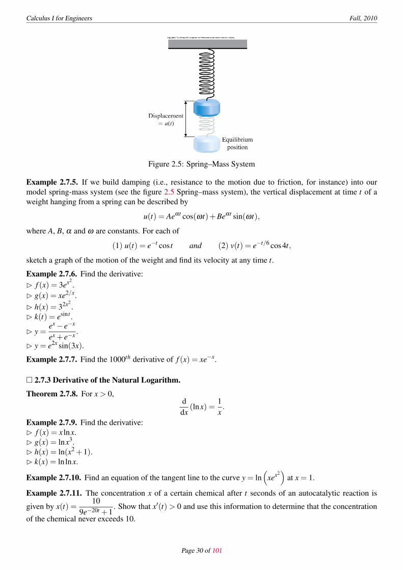
Figure 2.5: Spring–Mass System
Example 2.7.5. If we build damping (i.e., resistance to the motion due to friction, for instance) into ourmodel spring-mass system (see the figure 2.5 Spring–mass system), the vertical displacement at time t of aweight hanging from a spring can be described by
u(t) = Aeαt cos(ωt)+Beαt sin(ωt),
where A, B, α and ω are constants. For each of
(1) u(t) = e−t cos t and (2) v(t) = e−t/6 cos4t,
sketch a graph of the motion of the weight and find its velocity at any time t.
Example 2.7.6. Find the derivative:� f (x) = 3ex2
.� g(x) = xe2/x.� h(x) = 32x2
.� k(t) = esin t .
� y =ex − e−x
ex + e−x .
� y = e2x sin(3x).
Example 2.7.7. Find the 1000th derivative of f (x) = xe−x.
□ 2.7.3 Derivative of the Natural Logarithm.
Theorem 2.7.8. For x > 0,ddx
(lnx) =1x.
Example 2.7.9. Find the derivative:� f (x) = x lnx.� g(x) = lnx3.� h(x) = ln(x2 +1).� k(x) = ln lnx.
Example 2.7.10. Find an equation of the tangent line to the curve y = ln(
xex2)
at x = 1.
Example 2.7.11. The concentration x of a certain chemical after t seconds of an autocatalytic reaction is
given by x(t) =10
9e−20t +1. Show that x′(t)> 0 and use this information to determine that the concentration
of the chemical never exceeds 10.
Page 30 of 101

Calculus I for Engineers Fall, 2010
□ 2.7.4 Logarithmic Differentiation.A clever technique called logarithmic differentiation uses the rules of logarithms to help find derivatives ofcertain functions for which we don’t presently have derivative formulas. For instance, note that the functionf (x) = xx is neither a power function because the exponent is not a constant and nor an exponential functionbecause the base is not constant.
Example 2.7.12. Find the derivative:� f (x) = xx, x > 0.� g(x) = xlnx.� h(x) = xsinx.� k(x) = (cosx)x.
Example 2.7.13. Find y′ = dy/dx if yx = xy.
Page 31 of 101

Calculus I for Engineers Fall, 2010
§2.8 Implicit Differentiation and Inverse Trigonometric Functions.
□ 2.8.1 Implicit Differentiation.Suppose that x and y satisfy the equation
x2 + y2 = 4
whose graph is a circle centered at the origin with radius 2. Our goal is to describe the slope of the tangentline to the curve at each point (x,y). Just as in the case where y is a function of x, we can define dy/dx to bethe slope of the tangent line to the graph at a point (x,y). To find dy/dx, we proceed as follows:Step 1. Differentiate each side of the equation with respect to x:
ddx
(x2 + y2)= d
dx4,
ddx
x2 +ddx
y2 = 0, 2x+2ydydx
= 0.
The equation of the circle implies
x2 + y2 = 4 ⇐⇒ y2 = 4− x2 ⇐⇒ y =±√
4− x2 ,
i.e., y is a function of x and so y2 is a composite function having the variable x and thus the Chain Rule
impliesddx
y2 = 2ydydx
. Be careful! y is not a constant with respect to x.
Step 2. Solve for dy/dx:
2x+2ydydx
= 0, 2ydydx
=−2x,dydx
=−2x2y
=−xy.
This is the process known as implicit differentiation. As you can see, it is based on the Chain Rule.
Example 2.8.1. Suppose that x and y satisfy the equation
x2 − xy+ y2 = 1
whose graph is an ellipse. (1) Find dy/dx and (2) find the points on the ellipse where the tangent line ishorizontal or vertical.
Example 2.8.2. Find the slope of the tangent line to the graph of x3y2 = xy3 +6 at the point (2,1).
Example 2.8.3. Find y′(x) = dy/dx for x2 + y3 −2y = 3. Then, find the slope of the tangent line at the point(2,1).
Example 2.8.4. Find y′(x) = dy/dx for x2y2 −2x = 4−4y. Then, find an equation of the tangent line atx = 2.
Example 2.8.5. Suppose that van der Waals’ equation for a specific gas is(P+
5V 2
)(V −0.03) = 9.7.
Thinking of the volume V as a function of pressure P, use implicit differentiation to find the derivativedVdP
at
the point (P,V ) = (5,1).
Remark 2.8.6 (Aside: General Version of van der Waals’ equation).(P+
an2
V 2
)(V −nb) = nRT.
where P is the pressure of the fluid, V is the total volume of the container containing the fluid, a is a measureof the attraction between the particles, b is the volume excluded by a mole of particles, n is the number ofmoles, R is the gas constant and T is the absolute temperature.
If you are interested, finddPdV
,dVdT
anddTdP
and checkdPdV
dVdT
dTdP
=−1.
Page 32 of 101

Calculus I for Engineers Fall, 2010
Example 2.8.7. Find y′′(x) =d2ydx2 implicitly for y2 +2e−xy = 6. Then find the value of y′′ at the point (0,2).
Example 2.8.8. Use implicit differentiation to find an equation of the tangent line to the curve at the givenpoint:
(1) 2(x2 + y2)2 = 25(x2 − y2), (3,1); (2) y2 = x3 +3x2, (1,−2).
The graphs of (1) and (2) are called the lemniscate and the Tschirnhausen cubic, respectively. See thefigure 2.6.
Figure 2.6: Lemniscate 2(x2 + y2)2 = 25(x2 − y2) (Left) and Tschirnhausen Cubic y2 = x3 +3x2 (Right)
□ 2.8.2 Derivatives of the Inverse Trigonometric Functions.Let us recall from the Section 2.5 The Chain Rule: a function g is called the inverse function of f if( f ◦g)(x) = f (g(x)) = x and (g◦ f )(x) = g( f (x)) = x. The inverse function of f is denoted by f−1 andso g = f−1.The trigonometric functions have the inverse functions when we restrict the domains of sinx, cosx and tanx by[−π/2,π/2], [0,π] and [−π/2,π/2], respectively. The inverse functions of sinx, cosx and tanx are denotedby either sin−1 x, cos−1 x, and tan−1 x or arcsinx, arccosx and arctanx.But be careful!
arcsinx = sin−1 x = (sinx)−1 =1
sinx,
which is also same to other trigonometric functions.• Domain and Range of Inverse Trigonometric Functions
1. Considering the restricted domain [−π/2,π/2], sinx has the range [−1,1]. It implies that the inversefunction sin−1 x has the domain [−1,1] and the range [−π/2,π/2].
2. Considering the restricted domain [0,π], cosx has the range [−1,1]. It implies that the inverse functioncos−1 x has the domain [−1,1] and the range [0,π].
3. Considering the whole domain (−π/2,π/2), tanx has and range R. Its inverse function tan−1 x has thedomain R and range (−π/2,π/2).
See the figures 2.7, 2.8 and 2.9 below on the graphs of the trigonometric and inverse trigonometric functions.Using the implicit differentiation or derivatives of inverse functions in the Section 2.5 The Chain Rule, wededuce the following derivatives of the inverse trigonometric functions.
Theorem 2.8.9.
ddx
sin−1 x =1√
1− x2, (−1 < x < 1),
ddx
cos−1 x =− 1√1− x2
, (−1 < x < 1),
ddx
tan−1 x =1
1+ x2 ,ddx
cot−1 x =− 11+ x2 ,
Page 33 of 101

Calculus I for Engineers Fall, 2010
Figure 2.7: Graphs of sinx (Left) on [−π/2,π/2] and sin−1 x (Right) on [−1,1]
Figure 2.8: Graphs of cosx (Left) on [0,π] and cos−1 x (Right) on [−1,1]
Figure 2.9: Graphs of tanx (Left) on (−π/2,π/2) and tan−1 x (Right) on R
ddx
sec−1 x =1
|x|√
x2 −1, (|x|> 1),
ddx
csc−1 x =− 1|x|
√x2 −1
, (|x|> 1).
PROOF. Let us prove only the first result.
Page 34 of 101

Calculus I for Engineers Fall, 2010
(1) Implicit Differentiation Technique: Let y = sin−1 x. Then,
y = sin−1 x ⇐⇒ siny = x − π2≤ y ≤ π
2.
Implicitly differentiating the second equation, we get
cosydydx
=dxdx
= 1 ⇐⇒ dydx
=1
cosy.
The equation siny = x implies cosy =√
1− x2 , because sin2 y+ cos2 y = 1, i.e., cos2 y = 1− sin2 y = 1− x2
and −π/2 ≤ y ≤ π/2. Hence, the result becomes
dydx
=1
cosy=
1√1− x2
⇐⇒ ddx
sin−1 x =1√
1− x2−1 < x < 1.
(2) Formula on Derivative of Inverse Function (Section 2.5): Since g(x) = sin−1 x is the inverse of the sinefunction f (x) = sinx with −π/2 ≤ x ≤ π/2, the formula implies
g′(x) =1
f ′(g(x))⇐⇒ g′(x) =
1cosg(x)
⇐⇒ ddx
sin−1 x =1
cos(sin−1 x
) .Let sin−1 x = θ ∈ [−π/2,π/2]. Then x = sinθ and again sin2 θ + cos2 θ = 1 implies cos2 θ = 1− sin2 θ =1− x2 and cosθ =
√1− x2 (, because θ ∈ [−π/2,π/2]). Hence, the result becomes
dydx
=1
cos(sin−1 x
) = 1cosθ
=1√
1− x2⇐⇒ d
dxsin−1 x =
1√1− x2
−1 < x < 1. □
Example 2.8.10. Compute the derivative:� cos−1(3x2).� (sec−1 x
)2.
� tan−1(x3).
Example 2.8.11. One of the guiding principles of most sports is to “keep your eye on the ball.” In baseball,a batter stands 2 feet from home plate as a pitch is thrown with a velocity of 130 ft/s (about 90 mph). Atwhat rate does the batter’s angle of gaze need to change to follow the ball as it crosses home plate? See thefigure 2.10 below.
Figure 2.10: Baseball
§2.9 The Mean Value Theorem.Skip. Please read the textbook.
Page 35 of 101

Calculus I for Engineers Fall, 2010
Page 36 of 101

Chapter 3
Applications of Differentiation
§3.1 Linear Approximations and Newton’s Method.Skip. Please read the textbook.
§3.2 Indeterminate Forms and L’Hopital’s Rule.
□ 3.2.1 Introduction.For the given two polynomials,
P(x) = anxn +an−1xn−1 + · · ·+a2x2 +a1x+a0, and Q(x) = bmxm +bm−1xm−1 + · · ·+b2x2 +b1x+b0,
where a0, . . . ,an and b0, . . . ,bm are all constants, let us discuss the limit of the rational function P(x)/Q(x) asx → a.
(1) a is a number:(i) If Q(a) = 0 and P(a) = 0, then
limx→a
P(x)Q(x)
= some number.
(ii) If Q(a) = 0 but P(a) = 0, then
limx→a
P(x)Q(x)
=±∞.
(iii) If Q(a) = 0 but P(a) = 0, then
limx→a
P(x)Q(x)
= 0.
(iv) If Q(a) = 0 and P(a) = 0, then we use L’Hopital’s Rule (Subsection 3.2.3).(2) a =±∞:
(i) If degQ = m > n = degP, then
limx→a
P(x)Q(x)
= 0.
(ii) If degQ = m < n = degP, then
limx→a
P(x)Q(x)
=±∞.
(iii) If degQ = m = n = degP, then
limx→a
P(x)Q(x)
=an
bm.
Example 3.2.1. Evaluate the limit:
limx→1
x2 +5x+1
, limx→1
x2 +5x−1
, limx→1
x−1x2 +5
, limx→∞
x2 +1x3 +5
, limx→∞
x3 +5x2 +1
, limx→∞
2x2 +3x−5x2 +4x−11
.
We recall a useful theorem: Theorem 3.1 on page 88 (textbook) in Section 3.1 Computation of Limits.
Theorem 3.2.2. Suppose that limx→a
f (x) and limx→a
g(x) both exist and let c be any constant. The following thenapply:
37

Calculus I for Engineers Fall, 2010
(i) limx→a
[c · f (x)] = c · limx→a
f (x),
(ii) limx→a
[ f (x)±g(x)] = limx→a
f (x)± limx→a
g(x),
(iii) limx→a
[ f (x) ·g(x)] =[
limx→a
f (x)][
limx→a
g(x)],
(iv) limx→a
f (x)g(x)
=limx→a f (x)limx→a g(x)
(if limx→a g(x) = 0).
□ 3.2.2 Indeterminate Forms: 0/0 and Infinity/Infinity.In the previous subsection, we have discussed the limit of the rational function of polynomials. Now, weconsider a particular case with general functions f (x) and g(x),
limx→a
f (x)g(x)
.
If limx→a f (x) = 0 = limx→a g(x), then the limit is in the form of00
.
If limx→a f (x) =±∞ = limx→a g(x), then the limit is in the form of∞∞
.
Those two forms are called the indeterminate forms. We use L’Hopital’s Rule to compute those indetermi-nate forms.
□ 3.2.3 L’Hopital’s Rule.
Theorem 3.2.3. Suppose that f and g are differentiable on the interval (a,b), except possibly at some fixedpoint c ∈ (a,b) and that g′(x) = 0 on (a,b), except possibly at c.
Suppose further that limx→c
f (x)g(x)
has the indeterminate form00
or∞∞
and that limx→c
f ′(x)g′(x)
= L (or ±∞). Then,
limx→c
f (x)g(x)
= limx→c
f ′(x)g′(x)
.
The conclusion of Theorem 3.2.3 also holds if limx→cf (x)g(x) is replaced with any of the limits limx→c+
f (x)g(x) ,
limx→c−f (x)g(x) , limx→∞
f (x)g(x) or limx→−∞
f (x)g(x) . (In each case, we must make appropriate adjustments to the
hypotheses.)
Example 3.2.4. Evaluate the limit.
limθ→0
sinθθ
, limθ→0
1− cosθθ
, limθ→0
1− cosθsinθ
.
Example 3.2.5. Evaluate the limit.
limx→∞
ex
x, lim
x→∞
x2
ex , limx→∞
lnxex , lim
x→∞
ex
lnx.
Example 3.2.6. Evaluate the limit.
limx→0
x2
ex −1, lim
x→0+
lnxcscx
.
Page 38 of 101
Calculus I for Engineers Fall, 2010
□ 3.2.4 Other Indeterminate Forms.We study other indeterminate forms via examples.
Example 3.2.7 (∞−∞ form). Evaluate the limit.
limx→0
(1x2 −
1x4
), lim
x→0
(1
ln(x+1)− 1
x
).
Example 3.2.8 (0 ·∞ form). Evaluate limx→∞
1x
lnx.
Example 3.2.9 (1∞ form). Evaluate limx→1+
x1
x−1 .
Example 3.2.10 (00 form). Evaluate limx→0+
(sinx)x.
Example 3.2.11 (∞0 form). Evaluate limx→∞
(x+1)2x .
Page 39 of 101

Calculus I for Engineers Fall, 2010
§3.3 Maximum and Minimum Values.
□ 3.3.1 Absolute Extrema.
Definition 3.3.1. For a function f defined on a set S of real numbers and a number c ∈ S,
(1) f (c) is the absolute maximum of f on S if f (c)≥ f (x) for all x ∈ S and(2) f (c) is the absolute minimum of f on S if f (c)≤ f (x) for all x ∈ S.
An absolute maximum or an absolute minimum is referred to as an absolute extremum. If a function hasmore than one extremum, we refer to these as extrema (the plural form of extremum).
Example 3.3.2. Locate any absolute extrema of the given function on the given interval:� f (x) = x2 −9 on (−∞,∞).� f (x) = x2 −9 on (−3,3).� f (x) = x2 −9 on [−3,3].
We have seen that a function may or may not have absolute extrema, depending on the interval on which weare looking.
Example 3.3.3. Locate all absolute extrema of the given function on the given interval:
� f (x) =1x
on [−3,3].
� f (x) = cosx on (−∞,∞).
Example 3.3.4. From the graph of the function f (x) = x2, we see that this function has the absolute minimumvalue of f (0) = 0 at x = 0, but no absolute maximum value.
Example 3.3.5. From the graph of the function f (x) = x3, we see that this function has neither an absolutemaximum value nor an absolute minimum value. In fact, it has no local extreme values either.
Theorem 3.3.6 (Extreme Value Theorem). A continuous function f defined on a closed and bounded interval[a,b] attains both an absolute maximum and an absolute minimum on that interval. That is, if f is continuouson a closed and bounded interval [a,b], then f attains an absolute maximum value f (c) and an absoluteminimum value f (d) at some numbers c and d in [a,b].
Example 3.3.7. Find the absolute extrema of f (x) = 1/x on the interval [1,3].
□ 3.3.2 Local Extrema.
Definition 3.3.8.
(1) f (c) is a local maximum of f if f (c)≥ f (x) for all x in some open interval containing c.(2) f (c) is a local minimum of f if f (c)≤ f (x) for all x in some open interval containing c.
In either case, we call f (c) a local extremum of f .
Local maxima and minima (the plural forms of maximum and minimum, respectively) are sometimes referredto as relative maxima and minima, respectively.Notice from the figure above that each local extremum seems to occur either(i) at a point where the tangent line is horizontal (i.e., where f ′(x) = 0), or(ii) at a point where the tangent line is vertical (i.e., where f ′(x) is undefined), or(iii) at a corner (again, where f ′(x) is undefined).
Example 3.3.9. Locate any local extrema for the given function and describe the behavior of the derivativeat the local extremum: f (x) = 9− x2 and f (x) = |x|.
Page 40 of 101

Calculus I for Engineers Fall, 2010
Figure 3.1: Various Local Extrema
□ 3.3.3 Critical Number.
Definition 3.3.10. A number c is called a critical number of f if
(1) c is in the domain of f and(2) either f ′(c) = 0 or f ′(c) is undefined.
We recall the observation that local extrema occur only at points where the derivative is zero or undefined.We state this formally in a theorem.
Theorem 3.3.11 (Fermat’s Theorem). Suppose that f (c) is a local extremum (local maximum or local mini-mum). Then c must be a critical number of f , i.e., either f ′(c) = 0 or f ′(c) is undefined.
Example 3.3.12. Find the critical numbers and local extrema of the given function:� f (x) = 2x3 −3x2 −12x+5.� f (x) = (3x+1)2/3.� f (x) = x3/5(4− x).
Remark 3.3.13 (Very Important Remark). Fermat’s Theorem says that local extrema can occur only atcritical numbers. This does not say that there is a local extremum at every critical number.
Example 3.3.14. Find the critical numbers and local extrema of the given function: f (x)= x3 and f (x)= x1/3.
You should not forget the first condition on the critical number. The critical number must be in the domain ofthe function.
Example 3.3.15. Find all the critical numbers of f (x) =2x2
x+2.
We have observed that local extrema occur only at critical numbers and that continuous functions must havean absolute maximum and an absolute minimum on a closed, bounded interval. However, we haven’t yetreally been able to say how to find these extrema. The following Theorem is particularly useful.
Theorem 3.3.16 (CANDIDATE OF ABSOLUTE EXTREMA). Suppose that f is continuous on the closed in-terval [a,b]. Then, the absolute extrema of f must occur(i) either at an endpoint (a or b) of the interval, or (ii) at a critical number.
When we use the terms maximum, minimum or extremum without specifying absolute or local, we willalways be referring to absolute extrema.
Remark 3.3.17 (CLOSED INTERVAL METHOD). The Theorem above gives us a simple procedure for findingthe absolute extrema of a continuous function on a closed, bounded interval:
Page 41 of 101

Calculus I for Engineers Fall, 2010
Step 1. Find all critical numbers in the interval and compute function values at these points.Step 2. Compute function values at the endpoints.Step 3. The largest function value is the absolute maximum and the smallest function value is the absoluteminimum.
Example 3.3.18. Find the absolute extrema of the given function on the given interval:� f (x) = 2x3 −3x2 −12x+5 on [−2,4].� f (x) = 4x3 −8x2 +5x on [0,1].� f (x) = x3 −3x2 +1 on [−1/2,4].� f (x) = x+2cosx on [0,2π].
Sometimes we need to use a calculator or a computer for the computation.
Example 3.3.19. Find the absolute extrema of the given function on the given interval:� f (x) = 4x5/4 −8x1/4 on [0,4].� f (x) = x3 −5x+3sinx2 on [−2,2.5].
Page 42 of 101

Calculus I for Engineers Fall, 2010
§3.4 Increasing and Decreasing Functions.In this section, we see how to determine which critical numbers correspond to local extrema. At the sametime, we will learn more about the connection between the derivative and graphing.
□ 3.4.1 Increasing and Decreasing Functions.
Definition 3.4.1. For every x1, x2 ∈ I with x1 < x2,
1. f (x1)< f (x2) −→ f is (strictly) increasing on an interval I(i.e., f (x) gets larger as x gets larger).
2. f (x1)> f (x2) −→ f is (strictly) decreasing on an interval I(i.e., f (x) gets smaller as x gets larger).
Theorem 3.4.2. Suppose f is differentiable on an interval I.
1. f ′(x)> 0 for all x ∈ I −→ f is increasing on I.2. f ′(x)< 0 for all x ∈ I −→ f is decreasing on I.
Example 3.4.3. Find the intervals where the function is increasing or decreasing. (Hint: Sign Chart.)� f (x) = 3x4 −4x3 −12x2 +5.� y = x3 −3x2 −9x+1.� y = sin2 x.
Example 3.4.4. Draw a graph of the given function showing all local extrema:� f (x) = 2x3 +9x2 −24x−10.� f (x) = 3x4 +40x3 −0.06x2 −1.2x. (Hint: f ′(x) = 12(x−0.1)(x+0.1)(x+10).)
□ 3.4.2 Critical Point Classification.Given a critical number c of a function f , how can we tell whether f (c) is a local extreme value? And if it is,how can we tell whether it’s a local maximum or a local minimum?
Theorem 3.4.5 (First Derivative Test). Suppose that f is continuous on the interval [a,b] and c ∈ (a,b) is acritical number.
1. If f ′(x)> 0 for all x∈ (a,c) and f ′(x)< 0 for all x∈ (c,b) (i.e., f changes from increasing to decreasingat c), then f (c) is a local maximum.
2. If f ′(x)< 0 for all x∈ (a,c) and f ′(x)> 0 for all x∈ (c,b) (i.e., f changes from decreasing to increasingat c), then f (c) is a local minimum.
3. If f ′(x) has the same sign on (a,c) and (c,b), then f (c) is not a local extremum.
a c b Classification
f ′ + 0 − f (c) is a local maximum
f ′ − 0 + f (c) is a local minimum
f ′ + 0 + f (c) is not a local extremum
f ′ − 0 − f (c) is not a local extremum
Example 3.4.6. Find the local extrema of the given function. (Hint: Sign Chart.)� f (x) = 3x4 −4x3 −12x2 +5.� f (x) = x+2sinx on the interval [0,2π].� f (x) = 3x5 +5x3.� f (x) = 2x3 +9x2 −24x−10.
Page 43 of 101

Calculus I for Engineers Fall, 2010
� f (x) = x5/3 −3x2/3.
� f (x) =1− x
x2 .
� f (x) = x2/3(15x2 −72x+120).
Example 3.4.7. (1) Find all critical numbers and (2) use the First Derivative Test to classify each as thelocation of a local maximum, local minimum or neither.� y = x4 +4x3 −2.� y = xe−2x.� y =
x1+ x3 .
Page 44 of 101
Calculus I for Engineers Fall, 2010
§3.5 Concavity and the Second Derivative Test.
□ 3.5.1 Concavity.When we say the graph of a function is increasing, it is not clear because there are two types of increasinggraphs: concave up and concave down. Similarly, we have two types of decreasing graphs. So we have total4 types: increasing concave up, increasing concave down and decreasing concave up, decreasing concavedown. In this section, we use the Second Derivative Test to determine the concavity.
Definition 3.5.1. For a function f that is differentiable on an interval I, the graph of f is
1. concave up on I if f ′ is increasing on I or2. concave down on I if f ′ is decreasing on I.
Be Careful: The condition is about the increment of the derivative of f , not f itself.
Theorem 3.5.2. Suppose that f ′′ exists on an interval I.
1. f ′′(x)> 0 on I −→ the graph of f is concave up on I.2. f ′′(x)< 0 on I −→ the graph of f is concave down on I.
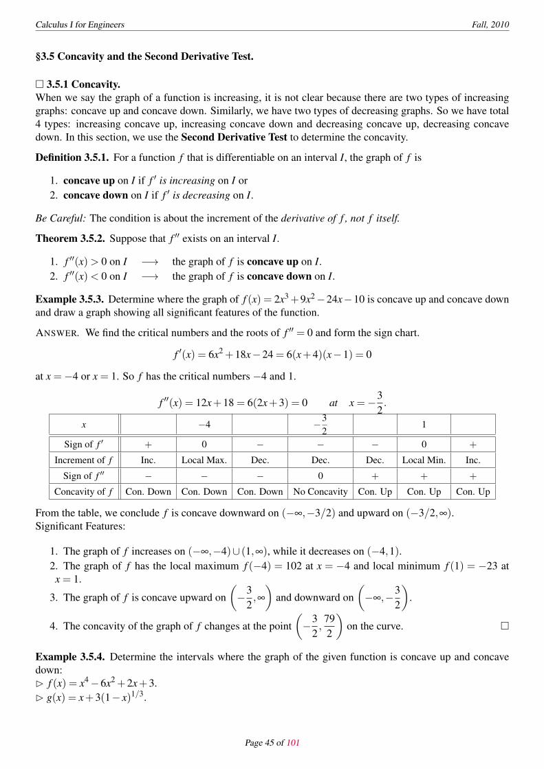
Example 3.5.3. Determine where the graph of f (x) = 2x3+9x2−24x−10 is concave up and concave downand draw a graph showing all significant features of the function.
ANSWER. We find the critical numbers and the roots of f ′′ = 0 and form the sign chart.
f ′(x) = 6x2 +18x−24 = 6(x+4)(x−1) = 0
at x =−4 or x = 1. So f has the critical numbers −4 and 1.
f ′′(x) = 12x+18 = 6(2x+3) = 0 at x =−32.
x −4 −32
1
Sign of f ′ + 0 − − − 0 +
Increment of f Inc. Local Max. Dec. Dec. Dec. Local Min. Inc.
Sign of f ′′ − − − 0 + + +
Concavity of f Con. Down Con. Down Con. Down No Concavity Con. Up Con. Up Con. Up
From the table, we conclude f is concave downward on (−∞,−3/2) and upward on (−3/2,∞).Significant Features:
1. The graph of f increases on (−∞,−4)∪ (1,∞), while it decreases on (−4,1).2. The graph of f has the local maximum f (−4) = 102 at x = −4 and local minimum f (1) = −23 atx = 1.
3. The graph of f is concave upward on(−3
2,∞)
and downward on(−∞,−3
2
).
4. The concavity of the graph of f changes at the point(−3
2,792
)on the curve. □
Example 3.5.4. Determine the intervals where the graph of the given function is concave up and concavedown:� f (x) = x4 −6x2 +2x+3.� g(x) = x+3(1− x)1/3.
Page 45 of 101

Calculus I for Engineers Fall, 2010
□ 3.5.2 Second Derivative Test.
Definition 3.5.5. Suppose that f is continuous on the interval (a,b) and that the graph changes concavity ata point c ∈ (a,b) (i.e., the graph is concave down on one side of c and concave up on the other). Then, thepoint (c, f (c)) is called an inflection point of f .
Example 3.5.6. Determine where the graph of the given function is concave up and concave down, find anyinflection points and draw a graph showing all significant features:� f (x) = x4 −6x2 +1.� g(x) = x4.
Theorem 3.5.7 (Second Derivative Test). Suppose that f is continuous on the interval (a,b) and f ′(c) = 0,for some number c ∈ (a,b).
1. f ′′(c)< 0 −→ f (c) is a local maximum.2. f ′′(c)> 0 −→ f (c) is a local minimum.
Example 3.5.8. Use the Second Derivative Test to find the local extrema of f (x) = x4 −8x2 +10.
ANSWER. We find the critical numbers and the roots of f ′′ = 0 and form the sign chart.
f ′(x) = 4x3 −16x = 4x(x−2)(x+2) = 0
at x = 0, −2 or x = 2. So f has the critical numbers 0 and −2 and 2.
f ′′(x) = 12x2 −16 = 12(
x− 2√3
)(x+
2√3
)= 0 at x =± 2√
3.
x −2 − 2√3
02√3
2
Sign of f ′′ + 0 − 0 +
Local Extrema of f (x) Local Min. Inflection Local Max. Inflection Local Min.
From the table (the third row of the table comes by the Second Derivative Test), we conclude that the graphof f has the local minimum values f (−2) = −6 = f (2), while it has the local maximum value f (0) = 10.Since the concavity of the graph changes at
(−2/
√3 ,10/9
)and
(2/
√3 ,10/9
), so they are the inflection
points of the graph. □
Example 3.5.9. Find all critical numbers and use the Second Derivative Test to determine all local extrema:� f (x) = x4 +4x2 +1.� g(x) = e−x2
.
Remark 3.5.10. If f ′′(c) = 0 or f ′′(c) is undefined, the Second Derivative Test yields no conclusion. Thatis, f (c) may be a local maximum, a local minimum or neither. In this event, we must rely solely on firstderivative information (i.e., the First Derivative Test) to determine whether f (c) is a local extremum.
Example 3.5.11. Use the Second Derivative Test to classify any local extrema:� f (x) = x3.� g(x) = x4.� h(x) =−x4.
Example 3.5.12. Draw a graph of the given function showing all significant features:
� f (x) = x+25x
.
� g(x) = (x+2)1/5 +4.
Page 46 of 101

Calculus I for Engineers Fall, 2010
Example 3.5.13. Determine all significant features by hand and sketch a graph:� f (x) = x lnx.� g(x) =
xx+2
.
§3.6 Overview of Curve Sketching.Skip. Please read the textbook.
Page 47 of 101

Calculus I for Engineers Fall, 2010
§3.7 Optimization.
□ 3.7.1 Guideline.We follow the guideline to solve an optimization problem.
1. If there’s a picture to draw, draw it! Don’t try to visualize how things look in your head. Put a picturedown on paper and label it.
2. Determine what the variables are and how they are related.3. Decide what quantity needs to be maximized or minimized.4. Write an expression for the quantity to be maximized or minimized in terms of only one variable. To do
this, you may need to solve for any other variables in terms of this one variable.5. Determine the minimum and maximum allowable values (if any) of the variable you’re using.6. Solve the problem. (Be sure to answer the question that is asked.)
□ 3.7.2 Area.
Figure 3.2: Rectangular Space
Example 3.7.1. You have 40 (linear) feet of fencing with which to enclose a rectangular space for a garden.Find the largest area that can be enclosed with this much fencing and the dimensions of the correspondinggarden. See the figure 3.2.
ANSWER. Let x and y be width and length of the rectangle, respectively. Then the area A is expressed by
A = xy. (3.7.1)
The given information implies2x+2y = 40 −→ x+ y = 20. (3.7.2)
That is, we want to find the maximum value of A = xy where x and y satisfies x+ y = 20.From the equation (3.7.2), we have y = 20− x. Putting it into the equation (3.7.1), we get
A(x) = x(20− x).
The maximum value of A(x) = x(20− x) occurs at the critical number x = 10, which implies y = 10. Thusthe largest area is A = 100. □Example 3.7.2. You have 8 (linear) feet of fencing with which to enclose a rectangular space for a garden.Find the largest area that can be enclosed with this much fencing and the dimensions of the correspondinggarden.
ANSWER. The largest area is A = 4 with width 2 and length 2. □
Example 3.7.3. Find the area of the largest rectangle that can be inscribed in the ellipsex2
a2 +y2
b2 = 1, wherea and b are nonzero constants.
Page 48 of 101

Calculus I for Engineers Fall, 2010
Figure 3.3: Cardboard
□ 3.7.3 Volume.
Example 3.7.4. A square sheet of cardboard 18′′ on a side is made into an open box (i.e., there’s no top),by cutting squares of equal size out of each corner and folding up the sides along the dotted lines. Find thedimensions of the box with the maximum volume. See the figure 3.3.
ANSWER. Let x be the length of one side of the square cut. Then the length of the side of the square sheetbecomes 18−2x. So the volume V of the box becomes V (x) = x(18−2x)2, because it has the width 18−2xand length 18−2x and height x. We want to maximize the volume V . From the graph of x(18−2x)2 or bythe argument on critical numbers and the maximum values, we deduce the maximum value of the volumeoccurs at the critical number x = 3. Thus the maximum volume is V = 432 with width 12, length 12, andheight 3. □
Example 3.7.5. A square sheet of cardboard 6′′ on a side is made into an open box (i.e., there’s no top),by cutting squares of equal size out of each corner and folding up the sides along the dotted lines. Find thedimensions of the box with the maximum volume.
ANSWER. The maximum volume is V = 16 with width 4, length 4 and height 1. □
Example 3.7.6. If 1200 cm2 of material is available to make a box with a square base and an open top, findthe largest possible volume of the box.
□ 3.7.4 Closest Point to Curve.
Example 3.7.7. Find the point on the parabola y = 9− x2 closest to the point (3,9). See the figure 3.4.
ANSWER. Using the usual distance formula, we find that the distance between the point (3,9) and any point(x,y) is
d =√(x−3)2 +(y−9)2 .
If the point (x,y) is on the parabola, it should satisfy the equation y = 9− x2. So the distance becomes
d =√
(x−3)2 +(9− x2 −9)2 =√(x−3)2 + x4
We want to find x minimizing the distance d. For easy computation, we find x minimizing d2. (Note thatx = a minimizes d if and only if x = a minimizes d2.)By the First Derivative Test and the techniques/concepts in previous sections, d2 has the minimum value 5 atx = 1. Therefore, the closest point on the parabola is (x,y) = (1,8) and the closest distance is
√5 . □
Page 49 of 101

Calculus I for Engineers Fall, 2010
Figure 3.4: Closest Point
Example 3.7.8. Find the point on the given curve closest to the given point:� y = x2 to the point (0,1).� y = 4x+7 to the origin.
Example 3.7.9. Find the points on the ellipse 4x2 + y2 = 4 that are farthest away from the point (1,0).
Remark 3.7.10 (Important!). Check the function values at the critical numbers and at the endpoints. Do notsimply assume (even by virtue of having only one critical number) that a given critical number correspondsto the extremum you are seeking.
□ 3.7.5 Soda Can & Highway.
Figure 3.5: Soda Can and Highway
Example 3.7.11. A soda can is to hold 12 fluid ounces. Find the dimensions that will minimize the amountof material used in its construction, assuming that the thickness of the material is uniform (i.e., the thicknessof the aluminum is the same everywhere in the can). See the figure 3.5.
ANSWER. Please read the textbook solution. □
Example 3.7.12. The state wants to build a new stretch of highway to link an existing bridge with a turnpikeinterchange, located 8 miles to the east and 8 miles to the south of the bridge. There is a 5–mile–wide stretchof marshland adjacent to the bridge that must be crossed. Given that the highway costs $10 million per mileto build over the marsh and only $7 million to build over dry land, how far to the east of the bridge shouldthe highway be when it crosses out of the marsh? See the figure 3.5.
Page 50 of 101
Calculus I for Engineers Fall, 2010
ANSWER. Total cost is obtained as follows:
Total cost = 10 × (distance across marsh) + 7 × (distance across dry land).
Letting x represent the distance in question, by the Pythagorean theorem, we get the cost function C(x) =10
√x2 +52 + 7
√(8− x)2 +32 . So we want to minimize this cost function. By the argument in previous
sections and using a calculator, we obtain the minimum value C(xc) ≈ $98.9 million at the critical numberxc ≈ 3.560052. □
The problems in this section are applications of derivatives, especially the arguments used in curve sketching.Definitely the problems are not easy to solve. As the first step of solving a word problem, you should be ableto set up the mathematical expressions and for this work, you need to practice by solving lots of problems.Solve Solve Solve Lots of Problems and Practice Practice Practice.
Page 51 of 101

Calculus I for Engineers Fall, 2010
§3.8 Related Rates.A problem on related rates is about setting up an equation of (usually) two different rates of change andsolving the equation for a desired rate of change.
□ 3.8.1 Spreading Oil.
Figure 3.6: Spreading Oil
Example 3.8.1. An oil tanker has an accident and oil pours out at the rate of 150 gallons per minute (i.e.,150/7.5 = 20 ft3/min). Suppose that the oil spreads onto the water in a circle at a thickness of 1/120 ft.Given that 1 ft3 equals 7.5 gallons, determine the rate at which the radius of the spill is increasing when theradius reaches 500 feet. See the figure 3.6.
ANSWER. Volume of the oil spreading onto the water is obtained by the multiplication of the depth of the oilin the water and the area covered by the oil, that is,• Key Equation in Spreading Oil Problem:
V = (depth) · (area) =1
120·πr2, i.e., V =
πr2
120
where r is the radius of the circle covered by the oil. As time passes by, the radius of the circle increases andso the volume also increases. It implies that r and V are functions of time t. The given information gives
dV (t)dt
=1507.5
= 20 ft3/min.
The problem is to finddrdt
when r = 500. Implicitly differentiating the equation above with respect to time t,we have
dV (t)dt
=ddt
(πr2(t)
120
)=
2πr(t)120
dr(t)dt
, i.e.,dr(t)
dt=
60πr(t)
dV (t)dt
.
Therefore, we deducedr(t)
dt
∣∣∣∣r(t)=500
=60
500π·20 =
2.4π
≈ 0.76394. □
Based on the example above, we may set up an outline for solving a problem of related rates.• Outline:
1. Make a simple sketch, if appropriate.2. Set up an equation relating all of the relevant quantities.3. Differentiate (implicitly) both sides of the equation with respect to time (t).4. Substitute in values for all known quantities and derivatives.
Page 52 of 101

Calculus I for Engineers Fall, 2010
5. Solve for the remaining rate.
Exercise 3.8.2. Oil spills out of a tanker at the rate of 12 ft3/min. The oil spreads in a circle with a thicknessof 1/96 ft. Determine the rate at which the radius of the spill is increasing when the radius reaches 100 feet.
Exercise 3.8.3. Oil spills out of a tanker at the rate of g ft3/min. The oil spreads in a circle with a thicknessof 1/48 ft. Given that the radius of the spill is increasing at a rate of 0.6 ft/min when the radius equals 100feet, determine the value of g.
□ 3.8.2 Ladder.
Figure 3.7: Ladder
Example 3.8.4. A 10–foot ladder leans against the side of a building. If the top of the ladder begins to slidedown the wall at the rate of 2 ft/sec, how fast is the bottom of the ladder sliding away from the wall when thetop of the ladder is 8 feet off the ground? See the figure 3.7.
ANSWER. Let x and y be the distance from the wall to the bottom of the ladder and the distance from theground to the top of the ladder, respectively. Then we observe the following three useful phenomena:
1. As x increases, y decreases and vice versa.2. We observe that both x and y are functions of time t.3. The faster the top of the ladder slides down, the faster the bottom moves away from the wall. That is,the speed y′(t) at which the top slides down is proportional to the one x′(t) at which the bottom movesaway.
Since the ladder is sliding down the wall at the rate of 2 ft/sec, we havedy(t)
dt=−2. (Note the minus sign.)
The Pythagorean Theorem implies• Key Equation in Ladder Problem:
x2(t)+ y2(t) = 102
Differentiating both sides of the equation with respect to time t gives us
2x(t)dx(t)
dt+2y(t)
dy(t)dt
= 0, i.e.,dx(t)
dt=−y(t)
x(t)dy(t)
dt=− y(t)√
100− y2(t)
dy(t)dt
.
When y(t) = 8, thus we deduce the speed x′(t) at which the bottom of the ladder moves away from the wall:
dx(t)dt
=− 8√100−82
(−2) =83. □
Exercise 3.8.5. A 10–foot ladder leans against the side of a building as in the example above. If the bottomof the ladder is pulled away from the wall at the rate of 3 ft/s and the ladder remains in contact with the wall,find the rate at which the top of the ladder is dropping when the bottom is 6 feet from the wall.
Page 53 of 101

Calculus I for Engineers Fall, 2010
Exercise 3.8.6. In the exercise above, find the rate at which the angle between the ladder and the horizontalis changing when the bottom of the ladder is 6 feet from the wall.
□ 3.8.3 Car Speed.
Figure 3.8: Car Speed
Example 3.8.7. A car is traveling at 50 mph due south at a point 1/2 mile north of an intersection. A policecar is traveling at 40 mph due west at a point 1/4 mile east of the same intersection. At that instant, theradar in the police car measures the rate at which the distance between the two cars is changing. What doesthe radar gun register? If the police car is not moving, does this make the radar gun’s measurement moreaccurate? See the figure 3.8.
ANSWER. Let x and y be the distance from the intersection to the police car and to the car, respectively. Thenwe observe
1. x and y are functions of time t,2. the distance d(t) between those two cars is obtained by the Pythagorean Theorem:
d2(t) = x2(t)+ y2(t),
3. x′(t) =−40 and y′(t) =−50 and it is asked to find d′(t).
Implicitly differentiating both sides of the equation with respect to t, we get
2d(t)d′(t) = 2x(t)x′(t)+2y(t)y′(t), d′(t) =x(t)x′(t)+ y(t)y′(t)
d(t)=
x(t)x′(t)+ y(t)y′(t)√x2(t)+ y2(t)
.
Thus when x(t) = 1/4 and y(t) = 1/2, we have
d′(t) =x(t)x′(t)+ y(t)y′(t)√
x2(t)+ y2(t)=
(1/4) · (−40)+(1/2) · (−50)√(1/4)2 +(1/2)2
≈−62.6.
and so the radar gun registers 62.6 mph. Note that this is a poor estimate of the car’s actual speed. For thisreason, police nearly always take radar measurements from a stationary position. □Exercise 3.8.8. A plane is located x = 40 miles (horizontally) away from an airport at an altitude of h miles.Radar at the airport detects that the distance s(t) between the plane and airport is changing at the rate ofs′(t) =−240 mph. If the plane flies toward the airport at the constant altitude h = 4, what is the speed |x′(t)|of the airplane? Based on your answers, how important is it to know the actual height of the airplane?
Page 54 of 101
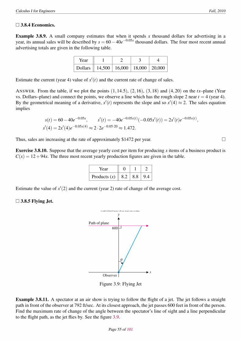
Calculus I for Engineers Fall, 2010
□ 3.8.4 Economics.
Example 3.8.9. A small company estimates that when it spends x thousand dollars for advertising in ayear, its annual sales will be described by s = 60−40e−0.05x thousand dollars. The four most recent annualadvertising totals are given in the following table.
Year 1 2 3 4
Dollars 14,500 16,000 18,000 20,000
Estimate the current (year 4) value of x′(t) and the current rate of change of sales.
ANSWER. From the table, if we plot the points (1,14.5), (2,16), (3,18) and (4,20) on the tx–plane (Yearvs. Dollars–plane) and connect the points, we observe a line which has the rough slope 2 near t = 4 (year 4).By the geometrical meaning of a derivative, x′(t) represents the slope and so x′(4) ≈ 2. The sales equationimplies
s(t) = 60−40e−0.05x, s′(t) =−40e−0.05x(t)(−0.05x′(t)) = 2x′(t)e−0.05x(t),
s′(4) = 2x′(4)e−0.05x(4) ≈ 2 ·2e−0.05·20 ≈ 1.472.
Thus, sales are increasing at the rate of approximately $1472 per year. □
Exercise 3.8.10. Suppose that the average yearly cost per item for producing x items of a business product isC(x) = 12+94x. The three most recent yearly production figures are given in the table.
Year 0 1 2
Products (x) 8.2 8.8 9.4
Estimate the value of x′(2) and the current (year 2) rate of change of the average cost.
□ 3.8.5 Flying Jet.
Figure 3.9: Flying Jet
Example 3.8.11. A spectator at an air show is trying to follow the flight of a jet. The jet follows a straightpath in front of the observer at 792 ft/sec. At its closest approach, the jet passes 600 feet in front of the person.Find the maximum rate of change of the angle between the spectator’s line of sight and a line perpendicularto the flight path, as the jet flies by. See the figure 3.9.
Page 55 of 101

Calculus I for Engineers Fall, 2010
ANSWER. Let the observer be at the origin (0,0) in the xy–plane and the line y(t) = 600 be the path of theflight. Then at time t, the plain is located at (x(t),y(t)). Let θ be the angle between the y–axis and the lineconnecting two points (0,0) and (x(t),y(t)). Since x(t) and y(t) depend on time t, the angle should also thefunction of time t.From triangle geometry, we have an equation• Key Equation in Flying Jet Problem:
tanθ(t) =x(t)y(t)
Implicitly differentiating the equation with respect to time t produces
(sec2 θ(t)
)θ ′(t) =
x′(t)y(t)− x(t)y′(t)y2(t)
, θ ′(t) =x′(t)y(t)− x(t)y′(t)
y2(t)cos2 θ(t).
With the jet moving left to right along the line y(t) = 600, we have y′(t) = 0 and x′(t) = 792. Plugging theminto the differential equation, we get
θ ′(t) =792 ·600− x(t) ·0
6002 cos2 θ(t) =792600
cos2 θ(t) = 1.32cos2 θ(t).
The maximum value of θ ′(t) is 1.32 and it occurs when cos2 θ(t) = 1, i.e., cosθ(t) =±1, i.e.,
θ(t) = 0,±π,±2π,±3π, . . . ,nπ,
where n = 0,±1,±2,±3, . . . . However, we cannot have other values of θ(t) except θ(t) = 0. (Why? Forexample, θ(t) = π means the plane flies along y(t) =−600 and it is not true.)Therefore, we conclude that the maximum rate of angle change is 1.32 radians/second. This occurs whenθ = 0, that is, when the jet reaches its closest point to the observer. (Think about this; it should match yourintuition!) Since humans can track objects at up to about 3 radians/second, this means that we can visuallyfollow even a fast jet at a very small distance. □
Exercise 3.8.12. A camera tracks the launch of a vertically ascending spacecraft. The camera is located atground level 2 miles from the launch–pad. If the spacecraft is 3 miles up and traveling at 0.2 mile per second,at what rate is the camera angle (measured from the horizontal) changing?
Exercise 3.8.13. Suppose a 6–ft–tall person is 12 ft away from an 18–ft–tall lamppost. If the person ismoving away from the lamppost at a rate of 2 ft/s, at what rate is the length of the shadow changing?
Exercise 3.8.14. Water is being pumped into a spherical tank of radius 60 feet at the constant rate of 10 ft3/s.Find the rate at which the radius of the top level of water in the tank changes when the tank is half full.
§3.9 Rates of Change in Economics and the Sciences.Skip. Please read the textbook.
Page 56 of 101

Chapter 4
Integration
§4.1 Antiderivatives.
□ 4.1.1 Antiderivative.Given a function f , we want to find another function F such that F ′ = f . We call such a function F anantiderivative of f .
Example 4.1.1. Find an antiderivative of f (x) = x2.
ANSWER. Notice that F(x) =x3
3is an antiderivative of f (x), because
F ′(x) =ddx
(x3
3
)= x2.
Further, observe thatddx
(x3
3+5)= x2,
so that G(x) =x3
3+5 is also an antiderivative of f . In fact, for any constant c, we have
ddx
(x3
3+ c)= x2.
Thus, H(x) =x3
3+ c is also an antiderivative of f (x), for any choice of the constant c. This gives us a family
of antiderivative curves. □
In general, observe that if F is any antiderivative of f and c is any constant, then
ddx
(F(x)+ c) = F ′(x)+0 = f (x).
Thus, F(x)+ c is also an antiderivative of f (x), for any constant c. On the other hand, are there any otherantiderivatives of f (x) besides F(x)+ c? The answer is no.
Theorem 4.1.2. Suppose that F and G are both antiderivatives of f on an interval I. Then,
G(x) = F(x)+ c
for some constant c.
□ 4.1.2 Indefinite Integral.
Definition 4.1.3. Let F be any antiderivative of f . The indefinite integral of f (x) (with respect to x), isdefined by ˆ
f (x) dx = F(x)+ c
where c is an arbitrary constant (the constant of integration).
57

Calculus I for Engineers Fall, 2010
The process of computing an integral is called integration. Here, f is called the integrand and the term dxidentifies x as the variable of integration.
Example 4.1.4. Evaluateˆ
3x2 dx.
ANSWER. You should recognize 3x2 as the derivative of x3 and so,ˆ
3x2 dx = x3 + c. □
Example 4.1.5. Evaluateˆ
t5 dt.
ANSWER. We know thatddt
(t6)= 6t5 and so,
ddt
(t6
6
)= t5. Therefore,
ˆt5 dt =
t6
6+ c. □
Theorem 4.1.6 (POWER RULE). For any rational (in fact, any real) power r =−1,
ˆxr dx =
xr+1
r+1+ c.
Example 4.1.7. Evaluateˆ
x17 dx.
ANSWER. From the power rule, we have
ˆx17 dx =
x17+1
17+1+ c =
x18
18+ c. □
Example 4.1.8. Evaluateˆ
1x3 dx.
ANSWER. We can use the power rule if we first rewrite the integrand. We have
ˆ1x3 dx =
ˆx−3 dx =
x−3+1
−3+1+ c =−x−2
2+ c =− 1
2x2 + c. □
Example 4.1.9. Evaluate the indefinite integrals: (1)ˆ √
x dx, (2)ˆ
13√
xdx.
ANSWER. (1) We first rewrite the integrand and then apply the power rule. We have
ˆ √x dx =
ˆx1/2 dx =
x1/2+1
1/2+1+ c =
x3/2
3/2+ c =
23
x3/2 + c.
(2) Similarly, ˆ13√
xdx =
ˆx−1/3 dx =
x−1/3+1
−1/3+1+ c =
x2/3
2/3+ c =
32
x2/3 + c. □
Page 58 of 101

Calculus I for Engineers Fall, 2010
By the differentiation rules, it is easy to get the following results:ˆ
xr dx =xr+1
r+1+ c, for r =−1
ˆsecx tanxdx = secx+ c
ˆsinxdx =−cosx+ c
ˆcscxcotxdx =−cscx+ c
ˆcosxdx = sinx+ c
ˆex dx = ex + c
ˆsec2 xdx = tanx+ c
ˆe−x dx =−e−x + c
ˆcsc2 xdx =−cotx+ c
ˆ1√
1− x2dx = sin−1 x+ c
ˆ1
1+ x2 dx = tan−1 x+ cˆ
1|x|
√x2 −1
dx = sec−1 x+ c
Theorem 4.1.10 (LINEARITY). Suppose that f and g have antiderivatives. Then, for any constants a and b,ˆ
[a f (x)+bg(x)] dx = aˆ
f (x)dx+bˆ
g(x)dx
Example 4.1.11. Evaluateˆ(3cosx+4x8)dx.
ANSWER.3ˆ
cosxdx+4ˆ
x8 dx = 3sinx+49
x9 + c. □
Example 4.1.12. Evaluateˆ (
3ex − 21+ x2
)dx.
ANSWER.3ˆ
ex dx−2ˆ
11+ x2 dx = 3ex −2tan−1 x+ c. □
Theorem 4.1.13. For x = 0,ddx
ln |x|= 1x
Example 4.1.14. For any x for which tanx = 0, evaluateddx
ln | tanx|.
ANSWER. By the chain rule, we have
ddx
ln | tanx|= (tanx)′
tanx=
sec2 xtanx
=1
sinxcosx. □
Corollary 4.1.15 (APPLICATION OF DERIVATIVE OF NATURAL LOG).ˆ
1x
dx = ln |x|+ c for x = 0ˆ
f ′(x)f (x)
dx = ln | f (x)|+ c when f (x) = 0
Example 4.1.16. Evaluateˆ
sec2 xtanx
dx.
Page 59 of 101

Calculus I for Engineers Fall, 2010
ANSWER. Notice that the numerator (sec2 x) is the derivative of the denominator (tanx). So we have
ˆsec2 xtanx
dx = ln | tanx|+ c. □
It is important to recognize when you cannot find an antiderivative.
Example 4.1.17. Which of the following integrals can you evaluate given the rules developed in this section?
(i)ˆ
13√x2
dx, (ii)ˆ
secxdx, (iii)ˆ
2xx2 +1
dx,
(iv)ˆ
x3 +1x
dx, (v)ˆ
(x+1)(x−1)dx, (vi)ˆ
xsin(2x)dx.
ANSWER. Parts (ii) and (vi) require us to find functions whose derivatives equal secx and xsin(2x). As yet,we cannot evaluate these integrals. □
Example 4.1.18. If an object’s downward acceleration is given by y′′(t)=−32 ft/s2, find the position functiony(t). Assume that the initial velocity is y′(0) =−100 ft/s and the initial position is y(0) = 100000 ft.
ANSWER. We have to undo two derivatives, so we compute two antiderivatives.(1) Antiderivative of acceleration gives the velocity of the object:
y′(t) =ˆ
y′′(t)dt =ˆ
−32dt =−32t + c.
Since y′(0) =−100, so c =−100 and y′(t) =−32t −100.(2) Antiderivative of velocity gives the position of the object:
y(t) =ˆ
y′(t)dt =ˆ
(−32t −100) dt =−16t2 −100t + c.
Since y(0) = 100000, so c = 100000 and thus y(t) =−16t2 −100t +100000.Keep in mind that this models the object’s height assuming that the only force acting on the object is gravity(i.e., there is no air drag or lift). □
§4.2 Sums and Sigma Notation.Skip. Please read the textbook.
§4.3 Area.Skip. Please read the textbook.
Page 60 of 101

Calculus I for Engineers Fall, 2010
§4.4 The Definite Integral.We have studied the antiderivative and indefinite integral of a function. The indefinite integral is also afunction for a fixed constant. For two points in the domain of the integral, we can consider the difference ofthe integral values at those points.
Theorem 4.4.1. If f is continuous on the closed interval [a,b], then f is integrable on [a,b].
This theorem says that for a function which is continuous on [a,b], the difference of the integral values at anytwo points in [a,b] exists uniquely as a finite number.
Theorem 4.4.2 (LINEARITY & SEPARATION). If f and g are integrable on [a,b], then the following are true.(1) For any constants c and d,
ˆ b
a[c f (x)+dg(x)] dx = c
ˆ b
af (x)dx+d
ˆ b
ag(x)dx
(2) For any c in [a,b], ˆ b
af (x)dx =
ˆ c
af (x)dx+
ˆ b
cf (x)dx
There are various types of averages: arithmetic average, geometric average, ensemble average, etc. Whenwe say the average, usually it means the arithmetic average. For example, the arithmetic average of threenumbers 4, 10, 1 is obtained by (4+ 10+ 1)/3 = 5. For a given function f on a closed interval [a,b], thefunction f has infinitely many values. How can we compute the arithmetic average of those function values?The average value, fave, is defined by
fave =1
b−a
ˆ b
af (x)dx
Example 4.4.3. Compute the average value of f (x) = sinx on the interval [0,π].
ANSWER.
fave =1
π −0
ˆ π
0sinxdx =
1π
ˆ π
0sinxdx =
2π. □
In next section, we will study how to compute the integral.
Page 61 of 101

Calculus I for Engineers Fall, 2010
§4.5 The Fundamental Theorem of Calculus.
□ 4.5.1 The Fundamental Theorem of Calculus.In this section, we will study one of the most important formulas in calculus, which is called the “fundamentaltheorem of calculus.”
Theorem 4.5.1 (FUNDAMENTAL THEOREM OF CALCULUS (FTC), PART I). If f is continuous on [a,b]and F is any antiderivative of f , then
ˆ b
af (x)dx = F(b)−F(a).
Remark 4.5.2. We will often use the notation[F(x)
]x=b
x=a= F(b)−F(a) or
[F(x)
]b
a= F(b)−F(a) or F(x)
∣∣∣ba= F(b)−F(a).
This enables us to write down the antiderivative before evaluating it at the endpoints.
Example 4.5.3. Computeˆ 2
0(x2 −2x)dx.
ANSWER. Notice that f (x)= x2−2x is continuous on the interval [0,2] and so, we can apply the FundamentalTheorem. We find an antiderivative by the power rule and simply evaluate:
ˆ 2
0(x2 −2x)dx =
(x3
3− x2
)∣∣∣∣20=
(83−4)−0 =−4
3. □
Example 4.5.4. Compute the definite integrals:
�ˆ 4
1
(√x − 1
x2
)dx.
�ˆ 4
0e−2x dx+
ˆ −1
−3
2x
dx+ˆ x
112t5 dt.
Example 4.5.5. Find the area of the region bounded by the curve f (x) = sinx and the x–axis on the interval[0,π].
Theorem 4.5.6 (FUNDAMENTAL THEOREM OF CALCULUS (FTC), PART II). If f is continuous on [a,b]and F(x) =
´ xa f (t)dt, then F ′(x) = f (x) on [a,b]. That is,
ddx
[ˆ x
af (t)dt
]= f (x).
Example 4.5.7. Find the derivative F ′:
� F(x) =ˆ x
1(t2 −2t +3)dt.
� F(x) =ˆ x2
2cos t dt.
The general form of the chain rule used in the 2nd example above is as follows.
Page 62 of 101

Calculus I for Engineers Fall, 2010
□ 4.5.2 Application of Fundamental Theorem of Calculus.
Corollary 4.5.8.
ddx
[ˆ u(x)
af (t)dt
]= f (u(x))
du(x)dx
ddx
[ˆ b
v(x)f (t)dt
]=− f (v(x))
dv(x)dx
ddx
[ˆ u(x)
v(x)f (t)dt
]= f (u(x))
du(x)dx
− f (v(x))dv(x)
dx
Example 4.5.9. Find the derivative of F(x) =ˆ x2
2x
√t2 +1 dt.
Example 4.5.10. Suppose the (downward) velocity of a sky diver is given by v(t) = 30(1− e−t) ft/s for the
first 5 seconds of a jump. Compute the distance fallen.
ANSWER. The distance d is obtained by the integral d =
ˆ 5
0v(t)dt = 120+30e−5 ≈ 120.2 ft. □
The definite integral of velocity gives the total change of the distance function over the given time interval.
Example 4.5.11. Suppose that water flows in and out of a storage tank. The net rate of change (that is, therate in minus the rate out) of water is f (t) = 20(t2 −1) gallons per minute.(1) For 0 ≤ t ≤ 3, determine when the water level is increasing and when the water level is decreasing.(2) If the tank has 200 gallons of water at time t = 0, determine how many gallons are in the tank at timet = 3.
ANSWER. Let w(t) be the number of gallons in the tank at time t.(1) Notice that the water level decreases if w′(t) = f (t)< 0. We have
f (t) = 20(t2 −1)< 0, for 0 ≤ t < 1.
Alternatively, the water level increases if w′(t) = f (t)> 0. In this case, we have
f (t) = 20(t2 −1)> 0, for 1 < t ≤ 3.
(2) We start with w′(t) = 20(t2 −1). Integrating from t = 0 to t = 3, we have
ˆ 3
0w′(t)dt =
ˆ 3
020(t2 −1)dt.
Evaluating the integrals on both sides yields
w(3)−w(0) = 20(
t3
3− t)∣∣∣∣t=3
t=0.
Since w(0) = 200, we have w(3)−200 = 20(9−3) = 120 and hence, w(3) = 200+120 = 320, so that thetank will have 320 gallons at time t = 3. □
Notice that although we don’t know how to evaluate the integral, we can use the Fundamental Theorem toobtain some important information about the function.
Page 63 of 101

Calculus I for Engineers Fall, 2010
Example 4.5.12. For the function F(x) =ˆ x2
4ln(t3 +4)dt, find an equation of the tangent line to the curve
of y = F(x) at x = 2.
ANSWER. Notice that there are almost no function values that we can compute exactly, yet we can easilyfind an equation of a tangent line! From Part II of the Fundamental Theorem of Calculus and the chain rule,we get the derivative
F ′(x) = 2x ln(x6 +4).
So, the slope at x = 2 is F ′(2) = 4ln68. The tangent lines passes through the point with x = 2 and so we get
y = F(2) =ˆ 4
4ln(t3 +4)dt = 0. An equation of the tangent line is then
y = (4ln68)(x−2). □
• Beyond Formulas: The two parts of the Fundamental Theorem are different sides of the same theoreticalcoin. Recall the conclusions of Parts I and II of the Fundamental Theorem:
ˆ b
aF ′(x)dx = F(b)−F(a) and
ddx
ˆ x
af (t)dt = f (x).
In both cases, we are saying that differentiation and integration are in some sense inverse operations: theireffects (with appropriate hypotheses) cancel each other out. This fundamental connection is what unifiesseemingly unrelated calculation techniques into the calculus. What are some results in algebra and trigonom-etry that similarly tie together different areas of study and are thus fundamental results?
Page 64 of 101

Calculus I for Engineers Fall, 2010
§4.6 Integration by Substitution.
□ 4.6.1 Introduction.In this section, we expand our ability to compute antiderivatives by developing a useful technique calledintegration by substitution. This method gives us a process for helping to recognize a whole range of newantiderivatives.
Example 4.6.1. Evaluateˆ
2xex2dx.
ANSWER. Notice that 2x is the derivative of x2 and x2 already appears in the integrand, as the exponent ofex2
. Further, by the chain rule, for F(x) = ex2,
F ′(x) = ex2 ddx
(x2) = 2xex2,
which is the integrand. To finish this example, recall that we need to add an arbitrary constant, to get
ˆ2xex2
dx = ex2+ c. □
Note that, in general, if F is any antiderivative of f , then from the chain rule, we have
ddx
[F(u)] = F ′(u)dudx
= f (u)dudx
.
From this, we have thatˆ
f (u)dudx
dx =ˆ
ddx
[F(u)]dx = F(u)+ c =ˆ
f (u)du,
since F is an antiderivative of f . If you read the expressions on the far left and the far right sides of theequation above, this suggests that
du =dudx
dx.
So, if we cannot compute the integralˆ
h(x)dx directly, we often look for a new variable u and function f (u)
for which ˆh(x)dx =
ˆf (u(x))
dudx
dx =ˆ
f (u)du,
where the last integral is easier to evaluate than the first.
Remark 4.6.2 (HOW TO CHOOSE NEW VARIABLE). In deciding how to choose a new variable, there areseveral things to look for:
1. terms that are derivatives of other terms (or pieces thereof ) and2. terms that are particularly troublesome. (You can often substitute your troubles away.)
Example 4.6.3. Evaluateˆ
(x3 +5)100(3x2)dx.
Page 65 of 101

Calculus I for Engineers Fall, 2010
□ 4.6.2 Integration By Substitution.Integration by substitution consists of the following general steps.
1. Choose a new variable u: a common choice is the innermost expression or “inside” term of a compositionof functions. (In example above, note that x3 +5 is the inside term of (x3 +5)100.)
2. Compute du =dudx
dx.
3. Replace all terms in the original integrand with expressions involving u and du.4. Evaluate the resulting (u) integral. If you still can’t evaluate the integral, you may need to try a different
choice of u.5. Replace each occurrence of u in the antiderivative with the corresponding expression in x.
Always keep in mind that finding antiderivatives is the reverse process of finding derivatives. In examplebelow, we are not so fortunate as to have the exact derivative we want in the integrand.
Example 4.6.4. Evaluate the integrals:
�ˆ
xcos(x2)dx.
�ˆ
(3sinx+4)5 cosxdx.
�ˆ
sin√
x√x
dx.
�ˆ
x2
x3 +5dx.
The last example is an illustration of a very common type of integral, one where the numerator is the derivativeof the denominator More generally, we have the result in the following Theorem.
Theorem 4.6.5 (INTEGRATION BY SUBSTITUTION INVOLVED WITH LOGARITHMIC DIFFERENTIATION).For any continuous function f , ˆ
f ′(x)f (x)
dx = ln | f (x)|+ c
provided f (x) = 0.
You should recall that we already stated this result in section 4.1. It is important enough to repeat here in thecontext of substitution.
Example 4.6.6. Evaluate the integrals:
�ˆ
tanxdx.
�ˆ
(tan−1 x)2
1+ x2 dx.
So far, every one of our examples has been solved by spotting a term in the integrand that was the derivativeof another term. We present an integral now where this is not the case, but where a substitution is made todeal with a particularly troublesome term in the integrand.
Example 4.6.7. Evaluateˆ
x√
2− x dx.
Page 66 of 101

Calculus I for Engineers Fall, 2010
□ 4.6.3 Integration By Substitution in Definite Integral.There is only one slight difference in using substitution for evaluating a definite integral: you must alsochange the limits of integration to correspond to the new variable. The procedure here is then preciselythe same as that used for example above, except that when you introduce the new variable u, the limits ofintegration change from x = a and x = b to the corresponding limits for u : u = u(a) and u = u(b). We have
ˆ x=b
x=af (u(x))u′(x)dx =
ˆ u=u(b)
u=u(a)f (u)du.
Caution! You must change the limits of integration (i.e., endpoints of the interval in the definite integral)as soon as you change variables!
Example 4.6.8. Evaluateˆ 2
1x3√
x4 +5 dx.
It may have occurred to you that you could use a substitution in a definite integral only to find an antiderivativeand then switch back to the original variable to do the evaluation. Although this method will work for manyproblems, we recommend that you avoid it, for several reasons. First, changing the limits of integration is notvery difficult and results in a much more readable mathematical expression. Second, in many applicationsrequiring substitution, you will need to change the limits of integration, so you might as well get used todoing so now. See and compare the two solutions to the following problem.
Example 4.6.9. Computeˆ 3
0te−
t22 dt.
ANSWER 1. RECOMMENDABLE. The substitution u =−t2/2 implies du =−t dt. The endpoints t = 0 andt = 3 of the integral interval correspond to u = 0 and u =−9/2, respectively. Thus, the definite integral isconverted and computed:
ˆ t=3
t=0te−
t22 dt =−
ˆ u=− 92
u=0eu du =− [eu]
u=− 92
u=0 =−e−92 +1. □
ANSWER 2. NOT RECOMMENDABLE. The substitution u =−t2/2 implies du =−t dt. So the indefiniteintegral is converted and the definite integral is computed:
ˆte−
t22 dt =−
ˆeu du =−eu + c =−e−
t22 + c −→
ˆ t=3
t=0te−
t22 dt =−
[e−
t22
]t=3
t=0=−e
92 +1. □
§4.7 Numerical Integration.Skip. Please read the textbook.
Page 67 of 101

Calculus I for Engineers Fall, 2010
§4.8 The Natural Logarithm as an Integral.
Definition 4.8.1. For x > 0, we define the natural logarithm function, written lnx, by
lnx =ˆ x
1
1t
dt.
We recall the Properties of Logarithmic Function: For any positive real numbers a and b and any rationalnumber r,
ln1 = 0 ln(ab) = lna+ lnb
ln(a
b
)= lna− lnb ln(ar) = r lna.
and also recall the Basic Properties of Exponential Function:
elnx = x (for x > 0), lnex = x, eres = er+s,er
es = er−s, (er)t = ert ,
where r and s are any real numbers and t is any rational number. It is also worth to memorize
bx = elnbx= ex lnb, for b > 0.
Theorem 4.8.2. For any base a > 0 (a = 1) and any x > 0,
loga x =lnxlna
.
Page 68 of 101

Chapter 5
Applications of the Definite Integral
§5.1 Area Between Curves.
□ 5.1.1 Region Bounded by Upper and Lower Curves.Let us start with recalling that the area A of the region under the curve y = f (x) and above the x–axis fromx = a to x = b is
A =
ˆ b
af (x)dx.
In fact, the full expression of this equation is as follows:
A =
ˆ x=b
x=a( f (x)−0) dx,
where y = 0 represents the x–axis. By generalizing this argument, the area A of the region under the graph ofy = f (x) (upper one) and above the graph of y = g(x) (lower one) from x = a to x = b is
A =
ˆ x=b
x=a( f (x)−g(x)) dx.
We summarize in the Theorem.
Theorem 5.1.1. The region between two graphs y = f (x) (upper one) and y = g(x) (lower one) from x = ato x = b has the area A:
A =
ˆ x=b
x=a( f (x)−g(x)) dx.
Remark 5.1.2. The formula above is valid only when the graph of y = f (x) is higher than the graph ofy = g(x) on the interval [a,b]. The area A of the region under the x–axis and above the graph of y = f (x) fromx = a to x = b is
A =
ˆ b
a(0− f (x)) dx.
Example 5.1.3. Sketch and find the area of the region bounded by the graphs of y = x2 −1 and y = x2/2.
Figure 5.1: Region Bounded by y = x2 −1 and y = x2/2
69
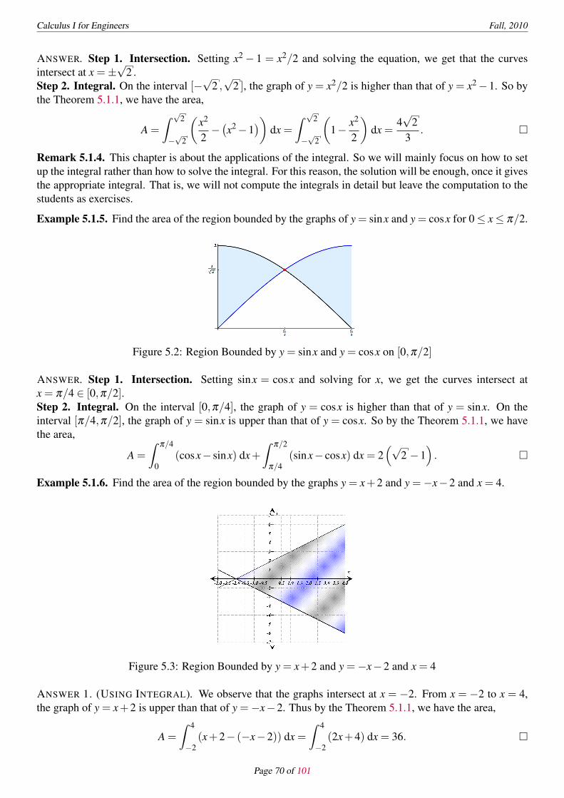
Calculus I for Engineers Fall, 2010
ANSWER. Step 1. Intersection. Setting x2 − 1 = x2/2 and solving the equation, we get that the curvesintersect at x =±
√2 .
Step 2. Integral. On the interval [−√
2 ,√
2 ], the graph of y = x2/2 is higher than that of y = x2 −1. So bythe Theorem 5.1.1, we have the area,
A =
ˆ √2
−√
2
(x2
2−(x2 −1
))dx =
ˆ √2
−√
2
(1− x2
2
)dx =
4√
23
. □
Remark 5.1.4. This chapter is about the applications of the integral. So we will mainly focus on how to setup the integral rather than how to solve the integral. For this reason, the solution will be enough, once it givesthe appropriate integral. That is, we will not compute the integrals in detail but leave the computation to thestudents as exercises.
Example 5.1.5. Find the area of the region bounded by the graphs of y = sinx and y = cosx for 0 ≤ x ≤ π/2.
Figure 5.2: Region Bounded by y = sinx and y = cosx on [0,π/2]
ANSWER. Step 1. Intersection. Setting sinx = cosx and solving for x, we get the curves intersect atx = π/4 ∈ [0,π/2].Step 2. Integral. On the interval [0,π/4], the graph of y = cosx is higher than that of y = sinx. On theinterval [π/4,π/2], the graph of y = sinx is upper than that of y = cosx. So by the Theorem 5.1.1, we havethe area,
A =
ˆ π/4
0(cosx− sinx) dx+
ˆ π/2
π/4(sinx− cosx) dx = 2
(√2 −1
). □
Example 5.1.6. Find the area of the region bounded by the graphs y = x+2 and y =−x−2 and x = 4.
Figure 5.3: Region Bounded by y = x+2 and y =−x−2 and x = 4
ANSWER 1. (USING INTEGRAL). We observe that the graphs intersect at x = −2. From x = −2 to x = 4,the graph of y = x+2 is upper than that of y =−x−2. Thus by the Theorem 5.1.1, we have the area,
A =
ˆ 4
−2(x+2− (−x−2)) dx =
ˆ 4
−2(2x+4) dx = 36. □
Page 70 of 101

Calculus I for Engineers Fall, 2010
ANSWER 2. (USING FIGURE). If we look at the figure 5.3, then we observe the region is in fact a lyingtriangle with base length 12 and height 6. Hence, the triangle has the area 12(6)(1/2) = 36, which is exactlysame as in the solution above. It is easy to see that this way of solving is much better than the solution above(using integral). The key point to be aware of is to sketch the region and find an easier way than using theintegral. □
□ 5.1.2 Region Bounded by Right and Left Curves.As the second topic of this section, we consider the region bounded by two graphs x = f (y) and x = g(y).
Theorem 5.1.7. The area A of the region bounded by x = f (y) (right boundary curve) and x = g(y) (leftboundary curve) from y = c to y = d is obtained as follows:
A =
ˆ y=d
y=c( f (y)−g(y)) dy.
Example 5.1.8. Find the area of the region bounded by the graphs of y = x−1 and y2 = 2x+6.
Figure 5.4: Region Bounded by y = x−1 and y2 = 2x+6 and Region Bounded by x = 3y and x = 2+ y2
ANSWER. Step 1. Intersection. Setting up y+ 1 = x = (y2 − 6)/2 and solving the equation y+ 1 = (y2 −6)/2, we have that the curves intersect at y =−2 and y = 4.Step 2. Integral. On the interval [−2,4], the graph of x = y+ 1 is the right boundary curve while that ofx = y2/2−3 is the left boundary curve of the region. Hence, by the Theorem 5.1.7, we have the area,
A =
ˆ 4
−2
(y+1−
(y2
2−3))
dy =ˆ 4
−2
(y− y2
2+4)
dy = 18. □
Example 5.1.9. Find the area of the region bounded by the graphs of x = 3y and x = 2+ y2.
ANSWER. Step 1. Intersection. Setting up 3y = x = 2+ y2 and solving the equation 3y = 2+ y2, we havethat the curves intersect at y = 1 and y = 2.Step 2. Integral. On the interval [1,2], the graph of x = 3y is the right boundary curve while that of x = 2+y2
is the left boundary curve of the region. Hence, by the Theorem, we have the area,
A =
ˆ 2
1
(3y−
(2+ y2)) dy =
ˆ 2
1
(3y−2− y2) dy =
16. □
Page 71 of 101

Calculus I for Engineers Fall, 2010
§5.2 Volume: Slicing, Disks and Washers.Let us start with recalling that a line can be viewed as the collection of points, the area inside a region canbe viewed as the collection of lengths of lines crossing the region, and the volume of a solid can be viewedas the collection of cross–sectional areas. From these viewpoints, a line is described by f (x) for a ≤ x ≤ b,the area is A =
´ ba f (x)dx and finally the volume is V =
´ ba A(x)dx, where A(x) is the cross–sectional area. In
this section, we study on how to find the volume.
□ 5.2.1 Volume by Slicing.Consider a cylinder (= any solid whose cross sections perpendicular to some axis running through the solidare all the same), e.g., pyramid.In general, the volume of any cylinder is found by
V = (cross–sectional area)× (height).
When we express this formula by using the integral, we have the formula,
V =
ˆ b
aA(x)dx,
where A(x) represents the cross–sectional area of the cylinder at height x. In fact, when we collect(= in-tegrate) all the cross–sectional areas(= A(x)) within the given height(= [a,b]), we obtain the volume(=´ b
a A(x)dx).
Example 5.2.1. For the tent given in the figure 5.5, find the volume.
Figure 5.5: Tent
ANSWER. If we cut the tent cross–sectionally and vertically, we observe the cross section is a triangle withbase 4 and height 10. It has the area 4(10)(1/2) = 20. Since the width of the tent is 38, the volume is obtainedby V = 20(38) = 760. □
Example 5.2.2. The Pyramid Arena in Memphis has a square base of side approximately 600 feet and a heightof approximately 320 feet. See the figure 5.6. Find the volume of the pyramid with these measurements.
ANSWER 1. By the formula, we get
V =
ˆ 320
0A(x)dx,
where A(x) is the cross–sectional area at height x. If f (x) represents the side length of the square cross sectionat height x, we know that f (0) = 600, f (320) = 0 and f (x) is a linear function. The slope of the line is
m =600−00−320
=−158
Page 72 of 101

Calculus I for Engineers Fall, 2010
Figure 5.6: The Pyramid Arena in Memphis and Projection
and we use the y–intercept of 600 to get
f (x) =−158
x+600.
Since this is the length of a side of a square, the cross–sectional area is simply the square of this quantity, i.e.,
A(x) = f 2(x) =(−15
8x+600
)2
.
Therefore, we deduce
V =
ˆ 320
0A(x)dx =
ˆ 320
0
(−15
8x+600
)2
dx = 38,400,000 ft2. □
ANSWER 2. Look at the figure 5.6. When we lay down the pyramid and see from one side of the pyramid,we can get the figure above. The equations of the upper and lower lines are easy to be found:
f (x) =−300320
x+300 =−1516
x+300 (Upper Line)
g(x) =300320
x−300 =1516
x−300 (Lower Line)
It implies that for a fixed x, we have the length of a side of a square,
f (x)−g(x) =−158
x+600,
and thus the cross–sectional area is simply the square of this quantity, i.e.,
A(x) = ( f (x)−g(x))2 =
(−15
8x+600
)2
.
Therefore, we deduce
V =
ˆ 320
0A(x)dx =
ˆ 320
0
(−15
8x+600
)2
dx = 38,400,000 ft2. □
Exercise 5.2.3. A church steeple is 30 feet tall with square cross sections. The square at the base has side 3feet and the side varies linearly in between. Compute the volume.
Page 73 of 101

Calculus I for Engineers Fall, 2010
Exercise 5.2.4. A church steeple is 30 feet tall with square cross sections. The square at the base has side 3feet, the square at the top has side 1/2 feet and the side varies linearly in between. Compute the volume.
Example 5.2.5. Suppose that a dome has circular cross sections, with outline
y =±√
452(90− x) (0 ≤ x ≤ 90).
Find the volume of the dome.
Figure 5.7: Graph of y =±√
452 (90− x) on [0,90]
ANSWER. The (vertical) cross section is a circle of radius√
(45/2)(90− x) . So the area inside the circle isπ(45/2)(90− x) and the volume is obtained as follows:
V =
ˆ 90
0A(x)dx =
45π2
ˆ 90
0(90− x) dx = 91125π. □
Exercise 5.2.6. The outline of a dome is given by
y = 60− x2
60, (−60 ≤ x ≤ 60),
with circular cross–sections perpendicular to the y–axis. Find its volume.
□ 5.2.2 Method of Disks.We use this method to get the volume of a solid of revolution.Suppose that 0 ≤ f (x) and f is continuous on the interval [a,b]. Take the region bounded by the curvey = f (x) and the x–axis, for a ≤ x ≤ b, and revolve it about the x–axis, generating a solid. We can find thevolume of this solid by slicing it perpendicular to the x–axis and recognizing that each cross section is acircular disk of radius r = f (x). Then we have that the volume of the solid is
V =
ˆ b
a(cross–sectional area πr2)dr =
ˆ b
aπ f 2(x)dx.
Example 5.2.7. Revolve the region under the curve y =√
x on the interval [0,4] about the x–axis and findthe volume of the resulting solid of revolution.
ANSWER. It’s critical to draw a picture of the region and the solid of revolution, so that you get a clear ideaof the radii of the circular cross sections. The radius of each cross section is given by r =
√x . We get the
volume:
V =
ˆ 4
0π(√
x)2 dx =
ˆ 4
0πxdx. □
Page 74 of 101

Calculus I for Engineers Fall, 2010
Figure 5.8: Solid formed by revolving region under y =√
x on [0,4] about x–axis
Exercise 5.2.8. Find the volume of the solid which is formed by revolving the region bounded by y = 2− x,x = 0, and y = 0 about the x–axis.
In a similar way, suppose that 0 ≤ g(y) and g is continuous on the interval [c,d]. Then, revolving the regionbounded by the curve x = g(y) and the y–axis, for c ≤ y ≤ d, about the y–axis generates a solid. Once again,the cross sections of the resulting solid of revolution are circular disks of radius r = g(y). All that has changedhere is that we have interchanged the roles of the variables x and y. The volume of the solid is then given by
V =
ˆ d
c(cross–sectional area πr2)dr =
ˆ d
cπg2(y)dy.
Example 5.2.9. Find the volume of the solid resulting from revolving the region bounded by the curvesy = 4− x2 and y = 1 from x = 0 to x =
√3 about the y–axis.
Figure 5.9: Solid formed by revolving region between y = 4− x2 and y = 1 on [0,√
3 ] about y–axis
ANSWER. The radius of any of the circular cross sections is given by x. So, we must solve the equationy = 4− x2 for x, to get x =
√4− y . Since the surface extends from y = 1 to y = 4, the volume is given by
V =
ˆ 4
1π(√
4− y)2
dy =ˆ 4
1π (4− y) dy. □
Exercise 5.2.10. Find the volume of the solid which is formed by revolving the region bounded by y = ex,x = 0, and y = e about the y–axis.
Page 75 of 101

Calculus I for Engineers Fall, 2010
□ 5.2.3 Method of Washers.A solid may have a cavity or “hole” in it. It occurs when a region is revolved about a line other than thex–axis or the y–axis. We explain the method through an example.
Example 5.2.11. Let R be the region in the first quadrant bounded by the graphs of y = x2/4 and y = 1.Compute the volume of the solid formed by revolving R about (1) the y–axis, (2) the x–axis and (3) the liney = 2.
Figure 5.10: Region in the first quadrant bounded by y = x2/4, x = 0 and y = 1
ANSWER. (1) the y–axis: The radius of the solid is x =√
4y . Hence, by the formula,
V =
ˆ 1
0π(√
4y)2
dy = 4πˆ 1
0ydy.
(2) the x–axis: Revolving the region R about the x–axis produces a cavity in the middle of the solid. Ourstrategy is to compute the volume Voutside of the outside of the object (as if it were filled in) and then subtractthe volume Vinside of the cavity.The solid of the outside of the object has the radius y = 1, while the one inside has y = x2/4. Hence,
V =Voutside −Vinside =
ˆ 2
0π12 dx−
ˆ 2
0π(
x2
4
)2
dx = πˆ 2
0
(1− x4
16
)dx.
(3) the line y = 2: Just like the case (2) above, we have a cavity in the middle of the solid. In this case, thesolid of the outside of the object has the radius y = 2− x2/4, while the one inside has y = 2−1. Hence,
V =Voutside −Vinside =
ˆ 2
0π(
2− x2
4
)2
dx−ˆ 2
0π (2−1)2 dx = π
ˆ 2
0
(4− x2 +
x4
16−1)
dx. □
Exercise 5.2.12. Let R be the region bounded by y = x2 and y = 4. Compute the volume of the solid formedby revolving R about the given line. (1) y = 4, (2) the y–axis, (3) y = 6, (4) y =−2, (5) x = 2, (6) x =−4.
Page 76 of 101
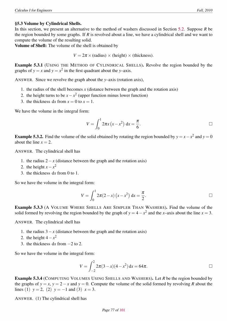
Calculus I for Engineers Fall, 2010
§5.3 Volume by Cylindrical Shells.In this section, we present an alternative to the method of washers discussed in Section 5.2. Suppose R bethe region bounded by some graphs. If R is revolved about a line, we have a cylindrical shell and we want tocompute the volume of the resulting solid.Volume of Shell: The volume of the shell is obtained by
V = 2π × (radius) × (height) × (thickness).
Example 5.3.1 (USING THE METHOD OF CYLINDRICAL SHELLS). Revolve the region bounded by thegraphs of y = x and y = x2 in the first quadrant about the y–axis.
ANSWER. Since we revolve the graph about the y–axis (rotation axis),
1. the radius of the shell becomes x (distance between the graph and the rotation axis)2. the height turns to be x− x2 (upper function minus lower function)3. the thickness dx from x = 0 to x = 1.
We have the volume in the integral form:
V =
ˆ 1
02πx
(x− x2) dx =
π6. □
Example 5.3.2. Find the volume of the solid obtained by rotating the region bounded by y = x−x2 and y = 0about the line x = 2.
ANSWER. The cylindrical shell has
1. the radius 2− x (distance between the graph and the rotation axis)2. the height x− x2
3. the thickness dx from 0 to 1.
So we have the volume in the integral form:
V =
ˆ 1
02π(2− x)
(x− x2) dx =
π2. □
Example 5.3.3 (A VOLUME WHERE SHELLS ARE SIMPLER THAN WASHERS). Find the volume of thesolid formed by revolving the region bounded by the graph of y = 4− x2 and the x–axis about the line x = 3.
ANSWER. The cylindrical shell has
1. the radius 3− x (distance between the graph and the rotation axis)2. the height 4− x2
3. the thickness dx from −2 to 2.
So we have the volume in the integral form:
V =
ˆ 2
−22π(3− x)(4− x2)dx = 64π. □
Example 5.3.4 (COMPUTING VOLUMES USING SHELLS AND WASHERS). Let R be the region bounded bythe graphs of y = x, y = 2− x and y = 0. Compute the volume of the solid formed by revolving R about thelines (1) y = 2, (2) y =−1 and (3) x = 3.
ANSWER. (1) The cylindrical shell has
Page 77 of 101

Calculus I for Engineers Fall, 2010
1. the radius 2− y (distance between the graph and the rotation axis)2. the height (2− y)− y3. the thickness dy from 0 to 1.
So we have the volume in the integral form:
V =
ˆ 1
02π(2− y) [(2− y)− y] dy =
10π3
.
(2) The cylindrical shell has
1. the radius y− (−1) (distance between the graph and the rotation axis)2. the height (2− y)− y3. the thickness dy from 0 to 1.
So we have the volume in the integral form:
V =
ˆ 1
02π [y− (−1)] [(2− y)− y] dy =
8π3.
(3) Notice that to find the volume using cylindrical shells, we would need to break the calculation into twopieces, since the height of the cylindrical shells would be different for x ∈ [0,1] than for x ∈ [1,2]. On theother hand, this is done easily by the method of washers, i.e., volume desired = volume of outer shell −volume of inner shell:
V =
ˆ 1
0π[(3− y)2 − [3− (2− y)]2
]dy = 4π. □
Exercise 5.3.5. Find the volume of the solid obtained by rotating about the y–axis the region bounded byy = 2x2 − x3 and y = 0.
A summary of strategies for computing volumes of solids of revolution.Volume of Solid Formed by Revolution
1. Sketch the region to be revolved.2. Determine the variable of integration (x if the region has a well–defined top and bottom, y if the region
has well–defined left and right boundaries).3. Based on the axis of revolution and the variable of integration, determine the method (disks or washers
for x–integration about a horizontal axis or y–integration about a vertical axis, shells for x–integrationabout a vertical axis or y–integration about a horizontal axis).
4. Label your picture with the inner and outer radii for disks or washers; label the radius and height forcylindrical shells.
5. Set up the integral(s) and evaluate.
§5.4 Arc Length and Surface Area.Skip. Please read the textbook.
§5.5 Projectile Motion.Skip. Please read the textbook.
§5.6 Applications of Integration to Physics and Engineering.Skip. Please read the textbook.
§5.7 Probability.Skip. Please read the textbook.
Page 78 of 101

Chapter 6
Integration Techniques
§6.1 Review of Formulas and Techniques.
Example 6.1.1. Evaluateˆ
sin(ax)dx for a = 0.
ANSWER. Let u = ax. Then du = adx, i.e., dx = du/a. So the integral becomesˆ
sin(ax)dx =1a
ˆsinudu =−1
acosu+ c =−1
asin(ax)+ c,
where c is a constant. □
Example 6.1.2. Evaluateˆ
1a2 + x2 dx for a = 0.
ANSWER. We rewrite the integrand:
1a2 + x2 =
1a2(1+ x2/a2)
=1a2
11+(x/a)2 .
So the integral becomes ˆ1
a2 + x2 dx =1a2
ˆ1
1+(x/a)2 dx.
We use the substitution technique: u = x/a, du = dx/a, i.e., dx = adu.ˆ
1a2 + x2 dx =
1a2
ˆ1
1+(x/a)2 dx =aa2
ˆ1
1+u2 du =1a
ˆ1
1+u2 du
=1a
tan−1 u+ c =1a
tan−1(x
a
)+ c,
where c is a constant. □
Example 6.1.3. Evaluateˆ
(x2 −5)2 dx.
ANSWER. We just expand the integrand (x2 −5)2 and integrate:ˆ
(x2 −5)2 dx =ˆ (
x4 −10x2 +25)
dx =15
x5 − 103
x3 +25x+ c,
where c is a constant. □
For next two examples, we need the following technique.
Remark 6.1.4 (METHOD OF COMPLETING SQUARE). For a quadratic function f (x) = ax2+bx+c, we wantto find its vertex form, i.e.,
f (x) = ax2 +bx+ c = a(x−A)2 +B,
where A and B are constants and (A,B) is called the vertex of the graph of the quadratic function f . How canwe find A and B? Since the vertex is a local extremum, we use the critical number.
f ′(x) = 2ax+b = 0 at x =− b2a
,
79

Calculus I for Engineers Fall, 2010
which is the critical number of f . At this point, f has the value
f(− b
2a
)= a
(− b
2a
)2
+b(− b
2a
)+ c =−b2 −4ac
4a.
Thus, the graph of f has the local extrema at the point (x,y) = (−b/(2a),−(b2 − 4ac)/4a) and it impliesA =−b/(2a) and B =−(b2 −4ac)/4a:
f (x) = ax2 +bx+ c = a(
x+b
2a
)2
− b2 −4ac4a
.
Example 6.1.5 (Difficult). Evaluateˆ
1√−5+6x− x2
dx.
ANSWER. First, we convert the quadratic function −5+6x− x2 into the one of vertex form:
−5+6x− x2 =−(x−3)2 +4,
which implies
1√−5+6x− x2
=1√
4− (x−3)2=
1√4[1−( x−3
2
)2] =
12
1√1−(x−3
2
)2.
Hence, the integral becomesˆ
1√−5+6x− x2
dx =12
ˆ1√
1−( x−3
2
)2dx.
Now the substitution u = (x−3)/2 implies du = dx/2, i.e., dx = 2du, and soˆ
1√−5+6x− x2
dx =12
ˆ1√
1−(x−3
2
)2dx =
22
ˆ1√
1−u2du
=
ˆ1√
1−u2du = sin−1 u+ c = sin−1
(x−3
2
)+ c,
where c is a constant. □
Example 6.1.6 (Difficult). Evaluateˆ
4x+12x2 +4x+10
dx.
ANSWER. We convert the quadratic function into the one of vertex form and of more useful form:
2x2 +4x+10 = 2(x+1)2 +8 = 2[(x+1)2 +4
]= 8
[(x+1
2
)2
+1
].
With this, the integral becomesˆ
4x+12x2 +4x+10
dx =18
ˆ4x+1( x+12
)2+1
dx.
The substitution u = (x+1)/2 implies du = dx/2, i.e., dx = 2du and
2u = x+1, x = 2u−1, 4x+1 = 4(2u−1)+1 = 8u−3.
Page 80 of 101

Calculus I for Engineers Fall, 2010
With all the information, we change the integral:ˆ
4x+12x2 +4x+10
dx =18
ˆ4x+1(x+12
)2+1
dx =28
ˆ8u−3u2 +1
du =14
ˆ8u−3u2 +1
du
=14
ˆ8u
u2 +1du+
14
ˆ−3
u2 +1du =
ˆ2u
u2 +1du− 3
4
ˆ1
u2 +1du
= ln(u2 +1
)− 3
4tan−1 u+ c = ln
[(x+1
2
)2
+1
]− 3
4tan−1
(x+1
2
)+ c,
where c is a constant. Here when evaluating the integral of 2u/(u2 + 1), we have used another substitutionv = u2 +1. □
Page 81 of 101

Calculus I for Engineers Fall, 2010
§6.2 Integration by Parts.
□ 6.2.1 Integration by Parts: No Repetition.We recall that the chain rule in differentiation gives the substitution method in integration. The productrule in differentiation gives the integration by parts formula in integration.The product rule in differentiation says:
[ f (x)g(x)]′ = f ′(x)g(x)+ f (x)g′(x).
When we take the integral on both sides of the equation, we getˆ
[ f (x)g(x)]′ dx =ˆ [
f ′(x)g(x)+ f (x)g′(x)]
dx
=
ˆf ′(x)g(x)dx+
ˆf (x)g′(x)dx.
Ignoring the constant of integration, the integral on the left–hand side is simply f (x)g(x), i.e., the equationbecomes
f (x)g(x) =ˆ
f ′(x)g(x)dx+ˆ
f (x)g′(x)dx.
By rearranging it, we deduce the following theorem.
Theorem 6.2.1 (INTEGRATION BY PARTS).ˆ
f (x)g′(x)dx = f (x)g(x)−ˆ
f ′(x)g(x)dx, (6.2.1)
and ˆf ′(x)g(x)dx = f (x)g(x)−
ˆf (x)g′(x)dx. (6.2.2)
Either (6.2.1) or (6.2.2) is called the integration by parts formula.
Remark 6.2.2 (ANOTHER FORM). Let u = f (x) and v = g(x). Then we have
dudx
=ddx
f (x) = f ′(x), i.e., du = f ′(x)dx,
dvdx
=ddx
g(x) = g′(x), i.e., dv = g′(x)dx.
With this setup, the formula (6.2.1) becomesˆ
udv = uv−ˆ
vdu, (6.2.3)
which is another form of the integration by parts formula.
The textbook uses the uv–form (6.2.3). Personally, I prefer the formula (6.2.1). When can this formula beuseful? When should we use the formula? Why is the formula very powerful? We have two integrals in theformulas (6.2.1), (6.2.2) and (6.2.3): the one in the left–hand side and the other in the right–hand side. Whenwe use the formula to the integral in the left–hand side, we obtain the integral in the right–hand side. So ifthe resulting integral (the one in the right–hand side) is more complicated than the original integral (the onein the left–hand side), then the formula is useless. The reason why we use the formula is to convert the givenintegral into a simpler integral so that we can solve the integral easily. Please keep in mind that the resultingintegral (the one in the right–hand side) should be much simpler than the original integral (the one in theleft–hand side).
Page 82 of 101

Calculus I for Engineers Fall, 2010
Example 6.2.3. Evaluateˆ
xsinxdx.
ANSWER. There are two functions x and sinx inside the integral. We have two choices.Choice 1 f (x) = x and g′(x) = sinx. We deduce
f ′(x) = 1, g(x) =−cosx.
By the integration by parts formula, we obtainˆ
xsinxdx =ˆ
f (x)g′(x)dx
= f (x)g(x)−ˆ
f ′(x)g(x)dx =−xcosx−ˆ
1(−cosx)dx
=−xcosx+ˆ
cosxdx =−xcosx+ sinx+ c, (6.2.4)
where c is a constant.Choice 2 f (x) = sinx and g′(x) = x. We deduce
f ′(x) = cosx, g(x) =12
x2.
By the integration by parts formula, we obtainˆ
xsinxdx =ˆ
f (x)g′(x)dx
= f (x)g(x)−ˆ
f ′(x)g(x)dx =12
x2 sinx− 12
ˆx2 cosxdx.
The resulting integralˆ
x2 cosxdx is much more difficult to solve than the original integralˆ
xsinxdx. For
this reason, we observe that the second choice is bad and it makes the integration by parts formula to beuseless. □
The example above raises two issues.• Issue 1: When we use the formula, it is very important to choose a better setup (Choice 1 rather thanChoice 2). Which setup is a better one? In Choice 1 with f (x) = x, we have f ′(x) = 1, which is in theresulting integral. But in choice 2 with f (x) = sinx, we have f ′(x) = cosx, which is in the resulting integral.So a better setup should have f (x) as a function which can be vanished under the differentiation.• Issue 2: In the solution (Choice 1), we did not use the antiderivative g(x) = −cosx+ c of g′(x) = sinx,where c is a constant. Let us use the full expressions for f (x) = x and g′(x) = sinx:
f ′(x) = 1, g(x) =−cosx+ c,
where c is a constant. By the integration by parts formula, we obtainˆ
xsinxdx =ˆ
f (x)g′(x)dx = f (x)g(x)−ˆ
f ′(x)g(x)dx
= x(−cosx+ c)−ˆ
1(−cosx+ c) dx =−xcosx+ cx+ˆ
cosxdx−ˆ
cdx
=−xcosx+ cx+ˆ
cosxdx− cx =−xcosx+ˆ
cosxdx =−xcosx+ sinx+d,
where d is a constant. We have the same result as the equation (6.2.4) in the solution. For this reason, we donot put the constant of integration in the antiderivative g(x) of g′(x).
Page 83 of 101

Calculus I for Engineers Fall, 2010
Exercise 6.2.4. Evaluateˆ
xcosxdx.
ANSWER. If you get the integrand, xcosx, by differentiating your answer, then your answer is correct. □
Example 6.2.5. Evaluateˆ
lnxdx.
ANSWER. Since lnx = (lnx)1, so we can choose f (x) = lnx and g′(x) = 1 so that
f ′(x) =1x, g(x) = x.
By the integration by parts formula, we obtainˆ
lnxdx =ˆ
f (x)g′(x)dx = f (x)g(x)−ˆ
f ′(x)g(x)dx
= x lnx−ˆ
1x
xdx = x lnx−ˆ
dx = x lnx− x+ c = x(lnx−1)+ c,
where c is a constant. □
Exercise 6.2.6. Evaluateˆ
(lnx)2 dx.
ANSWER. When you differentiate your answer and get the integrand, (lnx)2, your answer is correct. □
□ 6.2.2 Integration by Parts: Repetition.Frequently, we need to use the integration by parts formula repeatedly.
Example 6.2.7. Evaluateˆ
x2 sinxdx.
ANSWER. Let f (x) = x2 and g′(x) = sinx. Then we deduce
f ′(x) = 2x, g(x) =−cosx.
By the integration by parts formula, we obtainˆ
x2 sinxdx =−x2 cosx+2ˆ
xcosxdx. (6.2.5)
For the second integral in the right–hand side, we choose f (x) = x and g′(x) = cosx to use the integration byparts formula again:
f ′(x) = 1, g(x) = sinx.
The integration by parts formula impliesˆ
xcosxdx = xsinx−ˆ
sinxdx = xsinx+ cosx+ c, (6.2.6)
where c is a constant.Putting the result (6.2.6) to the equation (6.2.5), we conclude
ˆx2 sinxdx =−x2 cosx+2
ˆxcosxdx =−x2 cosx+2(xsinx+ cosx+ c)
=−x2 cosx+2xsinx+2cosx+2c =(−x2 +2
)cosx+2xsinx+d,
where d is a constant. □
Page 84 of 101

Calculus I for Engineers Fall, 2010
Exercise 6.2.8. Evaluateˆ
x2e3x dx.
ANSWER. If you get the integrand, x2e3x, by differentiating your answer, then your answer is correct. □
Example 6.2.9. Evaluateˆ
e2x sinxdx.
ANSWER. Let f (x) = e2x and g′(x) = sinx. Then we get
f ′(x) = 2e2x, g(x) =−cosx.
The integration by parts formula impliesˆ
e2x sinxdx =−e2x cosx+2ˆ
e2x cosxdx. (6.2.7)
For the second integral in the right–hand side, we choose f (x) = e2x and g′(x) = cosx to use the integrationby parts formula again:
f ′(x) = 2e2x, g(x) = sinx.
The integration by parts formula impliesˆ
e2x cosxdx = e2x sinx−2ˆ
e2x sinxdx (6.2.8)
where c is a constant.Putting the result (6.2.8) to the equation (6.2.7), we conclude
ˆe2x sinxdx =−e2x cosx+2
ˆe2x cosxdx =−e2x cosx+2
(e2x sinx−2
ˆe2x sinxdx
)=−e2x cosx+2e2x sinx−4
ˆe2x sinxdx
= e2x (−cosx+2sinx)−4ˆ
e2x sinxdx. (6.2.9)
Observe that the last integral that we started with. Treating the integral´
e2x sinxdx as the unknown, we canadd 4
´e2x sinxdx on both sides of equation (6.2.9), leaving
5ˆ
e2x sinxdx = e2x (−cosx+2sinx)+ c,
where we have added the constant of integration c on the right–hand side. Dividing both sides by 5 givesˆ
e2x sinxdx =15
e2x (−cosx+2sinx)+d,
where we have replaced the constant for integration c/5 by d. □
Remark 6.2.10. Let us solve the Example above in a different way. Let f (x) = e2x and g′(x) = sinx. Thenwe get
f ′(x) = 2e2x, g(x) =−cosx.
The integration by parts formula impliesˆ
e2x sinxdx =−e2x cosx+2ˆ
e2x cosxdx. (6.2.10)
Page 85 of 101

Calculus I for Engineers Fall, 2010
For the integral in the right–hand side of the equation (6.2.10), we choose f (x) = cosx and g′(x) = e2x to usethe integration by parts formula again:
f ′(x) =−sinx, g(x) =e2x
2.
The integration by parts formula implies
ˆe2x cosxdx =
e2x
2cosx+
12
ˆe2x sinxdx (6.2.11)
where c is a constant. Putting the result (6.2.11) to the equation (6.2.10), we conclude
ˆe2x sinxdx =−e2x cosx+2
ˆe2x cosxdx =−e2x cosx+2
(e2x
2cosx+
12
ˆe2x sinxdx
)=−e2x cosx+ e2x cosx+
ˆe2x sinxdx =
ˆe2x sinxdx.
So we have deduced nothing in the end. It’s because we switched the order for the second integral. If wechoose f (x) = exponential function and g′(x) = trigonometric function for the first integral (6.2.10), thenfor the second integral (6.2.11), we should keep the order, i.e., f (x) = exponential function and g′(x) =trigonometric function for the second integral (6.2.11).
Exercise 6.2.11. Evaluateˆ
e2x cosxdx.
ANSWER. If you get the integrand, e2x cosx, by differentiating your answer, then your answer is correct. □
Example 6.2.12 (Reduction Formula). For any positive integer n, the integration by parts formula impliesˆ
xnex dx = xnex −nˆ
xn−1ex dx.
Example 6.2.13. Evaluateˆ
x4ex dx.
ANSWER. By the reduction formula, we haveˆ
x4ex dx = x4ex −4ˆ
x3ex dx.
Again by the reduction formula, we haveˆ
x4ex dx = x4ex −4(
x3ex −3ˆ
x2ex dx)= x4ex −4x3ex +12
ˆx2ex dx.
Again by the reduction formula, we haveˆ
x4ex dx = x4ex −4x3ex +12ˆ
x2ex dx
= x4ex −4x3ex +12(
x2ex −2ˆ
xex dx)
= x4ex −4x3ex +12x2ex −24ˆ
xex dx.
Page 86 of 101

Calculus I for Engineers Fall, 2010
Again by the reduction formula, we haveˆ
x4ex dx = x4ex −4x3ex +12x2ex −24ˆ
xex dx
= x4ex −4x3ex +12x2ex −24(
xex −ˆ
ex dx)
= x4ex −4x3ex +12x2ex −24(xex − ex + c)
=(x4 −4x3 +12x2 −24x+24
)ex +d,
where c and d are arbitrary constants. □
□ 6.2.3 Integration by Parts Formula for Definite Integrals.The integration by parts algorithm for definite integrals is simply
ˆ b
af (x)g′(x)dx =
[f (x)g(x)
]b
a−ˆ b
af ′(x)g(x)dx.
Example 6.2.14. Evaluateˆ 2
1x3 lnxdx.
ANSWER. We choose f (x) = lnx and g′(x) = x3. Then,
f ′(x) =1x, g(x) =
x4
4.
By the integration by parts formula, we have
ˆ 2
1x3 lnxdx =
x4
4
[lnx]2
1− 1
4
ˆ 2
1x3 dx =
x4
4
[lnx]2
1− 1
16
[x4]2
1
=164
ln2− 116(24 −14)= 4ln2− 15
16. □
Exercise 6.2.15. Evaluateˆ 1
0xsin(2x)dx.
Integration by parts formula is the most powerful tool in our integration arsenal.
Page 87 of 101

Calculus I for Engineers Fall, 2010
§6.3 Trigonometric Techniques of Integration.In this section, we study two topics: Integrals Involving Powers of Trigonometric Functions and Trigonomet-ric Substitution.The following results will be useful computing the integrals of trigonometric functions:
ˆsin(ax) dx =−1
acos(ax)+ c,
ˆcos(ax) dx =
1a
sin(ax)+ c,ˆ
tan(ax) dx =−1a
ln |cos(ax) |+ c =1a
ln |sec(ax) |+ c,ˆ
sec2 (ax) dx =1a
tan(ax)+ c,ˆ
sec(ax) tan(ax) dx =1a
sec(ax)+ c
□ 6.3.1 Integrals Involving Powers of Trigonometric Functions.We develop the method to evaluate an integral of trigonometric functions of various forms. Two forms arediscussed: ˆ
sinm xcosn xdx, andˆ
tanm xsecn xdx,
where m and n are positive integers.Form I. ˆ
sinm xcosn xdx
Form I-Case 1. m or n is an odd positive integer.Method. • When m is odd:
1. Isolate one factor of sinx.2. Replace any factors of sin2 x with 1− cos2 x.3. Make the substitution u = cosx.
• When n is odd:
1. Isolate one factor of cosx.2. Replace any factors of cos2 x with 1− sin2 x.3. Make the substitution u = sinx.
Example 6.3.1. Evaluateˆ
sinxcos4 xdx.
ANSWER. Even though the integrand is of form with m = 1, we do not have to use the method. The simplesubstitution u = cosx implies du =−sinxdx and so
ˆsinxcos4 xdx =−
ˆu4 du =−u5
5+ c =−cos5 x
5+ c,
where c is a constant. □
Example 6.3.2. Evaluateˆ
sin3 xcos4 xdx.
ANSWER. Since the integrand is of form with m = 3, we use the method (the one when m is odd).ˆ
sin3 xcos4 xdx =ˆ
sinxsin2 xcos4 xdx =ˆ
sinx(1− cos2 x)cos4 xdx.
Page 88 of 101

Calculus I for Engineers Fall, 2010
The substitution u = cosx implies du =−sinxdx and soˆsin3 xcos4 xdx =
ˆsinx(1− cos2 x)cos4 xdx =−
ˆ(1−u2)u4 du =
ˆ (u6 −u4
)du
=u7
7− u5
5+ c =
cos7 x7
− cos5 x5
+ c =cos5 x
35(5cos2 x−7
)+ c,
where c is a constant. □
Example 6.3.3. Evaluateˆ √
sinx cos5 xdx.
ANSWER. Since the integrand is of form with n = 5, we use the method (the one when n is odd).ˆ √sinx cos5 xdx =
ˆ √sinx (cos2 x)2 cosxdx =
ˆ √sinx (1− sin2 x)2 cosxdx.
The substitution u = sinx implies du = cosxdx and soˆ √sinx cos5 xdx =
ˆ √sinx (1− sin2 x)2 cosxdx
=
ˆ √u (1−u2)2 du =
ˆ √u(u4 −2u2 +1
)du =
ˆ [u9/2 −2u5/2 +u1/2
]du
=2u11/2
11− 4u7/2
7+
2u3/2
3+ c =
2sin11/2 x11
− 4sin7/2 x7
+2sin3/2 x
3+ c
=2sinx
√sinx
231(21sin4 x−66sin2 x+77
)+ c,
where c is a constant. □
Form I-Case 2. m and n are even positive integers.Method. We use the half–angle formulas:
sin2 x =1− cos(2x)
2, and cos2 x =
1+ cos(2x)2
.
Example 6.3.4. Evaluateˆ
sin2 xdx.
ANSWER. By the half–angle formula, we haveˆ
sin2 xdx =12
ˆ[1− cos(2x)] dx =
12
[x− sin(2x)
2
]+ c =
14[2x− sin(2x)]+ c,
where c is a constant. □
Example 6.3.5. Evaluateˆ
cos4 xdx.
ANSWER. By the half–angle formula, we haveˆ
cos4 xdx =ˆ(cos2 x)2 dx =
ˆ (1+ cos(2x)
2
)2
dx
=14
ˆ (1+2cos(2x)+ cos2(2x)
)dx =
14
ˆ (1+2cos(2x)+
1+ cos(4x)2
)dx
=14
[x+ sin(2x)+
12
(x+
sin(4x)4
)]+ c =
132
[12x+8sin(2x)+ sin(4x)]+ c,
where c is a constant. □
Page 89 of 101

Calculus I for Engineers Fall, 2010
Form II. ˆtanm xsecn xdx
Form II-Case 1. m is an odd positive integer.Method.
1. Isolate one factor of tanxsecx.2. Replace any factors of tan2 x with sec2 x−1.3. Make the substitution u = secx.
Example 6.3.6. Evaluateˆ
tan3 xsec3 xdx.
ANSWER. By the method, we isolate tanx and rewrite the integral:ˆ
tan3 xsec3 xdx =ˆ
tan2 xsec2 x tanxsecxdx =ˆ (
sec2 x−1)
sec2 x tanxsecxdx.
The substitution u = secx implies du = secx tanxdx and soˆ
tan3 xsec3 xdx =ˆ (
sec2 x−1)
sec2 x tanxsecxdx =ˆ (
u2 −1)
u2 du
=
ˆ (u4 −u2) du =
u5
5− u3
3+ c =
sec5 x5
− sec3 x3
+ c,
where c is a constant. □
Form II-Case 2. n is an even positive integer.Method.
1. Isolate one factor of sec2 x.2. Replace any factors of sec2 x with 1+ tan2 x.3. Make the substitution u = tanx.
Example 6.3.7. Evaluateˆ
tan2 xsec4 xdx.
ANSWER. By the method, we isolate sec2 x and rewrite the integral:ˆ
tan2 xsec4 xdx =ˆ
tan2 xsec2 xsec2 xdx =ˆ
tan2 x(1+ tan2 x)sec2 xdx.
The substitution u = tanx implies du = sec2 xdx and soˆ
tan2 xsec4 xdx =ˆ
tan2 x(1+ tan2 x)sec2 xdx =ˆ
u2(1+u2)du
=
ˆ (u2 +u4) du =
u3
3+
u5
5+ c =
tan3 x3
+tan5 x
5+ c,
where c is a constant. □
Form II-Case 3. m is an even positive integer and n is an odd positive integer.Method.
1. Replace any factors of tan2 x with sec2 x−1.
Page 90 of 101

Calculus I for Engineers Fall, 2010
2. Use the special reduction formula: for any integer a > 1,ˆ
seca xdx =1
a−1seca−2 x tanx+
a−2a−1
ˆseca−2 xdx.
Example 6.3.8. Evaluateˆ
secxdx.
ANSWER 1 (TEXTBOOK).
ˆsecxdx =
ˆsecx
(secx+ tanxsecx+ tanx
)dx =
ˆsec2 x+ secx tanx
secx+ tanxdx.
The substitution u = secx+ tanx implies du =(secx tanx+ sec2 x
)dx and so
ˆsecxdx =
ˆsec2 x+ secx tanx
secx+ tanxdx =
ˆ1u
du = ln |u|+ c = ln |secx+ tanx|+ c,
where c is a constant. □
ANSWER 2 (IDENTITY). We observe
tanx+cosx
1+ sinx=
sinxcosx
+cosx
1+ sinx=
sinx+ sin2 x+ cos2
cosx(1+ sinx)=
sinx+1cosx(1+ sinx)
=1
cosx= secx.
Using the identity, we haveˆ
secxdx =ˆ
tanxdx+ˆ
cosx1+ sinx
dx
=
ˆsinxcosx
dx+ˆ
cosx1+ sinx
dx =− ln |cosx|+ ln |1+ sinx|+ c.
Here for the first integral, the substitution u = cosx is used while v = 1+ sinx is used for the second integral.□
ANSWER 3 (PARTIAL FRACTION IN SECTION 6.4). We observe
secx =1
cosx=
cosxcos2 x
=cosx
1− sin2 x=
cosx(1+ sinx)(1− sinx)
=12
[cosx
1+ sinx+
cosx1− sinx
],
by the Partial Fraction Technique in Section 6.4. Using the fractions, we get
ˆsecxdx =
12
[ˆcosx
1+ sinxdx+
ˆcosx
1− sinxdx]=
12[ln |1+ sinx|− ln |1− sinx|]+ c
Here for the first integral, the substitution u = 1+ sinx is used while v = 1− sinx is used for the secondintegral. □
The three results look different. But in fact, they are all same. One can prove this by using the basic formulason trigonometric functions.
Page 91 of 101

Calculus I for Engineers Fall, 2010
□ 6.3.2 Trigonometric Substitution.When the integrand is of form
√a2 − x2 ,
√a2 + x2 or
√x2 −a2 for some a > 0, we use the so–called
trigonometric substitution to evaluate the integral. We discuss three integrals: integrals involving√
a2 − x2 ,√a2 + x2 and
√x2 −a2 for some a > 0.
Case 1. Integral involving√
a2 − x2 .Method. We use the substitution u= asinθ with −π/2≤ θ ≤ π/2. (One can take u= acosθ with 0≤ θ ≤ π .)The identity 1− sin2 θ = cos2 θ plays the important role.
Example 6.3.9. Evaluateˆ 1
0
x√4− x2
dx.
ANSWER 1. (USING TRIGONOMETRIC SUBSTITUTION x = 2sinθ ). Let x= 2sinθ with −π/2≤ θ ≤ π/2.Then √
4− x2 =√
4−4sin2 θ =
√4(1− sin2 θ) =
√4cos2 θ
=√(2cosθ)2 = |2cosθ |= 2cosθ , dx = 2cosθ dθ ,
x = 0 −→ 0 = 2sinθ , θ = 0; and x = 1 −→ 1 = 2sinθ , θ =π6.
Hence, the integral becomes
ˆ 1
0
x√4− x2
dx =ˆ π/6
0
2sinθ2cosθ
2cosθ dθ = 2ˆ π/6
0sinθ dθ =−2
[cosθ
]π/6
0= 2−
√3 . □
ANSWER 2. (USING SUBSTITUTION u =√
4− x2 ). Let u =√
4− x2 . Then
u2 = 4− x2, 2udu =−2xdx, xdx =−udu
x = 0 −→ u =√
4−02 = 2; and x = 1 −→ u =√
4−12 =√
3 .
Hence, the integral becomes
ˆ 1
0
x√4− x2
dx =ˆ √
3
2
1u(−u)du =
ˆ 2
√3
1du = 2−√
3 . □
Case 2. Integral involving√
a2 + x2 .Method. We use the substitution u = a tanθ with −π/2 < θ < π/2. The identity tan2 θ +1 = sec2 θ playsthe important role.
Example 6.3.10. Evaluateˆ
1√x2 +4
dx.
ANSWER. Let x = 2tanθ with −π/2 < θ < π/2. Then we have√x2 +4 =
√4tan2 θ +4 =
√4(tan2 θ +1) =
√4sec2 θ
=√(2secθ)2 = |2secθ |= 2secθ , dx = 2sec2 θ dθ .
Hence, the integral becomesˆ
1√x2 +4
dx =ˆ
12secθ
(2sec2 θ)dθ =
ˆsecθ dθ = ln |secθ + tanθ |+ c,
where c is an arbitrary constant.
Page 92 of 101

Calculus I for Engineers Fall, 2010
WE MUST BE CAREFUL! This should not be the end of the solution, because the result is the function ofθ , while the integral given in the problem is the function of x. So, we should convert the resulting functionof θ into the function of x. How? The substitution x = 2tanθ implies
tanθ =x2, cosθ =
2√x2 +4
, sinθ =x√
x2 +4,
by considering a right triangle with angle θ . Thus, finally, we haveˆ
1√x2 +4
dx = ln |secθ + tanθ |+ c = ln
∣∣∣∣∣√
x2 +42
+x2
∣∣∣∣∣+ c
= ln
∣∣∣∣∣√
x2 +4 + x2
∣∣∣∣∣+ c = ln∣∣∣√x2 +4 + x
∣∣∣− ln2+ c = ln∣∣∣√x2 +4 + x
∣∣∣+d,
where d =− ln2+ c is an arbitrary constant. □
Case 3. Integral involving√
x2 −a2 .Method. We use the substitution u = asecθ with θ ∈ [0,π/2)∪ (π/2,π]. The identity sec2 θ − 1 = tan2 θplays the important role.
Example 6.3.11. Evaluateˆ
x3√
x2 −1 dx.
ANSWER. Let x = secθ with θ ∈ [0,π]−{π/2}. Then we have√x2 −1 =
√sec2 θ −1 =
√tan2 θ , dx = tanθ secθ dθ .
Hence, the integral becomesˆx3√
x2 −1 dx =ˆ
sec3 θ√
tan2 θ (tanθ secθ)dθ =
ˆtan2 θ sec4 θ dθ
=tan5 θ
5+
tan3 θ3
+ c,
by the Example 6.3.7. The substitution x = secθ implies
cosθ =1x, sinθ =
√x2 −1
x, tanθ =
√x2 −1 ,
by considering a right triangle with angle θ . Thus, finally, we have
ˆx3√
x2 −1 dx =tan5 θ
5+
tan3 θ3
+ c =
(√x2 −1
)5
5+
(√x2 −1
)3
3+ c
=(x2 −1)5/2
5+
(x2 −1)3/2
3+ c,
where c is an arbitrary constant. □
We summarize the three trigonometric substitutions presented here in the following table.
Expression Trigonometric Substitution Interval Identity√
a2 − x2 x = asinθ −π/2 ≤ θ ≤ π/2 1− sin2 θ = cos2 θ√
a2 + x2 x = a tanθ −π/2 < θ < π/2 1+ tan2 θ = sec2 θ√
x2 −a2 x = asecθ θ ∈ [0,π]−{π/2} sec2 θ −1 = tan2 θ
Page 93 of 101

Calculus I for Engineers Fall, 2010
§6.4 Integration of Rational Functions using Partial Fractions.
□ 6.4.1 Division Algorithm.A rational number is of form p/q, where p and q = 0 are integers. A rational function is of form P(x)/Q(x),where P(x) and Q(x) = 0 are polynomials.By the Division Algorithm on rational numbers, a rational number 9/4 can be expressed:
94= 2+
14.
By the Division Algorithm on rational functions (which will be explained in class), a rational function (2x+3)/(x+7) can be expressed:
2x+3x+7
= 2− 11x+7
.
As another example, we getx3 +2x2 +6x+6
x+1= x2 + x+5+
1x+1
.
When do we use the algorithm? In a rational number p/q, when p is bigger than or equal to q, we use thealgorithm. By the same reason, in a rational function P(x)/Q(x), when the degree of the polynomial P(x) isbigger than or equal to the degree of the polynomial Q(x), we use the algorithm.Why do we use the algorithm? It’s because we can evaluate the integral of the rational function easily:
ˆ2x+3x+7
dx =ˆ (
2− 11x+7
)dx = 2x−11ln |x+7|+ c,
ˆx3 +2x2 +6x+6
x+1dx =
ˆ (x2 + x+5+
1x+1
)dx =
x3
3+
x2
2+5x+ ln |x+1|+ c,
where c is an arbitrary constant.Applying the Division Algorithm to a rational function P(x)/Q(x), we have
P(x)Q(x)
= R(x)+S(x)Q(x)
,
where S(x) is a polynomial which has the degree less than the degree of the polynomial Q(x). We develop amethod to separate S(x)/Q(x) into several terms so that we can integrate P(x)/Q(x) much easily. We studyonly three forms of S(x)/Q(x).
□ 6.4.2 Form I. S(x)(ax+b)(cx+d) , where the degree of the polynomial S(x) is less than 2.
Let us start with an example.
Example 6.4.1. ˆ3
x2 + x−2dx.
ANSWER. We observe1
x−1− 1
x+2=
x+2− (x−1)(x−1)(x+2)
=3
x2 + x−2. (6.4.1)
It implies ˆ3
x2 + x−2dx =
ˆ (1
x−1− 1
x+2
)dx = ln |x−1|− ln |x+2|+ c,
where c is an arbitrary constant. □
Page 94 of 101

Calculus I for Engineers Fall, 2010
How can we deduce the left–hand side of the equation (6.4.1) in the solution above? We use the followingtechnique.Technique Using Partial Fractions (Linear Denominator)Step 1. Factor the Denominator.
3x2 + x−2
=3
(x−1)(x+2). (6.4.2)
Step 2. Rewrite into Terms of Factors.
3x2 + x−2
=3
(x−1)(x+2)=
Ax−1
+B
x+2, (6.4.3)
where A and B are constants. We will find them in the next step.Step 3. Find Constants. Multiplying the equation (6.4.3) by (x−1)(x+2), we get
3 =3(x−1)(x+2)(x−1)(x+2)
=A(x−1)(x+2)
x−1+
B(x−1)(x+2)x+2
= A(x+2)+B(x−1),
i.e., 3 = A(x+2)+B(x−1). (6.4.4)
Putting x = 1 into the equation (6.4.4), we get 3 = 3A, A = 1.Putting x =−2 into the equation (6.4.4), we get 3 =−3B, B =−1. Therefore, the equation (6.4.3) becomes
3x2 + x−2
=1
x−1− 1
x+2.
The right–hand side of the equation, 1x−1 −
1x+2 , is called the partial fractions decomposition of the left–hand
side, 3x2+x−2 .
Example 6.4.2. Evaluateˆ
1x2 + x−6
dx.
ANSWER. We rewrite the integrand as follows and find the constants A, B:
1x2 + x−6
=1
(x−2)(x+3)=
Ax−2
+B
x+3.
Multiplying the equation by (x−2)(x+3), we get
1 = A(x+3)+B(x−2).
Putting x = 2 into the equation, we have 1 = 5A, A = 1/5.Putting x =−3 into the equation, we have 1 =−5B, B =−1/5. Therefore, we deduce
1x2 + x−6
=1
(x−2)(x+3)=
15· 1
x−2− 1
5· 1
x+3=
15
(1
x−2− 1
x+3
).
Using the equation, we evaluate the given integral:
ˆ1
x2 + x−6dx =
15
ˆ (1
x−2− 1
x+3
)dx =
15(ln |x−2|− ln |x+3|)+ c. □
Example 6.4.3. Evaluateˆ
3xx2 −3x−4
dx.
Page 95 of 101

Calculus I for Engineers Fall, 2010
ANSWER. We rewrite the integrand as follows and find the constants A, B:
3xx2 −3x−4
=3x
(x−4)(x+1)=
Ax−4
+B
x+1.
Multiplying the equation by (x−4)(x+1), we get
3x = A(x+1)+B(x−4).
Putting x = 4 into the equation, we have 12 = 5A, A = 12/5.Putting x =−1 into the equation, we have −3 =−5B, B = 3/5. Therefore, we deduce
3xx2 −3x−4
=3x
(x−4)(x+1)=
125· 1
x−4+
35· 1
x+1=
35
(4
x−4+
1x+1
).
Using the equation, we evaluate the given integral:ˆ
3x(x−4)(x+1)
dx =35
ˆ (4
x−4+
1x+1
)dx =
35(4ln |x−4|+ ln |x+1|)+ c. □
Remark 6.4.4 (ASIDE). Evaluateˆ
ax+b(cx+d)(ex+ f )
dx.
ANSWER. We rewrite the integrand as follows and find the constants A, B:
ax+b(cx+d)(ex+ f )
=A
cx+d+
Bex+ f
.
Multiplying the equation by (cx+d)(ex+ f ), we get
ax+b = A(ex+ f )+B(cx+d).
Putting x =−d/c into the equation, we have
−adc+b = A
(−de
c+ f), −ad +bc = A(−de+ f c) , A =
ad −bcde− f c
.
Putting x =− f/e into the equation, we have
−a fe+b = B
(−c f
e+d), −a f +be = B(−c f +de) , B =
be−a fde− c f
.
Therefore, we deduce
ax+b(cx+d)(ex+ f )
=ad −bcde− f c
· 1cx+d
+be−a fde− c f
· 1ex+ f
=1
de− f c
(ad −bccx+d
+be−a fex+ f
).
Using the equation, we evaluate the given integral:ˆ
ax+b(cx+d)(ex+ f )
dx =1
de− f c
ˆ (ad −bccx+d
+be−a fex+ f
)dx
=1
de− f c
(ad −bc
cln |cx+d|+ be−a f
eln |ex+ f |
)+ c. □
We can generalize the method to the fraction whose denominator has three terms.
Page 96 of 101

Calculus I for Engineers Fall, 2010
Example 6.4.5. Evaluate3x2 −7x−2
x3 − xdx.
ANSWER. We rewrite the integrand as follows and find the constants A, B, and C:
3x2 −7x−2x3 − x
=3x2 −7x−2
x(x−1)(x+1)=
Ax+
Bx−1
+C
x+1.
Multiplying the equation by x(x−1)(x+1), we get
3x2 −7x−2 = A(x−1)(x+1)+Bx(x+1)+Cx(x−1).
Putting x = 0 into the equation, we have −2 =−A, A = 2.Putting x = 1 into the equation, we have −6 = 2B, B =−3.Putting x =−1 into the equation, we have 8 = 2C, C = 4. Therefore, we deduce
3x2 −7x−2x3 − x
=3x2 −7x−2
x(x−1)(x+1)=
2x− 3
x−1+
4x+1
.
Using the equation, we evaluate the given integral:
ˆ3x2 −7x−2
x3 − xdx =
ˆ (2x− 3
x−1+
4x+1
)dx = 2ln |x|−3ln |x−1|+4ln |x+1|+ c. □
Example 6.4.6. Evaluateˆ
3x+8x3 +5x2 +6x
dx.
ANSWER. We rewrite the integrand as follows and find the constants A, B, and C:
3x+8x3 +5x2 +6x
=3x+8
x(x+2)(x+3)=
Ax+
Bx+2
+C
x+3.
Multiplying the equation by x(x+2)(x+3), we get
3x+8 = A(x+2)(x+3)+Bx(x+3)+Cx(x+2).
Putting x = 0 into the equation, we have 8 = 6A, A = 4/3.Putting x =−2 into the equation, we have 2 = 2B, B = 1.Putting x =−3 into the equation, we have −1 = 3C, C =−1/3. Therefore, we deduce
3x+8x3 +5x2 +6x
=3x+8
x(x+2)(x+3)=
43· 1
x+
1x+2
− 13· 1
x+3.
Using the equation, we evaluate the given integral:
ˆ3x+8
x3 +5x2 +6xdx =
ˆ (43· 1
x+
1x+2
− 13· 1
x+3
)dx =
43
ln |x|+ ln |x+2|− 13
ln |x+3|+ c. □
Page 97 of 101

Calculus I for Engineers Fall, 2010
□ 6.4.3 Form II. S(x)(ax+b)n , where the degree of the polynomial S(x) is less than n.
Let us start with an example.
Example 6.4.7. ˆ2x+3(x−1)2 dx.
ANSWER. We rewrite the integrand as follows and find the constants A, B:
2x+3(x−1)2 =
Ax−1
+B
(x−1)2 .
Multiplying the equation by (x−1)2, we get
2x+3 = A(x−1)+B.
Putting x = 1 into the equation, we have 5 = B.Putting x = 2 into the equation, we have 7 = A+B, A = 7−B.Since B = 5, so A = 7−5 = 2. Therefore, we deduce
2x+3(x−1)2 =
2x−1
+5
(x−1)2 .
Using the equation, we evaluate the given integral:ˆ
2x+3(x−1)2 dx =
ˆ (2
x−1+
5(x−1)2
)dx = 2ln |x−1|− 5
x−1+ c. □
Technique Using Partial Fractions (Repetition)The main idea of the method is to separate the rational function in the following form:
2x+3(x−1)2 =
Ax−1
+B
(x−1)2 .
Generally,S(x)
(ax+b)n =A1
ax+b+
A2
(ax+b)2 + · · ·+ An−1
(ax+b)n−1 +An
(ax+b)n .
Then the integral becomesˆ
S(x)(ax+b)n dx
=
ˆ (A1
ax+b+
A2
(ax+b)2 + · · ·+ An−1
(ax+b)n−1 +An
(ax+b)n
)dx
=A1
aln |ax+b|− A2
a· 1
ax+b+ · · ·− An−1
an· 1(ax+b)n −
An
a(n+1)· 1(ax+b)n+1 + c.
Example 6.4.8. Evaluateˆ
5x2 +20x+6x3 +2x2 + x
dx.
ANSWER. We rewrite the integrand as follows and find the constants A, B, and C:
5x2 +20x+6x3 +2x2 + x
=5x2 +20x+6
x(x+1)2 =Ax+
Bx+1
+C
(x+1)2 .
Multiplying the equation by x(x+1)2, we get
5x2 +20x+6 = A(x+1)2 +Bx(x+1)+Cx.
Page 98 of 101

Calculus I for Engineers Fall, 2010
Putting x = 0 into the equation, we have 6 = A.Putting x =−1 into the equation, we have −9 =−C, C = 9.Putting x = 1 into the equation, we have 31 = 4A+2B+c. Using A = 6 and C = 9, we get 31 = 24+2B+9,B =−1. Therefore, we deduce
5x2 +20x+6x3 +2x2 + x
=5x2 +20x+6
x(x+1)2 =6x− 1
x+1+
9(x+1)2 .
Using the equation, we evaluate the given integral:ˆ
5x2 +20x+6x3 +2x2 + x
dx =ˆ (
6x− 1
x+1+
9(x+1)2
)dx = 6ln |x|− ln |x+1|− 9
x+1+ c. □
Example 6.4.9. Evaluateˆ
x−1x3 +4x2 +4x
dx.
ANSWER. We rewrite the integrand as follows and find the constants A, B, and C:
x−1x3 +4x2 +4x
=x−1
x(x+2)2 =Ax+
Bx+2
+C
(x+2)2 .
Multiplying the equation by x(x+2)2, we get
x−1 = A(x+2)2 +Bx(x+2)+Cx.
Putting x = 0 into the equation, we have −1 = 4A, A =−1/4.Putting x =−2 into the equation, we have −3 =−2C, C = 3/2.Putting x =−1 into the equation, we have −2 = A−B−C, B =−1/4. Therefore, we deduce
x−1x3 +4x2 +4x
=x−1
x(x+2)2 =−14· 1
x− 1
4· 1
x+2+
32· 1(x+2)2 .
Using the equation, we evaluate the given integral:ˆ
x−1x3 +4x2 +4x
dx =ˆ (
−14· 1
x− 1
4· 1
x+2+
32· 1(x+2)2
)dx
=−14
ln |x|− 14
ln |x+2|− 32(x+2)
+ c
=−14
(ln |x|+ ln |x+2|+ 6
x+2
)+ c. □
□ 6.4.4 Form III. S(x)(ax2+bx+c)(dx2+ex+ f ) , where the degree of S(x) is less than 4.
Let us start with an example.
Example 6.4.10. ˆ2x2 −5x+2
x3 + xdx.
ANSWER. We rewrite the integrand as follows and find the constants A, B:
2x2 −5x+2x3 + x
=2x2 −5x+2
x(x2 +1)=
Ax+
Bx+Cx2 +1
.
Multiplying the equation by x(x2 +1), we get
2x2 −5x+2 = A(x2 +1)+(Bx+C)x = (A+B)x2 +Cx+A.
Page 99 of 101

Calculus I for Engineers Fall, 2010
Comparing the coefficients, we deduce
2 = A+B, −5 =C, 2 = A.
That is, A = 2, B = 0, and C =−5. It implies
2x2 −5x+2x3 + x
=2x− 5
x2 +1.
Using the equation, we evaluate the given integral:ˆ
2x2 −5x+2x3 + x
dx =ˆ (
2x− 5
x2 +1
)dx = 2ln |x|−5tan−1 x+ c. □
Technique Using Partial Fractions (Quadratic Denominator)The main idea of the method is to separate the rational function in the following form:
2x2 −5x+2x3 + x
=2x2 −5x+2
x(x2 +1)=
Ax+
Bx+Cx2 +1
,
and to compare the coefficients to find the constants A, B and C. Generally,
S(x)(a1x2 +b1x+ c1)(a2x2 +b2x+ c2) · · ·(anx2 +bnx+ cn)
=A1x+B1
a1x2 +b1x+ c1+
A2x+B2
a2x2 +b2x+ c2+ · · ·+ Anx+Bn
anx2 +bnx+ cn.
Example 6.4.11. Evaluateˆ
5x2 +6x+2(x+2)(x2 +2x+5)
dx.
ANSWER. We rewrite the integrand as follows and find the constants A, B and c:
5x2 +6x+2(x+2)(x2 +2x+5)
=A
x+2+
Bx+Cx2 +2x+5
.
Multiplying the equation by (x+2)(x2 +2x+5), we get
5x2 +6x+2 = A(x2 +2x+5)+(Bx+C)(x+2)
= (A+B)x2 +(2A+2B+C)x+5A+2C.
Comparing the coefficients, we deduce
5 = A+B, 6 = 2A+2B+C, 2 = 5A+2C.
That is, A = 2, B = 3, and C =−4. It implies
5x2 +6x+2(x+2)(x2 +2x+5)
=2
x+2+
3x−4x2 +2x+5
.
Using the equation, we evaluate the given integral:ˆ
5x2 +6x+2(x+2)(x2 +2x+5)
dx =ˆ (
2x+2
+3x−4
x2 +2x+5
)dx = 2ln |x+2|+
ˆ3x−4
x2 +2x+5dx,
where the second integral is a little bit complicated. See the following Remark. □
Page 100 of 101
Calculus I for Engineers Fall, 2010
Remark 6.4.12. How to integrate´ 3x−4
x2+2x+5 dx easily and effectively? We convert the quadratic function inthe denominator to be the one of vertex form. See the Remark 6.1.4 in Section 6.1.By the method of completing square, we have
x2 +2x+5 = (x+1)2 +4 −→ 3x−4x2 +2x+5
=3x−4
(x+1)2 +4=
3x−4
4[(x+1)2
4+1] =
3x−4
4
[(x+1
2
)2
+1
] .So the integral becomes ˆ
3x−4x2 +2x+5
dx =14
ˆ3x−4( x+12
)2+1
dx.
The substitution u = (x+1)/2 implies
du =dx2, dx = 2du, x = 2u−1.
So the integral becomesˆ
3x−4x2 +2x+5
dx =14
ˆ3x−4(x+12
)2+1
dx =14
ˆ3(2u−1)−4
u2 +12du
=12
ˆ6u−7u2 +1
du = 3ˆ
uu2 +1
du− 72
ˆ1
u2 +1du
=32
ln∣∣u2 +1
∣∣− 72
tan−1 u+ c
=32
ln
∣∣∣∣∣(
x+12
)2
+1
∣∣∣∣∣− 72
tan−1(
x+12
)+ c
=32
ln∣∣∣(x+1)2 +4
∣∣∣− 72
tan−1(
x+12
)+ c
=32
ln∣∣x2 +2x+5
∣∣− 72
tan−1(
x+12
)+ c,
where c is an arbitrary constant.
□ 6.4.5 Brief Summary of Integration Techniques.Skip. Please read the textbook.
§6.5 Integration Tables and Computer Algebra Systems.Skip. Please read the textbook.
§6.6 Improper Integrals.Skip. Please read the textbook.
Page 101 of 101