calculus 3 lecture notes

Auburn University

Calculus III

Lecture Notes

Author:James Hammer

E-Mail Address:[email protected]

May 5, 2014

Preface

This is meant as a teaching aid. It can be freely distributed andedited in any way. For a copy of the LATEX document, please emailthe author.

ii

Contents

12 Vectors and the Geometry of Space 112.1 Operations in 3-Space . . . . . . . . . . . . . . . . . . . . . . . . . . . . . . 1

12.1.1 Points . . . . . . . . . . . . . . . . . . . . . . . . . . . . . . . . . . . 112.1.2 Vectors . . . . . . . . . . . . . . . . . . . . . . . . . . . . . . . . . . . 212.1.3 Operations . . . . . . . . . . . . . . . . . . . . . . . . . . . . . . . . . 3

12.2 Equations in 3-Space . . . . . . . . . . . . . . . . . . . . . . . . . . . . . . . 512.3 Cylinders and Quadric Surfaces . . . . . . . . . . . . . . . . . . . . . . . . . 7

13 Vector Functions 1113.1 Vector Functions and Space Curves . . . . . . . . . . . . . . . . . . . . . . . 1113.2 Derivatives and Integrals of Vector Functions . . . . . . . . . . . . . . . . . . 14

13.2.1 Derivatives . . . . . . . . . . . . . . . . . . . . . . . . . . . . . . . . 1413.2.2 Integrals . . . . . . . . . . . . . . . . . . . . . . . . . . . . . . . . . . 15

13.3 Arc Length and Curvature . . . . . . . . . . . . . . . . . . . . . . . . . . . . 1613.3.1 Arc Length . . . . . . . . . . . . . . . . . . . . . . . . . . . . . . . . 1613.3.2 Curvature . . . . . . . . . . . . . . . . . . . . . . . . . . . . . . . . . 1713.3.3 Normal and Bi-normal Vectors . . . . . . . . . . . . . . . . . . . . . . 18

13.4 Motion in Space, Velocity, and Acceleration . . . . . . . . . . . . . . . . . . 20

14 Partial Derivatives 2114.1 Functions of Several Variables . . . . . . . . . . . . . . . . . . . . . . . . . . 21

14.1.1 Domain and Range . . . . . . . . . . . . . . . . . . . . . . . . . . . . 2114.1.2 Graphs . . . . . . . . . . . . . . . . . . . . . . . . . . . . . . . . . . . 2214.1.3 Level Curves . . . . . . . . . . . . . . . . . . . . . . . . . . . . . . . 23

14.2 Limits and Continuity . . . . . . . . . . . . . . . . . . . . . . . . . . . . . . 2414.3 Partial Derivatives . . . . . . . . . . . . . . . . . . . . . . . . . . . . . . . . 27

14.3.1 First Order Partial Derivatives . . . . . . . . . . . . . . . . . . . . . . 2714.3.2 Higher Order Partial Derivatives . . . . . . . . . . . . . . . . . . . . 28

14.4 Tangent Planes & Linear Approximation . . . . . . . . . . . . . . . . . . . . 2914.5 Chain Rule . . . . . . . . . . . . . . . . . . . . . . . . . . . . . . . . . . . . 31

14.5.1 Chain Rule . . . . . . . . . . . . . . . . . . . . . . . . . . . . . . . . 3114.5.2 Implicit Differentiation . . . . . . . . . . . . . . . . . . . . . . . . . . 33

14.6 Directional Derivatives & Gradient Vector . . . . . . . . . . . . . . . . . . . 3414.7 Maximum & Minimum Values . . . . . . . . . . . . . . . . . . . . . . . . . . 36

14.7.1 Local Extrema . . . . . . . . . . . . . . . . . . . . . . . . . . . . . . 36

iii

14.7.2 Absolute Extrema . . . . . . . . . . . . . . . . . . . . . . . . . . . . . 3814.8 Lagrange Multipliers . . . . . . . . . . . . . . . . . . . . . . . . . . . . . . . 39

15 Multiple Integrals 4115.1 Double Integrals over a Rectangle . . . . . . . . . . . . . . . . . . . . . . . . 41

15.1.1 Volumes as Double Integrals . . . . . . . . . . . . . . . . . . . . . . . 4115.2 Iterated Integrals . . . . . . . . . . . . . . . . . . . . . . . . . . . . . . . . . 4315.3 Double Integrals over General Regions . . . . . . . . . . . . . . . . . . . . . 46

15.3.1 Type 1 . . . . . . . . . . . . . . . . . . . . . . . . . . . . . . . . . . . 4615.3.2 Type 2 . . . . . . . . . . . . . . . . . . . . . . . . . . . . . . . . . . . 46

15.4 Change of Variables in Multiple Integrals . . . . . . . . . . . . . . . . . . . . 4915.5 Double Integrals in Polar Coordinates . . . . . . . . . . . . . . . . . . . . . . 51

15.5.1 Crash Course in Polar Coordinates . . . . . . . . . . . . . . . . . . . 5115.5.2 Double Integrals with Polar Coordinates . . . . . . . . . . . . . . . . 53

15.7 Triple Integrals . . . . . . . . . . . . . . . . . . . . . . . . . . . . . . . . . . 5815.8 Triple Integrals in Cylindrical Coordinates . . . . . . . . . . . . . . . . . . . 5915.9 Triple Integrals in Spherical Coordinates . . . . . . . . . . . . . . . . . . . . 61

16 Vector Calculus 6516.1 Vector Fields . . . . . . . . . . . . . . . . . . . . . . . . . . . . . . . . . . . 6516.2 Line Integrals . . . . . . . . . . . . . . . . . . . . . . . . . . . . . . . . . . . 68

16.2.1 Line Integrals in the Plane . . . . . . . . . . . . . . . . . . . . . . . . 6816.2.2 Line Integrals in Space . . . . . . . . . . . . . . . . . . . . . . . . . . 7116.2.3 Line Integrals of Vector Fields . . . . . . . . . . . . . . . . . . . . . . 72

16.3 The Fundamental Theorem of Line Integrals . . . . . . . . . . . . . . . . . . 7316.4 Green’s Theorem . . . . . . . . . . . . . . . . . . . . . . . . . . . . . . . . . 7716.5 Curl and Divergence . . . . . . . . . . . . . . . . . . . . . . . . . . . . . . . 80

16.5.1 Curl . . . . . . . . . . . . . . . . . . . . . . . . . . . . . . . . . . . . 8016.5.2 Divergence . . . . . . . . . . . . . . . . . . . . . . . . . . . . . . . . . 8216.5.3 Vector Forms of Green’s Theorem . . . . . . . . . . . . . . . . . . . . 83

16.6 Parametric Surfaces and Their Areas . . . . . . . . . . . . . . . . . . . . . . 8416.6.1 Parametric Surfaces . . . . . . . . . . . . . . . . . . . . . . . . . . . . 8416.6.2 Surface of Revolution . . . . . . . . . . . . . . . . . . . . . . . . . . . 8616.6.3 Tangent Planes . . . . . . . . . . . . . . . . . . . . . . . . . . . . . . 8616.6.4 Surface Area . . . . . . . . . . . . . . . . . . . . . . . . . . . . . . . . 87

16.7 Surface Integrals . . . . . . . . . . . . . . . . . . . . . . . . . . . . . . . . . 8816.8 Stokes’ Theorem . . . . . . . . . . . . . . . . . . . . . . . . . . . . . . . . . 90

iv

Chapter 12

Vectors and the Geometry of Space

12.1 Operations in 3-Space

We have a lot to cover this semester; however, it is important to have a good foundationbefore we trudge forward. In that vein, let’s review vectors and their geometry in space (R3)briefly.

12.1.1 Points

Definition 1 (Distance). Let P = (x1, y1, z1) and Q = (x2, y2, z2) be points in R3. Then thedistance from P to Q, denoted d(P,Q) is

d(P,Q) =

√(x2 − x1)2 + (y2 − y1)2 + (z2 − z1)2.

Problem 2. Show that (x− y)2 = (y − x)2 .

1

Hammer 2 Calculus III Lecture Notes

Definition 3 (Planes in R3). Planes in R3 are denoted as x = a, y = b, or z = c, where a, b,and c are real numbers (henceforth we will denote the fact that a, b, and c are real numbersas a, b, c ∈ R.)

Recall 4. A circle in R2 is defined to be all of the points in the plane (R2) that areequidistant from a central point.

A natural generalization of this to 3-space would be to say that a sphere is defined tobe all of the points in R3 that are equidistant from a central point C. This is exactly whatthe following definition does!

Definition 5 (Sphere). Let C = (h, k, l) be the center of a sphere. Then the sphere centeredat C with radius r is defined by the equation

(x− h)2 + (y − k)2 + (z − l)2 = r2.

That is to say that this defines all points (x, y, z) ∈ R3 that are a distance r from the centerpoint of the sphere.

12.1.2 Vectors

Definition 6. A vector is a mathematical object that stores both length (which we willcall magnitude) and direction.

Definition 7 (Vector Between Two Points). Let P = (x1, y1, z1) and Q = (x2, y2, z2) . Then

the vector with initial point P and terminal point Q (denoted⇀PQ) is defined by

⇀PQ = 〈x2 − x1, y2 − y1, z2 − z1〉 .

Definition 8 (Vector Equality). Two vectors are said to be equal if and only if they havethe same length and direction, regardless of their position in R3. That is to say that a vectorcan be moved anywhere in space as long as the magnitude and direction are preserved.

Convention 9. For convenience, we use something called the position vector to denotethe family of vectors with a given direction and magnitude. The position vector, ⇀v =〈v1, v2, v3〉 , is formed by making the initial point of the vector the origin, O = (0, 0, 0) , andterminal point (v1, v2, v3)

Definition 10 (Magnitude (A.K.A. Length or Norm)). Let ⇀v = 〈v1, v2, v3〉 . Then the mag-nitude of ⇀v (denoted |⇀v| or sometimes ‖⇀v‖) is defined by

|⇀v| =√v21 + v22 + v23.

Auburn University May 5, 2014

12.1. Operations in 3-Space Hammer 3

12.1.3 Operations

Definition 11 (Vector Addition). Let ⇀u = 〈u1, u2, u3〉 and ⇀v = 〈v1, v2, v3〉. Then

⇀u + ⇀v = 〈u1 + v1, u2 + v2, u3 + v3〉 .

Definition 12 (Scalar Multiplication). Let ⇀v = 〈v1, v2, v3〉 and k ∈ R. Then

k⇀v = 〈kv1, kv2, kv3〉 .

Definition 13 (Unit Vector). A unit vector is a vector whose magnitude is 1. Note thatwe can given a vector ⇀v, we can form a unit vector v by dividing by the magnitude of ⇀v.That is to say, Let ⇀v = 〈v1, v2, v3〉 . Then

v =1

|⇀v| 〈v1, v2, v3〉 .

Definition 14 (Standard Vectors). Any vector can be denoted as the linear combination of

the standard unit vectors i = 〈1, 0, 0〉 , j = 〈0, 1, 0〉 , and k = 〈0, 0, 1〉 . So given a vector⇀v = 〈v1, v2, v3〉 , one can express it with respect to the standard vectors as

⇀v = 〈v1, v2, v3〉 = v1i + v2j + v3k.

This text, however, will more often than not use the angle brace notation.

Definition 15 (Dot Product). Let ⇀u = 〈u1, u2, u3〉 and ⇀v = 〈v1, v2, v3〉. Then the dotproduct or Euclidean Inner Product as it is sometimes referred is

⇀u · ⇀v = u1v1 + u2v2 + u3v3 = |⇀u| |⇀v| cos (θ) .

Theorem 16. Two nonzero vectors ⇀u and ⇀v are orthogonal if and only if ⇀u · ⇀v = 0.

Problem 17. Show that if two non-zero vector are orthogonal then ⇀u · ⇀v = 0.

May 5, 2014 Auburn University


Definition 18 (Cross Product). Let ⇀u = 〈u1, u2, u3〉 and ⇀v = 〈v1, v2, v3〉. Then the crossproduct is the determinant of the following matrix:

⇀u× ⇀v =

∣∣∣∣∣∣∣∣∣

i j k

u1 u2 u3

v1 v2 v3

∣∣∣∣∣∣∣∣∣

=

∣∣∣∣∣∣u2 u3

v2 v3

∣∣∣∣∣∣i−

∣∣∣∣∣∣u1 u3

v1 v3

∣∣∣∣∣∣j +

∣∣∣∣∣∣u1 u2

v1 v2

∣∣∣∣∣∣k

= 〈u2v3 − u3v2, u3v1 − u1v3, u1v2 − u2v1〉 .

Observation 19. The cross product of two vectors ⇀u and ⇀v gives us a vector that is orthog-onal to both ⇀u and ⇀v.

Definition 20 (Equivalent to Cross Product). Let ⇀u = 〈u1, u2, u3〉 and ⇀v = 〈v1, v2, v3〉.Then the cross product can also be defined as

|⇀u× ⇀v| = |⇀u| |⇀v| sin (θ) .

Problem 21. Show that is two non-zero vectors ⇀u and ⇀v are parallel if and only if ⇀u×⇀v = ⇀0.


12.2. Equations in 3-Space Hammer 5

12.2 Equations in 3-Space

Equation 22 (Parametrization of a Line). Let O = (0, 0, 0) be the origin in R3, P0 =(x0, y0, z0) be a point in R3, and ⇀v = 〈A,B,C〉 be a vector in R3 parallel to the line beingparametrized. Then the line through P0 parallel to ⇀v is

⇀r(t) =⇀OP0 + t⇀v t ∈ R.

This can also be written as

x = x0 + At, y = y0 +Bt, z = z0 + Ct t ∈ R.

or as the symmetric equation

x− x0A

=y − yoB

=z − z0C

.

P

v

Figure 12.1: Parametrization of a Line

Equation 23 (Parametrization of a Line Segment). Let O denote the origin, P be the initialpoint of a line segment, and Q be the terminal point of a line segment. Then the line segmentPQ can be parametrized as

⇀r(t) = (1− t)⇀OP + t⇀OQ 0 ≤ t ≤ 1.

P

Q

Figure 12.2: Parametrization of a Line Segment



Problem 24. Find a vector equation and parametric equation for the line that passesthrough the point (5, 1, 3) and is parallel to the vector 〈1, 4,−2〉 .

Problem 25. Find the parametric Equation of the line segment from (2, 4,−3) to (3,−1, 1).

Equation 26 (Planes). Let P0 = (x0, y0, z0) be a point in the plane and ⇀n = 〈a, b, c〉 be avector normal to the plane. Then the equation of the plane is

a (x− x0) + b (y − y0) + c (z − z0) .


12.3. Cylinders and Quadric Surfaces Hammer 7

12.3 Cylinders and Quadric Surfaces

Definition 27 (Cylinder). A cylinder is a surface that consists of all lines that are parallelto a given line and pass through a given plane curve.

Problem 28. Sketch y = x2 in R3.

Problem 29. Sketch x2 + y2 = 1 in R3.

Problem 30. Sketch y2 + z2 = 1 in R3.



Definition 31 (Quadric Surfaces). A quadric surface is the graph of a second-degreeequation in three variables x, y, and z. By translation and rotation, we can write the standardform of a quadric surface as

Ax2 +By2 + Cz2 + J = 0 or Ax2 +By2 + Iz = 0.

Definition 32 (Trace). The trace of a surface in R3 is the graph in R2 obtained by allowingone of the variables to be a specific real number. For example, x = a.

Problem 33. Use the traces of the quadric surface to sketch x2 +y2

9+z2

4= 1.

Problem 34. Use the traces to sketch z = 4x2 + y2.


12.3. Cylinders and Quadric Surfaces Hammer 9

Problem 35. Sketch z = y2 − x2.

Problem 36. Sketchx2

4+ y2 − z2

4= 1

Suggested Problems: Section 12.6 : 3− 8, 11− 20


Chapter 13

Vector Functions

13.1 Vector Functions and Space Curves

Definition 37 (Vector Function (or Vector Valued Function)). A vector function is afunction whose domain is R and whose range is a set of vectors. That is, a vector functioncan be written as ⇀r(t) = 〈f(t), g(t), h(t)〉 .

Problem 38. What is the domain of ⇀r(t) =⟨t3, ln (3− t) ,

√t⟩

Theorem 39. If ⇀r(t) = 〈f(t), g(t), h(t)〉 , then limt→a

⟨limt→a

f(t), limt→a

g(t), limt→a

h(t)⟩.

Problem 40. Find limt→0

⇀r(t) given ⇀r(t) =

⟨1 + t3, te−t,

sin (t)

t

⟩

11


Definition 41 (Continuity at a Point). A vector function ⇀r(t) is continuous at a pointa if lim

t→a⇀r(t) = ⇀ra. That is to say that if f(t), g(t), and h(t) are continuous at a, then ⇀r(t) is

continuous at a.

Definition 42 (Space Curve). If ⇀r(t) is continuous on an interval I, then ⇀r is called a spacecurve over the interval I.

Definition 43. A space curve ⇀r(t) = 〈f(t), g(t), h(t)〉 has parametrization

x = f(t) y = g(t) z = h(t) t ∈ dom (⇀r(t)) .

Problem 44. Describe and parametrize ⇀r(t) = 〈1 + t, 2 + 5t,−1 + 6t〉 .

Problem 45. Sketch ⇀r(t) = 〈cos(t), sin(t), t〉 .


13.1. Vector Functions and Space Curves Hammer 13

Problem 46. Find a vector equation and a parametric equation for the line segment thatjoins the point P = (1, 3,−2) to Q = (2,−1, 3).

Problem 47. Find the vector function that represents the curve of the intersection of thecylinder x2 + y2 = 1 and the plane y + z = 2.

Suggested Problems: Section 13.1 : 7− 14, 28, 30.



13.2 Derivatives and Integrals of Vector Functions

13.2.1 Derivatives

Definition 48 (Vector Function Derivative). If ⇀r(t) = 〈f(t), g(t), h(t)〉 be a vector functionwhere f, g, and h are differentiable functions, then

⇀r′(t) = 〈f ′(t), g′(t), h′(t)〉 .

Problem 49. Find the derivative of ⇀r(t) = 〈1 + t3, te−t, sin (2t)〉 and use it to find the unittangent vector at t = 0.

Problem 50. Find the parametric equation for the tangent line to the helix x = 2 cos(t), y =

sin(t), z = t at the point(

0, 1,π

2

).


13.2. Derivatives and Integrals of Vector Functions Hammer 15

Theorem 51. When taking derivative, all of the standard methods work, but now we havetwo different types of multiplication. Hence, the following two operations hold:

• d

dt(⇀u (t) · ⇀v (t)) = ⇀u′(t) · ⇀v(t) + ⇀u(t) · ⇀v′(t).

• d

dt(⇀u (t)× ⇀v (t)) = ⇀u′(t)× ⇀v(t) + ⇀u(t)× ⇀v′(t).

13.2.2 Integrals

Definition 52 (Vector Function Integration). Let ⇀r(t) = 〈f(t), g(t), h(t)〉 be a vector func-

tion. Then

ˆ b

a

⇀r(t) dt =

⟨ˆ b

a

f(t) dt,

ˆ b

a

g(t) dt,

ˆ b

a

h(t) dt

⟩

Problem 53. Evaluate´ π

2

0⇀r(t) dt given ⇀r(t) = 〈2 cos(t), sin(t), 2t〉 .

Suggested Problems: Section 13.2 : 9− 26, 35− 40.



13.3 Arc Length and Curvature

13.3.1 Arc Length

Definition 54 (Arc Length). Let ⇀r(t) = 〈f(t), g(t), h(t)〉 be a vector function. Then thearc length (sometimes just referred to as length) is

L =

ˆ b

a

∣∣∣limh→0

⇀r(t+h)−⇀r(t)h

∣∣∣ dt

=

ˆ b

a

|⇀r′(t)| dt

=

ˆ b

a

√[f ′ (t)]2 + [g′ (t)]2 + [h′ (t)]2 dt

=

ˆ b

a

√(dxdt

)2+(dydt

)2+(dzdt

)2dt.

Notation 55.ds

dt= |⇀r′(t)| .

Definition 56 (Arc Length Function). Let s(t) represent the length of a curve from ⇀r(a) to⇀r(t). Then s(t) is defined as

s(t) =

ˆ t

a

|⇀r′(u)| du =

ˆ t

a

√(dx

du

)2

+

(dy

du

)2

+

(dz

du

)2

du.

Problem 57. Find the length of the arc of the circular helix with vector equation ⇀r(t) =〈cos(t), sin(t), t〉 from (1, 0, 0) to (1, 0, 2π).


13.3. Arc Length and Curvature Hammer 17

13.3.2 Curvature

Definition 58 (Curvature). The curvature, κ, of a curve C at a given point is a measureof how quickly the curve changes directions at that point. That is to say that it is themagnitude of the rate of change of the unit tangent vector with respect to the arc length.Hence, we have

κ =

∣∣∣∣∣d⇀Tds

∣∣∣∣∣ =

∣∣∣⇀T′(t)∣∣∣

|⇀r′(t)| , where ⇀T =⇀r′(t)

|⇀r′(t)| .

A sometimes more convenient way to use this is

κ =|⇀r′(t)× ⇀r′′(t)||⇀r′(t)|3

.

Problem 59. Find the curvature of the twisted cubic ⇀r(t) = 〈t, t2, t3〉 at a general point,and at (0, 0, 0).



13.3.3 Normal and Bi-normal Vectors

Definition 60 (Unit Tangent Vector). Given a curve C, the unit tangent vector, ⇀T, isthe vector that touches the curve at a given point and points in the same direction as thecurve.

Definition 61 ((Unit) Normal Vector). Given a curve C, the normal vector, ⇀N, is thederivative of the tangent vector divided by the magnitude. It points into the curve. That isto say

⇀N =⇀T′(t)∣∣∣⇀T′(t)

∣∣∣.

Definition 62 (Bi-normal Vector). The bi-normal vector, ⇀B, is the (unit) vector that is

perpendicular to both ⇀T and ⇀N. That is to say that it is the cross product of the tangentvector and the normal vector. In terms of direction, it obeys the right hand rule. In otherwords,

⇀B = ⇀T×⇀N.

N

BT

C

Figure 13.1: Frenet-Serret Equations

Problem 63. Find the Frenet-Serret Equations of the circular helix ⇀r(t) = 〈cos(t), sin(t), t〉 .


13.3. Arc Length and Curvature Hammer 19

Definition 64 (Normal Plane). The Normal Plane is defined by ⇀N and ⇀B. It represents

all vectors that are perpendicular to ⇀T.

Definition 65 (Osculating (or Kissing) Plane). The osculating plane is the plane defined

by ⇀T and ⇀N. It represents the plane that most closely fits the curve at that point.

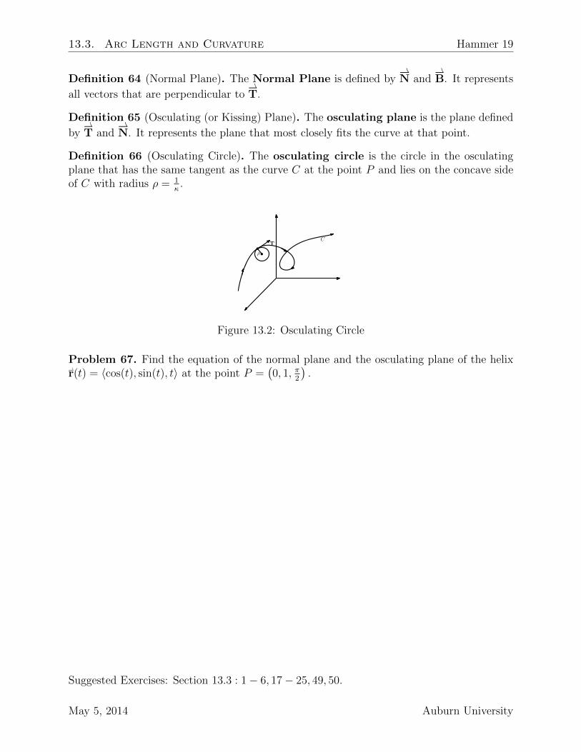
Definition 66 (Osculating Circle). The osculating circle is the circle in the osculatingplane that has the same tangent as the curve C at the point P and lies on the concave sideof C with radius ρ = 1

κ.

TC

ρ

Figure 13.2: Osculating Circle

Problem 67. Find the equation of the normal plane and the osculating plane of the helix⇀r(t) = 〈cos(t), sin(t), t〉 at the point P =

(0, 1, π

2

).

Suggested Exercises: Section 13.3 : 1− 6, 17− 25, 49, 50.



13.4 Motion in Space, Velocity, and Acceleration

Definition 68 (Velocity, Acceleration, & Speed). Let ⇀r(t) be a position vector for a particleat time t. Then the velocity of the particle at time t is ⇀v(t) = ⇀r′(t) and the accelerationof the particle at time t is ⇀a(t) = ⇀v′(t) = ⇀r′′(t). The speed of the particle at time t is definedby |⇀v(t)| = |⇀r′(t)| .

Problem 69. Given a position vector ⇀r(t) = 〈t3, t2〉 , find the velocity, speed, and accelera-tion at t = 1.

Problem 70. A moving particle starts at an initial position ⇀r(0) = 〈1, 0, 0〉, has initialvelocity ⇀v(0) = 〈1,−1, 1〉, and acceleration is defined by ⇀a(t) = 〈4t, 6t, 1〉 . Find the particle’sposition and velocity at time t.


Chapter 14

Partial Derivatives

14.1 Functions of Several Variables

14.1.1 Domain and Range

Definition 71 (Function of Two Variables). A function of two variables, f , is a rulethat assigns each ordered pair of real numbers (x, y) in a set D ⊂ R2 a unique real numberdenoted z = f(x, y). The set D is called the domain of f and the set of values that arereturned (the z values) are called the range. In shorthand, we say

f : R2 → R.

Definition 72. Let f be a function of two variables, z = f(x, y). Then x and y are calledindependent variables and z is called a dependent variable.

Problem 73. Let f(x, y) =

√x+ y + 1

x− 1Evaluate f(3, 2) and give its domain.

Problem 74. Find the domain of f(x, y) = x ln (y2 − x) .

21


Problem 75. Find the domain and range of f(x, y) =√

9− x2 − y2.

14.1.2 Graphs

Definition 76 (Graph). If f is a function of two variables with domain D, then the graphof f is the set of all points (x, y, z) ∈ R3 such that z = f(x, y) for all (x, y) ∈ D.

Problem 77. Sketch the graph of f(x, y) = 6− 3x− 2y.

Problem 78. Sketch the graph of g(x, y) =√

9− x2 − y2.


14.1. Functions of Several Variables Hammer 23

14.1.3 Level Curves

Definition 79 (Level Curves). The level curves of a function of two variables, f , are thecurves of the equation f(x, y) = k for some k ∈ K ⊂ R.

Problem 80. Sketch the level curves of f(x, y) = 6− 3x− 2y for k = {−6, 0, 6, 12} .

Problem 81. Sketch the level curves of g(x, y) =√

9− x2 − y2 for k = {0, 1, 2, 3}

Problem 82. Sketch the level curves of h(x, y) = 4x2 + y2 + 1.




14.2 Limits and Continuity

Theorem 83 (Limits Along a Path). If lim(x,y)→(a,b)

f(x, y) = L1 as (x, y) approaches (a, b)

along the path C1 and lim(x,y)→(a,b)

f(x, y) = L2 6= L1 as (x, y) approaches (a, b) along the path

C2, then lim(x,y)→(a,b)

f(x, y) does not exist.

Problem 84. Show lim(x,y)→(0,0)

x2 − y2x2 + y2

does not exist.

Problem 85. Does lim(x,y)→(0,0)

xy

x2 + y2exist?


14.2. Limits and Continuity Hammer 25


2xy

x2 + y2exist?


2xy

x2 + y2exist?


xy2

x2 + y4exist?



Definition 89 (Continuity). A function of two variables f is called continuous at a point(a, b) ∈ R2 if lim

(x,y)→(a,b)f(x, y) = f(a, b).

Problem 90. Is 2xyx2+y2

continuous at (1, 1)? What about (0, 0)? Why?

Problem 91. Use the squeeze theorem to show that lim(x,y)→(0,0)

3x2y

x2 + y2= 0.

Problem 92. Where is f(x, y) = x2−y2x2+y2

continuous?



14.3. Partial Derivatives Hammer 27

14.3 Partial Derivatives

14.3.1 First Order Partial Derivatives

Definition 93 (Partial Derivatives). If f is a function of two variables, its partial deriva-tives are the functions fx = ∂f

∂xand fy = ∂f

∂ydefined by:

fx = ∂f∂x

= f(x+h,y)−f(x,y)h

fy = ∂f∂y

= f(x,y+h)−f(x,y)h

.

In other words, to find the partial derivative of f with respect to x (i.e. fx), simply take thederivative of f treating x as the variable and y as a constant. Similarly, to get the partialderivative with respect to y (i.e. fy), simply take the derivative of f treating y as the variableand x as a constant.

Observation 94. The partial derivative with respect to x represents the slope of the tangentlines to the curve that are parallel to the xz-plane (i.e. in the direction of 〈1, 0, . . .〉).Similarly, the partial derivative with respect to y represents the slope of the tangent lines tothe curve that are parallel to the yz-plane (i.e. in the direction of 〈0, 1, . . .〉).

Problem 95. If f(x, y) = x3 + x2y3 − 2y2, find fx(2, 1) and fy(2, 1).

Problem 96. Let f(x, y) = sin

(x

1 + y

). Find the first order partial derivatives of f(x, y).



Problem 97. Let z = f(x, y). Find∂z

∂xand

∂z

∂yof x3 + y3 + z3 + 6xyz = 1.

14.3.2 Higher Order Partial Derivatives

Problem 98. Find the second order partial derivatives of f(x, y) = x3 + x2y3 − 2y2.

Theorem 99 (Clairaut). Suppose f(x, y) is defined on a disk D ⊂ R2. Then

fxy = fyx.

Problem 100. Calculate fxxyz(x, y) given f(x, y, z) = sin (3x+ yz)

Suggested Problems: Section 14.3 : 15− 44, 47− 52, 53− 58, 63− 66.


14.4. Tangent Planes & Linear Approximation Hammer 29

14.4 Tangent Planes & Linear Approximation

Goal 101. As one zooms into a surface, the more the surface resembles a plane. MoreSpecifically, the surface looks more and more like the tangent plane. Some functions aredifficult to evaluate at a point; so, the equation of the tangent plane (which is much simpler)is used to approximate the value of that curve at a given point.

Theorem 102 (Equation of Tangent Plane). Suppose that f(x, y) has continuous partialderivatives. An equation of the tangent plane (equivalently, the linear approximation) to thesurface z = f(x, y) at the point P = (x0, y0, z0) is

z − z0 = fx (x0, y0) (x− x0) + fy (x0, y0) (y − y0) .

Problem 103. Find an equation for the tangent plane to the elliptic paraboloid z = 2x2+y2

at the point (1, 1, 3).

Problem 104. Give the linear approximation of f(x, y) = xexy at (1, 0). Then use this toapproximate f(1.1,−0.1).



Problem 105. Find the linear approximation of f(x, y) =√

25− x2 − y2 centered at (−3, 0)to evaluate f(−3.04, 0.09).

Problem 106. Find the linear approximation of the function f (x, y, z) = x3√y2 + z2 at

the point (2, 3, 4) and use it to estimate the number (1.98)3√

(3.10)2 + (3.97)2.

Suggested problems: Section 14.4 : 1− 6, 11− 16.


14.5. Chain Rule Hammer 31

14.5 Chain Rule

14.5.1 Chain Rule

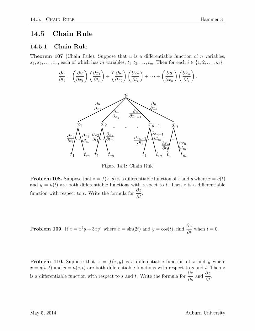
Theorem 107 (Chain Rule). Suppose that u is a differentiable function of n variables,x1, x3, . . . , xn, each of which has m variables, t1, t2, . . . , tm. Then for each i ∈ {1, 2, . . . ,m},

∂u

∂ti=

(∂u

∂x1

)(∂x1∂ti

)+

(∂u

∂x2

)(∂x2∂ti

)+ · · ·+

(∂u

∂xn

)(∂xn∂ti

).

u

x1 x2 xn−1 xn

t1 tm t1 tm t1 tm t1 tm

∂u∂x1

∂x1∂t1

∂x1∂tm

∂x2∂t1

∂x2∂tm ∂xn−1

∂t1

∂xn−1∂tm

∂xn∂t1

∂xn∂tm

∂u∂x2

∂u∂xn−1

∂u∂xn

Figure 14.1: Chain Rule

Problem 108. Suppose that z = f(x, y) is a differentiable function of x and y where x = g(t)and y = h(t) are both differentiable functions with respect to t. Then z is a differentiable

function with respect to t. Write the formula for∂z

∂t.

Problem 109. If z = x2y + 3xy4 where x = sin(2t) and y = cos(t), find∂z

∂twhen t = 0.

Problem 110. Suppose that z = f(x, y) is a differentiable function of x and y wherex = g(s, t) and y = h(s, t) are both differentiable functions with respect to s and t. Then z

is a differentiable function with respect to s and t. Write the formula for∂z

∂sand

∂z

∂t.



Problem 111. If z = ex sin(y) where x = st2 and y = s2t, find∂z

∂sand

∂z

∂t.

Problem 112. Write the chain rule for w = f(x, y, z, t), where x = x(u, v), y = y(u, v), z =

z(u, v), and t = t(u, v). That is, find∂w

∂uand

∂w

∂v.

Problem 113. If g(s, t) = f (s2 − t2, t2 − s2) and f is differentiable, show that g satisfiesthe equation

t∂g

∂s+ s

∂g

∂t= 0.


14.5. Chain Rule Hammer 33

14.5.2 Implicit Differentiation

F

x y

x y

∂x∂x

∂y∂x

∂F∂y

∂F∂x

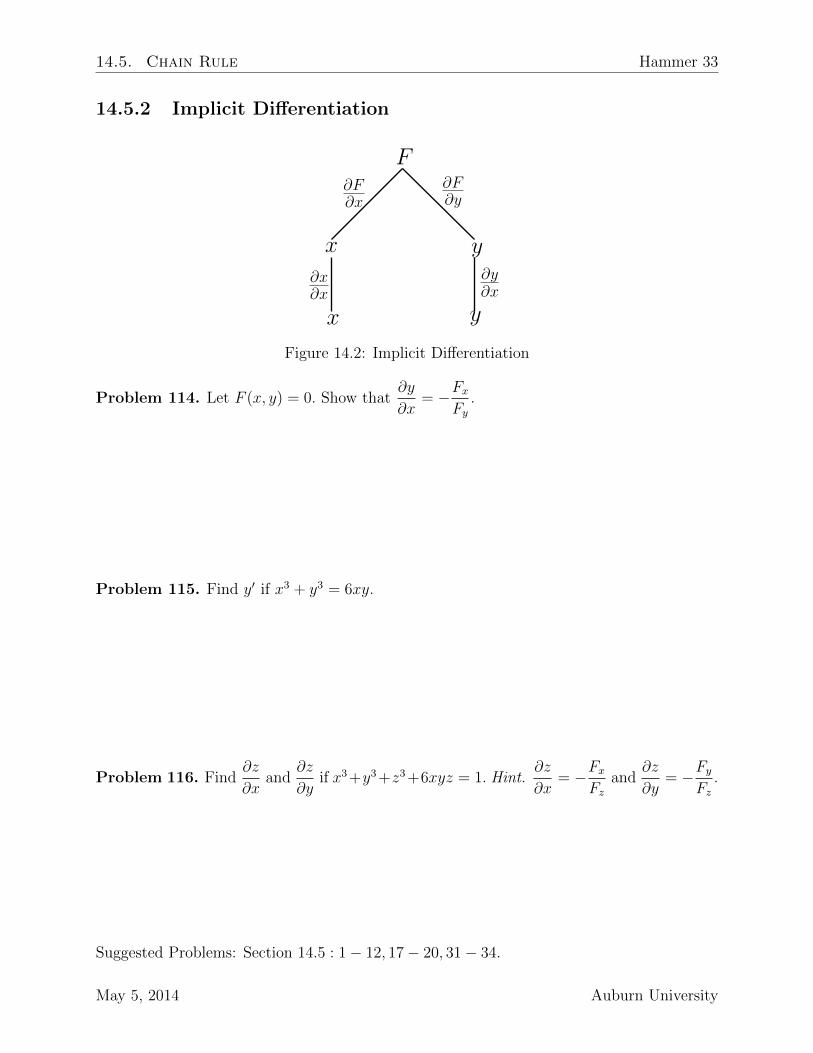
Figure 14.2: Implicit Differentiation

Problem 114. Let F (x, y) = 0. Show that∂y

∂x= −Fx

Fy.

Problem 115. Find y′ if x3 + y3 = 6xy.

Problem 116. Find∂z

∂xand

∂z

∂yif x3+y3+z3+6xyz = 1. Hint.

∂z

∂x= −Fx

Fzand

∂z

∂y= −Fy

Fz.

Suggested Problems: Section 14.5 : 1− 12, 17− 20, 31− 34.



14.6 Directional Derivatives & Gradient Vector

Goal 117. It would be nice to be able to find the slope of the tangent line to a curve C ona surface S in the direction of a unit vector ⇀u = 〈a, b〉 .

u

m = DufS

C

Figure 14.3: Directional Derivative

Definition 118 (The “Del” Operator). For ease of notation, we denote “del” (∇) as ∇ =⟨∂∂x, ∂∂y, ∂∂z

⟩.

Definition 119 (Gradient). Let f be a differentiable function of two variables, x and y.Then the gradient of f is the vector function

∇f(x, y) = 〈fx(x, y), fy(x, y)〉 .

Theorem 120 (Directional Derivative). If f is a differentiable function of x and y, then fhas a directional derivative in the direction of any unit vector u = 〈a, b〉 and

Duf(x, y) = ∇f(x, y) · ⇀u = fx(x, y)a+ fy(x, y)b.

Equivalently, we can say

Duf(x, y) = fx(x, y) cos(θ) + fy(x, y) sin(θ),

where θ represents the angle of the unit vector.

Note 121. The only reason we are restricting the directional derivative to the unit vector isbecause we care about the rate of change in f per unit distance. Otherwise, the magnitudeis irrelevant.

Problem 122. If f(x, y) = sin(x) + exy, find ∇f(x, y) and ∇f(0, 1).


14.6. Directional Derivatives & Gradient Vector Hammer 35

Problem 123. Find the directional derivative D⇀uf(x, y) if f(x, y) = x3 − 3xy + 4y2 and ⇀uis the unit vector given by the angle θ = π

6.

Problem 124. Find the directional derivative of f(x, y) = x2y3 − 4y at the point (2,−1)and in the direction of the vector ⇀v = 〈2, 5〉 .

Problem 125. If f(x, y, z) = x sin(yz), find the directional derivative of f(1, 3, 0) in thedirection of ⇀v = 〈1, 2,−1〉 .




14.7 Maximum & Minimum Values

14.7.1 Local Extrema

Definition 126 (Local Minimum). A function f of two variables x and y has a localminimum at the point (a, b) if f(x, y) ≤ f(a, b) when (x, y) is near (a, b).

Definition 127 (Local Maximum). A function f of two variables x and y has a localminimum at the point (a, b) if f(x, y) ≥ f(a, b) when (x, y) is near (a, b).

Theorem 128 (First Partial Test). If f has a local extreme at (a, b) and the first orderpartials exist, then fx(a, b) = 0 and fy(a, b) = 0.

Theorem 129 (Second Partial Test). Suppose that the second order partial derivatives off are continuous on the disc centered at (a, b) and suppose that fx(a, b) = fy(a, b) = 0. LetD = D(a, b) = fxx(a, b)fyy(a, b)− [fxy (a, b)]2 .

• If D > 0 and fxx(a, b) > 0, then f(a, b) is a local minimum.

• If D > 0 and fxx(a, b) < 0, then f(a, b) is a local maximum.

• If D < 0, then f(a, b) is a saddle point.

• If D = 0, then no conclusion can be drawn from this test.

Note 130. There is nothing sacred about fxx. D > 0 means that both fxx and fyy have thesame sign. Moreover, we could equivalently check fyy instead of fxx in those cases.

Problem 131. Find all local extrema of f(x, y) = x4 + y4 − 4xy + 1.


14.7. Maximum & Minimum Values Hammer 37

Problem 132. Find the shortest distance from the point (1, 0,−2) to the plane x+2y+z = 4.

Problem 133. A topless rectangular box is made from 12m2 of cardboard. Find the di-mensions of the box that maximizes the volume of the box.



14.7.2 Absolute Extrema

Theorem 134 (Existence). If f is continuous on a closed and bounded set D ⊂ R2, thenf attains an absolute maximum value f(x1, y1) and an absolute minimum value f(x2, y2) atsome points (x1, y1) and (x2, y2) in D.

Strategy 135. To find absolute extrema,

1. Find critical points and values of f at those critical points

2. Find the extreme values that occur on the boundary. Find the values of f at thosepoints.

3. Compare all of those values for the largest and smallest values.

Problem 136. Find the absolute extrema of f(x, y) = x2 − 2xy + 2y on the rectangleR = [0, 3]× [0, 2] = {(x, y) | 0 ≤ x ≤ 3, 0 ≤ y ≤ 2} .



14.8. Lagrange Multipliers Hammer 39

14.8 Lagrange Multipliers

Goal 137. To have a way of finding absolute extrema of a function that is subject to certainconstraints.

Strategy 138 (Lagrange Multipliers). Let k ∈ R. To find the maximum and minimumvalues of f(x, y, z) subject to g(x, y, z) = k,

• Find all values of x, y, z, and λ such that ∇f(x, y, z) = λ∇g(x, y, z) and g(x, y, z) = k.

• Evaluate all of these points to find the maximum and minimum values.

Problem 139. A topless rectangular box is made from 12m2 of cardboard. Find the di-mensions of the box that maximizes the volume of the box.



Problem 140. Find the extreme values of f(x, y) = x2 + 2y2 on the circle x2 + y2 = 1.

Problem 141. Find the maximum value of f(x, y, z) = x + 2y + 3z on the curve of theintersection of the plane x− y + z = 1 and the cylinder x2 + y2 = 1.

Suggested Problems: Section 14.8 : 3− 18


Chapter 15

Multiple Integrals

15.1 Double Integrals over a Rectangle

Recall 142. We know the following from Calculus I:

1. We defined the integral in terms of Riemann Sums.

2. That is, we found the area underneath the curve y = f(x) by dividing the area intorectangles. We then added up their areas to get the area under the curve.

3. We then found the exact area of this by evaluating

ˆ b

a

f(x) dx = limn→∞

n∑

i=1

f(x∗i ) ∆x.

15.1.1 Volumes as Double Integrals

Let R = [a, b]× [c, d] = {(x, y) ∈ R2 | a ≤ x ≤ b, c ≤ y ≤ d} define a rectangle.Let S = {(x, y, z) ∈ R3 | 0 ≤ z ≤ f(x, y), (x, y) ∈ R} define the solid that lies above R.

Goal 143. We want to divide R into rectangular prisms (show boxes) with the goal ofadding up all of their volumes to give us the volume underneath the curve f(x, y).

Let (x∗ij, y∗ij) denote a sample point in each division Rij.

Let ∆A = ∆x∆y denote the area of each Rij. Then we can express this volume as

V ≈n∑

i=1

n∑

j=1

f(x∗ij, y∗ij) ∆A.

Definition 144 (Double Integral). The Double Integral of f over the rectangle R is

¨

R

f(x, y) dA = limm,n→∞

n∑

i=1

n∑

j=1

f(x∗ij, y∗ij) ∆A.

41


We can simplify this if we choose each sample point, (x∗ij, y∗ij), to be the point in the

upper right corner of each sub-rectangle. Call this point (xi, yj). Then we get:

V =

¨

R

f(x, y) dA = limm,n→∞

n∑

i=1

n∑

j=1

f(xi, yj) ∆A.

Problem 145. Estimate the volume of the solid that lies above the square R = [0, 2]× [0, 2]and below the elliptic paraboloid z = 16 − x2 − 2y2. Divide R into four equal squares andchoose the sample point to be the upper right corner of each square Rij. Approximate theVolume.

Problem 146. Estimate the volume of the solid that lies above the square R = [0, 2]× [1, 2]and below the function x− 3y2. Divide R into four equal rectangles and choose the samplepoint to be the midpoint of each rectangle Rij. Approximate the volume.

Suggested Homework: p. 981 exercises 1-5, 11-13.


15.2. Iterated Integrals Hammer 43

15.2 Iterated Integrals

Okay; so, taking these Riemann Sums is a bit of a pain.

Recall 147. In Calculus I, we equated these Riemann sums to the definition of an integral.We will attempt to do the same thing here; however, we will be using two partial integralsto do this.

Suppose that f is a function of two variables that is integrable on the rectangle R =[a, b]× [c, d].

Definition 148 (Partial Integral w.r.t. y). We define´ dcf(x, y) dy as the partial integral

with respect to y. We evaluate this integral by treating x as a constant, and integrate f(x, y)with respect to y. We can then use the fundamental theorem of calculus part 2 (theorem 224)to evaluate the integral at on the interval [c, d].

Definition 149 (Partial Integral w.r.t. x). We define´ baf(x, y) dx as the partial integral

with respect to x. We evaluate this integral by treating y as a constant, and integrate f(x, y)with respect to x. We can then use the fundamental theorem of calculus part 2 to evaluatethe integral at on the interval [a, b].

Definition 150 (Double Integral). The double integral is defined as follows:

ˆ b

a

ˆ d

c

f(x, y) dx dy =

ˆ b

a

[ˆ d

c

f(x, y) dx

]dy.

In other words, we work this integral from the inside out.

Problem 151. Evaluate the integrals (a)

ˆ 3

0

ˆ 2

1

x2y dy dx, and (b)

ˆ 2

1

ˆ 3

0

x2y dx dy.



Theorem 152 (Fubini). If f is continuous on the rectangle R = {(x, y) ∈ R2 | a ≤ x ≤b, c ≤ y ≤ d}, then

¨

R

f(x, y) dA =

ˆ b

a

ˆ d

c

f(x, y) dy dx =

ˆ d

c

ˆ b

a

f(x, y) dx dy

Problem 153. Evaluate the double integral

¨

R

(x− 3y2) dA, where R = {(x, y) ∈ R2 | 0 ≤

x ≤ 2, 1 ≤ y ≤ 2}.

Problem 154. Evaluate

¨

R

y sin(xy) dA, where R = [1, 2]× [0, π].


15.2. Iterated Integrals Hammer 45

Problem 155. Find the volume of the solid S that is bounded by the elliptic paraboloidx2 + 2y2 + z = 16, the planes x = 2 and y = 2, and the three coordinate planes.

Problem 156. Find the volume of the solid that lies under the hyperbolic paraboloid z =3y2 − x2 + 2 and above the rectangle R = [−1, 1]× [1, 2].

Suggested Homework p. 987, 1-20, 25-30



15.3 Double Integrals over General Regions

Question 157. Okay, So now we know how to find the volume of the region under a surfacegiven that the the projection of the region down to the xy-plane is rectangular. What if thatregion is defined as the boundary between two functions?

15.3.1 Type 1

Type I regions are regions of the form R = {(x, y) ∈ R2 | a ≤ x ≤ b, g1(x) ≤ y ≤ g2(x)}.That is to say that the region in the xy-plane looks like this:

RR

a b

y = g2(x)

y = g1(x)

Figure 15.1: Type 1 Double Integral

Moreover, if f if continuous on a Type I region, then

¨

R

f(x, y) dA =

ˆ b

a

ˆ g2(x)

g1(x)

f(x, y) dy dx.

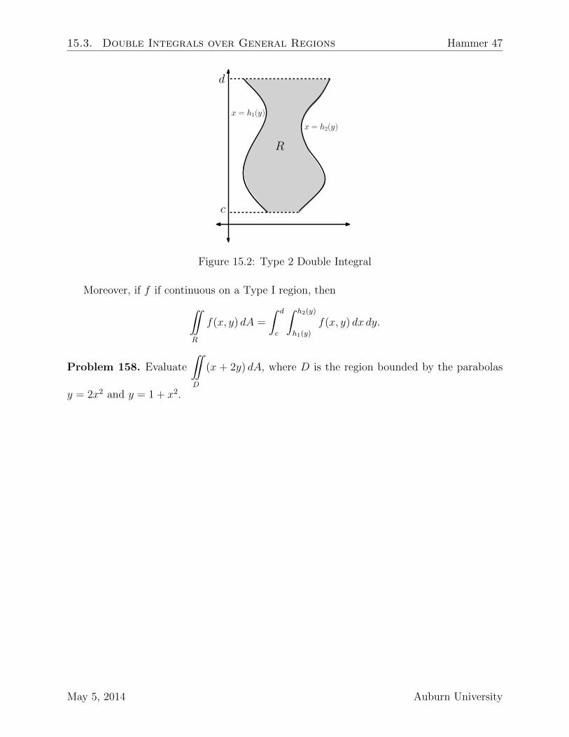
15.3.2 Type 2

Type II regions are regions of the form R = {(x, y) ∈ R2 | h1(y) ≤ x ≤ h2(y), c ≤ y ≤ d}.That is to say that the region in the xy-plane looks like this:


15.3. Double Integrals over General Regions Hammer 47

RR

c

d

x = h1(y)

x = h2(y)

Figure 15.2: Type 2 Double Integral

Moreover, if f if continuous on a Type I region, then

¨

R

f(x, y) dA =

ˆ d

c

ˆ h2(y)

h1(y)

f(x, y) dx dy.


¨

D

(x + 2y) dA, where D is the region bounded by the parabolas

y = 2x2 and y = 1 + x2.




¨

D

xy dA, where D is the region bounded by the line y = x − 1

and the parabola y2 = 2x+ 6.

Problem 160. Show that

¨

D

1 dA = AD, where AD denotes the area of the region D.

Suggested Homework: p 995, 1-10, 17-32


15.4. Change of Variables in Multiple Integrals Hammer 49

15.4 Change of Variables in Multiple Integrals

We have done changes of variables several times in the past. Dating as far back as Calculus Iwhen we learned u -substitution, we started using changes of variables (we made u = g(x).)

Goal 161. The goal of this section is to write a general form for a change of variables. Inother words, is there a transformation on the function we can do to make the integral easier.

Definition 162 (Transformation). A change of variables is a transformation , T , fromthe uv-plane to the xy-plane, T (u, v) = (x, y), where x and y are related to u and v by theequations

x = g(u, v) y = h(u, v).

We usually take these transformations to be C1-Transformation, meaning g and h havecontinuous first-order partial derivatives.

u

v

x

y

S RT−1

T

Figure 15.3: Transformation

Definition 163 (Jacobian). The Jacobian of the transformation T given by x = g(u, v)and y = h(u, v) is

∂(x, y)

∂(u, v)=

∣∣∣∣∣∣

∂x∂u

∂x∂v

∂y∂u

∂y∂v

∣∣∣∣∣∣=

(∂x

∂u

)(∂y

∂v

)−(∂x

∂v

)(∂y

∂u

).

Theorem 164 (Double Integral Change of Variable). Suppose that T is a C1-transformationwhose Jacobian is nonzero, and suppose that T maps a region S int he uv-plane onto a regionR in the xy-plane. Let f be a continuous function on R. Suppose also that T is a one-to-onetransformation except perhaps along the boundary of the regions. Then

¨

R

f(x, y) dA =

¨

S

f(x(u, v), y(u, v))

∣∣∣∣∂(x, y)

∂(u, v)

∣∣∣∣ du dv.



Problem 165. Evaluate˜R

x + y dA where R is the trapezoidal region with vertices given

by (0, 0), (5, 0),(52, 52

), and

(52,−5

2

)using the transformation x = 2u+ 3v and y = 2u− 3v.

Problem 166. Evaluate the integral˜R

e(x+y)/(x−y) dA, where R is the trapezoidal region

with vertices (1, 0), (2, 0), (0,−2), and (0,−1).

Suggested Homework: p. 1047, 15-20


15.5. Double Integrals in Polar Coordinates Hammer 51

15.5 Double Integrals in Polar Coordinates

15.5.1 Crash Course in Polar Coordinates

We have spent most of our lives in the Cartesian Coordinate System, which was inventedby none other than Rene Descartes, who was because he thought. Sometimes, however,functions (and consequently integrals) become simpler when expressed in different coordinatesystems. There are many different coordinate systems. Today, however, we will focus on onethat was invented by Sir Isaac Newton – the Polar Coordinate System.

Definition 167 (Origin & polar axis). First, we must pick a special point in the plane –the origin. Once we have the origin, draw a ray from the origin in any direction. This rayis called the polar axis.

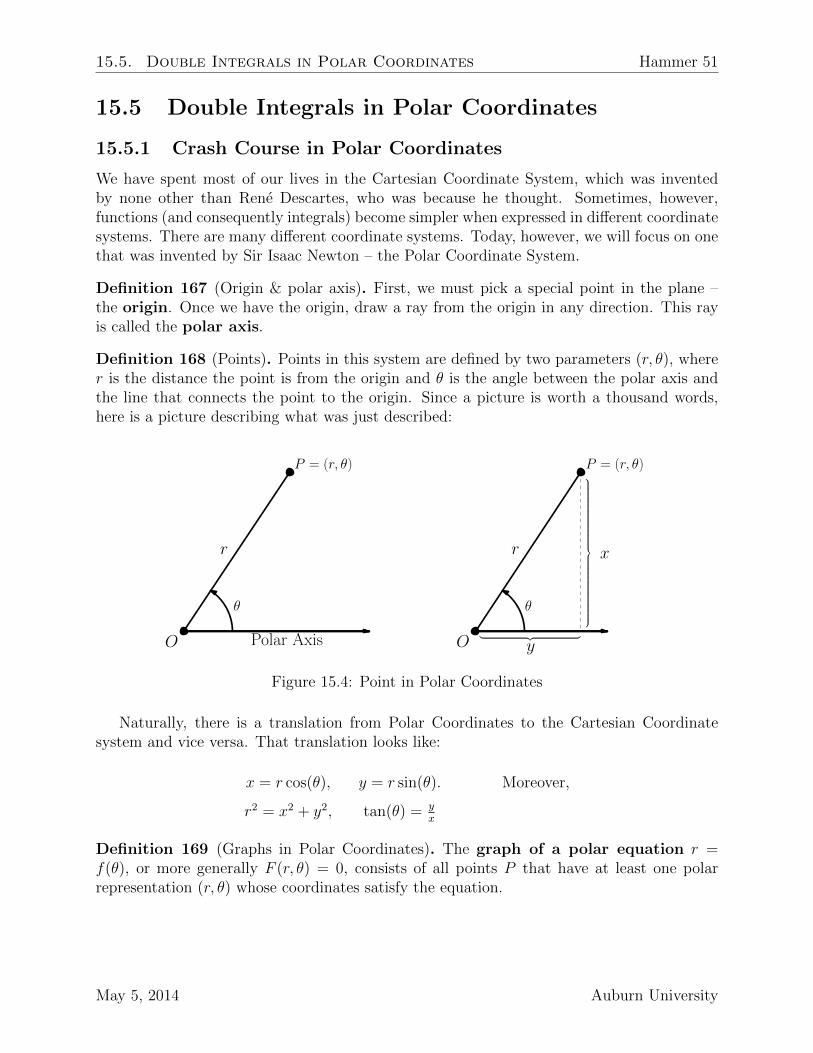
Definition 168 (Points). Points in this system are defined by two parameters (r, θ), wherer is the distance the point is from the origin and θ is the angle between the polar axis andthe line that connects the point to the origin. Since a picture is worth a thousand words,here is a picture describing what was just described:

P = (r, θ)

θ

r

O Polar Axis

P = (r, θ)

θ

r

O

x

y

︸︷︷︸

Figure 15.4: Point in Polar Coordinates

Naturally, there is a translation from Polar Coordinates to the Cartesian Coordinatesystem and vice versa. That translation looks like:

x = r cos(θ), y = r sin(θ). Moreover,

r2 = x2 + y2, tan(θ) = yx

Definition 169 (Graphs in Polar Coordinates). The graph of a polar equation r =f(θ), or more generally F (r, θ) = 0, consists of all points P that have at least one polarrepresentation (r, θ) whose coordinates satisfy the equation.



Example 170. The graph representing the polar equation r = 2 is

0°

45°

90°

135°

180°

225°

270°

315°

0.51.0

1.52.0

2.53.0

Figure 15.5: r = 2

Example 171. The graph representing the polar equation θ = 1 is

0°

45°

90°

135°

180°

225°

270°

315°

0.20.4

0.60.8

1.0

Figure 15.6: θ = 1

Example 172. The graph representing the polar equation r = 2 cos(θ) is

0°

45°

90°

135°

180°

225°

270°

315°

0.51.0

1.52.0

Figure 15.7: r = 2 cos(θ)



Example 173. The graph representing the polar equation r = 1 + sin(θ) is

0°

45°

90°

135°

180°

225°

270°

315°

0.51.0

1.52.0

Figure 15.8: r = 1 + sin(θ)

Example 174. The graph representing the polar equation r = cos(2θ) is

0°

45°

90°

135°

180°

225°

270°

315°

0.20.4

0.60.8

1.0

Figure 15.9: r = cos(2θ)

15.5.2 Double Integrals with Polar Coordinates

In the polar coordinate system, a rectangle in the rθ-plane can be defined as

R = {(r, θ) | a ≤ r ≤ b, α ≤ θ ≤ β} .

R

r = a

r = b

θ = α

θ = β

α

β

Figure 15.10: Rectangle in Polar Coordinates



We can divide up this rectangle just as we did in section 15.1, dividing the rectangleinto tiny rectangular prisms and summing up their volumes. Moreover, we can generalizeFubini’s theorem (theorem 152) as follows:

Problem 175. Show that when dealing with polar coordinates, dA = r dr dθ.

Theorem 176 (Polar version of Fubini’s Theorem). If f is continuous on the polar rectangleR given by 0 ≤ a ≤ r ≤ b, α ≤ θ ≤ β, where 0 ≤ β − α ≤ 2π, then

¨

R

f(x, y) dA =

ˆ β

α

ˆ b

a

f(r cos(θ), r sin(θ)) r dr dθ

Note: Do not forget the r before the dr dθ!


¨

R

(3x + 4y2) dA, where R is the region in the upper half-plane

bounded by the circles x2 + y2 = 1 and x2 + y2 = 4.



Problem 178. Find the volume of the solid bounded by the plane z = 0 and the paraboloidz = 1− x2 − y2.

Theorem 179 (Polar version of section 15.3.2). If f is continuous on a polar region of theform D = {(r, θ) | α ≤ θ ≤ β, h1(θ) ≤ r ≤ h2(θ)}, then

¨

D

f(x, y) dA =

ˆ β

α

ˆ h2(θ)

h1(θ)

f(r cos(θ), r sin(θ)) r dr dθ

R

r = h1(θ)

r = h2(θ)

θ = α

θ = β

α

β

R

Figure 15.11: Polar version of section 15.3.2



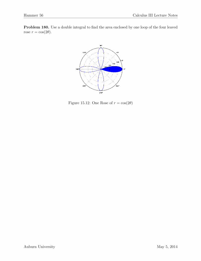
Problem 180. Use a double integral to find the area enclosed by one loop of the four leavedrose r = cos(2θ).

Figure 15.12: One Rose of r = cos(2θ)



Problem 181. Find the volume of the solid that lies under the paraboloid z = x2 + y2,above the xy-plane, and inside the cylinder x2 + y2 = 2x.

Hint.

• First, find what the “rectangle” in polar coordinates looks like.

• That is to say, translate x2 + y2 = 2x into polar coordinates and see what that regionlooks like.

• This will be your “rectangle.”

• Then, look at z = x2 + y2 as a polar function.

• Use this as your integrand.

• Evaluate.

• Don’t forget the r in “r dr dθ”!

Suggested Homework: p. 1002, 7-27 odd.



15.7 Triple Integrals

Remark 182. The interpretation of the triple integral˝E

f(x, y, z) dV , where f(x, y, z) ≥ 0

is the “hyper-volume” of a four-dimensional object, which is interesting, but admittedly notvery useful. Of course, E represents a subset of the domain of f , which lives in fourth-dimensional space.

Remark 183. The triple integral˝E

f(x, y, z) dV can be interpreted in different ways in

different (useful) physical situations, depending on the interpretation of x, y, and z as wellas what f(x, y, z) represents.

Theorem 184 (Generalization of Problem 160). The volume V (E) of a subset E of R3 iscan be evaluated by the following:

V (E) =

˚

E

1 dV.

Problem 185. Use the triple integral to find the volume of the tetrahedron T bounded bythe planes x+ 2y + z = 2, x = 2y, x = 0, and z = 0.

Suggested Homework: p. 1025, 3-8, 9-11.


15.8. Triple Integrals in Cylindrical Coordinates Hammer 59

15.8 Triple Integrals in Cylindrical Coordinates

Definition 186 (Points in Cylindrical Coordinates). In the cylindrical coordinate system,a point P in three-dimensional space is represented as an ordered triple (r, θ, z), where rand θ are polar coordinates of the projection of P onto the xy-plane and z is the directeddistance from the xy-plane to P .

Theorem 187 (Conversion: Cylindrical ↔ Rectangular).

Cylindrical→ Rectangular: x = r cos(θ) y = r sin(θ) z = z

Rectangular→ Cylindrical: r2 = x2 + y2 tan(θ) =(yx

)z = z

Theorem 188 (Cylindrical Version of Fubini’s Theorem). Let E = {(x, y, z) ∈ R3 | (x, y) ∈D, u1(x, y) ≤ z ≤ u2(x, y)} be a region in R3 whose projection down to the xy-plane, D, isa region that satisfies theorem 176. That is, D = {(r, θ) | α ≤ θ ≤ β, h1(θ) ≤ r ≤ h2(θ)}.Then

˚

E

f(x, y, z) dV =

ˆ β

α

ˆ h2(θ)

h1(θ)

ˆ u2(r cos(θ),r sin(θ))

u1(r cos(θ),r sin(θ))

f(r cos(θ), r sin(θ), z) r dz dr dθ.

θ = α

θ = β

r = h2(θ)

r = h1(θ)

z = u2(x, y)

z = u1(x, y)

Figure 15.13: Cylindrical Version of Fubini’s Theorem



Problem 189. (a) Plot the point with cylindrical coordinates (2, 2π3, 1) and find its rectan-

gular coordinates.(b) Find cylindrical coordinates of the point with rectangular coordinates (3,−3, 7).


ˆ 2

−2

ˆ √4−x2−√4−x2

ˆ 2

√x2+y2

(x2 + y2) dz dy dx.

Hint. Change the triple integral into cylindrical coordinates.

Suggested Homework: p. 1031, 1-4, 7-24.


15.9. Triple Integrals in Spherical Coordinates Hammer 61

15.9 Triple Integrals in Spherical Coordinates

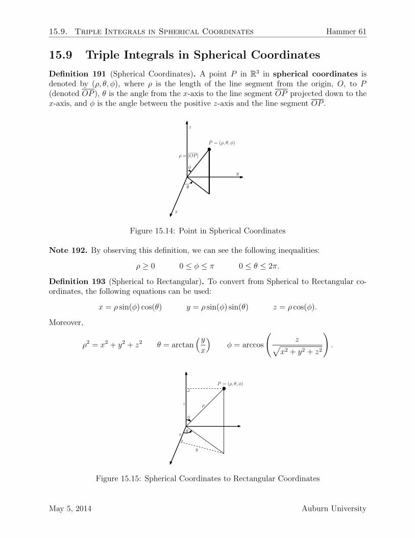
Definition 191 (Spherical Coordinates). A point P in R3 in spherical coordinates isdenoted by (ρ, θ, φ), where ρ is the length of the line segment from the origin, O, to P(denoted OP ), θ is the angle from the x-axis to the line segment OP projected down to thex-axis, and φ is the angle between the positive z-axis and the line segment OP .

P = (ρ, θ, φ)

ρ = |OP |

θ

φ

x

y

z

Figure 15.14: Point in Spherical Coordinates

Note 192. By observing this definition, we can see the following inequalities:

ρ ≥ 0 0 ≤ φ ≤ π 0 ≤ θ ≤ 2π.

Definition 193 (Spherical to Rectangular). To convert from Spherical to Rectangular co-ordinates, the following equations can be used:

x = ρ sin(φ) cos(θ) y = ρ sin(φ) sin(θ) z = ρ cos(φ).

Moreover,

ρ2 = x2 + y2 + z2 θ = arctan(yx

)φ = arccos

(z√

x2 + y2 + z2

).

P = (ρ, θ, φ)

ρ

θ

φ

x

y

z

Figure 15.15: Spherical Coordinates to Rectangular Coordinates



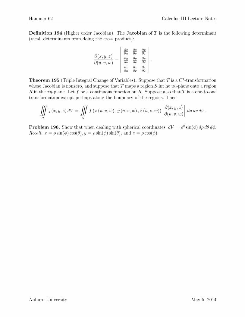
Definition 194 (Higher order Jacobian). The Jacobian of T is the following determinant(recall determinants from doing the cross product):

∂(x, y, z)

∂(u, v, w)=

∣∣∣∣∣∣∣∣∣

∂x∂u

∂x∂v

∂x∂2

∂y∂u

∂y∂v

∂y∂2

∂z∂u

∂z∂v

∂z∂2

∣∣∣∣∣∣∣∣∣.

Theorem 195 (Triple Integral Change of Variables). Suppose that T is a C1-transformationwhose Jacobian is nonzero, and suppose that T maps a region S int he uv-plane onto a regionR in the xy-plane. Let f be a continuous function on R. Suppose also that T is a one-to-onetransformation except perhaps along the boundary of the regions. Then

˚

R

f(x, y, z) dV =

˚

S

f (x (u, v, w) , y (u, v, w) , z (u, v, w))

∣∣∣∣∂(x, y, z)

∂(u, v, w)

∣∣∣∣ du dv dw.

Problem 196. Show that when dealing with spherical coordinates, dV = ρ2 sin(φ) dρ dθ dφ.Recall. x = ρ sin(φ) cos(θ), y = ρ sin(φ) sin(θ), and z = ρ cos(φ).


15.9. Triple Integrals in Spherical Coordinates Hammer 63

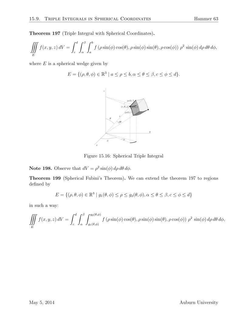
Theorem 197 (Triple Integral with Spherical Coordinates).

˚

E

f(x, y, z) dV =

ˆ d

c

ˆ β

α

ˆ b

a

f (ρ sin(φ) cos(θ), ρ sin(φ) sin(θ), ρ cos(φ)) ρ2 sin(φ) dρ dθ dφ,

where E is a spherical wedge given by

E = {(ρ, θ, φ) ∈ R3 | a ≤ ρ ≤ b, α ≤ θ ≤ β, c ≤ φ ≤ d}.

Figure 15.16: Spherical Triple Integral

Note 198. Observe that dV = ρ2 sin(φ) dρ dθ dφ.

Theorem 199 (Spherical Fubini’s Theorem). We can extend the theorem 197 to regionsdefined by

E = {(ρ, θ, φ) ∈ R3 | g1(θ, φ) ≤ ρ ≤ g2(θ, φ), α ≤ θ ≤ β, c ≤ φ ≤ d}

in such a way:

˚

E

f(x, y, z) dV =

ˆ d

c

ˆ β

α

ˆ g2(θ,φ)

g1(θ,φ)

f (ρ sin(φ) cos(θ), ρ sin(φ) sin(θ), ρ cos(φ)) ρ2 sin(φ) dρ dθ dφ,




˚

B

e

(3√x2+y2+z2

)2dV, where B is the unit ball

B ={

(x, y, z) | x2 + y2 + z2 ≤ 1}.

Problem 201. Use spherical coordinates to find the volume of the solid that lies above thecone z =

√x2 + y2 and below the sphere x2 + y2 + z2 = z

Suggested Homework: p. 1037, 17,18,21-26


Chapter 16

Vector Calculus

16.1 Vector Fields

Definition 202 (Two-Dimensional Vector Field). Let D be a set in R2. A vector field of

R2 is a function ⇀F that assigns to each point (x, y) in D a two-dimensional vector ⇀F(x, y).

Definition 203 (n-Dimensional Vector Field). Let E be a set in Rn. A vector field of

Rn is a function ⇀F that assigns to each point (x1, x2, . . . , xn) in E an n-dimensional vector⇀F(x1, x2, . . . , xn).

Problem 204. A vector field on R2 is defined by ⇀F(x, y) = 〈−y, x〉. Describe ⇀F by sketching

some of the vectors ⇀F(x, y).

65


Problem 205. Show that each vector defined in the vector field from problem 204 is tangentto a circle with center at the origin. Hint. Let ⇀x = 〈x, y〉 (this is called the position vector).Use the dot product to show that they are perpendicular.

Problem 206. Sketch the vector field of R3 given by ⇀F(x, y, z) = 〈0, 0, z〉 .


16.1. Vector Fields Hammer 67

Definition 207 (Gradient Field). Since the gradient of a function is the vector of partialderivatives, it is really a vector field called the gradient vector field. Namely, if f(x, y)is a function of two variables, ∇f(x, y) = 〈fx(x, y), fy(x, y)〉 is a gradient vector field of R2.Similarly, if f is a function of three variables, ∇f(x, y, z) = 〈fx(x, y, z), fy(x, y, z), fz(x, y, z)〉is a gradient vector field of R3.

Problem 208. Find the gradient vector field of f(x, y) = x2y−y3. Plot the gradient vectorfield together with a contour map of f . How are they related?

Suggested Problems: p. 1061, 1-14



16.2 Line Integrals

Up to this point, our intervals of integration were always either bijective function or a closedinterval [a, b]. In this section, we will be integrating over a parametrized curve instead of anice interval as before.

16.2.1 Line Integrals in the Plane

Goal 209. To integrate functions along a curve as opposed to along an interval.

Recall 210 (Arc Length). The length along a curve C is L =

ˆ b

a

√(∂x

∂t

)2

+

(∂y

∂t

)2

dt

Definition 211. (Line Integral with respect to Arc Length) If f is defined on a smoothcurve C (parametric equation with respect to t), then the line integral of f along C inR2 is ˆ

C

f(x, y) ds =

ˆ b

a

f(x(t), y(t))

√(∂x

∂t

)2

+

(∂y

∂t

)2

dt.

Problem 212. Evaluate´C

(2+x2y) ds, where C is the upper half of the unit circle x2+y2 = 1.


16.2. Line Integrals Hammer 69

True Fact 213. If C is the union of finitely many smooth surves C1, C2, . . . , Cn, then

ˆ

C

f(x, y) ds =

ˆ

C1

f(x, y) ds+

ˆ

C2

f(x, y) ds+ · · ·+ˆ

Cn

f(x, y) ds.


2x ds, where C consists of the arc C1 of the parabola y = x2 from

(0, 0) to (1, 1) followed by the vertical line segment C2 from (1, 1) to (1, 2).

Definition 215 (Line Integral with respect to x and y). Let x = x(t), y = y(t), dx = x′(t) dt,and dy = y′(t) dt. Then the line integral with respect to x and y are respectively:

´C

f(x, y) dx =´ baf(x(t), y(t))x′ dt

´C

f(x, y) dy =´ baf(x(t), y(t))y′ dt




y2 dx+ x dy, where

• C is the line segment from (−5,−3) to (0, 2). Recall. The vector representation of theline segment starting at ⇀r0 and ending at ⇀r1 is given by ⇀r(t) = (1− t)⇀r0 + t⇀r1.

• C is the arc of the parabola x = 4− y2 from (−5, 3) to (0, 2).


16.2. Line Integrals Hammer 71

16.2.2 Line Integrals in Space

First, the definition for the line integral with respect to arc length (definition 211) can begeneralized as follows:

Definition 217. (Line Integral with respect to Arc Length) If f is defined on a smoothcurve C (parametric equation with respect to t), then the line integral of f along C inR3 is ˆ

C

f(x, y, z) ds =

ˆ b

a

f(x(t), y(t), z(t))

√(∂x

∂t

)2

+

(∂y

∂t

)2

+

(∂z

∂t

)2

dt.


y sin(z) ds, where C is the circular helix given by the equation

x = cos(t), y = sin(t), z = t, 0 ≤ t ≤ 2π.


y dx+ z dy + x dz, where C consists of the line segment C1 from

(2, 0, 0) to (3, 4, 5), followed by the vertical line segment C2 from (3, 4, 5) to (3, 4, 0).



16.2.3 Line Integrals of Vector Fields

Definition 220 (Line Integral of Vector Field). Let ⇀F be a continuous vector field definedon a smooth curve C given by a vector function ⇀r(t), a ≤ t ≤ b. Then the line integral of⇀F along C is ˆ

C

⇀F · d⇀r =

ˆ b

a

⇀F(⇀r(t)) · ⇀r′(t) dt =

ˆ

C

⇀F ·⇀T ds.


⇀F · d⇀r, where ⇀F(x, y, z) = 〈xy, yz, zx〉 and C is the twisted cubic

given by x = t, y = t2, z = t3, 0 ≤ t ≤ 1.

Theorem 222 (Equivalent to definition 220). Let ⇀F = 〈P,Q,R〉. Then

ˆ

C

⇀F · d⇀r =

ˆ

C

P dx+Qdy +Rdz.

Problem 223. Take another look at problem 219. Express problem 219 as´C

⇀F · d⇀r, where

⇀F(x, y, z) = 〈y, z, x〉 .

Suggested Homework: p. 1072, 1-16, 19-22


16.3. The Fundamental Theorem of Line Integrals Hammer 73

16.3 The Fundamental Theorem of Line Integrals

Recall 224 (Fundamental Theorem of Calculus part II). If f is continuous on [a, b], then

ˆ b

a

f(x) dx = F (b)− F (a),

where F is any antiderivative of f , that is, a function such that F ′ = f.

Goal 225. It would be nice to get a generalization of the fundamental theorem of calculuspart II (224) to line integrals.

Theorem 226 (Fundamental Theorem of Line Integrals). Let C be a smooth curve givenby the vector function ⇀r(t), a ≤ t ≤ b. Let f be a differentiable function of two or threevariables whose gradient vector ∇f is continuous on C. Then

ˆ

C

∇f · d⇀r = f(r(b))− f(r(a)).

Definition 227 (Conservative Vector Field & Potential Functions). ⇀F is a conservative

vector field if there is a function f such that ⇀F = ∇f . The function f is called a potentialfunction for the vector field.

Observation 228 (Independence of Path). In general,Ć1

⇀F ·d⇀r 6=Ć2

⇀F ·d⇀r; however, theorem

226 says thatĆ1

⇀F · d⇀r =Ć2

⇀F · d⇀r whenever ⇀F is a conservative vector field! Thus, we can

say that line integrals of conservative vector fields are independent of path.

Problem 229. Find a function f such that ⇀F(x, y) = 〈x2, y2〉 = ∇f and use this to evaluateĆ

⇀F · d⇀r along the arc C of the parabola y = 2x2 from (−1, 2) to (2, 8).



Definition 230 (Closed Curve). A curve is called closed if its terminal point coincides withits initial point. That is to say that ⇀r(a) = ⇀r(b).

C = r(t)

r(a) = r(b)

Figure 16.1: Closed Curve

Theorem 231.Ć

⇀F · d⇀r is independent of path in D if and only ifĆ

⇀F · d⇀r = 0 for every

closed path C in D.

Definition 232. (Open Set) A set D is said to be open if every point P in D has a disk withcenter P that is contained wholly and solely in D. Note. D cannot contain any boundarypoints.

P

D

Figure 16.2: Open Set

Definition 233. (Connected Set) A set D is said to be connected if for every two pointsP and Q in D, there exists a path which connects P to Q.

P

DQ

rPQ

Figure 16.3: Connected Set

Theorem 234. Suppose that ⇀F is a vector field that is continuous on an open connected

region D. IfĆ

⇀F · d⇀r is independent of path in D, then ⇀F is a conservative vector field on D.

That is to say that there exists a function f such that ∇f = ⇀F.


16.3. The Fundamental Theorem of Line Integrals Hammer 75

Theorem 235 (Clairaut’s Theorem for Conservative Vector Fields). If ⇀F(x, y) = 〈P (x, y), Q(x, y)〉is a conservative vector field, where P and Q have continuous first order partial derivativeson a domain D, then throughout D, we have

∂P

∂y=∂Q

∂x.

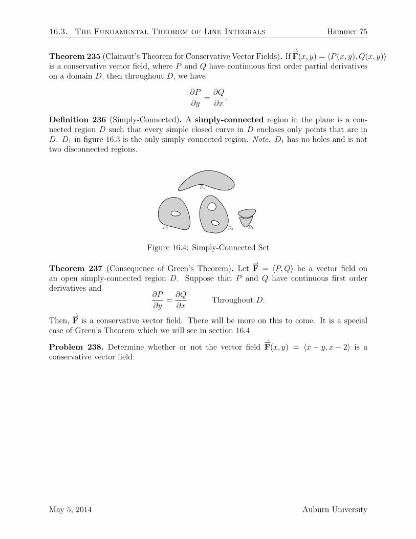
Definition 236 (Simply-Connected). A simply-connected region in the plane is a con-nected region D such that every simple closed curve in D encloses only points that are inD. D1 in figure 16.3 is the only simply connected region. Note. D1 has no holes and is nottwo disconnected regions.

D1

D2 D3D4

Figure 16.4: Simply-Connected Set

Theorem 237 (Consequence of Green’s Theorem). Let ⇀F = 〈P,Q〉 be a vector field onan open simply-connected region D. Suppose that P and Q have continuous first orderderivatives and

∂P

∂y=∂Q

∂xThroughout D.

Then, ⇀F is a conservative vector field. There will be more on this to come. It is a specialcase of Green’s Theorem which we will see in section 16.4

Problem 238. Determine whether or not the vector field ⇀F(x, y) = 〈x− y, x− 2〉 is aconservative vector field.



Problem 239. Determine whether or not the vector field ⇀F(x, y) = 〈3 + 2xy, x2 − 3y2〉 is aconservative vector field.

Problem 240. If ⇀F(x, y, z) = 〈y2, 2xy + e3z, 3ye3z〉 , find a function f such that ∇f = ⇀F.

Suggested Problems: p. 1082, 3-10, 12-18


16.4. Green’s Theorem Hammer 77

16.4 Green’s Theorem

Definition 241 (Orientation). Traversing a curve C in a counterclockwise direction is saidto be a positive orientation of the curve C. Similarly, traversing a curve C in a clockwisedirection is said to be a negative orientation of a curve C.

CC

D D

Positive Orientation Negative Orientation

Figure 16.5: Orientation

Theorem 242 (Green’s Theorem). Let C be a positively oriented, piecewise-smooth, simpleclosed curve in the plane and let D be the region bounded by C. If P and Q have continuouspartial derivatives on an open region that contains D, then

ˆ

C

P dx+Qdy =

¨

D

(∂Q

∂x− ∂P

∂y

)dA.

Notation 243. We denote the line integral calculated by using the positive orientation ofthe closed curve C by

¸C

P dx + Qdy,�C

P dx + Qdy, orflC

P dx + Qdy,. We denote line

integrals calculated by using the negative orientation of the closed curve C byıC

P dx+Qdy,

Theorem 244 (Area Using Green’s theorem). The area of a region D can be calculatedusing Green’s Theorem as follows:

AD =

˛

C

x dy = −˛

C

y dx =1

2

˛

C

x dy − y dx.




x4 dx + xy dy, where C is the triangular curve consisting of the

line segments from (0, 0) to (1, 0), from (1, 0) to (0, 1), and from (0, 1) to (0, 0).


˛

C

(3y − esin(x)

)dx +

(7x+

√y4 + 1

)dy, where C is the circle

x2 + y2 = 9.


16.4. Green’s Theorem Hammer 79

Problem 247. Find the area enclosed by the ellipsex2

a2+y2

b2= 1. Hint. The ellipse has a

parametric equation x = a cos(t), y = b sin(t), where 0 ≤ t ≤ 2π.

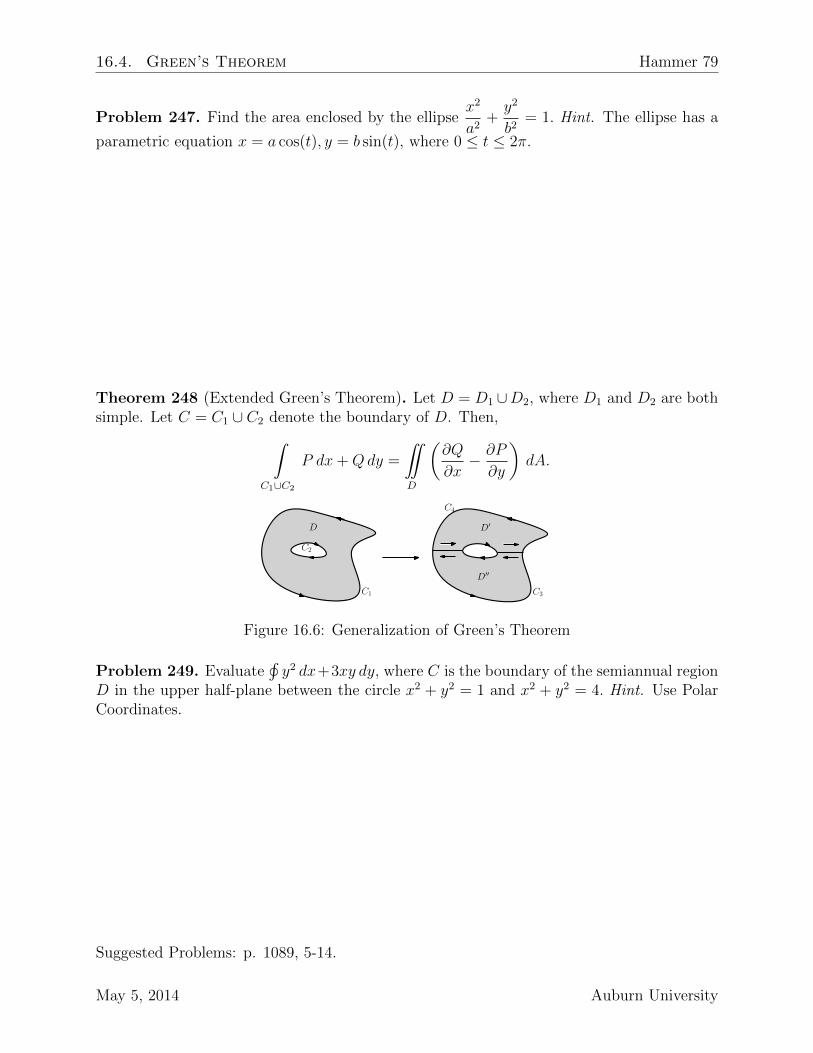
Theorem 248 (Extended Green’s Theorem). Let D = D1 ∪D2, where D1 and D2 are bothsimple. Let C = C1 ∪ C2 denote the boundary of D. Then,

ˆ

C1∪C2

P dx+Qdy =

¨

D

(∂Q

∂x− ∂P

∂y

)dA.

D

C1

C2

D′′

D′

C3

C4

Figure 16.6: Generalization of Green’s Theorem

Problem 249. Evaluate¸y2 dx+3xy dy, where C is the boundary of the semiannual region

D in the upper half-plane between the circle x2 + y2 = 1 and x2 + y2 = 4. Hint. Use PolarCoordinates.

Suggested Problems: p. 1089, 5-14.



16.5 Curl and Divergence

16.5.1 Curl

We now define a the curl of a function, which helps us represent rotations of different sortsin physics and such fields. It can be used, for instance, to represent the velocity field in fluidflow.

Recall 250 (Del). For ease of notation, we denote “del” (∇) as ∇ =⟨∂∂x, ∂∂y, ∂∂z

⟩.

Definition 251 (Curl). Let ⇀F = 〈P,Q,R〉 be a vector field in R3. The curl of ⇀F is definedas:

curl ⇀F = ∇× ⇀F

=

∣∣∣∣∣∣∣∣∣

i j k

∂∂x

∂∂y

∂∂z

P Q R

∣∣∣∣∣∣∣∣∣=

⟨(∂R∂y− ∂Q

∂z

),(∂P∂z− ∂R

∂x

),(∂Q∂x− ∂P

∂y

)⟩.

Problem 252. If ⇀F(x, y, z) = 〈xz, xyz,−y2〉 , find the curl ⇀F.


16.5. Curl and Divergence Hammer 81

Theorem 253. If f is a function of three variables that has continuous second order partialderivatives, then curl (∇f) = ⇀0.

Problem 254. Prove theorem 253.

Theorem 255. If ⇀F is a vector field defined on all R3 whose component functions have

continuous partial derivatives and curl ⇀F = ⇀0, then ⇀F is a conservative vector field.

Problem 256. Show that the vector field ⇀F(x, y, z) = 〈xz, xyz,−y2〉 is not conservative.



16.5.2 Divergence

The divergence can be understood once again in terms of fluid flow. If ⇀F is the velocity of a

fluid, then the divergence of ⇀F represents the net rate of change with respect to time of themass of the fluid per unit volume.

Definition 257 (Divergence). If ⇀F = 〈P,Q,R〉, then the divergence, div ⇀F, is defined as

div ⇀F = ∇ · ⇀F =∂P

∂x+∂Q

∂y+∂R

∂z.

Problem 258. If ⇀F(x, y, z) = 〈xz, xyz,−y2〉 , find div ⇀F.

Theorem 259. If ⇀F = 〈P,Q,R〉 is a vector field in R3 and P,Q, and R have continuoussecond order partial derivatives, then

div(

curl ⇀F)

= 0.

Problem 260. Prove theorem 259


16.5. Curl and Divergence Hammer 83

16.5.3 Vector Forms of Green’s Theorem

Green’s theorem as we have studied in section 16.4 can be viewed as the line integral of

the tangential component of ⇀F along the curve C as the double integral of the vertical

components of the curl ⇀F over the region D enclosed by C. That is to say,

Theorem 261 (Line Integral of Tangential Component). Let C be a positively oriented,piecewise-smooth, simple closed curve in the plane and let D be the region bounded by C.If P and Q have continuous partial derivatives on an open region that contains D, then the

line integral of the tangential component of ⇀F along a curve C is

˛

C

⇀F · d⇀r =

¨

D

(curl ⇀F

)· ⇀k dA.

A similar thing can be said for the line integral of the normal component of ⇀F along thecurve C.

Definition 262 (Outward Unit Normal Vector). Let ⇀r(t) denote the vector equation of thecurve C. That is, ⇀r(t) = 〈x(t), y(t)〉 , a ≤ t ≤ b.The outward unit normal vector, ⇀n(t) isdefined as

⇀n(t) =

⟨y′(t)

|⇀r′(t)| ,−x′(t)

|⇀r′(t)|

⟩.

Theorem 263 (Line Integral of Normal Component). Let C be a positively oriented,piecewise-smooth, simple closed curve in the plane and let D be the region bounded byC. Let ⇀n denote the outward unit normal vector of C. If P and Q have continuous partialderivatives on an open region that contains D, then the line integral of the normal component

of ⇀F along a curve C is ˛

C

⇀F · ⇀n ds =

¨

D

div ⇀F(x, y) dA.

Suggested Problems: p. 1097, 1-8, 13-18,



16.6 Parametric Surfaces and Their Areas

16.6.1 Parametric Surfaces

Goal 264. This section will aim to describe surfaces by a function ⇀r(u, v) = x(u, v)i +

y(u, v)j + z(u, v)k in a similar way that we described vector functions by ⇀r(t) in previouschapters.

Problem 265. Identify and sketch the surface with vector equation ⇀r(u, v) = 〈2 cos(u), v, 2 sin(u)〉 .

Problem 266. Find a parametric representation of the sphere x2 + y2 + z2 = a2.


16.6. Parametric Surfaces and Their Areas Hammer 85

Problem 267. Find a parametric representation for the cylinder x2 + y2 = 4, where 0 ≤z ≤ 1.

Problem 268. Find a vector function that represents the elliptic paraboloid z = x2 + 2y2.

Problem 269. Find a parametric representation for the surface z = 2√x2 + y2, that is, the

top half of the cone z2 = 4x2 + 4y2.



16.6.2 Surface of Revolution

Theorem 270 (Parametrization of Surface of Revolution). Consider a surface S that canbe obtained by rotating a curve y = f(x) from a ≤ x ≤ b about the x-axis, where f(x) ≥ 0.Let θ be the angle of ration of the surface. Then the surface can be parametrized by

x = x y = f(x) cos(θ) z = f(x) sin(θ).

Problem 271. Find parametric equations for the surface generated by rotating the curvey = sin(x) from 0 ≤ x ≤ 2π about the x-axis.

16.6.3 Tangent Planes

Theorem 272 (Normal Vector to a Surface). Let S be a surface defined by ⇀r(u, v) =

x(u, v)i + y(u, v)j + z(u, v)k. To define the tangent plane at a point P0 = (u0, v0), we mustfirst find a normal vector to the surface at P0. In this vein, define

⇀rv =⟨∂x∂v

(u0, v0),∂y∂v

(u0, v0),∂z∂v

(u0, v0)⟩

⇀ru =⟨∂x∂u

(u0, v0),∂y∂u

(u0, v0),∂z∂u

(u0, v0)⟩.

We use these to give us a normal vector ⇀n(u0, v0) = ⇀ru × ⇀rv. This can be used to find theequation of a tangent plane as in 12.2

Problem 273. Find the tangent plane to the surface with parametric equations x = u2, y =v2, and z = u+ 2v at the point (1, 1, 3).


16.6. Parametric Surfaces and Their Areas Hammer 87

16.6.4 Surface Area

Definition 274 (Surface Area). If a smooth parametric surface S is given by the equation⇀r(u, v) = x(u, v)i + y(u, v)j + z(u, v)k, (u, v) ∈ D and S is covered just once as (u, v) rangesthrough the parameter domain D, then the surface area of S is

A(S) =

¨

D

|⇀ru × ⇀rv| dA,

where ⇀ru =⟨∂x∂u, ∂y∂u, ∂z∂u

⟩and ⇀rv =

⟨∂x∂v, ∂y∂v, ∂z∂v

⟩.

Problem 275. Find the surface area of a sphere with radius a.

Suggested Problems: p. 1108, 3− 6, 19− 26, 37, 38, 39− 45.



16.7 Surface Integrals

Definition 276 (Surface Integral). Suppose S is a surface with vector equation ⇀r(u, v) =

x(u, v)i + y(u, v)j + z(u, v)k, (u, v) ∈ D. Then the surface integral of f over the surfaceS is ¨

S

f(x, y, z) dS =

¨

D

f (⇀r (u, v)) |⇀ru × ⇀rv| dA.

where ⇀ru =⟨∂x∂u, ∂y∂u, ∂z∂u

⟩and ⇀rv =

⟨∂x∂v, ∂y∂v, ∂z∂v

⟩.

Problem 277. Compute the surface integral˜S

x2 dS, where S is the unit sphere x2 + y2 +

z2 = 1.

Theorem 278 (Surface Integral of Graphs). Let S be a surface with equation z = g(x, y).Moreover, S has parametrization

x = x y = y z = g(x, y),

and the surface integral is

¨

S

f(x, y, z) dS =

¨

D

f (x, y, g (x, y))

√(∂z

∂x

)2

+

(∂z

∂y

)2

+ 1 dA.

Problem 279. Evaluate˜S

y dS, where S is the surface z = x + y2 from 0 ≤ x ≤ 1 and

0 ≤ y ≤ 2.


16.7. Surface Integrals Hammer 89

Definition 280 (Orientable Surface). A surface is called orientable if it has two sides.

Definition 281 (Surface Integral over Vector Field). If ⇀F is a continuous vector field defined

on an oriented surface S with unit normal vector ⇀n, then the surface integral of ⇀F overS is ¨

S

⇀F · d⇀S =

¨

S

⇀F · ⇀n dS = ⇀F · (⇀ru × ⇀rv) dA.

This integral is also called the flux of ⇀F across S.

Problem 282. Find the flux of the vector field ⇀F(x, y, z) = 〈z, y, x〉 across the unit spherex2 + y2 + z2 = 1.

Problem 283. Evaluate˜S

⇀F · d⇀S, where ⇀F(x, y, z) = 〈y, x, z〉 and S is the boundary of the

solid region E enclosed by the paraboloid z = 1− x2 − y2 and the plane z = 0.

Suggested Problems: p. 1120, 5− 10, 21− 25



16.8 Stokes’ Theorem

Theorem 284 (Stoke’s Theorem). Let S be an oriented piecewise-smooth surface that isbounded by a simple, closed, piecewise-smooth boundary curve C with positive orientation.

Let ⇀F be a vector field whose components have continuous partial derivatives on an openregion in R3 that contains S. Then

ˆ

C

⇀F · d⇀r =

¨

S

curl ⇀F · d⇀S.


⇀F · d⇀r, where ⇀F(x, y, z) = 〈−y2, x, z2〉 and C is the curve of

intersection of the plane y + z = 2 and the cylinder x2 + y2 = 1.

Problem 286. Use Stoke’s Theorem to compute the integral˜S

curl ⇀F·d⇀S, where ⇀F(x, y, z) =

〈xx, yz, xy〉 and S is the part of the sphere x2 + y2 + z2 = 4 that lies inside the cylinderx2 + y2 = 1 and above the xy-plane.

Suggested Problems: p. 1127, 2− 10.


calculus 3 lecture notes

Documents

double integrals

surface integrals

multiple integrals

iterated integrals

vector calculus

vector forms of greens

space curves

space r3briefly