Calculations in Star Charts

Yuk Tung Liu

2018-07-10

This document lists the equations used in the calculations on the webpages local star chartsand equatorial star charts.

1 Location, Date and Time

The local star chart page uses the computer’s clock to obtain the current local time and thenuses it to calculate the local sidereal times and plot star charts on two locations. The two defaultlocations are at longitude 88.2434W, latitude 40.1164N (Champaign, IL, USA) and at longitude88.2434W, latitude 30S. Sidereal times and star charts at other locations and times can beobtained by clicking the Locations and Times button at the top of the page and filling in the form.

The two default locations can be changed by modifying the init cont() function in the filesidereal.js. The variables place1 is the name of location 1, long1 is the longitude of location 1in degrees (negative to the west of Greenwich and positive to the east of Greenwich), lat1 is the(geodetic) latitude of location 1 in degrees (negative in the southern hemisphere and positive in thenorthern hemisphere). The javascript object tz1 stores the time zone information of location 1:tz1.tz is the time zone offset in minutes, i.e. the difference between the local time and UT (positiveif the local time is behind UT and negative if the local time is ahead of UT); tz1.tzString storesthe string “GMT±hhmm”, where ±hhmm provides the time zone information. Currently, tz1 isset according to the information obtained from the computer clock. The variables place2, long2,lat2, and tz2 store the corresponding information for location 2.

Location 1 can also be determined from user’s IP address using the server on http://ip-api.com/.This option is currently disabled. It can be enabled by setting the variable iplookup to true insidefunction init() in the file sidereal.js.

2 Sidereal Time, UT1, UTC, and Civil Time

Sidereal time is defined as the hour angle of the vernal equinox. Thus, it depends on the observationpoint and how the vernal equinox and equator are defined. The celestial equator and equinoxesmove with respect to an inertial frame because of the tidal torques of the Moon, Sun and planets onthe oblate Earth. When the effect of precession, but not nutation, is included, the resulting equatorand equinoxes are called the mean equator and equinoxes. When both precession and nutationare included, the resulting equator and equinoxes are called the true equator and equinoxes.

The mean sidereal time is the hour angle of the mean vernal equinox of date, i.e. it is the angle,measured along the mean equator, from the observer’s meridian to the great circle that passesthrough the mean vernal equinox and the mean celestial poles. The apparent sidereal time is the

1

hour angle of the true vernal equinox of date. Apparent sidereal time minus mean sidereal time isthe equation of the equinoxes.

The Greenwich sidereal time (GST) is the sidereal time measured at Greenwich. In particular,Greenwich mean sidereal time (GMST) is the mean sidereal time at Greenwich. Greenwich ap-parent sidereal time (GAST) is the apparent sidereal time at Greenwich. The local sidereal time(LST) is related to the GST by

LST = GST + λ, (1)

where λ is the longitude of the observation point, positive if it is to the east of Greenwich andnegative if it is to the west of Greenwich.

Universal Time (UT) is a time standard based on Earth’s rotation with respect to the Sun.There are several versions of universal time. The most commonly used are UT1 and the Coordi-nated Universal Time (UTC).

Prior to 1 January 2003, UT1 was defined by a specified function of GMST. Starting from1 January 2003, UT1 is defined as a linear function of the Earth rotation angle (ERA). ERA isthe modern version of the Greenwich sidereal time. It is defined as the angle measured along thetrue equator between Celestial Intermediate Origin (CIO) and the Terrestrial Intermediate Origin(TIO). CIO is the modern version of the vernal equinox and TIO is the modern version of theGreenwich meridian.

Recall that GMST is the hour angle of the mean vernal equinox measured from the Greenwichmeridian. The mean vernal equinox moves with respect to an inertial frame because of precession.The dominant component is the westward motion of 50.3′′ per year. CIO, on the other hand, isdefined to be non-rotating. Its position at J2000.0 is the mean vernal equinox at J2000.0. Itsposition at other times is always on the true equator. As the true equator moves, the path of theCIO in space is such that the point has no instantaneous east-west velocity along the true equator.TIO is a modern version of the prime meridian on Earth. Unlike the Greenwich meridian, TIOis not fixed on the geographic surface on Earth. It is defined kinematically such that there isno component of polar motion about the pole of rotation. To sum up, CIO replaces the movingequinox as the origin of the celestial coordinate system; TIO replaces the Greenwich meridian asthe origin of the longitude; and ERA replaces GST as a measure of Earth’s rotation.

As explained in Section 3.2 of Explanatory Supplement to the Astronomical Almanac1 Earth’srotation is not uniform. There are three kinds of variations in Earth’s rotation: (1) steady decel-eration, (2) random fluctuations, and (3) periodic changes. Measurements show that the lengthof a day is on average increasing at a rate of 1.7 ms per century. The tidal friction from the Moonand Sun causes the increase in the length of a day by 2.3 ms per century. The 0.6 ms per centurydiscrepancy between the measured deceleration and the deceleration caused by the tidal frictionis possibly associated with changes in the figure of the Earth caused by post-glacial rebound orwith deep ocean dissipation. The random fluctuations in Earth’s rotation is probably caused bythe interaction of the core and mantle of the Earth. The periodic changes in Earth’s rotation ismainly caused by meteorological effects and periodic variations caused by luni-solar tides.

Because of the random components in the rotation of the Earth, accurate value of ERA mustbe obtained from observations. It is determined by Very Long Baseline Interferometry (VLBI)measurements of selected extra-galactic radio sources, mostly quasars, and interpolated by trackingof GPS satellites. Once the ERA, θ, is measured, UT1 is defined by the linear equation (IAU

1Explanatory Supplement to the Astronomical Almanac, ed. by S.E. Urban and P.K. Seidelmann, 3rd edition,University Science Books, Mill Valley, California (2013).

2

Resolution B1.8)

θ(DU) = 2π(0.7790572732640 + 1.00273781191135448DU), (2)

where DU = Julian UT1 date− 2451545.0. Note that UT1 is defined by equation (2).The nonuniformity of UT1 is inconvenient for many applications. As a result, UTC is in-

troduced to approximate UT1. UTC is defined by two components: International Atomic Time(TAI) and UT1. TAI is a weighted average of the time kept by over 400 atomic clocks in over 50national laboratories worldwide. Each second in a TAI is one SI second, defined as the duration of9,192,631,770 periods of the radiation corresponding to the transition between the two hyperfinelevels of the ground state of the caesium-133 atom. UTC is defined to be TAI plus an integralnumber of seconds. The duration of one second in UTC is therefore exactly equal to one SI second.Leap seconds are added to ensure approximate agreement with UT1: |UTC− UT1| < 0.9s. As oftoday (2018-07-10), a total of 27 leap seconds have been inserted since the system of adjustmentwas implemented in 1972. The most recent leap second occurred on December 31, 2016 at 23:59:60UTC.

Civil time is related to UTC by a UTC offset. A UTC offset is a multiple of 15 minutes, andthe majority of offsets are in whole hours. On our webpages, civil (local) times are expressed asGMT±hhmm, where ±hhmm indicates the UTC offset. For example, GMT-0600 means the localtime is UTC - 6 hours; GMT+0545 means the local time is UTC + 5 hours and 45 minutes.

GMST and GAST are related to ERA by the equations

GMST = θ − Eprec , GAST = θ − Eprec + Ee, (3)

where Eprec is the accumulated precession of the equinoxes and Ee is the equation of the equinox.The formula for Eprec is given by equation (3.4) in Explanatory Supplement to the AstronomicalAlmanac:

Eprec(T ) = −0′′.014506− 4612′′.16534T − 1′′.3915817T 2 + 4′′.4× 10−7T 3 + 2′′.9956× 10−5T 4, (4)

where T = (JD− 2451545)/36525 is the Julian century from J2000.0, measured in the terrestrialtime (TT, see the next section). The expression for Ee is given by equation (3.5) in ExplanatorySupplement to the Astronomical Almanac. I only consider the dominant term:

Ee = ∆ψ cos εA, (5)

where ∆ψ is the nutation in longitude and εA is the mean obliquity of the ecliptic. The expressionsfor ∆ψ and εA are given by equations (28) and (26) in Section 7.5. The error in Ee in omittingother terms in equation (3.5) of the book is less than 0.003′′.

The local sidereal times displayed on the local star charts webpage are the local mean siderealtime LMST computed using equations (1), (2), (3), (4) and (16) with UT1 replaced by UTCobtained from the computer clock or obtained from user input. TT is calculated by TT = UT1 +∆T with ∆T computed by the fitting formulae of Espenak and Meeus.

In the actual code, GMST (in hours) is computed by the expression

GMST = 6.697374558336001 + 0.06570748587250752DU0 + 1.00273781191135448h+2.686296296296296× 10−7 + 0.08541030618518518T+2.577003148148148× 10−5T 2, (6)

3

where DU0 = int(DU − 0.5) + 0.5 is the value of DU at the previous midnight (0h) UT1 and soDU0 always ends in .5 exactly. The function int(x) denotes the largest integer smaller than x. Thevariable h = 24(DU − DU0) is the number of hours between DU and DU0. Equation (6) comesfrom the fact that

24(0.7790572732640 + 1.00273781191135448DU) mod 24= 24[0.7790572732640 + 1.00273781191135448(DU0 +H/24)] mod 24= (18.697374558336 +DU0 + 0.06570748587250752DU0 + 1.00273781191135448H) mod 24= (6.697374558336001 + 0.06570748587250752DU0 + 1.00273781191135448H) mod 24 (7)

since DU0 is a half integer and so DU0 mod 24 = 12. Note that the a mod b is defined as theremainder of a divided by b:

a mod b ≡ a− b · int(b/a). (8)

Note that polynomials of T higher than T 2 are not included in equation (6) because they adda small correction to GMST for |T | < 10, which is the time span equation (4) is intended for, butbecome unusually large when extrapolated to large T .

3 Ephemeris Time and Dynamical Time

From the 17th century to the late 19th century, planetary ephemerides were calculated usingtime scales based on Earth’s rotation. It was assumed that Earth’s rotation was uniform. Asthe precision of astronomical measurements increased, it became clear that Earth’s rotation is notuniform. Ephemeris time (ET) was introduced to ensure a uniform time for ephemeris calculations.It was defined by the orbital motion of the Earth around the Sun instead of Earth’s spin motion.However, a more precise definition of times is required when general relativistic effects need to beincluded in ephemeris calculations.

In general relativity, the passage of time measured by an observer depends on the spacetimetrajectory of the observer. To calculate the motion of objects in the solar system, the mostconvenient time is a coordinate time, which does not depend on the motion of any object but isdefined through the spacetime metric. In the Barycentric Celestial Reference System (BCRS), thespacetime coordinates are (t, xi) (i = 1, 2, 3). Here the time coordinate t is called the barycentriccoordinate time (TCB). The spacetime metric for the solar system can be written as [see Eq. (2.38)in Explanatory Supplement to the Astronomical Almanac]

ds2 = −(

1− 2w

c2+

2w2

c4

)d(ct)2 − 4wi

c3d(ct)dxi + δij

[1 +

2w

c2+O(c−4)

]dxidxj, (9)

where sum over repeated indices is implied. The scalar potential w reduces to the Newtoniangravitational potential −Φ in the Newtonian limit, where

Φ(t,x) = −G∫d3x′

ρ(t,x′)

|x− x′|(10)

and ρ is the mass density. The vector potential wi satisfies the Poisson equations with the sourceterms proportional to the momentum density.

TCB can be regarded as the proper time measured by an observer far away from the solarsystem and is stationary with respect to the solar system barycenter. The equations of motion for

4

solar system objects can be derived in the post-Newtonian framework. The result is a system ofcoupled differential equations and can be integrated numerically. In this framework, TCB is thenatural choice of time parameter for planetary ephemerides. However, since most measurementsare carried out on Earth, it is also useful to set up a coordinate system with origin at the Earth’scenter of mass. In the geocentric celestial reference system (GCRS), the spacetime coordinatesare (T,X i), where the time parameter T is called the geocentric coordinate time (TGC). GCRS iscomoving with Earth’s center of mass in the solar system, and its spatial coordinates X i are chosento be kinematically non-rotating with respect to the barycentric coordinates xi. The coordinatetime TCG is chosen so that the spacetime metric has a form similar to equation (9). Since GCRSis comoving with the Earth, it is inside the potential well of the solar system. As a result, TCGelapses slower than TCB because of the combined effect of gravitational time dilation and specialrelativistic time dilation. The relation between TCB and TCG is given by [equation (3.25) inExplanatory Supplement to the Astronomical Almanac]

TCB− TCG = c−2

[∫ t

t0

(v2e

2− Φext(xe)

)dt+ ve · (x− xe)

]+O(c−4), (11)

where xe and ve are the barycentric position and velocity of the Earth’s center of mass, and x isthe barycentric position of the observer. The external potential Φext is the Newtonian gravitationalpotential of all solar system bodies apart from the Earth. The constant time t0 is chosen so thatTCB=TCG=ET at the epoch 1977 January 1, 0h TAI.

Since the definition of TCG involves only external gravity, TCG’s rate is faster than TAI’sbecause of the relativistic time dilation caused by Earth’s gravity and spin. The terrestrial time(TT), formerly called the terrestrial dynamical time (TDT), is defined so that its rate is the sameas the rate of TAI. The rate of TT is slower than TCG by −Φeff/c

2 on the geoid (Earth surface atmean sea level), where Φeff = ΦE − v2

rot/2 is the sum of Earth’s Newtonian gravitational potentialand the centrifugal potential. Here vrot is the speed of Earth’s spin at the observer’s location.The value of Φeff is constant on the geoid because the geoid is defined to be an equipotentialsurface of Φeff . Thus, dTT/dTCG = 1− LG and LG is determined by measurements to be LG =6.969290134×10−10. Therefore, TT and TCG are related by a linear relationship [equation (3.27)in Explanatory Supplement to the Astronomical Almanac]:

TT = TCG− LG(JDTCG − 2443144.5003725) · 86400 s, (12)

where JDTCG is TCG expressed as a Julian date (JD). The constant 2443144.5003725 is chosenso that TT=TCG=ET at the epoch 1977 January 1 0h TAI (JD = 2443144.5003725). Since therate of TT is the same as that of TAI, the two times are related by a constant offset:

TT = TAI + 32.184 s. (13)

The offset arises from the requirement that TT match ET at the chosen epoch.TCB is a convenient time for planetary ephemerides, whereas TT can be measured directly

by atomic clocks on Earth. The two times are related by equations (11) and (12) and must becomputed by numerical integration together with the planetary positions. TT is therefore notconvenient for planetary ephemerides. The barycentric dynamical time (TDB) is introduced toapproximate TT. It is defined to be a linear function of TCB and is set as close to TT as possible.Since the rates of TT and TCB are different and are changing with time, TT cannot be writtenas a linear function of TCB. The best we can do is to set the rate of TDB the same as the rate

5

of TT averaged over a certain time period, so that there is no long-term secular drift between TTand TDB over that time period. The resulting deviation between TDB and TT has componentsof periodic variation caused by the eccentricity of Earth’s orbit and the gravitational fields of theMoon and planets. TDB is now defined by the IAU 2006 resolution 3 as

TDB = TCB− LB(JDTCB − 2443144.5003725) · 86400 s− 6.55× 10−5 s, (14)

where LB = 1.550519768× 10−8 and JDTCB is TCB expressed as a Julian date (JD). The value ofLB can be regarded as 1− dTT/dt averaged over a certain time period.

TDB is a successor of ET. It is practically equivalent to the JPL ephemeris time argument Teph

used by the Jet Propulsion Laboratory to calculate high-precision ephemerides of the Sun, Moonand planets. The relationship between TT and TDB can be written as (Figure 3.2 in ExplanatorySupplement to the Astronomical Almanac]

TDB = TT + 0.001658s sin(g + 0.0167 sin g)+ lunar and planetary terms of order 10−5 s+ daily terms of order10−6 s, (15)

where g is the mean anomaly of Earth in its orbit (and hence g + 0.0167 sin g is the approximatevalue of the eccentric anomaly since 0.0167 is Earth’s orbital eccentricity). A more detailedexpression is given by equation (2.6) in The IAU Resolutions on Astronomical Reference Systems,Time Scales, and Earth Rotation Models, Circular 179, U.S. Naval Observatory, Washington, D.C.The difference between TDB and TT remains under 2 ms for several millennia around the presentepoch. Hereafter, TT and TDB will be used interchangeably.

4 Delta T

∆T is defined to be the difference between TT and UT:

∆T = TT− UT, (16)

where UT can be UT1 (before 1962) or UTC (in and after 1962). Since UTC = TAI−∆(AT) andTT = TAI + 32.184 s,

TT− UTC = 32.184 s + ∆(AT), (17)

where ∆(AT) = 10s+ total number of leap seconds added to UTC since 1972.Past values of ∆T can be deduced from historical records. Analytic expressions for ∆T have

been derived to fit the data. On our webpages, the value of ∆T is computed using the analyticexpressions by Espenak and Meeus to convert UT to TT. It should be noted that almost allcomputations involving the Sun, Moon, planets and stars are based on TT. The only exception iscomputing the sidereal time, in which there is a term linear in UT1 by definition.

5 Calendars

Our webpages use the Gregorian calendar on and after October 15, 1582 (JD 2299160.5) and Juliancalendar before that day. Note that October 4, 1582 (JD 2299159.5) was followed by October 15,1582 because of the Gregorian calendar reform. Our webpages take this into account. However,

6

it should be noted that only Italy, Spain and Portugal adopted the new calendar on this date.Over the next three centuries, the Protestant and Eastern Orthodox countries also adopted thenew calendar, with Greece being the last European country to adopt the calendar in 1923.

Conversion between Julian date and calendar date is implemented by the algorithm in Sec-tion 2.2 of the book Astronomy on the Personal Computer by O. Montenbruck and T. Pfleger,4th edition, Springer 2000 (corrected fourth printing 2009).

6 Celestial Coordinate Systems

6.1 International Celestial Reference System (ICRS)

As mentioned in Section 3, the solar system metric can be written in the Barycentric CelestialReference System (BCRS). The origin of the BCRS spatial coordinates is at the solar systembarycenter, i.e. the center of mass of the solar system. However, BCRS is a dynamical concept.The statement of “we use BCRS” in general relativity is equivalent to the statement “we usebarycentric inertial coordinates” in Newtonian mechanics. BCRS does not define the orientationof the coordinate axes.2

The International Celestial Reference System (ICRS) is a kinematical concept. Its origin is atthe solar system barycenter. The ICRS axes are intended to be fixed with respect to space. Theyare determined based on hundreds of extra-galactic radio sources, mostly quasars, distributedaround the sky. The ICRS axes are aligned with the equatorial system based on the J2000.0mean equator and equinox to within 17.3 milliarcseconds. The x-axis of the ICRS points in thedirection of the mean equinox of J2000.0. The z-axis points very close to the mean celestial northpole of J2000.0, and the y-axis is 90 to the east of the x-axis on the ICRS equatorial plane. Sothe ICRS is a right-handed rectangular coordinate system. The ICRS can be transformed to theequatorial system of J2000.0 by the frame bias matrix. However, since the difference between thetwo systems is tiny, I will not distinguish them.

It is assumed that the distant quasars and extragalactic radio sources do not rotate withrespect to asymptotically flat reference systems like BCRS. In principle this assumption shouldbe checked by testing if the motion of the solar system objects is compatible with the equation ofmotion based on BCRS, with no Coriolis and centrifugal forces. So far no deviations have beennoticed.

However, it is expected that the extra-galactic radio sources should show a secular aberrationdrift caused by the rotation of the solar system barycenter around the center of Milky Way, andthis drift was detected by analyzing decades of the very long baseline interferometry (VLBI) data(see Titov, Lambert & Gontier 2011). The magnitude of the drift is about 6 micro arcseconds peryear, which agrees with the prediction. This effect will need to be taken into account in the futureas measurement accuracies continue to improve.

Given the ICRS coordinates (x, y, z) of an object, the ICRS right ascension α and declinationδ are defined by the relation

x = r cosα cos δ , y = r sinα cos δ , z = r sin δ, (18)

2IAU 2006 Resolution B2 recommends that the BCRS definition is completed with the following: “For allpractical applications, unless otherwise stated, the BCRS is assumed to be oriented according to the ICRS axes.The orientation of the GCRS is derived from the ICRS-oriented BCRS.”

7

where r =√x2 + y2 + z2. Hence α = tan−1(y/x) and δ = sin−1(z/r). The quadrant of α has to

be determined appropriately from x and y. Hereafter, I will write α = arg(x+ iy) to indicate thatan appropriate quadrant should be used. Here arg(z) denotes the argument of a complex numberz. Any complex number z = x + iy can be written in the polar form z = |z|eiθ and arg(z) isdefined to be θ. Thus, given a pair (x, y), arg(x+ iy) mod 2π is unique. In the code, the functionatan2() is used in favor of atan() since the quadrant is taken care of by atan2() automatically.

6.2 Geocentric Celestial Reference System (GCRS)

The origin of Geocentric Celestial Reference System (GCRS) is at the center of mass of the Earth.Ignoring general relativistic correction, the GCRS spatial coordinates X i are related to the BCRSspatial coordinates xi by

X i = xi − xiE, (19)

where xiE are the BCRS coordinates of Earth’s center of mass. Relativistic correction adds termsof order (vE/c)

2 ∼ 10−8, which I ignore. Like BCRS, GCRS is a dynamical concept. In thefollowing, I will also use GCRS to refer to the coordinate system whose origin is at the geocenterand whose axes are oriented to the same directions as those of the ICRS.

The GCRS right ascension α and declination δ are defined in a similar way as the ICRScounterparts:

X = R cosα cos δ , Y = R sinα cos δ , Z = R sin δ, (20)

where R =√X2 + Y 2 + Z2.

6.3 Heliocentric Coordinates

Heliocentric coordinates are similar to the barycentric coordinates, except that the origin is locatedat the center of mass of the Sun. They are related to the barycentric coordinates by

xihelio = xi − xi, (21)

where xi are the barycentric coordinates of the Sun’s center of mass. Heliocentric coordinates areprimarily used in the computation of planetary positions. Since the Sun contains 99.86% of themass in the solar system, the solar system barycenter is very close to the Sun’s center of mass.

7 Precession and Nutation

The orientation of the coordinate axes described in Section 6 are fixed in space. This is convenientfor describing the positions of stars and planets. However, observations are made on Earth’ssurface, which is rotating. The transformation between the celestial coordinate systems and thehorizontal coordinate system centered on the observer involves taking into account Earth’s rotationand the orientation of Earth’s spin axis.

7.1 Precession, Nutation and Polar Motion

Earth’s spin axis changes its orientation in space because of luni-solar and planetary torques onthe oblate Earth. Earth’s spin axis also moves relative to the crust. This is called the polar motion.

8

The motion of Earth’s spin axis is composed of precession and nutation. Precession is the com-ponents that are aperiodic or have periods longer than 100 centuries. Nutation is the componentsthat are of shorter periods and its magnitude is much smaller. Motion with periods shorter thantwo days cannot be distinguished from components of polar motion arising from the tidal defor-mation of the Earth. They are considered as components of polar motion. Therefore, nutation isdefined as the periodic components in the motion of Earth’s spin axis with periods longer thantwo days but shorter than about 100 centuries.

The major component of precession is the rotation of Earth’s spin axis about the ecliptic polewith a period of about 26,000 years. This causes the vernal equinox to move westward by 50.3′′

per year. The principal period of nutation is 18.6 years, which is caused by the Moon’s orbitalplane precesses around the ecliptic. The amplitude of nutation is about 9′′. The amplitude of thepolar motion is about 0.3′′.

In addition, the orbital plane of the Earth around the Sun also moves slowly because ofplanetary perturbation. Hence the ecliptic moves slowly in space. This is called the precession ofthe ecliptic, to be distinguished from the precession of the equator3.

I do not include polar motion on the two webpages.

7.2 Equator, Ecliptic and Equinoxes

The Celestial Intermediate Pole (CIP) is the mean rotation axis of the Earth whose motion inspace contains aperiodic components as well as periodic components with periods greater thantwo days. The motion of CIP is described by precession and nutation.

The true equator is defined to be the plane perpendicular to the CIP that passes throughEarth’s center of mass. Thus, the true equator is constantly changing as a result of precession andnutation. The mean equator is the moving equator whose motion is prescribed only by precession.

Ecliptic generally refers to Earth’s orbital plane projected onto the celestial sphere. However,Earth’s orbital plane is changing because of planetary perturbation. To reduce uncertaintiesin the definition of the ecliptic, IAU have recommended that the ecliptic be defined as the planeperpendicular to the mean orbital angular momentum vector of the Earth-Moon barycenter passingthrough the Sun in the BCRS.

Equator and ecliptic intercepts at two points, called the vernal equinox and autumnal equinox.The true equinoxes are the two points at which the true equator and ecliptic intercepts. The meanequinoxes are the two points at which the mean equator and ecliptic intercepts.

7.3 Equatorial “Of Date” Coordinates

Equatorial coordinates are based on the equator and equinox. The x-axis points to the vernalequinox. The y-axis lies in the equatorial plane and is 90 to the east of the x-axis. The z-axispoints to the celestial pole. Since equator and equinoxes are moving, an epoch must be specified(e.g. J2000.0) to the coordinate system.

Right ascension and declination associated with the equatorial coordinates are defined by equa-tion (20) with (X, Y, Z) replaced by the equatorial coordinates. Right ascension and declinationbased on the true equator and equinox of date may be called the apparent right ascension anddeclination to distinguish them from those based on the mean equator and equinox of date.

3Precession of the equator was formerly called the luni-solar precession, and precession of the ecliptic wasformerly called the planetary precession. They are renamed because the terminologies are misleading. Planetaryperturbation also contributes to the precession of the equator, although the magnitude is much smaller.

9

One commonly used equatorial coordinate system is based on the mean equator and equinox ofJ2000.0. This coordinate system is essentially the same as the GCRS apart from a 17-milliarcseondoffset between the GCRS pole and the pole of the J2000.0 mean equatorial system, and a framebias matrix is required to transform from the GCRS to the J2000.0 mean equatorial system if highprecision is required.

The equatorial coordinates at epoch T2 are related to the equatorial coordinates at epoch T1

by a rotation matrix, which involves precession and nutation.

7.4 Precession Matrix

Denote X2 = (X2 Y2 Z2)T the equatorial coordinates based on the mean equator and equinoxat epoch T1 and X1 = (X1 Y1 Z1)T the equatorial coordinates based on the mean equator andequinox at epoch T2, where the superscript T denotes transpose. So X1 and X2 are columnvectors, and they are related by a 3D rotation described by the precession matrix P (T1, T2):

X2 = P (T1, T2)X1. (22)

The inverse transform isX1 = P−1(T1, T2)X2 = P T (T1, T2)X2. (23)

The second equation arises from the fact that a rotation matrix is orthogonal, i.e. its inverse isequal to its transpose. Denote P0(T ) = P (J2000.0, T ) the precession matrix from the epochJ2000.0 to the epoch T . Then

X2 = P0(T2)P0−1(T1)X1 = P0(T2)P0

T (T1)X1. (24)

On the two webpages, the matrix P0 is computed based on Vondrak, Capitaine and Wallace,A&A 534, A22 (2011) (see also the corrigendum, A&A 541, C1 (2012)). In particular, the Capi-taine et al parametrization is used in which P0 is given by equations (19) and (20) in the paper,with the precession angles χA, ψA and ωA given by equations (11), (13), Tables 4 and 6 in thepaper. The formulae are accurate within 200 millennia from J2000.0.

7.5 Nutation Matrix

Nutation is computed according to the IAU 2000A Theory of Nutation. The formulae are givenby Kaplan in The IAU Resolutions on Astronomical Reference Systems, Time Scales, and EarthRotation Models, Circular 179, U.S. Naval Observatory, Washington, D.C. The computation in-volves over 1000 terms. Since high precision is not needed, only the dominant terms are kept inthe calculation.

Let X0 be the column vector corresponding to the position of an object with respect to themean equator and equinox of date, andX be the column vector corresponding to the position withrespect to the true equator and equinox of date. Then the two vectors are related to by a nutationmatrix: X = NX0. The components of N are given by equation (5.21) of The IAU Resolutionson Astronomical Reference Systems, Time Scales, and Earth Rotation Models, Circular 179(seealso equation (6.41) of Explanatory Supplement to the Astronomical Almanac):

N11 = cos ∆ψN12 = − sin ∆ψ cos εA

10

N13 = − sin ∆ψ sin εAN21 = sin ∆ψ cos εN22 = cos ∆ψ cos ε cos εA + sin ε sin εA (25)

N23 = cos ∆ψ cos ε sin εA − sin ε cos εAN31 = sin ∆ψ sin εN32 = cos ∆ψ sin ε cos εA − cos ε sin εAN33 = cos ∆ψ sin ε sin εA + cos ε cos εA,

where εA is the mean obliquity of the ecliptic of date and ε is the true obliquity of the ecliptic ofdate. They are given by the equations

εA = 84381.′′406− 46.′′836769T − 0.′′0001831T 2 + 0.′′00200340T 3

−0.′′000000576T 4 − 0.′′0000000434T 5 (26)

ε = εA + ∆ε, (27)

where T is the TT Julian centuries from J2000.0. The nutation in longitude ∆ψ and nutationin obliquity ∆ε are each expressed by a sum over 1000 terms. The full formulae are given byequations (5.15)–(5.19) of The IAU Resolutions on Astronomical Reference Systems, Time Scales,and Earth Rotation Models, Circular 179with amplitudes and coefficients listed on pages 88–103.Since high precision is not required, I only keep terms with amplitudes greater than 0.05′′ for|T | < 50. Specifically, I use the following formulae for ∆ψ and ∆ε.

∆ψ = −(17.′′2064161 + 0.′′0174666T ) sin Ω− 1.′′3170906 sin(2F − 2D + 2Ω)−0.′′2276413 sin(2F + 2Ω) + 0.′′2074554 sin 2Ω + 0.′′1475877 sin l′

−0.′′0516821 sin(l′ + 2F − 2D + 2Ω) + 0.′′0711159 sin l (28)

∆ε = 9.′′2052331 cos Ω + 0.′′5730336 cos(2F − 2D + 2Ω)+0.′′0978459 cos(2F + 2Ω)− 0.′′0897492 cos 2Ω, (29)

where l is the mean anomaly of the Moon, l′ is the mean anomaly of the Sun, D is the meanelongation of the Moon from the Sun, Ω is the longitude of the ascending node of the Moon’smean orbit on the ecliptic measured from the mean equinox of date, F = L−Ω and L is the meanlongitude of the Moon. These five angles are given by equation (5.19) of The IAU Resolutions onAstronomical Reference Systems, Time Scales, and Earth Rotation Models, Circular 179:

l = 485868.′′249036 + 1717915923.′′2178T + 31.′′8792T 2 + 0.′′051635T 3 − 0.′′00024470T 4 (30)

l′ = 1287104.′′79305 + 129596581.′′0481T − 0.′′5532T 2 + 0.′′000136T 3 − 0.′′00001149T 4 (31)

F = 335779.′′526232 + 1739527262.′′8478T − 12.′′7512T 2 − 0.′′001037T 3 + 0.′′00000417T 4 (32)

D = 1072260.′′70369 + 1602961601.′′2090T − 6.′′3706T 2 + 0.′′006593T 3 − 0.′′00003169T 4 (33)

Ω = 450160.′′398036− 6962890.′′5431T + 7.′′4722T 2 + 0.′′007702T 3 − 0.′′00005939T 4 (34)

The expressions are taken from Simon et al. (1994), which recommends the optimal use in thetime span between 4000 BC and 8000 AD. On the two webpages, nutation is implemented in thetime span between 3000 BC and 3000 AD (−50 < T < 10).

7.6 Ecliptic North Pole

The position of ecliptic north pole is required to plot the ecliptic at a specific time on the horizontalstar charts and GCRS charts. For the horizontal star charts, the right ascension and declination

11

of the pole associated with the equator and equinox of date are required. For the GCRS charts,the GCRS right ascension and declination of the ecliptic pole is required. I ignore nutation andthe difference between GCRS and J2000.0 mean equatorial system. So only precession is includedin the calculation.

The Ra and Dec of the ecliptic north pole associated with the “of date” mean equatorialcoordinates are α = −π/2 and δ = π/2− εA, where εA is the mean obliquity of the ecliptic of date.The value of εA is calculated by equation (10) and Table 3 in Vondrak, Capitaine and Wallace.The formula applies over a much longer time span than the expression in equation (26). As shownin Figure 4 in Vondrak, Capitaine and Wallace, the variation in εA is about 2.7 over a time spanof 400,000 years.

The Ra and Dec of the ecliptic north pole associated with the J2000.0 mean equatorial coordi-nates are α0 = γ − π/2 and δ0 = π/2− ϕ. The formulae come from the definition of the angles γand ϕ. The angles γ and ϕ are calculated from equation (14) and Table 7 in Vondrak, Capitaineand Wallace. As shown in Figure 8 in Vondrak, Capitaine and Wallace, the variation in ϕ is about5 and variation in γ is about 13 over a time span of 400,000 years.

7.7 Galactic North Pole

The position of the galactic north pole is required to plot the galactic equator. I assume that thegalactic north pole is fixed in space, at least on a time span of 400 millennia. The right ascensionand declination of the galactic north pole with respect to the J2000.0 mean equator and equinoxare α0 = 12h51m26s and δ0 = 2707′42′′. The “of date” mean equatorial coordinates at other timesare computed by applying the precession matrix on the J2000.0 coordinates.

8 Topocentric Coordinates

Positions of celestial objects measured from Earth’s surface are called the topocentric position.The difference between the geocentric and topocentric position is called the diurnal parallax orgeocentric parallax. This effect is particularly important for the Moon, which can be as large as1, but small for the Sun (≤ 8.8′′) and planets. The topocentric position X ′ is related to thegeocentric position X by

X ′ = X −XL, (35)

where XL is the geocentric position of the location. The geocentric location XL can be specifiedby the World Geodetic System (WGS), which is a standard for use in cartography, geodesy, andsatellite navigation including GPS. The latest version of WGS is WGS 84. In WGS, positionsnear Earth’s surface are specified by geodetic coordinates that are referred to a reference spheroid(an ellipse of revolution). Following IERS 2010 conventions, Earth is modeled as a spheroid withequatorial radius a = 6378136.6 m and flattening f = (a − b)/a = 1/298.25642, where b is thepolar radius.

The geodetic coordinates are the geodetic latitude φ, geodetic longitude λ and height h abovethe geoid (Earth surface at mean sea level). Neglecting polar motion, XL can be expressed in the“of data” equatorial system by XL = (XL YL ZL)T with

XL = (aC + h) cosφ cos ts , YL = (aC + h) cosφ sin ts , ZL = (aS + h) sinφ, (36)

where ts is the local apparent sidereal time LAST, and

C = [cos2 φ+ (1− f)2 sin2 φ]−1/2 , S = (1− f)2C. (37)

12

On the local star chart webpage, nutation is also ignored and so ts is replaced by the local meansidereal time LMST. I also set h = 0, which causes an error smaller than 0.5′′ for the Moon ifh < 1 km.

The topocentric right ascension and declination are defined by equation (20) with X, Y , Zreplaced by X ′, Y ′ and Z ′.

9 Aberration of Light

Aberration of light arises from the finite speed of light. Suppose an observer sees an object in thedirection n, the direction of the object relative to another observer moving with velocity v will bein a direction n′. The unit vectors n and n′ are related by the Lorentz transformation. To orderv/c, the expression is the same as in Newtonian kinematics:

n′ =n+ β

|n+ β|, (38)

where β = v/c. The geocentric and topocentric positions of celestial objects are usually computedfrom the BCRS positions using equations (19) and (35). They refer to observers stationary withrespect to the solar system barycenter. Observers on Earth’s surface is moving with respect tothe solar system barycenter, and so the position has to be corrected for the aberration of light.

For observers on Earth’s surface, v has two components: Earth’s orbital velocity vE around thesolar system barycenter and Earth’s spin velocity vspin around its rotation axis. The total velocityis given by the vector sum v = vE + vspin (ignoring small relativistic corrections). The orbitalcomponent vE gives rises to the annual aberration of light and the spin component vspin gives rise tothe diurnal aberration of light. Earth’s orbital speed is vE ≈ 30 km/s and spin speed at the equatoris vspin = 0.465 km/s. The effect of the annual aberration of light is ∼ vE/c ∼ 10−4 rad ∼ 20.5′′.The effect of the diurnal aberration of light is ∼ vspin/c ∼ 0.3′′.

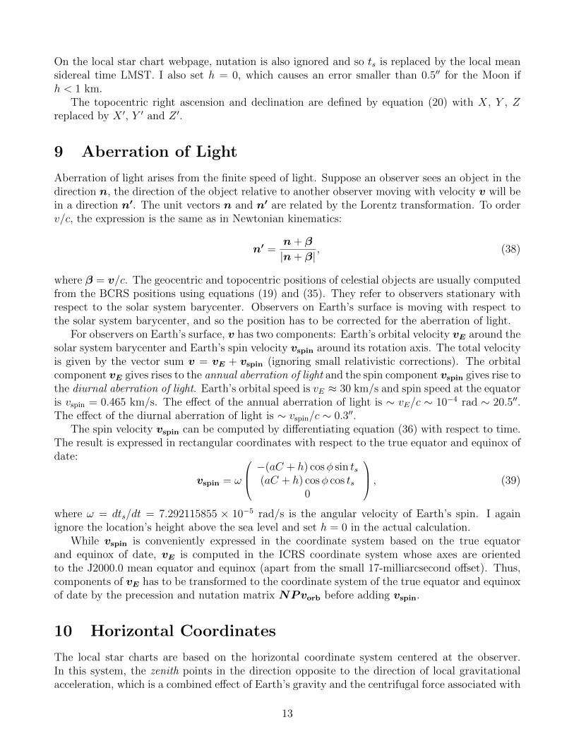
The spin velocity vspin can be computed by differentiating equation (36) with respect to time.The result is expressed in rectangular coordinates with respect to the true equator and equinox ofdate:

vspin = ω

−(aC + h) cosφ sin ts(aC + h) cosφ cos ts

0

, (39)

where ω = dts/dt = 7.292115855 × 10−5 rad/s is the angular velocity of Earth’s spin. I againignore the location’s height above the sea level and set h = 0 in the actual calculation.

While vspin is conveniently expressed in the coordinate system based on the true equatorand equinox of date, vE is computed in the ICRS coordinate system whose axes are orientedto the J2000.0 mean equator and equinox (apart from the small 17-milliarcsecond offset). Thus,components of vE has to be transformed to the coordinate system of the true equator and equinoxof date by the precession and nutation matrix NPvorb before adding vspin.

10 Horizontal Coordinates

The local star charts are based on the horizontal coordinate system centered at the observer.In this system, the zenith points in the direction opposite to the direction of local gravitationalacceleration, which is a combined effect of Earth’s gravity and the centrifugal force associated with

13

Earth’s spin. The horizon is the plane perpendicular to the zenith passing through the observer.The meridian is the great circle passing through the CIP and zenith.

The astronomical latitude is defined as π/2 minus the angle between the zenith and CIP. Theastronomical longitude is defined to be the difference between the local apparent sidereal timeLAST and the Greenwich apparent sidereal time GAST through equation (1). They are close tothe geodetic latitude and longitude but not exactly the same. This is because the geoid is anidealized surface and the observer location is usually above or below the surface and the localgravity points to a slightly different direction. In addition, the local gravity varies slightly as aresult of the changing tidal force, whereas the idealized geoid averages out the effect. Therefore,the direction of the zenith is not exactly perpendicular to the geoid surface. The astronomicalmeridian defined by the CIP and zenith deviates slightly from the geodetic meridian that passesthrough the observer’s location and the actual axis of figure through the center of the Earth. Thedeviation between these two sets of longitude and latitude is usually a few arcseconds. Largerdeviation may result in regions with large gravity anomaly. I ignore the difference between thesetwo sets of longitude and latitude on the two webpages.

Figure 1: Altitude and azimuth in the horizontal coordinate system. Source: Wikipedia

As shown in Figure 1, the altitude and azimuth are defined as angles relating the direction ofthe star to the horizon and the north direction.

If the topocentric equatorial “of date” coordinates of an object (X ′, Y ′, Z ′) are known, thealtitude and azimuth can be computed as follows. First, compute the topocentric right ascensionα and declination δ by α = arg(X ′ + iY ′) and δ = sin−1(Z ′/R′), where R′ =

√X ′2 + Y ′2 + Z ′2.

Next, calculate the hour angle, H, by H = ts − α. Here ts is the local apparent sidereal timeLAST. Finally, a and A are related to H and δ by

cos a sinA = − cos δ sinH (40)

cos a cosA = sin δ cosφ− cos δ cosH sinφ (41)

sin a = sin δ sinφ+ cos δ cosH cosφ. (42)

The altitude computed by these formulae does not include atmospheric refraction, which is signif-icant especially for objects close to the horizon.

14

11 Atmospheric Refraction

Atmospheric refraction changes the altitude of an object. The effect is particularly significantfor objects close to the horizon. At the horizon, refraction can raise the altitude of an objectby 34′. Atmospheric refraction depends on the local temperature, pressure, humidity and otherconditions. Sophisticated atmospheric refraction models involve numerical integration, but theaccuracy depends on the local conditions. On the local star chart webpage, I use a low-precisionfitting formula to model the atmospheric refraction. Sæmundsson’s formula is used in which thechange in altitude ∆a is given by

∆a = 1.02′(

P

101 kPa

)(283 K

T

)cot

(a+

10.3

a+ 5.11

), (43)

where T is temperature and P is pressure. In all calculations, I use T = 286 K and P = 101 kPa.

12 Map Projections

Given the positions of celestial objects in spherical coordinates (altitude, azimuth or GCRS Raand Dec), the final step is to plot them on the computer screen, which is a two-dimensional flatsurface. There are various methods to map a spherical surface to a flat surface. Distortion isunavoidable. Two projection methods are used in our star charts. Stereographic projection isused to generate the local star charts and the polar GCRS charts. Mollweide projection is usedto generate the all-sky GCRS chart.

Stereographic projection is commonly used in sky maps. The mapping is conformal and shapesare preserved over a small area. However, the mapping does not preserve area. For example, inthe local star charts a constellation is about twice as big when it is near the horizon than whenit is near the zenith. This effect is quite noticeable in animations showing the diurnal motion ofthe sky. This feature might not be as bad, since constellations do appear bigger when they areclose to the horizon because of the Moon illusion. However, it should be noted that stereographicprojection is not designed to model the Moon illusion.

Mollweide projection preserves areas but not angles. There is significant distortion in shapesin regions far away from the equator.

12.1 Local Star Charts

The local star charts are based on the horizontal coordinate system. The coordinates are (a,A)(altitude and azimuth). The mapping from (a,A) to the 2D flat surface (xg, yg) is done by thestereographic projection with the nadir as the projection point. Only objects above or on thehorizon (a ≥ 0) are plotted.

Before describing the equation of the mapping, it is useful to understand how the graph co-ordinate system is oriented. Graphs are drawn using the HTML canvas. As shown in Figure 2,in the HTML canvas coordinates (xg, yg) the upper-left corner is the origin (xg, yg) = (0, 0). Thex coordinate increases to the right and y coordinates increases downward. The coordinate of thelower-right corner is (xg, yg) = (w, h), where w is the width and h is the height of the canvas inpixels. In the local star charts, I set w = h = 800 pixels.

The mapping (a,A)→ (xg, yg) is given by

r = rh tan(π

4− a

2

), xg =

w

2+ r sinA , yg =

h

2+ r cosA, (44)

15

Figure 2: Graph coordinates in canvas. The origin is at the upper-left corner. The x coordinateincreases to the right and y coordinates increases downward. The coordinate of the lower-rightcorner is (w, h), where w is the width and h is the height of the canvas.

where rh = 0.47 max(w, h). The equation can be considered as two transformations: a → r and(r, A)→ (xg, yg). Under this mapping, the zenith is mapped to the center of the canvas. Contoursof a are circles of radius rh tan(π/4 − a/2) centered at the center of the canvas. Thus, the valueof rh is the radius of the horizon. The value 0.47 is to make rooms for drawing labels outside thehorizon.

12.2 GCRS Star Charts

12.2.1 Polar Charts

The first chart is centered at the GCRS north pole. It is generated by the stereographic projectionwith the GCRS south pole as the projection point. Only the region in the northern hemisphere isshown. The third chart is centered at the GCRS south pole. It is generated by the stereographicprojection with the GCRS north pole as the projection point.

In general, if αc and δc are the GCRS right ascension and declination at the center of the chart.The mapping (α, δ)→ (xg, yg) is given by

xg =w

2+rh(cos δc sin δ − sin δc cos δ cos ∆α)

1 + sin δc sin δ + cos δc cos δ cos ∆α, (45)

yg =h

2− rh cos δ sin ∆α

1 + sin δc sin δ + cos δc cos δ cos ∆α, (46)

where rh = 0.465 max(w, h) and ∆α = α−αc. The width and height are set to w = h = 700 pixels.For the first chart, δc = π/2. For the third chart, δc = −π/2. The value of αc determines theorientation of the GCRS Ra lines. For example, if αc = 0 in the first chart, the line α = 0 is ahorizontal line from the graph center (w/2, h/2) to the middle left point (w/2− rh, h/2).

Note that when δc = π/2, δ = a and ∆α = −π/2 − A, equations (45) and (46) reduce toequation (44) since it can be shown that tan(π/4− a/2) = cos a/(1 + sin a).

16

12.2.2 All-Sky Chart

The second GCRS chart is an all-sky chart. The GCRS right ascension at the center is set by theparameter αc. The canvas width and height are w = 800 pixels and h = 400 pixels. The chart isgenerated by the Mollweide projection. The mapping (α, δ)→ (xg, yg) is given by

xg =w

2− rhP

(α− αcπ

)cos θ , yg =

h

2− rh

2sin θ, (47)

where rh = 0.465 max(w, h) and θ satisfies the equation

2θ + sin 2θ = π sin δ. (48)

The above equation is solved by the Newton-Raphson method. The Newton-Raphson methodusually converges to machine roundoff precision within 6 iterations. However, it may fail veryclose to the poles (|δ| ≈ π/2). When the Newton solver fails to converge after 20 iterations, themethod of bisection is used instead, but this rarely, if ever, occurs.

In equation (47), the function P is defined as

P (x) = x− 2 · int(x+ 1

2

)(49)

so that P (x) ∈ [−1, 1) for any x ∈ (−∞,∞). This means that xg ∈ [w/2 − rh, w/2 + rh) and allpoints are inside an ellipse centered at (w/2, h/2) with a semi-major axis of rh and a semi-minoraxis of rh/2.

12.3 Joining Two Points by a Straight Line

In some cases (e.g. drawing constellation lines), I want to join two points rg1 = (xg1, yg1) andrg2 = (xg2, yg2) by a straight line on canvas. This is straightforward in most cases. However,in the stereographic charts, only half of the celestial sphere is plotted. If both points are insidethe chart, a straight line is drawn without any problem. If both points are outside the chart, noline will be drawn (even though it is possible to have a portion of the line inside the chart). Theproblem arises if one of the points is outside the chart. In this case, only the part of the lineinside the chart should be drawn. In the Mollweide chart, the whole celestial sphere is covered.However, in some cases it happens that the straight line connecting the two points crosses the leftand right boundary of the chart. In this case, the line should be broken into two: one joining rg1to the boundary and another joining rg2 to the boundary on the other side.

In the following I describe the mathematical detail in handling these cases.

12.3.1 Stereographic Charts

A point rg is inside the chart if |rg − rc| ≤ rh, where rc = (w/2, h/2) is the position vector of thecanvas center. Let ξ = rg − rc. Also denote ξ1 = rg1 − rc and ξ2 = rg2 − rc. Suppose that oneof the two points is outside the chart. Then either |ξ1| > rh or |ξ2| > rh. I will then replace thepoint outside the chart by a point on the line and on the chart boundary. Points on the straightline joining rg1 and rg2 can be described by the parametric equation

ξ(s) = ξ1 + s(ξ2 − ξ1), (50)

17

where s ∈ [0, 1]. The goal is to find s so that |ξ(s)| = rh, which is a quadratic equation in s. Thesolution of the quadratic equation is given by

s± =ξ2

1 − ξ1 · ξ2 ±√

(ξ21 − ξ1 · ξ2)2 + (r2

h − ξ21)|ξ2 − ξ1|2

|ξ2 − ξ1|2. (51)

The solution s = s+ should be used if |ξ2| > rh and s = s− should be used if |ξ1| > rh.In summary, if rg2 is outside the chart, the straight line should be the line joining rg1 to rg3,

whererg3 = rg1 + s+(rg2 − rg1). (52)

If rg1 is outside the chart, the straight line should be the line joining rg2 to rg3, where

rg3 = rg1 + s−(rg2 − rg1). (53)

12.3.2 Mollweide Chart

The central GCRS Ra is specified by the parameter αc. The left and right boundary of the chartis α = αc +π. Given two points rg1 and rg2, first determine whether the line joining them crossesthe boundary by calculating the following three quantities

∆x1 = P(α1 − αc − π

π

), ∆x2 = P

(α2 − αc − π

π

), ∆x12 = P

(α1 − α2

π

). (54)

The line will cross the boundary if the following conditions are satisfied: (1) ∆x1∆x2 < 0 and(2) |∆x1| + |∆x2| = |∆x12|. The first condition says that α1 and α2 are on the opposite side ofthe boundary Ra. The second condition says that the line that crosses the Ra boundary is theshortest line joining the two points. As an example, suppose rg1 = (−π/4, δ1), rg2 = (π/2, δ2)and αc = 0. It follows that ∆x1 = 3/4, ∆x2 = −1/2 and ∆x12 = −3/4. It is clear that α1 andα2 are on opposite sides of the boundary Ra αb = π, but the shortest line joining the two pointpasses through α = 0 instead of α = π and so the line does not cross the boundary Ra. Thesecond condition is violated in this case. Suppose that αc = π. Then the boundary Ra is αb = 0and so the line crosses the boundary. In this case, ∆x1 = −1/4, ∆x2 = 1/2, ∆x12 = −3/4, andboth conditions are indeed satisfied.

Suppose that the shortest line joining the two points does cross the boundary Ra. The linewill be split into two: a line joining rg1 and rg3, and a line joining rg2 and rg4, where rg3 is onthe chart boundary closest to rg1 and rg4 is on the chart boundary closest to rg2.

To calculate rg3, first compute the following vectors

ξ1 =rg1 − rc

rh, ξ2 =

rg2 − rcrh

. (55)

Next compute ξ′2 = (ξ′2x, ξ2y), where

ξ′2x =

ξ2x + 2 cos θ2 if x1 > 0ξ2x − 2 cos θ2 if x1 < 0

, (56)

and θ2 satisfies the equation 2θ2 +sin 2θ2 = π sin δ2. Defined in this way, the point r′g2 = xc+rhξ′2

is outside the chart. Next find rg3 on the line joining rg1 and r′g2 and on the chart boundary.Points on the line joining rg1 and r′g2 can be parameterized by the equation

ξ(s) = ξ1 + s(ξ′2 − ξ1), (57)

18

where s ∈ [0, 1]. The boundary of the chart is an ellipse centered at rc with a semi-major axisrh and a semi-minor axis rh/2. Hence, the point ξ is on the boundary if ξ2

x + 4ξ2y = 1, which is a

quadratic equation in s. The solution is given by

s =1− ξ2

1x − 4ξ21y

ξ1x∆ξx + 4ξ1y∆ξy +√

(ξ1x∆ξx + 4ξ1y∆ξy)2 + (∆ξ2x + 4∆ξ2

y)(1− ξ21x − 4ξ2

1y),

∆ξx = ξ′2x − ξ1x , ∆ξy = ξ2y − ξ1y, (58)

and rg3 is given by

rg3 = rc + rh[ξ1 + s(ξ′2 − ξ1)] = rg1 + rhs(ξ′2 − ξ1). (59)

Having computed rg3 = (xg3, yg3), rg4 = (xg4, yg4) can be computed by the equation

xg4 =w

2− xg3 , yg4 = yg3. (60)

13 Plotting Equator, Ecliptic and Galactic Equator

Ecliptic is plotted on a local star chart when the Ecliptic button below the chart is active. Eclipticis plotted on the GCRS charts when the Ecliptic button on the GCRS page is active. Galacticequator, as well as Milky Way boundary, is plotted on a local star chart when the Milky Waybutton below the chart is active. Galactic equator, as well as Milky Way boundary, is plotted onthe GCRS charts when the Milky Way button on the GCRS page is active.

In this section, I discuss the mathematical detail in plotting the equator, ecliptic and galacticequator, which are all great circles on the celestial sphere. They can be defined as the planeperpendicular to a pole. The general strategy is first to calculate the position of the pole inthe coordinate system the chart is based on. Then the coordinates of points on the great circleperpendicular to the pole can be parameterized by a parameter θ.

13.1 Local Star Charts

The coordinate system the local star charts based on is the horizontal coordinate system. Firstcalculate the altitude ap and azimuth Ap of the pole. Either a north pole or a south pole willwork. I choose the north pole.

The “of date” declination of the celestial north pole is δ = π/2. The “of date” Ra and Decof the ecliptic north pole are αp = −π/2 and δp = π/2 − εA, where the mean obliquity of theecliptic of date is computed by equation (10) and Table 3 in Vondrak, Capitaine and Wallace.The Ra and Dec of the galactic north pole with respect to J2000.0 mean equator and equinoxare αp0 = 12h51m26s and δp0 = 2707′42′′. The “of date” mean equatorial coordinates at othertimes are computed by applying the precession matrix on the J2000.0 coordinates. Specifically,the vector Xp = P0(T )Xp0 is calculated, where Xp0 is a column vector defined as

Xp0 = (cosαp0 cos δp0 sinαp0 cos δp0 sin δp0)T (61)

and the precession matrix P0(T ) is calculated by equations (20), (11), (13), Tables 4, 6 in Vondrak,Capitaine and Wallace. The “of date” Ra and Dec of the galactic north pole is then given byαp = arg(Xp + iYp) and δp = sin−1 Zp. Note that |Xp| = |Xp0| = 1 by construction.

19

Having computed the “of date” mean equatorial position of the pole, the hour angle is calcu-lated approximately by Hp = ts − αp, where ts is the local mean sidereal time (LMST) computedby ts = GMST+λ. Here λ is the longitude of the location and GMST is computed by equation (6).Note that LAST and the apparent position are not used in the computation because the correctionis small and can be ignored for plotting purpose.

The altitude ap and azimuth Ap are obtained by equations (40)–(42). Next calculate a vectorrp = (cosAp cos ap, sinAp cos ap, sin ap), which is a unit vector pointing in the direction of the polein the horizontal coordinate system. Denote rz = (0, 0, 1) the unit vector pointing towards thezenith. Define two unit vectors V and W as follows:

V =rz × rp|rz × rp|

, W = rp × V . (62)

It follows that both V and W are perpendicular to rp and so are on the great circle of interest.The great circle can be parameterized by the unit vector

C(θ) = cos θV + sin θW , (63)

where θ ∈ [0, 2π). The altitude and azimuth associated with C(θ) are A(θ) = arg(Cx(θ) + iCy(θ))and a(θ) = sin−1Cz(θ). The set of points a(θ), A(θ), θ ∈ [0, 2π) represents the great cicle in thehorizontal coordinate system. In addition, it is easy to show that

rz ·C(θ) =1− (rz · rp)2

|rz × rp|sin θ. (64)

It follows that rz ·C(θ) ≥ 0 for θ ∈ [0, π]. These are the points on the great circle that are aboveor on the horizon. The canvas coordinates of these points are calculated by equation (44). Thesepoints can then be joined by a curve representing the great circle on the canvas.

13.2 GCRS Charts

The coordinate system is the GCRS equatorial coordinate system, which is essentially the same asthe J2000.0 mean equatorial coordinate system except for the 17-milliarcsecond offset between theirpoles. I treat these two systems as identical because of the small offset. In this coordinate system,the coordinates of the north pole of the ecliptic of date are αp = γ − π/2 and δp = π/2− ϕ. Theangles γ and ϕ are calculated from equation (14) and Table 7 in Vondrak, Capitaine and Wallace.The coordinates of the galactic north pole are αp = 12h51m26s and δp = 2707′42′′.

The procedure of plotting the great circle perpendicular to the pole is similar to that de-scribed in the previous subsection. The unit vector associated with the pole is computed byrp = (cosαp cos δp, sinαp cos δp, sin δp). The unit vector associated with the GCRS north pole isrz = (0, 0, 1). Define two unit vectors

V =rz × rp|rz × rp|

, W = rp × V . (65)

It follows that both V and W are perpendicular to rp and so are on the great circle of interest.The great circle can now be parameterized by the unit vector

C(θ) = cos θV + sin θW , (66)

20

where θ ∈ [0, 2π). The GCRS Ra and Dec associated with C(θ) are α(θ) = arg(Cx(θ) + iCy(θ))and δ(θ) = sin−1Cz(θ). The set of points α(θ), δ(θ), θ ∈ [0, 2π) represents the great cicle in theGCRS coordinate system. The canvas coordinates of these points are given by equations (45)–(46)for the polar charts and equation (47) for the all-sky chart. Half of the great circle will appear oneach of the polar charts and the full great circle will appear in the all-sky chart.

14 Stars

14.1 Database

The star data used on our webpages are a subset of the HYG 3.0 database. The database isconstructed using the following procedure. All data processing was done using the R software.

1. Remove the Sun, Capella B and α Cen B from the database. Capella B and Capella Aare too close to be separated on our star charts. They have slightly different 3D motions(constructed from the database) that will separate them in the distant future and distantpast. That is why Capella B is removed. α Cen B is removed for the same reason.

2. The ICRS rectangular coordinates of each star are computed from their distance D0, J2000.0α0 and δ0 by x0 = D0 cosα0 cos δ0, y0 = D0 sinα0 cos δ0 and z0 = D0 sin δ0. These arecomponents of the ICRS position vector r(t) at t =J2000.0. Note that a value of 100,000is assigned to D0 if the distance of a star is unknown or its value is dubious. This will notcause much trouble since it is the angular direction of the star that is important, but it needsto be kept in mind for calculations involving D0.

3. ICRS components of a star’s 3D velocity is computed from its distance D0, J2000.0 α0 andδ0, proper motions µα, µδ and radial velocity vr according to the equation

v = D0µαeα +D0µδeδ + vrer, (67)

eα = − sinα0 cos δ0x+ cosα0 cos δ0y (68)

eδ = − cosα0 sin δ0x− sinα0 sin δ0y + cos δ0z (69)

er = cosα0 cos δ0x+ sinα0 cos δ0y + sin δ0z. (70)

All components of v, vx, vy and vz, are converted to pc/(Julian century) for convenience oflater calculations.

4. Our webpages draw star charts in the time range J2000.0±200,000 years. For stars withreliable measured distance (D0 6= 105), their minimum distance and magnitude in the timeintervals J2000.0±200,000 years are calculated as follows. The ICRS position vector of thestar as a function of t (neglecting light-time correction) is given by

r(t) = r0 + v∆t, (71)

where r0 is the position vector of the star at t = t0=J2000.0 and ∆t = t − t0. Here it isassumed that the star moves with a constant velocity v. The distance is minimum whenv · r(t) = 0, which gives

∆tmin = −r0 · vv2

. (72)

21

Since time is restricted to |∆t| < 2 × 105 years, set ∆tmin = −2 × 105 years if ∆tmin <−2 × 105 years and ∆tmin = 2 × 105 years if ∆tmin > 2 × 105 years. Then the minimumdistance in the time interval is

Dmin = |r0 + v∆tmin| (73)

and the minimum magnitude of the star is calculated by the inverse square law as

mmin = m0 + 5 log10(Dmin/D0), (74)

where m0 is the star’s magnitude at t = t0 and D0 = |r0| is the star’s distance at t = t0.

5. Stars with mmin > 5.3 are removed from the database since 5.3 is the limiting magnitude ofstars that will be plotted on our star charts. The resulting database contains 2559 stars.

6. For the purpose of drawing constellation lines, certain stars are manually selected for eachconstellation line segment. They are specified by either the star’s proper name, Bayer/Flamsteedname, or hip number. They are then converted to the index numbers in the database.

7. For each of the 88 constellations, approximate values of the ICRS Ra and Dec of the constel-lation are entered manually. The constellation labels, when active, will be plotted at theselocations. For the constellations Hydra, Serpens and Eridanus, two locations are indicatedbecause of their large size or topology.

8. The final data are put into JSON format and outputted to the JavaScript file brghtStars.js,which contains functions returning JavaScript objects.

14.2 Light-time Correction

Light-time correction arises from the finite speed of light. It is usually included in the calculationof the apparent positions of planets, but usually not applied to the positions of stars because theirmotion and distance are not known accurately. Our webpages do not include light-time correctionfor stars. The detail calculation is presented here so that it can be implemented when accuratedata are available in the future. The equations derived in this subsection are essentially the sameas those in Stumpff [A&A 144, 232 (1985)], but are derived using a different approach.

The observed barycentric position of a star at time t is the “true” position of the star at theretarded time tr

r∗(t) = r(tr). (75)

The retarded time tr satisfies the equation

tr(t) = t− D(tr)

c, (76)

where D(tr) = |r(tr)| is the barycentric distance of the star at the retarded time and c is the speedof light. Differentiating equation (75) with respect to t gives

v∗(t) = r∗(t) = v(tr)dtrdt. (77)

22

It follows from (76) that

dttdt

= 1− vrc

dtrdt

⇒ dtrdt

=1

1 + βr(tr), (78)

where vr = dD/dt is the radial velocity and βr = vr/c. Combining equations (77) and (78) gives

v∗(t) =v(tr)

1 + βr(tr). (79)

Thus, the observed tangential velocity, v∗T (t) = Dµαeα +Dµδeδ is related to the true tangentialvelocoty at the retarded time vT (tr) by

v∗T (t) =vT (tr)

1 + βr(tr). (80)

This formula explains the origin of the observed superluminal motion of jets in some active galaxies:if a jet moving close to the speed of light is moving at a very small angle towards the observer,1 + βr 1 and it is possible to have v∗T > c. Equation (80) is usually derived by drawing afigure showing the geometry between the source and observer. The derivation presented hereis mathematically more straightforward but the physics behind the formula is illustrated moreclearly in the conventional derivation. For stars in the vicinity of the Sun, βr ∼ 10−4 and so thecorrection to the tangential velocity is very small. The radial velocity vr is related to the redshiftz by the special relativistic Doppler formula

1 + z =1 + βr√1− β2

, (81)

where β = v/c =√v2T + v2

r/c. Thus, equations (80) and (81) must be solved together to obtain vTand vr from the observed quantities v∗T and z. Once vT and vr are computed, the true velocityv(tr) is obtained. I assume that v is constant, which is in general a good approximation since thetime scale of galactic rotation in the solar neighborhood is 108 years and is much longer than thetime span considered here.

Suppose the apparent position at time t0, r∗(t0), and the velocity v is known, the observedposition at time t = t0 + ∆t is given by

r∗(t) = r(tr(t)) (82)

with

tr(t) = t− D(tr(t))

c= t0 + ∆t− D(tr(t0))

c+D(tr(t0))−D(tr(t))

c

= tr(t0) + (1 + f)∆t, (83)

where

f =D(tr(t0))−D(tr(t))

c∆t. (84)

Denote r∗0 = r∗(t0) = r(tr(t0)), D0 = D(tr(t0)) = |r∗0|, and D = D(tr(t)) = |r∗(t)|. It followsfrom equation (82), (83) and r(t2) = r(t1) + v(t2 − t1) that

r∗(t) = r∗0 + (1 + f)v∆t. (85)

23

It follows from (84) thatD = D(tr(t)) = |r∗(t)| = D0 − fc∆t. (86)

Combining equations (85) and (86) yields

D0 − fc∆t = |r∗0 + (1 + f)v∆t|. (87)

Squaring both sides of the above equation gives

(D0 − fc∆t)2 = D20 + 2(1 + f)∆tr∗0 · v + (1 + f)2v2∆t2. (88)

This is a quadratic equation in f and the solution is given by

f = − 2s0 · β + β2∆t

s0 + s0 · β + β2∆t+√Q, (89)

where s0 = r∗0/c, β = v/c, s0 = |s0|, β = |β| and

Q = (s0 + s0 · β + β2∆t)2 + (1− β2)(2s0 · β + β2∆t). (90)

Equations (85) and (89) can be used to update the apparent position of a star from time t0 to t.The term fv∆t is an extra term arising from the light-time correction. The value of f is of orderβ, which is ∼ 10−4 for stars in the solar neighborhood. Since the fractional accuracy of v is muchlarger than 10−4 in the data used by our webpages, including the light-time correction will notimprove the accuracy of a star’s position.

14.3 Plotting Stars

Geocentric apparent positions of stars at a given time are required to plot the stars in the GCRSstar charts. Topocentric apparent positions of stars are required to plot the stars in the local starcharts. Chapter 7 of Explanatory Supplement to the Astronomical Almanacprovides a detailedprocedure in computing the apparent positions of stars. For geocentric apparent positions, thestars’ space motion, annual parallax, gravitational deflection of light by the Sun, and annualaberration of light should be included. For topocentric positions, precession, nutation, polarmotion, diurnal aberration of light and atmospheric refraction should also be included.

Apart from precession and space motion, all the other effects mentioned are periodic or nonac-cumulative. Annual parallax is inversely proportional to the star’s distance. It is very small. Theparallax of the closest stars is about 0.75′′. Gravitational deflection of light is only significant ifthe star is in a direction very close to the Sun. However, the maximum deflection angle is only1.75′′. Annual aberration of light causes a shift in a star’s position by 20.5′′ over the course of ayear. The effect of nutation is about 9′′. The effect of diurnal aberration is smaller than 0.32′′.Polar motion affects a star’s position by about 0.3′′. Atmospheric refraction can change a star’sposition by 34′ if it is close to the horizon. On our webpages, only the space motion, precessionand atmospheric refraction are included when plotting stars.

A star’s ICRS position at time t (neglecting light-time correction) is calculated according tothe equation

r(t) = r0 + v(t− t0), (91)

where t0 =J2000.0 and r0 = D0(cosα0 cos δ0 sinα0 cos δ0 sin δ0)T is the ICRS position vector att = t0, α0 and β0 are the star’s ICRS Ra and Dec at J2000.0, and D0 = |r0| =

√r0Tr0 is the

24

distance of the star at t = t0. Since parallax is ignored, the star’s GCRS position is the sameas its ICRS position: X(t) = r(t). The GCRS Ra and Dec of the star at time t is thereforeα = arg(X + iY ) and δ = sin−1(Z/D), where D = |X(t)| = |r(t)|. The magnitude of the star attime t is

m(t) = m0 + 5 log10(D/D0), (92)

where m0 is the star’s magnitude at t = t0. The star can now be plotted on the GCRS star charts:its canvas coordinates on the star charts are given by equations (45)–(47). A star is representedby a filled circle with size proportional to its magnitude m(t).

To plot a star on the local star charts, altitude a and azimuth A are required at the givenlocation. First, the “of date” equatorial coordinates are computed by the precession matrix:X ′(t) = P0(T )X(t), where T is the TT Julian centuries of t from t0. The precession matrixP0(T ) is calculated by equations (20), (11), (13), Tables 4, 6 in Vondrak, Capitaine and Wallace.The “of date” Ra and Dec of the star is α = arg(X ′ + iY ′) and δ = sin−1(Z ′/D). The hour angleof the star is H = ts−α, where ts is the local sidereal time (LMST) computed by ts = GMST +λ.Here λ is the longitude of the location and GMST is computed by equation (6). Next a andA are computed using equations (40)–(42). Then the altitude is adjusted by the atmosphericrefraction according to equation (43). The star can now be plotted on a local star chart: itscanvas coordinates are given by equation (44).

14.4 Popup Box

Stars in the charts can be clicked and a popup box will appear. The popup box shows furtherinformation about the star: its name, constellation, apparent magnitude, distance, spectral type,color index, J2000.0 Ra and Dec, apparent position respect to the true equator and equinox ofdate, altitude, azimuth, rise, set and upper transit times.

If a star’s proper name is available, it is displayed in the popup box together with its Bayername (e.g. Procyon, α CMi). If both the proper name and Bayer name are not available, Flamsteedname is displayed (e.g. 50 Cas). If proper name, Bayer name and Flamsteed name are not available,the HIP number is displayed (e.g. hip 33694). The constellation the star is in refers to the epochJ2000.0. Some stars may be in a different constellation at other times because of their spacemotion, but their constellation information will not be updated.

When the time is between 3000 BC and 3000 AD, the position of a star with respect tothe J2000.0 mean equator and equinox are corrected for proper motion and annual parallax.The apparent position with respect to the true equator and equinox of date are corrected forprecession, nutation, and aberration of light in addition to proper motion and parallax. Outsidethe time interval 3000 BC – 3000 AD, only proper motion is included in the J2000.0 position andonly precession and proper motion are included in the “of date” position.

A star’s annual parallax is calculated by computing the star’s geocentric position X from itsBCRS position r using X = r− rE, where rE is Earth’s barycentric position, computed using anapproximate formula provided by JPL.

After parallax is included, components of a star’s position vector in the rectangular equatorialcoordinates of the true equator and equinox of date are computed using the precession and nutationmatrix: X ′ = NPX. Here P is the precession matrix P0(T ) andN is nutation matrix calculatedby equation (25).

To compute the aberration of light, vE = rE has to be calculated first. This is done bydifferentiating JPL’s approximate formula for rE (see the next section). The resulting vE is

25

expressed in the ICRS rectangular coordinate system. It is then transformed to the rectangularequatorial coordinate system of the true equator and equinox of date by applying the precessionand nutation matrix NPvE. Then the direction of the star is modified by the annual aberrationaccording to equation (38) with n = X ′/|X ′| and β = NPvE/c. The corrected α and δ aregiven by α = arg(n′x+ in′y) and δ = sin−1 n′z. These are the apparent Ra and Dec of date displayedin the popup box of stars in the GCRS charts.

For the popup box in the local star charts, I also include diurnal aberration of light by addingNPvE to vspin calculated from equation (39). The vector n′ is calculated by equation (38) withβ = (NPvE + vspin)/c. The resulting α and δ derived from n′ thus include both annual anddiurnal aberration of light.

The computation of stellar parallax requires rE and the computation of stellar aberrationrequires vE. Both vectors are calculated based on JPL’s approximate formula, which is accurateonly in the time interval between 3000 BC and 3000 AD. The formulae for the nutation matrixN also become inaccurate far away from this interval. That is why nutation, stellar parallax andaberration are not computed outside this time interval even in the popup box.

In the local star charts, altitude a and azimuth A in the popup box are calculated in the exactsame way as in the previous subsection if the time is outside the interval 3000 BC and 3000 AD.When the time is between 3000 BC and 3000 AD, a star’s apparent Ra and Dec corrected forspace motion, parallax, precession, nutation and aberration of light are used to compute a andA. Specifically, the hour angle is computed using H = ts − α, where ts is the local apparentsidereal time calculated from ts = GAST +λ. The Greenwich apparent sidereal time is calculatedusing GAST = GMST + Ee, with GMST computed from equation (6) and Ee computed fromequations (5), (28) and (26). Next a and A are computed using equations (40)–(42). Then thealtitude is adjusted by the atmospheric refraction according to equation (43).

15 Sun and Planets

15.1 Approximate Positions of Planets

For the purpose of plotting the Sun and planets on the star charts, the heliocentric position r ofeach of the eight planets in the solar system is computed by the low-precision formulae providedby JPL (also given in Section 8.10 of Explanatory Supplement to the Astronomical Almanac).The formulae are based on Kepler’s equations of motion with the osculating orbital elementsdetermined by fitting the JPL ephemerides. The approximate heliocentric velocity r can bederived by differentiating the position vector from the approximate formulae. Time derivativesof the orbital elements that are unchanged in the absence of perturbation are ignored. In otherwords, the computed r is based on Kepler’s equations of motion applied on the osculating orbit.The geocentric position of a planet, including the light-time correction, is calculated using theequation

X(t) = r(tr)− rEM(t) ≈ r(t)− r(t)∆t− rEM(t), (93)

where rEM is the heliocentric position of the Earth-Moon barycenter and the light time is approx-imated by ∆t ≈ |r(t)−rEM(t)|/c. Note that I ignore the small difference between the heliocentricposition of the Earth-Moon barycenter and that of the Earth barycenter, which causes an errorof order 6.5′′/(Dgeo/AU), where Dgeo is the distance of the planet/Sun from Earth’s barycenter.This error is in general smaller than the accuracy of the JPL formulae. Equation (93) is used tocompute the GCRS positions of Mercury, Venus, Mars, Jupiter, Saturn, Uranus and Neptune. For

26

the Sun, the GCRS position is simply

X(t) = −rEM(t). (94)

The effect of light-time correction is of order v/c, where v is the orbital speed of the planet around

the Sun. It follows from Kepler’s laws that v/c ∼ 20.5′′/√a/AU, where a is the orbital semi-

major axis of the planet. The light-time correction is not very big and can be ignored for plottingpurpose. It is included in the calculation simply because the computation of r is not expensive.

The accuracy of the JPL formulae is stated on this page (also given in Section 8.10 of Explana-tory Supplement to the Astronomical Almanac). This accuracy is more than enough for plottingthe Sun and planets on the star charts on our webpages. However, it should be noted that theJPL formulae are only accurate in the time interval between 3000 BC and 3000 AD. Beyond thesetimes, positions of the Sun and planets will be off, and the Sun can be seen to go off the eclipticfor times well beyond the interval.

15.2 Plotting the Sun and Planets

The procedure of plotting the Sun and planets is similar to that for stars. If high precision isrequired, in addition to the light-time correction, effects including the gravitational deflection oflight and annual aberration of light are required to compute the apparent GCRS positions of theplanets. For topocentric positions, geocentric parallax, diurnal aberration of light, precession,nutation, polar motion and atmospheric refraction should also be included. On the two webpages,I only include the light-time correction, precession and atmospheric refraction. The geocentricparallax for the Sun and planets are small enough (usually < 10′′) to be neglected for plottingpurpose.

Having computed the geocentric positions of the Sun and planets using equation (93) and(94), their GCRS Ra and Dec are calculated by α = arg(X + iY ) and δ = sin−1(Z/Dgeo), whereDgeo =

√X2 + Y 2 + Z2 is the geocentric distance. The Sun and planets can now be plotted on

the GCRS charts: their canvas coordinates on the charts are given by equations (45)–(47).For the local star charts, the altitude a and azimuth A are required at the given location. First,

the “of date” equatorial coordinates are computed by the precession matrix: X ′(t) = P0(T )X(t),where T is the TT Julian centries from J2000.0. The “of date” Ra and Dec are then calculated byα = arg(X ′+ iY ′) and δ = sin−1(Z ′/Dgeo). The hour angle is given by H = ts−α, where ts is thelocal sidereal time (LMST) computed by ts = GMST + λ. Here λ is the longitude of the locationand GMST is computed by equation (6). Next a and A are computed using equations (40)–(42).Then the altitude is adjusted by the atmospheric refraction according to equation (43). TheSun and planets can now be plotted on a local star chart: their canvas coordinates are given byequation (44).

15.3 Popup Box

The Sun and planets in the star charts can be clicked and a popup box will appear displayingthe information: heliocentric and geocentric distance, angular diameter, elongation, apparentmagnitude, GCRS Ra and Dec, topocentric Ra and Dec, altitude and azimuth, rise, set and uppertransit times. Positions of the Sun and planets displayed in the popup box are calculated by moreaccurate formulae. The detail calculations are described below.

27

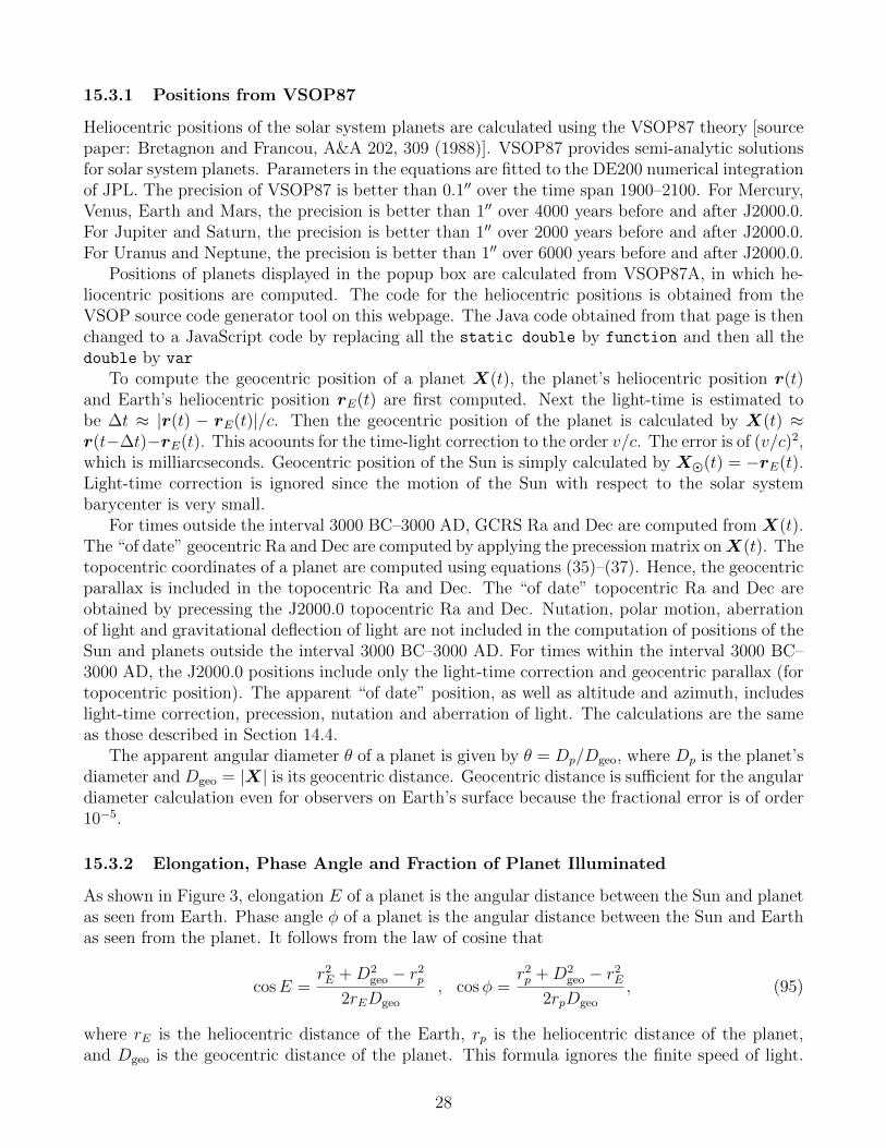
15.3.1 Positions from VSOP87

Heliocentric positions of the solar system planets are calculated using the VSOP87 theory [sourcepaper: Bretagnon and Francou, A&A 202, 309 (1988)]. VSOP87 provides semi-analytic solutionsfor solar system planets. Parameters in the equations are fitted to the DE200 numerical integrationof JPL. The precision of VSOP87 is better than 0.1′′ over the time span 1900–2100. For Mercury,Venus, Earth and Mars, the precision is better than 1′′ over 4000 years before and after J2000.0.For Jupiter and Saturn, the precision is better than 1′′ over 2000 years before and after J2000.0.For Uranus and Neptune, the precision is better than 1′′ over 6000 years before and after J2000.0.

Positions of planets displayed in the popup box are calculated from VSOP87A, in which he-liocentric positions are computed. The code for the heliocentric positions is obtained from theVSOP source code generator tool on this webpage. The Java code obtained from that page is thenchanged to a JavaScript code by replacing all the static double by function and then all thedouble by var

To compute the geocentric position of a planet X(t), the planet’s heliocentric position r(t)and Earth’s heliocentric position rE(t) are first computed. Next the light-time is estimated tobe ∆t ≈ |r(t) − rE(t)|/c. Then the geocentric position of the planet is calculated by X(t) ≈r(t−∆t)−rE(t). This acoounts for the time-light correction to the order v/c. The error is of (v/c)2,which is milliarcseconds. Geocentric position of the Sun is simply calculated by X(t) = −rE(t).Light-time correction is ignored since the motion of the Sun with respect to the solar systembarycenter is very small.

For times outside the interval 3000 BC–3000 AD, GCRS Ra and Dec are computed from X(t).The “of date” geocentric Ra and Dec are computed by applying the precession matrix onX(t). Thetopocentric coordinates of a planet are computed using equations (35)–(37). Hence, the geocentricparallax is included in the topocentric Ra and Dec. The “of date” topocentric Ra and Dec areobtained by precessing the J2000.0 topocentric Ra and Dec. Nutation, polar motion, aberrationof light and gravitational deflection of light are not included in the computation of positions of theSun and planets outside the interval 3000 BC–3000 AD. For times within the interval 3000 BC–3000 AD, the J2000.0 positions include only the light-time correction and geocentric parallax (fortopocentric position). The apparent “of date” position, as well as altitude and azimuth, includeslight-time correction, precession, nutation and aberration of light. The calculations are the sameas those described in Section 14.4.

The apparent angular diameter θ of a planet is given by θ = Dp/Dgeo, where Dp is the planet’sdiameter and Dgeo = |X| is its geocentric distance. Geocentric distance is sufficient for the angulardiameter calculation even for observers on Earth’s surface because the fractional error is of order10−5.

15.3.2 Elongation, Phase Angle and Fraction of Planet Illuminated

As shown in Figure 3, elongation E of a planet is the angular distance between the Sun and planetas seen from Earth. Phase angle φ of a planet is the angular distance between the Sun and Earthas seen from the planet. It follows from the law of cosine that

cosE =r2E +D2

geo − r2p

2rEDgeo

, cosφ =r2p +D2

geo − r2E

2rpDgeo

, (95)

where rE is the heliocentric distance of the Earth, rp is the heliocentric distance of the planet,and Dgeo is the geocentric distance of the planet. This formula ignores the finite speed of light.

28

Figure 3: Elongation E and phase angle φ of a planet.

In principle, ray tracing is needed if high precision is required. More accurate formulae are

cosE(t) = − rE(t) ·Xp(t)

|rE(t)||Xp(t)|, cosφ(t) = − [rE(tr)− rp(t)] · rp(t)

|rE(tr)− rp(t)||rp(tr)|, (96)

where the retarded time tr satisfies the equation tr = t− |rE(tr)− rp(t)|/c and I ignore the Sun’smotion with repsect to the solar system barycenter, aberration of light and gravitational deflectionof light. The equation for the elongation is easy to calculate. It follows from

rE = −rE

cosα cos δsinα cos δ

sin δ

(97)

Xp = |Xp|

cosαp cos δpsinαp cos δp

sin δp

(98)

and the addition formula of the cosine function that

cosE = sin δ sin δp + cos δ cos δp cos(α − αp). (99)

Accurate computation of φ is slightly more involved. However, elongation and phase angle areusually not quantities of great interest and so they are not calculated to high precision. I simplyuse equation (95) and light-time correction is not done carefully for the three distances.

In the popup box for a planet, the elongation is displayed accurate to 0.1 and the directionof the planet relative to the Sun is indicated by either W or E. E means the planet is to the eastof the Sun and W means it is to the west of the Sun. To be more specific, E means λp − λ > 0and W means λp − λ < 0. Here λp and λ are the ecliptic longitude of the planet and the Sun,respectively. The difference λp − λ is restricted to the range [−π, π).

It can be shown (see e.g., Section 17.4 of Green, Spherical Astronomy, Cambridge UniversityPress 1985) that the fraction of a spherical planet illuminated by the Sun is

F =1 + cosφ

2. (100)

29

In the popup box for a planet, F is displayed to two decimal places. All planets are modelled asspheres, although the deviation from a sphere is substantial for Jupiter and Saturn. The value ofF for Jupiter, Saturn, Uranus and Neptune is almost 1 at all times because of their large distancesfrom the Sun.

15.3.3 Apparent Magnitude

The apparent magnitude of a planet depends on its heliocentric distance rp, geocentric distanceDgeo and its phase angle φ. The magnitude can be written as

m = m0 + 5 log10

rpDgeo

AU2 + ∆m(φ), (101)

where m0 is a constant and ∆m(φ) is the variation of apparent magnitude as a function of φ. Thevariation arises from the fraction of the planet illuminated and the property of diffuse reflectionfrom the planet’s surface/atmosphere. The function ∆m(φ) is determined empirically and is listedin Table 10.6 of Explanatory Supplement to the Astronomical Almanacand errata. The table isreproduced below with errors corrected. The phase angle φ is in degrees.

Planet m0 ∆mMercury -0.60 0.0498φ− 0.000488φ2 + 3.02× 10−6φ3

Venus -4.47 0.0103φ+ 5.7× 10−5φ2 + 1.3× 10−7φ3 for 2.2 < φ < 163.6

Venus 0.98 −0.0102φ for 163.6 < φ < 170.2

Mars -1.52 0.016φJupiter -9.40 0.005φSaturn -8.88 0.044φ− 2.6| sin e|+ 1.25 sin2 eUranus -7.19 0.002φ

Neptune -6.87 0Note that ∆m is undefined for Venus when 0 < φ < 2.2 and when 170.2 < φ < 180. In the

popup box, the expression for 2.2 < φ < 163.6 is used when 0 < φ < 2.2 and the expressionfor 163.6 < φ < 170.2 is used when 170.2 < φ < 180.

Saturn’s magnitude calculation is more complicated because its rings have significant contri-bution to Saturn’s brightness. As a result, the terms −2.6| sin e|+1.25 sin2 e appear in the formulafor Saturn’s magnitude. Here e is the Saturnocentric sub-Earth latitude, which determines theorientation of Saturn’s rings seen from Earth. The value of e is computed as follows. First computethe J2000.0 Ra and Dec of Saturn’s north pole according to

α0 = 40.589− 0.036T , δ0 = 83.537− 0.004T, (102)

where T is the TT Julian century from J2000.0. Next compute the unit vector e3 pointing in thedirection of Saturn’s rotation axis:

e3 =

cos δ0 cosα0

cos δ0 sinα0

sin δ0

(103)

Finally, the value of sin e is given by

sin e =XS · e3|XS|

, (104)

where XS is Saturn’s geocentric position.

30

16 Moon

16.1 Lunar Ephemeris

Position of the Moon is calculated based on the ELP/MPP02 series. A JavaScript code is createdbased on the source code provided by the authors on this ftp site. The JavaScript code hasbeen tested by comparing the results with those of the FORTRAN code on the ftp site. I findagreement to within 12 to 13 significant figures. The deviation is most likely caused by theaccumulated roundoff error.

ELP/MPP02 is a semi-analytic solution for the lunar motion. There are parameters in themodel that are fitted to either the lunar laser ranging (LLR) data or fitted to JPL’s DE405/DE406ephemerides. Parameters fitted to DE405/DE406 are used on our webpages. The deviationbetween the positions in ELP/MPP02 and DE405/406 is less than 3.5′′ in ecliptic longitude and0.8′′ in ecliptic latitude over the time span from 3000 BC to 3000 AD.

The full ELP/MPP02 series can be written in the form

V (T ) = W (T ) +3∑i=0

T i∑j

A(V )ij sin

[φ

(V )ij (T )

](105)

U(T ) =3∑i=0

T i∑j

A(U)ij sin

[φ

(U)ij (T )

](106)

r(T ) = r0 +3∑i=0

T i∑j

A(r)ij sin

[φ

(r)ij (T )

], (107)

where V , U , and r are the ecliptic longitude, ecliptic latitude, and geocentric distance of the Moon,respectively, T is the TT Julian century from J2000.0, W is the mean longitude of the Moon, r0 isa constant. For the terms in the sum, A

(U)ij , A

(V )ij , A

(r)ij are constants. The phase angles φ

(U)ij , φ

(V )ij ,

φ(r)ij are linear functions of 13 angles ak (k = 1, 2, · · · , 13) related to the mean positions and orbital

parameters of the Moon and solar system planets. The functions W (T ) and ak(T ) are expressedas polynomial functions of T up to and including T 4.

The full series involves about 36,000 terms. Since high accuracy is not needed for our use, Itruncate the series by the following procedure:4

• Choose four parameters A(U)th , A

(V )th , A

(r)th and τ .

• Drop the terms in the series with A(U)ij < A

(U)th /τ i, A

(V )ij < A

(V )th /τ i, and A

(r)ij < A

(r)th /τ

i.

It is clear that the smaller the parameters A(U)th , A

(V )th , and A

(r)th , the closer the truncated series

is to the original series. The parameter τ has a unit of time and is chosen to be 50 Juliancenturies, which is the time span covered by the ELP/MPP02 series. Two sets of truncated seriesare created using two set of parameters. I call the two sets of truncated series ELP/MPP02L andELP/MPP02C.

ELP/MPP02L is a low-precision series, created using A(U)th = A

(V )th = 30′′, A

(r)th = 100 km, and

τ = 50 Julian centuries. It is used for plotting the Moon on our star charts. The resulting seriesconsists of about 40 terms. The accuracy of ELP/MPP02L is estimated by comparing it with

4I have created this GitHub repository to provide C++ subroutines to implement the ELP/MPP02 series,construct truncated series, and generate JavaScript code to calculate the truncated series.

31

the full series. Specifically, 10,000 random values of T are chosen between -50 and 50. Values ofU(T ), V (T ), and r(T ) at these times are computed for both the ELP/MPP02L series and the fullseries. I find that the maximum differences between ELP/MPP02L and ELP/MPP02 are 233′′ forV , 152′′ for U and 352 km for r. The root mean square of the differences are 47′′ for V , 33′′ for Uand 86 km for r. This accuracy is sufficient for our plotting purpose.

ELP/MPP02C is created using A(U)th = A

(V )th = 0.001′′, A

(r)th = 0.1 km, and τ = 50 Julian

centuries. It is used in the calculation in the popup box. The resulting series consists of about3750 terms. The accuracy of ELP/MPP02C is estimated in the same way as above. I find thatthe maximum differences between ELP/MPP02C and ELP/MPP02 over the time span |T | < 50are 0.1′′ for V , 0.08′′ for U and 1.9 km for r. The root mean square of the differences are 0.02′′ forV , 0.01′′ for U and 0.4 km for r. The error of this truncated series is lower than the error of theapparent position caused by our ignoring the effect of polar motion.

Once U , V and r are computed, rectangular components of the geocentric position of theMoon with respect to the ecliptic and mean equinox of J2000.0 are obtained by taking intoaccount precession and transformation from spherical to Cartesian coordinates. The procedure isdescribed in the pdf document on the ftp site. Equatorial coordinates of J2000.0 mean equator andequinox are then computed by rotating the ecliptic coordinates by the angle ε0 = 2326′21.406′′

(mean obliquity of the ecliptic at J2000.0) about the x-axis. The J2000.0 equatorial coordinatesare basically the GCRS coordinates, apart from the tiny difference between these two systemscaused by the 17-milliarcsecond offset, which I ignored. Light-time correction and aberrationof light is implemented by first computing the geocentric distance r(t) using equation (107).Then the retarded geocentric position is calculated by X(tr) = X(t − r(t)/c). Note that theretarded geocentric position includes both the light-time correction and aberration of light sinceX(tr) = rM (tr)− rE(tr), where rM and rE are the barycentric position of the Moon and Earth,respectively. Light-time corrected geocentric position is rM (tr) − rE(t), and rM (tr) − rE(tr)includes both light-time correction and annual aberration to first order in v/c (see Section 7.2.3.5of Explanatory Supplement to the Astronomical Almanac). The combined effect is called planetaryaberration. Planetary aberration shifts the Moon’s position by about 1′′. Hence the correction isignored when using the low-precision ELP/MPP02L series.

16.2 Plotting the Moon

GCRS position of the Moon is calculated using the low-precision ELP/MPP02L series. GCRS Raand Dec are then calculated using α = arg(X + iY ) and δ = sin−1(Z/r). The Moon can now beplotted on the GCRS charts: its canvas coordinates are given by equations (45)–(47).

For the local star charts, the altitude a and azimuth A are required at the given location. First,the “of date” geocentric equatorial coordinates are computed by applying the precession matrix onX. Since the Moon is close to the Earth, the geocentric parallax is significant, which is accountedfor by computing its topocentric position using equations (35)–(37). The “of date” topocentricRa and Dec is then calculated by αtopo = arg(Xtopo + iYtopo) and δtopo = sin−1(Ztopo/Dtopo), where

Dtopo =√X2

topo + Y 2topo + Z2

topo is the topocentric distance of the Moon. The hour angle is given

by H = ts − αtopo, where ts is the local sidereal time (LMST). Next a and A are computed usingequations (40)–(42). Then the altitude is adjusted by the atmospheric refraction according toequation (43). The Moon can now be plotted on a local star chart: its canvas coordinates aregiven by equation (44).

32

16.3 Popup Box

In the popup box, the Moon’s position is calculated using the higher precision ELP/MPP02Cand with planetary aberration corrected. Geocentric position, topocentric position, altitude andazimuth are computed in the same way as described above when the time is outside the interval3000 BC–3000 AD. For times within the interval 3000 BC–3000 AD, the J2000.0 positions includeonly the planetary aberration and geocentric parallax (for topocentric position). The apparent “ofdate” position, as well as altitude and azimuth, includes planetary aberration, precession, nutationand diurnal aberration of light. The calculations of precession and nutation are the same as thosedescribed in Section 14.4. For diurnal aberration, the vector n′ is calculated by equation (38)with n = X ′/|X ′|, X ′ = X(tr) −XL, and β = vspin/c. The geocentric position vector XL ofthe location is calculated by equations (36) and (37). The spin velocity vspin/c is calculated byequation (39).

Figure 4: Geometry of the Sun, Moon and Earth.

Elongation E and phase angle φ can be calculated using equations similar to equation (95).However, it is easier to use equation (99) to calculate E. For φ, the Moon’s heliocentric positionrM needs to be computed. As shown in Figure 4, rM = rE + r, where rE is the heliocentricposition of the Earth and r is the geocentric position of the Moon. It follows that

r2M = |rE + r|2 = r2

E + 2r · rE + r2 = r2E − 2rrE cosE + r2 = r2

E(1− 2σ cosE + σ2), (108)

where σ = r/rE and I have used the fact that r ·rE = −rrE cosE. The phase angle can be writtenas

cosφ =r2M + r2 − r2

E

2rrM=

σ − cosE√1− 2σ cosE + σ2

. (109)

Since r ≈ 3.8 × 105 km and rE ≈ 1.5 × 108 km, σ ≈ 2.5 × 10−3 1. Hence cosφ ≈ − cosE orφ ≈ π−E. This approximate relation between E and φ can be understood geometrically. As seenin Figure 4, when r rM and r rE, the line joining the Moon and the Sun and the line joiningthe Earth and the Sun are nearly parallel. It follows from the Euclidean geometry that φ+E = πif the two lines were parallel. Since the two lines are nearly parallel, the relation is approximate.In fact, φ + E = π − p, where p is the angular separation between the Earth and Moon as seenfrom the Sun or the parallax of the Sun using Earth-Moon as the baseline. The difference betweenφ and π − E is p ∼ r/rE = σ ≈ 2.5 × 10−3 radians or 0.15. In the popup box, φ is computedaccording to equation (109) without using the approximation.

The apparent magnitude of the Moon is calculated using the following approximate formula:

m = −12.73 + 0.026φ+ 4× 10−9φ4 + 5 log10

(r

384400 km· rM

1 AU

), (110)

where φ is the phase angle in degrees. This formula appears in Astronomy and the Limits ofVision by B.E. Schaefer, Vistas in Astronomy, 36, 311 (1993). It appears that this formula is used

33

by JPL’s Horizons website since their data closely match the formula. The JPL website statesthat when the phase angle < 7 (within ∼ one day of full Moon), computed magnitude tends tobe about 0.12 too small. That is, the formula does not account for opposition surge. It also doesnot account for the decrease in brightness when lunar eclipses occur.

17 Rise, Set, Upper Transit and Twilight

The rise, set, and upper transit times of celestial objects, as well as the beginning and ending oftwilight, are computed in the popup box, and on the rise/set page when the Rise and Set Timesbutton on the local star chart page is clicked. This section describes the method and algorithmused to do the calculation.

The rise and set times of a celestial object are defined as the times when the upper limb of theobject touches the horizon. Since the horizon depends on the observer’s location, the rise and settimes are different for different observers. The rise and set times are the times when the apparenttopocentric altitude of the upper limb of the object is 0. The geocentric altitude of the object’scenter at the rise and set times is

ars = p−∆a− s, (111)

where p is the geocentric parallax, ∆a is the correction of the altitude due to atmospheric refractionand s is the angular radius of the object. The atmospheric refraction term ∆a varies dependingon the local conditions. For the Sun and Moon, p and s also vary slightly. Since the rise and settimes are usually calculated to an accuracy of a couple of minutes, average values of ∆a, p and sare used. The term ∆a is usually set to 34′. For the Sun, p ≈ 8.8′′, s ≈ 16′ and so ars = 50′ forsunrise and sunset. For the Moon, p ≈ 57′, s ≈ 15′ and so ars = 8′. For planets and stars, p ∆aand s ∆a, and so I simply set ars = −34′.

Twilight is usually divided into three phases. The beginning and ending of the civil twilightare the times when the Sun’s center is 6 below the horizon. When the civil twilight ends, thesky is dark enough for the brightest stars to be visible. The beginning and ending of the nauticaltwilight are the times when the Sun’s center is 12 below the horizon. When the nautical twilightends, the sky is so dark that the horizon is no longer visible. The beginning and ending of theastronomical twilight are the times when the Sun’s center is 18 below the horizon. They mark thebeginning and ending of the night time. When the astronomical twilight ends, the faintest starsare visible (in regions with clear sky and no light pollution). Thus, ars = −6 for civil twilight,ars = −12 for nautical twilight and ars = −18 for astronomical twilight.

Transits are defined as the times when the object crosses the meridian, which are the timeswhen the hour angle of the object is 0 or π. The H = 0 transit is called the upper transit and theH = π transit is called the lower transit.

Since the rise, set, and upper transit time calculation does not require high precision. Low-precision formulae for the positions of the Sun, Moon and planets are used. In addition, nutation,polar motion, aberration of light, and gravitational deflection of light by the Sun are ignored.

17.1 Stars

The rise and set times of stars can be computed relatively easily since their “of date” right ascensionand declination do not change much during the course of a day.

34

It follows from equation (42) that

cosH =sin a− sin δ sinφ

cos δ cosφ. (112)

Here δ is the “of date” declination of the star. Since −1 ≤ cosH ≤ 1,

−1 ≤ sin a− sin δ sinφ

cos δ cosφ≤ 1 (113)

or− cos δ cosφ+ sin δ sinφ ≤ sin a ≤ cos δ cosφ+ sin δ sinφ. (114)

It follows from the addition formula of the cosine function that

− cos(δ + φ) ≤ sin a ≤ cos(δ − φ) (115)

which can be written as

sin(|δ + φ| − 90) ≤ sin a ≤ sin(90 − |δ − φ|). (116)

Since |δ| ≤ 90 and |φ| ≤ 90, |δ + φ| − 90 ∈ [−90, 90] and 90 − |δ − φ| ∈ [−90, 90]. Bydefinition, the amplitude a ∈ [−90, 90]. Since sine is an increasing function in [−90, 90],

|δ + φ| − 90 ≤ a ≤ 90 − |δ − φ|. (117)

The minimum and maximum geocentric altitude are

amin = |δ + φ| − 90 , amax = 90 − |δ − φ|. (118)

The maximum altitude occurs when the hour angle H = 0, which is the upper transit. Theminimum altitude occurs when H = 180, which is the lower transit.

For a given latitude φ, there are stars with amin > ars. These stars are always above thehorizon. They are called the circumpolar stars. A star is circumpolar if its declination satisfiesthe condition δ > 8926′ − φ or δ < −(8926′ + φ). Since |δ| ≤ 90, only the first inequality isrelevant for northern hemisphere observers with φ > 34′. Only the second inequality is relevantfor southern hemisphere observers with φ < −34′. Both inequalities are relevant only for observersvery close to the equator with |φ| < 34′.

There are also stars with amax < ars. These stars are always below the horizon. They arealways invisible at the location. A star is always invisible if its declination satisfies the conditionδ < −(9034′−φ) or δ > 9034′+φ. Only the first inequality is relevant for observers with φ > 34′.Only the second inequality is relevant for observers with φ < −34′. For observers with |φ| ≤ 34′,there are no stars that are always invisible.

Thus the rise and set times are for stars that are not circumpolar and not always invisible. Forthese stars, the hour angle at the rise and set times are given by equation (112) with a = ars:

H± = ± cos−1 sin ars − sin δ sinφ

cos δ cosφ, (119)

When H > 0, the star is on the west side of the meridian. When H < 0, the star is on the eastside of the meridian. Thus, the + sign is for the set time and − sign is for the rise time. Thesidereal time at the rise and set times are given by

ts± = H± + α, (120)

35

where α is the “of date” right ascension of the star. Over the course of a day, the sidereal timeadvances at a rate 1.00273781191135448 faster than the clock time based on UTC, as indicatedby equation (6) (terms involving T are practically constant over the course of a day). To calculatethe rise and set times at a given time zone, first calculate the sidereal time ts0 at the midnight ofthe given time zone by

ts0 = LMST(DUm, T (DUm)) = GMST(DUm, T (DUm)) + λ, (121)

where λ is the location’s longitude, DUm = Julian UT1 date at midnight local time − 2451545.0,and T (DUm) is the TT Julian century from J2000.0 at DUm. In other words,

T (DUm) =DUm

36525+ ∆T (DUm), (122)

where ∆T is the difference between TT and UT1 described in Section 4. The Greenwich siderealtime GMST is calculated using equation (6) and ∆T is calculated using the fitting formula byEspenak and Meeus. The sidereal time ts at any later time of the date is given by ts = ts0 +1.00273781191135448h′, where h′ = 24(DU−DUm) is the number of hours past the local midnight.The local times at which the setting and rising of the star occur on a given date are

h′± =(H± + α− ts0) mod 24h

1.00273781191135448. (123)

Upper transit time is the time when the hour angle H = 0. Hence

h′upper transit =(α− ts0) mod 24h

1.00273781191135448. (124)

Note that equations (123) and (124) imply that h′ can never be greater than 24/1.00273781191135448.This is because one sidereal day is 1/1.00273781191135448 days = 23h56m4s and is smaller than24 hours. Thus, if the rise/set/upper transit time occurs bewteen 0h and 0h03m56s, there willbe another rise/set/upper transit occurring on the same day with h′ > 24/1.00273781191135448.This occurs only once every year for each case and I ignore them.

17.2 Sun, Moon and Planets

The equations for the rise, set, upper transit times of the Sun, Moon and planets, as well as thebeginning and ending of twilight, are still given by equations (123) and (124). The only differenceis that the right ascension and declination for the Sun, Moon and planets change more rapidlyover the course of a day. The two equations should be written more clearly as follows.

h′± =(H±(δ(h′±)) + α(h′±)− ts0) mod 24h

1.00273781191135448(125)

h′upper transit =(α(h′upper transit)− ts0) mod 24h

1.00273781191135448(126)

These equations explicitly indicate that the rise/set/upper transit time depends on the values ofα and δ at the rise/set/upper transit time. Since α and δ can no longer be considered as constantsover the course of a day, the unknown rise/set/upper transit time appears on both sides of theequations. The equations may be solved iteratively. For the Sun and planets, α and δ change

36

slowly over the course of a day. Treating them as constants will not cause an error of more thana few minutes, which is sufficient. However, the Moon moves rapidly over the course of a day andtreating α and δ as constants will cause a large error.

There are two other complications. The time between two successive rise/set/upper transittimes is one sidereal day for stars. This is not true for the Sun, Moon and planets. The mostextreme case is the Moon, where the average time between two successive rise/set/upper transittimes is 24 hours and 50 minutes. As a result, it is possible to have no rise/set/transit on a givenday. Another complication is that at high latitudes, the rise and set times of the Sun, Moon andplanets are sensitive to the change in declination when the object is close to being circumpolaror close to being invisible all day. These two complications make the iterative procedure difficultto implement. As a result, I use the algorithm described in Sections 3.7 and 3.8 of the bookAstronomy on the Personal Computer by O. Montenbruck and T. Pfleger, 4th edition, Springer2000 (corrected fourth printing 2009) to calculate the rise, set and transit times. The algorithmis based on quadratic interpolation.

The idea is to first calculate the hour angle H(h′) and altitude a(h′) at local times 0h, 1h, ...,24h, i.e. at h′ = 0, 1, ..., 24. Divide the day into 12 intervals: [0h, 2h), [2h, 4h), ..., [22h, 24h). Nextvalues of H(h′) and a(h′) in each of the 12 intervals are approximated by a quadratic interpolation.Therefore, there are approximate analytic formulae for H(h′) and a(h′) throughout the day andthe rise, set, and upper transit times are then solved by the equations a(h′) = ars and H(h′) = 0using analytic expressions.

The procedure for the rise, set, beginning and ending of twilight works as follows. For h′ in aparticular time interval, define

x = h′ − h′0 , y = sin[a(h′)]− sin ars, (127)

where h′0 is the mid-point of the time interval. Thus x ∈ [−1, 1) and y = 0 at the rise and settimes. Next, fit a quadratic curve y(x) = c2x

2 + c1x+ c0 in the interval based on the three valuesof y at x = −1, 0 and 1:

y− = y(−1) = c2 − c1 + c0 , y0 = y(0) = c0 , y+ = y(1) = c2 + c1 + c0. (128)

Values of c0, c1, and c2 are easily solved to give

c2 = (y+ + y0)/2− y0 , c1 = (y+ − y−)/2 , c0 = y0. (129)

The quadratic equation y(x) = 0 has roots if c21 − 4c0c2 ≥ 0 and the roots are given by x± =

(−c1±√c2

1 − 4c0c2)/(2c2). The quadratic function y(x) reaches an extremum at xm = −c1/(2c2).However, the function y(x) only applies in the interval x ∈ [−1, 1). In general, there can be 0, 1or 2 roots in the interval [−1, 1). Let’s consider these three cases.

Case 1: There is no root in the interval [−1, 1). No rising and setting occurs in this timeinterval. Move on to the next time interval.

Case 2: There is one root, x1, in the interval [−1, 1). Either rising or setting occurs in thistime interval at h′ = h′0 + x1. It is rising if y− < 0 and y+ > 0; it is setting if y− > 0 and y+ < 0.

Case 3: There are two roots, x1 and x2, in the interval [−1, 1). Suppose x2 > x1. Then risingand setting both occur in this time interval and the extremum xm = (x1 +x2)/2 is also inside thisinterval. If y(xm) > 0, the object rises at h′ = h′0 +x1, reaches a maximum altitude at h′ = h′0 +xmand sets at h′ = h′0 +x2. If y(xm) < 0, the object sets at h′ = h′0 +x1, reaches a minimum altitudeat h′ = h′0 + xm and rises at h′ = h′0 + x2.

37

By going through all the 12 intervals, the rise and set times can be found. For the upper transittime, the calculation is done in a similar way. I set y = H(h′) in this case. Care must be takenwhen calculating the roots of y = 0. If α(h′) and δ(h′) are constants, y will be a linear functionof x and so c2 = 0. For the Sun and planets, α(h′) and δ(h′) are nearly constants and so y(x) isclose to being a linear function with |c2| 1. One of the roots is close to −c0/c1 and the otheris close to −c1/c2. The root close to −c0/c1 can be calculated using the expression x1 = −2c0/D

and the one close to −c1/c2 can be calculated using x2 = −D/(2c2), where D = c1 +√c2

1 − 4c0c2

if c1 > 0 and D = c1 −√c2

1 − 4c0c2 if c1 < 0. Since |c2| 1, it is almost certain that the rootclose to −c1/c2 is outside the interval [−1, 1). Only the root close to −c1/c2 has a chance of beinginside the interval [−1, 1). Normal celestial objects are not moving fast enough for there to be twoupper transits occurring in a two-hour time interval and so Case 3 will never occur.

The algorithm described above has been tested on stars and the times computed match thosecalculated using equations (123) and (124). The difference is at most one minute. As in the caseof stars, on rare occasions there could be more than one rise/set/upper transit times for the Sunand planets on a day. The algorithm described above can find all of them, but only the earliesttime is reported in the popup box and on the rise/set page.

38