calculation of in-flight cruise performance for integration ... · calculation of in-flight...
TRANSCRIPT

Calculation of in-flight cruise performance for integration inan EFB System
Development of a Computational Methodology
Tiago de Almeida Torre
Thesis to obtain the Master of Science Degree in
Aerospace Engineering
Supervisors: Prof. António José Nobre Martins AguiarEng. Carlos Fernando da Costa Figueiredo
Examination Committee
Chairperson: Prof. Filipe Szolnoky Ramos Pinto CunhaSupervisor: Prof. António José Nobre Martins Aguiar
Member of the Committee: Prof. Pedro da Graça Tavares Álvares Serrão
December 2016

ii

”I can do all things through Him who strengthens me”
Philippians 4:12-14
iii

iv

Acknowledgments
There’s a group of individuals without whom this work would not have been possible, and to them I
express my deepest gratitude:
First and foremost I thank Prof. Antonio Aguiar for granting me the opportunity to participate in a
tremendously interesting project, and dedicate a part of his valuable time in sponsoring and supporting
this thesis.
To Eng. Carlos Figueiredo, lead Eng. of TAP’s Electronic Flight Bag solution, I can’t thank enough for
all the time he invested in me, guiding me throughout the project and helping me whenever he could.
Lastly express my appreciation for all the help and feedback provided by Eng. Jorge Frade and Eng.
Pedro Pereira, and to Marılia Santos and Vera Batista for making my time at TAP an even more pleasant
and remarkable experience.
v

vi

Resumo
As tecnologias de informacao estao a revolucionar as operacoes da aviacao comercial, dentro e fora do
cockpit. Processos manuais e documentacao impressa vao sendo substituıdos por sistemas computa-
dorizados, gracas a crescente portabilidade e poder computacional dos dispositivos eletronicos.
Os pilotos usam dispositivos eletronicos portateis conhecidos como Electronic Flight Bags (EFB),
que permitem uma maior eficiencia e seguranca operacional das aeronaves. O uso de sistemas
EFB tem crescido de forma significativa nos ultimos anos. O EFB maximiza o potencial de ferramen-
tas de calculo de desempenho e documentacao importante, tornando-os acessıveis aos membros da
tripulacao, onde quer que estejam.
Este trabalho tem como objetivo o desenvolvimento de uma ferramenta computacional que permite
que membros da tripulacao calculem perfis de voo para situacoes de emergencia, aproveitando os
mais recentes dados meteorologicos. A informacao meteorologica que e disponibilizada antes de um
voo esta sujeita a sofrer alteracoes. Isto implica que, a medida que ela se vai alterando, poderao surgir
melhores rotas de escape para situacoes de emergencia. Este trabalho ajuda a companhia a aproveitar
essas alteracoes da previsao meteorologica, aumentando a seguranca operacional.
A aplicacao permite que o utilizador calcule perfis de emergencia para falhas de pressurizacao e/ou
de motor. Comparando o perfil calculado com as altitudes mınimas de voo, o software consegue deter-
minar se o perfil satisfaz os requisitos impostos pela legislacao para o tipo de falha em causa. Integrada
no EFB da TAP, esta ferramenta beneficiara a forma como as rotas de emergencia sao geridas, aumen-
tando a seguranca em caso de emergencia.
Palavras-chave: Electronic Flight Bag, Descida de Emergencia, Desempenho de Aeron-
aves, Falha de Motor, Despressurizacao
vii

viii

Abstract
Information technology is slowly but surely revolutionizing commercial aviation operations, in and out of
the cockpit. Manual processes and paper documentation are gradually being replaced by computerized
systems, thanks to the increasing computational power and portability of electronic devices.
Flight Crew members use portable electronic devices, known as Electronic Flight Bags (EFB), which
unlock a higher operational safety and efficiency. The use of EFB systems by airline companies has
been growing significantly in recent years. It unleashes the potential of aircraft performance tools and
critical documentation by making it portable and accessible to flight crew members, without the need to
carry large or heavy bags.
The present work focuses on the development of a computational tool that allows flight crew members
to compute emergency descent profiles in real time, taking the most recent meteorological information
into consideration. Atmospheric information released before a flight is prone to change. This implies
that safer emergency routes are likely to arise as atmospheric data gets updated. This work helps the
airline take advantage of those atmospheric updates, and make flight operations safer.
The application allows the user to compute emergency descent profiles for depressurization and
engine failure scenarios. By comparing the computed profile against minimum flyable altitudes, the
application can rapidly verify if the calculated flight path satisfies regulatory requirements for the targeted
emergency procedure. Integrated in TAP’s EFB solution, this tool could prove to be a game changer in
how escape routes are managed.
Keywords: Electronic Flight Bag, Emergency Descent, Aircraft Performance, Engine Failure,
Depressurization
ix

x
Contents
Acknowledgments . . . . . . . . . . . . . . . . . . . . . . . . . . . . . . . . . . . . . . . . . . . v
Resumo . . . . . . . . . . . . . . . . . . . . . . . . . . . . . . . . . . . . . . . . . . . . . . . . . vii
Abstract . . . . . . . . . . . . . . . . . . . . . . . . . . . . . . . . . . . . . . . . . . . . . . . . . ix
List of Tables . . . . . . . . . . . . . . . . . . . . . . . . . . . . . . . . . . . . . . . . . . . . . . xvii
List of Figures . . . . . . . . . . . . . . . . . . . . . . . . . . . . . . . . . . . . . . . . . . . . . xix
Nomenclature . . . . . . . . . . . . . . . . . . . . . . . . . . . . . . . . . . . . . . . . . . . . . . xxi
1 Introduction 1
1.1 Motivation . . . . . . . . . . . . . . . . . . . . . . . . . . . . . . . . . . . . . . . . . . . . . 1
1.2 Objectives . . . . . . . . . . . . . . . . . . . . . . . . . . . . . . . . . . . . . . . . . . . . . 2
1.3 Thesis Outline . . . . . . . . . . . . . . . . . . . . . . . . . . . . . . . . . . . . . . . . . . 2
2 The Electronic Flight Bag 3
2.1 What is an Electronic Flight Bag? . . . . . . . . . . . . . . . . . . . . . . . . . . . . . . . . 3
2.1.1 Classification of EFB systems . . . . . . . . . . . . . . . . . . . . . . . . . . . . . . 3
2.2 The evolution of the EFB . . . . . . . . . . . . . . . . . . . . . . . . . . . . . . . . . . . . . 4
2.3 Arguments for and against the adoption of EFB systems . . . . . . . . . . . . . . . . . . . 6
2.4 EFB applications for Cruise flight . . . . . . . . . . . . . . . . . . . . . . . . . . . . . . . . 8
2.4.1 Examples . . . . . . . . . . . . . . . . . . . . . . . . . . . . . . . . . . . . . . . . . 8
2.4.2 Remarks and technical considerations . . . . . . . . . . . . . . . . . . . . . . . . . 9
3 Introduction to Aircraft Performance 11
3.1 International Standard Atmosphere (ISA) . . . . . . . . . . . . . . . . . . . . . . . . . . . 11
3.1.1 Important units . . . . . . . . . . . . . . . . . . . . . . . . . . . . . . . . . . . . . . 11
3.1.2 ISA properties at sea-level . . . . . . . . . . . . . . . . . . . . . . . . . . . . . . . 11
3.1.3 Temperature modeling . . . . . . . . . . . . . . . . . . . . . . . . . . . . . . . . . . 12
3.1.4 Pressure and density modeling . . . . . . . . . . . . . . . . . . . . . . . . . . . . . 13
3.2 Operating speeds . . . . . . . . . . . . . . . . . . . . . . . . . . . . . . . . . . . . . . . . 16
3.2.1 Calibrated Air Speed (CAS) . . . . . . . . . . . . . . . . . . . . . . . . . . . . . . . 16
3.2.2 Indicated Air Speed (IAS) . . . . . . . . . . . . . . . . . . . . . . . . . . . . . . . . 17
3.2.3 True Air Speed (TAS) . . . . . . . . . . . . . . . . . . . . . . . . . . . . . . . . . . 17
3.2.4 Ground Speed (GS) . . . . . . . . . . . . . . . . . . . . . . . . . . . . . . . . . . . 17
xi

3.2.5 Mach Number . . . . . . . . . . . . . . . . . . . . . . . . . . . . . . . . . . . . . . 17
3.2.6 TAS variations . . . . . . . . . . . . . . . . . . . . . . . . . . . . . . . . . . . . . . 18
3.2.7 Important Speed Definitions . . . . . . . . . . . . . . . . . . . . . . . . . . . . . . . 18
3.3 Wing Theory . . . . . . . . . . . . . . . . . . . . . . . . . . . . . . . . . . . . . . . . . . . 19
3.3.1 Aerodynamic forces and moments on airfoils . . . . . . . . . . . . . . . . . . . . . 19
3.3.2 Aerodynamic forces and moments on wings . . . . . . . . . . . . . . . . . . . . . . 21
3.4 Flight Mechanics for level flight . . . . . . . . . . . . . . . . . . . . . . . . . . . . . . . . . 22
3.4.1 Standard Lift Equation . . . . . . . . . . . . . . . . . . . . . . . . . . . . . . . . . . 22
3.4.2 Standard Drag Equation . . . . . . . . . . . . . . . . . . . . . . . . . . . . . . . . . 22
4 Descent and Drift down Performance and Operations 23
4.1 Descent and Drift Down Performance . . . . . . . . . . . . . . . . . . . . . . . . . . . . . 23
4.1.1 Drift down condition . . . . . . . . . . . . . . . . . . . . . . . . . . . . . . . . . . . 23
4.1.2 Definition of Angles and Axis systems . . . . . . . . . . . . . . . . . . . . . . . . . 23
4.1.3 Equations of motion . . . . . . . . . . . . . . . . . . . . . . . . . . . . . . . . . . . 24
4.1.4 Descent Gradient (γ) . . . . . . . . . . . . . . . . . . . . . . . . . . . . . . . . . . . 25
4.1.5 Rate of Descent (RD) . . . . . . . . . . . . . . . . . . . . . . . . . . . . . . . . . . 25
4.2 Drift down ceiling . . . . . . . . . . . . . . . . . . . . . . . . . . . . . . . . . . . . . . . . . 26
4.3 Influencing Parameters . . . . . . . . . . . . . . . . . . . . . . . . . . . . . . . . . . . . . 26
4.3.1 Altitude effect . . . . . . . . . . . . . . . . . . . . . . . . . . . . . . . . . . . . . . . 26
4.3.2 Temperature effect . . . . . . . . . . . . . . . . . . . . . . . . . . . . . . . . . . . . 27
4.3.3 Weight effect . . . . . . . . . . . . . . . . . . . . . . . . . . . . . . . . . . . . . . . 28
4.3.4 Longitudinal Wind Effect . . . . . . . . . . . . . . . . . . . . . . . . . . . . . . . . . 28
4.4 Descent Speeds . . . . . . . . . . . . . . . . . . . . . . . . . . . . . . . . . . . . . . . . . 29
4.4.1 Descent at given MACH/IAS Law . . . . . . . . . . . . . . . . . . . . . . . . . . . . 29
4.4.2 Descent at Minimum Gradient (Drift Down) . . . . . . . . . . . . . . . . . . . . . . 30
4.4.3 Descent at Minimum Rate of Descent . . . . . . . . . . . . . . . . . . . . . . . . . 30
4.4.4 Emergency Descent . . . . . . . . . . . . . . . . . . . . . . . . . . . . . . . . . . . 30
5 Pressurization Systems and Failures 31
5.1 Pressurization Systems . . . . . . . . . . . . . . . . . . . . . . . . . . . . . . . . . . . . . 31
5.1.1 Requirements . . . . . . . . . . . . . . . . . . . . . . . . . . . . . . . . . . . . . . . 31
5.2 Oxygen systems . . . . . . . . . . . . . . . . . . . . . . . . . . . . . . . . . . . . . . . . . 33
5.2.1 Gaseous Oxygen Systems . . . . . . . . . . . . . . . . . . . . . . . . . . . . . . . 34
5.2.2 Chemical Oxygen Systems . . . . . . . . . . . . . . . . . . . . . . . . . . . . . . . 34
5.3 Emergency Descent Procedures . . . . . . . . . . . . . . . . . . . . . . . . . . . . . . . . 34
5.3.1 Passenger Oxygen Requirements . . . . . . . . . . . . . . . . . . . . . . . . . . . 34
5.3.2 Flight Profile . . . . . . . . . . . . . . . . . . . . . . . . . . . . . . . . . . . . . . . 35
5.3.3 Obstacle Clearance . . . . . . . . . . . . . . . . . . . . . . . . . . . . . . . . . . . 37
5.3.4 Route Study . . . . . . . . . . . . . . . . . . . . . . . . . . . . . . . . . . . . . . . 38
xii

6 Engine Failure(s) 39
6.1 Drift Down procedure . . . . . . . . . . . . . . . . . . . . . . . . . . . . . . . . . . . . . . 39
6.2 Gross vs. Net Flight Path . . . . . . . . . . . . . . . . . . . . . . . . . . . . . . . . . . . . 39
6.2.1 Gross Flight Path . . . . . . . . . . . . . . . . . . . . . . . . . . . . . . . . . . . . . 40
6.2.2 Net Flight Path . . . . . . . . . . . . . . . . . . . . . . . . . . . . . . . . . . . . . . 40
6.3 Obstacle clearance . . . . . . . . . . . . . . . . . . . . . . . . . . . . . . . . . . . . . . . . 41
6.3.1 Lateral Clearance . . . . . . . . . . . . . . . . . . . . . . . . . . . . . . . . . . . . 41
6.3.2 Vertical Clearance . . . . . . . . . . . . . . . . . . . . . . . . . . . . . . . . . . . . 42
7 Emergency Profile Application (EPA) 45
7.1 Description . . . . . . . . . . . . . . . . . . . . . . . . . . . . . . . . . . . . . . . . . . . . 45
7.2 Objectives . . . . . . . . . . . . . . . . . . . . . . . . . . . . . . . . . . . . . . . . . . . . . 45
7.3 Software Tools . . . . . . . . . . . . . . . . . . . . . . . . . . . . . . . . . . . . . . . . . . 46
7.3.1 Airbus PEP . . . . . . . . . . . . . . . . . . . . . . . . . . . . . . . . . . . . . . . . 46
7.3.1.1 IFP module . . . . . . . . . . . . . . . . . . . . . . . . . . . . . . . . . . . 46
7.3.1.2 PEP calculation queue . . . . . . . . . . . . . . . . . . . . . . . . . . . . 47
7.3.1.3 Input and Output . . . . . . . . . . . . . . . . . . . . . . . . . . . . . . . . 47
7.3.1.4 Input files (.DAT) . . . . . . . . . . . . . . . . . . . . . . . . . . . . . . . . 47
7.3.1.5 Output files (.PRN) . . . . . . . . . . . . . . . . . . . . . . . . . . . . . . 48
7.3.2 APCMTP tool . . . . . . . . . . . . . . . . . . . . . . . . . . . . . . . . . . . . . . . 48
7.3.3 Microsoft Visual Studio . . . . . . . . . . . . . . . . . . . . . . . . . . . . . . . . . 48
7.3.4 dBForge for SQL Server . . . . . . . . . . . . . . . . . . . . . . . . . . . . . . . . . 49
7.4 Flowchart Symbols . . . . . . . . . . . . . . . . . . . . . . . . . . . . . . . . . . . . . . . . 49
7.5 Application Structure . . . . . . . . . . . . . . . . . . . . . . . . . . . . . . . . . . . . . . . 49
7.6 Configuration of Input Data . . . . . . . . . . . . . . . . . . . . . . . . . . . . . . . . . . . 50
7.6.1 PEP Parameters . . . . . . . . . . . . . . . . . . . . . . . . . . . . . . . . . . . . . 50
7.6.2 Data Retrieval Process . . . . . . . . . . . . . . . . . . . . . . . . . . . . . . . . . 51
7.6.3 Required Data . . . . . . . . . . . . . . . . . . . . . . . . . . . . . . . . . . . . . . 52
7.6.4 User Interface (UI) . . . . . . . . . . . . . . . . . . . . . . . . . . . . . . . . . . . . 54
7.7 Computation of Flight Profile . . . . . . . . . . . . . . . . . . . . . . . . . . . . . . . . . . 54
7.7.1 Depressurization Mode (DM) . . . . . . . . . . . . . . . . . . . . . . . . . . . . . . 55
7.7.1.1 Profile Configuration . . . . . . . . . . . . . . . . . . . . . . . . . . . . . . 55
7.7.1.2 Configure Next Branch . . . . . . . . . . . . . . . . . . . . . . . . . . . . 59
7.7.1.3 Run PEP simulations . . . . . . . . . . . . . . . . . . . . . . . . . . . . . 59
7.7.1.4 Add Weather Information . . . . . . . . . . . . . . . . . . . . . . . . . . . 60
7.7.1.5 Store Results (Intermediate Results) . . . . . . . . . . . . . . . . . . . . 60
7.7.1.6 Branch Verification and Correction . . . . . . . . . . . . . . . . . . . . . . 60
7.7.1.7 Store the Fully Validated Profile . . . . . . . . . . . . . . . . . . . . . . . 61
7.7.2 Engine Failure Mode (EFM) . . . . . . . . . . . . . . . . . . . . . . . . . . . . . . . 62
xiii

7.7.2.1 Configure Drift Down Profile . . . . . . . . . . . . . . . . . . . . . . . . . 63
7.7.2.2 Run PEP simulations . . . . . . . . . . . . . . . . . . . . . . . . . . . . . 63
7.7.2.3 Add Weather Information . . . . . . . . . . . . . . . . . . . . . . . . . . . 64
7.7.2.4 Store Full Profile Path . . . . . . . . . . . . . . . . . . . . . . . . . . . . . 64
7.7.2.5 Convert to Net Flight Path . . . . . . . . . . . . . . . . . . . . . . . . . . . 64
7.7.3 Pep Computation Process . . . . . . . . . . . . . . . . . . . . . . . . . . . . . . . . 64
7.7.4 Adding Weather Information to Existing Branches . . . . . . . . . . . . . . . . . . 66
7.7.4.1 Retrieve Branch Length . . . . . . . . . . . . . . . . . . . . . . . . . . . . 67
7.7.4.2 Retrieve Relevant WPTs in the Branch Vicinity . . . . . . . . . . . . . . . 67
7.7.4.3 Retrieve Atmospheric Data for WPTs . . . . . . . . . . . . . . . . . . . . 67
7.7.4.4 Compute Average Values per Altitude . . . . . . . . . . . . . . . . . . . . 67
7.7.5 Auxiliary Tools and Methods . . . . . . . . . . . . . . . . . . . . . . . . . . . . . . . 71
7.7.5.1 Distance Between Two Coordinates . . . . . . . . . . . . . . . . . . . . . 71
7.7.5.2 Initial and Final Bearing Between Two Coordinates . . . . . . . . . . . . . 71
7.7.5.3 Destination Point given Initial Bearing and Distance from Starting Point . 72
7.8 Verification of MA constraints . . . . . . . . . . . . . . . . . . . . . . . . . . . . . . . . . . 72
7.9 Report Result to User . . . . . . . . . . . . . . . . . . . . . . . . . . . . . . . . . . . . . . 73
7.10 TAP’s EFB Database . . . . . . . . . . . . . . . . . . . . . . . . . . . . . . . . . . . . . . . 73
7.10.1 Existing entries . . . . . . . . . . . . . . . . . . . . . . . . . . . . . . . . . . . . . . 73
7.10.1.1 FMS . . . . . . . . . . . . . . . . . . . . . . . . . . . . . . . . . . . . . . . 73
7.10.1.2 STATIC . . . . . . . . . . . . . . . . . . . . . . . . . . . . . . . . . . . . . 73
7.10.1.3 EFBDB . . . . . . . . . . . . . . . . . . . . . . . . . . . . . . . . . . . . . 74
7.10.2 Entries added . . . . . . . . . . . . . . . . . . . . . . . . . . . . . . . . . . . . . . . 74
7.10.2.1 FCOM Descent Profile Configuration String . . . . . . . . . . . . . . . . . 74
7.10.2.2 CDL Items . . . . . . . . . . . . . . . . . . . . . . . . . . . . . . . . . . . 74
7.10.2.3 PEP’s Database Files . . . . . . . . . . . . . . . . . . . . . . . . . . . . . 75
7.10.2.4 Grid MORA . . . . . . . . . . . . . . . . . . . . . . . . . . . . . . . . . . . 75
8 Results 77
8.1 Flight Scenario . . . . . . . . . . . . . . . . . . . . . . . . . . . . . . . . . . . . . . . . . . 77
8.2 Depressurization Mode Computation . . . . . . . . . . . . . . . . . . . . . . . . . . . . . . 78
8.2.1 Computation Results . . . . . . . . . . . . . . . . . . . . . . . . . . . . . . . . . . . 78
8.2.2 Results Discussion . . . . . . . . . . . . . . . . . . . . . . . . . . . . . . . . . . . . 79
8.3 Engine Failure Mode Computation . . . . . . . . . . . . . . . . . . . . . . . . . . . . . . . 79
8.3.1 Computation Results . . . . . . . . . . . . . . . . . . . . . . . . . . . . . . . . . . . 79
8.3.2 Results Discussion . . . . . . . . . . . . . . . . . . . . . . . . . . . . . . . . . . . . 80
8.4 Combined Results . . . . . . . . . . . . . . . . . . . . . . . . . . . . . . . . . . . . . . . . 80
xiv
9 Conclusion 81
9.1 Balance . . . . . . . . . . . . . . . . . . . . . . . . . . . . . . . . . . . . . . . . . . . . . . 81
9.2 Future Work . . . . . . . . . . . . . . . . . . . . . . . . . . . . . . . . . . . . . . . . . . . . 82
Bibliography 83
A Regulation Transcripts 85
A.1 Commission Regulation (EU) Reg. 965-2012 . . . . . . . . . . . . . . . . . . . . . . . . . 85
A.1.1 CAT.IDE.A.230 First-aid oxygen . . . . . . . . . . . . . . . . . . . . . . . . . . . . . 85
A.1.2 CAT.IDE.A.235 Supplemental oxygen — pressurised aeroplanes . . . . . . . . . . 86
A.1.3 CAT.POL.A.215 En-route — one-engine-inoperative (OEI) . . . . . . . . . . . . . . 87
A.1.4 CAT.POL.A.220 En-route — En-route — aeroplanes with three or more engines,
two engines inoperative . . . . . . . . . . . . . . . . . . . . . . . . . . . . . . . . . 88
A.2 CS-25 Amendment 18 . . . . . . . . . . . . . . . . . . . . . . . . . . . . . . . . . . . . . . 88
A.2.1 CS 25.123 . . . . . . . . . . . . . . . . . . . . . . . . . . . . . . . . . . . . . . . . 89
A.3 Annex VIII the draft Commission Regulation on ‘Air Operations - OPS’ Part-SPO - IR . . . 89
A.3.1 SPO.OP.125 Minimum obstacle clearance altitudes — IFR flights . . . . . . . . . . 89
A.4 Acceptable Means of Compliance (AMC) and Guidance Material (GM) to Part-CAT . . . . 89
A.4.1 GM1 CAT.OP.MPA.145(a) Establishment of minimum flight altitudes . . . . . . . . 89
B Results 91
C Classes 96
C.1 ProfileCOORD.vb . . . . . . . . . . . . . . . . . . . . . . . . . . . . . . . . . . . . . . . . . 96
C.2 Branch.vb . . . . . . . . . . . . . . . . . . . . . . . . . . . . . . . . . . . . . . . . . . . . . 96
D User Interface (UI) 98
xv

xvi

List of Tables
6.1 Gradient Penalties applied to Gross Flight Paths . . . . . . . . . . . . . . . . . . . . . . . 41
7.1 Profile Configuration vs. Initial Altitude . . . . . . . . . . . . . . . . . . . . . . . . . . . . . 59
A.1 Oxygen minimum requirements for pressurized aeroplanes . . . . . . . . . . . . . . . . . 87
C.1 ProfileCOORD Object Class - Stored Variables . . . . . . . . . . . . . . . . . . . . . . . . 96
C.2 Branch Object Class - Stored Variables . . . . . . . . . . . . . . . . . . . . . . . . . . . . 97
xvii

xviii
List of Figures
2.1 Garmin GNS 530 . . . . . . . . . . . . . . . . . . . . . . . . . . . . . . . . . . . . . . . . . 4
2.2 Fujitsu P600 . . . . . . . . . . . . . . . . . . . . . . . . . . . . . . . . . . . . . . . . . . . 5
2.3 Airbus FlySmart for iPad . . . . . . . . . . . . . . . . . . . . . . . . . . . . . . . . . . . . . 6
3.1 ISA Temperature distribution . . . . . . . . . . . . . . . . . . . . . . . . . . . . . . . . . . 13
3.2 Vertical forces acting on sample atmosphere particle . . . . . . . . . . . . . . . . . . . . . 13
3.3 CAS Determination Process . . . . . . . . . . . . . . . . . . . . . . . . . . . . . . . . . . . 17
3.4 Ground Speed and Drift Angle . . . . . . . . . . . . . . . . . . . . . . . . . . . . . . . . . 18
3.5 TAS variations - Climb profile 300 Kt / M0.78 . . . . . . . . . . . . . . . . . . . . . . . . . 19
3.6 Definition of Section (Airfoil) Forces and Moment . . . . . . . . . . . . . . . . . . . . . . . 21
3.7 Balance of Forces for Steady Level Flight . . . . . . . . . . . . . . . . . . . . . . . . . . . 22
4.1 Forces and angles in an un-accelerated (Drift down) Descent . . . . . . . . . . . . . . . . 24
4.2 Descent gradient and Rate of Descent versus Altitude and TAS . . . . . . . . . . . . . . . 27
4.3 Descent gradient and Rate of Descent versus Weight and TAS . . . . . . . . . . . . . . . 28
4.4 Headwind effect on Descent Gradient and Rate of Descent . . . . . . . . . . . . . . . . . 29
4.5 Descent profile at given MACH/IAS law . . . . . . . . . . . . . . . . . . . . . . . . . . . . 30
5.1 Air Pressurization System for Turbofan Aircraft . . . . . . . . . . . . . . . . . . . . . . . . 32
5.2 Cabin pressure envelope for Airbus A330 . . . . . . . . . . . . . . . . . . . . . . . . . . . 33
5.3 Depressurization descent profile for Airbus A330 . . . . . . . . . . . . . . . . . . . . . . . 36
5.4 Oxygen vs. performance profile of A319 - 21 min oxygen system . . . . . . . . . . . . . . 36
5.5 Obstacle Clearance Profile – Depressurization . . . . . . . . . . . . . . . . . . . . . . . . 38
5.6 Obstacle Clearance Profiles – Engine and Depressurization . . . . . . . . . . . . . . . . . 38
6.1 Descent Drift Down Procedure . . . . . . . . . . . . . . . . . . . . . . . . . . . . . . . . . 40
6.2 Gross and Net Drift Down Descent Flight Path . . . . . . . . . . . . . . . . . . . . . . . . 41
6.3 Lateral Obstacle Clearance . . . . . . . . . . . . . . . . . . . . . . . . . . . . . . . . . . . 42
6.4 Vertical Obstacle Clearance - 1000ft Rule . . . . . . . . . . . . . . . . . . . . . . . . . . . 43
6.5 Vertical Obstacle Clearance - 2000ft Rule . . . . . . . . . . . . . . . . . . . . . . . . . . . 44
7.1 Flowchart Symbols Legend . . . . . . . . . . . . . . . . . . . . . . . . . . . . . . . . . . . 49
xix

7.2 EPA Basic Structure . . . . . . . . . . . . . . . . . . . . . . . . . . . . . . . . . . . . . . . 50
7.3 PEP Parameters Overview . . . . . . . . . . . . . . . . . . . . . . . . . . . . . . . . . . . 51
7.4 EPA Data Retrieval Algorithm . . . . . . . . . . . . . . . . . . . . . . . . . . . . . . . . . . 52
7.5 Data required by EPA . . . . . . . . . . . . . . . . . . . . . . . . . . . . . . . . . . . . . . 53
7.6 EPA Profile Computation Algorithm for Depressurization Mode . . . . . . . . . . . . . . . 56
7.7 Depressurization Profile for Different Starting Altitudes (12 min oxygen system) . . . . . . 57
7.8 Determination of Initial Cruise Duration 4t∗ . . . . . . . . . . . . . . . . . . . . . . . . . . 58
7.9 Determination of Initial Cruise Duration 4t . . . . . . . . . . . . . . . . . . . . . . . . . . . 58
7.10 Fixed and Adjustable Branches for 12 min Oxygen Profile . . . . . . . . . . . . . . . . . . 61
7.11 Fixed and Adjustable Branches for 21 min Oxygen Profile . . . . . . . . . . . . . . . . . . 62
7.12 EPA Profile Computation Algorithm for Engine Failure Mode . . . . . . . . . . . . . . . . . 63
7.13 Actual vs. Desired Integration of PEP computations into EPA . . . . . . . . . . . . . . . . 65
7.14 Computation of Atmospheric Conditions per Branch . . . . . . . . . . . . . . . . . . . . . 66
7.15 Relevant WPTs for Branch Atmospheric Data Computations . . . . . . . . . . . . . . . . . 68
7.16 Branch Segmentation for Averaging of WC at a certain FL . . . . . . . . . . . . . . . . . . 69
7.17 Branch Segment Sample . . . . . . . . . . . . . . . . . . . . . . . . . . . . . . . . . . . . 69
8.1 Depressurization Profile computed by EPA . . . . . . . . . . . . . . . . . . . . . . . . . . 78
8.2 Drift Down Profile computed by EPA . . . . . . . . . . . . . . . . . . . . . . . . . . . . . . 80
8.3 Combined Results - Depressurization and Engine Failure . . . . . . . . . . . . . . . . . . 80
B.1 PEP .PRN results file - Emergency Descent from FL400 to FL180 . . . . . . . . . . . . . 91
B.2 EPA Depressurization Mode - Final Results of All Computed Branches - Page 1 . . . . . . 92
B.3 EPA Depressurization Mode - Final Results of All Computed Branches - Page 2 . . . . . . 93
B.4 EPA Drift Down Computation - Final Results . . . . . . . . . . . . . . . . . . . . . . . . . . 94
B.5 Result Profiles - Depressurization and Drift Down . . . . . . . . . . . . . . . . . . . . . . . 95
D.1 Flight ID Prompt before allowing any other Inputs to be entered . . . . . . . . . . . . . . . 98
D.2 General Input Options accessible to the User . . . . . . . . . . . . . . . . . . . . . . . . . 98
D.3 Cruise-specific UI Options . . . . . . . . . . . . . . . . . . . . . . . . . . . . . . . . . . . . 99
D.4 Descent-specific UI Options . . . . . . . . . . . . . . . . . . . . . . . . . . . . . . . . . . . 99
D.5 Coordinate calculation utility . . . . . . . . . . . . . . . . . . . . . . . . . . . . . . . . . . . 99
xx

Nomenclature
ACARS Aircraft Communications Addressing and Reporting System
AFM Aircraft Flight Manual
AIP Aeronautical Information Publication
AIRAC Aeronautical Information Regulation And Control
AIRE Atlantic Interoperability Initiative to Reduce Emissions
AMC Acceptable Means of Compliance
ARINC Aeronautical Radio, Incorporated
BLT Boeing Laptop Tool
c-PED controlled Portable Electronic Device
CAS Calibrated Air Speed
DA Drift Angle
DB Database
DM Depressurization Mode
EASA European Aviation Safety Agency
EFB Electronic Flight Bag
EFM Engine Failure Mode
EPA Emergency Profile Application
FAA Federal Aviation Administration
FCOM Flight Crew Operating Manual
FL Flight Level
FMS Flight Management System
GD Green Dot speed
xxi

GPS Global Positioning System
GS Ground Speed
HSP High Speed Performance
IAP Instrument Approach Plate
IAS Indicated Air Speed
IDE Integrated Development Environment
IFP In Flight Performance
ISA International Standard Atmosphere
LSP Low Speed Performance
MA Minimum Altitude
MCT Maximum Continuous Thrust
MEA Minimum en-route altitude
MGA Minimum grid altitude
MOCA Minimum obstacle clearance altitude
MORA Minimum off-route altitude
MTCA Minimum terrain clearance altitude
NAT North Atlantic
NOTAM Notice to Airmen
OEI One Engine Inoperative
PDA Personal Digital Assistant
PED Portable Electronic Device
PEP Performance Engineer’s Program
RD Rate of Descent
RNP Required Navigation Performance
SATCOM Satellite Communication
TAS True Air Speed
TDI Temperature Deviation from ISA
TOD Top of Descent
xxii

UI User Interface
VB Visual Basic
VHF Very High Frequency
WC Wind Component
α Angle of attack
γ Flight path angle
λ Longitude
µ Coefficient of viscosity
φ Latitude
φT Thrust inclination angle
ρ Density
θ Pitch angle; Bearing
a Lapse rate of the atmosphere; Speed of Sound
c Wing chord
CD Drag coefficient
CL Lift coefficient
D Drag
d Distance
F Force
g Gravitational constant
h Altitude
K Correction factor
L Lift
M Mach number
p Pressure
q Dynamic pressure
xxiii

R Gas constant
R Reynolds number; Earth mean radius
S Characteristic area
T Temperature; Thrust
V Velocity
W Weight
Xb Body fixed axis
XS Stability axis
Z Stability Z-axis
xxiv

1. Introduction
This thesis was developed as the result of an internship at TAP Portugal’s Flight Operations Technical
Support, in the eOPS group. TAP is the biggest Portuguese airline, operating more than 2500 flights a
week to 82 destinations in 35 countries. It operates a total of 77 aircraft, 61 of them manufactured by
Airbus [1].
The present work is intended to aid in the development of TAP’s Electronic Flight Bag (EFB) system,
through the design of a cruise-specific application targeted for emergency situations. TAP’s EFB team
is dedicated to the design of powerful, user-friendly software tools capable of providing pilots with useful
and empowering operational insights, in and out of the cockpit.
1.1 Motivation
The evolution of information technology and computer devices, especially portable ones, continues to
bring economical and operational benefits to a great number of industries. The commercial aviation
industry is one of the markets where the potential of such devices can still be greatly explored.
Aircraft operators use portable electronic devices on board known as EFBs, which unlock a great
number of benefits and translate into higher levels of operational safety and efficiency. The use of
EFB systems by airline companies has been growing a lot in recent years. It unlocks the potential of
aircraft performance tools and critical documentation by making it portable and accessible to flight crew
members.
Performance calculation tools is one of the areas with great potential for future EFB applications.
They provide the necessary means for optimized route planning and maximum operational efficiency.
At the end of the day, it all comes down to reducing operational costs and maximizing safety by taking
advantage of the increasing amount of data and making it useful for flight personnel.
Presently, emergency escape routes are reviewed at least three hours before a flight, when the
Operational Flight Plan (OFP) is released. The available atmospheric information is used to verify that
pilots follow safe alternate routes in case of emergency scenarios. However, atmospheric conditions
are prone to change after the OFP has been released. Especially during the course of long flights, it is
expected that weather conditions are not exactly the ones predicted in the OFP.
There’s a need for a more dynamic processing of atmospheric data. As weather updates get released
during the course of the flight, it would be beneficial to verify if the initially planned escape routes remain
1

the best option. Flight crew would greatly benefit from a tool with which they can automatically scan the
remaining route for the best emergency descent procedures. The development of such a tool and the
computational methodology that supports it is the main motivation for this work.
1.2 Objectives
The main purpose of this work is to develop a cruise performance calculation methodology for emer-
gency situations, focusing on the 2 following aspects:
1. Drift Down Profiles with Engine Failure, taking into account actual atmospheric conditions
2. Depressurization Emergency Descent Profiles, taking into account actual atmospheric conditions
The developed methodology should allow the user to compute a descent profile for the two scenarios
mentioned above, and verify if the profile is valid according to geographical restrictions and aviation
regulation requirements. To verify this, it should take the most updated atmospheric conditions into
account, in order to maximize the usefulness of the results.
The application to be engineered isn’t intended for immediate deployment. Instead, it should provide
a solid computational foundation upon which TAP’s EFB team can build on and expand its functionality.
The important aspect of this work is not about how user friendly or well-designed the interface is, but
how the developed computational algorithms and strategies can be later applied on TAP’s EFB solution.
1.3 Thesis Outline
The Thesis is divided into nine chapters.
In Chapter 2, the author presents information about EFB systems and their potential impact on the
commercial aviation industry.
In Chapter 3, a brief introduction to important aircraft performance concepts is made, exposing rele-
vant definitions and some of the laws that rule aircraft flight mechanics.
In Chapter 4, a brief look is taken on descent and drift down performance, and the operational
procedures that support them.
In Chapter 5, an analysis of pressurization systems is presented, and the regulations that rule the
procedures and behavior in case of failure of these systems.
In Chapter 6, the author analyzes engine failure scenarios, and the the regulatory requirements that
apply to these situations.
In Chapter 7, the author presents the computational tool that was developed to achieve the objectives
of this work.
In Chapter 8, some calculations results are presented, and the functioning of the tool presented in
Chapter 7 is verified.
In Chapter 9, a balance of the achieved objectives is presented, along with a brief conclusion.
2

2. The Electronic Flight Bag
The present chapter serves as an introduction to the concept of the Electronic Flight Bag (EFB), as well
as a means to understand its origins and relevance in the aviation industry. Such a system is the reason
for the development of this work. By the end of the chapter the reader will have a better understanding
of how the EFB impacts the pilot, the airline and other stakeholders. Section 2.1 introduces and explains
the concept of the EFB. Section 2.2 presents a brief history of the evolution of EFBs. Section 2.3 focuses
on advantages and disadvantages regarding the adoption of EFB systems by airlines. The final Section
2.4 presents some applications of EFB systems for cruise flight.
2.1 What is an Electronic Flight Bag?
According to European Aviation Safety Agency’s (EASA) AMC1 20-25, EFB is defined as ”An informa-
tion system for flight deck crew members which allows storing, updating, delivering, displaying, and/or
computing digital data to support flight operations or duties” [2].
The EFB is, as the name suggests, is an electronic version of the pilot’s Flight Bag. The Flight
Bag is a device that carries printed documentation that pilots need while they operate an aircraft. This
documentation can include flight manuals, operational manuals and navigation charts [3]. The weight
and dimensions of flight bags can vary, and some of them are complemented with on-board libraries,
which store relevant documentation and stay in the cockpit at all times. The Flight Bag of TAP’s personnel
used to weigh around 20kg before part of the documentation it contained started to become available
on its electronic counterpart. Other airlines have or used to have Flight Bags with similar figures before
adopting an EFB system [4].
2.1.1 Classification of EFB systems
According to AMC 20-25, the EFB hardware can be subdivided into two categories: Portable and In-
stalled EFB. An installed EFB host platform is one that is installed in the aircraft and is considered as an
aircraft part. A portable EFB, on the contrary, is not part of the certified aircraft configuration [2].
The fact that the EFB is ultimately an electronic device, with an installed CPU, means that it pos-
sesses the capability to perform computations that can aid in aircraft operations. EFBs can host a vast
type of applications, which are subdivided into three categories according to AMC 20-25: Type A, Type1Acceptable Means of Compliance
3

B and Miscellaneous (non-EFB) applications.
Type A applications are those ”whose failure or misuse has no safety effect” [2]. Type B applications
can result in only minor failure conditions should they fail or be misused, and they ”do neither substitute
nor duplicate any system or functionality required by airworthiness regulations, airspace requirements, or
operational rules” [2]. Miscellaneous software applications are non-EFB applications, and they support
function(s) not directly related to operations conducted by the flight crew on the aircraft [2].
Portable EFB hardware can host Type A, Type B and Miscellaneous application. Installed EFBs, on
the other hand, can only host Type A and Type B applications.
2.2 The evolution of the EFB
It is difficult to name a date or restricted timeframe when one could say with certainty that the idea of
the EFB first appeared. Since the beginning of aviation, most of the information a pilot needs in flight
has been printed and available in paper format. The evolution of technology lead to a rising integration
of more and more systems, and to the development of computer devices and displays.
One good example is the adoption of the Global Positioning System (GPS) in the aviation and by
airline companies. As GPS devices became more common and accessible, more features began to be
incorporated into them. Some included Very High Frequency (VHF) Radio, like the Garmin GNS 530,
depicted in figure 2.1. Others displayed weather information. Later on, they began to show electronic
approach plates and airfield diagrams. These advances where facilitated after Jeppesen, the global
provider of Instrument Approach Plates (IAP) and navigation charts to commercial aviation, began re-
leasing their products in electronic format. The growing set of features and usability of these first EFBs
allowed the removal of a substantial amount of paper from the cockpit.
Figure 2.1: Garmin GNS 530 with incorporated VHF [5]
The less strict regulation of business jet operators allowed this group to faster implement EFBs in
their cockpits. Flight Options, a fractional jet operator, was one of the first to fit its entire fleet of 88
business jets with EFBs. Jim Miller, Flight Options vice president, stated that “the FAA really didn’t know
what to do about electronic charts no one had seriously addressed electronic flight bags at that point.
4
When Flight Options unilaterally said it was going to remove paper charts from its airplanes and use
electronic flight bags, people finally began thinking about it.”
From that point on, aircraft legislators began adjusting their regulations in order to respond to the
growing usage of EFBs. Soon after Flight Options move, Federal Aviation Administration (FAA) launched
an Advisory Circular entitled AC 120-EFB, Guidelines for the Certification, Airworthiness, and Opera-
tional Approval of Electronic Flight Bag Computing Devices [6].
Aircraft manufacturers have also moved in to make it easier for operators to use EFB devices. Boeing
launched the Boeing Laptop Tool (BLT) and started to include this software tool along with its aircraft
[7]. This windows-compatible software allowed pilots to consult flight and operation manuals, minimum
equipment lists, dispatch deviation guides and other relevant documentation. It also included Jeppe-
sen’s JeppView FliteDeck software, which displayed electronic approach plates and enroute charts.
Additionally, BLT included dedicated computation tools for Takeoff & Landing Performance and Weight
and Balance, allowing operators to maximize payload. This kind of solutions accelerated the adoption
of EFB solutions in the cockpit. Following certification guidelines from FAA and EASA, airlines started
to configure their EFB systems. From Personal Digital Assistants (PDA) to Tablet PCs, a wide range of
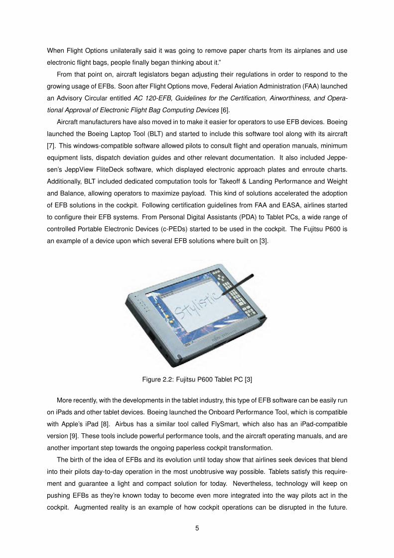
controlled Portable Electronic Devices (c-PEDs) started to be used in the cockpit. The Fujitsu P600 is
an example of a device upon which several EFB solutions where built on [3].
Figure 2.2: Fujitsu P600 Tablet PC [3]
More recently, with the developments in the tablet industry, this type of EFB software can be easily run
on iPads and other tablet devices. Boeing launched the Onboard Performance Tool, which is compatible
with Apple’s iPad [8]. Airbus has a similar tool called FlySmart, which also has an iPad-compatible
version [9]. These tools include powerful performance tools, and the aircraft operating manuals, and are
another important step towards the ongoing paperless cockpit transformation.
The birth of the idea of EFBs and its evolution until today show that airlines seek devices that blend
into their pilots day-to-day operation in the most unobtrusive way possible. Tablets satisfy this require-
ment and guarantee a light and compact solution for today. Nevertheless, technology will keep on
pushing EFBs as they’re known today to become even more integrated into the way pilots act in the
cockpit. Augmented reality is an example of how cockpit operations can be disrupted in the future.
5

Figure 2.3: Airbus FlySmart for iPad [9]
Head-up Displays, integrated in wearable glasses, that can give the pilot contextual information in an
advanced way, are an example of how EFBs can be revolutionized. Important information could thereby
be directly visible to the pilot, without him having to look at any other device. Aero Glass is an example
of a company developing a solution like this [10]. What sets this solution apart from conventional fixed
HUDs, often seen in military fighters, is that the displayed information depends on the direction in which
the pilot is looking.
2.3 Arguments for and against the adoption of EFB systems
Like any other operational change to be carried out, the adoption of EFB systems has arguments that
speak for and against it. What follows is a summarized analysis which covers some of the most relevant
points, to better understand how EFB solutions can impact airline operations.
Benefits
The reasons that speak in favor of the adoption of EFB systems by airlines can be divided in two main
topics.
The first one is the significant reduction of paper-based documentation, allowing it to be accessed
digitally instead. Flight-specific documentation printed before the flight, maps, performance charts and
tables are replaced by a single electronic device, lighter and more compact than the traditional Flight
Bag. In the case of American Airlines, the adoption of an iPad EFB solution meant saving US$1,2 Million
yearly in fuel costs due to the reduction in weight [4]. The savings in fuel and gas emissions, together
with reduced printing and distribution costs, make the reduction of paper a strong argument.
The second big advantage of the EFB is the potential for increased fuel and operational efficiency,
as well as operational safety. The EFB’s CPU has the ability to calculate key parameters and values. It
can present the pilot with tailored information based on the actual aircraft status and atmospheric data.
6

This eliminates the need of interpolating given performance values of the aircraft’s reference manuals, as
FCOMs and QRHs, which are in turn the product of discrete calculations made on the ground. Moreover,
it can display the desired information in a customized layout. NOTAMs, weather information and others
are all easily displayable and accessible.
Drawbacks
Despite having a lot in its favor, the implementation of EFB systems has some risks and disadvantages
that are worth taking a look at.
The first and most significant inconvenience is the initial investment required. The hardware used
for EFB systems is often a c-PED, which has a significant cost associated to it. Due to the high num-
ber of devices that need to be acquired (usually one per pilot, plus development and testing units..),
the adoption cost rises fast. This adds up to the cost of all the software to be installed in the c-PEDs.
Alternatively, as in TAP’s case, some airlines choose to develop their own software in-house. This has
the advantage of allowing to build a custom solution, tailored to the airline’s specific needs. The down-
side of this approach is the extra cost associated with R&D, which includes extra man-hours, training,
equipment, licensing and others.
Parallel to the already mentioned costs, one has to take into account the transformation of the doc-
umentation infrastructure to support a fully digital solution. The documents may already be available
in digital format, but the way they are organized and delivered to the EFBs has to be studied. The
server and database architecture necessary to guarantee the pilots always have access to the neces-
sary documents and information is an important point in the process, which requires careful planning
and implementation.
Training the crew members on how to use the new EFB system is equally necessary, and also
consumes resources. Another point associated with this, which is the need to consider and study human
factors. The efficiency of the interaction of pilots with the EFB system, and the way this interaction affects
the pilot’s ability to perform his remaining duties within the operational requirements have to be carefully
analyzed [3].
Digital security is another important issue and has to be taken into account to prevent loss or stealing
of information. With a rising connectivity between devices, including connections between the aircraft
and the EFB, it is crucial that any undesired access is successfully blocked. The whole server infras-
tructure and database also need to be protected accordingly.
Remarks
If an airline has the necessary resources to implement an EFB solution and cover the initial costs that
this implies, it will benefit from it in the long run. The versatility and potential of EFB systems is very
significant, and this ends up translating into a positive impact on the airline’s balance sheets at the end
of the year, as on its environmental footprint and operational safety [11].
7
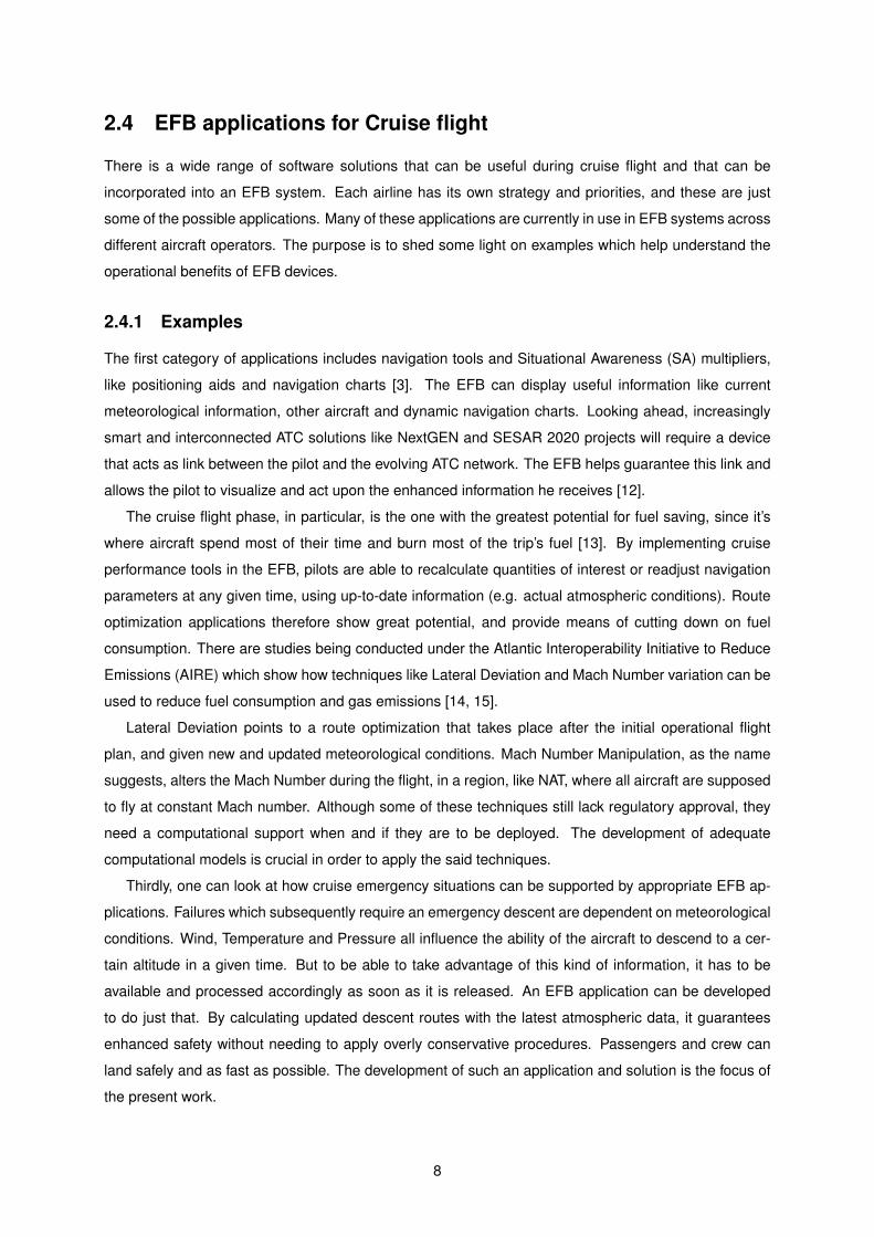
2.4 EFB applications for Cruise flight
There is a wide range of software solutions that can be useful during cruise flight and that can be
incorporated into an EFB system. Each airline has its own strategy and priorities, and these are just
some of the possible applications. Many of these applications are currently in use in EFB systems across
different aircraft operators. The purpose is to shed some light on examples which help understand the
operational benefits of EFB devices.
2.4.1 Examples
The first category of applications includes navigation tools and Situational Awareness (SA) multipliers,
like positioning aids and navigation charts [3]. The EFB can display useful information like current
meteorological information, other aircraft and dynamic navigation charts. Looking ahead, increasingly
smart and interconnected ATC solutions like NextGEN and SESAR 2020 projects will require a device
that acts as link between the pilot and the evolving ATC network. The EFB helps guarantee this link and
allows the pilot to visualize and act upon the enhanced information he receives [12].
The cruise flight phase, in particular, is the one with the greatest potential for fuel saving, since it’s
where aircraft spend most of their time and burn most of the trip’s fuel [13]. By implementing cruise
performance tools in the EFB, pilots are able to recalculate quantities of interest or readjust navigation
parameters at any given time, using up-to-date information (e.g. actual atmospheric conditions). Route
optimization applications therefore show great potential, and provide means of cutting down on fuel
consumption. There are studies being conducted under the Atlantic Interoperability Initiative to Reduce
Emissions (AIRE) which show how techniques like Lateral Deviation and Mach Number variation can be
used to reduce fuel consumption and gas emissions [14, 15].
Lateral Deviation points to a route optimization that takes place after the initial operational flight
plan, and given new and updated meteorological conditions. Mach Number Manipulation, as the name
suggests, alters the Mach Number during the flight, in a region, like NAT, where all aircraft are supposed
to fly at constant Mach number. Although some of these techniques still lack regulatory approval, they
need a computational support when and if they are to be deployed. The development of adequate
computational models is crucial in order to apply the said techniques.
Thirdly, one can look at how cruise emergency situations can be supported by appropriate EFB ap-
plications. Failures which subsequently require an emergency descent are dependent on meteorological
conditions. Wind, Temperature and Pressure all influence the ability of the aircraft to descend to a cer-
tain altitude in a given time. But to be able to take advantage of this kind of information, it has to be
available and processed accordingly as soon as it is released. An EFB application can be developed
to do just that. By calculating updated descent routes with the latest atmospheric data, it guarantees
enhanced safety without needing to apply overly conservative procedures. Passengers and crew can
land safely and as fast as possible. The development of such an application and solution is the focus of
the present work.
8

2.4.2 Remarks and technical considerations
For many of the above-mentioned applications, it is required that the EFB device has access to navi-
gational data and atmospheric information. This means that there is an increased need for EFBs to be
connected to the avionics of the aircraft, as well as to external servers on the ground. The greater the
amount of data to be processed by EFBs, the larger the bandwidth required.
On ground, this can be accomplished through local EFB databases which are updated shortly before
the flight. Through Wi-Fi and 3G/4G, airlines can get ground access to the internet from almost anywhere
in the world. Pilots can thereby download the latest flight documentation and atmospheric data while
still on ground. EFBs establish the link between the aircraft and the airline’s ground systems and data
storage facilities.
In the air, however, communications are more limited and costly. Should it be necessary to extract
information for the EFB’s database (e.g weather data), there are only a few different solutions available.
The most ancient one is the Aircraft Communications Addressing and Reporting System (ACARS).
ACARS is a technology that was launched in 1978 [16] by ARINC and was initially used to deliver
messages between the aircraft and ground stations, through VHF communication. The system has
evolved into allowing other forms of data transmission besides VHF, which expanded its geographical
coverage. Besides serving ATC purposes, ACARS allows the aircraft to communicate with its ground
base [17]. With a growing set of data being transferred to as from the aircraft, ACARS is reaching its
limit and in future more modern solutions are required [18].
Satellite communications (SATCOM) have been evolving together with the growing sophistication of
satellites and onboard aircraft equipment. They have the ability to keep the aircraft connected, even
in the most remote locations like oceans, where traditional ACARS coverage is limited. In the last few
years, solutions like Inmarsat’s Swiftbroadband and Iridium are helping push aircraft communication
forward [19, 20], allowing EFBs to equally evolve and gain access to increased amounts of information.
9

10

3. Introduction to Aircraft Performance
This chapter is intended to introduce important aspects of aircraft performance that serve as a base for
the present work. The chapter intends to give the reader a basic understanding on the fundamental
performance concepts that lie behind the software that was developed.
Section 3.1 describes the International Standard Atmosphere. Section 3.2 presents important speed
definitions. Section 3.3 introduces the basic wing theory and how the equations that rule the flight
dynamics can be obtained. The last Section 3.4 presents the equations that rule level flight.
3.1 International Standard Atmosphere (ISA)
The atmosphere is a gaseous envelope that surrounds the earth. Since its properties vary geographi-
cally, it was necessary to come up with a standardized set of conditions called the International Standard
Atmosphere (ISA) [21]. The first two layers of the atmosphere, the troposphere and the stratosphere,
are the most relevant for subsonic aircraft, and will be the focus of the current section [22].
3.1.1 Important units
Following units are going to be used throughout the work:
Altitude feet [ft] or FL*
Density kilogram per cubic meter [ kgm3 ]
Distance nautical miles [NM ]
Mass kilogram [kg]
Pressure hectopascal [hPa]
Temperature Kelvin [K] or Degree Celsius [◦C]
*Note: FL stands for Flight Level and is no physical unit. It is used to display an altitude value in hundreds
of feet (e.g. the altitude 40000ft corresponds to FL400).
3.1.2 ISA properties at sea-level
According to the standard atmosphere, the physical properties at sea-level are the following [21, 22]:
11

g0 = 9, 806m
s2
p0 = 1013, 25hPa
T0 = 15 ◦C = 288, 15K
ρ0 = 1, 225kg
m3
(3.1)
3.1.3 Temperature modeling
In ISA it is assumed that below the tropopause (hTP = 36089 ft), the temperature drops at a constant
rate of a = −0, 0019812◦Cft with increasing altitude. This constant is referred to as the lapse rate of the
atmosphere. Therefore, for any two given altitudes h and h1, where h > h1, with respective temperatures
T and T1, one can write [22]:
a =T − T1h− h1
(3.2)
Reformulating, one can get the temperature at any desired altitude h, if the temperature at a reference
altitude h1 is known:
T (h) = T1 + a(h− h1) (3.3)
Choosing the sea-level as reference, h1 = 0 and T1 = T0.
Above the tropopause (h > 36089 ft), the temperature is constant (ISA model) and equal to -56,5◦C
[22].
Summing up, the temperature is distributed like so:
T [◦C] =
{15− 0, 0019812 · h [ft] 0 ≤ h ≤ hTP (3.4a)
−56, 5 hTP < h (3.4b)
or
T [K] =
{288, 15− 0, 0019812 · h [ft] 0 ≤ h ≤ hTP (3.5a)
216, 65 hTP < h (3.5b)
Where h is the altitude measured in feet (ft) and hTP = 36089 ft.
Figure 3.1 shows a graphical representation of the temperature distribution for the standard atmo-
sphere.
12

Figure 3.1: ISA Temperature distribution [21]
3.1.4 Pressure and density modeling
To determine the distribution of pressure and density on the atmosphere, consider the vertical force
equilibrium of an infinitesimally small particle of air, represented in Fig. 3.2.
Figure 3.2: Vertical forces acting on sample atmosphere particle [22]
The force equilibrium on the particle can be expressed like so:
p dxdy − (p+ dp) dxdy − ρg dxdydh = 0 (3.6)
Simplifying Eq. (3.6) yields:
dp = − ρg dh (3.7)
In the context of the ISA, air is considered a perfect gas, thus being subject to the equation of state
[22]:
13

p = ρgRT (3.8)
Where R = 29, 26mK = 95, 997 ftK is the gas constant for dry air and subject to the earth’s gravitational
acceleration; T is the absolute temperature of the gas in degrees Kelvin (K).
Dividing Eq. (3.7) by Eq. (3.8) yields:
dp
p= − dh
RT(3.9)
Since the temperature behaves differently in the troposphere and the stratosphere, it is best to ana-
lyze the pressure and density in both of these regions separately.
Pressure and density in Troposphere - 0 ≤ h < 36089ft
Due to the lapse rate in the tropopause, the temperature is not constant and therefore one has to relate
its variation dT with the variation of altitude dh.
The differentiation of Eq. (3.3) gives this relation:
dT = a dh (3.10)
Substituting this result in Eq. (3.9):
dp
p= − dT
aRT(3.11)
The integration of Eq. (3.11) provides the relationship between the pressure at any given altitude
and the pressure at a reference altitude (analog to Eq. (3.3)):
p
p1=
(T
T1
)− 1aR
=
{1 +
a
T1(h− h1)
}− 1aR
(3.12)
For the density one can insert the equation of state (Eq. 3.8) into the last expression, which yields:
ρ
ρ1=
(p
p1
)(T
T1
)=
(T
T1
)(− 1aR−1
)(3.13)
It is convenient to choose the sea-level as reference altitude, similarly to what was done with the
temperature. This results in the final expressions which describe the pressure and density distribution
in the troposphere:
p [hPa] = 1013, 25
(1− 0, 0019812 · h[ft]
288, 15
)5,2579
(3.14)
ρ [kg /m3] = 1, 225
(1− 0, 0019812 · h[ft]
288, 15
)4,2579
(3.15)
14

Where − 1aR = − 1
−0,0019812 Kft ·95,997ftK
= 5, 2579
Pressure and density in Stratosphere - 36089ft ≤ h
Since the temperature in the stratosphere is assumed constant at TZ2 = −56, 5◦C = 216, 65K, one can
integrate Eq. (3.9) directly, obtaining:
ln
(p
pref
)= −
(h− hrefRT
)(3.16)
Solving this result for p yields:
p = pref · e
{−(h−href
RT
)}(3.17)
Selecting href = 36089 ft, one knows from Eq. (3.14) that
pref = p(href = 36089 ft) = 1013, 25 ·(
1− 0, 0019812 · 36089
288, 15
)5,2579
= 226, 2hPa,
and from Eq. (3.5a) that Tref = 216, 65K.
Remembering that R = 95, 997 ftK and inserting the above results in Eq. (3.17) one gets following result:
p [hPa] = 226, 2 · e−(h[ft]−36089
20797,8
)(3.18)
From the equation of state (3.8) one can write that:
ρ1ρ2
=p1p2
(3.19)
Reformulating:
ρ1 = p1 ·ρ2p2
(3.20)
Choosing the references ρ2 and p2 as the density and pressure at h2 = 36089 ft, respectively, and
consulting Eqs. (3.14) and (3.15):
ρ1 = p1 · 0, 001608 (3.21)
This results in the expression for the density distribution in the first layer of the stratosphere:
ρ [kg /m3] = 0, 3637 · e−(h[ft]−36089
20797,8
)(3.22)
Summarized results
The pressure and density distribution equations are presented once more, for facilitated reference:
15

p [hPa] =
1013, 25
(1− 0, 0019812 · h[ft]
288, 15
)5,2579
0 ≤ h ≤ hTP (3.23a)
226, 2 · e−(h[ft]−36089
20797,8
)hTP < h (3.23b)
ρ [kg /m3] =
1, 225
(1− 0, 0019812 · h[ft]
288, 15
)4,2579
0 ≤ h ≤ hTP (3.24a)
0, 3637 · e−(h[ft]−36089
20797,8
)hTP < h (3.24b)
Where h is the altitude measured in feet (ft) and hTP = 36089 ft.
3.2 Operating speeds
When an aircraft is flying, there are a number of distinct speed definitions which are applied with different
purposes. Some help the flight crew manage the flight, while others are used for navigational and
performance study and optimization purposes. The following subsections include an explanation each
of these speeds (adapted from [21]).
3.2.1 Calibrated Air Speed (CAS)
The Calibrated Air Speed (CAS) is obtained from the difference between the total pressure (pt) and the
static pressure (ps). This difference is called dynamic pressure (q).
q = pt − ps (3.25)
The dynamic pressure cannot be measured directly, and is therefore obtained through two types of
probes. One is responsible for the measurement of the total pressure, while the other probes measure
the static pressure (Fig. 3.3).
The total pressure pt is measured by a forward-facing tube, called pitot tube, which is placed near the
nose of the aircraft, where the airflow is stopped. This allows the pitot tube to read the impact pressure,
which accounts for the ambient pressure (static aspect) and the movement of the airplane (dynamic
aspect).
The static pressure ps is measured through several of static ports placed perpendicularly to the
airflow. The static ports are symmetrically disposed on both sides of the airplane, to eliminate sideslip
errors.
CAS = f(pt − ps) = f(q) (3.26)
16
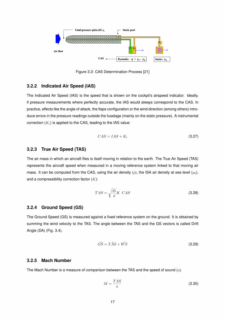
Figure 3.3: CAS Determination Process [21]
3.2.2 Indicated Air Speed (IAS)
The Indicated Air Speed (IAS) is the speed that is shown on the cockpit’s airspeed indicator. Ideally,
if pressure measurements where perfectly accurate, the IAS would always correspond to the CAS. In
practice, effects like the angle of attack, the flaps configuration or the wind direction (among others) intro-
duce errors in the pressure readings outside the fuselage (mainly on the static pressure). A instrumental
correction (Ki) is applied to the CAS, leading to the IAS value:
CAS = IAS +Ki (3.27)
3.2.3 True Air Speed (TAS)
The air mass in which an aircraft flies is itself moving in relation to the earth. The True Air Speed (TAS)
represents the aircraft speed when measured in a moving reference system linked to that moving air
mass. It can be computed from the CAS, using the air density (ρ), the ISA air density at sea level (ρ0),
and a compressibility correction factor (K):
TAS =
√ρ0ρK CAS (3.28)
3.2.4 Ground Speed (GS)
The Ground Speed (GS) is measured against a fixed reference system on the ground. It is obtained by
summing the wind velocity to the TAS. The angle between the TAS and the GS vectors is called Drift
Angle (DA) (Fig. 3.4).
~GS = ~TAS + ~WS (3.29)
3.2.5 Mach Number
The Mach Number is a measure of comparison between the TAS and the speed of sound (a).
M =TAS
a(3.30)
17
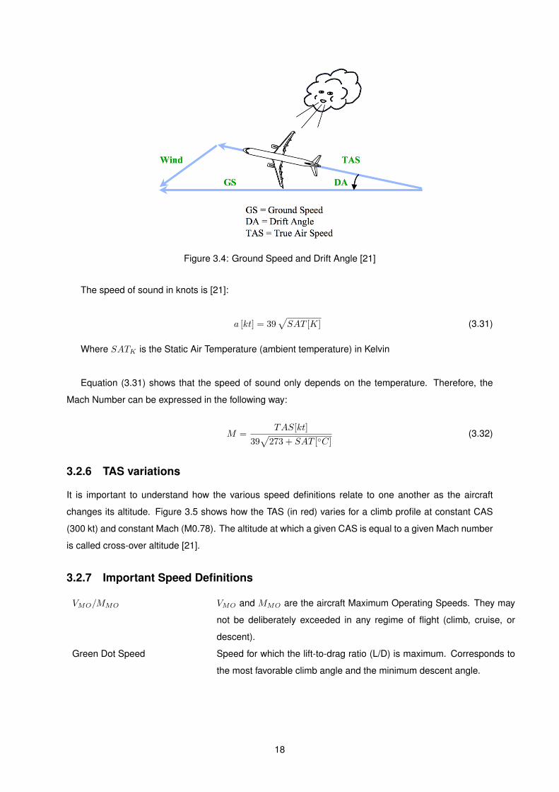
Figure 3.4: Ground Speed and Drift Angle [21]
The speed of sound in knots is [21]:
a [kt] = 39√SAT [K] (3.31)
Where SATK is the Static Air Temperature (ambient temperature) in Kelvin
Equation (3.31) shows that the speed of sound only depends on the temperature. Therefore, the
Mach Number can be expressed in the following way:
M =TAS[kt]
39√
273 + SAT [◦C](3.32)
3.2.6 TAS variations
It is important to understand how the various speed definitions relate to one another as the aircraft
changes its altitude. Figure 3.5 shows how the TAS (in red) varies for a climb profile at constant CAS
(300 kt) and constant Mach (M0.78). The altitude at which a given CAS is equal to a given Mach number
is called cross-over altitude [21].
3.2.7 Important Speed Definitions
VMO/MMO VMO and MMO are the aircraft Maximum Operating Speeds. They may
not be deliberately exceeded in any regime of flight (climb, cruise, or
descent).
Green Dot Speed Speed for which the lift-to-drag ratio (L/D) is maximum. Corresponds to
the most favorable climb angle and the minimum descent angle.
18

Figure 3.5: TAS Variations - Climb profile 300 Kt / M0.78 [21]
3.3 Wing Theory
3.3.1 Aerodynamic forces and moments on airfoils
When an airfoil is situated in a moving stream of fluid (air in this case), an aerodynamic force acts on the
airfoil. This force (F ) depends upon six variables [22]:
• air velocity, V
• air density, ρ
• characteristic area, S
• coefficient of viscosity, µ
• speed of sound, a
• angle of attack, α
A dimensional analysis can be used in order to find the general form of this dependance. This
problem has six dimensional variables (F , V , ρ, S, µ and a) and three independent units (length, l,
mass, m and time, t). According to Buckingham’s π-theorem [23] this means that three dimensionless
parameters can be found. Using V, ρ and S as repeating variables, one obtains the three dimensionless
parameters as a function of the repeating variables, and of F , µ and Va, respectively:
π1 = V aρbSdF (3.33)
π2 = V aρbSdµ (3.34)
π2 = V aρbSdV a (3.35)
Writing equation 3.33 in terms of the fundamental units l, m and t yields:
π1 =
(l
t
)a (ml3
)b (l2) d(ml
t2
)(3.36)
19
Since π1 is dimensionless, the powers of l, m and t on the right side must respectively sum to zero:
for l: 0 = a− 3b+ 2d+ 1
for m: 0 = b+ 1
for t: 0 = −a− 2
(3.37)
Solving the three equations in (3.37) results in: a = −2, b = −1 and d = −1. Inserting this result in
(3.36) one gets
π1 =F
ρV 2S(3.38)
Following the same procedure for (3.34) and (3.35) following solutions are obtained:
π2 =µ
ρV S1/2 (3.39)
π3 =VaV
(3.40)
The dimensionless equation which governs the aerodynamic forces can be written in the following
way, according to the π-theorem:F
ρV 2S= f
(µ
ρV S1/2 ,VaV, α
)(3.41)
Replacing S1/2 by c, the chord of the airfoil, one can see how Eq. (3.41) contains two important
parameters:
Mach number: M =V
Va(3.42)
and
Reynolds number: RN =ρV c
µ(3.43)
Replacing the two expressions above in Eq. (3.41) one can write:
F = ρV 2S f (RN ,M, α) (3.44)
Where S is the wing area. For the force perpendicular to the free stream (lift force), it is common to
introduce the following dimensionless expression [22]:
f (RN ,M, α) =Cl2
(3.45)
Where Cl is the so-called the sectional lift coefficient. Also, for airfoils, let S = c · 1, i.e. the area per
unit span. It is now possible to write Eq. (3.44) in its conventional form:
l = Cl1
2ρV 2c = Clqc (3.46)
20

Where q is the dynamic pressure. Doing the same for the drag force (i.e. the force acting parallel to
the free stream) one gets:
d = Cd1
2ρV 2c = Cdqc (3.47)
Where Cd is the so-called the sectional lift coefficient.
The dimensionless coefficients Cl and Cd are functions of α, RN and M . By using a similar process
a pitching coefficient cm can be found such that the sectional pitching moment can be computed from:
m = cm1
2ρV 2c2 = cmqc
2 (3.48)
Where Cd is the so-called the sectional lift coefficient. It is defined positive when the moment is
nose-up [22].
Figure 3.6: Definition of Section (Airfoil) Forces and Moment [22]
3.3.2 Aerodynamic forces and moments on wings
The Eqs. (3.46) through (3.48) give the equations for the lift, drag and pitching moment coefficient acting
on airfoils. For the wing one can write following expressions for the (planform) lift, drag, and moment
coefficients, by analogy [22]:
L = CL1
2ρ V 2S = CL q S (3.49)
D = CD1
2ρ V 2S = CD q S (3.50)
M = Cm1
2ρ V 2c2 = Cm q S c (3.51)
Where c is the mean geometric chord of the wing, usually chosen as the characteristic length required
to define the wing pitching moment coefficient. It is defined as [22]:
c =2
S
∫ b/2
0
c2dy (3.52)
Where b is the wing span.
21

3.4 Flight Mechanics for level flight
To understand how aerodynamic forces and other forces act on airplanes during the different flight
phases, it is best to start off by understanding the steady level flight mechanics.
For a flight at constant TAS and altitude, all forces and moments acting on the aircraft balance each
other. The forces applied to the aircraft can be grouped into four fundamental ones: Lift (L), Thrust (T ),
Drag (D) and Weight (W ).
Figure 3.7: Balance of Forces for Steady Level Flight (adapted from [21])
3.4.1 Standard Lift Equation
Recalling Eq. (3.49) and knowing that the lift in level flight is just enough to balance the weight of the
aircraft, one can write [22]:
L = W = m · g =1
2ρ (TAS)2S CL (3.53)
3.4.2 Standard Drag Equation
Analog to Eq. (3.53), the same can be done for the longitudinal axis, starting from Eq. (3.50). The
engine thrust balances the drag force, and therefore [22]:
D = T =1
2ρ (TAS)2S CD (3.54)
22
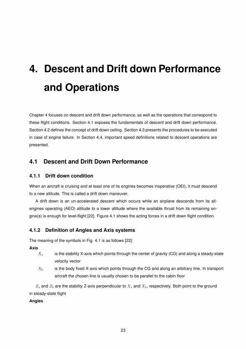
4. Descent and Drift down Performance
and Operations
Chapter 4 focuses on descent and drift down performance, as well as the operations that correspond to
these flight conditions. Section 4.1 exposes the fundamentals of descent and drift down performance.
Section 4.2 defines the concept of drift down ceiling. Section 4.3 presents the procedures to be executed
in case of engine failure. In Section 4.4, important speed definitions related to descent operations are
presented.
4.1 Descent and Drift Down Performance
4.1.1 Drift down condition
When an aircraft is cruising and at least one of its engines becomes inoperative (OEI), it must descend
to a new altitude. This is called a drift down maneuver.
A drift down is an un-accelerated descent which occurs while an airplane descends from its all-
engines operating (AEO) altitude to a lower altitude where the available thrust from its remaining en-
gine(s) is enough for level-flight [22]. Figure 4.1 shows the acting forces in a drift down flight condition.
4.1.2 Definition of Angles and Axis systems
The meaning of the symbols in Fig. 4.1 is as follows [22]:
AxisXs is the stability X-axis which points through the center of gravity (CG) and along a steady-state
velocity vector
Xb is the body fixed X-axis which points through the CG and along an arbitrary line. In transport
aircraft the chosen line is usually chosen to be parallel to the cabin floor
Zs and Zb are the stability Z-axis perpendicular to Xs and Xb, respectively. Both point to the ground
in steady-state flight
Angles
23
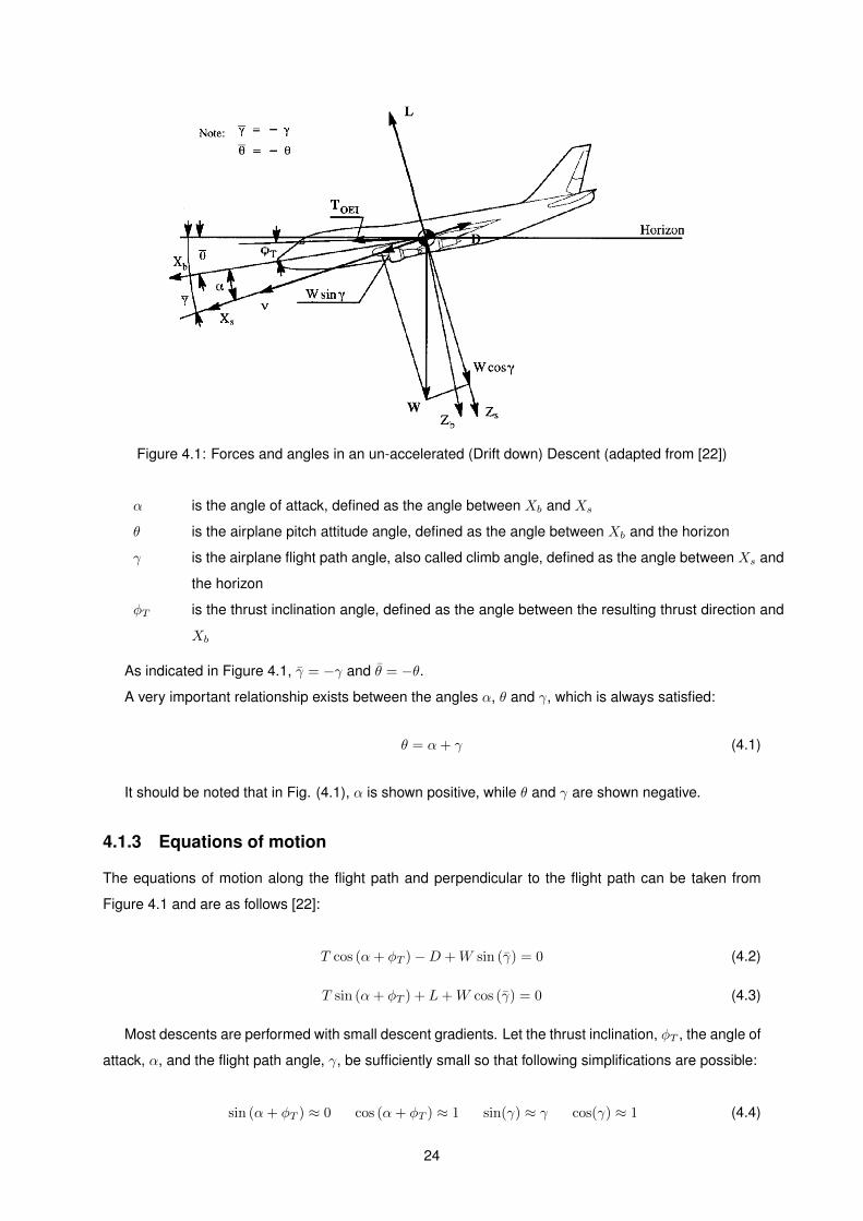
Figure 4.1: Forces and angles in an un-accelerated (Drift down) Descent (adapted from [22])
α is the angle of attack, defined as the angle between Xb and Xs
θ is the airplane pitch attitude angle, defined as the angle between Xb and the horizon
γ is the airplane flight path angle, also called climb angle, defined as the angle between Xs and
the horizon
φT is the thrust inclination angle, defined as the angle between the resulting thrust direction and
Xb
As indicated in Figure 4.1, γ = −γ and θ = −θ.
A very important relationship exists between the angles α, θ and γ, which is always satisfied:
θ = α+ γ (4.1)
It should be noted that in Fig. (4.1), α is shown positive, while θ and γ are shown negative.
4.1.3 Equations of motion
The equations of motion along the flight path and perpendicular to the flight path can be taken from
Figure 4.1 and are as follows [22]:
T cos (α+ φT )−D +W sin (γ) = 0 (4.2)
T sin (α+ φT ) + L+W cos (γ) = 0 (4.3)
Most descents are performed with small descent gradients. Let the thrust inclination, φT , the angle of
attack, α, and the flight path angle, γ, be sufficiently small so that following simplifications are possible:
sin (α+ φT ) ≈ 0 cos (α+ φT ) ≈ 1 sin(γ) ≈ γ cos(γ) ≈ 1 (4.4)
24

With these assumptions, Eqs. (4.2) and (4.3) become:
T −D +W · γ = 0 (4.5)
L = W (4.6)
4.1.4 Descent Gradient (γ)
The expression for the descent angle is, from Eq. (4.5):
γ =D − TW
(4.7)
Thus, for a given weight, the descent gradient is maximum when the Drag is maximum and the Thrust
is minimum.
Regular descents, as well as emergency descents, are carried out at Flight Idle thrust (where T ≈ 0),
and the expression for γ becomes:
γ =D
W(4.8)
By introducing L/D (Lift to Drag ratio), and since L = W from Eq. (4.6):
γ =D
L=
1LD
(4.9)
Rewriting the expression, in percent:
γ [%] =100LD
(4.10)
At a given weight, the descent gradient is minimum when the Drag is minimum, or when the Lift-to-
Drag is maximum. The minimum descent angle TAS is, therefore, the Green Dot Speed1.
In a drift down maneuver, the remaining engine(s) are kept at Maximum Continuous Thrust (MCT).
This is the maximum thrust that can be used unlimitedly in flight. For this case, Eq. (4.7) becomes:
γ =DOEI − TOEI
W=TreqOEI
− TavOEI
W(4.11)
Where TreqOEIcorresponds to the thrust required to overcome the Drag force acting on the aircraft,
and TavOEIis the available thrust of the remaining engine(s) at MCT setting.
4.1.5 Rate of Descent (RD)
The rate of descent, RD, is defined as:
RD = −dhdt
= −V · sin γ = V · sin γ ≈ V · γ (4.12)
1Subsection 3.2.7
25

Inserting this relation in Eq. (4.7) yields:
RD =(D − T ) · V
W(4.13)
For drift down condition, Eq. (4.13) becomes:
RD =(TreqOEI
− TavOEI) · V
W(4.14)
4.2 Drift down ceiling
Initially, when the drift down begins, the available thrust is not enough to balance the Drag force of the
aircraft (TreqOEI> TavOEI
). Inserting this result in Eqs. (4.11) and (4.14), one can see that the aircraft
starts descending:
γ > 0 and RD > 0
Recalling Eqs. (3.54) and (4.11) one can write:
TreqOEI=
1
2ρ (TAS)2S CD (4.15)
Which shows how the required thrust is strongly related to the aircraft TAS.
Due to the lack of thrust, the Drag force causes the aircraft decelerate, and to reduce its TAS.
From Eq. (4.15), TreqOEIalso diminishes. Eventually the required thrust balances the available thrust
(TreqOEI= TavOEI
). From Eqs. (4.11) and (4.14):
γ = 0 and RD = 0
When this happens, the aircraft has reached the so called drift down ceiling, and stops descend-
ing further. The drift down ceiling is the maximum altitude that can be flown in level flight, at green dot
speed [21].
4.3 Influencing Parameters
There are several different parameters that influence the descent performance. This is of particular
importance to the present work, since the goal is to take these parameters into account for an increased
operational safety when performing emergency descent procedures. By understanding how the descent
performance correlates to them, one can better understand the impact of the work being presented.
4.3.1 Altitude effect
During a descent, the altitude of the aircraft decreases, thus increasing the air density (Eqs. (3.24a)
and (3.24b)) and the Drag force (Eq. 3.50). Since the descent gradient and the rate of descent are
26
both proportional to the Drag (Eqs. (4.7) to (4.14)), an increase in their magnitude is expected while the
aircraft descends.
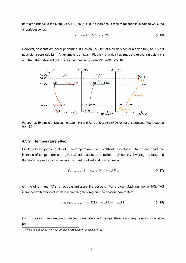
h ↓→ ρ ↑→ D ↑→ γ,RD ↑ (4.16)
However, descents are never performed at a given TAS, but at a given Mach or a given IAS, so it is not
possible to conclude [21]. An example is shown in Figure 4.2, which illustrates the descent gradient (γ)
and the rate of descent (RD) for a given descent profile M0.82/300kt/250kt2.
Figure 4.2: Example of Descent gradient (γ) and Rate of Descent (RD) versus Altitude and TAS (adaptedfrom [21])
4.3.2 Temperature effect
Similarly to the pressure altitude, the temperature effect is difficult to evaluate. On the one hand, the
increase of temperature on a given altitude causes a reduction in air density, lowering the drag and
therefore suggesting a decrease in descent gradient and rate of descent:
Th=constant ↑→ ρ ↓→ D ↓→ γ,RD ↓ (4.17)
On the other hand, TAS is not constant along the descent. For a given Mach number or IAS, TAS
increases with temperature thus increasing the drag and the descent parameters:
TM,IAS=constant ↑→ TAS ↑→ D ↑→ γ,RD ↑ (4.18)
For this reason, the variation of descent parameters with Temperature is not very relevant in aviation
[21].2Refer to Subsection 4.4.1 for detailed information on descent profiles
27

4.3.3 Weight effect
The Green dot speed (GD), which corresponds to the minimum descent gradient, depends on the aircraft
weight. In the standard descent speed range (between GD and VMO), the rate and gradient of the
descent decrease at higher weights. This is illustrated in Figure 4.3, and can be confirmed by analyzing
Eq. (3.49):
Figure 4.3: Descent gradient and Rate of Descent versus Weight and TAS (adapted from [21])
L = W · cos γ = CL1
2ρ V 2S (4.19)
The increase of weight at a given TAS and density can only be balanced by decreasing the descent
gradient (γ) or by increasing the Lift Coefficient (CL), which can be done with an increase in the angle
of attack (α). From Eq. (4.12), RD = TAS · γ, and thus the rate of descent will also decrease at higher
weights.
Summing up, in the standard descent speed range following rules apply:
W ↑→ γ, RD ↓ (4.20)
4.3.4 Longitudinal Wind Effect
Figure 4.4 shows that the longitudinal Wind component (along the horizon axis) has no effect on the
TAS, and thus it doesn’t affect the air descent gradient (γa). This means that for a given descent from
Top Of Descent (TOD) to a final altitude, the fuel and time required are not affected by headwind. The
affected descent parameters are the flight path angle (γg) and the Ground distance covered counting
from TOD [21].
Summing up, one can establish the following relations:
Headwind ↑ : RD→
Fuel and Time from TOD→
Descent gradient γg ↑
Ground distance from TOD ↓
28

Figure 4.4: Headwind effect on Descent Gradient and Rate of Descent (adapted from [21])
As a consequence of the reduced Ground distance during the descent, for a higher headwind com-
ponent, the aircraft is going to be able to spend more time in the preceding cruise. This means that its
going to cover a longer distance and spend more time at higher altitudes, which is beneficial for obstacle
clearance purposes.
4.4 Descent Speeds
Descent operations may be performed at different speeds, depending on their context. The most relevant
ones for the present work are presented below.
4.4.1 Descent at given MACH/IAS Law
A descent is usually executed at a sequence of constant Mach Number and IAS. For instance, a standard
flight profile for the Airbus A320 series is:
M0.78 / 300kt / 250kt
The TAS variation for this profile is shown in Figure 4.5. The three phases of this descent profile are:
• Above the crossover altitude: Descend at constant Mach = M0.78. Mach Number is maintained
at M0.78 to guarantee a fixed ratio between the TAS and the sound velocity, and to avoid high
speed buffeting. High speed buffeting is triggered at high Mach Number, where compressibility
effects produce shock waves on the upper part of the wing. After a certain Mach Number, the
airflow separates from the upper surface behind the shock wave, which becomes unstable and
induces buffeting. This is evidenced by severe vibrations
• Between the crossover altitude and 10000ft: Descend at constant IAS = 300kt. This is an
optimum descent speed, that can be maintained below M0.78.
• At and below 10000ft: Descend at constant IAS = 250kt (the speed is limited by ATC laws [21])
29
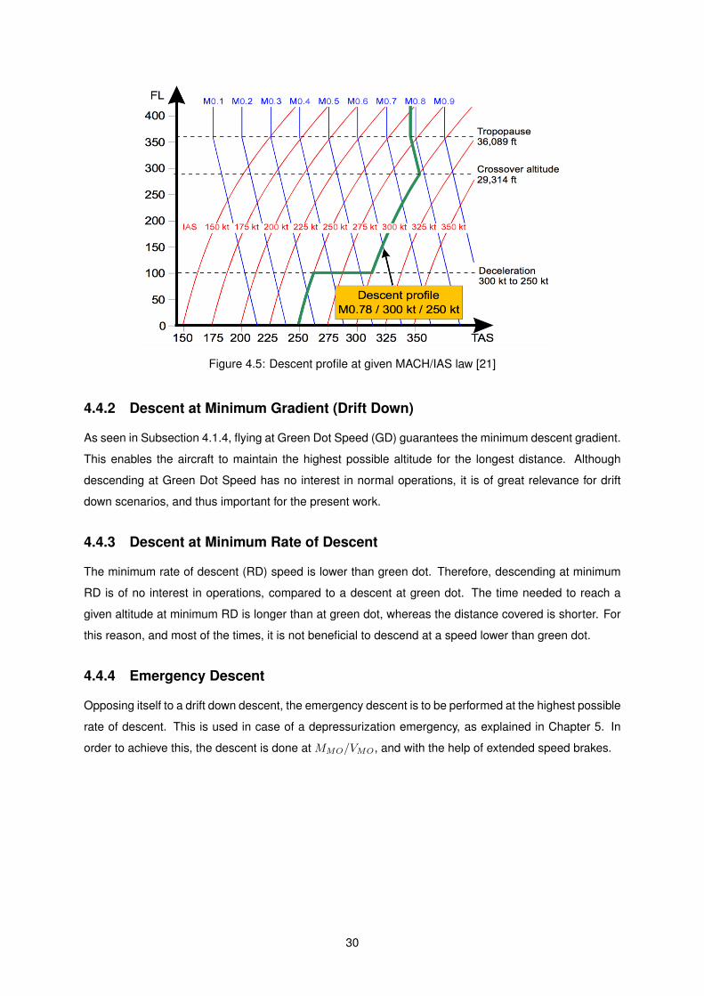
Figure 4.5: Descent profile at given MACH/IAS law [21]
4.4.2 Descent at Minimum Gradient (Drift Down)
As seen in Subsection 4.1.4, flying at Green Dot Speed (GD) guarantees the minimum descent gradient.
This enables the aircraft to maintain the highest possible altitude for the longest distance. Although
descending at Green Dot Speed has no interest in normal operations, it is of great relevance for drift
down scenarios, and thus important for the present work.
4.4.3 Descent at Minimum Rate of Descent
The minimum rate of descent (RD) speed is lower than green dot. Therefore, descending at minimum
RD is of no interest in operations, compared to a descent at green dot. The time needed to reach a
given altitude at minimum RD is longer than at green dot, whereas the distance covered is shorter. For
this reason, and most of the times, it is not beneficial to descend at a speed lower than green dot.
4.4.4 Emergency Descent
Opposing itself to a drift down descent, the emergency descent is to be performed at the highest possible
rate of descent. This is used in case of a depressurization emergency, as explained in Chapter 5. In
order to achieve this, the descent is done at MMO/VMO, and with the help of extended speed brakes.
30
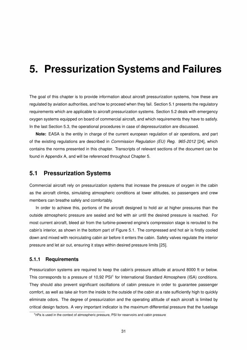
5. Pressurization Systems and Failures
The goal of this chapter is to provide information about aircraft pressurization systems, how these are
regulated by aviation authorities, and how to proceed when they fail. Section 5.1 presents the regulatory
requirements which are applicable to aircraft pressurization systems. Section 5.2 deals with emergency
oxygen systems equipped on board of commercial aircraft, and which requirements they have to satisfy.
In the last Section 5.3, the operational procedures in case of depressurization are discussed.
Note: EASA is the entity in charge of the current european regulation of air operations, and part
of the existing regulations are described in Commission Regulation (EU) Reg. 965-2012 [24], which
contains the norms presented in this chapter. Transcripts of relevant sections of the document can be
found in Appendix A, and will be referenced throughout Chapter 5.
5.1 Pressurization Systems
Commercial aircraft rely on pressurization systems that increase the pressure of oxygen in the cabin
as the aircraft climbs, simulating atmospheric conditions at lower altitudes, so passengers and crew
members can breathe safely and comfortably.
In order to achieve this, portions of the aircraft designed to hold air at higher pressures than the
outside atmospheric pressure are sealed and fed with air until the desired pressure is reached. For
most current aircraft, bleed air from the turbine-powered engine’s compression stage is rerouted to the
cabin’s interior, as shown in the bottom part of Figure 5.1. The compressed and hot air is firstly cooled
down and mixed with recirculating cabin air before it enters the cabin. Safety valves regulate the interior
pressure and let air out, ensuring it stays within desired pressure limits [25].
5.1.1 Requirements
Pressurization systems are required to keep the cabin’s pressure altitude at around 8000 ft or below.
This corresponds to a pressure of 10,92 PSI1 for International Standard Atmosphere (ISA) conditions.
They should also prevent significant oscillations of cabin pressure in order to guarantee passenger
comfort, as well as take air from the inside to the outside of the cabin at a rate sufficiently high to quickly
eliminate odors. The degree of pressurization and the operating altitude of each aircraft is limited by
critical design factors. A very important indicator is the maximum differential pressure that the fuselage1hPa is used in the context of atmospheric pressure, PSI for reservoirs and cabin pressure
31

Figure 5.1: Air Pressurization System for Turbofan Aircraft [26]
32
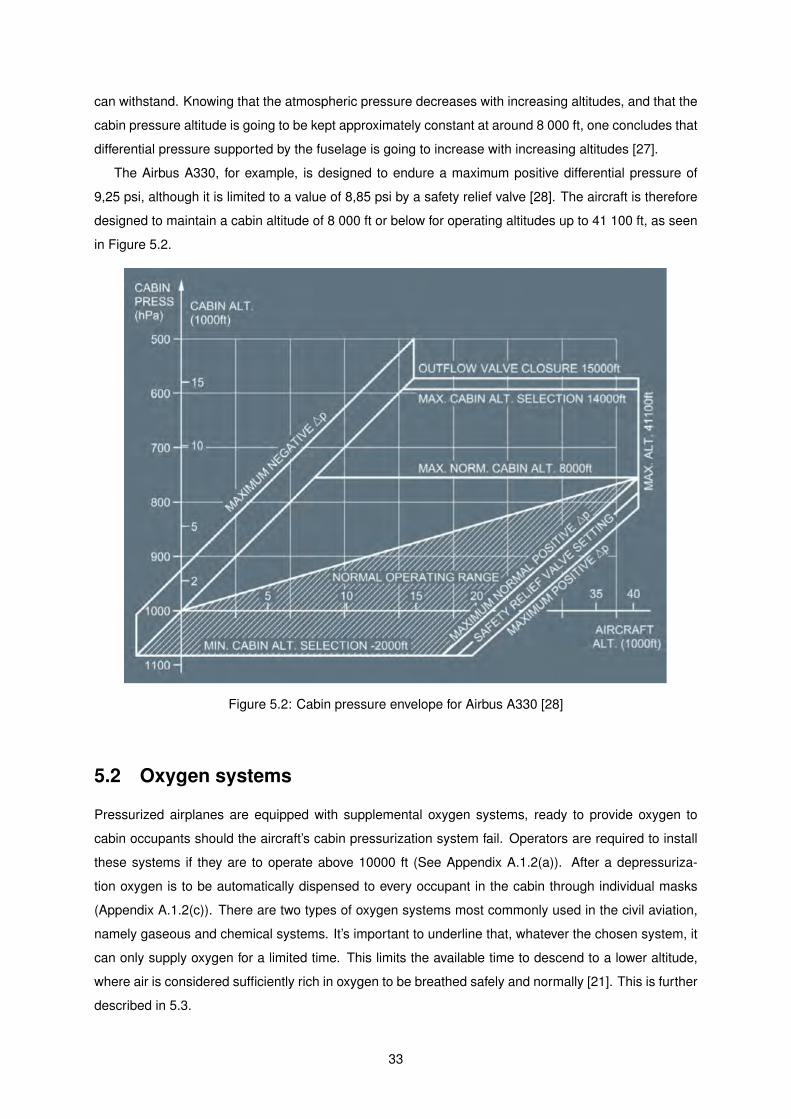
can withstand. Knowing that the atmospheric pressure decreases with increasing altitudes, and that the
cabin pressure altitude is going to be kept approximately constant at around 8 000 ft, one concludes that
differential pressure supported by the fuselage is going to increase with increasing altitudes [27].
The Airbus A330, for example, is designed to endure a maximum positive differential pressure of
9,25 psi, although it is limited to a value of 8,85 psi by a safety relief valve [28]. The aircraft is therefore
designed to maintain a cabin altitude of 8 000 ft or below for operating altitudes up to 41 100 ft, as seen
in Figure 5.2.
Figure 5.2: Cabin pressure envelope for Airbus A330 [28]
5.2 Oxygen systems
Pressurized airplanes are equipped with supplemental oxygen systems, ready to provide oxygen to
cabin occupants should the aircraft’s cabin pressurization system fail. Operators are required to install
these systems if they are to operate above 10000 ft (See Appendix A.1.2(a)). After a depressuriza-
tion oxygen is to be automatically dispensed to every occupant in the cabin through individual masks
(Appendix A.1.2(c)). There are two types of oxygen systems most commonly used in the civil aviation,
namely gaseous and chemical systems. It’s important to underline that, whatever the chosen system, it
can only supply oxygen for a limited time. This limits the available time to descend to a lower altitude,
where air is considered sufficiently rich in oxygen to be breathed safely and normally [21]. This is further
described in 5.3.
33
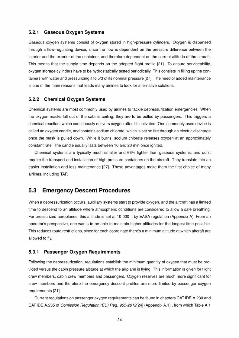
5.2.1 Gaseous Oxygen Systems
Gaseous oxygen systems consist of oxygen stored in high-pressure cylinders. Oxygen is dispensed
through a flow-regulating device, since the flow is dependent on the pressure difference between the
interior and the exterior of the container, and therefore dependent on the current altitude of the aircraft.
This means that the supply time depends on the adopted flight profile [21]. To ensure serviceability,
oxygen storage cylinders have to be hydrostatically tested periodically. This consists in filling up the con-
tainers with water and pressurizing it to 5/3 of its nominal pressure [27]. The need of added maintenance
is one of the main reasons that leads many airlines to look for alternative solutions.
5.2.2 Chemical Oxygen Systems
Chemical systems are most commonly used by airlines to tackle depressurization emergencies. When
the oxygen masks fall out of the cabin’s ceiling, they are to be pulled by passengers. This triggers a
chemical reaction, which continuously delivers oxygen after it’s activated. One commonly used device is
called an oxygen candle, and contains sodium chlorate, which is set on fire through an electric discharge
once the mask is pulled down. While it burns, sodium chlorate releases oxygen at an approximately
constant rate. The candle usually lasts between 10 and 20 min once ignited.
Chemical systems are typically much smaller and 66% lighter than gaseous systems, and don’t
require the transport and installation of high-pressure containers on the aircraft. They translate into an
easier installation and less maintenance [27]. These advantages make them the first choice of many
airlines, including TAP.
5.3 Emergency Descent Procedures
When a depressurization occurs, auxiliary systems start to provide oxygen, and the aircraft has a limited
time to descend to an altitude where atmospheric conditions are considered to allow a safe breathing.
For pressurized aeroplanes, this altitude is set at 10 000 ft by EASA regulation (Appendix A). From an
operator’s perspective, one wants to be able to maintain higher altitudes for the longest time possible.
This reduces route restrictions, since for each coordinate there’s a minimum altitude at which aircraft are
allowed to fly.
5.3.1 Passenger Oxygen Requirements
Following the depressurization, regulations establish the minimum quantity of oxygen that must be pro-
vided versus the cabin pressure altitude at which the airplane is flying. This information is given for flight
crew members, cabin crew members and passengers. Oxygen reserves are much more significant for
crew members and therefore the emergency descent profiles are more limited by passenger oxygen
requirements [21].
Current regulations on passenger oxygen requirements can be found in chapters CAT.IDE.A.230 and
CAT.IDE.A.235 of Comission Regulation (EU) Reg. 965-2012[24] (Appendix A.1) , from which Table A.1
34

was taken.
Following information is found in Table A.1:
• ”During the entire flying time where the cabin pressure altitude exceeds 15 000 ft, 100% of the
passengers have to be supplied with oxygen, but in no case less than 10 min’ supply.
• During the entire flying time where the cabin pressure altitude exceeds 14 000 ft but does not
exceed 15 000 ft, 30% of the passengers must have access to oxygen supplies.
• The remainder of the flying time when the cabin pressure altitude exceeds 10 000 ft but does not
exceed 14 000 ft, after the initial 30 min at these altitudes, 10% of the passengers have to be
supplied with oxygen”
The last point means that the aircraft can stay at 14 000 ft for close to 30 min without the need to dispense
any further oxygen through the breathing masks. When close to reaching the 30 min, it descends further
to 10 000 ft, where it can stay for as long as there’s possible to use portable oxygen in order to guarantee
supply for 2% of the passengers. This usually refrains to first-aid situations. If the portable oxygen runs
out, the aircraft has to descend to 8 000 ft (Appendix A.1.1(b)).
5.3.2 Flight Profile
The depressurization flight profile plots the maximum altitude at which the aircraft can fly any given time
after the failure occurs. As previously mentioned, it’s ideal to maximize the altitude while descending, in
order to minimize obstacle clearance issues. The altitude ceiling is limited by two factors:
• Oxygen system limitations
• Performance limitations
For route study purposes, cabin pressure altitude is considered the same as the aircraft’s pressure
altitude in case of a depressurization. This means that the previously mentioned oxygen requirements
in Section 5.3.1 can be transformed into a descent profile quite directly. This profile presents the oxygen
system limitations for the descent. The profile is dependent on the oxygen system aboard the aircraft:
• Chemical systems originate a fixed profile, which is published in the aircraft’s FCOM
• Gaseous systems’ descent profiles depend on the number of oxygen bottles installed, as well as
on the location of obstacles that are to be cleared by the airplane
Below is the descent profile for Airbus A330 (Figure 5.3), adapted from the aircraft’s FCOM manual.
This profile corresponds to the 21 min chemical oxygen system that some of TAP’s aircraft models have
installed on board.
Albeit serving as a guide, the above profile depicted in Figure 5.3 doesn’t take the performance
limitations of the aircraft into account. It plots the altitude in relation to the elapsed time. This is only
dependent on the oxygen system’s capability. Only by first converting it into a distance-based profile can
one depict the aircraft’s descent capability.
35
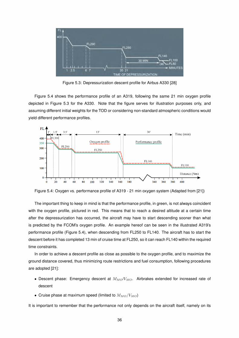
Figure 5.3: Depressurization descent profile for Airbus A330 [28]
Figure 5.4 shows the performance profile of an A319, following the same 21 min oxygen profile
depicted in Figure 5.3 for the A330. Note that the figure serves for illustration purposes only, and
assuming different initial weights for the TOD or considering non-standard atmospheric conditions would
yield different performance profiles.
Figure 5.4: Oxygen vs. performance profile of A319 - 21 min oxygen system (Adapted from [21])
The important thing to keep in mind is that the performance profile, in green, is not always coincident
with the oxygen profile, pictured in red. This means that to reach a desired altitude at a certain time
after the depressurization has occurred, the aircraft may have to start descending sooner than what
is predicted by the FCOM’s oxygen profile. An example hereof can be seen in the illustrated A319’s
performance profile (Figure 5.4), when descending from FL250 to FL140. The aircraft has to start the
descent before it has completed 13 min of cruise time at FL250, so it can reach FL140 within the required
time constraints.
In order to achieve a descent profile as close as possible to the oxygen profile, and to maximize the
ground distance covered, thus minimizing route restrictions and fuel consumption, following procedures
are adopted [21]:
• Descent phase: Emergency descent at MMO/VMO. Airbrakes extended for increased rate of
descent
• Cruise phase at maximum speed (limited to MMO/VMO)
It is important to remember that the performance not only depends on the aircraft itself, namely on its
36
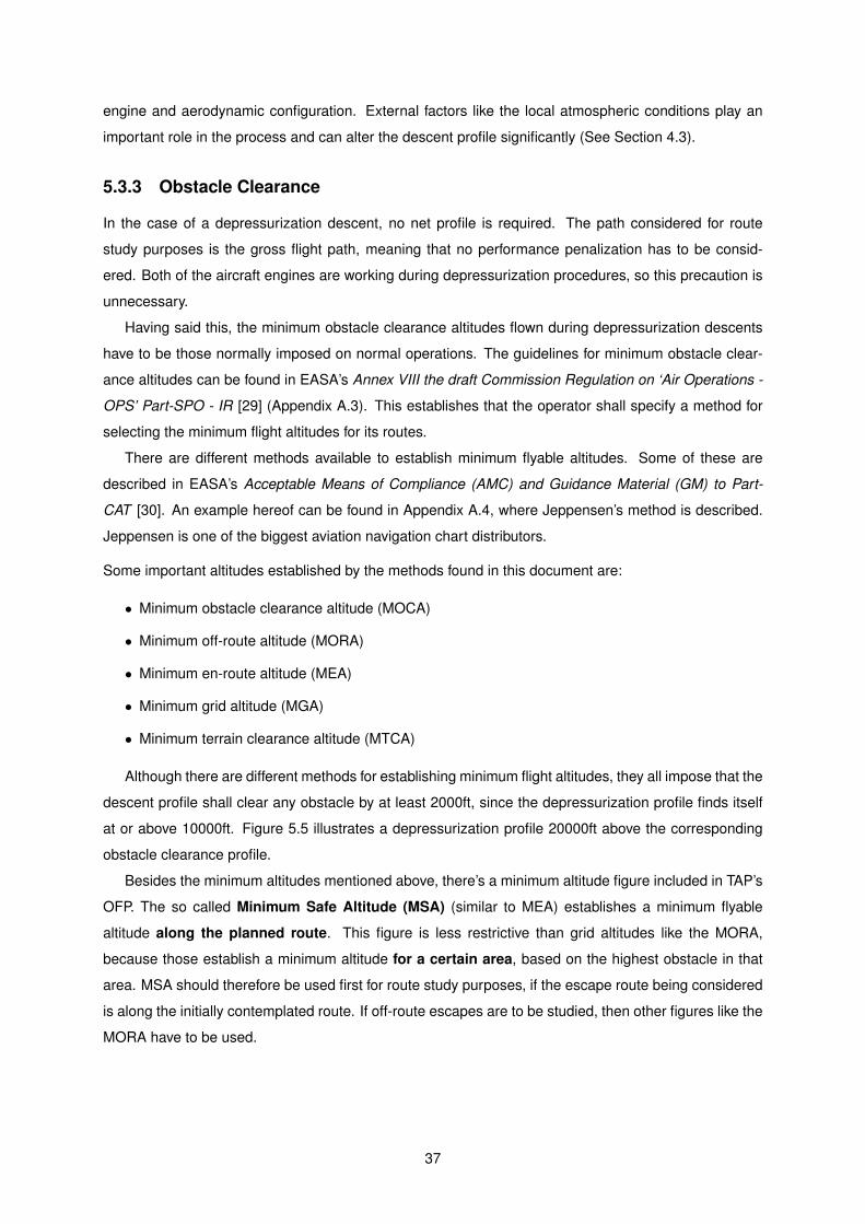
engine and aerodynamic configuration. External factors like the local atmospheric conditions play an
important role in the process and can alter the descent profile significantly (See Section 4.3).
5.3.3 Obstacle Clearance
In the case of a depressurization descent, no net profile is required. The path considered for route
study purposes is the gross flight path, meaning that no performance penalization has to be consid-
ered. Both of the aircraft engines are working during depressurization procedures, so this precaution is
unnecessary.
Having said this, the minimum obstacle clearance altitudes flown during depressurization descents
have to be those normally imposed on normal operations. The guidelines for minimum obstacle clear-
ance altitudes can be found in EASA’s Annex VIII the draft Commission Regulation on ‘Air Operations -
OPS’ Part-SPO - IR [29] (Appendix A.3). This establishes that the operator shall specify a method for
selecting the minimum flight altitudes for its routes.
There are different methods available to establish minimum flyable altitudes. Some of these are
described in EASA’s Acceptable Means of Compliance (AMC) and Guidance Material (GM) to Part-
CAT [30]. An example hereof can be found in Appendix A.4, where Jeppensen’s method is described.
Jeppensen is one of the biggest aviation navigation chart distributors.
Some important altitudes established by the methods found in this document are:
• Minimum obstacle clearance altitude (MOCA)
• Minimum off-route altitude (MORA)
• Minimum en-route altitude (MEA)
• Minimum grid altitude (MGA)
• Minimum terrain clearance altitude (MTCA)
Although there are different methods for establishing minimum flight altitudes, they all impose that the
descent profile shall clear any obstacle by at least 2000ft, since the depressurization profile finds itself
at or above 10000ft. Figure 5.5 illustrates a depressurization profile 20000ft above the corresponding
obstacle clearance profile.
Besides the minimum altitudes mentioned above, there’s a minimum altitude figure included in TAP’s
OFP. The so called Minimum Safe Altitude (MSA) (similar to MEA) establishes a minimum flyable
altitude along the planned route. This figure is less restrictive than grid altitudes like the MORA,
because those establish a minimum altitude for a certain area, based on the highest obstacle in that
area. MSA should therefore be used first for route study purposes, if the escape route being considered
is along the initially contemplated route. If off-route escapes are to be studied, then other figures like the
MORA have to be used.
37

Figure 5.5: Obstacle Clearance Profile – Depressurization [21]
5.3.4 Route Study
Generally speaking, both engine failure and depressurization must always be expected to occur at the
most critical points of the planned route. Moreover, since their descent profiles differ, the critical points
may differ between the two failure cases. It is important to notice, however, that regulations don’t
require to consider performance to cope with both failures simultaneously.
The disadvantage of dealing with both emergency scenarios separately, is that the number of critical
points and specific escape routes increases. This increases the workload of flight crews and thereby the
risk of errors.
For this reason, whenever possible, it is preferred to define identical critical points and escape routes
for all failure cases. This reduces the reaction time and the risk of committing mistakes. In such a case,
the route study should be based on the most penalizing descent profile. Figure 5.6 illustrates both
failure descent profiles for a A319 over a mountainous area.
Figure 5.6: Obstacle Clearance Profiles – Engine and Depressurization [21]
38
6. Engine Failure(s)
The present chapter presents the drift down procedure following engine failure situations (Section 6.1),
the difference between the gross and net drift down profiles (Section 6.2), and the obstacle clearance
requirements that are applied in such cases (Section 6.3).
The Regulations presented in the present chapter can be found in two documents, namely Commis-
sion Regulation (EU) Reg. 965-2012 [24] and EASA’s CS-25 Ammendment 18 [31].
6.1 Drift Down procedure
When at least one engine fails during normal operation, an emergency procedure is conducted with the
goal of safely landing the aircraft at a near aerodrome. The thrust of the remaining engine(s), when
one (or more) of them become inoperative, is set to Maximum Continuous Thrust (MCT) setting. The
available thrust at MCT is not enough to match the opposing drag force and to maintain the design cruise
scenario. The aircraft must reduce its speed and descend to a new altitude (drift down ceiling) where
level flight is possible.
This is called a drift down procedure, and it is described as follows:
1. Set remaining engine(s) to MCT
2. Decelerating to Green Dot Speed (GD)
3. Descend at GD speed until Drift down ceiling has been reached (Section 4.2)
Figure 6.1 illustrates a Drift Down Procedure for cruise engine failure.
As previously explained1, the GD speed allows the best Lift-to-drag ratio to be maintained, and
guarantees the highest possible altitude over the longest distance. This way, the number of possible
escape routes can be maximized.
6.2 Gross vs. Net Flight Path
For the purpose of being conservative, the flight path considered in aviation regulation for engine failure
situations doesn’t correspond to the flight path actually flown by the aircraft. The definitions of gross and
net flight paths are explained below.1Subsection 4.4.2
39
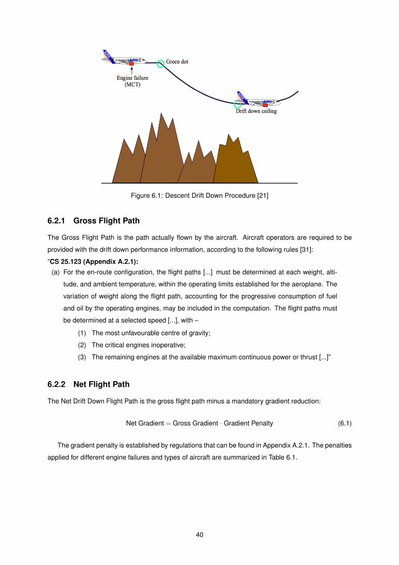
Figure 6.1: Descent Drift Down Procedure [21]
6.2.1 Gross Flight Path
The Gross Flight Path is the path actually flown by the aircraft. Aircraft operators are required to be
provided with the drift down performance information, according to the following rules [31]:
”CS 25.123 (Appendix A.2.1):
(a) For the en-route configuration, the flight paths [...] must be determined at each weight, alti-
tude, and ambient temperature, within the operating limits established for the aeroplane. The
variation of weight along the flight path, accounting for the progressive consumption of fuel
and oil by the operating engines, may be included in the computation. The flight paths must
be determined at a selected speed [...], with –
(1) The most unfavourable centre of gravity;
(2) The critical engines inoperative;
(3) The remaining engines at the available maximum continuous power or thrust [...]”
6.2.2 Net Flight Path
The Net Drift Down Flight Path is the gross flight path minus a mandatory gradient reduction:
Net Gradient = Gross Gradient – Gradient Penalty (6.1)
The gradient penalty is established by regulations that can be found in Appendix A.2.1. The penalties
applied for different engine failures and types of aircraft are summarized in Table 6.1.
40

Table 6.1: Gradient Penalties applied to Gross Flight Paths [21]
Gradient PenaltyTwo-engine aircraft Four-engine aircraft
Net flight path (one engine out) 1.1% 1.6%Net flight path (two engines out) - 0.5%
Figure 6.2: Gross and Net Drift Down Descent Flight Path (Adapted from [21])
6.3 Obstacle clearance
Emergency descents must evidently be performed without any collision, therefore obstacle clearance is
a central aspect in engine failure regulations. Lateral and vertical clearance rules are both described
in CAT.POL.A.215 and CAT.POL.A.220 (Appendix A.1.3 and A.1.4), for OEI and multiple engine failure
scenarios, respectively. They should be applied to the net flight path.
The obstacle clearance guidelines for OEI will be the focus of the present Section 6.3, but the reader
is encouraged to consult the regulatory transcripts for multiple engine failure in Appendix A.1.4.
6.3.1 Lateral Clearance
On the matter of lateral obstacle clearance margins during OEI situtations, the regulation states:
CAT.POL.A.215 (Appendix A.1.3)
” (c) [...] The net flight path shall clear [...] all terrain and obstructions along the route within 9,3 km
(5 NM) on either side of the intended track [...]
(d) The operator shall increase the width margins of [...] (c) to 18,5 km (10 NM) if the navigational
accuracy does not meet at least required navigation performance 5 (RNP5). ”
RNP5 means that a navigation system must be able to calculate its position to within a circle with a
radius of 5 Nautical Miles (NM) [32].
Figure 6.3 illustrates the rules cited above.
41
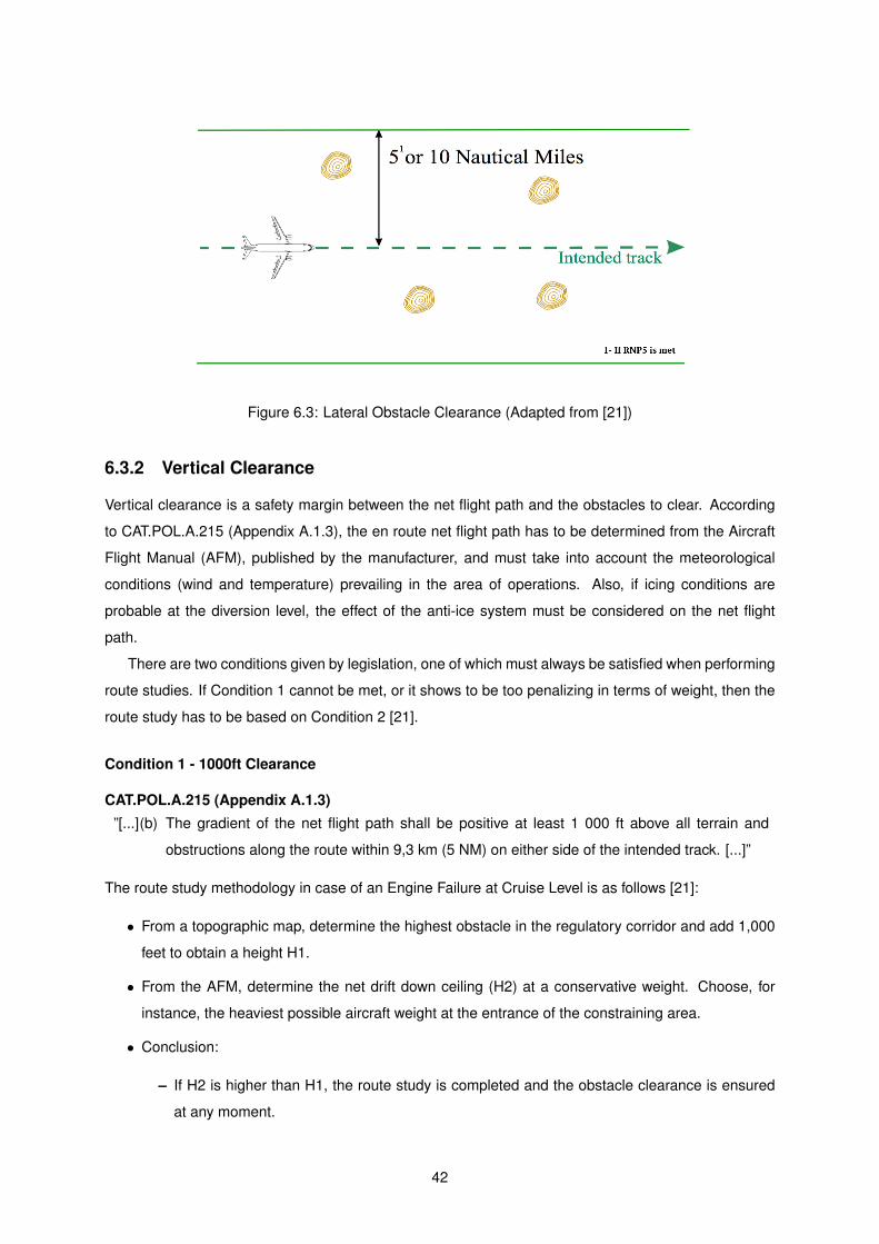
Figure 6.3: Lateral Obstacle Clearance (Adapted from [21])
6.3.2 Vertical Clearance
Vertical clearance is a safety margin between the net flight path and the obstacles to clear. According
to CAT.POL.A.215 (Appendix A.1.3), the en route net flight path has to be determined from the Aircraft
Flight Manual (AFM), published by the manufacturer, and must take into account the meteorological
conditions (wind and temperature) prevailing in the area of operations. Also, if icing conditions are
probable at the diversion level, the effect of the anti-ice system must be considered on the net flight
path.
There are two conditions given by legislation, one of which must always be satisfied when performing
route studies. If Condition 1 cannot be met, or it shows to be too penalizing in terms of weight, then the
route study has to be based on Condition 2 [21].
Condition 1 - 1000ft Clearance
CAT.POL.A.215 (Appendix A.1.3)
”[...](b) The gradient of the net flight path shall be positive at least 1 000 ft above all terrain and
obstructions along the route within 9,3 km (5 NM) on either side of the intended track. [...]”
The route study methodology in case of an Engine Failure at Cruise Level is as follows [21]:
• From a topographic map, determine the highest obstacle in the regulatory corridor and add 1,000
feet to obtain a height H1.
• From the AFM, determine the net drift down ceiling (H2) at a conservative weight. Choose, for
instance, the heaviest possible aircraft weight at the entrance of the constraining area.
• Conclusion:
– If H2 is higher than H1, the route study is completed and the obstacle clearance is ensured
at any moment.
42

Figure 6.4: Vertical Obstacle Clearance - 1000ft Rule (Adapted from [21])
– If H2 is lower than H1, then a more detailed study based on Condition 2 shall be conducted,
or a weight limitation at takeoff established, or a new route found.
Condition 2 - 2000ft Clearance
Condition 2 is only related engine to failures that occur during the cruise phase, which corresponds to
the focus of this work’s objective. When Condition 1 is not met, or when it is too limiting in terms of
weight, a drift down procedure should be planned, as detailed below:
CAT.POL.A.215 (Appendix A.1.3)
”[...](c) The net flight path shall permit the aeroplane to continue flight from the cruising altitude
to an aerodrome where a landing can be made in accordance with CAT.POL.A.225 or
CAT.POL.A.230, as appropriate. The net flight path shall clear vertically, by at least 2 000
ft, all terrain and obstructions along the route within 9,3 km (5 NM) on either side of the in-
tended track [...]”
It must be possible to perform an emergency descent and clear any obstacle by at least 2000ft, at
any given point along the operational route. When a drift down procedure has to be initiated, three
different scenarios exist:
• Turn Back - Turn around and follow the current route in the opposing direction
• Divert - Abandon the current route and proceed along an alternative one
• Continue - Continues along the current route
The methodology which allows to decide which of the three scenarios each point of a route corre-
sponds to can be found in Airbus’ ”Getting to Grips with Aircraft Performance” [21]. In the context of the
present work, the objective of the computational methodology to develop is simply to inform the user if
43

Figure 6.5: Vertical Obstacle Clearance - 2000ft Rule (Adapted from[21])
the descent can be performed along the planned route. In other words, it tests scenario three (”Con-
tinue”) and informs the user if this scenario is possible given current aircraft status and atmospheric
conditions.
44

7. Emergency Profile Application (EPA)
This chapter describes how the Emergency Profile Application (EPA) was developed, what objectives it
was set to achieve, the tools used for its development, as well as its internal structure and organization.
The chapter starts off with a description of the application in Section 7.1. Section 7.2 presents the
objectives that the application should achieve. Section 7.3 lists the software and tools used for building
the application. The symbology used in flowcharts throughout Chapter 7 is explained in Section 7.4.
Section 7.5 presents the application’s structure, dividing it into four main steps. These four steps are
presented in Sections 7.6 through 7.9. The final Section 7.10 presents some important information
regarding the usage of the EFB database by EPA.
7.1 Description
EPA is an application that allows the computation and verification of emergency flight profiles for de-
pressurization and engine failure scenarios. It computes flight performance using Airbus’ software, and
verifies if the flight profile can be executed, given current aircraft location and navigational constraints.
EPA’s tools are targeted at Flight Crew members (Captains and First Officers) and Flight Operations
Officers. By using updated meteorological conditions, the most reliable information is used, thus verifying
if the original procedures and escape routes released by flight dispatchers are still valid.
At this point, a connection between the EFB and the aircraft is inexistent. This means that aircraft
data like altitude, weight and coordinates have to be estimated, manually set or hardcoded. In the future,
parameters like these could be automatically sent from the aircraft to the EFB through a direct data link.
This would unlock the full potential of EPA. The software can then be expanded to analyze alternative
routes in case of failure, as updated meteorological information gets released. This would allow the
software to scan a whole route, identify critical points automatically and suggest appropriate escape
routes. The present version is the computational foundation upon which TAP’s EFB team can build
these additional features.
7.2 Objectives
The main purpose of EPA is to verify if, at any given point along a given route, an aircraft can follow an
emergency profile safely along the same route. The result gets reported back to the user.
45

The desired features for EPA are the following:
• Simple User Interface (UI)
• One-click calculation
• Supports both depressurization and engine failure
• Compares the calculated descent profile against geographical altitude constraints, and inform the
user if descent is possible
• Takes the most updated meteorological conditions into account when computing the profile
7.3 Software Tools
7.3.1 Airbus PEP
Airbus’ Performance Engineer’s Program (PEP) is a software developed by Airbus which contains per-
formance models of Airbus’ aircraft. It is distributed to Airbus clients, and allows performance engineers
to perform various types of calculations with Airbus’ airplanes. Each aircraft model is represented by
corresponding database files, which contain information on aerodynamics, propulsion and other sys-
tems.
The software allows the user to execute performance calculations for any flight phase, and fine-tuning
the simulation using a lot of input options. The simulation results contain information on how much fuel
is burned, the ground distance covered by the aircraft, the elapsed time, and other performance data.
PEP can be installed on a Windows machine and used as a standalone program. It contains various
calculation modules which each correspond to different flight and operational phases. They are divided
into two main categories:
• LSP - Low Speed Performance
• HSP - High Speed Performance
LSP is targeted at takeoff and landing calculations, whereas HSP contains modules dedicated to climb,
cruise, holding and descent phases, as well as some additional flight planning tools.
PEP serves as the computational motor for EPA’s performance calculations. Through the writing
of formatted input files and the injection of these into PEP, it’s possible to perform the performance
calculations required to fulfill EPA’s goals.
7.3.1.1 IFP module
The IFP (In-Flight Performance) module is one of PEP’s HSP tools, and is the one used for the current
project. IFP allows to simulate climb, cruise, descent, holding, acceleration or buffeting scenarios. For
each flight phase there are several calculation options available. A descent, for example, can be cal-
culated by a given descent gradient, descent rate, or using the ”emergency descent” option, where the
46
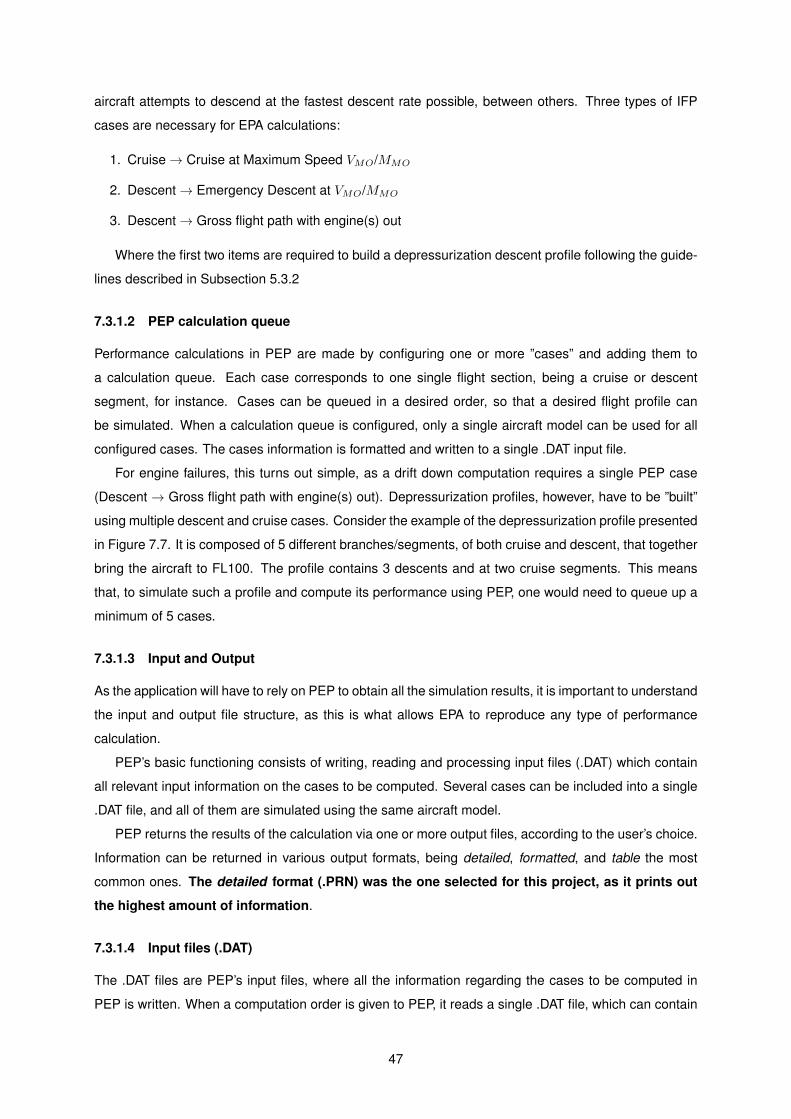
aircraft attempts to descend at the fastest descent rate possible, between others. Three types of IFP
cases are necessary for EPA calculations:
1. Cruise→ Cruise at Maximum Speed VMO/MMO
2. Descent→ Emergency Descent at VMO/MMO
3. Descent→ Gross flight path with engine(s) out
Where the first two items are required to build a depressurization descent profile following the guide-
lines described in Subsection 5.3.2
7.3.1.2 PEP calculation queue
Performance calculations in PEP are made by configuring one or more ”cases” and adding them to
a calculation queue. Each case corresponds to one single flight section, being a cruise or descent
segment, for instance. Cases can be queued in a desired order, so that a desired flight profile can
be simulated. When a calculation queue is configured, only a single aircraft model can be used for all
configured cases. The cases information is formatted and written to a single .DAT input file.
For engine failures, this turns out simple, as a drift down computation requires a single PEP case
(Descent → Gross flight path with engine(s) out). Depressurization profiles, however, have to be ”built”
using multiple descent and cruise cases. Consider the example of the depressurization profile presented
in Figure 7.7. It is composed of 5 different branches/segments, of both cruise and descent, that together
bring the aircraft to FL100. The profile contains 3 descents and at two cruise segments. This means
that, to simulate such a profile and compute its performance using PEP, one would need to queue up a
minimum of 5 cases.
7.3.1.3 Input and Output
As the application will have to rely on PEP to obtain all the simulation results, it is important to understand
the input and output file structure, as this is what allows EPA to reproduce any type of performance
calculation.
PEP’s basic functioning consists of writing, reading and processing input files (.DAT) which contain
all relevant input information on the cases to be computed. Several cases can be included into a single
.DAT file, and all of them are simulated using the same aircraft model.
PEP returns the results of the calculation via one or more output files, according to the user’s choice.
Information can be returned in various output formats, being detailed, formatted, and table the most
common ones. The detailed format (.PRN) was the one selected for this project, as it prints out
the highest amount of information.
7.3.1.4 Input files (.DAT)
The .DAT files are PEP’s input files, where all the information regarding the cases to be computed in
PEP is written. When a computation order is given to PEP, it reads a single .DAT file, which can contain
47

multiple cases. However, only a single aircraft model can be associated to that .DAT file, and thus all
cases in it (e.g. one cannot configure a cruise case for an A319 and an emergency descent for an A330
in the same .DAT).
Input .DAT files are formatted according to PEP’s specific rules, that can be consulted in PEP’s
documentation manuals [33]. Since there are a lot of details and rules in how the information has to be
organized in .DAT files, and the manual file would be to extensive to attach to this work, the author is just
going to expose what he believes will help the reader to better understand the interaction between EPA
and PEP.
Please consult the example .DAT file, written by EPA in the course of a Drift down profile computation,
and presented in Figure B.4 of Appendix B
The example of Appendix B begins by indicating the necessary PEP database files for that specific
computation. It has a single case of the type ”Gross flight path with engine(s) out”, identified by line 5 of
the file. Some figures like the initial altitude (38000ft) or the initial weight (150000kg) are easy to detect.
Others, like the code ”235” in line, indicate the type of case (in this case ”Gross flight path with engine(s)
out”).
The six lines preceding the word ”END” indicate the atmospheric conditions to be considered for the
case. The first three of these lines configure the Temperature ISA Deviation (TDI) per altitude, and the
last three indicate Wind Component (WC) values per altitude (see Subsection 7.7.4 for more information
on how TDI and WC are calculated).
7.3.1.5 Output files (.PRN)
After completing a computation, PEP returns a .PRN file. This file contains all the results of the executed
calculation. The structure of .PRN files is self-explanatory. Examples can be found in Figures B.2, B.3
and B.4 of Appendix B.
7.3.2 APCMTP tool
The APCMTP tool is a PEP module which runs independently. This means that it can be called and
executed without the need to launch PEP’s desktop application. The module is compatible with take-off
and landing performance, and doesn’t support cruise performance.
However, it has some flight planning tools, which, among other functions, allow the computation of
net drift down profiles. This feature was used to compute the net drift down profiles for EPA, and append
these results to the gross drift down profiles returned by PEP.
7.3.3 Microsoft Visual Studio
The Integrated Development Environment (IDE) used for the development of EPA was Microsoft Visual
Studio Professional Edition 2013. Visual Studio is the IDE over which TAP’s EFB team builds TAP EFB
solution.
Although TAP’s EFB solution is written in both C# and Visual Basic (VB), the EPA was exclusively
48
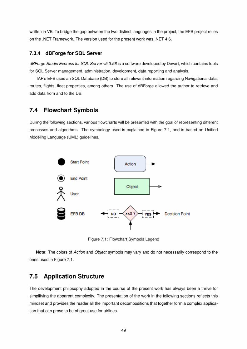
written in VB. To bridge the gap between the two distinct languages in the project, the EFB project relies
on the .NET Framework. The version used for the present work was .NET 4.6.
7.3.4 dBForge for SQL Server
dBForge Studio Express for SQL Server v5.3.56 is a software developed by Devart, which contains tools
for SQL Server management, administration, development, data reporting and analysis.
TAP’s EFB uses an SQL Database (DB) to store all relevant information regarding Navigational data,
routes, flights, fleet properties, among others. The use of dBForge allowed the author to retrieve and
add data from and to the DB.
7.4 Flowchart Symbols
During the following sections, various flowcharts will be presented with the goal of representing different
processes and algorithms. The symbology used is explained in Figure 7.1, and is based on Unified
Modeling Language (UML) guidelines.
Figure 7.1: Flowchart Symbols Legend
Note: The colors of Action and Object symbols may vary and do not necessarily correspond to the
ones used in Figure 7.1.
7.5 Application Structure
The development philosophy adopted in the course of the present work has always been a thrive for
simplifying the apparent complexity. The presentation of the work in the following sections reflects this
mindset and provides the reader all the important decompositions that together form a complex applica-
tion that can prove to be of great use for airlines.
49

EPA’s basic structure can be divided into four main steps:
1. Configuration of Input Data
2. Computation of Flight Profile
3. Verification of MA constraints
4. Report Result to User
The order of these steps is as presented above, and they can be organized in a flowchart as shown
on Figure 7.2.
Figure 7.2: EPA Basic Structure
All actions executed by EPA derive from these four main categories. Each stage is going to be
carefully analyzed in the following sections.
7.6 Configuration of Input Data
In order to compute an adequate flight profile, EPA requires data regarding the route, the aircraft and
atmospheric conditions. This data is required in order to write the input files that are to be read by PEP,
or to compute values for these input files.
The tools that the application includes allow it to be used in real-time, when emergencies occur.
Therefore, it should be efficient enough to calculate the desired profile in the shortest time possible.
Following the guidelines presented in Section 7.2, the UI should be as simple as possible, and the
calculation should be done with the lowest possible number of clicks.
To maximize its efficiency, EPA should determine the maximum amount of the necessary parameters
without any user interaction required. This is achieved through a connection to the EFB DB, where
different kinds of information on the flight and the aircraft can be retrieved.
7.6.1 PEP Parameters
Many of the configurable parameters presented to the user in EPA’s UI are based on PEP’s IFP module.
The IFP UI presents different input options when configuring PEP cases. Before launching a case
computation in PEP, the user can customize a large number of settings. These settings fall into the
50
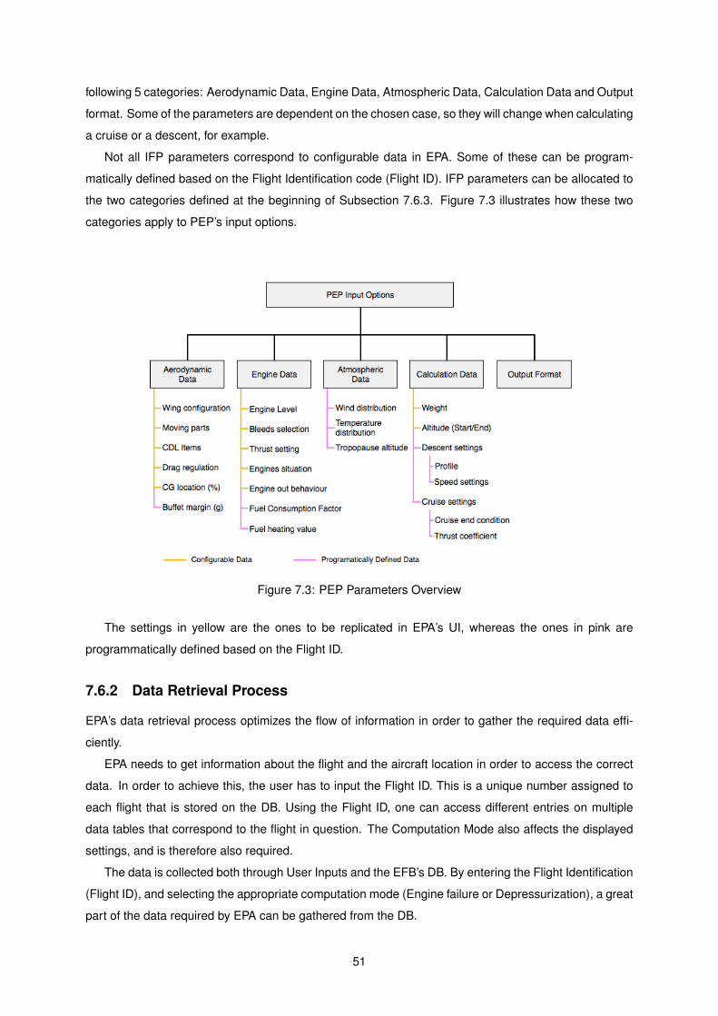
following 5 categories: Aerodynamic Data, Engine Data, Atmospheric Data, Calculation Data and Output
format. Some of the parameters are dependent on the chosen case, so they will change when calculating
a cruise or a descent, for example.
Not all IFP parameters correspond to configurable data in EPA. Some of these can be program-
matically defined based on the Flight Identification code (Flight ID). IFP parameters can be allocated to
the two categories defined at the beginning of Subsection 7.6.3. Figure 7.3 illustrates how these two
categories apply to PEP’s input options.
Figure 7.3: PEP Parameters Overview
The settings in yellow are the ones to be replicated in EPA’s UI, whereas the ones in pink are
programmatically defined based on the Flight ID.
7.6.2 Data Retrieval Process
EPA’s data retrieval process optimizes the flow of information in order to gather the required data effi-
ciently.
EPA needs to get information about the flight and the aircraft location in order to access the correct
data. In order to achieve this, the user has to input the Flight ID. This is a unique number assigned to
each flight that is stored on the DB. Using the Flight ID, one can access different entries on multiple
data tables that correspond to the flight in question. The Computation Mode also affects the displayed
settings, and is therefore also required.
The data is collected both through User Inputs and the EFB’s DB. By entering the Flight Identification
(Flight ID), and selecting the appropriate computation mode (Engine failure or Depressurization), a great
part of the data required by EPA can be gathered from the DB.
51
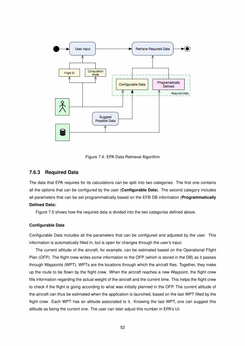
Figure 7.4: EPA Data Retrieval Algorithm
7.6.3 Required Data
The data that EPA requires for its calculations can be split into two categories. The first one contains
all the options that can be configured by the user (Configurable Data). The second category includes
all parameters that can be set programmatically based on the EFB DB information (Programmatically
Defined Data).
Figure 7.5 shows how the required data is divided into the two categories defined above.
Configurable Data
Configurable Data includes all the parameters that can be configured and adjusted by the user. This
information is automatically filled in, but is open for changes through the user’s input.
The current altitude of the aircraft, for example, can be estimated based on the Operational Flight
Plan (OFP). The flight crew writes some information to the OFP (which is stored in the DB) as it passes
through Waypoints (WPT). WPTs are the locations through which the aircraft flies. Together, they make
up the route to be flown by the flight crew. When the aircraft reaches a new Waypoint, the flight crew
fills information regarding the actual weight of the aircraft and the current time. This helps the flight crew
to check if the flight is going according to what was initially planned in the OFP. The current altitude of
the aircraft can thus be estimated when the application is launched, based on the last WPT filled by the
flight crew. Each WPT has an altitude associated to it. Knowing the last WPT, one can suggest this
altitude as being the current one. The user can later adjust this number in EPA’s UI.
52

Figure 7.5: Data required by EPA
53

Programmatically Defined Data
There is a limited amount of data that can be programmatically gathered from the EFB DB. Having
access to the Operational Flight Plan (OFP) and other data related to the flight and the aircraft, EPA can
gather a lot of the data it requires for future computations. This means that the data gathering process
can be made more efficient, consuming less time, which is highly desired in an emergency situation.
It is important to mention, however, that part of the Data required for EPA computations is not yet
retrievable from the aircraft/DB. The lack of connectivity between the EFB and the aircraft on TAP’s
current solution means that there is still room for improvement. In the future, parameters like the actual
weight of the aircraft, the current coordinates and altitude could be automatically sent from the aircraft
to the EFB through a direct data link.
This means that, for now, part of the data required to proceed with computations is hardcoded (See
Figure 7.5), or suggested to the user (e.g. current altitude). The application is modular, which means that
these values are variables that can later be fed by another programmable entity (e.g. aircraft information
module, to feed data from the aircraft to the EFB).
7.6.4 User Interface (UI)
Screenshots of EPA’s UI are presented in Appendix D.
The whole input options are blocked when the application is launched (Figure D.1), to point out to
the user that the first parameter to be entered is the Flight ID number. This number is an important key
to gather a lot of essential flight and aircraft data from the DB. As soon as the Flight ID is entered, the
remaining input options are unlocked and activated. The user can now select the computation mode,
specify the initial altitude, or customize the last waypoint.
In the ”General Tab” (Figure D.2), a miscellaneous set of options is presented according to the
specific aircraft and computation mode selected by the user.
For the Depressurization Mode, the ”Descent” (Figure D.4) and ”Cruise” (Figure D.3) tabs each show
specific options that only concern descent or cruise branches of the Depressurization Profile. In Engine
Failure Mode, only the inputs of the ”Descent” tab are kept active.
7.7 Computation of Flight Profile
The computation of the descent flight profile is the core component of the EPA. This is the part that
required the most work and code writing. It contains iterative cycles that allow descent profiles to be
calculated branch by branch, following FCOM and regulatory requirements. Atmospheric conditions are
computed based on information available in the DB, and appended to the PEP input files. Coordinate
tools have been developed to calculate distances, heading angles, and other quantities related to global
coordinates.
There are two computation modes configured into EPA. The first one is Depressurization Mode
(DM). As the name points out, this mode calculates a depressurization descent profile, based on the
54

oxygen system installed in the aircraft. The second mode is Engine Failure Mode (EFM), which is used
in case of drift down calculations following engine failure.
DM is fairly more complex than EFM, since the computation of a full depressurization profile requires
several PEP cases (see Subsection 7.3.1) to be computed in a row. Conversely, computing a drift down
for EFM requires a single PEP case.
7.7.1 Depressurization Mode (DM)
DM requires the profile to be computed branch by branch. A branch corresponds to either a cruise or
a descent segment of the depressurization profile. The different branches, when put together, form the
depressurization profile. To compute the full profile, EPA needs to first take it apart, and manage each
branch individually. This is the reason that DM into a more complex calculation procedure than EFM,
and is based on two main problems:
When a branch is computed, the cumulated time since the beginning of descent has to satisfy the
time and altitude constraints given by the FCOM descent profile. Consider the example in Figure 7.7,
which shows the descent profile of the A330 following FCOM guidelines. If the aircraft takes 13min to
get to the end of branch #2, then the preceding cruise branch (#2) has to be shortened by 2min, in order
to match the 11min requirement in the FCOM.
Since the computation of a given branch requires the weight of the aircraft at the beginning of that
branch, the preceding branch has to be computed first. Only after computing the preceding branch does
EPA have access to the weight at the end of the branch, and thus the initial weight of the next branch.
The algorithm used by EPA to compute a depressurization profile is shown on Figure 7.6. The
various steps that compose the algorithm are going to be explained in the following paragraphs, and
are:
• Profile Configuration
• Configure Next Branch
• Run PEP simulations
• Add Weather Information
• Store Results (Intermediate Results)
• Branch Verification and Correction
• Store the Fully Validated Profile
7.7.1.1 Profile Configuration
The depressurization profile of an aircraft in a given emergency situation depends on the conditions at
the beginning of the descent. Depending on the initial altitude, the aircraft may have to start descending
at an altitude lower than the one shown in the FCOM profile. The configuration and order of the profile
branches is therefore dependent on the current altitude at which the aircraft is flying before beginning
the descent.
55

Figure 7.6: EPA Profile Computation Algorithm for Depressurization Mode
If airplanes were always cruising at FL400, then the depressurization profile would always have the
layout of the FCOM, with three descent branches and two cruise branches:
1. Descent from FL400 to FL180
2. Cruise at FL180 for 7min
3. Descent from FL180 to FL140
4. Cruise at FL140 for 30min
5. Descent to FL100
On the other hand, if aircraft were constantly cruising at FL100, no depressurization profile would be
needed as the altitude is already sufficient for allowing the occupants to breathe safely. EPA needs to
be able to calculate a profile for any initial altitude in the interval 10000ft ≤ hi ≤ 40000ft.
Usually, the cruise altitude in a flight varies between FL350 and FL400. The tropopause altitude,
wind and temperature affect the optimal cruise altitude for a given weight.
Figure 7.7 illustrates the depressurization profile of the 12min oxygen system aboard some of the
TAP’s aircraft, which is going to be discussed in the following paragraphs.
In the FCOM profile, the profile is off-set by 1min to the right (horizontal axis). For EPA, the profile has
been altered to consider an immediate descent, starting at 0min from FL400. This is a more conservative
approach, and was decided together with TAP’s EFB team coordinator. In the future, this change can be
easily reverted in EPA’s code.
Both the 12 and 21 min profile are configured into EPA. By knowing which aircraft is active, the
application automatically computes the right depressurization profile. To obtain the Profile configuration
for the 21 min system (shown in Fig. 5.3), a similar methodology was configured into EPA. However, the
56
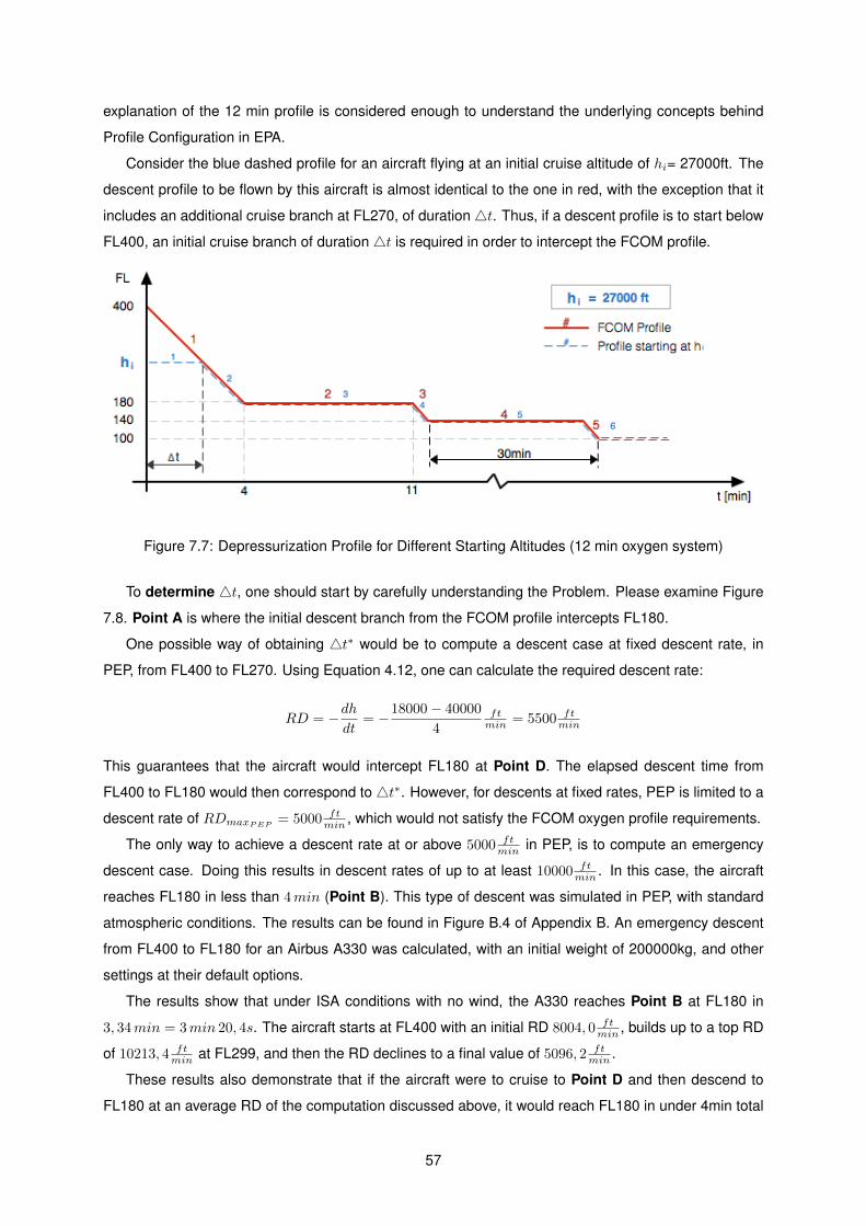
explanation of the 12 min profile is considered enough to understand the underlying concepts behind
Profile Configuration in EPA.
Consider the blue dashed profile for an aircraft flying at an initial cruise altitude of hi= 27000ft. The
descent profile to be flown by this aircraft is almost identical to the one in red, with the exception that it
includes an additional cruise branch at FL270, of duration 4t. Thus, if a descent profile is to start below
FL400, an initial cruise branch of duration 4t is required in order to intercept the FCOM profile.
Figure 7.7: Depressurization Profile for Different Starting Altitudes (12 min oxygen system)
To determine 4t, one should start by carefully understanding the Problem. Please examine Figure
7.8. Point A is where the initial descent branch from the FCOM profile intercepts FL180.
One possible way of obtaining 4t∗ would be to compute a descent case at fixed descent rate, in
PEP, from FL400 to FL270. Using Equation 4.12, one can calculate the required descent rate:
RD = −dhdt
= −18000− 40000
4ftmin = 5500 ft
min
This guarantees that the aircraft would intercept FL180 at Point D. The elapsed descent time from
FL400 to FL180 would then correspond to 4t∗. However, for descents at fixed rates, PEP is limited to a
descent rate of RDmaxPEP= 5000 ft
min , which would not satisfy the FCOM oxygen profile requirements.
The only way to achieve a descent rate at or above 5000 ftmin in PEP, is to compute an emergency
descent case. Doing this results in descent rates of up to at least 10000 ftmin . In this case, the aircraft
reaches FL180 in less than 4min (Point B). This type of descent was simulated in PEP, with standard
atmospheric conditions. The results can be found in Figure B.4 of Appendix B. An emergency descent
from FL400 to FL180 for an Airbus A330 was calculated, with an initial weight of 200000kg, and other
settings at their default options.
The results show that under ISA conditions with no wind, the A330 reaches Point B at FL180 in
3, 34min = 3min 20, 4s. The aircraft starts at FL400 with an initial RD 8004, 0 ftmin , builds up to a top RD
of 10213, 4 ftmin at FL299, and then the RD declines to a final value of 5096, 2 ft
min .
These results also demonstrate that if the aircraft were to cruise to Point D and then descend to
FL180 at an average RD of the computation discussed above, it would reach FL180 in under 4min total
57

Figure 7.8: Determination of Initial Cruise Duration 4t
time, at Point C. However, since Point D is not directly retrievable through PEP calculations, another
method for determining 4t is required:
Figure 7.9: Determination of Initial Cruise Duration 4t
Figure 7.9 shows the 4t which is going to be computed by EPA. Following procedure applies:
1. Compute emergency descent from FL400 to FL180 (ends at Point E)
2. Retrieve the intersection of emergency descent with the initial altitude (Point F)
3. Configure initial cruise branch with duration of 4t
4. Configure emergency descent after initial cruise branch, from initial altitude to FL180
For the A330 FCOM profile corresponding to the 12 min oxygen system (Figure 7.7), one could sum
up the profile configuration as shown in Table 7.1. The number and characteristics of the profile branches
depend first and foremost on the initial altitude at which the aircraft is cruising when the pressurization
failure occurs.
58

Table 7.1: Profile Configuration vs. Initial Altitude
Initial Altitude [ft] Required Branches18000 < hi ≤ 40000 Chi
Dhi→180@ 4 C180@ 11 D180→140 C140 D140→100
14000 < hi ≤ 18000 - - Chi @11 Dhi→140 C140 D140→100
10000 < hi ≤ 14000 - - - - ChiDhi→100
hi = 10000 - - - - - -
The letters C and D in Table 7.1 correspond to the required cruise and descent branches, respec-
tively; and their subscripts indicate the corresponding FL and the time limit at which some of them must
end, in min, counting from beginning of descent (CFL@ timelimit /Dinitial FL→final FL).
7.7.1.2 Configure Next Branch
Before computing one or more branches in PEP, EPA has to gather different types of data regarding
those branches. This data is then interpreted by specific EPA methods that output it to a formatted .DAT
file. The .DAT file holds formatted case configurations that are interpreted by PEP.
EPA uses an object class named Branch.vb to store each branch’s information. For a full list of all
the variables stored in the Branch.vb class, please consult Table C.2 (Appendix C).
The data that can be stored in Branch.vb objects includes:
• Type of Branch - Emergency Descent, Cruise at MMO/VMO (or Drift Down)
• Initial and final altitude
• Weight at beginning of the branch
• Fixed branch length or duration (cruise type branches)
• List of weather information by altitude (after it has been filled - 7.7.4)
• Navigational information - Start and End Coordinates, Initial Bearing, Last WPT
• Required PEP input variables
After having the required data stored in the Branch.vb class, EPA calls a method to write a .DAT file:
Private Sub InsertCase(writer As StreamWriter, ByRef branch As Branch)
InsertCase writes the required data stored in the argument branch to a .DAT file, using writer of the VB
type StreamWriter.
7.7.1.3 Run PEP simulations
The steps Run 1st PEP simulation and Run 2nd PEP simulation refer to the process of having PEP
read the .DAT files produced by EPA in order to compute the corresponding cases configured in them.
PEP returns a .PRN file that contains all the performance results of the configured cases. The difference
between the first and the second PEP simulation is that the latter includes the atmospheric data of the
respective branch.
For more information in PEP’s computation process, please refer to Subsection 7.7.3.
59
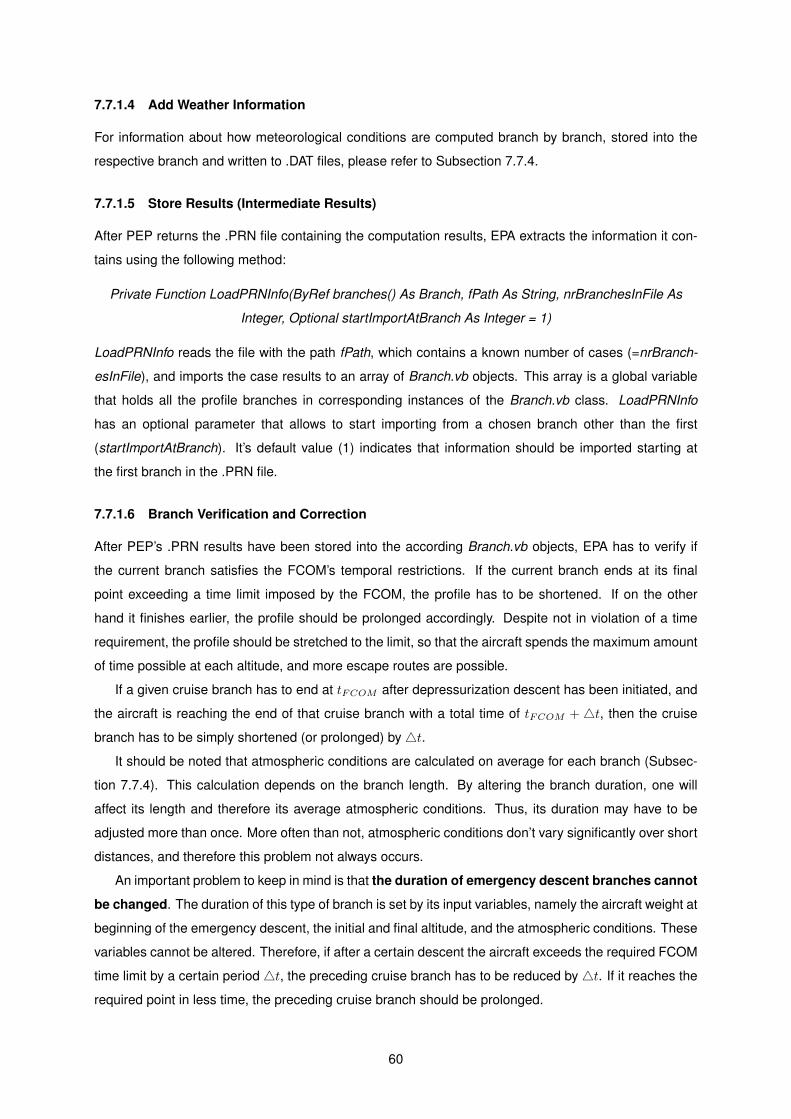
7.7.1.4 Add Weather Information
For information about how meteorological conditions are computed branch by branch, stored into the
respective branch and written to .DAT files, please refer to Subsection 7.7.4.
7.7.1.5 Store Results (Intermediate Results)
After PEP returns the .PRN file containing the computation results, EPA extracts the information it con-
tains using the following method:
Private Function LoadPRNInfo(ByRef branches() As Branch, fPath As String, nrBranchesInFile As
Integer, Optional startImportAtBranch As Integer = 1)
LoadPRNInfo reads the file with the path fPath, which contains a known number of cases (=nrBranch-
esInFile), and imports the case results to an array of Branch.vb objects. This array is a global variable
that holds all the profile branches in corresponding instances of the Branch.vb class. LoadPRNInfo
has an optional parameter that allows to start importing from a chosen branch other than the first
(startImportAtBranch). It’s default value (1) indicates that information should be imported starting at
the first branch in the .PRN file.
7.7.1.6 Branch Verification and Correction
After PEP’s .PRN results have been stored into the according Branch.vb objects, EPA has to verify if
the current branch satisfies the FCOM’s temporal restrictions. If the current branch ends at its final
point exceeding a time limit imposed by the FCOM, the profile has to be shortened. If on the other
hand it finishes earlier, the profile should be prolonged accordingly. Despite not in violation of a time
requirement, the profile should be stretched to the limit, so that the aircraft spends the maximum amount
of time possible at each altitude, and more escape routes are possible.
If a given cruise branch has to end at tFCOM after depressurization descent has been initiated, and
the aircraft is reaching the end of that cruise branch with a total time of tFCOM + 4t, then the cruise
branch has to be simply shortened (or prolonged) by 4t.
It should be noted that atmospheric conditions are calculated on average for each branch (Subsec-
tion 7.7.4). This calculation depends on the branch length. By altering the branch duration, one will
affect its length and therefore its average atmospheric conditions. Thus, its duration may have to be
adjusted more than once. More often than not, atmospheric conditions don’t vary significantly over short
distances, and therefore this problem not always occurs.
An important problem to keep in mind is that the duration of emergency descent branches cannot
be changed. The duration of this type of branch is set by its input variables, namely the aircraft weight at
beginning of the emergency descent, the initial and final altitude, and the atmospheric conditions. These
variables cannot be altered. Therefore, if after a certain descent the aircraft exceeds the required FCOM
time limit by a certain period 4t, the preceding cruise branch has to be reduced by 4t. If it reaches the
required point in less time, the preceding cruise branch should be prolonged.
60

Consider the depressurization profile analyzed in the paragraph ”Profile Configuration” of Subsec-
tion 7.7.1, and illustrated in Figure 7.10. The three cruise branches are the ones whose duration can be
modified by EPA, in order to meet the three FCOM constraints of the installed 12 min oxygen system:
1. Reach FL180 in 4min
2. Reach FL140 in 11min
3. Spend no more than an additional duration of 30 min cruising above FL100
Figure 7.10: Fixed and Adjustable Branches for 12 min Oxygen Profile
For the 21 min oxygen system, EPA compares the calculated branches against following FCOM
constraints, illustrated in Figure 7.11:
1. Reach FL290 in 1,5 min
2. Start descending from FL290 after 6 min
3. Reach FL250 in 7 min
4. Start descending from FL250 after 20 min
5. Reach FL140 in 21 min
6. Spend no more than an additional duration of 30 min cruising above FL100
The verification methodology for both systems is thus similar, with the difference being the number
of constraints that the 21 min system brings along.
7.7.1.7 Store the Fully Validated Profile
When the entire profile computation is completed and all the branches have been successfully validated
(step Profile Complete? in Figure 7.6 returns YES), EPA grabs the last .PRN file returned by PEP
and imports the entire information written in the file. PEP computes a series of figures from its initial
conditions until the final result. For example, the PEP .PRN file shown in Figure B.1 (Appendix B) lists
a total of 27 sub-computations. In former .PRN importations, EPA only needed the final figures of each
computation, to acquire the final weight, ground distance covered, total elapsed time, and other final
results of each branch. This was enough for branch validation purposes.
61

Figure 7.11: Fixed and Adjustable Branches for 21 min Oxygen Profile
For the next step of verifying the Minimum altitude requirements of the profile, however, EPA requires
all the figures computed by PEP, between the initial and final weight of each branch computation. This
allows EPA to build a set of points that together form the complete descent profile. These points are
stored in a dedicated class named ProfileCOORD.vb.
For MA verification purposes, only the values of altitude and distance need to be extracted from
these sub-computed results in the last .PRN file returned by PEP, and stored in instances of the class
ProfileCOORD.vb. In addition to this, other information is stored in these objects. The complete flight
profile is then stored in a VB variable of the type List (Of ProfileCOORD). Each item of the list, a so
called profile point, is of the type ProfileCOORD and contains following information:
• Geographical coordinates of the point
• Altitude
• MSA at the point’s coordinates
• MORA at the point’s coordinates
• Ground distance from the beginning of the profile
For detailed information on the variables stored in the object class ProfileCOORD, please consult
Table C.1 of Appendix C.
7.7.2 Engine Failure Mode (EFM)
Used in case of engine failure and drift down profile computation, the algorithm programmed into EPA
for EFM is similar to the one presented for DM (Subsection 7.7.1). However, due to the fact that a drift
down profile corresponds to a single case computation in PEP of type ”Gross flight path with engine(s)
out”, the simplicity for this mode is greatly increased. One important aspect to keep in mind about EFM
62
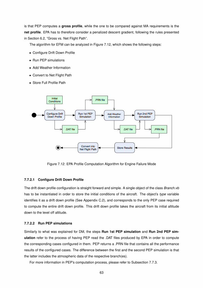
is that PEP computes a gross profile, while the one to be compared against MA requirements is the
net profile. EPA has to therefore consider a penalized descent gradient, following the rules presented
in Section 6.2, ”Gross vs. Net Flight Path”.
The algorithm for EFM can be analyzed in Figure 7.12, which shows the following steps:
• Configure Drift Down Profile
• Run PEP simulations
• Add Weather Information
• Convert to Net Flight Path
• Store Full Profile Path
Figure 7.12: EPA Profile Computation Algorithm for Engine Failure Mode
7.7.2.1 Configure Drift Down Profile
The drift down profile configuration is straight forward and simple. A single object of the class Branch.vb
has to be instantiated in order to store the initial conditions of the aircraft. The object’s type variable
identifies it as a drift down profile (See Appendix C.2), and corresponds to the only PEP case required
to compute the entire drift down profile. This drift down profile takes the aircraft from its initial altitude
down to the level off altitude.
7.7.2.2 Run PEP simulations
Similarly to what was explained for DM, the steps Run 1st PEP simulation and Run 2nd PEP sim-
ulation refer to the process of having PEP read the .DAT files produced by EPA in order to compute
the corresponding cases configured in them. PEP returns a .PRN file that contains all the performance
results of the configured cases. The difference between the first and the second PEP simulation is that
the latter includes the atmospheric data of the respective branch(es).
For more information in PEP’s computation process, please refer to Subsection 7.7.3.
63

7.7.2.3 Add Weather Information
For information about how meteorological conditions are computed branch by branch, stored into the
respective branch and written to .DAT files, please refer to Subsection 7.7.4.
7.7.2.4 Store Full Profile Path
Differing from what happens in DM, in EFM EPA only requires two computations to be executed by PEP
in order to have a full drift down profile, which already considers atmospheric information. A similar
procedure as the one presented in Paragraph ”Store the Fully Validated Profile” of Subsection 7.7.1
applies, in order to store the complete profile in dedicated EPA variables.
7.7.2.5 Convert to Net Flight Path
To compare the drift down profile against MA constraints, one has to utilize a net flight path instead of a
gross one (see Section 6.2 ”Gross vs. Net Flight Path”). Therefore, a net altitude needs to be attributed
to each gross altitude value of the gross profile, according to the rules exposed in Subsection 6.2.2.
PEP’s APCMTP module (subsection ??) executes this calculation so the net altitude values are also
computed using dedicated Airbus computation models. This returns a separate flight profile, which is
stored in ProfileCOORD.vb objects, similarly to the gross profile.
The altitude and distance values of this net profile are interpolated by EPA in order to assign a net
altitude value to each gross profile point. In the end, EPA saves a single list of profile points, each one
with a corresponding gross and net altitude value stored in it. This allows both profiles to be compared.
One corresponds to the one that the aircraft will be flying, and the other is just for MA verification
purposes.
7.7.3 Pep Computation Process
As previously mentioned, PEP is the computational motor of EPA. For EFM, only a few computations are
required to be executed by PEP. DM, on the other hand, can require several tens of computations. This
means that PEP computations should be as seamlessly integrated into EPA as possible. Ideally, EPA
would only be required to execute a batch file which would read the input .DAT file and return a .PRN file
with the computation results. This would allow PEP’s computations to translate into a few lines of code
in EPA, and to run in a very time efficient manner, requiring no interaction from the user. This solution
exists and can be distributed by Airbus.
This type of usability is also the one required if EPA is to be integrated in TAP’s EFB platform. Pilots
can’t afford to switch to PEP tens of times in order to compute each flight profile required for the purpose
of escape route analysis, and even less if conducting emergency procedures.
Unfortunately, as of the time at which this work was written, no solution was made available by Airbus
that allows PEP IFP computations to be executed without having to use the PEP desktop application.
This means that .DAT files have to be manually imported into PEP by EPA’s user, and manually run.
64

The only automation possible at this point, which was implemented by the author, is to place EPA on
hold, waiting for an updated .PRN file to be written by PEP. As soon as this happens, EPA detects the
updated file, and proceeds with the application’s duties.
Figure 7.13: Actual vs. Desired Integration of PEP computations into EPA
The comparison of both the current and the desired process of executing any given computation with
PEP is illustrated in Figure 7.13. Notice that, for the current implemented procedure, the user has to
complete at least two actions each and every time a calculation is to be executed. Each of these actions
require around 3 clicks or touches. This means that, for a depressurization profile with 8 branches, as
the one presented in Figure 7.11, with at least two computations per branch required, a minimum of
3 · 8 · 2 = 48 clicks would be required. This doesn’t take into account possible profile adjusts that EPA
needs to complete in order to correct the profile and tailor it to FCOM requirements.
One can conclude that, with current PEP integration into EPA, the proposed objectives presented in
Subsection 7.2, in particular the point ”One-click calculation”, cannot be met. Despite achieving a lot
of automatization in other areas like profile configuration and verification, PEP performance calculations
take up too much time to allow EPA to be used in flight, as of now.
65

7.7.4 Adding Weather Information to Existing Branches
The fact that EPA takes atmospheric information into account when computing flight profiles is one of its
crucial features to become a powerful and useful tool for flight crews. If a weather update is released
mid-flight, EPA’s computational tools allow the flight crew to check if current escape routes are still valid,
or if safer options can be found.
PEP allows the inclusion of atmospheric data in each case it computes. For EPA, this means storing
weather information in each one of its branches (instances of the Branch.vb class (Appendix C.2)). The
following two physical measures of atmospheric data can be included in PEP’s .DAT input files:
• Wind Component (WC) along the aircraft’s heading direction in knots [kt]
• Temperature Deviation from ISA conditions (TDI)
The heading angle is measured clockwise from the north. EPA calculates the aircraft heading angle
(see ”Auxiliary Tools and Methods”, 7.7.5), and projects the wind velocity along that direction to obtain
the WC.
The TDI is the difference between the actual temperature at a certain altitude and the one obtainable
from the ISA model at the same altitude. To obtain the TDI, EPA calculates the temperature using the
ISA model and then computes the difference of the temperature values in the DB to the calculated ISA
temperature.
PEP allows to include up to ten pairs of Altitude/TDI and ten pairs of Altitude/WC values for each
case it computes. Each pair thus indicates a TDI value and the altitude to which it corresponds. The
same applies for the WC. Between the altitudes inserted, PEP establishes intermediary values based
on linear interpolations.
EPA formats the data according to PEP’s documentation, and includes it in the .DAT input files where
the branch information is inserted. Since the information is inserted for each PEP case in the .DAT file,
and therefore for each EPA branch, there can only be one figure of either TDI or WC per altitude, for
the targeted branch. Therefore, the atmospheric values of a given branch have to be averaged per
altitude.
Figure 7.14: Computation of Atmospheric Conditions per Branch
Figure 7.14 presents the steps executed by EPA in order to fill a given branch (Branch.vb instance)
66

with atmospheric data (WC and TDI), which are explained in the coming paragraphs:
1. Retrieve Branch Length
2. Retrieve Relevant WPTs in the Branch Vicinity
3. Retrieve Atmospheric Data for WPTs
4. Compute Average Values per Altitude
7.7.4.1 Retrieve Branch Length
Using the results of the 1st PEP computation for the targeted branch (see Paragraph ”Run PEP simula-
tions” of 7.7.1.3), the branch length is known. This measure is used to weigh the atmospheric data of
each segment of the branch (explained below, ”Compute Average Values per Altitude”) and calculate a
single value of a given atmospheric value, per altitude and per branch.
7.7.4.2 Retrieve Relevant WPTs in the Branch Vicinity
To know how much of the branch’s length a given WPT occupies, EPA has to gather all WPTs that stand
in the vicinity of the targeted branch. This includes the last WPT immediately before the beginning of the
branch, all the WPTs along the branch, and the one immediately after. The relevant WPTs for a given
branch are illustrated in Figure 7.15, showing an arbitrary cruise branch at a certain altitude h, with an
unknown length. This branch has n WPTs in its inner. This means that while the aircraft is flying along
this branch, it passes along n WPTs. WPTs 0 and n+1 are the WPTs that the aircraft passes through
immediately before and after the branch, respectively. A total of n+2 WPTs are hence relevant for EPA’s
atmospheric calculations, as these will help average the atmospheric values for the branch.
7.7.4.3 Retrieve Atmospheric Data for WPTs
After EPA knows all relevant WPTs of the targeted branch, it retrieves the coordinates and the atmo-
spheric information for those WPTs, which is stored in the EFB’s DB, and originates from the OFP. In
the future, this same data could be updated during the flight, after the initial OFP is released, and loaded
into the DB.
Each WPT has information stored on wind direction, wind speed and temperature for the following
seven altitudes: FL100, FL250, FL320, FL340, FL360, FL380 and FL400. This means that, given the
(n+2) relevant WPTs found for the targeted branch, there are 3 · (n + 2) quantities to be retrieved per
altitude, or 7 · 3 · (n+ 2) = 21 · (n+ 2) values in total.
7.7.4.4 Compute Average Values per Altitude
As mentioned at the beginning of Subsection 7.7.4, EPA requires a single value of TDI and WC per
each altitude of a given branch, as these are the measures to be inserted into PEP’s .DAT files. The
atmospheric values of all the relevant WPTs of the branch have to be therefore averaged per altitude
and per branch. This means that the 21 · (n+ 2) values mentioned in the previous paragraph (”Retrieve
67

Figure 7.15: Relevant WPTs for Branch Atmospheric Data Computations
Atmospheric Data for WPTs”) should be reduced to 2 · 7 = 14 values in total. This corresponds to having
just one TDI and WC value per each one of the seven altitudes, along the whole branch.
Let’s go over this process of averaging the information for the branch and reducing the number of
values, step by step.
First, EPA calculates the aircraft heading direction (see Subsection 7.7.5, ”Auxiliary Tools and
Methods”) using the WPT information gathered in the previous step, and computes the wind velocity
component along that direction to obtain the WC. To obtain the TDI, EPA calculates the temperature
using the ISA model and then computes the difference of the temperature values in the DB to the
calculated ISA temperature. These computations are done for each one of the (n+2) WPTs.
There is now one value of TDI and WC per altitude for each one of the (n+2) WPTs, or 7 ·2 · (n+2) =
14 · (n+ 2) figures in total.
The next step is to average the data per segments. A segment is a sub-division of the branch at
a certain altitude, and has a single value of WC and TDI associated to it. The values stored per segment
are computed out of the (n+2) WPTs.
This segmentation can be done as shown in Figure 7.16, where an example is given for the averaging
of the WC at a certain Flight Level. A Branch of total length L is divided into (n+1) segments at each
altitude. The WPTs immediately before and after each of the segments have WC values indicated in the
vertical Axis.
To determine the average value of the WC or TDI for each of the (n+1) segments (WC will be used
as example), following rationale can be applied:
Consider an arbitrary segment as the one depicted in Figure 7.17. The segment starts at coordinate
68
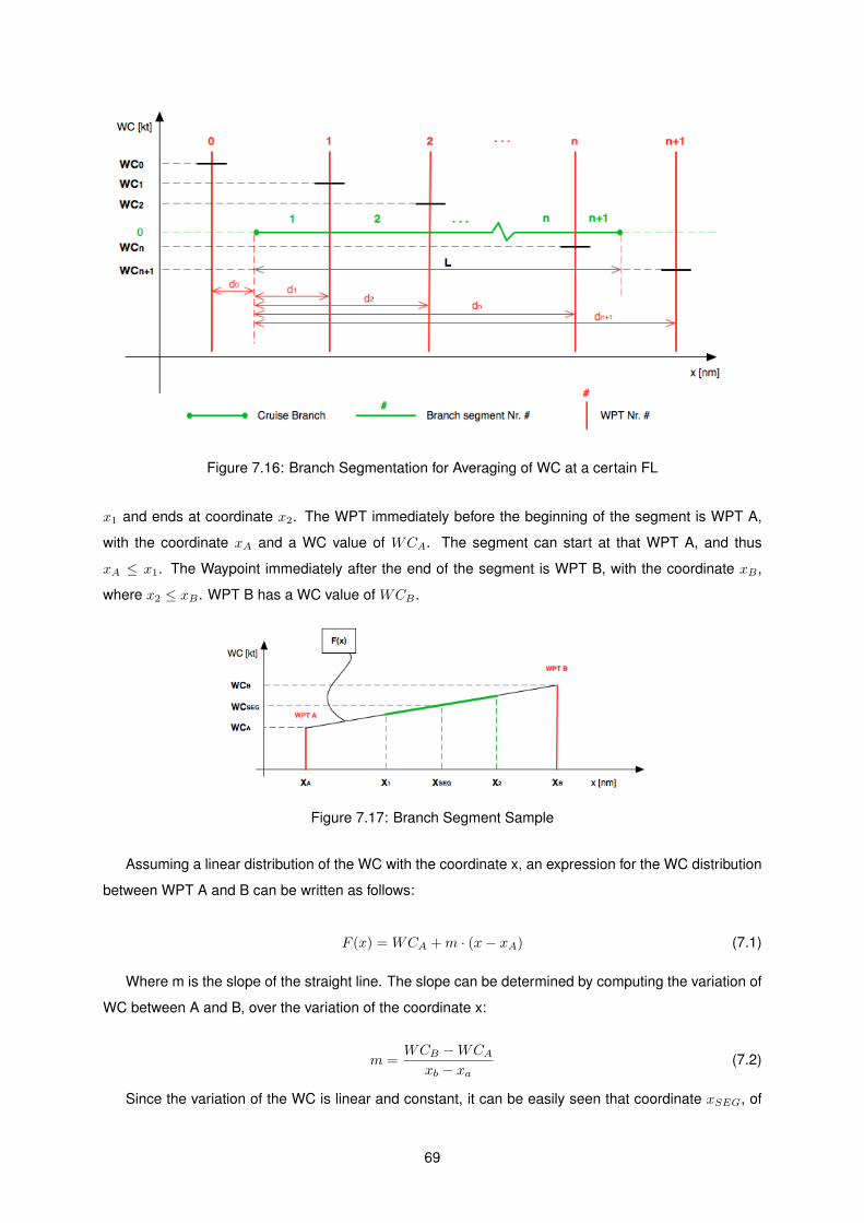
Figure 7.16: Branch Segmentation for Averaging of WC at a certain FL
x1 and ends at coordinate x2. The WPT immediately before the beginning of the segment is WPT A,
with the coordinate xA and a WC value of WCA. The segment can start at that WPT A, and thus
xA ≤ x1. The Waypoint immediately after the end of the segment is WPT B, with the coordinate xB ,
where x2 ≤ xB . WPT B has a WC value of WCB .
Figure 7.17: Branch Segment Sample
Assuming a linear distribution of the WC with the coordinate x, an expression for the WC distribution
between WPT A and B can be written as follows:
F (x) = WCA +m · (x− xA) (7.1)
Where m is the slope of the straight line. The slope can be determined by computing the variation of
WC between A and B, over the variation of the coordinate x:
m =WCB −WCA
xb − xa(7.2)
Since the variation of the WC is linear and constant, it can be easily seen that coordinate xSEG, of
69

the average segment value WCSEG, is exactly in the middle of coordinates x1 and x2. This means that,
if divided in two pieces, at xSEG, the WC distribution along the segment will be divided into two equally
long parts. One of them between x1 and xSEG, the other from xSEG to x2.
The expression for xSEG is thus:
xSEG =x2 − x1
2(7.3)
The average value of the segment, WCSEG, corresponds to the function F (x) at the coordinate
xSEG:
F (xSEG) = WCA +m · (xSEG − xA) =
WCSEG = WCA +m · (x2 − x12
− xA)(7.4)
This procedure is applied to determine one value of WC and TDI for each of the (n+1) segments of
the branch, at each of the seven available altitudes. At this point, 7 · 2 · (n+ 1) = 14 · (n+ 1) total values
of atmospheric quantities are left. To achieve the desired quantity of 14, and hence one WC and one
TDI value per altitude, one last step is required.
The last step is to average the values of all the segments at each altitude. Looking again at
Figure 7.16, each segment depicted has a certain length li, which is a fraction of the branch’s total
length, L. To average a value for the entire branch at a given altitude, each one of the 14 · (n+ 1) values
calculated in the last step gets attributed a certain weight, which is proportional to the length of the
segment it belongs to, compared to the branch’s total length. Summing the product of each segment’s
average value times its weight, one arrives at the average value for that altitude.
Mathematically, the following expression can be written for the average WC and TDI at a given
altitude h:
V ALAVG |h =
n+1∑i=1
liLV ALSEG (7.5)
Where:
• V AL can be either a WC or a TDI value
• V ALSEG is the averaged value for the segment i, at the considered altitude h
• li is the length of the segment i
• L is the total length of the branch
• h is one of the seven altitudes for which weather information is available in the DB (See previous
paragraph ”Retrieve Atmospheric Data for WPTs”)
After EPA finishes the process described in the preceding paragraphs, there is now just one TDI and
WC value per altitude, for the whole branch. This corresponds to fourteen values in total, which can now
be inserted in the .DAT file, along with the rest of the branch’s information.
70

7.7.5 Auxiliary Tools and Methods
Some tools have been developed to complement EPA’s functionality and execute repeating tasks through-
out the application. In this Subsection the author presents some of the most important ones, which were
developed for the calculation of quantities related to geographical coordinates.
A small utility was created which implements the formulas detailed below. Its simple UI can be viewed
in Figure D.5 of Appendix D, which demonstrates a sample calculation.
7.7.5.1 Distance Between Two Coordinates
EPA obtains the distance between two coordinates using the haversine formula. This formula derives
from a spherical earth model, and calculates the great circle distance between two points. Its accuracy is
satisfying for most applications, and results in about one meter of precision [34]. The distance d between
two coordinates, using the haversine formula, can be obtained as follows [35]:
4φ = φ2 − φ1
4λ = λ2 − λ1(7.6)
a = sin2(4φ2
)+ cosφ1 · cosφ2 · sin2
(4λ2
)(7.7)
c = 2 · atan2(√a ,√
1− a)
(7.8)
d = c ·R (7.9)
Where:
• φ is the latitude in radians
• λ is the longitude in radians
• R is the earth mean radius (R = 6371 km)
• φ1 and λ1 are the starting coordinates
• φ2 and λ2 are the destination coordinates
7.7.5.2 Initial and Final Bearing Between Two Coordinates
The initial bearing θi1→2between two points can be obtained from the following equation [35]:
θi1→2 = atan2 (sin4λ · cosφ2 , cosφ1 · sinφ2 − sinφ1 · cosφ2 · cos4λ) (7.10)
To obtain the final bearing between two points, EPA calculates the initial bearing from the final to the
initial point and sums 180 degrees to it. This result is divided by 360. The remainder of that division is
the final bearing between the two points:
θf1→2[deg] = (θi2→1
|degrees + 180)mod 360
71

7.7.5.3 Destination Point given Initial Bearing and Distance from Starting Point
Given a starting point (φ1,λ1), initial bearing θ, and a distance d, the following formula calculates the
latitude and longitude of the final point [35]:
φ2 = asin (sinφ1 · cos δ + cosφ1 · sin δ · cos δ)
λ2 = λ1 + atan2 (sin θ · sin δ · cosφ1 , cos δ − sinφ1 · sinφ2)(7.11)
Where δ = dR , remembering that R is the earth mean radius (R = 6371 km)
7.8 Verification of MA constraints
After having computed the descent flight profile, EPA needs to verify if the computed profile can be flown
safely, satisfying the obstacle clearance rules exposed in Subsection 5.3.3 (DM) and Section 6.3 (EFM).
At this point, wether coming from a DM or EFM profile computation, EPA holds all the profile points
in a single list of the type List(Of ProfileCOORD). This far, the ProfileCOORD objects in this list include
the altitude and coordinates of each one of the profile points (for more information on ProfileCOORD.vb
class, consult Appendix C.1). To compare these altitudes against MA constraints, these constraints first
have to be attributed to each one of the points.
Using each point’s coordinates, EPA retrieves two MA constraints for each of the profile points:
• MSA - Minimum Safe Altitude
• MORA - Minimum Off-route Altitude
The MSA is retrievable from the DB, and is released together with the flight’s OFP. It is usually
available for every cruise segment of the route, and therefore establishes the minimum flight altitude
between two route WPTs. EPA extracts the MSA of a given profile point by crossing the information
of the profile’s coordinates with the corresponding route segment. The MSA corresponds to the terrain
altitude with an additional margin of 2000ft.
The MORA, on the other hand, defines a MA for a certain rectangular area. Therefore, MA con-
straints imposed by MORA are less restrictive than the ones that derive from MSA. It clears all terrain
and man-made structures by 1000ft in areas at or below an elevation of 5000ft, and by 2000ft in areas
above an elevation of 5000ft. MORA information is listed in Aeronautical Information Publications (AIP),
released according to the Aeronautical Information Regulation And Control (AIRAC) cycle. EPA uses
Honeywell’s AIP, which is subscribed by TAP, and loads the MORA information onto the DB. It then uses
specifically developed methods to determine the MORA at a given geographic coordinate.
After EPA has gathered available information about the MSA and the MORA at the coordinates of
each profile point, it just compares the altitude of each point against those MA conditions.
The MSA is less restrictive than the MORA, and therefore the altitude of each profile point is first
compared against the MSA. Moreover, the availability of an MSA value depends on wether it was filled
72

in the OFP. If by any reason the MSA value is not available or retrievable from the DB, EPA compares
the altitude of that point against the MORA.
The procedure is simple: If EPA finds that any of the profile points has an altitude at or below the
MSA/MORA condition at that location, the profile cannot be flown, as it doesn’t meet regulatory approval.
If, on the other hand, all point altitudes are above their MSA/MORA requirement, the profile is safe.
7.9 Report Result to User
After establishing if the profile satisfies all MA constraints and meets regulatory approval (See Section
7.8), the result is communicated to the user with a simple message. This message indicates whether
the profile satisfies all MA constraints, or if it violates MA requirements at one or more of its points.
7.10 TAP’s EFB Database
TAP’s SQL DB served as a building block for the developed application. Data like aircraft, airport and
route information are regularly updated by TAP, and available to be used by the EFB applications. New
data was added to the DB when necessary, and the structure of some tables was expanded to meet the
requirements of the application. The names presented below may have been modified for confidentiality
purposes.
7.10.1 Existing entries
Most part of the information EPA needs was already available in the EFB’s DB to begin with. Tens of
tables facilitate the retrieval of almost all the information necessary for this project. The DB is divided
into three logical categories: FMS, STATIC and EFBDB.
7.10.1.1 FMS
The FMS category includes data tables with navigational information. Some of the one required by EPA
were:
• FMS Airports - Information on Airports like altitude, location, etc.
• FMS Airways - Information on all Airways on a global scale
• FMS GridMORA - Information about global MORA values
• FMS Waypoints - Information on all Waypoints on a global scale
7.10.1.2 STATIC
The STATIC category includes data tables with fleet information and other types of data not subject to
frequent change. These STATIC tables were relevant for EPA:
• STATIC Aircraft - TAP fleet information regarding each individual aircraft installed equipment and
specific configuration and performance data
73

• STATIC CDLItemList - CDL item information for every aircraft model of the fleet
• STATIC Properties - Properties of each aircraft model/version valid for every fleet aircraft of that
model
7.10.1.3 EFBDB
The EFBDB category includes data tables with OFPs, flight information and other operational information
that is frequently updated. Some important EFBDB tables for EPA include:
• EFBDB EFB Flights - Information and identification of all the flights stored in the DB
• EFBDB OFP COORD - WPT coordinates of stored flights
• EFBDB OFP RouteInfo - Route information of stored flights
• EFBDB OFP FL100 - Meteorological conditions at FL100 for cruise WPT of stored flights. The
same type of table is available for FL250, FL320, FL340, FL360, FL380 and FL400
7.10.2 Entries added
Besides collecting already existing data from the various DB tables, it was necessary to add entries to
some of the tables mentioned in Subsection 7.10.1.
7.10.2.1 FCOM Descent Profile Configuration String
This was perhaps the most relevant addition made to the DB. A string code was defined in order to
store each fleet aircraft’s depressurization profile information, used in EPA’s DM. Two distinct systems
are installed across TAP’s Airbus aircraft: A 12 min oxygen system, and a 21 min oxygen system. The
depressurization profiles for each one of the systems can be found in Figures 7.7 and 7.11, respectively.
In the chosen symbology, profile branches are separated by a semicolon (;), and the branch informa-
tion separated by two number signs (##). The first information of each branch is a type identifier of either
descent branch (D) or a cruise branch (C). For descent branches, initial and/or the final altitudes are
defined after the type identifier. For cruise branches, the duration is set after the identifier. For each one
of the branches, there’s an optional last parameter which indicates a time limit imposed by the FCOM,
in min. Please see the entries listed below, to better understand the encoding.Following strings were stored in the table STATIC Aircraft, in a new column named DEPRESSPROF,
for the 12 min and 21 min system profile, respectively:
• D##FL180##4;C##7##11;D##FL180##FL140;C##30;D##FL140##FL100
• D##FL290##1,5;C##3,5##5;D##FL290##FL250##6;C##13##19;D##FL250##FL140##20;C##30;D##FL140##FL100
7.10.2.2 CDL Items
The CDL Item configuration for some aircraft models was outdated or incomplete, and was accordingly
updated.
74

7.10.2.3 PEP’s Database Files
PEP’s IFP module has specific database files which specify engine, aerodynamic and other computa-
tional models for each aircraft. The name of these database files is required to be entered in the .DAT
files described in Subsection 7.3.1
7.10.2.4 Grid MORA
The table to fill the MORA information already existed in the DB (FMS GridMORA) but was empty.
The MORA information was loaded from Honeywell’s AIP and loaded into the table FMS GridMORA.
MORA values are separated by degrees of longitude and latitude. Every coordinate has a MORA value
attributed to it, which is valid until the next degree of longitude or latitude.
75

76

8. Results
This chapter will present calculations executed with EPA, and the results obtained. Some sample flight
routes were provided by TAP in order to test EPA’s functionalities. All flights provided are long haul flights
over the ocean. This means that the corresponding MA requirements at the chosen locations are at their
minimum.
Section 8.1 presents the flight scenario used by EPA to obtain a depressurization and a drift down
profile. The results obtained for DM (Section 8.2) and EFM (Section 8.3) are presented and discussed.
ICAO codes
During the course of this chapter, some International Civil Aviation Organization (ICAO) codes will be
used in order to refer to specific global locations like airports and aerial WPTs.
These include LPPT, KMIA, EMAKO and TASNI.
8.1 Flight Scenario
A specific flight scenario was chosen in order to demonstrate EPA’s functionality. The same flight sce-
nario will be used for both DM and EFM testing.
Flight Nr. 3051 is going to be utilized in order to test EPA’s DM and EFM. Flight 3051 departs from
Lisbon Airport (LPPT) and its destination is Miami’s International Airport (KMIA). The aircraft flying this
route is the Airbus A330-223, with a 12 min oxygen system on board.
The flight information table (OFP RouteInfo) was filled until the WPT EMAKO, simulating thus a
pressurization or engine failure that happened after the aircraft passed EMAKO and before it reached
the next WPT (TASNI). EMAKO is therefore the last WPT considered by EPA. According to flight data
records provided by TAP of the very same flight, after WPT EMAKO the aircraft had an initial weight
of close to 170000kg, and was cruising at 38000ft, as predicted in the OFP. These were therefore the
initial conditions chosen for this computation.
The WPT EMAKO has the following coordinates: (+31,397◦/-68,238◦) (LATITUDE/LONGITUDE).
TASNI has the coordinates (+30,9◦/-69,225◦). The two WPTs are 58,84NM away from each other, and
the bearing when the aircraft flies over EMAKO is 58,84◦.
Using the developed coordinate tools detailed in 7.7.5, a simple coordinate utility was developed to
perform calculations with coordinates. Using this utility, an arbitrary point after EMAKO was chosen. The
77

initial coordinates considered for this calculation are (+31,399◦/-68,575◦). These coordinates corre-
spond to a point situated 20 NM after the aircraft passes EMAKO. It is situated above the Atlantic Ocean.
This is assumed to be the point where the aircraft must start descending along its depressurization or
drift down profile. The calculation of these coordinates using the developed coordinate utility, can be
seen in Figure D.5 of Appendix D, where the utility’s UI is shown.
8.2 Depressurization Mode Computation
8.2.1 Computation Results
To compute the depressurization profile, EPA configured and executed a total of 22 PEP calculations.
Each one of these calculations translated into writing a .DAT file. These .DAT files contained one or
more PEP cases in it, each case corresponding to a profile branch. The last .PRN file, corresponding to
the 22nd calculation executed, can be consulted in Figures B.2 and B.3 of Appendix B.
The profile information was extracted to a .CSV file and is illustrated in Figure 8.1. The corresponding
values are shown in a table presented in Figure B.5 of Appendix B.
The aircraft takes a total of around 42 min and covers 286 NM before it reaches FL100. The MA
constraints, namely the MORA and the MSA are kept at their minimum throughout the flight path. There-
fore, EPA displayed a message at the end saying that the profile satisfies all regulatory requirements and
doesn’t violate any MA constraints.
During its computations, EPA verified each branch in order to adjust the cruise branches and max-
imize the time and distance at each altitude. If EPA didn’t have to verify and adjust the branches, it
would only require 12 computations. This would correspond to two computations per branch (the first to
compute the branch without atmospheric conditions, and the second already with this information).
Figure 8.1: Depressurization Profile computed by EPA
78

8.2.2 Results Discussion
To evaluate how well EPA performed in computing an adequate profile, please compare the results on
Figure 8.1 with the FCOM profile on Figure 7.7.
One can easily see that the time limits at 4 min and 11 min have been successfully respected.
As soon as the aircraft reaches the corresponding profile points, it starts descending along the next
branch. EPA successfully guarantees that the aircraft stays on each required altitude for the maxi-
mum amount of time and the for the longest distance possible.
The only observed FCOM requisite that EPA couldn’t keep was the last 30min time limit above
10000ft, starting from the point where the aircraft reaches 14000ft. The duration of the last two branches
combined is 30, 02min = 30min 1 seg. This error is however negligible:
4 = 0,0230 ≈ 0, 067%
It was expected that the profile would be safe to fly, without violating any MA constraints. The aircraft
is executing the depressurization maneuver over the ocean, so MA are at their minimum values.
8.3 Engine Failure Mode Computation
8.3.1 Computation Results
The same flight scenario was used by EPA in order to compute the drift down profile. The computation
of gross profile only required two PEP computations, and only a small fraction of time when compared to
DM. The final .PRN results file is presented in Figure B.4. These values correspond to the gross flight
path returned by PEP.
Using the methodology presented in 7.7.2.5, EPA obtained the net profile path. Both the gross and
the net profiles can be analyzed in Figure 8.3. The corresponding values are shown in a table presented
in Figure B.5 of Appendix B. Please note that the time axis corresponds to the gross profile path.
The gross profile is computed until it reaches the level-off altitude, at 27511ft. The aircraft takes
1h13min to reach this point, and covers a total distance of 400,3NM. If the flight were to continue at this
point, the aircraft would stop descending, and would start cruising again.
In contrast to this, the net profile is computed to and beyond its level-off point. The net level-off
altitude is situated 266 NM ahead of the TOD. The net profile reaches the gross level-off altitude 84 NM
beyond passing the TOD. This corresponds to approximately a fifth of the distance required to achieve
the gross level-off altitude.
The difference between gross and net level-off altitudes is 3495 ft, which corresponds to 3495·10027511 % =
12, 7% of the gross level-off altitude.
79

Figure 8.2: Drift Down Profile computed by EPA
8.3.2 Results Discussion
For the EFM, despite not having temporal constraints to compare the results against, like in DM, the
results are satisfactory. EPA successfully computes both the gross and the net profiles, and compares
the latter against the corresponding MA constraints. In an operational context, the gross profile is not
required, since the net profile is the one to be compared against MAs. However, it was easily obtainable
using the tools already developed for DM, and allows the user to easily compare both results.
8.4 Combined Results
Figure B.5 shows the three resulting profiles on overlapped, in order to visually be able to compare
them. One can see that the depressurization profile is by far the most penalizing in terms of altitude. It
maintains the initial 38000ft for just 1 min and 14 seconds, and afterwards starts descending at a RD of
over 11000 ftmin . After a ground distance of 31 NM the aircraft is already cruising at 18000ft, well below
the 33254ft at which the aircraft finds itself along the (net) drift down profile after an equivalent ground
distance from the TOD.
Figure 8.3: Combined Results - Depressurization and Engine Failure
80

9. Conclusion
This chapter presents the author’s final conclusions and a balance of how satisfactory the results were
regarding the initially proposed objectives.
9.1 Balance
Looking back to the objectives presented at the beginning of the work, in Section 1.2, one could say that
these were successfully accomplished. An application was developed, which allows its users to compute
flight profiles for emergency descent scenarios, for both depressurization and engine failure scenarios.
The application considers the most updated weather data, and also verifies the computed flight profiles
against the appropriate altitude constraints, determining wether the profile is valid or not.
However, the fulfillment of the objectives targeted at the application itself in Section 7.2 was not as
desired.
The second objective listed, one of the most important ones, couldn’t be achieved. The fact that
PEP’s computation cannot be dissociated from PEP’s desktop application, means that, for now, com-
putations have to be executed manually. This is a very time consuming process, as EPA requires a
high number of computations to complete a depressurization profile, for example. This issue should
be solved if EPA is to integrate more complex route analysis applications. It can be solved if Airbus
releases a batch application to TAP, which can be called to run PEP simulations independently from
PEP’s desktop application. For the computation of net drift down profiles, this issue in non-existent, as
the computation can be done from EPA itself, without having to launch PEP.
The remaining points listed in 7.2 were achieved with success. EPA integrates the minimum amount
of input options in its UI required to execute its computations, thus fulfilling the first point. It should be
noted that, as mentioned at the end of Section 1.2, the quality of the UI design is not the focus of the
present work, but rather its functionality.
The last three points were also successfully accomplished. Two modes were programmed into EPA,
one for each failure case. Each mode compares the calculated profile against altitude constraints and
informs the result to the user. Also, they both rely on the EFB DB to consider the most updated meteo-
rological conditions in its calculations.
All-in-all, one can say that the work presented achieved its proposed goals within the given con-
straints. EPA shouldn’t be viewed as a software with low operational application, but rather as a compu-
81

tational foundation with high-value tools, which TAP’s EFB team can build upon.
9.2 Future Work
As mentioned at the end of Section 9.1, EPA is a computational foundation upon which TAP’s EFB
team can build upon. Its tools can be applied to more robust and complex verification of escape routes,
making this process run in a seamless way, throughout the flight.
Currently, EPA only considers the main route in its calculations, meaning that it is along that route
that it calculates the emergency descent profiles. It is also along this route that EPA verifies if the profile
is valid and safe.
To expand its functionality, an important step is required. There is currently no data link from TAP’s
EFB solution to its aircraft, so data like current altitude, coordinates and weight of the aircraft have to be
manually inserted by the user, or estimated based on the flight information in the DB.
In the future, parameters like these could be automatically sent from the aircraft to the EFB through
a direct data link. Together with an independent execution of PEP’s computation module (see 7.7.3),
this would unlock the full potential of EPA. The software can then be expanded to analyze alternative
emergency routes. The application could then evolve into scanning entire flight routes, identify critical
points automatically and suggest appropriate escape routes, each time a new weather update becomes
available.
Flight crews can then be sure that the procedures they follow in case of failure rely on the most recent
meteorological conditions. This would translate into an improved operational safety in regard to cruise
emergency procedures.
82

Bibliography
[1] TAP. TAP’s Fleet, February 2016. URL http://www.tapportugal.com/Info/en/fleet-history/
fleet-2015.
[2] EASA. AMC 20-25: Airworthiness and Operational Consideration for Electronic Flight Bags (EFBs),
February 2014.
[3] U. Major Fredric S. Fitzsimmons. The Electronic Flight Bag: A multi-function Tool For The Modern
Cockpit, August 2002.
[4] M. Stibbe. American Airlines Pilots lose 40lb with Apple iPad Electronic Flight Bag. Forbes, May
2013.
[5] Garmin, August 2016. URL http://www8.garmin.com/specs/gns530.pdf.
[6] FAA. AC 120-76A: Guidelines for the Certification, Airworthiness, and Operational Approval of
Electronic Flight Bag Computing Devices, March 2003.
[7] S. Yukawa. Boeing Laptop Tool (BLT). NASA.
[8] Boeing. Onboard Performance Tool, 2012.
[9] EASA. EFB Evaluation Report: FlySmart with Airbus for iPad - V2. Technical report, December
2013.
[10] M. Thurber. Aero Glass Offers Aircraft Head-up Display on Wearable Glasses. AINonline, July
2014.
[11] D. A. Schonland. 2014 EFB Report, December 2014.
[12] L. Lovelady. The Connected Aircraft. Ascend, 2011.
[13] Airbus. Getting to grips with Fuel Economy, October 2014.
[14] A. A. NAV Portugal, TAP. NATCLM Project - Final Report, April 2010.
[15] T. S. ISAVIA, Icelandair. Reduction of Emissions on the North Atlantic by the Implementation of
ADS-B, April 2010.
[16] B. Carlsson. GLOBALink/VHF: The Future is Now. The Global Link, October 2002.
83

[17] SKYbrary. Aircraft Communications, Addressing and Reporting System, September
2016. URL http://www.skybrary.aero/index.php/Aircraft_Communications,_Addressing_
and_Reporting_System.
[18] H. Slutsken. What’s Next For ACARS? APEX, November 2014.
[19] M. Garcia. Hawaiian Airlines First to Commit to New Satellite Safety and Aircraft Tracking System.
Skift, September 2014.
[20] Iridium. Iridium SATCOM solutions, September 2016. URL https://www.iridium.com/
solutions/aviation/commercialaviation.
[21] Airbus. Getting to grips with aircraft performance, January 2002.
[22] D. C.-T. E. L. Dr. Jan Roskam. Airplane Aerodynamics and Performance. DARcorporation, 1997.
[23] E. Buckingham. On Physically Similar Systems: Illustrations of the Use of Dimensional Equations.
Number p.345-376. 1914.
[24] E. Comission. Comission Regulation (EU) No 965/2012, October 2012.
[25] SKYbrary. Aircraft Pressurisation Systems, August 2016. URL http://www.skybrary.aero/
index.php/Aircraft_Pressurisation_Systems.
[26] A. E. Jim Reed. How safe is air quality on commercial planes? BBS, June 2015.
[27] FAA. Aviation Maintenance Technician Airframe Handbook Vol. II, 2012.
[28] A330 Flight Crew Operating Manual. TAP, March 2015.
[29] EASA. Annex VIII the draft Commission Regulation on ‘Air Operations - OPS’, April 2012.
[30] EASA. Acceptable Means of Compliance (AMC) and Guidance Material (GM) to Part-CAT, October
2012.
[31] EASA. CS-25 Amendment 18 - Certification Specifications and Acceptable Means of Compliance
for Large Aeroplanes, June 2016.
[32] U. Avionics. Understanding Required Navigation Performance (RNP) and Area Navigation
(RNAV)Operations, October 2013.
[33] Airbus. PPM - Performance Programs Manual.
[34] J. Lawhead. Learning Geospatial Analysis with Python. Packt Publishing, 2015.
[35] E. Williams. Aviation Formulary V1.46.
84

A. Regulation Transcripts
A.1 Commission Regulation (EU) Reg. 965-2012
The following transcripts were directly taken from European Comission’s Commission Regulation (EU)
Reg. 965-2012 [24].
A.1.1 CAT.IDE.A.230 First-aid oxygen
” (a) Pressurised aeroplanes operated at pressure altitudes above 25 000 ft, in the case of opera-
tions for which a cabin crew member is required, shall be equipped with a supply of undiluted
oxygen for passengers who, for physiological reasons, might require oxygen following a cabin
depressurisation.
(b) The oxygen supply referred to in (a) shall be calculated using an average flow rate of at least
3 litres standard temperature pressure dry (STPD)/min/person. This oxygen supply shall be
sufficient for the remainder of the flight after cabin depressurisation when the cabin altitude
exceeds 8 000 ft but does not exceed 15 000 ft, for at least 2 % of the passengers carried, but
in no case for less than one person. ”
85
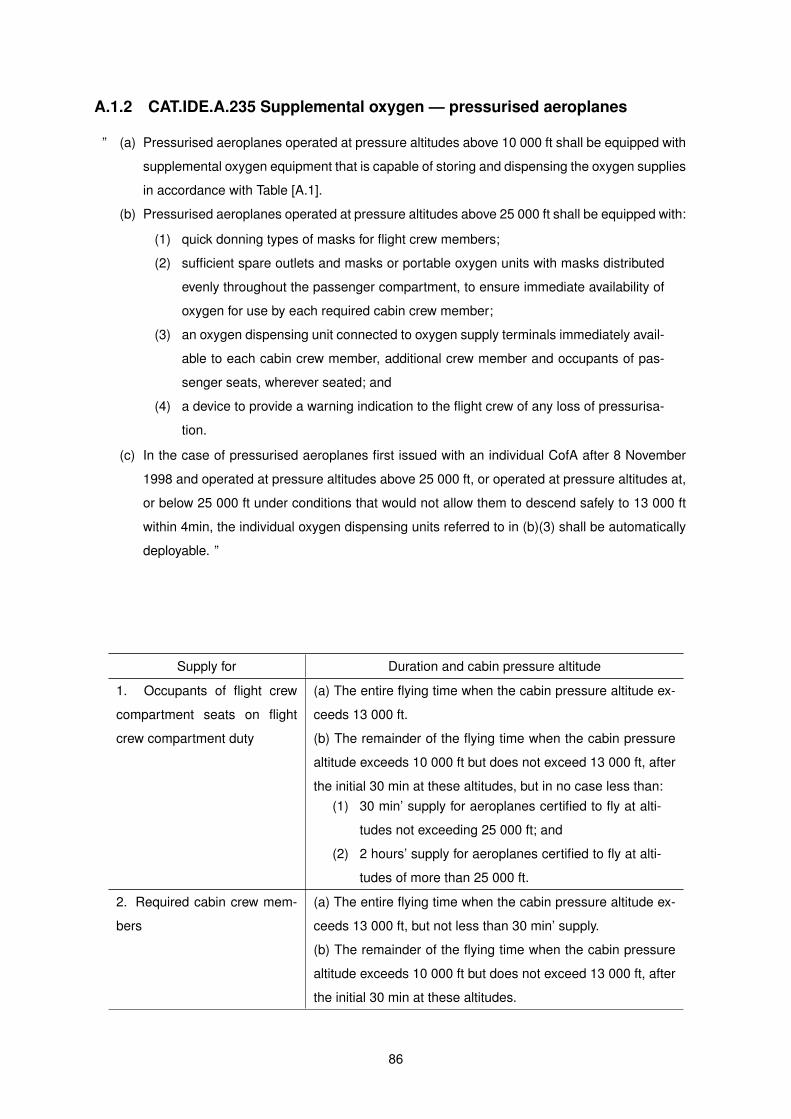
A.1.2 CAT.IDE.A.235 Supplemental oxygen — pressurised aeroplanes
” (a) Pressurised aeroplanes operated at pressure altitudes above 10 000 ft shall be equipped with
supplemental oxygen equipment that is capable of storing and dispensing the oxygen supplies
in accordance with Table [A.1].
(b) Pressurised aeroplanes operated at pressure altitudes above 25 000 ft shall be equipped with:
(1) quick donning types of masks for flight crew members;
(2) sufficient spare outlets and masks or portable oxygen units with masks distributed
evenly throughout the passenger compartment, to ensure immediate availability of
oxygen for use by each required cabin crew member;
(3) an oxygen dispensing unit connected to oxygen supply terminals immediately avail-
able to each cabin crew member, additional crew member and occupants of pas-
senger seats, wherever seated; and
(4) a device to provide a warning indication to the flight crew of any loss of pressurisa-
tion.
(c) In the case of pressurised aeroplanes first issued with an individual CofA after 8 November
1998 and operated at pressure altitudes above 25 000 ft, or operated at pressure altitudes at,
or below 25 000 ft under conditions that would not allow them to descend safely to 13 000 ft
within 4min, the individual oxygen dispensing units referred to in (b)(3) shall be automatically
deployable. ”
Supply for Duration and cabin pressure altitude
1. Occupants of flight crew
compartment seats on flight
crew compartment duty
(a) The entire flying time when the cabin pressure altitude ex-
ceeds 13 000 ft.
(b) The remainder of the flying time when the cabin pressure
altitude exceeds 10 000 ft but does not exceed 13 000 ft, after
the initial 30 min at these altitudes, but in no case less than:(1) 30 min’ supply for aeroplanes certified to fly at alti-
tudes not exceeding 25 000 ft; and
(2) 2 hours’ supply for aeroplanes certified to fly at alti-
tudes of more than 25 000 ft.
2. Required cabin crew mem-
bers
(a) The entire flying time when the cabin pressure altitude ex-
ceeds 13 000 ft, but not less than 30 min’ supply.
(b) The remainder of the flying time when the cabin pressure
altitude exceeds 10 000 ft but does not exceed 13 000 ft, after
the initial 30 min at these altitudes.
86
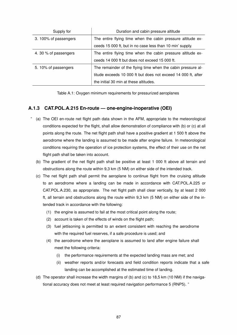
Supply for Duration and cabin pressure altitude
3. 100% of passengers The entire flying time when the cabin pressure altitude ex-
ceeds 15 000 ft, but in no case less than 10 min’ supply.
4. 30 % of passengers The entire flying time when the cabin pressure altitude ex-
ceeds 14 000 ft but does not exceed 15 000 ft.
5. 10% of passengers The remainder of the flying time when the cabin pressure al-
titude exceeds 10 000 ft but does not exceed 14 000 ft, after
the initial 30 min at these altitudes.
Table A.1: Oxygen minimum requirements for pressurized aeroplanes
A.1.3 CAT.POL.A.215 En-route — one-engine-inoperative (OEI)
” (a) The OEI en-route net flight path data shown in the AFM, appropriate to the meteorological
conditions expected for the flight, shall allow demonstration of compliance with (b) or (c) at all
points along the route. The net flight path shall have a positive gradient at 1 500 ft above the
aerodrome where the landing is assumed to be made after engine failure. In meteorological
conditions requiring the operation of ice protection systems, the effect of their use on the net
flight path shall be taken into account.
(b) The gradient of the net flight path shall be positive at least 1 000 ft above all terrain and
obstructions along the route within 9,3 km (5 NM) on either side of the intended track.
(c) The net flight path shall permit the aeroplane to continue flight from the cruising altitude
to an aerodrome where a landing can be made in accordance with CAT.POL.A.225 or
CAT.POL.A.230, as appropriate. The net flight path shall clear vertically, by at least 2 000
ft, all terrain and obstructions along the route within 9,3 km (5 NM) on either side of the in-
tended track in accordance with the following:
(1) the engine is assumed to fail at the most critical point along the route;
(2) account is taken of the effects of winds on the flight path;
(3) fuel jettisoning is permitted to an extent consistent with reaching the aerodrome
with the required fuel reserves, if a safe procedure is used; and
(4) the aerodrome where the aeroplane is assumed to land after engine failure shall
meet the following criteria:
(i) the performance requirements at the expected landing mass are met; and
(ii) weather reports and/or forecasts and field condition reports indicate that a safe
landing can be accomplished at the estimated time of landing.
(d) The operator shall increase the width margins of (b) and (c) to 18,5 km (10 NM) if the naviga-
tional accuracy does not meet at least required navigation performance 5 (RNP5). ”
87

A.1.4 CAT.POL.A.220 En-route — En-route — aeroplanes with three or more en-
gines, two engines inoperative
” (a) At no point along the intended track shall an aeroplane having three or more engines be more
than 90 min, at the all-engines long range cruising speed at standard temperature in still air,
away from an aerodrome at which the performance requirements applicable at the expected
landing mass are met, unless it complies with (b) to (f).
(b) The two-engines-inoperative en-route net flight path data shall allow the aeroplane to con-
tinue the flight, in the expected meteorological conditions, from the point where two engines
are assumed to fail simultaneously to an aerodrome at which it is possible to land and come
to a complete stop when using the prescribed procedure for a landing with two engines inop-
erative. The net flight path shall clear vertically, by at least 2 000 ft, all terrain and obstructions
along the route within 9,3 km (5 NM) on either side of the intended track. At altitudes and in
meteorological conditions requiring ice protection systems to be operable, the effect of their
use on the net flight path data shall be taken into account. If the navigational accuracy does
not meet at least RNP5, the operator shall increase the width margin given above to 18,5 km
(10 NM).
(c) The two engines shall be assumed to fail at the most critical point of that portion of the route
where the aeroplane is more than 90 min, at the all-engines long range cruising speed at stan-
dard temperature in still air, away from an aerodrome at which the performance requirements
applicable at the expected landing mass are met.
(d) The net flight path shall have a positive gradient at 1 500 ft above the aerodrome where the
landing is assumed to be made after the failure of two engines.
(e) Fuel jettisoning shall be permitted to an extent consistent with reaching the aerodrome with
the required fuel reserves, if a safe procedure is used.
(f) The expected mass of the aeroplane at the point where the two engines are assumed to fail
shall not be less than that which would include sufficient fuel to proceed to an aerodrome
where the landing is assumed to be made, and to arrive there at least 1 500 ft directly over
the landing area and thereafter to fly level for 15 min. ”
A.2 CS-25 Amendment 18
The following transcripts were directly taken from EASA’s CS-25 Amendment 18 - Certification Specifi-
cations and Acceptable Means of Compliance for Large Aeroplanes [24].
88
A.2.1 CS 25.123
” (a) For the en-route configuration, the flight paths prescribed in sub-paragraphs (b) and (c) of this
paragraph must be determined at each weight, altitude, and ambient temperature, within the
operating limits established for the aeroplane. The variation of weight along the flight path,
accounting for the progressive consumption of fuel and oil by the operating engines, may be
included in the computation. The flight paths must be determined at a selected speed not less
than VFTO, with –
(1) The most unfavourable centre of gravity;
(2) The critical engines inoperative;
(3) The remaining engines at the available maximum continuous power or thrust; and
(4) The means for controlling the engine-cooling air supply in the position that provides
adequate cooling in the hot-day condition.
(b) The one-engine-inoperative net flight path data must represent the actual climb performance
diminished by a gradient of climb of 1.1% for two-engined aeroplanes, 1.4% for three-engined
aeroplanes, and 1.6% for four- engined aeroplanes. [...]
(c) For three- or four-engined aeroplanes, the two-engine-inoperative net flight path data must
represent the actual climb performance diminished by a gradient climb of 0.3% for three-
engined aeroplanes and 0.5% for four- engined aeroplanes.”
A.3 Annex VIII the draft Commission Regulation on ‘Air Opera-
tions - OPS’ Part-SPO - IR
A.3.1 SPO.OP.125 Minimum obstacle clearance altitudes — IFR flights
” (a) The operator shall specify a method to establish minimum flight altitudes that provide the
required terrain clearance for all route segments to be flown in IFR.
(b) The pilot-in-command shall establish minimum flight altitudes for each flight based on this
method. The minimum flight altitudes shall not be lower than those published by the State
overflown.”
A.4 Acceptable Means of Compliance (AMC) and Guidance Mate-
rial (GM) to Part-CAT
A.4.1 GM1 CAT.OP.MPA.145(a) Establishment of minimum flight altitudes
”MINIMUM FLIGHT ALTITUDES
(c) [...] Jeppesen formula [...]
89
(1) MORA is a minimum flight altitude computed by Jeppesen from current opera-
tional navigation charts (ONCs) or world aeronautical charts (WACs). Two types
of MORAs are charted which are:
(i) route MORAs e.g. 9800a; and
(ii) grid MORAs e.g. 98.
(2) Route MORA values are computed on the basis of an area extending 10 NM to
either side of route centreline and including a 10 NM radius beyond the radio
fix/reporting point or mileage break defining the route segment.
(3) MORA values clear all terrain and man-made obstacles by 1 000 ft in areas where
the highest terrain elevation or obstacles are up to 5 000 ft. A clearance of 2 000 ft
is provided above all terrain or obstacles that are 5 001 ft and above.
(4) A grid MORA is an altitude computed by Jeppesen and the values are shown within
each grid formed by charted lines of latitude and longitude. Figures are shown in
thousands and hundreds of feet (omitting the last two digits so as to avoid chart
congestion). Values followed by ± are believed not to exceed the altitudes shown.
The same clearance criteria as explained in (c)(3) apply. ”
90

B. Results
AIRBUS IFP-V18.0 WJUN 2015 HSL_V1.0 INPUT DATA SLAT UP - FLAP UP AIRBRAKES EXTENDED C G POSITION : 37.0 % DRAG FACTOR 1.0000 FUEL FACTOR 1.0000 AVERAGE ENGINE - FLHV : 18590.BTU/LB
BLEED SELECTION: PACK FLOW: NORM CARGO COOLING: OFF WITHOUT ANTI-ICING 100. % AIR CONDITIONING WEIGHT : 200000. KG ISA + 0.0 DG.C 100.0 % OF IDL POWER EMERGENCY DESCENT : 0.86 MN / 330.00 KT ALT. ALTG WGHT MACH CAS TAS WIND TIME FUEL DIST RATE GRDT ALPH CL CD WFE FN N1 ( FT ) ( FT ) ( KG ) ( ) ( KT ) ( KT ) ( KT ) ( MN ) ( KG ) ( NM ) (FTMN) (DEG.) (DEG.) ( ) ( ) (KG/H) (DAN ) ( % ) 40000. 40000. 200000. 0.860 262.8 493.3 0.0 0.00 0. 0.0 -8004.0 -9.22 6.00 0.54877 0.08962 851. 89. 52.184 39000. 39000. 199998. 0.860 268.9 493.3 0.0 0.13 2. 1.0 -7945.6 -9.15 5.74 0.52316 0.08453 850. -10. 51.084 38000. 38000. 199996. 0.860 275.2 493.3 0.0 0.25 4. 2.0 -7898.4 -9.10 5.50 0.49872 0.07982 848. -114. 50.035 37000. 37000. 199995. 0.860 281.6 493.3 0.0 0.38 5. 3.1 -7863.0 -9.06 5.26 0.47539 0.07546 847. -224. 49.035 36089. 36089. 199993. 0.860 287.5 493.3 0.0 0.49 7. 4.0 -7840.5 -9.03 5.05 0.45509 0.07178 845. -328. 48.165 36089. 36089. 199993. 0.860 287.5 493.3 0.0 0.49 7. 4.0 -8669.5 -9.99 5.04 0.45380 0.07155 845. -328. 48.165 36000. 36000. 199993. 0.860 288.1 493.5 0.0 0.50 7. 4.1 -8671.4 -9.99 5.02 0.45187 0.07121 846. -338. 48.102 35000. 35000. 199991. 0.860 294.8 495.7 0.0 0.62 9. 5.0 -8787.6 -10.08 4.81 0.43068 0.06822 849. -458. 47.413 34000. 34000. 199990. 0.860 301.5 498.0 0.0 0.73 10. 5.9 -8929.5 -10.20 4.60 0.41062 0.06558 853. -578. 46.799 33000. 33000. 199988. 0.860 308.3 500.2 0.0 0.84 12. 6.9 -9135.5 -10.39 4.41 0.39156 0.06350 858. -702. 46.233 32000. 32000. 199987. 0.860 315.2 502.4 0.0 0.95 13. 7.7 -9423.7 -10.67 4.23 0.37343 0.06204 864. -831. 45.701 31000. 31000. 199985. 0.860 322.1 504.6 0.0 1.06 15. 8.6 -9741.7 -10.99 4.05 0.35623 0.06078 869. -964. 45.202 30000. 30000. 199984. 0.860 329.1 506.8 0.0 1.16 16. 9.4 -10157.0 -11.41 3.89 0.33982 0.06010 874. -1102. 44.733 29879. 29879. 199983. 0.860 330.0 507.1 0.0 1.17 17. 9.5 -10213.4 -11.47 3.87 0.33788 0.06005 875. -1119. 44.678 29879. 29879. 199983. 0.860 330.0 507.1 0.0 1.17 17. 9.5 -6876.2 -7.70 3.90 0.34166 0.06014 875. -1119. 44.678 29000. 29000. 199981. 0.846 330.0 500.5 0.0 1.30 19. 10.6 -6368.2 -7.22 3.74 0.34007 0.05552 890. -1155. 44.371 28000. 28000. 199979. 0.829 330.0 493.0 0.0 1.47 21. 12.0 -5516.5 -6.34 3.62 0.33852 0.04780 907. -1195. 44.036 27000. 27000. 199976. 0.814 330.0 485.7 0.0 1.65 24. 13.5 -5398.4 -6.30 3.58 0.33645 0.04672 924. -1235. 43.691 26000. 26000. 199973. 0.798 330.0 478.5 0.0 1.84 27. 15.0 -5401.7 -6.40 3.63 0.33435 0.04676 938. -1276. 43.296 25000. 25000. 199970. 0.783 330.0 471.5 0.0 2.02 30. 16.4 -5488.9 -6.60 3.77 0.33225 0.04755 948. -1337. 42.712 24000. 24000. 199967. 0.769 330.0 464.5 0.0 2.20 33. 17.8 -5469.1 -6.68 3.74 0.33037 0.04737 960. -1406. 42.102 23000. 23000. 199964. 0.754 330.0 457.7 0.0 2.39 36. 19.2 -5408.2 -6.70 3.70 0.32862 0.04683 975. -1479. 41.472 22000. 22000. 199961. 0.740 330.0 451.0 0.0 2.57 39. 20.6 -5343.9 -6.72 3.72 0.32693 0.04626 993. -1558. 40.824 21000. 21000. 199958. 0.726 330.0 444.4 0.0 2.76 42. 22.0 -5295.5 -6.76 3.72 0.32531 0.04584 1014. -1643. 40.158 20000. 20000. 199955. 0.713 330.0 437.9 0.0 2.95 45. 23.4 -5236.0 -6.78 3.72 0.32376 0.04545 1031. -1662. 39.582 19000. 19000. 199952. 0.700 330.0 431.6 0.0 3.14 48. 24.8 -5166.5 -6.79 3.72 0.32228 0.04507 1038. -1619. 39.046 18000. 18000. 199948. 0.687 330.0 425.3 0.0 3.34 52. 26.2 -5096.2 -6.79 3.72 0.32087 0.04471 1045. -1566. 38.508
AIRBUS IFP-V18.0 WJUN 2015 HSL_V1.0 INPUT DATA END
Figure B.1: PEP .PRN results file - Emergency Descent from FL400 to FL180
91

Cruise at maximum speed CLEAN CONFIGURATION C G POSITION : 37.0 % DRAG FACTOR 1.0000 FUEL FACTOR 1.0450 AVERAGE ENGINE - FLHV : 18590.BTU/LB
BLEED SELECTION: PACK FLOW: NORM CARGO COOLING: OFF WITHOUT ANTI-ICING 100. % AIR CONDITIONING TROPOPAUSE ALTITUDE : 54844. FT ALTITUDE : 38000.FT ISA + 0.0 DG.C AT SEA LEVEL WIND : -44.0 KT CRUISE AT VMO/MMO OR 100.0 % OF MCR THRUST OPTIMAL WEIGHT FOR FLIGHT LEVEL IS 158567. KG THRUST LIMITED WEIGHT EXCEEDS 170000. KG BUFFET LIMITED WEIGHT EXCEEDS 170000. KG WGHT MACH CAS TAS TIME FUEL DIST SR WFE EPR EGT CL CD ALPH FN PCFN N1 ( KG ) ( ) ( KT ) ( KT ) ( MN ) ( KG ) ( NM ) (NMKG) (KG/H) ( ) (DG.C) ( ) ( ) (DEG.) (DAN ) ( % ) ( % ) 170000. 0.854 273.2 503.7 0.00 0. 0.0 0.06875 6687. 1.424 435. 0.43401 0.02633 1.80 10072. 100.0 87.807 169862. 0.855 273.2 503.7 1.24 138. 9.5 0.06875 6687. 1.424 435. 0.43355 0.02632 1.80 10072. 100.0 87.807===================================================================================================================================================== Emergency descent SLAT UP - FLAP UP AIRBRAKES EXTENDED C G POSITION : 37.0 % DRAG FACTOR 1.0000 FUEL FACTOR 1.0450 AVERAGE ENGINE - FLHV : 18590.BTU/LB
BLEED SELECTION: PACK FLOW: NORM CARGO COOLING: OFF WITHOUT ANTI-ICING 100. % AIR CONDITIONING TROPOPAUSE ALTITUDE : 54700. FT WEIGHT : 169862. KG ISA: Temperature profile 100.0 % OF IDL POWER EMERGENCY DESCENT : 0.86 MN / 330.00 KT ALT. ALTG WGHT MACH CAS TAS WIND TIME FUEL DIST RATE GRDT ALPH CL CD WFE FN EPR ( FT ) ( FT ) ( KG ) ( ) ( KT ) ( KT ) ( KT ) ( MN ) ( KG ) ( NM ) (FTMN) (DEG.) (DEG.) ( ) ( ) (KG/H) (DAN ) ( ) 38000. 39866. 169862. 0.860 275.2 507.0 -44.0 0.00 0. 0.0 -11466.4 -14.93 4.66 0.41635 0.06789 1217. 390. 0.751 37000. 39103. 169860. 0.860 281.6 509.2 -38.0 0.09 2. 0.7 -11548.1 -14.91 4.46 0.39655 0.06546 1233. 316. 0.747 36000. 38297. 169858. 0.860 288.1 511.4 -32.0 0.17 4. 1.3 -11771.7 -15.06 4.27 0.37743 0.06380 1249. 237. 0.743 35000. 37223. 169856. 0.860 294.8 513.5 -31.0 0.27 6. 2.1 -9357.4 -11.84 4.13 0.36407 0.06270 1265. 154. 0.739 34000. 36150. 169854. 0.860 301.5 515.7 -30.0 0.37 8. 2.9 -9856.9 -12.39 3.95 0.34655 0.06151 1292. 89. 0.736 33000. 35208. 169852. 0.860 308.3 518.9 -33.5 0.48 10. 3.7 -8419.9 -10.61 3.81 0.33257 0.06105 1347. 66. 0.735 32000. 34258. 169849. 0.860 315.2 522.1 -37.0 0.60 13. 4.7 -8833.1 -11.18 3.65 0.31698 0.06059 1402. 37. 0.734 31000. 33351. 169847. 0.860 322.1 525.8 -35.4 0.69 15. 5.4 -11622.7 -14.69 3.46 0.29895 0.06038 1460. 8. 0.733 30000. 32432. 169845. 0.860 329.1 529.4 -33.9 0.78 17. 6.1 -12085.8 -15.20 3.32 0.28491 0.05986 1520. -25. 0.732 29879. 32320. 169845. 0.860 330.0 529.9 -33.7 0.79 17. 6.2 -12139.2 -15.26 3.30 0.28327 0.05977 1528. -29. 0.731 29879. 32320. 169845. 0.860 330.0 529.9 -33.7 0.79 17. 6.2 -7958.3 -9.95 3.36 0.28848 0.06002 1528. -29. 0.731 29000. 31502. 169841. 0.846 330.0 524.1 -32.3 0.91 21. 7.1 -7170.7 -9.08 3.28 0.28743 0.05424 1580. -38. 0.740 28000. 30560. 169838. 0.829 330.0 517.5 -30.7 1.05 24. 8.3 -6317.1 -8.11 3.19 0.28623 0.04789 1613. -82. 0.748 27000. 29606. 169833. 0.814 330.0 511.1 -29.1 1.21 29. 9.6 -6132.0 -7.99 3.19 0.28450 0.04673 1665. -64. 0.756 26000. 28641. 169829. 0.798 330.0 504.7 -27.6 1.38 33. 10.9 -6118.2 -8.09 3.27 0.28267 0.04688 1675. -41. 0.763 25000. 27666. 169824. 0.783 330.0 498.4 -26.0 1.54 38. 12.2 -6121.8 -8.22 3.39 0.28090 0.04783 1614. -111. 0.767 24000. 26512. 169820. 0.769 330.0 490.5 -25.9 1.71 42. 13.5 -5879.4 -8.00 3.36 0.27952 0.04779 1499. -261. 0.769 23000. 25363. 169816. 0.754 330.0 482.7 -25.7 1.88 46. 14.8 -5844.8 -8.07 3.32 0.27803 0.04733 1408. -392. 0.772 22000. 24219. 169811. 0.740 330.0 475.1 -25.6 2.05 51. 16.1 -5758.3 -8.06 3.33 0.27659 0.04681 1527. -317. 0.780 21000. 23078. 169807. 0.726 330.0 467.6 -25.5 2.22 55. 17.4 -5695.8 -8.09 3.33 0.27521 0.04639 1586. -306. 0.787 20000. 21941. 169802. 0.713 330.0 460.3 -25.3 2.40 60. 18.6 -5655.9 -8.15 3.33 0.27389 0.04600 1544. -403. 0.792 19000. 20809. 169798. 0.700 330.0 453.1 -25.2 2.58 64. 19.9 -5630.1 -8.23 3.32 0.27263 0.04563 1439. -567. 0.796 18000. 19680. 169794. 0.687 330.0 446.1 -25.1 2.76 68. 21.1 -5554.7 -8.23 3.32 0.27142 0.04529 1539. -469. 0.804===================================================================================================================================================== Cruise at maximum speed CLEAN CONFIGURATION C G POSITION : 37.0 % DRAG FACTOR 1.0000 FUEL FACTOR 1.0450 AVERAGE ENGINE - FLHV : 18590.BTU/LB
BLEED SELECTION: PACK FLOW: NORM CARGO COOLING: OFF WITHOUT ANTI-ICING 100. % AIR CONDITIONING TROPOPAUSE ALTITUDE : 55528. FT ALTITUDE : 18000.FT ISA + 0.0 DG.C AT SEA LEVEL WIND : -11.5 KT CRUISE AT VMO/MMO OR 100.0 % OF MCR THRUST OPTIMAL WEIGHT FOR FLIGHT LEVEL EXCEEDS 169794. KG THRUST LIMITED WEIGHT EXCEEDS 169794. KG BUFFET LIMITED WEIGHT EXCEEDS 169794. KG WGHT MACH CAS TAS TIME FUEL DIST SR WFE EPR EGT CL CD ALPH FN PCFN N1 ( KG ) ( ) ( KT ) ( KT ) ( MN ) ( KG ) ( NM ) (NMKG) (KG/H) ( ) (DG.C) ( ) ( ) (DEG.) (DAN ) ( % ) ( % ) 169794. 0.687 330.0 435.8 0.00 0. 0.0 0.05651 7509. 1.043 408. 0.27381 0.01745 1.14 10569. 63.6 73.835 169000. 0.687 330.0 435.8 6.35 794. 44.9 0.05656 7502. 1.043 408. 0.27254 0.01743 1.13 10556. 63.5 73.810 168918. 0.687 330.0 435.8 7.00 876. 49.5 0.05657 7502. 1.043 408. 0.27240 0.01743 1.12 10554. 63.5 73.808=====================================================================================================================================================
Figure B.2: EPA Depressurization Mode - Final Results of All Computed Branches - Page 192

Emergency descent SLAT UP - FLAP UP AIRBRAKES EXTENDED C G POSITION : 37.0 % DRAG FACTOR 1.0000 FUEL FACTOR 1.0450 AVERAGE ENGINE - FLHV : 18590.BTU/LB
BLEED SELECTION: PACK FLOW: NORM CARGO COOLING: OFF WITHOUT ANTI-ICING 100. % AIR CONDITIONING TROPOPAUSE ALTITUDE : 56232. FT WEIGHT : 168918. KG ISA: Temperature profile 100.0 % OF IDL POWER EMERGENCY DESCENT : 0.86 MN / 330.00 KT ALT. ALTG WGHT MACH CAS TAS WIND TIME FUEL DIST RATE GRDT ALPH CL CD WFE FN EPR ( FT ) ( FT ) ( KG ) ( ) ( KT ) ( KT ) ( KT ) ( MN ) ( KG ) ( NM ) (FTMN) (DEG.) (DEG.) ( ) ( ) (KG/H) (DAN ) ( ) 18000. 18876. 168918. 0.687 330.0 436.3 -10.5 0.00 0. 0.0 -5678.0 -7.96 3.31 0.27001 0.04518 1504. -461. 0.805 17000. 17807. 168913. 0.674 330.0 429.7 -10.5 0.18 5. 1.2 -5615.5 -7.99 3.30 0.26886 0.04487 1574. -437. 0.812 16000. 16741. 168909. 0.662 330.0 423.2 -10.6 0.36 9. 2.5 -5580.0 -8.05 3.30 0.26775 0.04458 1555. -543. 0.817 15000. 15678. 168904. 0.650 330.0 416.8 -10.7 0.54 14. 3.7 -5560.7 -8.14 3.29 0.26669 0.04430 1479. -732. 0.820 14000. 14616. 168900. 0.638 330.0 410.6 -10.7 0.72 18. 4.9 -5498.0 -8.17 3.28 0.26570 0.04391 1467. -779. 0.825===================================================================================================================================================== Cruise at maximum speed CLEAN CONFIGURATION C G POSITION : 37.0 % DRAG FACTOR 1.0000 FUEL FACTOR 1.0450 AVERAGE ENGINE - FLHV : 18590.BTU/LB
BLEED SELECTION: PACK FLOW: NORM CARGO COOLING: OFF WITHOUT ANTI-ICING 100. % AIR CONDITIONING TROPOPAUSE ALTITUDE : 56866. FT ALTITUDE : 14000.FT ISA + 0.0 DG.C AT SEA LEVEL WIND : -17.5 KT CRUISE AT VMO/MMO OR 100.0 % OF MCR THRUST OPTIMAL WEIGHT FOR FLIGHT LEVEL EXCEEDS 168900. KG THRUST LIMITED WEIGHT EXCEEDS 168900. KG BUFFET LIMITED WEIGHT EXCEEDS 168900. KG WGHT MACH CAS TAS TIME FUEL DIST SR WFE EPR EGT CL CD ALPH FN PCFN N1 ( KG ) ( ) ( KT ) ( KT ) ( MN ) ( KG ) ( NM ) (NMKG) (KG/H) ( ) (DG.C) ( ) ( ) (DEG.) (DAN ) ( % ) ( % ) 168900. 0.638 330.0 419.6 0.00 0. 0.0 0.05193 7744. 1.029 436. 0.26809 0.01720 1.13 10580. 69.5 73.322 168000. 0.638 330.0 419.6 6.98 900. 46.8 0.05198 7737. 1.029 436. 0.26667 0.01718 1.12 10566. 69.4 73.297 167000. 0.638 330.0 419.6 14.74 1900. 98.8 0.05203 7728. 1.028 436. 0.26509 0.01715 1.10 10551. 69.3 73.269 166000. 0.638 330.0 419.6 22.50 2900. 150.8 0.05209 7720. 1.028 436. 0.26350 0.01713 1.09 10536. 69.2 73.242 165130. 0.638 330.0 419.6 29.27 3770. 196.2 0.05213 7713. 1.028 436. 0.26212 0.01710 1.08 10522. 69.1 73.218===================================================================================================================================================== Emergency descent SLAT UP - FLAP UP AIRBRAKES EXTENDED C G POSITION : 37.0 % DRAG FACTOR 1.0000 FUEL FACTOR 1.0450 AVERAGE ENGINE - FLHV : 18590.BTU/LB
BLEED SELECTION: PACK FLOW: NORM CARGO COOLING: OFF WITHOUT ANTI-ICING 100. % AIR CONDITIONING TROPOPAUSE ALTITUDE : 57000. FT WEIGHT : 165130. KG ISA: Temperature profile 100.0 % OF IDL POWER EMERGENCY DESCENT : 0.86 MN / 330.00 KT ALT. ALTG WGHT MACH CAS TAS WIND TIME FUEL DIST RATE GRDT ALPH CL CD WFE FN EPR ( FT ) ( FT ) ( KG ) ( ) ( KT ) ( KT ) ( KT ) ( MN ) ( KG ) ( NM ) (FTMN) (DEG.) (DEG.) ( ) ( ) (KG/H) (DAN ) ( ) 14000. 15233. 165130. 0.638 330.0 419.6 -14.9 0.00 0. 0.0 -5456.1 -8.36 3.23 0.25968 0.04392 1502. -784. 0.825 13000. 14115. 165125. 0.627 330.0 413.1 -15.2 0.18 5. 1.2 -5383.3 -8.37 3.22 0.25875 0.04353 1561. -755. 0.830 12000. 13003. 165120. 0.616 330.0 406.7 -15.5 0.37 10. 2.4 -5327.2 -8.40 3.21 0.25786 0.04317 1573. -806. 0.835 11000. 11894. 165116. 0.605 330.0 400.5 -15.7 0.56 14. 3.6 -5286.0 -8.46 3.20 0.25700 0.04281 1536. -933. 0.839 10000. 10791. 165111. 0.594 330.0 394.4 -16.0 0.75 19. 4.8 -5240.2 -8.51 3.20 0.25618 0.04247 1498. -1030. 0.842
AIRBUS IFP-V18.0 WJUN 2015 HSL_V1.0 INPUT DATA END Figure B.3: EPA Depressurization Mode - Final Results of All Computed Branches - Page 2
93

CLEAN CONFIGURATION C G POSITION : 37.0 % DRAG FACTOR 1.0000 FUEL FACTOR 1.0450 AVERAGE ENGINE - FLHV : 18590.BTU/LB
BLEED SELECTION: PACK FLOW: NORM CARGO COOLING: OFF WITHOUT ANTI-ICING 125.8 % AIR CONDITIONING ONE ENGINE FAILURE TROPOPAUSE ALTITUDE : 56760. FT WEIGHT : 170000. KG ISA: Temperature profile 100.0 % OF MCN POWER DESCENT FROM 38000. FT AT DRIFT DOWN SPEED - GROSS FLIGHT PATH ALT. ALTG WGHT MACH CAS TAS WIND TIME FUEL DIST RATE GRDT ALPH CL CD WFE FN EPR ( FT ) ( FT ) ( KG ) ( ) ( KT ) ( KT ) ( KT ) ( MN ) ( KG ) ( NM ) (FTMN) (DEG.) (DEG.) ( ) ( ) (KG/H) (DAN ) ( ) 38000. 38644. 170000. 0.694 217.0 401.9 -11.0 0.00 0. 0.0 -720.9 -1.06 4.17 0.65763 0.03255 3321. 5001. 1.618 37000. 37918. 169917. 0.676 215.9 393.4 -8.5 1.49 83. 9.6 -624.0 -0.94 4.27 0.65979 0.03255 3413. 5194. 1.610 36000. 37148. 169818. 0.659 214.9 384.9 -6.0 3.20 182. 20.5 -544.3 -0.84 4.37 0.66215 0.03256 3509. 5397. 1.603 35000. 36251. 169699. 0.642 213.8 377.4 -6.0 5.20 301. 33.0 -453.0 -0.72 4.46 0.66471 0.03251 3626. 5614. 1.597 34000. 35344. 169552. 0.625 212.7 369.9 -6.0 7.59 448. 47.7 -383.8 -0.62 4.56 0.66748 0.03240 3748. 5839. 1.593 33000. 34299. 169371. 0.609 211.6 361.9 -7.0 10.44 629. 64.7 -319.5 -0.53 4.65 0.67046 0.03229 3866. 6074. 1.589 32000. 33254. 169149. 0.593 210.5 353.9 -8.0 13.84 851. 84.6 -268.6 -0.46 4.74 0.67363 0.03220 3989. 6320. 1.584 31000. 32296. 168874. 0.577 209.3 346.6 -7.9 17.91 1126. 107.8 -222.6 -0.39 4.85 0.67698 0.03213 4100. 6547. 1.574 30500. 31815. 168709. 0.570 208.7 343.0 -7.8 20.31 1291. 121.3 -194.3 -0.34 4.91 0.67873 0.03210 4162. 6671. 1.571 30000. 31333. 168515. 0.562 208.1 339.4 -7.7 23.09 1485. 136.7 -165.7 -0.30 4.96 0.68051 0.03207 4226. 6799. 1.567 29500. 30849. 168280. 0.555 207.5 335.8 -7.6 26.39 1720. 154.9 -136.9 -0.25 5.01 0.68234 0.03205 4290. 6929. 1.564 29250. 30606. 168142. 0.551 207.1 334.0 -7.6 28.32 1858. 165.4 -122.2 -0.22 5.03 0.68327 0.03204 4323. 6996. 1.562 29000. 30363. 167984. 0.547 206.8 332.2 -7.6 30.50 2016. 177.2 -107.5 -0.20 5.06 0.68420 0.03204 4357. 7067. 1.560 28750. 30120. 167802. 0.543 206.4 330.3 -7.5 33.00 2198. 190.7 -92.7 -0.17 5.08 0.68513 0.03206 4390. 7140. 1.559 28500. 29876. 167587. 0.539 206.1 328.5 -7.5 35.93 2413. 206.5 -77.6 -0.14 5.11 0.68608 0.03207 4424. 7214. 1.557 28375. 29754. 167461. 0.538 205.9 327.5 -7.5 37.63 2539. 215.5 -69.8 -0.13 5.12 0.68655 0.03208 4441. 7251. 1.556 28250. 29632. 167321. 0.536 205.6 326.6 -7.5 39.53 2679. 225.6 -62.0 -0.12 5.13 0.68701 0.03208 4459. 7288. 1.556 28125. 29510. 167160. 0.534 205.4 325.6 -7.4 41.68 2840. 237.1 -54.0 -0.10 5.14 0.68748 0.03209 4476. 7326. 1.555 28000. 29388. 166973. 0.532 205.2 324.6 -7.4 44.19 3027. 250.3 -45.7 -0.09 5.16 0.68794 0.03209 4493. 7364. 1.554 27875. 29265. 166746. 0.530 204.9 323.6 -7.4 47.21 3254. 266.3 -37.1 -0.07 5.17 0.68840 0.03210 4511. 7403. 1.554 27812. 29204. 166611. 0.529 204.8 323.1 -7.4 49.00 3389. 275.7 -32.4 -0.06 5.17 0.68862 0.03210 4520. 7423. 1.553 27750. 29143. 166454. 0.528 204.6 322.6 -7.4 51.08 3546. 286.7 -27.6 -0.05 5.18 0.68883 0.03209 4528. 7442. 1.553 27688. 29082. 166266. 0.526 204.4 322.0 -7.4 53.58 3734. 299.8 -22.5 -0.04 5.19 0.68904 0.03209 4537. 7462. 1.553 27656. 29051. 166154. 0.526 204.3 321.7 -7.4 55.06 3846. 307.5 -19.8 -0.04 5.19 0.68914 0.03209 4542. 7472. 1.553 27625. 29020. 166025. 0.525 204.2 321.4 -7.4 56.76 3975. 316.4 -16.9 -0.03 5.19 0.68924 0.03209 4546. 7483. 1.553 27594. 28990. 165871. 0.525 204.1 321.0 -7.4 58.79 4129. 327.1 -13.8 -0.03 5.19 0.68932 0.03208 4550. 7493. 1.553 27578. 28975. 165779. 0.524 204.0 320.8 -7.4 60.00 4221. 333.4 -12.1 -0.02 5.20 0.68936 0.03208 4552. 7498. 1.553 27562. 28959. 165674. 0.524 204.0 320.6 -7.4 61.39 4326. 340.6 -10.3 -0.02 5.20 0.68940 0.03208 4555. 7504. 1.553 27547. 28944. 165546. 0.523 203.9 320.4 -7.4 63.07 4454. 349.4 -8.3 -0.02 5.20 0.68942 0.03208 4557. 7509. 1.553 27539. 28936. 165470. 0.523 203.8 320.3 -7.4 64.08 4530. 354.7 -7.2 -0.01 5.20 0.68943 0.03207 4558. 7512. 1.553 27531. 28929. 165379. 0.523 203.8 320.2 -7.4 65.27 4621. 360.9 -5.9 -0.01 5.20 0.68944 0.03207 4559. 7515. 1.553 27527. 28925. 165326. 0.523 203.7 320.1 -7.4 65.97 4674. 364.5 -5.2 -0.01 5.20 0.68944 0.03207 4559. 7517. 1.553 27523. 28921. 165264. 0.523 203.7 320.0 -7.4 66.78 4736. 368.7 -4.4 -0.01 5.20 0.68944 0.03207 4560. 7518. 1.553 27520. 28917. 165190. 0.523 203.6 319.9 -7.4 67.75 4810. 373.8 -3.6 -0.01 5.20 0.68943 0.03206 4560. 7520. 1.553 27518. 28915. 165145. 0.522 203.6 319.9 -7.4 68.34 4855. 376.9 -3.0 -0.01 5.20 0.68943 0.03206 4561. 7521. 1.553 27516. 28913. 165091. 0.522 203.6 319.8 -7.4 69.06 4909. 380.6 -2.5 0.00 5.20 0.68942 0.03206 4561. 7522. 1.553 27514. 28911. 165021. 0.522 203.5 319.7 -7.4 69.98 4979. 385.4 -1.8 0.00 5.20 0.68940 0.03206 4561. 7523. 1.553 27512. 28909. 164900. 0.522 203.5 319.6 -7.4 71.58 5100. 393.7 -0.7 0.00 5.20 0.68937 0.03206 4561. 7524. 1.553 27511. 28909. 164804. 0.522 203.4 319.5 -7.4 72.84 5196. 400.3 0.0 0.00 5.20 0.68935 0.03205 4561. 7525. 1.553
Figure B.4: EPA Drift Down Computation - Final Results
94

d t h d t (gross) h (gross) h (net) MSA MORA[NM] [min] [ft] [NM] [min] [ft] [ft] [ft] [ft]
0 0,0 38000 0 0,0 38000 38000 2000 11009,5 1,2 38000 9,6 1,5 37000 36469 2000 1100
10,2 1,3 37000 20,5 3,2 36000 34757 2000 110010,8 1,4 36000 33 5,2 35000 32968 2000 110011,6 1,5 35000 47,7 7,6 34000 31061 2000 110012,4 1,6 34000 64,7 10,4 33000 29264 2000 110013,2 1,7 33000 84,6 13,8 32000 27448 2000 110014,2 1,8 32000 107,8 17,9 31000 25935 2000 110014,9 1,9 31000 121,3 20,3 30500 25371 2000 110015,6 2,0 30000 136,7 23,1 30000 24934 2000 110015,7 2,0 29879 154,9 26,4 29500 24582 2000 110015,7 2,0 29879 165,4 28,3 29250 24442 2000 110016,6 2,2 29000 177,2 30,5 29000 24318 2000 110017,8 2,3 28000 190,7 33,0 28750 24202 2000 110019,1 2,5 27000 206,5 35,9 28500 24118 2000 110020,4 2,6 26000 215,5 37,6 28375 24082 2000 110021,7 2,8 25000 225,6 39,5 28250 24054 2000 1100
23 3,0 24000 237,1 41,7 28125 24033 2000 110024,3 3,1 23000 250,3 44,2 28000 24018 2000 110025,6 3,3 22000 266,3 47,2 27875 24016 2000 110026,9 3,5 21000 275,7 49,0 27812 24021 2000 110028,1 3,6 20000 286,7 51,1 27750 24028 2000 110029,4 3,8 19000 299,8 53,6 27688 24044 2000 110030,6 4,0 18000 307,5 55,1 27656 24054 2000 110075,5 10,4 18000 316,4 56,8 27625 24068 2000 110080,1 11,0 18000 327,1 58,8 27594 24086 2000 110081,3 11,2 17000 333,4 60,0 27578 24097 2000 110082,6 11,4 16000 340,6 61,4 27562 24110 2000 110083,8 11,5 15000 349,4 63,1 27547 24128 2000 1100
85 11,7 14000 354,7 64,1 27539 24139 2000 1100131,8 18,7 14000 360,9 65,3 27531 24151 2000 1100183,8 26,5 14000 364,5 66,0 27527 24159 2000 1100235,8 34,2 14000 368,7 66,8 27523 24168 2000 1100281,2 41,0 14000 373,8 67,8 27520 24179 2000 1100282,4 41,2 13000 376,9 68,3 27518 24185 2000 1100283,6 41,4 12000 380,6 69,1 27516 24193 2000 1100284,8 41,6 11000 385,4 70,0 27514 24204 2000 1100
286 41,7 10000 393,7 71,6 27512 24223 2000 1100400,3 72,8 27511 24238 2000 1100
DEPRESSURIZATION MA ContraintsENGINE FAILURE
… …
MSA and MORA values constant throughout both profiles
Figure B.5: Result Profiles - Depressurization and Drift Down
95

C. Classes
C.1 ProfileCOORD.vb
The ProfileCOORD.vb class stores flight profile point belonging to either a depressurization profile or a
drift down profile. The variables stored by EPA in an object of this type can be seen in Table C.1.
Table C.1: ProfileCOORD Object Class - Stored Variables
Name VB Type Default DescriptiondistFromBeg Double 0 Distance of point from beginning of the profile [NM]timeFromBeg Double 0 Total time elapsed since first profile point [min]altitude Double 0 Point altitude [ft]altGross Double 0 Gross altitude [ft] - Drift Down profileCOORD OFP COORD Nothing Geographical Coordinates Object to store Latitude and Longitudemsa Double 0 MSA condition at this point’s coordinatedgridMORA Double 0 MORA condition at this point’s coordinated
Where the OFP COORD.vb class was developed by TAP’s EFB team to store coordinate information,
like latitude and longitude, and route Waypoint information.
C.2 Branch.vb
The Branch.vb class is used to store all the information required for PEP computations, branch by
branch. Each branch corresponds to a single PEP computation case, of the type Emergency Descent,
Cruise at MMO/VMO or Drift Down. The variables stored by EPA in an object of this type can be seen
in Table C.2.
96
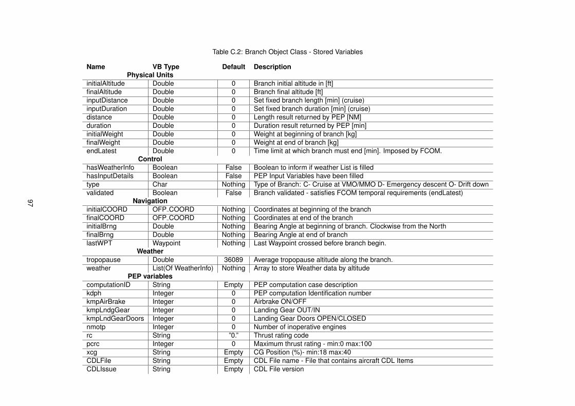
Table C.2: Branch Object Class - Stored Variables
Name VB Type Default DescriptionPhysical Units
initialAltitude Double 0 Branch initial altitude in [ft]finalAltitude Double 0 Branch final altitude [ft]inputDistance Double 0 Set fixed branch length [min] (cruise)inputDuration Double 0 Set fixed branch duration [min] (cruise)distance Double 0 Length result returned by PEP [NM]duration Double 0 Duration result returned by PEP [min]initialWeight Double 0 Weight at beginning of branch [kg]finalWeight Double 0 Weight at end of branch [kg]endLatest Double 0 Time limit at which branch must end [min]. Imposed by FCOM.
ControlhasWeatherInfo Boolean False Boolean to inform if weather List is filledhasInputDetails Boolean False PEP Input Variables have been filledtype Char Nothing Type of Branch: C- Cruise at VMO/MMO D- Emergency descent O- Drift downvalidated Boolean False Branch validated - satisfies FCOM temporal requirements (endLatest)
NavigationinitialCOORD OFP COORD Nothing Coordinates at beginning of the branchfinalCOORD OFP COORD Nothing Coordinates at end of the branchinitialBrng Double Nothing Bearing Angle at beginning of branch. Clockwise from the NorthfinalBrng Double Nothing Bearing Angle at end of branchlastWPT Waypoint Nothing Last Waypoint crossed before branch begin.
Weathertropopause Double 36089 Average tropopause altitude along the branch.weather List(Of WeatherInfo) Nothing Array to store Weather data by altitude
PEP variablescomputationID String Empty PEP computation case descriptionkdph Integer 0 PEP computation Identification numberkmpAirBrake Integer 0 Airbrake ON/OFFkmpLndgGear Integer 0 Landing Gear OUT/INkmpLndGearDoors Integer 0 Landing Gear Doors OPEN/CLOSEDnmotp Integer 0 Number of inoperative enginesrc String ”0.” Thrust rating codepcrc Integer 0 Maximum thrust rating - min:0 max:100xcg String Empty CG Position (%)- min:18 max:40CDLFile String Empty CDL File name - File that contains aircraft CDL ItemsCDLIssue String Empty CDL File version
97
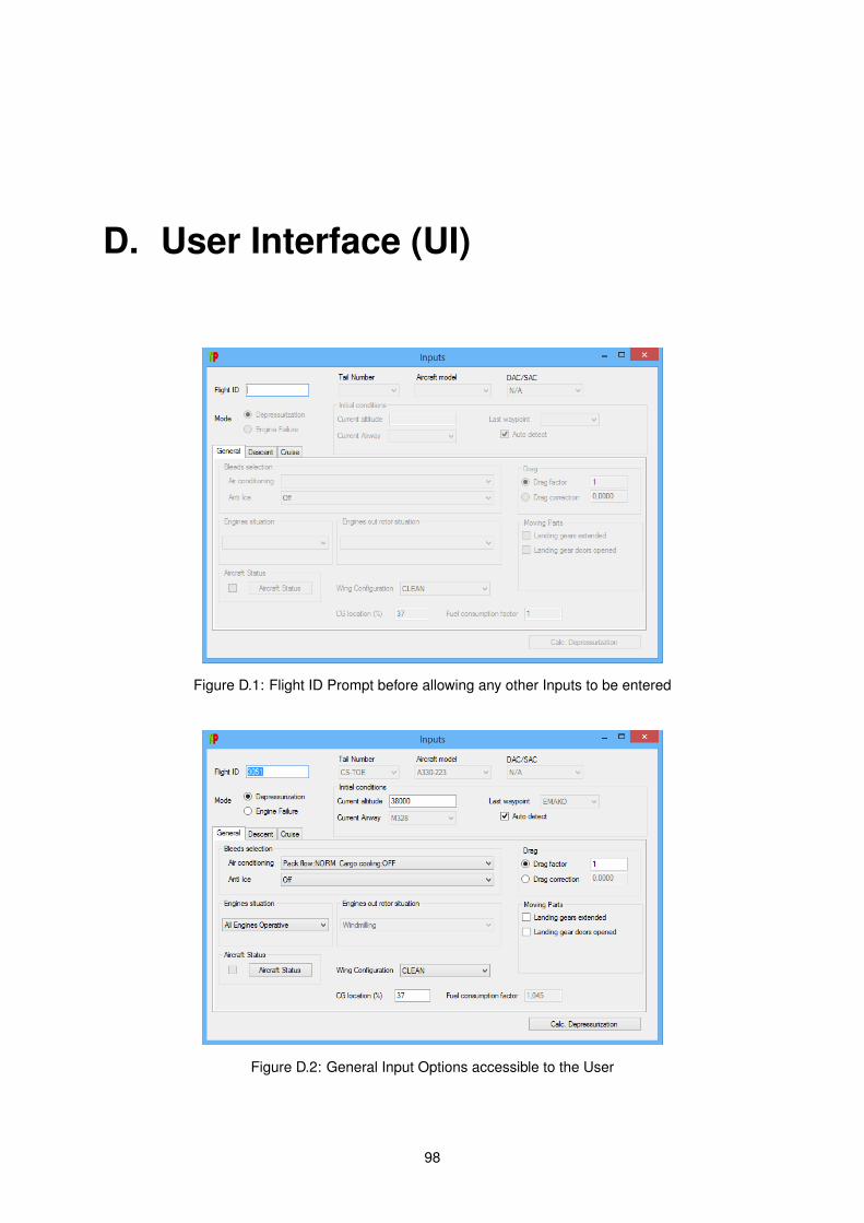
D. User Interface (UI)
Figure D.1: Flight ID Prompt before allowing any other Inputs to be entered
Figure D.2: General Input Options accessible to the User
98

Figure D.3: Cruise-specific UI Options
Figure D.4: Descent-specific UI Options
Figure D.5: Coordinate calculation utility
99