Cadmium content in sphalerites, copperores, soils and plants in southern Arizona

Item Type text; Thesis-Reproduction (electronic)

Authors Kresan, Peter Lawrence, 1948-

Publisher The University of Arizona.

Rights Copyright © is held by the author. Digital access to this materialis made possible by the University Libraries, University of Arizona.Further transmission, reproduction or presentation (such aspublic display or performance) of protected items is prohibitedexcept with permission of the author.

Download date 16/05/2018 23:39:28

Link to Item http://hdl.handle.net/10150/566610

CADMIUM CONTENT IN SPHALERITES, COPPER ORES,

SOILS AND PLANTS IN SOUTHERN ARIZONA

by

Peter Lawrence Kresan

A Thesis Submitted to the Faculty of

DEPARTMENT OF GEOSCIENCES

In Partial Fulfillment of the Requirements For the Degree of

• MASTER OF SCIENCE

In the Graduate College

THE UNIVERSITY OF ARIZONA

1 9 7 5

STATEMENT BY AUTHOR

This thesis has been submitted in partial fulfillment of re­quirements for an advanced degree at The University of Arizona and is deposited in the University Library to be made available to borrowers under rules of the Library.

Brief quotations from this thesis are allowable without special permission, provided that accurate acknowledgment of source is made. Requests for permission for extended quotation from or reproduction of this manuscript in whole or in part may be granted by the head of the major department or the Dean of the Graduate College when in his judg­ment the proposed use of the material is in the interests of scholar­ship. In all other instances, however, permission must be obtained from the author.

SIGNED:

APPROVAL BY THESIS DIRECTOR

This thesis has been approved on the date shown below:

Professor of GeosciencesDate

\J

ACKNOWLEDGMENTS

The completion of this thesis would not have been possible with­

out the generous assistance of certain individuals, agencies and com­

panies and the financial aid given to the Laboratory of Geochemistry by

a National Science Foundation Grant GA-31270, "Correlation and Chronol­

ogy of Ore Deposits and Volcanic Rocks."

Discussions with Dr. Paul E. Damon and Dr. Thomas S. Lovering

laid the groundwork for this thesis, I am especially grateful to

Professor Damon for his professional and personal encouragement. Dr.

Austin Long, Dr. Donald Livingston, Dr. Eric Baskin, and Robert Scar­

borough kindly provided advice on the analytical methods. Dr. Edward

McCullough's encouragement was greatly appreciated. Air pollution data

for the Tucson area were generously provided by Dr. Jarvis J. Moyers.

Phelps Dodge Corporation, Duval, American Smelting and Refining

Company, and Pima Mining Company provided valuable assistance and

cooperation in the collection of ore samples. I am especially grateful

to Richard Graeme for his aid in the collection of samples.

Kathleen Roe and Dr. Damon provided immensely helpful criticisms

of an early draft of the thesis. Ideas and equipment for the production

of illustrations were provided by Donald B. Sayner.

Finally, I wish to thank my parents for their continued encour­

agement and unselfish support. Their enthusiasm and interest in my

endeavors have made my efforts all the more enjoyable.

iii

TABLE OF CONTENTS

Page

LIST OF T A B L E S ........ .............. ........................ vi

LIST OF ILLUSTRATIONS......................................... viii

A B S T R A C T ...........................'........... .'............ ix

1. INTRODUCTION . ............................. .................. 1

2. ANALYTICAL METHODS ........................................... 5

Sulfide Ore Analysis . , . ............................... 5Atomic Absorption Analysis of Sulfide Material .......... 8Soil and Plant Sampling and Digestion..................... 15

. Atomic Absorption Analysis of Soils and Plants .......... 17Analysis of Bat Guano............................... 17

3. CADMIUM CONTENT OF COPPER AND ZINC SULFIDES FROM PORPHYRYCOPPER DEPOSITS ............................................... 25

Cadmium Content of Chalcopyrite ........................... 26Cadmium Content of Sphalerite.......... .. . . ........... 29Total Amount of Cadmium Discharged ....................... 29

4. CADMIUM CONTAMINATION IN THE VICINITY OF COPPER SMELTERS . . . 32

Cadmium in Soils and Plants . ............................. 32Cadmium in Bat G u a n o .................... 34

5. CADMIUN IN THE TUCSON A I R ............................ 38

6. CADMIUM AND HUMAN H E A L T H ..................................... 51

7. SUMMARY AND CONCLUSIONS.........................■............ . 53

APPENDIX A: DESCRIPTION OF SULFIDE SAMPLES ................ . 55

APPENDIX B: SUMMARY OF THE ANALYSIS OF CHALCOPYRITEAND SPHALERITE................................... 60

APPENDIX C: INSTRUMENTAL PARAMETERS AND CALIBRATIONCURVES FOR ATOMIC ABSORPTION STANDARDS ........... 63

iv

V

APPENDIX D:

TABLE OF CONTENTS— Continued

Page

AIR POLLUTION MONITORING DATA FOR 1974 ........ .. 72

REFERENCES . 85

LIST OF TABLES

Table Page

1. Correlation coefficients for the concentrations ofmetals in chalcopyrite and sphalerites . ................. 6

2. Interference effects of Zn, Fe and Cu ....................... 11

3. Average percent deviation from mean for atomic absorptionanalysis of sulfide.................. 11

4. Analysis of synthetic sulfide solutions ..................... 13

5. Analysis of United States National Bureau of Standardscopper concentrate . ............ 14

' 6.' Location of plant and soil samples in Sulfur Springs Valley . 16

7. Precision for soil and plant analysis.................. 18

8. Comparison of bat guano analytical techniques .............. 21

• 9. Average cadmium content of chalcopyrite from some coppermines in southeastern Arizona ....................... 27

10. Cadmium processed by Arizona copper smelters each yearas a trace component in chalcopyrite ..................... 28

11. Average cadmium contamination of sphalerite from somecopper mines in southeastern Arizona ......... 30

12. An inventory of the cadmium smelted by copper smeltersin southeastern Arizona................................. . 30

13. Analysis of soils from the Sulfur Springs Valley, Arizona . . 33

14. Analysis of plant material from the Sulfur Springs Valley,Arizona................................... 33

15. Cadmium content of bat guano versus Morenci copper production 35

16. Cadmium content of particulate matter from air pollutionmonitoring analysis (Arizona Department of Health 1969-1973) 39

vi

LIST OF TABLES-̂ ■.Continued

Table Page

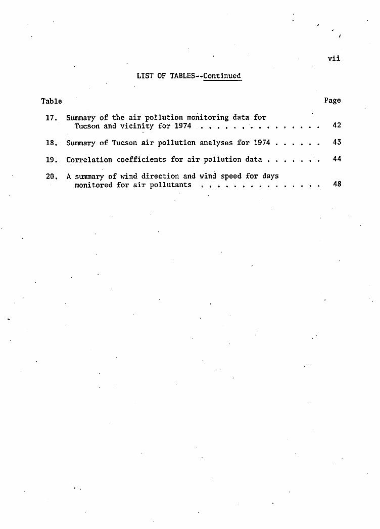
17. Summary of the air pollution monitoring data forTucson and vicinity for 1974 ............................. 42

18. Summary of Tucson air pollution analyses for 1974 .......... 43

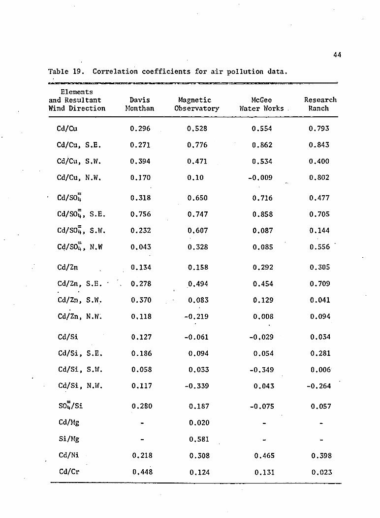
19. Correlation coefficients for air pollution d a t a .......... .. 44

20. A summary of wind direction and wind speed for daysmonitored for air pollutants . , . ............... .. 48

vii

LIST OF ILLUSTRATIONS

Figure Page

1. Flow of cadmium in the United States in 1968 3

2. Standard additions analysis for cadmium in the 1960 bat guano 22

3. Standard additions analysis for cadmium in the 1973 bat guano 23

4. Morenci copper production versus cadmium concentrationin bat g u a n o ......................................... .. . 36

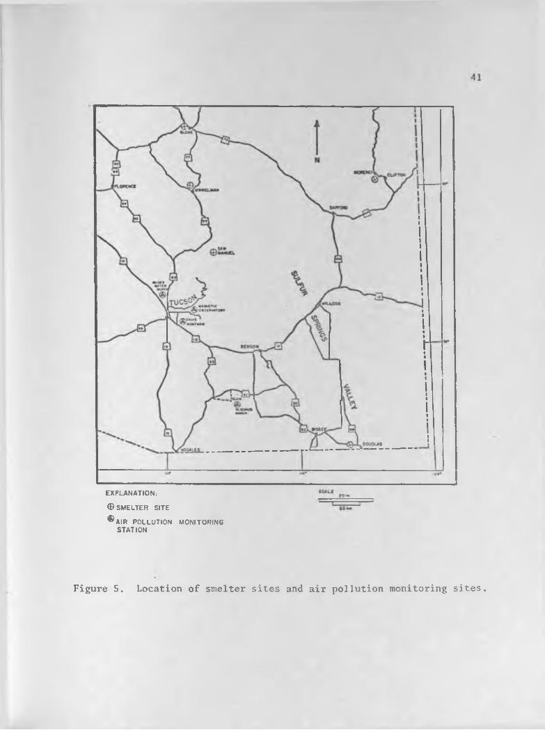
5. Location of smelter sites and air pollution monitoring sites 41

viii

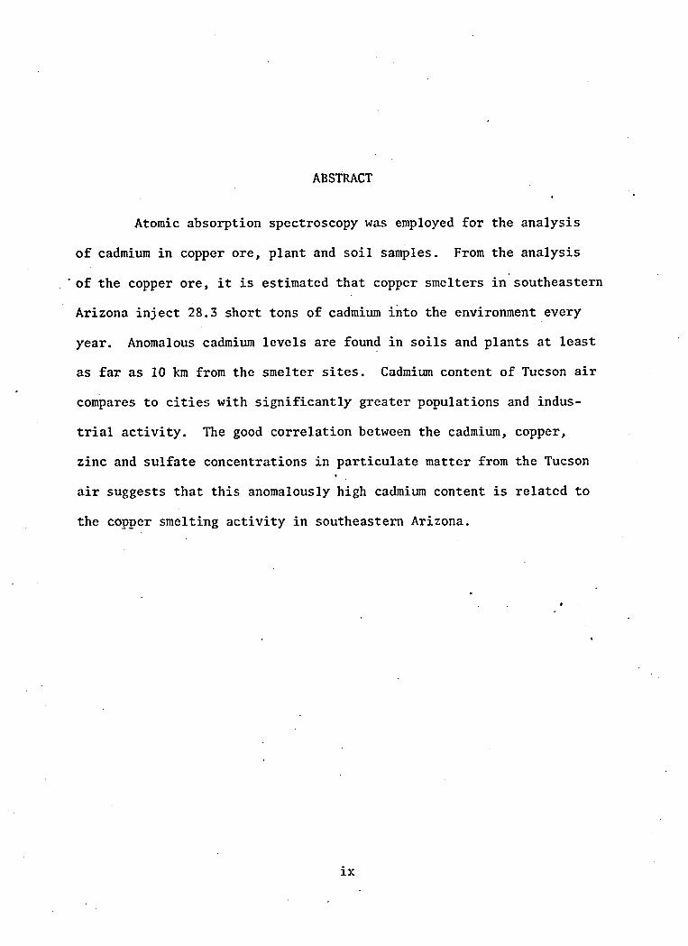
ABSTRACT

Atomic absorption spectroscopy was employed for the analysis

of cadmium in copper ore, plant and soil samples. From the analysis

' of the copper ore, it is estimated that copper smelters in southeastern

Arizona inject 28.3 short tons of cadmium into the environment every

year. Anomalous cadmium levels are found in soils and plants at least

as far as 10 km from the smelter sites. Cadmium content of Tucson air

compares to cities with significantly greater populations and indus­

trial activity. The good correlation between the cadmium, copper,

zinc and sulfate concentrations in particulate matter from the Tucson

air suggests that this anomalously high cadmium content is related to

the copper smelting activity in southeastern Arizona.

ix

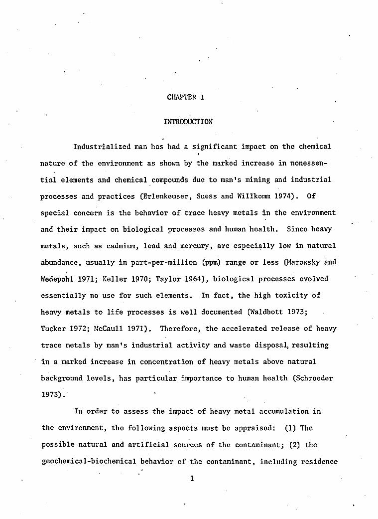
CHAPTER 1

INTRODUCTION

Industrialized man has had a significant impact on the chemical1

nature of the environment as shown by the marked increase in nonessen­

tial elements and chemical compounds due to man’s mining and industrial

processes and practices (Erlenkeuser, Suess and Willkomm 1974). Of

special concern is the behavior of trace heavy metals in the environment

and their impact on biological processes and human health. Since heavy

metals, such as cadmium, lead and mercury, are especially low in natural

abundance, usually in part-per-million (ppm) range or less (Marowsky and

Wedepohl 1971; Keller 1970; Taylor 1964), biological processes evolved

essentially no use for such elements. In fact, the high toxicity of

heavy metals to life processes is well documented (Waldbott 1973;

Tucker 1972; McCaull 1971). Therefore, the accelerated release of heavy

trace metals by man's industrial activity and waste disposal, resulting

in a marked increase in concentration of heavy metals above natural

background levels, has particular importance to human health (Schroeder

1973).

In order to assess the impact of heavy metal accumulation in

the environment, the following aspects must be appraised: (1) The

possible natural and artificial sources of the contaminant; (2) the

geochemical-biochemical behavior of the contaminant, including residence

1

2

times and chemical species; (3) the tendency for accumulation in a

reservoir, in particular, the tendency for incorporation and accumula­

tion in food chains; and (4) the toxicity levels or ranges for these

substances.

The two principal processes which emit cadmium are waste dis­

posal and metallurgical operations (Malin 1971). Because of cadmium's

• low boiling point (765 °C), the metal is readily volatilized during

incineration or pyro-processing of metals. Numerous authors have

reviewed the environmental geochemistry of cadmium (Sandstead 1974;

Fassett1972; Friberg, Piscator and Nordberg 1973). Recent researchers

also have studied the cadmium contamination associated with lead and

zinc smelters (Buchauer 1973; University of Missouri 1972). However,

the role of the copper smelting process as a source for cadmium emission

has not been investigated (refer to Figure 1). The copper smelters are

a likely cadmium source because the copper ores usually contain trace

quantities of cadmium sulfide.

The focus of this thesis is the source and distribution of

cadmium, a toxic heavy metal, in the environments of southeastern Ari­

zona with particular emphasis on quantitatively assessing the possible

contribution of copper smelting. Because southeastern Arizona is a

major copper province and smelting locality, this study focused on three

aspects of the cadmium distribution: (1) The cadmium content of the

copper ore and associated sphalerite; (2) cadmium concentrations in

soil, plants and fecal material from the vicinity of smelter sites;

and (3) the areal extent of the cadmium contamination.

Z-NCECONOMICS

' 'po te n tial os 'A A POLLUTION

■p o t e n t ia l CdNkO'L ANC WATER

p o l l u t io n ,v z ̂ yX c S T iM A T E o X

f AiR POLLUTION ’ f POM P N (X f SSING

V an d d is p o s a l J

c o al and fo ss il f u e ls(0 t Z O p p m l

SUPERPHOSPHATE Z ff) LPT- C4

DOMESTIC C» AND PB SMELTER

f l u e o u st

piSCELl a n EO'ISAND

u n a c c o u n t e d

USES AND ALL< 2%BATTERIES\1.

Ele c tr o p la tin g45- 49 9.

PAINTS A NO PKjM E N TS

ie-zi%p l a s t ic s15%

ME TAl i I iROiCAl USES A NO ALLOTS 2%

FUNC'CIOES

Figure 1. Flow of cadmium in the United States in 1968.

All flows are given as percentages of the total demand of 13.3 x 10^ lb. (From Sandstead 1974, p. 48.)

The analysis of sulfide ores, plants, soils and bat guano was

accomplished with a Perkin-Elmer atomic absorption spectrophotometer.

Specific analytical procedures are discussed in Chapter 2.

CHAPTER 2

ANALYTICAL METHODS

Sulfide Ore Analysis

Chalcopyrite and sphalerite ores were collected from five por­

phyry copper mines in southeastern Arizona, including Bisbee, Silverbell,

Pima, Mission and Sierrita. Sample locations and descriptions are

summarized in Appendix A.

Samples other than the massive sulfides were prepared for analy­

sis by first breaking up the ore material to 1/8 to 1/16 inch pieces.

The sulfide fraction was then concentrated by hand picking.

Mineral separations of exsolved sulfide mineral phases is an

extremely difficult task. So visual separation of small pieces of

chalcopyrite and sphalerite were considered to be adequate. To test

for possible contamination of sphalerite by chalcopyrite and vice

versa due to exsolution intergrowth, correlation coefficients were

determined for concentrations of cadmium with copper, zinc, manganese

and iron (refer to Table 1),

The negative correlation between cadmium and copper for sphaler­

ite suggests that the chalcopyrite exsolved in sphalerite may be di­

luting the cadmium content of the sphalerite. However, a negative

correlation between manganese and copper would also be expected, but

this is not the case. Furthermore, the concentration of copper in the

5

6

Table 1. Correlation coefficients for the concentrations of metals in chalcopyrite and sphalerites.

Correlation Coefficient

Sphalerite

Cd with Fe

Cd with Zn

Cd with Cu

Cd with Mn

Mn with Cu

Chalcopyrite

Cd with Zn

Cd with Mn

Cd with Cu

Cd with Fe

Mn with Cu

-0.4145

+0.5769

-0.5405

-0.5787

+0.1027

+0.4575

+0.0027

+0,0310

+0.0022

-0.1027

7sphalerite samples are consistent with the levels found in the sphaler­

ite from a lead-zinc deposit in which the copper concentration of the

sphalerite was between 0.02% and 0.7% (Boyle 1969).

It is difficult to evaluate the possible contribution of

exsolved sphalerite in chalcopyrite to the cadmium concentration in

the chalcopyrite. Although the correlation coefficient between cadmium

and zinc for the chalcopyrite is similar to sphalerite, the correla­

tions between cadmium and manganese, copper and iron in chalcopyrite

are not suggestive of a significant contamination problem. The

cadmium Content of the chalcopyrites, summarized in Appendix B, is

comparable to values determined by Burnham (1959) (the cadmium content

ranged from less than 1 ppm to 40 ppm) and Ivanov (1961) (cadmium con­

centrations ranged from 30 to 170 ppm).

All samples were crushed to less than 100 mesh in a shatterbox.

No attempt was made to get a pure concentrate of sulfides from the .

silicate phase because the digestion procedure differentially dis­

solved the sulfides. The silicate material remaining after digestion

was filtered from the solution, dried and weighed to correct the sample

weight for total sulfides minus silicates.

To prevent loss of sample due to the reactivity of sulfide

ores to mineral acids, chalcopyrite and sphalerite samples were

digested stepwise, very slowly. Between 0.2 and 0.3 grams of powdered

sulfide ore was weighed into a 50 ml acid-cleaned Erlenmeyer flask.

Approximately 4 ml of HgO was added to wet the sample. The 10 ml of

concentrated HC1 and 4 drops of concentrated HNO^ was added, and the

8

flask was covered with a watch glass and allowed to sit at room

temperature. After four hours, the flasks were heated to 90 °C,

increasing the heat slowly over a period of hours. When the sample

was cool, the sides of the flask were washed down with 1-2 ml of 90%

HNOg and the solution was reheated at a low temperature (70 °C). To

complete the digestion, 0.5 ml of a pre-mixed solution of two parts 90%

HNOj to three parts concentrated HC1 was added to the cooled solution.

After two to four hours the solution again was heated very slowly up

to 90 °C. A few hours at 90 °C was sufficient to finish the digestion.

The solution was then evaporated to near dryness at 90 °C and redis­

solved in 10 ml of 5% HC1 by heating. Once the material was redissolved,

the solution was filtered into a volumetric flask through an ashless

filter paper which had been pre-rinsed with 2% HC1 to volume for

analysis.

The filter paper then was stuffed into a porcelain crucible

which had been brought to a constant weight and pre-weighed. The cruci­

ble was then heated for one to two days at approximately 800 °C to burn

off the filter paper. After cooling to room temperature in a dissector,

the crucible was weighed to determine the amounts of silicate material

in the sulfide sample. The crucible was wiped clean and reweighed after

each analysis.

Atomic Absorption Analysis of Sulfide Material

Sulfide samples were analyzed for Cd, Zn, Cu, Fe and Mn using

a Perkin-Elmer 403 atomic absorption spectrophotometer and conventional

flame techniques (Perkin-Elmer 1971; Rubeska 1968). To measure

9

extremely low concentrations of Cd, the HGA-2000 graphite furnace acces­

sory was employed. Quantitative determination of metal concentration in

sample solutions was accomplished by bfacketting the unknowns with stan­

dard solutions close in concentrations to unknowns. Each split of the

unknown was analyzed five times in order to establish the precision for

the analysis.

The standard solutions were prepared from the SPEX grade chem­

ical compounds. The entire set of standard solutions were analyzed

before each batch of samples to provide a calibration curve and to

double check the standard solutions. Instrumental parameters and

calibration curves for each element are given in Appendix C.

A series of tests to determine whether major constituents in

the sample would interfere with the analyses for a particular element,

showed very minor interference problems at the concentration ranges in

which the analyses were performed. The effect of variable sulfate ion

concentration on metal analysis was investigated by preparing a series

of solutions for which the concentration of Zn, Cu, Fe> Cd and Mn were

constant but the SO” ion concentration varied between 0 and 17,000 ppm.

The analyses of Cd, Fe and Mn were not influenced by variations of SO^

within this range. However, SO” concentrations greater than 1000 ppm

suppressed Cu and Zn values slightly. At 17,000 ppm SO” , Zn absorbence

was suppressed 6% and Cu absorbence was suppressed 5%.

Because of the variability and high concentration of Zn, Cu and

Fe relative to Mn and Cd in the sample solutions, analyses were per­

formed to determine whether Zn, Cu or Fe interfered with the

10determination of Cd or Mn (Table 2). Two minor effects were noted:

(1) Cd values are enhanced in solutions containing a 1000 pmm or

greater Zn, and for 5000 ppm Zn, Cd absorbence was enhanced 12%;

(2) Mn values are enhanced in solutions containing 200 ppm or greater

Fe, and for 5000 ppm Fe, Mn absorbence was enhanced 3.6%. In order to

minimize these minor interference effects, the standard solutions were

prepared with a matrix of SO", Fe, Zn and Cu that approximated the

unknown solution to be analyzed.

For sample solutions containing greater than 0.05 ppm Cd,

conventional flame atomic absorption methods were utilized for the Cd

analysis. However, some chalcophyrite solutions contained much lower

Cd content. As a result, flameless atomic absorption techniques, using

the HGA-2000 graphite furnace and deuterium arc background corrector

coupled to the Perkin-Elmer 403 spectrophotometer, were employed for the

analysis of solutions containing between 0.0008 ppm and 0.05 ppm Cd.

Again, unknowns were bracketted with standard solutions to calibrate

the absorbence range analyzed. A summary of instrumental parameters

and calibration curves are given in Appendix C. ,

The percent deviation in five analyses of the same sample split

is summarized in Table 3. For the conventional atomic absorption

methods, the analysis was not accepted if the variation between the

two splits was greater than 5%, A 15% variation was accepted for the

graphite furnace analyses. In order to test the accuracy of the sul­

fide analysis, synthetic sulfide solutions were carefully prepared from

SPEX grade chemicals, and NBS standard copper concentrate samples were

11

Table 2, Interference effects of Zn, Fe and Cu,

Metal Concentration Range Effect

Zn 0 - 5,000 ppm • None for Mn1000 ppm and greater enhanced Cd values

Cu 0 - 5,000 ppm None for MnNone for Cd

Fe 0 - 5,000 ppm None for Cd200 ppm and greater enhanced Mn values

Table 3. Average percent deviation from mean analysis of sulfide.

for atomic absorption

Metal # AnalysesRange of

% DeviationAverage %

Deviation from Mean

Cda • 20 1-7 3

Cdb 12 1-15 6

Mn 30 1-8 3

Fe 38 1-6 2.5

Cu 38 0.3—5 2

Zn ' 38 1-5 2.4

^conventional atomic absorption.

^HGA-2000 graphite furnace, flameless method.

12

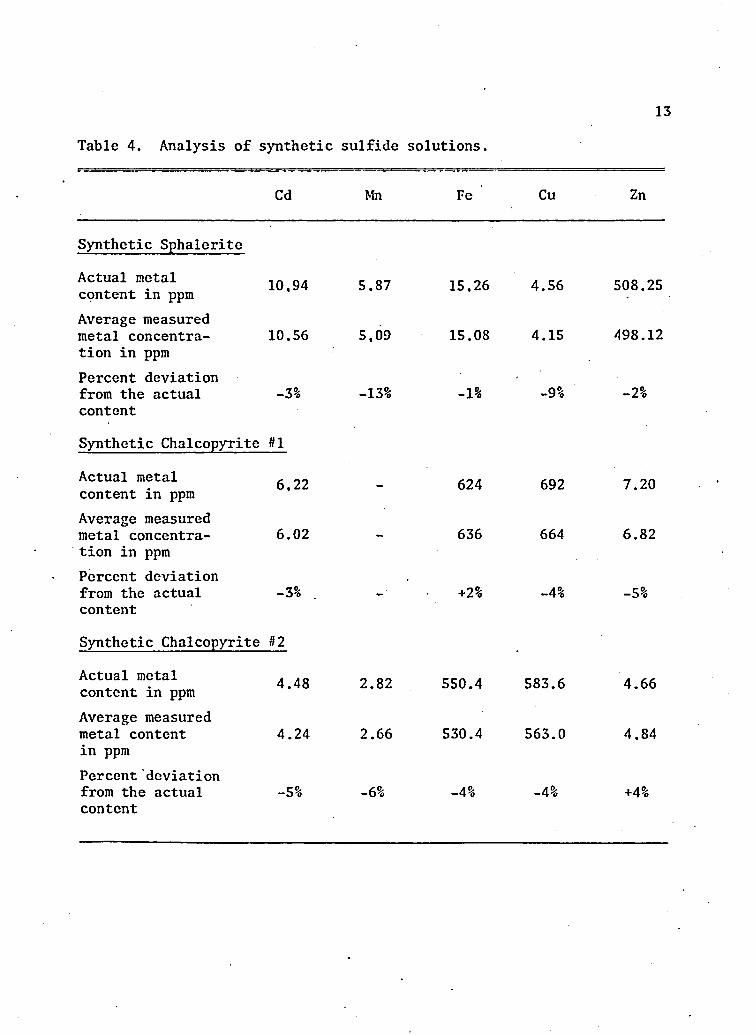
analyzed. The synthetic sulfide solutions were prepared because the

only certified analysis on the NBS materials was for copper. Table 4

summarizes the results from the analysis of the synthetic standards

and Table 5 gives the analysis of the NBS standard materials.

The analyses of synthetic sphalerite and chalcopyrite, given

in Table 4, show a systematic bias with most of the measured metal con­

centrations lower than the actual reported metal content. The fact

that the measured copper concentration in the NBS standards (refer to

Table 5) is higher than the certified copper content suggests that the■

problem is not in the measurements but with the preparation of the

synthetic standard solutions. The synthetic standard solutions were

prepared because interlaboratory standards with the required analyses

were not available for sulfide ore samples.

During the preparation of the synthetic standard chalcopyrite

and sphalerite, possible loss of constituents could have occurred.

Such a loss would result in the measured metal concentrations being

lower than the apparent actual metal content. Even though the syn­

thetic chalcopyrite and sphalerite solutions were treated identically

to the sulfide ore samples, their preparation necessitated an additional

number of solution transfers, during which there may have been incom­

plete transfer. Sample loss could have also occurred during the

reaction of the pure metals with mineral acids. Pure metal powders

were used to prepare the standard ore solutions and even in dilute

acids these substances react strongly. Because the reaction is

accompanied by some splattering, metals were dissolved very slowly

13

Table 4. Analysis of synthetic sulfide solutions.

Cd Mn Fe Cu Zn

Synthetic Sphalerite

Actual metal content in ppm 10,94 5.87 15.26 4.56 508.25

Average measured metal concentra­tion in ppm

10.56 5,09 15.08 4.15 498.12

Percent deviation from the actual content

-3% -13% -1% -9% -2%

Synthetic Chalcopyrite #1

Actual metal content in ppm 6,22 - 624 692 7.20

Average measured metal concentra­ 6.02 636 664 6.82tion in ppmPercent deviation from the actual content

-3% . ■ - +2% -4% -5%

Synthetic Chalcopyrite #2

Actual metal content in ppm 4.48 2.82 550.4 583.6 4.66

Average measured metal content 4.24 2.66 530.4 563.0 4.84in ppmPercent deviation from the actual -5% -6% -4% -4% +4%content

14

Table 5, Analysis of United States National Bureau of Standards copper concentrate,

% Deviationf.-v Measured Copper ,2-x Certified* Between (1)

Sample ̂ ̂ Concentration ̂' Copper Content and (2)

NBS #332■

CopperConcentrate

29.05% ± 0.29% 28.45% ± 0.08% +2%

NBS #330 Mill Heads 0.88% ± 0,04% 0.84% + 0.01% +5%

*National Bureau of Standards (1974).

15

in a tall necked volumetric flask, covered with a watch glass. Still,

some loss may have occurred.

Soil and Plant Sampling and Digestion

Plant and soil samples were gathered along Route 666 which runs

generally north from Douglas, Arizona, in the Sulfur Springs Valley.

Both plants and soils were sampled in five localities, ranging from

2 km in distance from the Douglas Smelter, All samples were collected

at least 30 meters from any roadway.

The soil samples represent a composite sample of material from2the upper 5 cm of soil within 10 m area. During the collection, the

sample was sieved through a 10 mesh screen. The plant material repre­

sents a composite sample of all the dominant vegetation including woody

scrubs and grasses in the area the soil sample was collected. Because

the plant samples represent a composite sampling of all the dominant

vegetation and because there were no major changes in the vegetation

assemblage between the sampling site, possible species effects were

minimal. Detailed description of each sample locality is given in

Table 6.

Plant samples from the Sulfur Springs Valley were analyzed for

Cd, Cu and Zn content using standard atomic absorption methods. First,

the plant material was dried in an oven at about 110 0C until a dry

weight was reached. The dried plant matter was then ashed at 475 °C

for approximately seven days. About 0.2 g of the resulting white ash

was weighed into Teflon crucibles and mixed with 2 ml HgO and 2 ml of

a 1:3 mixture of concentrated HNO^ and 6M HC1. This digestion mixture

16

Table 6, Location of plant and soil samples Valley.

in Sulfur Springs

Sample No.Distance from Douglas

Smelter in km Location

1 72 1.6 km west on road to Cochise Stronghold in desert grasslands

2 28 Desert grasslands 2.4 km east on Leslie Canyon Road just south of McNeal, Arizona

3 10 Just off west side of Rt. 666 across from Douglas Airport and north from Bisbee Double Adobe Turnoff

4 6.25 A heavily grazed area 2.4 km east of Rt. 666 on Glenn Road and 183 m east of the railroad tracks

5 1.66 Just off Rt. 666 near Sacred Heart Cemetery

17

was heated in a Parr Bomb for five hours at 140 °C (Rantala and Loring

1973; Paus 1972), The cooled solution was then diluted to 50 ml with

2% HC1 for the atomic absorption analysis.

Soil samples from the Sulfur Springs Valley were analyzed for

Cd, Zn and Cu content using standard atomic absorption methods. The

soil material was first dried in an oven at 110 °C. Then approximately

10 g of soil was accurately weighed into Teflon crucibles. Each cruci­

ble was charged with 5 ml l^O, 10 ml concentrated HC1 and 5 ml 70% HNO^.

To moderate the reaction the digestion mixture was allowed to sit for a

day before the crucibles were slowly warmed. The resulting sludge was

then filtered clear and diluted to 100 ml with 2% HC1 for the atomic

absorption analysis. -

Atomic Absorption Analysis of Soils and Plants

The analysis of plant and soil solutions for Cd, Zn and Cu was

accomplished using conventional flame atomic absorption methods

(Perkin-Elmer 1971). Each sample was analyzed three to five times

(Table 7) for determining the percent deviation between analyses.

Calibration curves and instrumental parameters are given in Appendix C.

Analysis of Bat Guano

Bat guano samples, obtained from Dr. Michael Petit at Colorado

State University, were collected from a cave 4.25 miles down Eagle

Creek from the pump station near Morenci, Arizona. The location of

the bat cave is 33°01'SO" N lat., 109°24'55" W long. (Petit, Department

of Microbiology, Colorado State University, Fort Collins, Colorado

18

Table 7, Precision for soil and plant analyses.

Metal Analysis #Range of % Deviation

Average %Deviation from Mean

Plant Analysis '

Cd 5 2-7 4

Zn 5 0.1-2 1

Cu 5 1-7 3

Soil Analysis

Cd 5 1-2 2

Zn 5 1-2 2

Cu 5 1-8 3

80521, personal communication, July 1973), The bat guano deposit was

cored, layers in the core were dated and samples were extracted for

analysis.

Approximately five grams of dated guano material for each year

were supplied by Dr, Petit, Ages can be assigned to the guano layers

because stratification is a result of the annual activity of insect

larvae, which stir up the top-most material each spring. Since the bat

guano was cleaned from the cave in the early 1950*5 for fertilizer,

layers are given an age simply on the basis of their sequence in the

core.

After drying the guano in an oven at 120 °C to a constant

weight, samples were weighed in a porcelain crucible for ashing. Guano

and crucibles were checked for a constant weight so that an accurate

value for percent ash could be calculated. Guano was ashed in covered

crucibles heated to 450 °C in a furnace for five days until a gray-white

ash was obtained. Crucibles were allowed to cool to room temperature

in a desiccator before reweighing. The ashing temperature was carefully

controlled in order to assure full retention of cadmium in the guano

ash. A study by Ruck, Gluskoter and Shimp (1973) showed that cadmium

was retained in organic material oxidized at 450 °C. To test for the

loss of cadmium during the ashing procedure, a sample of the 1966 bat

guano was ashed by wet techniques using a Parr Bomb and concentrated

HNOg. The Parr Bomb, charged with the guano and concentrated HNO^,

was heated at 150 °C until the solution was clear (about 8 hours).

Cadmium analysis of this wet ashed guano compared to within 8% of that

19

20

for the furnace ash guano (Table 8). Actually, the wet ashed material'

gave a lower cadmium value, perhaps due to partial comp1exing of the

cadmium by soluble organic compounds.

Samples of approximately 0.1 to 0.2 g of bat guano ash were

carefully weighed in Teflon Parr Bomb for digestion. One milliliter

of redistilled water was used to wet the ash sample, the 2 ml of one

part 12M HNO^ to one part 6M HC1 was added. Bombs were then heated

in an oven for 4 to 6 hours at 130 °C to 140 °C. After digestion, the

sample solution was evaporated to near dryness on a hot plate (80 °C)

and redissolved in 2% HC1.

Bat guano solutions were analyzed for cadmium by conventional

flame atomic absorption (Perkin-Elmer 1971). To calibrate the absorb-

ence response, the unknown guano solutions were bracketted by standard

cadmium solutions (Appendix C) for calibration curves. Each guano

sample was analyzed in duplicate, and four to six analyses were run

for each split. The precision between replicate analyses of the same

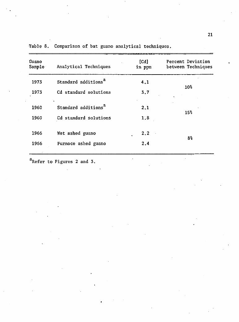
split averaged 7%, and maximum deviation accepted was 15%.

A test was performed to evaluate matrix interference effects by

comparing standard additions method for analysis (Perkin-Elmer 1971)

with the use of cadmium standard solutions to bracket the absorbence

response. The standard additions analysis is used for the analysis of

substances for which standards are difficult to prepare. Samples of the

1960 and 1973 bat guano were analyzed by the above two techniques. A

comparison of results is summarized in Table 8, and the standard addi­

tions analyses are presented in Figures 2 and 3, Using standard

21

•Table 8. Comparison of bat guano analytical techniques.

GuanoSample Analytical Techniques

[Cd] in ppm

Percent Deviation between Techniques

1973 Standard additions* 4.110%

1973 Cd standard solutions 3.7.

1960 Standard additions* 2.115%

1960 Cd standard solutions 1.8

1966 Wet ashed guano . 2.28%

1966 Furnace ashed guano 2.4

*Refer to Figures 2 and 3.

0.173

CADMIUM (In ppm) ADDED TO UNKNOWN SOLUTION

Figure 2. Standard additions analysis for cadmium in the 1960 bat guano.

Parameters: sample wt. = 0.58764 g (as ash), percent ash = 16,772%, dilutionfactor = 41.66, cadmium concentration in solution = 0.175 ppm. Therefore, cadmium in bat guano = 2.081 ppm.

to

OJ

600- s

' at at asCADMIUM (in ppm) ADDED TO UNKNOWN SOLUTIONS

04

Figure 3. Standard additions analysis for cadmium in 1973 bat guano.

Parameters: sample weight = 0.13552 g (in ash), percent ash = 11.818%, dilutionfactor = 125, cadmium concentration in solution = 0.0375 ppm. Therefore, cadmium concentration in bat guano = 4.09 ppm. tow

24

solutions for which no attempt was made to approximate the matrix of the

.guano solutions, the cadmium analysis of the guano agreed within 10% and

15% with the results obtained with standard additions analysis, which is

within the accepted range of deviation.

Because sodium has been noted (Friberg, Piscator and Nordberg.

1971, p. 17) to interfere with atomic absorption analysis of cadmium,

a series of cadmium solutions with varying sodium content were analyzed.

Within the concentration range for sodium in the guano solution

(between 0.005 and 0.01 M NaCl), no interference effects with the

cadmium analysis were noted.

CHAPTER 3

CADMIUM CONTENT OF COPPER AND ZINC SULFIDES FROM PORPHYRY COPPER DEPOSITS

The chemical behavior of cadmium and zinc is quite homologous

because of their similar outer electron configurations, electro­

negativity and second ionization potential (Krauskopf 1967). As a

result, cadmium commonly replaces zinc in sphalerite, making it the

principal cadmium-bearing mineral associated with copper porphyry

deposits. The cadmium content of sphalerite can be as high as a few

percent, in contrast to chalcopyrite, the principal ore, which generally

contains cadmium in the ppm range or less (Burnham 1959; Schroeder 1965;

Boyle 1969; Sangster 1968).

Although sphalerite is a major source for cadmium, the abundance

of zinc sulfide in the porphyry copper concentrate derived from mines

in southeastern Arizona runs from 0.5% to 0.05% or less (Cook, Anamax

Corp., Tucson, Arizona, personal communication, June 1975; Hutch,

Cypress-Pima Mine, Tucson, Arizona, personal communication, June 1975;

Rudy, Arizona Bureau of Mines, Tucson, Arizona, personal communication,

June 1975). However, because of the tremendous quantities of chalco-

pyrite mined and smelted from porphyry copper deposits, the chalcopyrite

may be as significant a source for cadmium as sphalerite. In order to

estimate the quantity of cadmium volatilized and emitted from the

25

26

copper smelters, samples of both sphalerite and chalcopyrite were

analyzed for cadmium. The analytical results are presented in Appendix

B and sample descriptions in Appendix A.

Cadmium Content of Chalcopyrite

To assess the amount of cadmium being smelted in southeastern

Arizona, the average cadmium content for chalcopyrite from five major

deposits was determined and the copper to cadmium ratio was calculated.

The total quantity of cadmium in chalcopyrite smelted is calculated by

multiplying the total copper produced by the copper to cadmium ratio.

(Refer to Table 9.) The average cadmium content of ore from the five

deposits sampled was assumed to be a representative value for porphyry

copper deposits in Arizona in order that the total cadmium mined by all

14 major copper mines could be estimated.

Because of the great variation in the cadmium content of copper

ore (not only between copper deposits but also within each deposit, as

shown in Appendix B) an estimate of the range in the quantity of cadmium

smelted with chalcopyrite is more meaningful. Table 10 shows that

between 1.6 and 91.5 short tons of cadmium were processes in 1972 as a

trace constituent of chalcopyrite by copper smelters in Arizona and

vicinity, based on the maximum and minimum Cu/Cd ratios. The average

amount of cadmium smelted was calculated to three short tons. However,

this is apparently on the low side because the ore from Mission Mine

alone may contribute five tons. (Refer to Table 9.)

Alternatively, the total cadmium processed as chalcopyrite can

be calculated assuming an average contribution of 1.54 tons of Cd per

Table 9. Average cadmium content of chalcopyrite from some copper mines in southeastern Arizona.

Location# of

SamplesAverage ppm Cadmium

Range in ppm Cadmium

Average ppm Copper x 104 • Cu/Cd

Total Cu Pro­duction 1972 in short tonsa

Total Cu Pro­cessed in short tons per year

Bisbee. 10 0.558 3.59 - n.d 31.03 556,000 50,272 0.0904

Sierrita 3 0.618 0.921 - 0.226 34.46 620,000 68,940 0.1110

Mission S 34.4 68.8 - 0.774 33.08 9,600 45,371 4.7252

Pina 4 1.20 1.94 - n.d. 30.27 253,000 82,841 0.3273

Silvcrbell 5 - 12.7 60.3 - n.d. 33.31 26,000 23,560 0.9008

Average 293,000 1,5387

aMoore (1972).

28

Table 10. Cadmium processed by Arizona copper smelters each year as a trace component in chalcopyrite.

Total copper production for Arizona in 1972 = 878,962 short tons (Moore 1972),

RangeCadmium in short tons/year

Cu/Cd Ratio processed as CuFeSg

Average 295,000 2.99

Maximum

Minimum

9,600 91.5

556,000 1.58Minimum 1.58

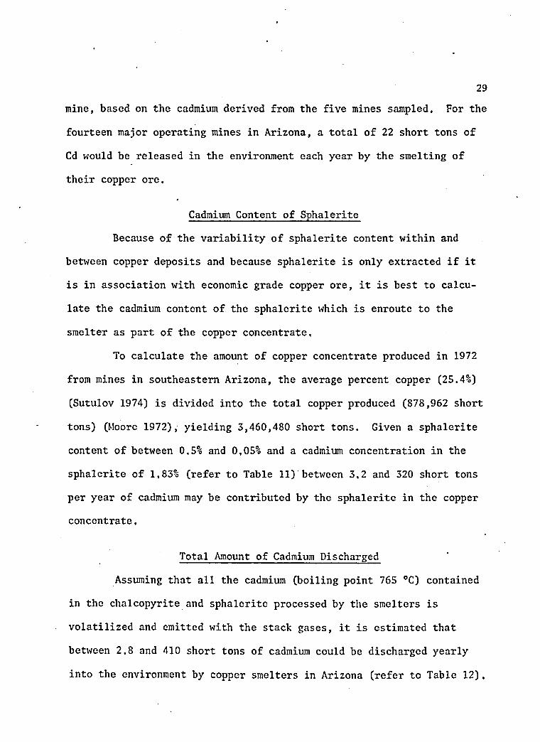
29mine, based on the cadmium derived from the five mines sampled. For the

fourteen major operating mines in Arizona, a total of 22 short tons of

Cd would be released in the environment each year by the smelting of

their copper ore.

Cadmium Content of Sphalerite

Because of the variability of sphalerite content within and

between copper deposits and because sphalerite is only extracted if it

is in association with economic grade copper ore, it is best to calcu­

late the cadmium content of the sphalerite which is enroute to the

smelter as part of the copper concentrate.

To calculate the amount of copper concentrate produced in 1972

from mines in southeastern Arizona, the average percent copper (25.4%)

(Sutulov 1974) is divided into the total copper produced (878,962 short

tons) (Moore 1972), yielding 3,460,480 short tons. Given a sphalerite

content of between 0.5% and 0,05% and a cadmium concentration in the

sphalerite of 1,83% (refer to Table 11) between 3,2 and 320 short tons

per year of cadmium may be contributed by the sphalerite in the copper

concentrate,

Total Amount of Cadmium Discharged

Assuming that all the cadmium (boiling point 765 °C) contained

in the chalcopyrite and sphalerite processed by the smelters is

volatilized and emitted with the stack gases, it is estimated that

between 2.8 and 410 short tons of cadmium could be discharged yearly

into the environment by copper smelters in Arizona (refer to Table 12),

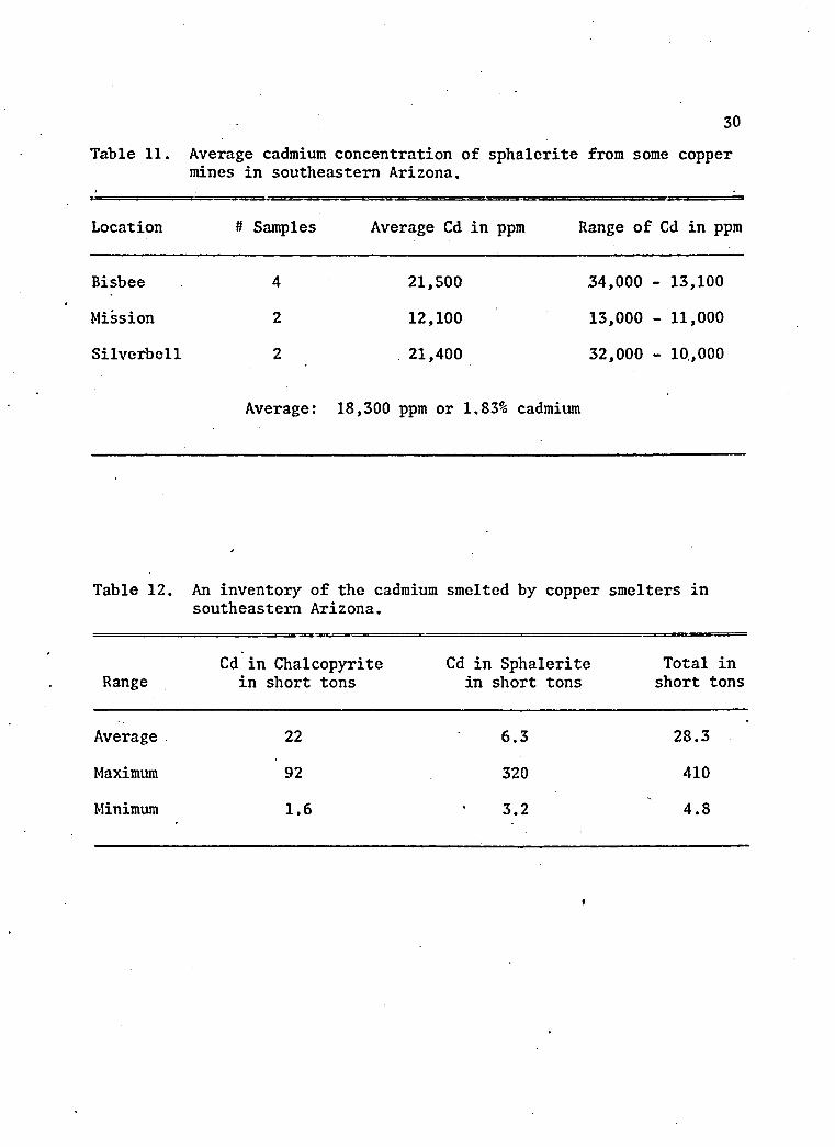
30Table 11. Average cadmium concentration of sphalerite from some copper

mines in southeastern Arizona.

Location # Samples Average Cd in ppm Range of Cd in ppm

Bisbee 4 21,500 34,000 - 13,100

Mission 2 12,100 13,000 - 11,000

Silverbell 2 21,400 32,000 - 10,000

Average: 18,300 ppm or 1.83% cadmium

Table 12. An inventory of the cadmium smelted by copper southeastern Arizona.

smelters in

RangeCd in Chalcopyrite

in short tonsCd in Sphalerite

in short tonsTotal in short tons

Average 22 6.3 28.3

Maximum 92 320 410

Minimum 1.6 • .w to 4.8

I

31

A reasonable average estimation of the total cadmium discharged

during 1972 is 28,3 short tons/year (refer to Table 12), based on the

following assumptions: (1) an average of 1.54 short tons of cadmium

was contained in the chalcopyrite smelted (refer to Table 9); (2) the

average cadmium concentration in sphalerite from porphyry copper depos­

its is 1.83% (refer to Table 11); and (3) the copper concentrate con­

tains an average of 0 .1% sphalerite.

CHAPTER 4

CADMIUM CONTAMINATION IN THE VICINITY OF COPPER SMELTERS

Cadmium in Soils and Plants

Soil and plant materials from the Sulfur Springs Valley, along

a gradient of distance from the Douglas Smelter, were analyzed for cad­

mium, zinc and copper. The average background level of cadmium in soils

is less than 1 ppm (Fassett 1972; Sandstead 1974). Background cadmium

levels for uncultivated plants is generally less than 0,05 ppm but can

range as high as 1.5 ppm (Schacklette 1972). The analyses presented in

Tables 13 and 14 show that significant amounts of cadmium accumulate in

the soils and plants in the areas around copper smelters, decreasing

systematically away from the smelter.

Since plants tend to accumulate cadmium with no known natural

means for elimination (Schacklette 1972, p. 1; John, Chuah and Van

Laerhoven 1972; Fassett 1972, p. 103), the cadmium levels in plants may

be a sensitive indicator of possible cadmium contamination. The back­

ground level of cadmium in mixed varieties of grass, shrubs and trees

in southwestern United States, generally falls below 0,25 ppm (Schack­

lette 1972, p. 4 and 7). The cadmium concentration in mixed plant

material from the Sulfur Springs Valley is significantly higher than

this background level, even at a distance of 72 km from the smelter.

32

33

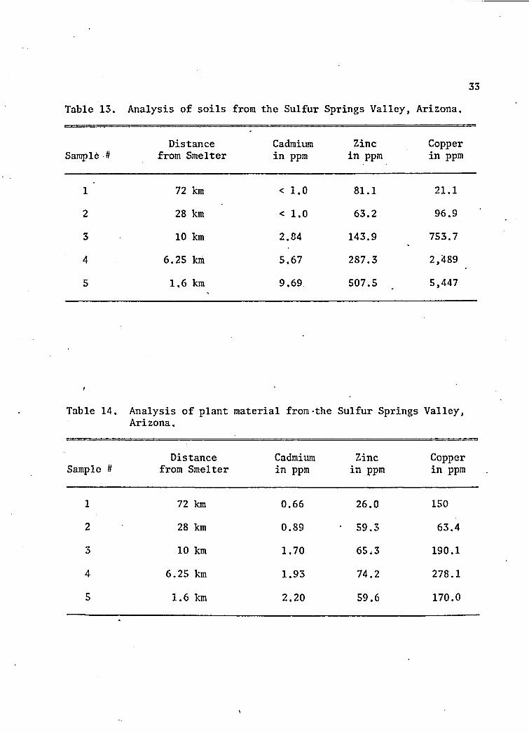
Table 13. Analysis of soils from the Sulfur Springs Valley, Arizona.

Sample #Distance

from SmelterCadmium in ppm

Zinc in ppm

Copper in ppm

1 72 km < 1,0 81.1 21.1

2 28 km < 1.0 63.2 96.9

3 10 km 2.84 143.9 753.7

4 6.25 km 5.67 287.3 2,489

5 1.6 km 9.69 507.5 5,447

I

Table 14. Analysis of plant material from the Sulfur Springs Valley, Arizona.

Sample #Distance

from SmelterCadmium in ppm

Zinc in ppm

Copper in ppm

1 72 km 0.66 26.0 ISO

2 28 km 0.89 • 59.3 63.4

3 10 km 1.70 65,3 190.1

4 6.25 km 1.93 74.2 278.1

5 1.6 km 2.20 59.6 170.0

Even though the soil is a less sensitive indicator than are plants, a

measurable increase in cadmium level in the soil was detected at a

distance of 10 km from the smelter.

Cadmium in Bat Guano

To determine if cadmium is being incorporated into the faunal

food chain, bat guano samples from a cave near Morenci, Arizona, were

analyzed for cadmium content. The analysis of annual layers of guano

for mercury had previously revealed a correlation between smelter pro­

duction and mercury content in the guano (Petit 1973). Dr. Petit

generously supplied the samples for the cadmium analysis for this

study.

The cadmium concentration in annual deposits of guano is given

in Table 15 and plotted along with smelter production levels in Figure

4. Table 15 shows some suggestive trends. Between 1962 and 1966 the

increase in cadmium concentration in the guano parallels the copper

production levels. Also, the dip in production during 1967 corresponds

to a major copper workman strike (a strike also occurred in 1959). The

correlation coefficient for the cadmium content of the bat guano vs.

the Morenci copper production was determined by Equation 1 (in next

chapter) to be +0.0991. Although the coefficient is positive, it is

not indicative of a strong relationship.

No strong relationship between the cadmium levels in the bat

guano and the Morenci copper production is recognizable. However,

various factors could diguise such a relationship. They include:

(1) changes in the cadmium concentration in the ores being smelted;

34

35

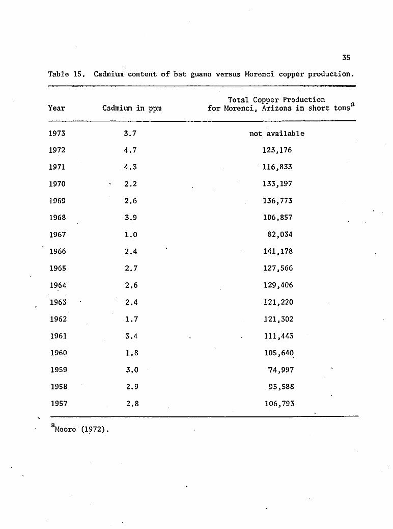
Table 15. Cadmium content of bat guano versus Morenci copper production.

Year Cadmium in ppmTotal Copper Production

for Morenci, Arizona in short tons

1973 3.7 not available

1972 4.7 123,176

1971 4.3 116,833

1970 • 2.2 133,197

1969 2.6 136,773

1968 3.9 106,857

1967 1.0 82,034

1966 2.4 141,178

1965 2.7 127,566

1964 2.6 129,406

1963 2.4 121,220

1962 1.7 121,302

1961 3.4 111,443

1960 1,8 105,640

1959 3.0 74,997

1958 2.9 .95,588

1957 2.8 106,793

‘W o r e (1972).

CADMIUM

CONTENT 9t BAT OUANO

4.5

4.0

\/si

COPPERPRODUCTIONI" ih e r l lene

>140,000

•135,000

130.000

125.000

120.000

•115,000

•110,000

•105,000

100,000

95.000

90.000

85.000

80.000

YEARS

Figure 4. Morenci copper production versus cadmium concentration in bat guano.

Refer to Table 15 for data.

wO'

37

(2) local inhomogeneity of the bat guano samples 5 (3) mixing of the bat

guano layers by slumping; (4) leaching of constituents from the guano by

urine and ground water; (5) changes in the bat colony; and (6) behavior

of cadmium in bats. It should also be noted that the guano material

supplied by Dr. Petit was peripheral to the central guano mound. So

the location on the floor from which the core samples were removed was

atypical, as it was not directly under the big crack in the ceiling

where the bats normally roost.

CHAPTER 5

CADMIUM IN THE TUCSON AIR

Arizona state air pollution monitoring analyses show that the

average cadmium concentration in air sampled from towns with copper

smelters is four times greater than for non-smelter areas in Arizona

and is comparable to air sampled from major urban and industrial cen­

ters of the United States (refer to Table 16). What is the possible

areal extent of this cadmium pollution? Is the cadmium emitted from

the copper smelters reaching major urban centers in the southwest?

To answer these questions, 50 days of the 1974 air pollution monitoring

data (Moyers 1974) for the Tucson Basin were evaluated for (1) correla­

tions between elements diagnostic of a particular industrial process

and (2) correlations between elemental concentrations and wind direction

as an attempt to pinpoint a particular source.

Elemental ratios for constituents in the air over Tucson show

that cadmium is approximately 1000 times more concentrated in atmospher­

ic particulate matter than in the average crustal material. Furthermore,

cadmium is most concentrated in particles having a mass medium equiva­

lent diameter (MMD) of 0.1 micron, whereas Al, Cd and Mn were associated

with particles of a 0.5 micron MMD. This concentration of cadmium in

particulates smaller in diameter relative to dust derived from natural

38

39Table 16. Cadmium content of particulate matter from air pollution

monitoring analysis (Arizona Department of Health 1969-1973)„

For Arizona as compared to other urban areas.

Location Sampling PeriodAverage Yearly Mean Cd in ug/m^

Range of Yearly Mean Cd in pg/rn^

Ajo 1969-1973 0.0048 0.015 - 0.001

Claypool(Miami) 1969-1973 0.0288 0.11 - 0.001

Clifton ' 1969-1973 0.0102 0.033 — 0.002

Douglas 1969-1973 0.0285 0.078 - 0.011

Hayden 1969S1973 0.1685 0.321 - 0.016

San Manuel 1969-197151973 o !oo7 0.019 - 0.002

Superior 1969-1973 0.0210 0.073 - 0.002

Winkelman 1970-1971 0.0155 0.027 - 0.004

Average for smelter sites 1969-1973 0.0248 0.054 - 0.006

Average for non-smelter sites

1969-1973 0.0064 0.025 - 0.001

State Average 1969-1973 0.0164 0.037 - 0.002

Tucson3 1974 0.0028 0.34 - 0.00007

Bronx, N.Y.^ - 0.014 0.022 - 0.006

Lower Manhattan, N.Y.b 0.023 0,036 — 0.009 '

Chicago, I11.C - - 0.08 - 0.005

Cincinnati, OhioC - 0.04 - 0.0001

foyers (1974) . ^Kncip et al. (1970, p. 146). C Friberg et al. (1973).

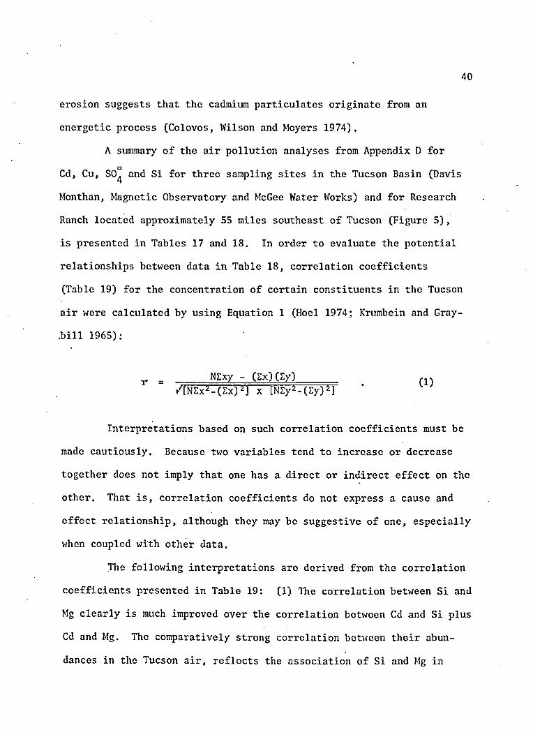
erosion suggests that the cadmium particulates originate from an

energetic process (Colovos, Wilson and Moyers 1974),

A summary of the air pollution analyses from Appendix D for

Cd, Cu, SO^ and Si for three sampling sites in the Tucson Basin (Davis

Monthan, Magnetic Observatory and McGee Water Works) and for Research

Ranch located approximately 55 miles southeast of Tucson (Figure 5),

is presented in Tables 17 and 18. In order to evaluate the potential

relationships between data in Table 18, correlation coefficients

(Table 19) for the concentration of certain constituents in the Tucson

air were calculated by using Equation 1 (Hoel 1974; Krumbein and Gray-

till 1965):

40

r = NExy - (Ex) (Zy)______ r ni/[NEx2-(Ex)2] x [NEyMEy)*)

Interpretations based on such correlation coefficients must be

made cautiously. Because two variables tend to increase or decrease

together does not imply that one has a direct or indirect effect on the

other. That is, correlation coefficients do not express a cause and

effect relationship, although they may be suggestive of one, especially

when coupled with other data.

The following interpretations are derived from the correlation

coefficients presented in Table 19: (1) The correlation between Si and

Mg clearly is much improved over the correlation between Cd and Si plus

Cd and Mg. The comparatively strong correlation between their abun­

dances in the Tucson air, reflects the association of Si and Mg in

EXPLANATION:

©SMELTER SITE

®AIR POLLUTION MONITORING STATION

Figure 5. Location of smelter sites and air pollution monitoring sites.

Table 17. Summary of the air pollution monitoring data for Tucson and vicinity for 1974

Derived from data from Moyers (1974). Refer also to Appendix D. Elemental analysis in ug/m3.

Location AverageDays w/N.E.

WindsDays w/S.E,

WindsDays w/S.W.

WindsDays s/N.W,

Winds

Days w/ Above Ave. Wind Speed

Days w/ Below Ave, Wind Speed

Average Wind Speed

(mph)

CADMIUM

Davis Monthan 0.00625 0.000223 0.00409 0.00652 0.00882 0.00550 0.006704 4.22

Magnetic Obs. 0.001933 0.000364 0.002336 0.001819 0.001823 0.002062 0.001947 3.90

McGee Water Wks. 0.001489 0.000105 0.001791 0.001902 0.000912 0.001354 0.001511 4.60

Research Ranch 0.001966 0.002254 0.002665 0.001522 0.001477 0.002336 0.001686 3.75

GOITER

Davis Monthan 0.0982 0.0469 0.1163 0.09558 0,08318 0.0796 0.1096 4.22

Magnetic Obs. 0.1501 0.1471 0.1818 0.1399 0.1263 ' 0.1178 0.1710 3.90

McGee Water Kks. 0.0653 0.0233 0.0982 0.0608 0.0352 0.0508 0.0854 4.60

Research Ranch 0.1128 0.1052 0.1599 0.0764 0.0890 0.1372 0.0944 3.75

SULFATE

Davis Monthan 4.89 1.88 6.71 3.87 4.097 4.01 • 5.33 4.22

Magnetic Obs. 4.20 15.20 4.83 3.21 2.59 3.44 4.72 3.90

McGee Water Kks. 4.69 1.67 7.01 3.76 2.29 4.13 5.01 4.60

Research Ranch 3.65 4.70 3.82 2.90 4.15 3.61 3.68 3.75

SILICON

Davis Monthan 16.69 2.19 13.57 17.21 19.55 21.40 13.63 4.22

Magnetic Obs. 16.40 1.86 14.00 20.53 15.36 22.20 14.01 3.90

McGee Water Kks. 11.30 0.97 11.37 11.13 12.04 11.85 10.92 4.60

Research Ranch 4.05 2.55 3.82 4.05 4.69 4.24 3.91 3.75

3Concentration in yg/m .

Table 18. Summary of Tucson air pollution analysis for 1974,

Location Cd Zn Cu s°: Si Cr Ni

DavisMonthan 0.00625 0.1894 0.09824 4.89 16.69 0.00584 0.0108

MagneticObservatory 0.001933 0.2142 0.1501 4.20 16.40 0.00431 . 0.00640

McGee Water Works 0.001489 0.1437 0.0653 4.69 11.30 0.00299 0.00471

Average for Tucson Basin 0.00322 0.1700 0.1045 4.59 14.87 0.00438 0.00730

ResearchRanch 0.001966 0.1330 0.1128 3.65 4.05 0.00292 0.00413

Standard Deviation for Analysis3

2.4% 12% 2.4% 10% 4.2% 7.6% 4.5%

aRamveiler and Moyers, 1974.

44

Table 19. Correlation coefficients for air pollution data.

Elements and Resultant Wind Direction

Davis Monthan

MagneticObservatory

McGeeWater Works

ResearchRanch

Cd/Cu 0.296 0.528 0.554 0.793

Cd/Cu, S.E. 0.271 0.776 0.862 0.843

Cd/Cu, S.W. 0.394 0.471 0.534 0.400

Cd/Cu, N.W. 0.170 0.10 -0.009 0.802

• Cd/SO4 0.318 0.650 0.716 0.477

Cd/SOij, S.E. 0.756 0.747 0.858 0.705

Cd/SO^, S.W. 0.232 0.607 0.087 0.144

C4/SO4 , N.W 0.043 0.328 0.085 0.556

Cd/Zn 0.134 0.158 0.292 0.305

Cd/Zn, S.E. • . 0.278 0.494 0.454 0.709

Cd/Zn, S.W. 0.370 0.083 0.129 0.041

Cd/Zn, N.W. 0.118 -0.219 0.008 0.094

Cd/Si 0.127 -0.061 -0.029 0.034

Cd/Si, S.E. 0.186 0.094 0.054 0.281

Cd/Si, S.W. 0.058 0.033 -0.349 0.006Cd/Si, N.W. 0.117 -0.339 0.043 -0.264

SO^/Si 0.280 0.187 -0.075 0.057

Cd/Mg - 0.020 - -

Si/Mg - 0.581 - -

Cd/Ni 0.218 0.308 0.465 0.398

Cd/Cr 0.448 0.124 0.131 0.023

45

natural crustal material. That cadmium does not correlate well with

either Si or Mg is not unexpected, since it has already been pointed

out that Cd concentration in the Tucson air is enhanced a 1000 times

over the average crustal abundance (Colovos et al. 1974). The corre­

lation coefficients reinforce the hypothesis that high Cd concentra­

tions in Tucson air were not related to natural erosional processes.

(2) It is interesing to note that Si concentrations in Tucson

air are higher during days of above average wind velocity (Table 18),

This is not surprising since higher winds will transport more dust.

However, Cd, Cu and SO^ concentrations tend to decrease somewhat for

days with above average winds. Also, Si concentration appears to be

greatest for days during which the winds blow from the southwest.

This is most likely related to the location of extensive mine tailing

ponds to the south southwest of Tucson. So, unlike Si content, the

concentrations of Cd, Cu and SOT in the air around Tucson are not4affected by wind velocity,

—(3) The correlation of SO^ to Si is relatively poor. This lack

of correlation is inferred to mean that the SO” is not being derived

from the dust as is the Si and Mg. In fact, the very good correlation

between SO” and Cd suggests that they may come from the same source.

The major source for atmospheric sulfur in the southeastern Arizona air

is the copper smelters, The tremendous quantities of SO^ emitted from

the smelters can be rapidly converted (a matter of hours) in the atmo­

sphere to SO^, especially in the presence of metal oxides and dust

particles which catalyze the reaction (Kellogg et al. 1972; Drone et al. 1968).

46(4) The fact that the Cd, Zn, Cu and SO^ correlate quite nicely

tends to "fingerprint” the copper smelters as their source. All four

constituents are emitted with the stack gases from copper smelters.

Even copper (boiling point 2592 °C) is emitted (probably as particulates)

as is evident from the analysis of the soils and plants in the Sulfur

Springs Valley (Tables 13 and 14). The fact that the correlations

between Cd and S0~, Zn and Cu are generally better than the correlations

between Cd and other elements such as Ni, Cr and Si, reinforces the

hypothesis that Cd, SO", Zn and Cu to a significant degree have a common

source, the copper smelters.

The correlation between Cd and Zn is low compared to that of Cd

with Cu and Cd with SO^. This can be explained by the fact that the

amount of sphalerite, the zinc bearing ore, smelted is much less (a

fraction of a percent) than the amount of chalcophyrite, the copper

bearing ore. Of course, a correlation between Cd and Zn is expected to

some degree because sphalerite can contain a percent or more of cadmium.

The cadmium anomaly at the Davis Monthan site will be discussed later.

(5) To further investigate the source of Cd in Tucson air,

correlation coefficients were calculated using data collected for days

of a particular wind direction. The major concentration of copper

smelters in Arizona is to the north northeast and southeast of Tucson.

Smelters to the north northeast of Tucson include San Manuel, Hayden

and Globe. Smelters in Douglas, Arizona, and Cananea, Mexico, are both

approximately 130 miles to the southeast of Tucson (refer to Figure 5).

No smelter sites are located to the northwest of Tucson.

47

Calculation of the correlation coefficients yielded improved

correlations between Cd and Cu, Zn and SOT when the winds are from the4southeast. This tends to implicate the Douglas and Cananea smelters

as contributing sources for the cadmium. For days with northwesterly

or southwesterly winds, the correlations are significantly diminished.

Correlations for days with northeasterly winds are, unfortunately,

meaningless because of the very few days during which northeasterly

winds occurred (Table 20),

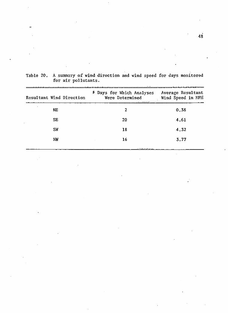
Possible natural weighting of the data due to a dominant

seasonal wind direction must be considered, since the prevailing winds

for the Tucson Basin are southerly in direction. However, Table 20

shows that the analyses were spread over days with a good representation

of southeast, northwest and southwest resultant wind directions. Never­

theless, the correlation between Cd and Si also improves for the south­

east wind direction (Table 19). This improved correlation between Cd

and Si suggests that other factors besides location of potential sources

are influencing the correlation coefficients.

There is also a potential problem with the extrapolation of the

resultant wind direction data for the Tucson Basin, which are collected

at the Tucson International Airport, to areas beyond the Basin. For

example, the wind direction information from the Tucson Airport was . /assumed to apply to the Research Ranch area 55 miles southeast of

Tucson. Douglas and Cananea are about 120 miles from Tucson and

separated by major mountain masses. To assume that wind directions

for Research Ranch or Douglas and Cananea are similar to the Tucson

48

Table 20. A summary of wind direction and wind speed for days monitored for air pollutants.

Resultant Wind Direction# Days for Which Analyses

Were DeterminedAverage Resultant Wind Speed in MPH

NE 2 0.38

SB 20 4.61

SW 18 4.32

NW 16 3.77

49

area may not be valid (Sellers, ̂ Department of Atmospheric Sciences,

University of Arizona, Tucson, Arizona, personal communication, 1975).

Although correlations between Cd and SO", Zn and Cu do compara­

tively improve when calculated for days with a southeasterly wind direc­

tion, the significance of this correlation is questionable. The lack

of data for regional weather conditions and the improved correlation

between Cd and Si for days with a southeasterly wind direction leaves

this aspect open for further studies.

(6) A cadmium anomaly for the Davis Monthan monitoring site is

shown in Table 17. This suggests that there is a source for atmospheric

cadmium in the vicinity of Davis Monthan Air Force Base. Although it

was considered unlikely that the cadmium came from the jet exhausts of

the aircraft associated with the base, correlation coefficients for Cd

with Cr and Ni were calculated because chromium and nickel are the prin­

cipal metals used in the combustion area of jet engines. The correla­

tion between Cd and Ni is lower for the Davis Monthan site than for the

other air pollution monitoring sites (refer to Table 19). Although Cd

and Cr concentrations in air correlate comparatively well for the Davis

Monthan site, the correlation may not necessarily mean equivalent

sources for both Cd and Cr, especially since the Cd and Ni association

is realtively poor.

x As it turns out, the most likely explanation for the high cad­

mium associated with the Davis Monthan site lies with a scrap metal

recovery plant. This metal recycling operation employs pyro-proccsses

for the recovery of metals from aircraft bearings. Some of the cadmium

50

in the electronic gear and associated lead, zinc and silver metals used

in the construction of aircraft parts is most likely volatilized during

the metal recovery processes,

The scrap metal recovery plant is a likely contributing source

of atmospheric cadmium in the Tucson Basin, However, this metal re­

cycling operations does not account for the strong correlation between

Cd, Cu, Zn and S0~ at the other air monitoring localities, because the

concentrations of Cu and Zn are comparatively low for the Davis Monthan

site (refer to Table 17).

Besides the metallurgical processes and aviation, the only

other possible major source for cadmium in the Tucson area is the auto­

mobile, Cadmium is apparently not exhausted from the automobile engine

(Cannon and Anderson 1971, p. 164), However, since cadmium can be a

trace constituent in tires and other auto components, soils and plants

in close vicinity to highways may contain unnaturally high cadmium

concentrations.

CHAPTER 6

CADMIUM AND HUMAN HEALTH

There is a growing belief that the hazard from cad­mium exposure may extend to the general population. It is conceivable that persons not exposed to cadmium by reasons of their occupation may inhale or inject cadmium to an extent sufficient to give rise to toxic effects (Kendrey and Roe 1969, p. 1206).

The toxic effects of cadmium are well documented (Flick, Kraybill and

Dimitroff 1971; Friberg et al. 1971; Perry 1971; Furst 1971; Perry 1968).

The impact of cadmium on human health has also been recognized (Lee

1972; Tucker 1972; Schroeder 1973). Health problems associated with

abnormal cadmium levels in humans include: (1) high blood pressure and

hypertension; (2) arteriosclerosis; (3) coronary occlusion; (4) strokes;

(5) cancer; (6) growth inhibition; and (7) liver and kidney diseases,

such as nephrosclerosis, renal necrosis and renal tubular dysfunction.

To ascertain whether incidences of diseases potentially related

to cadmium could be correlated to areas with smelters, data from the

Arizona Department of Health Services on the leading causes of death

for the fourteen counties in Arizona were analyzed. No systematic

relationships between counties containing major smelter sites and

diseases related to cadmium were recognized.

However, the breakdown of data on the county level may be at

too broad a scale to reveal such relationships. Comparison of data for51

52individual towns in Arizona would have been particularly useful, but

such data are not presently available. In addition, a large percentage

of people, especially in Pima and Maricopa counties, have moved into

Arizona recently. These new residents severaly bias the sampling

(Sauer and Brand 1971), Furthermore, human health is a function of a

complex assemblage of factors, so to resolve environmental high cadmium

concentrations as the principle cause of particular diseases, character­

istically high in some localities, may prove to be very difficult indeed.

There is, however, some tantalizing evidence to suggest that

there are high rates of lung cancer near copper and lead smelters

(Science News 1975). To resolve relationships between traces of heavy

metals and human disease, though, will require refinement of the health

and population data and continued research on mechanisms by which cad­

mium is distributed in the environment.

CHAPTER 7

SUMMARY AND CONCLUSIONS

Cadmium analysis of sulfide ores associated with copper por­

phyry deposits has shown that depending on the smelter production

levels, the concentration of cadmium in chalcopyrite and sphalerite,

and the amount of sphalerite associated with the deposit, a minimum-

maximum range of between 4.8 and 410 short tons of cadmium are emitted

each year from Arizona smelters. A reasonable average estimate of the

total cadmium discharged in 1972 by Arizona smelters is 28.3 short tons.

The cadmium.exhausted from the copper smelter contributes signi­

ficantly to the levels of cadmium in soils and plants within 10 km of

the smelter site. Cadmium concentrations for plants may be influenced

by the smelter emissions for as far as 72 km from the smelter locality.

The average mean cadmium concentration in the air for Arizona

towns with smelters is four times higher than for urban centers not in

the vicinity of a smelter. In fact, the cadmium content of the air for

smelter localities is comparable to the major industrial and population

centers of the United States.

Given the large quantity of cadmium emitted each year by the

eight major copper smelting operations in Arizona and the high concen­

tration of cadmium in the atmosphere close to smelter sites, the dis­

persion of this cadmium to major urban centers, such as Tucson, becomes

53

54

a plausible consequence. Evidence for the fact that the copper smelting

operations may contribute to the cadmium content in the Tucson air is

documented by the comparatively good correlation between cadmium and

copper, zinc and sulfate in the atmospheric particulate matter. In

Arizona, the principal industrial activity processing these elements in

tremedous quantities is the copper smelter. So the correlation between

cadmium, copper, zinc and sulfur tends to fingerprint the smelters as a

contributing source for these atmospheric pollutants.

The reduction of air pollution data for days with a particular

wind direction, yielded improved correlation coefficients for cadmium

with zinc, copper and sulfur. The complexity of the atmospheric circu­

lation patterns in southeastern Arizona and the lack of data concerning

the mixing of air masses between the major physiographic basins, pre­

cludes asserting any definitive relationships between cadmium pollution

in the Tucson Basin and a particular smelter operation, however.

Any relationship between environmentally high levels in cadmium

in Arizona with human health is not resolvable at this time. The com­

plexity of such a cause and effect relationship between cadmium and

human disease would necessitate a careful analysis of the causes of

death for towns with smelters as compared to communities without smel­

ters. Also, a better understanding as to the mechanisms by which heavy

metals arc dispersed in the atmosphere would aid in defining the

regional impact of the smelter emissions.

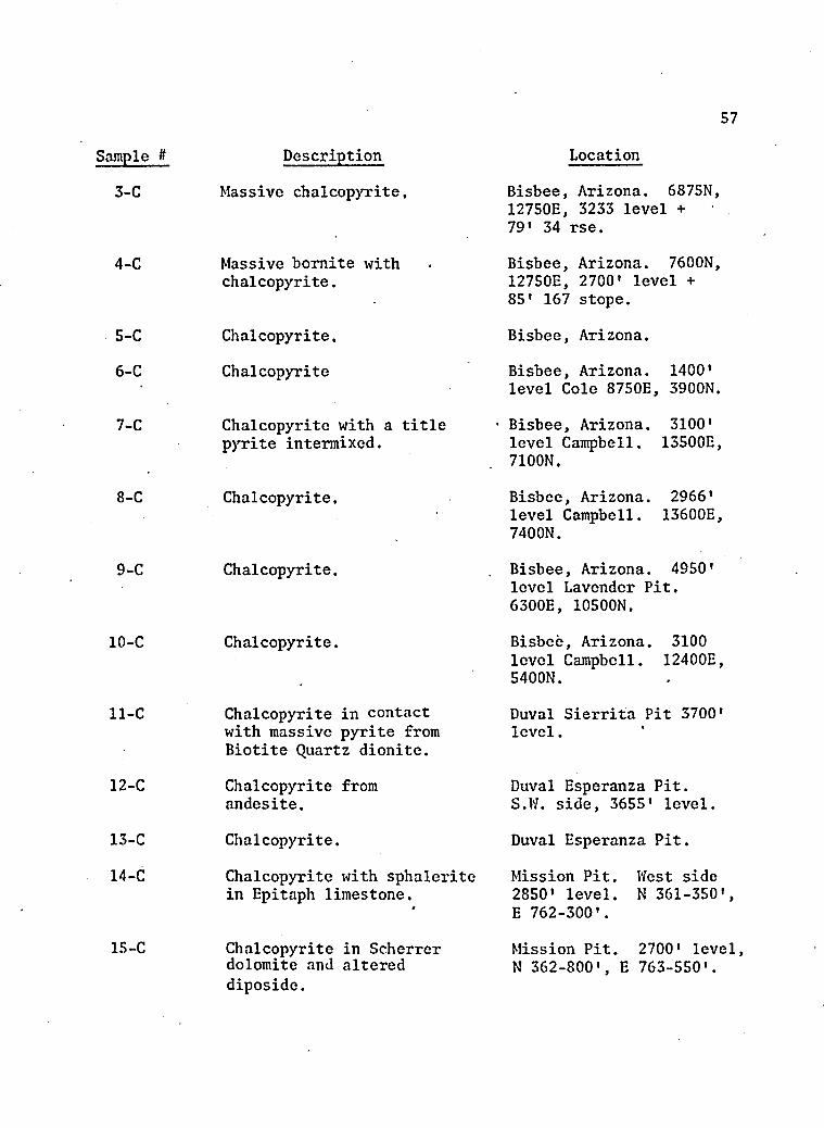
APPENDIX A

DESCRIPTION OF SULFIDE SAMPLES

55

56

Sample # Description Location

1-S Resinous yellow-brown massive sphalerite.

Iron Cap Mine, Globe, Az. Copper-silver sulfide deposit.

2-S Crystals of dark sphalerite coated with crystals of chalcopyrite.

Patagonia Mine.

3-S Massive sphalerite in limy Paleozoic sediments below dacite porphyry.

Silverbell Mine, Az, El Trio Pit from 2630 ft. level. 36300N, 17700E.

4-S Resinous yellow sphalerite mixed with pyrite in limy Paleozoic sediments,

Silverbell Mine, Az. El Trio Pit from 2630 ft. level. 36200N, 18350E.

5-S Sphalerite and chalcopyrite in Epitaph limestone.

Mission Pit, west side. 2850 ft. level. N361-350 ft., E 762-300 ft.

6-S •Sphalerite intermixed with quartz.

Mission Pit, Arizona.

7-S Resinous yellow sphalerite with quartz.

1400 ft. Junction Mine. Bisbee, Arizona.

8-S Sphalerite with galena. Junction Mine. Bisbee,Az. University of Arizona mineral museum speciment #947 D2621.

9-S Sphalerite with chalco­pyrite in limestone.

2700 ft. Junction Mine. Bisbee, Az. Drill core (+28).

. 10-S Sphalerite. San Xavier Extension Mine. Mineral Hill. University of Arizona mineral museum specimen #7220.

1-C Massive chalcopyrite. Sacremento Mine. Bisbee, Arizona.

2-C Chalcopyrite in silicates. Bisbee, Arizona. Drill core 7050N, 1289E, 2433» level, 22 stope.

57

Sample # Description Location

3-C Massive chalcopyrite, Bisbee, Arizona. 6875N, 12750E, 3233 level +79* 34 rse.

4-C Massive bomite with chalcopyrite.

Bisbee, Arizona. 7600N, 12750E, 2700' level +85' 167 stope.

5-C Chalcopyrite, Bisbee, Arizona.

6-C Chalcopyrite Bisbee, Arizona. 1400' level Cole 8750E, 3900N.

7-C Chalcopyrite with a title pyrite intermixed.

• Bisbee, Arizona. 3100' level Campbell. 13500E, 7100N.

8-C Chalcopyrite. Bisbee, Arizona. 2966' level Campbell. 13600E, 7400N.

9-C Chalcopyrite. Bisbee, Arizona. 4950' level Lavender Pit. 6300E, 10500N.

10-C Chalcopyrite. Bisbee, Arizona. 3100 level Campbell. 12400E, 5400N.

11-C Chalcopyrite in contact with massive pyrite from Biotite Quartz dionite.

Duval Sierrita Pit 3700' level.

12-C Chalcopyrite from andesite.

Duval Esperanza Pit. S.W. side, 3655' level.

13-C Chalcopyrite. Duval Esperanza Pit.

14-C Chalcopyrite with sphalerite in Epitaph limestone.

Mission Pit. West side 2850' level. N 361-350', E 762-300'.

15-C Chalcopyrite in Scherrer dolomite and altereddiposide.

Mission Pit. 2700' level N 362-800', E 763-550'.

58

Sample # Description Location

16-C Chalcopyrite in Concha limestone.

Mission Pit. 2770' level, West side of marble knoll, N 362-840*, E 763-700*.

17-C Chalcopyrite in Concha limestone.

Mission Pit. 2700* level, N 362-800*, E 762-850*.

18-C Chalcopyrite with some sphalerite in partially marbilized Concha limestone.

Mission Pit. 2700* level, N 362-600*, E 764-000*.

19-C Chalcopyrite with sphalerite in garnetiferous hornfeld contains greatest concentra­tion of zinc sulfides,

Pima Mine Pit, Arizona. 2790* level.

20-C Chalcopyrite in quartzite and elastics,

Pima Mine Pit, Arizona. 2870* level.

21-C ' Chalcopyrite in garnet hornfeld.

Pima Mine Pit, Arizona. 2470* level.

22-C Chalcopyrite and pyrite veins.

Pima Mine Pit, Arizona.

23-C Chalcopyrite vein in quartz monozite prophyry.

Silverbell Mine, Arizona. Drillhole core about 5000* N of El Trio Pit, D316, depth 165', 43000N, 15600E.

24-C Chalcopyrite in quartz mbnozite porphyry.

Silverbell Mine, Arizona. 2980* level. Oxide Pit, 29850N, 24700E.

25-C Massive chalcopyrite with intermixture of fine sphalerite in sediments.

Silverbell Mine, Arizona. 2470* level, El Trio Pit, 200* from district fault 36500N, 17600E.

26-C Chalcopyrite in dacite porphyry— some sphalerite.

Silverbell Mine, Arizona. 2470* level, El Trio Pit, 37500N, 18880E.

27-C Chalcopyrite in garneti­ferous tactite zone.

Silverbell Mine, Arizona. 3030* level, El Trio Pit, 37200N, 19100E,

Sample # Description Location

NBS #332

NBS #330

National Bureau of Standards Magma Mine, San ManuelCopper Concentrate, Arizona.

National Bureau of Standards Magma Mine, San Manuel Mill Heads, Arizona.

APPENDIX B

SUMMARY OF THE ANALYSIS OF CHALCOPYRITE AND SPHALERITE

60

Sample # Location % Silicate* tCd ppm Mri ppm Zn Cu %+ Fe %+

1-C Bisbee 0.668 < 0.08 741 0.0442 35.560 29.4972-C Bisbee 1.734 1,4368 45,027 0.0202 28.126 23.9235-C Bisbee 1.853 0.0864 1,564 0.0327 36.270 30.6714-C Bisbee 0.485 3.5962 853 0.2535 48.572 19.5105-C Bisbee 2.701 < 0.08 n.d. 0.0102 21.944 35.6426—C Bisbee 0.542 0.1697 5,233 0.0321 20.718 37.6807-C Bisbee 0.134 0.1163 1,888 0.0344 24.166 35.2638-C Bisbee 2.338 < 0.08 4,532 0.0392 28.764 34.1089-C Bisbee 4.041 0.1775 - 0.0269 31.765 31.586

10-C Bisbee 9.379 < 0.08 18,724 0.0184 34.396 28.74711-C Sierrita 0.606 0.921 45.0 0.2083 34.868 31.40112-C Sierrita 2.211 ' 0.226 < 0.1 0.1664 34.297 32.02413-C Sierrita 0.434 0.706 72.1 0.4381 34.218 28.93414-C Mission 3.429 51.60 927.0 1.8610 32.621 27.80015-C Mission 3.273 0.744 671.0 0.0104 31.900 30.20016-C Mission 6.552 1.582 242.7 2.4510 34.954 29.73917-C Mission 6.444 82.80 395.1 2.0175 34.570 29.78018-C Mission 12.544 68.80 5,397 1.8680 31.351 28.465

*% silicate reported as percentage of total ore sample

metal concentrations reported as concentration in sulfide phase

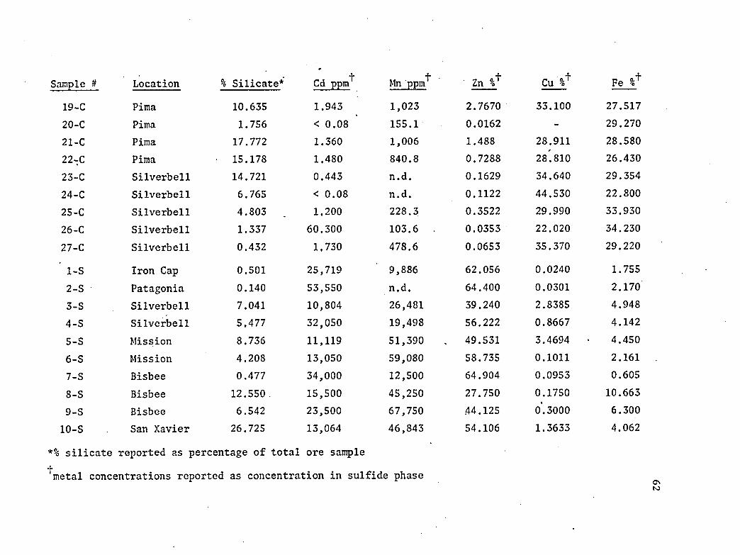
Sample # Location % Silicate* tCd ppm 4.Mn ppm Zn %t Cu %t Fe %+

19-C Pima 10.635 1.943 1,023 2.7670 33.100 27.51720-C Pima 1.756 < 0.08 155.1 0.0162 - 29.27021-C Pima 17.772 1.360 1,006 1.488 28.911 28.58022-C Pima 15.178 1.480 840.8 0.7288 28.810 26.43023-C Silverbell 14.721 0.443 n.d. 0.1629 34.640 29.35424-C Silverbell 6.765 < 0.08 n.d. 0.1122 44.530 22.80025-C Silverbell 4.803 1.200 228.3 0.3522 29.990 33.93026-C Silverbell 1.337 60.300 103.6 0.0353 22.020 34.23027-C Silverbell 0.432 1.730 478.6 0.0653 35.370 29.220

1-S Iron Cap 0.501 25,719 9,886 62.056 0.0240 1.7552-S Patagonia 0.140 53,550 n.d. 64.400 0.0301 2.1703-S Silverbell 7.041 10,804 26,481 39.240 2.8385 4.9484-S Silverbell 5.477 32,050 19,498 56.222 0.8667 4.1425-S Mission 8.736 11,119 51,390 49.531 3.4694 4.4506-S Mission 4.208 13,050 59,080 58.735 0.1011 2.1617-S Bisbee 0.477 34,000 12,500 64.904 0.0953 0.6058-S Bisbee 12.550 . 15,500 45,250 27.750 0.1750 10.6639-S Bisbee 6.542 23,500 67,750 44.125 0*. 3000 6.30010-S San Xavier 26.725 13,064 46,843 54.106 1.3633 4.062

*% silicate reported as percentage of total ore sample

metal concentrations reported as concentration in sulfide phase

APPENDIX C

INSTRUMENTAL PARAMETERS AND CALIBRATION CURVES FOR ATOMIC ABSORPTION STANDARDS

63

4000'

3000'

2000<

Imem<

1000*

10 20 SO 40 SOCADMIUM CONCENTRATION (p p m )

CADMIUM CALIBRATION CURVE

Instrumental Parameters: UV 229slit = 4 lamp @ 8 ma 3-slot burnerdetection limit = 0,02 yg/ml output in concentration mode

O.CZCADMIUM

I 0.0« 0.08CONCENTRATION (ppm)

IZOO*

1000

o eo o1

v> 400.

02 0.4 0.6 0.8CADMIUM CONCENTRATION (ppm )

CADMIUM CALIBRATION CURVES

Instrumental Parmeters: UV 229slit = 4lamp @ 8 ma3-slot burner paralleldetection limit = 0.01 pg/mloutput in concentration modeconcentration vernier = 5.00

O'

lOvl. sample

1 2 3 4 5 6 7 8 9 10Cd in ppm X 10“ 2

CADMIUM CALIBRATION CURVE FOR THE GRAPHITE FURNACE ANALYSIS

Instrumental Parameters: UV 229slit - 4 lamp 0 8 ma graphite furnace detection limit = 0.00001 yg/ml output in concentration mode concentration vernier = 1.00 dry 0 125 °C for 40 sec char 0 400 °C for 10 sec atomize 0 2000 °C for 10 sec argon purge rate 0 2 with auto

gas interruptdeuterium arc background corrector

Out. SAMPLE

CADMIUM CALIBRATION CURVES FOR THE GRAPHITE FURNACE ANALYSIS

Instrumental Parameters: UV 229slit = 4lamp @ 8 magraphite furnacedetection limit = 0,00001 pg/mloutput in concentration modeconcentration vernier =1.00dry @ 125 °C for 40 secchar @ 400 °C for 10 secatomize @ 2000 °C for 10 secargon pure rate @ 2 with auto gas interruptdeuterium arc background corrector ^

5000’

ZINC CALIBRATION CURVE

Instrumental Parameters: UV 214slit = 4 lamp @ 15 ma 3-slot burnerdetection limit = 0.018 pg/ml output in concentration mode

69

2000.

(ppm )CONCENTRATIONCOPPER

COPPER CALIBRATION CURVE

Instrumental Parameters: UV 325slit = 4 lamp @ 15 ma 3-slot burnerdetection limit = 0.09 pg/ml output in concentration mode

4000

3000.

? 2000.

IRON CONCENTRATION ( ppm)

IRON CALIBRATION CURVE

Instrumental Parameters: UV 248.3slit = 3lamp @ 30 ma

> 3-slot burnerdetection limit = 0,12 pg/ml output in concentration mode

2000'

£3 1000.

MANGANESE CONCENTRATION (ppm )

MANGANESE CALIBRATION CURVE

Instrumental Parameters: UV 279.5slit = 3 lamp @ 20 ma 3-slot burnerdetection limit = 0.055 pg/ml output in concentration mode

APPENDIX D

AIR POLLUTION MONITORING DATA FOR 1974

72

McGee Water Works,' Tucson

(Air Pollution Monitoring Analyses*)

ResultantDate Cd Cu sot Zn Si Cr Ni

Resultant Wind Dir.f

Wind Speed in mphf

1/3 0.00391 0.172 2.95 0.322 3.68 0,00227 0.00638 SW 2.81/5 0.000561 0.0329 0.24 0.284 1.74 0.00115 0.00337 SW 12.21/14 0.00950 0.372 35.21 0.253 5.04 0.00563 0.0157 SB 2.91/16 0.00701 0.226 21,6 0.437 8.88 0.00252 0.00526 SB 5.31/18 0.00371 0.147 6.68 0,257 5,24 0.00194 0.00447 SW 3.41/27 0.00137 0.0262 1.94 0.125 4,72 . 0,00220 0.00187 NW 4.81/29 0.00227 0.207 8.09 0.327 9.85 0.00186 0.00549 SB 2.81/31 0.00230 0.160 10.8 0.413 13.3 0.00362 0.00927 SB 3.22/2 0.000485 0.0521 1.88 0.0460 6.54 0.00126 0.00255 NW 3.22/9 0.00101 0.0736 1.45 0.0463 10,1 0.00344 0.00840 SB 15.52/13 0.000876 0.0567 1.92 0.190 11.5 0.00334 0.00248 NW 3.52/15 0.00395 0.170 13,85 0.413 10,4 0.00239 0.00418 » SB 2.82/24 0.00169 0.111 6.83 0.262 7.24 0.00260 0.00665 SB 10.02/26 0.00237 0.0787 2.36 0.173 18,71 0.00370 0.00496 SB 2.52/28 0.00246 0.0863 3,01 0.119 49.25 0.00712 0.00792 SB 3.83/2 0.000494 0.0868 2.57 0.154 14.6 0.00284 0.00158 SB 3.13/15 0.00054 0.0708 4.65 0.124 21.0 0.00432 0.00463 SB ' 2.5

*Moyers (1974). *̂U.S. Weather Service (1974).

Date Cd Cu SO4 Zn Si

5/24 0.000175 0.0360 1.69 0.101 4.593/26 ' 0.00219 0.0739 3.03 0.100 13.43/28 0,00129 0.0400 1.84 0.567 15.44/8 0.000427 0.0414 4.58 0.221 13,64/10 0.000496 0.0147 2.86 0.202 42.94/12 0.000611 0.00993 2.06 0.229 14.84/25 0.000198 0.0217 1.36 0.0494 9.664/27 0.000290 '0.0194 2.47 0.0787 8.765/6 0.00306 0.0457 . 3.49 0.0818 -5/8 0.000086 0.0165 2.6 0.0470 10.85/10 0.000002 0.0211 3.22 0.0944 11.35/19 0.000197 0.0265 1.16 0.0486 11.25/21 0.000760 0.388 4.04 0.0650 10.05/25 0.000624 0.0332 2.49 0.0636 14.75/25 0.00226 0.0306 4.87 0.0642 5,916/7 0.000712 0.0508 2.41 0.110 28.36/9 0.000605 0.0441 4.31 0.0584 -6/18 0.000990 0.0378 . - 0.0639 16.56/20 0.00583 0.0324 - 0.00878 14.26/22 0.00111 0.0256 - 0.0665 7.82

Resultant

Cr NiResultant Wind Dir.

Wind Speed in mph

0.00352 0.00378 NW 1.10.00290 0.00426 SW 4.10.00194 0.00243 SW 2.10.00182 0.00270 SE 5.10.00602 0.00575 NW 9.8 .0.000990 0,00223 NW 3.70.00321 • 0.00433 SE 6.70.000862 0.00250 SW 3.80.00191 0.00394 SE 2.00,00129 0.00179 NW 2.20.00243 0.00430 . SW 4.70.00266 0.00256 NW 11.20,00619 0.000610 NW 0.90.00258 0.00355 SW 6.80.00321 0.000648 SW 1.50.00647 0.00577 SW 15.10.00356 0.00511 SW 1.60.00395 0.00270 . NW 4.50.00400 0.00436 NW 6.10.00310 0.00414 NW 7.0

Resultant

Date Cd Cu SO4 Zn Si Cr NiResultant Wind Dir.

Wind Speed in mph

7/1 0.000915 0.0701 5.15 0.104 22.85 0.00619 0.00870 SW 5.17/14 0.000487 0.0302 4.14 0.00715 3.39 0.000906 0.00 SB 8.07/16 0.000413 0.0388 3.67 0.0800 6,06 0.00323 0.00215 SB ■ 8.17/18 0.00578 0.0415 2.58 0,0552 7.14 0.00346 0.00487 SW 5.27/20 0.000105 0.0233 1.67 0.0640 0.97 0.00592 0.0000995 NE 0.37/29 0.0000766 0.0267 2.7 0.0865 14.90 0.00302 0.000667 NW 1.17/31 0.000535 0.0223 2.5 0.108 3.52 0.00131 0.00250 NW 1.58/2 0.000847 0.0153 1.49 0.137 2.90 0.00 0.00174 SB 5.48/11 0.0000902 0.0161 2.21 0.0556 6.67 0.00185 0.0140 NW . 2.88/13 0.000349 0.0488 1.98 0.0416 3.48 0.00403 0.00620 SW 1.68/15 0.000608 0.0402 2.15 0.0758 6.58 0.00291 0.00296 SB 0.38/17 0.000278 0.0467 2.55 0.0655 2.28 0.00139 0.00456 SB 3.99/8 0.000405 0.0425 6.54 0.105 3.34 0.000478 0.00234 SB 1.79/10 0.000731 0.0643 8.8 0.157 16.78 0.00144 0.00628 SW 1.59/12 0.00146 0.0825 7.27 0.0682 8.35 0.00330 0.00653 SW 5.9

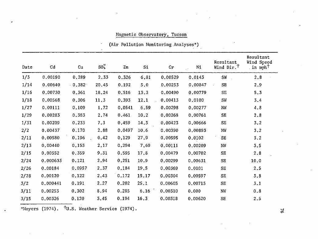
Magnetic Observatory, Tucson

(Air Pollution Monitoring.Analyses*)

Resultant

Date Cd Cu so; Zn Si Cr .. NiResultant Wind Dir.^

Wind Speed in mph’f

1/3 0.00190 0.289 2.33 0.326 6.81 0.00529 0.0143 SW . 2.81/14 0.00640 0.382 20.45 0.192 5.0 0.00253 0.00847 SE 2.91/16 0.00730 0.361 18.24 0.516 13,3 0.00490 0.00779 SE 5.31/18 0.00568 0.306 11.3 0.393 12.1 0.00413 0.0100 SW 3.41/27 0.00111 0.109 1.72 0.0541 6.59 0.00298 0.00277 NW 4.81/29 0.00283 0.383 2.74 0,461 10.2 0,00268 0.00761 SE 2.81/31 0.00209 0.233 7.3 0,459 14,3 0.00423 0.00666 SE 3.22/2 0.00437 0.170 2.88 0.0497 10.6 0.00390 0.00893 NW 3.22/11 0.00580 0.196 . 0.42 0,129 27.9 0.00595 0.0102 SE 3.22/13 0.00440 0.155 2.17 0.294 7.69 0.00111 0.00209 NW 3.52/15 0.00552 0.359 9.31 0.595 17.8 0.00479 0.00702 SE 2.82/24 0.000633 0.121 2,94 0,251 10.9 0.00299 0.00631 SE 10.02/26 0.00184 0.0957 2.37 0,184 19.5 0.00369 0.0101 SE 2.52/28 0.00120 0.122 2.43 0.172 15.17 0.00304 0.00597 SE 3.83/2 0.000441 0.191 2.27 0.202 25.1 0.00605 0.00715 SE 3.13/11 0.00255 0.302 8.94 0.285 6.16 ' 0.00310 0.000 NW 0.83/15 0.00326 0.120 3.45 0.194 16.3 0.00318 0.00620 SE 2.5

*Moyers (1974). "hl.S. Weather Service (1974).

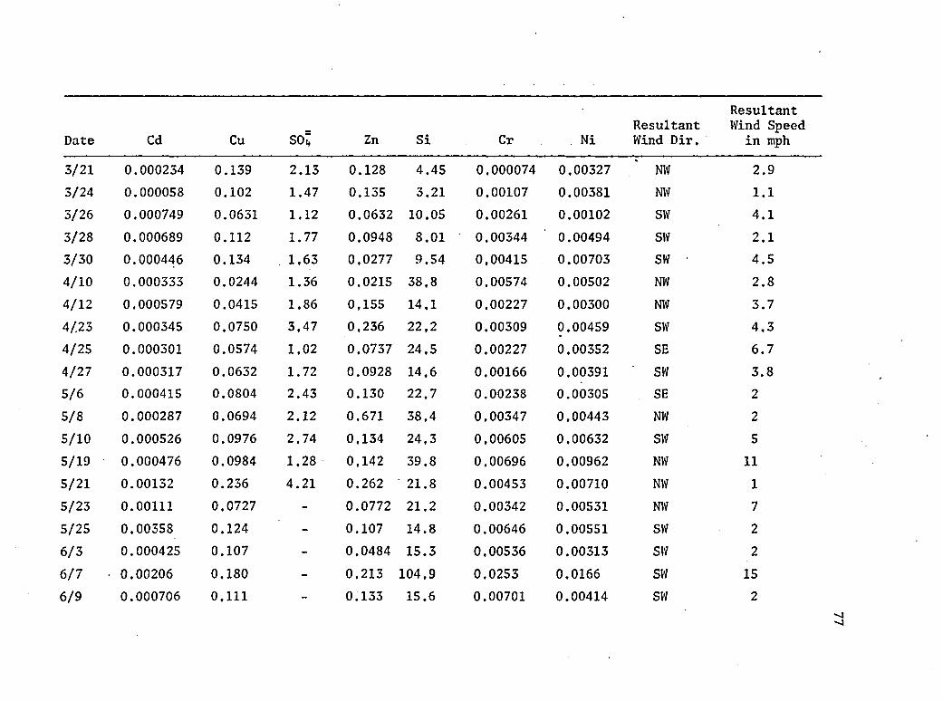
Date Cd Cu

3/21 0.000234 0.1395/24 0.000058 0.1023/26 0.000749 0.06313/28 0.000689 0.1123/30 0.000446 0.1344/10 0.000333 0.02444/12 0.000579 0.04154/23 0.000345 0.07504/25 0.000301 0.05744/27 0.000317 0.06325/6 0.000415 0.08045/8 0.000287 0.06945/10 0.000526 0.09765/19 0.000476 0.09845/21 0.00132 0.2365/23 0.00111 0.07275/25 0.00358 0.1246/3 0.000425 0.1076/7 • 0.00206 0.1806/9 0.000706 0.111

so; Zn Si

2 .1 3 0 .128 4 .4 5

1 .4 7 0 .135 3 .2 1

1 .12 0 .0632 10 .05

1 .7 7 0 .0948 8 .0 1

1 .6 3 0 .0277 9 .5 4

1 .3 6 0 .0215 3 8 .8

1 .8 6 0 ,155 14 .1

3 .4 7 0 ,236 2 2 ,2

1 .02 0 .0737 2 4 .5

1 .72 0 .0928 14 .6

2 .4 3 0 .1 3 0 2 2 .7

2 .1 2 0 .671 3 8 .4

2 .7 4 0 ,134 2 4 ,3

1 .2 8 0 .142 3 9 .8

4 .2 1 0 .262 2 1 .8

- 0 .0772 21 .2

- 0 .1 0 7 14 .8

- 0 .0484 15 .3

- 0 .2 1 3 104 ,9

- 0 .1 3 3 15 .6

Resultant

Cr . NiResultant Wind Dir.

Wind Speed in mph

0.000074 0.00327 NW 2 .9

0 .00107 0.00381 NW 1 .1

0 .00261 0.00102 sw 4 .1

0 .00344 0.00494 sw 2 .1

0 ,00415 0.00703 sw - 4 .5

0 ,00574 0.00502 NW 2 .8

0 ,00227 0.00300 NW 3 .7

0 .00309 0.00459 SW 4 .3

0 .00227 0.00352 SE 6 .7

0 .00166 0.00391 SW 3 .8

0.00238 0.00305 SE 2

0 .00347 0.00443 NW 20.00605 0.00632 SW 5

0.00696 0.00962 NW 11

0.00453 0.00710 NW 1

0.00342 0.00531 NW 7

0 .00646 0.00551 SW 2

0.00536 0.00313 SW 2

0 .0253 0.0166 SW 15

0.00701 0.00414 SW 2

Resultant

Date Cd Cu S04 Zn Si . Cr NiResultant Wind Dir.

Wind Speed in mph

6/18 0.00357 0.0880 - 0.0776 15.6 0.00396 0.00647 NW 46/22 0.00740 0.0691 - 0.0855 13.8 0.00442 0.00772 NW 77/1 0.00331 0.1320 - 0.138 50.71 0.0152 0.0135 SW 57/16 0.00102 0.0673 2.2 0.0524 3.13 0.00152 0.000 SE 87/18 0.00575 0.1203 1.7 0.207 5.10 0.00266 0.00422 SW 57/20 0.0000364 0.1471 1.38 0.0766 1.86 0.000 0.00634 NE 0.37/29 0.0000364 0.1237 2.1 0.113 .4.92 0.00129 0.000965 NW 17/31 0.000650 0.1762 2.35 0.176 7.62 0.00271 0.00352 NW 18/2 0.000627 0.0754 1.22 0.177 0.798 0.0000923 0.00172 SE 58/11 0.000289 0.1183 1.75 0,174 12.32 0.00474 0.00896 NW 38/13 0.000612 0.2378 1.84 0.120 12.77 0.00492 0.00860 SW 28/15 0.00136 0.1485 2.2 0.202 16.24 0.00419 0.0112 SE 0.38/17 0.000211 0.1408 2.29 0.252 6.48 0.00523 0.00675 SE 49/8 0.000812 0.1403 4.3 0.229 2.75 0.00304 0.00341 SE 29/10 0.00230 0.1336 5.67 0.238 11.18 0.00182 0.00493 SW 29/12 0.00224 0.1607 3.23 0.186 10.51 0.00505 0.0151 SW 6

Davis Monthan Air Force Base, Tucson (Air Pollution Monitoring Analyses*)

Resultant

Date Cd Cu so; Zn Si • Cr NiResultant Wind Dir.t

Wind Speed in mpht

1/5 0.0143 0.174 3.2 0.466 14.2 0.0109 0.0347 SW 2.81/5 0.00218 0.0428 0.44 0.129 46.4 0.00110 0.0226 SW 12.21/14 0.0233 0.369 21.52 0.261 17.4 0.0137 0.0185 SE 2.91/16 0.00945 0.210 19.28 0.592 23.8 0.0107 0.0103 SE 5.31/18 0.0156 0.352 14.14 0.467 20.6 0.00915 0.0180 SW - 3.41/27 0.000736 0.110 2.22 0.191 11.9 0.00506 0.00950 NW 4.81/29 0.00265 0.258 9.41 0.440 12.4 0.00647 0.0202 SE 2.81/31 0.00450 0.225 11.35 0.466 19.3 ' 0.00811 0.0291 SE 3.22/2 0.0339 0.135 4,76 0.159 15.9 0.00488 0.00821 , NW 3.22/11 0.00303 0.0955 4.84 0.0948 17.9 0.00766 0.0401 SE 3.22/13 0.0120 0.107 2.7 0.374 20.6 0.00709 0.0139 NW 3.52/15 0.00446 0.158 11.49 0.397 12.4 0,00471 0.0141 SE 2.82/24 0.00182 0.130 4.67 0.365 7.71 0.00231 0.00146 SE 10.02/26 0.00287 0.0866 3.24 0.250 15.2 0.00770 0.0113 SE 2.52/28 0.00377 0.0774 3.38 0.159 19.82 0.00707 0.0122 SE 3.83/2 0.000599 0.126 2.57 0.181 15.3 0.00470 0.0149 SE 3.13/11 0.00402 0.220 17.31 0.319 12.9 0.00426 0.00240 NW . 0.8 '

*Moyers (1974). "fy.S. Weather Service (1974).

Date Cd Cu SO 4 Zn Si

3/15 0.00690 0.0707 5.03 0.152 17.33/21 0.00658 0.0675 3.17 0.118 11.13/24 0.000458 0.0540 2.55 0.133 5.933/26 0.0206 0.0398 2.69 0.0987 13.03/28 0.0251 0.0825 1.68 0.123 16.83/30 0.000405 0.0362 2.28 0.0314 2,954/10 0.000674 0.0392 3.05 0.0650 50.14/12 0.000781 0.0332 2.3 0,224 12,524/21 0.000290 0.0374 2.99 0.156 13.64/23 0.000474 0.0948 3.19 0.0727 18.74/25 0.000500 0.0346 1,73 0.0801 24.34/27 0.000221 0.0427 2.26 0.0761 13.95/6 0.000121 0.0125 - 0,0540 3.935/8 0.000682 0.0719 3.32 0.0916 33.65/10 0.000240 0.0632 3.59 0.168 18.25/19 0.000924 0.0894 1.74 0,213 32.65/21 0.00473 0.130 5.89 0.167 13.65/23 0.00333 0.0664 2.71 0.0857 12.75/25 0.0103 0.124 5.52 0.107 13.96/3 0.000846 0.0674 2.76 0.0746 12.9

Resultant

Cr NiResultant Wind Dir.

Wind Speed in mph

0.00676 0.0164 SB 2.50.00530 - NW 2.90,00204 0.00203 NW 1.10,00344 0.00418 SW 4.10.0106 0.00750 SW 2.10.00171 0.00543 SW 4.50.0108 0.00715 NW 9.80.00207 0.00308 NW 3.70.00268 0.00609 SW 1.30.00280 0.00412 SW 4.30.00345 0.00318 SB 6.70.00241 0.00243 SW 3.80,000218 0.00218 SB 2.00.00563 0.00356 NW 2.20.00722 0.00637 SW 4.70.00815 0.00828 NW 11.20.00250 0,00486 NW 0.90.00761 0.00713 SW 6.80.00486 0.00276 SW • 1.50.00424 0.00105 SW 2.5

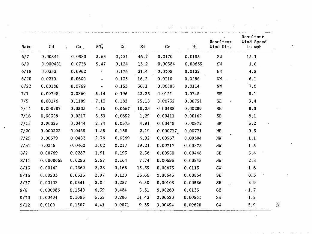
Date Cd . Cu. SO4 Zn Si Cr . Ni.Resultant Wind Dir.

Resultant Wind Speed

in mph

6/7 0.00844 0.0880 3.65 0,121 46.7 0.0170 0.0195 SW 15.16/9 0.000481 0.0738 5.47 0.124 13.2 0.00584 0.00635 SW 1.66/18 0.0353 0.0962 - 0.176 31.4 0.0105 0.0132 NW 4.56/20 0.0210 0.0600 - 0.133 16.2 0.0110 0.0286 NW 6.16/22 0.00186 0.0769 - 0.153 30.1 0.00808 0.0114 NW 7.07/1 0.00798 0.0860 5.14 0.196 43.25 0.0121 0.0145 SW 5.17/5 0.00146 0.1189 7,13 0.182 25.18 0.00732 0.00751 SB 9.47/14 0.000787 0.0533 4.16 0.0667 10.23 0.00485 0.00299 SB 8.07/16 0.00358 0.0317 3.39 0.0652 1.29 0.00411 0.00162 SB 8.17/18 0.00325 0.0444 2.74 0.0575 4.91 0.00448 0,00972 SW 5.27/20 0.000223 0.0469 1.88 0.130 2.19 0.000717 0.00771 NE 0.37/29 0.00379 0.0482 2.76 0.0569 6.92 0.00567 0.00304 NW 1.17/51 0.0245 0.0462 3.02 0,217 19.21 0.00717 0.00373 NW 1.58/2 0.00769 0.0287 1.91 0.193 2.56 0.00550 0.00448 SB 5.48/11 0.0000665 0.0293 2.57 0.164 7.74 0.00595 0.00848 NW 2.88/13 0.00142 0.1369 3.23 0.168 15.59 0.00675 0.0113 SW 1.68/15 0.00203 0.0516 2.97 0.120 13.66 0.00545 0.00864 SB 0.3 '8/17 0.00133 0.0541 3.0 • 0.287 6.50 0.00108 0.00586 SB 3.99/8 0.000883 0.1340 6.39 0.484 5.31 0.00260 0.0133 SB • 1.79/10 0,00404 0.1083 5.35 0.206 11.43 0.00620 0.00561 SW 1.59/12 0.0109 0,1507 4.41 0.0871 9.35 0.00454 0.00620 SW 5.9

Research Ranch, Arizona

(Air Pollution Monitoring Analyses*)

Resultant

Date Cd Cu SO4 Zn Si Cr NiResultant Wind Dir.f

Wind Speed in mph"i*

1/14 0.00081 0.0620 5,68 0.0968 3.0 0.00653 0.00288 SE 2.91/16 0.00147 0.0746 6.8 0.129 2.67 0.00488 0.000498 SE 5.31/18 0.00250 0.136 9.96 0.150 4.20 0.00234 0.000806 SW 3.41/27 0.00052 0.0338 9.52 0.0683 3.02 0.00122 0.000016 NW 4.81/29 0.00102 0.132 3.02 0.128 2.13 0.00146 0.00 SE 2.81/31 0.00283 0.137 6.05 0.175 3.50 0.00373 0.00468 SE 3.22/3 0.00259 0.187 9.39 0.257 8.53 0.0117 0.00311 NW 0.42/26 0.00325 0.117 3.23 0,174 6.13 0.00233 0.000178 SE 2.53/2 0.000490 0.0610 0.91 0.0952 4.13 0.00555 0.00250 SE 3.13/11 0.00431 0.148 7.84 0.160 2.30 0.00101 0.00186 NW 0.83/13 0.00348 0.179 11.24 0.149 3.36 0.00174 0.00106 NE 0.53/15 0.00100 0.0612 3.4 0.129 4.69 0.00119 0.00 SE 2.53/24 0.000017 0.0458 2.05 0.0683 2.29 0.000904 0.00 NW 1.13/26 0.00387 0.0772 1.31 0,0524 2.06 0.00162 0.00 SW 4.13/28 0.00408 0.0768 1.25 0.0390 9.80 0.00249 0.00 SW ■ 2.13/30 0.000724 0,0387 1.16 0.0670 3.23 0.00120 0.00 SW 4.5*Moyers (1974). "hl.S, Weather Service (1974).

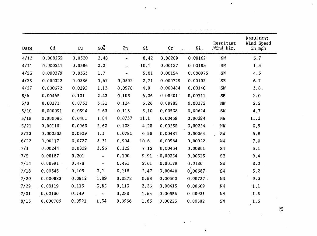
Date Cd Cu SO4 Zn Si

4/12 0.000235 0.0320 2.48 - 8.424/21 0.000241 0.0386 2.2 - 10.14/23 0.000379 0.0333 1.7 - 5.814/25 0.000322 0.0386 0.67 0.0592 2.714/27 0.000672 0.0292 1,13 0.0576 4.05/6 0.00465 0.131 2.43 0,103 6.265/8 0.00171 0.0733 3.51 0,124 6.265/10 0.000091 0.0594 2.63 0,113 5.105/19 0.000086 0.0461 1.04 0,0737 11.15/21 0.00110 0.0963 2.62 0.138 4.285/23 0.000335 0.0539 1.1 0.0781 6.586/22 0.00117 0.0727 3.31 0,994 10,67/1 0.00244 0.0829 3.56 0.125 7,157/5 0.00187 0.201 - 0.100 9.917/14 0.00591 0.478 - 0.451 2.017/18 0.00345 0.105 3.1 0.118 2.477/20 0.000883 0.0912 1.09 0.0872 0.687/29 0.00119 0.115 3.85 0.113 2.367/31 0.00130 0.149 . - 0,288 1.658/15 0.000706 0.0521 1.34 0.0956 1.63

ResultantResultant Wind Speed

Cr ......Ni Wind Dir. in mph

0.00209 0.00162 NW 3.70.00137 0.00183 sw 1.30,00154 0.000975 sw 4.30.000729 0.00102 SE 6.70.000484 0.00146 SW 3.80.00201 0.00111 SE 2.00.00285 0.00372 NW 2.20,00538 0,00624 SW 4.70,00459 0.00394 NW 11.20.00255 0,00254 NW 0.90,00481 0.00364 SW 6.80,00584 0.00922 NW 7.00,00434 0.00801 SW 5.10.00354 0.00515 SE 9.40.00179 0.0180 SE 8.00.00440 0.00687 SW 5.20.00500 0.00737 NE 0.30.00415 0.00609 NW 1.10.00355 0.00931 NW 1.50.00223 0.00502 SW 1.6

Date Cd Cu SO4 Zn Si Cr . NiResultant Wind Dir.

Resultant Wind Speed

in mph

8/15 0.000494 0.0374 0.95 0.0653 0,849 0.000 0.00365 SE 0.38/17 0.000454 0.0504 1.44 0.0641 1,57 0.00376 0.00411 SE 3.98/26 0.000979 0.0509 2.4 0.100 3,66 0.00593 0.00573 NW 0.28/28 0.000741 0.0533 2.42 0.0789 3.66 0.00532 0.00602 NW 1.98/30 0.00240 0.0454 1.78 0,110 3.60 0.00512 0.00837 NE 0.89/25 0.00905 0.510 7.03 0.471 4.41 0.00611 0.0155 SE 6.79/27 0.00140 0,0728 4.5 0.134 1.56 0.00367 0.00816 SW 3.810/6 0.00411 0.163 5.42 0.197 1,68 0.00362. 0.00661 NW 7.611/3 0.000225 0.0822 1.96 0,0425 0.717 0.000237 0.00223 SW 2.111/5 0.00372 0.145 4.97 0,0648 1,88 0.000578 0.00281 SW 0.911/7 0.00939 0.361 9.16 0.194 5.01 0.00169 0.00422 SE 9.111/9 0.00120 0.0700 2.26 0,0552 0,540 0.000780 0.00199 NW 2,911/18 0.00139 0.0314 1.23 0.0286 2.07 0.00113 0.00184 SW 3.111/20 0.00175 0.215 5.66 0.0781 2.40 0.000749 0.00232 SE 7.611/22 0.000021 0.153 7.28 0.0654 3,49 0.00212 0.00239 SW 2.712/1 0.00330 0.291 4.58 0.109 3,62 0.00175 0.00410 SE 4.612/3 ' 0.00441 0.132 4.3 0,0803 2,95 0.00427 0.00338 SE 5.512/5 0.00116 0.109 1.83 0.0488 1.01 0.00118 0.00243 SW 5.312/16 0.00114 0,137 3.16 0.101 1.91 0.00462 0.00378 SE • 3.112/18 0.00427 0.161 4.73 0.0734 6.89 0.00251 0.00268 SE 3.612/20 0.000602 0.0976 2.05 0.0353 3.49 0.00284 0.00317 SE 6.2

REFERENCES

Arizona Department of Health, 1969-1973, Particulate Monitoring Network Data, Environmental Health Services, Division of Air Pollution Control, 4019 N. 33rd Avenue, Phoenix, Arizona 85017.

Boyle, R. W., 1969, "The geochemistry of cadmium in the lead-zinc-silver deposits of the Keno Hill area, Yukon, Canada," in Problems of Geochemistry, ed. N. Khitarov, U.S. Department of Commerce, Clearinghouse for Federal Scientific and Technical Information, Springfield, Maryland, pp. 234-246.

Buchauer, M. M., 1973, "Contamination of soil and vegetation near a zinc smelter by zinc, cadmium, copper, and lead," Environ.Sci. and Technol., vol. 7, pp. 131-135.

Burnham, W. C., 1959, "Metallogenic provinces of the southwestern United States and New Mexico," New Mexico Bureau of Mines Research Bull. 65.

Cannon, H. L., and B. M. Anderson, 1971, "The geochemist's involvement with the pollution problem," in Environmental Geochemistry in Health and Disease, Geol. Soc. Amer, Memoir 123, pp. 155-177.

Colovos, G., G. S. Wilson, and J. L. Moyers, 1974, "Particle size deter­mination of trace elements in urban air," Intern. J. Envir.Anal. Chem., vol. 3, pp. 239-252.

Erlenkeuser, H., E. Suess, and H. Willkomm, 1974, "Industrializationaffects heavy metal and carbon isotope concentration in recent Baltic Sea sediments," Geochim. Cosmochim. Acta, vol. 38, pp. 823-842.

Fassett, D. W., 1972, "Cadmium," in Metallic Contaminants and HumanHealth, ed. D. H. K. Lee, Academic Press, New York, pp. 98-117.

Flick, D. F., H. F. Kraybill, and J. M. Dimitroff, 1971, "Toxic effects of cadmium: A review," Environ. Res., vol. 4, pp. 71-85.

Friberg, L., M. Piscator, and G. Nordberg, 1971, Cadmium in the Environ­ment , CRC Press, Ohio,

________ , 1973, Cadmium in the Environment II, U.S. Environmental Pro­tection Agency report - EPA-R2-75-190.

85

86

-f' •

Furst, A., 1971, "Trace elements related to specific chronic diseases: Cancer," in Environmental Geochemistry in Health and Disease, eds. H. L. Cannon and H. C. Hopps, Geol. Soc. Amer. Memoir 123, pp. 109-130.

Hoel, P. G,, 1974, Introduction to Mathematical Statistics, John Wiley, New York, pp. 89-92.

Ivanov, V. V., 1961, "Geochemistry of cadmium in the deposits of the Peputalskay group," Abs., Geokhimiya, no. 2, pp. 168-174.

John, M. K., H. H. Chuah, and C, J, Van Laerhoven, 1972, "Cadmium con­tamination of soil and its uptake by oats," Environ. Sci. and Technol., vol. 6, pp, 555-557,

Keller, W. D., 1970, "Geologic materials as sources of biologic nutrient elements," in Trace Substances in Environmental Health III, ed. D. D. Hemphill, University of Missouri, pp. 3-19.

Kellogg, W. W., R. D. Cadle, E. R. Allen, A. L, Lazrus, and E. A.Martel1, 1972, "The sulfur cycle," Science, vol. 175, pp. 587-596.

Kendrey, G., and F. J. C. Roe, 1969, "Cadmium toxicology," Lancet, vol. 1, pp, 1206.

Kneip, T. J., M. Eisenbud, C. Strehlow, and P. Freundenthal, 1970, "Airborne particulates in New York City," J. Air Poll.Control Assoc., vol. 20, pp. 144-149.

Krauskopf, K., 1967, Introduction to Geochemistry, McGraw Hill, New York, pp. 128-138, 643,

Krumbein, W. C., and F. A. Graybill, 1965, An Introduction to Statisti- cal Models in Geology, McGraw Hill, New York, pp. 234-245.

Lee, D. H. K., ed., 1972, Metallic Contaminants and Human Health, Academic Press, New York.

Maiin, M. H., 1971, "Metals focus shifts to cadmium," Environ. Sci. and Technol., vol. 5, pp. 754-755,

Marowsky, G,, and K. H. Wedepohl, 1971, "General trends in the behavior of Cd, Hg, Tl, and Bi in some major rock forming processes," Geochim. Cosmochim. Acta, vol. 35, pp. 1255-1267.

McCaull, J., 1971, "Building a shorter life," Environment, vol. 13, pp. 3-15.

87

Moore, L., 1972, ’’Mineral industry in Arizona,” U.S. Bureau of Mines Mineral Yearbook, U.S, Dept, of the Interior, pp. 1-25.

Moyers, J. L., 1974, unpublished data. Atmospheric Analysis Laboratory, Department of Chemistry, University of Arizona, Tucson.

National Bureau of Standards, 1974, Office of Standard Reference Mate­rials, Institute for Material Research, Washington, D.C. 20234.

Paus, P. E,, 1972, "Bomb decomposition of biological materials," Atomic Absorption Newsletter, vol. 11, p, 129.

Perkin-Elmer, 1971, Manual: Analytical Methods for Atomic AbsorptionSpectrophotometry, Norwalk, Connecticut,

Perry, H. M., 1968, "Hypertension and trace metals, with particular emphasis on cadmium," in Trace Substances in Environmental Health II, ed. D, D. Hemphill, University of Missouri, pp. 101-125.

_______ , 1971, "Trace elements related to cardiovascular disease," inEnvironmental Geochemistry in Health and Disease, eds. H. L. Cannon and H. C. Hopps, Geol. Soc. Amer. Memoir 123, pp. 179-195.

Petit, M., 1973, "Analysis of stratified vertebrate excretions as a method of obtaining a chronological record of environmental chemicals in mammalian food chains," reported at meeting of The Arizona Academy of Science, May 4-5, 1973, University of Arizona, Tucson, Arizona,

Rantala, R, I. T., and D, H. boring, 1973, "New low-cost Teflon decompo­sition vessel," Atomic Absorption Newsletter, vol, 12, pp. 97-99.

Ranweiler, L. E., and J. L, Moyers, 1974, "Atomic absorption procedure for analysis of metals in atmospheric particulate matter," Environ. Sci. and Technol., vol. 8, pp. 152-156.

Rubeska, I., 1968, "The determination of trace elements in sulfidematerials by atomic absorption spectrophotometry with absorp­tion tubes," Anal. Chim. Acta, vol. 40, pp. 187-194.

Ruck, R., H. Gluskoter, and N. Shimp, 1973, "Occurrence and distribution of potentially volatile trace elements in coal: An interimreport," Environ. Geol. Notes 61, Illinois State Geol. Survey,p. 6.

Sandstead, H. H., 1974, "Cadmium, zinc, and lead," Geochemistry and the Environment, vol. 1, National Academy of Sciences, pp. 43-56.

88

Gangster, D. E., 1968, "Some chemical features of lead-zinc deposits in carbonate rocks," Geol. Survey of Canada Paper 68-39.

Sauer, H. I., and F. R. Brand, 1971, "Geographic patterns in the risk of dying," in Environmental Geochemistry in Health and Disease, eds. H. L. Cannon and H. C. Hopps, Geol. Soc. Amer. Memoir 123, p. 145.

Schacklette, H. T., 1972, "Cadmium in plants," Geol. Survey Bull. 1314-G.

Schroeder, H. A., 1973, The Trace Elements and Man, Devin-Adair, Connect­icut, pp. 97-114.

Schroeder, H, J., 1965, "Cadmium: Mineral facts and problems," U.S.Dept, of the Interior, Bureau of Mines Bull. 630, p. 165.

Science News, 1975, "Cancer and chemicals: Risks mapped," vol. 107,May 3rd.

Sutulov, A., 1974, Copper Porphyries, University of Utah Press, Salt Lake City, p. 108.

Taylor, S. R., 1964, "Abundance of chemical elements in the continental crust: A new table," Geochim, Cosmochim. Acta, vol. 28,pp. 1273-1285.

Tucker, A., 1972, The Toxic Metals, Earth Island Ltd., London, pp. 174-207.

University of Missouri, 1972, "Study of lead, copper, zinc, and cadmium contamination of food chains of man," U.S. Environmental Protec­tion Agency report - EPA-R3-73-034.

Urone, P., H. Lutsep, C. M. Noyes, and J. F. Parcher, 1968, "Staticstudies of sulfur dioxide reaction in air," Environ. Sci. and Technol., vol. 2, pp. 611-618.

U.S. Weather Service, 1974, Local Climatological Data-Tucson, Inter­national Airport, Tucson, Arizona.

Waldbott, G. L., 1973, Health Effects of Environmental Pollutants,C. V. Mosby, St. Louis, pp. 161-164.

0240635&0