c4 revision notes

7/31/2019 C4 Revision Notes

http://slidepdf.com/reader/full/c4-revision-notes 1/15

Partial Fractions

An algebraic fraction such as can be broken down into simpler parts

called partial fractions so that it is in the form

Once a fraction has been split into its constituents, it can be used in integration and

binominal theorem.

Splitting Into Partial Fractions

Partial Fractions can be split up in two ways: substitution or equating coefficients.

Substitution:

This is used for general algebraic fractions with two or three factors, without a

repeated denominator.

1. The first step in this process would be to make the algebraic fraction equal

partial fractions with all possible denominators, A and B as constant numerators.

2. Multiply the numerator of A, by the denominator of B. Then make these equal

to the numerator of the original expression. It will now be in the form of

3. Substitute in values of x that will make one of the brackets zero. Then use this to

work out the value of A and B. Then replace them as the numerators and you

have your partial fractions.

Equating Coefficients:

This follows the same first two steps as substitution, however sometimes,

substitution will not work. In this case, you can equate the coefficients of x and the

constants to work out A and B.

1. Follow the first two steps of substitution

2. Expand the brackets so that you end up with something in the form

3. Make the coefficient of x equal to (A+B)x. This gives you one simple equation.

4. Do the same thing for the constants (A-3B) and the constant on the end of the

original expression. You now have two simple equations that can be solved using

simultaneous equations.

Both of these techniques can be used when the fraction has more than two factors

(ie. use A, B and C) or one that has a repeated linear factor.

An algebraic fraction is improper when the degree of the numerator is equal to,

or larger than, the degree of the denominator. An improper fraction must be

divided first to obtain a number and a proper fraction before it can be expressed

as partial fractions



Co-ordinate Geometry

A parametric equation of a curve is one which does not give the relationship

between x and y directly but rather uses a third variable, typically t, to do so. Thethird variable is known as the parameter. A simple example of a pair of parametric

equations: x = 5t + 3

y = t2

+ 2t

Converting to Cartesian

You need to be able to find the Cartesian equation of the curve from parametric

equations, that is the equation that relates x and y directly. To do this you need to

eliminate the parameter. The easiest way to do this is to rearrange on parametric

equation to get the parameter as the subject and then substitute this into the other

equation.

A circle with an origin (a, b) has the parametric equations:

You can use the result to derive these. As before, θ is the

parameter instead of t in the equations. You need to be able to recognise these as

parametric equations of circles in the exam.

Integration

To find the area under a parametric curve, you integrate y and multiply it by the

differential of the x equation.

Differentiation

To differentiate a set of parametric equations, differentiate them separately and

divide the differential of y by the differential of x.



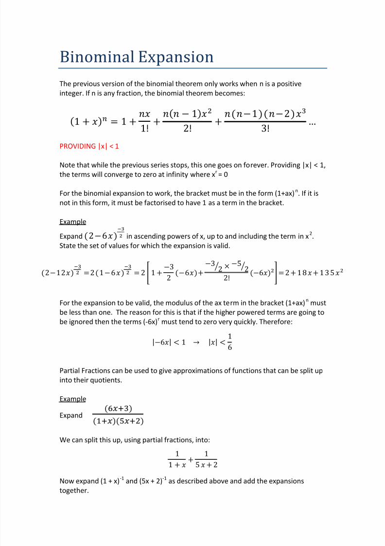
Binominal Expansion

The previous version of the binomial theorem only works when n is a positive

integer. If n is any fraction, the binomial theorem becomes:

PROVIDING |x| < 1

Note that while the previous series stops, this one goes on forever. Providing |x| < 1,

the terms will converge to zero at infinity where xr= 0

For the binomial expansion to work, the bracket must be in the form (1+ax)n. If it isnot in this form, it must be factorised to have 1 as a term in the bracket.

Example

Expand in ascending powers of x, up to and including the term in x2.

State the set of values for which the expansion is valid.

⁄ ⁄

For the expansion to be valid, the modulus of the ax term in the bracket (1+ax)n

must

be less than one. The reason for this is that if the higher powered terms are going to

be ignored then the terms (-6x)r

must tend to zero very quickly. Therefore:

|| || Partial Fractions can be used to give approximations of functions that can be split up

into their quotients.

Example

Expand

We can split this up, using partial fractions, into:

Now expand (1 + x)-1 and (5x + 2)-1 as described above and add the expansions

together.



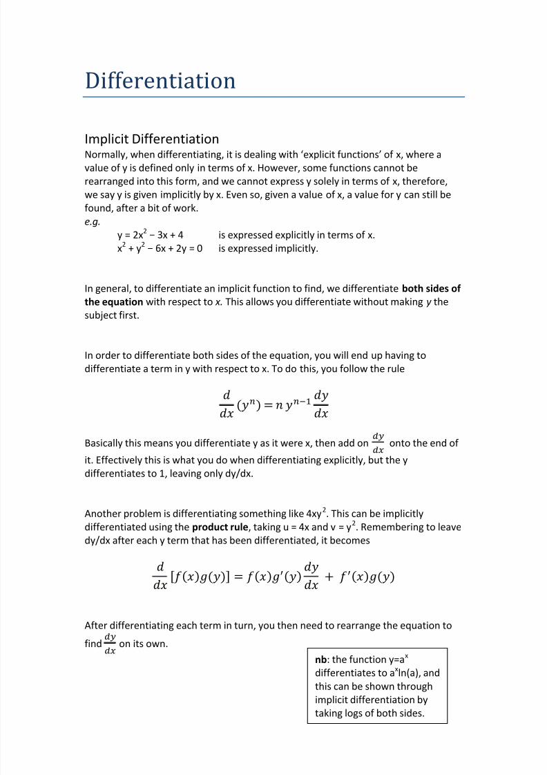
Differentiation

Implicit DifferentiationNormally, when differentiating, it is dealing with ‘explicit functions’ of x, where a

value of y is defined only in terms of x. However, some functions cannot be

rearranged into this form, and we cannot express y solely in terms of x, therefore,

we say y is given implicitly by x. Even so, given a value of x, a value for y can still be

found, after a bit of work.

e.g.

y = 2x2 − 3x + 4 is expressed explicitly in terms of x.

x2

+ y2 − 6x + 2y = 0 is expressed implicitly.

In general, to differentiate an implicit function to find, we differentiate both sides of

the equation with respect to x. This allows you differentiate without making y the

subject first.

In order to differentiate both sides of the equation, you will end up having to

differentiate a term in y with respect to x. To do this, you follow the rule

Basically this means you differentiate y as it were x, then add on onto the end of

it. Effectively this is what you do when differentiating explicitly, but the y

differentiates to 1, leaving only dy/dx.

Another problem is differentiating something like 4xy2. This can be implicitly

differentiated using the product rule, taking u = 4x and v = y2. Remembering to leave

dy/dx after each y term that has been differentiated, it becomes

After differentiating each term in turn, you then need to rearrange the equation to

find on its own.

nb: the function y=ax

differentiates to axln(a), and

this can be shown through

implicit differentiation by

taking logs of both sides.



Parametric Differentiation

When a curve is described by parametric equations:

1. You differentiate x and y with respect to the parameter t.

2. Then you use the chain rule in the rearranged form

Differentiating ax

This function describes growth and decay, and its derivative gives a measure of the

rate of change of this growth/decay.

Since , taking logs of both sides gives . Using implicit

differentiation to differentiate :

This result needs to be learn, and is not given in the formula sheet.

Setting up Differential EquationsYou can set up simple differential equations from information given in context. This

may involve using connected rates of change, or ideas of proportion.

e.g. “Newton’s Law of Cooling states that the rate of loss of temperature is

proportional to the excess temperature of the body compared to its surroundings.

Write an equation that expresses this law ”

Let the temperature of the body be , and the time be t seconds. This means (-o)

is the difference in temperature. From the law, we can deduce

Whenever there is a proportional relationship, a constant k can be used to replace

the proportionality sign (-k if the relationship decreases). So in answer to the

question, the equation that expresses this law is .

Connected Rates of Change can also be used when setting up differential equations.

To do this, you would set up two normal equations. Differentiate each one seperatly

and then connect them to find a third differential equation by using the chainrule/connected rates of change.



Connected Rates of Change

The gradient function of a curve measures the rate at which the curve increases

or decreases.

Many questions in mathematics involve finding rates at which they change. These

can be connected using the chain rule. These types of questions involve

differentiation. Usually they involve differentiating with respect to time.

The key to doing these problems is to identify three components and write them

down mathematically:

What you are given

What is required

What is the connection between the two items above. (Sometimes the chain

rule must be used to establish a connection).

Example:

‘ A pebble is dropped into a pond and forms ripples. The radius of this increases by

3cm per minute. What is the rate of change of area when the ripple is 15cm in

radius? ’

We are given a relationship between radius and time, and area and radius. From this,

we need to find a relationship between area and time, input values from the two

relationships given, to find a value for the third relationship.

From the second sentence, comparing radius to time is equal to an increase of 3:

Using the formula for the area of a circle:

We now have two differential equations that can be used along with the chain rule

to find the rate of change of area at 15cm.



Integration

Much of the integration outlined below relies on the reverse chain rule. When

functions are differentiated using the chain rule, they are multiplied by thedifferential inside the bracket. Therefore when integrating, the reverse chain rule

means that you must divide by the differential inside the bracket (ie perform the

inverse operation).

This technique only works for linear transformations such as .

In general, the reverse chain rule for linear functions is:

Using the reverse of the chain rule, the following generalisations can be found:

| |



Integration By SubstitutionAs the name of the method suggests, we proceed by making an algebraic

substitution. The aim is to replace every expression involving x in the original

problem with an expression involving u.

Let u = part of the expression, usually the part in brackets or the denominator

If necessary, express other parts of the function in terms of u

Differentiate u to find ⁄

Re-arrange to find dx in terms of du as we need du and dx if we are to integrate

an expression in u, i.e we need to find du/dx dx = … du

Substitute the expression found above for dx , back into the original integral and

integrate in terms of du

It should now be reasonably easy to integrate u

If necessary, use u=f(x) to change the values for the limits of integration

Put your x ’s back in again at the end and finish up.

Example

Suppose we wish to find ∫

We make the substitution .

The integral becomes ∫

The limits of integration have been explicitly written the variable given to emphasise

that those limits were on the variable x and not u. We can write these as limits on u

using the substitution . Clearly, when , and when .

With the new limits, the function we need to integrate is:

[

]

* + *

+

Note that in this example there is no need to convert the answer given in terms of u

back into one in terms of x because we had already converted the limits on x intolimits on u.



Integration By PartsFunctions often arise as products of other functions, and we may be required to

integrate these products. For example, we may be asked to determine ∫ .

Here, the integrand is the product of the functions and . A rule exists for

integrating products of functions, the reverse of the product rule – integration byparts.

The formula is derived by rearranging the product rule and integrating both sides.

Care must be taken over the choice of and ⁄ . The aim is to ensure that it is

simpler to integrate than

. So choose to be easy to differentiate and

to be

easy to integrate.

Generally, this means choose u to be the simpler of the two functions. The exception

to this rule is when integrating . In this case, would have to equal u, as there

is no standard integral, meaning it has to be differentiated instead as u.

Sometimes it needs to be used twice within one expression as the second part of the

formula will set up another equation that needs to be integrated by parts.

Alternatively, if it gives the same answer as the original equation you are trying to

integrate, move it to the other side of the equals sign, and use the fact that

Numerical IntegrationThe trapezium rule provides you with a way to estimate the value of an integral youcannot do. It involves splitting the area under the under up into trapeziums which

are then totalled to give an estimate for the area.

The trapezium rule is as follows:

Increasing the number of trapeziums will improve the accuracy of this method. The

error can be worked out by finding the difference in the true value and theapproximation, and dividing this by the true value.

When using integration by parts, decide which part will be which, the integrate so

that you know u, v, du/dx and dv/dx

Then plug them into the formula, and solve using limits where given.



Volumes of Revolution

We sometimes need to calculate the volume of a solid which can be obtained by

rotating a curve about the x-axis. There is a straightforward technique which enables

this to be done, using integration.

Imagine that the part of a curve between the coordinates x = a, and x = b, is rotatedabout the x-axis through 360◦

. The curve would then map out the surface of a solid

as it rotated. Such solids are called solids of revolution. The formula to work out the

volume of these solid is:

Sometimes, the equation of the curve may be given parametrically. You can

integrate in terms of the parameter by changing the variable in a similar way to that

used when integrating by substitution.

Differential EquationsIn general a differential equation may have x and y terms on both sides, but if the

equation is of a certain form , we can rearrange to have all

terms including x on the right hand side and all terms including y on the left hand

side. This is called separation of variables. This would leave us with

Both sides of the equation can now be integrated

Technically

is not a fraction, but can often be handled as if it were one.

Integrating both sides would normally give rise to a constant of integration on both

sides, but convention has it that these are combined into one. When integrating

gives an equation in the form of logs, the +C is often denoted by , which can then

be manipulated algebraically like the other terms.

A particular solution is found when certain conditions are assumed, called the

starting conditions, and the constant of integration can be calculated.



Vectors

A scalar has magnitude only. e.g. length or distance, speed, area, volumes.

A vector has magnitude AND direction. e.g. velocity, acceleration, momentum.Moving from point A to B is called a translation, and the vector a translation vector.

The length of the line in the diagram represents the

magnitude of the vector and vectors are equal if the

magnitude and direction are the same.

Vectors are parallel if they have the same direction and

are scalar multiples of the original vector. e.g. the

vector 3b is parallel to the vector b.

The vector −2b is 2 times the magnitude of b and in the

opposite direction.

Adding two vectors means finding the shortcut of their

journeys. This is the same as making one translation

followed by another.

c = a + b

If , then

The modulus of a vector is another name for its magnitude.

The modulus of vector a is written || The modulus for vector is written as ||

You can calculate the length using Pythagoras’s theorem:

√



Position VectorsPosition vectors are the vector equivalent of a set of co-ordinates. The position

vector allows a translation vector to be fixed in space, using the origin as its fixed

reference point. The position vectors of a point A, with co-ordinates (5, 2), is the

vector which takes you from the origin to the point (5, 2). So the co-ordinates of point A are the same as the translation vector from point O to A.

∴ position vector of (5, 2) ()

Scalar Multiplication of Vectors

If

, and

is a constant number, then

The constant k is called a scalar because it ‘scales up’ the length of the vector.

If , then the two vectors will look like this:

Vectors are parallel if one is a scalar multiple of the other.

If ( ), and (), then a and c are parallel because ()

Any vector parallel to the vector a may be written as λ a, where λ is a non-

zero scalar.



The Unit VectorsA unit vector is a vector with magnitude (or modulus) of 1.

Any vector can be given as a multiple of

()

or

()

In 2-D the unit vectors are i and j. They are parallel to the x-axis and the y-axis, and

in the direction of x increasing and y increasing respectively, where:

() and ()

You can write a vector with Cartesian components as a column matrix:

The modulus (or magnitude) of is √

The distance between two points is √

In 3-D the unit vectors are i, j and k. Cartesian coordinate axis in three dimensions

are usually called the x, y and z axes, each being at right angles to each other.

Any vector can be written in terms of i, j and k.

The modulus (or magnitude) of is √

The distance between two points is

√



Scalar (Dot) Product

This is where two vectors are multiplied together. One form of multiplication is the

scalar product. The answer is interpreted as a single number, which is a scalar. This is

also known as the ‘DOT’ product, where a dot is used instead of a multiplication sign. The scalar product between two vectors a and b is defined as the size of a multiplied

by the size of b and the cosine of the angle between them.

There are two methods that can be used to calculate the scalar product:

1. ||||

Where

is the angle between a and b, and the two vectors are pointing away from

their intersection.

f two vectors are perpendicular, the angle between them is . This means that|||| .

The non-zero vectors a and b are perpendicular if and only if

Also, because

,

If a and b are parallel, ||||, and in particular ||

2. If and , then

If p and q are parallel then q = 0, ∴ and | | | | If p and q are perpendicular then q = 90, ∴ and

If p · q = 0, then either | p | = 0, | q | = 0 or p and q are perpendicular



Vector Equations of Straight LinesSuppose a traight likne passes through a given point A, with a position vector a, and

is parallel to the given vector b. Only one such line is possible.

Vectors an be used to describe straight lines, by giving one vector to show a point on

the line, then another to show its gradient and the direction.

A vector equation of a straight line passing through the point A with position vector

a , and parallel to vector b is

where t is a scalar parameter

By taking different values of the paramater t, you can find the position vectors of

points that lie on the straight line.

The vector equation of a line that passes through two points A & B can be found.

Here, we have two possible vectors that could be used as

position vectors (a and b), and the vector as the

direction vector. This can be denoted by – . This

means that the equation of the vector is .

A vector equation of a straight line passing through the

points A and B with position vectors a and b respectively,

is

An alternative form of the vector equation of a straight line is if

and then

Lines do not often intersect in 3-D, but if they do, you need to equate the x, y and z

components, and use simultaneous equations to check that they are all equal. The

values of x, y and z will show the coordinates at which they intersect. For this to

work, they should have different parameters, and be in the 3rd form shown above.

Also, if a line meets in 2-D, but not in 3-D, it is called skew.

c4 revision notes

Documents