ASC Report No. 30/2014

C++11 Implementation of Finite

Elements in NGSolve

J. Schöberl

Institute for Analysis and Scienti�c Computing �

Vienna University of Technology � TU Wien

www.asc.tuwien.ac.at ISBN 978-3-902627-05-6

Most recent ASC Reports

29/2014 A. Arnold and J. Erb

Sharp entropy decay for hypocoercive and non-symmetric Fokker-Planck equa-tions with linear drift

28/2014 G. Kitzler and J. Schöberl

A high order space momentum discontinuous Galerkin method for the Boltz-mann equation

27/2014 W. Auzinger, T. Kassebacher, O. Koch, and M. Thalhammer

Adaptive splitting methods for nonlinear Schrödinger equations in the semiclas-sical regime

26/2014 W. Auzinger, R. Stolyarchuk, and M. Tutz

Defect correction methods, classic and new (in Ukrainian)

25/2014 J.M. Melenk and T.P. Wihler

A posteriori error analysis of hp-FEM for singularly perturbed problems

24/2014 J.M. Melenk and C. Xenophontos

Robust exponential convergence of hp-FEM in balanced norms for singularlyperturbed reaction-di�usion equations

23/2014 M. Feischl, G. Gantner, and D. Praetorius

Reliable and e�cient a posteriori error estimation for adaptive IGA boundaryelement methods for weakly-singular integral equations

22/2014 W. Auzinger, O. Koch, and M. Thalhammer

Defect-based local error estimators for high-order splitting methodsinvolving three linear operators

21/2014 A. Jüngel and N. Zamponi

Boundedness of weak solutions to cross-di�usion systems from population dy-namics

20/2014 A. Jüngel

The boundedness-by-entropy principle for cross-di�usion systems

Institute for Analysis and Scienti�c ComputingVienna University of TechnologyWiedner Hauptstraÿe 8�101040 Wien, Austria

E-Mail: admin@asc.tuwien.ac.at

WWW: http://www.asc.tuwien.ac.at

FAX: +43-1-58801-10196

ISBN 978-3-902627-05-6

c© Alle Rechte vorbehalten. Nachdruck nur mit Genehmigung des Autors.

ASCTU WIEN

C++11 Implementation of Finite Elements in NGSolve

Joachim Schoberl

September 26, 2014

Abstract

We discuss an object oriented design of finite element core functionality. It allows toseparate the mathematical definition of the finite element basis functions, the efficient im-plementation of operations, and the calculation of stiffness matrices and residual vectors.

We show how features of the C++11 programming language help to reduce codecomplexity and thus allow for additional performance optimization such as vectorization.

The presented techniques are implemented in the open source finite element packageNGSolve.

1 Introduction

The finite element method is the major numerical method for the numerical approximationof partial differential equations [6]. While continuous finite element methods fit well forelliptic and parabolic equations, discontinuous Galerkin methods are particularly efficient forhyperbolic equations [12]. The combination of local mesh refinement and variable distributionof polynomial orders lead to highly accurate hp-finite element methods, see [29, 27, 14, 8, 12].

Efficient coding of hp-FEM is a challenging endeavor. Here, the sophisticated use ofmodern programming languages such as C++ helps a lot. It allows to express the mathe-matical concepts directly in computer programs. Since its beginning, the C++ programminglanguage allows to combine high performance computing with object oriented design. In par-ticular, template-based compile time polymorphism [30, 31, 3] allows generic programmingwithout performance penalties. Recent C++ language developments have been combined inthe new standard C++11. It is included in the latest version of Stroustrup’s textbook [28].Citing Stroustrup from http://www.stroustrup.com/C++11FAQ.html: Surprisingly, C++11feels like a new language: The pieces just fit together better than they used to and I find ahigher-level style of programming more natural than before and as efficient as ever.

There are several widely used open source finite element packages available: DUNE [4]with its module DUNE-FEM [7], deal.II [2], Life [23] which evolved into Feel++ [24], Elmer[19], FEMSTER [5], Freefem++ [11], 3Dhp[9]. The techniques presented in the current workare implemented in the finite element library NGSolve [25], version 5.3. We mention thespecial purpose compilers FIAT [15] and the framework FEniCS [18], which produce machinecode directly from the mathematical formulation of finite elements.

This paper discusses the core functionality of finite element routines, namely the evaluationof and operations with shape functions and its derivatives. The element matrix and elementvector calculation routines have to compute all basis functions. When computing residualsof non-linear problems, evaluating operators for instationary equations, or even when solvinglinear problems in a matrix free way, one needs the evaluation of finite element functions in

1

class FiniteElement {int ndof ; // number o f b a s i s f u n c t i o n sint order ; // h i g h e s t po lynomia l order

public :int GetOrder ( ) { return order ; }int GetNDof ( ) { return ndof ; }virtual ELEMENT TYPE GetElementType ( ) = 0 ;virtual s t r i n g GetElementName ( ) = 0 ;

} ;

Listing 1: class FiniteElement

the integration points. In addition, gradients are needed, and the transpose operations. Weaim in optimizing these functions, while keeping the code structure transparent.

One new key feature of C++11 are lambda functions, which are used here as follows:The specific finite element class implements shape functions. The functionality layer classesimplement what to do with these shape funcitons. These operations are specified as lambdafunctions, and are applied to the shape functions. Mathematically speaking, a lambda func-tion is an element of the dual space. The techniques presented in the current work have beenimplemented within the standard C++ programming language using classes before. But, thenew C++11 syntax allowed the simplification of a large portion of the code. The C++11syntax is supported by the major compilers at time of writing this work.

Modern microprocessors can perform several operations of the same type simultaneously(SIMD - single instruction multiple data), even within one core. Now very popular and low-cost general purpose GPU devices can even compute with typically 32 synchronous threadsper processor core. These processor architecture is very well suited for performing equivalentoperations in many integration points. But, while computing power is increasing very fast,the access to memory, and even caches, becomes more and more a bottleneck. The GPUcores even have only a small number of registers as fast local memory. Thus, it is a primarygoal to eliminate the need of temporary memory.

2 Finite elements and element matrix integration

The NGSolve finite element class hierarchy is drawn in Figure 1. The base class for all finiteelements is FiniteElement, see Listing 1. It provides the common functionality of all finiteelements. It stores the number of basis functions, and the maximal polynomial degree asclass members and provides query functions to them. In addition, it provides a query to theelement-type (ET QUAD, ET HEX etc.) as well as the name of the element which is useful fordebugging.

The next level in the class hierarchy specifies the type of the finite element, and the spacedimension via a template argument. For second order elliptic equations we need continuous,scalar valued basis functions. The element provides the basis functions on the referenceelement, and also the gradients of them. Other types of elements are vectorial finite elements,which are conforming in H(curl) or H(div), and are needed for solving electromagnetic fieldproblems and some flow models. These elements must compute the vector-valued shape

2

H1HighOrderFE<ET_TRIG>

T_CalcShape()

FiniteElement

GetNDof() : intGetOrder() : intGetElementType() : ELEMENT_TYPE

L2HighOrderFE<ET_TET>

T_CalcShape()

DIM : intHDivFiniteElement

CalcShape()CalcDivShape()

H1HighOrderFE<ET_QUAD>

T_CalcShape()

FELT_ScalarFiniteElement

CalcShape()CalcDShape()

DIM : intHCurlFiniteElement

CalcShape()CalcCurlShape()

DIM : intScalarFiniteElement

CalcShape()CalcDShape()Evaluate()EvaluateGrad()

Diagram: FiniteElement Page 1Figure 1: FiniteElement class-diagram The root is the common base class FiniteElement.The user works with the second level, for example a three-dimensional H(curl) finite elementHCurlFiniteElement<3>. The third level is the implementation of functionality, includingspecial hardware tuning. The fourth level implements the specific finite element shape func-tions.

3

template <int DIM>class Sca larF in i t eE lement : public FiniteElement {public :

virtual void CalcShape ( const In t eg ra t i onPo in t & ip ,FlatVector<double> shape ) = 0 ;

virtual void CalcDShape ( const In t eg ra t i onPo in t & ip ,FlatMatrixFixWidth<DIM, double> dshape )=0;

. . .} ;

Listing 2: ScalarFiniteElement

functions, and the curl or divergence of them.Element matrix calculation and similar functions work with the abstract intermediate

class ScalarFiniteElement<DIM> (see Listing 2) without knowing the particular finite ele-ment class provided. Here, we use the traditional C++ run-time polymorphism via virtualfunctions. The FlatVector template class is a cheap implementation of a vector in the senseof linear algebra. It only contains the vector-size and the data pointer. The constructor justcopies the pointer (and no data), the destructor does not free any memory. Thus, a callby value argument is efficient for a FlatVector, and similar for the FlatMatrixFixWidth, amatrix with fixed width. Fixing the width at compile-time helps the compiler optimizing theindex calculation.

A simple implementation of element matrix calculation for the Laplace operator is given inListing 3. The input is a finite element object, and the transformation from reference elementto physical element. It computes the element matrix, which is already allocated by the caller.The LocalHeap is a class providing fast allocation of temporary small memory blocks. Thewhole memory is freed after finishing each element.

Since the common argument of the virtual function CalcElementMatrix must be the baseclass FiniteElement, and we know we are dealing with scalar elements in DIM dimensions, wecan cast up to that class. The IntegrationRule provides a numerical integration formula onthe reference element of given geometry and order. The bracket operator applied to it deliversan integration-point, which contains the coordinates on the reference-element as well as theintegration weight. In the loop over integration points we compute the mapped integrationpoint and the Jacobian from the abstract element transformation. Next we compute thematrix of shape function gradients on the reference element. The push-forward is computedby a matrix-matrix product with the inverse Jacobian. Finally, we update the matrix by amatrix-matrix product. The linear algebra is based on an own implementation of expressiontemplates [30, 31, 10]. The dominant costs are the last matrix-matrix product. It is reducedby unrolling the integration loop and combining a few integration points such that the innerdimension of the matrix-matrix product increases.

The FESpace is the instance generating the specific finite element object, see Listing 4.It has access to the mesh data structure. A particular class derived from FESpace isH1HighOrderFESpace, which provides an arbitrary order finite element sub-space of theSobolev-Space H1. The virtual function GetFE allocates an object of the specific H1-conforming finite element of given order. For performance reasons, the allocation is on theLocalHeap. Global element vertex numbers are provided to the element for consistent ori-

4

template <int DIM> void Lap lac e In t eg ra to r : :CalcElementMatrix ( const FiniteElement & b a s e f e l ,

const ElementTransformation & tra fo ,Matrix<> & elmat , LocalHeap & lh )

{const Sca larFin i teElement<DIM> & f e l =

static cast<const Sca larFin i teElement<DIM>&> ( b a s e f e l ) ;In t eg ra t i onRu l e i r ( f e l . GetElementType ( ) , 2∗ f e l . GetOrder ( ) ) ;MatrixFixWidth<DIM, double> dshape ( f e l . GetNDof ( ) , lh ) ;MatrixFixWidth<DIM, double> dshape r e f ( f e l . GetNDof ( ) , lh ) ;

elmat = 0 . 0 ;for ( int i = 0 ; i < i r . S i z e ( ) ; i++){

MappedIntegrationPoint<DIM,DIM> mip( i r [ i ] , t r a f o ) ;f e l . CalcDShape ( i r [ i ] , d shape r e f ) ;dshape = dhape re f ∗ mip . GetJacobianInverse ( ) ;double f a c t o r = i r [ i ] . Weight ( )∗mip . GetMeasure ( ) ;elmat += fac ∗ dshape∗Trans ( dshape ) ;

}}

Listing 3: Element matrix calculation

entation of edge- and face-bubble functions. The template class H1HighOrderFE is a derivedclass from ScalarFiniteElement.

3 Element functionality

The template class H1HighOrderFE<ELEMENT TYPE> implements shape functions for the par-ticular element geometries. The CalcShape method computes all shape functions in a givenpoint, and CalcDShape computes the matrix of shape function gradients. Additional functionshelp to speed up certain finite element computations.

Our approach is to implement just one template function T CalcShape which is able tocompute shapes, gradients, etc. This is obtained by keeping the variable types generic. Sub-stituting the template arguments defines the particular operation. The operation is providedby the intermediate class T ScalarFiniteElement in Listing 7.

Finite elements for H1 require basis functions connected with vertices, edges, faces (3Donly), and cells. Typically, these blocks are built from Legendre and Jacobi orthogonalpolynomials. An L2-orthogonal basis on simplices is provided via the Dubiner-Basis [14]

Basis functions of total order p for the triangle are given in terms of barycentric coordi-nates λ:

Vertex basis: ϕV = λV

Edge basis: ϕE,i = λE1λE2PSi (λE1 − λE2 , λE1 + λE2) 0 ≤ i ≤ p− 2

Cell basis: ϕT,ij = λ1λ2λ3PSi (λ1 − λ2, λ1 + λ2)P

(0,2i+1)j (2λ3 − 1) i+ j ≤ p− 3

5

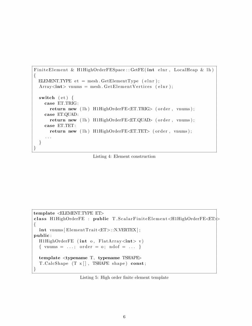
FiniteElement & H1HighOrderFESpace : : GetFE( int e lnr , LocalHeap & lh ){

ELEMENT TYPE et = mesh . GetElementType ( e l n r ) ;Array<int> vnums = mesh . GetElementVert ices ( e l n r ) ;

switch ( e t ) {case ET TRIG :

return new ( lh ) H1HighOrderFE<ET TRIG> ( order , vnums ) ;case ET QUAD:

return new ( lh ) H1HighOrderFE<ET QUAD> ( order , vnums ) ;case ET TET:

return new ( lh ) H1HighOrderFE<ET TET> ( order , vnums ) ;. . .

}}

Listing 4: Element construction

template <ELEMENT TYPE ET>class H1HighOrderFE : public T ScalarFin iteElement<H1HighOrderFE<ET>>{

int vnums [ ElementTrait<ET> : :N VERTEX ] ;public :

H1HighOrderFE ( int o , FlatArray<int> v ){ vnums = . . . ; o rder = o ; ndof = . . . }

template <typename T, typename TSHAPE>T CalcShape (T x [ ] , TSHAPE shape ) const ;

}

Listing 5: High order finite element template

6

Here, the scaled Legendre polynomial is defined as

PSi (x, t) = Pi(x/t)t

i.

It is a bivariate polynomial of total polynomial degree i, and can be evaluated by a verysimilar three-term recurrence as the usual Legendre Polynomial [26, 32].

Orthogonal polynomial functions in NGSolve evaluate all polynomials up to the givenorder n in one point x. The result is stored in the values array:

template <typename T, typename TVAL>void LegendrePolynomial : : Eval ( int n , T x , TVAL && va lues ) ;

Note, the values array is defined as a C++11 right-value object which allows to provideautomatic objects. Its elements values[i] must be left-values. Multiplying all polynomialsby a factor c can be optimized by multiplying just the two initial polynomials by the factor,the three-term recurrence delivers the multiplied polynomials for all other orders. This isimplemented in:

template <typename T, typename Tc , typename TVAL>void LegendrePolynomial : : EvalMult ( int n , T x , Tc c , TVAL && va lues ) ;

Note that without this function one had to compute the usual polynomials first, store them,and multiply all polynomials later. This additional function eliminates the need for the localtemporary memory.

The implementation of the basis functions for the H1-conforming triangular element isgiven in Listing 6. It allows also to give individual polynomial orders for edges and theinterior. The GetEdgeSort method gives the local vertex numbers of the ith edge such thatvnums[e[0]] < vnums[e[1]]. This ensures a consistent parametrization of the edge acrossneighboring elements. We note that the generic object shape is supposed to behave like asimple C - array. It needs the bracket access operator for its elements, and the usual pointerarithmetic pointer+int to give an offset. This allows to store the orthogonal polynomials foredges and the cell directly in the corresponding sub-arrays.

We repeat that we only have to implement this one function defining the basis-functions,and use C++ template mechanism to generate code for computing gradients, and otheroperations.

The actual operations are triggered from the intermediate class T ScalarFiniteElement.We use the Barton-Nackman trick: The specific element is a derived class, which hands overitself as a template argument (FEL) to its base class. To call functions of the specific class,the intermediate class can static up-cast itself to FEL, i.e. the derived class. This kind ofcompile-time polymorphism avoids the performance penalty of virtual functions, and allowsaggressive inlining of the compiler.

The gradients are calculated by automatic differentiation implemented via the classAutoDiff. In contrast to numerical differentiation, automatic differentiation calculates ex-act derivatives. Precisely, we use the forward differentiation technique based on operatoroverloading. An object of type AutoDiff<DIM> stores a value, and DIM partial derivatives.Adding two AutoDiff variables (via the overloaded +-operator), just adds values and deriva-tives. Multiplication multiplies values, and implements the product rule, i.e.

product.deriv[i] = a.value ∗ b.deriv[i] + b.value ∗ a.deriv[i].

The AutoDiff class has two constructors:

7

template<> template<typename T, typename TSHAPE>void H1HighOrderFE Shape<ET TRIG> : :T CalcShape (T x [ ] , TSHAPE & shape ) const{

// b a r y c e n t r i c c o o r d i n a t e sT lam [ 3 ] = { x [ 0 ] , x [ 1 ] , 1−x [0]−x [ 1 ] } ;

// ver tex−based b a s i s f u n c t i o n sfor ( int i = 0 ; i < N VERTEX; i++) shape [ i ] = lam [ i ] ;

int i i = N VERTEX;// edge−based b a s i s f u n c t i o n sfor ( int i = 0 ; i < N EDGE; i++)

i f ( o rder edge [ i ] >= 2){

INT<2> e = GetEdgeSort ( i , vnums ) ;LegendrePolynomial : :

EvalScaledMult ( o rder edge [ i ]−2 ,lam [ e [1 ] ] − lam [ e [ 0 ] ] , lam [ e [ 0 ] ] + lam [ e [ 1 ] ] ,lam [ e [ 0 ] ] ∗ lam [ e [ 1 ] ] , shape+i i ) ;

i i += order edge [ i ]−1;}

// c e l l −based b a s i s f u n c t i o n si f ( o r d e r f a c e [ 0 ] >= 3){

INT<3> f = GetFaceSort (0 , vnums ) ;DubinerBasis : : EvalMult ( o r d e r f a c e [0 ]−3 ,

lam [ f [ 0 ] ] , lam [ f [ 1 ] ] ,lam [ f [ 0 ] ] ∗ lam [ f [ 1 ] ] ∗ lam [ f [ 2 ] ] ,shape+i i ) ;

}}

Listing 6: High order triangular finite element

8

template <typename FEL, ELEMENT TYPE ET>class T ScalarFin i teElement :

public Sca larFin i teElement<ElementTrait<ET> : :DIM>{

enum { DIM = ElementTrait<ET> : :DIM } ;public :

virtual void CalcShape ( const In t eg ra t i onPo in t & ip ,FlatVector<double> shape )

{static cast<const FEL∗> ( this ) −> T CalcShape ( ip , shape ) ;

}

virtual void CalcDShape ( const In t eg ra t i onPo in t & ip ,FlatMatrixFixWidth<DIM, double> dshape )

{AutoDiff<DIM> adp [DIM ] ;for ( int i = 0 ; i < DIM; i++)

adp [ i ] = AutoDiff<DIM> ( ip ( i ) , i ) ;

Array<AutoDiff<DIM>> adshape ( ndof ) ;

static cast<const FEL∗> ( this ) −> T CalcShape ( adp , adshape ) ;

for ( int i = 0 ; i < ndof ; i++)adshape [ i ] . StoreGradient ( dshape .Row( i ) ) ;

}} ;

Listing 7: T ScalarfiniteElement using Barton-Nackman trick

9

virtual void CalcDShape ( const In t eg ra t i onPo in t & ip ,FlatMatrixFixWidth<DIM, double> dshape )

{AutoDiff<DIM> adp [DIM ] ;for ( int i = 0 ; i < DIM; i++)

adp [ i ] = AutoDiff<DIM> ( ip ( i ) , i ) ;

static cast<const FEL∗> ( this ) −>T CalcShape ( adp , [& ] ( int i , AutoDiff<DIM> va l )

{ va l . StoreGradient ( dshape .Row( i ) ) ; } ) ;}

Listing 8: Lambda function

AutoDif f (double va l ) ;AutoDif f (double val , int i ) ;

The first one assigns the value, and zeros the gradient. The second one assigns the value, andsets the gradient to the ith unit-vector.

The CalcDShape method in Listing 7 uses DIM AufoDiff variables for the coordinates.The first one is initialized with the x-component with the 0th unit-vector as gradient. Thesecond one as y-coordinate with the 1st unit-vector as gradient, etc. The generic T CalcShape

template method is instantiated with AutoDiff variables. This type propagates down throughthe evaluation of orthogonal polynomials. Whenever a basis-function is calculated and storedin the result array, it contains the value in the point as well as the gradient of the basisfunction in the point.

One drawback of the CalcDShape method in Listing 7 is the need of temporary memoryfor storing the full AutoDiff shape function values, while only the gradient part is needed asoutput. This temporary memory will be eliminated by the lambda-function technique.

4 Lambda functions for finite element operations

The implementation of the finite element classes computes basis functions, and stores theresult in the generic shape array, e.g.

shape [ i ] = lam [ i ] ;

We now develop a mechanism to redefine the array member write access to our needs. Theparticular operation is provided by a lambda-function. Assume for a moment, we assign shapefunctions via a 2-parameter function call

shape ( i , lam [ i ] ) ;

instead of the more intuitive array element assignment. This is now a function call to theshape object. The C++11 lambda-function syntax allows to define a function (the lambda-function) directly as a function call argument, see Listing 8.

The new syntax deserves some explanation. The lambda functions is started by the (newC++11) scope operator [&], which allows to access all variables in the enclosing scope fromthe lambda function. The arguments come next, in our case the number of the shape function

10

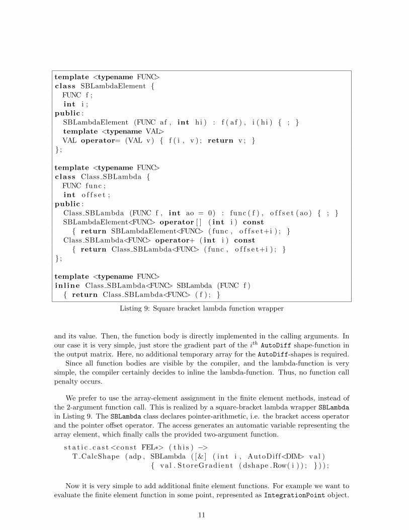
template <typename FUNC>class SBLambdaElement {

FUNC f ;int i ;

public :SBLambdaElement (FUNC af , int hi ) : f ( a f ) , i ( h i ) { ; }template <typename VAL>VAL operator= (VAL v ) { f ( i , v ) ; return v ; }} ;

template <typename FUNC>class Class SBLambda {

FUNC func ;int o f f s e t ;

public :Class SBLambda (FUNC f , int ao = 0) : func ( f ) , o f f s e t ( ao ) { ; }SBLambdaElement<FUNC> operator [ ] ( int i ) const{ return SBLambdaElement<FUNC> ( func , o f f s e t+i ) ; }

Class SBLambda<FUNC> operator+ ( int i ) const{ return Class SBLambda<FUNC> ( func , o f f s e t+i ) ; }

} ;

template <typename FUNC>inl ine Class SBLambda<FUNC> SBLambda (FUNC f ){ return Class SBLambda<FUNC> ( f ) ; }

Listing 9: Square bracket lambda function wrapper

and its value. Then, the function body is directly implemented in the calling arguments. Inour case it is very simple, just store the gradient part of the ith AutoDiff shape-function inthe output matrix. Here, no additional temporary array for the AutoDiff-shapes is required.

Since all function bodies are visible by the compiler, and the lambda-function is verysimple, the compiler certainly decides to inline the lambda-function. Thus, no function callpenalty occurs.

We prefer to use the array-element assignment in the finite element methods, instead ofthe 2-argument function call. This is realized by a square-bracket lambda wrapper SBLambdain Listing 9. The SBLambda class declares pointer-arithmetic, i.e. the bracket access operatorand the pointer offset operator. The access generates an automatic variable representing thearray element, which finally calls the provided two-argument function.

s t a t i c c a s t <const FEL∗> ( t h i s ) −>T CalcShape ( adp , SBLambda ( [& ] ( i n t i , AutoDiff<DIM> va l )

{ va l . StoreGradient ( dshape .Row( i ) ) ; } ) ) ;

Now it is very simple to add additional finite element functions. For example we want toevaluate the finite element function in some point, represented as IntegrationPoint object.

11

double T ScalarFin i teElement : :Evaluate ( In t eg ra t i onPo in t & ip , FlatVector<double> c o e f s ){

Vector<double> temp ( ndof ) ;CalcShape ( ip , temp ) ;return InnerProduct ( temp , c o e f s ) ;

}

Listing 10: Traditional evaluation using temporary memory

double T ScalarFin i teElement : :Evaluate ( In t eg ra t i onPo in t & ip , FlatVector<double> c o e f s ){

double sum = 0 ;static cast<const FEL∗> ( this ) −>

T CalcShape ( ip , SBLambda ( [ & ] ( int i , double va l ){ sum += c o e f s ( i ) ∗ va l ; } ) ) ;

return sum ;}

Listing 11: Evaluation using lambda functions

The common way is to calculate the shape functions in the point (and store them in sometemporary memory), and form the inner product with the coefficient vector, see Listing 10.Again, the drawback is the need of temporary memory.

By means of the lambda-functions, we can immediately update the sum of the innerproduct as soon as a shape function is available. This avoids to move the whole shapefunction vector to memory. An intuitive implementation is given in Listing 11. Note, addingthis one short function immediately adds the functionality for all elements derived fromT ScalarFiniteElement.

5 Vectorial finite elements

The discretization of Maxwell’s equations requires H(curl) conforming Nedelec elements [21,20]. The classical approach is to define a polynomial space, and the degrees of freedom as linearfunctions. The construction of Demkowicz et al [9] relies on projection based interpolationprocedures, which is also reflected in the implementation. The approach from [1, 26, 32]directly defines the high order basis functions for the Nedelec space. In [32], basis functionsfor triangles, quadrilaterals, tetrahedral, prismatic and hexahedral elements are given.

12

C++ object basis function curl of basis function

Du (u) ϕ = ∇u 0uDv minus vDu (u,v) ϕ = u∇v − v∇u 2∇u×∇vwuDv minus wvDu (u,v,w) ϕ = wu∇v − wv∇u ∇(uw)×∇v +∇u×∇(vw)

Table 1: H(curl) basis function objects

The triangular element from [26] has basis functions

ϕE,0 := λE1∇λE2 − λE2∇λE2

ϕE,i := ∇(λE1λE2P

Si−1(λEi − λEj , λEi + λEj )

)and for ui := λ1λ2P

Si (λ1 − λ2, λ1 + λ2) and vj := λ3Pj(2λ3 − 1)

ϕ1T,ij := ∇(uivj), i+ j ≤ p− 2

ϕ2T,ij := ui∇vj − vj∇ui, i+ j ≤ p− 2

ϕ3T,i = (λ1∇λ2 − λ2∇λ1)vj , j ≤ p− 2

The lowest order edge-basis functions are the well known Whitney forms. Also all otherH(curl) basis functions are defined via scalar polynomials and gradients of scalar polynomials.This is the same also for the other element geometries, as well as in 3D. We implement thebasis functions utilizing this structure, see Listing 12. The basis-functions are defined via theobjects from Table 1.

Now, the template argument TSHAPE in calling T CalcShape, decides whether we wantto compute the values of the shape functions, or its curl: If the elements of TSHAPE are oftype HCurlShape, then implicit conversion operators from Du, uDv minus vDu, etc., calculatethe shape function value. If the elements are of type HCurlCurlShape, implicit conversionoperators calculate the curl, see Listing 13.

6 Vectorization of finite element operations

Modern Intel and Intel-compatible microprocessors, as well as general purpose graphics pro-cessing units (GPGPUs or just GPUs) by Nvidia and others are designed to profit from thesingle-instruction multiple-data (SIMD) paradigm. For example, Intel’s recent AVX - tech-nology allows to calculate with four double precision numbers simultaneously in one processorcore. Nvidia’s GPU multi-processors compute with 32 threads simultaneously. Such SIMDinstructions can be used for evaluating shape functions in several integration points simulta-neously: data (the coordinates) is different, but the operations are the very same. A moreand more serious bottleneck is the access to memory, even to the first level cache. GPUshave only a relatively small number of double precision registers (up to 128 in the Keplerdevice, and less if higher block-level parallelism is aspired). Thus, eliminating local arrays isan important goal.

A proper interface allowing SIMD parallelization behind the scenes are functions basedon whole integration-rules, rather then on individual points. Two such functions are:

void Sca larFin i teElement<DIM> : :Evaluate ( In t eg ra t i onRu l e & i r ,

FlatVector<> coe f s , FlatVector<> v a l s ) ;

13

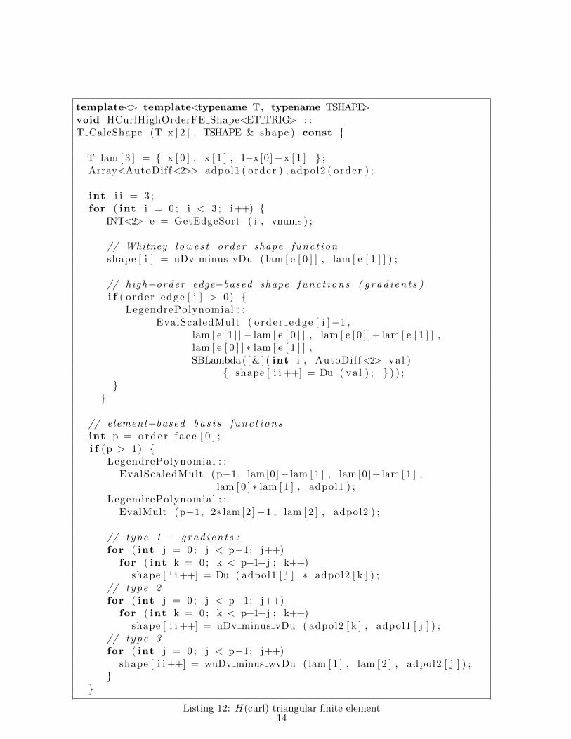
template<> template<typename T, typename TSHAPE>void HCurlHighOrderFE Shape<ET TRIG> : :T CalcShape (T x [ 2 ] , TSHAPE & shape ) const {

T lam [ 3 ] = { x [ 0 ] , x [ 1 ] , 1−x [0]−x [ 1 ] } ;Array<AutoDiff<2>> adpol1 ( order ) , adpol2 ( order ) ;

int i i = 3 ;for ( int i = 0 ; i < 3 ; i++) {

INT<2> e = GetEdgeSort ( i , vnums ) ;

// Whitney l o w e s t order shape f u n c t i o nshape [ i ] = uDv minus vDu ( lam [ e [ 0 ] ] , lam [ e [ 1 ] ] ) ;

// high−order edge−based shape f u n c t i o n s ( g r a d i e n t s )i f ( o rder edge [ i ] > 0) {

LegendrePolynomial : :EvalScaledMult ( o rder edge [ i ]−1 ,

lam [ e [1 ] ] − lam [ e [ 0 ] ] , lam [ e [ 0 ] ] + lam [ e [ 1 ] ] ,lam [ e [ 0 ] ] ∗ lam [ e [ 1 ] ] ,SBLambda ( [ & ] ( int i , AutoDiff<2> va l )

{ shape [ i i ++] = Du ( va l ) ; } ) ) ;}

}

// element−based b a s i s f u n c t i o n sint p = o r d e r f a c e [ 0 ] ;i f (p > 1) {

LegendrePolynomial : :EvalScaledMult (p−1, lam [0]− lam [ 1 ] , lam [0 ]+ lam [ 1 ] ,

lam [ 0 ] ∗ lam [ 1 ] , adpol1 ) ;LegendrePolynomial : :

EvalMult (p−1, 2∗ lam [2]−1 , lam [ 2 ] , adpol2 ) ;

// type 1 − g r a d i e n t s :for ( int j = 0 ; j < p−1; j++)

for ( int k = 0 ; k < p−1− j ; k++)shape [ i i ++] = Du ( adpol1 [ j ] ∗ adpol2 [ k ] ) ;

// type 2for ( int j = 0 ; j < p−1; j++)

for ( int k = 0 ; k < p−1− j ; k++)shape [ i i ++] = uDv minus vDu ( adpol2 [ k ] , adpol1 [ j ] ) ;

// type 3for ( int j = 0 ; j < p−1; j++)

shape [ i i ++] = wuDv minus wvDu ( lam [ 1 ] , lam [ 2 ] , adpol2 [ j ] ) ;}

}

Listing 12: H(curl) triangular finite element14

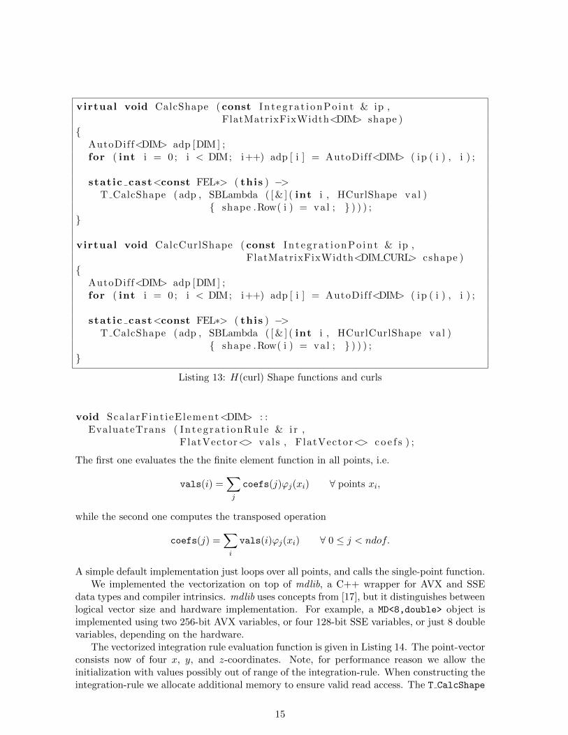
virtual void CalcShape ( const In t eg ra t i onPo in t & ip ,FlatMatrixFixWidth<DIM> shape )

{AutoDiff<DIM> adp [DIM ] ;for ( int i = 0 ; i < DIM; i++) adp [ i ] = AutoDiff<DIM> ( ip ( i ) , i ) ;

static cast<const FEL∗> ( this ) −>T CalcShape ( adp , SBLambda ( [ & ] ( int i , HCurlShape va l )

{ shape .Row( i ) = va l ; } ) ) ) ;}

virtual void CalcCurlShape ( const In t eg ra t i onPo in t & ip ,FlatMatrixFixWidth<DIM CURL> cshape )

{AutoDiff<DIM> adp [DIM ] ;for ( int i = 0 ; i < DIM; i++) adp [ i ] = AutoDiff<DIM> ( ip ( i ) , i ) ;

static cast<const FEL∗> ( this ) −>T CalcShape ( adp , SBLambda ( [ & ] ( int i , HCurlCurlShape va l )

{ shape .Row( i ) = va l ; } ) ) ) ;}

Listing 13: H(curl) Shape functions and curls

void Sca larFint ieElement<DIM> : :EvaluateTrans ( In t eg ra t i onRu l e & i r ,

FlatVector<> vals , FlatVector<> c o e f s ) ;

The first one evaluates the the finite element function in all points, i.e.

vals(i) =∑j

coefs(j)ϕj(xi) ∀ points xi,

while the second one computes the transposed operation

coefs(j) =∑i

vals(i)ϕj(xi) ∀ 0 ≤ j < ndof.

A simple default implementation just loops over all points, and calls the single-point function.We implemented the vectorization on top of mdlib, a C++ wrapper for AVX and SSE

data types and compiler intrinsics. mdlib uses concepts from [17], but it distinguishes betweenlogical vector size and hardware implementation. For example, a MD<8,double> object isimplemented using two 256-bit AVX variables, or four 128-bit SSE variables, or just 8 doublevariables, depending on the hardware.

The vectorized integration rule evaluation function is given in Listing 14. The point-vectorconsists now of four x, y, and z-coordinates. Note, for performance reason we allow theinitialization with values possibly out of range of the integration-rule. When constructing theintegration-rule we allocate additional memory to ensure valid read access. The T CalcShape

15

template <class FEL, ELEMENT TYPE ET>void T ScalarFin iteElement<FEL,ET> : :Evaluate ( const In t eg ra t i onRu l e & i r , FlatVector<double> coe f s ,

FlatVector<double> v a l s ) const{

for ( int i = 0 ; i < i r . GetNIP ( ) ; i += 4) {

Vec<DIM, MD<4>> pt ;for ( int k = 0 ; k < DIM; k++)

pt [ k ] = MD<4> ( i r [ i ] ( k ) , i r [ i +1](k ) , i r [ i +2](k ) , i r [ i +3](k ) ) ;

MD<4> sum = 0 . 0 ;T CalcShape (&pt ( 0 ) , SBLambda ( [&] ( int j , MD<4> va l )

{ sum += c o e f s ( j )∗ va l ; } ) ) ;

MD<4,mask64> mask = MD<4, int > : : F i r s t I n t ( ) < i r . GetNIP ( ) − i ;sum . Store (& v a l s ( i ) , mask ) ;

}}

Listing 14: Evaluate function using SIMD operations

computes now all shape functions for four points simultaneously. The values are added up tothe four summation variables. The resulting values are stored to the vals result vector. Here,we use a bit-mask to write only into valid memory. The simultaneous integer comparison andmasked write are provided by hardware, which is faster than the alternative of four conditionalbranch instructions.

7 Timings

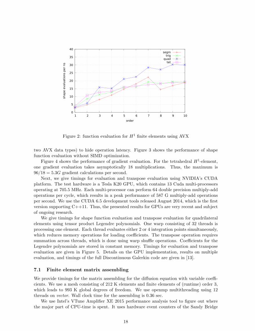
First, we measure the performance of finite element function evaluation on CPUs and GPUs.Our first test system, referred to as vector consists of two Sandy Bridge Intel processorsE5-2620, each of them contains 6 cores operating at 2GHz. It supports AVX SIMD - instruc-tions. The peak performance of this system is 2 processors× 6 cores× 4 AVX× 2 GHz = 96Gmultiplications and additions per second.

First, we measure the performance of shape function evaluation and gradient evaluationfor H1 finite elements. For this, we compute

∑Ni=1 uiϕi(xj) and

∑Ni=1 ui∇ϕi(xj) in a set of

integration points {xj}, where the order of the integration rule is twice the element order.We call the function evaluation in an openmp-parallel loop. We use hyper-threading and thus24 threads are generated. We note that all computations are performed within level 1 caches,so essentially floating point performance is measured.

The inner-most loop for triangles and tetrahedral elements is the evaluation of Jacobipolynomials, which takes 3 multiplication, plus one additional multiplication for the coeffi-cient. The results in Figure 2 show 19 G shape function evaluation for higher polynomialorders, which corresponds to 76 G multiplication. Thus, the floating point efficiency is closeto optimum, namely 80%. We use simultaneous evaluation of eight integration points (i.e.

16

template <class FEL, ELEMENT TYPE ET>void T ScalarFin iteElement<FEL,ET> : :Evaluate ( const In t eg ra t i onRu l e & i r , FlatVector<double> coe f s ,

FlatVector<double> v a l s ) const{

for ( int i = threadIdx . x ; i < i r . GetNIP ( ) ; i += blockDim . x ) {Vec<DIM> pt = i r [ i ] . Point ( ) ;double sum = 0 ;T CalcShape (&pt ( 0 ) , SBLambda ( [& ] ( int j , double shape )

{ sum += c o e f s ( j )∗ shape ; } ) ) ;v a l s ( i ) = sum ;

}}

Listing 15: Evaluate function using CUDA

template <class FEL, ELEMENT TYPE ET>void T ScalarFin iteElement<FEL,ET> : :EvaluateTrans ( const In t eg ra t i onRu l e & i r , FlatVector<double> vals ,

FlatVector<double> c o e f s ) const{

for ( int i 0 = 0 ; i 0 < i r . GetNIP ( ) ; i 0 += blockDim . x ) {int i = i 0 + threadIdx . x ;Vec<DIM> pt = i r [ i ] . Point ( ) ;double v = ( i < i r . GetNIP ( ) ) ? v a l s ( i ) : 0 ;T CalcShape (&pt ( 0 ) , SBLambda ( [& ] ( int j , double shape ){ double sum = HorizontalSum ( v∗ shape ) ;

i f ( threadIdx . x == 0) c o e f s ( j ) = sum ; } ) ) ;}

}

Listing 16: Transpose evaluate using CUDA

17

0

5

10

15

20

25

30

35

40

1 2 3 4 5 6 7 8 9 10

shap

e e

valu

ati

ons

per

ns

order

segmtrig

quadtet

Figure 2: function evaluation for H1 finite elements using AVX

two AVX data types) to hide operation latency. Figure 3 shows the performance of shapefunction evaluation without SIMD optimization.

Figure 4 shows the performance of gradient evaluation. For the tetrahedral H1-element,one gradient evaluation takes asymptotically 18 multiplications. Thus, the maximum is96/18 = 5.3G gradient calculations per second.

Next, we give timings for evaluation and transpose evaluation using NVIDIA’s CUDAplatform. The test hardware is a Tesla K20 GPU, which contains 13 Cuda multi-processorsoperating at 705.5 MHz. Each multi-processor can perform 64 double precision multiply-addoperations per cycle, which results in a peak performance of 587 G multiply-add operationsper second. We use the CUDA 6.5 development tools released August 2014, which is the firstversion supporting C++11. Thus, the presented results for GPUs are very recent and subjectof ongoing research.

We give timings for shape function evaluation and transpose evaluation for quadrilateralelements using tensor product Legendre polynomials. One warp consisting of 32 threads isprocessing one element. Each thread evaluates either 2 or 4 integration points simultaneously,which reduces memory operations for loading coefficients. The transpose operation requiressummation across threads, which is done using warp shuffle operations. Coefficients for theLegendre polynomials are stored in constant memory. Timings for evaluation and transposeevaluation are given in Figure 5. Details on the GPU implementation, results on multipleevaluation, and timings of the full Discontinuous Galerkin code are given in [13].

7.1 Finite element matrix assembling

We provide timings for the matrix assembling for the diffusion equation with variable coeffi-cients. We use a mesh consisting of 212 K elements and finite elements of (runtime) order 3,which leads to 993 K global degrees of freedom. We use openmp multithreading using 12threads on vector. Wall clock time for the assembling is 0.36 sec.

We use Intel’s VTune Amplifier XE 2015 performance analysis tool to figure out wherethe major part of CPU-time is spent. It uses hardware event counters of the Sandy Bridge

18

0

2

4

6

8

10

1 2 3 4 5 6 7 8 9 10

shap

e e

valu

ati

ons

per

ns

order

segmtrig

quadtet

Figure 3: function evaluation for H1 finite elements without SIMD

0

2

4

6

8

10

12

14

1 2 3 4 5 6 7 8 9 10

gra

die

nt

evalu

ati

ons

per

ns

order

segmtrig

quadtet

Figure 4: gradient evaluation for H1 finite elements using AVX

19

0

10

20

30

40

50

60

70

80

0 2 4 6 8 10 12 14 16 18 20

shap

e e

valu

ati

ons

per

ns

order

eval - 2 p/thdeval - 4 p/thd

evaltrans - 2 p/thdevaltrans - 4 p/thd

Figure 5: evaluation and transpose for L2 quadrilateral on Kepler GPU

processor. We give the result of the CPU CLK UNHALTED.THREAD counter, which gives theactive core cycles.

12 active cores at 2 GHz perform 8640 M cycles within 0.36 seconds, which correspondswell to the measured 8370 M cycles in total.

Out of these, 4299 M cylces are spent for the element matrix calculation. Element matricesare of dimension 20 by 20, and 14 integration points are used. Assembling of the elementmatrices into the global sparse matrix takes 3052 M cycles. Our multithreading algorithmuses coloring, such that parallel assembling can be done without locks (critical sections). Theglobal matrix is stored in shared memory, which is the bottle-neck in the assembling routine.The MPI-parallel version benefits from the NUMA memory architecture, and the assemblingcan be significantly improved. 583 M cycles are spent for the logic, namely constructing thefinite element, and collecting degrees of freedom.

The calculation of one element matrix takes 4299 M / 212 K = 20278 core cycles, where7382 cycles are spent for computing the mapped gradients. These are 7382/(14 × 20) = 26cycles per gradient evaluation. Thus, all cores compute 12 cores × 4 AVX × 2GHz/26 = 3.7gradients per nano-second, which corresponds well with Figure 4.

The second major part in element calculation is computing all inner products∑xk

(wkλ(xk)∇ϕi(xk)) · ∇ϕj(xk). This is done by a matrix-matrix multiplication, againusing AVX optimization. The cpu-time for third order elements is approximately the sameas calculating the shape function gradients.

7.2 Discussion and further improvements

In the present manuscript we have presented a high level implementation of finite elementoperations. We have demonstrated high floating point performance reaching 80 % of peakon CPUs with AVX operations. Since the evaluation of shape functions take in average 4multiplications per point and shape function, this factor of 4 is lost in competition with pre-computed matrices, and performing linear algebra operations using vendor BLAS functions.The matrix operations are in particular efficient when equivalent elements are combined, and

20

element matrix calculation 4299 shape gradient calc 1565matrix matrix product 1552mult coefficients 514integration rule 224etc 444

global matrix assembling 3052

logic: generate fe, dofs 583etc 373

total 8307

Table 2: million core cycles for matrix assembling

0

200

400

600

800

1000

1200

2 4 6 8 10 12

shap

e e

valu

ati

ons

per

ns

order

eval L2-tet

Figure 6: function evaluation by sum-factorization and AVX for L2 tetrahedral elements

matrix-matrix products are computed. But, this coding technique requires a restructuring ofthe element loop by grouping equivalent elements. In certain applications we also improvethe evaluation by combining evaluation for several vectors, for example when dealing withsystems of equations.

Another possibility for improvement is the utilization of tensor product structure of shapefunctions and integration rules, known as sum-factorization [22, 14]. This allows to reducethe complexity of evaluation from p2d to pd+1. We are currently working on a vectorizedimplementation of sum-factorization following the programming techniques presented in thispaper. A preliminary result for evaluation of tetrahedral L2-elements using the Dubiner basisis given in Figure 6. Measurements were done on the 12 core system vector. At order 5,this version beats evaluation by matrix-multiplication at peak performance, at order 10 theadvantage is a factor more than 6.

Acknowledgement: The author wants to thank Matthias Hochsteger for helping withthe GPU-version of finite element function evaluation.

21

References

[1] M. Ainsworth and J. Coyle. Hierarchic Finite Element Bases on Unstructured TetrahedralMeshes. Int. J. Num. Meth. Eng., 58(14), 2103-2130.

[2] W. Bangerth, R. Hartmann, and G. Kanschat. deal.II – a General Purpose ObjectOriented Finite Element Library. ACM Trans. Math. Softw., 33(4), 24/1–24/27, 2007

[3] J. Barton, L.R. Nackman. Scientific and Engineering C++: An Instroduction withAdvanced Techniques and Examples. Addison-Wesley Professional, 1994

[4] P. Bastian, M. Blatt, A. Dedner, C. Engwer, R. Klfkorn, R. Kornhuber, M. Ohlberger,O. Sander. A Generic Grid Interface for Parallel and Adaptive Scientific Computing.Part II: Implementation and Tests in DUNE. Computing, 82(2-3), 121–138, 2008

[5] P. Castillo, R. Rieben, D. White FEMSTER : An Object-Oriented Class Library ofHigh-Order Discrete Differential Forms ACM Trans. Math. Softw., 31(4), 425–457, 2005

[6] P.G. Ciarlet. The finite element method for elliptic problems. North-Holland, Amsterdam,1978.

[7] A. Dedner, R. Klofkorn, M. Nolte, M. Ohlberger A generic interface for parallel andadaptive scientific computing: Abstraction principles and the DUNE-FEM module. Com-puting 90(3), 165–196, 2011

[8] L. Demkowicz Computing with hp-adaptive finite elements. I. One and two dimensionalelliptic and maxwell problems Chapman & Hall / CRC Press, Boca Raton, FL, 2006

[9] L. Demkowicz Computing with hp-adaptive finite elements. II. Frontiers: Three dimen-sional elliptic and Maxwell problems with applications Chapman & Hall / CRC Press,Boca Raton, FL, 2008

[10] G. Guennebaud, B. Jacob. EIGEN - a C++ linear algebra library available fromhttp://eigen.tuxfamily.org

[11] F. Hecht. Freefem++. http:/www.freefem.org/ff++

[12] J. S. Hesthaven and T. Warburton. Nodal Discontinuous Galerkin Methods—Algorithms,Analysis and Applications. Text in Applied Mathematics. Springer, 2007.

[13] M. Hochsteger. High Order Discontinuous Galerkin Methods on GPUs. Master’s Thesis,Inst. Analysis and Scientific Computing, Vienna UT, 2014

[14] G. E. Karniadakis and S. J. Sherwin. Spectral/hp Element Methods for ComputationalFluid Dynamics. Oxford Science Publications, 2005

[15] R.C. Kirby, Algorithm 839: FIAT, a new paradigm for computing finite element basisfunctions, ACM Trans. Math. Software, 30(4), 502–516, 2004

[16] A. Klockner, T. Warburton, J. Bridge, J.S. Hesthaven Nodal discontinuous Galerkinmethods on graphics processors. J Comp. Phys. 228(21), 7863–7882, 2009

22

[17] M. Kretz and V. Lindenstrutz. Vc: A C++ library for explicit vectorization Softw.Pract. Exper,00, 1–18, 2011.

[18] A. Logg, K.-A. Mardal, G.N. Wells (eds) Automated Solution of Differential Equations bythe Finite Element Method. The FEniCS Book. Lecture notes in Computational Scienceand Engineering 84. Springer, 2011

[19] M. Lyly, J. Ruokolainen, and E. Jarvinen. ELMER - A finite element solver for multi-physics. CSC-report on scientific computing, 156–159, 1999-2000

[20] P. Monk, Finite Element Methods for Maxwell’s Equations. Oxford University Press,2003.

[21] J.C. Nedelec. A new family of mixed finite elements in R3, Num. Math., 50, 57–81, 1986.

[22] S.A.Orszag. Spectral methods for problems in complex geometries, J. Comp. Phys. 37,70-92, 1980.

[23] C. Prud’homme. Life: Overview of a Unified C++ Implementation of the Finite andSpectral Element Methods in 1D, 2D and 3D. in Applied Parallel Computing. LectureNotes in Computer Science Volume 4699, 712–721, 2007

[24] C. Prud’Homme, V. Chabannes, V. Doyeux; M. Ismail, A. Samake, G. Pena Feel++: AComputational Framework for Galerkin Methods and Advanced Numerical Methods inESAIM: Proceedings 38, 429–455, 2012

[25] J. Schoberl. NGSolve Finite Element Library http://sourceforge.net/projects/ngsolve

[26] J. Schoberl and S. Zaglmayr, High order Nedelec elements with local complete sequenceproperties, COMPEL, 24, 2, 374–384(11), 2005.

[27] C. Schwab. p- and hp- Finite Element Methods: Theory and Applications in Solid andFluid Mechanics. Clarendon Press, 1998

[28] B. Stroustrup. The C++ Programming Language, 4th edition. Pearson Education, Ind.,2013

[29] B. Szabo and I. Babuska. Finite Element Analysis. Wiley, 1991.

[30] T. Veldhuizen. Expression Templates. C++ Report 7(5), 26-31, 1995.

[31] T. Veldhuizen. Techniques for Scientific C++. Indiana University Computer ScienceTechical Report #542, 2000

[32] S. Zaglmayr, High Order Finite Element Methods for Electromagnetic Field Computa-tion, PhD dissertation, Johannes Kepler Universitat Linz, Austria, 2006.

23