c ovariance data in the fast neutron region · c ovariance data in the fast neutron region nuclear...
TRANSCRIPT

Covariance Data in theFast Neutron Region
Nuclear Science2011
N U C L E A R E N E R G Y A G E N C Y
International EvaluationCo-operation, Volume 24
Covariance Data in the Fast N
eutron Region
-1.0
-0.5
0.0
0.5
1.0
12 16 20 24 28 32Incident Neutron Energy (MeV)
12
16
20
24
28
32
Incid
ent N
eutro
n En
ergy
(MeV
)
-1.0
-0.5
0.0
0.5
1.0
10.0 12.6 15.8 19.9 25.1 31.6Incident Neutron Energy (MeV)
10.0
12.6
15.8
19.9
25.1
31.6
Incid
ent N
eutro
n En
ergy
(MeV
)
2011

Nuclear Science NEA/NSC/WPEC/DOC(2010)427 NEA/WPEC-24
International Evaluation Co-operation
Volume 24
Covariance Data in the Fast Neutron Region
A report by the Working Party on International Evaluation Co-operation of the NEA Nuclear Science Committee
Co-ordinator Monitor
M. Herman A. Koning Brookhaven National Laboratory Nuclear Research & Consultancy Group United States The Netherlands
© OECD 2011
NUCLEAR ENERGY AGENCY
Organisation for Economic Co-operation and Development

ORGANISATION FOR ECONOMIC CO-OPERATION AND DEVELOPMENT The OECD is a unique forum where the governments of 34 democracies work together to address
the economic, social and environmental challenges of globalisation. The OECD is also at the forefront of efforts to understand and to help governments respond to new developments and concerns, such as corporate governance, the information economy and the challenges of an ageing population. The Organisation provides a setting where governments can compare policy experiences, seek answers to common problems, identify good practice and work to co-ordinate domestic and international policies.
The OECD member countries are: Australia, Austria, Belgium, Canada, Chile, the Czech Republic, Denmark, Estonia, Finland, France, Germany, Greece, Hungary, Iceland, Ireland, Israel, Italy, Japan, Korea, Luxembourg, Mexico, the Netherlands, New Zealand, Norway, Poland, Portugal, the Slovak Republic, Slovenia, Spain, Sweden, Switzerland, Turkey, the United Kingdom and the United States. The Commission of the European Communities takes part in the work of the OECD.
OECD Publishing disseminates widely the results of the Organisation’s statistics gathering and research on economic, social and environmental issues, as well as the conventions, guidelines and standards agreed by its members.
This work is published on the responsibility of the Secretary-General of the OECD. The opinions expressed and arguments employed herein do not necessarily reflect the official views of the
Organisation or of the governments of its member countries.
NUCLEAR ENERGY AGENCY The OECD Nuclear Energy Agency (NEA) was established on 1st February 1958 under the name of
the OEEC European Nuclear Energy Agency. It received its present designation on 20th April 1972, when Japan became its first non-European full member. NEA membership today consists of 29 OECD member countries: Australia, Austria, Belgium, Canada, the Czech Republic, Denmark, Finland, France, Germany, Greece, Hungary, Iceland, Ireland, Italy, Japan, Luxembourg, Mexico, the Netherlands, Norway, Poland, Portugal, Republic of Korea, the Slovak Republic, Spain, Sweden, Switzerland, Turkey, the United Kingdom and the United States. The Commission of the European Communities also takes part in the work of the Agency.
The mission of the NEA is:
– to assist its member countries in maintaining and further developing, through international co-operation, the scientific, technological and legal bases required for a safe, environmentally friendly and economical use of nuclear energy for peaceful purposes, as well as
– to provide authoritative assessments and to forge common understandings on key issues, as input to government decisions on nuclear energy policy and to broader OECD policy analyses in areas such as energy and sustainable development.
Specific areas of competence of the NEA include safety and regulation of nuclear activities, radioactive waste management, radiological protection, nuclear science, economic and technical analyses of the nuclear fuel cycle, nuclear law and liability, and public information.
The NEA Data Bank provides nuclear data and computer program services for participating countries. In these and related tasks, the NEA works in close collaboration with the International Atomic Energy Agency in Vienna, with which it has a Co-operation Agreement, as well as with other international organisations in the nuclear field.
Corrigenda to OECD publications may be found on line at: www.oecd.org/publishing/corrigenda. © OECD 2011
You can copy, download or print OECD content for your own use, and you can include excerpts from OECD publications, databases and multimedia products in your own documents, presentations, blogs, websites and teaching materials, provided that suitable acknowledgment of OECD as source and copyright owner is given. All requests for public or commercial use and translation rights should be submitted to [email protected]. Requests for permission to photocopy portions of this material for public or commercial use shall be addressed directly to the Copyright Clearance Center (CCC) at [email protected] or the Centre français d’exploitation du droit de copie (CFC) [email protected].
FOREWORD
COVARIANCE DATA IN THE FAST NEUTRON REGION – © OECD/NEA 2011 3
Foreword
The Working Party on International Nuclear Data Evaluation Co-operation (WPEC) was established under the aegis of the OECD/NEA Nuclear Science Committee (NSC) to promote the exchange of information on nuclear data evaluations, validation and related topics. Its aim is also to provide a framework for co-operative activities between the members of the major nuclear data evaluation projects. This includes the possible exchange of scientists in order to encourage co-operation. Requirements for experimental data resulting from this activity are compiled. The WPEC determines common criteria for evaluated nuclear data files with a view to assessing and improving the quality and completeness of evaluated data.
The parties to the project are: ENDF (United States), JEFF/EFF (NEA Data Bank member countries) and JENDL (Japan). Co-operation with evaluation projects of non-OECD countries, specifically the Russian BROND and Chinese CENDL projects, are organised through the Nuclear Data Section of the International Atomic Energy Agency (IAEA).
The following report has been issued by WPEC Subgroup 24, whose mission was to review methodologies and develop tools for producing data uncertainties (covariance data) in the fast neutron energy region. These involve both least-squares procedures and, more recently, stochastic (Monte Carlo) techniques. Since all modern approaches depend on extensive usage of nuclear reaction modelling, consideration is given to recent attempts to determine the extent to which nuclear modelling deficiencies contribute to the uncertainty of contemporary nuclear data evaluation.
The opinions expressed in this report are those of the authors only and do not necessarily represent the position of any member country or international organisation.
MEMBERS OF SUBGROUP 24
4 COVARIANCE DATA IN THE FAST NEUTRON REGION – © OECD/NEA 2011
Members of Subgroup 24
E. Bauge Commissariat à l’énergie atomique (CEA)
France
R. Capote International Atomic Energy Agency (IAEA)
Austria
U. Fisher, A.Yu. Konobeyev, P.E. Pereslavtsev Karlsruhe Institute of Technology
Germany
M. Herman, P. Obložinský, M.T. Pigni Brookhaven National Laboratory (BNL)
United States
T. Kawano, P. Talou Los Alamos National Laboratory (LANL)
United States
I. Kodeli, A. Trkov Jozef Stefan Institute
Slovenia
A. Koning, D. Rochman Nuclear Research and Consultancy Group (NRG)
The Netherlands
H. Leeb, D. Neudecker Atominstitut der Österreichischen Universitäten
Technische Universität Wien Austria
D.L. Smith Argonne National Laboratory (ANL)
United States

TABLE OF CONTENTS
COVARIANCE DATA IN THE FAST NEUTRON REGION – © OECD/NEA 2011 5
Table of contents
Foreword ............................................................................................................ 3
Members of Subgroup 24 ................................................................................. 4
1 Introduction ............................................................................................... 11
2 Overview of covariance methodologies ............................................... 13
2.1 Uncertainty reduction by interpolation ......................................... 15
2.2 Model parameter fitting ................................................................... 16
3 Unified Monte Carlo approach ............................................................... 19
3.1 Introduction ....................................................................................... 19
3.2 General observations ........................................................................ 19
3.3 Formalism and some practical issues ............................................ 20
3.3.1 Basic concept .......................................................................... 20
3.3.2 Some practical considerations ............................................. 24
3.3.3 “Brute Force” (BF) Monte Carlo approach ........................... 26
3.3.4 The Metropolis Monte Carlo approach ............................... 28
3.4 Examples ............................................................................................ 30
3.4.1 Direct cross-section data....................................................... 30
3.4.2 Inclusion of cross-section ratio data ................................... 32
3.4.3 Inclusion of integral cross-section data .............................. 34
3.4.4 Logarithmic transformation of data .................................... 34
3.5 Practical implementation of the UMC approach .......................... 35
3.5.1 Use of experimental data ...................................................... 38
3.6 Conclusions ....................................................................................... 39
4 Conventional Monte Carlo approaches ................................................ 41
4.1 TALYS-MC approach ........................................................................ 41
4.1.1 Filtered Monte Carlo method ............................................... 41
4.1.2 Total Monte Carlo ................................................................... 43
4.2 Backward-Forward Monte Carlo approach ................................... 46
4.2.1 Backward Monte Carlo .......................................................... 47
TABLE OF CONTENTS
6 COVARIANCE DATA IN THE FAST NEUTRON REGION – © OECD/NEA 2011
4.2.2 Forward Monte Carlo ............................................................. 48
4.2.3 Set-up of the BFMC procedure ............................................. 49
4.2.4 Results ...................................................................................... 50
4.3 EMPIRE-MC + Generalised Least Squares approach ..................... 53
4.3.1 EMPIRE-MC .............................................................................. 53
4.3.2 EMPIRE-MC + GLS ................................................................... 54
5 Deterministic EMPIRE-Kalman approach ............................................ 55
5.1 Example of application of EMPIRE-Kalman approach in EMPIRE ........................................................................................... 57
6 GANDR approach ...................................................................................... 65
6.1 Introduction ....................................................................................... 65
6.2 Methodology of covariance estimation ......................................... 65
6.3 Database support for large-scale projects ..................................... 66
6.4 The global assessment ..................................................................... 67
7 Dispersion analysis ................................................................................. 69
8 Avoiding unphysically low uncertainties ........................................... 71
8.1 Model defects..................................................................................... 71
8.1.1 Model defects from scaling procedure ................................ 72
8.1.2 Model defects associated with remodelling ....................... 73
8.1.3 Example ................................................................................... 73
8.1.4 Scaling in the EMPIRE-Kalman approach ........................... 76
9 Comparison of different methods ......................................................... 79
9.1 Comparison of model-based covariances obtained with Monte Carlo and Kalman ................................................................. 79
9.2 Inclusion of experimental data ....................................................... 80
10 Covariances for experimental data ....................................................... 87
10.1 Estimation of unknown systematic uncertainties ....................... 87
11 Conclusions ............................................................................................... 91
References .......................................................................................................... 97

LIST OF FIGURES AND TABLES
COVARIANCE DATA IN THE FAST NEUTRON REGION – © OECD/NEA 2011 7
List of figures
1 Uncertainties and correlation matrices for the evaluated data ......... 16
2 Uncertainty extrapolation by using a nuclear reaction model with the Kalman code .............................................................................. 17
3 Comparison of Brute Force (BF) and Metropolis (METR) chi-square convergence ........................................................................... 32
4 The relative error of asymptotic values of nuclear level density parameters in generalised superfluid model obtained in Ref. [27] from the analysis of experimental data ................................. 37
5 Comparison of correlation matrices for the 52Cr(n,n′) reaction cross-section obtained using nuclear models implemented in TALYS and in ALICE/ASH code .................................. 37
6 Correlation matrices for proton and 24Na production cross-sections in the interaction of protons with 56Fe calculated using intranuclear cascade evaporation model ................ 38
7 Flow chart of automated, reproducible evaluation process ............... 45
8 Total Monte Carlo: Loop over all basic physics and application software ...................................................................................................... 45
9 Comparison between mean cross-section vector and error band for the n+239Pu reaction with the corresponding experimental data ..................................................................................... 51
10 Incident neutron energy-dependent BFMC correlation matrices for 239Pu(n,γ), 239Pu(n,f) and 239Pu(n,2n) .................................................... 52
11 Reaction 55Mn(n,tot); prior, posterior and ENDF/B-VII.0 cross-sections are compared with experimental data [58-60] ........... 58
12 Reaction 55Mn(n,inl); prior, posterior and ENDF/B-VII.0 cross-sections are compared with experimental data ........................ 59
13 Reaction 55Mn(n,2n); prior, posterior and ENDF/B-VII.0 cross-sections are compared with experimental data [61-72] ........... 59
14 Reaction 55Mn(n,γ); prior, posterior and ENDF/B-VII.0 cross-sections are compared with experimental data ........................ 60
15 Reaction 90Zr(n,tot); prior, posterior and ENDF/B-VII.0 cross-sections are compared with experimental data [74-77] ........... 61
16 Reaction 90Zr(n,el); prior, posterior and ENDF/B-VII.0 cross-sections are compared with experimental data ........................ 61

LIST OF FIGURES AND TABLES
8 COVARIANCE DATA IN THE FAST NEUTRON REGION – © OECD/NEA 2011
17 Reaction 90Zr(n,inl); prior, posterior and ENDF/B-VII.0 cross-sections are shown......................................................................... 62
18 Reaction 90Zr(n,2n); prior, posterior and ENDF/B-VII.0 cross-sections are compared with experimental data [78-82] ........... 62
19 10B total cross-section after introduction of EXFOR total cross-sections ............................................................................................ 68
20 Ratio of cross-sections for 56Fe(n,n′) reaction available in JEFF-3.1 and JENDL-3.3 libraries to the ENDF/B-VII.0 ........................... 70
21 (a) The scaling factor and (b) the square root of the variances in % of the model cross-section for n-16O total cross-sections for both methods ...................................................................................... 74
22 Correlation matrix of the model defects in the total cross-sections of oxygen using the scaling procedure of Section 8.1.1 ....................... 75
23 Correlation matrix of the model defects in the total cross-sections of oxygen using the remodelling procedure ......................................... 75
24 Effect of 5% variation of the depth of the real optical potential on the 93Nb(n,tot) cross-section ............................................................... 76
25 Cross-sections and uncertainties for 90Zr(n,tot) obtained by applying standard EMPIRE-Kalman method constrained by the four experimental data sets.............................................................. 78
26 Comparison of the model-based cross-section uncertainties obtained with Kalman and Monte Carlo methods for 89Y+n reactions........................................................................................... 80
27 Comparison of the model-based cross-section correlations for the 89Y(n,tot) reaction obtained with Kalman and Monte Carlo methods ............................................................................... 81
28 Comparison of the 89Y(n,2n) cross-section uncertainties obtained with GANDR and Kalman illustrating inclusion of experimental data ................................................................................ 82
29 Comparison of the 89Y(n,2n) cross-sections and uncertainties obtained with Kalman .............................................................................. 83
30 The correlation matrix for the 89Y(n,2n) reaction obtained with Kalman using full set of experimental data for all reaction channels; the same for MC method ....................................................... 84
31 Uncertainties of the 89Y(n,tot) cross-sections obtained with Kalman including (n,tot) data by Abfalterer, (n,tot) data by Foster and Abfalterer, and full set of experimental data for all reaction channels ................................................................................ 85

LIST OF FIGURES AND TABLES
COVARIANCE DATA IN THE FAST NEUTRON REGION – © OECD/NEA 2011 9
32 Distribution of relative uncertainties for the fission cross-section data of 235U in accordance with the unrecognised error-estimation method ................................................ 88
33 Relative uncertainties of the fission cross-section evaluations for 235U adopted in different libraries ..................................................... 89
List of tables
1 Prior and experimental values ................................................................... 31
2 Prior and experimental values ................................................................... 33
3 Uncertainties of some nuclear model parameters for 206Pb, given as fraction (%) of the absolute value .............................. 44
4 Global uncertainties of some nuclear model parameters, given as fraction (%) of the absolute value ........................ 44

INTRODUCTION
COVARIANCE DATA IN THE FAST NEUTRON REGION – © OECD/NEA 2011 11
1. Introduction
During the past decade, there has been a dramatic increase in the demand for evaluated nuclear data that are comprehensive in scope with respect to both materials and reaction processes included, and that provide some specification of estimated uncertainties in the results. This demand has come about because of a renewed interest in the nuclear power option as a means to satisfy the energy needs of society while at the same time limiting the emission of gaseous carbon compounds that may contribute significantly to global warming. The concern about data uncertainties is related to the need to ensure that nuclear power will be safe, reliable and economically competitive with other alternative energy options (e.g. wind, solar, geothermal, etc.). Modern nuclear systems analysis procedures are now able to accommodate nuclear data uncertainties thereby providing further stimulus for their provision.
Along with the growing demand for evaluated nuclear data has come considerable progress in evaluation methodologies. Subgroup 24 of the NEA Working Party for Evaluation Co-operation (WPEC) was established in 2006 in response to the need to further stimulate development of these methodologies as they apply to the fast neutron region, i.e. that energy region above the region dominated by resolved and partially resolved or fully unresolved resonances, and to document progress in this area. The evaluations in this region address cross-sections, particle emission angular distributions, nu-bar (for fission), and certain other observables which are generally considered to vary smoothly with incident neutron energy. These evaluations utilise input data from experiments as well as theoretical nuclear modelling to varying degrees depending on the circumstances.
In the case of experimental data, there is the need to deal with discrepancies as well as statistical fluctuations that lead to results that generally depart from ideal smoothness. On the other hand, results from nuclear modelling generally suffer to varying extent from model deficiencies that can lead to a failure to agree both in shape and amplitude with corresponding measured values. These are not new problems, but recently greater attention has been paid to dealing with such practical issues. Part of this concern is related to the need, as indicated above, to provide fairly reliable (or at least plausible) estimates of uncertainty in the evaluated results.
INTRODUCTION
12 COVARIANCE DATA IN THE FAST NEUTRON REGION – © OECD/NEA 2011
Three decades ago, a major step forward in evaluation methodology for the fast neutron region was the widespread implementation of least-squares procedures (both ordinary and generalised) to merge various combinations of experimental and model-calculated nuclear data in performing the evaluations, as alternatives to older subjective methods that can best be described as “drawing eye-guides through available experimental data”. Many of these least-squares procedures are still in common use today. This subgroup summary report will not discuss the older manifestations of these venerable methods since they are very widely documented [1]. Instead, the newer approaches to nuclear data evaluation are emphasised. These involve both least-squares procedures and more recent approaches that involve stochastic (Monte Carlo) techniques. Also, consideration is given to recent attempts to determine the extent to which nuclear modelling deficiencies contribute to the uncertainty of contemporary nuclear data evaluation.
The growing interest in nuclear data uncertainties has led to the organisation of two workshops under the auspices of this subgroup that were specifically devoted to the topic [2,3]. Reports from these workshops are given in the references. Although considerable material from these workshops is certainly included in this report, the present document is not just a summary of these earlier activities. However, the contributions herein may, in some cases, be composites of material taken from these presentations as well as other published sources.

OVERVIEW OF COVARIANCE METHODOLOGIES
COVARIANCE DATA IN THE FAST NEUTRON REGION – © OECD/NEA 2011 13
2. Overview of covariance methodologies
Covariances of nuclear data, in principle, can be obtained by sole analysis of experimental data if there are enough measurements to adequately define all reactions of interest in their respective energy ranges. Such analyses can be reinforced using an informative prior provided by the model calculations. The well known examples of such an approach are evaluations performed for a few structural isotopes by Vonach and Tagesen [4-7] within the framework of Bayesian statistics using the GLUCS [8] code. The resulting covariance matrices are almost diagonal with highly optimistic variances. The current exercise, in general, focuses on the contemporary methods that are contingent on the reaction theory modelling. These methods can be classified in three categories: i) deterministic [e.g. Kalman [9] filter closely related to the Generalised Least Square Method (GLSM)]; ii) stochastic ones that involve Monte Carlo calculations using random set of model parameters; iii) hybrid approaches that combine features of the deterministic and stochastic treatments. All these methods have their advantages and drawbacks and it is expected that all of them will play a role in future studies and practical evaluations of covariances.
The deterministic methods are based on the Bayesian updating procedure and propagate nuclear model parameter uncertainties to the cross-sections. They require, generally, less sweeps of reaction calculations than Monte Carlo approaches, being thus more manageable than their stochastic counterparts. The major advantage of the deterministic methods is their capability to include experimental data and propagating experimental results and their uncertainties back to the reaction model parameters. In this sense, deterministic approaches constitute a comprehensive and powerful evaluation tool that allow to adjust model calculations to fit experimental data and produce recommended cross-sections producing simultaneously cross-section covariances, improved model parameters and parameter covariances. The drawbacks of the deterministic procedures are their implicit assumption of the linear dependence on the parameters and Gaussian distribution of the results. None of these conditions is actually fulfilled in the real evaluation practice. In addition, deterministic methods are not able to cope with the uncertainties of discrete quantities such as number of nuclear levels, spins and parities.
OVERVIEW OF COVARIANCE METHODOLOGIES
14 COVARIANCE DATA IN THE FAST NEUTRON REGION – © OECD/NEA 2011
Stochastic methods are virtually not affected by the above-mentioned shortcomings of the deterministic methods. They do not require a priori assumptions regarding probability distribution of the result and can easily deal with the discrete quantities. The major drawback of the currently used methods is their inability of incorporating experimental data in a rigorous manner. Only the Universal Monte Carlo (UMC) approach, recently proposed by D. Smith, offers a possibility of including experimental data in a mathematically correct way. This formalism is, however, computationally intensive and has not yet been widely used for nuclear data evaluation.
A simplified variant of the stochastic approach is being employed by the TALYS [13] team. First, the optimal set parameters, which reproduces experimental data, is searched. Then hundreds or thousands of reaction calculations with random sets of model parameters are performed and stored. The experimental data and their uncertainties are accounted for by accepting those calculations that are within a prescribed limit from the optimal cross-sections and rejecting all those which do not fulfil this condition. Standard statistical analysis can then be used on the accepted set of calculations to obtain cross-section as well as parameter covariances. The natural extension of this approach is to follow the reaction calculations with ENDF-6 formatting, processing and transport calculations to compare results directly with the integral experiments observables. Calculations of this type were successfully carried out by the TALYS developers. The approach offers several clear advantages: it eliminates non-linearity issues, and needs no new formats or processing capabilities, since basically no covariances are involved. It also ensures that the cross-section uncertainties follow common sense, since this is the way they were imposed. The latter advantage is at the same time the major formal drawback of the approach since, in spite of the advanced modelling and tremendous calculation effort involved, the actual uncertainties are essentially left to the ad hoc judgment of the evaluator. In addition, sensitivity profiles are neither being used nor readily available.
Another stochastic approach is the Backward-Forward Monte Carlo (BFMC), which consists in two steps: the Backward Monte Carlo step, where the distribution of model parameters leading to observables consistent with the experimental data is obtained, and the Forward Monte Carlo step, where the distribution of model parameters is propagated to observables. Distributions of the latter are analysed to produce uncertainties and their correlations. The covariance matrix resulting from the BFMC procedure only reflects the experimental data used to constrain model parameter values as well as the response of the model to variations of model parameters.
A hybrid approach that makes use of the GANDR code system has been proposed by A. Trkov [14]. Here, Monte Carlo reaction calculations with a

OVERVIEW OF COVARIANCE METHODOLOGIES
COVARIANCE DATA IN THE FAST NEUTRON REGION – © OECD/NEA 2011 15
reaction model code (e.g. EMPIRE [15]) are used to produce informative cross-section prior and the related covariance matrix. Then, this prior is combined with the experimental data through the GLSM fitting. This compromise brings experimental data into analysis preserving some of the advantages of the stochastic methods (e.g. ability to consider uncertainties of the discrete quantities) but invokes a linearity assumption in the GLSM fitting phase and loses the possibility of providing feedback on the model parameters and their covariances.
2.1 Uncertainty reduction by interpolation
Discussions in this subsection are general, and the word “data” means any kind of nuclear data for which we are going to provide their covariances. However, the data here are often cross-sections, and their abscissa implies an incident neutron energy.
The uncertainty (covariance) evaluation for nuclear data is primarily based on the experimental data and their uncertainties. One may also claim that the covariance evaluation can be done purely by the theoretical modelling. However, the model parameters are always tuned to reproduce experimental data available. In this sense the covariance evaluation still cannot be free from the knowledge provided by experiments. The covariance of experimental data includes statistical components and systematic components, and the systematic errors in the data bring correlations among the data points, not only within the same experiment but also between different experiments.
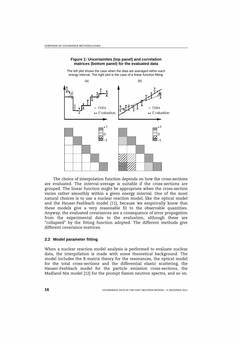
The evaluation of covariance data for the evaluated nuclear data libraries consists of reallocation of the experimental covariances onto the evaluating data grid. The uncertainties on the data grid are determined by how the experimental covariances are interpolated; the data are averaged within a given energy interval, the data are expressed by a simple analytic form, or the data are fitted by the theoretical model. The covariance matrix obtained depends on this interpolation scheme. Figure 1 shows simple examples of correlation matrices for two different interpolation schemes. In the left plot, uncertainty in each interval is determined by both the uncertainties of the data and the number of data points in the interval. In case the data are not correlated, all the off-diagonal elements of the evaluated correlation matrix become zero. When the data are correlated, the correlation coefficients of the data are re-mapped onto the evaluation grids accordingly. The right plot shows the case when the data are fitted by a linear function. The linear function behaves like a seesaw, and a strong anti-correlation appears between both edges of the segment.
OVERVIEW OF COVARIANCE METHODOLOGIES
16 COVARIANCE DATA IN THE FAST NEUTRON REGION – © OECD/NEA 2011
Figure 1: Uncertainties (top panel) and correlation matrices (bottom panel) for the evaluated data
The left plot shows the case when the data are averaged within each energy interval. The right plot is the case of a linear function fitting.
(a) (b)
The choice of interpolation function depends on how the cross-sections are evaluated. The interval-average is suitable if the cross-sections are grouped. The linear function might be appropriate when the cross-section varies rather smoothly within a given energy interval. One of the most natural choices is to use a nuclear reaction model, like the optical model and the Hauser-Feshbach model [11], because we empirically know that these models give a very reasonable fit to the observable quantities. Anyway, the evaluated covariances are a consequence of error propagation from the experimental data to the evaluation, although these are “collapsed” by the fitting function adopted. The different methods give different covariance matrices.
2.2 Model parameter fitting
When a nuclear reaction model analysis is performed to evaluate nuclear data, the interpolation is made with some theoretical background. The model includes the R-matrix theory for the resonances, the optical model for the total cross-sections and the differential elastic scattering, the Hauser-Feshbach model for the particle emission cross-sections, the Madland-Nix model [12] for the prompt fission neutron spectra, and so on.
OVERVIEW OF COVARIANCE METHODOLOGIES
COVARIANCE DATA IN THE FAST NEUTRON REGION – © OECD/NEA 2011 17
Relying on our a priori knowledge, the model describes all observable quantities well, and the uncertainties in the model calculation are ascribed to the model parameters – resonance parameters, optical model potentials, level densities, etc. Correlations in the evaluated data exist even if experimental data are uncorrelated, because the model tells us that in general a physical quantity varies continuously.
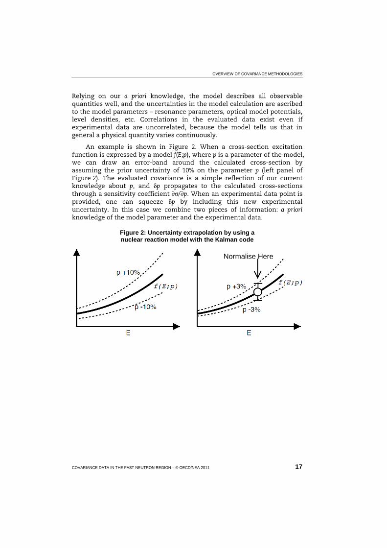
An example is shown in Figure 2. When a cross-section excitation function is expressed by a model f(E;p), where p is a parameter of the model, we can draw an error-band around the calculated cross-section by assuming the prior uncertainty of 10% on the parameter p (left panel of Figure 2). The evaluated covariance is a simple reflection of our current knowledge about p, and δp propagates to the calculated cross-sections through a sensitivity coefficient ∂σ/∂p. When an experimental data point is provided, one can squeeze δp by including this new experimental uncertainty. In this case we combine two pieces of information: a priori knowledge of the model parameter and the experimental data.
Figure 2: Uncertainty extrapolation by using a nuclear reaction model with the Kalman code
Normalise Here


UNIFIED MONTE CARLO APPROACH
COVARIANCE DATA IN THE FAST NEUTRON REGION – © OECD/NEA 2011 19
3. Unified Monte Carlo approach
3.1 Introduction
A “Unified Monte Carlo” (UMC) approach to fast neutron cross-section data evaluation that incorporates both model-calculated and experimental information in a consistent manner, and offers several advantages as compared to other contemporary methods, is described in this section. The technique is based on applications of Bayes’ theorem and the principle of maximum entropy as well as on fundamental definitions from probability theory. This section describes the mathematical formalism, discusses various related practical considerations, provides several numerical examples to illustrate the method, and offers some conclusions about the viability as well as the benefits and limitations of this method in realistic evaluation applications.
3.2 General observations
Nuclear data, such as neutron cross-sections, that are required for applications in nuclear science are rarely obtained directly from experiments or theoretical calculations. Instead, cross-section values extracted from formal evaluated nuclear data libraries are utilised. These evaluated results amount to best-estimate determinations of the physical parameters that are generally based on evaluator examination of all the pertinent information, including that derived from both measurements and theoretical modelling. Over the years, nuclear data evaluation methodology has evolved from largely subjective approaches to relatively rigorous analytical procedures that attempt to combine all the available information in a consistent manner to produce the recommended values. Most of the more recent approaches strive to minimise subjective biases while at the same time making optimal use of all pertinent information. Descriptions of various analytical techniques employed for nuclear data evaluation can be found in the extensive literature on this subject [16].
The present approach to generating evaluated cross-sections in the fast neutron region is based on Monte Carlo simulation rather than on purely deterministic analyses as is the case with several other contemporary methods. It is referred to as the Unified Monte Carlo (UMC) approach

UNIFIED MONTE CARLO APPROACH
20 COVARIANCE DATA IN THE FAST NEUTRON REGION – © OECD/NEA 2011
because unlike other Monte Carlo techniques used in evaluating nuclear data it is capable of incorporating both experimental and theoretical information in a consistent (unified) manner within the framework of Monte Carlo simulation.
Section 3.3 describes the mathematical formalism upon which the UMC approach is based and considers some practical issues associated with applying this method. Section 3.4 provides several detailed examples to illustrate the method and explore its potential as well as the limitations. Finally, Section 3.6 offers some conclusions about the viability of this method in realistic situations, based on experience acquired from the investigations that led to its development, points out some important advantages of this approach compared with other contemporary evaluation methods and suggests some areas for future investigation of the UMC approach.
3.3 Formalism and some practical issues
3.3.1 Basic concept
The present method, like many others, finds its origins in Bayes’ theorem. This theorem is non-controversial and can be derived easily from the basic postulates of probability theory following some simple steps involving the algebra of probabilities [16,17]. Bayes’ theorem provides a rigorous procedure for learning from experience by establishing a simple formula that relates prior and posterior information. For the present purposes, we will express Bayes’ theorem in terms of probability density functions rather than actual probabilities. In the following discussion, items expressed in bold font represent vectors and matrices while those in ordinary font are scalars. The symbol “•” is used to represent vector (or matrix) multiplication. The symbol “×” signifies scalar multiplication; it is used only in situations where it is needed for clarity.
Let yE represent a collection of measured (experimental) quantities with a corresponding covariance matrix VE that expresses their uncertainties as well as correlations. Let us suppose that there are n elements in the vector yE and n2 elements in the n × n matrix VE. VE must be a symmetric matrix, so the actual number of distinct elements in this matrix is n(n + 1)/2. It must also be a positive definite matrix. Furthermore, let σC represent a collection of quantities representing the prior information available before considering the experimental data. Usually, these prior results are calculated by means of nuclear modelling. The uncertainties and their correlations corresponding to these prior values are represented by a covariance matrix VC. We assume that there are m calculated quantities and that the corresponding covariance matrix has dimensions m × m. It must also be symmetric and positive definite. For convenience, we use the symbol σ to signify all the quantities being evaluated even though

UNIFIED MONTE CARLO APPROACH
COVARIANCE DATA IN THE FAST NEUTRON REGION – © OECD/NEA 2011 21
this collection might include not just cross-sections but other observables as well (e.g. angular distributions).
A method for generating VC by Monte Carlo simulation when the prior is based on nuclear modelling has been suggested by D. Smith and the concept is discussed in some detail in [18]. Basically, this approach involves use of Monte Carlo simulation to propagate uncertainties of the nuclear model parameters through to the computed physical observable quantities. We will not dwell on the matter of how nuclear model parameters and their uncertainties and correlations (if any are non-zero) are chosen to provide the most reasonable values for σC and VC. Thus, an evaluator generates prior estimates of the physical quantities by means of nuclear modelling and then “refines” the evaluation by incorporating experimental data in the evaluation procedure, through a merging process to be described in this section. If no relevant experimental data exist, then the evaluation will be based on nuclear modelling alone and the evaluator’s job is finished.
In the present context, Bayes’ theorem is embodied in the following formula [16,17]:
( ) ( ) ( )CCEE ,p,CLp VVy σσσσ 0= (1)
In this equation, p is the a posteriori (posterior) probability density function, p0 is the a priori (prior) probability density function, “L” is a likelihood function (also a probability density function), and “C” is a normalisation constant. This constant is chosen so that the following normalisation condition is satisfied:
( ) =S
dp 1σσ (2)
where dσ is a volume element (voxel) in the m-dimensional space of possible values for σ and S is the region of that space over which one must integrate in order to effectively achieve convergence. By convergence it is meant that increasing the size of S would not change the value of the integral in Eq. (2) significantly. In practice it is not necessary to know the value of C since it is essentially irrelevant to the procedures used for the Monte Carlo analysis.
It is important to understand that while the components of σ are random variable arguments of the indicated functions, yE, VE, σC and VC are simply collections of fixed numbers insofar as the present evaluation procedure is concerned. Since σ is a vector, it has the following m components: σ1, σ2, …, σi, …, σm. The solution to the evaluation problem is completely embodied in the probability density function p(σ). In probability theory, the “best estimate” value for a random variable, e.g. in this case for
UNIFIED MONTE CARLO APPROACH
22 COVARIANCE DATA IN THE FAST NEUTRON REGION – © OECD/NEA 2011
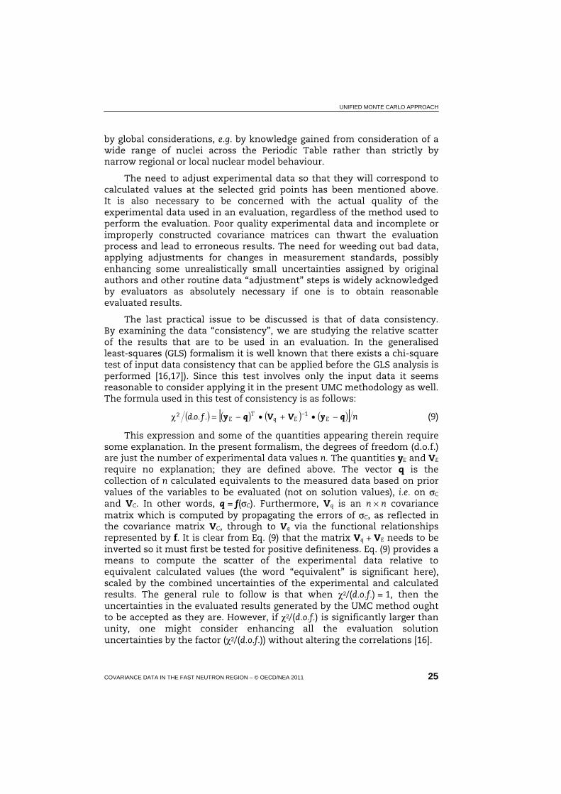
σi, is defined as its expectation value (better known as “mean value”) with respect to the associated probability density function. Therefore:
( ) ( )m,idpS
ii 1=σ=σ σσ (3)
is the evaluated value that is sought for the variable σi.
The same reasoning can be applied to generate a formula for determining elements of the evaluation solution covariance matrix Vσ:
( ) ( ) ( )m,j,i,Cov jijiijji 1=σσ−σσ==σσ σV (4)
where <…> represents multivariate integration of the indicated quantities in the same manner as shown for σi in Eq. (3). Note that when i = j we obtain the variances from Eq. (4) while the off-diagonal elements (often referred to as “covariances”) are obtained when i ≠ j.
Eqs. (1)-(4) provide all that is needed – at least conceptually – to perform an evaluation of the components of σ and determine the covariance matrix Vσ.
It is crucial to know exactly what forms the functions p0 and L should take since without this knowledge numerical analysis is impossible. Bayes’ formula, i.e. Eq. (1), offers no specific guidance in this matter. Fortunately, a rigorous solution to this problem can be found in the pioneering work on information entropy by Shannon (in the 1940s), Jaynes (in the 1960s), and other statisticians of this period [16]. The principle of maximum (information) entropy states that if all we know about a collection of random variables can be summarised by giving their mean values and associated covariance matrix, then the best estimate for the form of the appropriate probability density function is a multivariate normal function (Gaussian). Thus, in our case we have the following expression for p0:
( ) ( ) ( ) ( )[ ]{ }CCT
CCC ~,p σσσσσσ −••−− −10 21exp VV (5)
By pursuing the same line of reasoning one is led to postulate the following expression for the likelihood function L:
( ) ( ) ( ) ( )[ ]{ }EET
EEE ~,L yyyyVy −••−− −121exp Vσ (6)
In these formulas 1−CV and 1−
EV are inverse matrices, “T” denotes the
transpose of the indicated vector, and the symbol “~” indicates that the respective normalisation constants are not shown explicitly. They are actually not needed as is shown below. It is clear why VC and VE must be square, symmetric, positive definite matrices; they have to be inverted. The reason why “y” and “yE” appear in Eq. (6) rather than “σ”-type variables is that the relationship between the experimental data yE and the variables σ

UNIFIED MONTE CARLO APPROACH
COVARIANCE DATA IN THE FAST NEUTRON REGION – © OECD/NEA 2011 23
to be evaluated may be indirect. For example, the experimental data may represent ratios of the variables to be evaluated or they may be integral quantities. In fact, it is appropriate to define y by the expression y = f(σ), where f represents a vector collection of m scalar functions f1, f2, …, fi, …, fm each of whose variables are one or more of the elements of σ.
While the conditions that lead to a multivariate normal probability density function for both the prior and likelihood distributions are relatively common ones, it should be noted that other functions may be more appropriate in applications where alternative information is available, e.g. as shown below and as is mentioned in [16]. For example, if there are estimates of the mean values but no uncertainty information, then an exponential function should be used. Another example might be that both central values and covariance matrices are available but the uncertainties are very large. Under these conditions, lognormal distributions should be used rather than normal distributions [19]. Lastly, if the experimental information is based entirely on raw detectors counts, then a Poisson distribution might be appropriate for the likelihood function.
When Eqs. (1), (5), and (6) are combined, one obtains the expression:
( ) ( ) ( ) ( ){ } ( ) ( ){ }[ ]{ }CCT
CEET
E~p σσσσσ −••−+−••−− −− 1121exp VyyVyy (7)
Once again, the implied normalisation constant is omitted for the reason mentioned above. Although it is not relevant to the present derivation, it is interesting to note that if we were to assume that the best solution for the evaluation corresponds to values of the components of σ that maximise p(σ), then we would require that:
( ) ( )[ ] ( ) ( )[ ] imumminCCT
CEET
E =−••−+−••− −− σσσσ 11 VyyVyy (8)
However, this would be an appropriate assumption only if p(σ) is a multivariate normal distribution with respect to the variables σ [16]. Acceptance of this assumption leads directly to the well-known generalised least-squares (GLS) formalism [16,17].
Eq. (7), combined with Eqs. (2), (3) and (4) provides a way to carry out the numerical analysis required to produce an evaluation based on a direct consideration of the underlying probability density function. The difficulty in applying this approach lies in the need to find a viable way to compute multi-dimensional integrals. This is a formidable challenge to deterministic numerical computation when even a few variables are involved and probably impractical when many variables have to be considered as is the case for a typical evaluation. However, such calculations should be amenable to analysis by Monte Carlo simulation, at least to precisions which, in principle, are limited only by the number of traced histories. This is one of the premises upon which the present method is based.

UNIFIED MONTE CARLO APPROACH
24 COVARIANCE DATA IN THE FAST NEUTRON REGION – © OECD/NEA 2011
3.3.2 Some practical considerations
The following issues must be considered in practical applications of the UMC method: convergence of the numerical analysis, the compatibility of prior and experimental information, the independence of prior and experimental data, appropriate preparation of the measured data, and the consistency of prior and experimental information.
The input experimental and model-calculated information must be compatible. In setting up an evaluation exercise an evaluator needs to establish grid points (or node points) that define the scope of the evaluation. These grid points are characterised by such parameters as incident neutron energy, particle emission angle, etc. The situation is unambiguous for model-calculated prior results since they can be generated in a straightforward manner for all selected node points. For experimental results the situation is murkier. There are two issues involved. As indicated above, there is a reason why prior and posterior (solution) quantities are labelled “σ” while “y” is used to designate experimental results. The experimental results may be more complicated than simple cross-sections. Consider a particular example. Among the experimental data included in vector yE, suppose one particular component, say yE7, corresponds to a measured differential cross-section ratio involving cross-sections associated with grid points 6 and 18. We then require that y7 = f7(σ) = (σ6/σ18). This must be reflected in the explicit expression for p(σ). Another issue to consider is that to be perfectly compatible all input experimental information must be adjusted to correspond to the selected grid points. An example will clarify this point. Referring to the discussion above, let us suppose that the neutron energy corresponding to grid point 6 is 5 MeV while that for grid point 18 is 14 MeV. Then y7, as defined above, is meant to represent a ratio corresponding exactly to these two energies. However, let us suppose that the measured value yE7 actually corresponds to a ratio involving experimental energies 4.9 MeV and 14.1 MeV. Then, it is necessary to adjust the measured value yE7 as needed so that it is compatible with y7. These details are not unique to the present method. In principle, they need to be considered in order to apply correctly any of the more commonly used evaluation techniques, including the ordinary or generalised least-squares (GLS) methods.
The formalism for the UMC method described in Section 3.2 requires that the prior information and the experimental information that are to be merged to generate an evaluation be independent. Therefore, it is important that the selection of nuclear model parameters and their uncertainties be influenced as little as possible by experimental data relevant to the specific nucleus for which the evaluation in question is being carried out. A reasonable way to achieve an adequate degree of independence is for the choice of nuclear model parameters used to generate the prior to be guided
UNIFIED MONTE CARLO APPROACH
COVARIANCE DATA IN THE FAST NEUTRON REGION – © OECD/NEA 2011 25
by global considerations, e.g. by knowledge gained from consideration of a wide range of nuclei across the Periodic Table rather than strictly by narrow regional or local nuclear model behaviour.
The need to adjust experimental data so that they will correspond to calculated values at the selected grid points has been mentioned above. It is also necessary to be concerned with the actual quality of the experimental data used in an evaluation, regardless of the method used to perform the evaluation. Poor quality experimental data and incomplete or improperly constructed covariance matrices can thwart the evaluation process and lead to erroneous results. The need for weeding out bad data, applying adjustments for changes in measurement standards, possibly enhancing some unrealistically small uncertainties assigned by original authors and other routine data “adjustment” steps is widely acknowledged by evaluators as absolutely necessary if one is to obtain reasonable evaluated results.
The last practical issue to be discussed is that of data consistency. By examining the data “consistency”, we are studying the relative scatter of the results that are to be used in an evaluation. In the generalised least-squares (GLS) formalism it is well known that there exists a chi-square test of input data consistency that can be applied before the GLS analysis is performed [16,17]). Since this test involves only the input data it seems reasonable to consider applying it in the present UMC methodology as well. The formula used in this test of consistency is as follows:
( ) ( ) ( ) ( )[ ] n.f.o.d EEqT
E qyVVqy −•+•−=χ −12 (9)
This expression and some of the quantities appearing therein require some explanation. In the present formalism, the degrees of freedom (d.o.f.) are just the number of experimental data values n. The quantities yE and VE require no explanation; they are defined above. The vector q is the collection of n calculated equivalents to the measured data based on prior values of the variables to be evaluated (not on solution values), i.e. on σC and VC. In other words, q = f(σC). Furthermore, Vq is an n × n covariance matrix which is computed by propagating the errors of σC, as reflected in the covariance matrix VC, through to Vq via the functional relationships represented by f. It is clear from Eq. (9) that the matrix Vq + VE needs to be inverted so it must first be tested for positive definiteness. Eq. (9) provides a means to compute the scatter of the experimental data relative to equivalent calculated values (the word “equivalent” is significant here), scaled by the combined uncertainties of the experimental and calculated results. The general rule to follow is that when χ2/(d.o.f.) = 1, then the uncertainties in the evaluated results generated by the UMC method ought to be accepted as they are. However, if χ2/(d.o.f.) is significantly larger than unity, one might consider enhancing all the evaluation solution uncertainties by the factor (χ2/(d.o.f.)) without altering the correlations [16].

UNIFIED MONTE CARLO APPROACH
26 COVARIANCE DATA IN THE FAST NEUTRON REGION – © OECD/NEA 2011
3.3.3 “Brute Force” (BF) Monte Carlo approach
We now turn attention to the issue of Monte Carlo simulation to evaluate the integrals mentioned earlier in this section. This is at the heart of the UMC technique.
Let us imagine pursuing K Monte Carlo histories. For each history a potential solution vector σk(k = 1,K) is generated. Each component of this vector is selected at random from its associated uniform distribution independently from all the others. A typical sampling range would be defined by:
( )K,k;m,imaxiikmini 11 ==σ≤σ≤σ −− (10)
Expressed another way, σik is generated using the following formula:
( ) ( )ikminimaximiniik RN×σ−σ+σ=σ −−− (11)
where (RN)ik represents a real random number uniformly selected from the interval (0,1). The indicated intervals define a unique “rectangular” region S in m-dimensional space with volume V(S) given by the formula:
( ) ( )minimaxim,iSV −−= σ−σΠ= 1 (12)
The “size” of this sample space must be finite and it is determined in terms of the metric Ψ[(Vc)ii]1/2 where Ψ > 0 can be varied to test for the convergence.
Since the evaluation process is based on Eqs. (2), (3), (4) and (7) we proceed next to specify forms for these equations that are amenable to one type of Monte Carlo analysis which will be referred to henceforth in this section as the “Brute Force” (BF) Monte Carlo method. The equivalent of Eq. (3) is:
( )[ ] ( )[ ] ( )m,ipp kK,kkikK,kKi 111 =ΣσΣ=σ == σσ (13)
while in the same fashion the equivalent to Eq. (4) is:
( ){ } ( ){ } ( )m,j,iV,CovKjKiKjiKijKji 1=σ×σ−σσ=σ=σσ (14)
To avoid confusion, we note that:
( )[ ] ( )[ ] ( )m,j,ipp kK,kkjkikK,kKji 111 =ΣσσΣ=σσ == σσ (15)
The expressions found in the denominators of Eqs. (13) and (15) are there to ensure proper normalisation. The index K that appears as a subscript in Eqs. (13), (14) and (15) suggests that the values determined using these equations will depend quite strongly on the chosen number of histories K, at least for relatively small K. In fact, for small K the results are essentially meaningless. However, as K becomes large it is anticipated that

UNIFIED MONTE CARLO APPROACH
COVARIANCE DATA IN THE FAST NEUTRON REGION – © OECD/NEA 2011 27
these quantities should converge toward the values that would be obtained if the corresponding numerical integrations were actually performed as originally indicated in Eqs. (2),(3) and (4). How large does K have to be to achieve acceptable convergence? This can only be ascertained from experience. This BF Monte Carlo approach has been demonstrated to work very well in other types of analyses of complex nuclear systems with many variables, so it seems reasonable to apply it to the evaluation of nuclear data provided that convergence is achieved; however, that may be costly of both time and computer power.
Thus, we see that the UMC evaluation method amounts to employing Bayes’ theorem and the principle of maximum entropy, along with the given prior and measured values and their covariance matrix elements as constants, to generate a posterior probability density function p for the random variables σ that correspond to the evaluation in question. The evaluated values < σ > are the first moments (or mean values) of the probability density function p while the elements of the solution covariance matrix Vσ are derived from the second moments of p. The integrals required to determine the mean values and the covariance matrix elements can be estimated by the BF Monte Carlo simulation rather than by deterministic numerical computations if a sufficient number of “histories” is considered.
The UMC method will not succeed unless the quantities computed by BF Monte Carlo simulation using Eqs. (12),(13) and (14) actually converge to stable values as K becomes large. Therefore, it is essential to test convergence by examining the trend of all expressions of the form < … >K (or ratios of these quantities) as K becomes large. Rather than using sophisticated tests, simple plots of < … >K versus K may suffice in many instances. Another convergence issue involves ensuring that these sums converge to values close to the true value of the multivariable integrals that are being estimated. In the BF Monte Carlo method, this requires that the “volume” V(S) of the sampling space S be sufficiently large and all encompassing of the majority of the “strength” reflected in the posterior probability function. In particular, one needs to be certain that it is large enough so that outside region S the magnitude of the posterior probability density function p, and contributions to the indicated integrals, are vanishingly small. More precisely, we require that if a sampled vector σk is not contained in S, then p(σk) ≈ 0. Of course, one could ensure this by choosing S to be very large.
However, the penalty to pay for such a conservative choice in the BF Monte Carlo method is that K would also need to be extremely large in order to achieve acceptable convergence. This, in turn, could lead to excessively long computation times. Clearly, a trade-off between the sizes of S and K is needed. Experience will have to be the guide in dealing with
UNIFIED MONTE CARLO APPROACH
28 COVARIANCE DATA IN THE FAST NEUTRON REGION – © OECD/NEA 2011
this issue. Finally, it is certain that a wide dynamic range of real number values will be encountered in computations of the p(σk) weighting factors. Therefore, a high degree of numerical precision is essential when performing realistic BF Monte Carlo evaluations if one aims to achieve accurate results that are not afflicted by numerical round-off effects.
3.3.4 The Metropolis Monte Carlo approach
The “Brute Force” (BF) Monte Carlo approach described above was the first method we considered in demonstrating the UMC technique, and it is the easiest approach to understand. However, it is probably not the best one. It was soon discovered in considering the examples chosen for our work that this method is very inefficient. Therefore, a second method, known as the Metropolis sampling technique [20], was considered. The Metropolis (METR) algorithm was first introduced by Metropolis, et al. [21] and later generalised by Hastings [22]. It was designed to sample from complicated, high-dimensional probability density functions (PDF) that are difficult or inefficient to deal with directly, e.g. such as those encountered in applying the UMC method. The random sampling of states by the BF Monte Carlo approach is very inefficient since the PDF encountered in typical evaluation scenarios tend to be fairly localised in the m-dimensional solution space. This is especially true when accurate and consistent experimental data are involved. This leads to a substantial reduction of the significant integration volume so it is essential to apply an importance sampling method to suppress random sampling of the far more numerous irrelevant configurations while achieving the same level of accuracy over the whole cross-section energy range.
In Bayesian applications the normalisation factor is usually difficult to compute in the BF Monte Carlo method other than by the sampling procedure described above, so the ability to produce a sample without knowing the constant of proportionality is also a significant advantage of METR. The generated sequence can be used in a Markov chain Monte Carlo simulation to compute moments of the distribution such as the integrals described above.
The METR algorithm generates a Markov chain in which each state x(t + 1) depends only on the previous state x(t). The algorithm uses a “proposal density” Q(x), which depends on the current state x(t), to generate a new proposed sample x′. The proposal, usually called a “move”, is accepted as the next value x′ = x(t + 1) if it satisfies the probability condition P(x(t + 1)) > γ P(x(t)), with γ being a random number between 0 and 1. If the proposal is rejected, the current x(t) is kept, i.e. x(t + 1) = x(t).
There are no specific rules for selection of the “proposal density” although this procedure is a key to convergence of the Markov chain. This idea is applied here as follows: The model average values and standard
UNIFIED MONTE CARLO APPROACH
COVARIANCE DATA IN THE FAST NEUTRON REGION – © OECD/NEA 2011 29
deviations are taken to be σCi and [(Vσ)ii]1/2, respectively. Thus, a Metropolis “move” is defined by:
( ) ( ) ( )[ ] 2112 iiCVtxx δ−γ+=′ (16)
Here, x(t = 0) = σC and δ signifies a “step” of the move in the m-dimensional space. The Markov chain is expected to start from a random initial value x(t = 0). This algorithm is then applied again and again (for many iterations) until the initial state is “forgotten”. The final outcome must not depend on the choice of initial state. The samples which are discarded in the conduct of this procedure are known collectively as “burn-in”.
In this investigation, 10% of the requested total number of samples were treated as “burn-in”. The Metropolis “move” usually has to be tuned during the burn-in period. In our applications of this approach the move step parameter δ was tuned by finding a corresponding “acceptance rate”. This represents the fraction of proposed samples that were accepted in a window of the last “N” samples.
The desired acceptance rate depends on the target distribution and, again in our case, on the chosen step δ. As δ increases, the new point x′ in the multi-dimensional space is located “further” from the previous point x(t) and the acceptance ratio decreases. It has been shown theoretically that the ideal acceptance rate is approximately 23% for an N-dimensional Gaussian target distribution similar to most of the studied PDF.
If the step δ is too small the chain will “mix” slowly, i.e. the acceptance rate will be too high. Then, the sampling path will wander randomly around the variable space “slowly” and converge “slowly” to the desired solution. This limit was not encountered, even for steps as small as 2% of the model uncertainty [(Vσ)ii]1/2, i.e. for δ = 0.02. On the other hand, if the step δ is too large the acceptance rate will be very low because the proposals are likely to venture into regions of much lower probability density so that P(x(t + 1))/P(x(t)) >> 1. At some point in this process the step becomes so large that P(x(t + 1))/P(x(t)) ≈ 0 and the chain will not move at all from its initial point. We found that this usually happens for step parameter values δ > 1.
The moments of the PDF are calculated from the sampled Monte Carlo chain {x(t)} regardless of whether a move is accepted or not. Along the way, some consecutive sampled points x(t) are skipped to avoid the possibility of introducing biases resulting from short-term correlations. Since METR Monte Carlo is known to be much more efficient and computationally faster than BF Monte Carlo sampling for localised probability distributions such as those usually involved in UMC, it was our goal to confirm that it can be applied with confidence in UMC analyses.

UNIFIED MONTE CARLO APPROACH
30 COVARIANCE DATA IN THE FAST NEUTRON REGION – © OECD/NEA 2011
3.4 Examples
In evaluating nuclear cross-section data one encounters directly measured cross-sections, cross-section ratios and integral data. Included are data with large errors and small errors, strong and weak correlations and discrepant values. Prior cross-sections σC from nuclear modelling usually exhibit strongly correlated uncertainties, but the possibility of vanishing correlations has been considered for completeness.
We have examined four distinct scenarios of hypothetical experimental data representative of what might be observed in realistic evaluation problems: i) directly measured cross-sections; ii) included cross-section ratios; iii) included integral data; iv) data sets with values having very large errors (non-normal probability distributions). Each case is discussed separately below. For most cases, 3.6 × 10⁷ histories were traced in the BF simulations while 3.6 × 10⁶ histories were traced in METR simulations. As is shown below, this was found to be adequate in most cases.
3.4.1 Direct cross-section data
If there is a one-to-one relationship between model-calculated and experimental data, e.g. if what are calculated and measured are both comparable cross-sections (the same can be said for angular distributions and other observables), it can then be shown that Eq. (7) is a true normal distribution with a solution mean-value vector and covariance matrix that correspond exactly to the well-known generalised least squares (GLS) solution [16,17]. Therefore, applying the UMC method to examples of this nature tests its validity through comparisons with the corresponding GLS solution. The first set of hypothetical data to be considered here is shown in Table 1. Strong correlations were assumed for the prior values. They corresponded to 0.95 for adjacent nodes and no less than 0.7 for the most widely separated nodes. The word “Node” is used here to represent an integer index value that uniquely identifies the prior and experimental values that are being compared. In a more realistic situation the word “Node” would most likely be replaced by “Energy”, and specific energies would be given instead of integer index values. The experimental correlations are: C(3,1) = C(1,3) = 0.20 and C(5,2) = C(2,5) = 0.80, with all others being zero.
In this data set there is no experimental value for Node 7. This is often the case for real evaluations since nuclear-model results can be obtained for all established node points, but this is not always possible in experiments. BF simulations were performed for ψ = 0.50, 0.75, 1.00, 1.50, 1.75, 2.00, 2.50, 3.00 and 3.50. The solution mean values agreed with corresponding GLS values for all node points to < 1.5% provided that ψ was in the range 1.00 to 2.50. The best result was obtained with ψ = 1.5 (< 0.5%
UNIFIED MONTE CARLO APPROACH
COVARIANCE DATA IN THE FAST NEUTRON REGION – © OECD/NEA 2011 31
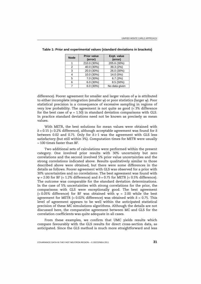
Table 1: Prior and experimental values (standard deviations in brackets)
Node Prior value
(error) Expt. value
(error) 1 210.0 (30%) 205.6 (30%) 2 040.0 (30%) 039.3 (2%)0 3 020.0 (30%) 026.0 (30%) 4 010.0 (30%) 14.0 (5%) 5 007.0 (30%) 06.7 (3%) 6 006.0 (30%) 008.5 (50%) 7 006.0 (30%) No data given
difference). Poorer agreement for smaller and larger values of ψ is attributed to either incomplete integration (smaller ψ) or poor statistics (larger ψ). Poor statistical precision is a consequence of excessive sampling in regions of very low probability. The agreement is not quite as good (< 3% difference for the best case of ψ = 1.50) in standard deviation comparisons with GLS. In practice standard deviations need not be known as precisely as mean values.
With METR, the best solutions for mean values were obtained with δ = 0.15 (< 0.2% difference), although acceptable agreement was found for δ between 0.02 and 0.75. Only for δ ≥ 1 was the agreement with GLS less satisfactory (but still within 3%). Computation times for METR were usually ≈ 100 times faster than BF.
Two additional sets of calculations were performed within the present category. One involved prior results with 30% uncertainty but zero correlations and the second involved 5% prior value uncertainties and the strong correlations indicated above. Results qualitatively similar to those described above were obtained, but there were some differences in the details as follows. Poorer agreement with GLS was observed for a prior with 30% uncertainties and no correlations. The best agreement was found with ψ = 2.00 for BF (< 1.2% difference) and δ = 0.75 for METR (< 0.5% difference). The outcome was comparable for the standard deviation determinations. In the case of 5% uncertainties with strong correlations for the prior, the comparisons with GLS were exceptionally good. The best agreement (< 0.05% difference) for BF was obtained with ψ = 2.00 while the best agreement for METR (< 0.02% difference) was obtained with δ = 0.75. This level of agreement appears to be well within the anticipated statistical precision of these MC simulations algorithms. Although the details are not discussed here, the comparative agreement between MC and GLS for the correlation coefficients was quite adequate in all cases.
From these examples, we confirm that UMC yields results which compare favourably with the GLS results for direct cross-section data, as anticipated. Since the GLS method is much more straightforward and less

UNIFIED MONTE CARLO APPROACH
32 COVARIANCE DATA IN THE FAST NEUTRON REGION – © OECD/NEA 2011
computationally intensive than the UMC method, it is clearly the preferred approach for merging model-calculated and experimental results when only direct cross-sections are involved.
Additional calculations were performed using a typical case in this category to explore the path to convergence for both BF and METR in applying UMC. Calculations were made with various numbers of sampling histories ranging from 103 to 108. Comparisons were then based on plotting the obtained chi-square values versus numbers of histories for BF and METR in comparison to the constant GLS value.
The superiority of METR convergence to the BF approach is dramatic as can be seen in Figure 3. The chi-square values from each MC approach eventually converged to a common chi-square value (that of GLS) after 108 histories. However, while the METR results are clearly fully converged after ≈ 105 histories, the BF results are seen to still fluctuate considerably even after 107 histories.
Figure 3: Comparison of Brute Force (BF) and Metropolis (METR) chi-square convergence
3.4.2 Inclusion of cross-section ratio data
When experimental cross-section ratio data are included in an evaluation, the PDF is no longer normal with respect to the solution variables σ. The PDF is therefore “skewed” and its peak location is no longer identical to the mean value location as it is for a Gaussian PDF. Then, GLS will yield an approximate solution while the UMC solution should approach the true solution (consistent with the UMC assumptions stated above) to a precision allowed by the chosen MC simulation procedure.
The example considered here has two node points. Two prior cross-sections were assumed along with their errors and correlation. Furthermore, two experimental values were considered, one is an explicitly

UNIFIED MONTE CARLO APPROACH
COVARIANCE DATA IN THE FAST NEUTRON REGION – © OECD/NEA 2011 33
measured cross-section for Node 1 and the second a ratio of the cross-section for Node 2 to that of Node 1, as shown in Table 2. This problem was analysed by GLS, BF and METR. Several combinations of data input values, errors and correlations were considered in this example.
Table 2: Prior and experimental values (standard deviations in brackets)
Node Prior cross-sections
(error) Expt. data
(error)
1 210.0 (30%) σ1 = 205.6 (30%)
2 032.0 (30%) Exp. ratio = σ2/σ1
The experimental ratio value was taken to be either 0.209 (discrepant) or 0.15 (consistent), with 1%, 5% or 30% error, and uncorrelated to the Node 1 cross-section. The prior values were assumed to be either uncorrelated or 0.95 correlated. The agreement between the BF and METR simulations was generally very good (within < 1%). Only for one extreme case (denoted henceforth as “ExC”) involving 1% experimental ratio error and a 0.95 correlation for the prior data did the BF and METR results differ noticeably (by ≈ 5%). This difference is likely due to deficiencies in the BF simulation (e.g. incomplete integration and/or inadequate convergence).
Since the METR calculations have been shown to be robust, efficient and more reliable than BF, the discussion here focuses on comparisons between METR and GLS for all cases.
First, we considered the case where the experimental ratio value is discrepant (ratio = 0.209) compared to the prior information. If 1% error is assumed for this ratio, with 0.95 correlated prior values, the GLS and UMC solution values differ by ≈ 30% (“ExC”). A projection plot of the prior and experimental PDF for “ExC” was generated along with the composite PDF. The experimental component is very obviously skewed. It was seen that in “ExC” the composite PDF for UMC peaks at a location quite different from the two peaked component PDF. Increasing the ratio error to 5% while retaining 0.95 prior correlation reduces the differences between UMC and GLS to ≈ 20%.
Eliminating the model correlation leads to differences between GLS and UMC of < 2%. An increase of the experimental ratio error to 30% results in negligible differences (0.1%) between GLS and UMC solutions, even for the case of a 0.95 prior correlation. If a consistent (non-discrepant) experimental ratio value is used (ratio = 0.15), the differences between GLS and UMC are < 3% in all cases, but these are real differences that would be absent if no ratio data were included.
Thus, inclusion of ratio data can lead to major differences between UMC and GLS solutions, especially if the ratios are accurate and discrepant
UNIFIED MONTE CARLO APPROACH
34 COVARIANCE DATA IN THE FAST NEUTRON REGION – © OECD/NEA 2011
and the prior values are strongly correlated. Both GLS and UMC strive to “fit” accurately known information and to preserve “stiffness” imposed by strong prior correlations. Even when GLS and UMC yield very different solutions, the ratios calculated from them usually agree quite well if the experimental ratio error is small.
3.4.3 Inclusion of integral cross-section data
In order to examine the effect of integral cross-section data, a seventh experimental value was added to the problem described in Section 3.4.1 (Table 1). This hypothetical integral cross-section was assumed to be a spectrum average of cross-sections for all seven nodes. The weights assumed for Nodes 1 through 7 were: 0.1, 0.2, 0.3, 0.2, 0.1, 0.05 and 0.05, respectively. A total of eight configurations were considered in which the prior correlations as well as prior errors were varied: strong or zero correlation and either 5% or 30% error. The integral value experimental error was assumed to be small in all cases (2%). GLS and UMC calculations were performed (both BF and METR). METR agrees closely with the GLS for both mean values and standard deviations. Small differences were seen between BF results and the other approaches, probably due to inadequate convergence of BF runs for 3.6 × 10⁷ histories (e.g. see Figure 3).
Thus, we conclude that if the experimental data consist only of direct cross-sections and linearly weighted averages (“spectrum-average”) UMC (METR) can be used reliably while GLS provides equally acceptable solutions.
3.4.4 Logarithmic transformation of data
When data errors exceed 30%, random sampling might produce non-physical negative values in the UMC method. One way to avoid this would be to transform all “real” space data to natural logarithmic (ln) values, and assume these values to be normally distributed (lognormal distribution) for sampling purposes. Logarithmic transformations will transform ratio data to linear data since ln (x/y) = ln (x) – ln (y). This approach is used by Kawano, et al. in the GLS code SOK [10].
It is therefore apparent that if only direct cross-sections and ratios are included in the evaluated data, the corresponding probability distribution for logarithmically transformed variables should be normal. The GLS solution in the space of logarithmically transformed variables will then be comparable to the UMC solution, but these solutions could very well differ from those performed in “real” (untransformed) space.
To explore this issue, eight GLS and UMC (only METR) calculations were performed. Four of these were in “real” space and four in logarithmically transformed space. Two of these considered direct cross-sections and two

UNIFIED MONTE CARLO APPROACH
COVARIANCE DATA IN THE FAST NEUTRON REGION – © OECD/NEA 2011 35
node points having modest (5%) or large (50%) errors for both the prior values and two equivocally accurate direct experimental cross-sections. A 0.95 correlation was assumed for the prior values and a 0.50 correlation for the experimental data. GLS and UMC agree very well for these cases.
The case “ExC” described above was considered next. GLS and UMC produced results differing by ≈ 30% as mentioned earlier. If the variables are logarithmically transformed, the GLS and UMC solutions agree quite well. However these results are consistent with the GLS solution in “real” space which is believed to be wrong, according to the underlying assumptions of UMC.
Finally, an additional case was analysed by GLS and UMC in both “real” and logarithmically transformed space. It was assumed that the prior errors were 60%, and that they were correlated by either 0.95 or zero. The outcome was similar to that just described except the discrepancy for 0.95 correlation was ≈ 8% (rather than ≈ 30%). This might be expected considering the greater breadth, and hence overlap, of the component PDF mentioned above. It was also seen that a BF sampling exercise yielded 12% negative values for 60% prior error whereas METR produced negligible negative values in “real” sampling space.
We conclude from this that logarithmic transformation of variables (either with GLS or UMC) does not circumvent the erroneous biases that can occur when ratio data are considered. Only UMC, applied in “real” space, will then yield proper solutions.
3.5 Practical implementation of the UMC approach
The UMC approach has been implemented in a computer system BEKED [Die BEwertung der KErnDaten (Evaluation of nuclear data)] recently developed at Karlsruhe Institute of Technology (KIT, FZK). Covariance matrices for cross-sections predicted by nuclear models are obtained using the Monte Carlo method described in Ref. [25]. The generation of covariances involves: i) definition of the best set of parameters for the best nuclear models used for the cross-section calculation; ii) definition of uncertainties of model parameters; iii) Monte Carlo generation of N input data sets for the selected models; iv) model calculations with randomised input files; v) calculation of covariance matrices Cov for particular reactions using standard expression:
( )( )=
− σ−σσ−σ=N
kjjkiikij NCov
100
1 (17)
where σik is the cross-section corresponding to the i-th primary neutron energy in the k-th Monte Carlo history, σi0 is the cross-section obtained

UNIFIED MONTE CARLO APPROACH
36 COVARIANCE DATA IN THE FAST NEUTRON REGION – © OECD/NEA 2011
using the “best” set of model parameters as described below. The corresponding correlation matrix is equal to:
( ) 21−×= jjiiijij CovCovCovC (18)
The quality of the data evaluation especially at the absence of measurements can be improved by their use for calculations of various methods or nuclear models, e.g. models for the description of nuclear level density. Results of such calculations should be presented as the statistically weighted sum of values obtained in different sets of calculations. In this case the value of σi0 is calculated as follows:
( ) ( )=
σ=σM
mm,imi w
100 (19)
where σi,0(m) is the cross-section calculated for the i-th neutron energy using the “best” set of parameters of the nuclear model m selected for calculations, e.g. the level density model, wm is the statistical weight of the m model obtained from the comparison of the cross-sections calculated using this model and experimental data [26], M is the number of models applied in the calculations.
The input data for adopted models are generated using Monte Carlo method taking into account the relative weights w(m). The procedure also includes the variation of parameters of the optical and pre-equilibrium models. Uncertainties of nuclear model parameters used in covariance calculations are obtained from the available information, as shown in Figure 4 in the case of the level density generalised superfluid model. The relative errors of the asymptotic value of the level density parameter were obtained using available experimental data [27].
Using BEKED the computation of covariances can be performed with TALYS [28], ALICE/ASH [29], ECIS [30], CASCADE [31] and other codes. Figure 5 shows the example of correlation matrices for the inelastic scattering of neutrons from the 52Cr obtained using TALYS and ALICE/ASH codes. This interesting comparison demonstrates that the overall structure of the two correlation matrices is quite similar in spite of the differences in the reaction modelling. The two matrices differ, however, in details, which reflects the fundamental fact that covariances are related to the method employed in the evaluation.
Figure 6 shows examples of correlation matrices calculated for proton production cross-sections and yields of 24Na in the p + 56Fe reaction at incident proton energies up to 1 GeV. The cross-section calculations were performed using intranuclear cascade evaporation model implemented in the CASCADE code [31].

UNIFIED MONTE CARLO APPROACH
COVARIANCE DATA IN THE FAST NEUTRON REGION – © OECD/NEA 2011 37
Figure 4: The relative error of asymptotic values of nuclear level density parameters in generalised superfluid model obtained in Ref. [27] from the
analysis of experimental data. The average value δaasymp/aasymp is 0.042.
Figure 5: Comparison of correlation matrices for the 52Cr(n,n′) reaction cross-section obtained using nuclear models
implemented in TALYS (left) and in ALICE/ASH code (right)
40 80 120 160 200 240
Mass number
0.35
0.30
0.25
0.20
0.15
0.10
0.05
0.00
δaas
ymp/
a asy
mp

UNIFIED MONTE CARLO APPROACH
38 COVARIANCE DATA IN THE FAST NEUTRON REGION – © OECD/NEA 2011
Figure 6: Correlation matrices for proton (left) and 24Na (right) production cross-sections in the interaction of protons with 56Fe
calculated using intranuclear cascade evaporation model [31]
3.5.1 Use of experimental data
The evaluation of cross-sections and covariances with the BEKED code can be performed using the unified Monte Carlo approach [23] or the generalised least-squares method [24]. In the former case the following expressions are used:
( ) ( )
( ) ( )1
11
1
11
−
==
−
==
σσσσ=
σσσ=σ
N
kk
N
kkjkikij
N
kk
N
kkik
evai
ppV
pp
(20)
( ) ( ) ( )2
111
−
===
σσσσσ−
N
kk
N
kkjk
N
kkik ppp (21)
where k index refers to the k-th Monte Carlo history, σik is selected randomly using the uniform probability distribution:
( ) ( ) ( )( )minmaxmin iiiik σ−σξ+σ=σ (22)
with ξ being a random number between 0 and 1 and:
( ) ( ) ( ) ( ) ( )[ ]( )calccalcT
calcT VV.p σ−σ××σ−σ+σ−σ××σ−σ−∝σ −− 1
exp1
expexp50exp (23)
where V is the covariance matrix, index exp corresponds to experimental data while calc to results of model calculations.

UNIFIED MONTE CARLO APPROACH
COVARIANCE DATA IN THE FAST NEUTRON REGION – © OECD/NEA 2011 39
3.6 Conclusions
The Unified Monte Carlo (UMC) method has been demonstrated to yield evaluated results with values that are close to those provided by the Generalised Least Squares method (GLS) in situations where the conditions are consistent with the approximations inherent to the GLS approach. In other instances, the UMC method yields results that differ from GLS. Then, the UMC methods are likely to yield better solutions. The lognormal function, transformed to normal by use of a logarithmic transformation of variables, can be used to good advantage in both UMC and GLS applications. It has been demonstrated that the exponential and uniform distributions tend to be problematic and should probably be avoided in evaluation applications.
The Metropolis Monte Carlo technique has been demonstrated to be superior to the Brute Force Monte Carlo approach in all situations owing to the fact that it converges far quicker to the correct results. So far, however, the only practical implementation of the UMC is the Brute Force approach described in the previous subsection. Additional work is required to develop the Metropolis approach which would greatly facilitate practical use of UMC in routine estimation of nuclear reaction covariances. The results reported so far indicate that such an approach may be practical even in more complex situations.
A final, related consideration stems from the fact that the experimental data available in the EXFOR archival system often have errors and/or lack uncertainty information. The UMC method requires this detailed uncertainty data to perform properly. Hopefully, the database of experimental reaction data will eventually improve with time, and the errors in older data sets will be cleaned to a large extent. These advances will surely help in any future attempts to use the UMC method for routine production of evaluations.


CONVENTIONAL MONTE CARLO APPROACHES
COVARIANCE DATA IN THE FAST NEUTRON REGION – © OECD/NEA 2011 41
4. Conventional Monte Carlo approaches
In this section we describe formulations of the Monte Carlo method, which compared to the UMC, invoke less rigorous procedures for including experimental data. In spite of this imperfection, these formulations were extensively and successfully used to produce numerous files with covariances.
4.1 TALYS-MC approach
4.1.1 Filtered Monte Carlo method
The Monte Carlo method implemented at NRG basically concerns the idea of Smith [18] applied to TALYS. The method is based on nuclear model uncertainties only, in which the nuclear model parameter uncertainties are chosen such that the existing experimental uncertainties (or rather, spread of experimental results) are reproduced as well as possible. In addition, for nuclear data library production further “unphysical” adjustment of uncertainties may be applied, awaiting more successful, or at least rigorous, methods as UMC.
The basis of the method is to let TALYS perform many calculations, whereby each time all L elements of the parameter vector p
are randomly
sampled from a normal distribution with a specific width Δpl for each parameter pl, i.e.:
( ) ( ) L,l,ppp llk
l 10 =Δ±= (24)
where we have added a superscript (k) to denote the k-th TALYS run, i.e.:
( ) ( )( )kk T p =σ (25)
where σ is the “cross-section” vector. The initial set of input parameters, the central values, is denoted as ( )0p
and the corresponding initial
calculated cross-section vector as ( )0σ . This initial set can represent e.g. the best possible fit to experiment, or a global calculation. After the initial calculation, the first set of random parameters ( )1p
will lead to a set of
cross-sections ( )1σ that is different from ( )0σ . From the results, we can

CONVENTIONAL MONTE CARLO APPROACHES
42 COVARIANCE DATA IN THE FAST NEUTRON REGION – © OECD/NEA 2011
obtain the single covariance matrix element ( ) ( )( ) ( ) ( )( )0101jjii σ−σσ−σ which is a
measure of the change of σj relative to the change of σi. In a Monte Carlo approach, as a single covariance matrix element alone is rather meaningless, since all parameters are simultaneously sampled from a random distribution, and no significant information is available after one run. However, after performing many calculations, all statistical information like average values, uncertainties and covariance matrices will gradually become available. The average covariance matrix for cross-sections is given by:
( ) ( )( ) ( ) ( )( ) N,j,i,K
VK
kj
kji
kiij 1
1
1
00 =σ−σσ−σ= =
(26)
where K is the total number of TALYS runs needed for statistical convergence. Similarly, the average relative covariance matrix for cross-sections can be obtained:
( ) ( )( ) N,j,i,VR jiijij 100 =σσ= (27)
The average calculated cross-sections are:
( ) N,i,K
K
k
kii 1
1
1
=σ=σ =
(28)
for which one would expect that ( )0ii σ≈σ for all elements i. The square root
of the diagonal elements of the relative covariance matrix R represents the uncertainty. Hence, the final calculated cross-sections together with their uncertainties can be expressed as:
( ) N,i,Riiii 11final =±σ=σ (29)
We can construct similar statistical quantities for the L model parameters that we use in every run, such as the average covariance matrix for model parameters:
( ) ( )( ) ( ) ( )( ) L,m,l,ppppK
PK
k
mk
mlk
llm 11
1
00 =−−= =
(30)
while the average model parameters are:
( ) L,l,pK
pK
k
kll 1
1
1
== =
(31)
where we should obtain ( )0ll pp ≈ . The final model parameters with their
uncertainties are:
( ) L,l,Rpp Pllll 11final =±= (32)
CONVENTIONAL MONTE CARLO APPROACHES
COVARIANCE DATA IN THE FAST NEUTRON REGION – © OECD/NEA 2011 43
Of course, Eqs. (30)-(32) are meaningless when we take uncorrelated, randomly sampled parameters as a starting point: after enough iterations, we will simply obtain as a result what we put in, provided the random generator is reliable. The parameter covariance matrix will be Plm = 0 for l ≠ m, since we assume to have no a priori knowledge of the correlation of the model parameters. Also, Eq. (32) becomes equal to Eq. (24). The statistical expressions for the model parameters do however become meaningful when we introduce parameter correlations and these emerge naturally when we take experimental data into account.
As mentioned before, we use the collection of experimental data as a visual guide to obtain realistic results, i.e. we do not literally include them in the optimisation scheme. To obtain the final cross-section uncertainties and the parameter correlations, we use a simple binary reject/accept method: we put an uncertainty band around the best, or global, data set ( )0σ , such that the available scattered experimental data falls more or less inside this uncertainty band. We then ensure that our initial parameter uncertainties produce cross-section uncertainty bands that are somewhat larger than those indicated by the experimental data. If the calculated cross-sections of a random TALYS run all fall inside the experimentally determined uncertainty band we accept the input parameter set, otherwise we reject it. We generally aim for an accept/reject ratio of 1:3. After enough iterations, a full parameter covariance matrix is obtained, which now includes off-diagonal correlations since only certain combinations of nuclear model parameters led to results that were accepted. Simultaneously, the entire cross-section covariance matrix is available.
We have applied the random covariance method consistently for the construction of the TENDL library [33], but also for in-depth evaluations, such as for all Pb and Bi isotopes [34]. The final parameter uncertainties used for our 206Pb evaluation are given in Table 3. It is interesting to compare them with the global parameter uncertainties of Table 4, which are used if no experimental data is available. To obtain realistic uncertainties for 206Pb, i.e. smaller than global uncertainties because experimental data is available, some of the parameters were reduced with respect to the global parameters.
4.1.2 Total Monte Carlo
With the Monte Carlo covariance method, a single ENDF-6 covariance data file is created by averaging the hundreds to thousands of complete nuclear data sets coming from TALYS or other codes, see the box at the lower left hand side of Figure 7. An alternative approach is to take the effect of a single random sampling of nuclear model parameters all the way to the end, i.e. to create one ENDF-6 file per random set of input parameters, process it and perform an applied calculation. This process is depicted in Figure 8. In other words, every random cross-section curve is stored in a

CONVENTIONAL MONTE CARLO APPROACHES
44 COVARIANCE DATA IN THE FAST NEUTRON REGION – © OECD/NEA 2011
Table 3: Uncertainties of some nuclear model parameters for 206Pb, given as fraction (%) of the absolute value
Consult Ref. [35] for a detailed description of these parameters
Parameter Uncertainty
(%) Parameter
Uncertainty(%)
Parameter Uncertainty
(%)
rV 01.5 nd1 09.4 Γγ 50.0
aV 02.0 nd2 10. a (207Pb) 04.5
nv1 01.9 nd3 09.4 a (206Pb) 06.5
nv 2 03.0 rSO 09.7 a (205Pb) 06.5
nv 3 03.1 aSO 10.0 σ2 19.0
nv 4 05.0 nsov 1 05.0 gπ (207Pb) 06.5
nw1 09.7 nsov 2 10.0 gν (207Pb) 06.5
nw 2 10.0 nsow 1 20.0
rD 03.5 nsow 2 20.0
aD 04.0 M2 21.0
Table 4: Global uncertainties of some nuclear model parameters, given as fraction (%) of the absolute value
Consult Ref. [35] for a detailed description of these parameters
Parameter Uncertainty
(%) Parameter
Uncertainty(%)
Parameter Uncertainty
(%)
rV 02.0 nd1 10.0 Γγ 50.
aV 02.0 nd2 10.0 a 07.
nv1 02.0 nd3 10.0
nv 2 03.0 rSO 10.0
nv 3 04.0 aSO 10.0 σ2 30.
nv 4 05.0 nsov 1 05.0 gπ (207Pb) 07.
nw1 10.0 nsov 2 10.0 gν (207Pb) 07.
nw 2 10.0 nsow 1 20.0
rD 04.0 nsow 2 20.0
aD 04.0 M2 25.0
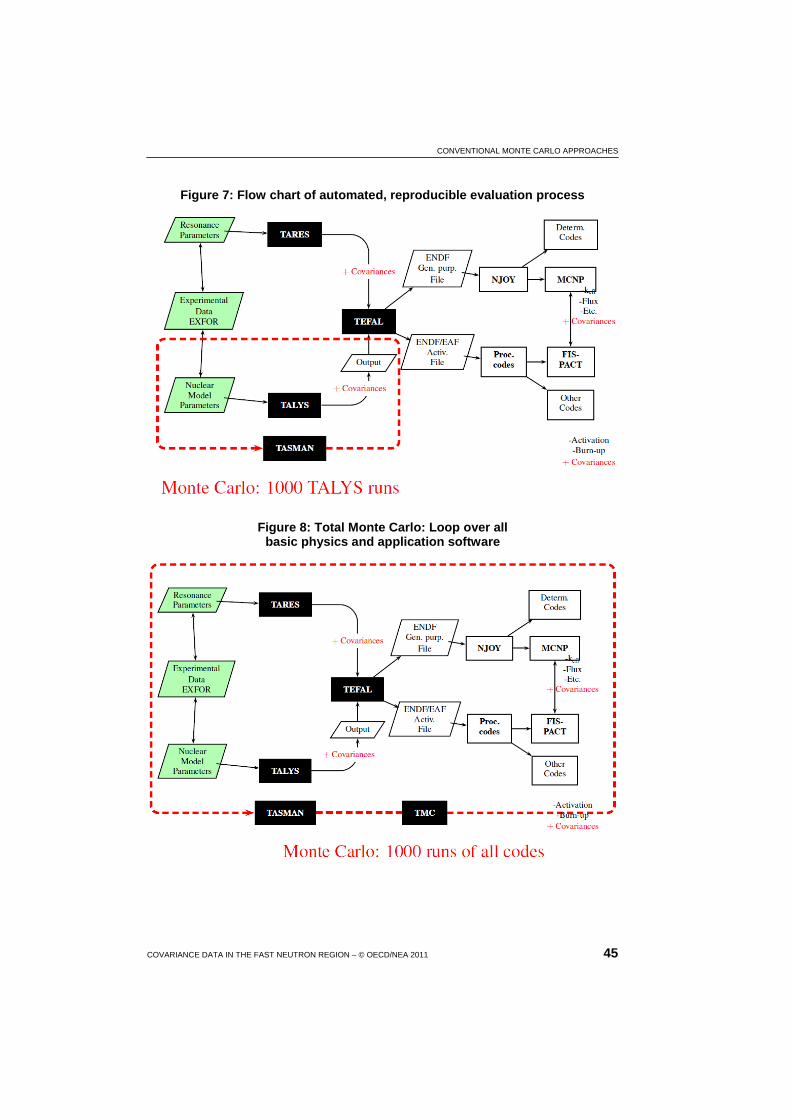
CONVENTIONAL MONTE CARLO APPROACHES
COVARIANCE DATA IN THE FAST NEUTRON REGION – © OECD/NEA 2011 45
Figure 7: Flow chart of automated, reproducible evaluation process
Figure 8: Total Monte Carlo: Loop over all basic physics and application software
CONVENTIONAL MONTE CARLO APPROACHES
46 COVARIANCE DATA IN THE FAST NEUTRON REGION – © OECD/NEA 2011
different ENDF-6 file, while every ENDF-6 file is complete for all quantities, i.e. MF1-15 are used. This approach was later coined (by Mike Herman) “Total” Monte Carlo and is an interesting alternative to uncertainty propagation with perturbation and covariance software. The general principle [36], could easily be applied in criticality studies [37], safety coefficients for fast reactors [38] and fusion [39].
A final, important, point to note here is that the Monte Carlo covariance route (Figure 7) and the Total Monte Carlo route (Figure 8): i) benefit from the same advantages such as the ability to handle non-linearities, etc.; ii) suffer from the same shortcomings at the front end of our scheme, such as the absence of a rigorous formalism of including experimental uncertainties (UMC). Hence, if UMC or another improvement is implemented at the front end of our cross-section uncertainty propagation system, it will consistently improve both routes. Independent of this degree of sophistication is our belief that if the results of the two routes differ, it is the covariance route which needs to come up with an explanation.
4.2 Backward-Forward Monte Carlo approach
With increasing reliance on nuclear models like TALYS [13] or EMPIRE [15] to produce evaluated data, there is a quest for a methodology to evaluate the covariance data that closely reflects the methods used for evaluating the data itself. For example, the continuum region of the 238U and 239Pu JEFF-3.1 [40] file was evaluated using the so-called “all-model” methodology, where all the cross-sections originate from one TALYS calculation with model parameters adjusted in order to account for the available relevant experimental data [42]. The Backward-Forward Monte-Carlo (BFMC) methodology, described in [41], was designed to stay close to the “all-model” evaluation procedure, so that the associated uncertainties truly reflect the uncertainties stemming from the evaluation methodology. The BFMC method relies on the sampling of model parameter space, and on the use of generalised χ2 estimator to quantify the likelihood of each model calculation result with respect to a given set of experimental constraints. The derived model parameter distribution is then sampled and the image of that sampling through the model code is analysed in terms of covariance matrix, which quantifies the uncertainties associated with the evaluated data.
The BFMC method rests on the assumption that the uncertainties associated with the evaluated data come from a poor knowledge of the model parameter, whose values must be adjusted in order to account for a body of experimental data. In this method, the model error component stemming from the inability of the model to account for all the experimental data is neglected. Therefore, the covariance matrix resulting from the BFMC procedure only reflects the experimental data used to constrain the model

CONVENTIONAL MONTE CARLO APPROACHES
COVARIANCE DATA IN THE FAST NEUTRON REGION – © OECD/NEA 2011 47
parameter values as well as the response of the model to variations of model parameters. The BFMC method consists in two steps: the Backward Monte Carlo step, where the distribution of model parameters leading to observables that are consistent with the experiential data is obtained, and the Forward Monte Carlo step, where that distribution of model parameters is propagated in order to obtain a sampling of observables, which is analysed in terms of mean vector and covariance matrix. As indicated by the Monte Carlo name, the BFMC method represents the model parameter and observable probability distribution functions (PDF) by their Monte Carlo sampling.
4.2.1 Backward Monte Carlo
For a n-dimensional model parameter { }np,,p 1 , an N-sized, uniform and uncorrelated sampling { } N,,inp,,p 11 = can be built. For each sample,
{ }inp,,p 1 , one can associate the sample { }ims,,s 1 of the m observable
produced by using that model parameter sample as input for the model. In order to quantify the distance between the calculated observables sample { }ims,,s 1 and the vector of comparable experimental data { }me,,e 1 , the
generalised χ2 is used as an estimator:
( )( ) ( )=′
′− ′−′ν−=χ
m,,l,llllllli sese
1
12 (33)
In Eq. (33), ν is the covariance matrix associate with the experimental data set used to constrain the model parameter space. Thus, for each value of the index i, we associate the model parameter { }inp,,p 1 , its image
{ }ims,,s 1 through the model code, and the estimator 2iχ the distance
between that observable sample and the selected set of experimental data { }me,,e 1 . That 2
iχ can then be introduced in a likelihood function that will
weight the { }inp,,p 1 sample more when the associated observables { }ims,,s 1 are close to the experimental data. As in [41,43], the selected
function is:
χχ
−=2
2
2
expmin
ii Cw (34)
where 2minχ represents the minimal value of 2
iχ over a whole sampling
(which must be large enough for 2minχ to be a good approximation of the true
minimum), and C a normalising constant. The use of the non-rigorously derived form for the likelihood function can be justified as an attempt to take into account the defaults of the model and not to attribute to the parameters, a minute weight originating from model defects.

CONVENTIONAL MONTE CARLO APPROACHES
48 COVARIANCE DATA IN THE FAST NEUTRON REGION – © OECD/NEA 2011
The weighted sampling of the model parameters can then be analysed in terms of a mean vector p and covariance vector P. The ith element of the mean vector pi = < pi > is bult as follows:
Σ ==
=N,,i
ii
iN,,i
i pww
Pp 11
1 (35)
and the matrix element Pij of P is written [using the notations of Eq. (35)]:
( )( )jjiiij ppppP −−= (36)
At this step, we have obtained the mean and covariance matrix of a sampling of a PDF of model parameters which produce a sampling of physical observables that is consistent (in the χ2 sense) with the experimental data.
Before going on to the forward step, let us interpret what is done in the Backward Mont Carlo step. The Backward step can be interpreted as a Bayesian-like calibration of the model parameter space, with experimental constraints in the physical observables space. In such an interpretation, the prior would be the uniform and uncorrelated PDF of the model parameter, and the likelihood function given in Eq. (34) from the generalised χ2 of Eq. (33).
4.2.2 Forward Monte Carlo
The Forward Monte Carlo step is more straightforward than the Backward one: a given PDF of model parameters is sampled, and its image through the model is a sampling of the distribution of observables that represents both the response of the model to parameter variations and the experimental data set that was used to constrain the PDF of model parameters.
Starting from the p mean vector and P covariance matrix of the distribution resulting from the Backward Monte Carlo, and G a sampling of a N-dimensional multivariate unit Gaussian distribution, a sampling of the Backward Monte Carlo parameter distribution is produced:
( ) pGPp,pf n +=1 (37)
from each { }inp,,p 1 sample obtained in this way, the associated observables { }ims,,s 1 can be calculated though the model. That sampling
of the observables can again be analysed in terms of a mean vector s and covariance matrix S. This S is the covariance matrix of the evaluated data we are looking for.
CONVENTIONAL MONTE CARLO APPROACHES
COVARIANCE DATA IN THE FAST NEUTRON REGION – © OECD/NEA 2011 49
4.2.3 Set-up of the BFMC procedure
In order to set up the BFMC method, several choices need to be made. Those choices will be illustrated by the evaluation of n+239Pu covariances that are proposed for the next version of the JEFF file.
The model code used was TALYS [13]. The energy mesh on which model calculations are performed must be chosen in a way that compromises between the calculation time and matching the experimental data mesh. A 50 point mesh is chosen between 1 keV and 20 MeV. A cubic interpolation algorithm used to evaluate the calculated values at the precise experimental energies is also chosen.
The differential experimental data used to calculate the value of the generalised χ2 [e in Eq. (33)] must be selected among the known “good” data sets. It is sometimes averaged over energy, in the case of high resolution data at lower energy which exhibit resonant behaviour that continuum models (like those of TALYS) are unable to reproduce. The data is also sometimes down-sampled to allow for a closer match between the calculation mesh and the experimental mesh. For n+239Pu, the final data consists of four (n,γ) data sets with 37 total experimental points, seven (n,f) data sets with 210 points (after averaging and down sampling), three (n,2n) data set with 31 points and one (n,3n) data set with 1 point.
The experimental covariance matrix ν entering Eq. (33) must be evaluated by analysing the original papers for each of the chosen data sets, including correlation within and among data sets.
The calculation of the keff in the JEZBEL [44] integral experiment is linearised and that value is integrated to the generalised χ2 [Eq. (33)] representing the experimental constraints to the model parameter values.
Since it is not practical to sample over more than 450 adjusted model parameters [45] for the evaluation of 239Pu neutronic cross-sections in the continuum, a subset of “dominant” model parameters is chosen. At this point, two types of criteria were used to select parameters. The first one is obviously being “dominant” (defined as having a large and global influence on calculated cross-sections over a large energy range). The second one has to do with the computational feasibility of the model parameter sampling. For example, sampling from the parameters associated with dispersive optical model potential (OMP) would cause calculation time in excess of five hours per sample. Excluding these parameters bring the calculation time down to six minutes per sample. Therefore, OMP parameters were not sampled, and this constitutes a major limitation of that work on n+239Pu covariances. Nine model parameters were selected: the inner fission barrier heights for the 237,238,239,240Pu compound nuclei, the level density parameters for the 237,238,239,240Pu compound nuclei and the total gamma decay width for the 240Pu compound nucleus.
CONVENTIONAL MONTE CARLO APPROACHES
50 COVARIANCE DATA IN THE FAST NEUTRON REGION – © OECD/NEA 2011
The prior distribution of model parameters was chosen to be centred on the values used in the evaluation [45], and given a uniform sampling relative range of 10% for barrier heights, 20% for level density parameters and 30% for the total gamma decay width.
The sampling size for the Backward Monte Carlo is 10 000 samples, and 5 000 samples for the Forward step.
The above choices totally determine the outcome of the BFMC process which is then automated to run on a computer.
4.2.4 Results
The result of the Backward Monte Carlo process consists in the vector of the mean values as well as the covariance matrix of the sampled parameter set, conditioned by the set of experimental constraints. In the case of n+239Pu, the vector of mean parameter values resulting from the BMC step comes in perfect agreement (within standard deviations) with the prior values, confirming the original good optimisation of the parameter values used in the evaluation.
The relative standard deviations associated with inner fission barrier heights are small (always less than 1%) down to 0.1% for the barrier height of the 240Pu compound nucleus. For level density parameters, relative standard deviations range from 3% to 8%, and for the gamma total width it is of the order of 5%. The correlation matrix associated with the BMC covariance matrix exhibits very low correlations between parameters, except for the correlation between the level density parameters of the 239Pu and 240Pu compound nuclei. Finally, it must be stressed that the BMC solution for the model parameter distribution is conditional to the more than 450 un-sampled model parameters, and that it is not likely to be the absolute optimal choice of model parameters.
Once the mean vector and covariance matrix of model parameters obtained from the Backward step are introduced in the Forward step, a sampling of observables is obtained and its mean vector and covariance matrix can be calculated. The mean vector and diagonal part of the covariance matrix are shown in Figure 9 and compared to the experimental data which was used to constrain the model parameter distribution. Inspection of Figure 9 allows to visually check that the error bands provide a good representation of the experimental values, their dispersion and their error bars. It should be noted that at energies higher than 14 MeV, the evaluated (n,2n) cross-sections and error band do not overlap with the experimental data. Excluding the possibility of experimental errors, that difference can be attributed to two possible causes: it is either a manifestation of missing an important parameter in the sampled
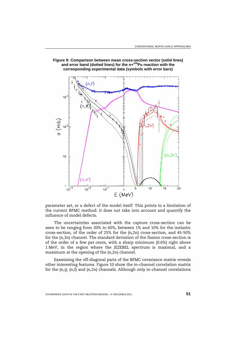
CONVENTIONAL MONTE CARLO APPROACHES
COVARIANCE DATA IN THE FAST NEUTRON REGION – © OECD/NEA 2011 51
Figure 9: Comparison between mean cross-section vector (solid lines) and error band (dotted lines) for the n+239Pu reaction with the corresponding experimental data (symbols with error bars)
parameter set, or a defect of the model itself. This points to a limitation of the current BFMC method: it does not take into account and quantify the influence of model defects.
The uncertainties associated with the capture cross-section can be seen to be ranging from 20% to 60%, between 1% and 10% for the inelastic cross-section, of the order of 25% for the (n,2n) cross-section, and 45-50% for the (n,3n) channel. The standard deviation of the fission cross-section is of the order of a few per cents, with a sharp minimum (0.6%) right above 1 MeV, in the region where the JEZEBEL spectrum is maximal, and a maximum at the opening of the (n,2n) channel.
Examining the off-diagonal parts of the BFMC covariance matrix reveals other interesting features. Figure 10 show the in-channel correlation matrix for the (n,γ), (n,f) and (n,2n) channels. Although only in-channel correlations
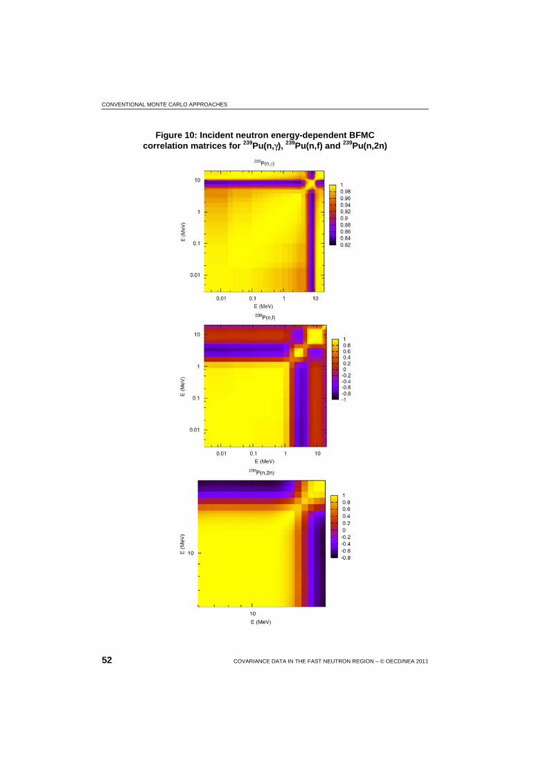
CONVENTIONAL MONTE CARLO APPROACHES
52 COVARIANCE DATA IN THE FAST NEUTRON REGION – © OECD/NEA 2011
Figure 10: Incident neutron energy-dependent BFMC correlation matrices for 239Pu(n,γ), 239Pu(n,f) and 239Pu(n,2n)
CONVENTIONAL MONTE CARLO APPROACHES
COVARIANCE DATA IN THE FAST NEUTRON REGION – © OECD/NEA 2011 53
are shown, cross-channel correlation matrices are also produced by the BFMC process. In the figure, the capture cross-section is obviously strongly correlated across the whole energy range, a behaviour that is characteristic of model-driven covariance matrices. Examination of the correlation matrix of the fission cross-section reveals that the 1 MeV to 20 MeV energy spread partitioned into three distinct ranges, corresponding to the first, second and third fission chances. Each of these three energy ranges exhibits strong correlations within that range and strong anti-correlations with the neighbouring ranges. Like the capture cross-section, that behaviour is characteristic of a model-driven covariance matrix. Finally, the correlation matrix of the (n,2n) cross-section exhibits a similar behaviour to that of the fission channel. While some may view the characteristic stiffness model-driven behaviour as undesirable, it can be argued that since the BFMC process closely follows the procedure used by some evaluators in the evaluation process, the end result of the BFMC procedure provides a realistic assessment of the uncertainties associated with that evaluated data. Nevertheless, as evidenced by the problem of too-narrow uncertainties for the (n,2n) channel above 14 MeV, the BFMC method is still missing a key ingredient, namely the quantification of model defects, and the inclusion of that component is also likely to alter the overall shape of the correlation matrices.
In [43], the case of neutron-induced reactions on 89Y has been used for a comparison between the covariances produced by the BFMC process and those resulting from the GNASH-Kalman method. That comparison showed that the covariance matrices produced with these two methods are relatively similar, although sizable differences (up to a factor of two) were observed for standard deviations.
4.3 EMPIRE-MC + Generalised Least Squares approach
The Hybrid method MC+GLSQ is similar to the UMC (Chapter 3) and Filtered Monte Carlo (Section 4.1.1) approaches as concerns dealing with modelling uncertainties to estimate the model prior. However, experimental data are incorporated into the evaluation by the GLSQ method, which combines properly-weighed experimental and model covariance matrices. As discussed above, such a method had been demonstrated to be equivalent to the UMC method as long as we are dealing with measurements of cross-sections but not their ratios [20].
4.3.1 EMPIRE-MC
The Monte Carlo (MC) method can be used in EMPIRE in the fast neutron region to generate model covariances. Its application to determination of covariances for the nuclear reaction observables is very transparent [47].
CONVENTIONAL MONTE CARLO APPROACHES
54 COVARIANCE DATA IN THE FAST NEUTRON REGION – © OECD/NEA 2011
First, model input parameters that play a significant role in defining reaction observables of interest are identified. Uncertainty of those parameters is usually taken as recommended in RIPL [50]. Scaling (normalisation) parameters can also be introduced to consider model defects. Then, the EMPIRE code is run a number of times with relevant input parameters being drawn randomly within the assumed limits around the central (optimal) values of the parameters. Typically, a Gaussian distribution is used for drawing but there is also a provision for the uniform one. Each such calculation covers the desired incident energy range and produces a full set of cross-sections, spectra, angular distributions and other observables. Standard statistical methods are used to obtain mean values and covariances (first and second moment of the distribution) for the calculated quantities automatically including cross-reaction correlations. The same approach can also be used for estimating cross-correlations between any two quantities.
The MC calculations are conceptually straightforward and free of certain simplifying assumptions, e.g. the assumption of a linear response of the observables to the variation of parameters, which is inherent in the Kalman method. There is no need for a preliminary sensitivity calculation and the computing time is independent of the employed number of model parameters. These advantages come at a price – the number of required calculations is in the range of hundreds and the convergence of the results has to be demonstrated. Furthermore, the model-based covariances obtained with the MC method constitute a reliable benchmark for validating faster but linear-model calculations with the Kalman code.
4.3.2 EMPIRE-MC + GLS
The EMPIRE-MC method has no provision for incorporating experimental data; the uncertainties and correlations depend only on the assumed uncertainties of the model parameters and model defects. However, the thus-obtained covariance matrix can be used as a prior in a full analysis by the generalised least-squares method, taking experimental data and their uncertainties rigorously into account.
This method was employed in recent IAEA evaluations to stochastically generate a set of prior cross-section values and their covariance matrix using the nuclear modelling code EMPIRE (EMPIRE-MC). This prior information was then combined deterministically with available experimental data using the GANDR system [14,88-90] to provide the final evaluations (e.g. evaluation of neutron-induced reactions on tungsten isotopes [56]). Such an approach properly combines all non-linearities from the model with experimental data including both experimental uncertainties and correlations.

DETERMINISTIC EMPIRE-KALMAN APPROACH
COVARIANCE DATA IN THE FAST NEUTRON REGION – © OECD/NEA 2011 55
5. Deterministic EMPIRE-Kalman approach
The Kalman filter technique is used both in the resonance and in the fast neutron region. It is based on minimum variance estimation and naturally combines covariances of model parameters, of experimental data and of cross-sections. This universality is a major advantage of the method. Kalman uses measurements along with their uncertainties to constrain covariances of the model parameters via the sensitivity matrix. Then, the final cross-section covariances are calculated from the updated covariances for model parameters. This procedure consistently accounts for the experimental uncertainties and the uncertainties of the model parameters ensuring that the final cross-section uncertainties are at least as good as the smaller of the two.
The key ingredient of the method is the sensitivity matrix, which represents complex nuclear reaction calculations. If we denote the combination of nuclear reaction models as an operator M̂ that transforms the vector of model parameters p into a vector of cross-sections σ(p) for a specific reaction channel, then the sensitivity matrix S can be interpreted as the linear term in the expansion of the operator M̂ :
( )
( ) ( ) +δ+σ=δ+
σ=
pSpppM
ppM
ˆ
ˆ (38)
We use “hat” to stress that M̂ is the operator rather than a matrix. In practice, the elements si,j of the sensitivity matrix are calculated numerically as partial derivatives of the cross-sections σ at the energy Ei with respect to the parameter pj:
( )
j
ij,i
p
,Es
∂σ∂
=p
(39)
In case of covariance determination, the initial values of the parameters, p0, are already optimised, i.e. when used in the model calculations they provide the evaluated cross-sections. Their covariance matrix P0 is assumed to be diagonal while the uncertainties of the parameters are estimated using systematics, independent measurements or educated guesses. The model-based covariance matrix (prior) for the

DETERMINISTIC EMPIRE-KALMAN APPROACH
56 COVARIANCE DATA IN THE FAST NEUTRON REGION – © OECD/NEA 2011
cross-sections, C0, can be obtained through a simple error propagation formula:
T00 SSPC = (40)
where superscript T indicates a transposed matrix.
The experimental data, if available, are included through a sequential update of the parameter vector p and the related covariance matrix P as:
( )( )
nnnnn
nnnnnn
SPQSPPP
pQSPpp
1T
1
exp11
T1
++
+++
−=
σ−σ+= (41)
Here:
( ) 1exp11
−++ += nnn CCQ (42)
where n = 0,1,2,… and n + 1 denotes update related to the sequential inclusion of the (n + 1)th experimental data set. In particular, the subscript 1 ≡ 0 + 1 denotes updating model prior (n = 0) with the first experiment. Vector pn+1 contains the improved values of the parameters starting from the vector pn, and Pn+1 is the updated covariance matrix of the parameters pn+1.
The exp1+nC is the cross-section covariance matrix for the (n + 1)th experiment.
The updated (posterior) covariance matrix for the cross-sections is obtained by replacing P0 with Pn+1 in Eq. (40):
T11 SSPC ++ = nn (43)
The updating procedure described above is often called Bayesian, although Eqs. (40)-(43) can be derived without any reference to the Bayes’ theorem as shown in Ref. [52].
The experimental covariance matrix, expnC , is usually non-diagonal,
due to the correlations among various energy points Ei. Assuming that systematic experimental uncertainties are fully correlated, the matrix elements are expressed through the statistical, expsta
nσΔ , and systematic, expsysnσΔ , experimental uncertainties. This yields:
( )( ) ( )( )2expsta2expstaexpinini,in EEc σΔ+σΔ= (44)
and, for i ≠ k:
( ) ( )knink,in EEc expsysexpsysexp σΔ×σΔ= (45)
An important technical issue, which has to be addressed in most of the covariance methods, is ensuring that the energy grid, Ei, for the model calculations and experimental data is the same to enable matrix operations

DETERMINISTIC EMPIRE-KALMAN APPROACH
COVARIANCE DATA IN THE FAST NEUTRON REGION – © OECD/NEA 2011 57
in Eqs. (40)-(43). In the Kalman code this is achieved by bi-spline interpolation of model cross-sections and sensitivity matrices.
The above description can easily be generalised to account for correlations among different experiments. To this end one should construct a single vector containing all experimental points and the related covariance matrix, which now may contain blocks correlating different experiments. Only one update is needed in such a case but the covariance matrices are much bigger (in the current implementation of the Kalman filter the model-based covariance matrix is expanded to match the experimental one).
The quality and consistency of the evaluated cross-sections can be assessed by scalar quantity:
( )( ) ( ) ( )( )=
−σ−σσ−σ=χ
N
nnnn
1
Nexp1expT
Nexp2 pCp (46)
where pN is the final set of model parameters corresponding to the inclusion of N experiments. A value of χ2 per degree of freedom exceeding unity indicates underestimation of the evaluated uncertainties. It is a fairly common practice to multiply such uncertainties by a square root of χ2 per degree of freedom to address this issue.
The evaluator may choose to perform a sequential update using experimental data for several/all reactions or just for a single one. In the former case, all considered reactions are correlated and unique set of parameters along with the related covariance matrix are produced. On the other hand, poor experimental data in one reaction channel can negatively influence predictions for other channels.
We note that EMPIRE-Kalman system is a general and powerful tool for evaluation of nuclear reactions. In addition to covariance calculations it may also be used to adjust model parameters to reproduce experimental cross-sections and other observables within the selected reaction models and initial uncertainties of model parameters. Therefore, the Kalman filter can be used throughout the evaluation procedure to ensure consistency between cross-sections, model parameters and related covariance matrices.
5.1 Example of application of EMPIRE-Kalman approach in EMPIRE
Application of the EMPIRE-Kalman approach is illustrated in two examples. We calculated neutron cross-sections and their covariance matrices for 55Mn and 90Zr at 63 incident energies between 1 keV and 25 MeV, considering the five reaction channels, total, elastic, inelastic, (n,2n), and capture. We used data from 22 experiments for 55Mn and 7 experiments for 90Zr. First, we discuss 55Mn and focus on energies above the ORNL evaluation [87], that is, above 122 keV.

DETERMINISTIC EMPIRE-KALMAN APPROACH
58 COVARIANCE DATA IN THE FAST NEUTRON REGION – © OECD/NEA 2011
Figure 11 compares our total cross-sections with ENDF/B-VII.0 and three sets of experimental data [58-60] found to be the basis of the ENDF/B-VII.0 evaluation. The optical model predicts a smooth, averaged behaviour of cross-sections and cannot reproduce fluctuating values extending as high as 4 MeV and adopted by the ENDF/B-VII.0. Accordingly, below 4 MeV we adopted the uncertainties deduced from the experiments. Since related experimental information was limited, we estimated these uncertainties conservatively as 5%. At higher energies, our uncertainties are based on Kalman and take into account careful measurement by Cierjacks, et al. [58].
Figure 11: Reaction 55Mn(n,tot); prior, posterior and ENDF/B-VII.0 cross-sections are compared with experimental data [58-60]
Relative uncertainties are in red (point-wise representation)
In Figure 12, 55Mn(n,n′) reaction is shown. Our cross-sections are in reasonable agreement with the ENDF/B-VII.0 evaluation. Relative uncertainties are fairly large at the threshold region, while in the energy range of about 0.7-10 MeV they drop to about 15-30%. As expected, the uncertainties rise at higher energies where cross-sections become small.
Cross-sections for 55Mn(n,2n), obtained with EMPIRE-Kalman using the experimental data of Refs. [61-72], appear to agree well with ENDF/B-VII.0 as shown in Figure 13. Relative uncertainties exhibit expected U-shape, starting with large values at the threshold region of ~10 MeV, and essentially flat up to about 22 MeV. At even higher energies, in the absence of experimental data, the uncertainties again increase.

DETERMINISTIC EMPIRE-KALMAN APPROACH
COVARIANCE DATA IN THE FAST NEUTRON REGION – © OECD/NEA 2011 59
Figure 12: Reaction 55Mn(n,inl); prior, posterior and ENDF/B-VII.0 cross-sections are compared with experimental data
Relative uncertainties are in red
Figure 13: Reaction 55Mn(n,2n); prior, posterior and ENDF/B-VII.0 cross-sections are compared with experimental data [61-72]
Relative uncertainties are in red

DETERMINISTIC EMPIRE-KALMAN APPROACH
60 COVARIANCE DATA IN THE FAST NEUTRON REGION – © OECD/NEA 2011
Figure 14 displays 55Mn radiative capture cross-sections and their uncertainties. Similar to the (n,tot) reaction, below 1 MeV the ENDF/B-VII.0 adopted fluctuating cross-sections following the experiment by Garg, et al. [73]. Consequently, we adopted Garg’s experimental uncertainties. At higher energies the EMPIRE-Kalman method was adopted. Relative uncertainties are lower than 10% in the energy range of 0.1-15 MeV, followed by the expected sharp increase at higher energies.
Figure 14: Reaction 55Mn(n,γ); prior, posterior and ENDF/B-VII.0 cross-sections are compared with experimental data
Relative uncertainties are in red
We proceed with the discussion of 90Zr reactions showing first 90Zr(n,tot) and 90Zr(n,el) in Figures 15 and 16. Total as well as elastic cross-sections compare well with ENDF/B-VII.0 and experimental data. Except for the low-energy region, the uncertainties are fairly flat around 2.5%. In contrast, uncertainties for (n,inl) are much larger throughout the whole energy range (Figure 17) since no experimental data were used.
Finally, in Figure 18 the 90Zr(n,2n) cross-sections obtained with the EMPIRE-Kalman method are shown. Compared are prior, posterior and ENDF/ B-VII.0 cross-sections with experimental data [78-82] included in our evaluation showing good agreement with both ENDF/B-VII.0 and data. Relative cross-section uncertainties exhibit the expected U-shape.

DETERMINISTIC EMPIRE-KALMAN APPROACH
COVARIANCE DATA IN THE FAST NEUTRON REGION – © OECD/NEA 2011 61
Figure 15: Reaction 90Zr(n,tot); prior, posterior and ENDF/B-VII.0 cross-sections are compared with experimental data [74-77]
Relative uncertainties are in red
Figure 16: Reaction 90Zr(n,el); prior, posterior and ENDF/B-VII.0 cross-sections are compared with experimental data
Relative uncertainties are shown in red

DETERMINISTIC EMPIRE-KALMAN APPROACH
62 COVARIANCE DATA IN THE FAST NEUTRON REGION – © OECD/NEA 2011
Figure 17: Reaction 90Zr(n,inl); prior, posterior and ENDF/B-VII.0 cross-sections are shown
Relative uncertainties are in red
Figure 18: Reaction 90Zr(n,2n); prior, posterior and ENDF/B-VII.0 cross-sections are compared with experimental data [78-82]
Relative uncertainties are shown in red
DETERMINISTIC EMPIRE-KALMAN APPROACH
COVARIANCE DATA IN THE FAST NEUTRON REGION – © OECD/NEA 2011 63
These covariances should be considered as being of intermediate quality. For high-fidelity results one should perform a complete re-evaluation of cross-sections simultaneously with covariances analysing all experimental data. 55Mn represents the additional challenge due to high-resolution measurements that exhibit strong fluctuations up to a few MeV.


GANDR APPROACH
COVARIANCE DATA IN THE FAST NEUTRON REGION – © OECD/NEA 2011 65
6. GANDR approach
6.1 Introduction
The GANDR system [88,89] is a suite of Fortran programs and associated data libraries that can be applied to a variety of tasks in the evaluation of neutron-induced nuclear reaction data. While the underlying statistical engine ZOTTVL [90] is application independent, a number of features have been included in GANDR to support the Global Assessment of Nuclear Data. The term “global assessment” refers to the simultaneous evaluation, or estimation, of the covariances of nuclear reaction data for many target nuclei (typically over 100), using methods that, while approximate, automatically enforce a high level of nuclide-to-nuclide consistency. An evaluation framework that is suitable for a global assessment of nuclear data is described below.
6.2 Methodology of covariance estimation
Because of the large scope of a global data assessment, it is essential to employ procedures that avoid extensive “tuning” to accommodate individual situations. While this is necessary, it is also permissible, because the ultimate goal is to provide a consistent uncertainty baseline for experiment planning, not necessarily to provide a complete characterisation of all aspects of the data and their uncertainties. In this respect, global data assessment differs from “data evaluation”.
In the current framework, we make the simplifying assumption that most fine details, such as the energy-dependent shape of the cross-section in the neighbourhood of individual resonances, fine details of neutron scattering angular distributions, and most emitted-particle angle-energy distributions, are sufficiently constrained by nuclear physics that they can be treated as known quantities.
In contrast, nuclear physics provides relatively little guidance on the absolute magnitude of integrated neutron cross-sections. The accuracy of evaluated data averaged over an energy region rests ultimately on the absolute accuracy of available measurements in that region. Unfortunately, real measurements are susceptible to various types of measurement error,

GANDR APPROACH
66 COVARIANCE DATA IN THE FAST NEUTRON REGION – © OECD/NEA 2011
such as problems with regard to the determination of the neutron flux, sample size, background or detector efficiency.
We take into account such measurement uncertainties by assuming that the true value of each reaction cross-section of interest differs from the best existing evaluation by a smoothly varying correction function A(E). The global approach allocates to each material 25 “reaction types” (some being “lumped partial” reactions), so that exactly 25 functions A(E) are defined for each material. The “global evaluation of data uncertainties” refers to a determination of the uncertainty in the functions A(E). In addition, each function is allowed to vary freely only at a modest number of energy “nodes”, the function being obtained at other energies by linear-linear interpolation. The parameters of the global assessment, then, are the numerical values of the 25 functions A(E) at the set of energy nodes selected for each material.
An energy grid that seems suitable for global data assessment is given in Table 1-1 of [89]. This grid includes 74 nodes spanning the energy range from 10–5 eV to 150 MeV, which is the range covered by several recently released data libraries.
The energy grid in the lower eV range is covered, for the most part, with quarter-lethargy steps (four steps per decade). Fifth-lethargy steps are employed from 0.1-100 keV, and tenth-lethargy steps from 0.1-150 MeV. In the important thermal energy range from 0.01-0.1 eV, a higher density is employed. In the cold-neutron range below 10–3 eV, a lower density is used.
For practical reasons, a fixed limit of 700 parameters is imposed for each GANDR material. The dimensioning of arrays in the programs permits the simultaneous evaluation of these 700 parameters for up to 130 materials, giving a total of 91 000 parameters. In the present GANDR framework, global data assessment proceeds by repeatedly updating the full covariance matrix of the indicated 91 000 parameters. This matrix is large, but manageable, with one full copy occupying 33.2 gigabytes of disk space.
To save space, the programming logic of the GANDR programs eliminates parameters associated with neutron energies falling below reaction thresholds. Even with this space-saving feature, meeting the 700-parameter limit requires that the above-mentioned 74-node evaluation grid be “thinned” for 32 of the current 130 materials. For actinides, we employ a thinning scheme that preserves this grid in the important energy range from 0.01 eV to 40 MeV.
6.3 Database support for large-scale projects
In addition to the mentioned Fortran programs, the distributed GANDR system includes numerical files that provide support for large-scale
GANDR APPROACH
COVARIANCE DATA IN THE FAST NEUTRON REGION – © OECD/NEA 2011 67
evaluation projects. One is the Master PENDF Library (MPL), and the other is the Master EXFOR Library (MEL).
In the GANDR evaluation framework, the final evaluated energy-dependent cross-sections for a given reaction are considered to be the reference values taken from the MPL, multiplied by the statistically adjusted correction function A(E). In the current release, GANDR-3.1, the MPL is based on pointwise processing of ENDF/B-VII.0 with NJOY99.259. Resonances were reconstructed with an error tolerance of 0.2% and the data were Doppler-broadened to 300 K.
The current MEL was constructed from the international EXFOR library [91], available online and on electronic media from the international data centres [92]. We currently access EXFOR in the Linux environment using the ENDVER-GUI package produced on CD-ROM by the Nuclear Data Section of the International Atomic Energy Agency in May 2005.
More specific information regarding the preparation of the MEL is contained in Ref. [93]. The current MPL and MEL are contained in ASCII format in the large auxiliary data file GFILES (gfiles.tar.gz), which is available online, along with the GANDR-3.1 codes and documentation, at www-nds.iaea.org/gandr.
6.4 The global assessment
In performing the present global data assessment, we first initialised the 91 000 nodal values of the functions A(E) to unity, and we introduced a non-informative prior (100% uncertainty, fully uncorrelated) for the covariances of these values.
We then introduced, from MEL, measurements of total cross-sections for 6Li, 10B, 197Au, 235U, 238U and 239Pu. Measurements of the totals on different targets are only weakly correlated, so it is possible to incorporate total cross-section data in a series of single-material library updates.
In a typical situation, a series of data measurements has a mixture of correlated (e.g. sample size) and uncorrelated (e.g. counting statistics) uncertainties. EXFOR provides no information regarding the extent of data correlations. For this reason, the GANDR system provides tools for the user to supplement the EXFOR uncertainty information with private estimates of correlated uncertainties. In the default correlated-uncertainty treatment, the standard deviation due to fully correlated uncertainties is assumed to have a constant magnitude equal to one-half the standard deviation due to uncorrelated uncertainties (as reported in EXFOR) for the most accurately measured point in a given author’s data.
The assumption of significant correlated uncertainty can be used to advantage in reducing the computational requirements of the task. In the
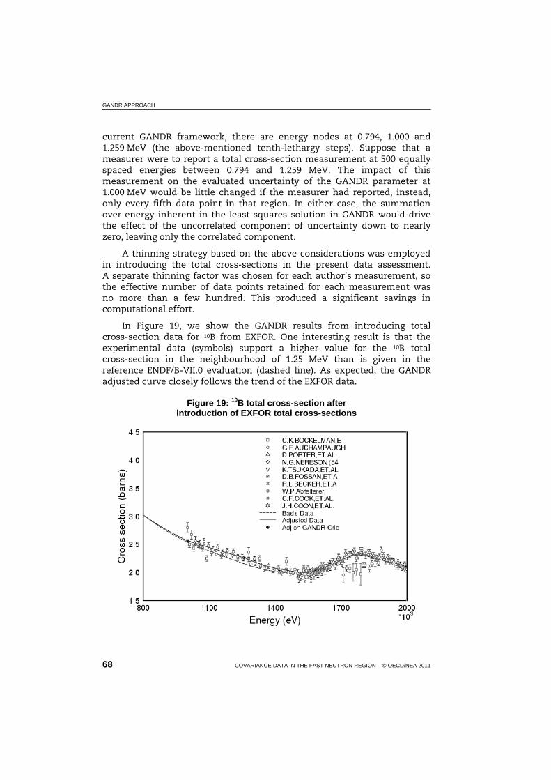
GANDR APPROACH
68 COVARIANCE DATA IN THE FAST NEUTRON REGION – © OECD/NEA 2011
current GANDR framework, there are energy nodes at 0.794, 1.000 and 1.259 MeV (the above-mentioned tenth-lethargy steps). Suppose that a measurer were to report a total cross-section measurement at 500 equally spaced energies between 0.794 and 1.259 MeV. The impact of this measurement on the evaluated uncertainty of the GANDR parameter at 1.000 MeV would be little changed if the measurer had reported, instead, only every fifth data point in that region. In either case, the summation over energy inherent in the least squares solution in GANDR would drive the effect of the uncorrelated component of uncertainty down to nearly zero, leaving only the correlated component.
A thinning strategy based on the above considerations was employed in introducing the total cross-sections in the present data assessment. A separate thinning factor was chosen for each author’s measurement, so the effective number of data points retained for each measurement was no more than a few hundred. This produced a significant savings in computational effort.
In Figure 19, we show the GANDR results from introducing total cross-section data for 10B from EXFOR. One interesting result is that the experimental data (symbols) support a higher value for the 10B total cross-section in the neighbourhood of 1.25 MeV than is given in the reference ENDF/B-VII.0 evaluation (dashed line). As expected, the GANDR adjusted curve closely follows the trend of the EXFOR data.
Figure 19: 10B total cross-section after introduction of EXFOR total cross-sections
DISPERSION ANALYSIS
COVARIANCE DATA IN THE FAST NEUTRON REGION – © OECD/NEA 2011 69
7. Dispersion analysis
Differences among various evaluated files may provide a useful indication of the common-sense uncertainties. It is quite intuitive that recommended uncertainty should not be drastically different from the spread of evaluations available in the major libraries. In particular, uncertainties considerably smaller than the spread of the evaluations raise a justified concern.
The dispersion analysis is of non-statistical nature and reflects vagueness of the available experimental information, ambiguity in the evaluation methodology including nuclear reaction modelling as well as difference of opinion among the evaluators. All these factors are consistent with our understanding of the uncertainties (or in general covariances) as the measure of dubiety in the final result. The dubiety reflecting our knowledge and associated with the choice of experimental database, nuclear reaction theory and their utilisation in deriving the recommended values.
In order for the dispersion analysis to be sensible a few basic conditions must be met:
• Ideally, the same, or at least qualitatively equivalent, experimental databases should be used by all evaluators, which implies that the evaluations should be performed within a limited period of time.
• The evaluations should be of comparable quality, i.e. should use the established techniques and up-to-date modelling so that it is impossible to argue that one of the evaluations is clearly superior to others.
• Obviously, the analysed evaluations must result from independent work by different groups.
If any of these conditions is not fulfilled the dispersion analysis might be meaningless or misleading. For example, the presence of a very precise and reliable experiment in one or more evaluations disqualifies those evaluations in which this particular experiment is not taken into account. Similarly, obviously poor and discrepant evaluations should be excluded from the analysis. In both cases, their inclusion would cause permanent overestimation of uncertainties.

DISPERSION ANALYSIS
70 COVARIANCE DATA IN THE FAST NEUTRON REGION – © OECD/NEA 2011
With the above conditions taken into account the dispersion analysis might be a useful tool for establishing sensible uncertainty margins and screening for unrealistically small or large uncertainties. In Figure 20 we show an example of inelastic scattering of neutrons on 56Fe. In the threshold region differences among cross-sections recommended in ENDF/ B-VII.0, JEFF-3.1 and JENDL-3.3 reach 30%, which dramatically exceeds the uncertainty of 1.8% claimed by JEFF-3.1. In this context the 18% reported by JENDL-3.3 seems more realistic.
Figure 20: Ratio of cross-sections for 56Fe(n,n′) reaction available in JEFF-3.1 and JENDL-3.3 libraries to the ENDF/B-VII.0
In order to smooth strong fluctuations the cross-sections were averaged over 40 energy bins. Compare dispersion among evaluations with the uncertainties quoted by JEFF-3.1 and JENDL-3.3.
Neutron Group Energy (MeV)

AVOIDING UNPHYSICALLY LOW UNCERTAINTIES
COVARIANCE DATA IN THE FAST NEUTRON REGION – © OECD/NEA 2011 71
8. Avoiding unphysically low uncertainties
8.1 Model defects
The collision of a nucleon with a nucleus represents a quantum mechanical many-body problem for which no rigorous ab initio calculations starting from the nucleon-nucleon interaction are feasible at present. In order to overcome this problem, nuclear models have been formulated, which describe various aspects of the collision. Usually these models contain effective parameters simulating specific features of the many-body problem, but obviously they cannot account for all peculiarities of the reaction processes. Especially it may happen that variation of the model parameters over the whole domain does not match the actual value of the observable. This so-called model defect has to be taken into account in an evaluation of nuclear data based on modelling.
Estimates of the model defects and the associated covariance matrices are difficult because the failures are of non-statistical nature and cannot be determined via theoretical considerations. In order to quantify model defects one must take recourse to experimental data. However, double counting must be avoided using e.g. only data of neighbouring nuclei in the same energy range, which are not used in a subsequent evaluation.
At present there exists no established method to determine model defects. In the following we propose two procedures: i) the scaling procedure which defines energy-independent scaling factors for each reaction channel of the isotope; ii) remodelling which defines an energy-dependent scaling factor for each reaction channel.
First let us define the common framework: experimental data from N neighbouring isotopes are used which are presumed to be equally well described by the applied model as the isotope actually considered. This procedure is based on the condition that for most of the neighbouring isotopes experimental data are available within a certain energy range. The energy region is divided into M bins with energy Em, m = 1,…,M at the centre of the m-th bin. In addition, an index set Ebin(m,n) is introduced in order to identify experimental data points for the n-th isotope in the energy bin m. We introduce the bin quantities:
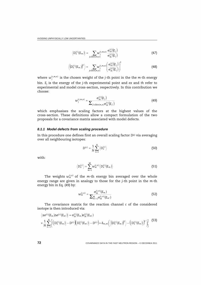
AVOIDING UNPHYSICALLY LOW UNCERTAINTIES
72 COVARIANCE DATA IN THE FAST NEUTRON REGION – © OECD/NEA 2011
( ) ( ) ( )
( )
( ) ( )( ) ( )jc
th
jc
ex
n,mEbinj
n,m,cjm
cn
E
EwED
σ
σ=
∈
(47)
( ) ( )( ) ( )
( )
( ) ( )( ) ( )
22
σ
σ=
∈ jc
th
jc
ex
n,mEbinj
n,m,cjm
cn
E
EwED (48)
where ( )n,m,cjw is the chosen weight of the j-th point in the the m-th energy
bin. Ej is the energy of the j-th experimental point and ex and th refer to experimental and model cross-section, respectively. In this contribution we choose:
( )( ) ( )( )
( ) ( )jc
thn,mEbinj
jc
thn,m,cj
E
Ew
′∈′ σ
σ= Σ (49)
which emphasises the scaling factors at the highest values of the cross-section. These definitions allow a compact formulation of the two proposals for a covariance matrix associated with model defects.
8.1.1 Model defects from scaling procedure
In this procedure one defines first an overall scaling factor D(c) via averaging over all neighbouring isotopes:
( ) ( )=
=N
n
cn
c DN
D1
1 (50)
with:
( ) ( ) ( ) ( )=
=M
m
mc
nn,c
mc
n EDwD1
(51)
The weights ( )n,cmw of the m-th energy bin averaged over the whole
energy range are given in analogy to those for the j-th point in the m-th energy bin in Eq. (49) by:
( )( ) ( )
( ) ( )mn,c
thMm
mn,c
thn,cm
E
Ew
′=′ σ
σ= Σ 1
(52)
The covariance matrix for the reaction channel c of the considered isotope is then introduced via:
( ) ( ) ( ) ( ) ( ) ( ) ( ) ( )
( ) ( ) ( )( ) ( ) ( ) ( )( ) ( ) ( )( ) ( ) ( )( )=
′′
′′
−δ+−−×
σσ=σΔσΔN
n
mc
nmc
nm,mc
mc
nc
mc
n
mc
thmc
thmc
mc
EDEDDEDDEDN
EEEE
1
221 (53)

AVOIDING UNPHYSICALLY LOW UNCERTAINTIES
COVARIANCE DATA IN THE FAST NEUTRON REGION – © OECD/NEA 2011 73
The first term of Eq. (53) is due to the defect of the model, while the second term reflects the uncertainty in the scaling factor due to the limited accuracy of the experimental data. However, it must be remarked that even if Eq. (53) is a reasonable ansatz, it is not fully of statistical nature.
8.1.2 Model defects associated with remodelling
The formulation of an energy-dependent scaling factor:
( ) ( ) ( ) ( )=
=N
n
mc
nmc ED
NED
1
1 (54)
changes the inherent features of the original model (e.g. the energy dependence) and we denote this procedure as remodelling. A reasonable covariance matrix is given by:
( ) ( ) ( ) ( ) ( ) ( ) ( ) ( )( ) ( ) ( ) ( ) ( ) ( )( ) ( ) ( )( )
=′′
′′
−δ+ΔΔ×
σσ=σΔσΔN
nm
cnm
cnm,mm
cnm
cn
mc
thmc
thmc
mc
EDEDEDEDN
EEEE
1
221 (55)
with:
( ) ( ) ( ) ( ) ( ) ( )mc
mc
nmc
n EDEDED −=Δ (56)
8.1.3 Example
The procedures defined in this section allow estimating the model defects, comprising the corrections of the mean value and the associated covariance matrix for the relevant reactions. In order to show the feasibility we apply the procedure to neutron-induced reactions of oxygen in the energy range between 5 and 60 MeV. Apart from a slightly adapted neutron-oxygen optical potential we use the code TALYS with default parameters as nuclear model description. We tested both procedures using total cross-section data from the EXFOR library of the neighbouring nuclei 12C, 14N, 19F, 23Na and 24Mg. In Figure 21(a) the scaling factor D(c) = 0.9735 as well as the energy-dependent remodelling factor D(c)(Em) are displayed. The latter exhibits only a small energy dependence beyond 20 MeV resulting in similar uncertainties of the model defects for both methods [Figure 21(b)].
In Figure 22 we show the correlation matrix due to model defects for the total cross-sections obtained by the scaling method of Section 8.1.1. In Figure 23 the same correlation matrix obtained via the remodelling procedure of Section 8.1.2 is displayed in comparison to Figure 22.
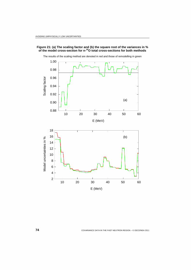
AVOIDING UNPHYSICALLY LOW UNCERTAINTIES
74 COVARIANCE DATA IN THE FAST NEUTRON REGION – © OECD/NEA 2011
Figure 21: (a) The scaling factor and (b) the square root of the variances in % of the model cross-section for n-16O total cross-sections for both methods
The results of the scaling method are denoted in red and those of remodelling in green
10 20 30 40 50 60
E (MeV)
1.00
0.98
0.96
0.94
0.92
0.90
0.88
Sca
ling
fact
or
(a)
(b)
10 20 30 40 50 60
E (MeV)
Mod
el u
ncer
tain
ties
in %
18
16
14
12
10
8
6
4
2
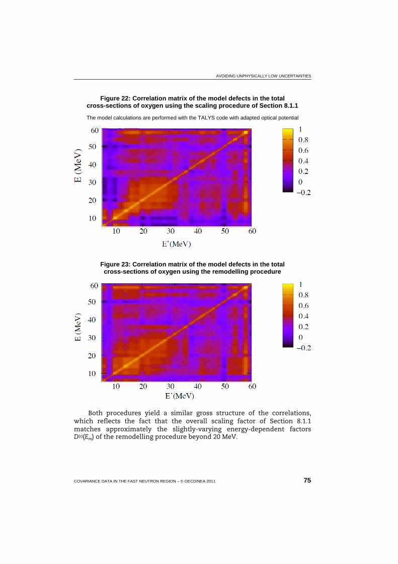
AVOIDING UNPHYSICALLY LOW UNCERTAINTIES
COVARIANCE DATA IN THE FAST NEUTRON REGION – © OECD/NEA 2011 75
Figure 22: Correlation matrix of the model defects in the total cross-sections of oxygen using the scaling procedure of Section 8.1.1
The model calculations are performed with the TALYS code with adapted optical potential
Figure 23: Correlation matrix of the model defects in the total cross-sections of oxygen using the remodelling procedure
Both procedures yield a similar gross structure of the correlations, which reflects the fact that the overall scaling factor of Section 8.1.1 matches approximately the slightly-varying energy-dependent factors D(c)(Em) of the remodelling procedure beyond 20 MeV.

AVOIDING UNPHYSICALLY LOW UNCERTAINTIES
76 COVARIANCE DATA IN THE FAST NEUTRON REGION – © OECD/NEA 2011
8.1.4 Scaling in the EMPIRE-Kalman approach
The concept of scaling model predictions, or lack of such a possibility within the model formulation, was recognised to contribute to unrealistically low uncertainties often resulting from the Kalman filter analysis involving a vast amount of experimental data. The uncertainties obtained in such cases are far lower than systematic uncertainties even of the most precise measurement. This happens even for a single experiment in spite of the fact that proper experimental covariances, accounting for systematic uncertainties, are supplied as an input to the Kalman code. This issue raises serious concerns and puts the validity of the approach in question.
One of the sources of the problem is the implicit Kalman filter assumption that the model itself is perfect. Thus, any uncertainties in model calculations are only due to the uncertainties of the model parameters. Often, the shape of a calculated excitation function is constrained, i.e. even with a substantial variation of model parameters it is not possible to alter the shape or the absolute value of the function in an arbitrary fashion. This point is illustrated in the example of the 93Nb(n,tot) reaction in Figure 24. The depth and radius of the real part of the optical model potential are essentially determining the shape and magnitude of the total cross-section. The two quantities are known to be strongly correlated, therefore it is
Figure 24: Effect of 5% variation of the depth of the real optical potential on the 93Nb(n,tot) cross-section
The baseline values are in red
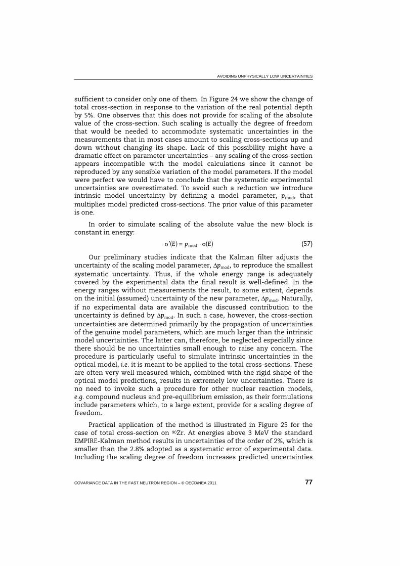
AVOIDING UNPHYSICALLY LOW UNCERTAINTIES
COVARIANCE DATA IN THE FAST NEUTRON REGION – © OECD/NEA 2011 77
sufficient to consider only one of them. In Figure 24 we show the change of total cross-section in response to the variation of the real potential depth by 5%. One observes that this does not provide for scaling of the absolute value of the cross-section. Such scaling is actually the degree of freedom that would be needed to accommodate systematic uncertainties in the measurements that in most cases amount to scaling cross-sections up and down without changing its shape. Lack of this possibility might have a dramatic effect on parameter uncertainties – any scaling of the cross-section appears incompatible with the model calculations since it cannot be reproduced by any sensible variation of the model parameters. If the model were perfect we would have to conclude that the systematic experimental uncertainties are overestimated. To avoid such a reduction we introduce intrinsic model uncertainty by defining a model parameter, pmod, that multiplies model predicted cross-sections. The prior value of this parameter is one.
In order to simulate scaling of the absolute value the new block is constant in energy:
( ) ( )EpE σ⋅=σ′ mod (57)
Our preliminary studies indicate that the Kalman filter adjusts the uncertainty of the scaling model parameter, Δpmod, to reproduce the smallest systematic uncertainty. Thus, if the whole energy range is adequately covered by the experimental data the final result is well-defined. In the energy ranges without measurements the result, to some extent, depends on the initial (assumed) uncertainty of the new parameter, Δpmod. Naturally, if no experimental data are available the discussed contribution to the uncertainty is defined by Δpmod. In such a case, however, the cross-section uncertainties are determined primarily by the propagation of uncertainties of the genuine model parameters, which are much larger than the intrinsic model uncertainties. The latter can, therefore, be neglected especially since there should be no uncertainties small enough to raise any concern. The procedure is particularly useful to simulate intrinsic uncertainties in the optical model, i.e. it is meant to be applied to the total cross-sections. These are often very well measured which, combined with the rigid shape of the optical model predictions, results in extremely low uncertainties. There is no need to invoke such a procedure for other nuclear reaction models, e.g. compound nucleus and pre-equilibrium emission, as their formulations include parameters which, to a large extent, provide for a scaling degree of freedom.
Practical application of the method is illustrated in Figure 25 for the case of total cross-section on 90Zr. At energies above 3 MeV the standard EMPIRE-Kalman method results in uncertainties of the order of 2%, which is smaller than the 2.8% adopted as a systematic error of experimental data. Including the scaling degree of freedom increases predicted uncertainties
AVOIDING UNPHYSICALLY LOW UNCERTAINTIES
78 COVARIANCE DATA IN THE FAST NEUTRON REGION – © OECD/NEA 2011
Figure 25: Cross-sections (black lines) and uncertainties (dashed red lines) for 90Zr(n,tot) obtained by applying standard EMPIRE-Kalman
method constrained by the four experimental data sets
The solid red line demonstrates increase of the uncertainties resulting from adding the scaling degree of freedom
in the whole energy range. In particular, at energies above 3 MeV, the calculated uncertainties are always above the expected 2.8% limit, indicating that the rigidity of the model is responsible for the suspiciously small uncertainties. Simulating intrinsic model uncertainty by introducing scaling degree of freedom is a simple and effective way of alleviating the problem.
Correlated sampling of energy-dependent scaling parameters, a conceptually similar solution, has also been adopted for the MC approach in EMPIRE. In this way, the minimum uncertainty of the calculated cross-section is limited by the uncertainty of the scaling parameter which is taken as the model uncertainty.
We note that scaling of the prior combined with the experimental systematic uncertainty might open the door for the Peelle’s Pertinent Puzzle [83-86]. The Kalman-predicted posterior cross-sections may deviate from the experimental data, and adequate measures should be taken to prevent it.

COMPARISON OF DIFFERENT METHODS
COVARIANCE DATA IN THE FAST NEUTRON REGION – © OECD/NEA 2011 79
9. Comparison of different methods
9.1 Comparison of model-based covariances obtained with Monte Carlo and Kalman
In this section Kalman and MC approaches are compared, and it is attempted to understand their differences. The EMPIRE code was used to perform nuclear reaction calculations, which enter both approaches, keeping inputs in both methods identical. Thus, the potential source of discrepancies, inevitable if two different reaction codes were used, was avoided. Calculations were performed for total, elastic, inelastic, (n,2n), capture, (n,p) and (n,α) reactions on 89Y up to an incident energy of 20 MeV. The same uncertainties of model parameters were assumed and the MC parameters were sampled from a Gaussian distribution.
Uncertainties of the considered cross-sections resulting from the variation of a single model parameter were compared. Figure 26 shows such a comparison for one of the key parameters – depth of the real part of the optical potential. There is a reasonable agreement between model-based uncertainties obtained using the MC and Kalman methods. Also, for the remaining parameters the results are close to each other. The only exception is the pre-equilibrium strength, for which the non-negligible differences were obtained. The reason for this discrepancy might be related to the fact that the relatively strong variation (20%) used in the calculations, together with the Gaussian distribution, allowed for values considerably far from the central value in the MC simulations. Because of this, the MC results may be demonstrating sensitivity to the non-linear dependence of the cross-sections on the parameters.
Figure 27 compares correlation matrices for the total cross-sections. Again, both methods yield essentially equivalent results – the chess-board like pattern in the correlation matrix is the same in both methods. Only the transition between negative and positive correlations above 10 MeV is more gradual in the MC than in the Kalman approach.
These numerical tests indicate that, in absence of experimental data, both methods are practically equivalent as long as the non-linearity (higher-order) effects in the Kalman approach are taken into account. To minimise the impact of non-linearity, it was found that the sensitivity

COMPARISON OF DIFFERENT METHODS
80 COVARIANCE DATA IN THE FAST NEUTRON REGION – © OECD/NEA 2011
matrix should be calculated using model parameter variations that are close to the parameter uncertainties.
9.2 Inclusion of experimental data
Inclusion of experimental data into the covariance determination still appears to be a major issue. The Kalman method accounts for them naturally but suffers from the general deficiency of all least squares type approaches – uncertainties tend to reach values that are considered far too small if very many experimental data are included in the analysis. One practical remedy to this problem is to prevent uncertainties of the model parameters to fall below some sensible limit (say 3%). While this procedure is simple and effective, it introduces a highly arbitrary component into the estimation of uncertainties. In the present comparison we have refrained from resorting to this solution.
The classical formulation of the MC approach does not account for the experimental data. Thus, in the present study, the prior (model-based cross-section covariance), obtained with the EMPIRE-MC calculations, was fed into the Generalised Least Squares code ZOTT that was incorporated in a more general GANDR system by D.W. Muir [51]. In the following, we refer to this approach as EMPIRE-MC-GANDR. The same nuclear reaction input was used to produce sensitivity matrices for Kalman and the MC based priors for GANDR.
Figure 26: Comparison of the model-based cross-section uncertainties obtained with Kalman (black) and Monte Carlo (red) methods for 89Y+n reactions
Calculated uncertainties result from the variation of the real depth of the optical potential
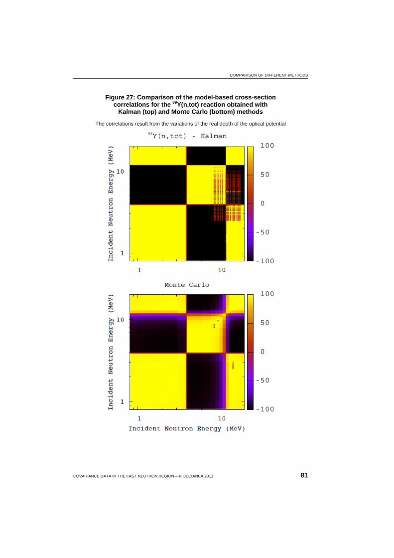
COMPARISON OF DIFFERENT METHODS
COVARIANCE DATA IN THE FAST NEUTRON REGION – © OECD/NEA 2011 81
Figure 27: Comparison of the model-based cross-section correlations for the 89Y(n,tot) reaction obtained with
Kalman (top) and Monte Carlo (bottom) methods
The correlations result from the variations of the real depth of the optical potential
100
500
000
-500
-100
100
500
000
-500
-100
89Y(n,tot) - Kalman

COMPARISON OF DIFFERENT METHODS
82 COVARIANCE DATA IN THE FAST NEUTRON REGION – © OECD/NEA 2011
Figure 28 illustrates the effect of including experimental uncertainties of the 89Y(n,2n) reaction, estimated using the two methods. The pure model-based predictions are very similar. (flat behaviour of the GANDR results at higher energies is believed to be an artefact related to the too-coarse energy mash). As expected, adding experimental data reduces uncertainties in both methods, but the reduction in the Kalman approach is stronger than in the GANDR method. One should note, however, that cross-correlations between different experiments were considered in GANDR but not in Kalman. Inclusion of the experimental data for all of the remaining channels (including nearly 1 000 points for the total) reduces (n,2n) uncertainties by about 30% in GANDR. In Kalman this difference is practically negligible around 14-15 MeV, i.e. in the range in which many (n,2n) measurements are available as can be seen in Figure 29. This figure also shows the effect of including all experimental data on the posterior cross-sections. Additional experimental points constrain model parameters so that the fit is slightly worse than in the case of using (n,2n) data only. There is a considerable advantage in simultaneously reproducing all reaction channels with the same set of model parameters, as cross-correlations among various reaction channels are also produced.
Figure 28: Comparison of the 89Y(n,2n) cross-section uncertainties obtained with GANDR (solid lines) and Kalman
(dashed lines) illustrating inclusion of experimental data
The top panel shows the model-based uncertainties (prior), the middle panel includes (n,2n) data only, and the bottom panel includes experimental data for all reaction channels

COMPARISON OF DIFFERENT METHODS
COVARIANCE DATA IN THE FAST NEUTRON REGION – © OECD/NEA 2011 83
Figure 29: Comparison of the 89Y(n,2n) cross-sections and uncertainties obtained with Kalman
“Prior” indicates default calculations and related model-based uncertainties, “(n,2n)” takes into account (n,2n) experimental data, and “Full” includes experimental data for all reaction channels
Figure 30 presents correlation matrices obtained with the two methods. The comparison is to some extent obscured by the low-energy resolution in the case of GANDR, but the general structure of the two matrices can be considered similar. In the Kalman matrix one notes relatively weak correlations below 15 MeV due to a large number of experimental data available in this region. At higher energies, the correlations are stronger as expected for the model dominated cases. The anti-correlations observed above 28 MeV can be explained as due to the pre-equilibrium emission that decreases (n,2n) cross-sections in the maximum of the excitation function and increases them in the high-energy tail.
Finally, in Figure 31 we show 89Y(n,tot) and illustrate the effect of including experimental data on the uncertainties of the total cross-section using the Kalman method. We note that a 2.8% systematic error was assumed for all experiments but no cross-correlations were allowed. Using the extended set of Abfalterer data (>400 points), the uncertainties are of the order of 1.5%. Adding about 200 points by Foster brings them down to about 1%, and including the remaining experiments results in a further reduction to about 0.75%. Many experimentalists would consider such low uncertainties as unrealistic.
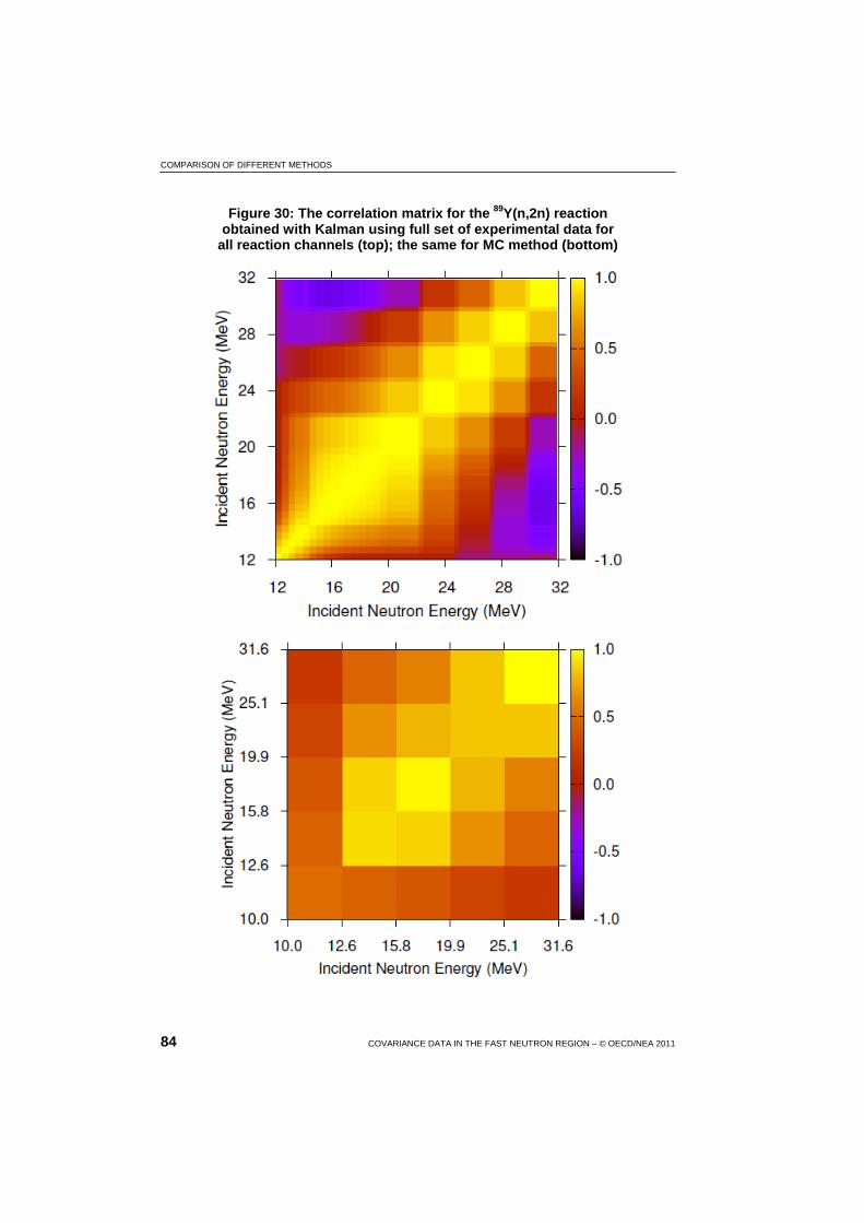
COMPARISON OF DIFFERENT METHODS
84 COVARIANCE DATA IN THE FAST NEUTRON REGION – © OECD/NEA 2011
Figure 30: The correlation matrix for the 89Y(n,2n) reaction obtained with Kalman using full set of experimental data for
all reaction channels (top); the same for MC method (bottom)
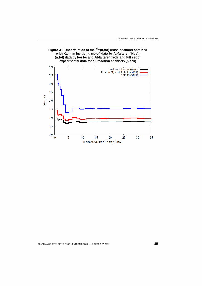
COMPARISON OF DIFFERENT METHODS
COVARIANCE DATA IN THE FAST NEUTRON REGION – © OECD/NEA 2011 85
Figure 31: Uncertainties of the 89Y(n,tot) cross-sections obtained with Kalman including (n,tot) data by Abfalterer (blue),
(n,tot) data by Foster and Abfalterer (red), and full set of experimental data for all reaction channels (black)


COVARIANCES FOR EXPERIMENTAL DATA
COVARIANCE DATA IN THE FAST NEUTRON REGION – © OECD/NEA 2011 87
10. Covariances for experimental data
10.1 Estimation of unknown systematic uncertainties
The analysis of uncertainties for the BROND-3 evaluations is carried out now on the basis of the unrecognised error-estimation method [95]. Along with a consistent consideration of statistical errors of experimental data the method allows to determine some systematic data uncertainties usually underestimated by their authors and to establish also some implicit correlations of data. This approach was used successfully for evaluations of the standard neutron cross-sections [96] and is nowadays routinely applied to construct the uncertainties and corresponding covariance matrices of the main reactor structural materials and most important fissile nuclei for the BROND-3 library.
Construction of the covariance matrices for evaluated uncertainties is usually confronted by two principal difficulties. The first relates to a disagreement between the uncertainty distribution based on the error estimations declared by authors and the reasonable statistical laws for uncertainties. Attempts to improve the distribution by rejection of some outlying data introduce badly controlled uncertainties in results and thwarts the proper estimation of systematic uncertainties, which are crucial for a complete uncertainty evaluation of all available data.
The second difficulty of the covariance construction is connected with the essential differences of matrices obtained with various approximating functions even if the resulting descriptions are practically indistinguishable. As a rule, the local uncertainties corresponding to the diagonal matrix elements increase for a large number of approximating parameters, but the off-diagonal elements responsible for correlations decrease. As a result, the uncertainty of any integral function averaged over a broad energy spectrum depends on the local uncertainties in a rather complex way and is very sensitive to evaluations of long-range systematic uncertainties.
Our method of the unrecognised error estimation is based on a priori equal reliability of all available experimental data, of course excluding proven erroneous results. However, the systematic and statistic uncertainties of each experimental work are determined in accordance with the observed distribution of data. Some initial description of data is required at the

COVARIANCES FOR EXPERIMENTAL DATA
88 COVARIANCE DATA IN THE FAST NEUTRON REGION – © OECD/NEA 2011
beginning and deviations from it can be considered as the selective values of uncertainties. The averaged deviation of experimental data from the approximating function is regarded for each analysed work as its systematic error and the deviations of experimental points from an approximant shifted on the systematic error are regarded as the statistical errors. An optimal description of all data is achieved by the traditional iteration procedure minimising mean square deviations with the obtained statistical and systematic errors. The rational functions of an optimal order are used for the corresponding approximants (the Pade approximation) and the problem of small uncertainties (the Peelle paradox [83-86]) is taken into consideration under the minimisation process and a construction of the resulting covariance matrices for the approximating function. More details of the method can be found in Ref. [95].
To display the main features of our approach the results of the fission cross-section analysis of 235U can be used. In accordance with the EXFOR library this cross-section was measured for the neutron energies from 2 keV up to 20 MeV in 107 experiments and the available data include more than 10 000 points. After averaging over the intermediate resonance fluctuations and a rejection of old low-accuracy measurements, 84 experiments with 2 311 points were conserved in the analysis. The results of 32 experiments, which contain one or two points only, were then combined and considered as one experiment. The obtained distribution of the systematic and averaged statistical uncertainties for the selected experiments is shown in Figure 32.
Figure 32: Distribution of relative uncertainties for the fission cross-section data of 235U in accordance with the unrecognised error-estimation method
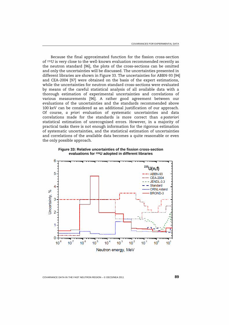
COVARIANCES FOR EXPERIMENTAL DATA
COVARIANCE DATA IN THE FAST NEUTRON REGION – © OECD/NEA 2011 89
Because the final approximated function for the fission cross-section of 235U is very close to the well-known evaluation recommended recently as the neutron standard [96], the plots of the cross-sections can be omitted and only the uncertainties will be discussed. The uncertainties presented in different libraries are shown in Figure 33. The uncertainties for ABBN-93 [94] and CEA-2004 [97] were obtained on the basis of the expert estimations, while the uncertainties for neutron standard cross-sections were evaluated by means of the careful statistical analysis of all available data with a thorough estimation of experimental uncertainties and correlations of various measurements [96]. A rather good agreement between our evaluations of the uncertainties and the standards recommended above 100 keV can be considered as an additional justification of our approach. Of course, a priori evaluation of systematic uncertainties and data correlations made for the standards is more correct than a posteriori statistical estimation of unrecognised errors. However, in a majority of practical tasks there is not enough information for the rigorous estimation of systematic uncertainties, and the statistical estimation of uncertainties and correlations of the available data becomes a quite reasonable or even the only possible approach.
Figure 33: Relative uncertainties of the fission cross-section evaluations for 235U adopted in different libraries


CONCLUSIONS
COVARIANCE DATA IN THE FAST NEUTRON REGION – © OECD/NEA 2011 91
11. Conclusions
Subgroup 24 was established to develop a methodology for production of covariance data in the fast neutron region. The subgroup concentrated on the methods that invoke statistical theory of nuclear reactions, which underlies most of the neutron nuclear data evaluations. Therefore, scant attention was paid to the fitting procedures using non-informative prior, e.g. least-squares fitting, since these have already been amply documented.
The statistical theory is understood here in a somewhat broader sense. We classify in this category not only the compound nucleus model, but also optical model, coupled channels and distorted wave Born approximation, as well as pre-equilibrium models including their classical and quantum mechanical formulations. All these models involve statistical averaging over many nuclear states in the incoming channel and usually also in the outgoing channel. In general, full sets of these models are needed to describe neutron-induced reactions. Because of the focus on the statistical model we excluded from our considerations light nuclei since these have to be treated in terms of the R-matrix or few-body theories.
Nuclear reaction theory plays a central role in the determination of covariances in the broad energy range for a complete set of reaction channels and observables. Theory constraints also provide a major source of cross-correlations among different reaction channels as well as among different isotopes. For the nuclei or reaction channels for which no measurements are available any estimates of covariances must resort to the nuclear reaction theory, since propagation of the model parameter uncertainties is the only viable possibility. For such cases, uncertainties of the model parameters become critical as the only source of information for generating cross-section covariances.
Capabilities to generate covariances in the fast neutron region have been established in several laboratories world wide (e.g. BNL, LANL, IAEA, IPPE Obninsk, JAEA, KAERI, NRG Petten). The approaches considered in the Subgroup 24 exercise were: Unified Monte Carlo, Filtered Monte Carlo, Monte Carlo Reject/Accept method, Total Monte Carlo, Kalman and GANDR. All these approaches have been implemented directly or indirectly in the existing nuclear reaction codes such as CoH, EMPIRE, McGNASH and TALYS. The intense activity carried out in the participating laboratories over the

CONCLUSIONS
92 COVARIANCE DATA IN THE FAST NEUTRON REGION – © OECD/NEA 2011
last four years produced sufficient results to define and understand the strengths and weaknesses of current covariance methodologies and their implementation.
The approaches discussed in this report were divided into two major groups – stochastic and deterministic. The first group contains various implementations of the Monte Carlo method while the latter is represented by the Kalman filter and the least-squares method using an informative prior as implemented in the GANDR system 1 . The approaches were compared analysing their inherent approximations, results obtained, applicability to various applications and convenience of use. There is no clear winner in this competition and most of the approaches are expected to be used by the evaluators, depending on the application and available resources. Let us summarise our findings grouping them, this time, by the desired features rather than by approaches.
Inclusion of experimental data is obviously the fundamental consideration for the quantification of uncertainties. Among the considered approaches only Unified Monte Carlo, Backward-Forward Monte Carlo, Kalman filter, and GANDR GLSQ fitting are able to include experimental results in a way that is statistically sound. The Straight Monte Carlo approach has no provision for including experimental data. The Filtered Monte Carlo, as well as the derived Total Monte Carlo method can do it but both methods depend on the subjective judgement of the evaluator, who arbitrarily decides what is accepted or rejected. In some cases, however, this drawback might be considered an advantage as it allows avoiding unreasonably small uncertainties that tend to be produced by the more statistically sound approaches.
If calculation speed is a major concern then deterministic methods offer a clear advantage since the number of times the reaction calculations have to performed are usually twice the number of varied model parameters (sensitivity matrices are calculated independently for each perturbed parameter). Unless this number is extremely large, say several hundred or more, deterministic calculations require much less computational effort than the Monte Carlo approaches. Should the number of parameters be high, the advantage of the deterministic calculations is less evident since Monte Carlo calculations vary all parameters in each run and thus are not so sensitive to the number of parameters. Even in this case, however, a good practice is to have considerably more calculations than varied parameters. 1. In the present report we have used the GANDR system in conjunction with the Monte Carlo generated prior. We have shown, however, that deterministic priors are essentially equivalent to the Monte Carlo priors as long as the non-linearity effects are not too pronounced. Therefore, deterministic priors, calculated by propagating model uncertainties into cross-sections and their covariances could also be used in the GLSQ-based GANDR system.

CONCLUSIONS
COVARIANCE DATA IN THE FAST NEUTRON REGION – © OECD/NEA 2011 93
The Kalman filter method is also preferable when adjustment of the model parameters to the differential or integral data is performed. The key ingredients of such adjustment are sensitivity matrices and covariances for the model parameters which are natural outcomes of the Kalman filter procedure but are usually neither needed nor generated in the Monte Carlo approaches. In this sense the Kalman filter is a convenient evaluation tool comprising estimation of cross-sections and covariances.
The non-linearity effects, if significant, might complicate analysis and invalidate usage of covariances altogether. The Kalman filter relies on the assumption that the cross-sections respond linearly to the perturbation of the model parameters. The whole concept of the covariance matrices is based on the assumption that uncertainties are propagated linearly. The Total Monte Carlo is the only approach for propagating model parameter uncertainties to integral quantities without facing the non-linearity issues. There are numerical indications confirming the presence of non-linearity effects but it is not yet clear whether these effects are significant in comparison with the accuracy of the whole procedure for determining uncertainties.
For the global estimates involving large-scale covariances between different reactions as well as materials the GANDR system is the only available framework. So far, it has been applied for cross-correlations between reactions in individual isotopes. It has been designed, however, for considering cross-correlations among multiple materials.
The persistent problem, encountered in statistically sound approaches is that uncertainty estimates are often unrealistically low. The most known are the uncertainties of standards in ENDF/B-VI.8 that were increased by the CSEWG experts, since considered to be largely underestimated. This raises serious concerns as the users, as a matter of principle, might lose confidence in the practical usability of the covariances. Addressing this issue is fundamental for the future of the field as well as for the further development of nuclear techniques and applications for which realistic and reliable estimates of the security margins are a necessity. Subgroup 24 made several attempts to understand the low values of the uncertainties. Three reasons recognised as potential cause of low uncertainties are summarised below.
The rigidity of the nuclear reaction model used in the analysis (see Section 8.1) of the experimental data may result in uncertainties lower than the systematic error in the measurement. Relaxing this rigidity by allowing for scaling of cross-sections and eventually also for modifying the shape (remodelling) increases the predicted uncertainties to (or above) the level of the systematic uncertainties. One should be aware, however, that such scaling may trigger the Pertinent Peele Puzzle, which then must be addressed.
CONCLUSIONS
94 COVARIANCE DATA IN THE FAST NEUTRON REGION – © OECD/NEA 2011
Often ignored correlations among experiments are another reason leading to underestimation of uncertainties [54]. This problem is inherent in the Bayesian approach in which subsequent updates (experiments) are considered to be independent. The same problem appears, however, in any approach if correlations among measurements are ignored. Then, the systematic uncertainties in different experiments become statistical and the final uncertainty for the average of N experiments scales approximately as ( )N1 . Unfortunately, it is extremely difficult, if not impossible, to
estimate cross-measurement correlations.
Last but not least are the hidden systematic uncertainties, i.e. errors of which the experimentalists were unaware. These might be perceived by analysing discrepancy among the measurements as suggested in Section 10.
The three effects mentioned above, when taken into account, effectively increase recommended uncertainties. It remains to be proved, however, that they are sufficient to cure the problem of unrealistically low uncertainties in all cases.
For some nuclei with A < 100 strong fluctuations have been observed in a few MeV region. These cannot be described by any model calculations. There is no consensus concerning how such cases should be treated in covariances based on the model calculations.
With all the methods close at hand, it has to be admitted that estimation of the covariances is, to a large extent, affected by a subjective evaluator’s judgement. Such factors as selection of the method, choice of the experimental data and the way these data are treated in the evaluation procedure (e.g. estimation of the systematic uncertainties and correlations among experiments) may have a dramatic impact on the final covariances and cause uncertainties recommended by different evaluators to differ by more than 100%. It is by no means surprising, since the dispersion analysis also shows that cross-sections recommended by different evaluators often differ by several standard deviations. It can be expected that further refinement of the covariance methodology, greater experience in using it, and new, more precise, and well-documented measurements will eventually reduce this ambiguity. Until then, discrepant data and even more discrepant uncertainties will simply have to be coped with.
When dealing with discrepant uncertainty information, it should be emphasised that covariances are not physical quantities and therefore cannot be investigated experimentally. There is, however, a justified concern regarding reliability of the covariances associated with a given evaluation. Contrary to the resonance region, in which several integral quantities (e.g. resonance integrals and 30 keV Maxwellian averages) are available, there are no similar measures at our disposal for validation of covariances in the fast neutron region. In principle, clean integral experiments with fast

CONCLUSIONS
COVARIANCE DATA IN THE FAST NEUTRON REGION – © OECD/NEA 2011 95
neutrons could be used for this purpose. Covariances of the nuclear data could be propagated through the transport calculations to obtain uncertainty of the integral quantity. If the calculated and the measured values are consistent within the combined experimental and propagated uncertainties the comparison might be considered a successful validation of the proposed covariances. It should be kept in mind, however, that in most cases such validation would probe a set of covariances for different reactions and possibly different materials rather than the specific covariance matrix for a single reaction. So far, such validations have not been performed on a large scale.
The activities of Subgroup 26 have increased awareness of covariances in the nuclear data community. As a result, covariance capabilities have been developed in all major nuclear reaction codes used for nuclear data evaluation. Several large-scale projects have been undertaken to produce a vast amount of covariances for the existing libraries. Specific examples include: WPEC Subgroup 26, US “Low-fidelity Project”, Japanese Actinoid file later incorporated into JENDL-4.0, successive releases of the TENDL library, a whole series of AFCI libraries culminating with AFCI-2.0, and the ongoing effort to produce covariances for ENDF/B-VII.1. Although a large part of these early attempts should be considered an exercise helping to master covariance methodology, a principal concept has been affirmed – each new evaluation must contain covariance data. It is clear that further investigations of these evaluation methods is warranted to better identify their individual strengths and weaknesses as well as ranges of applicability. Attempts should be made to eliminate to the extent possible instances where evaluations by the different methods using similar input lead to uncertainties that do not adequately cover observed dispersions between the evaluated central values.


REFERENCES
COVARIANCE DATA IN THE FAST NEUTRON REGION – © OECD/NEA 2011 97
References
[1] Smith, D.L., Probability, Statistics, and Nuclear Data Uncertainties in Nuclear Science and Technology, American Nuclear Society, LaGrange Park, IL, USA (1991).
[2] Smith, D., Workshop on Neutron Cross Section Covariances, Port Jefferson, NY, 27-28 June 2008.
[3] Smith, D., Covariance Workshop, Port Jefferson, NY, 23 June 2009.
[4] Vonach, H., et al., Physics Data, 13, 7 (1992).
[5] Tagesen, S., Proc. Int. Conf. on Nuclear Data for Science and Technology, Gatlinburg, TN, 1994, J.K. Dickens (Ed.), Verlag, Ort (1995), p. 620.
[6] Tagesen, S., H. Vonach, V.G. Pronyaev, Proc. Int. Conf. on Nuclear Data for Science and Technology, Trieste, 1997, G. Reffo, A. Ventura, C. Grandi (Eds.), Verlag, Ort (1997), p. 271.
[7] Tagesen, S., H. Vonach, A. Wallner, J. Nucl. Sci. and Techn., 2, 140 (2002).
[8] Hetric, D.M., C.Y. Fu, GLUCS: A Generalized Least-Squares Program for Updating Cross-section Evaluations with Correlated Data Sets, ORNL/TM-7341 (1980).
[9] Kawano, T., K. Shibata, Covariance Evaluation System, JAERI Data/Code, Japan Atomic Energy Research Institute, Tokai, Japan (1997).
[10] Kawano, T., et al., “Simultaneous Evaluation of Fission Cross Sections of Uranium and Plutonium Isotopes for JENDL-3.3”, J. Nucl. Sci. Technol., 37, No. 4, pp. 327-334 (2000).
[11] Hauser, W., H. Feshbach, “The Inelastic Scattering of Neutrons”, Phys. Rev., 87, 366 (1952).
[12] Madland, D.G., J.R. Nix, “New Calculation of Prompt Fission Neutron Spectra and Averaged Prompt Neutron Multiplicities”, Nucl. Sci. Eng., 81, 213 (1982).
[13] Koning, A.J., “New Working Methods for Nuclear Data Evaluation: How to Make a Nuclear Data Library”, Proc. Int. Conf. on Nuclear Data for Science and Technology, O. Bersillon, et al. (Eds.), EDP Sciences (2008), DOI:10.105/ndata:07683.
REFERENCES
98 COVARIANCE DATA IN THE FAST NEUTRON REGION – © OECD/NEA 2011
[14] Muir, D.W., et al., “The Global Assessment of Nuclear Data, GANDR”, Proc. Int. Conf. on Nuclear Data for Science and Technology, Nice, France, 22-27 April 2007, O. Bersillon, et al. (Eds.), EDP Sciences (2008), http://dx.doi.org/10.1051/ndata:07635.
[15] Herman, M., et al., “EMPIRE: Nuclear Reaction Model Code System for Data Evaluation”, Nucl. Data Sheets, 108, 2655-2715 (2007).
[16] Smith, D.L., Probability, Statistics, and Data Uncertainties in Nuclear Science and Technology, American Nuclear Society, La Grange Park, Illinois (1991).
[17] Smith, D.L., A Least-squares Computational “Tool Kit”, ANL/NDM-128, Argonne National Laboratory (1993).
[18] Smith, D.L., Covariance Matrices for Nuclear Cross Sections Derived from Nuclear Model Calculations, ANL/NDM-159, Argonne National Laboratory (2004).
[19] Smith, D.L., D.G. Naberejnev, L.A. Van Wormer, “Large Errors and Severe Conditions”, Nuclear Instruments and Methods in Physics Research, A488, 342 (2002).
[20] Capote, R., D.L. Smith, “An Investigation of the Performance of the Unified Monte Carlo Method of Neutron Cross Section Data Evaluation”, Nucl. Data Sheets, 109, 2768 (2008).
[21] Metropolis, N., et al., J. Chem. Phys. 21, pp. 1087-1091 (1953).
[22] Hastings, W.K., Biometrika, 57, pp. 97-109 (1970).
[23] Smith, D.L., A Unified Monte Carlo Approach to Fast Neutron Cross Section Data Evaluation, ANL/NDM-166, Argonne National Laboratory (2008).
[24] Smith, D.L., A Least-squares Computational Tool Kit, ANL/NDM-128, Argonne National Laboratory (1993).
[25] Smith, D.L., Covariance Matrices for Nuclear Cross Sections Derived from Nuclear Model Calculations, ANL/NDM-159, Argonne National Laboratory (2004).
[26] Konobeyev, A.Yu., U. Fischer, “Global Comparison of TALYS and ALICE Code Calculations with Measured Neutron and Proton Induced Reaction Cross-sections at Energies Up to 150 MeV”, Proc. 5th Workshop on Neutron Measurements, Evaluations and Applications Nuclear Data for Sustainable Nuclear Energy (NEMEA-5), Ljubljana, Slovenia, 27-29 October 2008.
[27] Ignatyuk, A.V., “Level Densities”, Handbook for Calculations of Nuclear Reaction Data, IAEA- TECDOC-1034, Vienna, Austria (1998), p. 65, www-nds.iaea.or.at/ripl/ripl_handbook.htm.
REFERENCES
COVARIANCE DATA IN THE FAST NEUTRON REGION – © OECD/NEA 2011 99
[28] Koning, A.J., S. Hilaire, M. Duijvestijn, TALYS-1.0 (2007), www.talys.eu.
[29] Broeders, C.H.M., et al., ALICE/ASH – Pre-Compound and Evaporation Model Code System for Calculation of Excitation Functions, Energy and Angular Distributions of Emitted Particles in Nuclear Reactions at Intermediate Energies, FZKA 7183, Forschungszentrum Karlsruhe (2006), http://bibliothek.fzk.de/zb/berichte/FZKA7183.pdf.
[30] Raynal, J., “ECIS96”, Proceeding of the Specialists’ Meeting on the Nucleon Nucleus Optical Model Up to 200 MeV, Bruyères-le-Châtel, France, 13-15 November 1996, OECD/NEA, Paris, www.nea.fr/html/science/om200/raynal.pdf.
[31] Barashenkov, V.S., Comp. Phys. Comm., 126, 28 (2000).
[32] Mughabghab, S., Atlas of Neutron Resonances. Resonance Parameters and Thermal Cross Sections, 5th Edition, Elsevier (2006).
[33] Koning, A.J., D. Rochman, “Modern Nuclear Data Evaluation: Straight from Nuclear Physics to Applications”, Proceedings of the International Conference on Nuclear Data for Science and Technology, 26-30 April 2010, Jeju, Korea, forthcoming.
[34] Rochman, D., A.J. Koning, “Pb and Bi Neutron Data Libraries with Full Covariance Evaluation and Improved Integral Tests”, Nucl. Instr. Meth., A589, pp. 85-108 (2008).
[35] Koning, A.J., et al., Nucl. Sci. and Engineering, 156, 357 (2007).
[36] Koning, A.J., D. Rochman, “Towards Sustainable Nuclear Energy: Putting Nuclear Physics to Work”, Ann. Nuc. En., 35, pp. 2024-2030 (2008).
[37] Rochman, D., A.J. Koning, S.C. van der Marck, “Uncertainties for Criticality-safety Benchmarks and keff Distributions”, Ann. Nuc. En., 36 810-831 (2009).
[38] Rochman, D., et al., “On the evaluation of 23Na Neutron-induced Reactions and Validations”, Nucl. Instr. Meth., A612, 374 (2010).
[39] Rochman, D., A.J. Koning, S.C. van der Marck, “Exact Nuclear Data Uncertainty Propagation for Fusion Design”, Fusion Engineering and Design, 85, 669-682 (2010).
[40] Nuclear Energy Agency (NEA), The JEFF 3.1 Nuclear Data Library, JEFF Report 21, OECD/NEA, Paris (2006).
[41] Bauge, E., S. Hilaire, P. Dossantos-Uzarralde, Proceedings of the International Conference on Nuclear Data for Science and Technology, 22-27 April 2007, Nice, France, O. Bersillon, et al. (Eds.), EDP Sciences (2008), p. 259.

REFERENCES
100 COVARIANCE DATA IN THE FAST NEUTRON REGION – © OECD/NEA 2011
[42] Lopez-Jimenez, M.J., B. Morillon, P. Romain, Annals of Nucl. Energy, Vol. 32, 195 (2005).
[43] Chadwick, M.B., et al., Nuclear Data Sheets, 108, 2742 (2007).
[44] International Handbook of Evaluated Criticality Safety Benchmark Experiments, entry PU-MET-FAST-01, OECD/NEA, Paris (2009).
[45] Romain, P., private communication.
[46] Herman, M., et al., “EMPIRE: Nuclear Reaction Model Code System for Data Evaluation”, Nuclear Data Sheets, Vol. 108, No. 12, pp. 2655-2715 (2007).
[47] Smith, D., Covariance Matrices for Nuclear Cross Sections Derived from Nuclear Model Calculations, ANL/NDM-159, Argonne National Laboratory (2004).
[48] Pritychenko, B., A. Sonzogni, “Sigma: Web Retrieval Interface for Nuclear Reaction Data”, Nuclear Data Sheets, Vol. 109, No. 12, pp. 2822-2827 (2008).
[49] Arcilla, R., et al., “Processing of Neutron Cross Section Covariances Using NJOY-99 and PUFF-IV”, Nuclear Data Sheets, Vol. 109, No. 12, pp. 2910-2914 (2008).
[50] Capote, R., et al., “RIPL Reference Input Parameter Library for Calculation of Nuclear Reactions and Nuclear Data Evaluations”, Nuclear Data Sheets, 110, 3107-3214 (2009).
[51] Muir, D.W., A. Mengoni, I. Kodeli, “Integration International Standards Evaluation into a Global Data Assessment”, Nuclear Data Sheets, Vol. 109, No. 12, pp. 2874-2879 (2008).
[52] Muir, D.W., “Evaluation of Correlated Data Using Partitioned Least Squares: A Minimum-variance Derivation”, Nucl. Sci. Eng., Vol. 101, pp. 88-93 (1989).
[53] Chadwick, M., P. Obložinský, M. Herman, et al., “ENDF/B-VII.0: Next Generation Evaluated Nuclear Data Library for Nuclear Science and Technology”, Nuclear Data Sheets, Vol. 107, No. 12, pp. 2931-3118 (2006).
[54] Leeb, H., D. Neudecker, Th. Srdinko, “Consistent Procedure for Evaluation Based on Modeling”, Nuclear Data Sheets, Vol. 109, No. 12, pp. 2762-2767 (2008).
[55] Little, R., et al., “Low-fidelity Covariance Project”, Nuclear Data Sheets, Vol. 109, No. 12, pp. 2828-2833 (2008).
[56] Trkov, A., et al., “Evaluation of Tungsten Nuclear Reaction Data with Covariances”, Nuclear Data Sheets, Vol. 109, No. 12, pp. 2905-2909 (2008).
REFERENCES
COVARIANCE DATA IN THE FAST NEUTRON REGION – © OECD/NEA 2011 101
[57] Pigni, M., M. Herman, P. Obložinský, “Estimated 55Mn and 90Zr Covariances in the Fast Neutron Region”, Nuclear Data Sheets, Vol. 109, No. 12, pp. 2900-2904 (2008).
[58] Cierjacks, S., P. Forti, D. Kopsch, et al., High Resolution Total Neutron Cross Sections for Na, Cl, K, V, Mn and Co between 0.5 and 30 MeV, Kernforschungszentrum Karlsruhe Reports, 1000, Supp. 2 (1969).
[59] Pineo, W.F.E., M. Divadeenam, E.G. Bilpuch, et al., “Neutron Strength Functions and Average Total Cross Sections II. The Behavior of the Average Cross Sections and the S-wave Scattering Lengths”, Ann. Phys., 84, 165 (1974).
[60] Garg, J.B., J. Rainwater, W.W. Havens Jr., “Neutron Resonance Spectroscopy in Vanadium, Manganese, and Cobalt”, Nucl. Sci. Eng., 65, 76 (1978).
[61] Filatenkov, A.A., et al., Systematic Measurement of Activation Cross Sections at Neutron Energies from 13.4 to 14.9 MeV, Khlopin Radiev. Inst., Leningrad Reports (1999).
[62] Bostan, M., S.M. Qaim, “Excitation Functions of Threshold Reactions on 45Sc and 55Mn Induced by 6 to 13 MeV Neutrons”, Phys. Rev., C 49, 266 (1994).
[63] Kimura, I., K. Kobayashi, “Calibrated Fission and Fusion Neutron Fields at the Kyoto University Reactor”, Nucl. Sci. Eng., 106, 332 (1990).
[64] Lu Han-Lin, et al., Measurement of Cross Sections for the (n,2n) Reaction of 55Mn, 58Ni, 59Co, 93Nb, 181Ta and 197Au, Chinese report to the INDC, 16 (1989).
[65] Ikeda, Y., C. Konno, K. Oishi, et al., Activation Cross Section Measurements for Fusion Reactor Structural Materials at Neutron Energy from 13.3 to 15.0 MeV Using FNS Facility, JAERI Reports 1312 (1988).
[66] Greenwood, L.R., “Recent Research in Neutron Dosimetry and Damage Analysis for Materials Irradiations”, American Soc. of Testing and Materials Reports, 956, 743 (1987).
[67] Meadows, J.W., D.L. Smith, M.M. Bretscher, et al., “Measurement of 14.7 MeV Neutron-activation Cross Sections for Fusion”, Ann. Nucl. Energy, 14, 489 (1987).
[68] Bahal, B.M., R. Pepelnik, “Cross Section Measurements of Cr, Mn, Fe, Co, Ni for an Accurate Determination of These Elements in Natural and Synthetic Samples Using a 14 MeV Neutron Generator”, Series GKSS (Ges.Kernen.-Verwertung, Schiffbau and Schiffahrt), 84E (1984).
REFERENCES
102 COVARIANCE DATA IN THE FAST NEUTRON REGION – © OECD/NEA 2011
[69] Berrada, M., Measurement and Analysis of 14 MeV Neutron Nuclear Reaction Cross-Sections by X and Gamma Spectroscopy, private communication (1984).
[70] Auchampaugh, G.F., D.M. Drake, L.R. Veeser, “Neutron Cross Section Programs in the Energy Region from 1 to 24 MeV at the LASL Van de Graaff Facilities”, Symp. on Neutr. Cross-Sect. 10-40 MeV, Brookhaven, 1977 (1977).
[71] Maslov, G.N., F. Nasyrov, N.F. Pashkin, “The Experimental Cross Sections of the Nuclear Reactions for 14 MeV Neutrons”, Yadernye Konstanty, 9, 50 (1972).
[72] Menlove, H.O., et al., “Activation Cross Sections for the 19F(n,2n)18F, 23Na(n,2n)22Na, 55Mn(n,2n)54Mn, 115In(n,2n)114mIn, 165Ho(n,2n)164mHo, 115In(n,n)11mIn, and 27Al(n,α)24Na reactions”, Phys. Rev., 163, 1308 (1967).
[73] Garg, J.B., R.L. Macklin, J Halperin, “Neutron Capture Cross Section of Manganese”, Phys. Rev., C 19, 2079 (1978).
[74] Stooksberry, R.W., J.H. Anderson, “Measurement of the Neutron Total Cross Sections of Zircaloy-2, Zirconium-90 and C between 0.4 and 2.0 MeV”, Nucl. Sci. Eng., 51, 235 (1973).
[75] Pasechnik, M.V., M.B. Fedorov, V.D. Ovdienko, et al., “Total Neutron Cross-sections for Molybdenum and Zirconium at Low Energies”, All Union Conference on Neutron Physics, Kiev, 15-19 September 1980, 1, 304 (1980).
[76] Guenther, P., et al., “90Zr and 92Zr: Neutron Total and Scattering Cross Sections”, Phys. Rev. C 12, 1797 (1975).
[77] Finlay, R.W., et al., “Neutron Total Cross Sections at Intermediate Energies”, Phys. Rev. C 47, 237 (1993).
[78] Pavlik, A., G. Winkler, H. Vonach, “Precise Measurement of Cross Sections for the 90Zr(n,2n)89Zr Reaction from Threshold to 20 MeV”, Nucl. and Part. Phys., 8, 1283 (1982).
[79] Wen-Rong, Zhao, Lu Han-Lin, Fan Pei-Guo, “Measurement of Cross Section for the Reaction 90Zr(n,2n)89Zr”, Chinese J.of Nuclear Physics (Beijing), 6, 80 (1984).
[80] Molla, N.I., R.U. Miah, M. Rahman, et al., “Excitation Functions of Some (n,p), (n,2n) and (n,α) Reactions on Nickel, Zirconium and Niobium Isotopes in the Energy Range 13.63-14.83 MeV”, Int. Conf. on Nuclear Data for Science and Tech., Jülich, Germany, 13-17 May 1991, Proc. 355 (1991).
REFERENCES
COVARIANCE DATA IN THE FAST NEUTRON REGION – © OECD/NEA 2011 103
[81] Kobayashi, K., I. Kimura, Activation Cross Sections Measured with 14.1 MeV Neutrons from 6-LiD Converters, Japanese report to NEANDC, 116 (1988).
[82] Bayhurst, B.P., J.S. Gilmore, R.J. Prestwood, et al., “Cross Sections for (n,xn) Reactions Between 7.5 and 28 MeV”, Phys. Rev. C 12, 451 (1975).
[83] Peelle, R.W., “Peelle’s Pertinent Puzzle”, informal ORNL memorandum, 13 October 1987.
[84] Smith, D., V.G. Pronyaev, INDC(NDS)-438, pp. 146-158, IAEA (2003).
[85] Hanson, K.M., T. Kawano, P. and Talou, Proceedings ND2004, p. 304, AIP (2005).
[86] Chiba, S., D.L. Smith, A Suggested Procedure for Resolving an Anomaly in Least-squares Data Analysis Known as Peelle’s Pertinent Puzzle and the General Implications for Nuclear Data Evaluation, ANL/NDM-121, Argonne National Laboratory (1991).
[87] Derrien, H., et al., “Evaluation of the Resonance Parameters of 55-Mn in the Energy Range from 0 to 122 keV”, included in ENDF/A library, March 2008.
[88] Muir, D.W., et al., “The Global Assessment of Nuclear Data, GANDR”, Proc. Int. Conf. on Nuclear Data for Science and Technology, 22-27 April 2007, Nice, France, O. Bersillon (Eds.), EDP Sciences (2008), http://dx.doi.org/10.1051/ndata:07635.
[89] Muir, D.W., “Global Assessment of Nuclear Data Requirements (GANDR Project). Volume 1. Project Overview”, www-nds.iaea.org/gandr/docs.html.
[90] Muir, D.W., “Global Assessment of Nuclear Data Requirements (GANDR Project). Volume 2. The ZOTTVL Program”, www-nds.iaea.org/gandr/docs.html.
[91] McLane, V. (Ed.), EXFOR Systems Manual, BNL-NCS-63330-04/01, Brookhaven National Laboratory (2001).
[92] Nordborg, C., et al, “The Nuclear Data Centers Network”, Nuclear Data for Science and Technology, Conf. Proc. Vol. 59, G. Reffo, A. Ventura, C. Grandi (Eds.), Bologna (1997).
[93] Muir, D.W., “Global Assessment of Nuclear Data Requirements (GANDR Project). Volume 5. Preparation of the EXFOR Master Library for the GANDR Project”, www-nds.iaea.org/gandr/docs.html.
[94] Abagyan, L.P., et al., Handbook: Group Constants For Reactor Calculations, Energoizdat, Moscow (1981) (in Russian).

REFERENCES
104 COVARIANCE DATA IN THE FAST NEUTRON REGION – © OECD/NEA 2011
[95] Gai, E.V., “Some Algorithms for the Nuclear Data Evaluation and the Covariance Matrix Construction”, Voprosy Atomnoi Nauki i Tekhniki, ser. Nuclear Constants, Issue 1, p. 56 (2007).
[96] Badikov, S.A., et al., International Evaluation of Neutron Cross Section Standards, IAEA, Vienna, Austria (2007).
[97] Finck, P.J., et al., “Developments in Nuclear Energy Technologies and Nuclear Data Needs”, Proceedings. International Conference on Nuclear Data for Science and Technology, R. Haight, et al. (Eds.), p. 3, Santa Fe, NM, 26 September-1 October 2004, AIP (2005).